instituto superior de engenharia de lisboa · a analise de falha foi baseada num modelo com o...

INSTITUTO SUPERIOR DE ENGENHARIA DE LISBOA

Mechanical Engineering Department

ISEL

Modelling and aerodynamic simulation of a vehicle

and failure analysis of a laminated front fender. (Project VEECO)

VIRGÍLIO OLIVEIRA DOMINGUES SESTA

(Bachelor degree in Mechanical Engineering)

Master Thesis in mechanical engineering field of maintenance and production

Supervision:

Ph.D. Maria Amélia Ramos Loja

Co-Supervision:

MSc Afonso Manuel de Sousa Leite

Jury:

President:

Ph.D. João Carlos Quaresma Dias

Vogues:

Ph.D. Jorge Manuel Fernandes Trindade

Ph.D.Victor Manuel dos Reis Franco Correia


MSc Afonso Manuel daCosta Leite

April 2014

INSTITUTO SUPERIOR DE ENGENHARIA DE LISBOA

Mechanical Engineering Department

ISEL

Modelling and aerodynamic simulation of a vehicle

and failure analysis of a laminated front fender. (Project VEECO)

VIRGÍLIO OLIVEIRA DOMINGUES SESTA

(Bachelor degree in Mechanical Engineering)

Master Thesis in mechanical engineering field of maintenance and production

Supervision:


Co-Supervision:

MSc Afonso Manuel de Sousa Leite

Jury:

President:

Ph.D. João Carlos Quaresma Dias

Vogues:

Ph.D. Jorge Manuel Fernandes Trindade

Ph.D. Victor Manuel dos Reis Franco Correia


MSc Afonso Manuel da Costa Leite

April 2014

i

ACKNOWLEDGMENTS

The development of this master thesis was only possible with the collaboration

of some people and entities. The author would like to thank the time and attention

provided by the supervisor, Professor Maria Amélia Ramos Loja, that helped overcome

the issues encountered during the work, and was always available to help improving the

final result whether with suggestions or advices.

Special thanks to engineers Paulo Almeida, and Celso Menaia, for their time and

availability to help during the course of this work, not only with issues directly related

to the project but also providing all the help in every occasion.

A deeply thank for all the love, support, opportunities and education provided by

my parents, specially my mother who gave me a wonderful education, and helped in

many occasions. When no one else believed in my success she was the one to encourage

me to go on.

All the encouraging words and support received from all the friends and

colleagues that helped the author keep on the work. And a special thanks to my

girlfriend Marisa for the comprehension and love.

Finally to V.E. – Fabricação de veículos de tracção eléctrica, and the CEO, Mr.

João Oliveira, by the leadership in the Project VEECO (Ecologic electric vehicle), the

will to make the project happen and also the time and patience to endure through the

entire process, and to all the personal in the CIPROMEC, particularly Mr. Carlos Lucas,

for the time and patience to help, and the enthusiasm shown for the work developed.

iii

ABSTRACT

The main goals of this project were the development of the body for an electric

vehicle and the study of the front fender.

Various aspects related with the project of a fiberglass component were

addressed in this work like the choice of materials, and manufacturing processes of

composite materials.

The model was entirelly designed using the software CATIA V5 and based in

that model the aerodynamic studie was conducted using the software ANSYS 11.

This study used Computacional Fluid Dynamics code, ANSYS-CFX to predict

the static aerodynamic characteristics of the vehicle VEECO. The study was conducted

for several wind speeds. The results were compared against experimental data from

actual wind tunnel tests.

In order to test the front fender, this was modeled seperatly and imported to

ANSYS classic. A model with solid elements and a tailored mesh was developed,

having one element per ply in the through the thickness direction and accounting for

aspects like contact and laminate layup. Failure analysis was made by a progressive

damage model with a set of Hashin type failure criteria.

Keywords:

Design with CATIA V5, ANSYS workbench and ANSYS classic, Aerodynamic study,

Stress analysis

v

RESUMO

Os principais objectivos deste trabalho foram o desenvolvimento da carroceria

para um veículo eléctrico, e o estudo do pára-choques dianteiro.

Foi também necessário estudar processos de fabrico adequados para a situação e

para o tipo de produção desejado, bem como a seleção de materiais.

O modelo foi todo desenhado utilizando o software CATIA V5, e baseado neste

modelo foi feito o ensaio aerodinamico recorrendo ao software ANSYS 11.

O estudo teve por base o código de CFD do ANSYS e serviu para determinar as

caracteristicas aerodinamicas do VEECO. Este estudo foi feito com diferentes

velocidades e os resultados foram depois comparados com os valores obtidos do ensaio

em tunel de vento real.

De modo a testar o para-choques, este foi modelado separadamente e importado

para ANSYS classic, onde foi criado um modelo de elementos finitos e a respectiva

malha. O modelo desenvolvido contava com um elemento por camada na direção da

espessura e teve em conta aspectos como o contacto interlaminar e a direção de

laminação. A analise de falha foi baseada num modelo com o criterio de Hashin como

critério de falha.

Palavras chave:

Modelação em CATIA V5, Ensaios em ANSYS workbench e ANSYS classic, Estudos

aerodinâmicos, análise de elementos finitos.

vi

LIST OF SYMBOLS

γij Engineering shear strain associated to plane ij (i≠j)

εii Normal strain along direction i

εij Shear strain associated to plane ij (i≠j)

θ Angle between the laminate axis (x) and fibre direction (1)

μ Coefficient of viscosity

ρ Fluid density

σii Normal stress along direction i

σij Shear stress on ij plane (i≠j)

τ Surface shear force

υij Poisson‟s ratio

δ Displacements 0 0,x y Mid-plane extensional strains along x and y directions 0 0 0, ,x y xyk k k Mid-plane curvatures

[A] Laminate membrane stiffness matrix

[B] Laminate membrane-bending coupling stiffness matrix

[D] Laminate bending stiffness matrix

,G LF F Forces vectors

[J] Jacobian matrix

[K] Stiffness matrix

[S] Compliance matrix

Q Transformed reduced stiffness matrix

[T] Reduced transformation matrix

2D Two dimensional

3D Three dimensional

A

Area

fC , DC ,

LC Friction, drag and lift coefficients

Ef, Em Fibre and matrix Young‟s modulus

Ei Elasticity modulus along direction i

Gij Shear modulus associated to plane ij

H Total laminate thickness

hk Thickness of kth layer

L

Length

vii

Mij Resultant moments on laminate coordinate system

Nij Resultant forces on laminate coordinates system

p Pressure

eR Reynolds number

Sij Compliance coefficients

V

Velocity

Vf , Vm Fibre and matrix volume fractions

w Width

XC , YC , ZC

Longitudinal, transverse in-plane and out-of-plane lamina

compression strength

XT , YT , ZT

Longitudinal, transverse in-plane and out-of-plane lamina

tension strength

zk , zk-1 Thickness coordinates of a kth lamina

viii

INDEX

I. Introduction ....................................................................................................... 7

I.1. Presentation of the project ........................................................................ 7

I.2. Problem statement ..................................................................................... 7

I.3. Objectives to be achieved .......................................................................... 8

PART I ........................................................................................................................... 10

Chapter I 10

1. Modelling ......................................................................................................... 10

1.1. 3D Modelling ................................................................................................ 10

1.2. Door and hood hinge ................................................................................... 25

2. Construction of the model to test ................................................................... 26

Chapter II 33

3. Aerodynamics .................................................................................................. 33

3.1. The wind tunnel ........................................................................................... 36

3.2. The Reynolds number: ................................................................................. 39

3.3. Boundary layer characteristics ..................................................................... 41

3.4. Transition and laminar bubble ..................................................................... 43

3.5. Bernoulli equation for pressure ................................................................... 44

3.6. Application example ..................................................................................... 45

3.7. Drag, lift and side forces .............................................................................. 47

4. ANSYS CFD analysis .......................................................................................... 53

4.1. Creating the simulation ................................................................................ 58

4.2. Yplus targets ................................................................................................. 63

5. Wind tunnel testing ......................................................................................... 69

5.1. The wind tunnel ........................................................................................... 69

5.2. Test Section .................................................................................................. 71

5.3. Corrections ................................................................................................... 71

5.4. Model force, moment, and pressure measurements .................................. 72

5.5. Testing automobiles and trucks ................................................................... 72

5.6. Testing scale models of cars and small trucks ............................................. 72

5.7. Low speed wind tunnel ................................................................................ 76

6. Wind tunnel analysis ........................................................................................ 77

6.1. Introduction ................................................................................................. 77

6.1.1. Inertia .................................................................................................... 77

6.1.2. Viscosity ................................................................................................ 77

ix

6.1.3. Gravity ................................................................................................... 77

6.1.4. Compressibility ...................................................................................... 78

6.2. Application ................................................................................................... 78

6.3. Wind tunnel characteristics ......................................................................... 79

6.4. Instrumentation ........................................................................................... 81

6.5. Test procedure ............................................................................................. 81

7. Conclusions on the work .................................................................................. 85

8. Suggestions of improvement ........................................................................... 90

PART II ......................................................................................................................... 91

Chapter I 91

9. Overview .......................................................................................................... 91

10. Composite technology ................................................................................. 91

10.1. Materials ................................................................................................... 94

10.1.1. Fibreglass .............................................................................................. 94

10.1.2. Natural fibers ........................................................................................ 95

10.1.3. Carbon fiber .......................................................................................... 95

10.1.4. Resins .................................................................................................... 95

10.1.5. Mats, fabrics and preforms................................................................... 97

11. Manufacturing processes ........................................................................... 101

11.1. Introduction ............................................................................................ 101

11.2. Hand lay up or wet lay up ....................................................................... 101

11.3. RTM ......................................................................................................... 103

12. Recycling of composite materials .............................................................. 108

13. Mechanics of composite materials ............................................................ 114

13.1. Reference system ................................................................................... 114

13.2. Elastic behaviour of an unidirectional composite layer ......................... 114

13.3. Constitutive relation and coordinate transformation ............................ 116

13.3.1. Constitutive relation ........................................................................... 116

14. Finite element analysis ............................................................................... 127

14.1. Brief overview ......................................................................................... 127

15. Failure analysis – brief overview ................................................................ 129

15.1. Introduction ............................................................................................ 129

15.2. Hashin 3D failure criteria ........................................................................ 132

15.3. Material property degradation ............................................................... 133

15.3.1. Matrix tensile and compressive cracking: .......................................... 133

15.3.2. Fiber tensile and compressive failure: ................................................ 134

15.3.3. Fiber-matrix shear-out: ....................................................................... 134

15.3.4. Delamination in tension and compression: ........................................ 135

16. Front fender ANSYS analysis ...................................................................... 136

x

16.1. Geometry ................................................................................................ 136

16.2. ANSYS element ....................................................................................... 138

16.3. Mesh creation ......................................................................................... 138

16.4. Boundary and loading conditions ........................................................... 139

16.5. Design details .......................................................................................... 141

16.6. Local analysis .......................................................................................... 143

16.7. Conclusions on the work ........................................................................ 146

17. Conclusions ................................................................................................ 148

18. Suggestions for further investigation ......................................................... 150

REFERENCES ........................................................................................................... 152

APPENDIX ................................................................................................................. 156

APPENDIX I ............................................................................................................ 156

Protocolo de ensaio: PROJECTO VEECO ............................................................ 156

APPENDIX II ........................................................................................................... 165

3DPrinter from fab-lab ...................................................................................... 165

APPENDIX III .......................................................................................................... 167

Resin MGS 418 Properties ................................................................................. 167

APPENDIX IV .......................................................................................................... 169

AGATE Database: 7781 Glass Fabric/ MGS 418 Wet Layup .............................. 169

Appendix V ............................................................................................................ 171

ISEL

Instituto Superior de Engenharia de Lisboa

PROJECT VEECO

1

FIGURES INDEX

Figure 1-Veeco model designed in Sketchup 10

Figure 2-Digitalization of the head light, left) original component, right) 3d model created 11

Figure 3-Reverse engineering-xvi 11

Figure 4-Design in Sketchup, and assembly of components 12

Figure 5-CATIA V5 environment. 12

Figure 6-CatiaV5 imported surface (left)-Surface divided in polygons (right) 13

Figure 7-Detailed view from the side window 14

Figure 8-Detailed information regarding the cloud of points generated in CATIA V5. 14

Figure 9-Detailed information of figure 8. 15

Figure 10-Design in CATIAV5 separated surfaces to compose the all body. 15

Figure 11-CATIAV5 automatic surface design from the imported model. 16

Figure 12-Automatic tool to generate a test surface in CATIA V5. 16

Figure 13-CATIAV5 automatically generated surface front end detail. 17

Figure 14-CATIAV5 automatic generated surface, detail on the door deformation. 17

Figure 15-CATIA V5-Reference lines from imported geometry. 17

Figure 16-CATIA V5 Tool to create reference lines. 18

Figure 17-CATIA V5 Tree of operations. 19

Figure 18-CATIA V5 Tool to create Surfaces. 20

Figure 19-CATIA V5 Side fender development sequence. 21

Figure 20-Position of the 1st part from the side fender, Curvature relative to a plane. 21

Figure 21-Curve corrections using CATIA V5. 22

Figure 22-Side Fender surface construction CATIA V5. 22

Figure 23-CATIAV5-Guide line design technique, detail on the main guides 23

Figure 24-CATIAV5 surface quality assessment, using the reflect lines to detect imperfections. 23

Figure 25-CATIAV5 VEECO final design. 24

Figure 26 - Projection on plane tool, from CATIA V5. 24

Figure 27 – Projected area, using CATIA V5 tool (0.043m2) 25

Figure 28 CATIAV5 door and hood hinge design. 26

Figure 29 CATIAV5 door and hood hinge motion test 26

Figure 30-Model from 3D printer 27

Figure 31-Detail on the crack (Model from the 3D printer) 28

Figure 32-Detail on the reinforcement (Model from the 3D printer) 28

2

Figure 33-First model and solution side by side (Model from the 3D printer) 29

Figure 34-Rear part from the model(Model from the 3D printer)) 29

Figure 35-Front part from the model (Model from the 3D printer) 30

Figure 36-Assembling the model(Model from the 3D printer) 30

Figure 37-Complete model(model from the 3D printer) 31

Figure 38-Assembly process, front end (Model from the 3D printer) 31

Figure 39 Detail from the union (Model from the 3D printer) 32

Figure 40-Low pressure on the upper surface of the airfoil generates lift xvii 33

Figure 41 – Two bodies with same aerodynamic drag, despite the big difference in sizexvii 34

Figure 42-Directions used to identify the three components of aerodynamic force xvii 34

Figure 43-Attached flow over a streamlined car (A), locally separated flow behind a real automobile

(B) xvii 36

Figure 44-Side view representing velocity distribution near a flat plate in a free stream xvii 37

Figure 45-Typical velocity distribution within the boundary layer near a vehicle surface xvii 37

Figure 46-Laminar and turbulent flows, particles movement representation xvii 38

Figure 47-Velocity distribution between two parallel plates. Lower plate is static and the upper is

moving at a constant speed xvii 38

Figure 48-Variations on the thickness of the boundary layer along a flat plate xvii 41

Figure 49-Skin friction coefficient on a flat plate parallel to the flow, for laminar and turbulent

boundary layers versus the Reynolds number.xvii 42

Figure 50-Schematic description of the laminar bubble, transition from laminar to turbulent

boundary.xvii 44

Figure 51-Terminology relative to the equation (7) taken from xvii 46

Figure 52-Wake flow generated by a car body shape with flow separation at the base areaxvii 47

Figure 53-Coordinate system for aerodynamic loads on a vehicle, and frontal area used to define force

coefficients xvii 47

Figure 54-Variation of vehicle total drag and rolling resistance versus speed xvii 48

Figure 55-Effect of ground proximity on the aerodynamic lift and drag of two generic ellipsoids xvii 51

Figure 56-ANSYS user interface to import geometries. 53

Figure 57-Model imported from CATIA to ANSYS 54

Figure 58-Control volume used to simulate in ANSYS Workbench 54

Figure 59-Test volume and model meshed using ANSYS workbench 55

Figure 60-Test volume Mesh 1 using ANSYS Workbench 56

Figure 61-Model Mesh 1 using ANSYS Workbench 57

Figure 62 – Control volume Mesh 2 Using ANSYS Workbench 57

Figure 63 – Control volume Mesh 3 Using ANSYS Workbench 57

Figure 64 – Mesh Calculator (ANSYS Workbench tool) 58

Figure 65 – ANSYS Workbench CFX Pre setup 59

ISEL


PROJECT VEECO

3

Figure 66 – ANSYS Display monitors 62

Figure 67-ANSYS analysis for CFX, velocities plotted. 62

Figure 68-ANSYS Function Calculator 63

Figure 69 - Representation of X force component, numerical simulation in ANSYS 66

Figure 70 - Representation of Z force component, numerical simulation in ANSYS 66

Figure 72 - Forces developed in the model with ANSYS, for the 3rd mesh. 67

Figure 73-Increase of gas mileage obtained by rounding front of Volkswagen bus 73

Figure 74-Independence of truck drag with Reynolds number 74

Figure 75-Aerodynamic tunnel from the AFA facilities 80

Figure 76-Model in the test area(Model from the 3D printer) 82

Figure 77–Reference axis of the wind tunnel test balance – From HORIBA user manual 83

Figure 78 - Representation of the values of forces in x,y, and z directions 84

Figure 79 - Comparison between the analysis in ANSYS-CFX and wind tunnel F(X) Plotted 85

Figure 80 - Comparison between ANSYS-CFX and wind tunnel F(z) forces 86

Figure 81 - Comparison between ANSYS-CFX and wind tunnel F(Y) results 87

Figure 82- Fabric styles commonly used in composites: (a) plain weave; (b) twill; (c) twill; (d) harness

satin; (e) harness satinxxix 98

Figure 83 - Unidirectional fabric. 99

Figure 84- Laminate consolidation using grooved roller. 103

Figure 85 - Tooling selection related to production volume and component size 104

Figure 86 - Sealing arrangement of a foil. 107

Figure 87-Recycling system structure for composite materials xxxiv 110

Figure 88- A car possibly made of 100% recycled materials in 2015, 2030 or 2050? xxxiv 112

Figure 89 – Material coordinate system for a unidirectional lamina xxvi. 114

Figure 90-Stresses and their directions xix. 116

Figure 91 - Relation between laminate (x,y,z) and material coordinates systems (1,2,3). xxvi 118

Figure 92-Numbering of the layers and interface.xxvi 119

Figure 93- Force resultants representation xix 120

Figure 94 – Moment resultants representation xix 120

Figure 95-Undeformed and deformed geometries of a plate under the assumptions of FSDT. 123

Figure 96 – Ranking of the various failure theories, according to grades defined. xii 129

Figure 97-Front fender imported from ANSYS Workbench, areas plotted using ANSYS classic 136

Figure 98-Front Fender ANSYS test model 1 (CATIA V5) 137

Figure 99-Front Fender ANSYS test model 2 (CATIA V5) 137

Figure 100-Triangular elements mesh in ANSYS 138

4

Figure 101-Quadrilateral elements mesh in ANSYS 138

Figure 102-Final mesh used in ANSYS 139

Figure 103-Forces and constrains applied in the ANSYS test 140

Figure 104-Forces and constrains applied in the ANSYS test 141

Figure 105 Stress distribution represented by colors. The darker are the smaller. 144

Figure 106 – Failure criteria plotted in colours 144

Figure 107 – Command FAIL, USR4, used in ANSYS 145

Figure 108- Critical areass, ANSYS classic results. First lay-up. 146

Figure 109-First hand sketch of VEECO 151

Figure 110-Public presentation of the vehicle @ Casino de Lisboa 151

ISEL


PROJECT VEECO

5

TABLES INDEX

Table 1- Aerodynamic Coefficients 35

Table 2 -Density and Viscosity of Air and Water (at 20ºC, 1 atm) xvii 40

Table 3-Typical lift and drag coefficients for several configurations vehicles xvii 50

Table 4 – Mesh definitions 56

Table 5-Values from ANSYS test, force results when varying velocity (1st mesh) 64

Table 6-Values from ANSYS test, force results when varying velocity (2nd mesh) 65

Table 7-Values from ANSYS test, force results when varying velocity (3rd mesh) 65

Table 8-Typical values of drag coefficient based on frontal area for several types of vehicles xxv 73

Table 9-Maximum and minimum speed of air in the test section 80

Table 10-Dimensions of the test section 80

Table 11-Main characteristics of the Balance used in the test. 81

Table 12-Aerodynamic test speeds. 82

Table 13-Values from Wind tunnel test, force results when varying velocity 82

Table 14-Drag coefficient values calculated 83

Table 15-Percent Deviation between ANSYS and Wind Tunnel tests 86

Table 16-Percent Deviation between ANSYS and Wind Tunnel tests 87

Table 17-Corrosion properties of polyester and vinylester resins 97

Table 18-Mechanic and elastic properties of polyester and vinylester resins 97

Table 19-Methods for recycling different composite materials xxxiv 111

Table 20- Weight of the front fender for different materials. Volume of 0.00136305 m3 142

Table 21- Von Mises maximum and minimum stresses on carbon fibre front fender. 142

T able 22- Von Mises maximum and minimum stresses on glass fibre front fender. 142

Table 23- Von Mises maximum and minimum stresses on lineo-flax fibre front fender. 143

Table 24 – Von Mises stress values comparison for different composites. Lay-up (90/0/90)8 146

ISEL


PROJECT VEECO

7

I. Introduction

I.1. Presentation of the project Project VEECO was born in 2005, when the actual CEO of the company named VE

started to gain interest in electric vehicles seeing them as the upcoming future. Based on

the work developed since then, the company responded to a call from QREN in 2009.

The result was the approval of the project and so the research and development of an

electric vehicle started with a partnership between VE – Fabricação de Veículos de

Tracção Eléctrica Lda., and Instituto Superior de Engenharia de Lisboa (ISEL) with

support from EUREKA.

In order to create conditions to develop the project, ISEL came up with a

scholarship program to recruit students capable of working on the different areas

required and willing to develop a master thesis based on that work.

Nowadays, project VEECO is a consortium that has developed over the last 3 years

a full electric 3 wheel vehicle called VEECO RT (xvii). The prototype was presented in

February 2012.

The scholarship program brought together a multicultural group, counting with

students from South America and other countries, providing an enriching working

experience. As a substitute scholarship of Project VEECO, the work plan defined was

very similar to the one the previous scholarship had. The work developed followed the

main guide lines and although with some different objectives some were the same.

Despite the time frame the entire work plan passed to the next scholarship admitted,

indicating nothing or very little had been done.

I.2. Problem statement The project was divided in three main areas. Power train, which included the

batteries, engine, power controller, drive system and possibly the development of a

specially designed for the effect ABS system, chassis, responsible for the development

of the chassis and suspension, steering and other systems, and body, responsible for the

8

whole body and the study of some systems related to the body components, such as

doors and hood hinges.

Studies related to the aerodynamics and roll resistance were also an objective. As

the project was made from scratch, the work from the different areas was dependent

from each other and to ensure the proper working of the solutions chosen

communication assumed an extremely important role in the development phase. The

present document refers to the body area, and all the work developed in the definition of

this part.

Regarding the aerodynamic studies it is important to state that there are three ways

of conducting tests. The most obvious and time honoured is the use of a wind tunnel and

an actual model of the vehicle to be tested. This would yield the most accurate

aerodynamic characteristics of the vehicle. The second uses software that contains a

database of wind tunnel tests and other analytical data to predict the aerodynamic

characteristics of the vehicle. The third method is to use Computational Fluid Dynamics

(CFD) codes like ANSYS-CFX.

I.3. Objectives to be achieved The main objectives of the scholarship were the following:

3D Modelling- Design the exterior body of the car, using the software “CATIA V5”,

following the previous work of the two scholarships working in the project.

CFD(Computational Fluid Dynamics)-After modelling the body in the 3D software,

analyse the aerodynamic behaviour using the software “ANSYS-CFX” in order to

calculate the aerodynamic characteristics such as CD, CL, most commonly known as

Drag and Lift coefficients. Determine the value of CD and CL, using the air force Wind

Tunnel and compare results from both tests. Support the conclusions using aerodynamic

theory.

Composites- Carry out a static analysis using the software “ANSYS” classic. (FEA –

finite element analysis). Study manufacturing processes to produce the body using


Adding to these main objectives, the collaboration in other tasks needed within the

project, was also an important requirement. Tasks such as studying specific components

and its applicability or give technical support in the presentation of the car in car shows

or to investitures were also part of the tasks, among the follow up of the project.

ISEL


PROJECT VEECO

9

10

PART I

CHAPTER I

Modelling and construction of the scale model to test

1. Modelling

1.1. 3D Modelling

The first objective of the scholarship was to model the body of the car using the

software “CATIA V5”, starting with the work already initiated by the other two

scholarship colleagues. The vehicle was firstly designed using the “Google‟s” 3D

software called “Sketchup”. As shown in Figure 1. This work was done by Pedro

Almeida, the person responsible for the design of the vehicle.

Figure 1-Veeco model designed in Sketchup

“Sketchup” is a free software that allows free manipulation of 3D surfaces with

a very simple and user friendly interface, however with a greater number of limitations

concerning the present purposes. Based on the sketch from this software and using a

software called RHINO 4.0, the surface was converted to NURBS (Non Uniform

Rational B-Spline), allowing the export to other software‟s such as SOLIDWORKS and

CATIA V5. The process was conducted by Pedro Almeida since his work experience

with the software allowed a fast conversion. The surface composed by NURBS, allows

the transition to other platforms resulting in the possibility of machining a prototype in

real size. This was the base needed to initiate the modelling in CATIA V5 of the whole

body.

ISEL


PROJECT VEECO

11

In a first stage of the design there was the need to create 3D models of some

parts. These are road legal components that had to be used to keep the homologation

process possible. The head lights and the windshield are some of these components. In

Figure 2 it is possible to observe the representation of the digitalization process. To

make sure the model was the closest possible to the real component reducing the

necessity to rework the component, a simple process of reverse engineering was used.

The process was based in the digitalization of the component using coordinate points to

define the main lines of the design. By importing those coordinates into the computer

specific software, the 3D model was created by connecting those points and then

reconstructing the surface.

Figure 2-Digitalization of the head light, left) original component, right) 3d model created

Figure 3-Reverse engineering-xvi

In Figure 3 one can see a measuring arm taking points from a part and the

computer software is creating the 3D model.

12

With all the elements that influence directly the design of the prototype and

taking in consideration the necessary proportions of the body, the preliminary study

shown in Figure 4 was designed. The chassis is also represented.

Figure 4-Design in Sketchup, and assembly of components

The model designed in Sketchup was entirely constituted by polygons; which

had big dimensions to provide easy corrections of the design. As the design entered its

last stage the size of these polygons was reduced by dividing their area in two, allowing

a smoother surface and the possibility to start making mok-up studies.

Figure 5-CATIA V5 environment.

When the design was considered to be close to the final prototype the geometry

was imported using the software RHINO 4.0 and converted in to NURBS, to be after

ISEL


PROJECT VEECO

13

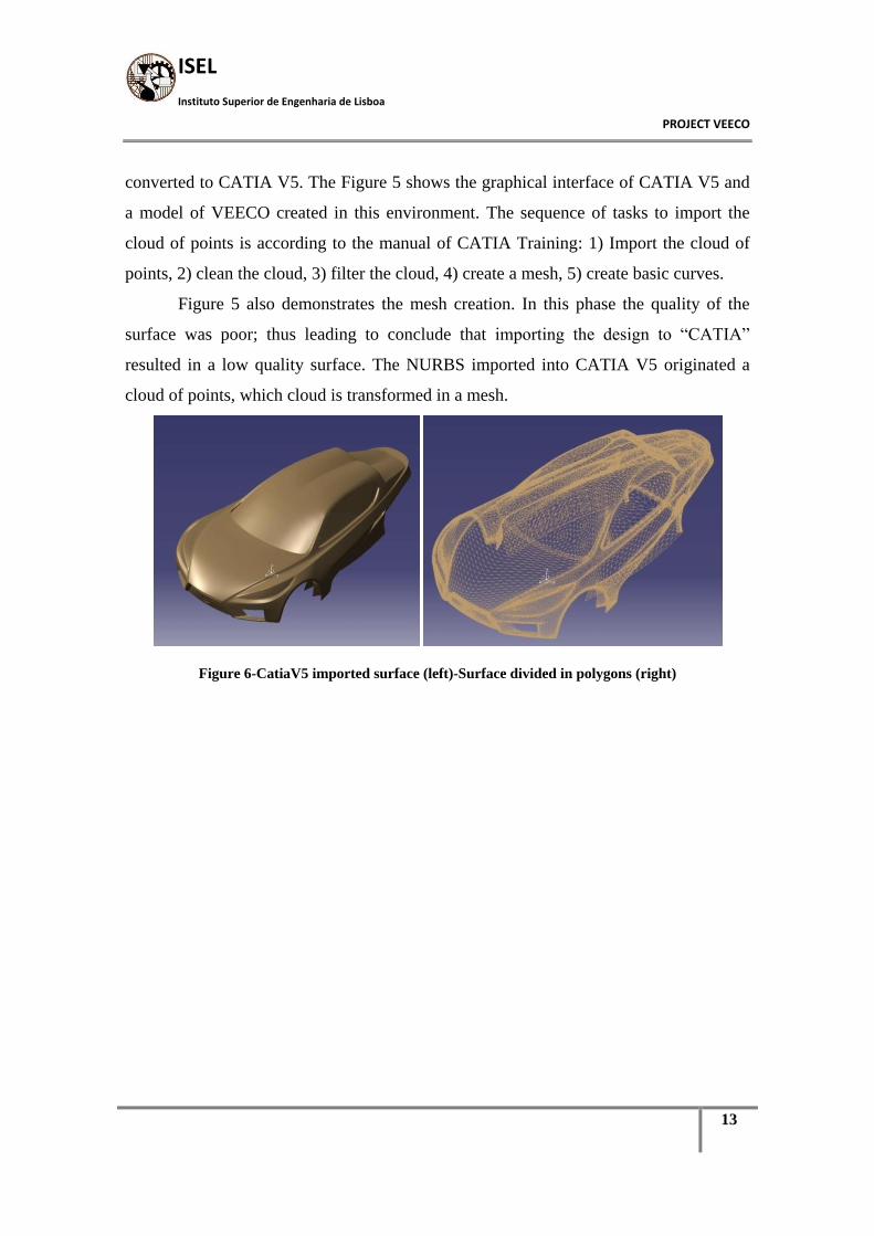
converted to CATIA V5. The Figure 5 shows the graphical interface of CATIA V5 and

a model of VEECO created in this environment. The sequence of tasks to import the

cloud of points is according to the manual of CATIA Training: 1) Import the cloud of

points, 2) clean the cloud, 3) filter the cloud, 4) create a mesh, 5) create basic curves.

Figure 5 also demonstrates the mesh creation. In this phase the quality of the

surface was poor; thus leading to conclude that importing the design to “CATIA”

resulted in a low quality surface. The NURBS imported into CATIA V5 originated a

cloud of points, which cloud is transformed in a mesh.

Figure 6-CatiaV5 imported surface (left)-Surface divided in polygons (right)

14

By carefully analysing Figure 6 it is possible to understand that in some areas

the mesh automatically generated was lacking quality as the detailed view in Figure 7

shows. The side window region shows a mesh highly non-homogeneous,.

Figure 7-Detailed view from the side window

These surfaces are generated by a cloud of points in which the software

automatically creates a mesh able to represent the geometry.

Figure 8-Detailed information regarding the cloud of points generated in CATIA V5.

ISEL


PROJECT VEECO

15

Figure 9-Detailed information of figure 8.

From this phase, Figure 8 and Figure 9, there were two ways to proceed. One

was to generate an automatic surface; the other was to create carefully the geometry,

one of this is needed because it is not possible to work on a cloud of points. Both

options are described after. The approach used by the other colleague, Fabiola Herrera,

was to model the surface in parts, intending to join them later on, forming a complete

body. The work in Figure 10 was entirely done by Fabiola.

Figure 10-Design in CATIAV5 separated surfaces to compose the all body.

This procedure involves a very complex process to align all the small surfaces

and guarantee the tangency between them, and it‟s extremely time consuming. This

kind of approach can lead to several problems, including distortion in the final

geometry.

16

This was the work made available, when the present study started associated to

the scholarship granted. It was decided by the author of this work to start with an

evaluation of the quality of the imported geometry. Using the original mesh created

from the Sketchup design, and with an automatic tool a first approach was created

Figure 11.

Figure 11-CATIAV5 automatic surface design from the imported model.

The tool used to perform this step can be seen in Figure 12, it is a module from

the shape design toolbox called Quick Surface Reconstruction and it is called automatic

Surface.

Figure 12-Automatic tool to generate a test surface in CATIA V5.

Although there are some parameters to be configured, the Automatic Surface feature

had an even poorer quality than the original Sketchup base. The details in the next

figures show the main problems Figure 13, Figure 14.

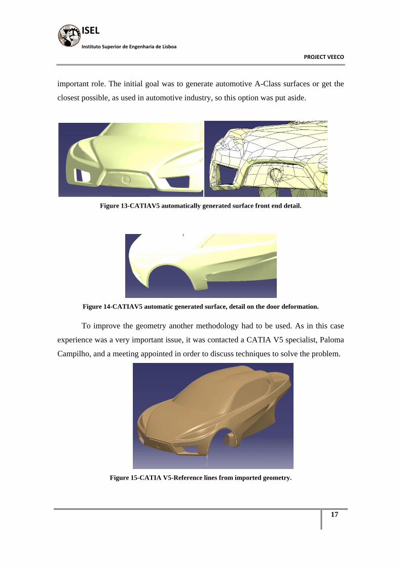
Bearing in mind the objective of studying in subsequent stages the body

behaviour in other software such as ANSYS, the quality of the surface assumed a very

ISEL


PROJECT VEECO

17

important role. The initial goal was to generate automotive A-Class surfaces or get the

closest possible, as used in automotive industry, so this option was put aside.

Figure 13-CATIAV5 automatically generated surface front end detail.

Figure 14-CATIAV5 automatic generated surface, detail on the door deformation.

To improve the geometry another methodology had to be used. As in this case

experience was a very important issue, it was contacted a CATIA V5 specialist, Paloma

Campilho, and a meeting appointed in order to discuss techniques to solve the problem.

Figure 15-CATIA V5-Reference lines from imported geometry.

18

Thus, a different approach was then planned, which passed by the usage of the

same basis of work, but instead of picking the entire surface, only the reference lines of

the design were used as in Figure 15 and created the design based on them. By using

guidelines for the main surfaces, and creating them the larger possible, the final result

would be better. Doing so, it was possible to achieve a better basis of work because it is

possible to control the development and the curvature even point-to-point if necessary.

The tool feature used in the process was “Curve on mesh” as observed in Figure 16.

Figure 16-CATIA V5 Tool to create reference lines.

ISEL


PROJECT VEECO

19

Figure 17-CATIA V5 Tree of operations.

The resulting curves sometimes did not satisfy the quality needed so a

reconstruction of the guide was required. The tools used in this process were a

combination of 4 workbenches, Quick surface reconstruction, Generative shape design,

Digitized shape editor and FreeStyle, all from the surface tools group. One of the

sequences used can be traced by the tree of operations Figure 17, where it can be seen

that the body side was created in a separated geometrical set, where the geometry was

paste to, and a first curve on the original mesh was created. As the quality of the mesh

was poor a guiding point was needed, “point.11” so that the curve on mesh 6 could be

created and could be totally tangent between each section. The sections were divided

using the Split tool and the resulting curve was a spline, which joined all the smaller

sections, with tangency continuity option enabled. A Curve smooth was used after, to

20

smoothen the profile, the idea was to eliminate the separation in the surface, since the

final tool to use was a multisection, as can be seen in Figure 18.

Figure 18-CATIA V5 Tool to create Surfaces.

In the automotive industry, it is very important to control the development of the

surfaces, which is possible by using this tool rather than by using the Automatic

Surfaces from FreeStyle or other workbenches dedicated to other applications. Other

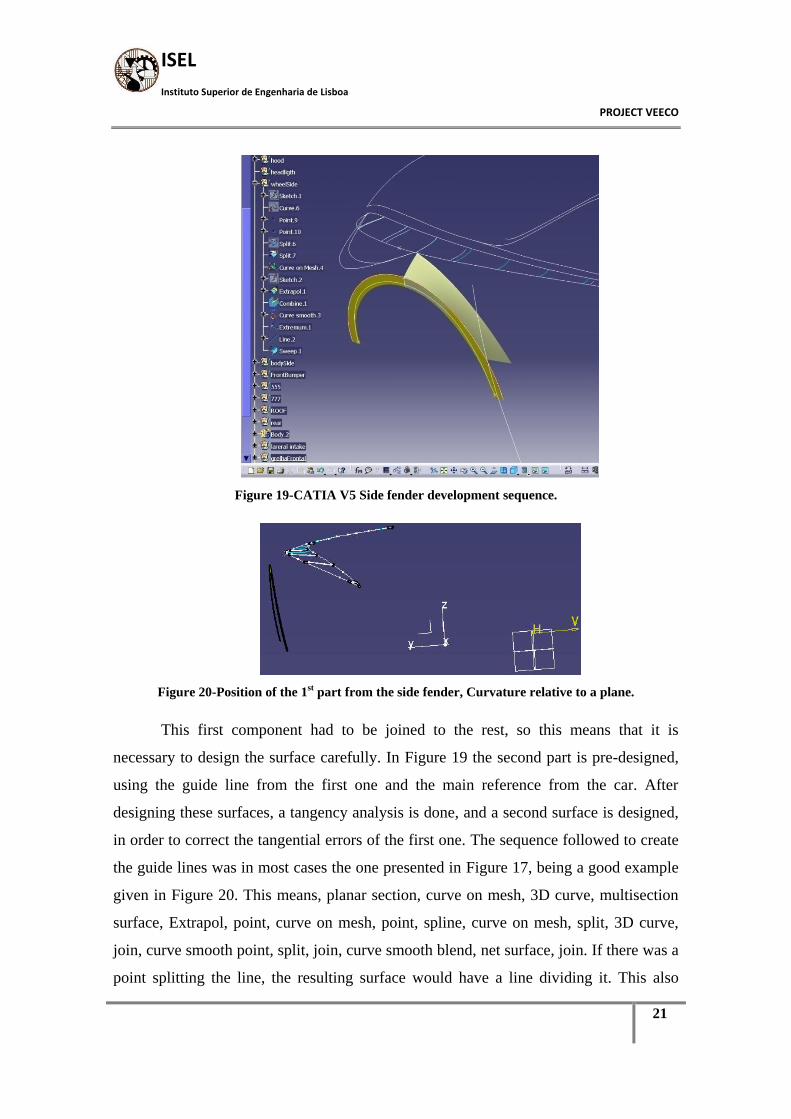
parts had a different way of being developed such as the side fender between the wheel

and the door. In this case it had to be done in several steps. In Figure 19 it is possible to

see some of the tools used, after having the basic curves, a Combine process had been

done to create the geometry of the profile and after this the curve had to be smoothened

and trimmed in order to have the resulting sweep which can be seen in Figure 19. The

first part designed was the outer side, to serve as a reference.

ISEL


PROJECT VEECO

21

Figure 19-CATIA V5 Side fender development sequence.

Figure 20-Position of the 1st part from the side fender, Curvature relative to a plane.

This first component had to be joined to the rest, so this means that it is

necessary to design the surface carefully. In Figure 19 the second part is pre-designed,

using the guide line from the first one and the main reference from the car. After

designing these surfaces, a tangency analysis is done, and a second surface is designed,

in order to correct the tangential errors of the first one. The sequence followed to create

the guide lines was in most cases the one presented in Figure 17, being a good example

given in Figure 20. This means, planar section, curve on mesh, 3D curve, multisection

surface, Extrapol, point, curve on mesh, point, spline, curve on mesh, split, 3D curve,

join, curve smooth point, split, join, curve smooth blend, net surface, join. If there was a

point splitting the line, the resulting surface would have a line dividing it. This also

22

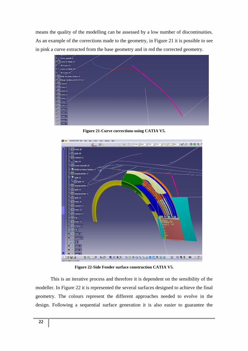
means the quality of the modelling can be assessed by a low number of discontinuities.

As an example of the corrections made to the geometry, in Figure 21 it is possible to see

in pink a curve extracted from the base geometry and in red the corrected geometry.

Figure 21-Curve corrections using CATIA V5.

Figure 22-Side Fender surface construction CATIA V5.

This is an iterative process and therefore it is dependent on the sensibility of the

modeller. In Figure 22 it is represented the several surfaces designed to achieve the final

geometry. The colours represent the different approaches needed to evolve in the

design. Following a sequential surface generation it is also easier to guarantee the

ISEL


PROJECT VEECO

23

tangency between surfaces. This technique turns the process more liable and the final

result was considerably better Figure 25 than the previous one.

In Figure 23 and Figure 24 it is possible to see the tests made to verify the final

quality of the surface. It was also decided to design half the car, and the parts in the

middle were designed as a unique so that the final result would not have separation lines

in the middle section, parts such as the bonnet are a good example of this.

Figure 23-CATIAV5-Guide line design technique, detail on the main guides

Figure 24-CATIAV5 surface quality assessment, using the reflect lines to detect imperfections.

The windows were also a concern so that the result would be feasible, in order to

guarantee this, extreme curvatures where avoided and intricate geometries where

simplified. The clearances, also a major concern, had to ensure a final product where the

other components would fit correctly. Although a test assembly of all components was

24

not possible, because, modelling the entire structure was not achievable in the available

time the chassis was several times mounted together with the body to perceive possible

product design failures in the future. Other parts have been modelled, such as structural

parts and some components like the suspension arm.

Figure 25-CATIAV5 VEECO final design.

Figure 26 - Projection on plane tool, from CATIA V5.

The final result was actually smoother than the previous one, so although there is

still a lot of room for improving geometries, such as the front grill created after.

ISEL


PROJECT VEECO

25

The study of the door hinge was also developed. The frontal area was calculated

using the Projection-on-plane tool Figure 26. This tool is often used in aerodynamics to

compute the area of the projected cloud (CATIA Generative shape design manual). The

projected cloud has to be edited to create a 2D plane and the resulting plane is measured

to determine the value of the projected area.

Figure 27 – Projected area, using CATIA V5 tool (0.043m2)

In Figure 27, the process is shown in the tree of operations, and the tool used to

measure the area is also present.

1.2. Door and hood hinge

The hinge is intended to support both the hood and the door. As the hood has a

special configuration the hinge had to have a second movement in order to create

clearance between the hood and the wind screen.

26

The movement includes a vertical and simultaneously forward movement. The

doors have a classic scissor movement that can be seen in other cars. The movement had

been tested in order to guarantee functional clearances. One important issue was to test

the simultaneous movement to seek clash problems. The hinge had to be redesigned

several times due to the compound movement.

Figure 28 CATIAV5 door and hood hinge design.

Figure 29 CATIAV5 door and hood hinge motion test

The shape had to be reinforced due to twisting of the main body that was not

dimensioned correctly in the first approach; the evolution resulted in a good final result

combining stiffness and a lightweight, Figure 28 and Figure 29.

2. Construction of the model to test

To conduct the aerodynamic test in the wind tunnel a scale model was built. The

model had to be accurate and represent the main characteristics and dimensions of the

vehicle so that the error introduced can be minimized.

ISEL


PROJECT VEECO

27

The scale defined was 1:5,56 the limitation on the test section dictated this scale. As

the model has been entirely designed in the software CATIA V5, the changes and

scaling were all made in the same software. Following the indications from the AFA

specialist the wheels were simplified, the bottom end was made plain, so that it could be

mounted in the balance, and the rear wheel was taken out from the study as it was

considered it did not influenced much the results. The model was then scaled to the

1:5,56 scale and the file was converted to be sent to FabLab in order to be build. The

model was build using a 3D Printer.

Due to the size of the model and the restrictions on the printer, it had to be separated

in 4 parts. The parts would be printed separately and then fixed together to complete the

model. Due to costs the thickness of the model had to be reduced to the minimum

possible in order to keep the costs low, so a first model with 1.5mm thick was then

redrawn to a thickness of 1mm, the edges had to be 4mm thick so that the assembly of

the several parts could be done.

The first model had problems of high stress concentrations, in some regions, and it

cracked when still being printed Figure 30 and Figure 31.

Figure 30-Model from 3D printer

28

Figure 31-Detail on the crack (Model from the 3D printer)

The solution found was a supportive structure on the inside Figure 32 and Figure

33 as it wouldn‟t change the outer shape and would bring benefits in terms of localized

resistance.

Figure 32-Detail on the reinforcement (Model from the 3D printer)

ISEL


PROJECT VEECO

29

Figure 33-First model and solution side by side (Model from the 3D printer)

With this problem corrected, the other components were printed as can be then

observed in Figure 34 and Figure 35.

Figure 34-Rear part from the model(Model from the 3D printer))

30

Figure 35-Front part from the model (Model from the 3D printer)

To assemble the parts one has used glue and bolts with nuts Figure 36, the

complete model can be observed in Figure 37.

Figure 36-Assembling the model(Model from the 3D printer)

ISEL


PROJECT VEECO

31

Figure 37-Complete model(model from the 3D printer)

The components were so thin that the reinforcement could be seen from the

outside Figure 38.

Although the surfaces were carefully sanded the union had some finishing

problems Figure 38 and Figure 39 that could later affect the test.

Figure 38-Assembly process, front end (Model from the 3D printer)

32

Figure 39 Detail from the union (Model from the 3D printer)

After the assembly process, the model was sanded and painted. The sanding had

to be done in stages in order to maintain the design stable so the whole model had to be

sanded several times paying attention to thickness.

ISEL


PROJECT VEECO

33

CHAPTER II

Aerodynamic and numerical simulation of the scale model

3. Aerodynamics

Since late years the vehicles shape and aerodynamics were more or less a

concern for car builders. Looking up at a 1916 race car the detail in building tapering-

boat tail shows that even at the dawn of the century aerodynamic drag reduction was a

primary concern in race car design.

According to the information extracted from (xvii):

The basic concept used on race cars is streamlining, since the objective is to

move more easily through the air (reducing drag results in faster moving). At a first

glance seems that the loads created by the motion of air are unimportant, especially

within the speed range of automobiles, but by doing a simple test such as extend the

hand out of a car side window, will demonstrate the importance of the forces exerted by

air. Another example is the airplane that can lift several tons of cargo and passengers

using only the power generated by their jet engines, these engines provide only the

thrust needed to overcome the airplane drag.

In order to explain the creation of aerodynamic forces a typical cross section of a

wing is shown in Figure 40.

Figure 40-Low pressure on the upper surface of the airfoil generates lift xvii

Assuming it moves from right to left, due to the shape and angle of the airfoil

section the air will move faster on the upper surface than on the lower one, this

difference creates a low pressure on the upper surface and a higher on the lower one,

34

this pressure difference is the responsible for the force that lifts an airplane. Note that

when used on a race car the airfoil is inverted in order to obtain the forces needed. As a

downside of this theory when a wing generates lift, drag is also generated.

Drag is most of the times smaller than the lift and can be reduced by streamlining the

vehicle (having a smooth external surface), and any improvement in a vehicle drag can

improve the fuel economy. A practical demonstration on reducing drag by streamlining

can be demonstrated by a visual comparison as represented in Figure 41.

Figure 41 – Two bodies with same aerodynamic drag, despite the big difference in sizexvii

The image shows a cross section of a long circular rod (small circle) which has

the same drag as a much thicker and large airfoil. Adding to the drag and lift forces

there is also a side force component which needs to be added to the analysis.

The summation of the main forces applied to a moving vehicle in terms of

aerodynamics, and how they interact in the vehicle can be seen in Figure 42. This is

only valid if considering the vehicle is moving forward.

Figure 42-Directions used to identify the three components of aerodynamic force xvii

The force pointing backward is the Drag, and resists the movement. The force

component pointing upwards is the lift. This is very often disregarded by the everyday

driver although those who have experienced very high-speed driving may have noticed

that at that speed it comes out to be harder to keep the car going in a straight line. This

is due to this force and on passenger vehicles it becomes more noticeable on the rear

ISEL


PROJECT VEECO

35

wheels rather than in front ones. The third force showing here the side force (positive to

the right) is important to be taken in to account but with side winds of low intensity this

component of the aerodynamic load is small.

In car design it is possible to reduce the non-wanted effects of aerodynamic

forces such as the lift generated. Since most production cars have positive lift, a good

example is the application of a rear-deck mounted spoiler, as it is an efficient way to

reduce the lift on the rear wheels.

Another interesting example is what happened back in the late 1970´s when race

car engineers started to pay attention to the well-known fact among the aeronautical

community that the lift of a wing increased with ground proximity. This “ground effect”

works both for wings lifting upward and for inverted race car wings creating down

force. The practical result of this can be noticed by the flat shape used in most race cars.

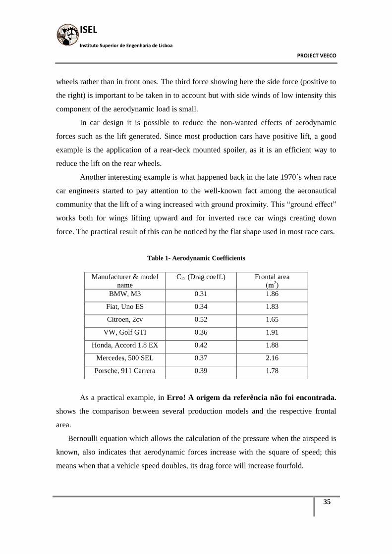
Table 1- Aerodynamic Coefficients

Manufacturer & model

name

CD (Drag coeff.) Frontal area

(m2)

BMW, M3 0.31 1.86

Fiat, Uno ES 0.34 1.83

Citroen, 2cv 0.52 1.65

VW, Golf GTI 0.36 1.91

Honda, Accord 1.8 EX 0.42 1.88

Mercedes, 500 SEL 0.37 2.16

Porsche, 911 Carrera 0.39 1.78

As a practical example, in Erro! A origem da referência não foi encontrada.

shows the comparison between several production models and the respective frontal

area.

Bernoulli equation which allows the calculation of the pressure when the airspeed is

known, also indicates that aerodynamic forces increase with the square of speed; this

means when that a vehicle speed doubles, its drag force will increase fourfold.

36

3.1. The wind tunnel

In a simple approach a wind tunnel is a long tunnel through which the air is blown

into by large fans. The main advantage is associated to its controlled environment where

airspeed, flow-direction, temperature, and other variables to be controlled and measured

are not influenced by outdoor weather. The vehicle to be tested is placed in a test area

where the airflow direction and speed are highly uniform. As the section is placed far

from the fan the pulsation and swirl caused by the rotating blades are avoided. The

wheels are placed on a rolling belt to simulate the moving ground, and there is a

sensitive balance placed at the lower end of the long rod holding the model from above

to measure forces such as lift and drag.

The smoke traces shown in the airflow near car being tested in wind tunnels are

called streamlines Figure 43. These streamlines are associated with the motion of the

fluid surrounding the vehicle. A steady-state flow when a vehicle is moving forward at a

steady speed, causes the fluid particles to move along the streamlines. These lines are

parallel to the local velocity direction. These lines are the result of injecting smoke in

the wind tunnel, so it is of most importance that the density does not vary between the

two fluids or the streamlines won‟t be followed. When streamlines near the solid

surface follow exactly the shape of the body the fluid is considered to be attached, if not

it is considered separated.

Figure 43-Attached flow over a streamlined car (A), locally separated flow behind a real

automobile (B) xvii

In order to reduce aerodynamic drag and increase down force it is very

important that the flow stays attached, and bearing in mind that the loads applied on a

vehicle moving throw air depend directly on the fluid material and its characteristics,

such as temperature, pressure, density and viscosity.

ISEL


PROJECT VEECO

37

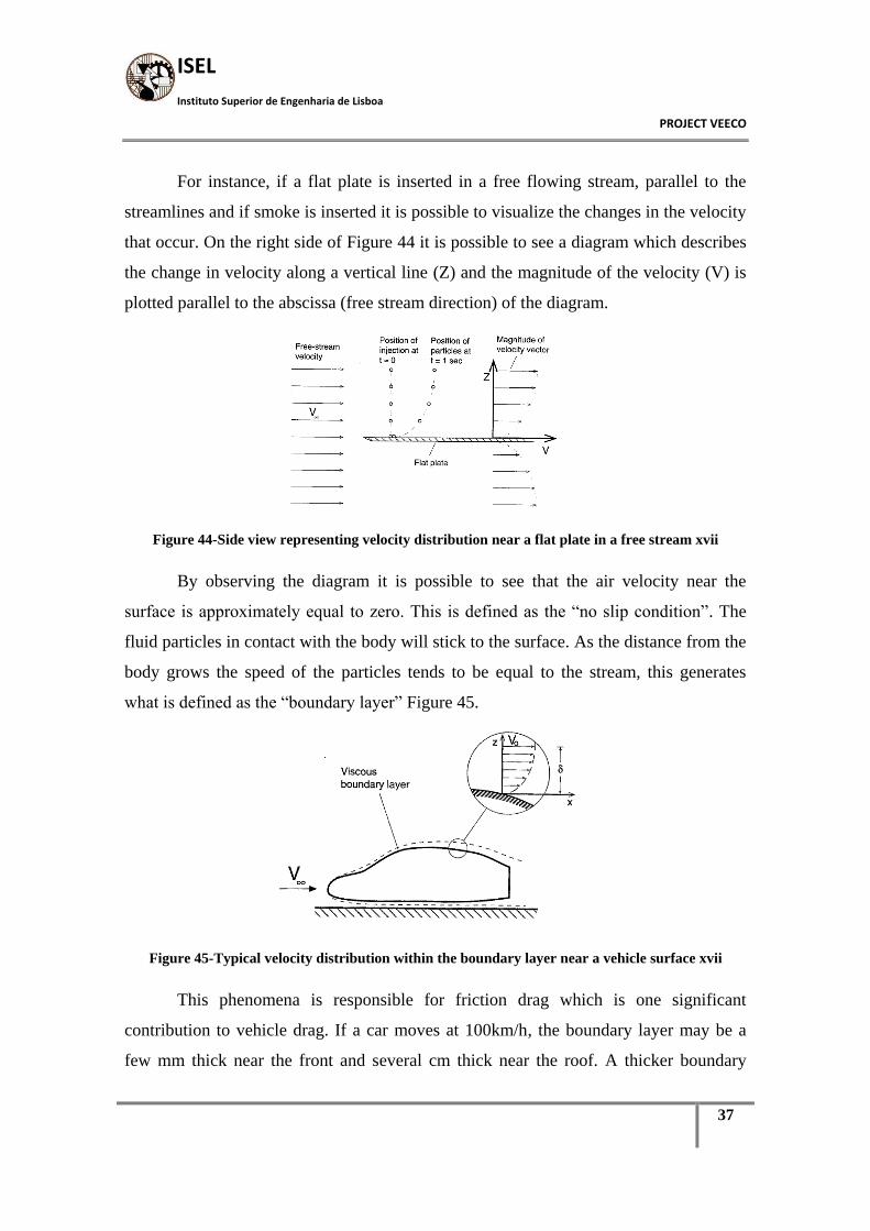
For instance, if a flat plate is inserted in a free flowing stream, parallel to the

streamlines and if smoke is inserted it is possible to visualize the changes in the velocity

that occur. On the right side of Figure 44 it is possible to see a diagram which describes

the change in velocity along a vertical line (Z) and the magnitude of the velocity (V) is

plotted parallel to the abscissa (free stream direction) of the diagram.

Figure 44-Side view representing velocity distribution near a flat plate in a free stream xvii

By observing the diagram it is possible to see that the air velocity near the

surface is approximately equal to zero. This is defined as the “no slip condition”. The

fluid particles in contact with the body will stick to the surface. As the distance from the

body grows the speed of the particles tends to be equal to the stream, this generates

what is defined as the “boundary layer” Figure 45.

Figure 45-Typical velocity distribution within the boundary layer near a vehicle surface xvii

This phenomena is responsible for friction drag which is one significant

contribution to vehicle drag. If a car moves at 100km/h, the boundary layer may be a

few mm thick near the front and several cm thick near the roof. A thicker boundary

38

layer creates more viscous friction drag, a too steep increase in this thickness can lead to

flow separation, resulting in additional drag.

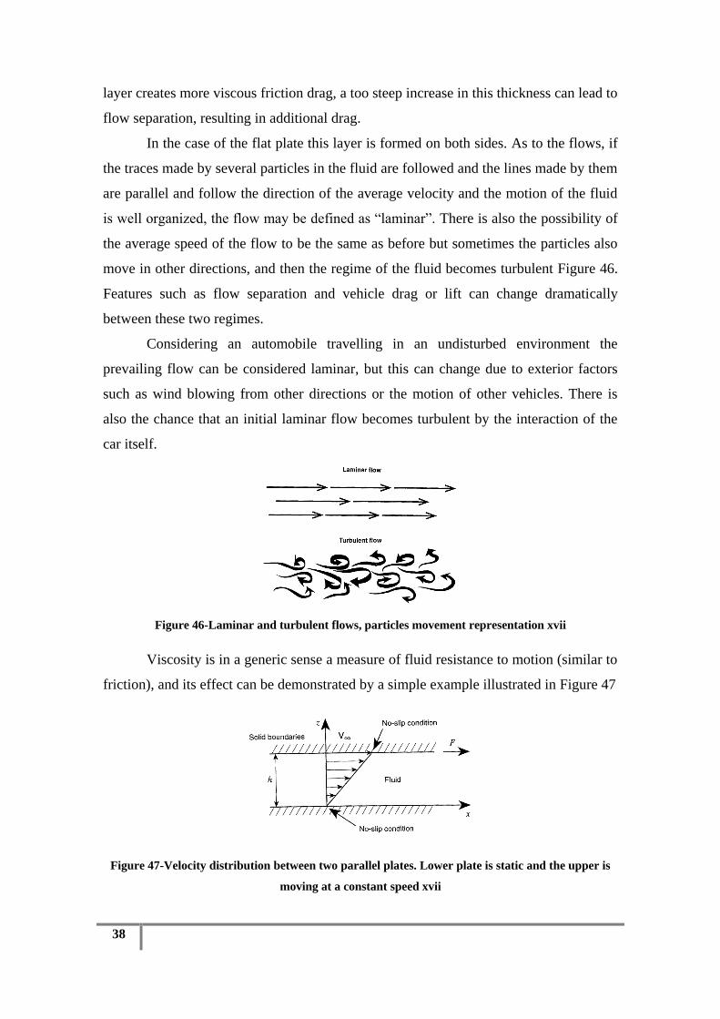
In the case of the flat plate this layer is formed on both sides. As to the flows, if

the traces made by several particles in the fluid are followed and the lines made by them

are parallel and follow the direction of the average velocity and the motion of the fluid

is well organized, the flow may be defined as “laminar”. There is also the possibility of

the average speed of the flow to be the same as before but sometimes the particles also

move in other directions, and then the regime of the fluid becomes turbulent Figure 46.

Features such as flow separation and vehicle drag or lift can change dramatically

between these two regimes.

Considering an automobile travelling in an undisturbed environment the

prevailing flow can be considered laminar, but this can change due to exterior factors

such as wind blowing from other directions or the motion of other vehicles. There is

also the chance that an initial laminar flow becomes turbulent by the interaction of the

car itself.

Figure 46-Laminar and turbulent flows, particles movement representation xvii

Viscosity is in a generic sense a measure of fluid resistance to motion (similar to

friction), and its effect can be demonstrated by a simple example illustrated in Figure 47

Figure 47-Velocity distribution between two parallel plates. Lower plate is static and the upper is

moving at a constant speed xvii

ISEL


PROJECT VEECO

39

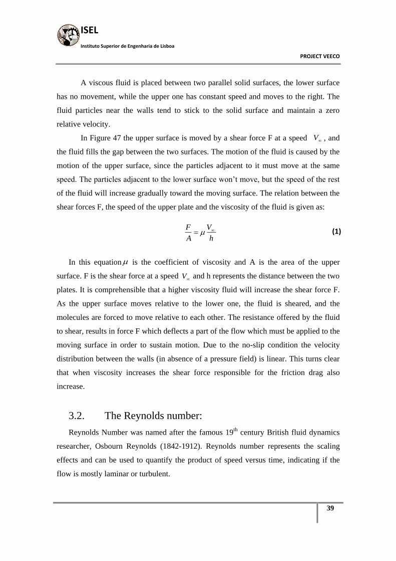
A viscous fluid is placed between two parallel solid surfaces, the lower surface

has no movement, while the upper one has constant speed and moves to the right. The

fluid particles near the walls tend to stick to the solid surface and maintain a zero

relative velocity.

In Figure 47 the upper surface is moved by a shear force F at a speed , and

the fluid fills the gap between the two surfaces. The motion of the fluid is caused by the

motion of the upper surface, since the particles adjacent to it must move at the same

speed. The particles adjacent to the lower surface won‟t move, but the speed of the rest

of the fluid will increase gradually toward the moving surface. The relation between the

shear forces F, the speed of the upper plate and the viscosity of the fluid is given as:

In this equation is the coefficient of viscosity and A is the area of the upper

surface. F is the shear force at a speed and h represents the distance between the two

plates. It is comprehensible that a higher viscosity fluid will increase the shear force F.

As the upper surface moves relative to the lower one, the fluid is sheared, and the

molecules are forced to move relative to each other. The resistance offered by the fluid

to shear, results in force F which deflects a part of the flow which must be applied to the

moving surface in order to sustain motion. Due to the no-slip condition the velocity

distribution between the walls (in absence of a pressure field) is linear. This turns clear

that when viscosity increases the shear force responsible for the friction drag also

increase.

3.2. The Reynolds number:

Reynolds Number was named after the famous 19th

century British fluid dynamics

researcher, Osbourn Reynolds (1842-1912). Reynolds number represents the scaling

effects and can be used to quantify the product of speed versus time, indicating if the

flow is mostly laminar or turbulent.

V

h

V

A

F

V

(1)

40

Reynolds number of a quarter scale model is ¼ of the full size model. This number

represents the ratio between inertial and viscous (friction) forces created in the air, being

expressed as:

Where is the fluid density, is the viscosity, V velocity, and L is some

characteristic length (of the vehicle).

An interesting feature of the Reynolds number is that two different flows can be

considered similar if their Reynolds number is the same. This number is

nondimensional. For a numerical example of the Reynolds Number, Veeco dimensions

were used. The car length is 3.56m, and a speed of 30m/s was assumed, the properties

of air are on Table 2. By analysing this table it is possible to understand the concepts

represented. Density and viscosity are indicated for air, water and a motor oil, all very

well known, this can give the perception in terms of the variables indicated in a very

practical way.

Table 2 -Density and Viscosity of Air and Water (at 20ºC, 1 atm) xvii

The subscript L indicates the value is based on the length of the vehicle. When

testing a scale model there are some problems that can arise such as, when testing a

small scale model (1/5 scale) conducted at low speeds (100 km/h) the value of the

Reynolds number may drop below 2x105, and if this happens the result may not be fully

applicable to the full size car.

VLRe

65 102.7108.156.33022.1

LeR

(2)

(3)

ISEL


PROJECT VEECO

41

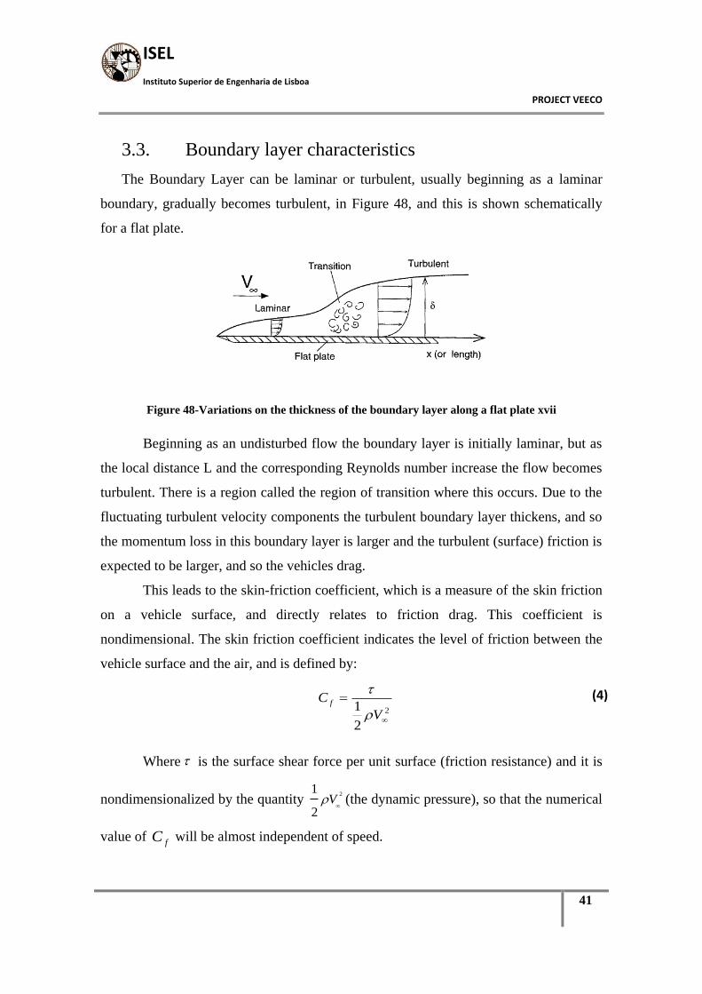
3.3. Boundary layer characteristics

The Boundary Layer can be laminar or turbulent, usually beginning as a laminar

boundary, gradually becomes turbulent, in Figure 48, and this is shown schematically

for a flat plate.

Figure 48-Variations on the thickness of the boundary layer along a flat plate xvii

Beginning as an undisturbed flow the boundary layer is initially laminar, but as

the local distance L and the corresponding Reynolds number increase the flow becomes

turbulent. There is a region called the region of transition where this occurs. Due to the

fluctuating turbulent velocity components the turbulent boundary layer thickens, and so

the momentum loss in this boundary layer is larger and the turbulent (surface) friction is

expected to be larger, and so the vehicles drag.

This leads to the skin-friction coefficient, which is a measure of the skin friction

on a vehicle surface, and directly relates to friction drag. This coefficient is

nondimensional. The skin friction coefficient indicates the level of friction between the

vehicle surface and the air, and is defined by:

Where is the surface shear force per unit surface (friction resistance) and it is

nondimensionalized by the quantity 2

1

2V

(the dynamic pressure), so that the numerical

value of fC will be almost independent of speed.

2

2

1

V

C f

(4)

42

The effect of speed in friction results in a reduction of the thickness of the

boundary layer as the speed builds up, this is result of the larger momentum (the

product of mass times velocity) of the free stream compared to the loss of momentum

caused by the viscosity near the solid surface, therefore the friction coefficient will be

reduced with increased flow speed. This can be seen by the typical experiment of a flat

plate submerged in a parallel flow Figure 48

Figure 49-Skin friction coefficient on a flat plate parallel to the flow, for laminar and turbulent

boundary layers versus the Reynolds number. xvii

From Figure 49 it is possible to conclude that there are two separate curves, one

for laminar and one for turbulent flow and both decrease with increasing Reynolds

number. It is possible to have laminar and turbulent flow for a large range of Reynolds

number. In this cases the friction in laminar flow is considerably lower which indicates

that for the purpose of drag reduction, laminar flow is preferred. There are some

interesting conclusions about the boundary layer:

Boundary layer thickness is larger for turbulent than for laminar flows

The skin friction coefficient becomes smaller with increased Reynolds number

(mainly for laminar flow)

At certain Reynolds number ranges both laminar and turbulent boundary layers

are possible. The nature of the actual boundary layer for a particular case

depends on flow disturbances, surface roughness, etc...

The skin friction coefficient is considerably larger for the turbulent boundary

layer (larger skin friction results in larger friction drag.)

ISEL


PROJECT VEECO

43

Because of the momentum transfer normal (perpendicular) to the direction of the

average speed in the case of a turbulent boundary layer, flow separations will be

delayed somewhat compared to a laminar boundary layer. This is an important

and indirect conclusion, but in many automotive applications it forces us to

prefer turbulent boundary layer in order to delay flow separation.

Bearing in mind these points, in order to keep the value of drag low, it is necessary

to maintain large regions of thin laminar boundaries and delayed transition, and when

flow separation is likely, such as in the rear section of the car it is better to have a

turbulent boundary layer (with drag penalty) but avoiding hard flow separations which

leads to the loss of down force.

3.4. Transition and laminar bubble

In automobile related aerodynamics the order of magnitude of the Reynolds number

will be about 107, and as shown in Figure 50 it is possible to have large regions of

laminar boundary layers. In order to reduce drag caused by skin friction it is important

to have laminar boundary layers, however if the curvature of the surface is too high the

flow may separate, and thus generated drag.

In Figure 50 it is shown a typical case where the initially laminar flow on a

streamlined hood tends to separate due to the curvature, and reattaches later. The

reattachment is generally the result of the boundary layer turning turbulent due to the

disturbance, and because of the large momentum transfer in the turbulent flow the

separation is delayed or even avoided. The early flow separation is called laminar

separation and the enclosed streamlines where the reversed flow exist, are called

laminar bubble.

This phenomenon is important because the laminar bubble area is sensitive and the

flow may separate entirely without a reattachment resulting in a drag increase.

44

Figure 50-Schematic description of the laminar bubble, transition from laminar to turbulent

boundary. xvii

Laminar bubble appears at low Reynolds number range (104 – 0.2x10

6) and

tends to disappear as the vehicle speed increases. This may be responsible for severe

discrepancies in flow visualization and aerodynamic data when comparing over a wide

range of speeds and becomes more pronounced when small scale wind tunnel models

are used to develop a high speed full scale vehicle.

It is possible to force the transition from laminar to turbulent flow within the

boundary layer by introducing disturbances. This is called “Tripping of the boundary

layer” and can be done by using small vortex generators (little wedges the height of the

boundary layer) or by placing a strip of coarse sanding paper on the desirable transition

line. Since turbulent boundary layer has a tendency to stay attached longer, some drag

benefits due to a reduction in separated flow can be gained by using this technique.

3.5. Bernoulli equation for pressure

“The shape of a moving vehicle causes the airflow to change both direction and

speed. This movement of the airflow near the body creates a velocity distribution which

in turns creates the aerodynamic loads acting on the vehicle”

Generally these loads can be divided into two different loads. The first is the shear (skin

friction) force which results from the viscous boundary layer, and acts tangentially to

the surface and contributes to the drag, the second is pressure, and acts in the normal to

the surface and contributes both to lift and drag, so that the vehicle down force is really

the added effect of the pressure distribution. The pressure force is caused primarily by

ISEL


PROJECT VEECO

45

the velocity outside the boundary layer, such as the V0 present in Figure 45. Note that

the velocity at the bottom of the boundary layer is zero.

Bernoulli equation describes the relation between air-speed and pressure, and it can be

applied to streamlines, along any point the relation between the local static pressure P,

density ( ), and velocity V is:

As the equation is to be used to compare the velocity and pressure between two

points in the flow, the value of the constant will not be important. When considering

smooth, attached and constant density flows, the equation can be used for any point in

the field and not on a streamline only.

3.6. Application example

Consider the flow over a vehicle moving forward at a speed of as in Figure 51; as

the vehicle deforms the streamlines, the velocity increases near the body. If considering

a point far ahead of the vehicle, the equation (5) can be written, and for a second point

on the body (point A) the same equation can be written. As the constant keeps its value

the resulting equation is the following:

The subscript letter A represents the quantities measured at point A. This means if

the ambient pressure ( p

) is known, vehicle speed (V

) and static pressure pA near the

vehicle surface the local air speed VA can be calculated using this equation.

Selecting another point in the flow where velocity is equal to zero on the moving

vehicle as in the case of an enclosed cavity created at the front of the car (point B),

writing the equation for this two points:

ConstVp

2

2

(5)

V

22

22

VpVp AA

(6)

2

2

VppB

(7)

46

As the velocity VB=0, and supposing the vehicle velocity is 30m/s and taking the

value of air density from Table 2 the result is a higher pressure at point B when

compared to the average atmospheric pressure

Figure 51-Terminology relative to the equation (7) taken from xvii

The result of the loads depends directly of the velocity near the vehicle surface,

(outside the boundary layer) which depends on the body shape. The shape will be

determinant to the resulting velocity field. A relation between pressure and the local

velocity has been established by Bernoulli, through an equation that states that if

airspeed varies as it flows around an object, then the pressure will change in an inverse

proportion to the square of the airspeed. As the air flows faster around the vehicle the

pressure will be reduced. The important conclusion to be drawn is in order to create

down force on a vehicle a faster flow must be created on the lower surface; this will

result in a lower pressure on the lower surface resulting in down force

In a favourable pressure gradient the flow stays attached longer and also the

boundary layer in undisturbed free streams will stay laminar for longer distances along

the body surfaces, these results in less friction and drag. Steep unfavourable pressure

gradients will initiate flow separations and transition to turbulent boundary layers

As an end reference it is important to refer the far field effects caused by the

flow field created by bodies moving through air, this track is called wake. Examples of

typical wakes can be the vortex wakes visible behind airplanes flying in humid air or

dust clouds which continue to roll behind a truck, long after it has passed by.

In Figure 52 the disturbance in the flow pattern behind the vehicle causes a

momentum loss which extends far behind the vehicle. If the velocity distribution is

measured at various heights “z” in the symmetry plane ahead of the vehicle at point A,

and then another measurement is taken at one car length the velocity profile indicates a

near uniform velocity distribution.

2 2

2

11.22 30 549

2 2B

Np p V

m

(8)

ISEL


PROJECT VEECO

47

Figure 52-Wake flow generated by a car body shape with flow separation at the base areaxvii

If the same measurement is made behind the vehicle even at a relatively large

distance of 10 to 20 body lengths the velocity will be different from the one in point B.

If the flow separates behind a body then such a wake will result, and in that area the

flow seems to be dragging behind the vehicle. The energy spent on dragging this wake

will be the drag, by comparison a perfect vehicle will have the flow attached and the

resultant drag will be very small.

3.7. Drag, lift and side forces

There are mainly two categories of aerodynamic forces acting on the vehicle. The

first is the pressure that acts normal to the surface and is responsible for a vehicle lift

and part of the drag. The second is the shear force which acts parallel to the body

surface and contributes only to drag. The resultant force that comes out of these

contributions can be divided into various components.

Figure 53-Coordinate system for aerodynamic loads on a vehicle, and frontal area used to define

force coefficients xvii

48

Based on the coordinate system in Figure 53 there can be defined three forces

and three moment coefficients, but the most important are Lift and Drag. The side force

would be important too but only takes part when strong side winds or when a taking

over manoeuvre is done, so the analysis will focus on the other two.

The drag force direction is parallel to the vehicles motion and points towards the

back of it, in the X direction. The side force is positive in the y direction, the lift acts

upward normal to the ground in to the z direction, while down force is equal to negative

lift and acts in to the Z direction. The advantage in defining non dimensional

coefficients for lift and drag is that their values will be independent of speed and will be

related to the shape of the vehicle only. An example is the results of a vehicle towing

experiment, in terms of the total towing force versus speed, are represented in Figure

54. The rolling resistance between the road and the tires is shown by the X symbols.

This usually changes only a bit with increased vehicle speed.

Figure 54-Variation of vehicle total drag and rolling resistance versus speed xvii

The total resistance, including aerodynamic drag increases very rapidly and

shows a parabolic curve fit ( with c being a constant) which indicates that

aerodynamic loads increase by the square of speed The solid triangular symbols

represent the measured data and usually at higher speeds the curve-fit is far better.

If the data is to be presented in a non-dimensional form the measured forces must be

divided by the square of the velocity.

If we plot the drag in terms of CD the result will be a straight horizontal line

indicating no change in the drag coefficient with speed.

2

VCD

V

ISEL


PROJECT VEECO

49

The reference area in the coefficient is usually the frontal area it is not

uncommon to find different aerodynamic coefficient values for the same vehicles, so a

deviation in the order of 5% in the data is fairly common. These values are affected by

force measuring methods, wind tunnel installations, wheel rotation, turbulence levels

and model size in the wind tunnel. The interest coefficients are then given as:

which represent respectively the drag D, Lift L and side force Y divided by the dynamic

pressure defined previously. As an example and having the drag coefficient CD=0.4, a

speed =30m/sec, we would have:

Having considered for the reference area, A, a cross section area =1.5m2, and an

air density (Table 2).

Table 3 shows the general range of the aerodynamic coefficients for some

generic shapes (to simplify the analysis all have the same frontal area A) in terms of

drag coefficient one of the worst cases is to have a plate perpendicular to the flow; thus

we start with a circular plate which has a CD of about 1.17 and zero lift (due to

symmetry) the reason for the large drag is that the circumference of the zero thickness

plate causes a flow separation, by increasing the plate thickness (stream wise the length

of the cylinder) the flow will have more length to return behind the body so drag will be

reduced. By streamlining the front and specially the after section of the cylinder flow

separation can be eliminated entirely and the drag coefficient falls to the very low range

near CD=0.04.

AV

YC

AV

LC

AV

DC

Y

L

D

2

2

2

2

1

2

1

2

1

(9)

V

NAVCD D 4.3295.13022.12

14.0

2

1 22

(10)

50

Table 3-Typical lift and drag coefficients for several configurations vehicles xvii

When trying to develop a streamlined shape for a road vehicle as in the fifth

figure, from Table 3, the flow near the ground is blocked and drag created on the

wheels, in these cases a value of 0.15 for CD is obtained.

Because of the ground proximity the flow is no longer symmetric and will have

larger speed and lower pressure near its roof line which results in positive lift.

A practical automobile will have more body details which in turns will cause

local flow separations and increased vehicle drag. Also the lower surface of this

vehicles is far from being smooth and therefore even more lift is created by typical

passenger cars CL=0.32.

There are 3 important conclusions to be taken:

For a streamlined body without flow separation the contribution of pressure

forces should cancel in the x direction Therefore drag is a result of skin friction

only. The estimated order of magnitude of the skin-friction effect on the drag

force is about CD=0.4

Longer bodies can have lower drag coefficient

Ground proximity can create aerodynamic lift, positive when the flow is limited

under the vehicle.

ISEL


PROJECT VEECO

51

Figure 55-Effect of ground proximity on the aerodynamic lift and drag of two generic ellipsoids xvii

The effect of ground proximity on the flow over bodies can be seen in Figure 55.

Consider the two generic bodies whose shape is based on elliptic sections both have the

same frontal area and volume, and measure their lift and drag as they approach the

ground in the case of the symmetric ellipsoid decreasing the ground clearance h will

cause the flow to accelerate under the body creating more down force the drag will

increase due to the increased flow separation behind the ellipsoid. This trend is reversed

in the flow over the semi ellipsoid, because the reduction in ground clearance tends to

block the flow under the body because of the sharp edges surrounding the lower surface,

the drag force follows a similar trend to that of the symmetric body but in the

experiment somewhat lower values for drag where obtained for the semi-ellipsoid.

ISEL


PROJECT VEECO

53

4. ANSYS CFD analysis

The ANSYS suit of programs includes two CFD codes, ANSYS-CFX is one of

them, and the other is FLUENT. ANSYS-CFX solver uses finite element (cell vertex

numeric) to discretize the domain whereas ANSYS-FLUENT uses finite volume

elements (cell- centred numeric). In this study, ANSYS-CFX Release 11.0 is used.

ANSYS-CFX is integrated into ANSYS Workbench Environment, which offers

users a graphical interface for which to access all the functions within ANSYS with

simple drag-and-drop operations. ANSYS-CFX itself consists of five modules,

Geometry (Design Modeller), Meshing, Setup (CFX-Pre), Solution (CFX Solver) and

Results (CFX Post).

The test was based on the tutorial “Blunt Body” from ANSYS help manuals;

although there are some modifications, the main process was kept.

After starting ANSYS Workbench and opening the CFX module, the geometry is

imported using the tab “Import External Geometry”. The geometry was previously

saved in IGS. In Figure 56 the tab is opened and the tool is highlighted.

Figure 56-ANSYS user interface to import geometries.

The result of the import procedure can be seen in Figure 57. It is important to refer

the geometry was imported from the IGS file created using CATIA V5.

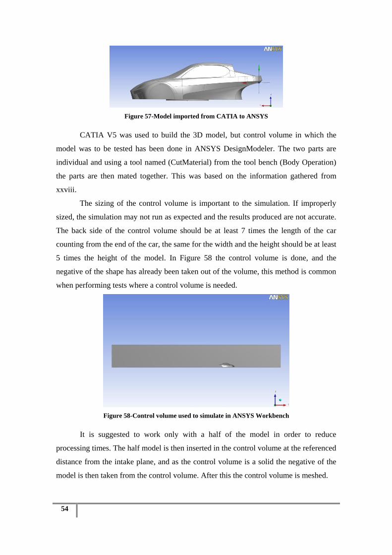
54

Figure 57-Model imported from CATIA to ANSYS

CATIA V5 was used to build the 3D model, but control volume in which the

model was to be tested has been done in ANSYS DesignModeler. The two parts are

individual and using a tool named (CutMaterial) from the tool bench (Body Operation)

the parts are then mated together. This was based on the information gathered from

xxviii.

The sizing of the control volume is important to the simulation. If improperly

sized, the simulation may not run as expected and the results produced are not accurate.

The back side of the control volume should be at least 7 times the length of the car

counting from the end of the car, the same for the width and the height should be at least

5 times the height of the model. In Figure 58 the control volume is done, and the

negative of the shape has already been taken out of the volume, this method is common

when performing tests where a control volume is needed.

Figure 58-Control volume used to simulate in ANSYS Workbench

It is suggested to work only with a half of the model in order to reduce

processing times. The half model is then inserted in the control volume at the referenced

distance from the intake plane, and as the control volume is a solid the negative of the

model is then taken from the control volume. After this the control volume is meshed.

ISEL


PROJECT VEECO

55

Figure 59-Test volume and model meshed using ANSYS workbench

Meshing is started by double clicking on the (Generate CFX Mesh) tab in the

Project Page. Six composite 2D regions where created, in order to identify the different

locations, the names where, Inlet, Outlet, Free1, Free2, SymP, and VEECO. This

regions represent the inlet of the flow, the outlet, the free regions (where there are no

walls, since the wind tunnel was the open kind), the symmetry plane (needed because

only half model was tested), and VEECO, this last one represented the half model to be

tested. This procedure also allows for different mesh settings in the different regions. In

this work the model imported from CATIA V5 had small edges, this had to be

redesigned and eliminated, or the mesh could not be done.

This analysis began with a simple and low refined mesh and evolved to a more

refined one in 2 steps, this allows comparing values between them and demonstrating

the importance of the mesh. The first approach was exactly as suggest in the tutorial

without inflation, the result can be observed in Figure 59 and Figure 60. The refinement

settings used are indicated in Table 4.

56

Table 4 – Mesh definitions

Mesh definitions

Mesh 1 Mesh 2 Mesh 3

Default Body Spacing Max. Spacing:

800mm

Max.

Spacing:300mm

Max. Spacing:100mm

Default Face Spacing Angular Resolution Angular Resolution Angular Resolution

Face Spacing

(Regarding only the

model)

Constant Edge

Length: 15mm

Constant Edge

Length: 10mm

Constant Edge Length:

15mm

Inflation No Number of Inflated

Layers: 5

No

Proximity No Surface Proximity:

Yes

Number of elements

Across the Gap: 3

Surface Proximity:

Yes

Number of elements

Across the Gap: 5

Number of Nodes 55010 64348 98747

Number of Elements 300760 299955 415319

Alongside with these settings the Physics Preference was CFD, and the Solver

Preference was CFX, were common to all the tests. It is important to refine the mesh

where the flow is predictable to be more complex, the options Inflation and Proximity

where used to improve the quality. This was done following the blunt body CFX mesh

help. The options taken to improve the quality of the mesh were chosen by following

the user manual from the software and, by evaluating the final results that were

effectively better as the mesh was improved. Due to the limited capacity of the

computer provided (only 4 Gb of memory) the inflation option was abandoned.

Figure 60-Test volume Mesh 1 using ANSYS Workbench

ISEL


PROJECT VEECO

57

Figure 61-Model Mesh 1 using ANSYS Workbench

Figure 62 – Control volume Mesh 2 Using ANSYS Workbench

Figure 63 – Control volume Mesh 3 Using ANSYS Workbench

Observing Figure 60, Figure 61,Figure 62 and Figure 63 the evolution of the

mesh becomes quite noticeable. In the 3rd

mesh the amount of elements around the

geometry demonstrates the option taken. In Figure 64 the Mesh Calculator tool from

ANSYS displays the information on the meshes used.

58

Figure 64 – Mesh Calculator (ANSYS Workbench tool)

Analysing this information the number of nodes increase, although the number

of elements slightly decreases when the inflation tool is used as the number of

tetrahedral. The number of wedges and pyramids increases, although there are no

hexahedra elements. In general, a good quality mesh can be defined as one that has the

proper refinements around the primary areas of interest, the edges and shape of the

geometry should also remain well defined and not altered by the mesh in any way. A

proper inflation layer growing outward from the body is also desirable to produce better

definition of the boundary layer. This information was gathered by reading the ANSYS

Workbench manuals and by performing the tutorials available. In this case the inflation

approach was not possible in the 3rd

mesh (although attempted, it was made unavailable

by the mesher) so a large increase in the number of elements was chosen. The file is

created and has the “.gtm” extension; this is an option that can be selected from the

options menu. The solution time of the first run was approximately eight hours, the

number of runs made for each mesh varied between fifteen to twenty, depending on the

results and the final mesh took ten hours to run each time some change was made.

4.1. Creating the simulation

After the file is created the test can be performed, and to do so, the tutorial guide

from ANSYS cfx help, “Flow around a blunt body” was followed.

The software ANSYS Workbench is started and the module CFX-Pre is

selected, a new simulation is started using the New Simulation tab and the mesh file can

be imported, just by using the Import Mesh tab and selecting the previously created

“gtm” file.

The method employed to simulate the wind tunnel in the control volume is to

have one inlet, and one outlet. The free walls represent the open volume of the real wind

tunnel, and the symmetry simulates the other half of the model. The inlet will have only

ISEL


PROJECT VEECO

59

the u velocity component, this method allows the reuse of the same mesh for all

simulation runs at different wind speeds, by just updating the inlet velocity components.

In Figure 65 the inlet is represented by the arrows pointing –x direction at the top of the

control volume, the outlet is the other side with the arrows pointing out. The symmetry

plane is represented by the red arrows.

Figure 65 – ANSYS Workbench CFX Pre setup

The setup was defined as follows; the default Analysis Type specified is for a

steady state, this should be checked under “Simulation”, “Analysis Type” then

“Analysis Type” entry.

The domain has to be created taking in consideration several aspects, as the flow

in the domain is expected to be turbulent and approximately isothermal, the Shear Stress

Transport (SST) turbulence model with automatic wall function treatment will be used

because of its highly accurate predictions of flow separation. To take advantage of the

SST model, the boundary layer should be resolved with at least 10 mesh nodes. In this

study an ideal gas is used, since when modelling a compressible flow using the ideal gas

approximation to calculate density variations, it is important to set a realistic reference

pressure, because some fluid properties depend on the absolute fluid pressure(calculated

as the static pressure plus the reference pressure). The domain created by using the icon

60

“Domain” is named as VEECO, and the settings are, Basic Settings-Fluid List- Air Ideal

Gas, under this tab the reference pressure is set to 1 atm. The tab Fluid models is

selected and the heat transfer option is set to Isothermal, under it, the temperature is set

to 298.15 [K] (equivalent to 25º)since this was the highest value achieved in the real

wind tunnel, the Turbulence Options is set to Shear Stress Transport. Then the

composite region is created by selecting from the main menu Insert-Composite Region,

the region is named Free Walls (This include Free1 and Free2). The boundary

conditions are next and the first is named Inlet, the boundary type is set to inlet as the

location, the boundary details are flow regime set to Subsonic, mass and momentum

option set to normal speed and defined as 13.9 m/s, this value is updated then in the next

simulations. The Eddy Len. Scale is set to 0.1m. The Outlet is defined as an outlet type

and the relative pressure set to 0 Pa. FreeWalls is the Wall boundary type and the wall

influence on flow is set to free Slip. SymP is the symmetry plane and the boundary type

is set to Symmetry. The last Boundary Condition is the VEECO model and the

boundary type is set to wall, the wall influence on flow option is set to No Slip.

The Global Initialization tab is selected and the Global Settings set are, Initial

Conditions – Cartesian Velocity Components – Option- Automatic with value,

Cartesian Velocity Components- U-13.9m/s, the others are set to 0 m/s. The turbulence

Eddy dissipation is selected. The solver control defines the maximum number of

iterations set to 60 with a convergence criterion of 1e-05, which means the software

assumes the solution of the problem is converging when the residual value of the

equations defining pressure, mass continuity, and turbulence are lower than the value

defined by the user . The Physical Timescale is selected and the physical timescale set

to 2 s. The solver file is initiated by the tab Write solver file, the results are saved to a

file pre-defined. The files generated are, “ANSYS CFX Pre” file, with the extension

“.cfx” this file contains the definitions for the test, “ANSYS CFX Solver” file, with the

extension “. def" this file allows the simulation to be started in any other computer with

the software installed, and “ ANSYS CFX Post” file with the extension “.resl” this

contains the results from the simulations.

The results are obtained using the CFX-Solver Manager; this is started by

double clicking on the “Solution” tab in the CFX workspace. The “Define Run” dialog

is first displayed; this allows portioning of the problem as well as adjusting the memory

allocation to each of the processing stages of the solver. For this simulation, the default

ISEL


PROJECT VEECO

61

memory settings were used. The “Initialization Option” was set to “Current Solution

Data”. In order to reduce the computational time, the problem can be split up into

several parts and solved in parallel. In this simulation, the problem was split up into four

parts to fully utilize the dual-Core processor in the computer used to run ANSYS. The

“Run Mode selected to “HP MPI Local Parallel” and the number of partitions increased

to four.

The display monitors show the progress of the simulation in terms of the value

of the residuals and plots the residuals. The display monitors also show all errors that

may result from the simulation as well as the total time taken for the simulation to

complete. A screenshot of the display monitors is shown in Figure 66. For certain

meshes; the residuals may not converge satisfactorily down to 1x10-5

. For these

simulations, the results may also not be as accurate as expected. As such, the mesh

should be refined further and the simulation rerun.

This is an iterative process that is very time consuming. In some cases, the

residuals start to oscillate and further convergence was not possible. This behaviour

made impossible to continue simulating since the oscillations only increased. In such

situations, the simulation could stop prematurely and the result at that iteration was

taken as the final result. A minimum convergence tolerance value down to 1x10-4

would

be required for reasonable results. However it was not possible to obtain a better

behaviour of the model, and because of that these studies were not conclusive, therefore

further studies would be needed.

62

Figure 66 – ANSYS Display monitors

After the simulation run has ended the CFX-Post is started by double clicking on

the “Results” tab in the CFX workspace.

The result can be plotted in several ways, one is velocity, drawing the stream

lines where it varies, using a colour scale to identify variations and possibly areas where

the flow gets more turbulent as in Figure 67.

Figure 67-ANSYS analysis for CFX, velocities plotted.

Several simulation runs were conducted, varying the velocity, so that a

comparison with the test in the wind tunnel could be done.

ISEL


PROJECT VEECO

63

The forces on the model can be calculated using “Calculator” tab. The “Function

Calculator” is used to calculate FX (Drag Force), FY (Side Force) and FZ (Lift Force). In

this method of simulation selected FX, FY and FZ correspond to the Normal force. The

force calculated is the one generated on the mesh, this is independent of the symmetry

plane for the flow, so in this case the force is representative of half model, so the result

has to be multiplied by two to get the correct reading.

This is valid for lift and drag, as to the lateral force the reading can be

considered zero as the other half would generate exactly a symmetric force leading to

the result between them being zero.

A screenshot of the Function Calculator is presented in Figure 68.

Figure 68-ANSYS Function Calculator

4.2. Yplus targets

The Yplus is a non-dimensional wall distance for wall bounded flow that is defined by:

Where *u is the friction velocity, y is the distance to the nearest wall and is the local

kinematic viscosity of the fluid. This non-dimensional value is a measure of the quality

of the mesh in the boundary layer around the test object. Based on the boundary layer

theory, Yplus is the local thickness Reynolds number. In CFD it is a nondimensional

yuy

*

(11)

64

distance from the wall to the first grid point. CFD codes assume that the viscous

sublayer occur between the wall and the first grid point. This is the point where the code

switches from the log-law to the viscous sub-layer and it should occur at a value of

around 30. If the mesh is too fine near the wall, the value of Yplus will be small, and the

near wall velocity will be over predicted. If the value is too high the code will apply the

law of the wall to the outer wake where it is not valid.

The target of the simulations was to get the Yplus below 10 versus trying to

optimize the mesh to reduce Yplus values to near unity. This trade-off was considered

due to the long computational times required and the large number of data points that

needed to be collected. The values of Yplus achieved for this test case were 207.804,

509.446 and 8032. Therefore also in this case the results did not correspond to the

requisites that were previously mentioned, and further studies would be needed to

eliminate the problems found.

Since the values from the wind tunnel are the forces acting in the model, the tests in

ANSYS where conducted in the same way. Varying the velocity according to what was

made in the Wind tunnel the results are presented in Table 5.

Table 5-Values from ANSYS test, force results when varying velocity (1st mesh)

Wind Speed

m/s

F(x) (Drag)

N

F(y) (Side Force)

N

F(z) (Lift)

N

13.9 -1.30 0 -0.32

19.9 -2.62 0 -0.78

31.62 -6.53 0 -2.29

36.7 -8.77 0 -3.21

41.65 -11.27 0 -4.26

45.3 -13.31 0 -5.13

51.5 -17.18 0 -6.8

55.56 -20 0 -8.03

59.9 -23.24 0 -9.44

Runs where repeated, changing the mesh for several velocities (Table 6 - Table 7).

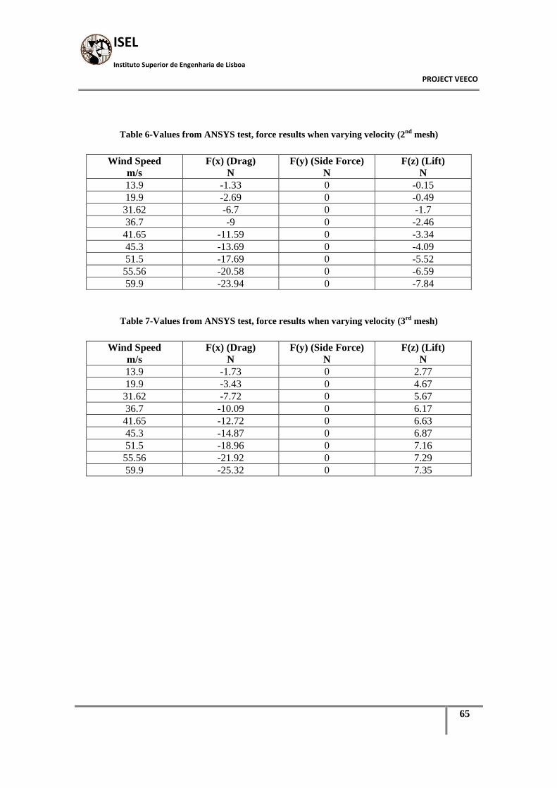
ISEL


PROJECT VEECO

65

Table 6-Values from ANSYS test, force results when varying velocity (2nd

mesh)

Wind Speed

m/s

F(x) (Drag)

N

F(y) (Side Force)

N

F(z) (Lift)

N

13.9 -1.33 0 -0.15

19.9 -2.69 0 -0.49

31.62 -6.7 0 -1.7

36.7 -9 0 -2.46

41.65 -11.59 0 -3.34

45.3 -13.69 0 -4.09

51.5 -17.69 0 -5.52

55.56 -20.58 0 -6.59

59.9 -23.94 0 -7.84

Table 7-Values from ANSYS test, force results when varying velocity (3rd

mesh)

Wind Speed

m/s

F(x) (Drag)

N

F(y) (Side Force)

N

F(z) (Lift)

N

13.9 -1.73 0 2.77

19.9 -3.43 0 4.67

31.62 -7.72 0 5.67

36.7 -10.09 0 6.17

41.65 -12.72 0 6.63

45.3 -14.87 0 6.87

51.5 -18.96 0 7.16

55.56 -21.92 0 7.29

59.9 -25.32 0 7.35

66

Figure 69 - Representation of X force component, numerical simulation in ANSYS

Figure 70 - Representation of Z force component, numerical simulation in ANSYS

13,9 19,9 31,62 36,7 41,65 45,3 51,5 55,56 59,9

F X (N) Mesh 1 -1,30 -2,62 -6,53 -8,77 -11,27 -13,31 -17,18 -20,00 -23,24

F X (N) Mesh 2 -1,33 -2,69 -6,70 -9,01 -11,58 -13,69 -17,69 -20,58 -23,94

F X (N) Mesh 3 -1,73 -3,43 -7,72 -10,09 -12,72 -14,87 -18,96 -21,92 -25,32

-30

-25

-20

-15

-10

-5

0

Fo

rce

(N)

Speed (m/s)

Force in X (Drag) - ANSYS

13,9 19,9 31,62 36,7 41,65 45,3 51,5 55,56 59,9

F Z (N) Mesh 1 -0,32 -0,78 -2,29 -3,21 -4,26 -5,13 -6,80 -8,03 -9,44

F Z (N) Mesh 2 -0,15 -0,49 -1,70 -2,46 -3,34 -4,09 -5,52 -6,59 -7,83

F Z (N) Mesh 3 2,77 4,67 5,67 6,17 6,63 6,87 7,16 7,29 7,35

-12

-10

-8

-6

-4

-2

0

2

4

6

8

10

Fo

rce

(N)

Speed (m/s)

Force in Z (Lift) - ANSYS

ISEL


PROJECT VEECO

67

Figure 71 - Forces developed in the model with ANSYS, for the 3rd

mesh.

The results are presented in Figure 69, Figure 70. Taking in consideration the values

from Figure 71, it becomes clear the importance of the mesh used. In the roughest mesh

the result force indicated down force, but the finest mesh indicates the presence of lift,

when comparing the values from drag and lift directly the first two values indicates the

tendency to generate more lift than drag, but then, the overall tendency is to have more

drag than lift. An interesting fact is the value of the force in the Z axis that indicates the

presence of lift; this might be due to the specific geometry of the body. It is important to

take in consideration that the test can be improved over time and the values achieved

can modify. When the comparison between tests is made further ahead the conclusions

taken are analysed in a more accurate way.

13,9 19,9 31,62 36,7 41,65 45,3 51,5 55,56 59,9

F X (N) Mesh 3 -1,73 -3,43 -7,72 -10,09 -12,72 -14,87 -18,96 -21,92 -25,32

F Y (N) Mesh 3 0,00 0,00 0,00 0,00 0,00 0,00 0,00 0,00 0,00

F Z (N) Mesh 3 2,77 4,67 5,67 6,17 6,63 6,87 7,16 7,29 7,35

-30

-25

-20

-15

-10

-5

0

5

10

Fo

rce

(N)

Speed (m/s)

Forces developed- ANSYS

ISEL


PROJECT VEECO

69

5. Wind tunnel testing

5.1. The wind tunnel

According to the information present in xxv, by the 18th

and 19th

centuries it was

realized that the knowledge of what we now call aerodynamics was very small. This led

to the concept of building instrumented facilities to measure aerodynamic forces and

moments.

The early experimenters recognized that aerodynamic forces were a function of the

relative velocity between the air and the model. Thus one could move the model

through still air or let the air move past a stationary model. Initially this led to use of

nature natural winds as a source of moving air, but the perversity of nature quickly led

to the building of mechanical devices to move the model through the air. The simplest

method of accomplishing this was to mount the model on a whirling arm that could be

powered by falling weights and pulleys.

In the 18th

century, Robins, one of the early experimental aerodynamicists used a

whirling arm to study various shapes. He reached the conclusion that the relationships

among body shape, orientation to the relative wind, and aerodynamic forces was much

more complex than indicated by the then current theory.

Near the end of the 19th

century the major fault of a whirling arm was apparent. This

fault was that the wing was forced to fly in its own disturbed wake. This led to the wind

tunnel where the model was held stationary and the air was moved past the model.

Although wind tunnels have been built in many different configurations, they all

have four basic parts, which are:

A contoured duct to control the passage of the working fluid through the test

section where the model is mounted.

A drive system to move the working fluid through the duct.

A model of the test object, which is either full size or, more often, a reduced-

scale model.

70

Instrumentation that may either be quite simple, such as a spring scale to

measure force, or extremely complex such as a modern balance feeding its

output to relatively large digital computers

The Wright brothers started by using the natural wind to conduct experiments and

realized that the accepted aerodynamic design data were in error, so they designed a

second version of the test glider in 1901 and used their results, but the pitching moment

due to large airfoil camber made the glider difficult to control. This result forced them

to reduce the camber. By now the Wrights were convinced that the available

aerodynamic data were in error and they decided to rely on their own data.

The Wrigths then used a bicycle to provide wind to compare two test models

mounted on a horizontal wheel ahead of the bicycle. The crude data from these tests

reinforced their opinion to reject all published data. They then build a wind tunnel; first

a simple tunnel and then a larger and more sophisticated tunnel with a 16×16 sq. in. test

section to obtain data for their No. 3 glider in 1902. Curiously, the only mistake the

wrights made in their large wind tunnel was the placement of the fan upstream of the

test section. The use of honey-combs and screens reduced, but did not remove, the fan

swirl and turbulence. Although it was the Wright brothers that conclusively

demonstrated the value of wind tunnels in aerodynamic design in 1903, it was the

Europeans who capitalized on this fact by using about a dozen major wind tunnels built

in government-funded aeronautical laboratories to achieve technical leadership in

aviation between 1903 and 1914.

No single wind tunnel is adequate for all possible aerodynamic tests. In general,

wind tunnels can be divided into four broad categories by their speed ranges:

Subsonic- with a maximum Mach number of up to 0.4

Transonic – with a maximum Mach number to 1.3

Supersonic-with a maximum Mach number up to 4.0 to 5.0

Hypersonic- with a Mach number to 5.0 or higher

There are special-purpose subsonic tunnels, such as spin tunnels, icing tunnels,

meteorological tunnels, and tunnels designed for the testing of buildings. The rest of the

low-speed tunnels can be classified as general purpose tunnels. These tunnels can be

adapted for many types of special tests, such as buildings, flutter, store separations,

windmills, skiers, skydivers, or dynamic tests for spins. Basically they are designed to

test vehicles and their component parts. These tunnels will often have large test sections

ISEL


PROJECT VEECO

71

for V/STOL, full scale of smaller aircraft, and automobiles. In the medium size tunnels

with a test-section area around 100 sq. ft. large amounts of both research and aircraft

developments testing is accomplished. With smaller size test sections, the tunnels are

used for research and instructional purposes. Ideally, the size of the tunnel is determined

by its purpose.

The purpose of a wind tunnel is to provide a uniform and controllable air flow in

the test section that passes over the model. In an ideal case, the model should be tested

at the same Reynolds and Mach number as the full-scale vehicle. This, leads to a full-

scale model, a very large tunnel, and very expensive models, or smaller pressurized or

cryogenic tunnels, also with expensive models. Matching Reynolds and Mach number

are mutually contradictory when using scale models. The Reynolds number is

proportional to the ratio of inertia forces to viscous forces and the behaviour of

boundary layers and wakes is influenced by Reynolds number. The Mach number is

proportional to the ratio of inertial to elastic forces, taken as the square root of

V2/a

2=M

2. The change in gas properties such as density in passing through shock or

compression waves depends on the Mach number. If the flow cannot be considered

incompressible, the Mach number must be matched. Usually it is not necessary to

produce the full-scale Reynolds number, but it must be of a reasonable value.

When the Mach number is much less than 1, this tends to require a tunnel speed

approximately equal to the full-scale ratio between the scale-model and the real vehicle.

5.2. Test Section

Over the years many shapes have been used for test sections, such as round,

elliptical, square, rectangular, hexagonal, octagonal, rectangular with filleted corners,

flat ceiling, and floor with half round ends, the difference in losses in the test section

due to the tunnel shape are negligible.

5.3. Corrections

As the air proceeds along the test section the boundary layer thickens. This action

reduces the effective area of the jet and causes an increase of velocity. The velocity

72

increase in turn produces a drop in local static pressure, tending to draw the model

downstream. This added drag is called “horizontal buoyancy”

5.4. Model force, moment, and pressure measurements

The purpose of the load measurements in the model is to make available the forces,

moments, and pressures so that they may be corrected for tunnel boundary and scale

effects, and utilized in predicting the performance of the full-scale model.

The loads may be obtained by any of three methods:

Measuring the actual forces and moments with a wind tunnel balance

Measuring the effect that the model has on the airstream by wake surveys and

tunnel-wall pressures

Measuring the pressure distribution over the model by means of orifices

connected to pressure measuring devices.

The method available in the tunnel used is “Balances”, wherein the wind tunnel

balance must separate the forces and moments and accurately present the small

differences in large forces, all without appreciable model deflection.

5.5. Testing automobiles and trucks

Tunnel testing can help improve the mileage of a car. The automotive engineer uses

two types of wind tunnels: standard tunnels for testing scale models(mostly for drag)

and full-scale automotive tunnels, wherein the car or small truck is tested with the

engine running and putting out the proper power for the speed. It is interesting that there

is no counterpart of the full-scale auto test in the aviation world. That would require an

enormous tunnel with incredible heat removal capabilities. As a counterbalance, a wind

tunnel test of an airplane model does not require the presence of a host of experts

covering each of the many auto components which may be under test.

5.6. Testing scale models of cars and small trucks

Because typical car drag at 55 mph accounts for about 60% of the total power, the

great preponderance of the scale model testing is concerned with the reduction of drag.

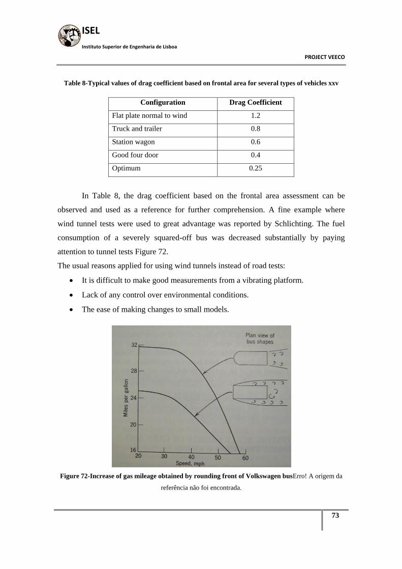
ISEL


PROJECT VEECO

73

Table 8-Typical values of drag coefficient based on frontal area for several types of vehicles xxv

Configuration Drag Coefficient

Flat plate normal to wind 1.2

Truck and trailer 0.8

Station wagon 0.6

Good four door 0.4

Optimum 0.25

In Table 8, the drag coefficient based on the frontal area assessment can be

observed and used as a reference for further comprehension. A fine example where

wind tunnel tests were used to great advantage was reported by Schlichting. The fuel

consumption of a severely squared-off bus was decreased substantially by paying

attention to tunnel tests Figure 72.

The usual reasons applied for using wind tunnels instead of road tests:

It is difficult to make good measurements from a vibrating platform.

Lack of any control over environmental conditions.

The ease of making changes to small models.

Figure 72-Increase of gas mileage obtained by rounding front of Volkswagen busErro! A origem da

referência não foi encontrada.

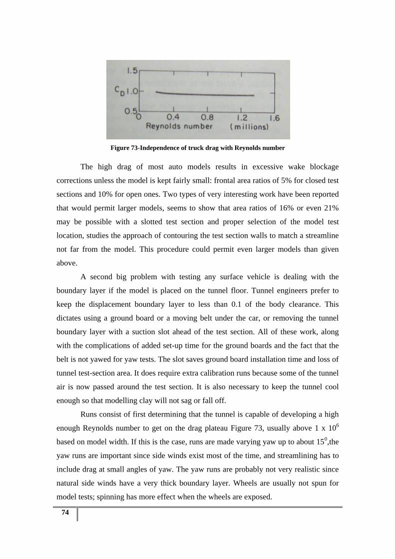
74

Figure 73-Independence of truck drag with Reynolds number

The high drag of most auto models results in excessive wake blockage

corrections unless the model is kept fairly small: frontal area ratios of 5% for closed test

sections and 10% for open ones. Two types of very interesting work have been reported

that would permit larger models, seems to show that area ratios of 16% or even 21%

may be possible with a slotted test section and proper selection of the model test

location, studies the approach of contouring the test section walls to match a streamline

not far from the model. This procedure could permit even larger models than given

above.

A second big problem with testing any surface vehicle is dealing with the

boundary layer if the model is placed on the tunnel floor. Tunnel engineers prefer to

keep the displacement boundary layer to less than 0.1 of the body clearance. This

dictates using a ground board or a moving belt under the car, or removing the tunnel

boundary layer with a suction slot ahead of the test section. All of these work, along

with the complications of added set-up time for the ground boards and the fact that the

belt is not yawed for yaw tests. The slot saves ground board installation time and loss of

tunnel test-section area. It does require extra calibration runs because some of the tunnel

air is now passed around the test section. It is also necessary to keep the tunnel cool

enough so that modelling clay will not sag or fall off.

Runs consist of first determining that the tunnel is capable of developing a high

enough Reynolds number to get on the drag plateau Figure 73, usually above 1 x 106

based on model width. If this is the case, runs are made varying yaw up to about 150,the

yaw runs are important since side winds exist most of the time, and streamlining has to

include drag at small angles of yaw. The yaw runs are probably not very realistic since

natural side winds have a very thick boundary layer. Wheels are usually not spun for

model tests; spinning has more effect when the wheels are exposed.

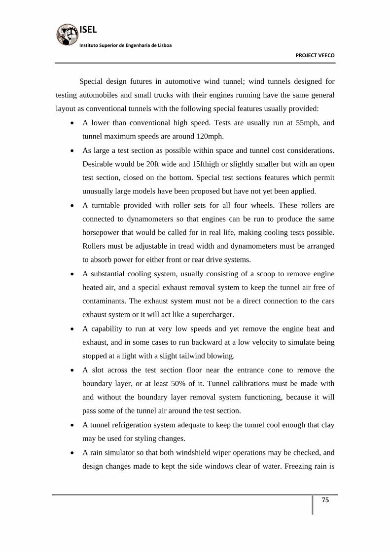
ISEL


PROJECT VEECO

75

Special design futures in automotive wind tunnel; wind tunnels designed for

testing automobiles and small trucks with their engines running have the same general

layout as conventional tunnels with the following special features usually provided:

A lower than conventional high speed. Tests are usually run at 55mph, and

tunnel maximum speeds are around 120mph.

As large a test section as possible within space and tunnel cost considerations.

Desirable would be 20ft wide and 15fthigh or slightly smaller but with an open

test section, closed on the bottom. Special test sections features which permit

unusually large models have been proposed but have not yet been applied.

A turntable provided with roller sets for all four wheels. These rollers are

connected to dynamometers so that engines can be run to produce the same

horsepower that would be called for in real life, making cooling tests possible.

Rollers must be adjustable in tread width and dynamometers must be arranged

to absorb power for either front or rear drive systems.

A substantial cooling system, usually consisting of a scoop to remove engine

heated air, and a special exhaust removal system to keep the tunnel air free of

contaminants. The exhaust system must not be a direct connection to the cars

exhaust system or it will act like a supercharger.

A capability to run at very low speeds and yet remove the engine heat and

exhaust, and in some cases to run backward at a low velocity to simulate being

stopped at a light with a slight tailwind blowing.

A slot across the test section floor near the entrance cone to remove the

boundary layer, or at least 50% of it. Tunnel calibrations must be made with

and without the boundary layer removal system functioning, because it will

pass some of the tunnel air around the test section.

A tunnel refrigeration system adequate to keep the tunnel cool enough that clay

may be used for styling changes.

A rain simulator so that both windshield wiper operations may be checked, and

design changes made to kept the side windows clear of water. Freezing rain is

76

also needed. Leaks may be discovered, but are considered bad manufacturing

procedure rather than part of the tests.

Auxiliary hot water facilities such that cars can have cooling studies made

without the engines running; hot water being pumped through the cooling

system and its efficacy measured. This is done to make sure styling changes

have not hurt cooling prospects in proposed designs for which engines are not

yet ready.

5.7. Low speed wind tunnel

A low-speed wind tunnel is a tunnel where the speed achieved is below 300 mph or

so. Wind tunnels offer a rapid, economical, and accurate mean for aerodynamic

research.

ISEL


PROJECT VEECO

77

6. Wind tunnel analysis

6.1. Introduction

The Portuguese Air force aerodynamic testing infrastructure, has assumed an

important role in investigation and development of several national and also

international projects. These facilities are designed for Aerospatiale development more

specifically for project validation and certification.

When testing, it is important to define what needs to be measured and how to

perform the measurements. The forces developed by the movement of a body in a fluid

are due to the fluid properties. The properties to be considered are as follows:

6.1.1. Inertia Inertia is proportional to the mass and acceleration of the fluid disturbed.

Considering a constant volume subjected to a constant acceleration:

where:

6.1.2. Viscosity The force developed due to this characteristic of the fluid is given as:

where is the viscosity coefficient

6.1.3. Gravity

being g the gravitational acceleration.

2233

Vl

l

V

Vl

t

VlF

(12)

3

1

/

.

density kg m

l Dimension m

V Velocity m s

t Time s

VlF

11.. smKg

glF 3

(13)

(14)

78

6.1.4. Compressibility The compressibility relates to the relative volume change of a fluid as a response

to a force applied to it. It is defined by the letter E and its unities are N.m-2

.

When a body is immersed in a flow the main forces that interact are defined by

the following formulas:

Reynolds number = Inertia/Viscosity=

Mach number = Inertia/Compressibility=

Froude number = Inertia/Gravity=

Considering a real body and a scale model, if both are being tested with the same

Reynolds, Mach and Froude numbers the flow on both can be considered to be

identical. The resultant forces and moments can be related directly between them.

6.2. Application

When the models used are rigid and stationary there is no need to guarantee the

equivalence between Froude numbers. Mach number equivalencies is only important

when the velocities are high, making the effect of compressibility be more important

than the ones of viscosity, in reduced velocities (M smaller than 0.3) this equivalence is

not necessary, leaving only the equivalence between Reynolds numbers to be

determined.

As for a fixed geometry the flow field will be characterized only by the Reynolds

number (Although this statement refers to an over-simplification, because the

turbulence characteristics of the oncoming flow also influence the details of the flow

field), the aerodynamic force will only depend on the Reynolds number. If an

aerodynamic force like drag (d) is made dimensionless by introducing a force

coefficient defined as

2ElF

Vl

a

V

lg

2V

(15)

AV

DCd

2

2

1

(16)

ISEL


PROJECT VEECO

79

To note that:

Meaning CD is only a function of Re. In order to relate the test results from the model to

the real vehicle it is necessary for them to be dynamically similar for the forces to be

scale invariant.

This can only be achieved if the relation in (18) is valid. (the suffices m and v

relate to model and real vehicle) Usually it is not practical to use another fluid but air

for the model tests, and for standard wind-tunnels the air properties in the wind-tunnel

are not greatly different from those experienced by the prototype, which implies:

From (19), if the scale model is 1/5, the result will be , which means

that a real vehicle speed of 100km/hr relates to a model speed of 500km/hr. When the

speed reaches this value the compressibility effects are no longer negligible. In practice

it is extremely hard to achieve dynamic similarity between the models. To solve these

problems the use of large and expensive facilities that can compress the air (there by

increasing its density) and large models make possible the dynamic similarities.

The restriction for the model was the dimensions of the wind tunnel. Due to this the

scale used was 1:5.56.

6.3. Wind tunnel characteristics

Aerodynamic test where conducted in the laboratory of aeronautics in the

Portuguese air force academy.

This tunnel is subsonic of incompressible flow of the Gottingen kind, and can

operate in open or closed section Figure 74.

It is composed by a DC motor controlled by a potentiometer that actuates a simple

axial ventilator which is responsible for the air flow in the tunnel, an open jet test

(Re)FCd

vm ReRe

(17)

(18)

v

m

vm V

L

LV (19)

vm VV 5

80

section, anti-turbulence screens, contraction cone, collector, two diffusers and four

groups of guiding vanes.

Figure 74-Aerodynamic tunnel from the AFA facilities

In Table 9 the maximum and minimum speed values of the air in the test section of

the wind tunnel, are indicated.

Table 9-Maximum and minimum speed of air in the test section

Max. 70m/s

Min. 5m/s

The open jet test section has the following dimensions: (Table 10)

Table 10-Dimensions of the test section

Length 2.0 m

Height 0.8 m

Width 1.3 m

The tunnel is equipped with 15 pressure measuring ports and a thermometer.

The temperature is needed to calculate air density, which is given as:

where:

R - Perfect gas constant

T - Temperature [K]

The static ambient pressure can be taken from a barometer placed near the working

area.

RTP (20)

ISEL


PROJECT VEECO

81

6.4. Instrumentation

The tunnel is equipped with an aerodynamic balance of six components (3 forces

and 3 momentums), the models to test should be connected to the balance by a rigid

connection in a way the forces and moments are directly transmitted to the balance. The

values measured are transmitted to a computer that has software to calculate only the

aerodynamic forces and momentum actuating the model. The balance characteristics are

represented in Table 11. The accuracy of the balance is +- 1N for forces and +-0.5N/m

for momentum.

Table 11-Main characteristics of the Balance used in the test.

Max weight 50Kg

Max distance from the C.G. of

the model to the fixing point.

250mm

Max. Forces

Resistance +-670N

Lateral force +-670N

Lift +-1340N

Max. Momentums

Roll 54Nm

Pitching 54Nm

Yawing 68Nm

6.5. Test procedure

In general the flow in the test area of aerodynamic tunnels is not aligned with the

longitudinal axis, having some cross flow or up flow. The vertical component is some

part due to the balance; which deflects a part of the flow. A correction for this can be

determined by testing the model in its normal position and then in an inverted position,

although this is more indicated for airplane models, in the case of a car the all body is in

the zone of the steady flow.

82

The model was bolted to the balance and aligned with the flow Figure 75, and the test

started.

Figure 75-Model in the test area(Model from the 3D printer)

The tests were conducted at several speeds in order to determine the Drag

coefficient. The speed of the wind tested can be seen in Table 12.

Table 12-Aerodynamic test speeds.

Test Number Wind Speed (m/s)

1 13.9

2 19.9

3 31.62

4 36.7

5 41.65

6 45.3

7 51.5

8 55.56

9 59.9

In each test 6 measures were made, the variables measured were Fx, Fy, and Fz,

and Mx, My, Mz. The values are presented in Table 13.

Table 13-Values from Wind tunnel test, force results when varying velocity

Wind Speed

m/s

F(x) (Drag)

N

F(y) (Lift)

N

F(z) (Side Force)

N

13.9 -1.37 -3.13 -0.07

19.9 -2.73 -6.35 -0.13

31.62 -6.86 -15.48 -0.37

36.7 -9.27 -20.75 -0.5

41.65 -11.88 -26.25 -0.64

45.3 -14.20 -30.49 -0.81

51.5 -18.26 -38.29 -0.9

55.56 -21.46 -44.44 -0.9

59.9 -24.93 -54.3 -1.33

ISEL


PROJECT VEECO

83

The axes of the wind tunnel where confirmed with respective user manual, as

indicated in Figure 76. The X axis represents the drag, Y axis the lift and the Z axis the

lateral forces. The direction of the axis is also important to note. Although X axis is in

the same position as in the ANSYS program the Y axis is the equivalent to the Z axis

from ANSYS and the direction is positive downwards.

Figure 76–Reference axis of the wind tunnel test balance – From HORIBA user manual

As the axis from the balance where corrected, the values were used directly to

calculate Drag. (Table 14)

Table 14-Drag coefficient values calculated

Test Number Drag coeff.

1 0.28

2 0.27

3 0.26

4 0.27

5 0.27

6 0.27

8 0.27

9 0.27

Average Value 0.27

The values of Drag indicated in Table 14 where calculated using eq.(16), with a

frontal area of 0.043m2, and a value of 1.184 Kg/m

3, for .

The values from the Fy component also suggest the existence of lift generated

by the car, and it actually increases as the speed builds up. This can be seen in Table 13

and Figure 77.

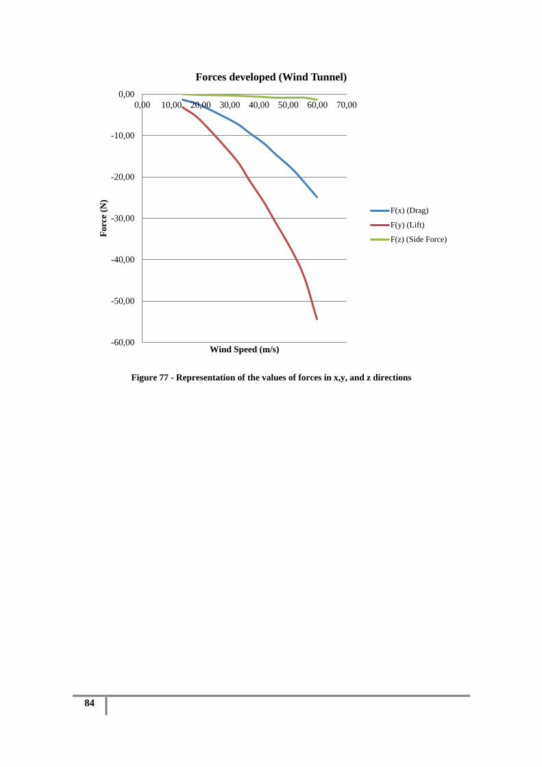
84

Figure 77 - Representation of the values of forces in x,y, and z directions

-60,00

-50,00

-40,00

-30,00

-20,00

-10,00

0,00

0,00 10,00 20,00 30,00 40,00 50,00 60,00 70,00F

orc

e (N

)

Wind Speed (m/s)

Forces developed (Wind Tunnel)

F(x) (Drag)

F(y) (Lift)

F(z) (Side Force)

ISEL


PROJECT VEECO

85

7. Conclusions on the work

In order to compare the results from the Wind Tunnel and from ANSYS-CFX, the

3rd

mesh was selected since the results tended to be more close to the ones from the real

tests, thus seeming to indicate that the more refined mesh had a better quality. As one of

the objectives of this work was to compare the results from the CFD and the real test,

and taking into consideration that the values from the wind tunnel test were more

realistic, the 3rd

mesh seemed to be the reasonable choice as the values tended to

confirm what the wind tunnel test show, at least at an initial stage. It also indicated the

importance of tailoring the mesh to the objective since the results from the other meshes

contradict the ones from the last one. It would be a gross mistake to allege the results

from the wind tunnel are not correct based on the first two meshes since the values

change when the mesh quality increases. It is however important to say that further

studies would be required, as the present ones were not conclusive.

The values from the three different axis forces for the several wind velocities are

compared separately in graphs.

Figure 78 - Comparison between the analysis in ANSYS-CFX and wind tunnel F(X) Plotted

13,9 19,9 31,62 36,7 41,65 45,3 51,5 55,56 59,9

F X (N) Mesh 3 -1,73 -3,43 -7,72 -10,09 -12,72 -14,87 -18,96 -21,92 -25,32

F X (N) Wind Tunnel -1,37 -2,73 -6,86 -9,27 -11,88 -14,20 -18,26 -21,46 -24,93

-30

-25

-20

-15

-10

-5

0

Fo

rce

(N)

Speed (m/s)

Forces developed ( Drag)- ANSYS vs Wind Tunnel

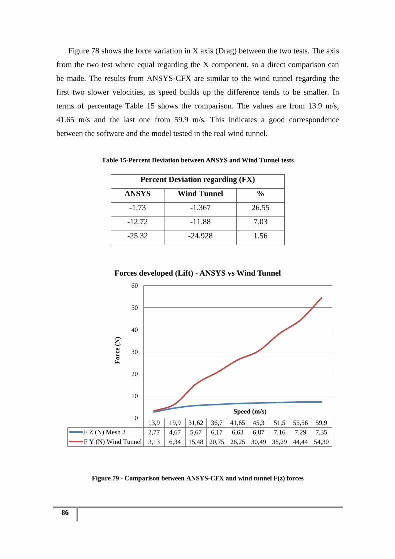
86

Figure 78 shows the force variation in X axis (Drag) between the two tests. The axis

from the two test where equal regarding the X component, so a direct comparison can

be made. The results from ANSYS-CFX are similar to the wind tunnel regarding the

first two slower velocities, as speed builds up the difference tends to be smaller. In

terms of percentage Table 15 shows the comparison. The values are from 13.9 m/s,

41.65 m/s and the last one from 59.9 m/s. This indicates a good correspondence

between the software and the model tested in the real wind tunnel.

Table 15-Percent Deviation between ANSYS and Wind Tunnel tests

Percent Deviation regarding (FX)

ANSYS Wind Tunnel %

-1.73 -1.367 26.55

-12.72 -11.88 7.03

-25.32 -24.928 1.56

Figure 79 - Comparison between ANSYS-CFX and wind tunnel F(z) forces

13,9 19,9 31,62 36,7 41,65 45,3 51,5 55,56 59,9

F Z (N) Mesh 3 2,77 4,67 5,67 6,17 6,63 6,87 7,16 7,29 7,35

F Y (N) Wind Tunnel 3,13 6,34 15,48 20,75 26,25 30,49 38,29 44,44 54,30

0

10

20

30

40

50

60

Fo

rce

(N)

Speed (m/s)

Forces developed (Lift) - ANSYS vs Wind Tunnel

ISEL


PROJECT VEECO

87

Figure 79 refers to the lift force, but as the axis systems are different from the two

tests in ANSYS-CFX its Z in the Wind Tunnel it was represented by Y, and the value

was negative since the positive side pointed to the ground and the directions of the force

is upwards. To be able to compare both values sets, the ones from the Wind Tunnel

where turned positive. Table 16 shows the comparison. In this case the difference tends

to be greater as the speed builds up, which can be partially due to the mesh quality.

Table 16-Percent Deviation between ANSYS and Wind Tunnel tests

Percent Deviation regarding (FZ (ANSYS) and FY (Wind Tunnel))

ANSYS Wind Tunnel %

2.77 3.13 11.64

6.63 26.25 74.74

7.35 54.30 86.45

Figure 80 - Comparison between ANSYS-CFX and wind tunnel F(Y) results

13,9 19,9 31,62 36,7 41,65 45,3 51,5 55,56 59,9

F Y (N) Mesh 3 0,00 0,00 0,00 0,00 0,00 0,00 0,00 0,00 0,00

F Z (N) Wind Tunnel 0,07 0,13 0,37 0,50 0,64 0,81 0,89 0,90 1,33

-1

-1

0

1

1

2

2

3

3

4

4

Fo

rce

(N)

Speed (m/s)

Forces developed (Side Force)- ANSYS vs Wind Tunnel

88

Figure 78, Figure 79, and Figure 80 present the graphs of experimental versus

ANSYS-CFX data for this test case. The experimental results are represented by the red

line, and the results of ANSYS-CFX are represented by the blue one.

The results show differences between the tests. This was expected as turbulence

models used in ANSYS-CFX still cannot fully describe turbulent behaviour and hence

its effects on drag. Analysing the force in X component (Drag), the software tends to

achieve a value quite similar to the wind tunnel and as speed builds up the difference

decreases, and by comparing the results from the other meshes the value tends to

become more close to the wind tunnel as the quality of the mesh improves, this

indicates the importance of a good mesh. Comparing the values of lift in the first two

velocities, ANSYS-CFX run, yields values very similar to the ones of the wind tunnel

although this changes with the increase in velocity. The value for the drag coefficient

resulted to be low, 0.27. In appendix (Appendix I) one can find the procedure for a coast

down test that resulted in a value of 0.38.

This difference may be due to several aspects, such as the problems with the model,

the outside surface was very rough, and this many times leads to a delay in the

detachment of the boundary layer leading to a decrease in drag.

The amount of simplifications that had to be used influenced the results, and

possibly led to the low drag value. During the wind tunnel test when the speed reached

41.65m/s the model started to vibrate, and as the speed build up the vibration increased,

this may have led to incorrect values of force measured. The fact of the model was

attached to a steady plate created an incorrect ground effect, since in real conditions

there is a big difference between the speed of the road and the vehicle. Using the

software ANSYS it is possible to rapidly identify critical zones where for instance the

speed reaches the highest value or where is most probable to appear turbulent flow or

detachment in the boundary layer.

The value of the force measured in the Y axis (Wind Tunnel Test), is an indicator

that the shape is prone to generate lift, this means it can benefit from an accurate study

regarding this subject.

The force present in the Z axis (Wind Tunnel Test) is due to misalignments of the

model in relations with the direction of the flow.

A fact to be taken in consideration is, the ANSYS-CFX study was made to simulate

the wind tunnel test, this means the conditions of the wind tunnel where reproduced in

ISEL


PROJECT VEECO

89

the software in order to be possible to make a direct comparison between the results

gathered in the two.

By analysing Figure 67 becomes quite obvious that the rear section after the rear

window is where the boundary layer detaches from the surface abruptly; studying this

phenomenon more carefully may lead to a smoother transition in this area.

An ANSYS-CFX computation of the flow over a 3D model of VEECO, and the

results compared against experimental data obtained from wind tunnel tests, show that

for drag calculations the results are not reliable, this might be due the turbulence models

used. Further research and improvements with regard to turbulence models must be

made in order to improve computational codes and accuracy of predicting flow

behaviour. Considerable time and computational power was also expended in the use of

ANSYS-CFX to complete the simulations for this research. All this work was a good

indicator that some measures had to be taken regarding the lift generated by the shape of

the vehicle and a rear spoiler was applied in order to reduce this effect. Many times the

best shape in terms of aerodynamics isn‟t the best looking one and in this case the same

happened. For instance, after the simulations and the general study one of the

conclusions was that if the air intake was not really necessary for cooling or any other

specific purpose it should be totally closed, this was because the channel made in such

an opening would take a negative effect in drag, but this conclusion was not taken in

consideration in the final design. The advantage of being a reverse trike could be better

exploited, by tailoring the rear section to have a smooth flow over it as it is pointed in

the first part of this chapter, this would lead to a delay in the detachment of the

boundary layer hence benefiting the drag value.

Globally, it is important to refer, that considering some drawbacks found in different

stages of this study, it would be important to improve this study, trying to eliminate

them.

90

8. Suggestions of improvement

The way the wind tunnel test was conducted can benefit from improvements, such

as the measuring of the pressure gradient along the model to conclude on the

detachment of the boundary layer. The use of smoke can be a help in order to visually

determine if the flow is correct or are some factors to be corrected.

The model used in ANSYS can be improved, and even the mesh used can be

reworked in the areas where the flow is not linear.

Control points can be added in order to make a direct comparison between the values

measured in the tunnel and in the software, variables such as pressure, and wind

direction can be of interest to compare.

The project could benefit from the investment in a better testing model, more

able to withstand the forces generated during the wind tunnel testing, and elaborating a

development plan aiming the aerodynamic efficiency of the vehicle, to be developed in

the wind tunnel.

In the course of the study, it was observed that there were not many examples

using ANSYS-CFX for simulating vehicles. ANSYS-FLUENT is the more common

choice.

Improve the model and add to the simulations a rolling base, in order to simulate

the road effect.

Thus some further studies would be useful to can compare the results, namely by

using ANSYS-FLUENT for the same geometry files. In this study, a plane of symmetry

was used to reduce computational time required for doing each simulation; a test with a

full model could reveal asymmetrical flow. It is also possible that the model may have

inaccuracies and this may lead to differences in the results, a study to compare geometry

could also benefit the final results and conclusions.

One important fact to be confirmed is the type of regime of the flow, and to test

this a more refined mesh is needed, and if the values get more far from the wind tunnel

test results it indicates a non-static regime.

ISEL


PROJECT VEECO

91

PART II

CHAPTER I

Analysis of a laminated front fender

9. Overview

Commonly all engineering structures are made by the combination of several

materials, the selection of those rely on their mechanical behaviour and ability to satisfy

project requirements.

With the adoption of fiber reinforced composites the structures gained in weight and

durability, and more important, the range of design possibilities was considerably

widened.

10. Composite technology

In a general manner composite materials are the result from the microscopic

combination of two or more different materials that originate different recognizable

phases after combination, regarding the constituents must also be present in reasonable

proportions. Five percent by weight is randomly considered to be the minimum. There

are more requirements, material must furthermore be considered to be „„man made”.

That is to say it must have been produced by mixing of constituents. For example an

alloy which forms a distinct two phase microstructure as a consequence of solidification

or heat treatment would not therefore be considered as a composite material. On the

other hand, if ceramic fibers were to be mixed with a metal to produce a material

consisting of a dispersion of the ceramic within the metal; this would be taken as a

composite.

The final properties obtained are a combination of the ones from the constituent

materials, composites are the result of combining fibers of various materials, typically

glass, carbon and aramid that are bonded together by a matrix material, usually called

resin. The matrix material can be thermoplastic or thermo set, depending on weather the

cure process of the resin is caused by variation of the temperature or by a chemical

92

reaction. The increasing applications of composite materials, which range from

aerospace and aeronautics to automotive and marine industries among others, are a

result of the advantages that these materials provide in comparison with the so called

“conventional” materials. The advantages are (Based in the information extracted from

xxii):

High specific elastic and mechanical properties- Properties divided by the

material density. This allows considerable weight savings when compared

with conventional materials;

Thermal and electric insulation or conductivity, depending on the material

selection;

Very good fatigue resistance when compared to metal and aluminum, due to

the heterotrophic nature of materials;

Natural high corrosion resistance. Even in extremely aggressive

environments the resin formulation can be tailored to minimize corrosion;

Good impact and wear resistance, especially with glass and aramid fibers.

Although metals tend to have better impact properties;

Low thermal expansion coefficients, that provide good dimensional stability;

Composite materials dampen vibrations and sound an order of magnitude

lower than metals;

The tooling costs of composite materials are lower than the ones for metals.

This is a very important feature, when considering life cycle costs;

Possibility of tailoring the fire and smoke resistance.

The possibility of tailoring all the material elastic and mechanical properties

to each application, and to each section of component

Possibility of part integration, reducing the parts and joints count;

Observing the list of advantages it comes clear that these materials are a revolution

to designers so much is the freedom in moulding the components and shaping.

Nevertheless, some disadvantages should be taken in consideration:

Higher costs than conventional materials;

Very wide range of materials and manufacturing processes, that condition the

design and make selection a hard task;

ISEL


PROJECT VEECO

93

Less data available and high complex behaviour make design and analysis more

difficult and prone to errors;

Composite have brittle behaviour since they lack plastic deformation. This

characteristic also leads to very high stress concentration factors in holes or

bolted joints, that can reach values of K=8. This fact makes joint efficiency of

bolted joints lower than in conventional materials, and cause the probability of

catastrophic failure to be higher;

The properties and quality of the parts produced depend largely on the

manufacturing process. In manual processes, the quality of the part is also

dependent on the manufacture experience and ability. This causes great

variability;

Inexistence of feasible manufacture processes that allow very high production

rates. Although this is changing with the automation and the evolution seen in

manufacturing processes like pultrusion, resin transfer moulding (RTM),

Structural reaction injection moulding (SRIM), and compression moulding of

sheet metal compound (SMC). The use of thermoplastic resins allows higher

production rates;

Advanced composite materials are limited on the maximum temperature they

can resist. This limitation is caused mainly by the matrix degradation. Although,

special resins have been conceived, like bismaleimids, that allow service

temperatures up to 200ºC;

Composite materials absorb moisture. This causes swelling and dimensional

distortion of the parts produced. The adequate selection of resins, gel coats and

respective thicknesses can minimize this problem;

The disposal costs are high due to the inability to recycle thermoset composites.

Composite structures made with thermoplastic matrix offer advantage in this

topic;

Composite can fail in multiple modes, and their failure is harder to predict ;

94

Styrene and other volatile emissions from some of the resins are controlled by

normative rules, and they can cause health problems to those that are exposed.

Although this is only a problem for open-moulding fabrication processes.

As to the present work, it is important to notice that the body was totally made of

fiber glass, due to its cost effective relation, and easy to model, when compared to other

materials of the same kind.

10.1. Materials

Mainly the information referred is based in ref.xxii. Unless otherwise mentioned.

10.1.1. Fibreglass Fibreglass is made by extrusion of molten glass through thin orifices. The

extruded filaments can then be grouped in strands or yarns. The composition of the

glass used allows tailoring the fiber properties. Several compositions are used

nowadays, which include E glass, S glass Te glass, R glass and other compositions for

specific purposes.

E glass is the choice for general purpose applications, accounting for 90% of the

fibreglass market, the high environmental impact and disposal cost of general purpose

fibers led to the development of boron/free and fluorine-free compositions. These are

considered environmentally friendly and have the advantage of having seven times

higher corrosion resistance than that of boron containing E-glass. This should be

considered in the life cycle cost of the part to be manufactured. Currently, compositions

of 0 to 10% in weight of boron oxide are certified for general purpose applications. S,

Te and R glass are considered high strength fibers. They all can offer up to 15% higher

strength than E glass at room temperature, but their main advantage relies on their

ability to withstand higher in use temperatures than E/glass. The major finished forms

of E-glass fibers are continuous roving, woven roving*fabric (fibreglass mat, chopped

strand and yarns for textile applications. It is important to keep in mind that the greater

the number of filaments per tow, the lower the cost. Polyester, vynylester and epoxy

resin systems are widely used with glass fibers.

ISEL


PROJECT VEECO

95

10.1.2. Natural fibers Plant and animal derived natural fibers, natural composite matrix materials and

biocomposites, are beginning to find their way into commercial applications in today's

market. Some represent already commercial technologies or commercial developments

and others represent significant recent research advances.

Use of natural fibres reduces weight by 10 per cent and lowers the energy

needed for production by 80 per cent, while the cost comparable fibreglass-reinforced

component, according to Professor Heinrich Flegel, director of Production Technology

at the DaimlerChrysler Research Centre in Ulm, Germany.

10.1.3. Carbon fiber

What we usually call carbon fibre is actually a weave of carbon fibres embedded

in a plastic (polymer) matrix. Carbon fibre strictly speaking is very strong in tension, it's

stronger than steel (as are the glass fibres in fibreglass). It's not so strong in compression

though; if you suspend carbon fibre threads in something that's very strong in

compression, the final material can be stronger than any single substance. For most

carbon fibre applications, the other material is usually a type of resin plastic, often an

epoxy resin or other polymers.

The basics of carbon fibre and fibreglass production are pretty similar. A mould

is produced of the part required. Sections of fibre matting are placed in the mould, and

then the resin is introduced and soaks into the fibres. When properly designed and

manufactured, carbon fibre composite components have a very long fatigue life. This

property means that designers no longer have to “over build” parts to deal with fatigue

as is done with aluminium components leading to even lighter parts

10.1.4. Resins

The choice of a resin mainly depends of several parameters, namely its tensile

strength and modulus, its compressive strength and modulus, the strains, price, the ease

associated to the processing (viscosity, gel time, exothermal temperature peak), its

96

durability in service conditions, its toughness, the heat resistance and the heat deflection

temperature or glass transition temperature, as well as the flammability and the material

availability.

The resin system is composed of the base resin (polyester, epoxy, etc…),

curatives and modifiers. All these components contribute to the physical and

mechanical performance of the part. Curatives are the compounds that allow the resin to

react and cure. There are curatives for room temperature cure, room or elevated

temperature cure and elevated temperature cure. Resin systems for room temperature

cure should be mixed in small quantities and used immediately. The development of

low temperature curing resins for high service temperature allowed the use of

composites in applications where they previously weren‟t economically feasible. A

good reference is the lower the performance temperature of a resin, the lower the cost.

Modifiers are compounds that are mixed with the resin in order to modify its

properties. There are modifiers that improve the toughness of the resin, the strain, the

mechanical properties, the gel time, the heat, flammability resistance, etc… Although

the various modifiers have a specific purpose, they may affect negatively other resin

properties. This leads to trade-offs that should be analysed when the final resin

composition is chosen, and should be carefully pondered. The gel time of a resin should

be enough to allow proper impregnation and extract excess resin. A safety margin

should be considered, since the absorption of air or other contaminants may affect the

resin properties. Testing the resin prior to infusion or impregnation is always a good

practice, especially for large parts. Typical gel times vary from 20 minutes to several

hours, and they can be changed using modifiers to fit the needs of a certain application

or curing conditions available.

The mixing of the resin should be done carefully to prevent dragging in excessive

air. The air incorporated in the resin can interfere with its properties and cause voids in

the laminate. To avoid this, the resin should be degassed before and after mixing,

depending on the purpose. Degassing can affect the resin‟s cure. Epoxies are widely

used because of its low cost, good mechanical properties and chemical and solvent

resistance. Polyester resin composites are very cost effective, since their properties can

be adjusted to a broad range of applications, requiring minimum setup costs. One

ISEL


PROJECT VEECO

97

common modification to polyester is the altering of its hydrophobicity in marine or

similar applications.

Vinylester resins are from the polyester family, having improved corrosion

resistance and mechanical properties. They combine these improvements with higher

toughness and better fatigue behaviour. They are often used in structural components,

but they are more difficult to adapt to certain applications than general unsaturated

polyester resins. A major problem related with the use of unsaturated polyester resins is

its volumetric shrinkage upon cure that can reach values up to 8%, especially when

elevated cure temperatures are used. The use of low-profile additives can allow the

achievement of good surface qualities and good dimensional stabilities of a part, since it

can reduce or even eliminate the shrinkage. In Table 17 and Table 18 it is possible to

see the properties of unsaturated polyester resins and its resistance to corrosion.

Table 17-Corrosion properties of polyester and vinylester resins

Table 18-Mechanic and elastic properties of polyester and vinylester resins

10.1.5. Mats, fabrics and preforms Fibreglass can be provided in different forms. One of these is fabrics, where

oriented fibreglass roving‟s, are woven into a fabric form. These have great application

98

in hand layup and panel moulding processes. Fibers can also be provided in mats or

chopped strands. The direction along the long axis of the fabric roll is called warp, and

the direction normal to the warp is called weft or fill. The main properties of a fabric are

performance and drapability. Performance is related with the fabric warp and fill count

(number of aligned fibers per transverse unit length), since it logically influences the

properties in these directions. Drapability is related with the ability of the fabric to

conform to a special surface with a given radius. The fabric rolls usually have a length

between 30 and 150 meters and a width of 910 to 3050 millimetres. There are plenty of

configurations for a fabric like plain, basket, satin and unidirectional. The increase of

the interlacing of a fabric/fibre reduces its fibre count and mechanical properties.

Figure 81- Fabric styles commonly used in composites: (a) plain weave; (b) twill; (c) twill; (d)

harness satin; (e) harness satinxxix

Plain fabrics have the most interlacing configuration, having equal properties in

the weft and fill directions. These make them more resistant to shear but greatly reduce

the fiber count in the warp and fill directions, making the fibers less resistant due to the

deformations imposed. Drapability is also lower in this kind of fabrics. Basket

configurations is a variation of the plain, were two yarns instead of one go over two

wefts and bellow the following two wefts. It improves the fiber count and reduces the

interlacing.

In the different fabric styles Figure 81- Fabric styles commonly used in

composites: (a) plain weave; (b) twill; (c) twill; (d) harness satin; (e) harness satin the

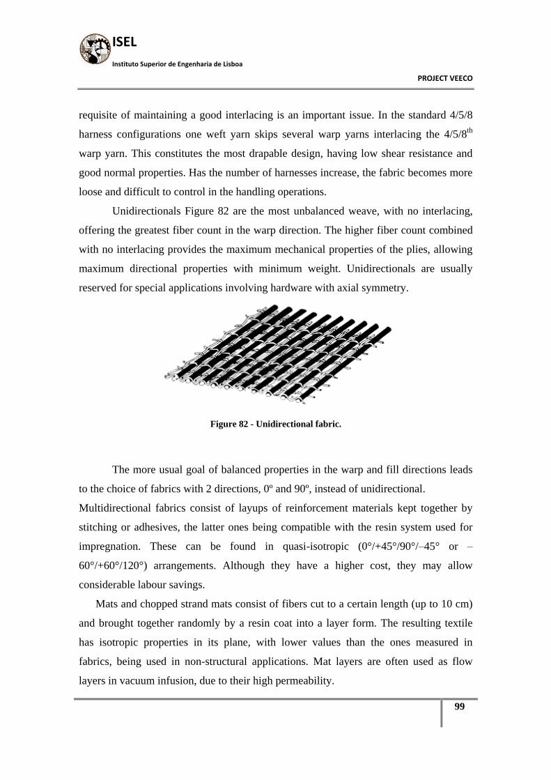
ISEL


PROJECT VEECO

99

requisite of maintaining a good interlacing is an important issue. In the standard 4/5/8

harness configurations one weft yarn skips several warp yarns interlacing the 4/5/8th

warp yarn. This constitutes the most drapable design, having low shear resistance and

good normal properties. Has the number of harnesses increase, the fabric becomes more

loose and difficult to control in the handling operations.

Unidirectionals Figure 82 are the most unbalanced weave, with no interlacing,

offering the greatest fiber count in the warp direction. The higher fiber count combined

with no interlacing provides the maximum mechanical properties of the plies, allowing

maximum directional properties with minimum weight. Unidirectionals are usually

reserved for special applications involving hardware with axial symmetry.

Figure 82 - Unidirectional fabric.

The more usual goal of balanced properties in the warp and fill directions leads

to the choice of fabrics with 2 directions, 0º and 90º, instead of unidirectional.

Multidirectional fabrics consist of layups of reinforcement materials kept together by

stitching or adhesives, the latter ones being compatible with the resin system used for

impregnation. These can be found in quasi-isotropic (0°/+45°/90°/–45° or –

60°/+60°/120°) arrangements. Although they have a higher cost, they may allow

considerable labour savings.

Mats and chopped strand mats consist of fibers cut to a certain length (up to 10 cm)

and brought together randomly by a resin coat into a layer form. The resulting textile

has isotropic properties in its plane, with lower values than the ones measured in

fabrics, being used in non-structural applications. Mat layers are often used as flow

layers in vacuum infusion, due to their high permeability.

ISEL


PROJECT VEECO

101

11. Manufacturing processes

11.1. Introduction

In the research made for the manufacturing methods, special attention was paid in

processes feasible for very low production volumes (less than 1000 parts per year).

This decision was made due to the nature of the project and the target market intended.

Other processes such as SMC could become an option in the future. With this in mind

the selected concurrent processes are hand lay-up and RTM, and particularly vacuum

infusion in the latter one. In both techniques the inclusion of inserts or foam cores is

feasible before impregnation or after impregnation. The information presented here was

mainly extracted from iii. The processes used to fabricate the vehicle body was RTM.

11.2. Hand lay up or wet lay up

This process is also known as contact moulding and open laminating. It‟s the most

ancient and widely used method of composite fabrication, having great application in

the boat industry. It has a production rate that varies from very few parts to 300

parts/year, allowing the construction of large and complicated shapes. One-off

mouldings are also possible with this method.

The materials used are dry fabrics, unidirectional and mats as reinforcement, and

liquid resin systems. The predominant resin types used are unsaturated polyesters and

epoxy vinylester resins, tailored to have the optimal viscosity at 18 – 25 ºC. It is

important to keep in mind that the lower the temperature, the greater the viscosity. The

material storage temperature and the temperature of the work area should be controlled.

Moulds for hand lay-up are usually made in composite materials, having a finishing

high-gloss layer of gel coat to improve mould durability and part surface quality. Cast

moulds and electroformed nickel-shell moulds have a longer mould life in normal use,

being feasible for large production rates.

Hand lay-up can be described by the following steps:

1. The open and rigid mould surface is cleaned and prepared with a suitable

mould release agent;

102

2. After the mould release agent is cured, 2 layers of gel coat can be applied

using a soft brush or tailored spray equipment. The gel coat may be already

catalyzed or may need to be mixed with a catalyser to cure. Usually, the gel

coat layer has a thickness between 400 to 700 µm and is applied in 2 layers.

This allows to estimate the gel coat amount needed, knowing the mould area;

3. After the gel coat cure, the resin system consisting of resin mixture and

catalyser are mixed. Care should be taken to avoid the formation of air

bubbles in the resin, and it may need to be degassed before being applied.

This is to avoid the effect of moisture in the resin properties. After mixing

and degassing, the resin is applied evenly over the gel coat using a soft brush

or a synthetic hair roller, as in Figure 83. It may be applied manually from a

container or via a resin dispenser roller system. The latter one allows to save

resin and is cleaner, but requires a resin-pumping and connected roller

system;

4. When the first layer of resin is chemically active – partially gelled and

devolatilized - the first layer of dry material can be placed in the adequate

position. Timing the interface is crucial for a good bond. The positioning is

followed by careful sanding and cleaning of the new surface, in order to

receive a new resin layer. The consolidation of the layer is made using a

grooved metal roller, and is followed by an 8 to 24 hours cure at room

temperature. After this the successive layers can be applied in the same way

as the first;

5. In the end a top coat of pigmented or non-pigmented resin can be applied,

both for cosmetic purposes and to protect the underlying laminate.

To enhance the durability of the parts made and avoid moisture issues, care

should be taken to assure an even distribution and correct thickness of the gel coat layer.

In marine applications, where surface smoothness and resistance to osmosis and

blistering (respectively water absorption and swelling) are extremely important, it is

usual to apply a chopped strand mat layer after the gel coat. The styrene and other

volatiles emissions in this method put requirements regarding protection for the

workers, ventilation and filtering systems. In fact, the increasingly tight regulations

regarding styrene and other volatiles emissions have led many companies to shift from

ISEL


PROJECT VEECO

103

open moulding to vacuum infusion. This fact has also led to the development of low

styrene resin formulations.

The major drawbacks related with hand lay-up are the part properties being

highly dependent on the worker skills, and the intensive labour required. In fact, both

the long term and short term properties of the components are dependent not only on the

materials used, but also on the quality of the craftsmanship. Short term properties

include mechanical properties and electrical resistance. Typical long term properties are

heat aging, weather, corrosion, fatigue and creep resistance. Long term properties are

affected by intensity and type of external exposure, laminator skills, workshop

conditions and state of cure when put into service.

Figure 83- Laminate consolidation using grooved roller.

11.3. RTM

Resin Transfer Moulding (RTM) is part of a group of manufacturing techniques that

are commonly called liquid composite moulding. These techniques rely on the

impregnation of a dry stationary fiber bed, making use of liquid resin systems driven by

a pressure gradient between the inlet and the outlet ports. The difference between the

various RTM techniques is related with the way the pressure gradient is created, and the

nature of the tooling used. Usually, thermosetting resins are used, but not only. The

reinforcement materials used are dry fabrics, unidirectional, mats and stitched

multidirectional fabrics.

104

The great advantage of liquid composite moulding is the possibility of tailoring the

manufacturing process to the production rate and performance required for a certain

part. While vacuum driven impregnation with only one rigid mould is preferred for very

low production rates and large parts, more advanced techniques that make use of two

hard moulds and reactive flow can be used for larger production rates. This methods are

only feasible until moderate production rates are reached (100 000 parts/year). Figure

84 shows the tailoring of the manufacturing process.

Figure 84 - Tooling selection related to production volume and component size Erro! A origem da

referência não foi encontrada.

Liquid injection competes with every open mould and closed mould

manufacturing technique, including hand lay-up. The main reasons for the growth that

these methods are experiencing are the increasing regulations and laws regarding

styrene and other volatiles emissions, and the development of new fabrics and resins

that created opportunities for savings in areas such as automotive and aerospace. In the

latter, liquid injection moulding competes now in part performance with autoclave

prepegs.

Usually, RTM relates to a restricted family of methods that use hard tooling

composed of a cavity and male mould, and positive pressure gradient between the resin

inlet and the mould. This methods have their principal range of interest for production

rates around 35 000 parts per year.

Since the scope of this project is related with techniques that can compete with

hand lay-up, one method from the liquid resin family stands out: vacuum infusion.

This method is applied economically for very low rates of production (less than 1000

parts/year), having initially been developed to compete with hand lay-up. Actually, with

ISEL


PROJECT VEECO

105

minor modifications, it is possible to convert moulds used for hand lay-up or spray lay-

up to vacuum infusion. With the development of new materials and techniques, it has

also been found that vacuum infusion can compete with prepreg compression moulding

and prepreg vacuum bagging.

In Vacuum Infusion, the liquid resins flow is created by sealing the preform

between the relatively stiff mould cavity and a sealant, and applying a vacuum pressure

in the outlet port, conveniently located to enhance the impregnation. This vacuum

compacts the preform, and removes the entrapped air, reducing the void content and

improving the part quality and properties. Since the clamping pressure is the

atmospheric, the rigidity required for the tool is minimal, but the filling times are higher

than RTM, as pressure gradients are limited to 1 bar. It is usual to make the moulds

using gel-coated glass/epoxy laminates.

It is difficult to create a line between what is vacuum infusion and other

techniques, since the tailoring of the manufacturing process often leads to choices that

rely upon the experience of the manufacturer and upon the physical knowledge of the

process by the engineer. Figure 84 relates the RTM manufacturing possibilities with the

required part size and component volume. As it can be seen, the disposable or reusable

foil that seals the mould can be substituted by a reusable fibreglass shell, provided that

the right sealing is applied. These shells are usually made using the rigid mould, with

thicknesses ranging from 1 to 5 mm. This modification improves the cosmetics of the

sealed face of the component, enhances the achievement of good geometric tolerances

and diminishes the probability of leakages, the main problem related with vacuum

infusion.

Permeability and porosity, respectively the resistance a fabric offers to liquid

passing through its thickness and its percentage of voids, are key elements that have to

be carefully considered in the reinforcement type selection, since the degree, quality and

time of the impregnation is heavily dependent on these factors. Permeability grows as

the fiber count of a fabric decreases. This means that a unidirectional fabric is less

permeable than a plain weave fabric. This property can be used to improve and control

the impregnation, making use of mats adequately placed in the laminate thickness.

Since mats are very permeable, they function as flow layers for the resin impregnation,

106

special fabrics for vacuum infusion have been developed, having enhanced

permeability. When the permeability between layers is not very different, a rule of

mixtures to determine overall laminate permeability can be used.

Another very important aspect that made vacuum infusion possible was the

development of low viscosity and high gel time resins. The resin systems used include

polyesters, epoxies and vinylesters. To assure proper impregnation and acceptable

filling times, they should have a viscosity between 100 to 400 mPa.s and a gel time

longer than the filling time. Reaction diluents may be used to lower the viscosity. The

resin components should arrive at least 24 hours prior to impregnation to acquire the

room temperature, and should only be mixed after the leakage tests are conducted.

The injection strategy should be carefully chosen in accordance to the part

geometry, since it highly influences the filling times and the likelihood of dry spots

formation. Preliminary injection tests should be conducted to test material permeability

and the flow on critical areas such as tight corners. It is important to remember that the

larger the part, the larger the risk of something going wrong. To achieve the better

properties for the components, when the injection process is finished the pressure in the

outlet should be increased and the inlet closed, letting the part achieve a uniform

pressure distribution. When gelation of the resin is achieved, the outlet port can be

closed.

Has to sealing of the mould, some considerations should be made. When sealing

foils are used, they should be draped over the mould and sealed using tacky tape. With

thin shells, rubber or silicone O-rings are usually selected and integrated in a slot made

for that purpose. Double sealing is very often used, since leakage problems are the main

concern in this technique. Logically, care should be taken to assure that the tooling and

materials used are compatible with the resin system and do not corrode. Before

impregnation, leakage tests are conducted consisting of pressurization on the foil and

measurement of the pressure decay after 1 or 2 minutes. Values of 100 to 200 Pa are

accepted, but for larger parts larger values can be feasible. Figure 85 shows the sealing

arrangement of a foil. When leaks in the foil occur, they can be detected by tracing air

bubbles in the resin flow. When the issue is located, it can be fixed using tacky tape.

Inspection of large parts like a 17 meters hull can easily take one day.

ISEL


PROJECT VEECO

107

Figure 85 - Sealing arrangement of a foil.

Since the cure of the resin is made at once, better part properties together with

time and labour savings can be achieved, when compared to hand layup. Although this

is often an advantage, it can become problematic with large thicknesses and when

significant variations in thickness occur. This is caused by the heat released by the

exothermal curing reactions. In thick sections, the heat released in the inner layers is not

drained, causing excessive cure temperatures. In components with various thicknesses,

since the same resin system is used for all the part, decreased cure temperature for thin

sections and/or excessive cure temperature for thicker sections can occur. This in turn

may cause distortions, cracks or other defects on the laminates. To correct these

problems the resin formulation can be adjusted to produce less vigorous reactions, and

cracks can be minimized. Testing the resin on small parts is always a good practice to

find possible problems.

The possibility of using emergency equipment like syringes or auxiliary inlet or

outlet ports are a great advantage over other closed mould techniques, since these allow

to avoid the infusion failure of large parts.

108

12. Recycling of composite materials

In the last years the usage of composite materials has grown; this is largely due to its

ability to adapt to various situations. Design engineers can benefit from higher strength,

lower weight and less maintenance, which is very interesting in the transport sector

where less weight directly relates to less energy consumption and a smaller

environmental impact (less CO2 emissions). Composite materials are also used in

aerospace, renewable energies industries, reinforcement of buildings and others. The

usage in the different areas can be seen in Graphic 1, where it´s separated by

percentages.

There are three types of composite materials that are most commonly used in

engineering applications, polymer-matrix composites (PMC), metal-matrix composites

(MMC), and ceramic-matrix composites (CMC).

They are classified according to the reinforcement types, particulate composite, fiber

-reinforced composites and structural composites. Statistics indicate that the production

of composites reached a value of about 7 million tons in the year 2000; the

thermoplastics are the ones that have the biggest grown rate in the recent years. xxxiv

Recycling materials such as metals, glass, thermal plastics and many others is a

common situation, but composite materials due to its special composition have not yet

been properly recycled. The heterogeneous nature of the matrix and the reinforcement

are responsible for very poor recyclability being the thermoset based the worst case.

The ever growing restrictions on environmental legislations call for all

engineering materials to be properly recovered and recycled, from end-of-life (EOL)

products. Currently the recycling operations for main stream composites are restricted to

the technological procedures available and economic values, being the difficulty to

liberate homogeneous particles from the composite material a hard challenge. Recycling

composite materials is dependent of reinforcements that were used and the matrix they

are on, this dictates that the activities are limited to the down recycling such as energy

or fuel recovery with little materials recovery such as reinforcement fibers.

Due to more restrictive legislation, extensive R&D activities have been

conducted and resulted in the development of three categories: mechanical recycling,

thermal recycling, and chemical recycling.

ISEL


PROJECT VEECO

109

Graphic 1-Application of composite materials xxxiv

Mechanical recycling implies shredding and grinding, followed by screening to

separate fiber-rich and resin-rich fractions for re-use.

The quality of the recyclates is generally low and the method is very energy-

intensive. To perform thermal recycling, high temperatures are needed (from 300, up to

1000ºC) to decompose the resin and separate the reinforcement fibers and fillers.

Although inorganic fillers and clean fibers are re-generated and secondary fuel or

thermal energy can be produced through pyrolysis, gasification or combustion, the

quality of the recovered fibers or filler materials degrades to a varying extent during the

process.

Thermal recycling of composite waste basically sets in three types of operations:

1. Incineration or combustion for energy recovery only

2. Combustion for fiber and filler recycling with energy recovery

3. Pyrolysis with both fiber and fuel recovery.

Only the last process can be considered directly as recycling since the other ones do

not commit for direct recycling and need a post-processing of the waste.

Chemical recycling focuses in chemical depolymerisation or removal of the matrix

and liberation of fibers for further recycling, by using organic or inorganic solvent.

However, lack of flexibility and generation of waste chemicals with environmental

concerns lead to the partial stagnation in investigation, nevertheless a cleaner process

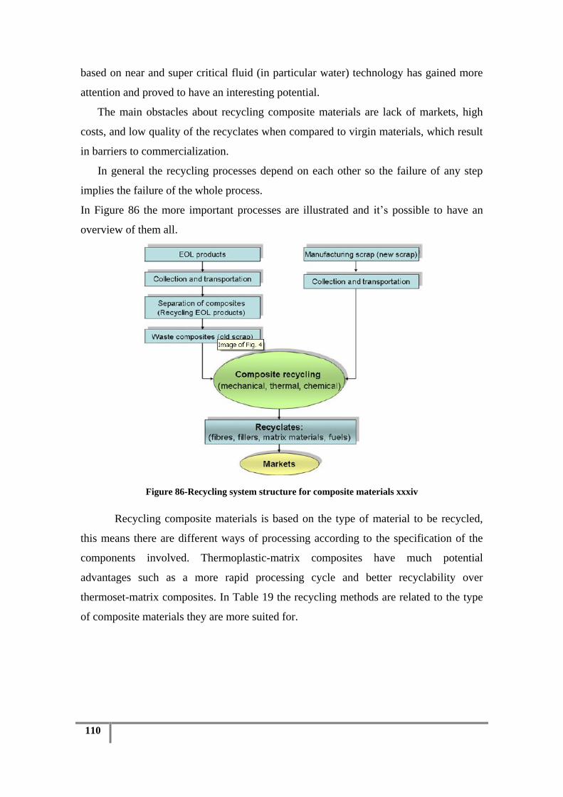
110

based on near and super critical fluid (in particular water) technology has gained more

attention and proved to have an interesting potential.

The main obstacles about recycling composite materials are lack of markets, high

costs, and low quality of the recyclates when compared to virgin materials, which result

in barriers to commercialization.

In general the recycling processes depend on each other so the failure of any step

implies the failure of the whole process.

In Figure 86 the more important processes are illustrated and it‟s possible to have an

overview of them all.

Figure 86-Recycling system structure for composite materials xxxiv

Recycling composite materials is based on the type of material to be recycled,

this means there are different ways of processing according to the specification of the

components involved. Thermoplastic-matrix composites have much potential

advantages such as a more rapid processing cycle and better recyclability over

thermoset-matrix composites. In Table 19 the recycling methods are related to the type

of composite materials they are more suited for.

ISEL


PROJECT VEECO

111

Table 19-Methods for recycling different composite materials xxxiv

Developing recyclable composite materials is an issue that can be addressed to

different areas one of them is research and development, commonly known as R&D, the

problem can be divided in three main areas, this turn out as R&D challenges, such as:

Recycling of composite materials and their constituents.

Product design and engineering for end-use properties focusing on recyclability.

Maximization of product quality of each material use.

A fact not to be disregarded is EU directives for ELVs (End of life vehicles) require

85% materials reuse and recycling or 95% reuse and recovery including a maximum

10% energy recovery, compared to 80% materials reuse and recycling since 2006.

The main challenge about recycling composite materials is to be able in a near

future to build transportation out of recycled material Figure 87.

112

Figure 87- A car possibly made of 100% recycled materials in 2015, 2030 or 2050? xxxiv

Recycling is becoming an issue, if the analysis is made from a resource

availability point of view, this means the technology has to be developed,

infrastructures created and legislation suited to the needs. The process can not only be

directed to the valuable reinforcement materials (carbon, glass fibres and alike) but also

organic polymer matrix materials need to be recycled or will start to become scarcer

which will lead to an increase in price. Processes like burning or incineration have to be

abandoned and waste separation can provide the opportunity to recycle valuable

materials like composite car parts, combined with the evolution of the manufacturing

process and a wider tolerance to use recycled fibres in new components, will encourage

the process. Recycling can also benefit from legislation incentives, benefiting all the

parties‟ intervenient in the process in order to compensate the high cost based on state

of the art technologies. The use of non-remeltable thermoset matrix will be replaced by

thermoplastics. The contradiction between the heterogeneity and recyclability would

become less critical, and the market adjusted to an increasingly usage of recycled


Sustainable and environmentally friendly solutions are becoming an effective

requisite, so reusing and recycling composites are an important issue as important as

their usually mentioned advantages.

ISEL


PROJECT VEECO

113

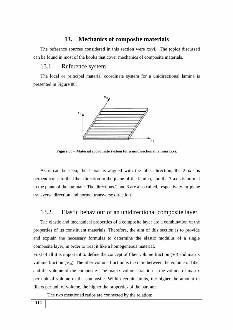
114

13. Mechanics of composite materials

The reference sources considered in this section were xxvi, The topics discussed

can be found in most of the books that cover mechanics of composite materials.

13.1. Reference system

The local or principal material coordinate system for a unidirectional lamina is

presented in Figure 88:

Figure 88 – Material coordinate system for a unidirectional lamina xxvi.

As it can be seen, the 1-axis is aligned with the fiber direction, the 2-axis is

perpendicular to the fiber direction in the plane of the lamina, and the 3-axis is normal

to the plane of the laminate. The directions 2 and 3 are also called, respectively, in-plane

transverse direction and normal transverse direction.

13.2. Elastic behaviour of an unidirectional composite layer

The elastic and mechanical properties of a composite layer are a combination of the

properties of its constituent materials. Therefore, the aim of this section is to provide

and explain the necessary formulas to determine the elastic modulus of a single

composite layer, in order to treat it like a homogeneous material.

First of all it is important to define the concept of fiber volume fraction (Vf) and matrix

volume fraction (Vm). The fiber volume fraction is the ratio between the volume of fiber

and the volume of the composite. The matrix volume fraction is the volume of matrix

per unit of volume of the composite. Within certain limits, the higher the amount of

fibers per unit of volume, the higher the properties of the part are.

The two mentioned ratios are connected by the relation:

ISEL


PROJECT VEECO

115

(21)

The determination of the elastic constants is based on a micromechanical analysis,

in other words, in the way in which the fibers and the matrix interact. There are different

approaches to solve this problem, namely by using numerical models like in finite

element analysis, using models based on the theory of elasticity and the rule-of mixture

models based in strength of materials approach. In this analysis, some assumptions are

made: both the matrix and the fibers are linearly elastic; the fibers are infinitely long

and the fibers are spaced periodically in square packed or hexagonal packed arrays.

Accurate formulas to analytically predict the necessary elastic properties of a

transversely isotropic lamina are presented below based on a study from Berthelot

(2007). The longitudinal Young´s modulus ( 1E ) and the Poisson‟s ratio ( 12 ) are

determined from the law of mixtures. This law interpolates the respective properties

between the constituent materials:

(22)

Where the subscripts “f” and “m” identify the matrix and fiber properties

respectively. The transverse in-plane elasticity modulus ( 2E ) is determined from an

elasticity solution provided in Voyiadjis et al (2005):

(23)

The longitudinal shear modulus, 12G , is determined by an exact solution from a

classical approach of the mechanics of deformable solids (elasticity solution):

(24)

mf VV 1

mmff

mmff

VV

EVEVE

1212

11

mmff

mmfmfmfm

m

mmff

mffmmffff

f

m

mm

f

ff

VEVE

VEVEE

VEVE

VEEVE

E

V

E

V

E

1

121

2

1

12121121

22

11

1

1

)1()1(

)1()1(12

fmff

fmff

mVGVG

VGVGGG

116

13.3. Constitutive relation and coordinate transformation

13.3.1. Constitutive relation The constitutive law for an orthotropic material in the material reference system

is given as follows:

(25)

being the meaning of the stress components can be seen in Figure 89.

Figure 89-Stresses and their directions xix.

Or, in a simplified way, S , where S is the compliance matrix. The

elements of the compliance matrix can be identified by the notationijS , where “i” is the

number of the line and “j” is the number of the column of the element. The inverse of

the compliance matrix is called the stiffness matrix, and allows the calculation of the

stresses having the strains, using the relation C , where 1 SC . It is

important to note that some of the properties that are input in the matrices are not

independent, since the following reciprocity relations between elastic modulus and

Poisson‟s ratio stand:

(26)

12

13

23

3

2

1

12

13

23

32

23

1

13

3

32

21

12

3

31

2

21

1

12

13

23

3

2

1

100000

01

0000

001

000

0001

0001

0001

G

G

G

EEE

EEE

EEE

12 21 13 31 23 32

1 2 1 3 2 3

; ; E E E E E E

ISEL


PROJECT VEECO

117

Most laminated composite materials are considered transversely isotropic. This

definition is characterized by an equal behaviour in the 2 and 3 directions. This leads to

32 EE , 1312 and 1312 GG . In addition, the following relation stands:

(27)

As it can be seen, only five material properties are needed in order to completely

define a transversely isotropic material: 231221 ,,, EE and 12G . For most applications,

where the thickness of the laminate is small compared with the other dimensions, some

simplifications are usually applied. It is assumed that the lamina is under plane stress in

plane 12, thus the normal and transverse shear stresses along the direction 3 are

negligible. These simplifications are associated to the following assumptions:

All layers are perfectly bonded, and the strains are continuous throughout the

laminate thickness.

Plane sections before the deformation remain plane after the deformation

take place.

A straight line perpendicular to the laminate middle surface remains straight

and perpendicular to the middle surface after deformation.

By assuming these main lines, we are considering to be in the domain of

applicability of the Classical Laminate Theory (CLT), and because of this, the

constitutive relation becomes simpler, as it can be seen:

(28)

and

(29)

)1(2 23

223

EG

12

2

1

66

2212

1211

12

2

1

00

0

0

Q

QQ

QQ

12

2

1

66

2212

1211

12

2

1

00

0

0

S

SS

SS

118

Where S and Q are called the reduced compliance matrix, and the reduced stiffness

matrix respectively. Since it is necessary to know the properties of a composite lamina

in any direction, the concept of transformation matrix is now introduced. It allows the

determination of the stresses or strains in any direction within the plane of the lamina.

Figure 90 - Relation between laminate (x,y,z) and material coordinates systems (1,2,3). xxvi

In the following relations θ is the angle between the global coordinate system of

the laminate and the local coordinate system of the lamina, as it can be seen in figure

90.

(30)

Or in simplified form:

(311)

The same relation can be used in the following form, in order to determine the

global stresses:

(32)

It is important to state that the above relations can also be used in a similar way

for the calculation of the local and global strains. By doing this it is possible to obtain

the transformed reduced stiffness matrix Q . Having these new matrices defined, it is

now possible to establish the following relations:

(33)

2 2

1

2 2

2

2 2

12

cos 2.cos .

cos 2.cos .

cos . cos . cos

x

y

xy

sen sen

sen sen

sen sen sen

xy

y

x

T

12

2

1

12

2

1

1

T

xy

y

x

xy

y

x

xy

y

x

S

xy

y

x

xy

y

x

Q

ISEL


PROJECT VEECO

119

The coefficients associated to these stiffness and compliance matrices are widely

disseminated in the literature of composite materials. Since we already have the

necessary relations for a lamina, it is now necessary to use a method to determine the

stresses and strains in the various layers of a laminate. Since laminates usually have

planar dimensions several times higher than their thickness, they are usually treated as

plate elements. To this purpose a reference system associated to the laminate, and a

numerating scheme of the layers is adopted, as it can be seen in Figure 91. The origin of

the through the thickness coordinate is located in the middle surface, and it is oriented

downwards. The middle surface can be located inside a layer or in an interface. The first

layer is on the surface of the most negative location and the nth

layer is on the surface of

the most positive location. The location and designation of the interfaces between layers

(z) can be seen in Figure 91. The thickness of a layer (hk) is calculated using

kkk zzh 1 . The total thickness of the laminate is H.

Figure 91-Numbering of the layers and interface. xxvi

120

Since plane stress is assumed, it is possible to determine the stresses on one

layer of the laminate knowing the middle surface strains and curvatures, through the

simplified constitutive relation:

(33)

Where 0

x and 0

y are the middle surface extensional strains along the x and y

axis, 0

xk , and 0

yk are the middle surface curvatures in the same directions, 0

xy and 0

xyk are

the middle surface in-plane shear strain and the middle surface twisting curvature.

It is important to note that since the orientation of the material varies from layer

to layer, the stresses through the thickness do not vary linearly. After determining the

stresses in each layer, these are integrated along the thickness of the laminate in order to

determine the stress resultants:

(34)

The force resultants, N, and the moment resultants, M, are the forces and

moments applied per unit width of the cross section of the laminate. Their

representation can be seen in Figure 92 and Figure 93.

Figure 92- Force resultants representation xix

Figure 93 – Moment resultants representation xix

00

00

00

662616

262212

161211

.

.

.

xyxy

yy

xx

xy

y

x

kz

kz

kz

QQQ

QQQ

QQQ

/2 /2 /2

/2 /2 /2

/2 /2 /2

/2 /2 /2

. . . . . .

H H H

x x y y xy xy

H H H

H H H

x x y y xy xy

H H H

N dz ; N dz ; N dz

M z dz ; M z dz ; M z dz

ISEL


PROJECT VEECO

121

In most engineering problems, the force and moment resultant are given and the

strains and curvatures of the laminate are the unknowns. So it can be helpful to present

the formulation of the matrices A, B and D widely used in the analysis of composite

laminates. So for the force and moment resultants of one particular layer k:

(36)

Since the stiffness matrix and the reference surface strains and curvatures are not

dependent on z, they can be taken out of the two integrals that result from the

multiplication of the stiffness matrix with the strain and curvatures vectors.

Then, the following result is obtained:

(37)

Solving the integrals, we obtain the A, B and D matrices that relate force and

moment resultants with the extensional strains and surface curvatures. Making the

0 0

11 12 161

0 0

12 22 26

0 0

16 26 66

0 0

11 12 16

0 0

12 22 26

0 0

16 26 66

.

.

.

.

.

.

k

x x xZk

y y y

Zk

xy xyxy k

k

x x x

y y y

xy xyxy k

N Q Q Q z k

N Q Q Q z k dz

Q Q Q z kN

M Q Q Q z k

M Q Q Q z k

Q Q Q z kM

1

. .

Zk

Zk

z dz

0 0

11 12 16 11 12 161 1

0 0

12 22 26 12 22 26

0 0

16 26 66 16 26 66

11 12 16

12 22 26

16 26 6

k k

x x xZk Zk

y y y

Zk Zk

xy xyxy k

x

y

xy k

N Q Q Q Q Q Q k

N Q Q Q dz Q Q Q k zdz

Q Q Q Q Q Q kN

M Q Q Q

M Q Q Q

Q Q QM

0 0

11 12 161 1

0 0 2

12 22 26

0 0

6 16 26 66

k k

x xZk Zk

y y

Zk Zk

xy xy

Q Q Q k

zdz Q Q Q k z dz

Q Q Q k

122

summation of the moments and force resultants throughout the thickness of the laminate

composed of N layers, the following relations are obtained for the entire laminate:

(38)

Where:

(39)

The A matrix relates the in-plane normal and shear stresses with the in- plane

normal and shear strains. The B matrix relates the normal and shear stresses with the

bending and twisting curvatures and the moment resultants with the in-plane normal and

shear strains. From this relation, if B ≠ 0, normal stresses cause bending and twisting of

the laminate and bending and twisting moments cause normal and shear strains. Finally,

the D matrix relates moment resultants with bending and twisting curvatures. Some of

the layups available are described below. A symmetric laminate consists of a stacking

sequence where for every lamina with a specific thickness, material properties and

orientation, exists another layer in the opposite side of the reference surface and at the

same distance from it, with the same exact characteristics. If each layer moment is

counteracted by an equal moment with opposite sign from the other side of the reference

surface, the resultant moment is zero. A laminate is balanced when for every lamina

with a specific thickness, material properties and orientation; there is another layer in

the laminate thickness with the same properties but opposite fiber orientation. For these

laminates, there is no coupling between the normal stresses and the shear strains. This

means that the components A16 and A26 are always zero. Symmetric and balanced

0

0

0

662616

262212

161211

0

0

0

662616

262212

161211

0

0

0

662616

262212

161211

0

0

0

662616

262212

161211

xy

y

x

xy

y

x

kxy

y

x

xy

y

x

xy

y

x

kxy

y

x

k

k

k

DDD

DDD

DDD

BBB

BBB

BBB

M

M

M

k

k

k

BBB

BBB

BBB

AAA

AAA

AAA

N

N

N

1

1

2 2

1

1

3 3

1

1

( ) ( )

1( ) ( )

2

1( ) ( )

3

N

ij ij k k k

k

N

ij ij k k k

k

N

ij ij k k k

k

A Q z z

B Q z z

D Q z z

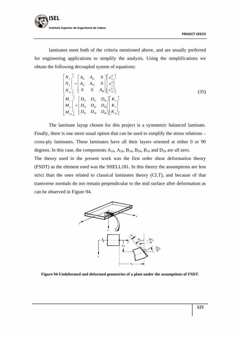
ISEL


PROJECT VEECO

123

laminates meet both of the criteria mentioned above, and are usually preferred

for engineering applications to simplify the analysis. Using the simplifications we

obtain the following decoupled system of equations:

(35)

The laminate layup chosen for this project is a symmetric balanced laminate.

Finally, there is one more usual option that can be used to simplify the stress relations –

cross-ply laminates. These laminates have all their layers oriented at either 0 or 90

degrees. In this case, the components A16, A26, B16, B26, B16 and D26 are all zero.

The theory used in the present work was the first order shear deformation theory

(FSDT) as the element used was the SHELL181. In this theory the assumptions are less

strict than the ones related to classical laminates theory (CLT), and because of that

transverse normals do not remain perpendicular to the mid surface after deformation as

can be observed in Figure 94.

Figure 94-Undeformed and deformed geometries of a plate under the assumptions of FSDT.

xy

y

x

xy

y

x

xy

y

x

xy

y

x

K

K

K

DDD

DDD

DDD

M

M

M

A

AA

AA

N

N

N

662616

262212

161211

0

0

0

66

2212

1211

00

0

0

124

The displacement field associated to the first-order shear deformation theory can

be written as:

(361)

where 0 0 0, ,u v w are midplane displacements along directions x,y,z and ,x y

rotations around the y and x axis respectively.

0

0

0

( , , ) ( , ) ( , )

( , , ) ( , ) ( , )

( , , ) ( , )

x

y

u x y z u x y z x y

v x y z v x y z x y

w x y z w x y

ISEL


PROJECT VEECO

125

The corresponding deformations, considering only linear contributions are:

It is possible to conclude that in the present case, we have additionally the possibility to

consider the existence of transverse shear deformations ,xz yz (disregarded in the

classical theory) and the associated stresses. Therefore in this case, it would be possible

to characterize the corresponding shear stresses.

00

00

0000

yy

y

y

xxx

x

zky

zy

v

y

v

y

v

zkx

zx

u

x

u

00 0 0

0 0

0

0

0

0

yx

xy xy xy

xz x

yz y

u v u vz zk

y x y x y x

u w w

z x x

v w w

z y y

(37)

ISEL


PROJECT VEECO

127

14. Finite element analysis

14.1. Brief overview

The finite element method is a powerful and versatile tool that is widely used to

obtain solutions in complex engineering problems. It consists in the division of a body

into small connected entities – elements. This approach allows the problem to be

transformed into a set of equations that can be solved by well-known procedures of

linear algebra. The use of such method for complex structures and complex problem‟s

nature require a powerful computational effort. The technological growth that

computers experienced in the last decade made it possible to apply finite element

analysis to problems ranging from fluid mechanics to structural assessment, improving

the reliability of the designs at increasingly low costs.

A fundamental step of the finite element method in structural analysis is the

computation of a global stiffness matrix for the system - GK . Such matrix relates the

forces applied to the nodes of the elements, GF , to the displacements that such nodes

experience G :

(38)

By observing this relation, it can be viewed as a linear spring that experiences a

deformation when a force is applied, with the difference that in the present study we do

not have a single axial displacement but a significant number of independent

displacements and rotations associated to each of the nodes that constitute the mesh of

the component analysed.

The global matrices (i.e. the matrices related to the whole discretized domain in

the global reference system) are obtained by previously calculating and assembling the

local stiffness matrices and element forces vectors for the various elements that

constitute the mesh.

The number of rows from GF , G and the number of rows and columns of GK

are equal to the number of degrees of freedom from the system.

G G GK F

128

Concerning to the element matrices/vectors ( LF , L and LK ), they have a

dimension that is related to the number of degrees of freedom per element. For the

element used, each node has 6 degrees of freedom 3 mid-plane displacements along the

axes x, y and z and 3 rotations around these axes. The choice of the type of the

elements, and specifically the degrees of freedom that they allow for their nodes, are

crucial to adequately model the problem of interest.

As an example of a local system of equations, assuming that the element allows

only displacements along the x and y axis, and that the system has 3 nodes A, B and C,

being the nodes B and C constrained in all the directions, the local system of equations

would assume the following form:

(39)

Where the terms ijk result from the expressions that relate the forces applied in

the nodes to the respective displacements that the element experiences, in any point

along its length as well as the theory upon the model is based. It is important to note that

the matrix system above requires a number of unknowns equal to the number of known

values of displacements/forces, to allow the determination of a unique solution for the

system.

11 12 13 14 15 16

21 22 23 24 25 26

31 32 33 34 35 36

41 42 43 44 45 46

51 52 53 54 55 56

61 62 63 64 65 66

0

0

0

0

0

0

L L L

Ax

Ay

Bx

By

Cx

Cy

K F

k k k k k k

k k k k k k

Rk k k k k k

Rk k k k k k

Rk k k k k k

Rk k k k k k

ISEL


PROJECT VEECO

129

15. Failure analysis – brief overview

15.1. Introduction

To discuss failure analysis in composites, it is important to mention the work

conducted by Hinton et al (2004), where important conclusions were taken regarding

this theme. This work was the result of a meeting in 1991 of specialists in the theme of

failure of composite materials, in St. Albans, United Kingdom. From this meeting it was

concluded that the failure criteria used until that date lacked credibility and there was no

definition for failure in composite materials. This was the starting point for the work

developed by Hinton et al in the following 12 years. It consisted in inviting the authors

of the various failure criteria available to participate in the task, and designing

experiments to adequately compare the accuracy of the various failure predictions.

Some authors accepted the invitations, others declined. Z. Hashin, known for the widely

used failure criteria that he developed x, was included in the latter ones. He developed

micromechanics piecewise failure criteria that accounted for the various material failure

modes, allowing predictions of failure load and failure mode.

Figure 95 – Ranking of the various failure theories, according to grades defined. xii

His approach served as an inspiration and as the base to the Puck failure criteria,

which was included in the World Wide failure exercise. This exercise evaluated 15

failure criteria among which were interactive failure criteria, piecewise failure criteria

130

and progressive damage approaches. The results from the various failure criteria tested

are presented in Figure 95. Grade A represents an error between predictions and

experimental results lower than 10%; Grade B an error between predictions and

experimental results between 10% and 50% and grade C an error between predictions

and experimental results higher than 50%.

Has it can be seen, Zinoviev, Bogetti, Puck, Cuntze and Tsai B failure criteria

present the higher rate of Grade A + Grade B predictions. Among these, Puck‟s failure

criteria present the higher rate of grade A predictions, seconded by Cuntz. The

description of these failure criteria by their originators was included in the Hinton et al

work, and all of them have advantages and short comings.

More recently, new failure criteria have been developed. Among these, LaRC04

described in Pinho et al (2005) appears to be very reliable. The latter criterion allows the

determination of micromechanical subcritical failure modes of the fiber and matrix, but

requires additional experimental tests to determine the components of the fracture

toughness. Innovative aspects of this approach are an increased detail of the failure

modes models and the possibility of distinguishing the transverse tensile strength of the

plies based on their thickness and location on the laminate - embedded or superficial

ply.

Failure criteria can be divided in two categories: phenomenological failure

criteria (Ex: Hashin and Puck) and non-phenomenological failure criteria (Ex: Tsai-Wu

and Tsai Hill). The first ones are characterized by allowing the assessment of the type

and mode of material failure that occurs, and the second ones are characterized by only

predicting when the material fails, not specifying how. The latter 2 categories can be

further divided in interactive (Ex: Tsai Wu and Tsai-Hill), partially interactive (Ex:

Puck and Hashin) and non-interactive failure criteria (Ex: Maximum strain and

Maximum stress). Interactive failure criteria make use of all the components of the state

of stress of the material in a single formula to predict failure. Partially interactive failure

criteria do the same but with more than one formula, to account for different failure

modes. Non interactive failure criteria assume that each component of the stress/strain

state of the material is not affected by the other ones.

Fracture mechanics methods use the concepts of linear elastics fracture

mechanics. Such approaches assume a damage zone represented by a crack of specified

length in the boundary of a laminate, kept closed by cohesive forces.

ISEL


PROJECT VEECO

131

Progressive damage models were created to allow the determination of the damage that

occurs prior to final failure of a laminate. They simulate the damage initiation and

growth, using elastic property degradation that is usually a function of the type of

failure that occurred. For this purpose, piecewise failure criteria are needed for the

determination of the various types of failure possible. The need for 3 dimensional finite

element models is explained by the three dimensional failure mechanisms that govern

delamination, and the through the thickness effects. Some works that used 3

dimensional progressive failure models are the ones from Shokrieh et al (1996) and

Camanho and Matthews (1999). The first one served as the basis for the works from

Okutan (2001) and Tserpes et al (2001).

The progressive damage models that are going to be described in the next

paragraphs share some common principles. Hashin type failure criteria are used in a

piecewise form to detect different types of failure and all the analysis are divided in 3

steps: Stress analysis, failure analysis and material degradation rules. Failure analysis is

performed after stress analysis and, according to the type of failure detected; the

material elastic properties are degraded to simulate the loss of strength in a per element

basis. After this; if the criteria for final failure is not met, another iteration is run where

the load that acts on the laminate is incremented. The steps mentioned are repeated until

final failure is reached. Direct mesh generation was used in all the models. This is

crucial since the progression of the damage is seen on an element basis, and the

trajectory and location of the damage is what allow conclusions to be drawn about the

type of failure detected.

Shear-out failure can be regarded as a special case of bearing failure, and it is

assumed to be caused by in plane shear stresses. It occurs in laminates where the end

distance is small. It can also occur in highly orthotropic laminates, independently of the

end distance (Hart-Smith, 1976).

Cleavage is a mixture of net-section and shear out failure modes, and it is caused by

an inadequate end distance and too few transverse plies.

132

15.2. Hashin 3D failure criteria

3D Hashin failure criteria was first presented is Hashin (1980). It is a partially

interactive phenomenological failure criteria, based in micromechanics. This means that

it takes into account the interaction at microscopically level between the matrix and the

fiber. The reason why this criteria was chosen for this work is related to the fact that this

procedure was available for this purpose and also because of the good predictions

achieved in previous works like Camanho and Matthews (1999) and Okutan (2001).

The failure criteria used to detect the different types of failure predicted by the model

are presented in the following paragraphs, as they were reported by Tserpes et al (2008).

Matrix tensile and compressive cracking (σYY > 0):

(45)

Matrix tensile and compressive failure (σYY< 0):

(46)

Fibre tensile failure (σXX> 0):

(47)

Fibre compressive failure (σXX < 0):

(48)

1

222

YZ

YZ

XY

XY

T

YY

SSY

1

222

yz

yz

xy

xy

C

YY

SSY

1

222

YZ

YZ

XY

XY

T

XX

SSX

1

C

XX

X

ISEL


PROJECT VEECO

133

Fibre-Matrix shear-out (σXX < 0):

This is an addiction to the original failure criteria made by Lessard (1989), to

include the effect of the in-plane shear stress in the behaviour of an unidirectional ply:

(49)

Delamination in tension (σZZ > 0):

(40)

Delamination in compression (σZZ < 0):

(41)

15.3. Material property degradation

The elastic property degradations that are applied in a per element basis after the

detection of the various modes of failure are presented in the next paragraphs as stated

in Tserpes et al (2008).

15.3.1. Matrix tensile and compressive cracking: When matrix tensile or compressive failure is detected in a ply, it is assumed

that the matrix cannot carry any load. This leads to:

1

222

XZ

XZ

XY

XY

C

XX

SSX

1

222

YZ

YZ

XZ

XZ

T

ZZ

SSZ

1

222

YZ

YZ

XZ

XZ

C

ZZ

SSZ

00 XYYY andE

134

(42)

15.3.2. Fiber tensile and compressive failure: When the fiber in an element fails, it is assumed that that element cannot carry

any load. This leads to a reduction in the elastic properties of the element in the

following way:

(43)

15.3.3. Fiber-matrix shear-out: When fiber matrix shear-out is detected, it is assumed that the laminate can carry

longitudinal and transverse loads, but not in-plane shear loads.

0

0

XZYZXY

XZYZXYZZYYXX GGGEEE

ISEL


PROJECT VEECO

135

This leads to the following elastic properties degradation:

(54)

15.3.4. Delamination in tension and compression: When an element fails by delamination, it is assumed that it loses the ability to

carry any loads along the through the thickness direction. This causes the material

elastic properties to be changed to:

(55)

So according to Hashin method, when these situations occur, a new calculation stage is

initiated, which for different subsequent steps, can give the progression of the damage.

0

0

XY

XYG

0

0

XZYZ

XZYZZZ GGE

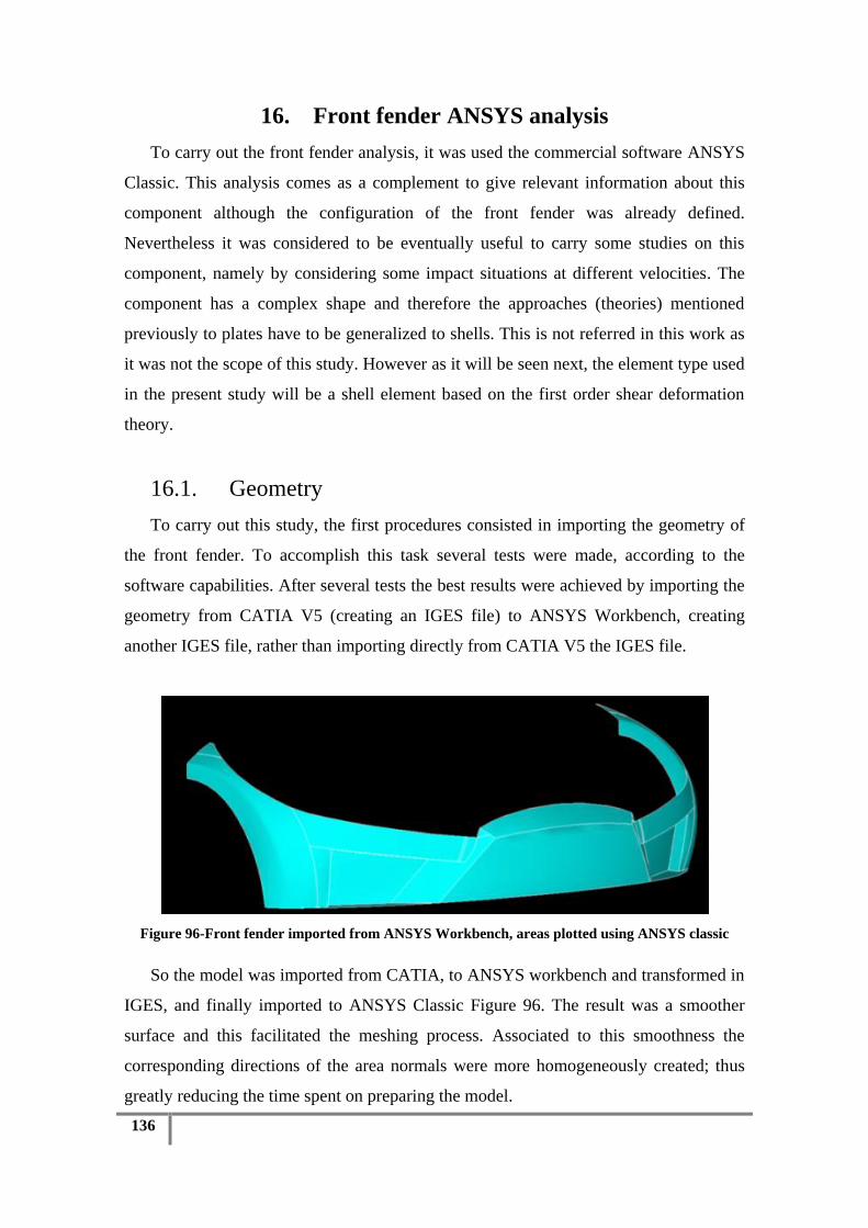
136

16. Front fender ANSYS analysis

To carry out the front fender analysis, it was used the commercial software ANSYS

Classic. This analysis comes as a complement to give relevant information about this

component although the configuration of the front fender was already defined.

Nevertheless it was considered to be eventually useful to carry some studies on this

component, namely by considering some impact situations at different velocities. The

component has a complex shape and therefore the approaches (theories) mentioned

previously to plates have to be generalized to shells. This is not referred in this work as

it was not the scope of this study. However as it will be seen next, the element type used

in the present study will be a shell element based on the first order shear deformation

theory.

16.1. Geometry

To carry out this study, the first procedures consisted in importing the geometry of

the front fender. To accomplish this task several tests were made, according to the

software capabilities. After several tests the best results were achieved by importing the

geometry from CATIA V5 (creating an IGES file) to ANSYS Workbench, creating

another IGES file, rather than importing directly from CATIA V5 the IGES file.

Figure 96-Front fender imported from ANSYS Workbench, areas plotted using ANSYS classic

So the model was imported from CATIA, to ANSYS workbench and transformed in

IGES, and finally imported to ANSYS Classic Figure 96. The result was a smoother

surface and this facilitated the meshing process. Associated to this smoothness the

corresponding directions of the area normals were more homogeneously created; thus

greatly reducing the time spent on preparing the model.

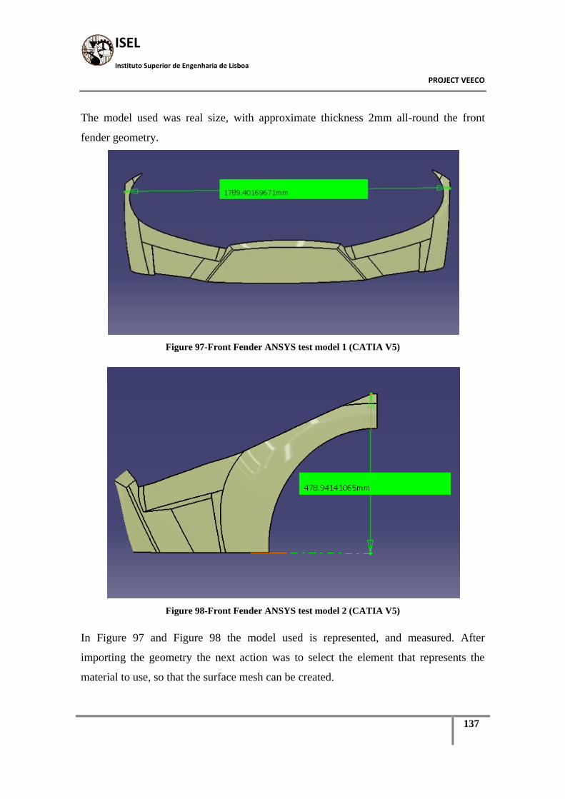
ISEL


PROJECT VEECO

137

The model used was real size, with approximate thickness 2mm all-round the front

fender geometry.

Figure 97-Front Fender ANSYS test model 1 (CATIA V5)

Figure 98-Front Fender ANSYS test model 2 (CATIA V5)

In Figure 97 and Figure 98 the model used is represented, and measured. After

importing the geometry the next action was to select the element that represents the

material to use, so that the surface mesh can be created.

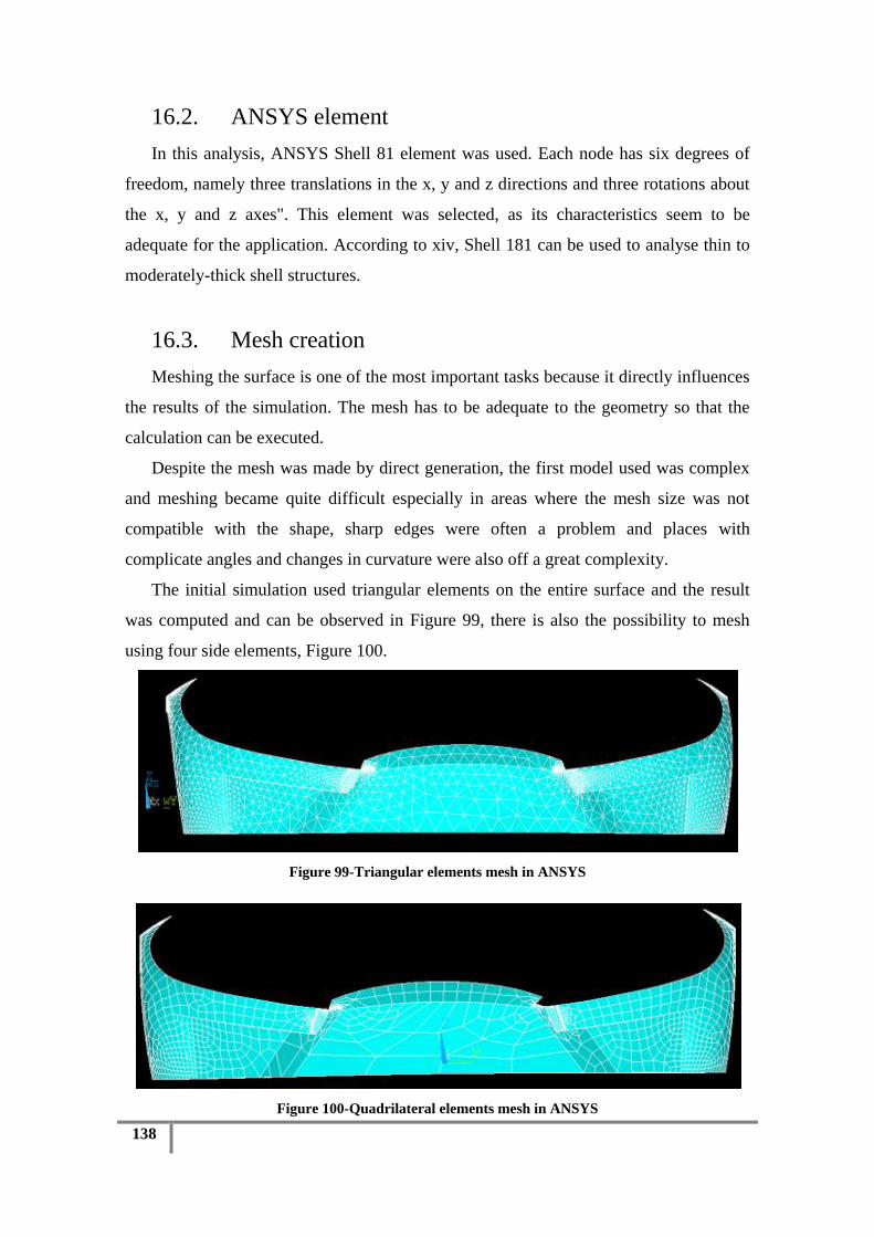
138

16.2. ANSYS element

In this analysis, ANSYS Shell 81 element was used. Each node has six degrees of

freedom, namely three translations in the x, y and z directions and three rotations about

the x, y and z axes". This element was selected, as its characteristics seem to be

adequate for the application. According to xiv, Shell 181 can be used to analyse thin to

moderately-thick shell structures.

16.3. Mesh creation

Meshing the surface is one of the most important tasks because it directly influences

the results of the simulation. The mesh has to be adequate to the geometry so that the

calculation can be executed.

Despite the mesh was made by direct generation, the first model used was complex

and meshing became quite difficult especially in areas where the mesh size was not

compatible with the shape, sharp edges were often a problem and places with

complicate angles and changes in curvature were also off a great complexity.

The initial simulation used triangular elements on the entire surface and the result

was computed and can be observed in Figure 99, there is also the possibility to mesh

using four side elements, Figure 100.

Figure 99-Triangular elements mesh in ANSYS

Figure 100-Quadrilateral elements mesh in ANSYS

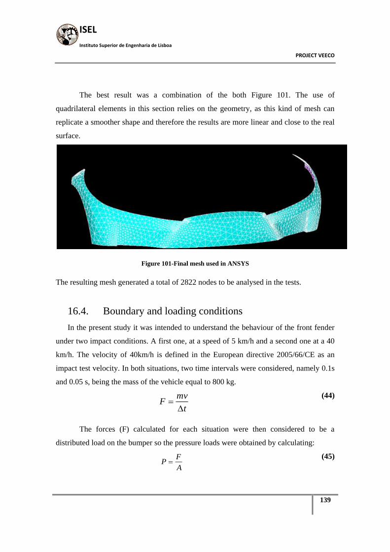
http://mostreal.sk/html/elem_55/chapter4/ES4-181.htm


ISEL


PROJECT VEECO

139

The best result was a combination of the both Figure 101. The use of

quadrilateral elements in this section relies on the geometry, as this kind of mesh can

replicate a smoother shape and therefore the results are more linear and close to the real

surface.

Figure 101-Final mesh used in ANSYS

The resulting mesh generated a total of 2822 nodes to be analysed in the tests.

16.4. Boundary and loading conditions

In the present study it was intended to understand the behaviour of the front fender

under two impact conditions. A first one, at a speed of 5 km/h and a second one at a 40

km/h. The velocity of 40km/h is defined in the European directive 2005/66/CE as an

impact test velocity. In both situations, two time intervals were considered, namely 0.1s

and 0.05 s, being the mass of the vehicle equal to 800 kg.

(44)

The forces (F) calculated for each situation were then considered to be a

distributed load on the bumper so the pressure loads were obtained by calculating:

(45)

A

FP

mvF

t

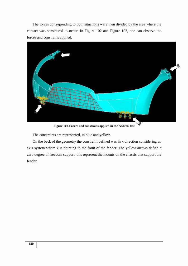
140

The forces corresponding to both situations were then divided by the area where the

contact was considered to occur. In Figure 102 and Figure 103, one can observe the

forces and constrains applied.

Figure 102-Forces and constrains applied in the ANSYS test

The constraints are represented, in blue and yellow.

On the back of the geometry the constraint defined was in x direction considering an

axis system where x is pointing to the front of the fender. The yellow arrows define a

zero degree of freedom support, this represent the mounts on the chassis that support the

fender.

ISEL


PROJECT VEECO

141

Figure 103-Forces and constrains applied in the ANSYS test

The area in red is the front grill where the pressure was applied in the test.

16.5. Design details

DOD MIL-HDBK-17-3F (2002) and Gay (2003) mention that a laminate shouldn‟t

have more than 4 consecutive layers with the same direction, in order to avoid excessive

interlaminar shear stresses and consequent delaminations. The more plies with the same

orientation are stacked together, the higher the interlaminar shear stresses become,

increasing the probability of failure by delamination.

The properties used for the lamina were taken from AGATE database (APPENDIX

IV

AGATE Database: 7781 Glass Fabric/ MGS 418 Wet Layup) for illustrative

purposes. The combination of Hexcel 7781 Glass Fabric with MGS 418 epoxy resin

tailored for wet layup was used. In fact, since the certification of materials requires a

long process composed of extensive experimental substantiation. Material properties for

composites can also be found in DOD MIL-HDBK-17-2F (2002).

142

The laminate used is quasi-isotropic with the following plies, 45º direction ply, -45º

direction ply, 0º direction ply, 0º direction ply, -45º direction ply and 45º direction ply.

This configuration repeats until a 2.4 mm section is obtained. Each ply has 0.1mm

thick.

The total thickness is 2.4mm, constituted by 24 layers. Also a different laminate

direction with the following plies, 90º direction ply, 0º direction ply, 90º direction ply,

0º direction ply, with also 2.4mm thick. Three materials where tested to the same

conditions, Hexcel 7781 Glass Fabric with MGS 418 epoxy resin, Natural Fiber-

LINEO-FLAX PRE PEG, then Carbon Fiber-Carbon/Epoxy (AS/3501), all these

materials where referenced based on the data sheet given by the manufacturer.

Table 20- Weight of the front fender for different materials. Volume of 0.00136305 m3

Material Weight (kgf)

Glass Fabric 3.52

LINEO Flax 2.38

Carbon Fiber 2.00

The difference in weight for the different materials can be seen in Table 20 and

provide a comparison that can be useful for a further selection parameter. In Table 21, T

able 22and Table 23it is summarised the maximum and minimum values of the Von

Mises stresses found in each case considered. The values are referred to a lamina.

Table 21- Von Mises maximum and minimum stresses on carbon fibre front fender.

Lay up

Velocity

(m/s)

Time

interval (s) Force (N)

Pressure

(Pa)

Max Stress

(Pa)

Min Stress

(Pa)

(90 / 0 / 90)8 5 0.1 11111 70770.7 1.14E+09 -6.47E+08

5 0.05 22222 1.42E+05 2.28E+09 -1.29E+09

40 0.1 88888.9 566171.3 9.11E+09 -5.18E+09

40 0.05 177777.8 1132342.7 1.82E+10 -1.04E+10

(45 / -45 / 0)8 5 0.1 11111 70770.7 4.13E+08 -5.26E+08

5 0.05 22222 141541.4 1.55E+09 -2.12E+07

40 0.1 88888.9 566171.3 8.38E+09 -3.91E+09

40 0.05 177777.8 1132342.7 1.09E+10 -2.31E+09

T able 22- Von Mises maximum and minimum stresses on glass fibre front fender.

ISEL


PROJECT VEECO

143

Lay up

Velocity

(m/s)

Time


Pressure

(Pa)

Max Stress

(Pa)

Min Stress

(Pa)

(90 / 0 / 90)8 5 0.1 11111 70770.7 3.98E+08 -2.26E+08

5 0.05 22222 1.42E+05 7.93E+08 -4.51E+08

40 0.1 88888.9 566171.3 3.39E+09 -1.93E+09

40 0.05 177777.8 1132342.7 7.03E+09 -4.00E+09

(45 / -45 / 0)8 5 0.1 11111 70770.7 1.45E+08 -1.85E+08

5 0.05 22222 141541.4 5.55E+08 -7.58E+06

40 0.1 88888.9 566171.3 3.00E+09 -1.40E+09

40 0.05 177777.8 1132342.7 3.82E+09 -8.20E+08

Table 23- Von Mises maximum and minimum stresses on lineo-flax fibre front fender.

Lay up

Velocity

(m/s)

Time


Pressure

(Pa)

Max Stress

(Pa)

Min Stress

(Pa)

(90 / 0 / 90)8 5 0.1 11111 70770.7 7.43E+08 -4.22E+08

5 0.05 22222 1.42E+05 1.50E+09 -8.51E+08

40 0.1 88888.9 566171.3 5.98E+09 -3.40E+09

40 0.05 177777.8 1132342.7 1.19E+10 -6.75E+09

(45 / -45 / 0)8 5 0.1 11111 70770.7 2.73E+08 -3.48E+08

5 0.05 22222 141541.4 1.02E+09 -1.39E+07

40 0.1 88888.9 566171.3 5.46E+09 -2.55E+09

40 0.05 177777.8 1132342.7 7.17E+09 -1.52E+09

As can be observed the stacking type (45 / -45 / 0)8 yields lower values of stress

under similar conditions when compared to the other laminate stacking sequence. It can

also be observed that a lower time interval leads in any situation to higher values of

stresses which can be a dangerous situation concerning to failure occurrence.

16.6. Local analysis

The model was tested using the Hashin 3D failure criteria. The guide from vi was

the base for this programming. This process is started by obtaining the element stresses

along the global coordinate system directions using the ETABLE command. The

required Hashin failure criteria, was then programmed by some calculations on the

gathered ETABLE stress values. After computing these matrices, a failure check was

144

performed. Following the method described before, the type of failure was in general

fibre failure. (Appendix V for fibre glass)

It was also possible to calculate on-the-fly rather than calculate then store in a result

file, the benefit is that multiple failure criteria do not increase the size of the results file.

The source of the program to compute the failure check criteria was xxxi, an also the

indications from xxviii.

One hypothesis of presenting values is to plot the failure criteria results as in Figure

104, were the colours represent the distribution of stresses values obtained by the failure

criteria.

Figure 104 Stress distribution represented by colors. The darker are the smaller.

Figure 105 – Failure criteria plotted in colours

It is important to note that Figure 105 represents a situation where the applied

pressure progressively increases to the point of failure in the glass fibre component. In

order to understand the type of failure that occurred, the strength ratio is used. This is

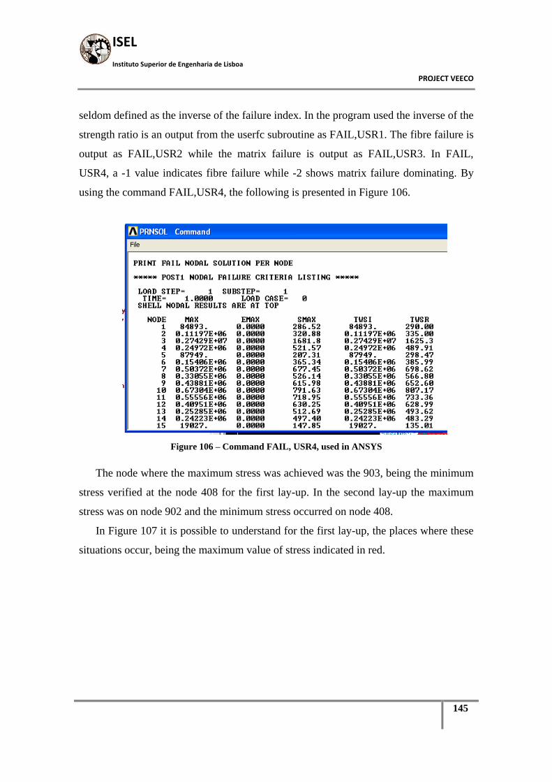
ISEL


PROJECT VEECO

145

seldom defined as the inverse of the failure index. In the program used the inverse of the

strength ratio is an output from the userfc subroutine as FAIL,USR1. The fibre failure is

output as FAIL,USR2 while the matrix failure is output as FAIL,USR3. In FAIL,

USR4, a -1 value indicates fibre failure while -2 shows matrix failure dominating. By

using the command FAIL,USR4, the following is presented in Figure 106.

Figure 106 – Command FAIL, USR4, used in ANSYS

The node where the maximum stress was achieved was the 903, being the minimum

stress verified at the node 408 for the first lay-up. In the second lay-up the maximum

stress was on node 902 and the minimum stress occurred on node 408.

In Figure 107 it is possible to understand for the first lay-up, the places where these

situations occur, being the maximum value of stress indicated in red.

146

Figure 107- Critical areass, ANSYS classic results. First lay-up.

16.7. Conclusions on the work

The main objective of the tests developed was to compare the way the different

materials react when subjected to a pressure load. This load was intended to simulate an

impact, in two different situations of velocities and time of impact.

When the time interval is smaller, the pressure applied will be greater and

consequently the values of the stresses will be greater. Considering one of the situations

studied, concerning to velocity (5 km/h) and time interval (0.1 s) for the first lay-up

scheme, it is possible to summarize the results on Table 24.

Table 24 – Von Mises stress values comparison for different composites. Lay-up (90/0/90)8

Lay-up Material Max. Stress (Pa) Min. Stress (Pa)

(90/0/90)8 Glass Fibre 3.98E+08 -2.26E08

Natural Fibre 7.43E+08 -4.22E+08

Carbon Fibre 1.14E+09 -6.47E+08

(45/-45/0)8 Glass Fibre 1.45E+08 -1.85E+08

Natural Fibre 2.73E+08 -3.48E+08

Carbon Fibre 4.13E+08 -5.26E+08

ISEL


PROJECT VEECO

147

As can be observed the carbon fibre composite, presents higher values of stresses and

the glass fibre solution the lower ones. The results from the natural fibre composite

considered can be an interesting option if the sustainability is also a decision parameter.

When comparing the two lay-ups tested it can be concluded that the second lay-up yield

lower values of maximum stresses no matter the composite considered. The values are

considerably high for this type of test, so this could benefit from a review in a further

development.

Concerning to the failure study, it can also be concluded that the fender would possibly

fail in the case of a crash, so this information may be useful to a possible improvement

in the design. The areas where the failure is visible to occur could be reinforced by

means of over thickness for instance.

148

17. Conclusions

The work developed in the different areas was made to fulfil the needs of the

VEECO project. Although the objectives were defined in the beginning of the project

they were adapted during the time the internship took place. Some of the work was not

directly related to matters referred in this thesis, but represented the needs of the

company.

The aerodynamic studies were used to improve the final design present in the

vehicle although there is a compromise between the designer decisions and the

efficiency. The front fender in composite material was to be included in the vehicle

options list; the interest was to analyse a possible benefit from a lower weight with a

resistance that could answer the requisites..

Although the time spent on the different type of studies ranged by the project was

considerable it is recognized that more tests and other type of methodologies and

analyses would be necessary to obtain a more detailed and more conclusive results

could be obtained.

As in a project of this kind the costs are always a major concern, the cheapest

options available are the combination of glass fibre (E-glass) with polyester resin. This

combination provides the necessary properties for the current application, since the

fibres govern the component properties and polyester is cheaper, versatile and widely

used. As to the manufacturing options that better fit this application, it would be elected

hand lay-up and vacuum infusion, due to the low cost and low rates of production

required. Vacuum infusion allows of course, lower production times, better part

properties and savings in labour and materials. The drawback of this method is that it is

not widely used, requiring a lot of trial and error experience to avoid infusion errors and

produce parts with the necessary quality. If the number of parts increases there are some

other options that can be more cost effective. The whole quality is a fundamental factor

that goes from the reliability of the each component to aesthetical reasons associated to

the part or the vehicle as a whole.

All the studies developed in this work were conducted with the help of the

manufacturer of the vehicle, and many aspects where tailored to represent the real

working situation of it. The results were many times taken in consideration when

developing the parts. As example the position of the front fender brackets, and the rear

ISEL


PROJECT VEECO

149

section of the body were considerably altered when the results were delivered to the

manufacturer. The participation on this project was a very enriching experience. Despite

having already worked with OEM companies the methodologies used where different in

many aspects. The sharing of knowledge and working experience is invaluable. This

kind of projects can be very interesting in terms of collaboration between universities

and small industries and both can take benefits from it, and the sharing of knowledge is

an important point.

150

18. Suggestions for further investigation

The CATIA design can be developed in order to improve the surfaces so that the

machining process can become faster. It is also important to study if the design can be

improved in the way of reducing production costs, or in order to accommodate different

materials and solutions. In the development of a series production vehicle several

hundred euros are spent in this processes, and the final quality improves, the author of

this work had the possibility to work in this kind of development in Autoeuropa, where

the production of the V.W. Scirocco was taking place, and many of the knowledge

learned at the time was transferred and adapted in this work. The project is still going on

and as an evolving prototype it is possible to improve in all areas, taking in

considerations the limitations regarding the budget available. Some design details such

as the front air intakes can be redraw using calculation of heat transmission and their

dimension adjusted to the real needs of the vehicle.

Regarding aerodynamics several improvements can be made in order to take

advantage of the shape of the vehicle. For instance, in the new phase of the project the

aerodynamic studies from this work where used to develop a range extender for the

vehicle, this also indicates the level of trust from the results obtained from the wind

tunnel.

Studies can be made to calculate a stiffer front fender or even to improve the amount

of material used in the production. A study of the mounting brackets and energy

absorption can be conducted using the models created, and several material options can

be taken in consideration for the different locations. A study aiming to the holes drilled

in the composite structures can be conducted and the methodologies used can benefit

from it.

Summing up all these possibilities the objective can only be one, improve the work

already done, and develop the concept. From a hand sketch as in Figure 108, to the final

concept presented to the public in Figure 109, all the work was developed by the team,

including the presentation.

ISEL


PROJECT VEECO

151

Figure 108-First hand sketch of VEECO

Figure 109-Public presentation of the vehicle @ Casino de Lisboa

152

REFERENCES

i. Anderson, J. D., Fundamentals of Aerodynamics, Second Edition, McGraw-Hill, Inc.

1991, pp156-160 or ref 2.2 pp32-35

ii. ANSYS Version 11.0, Release 11.0-Documentation for ANSYS, Swanson Analysis

Systems, Inc., Houston, TX, USA, 2007.

iii. ASM International. “Composites” in “ASM Handbook”. Volume 21. ed. 2001

iv. D.D. beals and W.R. Corliss, Wind tunnels of NASA, NASA SP 440, 1981.

v. DOD MIL-HDBK-17-2F. Composite Materials Handbook Volume 2: Polymer Matrix

Composites Materials properties. Department of Defense Handbook, Washington D.C,

2002.

vi. Erik Lund, Department of Mechanical and Manufacturing Engineering, Guide for Exercise

11 in Course on Mechanics of Composite Materials and Structures, 2012 FEA of

Laminated Composite Structures using ANSYS By, Aalborg University

vii. Gay, Daniel; Hoa, Suong V.; Tsai, Stephen W. Composite Materials Design and

Applications. CRC Press LLC, 2003.

viii. Gillespie, Thomas D., Fundamentals of vehicle dynamics,Warrendale: Society of

Automotive Engineers, 1992, ISBN 1-56091-199-9

ix. H. Schlichting, Aerodynamic Problems of Motor Cars, AGARD Report, 307, 1960.

x. Hashin, Z. e Rotem, A., A Fatigue Failure Criterion for Fibre Reinforced Materials,

Journal of Composite Materials, Vol. 7, pp. 448-464, 1973.

xi. Hashin, Z., Failure Criteria for Unidirectional Fibre Composites, Journal of Applied

Mechanics, Vol. 47, pp. 329-334, 1980.

xii. Hinton, M. J., Kaddour, A. S., Soden, P. D. Failure Criteria in Fibre Reinforced Polymer

Composites: The World-Wide Failure Exercise. Elsevier, 2004.

xiii. Hutton, David V. Fundamentals of finite element analysis, McGraw Hill, 2004

xiv. Information available from: http://mostreal.sk/html/elem_55/chapter4/ES4-181.htm

xv. Information available from: http://pt.scribd.com/doc/92999871/FEM-ANSYS-Composites-

Guide

xvi. Information available in: http://www.qmtmag.com/display_eds.cfm?edno=7069793

xvii. Information available in: www.veeco.pt

xviii. J. D. Whitfield, J. L. Jacobs, W. E. Dietz, and S. R. Pate, Demonstration of an Adaptive

Wall Concept Applied to an Automotive Wind Tunnel, SAE Wind Tunnel, AIAA PAPER

82-0584, 1982


http://pt.scribd.com/doc/92999871/FEM-ANSYS-Composites-Guide

http://pt.scribd.com/doc/92999871/FEM-ANSYS-Composites-Guide

http://www.qmtmag.com/display_eds.cfm?edno=7069793

http://www.veeco.pt/

ISEL


PROJECT VEECO

153

xix. Jones, R. M. Mechanics of Composite Materials. 2nd Edition. Philadelphia, Taylor &

Francis, 1999.

xx. K. B. Kelly, L. G. Provencher, and F. K. Schenkel, the General Motors Aerodynamics

Laboratory, A Full Scale Automotive Wind Tunnel, SAE 820371, 1982.

xxi. Katz, Joseph Race car aerodynamics Designing for speed

xxii. Mazumdar, Sanjay K. Composites Manufacturing Materials, Product and Process

Engineering. CRC Press LLC, 2002.

xxiii. Peters, S.T., Handbook of Composites, Second Edition, Chapman & Hall, London, UK,

1998.

xxiv. Proceedings of the Institution of Mechanical Engineers, Part D: Journal of Automobile

Engineering Development of CAD models from sketches: a case study for automotive

applications

xxv. Rae, William H. Jr. and Pope, Alan , (1984). Low-Speed wind Tunnel Testing second

edition

xxvi. Reddy, J. N. Mechanics of Laminated Composite Plates and Shells: Theory and Analysis.

2nd Ed. CRC Press, 2004.

xxvii. S. Raimondo and P.J.F. Clark, Slotted Wall test Section for Automotive Aerodynamic

Test Facilities, AIAA paper 82-0585, 1982

xxviii. Santos, André Pedro(2009), Wells Turbine: Fiberglass Flanges, Master thesis.

xxix. Savage GM, Formula 1 Composite Engineering, Engineering Failure Analysis 17(2010)

92-15)

xxx. Simone Sebben, Numerical Flow Simulation of a Detailed Car Underbody, SEA2001-01-

0703.

xxxi. Voyiadjis, George Z.; Kattan, Peter I. Mechanics of Composite Materials with MATLAB

xxxii. Williams, George I. and Wool, Richard P. , Composite from Natural Fibers and Soy Oil

Resins, Applied Composite Materials 7: 421-432, 2000

xxxiii. Wolf-Heinrich Hucho, Aerodynamics of Road Vehicles, Ed. , SAE - Society of automotive

Engineers, Inc, Warrendale, Pa, 1998ISBN 0-7680-0029-7

xxxiv. Y. Yang, et al., Recycling of composite materials, Chem. Eng. Process. (2011),

doi:10.1016/j.cep.2011.09.007

ISEL


PROJECT VEECO

155

156

APPENDIX

APPENDIX I

Protocolo de ensaio: PROJECTO VEECO

Protocolo de ensaio para a determinação da força de atrito de rolamento e coeficiente aerodinâmico do veículo

automóvel desenvolvido.

PROJECTO VEECO

(ref. VEECO nº003408)

Pedro Fonte

Rita Pereira

ISEL, 2011

Introdução

O presente protocolo destina-se a ser aplicado no ensaio do protótipo de um veículo de propulsão eléctrico

desenvolvido pela empresa Veículo Eléctrico Ecológico em parceria com o Instituto Superior de Engenharia de

Lisboa e financiado ao abrigo do programa QREN (refª 003408).

Enquadramento científico

Durante o deslocamento de um veículo automóvel, das várias forças que atuam sobre ele, existem algumas

que se podem considerar mais importantes, nomeadamente as forças de atrito de rolamento, de atrito aerodinâmico e

o efeito da inclinação do veículo, tal como apresentado na expressão (1). Este conhecimento é fundamental uma vez

que é a partir do seu conhecimento que se pode de algum modo ter uma ideia dos consumos e autonomia dos

veículos.

212T rr DR C mg v C A mgsen (1)

Força de atrito de rolamento

Esta força, representada pelo primeiro membro da expressão (1), verifica-se fundamentalmente, entre os

pneumáticos e o pavimento sobre o qual eles rolam. Segundo vários estudos, circulando a baixa velocidade, a força

de atrito de rolamento é aquela que assume maior importância, só começando a ser igualada pelo atrito aerodinâmico

acima de aproximadamente 70 Km/h, segundo os mesmos alguns autores.

Fundamentalmente existem 7 mecanismos responsáveis pela resistência de rolamento:

Perda de energia devido à deformação das paredes laterais dos pneumáticos junto da área de contacto

com pavimento;

ISEL


PROJECT VEECO

157

Perdas devido à deformação dos elementos do terreno;

Deslizamento dos pneumáticos radial e longitudinalmente;

Deflexão da superfície da estrada;

Deslizamento da superfície de contacto;

Atrito aerodinâmico ao nível das rodas;

Trepidação.

Considerando um veículo como um todo, considera-se o atrito de rolamento total como o somatório do atrito

individual de cada roda. Podendo muito sumariamente ser caracterizado pela expressão(2), em que Crr representa o

coeficiente de atrito, m a massa do veículo e g a aceleração gravítica:

rr rrF C mg (2)

Nesse sentido, este protocolo pretende definir os ensaios experimentais a efectuar no terreno que permitam

conhecer o valor do atrito de rolamento em regime permanente com uma precisão aceitável. Desse modo, não se

pretende estudar a sua variação dinâmica, o que obrigaria a cálculos teóricos profundos. Assim, e a priori são

desprezados o peso dinâmico do veículo, os efeitos de aceleração, as forças de arrasto e a componente vertical do ar

que só por si não apresentariam uma mais-valia na precisão dos resultados e obrigariam a cálculos complicados.

Fatores que definem o coeficiente de atrito de rolamento

O coeficiente de atrito de rolamento pretende expressar algumas das propriedades físicas que ocorrem entre

os pneumáticos e o pavimento, propriedades essas que são complexas e interdependentes. Nesse sentido, e de forma a

enquadrar o protocolo, são analisadas alguns dos fatores que mais influenciam o coeficiente de atrito:

Temperatura dos pneumáticos

Uma grande percentagem do atrito de rolamento em superfícies pavimentadas deriva da deflexão e perdas

de energia na borracha dos pneumáticos por efeito de histerese, o que conduz a uma alteração da temperatura. O

efeito de histerese deriva dos consecutivos ciclos de deformação e recuperação da forma do pneumático, em que a

diferença entre as duas se traduz em perdas. Nesse sentido, com o aumento da temperatura o atrito de rolamento tende

a diminuir. Tipicamente desde o arranque com os pneus considerados “frios”, é desejável percorrer uma distância

nunca inferior a 35 Km para se considerar uma temperatura estável ou em alternativa, faz-se rolar os pneumáticos

durante cerca de 20 minutos.

Carga/Pressão

A pressão nos pneumáticos está intimamente ligada à sua elasticidade e em combinação com a carga,

determina a deflexão da superfície entre o pneumático e o pavimento para além da deformação do pavimento.Num

pavimento compacto, tal como aquele em que será suposto o veículo circular, o coeficiente diminuirá com o aumento

da pressão. Assim será aconselhável que o ensaio seja efectuado com os pneumáticos cheios à pressão indicada para

uma carga média (dois ocupantes adultos sem bagagem).

Velocidade

158

O coeficiente de rolamento é directamente proporcional à velocidade uma vez, para lá da temperatura, faz

variar a flexão e a vibração do pneumático, embora a baixas velocidade o seu efeito seja reduzido podendo se

considerado constante para efeitos de cálculo. Geralmente a influência é maior quando o aumento da velocidade é

combinado com pressões baixas.

Material e desenho

Também a constituição do pneumático, espessura, tipo de borracha e perfil influenciam o atrito de

rolamento. Pelo que o veículo deverá ser ensaiado com os pneumáticos de série.

Ensaios típicos aos pneumáticos

Existem vários protocolos de ensaios laboratoriais específicos para o cálculo da resistência de rolamento

especificamente focados nos pneumáticos, nomeadamente:

SAE 1269

SAE J2452

ISO 18164

ISO 28580

Em que fundamentalmente são executados três tipos de ensaios, força, potência e binário e divididos em single-

point e multi-point. Este último usa mais do que um conjunto de condições para testar os pneumáticos, normalmente

variando a velocidade a pressão e/ou a carga. Todos eles têm obrigatoriamente de ser executados em laboratório com

equipamento próprio. Pelo que neste documento se pretende apresentar um método alternativo e prático que possa ser

aplicado ao veículo ao invés dos pneumáticos isoladamente.

Coeficiente aerodinâmico

Enquadramento científico

A aerodinâmica tem uma forte influência no design do veículo, no entanto este design é primordialmente

determinado por outros factores, tais como: funcionalidade, segurança, regulamentação, economia e estética.

A consciência acerca da importância do coeficiente aerodinâmico está associada a crises energéticas, uma

vez que estando optimizado o rendimento das máquinas motrizes dos veículos, quer sejam elas motores de combustão

interna ou motores eléctricos, uma alternativa viável consiste em alterar a forma do próprio veículo com o intuito de o

tornar mais económico.

Existem abordagens teóricas, com maior ou menor nível de complexidade e exatidão para determinação do

coeficiente aerodinâmico de um automóvel. Contudo os valores mais corretos são aqueles que se determinam na

prática, em ensaios em túnel de vento.

Uma vez que o estudo do coeficiente aerodinâmico se insere no domínio da dinâmica dos fluidos,

consubstancia o facto de atualmente serem os software de computação e desenho mecânico aqueles que apresentam

maior fiabilidade no cálculo do coeficiente aerodinâmico e que mais se aproximam do valor obtido em ensaio prático

realizado em túnel de vento.

Concluindo esta introdução genérica e muito resumida, é de salientar o facto de serem os valores obtidos

em simulação computacional aqueles que se devem considerar numa abordagem analítica.

ISEL


PROJECT VEECO

159

Apresenta-se seguidamente as diversas abordagens que consubstanciam a determinação do coeficiente

aerodinâmico sob o ponto de vista académico e analítico. No procedimento experimental, pode encontrar-se uma

abordagem prática para determinação aproximada do coeficiente aerodinâmico através de ensaios realizados no

terreno.

Análise do coeficiente aerodinâmico

A análise do coeficiente aerodinâmico pode ser efetuada recorrendo a:

a) Exame dos mecanismos físicos que geram o coeficiente aerodinâmico

b) Alocação de frações do coeficiente aerodinâmico ao local de origem

c) Investigação do efeito aerodinâmico no campo de fluxo envolvente

As três abordagens podem conduzir a resultados corretos, contudo a conjugação de diferentes metodologias de

análise conduzem a erros significativos.

a) Mecanismos físicos:

A causa física do coeficiente aerodinâmico poderá ser melhor compreendida através da comparação do fluxo de

ar em torno do automóvel com o fluxo de ar ideal (em meios onde não existe fricção).

Para um ponto de vista experimental o cálculo do integral das pressões e tensões tangenciais aparenta ser

demasiado académico; Durante o desenvolvimento de um automóvel real, as pressões de superfície são medidas para

um número limite de pontos em zonas específicas da superfície do corpo, por outro lado as tensões tangenciais nem

sequer são mensuráveis.

No entanto, a abordagem torna-se viável quando o fluxo em torno do automóvel é calculado recorrendo a

software CFD (ComputationalFluidDynamics). Desta forma o coeficiente pode ser determinado através da integração

das pressões, do cálculo das tensões tangenciais e da resistência do ar. De acordo com as seguintes equações,

respectivamente:

sinpD p dS (3)

coswDf dS (4)

p fD D D (5)

Onde p representa a pressão, representa o ângulo formado entre o vetor tensão tangencial, , à superfície

e a horizontal, sendo a viscosidade dada pela lei de Newton para um fluxo paralelo a uma parede, de acordo com a

equação:

du

dy (6)

160

Entende-se por viscosidade a fricção molecular entre as partículas de fluido; relaciona o momento do fluxo

com o gradiente da velocidade . O factor , denomina-se viscosidade dinâmica.

A alternativa aos cálculos apresentados consiste em computar o efeito aerodinâmico no campo de fluxo

envolvente.

b) Alocação de fracções do coeficiente aerodinâmico ao local de origem

Consiste numa subdivisão aproximada do coeficiente aerodinâmico de acordo com as regiões que lhe dão

origem, tal como se esquematiza no diagrama da figura 1.

Figura 1- Partição do coeficiente aerodinâmico de acordos com os seus locais de

origem

De uma forma resumida para um corpo com linhas suaves e sem protuberâncias podem-se distinguir quatro

zonas geométricas:

Extremidade frontal;

Inclinaçãotraseira;

Base (i.e., painel vertical na traseira);

Painéis laterais, tejadilho e parte de baixo do automóvel.

Caso as zonas acima descritas sejam classificadas de acordo com as designações coeficiente aerodinâmico de

pressão e de fricção, torna-se evidente que as primeiras três zonas estão sujeitas a um coeficiente aerodinâmico de

pressão, estando as últimas (painéis laterais, tejadilho e parte de baixo do automóvel) sujeitas a um coeficiente

aerodinâmico de fricção.

c) Investigação do efeito aerodinâmico no campo de fluxo envolvente

coeficiente aerodinamico

total

campo de fluxo externo

corpo

parte de cima

do automóvel

parte de baixo do automóvel

(incluindo rodas)

protuberâncias

(espellhos, etc.)

campo de fluxo interno

admissão de ar aquecimento,

refrigeração, ar condicionado

componentes

(travões, etc.)

ISEL


PROJECT VEECO

161

O efeito de perturbação do ambiente à custa de um automóvel em movimento é detectado numa área

considerável, tal como se apresenta simbolicamente na figura 2. A partir das distribuições das pressões e velocidades

nas fronteiras do volume de controlo, podem-se retirar conclusões acerca das forças e momentos que atuam no

automóvel, nomeadamente acerca do coeficiente aerodinâmico através da aplicação do seguinte teorema:

2 2 2

1 1D p totalS S S

u u wC A C dS dS dS

V V V

(7)

Sendo:

, o coeficiente aerodinâmico;

A, a área frontal do automóvel;

, Coeficiente de pressão total;

u,v, w , componentes da velocidade segundo os três eixos cartesianos;

V, velocidade de rolamento;

S, superfície de controlo.

Figura 2 – Volume de controlo em torno do automóvel ao qual se aplica o teorema (11)

O coeficiente de atrito calculado de acordo com a expressão (11) tende a ser superior ao determinado em

túnel de vento, caso o chão do túnel de evento seja estacionário.

162

Considerações para o ensaio

O ensaio deve ser feito no tipo de superfície em que o veículo foi projectado para circular e que se

apresente seco.

Os pneumáticos devem ser cheios com a pressão recomendada pelo fabricante e o veículo deverá circular com uma

carga média, aproximadamente dois passageiros adultos sem bagagem.

O veículo deverá circular durante 20 minutos antes de se dar início ao teste para os pneumáticos atingirem a

temperatura média de circulação após o qual se deverá dar início ao ensaio.

O local do ensaio deverá ser o mais plano possível de modo a poder desprezar-se o efeito da inclinação.

Cada um dos ensaios terá obrigatoriamente de ser repetido nas mesmas condições circulando em sentidos opostos.

Procedimento para a determinação do coeficiente de atrito de rolamento

1 - Partindo de uma velocidade reduzida e constante (5 a 10 Km/h), contar o tempo decorrido entre o

momento em que se liberta o acelerador e a paragem total do veículo tomando nota do valor da velocidade inicial e

do tempo decorrido.

2 - Repetir o teste para valores de velocidade crescentes repetindo os procedimentos de 1. Quando a relação

velocidade inicial/tempo de paragem for diferente dos valores anteriores o ensaio deixa de ser válido uma vez que o

efeito do atrito aerodinâmico se começa a fazer sentir.

3 - Os testes deverão ser repetidos em direcções opostas, num mínimo de 3 vezes, e calculadas as médias

para cancelar o efeito da inclinação do piso. Deste modo obtêm-se o valor de rrC g através da expressão (8):

rr

vC g

t

(8)

Na impossibilidade de ler a velocidade com exactidão o mesmo procedimento poderá ser repetido medindo

a distância percorrida e o tempo, aplicando-se de seguida a expressão (9):

2

2rr

dC g

t (9)

A muito baixa velocidade poder-se-ão registar fenómenos de não linearidades introduzidas pelos

pneumáticos. Nesse caso poder-se-á calcular a desaceleração medindo a velocidade e o tempo que decorre entre dois

valores de velocidade.

No caso da precisão na leitura da velocidade ser baixa, a desaceleração poderá ser calculada através do

tempo e da distância. Nesse sentido poderão ser feitas por exemplo três marcações no pavimento e fazendo-se a

ISEL


PROJECT VEECO

163

medição entre a primeira e a segunda marca (x1,t1) e primeira e terceira marca(x2,t2), calculando então pela expressão

(10):

2 1

2 1 2 1

2rr

x xC g

t t t t

(10)

Determinação do coeficiente de atrito aerodinâmico de acordo com a

expressão (1)

Considerando que o feito da inclinação do terreno é anulado pela médias das medições e que se trata de uma

desaceleração a expressão, pode ser descrita por (11).

21

2T rr d

dVF m C mg C AV

dt (11)

Dividindo a expressão (11)pela massa, resultará uma aceleração que poderá ser descrita por(12).

21

2rr d

dVC g C V

dt m (12)

Verifica-se que a desaceleração do veículo dependerá tanto do atrito de rolamento como do atrito

aerodinâmico. Como tal após o cálculo do valor de Crrg e considerando-o constante repete-se o ensaio para

velocidade crescentes (até à velocidade máxima do veículo) registando-se os valores de velocidade inicial e o tempo

de paragem. Através da expressão (13), após integração de (12), e com o conhecimento do valore de Crrg é possível

calcular o valor de 2DC A

m

representado por b correspondendo aarrC g .

inicial

bV tg t ab

a (13)

Após a construção do gráfico de dispersão para vários valores de velocidade inicial startt f V , é

aconselhável repetir os testes para valores aleatoriamente escolhidos para a validação do gráfico.

A determinação de b, poderá ser feita entre outras formas recorrendo a uma ferramenta de cálculo, atribuir e

verificar valores de b.

Resultados esperados e validação

Tal como foi indicado em 3.3.1, presentemente os valores de coeficientes de atrito aerodinâmico mais fiáveis são

aqueles que resultam desoftwares de computação e desenho mecânico. Como tal espera-se uma diferença entre os

resultados simulados e experimentais embora coma mesma ordem de grandeza. Quanto ao coeficiente de atrito de

rolamento poderá ser facilmente comparado com os valores tabelados de coeficiente de atrito fornecidos por várias

marcas de pneumáticos.

164

Results calculated after the tests:

Table:

Cx Cr

1st Test 0.315583 0.014559

2nd Test 0.407269 0.022326

3rd Test 0.245172 0.016771

4th Test 0.440272 0.02234

5th Test 0.247688 0.014423

6th Test 0.398532 0.022709

7th Test 0.22238 0.01722

Probable value 0.327 0.019

The probable value is obtained making the median value.

ISEL


PROJECT VEECO

165

APPENDIX II

3DPrinter from fab-lab

A impressora “3D DIMENSION ELITE “permite criar modelos

tridimensionais com detalhes muito precisos usando um processo aditivo,

camada a camada, com recurso à deposição de dois tipos de materiais:

O material que cria as peças modeladas “ABSPlus” e o material de suporte

(SST) que é solúvel e é retirado no fim.

A impressão 3D envolve a construção de um modelo 3D criado a partir de um

ficheiro digital CAD.

Software

Software: CATALYST EX

File format: .STL

Model material:

ABSplus in ivory, white, black, red, olive green, nectarine, fluorescent yellow, blue or

gray.

Support material:

Soluble Support Technology (SST)

Build Size:

203 x 203 x 305 mm (8 x 8 x 12 in.)

Layer thickness:

0.178 mm (.007 in.) or 0.254 mm (.010 in.) of precisely deposited ABSplus model and

support material

166

Workstation compatibility:

Windows® XP / Windows Vista® / Windows® 7

Network connectivity:

Ethernet TCP/IP 10/100Base-T

Size and weight:

686 x 914 x 1041 mm (27 x 36 x 41 in.)

136 kg (300 lbs.)

Power requirements:

110-120 VAC, 60 Hz, minimum 15A dedicated circuit;

or 220-240 VAC 50/60 Hz, minimum 7A dedicated circuit.

Information gathered from: http://www.dimensionprinting.com/3d-printers/printing-

productspecs-elite.aspx

http://www.dimensionprinting.com/3d-printers/printing-productspecs-elite.aspx

http://www.dimensionprinting.com/3d-printers/printing-productspecs-elite.aspx

ISEL


PROJECT VEECO

167

APPENDIX III

Resin MGS 418 Properties Courtesy of MGS Company:

ISEL


PROJECT VEECO

169

MATERIAL: Lancair 7781 Glass Fabric / MGS 418 Wet Layup 7781/MGS 418

Summary

FIBER: BGF 7781 Glass Fabric RESIN: MGS 418

Tg (dry): 216.4F Tg (wet): 209.9F Tg METHOD: DMA (SRM 18-94)

PROCESSING: Vacuum bag cure (22+ in. Hg.): 170-230 10F for 5.5-24 hours

Date of fiber manufacture 10/9/98 Date of testing 10/26/99 – 12/15/99

Date of resin manufacture Unknown Date of data submittal 12/15/99

Date of composite manufacture 6/98 – 3/99 Date of analysis 10/28/99 – 12/15/99

LAMINA MECHANICAL PROPERTY SUMMARY Data Reported as: Measured

(Normalized by CPT=0.0108 in.)

CTD RTD ETD ETW

B-Basis Mean B-Basis Mean B-Basis Mean B-Basis Mean

F2tu

(ksi) 52.02 (54.54)

60.89 (59.83)

41.85 (41.25)

48.99 (47.89)

36.06 (35.48)

42.21 (41.19)

31.05 (33.00)

36.34 (38.31)

E2t (Msi) --- 3.42

(3.37) --- 2.39

(2.33) --- 2.10

(2.05) --- 2.65

(2.82)

21tu

(ksi) --- 0.175 --- 0.118 --- 0.087 --- 0.107

F2cu

(ksi) 58.13 (57.17)

66.72 (67.30)

45.11 (42.64)

51.77 (50.19)

27.41 (25.93)

31.45 (30.52)

25.35 (25.20)

29.10 (29.67)

E2c (Msi) --- 2.27

(2.31) --- 3.16

(3.07) --- 3.06

(2.97) --- 2.14

(2.17)

F12su

(ksi) 19.67 21.16 14.36 15.45 8.74 9.41 7.68 8.26

G12s (Msi) --- 0.63 --- 0.44 --- 0.23 --- 0.25

F13su**

(ksi) --- --- 7.00 7.59 --- --- --- ---

** Apparent interlaminar shear strength

APPENDIX IV

AGATE Database: 7781 Glass Fabric/ MGS 418 Wet Layup

170

Mate

rial:

La

nca

ir 77

81

Gla

ss F

ab

ric/ M

GS

41

8 W

et L

ayu

p

Resin

co

nte

nt:

34 - 3

6 w

t%C

om

p. d

en

sity

:1.7

0 - 1

.74 g

/cc

Fib

er v

olu

me:

43 - 4

5 %

Vo

id c

on

ten

t:5.5

to 6

.4 %

Test m

eth

od

:A

ST

M D

953-9

5

Typ

e o

f be

arin

g te

st:

Double

Shear P

in B

earin

g

Fa

ste

ne

r Typ

e:

Hard

ened S

teel P

in

To

rqu

e:

N/A

No

rmaliz

ed

by:

Not n

orm

aliz

ed

CT

DR

TD

ET

W

Test T

em

pe

ratu

re [°F

]-6

575

180

Mo

istu

re C

on

ditio

nin

gdry

dry

equilib

rium

Eq

uilib

rium

at T

, RH

as fa

bric

ate

das fa

bric

ate

d145F

, 85%

So

urc

e c

od

eM

V#X

XX

XB

MV

#X

XX

XA

MV

#X

XX

XF

Dia

mete

r[in]

0.1

875

0.2

50

0.3

75

0.1

875

0.2

50

0.3

75

0.1

875

0.2

50

0.3

75

0.1

875

0.2

50.3

75

Mean

51.3

251.5

636.1

239.0

523.6

723.4

7

Fb

uM

inim

um

49.2

349.1

634.8

736.5

222.7

522.5

2

(ksi)

Maxim

um

53.1

953.2

338.1

440.7

125.2

325.1

2

[0/4

5/0

]s (6

plie

s)

C.V

.(%)

2.9

23.2

93.3

53.3

53.7

23.7

9

tp

ly : 0.0

098 - 0

.0107 in

.

Fa

ilure

Mo

de

Bearin

gB

earin

gB

earin

gB

earin

gB

earin

gB

earin

g

No

. Sp

ecim

en

s6

77

88

9

No

. Batc

he

s1

11

11

1

Mean

74.9

652.1

754.0

544.0

633.5

631.7

1

Fb

uM

inim

um

70.8

250.1

153.0

142.9

131.4

930.6

2

(ksi)

Maxim

um

79.1

553.8

454.8

344.8

636.3

132.7

5

[(0/4

5)5 ]

s (20 p

lies)

C.V

.(%)

3.9

52.3

51.1

51.7

04.7

82.0

3

tp

ly : 0.0

104 - 0

.0107 in

.

Fa

ilure

Mo

de

Bearin

gLate

ral

Bearin

gLate

ral

Bearin

gB

earin

g

No

. Sp

ecim

en

s7

66

69

9

No

. Batc

he

s1

11

11

1

Be

arin

g S

tren

gth

G/E

p7781 G

lass F

ab

ric/ M

GS

418 W

et L

ayu

p

ISEL


PROJECT VEECO

171

Appendix V

The ANSYS code is relative to the glass fibre test.

!STRENGHT VALUES FOR 3D HASHIN FAILURE CRITERIA:

XTEN=284418750

XCMP=-294002800

YTEN=284418750

YCMP=-294002800

ZTEN=460e6

ZCMP=-410e6

XY=99012200

YZ=42e6

XZ=42e6

XTENINV=XTEN**(-1)

XCMPINV=XCMP**(-1)

YTENINV=YTEN**(-1)

YCMPINV=YCMP**(-1)

ZTENINV=ZTEN**(-1)

ZCMPINV=ZCMP**(-1)

XYINV=XY**(-1)

YZINV=YZ**(-1)

XZINV=XZ**(-1)

!Extraction of the stress values on an element basis:

ETABLE,SX,S,X

ETABLE,SY,S,Y

ETABLE,SZ,S,Z

ETABLE,SXY,S,XY

ETABLE,SYZ,S,YZ

ETABLE,SXZ,S,XZ

!Calculations performed in order to store the value of the failure criteria in the element table

SMULT,MTC1,SY,SY,YTENINV,YTENINV

SMULT,MTC2,SXY,SXY,XYINV,XYINV

SMULT,MTC3,SYZ,SYZ,YZINV,YZINV

SADD,MTC4,MTC1,MTC2

SADD,MTC,MTC3,MTC4

SMULT,MCC1,SY,SY,YCMPINV,YCMPINV

SMULT,MCC2,SXY,SXY,XYINV,XYINV

SMULT,MCC3,SYZ,SYZ,YZINV,YZINV

SADD,MCC4,MCC1,MCC2

SADD,MCC,MCC3,MCC4

SMULT,FTF1,SX,SX,XTENINV,XTENINV

SMULT,FTF2,SXY,SXY,XYINV,XYINV

SMULT,FTF3,SXZ,SXZ,XZINV,XZINV

172

SADD,FTF4,FTF1,FTF2

SADD,FTF,FTF3,FTF4

SMULT,FCF,SX,SX,XCMPINV,XCMPINV

SMULT,FMSO1,SX,SX,XCMPINV,XCMPINV

SMULT,FMSO2,SXY,SXY,XYINV,XYINV

SMULT,FMSO3,SXZ,SXZ,XZINV,XZINV

SADD,FMSO4,FMSO1,FMSO2

SADD,FMSO,FMSO3,FMSO4

SMULT,DELT1,SZ,SZ,ZTENINV,ZTENINV

SMULT,DELT2,SXZ,SXZ,XZINV,XZINV

SMULT,DELT3,SYZ,SYZ,YZINV,YZINV

SADD,DELT4,DELT1,DELT2

SADD,DELT,DELT3,DELT4

SMULT,DELC1,SZ,SZ,ZCMPINV,ZCMPINV

SMULT,DELC2,SXZ,SXZ,XZINV,XZINV

SMULT,DELC3,SYZ,SYZ,YZINV,YZINV

SADD,DELC4,DELC1,DELC2

SADD,DELC,DELC3,DELC4

!Storing the various failure criteria results:

*DO,j,1,MAXEL,1

*GET,MTC(j,i+1),ETAB,11,ELEM,j

*ENDDO

*DO,j,1,MAXEL,1

*GET,MCC(j,i+1),ETAB,16,ELEM,j

*ENDDO

*DO,j,1,MAXEL,1

*GET,FTF(j,i+1),ETAB,21,ELEM,j

*ENDDO

*DO,j,1,MAXEL,1

*GET,FCF(j,i+1),ETAB,22,ELEM,j

*ENDDO

*DO,j,1,MAXEL,1

*GET,FMSO(j,i+1),ETAB,27,ELEM,j

*ENDDO

*DO,j,1,MAXEL,1

*GET,DELT(j,i+1),ETAB,32,ELEM,j

*ENDDO

*DO,j,1,MAXEL,1

*GET,DELC(j,i+1),ETAB,37,ELEM,j

*ENDDO

/SOLU

instituto superior de engenharia de lisboa · a analise de falha foi baseada num modelo com o...

Documents