livros grátislivros01.livrosgratis.com.br/cp004811.pdf · resumo in tro du c ~ ao o crescimen to...
TRANSCRIPT

Adriana de Andrade Oliveira
Um Arcabou�co para Engenharia de Tr�afego em Redes
MPLS
Tese apresentada ao Curso de P�os-
Gradua�c~ao em Ciencia da Computa�c~ao da
Universidade Federal de Minas Gerais como
requisito parcial para a obten�c~ao do grau de
Doutor em Ciencia da Computa�c~ao.
Universidade Federal de Minas Gerais
Belo Horizonte, Outubro de 2005

Livros Grátis
http://www.livrosgratis.com.br
Milhares de livros grátis para download.

Resumo
Introdu�c~ao
O crescimento do uso da Internet, juntamente com a diversi�ca�c~ao de suas aplica�c~oes, trouxe
novos desa�os �a �area de projeto e planejamento de redes. Um desses desa�os �e utilizar e�-
cientemente a infra-estrutura de rede existente, oferecendo servi�cos com diferenciados n��veis
de qualidade. Em redes orientadas a conex~ao, a transferencia de informa�c~ao entre usu�arios
�nais, com determinados n��veis de qualidade, �e conseguida pelas pr�oprias fun�c~oes de rede que
selecionam e alocam recursos da rede. J�a em redes IP (Internet Protocol), redes sem conex~ao,
esta �e uma necessidade nova, j�a que n~ao existe o conceito de reserva de recursos.
Em redes IP, freq�uentemente se percebe a concentra�c~ao do uxo em algumas partes da
rede enquanto outras partes permanecem sub-utilizadas. A m�a utiliza�c~ao de recursos exis-
tentes �e devida �a m�a distribui�c~ao do tr�afego feita pelos algoritmos de roteamento, que buscam
geralmente o menor caminho da origem at�e o destino e n~ao levam em considera�c~ao o tr�afego
j�a existente nesse caminho mais curto. Portanto, para tornar realidade o provisionamento de
qualidade de servi�co (QoS) em redes IP, torna-se necess�ario o desenvolvimento de ferramentas
de Engenharia de Tr�afego para redes IP.
As ferramentas de Engenharia de Tr�afego s~ao respons�aveis por v�arias fun�c~oes de gerenci-
amento do tr�afego. Entre elas podem ser citadas o estabelecimento de pol��ticas para controle
de admiss~ao de requisi�c~oes, controle e determina�c~ao de rotas f��sicas para os uxos, assim como
a reserva de recursos e controle da rede em diferentes escalas de tempo. A combina�c~ao de
tecnologias de comuta�c~ao de r�otulos e mecanismos de roteamento que levam em considera�c~ao
m�etricas de desempenho da rede e, ao mesmo tempo, permitem aos administradores in uen-
ciar as decis~oes de roteamento baseados em suas prefererencias parece ser uma solu�c~ao para
se fazer Engenharia de Tr�afego na Internet de maneira e�ciente e com custo razo�avel.
i

ii RESUMO ESTENDIDO
O MPLS (Multi-Protocol Label Switching) �e um mecanismo de encaminhamento de pa-
cotes, que re�une t�ecnicas de transmiss~ao orientadas a conex~ao e protocolos de roteamento, para
simpli�car o processamento de pacotes nos roteadores que �cam no caminho entre a origem e
o destino do uxo [Awduche, 1999]. Os pacotes s~ao rotulados ao entrar em um dom��nio com
suporte a MPLS e a classi�ca�c~ao e o posterior encaminhamento por uma determinada rota s~ao
de�nidos baseados nestes r�otulos. O MPLS surge como aliado da Engenharia de Tr�afego uma
vez que apresenta a funcionalidade de cria�c~ao de rotas expl��citas e, atrav�es desse mecanismo,
possibilita a otimiza�c~ao da utiliza�c~ao dos recursos da rede.
Como o MPLS desacopla roteamento de pacotes de encaminhamento de pacotes, ele �e
capaz de suportar diferentes pol��ticas de roteamento; o que �e dif��cil ou quase imposs��vel de se
fazer apenas com o encaminhamento convencional da camada de rede. Esse trabalho trata do
problema de sele�c~ao das rotas f��sicas dos LSPs (Label Switched Paths) em redes MPLS (Multi-
Protocol Label Switching), que consiste na de�ni�c~ao de rotas para os LSPs que minimizem o
n�umero total de saltos utilizados no roteamento e o n�umero total de requisi�c~oes rejeitadas.
De�ni�c~ao do Problema e Contribui�c~oes
O objetivo deste trabalho �e o projeto e a valida�c~ao atrav�es de simula�c~ao de um arcabou�co
para engenharia de tr�afego em redes MPLS. Dentre os problemas de engenharia de tr�afego
existentes, foi dada prioridade ao problema de de�ni�c~ao de rotas f��sicas para LSPs.
Inicialmente propomos um modelo linear inteiro para solucionar o problema de maneira
exata. Esse modelo tenta balancear a carga na rede enquanto minimiza a taxa de rejei�c~ao.
O objetivo �e otimizar o desempenho global da rede roteando as requisi�c~oes atrav�es de enlaces
sub-utilizados melhorando a utiliza�c~ao da infra-estrutura instalada.
O problema de roteamento em redes MPLS �e NP-completo e o tempo necess�ario para
se encontrar a solu�c~ao exata para o mesmo �e invi�avel na pr�atica. Assim, heur��sticas goram
propostas para resolver o modelo e foi feita uma compara�c~ao das solu�c~oes obtidas com as
heur��sticas com a solu�c~ao �otima obtida atrav�es do CPLEX [ILOG, 2002].
Nossa heur��stica �e baseada em algoritmos gen�eticos, onde utilizamos a combina�c~ao de
pol��ticas de roteamento com movimentos adaptativos de rotas para se obter a solu�c~ao. As tres
pol��ticas de roteamento utilizadas s~ao baseadas em menor caminho, maior balanceamento ou

RESUMO ESTENDIDO iii
limita�c~ao de tr�afego. Os movimentos adaptativos s~ao utilizados para ajuste do roteamento,
fornecendo uma maior exibilidade �as pol��ticas. Quando h�a a possibilidade de rejei�c~ao de
uma requisi�c~ao, reroteamentos s~ao realizados para atender a essa requisi�c~ao sem um grande
preju��zo das requisi�c~oes j�a estabelecidas.
Para analisar o desempenho do algoritmo gen�etico, foram estudados v�arios cen�arios e
foram feitas v�arias simula�c~oes. Os resultados mostram que o algoritmo gen�etico executa muito
mais r�apido que a ferramenta comercial utilizada para resolver o modelo de forma exata. Os
resultados tamb�em mostram que o uso do algoritmo gen�etico diminui consideravelmente a
quantidade de requisi�c~oes rejeitadas na rede.
Al�em do caso cl�assico de chegada de novas requisi�c~oes, esse trabalho tamb�em trata do
problema de ajuste do roteamento em diversos outros casos de mudan�cas na rede. Foram
executados v�arios experimentos e resultados satistat�orios foram encontrados, mostrando que
o algoritmo gen�etico �e tamb�em apropriado para o roteamento on-line. Deve-se ressaltar que
h�a um aumento no custo do roteamento on-line devido ao reroteamento necess�ario.
Chamamos grooming o processo de ajuste on-line do roteamento da rede. Ele ocorre tanto
quando uma nova requisi�c~ao surge quanto um novo elemento de rede �e con�gurado, LSPs s~ao
terminados ou elementos de rede se recuperam de falhas. Resumindo, o grooming da rede
�e necess�ario quando decis~oes de roteamento tomadas no passado n~ao s~ao mais e�cientes no
presente. Um mecanismo de detec�c~ao de mudan�cas de tr�afego �e proposto para engatilhar
o processo de grooming. Esse mecanismo �e baseado em cartas de controle. Resultados de
simula�c~ao indicam que um melhor desempenho �e alcan�cado atrav�es do uso dos mecanismos
propostos.
Trabalhos Relacionados
Alguns conceitos b�asicos referentes �a QoS que s~ao tratados neste trabalho s~ao apresen-
tados em [Guerin et al., 1997], [Crawley et al., 1998], [Xiao et al., 1999], entre outros. Em
[Awduche, 1999], a aplica�c~ao de MPLS para Engenharia de Tr�afego em redes IP �e discutida.
Um dos esquemas de roteamento dinamico mais citados, Minimum Interference Routing
Algorithm (MIRA) [Kar et al., 2000], �e baseado em uma heur��stica para sele�c~ao de rotas on-
line. A id�eia principal da heur��stica �e explorar o conhecimento dos pares de entrada e sa��da da

iv RESUMO ESTENDIDO
rede, buscando evitar rotear as requisi�c~oes em enlaces que poder~ao interferir em requisi�c~oes
futuras.
As principais desvantagens desse esquema s~ao a complexidade computacional necess�aria
para implement�a-lo, a falta de balanceamento de carga obtida em algumas topologias, como
demonstrado em [Wang et al., 2002] e o fato de que ele n~ao leva em considera�c~ao a carga
atual da rede na tomada de decis~oes, como demonstrado em [Boutaba et al., 2002]. Nosso
esquema tenta manter seu custo computacional similar ao custo de algoritmos de roteamento
tradicionais e tenta conciliar simplicidade, acur�acia e custo computacional.
Em [Yilmaz and Matta, 2002] um estudo do algoritmo MIRA e de um algoritmo Pro�le-
Based �e apresentado mostrando topologias onde o desempenho do algoritmo MIRA �e melhor
que o do algoritmo Pro�le-Based. Em [Figueiredo et al., 2004] um novo algoritmo de m��nima
interferencia �e apresentado. A vantagem desse algortimo �e que o mesmo n~ao computa o uxo
m�aximo para todos os casos, como no caso do MIRA. S~ao comparados os resultados desse
novo algoritmo, com os resultados do MIRA e de um algoritmo baseado no menor caminho
com maior banda (WSP). Os autores n~ao consideram entretanto reroteamento e apresentam
uma fun�c~ao objetivo diferente da apresentada nesse trabalho.
Em [Salvadori and Battiti, 2003] um esquema de balanceamento de carga para redes MPLS
�e apresentado. A id�eia �e minimizar o congestionamento da rede atrav�es de altera�c~oes locais
em algumas rotas. A principal diferen�ca entre o esquema proposto nessa tese e o esquema
proposto por eles �e que eles buscam o melhor caminho alternativo para rerotear e a sua
fun�c~ao objetivo �e maximizar a capacidade dispon��vel na rede. Em nossa proposta, o algoritmo
pretende minimizar o n�umero de rejei�c~oes e, em caso de reroteamento, ele busca por uma
solu�c~ao alternativa que satisfa�ca a demanda e n~ao exceda o n�umero de saltos da solu�c~ao �otima
por uma grande margem. Essa solu�c~ao alternativa n~ao �e necessariamente �otima, j�a que a
busca por uma solu�c~ao alternativa n~ao �e feita como em [Salvadori and Battiti, 2003].
O esquema de Salvadori apresenta um aspecto preventivo uma vez que ele inicia o procedi-
mento de reroteamento quando a con�gura�c~ao de um LSP causa a detec�c~ao de uma situa�c~ao de
congestionamento. Nosso esquema n~ao apresenta o aspecto preventivo e tenta rerotear algum
LSP apenas quando uma nova requisi�c~ao chega e n~ao h�a rota dispon��vel com um n�umero de
saltos aceit�avel.

RESUMO ESTENDIDO v
Em [Nobre et al., 2005] um esquema de balanceamento de carga baseado no trabalho de
[Salvadori and Battiti, 2003] �e apresentado. A principal diferen�ca �e a fun�c~ao objetivo utilizada
que trata o problema de atraso causado pelo uso de rotas longas no reroteamento. Um algo-
ritmo on-line muito interessante tamb�em foi apresentado em [Boutaba et al., 2002], embora
eles n~ao considerem reroteamento em seu esquema.
Alguns modelos lineares inteiros foram propostos para solucionar o problema de rotea-
mento o�ine em redes MPLS, tais como [Girish et al., 2000], [Liu, 2003], [Chou, 2004],
[Dias et al., 2003] e [Dias and Camponogara, 2003]. Outros modelos foram apresenta-
dos em �areas a�ns como roteamento de circuitos [Resende and Ribeiro, 2003]. Em
[Fortz and Thorup, 2000], o objetivo dos autores foi otimizar o estabelecimento de pesos nos
enlaces, para o protocolo OSPF (Open Shortest Path First), baseado nas demandas projetadas.
Todos os modelos tratam de uma fun�c~ao com um �unico objetivo, com exce�c~ao de
[Chou, 2004]. N~ao �e apresentado como o modelo poderia ser utilizado em uma vers~ao on-
line do problema. N~ao s~ao apresentados resultados para diversas topologias e tr�afegos. Nesse
trabalho, al�em de compararmos a solu�c~ao obtida pela heur��stica com a solu�c~ao exata, experi-
mentos foram feitos simulando a rede em opera�c~ao.
Em [Dias et al., 2003], [Dias and Camponogara, 2003] e [Resende and Ribeiro, 2003] difer-
entes heur��sticas s~ao utilizadas para resolver os modelos propostos: relaxa�c~ao lagrangeana e
GRASP, respectivamente. A vantagem da utiliza�c~ao da heur��stica evolucion�aria �e que v�arias
pol��ticas podem ser usadas para inicializa�c~ao da popula�c~ao inclu��ndo pol��ticas utilizadas na
solu�c~ao obtida pelo GRASP, por exemplo.
Em [Capone et al., 2005] alguns dos principais esquemas de roteamento dinamico s~ao re-
visados e seu desempenho �e comparado. Nenhuma referencia �e feita a esquemas baseados em
algoritmos gen�eticos.
Roteamento em Redes MPLS
Para solucionar o problema de roteamento em redes MPLS, um modelo linear inteiro de duas
fases foi proposto. Sua fun�c~ao objetivo �e a minimiza�c~ao do n�umero de rejei�c~oes de requisi�c~oes
de LSPs e a minimiza�c~ao do n�umero de saltos utilizado no roteamento.
No primeiro passo, minimizamos a utiliza�c~ao m�axima dos enlaces e o problema �e formulado

vi RESUMO ESTENDIDO
como mostrado a seguir:
P1 :Min� (1)
Subject to:
KX
k=1
xkij � ��ij 8(i; j) 2 E (2)
X
(i;j)2E
xkij �X
(j;i)2E
xkji = dki 8i 2 V; 8k 2 K (3)
xkij 2 0; 1 8(i; j) 2 E; 8k 2 K (4)
Fa�camos �� o valor �otimo obtido no primeiro passo da otimiza�c~ao. O segundo passo da
otimiza�c~ao �e minimizar o n�umero de saltos, respeitando o limite de utiliza�c~ao de�nido no
primeiro passo. A formula�c~ao matem�atica para o segundo passo �e mostrada no modelo P2.
P2 :MinX
(i;j)2E
KX
k=1
xkij +KX
k=1
M(1� ak) (5)
Subject to:
KX
k=1
xkij � ���ij 8(i; j) 2 E (6)
X
(i;j)2E
xkij �X
(j;i)2E
xkji = dki ak 8i 2 V; 8k 2 K (7)
KX
k=1
ak >= C (8)
xkij 2 0; 1 8(i; j) 2 E; 8k 2 K (9)
ak 2 0; 1 8k 2 K (10)
O modelo de dois passos foi resolvido utilizando-se o CPLEX e notamos que tempo de
execu�c~ao observado �e invi�avel de ser utilizado na pr�atica.
Demonstramos todavia nesse cap��tulo as vantagens do uso de t�ecnicas de otimiza�c~ao na
de�ni�c~ao das rotas dos LSPs. As simula�c~oes da rede em opera�c~ao, utilizando a ferramenta de
simula�c~ao NS [McCanne and Floyd, 2003], onde todas as mensagens do protocolo s~ao levadas
em conta, demonstram as vantagens da de�ni�c~ao das rotas f��sicas atrav�es do modelo linear em
contra-posi�c~ao com a de�ni�c~ao das rotas f��sicas utilizando o menor caminho.

RESUMO ESTENDIDO vii
Algoritmos Gen�eticos
Como discutido anteriormente, a solu�c~ao do modelo matem�atico criado para o problema de
roteamento consiste de tarefas que s~ao computacionalmente intensas e para as quais nenhum
algoritmo em tempo polinomial �e conhecido [Fortz et al., 2002].
As t�ecnicas para se resolver problemas de otimiza�c~ao podem ser divididas em m�etodos
exatos e m�etodos heur��sticos. M�etodos exatos apresentam uma solu�c~ao �otima no �nal do
processamento, mas levam tempo exponencial para obter essa solu�c~ao. Por outro lado, m�etodos
heur��sticos n~ao garantem a obten�c~ao de solu�c~oes �otimas, mas eles tipicamente obtem uma
solu�c~ao pr�oxima da �otima em um tempo relativamente curto e permitem que informa�c~oes
adicionais sejam usadas na busca pela solu�c~ao.
A natureza do problema que estamos tratando n~ao permite que utilizemos m�etodos exatos
para resolver instancias de tamanho moderado, qui�c�a instancias reais. Para lidar como essas
di�culdades, propomos o uso de heur��sticas baseadas em algoritmos evolutivos para a solu�c~ao
do problema de roteamento. Especi�camente, implementamos um algoritmo gen�etico e com-
paramos seu resultado com a solu�c~ao �otima. Validamos o uso de algoritmos gen�eticos para
resolver o modelo e obter solu�c~oes pr�oximas da �otima em um tempo fact��vel de ser usado na
vida real.
Usando Algoritmos Gen�eticos Online
Anteriormente descrevemos nossa contribui�c~ao na implementa�c~ao de um algoritmo gen�etico
que alcan�ca um desempenho pr�oximo do �otimo, em um tempo razo�avel. Nosso esquema de
roteamento conseguiu reduzir substancialmente o n�umero de requisi�c~oes rejeitadas em com-
para�c~ao com o esquema b�asico utilizado atualmente.
Nossa solu�c~ao utiliza o conhecimento pr�evio das requisi�c~oes, ou seja, assumimos que todos
os LSPs a serem roteados s~ao conhecidos no momento em que o roteamento �e feito. Na pr�atica
entretanto �e comum que novas requisi�c~oes aparecam, novos elementos de rede tenham que ser
con�gurados e enlaces e/ou nodos falhem. Consequentemente, mecanismos de roteamento
devem ser adaptativos usando uma estrat�egia on-line.
Nesse cap��tulo demonstramos como o algoritmo gen�etico proposto para resolver o prob-

viii RESUMO ESTENDIDO
lema de maneira o�ine pode ser utilizado on-line. Foram executados v�arios experimentos e
resultados satistat�orios foram encontrados.
Monitora�c~ao de Tr�afego e Grooming da Rede
Uma vez que decis~oes on-line podem resultar em solu�c~oes n~ao �otimas e j�a que o tr�afego
pode mudar com o tempo, as rotas devem ser constantemente monitoradas e em alguns casos
alteradas. Propomos um mecanismo para lidar com a natureza dinamica do tr�afego na Internet
baseado na monitora�c~ao do tr�afego utilizando cartas de controle. O objetivo de cartas de
controle �e detectar se um determinado processo est�a sob controle, ou seja, o processo apresenta
as m�etricas esperadas.
Uma vez que a noti�ca�c~ao de toda mudan�ca em um enlace n~ao �e escal�avel, o esquema
proposto tenta determinar se a mudan�ca percebida �e uma varia�c~ao natural ou se �e devida
a um fato inesperado. Dessa forma, as noti�ca�c~oes de mudan�ca do estado de um enlace
ocorrer~ao somente em casos reais de altera�c~ao do tr�afego, o que reduz o volume de dados na
rede. Nesse trabalho, esse mecanismo �e usado para de�nir o momento em que o grooming deve
acontecer. Chamamos grooming o processo de ajuste do roteamento da rede. O grooming da
rede �e necess�ario quando decis~oes de roteamento tomadas no passado n~ao s~ao mais e�cientes
no presente.
Aplicamos cartas de controles computadas de duas maneiras: EWMA e XBar
[Montgomery, 1990]. Diversos experimentos foram executados com dados sint�eticos para
demonstrar as principais vantagens de cada tipo de carta. Cartas EWMA devem ser us-
adas quando �e necess�ario responder rapidamente a pequenas mudan�cas. Cartas XBar devem
ser usadas quando mudan�cas em maio escala devem ser detectadas.
Experimentos mostram que �e vantajoso o uso de cartas de controle para detectar mudan�cas
no tr�afego da rede e permitir que os protocolos de roteamento respondam apropriadamente a
elas.

RESUMO ESTENDIDO ix
Conclus~oes
Nessa tese o problema de roteamento o�ine e on-line de LSPs em redes MPLS foi tratado. A
qualidade de servi�co em redes MPLS pode ser melhorado atrav�es do c�alculo de rotas expl��citas
para os LSPs. As principais contribui�c~oes dessa tese s~ao:
� Propusemos um modelo linear inteiro para o problema de roteamento o�ine de LSPs
em uma rede MPLS. O modelo tenta balancear a carga da rede, minimizando a sua taxa
de rejei�c~ao.
� Propusemos um algoritmo gen�etico que resolve o problema de roteamento de LSPs em
uma rede MPLS de maneira heur��stica. Esse algoritmo �e baseado um v�arias pol��ticas, que
roteiam os LSPs usando diferentes crit�erios, e baseado na combina�c~ao dessas pol��ticas
com os movimentos adaptativos. Os movimentos adaptativos s~ao respons�aveis pelo
ajuste da rede em casos onde as pol��ticas n~ao s~ao su�cientemente ex��veis. A execu�c~ao
do algoritmo gen�etico �e muito mais r�apida que a execu�c~ao da ferramenta comercial
CPLEX, que resolve o modelo de maneira exata. O uso das rotas calculadas pelo al-
goritmo gen�etico s~ao melhores que as rotas computadas pelo esquema de roteamento
padr~ao do MPLS.
� Propusemos e veri�camos o uso do algoritmo gen�etico para resolver o problema do rotea-
mento dinamico em redes MPLS.
� Propusemos uma t�ecnica de grooming e um mecanismo para detec�c~ao de mudan�cas de
tr�afego. Demonstramos como a estrat�egia de grooming pode ser aplicada em caso de um
aumento dos recursos da rede. Demonstramos tamb�em como o mecanismo de detec�c~ao
de mudan�cas na utiliza�c~ao dos enlaces pode ser utilizado para iniciar o processo de
goorming.
O modelo linear inteiro foi resolvido pelo CPLEX. Entretanto, o tempo necess�ario para
solucionar o modelo de maneira exata n~ao �e vi�avel na pr�atica. Por isso, o algoritmo gen�etico
foi desenvolvido para solucionar o modelo de maneira heur��stica. O modelo linear inteiro foi
muito �util como uma ferramenta formal de de�ni�c~ao do problema, mas sua solu�c~ao de maneira

x RESUMO ESTENDIDO
exata consome muito tempo, j�a que o mesmo pode ser classi�cado como sendo um problema
NP-dif��cil.
V�arias simula�c~oes foram feitas para se veri�car o desempenho do algoritmo gen�etico em
diferentes cen�arios de tr�afego, com diferentes topologias de rede e diferentes pol��ticas de rotea-
mento. Foram simulados cen�arios sem e com o uso de movimentos adaptativos, de maneira
on-line e o�ine.
Os resultados das simula�c~oes foram comparados com os resultados obtidos pelo CPLEX.
Os resultados obtidos pelo algoritmo gen�etico foram bastante satisfat�orios, demonstrando que
o mesmo �e capaz de extrair a melhor solu�c~ao apresentada pelas diversas pol��ticas.
Estudamos o uso do algoritmo gen�etico on-line junto com t�ecnicas de reroteamento, que
podem acontecer quando um novo elemento de rede �e con�gurado, LSPs s~ao �nalizados ou
um elemento de rede se recupera de falhas. Apresentamos a utiliza�c~ao de cartas de controle
como mecanismo de detec�c~ao de mudan�cas de utiliza�c~ao dos enlaces. As cartas de controle
s~ao o gatilho para o processo de ajuste da rede, de�nindo o momento em que o reroteamento
deve ser feito. Simula�c~oes indicam que a utiliza�c~ao desses mecanismos resulta em um melhor
desempenho da rede.
Devido a enorme importancia de exibilidade e capacidade de adapta�c~ao, acreditamos que
algoritmos gen�eticos s~ao muito convenientes para roteamento on-line. O algoritmo gen�etico
proposto nesse trabalho pode ser estendido com novas pol��ticas de roteamento.
Trabalhos Futuros
H�a diversas possibilidades de se estender o trabalho apresentado nessa tese. Uma possibili-
dade �e analisar a in uencia da topologia da rede nas pol��ticas propostas e nos algoritmos de
roteamento em geral. Notamos que redes com a mesma carga apresentam comportamento
diferente devido a sua topologia.
Outra importante face do processo de roteamento que pode ser investigada �e seu aspecto
temporal. A granularidade das decis~oes de roteamento podem variar em uma escala menor
entre o�ine e on-line. O uso de t�ecnicas de ajuste da rede associadas com ferramentas de
monitora�c~ao podem melhorar o desempenho das redes.
Ainda em rela�c~ao ao processo de grooming, um fato n~ao tratado nessa tese e que deveria

RESUMO ESTENDIDO xi
ser investigado �e a escolha das ferramentas de predi�c~ao de tr�afego. Junto com ferramentas
de monitora�c~ao, t�ecnicas de predi�c~ao podem levar o processo de grooming a obter melhores
resultados.

xii RESUMO ESTENDIDO

Adriana de Andrade Oliveira
A Framework for TraÆc Engineering in MPLS
Networks
Thesis presented to the Doctoral Program
in Computer Science of the Federal Univer-
sity of Minas Gerais in partial ful�llment of
the requirements for the degree of Doctor of
Philosophy.
Federal University of Minas Gerais
Belo Horizonte, October, 2005

Abstract
This work addresses the problem of physical route selection for Label Switched Paths (LSPs)
in Multi-Protocol Label Switching (MPLS) networks. The route selection problem consists of
de�ning routes for LSPs trying to minimize the total number of hops and the total number of
rejections.
The LSPs path selection problem is addressed through two di�erent approaches: on-line
and o�ine. We propose an ILP (Integer Linear Programming) model to solve the o�ine
problem in an exact manner. This model tries to balance the network load while minimizing
the network rejection rate. The goal is to optimize the overall network performance by routing
requests through under-utilized links improving the utilization of the installed infrastructure.
Various issues concerning the execution time necessary to solve the model are noticed and
a genetic algorithm (GA) is developed to address theses issues. The GA is based on the
combination of routing policies and adaptive route movements.
In order to analyze the genetic algorithm's performance various scenarios are studied and
simulations are conducted. Simulation results show that the GA executes much faster than
the commercial tool used to solve the model in an exact manner. Results also show that the
use of the GA considerably decreases the amount of rejected requests in the network.
Experiments were conducted and satisfactory results were found showing that the GA is
also suitable for on-line routing. This work also addresses the problem of adjusting the network
routing in other cases besides the arrival of new requests. The process of adjusting the network
routing is called Grooming and it occurs when a new network element is con�gured, LSPs are
torn down or a network element recovers from failure. Network Grooming is necessary when
routing decisions taken in the past are no longer eÆcient.
A traÆc/resource change detection mechanism is proposed to trigger the Grooming process.
This mechanism is based on control charts and is used in the context of de�ning the moment the
i

ii ABSTRACT
Grooming should take place. Simulation results indicate that better performance is achieved
using the proposed mechanisms.

Contents
List of Acronyms vii
List of Figures ix
List of Tables x
1 Introduction 1
1.1 Motivation . . . . . . . . . . . . . . . . . . . . . . . . . . . . . . . . . . . . . . 11.2 Problem De�nition and Objectives . . . . . . . . . . . . . . . . . . . . . . . . 21.3 Contributions . . . . . . . . . . . . . . . . . . . . . . . . . . . . . . . . . . . . 31.4 Organization of this work . . . . . . . . . . . . . . . . . . . . . . . . . . . . . 4
2 Background 6
2.1 Intra-Domain IP Routing . . . . . . . . . . . . . . . . . . . . . . . . . . . . . . 62.2 TraÆc Engineering . . . . . . . . . . . . . . . . . . . . . . . . . . . . . . . . . 7
2.2.1 MPLS . . . . . . . . . . . . . . . . . . . . . . . . . . . . . . . . . . . . 92.3 Related Work . . . . . . . . . . . . . . . . . . . . . . . . . . . . . . . . . . . . 10
3 Routing in MPLS Networks 13
3.1 Introduction . . . . . . . . . . . . . . . . . . . . . . . . . . . . . . . . . . . . . 133.2 Mathematical Formulation . . . . . . . . . . . . . . . . . . . . . . . . . . . . . 143.3 Experiments . . . . . . . . . . . . . . . . . . . . . . . . . . . . . . . . . . . . . 16
3.3.1 Topologies . . . . . . . . . . . . . . . . . . . . . . . . . . . . . . . . . . 163.3.2 TraÆc Scenarios . . . . . . . . . . . . . . . . . . . . . . . . . . . . . . 173.3.3 CPLEX . . . . . . . . . . . . . . . . . . . . . . . . . . . . . . . . . . . 18
3.4 NS Simulations . . . . . . . . . . . . . . . . . . . . . . . . . . . . . . . . . . . 213.4.1 Default MPLS x MPLS with Two-Step Model . . . . . . . . . . . . . . 22
3.5 Concluding Remarks . . . . . . . . . . . . . . . . . . . . . . . . . . . . . . . . 25
4 Genetic Algorithms 26
4.1 Background . . . . . . . . . . . . . . . . . . . . . . . . . . . . . . . . . . . . . 264.2 Genetic Representation . . . . . . . . . . . . . . . . . . . . . . . . . . . . . . . 284.3 Population Initialization . . . . . . . . . . . . . . . . . . . . . . . . . . . . . . 29
4.3.1 Using Policies . . . . . . . . . . . . . . . . . . . . . . . . . . . . . . . . 304.3.2 Adaptive Movements - Reducing Rejection . . . . . . . . . . . . . . . . 31
4.4 Fitness Function . . . . . . . . . . . . . . . . . . . . . . . . . . . . . . . . . . 334.5 Elite De�nition . . . . . . . . . . . . . . . . . . . . . . . . . . . . . . . . . . . 34
iii

iv ABSTRACT
4.6 Selection Methods . . . . . . . . . . . . . . . . . . . . . . . . . . . . . . . . . . 344.7 Heuristic Crossover . . . . . . . . . . . . . . . . . . . . . . . . . . . . . . . . . 344.8 Experiments . . . . . . . . . . . . . . . . . . . . . . . . . . . . . . . . . . . . . 35
4.8.1 Input Parameters Description . . . . . . . . . . . . . . . . . . . . . . . 354.8.2 Input Parameters Analysis . . . . . . . . . . . . . . . . . . . . . . . . . 364.8.3 Comparison with the CPLEX Results . . . . . . . . . . . . . . . . . . . 41
4.9 Concluding Remarks . . . . . . . . . . . . . . . . . . . . . . . . . . . . . . . . 43
5 Using the Genetic Algorithm On-Line 45
5.1 On-line Routing Scheme . . . . . . . . . . . . . . . . . . . . . . . . . . . . . . 455.2 Experiments . . . . . . . . . . . . . . . . . . . . . . . . . . . . . . . . . . . . . 47
5.2.1 Policies Con�guration - Number of Alternative Routes . . . . . . . . . 475.2.2 Policies Comparison - Cost . . . . . . . . . . . . . . . . . . . . . . . . . 485.2.3 Policies Comparison - Rerouting . . . . . . . . . . . . . . . . . . . . . . 505.2.4 Setting Dynamic Paths . . . . . . . . . . . . . . . . . . . . . . . . . . . 515.2.5 Link Failure . . . . . . . . . . . . . . . . . . . . . . . . . . . . . . . . . 52
5.3 Concluding Remarks . . . . . . . . . . . . . . . . . . . . . . . . . . . . . . . . 54
6 TraÆc Monitoring and Network Grooming 56
6.1 Motivation . . . . . . . . . . . . . . . . . . . . . . . . . . . . . . . . . . . . . . 566.2 TraÆc Monitoring . . . . . . . . . . . . . . . . . . . . . . . . . . . . . . . . . . 576.3 SPC - Statistical Process Control . . . . . . . . . . . . . . . . . . . . . . . . . 58
6.3.1 XBar-charts . . . . . . . . . . . . . . . . . . . . . . . . . . . . . . . . . 586.3.2 EWMA-charts . . . . . . . . . . . . . . . . . . . . . . . . . . . . . . . . 59
6.4 Control Charts Experimental Results . . . . . . . . . . . . . . . . . . . . . . . 606.4.1 Detecting Utilization Mean Changes Through XBar-charts . . . . . . . 606.4.2 Detecting Utilization Mean Changes Through EWMA-charts . . . . . . 616.4.3 XBar-charts x EWMA-charts . . . . . . . . . . . . . . . . . . . . . . . 61
6.5 TraÆc Changes Detection Scheme . . . . . . . . . . . . . . . . . . . . . . . . . 646.6 Experimental Results . . . . . . . . . . . . . . . . . . . . . . . . . . . . . . . . 656.7 Concluding Remarks . . . . . . . . . . . . . . . . . . . . . . . . . . . . . . . . 66
7 Conclusions 70
7.1 Summary of Accomplished Work . . . . . . . . . . . . . . . . . . . . . . . . . 707.2 Future Work . . . . . . . . . . . . . . . . . . . . . . . . . . . . . . . . . . . . . 72
A Detailed Results 78
A.1 Chapter 4 . . . . . . . . . . . . . . . . . . . . . . . . . . . . . . . . . . . . . . 78A.1.1 Genetic Algorithm Input Parameter Analysis . . . . . . . . . . . . . . . 78A.1.2 CPLEX and GA Comparison . . . . . . . . . . . . . . . . . . . . . . . 78
A.2 Chapter 5 . . . . . . . . . . . . . . . . . . . . . . . . . . . . . . . . . . . . . . 86A.2.1 Policies Con�guration - Number of Alternative Routes . . . . . . . . . 86A.2.2 Policies Comparison - Cost . . . . . . . . . . . . . . . . . . . . . . . . . 92A.2.3 Policies Comparison - Rerouting . . . . . . . . . . . . . . . . . . . . . . 94A.2.4 Setting Dynamic Paths . . . . . . . . . . . . . . . . . . . . . . . . . . . 96A.2.5 Link Failure . . . . . . . . . . . . . . . . . . . . . . . . . . . . . . . . . 99

CONTENTS v
A.3 Chapter 6 . . . . . . . . . . . . . . . . . . . . . . . . . . . . . . . . . . . . . . 104A.3.1 TraÆc Changes Detection Scheme . . . . . . . . . . . . . . . . . . . . . 104

List of Acronyms
AB Adaptive Load Balanced
ALU Adaptive Limited Utilization
AMH Adaptive Min Hop
ARS Adaptive Routing Scheme
B Load Balanced
EWMA Exponentially Weight Moving Average
GA Genetic Algorithm
ILP Integer Linear Programming
IP Internet Protocol
LSP Label Switched Path
LU Limited Utilization
MH Min Hop
MPLS Multi-Protocol Label Switching
NS Network Simulator
OSPF Open Shortest Path First
QoS Quality of Service
SNMP Simple Network Management Protocol
vi

ACRONYMS vii
SPC Statistical Process Control
TE TraÆc Engineering
MIRA Minimum Interference Routing Algorithm
WSP Widest Shortest Path

List of Figures
2.1 The Fish . . . . . . . . . . . . . . . . . . . . . . . . . . . . . . . . . . . . . . . 7
3.1 Topologies Used in the Experiments . . . . . . . . . . . . . . . . . . . . . . . . 17
4.1 Example - Mesh Topology . . . . . . . . . . . . . . . . . . . . . . . . . . . . . 284.2 Various Results For Carrier Network Using Genetic Algorithms . . . . . . . . . 374.3 Population Initialization Strategy In uence . . . . . . . . . . . . . . . . . . . . 394.4 Number of Alternative Routes In uence . . . . . . . . . . . . . . . . . . . . . 404.5 CPLEX and GA Results Comparison for the Carrier Network . . . . . . . . . 43
5.1 Topologies Used in the Experiments . . . . . . . . . . . . . . . . . . . . . . . . 485.2 In uence of Number of Alternative Routes on the Policies Cost . . . . . . . . . 495.3 Cost for Each Policy as a Function of the Number of Flows For Carrier Network 505.4 Reroutes over Number of Flows For Carrier Network . . . . . . . . . . . . . . 515.5 Cost as a Function of LSP Holding Time For Carrier Network . . . . . . . . . 525.6 Number of Reroutes Needed for Each Policy in Case of Link Failure For Carrier
Network . . . . . . . . . . . . . . . . . . . . . . . . . . . . . . . . . . . . . . . 535.7 % of Successful Rerouting in Case of Link Failure For Carrier Network . . . . 54
6.1 In uence of Sample Size in XBar-charts . . . . . . . . . . . . . . . . . . . . . . 626.2 In uence of � in EWMA-charts . . . . . . . . . . . . . . . . . . . . . . . . . . 636.3 XBar and EWMA Results for Both Test Scenarios . . . . . . . . . . . . . . . . 646.4 AMH Grooming Results For Carrier Network . . . . . . . . . . . . . . . . . . 676.5 AB Grooming Results for Carrier Network . . . . . . . . . . . . . . . . . . . . 686.6 ALU Grooming Results for Carrier Network . . . . . . . . . . . . . . . . . . . 69
A.1 Various Results For Mesh Network Using Genetic Algorithms . . . . . . . . . . 79A.2 Various Results For Ring Network Using Genetic Algorithms . . . . . . . . . . 80A.3 Various Results For NSF Network Using Genetic Algorithms . . . . . . . . . . 81A.4 Various Results For Dora Network Using Genetic Algorithms . . . . . . . . . . 82A.5 Various Results For Sul Network Using Genetic Algorithms . . . . . . . . . . . 83A.6 CPLEX and GA Results Comparison for the Mesh Network . . . . . . . . . . 84A.7 CPLEX and GA Results Comparison for the Ring Network . . . . . . . . . . . 84A.8 CPLEX and GA Results Comparison for the NSF Network . . . . . . . . . . . 85A.9 CPLEX and GA Results Comparison for the Dora Network . . . . . . . . . . . 85A.10 CPLEX and GA Results Comparison for the Sul Network . . . . . . . . . . . . 86A.11 In uence of Number of Alternative Routes on the Policies Cost For Mesh . . . 87A.12 In uence of Number of Alternative Routes on the Policies Cost For Ring . . . 88
viii

LIST OF FIGURES ix
A.13 In uence of Number of Alternative Routes on the Policies Cost For NSF . . . 89A.14 In uence of Number of Alternative Routes on the Policies Cost For Dora . . . 90A.15 In uence of Number of Alternative Routes on the Policies Cost For Sul . . . . 91A.16 Cost for Each Policy Over the Number of Flows For Mesh Network . . . . . . 92A.17 Cost for Each Policy Over the Number of Flows For Ring Network . . . . . . . 92A.18 Cost for Each Policy Over the Number of Flows For NSF Network . . . . . . . 93A.19 Cost for Each Policy Over the Number of Flows For Dora Network . . . . . . 93A.20 Cost for Each Policy Over the Number of Flows For Sul Network . . . . . . . 94A.21 Reroutes over Number of Flows For Mesh Network . . . . . . . . . . . . . . . 94A.22 Reroutes over Number of Flows For Ring Network . . . . . . . . . . . . . . . . 95A.23 Reroutes over Number of Flows For NSF Network . . . . . . . . . . . . . . . . 95A.24 Reroutes over Number of Flows For Dora Network . . . . . . . . . . . . . . . . 96A.25 Reroutes over Number of Flows For Sul Network . . . . . . . . . . . . . . . . . 96A.26 Cost as a Function of LSP Holding Time For Mesh Network . . . . . . . . . . 97A.27 Cost as a Function of LSP Holding Time For Ring Network . . . . . . . . . . . 97A.28 Cost as a Function of LSP Holding Time For NSF Network . . . . . . . . . . . 98A.29 Cost as a Function of LSP Holding Time For Dora Network . . . . . . . . . . 98A.30 Cost as a Function of LSP Holding Time For Sul Network . . . . . . . . . . . 99A.31 Reroutes Needed for Each Policy in Case of Link Failure For Mesh Network . . 99A.32 Reroutes Needed for Each Policy in Case of Link Failure For ring Network . . 100A.33 Reroutes Needed for Each Policy in Case of Link Failure For NSF Network . . 100A.34 Reroutes Needed for Each Policy in Case of Link Failure For Dora Network . . 101A.35 Reroutes Needed for Each Policy in Case of Link Failure For Sul Network . . . 101A.36 % of Successful Rerouting in Case of Link Failure For Mesh Network . . . . . 102A.37 % of Successful Rerouting in Case of Link Failure For Ring Network . . . . . . 102A.38 % of Successful Rerouting in Case of Link Failure For NSF Network . . . . . . 103A.39 % of Successful Rerouting in Case of Link Failure For Dora Network . . . . . . 103A.40 % of Successful Rerouting in Case of Link Failure For Sul Network . . . . . . . 104A.41 AMH Grooming Results For Mesh Network . . . . . . . . . . . . . . . . . . . 105A.42 AB Grooming Results for Mesh Network . . . . . . . . . . . . . . . . . . . . . 106A.43 ALU Grooming Results for Mesh Network . . . . . . . . . . . . . . . . . . . . 107A.44 AMH Grooming Results for Ring Network . . . . . . . . . . . . . . . . . . . . 108A.45 AB Grooming Results for Ring Network . . . . . . . . . . . . . . . . . . . . . 109A.46 ALU Grooming Results for Ring Network . . . . . . . . . . . . . . . . . . . . 110A.47 AMH Grooming Results for NSF Network . . . . . . . . . . . . . . . . . . . . 111A.48 AB Grooming Results for NSF Network . . . . . . . . . . . . . . . . . . . . . 112A.49 ALU Grooming Results for NSF Network . . . . . . . . . . . . . . . . . . . . . 113A.50 AMH Grooming Results for Dora Network . . . . . . . . . . . . . . . . . . . . 114A.51 AB Grooming Results for Dora Network . . . . . . . . . . . . . . . . . . . . . 115A.52 ALU Grooming Results for Dora Network . . . . . . . . . . . . . . . . . . . . 116A.53 AMH Grooming Results for Sul Network . . . . . . . . . . . . . . . . . . . . . 117A.54 AB Grooming Results for Sul Network . . . . . . . . . . . . . . . . . . . . . . 118A.55 ALU Grooming Results for Sul Network . . . . . . . . . . . . . . . . . . . . . 119

List of Tables
3.1 Topologies Characterization . . . . . . . . . . . . . . . . . . . . . . . . . . . . 173.2 LSP De�nitions . . . . . . . . . . . . . . . . . . . . . . . . . . . . . . . . . . . 183.3 �� - Minimum Load on the Most Utilized Link (1.0 represents 100%) . . . . . 193.4 CPLEX Execution Time in Seconds (Max. 30min) . . . . . . . . . . . . . . . . 193.5 Minimum Number of Hops and Minimum Rejection With a Non Balanced Load 203.6 Minimum Number of Hops and Minimum Rejection With a Balanced Load . . 203.7 Percentage of Packets Dropped when using MPLS Default Scheme . . . . . . . 233.8 Percentage of Packets Dropped when using Routes Computed by Two-Step Model 233.9 Average Packet Delay when using Routes Computed by Two-Step Model . . . 233.10 Average Route Size when using Routes Computed by Two-Step Model . . . . 243.11 Average Packet Delay when using Routes Computed by MPLS Default Scheme 243.12 Average Route Size when using Routes Computed by MPLS Default Scheme . 243.13 Degradation of Average Packet Delay for the Schemes . . . . . . . . . . . . . . 25
4.1 LSP Requests . . . . . . . . . . . . . . . . . . . . . . . . . . . . . . . . . . . . 294.2 Possible Gene Values . . . . . . . . . . . . . . . . . . . . . . . . . . . . . . . . 294.3 Possible Chromosome Values . . . . . . . . . . . . . . . . . . . . . . . . . . . 294.4 Population Initialization Strategies . . . . . . . . . . . . . . . . . . . . . . . . 334.5 GA Results as a Function of Population Size and Number of Routes . . . . . . 414.6 GA Results as a Function of Number of Iterations and Number of Routes . . . 414.7 Number of Rejections and Number of Hops Using the Genetic Algorithm . . . 424.8 GA Average Execution Time for Di�erent TraÆc and Topologies . . . . . . . 42
6.1 Examples of some A2 values . . . . . . . . . . . . . . . . . . . . . . . . . . . . 596.2 Some D2 values . . . . . . . . . . . . . . . . . . . . . . . . . . . . . . . . . . . 60
x

Chapter 1
Introduction
In this chapter, we present our motivation, the problem de�nition and our objectives. We also
present a summary of our contribution and the organization of this thesis.
1.1 Motivation
In recent years there has been a tremendous growth of the Internet. Various real-time services
are being deployed and new applications such as streaming media and voice over IP present
new traÆc patterns and new demands to the network. Pressures are being placed on Internet
protocols to support quality of service.
The Internet is currently based on the best-e�ort paradigm, which, despite being highly
scalable, cannot provide the hard guarantees that is desired by most time-critical bandwidth
intensive applications. Normally, IP traÆc follows rules established by routing protocols, such
as OSPF. Each router computes the shortest paths using weights assigned by the network
operator, and creates destination tables used to direct each IP packet to the next router on
the path to its �nal destination. There is no service di�erentiation in IP networks.
Besides no service di�erentiation, shortest path destination based routing often leads to
unbalanced traÆc distribution across the network. Sometimes the traÆc ows through the
same set of links, which are part of the shortest path, creating the so called hot spots, while
other parts of the network have very light traÆc loads.
This fact has prompted a fairly large research e�ort to harness the unused resources to run
1

2 CHAPTER 1. INTRODUCTION
useful work. There is a need for traÆc engineering tools, since controlling how traÆc ows
through the network is one of the traÆc engineering functions.
The ability to control the traÆc is precisely what the MPLS [Awduche et al., 1999] tech-
nology provides. MPLS is a packet label-based switching technique where packets are assigned
a short and �xed-length data header, a label, which identi�es the path the packets will follow
in the network as well as the treatment the packets will receive in the network. MPLS allows
sophisticated routing control capabilities to be introduced into IP networks, such as explicit
routing, and can help to build backbone networks that better support QoS traÆc. MPLS
plays a key role by providing services unsupported by the IP protocol.
TraÆc Engineering is an essential ingredient for guaranteeing QoS and for eÆcient design
and operation of IP/MPLS networks. Nevertheless the use of MPLS and its explicit route
feature depends on the use of optimization techniques to de�ne the best routes for the LSPs.
This work addresses the problem of traÆc engineering in MPLS networks by presenting a
new routing scheme that copes with congestion and lack of load balancing. It uses the explicit
routing feature of a MPLS network associated with constraint-based routing and rerouting
techniques.
Our research goal aims to deliver an adaptive routing scheme that is able to automatically
and dynamically manage network traÆc within a delimited administrative domain. This
scheme would be capable of automatically rerouting traÆc, redirecting it from congested
paths to less congested routes, thereby improving overall network performance.
At the heart of this scheme lies an optimization algorithm, responsible for granting and
refusing admission to new traÆc requests and establishing the best routes according to a
number of criteria for the granted requests.
1.2 Problem De�nition and Objectives
This work addresses the problem of de�ning the route con�guration for LSPs in a MPLS
capable network. We are particularly interested in using optimization techniques to �nd the
best routes available.
The problem we are addressing in this thesis can be stated as follows: given a set of
requests, how to con�gure the routes in the network so that the number of requests rejected

1.3. CONTRIBUTIONS 3
and the routing cost are minimized? The routing cost in this work is de�ned as the total
number of hops used to route the LSP requests.
The path selection problem is addressed through three di�erent approaches. We solve the
problem statically, based on its integer linear formulation, we solve it statically using a genetic
algorithm, and we also solve it dynamically using the same GA.
To our knowledge there is only one work using GA in the context of MPLS networks
and their work di�ers in all important aspects of genetic algorithms [Hong et al., 2003].
Their objective function does not take into account the possibility of rejections. Their def-
inition and implementation of the genetic representation is di�erent from ours as well as
the de�nition and implementation of the genetic operators. Our work has a simple and
clear de�nition and implementation of the genetic representation as well of the genetic op-
erators and still presents fast and reliable results. There are some related works such as
[Buriol, 2003, Buriol et al., 2005, Ericsson et al., 2002] but they are used in the context of
OSPF. The GA is used to set weights to the links and does not di�erentiate routes when the
request has the same origin-destination pair.
The GA together with the traÆc change detection mechanism and the grooming techniques
proposed in this thesis represent a new approach in the design of routing solutions to MPLS
networks.
In order to analyze the heuristic's performance some scenarios are studied and simulations
are conducted. Simulation results show that when using the GA the amount of rejected
requests in the network decreases. Furthermore, results also indicate that we can approach
the best performance in the LSPs routing using grooming techniques.
1.3 Contributions
This work presents the design and evaluation of a new adaptive routing scheme for MPLS
capable networks with load balancing, and minimal rejection rates and minimal cost goals. To
achieve these objectives, we model the path selection mechanism as an integer linear problem
and use an evolutionary heuristic to solve it, since the problem is proved to be NP-hard
[Fortz et al., 2002].
Besides being used to solve the o�ine version of this problem, we also propose the use

4 CHAPTER 1. INTRODUCTION
of the same genetic algorithm on-line. The policies used in the GA together with adaptive
route movements are suitable for dynamic routing, since by dynamically changing routes the
algorithm accepts more requests and improves the network performance. To evaluate the
proposed routing scheme simulations are built and numerical results are presented.
We also propose a traÆc change detection mechanism to be used with the adaptive move-
ments. Since some on-line routing decisions can lead to non-optimal solutions and since traÆc
can change over time, the routes should be constantly monitored and in some cases even
groomed.
To cope with the traÆc change detection problem, control charts are applied. Experiments
are run with two types of control charts: EWMA and XBar-Charts. They show that is
feasible to use control charts for traÆc change detection, since it provides information about
the network conditions to the routing algorithms.
In summary, the main contributions of this work are:
� The use of an evolutionary heuristic based on genetic algorithms to solve the problem
of routing LSPs in a MPLS network.
� The use of the genetic algorithm on-line.
� The design of a traÆc change detection tool that monitors the network.
� The combination of the traÆc change detection tool with the path selection module.
With this combination, better results can be obtained since we are de�ning routes for
LSPs based on topology con�guration and traÆc conditions as well.
Another important contribution of this thesis, although it is not a primary contribution,
is the implementation of a framework that combines all aspects of the simulations. We have
used it to study several scenarios of traÆc and topology de�nition and our intention is to make
it available to other research groups.
1.4 Organization of this work
This work is organized as follows: in the next chapter we brie y survey the related work and
available technology. In Chapter 3, we present the mathematical model and its exact solu-

1.4. ORGANIZATION OF THIS WORK 5
tion. Chapter 3 also presents the genetic algorithm developed and shows the simulations of
various network scenarios. In Chapter 4, we present some simulations performed using NS
[McCanne and Floyd, 2003] to show the e�ectiveness of the proposed solution in the opera-
tional environment. Chapter 5 presents the results for using the GA on-line and discusses
some important issues that appear when traÆc or topology changes. Chapter 6 describes how
control charts can be used as a traÆc change detection mechanism. Finally, Chapter 7 brings
the conclusion of this thesis and the possibilities for future work.

Chapter 2
Background
In this chapter, we will present some background information on IP routing, traÆc engineering
and MPLS. We also discuss related work and how our work di�ers from it.
2.1 Intra-Domain IP Routing
The exponential growth of the Internet has placed heavy burdens on network management
and control operations. The Internet is expected to become a carrier for voice, video and
data applications. To support the requirements of multimedia applications it is essential to
incorporate new technologies into its infrastructure. QoS provisioning and resource usage
optimization are two essential attributes that these new technologies should have.
The optimized use of resources is a necessary step in order to avoid traÆc congestion
and degradation of services. Adding more resources to the network may temporarily relieve
congestion conditions, but it is not a cost-e�ective solution in the long-run. The optimized
use of resources is accomplished by traÆc engineering that consists of a number of procedures
such as traÆc measurements, characterization and load balancing [Liu et al., 2000].
The e�ectiveness of traÆc engineering is directly governed by the routing process, which
controls the ow of requests. Shortest path routing is suÆcient for achieving connectivity but
does not always make good use of available network resources and is not satisfactory from a
traÆc engineering point of view. Besides, in traditional IP routing, all packets with the same
destination address have to follow the same path through the network and these paths have
6

2.2. TRAFFIC ENGINEERING 7
often been computed based on static and single link metrics. These problems can cause traÆc
concentration and thus degradation in quality of service.
The problems can be illustrated by the famous �sh example in Figure 2.1. Because of IP's
shortest path destination based routing, all traÆc from R1 to R6 and R2 to R6 will follow the
upper path. Consequently, the sub-path R3-R4-R5 may get over-utilized while the alternate
path R3-R7-R8-R5 stays under-utilized.
Figure 2.1: The Fish
Nevertheless, it was shown in [Savage et al., 1999] that at any time there are many potential
paths through the internet connecting any two hosts. They also showed that there is a great
diversity in the end-to-end performance observed on the Internet. In their work, for 30-80%
of the paths they examined, there was an alternate path with signi�cantly superior quality.
In this context, solutions were proposed to increase utilization of the network; among them
are per-packet dynamic routing and per- ow explicit routing. Although per-packet dynamic
routing is e�ective for load balancing, it is diÆcult to deploy because of potential routing
oscillations [Yilmaz and Matta, 2002]. Consequently, the focus changed to solutions using
explicitly routed paths.
2.2 TraÆc Engineering
The best e�ort nature of the current Internet makes it virtually impossible to provide minimal
QoS guarantees for the applications. Currently in IP networks, packets are routed at each
node based only on the destination address stored at their headers. Packets belonging to
distinct applications but with the same source-destination pair may pass through the same
path. In an IP network, various links stay underutilized most of the time, while others are
congested, creating the known hot spot problem.

8 CHAPTER 2. BACKGROUND
This presents at least two inconvenient situations. First, the application packets with dif-
ferent QoS requirements will receive the same treatment, which may compromise the o�ering of
guaranteed QoS for those packets demanding the highest QoS level. Secondly, this forwarding
approach produces an uneven utilization of the routes going to the same destination.
This is the main motivation for optimizing resource utilization as well as for the adoption of
intelligent network load balancing. TraÆc Engineering (TE) is the process of controlling how
traÆc ows through a network so as to optimize resource utilization and network performance.
A number of techniques were proposed to provide TE in IP networks. Among the most pop-
ular are Integrated Services (IntServ) [Seaman et al., 2000], Di�erentiated Services (Di�Serv)
[Blake et al., 1998], Constraint-Based Routing (CBR) [Apostolopoulos et al., 1999], and, more
recently, Multi Protocol Label Switching [Awduche et al., 1999, Boyle et al., 2002].
IntServ and Di�Serv were the two �rst attempts of the Internet community to support
QoS in the Internet. The IntServ solution weakness is its lack of scalability, since the resource
reservation process is made on a per- ow basis. Di�Serv relies on traÆc conditioners sitting at
the edge of the network to perform traÆc engineering functions such as: traÆc classi�cation,
marking, shaping and policing. Nevertheless, the Di�Serv model does not attempt to guarantee
a level of service. It rather strives for a relative ordering of aggregations such that one traÆc
aggregation will receive better or worse treatment relative to other aggregations. Admission
control at the boundary does not consider the availability of resources in the Di�Serv network
region along a speci�c path.
Constraint-Based Routing (CBR) is a process that is able to �nd paths that are subject
to multiple quantitative as well as qualitative constraints.
Multi-Protocol Label Switching has been widely recognized as an important traÆc engi-
neering tool for IP networks. The explicit routing feature of MPLS was introduced to address
the shortcomings associated with current IP routing schemes, which are hampered by the
requirement to forward packets based only on destination addresses along shortest paths com-
puted using mostly static and non-traÆc related link's metrics. With the MPLS explicit route
feature, the ow no longer has to follow the shortest path route de�ned for it.
Several ongoing works are already proposing mechanisms to combine some of the techniques
described. CBR, for example, is an important tool to be used in conjunction with MPLS for

2.2. TRAFFIC ENGINEERING 9
arranging how traÆc ows through the network and improving its utilization.
Although all proposed techniques allow an increase in the quality of services provided, they
do not address the problem of dynamically balancing the traÆc on the network to achieve
congestion control. Our work addresses this problem. It tries to control the routing scheme
of an MPLS network based on a series of policies, adaptive movements of routes and a traÆc
change detection tool.
2.2.1 MPLS
In recent years there has been active research in the �eld of MPLS and an increasing number
of networks are supporting this technology. MPLS has recently emerged to facilitate the
network traÆc engineering, which can be achieved by directing packet ows over paths that
satisfy multiple requirements.
MPLS is a switching technology to forward packets based on a short, �xed length identi�er,
a label. Labels are used as indexes of a table that contains the connection path. Using indexing
instead of longest pre�x matching, MPLS achieves fast forwarding.
An MPLS network consists of label switched paths (LSPs) and edge/core label switch
routers (LSRs). The LSRs store the label translation tables. Core LSRs provide transit
services in the middle of the network while edge LSRs provide an interface with external
networks.
LSPs are virtual unidirectional paths established from the sender to the receiver. Packets
with identical labels are forwarded on the same LSP. An extension of the Resource reSerVation
Protocol (RSVP) is used to establish and maintain LSPs in the backbone.
In [Awduche, 1999], the applications of MPLS to traÆc engineering in IP networks are
discussed. Many problems such as the de�nition of the network topology, LSP dimensioning,
LSP setup/tear-down procedures, LSP routing and LSP adaptation for incoming resources
requests need to be solved.
Two di�erent approaches can be used for MPLS network design: traÆc-driven and
topology-driven. In the traÆc-driven approach, the LSP is established on demand accord-
ing to a request for a ow, traÆc trunk or bandwidth reservation. The LSP is released when
the request becomes inactive.

10 CHAPTER 2. BACKGROUND
In the topology-driven approach, the LSP is established in advance according to the routing
protocol information, i.e., when a routing entry is generated by the routing protocol. The
advantage of the traÆc-driven approach is that only the required LSPs are setup, while in the
topology-driven approach, the LSPs are established in advance even if no data ow occurs.
Our work can be classi�ed as using a traÆc-driven approach.
2.3 Related Work
Reactive congestion management policies react to congestion by initiating relevant actions
to reduce them, while preventive policies prevent congestion on the basis of estimates of
future potential problems. Most of the proposed congestion control schemes in the liter-
ature are preventive: they allocate paths in the network in order to prevent congestion,
while only a few are reactive, which means they act only when problems start to appear
[Salvadori and Battiti, 2003]. Our scheme can be classi�ed as hybrid. It uses adaptive move-
ments to reroute LSPs when there is a possibility that a new LSPs will be discarded, which
gives an reactive characteristic to the scheme. But it also has a preventive facet since the
policies can control the utilization on each link.
One of the most cited preventive dynamic routing schemes for MPLS networks, Minimum
Interference Routing Algorithm (MIRA) [Kar et al., 2000], is based on a heuristic dynamic on-
line path selection algorithm. The key idea is to exploit the knowledge of ingress-egress pairs
to avoid routing over links that could interfere with potential future path setups. The main
weaknesses of this scheme are the computational complexity necessary to implement it, the
unbalanced network utilization for some network topologies as shown in [Wang et al., 2002]
and the fact that it does not take into account the current traÆc load in routing decisions
[Boutaba et al., 2002]. In our scheme, we tried to keep the computational cost of routing at
a level comparable to that of traditional routing algorithms. Our scheme tries to compromise
between simplicity, accuracy and computational cost.
In [Yilmaz and Matta, 2002] a study of MIRA and a Pro�le-Based algorithm is presented
and they show topologies where the MIRA algorithm performs better.
In [Figueiredo et al., 2004] a new minimum interference routing algorithm was presented.
The advantage of this algorithm is that it does not compute the maximum ow for critical

2.3. RELATED WORK 11
edges detection. They compare their results against MIRA and Widest Shortest Path (WSP).
They do not consider rerouting in their scheme and their objective function is di�erent than
ours.
In [Salvadori and Battiti, 2003] a load-balancing scheme for an MPLS network was pre-
sented. The idea was to minimize the congestion of the network by performing local modi�-
cations to the routes. The main di�erences between our scheme and theirs is that they search
the best alternative path to reroute and their objective function is to maximize the available
capacity on the network. In our scheme, the algorithm wants to minimize the number of re-
jections and in case of rerouting it searches for one alternative path that satis�es the demand
and has a number of hops that does not exceed the shortest path by much.
Their scheme also shows a preventive aspect since it triggers the rerouting procedure when
the set up of a new LSP causes the detection of network congestion. Our scheme does not
present this preventive aspect and tries to reroute a LSP only if a new request arrives and
there is no route available or the one that is available is very long. Our scheme uses control
charts to detect traÆc changes on links that can enhance the actual network con�guration and
the process of enhancing the network is called grooming. It is not a preventive mechanism.
In [Nobre et al., 2005] a load balancing scheme is presented based on the work presented in
[Salvadori and Battiti, 2003]. The main di�erence is the objective function since the authors
do not address the delay problem caused by the use of longer routes.
A very interesting on-line algorithm was shown in [Boutaba et al., 2002], although they do
not consider LSP rerouting in their scheme.
Some integer linear models were proposed to solve the problem of o�ine routing in MPLS
networks, such as [Girish et al., 2000] and [Liu, 2003], [Chou, 2004], [Dias et al., 2003] and
[Dias and Camponogara, 2003]. Other models were presented in similar areas such as circuit
routing [Resende and Ribeiro, 2003]. All models deal with a single objective function with
the exception of the work in [Chou, 2004]. They do not show how the model could be used
in an on-line version of the problem, which is the more realistic case. Also they do not show
results for various topologies and traÆc scenarios. In our work besides comparing the solution
obtained by the heuristic with the exact solution, we also run the experiments in an operational
environment.

12 CHAPTER 2. BACKGROUND
In [Dias et al., 2003], [Dias and Camponogara, 2003] and [Resende and Ribeiro, 2003] dif-
ferent heuristics are used to solve the model: Lagrangean relaxation and GRASP, respectively.
The advantage of using an evolutionary heuristic as we do is that various policies can be used
as the initial population including the policy used in the GRASP solution.
In [Capone et al., 2005] some of the major dynamic QoS routing schemes are reviewed
and their performance is compared. No reference is made to any scheme based on genetic
algorithms showing the novelty of our approach.

Chapter 3
Routing in MPLS Networks
In this chapter we propose a two-step ILP model, which has as its objective function the
minimization of the number of rejections and of the number of hops when routing LSPs
requests in MPLS networks. We also present some results obtained solving the model using
CPLEX.
3.1 Introduction
A MPLS network provides a set of long-term virtual paths between endpoints on a backbone
network. There are numerous choices in designing an MPLS-based traÆc engineering scheme,
but it is known that the e�ectiveness of this scheme is directly governed by the routing process.
This chapter deals with the problem of establishing routes for a set of LSP requests that
take into account total number of hops and rejection rate, where the �nal objective function is
a combination of the two criteria. In our approach, the objective function can be parameterized
to change the utilization priority or number of rejections according to administrative rules.
Most of the traÆc engineering problems that arise from the task of managing traÆc
in MPLS networks can be posed as an integer linear programming (ILP) problem. We
point out that the single objective traÆc engineering formulations proposed in the litera-
ture address only one particular aspect of the traÆc engineering problem [Dias et al., 2003,
Boutaba et al., 2002].
13

14 CHAPTER 3. ROUTING IN MPLS NETWORKS
3.2 Mathematical Formulation
Let G = (V;E) be a directed graph representing the MPLS network under study. Let E
denote the set of links that connect the backbone nodes, and V = 1; � � � ; n denote the set of
backbone nodes, where MPLS routers reside. For each link (i; j) 2 E, let �ij denote the link
bandwidth (the maximum kbits/sec rate) allowed to be routed on the link or the link capacity.
The set K of LSPs to be routed is represented by a list of origin-destination (O-D) pairs
K = f(o1; d1); (o2; d2); � � � ; (on; dn)g
where we associate with each pair a bandwidth requirement. Each commodity k 2 K is a LSP
to be routed, associated with an origin-destination pair and with a bandwidth requirement or
demand (dki ).
A route for LSP (o; d) is a sequence of adjacent links, where the �rst link originates in
node o and the last link terminates in node d. A set of routing assignments is feasible, if for
all links (i; j) 2 E, the total LSP e�ective bandwidth requirements routed on (i; j) does not
exceed ��ij, where � represents the maximum utilization allowed in the links.
Network load balancing is achieved by minimizing the load on the most utilized link.
Routing assignments with minimum LSP delays may not achieve the best link load balance.
Likewise, routing assignments having the best link load balance may not minimize LSP delays.
A compromising objective is to route all LSPs in set K such that a desired point in the trade-
o� curve between LSP delays and link load balancing is achieved. Our problem is modeled
using an approach consisting of two steps. In the �rst step, we minimize the maximum link
utilization and the problem is stated as follows:
The ultimate objective is to minimize the load, �, on the most utilized link. The �rst
group of constraints (3.2) imposes limits on traÆc over the links, while the second group of
constraints (3.3) guarantees ow conservation. The demand dki takes the value 1 if the node i
is a LSP ingress node, it takes the value -1 if the node i is a LSP egress node and it takes the
value 0 otherwise. The variable xkij takes the value 1 if, and only if, the virtual path of the
k � th LSP goes through the link (i; j).
Let �� be the optimal value of � obtained in the �rst optimization step. The second

3.2. MATHEMATICAL FORMULATION 15
P1 :Min� (3.1)
Subject to:
KX
k=1
xkij � ��ij 8(i; j) 2 E (3.2)
X
(i;j)2E
xkij �X
(j;i)2E
xkji = dki 8i 2 V; 8k 2 K (3.3)
xkij 2 0; 1 8(i; j) 2 E; 8k 2 K (3.4)
optimization step is to minimize the cost subject to the constraint that all link utilization
remains under ��.
The mathematical formulation for the second step is shown in Model P2. The parameter
M indicates the penalty given to rejections. In our experiments, M is set to 10. The ultimate
objective is to minimize the number of hops and number of rejections while balancing the
load.
If �� is less than 1, it means that no LSP rejections have to happen. If �� is greater than
1, our solution will allow rejections to happen.
P2 :MinX
(i;j)2E
KX
k=1
xkij +KX
k=1
M(1� ak) (3.5)
Subject to:
KX
k=1
xkij � ���ij 8(i; j) 2 E (3.6)
X
(i;j)2E
xkij �X
(j;i)2E
xkji = dki ak 8i 2 V; 8k 2 K (3.7)
KX
k=1
ak >= C (3.8)
xkij 2 0; 1 8(i; j) 2 E; 8k 2 K (3.9)
ak 2 0; 1 8k 2 K (3.10)
The constraints in the second optimization step are the same as those in the �rst step,
except for constraint (3.7) and (3.8). The variable ak takes the value 1 if, and only if, the k�th
LSP is accepted into the network, allowing the network to reject requests. The parameter C

16 CHAPTER 3. ROUTING IN MPLS NETWORKS
indicates the minimum number of LSPs that need to be provided and it is used in the constraint
(3.8). Ideally, C should be equal to the number of LSP requests.
The mathematical programming formulation of this problem consists of tasks that are
computationally hard and for which no polynomial-time algorithm is known. The proposed
optimization problem is NP-hard [Fortz et al., 2002] and involves a large number of variables.
In [Salvadori and Battiti, 2003], it was shown that min max utilization is an appropriate
objective function for a heavily loaded network, while end to end delay is a more appropri-
ate optimization objective for lightly loaded conditions, at which most of the backbones are
operating. The approach presented is exible enough to deal with both scenarios.
3.3 Experiments
We solved the two-step model using CPLEX [ILOG, 2002] for a series of topologies and traÆc
scenarios. The model was written using AMPL [Fourer, 2002]. The CPLEX version was
9.0. The topologies and traÆc scenarios used in the experiments are described in the next
subsections.
3.3.1 Topologies
The network topologies used in this work are shown in Figure 3.1. They were chosen because
they represent either real networks (Ring, NSF, Carrier) or they were used in related studies
as examples of common topologies (Dora, Sul). Some detailed information about the network
topology's characteristics is presented on Table 3.1.
The simple 6-node network has mesh characteristics. It is used for illustrative pur-
poses and to get the numerical examples for large complex problems. The second topol-
ogy is a telecommunication metropolitan network, composed of four rings. This is a typi-
cal topology showing how today's backbone networks are interconnected. The third topol-
ogy is widely used as an illustrative wide-area backbone network topology. The fourth
topology is a modi�ed version of a well connected carrier's IP backbone topology, widely
used for simulation experiments. The �fth and sixth topologies were used in related work
[Dias et al., 2003, Kar et al., 2000, Boutaba et al., 2002].

3.3. EXPERIMENTS 17
1
3
5
2
0
4
(a) Mesh
3
4
210
12
8
9
11
5
14
15
1
13
6
7
(b) Ring
GA
NE
IL
MI NY
MD
NJPA
WA
CA1
CA2
UT
CO
TX
(c) NSF
1
2
4
5
6
7 9
11
123
810
13
1418
17
16
15
19
20
21
22
23
24
(d) Carrier (e) Dora (f) Sul
Figure 3.1: Topologies Used in the Experiments
Table 3.1: Topologies CharacterizationTopology Nodes Bi-directional Links Avg Nodal Degree Avg. Num. Hops
Mesh 6 8 2.67 1.53Ring 15 21 2.8 2.42NSF 14 19 3.0 2.14
Carrier 24 43 3.58 2.99Dora 15 26 3.46 2.25Sul 9 16 3.22 1.72
3.3.2 TraÆc Scenarios
The sets of requests used in the experiments range from light to heavy traÆc scenarios. For
the simulation study, source-destination pairs were chosen by chance to represent the LSPs
and are de�ned in Table 3.2.
Each simulation consists of a set of CBR type data ows, each with transmission rates set

18 CHAPTER 3. ROUTING IN MPLS NETWORKS
Table 3.2: LSP De�nitionsTopology LSPs
Mesh (0,4) (2,0) (3,2) (4,1) (5,3)Ring (3,1) (8,5) (10,14) (11,6) (12,7)NSF (0,5) (1,12) (4,13) (7,3) (11,6)
Carrier (1,12) (3,5) (3,10) (7,13) (11,18)(14,5) (15,22) (20,21) (20,24)
Dora (0,12) (3,1) (4,8) (4,14)Sul (1,6) (1,8) (1,9) (2,5) (2,6) (5,2)
(6,2) (8,1) (8,2) (8,5)
at 200 Kbps. The number of data ows varied from 10 up to 50. The purpose of this workload
is to contrast the performance of the proposed algorithm with that of conventional routing.
Based on the LSPs de�nition presented in Table 3.2 we generated various traÆc sce-
narios by con�guring the number of requests to vary from 10 to 50 with a step of 10 re-
quests as described in [Boutaba et al., 2002, Kar et al., 2000, Dias and Camponogara, 2003,
Salvadori and Battiti, 2003]. For each traÆc scenario and topology, we show the results over
5 run trials and the standard deviation.
3.3.3 CPLEX
Computing the Minimum Load on the Most Utilized Link - Computing ��
Our �rst step was to �nd the solution for our test scenarios using the two-step model proposed.
We executed the Model P1 using CPLEX and therefore computed the minimum load on the
most utilized link for all traÆc scenarios and topologies.
The results are described in Table 3.3. Each element of the Table 3.3 reports the average
minimum load on the most utilized link for each number of ows over 5 run trials and its
standard deviation (within brackets).
As expected, the load in the most utilized link increases as the number of ows increases.
It can be noticed that there are values in the Table 3.3 greater than 1.0. This means that
some LSPs will be rejected when the second model is executed.
We noticed from Table 3.4 that the Model P1 can take more that 30 minutes to execute in
some cases. No conclusion could be made about the relation of the number of ows and the

3.3. EXPERIMENTS 19
Table 3.3: �� - Minimum Load on the Most Utilized Link (1.0 represents 100%)Topology Number of Flows
10 20 30 40 50
Mesh 0.72 (0.10) 1.32 (0.16) 1.96 (0.20) 2.64 (0.15) 3.04 (0.15)Ring 0.56 (0.15) 0.84 (0.08) 1.40 (0.13) 1.64 (0.08) 2.08 (0.16)NSF 0.48 (0.10) 0.76 (0.08) 1.04 (0.08) 1.40 (0.13) 1.84 (0.20)
Carrier 0.36 (0.08) 0.60 (0.00) 0.80 (0.13) 1.0 (0.00) 1.3 (0.10)Dora 0.33 (0.00) 0.50 (0.00) 0.67 (0.00) 0.86 (0.07) 1.17 (0.00)Sul 0.88 (0.16) 1.44 (0.20) 1.92 (0.39) 2.98 (0.39) 3.36 (0.54)
Table 3.4: CPLEX Execution Time in Seconds (Max. 30min)Top. Number of Flows
10 20 30 40 50
Mesh 0.04 (0.07) 0.02 (0.00) 0.02 (0.01) 363.81 (813.44) 0.05 (0.00)Ring 0.02 (0.01) 362.19 (809.79) 723.78 (990.96) 1088.41 (888.61) 361.71 (723.13)NSF 0.03 (0.01) 375.43 (801.44) 722.83 (989.65) 1102.77 (964.09) 361.34 (807.50)
Carrier 653.36 (746.87) 362.25 (807.24) 362.14 (809.37) 1809.59 (2.52) 1813.18 (1.38)Dora 9.76 (4.99) 743.44 (973.78) 1084.52 (989.93) 361.92 (809.02) 1810.43 (0.44)Sul 0.02 (0.00) 0.03 (0.01) 0.04 (0.01) 0.05 (0.01) 0.07 (0.02)
time necessary to solve the model. It seems that the model can be solved quickly when the
combination topology-traÆc has a reduced number of options.
This experiment shows that the execution time is heavily dependent on the topology and
the source-destination pairs. It also shows that the execution time in CPLEX varies a lot.
Therefore, the use of CPLEX to solve the model in the operational environment will not be
possible.
The combinatorial nature of the problem makes the execution time very long even for small
networks. These experiments showed the problem of performance that we are facing; since
this problem is NP-hard [Fortz et al., 2002].
Minimum Number of Hops and Minimum Rejection Rate
After computing ��, the second step, model P2, which was created to allow LSP rejections was
implemented using CPLEX. In this model, one LSP can be accepted or not. If it is accepted, it
obeys the capacity constraints and tries to �nd the shortest possible path, keeping the network
load balanced.

20 CHAPTER 3. ROUTING IN MPLS NETWORKS
As previously explained, when we use the maximum load computed by the �rst step of the
model as a constrain, we obtain a solution where the traÆc is balanced. This is true in the
cases where the maximum load is less than 1.0. If we set the maximum load to 1.0 in all links,
as OSPF, the solution will not be balanced.
The results for this step are presented in Tables 3.5 and 3.6, that represent the OSPF
solution and the balanced solution respectively.
Table 3.5: Minimum Number of Hops and Minimum Rejection With a Non Balanced LoadTopology Number of Flows
10 20 30 40 50
Rej. Hops Rej. Hops Rej. Hops Rej. Hops Rej. HopsMesh 0 20 1 48 11 148 20 240 30 340Ring 0 29 0 68 2 137 10 231 20 331NSF 0 30 0 63 0 103 6 184 17 289
Carrier 0 25 0 54 0 77 0 134 6 189Dora 0 33 0 68 0 98 0 137 1 204Sul 0 14 3 57 10 131 5 117 14 206
Table 3.6: Minimum Number of Hops and Minimum Rejection With a Balanced LoadTopology Number of Flows
10 20 30 40 50
Rej. Hops Rej. Hops Rej. Hops Rej. Hops Rej. HopsMesh 0 20 1 48 11 148 20 240 30 340Ring 0 35 0 81 2 137 10 231 20 331NSF 0 30 0 70 0 103 6 184 17 289
Carrier 0 28 0 58 0 87 0 134 6 189Dora 0 35 0 73 0 109 0 146 1 204Sul 0 16 3 57 10 131 5 117 14 206
It is noticeable that there is a small increase in the number of hops for the balanced solution
when the network load is less than 1.0. When the network is overloaded, the solutions are
the same. Despite having the same total number of hops or very similar results, the selected
routes were sometimes very di�erent, meaning that they were using di�erent routes with equal
number of hops.
Although the results look the same or even worse for the balanced solution, we could
notice after simulating the networks in operation that using alternative routes help avoiding

3.4. NS SIMULATIONS 21
congestion in some links and improve average packet delay and average number of drops. The
results are presented in the next Section.
It is important to notice that the load computed by the model does not take into account
the overhead due to the protocol messages. Therefore, it is important to simulate the solutions
in an operational environment as will be shown in the next section.
Another conclusion is that it is worth caring for load balance in cases were changing the
load in some links could avoid rejections and this point will be explored in the next chapter.
3.4 NS Simulations
A series of experiments were conducted to demonstrate the following points: (1) the need for
optimization techniques to better con�gure the LSPs in a MPLS network and (2) the need for
simulations of the network in operation taking into account protocol messages overhead.
These experiments show how a naive con�guration of the LSPs leads to bad network
performance when compared to a smarter one, obtained by our model. To simulate the MPLS
network in the operational environment, simulations were conducted using the well known
Network Simulator [McCanne and Floyd, 2003].
NS is an event-driven network simulator. It has an extensible background engine im-
plemented in C++ that uses OTcl as the command and con�guration interface. Thus, a
simulation is de�ned by an OTcl script.
Algorithm 1 OTcl Script De�ning the Main Simulation
1: set ns [new Simulator]2: set na [open nsf MPLS.tr w]3: set nf [open nsf MPLS.nam w]4: Classi�er/Addr/MPLS set control driven 15: $ns trace-all $na6: $ns namtrace-all $nf7: $ns at 0.0 "record"8: source topo.tcl9: source trafego.tcl10: source start.tcl11: source rotas.tcl12: source stop.tcl13: $ns at 10.1 "�nish"14: $ns run

22 CHAPTER 3. ROUTING IN MPLS NETWORKS
In a OTcl script, we have to de�ne: a network topology and a traÆc pattern. We can also
include commands to collect statistics and to write simulation results to an output �le.
Algorithm 1 shows the main script used in our simulations. This script uses various other
scripts to de�ne speci�c parts of the simulation, such as topology, traÆc, events, explicit
routes, statistical purposes commands.
Algorithm 2 shows some of the methods used to set up the explict routes computed by
our Two-Step Model. The method setup-erlsp is one of the methods include in the MPLS
package. The �rst line on this example shows that there will be an explicit route going from
node 0 to node 2, passing through node 1.
Algorithm 2 OTcl Script De�ning the Explicit Routes for LSPs
1: $ns at 0.0 "$LSRn0 setup-erlsp 2 0 1 2 322"2: $ns at 0.0 "$LSRn3 setup-erlsp 4 3 4 40"3: $ns at 0.0 "$LSRn5 setup-erlsp 1 5 2 1 412"4: $ns at 0.0 "$LSRn1 setup-erlsp 0 1 0 200"
A Java program is responsible for generating the OTcl scripts. It uses as input �les the
network topology, the traÆc �le and the explicit routes computed by our two-step model.
3.4.1 Default MPLS x MPLS with Two-Step Model
Our hypothesis is that the routes found by the optimization method are much better than
the routes found using the default approach. Even when the load in the network is under 1.0,
there will be congestion and packets dropped due to delays caused by the protocols messages.
The number of packets dropped will decrease substantially and the overall throughput will
increase if the proposed strategy is implemented, instead of the default approach.
The experiments are conducted for all topologies and traÆc scenarios where the network
maximum load as computed by the model P1 is less than 1.0 - see Table 3.3. The metrics used
to compare the solutions are: the number of packets dropped and the average packet delay.
In theory, no packet should be dropped.
Each element of the Table 3.7 reports the percentage of packet drops for each number of
ows in NS using the default routing scheme over 5 run trials and its standard deviation(within
brackets).

3.4. NS SIMULATIONS 23
Table 3.7: Percentage of Packets Dropped when using MPLS Default SchemeTopology Number of Flows
10 20 30 40 50
Mesh 0.01 (0.02) { { { {Ring 0.00 (0.00) 0.13 (0.04) { { {NSF 0.03 (0.05) 0.22 (0.04) 0.36 (0.00) { {
Carrier 0.00 (0.00) 0.03 (0.04) 0.08 (0.04) 0.16 (0.10) {Dora 0.00 (0.00) 0.04 (0.01) 0.21 (0.04) 0.33 (0.04) {Sul 0.01 (0.01) { { { {
Table 3.8: Percentage of Packets Dropped when using Routes Computed by Two-Step ModelTopology Number of Flows
10 20 30 40 50
Mesh 0.0 (0.00) { { { {Ring 0.0 (0.00) 0.03 (0.04) { { {NSF 0.0 (0.00) 0.0 (0.00) 0.05 (0.02) { {
Carrier 0.0 (0.00) 0.0 (0.00) 0.02 (0.03) 0.05 (0.01) {Dora 0.0 (0.00) 0.0 (0.00) 0.01 (0.01) 0.05 (0.04) {Sul 0.0 (0.00) { { { {
Tables 3.8 and 3.7 shows that our approach outperforms conventional routing. Under
normal operation conditions the packet discard rate is almost null for our solution, while
sometimes over 10 % for conventional routing. Under heavily loaded traÆc conditions, number
of ows greater than 30, the packet discard rate is over 30% for conventional routing whereas
below 3% if our solution is implemented.
Table 3.9: Average Packet Delay when using Routes Computed by Two-Step ModelTopology Number of Flows
10 20 30 40 50
Mesh 0.08 (0.00) | | | |Ring 0.10 (0.00) 0.18 (0.07) | | |NSF 0.09 (0.01) 0.10 (0.01) 0.23 (0.01) | |
Carrier 0.09 (0.00) 0.10 (0.00) 0.13 (0.04) 0.20 (0.02) |Dora 0.09 (0.01) 0.09 (0.01) 0.14 (0.03) 0.18 (0.03) |Sul 0.08 (0.00) | | | |
Tables 3.9 and 3.10 plot the average packet delay time and the average route size for the
two-step solution. Tables 3.11 and 3.12 plot the average packet delay time and the average

24 CHAPTER 3. ROUTING IN MPLS NETWORKS
Table 3.10: Average Route Size when using Routes Computed by Two-Step ModelTopology Number of Flows
10 20 30 40 50
Mesh 3.94 (0.06) { { { {Ring 5.42 (0.23) 4.97 (0.23) { { {NSF 5.24 (0.12) 5.20 (0.12) 4.95 (0.12) { {
Carrier 5.06 (0.28) 5.27 (0.15) 4.84 (0.26) 4.91 (0.01) {Dora 5.12 (0.17) 5.42 (0.20) 5.24 (0.15) 5.04 (0.26) {Sul 3.70 (0.08) { { { {
route size for the MPLS default scheme solution.
Table 3.11: Average Packet Delay when using Routes Computed by MPLS Default SchemeTopology Number of Flows
10 20 30 40 50
Mesh 0.09 (0.06) | | | |Ring 0.07 (0.00) 0.17 (0.05) | | |NSF 0.12 (0.06) 0.24 (0.04) 0.23 (0.00) | |
Carrier 0.05 (0.00) 0.07 (0.03) 0.10 (0.02) 0.15 (0.01) |Dora 0.06 (0.00) 0.13 (0.00) 0.16 (0.02) 0.15 (0.02) |Sul 0.13 (0.07) | | | |
Table 3.12: Average Route Size when using Routes Computed by MPLS Default SchemeTopology Number of Flows
10 20 30 40 50
Mesh 3.38 (0.12) { { { {Ring 3.65 (0.13) 3.18 (0.24) { { {NSF 3.53 (0.26) 2.94 (0.24) 2.23 (0.02) { {
Carrier 2.90 (0.08) 2.86 (0.09) 2.77 (0.20) 2.41 (0.38) {Dora 3.68 (0.17) 3.83 (0.08) 3.09 (0.26) 2.53 (0.24) {Sul 2.89 (0.18) { { { {
When we compare the average packet delay in the two cases, Tables 3.9 and 3.11, we can
notice that the average delay increases. We could notice that the routes where congested when
using the default MPLS scheme cause the average packet drop is much higher, varying from
10% up to 40% when the load increases, results shown in Table 3.7. The increase in average
delay is probably due to the increase on the number of packets in the MPLS network, since

3.5. CONCLUDING REMARKS 25
the rejection rate is smaller. Therefore, the increase in delay is compensated by the decrease
in the number of packets dropped.
The degradation experienced by the MPLS default scheme is slightly higher than the degra-
dation experienced by the two-step model scheme as showed in Table 3.13. The degradation
was computed dividing the maximum average packet delay by the minimum average packet
delay for all traÆc scenarios.
Table 3.13: Degradation of Average Packet Delay for the SchemesTopology Default Scheme Two-Step Scheme
Mesh { {Ring 2.43 1.8NSF 2.00 2.56
Carrier 3.00 2.22Dora 2.66 2.00Sul { {
The experiments described in this section show the importance of using alternative paths
to balance the traÆc load in MPLS networks. The packet discard rate is considerably reduced
by the use of the routes de�ned by the two-step model.
3.5 Concluding Remarks
In this chapter, we presented a formal model to solve the problem of LSP routing in MPLS
networks. The model was executed using CPLEX and it was noticed that another method to
solve the model is necessary since CPLEX takes too long to �nd the exact answer.
This chapter also demonstrates the e�ectiveness of the application of optimization tech-
niques to traÆc management in computer networks. It validates the use of optimization tech-
niques for improving performance of IP networks over MPLS. It is a contribution to achieve
QoS in MPLS networks.
Another importance of this chapter is that it presents the simulations run in an operational
environment, where signaling and resource reservation messages where taken into account.

Chapter 4
Genetic Algorithms
As discussed in Chapter 3, the mathematical programming formulation for the routing problem
consists of tasks that are computationally hard and for which no polynomial-time algorithm
is known. The proposed optimization problem is NP-hard [Fortz et al., 2002] and involves a
large number of variables.
The techniques for solving IP problems can be broadly divided into exact and heuristic
methods. Exact methods produce an optimal solution at termination, but can take exponential
time to reach one. Heuristic methods on the other hand do not have guarantees but they
typically yield near-optimal solutions quickly and allow human insight to be embedded into
the solution procedure.
In this chapter, we propose the use of heuristics as a means to yield near-optimal solutions,
but in a reasonably short time period. Our heuristic is derived from evolutionary algorithms.
4.1 Background
A genetic algorithm (GA) is a search technique used to �nd approximate solutions to com-
binatorial optimization problems [Reeves, 1993]. Genetic algorithms are a particular class
of evolutionary algorithms that use techniques inspired by evolutionary biology such as in-
heritance, mutation, natural selection, and recombination (or crossover) [Goldberg, 1989]. A
genetic algorithm pseudo code is shown in 3.
Genetic algorithms are typically implemented as a computer simulation in which a popu-
26

4.1. BACKGROUND 27
Algorithm 3 Genetic Algorithm Pseudo Code1: Choose initial population of size M2: repeat
3: Evaluate the �tnesses of the population4: Sort the population based on �tness5: Select (C) pairs to be parent's candidates6: Mate pairs at random7: Apply crossover operator8: Keep only one child9: Select (M-C) best-ranking individuals10: to form the elite11: until terminating condition
lation of abstract representations of candidate solutions to an optimization problem evolves
toward better solutions. The abstract representations of candidate solutions are called chro-
mosomes, individuals or organisms.
Initially several chromosomes are generated to form an initial pool of possible solutions:
the �rst generation pool. This may be totally random, or we may seed the gene pool with
hints to form an initial pool of possible solutions. In our approach, we used policies to create
the initial pool and this will be better explained in Section 4.3.
The evolution starts from the �rst generation pool and happens in generations. During
each successive generation, each chromosome is evaluated, and a value of �tness is returned.
The �tness function represent the condition of being suitable. In genetic algorithms, �tness is
used to guide the search by deciding which chromosomes will be used as future points to look
for better solutions. The pool is sorted based on their �tness values, with those having better
�tness ranked at the top, the �tness function will represent our objective function.
The next step is to generate a second generation pool of chromosomes, which is done using
any or all of the genetic operators: selection, crossover and mutation. A pair of chromosomes
are selected for breeding. In Holland's original GA [Holland, 1973], one parent is selected on
a �tness basis while the other parent is chosen randomly. Various possibilities exist for the
selection of parents.
Following selection, the crossover operation is performed upon the selected chromosomes.
They are then mated by choosing a crossover point X at random, with the o�spring consisting
of the pre-X section of one parent followed by the post-X section of the other parent. One

28 CHAPTER 4. GENETIC ALGORITHMS
of the existing population is chosen at random and replaced by one of the o�spring. Most
genetic algorithms will have a probability of crossover, typically between 0.6 and 1.0.
In another version of this procedure, the whole population is changed en bloc after a number
of M trials, rather than incrementally. Many other variations are possible: both parents can
be selected on a �tness basis, mutation can be applied, more than one crossover point can be
used, and so on. However, in many cases, the simple genetic algorithm involving just crossover
and mutation has proved to be powerful enough. This process is repeated until a chromosome
is produced which gives a solution that is good enough.
The three most important aspects of using genetic algorithms are: (1) de�nition and
implementation of the genetic representation, (2) de�nition and implementation of the genetic
operators, and (3) de�nition of the �tness or objective function . Once these three have been
de�ned, the generic genetic algorithm should work fairly well.
In the following subsections, we will describe in detail our approach. The genetic algorithm
was implemented using Java.
4.2 Genetic Representation
In our approach, the chromosome represents a solution for the problem, i.e, the set of paths
that can be used by all LSPs. Each gene in the chromosome represents a possible path for a
speci�c LSP. Each chromosome has the number of genes equal to the number of LSPs in the
problem. The locus of a gene is the LSP identi�cation k = 1; � � � ; K. Thus, the value of the
i� th gene of the chromosome represents a possible path for the i� th LSP.
1
3
5
2
0
4
Figure 4.1: Example - Mesh Topology

4.3. POPULATION INITIALIZATION 29
Table 4.1: LSP RequestsTopology LSPs
Mesh (0,4) (3,2) (5,3)
Let's use as an example the network shown in Figure 4.1. Given the LSP's requests shown
in Table 4.1, we will show how the genetic representation would work.
The gene alleles represent the gene possible values. Here the alleles represent the possible
routes for each LSP. In our solution, we limited the number of possible routes to a parameter
K. We work with the K �rst shortest paths. If K = 2 we would have a con�guration as
shown in Table 4.2.
Table 4.2: Possible Gene ValuesLSP Allele 1 Allele 2
1 0-3-4 0-1-2-42 3-1-2 3-4-23 5-4-3 5-2-4-3
When K = 2 and the number of chromosomes in our population is three, we can have
the genes and chromosomes con�guration shown in Table 4.3 at some time in our simulation.
This con�guration can represent the �rst generation pool or some generation obtained due to
some genetic operator.
Table 4.3: Possible Chromosome ValuesChromosome Gene 1 Gene 2 Gene 3
1 0-3-4 3-1-2 5-4-32 0-1-2-4 3-4-2 5-4-33 0-3-4 3-4-2 5-2-4-3
4.3 Population Initialization
Our �rst attempt was to de�ne the �rst generation pool using a random function. Therefore,
in a pre-processing phase of the algorithm, the �rst K shortest paths available for each LSP

30 CHAPTER 4. GENETIC ALGORITHMS
were calculated, using Djikstra's algorithm. Then, for each LSP, one of the K LSPs routes
was chosen by chance, de�ning the genes for the chromosomes.
Besides the number of alternative routes, K, the population size or number of chromosomes
is also a parameter in our implementation.
4.3.1 Using Policies
After some experiments, we noticed that the initial population could be improved leading to a
faster convergence of the algorithm to a better solution. Hence, three policies were de�ned to
address the problem of initial population de�nition. Instead of picking a route by chance, we
started using di�erent criteria to choose the routes to compose the chromosomes. The polices
implemented are: min-hop (MH), limited utilization (LU) and load balance (B) and will be
described in detail.
MH - Min Hop
This algorithm tries to grant to each LSP request the shortest route possible for that LSP.
The �nal solution would have the minimum number of hops possible.
This algorithm works as following: for each LSP request, it is veri�ed if the shortest route
residual bandwidth is suÆcient to satisfy the LSP demand. If yes, the LSP is allocated to this
route, otherwise the next route is checked and this process is repeated till all possible routes
are veri�ed.
In other words, in the min-hop algorithm, the path from the ingress to the egress node
with the least number of feasible links is chosen. This algorithm is the most commonly used
algorithm for routing LSPs.
It is worth noticing that in this algorithm the LSPs are routed based on their arrival order.
LU - Limited Utilization
This algorithm tries to balance the network load imposing a limit on link utilization to avoid
congestion. It is an extension of the MH algorithm but besides being feasible the link utilization
must be below a certain limit.

4.3. POPULATION INITIALIZATION 31
This algorithm works as following: for each LSP request, it is veri�ed if the shortest route
residual bandwidth is suÆcient to satisfy the LSP demand and if it is below a certain limit.
If yes, the LSP is allocated to this route, otherwise the next route is checked and this process
is repeated till all possible routes are veri�ed.
It is worth noticing that in this algorithm the LSPs are routed based on their arrival order.
B - Load Balance
This algorithm tries to balance the load among the routes. It looks for the route with the best
residual/capacity ratio to allocate the LSP. It is also an extension of the MH algorithm.
We de�ne the residual bandwidth along a link to be the di�erence between the bandwidth
of the link and the sum of the LSP demands that are already routed on that link.
This algorithm works as following: for each LSP request, it is veri�ed which route has
the maximum value for the residual/capacity ratio and has suÆcient bandwidth to satisfy the
LSP demand. This route is allocated to this LSP.
It is worth noticing that in this algorithm the LSPs are routed based on their arrival order.
4.3.2 Adaptive Movements - Reducing Rejection
The policies described previously routed the LSP requests based on their arrival order. After
running some experiments, we noticed that changing the routes of previously accepted requests
could reduce the number of LSPs rejection. Hence an adaptive scheme was proposed to solve
the problem of accommodating requests that would normally be rejected.
The adaptive movements idea came from [Salvadori and Battiti, 2003]. But in their work
they reroute or move some LSPs to obtain the best solution. In our work [Oliveira et al., 2005,
Oliveira and Mateus, 2005b], we will reroute or move a LSP only to allow another LSP to be
accepted in the network. We will not test all possibilities, looking for the best solution. This
small modi�cation will improve the performance of our algorithm.
In summary, the adaptive movements or adaptive routing scheme (ARS) is a rerouting
technique that will be combined with the policies previously described to decrease the network
rejection rate.
The algorithm presented in 4 is the pseudo-code for the adaptive routing scheme. This

32 CHAPTER 4. GENETIC ALGORITHMS
algorithm works as following: for each LSP request, a route is calculated, based on the chosen
policy: MH, LU or B. If the policy can not �nd a route or if the route found is too long, the
ARS tries to change previously accepted LSPs routes to accept the new LSP or to install it
in a better way. A route is considered too long if it is at a distance D or greater than D of
the shortest path.
The adaptive scheme then searches for the congested link in the �rst shortest path route.
For this link, it checks the LSPs that were already allocated to that link - line 5. If there
is a LSP that uses more bandwidth than that requested by the new request and can be
moved to another route with a length increase of maximum D hops, lines 6-8, the LSP routes
are changed, otherwise nothing is done. In [Salvadori and Battiti, 2003], this search will be
exhaustive, compromising performance at some extent.
Algorithm 4 Adaptive Movements Pseudo Code
1: route = alocateOneRoute(new LSP, demand);2: if route does not exist or route > minRoute+D then
3: �nd the congested link in one of the available routes;4: repeat
5: for all each LSP that crosses this link do6: if (LSP.demand > newLSP.demand) then7: �nd a newroute such as newroute � LSP.route +D;8: end if
9: end for
10: until found or LSPs are �nished;11: if found() then12: changeRoutes;13: end if
14: end if
In summary, the ARS will reroute a LSP only when a new LSP will be otherwise rejected
or when the change of number of hops for the new one is considerable, which means that the
overall delay of the network would be reduced as shows the condition in line 2 of the algorithm.
The policies previously de�ned are combined with the adaptive movements generated three
new possible ways to establish the �rst generation pool: adaptive min-hop (AMH), adaptive
limited utilization (ALU) and adaptive load balance (AB). Table 4.4 summarizes all strategies
that will be used in the population initialization phase.

4.4. FITNESS FUNCTION 33
Table 4.4: Population Initialization StrategiesPolicy Description
MH Uses feasible routes with minimal number of hops.AMH Uses feasible routes with minimal number of hops.
Reroutes when necessaryLU Uses feasible routes with minimal number of hops and
with utilization below a certain limit.ALU Uses feasible routes with minimal number of hops and
with utilization below a certain limit. Reroutes when necessary.B Uses feasible routes with minimal number of hops and
with better residual/capacity ratio.AB Uses feasible routes with minimal number of hops and
with better residual/capacity ratio. Reroutes when necessary.
4.4 Fitness Function
In genetic algorithms, �tness is used to guide the search by deciding which chromosomes will be
used as future points to look for better solutions. The �tness function represent the condition
of being suitable.
In our work, the �tness value of a chromosome will be the number of requests that are
rejected due to lack of bandwidth in a path and the total number of links (hops) used in the
solution, as shown in equation 4.1. M is a parameter that can be used by the network operator
to give more priority to solutions with a lower number of hops or to solutions with a lower
number of rejections.
Fitness(x) = total number of hops+M:total number of rejections (4.1)
Our �tness function is like the objective function of the second step of our ILP model
described in Chapter 3. Therefore, the best solutions will have the lowest �tness values.
The load balanced solutions obtained when using the �rst part of the ILP model will be
obtained by the genetic algorithm through the use of the policies: AMH, B, AB, LU and ALU.
In our implementation, the �tness function will be used for the elite de�nition and algorithm
termination.

34 CHAPTER 4. GENETIC ALGORITHMS
4.5 Elite De�nition
When creating a new population by crossover and mutation, we have a big chance to loose the
best chromosome. Elitism is the name of the method that �rst copies the best chromosome (or
few best chromosomes) to the new population. Elitism can rapidly increase the performance
of GA, because it prevents the loss of the best solution found so far.
In our approach, some of the better chromosomes from one generation are carried over to
the second, unaltered. To de�ne the better chromosomes, the �tness function is used.
4.6 Selection Methods
The selection method determines how individuals are chosen for mating. If you use a selection
method that picks only the best individual, then the population will quickly converge to that
individual. So the selector should be biased toward better individuals, but should also pick
some that are not quite as good, but hopefully have some good genetic material in them.
In our implementation, a number of individuals are picked using random selection as par-
ents candidates. Then, for each mating iteration, two chromosomes are selected from the
parent's candidates group. The �tness function is not used at this moment, since the bias
toward the better solutions is already achieved by the use of elitism.
4.7 Heuristic Crossover
In our approach, the crossover occurs in the following way: for each mating pair, the parent's
genes are compared. Since each gene is a route to a LSP, the metric used to compare the
genes is their number of hops. The best gene (route with less number of hops) is copied to
the o�spring.
It is worth noticing that only one o�spring is generated. With the genes selected, we
compute the number of rejections and number of hops to calculate the o�spring �tness value.

4.8. EXPERIMENTS 35
4.8 Experiments
The experiments will show the performance yielded by the heuristic against that obtained
solving the integer linear formulation using CPLEX. Our hypothesis is that the genetic algo-
rithm will be able to �nd a good solution much faster than using CPLEX. To compare the
results, we used the same topologies and traÆc scenarios described in Chapter 3.
Since the GA can obtain di�erent results depending on the parameters con�guration, we
�rst determined the best GA solution and then compared this solution to the solution obtained
by CPLEX.
4.8.1 Input Parameters Description
In our implementation, the genetic algorithm receives four parameters as the input:
� number of possible routes (K),
� population initialization strategy,
� population size,
� number of iterations.
The number of possible routes in the experiments varied from 2 to 5. This interval was
chosen due to the observation of the average number of alternative routes available for the
topologies studied. The average ranged from 2 to 5.
The way the population was initialized was also a parameter:
� 0 - when initialized by chance
� 1 - when initialized using the policies
If the initialization strategy is 0, all the chromosomes in the population are chosen ran-
domly. If the initialization strategy is set to 1, the �rst 6 chromosomes were initialized using
the policies and the rest was chosen randomly.
The population size varied from 5 to 25 with a step of 5. This interval was chosen due to the
observation that the policies have a huge in uence on the algorithm performance. Since the

36 CHAPTER 4. GENETIC ALGORITHMS
number of policies is 6, varying the population size from 5 to 25 would allow some randomized
solutions to be also present.
The number of iterations varied from 5 to 25 with a step of 5. Since the best solutions
for the GA using policies were found in the �rst 5 iterations of the algorithm, we de�ned the
interval to vary from 5 to 25 to allow the con�rmation of the solution and not to pick a local
optimal as solution.
4.8.2 Input Parameters Analysis
The 200 combinations of parameters - number of routes (4) x population initialization strategy
(2) x population size (5) x number of iterations (5) - were run for all traÆc scenarios and all
topologies.
To analyze the performance of the genetic algorithm as well as the parameter in uence
on the GA solution, we decided to focus on the Carrier topology. This topology was chosen
because it is a modi�ed version of a well connected carrier's IP backbone topology, widely
used for simulations experiments. It also presents traÆc scenarios that range from lightly to
heavily loaded, as can be seen in Table 3.3.
In Figure 4.2, we show the di�erent results obtained for the di�erent options of parameters.
The results for other topologies can be seen in the Appendix. The graphs in Figure 4.2 show
the �tness obtained with each possible parameter combination (200 points in the abscissa)
with traÆc varying from 10 to 50 LSP requests with a step of 10.
Since analyzing each combination individually would be very diÆcult, we decided to plot
all 200 combinations to check if some of them would immediately show a better result.
It can be noticed that all graphics present clusters of regions where the �tness of the
solutions are very similar, this regions are the horizontal lines in the graphs.
When traÆc load is low (10 and 20) requests, the results for all combinations are practically
the same. When traÆc load increases, the parameters start to make a di�erence but even so it
can be noticed that all graphs present horizontal lines, representing clusters of good solutions.
We analyzed these clusters to check which parameters were in uencing more the solutions.

4.8. EXPERIMENTS 37
15
20
25
30
35
20 40 60 80 100 120 140 160 180 200
Fitness
Genetic Algoritm Option
Carrier
(a) TraÆc Scenario - 10
40
45
50
55
60
65
70
75
80
20 40 60 80 100 120 140 160 180 200
Fitness
Genetic Algoritm Option
Carrier
(b) TraÆc Scenario - 20
60
70
80
90
100
110
120
130
140
150
20 40 60 80 100 120 140 160 180 200
Fitness
Genetic Algoritm Option
Carrier
(c) TraÆc Scenario - 30
130
140
150
160
170
180
190
200
20 40 60 80 100 120 140 160 180 200
Fitness
Genetic Algoritm Option
Carrier
(d) TraÆc Scenario - 40
180
200
220
240
260
280
300
20 40 60 80 100 120 140 160 180 200
Fitness
Genetic Algoritm Option
Carrier
(e) TraÆc Scenario - 50
Figure 4.2: Various Results For Carrier Network Using Genetic Algorithms

38 CHAPTER 4. GENETIC ALGORITHMS
Population Type
In Figure 4.3, it can be seen that the results obtained by initializing the population by chance,
option of population initialization strategy set to 0, is inferior to the results obtained by
initializing the population using the policies, option of population initialization strategy set
to 1.
The results were shown when traÆc is equal to 10, 30 and 50 requests. The number of
points in each graph is now 100 since the population initialization strategy results are shown
in two di�erent graphs.
The best values (lower values) represent the solutions obtained by running the GA with
the option of population initialization strategy set to 1. The solutions obtained initializing
the population by chance are worse and are not as concentrated around some values as the
ones obtained when initializing the population using policies. This result clearly shows that
the use of the policies help the genetic algorithm to convergence faster to better solutions.
Number of Alternative Routes
It can be seen in Figure 4.3, for the graphs showing the results when the population was
initialized using policies, that the number of alternative routes is not important when the
traÆc load is low. When the traÆc load is 10 requests, the results were almost identical.
When the traÆc load increases, it is noticeable that 2 or 3 horizontal lines appear in the
graph. The best results when the traÆc load is 30 requests are obtained when the number of
alternative routes is 3. This can be explained by the fact that using 2 alternative routes was
not enough to balance the traÆc and using 4 or 5 alternative routes lead to longer routes.
When the traÆc load is 50 requests, 3 lines are noticed. To certify the in uence of the
number of alternative routes, we analyzed in detail the results when the traÆc load is 50
requests and the results are shown in Figure 4.4. The number of points in the graph for each
line is now 25 since the results for di�erent number of alternative routes are shown in four
di�erent lines.
The worst solution is obtained when the number of alternative routes is set to 2. The
solutions get better as we increase the number of alternative routes. The intermediate solution
is obtained when the number of alternative routes is set to 3 and the best solution is obtained

4.8. EXPERIMENTS 39
10
15
20
25
30
35
40
10 20 30 40 50 60 70 80 90 100
Fitness
Population Initialized By Chance
Carrier
(a) TraÆc 10 - Initialization By Chance
10
15
20
25
30
35
40
10 20 30 40 50 60 70 80 90 100
Fitness
Population Initialized By Policies
Carrier
(b) TraÆc 10 - Initialization By Policies
20
40
60
80
100
120
140
160
10 20 30 40 50 60 70 80 90 100
Fitness
Population Initialized by Chance
Carrier
(c) TraÆc 30 - Initialization By Chance
20
40
60
80
100
120
140
160
10 20 30 40 50 60 70 80 90 100
Fitness
Population Initialized by Policies
Carrier
(d) TraÆc 30 - Initialization By Policies
200
220
240
260
280
300
10 20 30 40 50 60 70 80 90 100
Fitness
Population Initialized by Chance
Carrier
(e) TraÆc 50 - Initialization By Chance
200
220
240
260
280
300
10 20 30 40 50 60 70 80 90 100
Fitness
Population Initialized by Policies
Carrier
(f) TraÆc 50 - Initialization By Policies
Figure 4.3: Population Initialization Strategy In uence

40 CHAPTER 4. GENETIC ALGORITHMS
with the number of alternative routes set to 4 and 5. It is noticeable that the results are the
same when 4 or 5 alternative routes are used.
200
210
220
230
240
250
5 10 15 20 25
Fitness
Number of Alternative Routes
Carrier
two routesthree routesfour routesfive routes
Figure 4.4: Number of Alternative Routes In uence
Hence, we conclude that when the network load increases, the use of alternative routes
is crucial to obtain good solutions. The number of alternative routes have to be de�ned
experimentally cause it depends on traÆc and network topology.
Population Size
The population size does not in uence the GA when it is using the policies, since as long as
it has the 6 best �tness values, it can converge to a good solution.
The population size does in uence the GA when its population is initialized randomly.
This is expected since the more di�erent solutions the GA has, the easier it is to �nd good
solutions. The results for the tests executed �xing the scenario to 30 LSP requests and 10
iterations are shown in Table 4.5.
It can be noticed that the population size and the number of iterations are related. When
the population size increases, the number of di�erent solutions also increases and it is necessary
to have a number of iterations suÆcient to search the pool of options, otherwise the gains of
increasing the population size are not obvious, as can be shown for the population size equal

4.8. EXPERIMENTS 41
Table 4.5: GA Results as a Function of Population Size and Number of RoutesPopulation Size Number of Routes
2 3 4 5
5 83 89 80 9110 82 91 95 10315 77 94 81 10020 79 99 89 112
to 10 and number of routes equal to 4. There are more options to search than the 10 allowed
iterations.
Number of Iterations
The number of iterations is less that 5 when the GA uses the policies. When the population
is initialized randomly, the results show that increasing the number of iterations improves
the result. But the number of iterations necessary to give a good solution must be de�ned
experimentally.
The results for the tests executed, �xing the scenario to 30 LSP requests and population of
size 10 are shown in Table 4.6. In this example, the optimum was reached with 25 iterations
and number of routes equal to 2 or 3. When the number of routes increases, the number of
iterations must increase too, since the space of solutions grown.
Table 4.6: GA Results as a Function of Number of Iterations and Number of RoutesNumber of Iterations Number of Routes
2 3 4 5
5 110.0 108.0 89.0 106.010 82.0 91.0 95.0 103.015 83.0 90.0 94.0 93.020 84.0 82.0 81.0 89.025 77.0 77.0 90.0 81.0
4.8.3 Comparison with the CPLEX Results
The solutions found by the best execution of the genetic algorithm are shown in Table 4.7.
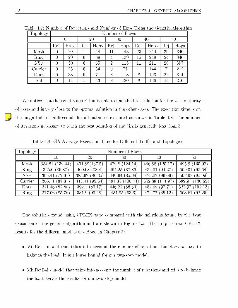
42 CHAPTER 4. GENETIC ALGORITHMS
Table 4.7: Number of Rejections and Number of Hops Using the Genetic AlgorithmTopology Number of Flows
10 20 30 40 50
Rej. Hops Rej. Hops Rej. Hops Rej. Hops Rej. HopsMesh 0 20 1 48 11 148 20 240 30 340Ring 0 29 0 68 4 139 15 248 24 340NSF 0 30 0 65 2 118 11 211 20 307
Carrier 0 25 0 54 0 77 1 144 7 212Dora 0 33 0 71 3 118 8 193 22 314Sul 0 14 1 43 8 120 8 136 14 210
We notice that the genetic algorithm is able to �nd the best solution for the vast majority
of cases and is very close to the optimal solution in the other cases. The execution time is on
the magnitude of milliseconds for all instances executed as shown in Table 4.8. The number
of iterations necessary to reach the best solution of the GA is generally less than 5.
Table 4.8: GA Average Execution Time for Di�erent TraÆc and Topologies
Topology Number of Flows10 20 30 40 50
Mesh 334.81 (139.44) 401.89(137.5) 429.8 (124.14) 466.88 (125.17) 495.9 (135.02)Ring 325.6 (80.37) 400.08 (88.4) 454.25 (87.86) 484.01 (94.27) 509.31 (98.64)NSF 305.41 (77.01) 383.62 (86.35) 440.64 (85.09) 475.03 (90.66) 502.63 (95.99)
Carrier 366.11 (87.01) 445.41 (92.54) 491.35 (100.44) 552.88 (114.97) 589.91 (130.62)Dora 321.46 (82.86) 392.1 (89.17) 446.22 (88.83) 482.69 (97.71) 522.97 (102.13)Ring 317.06 (85.76) 381.9 (90.48) 431.95 (83.6) 472.77 (89.12) 508.61 (92.25)
The solutions found using CPLEX were compared with the solutions found by the best
execution of the genetic algorithm and are shown in Figure 4.5. The graph shows CPLEX
results for the di�erent models described in Chapter 3:
� MinRej - model that takes into account the number of rejections but does not try to
balance the load. It is a lower bound for our two-step model.
� MinRejBal - model that takes into account the number of rejections and tries to balance
the load. Gives the results for our two-step model.

4.9. CONCLUDING REMARKS 43
� Genetico - heuristic that takes into account the number of rejections and tries to balance
the load using policies.
20
40
60
80
100
120
140
160
180
200
220
5040302010
Fitness
Number of LSP Requests
Carrier
MinRejMinRejBalGenetic
Figure 4.5: CPLEX and GA Results Comparison for the Carrier Network
For the scenarios with light traÆc, the GA results are similar to the lower bound, where
there is no need for load balancing. When the traÆc load starts to increase, the GA solution
is between the ones found when the traÆc is balanced and the solutions found when it is not
balanced.
When the network is overloaded, the GA results found are on average 20% worse than the
best solution, but this is not very problematic, since our goal is to obtain good solutions when
the load is within the network capacity and the network is still congested.
4.9 Concluding Remarks
The nature of the problem we are addressing prevents the use of exact methods to solve
instances of moderate size, let alone instances of typical size in real-time. To cope with
these diÆculties, we propose the use of heuristics to solve the problem. Speci�cally, a genetic
algorithm was implemented and compared to the optimal solution.
This Chapter validates the use of use of heuristics to obtain the solutions in a time period
that is practical in real life. The execution of the two-step model proposed in Chapter 3 using

44 CHAPTER 4. GENETIC ALGORITHMS
CPLEX takes longer and it is more complicated since it has to occur in phases.
In this chapter, we present a genetic algorithm for LSP routing, which main goal is min-
imizing the network rejection rate. It is possible, in the population initialization phase, to
reroute a LSP to avoid congested links even choosing longer paths, in order to balance the
overall link loads and to allow a better use of the networks resources.
The fact that traÆc changes, new LSP requests arrive, and node/link failures happen
show however that over time the routing decisions taken now will cause some ineÆciency in
the future and occasional rerouting may be needed.
This fact encouraged the study of the on-line version of the problem of alternative path
selection in MPLS networks. Another interesting problem to investigate is the detection of the
moment when a rerouting is needed. Hence, the next steps in our work are: on-line routing
and traÆc change/rerouting needs detection.

Chapter 5
Using the Genetic Algorithm On-Line
There are two issues that must be addressed when dealing with the design of a routing mecha-
nism in an IP network: (1) lack of load balancing and (2) the highly dynamic nature of traÆc
demands. Chapters 3 and 4 discussed o�ine solutions for the lack of load balance in IP net-
works. On that moment, our solutions pro�ted from the prior knowledge of the LSP requests.
We assumed that all LSPs to be routed and their resource requests were known at the time
the routing was done and the determination of the optimal paths for the LSPs required the
solution of an optimization problem. One of our contributions was the implementation of a
genetic algorithm that achieves near optimum performance in a reasonable time period.
In practice however it is likely that new requests need to be setup, new network elements
need to be con�gured or links and/or nodes face failures and/or recoveries. Consequently,
routing mechanisms should try to be very adaptive using an on-line approach.
In this chapter, we address the problem of on-line LSP routing; the main goal still being
the minimization of the network rejection rate and number of hops. We will show how the
genetic algorithm proposed for o�ine routing can be used on-line.
5.1 On-line Routing Scheme
Based on the previously conducted experiments, we noticed that our evolutionary routing
scheme, the GA with the adaptive movements and policies described in Chapter 4 (Adaptive
Routing Scheme), could be used to compute an on-line solution for the LSP routing problem.
45

46 CHAPTER 5. USING THE GENETIC ALGORITHM ON-LINE
The main di�erence between the use of the GA o�ine and its use on-line is the fact that
while the adaptive movements in the o�ine approach do not have any operational consequence,
they can hurt the network performance when executed on-line due to the intrinsic cost of LSPs
rerouting.
Besides most part of the on-line algorithms use one policy only (OSPF, WSP) and our
GA will make a crossover of various policies. In a �rst step, the solutions will be computed
by each policy simulating the population inititalization phase online. The second step will be
the crossover of the solutions.
The proposed on-line path selection scheme works as follows: when a request arrives at the
network, it tries to �nd a route to allocate to it. When trying to �nd a route for a request,
the policies described in Chapter 4 (MH, AMH, LU, ALU, B and AB) will be used.
Then one of three situations can occur for each of the policies individually:
1. a route with maximum D hops di�erence from the shortest route is found,
2. a very long route is found,
3. there is no route available.
If no route is found, meaning that the request will be rejected, or if a very long route is
found, meaning that the delay for that request will be big, the algorithm tries to reallocate
some LSP. It will try to �nd a LSP that can be rerouted to leave space for the new request
that just arrived.
To choose a LSP to be rerouted, all policies use the adaptive movements algorithm that
searches for the most utilized link in the set of alternative routes of the request that just
arrived. Then it checks for each LSP that crosses this link to see if this LSP has a demand
greater than the demand of the new request and if there is an alternative route for this LSP.
Our approach tries to reroute just one LSP, since rerouting of a large number of LSPs
is operationally undesirable. The algorithm stops when it �nds one LSP that satis�es the
constraints or when no LSP is found.
This strategy is similar to the adaptive movements described in Chapter 4. It is worth
mentioning that the adaptive movements before had no cost since we were working o�ine.
Now, the trade-o� between rerouting and/or rejecting some LSPs has to be considered.

5.2. EXPERIMENTS 47
Each policy will therefore propose one con�guration which will be used by the genetic
algorithm for crossover. Each policy will have its cost based on number of rejections and
number of hops and also the number of reroutes necessary to be applied. The GA rerouting
cost will be the rerouting cost of the chosen option for that LSP.
5.2 Experiments
Our �rst experiments were created to check the in uence of each policy on the GA solution.
We wanted to know if only using one of the policies on-line would be better than using the
GA.
The second set of experiments were created to check the performance of the GA when
LSP setup needed to be more dynamic - short-lived LSPs and in case of link failures. These
experiments were used in [Boutaba et al., 2002] and [Kar et al., 2000] to prove the advantages
of their algorithm and is reproduced here with the same motivation.
The topologies used in the experiments are the same topologies used throughout this work,
see Figure 5.1.
5.2.1 Policies Con�guration - Number of Alternative Routes
In this experiment, we show the in uence of the number of alternative routes on the �nal cost
obtained by each policy, i.e., each policy is executed with a di�erent number of alternative
routes. The results for Carrier topology are shown in Figure 5.2. The results for the other
topologies can be seen in the Appendix.
A total of 50 static path setup requests are sent to the network. Static paths resemble
long-lived tunnels in MPLS networks and once established stay in the network until the end
of the simulation.
The optimal result obtained using the ILP model described in Chapter 3 is compared to
the result obtained using the policies described for the initialization phase of the population
for the GA described in Chapter 4.
The two best number of alternative routes for most of the policies is four or �ve. The only
exception is for Adaptive Balance policy that has the best performance when the number of

48 CHAPTER 5. USING THE GENETIC ALGORITHM ON-LINE
1
3
5
2
0
4
(a) Mesh
3
4
210
12
8
9
11
5
14
15
1
13
6
7
(b) Ring
GA
NE
IL
MI NY
MD
NJPA
WA
CA1
CA2
UT
CO
TX
(c) NSF
1
2
4
5
6
7 9
11
123
810
13
1418
17
16
15
19
20
21
22
23
24
(d) Carrier (e) Dora (f) Sul
Figure 5.1: Topologies Used in the Experiments
alternative routes is two for the topologies Dora, NSF and Carrier. This can be explained by
the fact that these topologies are less loaded than the other ones and the traÆc is already
balanced, without hot spots. Therefore they do not need to used the alternative routes so
much.
5.2.2 Policies Comparison - Cost
Once we �nd the best con�guration for each policy, we compare the policies considering the
total cost, which is equal to the objective function used for the ILP model and equal to the
�tness function used for the GA. The results are shown in Figure 5.3.
It is noticeable that the policy LU obtains the worst results. It is not clear from the results
that one policy is much better than the others. The best polices are B, MH, AMH and ALU
with very similar results when the network is lightly loaded. The policy AB performance

5.2. EXPERIMENTS 49
0
50
100
150
200
250
0 10 20 30 40 50
Cost
Number of Flows
Carrier
optimo2345
(a) Min-Hop Policy
0
50
100
150
200
250
0 10 20 30 40 50
Cost
Number of Flows
Carrier
optimo2345
(b) Adaptive Min-Hop Policy
0
50
100
150
200
250
0 10 20 30 40 50
Cost
Number of Flows
Carrier
optimo2345
(c) Balance Policy
0
50
100
150
200
250
300
0 10 20 30 40 50
Cost
Number of Flows
Carrier
optimo2345
(d) Adaptive Balance Policy
0
50
100
150
200
250
300
0 10 20 30 40 50
Cost
Number of Flows
Carrier
optimo2345
(e) Limited Utilization Policy
0
50
100
150
200
250
0 10 20 30 40 50
Cost
Number of Flows
Carrier
optimo2345
(f) Adaptive Limited Utilization Policy
Figure 5.2: In uence of Number of Alternative Routes on the Policies Cost

50 CHAPTER 5. USING THE GENETIC ALGORITHM ON-LINE
0
50
100
150
200
250
300
0 10 20 30 40 50
Cost
Number of Flows
Carrier
optimogenetic
mhamh
bablu
alu
Figure 5.3: Cost for Each Policy as a Function of the Number of Flows For Carrier Network
varies a lot and is the best one for some topologies and the worst for other topologies.
This experiment showed that we could not use only one policy in our on-line solution. The
combination of the policies solutions due to the crossover executed by the genetic algorithm
gave the best results in overall. The genetic solution is generally equal to the best solution
found by any of the policies.
5.2.3 Policies Comparison - Rerouting
Figure 5.4 presents the number of adaptive movements executed by each policy as the number
of ows increases. The policies MH, B and LU do not execute adaptive movements. The
policies AMH, AB and ALU use the adaptive movements to reroute some LSPs trying to
minimize the rejection rate.
For lightly loaded scenarios, like Carrier and Dora, the AB policy executes more move-
ments, since it tries to keep the traÆc balanced at all times. The policies AMH and ALU start
the movements when the network starts facing congestion. This is a trade-o� to keep in mind,
since the performance of ALU is not far from the best solution and it does fewer reroutings

5.2. EXPERIMENTS 51
for lightly loaded networks.
0
2
4
6
8
10
12
14
16
0 5 10 15 20 25 30 35 40 45 50
Number of Reroutes
Number of Flows
Carrier
amhab
alu
Figure 5.4: Reroutes over Number of Flows For Carrier Network
5.2.4 Setting Dynamic Paths
In this experiment a total of 1000 setup requests are sent to the network. The experiment's
goal is to verify the in uence of the LSP's holding time on the policies behavior. The holding
time of the LSPs ranged from 25 time-units to 300 time-units. The cost as a function of
rejections and hops was the metric used to compare the policies and the genetic algorithm.
This experiment is similar to the experiments described in [Boutaba et al., 2002] as well as
the experiment setup: number of request generated and holding time range.
It is noticeable from Figure 5.5 that the genetic algorithm has the performance very similar
to the best policy. Also, the policy that gets the best performance varies from one scenario to
the other.
The AB policy has very good results in the most part of the experiments. The other policies
have similar results when the network is less congested: in the Dora and Carrier topologies
for example.

52 CHAPTER 5. USING THE GENETIC ALGORITHM ON-LINE
This experiment shows the advantage of using the genetic algorithm instead of one single
policy. The GA is exible and has the result of the best policy in most part of the time.
5000
5500
6000
6500
7000
7500
8000
8500
9000
9500
10000
2752251751257525
Cost
Holding Time
MHAMH
B
ABLU
ALU
genetic
Figure 5.5: Cost as a Function of LSP Holding Time For Carrier Network
5.2.5 Link Failure
It is expected that routing decisions taken on-line cause ineÆciency in the network over time
and, for this reason, occasional network grooming will be necessary. In this context, network
grooming means LSP rerouting in an attempt to keep network resources optimally allocated.
Dynamic traÆc changes or topology changes demand a reevaluation or grooming of the
previous routing solution. Grooming of LSPs can happen:
1. when a link or a node recovers from a failure,
2. when a new network element enter in the network,
3. when a LSP is torn down.

5.2. EXPERIMENTS 53
To check the performance of the policies in case of a link failure, the following experiment
was designed: in each trial of this experiment, one link is intentionally taken down from the
network and the number of LSPs requiring rerouting and the percentage of successful reroutes
are recorded. The experiment is repeated for all links.
This experiment is similar to the experiments described in [Kar et al., 2000] and
[Boutaba et al., 2002]. Several points of link failure are de�ned for the topologies studied.
The results are shown in Figures 5.6 and 5.7.
0
0.2
0.4
0.6
0.8
1
1.2
1.4
1.6
453525155
Reroutes Needed
Number of Flows
MHAMH
BAB
LUALU
Figure 5.6: Number of Reroutes Needed for Each Policy in Case of Link Failure For CarrierNetwork
It is noticeable from Figure 5.6 that the policy AB is the best for less loaded networks,
but it increases the number of reroutings rapidly when the load increases. When the network
becomes congested, the policy LU is the policy that requires the less number of reroutings.
For the most part of topologies, the number of reroutings needed is less than 2. It can be
noticed that the di�erence among the policies is small when the network is not congested.
We can notice that the policy LU is very successful in �nding new routes for the LSPs
since it does not have much to reroute. Figure 5.7 shows that for all policies the success rate
in �nding new routes for LSPs after a link failure is more than 50%. The policy LU is the

54 CHAPTER 5. USING THE GENETIC ALGORITHM ON-LINE
0.75
0.8
0.85
0.9
0.95
1
453525155
Sucessful Reroutes
Number of Flows
MHAMH
BAB
LUALU
Figure 5.7: % of Successful Rerouting in Case of Link Failure For Carrier Network
best since it leaves more space for future requests. The policy AB has already balanced the
traÆc and has fewer options in case of link failures.
5.3 Concluding Remarks
Routing mechanisms for MPLS networks carry out critical functions for the performance of
these networks. They take on the responsibility for resource management and load balancing.
This chapter addresses the problem of adaptive routing in MPLS networks.
It was observed that with the proposed scheme we have obtained substantial reduction
in the number of rejected requests in comparison with the basic strategy used nowadays, the
default minimum number of hops scheme.
Although the results are encouraging, there are several aspects of the proposal for which
additional work is needed. Link failures and LSP request arrivals are straight forward to detect.
TraÆc changes due to new network elements becoming available or ending of a request are
more complex.

5.3. CONCLUDING REMARKS 55
A trigger mechanism for example will be necessary to de�ne the moment when grooming
needs to occur. This trigger mechanism should detect traÆc changes and start the grooming
process. In the next chapter, the combination of rerouting mechanisms and monitoring tools
will be studied.

Chapter 6
TraÆc Monitoring and Network
Grooming
Since some on-line routing decisions can lead to non-optimal solutions and since traÆc can
change over time, the routes should be constantly monitored and in some cases even groomed.
In this chapter we propose a traÆc change detection mechanism to be used with the grooming
scheme.
To cope with the traÆc change detection problem, control charts are applied. Experiments
are run with two types of control charts: EWMA and XBar-charts and they show that is
feasible to use control charts for traÆc change detection.
6.1 Motivation
One of the modern trends of Internet design is that lower level transport protocols should
be network conscious and adaptive. They should monitor network conditions and answer
appropriately to changes in these conditions, which requires using network information from
the recent past to guide future behavior. There is much interest in using network measurements
for both modeling and operational purposes.
In this chapter we proposed a mechanism to deal with the dynamic nature of Internet
traÆc based on traÆc monitoring and control charts. Since it is not scalable to distribute
every change in the link states the proposed scheme will try to �gure out if and why the
56

6.2. TRAFFIC MONITORING 57
traÆc changed: if the change in traÆc is due to common variation or if it is due to unexpected
facts, such as a link or a router failure. With this approach, a link state update will be
triggered only when a subtle traÆc change occurs. This approach reduces the volume of
updates of traÆc information on the network.
This traÆc change detector will be used to trigger the load balancing mechanisms. It will
check traÆc tendency based on XBar-charts or EWMA-charts [Montgomery, 1990]. XBar-
charts and EWMA-charts are control charts and their goal is to detect if a process is under
control, which means that the process is presenting the expected metrics. In our work, we will
monitor the utilization of a link and check if it is viewing the expected load.
6.2 TraÆc Monitoring
A network can be monitored either in an active or passive manner. The �rst manner gives a
measure of the performance of the network whereas the latter gives a measure of the workload
on the network. Both have their merits and should be regarded as complimentary.
The active approach relies on the capability to inject packets into the network and then
measure the services obtained from it. It introduces extra traÆc into the network, but it has
the advantage of measuring the desired quantities at the desired time.
Passive measurements are carried out by observing normal network traÆc, without the
extra load. The passive approach measures the real traÆc, but the amount of data accumulated
can be substantial because the network will be polled often for information.
There are various quantities of interest that can be insightful about the state of the network.
Available bandwidth together with latency, loss, etc., can predict the performance of the
network. Based on the available bandwidth , the operator can obtain information about
the congestion, decide the admission control, perform routing, etc. For MPLS networks, the
available bandwidth information can be used to decide LSP setups, routing and preemption.
Therefore, obtaining an accurate measurement of the available bandwidth can be crucial to
e�ective deployment of QoS services in a network.
In this work, the passive approach is used. The link's available bandwidth is monitored to
check for rerouting needs.

58 CHAPTER 6. TRAFFIC MONITORING AND NETWORK GROOMING
6.3 SPC - Statistical Process Control
6.3.1 XBar-charts
Shewhart's statistical process control [Hansen, 1963] is a methodology for charting processes
in XBar-charts and quickly determining when the process is out of control. The XBar will
actually the mean of the process being measured (X).
A series of rules exist to detect conditions in which the process is behaving abnormally to
the extent that an out of control condition is declared. In this work, we used the extreme
point condition test. Therefore, the process is out of control where a point is either above the
upper limit or below the lower limit of the chart.
In our work, if the bandwidth is above the upper limit or below the lower limit it means
that a link is broken or a router is not working.
The XBar-chart is computed from M data points, which are ordered in time. These points
are in fact the mean of N data points measured, X1; � � � ; XM . Our M data points will be the
mean of N measurements of a link bandwidth; what can be easily obtained via SNMP.
In order to compute the chart's control limits it is necessary to compute the population
mean, X, and the mean range, R.
The range of an interval, for instance R1, is the di�erence between the largest and the
smallest value at this interval.
X =X1 +X2 + :::+XM
M(6.1)
R =R1 +R2 + :::+RM
M(6.2)
The chart limits are calculated as follows:
LowerLimit(LL) = X �A2(n)R (6.3)
UpperLimit(UL) = X +A2(n)R (6.4)

6.3. SPC - STATISTICAL PROCESS CONTROL 59
where A2 values depend on N , as shown in Table 6.1.
Table 6.1: Examples of some A2 valuesN 2 3 4 5 6 7 8 9A2 1.880 1.023 0.729 0.577 0.483 0.419 0.373 0.337
These limits actually represent a distance bellow or above the mean by 3 times the standard
deviation. In this work, the control charts, XBar-chart and EWMA-chart, will be used to check
the average bandwidth utilization for a link.
6.3.2 EWMA-charts
An Exponentially Weighted Moving Average chart, EWMA-chart, is used when it is desirable
to detect out-of-control situations very quickly [Montgomery, 1990].
It has a built in mechanism for incorporating information from all previous data and
weighting more the current information through �, as can be noticed in Equation 6.6. The
equations 6.5 - 6.10 are used to compute the EWMA-chart.
X(0) =X1 +X2 + :::+XM
M(6.5)
X(i) = �X i + (1� �)X(i� 1) (6.6)
The upper (ULi) and lower (LLi) limits are calculated as follows :
Sigma =R
D2(N)(6.7)
Fi =
s(�
1� �)[1� (1� �)2i] (6.8)
LowerLimit(LLi) = X(0)� 3 � SigmapN
Fi (6.9)
UpperLimit(ULi) = X(0) +3 � Sigmap
NFi (6.10)

60 CHAPTER 6. TRAFFIC MONITORING AND NETWORK GROOMING
where D2 values depend on N, as shown in Table 6.2.
Table 6.2: Some D2 values
N 2 3 4 5 6 7 8 9D2 1.128 1.693 2.059 2.326 2.534 2.704 2.847 2.970
A tutorial in control charts can be found in [Sytsma and Manley, 1999] as well as a more
detailed information about the formulas and tables.
6.4 Control Charts Experimental Results
In this work, to test the use of control charts for traÆc change detection, synthetic data is gen-
erated, based on the exponential distribution function. Most studies in network simulation use
a Poisson distribution to model the arrival of request and an exponential distribution to model
the request holding time [Boutaba et al., 2002, Dias et al., 2003, Salvadori and Battiti, 2003].
Two traÆc scenarios are synthetically generated. The list bellow describes the scenarios
and the purpose of the test.
� First Scenario: Increasing TraÆc - in the beginning the traÆc follows a exponential dis-
tribution with mean 10 Mbps. Then four spaced in time peaks are generated increasing
the mean in 15%.
� Second Scenario: Decreasing TraÆc - in the beginning the traÆc follows a distribution
with mean 10 Mbps. Then four spaced in time peaks are generated decreasing the mean
in 15%.
Our �rst test will try to verify what is the best value of the N and � for the data gener-
ated. It is worth noticing that the test scenarios were generated synthetically and the best
con�guration will be the one that can detect the 4 peaks generated.
6.4.1 Detecting Utilization Mean Changes Through XBar-charts
It can be seen in Figure 6.1 the in uence of the sample size, N, for the XBar-chart. We use
2000 points, M is set to 20 and N is set to: 3, 6 and 9. The number of points in the X axis

6.4. CONTROL CHARTS EXPERIMENTAL RESULTS 61
in each graph can be calculated as 2000=20 �N .
All charts detect an increase in the mean but the chart with N = 3 detect precisely the
four peaks. The other charts present the four peaks within the limits.
6.4.2 Detecting Utilization Mean Changes Through EWMA-charts
Several experiments are run using di�erent values for � in EWMA-charts: 0.1, 0.2, 0.3, 0.5
and 0.7. Bigger � value means that more importance is given to the current data.
It can be seen in Figure 6.2 that as � increases the limits of the EWMA-chart are more
distant. For small � values, the traÆc changes are detected, since the EWMA-chart is expected
to be more conservative.
6.4.3 XBar-charts x EWMA-charts
If we compare XBar-charts and EWMA-charts, it is noticeable in Figure 6.3 that the EWMA-
chart reacts faster, adjusting its limits according to the data.
The experiments are run with M set to 20, N set to 3 for the XBar-chart and � set to 0.3
for the EWMA-chart. Figure 6.3 shows the best results of the two charts for the two scenarios:
increasing and decreasing traÆc.
The results for both control charts were very similar. It is interesting to keep in mind some
advantages and/or disadvantages of each one. The main advantages of EWMA are: (1) they
detect out-of-control conditions more quickly, (2) detection can be done by using only one
rule - the point has to be inside the 3 standard deviation limits to be considered in control.
The EWMA worst disadvantage is that it is more diÆcult to construct. Its value at time t is
computed recursively from the past points.
Despite being easier to calculate, XBar-charts have more rules to test in order to detect
abnormal situations than EWMA-charts [Hansen, 1963].
In this work, we used XBar-charts cause they are easier to compute and the rule used in the
experiments to detect out-of-control situations was the simple rule: extreme point condition.

62 CHAPTER 6. TRAFFIC MONITORING AND NETWORK GROOMING
9.99
9.995
10
10.005
10.01
10.015
10.02
10.025
10.03
10.035
10.04
0 5 10 15 20 25 30 35
dataxbar
upperlower
(a) n=3
9.995
10
10.005
10.01
10.015
10.02
10.025
0 2 4 6 8 10 12 14 16
dataxbar
upperlower
(b) n=6
10
10.002
10.004
10.006
10.008
10.01
10.012
10.014
10.016
10.018
10.02
0 2 4 6 8 10
dataxbar
upperlower
(c) n=9
Figure 6.1: In uence of Sample Size in XBar-charts

6.4. CONTROL CHARTS EXPERIMENTAL RESULTS 63
10
10.005
10.01
10.015
10.02
10.025
10.03
10.035
10.04
0 5 10 15 20 25 30 35
dataxbarxhat
upperlower
(a) �=0.1
10
10.005
10.01
10.015
10.02
10.025
10.03
10.035
10.04
0 5 10 15 20 25 30 35
dataxbarxhat
upperlower
(b) �=0.2
9.995
10
10.005
10.01
10.015
10.02
10.025
10.03
10.035
10.04
0 5 10 15 20 25 30 35
dataxbarxhat
upperlower
(c) �=0.3
9.99
9.995
10
10.005
10.01
10.015
10.02
10.025
10.03
10.035
0 5 10 15 20 25 30 35
dataxbarxhat
upperlower
(d) �=0.5
9.98
9.99
10
10.01
10.02
10.03
10.04
0 5 10 15 20 25 30 35
dataxbarxhat
upperlower
(e) �=0.7
Figure 6.2: In uence of � in EWMA-charts

64 CHAPTER 6. TRAFFIC MONITORING AND NETWORK GROOMING
9.99
9.995
10
10.005
10.01
10.015
10.02
10.025
10.03
10.035
10.04
0 5 10 15 20 25 30 35
dataxbar
upperlower
(a) xbar increasing
9.98
9.985
9.99
9.995
10
10.005
10.01
10.015
10.02
10.025
10.03
0 5 10 15 20 25 30 35
dataxbar
upperlower
(b) xbar decreasing
10.002
10.004
10.006
10.008
10.01
10.012
10.014
10.016
10.018
10.02
10.022
0 2 4 6 8 10 12
dataxbarxhat
upperlower
(c) ewma increasing
9.998
10
10.002
10.004
10.006
10.008
10.01
10.012
10.014
10.016
10.018
0 2 4 6 8 10 12
dataxbarxhat
upperlower
(d) ewma decreasing
Figure 6.3: XBar and EWMA Results for Both Test Scenarios
6.5 TraÆc Changes Detection Scheme
After discussing how control charts work, we propose a grooming scheme for MPLS networks
based on a traÆc change detection mechanism.
Our previously described adaptive routing scheme or adaptive movements scheme will be
combined with the control charts in the following way: each ingress node in the network
monitors its links verifying if the link utilization is under control.
If a link/node failure occurs or if a LSP is torn down, probably the link's utilization will
be a�ected. Thus, if an out-of-control situation is detected, a rerouting o�ine mechanism is
triggered.

6.6. EXPERIMENTAL RESULTS 65
Algorithm 5 gives the proposed scheme pseudo-code.
Algorithm 5 Grooming/Monitoring Pseudo Code
1: calculateOptimalRouting();2: for all Links do3: calculateControlChart();4: end for
5: loop
6: if monitorLink detects traÆc has changed then7: updateControlChart();8: getUpdatedTopology();9: recomputeRouting();10: end if
11: end loop
The �rst step of the proposed scheme is the optimal routing computation. If nothing
abnormal happens, the optimal routing will be used in the network without changes. The
control charts are also computed and they will be used to monitor each ingress router. If a
traÆc change is detected, the control chart is updated and the grooming process is trigged. The
grooming process consists of rerouting of LSPs in order to increase the network performance.
6.6 Experimental Results
An experiment is conducted showing how the grooming process can help the achievement of
better network performance. The experiment works in the following way: in the �rst step a
series of requests are optimally routed. Then some requests are �nished, i.e. the bandwidth
reserved for these requests becomes available again, opening space for recon�guration of the
already installed LSPs.
In the experiments, we de�ned the LSPs to be �nished using an uniform distribution. The
goal of the experiment is to check if the bandwidth decrease in the links will be detected and
if some rerouting will happen improving the network delay time (less hops used to route some
LSPs). In the �rst set of experiments, after the decrease in utilization is detected nothing
is done. In the second set of experiments, after the decrease in utilization is detected, the
grooming will happen.
The metric used to compare the bene�ts of grooming are residual bandwidth and number

66 CHAPTER 6. TRAFFIC MONITORING AND NETWORK GROOMING
of hops (cost) and the results are presented for the policies that are adaptive in Figures 6.4, 6.5
and 6.6 for the Carrier network. The network residual bandwidth is computing by adding the
residual bandwidth of all links.
When we vary the policy, we vary the network status in terms of bandwith utilization
in each link. For all policies and topologies, the cost decreased and the residual bandwidth
increased when the grooming process was used in comparison with the case when no grooming
was done, specially in the cases where the network was more congested, i.e. number of ows
greater than 30.
6.7 Concluding Remarks
In this chapter we show that control charts could be used to monitor network conditions and
allow the routing protocol to respond appropriately to them.
Two di�erent types of control charts are evaluated and several experiments are run on
synthetic data to show the main advantages of each type of control chart. EWMA-charts
should be used when it is necessary to quickly react to small changes. XBar-charts should be
used when major changes should be detected. Its main advantage is its simplicity and low
overhead.
A grooming scheme is proposed and associated with control charts. Experiments show
that better network performance can be achieved with the use of these tools.

6.7. CONCLUDING REMARKS 67
20
40
60
80
100
120
140
Cost
Number of LSPS
Carrier
Without Grooming With Grooming
(a) Cost
0.65
0.7
0.75
0.8
0.85
0.9
0.95
Residual
Number of LSPS
Carrier
Without Grooming With Grooming
(b) % of Residual Bandwidth
Figure 6.4: AMH Grooming Results For Carrier Network

68 CHAPTER 6. TRAFFIC MONITORING AND NETWORK GROOMING
40
60
80
100
120
140
160
180Cost
Number of LSPS
Carrier
Without Grooming With Grooming
(a) Cost
0.6
0.65
0.7
0.75
0.8
0.85
0.9
0.95
Residual
Number of LSPS
Carrier
Without Grooming With Grooming
(b) % of Residual Bandwidth
Figure 6.5: AB Grooming Results for Carrier Network

6.7. CONCLUDING REMARKS 69
20
40
60
80
100
120
140
Cost
Number of LSPS
Carrier
Without Grooming With Grooming
(a) Cost
0.65
0.7
0.75
0.8
0.85
0.9
0.95
Residual
Number of LSPS
Carrier
Without Grooming With Grooming
(b) % of Residual Bandwidth
Figure 6.6: ALU Grooming Results for Carrier Network

Chapter 7
Conclusions
In this chapter we present a summary of this thesis, highlighting its main contributions. We
also present future directions for this work.
7.1 Summary of Accomplished Work
In this thesis, the problem of o�ine and on-line routing of LSPs in MPLS networks has been
addressed. QoS in MPLS networks can be improved with eÆcient ways of computing explicit
routes for LSPs.
This work main contributions to the state-of-the-art are:
� We proposed an ILP model that solves the o�ine problem of routing LSPs in a MPLS
network in an exact manner. This model tries to balance the network load while mini-
mizing the network rejection rate.
� We proposed a genetic algorithm that solves the o�ine problem of routing LSPs in a
MPLS network in an heuristic manner. This algorithm is based on various policies,
which route the LSPs using di�erent criteria, and based on the combination of these
policies with adaptive movements. The adaptive movements are responsible for network
grooming in cases where the policy is not exible enough. The execution time of the GA
is much better than the execution time of CPLEX. The use of explicit routes computed
by our approach is also better than the use of MPLS default routing scheme.
70

7.1. SUMMARY OF ACCOMPLISHED WORK 71
� We proposed and veri�ed the use of the genetic algorithm to solve the on-line problem
of routing LSPs in a MPLS network. The genetic algorithm can automatically solve the
problem of �nding the best policy for di�erent topologies and traÆc demands.
� We proposed a network grooming technique and a traÆc change detection mechanism.
We showed how the grooming technique can be applied to rerouting in case of an increase
in the availability of network resources. We also showed how the link utilization changes
detection mechanism can be used to trigger the grooming process.
The ILP model was solved using CPLEX. Various issues concerning the execution time
necessary to solve the model were noticed and the genetic algorithm was developed to address
theses issues. While being very useful as a formal tool to de�ne the problem, the ILP model
resolution is very timing consuming, and the ILP model being classi�ed as a NP-hard problem.
Simulations were conducted in order to check the performance of the genetic algorithm
in di�erent traÆc scenarios, di�erent topologies, di�erent policies, with and without adaptive
movements, and o�ine and on-line. The simulation results were compared to optimal results
obtained through the ILP model. The obtained results with the genetic algorithm were very
satisfactory showing that it is able to extract the best performance of various distinct policies
for various situations.
We also investigated the possibility of using the genetic algorithm for network grooming,
which can happen when a new network element is con�gured, LSPs are torn down or a network
element recovers from failure. We presented a utilization detection mechanism based on control
charts for triggering the grooming process.
The utilization changes detection mechanism was used in the context of de�ning the mo-
ment the grooming should take place. Simulation results indicate that we can achieve better
performance using the proposed mechanism.
Due to the paramount importance of being adaptive, we believe that genetic algorithms are
very suitable for on-line routing. Furthermore, we believe that the genetic algorithm proposed
in this work could be extended to other policies.

72 CHAPTER 7. CONCLUSIONS
7.2 Future Work
There are several possibilities for research in order to extend the work presented in this thesis.
One such possibility is to analyze the in uence of network topology in the policies proposed
and in routing algorithms in general. It was noticed that networks with the same load have
completely di�erent behavior due to its topology.
Another important facet of the routing process that could be investigated is its temporal
aspect. The granularity of routing decisions can vary in a thiner scale besides going from
o�ine to on-line routing. The use of grooming techniques associated with monitoring tools
can bring important improvements to network performance.
Still regarding the grooming process, an aspect that we have not addressed in this thesis
and that should be investigated in future research is the choice of traÆc prediction tools.
Together with monitoring tools, prediction tools could lead the grooming process to a better
result.

Bibliography
[Ahuja et al., 1993] Ahuja, R. K., Magnanti, T. L., and Orlin, J. B. (1993). Network Flows:Theory, Algorithms, and Applications. Prentice Hall.
[Anjali, 2002] Anjali, T. e. a. (2002). A New Path Selection Algorithm for MPLS NetworksBased on Available Bandwidth Estimation. QoFIS, pages 205{214.
[Apostolopoulos et al., 1999] Apostolopoulos, G., Williams, D., Kamat, S., Guerin, R., Orda,A., and Przygienda, T. (1999). RFC 2676: QoS Routing Mechanisms and OSPF Extensions.
[Aukia et al., 2000] Aukia, P., Kodialam, M., Koppol, P., Sarin, H., and Suter, B. (2000).RATES: A Server for MPLS TraÆc Engineering. IEEE Network Magazine, 14(2):34{41.
[Awduche et al., 2002] Awduche, D., Chiu, A., Elwalid, A., Widjaja, I., and Xiao, X. (2002).RFC 3272: Overview and Principles of Internet TraÆc Engineering.
[Awduche et al., 1999] Awduche, D., Malcolm, J., Agogbua, J., O'Dell, M., and McManus, J.(1999). RFC 2702: Requirements for TraÆc Engineering Over MPLS.
[Awduche, 1999] Awduche, D. O. (1999). MPLS and TraÆc Engineering in IP Networks.IEEE Communications Magazine, 37(12):42{47.
[Awduche et al., 2001] Awduche, D. O., Berger, L., Gan, D., Li, T., Srinivasan, V., andSwallow, G. (2001). RFC 3209: RSVP-TE: extensions to RSVP for LSP tunnels.
[Awduche and Jabbari, 2002] Awduche, D. O. and Jabbari, B. (2002). Internet TraÆc Engi-neering using Multiprotocol Label Switching (MPLS). Computer Networks, 40:111{129.
[Bertsekas and Gallager, 1992] Bertsekas, D. and Gallager, R. (1992). Data Networks. Pren-tice Hall.
[Black, 2001] Black, U. (2001). MPLS and Label Switching Networks. Prentice Hall.
[Blake et al., 1998] Blake, S., Black, D., Carlson, M., Davies, E., Wang, Z., and Weiss, W.(1998). RFC 2475: An Architecture for Di�erentiated Services.
[Boutaba et al., 2002] Boutaba, R., Szeto, W., and Iraqi, Y. (2002). DORA: EÆcient Routingfor MPLS TraÆc Engineering. Journal of Network and Systems Management, 10(3):309{325.
[Boyle et al., 2002] Boyle, J., Gill, V., Hannan, A., Cooper, D., Awduche, D., Christian, B.,and Lai, W. (2002). RFC 3346: Applicability Statement for TraÆc Engineering with MPLS.
73

74 BIBLIOGRAPHY
[Boyle et al., 2000] Boyle, J., Hannan, A., Gill, V., Cooper, D., Awduche, D., Christian, B.,and Lai, W. (2000). RFC 2998: A Framework for Integrated Services Operation over Di�servNetworks.
[Brunato et al., 2002] Brunato, M., Battiti, R., and Salvadori, E. (2002). Load Balancing inWDM Networks through Adaptive Routing Table Changes. Networking, pages 289{301.
[Buriol, 2003] Buriol, L. S. (2003). Roteamento do Tr�afego na Internet: Algoritmos paraProjeto e Opera�c~ao de Redes com Protocolo OSPF. PhD thesis, Unicamp.
[Buriol et al., 2005] Buriol, L. S., Resende, M. G. C., Ribeiro, C. C., and Thorup, M. (2005).A hybrid genetic algorithm for the weight setting problem in ospf/is-is routing. Networks,46(1):36{56.
[Capone et al., 2005] Capone, A., Fratta, L., and Martignon, F. (2005). Dynamic Online QoSRouting Schemes: Performance and Bounds. Computer Networks - Article in Press.
[Chou, 2004] Chou, C. T. (2004). TraÆc Engineering for MPLS-based Virtual Private Net-works. Computer Networks, 44:319{333.
[Coelho, 1998] Coelho, C. A. C. (1998). An Updated Survey of GA-Based MultiobjectiveOptimization Techniques. ACM Computing Surveys, 32(2):109{143.
[Crawley et al., 1998] Crawley, E., Nair, F., Rajagopalan, B., and Sandick, H. (1998).RFC2386: A Framework for QoS Based Routing in the Internet.
[Davie and Rekhter, 2000] Davie, B. and Rekhter, Y. (2000). MPLS: Technology and Appli-cations. Morgan Kaufmann.
[Dias and Camponogara, 2003] Dias, R. and Camponogara, e. a. (2003). Otimiza�c~ao La-grangeana Em Engenharia de Tr�afego para Redes IP sobre MPLS. XXI Simp�osio Brasileirode Redes de Computadores, pages 475{490.
[Dias et al., 2003] Dias, R. A., Camponogara, E., Farines, J.-M., Willrich, R., andCampestrini, A. (2003). Implementing TraÆc Engineering in MPLS-Based IP Networkswith Lagrangean Relaxation. IEEE ISCC, pages 373{378.
[Ericsson et al., 2002] Ericsson, M., Resende, M. G. C., and Pardalos, P. M. (2002). A GeneticAlgorithm for the Weight Setting Problem in OSPF Routing. J. Comb. Optim., 6(3):299{333.
[Feldmann and Rexford, 2001] Feldmann, A. and Rexford, J. (2001). IP Network Con�gura-tion for Intra-domain TraÆc Engineering. IEEE Network Magazine, 15(5):46{57.
[Figueiredo et al., 2004] Figueiredo, G. B., da Fonseca, N. L. S., and Monteiro, J. A. S. (2004).A Minimum Interference Routing Algorithm. IEEE Communications Society, 4:1942{1947.
[Fortz et al., 2002] Fortz, B., Rexford, J., and Thorup, M. (2002). TraÆc engineering withtraditional ip routing protocols. IEEE Communications Magazine, 10:118{124.

BIBLIOGRAPHY 75
[Fortz and Thorup, 2000] Fortz, B. and Thorup, M. (2000). Internet TraÆc Engineering byOptimizing OSPF Weights. IEEE INFOCOM, pages 519{528.
[Fourer, 2002] Fourer, R. (2002). Ima tutorial: Ampl - hands on session.
[Garey and Johnson, 1979] Garey, M. R. and Johnson, D. (1979). Computers and Intractabil-ity. Freeman.
[Girish et al., 2000] Girish, M., Zhou, B., and Hu, J.-Q. (2000). Formulation of the TraÆcEngineering Problems in MPLS Based IP Networks. IEEE ISCC, pages 214{219.
[Girish et al., 2003] Girish, M. K., Zhou, B., and Hu, J.-Q. (2003). An Algorithm for Rerout-ing in TraÆc Engineering of MPLS Based IP Networks. IP Operations and Management -IPOM, pages 115{118.
[Goldberg, 1989] Goldberg, D. E. (1989). Genetic Algorithms in Search, Optimization, andMachine Learning. Addison-Wesley.
[Guerin et al., 1997] Guerin, R., Orda, A., and D., W. (1997). QoS Routing Mechanisms andOSPF Extensions. IEEE Globecom, 3:1903{1908.
[Hansen, 1963] Hansen, B. L. (1963). Quality Control: Theory and Applications. Prentice-Hall.
[Henig, 1985] Henig, M. I. (1985). The shortest path problem with two objective functions.European Journal of Operational Research, 15:281{291.
[Holland, 1973] Holland, J. (1973). Genetic algorithms and the optimal allocations of trials.SIAM Journal of Computing, 2(2):88 { 105.
[Hong et al., 2003] Hong, L., Dong, B., and Wei, D. (2003). An Explicit Routing OptimizationAlgorithm for Internet TraÆc Engineering. Proceedings of the International Conference onCommunication Technology - ICCT 2003, 1:445{449.
[ILOG, 2002] ILOG (2002). Ilog ampl cplex system 8.0 - user's guide. http://www.ilog.com/products/cplex.
[Kar et al., 2000] Kar, K., Kodialam, M., and Lakshman, T. V. (2000). Minimum InterferenceRouting of Bandwidth Guaranteed Tunnels with MPLS TraÆc Engineering Applications.IEEE Journal on Selected Areas in Communications, 18(12):921{940.
[Katz et al., 2003] Katz, D., Yeung, D., and Kompella, K. (2003). RFC 3630: TraÆc Engi-neering (TE) Extensions to OSPF Version 2.
[Lee et al., 1995] Lee, W., Hluchyi, M., and Humblet, P. (1995). Routing Subject to Qualityof Service Constraints in Integrated Communication Networks. IEEE Network, pages 46{55.
[Li and Rekhter, 1998] Li, T. and Rekhter, Y. (1998). RFC 2430: Provider Architecture forDi�erentiated Services and TraÆc Engineering (PASTE).

76 BIBLIOGRAPHY
[Liu, 2003] Liu, X. (2003). Capacity and Flow Assignment Issues in MPLS Networks. Inter-national Journal of Network Management, 13:173{179.
[Liu et al., 2000] Liu, Z., Sun, Y., and Xue, X. (2000). A static routing algorithm used in theinternet traÆc engineering. 7th Asian-Paci�c Conference on Circuits and Systems (IEEEAPCCAS), pages 231{234.
[McCanne and Floyd, 2003] McCanne, S. and Floyd, S. (2003). Network simulator 2.
[Michalewicz and Fogel, 2000] Michalewicz, Z. and Fogel, D. B. (2000). How to Solve It:Modern Heuristics. Springer-Verlag.
[Montgomery, 1990] Montgomery, D. C. (1990). Introduction to Statistical Quality Control.John Wiley & Sons.
[Newhauser and Wolsey, 1998] Newhauser, G. L. and Wolsey, L. A. (1998). Integer and Com-binatorial Optimization. John Wiley & Sons.
[Nobre et al., 2005] Nobre, E., Ponte, P. R. X., Fernandes, M., and Celestino Jr, J. (2005). In-telliDylba: Um Esquema de Balanceamento de Carga para Redes MPLS Com AprendizadoDessassistido Baseado em L�ogica Difusa e Algoritmos Gen�eticos. XXIII Simp�osio Brasileirode Redes de Computadores.
[Oliveira et al., 2004a] Oliveira, A., Habib, E., and Mateus, G. (2004a). An Adaptive RoutingScheme for TraÆc Engineering in IP Networks vover MPLS. Proceeding of XII Latin-Ibero-American Conference on Operations Research.
[Oliveira and Mateus, 2005a] Oliveira, A. and Mateus, G. (2005a). MPLS: Quantitative Anal-ysis of LSP Setups(Poster). Proceedings of IEEE INFOCOM Student Workshop.
[Oliveira and Mateus, 2005b] Oliveira, A. and Mateus, G. (2005b). TraÆc Engineering: Con-trol Charts and LSPs. Proceeding of 12th International Conference on Telecommunications- ICT 2005.
[Oliveira et al., 2004b] Oliveira, A., Ravetti, M., and Mateus, G. (2004b). Using ControlCharts for TraÆc Change Detection in MPLS Networks(Poster). Proceeding of IEEE Mas-cots.
[Oliveira et al., 2005] Oliveira, A., Ravetti, M., and Mateus, G. (2005). TraÆc Engineering inMPLS Networks: ARS An Adaptive Routing Scheme Based on Control Charts. Proceedingof XXIII Simp�osio Brasileiro de Redes de Computadores.
[Reeves, 1993] Reeves, C. R. (1993). Modern Heuristic Techniques for Combinatorial Prob-lems. Halsted Press.
[Resende and Ribeiro, 2003] Resende, M. G. C. and Ribeiro, C. C. (2003). A GRASP withPath-Relinking for Private Virtual Circuit Routing. Networks, 41(3):104{114.
[Rosen et al., 2001] Rosen, E., Viswanathan, A., and Callon, R. (2001). RFC 3031: Multi-protocol Label Switching Architecture.

BIBLIOGRAPHY 77
[Salvadori and Battiti, 2003] Salvadori, E. and Battiti, R. (2003). A Load Balancing Schemefor Congestion Control in MPLS Networks. IEEE ISCC, pages 951{956.
[Savage et al., 1999] Savage, S., Collins, A., and E., H. (1999). The End-to-End E�ects ofInternet Path Selection. ACM SIGCOMM, pages 289{299.
[Seaman et al., 2000] Seaman, M., Smith, A., Crawley, E., and Wroclawski, J. (2000). RFC2815: Integrated Service Mappings on IEEE 802 Networks.
[Suri et al., 2001] Suri, S., Waldvogel, M., and Warkhede, P. R. (2001). Pro�le-based routing:A new framework for MPLS traÆc engineering. In Quality of Future Internet Services,pages 138{157.
[Sytsma and Manley, 1999] Sytsma, S. and Manley, K. (1999). Common Control Chart Cook-book. http://www.sytsma.com/tqmtools/charts.html.
[Uhlig, 2005] Uhlig, S. (2005). A Multiple-objectives Evolutionary Perspective to InterdomainTraÆc Engineering. International Journal of Computational Intelligence and Applications,5(2):1{16.
[Vanderbei, 1997] Vanderbei, R. J. (1997). Linear Programming: Foundations and Extensions.Kluwer Academic Publishers.
[Wang et al., 2002] Wang, B., Su, X., and Chen, C. P. (2002). A New Bandwidth GuaranteedRouting Algorithm for MPLS TraÆc Engineering. Proceedings of ICC, pages 1001{1005.
[Xiao et al., 1999] Xiao, X., Hannan, A., Bailey, B., and Ni, L. M. (1999). TraÆc Engineeringwith MPLS in the Internet. America's Network magazine, pages 32{37.
[Yilmaz and Matta, 2002] Yilmaz, S. and Matta, I. (2002). On the Scalability-PerformanceTradeo�s in MPLS and IP Routing. Technical Report - BUCS-TR-2002-013.
[Y.Wang and Z.Wang, 1999] Y.Wang and Z.Wang (1999). Explicit Routing Algorithms forInternet TraÆc Engineering. 8th Computer Communications and Networks, pages 582{588.
[Zhang and Wu, 2005] Zhang, S. and Wu, Z. (2005). Designs of Control Charts With Supple-mentary Runs Rules. computers and industrial engineering, 49:76{97.

Appendix A
Detailed Results
A.1 Chapter 4
A.1.1 Genetic Algorithm Input Parameter Analysis
The graphs in Figures A.1- A.5 plot the �tness obtained with each possible parameter com-bination (200 points in the abscissa) with traÆc varying from 10 to 50 LSP requests with astep of 10.
It can be noticed that all graphics present clusters of regions where the �tness of thesolutions are very similar.
When traÆc load is low (10 and 20) requests, the results for all combinations are practicallythe same. When traÆc load increases, the parameters start to make a di�erence but even so itcan be noticed that all graphs present horizontal lines, representing clusters of good solutions.
A.1.2 CPLEX and GA Comparison
The solutions found using CPLEX were compared with the solutions found by the best exe-cution of the genetic algorithm and are shown in Figures A.6 - A.10.
The graphs show CPLEX results for the di�erent models described in Chapter 3 for dif-ferent topologies:
� MinRej - model that takes into account the number of rejections but does not try tobalance the load. It is a lower bound for our two-step model.
� MinRejBal - model that takes into account the number of rejections and tries to balancethe load. Gives the results for our two-step model.
� Genetico - heuristic that takes into account the number of rejections and tries to balancethe load using policies.
For the scenarios with light traÆc, the GA results are similar to the lower hound, wherethere is no need for load balancing. When the traÆc load starts to increase, the GA solutionis between the ones found when the traÆc is balanced and the solutions found when it is notbalanced.
78

A.1. CHAPTER 4 79
18
18.5
19
19.5
20
20.5
21
21.5
22
20 40 60 80 100 120 140 160 180 200
Fitness
Genetic Algoritm Option
Mesh
(a) 10
46
48
50
52
54
56
58
60
20 40 60 80 100 120 140 160 180 200
Fitness
Genetic Algoritm Option
Mesh
(b) 20
145
150
155
160
20 40 60 80 100 120 140 160 180 200
Fitness
Genetic Algoritm Option
Mesh
(c) 30
238
240
242
244
246
248
250
20 40 60 80 100 120 140 160 180 200
Fitness
Genetic Algoritm Option
Mesh
(d) 40
338
340
342
344
346
348
350
20 40 60 80 100 120 140 160 180 200
Fitness
Genetic Algoritm Option
Mesh
(e) 50
Figure A.1: Various Results For Mesh Network Using Genetic Algorithms

80 APPENDIX A. DETAILED RESULTS
26
28
30
32
34
36
20 40 60 80 100 120 140 160 180 200
Fitness
Genetic Algoritm Option
Ring
(a) 10
50
60
70
80
90
100
110
20 40 60 80 100 120 140 160 180 200
Fitness
Genetic Algoritm Option
Ring
(b) 20
130
140
150
160
170
180
190
20 40 60 80 100 120 140 160 180 200
Fitness
Genetic Algoritm Option
Ring
(c) 30
230
240
250
260
270
280
290
300
20 40 60 80 100 120 140 160 180 200
Fitness
Genetic Algoritm Option
Ring
(d) 40
320
340
360
380
400
420
20 40 60 80 100 120 140 160 180 200
Fitness
Genetic Algoritm Option
Ring
(e) 50
Figure A.2: Various Results For Ring Network Using Genetic Algorithms

A.1. CHAPTER 4 81
26
28
30
32
34
20 40 60 80 100 120 140 160 180 200
Fitness
Genetic Algoritm Option
NSF
(a) 10
55
60
65
70
75
80
85
20 40 60 80 100 120 140 160 180 200
Fitness
Genetic Algoritm Option
NSF
(b) 20
110
120
130
140
150
160
20 40 60 80 100 120 140 160 180 200
Fitness
Genetic Algoritm Option
NSF
(c) 30
200
210
220
230
240
250
20 40 60 80 100 120 140 160 180 200
Fitness
Genetic Algoritm Option
NSF
(d) 40
300
310
320
330
340
350
20 40 60 80 100 120 140 160 180 200
Fitness
Genetic Algoritm Option
NSF
(e) 50
Figure A.3: Various Results For NSF Network Using Genetic Algorithms

82 APPENDIX A. DETAILED RESULTS
28
29
30
31
32
33
34
35
20 40 60 80 100 120 140 160 180 200
Fitness
Genetic Algoritm Option
Dora
(a) 10
65
70
75
80
85
90
95
100
20 40 60 80 100 120 140 160 180 200
Fitness
Genetic Algoritm Option
Dora
(b) 20
110
115
120
125
130
135
140
145
150
20 40 60 80 100 120 140 160 180 200
Fitness
Genetic Algoritm Option
Dora
(c) 30
180
190
200
210
220
230
240
250
20 40 60 80 100 120 140 160 180 200
Fitness
Genetic Algoritm Option
Dora
(d) 40
300
310
320
330
340
350
360
20 40 60 80 100 120 140 160 180 200
Fitness
Genetic Algoritm Option
Dora
(e) 50
Figure A.4: Various Results For Dora Network Using Genetic Algorithms

A.1. CHAPTER 4 83
5
10
15
20
25
20 40 60 80 100 120 140 160 180 200
Fitness
Genetic Algoritm Option
Sul
(a) 10
40
50
60
70
80
20 40 60 80 100 120 140 160 180 200
Fitness
Genetic Algoritm Option
Sul
(b) 20
100
110
120
130
140
150
160
170
20 40 60 80 100 120 140 160 180 200
Fitness
Genetic Algoritm Option
Sul
(c) 30
100
120
140
160
180
200
220
240
20 40 60 80 100 120 140 160 180 200
Fitness
Genetic Algoritm Option
Sul
(d) 40
150
200
250
300
350
20 40 60 80 100 120 140 160 180 200
Fitness
Genetic Algoritm Option
Sul
(e) 50
Figure A.5: Various Results For Sul Network Using Genetic Algorithms

84 APPENDIX A. DETAILED RESULTS
0
50
100
150
200
250
300
350
5040302010
Fitness
Number of LSP Requests
Mesh
MinRejMinRejBalGenetic
Figure A.6: CPLEX and GA Results Comparison for the Mesh Network
0
50
100
150
200
250
300
350
5040302010
Fitness
Number of LSP Requests
Ring
MinRejMinRejBalGenetic
Figure A.7: CPLEX and GA Results Comparison for the Ring Network

A.1. CHAPTER 4 85
0
50
100
150
200
250
300
350
5040302010
Fitness
Number of LSP Requests
NSF
MinRejMinRejBalGenetic
Figure A.8: CPLEX and GA Results Comparison for the NSF Network
0
50
100
150
200
250
300
350
5040302010
Fitness
Number of LSP Requests
Dora
MinRejMinRejBalGenetic
Figure A.9: CPLEX and GA Results Comparison for the Dora Network

86 APPENDIX A. DETAILED RESULTS
0
20
40
60
80
100
120
140
160
180
200
220
5040302010
Fitness
Number of LSP Requests
Sul
MinRejMinRejBalGenetic
Figure A.10: CPLEX and GA Results Comparison for the Sul Network
A.2 Chapter 5
A.2.1 Policies Con�guration - Number of Alternative Routes
The optimal result obtained using the ILP model described in Chapter 3 is compared to theresult obtained using the policies described for the initialization phase of the population forthe GA described in Chapter 4.
The two best number of alternative routes for most of the policies is four or �ve. The onlyexception is for Adaptive Balance policy that has the best performance when the number ofalternative routes is two for the topologies Dora, NSF and Carrier. The results are shown inFigures A.11 - A.15.

A.2. CHAPTER 5 87
0
50
100
150
200
250
300
350
0 10 20 30 40 50
Cost
Number of Flows
Mesh
optimo2345
(a) Min-Hop Policy
0
50
100
150
200
250
300
350
0 10 20 30 40 50
Cost
Number of Flows
Mesh
optimo2345
(b) Adaptive Min-Hop Policy
0
50
100
150
200
250
300
350
0 10 20 30 40 50
Cost
Number of Flows
Mesh
optimo2345
(c) Balance Policy
0
50
100
150
200
250
300
350
0 10 20 30 40 50
Cost
Number of Flows
Mesh
optimo2345
(d) Adaptive Balance Policy
0
50
100
150
200
250
300
350
400
0 10 20 30 40 50
Cost
Number of Flows
Mesh
optimo2345
(e) Limited Utilization Policy
0
50
100
150
200
250
300
350
400
0 10 20 30 40 50
Cost
Number of Flows
Mesh
optimo2345
(f) Adaptive Limited Utilization Policy
Figure A.11: In uence of Number of Alternative Routes on the Policies Cost For Mesh

88 APPENDIX A. DETAILED RESULTS
0
50
100
150
200
250
300
350
400
0 10 20 30 40 50
Cost
Number of Flows
Ring
optimo2345
(a) Min-Hop Policy
0
50
100
150
200
250
300
350
400
0 10 20 30 40 50
Cost
Number of Flows
Ring
optimo2345
(b) Adaptive Min-Hop Policy
0
50
100
150
200
250
300
350
400
0 10 20 30 40 50
Cost
Number of Flows
Ring
optimo2345
(c) Balance Policy
0
50
100
150
200
250
300
350
400
0 10 20 30 40 50
Cost
Number of Flows
Ring
optimo2345
(d) Adaptive Balance Policy
0
50
100
150
200
250
300
350
400
450
0 10 20 30 40 50
Cost
Number of Flows
Ring
optimo2345
(e) Limited Utilization Policy
0
50
100
150
200
250
300
350
400
0 10 20 30 40 50
Cost
Number of Flows
Ring
optimo2345
(f) Adaptive Limited Utilization Policy
Figure A.12: In uence of Number of Alternative Routes on the Policies Cost For Ring

A.2. CHAPTER 5 89
0
50
100
150
200
250
300
350
0 10 20 30 40 50
Cost
Number of Flows
NSF
optimo2345
(a) Min-Hop Policy
0
50
100
150
200
250
300
350
0 10 20 30 40 50
Cost
Number of Flows
NSF
optimo2345
(b) Adaptive Min-Hop Policy
0
50
100
150
200
250
300
350
0 10 20 30 40 50
Cost
Number of Flows
NSF
optimo2345
(c) Balance Policy
0
50
100
150
200
250
300
350
0 10 20 30 40 50
Cost
Number of Flows
NSF
optimo2345
(d) Adaptive Balance Policy
0
50
100
150
200
250
300
350
400
0 10 20 30 40 50
Cost
Number of Flows
NSF
optimo2345
(e) Limited Utilization Policy
0
50
100
150
200
250
300
350
0 10 20 30 40 50
Cost
Number of Flows
NSF
optimo2345
(f) Adaptive Limited Utilization Policy
Figure A.13: In uence of Number of Alternative Routes on the Policies Cost For NSF

90 APPENDIX A. DETAILED RESULTS
0
50
100
150
200
250
300
350
0 10 20 30 40 50
Cost
Number of Flows
Dora
optimo2345
(a) Min-Hop Policy
0
50
100
150
200
250
300
350
0 10 20 30 40 50
Cost
Number of Flows
Dora
optimo2345
(b) Adaptive Min-Hop Policy
0
50
100
150
200
250
300
350
0 10 20 30 40 50
Cost
Number of Flows
Dora
optimo2345
(c) Balance Policy
0
50
100
150
200
250
300
350
400
0 10 20 30 40 50
Cost
Number of Flows
Dora
optimo2345
(d) Adaptive Balance Policy
0
50
100
150
200
250
300
350
400
0 10 20 30 40 50
Cost
Number of Flows
Dora
optimo2345
(e) Limited Utilization Policy
0
50
100
150
200
250
300
350
0 10 20 30 40 50
Cost
Number of Flows
Dora
optimo2345
(f) Adaptive Limited Utilization Policy
Figure A.14: In uence of Number of Alternative Routes on the Policies Cost For Dora

A.2. CHAPTER 5 91
0
50
100
150
200
250
300
0 10 20 30 40 50
Cost
Number of Flows
Sul
optimo2345
(a) Min-Hop Policy
0
50
100
150
200
250
300
0 10 20 30 40 50
Cost
Number of Flows
Sul
optimo2345
(b) Adaptive Min-Hop Policy
0
50
100
150
200
250
300
0 10 20 30 40 50
Cost
Number of Flows
Sul
optimo2345
(c) Balance Policy
0
50
100
150
200
250
0 10 20 30 40 50
Cost
Number of Flows
Sul
optimo2345
(d) Adaptive Balance Policy
0
50
100
150
200
250
300
350
0 10 20 30 40 50
Cost
Number of Flows
Sul
optimo2345
(e) Limited Utilization Policy
0
50
100
150
200
250
300
0 10 20 30 40 50
Cost
Number of Flows
Sul
optimo2345
(f) Adaptive Limited Utilization Policy
Figure A.15: In uence of Number of Alternative Routes on the Policies Cost For Sul

92 APPENDIX A. DETAILED RESULTS
A.2.2 Policies Comparison - Cost
0
50
100
150
200
250
300
350
400
0 10 20 30 40 50
Cost
Number of Flows
Mesh
optimogenetic
mhamhbablualu
Figure A.16: Cost for Each Policy Over the Number of Flows For Mesh Network
0
50
100
150
200
250
300
350
400
0 10 20 30 40 50
Cost
Number of Flows
Ring
optimogenetic
mhamhbablualu
Figure A.17: Cost for Each Policy Over the Number of Flows For Ring Network
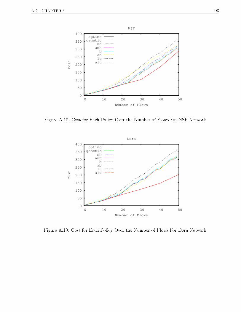
A.2. CHAPTER 5 93
0
50
100
150
200
250
300
350
400
0 10 20 30 40 50
Cost
Number of Flows
NSF
optimogenetic
mhamhbablualu
Figure A.18: Cost for Each Policy Over the Number of Flows For NSF Network
0
50
100
150
200
250
300
350
400
0 10 20 30 40 50
Cost
Number of Flows
Dora
optimogenetic
mhamhbablualu
Figure A.19: Cost for Each Policy Over the Number of Flows For Dora Network

94 APPENDIX A. DETAILED RESULTS
0
50
100
150
200
250
0 10 20 30 40 50
Cost
Number of Flows
Sul
optimogenetic
mhamhbablualu
Figure A.20: Cost for Each Policy Over the Number of Flows For Sul Network
Once we �nd the best con�guration for each policy, we compare the policies consideringthe total cost. The results are shown in Figures A.16 - A.20.
A.2.3 Policies Comparison - Rerouting
Figures A.21- A.25 present the number of reroutes needed by each policy as the number of ows increases.
0
0.5
1
1.5
2
2.5
3
3.5
4
0 5 10 15 20 25 30 35 40 45 50
Number of Reroutes
Number of Flows
Mesh
amhabalu
Figure A.21: Reroutes over Number of Flows For Mesh Network

A.2. CHAPTER 5 95
0
1
2
3
4
5
0 5 10 15 20 25 30 35 40 45 50
Number of Reroutes
Number of Flows
Ring
amhabalu
Figure A.22: Reroutes over Number of Flows For Ring Network
0
1
2
3
4
5
6
7
8
9
0 5 10 15 20 25 30 35 40 45 50
Number of Reroutes
Number of Flows
NSF
amhabalu
Figure A.23: Reroutes over Number of Flows For NSF Network

96 APPENDIX A. DETAILED RESULTS
0
2
4
6
8
10
12
0 5 10 15 20 25 30 35 40 45 50
Number of Reroutes
Number of Flows
Dora
amhabalu
Figure A.24: Reroutes over Number of Flows For Dora Network
0
0.5
1
1.5
2
2.5
3
3.5
4
0 5 10 15 20 25 30 35 40 45 50
Number of Reroutes
Number of Flows
Sul
amhabalu
Figure A.25: Reroutes over Number of Flows For Sul Network
A.2.4 Setting Dynamic Paths
Figures A.26- A.30 present the cost of each policy as a function of the LSP holding time.This experiment shows the advantage of using the genetic algorithm instead of one single
policy.

A.2. CHAPTER 5 97
4000
5000
6000
7000
8000
9000
10000
2752251751257525
Cost
Holding Time
MHAMHB
ABLU
ALU
genetic
Figure A.26: Cost as a Function of LSP Holding Time For Mesh Network
6500
7000
7500
8000
8500
9000
9500
10000
2752251751257525
Cost
Holding Time
MHAMHB
ABLU
ALU
genetic
Figure A.27: Cost as a Function of LSP Holding Time For Ring Network

98 APPENDIX A. DETAILED RESULTS
5500
6000
6500
7000
7500
8000
8500
9000
9500
10000
2752251751257525
Cost
Holding Time
MHAMHB
ABLU
ALU
genetic
Figure A.28: Cost as a Function of LSP Holding Time For NSF Network
6500
7000
7500
8000
8500
9000
9500
10000
10500
2752251751257525
Cost
Holding Time
MHAMHB
ABLU
ALU
genetic
Figure A.29: Cost as a Function of LSP Holding Time For Dora Network
The GA is exible and has the result of the best policy in most part of the time.

A.2. CHAPTER 5 99
4500
5000
5500
6000
6500
7000
7500
8000
8500
9000
9500
2752251751257525
Cost
Holding Time
MHAMHB
ABLU
ALU
genetic
Figure A.30: Cost as a Function of LSP Holding Time For Sul Network
A.2.5 Link Failure
Figures A.31- A.35 show the performance of each policy in case of a link failure.
0.5
1
1.5
2
2.5
3
3.5
4
453525155
Reroutes Needed
Number of Flows
MHAMH
BAB
LUALU
Figure A.31: Reroutes Needed for Each Policy in Case of Link Failure For Mesh Network

100 APPENDIX A. DETAILED RESULTS
0.5
0.6
0.7
0.8
0.9
1
1.1
1.2
1.3
1.4
1.5
453525155
Reroutes Needed
Number of Flows
MHAMH
BAB
LUALU
Figure A.32: Reroutes Needed for Each Policy in Case of Link Failure For ring Network
It is noticeable that the policy AB is the best for less loaded networks, but it increases thenumber of reroutings rapidly when the load increases. When the network becomes congested,the policy LU is the policy that requires the less number of reroutings. For the most part oftopologies, the number of reroutings needed is less than 2. It can be noticed that the di�erenceamong the policies is small when the network is not congested.
0.5
1
1.5
2
2.5
3
3.5
4
453525155
Reroutes Needed
Number of Flows
MHAMH
BAB
LUALU
Figure A.33: Reroutes Needed for Each Policy in Case of Link Failure For NSF Network

A.2. CHAPTER 5 101
0.5
1
1.5
2
2.5
3
3.5
4
453525155
Reroutes Needed
Number of Flows
MHAMH
BAB
LUALU
Figure A.34: Reroutes Needed for Each Policy in Case of Link Failure For Dora Network
0.5
1
1.5
2
2.5
3
3.5
4
453525155
Reroutes Needed
Number of Flows
MHAMH
BAB
LUALU
Figure A.35: Reroutes Needed for Each Policy in Case of Link Failure For Sul Network
Figures A.36 - A.40 show that for all policies the success rate in �nding new routes forLSPs after a link failure is more than 50%.

102 APPENDIX A. DETAILED RESULTS
0.4
0.5
0.6
0.7
0.8
0.9
1
453525155
Sucessful Reroutes
Number of Flows
MHAMH
BAB
LUALU
Figure A.36: % of Successful Rerouting in Case of Link Failure For Mesh Network
0.5
0.55
0.6
0.65
0.7
0.75
0.8
0.85
0.9
0.95
1
453525155
Sucessful Reroutes
Number of Flows
MHAMH
BAB
LUALU
Figure A.37: % of Successful Rerouting in Case of Link Failure For Ring Network
The policy LU is the best since it leaves more space for future requests. The policy ABhas already balanced the traÆc and has fewer options in case of link failures.

A.2. CHAPTER 5 103
0.65
0.7
0.75
0.8
0.85
0.9
0.95
1
453525155
Sucessful Reroutes
Number of Flows
MHAMH
BAB
LUALU
Figure A.38: % of Successful Rerouting in Case of Link Failure For NSF Network
0.6
0.65
0.7
0.75
0.8
0.85
0.9
0.95
1
453525155
Sucessful Reroutes
Number of Flows
MHAMH
BAB
LUALU
Figure A.39: % of Successful Rerouting in Case of Link Failure For Dora Network

104 APPENDIX A. DETAILED RESULTS
0.65
0.7
0.75
0.8
0.85
0.9
0.95
453525155
Sucessful Reroutes
Number of Flows
MHAMH
BAB
LUALU
Figure A.40: % of Successful Rerouting in Case of Link Failure For Sul Network
A.3 Chapter 6
A.3.1 TraÆc Changes Detection Scheme
The metric used to compare the bene�ts of grooming are residual bandwidth and number ofhops (cost) and the results are presented for the policies that are adaptive in Figures A.41- A.55 for all network topologies.
When we vary the policy, we vary the network status in terms of bandwith utilizationin each link. For all policies and topologies, the cost decreased and the residual bandwidthincreased when the grooming process was used in comparison with the case when no groomingwas done, specially in the cases where the network was more congested, i.e. number of owsgreater than 30.

A.3. CHAPTER 6 105
16
18
20
22
24
26
28
30
Cost
Number of LSPS
Mesh
Without Grooming With Grooming
(a) Cost
0.62
0.64
0.66
0.68
0.7
0.72
0.74
0.76
0.78
0.8
Residual
Number of LSPS
Mesh
Without Grooming With Grooming
(b) % of Residual Bandwidth
Figure A.41: AMH Grooming Results For Mesh Network

106 APPENDIX A. DETAILED RESULTS
20
30
40
50
60
70
80
90
100
110
Cost
Number of LSPS
Mesh
Without Grooming With Grooming
(a) Cost
0
0.1
0.2
0.3
0.4
0.5
0.6
0.7
Residual
Number of LSPS
Mesh
Without Grooming With Grooming
(b) % of Residual Bandwidth
Figure A.42: AB Grooming Results for Mesh Network

A.3. CHAPTER 6 107
16
18
20
22
24
26
28
30
Cost
Number of LSPS
Mesh
Without Grooming With Grooming
(a) Cost
0.62
0.64
0.66
0.68
0.7
0.72
0.74
0.76
0.78
0.8
Residual
Number of LSPS
Mesh
Without Grooming With Grooming
(b) % of Residual Bandwidth
Figure A.43: ALU Grooming Results for Mesh Network

108 APPENDIX A. DETAILED RESULTS
25
30
35
40
45
50
55
60
65
70
Cost
Number of LSPS
Ring
Without Grooming With Grooming
(a) Cost
0.7
0.72
0.74
0.76
0.78
0.8
0.82
0.84
0.86
0.88
0.9
Residual
Number of LSPS
Ring
Without Grooming With Grooming
(b) % of Residual Bandwidth
Figure A.44: AMH Grooming Results for Ring Network

A.3. CHAPTER 6 109
30
40
50
60
70
80
90
100
110
120
130
Cost
Number of LSPS
Ring
Without Grooming With Grooming
(a) Cost
0.45
0.5
0.55
0.6
0.65
0.7
0.75
0.8
0.85
Residual
Number of LSPS
Ring
Without Grooming With Grooming
(b) % of Residual Bandwidth
Figure A.45: AB Grooming Results for Ring Network

110 APPENDIX A. DETAILED RESULTS
25
30
35
40
45
50
55
60
65
70
Cost
Number of LSPS
Ring
Without Grooming With Grooming
(a) Cost
0.7
0.72
0.74
0.76
0.78
0.8
0.82
0.84
0.86
0.88
0.9
Residual
Number of LSPS
Ring
Without Grooming With Grooming
(b) % of Residual Bandwidth
Figure A.46: ALU Grooming Results for Ring Network

A.3. CHAPTER 6 111
20
30
40
50
60
70
80
Cost
Number of LSPS
NSF
Without Grooming With Grooming
(a) Cost
0.55
0.6
0.65
0.7
0.75
0.8
0.85
0.9
Residual
Number of LSPS
NSF
Without Grooming With Grooming
(b) % of Residual Bandwidth
Figure A.47: AMH Grooming Results for NSF Network

112 APPENDIX A. DETAILED RESULTS
30
40
50
60
70
80
90
100
Cost
Number of LSPS
NSF
Without Grooming With Grooming
(a) Cost
0.45
0.5
0.55
0.6
0.65
0.7
0.75
0.8
0.85
Residual
Number of LSPS
NSF
Without Grooming With Grooming
(b) % of Residual Bandwidth
Figure A.48: AB Grooming Results for NSF Network

A.3. CHAPTER 6 113
20
30
40
50
60
70
80
Cost
Number of LSPS
NSF
Without Grooming With Grooming
(a) Cost
0.55
0.6
0.65
0.7
0.75
0.8
0.85
0.9
Residual
Number of LSPS
NSF
Without Grooming With Grooming
(b) % of Residual Bandwidth
Figure A.49: ALU Grooming Results for NSF Network

114 APPENDIX A. DETAILED RESULTS
25
30
35
40
45
50
55
60
65
70
Cost
Number of LSPS
Dora
Without Grooming With Grooming
(a) Cost
0.88
0.89
0.9
0.91
0.92
0.93
0.94
0.95
0.96
Residual
Number of LSPS
Dora
Without Grooming With Grooming
(b) % of Residual Bandwidth
Figure A.50: AMH Grooming Results for Dora Network

A.3. CHAPTER 6 115
30
40
50
60
70
80
90
100
110
120
Cost
Number of LSPS
Dora
Without Grooming With Grooming
(a) Cost
0.8
0.82
0.84
0.86
0.88
0.9
0.92
0.94
0.96
Residual
Number of LSPS
Dora
Without Grooming With Grooming
(b) % of Residual Bandwidth
Figure A.51: AB Grooming Results for Dora Network

116 APPENDIX A. DETAILED RESULTS
25
30
35
40
45
50
55
60
65
70
Cost
Number of LSPS
Dora
Without Grooming With Grooming
(a) Cost
0.88
0.89
0.9
0.91
0.92
0.93
0.94
0.95
0.96
Residual
Number of LSPS
Dora
Without Grooming With Grooming
(b) % of Residual Bandwidth
Figure A.52: ALU Grooming Results for Dora Network

A.3. CHAPTER 6 117
10
15
20
25
30
35
40
45
50
55
Cost
Number of LSPS
Sul
Without Grooming With Grooming
(a) Cost
0.6
0.65
0.7
0.75
0.8
0.85
0.9
0.95
Residual
Number of LSPS
Sul
Without Grooming With Grooming
(b) % of Residual Bandwidth
Figure A.53: AMH Grooming Results for Sul Network

118 APPENDIX A. DETAILED RESULTS
10
20
30
40
50
60
70
80
Cost
Number of LSPS
Sul
Without Grooming With Grooming
(a) Cost
0.45
0.5
0.55
0.6
0.65
0.7
0.75
0.8
0.85
0.9
Residual
Number of LSPS
Sul
Without Grooming With Grooming
(b) % of Residual Bandwidth
Figure A.54: AB Grooming Results for Sul Network

A.3. CHAPTER 6 119
10
15
20
25
30
35
40
45
50
55
Cost
Number of LSPS
Sul
Without Grooming With Grooming
(a) Cost
0.6
0.65
0.7
0.75
0.8
0.85
0.9
0.95
Residual
Number of LSPS
Sul
Without Grooming With Grooming
(b) % of Residual Bandwidth
Figure A.55: ALU Grooming Results for Sul Network

Livros Grátis( http://www.livrosgratis.com.br )
Milhares de Livros para Download: Baixar livros de AdministraçãoBaixar livros de AgronomiaBaixar livros de ArquiteturaBaixar livros de ArtesBaixar livros de AstronomiaBaixar livros de Biologia GeralBaixar livros de Ciência da ComputaçãoBaixar livros de Ciência da InformaçãoBaixar livros de Ciência PolíticaBaixar livros de Ciências da SaúdeBaixar livros de ComunicaçãoBaixar livros do Conselho Nacional de Educação - CNEBaixar livros de Defesa civilBaixar livros de DireitoBaixar livros de Direitos humanosBaixar livros de EconomiaBaixar livros de Economia DomésticaBaixar livros de EducaçãoBaixar livros de Educação - TrânsitoBaixar livros de Educação FísicaBaixar livros de Engenharia AeroespacialBaixar livros de FarmáciaBaixar livros de FilosofiaBaixar livros de FísicaBaixar livros de GeociênciasBaixar livros de GeografiaBaixar livros de HistóriaBaixar livros de Línguas

Baixar livros de LiteraturaBaixar livros de Literatura de CordelBaixar livros de Literatura InfantilBaixar livros de MatemáticaBaixar livros de MedicinaBaixar livros de Medicina VeterináriaBaixar livros de Meio AmbienteBaixar livros de MeteorologiaBaixar Monografias e TCCBaixar livros MultidisciplinarBaixar livros de MúsicaBaixar livros de PsicologiaBaixar livros de QuímicaBaixar livros de Saúde ColetivaBaixar livros de Serviço SocialBaixar livros de SociologiaBaixar livros de TeologiaBaixar livros de TrabalhoBaixar livros de Turismo