resoluÇÃo em tomografia de tempo de ......resumo o aspecto fundamental na resolução limitante em...
TRANSCRIPT
Universidade Federal do Rio Grande do NorteCentro de Ciências Exatas e da Terra
Programa de Pós-Graduação em Geodinâmica e Geofísica
DISSERTAÇÃO DE MESTRADO
RESOLUÇÃO EM TOMOGRAFIA DE TEMPODE TRÂNSITO POÇO-A-POÇO: ADEPENDÊNCIA DA ILUMINAÇÃO
Autor:
Renato Ramos da Silva Dantas
Orientador:
Prof. Dr. Walter Eugênio de Medeiros (DGef/PPGG/UFRN)
Dissertação n.o 142/PPGG.
Natal, RN, 05 de Março de 2015
UNIVERSIDADE FEDERAL DO RIO GRANDE DO NORTECENTRO DE CIÊNCIAS EXATAS E DA TERRA
PROGRAMA DE PÓS-GRADUAÇÃO EM GEODINÂMICA E GEOFÍSICA
DISSERTAÇÃO DE MESTRADO
RESOLUÇÃO EM TOMOGRAFIA DE TEMPODE TRÂNSITO POÇO-A-POÇO: ADEPENDÊNCIA DA ILUMINAÇÃO
Autor:Renato Ramos da Silva Dantas
Dissertação apresentada em 05 de marçode dois mil e quinze, ao Programa de Pós-Graduação em Geodinâmica e Geofísica– PPGG, da Universidade Federal do RioGrande do Norte - UFRN como requisitoà obtenção do Título de Mestre em Geo-dinâmica e Geofísica, com área de con-centração em Geofísica.
Comissão Examinadora:
Prof. Dr. Walter Eugênio de Medeiros (DGef/PPGG/UFRN) - OrientadorProf. Dr. Jessé Carvalho Costa (UFPA) - Examinador externo
Prof. Dr. Roberto Hugo Bielschowsky (UFRN) - Examinador interno
Natal, RN, 05 de Março de 2015
Resumo
O aspecto fundamental na resolução limitante em tomografia de trânsito poço-a-poço é a ilu-
minação, um resultado bem conhecido mas não tão bem exemplificado. A resolução no caso 2D
é revisitada usando uma simples abordagem geométrica baseada na distribuição de aberturas an-
gulares e nas propriedades da Transformada de Radon. Analiticamente é mostrado que se uma
interface tem mergulhos contidos nos limites da abertura angular em todos os pontos, ela é corre-
tamente imageada no tomograma. Por inversão de dados sintéticos, esse resultado é confirmado
e é também evidenciado que artefatos isolados podem estar presentes quando o mergulho estiver
próximo do limite de iluminação. No sentido inverso, entretanto, se uma interface é interpretável
por um tomograma, mesmo uma interface aproximadamente horizontal, não há garantia de que
ela corresponda a uma interface verdadeira. De modo semelhante, se um corpo estiver presente na
região entre os poços, ele é imageado no tomograma de forma difusa, mas suas interfaces - em par-
ticular, as bordas verticais - podem não ser resolvidas, e artefatos adicionais podem estar presentes.
Novamente, no sentido inverso, não há garantia que uma anomalia isolada corresponda a um corpo
anômalo verdadeiro, pois sua anomalia pode também ser um artefato. Juntos, esses resultados
declaram o dilema dos problemas inversos mal-postos: ausência de garantia de correspondência
à distribuição verdadeira. As limitações devidas à iluminação podem não ser resolvidas pelo uso
de vínculos matemáticos. É mostrado que tomogramas poço-a-poço derivadas pelo uso de víncu-
los de esparsidade, usando tanto a Transformada de Cosseno Discreto como as bases Daubechies,
basicamente reproduzem as mesmas características vistas em tomogramas obtidos com o vínculo
de suavidade clássico. É necessário que interpretações sejam feitas sempre levando em conside-
ração as informações a priori e as limitações particulares devido à iluminação. Um exemplo de
interpretação de um levantamento de dados reais dentro deste contexto também é apresentado.
Palavras-chave: Tomografia poço-a-poço, Tomografia de tempo de trânsito, Transformada de
Radon, Vínculo de esparsidade.
i

Abstract
The key aspect limiting resolution in crosswell traveltime tomography is illumination, a well
known result but not as well exemplified. Resolution in the 2D case is revisited using a simple
geometric approach based on the angular aperture distribution and the Radon Transform proper-
ties. Analitically it is shown that if an interface has dips contained in the angular aperture limits
in all points, it is correctly imaged in the tomogram. By inversion of synthetic data this result is
confirmed and it is also evidenced that isolated artifacts might be present when the dip is near the
illumination limit. In the inverse sense, however, if an interface is interpretable from a tomogram,
even an aproximately horizontal interface, there is no guarantee that it corresponds to a true inter-
face. Similarly, if a body is present in the interwell region it is diffusely imaged in the tomogram,
but its interfaces - particularly vertical edges - can not be resolved and additional artifacts might
be present. Again, in the inverse sense, there is no guarantee that an isolated anomaly corresponds
to a true anomalous body because this anomaly can also be an artifact. Jointly, these results state
the dilemma of ill-posed inverse problems: absence of guarantee of correspondence to the true
distribution. The limitations due to illumination may not be solved by the use of mathematical
constraints. It is shown that crosswell tomograms derived by the use of sparsity constraints, using
both Discrete Cosine Transform and Daubechies bases, basically reproduces the same features seen
in tomograms obtained with the classic smoothness constraint. Interpretation must be done always
taking in consideration the a priori information and the particular limitations due to illumination.
An example of interpreting a real data survey in this context is also presented.
Keywords: Crosswell tomography, Traveltime tomography, Radon Transform, Sparsity cons-
traints.
ii
Agradecimentos
Agradeço, primeiramente, a Deus, por todas as oportunidades que tive e que poderei vir a ter,
inclusive uma das mais fundamentais, que é a de viver.
Agradeço ao CNPq pelo apoio financeiro.
Agradeço aos meus pais, Ruy Bezerra Dantas e Neide Ramos da Silva Dantas, e ao meu irmão,
Rafael Ramos da Silva Dantas, pela paciência, dedicação e compreensão (quase sobrenatural) que
eles sempre mostraram. Aproveito para agradecer também à finada Mel e a Barão, grandes seres
viventes que sabem ser leais e incríveis como nenhum ser humano conseguiria ser.
Agradeço ao meu orientador, Prof. Dr. Walter Eugênio de Medeiros, por ter me orientado por
dois anos (e, se Deus quiser, por mais quatro) com tanta paciência e dedicação, e pelas valiosas
contribuições humanas.
Agradeço aos membros da banca, Prof. Dr. Jessé Carvalho Costa e Prof. Dr. Roberto Hugo
Bielschowsky, pelas suas importantes contribuições a essa dissertação.
Agradeço ao Programa de Pós-Graduação em Geodinâmica e Geofísica, em especial à Nilda e ao
prof. Dr. Zorano, por todo o apoio oferecido durante esses dois anos.
Agradeço aos alunos do PPGG Márcio Barboza e Jerbeson Santana, pelos momentos de descon-
tração e pelas importantes discussões e contribuições.
Agradeço aos membros do Laboratório Sismológico da UFRN, por terem me incluído no meio
científico logo no início do curso. Não teria chegado até aqui sem esse apoio.
Aproveito para agradecer aos ex-alunos do PPGG Heleno Carlos, Bonnie Ives, Paulo Henrique e
Rosana Nascimento, e ao funcionário do DGef Rodrigo Pessoa, por me mostrarem (a tempo!) a
iii
ciência como ela é. E por todos os momentos de descontração.
Agradeço aos meus ex-colegas de turma do IFRN, por tudo o que fizeram por mim (e ainda fazem!)
até hoje. E por levarem o nome da Geologia e Mineração do IFRN à Geologia da UFRN, caminho
do qual acabei me desviando...
Agradeço aos professores do IFRN Mário Tavares, Alexandre Magno, Rogério Vidal, Moacir Ve-
ras, João Batista, Jomar de Freitas, dentre outros, por toda a preparação para uma vida de geocien-
tista que eles me proporcionaram.
Agradeço a meus colegas do (finado) fórum RPG Maker Brasil, pelas valiosas contribuições inte-
lectuais e lúdicas, que tanto me ajudaram com a prática de programação como com conhecimento
de relações interpessoais. Aproveito para agradecer a Jhonata Rodrigues, Lucimário Custódio e a
Nádja Batista, que conheci através desse fórum – eles já me ajudaram mais do que têm ideia.
Agradeço também ao prof. Jadson Tadeu e a Lucas Fonseca, Thiago Berto e a Cássio Souza, por
todas as (várias) derrotas que sofri em suas mãos!

Sumário
Resumo i
Abstract ii
Agradecimentos iii
Sumário v
1 Contextualização 1
1.1 Histórico e evolução da tomografia sísmica . . . . . . . . . . . . . . . . . . . . . 1
1.2 Problema direto . . . . . . . . . . . . . . . . . . . . . . . . . . . . . . . . . . . . 2
1.2.1 Formulação matemática . . . . . . . . . . . . . . . . . . . . . . . . . . . 2
1.2.2 Modelagem dos tempos de primeira chegada . . . . . . . . . . . . . . . . 3
1.2.3 Transformada de Radon . . . . . . . . . . . . . . . . . . . . . . . . . . . 4
1.3 Geometrias de aquisição . . . . . . . . . . . . . . . . . . . . . . . . . . . . . . . 5
1.3.1 Tomografia de superfície . . . . . . . . . . . . . . . . . . . . . . . . . . . 5
1.3.2 Tomografia poço-a-poço . . . . . . . . . . . . . . . . . . . . . . . . . . . 6
1.4 Aplicações . . . . . . . . . . . . . . . . . . . . . . . . . . . . . . . . . . . . . . . 8
2 Manuscrito submetido: "Resolution in crosswell traveltime tomography: the depen-
dence from illumination" 10
Referências bibliográficas 55
Apêndice A: Matriz de transformação 2D 58
v
Capítulo 1
Contextualização
1.1 Histórico e evolução da tomografia sísmica
Os primeiros trabalhos de tomografia como método de construção de uma imagem 2D da sub-
superfície surgiram no final da década de 70, impulsionados pelo avanço dos computadores, permi-
tindo a resolução das relativamente grandes sistemas de equações necessários para obter soluções
de inversões tomográficas. A espinha dorsal da tomografia está na teoria de inversão, desenvol-
vida por Backus and Gilbert (1970). Durante o final do século XX, tanto os instrumentos como a
técnica avançaram bastante, com a compreensão da aplicabilidade (e.g Bregman et al., 1989, Lanz
et al., 1998, White, 1989) e das limitações do método (e.g Day-Lewis and Lane, 2004, Goudswa-
ard et al., 1998, Menke, 1984, Rector III and Washbourne, 1994) e o desenvolvimento de métodos
de traçado de raio e de modelagem (e.g. Moser, 1991, Podvin and Lecomte, 1991, Vidale, 1988,
1990).
Alguns novos métodos de regularização foram desenvolvidos para os ambientes típicos investi-
gados pela tomografia (e.g. Zhdanov et al., 2006), e outros foram adaptados de outros métodos ge-
ofísicos (e.g. Ajo-Franklin et al., 2007). Contudo, o vínculo de suavidade (Tikhonov and Arsenin,
1977) continue sendo o mais utilizado em aplicações práticas, devido a sua fácil implementação e
a sua versatilidade Ajo-Franklin et al., 2007, já que supor uma distribuição suave de propriedades
físicas é uma hipótese perfeitamente razoável para a maioria dos ambientes geológicos. Recente-
mente, Lustig et al. (2007), em tomografia médica de raios-X, utilizaram um vínculo baseado na
teoria de compressed sensing (Candès et al., 2006, Donoho, 2006, Mallat, 2008), que aqui cha-
maremos de vínculo de esparsidade. O uso desse vínculo significa buscar soluções esparsas em
CAPÍTULO 1. CONTEXTUALIZAÇÃO 2
um certa base de representação. Para meios físicos naturais, essa é uma suposição razoável, o
que torna esse vínculo válido tanto em medicina como em outras áreas, inclusive geofísica (e.g.
Charléty et al., 2013, Jafarpour et al., 2009, Loris et al., 2007, Simons et al., 2011).
Com o avanço dos computadores, permitindo o uso, tanto acadêmico como industrial, de algo-
ritmos cada vez mais sofisticados, foi possível por em prática o método mais natural no avanço da
tomografia: ao invés de usar apenas uma fase, usar toda a informação contida nos traços sísmicos.
Isso constitui o método da inversão de forma de onda (Full Waveform Inversion, ou FWI; Virieux
and Operto, 2009). Esse método requer o uso de um modelo inicial cuidadosamente escolhido e
um altíssimo custo computacional. Contudo, esse método também traz um grande ganho em reso-
lução, especialmente importante para o imageamento de ambientes geológicos muito complexos.
Devido aos desafios que essa metodologia traz, seu desenvolvimento ainda está em andamento, e
resolver tais desafios é, provavelmente, o próximo passo para o avanço da tomografia sísmica.
1.2 Problema direto
1.2.1 Formulação matemática
A tomografia é uma técnica de imageamento do interior de corpos que se baseia na propagação
de ondas através de um número muito grande de caminhos de propagação, a depender das posições
de fonte e de receptor. Desse modo, cada unidade de volume do interior do corpo é atravessado por
uma grande quantidade de ondas que se propagam em diferentes direções. Os receptores registram
a forma completa da onda propagada, à qual podem estar também superpostas ondas indesejadas,
a exemplo das guias de ondas, quando se está lidando com tomografia de ondas de corpo. Para
a tomografia de tempo de trânsito, que é uma aproximação muito utilizada para ondas de corpo
(Nolet, 1987), é necessário identificar o tempo de chegada de uma das fases (em geral, a onda P), o
que é feito através da marcação da primeira chegada, de preferência após um pré-processamento,
para maximizar a razão sinal-ruído (Lo and Inderwiesen, 1994).
O problema da tomografia de tempo de trânsito consiste assim em reconstituir a distribuição
de velocidades (Ajo-Franklin, 2009, Ajo-Franklin et al., 2007, Charléty et al., 2013), em uma certa
CAPÍTULO 1. CONTEXTUALIZAÇÃO 3
região do espaço R , a partir dos tempos de trânsito medidos entre as fontes e os receptores situados
na fronteira de R . Nas aplicações em geofísica, usualmente há limitações severas no posiciona-
mento das fontes e dos receptores apenas em certos setores da fronteira, bem como restrições sobre
o numero de fontes. Uma configuração muito utilizada é a da tomografia poço-a-poço, em uma
versão 2-D do problema, que é o foco deste estudo. Nesta configuração, as fontes e receptores só
podem ser colocados ao longo dos poços, que são usualmente verticais.
Matematicamente, o problema da tomografia poço-a-poço pode ser formulado da seguinte ma-
neira:
A(s) = τ+n (1.1)
em que s = s(x,z) descreve a distribuição espacial de vagarosidade (inverso da velocidade) e
A(s) =∫
raysdl (1.2)
é o operador integral que modela, para um dado raio sísmico, o tempo de percurso τ registrado no
final do trajeto e n é o ruído contido na sua medida. Se o meio for discretizado em um conjunto de
N blocos, sendo Nx na horizontal e Nz na vertical, de tal forma que, para cada bloco, haja um par
ordenado correspondente (xi,zi), e que
N = NxNz (1.3)
podemos escrever uma versão discreta da equação 1.1 como:
Ai(s) = τi +ni (1.4)
em que s∈RN é um vetor de vagarosidades, τ+n∈RM é o vetor de tempos de trânsito observados,
que incorpora o ruído n, e A : RN → RM é um operador discreto de modelagem.
1.2.2 Modelagem dos tempos de primeira chegada
Há várias abordagens de modelagem disponíveis na literatura, desde soluções diretas da equa-
ção iconal (Vidale, 1988, 1990) a modelagem via traçado de raio utilizando o Princípio de Fermat
CAPÍTULO 1. CONTEXTUALIZAÇÃO 4
e teoria de grafos (Moser, 1991); neste trabalho, usamos a abordagem de Podvin and Lecomte
(1991). Ela consiste na utilização do Princípio de Huygens para o mapeamento das frentes de onda
na região investigada, possibilitando a modelagem do primeiro tempo de chegada. Para um meio
discretizado em Nz×Nx blocos, isso consiste em calcular o tempo de todas as chegadas no ponto
considerado e escolher o menor.
Tal procedimento pode ser levado à prática pelo Princípio de Huygens. Segundo esse princípio,
cada ponto contido em uma frente de onda pode ser tratado como uma fonte pontual secundária de
onda esférica, que emitem um pulso no momento de sua primeira chegada. Assim, cada vértice dos
blocos pode ser tratado como uma fonte. Então, a modelagem de Podvin and Lecomte (1991) pode
ser resumida no cálculo de todas as chegadas em um dado ponto oriundas das vértices vizinhas.
Podvin and Lecomte (1991) lida com as chegadas de ondas transmitidas, refratadas e difratadas.
O cálculo dos tempos de trânsito é feito considerando uma interpolação linear entre vértices
vizinhas, o que é equivalente a considerar uma aproximação local de onda plana. Todas as equações
para cálculo dos tempos de chegada de ondas transmitidas, refratadas e difratadas, tanto em meios
2D como 3D, seguindo essa abordagem são apresentadas por Podvin and Lecomte (1991). Note
que tal aproximação falha nas vizinhanças da fonte. Um simples procedimento de inicialização
pode ser utilizado para evitar essa imprecisão, que é calcular exatamente os tempos de trânsito na
maior caixa ao redor da fonte na qual a velocidade é homogênea.
Essa abordagem também possibilita traçado de raio a posteriori, caso seja necessário. Para
isso, basta traçar o raio, do receptor até a fonte, ao longo do negativo dos gradientes locais de
tempo.
1.2.3 Transformada de Radon
Em tomografia médica, a base teórica para os métodos de inversão utilizados nessa área envol-
vem a chamada transformada de Radon. Ela é uma soma integral sobre uma linha da função de
entrada s(x,z) (Kak and Slaney, 2001):
Rθ(t) =∫(θ,t) line
s(x,z)dl (1.5)
CAPÍTULO 1. CONTEXTUALIZAÇÃO 5
em que a linha (θ, t) é a linha ortogonal à reta que passa pela origem e faz um ângulo θ em relação
ao eixo x, e cortando essa reta num ponto distando t da origem. Por ser análogo à equação (1.2)
de tempo de trânsito em função da vagarosidade do meio, a aplicação natural dessa transformada
é em tomografia. Podemos ver um experimento tomográfico como uma amostragem de projeções
da transformada de Radon do meio investigado.
Pode-se mostrar que, dado um feixe de raios paralelos, ortogonais à linha de ângulo θ, a trans-
formada de Radon desse feixe será mapeada no espaço de Fourier do modelo verdadeiro, ao longo
de uma linha com ângulo θ. Esse é o teorema da seção de Fourier (Kak and Slaney, 2001). Esse
teorema é a base dos algoritmos de reconstrução utilizados na medicina, em que se tem acesso a
todas as vistas, e todos os raios podem ser considerados retos.
Se não houvesse restrições de iluminação da região entre os poços, o problema da tomografia
poço-a-poço linear poderia ser formulado como uma Transformada de Radon. Contudo, como as
fontes e receptores só podem ser colocadas nos poços, este problema de tomografia linear cor-
responde ao da Transformada de Radon com projeções incompletas Kak and Slaney (2001). Não
obstante, a Transformada de Radon fornece uma arcabouço para entendimento do problema que
pode ser extrapolado para o caso não linear.
1.3 Geometrias de aquisição
Existem duas geometrias básicas de aquisição de dados tomográficos: posicionar as fontes e
os receptores próximos da superfície (tomografia de superfície) ou em poços (tomografia poço-a-
poço).
1.3.1 Tomografia de superfície
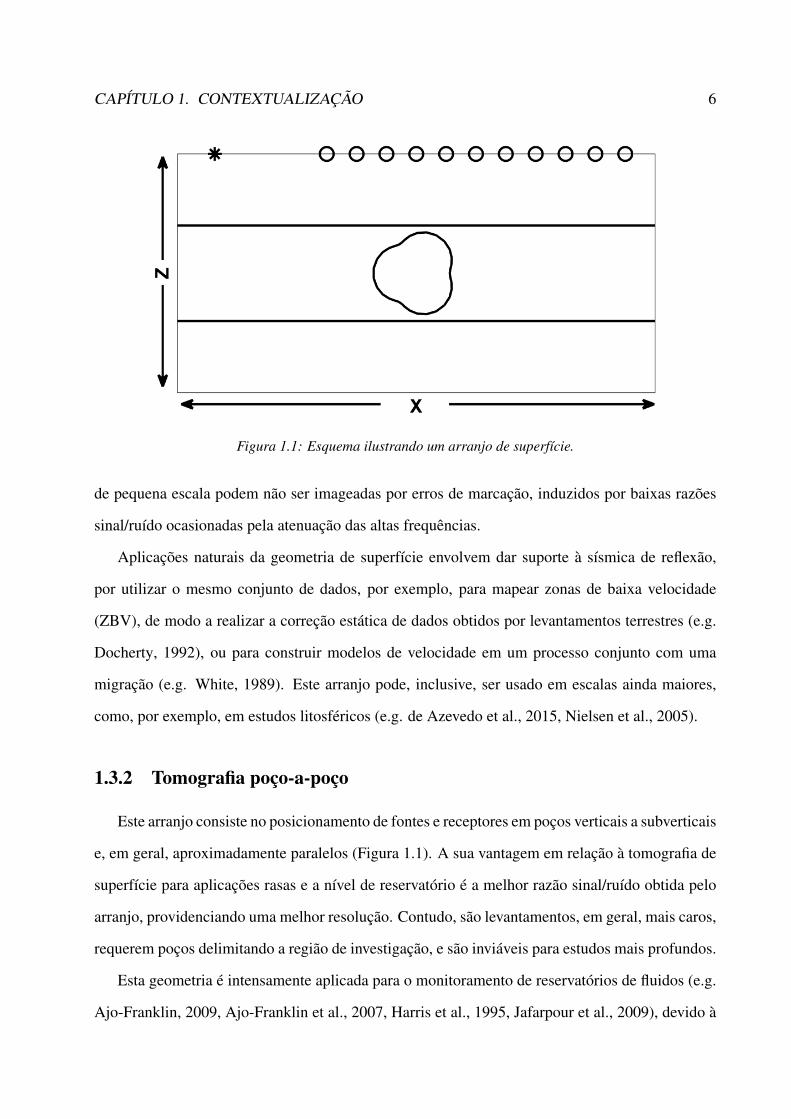
Este arranjo consiste no posicionamento de fontes e receptores aproximadamente alinhados e
próximos da superfície (Figura 1.1). Como pode utilizar os mesmos dados obtidos para uma sís-
mica de reflexão, por exemplo, a aquisição de superfície é relativamente barata, e a profundidade
de investigação pode alcançar até dezenas de quilômetros, a depender da frequência de aquisi-
ção e dos offsets (distância fonte-receptor) disponíveis. Contudo, em aplicações rasas, feições
CAPÍTULO 1. CONTEXTUALIZAÇÃO 6
Figura 1.1: Esquema ilustrando um arranjo de superfície.
de pequena escala podem não ser imageadas por erros de marcação, induzidos por baixas razões
sinal/ruído ocasionadas pela atenuação das altas frequências.
Aplicações naturais da geometria de superfície envolvem dar suporte à sísmica de reflexão,
por utilizar o mesmo conjunto de dados, por exemplo, para mapear zonas de baixa velocidade
(ZBV), de modo a realizar a correção estática de dados obtidos por levantamentos terrestres (e.g.
Docherty, 1992), ou para construir modelos de velocidade em um processo conjunto com uma
migração (e.g. White, 1989). Este arranjo pode, inclusive, ser usado em escalas ainda maiores,
como, por exemplo, em estudos litosféricos (e.g. de Azevedo et al., 2015, Nielsen et al., 2005).
1.3.2 Tomografia poço-a-poço
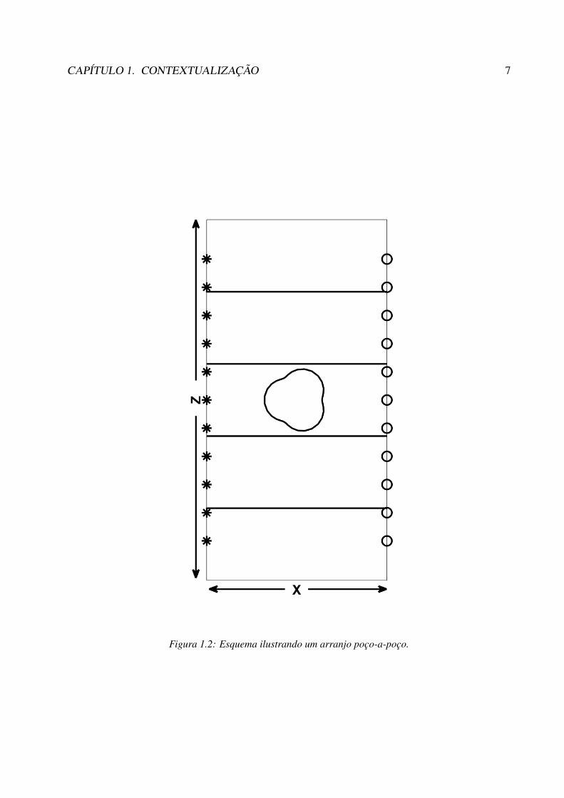
Este arranjo consiste no posicionamento de fontes e receptores em poços verticais a subverticais
e, em geral, aproximadamente paralelos (Figura 1.1). A sua vantagem em relação à tomografia de
superfície para aplicações rasas e a nível de reservatório é a melhor razão sinal/ruído obtida pelo
arranjo, providenciando uma melhor resolução. Contudo, são levantamentos, em geral, mais caros,
requerem poços delimitando a região de investigação, e são inviáveis para estudos mais profundos.
Esta geometria é intensamente aplicada para o monitoramento de reservatórios de fluidos (e.g.
Ajo-Franklin, 2009, Ajo-Franklin et al., 2007, Harris et al., 1995, Jafarpour et al., 2009), devido à
CAPÍTULO 1. CONTEXTUALIZAÇÃO 7
Figura 1.2: Esquema ilustrando um arranjo poço-a-poço.

CAPÍTULO 1. CONTEXTUALIZAÇÃO 8
sua alta resolução, permitindo um bom delineamento do reservatório e uma inferência da variação
espacial das propriedades permoporosas do meio (e.g. Lo and Inderwiesen, 1994), e ao fato de que,
nessas aplicações, em geral já há poços disponíveis para a aquisição. Também pode ser aplicado
para o auxílio de exploração e lavra de minas, nas quais as fontes e os receptores também podem
ser posicionadas em galerias (e.g. Gustavsson et al., 1986), formando um leque. Contudo, os
princípios da tomografia poço-a-poço são semelhantes neste caso (maior resolução em direções
ortogonais às galerias, menor resolução em direções paralelas).
1.4 Aplicações
A aplicação mais natural da tomografia é em exploração e explotação de recursos minerais. Co-
nhecer o substrato geológico é crucial em investigações geológicas, e métodos geofísicos oferecem
meios não-invasivos para obter informações sobre o meio investigado. Para o monitoramento de
reservatórios de hidrocarbonetos, a tomografia desempenha um grande papel por sua flexibilidade
de escalas de aplicação, atuando tanto em investigações regionais como em escala de laboratório.
O que possibilita o uso desse método para o monitoramento de reservatórios é a significativa sen-
sibilidade da velocidade de propagação das ondas elásticas à porosidade, à saturação e ao tipo de
fluido saturante (Schön, 2011), o que possibilita o delineamento do reservatório e o monitoramento
de fluxo de fluidos (e.g. Ajo-Franklin, 2009, Byun et al., 2010), dentre outros. A tomografia é es-
pecialmente importante para o estudo de áreas de descarte de lixo radioativo (e.g. Peterson et al.,
1985), e também está tendo uma grande atuação em projetos de injeção de CO2 (e.g. Ajo-Franklin,
2009, Byun et al., 2010, Harris et al., 1995). Ainda na questão exploratória, pode ser utilizada to-
mografia na exploração mineral em minas, mapeando tanto corpos mineralizados de alta densidade
como possíveis zonas de fraqueza, auxiliando na lavra da mina (e.g. Gustavsson et al., 1986).
A tomografia também tem importância em aplicações em escalas mais rasas. De Iaco et al.
(2003) e Lanz et al. (1998) mostram a utilidade e as limitações da tomografia na delimitação das
bases de aterros. Liu and Guo (2005) imageia a distribuição de velocidades da coluna de concreto
de uma ponte, de modo a avaliar a competência do material e localizar possíveis zonas de fraqueza.
Outra aplicação da tomografia em escala rasa é na investigação de sítios arqueológicos (Metwaly
CAPÍTULO 1. CONTEXTUALIZAÇÃO 9
et al., 2005, Polymenakos and Papamarinopoulos, 2005).
No outro extremo da resolução, a tomografia tem intensa aplicabilidade em estudos crustais.
Nielsen et al. (2005) estuda as sequências sedimentares da litosfera do sudeste do Mar do Norte.
de Azevedo et al. (2015) analisa a geometria da litosfera entre os crátons Amazônico e de São
Francisco.
Capítulo 2
Manuscrito submetido: "Resolution in
crosswell traveltime tomography: the
dependence from illumination"
Manuscrito submetido à revista Geophysics.

Resolution in crosswell traveltime tomography: the
dependence from illumination
Renato R.S. Dantas∗‡ and W.E. Medeiros∗†‡
∗Programa de Pos-graduacao em Geodinamica e Geofısica.
†Departamento de Geofısica
Centro de Ciencias Exatas e da Terra
Universidade Federal do Rio Grande do Norte – UFRN
59.072-970, Natal/RN, Brazil.
Phone: 55 84 3215 3794
‡INCT-GP/CNPq - Instituto Nacional de Ciencias e Tecnologia em Geofısica do Petroleo
- CNPq, Brazil.
(March 18, 2015)
Running head: Resolution in crosswell tomography
ABSTRACT
The key aspect limiting resolution in crosswell traveltime tomography is illumination, a
well known result but not as well exemplified. Resolution in the 2D case is revisited using
a simple geometric approach based on the angular aperture distribution and the Radon
Transform properties. Analitically it is shown that if an interface has dips contained in the
angular aperture limits in all points, it is correctly imaged in the tomogram. By inversion
of synthetic data this result is confirmed and it is also evidenced that isolated artifacts
might be present when the dip is near the illumination limit. In the inverse sense, however,
if an interface is interpretable from a tomogram, even an aproximately horizontal inter-
1
face, there is no guarantee that it corresponds to a true interface. Similarly, if a body is
present in the interwell region it is diffusely imaged in the tomogram, but its interfaces -
particularly vertical edges - can not be resolved and additional artifacts might be present.
Again, in the inverse sense, there is no guarantee that an isolated anomaly corresponds to
a true anomalous body because this anomaly can also be an artifact. Jointly, these results
state the dilemma of ill-posed inverse problems: absence of guarantee of correspondence to
the true distribution. The limitations due to illumination may not be solved by the use
of mathematical constraints. It is shown that crosswell tomograms derived by the use of
sparsity constraints, using both Discrete Cosine Transform and Daubechies bases, basically
reproduces the same features seen in tomograms obtained with the classic smoothness con-
straint. Interpretation must be done always taking in consideration the a priori information
and the particular limitations due to illumination. An example of interpreting a real data
survey in this context is also presented.
Keywords: Crosswell tomography, Traveltime tomography, Radon Transform, Sparsity
constraints.
2

INTRODUCTION
Crosswell traveltime tomography is an important tool for characterizing aquifers and oil
reservoirs (e.g. Harris et al., 1995; Day-Lewis and Lane, 2004; Plessix, 2006), and monitoring
gas carbon sequestration in geologic formations (e.g. Ajo-Franklin et al., 2007; Ajo-Franklin,
2009; Byun et al., 2010). Obtained tomograms can also be used as starting models for more
elaborated inversion methods, such as full waveform inversion (e.g. Wang and Rao, 2006;
Virieux and Operto, 2009).
In recent years, there has been efforts in developing tomography inversion methods based
on sparsity constraints both in crosswell (e.g. Gholami and Siahkoohi, 2010) and other
configurations (e.g. Loris et al., 2007). Sparsity constraints might have advantages over the
classic smoothness constraint because it might enhance edges (e.g. Lustig et al., 2007). In
this sense, sparsity is a constraint similar to total variation (Rudin et al., 1992) which can
be considered as an sparsity constraint but in the gradient of the physical property (Lustig
et al., 2007). However, constraints must be used with caution because they inevitably
introduce bias in the solution. Thus, their use should be preceded by a careful analysis of
the geophysical data resolution taken isolately, in order to identify which solution features
might be primarily attributed to the data, in contrast to other features that might represent
basically the bias associated to the constraints.
In investigating data resolution in crosswell tomography, Menke (1984) showed, by using
the Backus-Gilbert method (Backus and Gilbert, 1970), that the horizontal resolution is
sensibly worse than the vertical resolution for the straight-ray case. Rector III and Wash-
bourne (1994) showed that resolution is dependent on the avaliable angular aperture which
varies in the interwell region. Both Menke (1984) and Rector III and Washbourne (1994)
3
showed that resolution is higher in the central sector of the interwell region, a fact also
pointed by Day-Lewis and Lane (2004) as result of a geostatistical investigation. It is
widely recognized (e.g Menke, 1984; Rector III and Washbourne, 1994; Goudswaard et al.,
1998; Day-Lewis and Lane, 2004) that in crosswell traveltime tomography it is difficult to
reconstruct high-angle interfaces due to the absence of near-vertical rays. However, system-
atic approaches to investigate data resolution which might be easily adapted to particular
designs are still necessary. Here, it is resumed the approach of using the angular aper-
ture distribution, under the hypothesis that the interwell media is homogeneous (Rector III
and Washbourne, 1994), now in concurrence with the Radon Transform properties (Menke,
1984; Kak and Slaney, 2001), to characterize data resolution in 2D crosswell traveltime
tomography. Although both elements are valid only for the straight-ray case, they might
constitute good approximations for the nonlinear case, at least when the slowness contrasts
are smaller than 20% (Dines and Lytle, 1979; Bregman et al., 1989). As result it is devised
a framework to understand data resolution primarily based on simple geometric elements.
It is shown that this framework can be also used to verify which effects might be attributed
to constraint bias, to guide survey designs, and to assist in data interpretation.
TOMOGRAPHY AS AN INVERSE PROBLEM
Mathematical setting
Traveltime tomography obtains images of the Earth’s subsurface based on wave propagation
between sources and receivers. Once the cumbersome task of first break picking is realized
(Lo and Inderwiesen, 1994), traveltime tomography is basically an inverse problem (Nolet,
1987) aiming to estimate the slowness (inverse of velocity) distribution inside a region R,
4

given the measured traveltimes between souce-receiver pairs located in the boundary of R.
Under the validity of the ray tracing approach (Cerveny, 2005), the traveltime τ between a
source-receiver pair is given by
τ(s) =
∫
Lsd` (1)
where L is the ray path and s = s(`) is the slowness along L.
Survey designs for geophysical applications usually impose limited illumination as con-
sequence of positioning sources and receivers just in certain sectors of the R boundary. In
particular, for crosswell designs, sources and receivers can be placed just in the boreholes.
Here it is considered the 2-D discrete version of the P-wave crosswell tomography be-
tween two vertical boreholes. The slowness is defined by s(x, z), where x and z axes coincide
with the top horizontal and left vertical boundaries of the interwell region. This region is
discretized in a rectangular mesh containing N ordered elements with sizes ∆x and ∆z. The
associated slowness values sj ( = 1, 2, ...N) are arranjed in the vector array s ∈ RN . In ad-
dition, the M available source-receiver pairs are ordered and the measured traveltimes tobsi
(i = 1, 2, ...M) are arranjed in the vector array tobs ∈ RM . Thus, the crosswell traveltime
tomography problem can be formulated as
A(s) · s = tmod = tobs − n (2)
where A : RN → RM is a matrix array whose ı-th row approximates the ray path L
(Equation 1) for the ı-th source-receiver pair, and tobs is assumed to be the sum of tmod,
the parcel that can be explained by the model, and n, the remaining parcel or “noise”.
In general A depends on s and Equation 2 is nonlinear. There are several modelling
approaches to this equation (e.g. Vidale, 1988, 1990; Podvin and Lecomte, 1991; Moser,
1991). In this study, it is used the approach of Podvin and Lecomte (1991). If the slowness
5

contrasts are smaller than 20% (Dines and Lytle, 1979; Bregman et al., 1989), the ray path
can be approximated by just one straight line, A is then constant and the inverse problem
is linear. In this case, the crosswell tomography can be formulated as an incomplete Radon
Transform (Kak and Slaney, 2001; Menke, 2012).
Solution constraints
Estimating the slowness distribution using just the least-squares fitting of tmod and tobs in
Equation 2 is an ill-posed problem because its solution is neither unique nor stable. The
classic approach to regularize this problem (Tikhonov and Arsenin, 1977) is to impose also
the criteria of smooth variation of s(x, z) (in the `2 norm):
sest = arg mins{λ‖Ds‖22 + ‖As− tobs‖22} (3)
where sest is an estimate of s, λ is the Lagrange multiplier, and D is the finite difference
operator approximating the first or second order partial derivatives of s(x, z). In general,
a Lagrange multiplier should be chosen as the smallest value that still guarantees solution
stability under noise variation (Tikhonov and Arsenin, 1977). Utilizing the smoothness con-
straint results in obtaining diffuse estimates for s(x, z) usually lacking information on edge
localization. This bias is intrinsically associated to the smothness constraint; it also occurs
in other geophysical methods (e.g. Constable et al. (1987) for electromagnetic methods) or
even in other inverse problems (e.g. de Santana et al. (2008) for the history match problem
of an oil reservoir).
Alternative constraints for geophysical inverse problems exist as, for example, imposing
concentration of the anomalous material around a point (Last and Kubik, 1983) or around
an axis (Guillen and Menichetti, 1984), enhancing edges (Portniaguine and Zhdanov, 1999;
6

Youzwishen and Sacchi, 2006), or imposing convexity (Bjarnason and Menke, 1993; Silva
et al., 2000). Each constraint has an associated bias so that a constraint proposed for other
geophysical methods might be also utilized in crosswell tomography if the bias is compatible
with the geologic environment. For example, the approach of Guillen and Menichetti (1984)
for gravity inversion was adapted by Ajo-Franklin et al. (2007) for crosswell tomography.
Inspired by the compressed sensing theory (Mallat, 2008; Donoho, 2006; Candes et al.,
2006), utilizing the `1 norm in association with a basis transformation has received consid-
erable attention in geophysics (e.g. Loris et al., 2007; Jafarpour et al., 2009; Simons et al.,
2011; Charlety et al., 2013). This approach results in inversion problems in the form
sest = arg mins{λ‖b‖1 + ‖As− tobs‖22} (4)
s = Wb (5)
where b is a sparse representation of s under a suitable basis transform associated with the
matrix W (Mallat, 2008). In general W−1 = WT . W may represent a wavelet basis as,
for example, Discrete Cosine Transform (DCT) or Daubechies bases (DB) (Mallat, 2008).
Solutions of Equation 4 may present undesirable artifacts (Lustig et al., 2007; Gholami
and Siahkoohi, 2010). To mitigate their effects, Lustig et al. (2007) and Gholami and
Siahkoohi (2010) proposed to add in Equation 4 the total variation (TV) constraint (Rudin
et al., 1992):
sest = arg mins{µ‖Ds‖1 + λ‖b‖1 + ‖As− tobs‖22} (6)
where µ is another Lagrange multiplier and D is the finite difference operator approximating
the gradient of s(x, z). TV can be interpreted as a sparsity constraint but in the slowness
gradient (Lustig et al., 2007).
7
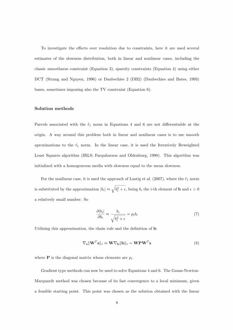
To investigate the effects over resolution due to constraints, here it are used several
estimates of the slowness distribution, both in linear and nonlinear cases, including the
classic smoothness constraint (Equation 3), sparsity constraints (Equation 4) using either
DCT (Strang and Nguyen, 1996) or Daubechies 2 (DB2) (Daubechies and Bates, 1993)
bases, sometimes imposing also the TV constraint (Equation 6).
Solution methods
Parcels associated with the `1 norm in Equations 4 and 6 are not differentiable at the
origin. A way around this problem both in linear and nonlinear cases is to use smooth
aproximations to the `1 norm. In the linear case, it is used the Iteratively Reweighted
Least Squares algorithm (IRLS; Farquharson and Oldenburg, 1998). This algorithm was
initialized with a homogeneous media with slowness equal to the mean slowness.
For the nonlinear case, it is used the approach of Lustig et al. (2007), where the `1 norm
is substituted by the approximation |bi| ≈√b2i + ε, being bi the i-th element of b and ε > 0
a relatively small number. So
∂|bi|∂bi≈ bi√
b2i + ε= pibi (7)
Utilizing this approximation, the chain rule and the definition of b:
∇s‖WT s‖1 ≈W∇b‖b‖1 = WPWT s (8)
where P is the diagonal matrix whose elements are pi.
Gradient type methods can now be used to solve Equations 4 and 6. The Gauss-Newton-
Marquardt method was chosen because of its fast convergence to a local minimum, given
a feasible starting point. This point was chosen as the solution obtained with the linear
8
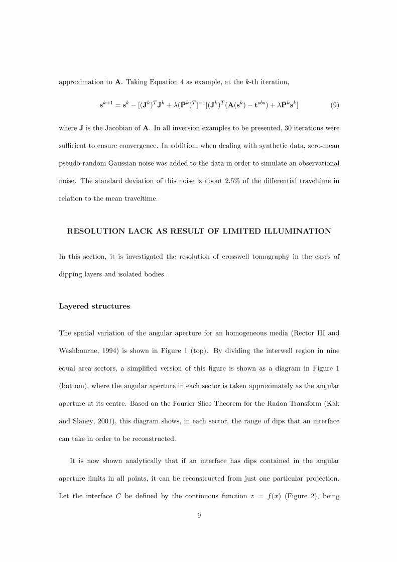
approximation to A. Taking Equation 4 as example, at the k-th iteration,
sk+1 = sk − [(Jk)TJk + λ(Pk)T ]−1[(Jk)T (A(sk)− tobs) + λPksk] (9)
where J is the Jacobian of A. In all inversion examples to be presented, 30 iterations were
sufficient to ensure convergence. In addition, when dealing with synthetic data, zero-mean
pseudo-random Gaussian noise was added to the data in order to simulate an observational
noise. The standard deviation of this noise is about 2.5% of the differential traveltime in
relation to the mean traveltime.
RESOLUTION LACK AS RESULT OF LIMITED ILLUMINATION
In this section, it is investigated the resolution of crosswell tomography in the cases of
dipping layers and isolated bodies.
Layered structures
The spatial variation of the angular aperture for an homogeneous media (Rector III and
Washbourne, 1994) is shown in Figure 1 (top). By dividing the interwell region in nine
equal area sectors, a simplified version of this figure is shown as a diagram in Figure 1
(bottom), where the angular aperture in each sector is taken approximately as the angular
aperture at its centre. Based on the Fourier Slice Theorem for the Radon Transform (Kak
and Slaney, 2001), this diagram shows, in each sector, the range of dips that an interface
can take in order to be reconstructed.
It is now shown analytically that if an interface has dips contained in the angular
aperture limits in all points, it can be reconstructed from just one particular projection.
Let the interface C be defined by the continuous function z = f(x) (Figure 2), being
9
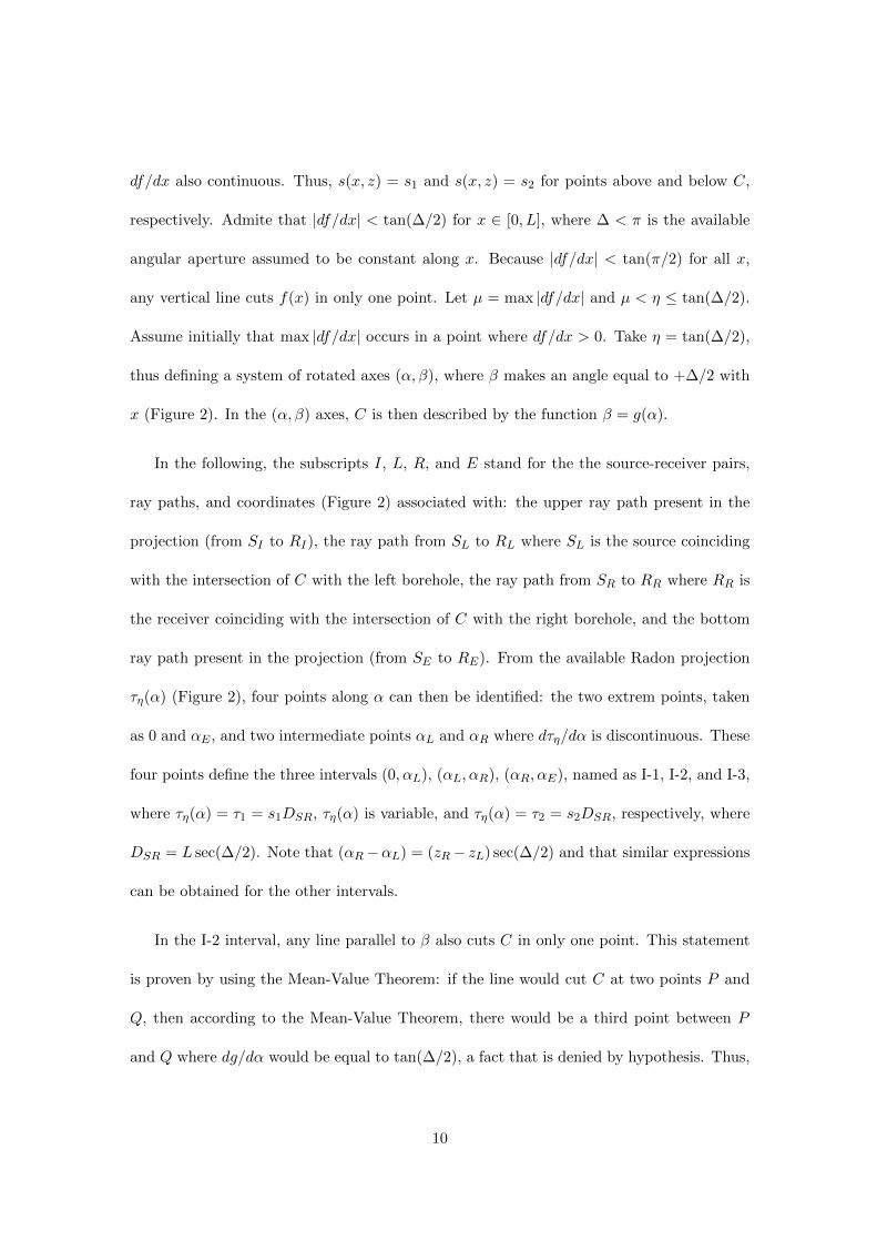
df/dx also continuous. Thus, s(x, z) = s1 and s(x, z) = s2 for points above and below C,
respectively. Admite that |df/dx| < tan(∆/2) for x ∈ [0, L], where ∆ < π is the available
angular aperture assumed to be constant along x. Because |df/dx| < tan(π/2) for all x,
any vertical line cuts f(x) in only one point. Let µ = max |df/dx| and µ < η ≤ tan(∆/2).
Assume initially that max |df/dx| occurs in a point where df/dx > 0. Take η = tan(∆/2),
thus defining a system of rotated axes (α, β), where β makes an angle equal to +∆/2 with
x (Figure 2). In the (α, β) axes, C is then described by the function β = g(α).
In the following, the subscripts I, L, R, and E stand for the the source-receiver pairs,
ray paths, and coordinates (Figure 2) associated with: the upper ray path present in the
projection (from SI to RI), the ray path from SL to RL where SL is the source coinciding
with the intersection of C with the left borehole, the ray path from SR to RR where RR is
the receiver coinciding with the intersection of C with the right borehole, and the bottom
ray path present in the projection (from SE to RE). From the available Radon projection
τη(α) (Figure 2), four points along α can then be identified: the two extrem points, taken
as 0 and αE , and two intermediate points αL and αR where dτη/dα is discontinuous. These
four points define the three intervals (0, αL), (αL, αR), (αR, αE), named as I-1, I-2, and I-3,
where τη(α) = τ1 = s1DSR, τη(α) is variable, and τη(α) = τ2 = s2DSR, respectively, where
DSR = L sec(∆/2). Note that (αR−αL) = (zR− zL) sec(∆/2) and that similar expressions
can be obtained for the other intervals.
In the I-2 interval, any line parallel to β also cuts C in only one point. This statement
is proven by using the Mean-Value Theorem: if the line would cut C at two points P and
Q, then according to the Mean-Value Theorem, there would be a third point between P
and Q where dg/dα would be equal to tan(∆/2), a fact that is denied by hypothesis. Thus,
10
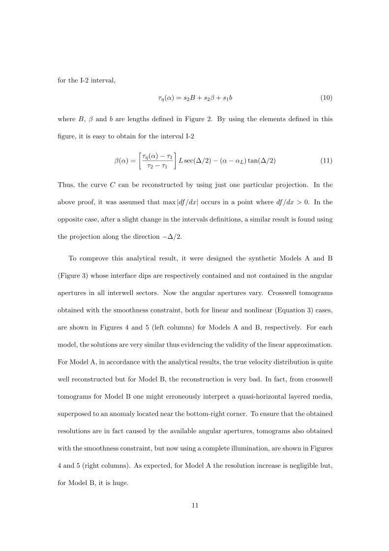
for the I-2 interval,
τη(α) = s2B + s2β + s1b (10)
where B, β and b are lengths defined in Figure 2. By using the elements defined in this
figure, it is easy to obtain for the interval I-2
β(α) =
[τη(α)− τ1τ2 − τ1
]L sec(∆/2)− (α− αL) tan(∆/2) (11)
Thus, the curve C can be reconstructed by using just one particular projection. In the
above proof, it was assumed that max |df/dx| occurs in a point where df/dx > 0. In the
opposite case, after a slight change in the intervals definitions, a similar result is found using
the projection along the direction −∆/2.
To comprove this analytical result, it were designed the synthetic Models A and B
(Figure 3) whose interface dips are respectively contained and not contained in the angular
apertures in all interwell sectors. Now the angular apertures vary. Crosswell tomograms
obtained with the smoothness constraint, both for linear and nonlinear (Equation 3) cases,
are shown in Figures 4 and 5 (left columns) for Models A and B, respectively. For each
model, the solutions are very similar thus evidencing the validity of the linear approximation.
For Model A, in accordance with the analytical results, the true velocity distribution is quite
well reconstructed but for Model B, the reconstruction is very bad. In fact, from crosswell
tomograms for Model B one might erroneously interpret a quasi-horizontal layered media,
superposed to an anomaly located near the bottom-right corner. To ensure that the obtained
resolutions are in fact caused by the available angular apertures, tomograms also obtained
with the smoothness constraint, but now using a complete illumination, are shown in Figures
4 and 5 (right columns). As expected, for Model A the resolution increase is negligible but,
for Model B, it is huge.
11
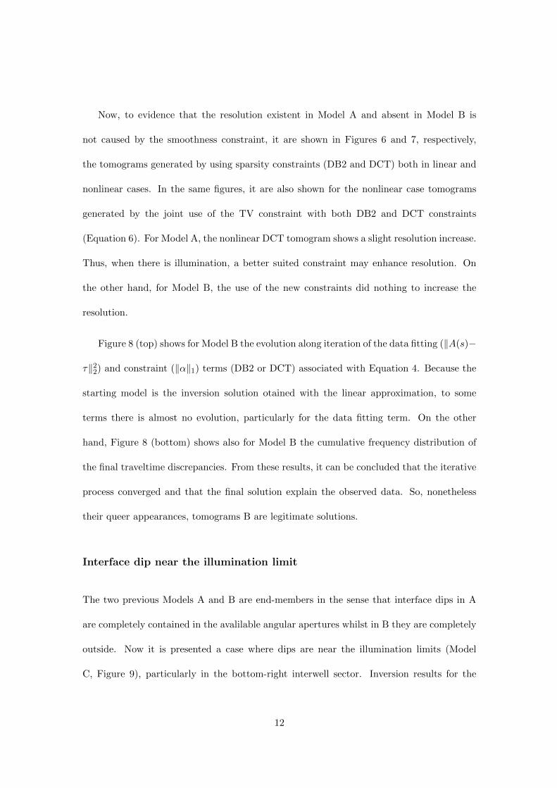
Now, to evidence that the resolution existent in Model A and absent in Model B is
not caused by the smoothness constraint, it are shown in Figures 6 and 7, respectively,
the tomograms generated by using sparsity constraints (DB2 and DCT) both in linear and
nonlinear cases. In the same figures, it are also shown for the nonlinear case tomograms
generated by the joint use of the TV constraint with both DB2 and DCT constraints
(Equation 6). For Model A, the nonlinear DCT tomogram shows a slight resolution increase.
Thus, when there is illumination, a better suited constraint may enhance resolution. On
the other hand, for Model B, the use of the new constraints did nothing to increase the
resolution.
Figure 8 (top) shows for Model B the evolution along iteration of the data fitting (‖A(s)−
τ‖22) and constraint (‖α‖1) terms (DB2 or DCT) associated with Equation 4. Because the
starting model is the inversion solution otained with the linear approximation, to some
terms there is almost no evolution, particularly for the data fitting term. On the other
hand, Figure 8 (bottom) shows also for Model B the cumulative frequency distribution of
the final traveltime discrepancies. From these results, it can be concluded that the iterative
process converged and that the final solution explain the observed data. So, nonetheless
their queer appearances, tomograms B are legitimate solutions.
Interface dip near the illumination limit
The two previous Models A and B are end-members in the sense that interface dips in A
are completely contained in the avalilable angular apertures whilst in B they are completely
outside. Now it is presented a case where dips are near the illumination limits (Model
C, Figure 9), particularly in the bottom-right interwell sector. Inversion results for the
12

linear and nonlinear aproximations, in each case using both smoothness and sparsity (DCT)
constraints, are shown in Figure 10. The same Lagrange multipliers used in Models A and
B were used now in Model C. In all tomograms the interface is approximately reconstructed,
being the resolution moderately better with DCT than with smoothness constraint, thus
reapeating the same resolution improvement observed in Model A.
However, in Figure 10 artifacts are present along the vertical boreholes and at top-left
and bottom-right corners (the bottom-right one is more visible because of its color) as
result of illumination lack. To give an independent comprovation of this fact, it is shown in
Figure 11 the best image that would be possible to obtain in Model C using the available
illumination. This image is not obtained with an inversion approach. Instead, it is the
image obtained by filtering the true Model C in the (kx, ky) domain preserving just the
wavenumbers associated with the avaliable angular aperture in each one of the nine equal
area sectors of the interwell region (Figure 1). This filtering procedure is detailed in the
Appendix A. Figure 11 shows similar artifacts although in a very attenuated version as
compared with Figure 10. Thus, if an interface dip is contained in the avaliable angular
aperture but near its limits, the interface is still correctly imaged but striking artifacts
might be also present in the tomogram.
Isolated body
It is investigated now the tomographic reconstruction of an isolated body in three different
sectors of the interwell region (Model D, Figure 12). Figures 13 and 14 show the inver-
sion results for the linear and nonlinear cases, respectively. The same Lagrange multipliers
previously used in Models A, B, and C were used now in all cases of Model D. For com-
13

parison, Figure 13 (top row) also shows the best images that would be possible to obtain
using the available illumination (see Appendix A for details). As expected, the tomograms
do not reconstruct the vertical edges which appear in a diffuse way. Even the horizontal
interfaces might be difficult to locate precisely from the tomograms, particularly in Case II.
In agreement with the available angular apertures (Figure 1), the best results are obtained
when the body is located in the central sector of the interwell region. Observe also that
when the body is in the upper-left sector, its effect is more pronounced than when it is
in the upper-middle sector, although the boundaries are poorly resolved. In summary, the
effects of an isolated body are present in the tomogram, although their vertical edges can
not be reconstructed. In addition, inversion solutions using either DCT or DB2 (not shown)
constraint reproduce the same features of the solution obtained with smoothness constraint.
CONSEQUENCIES
It are discussed now the consequencies of the above results for data interpretation and
survey design.
Interpreting interfaces and isolated bodies
It can be concluded that if the interface dip is contained inside the angular aperture limits,
it is correctly imaged in the tomogram (Model A). Unfortunately, the inverse is not true,
that is, if an interface is interpretable from a tomogram, even an aproximately horizontal
interface (Model B), there is no guarantee that it corresponds to a true interface. In
addition, interfaces can be only partially imaged, as the horizontal interfaces in Model D,
or be imaged with additional artifacts, as in Model C.
14
If an anomalous body is positioned inside the interwell region, its effects are present
in the tomogram (Model D, all cases), nonetheless artifacts might also be present and the
body’s interfaces might not be imaged, specially in the vertical. Even in the horizontal,
they might be uncorrectly posicioned from the tomogram interpretation (Model D, Case
II). Of course, the effects in the tomogram depend on the body volume and velocity contrast.
Again, the inverse is not true, that is, if a local anomaly is identified in a tomogram, there
is no guarantee that it corresponds to a true body because the anomaly can be alternatively
an artifact generated by an interface with dip near its illumination limits (Model C).
The above results states the dilemma of ill-posed inverse problems. In the inverse sense,
there is no guarantee of correspondence to the true distribution. Thus, interpreting crosswell
tomograms is a task intrinsically different from interpreting complete illumination tomo-
grams because there is no guarantee of correspondence to the true distribution, even if the
interpreter confines himself/herself to interpret features that would have been hypotheti-
cally illuminated. Thus, interpretation must be done taking in consideration always both
the limitations due to illumination and the available (or expected) geologic information. In
fact, the interpreter usually interprets acceptable or expected features, even if he/she is not
aware of this fact.
Designing surveys
Although crosswell survey design takes into account many technical aspects, including eco-
nomic ones, when planning a experiment one must try to maximize illumination. Suppose
that some previous information is available, including layers dip and approximate dimen-
sions of the anomalous bodies, as shown schematically in Figure 15. The following strategy
15

might be tried: (i) the vertical wells might be chosen trying to maximize the ratio between
interwell distance (X) and along-well depth (Z), and also trying to locate the anomalous
bodies around the interwell region center; (ii) sources and receivers might be positioned so
that the line joining the source and receiver centres have dip equal to the layers dip and pass
around the interwell region center; (iii) the interval between sources might not be equal to
the interval between the receivers in order to obtain higher angular apertures and ray-paths
delimitating the body edges, and (iv) a trade off must be done in order to maximize angular
apertures and minimize angular discretization.
Note that this strategy fairly well reproduces the results obtained by Ajo-Franklin (2009)
that formulated the survey design as an optimization problem. Certainly the most difficulty
stage is to perform the trade off between maximizing angular apertures and minimizing
angular discretization.
APPLICATION TO REAL DATA
The ideas developed along this manuscript are now applied to the real data set available
in the net as a tutorial test for the software Rayfract (Rayfract, 2014). These crosswell
traveltime data result from a survey performed by the IGT (International Geophysical
Technology) in an area of the Madrid-Barajas airport aiming to localize old galleries. The
same data were utilized by Gholami and Siahkoohi (2010) for an inversion using joint spar-
sity constraints and by Gokturkler (2009) for an inversion using the smoothness constraint
(1st order partial derivatives). Here, it is used the same discretization adopted by Gholami
and Siahkoohi (2010) (128 × 64).
The available angular apertures (homogeneous media approximation, Rector III and
16

Washbourne (1994)) are shown in Figure 16 (left column). As consequence of a lower X/Z
ratio, as compared with the design used in synthetic data (Figure 1), the angular aperture is
30% higher in the interwell central region. Tomograms obtained with smoothness (Equation
3) and DCT (Equation 4) constraints are also shown in Figure 16 (central and right columns,
respectively). The imaged features are similar to the ones obtained by both Gholami and
Siahkoohi (2010) and Gokturkler (2009). The estimated background velocity (1.8 m/ms -
2.0 m/ms) is consistent with the expected velocity for satured unconsolidated sandy-clay
materials (Prasad et al., 2004), which can also be attributed to possibly existent satured
landfill material. Contrasting to this background, there are both negative (lower than 1.7
m/ms) and positive (higher than 2.1 m/ms) anomaly regions.
Gholami and Siahkoohi (2010) highlighted the negative anomaly, with velocity around
1.5 m/ms, located in the interval depth 25 m - 28 m, interpreting it as water. This is a
plausible interpretation given that the anomaly has shape compatible with a gallery and
velocity value also compatible with an expected infilling of this gallery (water). The fact that
this anomaly is positioned near the interwell central region, where the angular aperture is
good, contributes to assign a relatively high confidence degree to this interpretation. Based
on the expected rectangular shape for a gallery, one can even try to locate both their
horizontal and vertical edges, and to interpret the positive anomaly above it as a thick
horizontal cap, maybe a human construction. However, more caution should be taken when
interpreting the positive anomalies localized in the top, bottom, and upper-right vertical
boundaries. In the context, they possibly represent isolated blocks of rock or even pieces
of human constructions. Nonetheless, it is difficult to interpret their shapes because of the
low illumination.
It is possible to design a special combination of sparsity constraints, as done by Gho-
17
lami and Siahkoohi (2010) to this context, in order to obtain vertical edges to all velocity
anomalies. Given the context, this is a valid bias. However, this sharp edge reconstructions,
particularly for the positive anomalies located near the tomogram borders, is due more to
the constraint bias than the geophysical data. So, the confidence degree attributed to these
mapped edges should be the same one attributed to the constraints.
CONCLUSIONS
This study presented a geometric approach based on the joint use of the angular aperture
distribution inside the interwell region and of the Radon Transform properties allowing to
understand the basic limitations of the crosswell traveltime tomography, nonetheless both
elements are just approximations. The key limitation of crosswell tomography is illumi-
nation, a well known result but not as well stressed or exemplified. Because illumination
is always incomplete, estimating the interwell velocity distribution from its tomogram is
an ill-posed problem because even uniqueness is guaranteed. In this sense, interpreting
crosswell tomograms is intrinsically different from interpreting tomograms resulting from
complete illumination experiments. Taking an extrem case as the key example, even if the
interpreted interface from a tomogram is approximately horizontal, there is no guarantee
that it corresponds to a true interface that would be completely contained in the illumina-
tion limits. Thus, interpretation must be done taking in consideration both the available
illumination and geologic information. Simple guides to survey design were also derived
from the approach.
The intrisic limitations due to illumination might not be solved by the use of mathe-
matical constraints. Crosswell tomograms derived by the use of sparsity constraints, for
example, even when conjugated with total variation constraint, might basically reproduce
18
the same features seen in tomograms obtained with the classic smoothness constraint. It
is true that special combinations of sparsity constraints might produce tomograms show-
ing sharp edges, even sharp vertical boundaries. However, these imaged interfaces result
primarily from the bias intrinsically associated to the constraints.
ACKNOWLEDGMENTS
CNPq is thanked for the MSc fellowship for RRSD, the research fellowship and associated
grant (Proc. 304301/2011-6) for WEM, and financial support by the INCT-GP. The Pod-
vin’s algorithm and the data of the Madrid-Barajas experiment were downloaded from the
net. Numerical results and figures were mainly produced using the Matlab software. Jesse
Costa is thanked for giving us a Fortran code for crosswell traveltime inversion.
19
APPENDIX A
FILTERING ACCORDINGLY TO THE ILLUMINATION LIMITS
Let s(kx, kz) = F{s(x, z)} be the Fourier Transform of s(x, z) which is a true distribution
of slowness. In addition, let ajmin and ajmax be the limiting angles in the (kx, kz) domain
associated with the avaliable angular aperture interval over the j−th sector representing
each one of the nine equal area sectors defined in the interwell region (Figure 1). So, it is
possible to filter s(kx, kz) to obtain sjF (kx, kz) that preserves just the information allowed
by the j-th angular aperture limits, that is
sjF (kx, kz) = s(kx, kz)Hj(kx, kz) (A-1)
where Hj(kx, kz) is the unit box-function defined over the angular sector associated with
the interval [ajmin, ajmax] and its angular supplement. Then, it is possible to obtain
sB(x, z) =9∑
j=1
F−1{sjF (kx, kz)}Bj(x, z) (A-2)
where Bj(x, z) is the unit box-function defined over the j−th rectangular sector. Under the
validity of the straight-ray assumption, sB(x, z) is the best image that would be possible to
obtain from a crosswell traveltime tomography because it is the true model filtered according
to the illumination limits.
20

REFERENCES
Ajo-Franklin, J. B., 2009, Optimal experiment design for time-lapse traveltime tomography:
Geophysics, 74, Q27–Q40.
Ajo-Franklin, J. B., B. J. Minsley, and T. M. Daley, 2007, Applying compactness constraints
to differential traveltime tomography: Geophysics, 72, R67–R75.
Backus, G., and F. Gilbert, 1970, Uniqueness in the inversion of inaccurate gross earth data:
Philosophical Transactions of the Royal Society of London A: Mathematical, Physical and
Engineering Sciences, 266, 123–192.
Bjarnason, I. T., and W. Menke, 1993, Application of the pocs inversion method to cross-
borehole imaging: Geophysics, 58, 941–948.
Bregman, N., R. Bailey, and C. Chapman, 1989, Crosshole seismic tomography: Geophysics,
54, 200–215.
Byun, J., J. Yu, and S. J. Seol, 2010, Crosswell monitoring using virtual sources and hori-
zontal wells: Geophysics, 75, SA37–SA43.
Candes, E. J., J. Romberg, and T. Tao, 2006, Robust uncertainty principles: Exact sig-
nal reconstruction from highly incomplete frequency information: IEEE Transactions on
Information Theory, 52, 489–509.
Cerveny, V., 2005, Seismic ray theory: Cambridge University Press.
Charlety, J., S. Voronin, G. Nolet, I. Loris, F. J. Simons, K. Sigloch, and I. C. Daubechies,
2013, Global seismic tomography with sparsity constraints: Comparison with smoothing
and damping regularization: Journal of Geophysical Research: Solid Earth, 118, 4887–
4899.
Constable, S. C., R. L. Parker, and C. G. Constable, 1987, Occam’s inversion: A practical
algorithm for generating smooth models from electromagnetic sounding data: Geophysics,
21
52, 289–300.
Daubechies, I., and B. J. Bates, 1993, Ten lectures on wavelets: The Journal of the Acous-
tical Society of America, 93, 1671–1671.
Day-Lewis, F., and J. Lane, 2004, Assessing the resolution-dependent utility of tomograms
for geostatistics: Geophysical Research Letters, 31, no. 7, L07503, March 18, 2015;
http://dx.doi.org/10.1029/2004GL019617.
de Santana, F. L., A. F. do Nascimento, and W. E. Medeiros, 2008, History match of a
real-scale petroleum reservoir model using smoothness constraint: Inverse Problems in
Science and Engineering, 16, 483–498.
Dines, K. A., and R. J. Lytle, 1979, Computerized geophysical tomography: Proceedings of
the IEEE, 67, no. 7, 1065–1073.
Donoho, D. L., 2006, Compressed sensing: IEEE Transactions on Information Theory, 52,
1289–1306.
Farquharson, C. G., and D. W. Oldenburg, 1998, Non-linear inversion using general mea-
sures of data misfit and model structure: Geophysical Journal International, 134, 213–
227.
Gholami, A., and H. Siahkoohi, 2010, Regularization of linear and non-linear geophysical ill-
posed problems with joint sparsity constraints: Geophysical Journal International, 180,
871–882.
Gokturkler, G., 2009, Seismic first-arrival tomography with functional description of trav-
eltimes: Journal of Geophysics and Engineering, 6, 374–385.
Goudswaard, J. C., F. P. Ten Kroode, R. K. Snieder, and A. R. Verdel, 1998, Detection of
lateral velocity contrasts by crosswell traveltime tomography: Geophysics, 63, 523–533.
Guillen, A., and V. Menichetti, 1984, Gravity and magnetic inversion with minimization of
22
a specific functional: Geophysics, 49, 1354–1360.
Harris, J. M., R. C. Nolen-Hoeksema, R. T. Langan, M. Van Schaack, S. K. Lazaratos,
and J. W. Rector III, 1995, High-resolution crosswell imaging of a west texas carbonate
reservoir: Part 1-project summary and interpretation: Geophysics, 60, 667–681.
Jafarpour, B., V. K. Goyal, D. B. McLaughlin, and W. T. Freeman, 2009, Transform-domain
sparsity regularization for inverse problems in geosciences: Geophysics, 74, R69–R83.
Kak, A. C., and M. Slaney, 2001, Principles of computerized tomographic imaging: Society
for Industrial and Applied Mathematics.
Last, B., and K. Kubik, 1983, Compact gravity inversion: Geophysics, 48, 713–721.
Lo, T.-w., and P. L. Inderwiesen, 1994, Fundamentals of seismic tomography: SEG Books,
volume 6 of Geophysical Monograph Series.
Loris, I., G. Nolet, I. Daubechies, and F. Dahlen, 2007, Tomographic inversion using l1-norm
regularization of wavelet coefficients: Geophysical Journal International, 170, 359–370.
Lustig, M., D. Donoho, and J. M. Pauly, 2007, Sparse MRI: The application of compressed
sensing for rapid MR imaging: Magnetic Resonance in Medicine, 58, 1182–1195.
Mallat, S., 2008, A wavelet tour of signal processing: the sparse way: Academic press.
Menke, W., 1984, The resolving power of cross-borehole tomography: Geophysical Research
Letters, 11, 105–108.
——–, 2012, Geophysical data analysis: discrete inverse theory: Academic press.
Moser, T., 1991, Shortest path calculation of seismic rays: Geophysics, 56, 59–67.
Nolet, G., 1987, Seismic tomography: with applications in global seismology and exploration
geophysics: Springer Science & Business Media, 5.
Plessix, R.-E., 2006, Estimation of velocity and attenuation coefficient maps from crosswell
seismic data: Geophysics, 71, S235–S240.
23
Podvin, P., and I. Lecomte, 1991, Finite difference computation of traveltimes in very
contrasted velocity models: a massively parallel approach and its associated tools: Geo-
physical Journal International, 105, 271–284.
Portniaguine, O., and M. S. Zhdanov, 1999, Focusing geophysical inversion images: Geo-
physics, 64, 874–887.
Prasad, M., M. Zimmer, P. Berge, and B. Bonner, 2004, Laboratory measurements of
velocity and attenuation in sediments: LLNL Rep. UCRL-JRNL, 205155, 34.
Rayfract, 2014, http://rayfract.com/tutorials/igta13.pdf, accessed 2014-07-07.
Rector III, J. W., and J. K. Washbourne, 1994, Characterization of resolution and unique-
ness in crosswell direct-arrival traveltime tomography using the fourier projection slice
theorem: Geophysics, 59, 1642–1649.
Rudin, L. I., S. Osher, and E. Fatemi, 1992, Nonlinear total variation based noise removal
algorithms: Physica D: Nonlinear Phenomena, 60, 259–268.
Silva, J. B., W. E. Medeiros, and V. C. Barbosa, 2000, Gravity inversion using convexity
constraint: Geophysics, 65, 102–112.
Simons, F. J., I. Loris, G. Nolet, I. C. Daubechies, S. Voronin, J. Judd, P. A. Vetter, J.
Charlety, and C. Vonesch, 2011, Solving or resolving global tomographic models with
spherical wavelets, and the scale and sparsity of seismic heterogeneity: Geophysical Jour-
nal International, 187, 969–988.
Strang, G., and T. Nguyen, 1996, Wavelets and filter banks: SIAM.
Tikhonov, A. N., and V. Y. Arsenin, 1977, Solutions of ill-posed problems: Winston.
Vidale, J., 1988, Finite-difference calculation of travel times: Bulletin of the Seismological
Society of America, 78, 2062–2076.
Vidale, J. E., 1990, Finite-difference calculation of traveltimes in three dimensions: Geo-
24
physics, 55, 521–526.
Virieux, J., and S. Operto, 2009, An overview of full-waveform inversion in exploration
geophysics: Geophysics, 74, WCC1–WCC26.
Wang, Y., and Y. Rao, 2006, Crosshole seismic waveform tomography–I. Strategy for real
data application: Geophysical Journal International, 166, 1224–1236.
Youzwishen, C., and M. Sacchi, 2006, Edge preserving imaging: Journal of Seismic Explo-
ration, 15, 45.
25
LIST OF FIGURES
Figure 1. Angular aperture as function of position in a homogeneous media between
two vertical boreholes (top) and its simplified version (bottom), where the angular aperture
in each sector is taken as the value at its centre, and the angles are in true scale. Sources and
receivers are shown in left and right boreholes, respectively. There are 64 equally spaced
sources (or receivers). The interwell region was discretized with 64 x 64 equal area elements.
Unless stated, this survey design and discretization are used for all inversion examples.
Figure 2. Schematic drawing illustrating the geometry used to prove analytically the
statement that an interface C can be reconstructed if, in each point (x, z), its dip is con-
tained in the angular aperture ∆. The interwell regions is separated in two parcels, above
e below C, where the slowness is equal to s1 and s2, respectively. See text for details.
Figure 3. Models A (top) and B (bottom) with illuminated and non-illuminated inter-
faces, respectively. That is, for Model A, in each interwell sector the interface dip (solid line)
is contained in the respective angular aperture interval (thin lines). The opposite happens
in Model B. Numbers indicate P-wave velocity in m/ms. Source and receiver positions are
shown in Figure 1.
Figure 4. Model A - Tomograms incorporating smoothness constraint for the linear
(top row) and nonlinear (bottom row, Equation 3) inversion cases, using both limited (left
column) and complete illumination (right column). To obtain complete illumination, it
were added (not shown) sources and receivers along the top and bottom horizontal borders,
repectively, using the same intervals between sources and receveirs shown in Figure 1. Thin
black lines show the true interfaces.
Figure 5. Model B - Tomograms incorporating smoothness constraint for the linear
(top row) and nonlinear (bottom row, Equation 3) inversion cases, using both limited (left
26

column) and complete illumination (right column). To obtain complete illumination, it
were added (not shown) sources and receivers along the top and bottom horizontal borders,
repectively, using the same intervals between sources and receveirs shown in Figure 1. Thin
black lines show the true interfaces.
Figure 6. Model A - Limited illumination tomograms incorporating sparsity constraints
for the linear (top row), nonlinear (middle row, Equation 4), and nonlinear plus total vari-
ation (bottom row, Equation 6) cases. Left and right columns show results for Daubechies
2 basis (DB2) and Discrete Cosine Transform (DCT), respectively.
Figure 7. Model B - Limited illumination tomograms incorporating sparsity constraints
for the linear (top row), nonlinear (middle row, Equation 4), and nonlinear plus total vari-
ation (bottom row, Equation 6) cases. Left and right columns show results for DB2 and
DCT constraints, respectively.
Figure 8. Model B - Evolution along iterations of the misfit (‖A(s)− τ‖22) and solution
norm (‖α‖1) terms both for DB2 and DCT nonlinear inversion cases (Equation 4) (top).
All terms were suitably normalized to the same scale. Cumulative frequency distribution
in percentage obtained for the fitting in the nonlinear inversions using DB2, DCT, and
smoothness (Equation 3) constraints (bottom).
Figure 9. Model C - Interface dip (solid line) near the illumination limits (thin lines).
Numbers indicate P-wave velocity in m/ms. Source and receiver positions are shown in
Figure 1.
Figure 10. Model C - Limited illumination tomograms incorporating smoothness (left
column) and DCT (right column) constraints both for the linear (top row) and nonlinear
(bottom row) inversion cases. Thin black lines show the true interface.
Figure 11. Model C - Best image that would be possible to obtain using the available
27
illumination under the validity of the straight-ray assumption. This image is obtained by
filtering the true Model C in the (kx, ky) domain preserving just the wavenumbers associ-
ated with the avaliable angular aperture in each one of the nine equal area sectors of the
interwell region (Figure 1). See Appendix A for details. Thin black line shows the true
interface.
Figure 12. Model D - Isolated body - Cases I, II, and III. In all cases, the body has
P-wave velocity equal to 1.5 m/ms and the background media has P-wave velocity equal
to 1.9 m/ms. Source and receiver positions are shown in Figure 1. Although the cases are
jointly drawn, the inversions are performed with just a body at a time.
Figure 13. Model D - Isolated body - Linear case. Best image (top row, see Appendix
A for details) and limited illumination tomograms incorporating smoothness (middle row)
and DCT (bottom row) constraints. Thin black lines show the true interfaces. Cases I, II,
and III are shown in the left, middle, and right columns, respectively.
Figure 14. Model D - Isolated body - Nonlinear case. Limited illumination tomo-
grams incorporating smoothness (top row) and DCT (bottom row) constraints. Thin black
lines show the true interfaces. Cases I, II, and III are shown in the left, middle, and right
columns, respectively.
Figure 15. Schematic drawing illustrating a near-optimum survey design. X and Z are
the interwell distance and along-well depth, respectively. SC and RC are the array centers
of sources (stars) and receivers (open circles), respectively. See the text for details.
Figure 16. Real data - Madrid-Barajas airport experiment. Angular aperture as func-
tion of position in a homogeneous media (left) and tomograms resulting from nonlinear
inversions using smoothness (middle, Equation 3) and DCT (right, Equation 4) constraints.
28
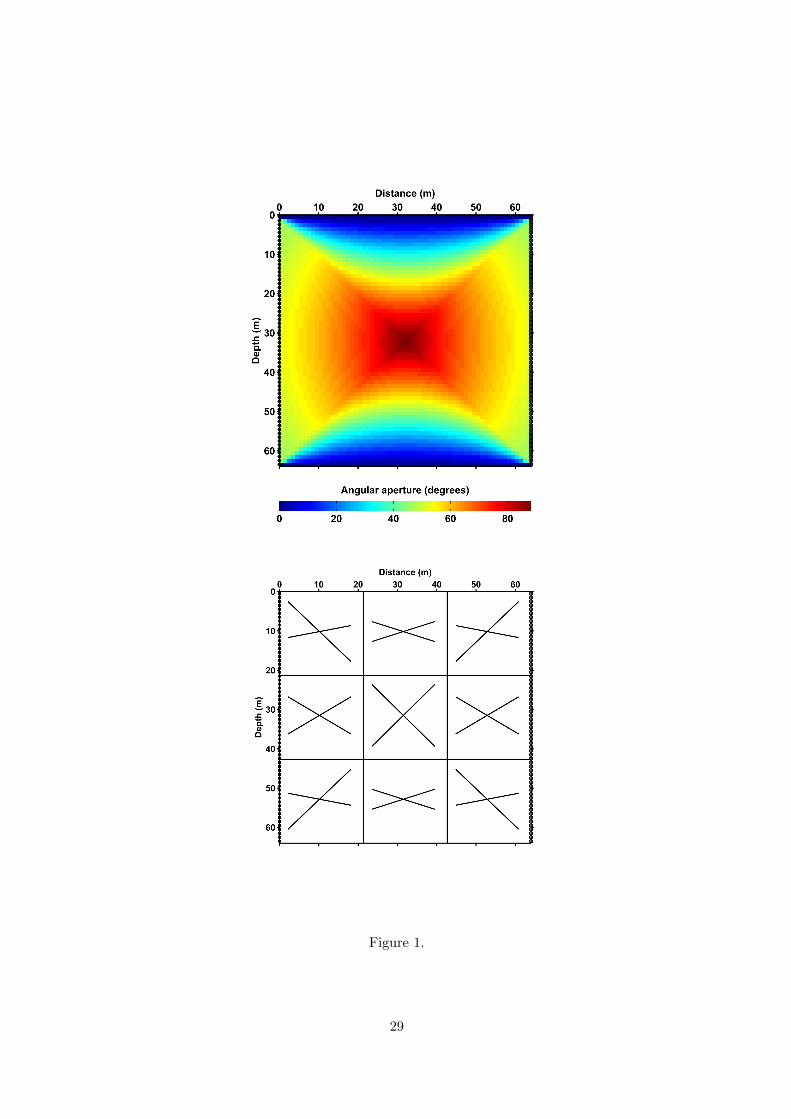
Figure 1.
29
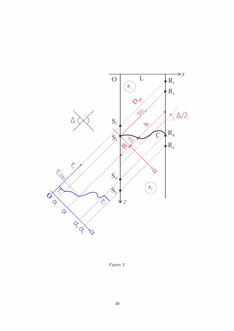
Figure 2.
30
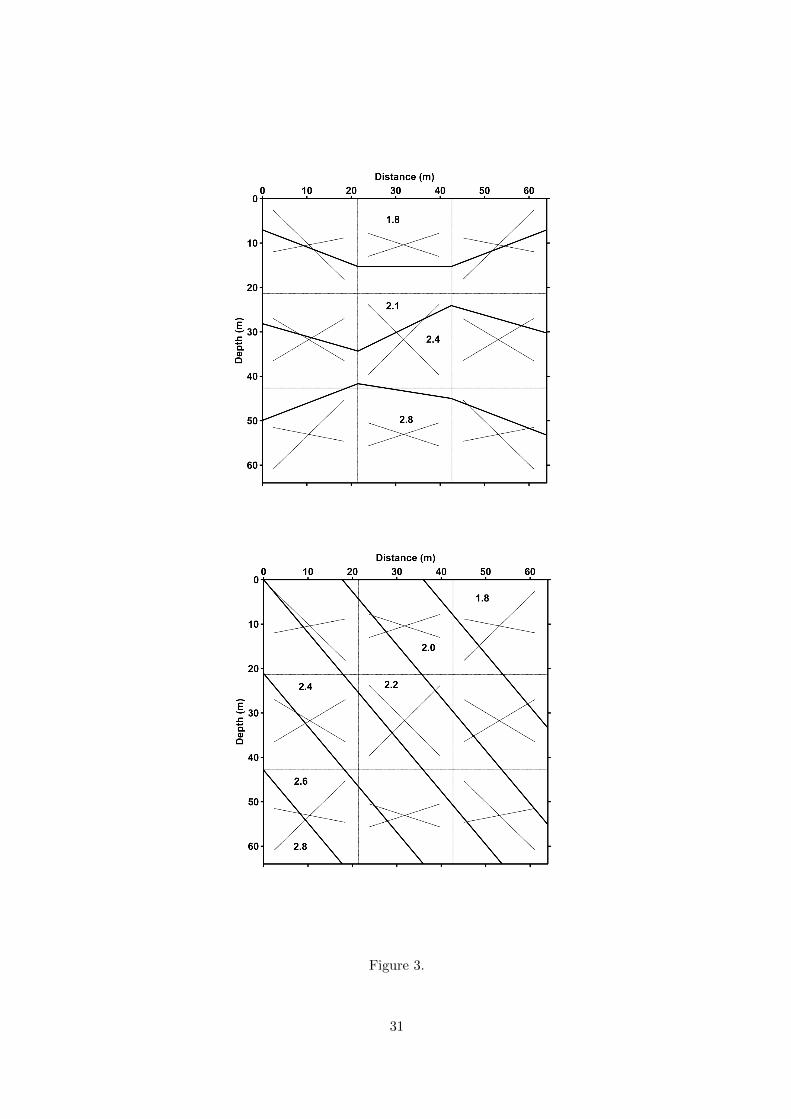
Figure 3.
31
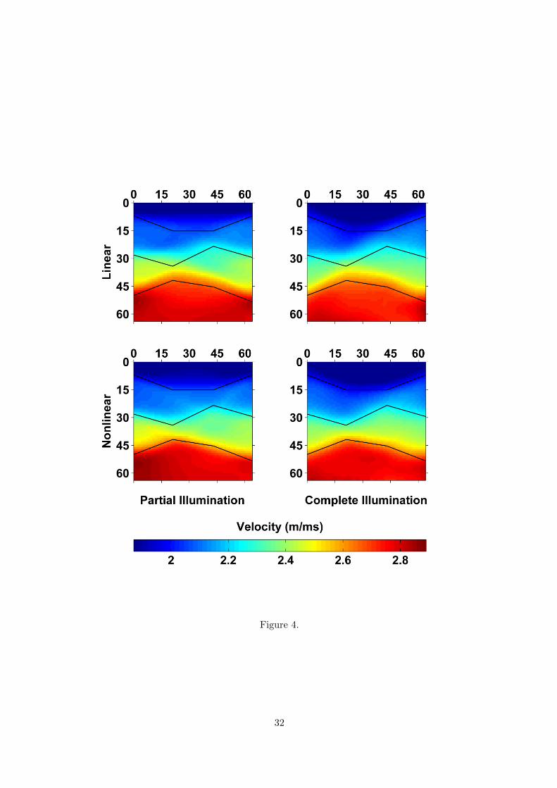
Figure 4.
32
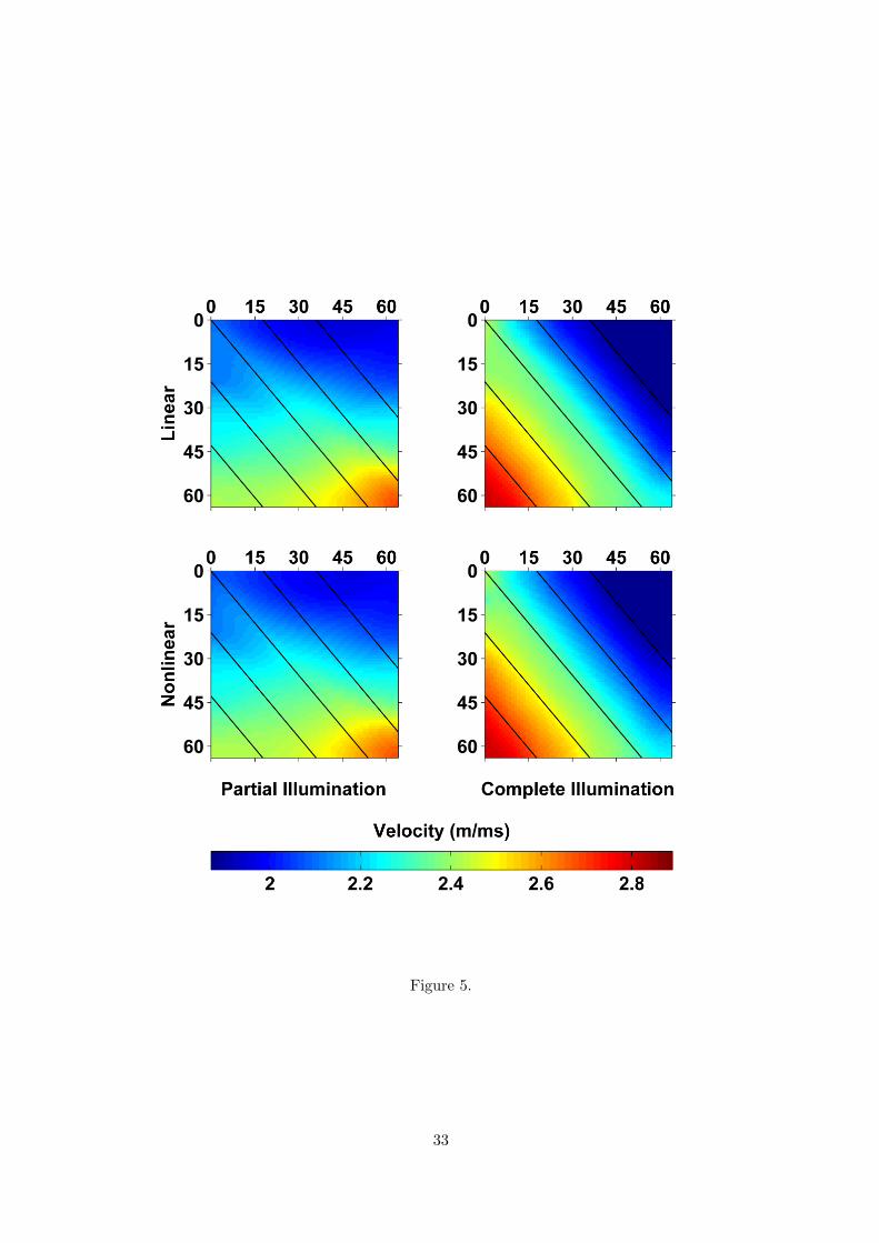
Figure 5.
33

Figure 6.
34
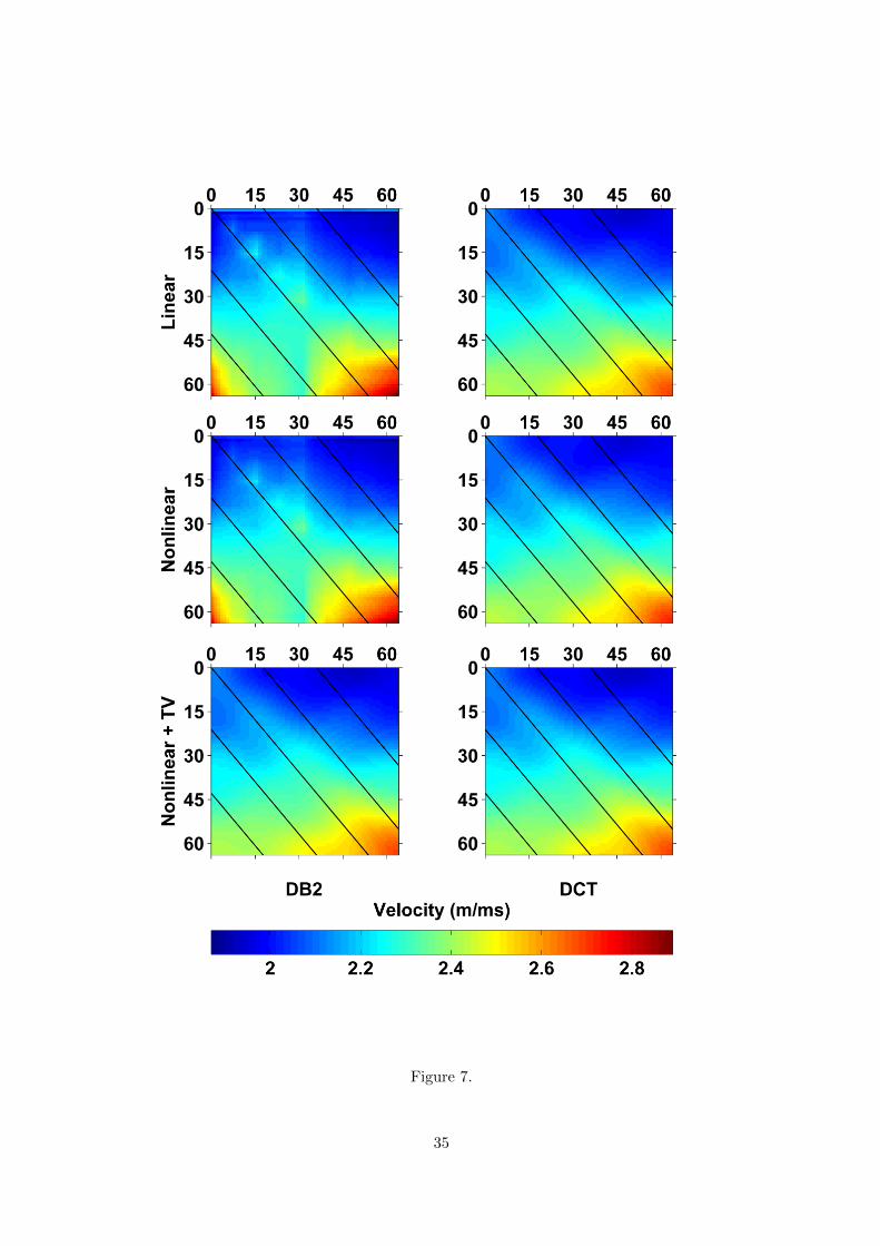
Figure 7.
35
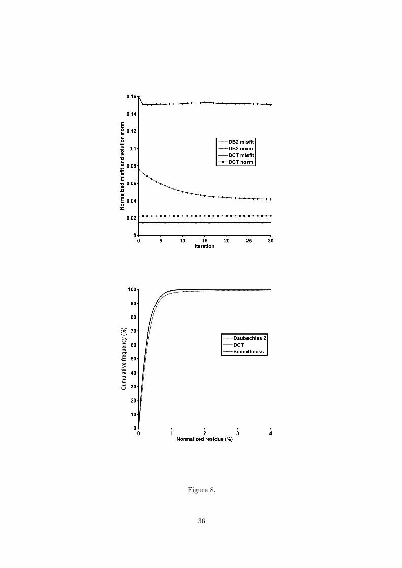
Figure 8.
36
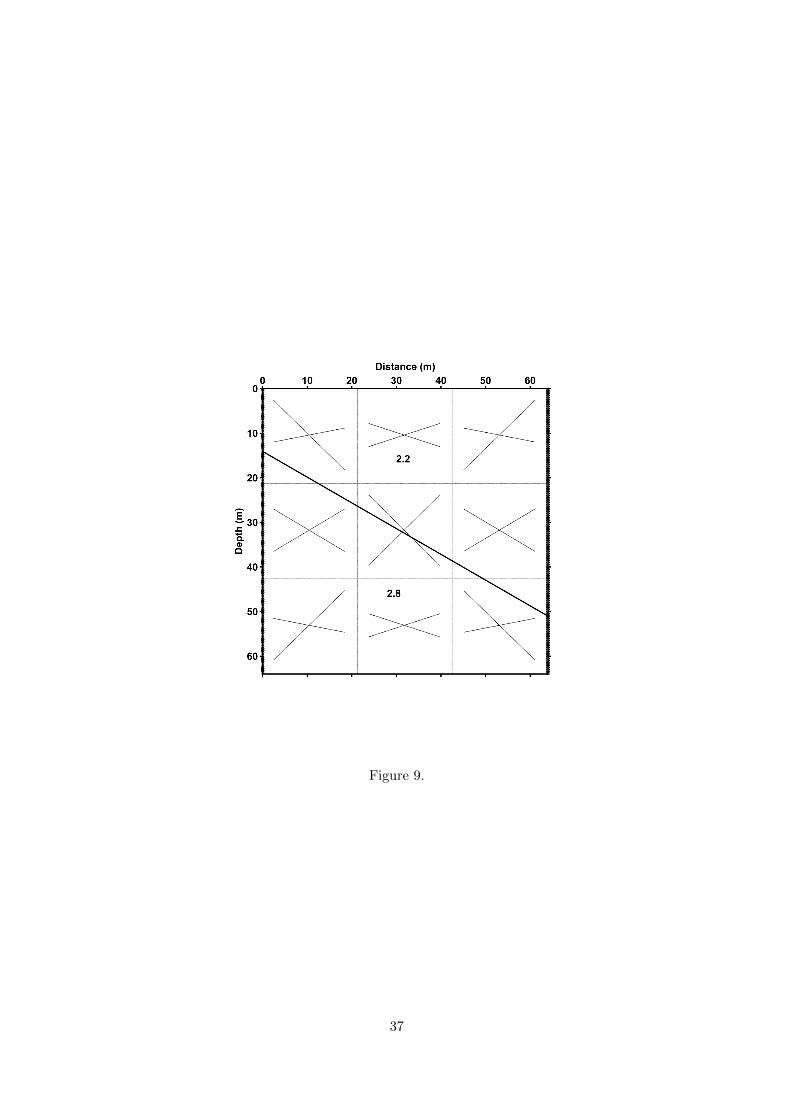
Figure 9.
37

Figure 10.
38
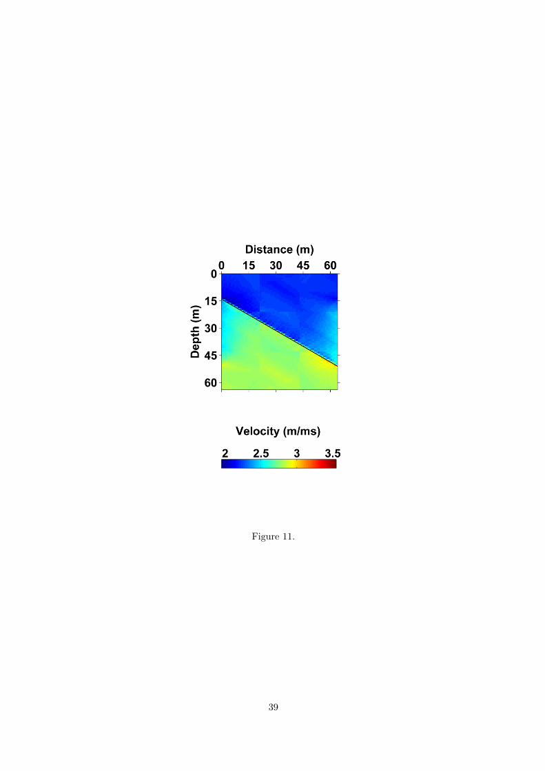
Figure 11.
39
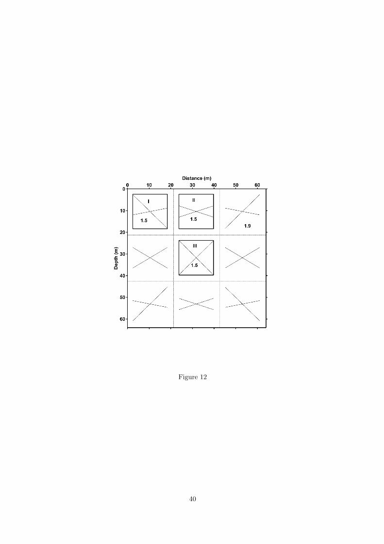
Figure 12
40
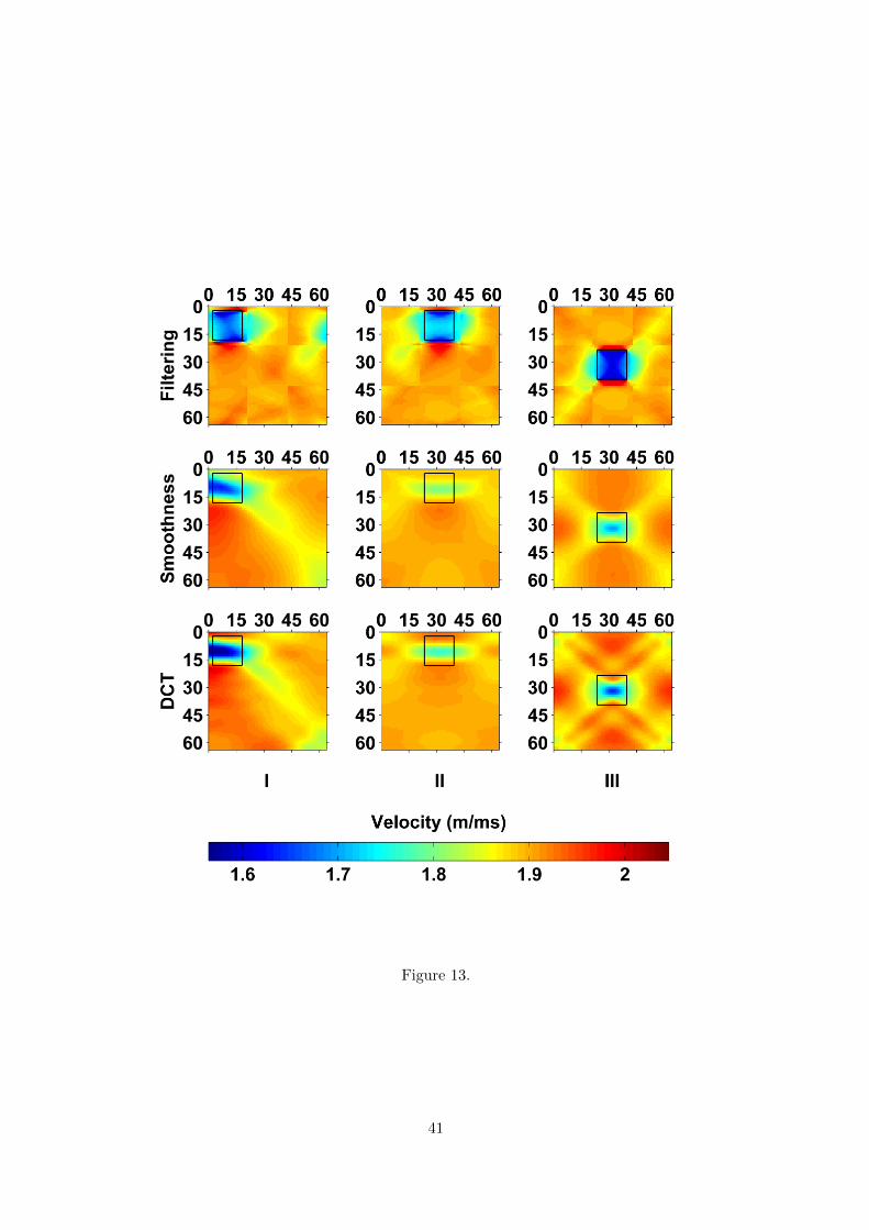
Figure 13.
41
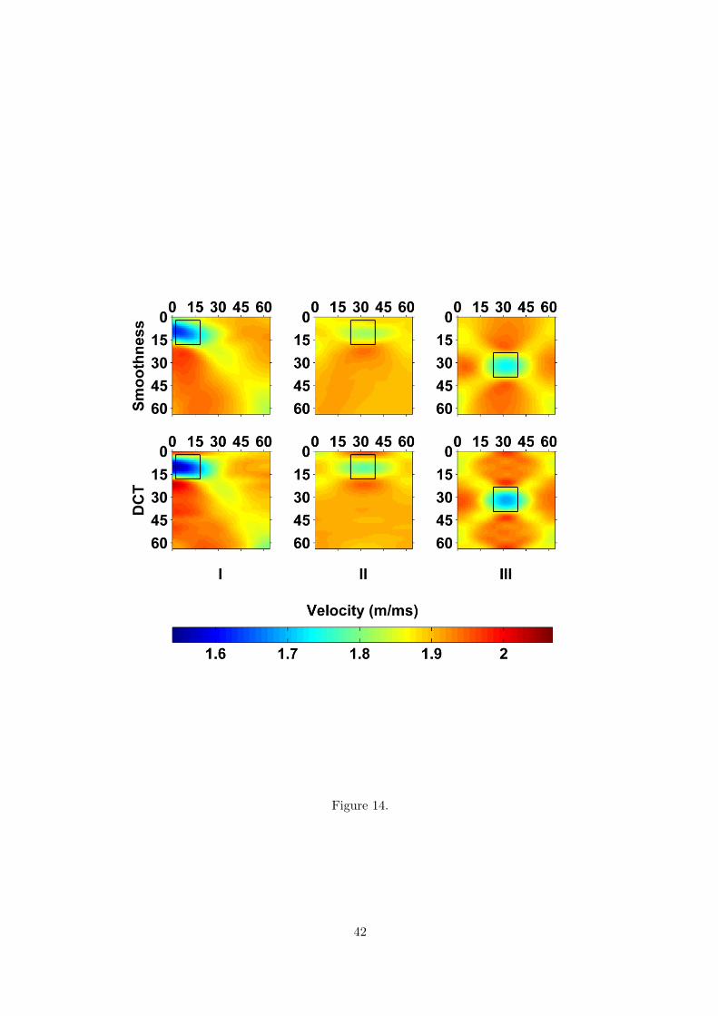
Figure 14.
42
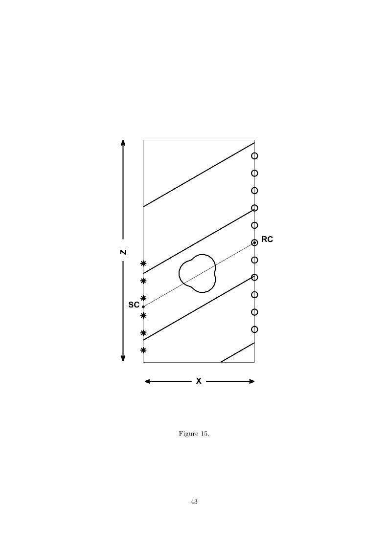
Figure 15.
43
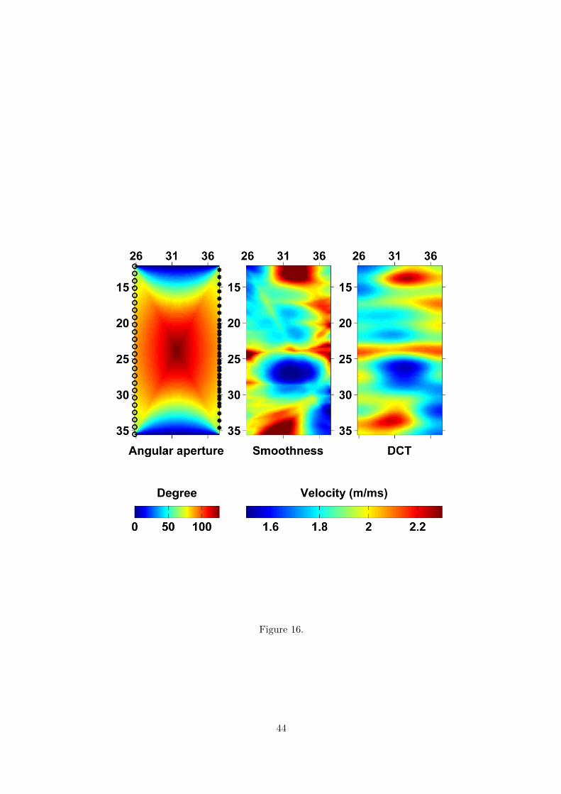
Figure 16.
44
Referências bibliográficas
Ajo-Franklin, J. B., 2009, Optimal experiment design for time-lapse traveltime tomography: Ge-
ophysics, 74, Q27–Q40.
Ajo-Franklin, J. B., B. J. Minsley, and T. M. Daley, 2007, Applying compactness constraints to
differential traveltime tomography: Geophysics, 72, R67–R75.
Backus, G., and F. Gilbert, 1970, Uniqueness in the inversion of inaccurate gross earth data: Phi-
losophical Transactions of the Royal Society of London A: Mathematical, Physical and Engine-
ering Sciences, 266, 123–192.
Bregman, N., R. Bailey, and C. Chapman, 1989, Crosshole seismic tomography: Geophysics, 54,
200–215.
Byun, J., J. Yu, and S. J. Seol, 2010, Crosswell monitoring using virtual sources and horizontal
wells: Geophysics, 75, SA37–SA43.
Candès, E. J., J. Romberg, and T. Tao, 2006, Robust uncertainty principles: Exact signal recons-
truction from highly incomplete frequency information: IEEE Transactions on Information The-
ory, 52, 489–509.
Charléty, J., S. Voronin, G. Nolet, I. Loris, F. J. Simons, K. Sigloch, and I. C. Daubechies, 2013,
Global seismic tomography with sparsity constraints: Comparison with smoothing and damping
regularization: Journal of Geophysical Research: Solid Earth, 118, 4887–4899.
Day-Lewis, F., and J. Lane, 2004, Assessing the resolution-dependent utility of tomograms for
geostatistics: Geophysical Research Letters, 31, no. 7.
de Azevedo, P. A., M. P. Rocha, J. E. P. Soares, and R. A. Fuck, 2015, Thin lithosphere between the
amazonian and são francisco cratons, in central brazil, revealed by seismic p-wave tomography:
Geophysical Journal International, 201, 61–69.
De Iaco, R., A. Green, H.-R. Maurer, and H. Horstmeyer, 2003, A combined seismic reflection
and refraction study of a landfill and its host sediments: Journal of Applied Geophysics, 52,
55
REFERÊNCIAS BIBLIOGRÁFICAS 56
139–156.
Docherty, P., 1992, Solving for the thickness and velocity of the weathering layer using 2-d refrac-
tion tomography: Geophysics, 57, 1307–1318.
Donoho, D. L., 2006, Compressed sensing: IEEE Transactions on Information Theory, 52, 1289–
1306.
Goudswaard, J. C., F. P. Ten Kroode, R. K. Snieder, and A. R. Verdel, 1998, Detection of lateral
velocity contrasts by crosswell traveltime tomography: Geophysics, 63, 523–533.
Gustavsson, M., S. Ivansson, P. Moren, and J. Pihl, 1986, Seismic borehole tomo-
graphy—measurement system and field studies: Proceedings of the IEEE, 74, no. 2, 339–346.
Harris, J. M., R. C. Nolen-Hoeksema, R. T. Langan, M. Van Schaack, S. K. Lazaratos, and J. W.
Rector III, 1995, High-resolution crosswell imaging of a west texas carbonate reservoir: Part
1-project summary and interpretation: Geophysics, 60, 667–681.
Jafarpour, B., V. K. Goyal, D. B. McLaughlin, and W. T. Freeman, 2009, Transform-domain spar-
sity regularization for inverse problems in geosciences: Geophysics, 74, R69–R83.
Kak, A. C., and M. Slaney, 2001, Principles of computerized tomographic imaging: Society for
Industrial and Applied Mathematics.
Lanz, E., H. Maurer, and A. G. Green, 1998, Refraction tomography over a buried waste disposal
site: Geophysics, 63, 1414–1433.
Liu, L., and T. Guo, 2005, Seismic non-destructive testing on a reinforced concrete bridge column
using tomographic imaging techniques: Journal of Geophysics and Engineering, 2, 23.
Lo, T.-w., and P. L. Inderwiesen, 1994, Fundamentals of seismic tomography: SEG Books, vo-
lume 6 of Geophysical Monograph Series.
Loris, I., G. Nolet, I. Daubechies, and F. Dahlen, 2007, Tomographic inversion using l1-norm
regularization of wavelet coefficients: Geophysical Journal International, 170, 359–370.
Lustig, M., D. Donoho, and J. M. Pauly, 2007, Sparse MRI: The application of compressed sensing
for rapid MR imaging: Magnetic Resonance in Medicine, 58, 1182–1195.
Mallat, S., 2008, A wavelet tour of signal processing: the sparse way: Academic press.
Menke, W., 1984, The resolving power of cross-borehole tomography: Geophysical Research
Letters, 11, 105–108.
REFERÊNCIAS BIBLIOGRÁFICAS 57
Metwaly, M., A. G. Green, H. Horstmeyer, H. Maurer, A. M. Abbas, et al., 2005, Combined
seismic tomographic and ultrashallow seismic reflection study of an early dynastic mastaba,
saqqara, egypt: Archaeological Prospection, 12, 245–256.
Moser, T., 1991, Shortest path calculation of seismic rays: Geophysics, 56, 59–67.
Nielsen, L., H. Thybo, and M. Glendrup, 2005, Seismic tomographic interpretation of paleozoic
sedimentary sequences in the southeastern north sea: Geophysics, 70, R45–R56.
Nolet, G., 1987, Seismic tomography: with applications in global seismology and exploration
geophysics: Springer Science & Business Media, 5.
Peterson, J. E., B. N. Paulsson, and T. V. McEvilly, 1985, Applications of algebraic reconstruction
techniques to crosshole seismic data: Geophysics, 50, 1566–1580.
Podvin, P., and I. Lecomte, 1991, Finite difference computation of traveltimes in very contrasted
velocity models: a massively parallel approach and its associated tools: Geophysical Journal
International, 105, 271–284.
Polymenakos, L., and S. Papamarinopoulos, 2005, Exploring a prehistoric site for remains of
human structures by three-dimensional seismic tomography: Archaeological Prospection, 12,
221–233.
Rector III, J. W., and J. K. Washbourne, 1994, Characterization of resolution and uniqueness in
crosswell direct-arrival traveltime tomography using the fourier projection slice theorem: Ge-
ophysics, 59, 1642–1649.
Schön, J. H., 2011, Physical properties of rocks: A workbook: Elsevier, 8.
Simons, F. J., I. Loris, G. Nolet, I. C. Daubechies, S. Voronin, J. Judd, P. A. Vetter, J. Charléty,
and C. Vonesch, 2011, Solving or resolving global tomographic models with spherical wavelets,
and the scale and sparsity of seismic heterogeneity: Geophysical Journal International, 187,
969–988.
Tikhonov, A. N., and V. Y. Arsenin, 1977, Solutions of ill-posed problems: Winston.
Vidale, J., 1988, Finite-difference calculation of travel times: Bulletin of the Seismological Society
of America, 78, 2062–2076.
Vidale, J. E., 1990, Finite-difference calculation of traveltimes in three dimensions: Geophysics,
55, 521–526.
REFERÊNCIAS BIBLIOGRÁFICAS 58
Virieux, J., and S. Operto, 2009, An overview of full-waveform inversion in exploration geophy-
sics: Geophysics, 74, WCC1–WCC26.
White, D., 1989, Two-dimensional seismic refraction tomography: Geophysical Journal Internati-
onal, 97, 223–245.
Zhdanov, M., G. Vignoli, and T. Ueda, 2006, Sharp boundary inversion in crosswell travel-time
tomography: Journal of Geophysics and Engineering, 3, 122.
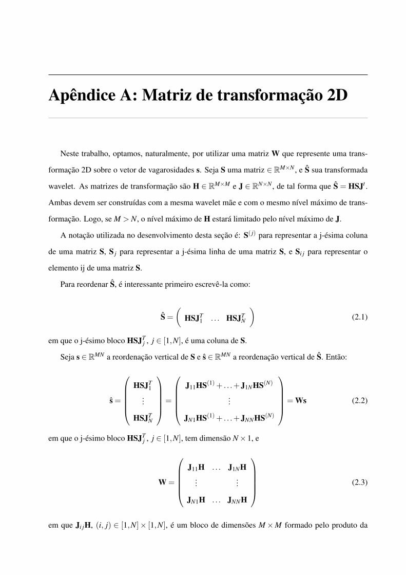
Apêndice A: Matriz de transformação 2D
Neste trabalho, optamos, naturalmente, por utilizar uma matriz W que represente uma trans-
formação 2D sobre o vetor de vagarosidades s. Seja S uma matriz ∈ RM×N , e S sua transformada
wavelet. As matrizes de transformação são H ∈ RM×M e J ∈ RN×N , de tal forma que S = HSJt .
Ambas devem ser construídas com a mesma wavelet mãe e com o mesmo nível máximo de trans-
formação. Logo, se M > N, o nível máximo de H estará limitado pelo nível máximo de J.
A notação utilizada no desenvolvimento desta seção é: S( j) para representar a j-ésima coluna
de uma matriz S, S j para representar a j-ésima linha de uma matriz S, e Si j para representar o
elemento ij de uma matriz S.
Para reordenar S, é interessante primeiro escrevê-la como:
S =
(HSJT
1 . . . HSJTN
)(2.1)
em que o j-ésimo bloco HSJTj , j ∈ [1,N], é uma coluna de S.
Seja s ∈ RMN a reordenação vertical de S e s ∈ RMN a reordenação vertical de S. Então:
s =
HSJT1
...
HSJTN
=
J11HS(1)+ . . .+J1NHS(N)
...
JN1HS(1)+ . . .+JNNHS(N)
= Ws (2.2)
em que o j-ésimo bloco HSJTj , j ∈ [1,N], tem dimensão N×1, e
W =
J11H . . . J1NH...
...
JN1H . . . JNNH
(2.3)
em que Ji jH, (i, j) ∈ [1,N]× [1,N], é um bloco de dimensões M×M formado pelo produto da
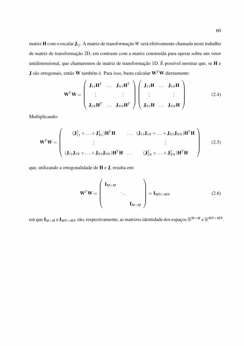
60
matriz H com o escalar Ji j. A matriz de transformação W será efetivamente chamada neste trabalho
de matriz de transformação 2D, em contraste com a matriz construída para operar sobre um vetor
unidimensional, que chamaremos de matriz de transformação 1D. É possível mostrar que, se H e
J são ortogonais, então W também é. Para isso, basta calcular WT W diretamente:
WT W =
J11HT . . . JN1HT
......
J1NHT . . . JNNHT
J11H . . . J1NH...
...
JN1H . . . JNNH
(2.4)
Multiplicando:
WT W =
(J211 + . . .+J2
N1)HT H . . . (J11J1N + . . .+JN1JNN)HT H
......
(J11J1N + . . .+JN1JNN)HT H . . . (J21N + . . .+J2
NN)HT H
(2.5)
que, utilizando a ortogonalidade de H e J, resulta em:
WT W =
IM×M
. . .
IM×M
= IMN×MN (2.6)
em que IM×M e IMN×MN são, respectivamente, as matrizes identidade dos espaços RM×M e RMN×MN .