partialleastsquaresregressiononsymmetric positive

Revista Colombiana de EstadísticaJunio 2013, volumen 36, no. 1, pp. 177 a 192

Partial Least Squares Regression on SymmetricPositive-Definite Matrices

Regresión de mínimos cuadrados parciales sobre matrices simétricasdefinidas positiva

Raúl Alberto Pérez1,a, Graciela González-Farias2,b

1Escuela de Estadística, Facultad de Ciencias, Universidad Nacional de Colombia,Medellín, Colombia

2Departamento de Probabilidad y Estadística, CIMAT-México Unidad Monterrey,Monterrey Nuevo León, México

Resumen

Recently there has been an increased interest in the analysis of differenttypes of manifold-valued data, which include data from symmetric positive-definite matrices. In many studies of medical cerebral image analysis, amajor concern is establishing the association among a set of covariates andthe manifold-valued data, which are considered as responses for characteriz-ing the shapes of certain subcortical structures and the differences betweenthem.

The manifold-valued data do not form a vector space, and thus, it is notadequate to apply classical statistical techniques directly, as certain opera-tions on vector spaces are not defined in a general Riemannian manifold. Inthis article, an application of the partial least squares regression methodol-ogy is performed for a setting with a large number of covariates in a euclideanspace and one or more responses in a curved manifold, called a Riemanniansymmetric space. To apply such a technique, the Riemannian exponentialmap and the Riemannian logarithmic map are used on a set of symmetricpositive-definite matrices, by which the data are transformed into a vectorspace, where classic statistical techniques can be applied. The methodologyis evaluated using a set of simulated data, and the behavior of the techniqueis analyzed with respect to the principal component regression.

Palabras clave: Matrix theory, Multicollinearity, Regression, Riemannmanifold.

aAssistant Professor. E-mail: [email protected] Professor. E-mail: [email protected]

177

178 Raúl Alberto Pérez & Graciela González-Farias

AbstractRecientemente ha habido un aumento en el interés de analizar diferentes

tipos de datos variedad-valuados, dentro de los cuáles aparecen los datos dematrices simétricas definidas positivas. En muchos estudios de análisis deimágenes médicas cerebrales, es de interés principal establecer la asociaciónentre un conjunto de covariables y los datos variedad-valuados que son con-siderados como respuesta, con el fin de caracterizar las diferencias y formasen ciertas estructuras sub-corticales.

Debido a que los datos variedad-valuados no forman un espacio vecto-rial, no es adecuado aplicar directamente las técnicas estadísticas clásicas,ya que ciertas operaciones sobre espacio vectoriales no están definidas enuna variedad riemanniana general. En este artículo se realiza una aplicaciónde la metodología de regresión de mínimos cuadrados parciales, para el en-torno de un número grande de covariables en un espacio euclídeo y una ovarias respuestas que viven una variedad curvada llamada espacio simétricoRiemanniano. Para poder llevar a cabo la aplicación de dicha técnica seutilizan el mapa exponencial Riemanniano y el mapa log Riemanniano so-bre el conjunto de matrices simétricas positivas definida, mediante los cualesse transforman los datos a un espacio vectorial en donde se pueden aplicartécnicas estadísticas clásicas. La metodología es evaluada por medio de unconjunto de datos simulados en donde se analiza el comportamiento de latécnica con respecto a la regresión por componentes principales.

Key words: multicolinealidad, regresión, teoría de matrices, variedadRiemanniana.

1. Introduction

In studies of diffusion tensor magnetic resonance imaging (TD-MRI), a diffusiontensor (DT) is calculated in each voxel of an imaging space, which describes thelocal diffusion of water molecules in various directions over this region of the brain.A sequence of images is used to measure this diffusion. The sequence includes anoise that produces uncertainty in the tensor estimation and in the estimation ofcertain quantities inherent to water molecules, such as eigenvalues, eigenvectors,the anisotropic fraction rate (FA) and the fiber trajectories, which are constructedbased on these last parameters. The diffusion-tensor imaging (DTI) is a powerfultool to quantitatively evaluate the integrity of the anatomic connectivity in thewhite matter of clinical populations. The methods used for the analysis of DTIat a group level include the statistical analysis of certain invariant measures, suchas eigenvalues, eigenvectors or principal directions, the anisotropic fraction, andthe average diffusivity, among others. However, these invariant measures do notcapture all of the information about the complete DTs, which leads to a decrease inthe statistical power of the DTI to detect subtle changes in white matter. Hence,new statistical methods are being developed to fully analyze the DTs as responsesand to establish their association with a set of covariates (Li, Zhu, Chen, Ibrahim,An, Lin, Hall & Shen 2009, Zhu, Chen, Ibrahim, Li & Lin 2009, Yuan, Zhu,Lin & Marron 2012). In some of these development the log-euclidean metric hasbeen used with the transformation of the DTs from a non-linear space into their

Revista Colombiana de Estadística 36 (2013) 177–192

PLS-Regression on SPD Matrices 179

logarithmic matrices on a Euclidean space. Semi-parametrical models have beenproposed to study the relationship between the set of covariates and the DTs asresponses. Estimation processes and hypotheses test based on test statistics and re-sampling methods have been developed to simultaneously evaluate the statisticalsignificance of linear hypotheses throughout large regions of interest (ROI).

An appropriate statistical analysis of DTs is important to understand the nor-mal development of the brain, the neurological bases of neuropsychiatric disordersand the joined effects of environmental and genetic factors on the brain struc-ture and function. In addition, any statistical method for complete diffusion ten-sors can be directly applied to positive-definitive tension matrices in computa-tional anatomy to understand the variations in shapes of brain-structure imaging(Grenander & Miller 1998, Lepore, Brun, Chou, Chiang, Dutton, Hayashi, Luders,Lopez, Aizenstein, Toga, Becker & Thompson 2008).

Symmetric positive-definite (SPD) matrix-valued data occur in a wide varietyof applications, such as DTI for example, where a SPD 3x3 DT, which tracks theeffective diffusion of the water molecules in certain brain regions, is estimated ateach voxel of an imaging space. Another application of SPD matrix-valued datacan be seen in studies on functional magnetic resonance imaging (fMRI), wherean SPD covariance matrix is calculated to delineate the functional connectivitybetween different neuronal assembles involved in the execution of certain complexcognitive tasks or in perception processes (Fingelkurts & Kahkonen 2005). De-spite the popularity of SPD matrix-valued data, there are few statistical methodsto analyze SPD matrices as response variables in a Riemannian manifold. Dataconsidered as responses with a small number of covariates of interest in a Euclid-ian space can be found from the following studies in the literature for statisticalanalysis using regression models of SPD matrices: Batchelor, Moakher, Atkinson,Calamante & Connelly (2005), Pennec, Fillard & Ayache (2006), Schwartzman(2006), Fletcher & Joshi (2007), Barmpoutis, Vemuri, Shepherd & Forder (2007),Zhu et al. (2009) and Kim & Richards (2010). However, because the SPD matrixdata do not form a vector space, classical multivariate regression techniques can-not be applied directly to establish the relationship between these types of dataand a set of covariates of interest.

In a setting with a large number of covariates with a high multicollinearity pres-ence and few available observations, no regression methods have been previouslyproposed to study the relationship between such covariates and the response vari-ables of SPD matrices living in non-Euclidian spaces. In this article, partial leastsquares (PLS) regression is proposed using a strategy of exponential and Rieman-nian logarithmic maps to transform data into Euclidian spaces. The developmentof the technique is similar to the scheme for the analysis of SPD matrices dataas responses in a classical regression model and in a local polynomial regressionmodel, as proposed in Zhu et al. (2009) and Yuan et al. (2012). The PLS regressionmodel is initially evaluated using a set of simulated data and statistical validationtechniques which currently exist, such as cross validation techniques. The behaviorof the PLS regression technique is analyzed by comparing it to that of the classicdimension-reduction technique, called principal component (PC) regression.



The article is structured as follows: In Section 2, a brief revision of the existingtheory for PC and the PLS regression classical model is outlined. In Section 3, someproperties of the Riemannian geometric structure of SPD matrices are reviewed.An outline of the regression models, as well as the estimation methods of theirregression coefficients are also presented. In Section 4, our PLS regression modelis presented, along with the estimation process used and their application andevaluation on a simulated-data set. In Section 5, conclusions and recommendationsfor future work are given.

2. Regression Methods

2.1. Classical Regression

We will examine the following data set {(xi, yi) : i = 1, 2, . . . , n}, composedof a response yi and a k × 1 covariate vector xi = (xi1, xi2, . . . , xik)T , where theresponse can be continuous, discrete, or qualitative observations, and the covariatescan be qualitative or quantitative. A regression model often includes two keyelements: A link function µi(β) = E[y|xi] = g(xi,β) and a residual εi = yi−µi(β),where βq×1 is a regression-coefficients vector and g(. , .): from Rk × Rq → R,(xi,β) → g(xi,β) with q = k + 1, can be known or unknown according to thetype of model: Parametric, not-parametric or semi-parametric. The parametricregression model can be defined as: yi = g(xi,β) + εi, with g(xi,β): Known andE[εi|xi] = 0,∀i = 1, 2, . . . , n, where the expectation is taken with respect to theconditional distribution of ε given x. The non-parametric model can be defined asyi = g(xi) + εi, with g(xi): Unknown and E[εi|xi] = 0.

For inference on β in the parametric case (or on g(.), in the non-parametriccase), at least three statistical procedurals are needed. First, an estimation methodneeds to be developed to calculate the estimate of the coefficients of vector β,denoted by β̂. Second, it needs to be proven that β̂ is a consistent estimator ofβ and that it has certain asymptotic properties. Third, test statistics need to bedeveloped for testing hypotheses with the form:

H0 : Hβ = b0 v.s Ha : Hβ 6= b0

where normally Hr×s, βs×1 and b0r×1 are a constant matrix, a regression-coefficientsvector and a constant vector respectively.

2.2. Regression in Sub-Spaces of Variables

In many practical situations, the number of variates is much greater than thequantity of available observations in the data set for a regression model, caus-ing the problem of multicollinearity between the predictors. Among the availableoptions for handling this problem are techniques based in explicit or implicit sub-spaces and the Bayesian approach, which includes additional information aboutthe parameters of the model. In the case of the sub-spaces, the regression is



realized within a feasible space of a lesser dimension. The sub-space may be con-structed explicitly with a geometric-type motivation derived from the use of latentvariables, or implicitly using regularization techniques to avoid the problem ofmulticollinearity. A latent variable is a non-observable variable that is inferredfrom other variables by being directly observed and measured. The introductionof latent variables allows to capture more relevant information about the covari-ates matrix, denoted by X, or information about the structure of the interactionbetween X and the response variables matrix, denoted by Y.

In this approach, latent, non-correlated variables are introduced, denoted byt1, t2, . . . , ta and u1,u2, . . . ,ua, where a is the number of componets retained. Theuse of latent variables allows for the factorization of low ranges of the predictorand/or the response matrix, which allows for the adjustment of a linear regressionmodel by least squares upon this set of latent variables.

The vectors loadings pk and qk, with k = 1, 2, . . . , a, generate a-dimensionalspaces, where the coefficients tk n×1 and uk n×1 are considered as latent variables.Among the approaches based on latent variables are PCR and PLS regression,which are briefly described below.

In PC regression, which was introduced in Massy (1965), latent variates calledprincipal components are obtained out of the correlation matrix X, denoted by R.PC regression avoids the problem of multicollinearity by reducing the dimensionof the predictors. The loadings {pk}ak=1 are taken as a-first eigenvectors of thespectral decomposition of R matrix, and these vectors are the directions thatmaximize the variance of the principal components. The principal componentsare defined using the projections of the X’s upon these directions. That is, theith principal component of X is defined as tk = Xpk so that pk maximizes thevariance of tk,

maxpk

〈Xpk,Xpk〉 = maxpk

pTkXTXpk

with pTk pk = 1 y pTk pl = 0, l < k. The principal components represent theselection of a new coordinate system obtained when rotating the original system ofaxes, X1, X2, . . . , Xp. All of the loadings or principal directions are then obtained,P = [p1|p2| · · · |pa]p×a, as are the projections of the X

′is on p′ks, that is, all of the

principal components, T = [t1|t2| · · · |ta]n×a, with the restrictions 〈tk, tl〉 = 0 and〈tk, tk〉 = V ar(tk) = λk, with λk: the eigenvalues associated with the eigenvectorsPk with λ1 ≥ λ2 ≥ . . . , λa. A regression model of Y is then adjusted againstthe latent variates T. Then, the response for Y-new ones is predicted associatedwith new observations of the predictors vector. In PC regression, the principalcomponents in the predictor space X’s are used without taking into account theinformation of the responses Y’s.

PLS regression was introduced in Wold (1975) and applied in the economicand social sciences fields. However, due to the contributions made by his sonin Wold, Albano, Dunn, Edlund, Esbensen, Geladi, Hellberg, Johansson, Lind-berg & Sjöström (1984), it gained great popularity in the area of chemometrics,where data characterized by many predictor variables with multicollinearity prob-lems and few available observations are analyzed. This happens in many studiesof imaging analysis. The PLS regression methodology generalizes and combines



characteristics of Principal Component Analysis (PCA) and Multiple RegressionAnalysis (MLR). Its demand and evidence has increased and it is being applied inmany scientific areas. PLS regression is similar to the canonic correlation analysis(CCA), but instead of maximizing the correlation, it maximizes the covariancebetween the components. That is, p and q directions are found so that

maxp,q〈Xp,Yq〉 = max

p,qpTXTYq

subject to ‖p‖ = ‖q‖ = 1

In general, the PLS regression is a two-phase process. First, the predictor ma-trix X is transformed with the help of the vector of response variables, Y, in amatrix of latent, non-correlated variables T = (t1, t2, . . . , tp), called PLS compo-nents. This distinguishes it from the PLS regression, in which the componentsare obtained using only the predictor matrix, X. Second, the estimated regressionmodel is adjusted using the original response vector and the PLS components aspredictors, and then, response for Y’new ones associated with future observationsof the repetition vector are of predict. A reduction of dimensionality is obtaineddirectly on the PLS components because they are orthogonal, and the number ofcomponents necessary for the regression analysis is much lower than the numberof original predictors. The process of maximizing the covariance instead of thecorrelation prevents the possible problem of numeric instability that can appearwhen using correlation, which is due to the division of covariances by variancesthat may be too small. The directions of the maximum covariance p and q amongthe PLS components can be found by the following eigen-decomposition problem:

XTYYTXp = λp and YTXXTYq = λq

with ‖p‖ = ‖q‖ = 1. The latent variates (or PLS components) are calculatedby projecting the X and Y data in the p and q directions, that is, t = Xp andu = Yq results in all latent components being obtained such that T = XP andU = YQ.

3. Geometrical Structure of Sym+(m)

A summary will now be given of some of the basic results of (Schwartzman2006) on the geometric structure of the Sym+(m) set as a Riemannian manifold.The Sym+(m) space is a sub-manifold of the Euclidian space Sym(m). Geometri-cally, the Sym+(m) and Sym(m) spaces are differential manifolds of m(m + 1)/2dimensions, and they are homeomorphically related by an exponential and log-arithmic transformation matrix. For any matrix A ∈ Sym(m), its exponentialmatrix is given by exp(A) =

∑∞k=1

Ak

k! ∈ Sym+(m). Reciprocally, for any matrixS ∈ Sym+(m), there is a log(S) = A ∈ Sym(m), such that exp(A) = S.

For responses in Euclidian spaces in non-parametric standard regression mod-els, E[S|X = x] is estimated. However, for responses on a curved space, the con-ditional expectancy of S, given x = x, cannot be defined. For µ(x) = E[S|X = x],



a tangent vector is introduced in µ(x) on Sym+(m). For a small scalar δ > 0,the differentiable map C : (−δ, δ) −→ Sym+(m), t → C(t), is considered suchthat C(0) = µ(x). A tangent vector in µ(x) is defined as the derivative of thesoft curve C(t), with respect to t, valued at t = 0. The set of all tangentvectors in µ(x) is called the tangent space of Sym+(m) in µ(x), and it is de-noted by Tµ(x)Sym+(m). This space can be identified by a copy of Sym(m).The Tµ(x)Sym+(m) space is equipped with an internal product 〈 . , . 〉, calleda Riemannian metric, which varies softly from point to point. For example, theFrobenius metric can be used as a Riemannian metric. For a given Riemannianmetric, 〈u , v〉 is calculated for any u and v in Tµ(x)Sym+(m), and then, thelength of the soft curve C(t) : [t0, t1] −→ Sym+(m) is calculated, which is equal

to: ‖C(t)‖ =∫ t1t0

√〈.

C(t),.

C(t)〉dt, where.

C(t) is the derivative of C(t), with re-spect to t. A geodesic is a soft curve in Sym+(m) with tangent vectors that donot change in length or direction along the curve. For any u ∈ Tµ(x)Sym+(m),there is a single geodesic, denoted by γµ(x)(t; u), with a dominion that containsthe range [0, 1], such that γµ(x)(0; u) = µ(x) and

.γµ(x)(0; u) = u.

The exponential Riemannian map is defined as

Expµ(x) : Tµ(x)Sym+(m) −→ Sym+(m) ; u −→ Expµ(x)(u) = γµ(x)(1; u) (1)

The inverse of the exponential Riemannian map, called a Riemannian logarithmicmap, is defined as

Logµ(x) : Sym+(m) −→ Tµ(x)Sym+(m) ; S −→ Logµ(x)(S) = u (2)

such that Expµ(x)(u) = S. Finally, the shortest distance between 2 points µ1(x)

and µ2(x) in Sym+(m), is called the geodesic distance and is denoted byg(µ1(x), µ2(x)), which satisfies

d2g(µ1(x), µ2(x)) = 〈Logµ1(x)µ2(x),Logµ1(x)µ2(x)〉 = ‖Logµ1(x)µ2(x)‖2g (3)

where d2g(. , .), denoted the geodesic distance.The residual from S with respect to µ(x), denoted by εµ(x), is defined as

εµ(x) = Logµ(x)S ∈ Tµ(x)Sym+(m). The vectorization of C = [cij ] ∈ Sym(m) is

defined as Vecs(C) =[c11 c12 . . . c1m c22 . . . c2m . . . cmm

]T ∈ Rm(m+1)

2 .The conditional expectancy of S, given x = x, is defined as the matrix µ(x) ∈Sym+(x), such that

E[Logµ(x)S|X = x] = E[εµ(x)|X = x] = 0m×m (4)

where the expectancy is taken component by component with respect to them(m+

1)-vector aleatory multivaried Vecs[Logµ(x)S] ∈ Rm(m+1)

2 .

3.1. Regression Model for Response Data in Sym+(m)

Because the DTs are in a non-linear space, it is theoretically and computation-ally difficult to develop a formal statistical framework that includes estimation



theory and hypothesis tests where by a set of covariates are used to directly pre-dict DTs as responses. With the recently developed log-Euclidian metric Arsigny,Fillard, Pennec & Ayache (2006), DTs can be transformed from non-linear spaceinto logarithmic matrices in a Euclidian space. Zhu et al. (2009) developed aregression model with the log-transformation of the DTs as the response. Themodel was based on a semi-parametric method, which avoids the specificationof parametric distributions for aleatory log-transformed DTs. Inference processeshave been proposed for estimating the regression coefficients and test statistics ofthis model to contrast linear hypotheses of unknown parameters as well as to testprocesses based on re-sampling methods to simultaneously evaluate the statisti-cal significance of linear hypotheses throughout large ROIs. The procedure forthe laying out of the local intrinsic polynomial regression model (RPLI) for SPDmatrices as a response is described below, ver Zhu et al. (2009).

The procedure to estimate µ(x) = E[S|X = x0] in the RPLI model will nowbe described. Because µ(x) is on a curved space, it cannot be directly expand toµ(x) in x = x0 using a Taylor series. Instead, the Riemannian logarithmic map ofµ(x) in µ(x0) on the space Tµ(x)Sym+(m) is considered, that is, we are consideringLogµ(x0)µ(x) ∈ Tµ(x)Sym+(m). Because Logµ(x0)µ(x) occupies a different tangentspace for each value of X, it can be transported from the common tangent spaceTImSym+(m) through the parallel transport given by:

Φµ(x0) : Tµ(x0)Sym+(m) −→ TImSym+(m);

Logµ(x0)µ(x) −→ Φµ(x0)(Logµ(x0)µ(x)) = Y (x) (5)

Its inverse is given by Logµ(x0)µ(x) = Φ−1µ(x0)(Y (x)) ∈ Tµ(x0)Sym

+(m).

For Logµ(x0)µ(x0) = Om ∈ Tµ(x0)Sym+(m), because Φµ(x0)(Om) = Y (x0) =

Om and because Y (x) y Y (x0) are in the same tangent space TImSym+(m), aTaylor series expansion can be used for Y (x) in x0. The following is obtained:

Logµ(x0)µ(x) = Φ−1µ(x0)(Y (x)) ≈ Φ−1µ(x0)

(k0∑k=1

Y (k)(x0)(x− x0)k

)(6)

with k0 as a whole and Y (k) as the kth derivative of Y (x) with respect to x dividedby por k!. Equivalently,

µ(x) = Expµ(x0)

(Φ−1µ(x0)

(Y (x)))

=

Expµ(x0)

(Φ−1µ(x0)

(k0∑k=1

Y (k)(x0)(x− x0)k

))= µ (x, α(x0), k0) (7)

where α(x0)-contains all the parameters in {µ(x0), Y (1)(x0), . . . , Y (k)(x0)}.For a set of vectors in Tµ(x)Sym+(m), various Riemannian metrics can be de-

fined. Among these metrics is the log-Euclidian metric, and some of its basicproperties will now be reviewed. Notations exp(.) and log(.) are used to rep-resent the exponential and log matrices, respectively; Exp and Log are used to



represent the exponential and logarithmic maps, respectively. The differential ofthe logarithmic matrix in µ(x) ∈ Sym+(m) is denoted by ∂µ(x)log.(u), which actson an infinitesimal movement u ∈ Tµ(x)Sym+(m). The log-Euclidian metric onSym+(m) is defined as:

〈u,v〉 := tr[(∂µ(x)log.u)(∂µ(x)log.v)

](8)

for u,v ∈ Tµ(x)Sym+(m).The geodesic γµ(x)(t; u)-is given by:

γµ(x)(t; u) := exp[log(µ(x)) + t∂µ(x)log.v

], ∀t ∈ R (9)

The differential of the exponential matrix is denoted by ∂log(µ(x))exp.(A), inlog(µ(x)) ∈ Sym(m) = Tµ(x)Sym+(m) which acts on an infinitesimal movementA ∈ Tlog(µ(x))Sym+(m). The exponential and logarithmic Riemannian maps aredefined, respectively, as follows: for S ∈ Sym+(m),

Expµ(x)(u) := exp[log(µ(x)) + ∂µ(x)log.(u)

];

Logµ(x)(S) := ∂log(µ(x))exp [log(S)− log(µ(x))] (10)

For µ(x) and S ∈ Sym+(m), the geodesic distance is given by:

d2g(µ(x),S) := tr[(log µ(x)− log(S))⊗2

](11)

with a⊗2 = aaT and with a-vector. For two matrices µ(x) and µ(x0) ∈ Sym+(m)and any uµ(x0) ∈ Tµ(x0)Sym

+(m), the parallel transport is defined as follows:

Φµ(x0) : Tµ(x0)Sym+(m) −→ TImSym+(m);

uµ(x0) −→ Φµ(x0)(uµ(x0)) := ∂µ(x0)log.(Uµ(x0)

)If uµ(x0) = Logµ(x0)µ(x) ∈ Tµ(x0)Sym

+(m), then

Y (x) = Φµ(x0)

(Logµ(x0)µ(x)

)= log µ(x)− log µ(x0) (12)

and µ(x) = exp [log µ(x0) + Y (x)].The residual of S with respect to µ(x) is defined as: εµ(x) := log(S)− log(µ(x))

with E[logS|X = x] = log µ(x). The model RPLI is defined as:

log(S|x) = log(µ(x)) + εµ(x) (13)

with E[εµ(x)] = 0, which indicates that E[logS|X = x] = log(µ(x)).

4. The PLS Regression Model

Suppose we have n DTs, denoted by Ti : i = 1, 2, . . . , n, obtained from a voxelcorrespondent with a normalized and especially re-oriented DTI from n subjects.The log-transformation of Tk is then obtained, which is denoted by

LT,i = (LiT(1,1), LiT(1,2)

, LiT(1,3), LiT(2,2)

, LiT(2,3), LiT(3,3)

)T (14)



where LiT(j,k)-denotes the (j, k)-element of the logarithm matrix of Tk. For each

individual, a set of covariates of interest is observed as well.In studies of medical images, many demographic or clinical measurements are

normally observed for different patients considered in a certain study. The amountof available information is abundant, and there may be problems of linear depen-dences between the covariates of interest, which generates the problem of multi-collinearity. In addition, available data to analyze the information are scarce. Forthe log-transformed DTs, a linear model is considered, which is given by:

LT,i1×6

= xi1×p

βp×6

+ εi1×6

, i = 1, 2, . . . , n (15)

orLTn×6

= Xn×p

Bp×6

+ εn×6

(16)

with E[ε|x] = 0n×p and Cov(ε|x) = Σnp×np and where X, Y=L, B, ε and Σ, arematrices representing the covariates, responses, regression coefficients, the modelerrors and covariance of ε|x.

Compared to the general lineal model, the model, based on the conditionalmean and covariance in equation (16)does not assume any distributional supposi-tions for the image measurements.

If θθθ(6p+21)×1 is the vector of unknown parameters contained in β and Σ, thento estimate θ, the objective function given by:

ln(θθθ) = −1

2

n∑i=1

(log|Σ|+ (LT,i − βxi)

TΣ−1(LT,i − βxi))

(17)

is maximized using the iterative algorithm proposed by Li et al. (2009).The regression model (16) has been adjusted using existing algorithms for PC

and PLS regression, following the steps described in Section 2.2 and taking intoaccount the log-transformations on the original data to transfer them to a Euclidianspace.

4.1. Evaluation of the PLS Regression Model with SimulatedData

The behavior of the PLS regression model is evaluated with sets of simulateddata, and predicted results are compared with those obtained using the PC tech-nique in the case of a design matrix of full range.

The settings considered to simulate the data are the following. First, a sampleof SPD matrices with a size of n = 20 with k = 15 covariates was generated froma multivariate normal distribution with a mean of zero and a covariance structuregiven by Σ = 0.6I6. Then, the sample size was increased to n = 30, and thenumber of covariates was increased from k = 15 to k = 40, with a covariancestructure given by Σ = 0.3I6 + 0.6161

T6 , with 16, a vector of ones. In both

settings, the values for the coefficients of beta were used in the matrix given by



p× 6, βk = [1 + 0.1× (k− 1)]T . The exponential of Σ was calculated to ensure itspositive definiteness. Results obtained in each scenario are expounded below.

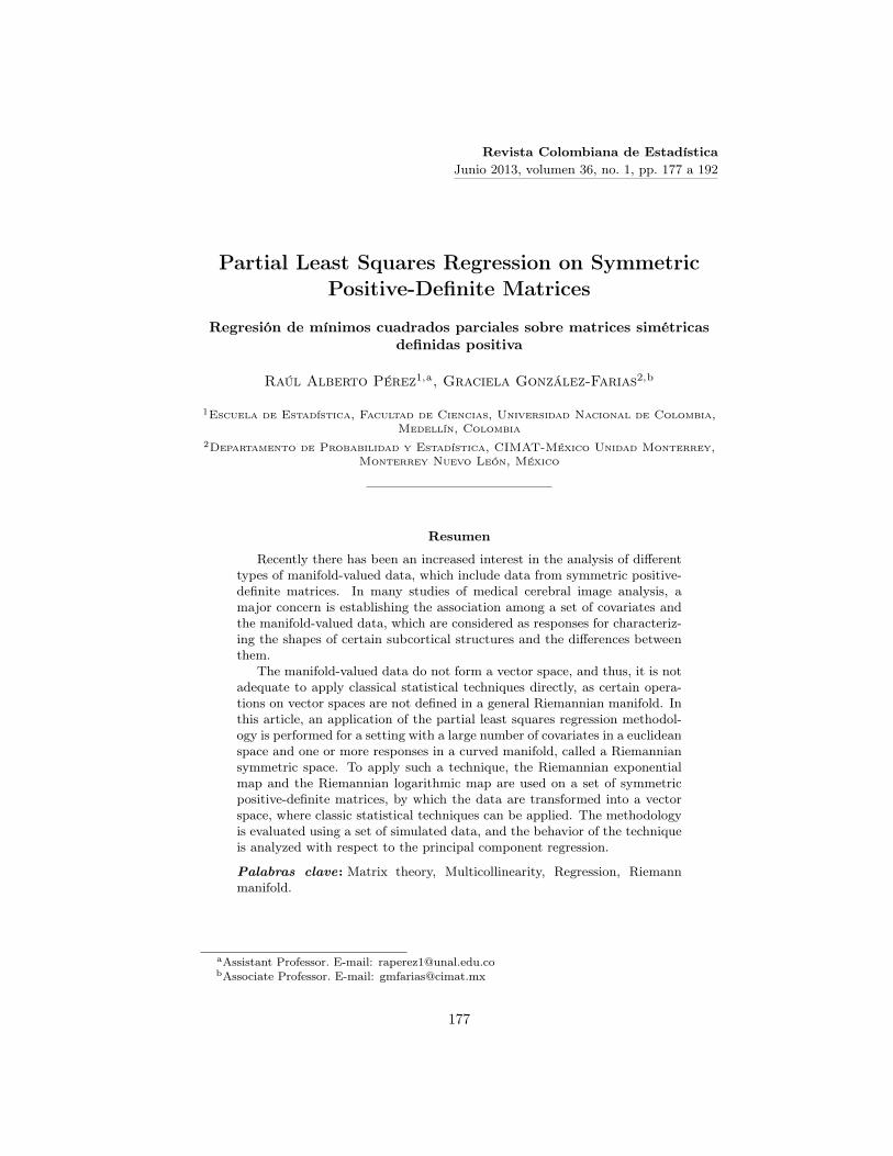
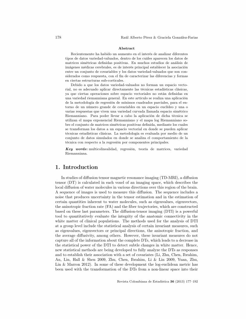
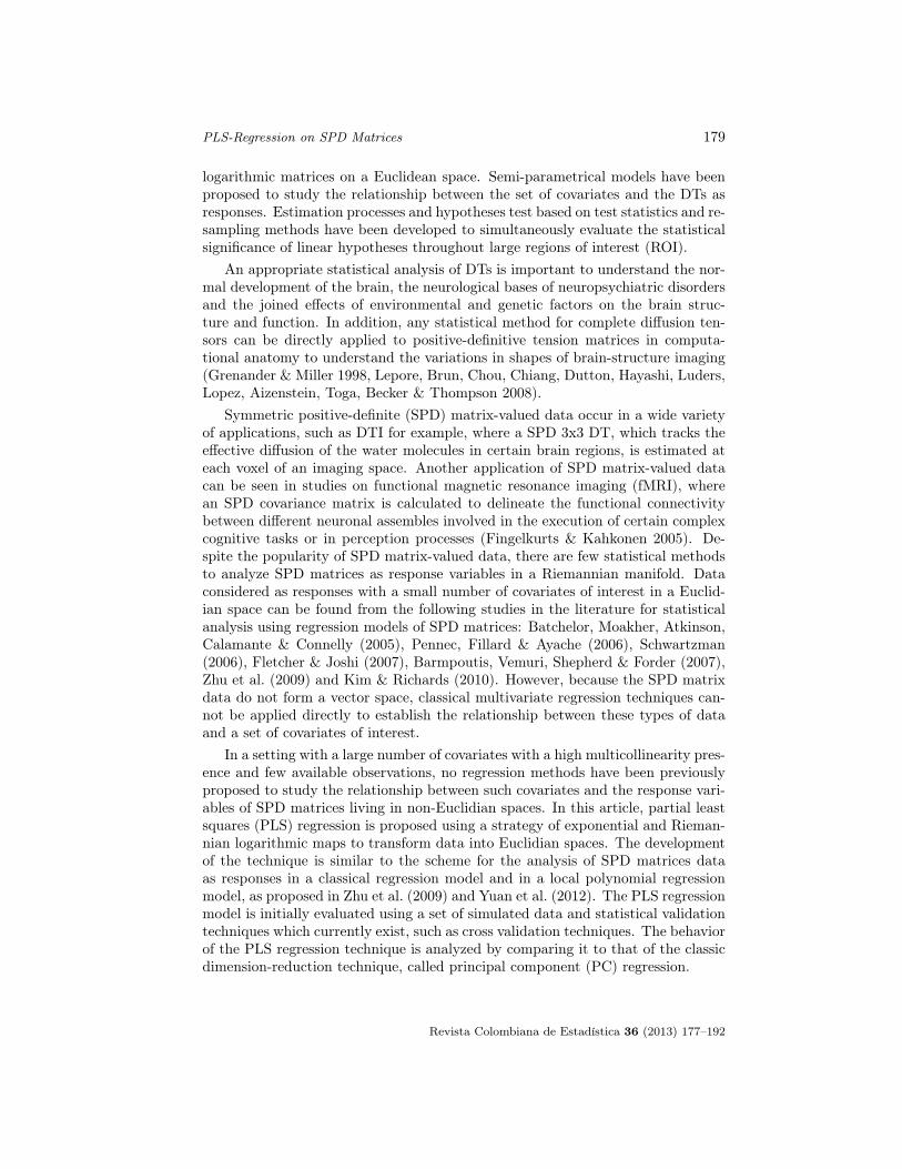
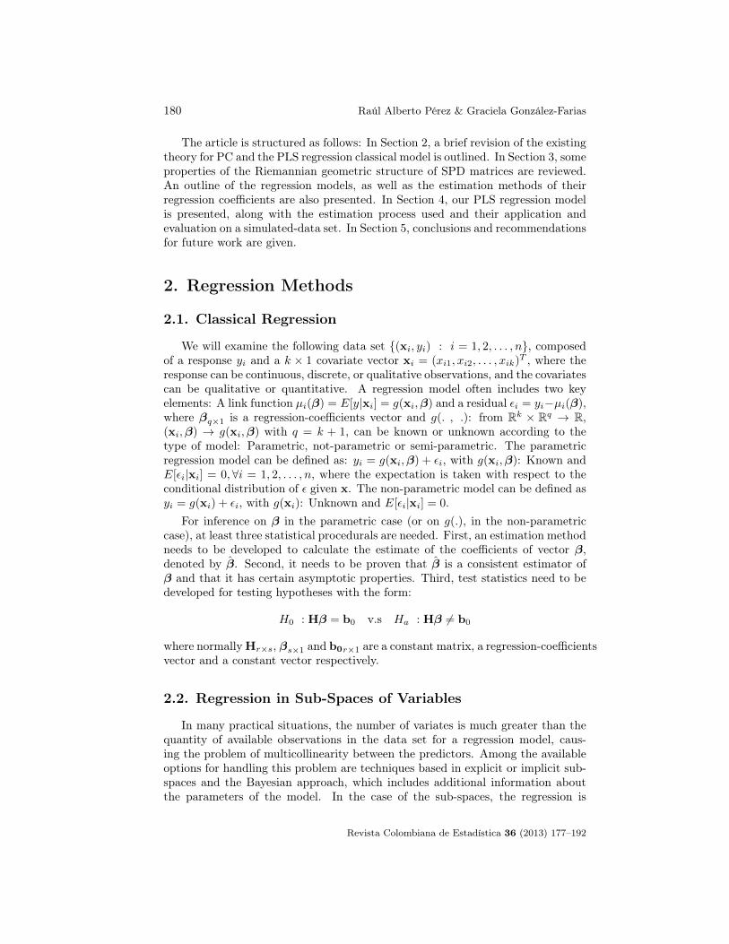
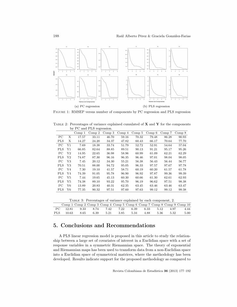
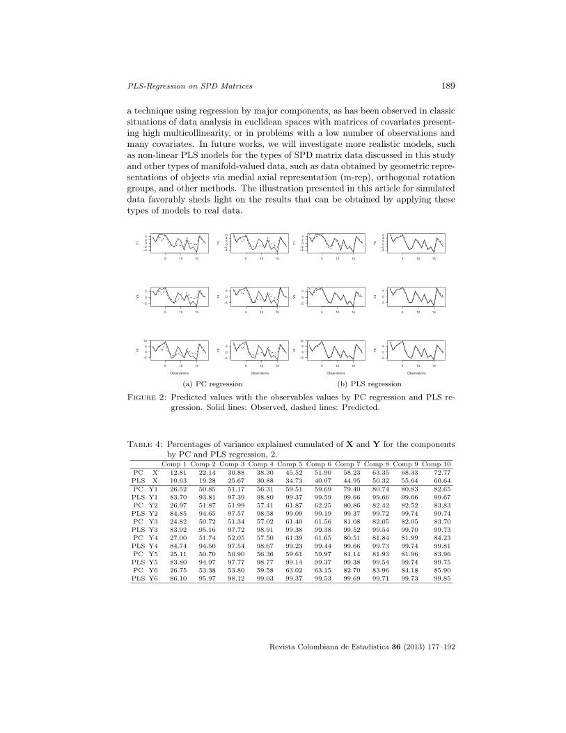
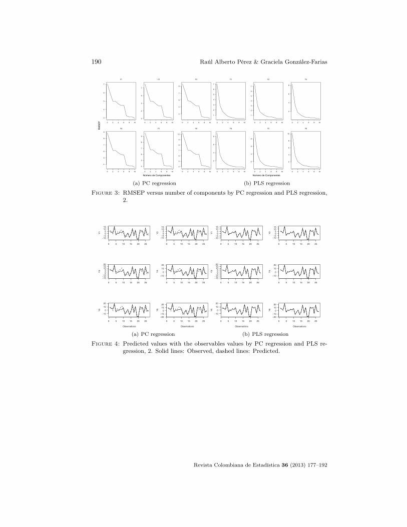
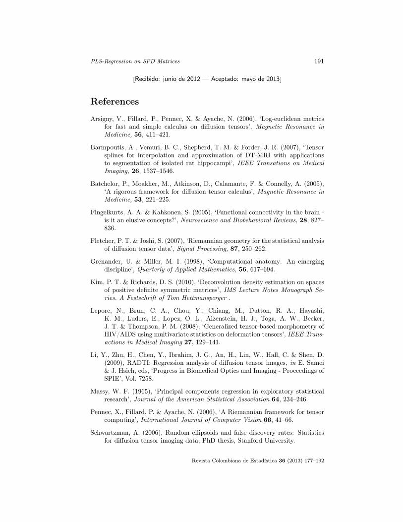
For the first setting, shown in Table 1, the percentages of variance explainedby each of the latent components through PC and PLS regression demonstratethat PC explains more of the variability of X than PLS regression, which is atypical result. In Table 2, the PLS components explain a higher percentage of thevariability of Y than the PC components; with two components, more than 80%of the variability in Y and approximately 20% of the variability in X is explained.Figure 1 shows the graphs of the square root of the prediction middle quadraticerror (RMSEP) against the number of components used in the cross validation(CV). Here, it can be observed that in PC, approximately four components wouldbe needed to explain a majority of the variability in the data. However, in PLS re-gression, three components are needed in most cases. In general, few repetition areshown through this illustration of the repetition results obtained by each method,when compared with the simulation. Figure 2 shows the graphs of the predicteddata with the observed responses. A greater precision in the adjustment can beobserved when PLS regression is used. For the second setting, Table 3 shows thepercentages of variance explained by each of the latent components using PC andPLS regression. Again, PC explains more of the variability of X than PLS regres-sion. Table 4 shows that the PLS components explain a greater percentage of thevariability of Y than the PLS components. In five components, more than 60% ofthe variability in Y and approximately 35% of the variability in X is explained.Figure 3 shows the graphs for the RMSEP against the number of components. Itcan be observed that in PC, approximately 7 components would be needed to ex-plain most of the variability of the data, while in PLS regression, five componentsare needed in most cases. Figure 4 shows the graphs of the predicted data alongwith the observed values of the responses; a greater precision in the adjustmentcan be observed when PLS regression is used.

Table 1: Percentages of variance explained by each component.Comp 1 Comp 2 Comp 3 Comp 4 Comp 5 Comp 6 Comp 7 Comp 8

PC 17.57 15.55 13.59 12.46 11.16 9.16 6.81 4.64PLS 14.27 9.93 10.16 13.45 12.60 5.75 4.46 7.07



0 2 4 6 8

2.2

2.4

2.6

2.8

3.0

3.2

Y1

0 2 4 6 8

2.2

2.4

2.6

2.8

3.0

3.2

3.4

3.6

Y2

0 2 4 6 8

3.0

3.5

4.0

Y3

0 2 4 6 8

3.0

3.5

4.0

4.5

Y4

0 2 4 6 8

3.0

3.5

4.0

4.5

Y5

0 2 4 6 8

3.0

3.5

4.0

4.5

Y6

Número de Componentes

RM

SE

P

(a) PC regression

0 2 4 6 8

1.0

1.5

2.0

2.5

3.0

Y1

0 2 4 6 8

0.5

1.0

1.5

2.0

2.5

3.0

3.5

Y2

0 2 4 6 8

1

2

3

4

Y3

0 2 4 6 8

1

2

3

4

Y4

0 2 4 6 8

1

2

3

4

5

Y5

0 2 4 6 8

1

2

3

4

Y6


(b) PLS regression

Figure 1: RMSEP versus number of components by PC regression and PLS regression

Table 2: Percentages of variance explained cumulated of X and Y for the componentsby PC and PLS regression.

Comp 1 Comp 2 Comp 3 Comp 4 Comp 5 Comp 6 Comp 7 Comp 8PC X 17.57 33.11 46.70 59.16 70.32 79.48 86.28 90.93PLS X 14.27 24.20 34.37 47.82 60.43 66.17 70.64 77.70PC Y1 7.69 18.38 33.74 51.79 52.72 52.91 54.64 57.04PLS Y1 66.85 82.64 88.85 89.51 90.13 91.21 95.17 95.26PC Y2 14.95 22.65 36.98 58.96 60.99 61.09 62.21 62.29PLS Y2 74.87 87.30 96.16 96.35 96.46 97.01 98.04 98.05PC Y3 7.45 20.12 34.30 55.21 56.38 56.43 56.44 56.77PLS Y3 70.51 88.00 94.72 95.05 96.33 97.57 97.67 97.78PC Y4 7.30 19.10 41.57 58.71 60.19 60.20 61.57 61.78PLS Y4 74.39 91.05 95.78 96.90 96.92 97.87 99.36 99.39PC Y5 7.44 19.65 45.13 60.30 60.66 61.30 62.61 62.93PLS Y5 74.38 89.10 93.22 95.70 96.19 96.62 97.51 98.38PC Y6 13.89 20.83 40.31 62.35 63.45 63.46 63.46 63.47PLS Y6 77.35 90.32 97.51 97.60 97.63 99.12 99.12 99.38

Table 3: Percentages of variance explained by each component, 2.Comp 1 Comp 2 Comp 3 Comp 4 Comp 5 Comp 6 Comp 7 Comp 8 Comp 9 Comp 10

PC 12.81 9.33 8.74 7.42 7.22 6.39 6.33 5.12 4.97 4.44PLS 10.63 8.65 6.39 5.21 3.85 5.34 4.88 5.36 5.32 5.00

5. Conclusions and Recommendations

A PLS linear regression model is proposed in this article to study the relation-ship between a large set of covariates of interest in a Euclidian space with a set ofresponse variables in a symmetric Riemannian space. The theory of exponentialand Riemannian maps has been used to transform data from a non-Euclidian spaceinto a Euclidian space of symmetrical matrices, where the methodology has beendeveloped. Results indicate support for the proposed methodology as compared to



a technique using regression by major components, as has been observed in classicsituations of data analysis in euclidean spaces with matrices of covariates present-ing high multicollinearity, or in problems with a low number of observations andmany covariates. In future works, we will investigate more realistic models, suchas non-linear PLS models for the types of SPD matrix data discussed in this studyand other types of manifold-valued data, such as data obtained by geometric repre-sentations of objects via medial axial representation (m-rep), orthogonal rotationgroups, and other methods. The illustration presented in this article for simulateddata favorably sheds light on the results that can be obtained by applying thesetypes of models to real data.

5 10 15

−4−2

024

Y1

5 10 15

−4−2

0246

Y2

5 10 15

−5

0

5

Y3

5 10 15

−5

0

5

Y4

5 10 15

−5

0

5

10

Observations

Y5

5 10 15

−5

0

5

Observations

Y6

(a) PC regression

5 10 15

−4−2

024

Y1

5 10 15

−4−2

0246

Y2

5 10 15

−5

0

5Y

3

5 10 15

−5

0

5

Y4

5 10 15

−5

0

5

10

Observations

Y5

5 10 15

−5

0

5

ObservationsY

6

(b) PLS regression

Figure 2: Predicted values with the observables values by PC regression and PLS re-gression. Solid lines: Observed, dashed lines: Predicted.

Table 4: Percentages of variance explained cumulated of X and Y for the componentsby PC and PLS regression, 2.

Comp 1 Comp 2 Comp 3 Comp 4 Comp 5 Comp 6 Comp 7 Comp 8 Comp 9 Comp 10PC X 12.81 22.14 30.88 38.30 45.52 51.90 58.23 63.35 68.33 72.77PLS X 10.63 19.28 25.67 30.88 34.73 40.07 44.95 50.32 55.64 60.64PC Y1 26.52 50.85 51.17 56.31 59.51 59.69 79.40 80.74 80.83 82.65PLS Y1 83.70 93.81 97.39 98.80 99.37 99.59 99.66 99.66 99.66 99.67PC Y2 26.97 51.87 51.99 57.41 61.87 62.25 80.86 82.42 82.52 83.83PLS Y2 84.85 94.65 97.57 98.58 99.09 99.19 99.37 99.72 99.74 99.74PC Y3 24.82 50.72 51.34 57.02 61.40 61.56 81.08 82.05 82.05 83.70PLS Y3 83.92 95.16 97.72 98.91 99.38 99.38 99.52 99.54 99.70 99.73PC Y4 27.00 51.74 52.05 57.50 61.39 61.65 80.51 81.84 81.99 84.23PLS Y4 84.74 94.50 97.54 98.67 99.23 99.44 99.66 99.73 99.74 99.81PC Y5 25.11 50.70 50.90 56.36 59.61 59.97 81.14 81.93 81.96 83.96PLS Y5 83.80 94.97 97.77 98.77 99.14 99.37 99.38 99.54 99.74 99.75PC Y6 26.75 53.38 53.80 59.58 63.02 63.15 82.70 83.96 84.18 85.90PLS Y6 86.10 95.97 98.12 99.03 99.37 99.53 99.69 99.71 99.73 99.85



0 2 4 6 8 10

3

4

5

6

7

Y1

0 2 4 6 8 10

3

4

5

6

7

Y2

0 2 4 6 8 10

4

5

6

7

8

Y3

0 2 4 6 8 10

4

5

6

7

8

9

Y4

0 2 4 6 8 10

4

5

6

7

8

9

Y5

0 2 4 6 8 10

4

5

6

7

8

9

10

Y6


RM

SE

P

(a) PC regression

0 2 4 6 8 10

1

2

3

4

5

6

7

Y1

0 2 4 6 8 10

1

2

3

4

5

6

7

Y2

0 2 4 6 8 10

2

4

6

8

Y3

0 2 4 6 8 10

2

4

6

8

Y4

0 2 4 6 8 10

2

4

6

8

Y5

0 2 4 6 8 10

2

4

6

8

10

Y6


(b) PLS regression

Figure 3: RMSEP versus number of components by PC regression and PLS regression,2.

0 5 10 15 20 25

−10−5

05

1015

Y1

0 5 10 15 20 25

−10−5

05

1015

Y2

0 5 10 15 20 25

−15−10−5

05

101520

Y3

0 5 10 15 20 25

−10

0

10

20

Y4

0 5 10 15 20 25

−10

0

10

20

Observations

Y5

0 5 10 15 20 25

−20−10

01020

Observations

Y6

(a) PC regression

0 5 10 15 20 25

−10−5

05

1015

Y1

0 5 10 15 20 25

−10−5

05

1015

Y2

0 5 10 15 20 25

−15−10−5

05

101520

Y3

0 5 10 15 20 25

−10

0

10

20

Y4

0 5 10 15 20 25

−10

0

10

20

Observations

Y5

0 5 10 15 20 25

−20−10

01020

Observations

Y6

(b) PLS regression

Figure 4: Predicted values with the observables values by PC regression and PLS re-gression, 2. Solid lines: Observed, dashed lines: Predicted.



[Recibido: junio de 2012 — Aceptado: mayo de 2013]

References

Arsigny, V., Fillard, P., Pennec, X. & Ayache, N. (2006), ‘Log-euclidean metricsfor fast and simple calculus on diffusion tensors’, Magnetic Resonance inMedicine, 56, 411–421.

Barmpoutis, A., Vemuri, B. C., Shepherd, T. M. & Forder, J. R. (2007), ‘Tensorsplines for interpolation and approximation of DT-MRI with applicationsto segmentation of isolated rat hippocampi’, IEEE Transations on MedicalImaging, 26, 1537–1546.

Batchelor, P., Moakher, M., Atkinson, D., Calamante, F. & Connelly, A. (2005),‘A rigorous framework for diffusion tensor calculus’, Magnetic Resonance inMedicine, 53, 221–225.

Fingelkurts, A. A. & Kahkonen, S. (2005), ‘Functional connectivity in the brain -is it an elusive concepts?’, Neuroscience and Biobehavioral Reviews, 28, 827–836.

Fletcher, P. T. & Joshi, S. (2007), ‘Riemannian geometry for the statistical analysisof diffusion tensor data’, Signal Processing, 87, 250–262.

Grenander, U. & Miller, M. I. (1998), ‘Computational anatomy: An emergingdiscipline’, Quarterly of Applied Mathematics, 56, 617–694.

Kim, P. T. & Richards, D. S. (2010), ‘Deconvolution density estimation on spacesof positive definite symmetric matrices’, IMS Lecture Notes Monograph Se-ries. A Festschrift of Tom Hettmansperger .

Lepore, N., Brun, C. A., Chou, Y., Chiang, M., Dutton, R. A., Hayashi,K. M., Luders, E., Lopez, O. L., Aizenstein, H. J., Toga, A. W., Becker,J. T. & Thompson, P. M. (2008), ‘Generalized tensor-based morphometry ofHIV/AIDS using multivariate statistics on deformation tensors’, IEEE Trans-actions in Medical Imaging 27, 129–141.

Li, Y., Zhu, H., Chen, Y., Ibrahim, J. G., An, H., Lin, W., Hall, C. & Shen, D.(2009), RADTI: Regression analysis of diffusion tensor images, in E. Samei& J. Hsieh, eds, ‘Progress in Biomedical Optics and Imaging - Proceedings ofSPIE’, Vol. 7258.

Massy, W. F. (1965), ‘Principal components regression in exploratory statisticalresearch’, Journal of the American Statistical Association 64, 234–246.

Pennec, X., Fillard, P. & Ayache, N. (2006), ‘A Riemannian framework for tensorcomputing’, International Journal of Computer Vision 66, 41–66.

Schwartzman, A. (2006), Random ellipsoids and false discovery rates: Statisticsfor diffusion tensor imaging data, PhD thesis, Stanford University.



Wold, H. (1975), ‘Soft modeling by latent variables; the non-linear iterative partialleast squares approach’, Perspectives in Probability and Statistics, pp. 1–2.

Wold, S., Albano, C., Dunn, W.J., I., Edlund, U., Esbensen, K., Geladi, P., Hell-berg, S., Johansson, E., Lindberg, W. & Sjöström, M. (1984), Multivariatedata analysis in chemistry, in B. Kowalski, ed., ‘Chemometrics’, Vol. 138 ofNATO ASI Series, Springer Netherlands, pp. 17–95.

Yuan, Y., Zhu, H., Lin, W. & Marron, J. S. (2012), ‘Local polynomial regression forsymmetric positive-definite matrices’, Journal of the Royal Statistical Society:Series B (Statistical Methodology) 74(4), 697–719.

Zhu, H. T., Chen, Y. S., Ibrahim, J. G., Li, Y. M. & Lin, W. L. (2009), ‘Intrinsicregression models for positive-definite matrices with applications to diffusiontensor imaging’, Journal of the American Statistical Association 104, 1203–1212.


partialleastsquaresregressiononsymmetric positive

Documents