cmp189 algoritmos geom tricos
TRANSCRIPT
CMP189Algoritmos
Geométricos
Prof. João Comba
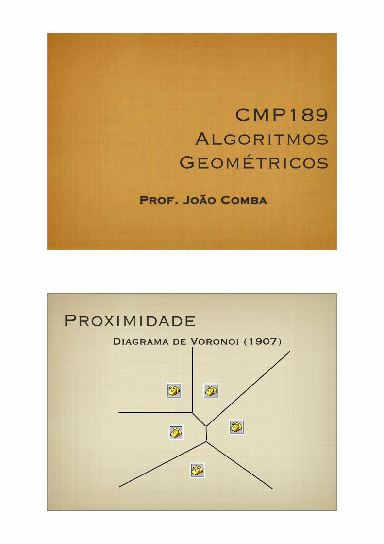
ProximidadeDiagrama de Voronoi (1907)
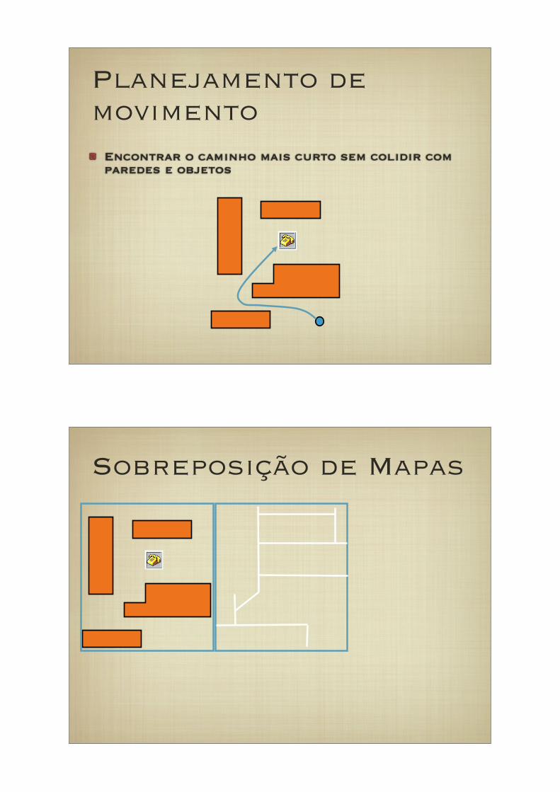
Planejamento de movimento
Encontrar o caminho mais curto sem colidir com paredes e objetos
Sobreposição de Mapas
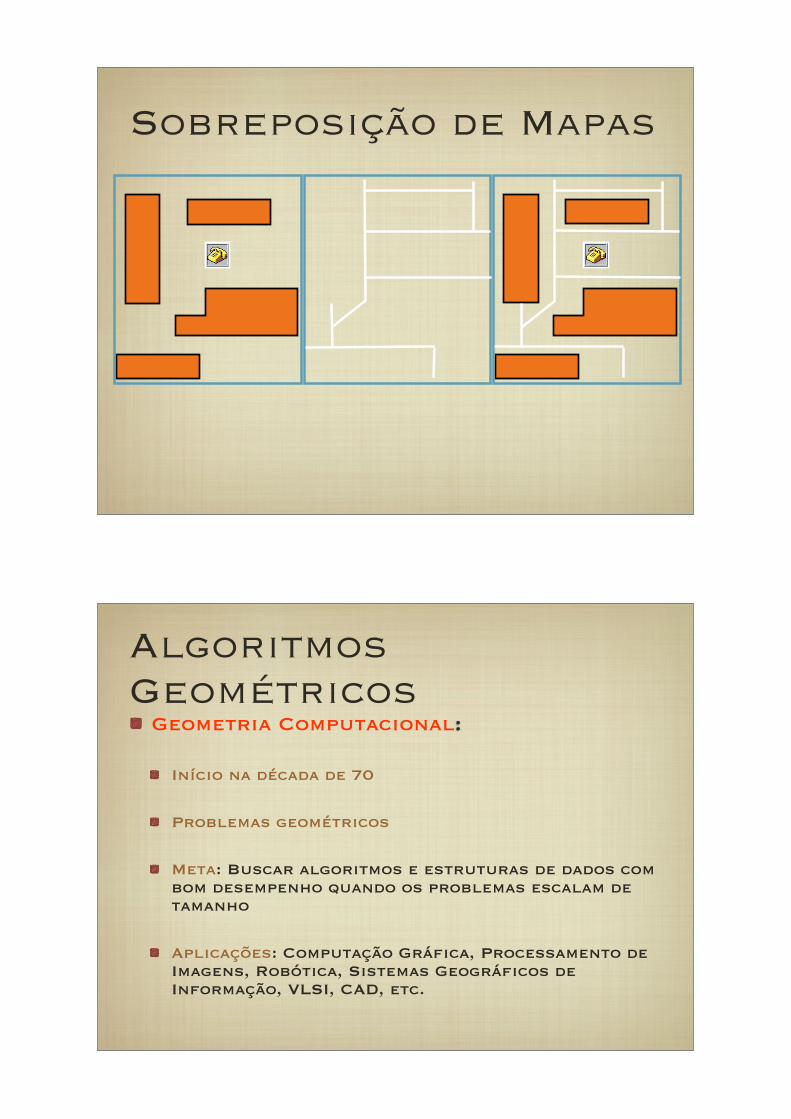
Sobreposição de Mapas
Algoritmos Geométricos
Geometria Computacional:
Início na década de 70
Problemas geométricos
Meta: Buscar algoritmos e estruturas de dados com bom desempenho quando os problemas escalam de tamanho
Aplicações: Computação Gráfica, Processamento de Imagens, Robótica, Sistemas Geográficos de Informação, VLSI, CAD, etc.
Algoritmos Geométricos
Problemas Típicos:
Entrada: Objetos Geométricos (pontos, linhas, planos, etc)
Saída: Resultados de consulta sobre os objetos, ou um novo objeto geométrico
Ingredientes:
Geometria, Topologia, Algoritmos, Estruturas de dados, Análise de algoritmos, Problemas numéricos
Algoritmos GeométricosLimitações Comuns:
Natureza discreta: aproximações discretas de fenômenos contínuos
Objetos planares ou lineares (aproximações de objetos curvos)
Permite concentrar em aspectos combinatórios dos problemas em detrimento de aspectos numéricos
Problemas de baixa dimensão
Primordialmente 2D (fácil de visualizar) e 3D (até certos limites)
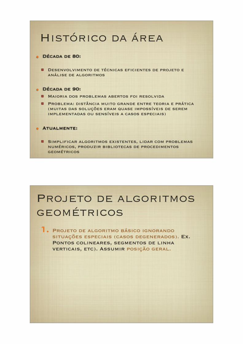
Histórico da área
• Década de 80:
Desenvolvimento de técnicas eficientes de projeto e análise de algoritmos
• Década de 90:
Maioria dos problemas abertos foi resolvida
Problema: distância muito grande entre teoria e prática (muitas das soluções eram quase impossíveis de serem implementadas ou sensíveis a casos especiais)
• Atualmente:
Simplificar algoritmos existentes, lidar com problemas numéricos, produzir bibliotecas de procedimentos geométricos
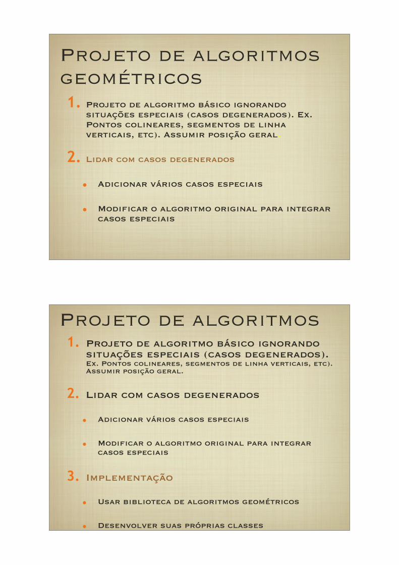
Projeto de algoritmos geométricos
1. Projeto de algoritmo básico ignorando situações especiais (casos degenerados). Ex. Pontos colineares, segmentos de linha verticais, etc). Assumir posição geral.
Projeto de algoritmos geométricos1. Projeto de algoritmo básico ignorando
situações especiais (casos degenerados). Ex. Pontos colineares, segmentos de linha verticais, etc). Assumir posição geral.
2. Lidar com casos degenerados
• Adicionar vários casos especiais
• Modificar o algoritmo original para integrar casos especiais
Projeto de algoritmos1. Projeto de algoritmo básico ignorando
situações especiais (casos degenerados). Ex. Pontos colineares, segmentos de linha verticais, etc). Assumir posição geral.
2. Lidar com casos degenerados
• Adicionar vários casos especiais
• Modificar o algoritmo original para integrar casos especiais
3. Implementação
• Usar biblioteca de algoritmos geométricos
• Desenvolver suas próprias classes
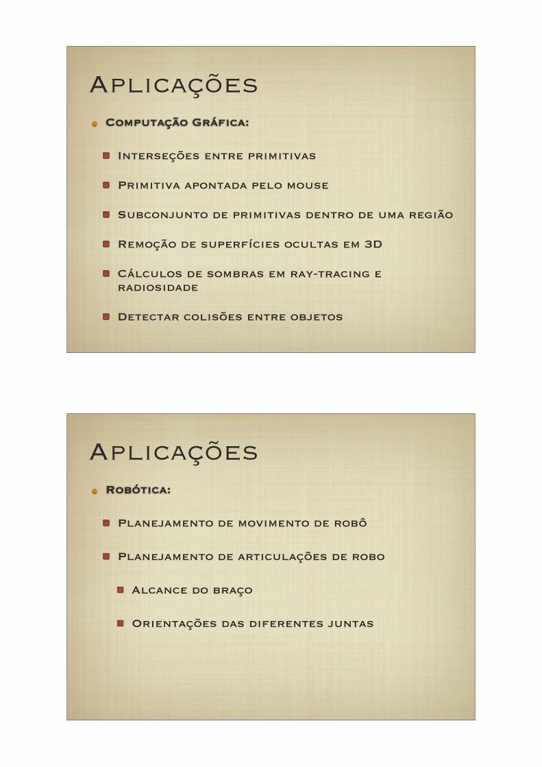
Aplicações
• Computação Gráfica:
Interseções entre primitivas
Primitiva apontada pelo mouse
Subconjunto de primitivas dentro de uma região
Remoção de superfícies ocultas em 3D
Cálculos de sombras em ray-tracing e radiosidade
Detectar colisões entre objetos
Aplicações
• Robótica:
Planejamento de movimento de robô
Planejamento de articulações de robo
Alcance do braço
Orientações das diferentes juntas
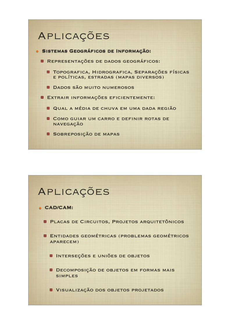
Aplicações• Sistemas Geográficos de Informação:
Representações de dados geográficos:
Topografica, Hidrografica, Separações físicas e políticas, estradas (mapas diversos)
Dados são muito numerosos
Extrair informações eficientemente:
Qual a média de chuva em uma dada região
Como guiar um carro e definir rotas de navegação
Sobreposição de mapas
Aplicações
• CAD/CAM:
Placas de Circuitos, Projetos arquitetônicos
Entidades geométricas (problemas geométricos aparecem)
Interseções e uniões de objetos
Decomposição de objetos em formas mais simples
Visualização dos objetos projetados

Conteúdo
1. Fundamentos
2. Interseções de Segmentos de Linha
3. Particionamento de Polígonos
4. Envoltórias Convexas
5. Diagramas de Voronoy
6. Triangulações de Delaunay
7. Algoritmos de Busca Pontual e Intervalar
8. Quadtrees, BSP-trees, R-trees
9. Grafos de Visibilidade
10.Planejamento de Movimento
Conteúdo • Técnicas de Projeto de Algoritmos
Lugares geométricos
Transformações geométricas
Dualidade
Space Sweep
Estruturas Hierárquicas
• Estruturas de Dados:
Cascadeamento Fracional
Estruturas de Dados Persistentes
Estruturas de Dados Cinéticas
Análise caso médio

Avaliação• Trabalhos teóricos e práticos
• Trabalho Final:Definido de comum acordo com o aluno / orientador
Alguns temas sugeridos
Sugestões por parte dos alunos são estimuladas
Preferencialmente dentro da área de pesquisa de mestrado
Resultados esperados: Artigo técnico mostrando os resultados obtidos (em inglês)
Apresentação final
• Prova Final
BibliografiaBIBLIOGRAFIA BÁSICA:
• Computational Geometry: Algorithms and Applications. M. de Berg, M. van Kreveld, M. Overmars, O. Scwarzkopf. Springer Verlag, 1997.
BIBLIOGRAFIA COMPLEMENTAR:
• Computational Geometry in C. Joseph O’Rourke. Cambridge University Press, 1993.
• Applications of Spatial Data Structures. Hanan Samet. Academic Press, 1990.
• Ruler, Compass, and Computer: The Design and Analysis of Geometric Algorithms. Leo Guibas, Jorge Stolfi
• Computational Geometry: Course Notes. David Mount (Univ. Of Maryland)
• Introduction to Algorithms. Cormen, Leiserson, Rivest. McGraw Hill.
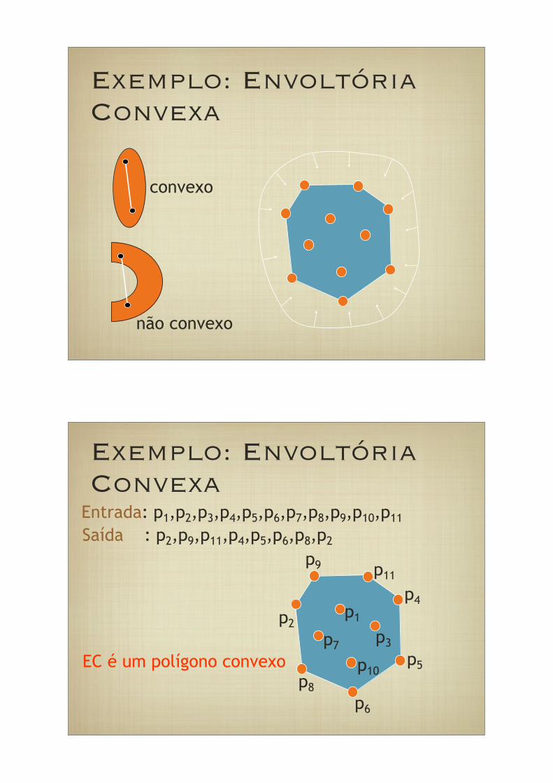
Exemplo: Envoltória Convexa
convexo
não convexo
Exemplo: Envoltória Convexa
p9
p2
p8
p6
p5
p4
p11
p1
p7p3
p10
Entrada: p1,p2,p3,p4,p5,p6,p7,p8,p9,p10,p11
Saída : p2,p9,p11,p4,p5,p6,p8,p2
EC é um polígono convexo
Exemplo: Envoltória Convexa
p9
p2
p8
p6
p5
p4
p11
p1
p7p3
p10
Envoltória Convexa 1
p9
p2
p8
p6
p5
p4
p11
p1
p7p3
p10
Envoltória Convexa 1
p9
p2
p8
p6
p5
p4
p11
p1
p7p3
p10
(n2-n)
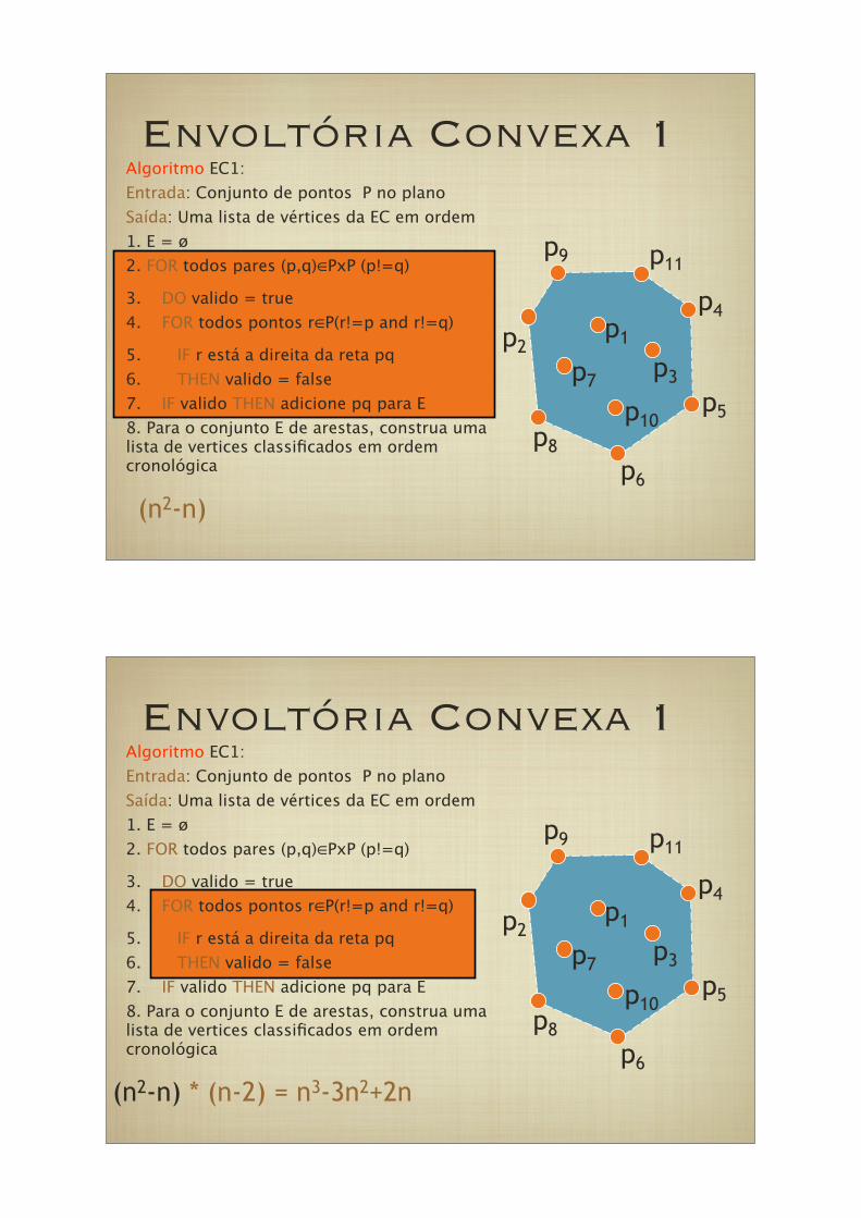
Algoritmo EC1:
Entrada: Conjunto de pontos P no plano
Saída: Uma lista de vértices da EC em ordem
1. E = ø
2. FOR todos pares (p,q)∈PxP (p!=q)
3. DO valido = true
4. FOR todos pontos r∈P(r!=p and r!=q)
5. IF r está a direita da reta pq
6. THEN valido = false
7. IF valido THEN adicione pq para E
8. Para o conjunto E de arestas, construa uma lista de vertices classificados em ordem cronológica
Envoltória Convexa 1
p9
p2
p8
p6
p5
p4
p11
p1
p7p3
p10
(n2-n) * (n-2) = n3-3n2+2n
Algoritmo EC1:
Entrada: Conjunto de pontos P no plano
Saída: Uma lista de vértices da EC em ordem
1. E = ø
2. FOR todos pares (p,q)∈PxP (p!=q)
3. DO valido = true
4. FOR todos pontos r∈P(r!=p and r!=q)
5. IF r está a direita da reta pq
6. THEN valido = false
7. IF valido THEN adicione pq para E
8. Para o conjunto E de arestas, construa uma lista de vertices classificados em ordem cronológica
Envoltória Convexa 1
p9
p2
p8
p6
p5
p4
p11
p1
p7p3
p10
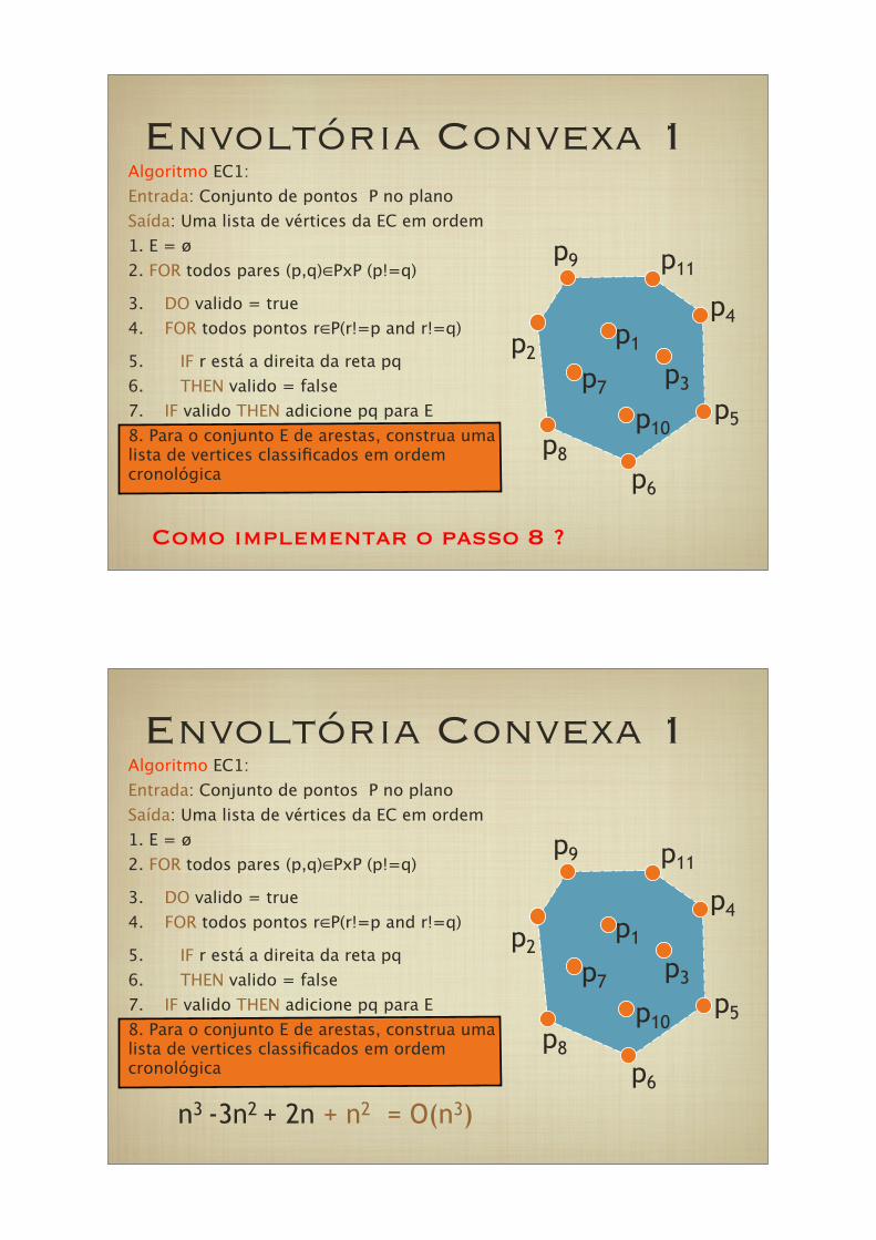
Algoritmo EC1:
Entrada: Conjunto de pontos P no plano
Saída: Uma lista de vértices da EC em ordem
1. E = ø
2. FOR todos pares (p,q)∈PxP (p!=q)
3. DO valido = true
4. FOR todos pontos r∈P(r!=p and r!=q)
5. IF r está a direita da reta pq
6. THEN valido = false
7. IF valido THEN adicione pq para E
8. Para o conjunto E de arestas, construa uma lista de vertices classificados em ordem cronológica
Como implementar o passo 8 ?
Envoltória Convexa 1
p9
p2
p8
p6
p5
p4
p11
p1
p7p3
p10
Algoritmo EC1:
Entrada: Conjunto de pontos P no plano
Saída: Uma lista de vértices da EC em ordem
1. E = ø
2. FOR todos pares (p,q)∈PxP (p!=q)
3. DO valido = true
4. FOR todos pontos r∈P(r!=p and r!=q)
5. IF r está a direita da reta pq
6. THEN valido = false
7. IF valido THEN adicione pq para E
8. Para o conjunto E de arestas, construa uma lista de vertices classificados em ordem cronológica
n3 -3n2 + 2n + n2 = O(n3)
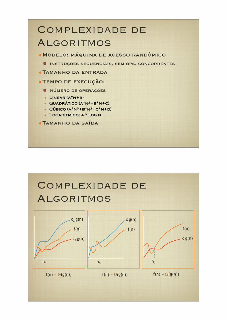
Complexidade de Algoritmos•Modelo: máquina de acesso randômico
instruções sequenciais, sem ops. concorrentes
•Tamanho da entrada
•Tempo de execução:
número de operações
• Linear (a*n+b)
• Quadrático (a*n2+b*n+c)
• Cúbico (a*n3+b*n2+c*n+d)
• Logarítmico: a * log n
•Tamanho da saída
Complexidade de Algoritmos
n0
c2 g(n)
c1 g(n)
f(n) = !(g(n))
f(n)
n0
c g(n)
f(n) = O(g(n))
f(n)
n0
c g(n)
f(n) = "(g(n))
f(n)
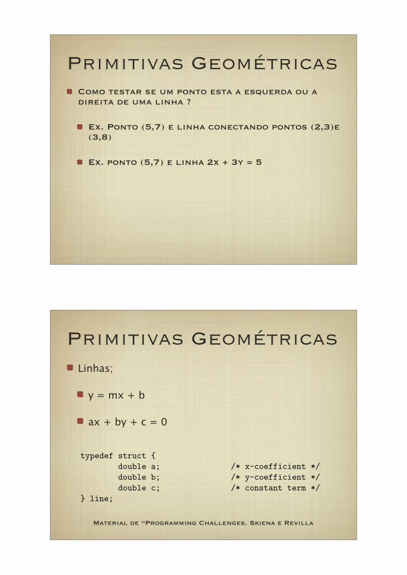
Primitivas GeométricasComo testar se um ponto esta a esquerda ou a direita de uma linha ?
Ex. Ponto (5,7) e linha conectando pontos (2,3)e (3,8)
Ex. ponto (5,7) e linha 2x + 3y = 5
Primitivas Geométricas
Linhas;
y = mx + b
ax + by + c = 0
292 13. Geometry
points (x1, y1) and (x2, y2) which lie on it. Lines are also completely describedby equations such as y = mx + b, where m is the slope of the line and b is they-intercept, i.e., the unique point (0, b) where it crosses the x-axis. The line l hasslope m = ∆y/∆x = (y1 − y2)/(x1 − x2) and intercept b = y1 − mx1.
Vertical lines cannot be described by such equations, however, because divid-ing by ∆x means dividing by zero. The equation x = c denotes a vertical line thatcrosses the x-axis at the point (c, 0). This special case, or degeneracy, requiresextra attention when doing geometric programming. We use the more generalformula ax + by + c = 0 as the foundation of our line type because it covers allpossible lines in the plane:
typedef struct {double a; /* x-coefficient */double b; /* y-coefficient */double c; /* constant term */
} line;
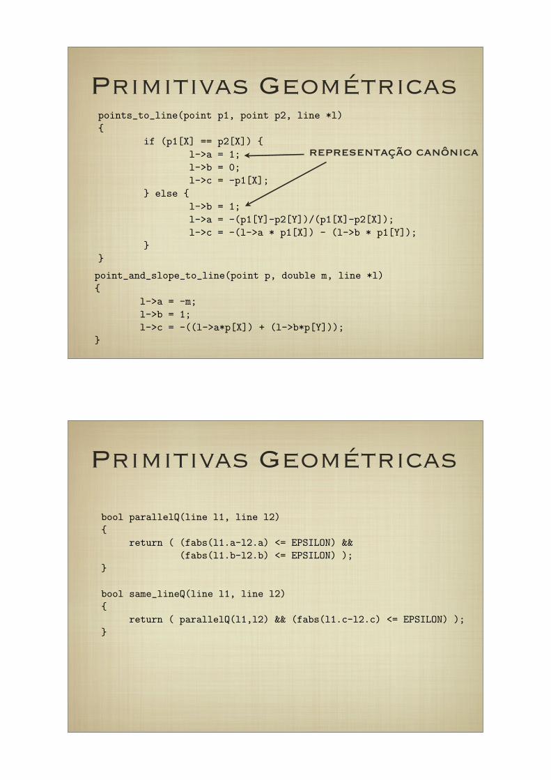
Multiplying these coefficients by any non-zero constant yields an alternate repre-sentation for any line. We establish a canonical representation by insisting thatthe y-coefficient equal 1 if it is non-zero. Otherwise, we set the x-coefficient to 1:
points_to_line(point p1, point p2, line *l){
if (p1[X] == p2[X]) {l->a = 1;l->b = 0;l->c = -p1[X];
} else {l->b = 1;l->a = -(p1[Y]-p2[Y])/(p1[X]-p2[X]);l->c = -(l->a * p1[X]) - (l->b * p1[Y]);
}}
point_and_slope_to_line(point p, double m, line *l){
l->a = -m;l->b = 1;l->c = -((l->a*p[X]) + (l->b*p[Y]));
}
• Intersection — Two distinct lines have one intersection point unless they areparallel; in which case they have none. Parallel lines share the same slope buthave different intercepts and by definition never cross.
Material de “Programming Challenges. Skiena e Revilla
Primitivas Geométricas
292 13. Geometry
points (x1, y1) and (x2, y2) which lie on it. Lines are also completely describedby equations such as y = mx + b, where m is the slope of the line and b is they-intercept, i.e., the unique point (0, b) where it crosses the x-axis. The line l hasslope m = ∆y/∆x = (y1 − y2)/(x1 − x2) and intercept b = y1 − mx1.
Vertical lines cannot be described by such equations, however, because divid-ing by ∆x means dividing by zero. The equation x = c denotes a vertical line thatcrosses the x-axis at the point (c, 0). This special case, or degeneracy, requiresextra attention when doing geometric programming. We use the more generalformula ax + by + c = 0 as the foundation of our line type because it covers allpossible lines in the plane:
typedef struct {double a; /* x-coefficient */double b; /* y-coefficient */double c; /* constant term */
} line;
Multiplying these coefficients by any non-zero constant yields an alternate repre-sentation for any line. We establish a canonical representation by insisting thatthe y-coefficient equal 1 if it is non-zero. Otherwise, we set the x-coefficient to 1:
points_to_line(point p1, point p2, line *l){
if (p1[X] == p2[X]) {l->a = 1;l->b = 0;l->c = -p1[X];
} else {l->b = 1;l->a = -(p1[Y]-p2[Y])/(p1[X]-p2[X]);l->c = -(l->a * p1[X]) - (l->b * p1[Y]);
}}
point_and_slope_to_line(point p, double m, line *l){
l->a = -m;l->b = 1;l->c = -((l->a*p[X]) + (l->b*p[Y]));
}
• Intersection — Two distinct lines have one intersection point unless they areparallel; in which case they have none. Parallel lines share the same slope buthave different intercepts and by definition never cross.
representação canônica
Primitivas Geométricas13.1. Lines 293
bool parallelQ(line l1, line l2){
return ( (fabs(l1.a-l2.a) <= EPSILON) &&(fabs(l1.b-l2.b) <= EPSILON) );
}
bool same_lineQ(line l1, line l2){
return ( parallelQ(l1,l2) && (fabs(l1.c-l2.c) <= EPSILON) );}
A point (x′, y′) lies on a line l : y = mx + b if plugging x′ into the formula for xyields y′. The intersection point of lines l1 : y = m1x + b1 and l2 : y2 = m2x + b2is the point where they are equal, namely,
x =b2 − b1
m1 − m2, y = m1
b2 − b1
m1 − m2+ b1
intersection_point(line l1, line l2, point p){
if (same_lineQ(l1,l2)) {printf("Warning: Identical lines, all points intersect.\n");p[X] = p[Y] = 0.0;return;
}
if (parallelQ(l1,l2) == TRUE) {printf("Error: Distinct parallel lines do not intersect.\n");return;
}
p[X] = (l2.b*l1.c - l1.b*l2.c) / (l2.a*l1.b - l1.a*l2.b);
if (fabs(l1.b) > EPSILON) /* test for vertical line */p[Y] = - (l1.a * (p[X]) + l1.c) / l1.b;
elsep[Y] = - (l2.a * (p[X]) + l2.c) / l2.b;
}
• Angles — Any two non-parallel lines intersect each other at a given angle. Linesl1 : a1x + b1y + c1 = 0 and l2 : a2x + b2y + c2 = 0, written in the general form,intersect at the angle θ given by:
tan θ =a1b2 − a2b1
a1a2 + b1b2
For lines in slope-intercept form this reduces to tan θ = (m2 − m1)/(m1m2 + 1).
Primitivas Geométricas
13.1. Lines 293
bool parallelQ(line l1, line l2){
return ( (fabs(l1.a-l2.a) <= EPSILON) &&(fabs(l1.b-l2.b) <= EPSILON) );
}
bool same_lineQ(line l1, line l2){
return ( parallelQ(l1,l2) && (fabs(l1.c-l2.c) <= EPSILON) );}
A point (x′, y′) lies on a line l : y = mx + b if plugging x′ into the formula for xyields y′. The intersection point of lines l1 : y = m1x + b1 and l2 : y2 = m2x + b2is the point where they are equal, namely,
x =b2 − b1
m1 − m2, y = m1
b2 − b1
m1 − m2+ b1
intersection_point(line l1, line l2, point p){
if (same_lineQ(l1,l2)) {printf("Warning: Identical lines, all points intersect.\n");p[X] = p[Y] = 0.0;return;
}
if (parallelQ(l1,l2) == TRUE) {printf("Error: Distinct parallel lines do not intersect.\n");return;
}
p[X] = (l2.b*l1.c - l1.b*l2.c) / (l2.a*l1.b - l1.a*l2.b);
if (fabs(l1.b) > EPSILON) /* test for vertical line */p[Y] = - (l1.a * (p[X]) + l1.c) / l1.b;
elsep[Y] = - (l2.a * (p[X]) + l2.c) / l2.b;
}
• Angles — Any two non-parallel lines intersect each other at a given angle. Linesl1 : a1x + b1y + c1 = 0 and l2 : a2x + b2y + c2 = 0, written in the general form,intersect at the angle θ given by:
tan θ =a1b2 − a2b1
a1a2 + b1b2
For lines in slope-intercept form this reduces to tan θ = (m2 − m1)/(m1m2 + 1).
Interseção entre duas linhas
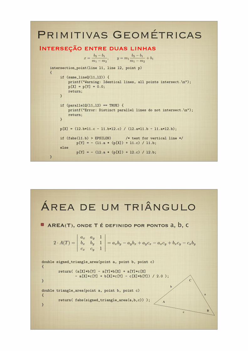
Área de um triângulo
AREA(T), onde T é definido por pontos a, b, c
13.2. Triangles and Trigonometry 297
Solving triangles is the art of deriving the unknown angles and edge lengths of atriangle given a subset of such measurements. Such problems fall into two categories:
• Given two angles and side, find the rest — Finding the third angle is easy, sincethe three angles must sum to 180o = π radians. The Law of Sines then gives us away to find the missing edge lengths.
• Given two sides and an angle, find the rest — If the angle lies between the twoedges, the Law of Cosines gives us the way to find the remaining edge length.The Law of Sines then enables us to mop up the unknown angles. Otherwise, wecan use the Law of Sines and the angle sum property to determine all angles, andthen the Law of Sines to get the remaining edge length.
The area A(T ) of a triangle T is given by A(T ) = (1/2)ab, where a is the altitude andb is the base of the triangle. The base is any one of the sides while the altitude is thedistance from the third vertex to this base, as shown in Figure 13.2(r). This altitudecan be easily calculated via trigonometry or the Pythagorean theorem, depending onwhat is known about the triangle.
Another approach to computing the area of a triangle is directly from its coordinaterepresentation. Using linear algebra and determinants, it can be shown that the signedarea A(T ) of triangle T = (a, b, c) is
2 · A(T ) =
∣∣∣∣∣∣
ax ay 1bx by 1cx cy 1
∣∣∣∣∣∣= axby − aybx + aycx − axcy + bxcy − cxby
This formula generalizes nicely to compute d! times the volume of a simplex in ddimensions.
Note that the signed areas can be negative, so we must take the absolute value tocompute the actual area. This is a feature, not a bug. We will see how to use the signof this area to build important primitives for computational geometry in Section 14.1.
double signed_triangle_area(point a, point b, point c){
return( (a[X]*b[Y] - a[Y]*b[X] + a[Y]*c[X]- a[X]*c[Y] + b[X]*c[Y] - c[X]*b[Y]) / 2.0 );
}
double triangle_area(point a, point b, point c){
return( fabs(signed_triangle_area(a,b,c)) );}
296 13. Geometry
b
a
A
B
C
a
b
c
Figure 13.2. Notation for solving triangles (l) and computing their area (r).
These functions are important, because they enable us to relate the lengths of anytwo sides of a right triangle T with the non-right angles of T . Recall that the hypotenuseof a right triangle is the longest edge in T , that edge opposite the right angle. The othertwo edges in T can be labeled as opposite or adjacent edges in relation to a given anglea, as shown in Figure 13.1(r). Then
cos(a) =|adjacent|
|hypotenuse| , sin(a) =|opposite|
|hypotenuse| , tan(a) =|opposite||adjacent|
These relations are worth remembering. As a mnemonic, we use the name of thefamous Indian Chief Soh-Cah-Toa, where each syllable of his name encodes a differentrelation. “Cah” means Cosine equals Adjacent over Hypotenuse, for example.
Chief Soh-Cah-Toa would not be of much use without inverse functions mappingcos(θ), sin(θ), and tan(θ) back to the original angles. These inverse functions are calledarccos, arcsin, and arctan, respectively. With them, we can easily compute the remainingangles of any right triangle given two side lengths.
These trigonometric functions are properly computed using Taylor series expansions,but don’t worry: the math library of your favorite programming language already in-cludes them. Trigonometric functions tend to be numerically unstable, so be careful. Donot expect that θ exactly equals arcsin(sin(θ)), particularly for large or small angles.
13.2.3 Solving TrianglesTwo powerful trigonometric formulae enable us to compute important properties oftriangles. The Law of Sines provides the relationship between sides and angles in anytriangle. For angles A, B, C, and opposing edges a, b, c (shown in Figure 13.2(l)),
a
sin A=
b
sin B=
c
sin C
The Law of Cosines is a generalization of the Pythagorean theorem beyond rightangles. For any triangle with angles A, B, C, and opposing edges a, b, c,
a2 = b2 + c2 − 2bc cos A
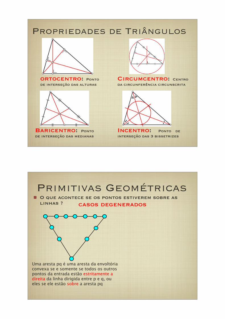
Propriedades de Triângulos
Circumcentro: Centro
da circunferência circunscrita
ortocentro: Ponto
de interseção das alturas
Baricentro: Ponto
de interseção das medianas
Incentro: Ponto de
interseção das 3 bissetrizes
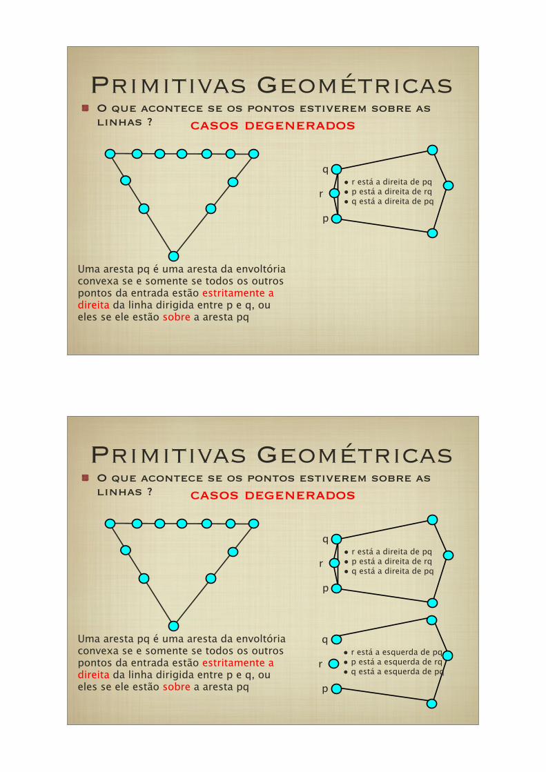
O que acontece se os pontos estiverem sobre as linhas ?
Primitivas Geométricas
casos degenerados
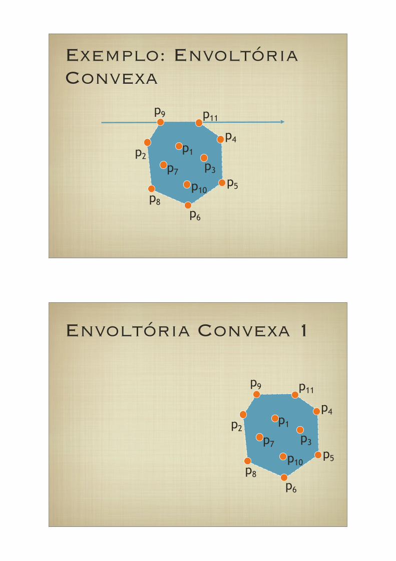
Uma aresta pq é uma aresta da envoltória convexa se e somente se todos os outros pontos da entrada estão estritamente a direita da linha dirigida entre p e q, ou eles se ele estão sobre a aresta pq
O que acontece se os pontos estiverem sobre as linhas ?
Primitivas Geométricas
casos degenerados
p
q
r
Uma aresta pq é uma aresta da envoltória convexa se e somente se todos os outros pontos da entrada estão estritamente a direita da linha dirigida entre p e q, ou eles se ele estão sobre a aresta pq
• r está a direita de pq
• p está a direita de rq
• q está a direita de pq
p
q
r• r está a esquerda de pq
• p está a esquerda de rq
• q está a esquerda de pq
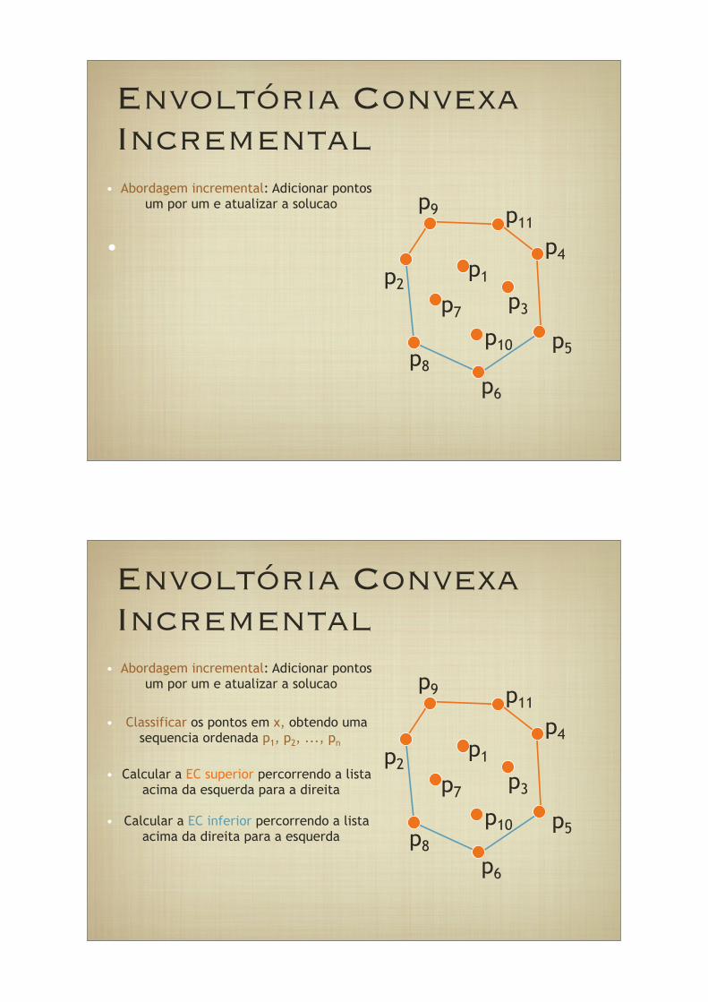
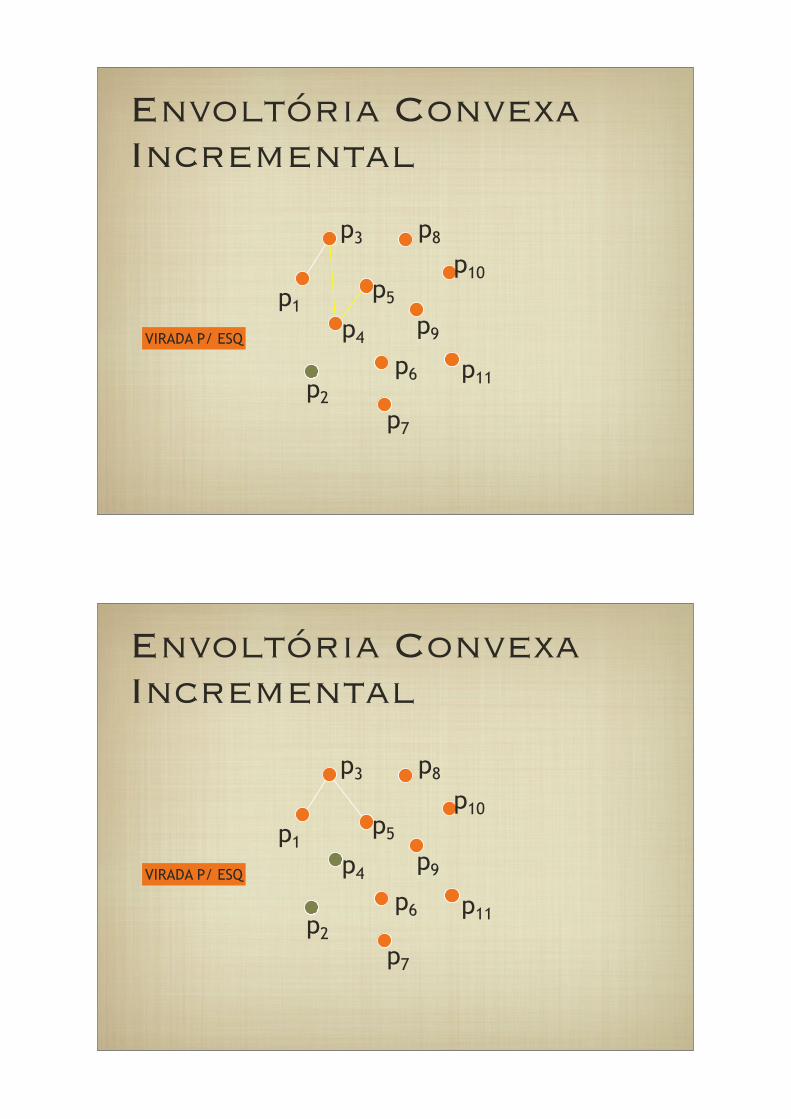
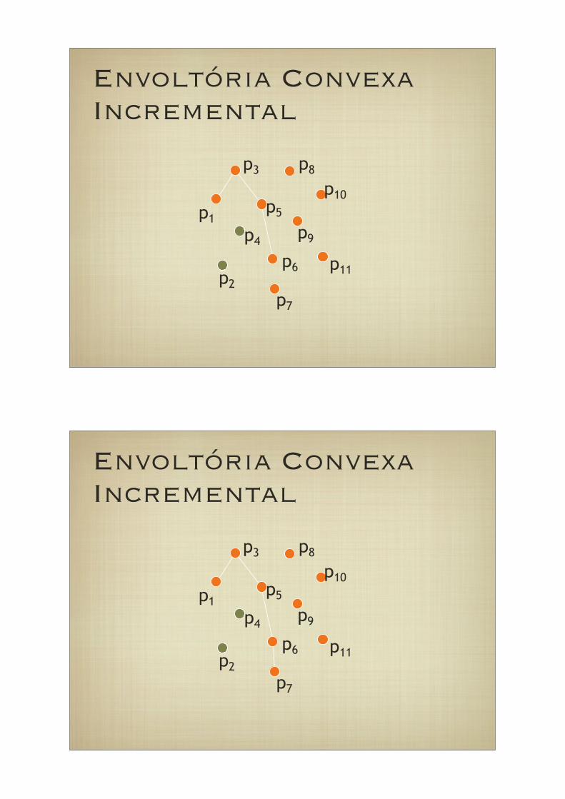
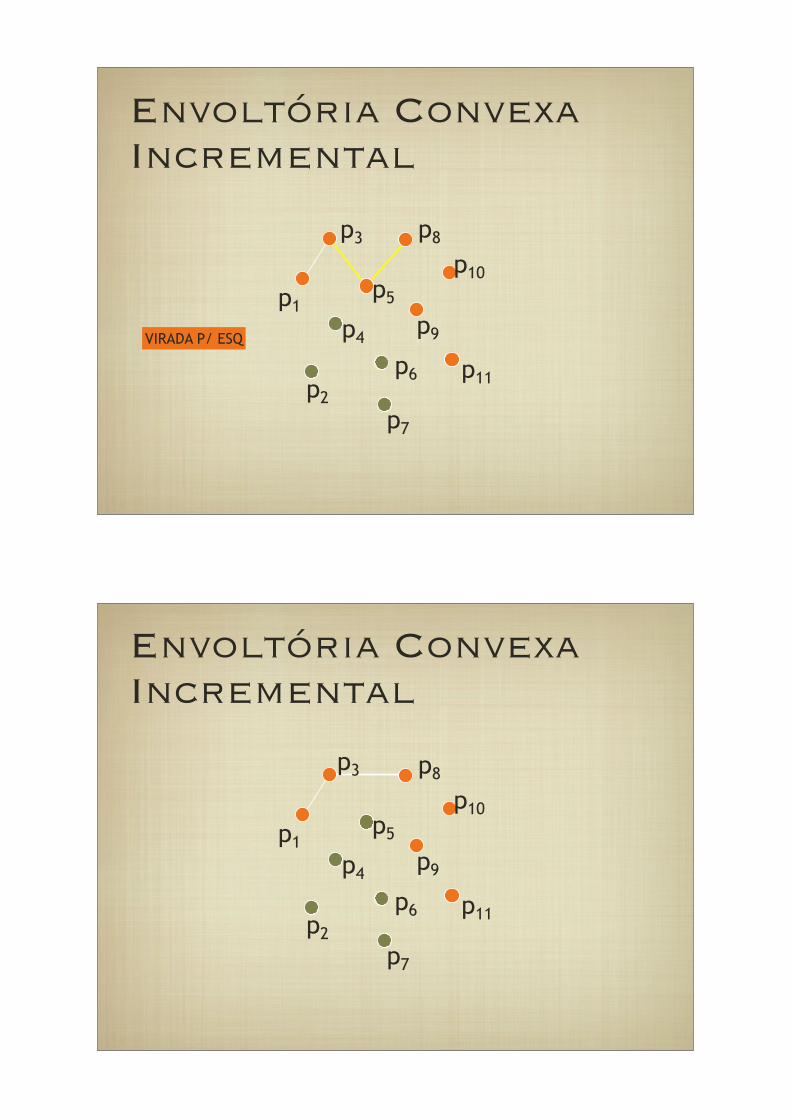
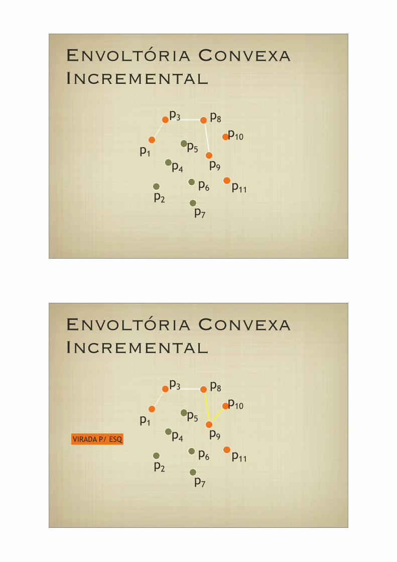
Envoltória Convexa Incremental
p9
p2
p8
p6
p5
p4
p11
p1
p7p3
p10
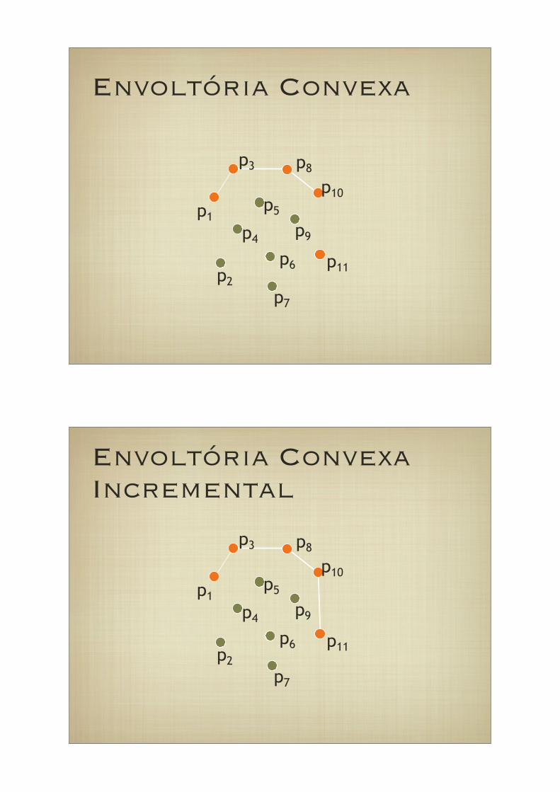
• Abordagem incremental: Adicionar pontos um por um e atualizar a solucao
•
Envoltória Convexa Incremental
p9
p2
p8
p6
p5
p4
p11
p1
p7p3
p10
• Abordagem incremental: Adicionar pontos um por um e atualizar a solucao
• Classificar os pontos em x, obtendo umasequencia ordenada p1, p2, ..., pn
• Calcular a EC superior percorrendo a lista acima da esquerda para a direita
• Calcular a EC inferior percorrendo a lista acima da direita para a esquerda
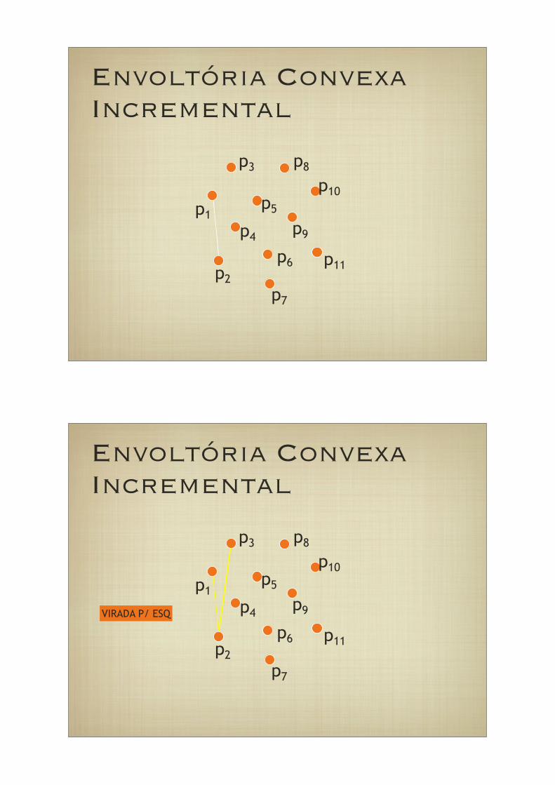
Envoltória Convexa Incremental
p3
p1
p2
p7
p11
p10
p8
p5
p4p9
p6
Envoltória Convexa Incremental
p3
p1
p2
p7
p11
p10
p8
p5
p4p9
p6
VIRADA P/ ESQ

Envoltória Convexa Incremental
p3
p1
p2
p7
p11
p10
p8
p5
p4p9
p6
Envoltória Convexa Incremental
p3
p1
p2
p7
p11
p10
p8
p5
p4p9
p6
Envoltória Convexa Incremental
p3
p1
p2
p7
p11
p10
p8
p5
p4p9
p6
VIRADA P/ ESQ
Envoltória Convexa Incremental
p3
p1
p2
p7
p11
p10
p8
p5
p4p9
p6
VIRADA P/ ESQ
Envoltória Convexa Incremental
p3
p1
p2
p7
p11
p10
p8
p5
p4p9
p6
Envoltória Convexa Incremental
p3
p1
p2
p7
p11
p10
p8
p5
p4p9
p6

Envoltória Convexa Incremental
p3
p1
p2
p7
p11
p10
p8
p5
p4p9
p6
VIRADA P/ ESQ
Envoltória Convexa Incremental
p3
p1
p2
p7
p11
p10
p8
p5
p4p9
p6
VIRADA P/ ESQ
Envoltória Convexa Incremental
p3
p1
p2
p7
p11
p10
p8
p5
p4p9
p6
VIRADA P/ ESQ
Envoltória Convexa Incremental
p3
p1
p2
p7
p11
p10
p8
p5
p4p9
p6
Envoltória Convexa Incremental
p3
p1
p2
p7
p11
p10
p8
p5
p4p9
p6
Envoltória Convexa Incremental
p3
p1
p2
p7
p11
p10
p8
p5
p4p9
p6
VIRADA P/ ESQ
Envoltória Convexa
p3
p1
p2
p7
p11
p10
p8
p5
p4p9
p6
Envoltória Convexa Incremental
p3
p1
p2
p7
p11
p10
p8
p5
p4p9
p6
Envoltória Convexa Incremental
p3
p1
p2
p7
p11
p10
p8
p5
p4p9
p6
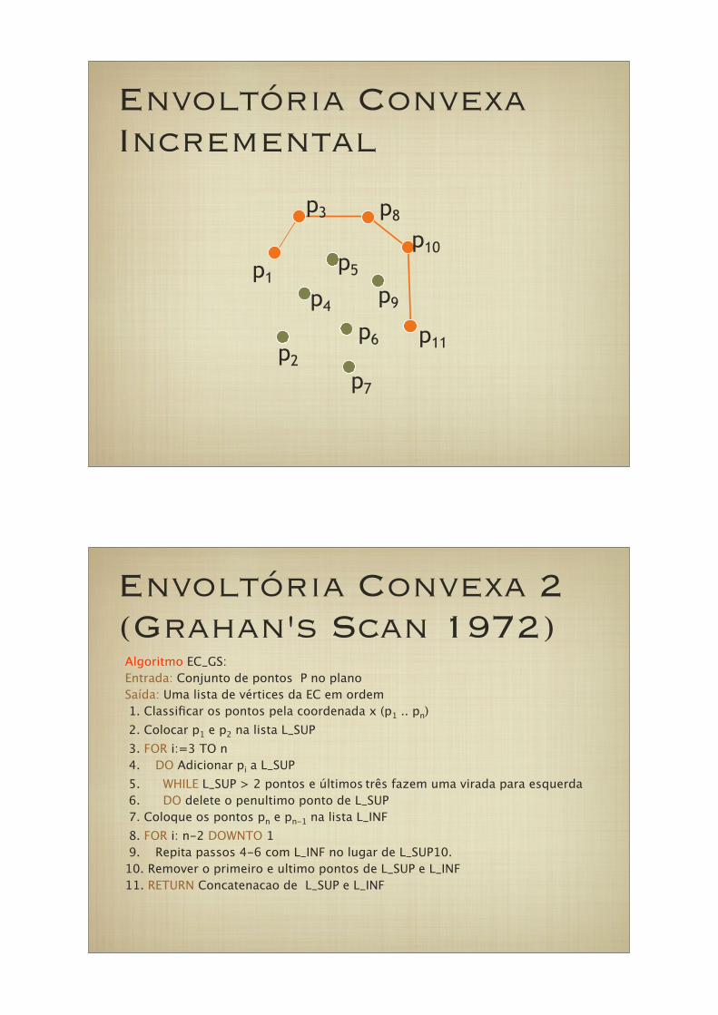
Envoltória Convexa 2 (Grahan's Scan 1972)
Algoritmo EC_GS:
Entrada: Conjunto de pontos P no plano
Saída: Uma lista de vértices da EC em ordem
1. Classificar os pontos pela coordenada x (p1 .. pn)
2. Colocar p1 e p2 na lista L_SUP
3. FOR i:=3 TO n
4. DO Adicionar pi a L_SUP
5. WHILE L_SUP > 2 pontos e últimos!três fazem uma virada para esquerda
6. DO delete o penultimo ponto de L_SUP
7. Coloque os pontos pn e pn-1 na lista L_INF
8. FOR i: n-2 DOWNTO 1
9. Repita passos 4-6 com L_INF no lugar de L_SUP10.
10. Remover o primeiro e ultimo pontos de L_SUP e L_INF
11. RETURN Concatenacao de L_SUP e L_INF
Envoltória Convexa 2
Algoritmo EC_GS:
Entrada: Conjunto de pontos P no plano
Saída: Uma lista de vértices da EC em ordem
1. Classificar os pontos pela coordenada x (p1 .. pn)
2. Colocar p1 e p2 na lista L_SUP
3. FOR i:=3 TO n
4. DO Adicionar pi a L_SUP
5. WHILE L_SUP > 2 pontos e últimos!três fazem uma virada para esquerda
6. DO delete o penultimo ponto de L_SUP
7. Coloque os pontos pn e pn-1 na lista L_INF
8. FOR i: n-2 DOWNTO 1
9. Repita passos 4-6 com L_INF no lugar de L_SUP10.
10. Remover o primeiro e ultimo pontos de L_SUP e L_INF
11. RETURN Concatenacao de L_SUP e L_INF
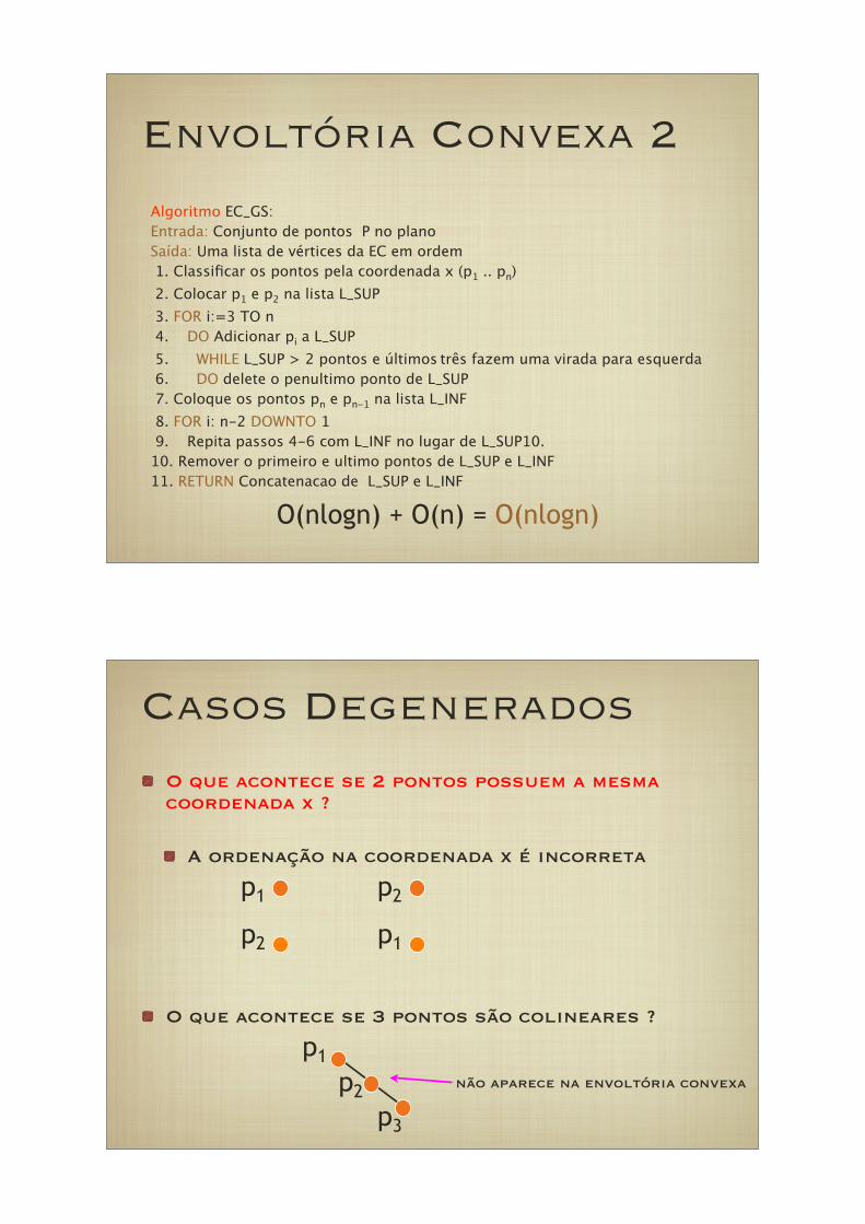
O(nlogn) + O(n) = O(nlogn)
Casos Degenerados
O que acontece se 2 pontos possuem a mesma coordenada x ?
A ordenação na coordenada x é incorreta
O que acontece se 3 pontos são colineares ?
p1
p2
p2
p1
p1
p2
p3
não aparece na envoltória convexa
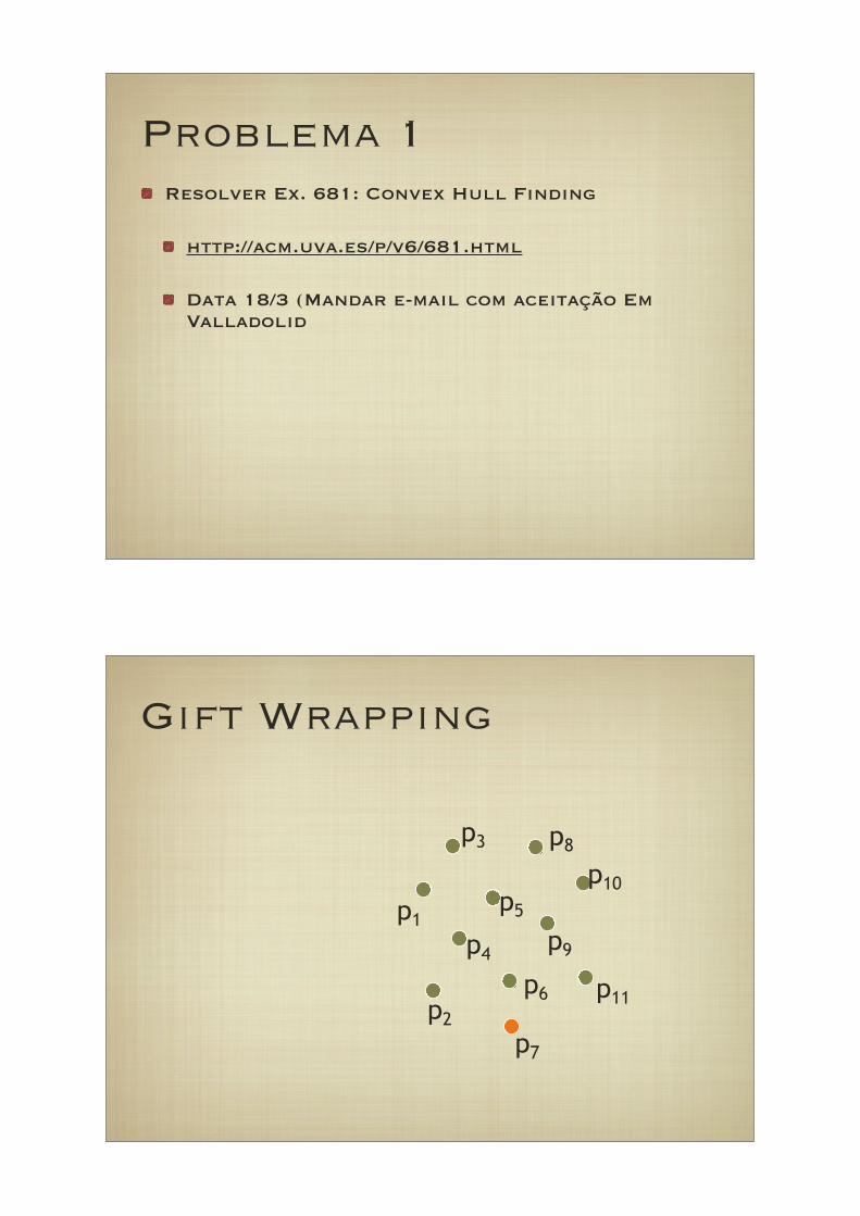
Problema 1Resolver Ex. 681: Convex Hull Finding
http://acm.uva.es/p/v6/681.html
Data 18/3 (Mandar e-mail com aceitação Em Valladolid
Gift Wrapping
p3
p1
p2
p7
p11
p10
p8
p5
p4p9
p6
Gift Wrapping
p3
p1
p2
p7
p11
p10
p8
p5
p4p9
p6
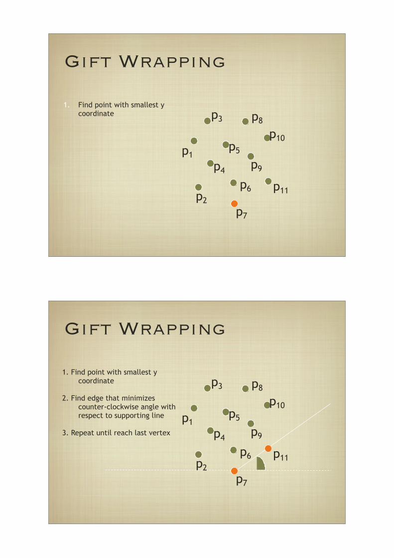
1. Find point with smallest y coordinate
Gift Wrapping
p3
p1
p2
p7
p11
p10
p8
p5
p4p9
p6
1. Find point with smallest y coordinate
2. Find edge that minimizes counter-clockwise angle with respect to supporting line
3. Repeat until reach last vertex
Gift Wrapping
p3
p1
p2
p7
p11
p10
p8
p5
p4p9
p6
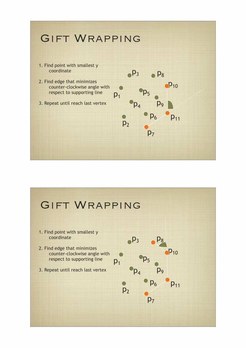
1. Find point with smallest y coordinate
2. Find edge that minimizes counter-clockwise angle with respect to supporting line
3. Repeat until reach last vertex
Gift Wrapping
p3
p1
p2
p7
p11
p10
p8
p5
p4p9
p6
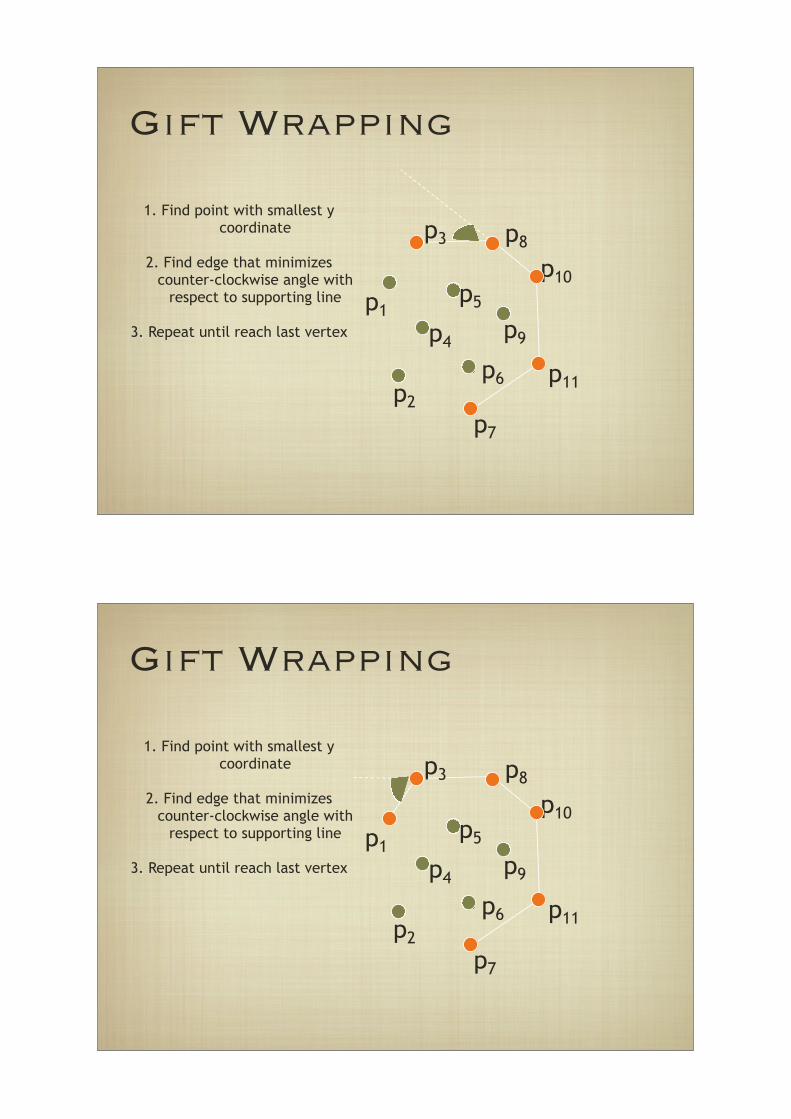
1. Find point with smallest y coordinate
2. Find edge that minimizes counter-clockwise angle with respect to supporting line
3. Repeat until reach last vertex
Gift Wrapping
p3
p1
p2
p7
p11
p10
p8
p5
p4p9
p6
1. Find point with smallest y coordinate
2. Find edge that minimizes counter-clockwise angle with
respect to supporting line
3. Repeat until reach last vertex
Gift Wrapping
p3
p1
p2
p7
p11
p10
p8
p5
p4p9
p6
1. Find point with smallest y coordinate
2. Find edge that minimizes counter-clockwise angle with
respect to supporting line
3. Repeat until reach last vertex
Gift Wrapping
p3
p1
p2
p7
p11
p10
p8
p5
p4p9
p6
1. Find point with smallest y coordinate
2. Find edge that minimizes counter-clockwise angle with
respect to supporting line
3. Repeat until reach last vertex
Gift Wrapping
p3
p1
p2
p7
p11
p10
p8
p5
p4p9
p6
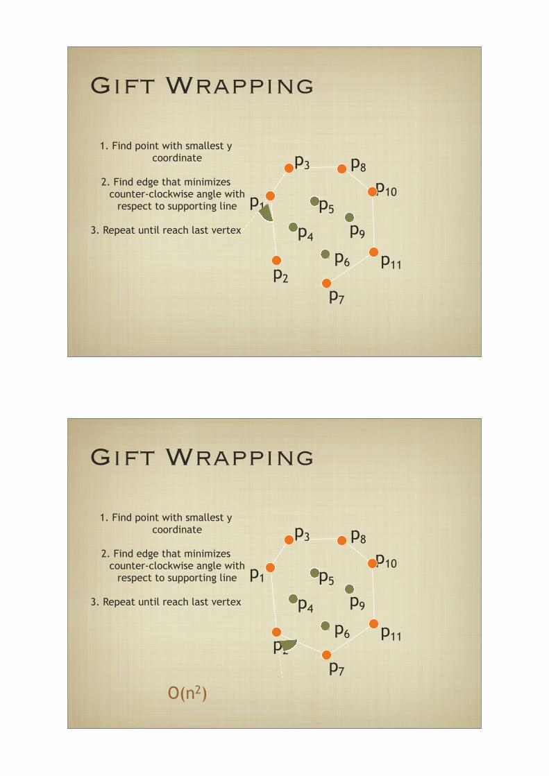
O(n2)
1. Find point with smallest y coordinate
2. Find edge that minimizes counter-clockwise angle with
respect to supporting line
3. Repeat until reach last vertex
Quickhull
p3
p1
p2
p7
p11
p10
p8
p5
p4p9
p6
Quickhull
p3
p1
p2
p7
p11
p10
p8
p5
p4p9
p6
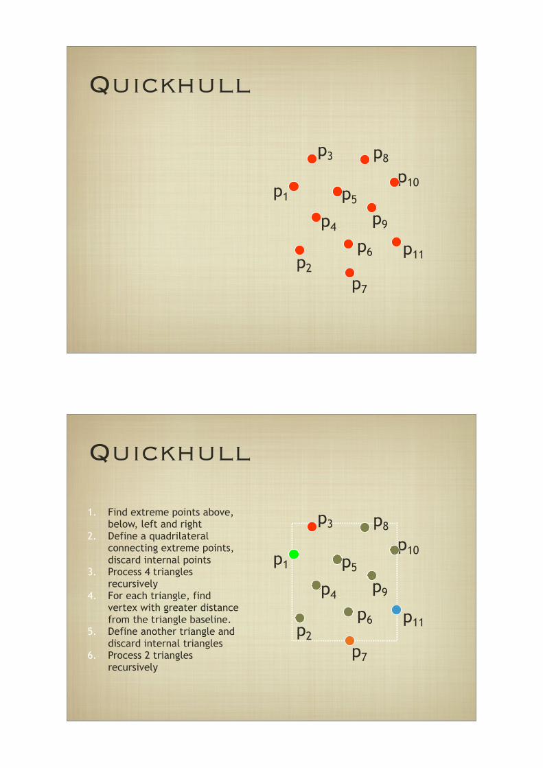
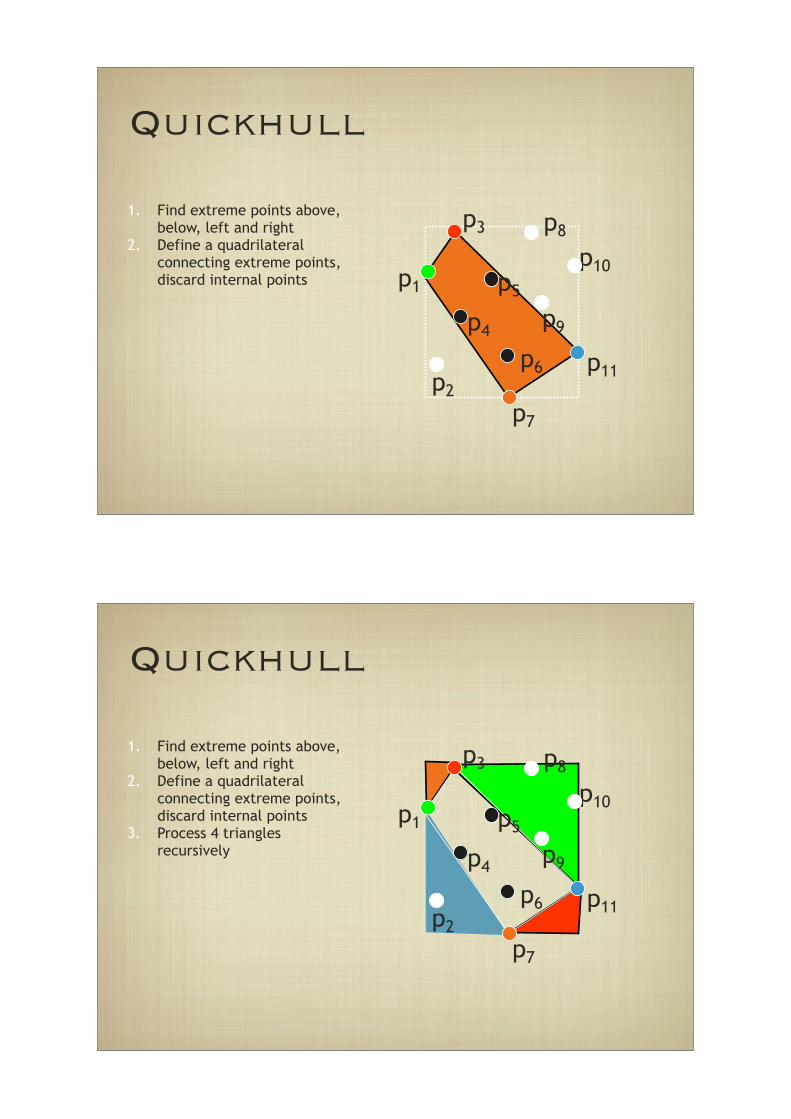
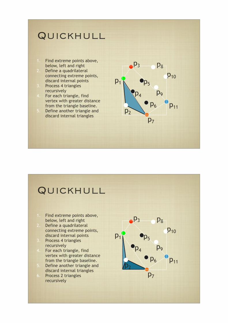
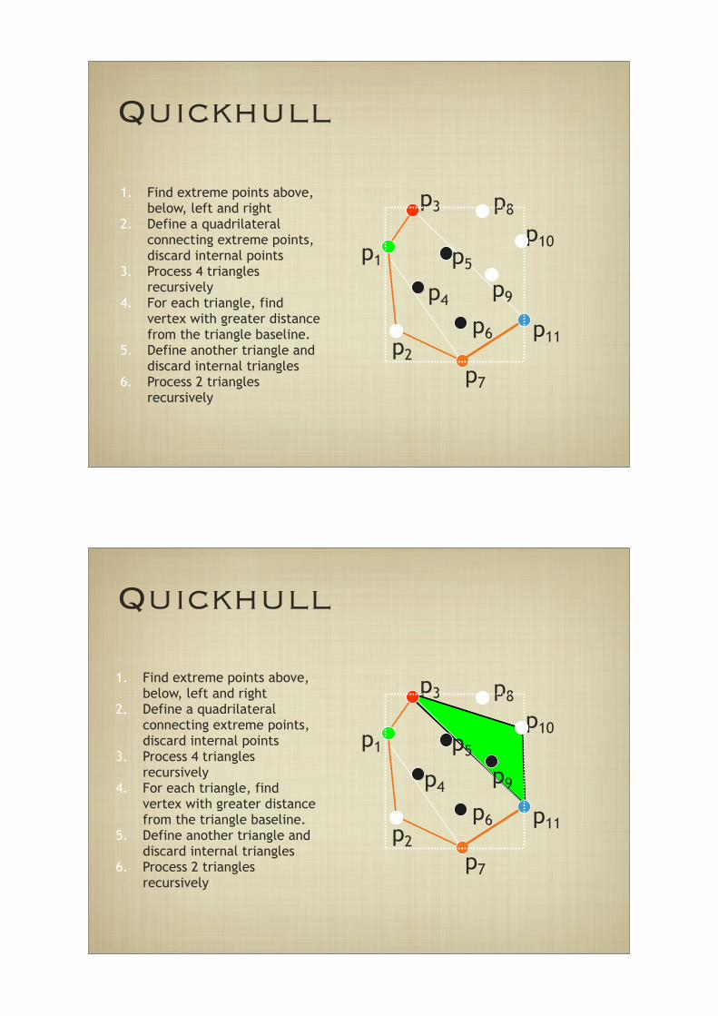
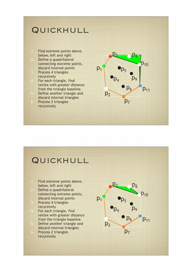
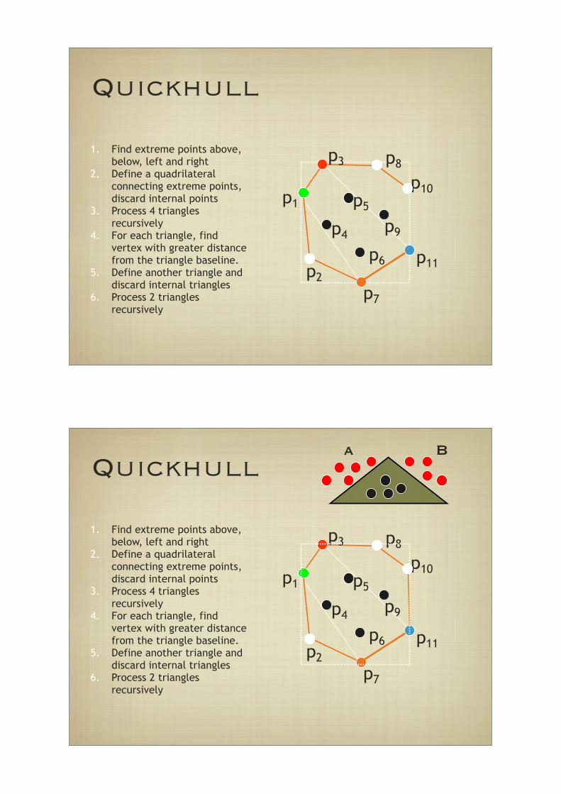
1. Find extreme points above, below, left and right
2. Define a quadrilateral connecting extreme points, discard internal points
3. Process 4 triangles recursively
4. For each triangle, find vertex with greater distance from the triangle baseline.
5. Define another triangle and discard internal triangles
6. Process 2 triangles recursively
Quickhull
p3
p1
p2
p7
p11
p10
p8
p5
p4p9
p6
1. Find extreme points above, below, left and right
2. Define a quadrilateral connecting extreme points, discard internal points
Quickhull
p3
p1
p2
p7
p11
p10
p8
p5
p4p9
p6
1. Find extreme points above, below, left and right
2. Define a quadrilateral connecting extreme points, discard internal points
3. Process 4 triangles recursively
Quickhull
p3
p1
p2
p7
p11
p10
p8
p5
p4p9
p6
1. Find extreme points above, below, left and right
2. Define a quadrilateral connecting extreme points, discard internal points
3. Process 4 triangles recursively
4. For each triangle, find vertex with greater distance from the triangle baseline.
5. Define another triangle and discard internal triangles
6. Process 2 triangles recursively
a B
Quickhull
p3
p1
p2
p7
p11
p10
p8
p5
p4p9
p6
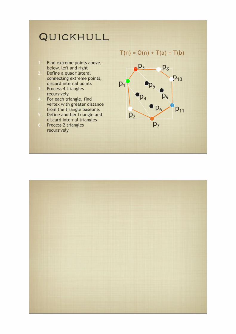
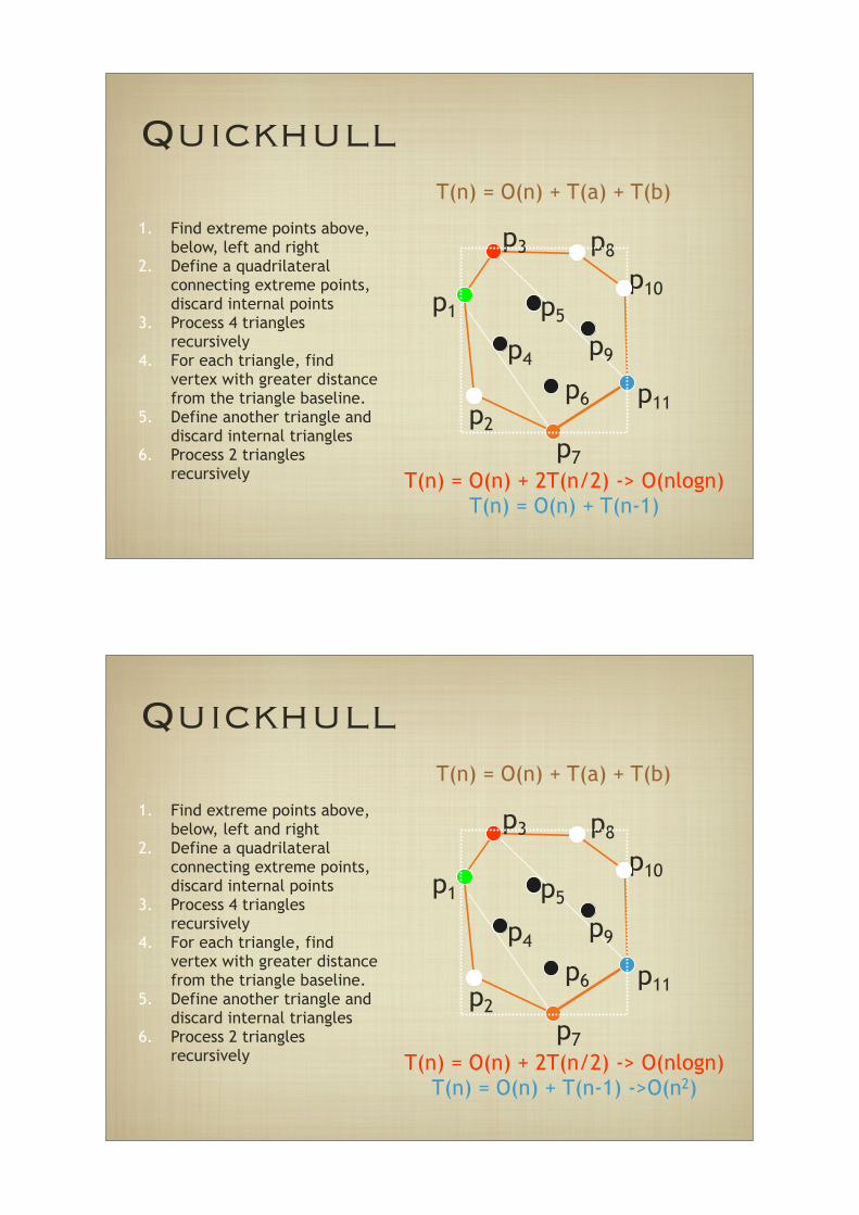
T(n) = O(n) + T(a) + T(b)
1. Find extreme points above, below, left and right
2. Define a quadrilateral connecting extreme points, discard internal points
3. Process 4 triangles recursively
4. For each triangle, find vertex with greater distance from the triangle baseline.
5. Define another triangle and discard internal triangles
6. Process 2 triangles recursively
Quickhull
p3
p1
p2
p7
p11
p10
p8
p5
p4p9
p6
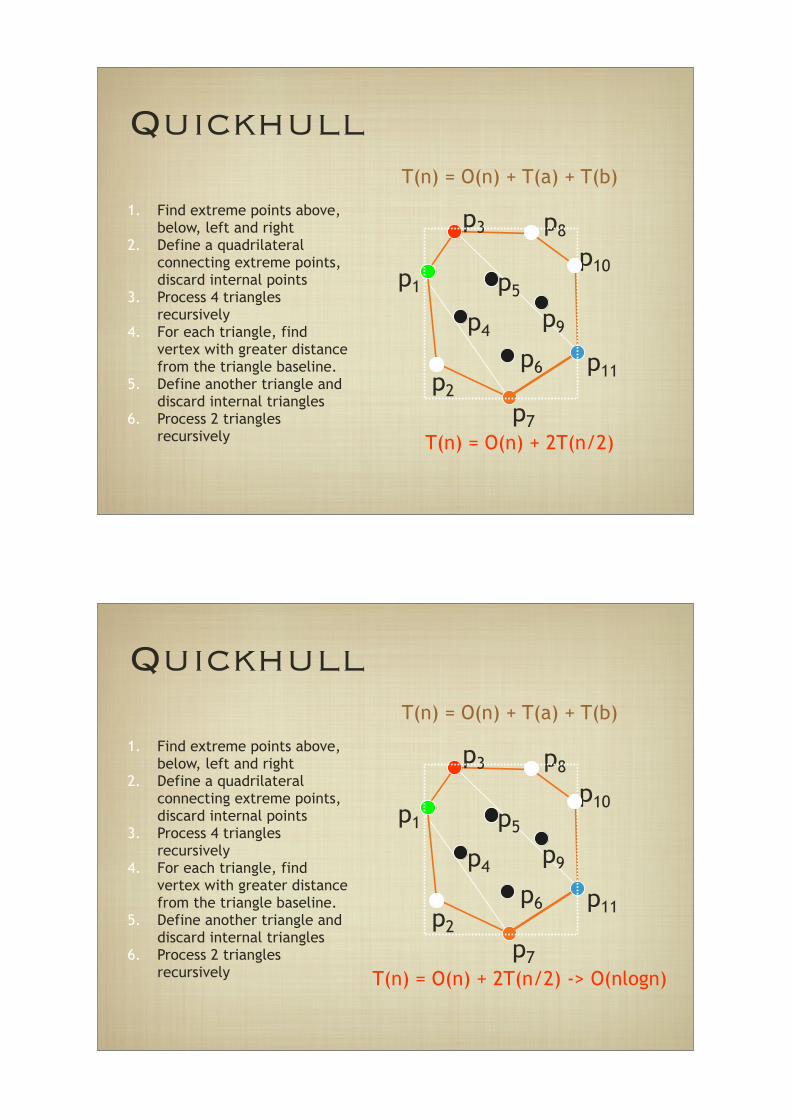
T(n) = O(n) + 2T(n/2)
T(n) = O(n) + T(a) + T(b)
1. Find extreme points above, below, left and right
2. Define a quadrilateral connecting extreme points, discard internal points
3. Process 4 triangles recursively
4. For each triangle, find vertex with greater distance from the triangle baseline.
5. Define another triangle and discard internal triangles
6. Process 2 triangles recursively
Quickhull
p3
p1
p2
p7
p11
p10
p8
p5
p4p9
p6
T(n) = O(n) + 2T(n/2) -> O(nlogn)
T(n) = O(n) + T(a) + T(b)
1. Find extreme points above, below, left and right
2. Define a quadrilateral connecting extreme points, discard internal points
3. Process 4 triangles recursively
4. For each triangle, find vertex with greater distance from the triangle baseline.
5. Define another triangle and discard internal triangles
6. Process 2 triangles recursively
Quickhull
p3
p1
p2
p7
p11
p10
p8
p5
p4p9
p6
T(n) = O(n) + 2T(n/2) -> O(nlogn)T(n) = O(n) + T(n-1)
T(n) = O(n) + T(a) + T(b)
1. Find extreme points above, below, left and right
2. Define a quadrilateral connecting extreme points, discard internal points
3. Process 4 triangles recursively
4. For each triangle, find vertex with greater distance from the triangle baseline.
5. Define another triangle and discard internal triangles
6. Process 2 triangles recursively
Quickhull
p3
p1
p2
p7
p11
p10
p8
p5
p4p9
p6
T(n) = O(n) + 2T(n/2) -> O(nlogn)T(n) = O(n) + T(n-1) ->O(n2)
T(n) = O(n) + T(a) + T(b)
1. Find extreme points above, below, left and right
2. Define a quadrilateral connecting extreme points, discard internal points
3. Process 4 triangles recursively
4. For each triangle, find vertex with greater distance from the triangle baseline.
5. Define another triangle and discard internal triangles
6. Process 2 triangles recursively
Divide-and-Conquer
p9
p8p6
p5
p4
p11
p1
p7 p3
p10
Divide-and-Conquer
p9
p8p6
p5
p4
p11
p1
p7 p3
p10
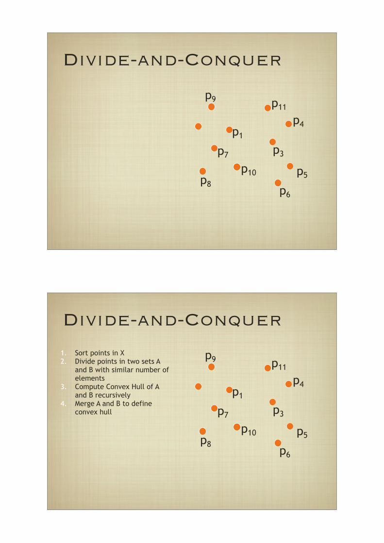
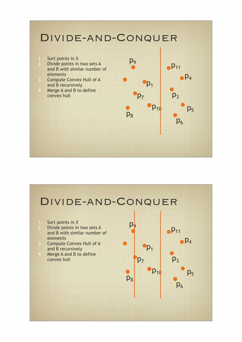
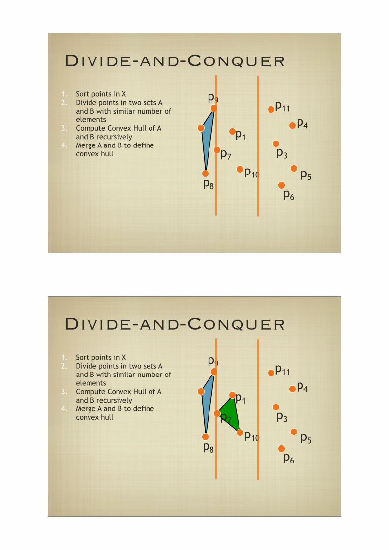
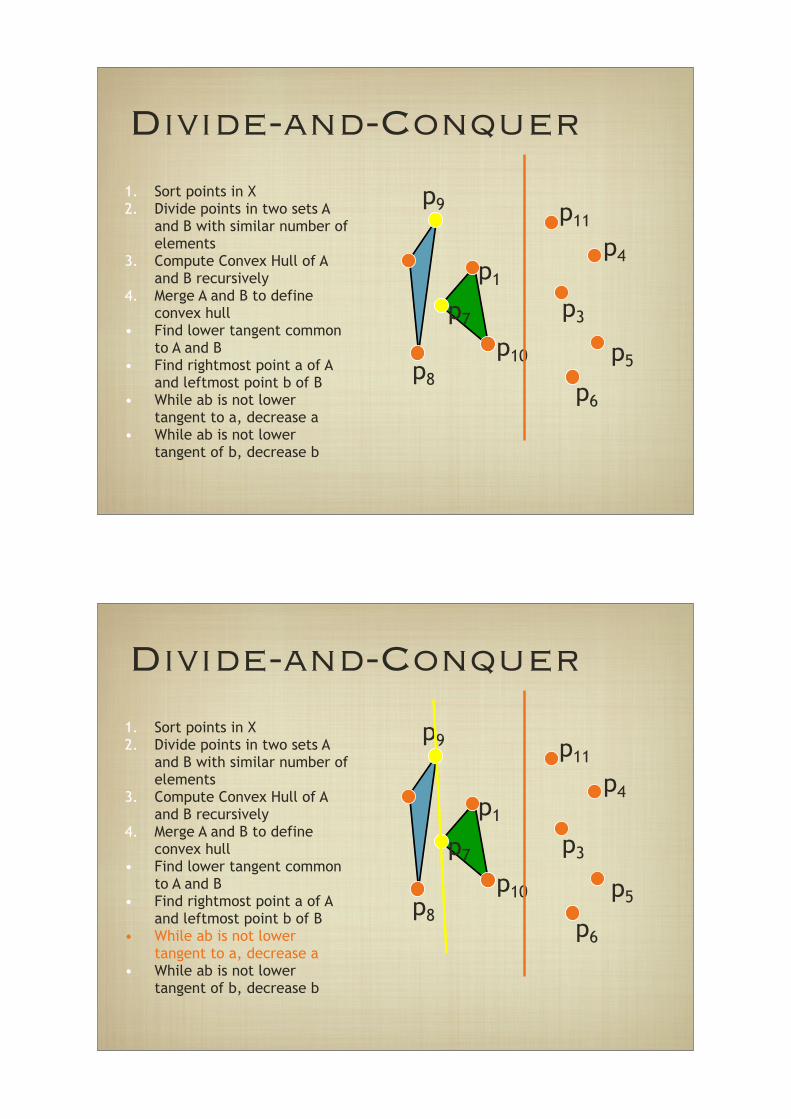
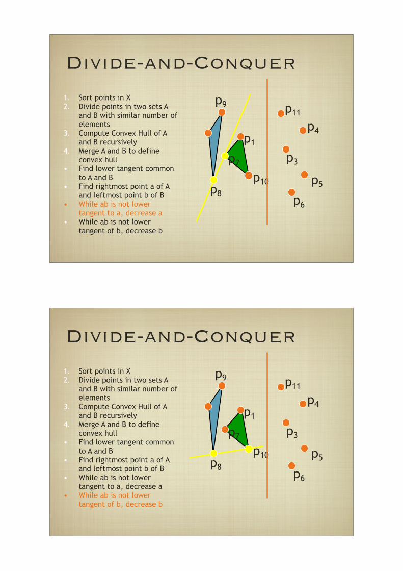
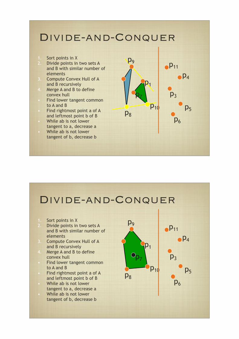
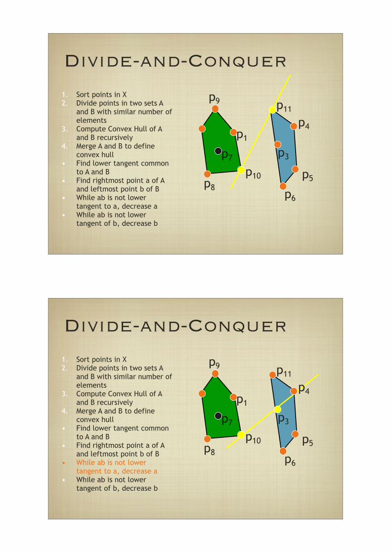
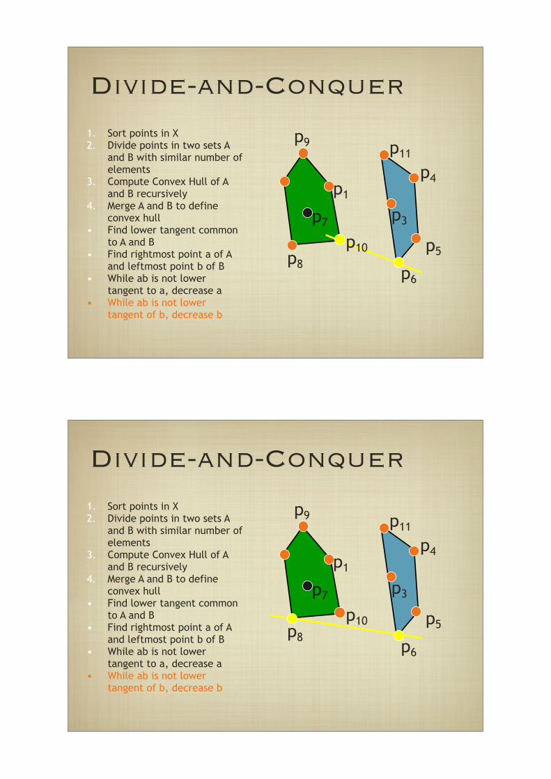
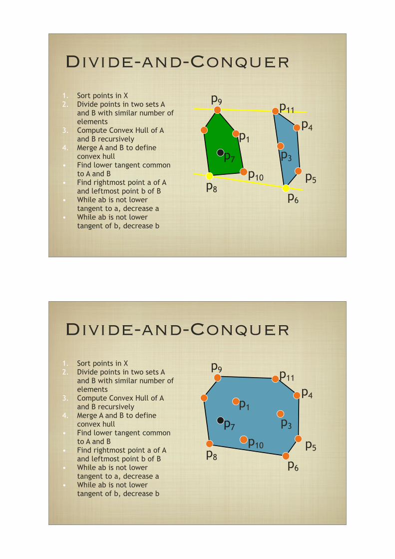
1. Sort points in X2. Divide points in two sets A
and B with similar number of elements
3. Compute Convex Hull of A and B recursively
4. Merge A and B to define convex hull
Divide-and-Conquer
p9
p8p6
p5
p4
p11
p1
p7 p3
p10
1. Sort points in X2. Divide points in two sets A
and B with similar number of elements
3. Compute Convex Hull of A and B recursively
4. Merge A and B to define convex hull
Divide-and-Conquer
p9
p8p6
p5
p4
p11
p1
p7 p3
p10
1. Sort points in X2. Divide points in two sets A
and B with similar number of elements
3. Compute Convex Hull of A and B recursively
4. Merge A and B to define convex hull
Divide-and-Conquer
p9
p8p6
p5
p4
p11
p1
p7 p3
p10
1. Sort points in X2. Divide points in two sets A
and B with similar number of elements
3. Compute Convex Hull of A and B recursively
4. Merge A and B to define convex hull
Divide-and-Conquer
p9
p8p6
p5
p4
p11
p1
p7 p3
p10
1. Sort points in X2. Divide points in two sets A
and B with similar number of elements
3. Compute Convex Hull of A and B recursively
4. Merge A and B to define convex hull
Divide-and-Conquer
p9
p8p6
p5
p4
p11
p1
p7 p3
p10
1. Sort points in X2. Divide points in two sets A
and B with similar number of elements
3. Compute Convex Hull of A and B recursively
4. Merge A and B to define convex hull
• Find lower tangent common to A and B
• Find rightmost point a of A and leftmost point b of B
• While ab is not lower tangent to a, decrease a
• While ab is not lower tangent of b, decrease b
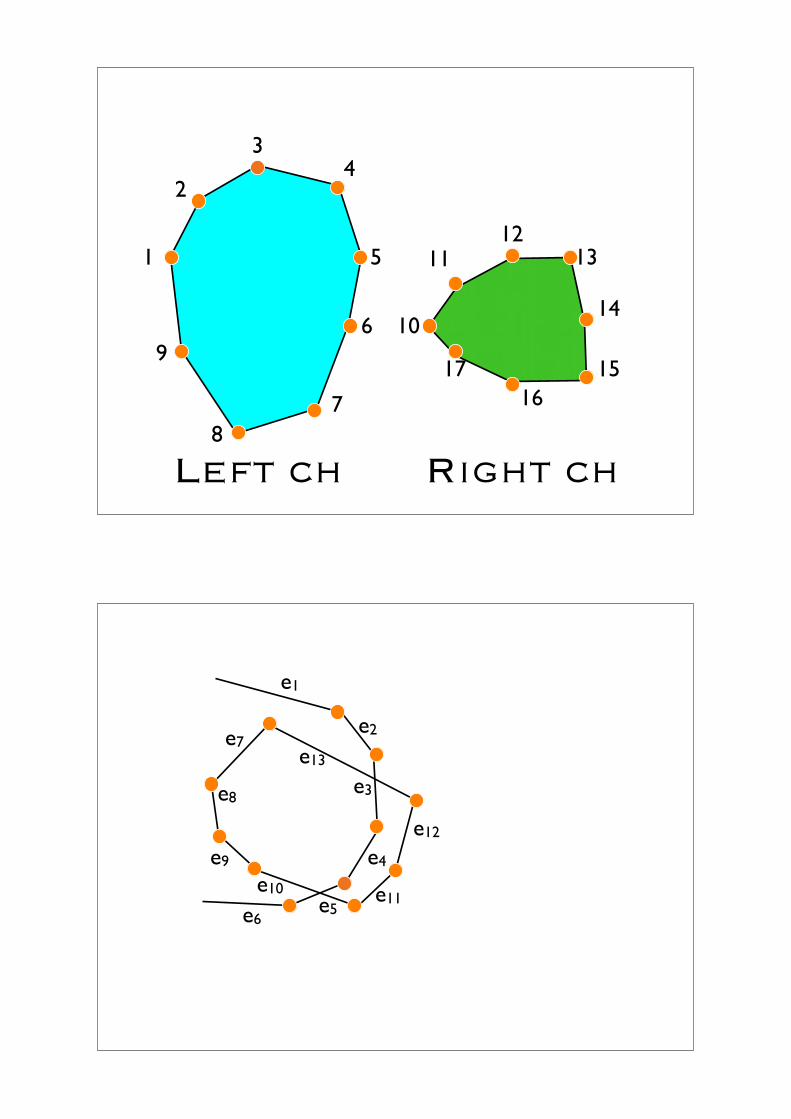
Right chLeft ch
1
2
3
4
5
6
7
8
9
10
11
12
13
14
15
16
17
e1
e2
e3
e4
e5e6
e7
e8
e9
e10 e11
e12
e13
21
34
56
7
8
910
11
12
13
14
15