universidade federal do rio grande do sul programa de … · tabela 1. lista de espécies e grupos...
TRANSCRIPT

UNIVERSIDADE FEDERAL DO RIO GRANDE DO SUL
INSTITUTO DE GEOCIÊNCIAS
PROGRAMA DE PÓS-GRADUAÇÃO EM GEOCIÊNCIAS
EVOLUÇÃO PALEOCEANOGRÁFICA E ESTRATIGRAFIA ISOTÓPICA COM
FORAMINÍFEROS PLANCTÔNICOS NO QUATERNÁRIO TARDIO DA
BACIA DE CAMPOS
SANDRO MONTICELLI PETRÓ
Orientador – Prof. Dr. João Carlos Coimbra
Coorientadora – Profa. Dra. Ana Maria Pimentel Mizusaki
Porto Alegre – 2013

UNIVERSIDADE FEDERAL DO RIO GRANDE DO SUL
INSTITUTO DE GEOCIÊNCIAS
PROGRAMA DE PÓS-GRADUAÇÃO EM GEOCIÊNCIAS
EVOLUÇÃO PALEOCEANOGRÁFICA E ESTRATIGRAFIA ISOTÓPICA COM
FORAMINÍFEROS PLANCTÔNICOS NO QUATERNÁRIO TARDIO DA
BACIA DE CAMPOS
SANDRO MONTICELLI PETRÓ
ORIENTADOR – Prof. Dr. João Carlos Coimbra
COORIENTADORA – Profa. Dra. Ana Maria Pimentel Mizusaki
COMISSÃO EXAMINADORA
Profa. Dra. Adriana Leonhardt – Instituto de Oceanografia, Universidade Federal do Rio Grande
Profa. Dra. Ana Luisa Carreño – Instituto de Geología, Universidad Nacional Autónoma de México
Profa. Dra. Karen Badaraco Costa – Instituto Oceanográfico, Universidade de São Paulo
Dissertação de Mestrado apresentada como requisito parcial para obtenção do Título de Mestre em Geociências.
Porto Alegre - 2013
Petró, Sandro Monticelli
Evolução Paleoceanográfica e Estratigrafia Isotópica com Foraminíferos Planctônicos no Quaternário Tardio da Bacia de Campos. / Sandro Monticelli Petró. - Porto Alegre: IGEO/UFRGS, 2013.
[60 f]. il.
Dissertação de Mestrado. - Universidade Federal do Rio Grande do Sul. Instituto de Geociências. Curso de Geologia. Porto Alegre, RS - BR, 2013.
Orientador: Prof. Dr. João Carlos Coimbra Co-Orientadora: Profa. Dra. Ana Maria Mizusaki
1. RNA’s. 2. 14C. 3. MIS. 4. Glacial. 5. Interglacial. 6. Quaternário. I. João Carlos Coimbra. II. Ana Maria Mizusaki. Título.
____________________________________________________
Catalogação na Publicação Biblioteca Geociências – UFRGS

II
AGRADECIMENTOS
Agradeço ao PRH-PB-215 pelo apoio financeiro na forma de bolsa, de custeio
das análises e de viagens a congressos e visitas técnicas.
Ao Prof. Dr. Kucera, da Universidade de Bremen, Alemanha, pelos cálculos
de paleotemperaturas.
À Petrobras pela doação das amostras ao Laboratório de Microfósseis
Calcários do IGeo/UFRGS.
À Profa. Dra. María Alejándra Gómez Pivel, da PUC-RS, pelo incentivo e
inúmeras discussões fundamentais para a realização desta dissertação
À toda equipe do Laboratório de Microfósseis Calcários da UFRGS.

III
RESUMO
Os foraminíferos são o grupo de microfósseis mais utilizado em bioestratigrafia, são
considerados os principais portadores de informações paleoceanográficas e
apresentam aplicações à análise de bacias sedimentares. O objetivo principal deste
trabalho é propor um modelo de reconstrução paleoceanográfica na Bacia de
Campos, analisando 61 amostras retiradas do testemunho GL-77, coletado no talude
inferior, offshore da bacia. O intervalo contempla os dois últimos ciclos Glacial-
Interglacial, correspondentes às biozonas de foraminíferos planctônicos W
(parcialmente), X, Y e Z. Por meio das análises de fauna total, datações em 14C e
análises isotópicas de δ18O e δ13C nas carapaças de foraminíferos planctônicos,
obtiveram-se estimativas de variações de paleoprodutividade, paleossalinidade e
paleotemperatura superficiais do mar; foi elaborado um modelo de idade e,
posteriormente, as estimativas de taxas de sedimentação. O modelo de idade
identificou o Último Máximo Glacial (UMG) e estimou as idades de alguns eventos
bioestratigráficos, como o datum YP.2, o limite MIS 3/4 (coincidente com o limite
Y2/Y3), o limite Y1/Y2 e o datum YP.4. As taxas de sedimentação estão
estranhamente elevadas na Biozona X (intervalo glacial) onde se esperaria taxas
menores. No Holoceno há uma elevada taxa de sedimentação, associada à
influência do delta do Rio Paraíba do Sul, na porção norte da bacia. As
paleotemperaturas reagem sazonalmente no intervalo glacial, onde a amplitude
entre verão e inverno é maior que a registrada nos períodos interglaciais. Foi
observada uma correlação das paleotemperaturas com as condições ambientais
marcadas pelas subzonas quentes e frias na Biozona X. Baseado na razão P/B pode
ser identificado um limite de sequências junto ao limite MIS 4/5. A paleossalinidade
reduz em intervalos de degelo. A paleoprodutividade diminui de 29 ka (limite MIS
2/3) ao UMG e aumenta próximo ao limite Pleistoceno/Holoceno. Finalmente, se
observou que a transição Pleistoceno/Holoceno ocorre dentro da Biozona Y, e não é
relacionada temporalmente ao início da Biozona Z.
Palavras chave: RNA’s, 14C, MIS, Glacial, Interglacial, Quaternário.

IV
ABSTRACT
Planktonic foraminifera is the most useful microfossil group for biostratigraphic
studies, being considered the main carriers of paleoceanographic information and
being applicable to the analysis of sedimentary basins. The main aim of this work is
to propose a paleoceanographic reconstruction model in the Campos Basin, by
analyzing 61 samples taken from the GL-77 core, collected at the lower continental
slope, in the offshore part of the basin. The interval comprises the last two Glacial-
Interglacial cycles, corresponding to the planktonic foraminifera biozones W
(partially), X, Y and Z. By means of analysis of the total fauna, datings in 14C and
isotopic analyses of δ18O and δ13C in shells of planktonic foraminifera estimates of
variations of paleoproductivity, paleosalinity and sea surface paleotemperature were
obtained; an age model and, posteriorly, the sedimentation rates were calculated.
The age model identified the Last Glacial Maximum (LGM) and estimated the ages of
a few biostratigraphic events, such as YP.2 datum, the MIS 3/4 boundary (which
coincides with the Y2/Y3 boundary), the Y1/Y2 boundary and the YP.4 datum. The
sedimentation rates are strangely elevated in Biozone X (glacial period) where lower
rates would be expected. In the Holocene there is an elevated sedimentation rate,
associated to the influence of the Paraíba do Sul River delta, at the northern portion
of the basin. The paleotemperatures oscillate seasonally in the glacial periods, when
the amplitude between summer and winter is larger than the one registered in the
interglacial periods. A correlation was observed between the paleotemperatures and
the environmental conditions characterized by the warm and cold subzones in
Biozone X. Based on the P/B ratio a limit of sequences can be identified next to the
MIS 4/5 boundary. Paleosalinity is reduced in deglaciation periods. Paleoproductivity
is reduced to 29 ka (MIS 2/3 boundary) by the LGM and increases near the
Pleistocene/Holocene boundary. Finally, it was observed that the
Pleistocene/Holocene transition occurs inside Biozone Y, and is not temporally
related to the beginning of Biozone Z.
Key words: ANN’s, 14C, MIS, Glacial, Interglacial, Quaternary.

V
Índice de Figuras
Figura 1. Mapa da localização do testemunho GL-77, no talude inferior da Bacia de
Campos. ................................................................................................................................. 10
Figura 2. Principais correntes oceânicas do Atlântico Sul (modificado de Peterson &
Stramma, 1991). No detalhe o diagrama T-S, com os índices termohalinos para cada
massa d'água (de acordo com Evans et al., 1983). ............................................................... 13
Figura 3. Arquitetura geral de uma rede neural artificial (modificado de Malmgren &
Nordlund, 1997; Kucera, 2003). .............................................................................................. 17
Figura 4. Esquema simplificado mostrando o comportamento dos isótopos de oxigênio
em função de variantes ambientais e o respectivo registro, durante a alternância de
períodos glaciais e interglaciais, observado em carbonatos marinhos (modificado de
White (2013) e <http://earthobservatory.nasa.gov/Features/Paleoclimatology_
OxygenBalance/>). ................................................................................................................. 21
Índice de Tabelas
Tabela 1. Lista de espécies e grupos taxonômicos do banco de dados para calibração das
RNA’s para o Oceano Atlântico Sul. Análise com base em kucera (2004). .............................. 18

VI
SUMÁRIO
1. INTRODUÇÃO E OBJETIVOS ................................................................................................... 7
2. ÁREA DE ESTUDO ..................................................................................................................... 9
2.1. Sedimentologia .................................................................................................................. 10
2.2. Oceanografia ...................................................................................................................... 11
2.3. Estado da Arte ................................................................................................................... 13
3. MATERIAL E MÉTODOS .......................................................................................................... 15
3.1. Paleotemperaturas ............................................................................................................ 15
3.2. Isótopos de Oxigênio ........................................................................................................ 18
3.3. Isótopos de Carbono ......................................................................................................... 20
3.4. Paleoprodutividade e paleossalinidade ......................................................................... 22
4. REFERÊNCIAS BIBLIOGRÁFICAS ........................................................................................ 24
5. MANUSCRITO SUBMETIDO À QUATERNARY INTERNATIONAL .................................. 28

7
1. INTRODUÇÃO E OBJETIVOS
Foraminíferos são protozoários rizópodes que secretam uma carapaça
calcária ou quitinosa ou a constroem a partir da aglutinação de fragmentos minerais
ou biogênicos. A carapaça é segmentada em uma série de câmaras que vão sendo
construídas ao longo da vida do organismo. Vivem, em sua grande maioria, em
ambiente marinho e apresentam hábito de vida planctônico ou bentônico. As formas
bentônicas habitam o fundo oceânico, junto ao sedimento, são abundantes na
plataforma e bons indicadores de variação paleoambiental. As formas planctônicas
têm a capacidade de se locomover na coluna d’água e, devido à sua abundância,
têm alto potencial de preservação e alta taxa de evolução, e assim constituem-se em
importantes indicadores de idade, sendo amplamente utilizadas na datação relativa
e na correlação das rochas sedimentares.
Os foraminíferos são também usados como proxy no estudo das alterações
oceanográficas e climáticas registradas no planeta desde o Paleozoico. Seus fósseis
são aplicados à análise de bacias desde os primórdios da indústria do petróleo, na
primeira metade do século XX, incluindo a datação relativa (biozoneamentos
internacionais), a reconstrução de paleoambientes e a identificação de variações do
nível do mar. O estudo dos foraminíferos fósseis permite estimar a profundidade,
temperatura e salinidade das águas superficiais e de fundo dos mares em que
viveram.
Em particular, os foraminíferos planctônicos fazem parte de um grupo de
microfósseis calcários encontrados no ambiente marinho, que tem sua ocorrência
restringida por certas condições ecológicas da massa d’água onde vivem, tais como:
temperatura, salinidade, profundidade da camada de mistura e disponibilidade de
alimento. Dessa forma, ao encontrarmos determinadas espécies em um testemunho,
podemos estimar as condições paleoclimáticas do ambiente onde o organismo vivia.
Os proxies utilizados neste trabalho correspondem à análise de fauna (com
aplicação de redes neurais artificiais), datações de 14C e isótopos estáveis de
carbono e oxigênio em foraminíferos planctônicos, com o objetivo de elaborar uma

8
proposta de evolução paleoceanográfica e correlação por estratigrafia isotópica no
intervalo Pleistoceno-Holoceno na Bacia de Campos. O período de tempo
correspondente ao Holoceno é contemplado na totalidade, porém o intervalo em
estudo não abrange todo o Pleistoceno, de forma que não foi possível refiná-lo
estratigraficamente, por isso optou-se pela designação de Quaternário tardio. Em
termos biestratigráficos, foram estudadas as biozonas de foraminíferos planctônicos
W (parcialmente), X, Y e Z, de Ericson & Wollin (1968).
Este trabalho tem como premissa que as condições ambientais controlam a
distribuição da fauna. As mudanças de condições ambientais geram um
desequilíbrio na razão entre isótopos estáveis (carbono e oxigênio), princípio
conhecido como fracionamento isotópico, cujas razões são preservadas em
microfósseis de organismos que precipitam carbonato em sua carapaça. Desta
forma, as razões isotópicas nas carapaças dos foraminíferos planctônicos
constituem um proxy para interpretações paleoambientais. Em outro aspecto,
sabendo-se que a ocorrência ou abundância de determinadas espécies reage às
mudanças climáticas, as variações nas associações fósseis ao longo do tempo
refletem uma mudança ambiental, principalmente de temperatura, que pode ser
estimada por métodos computacionais, neste caso as redes neurais artificiais
(RNA’s) de Kucera (2004).
O objetivo principal desta pesquisa é elaborar um modelo de evolução
paleoceanográfica e correlação por estratigrafia isotópica para os dois últimos ciclos
Glacial-Interglacial, contemplando as biozonas W (parcialmente), X, Y e Z de Ericson
& Wollin (1968) na Bacia de Campos. Foram elaborados um modelo de idade,
correlação por estratigrafia isotópica, estimativas de taxa de sedimentação e
paleoprodutividade, além de cálculos de paleotemperatura e paleossalinidade. Para
tanto, é aqui realizada uma análise conjunta de composição faunística por RNA’s,
das razões isotópicas do oxigênio e carbono e das datações pelo método
Accelerator Mass Spectrometry - AMS 14C em foraminíferos planctônicos obtidos do
testemunho GL-77, coletado no talude inferior desta bacia.

9
2. ÁREA DE ESTUDO
A Bacia de Campos localiza-se na Margem Continental Sudeste Brasileira, na
costa do Rio de Janeiro e sul do Espírito Santo, entre os paralelos 21º e 23ºS. A
bacia é limitada ao norte pelo Alto de Vitória, com a Bacia do Espírito Santo, e ao sul
pelo Alto de Cabo Frio, com a Bacia de Santos, e abrange aproximadamente
100.000 km2 de área (Fig.1).
A gênese da bacia envolve um contexto do tipo margem passiva, formada por
tectônica distensiva durante o Meso-Cenozóico. Sobre o embasamento econômico
constituído de rochas vulcânicas básicas com datação em torno de 120-130 Ma, são
reconhecidas as sequências continentais, de transição, de plataforma rasa e
plataforma profunda. Estas sequências são associadas com eventos vulcânicos
característicos e datadas, em média, de 90 e 60-30 Ma.
A sequência de interesse para este trabalho corresponde aos sedimentos do
Holoceno e parte do Pleistoceno, e inclui as formações Ubatuba (Membro Geribá),
Carapebus e Emboré (Membros São Tomé e Grussaí). Possui como limite inferior a
discordância de 1,6 Ma que se relaciona com a queda eustática global. O limite
superior corresponde aos sedimentos atuais do fundo marinho.
10
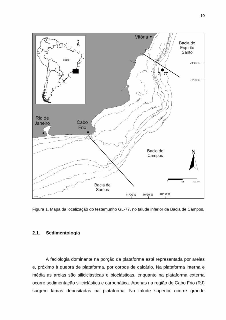
Figura 1. Mapa da localização do testemunho GL-77, no talude inferior da Bacia de Campos.
2.1. Sedimentologia
A faciologia dominante na porção da plataforma está representada por areias
e, próximo à quebra de plataforma, por corpos de calcário. Na plataforma interna e
média as areias são siliciclásticas e bioclásticas, enquanto na plataforma externa
ocorre sedimentação siliciclástica e carbonática. Apenas na região de Cabo Frio (RJ)
surgem lamas depositadas na plataforma. No talude superior ocorre grande

11
quantidade de sedimento arenoso, de natureza siliciclástica e bioclástica,
proveniente da plataforma. No talude médio e inferior predominam lamas, lamitos de
denudação e corais de águas profundas. O talude médio apresenta intercalações de
areia-lama com sedimento hemipelágico, e o talude inferior é coberto por marga
pelágica. Cânions lamosos e arenosos cortam o talude. Na região do sopé do talude
predominam cunhas de diamictitos e lamas que ocorrem também nas áreas mais
distais cortadas por raros cânions arenosos. Os sedimentos do Pleistoceno-
Holoceno são compostos por lamas siliciclásticas, com baixo teor carbonático e
matéria orgânica, intercaladas com areias turbidíticas (Caddah et al., 1998; Machado
et al., 2004; Winter et al., 2007).
2.2. Oceanografia
A área da Bacia de Campos está sob influência da Corrente do Brasil (CB). A
CB é uma corrente de contorno oeste, com origem na bifurcação da Corrente Sul
Equatorial, próximo à costa nordeste do Brasil, deslocando-se ao longo da costa
para o sul, até se encontrar com a Corrente das Malvinas (CM), na costa sul do
Brasil (Silveira et al., 2000) (Fig. 2).
A CB transporta, em superfície, Água Tropical (AT) com temperaturas
maiores que 20ºC e salinidade acima de 36‰ (Silveira et al., 2000). Abaixo dela flui
a Água Central do Atlântico Sul (ACAS) com temperaturas entre 6º e 20ºC e
salinidade entre 34,6 e 36‰ (Silveira et al., 2000). Esta massa d`água circula em
dois sentidos distintos: um para sul e outro para norte, sendo a bifurcação próximo
ao Cabo de São Tomé, 22ºS (Cirano et al., 2006). O limite entre estas duas massas
d’água coincide com a termoclina, profundidade onde ocorre uma queda brusca na
temperatura da água.
Na área correspondente à Bacia de Campos ocorrem importantes fenômenos
de ressurgência, próximos à cidade de Cabo Frio (RJ), devido a dois fenômenos:
ressurgência costeira e ressurgência de quebra de plataforma. A ressurgência

12
costeira é condicionada principalmente pelo regime de ventos na costa que empurra
a massa de água superficial para o interior do oceano, fazendo com que aflore a
água localizada logo abaixo. A ressurgência de quebra de plataforma é associada
aos vórtices e meandros ciclônicos da CB, cujo movimento provoca a subida da
ACAS para a plataforma (Campos et al., 1995 apud Silveira et al., 2000).
De modo geral, ao longo do oeste do Oceano Atlântico Sul a termoclina se
encontra mais profunda, em relação ao leste. Este fenômeno ocorre devido à
dinâmica da Corrente Sul Equatorial, que se movimenta para oeste, fazendo com
que aflorem águas profundas no leste do Atlântico. A ocorrência da zona de
ressurgência de Cabo Frio quebra esse padrão, e eleva localmente a profundidade
da termoclina.
Além da termoclina, a zona de ressurgência influencia na nutriclina,
profundidade onde há mudança brusca da produtividade, de modo a aumentar a
produtividade superficial da água do mar. Este fator faz com que ocorra uma
mudança local em relação ao padrão para águas tropicais, que geralmente são
oligotróficas, ou seja, pobres em nutrientes.

13
Figura 2. Principais correntes oceânicas do Atlântico Sul (modificado de Peterson & Stramma, 1991). No detalhe o diagrama T-S, com os índices termohalinos para cada massa d'água (de acordo com Evans et al., 1983).
2.3. Estado da Arte
Estudos sobre paleoceanografia do Quaternário no Atlântico Sul são recentes
e abrangem principalmente três grupos de microfósseis: foraminíferos, ostracodes e
nanofósseis calcários. A última década foi marcada por grandes avanços mundiais
nas pesquisas paleoceanográficas e, embora tenha havido alguns avanços nesta
área também no Atlântico Sul, em comparação aos demais oceanos as pesquisas
podem ser consideradas incipientes, principalmente levando-se em consideração a
extensão da margem continental brasileira e áreas adjacentes a serem exploradas.
Atualmente, o volume de dados disponíveis para o Atlântico Norte é imensamente

14
maior do que para o Atlântico Sul, e a margem ocidental desta bacia oceânica é
menos explorada do que a margem oriental, do ponto de vista paleoceanográfico.
Mesmo em estudos do Quaternário, o enfoque maior tem se voltado para a
bioestratigrafia. Vicalvi (1997, 1999), estudando a Bacia de Campos, propôs uma
subdivisão em zonas e subzonas bioestratigráficas, seguindo o modelo de Ericson e
Wollin (1968), baseando-se na ocorrência ou ausência de algumas espécies de
foraminíferos planctônicos. Sanjinés (2006) analisou três testemunhos coletados na
Bacia de Campos, cujos resultados constam em uma carta biocronoestratigráfica,
tendo o autor aplicado a metodologia da estratigrafia de sequências no intervalo
Pleistoceno-Holoceno. Tokutake (2005) e Maciel (2012) realizaram estudos
bioestratigráficos utilizando nanofósseis calcários. Ferreira et al. (2012) propuseram
um zoneamento paleoclimático com foraminíferos planctônicos para o Quaternário
da Bacia de Santos, bacia esta adjacente à Bacia de Campos.
Pelo fato dos foraminíferos planctônicos viverem em suspensão na coluna
d’água eles apresentam uma grande distribuição geográfica, o que nos permite aqui
extrapolar os limites da Bacia de Campos, relacionando outros trabalhos para o
Quaternário do Atlântico Sul. Toledo (2000) estudou as variações
paleoceanográficas no oeste do Atlântico Sul para os últimos 30 ka, baseado em
isótopos de oxigênio, foraminíferos planctônicos e nanofósseis calcários. Toledo et
al. (2007a) desenvolveram pesquisa sobre paleoprodutividade, enquanto Toledo et
al. (2007b) desenvolveram estudos sobre mudanças de salinidade superficial do mar
no oeste do Atlântico Sul. Pivel (2009) fez uma reconstrução da hidrologia superficial
do oeste do Atlântico Sul desde o Último Máximo Glacial (UMG) ao Recente.
Leonhardt (2011) elaborou uma reconstituição paleoceanográfica no Atlântico
Sudoeste, enfatizando as mudanças de paleoprodutividade, utilizando
cocolitoforídeos e isótopos.
15
3. MATERIAL E MÉTODOS
Foram analisadas 61 amostras do testemunho GL-77, coletado no talude
continental da Bacia de Campos, nas coordenadas 40º02'50"O e 21º12'22"S, sob
uma lâmina d’água de 1.287 m (Fig. 1). Todo o testemunho tem recuperação de
18,15 m descontínuos, porém neste trabalho foram utilizados os 14,65 m superiores.
O material encontra-se depositado no Laboratório de Microfósseis Calcários, do
Departamento de Paleontologia e Estratigrafia, do Instituto de Geociências da
UFRGS, sob número tombo M06306 (amostra 01) ao M06366 (amostra 61). Nestas
amostras foram conduzidas classificação de fauna total, análises de isótopos
estáveis de oxigênio e carbono e seis datações pelo método do 14C nas carapaças
de foraminíferos planctônicos. O processamento inicial das amostras tem maior
detalhamento no Capítulo 5 (MS submetido à QI). A partir destas análises foram
obtidas estimativas de variação de paleotemperatura, paleoprodutividade e
paleossalinidade superficiais da água do mar, além da elaboração de um modelo de
idade com as taxas de sedimentação.
3.1. Paleotemperaturas
A temperatura dos oceanos varia de acordo com a latitude, de um modo
geral, mais quente no equador, esfriando em direção aos polos e também à medida
que aumenta a profundidade na coluna d’água. A área em estudo é influenciada
pelas massas de água mais superficiais da CB: a AT e a ACAS, uma vez que os
foraminíferos planctônicos vivem em suspensão na coluna d’água, principalmente
em ou próximo à zona fótica.
As paleotemperaturas foram estimadas por um método computacional que
utiliza redes neurais artificiais (RNA’s) a partir dos valores de abundância relativa
das espécies em cada amostra (Malmgren & Nordlund, 1997). Os dados para os
cálculos consistem em uma tabela no Microsoft Excel em formato padrão, onde

16
constam as espécies ou grupos taxonômicos e as respectivas abundâncias relativas
(percentual) de cada amostra. Os cálculos foram realizados pelo Prof. Dr. Michal
Kucera, no Marum (Center for Marine Environmental Sciences), na Universidade de
Bremen, Alemanha.
A técnica das RNA’s (Malmgren & Nordlund, 1997) é considerada atualmente
a mais precisa das ferramentas disponíveis para cálculo de paleotemperaturas
baseadas na fauna de foraminíferos. Todas as técnicas existentes se baseiam no
fato da temperatura constituir a principal variável responsável pela distribuição das
espécies. As principais vantagens das RNA’s sobre as demais técnicas são a
capacidade de detectar padrões diferentes da dependência linear (Pozzi et al.,
2000), a menor dependência ao banco de dados de calibração e a capacidade de
extrapolação, ou seja, a estimativa de valores fora do espectro contido no banco de
dados de calibração.
A técnica das RNA’s (Malmgren & Nordlund, 1997) funciona com uma série
de unidades de processamento interligadas, onde há uma camada de entrada, uma
camada escondida e outra de saída (Fig. 3). Em um primeiro momento, na camada
de entrada é colocada a abundância relativa da composição faunística do banco de
dados de calibração, cujos parâmetros ambientais são conhecidos; estes dados são
recebidos pelas unidades de processamento (camada escondida); e na camada de
saída é gerado um valor de temperatura. Esta temperatura será comparada com a
temperatura real conhecida, gerando uma estimativa de erro. Este erro é colocado
no sistema para uma nova calibração das redes, então é efetuada nova estimativa
de temperatura. O processo se repete até o erro ser mínimo e constante. Após a
calibração da rede foi realizado o cálculo das paleotemperaturas com as
abundâncias de fauna das amostras deste trabalho. O método gera uma
temperatura de verão, uma de inverno e uma média anual.

17
Figura 3. Arquitetura geral de uma rede neural artificial (modificado de Malmgren & Nordlund, 1997; Kucera, 2003).
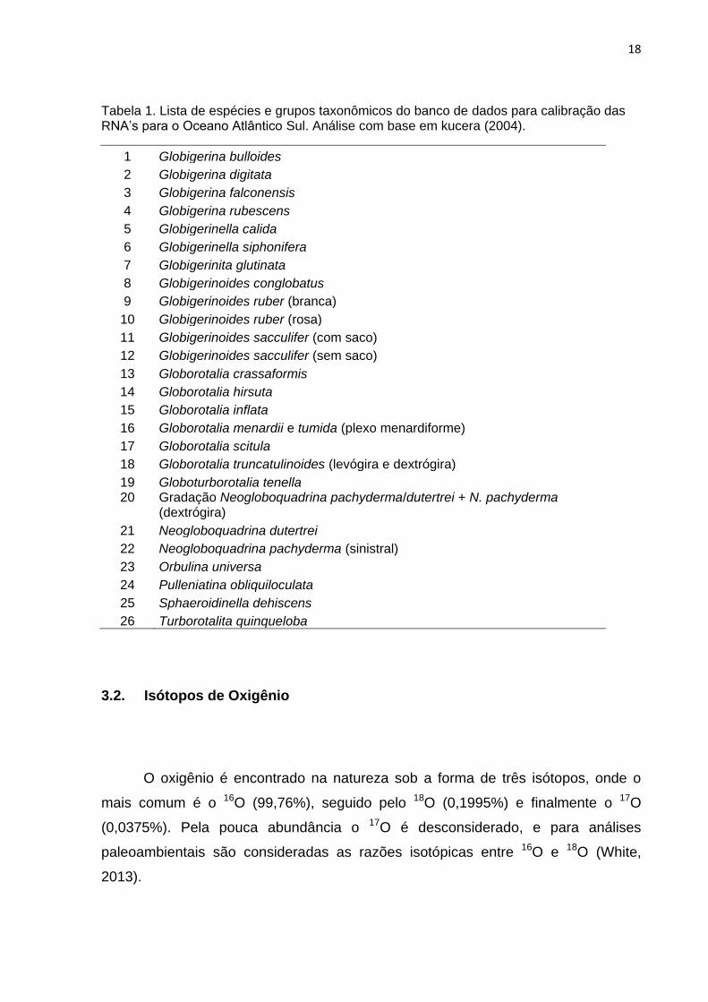
O cálculo das paleotemperaturas pelo método das RNA’s pode conter um erro
devido à ocorrência de espécies crípticas, que são morfologicamente semelhantes,
mas diferem pela genética e pelas preferências ambientais. Para minimizar esse
erro, o método prevê um banco de dados para calibração específico para cada
oceano (Kucera, 2004). Na tabela 1 estão listadas as espécies utilizadas para
calibração do Oceano Atlântico Sul.
18
Tabela 1. Lista de espécies e grupos taxonômicos do banco de dados para calibração das RNA’s para o Oceano Atlântico Sul. Análise com base em kucera (2004).
1 Globigerina bulloides
2 Globigerina digitata
3 Globigerina falconensis
4 Globigerina rubescens
5 Globigerinella calida
6 Globigerinella siphonifera
7 Globigerinita glutinata
8 Globigerinoides conglobatus
9 Globigerinoides ruber (branca)
10 Globigerinoides ruber (rosa)
11 Globigerinoides sacculifer (com saco)
12 Globigerinoides sacculifer (sem saco)
13 Globorotalia crassaformis
14 Globorotalia hirsuta
15 Globorotalia inflata
16 Globorotalia menardii e tumida (plexo menardiforme)
17 Globorotalia scitula
18 Globorotalia truncatulinoides (levógira e dextrógira)
19 Globoturborotalia tenella 20 Gradação Neogloboquadrina pachyderma/dutertrei + N. pachyderma
(dextrógira)
21 Neogloboquadrina dutertrei
22 Neogloboquadrina pachyderma (sinistral)
23 Orbulina universa
24 Pulleniatina obliquiloculata
25 Sphaeroidinella dehiscens
26 Turborotalita quinqueloba
3.2. Isótopos de Oxigênio
O oxigênio é encontrado na natureza sob a forma de três isótopos, onde o
mais comum é o 16O (99,76%), seguido pelo 18O (0,1995%) e finalmente o 17O
(0,0375%). Pela pouca abundância o 17O é desconsiderado, e para análises
paleoambientais são consideradas as razões isotópicas entre 16O e 18O (White,
2013).
19
O 16O, isótopo considerado mais leve, quando do processo de evaporação de
águas, associa-se à fase de vapor. O isótopo 18O, por sua vez, associa-se mais
facilmente com a fase líquida. O enriquecimento relativo no isótopo mais leve faz
com que a fase vapor seja considerada como empobrecida em relação ao padrão de
referência. A fase líquida torna-se então enriquecida no isótopo pesado, também
com relação ao padrão. Na figura 4-A pode-se ver que o processo de evaporação
leva à formação de nuvens empobrecidas e águas residuais enriquecidas no isótopo
pesado. À medida em que as nuvens se afastam do local de formação e vão
perdendo volume por precipitação, estas se tornam progressivamente mais
enriquecidas no isótopo leve. Desta forma, a precipitação nos polos é fortemente
empobrecida no isótopo pesado (Fig. 4-B). Como as geleiras são alimentadas por
água proveniente da atmosfera, em períodos glaciais, o avanço das calotas polares
aprisiona esta água empobrecida nos polos, tornando a água do mar desta época
enriquecida no isótopo pesado, enquanto um fenômeno oposto ocorre em períodos
interglaciais, pois o degelo retorna a água empobrecida ao oceano, equilibrando a
razão isotópica da água do mar (Fig. 4-C). Finalmente, esta variação na razão
isotópica fica registrada nas carapaças carbonáticas dos organismos, marcando
uma mudança climática ao longo do tempo, caracterizada por períodos glaciais e
interglaciais (Fig. 4-D) (White, 2013).
Com este processo, verifica-se que os isótopos de oxigênio constituem
excelente ferramenta para reconstruções paleoceanográficas, pois as testas
carbonáticas precipitam em equilíbrio isotópico com a água do mar da época em que
se formaram. As carapaças registram as proporções entre o 18O (isótopo pesado) e
o 16O (isótopo leve), segundo estudos realizados por Urey (1947), e, desta forma, se
pode reconstruir a variação entre períodos glaciais e interglaciais.
O sinal isotópico da amostra é obtido por uma equação que compara a razão
isotópica das carapaças analisadas com a razão isotópica de uma amostra padrão,
no caso deste trabalho o PBD (Pee Dee Belemnite). O sinal isotópico é obtido pela
seguinte equação (Faure, 1986):
δ18O = {[(18O/16O) amostra - (18O/16O) padrão] / [(18O/16O) padrão]} x 103
20
O valor é dado em unidades por mil (‰), e expressa o enriquecimento
isotópico da amostra em relação ao padrão. Valores mais positivos indicam
enriquecimento no 18O e valores mais negativos empobrecimento de 18O, sempre em
relação ao padrão. Nesta análise, o principal fator não é o valor absoluto do sinal
isotópico, mas a identificação de picos positivos ou negativos e, consequentemente,
a forma relativa da curva gerada (Fig. 4-D).
3.3. Isótopos de Carbono
O carbono também ocorre na natureza sob a forma de três isótopos (12C, 13C
e 14C), mas o 14C é radiogênico e não tem influência em análise de isótopos
estáveis. O 12C é assimilado preferencialmente pela atividade orgânica, enquanto o
13C, mais abundante, é mais facilmente assimilado em minerais de natureza
inorgânica, e sua razão isotópica preservada no CaCO3 das testas dos foraminíferos
representa índices de paleoprodutividade orgânica (White, 2013).
Em períodos de alta produtividade orgânica primária, na camada fótica do
mar, ocorre uma maior atividade fotossintética, e o 12C é consumido principalmente
por algas e plâncton. Se este material orgânico enriquecido no isótopo leve do
carbono (12C) decantar e for rapidamente preservado da oxidação, são formadas
rochas enriquecidas no carbono orgânico. Assim, a água superficial do mar fica
pobre em 12C e rica em 13C, ou seja, enriquecida em relação ao padrão. Em
períodos com baixa produtividade, a matéria orgânica rica em 12C não consegue se
preservar e o carbono orgânico retorna à coluna d’água, homogeneizando as razões
e tornando a água do mar relativamente empobrecida em 13C. Assim, carapaças de
foraminíferos conseguem também registrar a razão isotópica do carbono presente
na água à época de sua cristalização (White, 2013).

21
Figura 4. Esquema simplificado mostrando o comportamento dos isótopos de oxigênio em função de variantes ambientais e o respectivo registro, durante a alternância de períodos glaciais e interglaciais, observado em carbonatos marinhos (modificado de White, 2013 e <http://earthobservatory.nasa.gov/Features/Paleoclimatology_OxygenBalance/>).
22
Deve-se ter cuidado na interpretação dos isótopos de carbono, pois a
produtividade orgânica do mar pode ser favorecida pela ressurgência de águas sub-
superficiais. Estas águas se encontram numa profundidade onde provavelmente já
ocorreu a remineralização da matéria orgânica e, portanto é rica em nutrientes,
fazendo o sinal isotópico do 13C decrescer. Outro problema com os isótopos de
carbono é a dependência ao estágio ontogenético da carapaça, pois o carbonato
pode ou não estar em equilíbrio isotópico com a água do mar. Testas menores
tendem a diminuir o sinal isotópico, e as testas maiores se aproximam do sinal em
equilíbrio isotópico (Fraguas, 2009). Para minimizar este erro foram aqui
selecionadas as testas maiores para as análises isotópicas.
3.4. Paleoprodutividade e paleossalinidade
A produtividade das águas de um oceano é regulada pela entrada de luz na
zona fótica, necessária para a fotossíntese e, principalmente, pela disponibilidade de
nutrientes. As águas superficiais tendem a apresentar uma produtividade menor,
pois os organismos fotossintetizantes retiram e armazenam o carbono orgânico
durante o processo. Índices altos de produtividade ocorrem principalmente em águas
mais profundas, onde já ocorreu a remineralização da matéria orgânica, e também
em zonas de ressurgência, onde afloram águas profundas. Os proxies utilizados
para as estimativas de paleoprodutividade estão mais detalhados no Capítulo 5 (MS
submetido à QI).
A salinidade superficial média dos oceanos está em torno de 35‰ e sofre
alterações sazonais devido a vários fatores, como por exemplo, os diferentes
balanços entre evaporação e precipitação, e também sofre alterações pela influência
dos continentes (aporte de água doce) e das correntes oceânicas. Os menores
valores encontram-se nos polos e próximo ao equador, e os maiores estão próximos
à latitude 25º, em ambos os hemisférios. A salinidade dos oceanos também sofre
alterações ao longo do tempo, e pode ser estimada com a utilização de alguns
proxies, como é realizado neste trabalho.

23
Para as estimativas de paleossalinidade foi aplicado o método residual de
isótopos de oxigênio em Globigerinoides ruber (branca) como realizado por Toledo
et al., (2007b) para as bacias de Santos, Espírito Santo e Camamu. O método se
baseia no fato da composição isotópica do carbonato refletir principalmente a
temperatura e a composição isotópica da água do mar onde precipita (Emiliani,
1954). Existindo um indicador de temperatura independente da composição de
isótopos de oxigênio é possível excluir o efeito da temperatura do sinal isotópico
para obter a composição isotópica de oxigênio da água do mar. Neste caso, as
estimativas de paleotemperaturas independentes são fundamentadas na aplicação
das RNA’s, baseadas nas assembleias de foraminíferos planctônicos. Conhecendo a
relação existente entre a composição isotópica da água do mar e a salinidade, é
possível transformar as estimativas da composição isotópica de oxigênio da água
em estimativas de paleossalinidade. Os cálculos de paleossalinidade estão mais
detalhados no Capítulo 5 (MS submetido à QI).

24
4. REFERÊNCIAS BIBLIOGRÁFICAS
Caddah, L.F.G., Kowsmann, R.O., Viana, A.R. 1998. Slope sedimentary facies
associated with Pleistocene and Holocene sea-level changes, Campos Basin,
southeast Brazilian Margin. Sedimentary Geology, 115, 159-174.
Cirano M., Mata, M.M., Campos, E.J.D., Deiró, N.F.R. 2006. A circulação oceânica
de larga-escala na região oeste do Atlântico Sul com base no modelo de circulação
global OCCAM. Revista Brasileira de Geofísica, 24 (2), 209-230.
Emiliani, E. 1954. Depth habitats of some species of pelagic foraminifera as indicated
by oxygen isotope ratios. American Journal of Science, 252, 149-158.
Ericson, D.B., Wollin, G. 1968. Pleistocene climates and chronology of deep-sea
sediments. Science, 162 (3859), 1227-1234.
Evans, D.L., Signorini, S.R., Miranda, L.B. 1983. A note on the transport of the Brazil
Current. Journal of Physical Oceanography, 13 (9), 1732-1738.
Faure, G. 1986. Principles of isotope geology. New York, John Wiley & Sons, 587 p.
Ferreira, F., Leipnitz, I.I., Vicalvi, M.A., Sanjinés, A.E.S. 2012. Zoneamento
Paleoclimático do Quaternário da Bacia de Santos com base em foraminíferos
planctônicos. Rev. Bras. Paleontol., 15 (2), 173-188.
Fraguas, P.F. 2009. Relação entre o sinal isotópico de oxigênio e carbono e o
tamanho de testa de foraminíferos em amostras de topo de dois testemunhos da
Margem Continental Brasileira. Programa de Oceanografia Química e Geológica,
Instituto de Oceanográfico, Universidade de São Paulo. 105p. Dissertação de
Mestrado.
Kucera, M. 2003. Numerical approach to microfossil proxy data. Lecture notes for
Summer school Paleoceanography: Theory and field evidence. IAMC Geomare, pp.
66-90.

25
Kucera, M. 2004. Multiproxy approach for the reconstruction of the glacial ocean
surface (MARGO). Quaternary Science Reviews, 24 (2005), 813–819.
Leonhardt, A. 2001. Reconstituição Paleoceanográfica no Atlântico Sudoeste com
base em cocolitoforídeos durante o Quaternário tardio. Programa de Pós-Graduação
em Geociências, Instituto de Geociências, Universidade Federal do Rio Grande do
Sul. 161p. Tese de Doutorado.
Machado, L.C.R., Kowsmann, R.O., Almeida-Jr, W., Murakami, C.Y., Schreiner, S.,
Miller, D.J., Piauilino, P.O.V. 2004. Geometria da porção proximal do sistema
deposicional turbidítico moderno da Formação Carapebus, Bacia de Campos;
modelo de heterogeneidades de reservatório. Boletim de Geociências da Petrobras,
12 (2), 287-315.
Maciel, D.M., Alves, C.F., Ferreira, E.P. 2012. Bioestratigrafia com base em
Nanofósseis Calcários do testemunho GL-77, Bacia de Campos, Sudeste do Brasil.
Revista Brasileira de Paleontologia, 15 (2), 164-172.
Malmgren, B.A., Nordlund, U. 1997. Application of Artificial Neural Networks to
Paleoceanographic Data. Palaeogeography, Palaeoclimatology, Palaeoecology, 136,
359-373.
Peterson, R.G., Stramma, L. 1991. Upper-level circulation in the South Atlantic
Ocean. Progr. Oceanogr., 26 (1), 1-73.
Pivel, M.A.G. 2009. Reconstrução da hidrografia superficial do Atlântico Sul
Ocidental desde o Último Máximo Glacial a partir do estudo de foraminíferos
planctônicos. Programa de Oceanografia Química e Geológica, Instituto de
Oceanográfico, Universidade de São Paulo. 164p. Tese de Doutorado.
Pozzi, M., Malmgren, B.A., Monechi, S. 2000. Sea surface water temperature and
isotopic reconstructions from nannoplankton data using Artificial Neural Networks.
Paleontologia Eletronica. 3 (2), 4-14.
Sanjinés, A.E.S. 2006. Biocronoestratigrafia de foraminíferos em três testemunhos
do Pleistoceno-Holoceno do talude continental da Bacia de Campos, RJ – Brasil.
26
Programa de Pós-Graduação em Geologia, Instituto de Geociências, Universidade
Federal do Rio de Janeiro. 119p. Dissertação de Mestrado.
Silveira, I.C.A., Schmidt, A.C.K., Campos, E.J.D., Godoi, S.S., Ikeda, Y. 2000. A
Corrente do Brasil ao largo da costa leste brasileira. Revista Brasileira de
Oceanografia, 48 (2), 171-183.
Tokutake, L.R. 2005. Bioestratigrafia de nanofósseis calcários e estratigrafia de
isótopos (C e O) do talude médio, Quaternário, porção N da Bacia de Campos, ES.
Programa de Pós-Graduação em Geociências, Instituto de Geociências,
Universidade Federal do Rio Grande do Sul. 97p. Dissertação de Mestrado.
Toledo, F.A.L. 2000. Variações Paleoceanográficas nos Últimos 30.000 anos no
Oeste do Atlântico Sul : Isótopos Estáveis, Assembléias de Foraminíferos
Planctônicos e Nanofósseis Calcários. Programa de Pós-Graduação em
Geociências, Instituto de Geociências, Universidade Federal do Rio Grande do Sul.
245 p. Tese de Doutorado.
Toledo, F.A.L., Cachão, M., Costa, K.B., Pivel, M.A.G. 2007a. Planktonic
foraminífera, calcareous nannoplankton and ascidian variations during the last 25 kyr
in the Southwestern Atlantic: A paleoproductivity signature? Marine
Micropaleontology, 64, 67-79.
Toledo, F.A.L., Costa, K.B., Pivel, M.A.G. 2007b. Salinity changes in the western
tropical South Atlantic during the last 30 kyr. Global and Planetary Change, 57, 383-
395.
Urey, H. 1947. The thermodynamic properties of isotopic substances, J. Chem. Soc.,
1947: 562-581.
Vicalvi, M.A. 1997. Zoneamento bioestratigráfico e paleoclimático dos sedimentos do
Quaternário superior do talude da Bacia de Campos, RJ, Brasil. Boletim de
Geociências da Petrobras, 11 (1/2), 132-165.
Vicalvi, M.A. 1999. Zoneamento bioestratigráfico e paleoclimático do Quaternário
Superior do talude da Bacia de Campos e Platô de São Paulo adjacente, com base

27
em foraminíferos planctônicos. Programa de Pós-Graduação em Geologia, Instituto
de Geociências, Universidade Federal do Rio de Janeiro. 183p. Tese de Doutorado.
White, W.M. 2013. Geochemistry. Oxford, Wiley-Blackwell, 660p.
Winter, W.R., Jahnert, R.J., França, A.B. 2007. Bacia de Campos. Boletim de
Geociências da Petrobras, 15 (2), 511-529.

28
5. MANUSCRITO SUBMETIDO À QUATERNARY INTERNATIONAL
TÍTULO
PALEOCEANOGRAPHIC EVOLUTION AND ISOTOPIC
STRATIGRAPHY WITH PLANKTONIC FORAMINIFERA
(LATE QUATERNARY, CAMPOS BASIN)
AUTORES
Sandro Monticelli Petróa, María Alejandra Gómez Pivel
b, João Carlos Coimbra
c & Ana Maria
Pimentel Mizusakic
a Programa de Pós-Graduação em Geociências, Instituto de Geociências, Universidade Federal
do Rio Grande do Sul, Porto Alegre, RS, Brasil.
b Laboratório PaleoProspec, Faculdade de Informática, Pontifícia Universidade Católica do
Rio Grande do Sul, Porto Alegre, RS, Brasil.
c Departamento de Paleontologia e Estratigrafia, Instituto de Geociências, Universidade
Federal do Rio Grande do Sul, Porto Alegre, RS, Brasil.

29

30
PALEOCEANOGRAPHIC EVOLUTION AND ISOTOPIC
STRATIGRAPHY WITH PLANKTONIC FORAMINIFERA
(LATE QUATERNARY, CAMPOS BASIN)
Sandro Monticelli Petróa, María Alejandra Gómez Pivelb, João Carlos Coimbrac,
Ana Maria Pimentel Mizusakic
a Programa de Pós-Graduação em Geociências, Instituto de Geociências,
Universidade Federal do Rio Grande do Sul, CEP 91501-970, Cx. P. 15001, Porto
Alegre, Rio Grande do Sul, Brazil
b Laboratório PaleoProspec, Faculdade de Informática, Pontifícia Universidade
Católica do Rio Grande do Sul. Av Ipiranga 6681, Porto Alegre, RS, Brazil
c Departamento de Paleontologia e Estratigrafia, Instituto de Geociências,
Universidade Federal do Rio Grande do Sul, CEP 91501-970, Cx. P. 15001, Porto
Alegre, Rio Grande do Sul, Brazil
ABSTRACT
Planktonic foraminifera is the most useful microfossil group for biostratigraphic
studies, being considered the main carriers of paleoceanographic information and
being applicable to the analysis of sedimentary basins. The main aim of this work is
to propose a paleoceanographic reconstruction model in the Campos Basin, by
analyzing 61 samples taken from the GL-77 core, collected at the lower continental
slope, in the offshore part of the basin. The interval comprises the last two Glacial-
Interglacial cycles, corresponding to the planktonic foraminifera biozones W
(partially), X, Y and Z. By means of analysis of the total fauna, datings in 14C and
isotopic analyses of δ18O and δ13C in shells of planktonic foraminifera estimates of
variations of paleoproductivity, paleosalinity and sea surface paleotemperature were
obtained; an age model and, posteriorly, the sedimentation rates were calculated.

31
The age model identified the Last Glacial Maximum (LGM) and estimated the ages of
a few biostratigraphic events, such as YP.2 datum, the MIS 3/4 boundary (which
coincides with the Y2/Y3 boundary), the Y1/Y2 boundary and the YP.4 datum. The
sedimentation rates are strangely elevated in Biozone X (glacial period) where lower
rates would be expected. In the Holocene there is an elevated sedimentation rate,
associated to the influence of the Paraíba do Sul River delta, at the northern portion
of the basin. The paleotemperatures oscillate seasonally in the glacial periods, when
the amplitude between summer and winter is larger than the one registered in the
interglacial periods. A correlation was observed between the paleotemperatures and
the environmental conditions characterized by the warm and cold subzones in
Biozone X. Based on the P/B ratio a limit of sequences can be identified next to the
MIS 4/5 boundary. Paleosalinity is reduced in deglaciation periods. Paleoproductivity
is reduced to 29 ka (MIS 2/3 boundary) by the LGM and increases near the
Pleistocene/Holocene boundary. Finally, it was observed that the
Pleistocene/Holocene transition occurs inside Biozone Y, and is not temporally
related to the beginning of Biozone Z.
Key words: ANN’s, 14C, MIS, Glacial, Interglacial, Quaternary.
1. INTRODUCTION
Planktonic foraminifera are organisms which have their distribution controlled
by environmental conditions, such as temperature, salinity and organic productivity.
Changes in these variables along geological time influence the distribution and
abundance of the species in the fossil record, as well as generate an imbalance in
the isotopic ratios of carbon and oxygen, through biofractionation, whose ratios are
preserved in the microfossils carbonate shells. Therefore, the abundance of fauna
and the isotopic ratios, preserved in the planktonic foraminifera shells, constitute a
proxy for the interpretation of the paleoenvironmental evolution and for stratigraphic
correlations.

32
Generally speaking, studies on the paleoceanography of the South Atlantic
during the Quaternary are recent and are mainly comprised of three groups of
microfossils: foraminifera, ostracodes and calcareous nannofossils. However, the
researches with microfossils in the Campos Basin, situated in the Brazilian
continental margin, are more focused on the biostratigraphy of the Cretaceous and
Paleogene, with direct application to the petroleum industry, this basin being one of
the largest production areas in Brazil. The last decade was characterized by major
global advances in paleoceanographic research and, although there have been a few
advances in this area in the South Atlantic as well, when compared to other oceans
the researches may be considered incipient, especially when taken into account the
extension of the Brazilian continental margin and adjacent areas to be explored.
Currently, the volume of data available for the North Atlantic is immensely larger than
the one corresponding to the South Atlantic, and the western margin of this oceanic
basin is less explored than the eastern margin, from a paleoceanographic point of
view.
As previously mentioned, in the Campos Basin the studies with foraminifera
have been directed to the biostratigraphy, including the interval corresponding to the
Quaternary. Vicalvi (1997, 1999) has proposed a subdivision in biostratigraphic
zones and subzones, following the Ericson and Wollin model (1968), relying upon the
occurrence or absence of some species of planktonic foraminifera. Sanjinés (2006)
analyzed three cores collected in the Campos Basin (amongst them “GL-77”, the
object of this study), whose results appear in a biochronostratigraphic chart, the
author having applied the methodology of sequential stratigraphy in the Pleistocene-
Holocene interval of the basin. Tokutake (2005) and Maciel (2012) performed
biostratigraphic studies using calcareous nannofossils. Ferreira et al. (2012) have
proposed a paleoclimatic zoning with planktonic foraminifera for the Quaternary of
the Santos Basin, which is adjacent to the Campos Basin.
The main aim of this research is to formulate a paleoceanographic evolution
model for the two last Glacial-Interglacial cycles, covering biozones W (partially), X, Y
and Z of Ericson and Wollin (1968) in the Campos Basin. In order to accomplish it,
herein is carried out a joint analysis of the faunistic composition through artificial
neural networks (ANN’s), the isotopic oxygen and carbon ratios and the AMS 14C

33
dating in planktonic foraminifera obtained from the GL-77 core, collected in the lower
slope.
2. STUDY AREA
The analyzed core (“GL-77”) has been collected at the lower continental slope
in the north of the Campos Basin, offshore from the southeastern Brazilian
continental margin (Figure 1). The sequence of interest of this work corresponds to
the sediments of the Holocene and Pleistocene, Campos Group, Ubatuba Formation.
It has as its lower boundary the unconformity of 1.6 Ma, which is related to the global
eustatic fall, and the upper boundary is represented by the current sediments of the
seabed. There is a dominance of mudrocks and deep-water corals in the basin slope.
Muddy and sandy canyons are characteristic and separate the continental slope into
sections. At the foot of the continental slope, diamictite wedges and mud
predominate, and they also occur at the most distal areas intersected by rare sandy
canyons (Caddah et al., 1998; Machado et al., 2004; Winter et al., 2007).
The Campos Basin is under the influence of the Brazil Current (BC), which
transports Tropical Water (TW) at the surface and South Atlantic Central Water
(SACW) at the pycnocline layer (Silveira et al., 2000). In this basin, coastal upwelling
occurs in the summer, while shelf break upwelling occurs during the whole year,
decreasing locally the depth of thermocline and nutricline (Palma and Matano, 2009).

34
Figure 1. Location of the studied core GL-77, lower slope of the Campos Basin, SE Brazil.
3. MATERIAL AND METHODS
The GL-77 core was collected at the coordinates 40º02'50"W and 21º12'22"S,
in water depth of 1,287 m, with recovery of 18.15 m of discontinuous sediments, out
of which the upper 14.65 m were analyzed, totaling 61 irregularly spaced samples
(Figure 2). In each sample between 300 and 600 specimens of planktonic
foraminifera were collected, always taken from the >150 μm portion, and posteriorly

35
classified at the specific level. In some samples the minimum quantity of 300
specimens was not recovered due to the little quantity of material available (Appendix
B). On sample 25 (400 cm) only the <150 μm fraction was recovered and it was
discarded.
The core was previously studied from the biostratigraphic point of view by
Sanjinés (2006) and Maciel et al. (2012), using planktonic foraminifera and
calcareous nannofossils, respectively. The interval of interest consists of 61 samples,
comprising biozones W (partially), X, Y and Z of Ericson and Wollin (1968) (Figure 2).
In these samples, stable isotope analysis of carbon and oxygen (δ18O and δ13C) and
direct dating using AMS 14C-method were conducted in the shells of Globigerinoides
ruber (white). The classification of total fauna at the specific level was effected,
following the taxonomic criteria of Bé (1967, 1977), Bolli and Saunders (1989) and
Hemleben et al. (1989). The number of benthic foraminifera in each sample was also
registered in order to establish parameters of paleoproductivity and paleobathymetry.
From the results of these analyses, estimates of the past changes of sea surface
temperature (SST), productivity and sea surface salinity (SSS) were obtained,
besides absolute ages, age estimates and sedimentation rates.
The paleotemperature estimates were obtained through the technique of
Artificial Neural Networks – ANN’s (Malmgren and Nordlund, 1997). The ANN
technique analyzes the relative abundance of the total fauna in each sample and,
through comparison with a calibration database, whose environmental conditions are
known, it estimates a temperature and its respective error. The method has a
database for specific calibration for each ocean in order to minimize the error
generated by cryptic species, i.e., species which are morphologically similar, but
differ by their genetics and environmental preferences (Kucera, 2004). The technique
is based on the premise that temperature is the main factor controlling the faunal
distribution. The calculations were performed by Prof. Dr. Michal Kucera, at the
University of Bremen, in Germany.
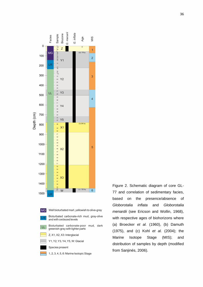
36
Figure 2. Schematic diagram of core GL-
77 and correlation of sedimentary facies,
based on the presence/absence of
Globorotalia inflata and Globorotalia
menardii (see Ericson and Wollin, 1968),
with respective ages of biohorizons where
(a) Broecker et al. (1960), (b) Damuth
(1975), and (c) Kohl et al. (2004); the
Marine Isotope Stage (MIS); and
distribution of samples by depth (modified
from Sanjinés, 2006).

37
The analyses of δ18O and δ13C, as mentioned above, were performed on the
species Globigerionoides ruber (white). In an initial stage the analysis of the samples
01 to 38 were performed at the Stable Isotope Laboratory at the University of
California, Santa Cruz (SIL-UCSC) and, following the need of extending the temporal
range for this study, samples 39 to 61 were also analyzed, at the Analytical
Laboratory for Paleoclimate Studies, of the University of Texas, Austin – TX. The six
14C AMS datings in the species G. ruber (white and pink) were carried out at Beta
Analytic Inc., Miami – FL.
Variations in the relative abundance of species associated with high
productivity, such as Globorotalia truncatulinoides (right coiling) and
Neogloboquadrina dutertrei, and the ratio between Globigerina bulloides and
Globigerinoides ruber (white), were considered for paleoproductivity estimates
(Conan et al., 2002). The ratio between planktonic and benthic foraminifera (P/B)
(Berguer and Diester-Haass, 1988) was also used. Finally, the carbon isotopes were
used as paleofertility indicators (Wefer et al., 1999).
For the paleosalinity estimates, the oxygen isotopes residual method in
Globigerinoides ruber (white) was applied. The method obtains the SSS as a function
of the δ18O in G. ruber and the average summer temperature, estimated in an
independent way from the isotopic method, in this case by the ANN’s, according to
the following equation (Toledo, 2007b):
SSS (‰) = 34.95 + 1,863 * [δ18OC – 25.78 + √ (16.87 + 0.347 * Tm) / 0,18]
Wherein:
SSS = summer sea surface salinity
δ18OC = oxygen isotopic composition of G. ruber
Tm = estimated average summer sea surface temperature.
38
The age model was constructed from the correlation of the δ18O record in
Globigerinoides ruber (white) with the high resolution curve of the SPECMAP
(Mapping Spectral Variability in Global Climate Project), of Martinson et al. (1987).
The SPECMAP data consists of a series of values of δ18O associated to the ages,
which can be correlated by the pattern of the isotopes curve. Finally, the model is
calibrated using 14C datings as control points. The correlation between these data
was performed using the program AnalySeries 1.1 (Paillard et al., 1996). The
sedimentation rates were also obtained based on the age model.
4. RESULTS AND DISCUSSION
4.1. Oxygen isotopes, age model and sedimentation rates
The δ18O record is the basis for the construction of the paleoceanographic
evolution model, from which, along with the datings, the age model was elaborated
and it also served to correlate the other data of this work. Marine Isotopic Stages
(MIS) 1 to 5 and the end of the MIS 6 were identified, the latter being supported by
the age model (Figure 3) and by the correlation with the ages of the limits between
MIS’s established by Lisiecki and Raymo (2005) (Figures 2 and 4a).
The results from the six AMS 14C datings performed in Globigerinoide ruber
shells are presented at table 1.

39
Table 1. Ages obtained by AMS 14C datings.
Sample
Age Measured
14C (y.B.P.) Error (y) Age conventional
Age calendar
(y.B.P.) Error (y)
2 1510 30 1900 1500 ± 120
7 6650 40 7070 7595 ± 95
9 10540 50 10920 12475 ± 135
12 17320 70 17730 20710 ± 330
14 21830 90 22230 26305 ± 315
21 42860 550 43250 44900 ± 260
The age model correlates the δ18O curve in Globigerinoides ruber (white) with
the standard curve of δ18O of the SPECMAP (Martinson et al., 1987), calibrated with
the six datings, and with two biostratigraphic datums of the core, the X/Y boundary
with an age of 84 ka (Damuth, 1975), between samples 37 and 38, and the boundary
W/X with an age of 130 ka (Kohl et al., 2004), between samples 59 and 60. Finally,
the Analyseries program (Paillard et al., 1996) interpolates the remaining points
automatically, generating an age for each sample (Appendix A). The age model has
obtained a correlation coefficient of -0.77 (Figure 3).

40
Figure 3. Correlation between δ18O in Globigerinoides ruber (white) and the SPECMAP
reference curve (Martinson et al. 1987). Vertical bars represent the correlation between the
samples dated by 14C and biostratigraphic datums, with the respective ages.
Biozone X, according to Sanjinés (2006), is not complete, occurring only three
(X1 a X3) of the 11 subzones (X1 a X11) of Vicalvi (1999), subdivided by the
oscillation between high and low percentages of Globorotalia menardii, with a
condensed section at the base. If this condensed section in fact exists, there may be
a punctual error in the age model, but it is known that this error does not influence
the sedimentation rate as a whole. Ferreira et al. (2012) has also divided Biozone X
in only three subzones in the Santos Basin, although with a different criterion, based
on Globorotalia truncatulinoides coiling change. The resolution of the sampling at
Biozone X is irregular, with an average of 30 cm of spacing, comprised of 22
samples. Thus, a sectioning of this biozone in 11 subzones becomes a non-
applicable datum due to low resolution, being used only in areas of high
sedimentation rate. Also, in these samples the same abundance of menardiforms
was not observed, which alternated between higher and lower than 5%, as in the
definition of the subzones X1 to X11 proposed by Vicalvi (1999). To avoid problems
with these datums, only the ages of bio-horizons W/X and X/Y were considered.
The age model has less precision at biozones W, X and part of Y due to the
absence of absolute datings. Between 50 ka and the Recent, the model presents a

41
better definition. From the ages generated for each sample the considerations related
below were made.
The datum YP.2 with an age estimated between 7.7 and 74.4 ka (Vicalvi 1999)
obtained different ages, between 60.884 and 63.168 ka, younger than the original
proposal. The boundary between the MIS 2 and the MIS 3 has an age of 57 ka
(Lisiecki and Raymo, 2005) and coincides with the Y2/Y3 boundary, estimated
between 56.317 and 58.601 ka.
Vicalvi (1999) has dated the biohorizon of the last disappearance of
Pulleniatina obliquiloculata, which marks the boundary of biozones Y2 and Y3 (datum
YP.3), between 42 and 45 ka. In this work the Y1/Y2 boundary was dated as 44.9 ka,
the same age as the peak of MIS 3, indicating that the P. obliquiloculata fauna has
been affected by the climatic change marked at the inflexion of the δ18O curve. For
the YP.3 datum at the GL-77 core an age between 44.25 and 45.16 ka was obtained,
which is within the variation spectrum proposed by Vicalvi (1999).
The Last Glacial Maximum (LGM) is usually associated with the last positive
peak at the δ18O, but this pattern sometimes undergoes local variations, since the
isotopic relation reflects the ice volume and is not necessarily in phase with the
climatic change (Imbrie and Kipp, 1971). So the LGM is defined as the interval with
duration of 4 ka, between 19 and 23 ka, for it is a chronological interval with greater
stability in the glacial climate (Mix et al., 2001). In sample 12 (108 cm) two indications
of the LGM occur, a positive peak in δ18O and a dating of 20.710 ± 0.33 ka. This point
is also correlated with the MIS 2 peak.
The last appearance of Pulleniatina obliquiloculata, denominated biohorizon
YP.4 by Sanjinés (2006), is dated as 15 ka (Bé et al., 1976). However, in the GL-77
core the age of this biohorizon was estimated between 12.475 and 14.645 ka.
According to the biostratigraphic interpretation by Sanjinés (2006), the Y/Z limit
corresponds to the Pleistocene/Holocene boundary. However, the
Pleistocene/Holocene boundary has an age determined as 11.7 ka (Stratigraphic
Chart 2013, Cohen et al., 2013), and in the age model the last sample of the
Pleistocene is dated as 12.475 ka, and the first sample of the Holocene has an age
estimated as 11.109 ka, the latter still belonging to Biozone Y. These results

42
demonstrate that the X/Y and the Pleistocene/Holocene boundaries are not
necessarily synchronous.
From the age model, the sedimentation rates could be estimated as a function
of the depth (Figure 4b). In a general way the sedimentation rates show elevated
values at the base of the interval, with a maximum of 14.34 cm/ka, and smaller
values on top, with a minimum of 3.91 cm/ka. The sedimentation rates are very
elevated at Biozone X (interglacial) in comparison to Biozone Y (glacial), which is not
coherent, since in the interglacial stage the eustatic level is more elevated and the
sedimentation should be smaller in distal deposits (Figure 4b), as it was observed by
Vicalvi (1999). From the base of the interval (130 ka) up to the LGM, the
sedimentation rates decrease continuously. From the LGM (20.71 ka) up to
approximately 15 ka the rates remain low, and between 15 ka and the Holocene the
sedimentation increases. In the top sample the sedimentation rate starts to decrease
again, reaching minimum values for the interval, but this is not a reliable rate due to
the low depth of the sample (2 cm), where the sediment is not very compacted when
compared to deeper samples, and there is a possible loss of part of the core top,
which is something relatively usual in the sampling of piston cores. The relative
elevation of the sedimentation rate at the Holocene possibly occurs due to an
influence of the Paraíba do Sul River Delta, which during this time has significantly
increased its input of sediment in the Campos Basin (Riccomini and Assumpção,
1999).
43
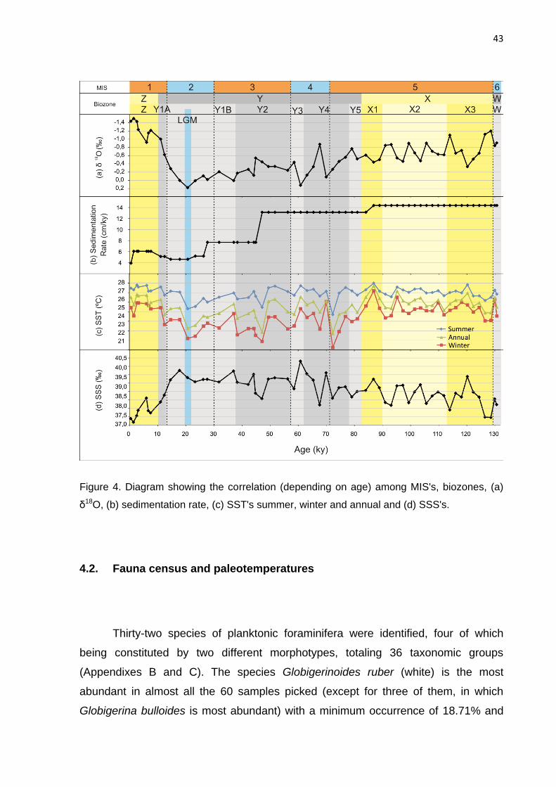
Figure 4. Diagram showing the correlation (depending on age) among MIS's, biozones, (a)
δ18O, (b) sedimentation rate, (c) SST's summer, winter and annual and (d) SSS's.
4.2. Fauna census and paleotemperatures
Thirty-two species of planktonic foraminifera were identified, four of which
being constituted by two different morphotypes, totaling 36 taxonomic groups
(Appendixes B and C). The species Globigerinoides ruber (white) is the most
abundant in almost all the 60 samples picked (except for three of them, in which
Globigerina bulloides is most abundant) with a minimum occurrence of 18.71% and

44
maximum occurrence of 62.17%. The species G. bulloides is the second most
abundant (up to 31.7%), with over 10% in 1/3 of the samples, especially at the base
of the interval. The species Globigerinoides ruber (pink) is the third most abundant,
with a minimum of 1.2% and a maximum of 18.5%. Other species also occur in more
than 10% in some samples: Globigerinita glutinata (up to 28.89%), Globigerinoides
sacculifer (without sac) (up to 22.39%), Globorotalia menardii (up to 28.7%),
Globorotalia crassaformis (up to 16.18%), Globorotalia inflata (up to 13.58%),
Globoturborotalita tenella (up to 11.03%), Globigerinoides conglobatus (up to
10.79%) and Globorotalia truncatulinoides (right-coiling) (up to 10.0%) (Figure 5).
The abundances of all samples are in appendixes B and C.
The calculations of the sea surface paleotemperatures based on the relative
abundance of fauna, have generated the mean summer, winter and annual SST
estimates (Figure 4c). The oscillation pattern is similar in the three curves and, in
general, the SSTs are more elevated at Biozones X and Z (interglacial). At Biozone Y
(glacial), three peaks of low SST occur, next to 70, 50 and 20 ka. The peak of low
SST at 20 ka is in accordance with the age model, for this point corresponds to the
LGM. From 20 ka to the Recent, the SSTs gradually increase, reflecting the warming
initiated after the LGM, still at Biozone Y, and extending up to the end of the
Holocene, already at Biozone X, which relates to the post-glacial period. In some
sections the ANN-based SST estimates are not reliable: 118 to 116 ka, 99 to 84 ka,
72 to 67 ka and 1,5 to 0 ka, due to the number of planktonic foraminifera recovered
for the classification not reaching the minimum of 300 specimens.

45
Figure 5. Most abundant species. 1 - Globigerina bulloides; 2 - Globigerinita glutinata; 3 -
Globigerinoides conglobatus; 4 - Globigerinoides ruber (white); 5 - Globigerinoides ruber
(pink); 6 - Globigerinoides sacculifer (without sac); 7 - Globorotalia crassaformis; 8 -
Globorotalia inflata; 9 - Globorotalia menardii; 10 - Globorotalia truncatulinoides (right
coiling); 11 - Globoturborotalita tenella. Where ‘a’ – umbilical view (frontal), ‘b’ – lateral view,
‘c’ – spiral view. Scale bars: 100 µm.

46
The curve generated by the ANN-based SST estimates follows the same
pattern as the δ18O record. A peak of low SST corresponding to the LGM is
observed, although it is not the coldest point in the interval. The SSTs at biozones X
and Y tend to lose precision in the calculations due to the method utilized (ANN’s),
for there is an influence of the glacial/interglacial cycles variation, which means that a
certain fossil assemblage may respond differently, when compared to a modern
assemblage, to different environmental conditions (Kucera, 2004). Biozone X
represents an interglacial climate, but it is also subdivided in warm and cold
subzones, subzones X1 to X11, in accordance with the changes in abundance of
Globorotalia menardii, where the “odd X’s” are warmer and the “even X’s” are colder
(Vicalvi, 1999). Despite the limitation of the technique, at Biozone X the SSTs behave
according to this pattern, with higher SSTs in X1 and X3, and lower SSTs in X2.
Seasonality changes were observed between glacial and interglacial intervals.
During glacial times, represented by Biozone Y, the SST range between the summer
and winter is larger, when compared to the variation between summer and winter
during interglacials (Biozones X and Z). This result shows that in the glacial period
the climate is subjected to a wider temperature range.
4.3. Paleosalinity
Generally speaking, the sea surface paleosalinity (SSS) increases from the
base of the interval up to the peak of MIS 4, estimated in 60.884 ka. Between this
peak and the LGM the SSS continues to show a wide range of oscillation, but stays
elevated. After the LGM the SSS decreases towards the Recent, as a result of the
feeding of the ocean by freshwater originating from the deglaciation in a global level
(Figure 4d).
The SSS, as would be expected, has presented a strong dependence on
δ18O, since the graph pattern is similar, i.e., for low values of δ18O the lowest values
of SSS are correlated. This may be as much an indicator of a limitation of the

47
technique as a low influence of the temperature on salinity, which is mainly regulated
by the isotopic composition of sea water.
4.4. Paleoproductivity
The indicators used are not in full agreement and, from the analysis of the
fauna and δ13C, three distinct models of paleoproductivity evolution were identified.
The first model was obtained by the data on abundance of Neogloboquadrina
dutertrei and Globorotalia truncatulinoides (right-coling) and is the most consistent,
for the curves present the greatest similarity with one another. Generally speaking,
this model has low productivity values at the base of the interval, with peaks of high
productivity at the end of the Biozone X (next to 90 ka), between 50 and 30 ka and
around 15 ka (between the LGM and the Pleistocene/Holocene boundary). In the
Holocene the model again suggests a low paleoproductivity (Figures 6, a-b).
The second model was obtained by the ratios of Globigerina bulloides and
Globigerinoides ruber (white) and proportion between planktonic and benthic
foraminifera (P/B), which share a similar behavior, having an elevated
paleoproductivity at the base of the interval, followed by reduction of productivity
towards the top (Figures 6, c-d). In particular, the P/B ratio may highlight an evolution
of regressive and transgressive cycles, where the abundance of benthic foraminifera
increases with the shallowing of the basin. With this criterion two system tracts were
observed, one regressive at the base followed by a transgressive one at the top, as it
was identified by Sanjinés (2006) for the interval, but with the sequence limit
identified in the transition between MIS 4 and MIS 5. The third model was observed
at δ13C, with relatively low values, irregularly oscillating from 130 to 50 ka, followed
by an increase in paleoproductivity from 50 ka up to the Holocene (Figure 6e).

48
Figure 6. Paleoproductivity indicators: (a) abundance of Neogloboquadrina dutertrei, (b)
abundance of Globorotalia truncatulinoides, (c) Globigerina bulloides/Globigerinoides ruber
ratio, (d) P/B ratio and (e) carbon isotopes. The paleoproductivity was identified based on
three different models, where (a) and (b) represent the first, (c) and (d) the second and (e) is
the third one.
The paleoproductivity indicators are not totally independent indicators, and
may suffer influence from other factors, diverging in certain intervals. The carbon
isotopic signal actually indicates paleofertility (Wefer et al., 1999) and has a different
behavior from the other paleoproductivity indicators. The relative abundance of the

49
species is a critical point, since the high ratio of a species may be, actually, the low
quantity of another one, since each species may respond in a different way to
environmental conditions.
The three paleoproductivity patterns identified are apparently heterogeneous,
but through fragmentation of certain parts a few similarities are observed. An interval
with a well-defined behavior is between the boundary of MIS’s 2/3 (29 ka) up to the
LGM, with a tendency of paleoproductivity reduction. Between the LGM and the
beginning of the Holocene the interval with the most consistent oscillation occurs,
which is observed in all the patterns, in which there is a tendency of an increase in
paleoproductivity, with a maximum peak oscillating between the end of the
Pleistocene and the beginning of the Holocene.
5. FINAL REMARKS
The evolution model of the last 130 ka observed at the GL-77 core, analyzed
here, shows some incoherencies, especially between biozones X and Z, where
distinct sedimentation rates and paleosalinities are observed, even though they
belong to stages with similar climate behavior, being both of an interglacial character.
In the age model the LGM was identified and the ages of a few biostratigraphic
events were defined, such as datum YP.2, estimated between 60.884 and 63.168 ka;
the boundary between MIS 3 and MIS 4, estimated between 56.317 and 58.601 ka,
coinciding with the Y2/Y3 boundary; the Y1/Y2 boundary was dated as 44.9 ka; and
the YP.4 datum was estimated as having an age between 12.475 and 14.645 ka. It
was observed that the Y/Z and Pleistocene/Holocene boundaries are not necessarily
synchronous, with the beginning of the Holocene being prior to Biozone Z.
The sedimentation rates are strangely elevated at Biozone X, for a
Highstand Systems Tract (HST) occurs, where lower rates for the lower continental
slope were expected. During the Holocene the sedimentation rate is higher due to
the influence of the Paraíba do Sul River Delta, at the northern portion of the basin.
50
In accordance with the P/B ratio, a sequence limit was identified at the transition
between MIS 4 and MIS 5.
The SSTs register a seasonal variability, for in the glacial interval the
amplitude between summer and winter is larger than the amplitude registered in
interglacial periods. A correlation was observed between the oscillation of SSTs and
the variation of the environmental conditions characterized by the relatively warm and
cold subzones in Biozone X. Paleosalinity reflects clearly the global ice volume
variation, with a reduction in the deglaciation period which occurs from the LGM to
the Recent. Paleoproductivity indicators suggest a reduction in the interval beginning
at 29 ka, at the boundary between MIS 2 and MIS 3, and ending near the LGM. Next
to the Pleistocene/Holocene boundary the same indicators present high values,
which may be related to changes in circulation associated with the reorganization of
the climate and the oceans in the transition between glacial and interglacial
conditions. Nevertheless, it is possible that in some periods such as the Y/Z transition
the fauna has not necessarily responded to the productivity, but to the SST.
Acknowledgements
The authors thank M. Kucera, from the University of Bremen, Germany, for his
help with the calculations for the analysis of ANN. The Petróleo Brasileiro S.A.
(PETROBRAS) is acknowledged for the donation of samples to the Laboratório de
Microfósseis Calcários (IGeo/UFRGS). The authors also thank the PRH-PB-215,
which granted a scholarship to the first author and supported the isotopic analysis
and datings, and the CNPq (Brazilian National Council for Scientific and
Technological Development) for its continued support for research in
palaeoceanography.

51
REFERENCES
Bé, A.W.H. 1967. Foraminifera families: Globigerinidae and Globorotaliidae. Conseil
Permanent International pour l’exploration de la mer. Zooplankton, Sheet 108. 9
pp.
Bé, A.W.H. 1977. An ecological, zoogeographic and taxonomic review of recent
planktonic foraminifera. In: Ramsay, A.T.S. (Ed.), Oceanic Micropaleontology,
Academic Press, London, pp. 1-100.
Bé, A. W. H., Damuth, J. E., Lott, L., Free, R. 1976. Late Quaternary Climatic Record
in Western Equatorial Atlantic Sediment. In: Cline, R.M., Hays, J.D. (Eds.),
Investigations of Late Quaternary Paleoceanography and Paleoclimatology.
Geological Society of America, Memoir 145, pp. 162-200.
Berguer, W. H., Diester-Haass, L. 1988. Paleoproductivity: The benthic/planktonic
ratio in foraminifera as a productivity index. Marine Geology, 81, 15-25.
Bolli, H.M., Saunders, J.B. 1989. Oligocene to Holocene low latitude planktic
foraminifera. In: Bolli, H.M., Saunders, J.B., Perch-Nielsen, K. (Eds.), Plankton
Stratigraphy, Vol.1. Cambridge Univ. Press, pp: 155-262.
Broecker, W.S., Ewing, M., Heezen, B.C. 1960. Evidence for abrupt change in
climate close to 11,000 years ago. American Journal of Science, 258, 429-448.
http://dx.doi.org/10.2475/ajs.258.6.429.
Caddah, L.F.G., Kowsmann, R.O., Viana, A.R. 1998. Slope sedimentary facies
associated with Pleistocene and Holocene sea-level changes, Campos Basin,
southeast Brazilian Margin. Sedimentary Geology, 115, 159-174.
Cirano M., Mata, M.M., Campos, E.J.D., Deiró, N.F.R. 2006. A circulação oceânica
de larga-escala na região oeste do Atlântico Sul com base no modelo de
circulação global OCCAM. Revista Brasileira de Geofísica, 24 (2), 209-230.

52
Cohen, K.M., Finney, S.C., Gibbard, P.L., Fan, J.-X. 2013. The ICS International
Chronostratigraphic Chart. Episodes, 36 (3), 199-204.
Conan, S. M.-H., Ivanova, E. M., Brummer, G.-J. A. 2002. Quantifying carbonate
dissolution and calibration of foraminiferal dissolution indices in the Somali Basin.
Marine Geology, 182, 325–349.
Damuth, J.E. 1975. Quaternary climate change as revealed by calcium-carbonate
fluctuations in western equatorial Atlantic sediments. Deep-Sea Research, 22,
725-743. http://dx.doi.org/10.1016/0011-7471(75)90078-9.
Ericson, D.B., Wollin, G. 1968. Pleistocene climates and chronology of deep-sea
sediments. Science, 162 (3859), 1227-1234.
http://dx.doi.org/10.1126/science.162.3859.1227.
Ferreira, F., Leipnitz, I.I., Vicalvi, M.A., Sanjinés, A.E.S. 2012. Zoneamento
Paleoclimático do Quaternário da Bacia de Santos com base em foraminíferos
planctônicos. Rev. Bras. Paleontol. 15 (2), 173-188.
Hemleben, C., Spindler, M., Anderson, O.R. 1989. Modern planktonic foraminifera.
Springer-Verlag, New York, 363 p.
Imbrie, J., Kipp, N.G. 1971. A New Micropaleontological Method for Quantitative
Paleoclimatology: Application to a Late Pleistocene Caribbean Core. In:
Turekian, K.K. (Ed.), Late Cenozoic Glacial Ages. Yale Univ. Press, New Haven,
pp.71-147.
Kohl, B. Fillon, R.H., Roberts, H.H. 2004. Foraminiferal biostratigraphy and
paleoenvironments of the Pleistocene Lagniappe Delta and related section,
Northeastern Gulf of Mexico. In: Anderson, B., Fillon R.H. (Eds.), Late
Quaternary Stratigraphic Evolution of the Northern Gulf of Mexico Margin.
Society for Sedimentary Geology, pp. 190-216.
http://dx.doi.org/10.2110/pec.04.79.0189.
Kucera, M. 2004. Multiproxy approach for the reconstruction of the glacial ocean
surface (MARGO). Quaternary Science Reviews, 24 (2005), 813–819.

53
Lisiecki, L.E., Raymo, M.E. 2005. A Pliocene-Pleistocene stack of 57 globally
distributed benthic δ18O records. Paleoceanography, 20 (1), p. PA1003.
http://dx.doi.org/10.1029/2004PA001071.
Machado, L.C.R., Kowsmann, R.O., Almeida-Jr, W., Murakami, C.Y., Schreiner, S.,
Miller, D.J., Piauilino, P.O.V. 2004. Geometria da porção proximal do sistema
deposicional turbidítico moderno da Formação Carapebus, Bacia de Campos;
modelo de heterogeneidades de reservatório. Boletim de Geociências da
Petrobras, 12 (2), 287-315.
Maciel, D.M., Alves, C.F., Ferreira, E.P. 2012. Bioestratigrafia com base em
Nanofósseis Calcários do testemunho GL-77, Bacia de Campos, Sudeste do
Brasil. Revista Brasileira de Paleontologia. 15 (2), 164-172.
Malmgren, B.A., Nordlund, U. 1997. Application of Artificial Neural Networks to
Paleoceanographic Data. Palaeogeography, Palaeoclimatology, Palaeoecology,
136, 359-373.
Martinson, D. G., Pisias, N.G., Hays, J.D., Imbrie, J., Moore, T.C., Shackleton, N.J.
1987. Age dating and the Orbital Theory of the Ice Ages: development of a high-
resolution 0 to 300,000-year chronostratigraphy. Quaternary Research, 27, 1-29.
Mix, A.C., Bard, E., Schneider, R. 2001. Environmental processes of the ice age:
land, oceans, glaciers (EPILOG). Quaternary Science Reviews, 20, 627-657.
Paillard, D., Labeyrie, L., Yiou, P. 1996. Macintosh program performs time-series
analysis. Eos, 77: 379.
Palma, E.D., Matano, R.P. 2009. Disentangling the upwelling mechanisms of the
South Brazil Bight. Continental Shelf Research, 29, 1525–1534.
Riccomini, C., Assumpção, M. 1999. Quaternary tectonics in Brazil. Episodes, 22
(3), 221-225.
Sanjinés, A.E.S. 2006. Biocronoestratigrafia de foraminíferos em três testemunhos
do Pleistoceno-Holoceno do talude continental da Bacia de Campos, RJ – Brasil.

54
Programa de Pós-Graduação em Geologia, Instituto de Geociências,
Universidade Federal do Rio de Janeiro. 119 p. M.Sc. Dissertation.
Silveira, I.C.A., Schmidt, A.C.K., Campos, E.J.D., Godoi, S.S., Ikeda, Y. 2000. A
Corrente do Brasil ao largo da costa leste brasileira. Revista Brasileira de
Oceanografia, 48 (2), 171-183.
Toledo, F.A.L., Costa, K.B., Pivel, M.A.G. 2007b. Salinity changes in the western
tropical South Atlantic during the last 30 kyr. Global and Planetary Change, 57,
383-395.
Tokutake, L.R. 2005. Bioestratigrafia de nanofósseis calcários e estratigrafia de
isótopos (C e O) do talude médio, Quaternário, porção N da Bacia de Campos,
ES. Curso de pós-graduação em Geociências, Universidade Federal do Rio
Grande do Sul, 97 p. M.Sc. Dissertation.
Vicalvi, M.A. 1997. Zoneamento bioestratigráfico e paleoclimático dos sedimentos do
Quaternário superior do talude da Bacia de Campos, RJ, Brasil. Boletim de
Geociências da Petrobras, 11 (1/2), 132-165.
Vicalvi, M.A. 1999. Zoneamento bioestratigráfico e paleoclimático do Quaternário
Superior do talude da Bacia de Campos e Platô de São Paulo adjacente, com
base em foraminíferos planctônicos. Programa de pós-graduação em Geologia,
Universidade Federal do Rio de Janeiro, 183 p. Ph.D. Thesis.
Wefer, G., Berger, W.H., Bijma, J., Fischer, G. 1999. Clues to ocean history: a brief
overview of proxies. In: Fischer, G., Wefer, G. (Eds.), Use of proxies in
paleoceanography: examples from the South Atlantic. Springer-Verlag, Berlim, 1-
68 p.
Winter, W.R., Jahnert, R.J., França, A.B. 2007. Bacia de Campos. Boletim de
Geociências da Petrobras, 15 (2), 511-529.
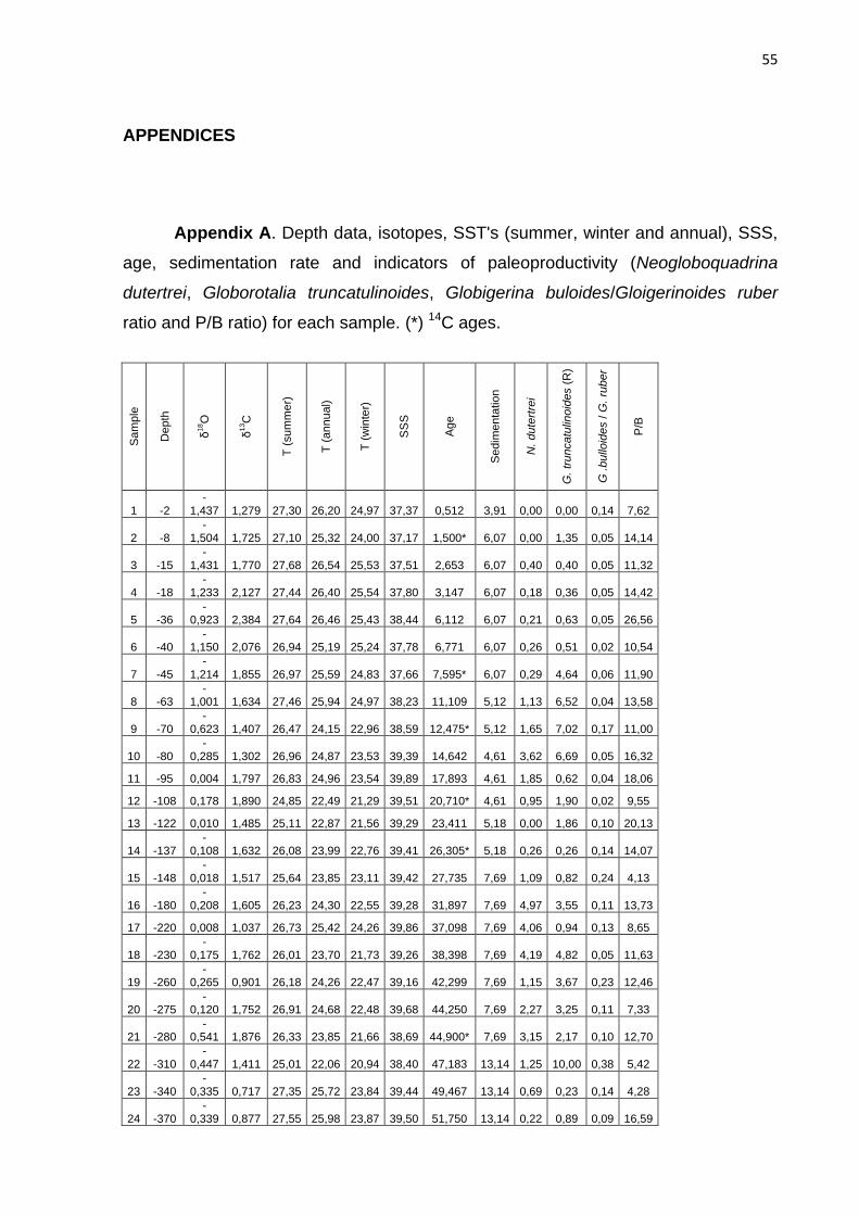
55
APPENDICES
Appendix A. Depth data, isotopes, SST's (summer, winter and annual), SSS,
age, sedimentation rate and indicators of paleoproductivity (Neogloboquadrina
dutertrei, Globorotalia truncatulinoides, Globigerina buloides/Gloigerinoides ruber
ratio and P/B ratio) for each sample. (*) 14C ages.
Sam
ple
Depth
δ18O
δ13C
T (
sum
mer)
T (
annu
al)
T (
win
ter)
SS
S
Age
Sedim
enta
tion
N. dute
rtre
i
G.
tru
ncatu
linoid
es (
R)
G .bullo
ides /
G.
ruber
P/B
1 -2 -
1,437 1,279 27,30 26,20 24,97 37,37 0,512 3,91 0,00 0,00 0,14 7,62
2 -8 -
1,504 1,725 27,10 25,32 24,00 37,17 1,500* 6,07 0,00 1,35 0,05 14,14
3 -15 -
1,431 1,770 27,68 26,54 25,53 37,51 2,653 6,07 0,40 0,40 0,05 11,32
4 -18 -
1,233 2,127 27,44 26,40 25,54 37,80 3,147 6,07 0,18 0,36 0,05 14,42
5 -36 -
0,923 2,384 27,64 26,46 25,43 38,44 6,112 6,07 0,21 0,63 0,05 26,56
6 -40 -
1,150 2,076 26,94 25,19 25,24 37,78 6,771 6,07 0,26 0,51 0,02 10,54
7 -45 -
1,214 1,855 26,97 25,59 24,83 37,66 7,595* 6,07 0,29 4,64 0,06 11,90
8 -63 -
1,001 1,634 27,46 25,94 24,97 38,23 11,109 5,12 1,13 6,52 0,04 13,58
9 -70 -
0,623 1,407 26,47 24,15 22,96 38,59 12,475* 5,12 1,65 7,02 0,17 11,00
10 -80 -
0,285 1,302 26,96 24,87 23,53 39,39 14,642 4,61 3,62 6,69 0,05 16,32
11 -95 0,004 1,797 26,83 24,96 23,54 39,89 17,893 4,61 1,85 0,62 0,04 18,06
12 -108 0,178 1,890 24,85 22,49 21,29 39,51 20,710* 4,61 0,95 1,90 0,02 9,55
13 -122 0,010 1,485 25,11 22,87 21,56 39,29 23,411 5,18 0,00 1,86 0,10 20,13
14 -137 -
0,108 1,632 26,08 23,99 22,76 39,41 26,305* 5,18 0,26 0,26 0,14 14,07
15 -148 -
0,018 1,517 25,64 23,85 23,11 39,42 27,735 7,69 1,09 0,82 0,24 4,13
16 -180 -
0,208 1,605 26,23 24,30 22,55 39,28 31,897 7,69 4,97 3,55 0,11 13,73
17 -220 0,008 1,037 26,73 25,42 24,26 39,86 37,098 7,69 4,06 0,94 0,13 8,65
18 -230 -
0,175 1,762 26,01 23,70 21,73 39,26 38,398 7,69 4,19 4,82 0,05 11,63
19 -260 -
0,265 0,901 26,18 24,26 22,47 39,16 42,299 7,69 1,15 3,67 0,23 12,46
20 -275 -
0,120 1,752 26,91 24,68 22,48 39,68 44,250 7,69 2,27 3,25 0,11 7,33
21 -280 -
0,541 1,876 26,33 23,85 21,66 38,69 44,900* 7,69 3,15 2,17 0,10 12,70
22 -310 -
0,447 1,411 25,01 22,06 20,94 38,40 47,183 13,14 1,25 10,00 0,38 5,42
23 -340 -
0,335 0,717 27,35 25,72 23,84 39,44 49,467 13,14 0,69 0,23 0,14 4,28
24 -370 -
0,339 0,877 27,55 25,98 23,87 39,50 51,750 13,14 0,22 0,89 0,09 16,59
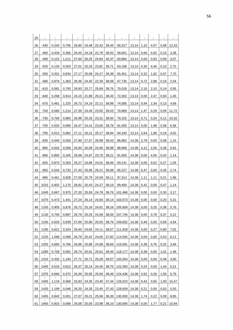
56
25 - - - - - - - - - - - - -
26 -430 -
0,243 0,706 26,90 24,48 22,42 39,45 56,317 13,14 1,10 4,57 0,08 12,43
27 -460 -
0,439 0,366 26,45 24,18 22,79 38,93 58,601 13,14 0,66 5,92 0,10 3,38
28 -490 0,122 1,211 27,60 26,25 24,84 40,37 60,884 13,14 0,00 0,93 0,09 3,07
29 -520 -
0,126 0,503 27,01 25,33 23,81 39,71 63,168 13,14 0,30 4,46 0,10 2,75
30 -550 -
0,331 0,834 27,17 25,69 24,27 39,38 65,451 13,14 0,32 1,62 0,07 7,70
31 -580 -
0,876 1,363 26,36 24,45 22,39 38,08 67,735 13,14 0,72 2,88 0,16 2,04
32 -610 -
0,081 0,793 26,93 25,77 25,69 39,76 70,018 13,14 2,10 2,10 0,14 0,95
33 -640 -
0,268 0,914 24,15 21,89 20,21 38,43 72,302 13,14 0,00 2,47 0,50 1,45
34 -670 -
0,461 1,225 26,72 24,19 22,11 38,98 74,585 13,14 0,94 2,34 0,13 4,69
35 -700 -
0,560 1,214 27,39 24,45 23,92 39,03 76,869 13,14 1,47 0,29 0,09 11,72
36 -730 -
0,769 0,883 26,98 25,33 23,31 38,50 79,152 13,14 0,71 0,24 0,11 10,32
37 -755 -
0,520 0,999 26,47 24,41 23,65 38,78 81,055 13,14 0,00 1,98 0,08 6,58
38 -795 -
0,612 0,882 27,11 26,21 25,17 38,84 84,100 13,14 2,64 1,89 0,19 4,02
39 -835 -
0,440 0,550 27,90 27,57 26,98 39,43 86,882 14,38 2,78 0,00 0,08 1,15
40 -865 -
0,502 0,599 26,94 26,09 24,90 38,98 88,968 14,38 4,12 2,06 0,36 0,91
41 -895 -
0,850 0,165 26,58 24,97 23,75 38,21 91,055 14,38 0,00 4,55 0,42 1,14
42 -925 -
0,870 -
0,303 26,27 24,89 24,01 38,06 93,141 14,38 0,00 9,52 0,27 1,05
43 -955 -
0,543 0,732 27,43 26,95 26,21 39,08 95,227 14,38 0,47 0,00 0,45 2,74
44 -985 -
0,461 0,828 27,09 25,79 24,59 39,11 97,314 14,38 1,11 1,11 0,21 1,96
45 -
1015 -
0,902 1,170 26,81 25,43 24,27 38,19 99,400 14,38 0,42 0,00 0,47 1,14
46 -
1045 -
0,667 0,975 27,20 25,93 24,78 38,76 101,486 14,38 0,00 0,00 0,30 3,17
47 -
1075 -
0,473 1,441 27,24 26,14 24,93 39,14 103,573 14,38 0,00 0,00 0,20 5,31
48 -
1105 -
0,905 0,876 26,72 25,16 24,61 38,16 105,659 14,38 0,00 0,25 0,38 5,76
49 -
1135 -
0,705 0,897 26,79 25,25 24,59 38,55 107,745 14,38 0,00 0,78 0,37 5,12
50 -
1165 -
0,633 0,939 27,00 25,90 25,55 38,76 109,832 14,38 0,49 0,00 0,69 4,94
51 -
1195 -
0,621 0,324 26,40 24,65 24,11 38,57 111,918 14,38 0,00 0,27 0,80 7,02
52 -
1225 -
1,098 0,099 26,79 25,42 24,65 37,82 114,005 14,38 0,00 0,00 0,53 6,12
53 -
1255 -
0,660 0,766 26,96 25,88 24,98 38,69 116,091 14,38 0,38 0,76 0,32 3,46
54 -
1285 -
0,728 0,581 26,74 25,91 25,61 38,49 118,177 14,38 0,38 0,00 1,01 1,48
55 -
1315 -
0,332 1,194 27,71 26,71 25,29 39,57 120,264 14,38 0,00 0,00 0,48 4,60
56 -
1345 -
0,516 0,812 26,37 25,14 24,45 38,75 122,350 14,38 0,24 0,00 1,44 5,21
57 -
1375 -
0,660 0,372 26,39 25,55 25,00 38,49 124,436 14,38 0,52 0,26 1,56 5,79
58 -
1405 -
1,119 -
0,068 25,83 24,35 23,40 37,44 126,523 14,38 0,43 0,65 1,00 15,47
59 -
1435 -
1,199 -
0,048 26,20 24,35 23,45 37,43 128,609 14,38 0,21 0,00 0,63 5,50
60 -
1455 -
0,842 -
0,001 27,07 26,21 25,96 38,39 130,000 14,38 1,74 0,22 0,09 8,85
61 -
1465 -
0,910 0,066 26,58 25,05 23,98 38,10 130,695 14,38 0,00 1,77 0,21 10,94

57
Appendix B. Absolute abundance of species. A
mo
str
a
Fra
çã
o
O.
un
ive
rsa
G.
co
ng
loba
tus
G.r
ub
er
(bra
nca
)
G.r
ub
er
(rosa
)
G.
ten
ella
G.
sa
ccu
life
r N
o s
ac
G.
sa
ccu
life
r c/s
ac
G.
sip
ho
nife
ra
G.
ca
lida
G.
bu
lloid
es
G.
falc
on
en
sis
G.
dig
ita
ta
H.
dig
ita
ta
G.
rube
sce
ns
G.
hu
mili
s
G.
qu
inq
ue
loba
N.
pa
ch
yd
erm
a L
N.
pa
ch
yd
erm
a R
N.
du
tert
rei
P.
ob
liqu
ilocu
lata
G.
infla
ta
G.
trun
ca
tulin
oid
es L
G.
trun
ca
tulin
oid
es R
G.
cra
ssa
form
is
G.
hirsu
ta
G.
scitu
la
G.
anfr
acta
G.
tum
ida
G.
mena
rdii
G.m
.fle
xuo
sa
(ne
o)
C.n
itid
a
G.
glu
tin
ata
T.iota
G.u
vu
la
S.
de
his
cen
s
G.
pu
mili
o
Não
id
en
tificad
o
F.
ben
tôn
icos
Fra
gm
en
tos
Tota
l F
ora
ms P
lan
ct
1
1/1
2
12
3
13
3
10
2
2
5
17
3 3 2 2 1
3
1
20
29
42
22
1
2
1/3
2
2
16
4
37
12
4 6
15
9 1 4 1
12
30
21
49
29
7
3
1/8
5
26
1
92
17
14
6
15
14
1 4 1
2 1
2
2 1 2
16
41
1
44
14
3
49
8
4
1/8
5
5
30
1
58
21
17
3
1
23
15
1 13
1
2
1 2 1
2 1
20
1
54
38
11
2
54
8
5
1/1
6
7
2
24
5
79
20
13
5
7
19
12
4 1 1 3 1 6
20
1
31
1 18
71
47
8
6
1/1
6
3
3
19
5
41
43
21
5
2
17
4 1
1 2 2
1
1
2
15
1
1
29
37
62
39
0
7
1/3
2
1
2
13
7
41
14
19
6
6
9
8 4 1 1
3 1
6
1
2 1
45
28
29
65
34
5
8
1/1
6
17
8
56
8
27
6
1
8
7
1 7 4
1 23
1 3 1
1 20
26
42
35
3
9
1/1
6
94
39
5
8
4
1
7
16
4 2
4
1 17
2 1
1 36
22
74
24
2
10
1/1
6
16
7
57
5
20
4
1
9
9 5 1 13
24
3 4 37
22
55
35
9
11
1/1
6
4
2
14
3
47
7
20
4
2
14
6
2 2 1 6 5
4
2
6 1
46
1 18
54
32
5
12
1/1
6
1
13
6
19
13
11
2 4
3
1 1 1
3 11
2
6
3
1
1 5
91
33
58
31
5
13
1/1
6
1
15
4
12
10
8 8
16
2 2 1 1
6 6
10
85
16
70
32
2
14
1/8
1
2
16
9
32
10
13
10
1
24
4 3 1 1 7
2
1
1 1 1
93
3 27
57
38
0
15
1/8
4
13
1
29
13
14
3
1
32
5 9 1
4 9
1
3
2
1
2
10
2
1 1 89
10
7
36
8
16
1/8
1
5
27
2
33
14
19
10
1
18
30
4 6 1 2
28
26
20
5 1
1 65
1 41
10
5
56
3
17
1/8
3
15
0
27
16
18
3 7
20
5 4 2
13
12
3
3 3 1
30
37
72
32
0
18
1/4
4
22
1
39
10
19
7 4
12
8 3 1
2
20
31
23
7 1 6
4
1 4
1
94
47
7
19
1/1
1
20
0
23
6
29
6 10
45
7 2
1
3
5 26
3
16
20
1
4 28
35
11
3
43
6
20
1/4
1
17
8
30
2
10
1 2
19
4 1 3
7 14
3
10
2 3 18
42
43
30
8
21
1/4
1
25
4
53
6
9
2 12
26
3 3 16
37
17
11
9 2 1
46
40
90
50
8
22
1/1
1
1
96
37
20
19
3 2
36
3 8 4
9
8
7
32
3 5 1
25
59
11
0
32
0
23
1/1
1
6
22
2
55
8
19
1 15
31
1 3 2
3
15
5
2
1
8
1
3 1
32
2
10
2
11
9
43
7
24
1/1
9
4
24
4
55
8
41
3 23
1
1
19
14
4
4
2
1
2 13
27
87
44
8
25
-
26
1/2
13
2
29
9
60
7
19
10
7
23
1 6
16
5 25
3
2
4 2
43
44
86
54
7
27
1/4
1
1
25
1
36
21
31
6 1
26
3
10
2
4
27
1 2 32
1
13
5
82
45
6
28
1/1
13
30
9
86
12
20
5 7
27
7 1 3
4
1
5
3 3 29
17
4
10
7
53
5
29
1/1
5
16
3
39
10
31
11
4
16
3 1 1
6
9
2
15
3 3
1 13
12
2
77
33
6
30
1/2
2
16
9
31
14
11
5 3
11
1 5 2
1
9
11
4
5
2 1 21
40
61
30
8
31
1/1
15
38
14
3
11
1
3
1
6
1 1
1
1
11
9
2
4
11
2
1 1
2 6
8
28
13
9
32
1/1
1
70
6
8
22
9
10
1 3 1 3
1
1 6 1
15
1
37
14
3
33
1/1
1
22
1
8
6 1
11
3 2 3
11
2
2
1 7 5
6
18
81
34
1/1
2
2
21
5
46
5
9
3
1
5
29
2 3 1
4
15
10
9
10
28
5
2 21
91
10
5
42
7
35
1/2
1
15
2
40
2
18
5
2
7
14
4 1
5
6
13
3
1
55
4 7 29
61
34
0
36
1/2
2
1
26
3
19
8
20
6
1
5
29
2 3
4
16
5
1
23
1 14
41
10
7
42
3

58
37
1/4
6
26
6
27
14
10
6
1
12
20
2 8 1
3
9
9
42
1 17
69
93
45
4
38
1/2
2
8
11
8
14
7
9 3
23
7 11
1
1
7
2
3 5
4
2
2 3
14
2 17
66
47
26
5
39
1/1
2
1
37
11
5 1
1
3 3 3
4 1
31
2 3 9
4
21
10
8
40
1/1
3
7
28
6
1
5
1
1 1
0
1 4 2
1
2
2 1
8
3 2
10
7
9
97
41
1/1
19
5
2
10
2
2
8 3
1 3
2
1 6 1
1 5
8
10
66
42
1/1
2
22
1 7 1
1
6 6
1 1
15
60
18
63
43
1/1
1
6
82
12
4
15
4
37
1 4 1
1
1 2 2
32
1 5 7
7
29
21
1
44
1/1
3
4
13
0
8
3
10
3
11
27
2 3
4 3
2
2
2 2
46
2 3
13
8
64
27
0
45
1/1
96
16
5
9 11
45
2 1 1 2 1 30
1 18
20
8
74
23
8
46
1/2
20
1
26
9
7
1
2
19
61
1 4 3 1 2 1
43
1
15
2
12
6
56
39
9
47
1/1
2
1
24
5
27
8
19
1 11
48
1 1 1 3 2
4
1 3
80
5 20
91
56
48
3
48
1/2
20
4
17
32
7 1
18
77
3 3 1
2
1
1 24
1 10
1 70
53
40
3
49
1/2
16
5
32
27
10
14
61
2 5
3 1
2 53
3 6 75
36
38
4
50
1/4
2
2
15
4
23
28
7 2
3
10
7
2 1
5
2
1
1
2 5 1 2
27
2 4 8
3
70
41
0
51
1/8
1
12
3
14
10
27
2
2
32
99
2 1 1 2 1
1 4 28
15
52
84
36
5
52
1/4
1
15
6
27
16
15
1
21
82
1 11
12
7 1 29
3 15
65
94
39
8
53
1/1
1
11
1
13
6
33
1
1
10
35
3 1
1
4 1
2
4
2
5 1
16
11
1 76
72
26
3
54
1/1
4
69
15
13
34
3
16
70
2 6 1
2
2
3 3 10
7
17
6
12
4
26
0
55
1/1
1
6
21
5
42
10
13
2 25
10
4
2 18
33
4 6 2
43
1 11
11
7
11
6
53
8
56
1/2
13
78
21
9
38
2
1
31
11
2
6 9 1
14
4 2 3
3
43
80
85
41
7
57
1/2
1
9
79
16
15
39
2 23
12
3
1 9
2 2
8 1
3
1 1
28
25
67
97
38
8
58
1/8
21
13
4
15
16
28
2
2
28
13
4
1 2
6 1
2 2
4 3 1
2 14
43
1
1
1 30
14
8
46
4
59
1/8
4
22
15
5
33
19
33
1
6
35
98
2 3 1 1
4 4
1 10
45
1
1 5
17
88
48
4
60
1/8
2
7
15
1
43
5
10
3
12
20
30
13
1
2 1 2
8 1 1
5 1
1 49
1 1 52
14
0
46
0
61
1/1
6
11
15
0
29
10
34
1
2
11
32
1 4 3
2
1
6
2 39
1
31
72
33
9
Appendix C. Relative abundance of species.
Am
ostr
a
O.
un
ive
rsa
G.
co
ng
loba
tus
G.r
ub
er
(bra
nca
)
G.r
ub
er
(rosa
)
G.
ten
ella
G.
sa
ccu
life
r N
o s
ac
G.
sa
ccu
life
r c/s
ac
G.
sip
ho
nife
ra
G.
ca
lida
G.
bu
lloid
es
G.
falc
on
en
sis
G.
dig
ita
ta
H. d
igita
ta
G.
rube
sce
ns
G.
hu
mili
s
G.
qu
inq
ue
loba
N. p
ach
yd
erm
a L
N. p
ach
yd
erm
a R
N. d
ute
rtre
i
P.
ob
liqu
ilocu
lata
G.
infla
ta
G.
trun
ca
tulin
oid
es L
G.
trun
ca
tulin
oid
es R
G.
cra
ssa
form
is
G.
hirsu
ta
G.
scitu
la
G.
anfr
acta
G.
tum
ida
G.
me
na
rdii
G.m
.fle
xuo
sa
(ne
o)
C.n
itid
a
G.
glu
tin
ata
T.iota
G.u
vu
la
S.
de
his
cen
s
G.
pu
mili
o
Não
id
en
tificad
o
1
0,0
0
0,9
0
55
,66
5,8
8
1,3
6
4,5
2
0,9
0
0,9
0
2,2
6
7,6
9
1,3
6
0,0
0
0,0
0
1,3
6
0,0
0
0,0
0
0,0
0
0,0
0
0,0
0
0,9
0
0,0
0
0,0
0
0,0
0
0,0
0
0,0
0
0,9
0
0,0
0
0,0
0
5,8
8
0,0
0
0,4
5
9,0
5
0,0
0
0,0
0
0,0
0
0,0
0
0,0
0
2
0,0
0
0,6
7
55
,22
12
,46
4,0
4
1,3
5
0,0
0
2,0
2
5,0
5
3,0
3
0,0
0
0,0
0
0,0
0
0,0
0
0,0
0
0,0
0
0,0
0
0,0
0
0,0
0
0,3
4
0,0
0
0,0
0
1,3
5
0,0
0
0,0
0
0,0
0
0,0
0
0,3
4
4,0
4
0,0
0
0,0
0
10
,10
0,0
0
0,0
0
0,0
0
0,0
0
0,0
0
3
0,0
0
1,0
0
52
,41
18
,47
3,4
1
2,8
1
0,0
0
1,2
0
3,0
1
2,8
1
0,2
0
0,0
0
0,0
0
0,8
0
0,0
0
0,0
0
0,0
0
0,2
0
0,4
0
0,0
0
0,0
0
0,2
0
0,4
0
0,4
0
0,0
0
0,2
0
0,0
0
0,4
0
3,2
1
0,0
0
0,0
0
8,2
3
0,0
0
0,0
0
0,0
0
0,0
0
0,2
0
4
0,9
1
0,9
1
54
,93
10
,58
3,8
3
3,1
0
0,5
5
0,1
8
4,2
0
2,7
4
0,1
8
0,0
0
0,0
0
2,3
7
0,0
0
0,0
0
0,0
0
0,0
0
0,1
8
0,3
6
0,1
8
0,0
0
0,3
6
0,0
0
0,1
8
0,3
6
0,0
0
0,1
8
3,6
5
0,0
0
0,1
8
9,8
5
0,0
0
0,0
0
0,0
0
0,0
0
0,0
0
5
1,4
6
0,4
2
51
,26
16
,53
4,1
8
2,7
2
1,0
5
1,4
6
3,9
7
2,5
1
0,0
0
0,0
0
0,0
0
0,8
4
0,0
0
0,0
0
0,0
0
0,0
0
0,2
1
0,0
0
0,2
1
0,0
0
0,6
3
0,0
0
0,2
1
0,0
0
0,0
0
1,2
6
4,1
8
0,0
0
0,2
1
6,4
9
0,0
0
0,2
1
0,0
0
0,0
0
0,0
0
6
0,7
7
0,7
7
50
,00
10
,51
11
,03
5,3
8
1,2
8
0,5
1
4,3
6
1,0
3
0,0
0
0,0
0
0,0
0
0,0
0
0,0
0
0,0
0
0,0
0
0,0
0
0,2
6
0,2
6
0,0
0
0,0
0
0,5
1
0,0
0
0,5
1
0,2
6
0,2
6
0,5
1
3,8
5
0,2
6
0,2
6
7,4
4
0,0
0
0,0
0
0,0
0
0,0
0
0,0
0

59
7
0,2
9
0,5
8
39
,71
11
,88
4,0
6
5,5
1
1,7
4
1,7
4
2,6
1
2,3
2
0,0
0
0,0
0
0,0
0
1,1
6
0,0
0
0,2
9
0,0
0
0,0
0
0,2
9
0,8
7
0,0
0
0,0
0
4,6
4
0,0
0
0,2
9
0,5
8
0,0
0
0,2
9
13
,04
0,0
0
0,0
0
8,1
2
0,0
0
0,0
0
0,0
0
0,0
0
0,0
0
8
0,0
0
0,0
0
50
,42
15
,86
2,2
7
7,6
5
1,7
0
0,2
8
2,2
7
1,9
8
0,2
8
0,0
0
0,0
0
1,9
8
0,0
0
0,0
0
0,0
0
0,0
0
1,1
3
0,2
8
0,0
0
0,0
0
6,5
2
0,2
8
0,0
0
0,8
5
0,0
0
0,2
8
0,2
8
0,0
0
0,0
0
5,6
7
0,0
0
0,0
0
0,0
0
0,0
0
0,0
0
9
0,0
0
0,0
0
38
,84
16
,12
2,0
7
3,3
1
1,6
5
0,4
1
2,8
9
6,6
1
0,0
0
0,0
0
0,0
0
1,6
5
0,0
0
0,0
0
0,0
0
0,8
3
1,6
5
0,4
1
0,0
0
0,0
0
7,0
2
0,0
0
0,0
0
0,8
3
0,0
0
0,4
1
0,4
1
0,0
0
0,0
0
14
,88
0,0
0
0,0
0
0,0
0
0,0
0
0,0
0
10
0,0
0
0,0
0
46
,52
15
,88
1,3
9
5,5
7
1,1
1
0,2
8
2,5
1
2,5
1
0,0
0
0,0
0
0,0
0
1,3
9
0,0
0
0,0
0
0,2
8
0,0
0
3,6
2
0,0
0
0,0
0
0,0
0
6,6
9
0,8
4
0,0
0
1,1
1
0,0
0
0,0
0
0,0
0
0,0
0
0,0
0
10
,31
0,0
0
0,0
0
0,0
0
0,0
0
0,0
0
11
1,2
3
0,6
2
44
,00
14
,46
2,1
5
6,1
5
1,2
3
0,6
2
4,3
1
1,8
5
0,6
2
0,0
0
0,0
0
0,6
2
0,0
0
0,0
0
0,3
1
0,0
0
1,8
5
0,0
0
1,5
4
1,2
3
0,6
2
1,8
5
0,0
0
0,0
0
0,0
0
0,0
0
0,0
0
0,0
0
0,3
1
14
,15
0,0
0
0,3
1
0,0
0
0,0
0
0,0
0
12
0,0
0
0,3
2
43
,17
6,0
3
4,1
3
3,4
9
0,6
3
0,0
0
1,2
7
0,9
5
0,3
2
0,0
0
0,0
0
0,0
0
0,0
0
0,3
2
0,0
0
0,3
2
0,9
5
0,0
0
3,4
9
0,6
3
1,9
0
0,9
5
0,3
2
0,3
2
0,0
0
0,0
0
0,0
0
0,0
0
1,5
9
28
,89
0,0
0
0,0
0
0,0
0
0,0
0
0,0
0
13
0,0
0
0,3
1
47
,83
3,7
3
3,1
1
2,4
8
0,0
0
0,0
0
2,4
8
4,9
7
0,6
2
0,0
0
0,0
0
0,6
2
0,0
0
0,0
0
0,0
0
0,3
1
0,0
0
0,3
1
1,8
6
0,0
0
1,8
6
3,1
1
0,0
0
0,0
0
0,0
0
0,0
0
0,0
0
0,0
0
0,0
0
26
,40
0,0
0
0,0
0
0,0
0
0,0
0
0,0
0
14
0,2
6
0,5
3
44
,47
8,4
2
2,6
3
3,4
2
2,6
3
0,0
0
0,2
6
6,3
2
1,0
5
0,0
0
0,0
0
0,7
9
0,0
0
0,0
0
0,2
6
0,0
0
0,2
6
0,0
0
1,8
4
0,5
3
0,2
6
0,2
6
0,0
0
0,2
6
0,0
0
0,0
0
0,0
0
0,0
0
0,2
6
24
,47
0,0
0
0,7
9
0,0
0
0,0
0
0,0
0
15
0,0
0
1,0
9
35
,60
7,8
8
3,5
3
3,8
0
0,0
0
0,8
2
0,2
7
8,7
0
1,3
6
0,0
0
0,0
0
2,4
5
0,0
0
0,0
0
0,0
0
0,2
7
1,0
9
0,0
0
2,4
5
0,2
7
0,8
2
0,5
4
0,2
7
0,5
4
0,0
0
0,0
0
0,0
0
0,0
0
0,0
0
27
,72
0,2
7
0,0
0
0,2
7
0,0
0
0,0
0
16
0,1
8
0,8
9
48
,31
5,8
6
2,4
9
3,3
7
1,7
8
0,1
8
3,2
0
5,3
3
0,7
1
0,0
0
0,0
0
1,0
7
0,0
0
0,1
8
0,0
0
0,3
6
4,9
7
0,0
0
4,6
2
0,0
0
3,5
5
0,8
9
0,0
0
0,1
8
0,1
8
0,0
0
0,0
0
0,0
0
0,0
0
11
,55
0,1
8
0,0
0
0,0
0
0,0
0
0,0
0
17
0,0
0
0,9
4
46
,88
8,4
4
5,0
0
5,6
3
0,9
4
0,0
0
2,1
9
6,2
5
1,5
6
0,0
0
0,0
0
1,2
5
0,0
0
0,0
0
0,0
0
0,6
3
4,0
6
0,0
0
3,7
5
0,0
0
0,9
4
0,9
4
0,0
0
0,9
4
0,0
0
0,0
0
0,0
0
0,0
0
0,3
1
9,3
8
0,0
0
0,0
0
0,0
0
0,0
0
0,0
0
18
0,0
0
0,8
4
46
,33
8,1
8
2,1
0
3,9
8
1,4
7
0,0
0
0,8
4
2,5
2
1,6
8
0,0
0
0,0
0
0,6
3
0,0
0
0,0
0
0,2
1
0,4
2
4,1
9
0,0
0
6,5
0
0,0
0
4,8
2
1,4
7
0,0
0
0,2
1
0,0
0
0,0
0
0,0
0
0,0
0
0,0
0
13
,42
0,0
0
0,2
1
0,0
0
0,0
0
0,0
0
19
0,0
0
0,2
3
45
,87
5,2
8
1,3
8
6,6
5
1,3
8
0,0
0
2,2
9
10
,32
0,0
0
0,0
0
0,0
0
1,6
1
0,0
0
0,4
6
0,2
3
0,6
9
1,1
5
0,0
0
5,9
6
0,6
9
3,6
7
4,5
9
0,2
3
0,9
2
0,0
0
0,0
0
0,0
0
0,0
0
0,0
0
6,4
2
0,0
0
0,0
0
0,0
0
0,0
0
0,0
0
20
0,0
0
0,3
2
57
,79
9,7
4
0,6
5
3,2
5
0,3
2
0,0
0
0,6
5
6,1
7
1,3
0
0,0
0
0,0
0
0,3
2
0,0
0
0,0
0
0,0
0
0,9
7
2,2
7
0,0
0
4,5
5
0,9
7
3,2
5
0,6
5
0,0
0
0,9
7
0,0
0
0,0
0
0,0
0
0,0
0
0,0
0
5,8
4
0,0
0
0,0
0
0,0
0
0,0
0
0,0
0
21
0,0
0
0,2
0
50
,00
10
,43
1,1
8
1,7
7
0,3
9
0,0
0
2,3
6
5,1
2
0,5
9
0,0
0
0,0
0
0,5
9
0,0
0
0,0
0
0,0
0
0,0
0
3,1
5
0,0
0
7,2
8
3,3
5
2,1
7
1,7
7
0,0
0
0,3
9
0,0
0
0,0
0
0,0
0
0,0
0
0,2
0
9,0
6
0,0
0
0,0
0
0,0
0
0,0
0
0,0
0
22
0,3
1
0,3
1
30
,00
11
,56
6,2
5
5,9
4
0,9
4
0,0
0
0,6
3
11
,25
0,9
4
0,0
0
0,0
0
2,5
0
0,0
0
0,0
0
0,0
0
0,0
0
1,2
5
2,8
1
2,5
0
2,1
9
10
,00
0,9
4
0,0
0
1,5
6
0,0
0
0,0
0
0,0
0
0,0
0
0,3
1
7,8
1
0,0
0
0,0
0
0,0
0
0,0
0
0,0
0
23
0,2
3
1,3
7
50
,80
12
,59
1,8
3
4,3
5
0,2
3
0,0
0
3,4
3
7,0
9
0,2
3
0,0
0
0,0
0
0,6
9
0,0
0
0,0
0
0,0
0
0,4
6
0,6
9
3,4
3
1,1
4
0,4
6
0,2
3
1,8
3
0,2
3
0,6
9
0,0
0
0,0
0
0,0
0
0,0
0
0,2
3
7,3
2
0,0
0
0,4
6
0,0
0
0,0
0
0,0
0
24
2,0
1
0,8
9
54
,46
12
,28
1,7
9
9,1
5
0,6
7
0,0
0
0,0
0
5,1
3
0,0
0
0,0
0
0,0
0
0,0
0
0,0
0
0,0
0
0,0
0
0,2
2
0,2
2
4,2
4
3,1
3
0,8
9
0,8
9
0,4
5
0,2
2
0,4
5
0,0
0
0,0
0
0,0
0
0,0
0
0,0
0
2,9
0
0,0
0
0,0
0
0,0
0
0,0
0
0,0
0
25
26
2,3
8
0,3
7
54
,66
10
,97
1,2
8
3,4
7
1,8
3
0,0
0
1,2
8
4,2
0
0,0
0
0,0
0
0,0
0
0,1
8
0,0
0
0,0
0
0,0
0
0,0
0
1,1
0
2,9
3
0,9
1
0,0
0
4,5
7
0,5
5
0,3
7
0,7
3
0,0
0
0,0
0
0,0
0
0,0
0
0,3
7
7,8
6
0,0
0
0,0
0
0,0
0
0,0
0
0,0
0
27
0,2
2
0,2
2
55
,04
7,8
9
4,6
1
6,8
0
1,3
2
0,0
0
0,2
2
5,7
0
0,0
0
0,0
0
0,0
0
0,0
0
0,0
0
0,0
0
0,0
0
0,0
0
0,6
6
2,1
9
0,4
4
0,8
8
5,9
2
0,2
2
0,0
0
0,4
4
0,0
0
0,0
0
0,0
0
0,0
0
0,0
0
7,0
2
0,0
0
0,2
2
0,0
0
0,0
0
0,0
0
28
0,0
0
2,4
3
57
,76
16
,07
2,2
4
3,7
4
0,9
3
0,0
0
1,3
1
5,0
5
1,3
1
0,0
0
0,0
0
0,0
0
0,0
0
0,0
0
0,1
9
0,0
0
0,0
0
0,5
6
0,7
5
0,1
9
0,9
3
0,5
6
0,0
0
0,5
6
0,0
0
0,0
0
0,0
0
0,0
0
0,0
0
5,4
2
0,0
0
0,0
0
0,0
0
0,0
0
0,0
0
29
0,0
0
1,4
9
48
,51
11
,61
2,9
8
9,2
3
3,2
7
0,0
0
1,1
9
4,7
6
0,8
9
0,0
0
0,0
0
0,0
0
0,0
0
0,0
0
0,3
0
0,0
0
0,3
0
1,7
9
2,6
8
0,6
0
4,4
6
0,8
9
0,0
0
0,8
9
0,3
0
0,0
0
0,0
0
0,0
0
0,0
0
3,8
7
0,0
0
0,0
0
0,0
0
0,0
0
0,0
0
30
0,0
0
0,6
5
54
,87
10
,06
4,5
5
3,5
7
1,6
2
0,0
0
0,9
7
3,5
7
0,3
2
0,0
0
0,0
0
1,6
2
0,0
0
0,0
0
0,0
0
0,6
5
0,3
2
2,9
2
3,5
7
1,3
0
1,6
2
0,6
5
0,0
0
0,3
2
0,0
0
0,0
0
0,0
0
0,0
0
0,0
0
6,8
2
0,0
0
0,0
0
0,0
0
0,0
0
0,0
0
31
0,0
0
10
,79
27
,34
10
,07
2,1
6
7,9
1
0,7
2
2,1
6
0,7
2
4,3
2
0,7
2
0,0
0
0,0
0
0,0
0
0,0
0
0,0
0
0,7
2
0,7
2
0,7
2
7,9
1
6,4
7
1,4
4
2,8
8
7,9
1
1,4
4
0,7
2
0,0
0
0,0
0
0,0
0
0,0
0
0,7
2
1,4
4
0,0
0
0,0
0
0,0
0
0,0
0
0,0
0
32
0,0
0
0,7
0
48
,95
4,2
0
5,5
9
15
,38
0,0
0
0,0
0
6,2
9
6,9
9
0,0
0
0,0
0
0,0
0
0,7
0
0,0
0
0,0
0
0,0
0
0,0
0
2,1
0
0,0
0
0,7
0
0,0
0
2,1
0
0,7
0
0,7
0
0,0
0
0,0
0
0,0
0
0,0
0
0,0
0
0,0
0
4,2
0
0,0
0
0,0
0
0,7
0
0,0
0
0,0
0
33
0,0
0
1,2
3
27
,16
1,2
3
9,8
8
7,4
1
0,0
0
0,0
0
1,2
3
13
,58
3,7
0
0,0
0
0,0
0
2,4
7
0,0
0
0,0
0
0,0
0
0,0
0
0,0
0
3,7
0
13
,58
2,4
7
2,4
7
1,2
3
0,0
0
0,0
0
0,0
0
0,0
0
0,0
0
0,0
0
0,0
0
8,6
4
0,0
0
0,0
0
0,0
0
0,0
0
0,0
0
34
0,4
7
0,4
7
50
,35
10
,77
1,1
7
2,1
1
0,7
0
0,2
3
1,1
7
6,7
9
0,4
7
0,0
0
0,0
0
0,7
0
0,0
0
0,0
0
0,0
0
0,2
3
0,9
4
3,5
1
2,3
4
2,1
1
2,3
4
6,5
6
1,1
7
0,4
7
0,0
0
0,0
0
0,0
0
0,0
0
0,0
0
4,9
2
0,0
0
0,0
0
0,0
0
0,0
0
0,0
0
35
0,2
9
0,0
0
44
,71
11
,76
0,5
9
5,2
9
1,4
7
0,5
9
2,0
6
4,1
2
0,0
0
0,0
0
0,0
0
1,1
8
0,0
0
0,0
0
0,0
0
0,2
9
1,4
7
1,7
6
3,8
2
0,8
8
0,2
9
16
,18
0,0
0
1,1
8
0,0
0
0,0
0
0,0
0
0,0
0
0,0
0
2,0
6
0,0
0
0,0
0
0,0
0
0,0
0
0,0
0
36
0,4
7
0,2
4
62
,17
4,4
9
1,8
9
4,7
3
1,4
2
0,2
4
1,1
8
6,8
6
0,4
7
0,0
0
0,0
0
0,0
0
0,0
0
0,0
0
0,0
0
0,0
0
0,7
1
0,9
5
3,7
8
1,1
8
0,2
4
5,4
4
0,2
4
0,0
0
0,0
0
0,0
0
0,0
0
0,0
0
0,0
0
3,3
1
0,0
0
0,0
0
0,0
0
0,0
0
0,0
0
37
0,0
0
1,3
2
58
,59
5,9
5
3,0
8
2,2
0
1,3
2
0,2
2
2,6
4
4,4
1
0,4
4
0,0
0
0,0
0
1,7
6
0,0
0
0,0
0
0,0
0
0,0
0
0,0
0
0,2
2
0,6
6
1,9
8
1,9
8
9,2
5
0,0
0
0,2
2
0,0
0
0,0
0
0,0
0
0,0
0
0,0
0
3,7
4
0,0
0
0,0
0
0,0
0
0,0
0
0,0
0
38
0,7
5
3,0
2
44
,53
5,2
8
2,6
4
3,4
0
0,0
0
0,0
0
1,1
3
8,6
8
2,6
4
0,0
0
0,0
0
4,1
5
0,0
0
0,0
0
0,3
8
0,3
8
2,6
4
0,7
5
1,1
3
0,0
0
1,8
9
1,5
1
0,7
5
0,7
5
0,0
0
1,1
3
5,2
8
0,7
5
0,0
0
6,4
2
0,0
0
0,0
0
0,0
0
0,0
0
0,0
0

60
39
1,8
5
0,9
3
34
,26
10
,19
4,6
3
0,0
0
0,0
0
0,9
3
0,9
3
2,7
8
0,0
0
0,0
0
0,0
0
2,7
8
0,0
0
0,0
0
0,0
0
0,0
0
2,7
8
3,7
0
0,0
0
0,0
0
0,0
0
0,0
0
0,0
0
0,0
0
0,0
0
0,9
3
28
,70
1,8
5
0,0
0
2,7
8
0,0
0
0,0
0
0,0
0
0,0
0
0,0
0
40
3,0
9
7,2
2
28
,87
6,1
9
1,0
3
5,1
5
1,0
3
1,0
3
0,0
0
10
,31
0,0
0
0,0
0
0,0
0
1,0
3
0,0
0
0,0
0
0,0
0
0,0
0
4,1
2
0,0
0
0,0
0
0,0
0
2,0
6
1,0
3
2,0
6
2,0
6
0,0
0
0,0
0
18
,56
3,0
9
0,0
0
2,0
6
0,0
0
0,0
0
0,0
0
0,0
0
0,0
0
41
0,0
0
0,0
0
28
,79
7,5
8
3,0
3
15
,15
0,0
0
3,0
3
3,0
3
12
,12
0,0
0
0,0
0
0,0
0
0,0
0
0,0
0
0,0
0
0,0
0
0,0
0
0,0
0
4,5
5
1,5
2
0,0
0
4,5
5
3,0
3
1,5
2
0,0
0
0,0
0
0,0
0
9,0
9
0,0
0
1,5
2
1,5
2
0,0
0
0,0
0
0,0
0
0,0
0
0,0
0
42
0,0
0
3,1
7
34
,92
1,5
9
0,0
0
11
,11
0,0
0
1,5
9
1,5
9
9,5
2
0,0
0
0,0
0
0,0
0
0,0
0
0,0
0
0,0
0
0,0
0
0,0
0
0,0
0
0,0
0
0,0
0
0,0
0
9,5
2
1,5
9
0,0
0
0,0
0
0,0
0
1,5
9
23
,81
0,0
0
0,0
0
0,0
0
0,0
0
0,0
0
0,0
0
0,0
0
0,0
0
43
0,4
7
2,8
4
38
,86
5,6
9
1,9
0
7,1
1
0,0
0
0,0
0
1,9
0
17
,54
0,4
7
0,0
0
0,0
0
1,9
0
0,0
0
0,0
0
0,0
0
0,0
0
0,4
7
0,4
7
0,4
7
0,0
0
0,0
0
0,0
0
0,0
0
0,9
5
0,0
0
0,9
5
15
,17
0,4
7
0,0
0
2,3
7
0,0
0
0,0
0
0,0
0
0,0
0
0,0
0
44
1,1
1
1,4
8
48
,15
2,9
6
1,1
1
3,7
0
0,0
0
1,1
1
4,0
7
10
,00
0,7
4
0,0
0
0,0
0
0,0
0
0,0
0
0,0
0
0,0
0
0,0
0
1,1
1
1,4
8
0,0
0
0,0
0
1,1
1
0,7
4
0,7
4
0,7
4
0,0
0
0,7
4
17
,04
0,7
4
0,0
0
1,1
1
0,0
0
0,0
0
0,0
0
0,0
0
0,0
0
45
0,0
0
0,0
0
40
,34
6,7
2
2,1
0
3,7
8
0,0
0
0,0
0
4,6
2
18
,91
0,8
4
0,0
0
0,0
0
0,4
2
0,0
0
0,0
0
0,0
0
0,0
0
0,4
2
0,0
0
0,0
0
0,0
0
0,0
0
0,8
4
0,0
0
0,4
2
0,0
0
0,0
0
12
,61
0,4
2
0,0
0
7,5
6
0,0
0
0,0
0
0,0
0
0,0
0
0,0
0
46
0,0
0
0,0
0
50
,38
6,5
2
2,2
6
1,7
5
0,2
5
0,5
0
4,7
6
15
,29
0,2
5
0,0
0
0,0
0
1,0
0
0,0
0
0,0
0
0,0
0
0,0
0
0,0
0
0,0
0
0,0
0
0,7
5
0,0
0
0,2
5
0,0
0
0,5
0
0,0
0
0,2
5
10
,78
0,0
0
0,2
5
3,7
6
0,0
0
0,5
0
0,0
0
0,0
0
0,0
0
47
0,4
1
0,2
1
50
,72
5,5
9
1,6
6
3,9
3
0,2
1
0,0
0
2,2
8
9,9
4
0,2
1
0,0
0
0,0
0
0,2
1
0,0
0
0,0
0
0,0
0
0,0
0
0,0
0
0,2
1
0,0
0
0,6
2
0,0
0
0,4
1
0,8
3
0,2
1
0,0
0
0,6
2
16
,56
1,0
4
0,0
0
4,1
4
0,0
0
0,0
0
0,0
0
0,0
0
0,0
0
48
0,0
0
0,0
0
50
,62
4,2
2
7,9
4
1,7
4
0,0
0
0,2
5
4,4
7
19
,11
0,0
0
0,0
0
0,0
0
0,7
4
0,0
0
0,0
0
0,0
0
0,0
0
0,0
0
0,7
4
0,0
0
0,0
0
0,2
5
0,5
0
0,2
5
0,2
5
0,0
0
0,0
0
5,9
6
0,2
5
0,0
0
2,4
8
0,0
0
0,2
5
0,0
0
0,0
0
0,0
0
49
0,0
0
0,0
0
42
,97
8,3
3
7,0
3
2,6
0
0,0
0
0,0
0
3,6
5
15
,89
0,5
2
0,0
0
0,0
0
0,0
0
0,0
0
0,0
0
0,0
0
0,0
0
0,0
0
0,0
0
0,0
0
1,3
0
0,7
8
0,0
0
0,2
6
0,5
2
0,0
0
0,0
0
13
,80
0,7
8
0,0
0
1,5
6
0,0
0
0,0
0
0,0
0
0,0
0
0,0
0
50
0,4
9
0,4
9
37
,56
5,6
1
6,8
3
1,7
1
0,0
0
0,0
0
5,6
1
26
,10
0,4
9
0,0
0
0,0
0
3,6
6
0,0
0
0,0
0
0,0
0
0,0
0
0,4
9
0,2
4
0,2
4
0,4
9
0,0
0
1,2
2
0,0
0
0,2
4
0,0
0
0,4
9
6,5
9
0,4
9
0,0
0
0,9
8
0,0
0
0,0
0
0,0
0
0,0
0
0,0
0
51
0,2
7
0,0
0
33
,70
3,8
4
2,7
4
7,4
0
0,5
5
0,5
5
8,7
7
27
,12
0,5
5
0,0
0
0,0
0
0,2
7
0,0
0
0,0
0
0,0
0
0,2
7
0,0
0
0,0
0
0,5
5
0,0
0
0,2
7
0,2
7
0,0
0
1,1
0
0,0
0
0,0
0
7,6
7
0,0
0
0,0
0
4,1
1
0,0
0
0,0
0
0,0
0
0,0
0
0,0
0
52
0,0
0
0,2
5
39
,20
6,7
8
4,0
2
3,7
7
0,0
0
0,2
5
5,2
8
20
,60
0,2
5
0,0
0
0,0
0
2,7
6
0,0
0
0,0
0
0,0
0
0,0
0
0,0
0
0,0
0
0,0
0
3,0
2
0,0
0
1,7
6
0,0
0
0,2
5
0,0
0
0,0
0
7,2
9
0,7
5
0,0
0
3,7
7
0,0
0
0,0
0
0,0
0
0,0
0
0,0
0
53
0,3
8
0,0
0
42
,21
4,9
4
2,2
8
12
,55
0,3
8
0,3
8
3,8
0
13
,31
0,0
0
0,0
0
0,0
0
1,1
4
0,0
0
0,0
0
0,0
0
0,3
8
0,3
8
1,5
2
0,0
0
0,3
8
0,7
6
1,5
2
0,7
6
1,9
0
0,0
0
0,3
8
6,0
8
0,0
0
0,0
0
4,1
8
0,0
0
0,3
8
0,0
0
0,0
0
0,0
0
54
0,0
0
1,5
4
26
,54
5,7
7
5,0
0
13
,08
0,0
0
1,1
5
6,1
5
26
,92
0,7
7
0,0
0
0,0
0
2,3
1
0,0
0
0,0
0
0,0
0
0,0
0
0,3
8
0,7
7
0,7
7
1,1
5
0,0
0
1,1
5
0,0
0
0,0
0
0,0
0
0,0
0
3,8
5
0,0
0
0,0
0
2,6
9
0,0
0
0,0
0
0,0
0
0,0
0
0,0
0
55
0,1
9
1,1
2
39
,96
7,8
1
1,8
6
2,4
2
0,3
7
0,0
0
4,6
5
19
,33
0,3
7
0,0
0
0,0
0
3,3
5
0,0
0
0,0
0
0,0
0
0,0
0
0,0
0
6,1
3
0,0
0
0,0
0
0,0
0
0,7
4
0,0
0
1,1
2
0,0
0
0,3
7
7,9
9
0,1
9
0,0
0
2,0
4
0,0
0
0,0
0
0,0
0
0,0
0
0,0
0
56
0,0
0
3,1
2
18
,71
5,0
4
2,1
6
9,1
1
0,4
8
0,2
4
7,4
3
26
,86
1,4
4
0,0
0
0,0
0
2,1
6
0,0
0
0,0
0
0,0
0
0,0
0
0,2
4
3,3
6
0,0
0
0,0
0
0,0
0
0,9
6
0,0
0
0,4
8
0,0
0
0,0
0
7,9
1
0,0
0
0,0
0
10
,31
0,0
0
0,0
0
0,0
0
0,0
0
0,0
0
57
0,2
6
2,3
2
20
,36
4,1
2
3,8
7
10
,05
0,5
2
0,0
0
5,9
3
31
,70
0,2
6
0,0
0
0,0
0
2,3
2
0,5
2
0,0
0
0,0
0
0,0
0
0,5
2
2,0
6
0,0
0
0,0
0
0,2
6
0,7
7
0,2
6
0,0
0
0,0
0
0,2
6
7,2
2
0,0
0
0,0
0
6,4
4
0,0
0
0,0
0
0,0
0
0,0
0
0,0
0
58
0,0
0
4,5
3
28
,88
3,2
3
3,4
5
6,0
3
0,4
3
0,4
3
6,0
3
28
,88
0,2
2
0,0
0
0,4
3
1,2
9
0,0
0
0,2
2
0,4
3
0,0
0
0,4
3
0,8
6
0,0
0
0,0
0
0,6
5
0,0
0
0,2
2
0,4
3
0,0
0
0,0
0
3,0
2
0,0
0
0,0
0
9,2
7
0,2
2
0,2
2
0,2
2
0,0
0
0,0
0
59
0,8
3
4,5
5
32
,02
6,8
2
3,9
3
6,8
2
0,2
1
1,2
4
7,2
3
20
,25
0,0
0
0,4
1
0,0
0
0,6
2
0,0
0
0,0
0
0,0
0
0,0
0
0,2
1
0,0
0
0,2
1
0,8
3
0,0
0
0,8
3
0,2
1
0,0
0
0,0
0
0,0
0
2,0
7
0,0
0
0,0
0
9,3
0
0,2
1
0,2
1
0,0
0
0,0
0
1,0
3
60
0,4
3
1,5
2
32
,83
9,3
5
1,0
9
22
,39
2,6
1
4,3
5
6,5
2
2,8
3
0,0
0
0,0
0
0,2
2
0,4
3
0,0
0
0,2
2
0,0
0
0,4
3
1,7
4
0,0
0
0,2
2
0,0
0
0,2
2
1,0
9
0,0
0
0,2
2
0,2
2
0,0
0
0,0
0
0,0
0
0,0
0
10
,65
0,0
0
0,2
2
0,0
0
0,2
2
0,0
0
61
0,0
0
3,2
4
44
,25
8,5
5
2,9
5
10
,03
0,2
9
0,5
9
3,2
4
9,4
4
0,2
9
0,0
0
0,0
0
0,0
0
0,0
0
0,0
0
0,0
0
1,1
8
0,0
0
0,8
8
0,5
9
0,2
9
1,7
7
0,5
9
0,0
0
0,0
0
0,0
0
0,0
0
0,0
0
0,0
0
0,0
0
11
,50
0,0
0
0,0
0
0,0
0
0,0
0
0,2
9