UFABC - Física Quântica - Curso 2017.3 Prof. Germán Lugones

Aula 4 O modelo atômico de Bohr

1

O modelo de Bohr

2

Em 1913, Niels Bohr propôs um modelo do átomo de hidrogênio que combinava o trabalho de Planck, Einstein e Rutherford e foi notavelmente bem sucedido na previsão do espectro observado do hidrogênio.

O modelo de Rutherford tinha atribuído carga e massa ao núcleo, mas nada dizia quanto à distribuição da carga e massa dos elétrons.

Bohr, supôs que o elétron no átomo de hidrogênio orbitava em torno do núcleo positivo, ligado pela atração eletrostática do núcleo.

A mecânica clássica permite órbitas circulares ou elípticas neste sistema, assim como no caso dos planetas orbitando o Sol. Por simplicidade, Bohr adotou órbitas circulares.

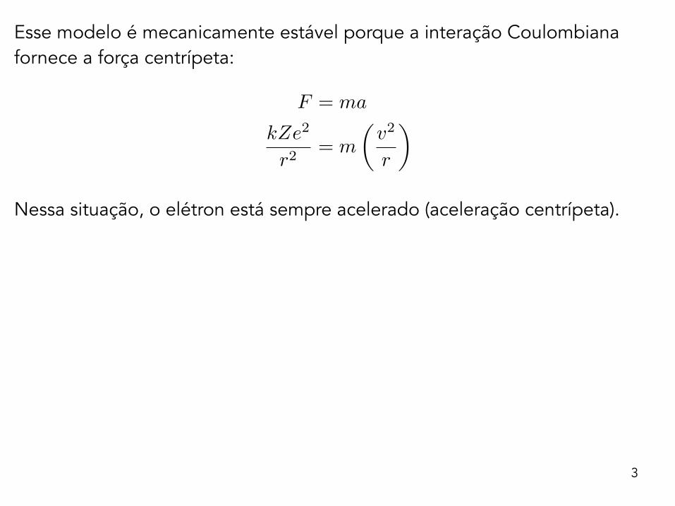
Esse modelo é mecanicamente estável porque a interação Coulombiana fornece a força centrípeta:

Nessa situação, o elétron está sempre acelerado (aceleração centrípeta).

3

F = ma

kZe2

r2= m

✓v2

r

◆

4

166 Chapter 4 The Nuclear Atom

simplicity, Bohr chose to consider circular orbits. Such a model is mechanically stable because the Coulomb poten-tial V � �kZe2�r provides the centripetal force

F �kZe2

r 2 �mv2

r 4-12

necessary for the electron to move in a circle of radius r at speed v, but it is electrically unstable because the electron is always accelerating toward the center of the circle. The laws of electrodynamics predict that such an accelerating charge will radiate light of frequency f equal to that of the periodic motion, which in this case is the frequency of revolution. Thus, classically,

f �v

2Pr� 4 kZe2

rm 5 1�2 12Pr

� 4 kZe2

4P2 m5 1�2 1

r 3�2 �1

r 3�24-13

The total energy of the electron is the sum of the kinetic and the potential energies:

E �12

mv2 � 4 � kZe2

r 5From Equation 4-12, we see that 1

2mv2 � kZe2�2r (a result that holds for circular motion in any inverse-square force field), so the total energy can be written as

E �kZe2

2r� kZe2

r � � kZe2

2r� �

1r 4-14

Thus, classical physics predicts that, as energy is lost to radiation, the electron’s orbit will become smaller and smaller while the frequency of the emitted radiation will become higher and higher, further increasing the rate at which energy is lost and end-ing when the electron reaches the nucleus (see Figure 4-15a). The time required for the electron to spiral into the nucleus can be calculated from classical mechanics and electrodynamics; it turns out to be less than a microsecond. Thus, at first sight, this model predicts that the atom will radiate a continuous spectrum (since the frequency

of revolution changes continuously as the electron spirals in) and will collapse after a very short time, a result that fortunately does not occur. Unless excited by some external means, atoms do not radiate at all, and when excited atoms do radiate, a line spectrum is emitted, not a continuous one.

Bohr “solved” these formidable difficulties with two decidedly nonclassical postulates. His first postulate was that electrons could move in certain orbits without radiating. He called these orbits sta-tionary states. His second postulate was to assume that the atom radiates when the electron makes a transition from one stationary state to another (Figure 4-15b) and that the frequency f of the emit-ted radiation is not the frequency of motion in either stable orbit but is related to the energies of the orbits by Planck’s theory

hf � Ei � Ef 4-15

where h is Planck’s constant and Ei and Ef are the energies of the initial and final states. The second assumption, which is equivalent to that of energy conservation with the emission of a photon, is

Niels Bohr explains a point in front of the blackboard (1956). [American Institute of Physics, Niels Bohr Library, Margrethe Bohr Collection.]

FIGURE 4-15 (a) In the classical orbital model, the electron orbits about the nucleus and spirals into the center because of the energy radiated. (b) In the Bohr model, the electron orbits without radiating until it jumps to another allowed radius of lower energy, at which time radiation is emitted.

(a) (b)G

G

G

G

G

TIPLER_04_153-192hr.indd 166 8/22/11 11:36 AM

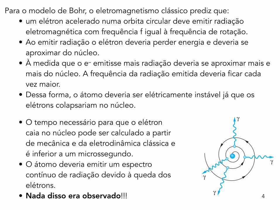
Para o modelo de Bohr, o eletromagnetismo clássico prediz que: • um elétron acelerado numa orbita circular deve emitir radiação

eletromagnética com frequência f igual à frequência de rotação. • Ao emitir radiação o elétron deveria perder energia e deveria se

aproximar do núcleo. • À medida que o e– emitisse mais radiação deveria se aproximar mais e

mais do núcleo. A frequência da radiação emitida deveria ficar cada vez maior.

• Dessa forma, o átomo deveria ser elétricamente instável já que os elétrons colapsariam no núcleo.

• O tempo necessário para que o elétron caia no núcleo pode ser calculado a partir de mecânica e da eletrodinâmica clássica e é inferior a um microssegundo.

• O átomo deveria emitir um espectro contínuo de radiação devido à queda dos elétrons.

• Nada disso era observado!!!

5

Bohr resolveu essas dificuldades formidáveis introduzindo dois postulados não-clássicos:

• Primeiro postulado: os elétrons podem se mover em certas órbitas sem irradiar. Ele chamou essas órbitas de estados estacionários.

• Segundo postulado: o átomo emite radiação quando o elétron faz uma transição de um estado estacionário para outro.

A freqüência da radiação está relacionada com as energias das órbitas pela fórmula de Planck:

hf = Ei - Ef (condição de frequência de Bohr)

onde h é a constante de Planck e Ei e Ef são as energias dos estados inicial e final.

A segunda hipótese, que é equivalente à conservação de energia na emissão de um fóton, é crucial porque se afasta completamente da teoria clássica, que exige que a freqüência da radiação seja igual à do movimento da partícula carregada.

6

Para determinar as energias das órbitas permitidas, Bohr fez uma terceira suposição, hoje conhecida como princípio de correspondência:

• Terceiro postulado (princípio de correspondência): No limite de grandes órbitas e grandes energias, os cálculos quânticos devem concordar com os cálculos clássicos.

Assim, as leis do mundo microscópico, quando estendidas ao mundo macroscópico, devem concordar com as leis clássicas da física (amplamente verificadas no mundo cotidiano).

O modelo detalhado do átomo de hidrogênio de Bohr foi posteriormente suplantado pela teoria quântica moderna. No entanto, sua condição de frequência e o princípio da correspondência permanecem como características essenciais da nova teoria quântica.

7

Em seu primeiro artigo, em 1913, Bohr apontou que seus resultados implicavam que o momento angular do elétron no átomo de hidrogênio podia assumir apenas valores que são múltiplos inteiros da constante de Planck divididos por 2𝜋. Isso estava em acordo com uma descoberta feita no ano anterior por J. W. Nicholson.

Ou seja, o momento angular L está quantizado: L pode assumir apenas os valores L= nh/(2𝜋), onde n é um número inteiro, n=1,2,3,… .

Em vez de seguir as complexidades da dedução de Bohr, usaremos a quantização do momento angular para encontrar as expressões que descrevem os estados estacionários.

O raciocino que segue aplica-se não apenas ao átomo de hidrogênio, mas também a qualquer átomo de carga nuclear +Ze com um único elétron orbital: e.g. Hélio ionizado (He+) ou Lítio duplamente ionizado (Li++).

Raio das órbitas estacionárias no átomo de Bohr

8

Se a carga do núcleo é +Ze e a do elétron –e, temos:

Por outro lado, de acordo com a quantização de Bohr do momento angular, temos:

onde n é um “número quântico” e ℏ=h/2𝜋 ("agá cortado”).

Combinando as dias Eqs. acima obtemos:

Elevando ao quadrado:

kZe2

r2= m

✓v2

r

◆) v =

✓kZe2

mr

◆1/2

L = mvr =nh

2⇡= n~ n = 1, 2, 3, · · ·

4-3 The Bohr Model of the Hydrogen Atom 167

crucial because it deviated from classical theory, which requires the frequency of radiation to be that of the motion of the charged particle. Equation 4-15 is referred to as the Bohr frequency condition.

In order to determine the energies of the allowed, nonradiating orbits, Bohr made a third assumption, now known as the correspondence principle, which had profound implications:

In the limit of large orbits and large energies, quantum calculations must agree with classical calculations.

Thus, the correspondence principle says that, whatever modifications of classical physics are made to describe matter at the submicroscopic level, when the results are extended to the macroscopic world, they must agree with those from the classical laws of phys-ics that have been so abundantly verified in the everyday world. While Bohr’s detailed model of the hydrogen atom has been supplanted by modern quantum theory, which we will discuss in later chapters, his frequency condition (Equation 4-15) and the cor-respondence principle remain as essential features of the new theory.

In his first paper,11 in 1913, Bohr pointed out that his results implied that the angular momentum of the electron in the hydrogen atom can take on only values that are integral multiples of Planck’s constant divided by 2P, in agreement with a discovery made a year earlier by J. W. Nicholson. That is, angular momentum is quantized; it can assume only the values nh�2P, where n is an integer. Rather than follow the intricacies of Bohr’s derivation, we will use the fundamental conclusion of angular momentum quantization to find his expression for the observed spectra. The development that follows applies not only to hydrogen, but to any atom of nuclear charge �Ze with a single orbital electron—for example, singly ionized helium He� or doubly ionized lithium Li2�.

If the nuclear charge is �Ze and the electron charge �e, we have noted (Equa-tion 4-12) that the centripetal force necessary to move the electron in a circular orbit is provided by the Coulomb force kZe2�r 2. Solving Equation 4-12 for the speed of the orbiting electron yields

v � 4 kZe2

mr 5 1�2 4-16

Bohr’s quantization of the angular momentum L is

L � mvr �nh2P

� n6 n � 1, 2, 3,c 4-17

where the integer n is called a quantum number and 6 � h�2P. (The constant 6, read “h-bar,” is often more convenient to use than h itself, just as the angular frequency V � 2P f is often more convenient than the frequency f.) Combining Equations 4-16 and 4-17 allows us to write for the circular orbits

r �n6mv �

n6m 4 rm

kZe2 5 1�2Squaring this relation gives

r 2 �n262

m2 4 rmkZe2 5

and canceling common quantities yields

rn �n262

mkZe2 �n2

a0

Z 4-18

TIPLER_04_153-192hr.indd 167 8/22/11 11:36 AM

4-3 The Bohr Model of the Hydrogen Atom 167

crucial because it deviated from classical theory, which requires the frequency of radiation to be that of the motion of the charged particle. Equation 4-15 is referred to as the Bohr frequency condition.

In order to determine the energies of the allowed, nonradiating orbits, Bohr made a third assumption, now known as the correspondence principle, which had profound implications:

In the limit of large orbits and large energies, quantum calculations must agree with classical calculations.

Thus, the correspondence principle says that, whatever modifications of classical physics are made to describe matter at the submicroscopic level, when the results are extended to the macroscopic world, they must agree with those from the classical laws of phys-ics that have been so abundantly verified in the everyday world. While Bohr’s detailed model of the hydrogen atom has been supplanted by modern quantum theory, which we will discuss in later chapters, his frequency condition (Equation 4-15) and the cor-respondence principle remain as essential features of the new theory.

In his first paper,11 in 1913, Bohr pointed out that his results implied that the angular momentum of the electron in the hydrogen atom can take on only values that are integral multiples of Planck’s constant divided by 2P, in agreement with a discovery made a year earlier by J. W. Nicholson. That is, angular momentum is quantized; it can assume only the values nh�2P, where n is an integer. Rather than follow the intricacies of Bohr’s derivation, we will use the fundamental conclusion of angular momentum quantization to find his expression for the observed spectra. The development that follows applies not only to hydrogen, but to any atom of nuclear charge �Ze with a single orbital electron—for example, singly ionized helium He� or doubly ionized lithium Li2�.

If the nuclear charge is �Ze and the electron charge �e, we have noted (Equa-tion 4-12) that the centripetal force necessary to move the electron in a circular orbit is provided by the Coulomb force kZe2�r 2. Solving Equation 4-12 for the speed of the orbiting electron yields

v � 4 kZe2

mr 5 1�2 4-16

Bohr’s quantization of the angular momentum L is

L � mvr �nh2P

� n6 n � 1, 2, 3, c 4-17

where the integer n is called a quantum number and 6 � h�2P. (The constant 6, read “h-bar,” is often more convenient to use than h itself, just as the angular frequency V � 2P f is often more convenient than the frequency f.) Combining Equations 4-16 and 4-17 allows us to write for the circular orbits

r �n6mv �

n6m 4 rm

kZe2 5 1�2Squaring this relation gives

r 2 �n262

m2 4 rmkZe2 5

and canceling common quantities yields

rn �n262

mkZe2 �n2

a0

Z 4-18

TIPLER_04_153-192hr.indd 167 8/22/11 11:36 AM

9

Portanto, obtemos que o raio das órbitas estacionárias é:

onde

é denominado raio de Bohr.

Assim, vemos que as órbitas estacionárias do primeiro postulado de Bohr têm raios quantizados, denotados pelo subíndice n em rn.

Observe que o raio Bohr a0 para o hidrogênio (Z=1) corresponde ao raio da órbita com n=1 (a menor órbita de Bohr possível para o elétron num átomo de hidrogênio).

Como rn ~ Z–1, as órbitas Bohr para átomos de um único elétron com Z>1 estão mais próximas do núcleo do que as órbitas correspondentes para o hidrogênio.

4-3 The Bohr Model of the Hydrogen Atom 167

crucial because it deviated from classical theory, which requires the frequency of radiation to be that of the motion of the charged particle. Equation 4-15 is referred to as the Bohr frequency condition.

In order to determine the energies of the allowed, nonradiating orbits, Bohr made a third assumption, now known as the correspondence principle, which had profound implications:

In the limit of large orbits and large energies, quantum calculations must agree with classical calculations.

Thus, the correspondence principle says that, whatever modifications of classical physics are made to describe matter at the submicroscopic level, when the results are extended to the macroscopic world, they must agree with those from the classical laws of phys-ics that have been so abundantly verified in the everyday world. While Bohr’s detailed model of the hydrogen atom has been supplanted by modern quantum theory, which we will discuss in later chapters, his frequency condition (Equation 4-15) and the cor-respondence principle remain as essential features of the new theory.

In his first paper,11 in 1913, Bohr pointed out that his results implied that the angular momentum of the electron in the hydrogen atom can take on only values that are integral multiples of Planck’s constant divided by 2P, in agreement with a discovery made a year earlier by J. W. Nicholson. That is, angular momentum is quantized; it can assume only the values nh�2P, where n is an integer. Rather than follow the intricacies of Bohr’s derivation, we will use the fundamental conclusion of angular momentum quantization to find his expression for the observed spectra. The development that follows applies not only to hydrogen, but to any atom of nuclear charge �Ze with a single orbital electron—for example, singly ionized helium He� or doubly ionized lithium Li2�.

If the nuclear charge is �Ze and the electron charge �e, we have noted (Equa-tion 4-12) that the centripetal force necessary to move the electron in a circular orbit is provided by the Coulomb force kZe2�r 2. Solving Equation 4-12 for the speed of the orbiting electron yields

v � 4 kZe2

mr 5 1�2 4-16

Bohr’s quantization of the angular momentum L is

L � mvr �nh2P

� n6 n � 1, 2, 3,c 4-17

where the integer n is called a quantum number and 6 � h�2P. (The constant 6, read “h-bar,” is often more convenient to use than h itself, just as the angular frequency V � 2P f is often more convenient than the frequency f.) Combining Equations 4-16 and 4-17 allows us to write for the circular orbits

r �n6mv �

n6m 4 rm

kZe2 5 1�2Squaring this relation gives

r 2 �n262

m2 4 rmkZe2 5

and canceling common quantities yields

rn �n262

mkZe2 �n2

a0

Z 4-18

TIPLER_04_153-192hr.indd 167 8/22/11 11:36 AM

168 Chapter 4 The Nuclear Atom

where

a0 �62

mke2 � 0.529 A� � 0.0529 nm 4-19

is called the Bohr radius. The Å, a unit commonly used in the early days of spectros-copy, equals 10�10 m or 10�1 nm. Thus, we find that the stationary orbits of Bohr’s first postulate have quantized radii, denoted in Equation 4-18 by the subscript on rn. Notice that the Bohr radius a0 for hydrogen (Z � 1) corresponds to the orbit radius with n � 1, the smallest Bohr orbit possible for the electron in a hydrogen atom. Since rn � Z �1, the Bohr orbits for single-electron atoms with Z � 1 are closer to the nucleus than the corresponding ones for hydrogen.

The total energy of the electron (Equation 4-14) then becomes, on substitution of rn from Equation 4-18,

En � � kZe2

2rn� �

kZe2

24mkZe2

n262 5En � �mk2

Z2 e4

262 n2 � �E0

Z2

n2 n � 1, 2, 3,c 4-20

where E0 � mk2 e4�262. Thus, the energy of the electron is also quantized; that is, the

stationary states correspond to specific values of the total energy. This means that energies Ei and Ef that appear in the frequency condition of Bohr’s second postulate must be from the allowed set En and Equation 4-15 becomes

hf � Eni� Enf

� �E0Z2

n2i

� 4 �E0Z2

n2f5

or

f �E0Z2

h4 1

n2f

� 1n2

i5 4-21

which can be written in the form of the Rydberg-Ritz equation (Equation 4-2) by sub-stituting f � c�L and dividing by c to obtain

1L

�E0 Z2

hc4 1

n2f

� 1n2

i5

or

1L

� Z2 R4 1

n2f

� 1n2

i5 4-22

where

R �E0

hc�

mk2 e4

4Pc63 4-23

is Bohr’s prediction for the value of the Rydberg constant.Using the values of m, e, c, and 6 known in 1913, Bohr calculated R and found

his result to agree (within the limits of uncertainties of the constants) with the value obtained from spectroscopy, 1.097 � 107 m�1. Bohr noted in his original paper that this equation might be valuable in determining the best values for the constants e, m, and 6 because of the extreme precision possible in measuring R. This has indeed turned out to be the case.

TIPLER_04_153-192hr.indd 168 8/22/11 11:36 AM

10

Níveis de energia do átomo de Bohr

A energia total do elétron é a soma das energias cinética e potencial.

Substituindo obtemos:

Agora, substituímos na expressão anterior e obtemos:

onde

166 Chapter 4 The Nuclear Atom

simplicity, Bohr chose to consider circular orbits. Such a model is mechanically stable because the Coulomb poten-tial V � �kZe2�r provides the centripetal force

F �kZe2

r 2 �mv2

r 4-12

necessary for the electron to move in a circle of radius r at speed v, but it is electrically unstable because the electron is always accelerating toward the center of the circle. The laws of electrodynamics predict that such an accelerating charge will radiate light of frequency f equal to that of the periodic motion, which in this case is the frequency of revolution. Thus, classically,

f �v

2Pr� 4 kZe2

rm 5 1�2 12Pr

� 4 kZe2

4P2 m5 1�2 1

r 3�2 �1

r 3�24-13

The total energy of the electron is the sum of the kinetic and the potential energies:

E �12

mv2 � 4 � kZe2

r 5From Equation 4-12, we see that 1

2mv2 � kZe2�2r (a result that holds for circular motion in any inverse-square force field), so the total energy can be written as

E �kZe2

2r� kZe2

r � � kZe2

2r� �

1r 4-14

Thus, classical physics predicts that, as energy is lost to radiation, the electron’s orbit will become smaller and smaller while the frequency of the emitted radiation will become higher and higher, further increasing the rate at which energy is lost and end-ing when the electron reaches the nucleus (see Figure 4-15a). The time required for the electron to spiral into the nucleus can be calculated from classical mechanics and electrodynamics; it turns out to be less than a microsecond. Thus, at first sight, this model predicts that the atom will radiate a continuous spectrum (since the frequency

of revolution changes continuously as the electron spirals in) and will collapse after a very short time, a result that fortunately does not occur. Unless excited by some external means, atoms do not radiate at all, and when excited atoms do radiate, a line spectrum is emitted, not a continuous one.

Bohr “solved” these formidable difficulties with two decidedly nonclassical postulates. His first postulate was that electrons could move in certain orbits without radiating. He called these orbits sta-tionary states. His second postulate was to assume that the atom radiates when the electron makes a transition from one stationary state to another (Figure 4-15b) and that the frequency f of the emit-ted radiation is not the frequency of motion in either stable orbit but is related to the energies of the orbits by Planck’s theory

hf � Ei � Ef 4-15

where h is Planck’s constant and Ei and Ef are the energies of the initial and final states. The second assumption, which is equivalent to that of energy conservation with the emission of a photon, is

Niels Bohr explains a point in front of the blackboard (1956). [American Institute of Physics, Niels Bohr Library, Margrethe Bohr Collection.]

FIGURE 4-15 (a) In the classical orbital model, the electron orbits about the nucleus and spirals into the center because of the energy radiated. (b) In the Bohr model, the electron orbits without radiating until it jumps to another allowed radius of lower energy, at which time radiation is emitted.

(a) (b)G

G

G

G

G

TIPLER_04_153-192hr.indd 166 8/22/11 11:36 AM

4-3 The Bohr Model of the Hydrogen Atom 167

crucial because it deviated from classical theory, which requires the frequency of radiation to be that of the motion of the charged particle. Equation 4-15 is referred to as the Bohr frequency condition.

In order to determine the energies of the allowed, nonradiating orbits, Bohr made a third assumption, now known as the correspondence principle, which had profound implications:

In the limit of large orbits and large energies, quantum calculations must agree with classical calculations.

Thus, the correspondence principle says that, whatever modifications of classical physics are made to describe matter at the submicroscopic level, when the results are extended to the macroscopic world, they must agree with those from the classical laws of phys-ics that have been so abundantly verified in the everyday world. While Bohr’s detailed model of the hydrogen atom has been supplanted by modern quantum theory, which we will discuss in later chapters, his frequency condition (Equation 4-15) and the cor-respondence principle remain as essential features of the new theory.

In his first paper,11 in 1913, Bohr pointed out that his results implied that the angular momentum of the electron in the hydrogen atom can take on only values that are integral multiples of Planck’s constant divided by 2P, in agreement with a discovery made a year earlier by J. W. Nicholson. That is, angular momentum is quantized; it can assume only the values nh�2P, where n is an integer. Rather than follow the intricacies of Bohr’s derivation, we will use the fundamental conclusion of angular momentum quantization to find his expression for the observed spectra. The development that follows applies not only to hydrogen, but to any atom of nuclear charge �Ze with a single orbital electron—for example, singly ionized helium He� or doubly ionized lithium Li2�.

If the nuclear charge is �Ze and the electron charge �e, we have noted (Equa-tion 4-12) that the centripetal force necessary to move the electron in a circular orbit is provided by the Coulomb force kZe2�r 2. Solving Equation 4-12 for the speed of the orbiting electron yields

v � 4 kZe2

mr 5 1�2 4-16

Bohr’s quantization of the angular momentum L is

L � mvr �nh2P

� n6 n � 1, 2, 3,c 4-17

where the integer n is called a quantum number and 6 � h�2P. (The constant 6, read “h-bar,” is often more convenient to use than h itself, just as the angular frequency V � 2P f is often more convenient than the frequency f.) Combining Equations 4-16 and 4-17 allows us to write for the circular orbits

r �n6mv �

n6m 4 rm

kZe2 5 1�2Squaring this relation gives

r 2 �n262

m2 4 rmkZe2 5

and canceling common quantities yields

rn �n262

mkZe2 �n2

a0

Z 4-18

TIPLER_04_153-192hr.indd 167 8/22/11 11:36 AM

166 Chapter 4 The Nuclear Atom

simplicity, Bohr chose to consider circular orbits. Such a model is mechanically stable because the Coulomb poten-tial V � �kZe2�r provides the centripetal force

F �kZe2

r 2 �mv2

r 4-12

necessary for the electron to move in a circle of radius r at speed v, but it is electrically unstable because the electron is always accelerating toward the center of the circle. The laws of electrodynamics predict that such an accelerating charge will radiate light of frequency f equal to that of the periodic motion, which in this case is the frequency of revolution. Thus, classically,

f �v

2Pr� 4 kZe2

rm 5 1�2 12Pr

� 4 kZe2

4P2 m5 1�2 1

r 3�2 �1

r 3�24-13

The total energy of the electron is the sum of the kinetic and the potential energies:

E �12

mv2 � 4 � kZe2

r 5From Equation 4-12, we see that 1

2mv2 � kZe2�2r (a result that holds for circular motion in any inverse-square force field), so the total energy can be written as

E �kZe2

2r� kZe2

r � � kZe2

2r� �

1r 4-14

Thus, classical physics predicts that, as energy is lost to radiation, the electron’s orbit will become smaller and smaller while the frequency of the emitted radiation will become higher and higher, further increasing the rate at which energy is lost and end-ing when the electron reaches the nucleus (see Figure 4-15a). The time required for the electron to spiral into the nucleus can be calculated from classical mechanics and electrodynamics; it turns out to be less than a microsecond. Thus, at first sight, this model predicts that the atom will radiate a continuous spectrum (since the frequency

of revolution changes continuously as the electron spirals in) and will collapse after a very short time, a result that fortunately does not occur. Unless excited by some external means, atoms do not radiate at all, and when excited atoms do radiate, a line spectrum is emitted, not a continuous one.

Bohr “solved” these formidable difficulties with two decidedly nonclassical postulates. His first postulate was that electrons could move in certain orbits without radiating. He called these orbits sta-tionary states. His second postulate was to assume that the atom radiates when the electron makes a transition from one stationary state to another (Figure 4-15b) and that the frequency f of the emit-ted radiation is not the frequency of motion in either stable orbit but is related to the energies of the orbits by Planck’s theory

hf � Ei � Ef 4-15

where h is Planck’s constant and Ei and Ef are the energies of the initial and final states. The second assumption, which is equivalent to that of energy conservation with the emission of a photon, is

Niels Bohr explains a point in front of the blackboard (1956). [American Institute of Physics, Niels Bohr Library, Margrethe Bohr Collection.]

FIGURE 4-15 (a) In the classical orbital model, the electron orbits about the nucleus and spirals into the center because of the energy radiated. (b) In the Bohr model, the electron orbits without radiating until it jumps to another allowed radius of lower energy, at which time radiation is emitted.

(a) (b)G

G

G

G

G

TIPLER_04_153-192hr.indd 166 8/22/11 11:36 AM

4-3 The Bohr Model of the Hydrogen Atom 167

crucial because it deviated from classical theory, which requires the frequency of radiation to be that of the motion of the charged particle. Equation 4-15 is referred to as the Bohr frequency condition.

In order to determine the energies of the allowed, nonradiating orbits, Bohr made a third assumption, now known as the correspondence principle, which had profound implications:

In the limit of large orbits and large energies, quantum calculations must agree with classical calculations.

Thus, the correspondence principle says that, whatever modifications of classical physics are made to describe matter at the submicroscopic level, when the results are extended to the macroscopic world, they must agree with those from the classical laws of phys-ics that have been so abundantly verified in the everyday world. While Bohr’s detailed model of the hydrogen atom has been supplanted by modern quantum theory, which we will discuss in later chapters, his frequency condition (Equation 4-15) and the cor-respondence principle remain as essential features of the new theory.

In his first paper,11 in 1913, Bohr pointed out that his results implied that the angular momentum of the electron in the hydrogen atom can take on only values that are integral multiples of Planck’s constant divided by 2P, in agreement with a discovery made a year earlier by J. W. Nicholson. That is, angular momentum is quantized; it can assume only the values nh�2P, where n is an integer. Rather than follow the intricacies of Bohr’s derivation, we will use the fundamental conclusion of angular momentum quantization to find his expression for the observed spectra. The development that follows applies not only to hydrogen, but to any atom of nuclear charge �Ze with a single orbital electron—for example, singly ionized helium He� or doubly ionized lithium Li2�.

If the nuclear charge is �Ze and the electron charge �e, we have noted (Equa-tion 4-12) that the centripetal force necessary to move the electron in a circular orbit is provided by the Coulomb force kZe2�r 2. Solving Equation 4-12 for the speed of the orbiting electron yields

v � 4 kZe2

mr 5 1�2 4-16

Bohr’s quantization of the angular momentum L is

L � mvr �nh2P

� n6 n � 1, 2, 3,c 4-17

where the integer n is called a quantum number and 6 � h�2P. (The constant 6, read “h-bar,” is often more convenient to use than h itself, just as the angular frequency V � 2P f is often more convenient than the frequency f.) Combining Equations 4-16 and 4-17 allows us to write for the circular orbits

r �n6mv �

n6m 4 rm

kZe2 5 1�2Squaring this relation gives

r 2 �n262

m2 4 rmkZe2 5

and canceling common quantities yields

rn �n262

mkZe2 �n2

a0

Z 4-18

TIPLER_04_153-192hr.indd 167 8/22/11 11:36 AM

168 Chapter 4 The Nuclear Atom

where

a0 �62

mke2 � 0.529 A� � 0.0529 nm 4-19

is called the Bohr radius. The Å, a unit commonly used in the early days of spectros-copy, equals 10�10 m or 10�1 nm. Thus, we find that the stationary orbits of Bohr’s first postulate have quantized radii, denoted in Equation 4-18 by the subscript on rn. Notice that the Bohr radius a0 for hydrogen (Z � 1) corresponds to the orbit radius with n � 1, the smallest Bohr orbit possible for the electron in a hydrogen atom. Since rn � Z �1, the Bohr orbits for single-electron atoms with Z � 1 are closer to the nucleus than the corresponding ones for hydrogen.

The total energy of the electron (Equation 4-14) then becomes, on substitution of rn from Equation 4-18,

En � � kZe2

2rn� �

kZe2

24mkZe2

n262 5En � �mk2

Z2 e4

262 n2 � �E0

Z2

n2 n � 1, 2, 3,c 4-20

where E0 � mk2 e4�262. Thus, the energy of the electron is also quantized; that is, the

stationary states correspond to specific values of the total energy. This means that energies Ei and Ef that appear in the frequency condition of Bohr’s second postulate must be from the allowed set En and Equation 4-15 becomes

hf � Eni� Enf

� �E0Z2

n2i

� 4 �E0Z2

n2f5

or

f �E0Z2

h4 1

n2f

� 1n2

i5 4-21

which can be written in the form of the Rydberg-Ritz equation (Equation 4-2) by sub-stituting f � c�L and dividing by c to obtain

1L

�E0 Z2

hc4 1

n2f

� 1n2

i5

or

1L

� Z2 R4 1

n2f

� 1n2

i5 4-22

where

R �E0

hc�

mk2 e4

4Pc63 4-23

is Bohr’s prediction for the value of the Rydberg constant.Using the values of m, e, c, and 6 known in 1913, Bohr calculated R and found

his result to agree (within the limits of uncertainties of the constants) with the value obtained from spectroscopy, 1.097 � 107 m�1. Bohr noted in his original paper that this equation might be valuable in determining the best values for the constants e, m, and 6 because of the extreme precision possible in measuring R. This has indeed turned out to be the case.

TIPLER_04_153-192hr.indd 168 8/22/11 11:36 AM

168 Chapter 4 The Nuclear Atom

where

a0 �62

mke2 � 0.529 A� � 0.0529 nm 4-19

is called the Bohr radius. The Å, a unit commonly used in the early days of spectros-copy, equals 10�10 m or 10�1 nm. Thus, we find that the stationary orbits of Bohr’s first postulate have quantized radii, denoted in Equation 4-18 by the subscript on rn. Notice that the Bohr radius a0 for hydrogen (Z � 1) corresponds to the orbit radius with n � 1, the smallest Bohr orbit possible for the electron in a hydrogen atom. Since rn � Z �1, the Bohr orbits for single-electron atoms with Z � 1 are closer to the nucleus than the corresponding ones for hydrogen.

The total energy of the electron (Equation 4-14) then becomes, on substitution of rn from Equation 4-18,

En � � kZe2

2rn� �

kZe2

24mkZe2

n262 5En � �mk2

Z2 e4

262 n2 � �E0

Z2

n2 n � 1, 2, 3,c 4-20

where E0 � mk2 e4�262. Thus, the energy of the electron is also quantized; that is, the

stationary states correspond to specific values of the total energy. This means that energies Ei and Ef that appear in the frequency condition of Bohr’s second postulate must be from the allowed set En and Equation 4-15 becomes

hf � Eni� Enf

� �E0Z2

n2i

� 4 �E0Z2

n2f5

or

f �E0Z2

h4 1

n2f

� 1n2

i5 4-21

which can be written in the form of the Rydberg-Ritz equation (Equation 4-2) by sub-stituting f � c�L and dividing by c to obtain

1L

�E0 Z2

hc4 1

n2f

� 1n2

i5

or

1L

� Z2 R4 1

n2f

� 1n2

i5 4-22

where

R �E0

hc�

mk2 e4

4Pc63 4-23

is Bohr’s prediction for the value of the Rydberg constant.Using the values of m, e, c, and 6 known in 1913, Bohr calculated R and found

his result to agree (within the limits of uncertainties of the constants) with the value obtained from spectroscopy, 1.097 � 107 m�1. Bohr noted in his original paper that this equation might be valuable in determining the best values for the constants e, m, and 6 because of the extreme precision possible in measuring R. This has indeed turned out to be the case.

TIPLER_04_153-192hr.indd 168 8/22/11 11:36 AM

11

Assim, a energia do elétron também está quantizada; isto é, os estados estacionários correspondem a valores específicos da energia total.

Isso significa que as energias Ei e Ef que aparecem na condição de frequência do segundo postulado de Bohr devem pertencer ao conjunto permitido de valores de En.

Portanto, a condição de frequência de Bohr fica:

ou, equivalentemente,

168 Chapter 4 The Nuclear Atom

where

a0 �62

mke2 � 0.529 A� � 0.0529 nm 4-19

is called the Bohr radius. The Å, a unit commonly used in the early days of spectros-copy, equals 10�10 m or 10�1 nm. Thus, we find that the stationary orbits of Bohr’s first postulate have quantized radii, denoted in Equation 4-18 by the subscript on rn. Notice that the Bohr radius a0 for hydrogen (Z � 1) corresponds to the orbit radius with n � 1, the smallest Bohr orbit possible for the electron in a hydrogen atom. Since rn � Z �1, the Bohr orbits for single-electron atoms with Z � 1 are closer to the nucleus than the corresponding ones for hydrogen.

The total energy of the electron (Equation 4-14) then becomes, on substitution of rn from Equation 4-18,

En � � kZe2

2rn� �

kZe2

24mkZe2

n262 5En � �mk2

Z2 e4

262 n2 � �E0

Z2

n2 n � 1, 2, 3,c 4-20

where E0 � mk2 e4�262. Thus, the energy of the electron is also quantized; that is, the

stationary states correspond to specific values of the total energy. This means that energies Ei and Ef that appear in the frequency condition of Bohr’s second postulate must be from the allowed set En and Equation 4-15 becomes

hf � Eni� Enf

� �E0Z2

n2i

� 4 �E0Z2

n2f5

or

f �E0Z2

h4 1

n2f

� 1n2

i5 4-21

which can be written in the form of the Rydberg-Ritz equation (Equation 4-2) by sub-stituting f � c�L and dividing by c to obtain

1L

�E0 Z2

hc4 1

n2f

� 1n2

i5

or

1L

� Z2 R4 1

n2f

� 1n2

i5 4-22

where

R �E0

hc�

mk2 e4

4Pc63 4-23

is Bohr’s prediction for the value of the Rydberg constant.Using the values of m, e, c, and 6 known in 1913, Bohr calculated R and found

his result to agree (within the limits of uncertainties of the constants) with the value obtained from spectroscopy, 1.097 � 107 m�1. Bohr noted in his original paper that this equation might be valuable in determining the best values for the constants e, m, and 6 because of the extreme precision possible in measuring R. This has indeed turned out to be the case.

TIPLER_04_153-192hr.indd 168 8/22/11 11:36 AM

168 Chapter 4 The Nuclear Atom

where

a0 �62

mke2 � 0.529 A� � 0.0529 nm 4-19

is called the Bohr radius. The Å, a unit commonly used in the early days of spectros-copy, equals 10�10 m or 10�1 nm. Thus, we find that the stationary orbits of Bohr’s first postulate have quantized radii, denoted in Equation 4-18 by the subscript on rn. Notice that the Bohr radius a0 for hydrogen (Z � 1) corresponds to the orbit radius with n � 1, the smallest Bohr orbit possible for the electron in a hydrogen atom. Since rn � Z �1, the Bohr orbits for single-electron atoms with Z � 1 are closer to the nucleus than the corresponding ones for hydrogen.

The total energy of the electron (Equation 4-14) then becomes, on substitution of rn from Equation 4-18,

En � � kZe2

2rn� �

kZe2

24mkZe2

n262 5En � �mk2

Z2 e4

262 n2 � �E0

Z2

n2 n � 1, 2, 3,c 4-20

where E0 � mk2 e4�262. Thus, the energy of the electron is also quantized; that is, the

stationary states correspond to specific values of the total energy. This means that energies Ei and Ef that appear in the frequency condition of Bohr’s second postulate must be from the allowed set En and Equation 4-15 becomes

hf � Eni� Enf

� �E0Z2

n2i

� 4 �E0Z2

n2f5

or

f �E0Z2

h4 1

n2f

� 1n2

i5 4-21

which can be written in the form of the Rydberg-Ritz equation (Equation 4-2) by sub-stituting f � c�L and dividing by c to obtain

1L

�E0 Z2

hc4 1

n2f

� 1n2

i5

or

1L

� Z2 R4 1

n2f

� 1n2

i5 4-22

where

R �E0

hc�

mk2 e4

4Pc63 4-23

is Bohr’s prediction for the value of the Rydberg constant.Using the values of m, e, c, and 6 known in 1913, Bohr calculated R and found

his result to agree (within the limits of uncertainties of the constants) with the value obtained from spectroscopy, 1.097 � 107 m�1. Bohr noted in his original paper that this equation might be valuable in determining the best values for the constants e, m, and 6 because of the extreme precision possible in measuring R. This has indeed turned out to be the case.

TIPLER_04_153-192hr.indd 168 8/22/11 11:36 AM

12

Usando f = c/𝜆, a expressão anterior fica:

ou

onde

A expressão acima coincide com a fórmula empírica de Rydberg-Ritz apresentada no capítulo anterior.

Usando os valores de m, e, c, h conhecidos em 1913, Bohr calculou R e encontrou que seu resultado concordava (dentro dos limites de incerteza das constantes) com o valor obtido a partir da espectroscopia! → sucesso do modelo de Bohr.

168 Chapter 4 The Nuclear Atom

where

a0 �62

mke2 � 0.529 A� � 0.0529 nm 4-19

is called the Bohr radius. The Å, a unit commonly used in the early days of spectros-copy, equals 10�10 m or 10�1 nm. Thus, we find that the stationary orbits of Bohr’s first postulate have quantized radii, denoted in Equation 4-18 by the subscript on rn. Notice that the Bohr radius a0 for hydrogen (Z � 1) corresponds to the orbit radius with n � 1, the smallest Bohr orbit possible for the electron in a hydrogen atom. Since rn � Z �1, the Bohr orbits for single-electron atoms with Z � 1 are closer to the nucleus than the corresponding ones for hydrogen.

The total energy of the electron (Equation 4-14) then becomes, on substitution of rn from Equation 4-18,

En � � kZe2

2rn� �

kZe2

24mkZe2

n262 5En � �mk2

Z2 e4

262 n2 � �E0

Z2

n2 n � 1, 2, 3,c 4-20

where E0 � mk2 e4�262. Thus, the energy of the electron is also quantized; that is, the

stationary states correspond to specific values of the total energy. This means that energies Ei and Ef that appear in the frequency condition of Bohr’s second postulate must be from the allowed set En and Equation 4-15 becomes

hf � Eni� Enf

� �E0Z2

n2i

� 4 �E0Z2

n2f5

or

f �E0Z2

h4 1

n2f

� 1n2

i5 4-21

which can be written in the form of the Rydberg-Ritz equation (Equation 4-2) by sub-stituting f � c�L and dividing by c to obtain

1L

�E0 Z2

hc4 1

n2f

� 1n2

i5

or

1L

� Z2 R4 1

n2f

� 1n2

i5 4-22

where

R �E0

hc�

mk2 e4

4Pc63 4-23

is Bohr’s prediction for the value of the Rydberg constant.Using the values of m, e, c, and 6 known in 1913, Bohr calculated R and found

his result to agree (within the limits of uncertainties of the constants) with the value obtained from spectroscopy, 1.097 � 107 m�1. Bohr noted in his original paper that this equation might be valuable in determining the best values for the constants e, m, and 6 because of the extreme precision possible in measuring R. This has indeed turned out to be the case.

TIPLER_04_153-192hr.indd 168 8/22/11 11:36 AM

168 Chapter 4 The Nuclear Atom

where

a0 �62

mke2 � 0.529 A� � 0.0529 nm 4-19

is called the Bohr radius. The Å, a unit commonly used in the early days of spectros-copy, equals 10�10 m or 10�1 nm. Thus, we find that the stationary orbits of Bohr’s first postulate have quantized radii, denoted in Equation 4-18 by the subscript on rn. Notice that the Bohr radius a0 for hydrogen (Z � 1) corresponds to the orbit radius with n � 1, the smallest Bohr orbit possible for the electron in a hydrogen atom. Since rn � Z �1, the Bohr orbits for single-electron atoms with Z � 1 are closer to the nucleus than the corresponding ones for hydrogen.

The total energy of the electron (Equation 4-14) then becomes, on substitution of rn from Equation 4-18,

En � � kZe2

2rn� �

kZe2

24mkZe2

n262 5En � �mk2

Z2 e4

262 n2 � �E0

Z2

n2 n � 1, 2, 3,c 4-20

where E0 � mk2 e4�262. Thus, the energy of the electron is also quantized; that is, the

stationary states correspond to specific values of the total energy. This means that energies Ei and Ef that appear in the frequency condition of Bohr’s second postulate must be from the allowed set En and Equation 4-15 becomes

hf � Eni� Enf

� �E0Z2

n2i

� 4 �E0Z2

n2f5

or

f �E0Z2

h4 1

n2f

� 1n2

i5 4-21

which can be written in the form of the Rydberg-Ritz equation (Equation 4-2) by sub-stituting f � c�L and dividing by c to obtain

1L

�E0 Z2

hc4 1

n2f

� 1n2

i5

or

1L

� Z2 R4 1

n2f

� 1n2

i5 4-22

where

R �E0

hc�

mk2 e4

4Pc63 4-23

is Bohr’s prediction for the value of the Rydberg constant.Using the values of m, e, c, and 6 known in 1913, Bohr calculated R and found

his result to agree (within the limits of uncertainties of the constants) with the value obtained from spectroscopy, 1.097 � 107 m�1. Bohr noted in his original paper that this equation might be valuable in determining the best values for the constants e, m, and 6 because of the extreme precision possible in measuring R. This has indeed turned out to be the case.

TIPLER_04_153-192hr.indd 168 8/22/11 11:36 AM

168 Chapter 4 The Nuclear Atom

where

a0 �62

mke2 � 0.529 A� � 0.0529 nm 4-19

is called the Bohr radius. The Å, a unit commonly used in the early days of spectros-copy, equals 10�10 m or 10�1 nm. Thus, we find that the stationary orbits of Bohr’s first postulate have quantized radii, denoted in Equation 4-18 by the subscript on rn. Notice that the Bohr radius a0 for hydrogen (Z � 1) corresponds to the orbit radius with n � 1, the smallest Bohr orbit possible for the electron in a hydrogen atom. Since rn � Z �1, the Bohr orbits for single-electron atoms with Z � 1 are closer to the nucleus than the corresponding ones for hydrogen.

The total energy of the electron (Equation 4-14) then becomes, on substitution of rn from Equation 4-18,

En � � kZe2

2rn� �

kZe2

24mkZe2

n262 5En � �mk2

Z2 e4

262 n2 � �E0

Z2

n2 n � 1, 2, 3,c 4-20

where E0 � mk2 e4�262. Thus, the energy of the electron is also quantized; that is, the

stationary states correspond to specific values of the total energy. This means that energies Ei and Ef that appear in the frequency condition of Bohr’s second postulate must be from the allowed set En and Equation 4-15 becomes

hf � Eni� Enf

� �E0Z2

n2i

� 4 �E0Z2

n2f5

or

f �E0Z2

h4 1

n2f

� 1n2

i5 4-21

which can be written in the form of the Rydberg-Ritz equation (Equation 4-2) by sub-stituting f � c�L and dividing by c to obtain

1L

�E0 Z2

hc4 1

n2f

� 1n2

i5

or

1L

� Z2 R4 1

n2f

� 1n2

i5 4-22

where

R �E0

hc�

mk2 e4

4Pc63 4-23

is Bohr’s prediction for the value of the Rydberg constant.Using the values of m, e, c, and 6 known in 1913, Bohr calculated R and found

his result to agree (within the limits of uncertainties of the constants) with the value obtained from spectroscopy, 1.097 � 107 m�1. Bohr noted in his original paper that this equation might be valuable in determining the best values for the constants e, m, and 6 because of the extreme precision possible in measuring R. This has indeed turned out to be the case.

TIPLER_04_153-192hr.indd 168 8/22/11 11:36 AM

13

No caso do do átomo de hidrogênio, os valores possíveis da energia previstos por Bohr são obtidos usando Z=1:

onde

é o valor da energia quando n=1.

E1 = – E0 é a energia do estado fundamental.

4-3 The Bohr Model of the Hydrogen Atom 169

The possible values of the energy of the hydrogen atom predicted by Bohr’s model are given by Equation 4-20 with Z � 1:

En � � mk2

e4

262 n2 � �

E0

n2 4-24

where

E0 �mk2

e4

262 � 2.18 � 10�18 J � 13.6 eV

is the magnitude of En with n � 1. E1(��E0) is called the ground state. It is conve-nient to plot these allowed energies of the stationary states as in Figure 4-16. Such a

FIGURE 4-16 (a) Energy-level diagram for hydrogen showing the seven lowest stationary states and the four lowest energy transitions each for the Lyman, Balmer, and Paschen series. There are an infinite number of levels. Their energies are given by En � �13.6�n2 eV, where n is an integer. The dashed line shown for each series is the series limit, corresponding to the energy that would be radiated by an electron at rest far from the nucleus (n 4 @) in a transition to the state with n � nf for that series. The horizontal spacing between the transitions shown for each series is proportional to the wavelength spacing between the lines of the spectrum. (b) The spectral lines corresponding to the transitions shown for the three series. Notice the regularities within each series, particularly the short-wavelength limit and the successively smaller separation between adjacent lines as the limit is approached. The wavelength scale in the diagram is not linear.

100 200 500 1000 2000�, nm

(a)

(b)

0–0.54

�5

–0.85 4–1.51 3

–3.40 2

Lyman series

Lyman

Balmer

Paschen

Balmer Paschen

–13.60 1

n

Ener

gy, e

V

TIPLER_04_153-192hr.indd 169 8/22/11 11:36 AM

4-3 The Bohr Model of the Hydrogen Atom 169

The possible values of the energy of the hydrogen atom predicted by Bohr’s model are given by Equation 4-20 with Z � 1:

En � � mk2

e4

262 n2 � �

E0

n2 4-24

where

E0 �mk2

e4

262 � 2.18 � 10�18 J � 13.6 eV

is the magnitude of En with n � 1. E1(��E0) is called the ground state. It is conve-nient to plot these allowed energies of the stationary states as in Figure 4-16. Such a

FIGURE 4-16 (a) Energy-level diagram for hydrogen showing the seven lowest stationary states and the four lowest energy transitions each for the Lyman, Balmer, and Paschen series. There are an infinite number of levels. Their energies are given by En � �13.6�n2 eV, where n is an integer. The dashed line shown for each series is the series limit, corresponding to the energy that would be radiated by an electron at rest far from the nucleus (n 4 @) in a transition to the state with n � nf for that series. The horizontal spacing between the transitions shown for each series is proportional to the wavelength spacing between the lines of the spectrum. (b) The spectral lines corresponding to the transitions shown for the three series. Notice the regularities within each series, particularly the short-wavelength limit and the successively smaller separation between adjacent lines as the limit is approached. The wavelength scale in the diagram is not linear.

100 200 500 1000 2000�, nm

(a)

(b)

0–0.54

�5

–0.85 4–1.51 3

–3.40 2

Lyman series

Lyman

Balmer

Paschen

Balmer Paschen

–13.60 1

n

Ener

gy, e

V

TIPLER_04_153-192hr.indd 169 8/22/11 11:36 AM

4-3 The Bohr Model of the Hydrogen Atom 169

The possible values of the energy of the hydrogen atom predicted by Bohr’s model are given by Equation 4-20 with Z � 1:

En � � mk2

e4

262 n2 � �

E0

n2 4-24

where

E0 �mk2

e4

262 � 2.18 � 10�18 J � 13.6 eV

is the magnitude of En with n � 1. E1(��E0) is called the ground state. It is conve-nient to plot these allowed energies of the stationary states as in Figure 4-16. Such a

FIGURE 4-16 (a) Energy-level diagram for hydrogen showing the seven lowest stationary states and the four lowest energy transitions each for the Lyman, Balmer, and Paschen series. There are an infinite number of levels. Their energies are given by En � �13.6�n2 eV, where n is an integer. The dashed line shown for each series is the series limit, corresponding to the energy that would be radiated by an electron at rest far from the nucleus (n 4 @) in a transition to the state with n � nf for that series. The horizontal spacing between the transitions shown for each series is proportional to the wavelength spacing between the lines of the spectrum. (b) The spectral lines corresponding to the transitions shown for the three series. Notice the regularities within each series, particularly the short-wavelength limit and the successively smaller separation between adjacent lines as the limit is approached. The wavelength scale in the diagram is not linear.

100 200 500 1000 2000�, nm

(a)

(b)

0–0.54

�5

–0.85 4–1.51 3

–3.40 2

Lyman series

Lyman

Balmer

Paschen

Balmer Paschen

–13.60 1

n

Ener

gy, e

V

TIPLER_04_153-192hr.indd 169 8/22/11 11:36 AM

15

O gráfico do slide anterior é chamado de diagrama de níveis de energia.

Neste diagrama são mostradas três séries de transições entre os estados estacionários, indicadas pelas setas verticais desenhadas entre os níveis.

A frequência da luz emitida em cada uma dessas transições é a diferença de energia dividida por h de acordo com a condição de frequência de Bohr.

A energia necessária para remover o elétron do átomo, 13.6 eV, é chamada de energia de ionização, ou energia de ligação, do elétron.

Na época em que o artigo de Bohr foi publicado, havia duas séries espectrais conhecidas para o hidrogênio:

• a série de Balmer, correspondente a nf = 2, ni = 3, 4, 5,. . . , • uma série com o nome de seu descobridor, Paschen (1908),

correspondente a nf = 3, ni = 4, 5, 6,. . . .

16

A equação deduzida por Bohr indicou que outras séries deviam existir para diferentes valores de nf:

• Em 1916, Lyman encontrou a série correspondente a nf = 1, • Em 1922 e 1924, Brackett e Pfund, respectivamente, encontraram séries

correspondentes a nf = 4 e nf = 5.

Calculando os comprimentos de onda para estas séries, vemos que apenas a série Balmer está principalmente na parte visível do espectro eletromagnético.

A série Lyman está no ultravioleta, as outras no infravermelho.

17

Correção da massa reduzida

Bohr supôs que o núcleo estava fixo no centro do átomo, o qual equivale a considerar que ele possui massa infinita. No entanto, numa análise mais detalhada devemos considerar que tanto o elétron quanto o núcleo se movem em torno do centro de massas do átomo.

Se o núcleo tem massa M, a sua energia cinética será 1/2 Mv2 = p2/(2m), onde p=Mv é o momentum.

Se assumirmos que o momentum total do átomo é zero, a conservação do momento requer que os momentos do núcleo e do elétron sejam iguais em magnitude. A energia cinética total é então:

onde é denominada massa reduzida do átomo.

𝜇 é ligeiramente diferente da massa do elétron.

4-3 The Bohr Model of the Hydrogen Atom 171

or

L � 4.87 � 10�7 m � 487 nm

Remarks: The difference in the two results is due to rounding of the Rydberg con-stant to three decimal places.

Reduced Mass CorrectionThe assumption by Bohr that the nucleus is fixed is equivalent to the assumption that it has infinite mass. In fact, the Rydberg constant in Equation 4-23 is normally written as R@, as we will do from now on. If the nucleus has mass M, its kinetic energy will be 12 Mv2 � p2�2M, where p � Mv is the momentum. If we assume that the total momen-tum of the atom is zero, conservation of momentum requires that the momenta of the nucleus and electron be equal in magnitude. The total kinetic energy is then

Ek �p2

2M�

p2

2m�

M � m2mM

p2 �p2

2M

where

M �mM

m � M�

m1 � m�M 4-25

This is slightly different from the kinetic energy of the electron because M, called the reduced mass, is slightly different from the electron mass. The results derived earlier for a nucleus of infinite mass can be applied directly to the case of a nucleus of mass M if we replace the electron mass in the equations by reduced mass M, defined by Equation 4-25. (The validity of this procedure is proven in most inter-mediate and advanced mechanics books.) The Rydberg constant (Equation 4-23) is then written

R �Mk2

e4

4Pc63 �mk2

e4

4Pc63 4 11 � m�M 5 � R@4 1

1 � m�M 5 4-26

This correction amounts to only 1 part in 2000 for the case of hydrogen and to even less for other nuclei; however, the predicted variation in the Rydberg constant from atom to atom is precisely that which is observed. For example, the spectrum of a sin-gly ionized helium atom, which has one remaining electron, is just that predicted by Equations 4-22 and 4-26 with Z � 2 and the proper helium mass. The current value for the Rydberg constant R@ from precision spectroscopic measurements12 is

R@ � 1.0973732 � 107 m�1 � 1.0973732 � 10�2 nm�1 4-27

Urey13 used the reduced mass correction to the spectral lines of the Balmer series to discover (in 1931) a second form of hydrogen whose atoms had twice the mass of ordinary hydrogen. The heavy form was called deuterium. The two forms, atoms with the same Z but different masses, are called isotopes.

EXAMPLE 4-7 Rydberg Constants for H and He� Compute the Rydberg con-stants for H and He� applying the reduced mass correction (m � 9.1094 � 10�31 kg, mp � 1.6726 � 10�27 kg, mA � 6.6447 � 10�27 kg).

CCR

29

TIPLER_04_153-192hr.indd 171 8/22/11 11:36 AM

4-3 The Bohr Model of the Hydrogen Atom 171

or

L � 4.87 � 10�7 m � 487 nm

Remarks: The difference in the two results is due to rounding of the Rydberg con-stant to three decimal places.

Reduced Mass CorrectionThe assumption by Bohr that the nucleus is fixed is equivalent to the assumption that it has infinite mass. In fact, the Rydberg constant in Equation 4-23 is normally written as R@, as we will do from now on. If the nucleus has mass M, its kinetic energy will be 12 Mv2 � p2�2M, where p � Mv is the momentum. If we assume that the total momen-tum of the atom is zero, conservation of momentum requires that the momenta of the nucleus and electron be equal in magnitude. The total kinetic energy is then

Ek �p2

2M�

p2

2m�

M � m2mM

p2 �p2

2M

where

M �mM

m � M�

m1 � m�M 4-25

This is slightly different from the kinetic energy of the electron because M, called the reduced mass, is slightly different from the electron mass. The results derived earlier for a nucleus of infinite mass can be applied directly to the case of a nucleus of mass M if we replace the electron mass in the equations by reduced mass M, defined by Equation 4-25. (The validity of this procedure is proven in most inter-mediate and advanced mechanics books.) The Rydberg constant (Equation 4-23) is then written

R �Mk2

e4

4Pc63 �mk2

e4

4Pc63 4 11 � m�M 5 � R@4 1

1 � m�M 5 4-26

This correction amounts to only 1 part in 2000 for the case of hydrogen and to even less for other nuclei; however, the predicted variation in the Rydberg constant from atom to atom is precisely that which is observed. For example, the spectrum of a sin-gly ionized helium atom, which has one remaining electron, is just that predicted by Equations 4-22 and 4-26 with Z � 2 and the proper helium mass. The current value for the Rydberg constant R@ from precision spectroscopic measurements12 is

R@ � 1.0973732 � 107 m�1 � 1.0973732 � 10�2 nm�1 4-27

Urey13 used the reduced mass correction to the spectral lines of the Balmer series to discover (in 1931) a second form of hydrogen whose atoms had twice the mass of ordinary hydrogen. The heavy form was called deuterium. The two forms, atoms with the same Z but different masses, are called isotopes.

EXAMPLE 4-7 Rydberg Constants for H and He� Compute the Rydberg con-stants for H and He� applying the reduced mass correction (m � 9.1094 � 10�31 kg, mp � 1.6726 � 10�27 kg, mA � 6.6447 � 10�27 kg).

CCR

29

TIPLER_04_153-192hr.indd 171 8/22/11 11:36 AM

18

Os resultados obtidos anteriormente para um núcleo de massa infinita podem ser aplicados diretamente ao caso de um núcleo de massa M se substituímos a massa dos elétrons nas equações pela massa reduzida. (A validade deste procedimento é demonstrada em cursos mais avançados de mecânica).

A constante de Rydberg é então escrita na forma:

Esta correção é bem pequena; equivale a apenas 1 parte em 2000 para o caso do hidrogênio e até mesmo para outros núcleos.

A variação prevista na constante de Rydberg de átomo para a átomo é precisamente a que se observa experimentalmente!

4-3 The Bohr Model of the Hydrogen Atom 171

or

L � 4.87 � 10�7 m � 487 nm

Remarks: The difference in the two results is due to rounding of the Rydberg con-stant to three decimal places.

Reduced Mass CorrectionThe assumption by Bohr that the nucleus is fixed is equivalent to the assumption that it has infinite mass. In fact, the Rydberg constant in Equation 4-23 is normally written as R@, as we will do from now on. If the nucleus has mass M, its kinetic energy will be 12 Mv2 � p2�2M, where p � Mv is the momentum. If we assume that the total momen-tum of the atom is zero, conservation of momentum requires that the momenta of the nucleus and electron be equal in magnitude. The total kinetic energy is then

Ek �p2

2M�

p2

2m�

M � m2mM

p2 �p2

2M

where

M �mM

m � M�

m1 � m�M 4-25

This is slightly different from the kinetic energy of the electron because M, called the reduced mass, is slightly different from the electron mass. The results derived earlier for a nucleus of infinite mass can be applied directly to the case of a nucleus of mass M if we replace the electron mass in the equations by reduced mass M, defined by Equation 4-25. (The validity of this procedure is proven in most inter-mediate and advanced mechanics books.) The Rydberg constant (Equation 4-23) is then written

R �Mk2

e4

4Pc63 �mk2

e4

4Pc63 4 11 � m�M 5 � R@4 1

1 � m�M 5 4-26

This correction amounts to only 1 part in 2000 for the case of hydrogen and to even less for other nuclei; however, the predicted variation in the Rydberg constant from atom to atom is precisely that which is observed. For example, the spectrum of a sin-gly ionized helium atom, which has one remaining electron, is just that predicted by Equations 4-22 and 4-26 with Z � 2 and the proper helium mass. The current value for the Rydberg constant R@ from precision spectroscopic measurements12 is

R@ � 1.0973732 � 107 m�1 � 1.0973732 � 10�2 nm�1 4-27

Urey13 used the reduced mass correction to the spectral lines of the Balmer series to discover (in 1931) a second form of hydrogen whose atoms had twice the mass of ordinary hydrogen. The heavy form was called deuterium. The two forms, atoms with the same Z but different masses, are called isotopes.

EXAMPLE 4-7 Rydberg Constants for H and He� Compute the Rydberg con-stants for H and He� applying the reduced mass correction (m � 9.1094 � 10�31 kg, mp � 1.6726 � 10�27 kg, mA � 6.6447 � 10�27 kg).

CCR

29

TIPLER_04_153-192hr.indd 171 8/22/11 11:36 AM

19

De acordo com o princípio de correspondência, quando os níveis de energia estão pouco espaçados, a quantização deve ter pouco efeito; i.e. os cálculos clássicos e quânticos devem dar os mesmos resultados.

No diagrama de níveis de energia apresentado antes, vemos que os níveis de energia estão muito próximos quando o número quântico n é grande.

Isso nos leva a um enunciado ligeiramente diferente do princípio da correspondência de Bohr: na região de números quânticos muito grandes (n neste caso), cálculos quânticos e cálculos clássicos devem produzir os mesmos resultados.

O principio de correspondência

20

Para mostrar que o modelo de Bohr do átomo de hidrogênio de fato obedece ao princípio da correspondência, comparemos a frequência de uma transição entre o nível ni = n e o nível nf = n–1 para n grande com a frequência clássica, que é a frequência de revolução do elétron.

Da equação obtida por Bohr obtemos:

No limite de n muito grande, temos:

172 Chapter 4 The Nuclear Atom

SOLUTION

For hydrogen:

RH � R@4 11 � m�MH

5 � R@4 11 � 9.1094 � 10�31�1.6726 � 10�27 5

� 1.09677 � 107 m�1

For helium: Since M in the reduced mass correction is the mass of the nucleus, for this calculation we use M equal to the A particle mass:

RHe � R@4 11 � m�MH

5 � R@4 11 � 9.1094 � 10�31�6.6447 � 10�27 5

� 1.09722 � 107 m�1

Thus, the two Rydberg constants differ by about 0.04 percent.

Correspondence PrincipleAccording to the correspondence principle, which applies also to modern quantum mechanics, when the energy levels are closely spaced, quantization should have little effect; classical and quantum calculations should give the same results. From the energy-level diagram of Figure 4-16, we see that the energy levels are close together when the quantum number n is large. This leads us to a slightly different statement of Bohr’s correspondence principle: In the region of very large quantum numbers (n in this case) quantum calculation and classical calculation must yield the same results. To see that the Bohr model of the hydrogen atom does indeed obey the correspon-dence principle, let us compare the frequency of a transition between level ni � n and level nf � n � 1 for large n with the classical frequency, which is the frequency of revolution of the electron. From Equation 4-22 we have

f �cL

�Z2

mk2 e4

4P63 6 1�n � 1�2 � 1n2 7 � Z2

mk2 e4

4P63 2n � 1

n2�n � 1�2

For large n we can neglect the ones subtracted from n and 2n to obtain

f �Z2

mk2 e4

4P63 2n3 �

Z2 mk2

e4

2P63 n3 4-28

The classical frequency of revolution of the electron is (see Equation 4-13)

frev �v

2Pr

Using v � n6�mr from Equation 4-17 and r � n262�mkZe2 from Equation 4-18, we obtain

frev ��n6�mr�

2Pr�

n62Pmr 2 �

n62Pm�n262�mkZe2�2

frev �m2

k2 Z2

e4 n6

2Pmn464 �mk2

Z2 e4

2P63 n3 4-29

which is the same as Equation 4-28.

TIPLER_04_153-192hr.indd 172 8/22/11 11:36 AM

172 Chapter 4 The Nuclear Atom

SOLUTION

For hydrogen:

RH � R@4 11 � m�MH

5 � R@4 11 � 9.1094 � 10�31�1.6726 � 10�27 5

� 1.09677 � 107 m�1

For helium: Since M in the reduced mass correction is the mass of the nucleus, for this calculation we use M equal to the A particle mass:

RHe � R@4 11 � m�MH

5 � R@4 11 � 9.1094 � 10�31�6.6447 � 10�27 5

� 1.09722 � 107 m�1

Thus, the two Rydberg constants differ by about 0.04 percent.

Correspondence PrincipleAccording to the correspondence principle, which applies also to modern quantum mechanics, when the energy levels are closely spaced, quantization should have little effect; classical and quantum calculations should give the same results. From the energy-level diagram of Figure 4-16, we see that the energy levels are close together when the quantum number n is large. This leads us to a slightly different statement of Bohr’s correspondence principle: In the region of very large quantum numbers (n in this case) quantum calculation and classical calculation must yield the same results. To see that the Bohr model of the hydrogen atom does indeed obey the correspon-dence principle, let us compare the frequency of a transition between level ni � n and level nf � n � 1 for large n with the classical frequency, which is the frequency of revolution of the electron. From Equation 4-22 we have

f �cL

�Z2

mk2 e4

4P63 6 1�n � 1�2 � 1n2 7 � Z2

mk2 e4

4P63 2n � 1

n2�n � 1�2

For large n we can neglect the ones subtracted from n and 2n to obtain

f �Z2

mk2 e4

4P63 2n3 �

Z2 mk2

e4

2P63 n3 4-28

The classical frequency of revolution of the electron is (see Equation 4-13)

frev �v

2Pr

Using v � n6�mr from Equation 4-17 and r � n262�mkZe2 from Equation 4-18, we obtain

frev ��n6�mr�

2Pr�

n62Pmr 2 �

n62Pm�n262�mkZe2�2

frev �m2

k2 Z2

e4 n6

2Pmn464 �mk2

Z2 e4

2P63 n3 4-29

which is the same as Equation 4-28.

TIPLER_04_153-192hr.indd 172 8/22/11 11:36 AM

21

Agora calculemos a frequência de revolução clássica:

Usando e obtemos:

Portanto, para n muito grande, a frequência de revolução clássica coincide com a frequência da luz emitida pelo átomo de Bohr.

172 Chapter 4 The Nuclear Atom

SOLUTION

For hydrogen:

RH � R@4 11 � m�MH

5 � R@4 11 � 9.1094 � 10�31�1.6726 � 10�27 5

� 1.09677 � 107 m�1

For helium: Since M in the reduced mass correction is the mass of the nucleus, for this calculation we use M equal to the A particle mass:

RHe � R@4 11 � m�MH

5 � R@4 11 � 9.1094 � 10�31�6.6447 � 10�27 5

� 1.09722 � 107 m�1

Thus, the two Rydberg constants differ by about 0.04 percent.

Correspondence PrincipleAccording to the correspondence principle, which applies also to modern quantum mechanics, when the energy levels are closely spaced, quantization should have little effect; classical and quantum calculations should give the same results. From the energy-level diagram of Figure 4-16, we see that the energy levels are close together when the quantum number n is large. This leads us to a slightly different statement of Bohr’s correspondence principle: In the region of very large quantum numbers (n in this case) quantum calculation and classical calculation must yield the same results. To see that the Bohr model of the hydrogen atom does indeed obey the correspon-dence principle, let us compare the frequency of a transition between level ni � n and level nf � n � 1 for large n with the classical frequency, which is the frequency of revolution of the electron. From Equation 4-22 we have

f �cL

�Z2

mk2 e4

4P63 6 1�n � 1�2 � 1n2 7 � Z2

mk2 e4

4P63 2n � 1

n2�n � 1�2

For large n we can neglect the ones subtracted from n and 2n to obtain

f �Z2

mk2 e4

4P63 2n3 �

Z2 mk2

e4

2P63 n3 4-28

The classical frequency of revolution of the electron is (see Equation 4-13)

frev �v

2Pr

Using v � n6�mr from Equation 4-17 and r � n262�mkZe2 from Equation 4-18, we obtain

frev ��n6�mr�

2Pr�

n62Pmr 2 �

n62Pm�n262�mkZe2�2

frev �m2

k2 Z2

e4 n6

2Pmn464 �mk2

Z2 e4

2P63 n3 4-29

which is the same as Equation 4-28.

TIPLER_04_153-192hr.indd 172 8/22/11 11:36 AM

172 Chapter 4 The Nuclear Atom

SOLUTION

For hydrogen:

RH � R@4 11 � m�MH

5 � R@4 11 � 9.1094 � 10�31�1.6726 � 10�27 5

� 1.09677 � 107 m�1

For helium: Since M in the reduced mass correction is the mass of the nucleus, for this calculation we use M equal to the A particle mass:

RHe � R@4 11 � m�MH

5 � R@4 11 � 9.1094 � 10�31�6.6447 � 10�27 5

� 1.09722 � 107 m�1

Thus, the two Rydberg constants differ by about 0.04 percent.

Correspondence PrincipleAccording to the correspondence principle, which applies also to modern quantum mechanics, when the energy levels are closely spaced, quantization should have little effect; classical and quantum calculations should give the same results. From the energy-level diagram of Figure 4-16, we see that the energy levels are close together when the quantum number n is large. This leads us to a slightly different statement of Bohr’s correspondence principle: In the region of very large quantum numbers (n in this case) quantum calculation and classical calculation must yield the same results. To see that the Bohr model of the hydrogen atom does indeed obey the correspon-dence principle, let us compare the frequency of a transition between level ni � n and level nf � n � 1 for large n with the classical frequency, which is the frequency of revolution of the electron. From Equation 4-22 we have

f �cL

�Z2

mk2 e4

4P63 6 1�n � 1�2 � 1n2 7 � Z2

mk2 e4

4P63 2n � 1

n2�n � 1�2

For large n we can neglect the ones subtracted from n and 2n to obtain

f �Z2

mk2 e4

4P63 2n3 �

Z2 mk2

e4

2P63 n3 4-28

The classical frequency of revolution of the electron is (see Equation 4-13)

frev �v

2Pr

Using v � n6�mr from Equation 4-17 and r � n262�mkZe2 from Equation 4-18, we obtain

frev ��n6�mr�

2Pr�

n62Pmr 2 �

n62Pm�n262�mkZe2�2

frev �m2

k2 Z2

e4 n6

2Pmn464 �mk2

Z2 e4

2P63 n3 4-29

which is the same as Equation 4-28.

TIPLER_04_153-192hr.indd 172 8/22/11 11:36 AM

172 Chapter 4 The Nuclear Atom

SOLUTION

For hydrogen:

RH � R@4 11 � m�MH

5 � R@4 11 � 9.1094 � 10�31�1.6726 � 10�27 5

� 1.09677 � 107 m�1

For helium: Since M in the reduced mass correction is the mass of the nucleus, for this calculation we use M equal to the A particle mass:

RHe � R@4 11 � m�MH

5 � R@4 11 � 9.1094 � 10�31�6.6447 � 10�27 5

� 1.09722 � 107 m�1

Thus, the two Rydberg constants differ by about 0.04 percent.

Correspondence PrincipleAccording to the correspondence principle, which applies also to modern quantum mechanics, when the energy levels are closely spaced, quantization should have little effect; classical and quantum calculations should give the same results. From the energy-level diagram of Figure 4-16, we see that the energy levels are close together when the quantum number n is large. This leads us to a slightly different statement of Bohr’s correspondence principle: In the region of very large quantum numbers (n in this case) quantum calculation and classical calculation must yield the same results. To see that the Bohr model of the hydrogen atom does indeed obey the correspon-dence principle, let us compare the frequency of a transition between level ni � n and level nf � n � 1 for large n with the classical frequency, which is the frequency of revolution of the electron. From Equation 4-22 we have

f �cL

�Z2

mk2 e4

4P63 6 1�n � 1�2 � 1n2 7 � Z2

mk2 e4

4P63 2n � 1

n2�n � 1�2

For large n we can neglect the ones subtracted from n and 2n to obtain

f �Z2

mk2 e4

4P63 2n3 �

Z2 mk2

e4

2P63 n3 4-28

The classical frequency of revolution of the electron is (see Equation 4-13)

frev �v

2Pr

Using v � n6�mr from Equation 4-17 and r � n262�mkZe2 from Equation 4-18, we obtain

frev ��n6�mr�

2Pr�

n62Pmr 2 �

n62Pm�n262�mkZe2�2

frev �m2

k2 Z2

e4 n6

2Pmn464 �mk2

Z2 e4

2P63 n3 4-29

which is the same as Equation 4-28.

TIPLER_04_153-192hr.indd 172 8/22/11 11:36 AM

172 Chapter 4 The Nuclear Atom

SOLUTION

For hydrogen:

RH � R@4 11 � m�MH

5 � R@4 11 � 9.1094 � 10�31�1.6726 � 10�27 5

� 1.09677 � 107 m�1

For helium: Since M in the reduced mass correction is the mass of the nucleus, for this calculation we use M equal to the A particle mass:

RHe � R@4 11 � m�MH

5 � R@4 11 � 9.1094 � 10�31�6.6447 � 10�27 5

� 1.09722 � 107 m�1

Thus, the two Rydberg constants differ by about 0.04 percent.

Correspondence PrincipleAccording to the correspondence principle, which applies also to modern quantum mechanics, when the energy levels are closely spaced, quantization should have little effect; classical and quantum calculations should give the same results. From the energy-level diagram of Figure 4-16, we see that the energy levels are close together when the quantum number n is large. This leads us to a slightly different statement of Bohr’s correspondence principle: In the region of very large quantum numbers (n in this case) quantum calculation and classical calculation must yield the same results. To see that the Bohr model of the hydrogen atom does indeed obey the correspon-dence principle, let us compare the frequency of a transition between level ni � n and level nf � n � 1 for large n with the classical frequency, which is the frequency of revolution of the electron. From Equation 4-22 we have

f �cL

�Z2

mk2 e4

4P63 6 1�n � 1�2 � 1n2 7 � Z2

mk2 e4

4P63 2n � 1

n2�n � 1�2

For large n we can neglect the ones subtracted from n and 2n to obtain

f �Z2

mk2 e4

4P63 2n3 �

Z2 mk2

e4

2P63 n3 4-28

The classical frequency of revolution of the electron is (see Equation 4-13)

frev �v

2Pr

Using v � n6�mr from Equation 4-17 and r � n262�mkZe2 from Equation 4-18, we obtain

frev ��n6�mr�

2Pr�

n62Pmr 2 �

n62Pm�n262�mkZe2�2

frev �m2

k2 Z2

e4 n6

2Pmn464 �mk2

Z2 e4

2P63 n3 4-29

which is the same as Equation 4-28.

TIPLER_04_153-192hr.indd 172 8/22/11 11:36 AM