o operador de laplace-beltrami discreto … · departamento de matemática o operador de...

Departamento de Matemática

O OPERADOR DE LAPLACE-BELTRAMI DISCRETO E APLICAÇÕES EM MALHAS

Aluno: Alice Herrera de Figueiredo

Orientador: Sinésio Pesco Introdução

Em computação gráfica, o operador de Laplace-Beltrami discreto tem diversas aplicações na geração e otimização geométrica de malhas. Entre as principais aplicações podemos destacar a suavização de malhas, edição de malhas, modelagem geométrica, reconstrução geométrica, geração de esqueletos, entre outras. Por essa diversidade de aplicações, e por ser um tema fundamental na área de computação gráfica, optamos por desenvolver um estudo de suas principais propriedades e implementar alguns exemplos que ilustrem essas aplicações.

No primeiro ano deste trabalho, o objetivo geral era estudar as propriedades do operador Laplace-Beltrami sobre malhas. Para isso, aplicamos esse operador em um modelo de geração de esqueletos usando o Laplaciano para realizar uma contração de uma malha ou de uma nuvem de pontos. No segundo ano, o objetivo geral é melhorar o efeito da contração a partir de implementações de controle da malha, visando acabar com os erros obtidos anteriormente.

Um esqueleto é uma estrutura 1D que representa uma versão simplificada da geometria de um objeto 3D. Eles são muito úteis em aplicações que necessitam de um estudo da sua forma e é por isso que utilizamos essa estratégia. O desafio dessa contração geométrica foi controlar o processo de contração tal que o resultado final preserve a forma do original ou características relevantes a um esqueleto. Para solucionar essa barreira, foi utilizado o operador Laplaciano que remove os detalhes geométricos nas direções normais e um outro termo que utiliza os vértices da malha para reter a informação geométrica desejada no esqueleto.

Trabalhos anteriores Existem várias aplicações deste método de geração de esqueletos. Uma delas está relacionada ao eixo mediano [1] e [2]. O eixo mediano de um objeto 3D é definido como o lugar dos centros de todas as esferas inscritas de raio máximo, e que muitas vezes contém elementos de superfície. Outra aplicação é o chamado "bone-skeleton" (osso do esqueleto), que é utilizado muito na animação de personagens [3]. Métodos para a curva de esqueleto podem ser classificados em duas categorias principais [4]: volumétricos e geométricos, dependendo se é uma representação interior ou é apenas a representação da superfície utilizada.


O Laplaciano Discreto

O operador de Laplace ou Laplaciano é um operador diferencial definido como o divergente do gradiente de uma função no espaço euclidiano:

O Δƒ Laplaciano (p) de uma função ƒ num ponto p, é a taxa que o valor médio de ƒ sobre esferas centradas em p, desvia-se de ƒ(p), enquanto o raio da esfera cresce.

Seja M uma malha triangular com n vértices, V o grupo de vértices dessa malha, E o grupo de arestas dessa malha e F o grupo de faces dessa malha [5]; Cada vértice i que pertence a M é representado usando as coordenadas cartesianas: vi = (xi, yi, zi ) . Definimos as δ-coordenadas de vi como sendo a diferença entre a coordenada absoluta de vi e o centro de massa considerando os seus vizinhos na malha. A transformação do vetor de coordenadas cartesianas para δ-coordenadas pode ser representado em forma de matriz. Para isso considere A a matriz de adjacências,

Considere di = (número de vértices vizinhos ao vértice i) e D a matriz diagonal onde Dii = di . Assim, a matriz que transforma as coordenadas absolutas em coordenadas relativas é:

A matriz L é chamada de Laplaciano topológico. As δ-coordenadas podem ser vistas como uma discretização do operador contínuo Laplace-Beltrami se assumirmos que a malha M é uma aproximação linear por partes de uma superfície. Logo, a δ-coordenada do vetor vi pode ser escrita como:

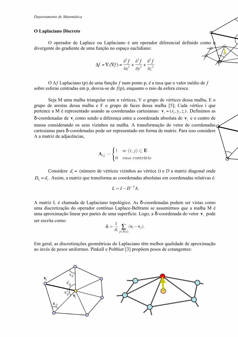
Em geral, as discretizações geométricas do Laplaciano têm melhor qualidade de aproximação ao invés de pesos uniformes. Pinkall e Polthier [3] propõem pesos de cotangentes:

O. Sorkine / Laplacian Mesh Processing

2.1. Basic definitions

Let M = (V,E,F) be a given triangular mesh with n ver-tices. V denotes the set of vertices, E denotes the set of edgesand F – the set of faces. Each vertex i ⇤M is convention-ally represented using absolute Cartesian coordinates, de-noted by vi = (xi,yi,zi). We first define the differential or⇤ -coordinates of vi to be the difference between the absolutecoordinates of vi and the center of mass of its immediateneighbors in the mesh,

⇤i = (⇤ (x)i ,⇤ (y)

i ,⇤ (z)i ) = vi�

1di

⇥j⇤N(i)

v j ,

where N(i) = { j |(i, j) ⇤ E} and di = |N(i)| is the numberof immediate neighbors of i (the degree or valence of i).

The transformation of the vector of absolute Cartesian co-ordinates to the vector of ⇤ -coordinates can be representedin matrix form. Let A be the adjacency (connectivity) matrixof the mesh:

Ai j =�

1 (i, j) ⇤ E0 otherwise,

and let D be the diagonal matrix such that Dii = di. Thenthe matrix transforming the absolute coordinates to relativecoordinates is

L = I�D�1A.

It is often more convenient to consider the symmetric versionof the L matrix, defined by Ls = DL = D�A,

(Ls)i j =

⇥⌅

⇤

di i = j�1 (i, j) ⇤ E0 otherwise.

That is, Ls x = D⇤ (x), Ls y = D⇤ (y), and Ls z = D⇤ (z), wherex is an n-vector containing the x absolute coordinates of allthe vertices and so on. See Figure 3 for an example of a meshand its associated matrices.

The matrix Ls (or L) is called the topological (or graph)Laplacian of the mesh [Fie73]. Graph Laplacians have beenextensively studied in algebra and graph theory [Chu97], pri-marily because their algebraic properties are related to thecombinatorial properties of the graphs they represent. Weshall look into some of these properties later on, in Sec-tions 2.2 and 3.

From a differential geometry perspective, the ⇤ -coordinates can be viewed as a discretization of the continu-ous Laplace-Beltrami operator [dC76], if we assume that ourmesh M is a piecewise-linear approximation of a smoothsurface. We can write the differential coordinate vector atvertex vi as

⇤i =1di

⇥j⇤N(i)

(vi�v j).

The sum above is a discretization of the following curvilin-ear integral: 1

|⌅|⇧

v⇤⌅ (vi�v)dl(v), where ⌅ is a closed simple

⇤i = 1di

⇥ j⇤N(i)(vi�v j) 1|⌅|

⇧v⇤⌅ (vi�v)dl(v)

Figure 1: The vector of the differential coordinates at avertex approximates the local shape characteristics of thesurface: the normal direction and the mean curvature.

��

��

��

��

��

�

�

Figure 2: The angles used in the cotangent weights and themean-value coordinates formulae for edge (i, j).

surface curve around vi and |⌅| is the length of ⌅ . It is knownfrom differential geometry that

lim|⌅|⇥0

1|⌅|

⌃

v⇤⌅(vi�v)dl(v) =�H(vi)ni ,

where H(vi) is the mean curvature at vi and ni is the surfacenormal. Therefore, the direction of the differential coordi-nate vector approximates the local normal direction and themagnitude approximates a quantity proportional to the lo-cal mean curvature [Tau95] (the normal scaled by the meancurvature is termed mean-curvature normal). Intuitively, thismeans that the ⇤ -coordinates encapsulate the local surfaceshape (see Figure 1).

It should be noted that geometric discretizationsof the Laplacian have better approximation qualities.Meyer et al. [MDSB03] propose employ the cotangentweights, first proposed by Pinkall and Polthier [PP93], in-stead of uniform weights:

⇤ ci =

1|�i| ⇥

j⇤N(i)

12(cot�i j + cot⇥i j)(vi�v j),

where |�i| is the size of the Voronoi cell of i and �i j, ⇥i j de-note the two angles opposite of edge (i, j) (see Figure 2),to approximate mean-curvature normals. These geometry-dependent weights lead to vectors ⇤ c

i with normal compo-nents only, unlike the previously defined ⇤i which also havetangential components and may be non-zero on planar 1-rings. The cotangent weights may be negative and problem-

c� The Eurographics Association 2005.


2.1. Basic definitions

Let M = (V,E,F) be a given triangular mesh with n ver-tices. V denotes the set of vertices, E denotes the set of edgesand F – the set of faces. Each vertex i ⇤M is convention-ally represented using absolute Cartesian coordinates, de-noted by vi = (xi,yi,zi). We first define the differential or⇤ -coordinates of vi to be the difference between the absolutecoordinates of vi and the center of mass of its immediateneighbors in the mesh,

⇤i = (⇤ (x)i ,⇤ (y)

i ,⇤ (z)i ) = vi�

1di

⇥j⇤N(i)

v j ,

where N(i) = { j |(i, j) ⇤ E} and di = |N(i)| is the numberof immediate neighbors of i (the degree or valence of i).

The transformation of the vector of absolute Cartesian co-ordinates to the vector of ⇤ -coordinates can be representedin matrix form. Let A be the adjacency (connectivity) matrixof the mesh:

Ai j =�

1 (i, j) ⇤ E0 otherwise,

and let D be the diagonal matrix such that Dii = di. Thenthe matrix transforming the absolute coordinates to relativecoordinates is

L = I�D�1A.

It is often more convenient to consider the symmetric versionof the L matrix, defined by Ls = DL = D�A,

(Ls)i j =

⇥⌅

⇤

di i = j�1 (i, j) ⇤ E0 otherwise.

That is, Ls x = D⇤ (x), Ls y = D⇤ (y), and Ls z = D⇤ (z), wherex is an n-vector containing the x absolute coordinates of allthe vertices and so on. See Figure 3 for an example of a meshand its associated matrices.

The matrix Ls (or L) is called the topological (or graph)Laplacian of the mesh [Fie73]. Graph Laplacians have beenextensively studied in algebra and graph theory [Chu97], pri-marily because their algebraic properties are related to thecombinatorial properties of the graphs they represent. Weshall look into some of these properties later on, in Sec-tions 2.2 and 3.

From a differential geometry perspective, the ⇤ -coordinates can be viewed as a discretization of the continu-ous Laplace-Beltrami operator [dC76], if we assume that ourmesh M is a piecewise-linear approximation of a smoothsurface. We can write the differential coordinate vector atvertex vi as

⇤i =1di

⇥j⇤N(i)

(vi�v j).

The sum above is a discretization of the following curvilin-ear integral: 1

|⌅|⇧

v⇤⌅ (vi�v)dl(v), where ⌅ is a closed simple

⇤i = 1di

⇥ j⇤N(i)(vi�v j) 1|⌅|

⇧v⇤⌅ (vi�v)dl(v)

Figure 1: The vector of the differential coordinates at avertex approximates the local shape characteristics of thesurface: the normal direction and the mean curvature.

��

��

��

��

��

�

�

Figure 2: The angles used in the cotangent weights and themean-value coordinates formulae for edge (i, j).

surface curve around vi and |⌅| is the length of ⌅ . It is knownfrom differential geometry that

lim|⌅|⇥0

1|⌅|

⌃

v⇤⌅(vi�v)dl(v) =�H(vi)ni ,

where H(vi) is the mean curvature at vi and ni is the surfacenormal. Therefore, the direction of the differential coordi-nate vector approximates the local normal direction and themagnitude approximates a quantity proportional to the lo-cal mean curvature [Tau95] (the normal scaled by the meancurvature is termed mean-curvature normal). Intuitively, thismeans that the ⇤ -coordinates encapsulate the local surfaceshape (see Figure 1).

It should be noted that geometric discretizationsof the Laplacian have better approximation qualities.Meyer et al. [MDSB03] propose employ the cotangentweights, first proposed by Pinkall and Polthier [PP93], in-stead of uniform weights:

⇤ ci =

1|�i| ⇥

j⇤N(i)

12(cot�i j + cot⇥i j)(vi�v j),

where |�i| is the size of the Voronoi cell of i and �i j, ⇥i j de-note the two angles opposite of edge (i, j) (see Figure 2),to approximate mean-curvature normals. These geometry-dependent weights lead to vectors ⇤ c

i with normal compo-nents only, unlike the previously defined ⇤i which also havetangential components and may be non-zero on planar 1-rings. The cotangent weights may be negative and problem-


€

Δf =∇.(∇f ) =∂2 f∂x2

+∂2 f∂y2

+∂2 f∂z 2


onde |Ωi| é o tamanho da célula Voronoi do vértice i e εij e γ ij são dois ângulos opostos da malha.

Esqueleto por Contração A aplicação que utilizamos foi a da Contração Geométrica [4], afim de utilizar o

modelo de geração de esqueletos. Esta contração remove detalhes e ruídos da superfície triangular a partir da aplicação do Laplaciano que suaviza a malha. Para realizarmos esta contração aplicamos mínimos quadrados: minimizar || Ax - b ||, onde A é a matriz abaixo , x é o resultado (no caso, as coordenadas dos novos vértices) e b é o vetor dos coeficientes conforme descrito abaixo:

A x = b Temos que Wh e Wl são matrizes diagonais e suas condições iniciais são:

onde A representa a área total da malha A cada iteração, resolvemos a equação mostrada acima, tendo como resultado os

novos vértices, e depois é preciso atualizar os pesos e refazer a matriz L (pelo método Laplaciano):

A aplicação dos mínimos quadrados foi realizada utilizando o pacote gsl [7].

To appear in the ACM SIGGRAPH conference proceedings

Figure 4: (Left) The 1D structure obtained by performing the connectivity surgery on the contracted mesh in Figure 1. (Middle) The inducedskeleton-mesh mapping. (Right) The resulting curve-skeleton after embedding refinement

single point. That is, we solve the following system for the vertexpositions:

!

WLLWH

"

V! =

!

0WHV

"

, (2)

where WL and WH are the diagonal weighting matrices that bal-ance the contraction and attraction constraints, respectively. Thei-th diagonal element of WL(WH ) is denoted WL,i (WH,i). Notethat the system (2) is over-determined. Thus, we solve it in theleast-squares sense, which is equivalent to minimizing the follow-ing quadratic energy:

#

#WLLV!##

2+!

i

W2H,i||v!i "vi||2, (3)

where the first term corresponds to the contraction constraints andthe second term corresponds to the attraction constraints.

Solving system (2) once does not collapse the entire model intoa 1D shape. It requires several iterations with proper weights forthe process to converge to a thin shape. After the first contractionstep, certain high-frequency details are filtered out and the mesh isnoticeably contracted. However, using the same weights WL andWH in subsequent iterations would not further contract the meshmuch, because the remaining details are retained by the current at-traction constraints. Therefore, to increase the collapsing speed, weincrease the contraction weight WL,i for every vertex i after eachiteration. In addition, to avoid over contraction, we update the at-traction weight WH,i for each vertex according to its collapsed de-gree determined by its local one-ring area. Specifically, we wantthe vertices with smaller contracted one-ring area to be attractedmore strongly to their current positions and thus contract less in thenext iteration. We find that such weight setting can retain the keyfeatures and appropriate branching structure in the contracted mesh.The iterative contraction process is as follow, where the superscriptst denote the iteration number:

1. Solve

!

WtLLt

WtH

"

Vt+1 =

!

0Wt

HVt

"

for Vt+1,

2. Update Wt+1L = sLWt

L and Wt+1H,i = W0

H,i

$

A0i /At

i , where Ati

and A0i are the current and the original one-ring areas, respec-

tively,

3. Compute the new Laplace operator Lt+1 with the current ver-tex positions Vt+1 using equation (1).

The initial ratio of the weights W0L and W0

H controls the smooth-ness and the degree of contraction of the first iteration result, thusit determines the amount of details retained in subsequent and finalcontracted meshes. Since the scale of the Laplacian coordinate isproportional to a vertex’s one-ring edge lengths (under the same lo-cal one-ring shape), the contraction forces from the Laplace equa-tions are smaller for denser models. Hence, to handle models of

different sizes and resolutions, we use the following default initial

setting: W0H = 1.0 and W0

L = 10"3#

A, where A is the average facearea of the model. Note that setting a uniform initial ratio of theseweights for all vertices works well even for meshes with irregu-lar sampling since the subsequent updating of weights is accordingto the local contraction degree which is resolution-independent. Wefound that this default setting produces good quality skeletons, withthe key features retained and small surface details filtered away. Allresults shown in this paper are obtained with this default setting.

In our experiments, we use sL = 2.0, which is found to contractall models efficiently, usually in less than 10 iterations. The it-erative updating stops when the ratio of the current and the orig-inal volumes of the model is smaller than the threshold "vol (weuse "vol = 1e" 6). Figure 1 shows the sequence of contraction re-sults for the raptor model. Each contraction iteration is essentiallyan analysis process, updating the attraction force of each vertexsmoothly based on its local contraction ratio. The forces are de-fined such that the contracted regions at the thinner branches act asstrong anchors retaining the key features of the object. The thin-ner regions of the model always collapse first, while the thickerregions take more iterations to collapse. The use of the curvature-flow Laplace operator also ensures that meshes with poor trianglequality are contracted well, with the triangle shapes maintained asmuch as possible during the iterative contraction (see Figure 2).

The iterative updating process increases the weights of the attrac-tion forces as the vertices become more contracted, thus the sys-tem matrix becomes more diagonally dominant as the iteration pro-gresses, making the updating process stable. During the construc-tion of the new linear system to be solved in the next iteration, wealso check for degenerate faces and avoid any possible numericalerrors, such as infinity values or divide-by-zero error. The geometrycontraction is a global constrained smoothing process, with high-frequency details and noise removed in each iteration (but with im-portant geometry details retained by the strong attraction forces),resulting in a smaller volume. The iterations converge when thevolume is close to zero.

5 Connectivity Surgery

We denote the contracted mesh as a 2D graph with vertex positionsV = [vT

1 , vT2 , . . . , vT

n ]T . The contracted mesh has an approximatezero volume with a shape that is visually a 1D skeleton. However,its connectivity is still that of the original mesh. To convert thecontracted mesh into a 1D graph, we apply a connectivity surgeryoperation. The surgery applies a series of edge-collapses to removecollapsed faces from the degenerated mesh, until all faces have beenremoved. The main requirement here is to retain the shape of thedegenerated mesh during this surgery process, while keeping suffi-cient skeletal nodes to maintain a fine correspondence between theskeleton and the original surface. We devise a cost function con-sisting of a shape term and a sampling term. The surgery operationis then an iterative greedy algorithm that collapses the edge having




!

WLLWH

"

V! =

!

0WHV

"

, (2)


#

#WLLV!##

2+!

i

W2H,i||v!i "vi||2, (3)



1. Solve

!

WtLLt

WtH

"

Vt+1 =

!

0Wt

HVt

"

for Vt+1,


L and Wt+1H,i = W0

H,i

$

A0i /At

i , where Ati


tively,






L = 10"3#






1 , vT2 , . . . , vT





!

WLLWH

"

V! =

!

0WHV

"

, (2)


#

#WLLV!##

2+!

i

W2H,i||v!i "vi||2, (3)



1. Solve

!

WtLLt

WtH

"

Vt+1 =

!

0Wt

HVt

"

for Vt+1,


L and Wt+1H,i = W0

H,i

$

A0i /At

i , where Ati


tively,






L = 10"3#






1 , vT2 , . . . , vT





!

WLLWH

"

V! =

!

0WHV

"

, (2)


#

#WLLV!##

2+!

i

W2H,i||v!i "vi||2, (3)



1. Solve

!

WtLLt

WtH

"

Vt+1 =

!

0Wt

HVt

"

for Vt+1,


L and Wt+1H,i = W0

H,i

$

A0i /At

i , where Ati


tively,






L = 10"3#






1 , vT2 , . . . , vT





!

WLLWH

"

V! =

!

0WHV

"

, (2)


#

#WLLV!##

2+!

i

W2H,i||v!i "vi||2, (3)



1. Solve

!

WtLLt

WtH

"

Vt+1 =

!

0Wt

HVt

"

for Vt+1,


L and Wt+1H,i = W0

H,i

$

A0i /At

i , where Ati


tively,






L = 10"3#






1 , vT2 , . . . , vT



Resultados Após a implementação da contração geométrica, foram encontrados alguns problemas

geométricos. A primeira dificuldade foi que a medida que contraímos a malha, começaram a surgir triângulos degenerados, ou seja, um dos ângulos é 0° ou 180°. Assim, no cálculo da matriz L, teremos elementos com pesos infinitos, pois como o seno do ângulo será nulo, a cotangente do ângulo será infinita. Isso faz com que o triângulo degenere. Com isso o sistema fica instável, o que faz com que a figura se distancie do resultado esperado: No início, a contração se direciona para um esqueleto, mas conforme as iterações ocorrem, percebe-se que em alguns locais a figura muda muito devido aos problemas geométricos.

A primeira estratégia para controlar o problema foi limitar as cotangentes, ou seja,

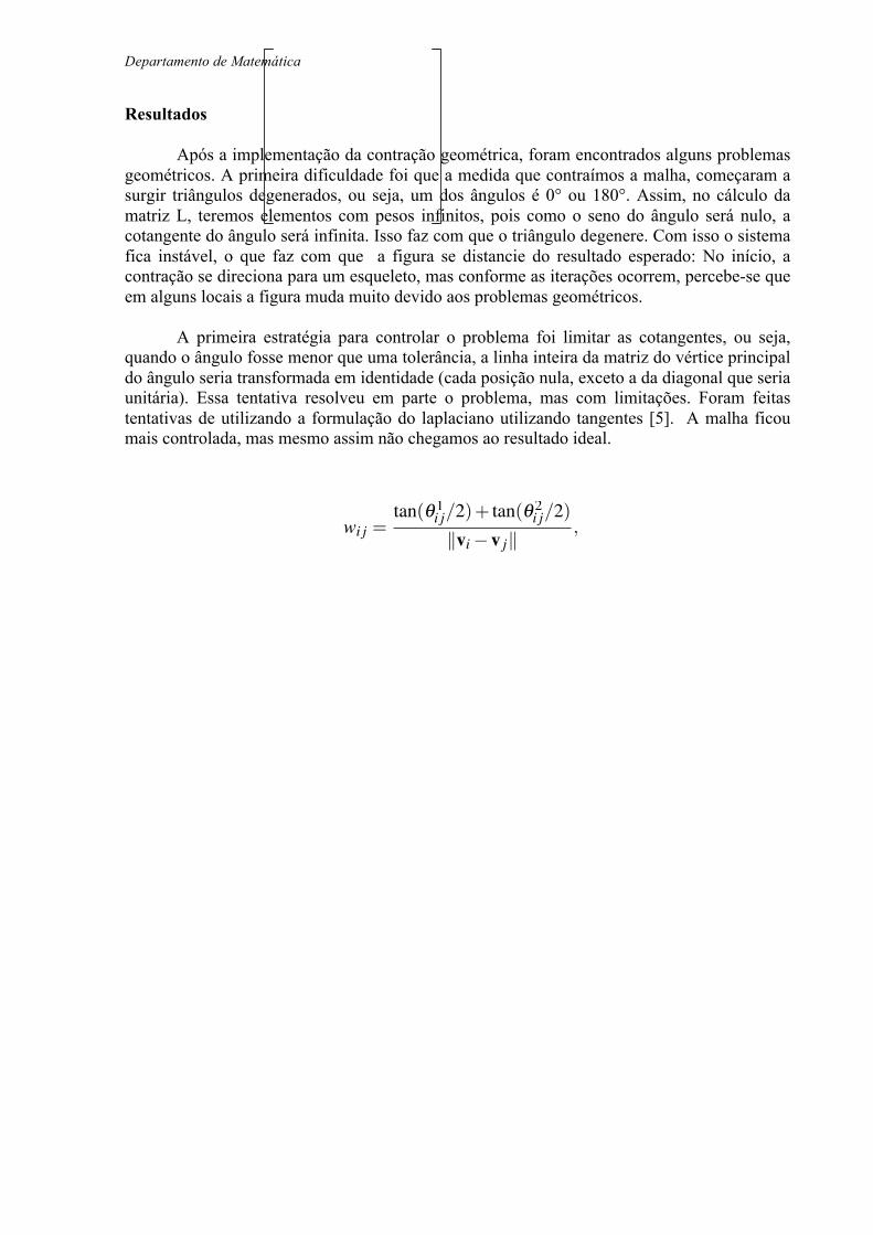
quando o ângulo fosse menor que uma tolerância, a linha inteira da matriz do vértice principal do ângulo seria transformada em identidade (cada posição nula, exceto a da diagonal que seria unitária). Essa tentativa resolveu em parte o problema, mas com limitações. Foram feitas tentativas de utilizando a formulação do laplaciano utilizando tangentes [5]. A malha ficou mais controlada, mas mesmo assim não chegamos ao resultado ideal.


–1–1 –1 –1–1 –1 –1–1 –1 –1 –1 –1

–1 –1 –1 –1–1 –1 –1–1 –1 –1 –1

–1 –1 –1 –1 –1 –1–1 –1 –1 –1 –1

–1–1–1–1 –1 –1 –1

43

54

34

66

34

The mesh The symmetric Laplacian Ls

–1–1 –1–1 –1 –1–1 –1 –1 –1 –1

–1 –1 –1 –1

–1 –1 –1 –1–1 –1 –1 –1 –1

–1 –1 –1

–1 –1 –1

43

54

46

6

4

–1–1 –1 –1–1 –1 –1–1 –1 –1 –1 –1

–1 –1 –1 –1–1 –1 –1–1 –1 –1 –1

–1 –1 –1 –1 –1 –1–1 –1 –1 –1 –1

–1–1–1–1 –1 –1 –1

43

54

34

66

34

11

Invertible Laplacian 2-anchor L

Figure 3: A small example of a triangular mesh and itsassociated Ls matrix (top right). Second row: a 2-anchor in-vertible Laplacian and a 2-anchor L matrix. The anchors aredenoted in the mesh by red.

atic to define for very large angles due to the properties ofcotangent near ⇥; convex weights that mimic the cotangentweights are called mean-value coordinates [Flo03]:

wi j =tan(⇤ 1

i j/2)+ tan(⇤ 2i j/2)

⇧vi�v j⇧,

where the ⇤ angles are depicted in Figure 2. These geomet-ric discretizations are beneficial for applications where themesh geometry is always known, such as mesh filtering andediting, since they approximate the differential propertiesmore accurately. However, in compression applications wewill define effective bases for geometry representation basedon the topological Laplacian, so that the weights in the oper-ator definition, and thus the bases themselves, are implicitlyencoded in the mesh connectivity and no extra informationis required to store them.

2.2. Surface reconstruction from � -coordinates

In the following, we will be working with the above defineddifferential surface representation. We will perform differ-ent operations on the � -coordinates, depending on the taskat hand. The final step of any such manipulation must be sur-face reconstruction, or, in other words, we need to recoverthe Cartesian coordinates of M ’s vertices.

Given a set of � -coordinates, can we uniquely restore theglobal coordinates? The immediate answer is no, because

the matrix L (or Ls) that we use to transform from global todifferential coordinates is singular, and therefore the expres-sion x = L�1� (x) is undefined. The sum of every row of L iszero, which implies that L has a non-trivial zero eigenvector(1,1, . . . ,1)T . The matrix is singular since the � -coordinatesare translation invariant: if we use weights wi j that sum upto 1 to define the Laplacian operator and we translate themesh by vector u to obtain the new vertices v⇤i then

L(v⇤i) = �j⌅N(i)

wi j(v⇤i�v⇤j) =

= �j⌅N(i)

wi j((vi +u)� (v j +u)) =

= �j⌅N(i)

wi j(vi�v j) = L(vi).

It follows that

rank(L) = n� k,

where k is the number of connected components of M , be-cause each connected component has one (translational) de-gree of freedom.

In order to uniquely restore the global coordinates, weneed to solve a full-rank linear system. Assuming M is con-nected, we need to specify the Cartesian coordinates of onevertex to resolve the translational degree of freedom. Substi-tuting the coordinates of vertex i is equivalent to droppingthe ith row and column from L, which makes the matrix in-vertible. However, as we shall see shortly, usually we placemore than one constraint on spatial locations of M ’s ver-tices. Denote by C the set of indices of those vertices whosespatial location is known. We have therefore |C| additionalconstraints of the form:

v j = c j, j ⌅C. (1)

If we assume w.l.o.g. that the vertices are indexed such thatC = {1,2, . . . ,m} then our linear system now looks like this:

�L

⌅ Im⇥m 0

⇥x =

�� (x)

⌅ c1:m

⇥. (2)

The same goes for y and z coordinate vectors, of course. Wedenote the system matrix in (2) by L. Note that we treatthe positional constraints (1) in the least-squares sense: in-stead of substituting them into the linear system, we add theabove equations as additional rows of the linear system. Thisway, for each j ⌅C we are also able to retain the “smooth-ness” term, i.e. the equation Lv j = � j. Please note that in ourdiscussion we will keep addressing (1) as “positional con-straints” or “modeling constraints”, although they may notbe fully satisfied by the least-squares solution. The weight⌅ > 0 can be used to tweak the importance of the posi-tional constraints (generally, every constraint may have itsown weight, and we can furthermore apply varying weightson the rows of the basic Laplacian matrix as well). The ad-ditional constraints make our linear system over-determined



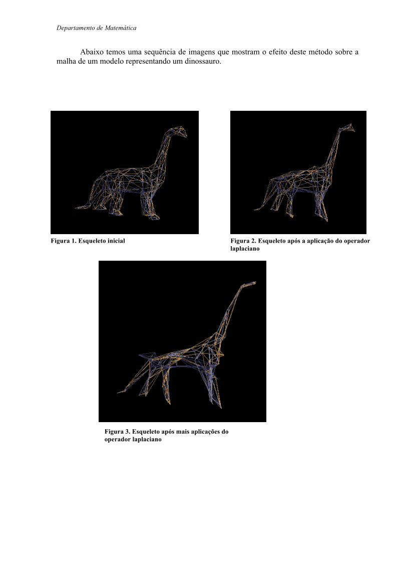
Abaixo temos uma sequência de imagens que mostram o efeito deste método sobre a malha de um modelo representando um dinossauro.

Figura 1. Esqueleto inicial Figura 2. Esqueleto após a aplicação do operador laplaciano

Figura 3. Esqueleto após mais aplicações do operador laplaciano


É possível perceber que a malha sofre uma contração tal que a cada iteração a malha se aproxima do esqueleto desejado.

A aplicação do método de mínimos quadrados a cada passo é lento, sendo necessário

otimizar o processo considerando que a matriz é esparsa. Inicialmente, o método apresentou resultados somente para malhas com reduzido número de vértices. O principal exemplo foi a malha de um dinossauro em que o número de vértices foi reduzido de 927 vértices para 187. Para outras malhas com um grande número de vértices, encontramos problemas tais como divergência de malha e excessivo esforço computacional. Esses problemas nos levaram a procurar uma nova forma para fazer essa iteração.

A limitação do número de vértices para um sistema de mínimos quadrados para esse

tipo de problema deve ser tratado por métodos iterativos. Assim, resolvemos modificar a parte do programa que realizava a operação de mínimos quadrados: Decidimos implementar o método de mínimos quadrados por um processo iterativo e não mais por uma função já pronta da biblioteca GSL [7]. Para isso, utilizamos o algoritmo do método do Gradiente Conjugado [8].

Essa iteração nos permite maior controle sobre o operador, o que nos possibilita um maior entendimento sobre o laplaciano e como ele afeta a figura. A iteração é a seguinte:

Assim, o resultado final é o x[k] que são os vértices da figura. A partir da implementação desta iteração junto ao programa, conseguimos realizar a

contração em outras malhas que antes não era possível pois geravam problemas já descritos antes.


Temos abaixo sequências de malhas sobre o efeito deste método modificado.

Figura 4. Malha Bretzel antes e depois de algumas iterações

Figura 5. Malha da Letra "O" antes e depois de algumas iterações


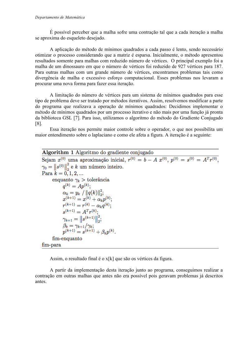
Nas três figuras possível ver a diferença da malha original para a segunda malha, o que mostra sucesso na realização da contração da malha.

Conclusões

A partir deste trabalho vimos que a técnica proposta em [4] é adequada apenas para malhas com muitos vértices e por isso tivemos que buscar outros métodos (o método iterativo) para poder aplicar a técnica em outras malhas.

Inicialmente o método apresentou dificuldades para gerar resultados na maioria dos exemplos selecionados. Foram essas dificuldades que levaram a busca de uma solução através dos métodos iterativos. Com a extensão realizada, o método pode ser aplicado a diferentes exemplos de malhas e conseguimos uma melhor visualização do efeito do operador Laplaciano sobre essas malhas.

Figura 6. Malha de pirâmides antes e depois de algumas iterações


Referências

1 - AMENTA, N., CHOI, S., AND KOLLURI, R. K. 2001. The power crust. In Symposium on Solid Modeling and Applications, 249– 266.

2 - DEY, T. K., AND SUN, J. 2006. Defining and computing curve- skeletons with medial geodesic function. In Symposium on Ge- ometry Processing, 143–152.

3 - BARAN, I., AND POPOVIC , J. 2007. Automatic rigging and ani- mation of 3D characters. ACM Trans. Graph. 26, 3, Article 72.

4 - AU Oscar Kin-Chung, TAI Chiew-Lan, CHU Hung-Kuo, COHEN-OR Daniel, LEE Tong-Yee . Skeleton extraction by mesh contraction. ACM Trans. Graph., v.27, n.3, Article 44, ago. 2008.

5 - SORKINE Olga. Laplacian Mesh Processing. EUROGRAPHS, 2005.

6 - BJÖRCK, A. Numerical Methods for Least Squares Problems. SIAM, Philadelphia, 1996. 2.2.3

7 - http://www.gnu.org/software/gsl/manual/html_node/ 8 - BORGES, Catiúscia. Reconstrução de Geometria Baseado na Conectividade e em Amostras da Malha. Dissertação de mestrado, Departamento de Matemática, PUC–Rio, 2007.

o operador de laplace-beltrami discreto … · departamento de matemática o operador de...

Documents