UNIVERSIDADE FEDERAL DE MINAS GERAIS

Instituto de Ciên ias Exatas � ICEX

Programa de Pós�Graduação em Físi a

TÍTULO: Tra� Model with an Absorbing Phase

Transition

Mauro Lu io Lobão Iannini

Belo Horizonte

2017

Mauro Lu io Lobão Iannini

TÍTULO: Tra� Model with an Absorbing Phase Transition

Tese apresentada ao Programa de Pós-

Graduação do Departamento de Fí-

si a do Instituto de Ciên ias Exatas da

Universidade Federal de Minas Gerais

omo requisito para obtenção do grau

de Doutor em Físi a.

Orientador: Ronald Di kman

Belo Horizonte

2017

Agrade imentos

A minha esposa Carmen, pelas in ontáveis vezes que pa ientemente respeitou o tempo

que pre isei para desenvolver esse trabalho.

Ao meu �lho Nathan, pelos pre iosos momentos que desfrutamos entre os intervalos

de trabalho.

Ao meu orientador Ronald Di kman que, além da imensa olaboração, a reditou no

trabalho e soube pa ientemente esperar pelos frutos que hoje olhemos.

À CAPES pelo apoio �na eiro a esse projeto.

i

Epígrafe

�I have not failed. I've just found 10,000 ways

that won't work.�

�Opportunity is missed by most people be ause it

is dressed in overalls and looks like work.�

Thomas Edison

ii

Abstra t

The ontribution of Nagel and S hre kenberg (NaS h) model in study of tra� models

is remarkable. First of all it is the �rst model based on ellular automata, the update

rules is quite simple but one of them has a spe ial importan e: the randomization pro ess.

This step introdu es a sto hasti parameter, the probability p, in the system apable of

reprodu e some features quite ommon in real tra� , e.g., the transition between free

�ow to jammed state. In original NaS h model the randomization pro ess produ es a lot

of unusual behaviours, for instan e we have the exaggerate de elerations due the addition

of randomization pro ess to the slowing down one. We propose a slight modi� ation in

randomization step that produ es two kinds of driver's behaviours: The sto hasti and

deterministi . The �rst one, as an original model, the drivers an de eleration in the

randomization pro ess with probability p. The se ond one annot. Despite of simpli ity,

this new model produ es interesting results as phase transition, hystereses and absorbing

state. The plane p − ρ is divided in three di�erent regions. The �rst one represents an

absorbing state, all ondu tors have deterministi behaviour. The se ond one the state

whi h both sort of behaviours oexists and the system never evolves to absorbing state

and the third one, in whi h the state of a system depends on its initially on�guration;

some distributions an evolve to absorbing states and others annot.

iii

Resumo

A ontribuição do modelo de Nagel e S hre kenberg (NaS h) no estudo dos modelos de

tráfego é notável. Ini ialmente foi o primeiro modelo baseado em aut�matos elulares om

regras de atualização bastante simples. Uma delas tem uma importân ia espe ial: o pro-

esso de randomização. Essa etapa introduz um parâmetro esto ásti o, a probabilidade

p, no sistema apaz de reproduzir algumas ara terísti as bastante omuns no tráfego

real, por exemplo, a transição entre o �uxo livre para o estado ongestionado. No modelo

NaS h original, o pro esso de randomização produz muitos omportamentos in omuns,

por exemplo, desa elerações exageradas devido à adição do pro esso de randomização ao

pro esso de adaptação. Propomos uma ligeira modi� ação no passo de randomização que

produz dois tipos de omportamentos do ondutor: O esto ásti o e o determinísti o. O

primeiro, omo no modelo original, os motoristas podem desa elerar no pro esso de ran-

domização om probabilidade p. O segundo não está sujeito à desa eleração nessa etapa.

Apesar da simpli idade, este novo modelo produz resultados interessantes omo transição

de fase, histerese, estado absorvente. O plano p−ρ é dividido em três regioês distintas. A

primeira representa um estado absorvente, todos os ondutores têm omportamento de-

terminísti o. A segunda, o estado em que ambos os tipos de omportamentos oexistem

e o sistema nun a evolui para estado absorvente e a ter eira, na qual o estado do sistema

depende da sua on�guração ini ial: algumas distribuições podem evoluir para estados

absorventes e outras não.

iv

List of Figures

1.1 Three phases . . . . . . . . . . . . . . . . . . . . . . . . . . . . . . . . . . 3

1.2 Three possible transitions in the fundamental diagram . . . . . . . . . . . 4

1.3 Wave propagation . . . . . . . . . . . . . . . . . . . . . . . . . . . . . . . . 5

1.4 Upstream and downstream fronts in the syn hronous �ow region . . . . . 6

1.5 Stable and Unstable dynami al models . . . . . . . . . . . . . . . . . . . . 8

2.1 A eleration step . . . . . . . . . . . . . . . . . . . . . . . . . . . . . . . . 9

2.2 Slowing down step . . . . . . . . . . . . . . . . . . . . . . . . . . . . . . . 10

2.3 Randomization step . . . . . . . . . . . . . . . . . . . . . . . . . . . . . . . 10

2.4 Displa ement step . . . . . . . . . . . . . . . . . . . . . . . . . . . . . . . . 11

2.5 Flux as a fun tion of density . . . . . . . . . . . . . . . . . . . . . . . . . . 13

2.6 Fundamental diagram for p = 0 . . . . . . . . . . . . . . . . . . . . . . . . 13

2.7 Order Parameter for p = 0 . . . . . . . . . . . . . . . . . . . . . . . . . . . 14

2.8 Relaxation parameter(p = 0) . . . . . . . . . . . . . . . . . . . . . . . . . . 15

2.9 Relaxation parameter(p > 0) . . . . . . . . . . . . . . . . . . . . . . . . . . 15

2.10 Spatial orrelations for p = 0 and p 6= 0. . . . . . . . . . . . . . . . . . . . 17

2.11 Correlation length . . . . . . . . . . . . . . . . . . . . . . . . . . . . . . . . 18

2.12 Relaxation time(p = 0) . . . . . . . . . . . . . . . . . . . . . . . . . . . . . 18

2.13 Relaxation time(p > 0) . . . . . . . . . . . . . . . . . . . . . . . . . . . . . 19

2.14 Stationary time for p = 0 and sizes L = 10000 and 50000. . . . . . . . . . . 20

2.15 Graph �ux versus density for p = 0.1 and graph showing maximum statio-

nary time for di�erent latti es . . . . . . . . . . . . . . . . . . . . . . . . . 20

2.16 Slowing down pro ess . . . . . . . . . . . . . . . . . . . . . . . . . . . . . . 22

2.17 1- luster approximation . . . . . . . . . . . . . . . . . . . . . . . . . . . . 24

2.18 Cluster on�guration . . . . . . . . . . . . . . . . . . . . . . . . . . . . . . 26

2.19 Comparison between 1- luster, 2- luster and Monte Carlo te hniques . . . 27

3.1 Typi al spa e-time diagram of the NS model . . . . . . . . . . . . . . . . . 31

3.2 Comparison between NS and SDNS models . . . . . . . . . . . . . . . . . . 32

3.3 Metastable states in the SDNS model . . . . . . . . . . . . . . . . . . . . . 33

3.4 Fundamental diagram and the orresponding velo ity-density urve. . . . . 33

3.5 Comparison between VDR and NS models . . . . . . . . . . . . . . . . . . 34

3.6 Spa e-time diagram of the VDR model . . . . . . . . . . . . . . . . . . . . 35

3.7 Fundamental diagram of the ruise- ontrol model . . . . . . . . . . . . . . 36

3.8 Spa e-time diagram of the ruise- ontrol model with many jams . . . . . . 37

3.9 Lifetime power law . . . . . . . . . . . . . . . . . . . . . . . . . . . . . . . 38

3.10 Comparison between theoreti al and numeri al simulations of the FI model. 39

3.11 Wang model diagram . . . . . . . . . . . . . . . . . . . . . . . . . . . . . . 40

v

3.12 Comparison between the fundamental diagrams of the NS and two-lane

models. . . . . . . . . . . . . . . . . . . . . . . . . . . . . . . . . . . . . . 42

3.13 Lane- hange frequen y in the two-lane model for di�erent braking parame-

ters p. . . . . . . . . . . . . . . . . . . . . . . . . . . . . . . . . . . . . . . 42

3.14 Comparison of the �ux per lane of the inhomogeneous model with the

orresponding homogeneous models for p = 0.4. . . . . . . . . . . . . . . . 43

4.1 The normalized �ux Q ≡ q/cmax and normalized mean velo ity υ = v/v0versus the normalized on entration η = c/cmax for cmaxτ = 0.1. . . . . . . 51

4.2 Distribution of desired velo ities and stationary velo ity distribution for

exponential desired velo ity distributions with η = 0.2 . . . . . . . . . . . . 52

4.3 Distribution of the desired velo ity and stationary velo ity distribution as

in Fig. 4.2 for η = 0.4. . . . . . . . . . . . . . . . . . . . . . . . . . . . . . 52

4.4 The �ux Q as a fun tion of the normalized on entration η in the Prigogine-Herman model using the distribution of desired velo ities of Eq. (4.27), with

va = 20. . . . . . . . . . . . . . . . . . . . . . . . . . . . . . . . . . . . . . 53

4.5 The stationary velo ity distribution and orresponding distribution of de-

sired velo ities, for on entrations in the individual �ow regime. . . . . . . 54

5.1 Flux j versus density in the NS and ANS models for probabilities p = 0.1and p = 0.5. . . . . . . . . . . . . . . . . . . . . . . . . . . . . . . . . . . . 59

5.2 Steady-state �ux versus density in the ANS model for p = 0.1, 0.3, 0.5, 0.7and 0.9. . . . . . . . . . . . . . . . . . . . . . . . . . . . . . . . . . . . . . 59

5.3 Dimer rea tion rules. . . . . . . . . . . . . . . . . . . . . . . . . . . . . . . 61

5.4 Pair onta t pro ess rules. . . . . . . . . . . . . . . . . . . . . . . . . . . . 62

5.5 Possible ANS absorbing states. . . . . . . . . . . . . . . . . . . . . . . . . 62

5.6 Fundamental Diagram for p = 1. . . . . . . . . . . . . . . . . . . . . . . . . 63

5.7 Steady-state �ux versus density for p = 0.1 and L = 105. . . . . . . . . . . 64

5.8 Steady-state �ux versus density as in Fig. 5.7, but for p = 0.5. . . . . . . . 65

5.9 Boundary between a tive and absorbing phases in the ρ - p plane. . . . . . 66

5.10 Steady-state a tivity ρa versus p for vehi le density ρ = 1/8. . . . . . . . . 67

5.11 Vehi le positions relative to the �rst vehi le versus time t for t ≥ 2, in a

system with N = 20, vmax = 2 and vehi le density ρ = 2/9. . . . . . . . . . 68

5.12 A tivity density versus number of vehi les for density 1/8 and (lower to

upper) p = 0.2679, 0.2681, 0.2683, 0.2685 and 0.2687. . . . . . . . . . . . . 72

5.13 Lifetime versus number of vehi les for density 1/8 and p = 0.2679, 0.2681,0.2683, 0.2685 and 0.2687. . . . . . . . . . . . . . . . . . . . . . . . . . . . 72

5.14 Moment ratio m versus re ipro al system size for density 1/8 and p =0.2679, 0.2681, 0.2683, 0.2685 and 0.2687. . . . . . . . . . . . . . . . . . . . 73

5.15 Curvature of ln ρa and ln τ as fun tions of lnN , as measured by the oe�-

ient b of the quadrati term in least-squares quadrati �ts to the data in

Figs. 5.12 and 5.13. . . . . . . . . . . . . . . . . . . . . . . . . . . . . . . . 73

5.16 Derivatives ofm, ln ρa and ln τ with respe t to p in the vi inity of pc, versusN for vehi le density ρ = 1/8. . . . . . . . . . . . . . . . . . . . . . . . . . 74

vi

Table of ontents

Resumo iv

1 Tra� Models 1

1.1 Hydrodynami models . . . . . . . . . . . . . . . . . . . . . . . . . . . . . 1

1.2 Three phases theory . . . . . . . . . . . . . . . . . . . . . . . . . . . . . . 2

1.3 Dynami al models . . . . . . . . . . . . . . . . . . . . . . . . . . . . . . . 6

2 NaS h Model 9

2.1 Model . . . . . . . . . . . . . . . . . . . . . . . . . . . . . . . . . . . . . . 9

2.2 S aling behaviour . . . . . . . . . . . . . . . . . . . . . . . . . . . . . . . . 13

2.2.1 Singularity . . . . . . . . . . . . . . . . . . . . . . . . . . . . . . . . 13

2.2.2 Density of nearest-neighbor pairs . . . . . . . . . . . . . . . . . . . 14

2.2.3 Spatial Correlations . . . . . . . . . . . . . . . . . . . . . . . . . . . 16

2.2.4 Relaxation time . . . . . . . . . . . . . . . . . . . . . . . . . . . . . 16

2.2.5 Dis ussion about riti ality in NS model . . . . . . . . . . . . . . . 19

2.3 Mean-�eld theory . . . . . . . . . . . . . . . . . . . . . . . . . . . . . . . . 21

2.3.1 N- luster approximation . . . . . . . . . . . . . . . . . . . . . . . . 25

2.3.2 2- luster approximation . . . . . . . . . . . . . . . . . . . . . . . . 26

3 Other ellular automata models 30

3.1 Changing the orders of substeps in the NS model . . . . . . . . . . . . . . 30

3.2 VDR model . . . . . . . . . . . . . . . . . . . . . . . . . . . . . . . . . . . 34

3.3 Cruise- ontrol model . . . . . . . . . . . . . . . . . . . . . . . . . . . . . . 35

3.4 Fukui�Ishibashi Model . . . . . . . . . . . . . . . . . . . . . . . . . . . . . 38

3.5 Wang Model . . . . . . . . . . . . . . . . . . . . . . . . . . . . . . . . . . . 39

3.6 Multilane tra� . . . . . . . . . . . . . . . . . . . . . . . . . . . . . . . . . 41

4 Kineti tra� theory 44

4.1 Introdu tion . . . . . . . . . . . . . . . . . . . . . . . . . . . . . . . . . . . 44

4.2 The Prigogine-Herman-Boltzmann equation . . . . . . . . . . . . . . . . . 45

4.3 Stationary solutions . . . . . . . . . . . . . . . . . . . . . . . . . . . . . . . 46

4.4 Individual and olle tive �ow . . . . . . . . . . . . . . . . . . . . . . . . . 47

4.5 Numeri al Solutions . . . . . . . . . . . . . . . . . . . . . . . . . . . . . . . 49

4.5.1 Numeri al Method . . . . . . . . . . . . . . . . . . . . . . . . . . . 50

4.6 Some distributions of desired velo ities . . . . . . . . . . . . . . . . . . . . 50

4.6.1 Exponential distribution of desired velo ities . . . . . . . . . . . . . 51

4.6.2 Gaussian distribution of desired velo ities . . . . . . . . . . . . . . 52

4.7 Paveri-Fontana model . . . . . . . . . . . . . . . . . . . . . . . . . . . . . . 54

vii

5 ANaS h Model 57

5.1 Introdu tion . . . . . . . . . . . . . . . . . . . . . . . . . . . . . . . . . . . 57

5.2 Model . . . . . . . . . . . . . . . . . . . . . . . . . . . . . . . . . . . . . . 58

5.2.1 Models with Many Absorbing States . . . . . . . . . . . . . . . . . 60

5.2.2 Spe ial ases: p = 0 and p = 1 . . . . . . . . . . . . . . . . . . . . . 61

5.3 Phase diagram . . . . . . . . . . . . . . . . . . . . . . . . . . . . . . . . . 63

5.3.1 Initial ondition dependen e . . . . . . . . . . . . . . . . . . . . . . 63

5.3.2 Order parameter . . . . . . . . . . . . . . . . . . . . . . . . . . . . 66

5.3.3 Reentran e . . . . . . . . . . . . . . . . . . . . . . . . . . . . . . . 67

5.4 Criti al behavior . . . . . . . . . . . . . . . . . . . . . . . . . . . . . . . . 68

5.4.1 Quasistationary simulation . . . . . . . . . . . . . . . . . . . . . . . 68

5.4.2 Criti al Exponents . . . . . . . . . . . . . . . . . . . . . . . . . . . 69

5.4.3 Criti al Exponents in the ANS model . . . . . . . . . . . . . . . . . 70

6 Summary and Open Questions 75

6.1 Summary . . . . . . . . . . . . . . . . . . . . . . . . . . . . . . . . . . . . 75

6.2 Open questions in the ANS model . . . . . . . . . . . . . . . . . . . . . . . 76

6.2.1 Criti al exponents . . . . . . . . . . . . . . . . . . . . . . . . . . . . 76

6.2.2 Mean-Field Theory . . . . . . . . . . . . . . . . . . . . . . . . . . . 76

6.2.3 Other CA models with ANS rules . . . . . . . . . . . . . . . . . . . 76

7 Appendix 77

7.1 Matriz T t. . . . . . . . . . . . . . . . . . . . . . . . . . . . . . . . . . . . 77

7.2 Mean Field Theory . . . . . . . . . . . . . . . . . . . . . . . . . . . . . . . 79

Bibliography 82

Published Arti les 85

viii

Chapter 1

Tra� Models

The ideas and te hniques of statisti al physi s are being used urrently to study several

aspe ts of omplex systems many of whi h are di�erent from the known domain of physi al

systems. Physi al, hemi al, earth, biologi al and so ial s ien es are examples of this

trend. Biologi al evolution of spe ies, formation and growth of ba terial olonies, folding

of proteins, �ow of vehi ular tra� and transa tions in �nan ial markets are just a few

examples of the extent of these appli ations. Most of these systems are interesting not

only from the point of view of Natural S ien es for fundamental understanding of how

Nature works but also from the points of view of applied s ien es and engineering for the

potential pra ti al use of the results of these investigations.

For a long time physi ists have been trying to understand the fundamental prin iples

governing the �ow of vehi ular tra� using theoreti al approa hes based on statisti al

physi s. The approa h of a physi ist is usually quite di�erent from that of a tra�

engineer. Physi ists have been trying to develop a model of tra� by in orporating

only the most essential elements needed to des ribe the general features of typi al real

tra� (minimal prin iples). The theoreti al analysis and omputer simulation of these

models not only provide deep insight into the properties of the model su h as phase

transition, metastable states, absorbing phases but also help us to understanding the

omplex phenomena observed in real tra� . Below we present a brief resume of the main

existing lass of tra� models. In tra� models di�erent approa hes have been used

in order to model tra� �ows using methods from physi s. There are several ways to

distinguish these theories, e.g., ma ros opi or mi ros opi , deterministi or sto hasti ,

dis rete or ontinuous, et . In this se tion we present the main approa hes used in tra�

study.

1.1 Hydrodynami models

The �rst ma ros opi des ription of tra� model was proposed by Lighthill and

Whitham (1955). The �uid-dynami model has its prin iples based on the assumption

that the number of vehi les does not hange, i.e., no vehi les are entering or leaving the

freeway. Another feature is that the tra� is onsidered as a ompressible �uid. The

onservation of the vehi le number leads to the ontinuity equation:

∂ρ(x, t)

∂t+

∂Q(x, t)

∂x= 0.

In this equation, we have two fun tions ρ(x, t) and Q(x, t), unless they are related to ea h

other we need more information to solve it. An alternative possibility is to assume that

1

Q(x, t) is determined primarily by the lo al density ρ(x, t) so that Q(x, t) an be treated

as a fun tion of only ρ(x, t). Consequently, the number of unknown variables is redu ed

to one as, a ording to this assumption, the two unknowns ρ(x, t) and Q(x, t) are not

independent of ea h other.

The Lighthill�Whitham�Ri hards theory is based on the assumption that:

Q(x, t) = q(ρ(x, t)), (1.1)

where q(ρ) is a fun tion of ρ. Su h a relation is known as a fundamental diagram. An ad-

ditional hypothesis about q(ρ(x, t) is needed for solving it, in this ase a phenomenologi al

relation extra ted from empiri al data or derived from more mi ros opi onsiderations

should be introdu ed. With the hypothesis in Eq. (1.1) the x-dependen e of Q(x, t) arisesonly from the x-dependen e of ρ(x, t) at the same time Q(x, t) = ρ(x, t)v(x, t) and the

x-dependen e of v(x, t) arises only from the x-dependen e of ρ(x, t). In this way, using

Eq. (1.1) the equation of ontinuity an be expressed as:

∂ρ(x, t)

∂t+

dq

dρ

∂ρ(x, t)

∂x= 0 (1.2)

with

dq

dρ= v(x, t) + ρ(x, t)

dv

dρ.

The Eq. (1.2) is nonlinear be ause, in general, dq/dρ depends on ρ. If dq/dρ were a

onstant v0, independent of ρ, Eq. (1.2) would be ome linear and the general solution

would be of the form:

ρ(x, t) = f(x− v0t), (1.3)

where f is an arbitrary fun tion of its argument. Su h a solution des ribes a density

wave motion, as an initial density pro�le would get translated by a distan e v0t in a time

interval t without any hange in its shape. If we de�ne a wave as a signal that is transferredfrom one part to another with a known velo ity of propagation, then the solutions of the

form Eq. (1.3) an be regarded as a density wave. There are several similarities between

the density wave and the known me hani al waves like, e.g., a ousti or elasti waves.

But the a ousti or elasti waves are solutions of linearized partial di�erential equations,

whereas the Eq. (1.2) is nonlinear, and hen e, dq/dρ is ρ-dependent. Waves of the type

des ribed by Eq. (1.2) are alled kinemati waves to emphasize their purely kinemati

origin, in ontrast to the dynami origin of the a ousti and elasti waves. We will present

an important use of the kinemati waves in the following se tion.

1.2 Three phases theory

In the tra� literature there is a phenomenologi al des ription presented by Kerner

[1℄. In this des ription ea h state is represented by a point in the phase spa e de�ned by

the �ux and density oordinates. Empiri ally the �ux is measured by the ratio between

the number of vehi les passing through a �xed dete tor and a set time interval (minutes,

hours et .). The density on the other hand orresponds to the number of vehi les per unit

of length. The use of only a �xed dete tor does not allow to �nd the density of dire t

form, on e known the �ux, the density is found by the relation:

2

ρ =q

vwith v =

1

m

m∑

i=1

vi. (1.4)

Where vi represents the velo ity of a vehi le i, v is the mean velo ity and q is the �ux.However, there are spe ial ases where this formulation an fail. It should be noted that

the vehi le density ρ is related to vehi les on a freeway se tion of a given length whereas

the vehi le speed is measured at the lo ation of the dete tor only and is averaged over

the time interval ∆t. In addition, low vehi le speeds an usually be measured to a lower

a ura y than higher vehi le speeds. As a result, at higher vehi le densities (lower average

vehi le speed), the vehi le density estimated via Eq. (1.4) an lead to a onsiderable error

in omparison with the real vehi le density. For this reason, empiri al data for higher

vehi le densities (more than 70 vehi les/km) are not usually onsidered. There are also

other ases why the estimation of the density via Eq. (1.4) an lead to a onsiderable error

at higher vehi le densities. In parti ular, this an o ur when the vehi le speed and �ux

are strongly spatially inhomogeneous. Thus, the averaging of the vehi le speed through

Eq. (1.4) gives a temporal averaging of the speed at the dete tor lo ation made during

some time interval. If tra� �ow is spatially inhomogeneous, this temporal averaging of

the speed an give a very di�erent average speed in omparison with a spatial averaging

of the vehi les speed made at a given instant on a freeway se tion of a given length

1

.

Figure 1.1: Illustrative �gure representing �ux as a fun tion of density. Note the lo ation of the three

phases.

The states originated by the empiri al data analysis are grouped in the q − ρ plane

into three distin t regions: free �ow (F), syn hronous �ow (S) and wide moving jam

(J). Free �ow is hara terized by weak intera tions between the vehi les; the mean speed

orresponds to the limit established by the freeway. The relationship between �ux and

density is pra ti ally linear and the slope of the line (builded by the points in the region

F ) orresponds to the maximum velo ity. Syn hronized �ow is hara terized by the

1

For a more detailed des ription of the measurements made by the dete tor and the restri tions

imposed by the use of this te hnique onsult Kerner [1℄ pp. 15 to 17.

3

existen e of intera tion between the vehi les so that the average speed is lower than

that of free �ow. The main hara teristi of this region is the apparent absen e of a

fun tional relationship between �ow and density. The points are s attered irregularly

over a large region of the q − ρ plane. The region J, in turn, is marked by su essive

de elerations and a elerations (stop and go tra� ) of vehi les when entering and exiting

the ongestion fronts. Generally the extension of this region is signi� ant, but the main

di�eren es between it and the syn hronized �ow are the high on entration of vehi les

and the low average speed developed (negligible �ux). We an see these states in Fig.

1.1. Before studying the propagation of waves in these phases we have to introdu e some

basi on epts. The distan e between two onse utive vehi les is 1/ρ, the �time� distan e

1/q and the average speed q/ρ. In the transitions between two states we will onsider, in

order to simplify the analysis, that the vehi les are at the same speed and equally spa ed.

The distan e, the time interval and the vehi les speed are de�ned a ording to the state

in whi h they are. The �gure 1.2 presents three possible transitions between states. Fig.

Figure 1.2: Illustrative �gure representing three state transitions. The �rst represents a transition where

the �ow is preserved. In the se ond and third transitions the �ow de reases and in reases respe tively.

1.2 shows the verti al lines in three di�erent situations, ea h line represents the front of

the sho k wave

2

. When the sho kwave propagation redu es the vehi les speed, we all

it an upstream front, when in reases, downstream front. For simpli ity we will onsider

the a eleration (or de eleration) of vehi les instantaneously at the moment they are

rea hed by su h fronts. The �rst transition is hara terized by keeping the �ux onstant,

onsequently the wavefront is �xed and does not move be ause the �uxes are equal on

both sides of the front. In the se ond transition the vehi les depart from a state where

2

We de�ne sho k waves as a sudden hange of the vehi les velo ity due to tra� onditions. In relation

to the freeway frame, the sho k wave an be at rest or in motion

4

the �ux is greater to another where the �ux is smaller. In this ase the upstream front

should move towards the region where the �ux is higher, be ause on the wave front frame

the input �ow must be equal to the output one. In the third transition, the downstream

front moves toward the region where the �ux is lower.

Figure 1.3: Illustrative �gure represented the propagation speed of the wave.

The meaning of the slope of the line joining the two states an be understood through

Fig. 1.3. In the �rst illustration, the wavefront is lo ated on the se ond vehi le (from

right to left) and moves toward the third one, lo ated on the left of the front. After the

time interval t the wavefront is on the third vehi le ausing immediate slowdown from v1to v2 and its distan e for the se ond vehi le from d1 to d2. At this point the distan es

traveled by the relative motion between [vup, v2℄ are:

(v1 + vup)t = d1 e (v2 + vup)t = d2.

Isolating t and remembering that d = 1ρ,

ρ1(v1 + vup) = ρ2(v2 + vup),

using q = ρv

vup =q2 − q1ρ1 − ρ2

.

The slope of the line joining the states represents the velo ity of the wavefront. This

analysis omes from wave kinemati theory. The three phases theory uses these results

to study vehi le behaviour in two distin t regions of S phase.

The steady propagation of the downstream front in a wide moving jam has mean velo ity

vg and an be represented in the �ow-density plane by a line. This line is alled �the line

J�. The slope of the line J is equal to the velo ity vg of this front. The left oordinates ofthe line J are related to the parameters of free �ow (ρmin, qout) exhibited by vehi les that

have a elerated from the standstill inside the jam. The right oordinates of the line J,

(ρmax, 0), are related to the vehi le density inside the jam ρmax where the vehi le speed

v is zero. These features have further been found in empiri al studies of wide moving

jam propagation by Kerner and Rehborn. The velo ity of the upstream fronts (1) and(2) are de�ned by the slope of the respe tive lines. Thus vup1 > vdown

g > vup2 and for this

reason the states lo ated above the line J are subje t to transition S → J while the states

lo ated below are not. A better explanation is given by Fig. 1.4, the arrows at the right

represent the empiri al downstream velo ity (vdown) and the arrows at the left represent

the upstream velo ity of the states 1 (upper arrow) and 2 (bottom arrow) respe tively.

5

Figure 1.4: Illustrative �gure represented the upstream and downstream fronts in two distin t regions

of region S.

We an see that in state (1) owing to vup1 > vdownthe wave responsible for jam formation

is faster than the wave responsible for free �ow. Thus the possible state rea hed by the

system is in the region J. But in the state (2) the jam formation is not possible, owing

to vup2 < vdownthe downstream front will rea h the upstream one. The omplete study of

the three phase theory an be found in [1℄ as well as the transitions between the phases

and other tra� features.

1.3 Dynami al models

The dynami al model is based on the equation of motion of ea h vehi le. This equation

has as an assumption the fa t that ea h driver of a vehi le responds to a stimulus from

other vehi les in some spe i� way. The response is expressed in terms of a eleration,

whi h is the only dire t ontrollable quantity for a driver. Generally, the stimulus and the

sensitivity may be a fun tion of the positions of vehi les, their time derivatives, and so on.

This fun tion is de ided by supposing that the drivers of vehi les obey postulated tra�

regulations at all times in order to avoid a idents. In the dynami al model we have two

kinds of stimulus: in the earliest dynami al models the di�eren e in the velo ities of the

n-th and (n+1)-th vehi les was assumed to be the stimulus for the n-th vehi le. In other

words, it was assumed that every driver tends to move with the same speed as that of the

orresponding leading vehi le so that

xn =1

τ

[xn+1(t)− xn(t)

],

where 1/τ is related with the driver's sensitivity. Other dynami al models take into

a ount the driver's own velo ity and the distan e to the vehi le ahead. All drivers have

the ommon sensitivities and the length of vehi le is negligible. We assume that ea h

6

vehi le has legal velo ity V 3

and that ea h driver of a vehi le responds to a stimulus

from the vehi le ahead of him. The drivers an ontrol the a eleration in su h a way

that they an maintain the legal safe velo ity a ording to the motion of the pre eding

vehi le. Then the dynami al equation of the system is obtained via:

xn = a[V (∆xn)− xn

], (1.5)

where

∆xn = xn+1 − xn,

for ea h vehi le number n (n = 1, 2, ..., N). N is the total number of vehi les, a is a

onstant representing the driver's sensitivity (whi h has been assumed to be independent

of n), and x is the oordinate of the nth vehi le. The dots denote di�erentiation with

respe t to time t. We assume here that the legal velo ity V (∆x) of vehi le number

n depends on the following distan e of the pre eding vehi le number n + 1. When the

headway be omes short the velo ity must be redu ed and be omes small enough to prevent

rashing into the pre eding vehi le. On the other hand, when the headway be omes longer

the vehi le an move with higher velo ity, although it does not ex eed the maximum

velo ity. Thus, V is a fun tion having the following properties: a monotoni ally in reasing

fun tion, and V (∆x) has an upper bound Vmax ≡ V (∆x → ∞) . Further, this model has

periodi boundary onditions: vehi les move on a ir uit with length L and the (N +1)thvehi le is identi al to the �rst vehi le. Depending on hoi e of V and the headway ∆x,the system an be stable or unstable.

In Fig. 1.5 the traje tories of a spe i� vehi le (the 50th vehi le) are shown in two

di�erent ases: the stable and unstable traje tories. In the stable ase, the vehi le moves

with onstant velo ity, i.e., the distan e in reases linearly. On the other hand, in the

unstable ase we observe a vehi le moving ba kward (v < 0). This always happens

whenever the solution of this model is in the unstable region. As long as we take the

models of a single lane, this means a ollision of two su essive vehi les. The above

behavior indi ates that, instead of ongestion, su h tra� a idents o ur everywhere.

Then, by hoosing an appropriate legal velo ity fun tion, we an modify the model so

that a vehi le never moves ba kward. In [2℄ another fun tion is proposed with intention

of preventing it. In addition to the models presented in this se tion we have to take into

a ount kineti models. In su h models tra� is treated as a gas of intera ting parti les

where ea h parti le represents a vehi le. The di�erent versions of the kineti theory of

vehi ular tra� have been developed by modifying the kineti theory of gases. Due to

the extensive study in this kind of model, we published an arti le entitled �Kineti theory

of vehi ular tra� �, in whi h we present the key features in the hapter 4.

3

the term �legal velo ity� was introdu ed in [2℄, although we think that the term �safety or desirable

velo ity� is more appropriate

7

Figure 1.5: Traje tories of a vehi le (the 50th vehi le) in two typi al ases. The stable ase de�ned by

L = 200 and N = 100 (dotted line) and the unstable ase de�ned by L = 50 and N = 100 (solid line).

8

Chapter 2

NaS h Model

2.1 Model

The NaS h model(NS) was the �rst tra� model based on a ellular automaton [3℄.

The model is de�ned on a one-dimensional latti e of length L, with periodi boundaries,

representing a single-lane freeway. Ea h site of the latti e an be in one of the vmax + 2states: It may be empty, or it may be o upied by one ar having an integer velo ity

between zero and vmax. Time, spa e, and velo ity are dis retized. The pro ess starts with

an initial distribution of N vehi les (N ≤ L). The state of system is updated at ea h

iteration a ording to the following steps: A eleration, de eleration, randomization and

displa ement. Ea h iteration, between two onse utive times (t and t + 1) onsists of 4steps a ording to the NS update rules: (t1, t2 , t3 and t+ 1). Note that the three initialsteps do not represent vehi le movement but only intermediate steps required for de�ning

the �nal speed just before the displa ement step. The update rules are:

1. A eleration

The velo ity of ea h vehi le with v < vmax is in reased by one unit. If a vehi-

le already possesses the maximum velo ity before this step, its velo ity remains

un hanged.

vj(t1) = min[vj(t) + 1, vmax].

Figure 2.1: An example of a eleration step. The �gure shows the vehi les on�guration before (upper)

and after (lower) the a eleration step. Note that the vehi les a elerate independent of the possibility

of displa ing with the new velo ity.

9

2. Slowing Down

All vehi les with vj(t1) > dj redu e their speed to vj(t2) = dj. Here, dj is de�nedas a number of empty ells between the ar j and j + 1. Thus

vj(t2) = min[dj(t), vj(t1)].

Figure 2.2: An example of slowing down step. The �gure shows the vehi les on�guration before

(upper) and after (lower) the slowing down step. Now the vehi les an adjust their velo ities a ording

to the distan e (headway) in relation to the forward vehi le.

3. Randomization

This step introdu es sto hasti ity in the model; without it the model would be

deterministi and the stationary state rea hed qui kly. In this step ea h vehi le

redu es its speed by one unit with probability p or maintains it with probability

1− p. Vehi les with v = 0 are not subje t to this step.

vj(t3) = max[vj(t2)− 1, 0], with probability p

vj(t3) = vj(t2), with probability 1− p.

Figure 2.3: An example of randomization step. The �gure shows the vehi les on�guration before

(upper) and after (lower) the randomization step. This step introdu es substantially modi� ation in

ma ros opi al tra� behaviour due the introdu tion of individual behaviour ( ontrolled by parameter p).In some ases drivers de elerated (at random), in others do not.

10

4. Displa ement

This step represents the displa ement of the vehi les a ording to the velo ity pre-

viously established.

vj(t+ 1) = vj(t3).

Figure 2.4: An example of displa ement. The �gure shows the vehi les on�guration before (upper)

and after (lower) the displa ement step. This step represents the �nal step in whi h the vehi les displa e

a ording to the velo ity de�ned in the previous step.

The randomization step is an essential omponent for the reprodu tion of the main fe-

atures presented in real tra� , e.g., the transition between free �ow to jammed state,

start-and-stop waves, and sho ks (due to driver overrea tion). This step in the model an

be ompared with the unpredi table rea tion of the drivers in front of tra� onditions

though in the NS model the probability p is independent of the tra� onditions, e.g.,

the density of vehi les on the latti e.

In Fig. 2.5 we present the graph �ux as a fun tion of density (also known as the funda-

mental diagram) for p = 0.1, 0.5 and 0.9. We observe the presen e of two bran hes; the

�rst one orresponds to the free �ow regime where the vehi les almost do not intera t

themselves due to the large distan es between them. In this ondition the se ond step in

the NS update rules pra ti ally does not apply. Let us set vmax = 5 and the states

|0〉 =

100000

............ |5〉 =

000001

,

for velo ities (the value in the line n orresponds to the probability of �nding a vehi le

with velo ity n− 1). The sto hasti matrix for a single vehi le is:

T =

p 0 0 0 0 01− p p 0 0 0 00 1− p p 0 0 00 0 1− p p 0 00 0 0 1− p p p0 0 0 0 1− p 1− p

.

11

Let Pt be the probability distribution of velo ities at the time t. The relation between

P(t) and P(t-1) is given by:

Pt = TPt−1.

Given the P0, Pt an be found via:

Pt = T tP0.

After a little algebrai work (for further details, see hapter 7), we have:

limt→∞

Pt =

0000p

1− p

.

After the vehi le attains the stationary state, the mean velo ity is:

v = p(vmax − 1) + (1− p)vmax ∴ v = vmax − p,

and the �ux q is

q = ρ(vmax − p). (2.1)

This analysis annot be used for higher densities sin e it does not take into a ount the

intera tions between the vehi les. When we onsider these intera tions the problem an-

not be solved in this way. We will see in se tion 2.3 a �rst analyti approa h (mean-�eld

theory) to this problem. Although the equation (2.1) annot be used for higher densities,

it explains the slight di�eren e between the slopes in the �rst bran h a ording to the

probability p. The se ond bran h orresponds to jammed state in whi h the intera tions

between the vehi les are more frequent. In this regime the presen e of start-and-stop wa-

ves and driver overrea tion is ommon. The overrea tion an be explained due to overlap

of two su essive de elerations; the �rst one due to the se ond step in the NS update ru-

les, the vehi les redu e their velo ities due the small distan e between them. The se ond

one is related to the randomization step, with probability p the vehi le may redu e, in

addition to the �rst de eleration, its velo ity by one more unit.

In the NS model two spe ial values (p = 0 and p = 1) produ e deterministi behaviour

in the system. In both ases the randomization step does not apply (in the �rst ase the

vehi les never redu e their velo ity while in se ond one, always redu e). For p = 0 and

ρ ≤ ρc1

(ρc = 1/(vmax + 1)) the system always evolves to absorbing state in whi h all

vehi les attain the maximum velo ity while for ρ > ρc the system evolves to a stationary

state with v = (1 − ρ)/ρ. For p = 1 and ρ ≤ 1/3 few initial states an evolve to a

stationary state with v 6= 0 sin e if a vehi le stops it never moves again. For ρ > 1/3 the

system, in a ertain moment, attains the absorbing state with v = 0.

1

For the deterministi ase, ρc is the riti al density

12

Figure 2.5: Fundamental diagram using Monte Carlo simulation for probabilities p = 0.1, 0.5, and 0.9.

2.2 S aling behaviour

In this se tion we will study the phase transition in the NS model. A spe ial ase in

the Ns model arises when p = 0. In addition to its deterministi behaviour we an assert

that there is a ontinuous phase transition at the point ρc. In the following subse tions

we dis uss some quantities that support this assertion.

2.2.1 Singularity

In Fig. 2.6 the fundamental diagram, for p = 0, exhibits a sharp hange at ρc; thissingularity is hara terized by a dis ontinuity in the �rst derivative. For p 6= 0 this hangeis smooth, as an be seen in Fig. 2.5.

Figure 2.6: Fundamental diagram for p = 0.

With the intention to study in more details the riti ality in this ase we should

13

look for an appropriate order parameter to des ribe the singularity shown in Fig. 2.6.

The natural andidate is the fra tion of jammed vehi les, e.g., vehi les with velo ities

smaller than vmax. Unfortunately in the deterministi model this fra tion and any related

quantities depend on the initial spatial distribution. So we propose an order parameter

M de�ned by:

M = 1− q

ρvmax.

For p = 0 and ρ > ρc,

v =1− ρ

ρ.

Remembering that q = ρv, we have

q = 1− ρ and vmax + 1 =1

ρc,

so that M is given by

M =

{0 (ρ ≤ ρc)

1vmax

ρ−ρcρρc

(ρ > ρc).

For p = 0 the graph M as a fun tion of ρ is shown in Fig. 2.7.

Figure 2.7: Order parameter for p = 0. Note the singularity at ρ = ρc.

2.2.2 Density of nearest-neighbor pairs

The density of nearest-neighbor pairs is given by:

m =1

L

L∑

i=1

nini+1,

with ni = 0 for an empty ell and ni = 1 for a ell o upied by a ar (irrespe tive of its

velo ity). In the ase p = 0, below the riti al density ρc this order parameter vanishes

sin e every ar has, at least, vmax empty sites in front and propagates with v = vmax.

In Fig. 2.8 a sharp transition o urs at ρc = 1vmax+1

. For densities below this point m

14

Figure 2.8: Figure extra ted from Ref. [4℄, p. 1311: order parameter as a fun tion of density for p = 0.Below the density ρc =

1vmax+1 m vanishes exa tly.

vanishes exa tly.

The Fig. 2.9 shows that the order parameter does not exhibit a sharp transition for

p > 0. Although m be omes rather small for small densities it is always di�erent from

zero. This situation is quite similar to the behaviour of order parameter in �nite systems

and there is no phase transition for p > 0.

Figure 2.9: Figure extra ted from Ref. [4℄, p. 1311: order parameter as a fun tion of density for

p > 0. It does not vanish exa tly for ρ < ρc, but onverges smoothly to zero even for small values of the

probability.

15

2.2.3 Spatial Correlations

A key feature of ontinuous phase transition is a diverging orrelation length at riti-

ality and a orresponding algebrai de ay of the orrelation fun tion. Using latti e gas

variables the density-density orrelation fun tion is given by

G(r) =1

L

L∑

i=1

nini+r − ρ2.

Considering the deterministi ase (p = 0) in the vi inity of the transition density one

observes a de ay of the amplitude of |G(r)| for larger values of the distan e between the

sites as shown in Fig. 2.10. Pre isely at ρc the orrelation fun tion is given by

G(r) =

{ρc − ρ2c r = 0, vmax + 1 ... n(vmax + 1)

−ρ2c otherwise.

At the transition point the system attains the absorbing state with the only possible state:

all vehi les have v = vmax and there are exa tly vmax empty ells in front ea h vehi le.

Considering small, but �nite, values of p the orrelation fun tion has the same stru ture

as in the deterministi ase, but the amplitude, rather than de aying algebrai ally, de ays

exponentially for all values of ρ.

The de ay of the amplitude determines the orrelation length for a given pair of (p, ρ),whi h is �nite for all densities with p > 0. The maximal value of the orrelation length

ξmax determines the transition density. As shown in the Fig. 4.7, the maxima value of

the orrelation length, as a fun tion of p, diverges at p → 0.

2.2.4 Relaxation time

An expe ted feature of a se ond order transition is the divergen e of the relaxation

time at the transition point. In this work we use two distin t but related de�nitions of

the relaxation time. The �rst, used in the literature [5℄ is relaxation time and the se ond

one is alled stationary time. One will see that both diverge at the transition point. The

relaxation time is de�ned based on the expe ted behaviour of the system a ording to the

fun tion v ∝ e−t/τ:

τ =

∫ ∞

0

[min(v∗(t), < v∞ >)− < v(t) >]dt. (2.2)

v, t and τ are dimensionless. v∗(t) denotes the average velo ity in the a eleration phase

t → 0 for low vehi le density ρ → 0. Be ause the vehi les do not intera t with ea h other,

v∗(t) = (1 − p)t holds in this regime. So the relaxation time is obtained by summing up

the deviations of the average velo ity < v∞ > from the values of a system with one single

vehi le that an move without intera tions with other ars ρ → 0. One �nds a maximum

of the relaxation, for the ase p = 0, at the density of maximum �ux. The riterion for

riti ality is power-law dependen e of τ and σ on system size a ording to:

τm(L) ∝ Lz, σ(L) ∝ L−1ν .

τm(L) is the maximum value of τ(ρ) in a ring of size L and σ(L) is the width in the middle

of the urve as a fun tion of size L. We an see the dependen e of these quantities on

16

Figure 2.10: Figure extra ted from Ref. [4℄, p. 1311 and 1312. (Left) Correlation fun tion in the

vi inity of the phase transition for the deterministi limit. At ρ = ρc the amplitude is independent of

the distan e r. In the vi inity of ρc the orrelation fun tion de ays algebrai ally. (Right) Correlation

fun tion for p > 0. The amplitude of the orrelation fun tion de ays exponentially for all values of ρ.

systems of size L in Fig. 2.12. For the deterministi ase the exponents are z = 0.53±0.04and υ = 2.01± 0.05 [4℄.

As we an see in Fig. 2.13, for p 6= 0 neither quantities τm(L) and σ(L) have the same

behaviour of the determinist ase. In our work we de�ne a quantity related to the rela-

xation time whi h we all the stationary time. This is the time that a system starting

from a random initial distribution with v = 0 takes to attain the mean velo ity of the

stationary state. In the stationary state, the mean velo ity of the system at a ertain

time �u tuates around its mean (taken during a meaningful interval of time), but in the

limit of big sizes this �u tuation amplitude tends to zero. So we de�ne the stationary

time the time that the system rea hes, for the �rst time, the expe ted mean velo ity of

the stationary state. For an improved estimate we take the mean stationary time over a

sample of 200 independent realizations, ea h with a di�erent initial ondition.

For p = 0 the stationary state is well-de�ned and the mean velo ity is:

v =

{vmax (ρ ≤ ρc)1−ρρ

(ρ > ρc).(2.3)

In Fig. 2.14 the stationary time learly diverges at ρc. A qualitative explanation

an help us to larify this behaviour: at small densities, the vehi les have large spa es

17

Figure 2.11: Figure extra ted from Ref. [4℄, p. 1313: orrelation length versus density for several pvalues. Note that, at the riti al point ρc = 1/3, the maximal value of the orrelation length diverges for

p → 0.

Figure 2.12: Figure extra ted from Ref. [4℄, p. 1310: relaxation time versus density for di�erent sizes

L of the latti e. These results are studied for vmax = 5 and p = 0.

between them, so it requires little time to attain the maximum velo ity and the system

an attain the stationary state in di�erent ways depending on the initial distribution. For

ρ = 1vmax+1

the spa e between the vehi les is just su� ient to a ommodate all vehi les

with maximum velo ity. So we have one way to �t all vehi les and depending on the

initial distribution, the system requires more time to rea h the stationary state.

The behaviour for p 6= 0 is di�erent. First of all the point, in whi h the stationary time

is maximum, is lo ated at a smaller density than that marking the point of maximum

�ux. Se ond the stationary time seems not to diverge with the system size. In Fig. 2.15

both features are shown. Note that the point where the stationary time is maximum does

not oin ide with the point with maximum �ux. Another di�eren e in relation to the

deterministi model is the behaviour of the stationary time in the vi inity of the riti al

point. For p = 0 the divergen e of the stationary time at the riti al point is lear but for

18

Figure 2.13: Figure extra ted from Ref. [4℄, p. 1310: relaxation time versus density for di�erent sizes

L of the latti e. These results are studied for vmax = 5 e p = 0.25.

the probabilisti ase the stationary time is maximum at a ertain point, but it does not

seem to diverge. Due to this, we prefer to label this point as Mst ( Maximum stationary

time) instead of labeling as riti al point. The s aling analysis of the Mst with latti e size

shows that the growth of Mst is insigni� ant and suggests that the stationary time does

not diverge in the limit of in�nite latti e sizes.

For p > 0 another indi ation for the absen e of riti al behaviour is the well established

fa t that the density of maximum �ux (ρ(qmax)) and the transition density (ρc) are di�e-rent for p 6= 0. Correlations obviously favor states with higher �ux (see, e.g., Fig. 2.10).

So it would be expe ted that the state with the strongest orrelations is also the state with

the highest �ux, as in the deterministi ase. Therefore it would be strange if the system

exhibits a se ond order phase transition with diverging orrelation length at ρc 6= ρ(qmax).

2.2.5 Dis ussion about riti ality in NS model

The addition of the probability p in NS model destroys the riti ality whatever the

quantity hosen (�ux, spatial orrelation et .). Analogous behavior is also found in the

Ising hain in a transverse �eld. The transverse �eld Γ is the ontrol parameter and

orresponds to the density ρ in the NS model whereas the temperature T orresponds to

the noise parameter p. Some authors [4℄ believe that this orresponden e an be used to

predi t s aling laws. Further the NS model does not have absorbing states whose existen e

is essential to establish ontinuous transition between a tive and ina tive states.

Some authors[4, 6℄ proposed di�erent kinds of order parameters. The idea is to use

quantities related with the fra tion of jammed vehi les, e.g., the fra tion of standing ars,

the ars with velo ity below vmax − 1 et . This attempt is based on a possible transition

des ribed by a sharp hange in free �ow to ongested one. The problem is �nding an

appropriate de�nition (parameter) for these regimes. For example the de�nition used by

19

Figure 2.14: Stationary time for p = 0 and sizes L = 10000 and 50000. Note that the divergen e of

stationary time at the riti al density ρc.

Figure 2.15: On the left, graph �ux versus density for p = 0.1. On the right, maximum stationary

time for di�erent latti e sizes.

[6℄ is:

Mi = 1− 1

2T ρi

t0+T∑

t=t0+1

li(t),

and

ρi =1

T

t0+T∑

t=t0+1

ni(t).

The se ond expression represents the density of ars on site i over a time period T ; t0 isthe relaxation time (usually t0 = 10L) and ni(t) is zero if the ell i is empty and one if

it is o upied at time t. In the �rst expression; li(t) is one if at time t − 1 the ell i iso upied (empty) and at time t it is empty (o upied); li(t) is zero if at both times the

ell i is o upied or empty. This hoi e of parameter is reated based on that a jammed

regime means that all ars are grouped in long lusters. For p = 0, like other quantitiesdis ussed previously, M = 0 at ρ 6 ρc and M 6= 0 at ρ > ρc. Here i is omitted be ause in

stationary state none of these parameters will be position dependent. A simple analysis

20

in the order parameter allows us to on lude that Mi = 0 only if all vehi le that o upied

the ell i at the time t − 1 moves to the other ells in the next time. This means that

the vehi les never stop due the intera tion between them (jammed formation), but we

know that even for small densities these intera tions always o ur. Finally, a ording to

the simple argument shown in [7℄, quantities related to the fra tion of vehi les annot be

used to identify a possible phase transition in NS model.

2.3 Mean-�eld theory

The exa t solution of NS model is found in two spe ial ases: For deterministi ase p =0 (already dis ussed) and for p > 0 with vmax = 1 [8℄. The other ases the exa t solution isunknown but an approximate solution via mean-�eld theory an help to understand some

aspe ts of the model. In this se tion we will use the method developed by Nagel et al.

in [8℄. The �rst attempt onsists in supposing the probability independen e in the form

p(1, 2..n) = p(1)p(2)....p(n), where p(i) denotes the probability that an event o urs at the

site i and p(1, 2, 3) denotes the probability that event n (n = 1, 2, 3) o urs simultaneously

at the sites i, i+ 1 and i+ 2. Instead of fo using on probabilisti evolutions of positions

and velo ities of ea h vehi le in latti e, we fo us on the probabilisti evolutions of sites.

Let the probability of a site i(i = 1, 2..L) is empty at time t be d(i, t) and the probability

of being o upied by a vehi le with velo ity α be cα(i, t). In this way the normalization

ondition implies:

d(i, t) + c0(i, t) + c1(i, t) + c2(i, t) + c3(i, t) + ....+ cvmax(i, t) = 1.

Let c(i, t) be the probability of site i at the time t to be o upied by a vehi le, so c(i, t) =∑vmaxj=0 cj(i, t) and the normalization ondition an be written as:

d(i, t) + c(i, t) = 1.

We use the same notation of sub-steps established in update rules, i.e., a eleration (t1),slowing down (t2), randomization (t3) and displa ement (t + 1). The temporal evolution

of the probabilities an be des ribed by the following sets of equations in ea h of the

sub-steps.

A eleration step

Following the a eleration substep all vehi les have v > 0, sin e this pro ess does not takeinto a ount if a vehi le an move with its updated velo ity without olliding with the

ar ahead. After this substep, probability of �nding a vehi le with v = vmax is the sum

of the probabilities of velo ities vmax and vmax − 1, just prior to a eleration, so:

c0(i, t1) = 0,

cα(i, t1) = cα−1(i, t) (0 < α < vmax),

cvmax(i, t1) = cvmax

(i, t) + cvmax−1(i, t).

Slowing down step

21

The probability cα(i, t2) has its origin in the evolution of the following probabilities

c0(i, t2) = c(i+ 1, t1)

vmax∑

β=1

cβ(i, t1) + c0(i, t1)

cα(i, t2) = c(i+ α + 1, t1)

α∏

j=1

d(i+ j, t1)

vmax∑

β=α+1

cβ(i, t1) + cα(i, t1)

α∏

j=1

d(i+ j, t1) (0 < α < vmax)

cvmax(i, t2) =

vmax∏

j=1

d(i+ j, t1)cvmax(i, t1). (2.4)

Figure 2.16: Figure ontains all possible on�gurations at the stage t1 apable of engendering the statev = α at the site i at the stage t2 . The values above the sites indi ate the position and the values below

all possible velo ities. Re all that

∑vmax

1 = c and∑vmax

0 = 1

To understanding the terms used in Eq. 2.4 we refer to the diagram in Fig. 2.16. The

�rst term on the right of c0(i, t2) and cα(i, t2) arises by onsidering that all vehi les with

v ≥ α + 1 are lo ated at the site i and, in the site i+ α + 1 there is a vehi le (no matter

what speed it has). In this way the vehi les at the site i will have, after the slowing downpro ess, velo ity α. The se ond term arises when the vehi le lo ated at site i has α or

more empty sites in front of it, no matter if in the site i + α + 1 has a vehi le or not.

The expression for cvmax(i, t2) re�e ts the requirement that the vehi le already had the

maximum velo ity at t1 and has at least vmax empty sites in front of it.

Randomization step

The equations at the randomization step are:

c0(i, t3) = c0(i, t2) + pc1(i, t2),

cα(i, t3) = qcα(i, t2) + pcα+1(i, t2) (0 < α < vmax),

cvmax(i, t3) = qcvmax

(i, t2).

The expression for c0(i, t3) re�e ts the requirement that, in the previous step, the vehi le

already had v = 0 due to slowing down pro ess or had v = 1 and de elerated due to

randomization one. The probability cα(i, t3) depends on the probabilities cα(i, t2) and

cα+1(i, t2). With probability q the vehi les with velo ity α (represented by the term

cα(i, t2)) will not redu e its speed and with probability p the vehi les with velo ity α+ 1(represented by the term cα+1(i, t2)) will redu e.

22

Displa ement step

In this step the probability cα(i, t3), de�ned a ording the three previous sub-steps, is

passed along to the ell i+ α. So

cα(i+ α, t+ 1) = cα(i, t3) (0 ≤ α ≤ vmax).

Grouping the equations, we have

c0(i, t+ 1) = c0(i, t)[c(i + 1, t) + pd(i+ 1, t)] + [c(i+ 1, t) + pd(i+ 1, t)c(i + 2, t)]

vmax∑

β=1

cβ(i, t),

cα(i, t+ 1) =α∏

j=1

d(i− α+ j, t)

[qcα−1(i− α, t) +

[qc(i+ 1, t) + pd(i+ 1, t)

]cα(i− α, t)

+[qc(i+ 1, t) + pd(i+ 1, t)c(i + 2, t)

] vmax∑

β=α+1

cβ(i− α, t)

](0 < α < vmax − 1),

cvmax−1(i, t+ 1) =

vmax−1∏

j=1

d(i − vmax + 1 + j, t)

[qcvmax−2(i− vmax + 1, t) +

(qc(i+ 1, t) + pd(i+ 1, t)

)

(cvmax−1(i− vmax + 1, t) + cvmax

(i− vmax + 1, t))]

,

cvmax(i, t+ 1) = q

vmax∏

j=1

d(i− vmax + j, t)

[cvmax−1(i− vmax, t) + cvmax

(i− vmax, t)

].

From cα(i, t+1), the probability cα(i, t+2) an be obtained doing the same steps developed

to �nd cα(i, t + 1) from cα(i, t), but for the obvious reason this pro edure is impra ti al.

The stationary state an be obtained by other means, e.g., numeri al solution. Instead

of looking for time-dependent solution, we study just the stationary states, when the

distributions c and d be ome spatial independent

c(i+ α) = c(i) and d(i+ α) = d(i) for all α,

so the equations are simpli�ed to read,

c0 = c0

(c+ pd

)+(1 + pd

)cvmax∑

β=1

cβ,

cα = dα

[qcα−1 +

(qc+ pd

)cα +

(q + pd

)c

vmax∑

β=α+1

cβ

](0 < α < vmax − 1),

cvmax−1 = dvmax−1

[qcvmax−2 +

(qc+ pd

)(cvmax−1 + cvmax

)],

cvmax= qdvmax

[cvmax−1 + cvmax

].

23

Another way of expressing these equations is rewrite them as a fun tion of c, p and d (for

further detail see the hapter 7). So

c0 =c2(1 + pd)

1− pd2,

c1 = qc2d1 + d+ pd2

(1− pd3)(1− pd2),

cα =1 + (q − p)dα

1− pdα+2dcα−1 −

qdα

1− pdα+2cα−2,

cvmax−1 =1− qdvmax

1− dvmax−1(q + pd)qdvmax−1cvmax−2,

cvmax=

qdvmax

1− qdvmax

cvmax−1.

With the intention of evaluating these approximation, we ompare in Fig. 2.17 these

results with those obtained by omputational simulation (Monte Carlo method).

Figure 2.17: Comparison between the Monte Carlo method and the 1- luster mean �eld theory for the

velo ities vmax = 1, 3 and 5. We use p = 0.5 for all ases.

This simple mean-�eld result yields, ompared with the Monte Carlo simulation, small

values for the �ux. This fa t an easily be understood sin e the redu tion to a single ar

problem ignores all spatial orrelations of the vehi les. Vehi les, for instan e, with high

24

velo ities tend to be equidistant and an therefore maintain a high velo ity with a larger

probability than in the mean-�eld system where is so mu h more di� ult to a elerate

and stay at high velo ities over a ertain time.

2.3.1 N- luster approximation

In order to improve the simple mean-�eld theory of the pre eding se tion we have

to take into a ount orrelations between neighboring sites. We divide the latti e into

segments or lusters of length n (n = 1, 2...) su h that two neighboring lusters have n−1sites in ommon. The probability of �nding a luster in the stationary state (σ1, ..., σn) willbe denoted by Pn(σ1, ..., σn). Due to the translational invarian e of the stationary state

of the system with periodi boundary onditions, one does not have to spe ify the a tual

lo ation of n- luster and the �rst ell of the luster will be numbered by 1. In the 1- lusterapproximation we have vmax + 2 possible states and in order to simplify the al ulations

we apply the four update rules in the order slowing down, randomization, displa ement

and a eleration instead of the order de�ned previously. This has the advantage that after

one update y le one ends up with the a eleration step and therefore no ar has velo ity

v = 0. It follows that every site j is in one of the vmax + 1 states where now 0 denotes an

empty site. So we eliminate one variable d of the equation system, but we have to take

into a ount for the �ux al ulation that v = vmax omes as a result of the a eleration

step applied in vmax − 1 and vmax (the last one does not a elerate). The probability of

�nding a state cn is:

P(c(n))=

∑

c(n+2vmax)

W(c(n+2vmax) → c(n)

)P(c(n+2vmax)

).

The term c(n+2vmax)denotes the state onstituted by the set of the states of n + 2vmax

ells. The �rst ell is labeled by 1− vmax and the last one n+ vmax, thus c(n+2vmax) = (1−

vmax, ..., n+ vmax). This additional extension of the luster o urs sin e all vehi les whi h

an drive into or out of the luster c(n) = (1, ..., n) within the next time step ontribute to

the transition ratesW . So we have to take into a ount not only the given luster, but also

the vmax sites to its left (with the variables (1− vmax, ..., 0)) and the vmax sites to its right

(with the variables (n+1, ..., n+ vmax)). The transition probability W(c(n+2vmax) → c(n)

)

is given by the update rules of NS model. The probability P(c(n+2vmax)

)is given by:

P(c(n+2vmax)

)=

0∏

i=1−vmax

P (ci | ci+1, ..., ci+n−1)∗P (c1, ..., cn)∗vmax∏

i=1

P (ci+1, ..., ci+n−1 | ci+n).

The onditional probability on the left-hand side is

P (ci | ci+1, ..., ci+n−1) =Pn(ci, ci+1, ..., ci+n−1)∑c Pn(c, ci+1, ..., ci+n−1)

,

and on the right-hand side is

P (ci, ..., ci+n−2 | ci+n−1) =Pn(ci, ci+1, ..., ci+n−1)∑

c Pn(ci, ..., ci+n−2, c).

To larify this method, we present in the next se tion the 2- luster approximation to solve

NS model with vmax = 1 and p = 0.5.

25

2.3.2 2- luster approximation

For the ase vmax = 1 we have to add two ells to the luster c(2), so:

P(c(2))=∑

c(4)

W(c(4) → c(2)

)P(c(4)).

Figure 2.18 shows all possible on�gurations for c(4) and their orresponding probabilities,

Figure 2.18: Figure showing all possible states of 4- luster (c(4)) and their orresponding probabilities

of evolving to states c(2).

by using the update rules of NS model, to evolve to the lusters c(2). The symbol α within

the ells means that independent of the state of this ell, the �nal state after the NS

update rules is un hanged. So we an �nd the probabilities P (1, 0), P (0, 1), P (1, 1) eP (0, 0) via:

P (1, 0) = qP (1, 0, 0, α) + pP (α, 1, 0, α) + qP (α, 1, 1, 0) + q2P (1, 0, 1, 0),

P (0, 1) = qP (α, 1, 0, α) + pP (0, 0, 1, 0) + p2P (1, 0, 1, 0) + 1P (0, 0, 1, 1) + pP (1, 0, 1, 1),

P (1, 1) = pP (α, 1, 1, 0) + qpP (1, 0, 1, 0) + 1P (α, 1, 1, 1) + qP (1, 0, 1, 1),

P (0, 0) = pP (1, 0, 0, α) + qP (0, 0, 1, 0) + qpP (1, 0, 1, 0) + 1P (0, 0, 0, α),

using

P (a, b, c, d) =P (a, b)

P (1, b) + P (0, b)P (b, c)

P (c, d)

P (c, 1) + P (c, 0),

and for determining the �ux we need to �nd only P (1, 0); we have:

P (1, 0) = q

[P (1, 0)

P (1, 0) + P (0, 0)P (0, 0)

P (0, α)

P (0, 1) + P (0, 0)

]+ p

[P (α, 1)

P (1, 1) + P (1, 0)P (1, 0)

P (0, α)

P (0, 1) + P (0, 0)

]

+q

[P (α, 1)

P (1, 1) + P (0, 1)P (1, 1)

P (1, 0)

P (1, 0) + P (1, 1)

]+ q2

[P (1, 0)

P (1, 0) + P (0, 0)P (0, 1)

P (1, 0)

P (1, 0) + P (1, 1)

].

26

Due to the parti le-hole symmetry P (1, 0) = P (0, 1) (in a losed ring one must have the

same number of (0, 1) and (1, 0) pairs, therefore o urring with the same probability).

The relations P (1, 1) + P (1, 0) = c and P (0, 0) + P (1, 0) = 1 − c = d are related to the

onservation of vehi les in the system. In this way P (1, 0) an be found easily by:

P (1, 0) = qP (1, 0)

1− c[1− c− P (1, 0)]1 + pP (1, 0) + q[c− P (1, 0)]

P (1, 0)

c+ q2

P (1, 0)

1− cP (1, 0)

P (1, 0)

c,

qcP (1, 0)[1− c− P (1, 0)] + pc(1− c)P (1, 0) + (1− c)q[c− P (1, 0)]P (1, 0) + q2P 3(1, 0)− c(c− 1)P (1, 0)

c(1− c)= 0,

qc[1− c− P (1, 0)] + pc(1− c) + q[1− c][c− P (1, 0)] + q2P 2(1, 0)− c(c− 1) = 0,

q2P 2(1, 0) + [−qc− q(1− c)]P (1, 0) + qc(1 − c) + pc(1− c) + qc(1− c)− c(1− c) = 0,

q2P 2(1, 0)− q(c+ 1− c)P (1, 0) + c(c− 1)[q + p+ q − 1] = 0,

q2P 2(1, 0)− qP (1, 0) + qc(c− 1) = 0,

qP 2(1, 0)− P (1, 0) + c(c− 1) = 0,

leading to

P (1, 0) =1−

√1− 4qc(1− c)

2q.

The �ux depends only on P (1, 0). So the �ux is determined by the evolution of the state

(1, 0) to (0, 1) (a ording to the randomization step, it o urs with probability q), thusthe �ux is given by:

f =1

2

[1−

√1− 4qc(1− c)

].

We an see in the Fig. 2.19 that the 2- luster approximation omes lose to the Monte

Figure 2.19: Graph omparing the 1- luster (simple mean-�eld method), 2- luster and Monte Carlo

te hniques for obtained the stationary �ux in NS model.

Carlo simulation. In fa t, going to the three- and higher- luster approximations one �nds

27

that the solution remains the same, indi ating that this is the exa t result. With this

approximation it is possible to write down a losed system of equations for the n- luster

probabilities Pn(σ1, ..., σn). The number of the equations is given by (vmax+1)n, the totalnumber of possible on�gurations of n site variable with vmax+1 possible states (without hange of the order of the update steps, one would have (vmax+2)n equations). In pra ti e

some of these equations turn out to be trivial so that the relevant number is less than

(vmax + 1)n. Due to the exponential growth with respe t to n one is, espe ially for larger

vmax, restri ted to only small luster lengths n (for the realisti value of vmax = 5, onehas, for the two- luster approximation, already 36 equations).

In Ref. [9℄ a rather simple extension of MFT is a omplished. The key idea is a redu tion

of the on�guration spa e by removing all states whi h annot by rea hed dynami ally.

In the ontext of ellular automata these states are alled Garden of Eden (GoE) states

or paradisi al states (be ause they annot be revisited). Part of the di� ulties ome from

the fa t that one uses parallel dynami s. This introdu es a non-lo al aspe t into the pro-

blem sin e the whole latti e is updated at on e. On the other hand, random-sequential

dynami s is mu h simpler to treat analyti ally. For vmax = 1, for instan e, simple mean-

�eld theory gives already the orre t steady state, i.e., there are no orrelations. A simple

example for vmax = 1 is the on�guration (•, 1, 2) of two onse utive ells, where `•' de-notes an empty ell and the numbers orrespond to the velo ities of the ars. Cars move

from left to right. Obviously the velo ity is just the number of ells the ar moved in the

previous time step. Therefore, the on�guration (•, 1, 2) ould have evolved only from a

state whi h has two ars in the leftmost ell. Sin e double o upations are not allowed

in the present model, states ontaining (•, 1, 2) are dynami ally forbidden, i.e., they are

GoE states.

We will use pMF for vmax = 1 and ompare with simple mean-�eld theory (1- luster).The 1- luster approximation yields the following set of equations:

c0 = c(c+ pdc), (2.5)

c1 = cd(qc+ d). (2.6)

By using pMF for vmax = 1, on�gurations like (0, 1) and (1, 1), i.e., a moving vehi-

le is dire tly followed by another ar, are not allowed. This is not possible as an be

seen by looking at the possible on�gurations at the previous timestep. The momentary

velo ity gives the number of ells that the ar moved in the previous timestep. In both

on�gurations the �rst ar moved one ell. Therefore, it is immediately lear that (0, 1)is a GoE state sin e otherwise there would have been a doubly o upied ell before the

last timestep. The on�guration (1, 1) is also not possible sin e both ars must have o -

upied neighbouring ells before the last timestep too. Therefore, a ording to rule R2,

the se ond ar ould not move. Comparing to the simple mean-�eld theory, only the �rst

equation is modi�ed. Note that only for c0 the equations are di�erent, for PMF theory

the state (c, c) is not a eptable be ause this on�guration an be broken down into the

states (1, 0), (1, 1), (0, 0) and (0, 1). The states (1, 1) and (0, 1) are not allowed, so only

(1, 0) and (0, 0) are possible states and we have to repla e in Eq. (2.5) c2 by cc0. The newset of equations is:

c0 = c(c0 + pdc),

c1 = cd(qc+ d).

28

Due to the modi� ation introdu ed in the �rst equation c0 + c1 6= c. For this reason, onehas to introdu e a normalization onstant η = 1

c0+dinto the equations:

c0 = ηc(c0 + pcd),

c1 = ηcd(qc+ d).

Expanding the �rst equation and remembering that c1 = c− c0, we have:

c1 =1−

√(d− c)2 + 4pcd2

2.

The �ux is given by c1 and we re over the exa t solution for the ase vmax = 1 found by

a 2- luster approximation. This result on�rms the expe tations mentioned above. One

an see learly that the di�eren e between random-sequential and parallel dynami s is the

existen e of GoE states in the latter. After eliminating these GoE states, no orrelations

are left in the redu ed on�guration spa e.

29

Chapter 3

Other ellular automata models

We present in this se tion a brief dis ussion about other ellular automata models.

Most of these models are slight modi� ations on the update rules of NS model. They

are of interest be ause NS model is a minimal model in the sense that all the four steps

are ne essary to reprodu e the basi features of real tra� ; however, additional rules are

needed to apture more omplex situations, e.g., metastable states. Some basi rules of

the NS model should be preserved in these new approa hes. For example step 1 in the

NS model re�e ts the general tenden y of the drivers to drive as fast as possible without

ex eeding the maximum speed limit. Step 2 is intended to avoid ollision between the

ars. The randomization in step 3 a ounts for the di�erent behavioural patterns of the

individual drivers, espe ially, nondeterministi a eleration as well as overrea tion while

slowing down; this is ru ially important for the spontaneous formation of tra� jams.

In addition, the use of a parallel updating s heme (instead of a random-sequential one)

is ru ial sin e it a ounts for the rea tion time and an lead to a hain of overrea tions.

As an example, suppose that a ar slows down in the randomization step. If the density

of ars is large enough this might for e the following ar also to brake in the de eleration

step. In addition, if p is larger than zero, it might brake even further in step 3. Eventually

this an lead to the stopping of a ar, thus reating a jam. This simple me hanism of

spontaneous jam formation is rather realisti and annot be modeled by the random-

sequential update.

In Fig. 3.1 we see the the spontaneous jam formation for p 6= 0 and its orresponding

ba kward motion (this feature is not present for p = 0).

3.1 Changing the orders of substeps in the NS model

The e�e t of hanging the substep order in the NS model is shown in Ref. [10℄. The

authors, initially, studied the following update rules:

1. A eleration

vj(t1) = min[vj(t) + 1, vmax].

2. Randomization

vj(t2) = max[vj(t1)− 1, 0] with probability p,

vj(t2) = vj(t1) with probability 1− p.

30

Figure 3.1: Figure extra ted of Ref. [10℄. Typi al spa e-time diagram of the NS model for (a) p = 0.25and ρ = 0.2, (b)p = 0 and ρ = 0.5.

3. Deterministi de eleration

vj(t3) = min[dj(t), vj(t2)].

4. Displa ement

xj(t + 1) = xj(t) + vj(t3).

The di�eren e between this model and the NS model is in the anti ipation of the ran-

domization step in relation to the de eleration one. The fundamental diagram with the

same simulation onditions as those of the NaS h model, is shown in Fig. 3.2. This �gure

indi ates that the model leads to a higher value of maximum �ux 40% higher than that

obtained with the NaS h model. When ompared to the NS model, this hanging leads

to a better approximation with the observed data in real tra� . In fa t, when a driver

�nds a high vehi le density ahead, he will �rst delay at random and estimate whether

he should de elerate or not by observing and evaluating his anti ipation velo ity and the

headway between su essive vehi les. If he �nds his anti ipation velo ity will surpass the

headway, he slows down. Due to the anti ipation of the randomization step, braking times

in the state of free �ow will be redu ed and more vehi les with the maximum velo ity will

ause an in rease of apa ity, while the fa t that vehi les annot maintain the maximum

velo ity at high density and, as well as the �u tuation of velo ity leads to the spontane-

ous formation of jams and apa ity drops. In ontrast to the NaS h model, the modi�ed

version allows more vehi les to maintain a higher or even maximum velo ity. This model

is thus alled the sensitive drive model or the SDNS model.

This model displays bistable states. They be omes lear if we start the system with two

di�erent initial onditions. One is the homogeneous distribution with the same headway;

the other is the megajam onsisting of one large ompa t luster of standing vehi les.

Thus we obtain the fundamental diagram with two bran hes as shown in Fig. 3.3. The

results of the VDR model arise from introdu ing two delay probabilities dependent on

velo ity instead of the onstant randomization in the NS model, while the same result in

this model omes from inter hanging the order of the deterministi de eleration and the

sto hasti one in the steps of the evolution rules.

31

Figure 3.2: Figure extra ted of Ref. [10℄; the fundamental diagram of SDNS and NS model for p = 0.25.

When the density is in the range ρ1 < ρ < ρ2, the �ux, in fundamental diagram, is

dis ontinuous. The upper bran h over the �ux qjam orresponds to the homogeneous

tra� �ow, whi h has larger �ow with no jam due to the redu tion of braking times in

the sensitive driving. This ase belongs to the free state and the �ux rea hes the maximum

as ρ ≈ 0.18. The lower bran h orresponds to the tra� jam; the �ux redu es rapidly

be ause of the in rease of the braking probability. It is evident that there is a hysteresis

loop in the fundamental diagram. From the simulated results, we an get the following

relations. In the regime of the upper bran h as 0 < ρ < ρ2, the average velo ity is that of

the free-�ow, vf = (1− p)vmax + p(vmax − 1) = vmax − p, therefore the �ux is:

q = ρvf = ρ(vmax − p).

In the regime of the lower bran h as ρ2 < ρ, the average waiting time Tw of the �rst

vehi les at the head of the megajam is given by Tw = 1/(1− p). The �ux is

q = (1− p)(1− ρ).

From the above analysis, the number of vehi les in the state of de eleration between

0 < ρ < ρ2 de reases and the apa ity of the road approa hes more losely the empiri al

data than that predi ted by the NS model due to the role of the sto hasti delay prior to

deterministi de eleration. The in rease in the number of braking vehi les in ρ1 < ρ < ρ2 isdue to the role of the sto hasti delay and deterministi de eleration at the same time will

frequently lead to the breakdown of �ow and so to a tra� jam. Therefore, a ording to

the authors of Ref. [10℄, the ex hange of the order of the sto hasti delay and deterministi

de eleration has signi� ant e�e t on tra� �ow. Another hange studied by these authors

onsists in hanging the update rules as follows:

1. Randomization

vj(t1) = max[vj(t)− 1, 0], with probability p,

vj(t1) = vj(t), with probability 1− p.

32

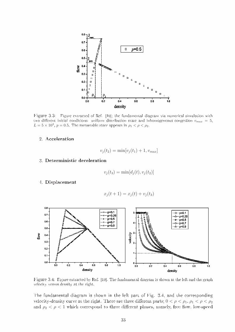
Figure 3.3: Figure extra ted of Ref. [10℄; the fundamental diagram via numeri al simulation with

two di�erent initial onditions: uniform distribution state and inhomogeneous ongestion vmax = 5,L = 5× 103, p = 0.5. The metastable state appears in ρ1 < ρ < ρ2.

2. A eleration

vj(t2) = min[vj(t1) + 1, vmax]

3. Deterministi de eleration

vj(t3) = min[dj(t), vj(t2)]

4. Displa ement

xj(t+ 1) = xj(t) + vj(t3)

Figure 3.4: Figure extra ted by Ref. [10℄. The fundamental diagram is shown at the left and the graph

velo ity versus density at the right.

The fundamental diagram is shown in the left part of Fig. 3.4, and the orresponding

velo ity-density urve at the right. There are three di�erent parts; 0 < ρ < ρ1, ρ1 < ρ < ρ2and ρ2 < ρ < 1 whi h orrespond to three di�erent phases, namely, free �ow, low-speed

33

�ow and jam. In this model we have an interesting situation; as the density ρ approa hes

0.5, the velo ity in low-speed �ow approa hes unity. The velo ity is:

v =

vmax ρ < ρ1,12ρ

− (1−2ρ)(2p−1)ρ

ρ1 < ρ < ρ2,1ρ− 1 ρ ≥ ρ2.

Where ρ1 =1−p

vmax+1−2pand ρ2 =

12.

The NS model is updated in sequen e R1-R2-R3 ( orresponding to a eleration-de eleration-

randomization), while the two models studied in Ref. [10℄ are R1-R3-R2 and R3-R1-R2.

The update rules R2-R1-R3, R2-R3-R1, and R3-R2-R1 are dis arded due the possibility

of ollisions between the vehi les.

3.2 VDR model

The velo ity-dependent randomization (VDR) model [11℄ adds a simple slow-to-start

rule to the NS model. Instead of using a unique de eleration probability p, these authorsin lude a velo ity dependen e in this parameter, so that p = p(v). For simpli ity, they

study the ase:

p(v) =

{p0 if v = 0

p if v > 0.

Sin e we are interested in hysteresis phenomena, we restri t ourselves to the ase p0 ≥ p.Note that for p0 = p the NaS h model is re overed. The parameters used are: maximum

velo ity vmax = 5, braking probability p = 164

for moving ars, p0 = 0.75 for stopped

ars, Ref. [11℄ reports numeri al simulations of periodi systems with L = 10000 latti e

sites. Fig. 3.5 shows the fundamental diagram of the VDR model. The average �ux

Figure 3.5: Figure extra ted of Ref [11℄. Di�eren e between fundamental diagrams of the VDR and

NS models.

j(ρ) an take two values in the density interval between ρ1 and ρ2 depending on the

initial ondition. The larger values of the average �ux are obtained using a homogeneous

34

initialization of the system. The lower bran h is obtained starting from a ompletely

jammed state. It is instru tive to ompare the fundamental diagram of the VDR model

with those of the orresponding NS models. For small densities ρ ≪ 1 there are no slow

ars in the VDR model sin e intera tions between ars are extremely rare. Here the �ux

is given by j(ρ) = ρ(vmax − p), i.e., identi al to the NS model with randomization p. Forlarge densities 1 − ρ ≪ 1 on the other hand, the �ux is given by j(ρ) = (1 − p0)(1 − ρ)whi h orresponds to the NS model with randomization p0. For densities lose to ρ = 1,only ars with velo ities v = 0 or v = 1 exist.

The mi ros opi stru ture of the jammed states in the VDR model di�ers from those

found in the NS model. While jammed states in the NS model ontain lusters with

an exponential size-distribution, one an �nd phase separation in the VDR model. The

reason for this behaviour is the redu tion of the out�ow from a jam. If the out�ow from

a jam is maximal, any small jam in the free �ow regime dissolves immediately sin e the

out�ow from su h a jam is larger than the global �ow. Therefore phase separation annot

o ur in that ase. However, if the out�ow from a jam is redu ed, the density in the

free �ow regime is smaller than the density of maximum �ux and ars an propagate

freely in the low density part of the latti e. Due to the redu tion of the density in the

free �ow regime, no spontaneous formation of jams is observed in the stationary state, if

�u tuations in the free �ow regime are rare. We an see this phase separation at Fig. 3.6.

Figure 3.6: Figure extra ted of Ref. [11℄. Spa e-time diagram of the VDR model for ρ = 0.15;L = 400; p = 0.01 and p0 = 0.5. The homogeneous initial state is not destroyed immediately, but after

approximately 93000 latti e updates. In the out�ow regime of the jam the density is redu ed ompared

to the average density.

3.3 Cruise- ontrol model

The ruise- ontrol ( ) model is a simpli�ed version of the NS model [12℄. This sim-

pli� ation an be des ribed as a � ruise ontrol limit�, sin e at su� iently low density all

vehi les move deterministi ally at maximum allowed velo ity. As in the NS model the

model is de�ned on a one-dimensional latti e of length L, representing a single-lane

35

freeway. Ea h site of the latti e an be in one of the vmax + 2 states: It may be empty,

or it may be o upied by one ar having an integer velo ity between zero and vmax. One

iteration onsists of the following steps, whi h are ea h performed simultaneously for all

vehi les. A vehi le is stationary when it travels at maximum velo ity vmax and has free he-

adway: d ≥ vmax. Su h a vehi le just maintains its velo ity. If a vehi le is not stationary,

it is jammed

1

. The following rules are applied to jammed vehi les.

1. A eleration

With probability 1/2, a vehi le with d ≥ v + 1 a elerates to v + 1, otherwise it

keeps the velo ity v. A vehi le with d = v just maintains its velo ity.

2. Slowing down and randomization

Ea h vehi le with d ≤ v − 1 slows down to v = d and an add further de eleration

a ording to:

v = max[v − 1, 0] with probability 1/2

v = v with probability 1/2

3. Displa ement

Ea h vehi le advan es v sites.

The randomization pro ess in this model an produ e overrea tion as in the NS model, but

di�erent from this, introdu es a nondeterministi a eleration. The fundamental diagram

was obtained numeri ally [12℄ as show in Fig. 3.7.

For a spatially in�nite system, the following results hold: for ρ < ρc jams present in

Figure 3.7: Figure extra ted of Ref. [12℄. Fundamental diagram of the ruise- ontrol model. The

dotted line represents deterministi tra� , i.e., when the initial state is prepared su h that for ea h ar

ngap > vmax and v = vmax. The points are measurement results starting from random initial onditions.

Ea h point orresponds to one run of a losed system of length L = 30000 and an average over 2.5× 106

iterations after dis arding a transient period of 5× 105 iterations.

the initial on�guration are eventually sorted out and the stationary deterministi state

is jam free with every vehi le moving at maximum velo ity. Thus, the �ux is a linear

fun tion of density with slope vmax = 5. This behavior is observed up to a maximum

1

In this model the on ept of jammed and stationary are di�erent than those used in models with

absorbing on�gurations, stationary means ina tive and jammed; a tive.

36

�ux jc(ρc). For ρ > ρc and ρ < 1vmax+1

the system is bistable. Starting from an initial

on�guration whi h has many jams, the jams in this ase are never sorted out. The steady

state is an inhomogeneous mixture of jam free regions and higher density jammed regions

(see Fig. 3.8). Clearly, these jammed regions de rease the average �ux in the system.

It is possible, nevertheless, to prepare initial on�gurations that have no jams. Sin e all

motion is deterministi in this state, the steady state will also have no jams and the �ux

will still be an in reasing fun tion of ρ (the dotted line in Fig. 3.7). This is possible up

to densities of

ρmax =1

vmax + 1,

leading to a maximum �ux of

qmax =vmax

vmax + 1.

This learly is mu h higher than the �ux q, for random initial onditions. It is in this

sense that this system is bistable. In addition to these features, the authors studied the

Figure 3.8: Figure extra ted of Ref. [12℄. Dots represent vehi les whi h move to the right. The

horizontal dire tion is spa e and the verti al dire tion (down) is (in reasing) time. We an see that

starting from an initial on�guration whi h has many jams, the jams never disappear.

behavior of the free regions when are perturbed. In the deterministi region, one ar

is randomly perturbed by redu ing its velo ity to zero. Many di�erent hoi es for the

lo al perturbation, however, give rise to the same large s ale behavior. The perturbed

ar eventually rea elerates to maximum velo ity. In the meantime, though, a following

ar may have ome too lose to the perturbed ar and have to slow down. This initiates

a hain rea tion�the emergent tra� jam. This de�nes the lifetime, t, of an emergent

tra� jam. Using simulation the authors determine the probability distribution of jams

as a fun tion of their lifetime, t. Figure 3.9 shows that for t > 100, this distribution

follows a power law

P (t) ∼ t−δ,

with δ = 1.5± 0.01.

37

Figure 3.9: Lifetime distribution P (t) for emergent jams in the out�ow region; average over more than

65000 lusters (avalan hes). The dotted line has slope

32 . Numeri ally imposed uto� at t = 106 (�gure

extra ted of Ref. [12℄).

3.4 Fukui�Ishibashi Model

Fukui and Ishibashi [13℄ have introdu ed a simpli�ed version of the NS model. The

main di�eren e to the NS model is the absen e of a velo ity memory

2

. All vehi les have an

intrinsi velo ity vmax. In ea h timestep, all drivers try to move at the maximum velo ity

vmax; i.e., they a elerate to it instantaneously. The Fukui�Ishibashi (FI) model is then

de�ned by the following set of rules:

1. A eleration

The a eleration step assures that FI model does not have velo ity memory sin e

the vehi le a elerates to the maximum velo ity or to the headway between it and

the following vehi le, so

vn = min[vmax, dn(t)].

2. Randomization

Only the vehi les with v = vmax are subje ted to the randomization step a ording

to

vn → vmax − 1 with probability f,

vn → vmax with probability 1− f .

3. Displa ement

xn = xn + vn.

Here, xn and vn denote the position and speed, respe tively, of the nth vehi le and dn =xn+1 − xn − 1, i.e., the number of empty ells in front of this ar (headway). The rules

have a simple interpretation; a vehi le that has at least vmax empty sites in front will

move vmax ells with probability 1− f or vmax − 1 ells with probability f . However, justin the ase that the headway is d < vmax at time t, then the vehi le moves d sites in the

2

In ea h iteration of the NS model, the velo ity v and headway d have to be a ounted for the update

pro ess.

38

next step. Here the randomization step is not applied. Therefore, �u tuations o ur only

at high speeds, whi h is just the opposite of the ruise- ontrol limit.

For vmax = 1, the FI model and the NS model are identi al sin e that in the NS model

with vmax = 1, only the vehi les with v = 1 are subje ted to the randomization step.

For general vmax, the FI model di�ers from the NS model in two aspe ts: the in rease

of the vehi les speed is not ne essarily gradual and the sto hasti delay (de eleration

step) applies only to high-speed vehi les. Due to these modi� ations, no overrea tions at

braking o ur and therefore the FI model does not exhibit spontaneous jamming. This

type of a eleration (where there is no need to keep tra k of velo ities) allows to introdu e

a mean-�eld te hnique that provides the exa t solution. These exa t solutions as well as

Monte Carlo simulations are shown in Fig 3.10.

Figure 3.10: Figure extra ted of Ref. [14℄. The fundamental diagram of the FI model with the

maximum ar velo ity M = 2 and for di�erent values of the degree of sto hasti delay f . The solid urves

are the theoreti al results. The points with di�erent symbols represent results obtained by numeri al

simulations.

3.5 Wang Model

By using the ar-oriented mean�eld (COMF) was possible to a hieve an exa t analy-

ti al result to the FI model [14℄. However, for the NS model with vmax > 1 and sto hasti

delay, no exa t solution has been found up to now. The a eleration and sto hasti delay

rules of the NS model lead to ompli ations in the time evolution of the �ux, and hen e

it is very di� ult to �nd exa t analyti al results. In order to understand how these rules

a�e t the evolution and the orresponding asymptoti state, Wang et al [15℄ study an

intermediate model that ombines features of both models.

The model is des ribed by the following update rules: Let Cn(t) be the number of

empty sites in front of the nth ar at time t, vn(t) be the number of sites that the nth

ar moves during the time t step, and M the maximum speed. The steps are:

1. Step 1

Let v′

n(t) = min(Cn(t),M), if v′

n(t) = Cn(t) the nth ar is �the ar that follows the

trail of the ar ahead�. This means that the nth ar may be ome the neighbor of

the ar ahead if the ar in front stops.

39

2. Step 2

Sto hasti delay is introdu ed in su h a way that all the ars whi h follow the trail

of their ar ahead have a probability f to move forward one site less than is allowed

by step 1, i.e., we have the following: vn(t) = v′

n(t) − 1, with probability f , ifv

′

n(t) = Cn(t) and v′

n(t) > 0.

3. Step 3

The nth ar moves vn(t) sites ahead.

The number of empty sites in front of the nth ar at time t+ 1 an be written as

Cn(t + 1) = Cn(t) + vn+1(t)− vn(t).

For this model, with a maximum ar velo ity vmax = M and a sto hasti delay probability

f , the velo ity of the nth ar at time step t as a fun tion of the inter ar spa ing Cn(t) an be written as

vn(t) =

M if c > M,

c− 1 with probability f if 0 < c ≤ M,

c with probability 1− f if 0 < c ≤ M,

0 if c = 0.

As in the FI model, this sort of a eleration allows to simplify the equations used in ar-

oriented mean �eld and produ es an exa t agreement between analyti al and numeri al

(Monte Carlo) results. These results are shown in Fig. 3.11.

Figure 3.11: The fundamental diagram with the maximum ar velo ity M = 2 and for di�erent

sto hasti delay probabilities f . The solid urves are theoreti al results. The points with di�erent symbols

represent numeri al simulations. The urves from the top down along the velo ity axis orrespond to

di�erent values of f ranging from f = 0 to 1 in steps of 0.1. (Figure extra ted of Ref [15℄.)

Although not stressed by the authors, this model presents an absorbing phase transi-

tion at ρc ≤ 1M+2

independent of f . For densities below ρc the stationary state is absorbingsin e the mean distan e between the vehi les is greater than M and a ording to the up-

date rules the vehi les are not subje t to the randomization step. These absorbing states

are not unique sin e they depend on the initial on�guration. For density ρc =1

M+2the

stationary state is unique and des ribed by v = M and C = M + 1.

40

3.6 Multilane tra�

For a realisti des ription of tra� on highways many authors, as dis ussed before,

improve the NS model by using modi�ed update rules making them more appropriate

for real tra� . Despite these e�orts a omplete des ription demands the use of multilane

lanes in tra� simulation. Beside the use of NS rules we know that the main ingredient

required for an appropriate hange of a single-lane CA model to multilane situations

is lane- hanging rules. Lane hanging rules for two-lane tra� an be symmetri or

asymmetri . For symmetri lane- hanging rules, overtaking is allowed in both lanes.

However, for asymmetri lane- hanging rules, overtaking is forbidden in one lane, e.g., in

the right lane ( this situation exists in many European ountries for example, Germany).

Generi ally, the de ision of drivers to hange lane is based on two riteria:

1. In entive riterion:

Drivers determine whether a lane hange improves the individual tra� situation,

e.g., to move at their desired velo ity.

va > gap with va = min(v + 1, vmax).

2. Safety riterion:

The tra� situation in the target lane is he ked, espe ially if the available gap for

a lane hange is enough for a se urity transition (without prevent the free �ow of

the prede essor vehi le lo ated in other lane).

gap

other

> gap,

gap

ba k

≥ vmax.

Here gap is the number of free ells between the ar and its prede essor in the a tual

lane; gap

other

and gap

ba k

are the headway in relation to its two neighbor ars, in the

other lane, ahead and behind respe tively. A lane- hange is then only performed if both

riteria are satis�ed. In general, the update in the two-lane models is divided into two

substeps: in one substep, the vehi les may hange lanes in parallel following the lane-

hanging rules and in the other substep, ea h vehi le may move forward e�e tively as in

the single-lane NS model. Drivers must �nd some in entive in hanging the lane. Two

obvious in entives are: the situation in the other lane is more onvenient for driving,

and the need to overtake the slow vehi le. We show some results about two-lane model

using symmetri lane- hanging rules, whi h are more relevant for tra� in towns and on

highways, where overtaking in both lanes is allowed.

Fig. 3.12 shows the fundamental diagram of a periodi two-lane system. The simulations

reprodu e well-known results, e.g., an in rease of the maximum �ux per lane ompared

to the �ux of a single-lane road. Another unexpe ted result is the existen e of a lo al

minimum of the lane- hanging frequen y near the density of maximum �ux for small

braking probabilities p (Fig. 3.13). The behavior of the lane- hanging frequen y an be

explained if one takes into a ount the number of empty ells ne essary for a lane- hanging

pro edure. Two prerequisites have to be ful�lled in order to initiate a lane hange. First,

the situation on the other lane must be more onvenient and se ond, the safety rules

must be ful�lled. Therefore, one needs typi ally 2vmax + 1 empty ells on the destination

lane for a lane- hanging maneuver in the free �ow regime (Fig. 3.13). Hen e, one �nds a

lo al maximum of the lane- hanging frequen y near ρs =1

2vmax+1if the ars are ordered

41

Figure 3.12: Flux per lane of the single-lane model ompared with the two-lane model for systems with

vmax = 5 and p = 0.5. (Figure extra ted of Ref [16℄).

homogeneously, whi h typi ally happens for small values of p. For larger values of p, e.g.,p = 0.5, no lo al maximum is observable. In reasing the density for su� iently small

values of p, one �nds a pronoun ed minimum of the lane- hanging frequen y. This an be

understood in the limit p → 0 where, for ρ = 1vmax+1

, the ars are perfe tly ordered with a

gap of vmax sites between onse utive vehi les. Obviously, in this ase both the in entive

and the safety riteria are never ful�lled and the lanes are ompletely de oupled. For

small p the ordering me hanism is still present and therefore the number of lane hanges

is drasti ally redu ed near ρ = 1vmax+1

.

Figure 3.13: Lane- hange frequen y in the two-lane model for di�erent braking parameters p (Figure

extra ted of Ref [16℄).

The features of two-lane tra� are the same for multiple lanes (taking into a ount

homogeneous systems). We now onsider di�erent types of ars whi h is obviously more

relevant for pra ti al purposes. As a �rst step towards realisti distributions of free �ow

velo ities the authors [16℄ have hosen two types of ars, e.g., slow ars with vsmax = 3and fast ars with vfmax = 5. Simulations were arried out with 5% of slow ars, whi h are

42

initially positioned randomly. The fast as well as the slow ars may use both lanes, i.e.,

both ars are treated equally with respe t to the lane- hanging behavior. In Fig. 3.14

the e�e ts of the slow ars on the average �ux of the two-lane system is ompared with

the fundamental diagram of a single-lane road with one slow ar. Sin e passing is not

allowed for a single-lane system, learly the slow ar dominates the average �ux at low

densities and platoon formation is observable. Surprisingly the two-lane system shows a

quite similar behavior, although passing is allowed and the fra tion of slow ars is rather

small. Although the multilane tra� models an adopt a lot of di�erent update rules, the

Figure 3.14: Comparison of the �ux per lane of the inhomogeneous model with the orresponding

homogeneous models for p = 0.4.(Figure extra ted of Ref [16℄).

results in terms of statisti al point of view ( riti ality, phase transition et .) do not di�er

when ompared with one-line models. For this reason we do not extend this dis ussion;

for a detailed des ription of multilane models see [17℄.

43

Chapter 4

Kineti tra� theory

4.1 Introdu tion

In kineti theory, tra� is treated as a gas of intera ting parti les where ea h parti-

le represents a vehi le. The di�erent versions of the kineti theory of vehi ular tra�

have been developed by modifying the kineti theory of gases. In the kineti theory of

gases, f(~r, ~v, t)d3rd3v denotes the number of mole ules whi h, at time t, have positions

lying within a volume element d3r about ~r and velo ities lying within the velo ity-spa e

element d3v about v. The Boltzmann equation, whi h des ribes the time evolution of the

distribution f(~r, ~v, t), is given by:

[∂f

∂t+ ~v.∇r + ~a.∇v

]f(~r, ~v, t) =

(∂f

∂t

)

coll

, (4.1)

where the symbols ∇r and ∇v denote gradient operators with respe t to ~r and ~v, respe -tively, while ~a is the external a eleration. The term (∂f

∂t)coll represents the rate of hange

of f , with time, whi h is aused by ollisions between mole ules.

In the earliest version of the kineti theory of vehi ular tra� , Prigogine and Herman[18,

19, 20℄ modi�ed the kineti theory of gases embodied in the Boltzmann equation. In their

model tra� is treated as a one-dimensional gas of intera ting parti les (vehi les) des ri-

bed by a distribution fun tion f(x, v, t), su h that f(x, v, t)dxdv represents the number

of vehi les with positions between x and x + dx and velo ities between v and v + dv at

time t. The distribution f is normalized so that

∫dvf(x, v, t) = c(x, t), (4.2)

where c(x, t) is the lo al density of vehi les. (Unless otherwise spe i�ed, all integrals run

from −∞ to ∞. Note that f(x, v, t) is zero for v < 0.)The time evolution of f is governed by a Boltzmann-like equation. The prin ipal

di�eren e with the original Boltzmann equation is the introdu tion of a distribution of

desired velo ities, f0(x, v, t), in the relaxation term, representing drivers' preferen es.

Spe i� ally, f0(x, v, t)dxdv is the number of vehi les between x and x+ dx whose drivers

have a preferred velo ity between v and v + dv at time t. The presen e of this fun tion

in the statisti al des ription is a novel feature, showing that the �parti les"in this system

have intentions unlike a mole ule, whi h does not have a desired velo ity.

44

Of prin ipal interest is the stationary velo ity distribution, whi h an be mu h di�erent

from the distribution of desired velo ities. We shall see that the stationary velo ity

distribution hanges abruptly at a spe i� density.

4.2 The Prigogine-Herman-Boltzmann equation

In one-way tra� , vehi les travel in one dimension, and Eq. (4.1) an be simpli�ed to

read[19, 20℄

∂f

∂t+ v

∂f

∂x=

(∂f

∂t

)

rel

+

(∂f

∂t

)

int

. (4.3)

where

∂f∂t rel

a ounts for the relaxation of f toward f0 in the absen e of intera tions of

the vehi les, while

∂f∂t int

a ounts for the hanges of f arising from intera tions among the

vehi les. Note that the term

∂f∂t int

on the right-hand side of Eq. (4.3) may be interpreted

as the analog of the term (∂f∂t)coll in the Eq. (4.1), whereas the term

∂f∂t rel

in Eq. (4.3)

may be interpreted as the ounterpart of the term ∇v.f(~r, ~v, t) in the Eq. (4.1).

The idea behind the relaxation term is that drivers adjust their velo ity to the desired

value, v0, on a time s ale T , alled the relaxation time. This assumption is embodied in

the expression, (∂f

∂t

)

rel

= −f − f0T

. (4.4)

In a spatially uniform system, in whi h f = f(v, t) and intera tions between drivers an

be ignored, the solution to Eq. (4.3) is

f(v, t) = f0(v) + [f(v, 0)− f0(v)]e−t/T . (4.5)

Exponential relaxation des ribes the approa h of many simple systems to a steady state.

In the ontext of the kineti theory of gases, an analogous simpli� ation involves repla ing

the ollision term with an expression of the form of Eq. (4.4); T be omes the ollision

time, and f0 is a lo al Maxwellian distribution.[21℄ As will be ome lear, Prigogine and

Herman[18℄ proposed that T depends on the on entration of vehi les on the road, and

the relaxation pro ess subsumes some rather ompli ated intera tions between drivers.

In the absen e of intera tions between the vehi les, the distribution fun tion evolves to

the distribution of desired velo ities a ording to Eq. (4.5). A derivation of the distribution

of desired velo ities from �rst prin iples would require knowledge of human behavior that

is beyond our present apabilities. One might try to determine the distribution of desired

velo ities empiri ally by studying the velo ity distribution at very low on entrations, but

we are unaware of studies of this kind. Prigogine and Herman simply investigated several

simple model distributions of the desired velo ities.[22℄

The intera tion term in Eq. (4.3) is based on the following assumptions:

1. The vehi les are point-like, that is, they do not o upy volume.

2. Vehi les remain in the same lane ex ept when passing another vehi le.

3. In an en ounter between two vehi les, one passes the other with probability P .

4. If one vehi le passes another, neither vehi le hanges its velo ity. In an en ounter

without passing, the faster vehi le redu es its velo ity to that of the slower one

ahead of it.

45

5. The slowing-down pro ess is instantaneous.

6. Only two-vehi le intera tions are onsidered.

7. The vehi les are statisti ally independent, that is, the joint two-vehi le distribution

is the produ t of single vehi le distributions: f(x, v, x′, v′, t) = f(x, v, t)f(x′, v′, t).

If we use these assumptions, we an write the intera tion term as,

(∂f

∂t

)

int

= f(x, v, t)

∫ ∞

v

du(1− P )(u− v)f(x, u, t)

− f(x, v, t)

∫ v

−∞

du(1− P )(v − u)f(x, u, t). (4.6)

The �rst term on the right-hand-side of Eq. (4.6) orresponds to intera tions between

vehi les with velo ities v and u > v; the latter are obliged to adopt the smaller velo ity

v resulting in an in rease in the number of vehi les with velo ity v. The se ond term

is related to intera tions between vehi les with velo ity v and u < v. In this ase, the

intera tion results in a de rease in the number of vehi les with velo ity v. By ombining

the two integrals, the intera tion term an be rewritten as,

(∂f

∂t

)

int

= (1− P )f(x, v, t)

∫du(u− v)f(x, u, t).

Be ause, ∫uf(x, u, t)du = c(x, t)v(x, t),

where v(x, t) denotes the lo al mean velo ity, and

∫du vf(x, u, t) = c(x, t)v,

we have, (∂f

∂t

)

int

= (1− P )c(x, t)[v(x, t)− v]f(x, v, t). (4.7)

If we insert the relaxation term, Eq. (4.4), and intera tion term, Eq. (4.7), into Eq. (4.3),

we obtain the Prigogine-Herman-Boltzmann equation for tra� :

∂f

∂t+ v

∂f

∂x= −f − f0

T+ (1− P )c(x, t)[v(x, t)− v]f. (Prigogine-Herman-Boltzmann)

(4.8)

Equation (4.8) is a nonlinear equation be ause v(x, t) is a fun tion (more pre isely, a

fun tional) of f(x, v, t). A full de�nition of the model requires that we spe ify how the

passing probability and relaxation time depend on the on entration. Before examining

spe i� hoi es, we onsider some general aspe ts of the solutions.

4.3 Stationary solutions

As dis ussed before, the quantity f0 is a distribution fun tion that hara terizes the

system in the absen e of intera tions between the ars. Therefore, f0 is onsidered to be

46

that distribution fun tion whi h would be a hieved by drivers if the intera tions between

them were negligible. The fun tion f0 an in orporate into the theory su h information

as the wishes of the drivers, response of the driver- ar system, speed limits, and the

hara teristi s of the road. The term (1 − P )c(x, t)[v(x, t) − v]f represents the hange

in f aused by intera tions in whi h ars, when intera ting with ars ahead moving with

slower speeds, either pass these ars or assume their slower speeds.

The homogeneous time-independent solution is:

f(v) =f0(v)

1− cT (1− P )[v − v]. (4.9)

where by homogeneous we mean that f0 is not spatially dependent. The quantity f(v)des ribes the situation in whi h there is a steady state between the slowing down of ars

aused by intera tion pro esses and the speeding up of ars aused by passing.

4.4 Individual and olle tive �ow

As indi ated by Eq. (4.9), we have to distinguish between two ases

• Case A: If we onsider the ase in whi h

1− Tc(1− P )v > 0.

Then the solution f in Eq. (4.9) is hanged to

f(v) =f0(v)

1 + Tc(1− P )(v − v). (4.10)

This solution redu es to the ideal or desired speed distribution fun tion in the limit

of vanishing on entration. However, it is lear that this solution annot, in general,

be valid for arbitrarily high on entrations be ause whenever

1− Tc(1− P )v < 0,

the distribution fun tion may be ome negative, whi h is learly impossible.

• Case B: In this ase we onsider:

1− Tc(1− P )v = 0. (4.11)

Then Eq. (4.9) redu es to

f(v) =f0(v)

Tc(1− P )v. (4.12)

The important feature to be noted here is that the homogeneous equation orresponding

to Eq. (4.12), namely,

Tc(1− P )vf(v) = 0,

admits the singular solution:

f(v) = αcδ(v),

47

where α is an arbitrary onstant and δ(v) is the Dira delta fun tion. Therefore, the

general solution of Eq. (4.12) is of the form

f(v) =f0(v)

Tc(1− P )v+ αcδ(v).

The solution given in Eq. (4.10) orresponds to what may be alled the individual �ow

pattern and is related in a simple way to the ideal or desired speed distribution fun tion.

The se ond solution orresponds, on the other hand, to what may be alled the olle tive

�ow pattern. Indeed, as shown by Eq. (4.11), the average speed then depends only

on the on entration, the probability of passing P , and the relaxation time T (both Pand T are themselves fun tions of the on entration), and is independent of the desired

speed distribution fun tion and, therefore, of the wishes of the drivers. This solution

is hara terized by the o urren e of a singularity at the origin. However, the riti al

on entration at whi h the individual �ow be omes olle tive does depend on the desired

speed distribution. In both ases the time-independent solution may be written in the

following form:

f(v) =f0(v)

1 + Tc(1− P )(v − v)+ αcδ(v), (4.13)

where α is an undetermined onstant that may be identi ally zero. This solution has to

satisfy the following two requirements:

• Normalization. This means that:

c =

∫ ∞

0

f0(v)dv

1 + Tc(1− P )(v − v)+ αc. (4.14)

• Average Speed. Multiplying Eq. (4.13) by v and integrating, we obtain the ondition

cv =

∫ ∞

0

f0(v)dvv

1 + Tc(1− P )(v − v). (4.15)

Eq. (4.15) with the aid of the normalization ondition Eq. (4.14) maybe transformed into

α(1− Tc(1− P )v) = 0.

We see, therefore, that we have two solutions. The �rst solution orresponds to α = 0(individual �ow), whereas the se ond orresponds to the ase

Tc(1− P )v = 1,

with α di�erent from zero ( olle tive �ow).

There is a striking analogy in the situation des ribed by these equations with Bose-

Einstein ondensation [23℄. In that ase, above a ertain on entration (for a given tem-

perature) the population distribution of an ideal Bose gas splits into two parts, a regular

part and a singular one. If the on entration is further in reased beyond its riti al va-

lue, the singular part in reases relative to the regular part. However, the Bose-Einstein

ondensation o urs for a quantum system in thermodynami equilibrium, whereas the

situation des ribed here is loser to a nonequilibrium stationary state.

48

4.5 Numeri al Solutions

To simplify the notation let,

γ ≡ cT (1− P ) and λ ≡ 1− γv(f), (4.16)

remembering the normalization ondition (Eq. (4.14)) and repla ing f0 =f0c, we have:

1 =

∫ ∞

0

f0dv

λ+ γv, (4.17)

for the individual �ow. As γ in reases, λ de reases, and be omes zero for γ = γc (re allthat λ annot be negative). So we an �nd γc via

∫f0dv

v= γc. (4.18)

From this point we have a transition between individual �ow to olle tive one and α an

be found via

1 =

∫f0dv

γv+ α. (4.19)

Prigogine and Herman [18℄ introdu ed further assumptions regarding the dependen e of

P and T on the on entration c, whi h we shall refer to as the Prigogine-Herman model.

We expe t the passing probability P to de rease with c, be ause drivers will �nd it more

di� ult to overtake a slower vehi le if adja ent lanes are ongested. (If vehi les were

truly point parti les, there would be no su h di� ulty.) Prigogine and Herman assumed

a linear relation between P and c, su h that P = 1 for c = 0, and de reases to zero at

some maximum on entration, cmax. That is,

P = 1− η with η =c

cmax

. (4.20)

They further proposed a on entration-dependent relaxation time,

T =τ(1− P )

P, (4.21)

where τ is a onstant with dimensions of time. Thus, a ording to Prigogine and Herman,

the greater the value of c, the smaller the value of P , and the longer it takes a driver to

attain the desired speed. In their model, T does not represent an intrinsi limitation of

drivers (that is, a rea tion time) or of their vehi les (inertia), be ause T → 0 as c → 0.Inserting Eqs. (4.20) and (4.21) in Eq. (4.16), we �nd,

γ =cmaxτη

3

1− η. (4.22)

For numeri al studies we always use the simpli�ed equation (4.17), remembering that

γ is given by Eq. (4.22) and λ by Eq. (4.16).

49

4.5.1 Numeri al Method

Consider the numeri al solution of Eq. (4.17), yielding the value of λ su h that the

integral is unity, given the fun tion f0(v) and γ, whi h is determined by the on entration

via Eq. (4.22). Although the numeri al method is simple, some are is required, be ause

in some ases the integral is improper.

Among the many methods for the numeri al evaluation of integrals, we hoose one that

is relatively simple yet a urate by �tting ubi polynomials through su essive groups of

four points,[24℄ whi h is equivalent to the following expression,

∫ xn

x1

y(x)dx ≃ h

[3

8y1 +

7

6y2 +

23

24y3 + y4 + y5 + · · ·

+ yn−4 + yn−3 +23

24yn−2 +

7

6yn−1 +

3

8yn

],

where h = (xn − x1)/(n− 1), yj ≡ y(xj), and xj ≡ x1 + (j − 1)h, for j = 1, . . . , n.Dealing with an in�nite range of integration requires greater are. We might trun ate

the integral, but the error depends on the hoi e of the uto�. A more appealing alter-

native is to hange variables to map the in�nite range of integration to a �nite one. For

an exponential distribution of desired velo ities, illustrated in Subse tion 4.6 , we are led

to Eq. (4.26) for whi h the substitution t = e−v/v0results in an integral over the �nite

interval:

1 =

∫ 1

0

dt

λ− γv0 ln t. (4.23)

On e we have a method for evaluating the integral over velo ities, we use a root-�nding

method to solve Eq. (4.26). For equations of the type used in Ref. [18℄ and the ones of

interest here, the se ant or Newton-Raphson methods are appropriate [25℄. Although

both are e� ient, we will use the se ant method, a re ursive method used to �nd the

solution to the equation f(x) = 0 via the relation,

xn+1 =xn−1f(xn)− xnf(xn−1)

f(xn)− f(xn−1),

starting from a pair of distin t initial values, x1 and x2. The idea is to follow the se ant

line to its x-inter ept and use that as an approximation for the root. This idea is similar

to the Newton-Raphson method, whi h follows the tangent line, but the se ant method

does not require knowledge of the derivative.

The omputational pro edure for solving Eq. (4.17) is as follows. Let g(λ, n) be the

value of the integral in Eq. (4.17) over the interval [v1, v2], given by a fun tion that employs

the method of Eq. (4.23) using n integration points. The latter is hosen a ording to the

desired pre ision, using a fun tion int(λ), whi h evaluates the integral using su essively

larger numbers of points, until the relative di�eren e is smaller than a ertain toleran e.

4.6 Some distributions of desired velo ities

As example, we present the study of two distributions of desired velo ities, the �rst

orresponds to exponential distribution of desired velo ities in whi h was dis ussed in Ref.

[18℄ and the se ond orresponds to Gaussian distribution of desired velo ities performed

in our arti le atta hed.

50

4.6.1 Exponential distribution of desired velo ities

As an illustration, we solve the Prigogine-Herman model for an exponential distribu-

tion of desired velo ities, as dis ussed in Ref. [18℄. Let

f0 = Θ(v)ηcmax

v0e−v/v0 , (4.24)

for whi h the mean velo ity is v0. In this ase the most probable desired velo ity is zero,

and be ause f0(v = 0) > 0, there is no transition. The stationary solution is

f =cmaxηe

−v/v0

v0(λ+ γv), (4.25)

where λ is determined by the normalization ondition,

1 =1

v0

∫ ∞

0

e−v/v0

λ+ γvdv. (4.26)

The value of λ for given values of γ and v0 is obtained numeri ally as we have des ribed.

Figure 4.1a shows the normalized �ux q/cmax as a fun tion of the normalized on en-

tration η = c/cmax. Note the linear relation between �ux and on entration for small η.In this regime the slope of ea h urve depends on v0, the average desired velo ity. At high

on entrations the normalized �ux is independent of v0. The mean velo ity is plotted

versus η in Fig. 4.1b for several values of v0. As for the ase of the normalized �ux, all

urves exhibit the same behavior at high on entrations.

(a) (b)

Figure 4.1: (a) The normalized �ux Q ≡ q/cmax and (b) normalized mean velo ity υ = v/v0 versus thenormalized on entration η = c/cmax for cmaxτ = 0.1 and mean desired velo ity v0. At low on entrations

the mean velo ity is lose to its desired value, and the normalized �ux is proportional to v0. At larger

on entrations the normalized �uxes for di�erent values of v0 approa h a ommon fun tion.

It is interesting to ompare the stationary velo ity distribution with the orresponding

distribution of desired velo ities. Figure 4.2 shows that the stationary velo ity distribution

is lose to the distribution of desired velo ities for a relatively low on entration (η =0.2). At a higher on entration (η = 0.4, Fig. 4.3), the two distributions di�er, with

higher probabilities for low velo ities in the stationary velo ity distribution than in the

distribution of desired velo ities.

51

Figure 4.2: (Color online) Distribution of desired velo ities (dashed lines) and stationary velo ity

distribution ( ontinuous lines) for exponential desired velo ity distributions with v0 as indi ated; η = 0.2.In all ases, the stationary distribution ex eeds the desired one at low velo ities, and vi e-versa.

Figure 4.3: (Color online) Distribution of the desired velo ity and stationary velo ity distribution as in

Fig. 4.2 for η = 0.4. At this on entration the di�eren es between the stationary and desired distributions

are more dramati than in Fig. 3.

4.6.2 Gaussian distribution of desired velo ities

We now onsider a more realisti example that has re eived little attention until now

� a Gaussian-like distribution of desired velo ities,

f0(v) = cA[e−(v−v0)2/v2a − e−v20/v

2a

]Θ(v) Θ(2v0 − v). (4.27)

52

The parameter v0 represents the mean desired velo ity, and va is a measure of the dis-

persion of the distribution. Be ause of the step fun tions, f0 is zero outside the interval

[0, 2v0]. The se ond term in bra kets ensures that f0 goes to zero ontinuously at the

endpoints of this interval. The normalization fa tor A is approximately (va√π)−1

for

v0 ≫ va.Be ause

∫(f0/v)dv < ∞, there is a transition between individual and olle tive �ow.

A ording to Eq. (4.18), the riti al point is given by

γc = A

∫ 2v0

0

dv

v

[e−(v−v0)2/v2a − e−v20/v

2a

],

whi h is readily evaluated numeri ally. We pro eed as before and al ulate the stationary

velo ity distribution, f(v), and the stationary mean velo ity and �ux. Figure 4.4 shows

the �ux Q as a fun tion of normalized on entration for several values of v0, and va = 20.As expe ted, the slope of q(η) jumps from a positive to a negative value at the transition

from individual to olle tive �ow. In the latter regime, q(η) is hara terized by a single

fun tion, independent of v0. The larger the value of v0, the smaller the riti al density ηc.

Figure 4.4: (Color online) The �ux Q as a fun tion of the normalized on entration η in the Prigogine-

Herman model using the distribution of desired velo ities of Eq. (4.27), with va = 20. The transition

points are ηc = 0.375, 0.395, 0.421, and 0.458, for for v0 = 120, 100, 80, and 60, respe tively. Above the

riti al on entration, the �ux follows a master urve independent of v0.

A notable aspe t of the transition is the sudden hange in the stationary distribution

at the riti al on entration at whi h the distribution splits into a regular and a singular

part. In Fig. 4.5, whi h ompares the stationary velo ity distribution and distribution

of desired velo ities for several on entrations in the individual �ow regime, we see that

the two distributions have the same area, as required by normalization. For η = 0.15the distributions are indistinguishable; at higher on entrations small di�eren es appear.

The riti al on entration, ηc = 0.421, represents the limit for individual �ow; for η > ηcthe stationary velo ity distribution is the sum of a regular part, given by f0/(γv), anda singular part, αcδ(v), with α given by Eq. (4.19). In Fig. 4.6 we ompare the regular

53

part of the stationary velo ity distribution with the orresponding distribution of desired

velo ities for η > ηc. The area of the regular part of the stationary velo ity distribution

is smaller than that of the distribution of desired velo ities. The di�eren e orresponds

to the δ-fun tion at the origin.

Figure 4.5: The stationary velo ity distribution (solid line) and orresponding distribution of desired

velo ities (dashed line), for on entrations in the individual �ow regime. The distribution of desired

velo ities is given by Eq. (4.27) with v0 = 80 and va = 20. The di�eren e between the stationary and

desired distributions grows with in reasing on entration.

4.7 Paveri-Fontana model

In the basi Prigogine-Boltzmann (PB) model, the hanges of vehi ular speeds are

assumed to be due to two main pro esses: the binary intera tion pro ess (namely, the

slowing down pro ess undergone by a fast ar whi h en ounters a slow one); and the

relaxation pro ess (the pro ess due to the hange in speed whi h o urs when a driver a -

elerates a vehi le towards a desired speed). Employing a set of appropriate assumptions,

the original Prigogine-Boltzmann equation was proposed, for the ase where drivers do

not hange their desired speeds a ording to tra� onditions. In order to a ount for the

adaptive behavior of drivers, that is in order to a ount for the fa t that tra� onditions

do a tually a�e t the �programs� (desired speeds) of drivers, an adjustment term was in-

trodu ed on the right side of the basi Prigogine-Boltzmann equation by Paveri-Fontana.

Let g(x, v, t;ω) be the one-vehi le distribution fun tion for vehi les whose desired speed

is ω. Namely, let g(x, v, t;ω)dxdvdω equal the (expe ted) number of vehi les, at time t,in dx (around x) and dv (around v) with desired speed in dω (around ω). Then one �nds

that:

f(x, v, t) =

∫ ∞

0

g(x, v, t;ω)dω and f0(x, ω, t) =

∫ ∞

0

g(x, v, t;ω)dv,

where f(x, v, t) and f0(x, ω, t) are the previously de�ned one-vehi le speed distribution

fun tion and desired speed distribution fun tion, respe tively. Vehi ular on entration

54

Figure 4.6: Regular part of the stationary velo ity distribution (solid line) and the orresponding

distribution of desired velo ities (dashed line) for densities in the olle tive �ow regime; parameters as in

Fig. 4.5. Note the di�eren es in amplitude between the stationary and desired distributions, asso iated

with a population of ars having velo ity zero in the stationary distribution.

c(x, t) and �ux q(x, t) are de�ned by:

c(x, t) =

∫ ∞

0

∫ ∞

0

g(x, v, t;ω)dωdv and q(x, t) =

∫ ∞

0

∫ ∞

0

vg(x, v, t;ω)dωdv

the assumptions regarding the intera tion term are the same as those employed by PB.

so (∂f

∂t

)

int

= f(x, v, t)

∫ ∞

v

(1− P )(u− v)g(x, u, t;ω)du

− g(x, v, t;ω)

∫ v

−∞

du(1− P )(v − u)f(x, u, t).

The improved Prigogine-Herman equation is:

[∂

∂t+ v

∂

∂x

]g(x, v, t;ω) +

∂

∂v

[ω − v0

Tg(x, v, t;ω)

]=

f(x, v, t)

∫ ∞

v

(1− P )(u− v)g(x, u, t;ω)du

−g(x, v, t;ω)

∫ v

−∞

du(1− P )(v − u)f(x, u, t),

with

f(x, v, t) =

∫ ∞

0

g(x, v, t;ω)dω.

The term ∂/∂v[[(ω−v)/T ]g(x, v, t;ω)] is related to relaxation. Di�erent from original PB

model for ea h x value, we expe t that a vehi le with initial velo ity v0 approa hes to its

desirable velo ity ω a ording to:

v(t) = ω − (w − v0)exp−t/T .

55

The a eleration of a vehi le moving with initial speed v0 and desired speed ω is

a =w − v0

T.

To ompare the equation proposed here with the original PB equation, note that the

main hange depends on the introdu tion of g(x, v, t;ω). The ollision pro ess is des ribedin the same way in both treatments. The des ription of the time relaxation pro ess is

based, in both approa hes, on assumption I (existen e of a unique time relaxation) and

assumption II (no hanges in driving programs): assumption III (on the exponential

approa h to the desired velo ity) repla es the assumption of an exponential relaxation.

The main short oming of the Paveri-Fontana equation is the di� ulty en ountered in

seeking analyti al solutions when the ollisional pro ess annot be negle ted. In this

sense, the PB equation is mu h easier to manipulate. Nevertheless this ontribution has

been used extensively in re ent approa hes in kineti models. Wagner et al. [26℄ proposed

a tra� �ow model using the desired velo ity proposed by Paveri and Fontana [27℄. By

taking into a ount the nonzero length of vehi les, these authors extend the des ription

of Paveri and Fontana to the high-density regime. In Ref. [28℄ a su essive slowing-

down pro ess is onsidered, in whi h drivers rea t to tra� onditions in a more autious

manner.

56

Chapter 5

ANaS h Model

5.1 Introdu tion

The Nagel-S hre kenberg (NS) model holds a entral position in tra� modeling via

ellular automata, be ause it reprodu es features ommonly found in real tra� , su h as

the transition between free �ow and a jammed state, start-and-stop waves, and sho ks

(due to driver overrea tion) [3℄. This simple model represents the e�e t of �u tuations

in driving behavior by in orporating a sto hasti element: the spontaneous redu tion of

velo ity with probability p.Although the NS model has been studied extensively, the nature of the transition

between free and jammed �ow, in parti ular, whether it orresponds to a riti al point,

remains ontroversial [5, 4, 7, 29℄. A proposed de�nition of the order parameter in the

NS model [30℄, and a subsequent omment [31, 32℄ are pertinent to this issue. A ording

to the authors of Ref. [31℄, results for the lifetime distribution, spatial orrelations, and

relaxation time provide eviden e for a � rossover type jamming transition"from free �ow

to the jammed regime, but not for a well de�ned phase transition.

In the original NS model, at ea h time step (spe i� ally, in the redu tion substep),

a driver with nonzero velo ity redu es her speed with probability p. Here we propose a

simple yet ru ial modi� ation, eliminating hanges in speed in this substep when the

distan e to the ar ahead is greater than the urrent speed. We believe that this rule

re�e ts driver behavior more faithfully than does the original redu tion step, in whi h

drivers may de elerate for no apparent reason. While one might argue that distra tions

su h as ell phones ause drivers to de elerate unne essarily, we an expe t that highways

will be in reasingly populated by driverless vehi les exhibiting more rational behavior.

The modi�ed model, whi h we all the Absorbing Nagel-S hre kenberg (ANS) model,

exhibits a line of absorbing-state phase transitions between free and ongested �ow in

the ρ − p plane. (Here ρ denotes the density, i.e., the number of vehi les per site.) The

modi� ation proposed here allows us to understand the nature of the phase transition in

the original model, and to identify a proper order parameter. The ANS model exhibits a

surprising reentrant phase diagram. Some time ago, Wang studied a model with the same

modi�ed redu tion step, and found that free �ow is absorbing for all densities ≤ 1/7,regardless of p [15℄. This model di�ers from ours in that a eleration to the maximum

allowed speed o urs in a single update, rather than in in rements.

Regarding the nature of the phase transition in the original NS model, the key insight

is that, for p = 0, it exhibits a transition between an absorbing state (free �ow) and an

a tive state ( ongested �ow) at density ρ = 1/(vmax+1), where vmax denotes the maximum

57

speed. Free �ow is absorbing be ause ea h ar advan es the same distan e in ea h time

step, so that the on�guration simply exe utes rigid-body motion (in the o-moving frame

it is frozen). We note that for ρ < 1/(vmax + 1), many absorbing on�gurations exist;

whi h one is attained by the dynami s depends on the initial ondition. Congested �ow, by

ontrast, is a tive in the sense that the distan es between vehi les hange with time. Below

the riti al density, a tivity (if present initially) dies out, and an absorbing on�guration

is rea hed; for ρ > 1/(vmax + 2) there must be a tivity, due to la k of su� ient spa e

between vehi les. Setting p > 0 in the original model is equivalent to in luding a sour e of

spontaneous a tivity. Sin e su h a sour e eliminates the absorbing state [33℄, the original

NS model does not possess a phase transition for p > 0. (It should nonetheless be possible

to observe s aling phenomena as p → 0.) A similar on lusion was rea hed by Souza and

Vilar [29℄, who drew an analogy between the phase transition at p = 0 and a quantum

phase transition at temperature T = 0. In their analogy, p > 0 orresponds to T > 0, forwhi h, sensu stri to, there is again no phase transition.

5.2 Model

The NS model and its absorbing ounterpart (ANS) are de�ned on a ring of L sites,

ea h of whi h may be empty or o upied by a vehi le with velo ity v = 0, 1, ..., vmax.

(Unless otherwise noted, we use vmax = 5, as is standard in studies of the NS model.)

The dynami s, whi h o urs in dis rete time, onserves the number N of vehi les; the

asso iated intensive ontrol parameter is ρ = N/L. Denoting the position of the i-thvehi le by xi, we de�ne the headway di = xi+1 − xi − 1 as the number of empty sites

between vehi les i and i+ 1. Ea h time step onsists of four substeps, as follows:

• Ea h vehi le with vi < vmax in reases its velo ity by one unit: vi → vi + 1

• Ea h vehi le with vi > di redu es its velo ity to vi = di.

• NS model: ea h vehi le redu es its velo ity by one unit with probability p.ANS model: ea h vehi le with vi=di redu es its velo ity by one unit with probabilityp.

• All vehi les advan e their position in a ord with their velo ity.

In pra ti e, given the velo ities vi and headways di, there is no need to keep tra k

of positions: the �nal substep is simply di → di − vi + vi+1 for i = 1, ..., N − 1, anddN → dN − vN + v1.

The modi� ation of the third substep leads to several notable hanges in behavior, as

re�e ted in the fundamental diagram shown in Fig. 5.1, whi h ontrasts the �ux-density

relation in the NS and ANS models. In the ANS model the �ux exhibits a dis ontinuous

�rst derivative at a ertain density ρc(p) (for any p between zero and one), while in the

NS model the �ux and other observables are smooth fun tions of density for p > 0.Thus the ANS model exhibits a phase transition for general p, whereas the NS model

has a phase transition only for p = 0 [30, 31℄. The �ux q generally takes its maximum

value at the transition. (For small p, however, maximum �ux o urs at a density above

ρc = 1/(vmax + 2), approa hing ρ = 1vmax+1

for p = 0). The low-density, absorbing phase

has vi = vmax and di ≥ vmax + 1, ∀i; in this phase all drivers advan e in a deterministi

manner, with the �ux given by j = ρvmax. In the a tive state, by ontrast, a nonzero

58

Figure 5.1: (Color online) Flux j versus density in the NS and ANS models for probabilities p = 0.1(upper) and p = 0.5 (lower). System size L = 105; vehi les are distributed randomly at t = 0. Error barsare smaller than symbols.

fra tion of vehi les have di ≤ vmax. For su h vehi les, hanges in velo ity are possible,

and the on�guration is nonabsorbing. The stationary �uxes in the NS and ANS models

di�er signi� antly over a onsiderable interval of densities, espe ially for high values of p.Below the riti al density ρc, this di�eren e is due the existen e of an absorbing phase in

the ANS model. For densities slightly above ρc, most vehi les have velo ity vi = vmax and

di = vmax + 1, although there is no absorbing state. As the density approa hes unity, the

di�eren es between the �uxes in the ANS and NS models be ome smaller.

Figure 5.2: (Color online) Steady-state �ux versus density in the ANS model for (a) p = 0.1, 0.3 and 0.5,and (b) p = 0.5, 0.7 and 0.9. Note that the density of maximum �ux �rst de reases, and then in reases,

with in reasing p; the minimum o urs near p ≃ 0.5. System size L = 105; vehi les are distributed

randomly at t = 0. Error bars are smaller than symbols.

For �xed de eleration probability p, the �ux j = ρv �rst grows, and then de reases as

we in rease the vehi le density ρ. An intriguing feature is the dependen e of the density

59

at maximum �ux on the probability p: Fig. 5.2 shows that the density at maximum �ux

de reases with in reasing p until rea hing a minimum near p = 0.5, and subsequently

in reases with in reasing p. This re�e ts the reentrant nature of the phase diagram, as

dis ussed in Se . 5.3.

5.2.1 Models with Many Absorbing States

The universality of DP (dire ted pe olation) riti al behavior for models with a unique

absorbing state is well established, models su h as the onta t pro ess (CP), S hlögl's �rst

model, and monomer-dimer model of Zi�, Gulari, and Barshad (ZGB) belong to the same

universality lass. The study of many other models demonstrates the robustness of DP

riti al behavior in spite of quite dramati di�eren es in the evolution rules of the various

models. Presently there is substantial eviden e in favor of the hypothesis that models

with a s alar order parameter exhibiting a ontinuous transition to a unique absorbing

state generi ally belong to the universality lass of dire ted per olation. For models with

more than one absorbing state there are no lear ideas about the possible universality

lasses.

A new kind of riti al behaviour at an absorbing-state phase transition was �rst de-

monstrated by Grassberger, Krause, and von der Twer in a study of a model involving the

pro esses X → 3X and 2X → 0. This model is very similar to a lass of models known

as bran hing annihilating walks (BAW). In the BAW a parti le jumps, with probability

p, to a nearest neighbor, and if this site is o upied both parti les are annihilated. With

probability 1 − p the parti le produ es n o�spring whi h are pla ed on the neighboring

sites. If an o�spring is reated on a site whi h is already o upied, it annihilates with the

o upying parti le leaving an empty site. For n even these models have non-DP beha-

vior, while for n odd the behavior is ompatible with DP. Note that in both the model

proposed by Grassberger, Krause, and von der Twer and in BAW with an even number

of o�spring the number of parti les is onserved modulo 2. This onservation law might

be responsible for the non-DP behaviour. So due the importan e in studying the riti al

behaviour of systems with many absorbing states, we present a brief dis ussion about

two models that show many absorbing states and have DP behaviour. These models are

Dimer rea tion model (DR) and pair onta t pro ess (PCP).

In a one-dimensional latti e the DR model [34℄ parti les may not o upy neighboring

sites. If sites i, i − 1, and i + 1 are va ant, we say that site i is open; adsorption

happens only at open sites. If we think of the sites as orresponding to bonds in the dual

latti e, the parti les orrespond to dimers o upying bonds in the dual latti e

1

. Suppose

a parti le has just arrived at site i. If sites i − 3, i − 2, i + 2, and i + 3 are all va ant,

the parti le remains. If any of the four sites is o upied, the new parti le rea ts with

one other parti le with probability 1 − p and remains with probability p. The se ond

neighbors have priority in the rea tion: the new parti le an rea t with a third neighbor

only if both se ond-neighbor sites are empty. The rea tion rules are illustrated in Fig.

5.3. We note that rea tions with third neighbors are essential, for without them there

is no a tive steady state even for p = 0. There are many absorbing on�gurations for

the DR: any on�guration without a three-site va an y luster, i.e., devoid of open sites.

1

The latti e points of the dual latti e are de�ned by the enters of the unit ells of the latti e. A bond

in the dual latti e is pla ed wherever it does not ross a bond of the latti e.

60

Figure 5.3: Illustrative pi ture shows dimer rea tion rules involving a newly adsorbed parti le (at the

enter of the luster) and a se ond or third neighbor.

Of these absorbing states, the one with maximal parti le density onsists of alternating

va ant and o upied sites; in the one with minimal density, o upied sites alternate with

pairs of va ant sites. Clearly any sequen e ogogogog, where o means o upied and g an

be a one- or two-site gap, is absorbing.

In Jensen's pair onta t pro ess PCP [35℄, ea h site of the one-dimensional latti e Zis either va ant or o upied by a parti le. Ea h nearest-neighbor (NN) pair of parti les

has a rate p of mutual annihilation, and a rate 1− p of attempted reation. In a reation

event involving parti les at sites i and i+1, a parti le may appear (with equal likelihood)

at site i i− 1 or at i+2, provided the hosen site is va ant. (Attempts to pla e a parti le

at an o upied site fail.) In an annihilation event, a NN pair of parti les is removed. The

rules are illustrated in Fig. 5.4 (a) and the possible absorbing states are shown in 5.4 (b).

In the ANS model the density ρ = 1/7 has an only absorbing on�guration omposed

by a homogeneous distribution (one vehi le followed by six empty ells). For densities

ρ < 1/7, many states are absorbing sin e di ≥ 6 and∑n

i=1 di = (1−ρ)L/ρ. We show in �g

5.5 the unique absorbing on�guration for ρ = 1/7 and possible absorbing on�gurations

for ρ = 1/8 and 1/9. We dis uss in the following se tions the riti al exponents of ANS

model and its universality lass.

5.2.2 Spe ial ases: p = 0 and p = 1

For the extreme values p = 0 and p = 1 the ANS model is deterministi ; these two

ases deserve omment. For ompleteness we mention the orresponding results pertaining

to the NS model given in [36℄, whi h also in ludes a dis ussion of mean �eld theories. For

p = 0, the NS and ANS models are identi al. The system rea hes an absorbing state,

vi = vmax, ∀i, for densities ρ ≤ 1/(vmax + 1). For higher densities we observe nonzero

a tivity in the steady state. We note however that there are spe ial on�gurations, in

whi h vi = di, ∀i, with some vi < vmax, whose evolution orresponds to a rigid rotation

of the pattern. (A simple example is vi = di = n, ∀i, with n = 1, 2, 3 or 4, and density

61

Figure 5.4: Illustrative pi ture shows the update rules of PCP model (a). Possible absorbing on�gu-

rations (b).

Figure 5.5: Illustrative pi ture shows the possible ANS absorbing on�gurations for densities ρ = 1/7,1/8 and 1/9. Note that for ρ = 1/7 the absorbing on�guration is unique.

ρ = 1/(n+1).) Sin e our interest here is in the model with 0 < p < 1 we do not omment

further on su h on�gurations.

For the NS model with p = 1, from one step to the next, ea h velo ity vi is nonin- reasing. (Of ourse vi → vi + 1 at the a eleration substep, but this is immediately

undone in the subsequent substeps.) Thus if the evolution leads to a state in whi h even

one vehi le has velo ity zero, all vehi les eventually stop. Su h an event is inevitable for

ρ > 1/3, sin e in this ase di ≤ 1 for at least one vehi le, whi h is obliged to have vi = 0

62

after one step. For ρ ≤ 13, steady states with nonzero �ux are possible, depending on

the hoi e of initial ondition. Su h on�gurations are metastable in the sense that the

stationary state depends on the initial distribution. In the ANS model with p = 1 the

mean velo ity in steady state is zero only for ρ ≥ 1/2. For ρ ≤ 1/(vmax +2), we �nd that

the system always rea hes an absorbing on�guration with v = vmax. In the remaining

interval, 1/(vmax + 2) < ρ ≤ 1/2, we �nd v = 1− 2ρ.

Figure 5.6: Fundamental Diagram for ANS model with p = 1.

5.3 Phase diagram

5.3.1 Initial ondition dependen e

In studies of tra� , states are alled metastable if they an be obtained from some,

but not all initial onditions [37, 38, 11, 39, 40℄; su h states are an essential omponent

of real tra� . Sin e the NS model is not apable of reprodu ing this feature, models with

modi�ed update rules have been investigated by several authors [37, 38, 11℄. In the ANS

model, by ontrast, there is a region in the ρ− p plane in whi h, depending on the initial

ondition, the system may evolve to an a tive state or an absorbing one. Our results

are onsistent with the usual s enario for absorbing-state phase transitions [33, 41, 42℄:

a tivity in a �nite system has a �nite lifetime; in the a tive phase, however, the mean

lifetime diverges as the system size tends to in�nity. Properties of the a tive phase may be

inferred from simulations that probe the quasistationary regime of large but �nite systems

[44℄.

To verify the existen e of metastable states in the ANS model, we study its evolution

starting from two very di�erent lasses of initial onditions (ICs): homogeneous and

jammed. In a homogeneous IC, the headways di are initially uniform as possible, given

the density ρ = 1/(1 + d), where d denotes the mean headway. In this ase the initial

velo ity is vmax for all vehi les. In a jammed IC, N vehi les o upy N ontiguous sites,

while the remaining N(ρ−1 − 1) sites are va ant; in this ase di = 0 for i = 1, ..., N − 1,

63

and only vehi le N has a nonzero initial velo ity (vN = vmax). Homogeneous ICs are

mu h loser to an absorbing on�guration than are jammed ICs. We note that random

initial onditions lead to the same steady state as jammed ICs.

Figure 5.7: (Color online) Steady-state �ux versus density for p = 0.1 and L = 105. Homogeneous

(stars) and jammed ( ir les) ICs lead to identi al stationary states (panel a) ex ept for a small interval

of densities near maximum �ux highlighted in panel b. Error bars are smaller than symbols.

Figure 5.7 shows the fundamental diagram obtained using homogeneous and jammed

ICs for p = 0.1; for this value of p the stationary state is the same, regardless of the IC,

ex ept near ρ = 17where, for the homogeneous ICs, an absorbing on�guration is attained,

having a greater steady-state �ux than obtained using jammed ICs. For higher probabi-

lities p, we �nd a larger interval of densities in whi h the stationary behavior depends in

the hoi e of IC. In Fig. 5.8, for p = 0.5, this interval orresponds to 0.118 ≤ ρ ≤ 0.143;higher �uxes (bla k points) are obtained using homogeneous ICs, and lower �uxes (red)

using jammed ICs. Homogeneous ICs rapidly evolve to an absorbing on�guration, while

jammed ICs, whi h feature a large initial a tivity, do not fall into an absorbing on�gu-

ration for the duration of the simulation (tmax = 107), for the system size (L = 105) usedhere. In Fig. 5.8, the �ux obtained using jammed ICs (red stars) exhibits a dis ontinuous

�rst derivative, signaling a ontinuous phase transition. The �ux for homogeneous ICs

(bla k ir les), exhibits a downward jump at ρ = 1/7. While the latter might be inter-

preted as eviden e of a dis ontinuous phase transition, we note that the absorbing state,

to whi h homogenous ICs evolve for smaller densities, eases to exist for ρ > 1/7. Thusρ = 1/7 an be seen as the terminal line of the absorbing phase. As in sandpile models,

the absorbing-state phase transition o urs at a smaller density (in the ANS model, that

marking the dis ontinuity in the derivative of j), at whi h a nonabsorbing (a tive) phase

�rst appears. For 0 < p < 1, the properties of the a tive phase (obtained using either

jammed or random ICs) are nonsingular at ρ = 1/7.Systemati investigation of the steady-state �ux obtained using homogeneous and

jammed ICs leads to the on lusion that the ρ - p plane an be divided into three regions.

To begin, we re all that for ρ > 1/(vmax + 2) and p > 0, the mean velo ity v must be

smaller than vmax. Thus the a tivity is nonzero and the on�guration (i.e., the set of

values vi and di) hanges with time. In this region, homogeneous and jammed ICs always

lead to the same steady state.

For ρ ≤ 1/(vmax + 2), absorbing on�gurations exist for any value of p. There is

nevertheless a region with ρ < 1/(vmax +2) in whi h a tivity is long-lived. In this region,

64

Figure 5.8: (Color online) Steady-state �ux versus density as in Fig. 5.7, but for p = 0.5.

whi h we all the a tive phase, the steady state depends on whether the IC has little

a tivity (homogeneous) or mu h a tivity (jammed). For smaller densities, all ICs evolve

to an absorbing on�guration; we all this the absorbing phase. The boundary between

the a tive and absorbing phases, determined via the riterion of di�erent steady states for

homogeneous and jammed ICs, is shown in Fig. 5.9. We note that in Wang's model [15℄

there are only two regions: an absorbing phase for ρ ≤ 1/7 and an a tive one for ρ > 1/7.Our results are onsistent with the following s enario, familiar from the study of

phase transitions to an absorbing state [33, 41, 42℄: for �nite systems, all ICs with ρ <1/(vmax +2) and p > 0 eventually fall into an absorbing on�guration. Within the a tive

phase, however, the mean lifetime of a tivity grows exponentially with system size. The

phase boundary represents a line of riti al points, on whi h the lifetime grows as a power

law of system size. (Further details on riti al behavior are dis ussed in Se . 5.4.) A

surprising feature of the phase boundary is that it is reentrant: for a given density in the

range 0.116 < ρ < 1/(vmax +2), the absorbing phase is observed for both small and large

p values, and the a tive phase for intermediate values. The reason for this is dis ussed in

Se . III.C. We denote the upper and lower bran hes of the phase boundary by p+(ρ) andp−(ρ), respe tively; they meet at ρc,< ≃ 0.116.

The phase boundary is singular at its small-p limit. As p tends to zero from positive

values, the riti al density approa hes 1/7, but for p = 0 the transition o urs at ρ = 1/6.The phase diagram of the ANS model for 0 < p < 1 is similar to that of a sto hasti

sandpile [45, 46℄. In the sandpile, there are no absorbing on�gurations for parti le density

ρ > zc−1, where zc denotes the toppling threshold; nevertheless, the absorbing-state phasetransition at a density stri tly smaller than this value. Similarly, in the ANS model there

are no absorbing on�gurations for ρ > 1/7, but the phase transition o urs at some

smaller density, depending on the de eleration probability p. Further parallels between

the ANS model and sto hasti sandpiles are noted below.

The phase boundary shown in Fig. 5.9 represents a preliminary estimate, obtained

using the following riterion. Points along the lower riti al line p−(ρ) orrespond to the

smallest p value su h that ea h of 200 arbitrary ICs remain a tive during a time of 107

steps, in a system of L = 105 sites. Similarly, p+(ρ) orresponds to the largest p value

su h that all 200 realizations remain a tive. For sele ted points, a pre ise determination

was performed, as des ribed in Se . 5.4. We defer a more pre ise mapping of the overall

phase diagram to future work.

65

Figure 5.9: (Color online) Boundary between a tive and absorbing phases in the ρ - p plane. Bla k

points ( ir les) joined by lines: preliminary estimates from initial- ondition dependen e as explained in

text. Isolated red points (stars): pre ise estimates obtained via �nite-size s aling as des ribed in Se . IV.

The open ir le at ρ = 1/7, p = 0 is not part of the phase boundary: for p = 0 the transition o urs at

ρ = 1/6. The open ir le ρ = 1/7, p = 1 marks the other end of the phase boundary; we note however

that at this point, all initial onditions evolve to the absorbing state.

The phase transitions at p−(ρ) and p+(ρ) appear to be ontinuous. Figure 5.10 shows

the steady-state a tivity (de�ned below) versus p for density ρ = 1/8. In the vi inity of

the transition, the urves be ome sharper with in reasing system size, as expe ted at a

ontinuous phase transition to an absorbing state.

5.3.2 Order parameter

Having identi�ed a ontinuous absorbing-state phase transition in the ANS model,

further analysis requires that we de�ne an appropriate order parameter or a tivity density.

Sin e the absorbing state is hara terized by vi = vmax, ∀i, one might be in lined to de�ne

the a tivity density simply as ρa = vmax − v. The problem with this de�nition is that not

all on�gurations with vi = vmax, ∀i are absorbing: a vehi le with di = vmax may redu e

its speed to vmax − 1, yielding a tivity in the �rst sense. We de�ne the a tivity density

as:

ρa = vmax − v + pρa,2 ≡ ρa,1 + pρa,2, (5.1)

where ρa,2 denotes the fra tion of vehi les with vi = di = vmax. A ording to this de�-

nition, the a tivity density is zero if and only if the on�guration is absorbing, that is,

if vi = vmax, and di > vmax, ∀i. Studies of large systems near the riti al point reveal

that ρa,1 >> ρa,2, so that the latter an be negle ted in s aling analyses. It is nonetheless

essential to treat on�gurations with ρa,2 > 0 as a tive, even if ρa,1 = 0.

66

Figure 5.10: (Color online) Steady-state a tivity ρa versus p for vehi le density ρ = 1/8. System sizes

(upper to lower urves) N = 1000, 2000 and 4000. Error bars smaller than symbols.

5.3.3 Reentran e

In this subse tion we dis uss the reason for reentran e, that is, why, for ρc,< < ρ < ρc,the system rea hes the absorbing state for large p as well as small p. Sin e de eleration

is asso iated with generation of a tivity (i.e., of speeds < vmax), a redu tion in a tivity

as p tends to unity seems ounterintuitive. The following intuitive argument helps to

understand why this happens. For p ≃ 0, vehi les rarely de elerate if they have su� ient

headway to avoid rea hing the position of the ar in front. This tends to in rease the

headway of the ar behind, so that (for ρ < ρc), all headways attain values ≥ vmax + 1,whi h represents an absorbing on�guration. For p = 1, a ar with speed vi = di alwaysde elerates, whi h tends to in rease its own headway. In either ase, p = 0 or p = 1, asredu ed headway (i.e., inter-vehi le intervals with di < vmax + 1) is transferred down the

line, vehi les may be obliged to de elerate, until the redu ed headway is transferred to an

interval with headway di large enough that no redu tion in velo ity is required. [Intervals

with di > vmax + 1, whi h we all troughs, always exist for ρ < ρc = 1/(vmax + 2)℄.When all redu ed headways are annihilated at troughs, the system attains an absorbing

on�guration.

Call events in whi h a vehi le having vi = di de elerates D events, and those in whi h

su h a vehi le does not de elerate N events. For ρ < ρc, if only D events (or only N events)

are allowed, the system attains an absorbing on�guration via annihilation of redu ed

headways with troughs. Thus some alternation between D and N events is required to

maintain a tivity, and the a tive phase orresponds to intermediate values of p.These observations are illustrated in Fig. 5.11, for a system of twenty vehi les with

vmax = 2 and density ρ = 2/9 < ρc = 0.25. Initially, all vehi les have vi = vmax. The

headways di initially alternate between three and four (the latter are troughs), ex ept

for d19 = 0 and d20 = 7. In the left panel, for p = 0, the system rea hes an absorbing

67

on�guration after four time steps. Similarly, in the right panel, for p = 1, an absorbing

on�guration is rea hed after 7 steps. For p = 0.6 (middle panel), the evolution is sto has-

ti . Most realizations rea h an absorbing on�guration rapidly, but some remain a tive

longer, as in the example shown here. From the distribution of D and N events, it appears

that a tivity persists when vehi les �rst su�er an N event, redu ing their own headway,

and subsequently (one or two steps later) su�er a D event, redu ing the headway of the

pre eding vehi le. Su h an alternation of N and D events allows a region with redu ed

headways to generate more a tivity before rea hing a trough [43℄.

Figure 5.11: Vehi le positions relative to the �rst (lowest) vehi le versus time t (horizontal) for t ≥ 2,in a system with N = 20, vmax = 2 and vehi le density ρ = 2/9 < ρc = 0.25. Initially, all vehi les havevi = vmax. The headways di initially alternate between three and four, ex ept for d19 = 0 and d20 = 7.Filled (open) ir les denote D (N) events, i.e., events in whi h a vehi le with speed v(i) = d(i) de elerates(does not de elerate). In an absorbing on�guration all velo ities are equal, yielding a set of horizontal

lines with spa ings ≥ vmax + 1. Left panel: p = 0, system ina tive for t > 4; right panel: p = 1, systemina tive for t > 7; enter panel: example of a realization with p = 0.6 in whi h a tivity persists until

t = 56 (evolution for t > 30 not shown).

5.4 Criti al behavior

5.4.1 Quasistationary simulation

Before studying the riti al behavior of the ANS model we dis uss brie�y quasistati-

onary simulations. Initially we have to de�ne the quasistationary distribution. We start

onsidering a ontinuous-time Markov pro ess Xt taking values n = 0, 1, 2, ..., S, with the

state n = 0 absorbing. We use pn(t) to denote the probability that Xt = n, given some

initial state X0. The survival probability Ps(t) = Σn≥1pn(t) is the probability that the

pro ess has not be ome trapped in the absorbing state up to time t. We suppose that as

t → ∞, pn(t) normalized by survival probability Ps(t), attain a time-independent form.

The quasistationary distribution pn is then de�ned via

pn = limt→∞pn(t)

Ps(t), (5.2)

68

with p0 = 0. The QS distribution is normalized. So

∑

n>1

pn = 1. (5.3)

In a onventional simulation the system starts from a random on�guration and after a

transient time one starts to measure quantities, e.g., order parameter, until the system

attains the absorbing state. We restart the simulation many times hoosing di�erent

random initial on�gurations. The problem in using this pro edure is time of simulation.

For many sto hasti pro ess with an absorbing state the quasistationary distributions

provide a wealth of information about their behavior. In applying �nite-size s aling theory

to ANS model, and similar models that have an absorbing state, a slight ompli ation

arises, namely that for a �nite system the only true stationary state is the absorbing

state. To solve this problem the authors [44℄ suggest a simulation s heme for sampling

the QS distribution. In a Monte Carlo simulation one generates a set of realizations of

a sto hasti pro ess. In what follows they all a simulation of the original pro ess Xt

possessing an absorbing state a onventional simulation. The goal is to de�ne a related

pro ess X∗t , whose stationary probability distribution is the quasistationary distribution

of Xt. To learn about the a tive state from simulations of �nite systems we study the

quasistationary state, whi h des ribes the statisti al properties of surviving trials following

an initial transient. When Xt enters the absorbing state, however, X∗t instead jumps

to a nonabsorbing one, and then resumes its usual evolution (with the same transition

probabilities as Xt), until su h time as another visit to the absorbing state is imminent.

Initial on�gurations are prepared by pla ing vehi les as uniformly as possible. A

vehi le j is hosen at random and its distan e from the vehi le ahead is redu ed by

dj → dj − 1, so dj−1 = dj−1 + 1. This pro edure is performed 2N times. As the system

evolves, a list of states is reated based on the system's evolution. Initially these �rst

states do not represent a good hoi e for quasistationary states. With the intention

of eliminating the vestiges of the initial on�guration, during the relaxation period the

probability of olle ting them is pr1. When the system attains the relaxation period,

the probability pr1 is redu es to pr2 and the list of olle ted states is sampled with less

frequen y. The number of states in this list is �xed (in our simulations we use 1000 states)but as the system does not attain the absorbing state these states are renewed onstantly.

In our simulation we used pr1 = 20/N and pr2 = pr1/10 = 2/N .

5.4.2 Criti al Exponents

A ording to �nite-size s aling theory (FSS), in the vi inity of the riti al point, in-

tensive properties depend strongly on the system size. In the ANS model, FSS implies

that the order parameter ρa depends on the system size and distan e from the riti al

point as

ρa(∆, L) ∝ L−β/υ⊥f(∆L1/υ⊥), (5.4)

where ∆ = ρ− ρc2

. When ∆ = 0 equation (5.4) yields

ρa(ρ, L) ∝ L−β/υ⊥ , (5.5)

for ∆ < 0 (sub riti al regime) ρa falls o� as L−1, while for ∆ > 0 (super riti al regime),

ρa approa hes a nonzero value as L → ∞. The s aling fun tion

f(x) ∝ xβfor x → ∞, (5.6)

2

in the ANS model, there is a riti al line in the ρ− p plane, and ∆ is the distan e from this line.

69

allows that ρa, when L → ∞, has a power law behaviour

ρa ∝ ∆β. (5.7)

In the vi inity of riti al point, the orrelation length ξ and orrelation time τ diverge

a ording to

ξ ∝ ∆−υ⊥and τ ∝ ∆−υ‖ . (5.8)

So we expe t that

τ(∆, L) ∝ Lzg(∆L1/υ⊥), (5.9)

where τ is the mean lifetime of a system and z = υ‖/υ⊥ is the dynami exponent. To

�nd the exponents β, υ⊥ we need to use another size s aling fun tion. Finite-size s aling

implies that for ρ ≃ ρc the moment ratio m = 〈ρ2a〉/ρ2a obeys the relation:

m(∆, L) ∝ fm(∆L1/υ⊥), (5.10)

where fm is a s aling fun tion. This implies that

∣∣∣∣∣∂m

∂ρ

∣∣∣∣∣ρc

∝ L1/υ⊥ , (5.11)

moreover, the �nite-size expression (5.4) implies that

∣∣∣∣∣∂ ln ρ

∂ρ

∣∣∣∣∣ρc

∝ L1/υ⊥ . (5.12)

Eventually a ording to �nite-size expression (5.9) we expe t that

∣∣∣∣∣∂ ln τ

∂ρ

∣∣∣∣∣ρc

∝ L1/υ⊥ . (5.13)

5.4.3 Criti al Exponents in the ANS model

We turn now to hara terizing the phase transition along the lines p−(ρ) and p+(ρ).Sin e the transition is ontinuous, this requires that we determine the asso iated riti al

exponents, in order to identify the universality lass of the ANS model. The analysis

turns out to be ompli ated by strong �nite-size e�e ts: di�erent from simple systems

exhibiting an absorbing-state phase transition, su h as the onta t pro ess, for whi h

studies of systems with L ≤ 1000 yield good estimates for riti al exponents [33℄, here we

require systems of up to 105 sites to obtain reliable results. We are nevertheless able to

report pre ise results at several points along the phase boundary.

We use quasistationary (QS) simulations to probe the behavior at long times onditi-

oned on survival of a tivity [44℄. Sin e the de eleration probability p is ontinuous while

the density ρ an only be varied in dis rete steps, we keep the latter �xed and vary the

former in ea h series of studies. As in other studies of QS behavior at absorbing-state

phase transitions, we fo us on the �nite-size s aling (FSS) of the a tivity density, ρa, thelifetime, τ , and the moment ratio m = 〈ρ2a〉/ρ2a, as fun tions of system size, N [33, 44℄. At

a riti al point, these variables are expe ted to exhibit s ale-free (power-law) dependen e

on N , that is, ρa ∼ N−β/ν⊥and τ ∼ N z

, where β is the order-parameter exponent and

70

ν⊥ the exponent that governs the divergen e of the orrelation length as one approa hes

the riti al point. In the a tive phase, ρa approa hes a nonzero onstant value, while τgrows exponentially as N → ∞. In the absorbing phase, ρa ∼ 1/N while τ grows more

slowly than a power law as N → ∞. At the riti al point, the moment ratio is expe ted

to onverge to a nontrivial limiting value, m = m∞ +O(N−λ), with λ > 0. In the a tive

(ina tive) phase, m urves sharply downward (upward) when plotted versus 1/N . These

are the riteria we employ to determine the riti al point, pc(ρ). The distan e from the

riti al point an be estimated from the urvature of log-log plots of ρa and τ versus N .

As noted in Se . III.B, the order parameter is the sum of two ontributions: ρa =ρa,1+pρa,2. In simulations, we therefore determine ρa,1 and ρa,2 separately. In the vi inity

of the riti al point we �nd ρa,1 ∼ N−0.5and ρa,2 ∼ N−0.9

, showing that the fra tion

ρa,2 of vehi les with vi = di = vmax de ays more rapidly than ρa,1 = vmax − v, so that it

makes a negligible ontribution to the a tivity density for large N . We therefore adopt

ρa,1 as the order parameter for purposes of s aling analysis. Con�gurations ρa,1 = 0 and

ρa,2 > 0 are nevertheless onsidered to be a tive; only on�gurations with vi = vmax and

di > vmax, ∀i, are treated as absorbing.

We study rings of 1000, 2000, 5000, 10 000, 20 000, 50 000 and 100 000 sites, al ulating

averages over a set of 20 to 160 realizations. Even for the largest systems studied, the

a tivity density rea hes a stationary value within 106 time steps. We perform averages

over the subsequent 108 steps. As detailed in [44℄, the QS simulation method probes the

quasistationary probability distribution by restarting the evolution in a randomly hosen

a tive on�guration whenever the absorbing state is rea hed. A list of Nc su h on�gura-

tions, sampled from the evolution, is maintained; this list is renewed by ex hanging one

of the saved on�gurations with the urrent one at rate pr. Here we use Nc = 1000, andpr = 20/N . During the relaxation phase, we use a value of pr that is ten times greater, to

eliminate the vestiges of the initial on�guration from the list. The lifetime τ is taken as

the mean time between attempts to visit an absorbing on�guration, in the QS regime.

Initial on�gurations are prepared by pla ing vehi les as uniformly as possible (for

example, for density ρ = 1/8, we set di = 7, ∀i), and then ex hanging distan es randomly.

In su h an ex hange a site j is hosen at random and the hanges dj → dj − 1 and

dj+1 → dj+1 + 1 are performed, respe ting the periodi boundary ondition, dN+1 ≡ d1.The random ex hange is repeated Ne times (in pra ti e we use Ne = 2N), avoiding,

naturally, negative values of dj. Sin e headways dj < vm are generated in this pro ess, at

the �rst iteration of the dynami s, velo ities vj < vmax arise, leading to a relatively large,

statisti ally uniform initial a tivity density.

We performed detailed studies for densities ρ = 1/8, on both the upper and lower

riti al lines, and for density 17/144 = 0.11805, on the lower line. Figures 5.12, 5.13 and

5.14 show, respe tively, the dependen e of the order parameter, lifetime and moment ratio

m on system size for density 1/8 and p values in the vi inity of the lower riti al line. In

the insets of Figs. 5.12 and 5.13 the values of ρa and τ are divided by the overall trend

to yield ρ∗a ≡ N0.5ρa and τ ∗ = τ/N . These plots make evident subtle urvatures hidden

in the main graphs, leading to the on lusion that pc(ρ = 1/8) is very near 0.2683.

A more systemati analysis involves the urvatures of these quantities: we �t quadrati

polynomials,

ln ρa = onst. + a lnN + b(lnN)2, (5.14)

and similarly for ln τ , to the data for the four largest system sizes. The oe� ient of

the quadrati term, whi h should be zero at the riti al point, is plotted versus p in

71

Figure 5.12: A tivity density versus number of vehi les for density 1/8 and (lower to upper) p = 0.2679,0.2681, 0.2683, 0.2685 and 0.2687. Error bars are smaller than symbols. Inset: s aled a tivity density

ρ∗a = N0.5ρa versus number of vehi les.

Figure 5.13: Lifetime versus number of vehi les for density 1/8 and (lower to upper) p = 0.2679, 0.2681,0.2683, 0.2685 and 0.2687. Error bars are smaller than symbols. Inset: s aled lifetime τ∗ = N−1.0τ versus

number of vehi les.

Fig. 5.15. Linear interpolation to b = 0 yields the estimates pc = 0.26830(3) (data for

a tivity density) and pc = 0.26829(2) (data for lifetime); we adopt pc = 0.26829(3) as our�nal estimate. (Figures in parentheses denote statisti al un ertainties.) The data for m,

although more s attered, are onsistent with this estimate: from Fig. 5.14 it is evident

that pc lies between 0.2681 and 0.2683.

To estimate the riti al exponents β/ν⊥ and z we perform linear �ts to the data for

ln ρa and ln τ versus lnN (again restri ted to the four largest N values), and onsider the

72

Figure 5.14: Moment ratio m versus re ipro al system size for density 1/8 and (upper to lower)

p = 0.2679, 0.2681, 0.2683, 0.2685 and 0.2687.

slopes as fun tions of p. Interpolation to pc yields the estimates: β/ν⊥ = 0.500(3) andz = 1.006(8). A similar analysis yields mc = 1.306(6). The prin ipal sour e of un ertaintyin these estimates is the un ertainty in pc.

Figure 5.15: (Color online) Curvature of ln ρa (�lled symbols) and ln τ (open symbols) as fun tions of

lnN , as measured by the oe� ient b of the quadrati term in least-squares quadrati �ts to the data in

Figs. 5.12 and 5.13. Straight lines are least-squares linear �ts to b versus de eleration probability p, forvehi le density ρ = 1/8. Inter epts with the line b = 0 furnish estimates of pc.

Using the data for ρa, τ and m we also estimate the riti al exponent ν⊥. Finite-sizes aling implies that the derivatives |dm/dp|, d ln τ/dp and d ln ρa/dp, evaluated at the

riti al point, all grow ∝ L1/ν⊥. We estimate the derivatives via least-squares linear

�ts to the data on an interval that in ludes pc. (The intervals are small enough that

73

the graphs show no signi� ant urvature.) Power-law dependen e of the derivatives on

system size is veri�ed in Fig. 5.16. Linear �ts to the data for the four largest sizes, for

ln ρp, ln τ , and m yield 1/ν⊥ = 0.494(15), 0.495(15), and 0.516(29), respe tively, leading

to the estimate ν⊥ = 2.00(5). Repeating the above analysis for simulations at vehi le

density ρ = 17/144, we �nd p−(17/144) = 0.4096(1), β/ν⊥ = 0.503(6), z = 1.011(15),m = 1.302(2), and ν⊥ = 2.02(2).

Figure 5.16: Derivatives of (lower to upper) m, ln ρa and ln τ with respe t to p in the vi inity of pc,versus N for vehi le density ρ = 1/8. Lines are least-squares linear �ts to the data.

Thus, for the two points studied on the lower riti al line, the results are onsistent

with a simple set of exponent values, namely, z = 1, ν⊥ = 2, and β = 1. The same set

of riti al exponents appears in a system of a tivated random walkers (ARW) on a ring,

when the walkers hop in one dire tion only [47℄. The riti al moment ratio for ARW is

mc = 1.298(4), quite near present estimates.

We suggest that these values hara terize a universality lass of absorbing-state phase

transitions in systems with a onserved density (of walkers in ARW, and of vehi les in

the present instan e), and anisotropi movement. The ARW with symmetri hopping is

known to belong to the universality lass of onserved dire ted per olation [48℄, whi h

also in ludes onserved sto hasti sandpiles [45, 46℄.

A study on the upper riti al line for vehi le density ρ = 1/8 yields results that are

similar but slightly di�erent. Repeating the pro edure des ribed above, we �nd p+(1/8) =0.89590(5), β/ν⊥ = 0.487(8), z = 1.021(15), ν⊥ = 1.98(6), and mc = 1.315(5). The

exponent values are su� iently near those obtained on the lower riti al line that one

might attribute the di�eren es to �nite-size e�e ts. We defer to future work more detailed

analyses, to determine whether s aling properties along the upper and lower riti al lines

di�er in any respe t.

74

Chapter 6

Summary and Open Questions

6.1 Summary

We review some tra� models studied in the literature. Start from the early models

(hydrodynami ) to the three phases theory (Kerner), we summarize the key aspe ts of

ea h model. We review the kineti theory of tra� proposed by Prigogine and Herman

in whi h the Boltzmann equation is adapted to vehi ular tra� .The kineti equation

and its solution is dis ussed, and a novel distribution of desired velo ities that is more

suitable for des ribing real tra� onditions is analyzed. We also study the stationary

velo ity distribution at the transition between individual and olle tive �ow patterns.

At this transition the distribution splits into a smoothly varying regular part, in whi h

vehi les have nonzero velo ities, and a singular one, orresponding to stopped vehi les.

Computational methods for obtaining the stationary velo ity distribution, and the full

spa e-time evolution of the vehi ular distribution, are explained.

After the kineti models, we study the ellular automaton (CA) models in whi h spa e,

time and velo ity are dis retized. The most known study via CA is the NS model. Despite

of your simpli ity, this model is apable of reprodu ing features ommonly found in real

tra� , su h as the transition between free �ow and a jammed state, start-and-stop waves,

and sho ks (due to driver overrea tion). This simple model represents the e�e t of varia-

tions in driving behavior by in orporating a simple sto hasti element: the spontaneous

redu tion of velo ity with probability p. Although the NS model has been studied exten-

sively, the nature of the transition between free and jammed �ow, in parti ular, whether

it orresponds to a riti al point, remains unsolved.

We onsider a version of the Nagel-S hre kenberg model in whi h probabilisti de ele-

ration is possible only for vehi les whose velo ity is equal to the headway, vi = di. In the

resulting ANS model, a free-�ow on�guration, vi = vmax and di > vmax, ∀i, is absorbingfor any value of the de eleration probability p. The phase transition in the original NS

model at de eleration probability p = 0 is identi�ed with the absorbing-state transition in

the ANS model: the two models are identi al for p = 0. In the original model, a nonzero

de eleration probability orresponds to a spontaneous sour e of a tivity whi h eliminates

the absorbing state, and along with it, the phase transition.

The ANS model, by ontrast, exhibits a line of absorbing-state phase transitions in

the ρ-p plane; the phase diagram is reentrant. We present preliminary estimates for the

phase boundary and several riti al exponents. The latter appear to be asso iated with a

universality lass of absorbing-state phase transitions in systems with a onserved density

and asymmetri hopping, su h as a tivated random walkers (ARWs) with parti le transfer

75

only in one dire tion [47℄. In this ontext it is worth noting that in tra� models, as well

as in sandpiles and ARW, a tivity is asso iated with a lo al ex ess of density: in sandpiles,

a tivity requires sites with an above-threshold number of parti les; in ARW, it requires

an a tive parti le jumping to a site o upied by an ina tive one; and in the ANS model,

it requires headways d smaller than vmax + 1. One may hope that the onne tion with

sto hasti sandpiles will lead to a better understanding of tra� models, and perhaps of

observed tra� patterns.

6.2 Open questions in the ANS model

6.2.1 Criti al exponents

From the diagram shown in Fig. 5.9 we know that for ea h density there are two

probabilities p+ and p− due the reentran e, i.e., the absorbing phase is reentrant. Sur-

prisingly, when we determine the riti al exponents for p+(1/8) and p−(1/8), there is a

slight di�eren e between them. We don't know if these di�eren es re�e t the asymptoti

behavior of the model, or should be attributed to �nite-size e�e ts. Furthermore, we need

to �nd the riti al probabilities for other densities to estimate with pre ision the phase

boundary. In future studies we shall investigate the possible di�eren es in the riti al

exponents a ording to the density.

6.2.2 Mean-Field Theory

A key hallenge in our work is to �nd an appropriate des ription of ANS model via

mean-�eld theory. Although the ANS model belongs to the same universality lass as

the asymmetri ARW model [47℄, the approa h used in the ARW model annot be used

here. The main reason is the di�eren e between the update pro edure: the ARW model

uses the sequential update rules while the ANS model uses parallel updating. Although

we try to develop an approa h based on the urrent mean �eld te hnique used in the NS

model [8℄, the �rst results show us that this approa h seems don't re ognize the absorbing

states. We think that one of the reasons is the assumption that in the stationary states, the

probability distributions be ome spatially independent. This assumption is true when the

system does not attain the absorbing state. We an use this approa h only for estimating

with better pre ision the fundamental diagram with vmax = 1 and vmax = 2.

6.2.3 Other CA models with ANS rules

We an implement the randomization step of the ANS model in other models already

studied in the literature. For instan e we an investigate the possible absorbing states in

an ANS version of a two-line model. We an introdu e vehi les with di�erent maximum

speeds and study the possible on�gurations of absorbing states. Furthermore we know,

from the other models as sandpile, onta t pro ess, a tivated random walkers et , that

the simple in lusion of a di�erent update rule an, in some ases, modify the riti al

exponents and therefore the universality lass.

76

Chapter 7

Appendix

7.1 Matriz T t

Although we an obtain the matrix T twriting down the initial state in the basis of

eigenve tors, the work in doing it in reases a ording to the value of vmax. For this reason

we prefer to adopt the following strategy: T tij means the probability of a vehi le starts at

the state |j − 1〉 and evolves to |i− 1〉 at the time t. The analysis for ea h initial state is

shown below. Pmnmeans the probability of the system starts with velo ity m and evolves

to velo ity n at the time t.

v(0) = 0

P 00(t) = pt

P 01(t) =

(t

1

)qpt−1

P 02(t) =

(t

2

)q2pt−2

P 03(t) =

(t

3

)q3pt−3

P 04(t) =

(t

4

)q4pt−4 +

(t− 1

5

)q5pt−5 . . .

(t− 1

t− 1

)qt−1p

P 05(t) =

(t− 1

4

)q5pt−5 . . .

(t− 1

t− 2

)qt−1p+

(t− 1

t− 1

)qt

v(0) = 1

77

P 11(t) = pt

P 12(t) =

(t

1

)qpt−1

P 13(t) =

(t

2

)q2pt−2

P 14(t) =

(t

3

)q3pt−3 +

(t− 1

4

)q4pt−4 . . .

(t− 1

t− 1

)qt−1p

P 15(t) =

(t− 1

3

)q4pt−4 . . .

(t− 1

t− 2

)qt−1p+

(t− 1

t− 1

)qt

v(0) = 2

P 22(t) = pt

P 23(t) =

(t

1

)qpt−1

P 24(t) =

(t

2

)q2pt−2 +

(t− 1

3

)q3pt−3 . . .

(t− 1

t− 1

)qt−1p

P 25(t) =

(t− 1

2

)q3pt−3 . . .

(t− 1

t− 2

)qt−1p+

(t− 1

t− 1

)qt

v(0) = 3

P 33(t) = pt

P 34(t) =

(t

1

)q1pt−1 +

(t− 1

2

)q2pt−2 . . .

(t− 1

t− 1

)qt−1p

P 35(t) =

(t− 1

1

)q2pt−2 . . .

(t− 1

t− 2

)qt−1p+

(t− 1

t− 1

)qt

The states orresponding to the velo ities vmax = 4 and vmax = 5 are absorbing, i.e., sin ethe on�guration starts or evolves to these states, the �nal state will be always |4〉 (withprobability p) and |5〉 (with probability q). So the matrix T

t

is:

T t =

pt 0 0 0 0 0(t1

)qpt−1 pt 0 0 0 0(

t2

)q2pt−2

(t1

)qpt−1 pt 0 0 0(

t3

)q3pt−3

(t2

)q2pt−2

(t1

)qpt−1 pt 0 0

p04(t) p14(t) p24(t) p34(t) p qp05(t) p15(t) p25(t) p35(t) p q

.

78

where

P j4(t) =

(t

4− j

)q4−jpt+j−4 +

t−1∑

i=5−j

(t− 1

i

)qipt−i

P j5(t) =

t−1∑

i=4−j

(t− 1

i

)qi+1pt−i−1

evaluating the limit

limt−→∞

(P j4(t)

P j5(t

)=

(t

4−j

)q4−jpt+j−4 +

(t−15−j

)q5−jpt+j−5 +

∑t−1i=4−j

(t−1i

)qipt−i

∑t−1i=4−j

(t−1i

)qi+1pt−i−1

for t → ∞, the two �rst terms of the numerator tend to zero, so

limt→∞

(pj4(t)

pj5(t

)=

∑t−1i=4−j

(t−1i

)qipt−i

∑t−1i=4−j

(t−1i

)qi+1pt−i−1

=p

q.

using

∑6i=1 T

tij = 1 e limt→∞

∑4i=1 T

tij = 0, we have that

P (t → ∞) =

0000p

1− p

.

7.2 Mean Field Theory

Solution for c0

Using

∑vmax

β=1 cβ = c− c0, we an �nd c0 as a fun tion of c, p e d;

c0(1− c− pd+ c+ pdc) = c2(1 + pd)

c0(1− pd(1− c)) = c2(1 + pd)

c0(1− pd2) = c2(1 + pd),

leading to

c0 =c2(1 + pd)

1− pd2.

Solution for c1

79

Using

∑vmax

β=2 cβ = c− c0 − c1, we an �nd c1

c1 = d[qc0 + (qc+ pd)c1 + (q + pd)c(c− c0 − c1)

]

c1(1− qcd− pd2 + qcd+ pd2c) = d[c0(q − qc− pdc) + (q + pd)c2

]

c1(1− pd2(1− c)) = d

[c2(1 + pd)(q − qc− pdc)

1− pd2+ (q + pd)c2

]

c1(1− pd3) =c2d

(1− pd2)

[q + q(1− c) + pdq(1− c)− pd2q + pd(1− c)− p2d2c− p2d3

]

c1(1− pd3) =c2d

(1− pd2)

[q(1 + d) + pd2[1− p(c+ d)]

]

c1(1− pd3) =c2d

(1− pd2)

[q(1 + d+ pd2)

],

leading to

c1 = qc2d1 + d+ pd2

(1− pd3)(1− pd2).

Solution for 1 < α < vmax − 1

To �nding a re ursion relation for the other oe� ients cα, we use the identity

cα − dcα−1 = dα

[q(cα−1 − cα−2) + (qc+ pd)(cα − cα−1) + (q + pd)c

[vmax∑

β=α+1

cα −vmax∑

β=α

cα

]]

cα − dcα−1 = dα[cα−1(q − qc− pd)− qcα−2 + (qc+ pd− qc− pdc)cα

]

cα − dcα−1 = dα[cα−1(q − qc− pd)− qcα−2 + pd2cα

]

cα(1− pdα+2) = dα[cα−1(qd− pd)

]+ dcα−1 − qdαcα−2

cα(1− pdα+2) = dcα−1

[(q − p)dα + 1

]− qdαcα−2,

leading to

cα =1 + (q − p)dα

1− pdα+2dcα−1 −

qdα

1− pdα+2cα−2.

Solution for cvmax

cvmax−1 and cvmax an be found via

cvmax−1 = dvmax−1[qcvmax−2 +

(qc+ pd

)(cvmax−1 + cvmax

)]

cvmax= qdvmax

[cvmax−1 + cvmax

]

80

we start, for simpli ity, with cvmax:

cvmax= qdvmax

[cvmax−1 + cvmax

]

cvmax(1− qdvmax) = qdvmaxcvmax−1cvmax

=qdvmax

1− qdvmax

cvmax−1,

leading to

cvmax=

qdvmax

1− qdvmax

cvmax−1 .

Solution for cvmax−1

cvmax−1 an be found developing the expressions:

cvmax−1 = dvmax−1[qcvmax−2 +

(qc+ pd

)(cvmax−1 + cvmax

)]

cvmax−1

[1− dvmax−1(qc+ pd)

(1 +

qdvmax

1− qdvmax

)]= qdvmax−1cvmax−2

cvmax−1

[1− dvmax−1(qc+ pd)

(1− qdvmax + qdvmax

1− qdvmax

)]= qdvmax−1cvmax−2

cvmax−1

[1− qdvmax − dvmax−1(qc+ pd)

1− qdvmax

]= qdvmax−1cvmax−2

cvmax−1

[1− dvmax−1(qd+ qc+ pd)

1− qdvmax

]= qdvmax−1cvmax−2,

leading to

cvmax−1 =1− qdvmax

1− dvmax−1(q + pd)qdvmax−1cvmax−2 .

81

Bibliography

[1℄ B. S. Kerner, The Physi s of Tra� , (Springer, Berlin, 2004).

[2℄ M. Bando, K. Hasebe, A. Nakayama, A. Shibata, and Y. Sugiyama, �Dynami al

model of tra� ongestion and numeri al simulation,� Phys. Rev. E 51, 1035�1042

(1995).

[3℄ K. Nagel and M. S hre kenberg, �A ellular automaton model for freeway tra� ,� J.

Phys. I (Fran e) 2, 2221�2229 (1992).

[4℄ B. Eisenblätter, L. Santen, A. S hads hneider, and M. S hre kenberg, �Jamming

transition in a ellular automaton model for tra� �ow,� Phys. Rev. E 57, 1309

(1998).

[5℄ G. Csányi and J. Kertész, �S aling behaviour in dis rete tra� models,� J. Phys. A

28, L427 (1995).

[6℄ L.C.Q. Vilar, A.M.C. de Souza, �Cellular automata models for general tra� ondi-

tions on a line,� Physi a A 211, 84-92 (1994)

[7℄ M. Gerwinski and J. Krug, �Analyti approa h to the riti al density in ellular

automata for tra� �ow,� Phys. Rev. E 60, 188 (1999).

[8℄ M. S hre kenberg, A. S hads hneider, K. Nagel and N. Ito, �Dis rete sto hasti mo-

dels for tra� �ow,� Phys. Rev. E 51, 2939 (1995).

[9℄ A. S hads hneider and M. S hre kenberg, �Garden of Eden states in tra� models,�

J. Phys. A: Math. Gen. 31, L225�L231 (1998).

[10℄ Y. Xue, L. Dong, L. Li, and S. Dai, �E�e ts of hanging orders in the update rules

on tra� �ow,� Phys. Rev. E 71, 026123 (2005).

[11℄ R. Barlovi , L. Santen, A. S hads hneider and M. S hre kenberg, �Metastable states

in ellular automata for tra� �ow,� Eur. Phys. J. B 5, 793 (1998).

[12℄ K. Nagel and M. Pa zuski, �Emergent tra� jams,� Phys. Rev. E 51 2909 (1995).

[13℄ Y. Ishibashi and M. Fukui, �One-Dimensional Fukui-Ishibashi Tra� Flow Model,�

J. Phys. So . Jpn. 63, 2882 (1994).

[14℄ B. Wang, L. Wang, P. M. Hui, and B. Hu, �Analyti al results for the steady state of

tra� �ow models with sto hasti delay,� Phys. Rev. E 58, 2876 (1998).

[15℄ L. Wang, B. Wang and B. Hu, �Cellular automaton tra� �ow model between the

Fukui-Ishibashi and Nagel-S hre kenber models,� Phys. Rev. E 63, 56117 (2001).

82

[16℄ W. Knospe, L. Santen, A. S hads hneider and M. S hre kenberg, �Disorder e�e ts in

ellular automata for two-lane tra� ,� Physi a A 265 614 (1999).

[17℄ K. Nagel, D. E. Wolf, P. Wagner, and P. Simon, �Two-lane tra� rules for ellular

automata: A systemati approa h,� Phys. Rev. E 58, 1425 (1998).

[18℄ I. Prigogine and R. C. Herman, Kineti Theory of Vehi ular Tra� (Elsevier, New

York, 1971).

[19℄ I. Prigogine and F. C. Andrews, �A Boltzmann-like approa h for tra� �ow,� Oper.

Res. 8, 789�797 (1960).

[20℄ I. Prigogine, R. C. Herman, and R. L. Anderson, �On the statisti al distribution

fun tion theory of tra� �ow,� Oper. Res. 10, 180�196 (1962).

[21℄ R. L. Libo�, Kineti Theory: Classi al, Quantum, and Relativisti Des riptions

(Springer-Verlag, New York, 2003).

[22℄ See Ref. [18℄, pp. 42�51 for further details.

[23℄ M. Plis hke and B. Bergersen, Equilibrium Statisti al Physi s (World S ienti� , Sin-

gapore, 1994).

[24℄ W. H. Press, S. A. Teukolsky, W. T. Velterling and B. P. Flannery, Numeri al Re ipies

in Fortran (Cambridge University Press, New York, 1993). See p. 128.

[25℄ See Ref. 21, p. 347 and 355.

[26℄ C. Wagner, C. Ho�mann, R. Solla her, J. Wagenhuber and B. S hurmann, �Se ond-

order ontinuum tra� �ow model,� Phys. Rev. E 54, 5073�5085 (1996).

[27℄ S. L. Paveri-Fontana, �On Boltzmann-like treatments for tra� �ow: A riti al review

of the basi model and an alternative proposal for dilute tra� analysis,� Trans. Res.

9, 225�235 (1975).

[28℄ C. Wagner, �Su essive de eleration in Boltzmann-like tra� equations,� Phys. Rev.

E 55, 6969�6978 (1997).

[29℄ A. M. C. Souza and L. C. Q. Vilar, �Tra� -�ow ellular automaton: Order parameter

and its onjugated �eld,� Phys. Rev. E 80, 021105 (2009).

[30℄ L. Roters, S. Lübe k and K. D. Usadel, �Criti al behaviour of a tra� �ow model,�

Phys. Rev. E 59, 2672 (1999).

[31℄ D. Chowdhury, J. Kertész, K. Nagel, L. Santen and A. S hads hneider, �Comment

on `Criti al behaviour of a tra� �ow model',� Phys. Rev. E 61, 3270 (2000).

[32℄ L. Roters, S. Lübe k and K. D. Usadel, �Reply to Comment on Criti al behaviour of

a tra� �ow model,� Phys. Rev. E 61, 3272 (2000).

[33℄ J. Marro and R. Di kman, Nonequilibrium Phase Transitions in Latti e Models (Cam-

bridge University Press, Cambridge, 1999).

[34℄ I. Jensen, R. Di kman, �Nonenquilibrium phase transition in systems with in�nitely

many absorbing states,� Phys. Rev. E 48, 1710 (1993).

83

[35℄ I. Jensen, �Criti al Behaviour of the Pair Conta t Pro ess,� Phys. Rev. Lett. 70, 1465

(1993). 34

[36℄ A. S hads hneider �The Nagel-S hre kenberg model revisited,� Eur. Phys. J. B 10,

573 (1999).

[37℄ M. Takayasu and H. Takayasu, �1/f noise in a tra� model,� Fra tals 1 4 860 (1993).

[38℄ S. C. Benjamin, N. F. Johnson, �Cellular automata models of tra� �ow along a

highway ontaining a jun tion,� J. Phys. A 29 3119 (1996).

[39℄ S. Krauss, P. Wagner and C. Gawron, �Metastable states in a mi ros opi model of

tra� �ow,� Phys. Rev. E 55, 5597 (1997).

[40℄ X. Li, Q. Wu and R. Jiang, �Cellular automaton model onsidering the velo ity e�e t

of a ar on the su essive ar,� Phys. Rev. E 64, 066128 (2001).

[41℄ G. Ódor, Universality In Nonequilibrium Latti e Systems: Theoreti al Foundations

(World S ienti� , Singapore, 2007).

[42℄ M. Henkel, H. Hinri hsen and S. Lube k, Non-Equilibrium Phase Transitions Volume

I: Absorbing Phase Transitions (Springer-Verlag, The Netherlands, 2008).

[43℄ J. M. Carlson, J. T. Chayes, E. R. Grannan, and G. H. Swindle, �Self-organized

riti ality in sandpiles: Nature of the riti al phenomenon,� Phys. Rev. A 42, 2467(R)

(1990).

[44℄ M. M. de Oliveira and R. Di kman, �How to simulate the quasistationary state,�

Phys. Rev. E 71, 016129 (2005).

[45℄ M. A. Muñoz, R. Di kman, R. Pastor-Satorras, A. Vespignani, and S. Zapperi, �Sand-

piles and absorbing-state phase transitions: re ent results and open problems,� in

Modeling Complex Systems, Pro eedings of the 6th Granada Seminar on Computa-

tional Physi s, J. Marro and P. L. Garrido, eds., AIP Conferen e Pro eedings v. 574

(2001).

[46℄ G. Pruessner, Self-Organised Criti ality, (Cambridge University Press, Cambridge,

2012). 44

[47℄ R. Di kman, L. T. Rolla and V. Sidoravi ius, �A tivated Random Walkers: Fa ts,

Conje tures and Challenges,� J. Stat. Phys. 138, 126 (2010).

[48℄ J. C. Mansur Filho and R. Di kman, �Conserved dire ted per olation: exa t quasis-

tationary distribution of small systems and Monte Carlo simulations,� J. Stat. Me h.

2011, P05029 (2011). 46

84

Published Arti les

85

COMPUTATIONAL PHYSICS

The Computational Physics Section publishes articles that help students and their instructors learn about

the physics and the computational tools used in contemporary research. Most articles will be solicited, but

interested authors should email a proposal to the editors of the Section, Jan Tobochnik (jant@kzoo.edu)

or Harvey Gould (hgould@clarku.edu). Summarize the physics and the algorithm you wish to include in

your submission and how the material would be accessible to advanced undergraduates or beginning

graduate students.

Kinetic theory of vehicular traffic

M. L. L. Ianninia) and Ronald Dickmanb)

Departamento de F�ısica, ICEx, Universidade Federal de Minas Gerais, Caixa Postal 702, Belo Horizonte,MG 30161-970, Brazil

(Received 24 March 2015; accepted 28 October 2015)

We review the kinetic theory of traffic proposed by Prigogine and Herman in which the Boltzmann

equation is adapted to vehicular traffic. The kinetic equation and its solution are discussed, and a

novel distribution of desired velocities that is more suitable for describing real traffic conditions is

analyzed. We also study the stationary velocity distribution at the transition between individual and

collective flow patterns. At this transition, the distribution splits into a smoothly varying regular part,

in which vehicles have nonzero velocities, and a singular one, corresponding to stopped vehicles.

Computational methods for obtaining the stationary velocity distribution and the full space-time

evolution of the vehicular distribution are explained. VC 2016 American Association of Physics Teachers.

[http://dx.doi.org/10.1119/1.4935895]

I. INTRODUCTION

The application of numerical and theoretical methodsdeveloped in physics to areas traditionally viewed as belong-ing to the social sciences has recently accelerated, with stud-ies of economic interactions,1,2 linguistics,3 and socialnetworks4 becoming standard fare in physics. Although thistrend might seem novel, it began, albeit slowly, some timeago. A case in point is the use of ideas from the kinetictheory of gases to describe vehicular traffic, pioneered byPrigogine and Herman,5–7 among others, more than sixtyyears ago.

Just as the statistical mechanics of molecular systemsdepends on a model of the molecules and their interactions,the study of traffic requires that we model the behavior ofdrivers. Once we have a suitable model, a system of manyinteracting molecules (or drivers) can be studied at variouslevels of detail: direct study (usually numerical) of a micro-scopic model, kinetic theory, or a macroscopic (thermody-namic or hydrodynamic) approach. An important class ofmicroscopic models of traffic are stochastic lattice systemsin which space, time, and vehicle velocities are all discre-tized. A key example is the stochastic cellular automatonintroduced by Nagel and Schreckenberg.8

Kinetic theory is an intermediate level of description,which follows the evolution of a probability distribution forsingle vehicles. It offers advantages and disadvantages com-pared to microscopic models. Among the advantages are thatthere is no need to discretize space, time, or velocity, and itrequires substantially less effort to analyze than a stochasticcellular automaton, which typically must be run repeatedlyto obtain reliable results. In some cases, analytical solutionsare possible, affording a certain insight. Thus kinetic theoryaffords a rapid and approximate survey of parameter space,

facilitating the identification of general trends. The principalshortcoming of kinetic theory is the absence of fluctuations,and events (such as traffic jams) that result from rare config-urations of drivers. Therefore, it is interesting to performboth simulations of detailed models and kinetic theories andto compare their results.

The initial efforts in modeling vehicular traffic via kinetictheory were made in an era of very limited computationalresources, so that large-scale simulations of stochastic cellu-lar automata were not an option. Nevertheless, it was possi-ble to draw interesting conclusions from kinetic theory. Themost remarkable conclusion is the conflict between thedesire of individual drivers to realize their own goals and theinteractions between vehicles that frustrate this desire. Theseinteractions lead to a clear distinction between individualand collective flow regimes. At a certain concentration, theflow patterns become independent of the desires of individ-ual drivers, and instead represent collective behavior.

In the earliest version of the kinetic theory of vehiculartraffic, Prigogine and Herman5–7 modified the kinetic theoryof gases embodied in the Boltzmann equation. In theirmodel, traffic is treated as a one-dimensional gas of interact-ing particles (vehicles) described by a distribution functionf ðx; v; tÞ, defined such that f ðx; v; tÞ dx dv represents the num-ber of vehicles with positions between x and x þ dx andvelocities between v and v þ dv at time t. The distribution fis normalized so thatð

dvf ðx; v; tÞ ¼ cðx; tÞ; (1)

where c(x, t) is the local density of vehicles. (Unless other-wise specified, all integrals run from �1 to 1. Note thatf ðx; v; tÞ is zero for v< 0.)

135 Am. J. Phys. 84 (2), February 2016 http://aapt.org/ajp VC 2016 American Association of Physics Teachers 135

The time evolution of f is governed by a Boltzmann-likeequation. The principal difference with the originalBoltzmann equation is the introduction of a distribution ofdesired velocities, f0ðx; v; tÞ, in the relaxation term, represent-ing drivers’ preferences. Specifically, f0ðx; v; tÞ dx dv is thenumber of vehicles between x and xþ dx, whose drivershave a preferred velocity between v and v þ dv at time t. Thepresence of this function in the statistical description is anovel feature, showing that the “particles” in this systemhave intentions unlike a molecule, which does not have adesired velocity.

Of principal interest is the stationary velocity distribution,which can be much different from the distribution of desiredvelocities. We shall see that the stationary velocity distribu-tion changes abruptly at a specific density.

In Sec. II, we outline the modifications in the Boltzmannequation introduced by Prigogine and Herman and empha-size the features relevant to vehicular traffic. For simplicity,we study in Sec. III only the stationary solutions. Despitethis simplicity, some notable features appear. This study isfollowed in Sec. IV by a discussion of the additional assump-tions regarding driver behavior incorporated in thePrigogine–Herman model. In Sec. V, we devise a numericalsolution method for the stationary velocity distribution, andapply it to two examples. Then in Sec. VI we turn to numeri-cal integration of the full space- and time-dependent equa-tion, propose a simple algorithm, and discuss two illustrativeexamples. Section VII summarizes our results, and is fol-lowed in Sec. IX by suggestions for further study.

II. THE PRIGOGINE–HERMAN–BOLTZMANN

EQUATION

In the kinetic theory of gases, the evolution of the distribu-tion function f ðx; v; tÞ is governed by the Boltzmannequation9

@f

@tþ v � $rf þ a � $vf ¼

@f

@t

� �coll

: (2)

Here, f ðx; v; tÞ d3x d3v is the number of molecules at time twith positions in the volume d3x centered on point x, andvelocities in the volume element d3v centered on velocity v.The terms v � $rf and a � $vf describe the redistribution ofmolecules due to changes in position and velocity, the latterresulting from an external force Fext, leading to an accelera-tion a ¼ Fext=m, where m is the molecular mass. (Note that$v denotes a gradient in velocity space.) These streamingterms derive from the motion of independent particles, andare equivalent to a continuity equation describing conserva-tion of the total number of molecules in the six-dimensionalspace of position and velocity. The right-hand-side of Eq. (2)describes the effect of interactions between particles and rep-resents the change in the number of molecules with velocityv due to collisions with other molecules at position x.

In one-way traffic, vehicles travel in one dimension, andEq. (2) can be simplified to read5,6

@f

@tþ v

@f

@x¼ @f

@t

� �rel

þ @f

@t

� �int

: (3)

The first term on the right-hand-side of Eq. (3) represents arelaxation process, and the second represents the interactions

between vehicles. The idea behind the relaxation term is thatdrivers adjust their velocity to the desired value v0 on a timescale T, called the relaxation time. This assumption isembodied in the expression

@f

@t

� �rel

¼ � f � f0

T: (4)

In a spatially uniform system, in which f ¼ f ðv; tÞ andinteractions between drivers can be ignored, the solutionto Eq. (3) is

f ðv; tÞ ¼ f0ðvÞ þ ½f ðv; 0Þ � f0ðvÞ�e�t=T : (5)

Exponential relaxation describes the approach of many simplesystems to a steady state. In the context of the kinetic theoryof gases, an analogous simplification involves replacing thecollision term with an expression of the form of Eq. (4); Tbecomes the collision time, and f0 is a local Maxwellian distri-bution.9 As will become clear, Prigogine and Herman7 pro-posed that T depends on the concentration of vehicles on theroad, and the relaxation process subsumes some rather com-plicated interactions between drivers.

In the absence of interactions between the vehicles, thedistribution function evolves to the distribution of desiredvelocities according to Eq. (5). A derivation of the distribu-tion of desired velocities from first principles would requireknowledge of human behavior that is beyond our presentcapabilities. One might try to determine the distribution ofdesired velocities empirically by studying the velocity distri-bution at very low concentrations, but we are unaware ofstudies of this kind. Prigogine and Herman simply investi-gated several simple model distributions of the desiredvelocities.10

The interaction term in Eq. (3) is based on the followingassumptions:

(1) The vehicles are point-like, that is, they do not occupyvolume.

(2) Vehicles remain in the same lane except when passinganother vehicle.

(3) In an encounter between two vehicles, one passes theother with probability P.

(4) If one vehicle passes another, neither vehicle changes itsvelocity. In an encounter without passing, the faster vehi-cle reduces its velocity to that of the slower one ahead ofit.

(5) The slowing-down process is instantaneous.(6) Only two-vehicle interactions are considered.(7) The vehicles are statistically independent; that is, the

joint two-vehicle distribution is the product of single ve-hicle distributions: f ðx; v; x0; v0; tÞ ¼ f ðx; v; tÞf ðx0; v0; tÞ.

If we use these assumptions, we can write the interactionterm as

@f

@t

� �int

¼ f x; v; tð Þð1

vdu 1� Pð Þ u� vð Þf x; u; tð Þ

� f x; v; tð Þðv

�1du 1� Pð Þ v� uð Þf x; u; tð Þ:

(6)

The first term on the right-hand-side of Eq. (6) correspondsto interactions between vehicles with velocities v and u> v;

136 Am. J. Phys., Vol. 84, No. 2, February 2016 M. L. L. Iannini and Ronald Dickman 136

the latter are obliged to adopt the smaller velocity v resultingin an increase in the number of vehicles with velocity v. Thesecond term is related to interactions between vehicles withvelocity v and u< v. In this case, the interaction results in adecrease in the number of vehicles with velocity v. Bycombining the two integrals, the interaction term can berewritten as

@f

@t

� �int

¼ 1� Pð Þf x; v; tð Þð

du u� vð Þf x; u; tð Þ: (7)

Becauseðuf ðx; u; tÞ du ¼ cðx; tÞ�vðx; tÞ; (8)

where �vðx; tÞ denotes the local mean velocity, andðdu vf ðx; u; tÞ ¼ cðx; tÞv; (9)

we have

@f

@t

� �int

¼ 1� Pð Þc x; tð Þ �v x; tð Þ � v½ �f x; v; tð Þ: (10)

If we insert the relaxation term, Eq. (4), and interaction term,Eq. (10), into Eq. (3), we obtain the Prigogine–Herman–Boltzmann equation for traffic

@f

@tþ v

@f

@x¼ � f � f0

Tþ 1� Pð Þc x; tð Þ �v x; tð Þ � v½ �f :

(11)

The above equation is a nonlinear equation because �vðx; tÞ isa function (more precisely, a functional) of f ðx; v; tÞ. A fulldefinition of the model requires that we specify how thepassing probability and relaxation time depend on the con-centration. Before examining specific choices, we considersome general aspects of the solutions.

III. STATIONARY SOLUTIONS

We consider uniform, stationary solutions in whichf ¼ f ðvÞ, c, and �v are time-independent. This case representsthe simplest situation that we might expect to hold at longtimes, far from any entrances and exits on a long, straighthighway. Due to the interactions between vehicles, thestationary solution f(v) is not usually equal to the distributionof desired velocities, f0ðvÞ. A spatially uniform, time-independent solution f(v) of Eq. (11) must satisfy

f vð Þ ¼ f0 vð Þ1� cT 1� Pð Þ �v � v½ � : (12)

The above equation is also nonlinear, because �v depends onf(v), and it has two kinds of solution corresponding to indi-vidual and collective flow patterns.

A. Individual and collective flow

To simplify the notation, let

c � cTð1� PÞ and k � 1� c�vðf Þ; (13)

so that Eq. (12) becomes

f ¼ f0k fð Þ þ cv

: (14)

In Eqs. (13) and (14), the parameter k is specifically writ-ten as a function of f to stress that the nonlinearityinduced by the term �v is included in k; from here on, wesimply write k.

Equation (14) implies that if k < 0, we can find values ofv such that kþ cv < 0 for fixed c. These values are physi-cally unacceptable because f(v) cannot be negative; only thevalues k > 0 and k¼ 0 have physical meaning. For k¼ 0,Eq. (14) reduces to

cvf ðvÞ ¼ f0ðvÞ: (15)

An important feature is that the homogeneous equationcvf ¼ 0 admits the singular solution f ¼ ac dðvÞ, where a isan arbitrary constant and dðvÞ is the Dirac delta function.Thus, for k¼ 0 the general solution is

f ¼ f0cvþ ac d vð Þ: (16)

For k > 0, we have Eq. (14). In either case the solutionmust be consistent with the conditions established by Eqs.(1) and (8)

c ¼ð

f0 dv

kþ cvþ ac (17)

and

c�v ¼ð

vf0 dv

kþ cv: (18)

Suppose that k > 0. The stationary velocity distribution isgiven by Eq. (14) in which f0 is a function and c is a constantdetermined by the concentration, relaxation time, and thepassing probability. The only unknown is the parameter k.We write f0ðvÞ ¼ c~f 0ðvÞ, and obtain from Eq. (17) (witha¼ 0) that

ð ~f 0 dv

kþ cv¼ 1 (19)

as the condition determining k. Once Eq. (19) is solved, themean velocity is given by �v ¼ ð1� kÞ=c, and the flux (thenumber of vehicles passing a given point per unit time) isq ¼ c�v. We see that, given the distribution of desired veloc-ities f0, the flux and mean velocity depend on c, T, and Ponly though the combination c. In most cases, the integral inEq. (19) needs to be evaluated numerically.

Because ~f 0 ¼ 0 for v< 0, we see that the integral in Eq.(19) is a decreasing function of c for fixed k. As c increases,k must therefore decrease. If

Ððf0=vÞ dv ¼ 1, then Eq. (19)

can always be satisfied for some k > 0, no matter how largec becomes. Divergence of the integral implies that f0 > 0 forv¼ 0; that is, there are drivers whose preferred velocity iszero. (Such drivers should stay off the road!) Thus, for aplausible distribution of desired velocities, we expectÐðf0=vÞ dv <1. In this case, we can define a critical value

cc from the condition

137 Am. J. Phys., Vol. 84, No. 2, February 2016 M. L. L. Iannini and Ronald Dickman 137

ð ~f 0 dv

v¼ cc: (20)

As c increases, k decreases and becomes zero for c ¼ cc.Recall that k cannot be negative. For c > cc, k remains zero,allowing the inclusion of the term / dðvÞ in f. The normal-ization condition now reads

1 ¼ð ~f 0 dv

cvþ a; (21)

showing that a, which governs the fraction of vehicles atrest, increases continuously from zero as c is increasedbeyond its critical value: a ¼ ðc� ccÞ=c for c > cc. In thisregime, �v ¼ 1=c regardless of the form of the distribution ofdesired velocities.

The appearance of a nonzero fraction of stopped vehiclesat c ¼ cc can be seen as a phase transition, formally analo-gous to that of Bose–Einstein condensation in an idealBose gas.11 In Bose–Einstein condensation, the density q0

of bosons in the state of zero momentum increases as q0

¼ q� qc for densities above the critical density, whichdepends on the particle mass and the temperature. Becausethe kinetic theory of traffic deals with classical objects, thisanalogy is purely formal.

One objective in the kinetic theory of traffic is to find thestationary velocity distribution f(v), given the concentrationc and a traffic model (or empirical data) consisting of the dis-tribution of desired velocities f0 and the functions P(c) andT(c). Then, given c the value of c is fixed, and all thatremains is to determine k via Eq. (19). A numerical solutionmethod is discussed in Sec. V.

An alternative approach is to rewrite Eq. (19) in the form

c ¼ð ~f 0 dv

k� þ v; (22)

where k� ¼ k=c. Equation (22) defines a function cðk�Þ,given the form of f0.

A simple yet illuminating application of this analysis isfor the case12 ~f 0 ¼ dðv� uÞ, that is, all drivers have thesame desired velocity u. (Perhaps all drivers wish to go asfast as possible, and all vehicles have a maximum speed ofu.) By using Eq. (22), we find that k ¼ max½0; 1� cu� andcc ¼ 1=u. For c > cc, the fraction of stopped vehicles isa ¼ 1� 1=ðcuÞ. The mean velocity is given by

�v ¼ u ðc < 1=uÞ1=c ðc > 1=uÞ:

�(23)

Thus, all drivers can move at their desired speed if c is nottoo large. When c exceeds cc, due to increased density,reduced passing probability, and/or longer relaxation time, acertain fraction of the vehicles are at rest.

Although these conclusions are consistent with our generalanalysis, there is something strange about this result. If allvehicles move at the same velocity u, there is no need forpassing, and each vehicle would simply maintain its velocity.Why would any vehicle have to stop in this situation? Theanswer is that, for c > cc, the distribution f ðvÞ ¼ f0ðvÞ¼ c dðv� uÞ continues to be a stationary solution of Eq.(11), but is unstable. To see this, suppose that at a certainmoment, a fraction a0 of the vehicles are stopped. If a0

decreases (increases) with time, then the solution f0ðvÞ is sta-ble (unstable). To implement the stability analysis, we per-turb the reference solution by letting

f ðv; tÞ ¼ c½a0 dðvÞ þ ð1� a0Þ dðv� uÞ�; (24)

with 0 < a0 < 1. If we substitute Eq. (24) in Eq. (11) andperform the integral over u, we obtain

c _a0½d vð Þ�d v�uð Þ�¼�a0c

T½d vð Þ�d v�uð Þ�þc2 1�Pð Þ

�½a0 d vð Þþ 1�a0ð Þd v�uð Þ�� ½�va0þ 1�a0ð Þ u�vð Þ�; (25)

where the dot denotes a time derivative. We equate coeffi-cients of dðvÞ and find

_a0 ¼ a0 c 1� Pð Þ 1� a0ð Þu� 1

T

� �: (26)

If we now let ~t ¼ t=T and ~c ¼ cu ¼ c=cc, Eq. (26) becomes

da0

d~t¼ ~c � 1ð Þa0 � ~ca2

0; (27)

which is the logistic or Pearl-Verhulst equation.13 It isstraightforward to show that the solution is

a0 tð Þ ¼ a0 0ð Þe�~t

1þ ja0 0ð Þ e�~t � 1½ � ; (28)

where � ¼ ~c � 1 ¼ ðc� ccÞ=cc and j ¼ c=ðc� ccÞ. Thisresult shows that for 0 < a0ð0Þ < 1, as t!1, a0ðtÞ ! 0 ifc � cc, and a0ðtÞ ! a ¼ ðc� ccÞ=c if c > cc. Thus, the solu-tion with all vehicles moving at the same velocity u is stableif and only if c < cc ¼ 1=u.

Another example that has an analytic solution is a distribu-tion of desired velocities uniform on the interval½v0 � va; v0 þ va�

~f 0 ¼H v� v0 � vað Þ½ �H v0 þ va � v½ �

2va; (29)

where HðyÞ is the step function, equal to zero for y< 0 andto unity for y> 0. (We assume v0 > va so that all driversprefer some nonzero speed.) In this case, the transitionoccurs at

c ¼ cc ¼1

2valn

v0 þ va

v0 � va

� �; (30)

and we have

k ¼ max½cfva cothðcvaÞ � v0g; 0�; (31)

leading to

�v ¼

1

cþ v0 � va coth cvað Þ c < ccð Þ

1

cc > ccð Þ:

8>>><>>>:

(32)

138 Am. J. Phys., Vol. 84, No. 2, February 2016 M. L. L. Iannini and Ronald Dickman 138

In Fig. 1, the dimensionless mean speed �v=v0 is plotted ver-sus cva for va ¼ v0=2.

IV. THE PRIGOGINE–HERMAN MODEL

Prigogine and Herman7 introduced further assumptionsregarding the dependence of P and T on the concentration c,which we shall refer to as the Prigogine–Herman model.

We expect the passing probability P to decrease with c,because drivers will find it more difficult to overtake aslower vehicle if adjacent lanes are congested. (Of course ifvehicles were truly point particles there would be no suchdifficulty.) Prigogine and Herman assumed a linear relationbetween P and c, such that P¼ 1 for c¼ 0 and decreases tozero at some maximum concentration cmax

P ¼ 1� g with g ¼ c

cmax

: (33)

They further proposed a concentration-dependent relaxationtime

T ¼ s 1� Pð ÞP

; (34)

where s is a constant with dimensions of time. Thus, accord-ing to Prigogine and Herman, the greater the value of c thesmaller the value of P and the longer it takes a driver toattain the desired speed. In their model, T does not representan intrinsic limitation of drivers (that is, a reaction time) orof their vehicles (inertia), because T ! 0 as c! 0. Byinserting Eqs. (33) and (34) into Eq. (13), we find

c ¼ cmaxsg3

1� g: (35)

Note that c > cmax is unphysical because it implies a nega-tive passing probability. However, there is no intrinsic mech-anism (such as a repulsive interaction between vehicles) formaintaining the concentration below its maximum value inEq. (11). Hence, in spatially nonuniform situations, the con-centration can evolve to exceed cmax in certain regions, even

if, initially, cðxÞ < cmax in the entire system. We considerexamples using the Prigogine–Herman model in Sec. V,once a suitable numerical method is developed.

V. NUMERICAL METHOD

Consider the numerical solution of Eq. (19), yielding thevalue of k such that the integral is unity, given the function~f 0ðvÞ and c, which is determined by the concentration via Eq.(35). Although the numerical method is simple, some care isrequired because in some cases the integral is improper.

Among the many methods for the numerical evaluation ofintegrals, we choose one that is relatively simple yet accurateby fitting cubic polynomials through successive groups offour points,14 which is equivalent to the expression

ðxn

x1

y xð Þdx ’ h

"3

8y1 þ

7

6y2 þ

23

24y3 þ y4 þ y5 þ � � �

þ yn�4 þ yn�3 þ23

24yn�2 þ

7

6yn�1 þ

3

8yn

#;

(36)

where h ¼ ðxn � x1Þ=ðn� 1Þ; yj � yðxjÞ, and xj � x1

þðj� 1Þh, for j ¼ 1;…; n.Dealing with an infinite range of integration requires

greater care. We might truncate the integral, but the errordepends on the choice of the cutoff. A more appealing alter-native is to change variables to map the infinite range of inte-gration to a finite one. For an exponential distribution ofdesired velocities, illustrated in Subsection V A, we are ledto Eq. (41), for which the substitution t ¼ e�v=v0 results in anintegral over a finite interval

1 ¼ð1

0

dt

k� cv0 ln t: (37)

Once we have a method for evaluating the integral overvelocities, we use a root-finding method to solve Eq. (41).For equations of the type used in Ref. 7 and the ones of inter-est here, the secant or Newton–Raphson methods are appro-priate.15 Although both are efficient, we will use the secantmethod, a recursive method used to find the solution to theequation f(x)¼ 0 via the relation

xnþ1 ¼xn�1f xnð Þ � xnf xn�1ð Þ

f xnð Þ � f xn�1ð Þ; (38)

starting from a pair of distinct initial values x1 and x2. Theidea is to follow the secant line to its x-intercept and use thatas an approximation for the root. This idea is similar to theNewton–Raphson method, which follows the tangent line,but the secant method does not require knowledge of thederivative.

The computational procedure for solving Eq. (19) is asfollows. Let gðk; nÞ be the value of the integral in Eq. (19)over the interval ½v1; v2�, given by a function that employsthe method of Eq. (36) using n integration points. The latteris chosen according to the desired precision, using a func-tion int(kÞ, which evaluates the integral using successivelylarger numbers of points until the relative difference issmaller than a certain tolerance. Pseudocode for this proce-dure is given by

Fig. 1. The (dimensionless) mean speed versus cva for a uniform distribution

of desired velocities, Eq. (29), with va ¼ v0=2. Note the discontinuous deriv-

ative signaling a transition from individual to collective behavior.

139 Am. J. Phys., Vol. 84, No. 2, February 2016 M. L. L. Iannini and Ronald Dickman 139

begindefine number of intervals n, increments, and precision ea1¼g(k,n)n¼nþsa2¼g(k,n)do while ja2�a1ja2

> ea1¼a2n¼nþsa2¼g(k,n)

end doint¼a2end

Because of the efficiency of the method described in Eq.(36), the function int(kÞ quickly converges to the correctvalue. We then search for the value of k yielding int ðk)¼ 1using the secant method. To begin we need a pair of distinctinitial values, k1 and k2, with 0 < ki � 1. We then evaluateint(k1Þ and int(k2Þ, and apply the secant method to obtain arefined estimate for k, which brings int(kÞ nearer to thedesired value of unity. The process is iterated until the rela-tive change in k is smaller than a specified tolerance e.Because intðkÞ is strictly decreasing on the interval ½0; 1�, thesecant method works efficiently to locate k. Pseudocode forthis procedure is given by

begindefine k1 and k2do while jk2 � k1j=k2 > ea¼ k2r1 ¼ intðk1Þ�1r2 ¼ intðk2Þ � 1k2 ¼ ½k1r2 � k2r1�=½r2 � r1�k1 ¼ a

end dok ¼ k2end

A. Exponential distribution of desired velocities

As an illustration, we solve the Prigogine–Herman modelfor an exponential distribution of desired velocities, as dis-cussed in Ref. 7. Let

f0 ¼ H vð Þ gcmax

v0

e�v=v0 ; (39)

for which the mean velocity is v0. In this case, the most prob-able desired velocity is zero, and because f0ðv ¼ 0Þ > 0,there is no transition. The stationary solution is

f ¼ cmaxge�v=v0

v0 kþ cvð Þ ; (40)

where k is determined by the normalization condition

1 ¼ 1

v0

ð10

e�v=v0

kþ cvdv: (41)

The value of k for given values of c and v0 is obtainednumerically as we have described.

The top panel in Fig. 2 shows the normalized flux Q¼ q=cmax as a function of the normalized concentration

g ¼ c=cmax. Note the linear relation between flux and con-centration for small g. In this regime, the slope of each curvedepends on v0, the average desired velocity. At high concen-trations, the normalized flux is independent of v0. The (nor-malized) mean velocity is plotted versus g in the bottompanel of Fig. 2 for several values of v0. As for the case of thenormalized flux, all curves exhibit the same behavior at highconcentrations.

It is interesting to compare the stationary velocitydistribution with the corresponding distribution of desiredvelocities. Figure 3 shows that the stationary velocity distri-bution is close to the distribution of desired velocities for arelatively low concentration (g ¼ 0:2). At a higher concen-tration (g ¼ 0:4, Fig. 4), the two distributions differ, withhigher probabilities for low velocities in the stationary ve-locity distribution than in the distribution of desiredvelocities.

B. Gaussian distribution of desired velocities

We now consider a more realistic example that hasreceived little attention until now—a Gaussian-like distribu-tion of desired velocities

Fig. 2. The normalized flux Q � q=cmax (top) and the normalized mean ve-

locity �v=v0 (bottom) versus the normalized concentration g ¼ c=cmax for

cmaxs ¼ 0:1 and mean desired velocity v0. At low concentrations, the mean

velocity is close to its desired value, and the normalized flux is proportional

to v0. At larger concentrations, the normalized fluxes for different values of

v0 approach a common function.

140 Am. J. Phys., Vol. 84, No. 2, February 2016 M. L. L. Iannini and Ronald Dickman 140

f0ðvÞ ¼ cA½e�ðv�v0Þ2=v2a � e�v2

0=v2

a �HðvÞHð2v0 � vÞ: (42)

The parameter v0 represents the mean desired velocity, andva is a measure of the dispersion of the distribution. Becauseof the step functions, f0 is zero outside the interval ½0; 2v0�.The second term in the square brackets ensures that f0 goesto zero continuously at the endpoints of this interval. Thenormalization factor A is approximately ðva

ffiffiffipp�1

forv0 va.

BecauseÐðf0=vÞ dv <1, there is a transition between

individual and collective flow. According to Eq. (20), thecritical point is given by

cc ¼ A

ð2v0

0

dv

ve� v�v0ð Þ2=v2

a � e�v20=v2

a

� ; (43)

which is readily evaluated numerically. We proceed asbefore and calculate the stationary velocity distribution f(v)and the stationary mean velocity and flux. Figure 5 showsthe flux Q as a function of normalized concentration for sev-eral values of v0, with va¼ 20. As expected, the slope of qðgÞ

jumps from a positive to a negative value at the transitionfrom individual to collective flow. In the latter regime, qðgÞis characterized by a single function, independent of v0. Thelarger the value of v0, the smaller the critical density gc.

A notable aspect of the transition is the sudden change inthe stationary distribution at the critical concentration atwhich the distribution splits into a regular and a singularpart. In Fig. 6, which compares the stationary velocity distri-bution and distribution of desired velocities for several con-centrations in the individual flow regime, we see that the twodistributions have the same area, as required by normaliza-tion. For g ¼ 0:15 the distributions are indistinguishable; athigher concentrations, small differences appear. The criticalconcentration, gc ¼ 0:421, represents the limit for individualflow; for g > gc the stationary velocity distribution is thesum of a regular part, given by f0=ðcvÞ, and a singular part,ac dðvÞ, with a given by Eq. (21). In Fig. 7, we compare theregular part of the stationary velocity distribution with thecorresponding distribution of desired velocities for g > gc.

Fig. 4. (Color online) Distribution of the desired velocity and stationary ve-

locity distribution as in Fig. 3 for g ¼ 0:4. At this concentration, the differ-

ences between the stationary and desired distributions are more dramatic

than in Fig. 3.

Fig. 5. (Color online) The flux Q as a function of the normalized concentra-

tion g in the Prigogine–Herman model using the distribution of desired

velocities of Eq. (42), with va¼ 20. The transition points are gc ¼ 0:375,

0.395, 0.421, and 0.458, for v0 ¼ 120, 100, 80, and 60, respectively. Above

the critical concentration, the flux follows a master curve independent of v0.

Fig. 6. The stationary velocity distribution (solid) and corresponding distri-

bution of desired velocities (dashed), for concentrations in the individual

flow regime. The distribution of desired velocities is given by Eq. (42) with

v0 ¼ 80 and va¼ 20. The difference between the stationary and desired dis-

tributions grows with increasing concentration.

Fig. 3. (Color online) Distribution of desired velocities (dashed) and station-

ary velocity distribution (solid) for exponential desired velocity distributions

with v0 as indicated; g ¼ 0:2. In all cases, the stationary distribution exceeds

the desired one at low velocities, and vice-versa.

141 Am. J. Phys., Vol. 84, No. 2, February 2016 M. L. L. Iannini and Ronald Dickman 141

The area of the regular part of the stationary velocity distri-bution is smaller than that of the distribution of desiredvelocities. The difference corresponds to the d-function atthe origin.

VI. NUMERICAL INTEGRATION OF THE

PRIGOGINE–HERMAN–BOLTZMANN EQUATION

The Prigogine–Herman–Boltzmann equation, Eq. (11),lends itself to numerical integration via straightforward dis-cretization of the position, time, and velocity, permitting usto explore the space and time dependence of the density andvelocity profiles. For simplicity, we adopt an explicit integra-tion scheme. Let the length of the system be L, with periodicboundaries. We represent the distribution function f ðx; v; tÞat a set of points

xn ¼ nL=N; n ¼ 0;…;N (44)

and velocities

vm ¼ mvmax=M; m ¼ 0;…;M ; (45)

where vmax is the maximum allowed velocity, larger than anyvelocity of interest in the problem under study. Similarly,time is discretized in steps tj ¼ jDt, where Dt is a time incre-ment chosen on the basis of efficiency, accuracy, and stabil-ity considerations. (A larger time increment reducescomputation time but leads to increased discretization errorsand possible numerical instabilities.)

Let f ðn;m; jÞ denote the value of f at position xn, for veloc-ity vm and time tj. The integration code uses Eq. (11) to con-struct the set of values f ðn;m; jþ 1Þ based on the f ðn;m; jÞ,via f ðn;m; jþ 1Þ ¼ f ðn;m; jÞ þ _f ðn;m; jÞDt, where the dotdenotes a time derivative. The essential element of the inte-gration algorithm is estimating the time derivatives of f.

From Eq. (11), we see there are three contributions to@f=@t, the first of which is �vð@f=@xÞ. In the discretized rep-resentation, we estimate the spatial derivative as

fx n;m; jð Þ ’ f n;m; jð Þ � f n� 1;m; jð Þ� N

L

� �: (46)

The spatial derivative fx at position xn is estimated usingthe value of f at this point and the one just to the left.Because vehicles move only to the right, there is littlesense in including the value of f at point xnþ1, as might bedone in a more symmetric integration scheme. Note thatstability requires that ðNvmax=LÞDt < 1; in practice we useDt � 0:01L=ðNvmaxÞ.

The second contribution to @f=@t is the term�½f ðvÞ � cf0ðvÞ�=T. (Here, the desired velocity distributionf0ðvÞ is multiplied by the local concentration c(x) because, innumerical implementations, it is convenient to normalizef0ðvÞ so that its integral over velocities is unity.) This contri-bution is readily evaluated once we have the local concentra-tion cðn; jÞ ¼

Pm f ðn;m; jÞ and an expression for the

relaxation time T. In the Prigogine–Herman model, the latteris given by Eq. (34), or simply T ¼ scðn; jÞ=½1� cðn; jÞ�,where we set cmax ¼ 1. Because the term under considerationinvolves a factor of 1=T, we cannot allow c¼ 0 anywhere.

The third contribution takes the discretized form½cðn; jÞ�2½�vðn; jÞ � vm�f ðn;m; jÞ, where we have used Eq. (33)and introduced �vðn; jÞ ¼

Pmvmf ðn;m; jÞ=cðn; jÞ. The follow-

ing pseudocode details the integration algorithm (se use peri-odic boundary conditions).

begindefine system size L, maximum velocityvmax, maximum time tmax,

number of positions N, number ofvelocities M, time step Dt, relaxa-tion parameter tau, and normalizeddesired distribution of velocitiesf0(m)

initialize f(n,m)t¼0for t�tmax

for n¼0, Nnm¼n-1if (n¼0) nm¼Nc(n)¼Rm f(n,m)�vðnÞ ¼ ½Rm vm � fðn; mÞ�=cðnÞrelax¼[1-c(n)]/[c(n) � tau]for m¼0, Mfx¼[f(n,m) - f(nm,m)] �(N/L)df1¼-vm � fxdf2¼-relax � [f(n,m) -c(n) � f0(m)]df3 ¼ ½cðnÞ�2 � ½�vðnÞ � vm� � fðn; m; jÞdf(n,m)¼df1 þ df2 þ df3

endendfor n¼0, Nfor m¼0, Mf(n,m)¼f(n,m) þ Dt � df(n,m)

endendt¼t þ Dt

end

As examples, we apply the integration code to twocases.16 In the first, the initial distribution of vehicles is in-homogeneous: the initial concentration is low (c¼ 0.01)except for a small region (2 < x � 3) that has c¼ 0.8. In thelow-concentration region, the initial velocity distribution istaken as the desired one, which is essentially Gaussian,f0ðjÞ ¼ Ae�10ðvj�1:6Þ2 , for j ¼ 2;…;M (and zero for j outside

Fig. 7. Regular part of the stationary velocity distribution (solid) and the cor-

responding distribution of desired velocities (dashed) for densities in the col-

lective flow regime; parameters as in Fig. 6. Note the differences in

amplitude between the stationary and desired distributions, associated with a

population of cars having velocity zero in the stationary distribution.

142 Am. J. Phys., Vol. 84, No. 2, February 2016 M. L. L. Iannini and Ronald Dickman 142

this set), giving a mean desired velocity of 1.5717. In theconcentrated region, the initial velocity is 0.08 for allvehicles. (Distance and velocity are dimensionless in thisexample; the system size L¼ 20.) Integration of Eq. (11)allows us to follow how the concentration and mean veloc-ity become uniform, as shown in Fig. 8.

In the second example, we seek the stationary concentrationand mean-velocity profiles in a system with a nonuniformdesired velocity distribution. Outside the region 8:5<x�10:5; f0ðjÞ is as in the previous example, but within thisregion we take f0ðjÞ¼Ae�12ðvj�0:8Þ2 for j¼2;…;M. The reduc-tion in mean desired speed by about half reflects a change indriving conditions, such as a speed trap or narrowing of theroad. The inhomogeneous desired velocity distribution causesa pile-up of vehicles (as well as a reduction in speed) withinthe “slow” region and well beyond it, as shown in Fig. 9. Inactual road traffic, we expect the concentration to take a higherthan average value to the left of the slow region as well, asdrivers slow down in anticipation of the congestion ahead.This feature of real traffic is absent in the Prigogine–Herman–Boltzmann model: drivers interact only with vehiclesat the same position and cannot adjust to road conditions aheadof them.

VII. DISCUSSION

We have seen that the Prigogine–Herman–Boltzmannequation describes some basic features of vehicular traffic,and that the Prigogine–Herman model,5–7 which introducesadditional hypotheses regarding driving behavior, leads tointeresting predictions such as a transition between individualand collective flows. Nevertheless, this approach has short-comings. Several problems with the Prigogine–Herman modelare discussed in Ref. 17. Letting the relaxation time T dependon the concentration introduces an effective interaction

between vehicles, in addition to the integral term, which rep-resents binary interactions. As a result, the clear separationbetween individual particle motion (streaming terms) and col-lisions in the original Boltzmann equation becomes somewhatmuddled in the Prigogine–Herman model.

Several modifications of the Prigogine–Herman–Boltzmannequation17–19 and of the Prigogine–Herman model have beenproposed to study traffic more realistically and to extend themodel to higher concentrations. The Prigogine–Herman modelwas modified by Paveri-Fontana17 to include the joint distri-bution of position x, velocity v, and desired velocity u. In theirdescription, gðx; v; u; tÞ dx dv du represents the number ofvehicles at time t, with position between x and xþ dx, havingvelocity between v and v þ dv, and desired velocity betweenu and u þ du. In this way, the model can include the strongcorrelation between drivers’ speed v and their desired speed u.For example, in the absence of interactions, we expectgðx; v; u; tÞ ! f0ðx; u; tÞdðv� uÞ as t!1.

Wagner et al.18 proposed a traffic flow model using thedesired velocity proposed by Paveri-Fontana.17 By takinginto account the nonzero length of vehicles, these authorsextend the description of Paveri-Fontana to the high-densityregime. In Ref. 19, a successive slowing-down process isconsidered, in which drivers react to traffic conditions in amore cautious manner.

Despite various criticisms,17–19 the Prigogine–Hermanmodel remains important. One can find applications of themodel in other contexts, for instance, to network traffic.20

Nelson and Sopasakis12 use the model to show that, undersome assumptions regarding the relaxation time and passingprobability, the stationary solution is not unique above a cer-tain density; the existence of multiple solutions reflects thetendency toward substantial scatter in observational data oftraffic flow at high concentrations.

Our impression is that although a passing probabilitythat decreases with vehicle concentration is reasonable, aconcentration-dependent relaxation time is not. The relaxationtime should rather reflect intrinsic limitations of the drivers (fi-nite reaction times) and their vehicles (inertia), which renderinstantaneous changes in speed impossible. A linear depend-ence of passing probability on concentration may also be

Fig. 8. Concentration (solid) and mean velocity (dashed) profiles obtained

from the Prigogine–Herman–Boltzmann equation via numerical integration,

for times (upper to lower) 0, 2, 4,…, 12. The mean velocity has been nor-

malized to the desired value of 1.5717. The concentration and mean velocity

gradually become uniform.

Fig. 9. Concentration (lower curve) and mean velocity (upper curve) profiles

in the steady state, obtained from the Prigogine–Herman–Boltzmann equa-

tion via numerical integration. The mean velocity has been normalized to its

desired value (outside the slow region) of 1.5717. The mean desired velocity

in the region between the vertical dashed lines is only half its value outside.

Note how the reduction in desired velocity leads to a higher concentration in

the slow region and well beyond it.

143 Am. J. Phys., Vol. 84, No. 2, February 2016 M. L. L. Iannini and Ronald Dickman 143

unrealistic. To move to the passing lane, drivers must find agap large enough to safely accommodate their vehicle. Resultsfrom the theory of liquids suggest that this probability decaysexponentially, not linearly with concentration. We further sug-gest that drivers adjust their desired speeds according to roadconditions, tending to reduce their desired speed as the concen-tration increases, so as to avoid collisions. If such alterationscan be introduced within the Prigogine–Herman–Boltzmannframework without undue complications, it may be possible toenhance understanding of traffic dynamics while providingmore reliable predictions.

VIII. COMPARISON WITH OTHER APPROACHES

The first deterministic continuous model of traffic was adynamical model21 based on the equations of motion of eachvehicle, which are solved numerically. Monte Carlo simula-tions of the Nagel–Schreckenberg cellular automaton show atransition from free flow to jammed traffic with increasingvehicle density.8 Both of these microscopic models have arelatively high level of detail as they describe individualdrivers’ behavior and pairwise interactions. An importantadvantage of microscopic models is their ability to describeevents triggered by fluctuations. Kinetic theories do notinclude fluctuations and can be interpreted as mean-field the-ories of traffic. Thus, they share many of the advantages anddisadvantages of mean-field theories of phase transitions.

Despite the successes of the Nagel–Schreckenberg autom-aton and other microscopic models, it is fair to say that theyrest on models of driving behavior that are no more realisticthan those used in kinetic theories. Notwithstanding the unre-alistic assumptions regarding individual drivers, microscopicmodels do capture collective behavior in the large-systemlimit. Kinetic theory also captures some aspects of thisbehavior. More recently, new macroscopic approaches totraffic have been developed, including a lattice Boltzmannmodel for traffic flow22 and the application of theChapman–Enskog and Grad methods to traffic theory.23

IX. SUGGESTIONS FOR FURTHER STUDY

The following projects involve possible improvements ofthe Prigogine and Herman model. Some have been appliedby Wagner18,19 to Fontana’s model.17 It is interesting tostudy the modifications in the stationary speed distributiondue to changes in the collision term of the Prigogine–Herman–Boltzmann equation.

The first modification is to incorporate the fact thatvehicles are not point-like objects but have a spatial exten-sion ‘, and require an additional safety distance srv, where sr

is the drivers’ reaction time. These changes result in areduced effective road length, reminiscent of the accessiblevolume in van der Waals theory. In particular, two modifica-tions are introduced in the interaction term:

(1) The effective volume is reduced. Suppose a road oflength L contains n vehicles; the concentration c ¼ n=L.The effective length is L� n‘� sr

Pni¼1 vi if we include

the vehicle length and the safety distance ds ¼ srv. Dueto the reduced effective length, the interaction frequencyis enhanced by

� c;�vð Þ ¼1

1� c ‘þ s�vð Þ ; (47)

where �v is the mean velocity. Because � and P are func-tions of c, we can define a modified interaction probabil-ity r ¼ �ðc;�vÞ½1� PðcÞ�.

(2) In the Prigogine–Herman model, vehicles with fixedspeed v interact with vehicles with speed u at the sameposition x. In the modified model, a vehicle with velocityu at position x interacts with vehicles with velocity v atposition xþ ‘þ su, and vehicles with velocity v at xinteract with those with velocity u at xþ ‘þ sv, so thatwe have

@f

@t

� �int

¼ð1

vdu r u� vð Þf xþ ‘þ us; v; tð Þf x; u; tð Þ

�ðv

�1du r v� uð Þf x; v; tð Þf xþ ‘þ vs; u; tð Þ:

(48)

The project consists in introducing these modifications inthe Prigogine–Herman–Boltzmann equation and, using thesame distribution of desired velocities, comparing the station-ary velocity distribution with that found using the originalPrigogine and Herman model. An interesting modification isto include different kinds of vehicles, with different lengthsand safety distances. For each kind of vehicle, we must assigna specific distribution function; vehicles of different kindsinteract with each other in the collision term. The stationarydistributions and the concentration marking the transitionfrom individual to collective flow now depend on the fractionsof vehicles belonging to each class.

ACKNOWLEDGMENTS

This work was supported by CNPq and CAPES, Brazil.

a)Electronic mail: lobao@div.cefetmg.brb)Electronic mail: dickman@fisica.ufmg.br1M. Patriarca and A. Chakraborti, “Kinetic exchange models: From molec-

ular physics to social science,” Am. J. Phys. 81, 618–623 (2013).2V. M. Yakovenko and J. Barkley Rosser, Jr., “Colloquium: Statistical

mechanics of money, wealth, and income,” Rev. Mod. Phys. 81,

1703–1726 (2009).3R. Reisenauer, K. Smith, and R. A. Blythe, “Stochastic dynamics of lexi-

con learning in an uncertain and nonuniform world,” Phys. Rev. Lett. 110,

258701-1–4 (2013).4C. Castellano, S. Fortunato, and V. Loreto, “Statistical physics of social

dynamics,” Rev. Mod. Phys. 81, 591–646 (2009).5I. Prigogine and F. C. Andrews, “A Boltzmann-like approach for traffic

flow,” Oper. Res. 8, 789–797 (1960).6I. Prigogine, R. C. Herman, and R. L. Anderson, “On the statistical distri-

bution function theory of traffic flow,” Oper. Res. 10, 180–196 (1962).7I. Prigogine and R. C. Herman, Kinetic Theory of Vehicular Traffic(Elsevier, New York, 1971).

8K. Nagel and M. Schreckenberg, “A cellular automaton model for freeway

traffic,” J. Phys. I (France) 2, 2221–2229 (1992).9R. L. Liboff, Kinetic Theory: Classical, Quantum, and RelativisticDescriptions (Springer-Verlag, New York, 2003).

10See Ref. 7, pp. 42–51 for further details.11M. Plischke and B. Bergersen, Equilibrium Statistical Physics (World

Scientific, Singapore, 1994).12P. Nelson and Sopasakis, “The Prigogine-Herman kinetic model predicts

widely scattered traffic flow data at high concentrations,” Trans. Res. B

32, 589–604 (1998).13M. Kot, Elements of Mathematical Ecology (Cambridge U.P., Cambridge,

2001).14W. H. Press, S. A. Teukolsky, W. T. Velterling, and B. P. Flannery, Numerical

Recipies in Fortran (Cambridge U.P., New York, 1993). See p. 128.15See Ref. 14, pp. 347, 355.

144 Am. J. Phys., Vol. 84, No. 2, February 2016 M. L. L. Iannini and Ronald Dickman 144

16In these studies we use vmax ¼ 2:0; N ¼ 10L, M ¼ 50, s ¼ 5:0, and

Dt ¼ 0:008L=ðNvmaxÞ.17S. L. Paveri-Fontana, “On Boltzmann-like treatments for traffic flow: A

critical review of the basic model and an alternative proposal for dilute

traffic analysis,” Trans. Res. 9, 225–235 (1975).18C. Wagner, C. Hoffmann, R. Sollacher, J. Wagenhuber, and B.

Schurmann, “Second-order continuum traffic flow model,” Phys. Rev. E

54, 5073–5085 (1996).19C. Wagner, “Successive deceleration in Boltzmann-like traffic equations,”

Phys. Rev. E 55, 6969–6978 (1997).

20I. Antoniou, V. V. Ivanov, and Yu. L. Kalinovsky, “Kinetic model of net-

work traffic,” Physica A 308, 533–544 (2002).21M. Bando, K. Hasebe, A. Nakayama, A. Shibata, and Y. Sugiyama,

“Dynamical model of traffic congestion and numerical simulation,” Phys.

Rev. E 51, 1035–1042 (1995).22J. Meng, Y. Qian, X. Li, and S. Dai, “Lattice Boltzmann model for traffic

flow,” Phys. Rev. E 77, 36108-1–9 (2008).23W. Marques, Jr. and A. R. M�endes, “On the kinetic theory of vehicular

traffic flow: Chapman-Enskog expansion versus Grad’s moment method,”

Physica A 392, 3430–3440 (2013).

145 Am. J. Phys., Vol. 84, No. 2, February 2016 M. L. L. Iannini and Ronald Dickman 145

PHYSICAL REVIEW E 95, 022106 (2017)

Traffic model with an absorbing-state phase transition

M. L. L. Iannini* and Ronald Dickman†

Departamento de Fısica and National Institute of Science and Technology for Complex Systems, ICEx,Universidade Federal de Minas Gerais, C. P. 702, 30123-970 Belo Horizonte, Minas Gerais, Brazil

(Received 14 November 2016; published 6 February 2017)

We consider a modified Nagel-Schreckenberg (NS) model in which drivers do not decelerate if their speed issmaller than the headway (number of empty sites to the car ahead). (In the original NS model, such a reduction inspeed occurs with probability p, independent of the headway, as long as the current speed is greater than zero.)In the modified model the free-flow state (with all vehicles traveling at the maximum speed, vmax) is absorbingfor densities ρ smaller than a critical value ρc = 1/(vmax + 2). The phase diagram in the ρ-p plane is reentrant:for densities in the range ρc,< < ρ < ρc, both small and large values of p favor free flow, while for intermediatevalues, a nonzero fraction of vehicles have speeds <vmax. In addition to representing a more realistic descriptionof driving behavior, this change leads to a better understanding of the phase transition in the original model. Ourresults suggest an unexpected connection between traffic models and stochastic sandpiles.

DOI: 10.1103/PhysRevE.95.022106

I. INTRODUCTION

The Nagel-Schreckenberg (NS) model holds a centralposition in traffic modeling via cellular automata, becauseit reproduces features commonly found in real traffic, suchas the transition between free flow and a jammed state,start-and-stop waves, and shocks (due to driver overreaction)[1]. This simple model represents the effect of fluctuationsin driving behavior by incorporating a stochastic element: thespontaneous reduction of velocity with probability p.

Although the NS model has been studied extensively,the nature of the transition between free and jammed flow,in particular, whether it corresponds to a critical point,remains controversial [2–5]. A proposed definition of theorder parameter in the NS model [6], and a subsequentcomment [7,8] are pertinent to this issue. According tothe authors of Ref. [7], results for the lifetime distribution,spatial correlations, and relaxation time provide evidence fora “crossover type jamming transition” from free flow to thejammed regime, but not for a well-defined phase transition.Modifications in the update rules of the NS model have beenfound to result in a phase transition [9,10]. Krauss et al. [11]proposed a generalized version of the NS model and showednumerically that free- and congested-flow phases may coexist.While the NS model does not exhibit metastable states, whichare important in observed traffic flow, including a slow-to-startrule, such that acceleration of stopped or slow vehicles isdelayed compared to that of moving or faster cars, can leadto metastability [12–14]. Takayasu and Takayasu [12] werethe first to suggest a cellular automaton (CA) model witha slow-to-start rule. Benjamin, Johnson, and Hui introduceda different slow-to-start rule in Ref. [13], while Barlovicet al. suggested a velocity-dependent randomization model[14]. Other models with metastable states are discussed inRefs. [15,16]. A review of CA traffic models is presented inRef. [17].

*lobao@div.cefetmg.br†dickman@fisica.ufmg.br

In the original NS model, at each time step (specifically, inthe reduction substep), a driver with nonzero velocity reducesher speed with probability p. Here we propose a simple yetcrucial modification, eliminating changes in speed in thissubstep when the distance to the car ahead is greater thanthe current speed. We believe that this rule reflects driverbehavior more faithfully than does the original reductionstep, in which drivers may decelerate for no apparent reason.While one might argue that distractions such as cell phonescause drivers to decelerate unnecessarily, we can expect thathighways will be increasingly populated by driverless vehiclesexhibiting more rational behavior. The modified model, whichwe call the absorbing Nagel-Schreckenberg (ANS) model,exhibits a line of absorbing-state phase transitions betweenfree and congested flow in the ρ-p plane. (Here ρ denotes thedensity, i.e., the number of vehicles per site.) The modificationproposed here allows us to understand the nature of the phasetransition in the original model, and to identify a proper orderparameter. The ANS model exhibits a surprising reentrantphase diagram. Some time ago, Wang studied a model withthe same modified reduction step, and found that free flowis absorbing for all densities �1/7, regardless of p [10].This model differs from ours in that acceleration to themaximum allowed speed occurs in a single update, rather thanin increments.

Regarding the nature of the phase transition in the originalNS model, the key insight is that, for p = 0, it exhibits atransition between an absorbing state (free flow) and an activestate (congested flow) at density ρ = 1/(vmax + 1), wherevmax denotes the maximum speed. Free flow is absorbingbecause each car advances the same distance in each timestep, so that the configuration simply executes rigid-bodymotion (in the co-moving frame it is frozen). We note thatfor ρ < 1/(vmax + 1), many absorbing configurations exist;which one is attained by the dynamics depends on the initialcondition. Congested flow, by contrast, is active in the sensethat the distances between vehicles change with time. Belowthe critical density, activity (if present initially) dies out, andan absorbing configuration is reached; for ρ > 1/(vmax + 2)there must be activity, due to lack of sufficient space betweenvehicles. Setting p > 0 in the original model is equivalent

2470-0045/2017/95(2)/022106(9) 022106-1 ©2017 American Physical Society

M. L. L. IANNINI AND RONALD DICKMAN PHYSICAL REVIEW E 95, 022106 (2017)

to including a source of spontaneous activity. Since such asource eliminates the absorbing state [19], the original NSmodel does not possess a phase transition for p > 0. (Itshould nonetheless be possible to observe scaling phenomenaas p → 0.) A similar conclusion was reached by Souza andVilar [5], who drew an analogy between the phase transition atp = 0 and a quantum phase transition at temperature T = 0.In their analogy, p > 0 corresponds to T > 0, for which, sensustricto, there is again no phase transition.

The remainder of this paper is organized as follows. In thenext section we define the ANS model, pointing out how itdiffers from the original NS model. In Sec. III we explainqualitatively the nature of the phase diagram, and reportsimulation results for the phase boundary. Section IV presentsresults on critical behavior, followed in Sec. V by a summaryand discussion of our findings.

II. MODEL

The NS model and its absorbing counterpart (ANS) aredefined on a ring of L sites, each of which may be empty oroccupied by a vehicle with velocity v = 0,1, . . . ,vmax. (Unlessotherwise noted, we use vmax = 5, as is standard in studies ofthe NS model.) The dynamics, which occurs in discrete time,conserves the number N of vehicles; the associated intensivecontrol parameter is ρ = N/L. Denoting the position of theith vehicle by xi , we define the headway di = xi+1 − xi − 1as the number of empty sites between vehicles i and i + 1.Each time step consists of four substeps, as follows:

(i) Each vehicle with vi < vmax increases its velocity byone unit: vi → vi + 1

(ii) Each vehicle with vi > di reduces its velocity to vi =di .

(iii) NS model: each vehicle reduces its velocity by oneunit with probability p.

(iv) ANS model: each vehicle with vi =di reduces itsvelocity by one unit with probability p.

(v) All vehicles advance their position in accord with theirvelocity.

In practice, given the velocities vi and headways di , there isno need to keep track of positions: the final substep is simplydi → di − vi + vi+1 for i = 1, . . . ,N − 1, and dN → dN −vN + v1.

The modification of the third substep leads to severalnotable changes in behavior, as reflected in the fundamentaldiagram shown in Fig. 1, which contrasts the flux-densityrelation in the NS and ANS models. In the ANS model theflux exhibits a discontinuous first derivative at a certain densityρc(p) (for any p between zero and one), while in the NS modelthe flux and other observables are smooth functions of densityfor p > 0. Thus the ANS model exhibits a phase transition forgeneral p, whereas the NS model has a phase transition onlyfor p = 0 [6,7]. The flux q generally takes its maximum valueat the transition. (For small p, however, maximum flux occursat a density above ρc = 1/(vmax + 2), approaching ρ = 1

vmax+1for p = 0.) The low-density absorbing phase has vi = vmax

and di � vmax + 1, ∀i; in this phase all drivers advance in adeterministic manner, with the flux given by j = ρvmax. In theactive state, by contrast, a nonzero fraction of vehicles have

FIG. 1. Flux j versus density in the NS and ANS models forprobabilities p = 0.1 (upper) and p = 0.5 (lower). System size L =105; vehicles are distributed randomly at t = 0. Error bars are smallerthan symbols.

di � vmax. For such vehicles, changes in velocity are possible,and the configuration is nonabsorbing. The stationary fluxes inthe NS and ANS models differ significantly over a considerableinterval of densities, especially for high values of p. Below thecritical density ρc, this difference is due the existence of anabsorbing phase in the ANS model. For densities slightly aboveρc, most vehicles have velocity vi = vmax and di = vmax + 1,although there is no absorbing state. As the density approachesunity, the differences between the fluxes in the ANS and NSmodels become smaller.

For fixed deceleration probability p, the flux j = ρv firstgrows, and then decreases as we increase the vehicle densityρ. An intriguing feature is the dependence of the density atmaximum flux on the probability p: Fig. 2 shows that thedensity at maximum flux decreases with increasing p untilreaching a minimum near p = 0.5, and subsequently increaseswith increasing p. This reflects the reentrant nature of the phasediagram, as discussed in Sec. III.

A. Special cases: p = 0 and p = 1

For the extreme values p = 0 and p = 1 the ANS model isdeterministic; these two cases deserve comment. For complete-ness we mention the corresponding results pertaining to the NSmodel given in Ref. [18], which also includes a discussion ofmean field theories. For p = 0, the NS and ANS models areidentical. The system reaches an absorbing state, vi = vmax,∀i, for densities ρ � 1/(vmax + 1). For higher densities weobserve nonzero activity in the steady state. We note howeverthat there are special configurations, in which vi = di , ∀i,with some vi < vmax, whose evolution corresponds to a rigidrotation of the pattern. [A simple example is vi = di = n,∀i, with n = 1, 2, 3, or 4, and density ρ = 1/(n + 1).] Sinceour interest here is in the model with 0 < p < 1 we do notcomment further on such configurations.

For the NS model with p = 1, from one step to the next,each velocity vi is nonincreasing. (Of course vi → vi + 1 at

022106-2

TRAFFIC MODEL WITH AN ABSORBING-STATE PHASE . . . PHYSICAL REVIEW E 95, 022106 (2017)

(a)

(b)

FIG. 2. Steady-state flux versus density in the ANS model for(a) p = 0.1, 0.3, and 0.5, and (b) p = 0.5, 0.7, and 0.9. Note thatthe density of maximum flux first decreases, and then increases, withincreasing p; the minimum occurs near p � 0.5. System size L =105; vehicles are distributed randomly at t = 0. Error bars are smallerthan symbols.

the acceleration substep, but this is immediately undone inthe subsequent substeps.) Thus if the evolution leads to astate in which even one vehicle has velocity zero, all vehicleseventually stop. Such an event is inevitable for ρ > 1/3, sincein this case di � 1 for at least one vehicle, which is obligedto have vi = 0 after one step. For ρ � 1

3 , steady states withnonzero flux are possible, depending on the choice of initialcondition. Such configurations are metastable in the sense thatthe stationary state depends on the initial distribution. In theANS model with p = 1 the mean velocity in steady state iszero only for ρ � 1/2. For ρ � 1/(vmax + 2), we find thatthe system always reaches an absorbing configuration withv = vmax. In the remaining interval, 1/(vmax + 2) < ρ � 1/2,we find v = 1 − 2ρ.

III. PHASE DIAGRAM

A. Initial condition dependence

In studies of traffic, states are called metastable if they canbe obtained from some, but not all initial conditions [12–16];such states are an essential component of real traffic. Sincethe NS model is not capable of reproducing this feature,models with modified update rules have been investigatedby several authors [12–14]. In the ANS model, by contrast,there is a region in the ρ-p plane in which, depending onthe initial condition, the system may evolve to an active stateor an absorbing one. Our results are consistent with the usualscenario for absorbing-state phase transitions [19–21]: activityin a finite system has a finite lifetime; in the active phase,however, the mean lifetime diverges as the system size tendsto infinity. Properties of the active phase may be inferred fromsimulations that probe the quasistationary regime of large butfinite systems [24].

To verify the existence of metastable states in the ANSmodel, we study its evolution starting from two very differentclasses of initial conditions (ICs): homogeneous and jammed.In a homogeneous IC, the headways di are initially are uniformas possible, given the density ρ = 1/(1 + d), where d denotesthe mean headway. In this case the initial velocity is vmax forall vehicles. In a jammed IC, N vehicles occupy N contiguoussites, while the remaining N (ρ−1 − 1) sites are vacant; in thiscase di = 0 for i = 1, . . . ,N − 1, and only vehicle N has anonzero initial velocity (vN = vmax). Homogeneous ICs aremuch closer to an absorbing configuration than are jammedICs. We note that random initial conditions lead to the samesteady state as jammed ICs.

Figure 3 shows the fundamental diagram obtained usinghomogeneous and jammed ICs for p = 0.1; for this value ofp the stationary state is the same, regardless of the IC, exceptnear ρ = 1

7 where, for the homogeneous ICs, an absorbingconfiguration is attained, having a greater steady-state fluxthan obtained using jammed ICs. For higher probabilities p,we find a larger interval of densities in which the stationarybehavior depends in the choice of IC. In Fig. 4, for p = 0.5,this interval corresponds to 0.118 � ρ � 0.143; higher fluxes(black points) are obtained using homogeneous ICs, and lowerfluxes (red) using jammed ICs. Homogeneous ICs rapidlyevolve to an absorbing configuration, while jammed ICs, whichfeature a large initial activity, do not fall into an absorbingconfiguration for the duration of the simulation (tmax = 107),for the system size (L = 105) used here. In Fig. 4, the fluxobtained using jammed ICs (red stars) exhibits a discontinuousfirst derivative, signaling a continuous phase transition. Theflux for homogeneous ICs (black circles), exhibits a downwardjump at ρ = 1/7. While the latter might be interpreted asevidence of a discontinuous phase transition, we note that theabsorbing state, to which homogenous ICs evolve for smallerdensities, ceases to exist for ρ > 1/7. Thus ρ = 1/7 can beseen as the terminal line of the absorbing phase. As in sandpilemodels, the absorbing-state phase transition occurs at a smallerdensity (in the ANS model, that marking the discontinuity inthe derivative of j ), at which a nonabsorbing (active) phasefirst appears. For 0 < p < 1, the properties of the active phase(obtained using either jammed or random ICs) are nonsingularat ρ = 1/7.

022106-3

M. L. L. IANNINI AND RONALD DICKMAN PHYSICAL REVIEW E 95, 022106 (2017)

(a)

(b)

FIG. 3. Steady-state flux versus density for p = 0.1 and L =105. Homogeneous (stars) and jammed (circles) ICs lead to identicalstationary states [panel (a)] except for a small interval of densitiesnear maximum flux highlighted in panel (b). Error bars are smallerthan symbols.

Systematic investigation of the steady-state flux obtainedusing homogeneous and jammed ICs leads to the conclusionthat the ρ-p plane can be divided into three regions. To begin,we recall that for ρ > 1/(vmax + 2) and p > 0, the meanvelocity v must be smaller than vmax. Thus the activity isnonzero and the configuration (i.e., the set of values vi and di)changes with time. In this region, homogeneous and jammedICs always lead to the same steady state.

For ρ � 1/(vmax + 2), absorbing configurations exist forany value of p. There is nevertheless a region with ρ <

1/(vmax + 2) in which activity is long-lived. In this region,which we call the active phase, the steady state depends onwhether the IC has little activity (homogeneous) or muchactivity (jammed). For smaller densities, all ICs evolve to anabsorbing configuration; we call this the absorbing phase. Theboundary between the active and absorbing phases, determinedvia the criterion of different steady states for homogeneous

(a)

(b)

FIG. 4. Steady-state flux versus density as in Fig. 3, but forp = 0.5.

and jammed ICs, is shown in Fig. 5. We note that in Wang’smodel [10] there are only two regions: an absorbing phase forρ � 1/7 and an active one for ρ > 1/7.

Our results are consistent with the following scenario,familiar from the study of phase transitions to an absorbingstate [19–21]: for finite systems, all ICs with ρ < 1/(vmax + 2)and p > 0 eventually fall into an absorbing configuration.Within the active phase, however, the mean lifetime of activitygrows exponentially with system size. The phase boundaryrepresents a line of critical points, on which the lifetime growsas a power law of system size. (Further details on criticalbehavior are discussed in Sec. IV.) A surprising feature ofthe phase boundary is that it is reentrant: for a given densityin the range 0.116 < ρ < 1/(vmax + 2), the absorbing phaseis observed for both small and large p values, and the activephase for intermediate values. The reason for this is discussedin Sec. III C. We denote the upper and lower branches of thephase boundary by p+(ρ) and p−(ρ), respectively; they meetat ρc,< � 0.116.

022106-4

TRAFFIC MODEL WITH AN ABSORBING-STATE PHASE . . . PHYSICAL REVIEW E 95, 022106 (2017)

FIG. 5. Boundary between active and absorbing phases in the ρ-pplane. Black points joined by lines: preliminary estimates from initial-condition dependence as explained in text. Isolated red points: preciseestimates obtained via finite-size scaling as described in Sec. IV. Theopen circle at ρ = 1/7, p = 0 is not part of the phase boundary: forp = 0 the transition occurs at ρ = 1/6. The open circle ρ = 1/7,p = 1 marks the other end of the phase boundary; we note howeverthat at this point, all initial conditions evolve to the absorbing state.

The phase boundary is singular at its small-p limit. Asp tends to zero from positive values, the critical densityapproaches 1/7, but for p = 0 the transition occurs at ρ = 1/6.The phase diagram of the ANS model for 0 < p < 1 is similarto that of a stochastic sandpile [22,23]. In the sandpile, there areno absorbing configurations for particle density ρ > zc − 1,where zc denotes the toppling threshold; nevertheless, theabsorbing-state phase transition at a density strictly smallerthan this value. Similarly, in the ANS model there are noabsorbing configurations for ρ > 1/7, but the phase transitionoccurs at some smaller density, depending on the decelerationprobability p. Further parallels between the ANS model andstochastic sandpiles are noted below.

The phase boundary shown in Fig. 5 represents a prelim-inary estimate, obtained using the following criterion. Pointsalong the lower critical line p−(ρ) correspond to the smallest pvalue such that each of 200 arbitrary ICs remain active during atime of 107 steps, in a system of L = 105 sites. Similarly, p+(ρ)corresponds to the largest p value such that all 200 realizationsremain active. For selected points, a precise determination wasperformed, as described in Sec. IV. We defer a more precisemapping of the overall phase diagram to future work.

The phase transitions at p−(ρ) and p+(ρ) appear to becontinuous. Figure 6 shows the steady-state activity (definedbelow) versus p for density ρ = 1/8. In the vicinity of thetransition, the curves become sharper with increasing systemsize, as expected at a continuous phase transition to anabsorbing state.

B. Order parameter

Having identified a continuous absorbing-state phase transi-tion in the ANS model, further analysis requires that we definean appropriate order parameter or activity density. Since the

FIG. 6. Steady-state activity ρa versus p for vehicle density ρ =1/8. System sizes (upper to lower curves) N = 1000, 2000, and 4000.Error bars smaller than symbols.

absorbing state is characterized by vi = vmax,∀i, one might beinclined to define the activity density simply as ρa = vmax − v.The problem with this definition is that not all configurationswith vi = vmax,∀i are absorbing: a vehicle with di = vmax mayreduce its speed to vmax − 1, yielding activity in the first sense.Since such a reduction occurs with probability p, it seemsreasonable to define the activity density as

ρa = vmax − v + pρa,2 ≡ ρa,1 + pρa,2, (1)

where ρa,2 denotes the fraction of vehicles with vi = di =vmax. According to this definition, the activity density iszero if and only if the configuration is absorbing, that is, ifvi = vmax and di > vmax, ∀i. Studies of large systems near thecritical point reveal that ρa,1 � ρa,2, so that the latter can beneglected in scaling analyses. It is nonetheless essential to treatconfigurations with ρa,2 > 0 as active, even if ρa,1 = 0.

C. Reentrance

In this subsection we discuss the reason for reentrance, thatis, why, for ρc,< < ρ < ρc, the system reaches the absorbingstate for large p as well as small p. Since deceleration isassociated with generation of activity (i.e., of speeds <vmax), areduction in activity as p tends to unity seems counterintuitive.The following intuitive argument helps to understand whythis happens. For p � 0, vehicles rarely decelerate if theyhave sufficient headway to avoid reaching the position ofthe car in front. This tends to increase the headway of thecar behind, so that (for ρ < ρc), all headways attain values�vmax + 1, which represents an absorbing configuration. Forp = 1, a car with speed vi = di always decelerates, whichtends to increase its own headway. In either case, p = 0 orp = 1, as reduced headway (i.e., inter-vehicle intervals withdi < vmax + 1) is transferred down the line, vehicles may beobliged to decelerate, until the reduced headway is transferredto an interval with headway di large enough that no reductionin velocity is required. [Intervals with di > vmax + 1, which wecall troughs, always exist for ρ < ρc = 1/(vmax + 2)]. Whenall reduced headways are annihilated at troughs, the systemattains an absorbing configuration.

022106-5

M. L. L. IANNINI AND RONALD DICKMAN PHYSICAL REVIEW E 95, 022106 (2017)

FIG. 7. Vehicle positions relative to the first (lowest) vehicleversus time t (horizontal) for t � 2, in a system with N = 20, vmax =2, and vehicle density ρ = 2/9 < ρc = 0.25. Initially, all vehicleshave vi = vmax. The headways di initially alternate between threeand four, except for d19 = 0 and d20 = 7. Filled (open) circles denoteD (N ) events, i.e., events in which a vehicle with speed v(i) = d(i)decelerates (does not decelerate). In an absorbing configuration allvelocities are equal, yielding a set of horizontal lines with spacings�vmax + 1. Left panel: p = 0, system inactive for t > 4; rightpanel: p = 1, system inactive for t > 7; center panel: example ofa realization with p = 0.6 in which activity persists until t = 56(evolution for t > 30 not shown).

Call events in which a vehicle having vi = di decelerates Devents, and those in which such a vehicle does not decelerateN events. For ρ < ρc, if only D events (or only N events)are allowed, the system attains an absorbing configuration viaannihilation of reduced headways with troughs. Thus somealternation between D and N events is required to maintainactivity, and the active phase corresponds to intermediatevalues of p.

These observations are illustrated in Fig. 7, for a system oftwenty vehicles with vmax = 2 and density ρ = 2/9 < ρc =0.25. Initially, all vehicles have vi = vmax. The headwaysdi initially alternate between three and four (the latter aretroughs), except for d19 = 0 and d20 = 7. In the left panel,for p = 0, the system reaches an absorbing configuration afterfour time steps. Similarly, in the right panel, for p = 1, an ab-sorbing configuration is reached after seven steps. For p = 0.6(middle panel), the evolution is stochastic. Most realizationsreach an absorbing configuration rapidly, but some remain ac-tive longer, as in the example shown here. From the distributionof D and N events, it appears that activity persists when vehi-cles first suffer an N event, reducing their own headway, andsubsequently (one or two steps later) suffer a D event, reducingthe headway of the preceding vehicle. Such an alternation ofN and D events allows a region with reduced headways togenerate more activity before reaching a trough [25].

IV. CRITICAL BEHAVIOR

We turn now to characterizing the phase transition along thelines p−(ρ) and p+(ρ). Since the transition is continuous, thisrequires that we determine the associated critical exponents,in order to identify the universality class of the ANS model.The analysis turns out to be complicated by strong finite-size effects: different from simple systems exhibiting an

absorbing-state phase transition, such as the contact process,for which studies of systems with L � 1000 yield goodestimates for critical exponents [19], here we require systemsof up to 105 sites to obtain reliable results. We are neverthelessable to report precise results at several points along the phaseboundary.

We use quasistationary (QS) simulations to probe thebehavior at long times conditioned on survival of activity [24].Since the deceleration probability p is continuous while thedensity ρ can only be varied in discrete steps, we keep thelatter fixed and vary the former in each series of studies.As in other studies of QS behavior at absorbing-state phasetransitions, we focus on the finite-size scaling (FSS) of theactivity density, ρa , the lifetime, τ , and the moment ratiom = 〈ρ2

a〉/ρ2a , as functions of system size, N [19,24]. At a

critical point, these variables are expected to exhibit scale-free(power-law) dependence on N , that is, ρa ∼ N−β/ν⊥ andτ ∼ Nz, where β is the order-parameter exponent and ν⊥the exponent that governs the divergence of the correlationlength as one approaches the critical point. In the activephase, ρa approaches a nonzero constant value, while τ growsexponentially as N → ∞. In the absorbing phase, ρa ∼ 1/N

while τ grows more slowly than a power law as N → ∞. Atthe critical point, the moment ratio is expected to converge toa nontrivial limiting value, m = m∞ + O(N−λ), with λ > 0.In the active (inactive) phase, m curves sharply downward(upward) when plotted versus 1/N . These are the criteria weemploy to determine the critical point, pc(ρ). The distancefrom the critical point can be estimated from the curvature oflog-log plots of ρa and τ versus N .

As noted in Sec. III B, the order parameter is the sumof two contributions: ρa = ρa,1 + pρa,2. In simulations, wetherefore determine ρa,1 and ρa,2 separately. In the vicinityof the critical point we find ρa,1 ∼ N−0.5 and ρa,2 ∼ N−0.9,showing that the fraction ρa,2 of vehicles with vi = di = vmax

decays more rapidly than ρa,1 = vmax − v, so that it makesa negligible contribution to the activity density for large N .We therefore adopt ρa,1 as the order parameter for purposesof scaling analysis. Configurations ρa,1 = 0 and ρa,2 > 0 arenevertheless considered to be active; only configurations withvi = vmax and di > vmax, ∀i, are treated as absorbing.

We study rings of 1000, 2000, 5000, 10 000, 20 000, 50 000,and 100 000 sites, calculating averages over a set of 20 to160 realizations. Even for the largest systems studied, theactivity density reaches a stationary value within 106 timesteps. We perform averages over the subsequent 108 steps.As detailed in Ref. [24], the QS simulation method probesthe quasistationary probability distribution by restarting theevolution in a randomly chosen active configuration wheneverthe absorbing state is reached. A list of Nc such configurations,sampled from the evolution, is maintained; this list is renewedby exchanging one of the saved configurations with the currentone at rate pr . Here we use Nc = 1000, and pr = 20/N .During the relaxation phase, we use a value of pr that isten times greater, to eliminate the vestiges of the initialconfiguration from the list. The lifetime τ is taken as the meantime between attempts to visit an absorbing configuration, inthe QS regime.

Initial configurations are prepared by placing vehicles asuniformly as possible (for example, for density ρ = 1/8, we

022106-6

TRAFFIC MODEL WITH AN ABSORBING-STATE PHASE . . . PHYSICAL REVIEW E 95, 022106 (2017)

FIG. 8. Activity density versus number of vehicles for density1/8 and (lower to upper) p = 0.2679, 0.2681, 0.2683, 0.2685, and0.2687. Error bars are smaller than symbols. Inset: scaled activitydensity ρ∗

a = N 0.5ρa versus number of vehicles.

set di = 7, ∀i), and then exchanging distances randomly. Insuch an exchange a site j is chosen at random and thechanges dj → dj − 1 and dj+1 → dj+1 + 1 are performed,respecting the periodic boundary condition, dN+1 ≡ d1. Therandom exchange is repeated Ne times (in practice we useNe = 2N ), avoiding, naturally, negative values of dj . Sinceheadways dj < vm are generated in this process, at the firstiteration of the dynamics, velocities vj < vmax arise, leadingto a relatively large, statistically uniform initial activity density.

We performed detailed studies for densities ρ = 1/8, onboth the upper and lower critical lines, and for density17/144 = 0.11805, on the lower line. Figures 8–10 show,respectively, the dependence of the order parameter, lifetimeand moment ratio m on system size for density 1/8 and p

values in the vicinity of the lower critical line. In the insets ofFigs. 8 and 9 the values of ρa and τ are divided by the overalltrend to yield ρ∗

a ≡ N0.5ρa and τ ∗ = τ/N . These plots make

FIG. 9. Lifetime versus number of vehicles for density 1/8 and(lower to upper) p = 0.2679, 0.2681, 0.2683, 0.2685, and 0.2687.Error bars are smaller than symbols. Inset: scaled lifetime τ ∗ =N−1.0τ versus number of vehicles.

FIG. 10. Moment ratio m versus reciprocal system size fordensity 1/8 and (upper to lower) p = 0.2679, 0.2681, 0.2683, 0.2685,and 0.2687.

evident subtle curvatures hidden in the main graphs, leadingto the conclusion that pc(ρ = 1/8) is very near 0.2683.

A more systematic analysis involves the curvatures of thesequantities: we fit quadratic polynomials,

ln ρa = const + a ln N + b(ln N )2, (2)

and similarly for ln τ , to the data for the four largest systemsizes. The coefficient of the quadratic term, which should bezero at the critical point, is plotted versus p in Fig. 11. Linearinterpolation to b = 0 yields the estimates pc = 0.26830(3)(data for activity density) and pc = 0.26829(2) (data forlifetime); we adopt pc = 0.26829(3) as our final estimate.(Figures in parentheses denote statistical uncertainties.) Thedata for m, although more scattered, are consistent with thisestimate: from Fig. 10 it is evident that pc lies between 0.2681and 0.2683.

FIG. 11. Curvature of ln ρa (filled symbols) and ln τ (opensymbols) as functions of ln N , as measured by the coefficient b of thequadratic term in least-squares quadratic fits to the data in Figs. 8 and9. Straight lines are least-squares linear fits to b versus decelerationprobability p, for vehicle density ρ = 1/8. Intercepts with the lineb = 0 furnish estimates of pc.

022106-7

M. L. L. IANNINI AND RONALD DICKMAN PHYSICAL REVIEW E 95, 022106 (2017)

FIG. 12. Derivatives of (lower to upper) m, ln ρa and ln τ withrespect to p in the vicinity of pc, versus N for vehicle density ρ = 1/8.Lines are least-squares linear fits to the data.

To estimate the critical exponents β/ν⊥ and z we performlinear fits to the data for ln ρa and ln τ versus ln N (againrestricted to the four largest N values), and consider the slopesas functions of p. Interpolation to pc yields the estimates:β/ν⊥ = 0.500(3) and z = 1.006(8). A similar analysis yieldsmc = 1.306(6). The principal source of uncertainty in theseestimates is the uncertainty in pc.

Using the data for ρa , τ , and m we also estimate thecritical exponent ν⊥. Finite-size scaling implies that thederivatives |dm/dp|, d ln τ/dp, and d ln ρa/dp, evaluated atthe critical point, all grow ∝L1/ν⊥ . We estimate the derivativesvia least-squares linear fits to the data on an interval thatincludes pc. (The intervals are small enough that the graphsshow no significant curvature.) Power-law dependence of thederivatives on system size is verified in Fig. 12. Linear fits tothe data for the four largest sizes, for ln ρp, ln τ , and m yield1/ν⊥ = 0.494(15), 0.495(15), and 0.516(29), respectively,leading to the estimate ν⊥ = 2.00(5). Repeating the aboveanalysis for simulations at vehicle density ρ = 17/144, we findp−(17/144) = 0.4096(1), β/ν⊥ = 0.503(6), z = 1.011(15),m = 1.302(2), and ν⊥ = 2.02(2).

Thus, for the two points studied on the lower criticalline, the results are consistent with a simple set of exponentvalues, namely, z = 1, ν⊥ = 2, and β = 1. The same set ofcritical exponents appears in a system of activated randomwalkers (ARW) on a ring, when the walkers hop in onedirection only [26]. The critical moment ratio for ARW ismc = 1.298(4), quite near present estimates. We suggest thatthese values characterize a universality class of absorbing-statephase transitions in systems with a conserved density (of

walkers in ARW, and of vehicles in the present instance), andanisotropic movement. The ARW with symmetric hopping isknown to belong to the universality class of conserved directedpercolation [27], which also includes conserved stochasticsandpiles [22,23].

A study on the upper critical line for vehicle densityρ = 1/8 yields results that are similar but slightly different.Repeating the procedure described above, we find p+(1/8) =0.89590(5), β/ν⊥ = 0.487(8), z = 1.021(15), ν⊥ = 1.98(6),and mc = 1.315(5). The exponent values are sufficiently nearthose obtained on the lower critical line that one mightattribute the differences to finite-size effects. We defer to futurework more detailed analyses, to determine whether scalingproperties along the upper and lower critical lines differ in anyrespect.

V. SUMMARY

We consider a version of the Nagel-Schreckenberg model inwhich probabilistic deceleration is possible only for vehicleswhose velocity is equal to the headway, vi = di . In theresulting ANS model, a free-flow configuration, vi = vmax anddi > vmax, ∀i, is absorbing for any value of the decelerationprobability p. The phase transition in the original NS model atdeceleration probability p = 0 is identified with the absorbing-state transition in the ANS model: the two models are identicalfor p = 0. In the original model, a nonzero decelerationprobability corresponds to a spontaneous source of activitywhich eliminates the absorbing state, and along with it, thephase transition.

The ANS model, by contrast, exhibits a line of absorbing-state phase transitions in the ρ-p plane; the phase diagramis reentrant. We present preliminary estimates for the phaseboundary and several critical exponents. The latter appear tobe associated with a universality class of absorbing-state phasetransitions in systems with a conserved density and asymmetrichopping, such as activated random walkers (ARWs) withparticle transfer only in one direction [26]. In this contextit is worth noting that in traffic models, as well as in sandpilesand ARW, activity is associated with a local excess of density:in sandpiles, activity requires sites with an above-thresholdnumber of particles; in ARW, it requires an active particlejumping to a site occupied by an inactive one; and in the ANSmodel, it requires headways d smaller than vmax + 1. Onemay hope that the connection with stochastic sandpiles willlead to a better understanding of traffic models, and perhapsof observed traffic patterns.

ACKNOWLEDGMENTS

This work was supported by CNPq and CAPES, Brazil.

[1] K. Nagel and M. Schreckenberg, A cellular automaton modelfor freeway traffic, J. Phys. I (France) 2, 2221 (1992).

[2] G. Csanyi and J. Kertesz, Scaling behavior in discrete trafficmodels, J. Phys. A 28, L427 (1995).

[3] B. Eisenblatter, L. Santen, A. Schadschneider, and M. Schreck-enberg, Jamming transition in a cellular automaton model fortraffic flow, Phys. Rev. E 57, 1309 (1998).

[4] M. Gerwinski and J. Krug, Analytic approach to the criticaldensity in cellular automata for traffic flow, Phys. Rev. E 60,188 (1999).

[5] A. M. C. Souza and L. C. Q. Vilar, Traffic-flow cellular automaton: Order parameter andits conjugated field, Phys. Rev. E 80, 021105(2009).

022106-8

TRAFFIC MODEL WITH AN ABSORBING-STATE PHASE . . . PHYSICAL REVIEW E 95, 022106 (2017)

[6] L. Roters, S. Lubeck, and K. D. Usadel, Critical be-havior of a traffic flow model, Phys. Rev. E 59, 2672(1999).

[7] D. Chowdhury, J. Kertesz, K. Nagel, L. Santen, and A.Schadschneider, Comment on “Critical behavior of a traffic flowmodel,” Phys. Rev. E 61, 3270 (2000).

[8] L. Roters, S. Lubeck, and K. D. Usadel, Reply to “Commenton ‘Critical behavior of a traffic flow model,’ ” Phys. Rev. E 61,3272 (2000).

[9] K. Nagel and M. Paczuski, Emergent traffic jams, Phys. Rev. E51, 2909 (1995).

[10] L. Wang, B. H. Wang, and B. Hu, Cellular automaton traffic flowmodel between the Fukui-Ishibashi and Nagel-Schreckenbermodels, Phys. Rev. E 63, 056117 (2001).

[11] S. Krauss, P. Wagner, and C. Gawron, Continuous limitof the Nagel-Schreckenberg model, Phys. Rev. E 54, 3707(1996).

[12] M. Takayasu and H. Takayasu, 1/f noise in a traffic model,Fractals 01, 860 (1993).

[13] S. C. Benjamin and N. F. Johnson, Cellular automata models oftraffic flow along a highway containing a junction, J. Phys. A29, 3119 (1996).

[14] R. Barlovic, L. Santen, A. Schadschneider, and M. Schreck-enberg, Metastable states in cellular automata for traffic flow,Eur. Phys. J. B 5, 793 (1998).

[15] S. Krauss, P. Wagner, and C. Gawron, Metastable states ina microscopic model of traffic flow, Phys. Rev. E 55, 5597(1997).

[16] X. Li, Q. Wu, and R. Jiang, Cellular automaton model consid-ering the velocity effect of a car on the sucessive car, Phys. Rev.E 64, 066128 (2001).

[17] A. Schadschneider, D. Chowdhury, and K. Nishinari, StochasticTransport in Complex Systems from Molecules to Vehicles(Elsevier, Oxford, 2011).

[18] A. Schadschneider, The Nagel-Schreckenberg model revisited,Eur. Phys. J. B 10, 573 (1999).

[19] J. Marro and R. Dickman, Nonequilibrium Phase Transitions inLattice Models (Cambridge University Press, Cambridge, 1999).

[20] G. Odor, Universality in Nonequilibrium Lattice Systems:Theoretical Foundations (World Scientific, Singapore, 2007).

[21] M. Henkel, H. Hinrichsen, and S. Lubeck, Non-EquilibriumPhase Transitions Volume I: Absorbing Phase Transitions(Springer-Verlag, The Netherlands, 2008).

[22] M. A. Munoz, R. Dickman, R. Pastor-Satorras, A. Vespig-nani, and S. Zapperi, in Sandpiles and absorbing-state phasetransitions: Recent results and open problems, in ModelingComplex Systems, Proceedings of the 6th Granada Seminar onComputational Physics, edited by J. Marro and P. L. Garrido,AIP Conf. Proc. No. 574 (AIP, New York, 2001), p. 102.

[23] G. Pruessner, Self-Organised Criticality (Cambridge UniversityPress, Cambridge, 2012).

[24] M. M. de Oliveira and R. Dickman, How to simulate thequasistationary state, Phys. Rev. E 71, 016129 (2005).

[25] J. M. Carlson, J. T. Chayes, E. R. Grannan, and G. H. Swindle,Self-organized criticality in sandpiles: Nature of the criticalphenomenon, Phys. Rev. A 42, 2467(R) (1990).

[26] R. Dickman, L. T. Rolla, and V. Sidoravicius, Activated randomwalkers: Facts, conjectures and challenges, J. Stat. Phys. 138,126 (2010).

[27] J. C. Mansur Filho and R. Dickman, Conserved directedpercolation: exact quasistationary distribution of small systemsand Monte Carlo simulations, J. Stat. Mech. (2011) P05029.

022106-9