Heat Transfer Research, 2010, Vol. 41, No. 3

Experiments and Simulations in TransientConjugated Conduction–Convection–Radiation

CAROLINA P. NAVEIRA-COTTAa*, MOHAMMED LACHIb,

MOURAD REBAYb, and RENATO M. COTTAa

aMechanical Engineering Department — COPPE & POLI — UFRJ,Universidade Federal do Rio de Janeiro,

Cx. Postal 68503 — Rio de Janeiro,RJ — Brasil — 21945-970

bLaboratoire GRESPI — Thermomécanique, Faculté des SciencesPB1039, 51687 Reims, France

Experimental results and hybrid numerical-analytical simulations arecritically compared for transient laminar forced convection over flatplates of non-negligible thickness, subjected to an applied wall heatflux at the fluid–solid wall interface. A conjugated conduction–con-vection–radiation problem is first formulated and then simplifiedthrough the employment of the Coupled Integral Equations Approach(CIEA) to reformulate the heat conduction problem on the plate byaveraging the related energy equation in the transversal direction. Apartial differential formulation for the transversally averaged wall tem-perature is obtained, and the boundary condition for the fluid in theheat balance at the solid–fluid interface is then rewritten. The coupledpartial differential equations within the thermal boundary layer arehandled by the Generalized Integral Transform Technique (GITT)under its partial transformation mode, combined with the method oflines implemented in the Mathematica 7.0 routine NDSolve. For theexperiments, an apparatus was employed involving an air blower andflash lamps that heat a vertical PVC plate of 33 cm in length and 12mm in thickness, while the temperature at the surface exposed to thecooling air is measured by infrared thermography. Thermocouplemeasurements are also utilized to provide estimates of heat losses atthe back surface of the plate. The transient evolution of the measuredsurface temperatures along the plate length are then critically com-

*Address all correspondence to C. P. Naviera-Cotta E-mail: cpncotta@hotmail.com

209 ISSN1064-2285©2010 Begell House, Inc.

pared against the simulation results in order to verify the proposedmodel.

* * *

Key words: forced convection, conjugated problem, infrared ther-mography, integral transforms

1. INTRODUCTION

The pioneering works of Perelman [1] and Luikov et al. [2] on conjugated convec-tion–conduction heat transfer problems have been challenging thermal sciences re-searchers along the last few decades. In engineering practice, most conjugatedproblems are handled in an iterative manner, by successively solving the convectionand conduction problems, eventually incorporating a radiation boundary condition, orjust by fully neglecting the coupling between the phenomena when accuracy is not ata premium. As one of the classical heat transfer problems, which frequently appearsin thermal engineering applications, it remains open in terms of exact analytical treat-ment. Nevertheless, hybrid numerical-analytical approaches are particularly well suitedin providing solutions to conjugated problems, which may lead to both accuracy im-provement with respect to the simplified engineering approaches and reduced compu-tational involvement in comparison to purely numerical methods [3–7]. One suchhybrid approach that has been previously employed in the solution of conjugatedproblems is known as the Generalized Integral Transform Technique (GITT), belong-ing to a class of methods that combine eigenfunction expansions with the numericalsolution of transformed differential systems [8–12]. On the other hand, the analysis oftransient forced convection problems has renewed the interest on interpretation ofconjugation effects, in light of the marked influence of both thermal capacitance andresistance of the solid walls on the fluid thermal behavior [13–16]. A number ofmixed experimental and theoretical works have also reported attempts to quantify andcovalidate the convective behavior under such transient conjugated conditions [17–19]. Also quite recently, a hybrid solution again based on the Generalized IntegralTransform Technique has been proposed to transient conjugated conduction–externalconvection problems [20, 21], which provided important physical interpretation of thetransient heat flux partition between the solid and the fluid for an imposed heat fluxat the solid–fluid interface.

Transient laminar forced convection over flat plates of non-negligible thickness,subjected to an applied wall heat flux at the fluid–solid interface, is thus analyzedhere. The work is aimed at verifying both the heat transfer modeling and the hybridnumerical-analytical solution methodology recently developed [20, 21] with the aid ofan experimental investigation with infrared thermography [18, 19]. A conjugated con-duction–convection–radiation model is constructed through the employment of the

210

Coupled Integral Equations Approach (CIEA) [9, 22] so as to reformulate the heatconduction problem on the plate, by averaging the related energy equation in thetransversal direction. As a result, a partial differential formulation for the transver-sally averaged wall temperature is obtained, rewriting the boundary condition for thefluid in the heat balance at the solid–fluid interface. From the available theoreticalvelocity distributions, the solution method is then proposed for the coupled partialdifferential equations within the thermal boundary layer, based on the Generalized In-tegral Transform Technique (GITT) [8]. The GITT is utilized under its partial trans-formation mode, combined with the method of lines implemented in the Mathematicacomputational system [23]. For the experimental results, an apparatus was employedinvolving an air blower to cool, and flash lamps to heat, a vertical PVC plate of 33cm in length and 12 mm in thickness, while the exposed surface temperature ismeasured by infrared thermography. Fluxmeter and thermocouple measurements arealso utilized to covalidate the infrared camera measurements and to provide estimatesof heat losses. The experimental configuration provides insulating boundaries in allsurfaces of the slab that are not being heated by the flash, but heat losses by naturalconvection and radiation may still occur in all non-illuminated faces. The transientevolution of the measured surface temperatures along the plate length is criticallycompared against the simulation results, and the model is then analyzed to illustratethe major effects that require refinement for a closer agreement with the experimentalfindings.

2. PROBLEM FORMULATION AND SOLUTION METHODOLOGY

The problem analyzed here is a more general version of that proposed by Naveiraet al. [21], so as to adequate the mathematical formulation to the experimental condi-tions, as will be discussed in what follows. It involves laminar incompressible flowof a Newtonian fluid over a flat plate, with steady-state flow but transient conjugatedheat transfer due to a possibly time- and space-variable non-contact heat flux, φ(x*,t), applied at the solid–fluid interface. The fluid flows with a free stream velocityu∞, which arrives at the plate front edge at a temperature T∞(t), which may varyalong the process. The wall is considered to participate in the heat transfer problem,with thickness e, and length L, exchanging heat by both convection to the fluid andradiation to the surroundings. Heat losses are also allowed at all the other surfacesnot directly heated by the applied front face heat flux. The boundary layer equationsare assumed to be valid for the flow and heat transfer problem within the fluid.Thus, the energy equations for the fluid and for the solid are given by:

,

0 ( *, ) , 0 < *< , >0,

2f f f f

f 2

*t

T ( x*, y*,t ) T ( x*, y*,t ) T ( x*, y*,t ) T ( x*, y*,t )u v

t x* y* y*

y* x t x L t

α

δ

∂ ∂ ∂ ∂+ + =

∂ ∂ ∂ ∂

< <

(1a)

211

with the initial, boundary, and interface conditions

As compared to the analysis in [21], the proposed problem, Eqs. (1), incorporatesthe possibility of heat losses also through all the solid boundaries that are not in di-rect contact with the flowing stream, through the specification of appropriate heattransfer coefficients at the boundary conditions, Eqs. (1h), (1j), and (1k), besides thetime varying free stream temperature and space and time variable prescribed interfaceheat flux. Most important, the present model allows for the conjugation with radiativeheat transfer at the fluid–solid interface, with a space variable emissivity, and permitsthat a variable effective heat transfer coefficient be specified at the back surface ofthe plate, that may or may not be insulated.

The formulation may now be simplified through the proposition of a lumped for-mulation for the wall, integrating its temperature field along the transversal direction,y*. Instead of employing the Classical Lumped System Analysis, which essentially as-sumes the wall temperature field to be uniform in the transversal direction, an im-

, 0 , 0 < *< , >0

2 2s s s

s 2 2

T ( x*, y*,t ) T ( x*, y*,t ) T ( x*, y*,t ) e y* x L tt x* y*

α⎛ ⎞∂ ∂ ∂= + − < <⎜ ⎟∂ ∂ ∂⎝ ⎠

(1b)

T

s

f

f s

ff s

0 (0) , , 0 < *< ,

0 (0) , 0 , 0 < *< ,

δ ( ) , 0 , >0,

0 0 , 0 , >0,

φ

t

s

y* 0 y* 0

f ( x*, y*, ) T 0 y* x L

T ( x*, y*, ) T e y* x L

*T ( x*, ,t ) T t x* L t

T ( x*, ,t ) T ( x*, ,t ) x* L t

TTk k ( x*y* y*

∞

∞

∞

= =

= < < ∞

= − < <

= < <

= < <

∂∂− = − +∂ ∂

( )

( )

( )

4 4s

ss s

f

ss 0 s

ss

ε σ 0 ( ) , 0 , >0,

, 0 , >0,

0 ( ) , 0 , >0,

( , 0 , >0,

effy* e

x* 0

Lx* L

,t ) ( x*) T ( x*, ,t ) T t x* L t

Tk h ( x*,t ) T ( t ) T x* L ty*

T ( , y*,t ) T t y* t

Tk h t ) T ( t ) T e y* tx*

Tk h ( t ) T (x*

∞

∞=−

∞

∞=

∞=

− − < <

∂− = − < <∂

= < < ∞

∂− = − − < <∂

∂− =∂

( )s , 0 , >0.t ) T e y* t− − < <

(1c)

(1d)

(1e)

(1f)

(1g)

(1h)

(1i)

(1j)

(1k)

212

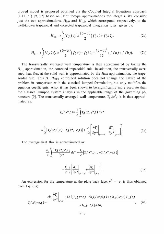
proved model is proposed obtained via the Coupled Integral Equations approach(C.I.E.A.) [9, 22] based on Hermite-type approximations for integrals. We considerjust the two approximations, H0,0 and H1,1, which correspond, respectively, to thewell-known trapezoidal and corrected trapezoidal integration rules, given by:

The transversally averaged wall temperature is then approximated by taking theH1,1 approximation, the corrected trapezoidal rule. In addition, the transversally aver-aged heat flux at the solid wall is approximated by the H0,0 approximation, the trape-zoidal rule. This H1,1/H0,0 combined solution does not change the nature of theproblem in comparison with the classical lumped formulation, but only modifies theequation coefficients. Also, it has been shown to be significantly more accurate thanthe classical lumped system analysis in the applicable range of the governing pa-rameters [9]. The transversally averaged wall temperature, Tav(x*, t), is thus approxi-mated as:

The average heat flux is approximated as:

An expression for the temperature at the plate back face, y* = –e, is thus obtainedfrom Eq. (3a):

( )

( ) ( )

0,0

1,1

2

2 12

b

a

b 2

a

( b a )H f ( y ) dy f ( a ) f ( b ) ,

( b a ) ( b a )H f ( y ) dy f ( a ) f ( b ) f '( a ) f '( b ) .

−→ ≅ +

− −→ ≅ + + +

∫

∫

(2a)

(2b)

[ ]

0

av s

ss s

1

1 02 12

e

s

y* e y* 0

T ( x*,t ) T ( x*, y*,t ) dy*e

T TeT ( x*, ,t ) T ( x*, e,t ) ,y* y*

−

=− =

≡

⎡ ⎤∂ ∂≈ + − + −⎢ ⎥∂ ∂⎢ ⎥⎣ ⎦

∫

(3a)

[ ]s s s

s s

s s

0

0

2

0

e

s

y* e y*

k T ( x*, y*,t ) kdy* T ( x*, ,t ) T ( x*, e,t )e y* e

k T Te .e y* y*

−

=− =

∂ ≡ − −∂

⎡ ⎤∂ ∂≈ +⎢ ⎥∂ ∂⎢ ⎥⎣ ⎦

∫

(3b)

s

s s av s s eff

seff s

12 6 0

6y* 0

Tek k T ( x*,t ) k T ( x*, ,t ) e h ( x*,t )T ( t )y*

T ( x*, e,t ) .e h ( x*,t ) k

∞=

∂ + − +∂

− =+

(4a)

213

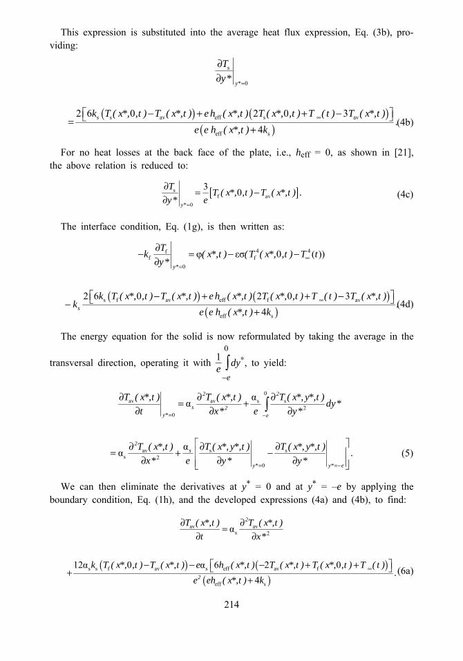
This expression is substituted into the average heat flux expression, Eq. (3b), pro-viding:

For no heat losses at the back face of the plate, i.e., heff = 0, as shown in [21],the above relation is reduced to:

The interface condition, Eq. (1g), is then written as:

The energy equation for the solid is now reformulated by taking the average in the

transversal direction, operating it with 1e ∫

−e

0

dy∗, to yield:

We can then eliminate the derivatives at y* = 0 and at y* = –e by applying theboundary condition, Eq. (1h), and the developed expressions (4a) and (4b), to find:

( ) ( )( )

s

0

s s av eff s av

eff s

2 6 0 2 0 34

y*

Ty*

k T ( x*, ,t ) T ( x*,t ) e h ( x*,t ) T ( x*, ,t ) T ( t ) T ( x*,t ).

e e h ( x*,t ) k

=

∞

∂∂

⎡ ⎤− + + −⎣ ⎦=+

(4b)

[ ]s

f av0

3 0y*

T T ( x*, ,t ) T ( x*,t ) .y* e=

∂ = −∂ (4c)

( ) ( )( )

4 4ff f

0

s f av eff f av

eff s

φ εσ 0 ( ))

2 6 0 2 0 34

y*

s

Tk ( x*,t ) (T ( x*, ,t ) T ty*

k T ( x*, ,t ) T ( x*,t ) e h ( x*,t ) T ( x*, ,t ) T ( t ) T ( x*,t )k .

e e h ( x*,t ) k

∞=

∞

∂− = − −∂

⎡ ⎤− + + −⎣ ⎦−+

(4d)

0av av s s

20

av s ss 2

0

αα

αα

2 2

s 2y* e

2s

y* y* e

T ( x*,t ) T ( x*,t ) T ( x*, y*,t ) dy*t x* e y*

T ( x*,t ) T ( x*, y*,t ) T ( x*, y*,t ) .x* e y* y*

= −

= =−

∂ ∂ ∂= +∂ ∂ ∂

⎡ ⎤∂ ∂ ∂= + −⎢ ⎥∂ ∂ ∂⎢ ⎥⎣ ⎦

∫

(5)

( ) ( )( )

av avs 2

s s f av s eff av f

eff s

α

12α 0 α 6 2 04

2

2

T ( x*,t ) T ( x*,t )t x*

k T ( x*, ,t ) T ( x*,t ) e h ( x*,t ) T ( x*,t ) T ( x*, ,t ) T ( t ).

e eh ( x*,t ) k∞

∂ ∂=∂ ∂

⎡ ⎤− − − + +⎣ ⎦++

(6a)

214

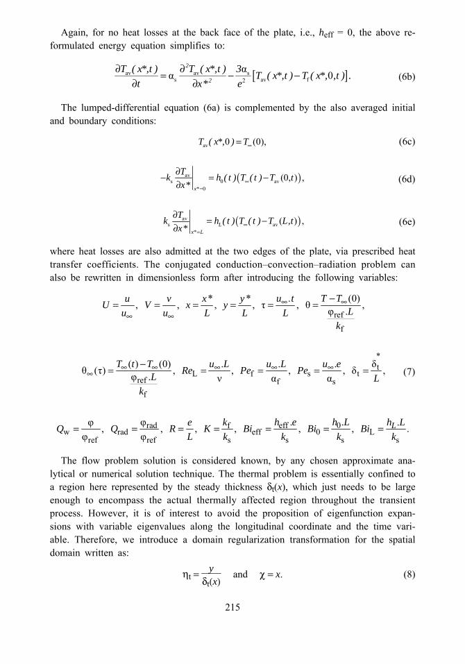
Again, for no heat losses at the back face of the plate, i.e., heff = 0, the above re-formulated energy equation simplifies to:

The lumped-differential equation (6a) is complemented by the also averaged initialand boundary conditions:

where heat losses are also admitted at the two edges of the plate, via prescribed heattransfer coefficients. The conjugated conduction–convection–radiation problem canalso be rewritten in dimensionless form after introducing the following variables:

The flow problem solution is considered known, by any chosen approximate ana-lytical or numerical solution technique. The thermal problem is essentially confined toa region here represented by the steady thickness δt(x), which just needs to be largeenough to encompass the actual thermally affected region throughout the transientprocess. However, it is of interest to avoid the proposition of eigenfunction expan-sions with variable eigenvalues along the longitudinal coordinate and the time vari-able. Therefore, we introduce a domain regularization transformation for the spatialdomain written as:

ηt = yδt(x)

and χ = x. (8)

[ ]av av s

s av f2

αα 02

2

T ( x*,t ) T ( x*,t ) 3 T ( x*,t ) T ( x*, ,t ) .t x* e

∂ ∂= − −∂ ∂

(6b)

( )

( )

av

avs 0 av

=0

avs av

0 (0),

(0, ) ,

( ) ,

x*

Lx* L

T ( x*, ) T

Tk h ( t ) T ( t ) T tx*

Tk h ( t ) T ( t ) T L,tx*

∞

∞

∞=

=

∂− = −∂

∂ = −∂

(6c)

(6d)

(6e)

ref

f

*t

L f s tref f s

f

rad eff 0fw rad eff 0

ref ref s s

. (0)* *, , , , τ , θ ,φ .

δ( ) (0) . . .θ (τ) , , , , δ ,φ . ν α α

φ .φ , , , , , φ φ

u t T Tu v x yU V x y Lu u L L Lk

T t T u L u L u eRe Pe PeL Lk

h e hkeQ Q R K Bi BiL k k

∞ ∞

∞ ∞

∞ ∞ ∞ ∞ ∞∞

−= = = = = =

−= = = = =

= = = = = = Ls s

. ., .LL h LBik k

=

(7)

215

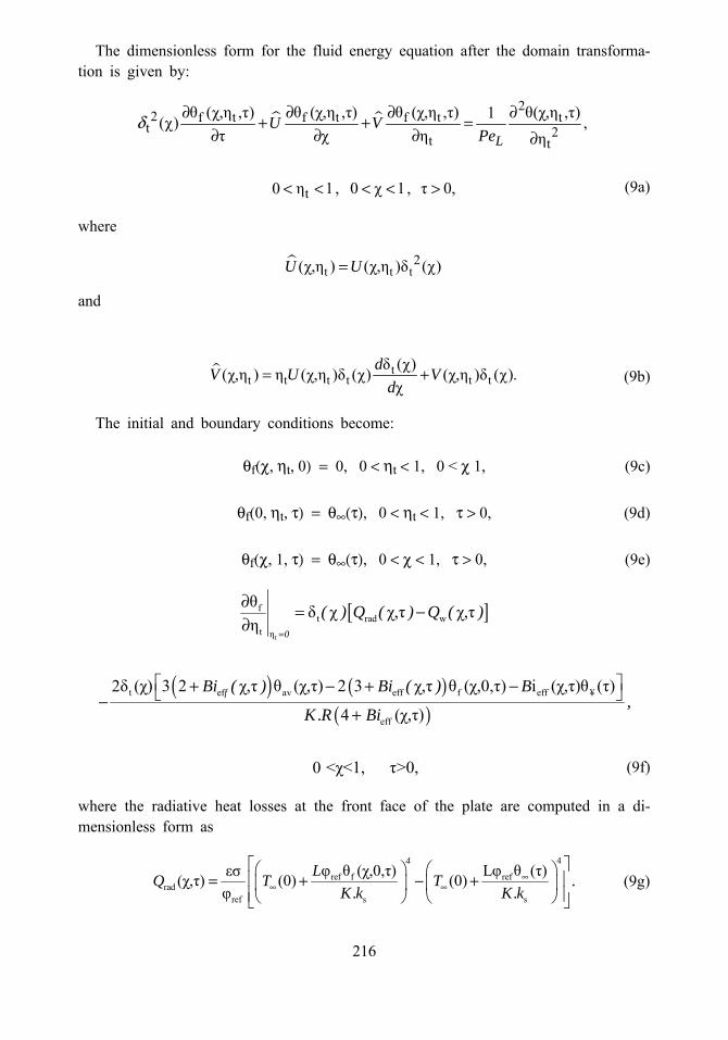
The dimensionless form for the fluid energy equation after the domain transforma-tion is given by:

where

The initial and boundary conditions become:

θf(χ, ηt, 0) = 0, 0 < ηt < 1, 0 < χ 1, (9c)

θf(0, ηt, τ) = θ∞(τ), 0 < ηt < 1, τ > 0, (9d)

θf(χ, 1, τ) = θ∞(τ), 0 < χ < 1, τ > 0, (9e)

where the radiative heat losses at the front face of the plate are computed in a di-mensionless form as

22 f t f t f t t

t 2t t

t

θ (χ,η ,τ) θ (χ,η ,τ) θ (χ,η ,τ) θ(χ,η ,τ)1(χ) ,τ χ η η

0 η 1, 0 χ 1, τ 0,

LU V

Peδ ∂ ∂ ∂ ∂+ + =

∂ ∂ ∂ ∂

< < < < > (9a)

t t t

tt t t t t t

2(χ,η ) (χ,η )δ (χ)

δ (χ)(χ,η ) η (χ,η )δ (χ) (χ,η )δ (χ).χ

U U

dV U Vd

=

= +

and

(9b)

[ ]

( ) ( )( )

t

ft rad w

t η

t ef av eff f eff ¥

eff

θ δ χ χ,τ χ,τη

2δ (χ) 3 2 χ,τ θ (χ,τ) 2 3 χ,τ θ (χ,0,τ) i (χ,τ)θ (τ)

4 (χ,τ)

0 <χ<1, τ>0,

0

f

( ) Q ( ) Q ( )

Bi ( ) Bi ( ) B,

K .R Bi

=

∂ = −∂

⎡ ⎤+ − + −⎣ ⎦−+

(9f)

4

ref f refrad

ref s s

φ θ (χ,0,τ) Lφ θ (τ)εσ(χ,τ) (0) (0)φ

4LQ T T .

K.k K.k∞

∞ ∞

⎡ ⎤⎛ ⎞ ⎛ ⎞⎢ ⎥= + − +⎜ ⎟ ⎜ ⎟⎢ ⎥⎝ ⎠ ⎝ ⎠⎣ ⎦

(9g)

216

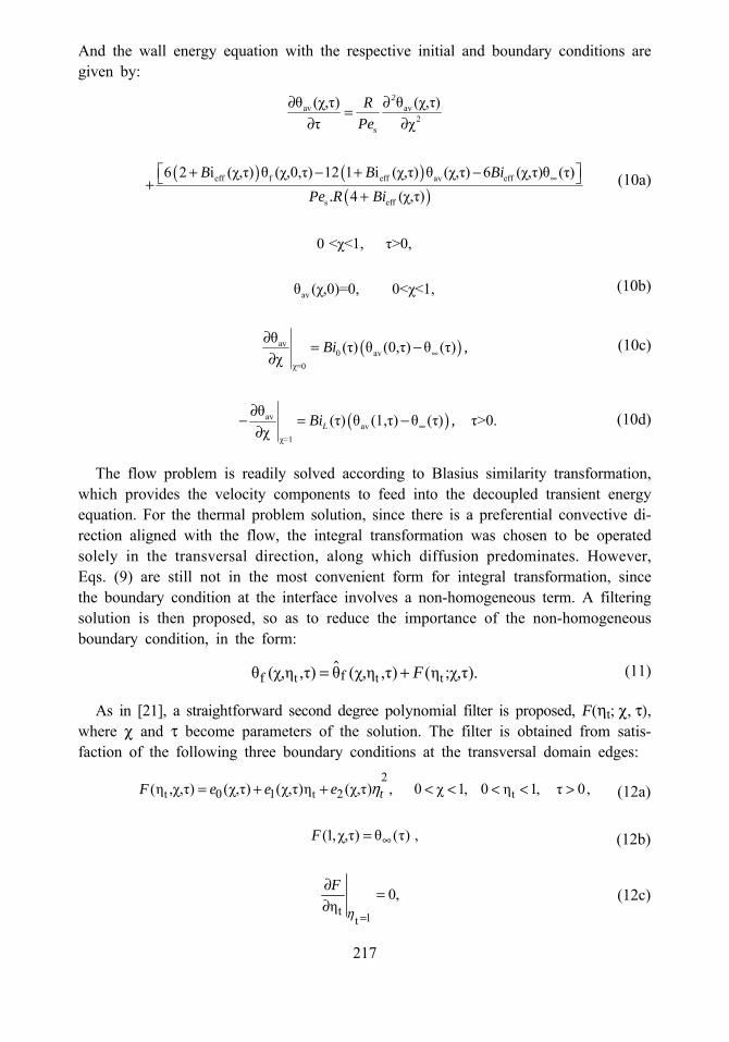
And the wall energy equation with the respective initial and boundary conditions aregiven by:

The flow problem is readily solved according to Blasius similarity transformation,which provides the velocity components to feed into the decoupled transient energyequation. For the thermal problem solution, since there is a preferential convective di-rection aligned with the flow, the integral transformation was chosen to be operatedsolely in the transversal direction, along which diffusion predominates. However,Eqs. (9) are still not in the most convenient form for integral transformation, sincethe boundary condition at the interface involves a non-homogeneous term. A filteringsolution is then proposed, so as to reduce the importance of the non-homogeneousboundary condition, in the form:

As in [21], a straightforward second degree polynomial filter is proposed, F(ηt; χ, τ),where χ and τ become parameters of the solution. The filter is obtained from satis-faction of the following three boundary conditions at the transversal domain edges:

( ) ( )( )

( )

av av2

s

eff f eff av eff

s eff

av

av0 av

χ=0

avav

χ=1

θ (χ,τ) θ (χ,τ)τ χ

6 2 i (χ,τ) θ (χ,0,τ) 12 1 i (χ,τ) θ (χ,τ) 6 (χ,τ)θ (τ)4 (χ,τ)

0 <χ<1, τ>0,

θ (χ,0)=0, 0<χ<1,

θ (τ) θ (0,τ) θ (τ)χ

θ (τ) θ (1χ

2

L

RPe

B B BiPe .R Bi

Bi ,

Bi

∞

∞

∂ ∂=∂ ∂

⎡ ⎤+ − + −⎣ ⎦++

∂ = −∂

∂− =∂

( ),τ) θ (τ) τ>0.,∞−

(10a)

(10b)

(10c)

(10d)

t t tffθ (χ,η ,τ) θ (χ,η ,τ) (η ;χ,τ).F= + (11)

t t t

1t

20 1 2

t

(η ,χ,τ) (χ,τ) (χ,τ)η (χ,τ) , 0 χ 1, 0 η 1, τ 0,

(1,χ,τ) θ (τ) ,

0,η

tF e e e

F

F

η

η

=

∞

= + + < < < < >

=

∂ =∂

(12a)

(12b)

(12c)

217

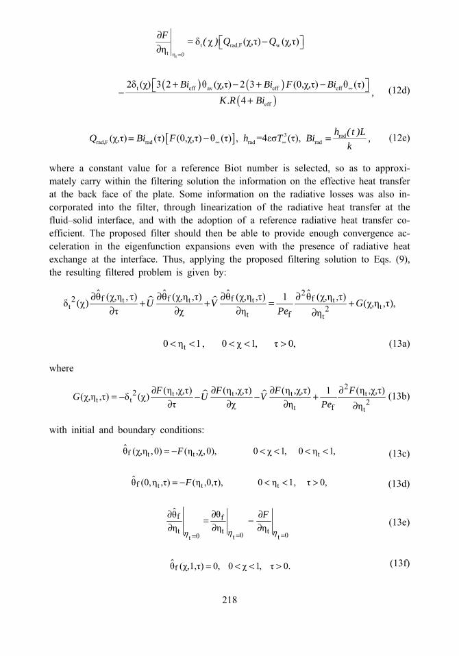
where a constant value for a reference Biot number is selected, so as to approxi-mately carry within the filtering solution the information on the effective heat transferat the back face of the plate. Some information on the radiative losses was also in-corporated into the filter, through linearization of the radiative heat transfer at thefluid–solid interface, and with the adoption of a reference radiative heat transfer co-efficient. The proposed filter should then be able to provide enough convergence ac-celeration in the eigenfunction expansions even with the presence of radiative heatexchange at the interface. Thus, applying the proposed filtering solution to Eqs. (9),the resulting filtered problem is given by:

where

with initial and boundary conditions:

( ) ( )( )

[ ]

t

t rad,F wt η

t eff av eff eff

eff

3 radrad,F rad rad rad

δ χ (χ,τ) (χ,τ)η

2δ (χ) 3 2 θ (χ,τ) 2 3 (0,χ,τ) θ (τ)

4

(χ,τ) (τ) (0,χ,τ) θ (τ) , =4εσ (τ),

0

F ( ) Q Q

Bi Bi F Bi,

K.R Bi

h ( t )LQ Bi F h T Bi ,k

=

∞

∞ ∞

∂⎡ ⎤= −⎣ ⎦∂

⎡ ⎤+ − + −⎣ ⎦−+

= − =

(12d)

(12e)

t t t t

t tt t

t

2f f f f2

2f

θ (χ,η , τ) θ (χ,η ,τ) θ (χ,η ,τ) θ (χ,η ,τ)1δ (χ) (χ,η ,τ),τ χ η η

0 η 1 , 0 χ 1, τ 0,

U V GPe

∂ ∂ ∂ ∂+ + = +∂ ∂ ∂ ∂

< < < < > (13a)

t t t t

t tt t

22

2f

(η ,χ,τ) (η ,χ,τ) (η ,χ,τ) (η ,χ,τ)1(χ,η ,τ) δ (χ)τ χ η η

F F F FG U VPe

∂ ∂ ∂ ∂= − − − +∂ ∂ ∂ ∂

(13b)

t t t

t t t

0 00 t tt

f

f

f f

t t t

f

θ (χ,η ,0) (η ,χ,0), 0 χ 1, 0 η 1,

θ (0,η ,τ) (η ,0,τ), 0 η 1, τ 0,

θθη η η

θ (χ,1,τ) 0, 0 χ 1, τ 0.

F

F

F

η ηη = ==

= − < < < <

= − < < >

∂∂ ∂= −∂ ∂ ∂

= < < >

(13c)

(13d)

(13e)

(13f)

218

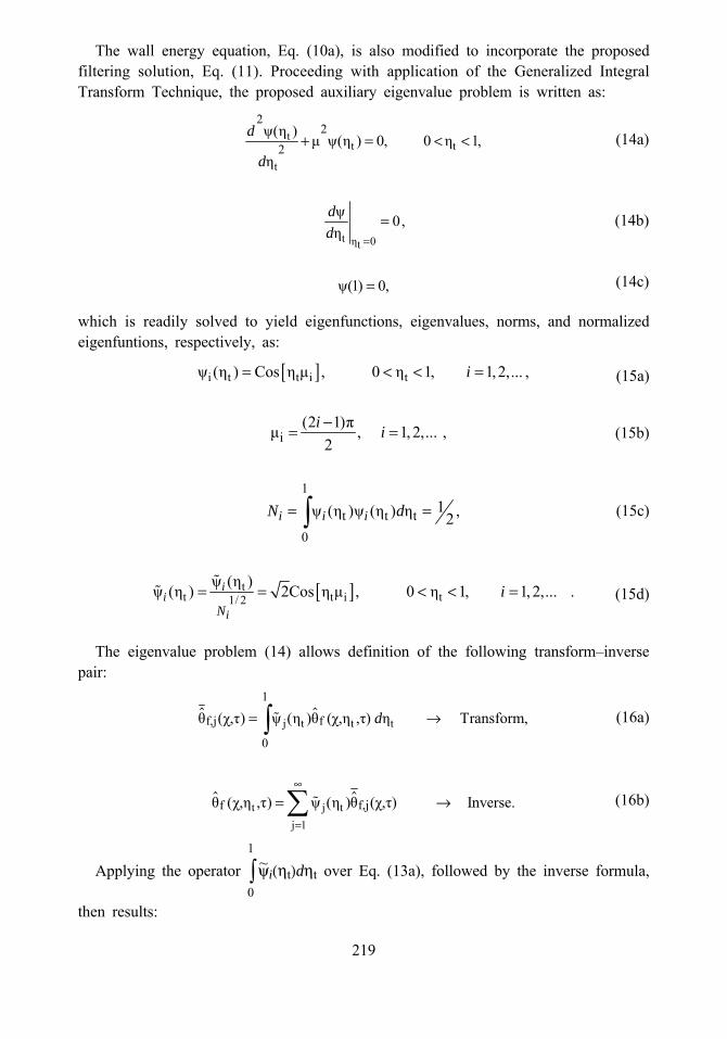
The wall energy equation, Eq. (10a), is also modified to incorporate the proposedfiltering solution, Eq. (11). Proceeding with application of the Generalized IntegralTransform Technique, the proposed auxiliary eigenvalue problem is written as:

which is readily solved to yield eigenfunctions, eigenvalues, norms, and normalizedeigenfuntions, respectively, as:

The eigenvalue problem (14) allows definition of the following transform–inversepair:

Applying the operator ∫ 0

1

ψ~ i(ηt)dηt over Eq. (13a), followed by the inverse formula,

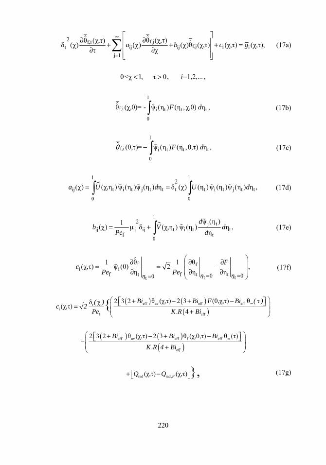
then results:

t

t t

t

t η 0t

22

2ψ(η ) μ ψ(η ) 0, 0 η 1,η

ψ 0,η

ψ(1) 0,

d

d

dd =

+ = < <

=

=

(14a)

(14b)

(14c)

[ ]

[ ]

i t t i t

tt t i t1/ 2

i

1

t t t0

ψ (η ) Cos η μ , 0 η 1, 1,2,... ,

(2 1)πμ , 1, 2,... ,2

1ψ (η )ψ (η ) η ,2

ψ (η )ψ (η ) 2Cos η μ , 0 η 1, 1, 2,... .ii

i

i i i

N

i

i i

N d

i

= < < =

−= =

= =

= = < < =

∫

(15a)

(15b)

(15c)

(15d)

j t t t

t j tj 1

1

f,j f

0

f f,j

θ (χ,τ) ψ (η )θ (χ,η ,τ) η Transform,

θ (χ,η ,τ) ψ (η )θ (χ,τ) Inverse.

d

∞

=

= →

= →

∫

∑

(16a)

(16b)

219

f,jf,i

f,jt ij ij ij 1

1

f,i i t t t

0

1

f,i i t t t

0

1

ij t i

0

2i

θ (χ,τ)θ (χ,τ)δ (χ) (χ) (χ)θ (χ,τ) (χ,τ) (χ,τ),τ χ

0<χ 1, τ 0, =1,2,... ,

θ (χ,0)= - ψ (η ) (η ,χ,0) η ,

(0,τ)= ψ (η ) (η ,0,τ) η ,

(χ) (χ,η )ψ (η

a b c g

i

F d

F d

a U

θ

∞

=

⎡ ⎤∂∂ ⎢ ⎥+ + + =⎢ ⎥∂ ∂

⎢ ⎥⎣ ⎦

< >

−

=

∑

∫

∫

∫1

t j t t t t i t j t t

0

1j t

ij j ij t i t tt

0

f fi i

t t tt tt

2

2

f

f f 0 00

)ψ (η ) η δ (χ) (η )ψ (η )ψ (η ) η ,

ψ (η )1(χ) μ δ (χ,η ) ψ (η ) η ,η

θ1 θ 1(χ,τ) ψ (0) 2 ,η η η

d U d

db V d

Pe d

FcPe Pe η ηη = ==

=

= +

⎛ ⎞∂∂ ∂⎜ ⎟= = −⎜ ⎟∂ ∂ ∂⎝ ⎠

∫

∫

(17a)

(17b)

(17c)

(17d)

(17e)

(17f)

( ) ( )( )

( ) ( )( )

eff av eff effi

f eff

eff av eff f eff

ef

rad rad

2 3 2 θ (χ,τ) 2 3 (0,χ,τ) θ τδ χ(χ,τ)4

2 3 2 θ (χ,τ) 2 3 θ (χ,0,τ) θ (τ)

(χ,τ) (χ,τ)

{

},

t

f

,F

Bi Bi F Bi ( )( )c 2Pe K.R Bi

Bi Bi Bi

K.R 4 Bi

Q Q

∞

∞

⎛ ⎞⎡ ⎤+ − + −⎣ ⎦= ⎜ ⎟⎜ ⎟+⎝ ⎠

⎛ ⎞⎡ ⎤+ − + −⎣ ⎦⎜ ⎟−⎜ ⎟+⎝ ⎠

+ −⎡ ⎤⎣ ⎦ (17g)

220

The wall heat transfer problem can then be described by the partial differentialequation (10a) coupled to the transformed fluid temperature fields. Equations (17) and(10) form an infinite coupled system of one-dimensional partial differential equationsfor the fluid transformed potentials and the wall average temperature. For computa-tional purposes this system is truncated to a sufficiently large finite order, N, for therequired convergence control. The PDE system is then numerically handled by rou-tine NDSolve of the Mathematica v.7.0 system [23]. Once the transformed potentialsare numerically computed, the inversion formula, Eq. (16b), is employed to recon-struct the filtered potentials, in explicit form in the transversal coordinate, and afteradding the filtering solution, F(ηt; χ, τ), the dimensionless temperature distribution,θt(χ, ηt, τ), is recovered everywhere within the boundary layer and along the transientprocess.

3. EXPERIMENTAL APPARATUS

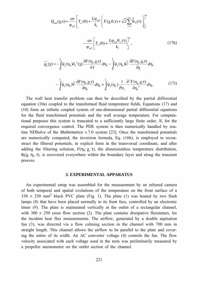
An experimental setup was assembled for the measurement by an infrared cameraof both temporal and spatial evolutions of the temperature on the front surface of a330 × 250 mm2 black PVC plate (Fig. 1). The plate (1) was heated by two flashlamps (8) that have been placed normally to its front face, controlled by an electronictimer (9). The plate is maintained vertically at the outlet of a rectangular channel,with 300 × 250 cross flow section (2). The plate contains dissipative fluxmeters, forthe incident heat flux measurements. The airflow, generated by a double aspirationfan (3), was directed via a flow calming section in the channel with 700 mm instraight length. This channel allows the airflow to be parallel to the plate and cover-ing the entire of its width. An AC converter voltage (4) controls the fan. The flowvelocity associated with each voltage used in the tests was preliminarily measured bya propeller anemometer on the outlet section of the channel.

4

reff,jrad

ref f

4

ref

ref f

21 1

t tt t t t ti i i

0 0

ti

φεσ(χ,τ) (0) (χ,0,τ) θ (τ)φ

φ θ (τ)εσ (0)φ

(η ,χ,τ) (η ,χ,τ)(χ) ψ (η )δ (χ) η ψ (η ) η

χ

ψ (η )

j 1

LQ T F 2k

LT ,k

F Fg d U d

V

τ

∞

∞=

∞∞

⎡ ⎤⎛ ⎞= + +⎢ ⎥⎜ ⎟

⎢ ⎥⎝ ⎠⎣ ⎦

⎡ ⎤− +⎢ ⎥

⎣ ⎦

∂ ∂= − −

∂ ∂

∂−

∑

∫ ∫

f

1 1t t

t t tit t0 0

(η ,χ,τ) (η ,χ,τ)1η ψ (η ) ηη η

2

2

F Fd d .Pe

∂+∂ ∂∫ ∫

(17h)

(17i)

221

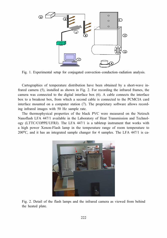
Cartographies of temperature distribution have been obtained by a short-wave in-frared camera (5), installed as shown in Fig. 2. For recording the infrared frames, thecamera was connected to the digital interface box (6). A cable connects the interfacebox to a breakout box, from which a second cable is connected to the PCMCIA cardinterface mounted on a computer station (7). The proprietary software allows record-ing infrared images with 50 Hz sample rate.

The thermophysical properties of the black PVC were measured on the NetzschNanoflash LFA 447/1 available in the Laboratory of Heat Transmission and Technol-ogy (LTTC/COPPE/UFRJ). The LFA 447/1 is a tabletop instrument that works witha high power Xenon-Flash lamp in the temperature range of room temperature to200oC, and it has an integrated sample changer for 4 samples. The LFA 447/1 is ca-

1

2

4

8

5

6

7

3

9

8

1

2

4

8

5

6

7

3

9

8

1

2

4

8

5

6

7

3

9

8

1

2

4

8

5

6

7

3

9

8

1

2

4

8

5

6

7

3

9

8

Fig. 1. Experimental setup for conjugated convection–conduction–radiation analysis.

Fig. 2. Detail of the flash lamps and the infrared camera as viewed from behindthe heated plate.

222

pable of measuring thermal diffusivity in the range of 0.01 mm2/s up to 1000 mm2/s,with an accuracy of 3–5% for most materials. The specific heat accuracy is 5–7%.This allows the calculation of the thermal conductivity in the range of 0.1 to 2000W/m⋅K with an accuracy of 3–7% for most materials [24]. The analysis of experi-mental data was performed with a software called Proteus, provided by Netzsch, pro-viding the following thermophysical properties estimates at 25oC: α = 0.144 mm2/s,k = 0.164 W/m⋅oC, and cp = 798 J/kg⋅oC.

4. RESULTS AND DISCUSSION

The experimental configuration considered in the present analysis adopts a blackPVC plate of 33 cm in height, thickness of 12 mm, and 20 cm wide. The configura-tion was aimed at insulating the PVC plate within a Styrofoam assembly of 8 cm inthickness at the back face and 3.8 cm at the lateral faces. The flash lamps are main-tained continuously heating the plate at the same power level.

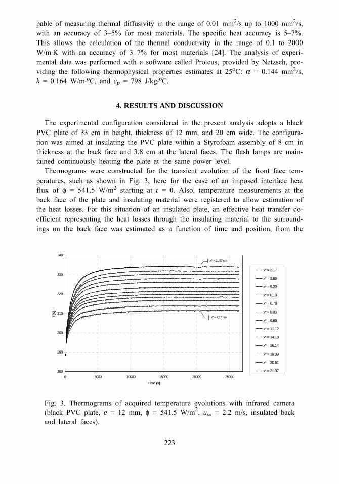
Thermograms were constructed for the transient evolution of the front face tem-peratures, such as shown in Fig. 3, here for the case of an imposed interface heatflux of φ = 541.5 W/m2 starting at t = 0. Also, temperature measurements at theback face of the plate and insulating material were registered to allow estimation ofthe heat losses. For this situation of an insulated plate, an effective heat transfer co-efficient representing the heat losses through the insulating material to the surround-ings on the back face was estimated as a function of time and position, from the

280

290

300

310

320

330

340

0 5000 10000 15000 20000 25000

Time (s)

T(K)

x* = 2.17

x* = 3.66

x* = 5.29

x* = 6.10

x* = 6.78

x* = 8.00

x* = 9.63

x* = 11.12

x* = 14.10

x* = 16.14

x* = 19.39

x* = 20.61

x* = 21.97

x* = 2,17 cm

x* = 21.97 cm

Fig. 3. Thermograms of acquired temperature evolutions with infrared camera(black PVC plate, e = 12 mm, φ = 541.5 W/m2, u∞ = 2.2 m/s, insulated backand lateral faces).

223

0 5000 10 000 15 000 20000 2500020 30 40

50

60 70

0.0216986 T(C)

t(s)

0 5000 10000 15000 20 000 25 000 20

30

40

50

60

700.0528904 T(C)

t(s)

0 5000 10 000 15 000 20000 2500020 30

40

50 60 70

0.0800137 T(C)

t(s)

0 5000 10000 15000 20 000 25 000 20

30

40

50

60

700.111205 T(C)

t(s)

0 5000 10 000 15 000 20000 2500020 30

40 50 60 70

0.141041 T(C)

t(s)

0 5000 10000 15000 20 000 25 000 20

30

40

50

60

700.187151 T(C)

t(s)

0 5000 10 000 15 000 20000 2500020 30 40 50 60 70

0.219699 T(C)

t(s)

0 5000 10000 15000 20 000 25 000 20

30

40

50

60

700.257671 T(C)

t(s)

Fig

224

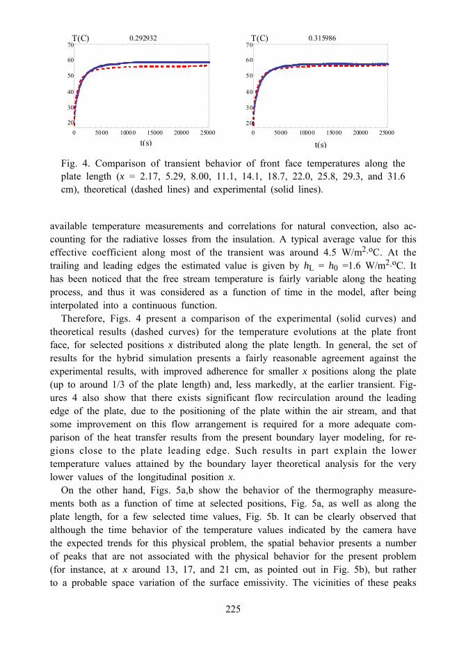
available temperature measurements and correlations for natural convection, also ac-counting for the radiative losses from the insulation. A typical average value for thiseffective coefficient along most of the transient was around 4.5 W/m2⋅oC. At thetrailing and leading edges the estimated value is given by hL = h0 =1.6 W/m2⋅oC. Ithas been noticed that the free stream temperature is fairly variable along the heatingprocess, and thus it was considered as a function of time in the model, after beinginterpolated into a continuous function.

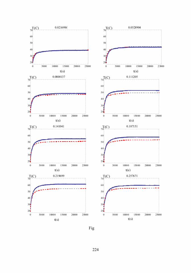
Therefore, Figs. 4 present a comparison of the experimental (solid curves) andtheoretical results (dashed curves) for the temperature evolutions at the plate frontface, for selected positions x distributed along the plate length. In general, the set ofresults for the hybrid simulation presents a fairly reasonable agreement against theexperimental results, with improved adherence for smaller x positions along the plate(up to around 1/3 of the plate length) and, less markedly, at the earlier transient. Fig-ures 4 also show that there exists significant flow recirculation around the leadingedge of the plate, due to the positioning of the plate within the air stream, and thatsome improvement on this flow arrangement is required for a more adequate com-parison of the heat transfer results from the present boundary layer modeling, for re-gions close to the plate leading edge. Such results in part explain the lowertemperature values attained by the boundary layer theoretical analysis for the verylower values of the longitudinal position x.

On the other hand, Figs. 5a,b show the behavior of the thermography measure-ments both as a function of time at selected positions, Fig. 5a, as well as along theplate length, for a few selected time values, Fig. 5b. It can be clearly observed thatalthough the time behavior of the temperature values indicated by the camera havethe expected trends for this physical problem, the spatial behavior presents a numberof peaks that are not associated with the physical behavior for the present problem(for instance, at x around 13, 17, and 21 cm, as pointed out in Fig. 5b), but ratherto a probable space variation of the surface emissivity. The vicinities of these peaks

0 5000 10 000 15 000 20000 2500020 30 40

50

60 70

t(s)

T(C) 0.292932

0 5000 10000 15000 20 000 25 000 20

30

40

50

60

70T(C) 0.315986

t(s) Fig. 4. Comparison of transient behavior of front face temperatures along the

plate length (x = 2.17, 5.29, 8.00, 11.1, 14.1, 18.7, 22.0, 25.8, 29.3, and 31.6cm), theoretical (dashed lines) and experimental (solid lines).

225

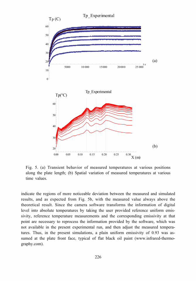
indicate the regions of more noticeable deviation between the measured and simulatedresults, and as expected from Fig. 5b, with the measured value always above thetheoretical result. Since the camera software transforms the information of digitallevel into absolute temperatures by taking the user provided reference uniform emis-sivity, reference temperature measurements and the corresponding emissivity at thatpoint are necessary to reprocess the information provided by the software, which wasnot available in the present experimental run, and then adjust the measured tempera-tures. Thus, in the present simulations, a plain uniform emissivity of 0.93 was as-sumed at the plate front face, typical of flat black oil paint (www.infrared-thermo-graphy.com).

5000 10 000 15000 20000 25 000t s

0

10

20

30

40

50

60 Tp (C)

Tp_Experimental

0.00 0.05 0.10 0.15 0.20 0.25 0.30X (m)

20

30

40

50

60

Tp_ExperimentalTp(°C)

Fig. 5. (a) Transient behavior of measured temperatures at various positionsalong the plate length; (b) Spatial variation of measured temperatures at varioustime values.

(a)

(b)

226

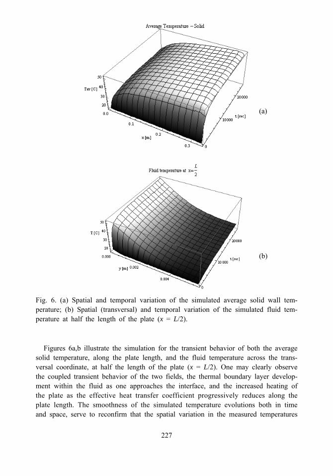
Figures 6a,b illustrate the simulation for the transient behavior of both the averagesolid temperature, along the plate length, and the fluid temperature across the trans-versal coordinate, at half the length of the plate (x = L/2). One may clearly observethe coupled transient behavior of the two fields, the thermal boundary layer develop-ment within the fluid as one approaches the interface, and the increased heating ofthe plate as the effective heat transfer coefficient progressively reduces along theplate length. The smoothness of the simulated temperature evolutions both in timeand space, serve to reconfirm that the spatial variation in the measured temperatures

Fig. 6. (a) Spatial and temporal variation of the simulated average solid wall tem-perature; (b) Spatial (transversal) and temporal variation of the simulated fluid tem-perature at half the length of the plate (x = L/2).

(a)

(b)

227

are not pertinent to the modeled heat transfer phenomena, but due to measurementdiscrepancies in light of surface conditions variability.

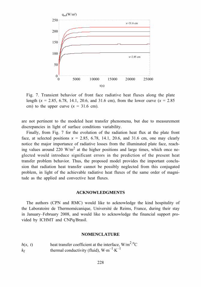
Finally, from Fig. 7 for the evolution of the radiation heat flux at the plate frontface, at selected positions x = 2.85, 6.78, 14.1, 20.6, and 31.6 cm, one may clearlynotice the major importance of radiative losses from the illuminated plate face, reach-ing values around 220 W/m2 at the higher positions and large times, which once ne-glected would introduce significant errors in the prediction of the present heattransfer problem behavior. Thus, the proposed model provides the important conclu-sion that radiation heat transfer cannot be possibly neglected from this conjugatedproblem, in light of the achievable radiative heat fluxes of the same order of magni-tude as the applied and convective heat fluxes.

ACKNOWLEDGMENTS

The authors (CPN and RMC) would like to acknowledge the kind hospitality ofthe Laboratoire de Thermomécanique, Université de Reims, France, during their stayin January–February 2008, and would like to acknowledge the financial support pro-vided by ICHMT and CNPq/Brasil.

NOMENCLATURE

h(x, t) heat transfer coefficient at the interface, W/m2⋅oCkf thermal conductivity (fluid), W⋅m–1⋅K–1

0 5000 10 000 15 000 20 000 25 000 0

50

100

150

200

250

t(s)

qrad(W/m²)

x=31.6 cm

x=2.85 cm

Fig. 7. Transient behavior of front face radiative heat fluxes along the platelength (x = 2.85, 6.78, 14.1, 20.6, and 31.6 cm), from the lower curve (x = 2.85cm) to the upper curve (x = 31.6 cm).

228

ks thermal conductivity (solid), W⋅m–1⋅K–1

L plate length, mPe Peclet numberQw dimensionless imposed interface heat fluxQrad dimensionless radiative heat flux at the front faceReL Reynolds numbert time variable, sT∞ free stream temperature, oCTf fluid temperature, oCTs solid temperature, oCTav averaged wall temperature, oCu∞ free stream velocity, m⋅s–1

u longitudinal velocity component, m⋅s–1

U dimensionless longitudinal velocity componentv transversal velocity component, m⋅s–1

V dimensionless transversal velocity componentx* longitudinal coordinate, mx dimensionless longitudinal coordinatey* transversal coordinate, my dimensionless transversal coordinateGreek symbolsαf thermal diffusivity (fluid), m2⋅s–1

αs thermal diffusivity (solid), m2⋅s–1

χ dimensionless transformed longitudinal coordinateηt dimensionless transformed transversal coordinateδ∗(x) velocity boundary-layer thickness, mδ(χ) dimensionless velocity boundary-layer thicknessδt

∗(x) thermal boundary-layer thickness, mδt(χ) dimensionless thermal boundary-layer thicknessθf dimensionless temperature (fluid)θav dimensionless averaged wall temperature (solid)ν kinematic viscosity, m2⋅s–1

τ dimensionless timeφ(x*, t) imposed interface heat flux, W/m2

φref reference heat flux at the interface, W/m2.

REFERENCES

1. Perelman, T. L. On conjugate problems of heat transfer, Int. J. Heat MassTransfer, Vol. 3, pp. 293–303, 1961.

2. Luikov, A. V., Aleksashenko, V. A., and Aleksashenko, A. A. Analytical meth-ods of solution of conjugated problems in convective heat transfer, Int. J. HeatMass Transfer, Vol. 14, pp. 1047–1056, 1971.

229

3. Guedes, R. O. C., Cotta, R. M., and Brum, N. C. L. Heat transfer in laminartube flow with wall axial conduction effects, J. Thermophys. Heat Transfer, Vol.5, No. 4, pp. 508–513, 1991.

4. Vynnycky, M., Kimura, S., Kanev, K., and Pop, I. Forced convection heat trans-fer from a flat plate: the conjugate problem, Int. J. Heat Mass Transfer, Vol.41, pp. 45–59, 1998.

5. Mossad, M. Laminar forced convection conjugate heat transfer over a flat plate,Heat Mass Transfer, Vol. 35, pp. 371–375, 1999.

6. Pozzi, A. and Tognaccini, R. Coupling of conduction and convection past animpulsively started semi-infinite flat plate, Int. J. Heat Mass Transfer, Vol. 43,pp. 1121–1131, 2000.

7. Lachi, M., Rebay, M., Mladin, E., and Padet, J. Integral approach of the tran-sient coupled heat transfer over a plate exposed to a variation in the input heatflux, ICHMT Int. Symp. Transient Convective Heat and Mass Transfer in Single& Two-Phase Flows, August, Cesme, Turkey, 2003.

8. Cotta, R. M. Integral Transforms in Computational Heat and Fluid Flow, CRCPress, Boca Raton, Florida, USA, 1993.

9. Cotta, R. M. and Mikhailov, M. D. Heat Conduction: Lumped Analysis, IntegralTransforms, Symbolic Computation, Wiley-Interscience, New York, 1997.

10. Cotta, R. M. (Ed.) The Integral Transform Method in Thermal and Fluids Sci-ences and Engineering, Begell House, New York, USA, 1998.

11. Santos, C. A. C., Quaresma, J. N. N., and Lima, J. A. Benchmark Results forConvective Heat Transfer in Ducts: — The Integral Transform Approach,ABCM Mechanical Sciences Series, Ed. E-Papers, Rio de Janeiro, 2001.

12. Cotta, R. M. and Mikhailov, M. D. Hybrid Methods and Symbolic Computa-tions, in: W. J. Minkowycz, E. M. Sparrow, and J. Y. Murthy (Eds.), Handbookof Numerical Heat Transfer, 2nd ed., Ch. 16, John Wiley, New York, pp. 493–522, 2006.

13. Cotta, R. M., Mikhailov, M. D., and Ozisik, M. N. Transient conjugated forcedconvection in ducts with periodically varying inlet temperature, Int J. Heat MassTransfer, Vol. 30, No. 10, pp. 2073–2082, 1987.

14. Guedes, R. O. C. and Cotta, R. M. Periodic laminar forced convection withinducts including wall heat conduction effects, Int. J. Eng. Sci., Vol. 29, No. 5,pp. 535–547, 1991.

15. Guedes, R. O. C., Cotta, R. M., and O..

zisik, M. N. Conjugated periodic turbu-lent forced convection in a parallel plate channel, J. Heat Transfer, Vol. 116,pp. 40–46, 1994.

16. Lachi, M., Cotta, R. M., Naveira, C. P., and Padet, J. Improved lumped-differ-ential formulation of transient conjugated conduction-convection in externalflow, in: Proc. 11th Brazilian Congress of Thermal Sciences and Engineering,ENCIT 2006, Curitiba, Brasil, Paper no. CIT06-0965, December 2006.

230

17. Remy, M., Degiovanni, A., and Maillet, D. Mesure de Coefficient d’E′changepour des E′coulements à Faible Vitesse, Rev. Gén. Therm., Vol. 397, pp. 28–42,1995.

18. Rebay, M., Lachi, M., and Padet, J. Mesure de coefficients de convection parméthode impulsionnelle–influence de la perturbation de la couche limite, Int. J.Thermal Sci., Vol. 41, pp. 1161–1175, 2002.

19. Rebay, M., Mladin, E., Chemin, S., and Stoian, M. Dissipative fluxmeter for thevalidation of the heat transfer coefficient measurement by the pulsed method,Eurotherm 2008, Eindhoven, Netherlands, June 2008.

20. Naveira, C. P., Cotta, R. M., Lachi, M., and Padet, J. Transient ConjugatedConduction-External Convection with Front Face Imposed Wall Heat Flux, in:Proc. IMECE2007, ASME International Mechanical Engineering Congress &Exposition, Paper no. IMECE2007-41417, Seattle, Washington, USA, November11–15, 2007.

21. Naveira, C. P., Lachi, M., Cotta, R. M., and Padet, J. Hybrid Formulation andSolution for Transient Conjugated Conduction-External Convection, Int. J. HeatMass Transfer, Vol. 52, Nos. 1–2, pp. 112–123, 2009.

22. Aparecido, J. B. and Cotta, R. M. Improved One-Dimensional Fin Solutions,Heat Transfer Eng., Vol. 11, No. 1, pp. 49–59, 1989.

23. Wolfram, S. The Mathematica Book, version 7.0, Cambridge-Wolfram Media,2008.

24. Pinto, C. S. C., Massard, H., Couto, P., Orlande, H. R. B., Cotta, R. M., andAmbrosio, M. C. R. Measurement of thermophysical properties of ceramics bythe flash method, METROSUL IV, 4th Congresso Latino-Americano de Metrolo-gia, Foz do Iguaçú, November 2004; also, Brazilian Archives of Biology andTechnology, Vol. 48, pp. 31–39, 2006.

�����

231