drop jet in crossflow: ale/fem simulations and interfacial...

Universidade do Estado do Rio de Janeiro

Centro de Tecnologia e Ciências

Faculdade de Engenharia

Gustavo Charles Peixoto de Oliveira

Drop Jet in Crossflow: ALE/Finite ElementSimulations and Interfacial Effects

Rio de Janeiro

2015


Drop Jet in Crossflow: ALE/FEM Simulationsand Interfacial Effects

Tese apresentada, como requisitoparcial para obtenção do título deDoutor em Ciências, ao Programade Pós-Graduação em EngenhariaMecânica, da Universidade do Es-tado do Rio de Janeiro. Área deconcentração: Fenômenos de Trans-porte.

Advisor: Prof. Ph.D. Norberto Mangiavacchi

Rio de Janeiro

2015

CATALOGAÇÃO NA FONTE

UERJ / REDE SIRIUS / BIBLIOTECA CTC/B

O48Oliveira, Gustavo Charles Peixoto de.

Drop jet in crossflow: ALE/finite element simulations and inter-facial effects / Gustavo Charles Peixoto de Oliveira. – 2015.

218 f.

Orientador: Norberto Mangiavacchi.Tese (Doutorado) – Universidade do Estado do Rio de Janeiro,

Faculdade de Engenharia.

1. Engenharia Mecânica. 2. Mecânica dos fluidos – Teses. 3. Es-coamento bifásico – Teses. 4. Método dos elementos finitos – Teses.I. Mangiavacchi, Norberto. II. Universidade do Estado do Rio deJaneiro. III. Título.

CDU 532

Autorizo, apenas para fins acadêmicos e científicos, a reprodução total ou parcial desta

dissertação, desde que citada a fonte.

Assinatura Data


Drop Jet in Crossflow: ALE/Finite Element Simulations

and Interfacial Effects

Tese apresentada, como requisitoparcial para obtenção do título de Doutorem Ciências, ao Programa de Pós-Graduaçãoem Engenharia Mecânica, da Universi-dade do Estado do Rio de Janeiro. Área deconcentração: Fenômenos de Transporte.

Aprovado em: 20 de fevereiro de 2015

Banca Examinadora:

Prof. Ph.D. Norberto Mangiavacchi (Orientador)Faculdade de Engenharia - UERJ

Prof. Ph.D. Carlos Antonio de MouraInstituto de Matemática e Estatística - UERJ

Prof. Ph.D. Leonardo Santos de Brito Alves (Co-orientador)Universidade Federal Fluminense

Prof. D.Sc. Álvaro Luiz Gayoso de Azeredo CoutinhoUniversidade Federal do Rio de Janeiro

Prof. D.Sc. José Henrique Carneiro de AraújoUniversidade Federal Fluminense

Rio de Janeiro

2015

DEDICATION

I dedicate this thesis to God, my Abba and manly father, who has bestowed upon me this

laurel, even after the most thoughtful mind inquires why; to the sovereignty of the Brazilian

science, even though my labour only sows a mere mustard seed.

ACKNOWLEDGMENTS

To God, loyal scholar, primer of all my ever-lacking science, for assisting me during

this long and laborious journey, conceiving me a bit more of knowledge, and battling beside

me. Only by Him I can go further beyond. Be Thou praised!

To LTCM staff at Ecole Polytechnique Fédérale de Lausanne while I was an internship

doctoral student, especially to Prof. John R. Thome, a hallmark in my career. I am very

propelled to send grateful votes to: Mrs. Nathalie Matthey and Cécile Taverney, for an

outstanding administrative support; Dr. Jackson Martinichen, for a Brazilian camaraderie

among multiple tongues and nations; Dr. Marco Milan, Dr. Sepideh Khodaparast, and Nicolas

Antonsen, for sharing an harmonious, silent, and quite serious office; Dr. Ricardo Lima, Dr.

Brian d’Entremont, Dr. Sylwia Szczukiewicz, Dr. Tom Saenen, Houxue “The Tiger” Huang,

Giulia Spinato, Luca Amalfi, Hamideh Jafarpoorchekab, and Nicolas Lamaison, for joyful and

festive days.

To Dr. Mirco Magnini, especially, for his priceless help since the first days at LTCM

(Grazie mille per la vostra collaborazione!); to Dr. Gustavo Anjos, for a long road of exchanged

information and namesake grace (Obrigado por toda força!), and to Dr. Bogdan Nichita, for

pleasant times beneath an unforgettable jingle: today, what time?

To Prof. Peter Monkewitz, for convivial moments and nobility of a wiser person.

To Prof. Anna Renda, par sa guidance à travers des beautés et des inspirations de la

langue française.

To Prof. Norberto Mangiavacchi and Prof. Leonardo Alves, my advisors in Brazil,

whom I could grasp a mix of benefits: friendship, instruction, and motivation.

To Prof. José Pontes, perennial friend, but in likeness of fatherhood, for all the prevail-

ing ages and epochs, undoubtedly.

To my coworkers at GESAR lab and at the old LMP lab. Altogether, for funny and

smiling days: behold here, Sonia Nina, Mariana Rocha, Cristiane Pimenta, Jorge Martins,

Rachel Lucena, Eduardo Vitral, Melissa Mabuias, and Ana Polessa; behold there, Renan

Teixeira, Flávio Santiago, and Ricardo Dias.

To closer friends who surrounded me along this trajectory, for too many special mo-

ments: Luís Otávio Olivatto, for being a great fellow under a single faith; Ruben and Sonia

Quaresma, for helping me to see new life elements while walking together with The Eternal;

Márcia Oliveira, for giving me hopeful words during lasting trouble times.

To some doctors, who were precious in determined times: Fabio Bolognani, Monica

Lima, Gualter Braga, and Gilberto Campos.

To my family and my grandmother, all of them cultivated somewhere inside the

seasons’ orchard.

To my source of poetry - much more than the years could spell again and again as

girlfriend - Viviane Penna, who, beside me, has acquired patience, perseverance, hope, and

love. Thank you, ו ! Also, my kind regards to her parents and relatives.

To State University of Rio de Janeiro, the Mechanical Engineering Program staff, my

classmates, and mainly to Prof. Rogério Gama and Prof. Carlos de Moura, for empathic

academic lectures.

To Prof. Álvaro Coutinho, whose esteem and respect I shall keep.

To Billy Pinheiro and Damares, on behalf of many other brethren, for a helper arm of

faith.

To CNPq-Brazil and the program “Science Without Borders”, sine qua non elements

that provided me with resources to the enrichment of my professional formation.

To CAPES-Brazil, for sponsoring this doctoral research.

Let my teaching drop as the rain, my speech distill as the dew, as the droplets on the fresh

grass and as the showers on the herb. (The Song of Moses)

Deuteronomy 32:2

RESUMO

OLIVEIRA, Gustavo Charles P. de Drop Jet in Crossflow: ALE/Finite Element Simulations and In-

terfacial Effects. 218 f. Tese (Doutorado em Engenharia Mecânica) - Faculdade de Engenharia,

Universidade do Estado do Rio de Janeiro (UERJ), Rio de Janeiro, 2015.

Um código computacional para escoamentos bifásicos incorporando metodologia

híbrida entre o Método dos Elementos Finitos e a descrição Lagrangeana-Euleriana Arbitrária

do movimento é usado para simular a dinâmica de um jato transversal de gotas na zona

primária de quebra. Os corpos dispersos são descritos por meio de um método do tipo

front-tracking que produz interfaces de espessura zero através de malhas formadas pela

união de elementos adjacentes em ambas as fases e de técnicas de refinamento adaptativo.

Condições de contorno periódicas são implementadas de modo variacionalmente consistente

para todos os campos envolvidos nas simulações apresentadas e uma versão modificada

do campo de pressão é adicionada à formulação do tipo “um-fluido” usada na equação da

quantidade de movimento linear. Simulações numéricas diretas em três dimensões são

executadas para diferentes configurações de líquidos imiscí veis compatíveis com resultados

experimentais encontrados na literatura. Análises da hidrodinâmica do jato transversal de

gotas nessas configurações considerando trajetórias, variação de formato de gota, espectro

de pequenas perturbações, além de aspectos complementares relativos à qualidade de malha

são apresentados e discutidos.

Palavras-chave: Jato Transversal; Lagrangeano-Euleriano Arbitrário; Elementos Finitos; Es-

coamento Bifásico; Condições de Contorno Periódicas.

ABSTRACT

A two-phase flow computational code taking a hybrid Arbitrary Lagrangian-Eulerian

description of movement along with the Finite Element Method is used to simulate the dy-

namics of an incompressible drop jet in crossflow in the primary breakup zone. Dispersed

entities are described by means of a front-tracking method which produces zero-thickness in-

terfaces through contiguous element meshing and adaptive refinement techniques. Periodic

boundary conditions are implemented in a variationally consistent way for all the scalar fields

involved in the presented simulations and a modified version of the pressure field is added

to the “one-fluid” formulation employed in the momentum equation. Three-dimensional

direct numerical simulations for different flow configurations of immiscible liquids pertinent

to experimental results found in literature. Analyses of the hydrodynamics of the drop jet in

crossflow in these configurations considering trajectories, drop shape variations, spectrum

of small disturbances, besides additional aspects relating to mesh quality are presented and

discussed.

Keywords: Jet in Crossflow; Arbitrary Lagrangian-Eulerian; Finite Element; Two-Phase Flow;

Periodic Boundary Conditions.

LIST OF FIGURES

Figure 1 Images from internet sites exemplifying physical conditions in which JICF

configurations are detected . . . . . . . . . . . . . . . . . . . . . . . . . . . . . . . . . . . . . . . . . . . . . . . . . . . . . . . . . . . 31

Figure 2 Descriptive sectioning of the jet in crossflow issued normally to the free stream. 32

Figure 3 Model of the jet in crossflow depicting the entrainment effect caused by the

free stream. . . . . . . . . . . . . . . . . . . . . . . . . . . . . . . . . . . . . . . . . . . . . . . . . . . . . . . . . . . . . . . . . . . . . . . . . . . . . . . 33

Figure 4 The jet in crossflow highlighting its vortical structures. . . . . . . . . . . . . . . . . . . . . . . . . . . . 33

Figure 5 Diagram of jet breakup for a gas-liquid pair. . . . . . . . . . . . . . . . . . . . . . . . . . . . . . . . . . . . . . . . . 42

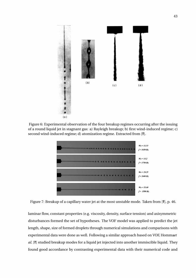
Figure 6 Experimental observation of breakup regimes of a round liquid jet in stag-

nant gas. . . . . . . . . . . . . . . . . . . . . . . . . . . . . . . . . . . . . . . . . . . . . . . . . . . . . . . . . . . . . . . . . . . . . . . . . . . . . . . . . . . 43

Figure 7 Breakup of a capillary water jet at the most unstable mode.. . . . . . . . . . . . . . . . . . . . . . 43

Figure 8 Breakup modes for a liquid jet injected into an immiscible liquid. . . . . . . . . . . . . . . 44

Figure 9 Primary breakup regime map for nonturbulent round liquid jets in gaseous

crossflow. . . . . . . . . . . . . . . . . . . . . . . . . . . . . . . . . . . . . . . . . . . . . . . . . . . . . . . . . . . . . . . . . . . . . . . . . . . . . . . . . . 45

Figure 10 Crossflow membrane emulsification process. . . . . . . . . . . . . . . . . . . . . . . . . . . . . . . . . . . . . . . 46

Figure 11 Drop formation and breakup of a calcia/alumina slag jet at high temperature. 47

Figure 12 Scheme representing the descriptions of movement. . . . . . . . . . . . . . . . . . . . . . . . . . . . . . 50

Figure 13 Mathematical representation of the descriptions of movement through

homeomorphisms. . . . . . . . . . . . . . . . . . . . . . . . . . . . . . . . . . . . . . . . . . . . . . . . . . . . . . . . . . . . . . . . . . . . . . 51

Figure 14 Outlook of the molecular inbalance in the surroundings of an arbitrary gas-

liquid interface. . . . . . . . . . . . . . . . . . . . . . . . . . . . . . . . . . . . . . . . . . . . . . . . . . . . . . . . . . . . . . . . . . . . . . . . . . 56

Figure 15 Uniform distribution of the surface tension over an infinitesimal area and

principal radii of curvature. . . . . . . . . . . . . . . . . . . . . . . . . . . . . . . . . . . . . . . . . . . . . . . . . . . . . . . . . . . . 58

Figure 16 Generalized domain including periodic boundaries for a two-phase flow

modelling.. . . . . . . . . . . . . . . . . . . . . . . . . . . . . . . . . . . . . . . . . . . . . . . . . . . . . . . . . . . . . . . . . . . . . . . . . . . . . . . . 60

Figure 17 Mesh elements comprising the region around the interface region and effect

of transition. . . . . . . . . . . . . . . . . . . . . . . . . . . . . . . . . . . . . . . . . . . . . . . . . . . . . . . . . . . . . . . . . . . . . . . . . . . . . . 61

Figure 18 3D mesh for an arbitrary two-phase flow configuration containing three

dispersed spherical elements confined into a microchannel. . . . . . . . . . . . . . . . . . . . . 63

Figure 19 3D mesh for a two-phase slug flow configuration. . . . . . . . . . . . . . . . . . . . . . . . . . . . . . . . . . 64

Figure 20 Representative behaviour of the Heaviside function over a two-dimensional

surface. . . . . . . . . . . . . . . . . . . . . . . . . . . . . . . . . . . . . . . . . . . . . . . . . . . . . . . . . . . . . . . . . . . . . . . . . . . . . . . . . . . . 71

Figure 21 SL method in a spatio-temporal context over a two-dimensional triangular

finite element mesh. . . . . . . . . . . . . . . . . . . . . . . . . . . . . . . . . . . . . . . . . . . . . . . . . . . . . . . . . . . . . . . . . . . . . 79

Figure 22 Different two-dimensional compositions of elements.. . . . . . . . . . . . . . . . . . . . . . . . . . . . 81

Figure 23 Two-time representation of a continuous interface Γ1. Dashed: time t0; thick:

time t ; dotted: trajectory. . . . . . . . . . . . . . . . . . . . . . . . . . . . . . . . . . . . . . . . . . . . . . . . . . . . . . . . . . . . . . . 84

Figure 24 Two-time representation of a piecewise linear interface Γ1h . Dashed: time t0;

thick: time t ; dotted: trajectory.. . . . . . . . . . . . . . . . . . . . . . . . . . . . . . . . . . . . . . . . . . . . . . . . . . . . . . . 84

Figure 25 Adaptive refinement strategies applied at interfaces and neighborhoods: (a)

criterion based on constant distance; (b) criterion based on distance from

the extrema points. . . . . . . . . . . . . . . . . . . . . . . . . . . . . . . . . . . . . . . . . . . . . . . . . . . . . . . . . . . . . . . . . . . . . . 85

Figure 26 MINI element 3D highlighting the sites for the degrees of freedom of velocity

and pressure. . . . . . . . . . . . . . . . . . . . . . . . . . . . . . . . . . . . . . . . . . . . . . . . . . . . . . . . . . . . . . . . . . . . . . . . . . . . . 95

Figure 27 Representations of the star S(i ) of the node i . . . . . . . . . . . . . . . . . . . . . . . . . . . . . . . . . . . . . . . 98

Figure 28 Possible range of geometrical operations for the discrete interface. . . . . . . . . . . . . 99

Figure 29 Sketch of topological mappings for generic geometries. . . . . . . . . . . . . . . . . . . . . . . . . . .102

Figure 30 Geometrical sketch of the PBC implementation for a 3D periodic finite ele-

ment mesh. . . . . . . . . . . . . . . . . . . . . . . . . . . . . . . . . . . . . . . . . . . . . . . . . . . . . . . . . . . . . . . . . . . . . . . . . . . . . . .103

Figure 31 Displacement of “leaked” departure points and Semi-Lagrangian correction. 116

Figure 32 Periodic domain of simulation for a Taylor vortex flow. . . . . . . . . . . . . . . . . . . . . . . . . . . .117

Figure 33 Relative error in L 2-norm of the velocity profile for the Taylor vortex flow. . . .119

Figure 34 Taylor vortex’s velocity profile vx . . . . . . . . . . . . . . . . . . . . . . . . . . . . . . . . . . . . . . . . . . . . . . . . . . . . .120

Figure 35 Taylor vortex’s velocity profile vy . . . . . . . . . . . . . . . . . . . . . . . . . . . . . . . . . . . . . . . . . . . . . . . . . . . . .121

Figure 36 Taylor vortex’s periodic pressure profile p. . . . . . . . . . . . . . . . . . . . . . . . . . . . . . . . . . . . . . . . . . .122

Figure 37 Scalar φ being carried by fluid flow. . . . . . . . . . . . . . . . . . . . . . . . . . . . . . . . . . . . . . . . . . . . . . . . . . .123

Figure 38 Arrangement of the unconfined in-line bubble plume: (a) extended plume

model; (b) detail of the periodic cell. . . . . . . . . . . . . . . . . . . . . . . . . . . . . . . . . . . . . . . . . . . . . . . . . .125

Figure 39 Augmented view of mesh displaying adaptive refinement strategies: circum-

ferential, at the bubble’s surface; azimuthal, at the cylindrical wrap region of

radius Rc surrounding it.. . . . . . . . . . . . . . . . . . . . . . . . . . . . . . . . . . . . . . . . . . . . . . . . . . . . . . . . . . . . . . .126

Figure 40 Computational mesh highlighting the bubble region: cut plane parallel to

the axis of rising of the plume. . . . . . . . . . . . . . . . . . . . . . . . . . . . . . . . . . . . . . . . . . . . . . . . . . . . . . . .127

Figure 41 Computational mesh highlighting the adaptive refinement provided by the

cylindrical wrap: top-view. . . . . . . . . . . . . . . . . . . . . . . . . . . . . . . . . . . . . . . . . . . . . . . . . . . . . . . . . . . . .127

Figure 42 Dimensionless rising velocities ubc (t) for three different configurations of

an air bubble rising immersed into a aqueous sugar solution. . . . . . . . . . . . . . . . . . .129

Figure 43 Elongation (φ) and flatness (ψ) ratios of the rising bubbles. . . . . . . . . . . . . . . . . . . . . .129

Figure 44 Bubbles’ spatial motion relative to the reference frame moving upwards

along with the center of mass. . . . . . . . . . . . . . . . . . . . . . . . . . . . . . . . . . . . . . . . . . . . . . . . . . . . . . . . .131

Figure 45 FFT-based spectrum of disturbance energy for the ten first harmonic modes

relative to the aspect ratios profiles. . . . . . . . . . . . . . . . . . . . . . . . . . . . . . . . . . . . . . . . . . . . . . . . . . .133

Figure 46 Dimensionless rising velocities ubc (t ) over the bubble’s reference frame for

the cases B1 and B2. . . . . . . . . . . . . . . . . . . . . . . . . . . . . . . . . . . . . . . . . . . . . . . . . . . . . . . . . . . . . . . . . . . . .134

Figure 47 Velocity field and bubble shape for the case B1: plane y x. . . . . . . . . . . . . . . . . . . . . . . .135

Figure 48 Velocity field and bubble shape for the case B1: plane zx. . . . . . . . . . . . . . . . . . . . . . . . .136

Figure 49 Velocity field and bubble shape for the case B2: plane y x. . . . . . . . . . . . . . . . . . . . . . . .137

Figure 50 Velocity field and bubble shape for the case B2: plane zx. . . . . . . . . . . . . . . . . . . . . . . . .138

Figure 51 Configuration of the drop jet in crossflow .. . . . . . . . . . . . . . . . . . . . . . . . . . . . . . . . . . . . . . . . . .139

Figure 52 Relation between fixed and moving reference frames in the DJICF flow.. . . . . . .140

Figure 53 Descriptive scheme of the moving frame technique for a drop in crossflow.. . .142

Figure 54 Past cylinder flow velocity profile as initial condition for the DJICF simulation.145

Figure 55 Meshes used for the DJICF simulations. . . . . . . . . . . . . . . . . . . . . . . . . . . . . . . . . . . . . . . . . . . . . .147

Figure 56 uc (t )-component of drop velocity - MS. . . . . . . . . . . . . . . . . . . . . . . . . . . . . . . . . . . . . . . . . . . . . .148

Figure 57 vc (t )-component of drop velocity - MS. . . . . . . . . . . . . . . . . . . . . . . . . . . . . . . . . . . . . . . . . . . . . .149

Figure 58 wc (t )-component of drop velocity - MS. . . . . . . . . . . . . . . . . . . . . . . . . . . . . . . . . . . . . . . . . . . . .149

Figure 59 uc (t )-component of drop velocity - WL. . . . . . . . . . . . . . . . . . . . . . . . . . . . . . . . . . . . . . . . . . . . . .150

Figure 60 vc (t )-component of drop velocity - WL. . . . . . . . . . . . . . . . . . . . . . . . . . . . . . . . . . . . . . . . . . . . . .150

Figure 61 wc (t )-component of drop velocity - WL. . . . . . . . . . . . . . . . . . . . . . . . . . . . . . . . . . . . . . . . . . . . .151

Figure 62 Streamlines and drop’s rims at t ≈ 0.30 - test (MS,2.0,1.5). . . . . . . . . . . . . . . . . . . . . . . .152



Figure 65 Streamlines and drop’s rims at t ≈ 0.37 - test (W L,2.0,1.5). . . . . . . . . . . . . . . . . . . . . . . .155



Figure 68 x y-plane drop trajectory - MS.. . . . . . . . . . . . . . . . . . . . . . . . . . . . . . . . . . . . . . . . . . . . . . . . . . . . . . . .158

Figure 69 xz-plane drop trajectory - MS. . . . . . . . . . . . . . . . . . . . . . . . . . . . . . . . . . . . . . . . . . . . . . . . . . . . . . . . .159

Figure 70 x y-plane drop trajectory - WL.. . . . . . . . . . . . . . . . . . . . . . . . . . . . . . . . . . . . . . . . . . . . . . . . . . . . . . . .160

Figure 71 xz-plane drop trajectory - WL. . . . . . . . . . . . . . . . . . . . . . . . . . . . . . . . . . . . . . . . . . . . . . . . . . . . . . . . .160

Figure 72 Drop shape variation - (MS, ·,1.5). . . . . . . . . . . . . . . . . . . . . . . . . . . . . . . . . . . . . . . . . . . . . . . . . . . .162



Figure 75 Drop shape variation - (W L, ·,1.5). . . . . . . . . . . . . . . . . . . . . . . . . . . . . . . . . . . . . . . . . . . . . . . . . . . .163



Figure 78 FFT-based spectrum (MS, ·,1.5). . . . . . . . . . . . . . . . . . . . . . . . . . . . . . . . . . . . . . . . . . . . . . . . . . . . . . .165



Figure 81 FFT-based spectrum (W L, ·,1.5). . . . . . . . . . . . . . . . . . . . . . . . . . . . . . . . . . . . . . . . . . . . . . . . . . . . . .167



Figure 84 Skinny triangles: needle and cap elements. . . . . . . . . . . . . . . . . . . . . . . . . . . . . . . . . . . . . . . . . .171

Figure 85 Skinny tetrahedra: needle, cap and sliver elements. . . . . . . . . . . . . . . . . . . . . . . . . . . . . . . .171

Figure 86 Histograms I (t )tet for group MS. . . . . . . . . . . . . . . . . . . . . . . . . . . . . . . . . . . . . . . . . . . . . . . . . . . . .173

Figure 87 Histograms I (t )tet for group WL. . . . . . . . . . . . . . . . . . . . . . . . . . . . . . . . . . . . . . . . . . . . . . . . . . . . .173

Figure 88 Flowchart I: pre-processing stage. . . . . . . . . . . . . . . . . . . . . . . . . . . . . . . . . . . . . . . . . . . . . . . . . . . . .181

Figure 89 Flowchart II: processing stage. . . . . . . . . . . . . . . . . . . . . . . . . . . . . . . . . . . . . . . . . . . . . . . . . . . . . . . . .182

Figure 90 Flowchart III: post-processing stage. . . . . . . . . . . . . . . . . . . . . . . . . . . . . . . . . . . . . . . . . . . . . . . . . .183

Figure 91 UML partial diagram of the in-house femSIM2D/3D code. . . . . . . . . . . . . . . . . . . . . . .184

Figure 92 Scheme for the calculation of the curvature.. . . . . . . . . . . . . . . . . . . . . . . . . . . . . . . . . . . . . . . .194

Figure 93 Example of a process of verification to detect errors in codes. . . . . . . . . . . . . . . . . . . .196

LIST OF TABLES

Table 1 ALE meshing parameters for surface operations. . . . . . . . . . . . . . . . . . . . . . . . . . . . . . . . . . .100

Table 2 Physical parameters of the Taylor vortex flow. . . . . . . . . . . . . . . . . . . . . . . . . . . . . . . . . . . . . . .118

Table 3 Physical property values for the numerical simulations: tests R1-R3. . . . . . . . . . . .128

Table 4 Physical property values for the numerical simulations of the rising bubble

plume tests. . . . . . . . . . . . . . . . . . . . . . . . . . . . . . . . . . . . . . . . . . . . . . . . . . . . . . . . . . . . . . . . . . . . . . . . . . . . . . .130

Table 5 Parameters of simulation according to the experiment no. 5 of Meister and

Scheele. . . . . . . . . . . . . . . . . . . . . . . . . . . . . . . . . . . . . . . . . . . . . . . . . . . . . . . . . . . . . . . . . . . . . . . . . . . . . . . . . . . .146

Table 6 Parameters of simulation according to the fluid combination no. 1(c) of

natural jet of Webster and Longmire. . . . . . . . . . . . . . . . . . . . . . . . . . . . . . . . . . . . . . . . . . . . . . . . .147

Table 7 Maximum disturbance energies and dominant modes of the spectral analyses.169

Table 8 FFT sampling ranges and disturbance attenuation thresholds for the spectral

analyses. . . . . . . . . . . . . . . . . . . . . . . . . . . . . . . . . . . . . . . . . . . . . . . . . . . . . . . . . . . . . . . . . . . . . . . . . . . . . . . . . . .170

Table 9 Mesh quality indicators relative to the statistical histograms. . . . . . . . . . . . . . . . . . . . .174

LIST OF SYMBOLS

Acronyms

ALE Arbitrary Lagrangian-Eulerian

CAD Computer-Aided Design

CFD Computational Fluid Dynamics

CIP Cubic Interpolated Profile

CK Chemical Kinetics

CSF Continuum Surface Force

CVP Counter-Rotating Vortex Pair

DBC Dirichlet Boundary Conditions

DJICF Drop Jet in Crossflow

DOFs Degrees of Freedom

FE Finite Element

FEM Finite Element Method

FFR Fixed Frame Reference

FFT Fourier Fast Transform

JICF Jet in Crossflow

KH Kelvin-Helmholtz

LBB Ladyzhenskaya-Babuska-Brezzi

LSA Linear Stability Analysis

LS Level-Set

MAC Marker-and-Cell

MFR Moving Frame Reference

NBC Neumann Boundary Conditions

OBC Open Boundary Conditions

PBC Periodic Boundary Conditions

RT Rayleigh-Taylor

VOF Volume of Fluid

Greek letters

β1 mesh parameter: pure Lagrangian motion

β2 mesh parameter: neighbourhood-based velocity smoothing

β3 mesh parameter: elastic-based velocity Laplacian smoothing

α backward displacement vector

χ position in the reference domain

δ δ function

δζ distribution over an interface

η distance to interface, or interface node

Γ boundary

γ1 mesh parameter: tangent iterface velocity magnitude

γ2 mesh parameter: elastic-based velocity node relocation

ι cardinality of nodes

ιp cardinality of pressure/scalar points

ιv cardinality of velocity points

κ curvature

λ barycentric coordinate, or jet-to-crossflow velocity ratio

µ dynamic viscosity

ν kinematic viscosity

Ω domain

ω frequency

Ω closure ofΩ

φ arbitrary scalar quantity

φ mapping function from referential domain to the spatial domain

Ψ mass concentration

ψ flatness ratio

Ψ mapping function from referential domain to the material domain

ρ density

σ surface tension

Σ surface tension matrix

τ time

λ second viscosity

µ viscosity ratio µ1µ2

φ elongation ratio

ρ density ratio ρ1ρ2

ϕ shape function

ϕ mapping function from material domain to spatial domain

$ circulation

% mass diffusivity coefficient

ξ Lagrangian interface point

ζ continuous surface

Roman letters

A area

a wave amplitude, or peak

B body

bc boundary condition discrete vector

F abstract source vector of fluid variables

Φ abstract unknown vector of fluid variables

X particle pathline

b body force, or discrete vector, or binormal vector

v particle velocity in the referential domain

c relative velocity between the fluid and the mesh

d differential

D discrete divergent matrix

e arbitrary function

e element index

E discrete pressure-related matrix

e error

F face of element

f frequency

F tensor, or force

f interfacial force

g gravity

G discrete gradient matrix

g gravity field

H Heaviside function

h Heaviside function discrete vector

I identity tensor or matrix

j flux of mass concentration

k wave number

K discrete viscosity-related matrix

l line element, or edge length

L length

m dimension

M mass matrix

n normal unit vector

o origin of fixed reference frame

p hydrostatic pressure

p discrete periodic pressure vector

p “pull” vector, or discrete pressure vector

r r.h.s. discrete vector

s curve element

s surface force

T simplex, or triangle, or tetrahedron

t time instant

p periodic pressure

T tensor

t tangent unit vector

u arbitrary function

U velocity

v fluid velocity

ve “elastic” velocity

v mesh velocity

w arbitrary weight function

w weight function discrete vector, or arbitrary vector

X position in the material domain

x position in the spatial domain

Superscripts

(·)1 dispersed phase

(·)2 continuous phase

(·)# intermediary, or provisional

(·)i indexing

(·)m dimension

(·)n iterative time step

(·)p interpolation order

(·)r integration order

(·)σ relative to surface tension

(·)∗ dimensionless

(·)T transpose

Subscripts

(·)0 initial condition, or compact support

(·)1 arbitrary index, or relative to dispersed phase

(·)2 arbitrary index, or relative to continuous phase

(·)A relative to area

(·)a arrival

(·)β relative to pressure gradient

(·)c relative to center of mass, or centroid

(·)cor r correction

(·)cr i t critical

(·)D Dirichlet

(·)d departure

(·)e element, or elementary

(·) f final

(·)h relative to refinement

(·)# provisional

(·)I relative to interface

(·)i , j node or point indexing

(·)L relative to lumped

(·)λ relative to jet-to-crossflow velocity ratio

(·)m mean, or intermediary

(·)mov moving

(·)N Neumman

(·)N S relative to Navier-Stokes

(·)P periodic

(·)∂ relative to boundary

(·)φ relative to elongation

(·)Ψ relative to mass concentration

(·)ψ relative to flatness

(·)r e f reference

(·)r el relative

(·)ρ relative to phase

(·)t relative to time, or compact support

Symbols

AmaxI

number of tetrahedra of maximum quality

∗ interelement Neumman contributions

interelement Neumman contributions

• interelement Neumman contributions

C a Capillary number

A periodic copying matrix-model

B “bubble” function space

E error in modulus

H Sobolev space

L Lebesgue space

M MINI element’s function space

N set of the vectors normal to a body’s surface

O order

P space of polynomial functions

Q space of trial functions for pressure

R space of weight functions

S space of trial functions for velocity

U periodic copying vector-model

V space of weight functions

X set of the points on a body’s surface

Y set of nodal variables (ipsis litteris: degrees of freedom)

· inner product

C F L Courant-Friedrichs-Lewy number

: tensor inner product

d A infinitesimal area

δ·,· Kronecker’s delta

∆t discrete time step

δt infinitesimal time

∆τ continuous time interval

∆x displacement

¦ interelement Neumman contributions

dim dimension

∇· divergent operator

dl infinitesimal line

D

Dτmaterial derivative operator

D

Dtmaterial derivative operator

.= “equivalent by input argument to”

dV infinitesimal volume

Eo Eötvös number

Eu Euler number

ei canonical unit vectors of R3

eP unit vector of periodic direction

ℑ imaginary part of a complex number

(·, ·) inner product, or bilinear form, or ordered pair

∇2 Laplace operator

“is associated to”

I(T ) radius ratio quality measure of T

Th tessellation, or triangulation, or tetrahedralization

Ω interior ofΩ

E disturbance maximum energy

L differential operator

P,Q projection operators

R fixed reference frame

R moving reference frame

N Archimedes number

∇ gradient operator

Oh Ohnesorge number

⊕ direct sum

⊗ tensor product

∂ partial derivative, or boundary

Pe Peclét number

O% mesh quality percentage at a fixed time

R1,R2 principal radii of curvatures

ℜ real part of a complex number

Re Reynolds number

Rm m−dimensional real vector space

∇× curl operator

Sc Schmidt number

St Strouhal number

? interelement Neumman contributions

T Γh discrete surface mesh

T Ωh discrete volume mesh

4 interelement Neumman contributions

∨ logical XOR (exclusive “or”)

F r Froude number

W e Weber number

CONTENTS

INTRODUCTION . . . . . . . . . . . . . . . . . . . . . . . . . . . . . . . . . . . . . . . . . . . . . . . . . . . . . . . . . . . . . . . . . . . . . . . . . 28

1 LITERATURE REVIEW . . . . . . . . . . . . . . . . . . . . . . . . . . . . . . . . . . . . . . . . . . . . . . . . . . . . . . . . . . . . . . . . . . . 30

1.1 Jet in crossflow: physics and models . . . . . . . . . . . . . . . . . . . . . . . . . . . . . . . . . . . . . . . . . . . . . . . . . . . 30

1.2 Jet in crossflow: a summary. . . . . . . . . . . . . . . . . . . . . . . . . . . . . . . . . . . . . . . . . . . . . . . . . . . . . . . . . . . . . . 34

1.3 Selected research milestone . . . . . . . . . . . . . . . . . . . . . . . . . . . . . . . . . . . . . . . . . . . . . . . . . . . . . . . . . . . . . 35

1.3.1 Issues on linear stability . . . . . . . . . . . . . . . . . . . . . . . . . . . . . . . . . . . . . . . . . . . . . . . . . . . . . . . . . . . . . . . . . . . 35

1.3.2 Other references . . . . . . . . . . . . . . . . . . . . . . . . . . . . . . . . . . . . . . . . . . . . . . . . . . . . . . . . . . . . . . . . . . . . . . . . . . . . 39

1.4 Instability and breakup in two-fluid jets . . . . . . . . . . . . . . . . . . . . . . . . . . . . . . . . . . . . . . . . . . . . . . 40

1.5 Purposes of this thesis . . . . . . . . . . . . . . . . . . . . . . . . . . . . . . . . . . . . . . . . . . . . . . . . . . . . . . . . . . . . . . . . . . . . 48

2 TWO-PHASE FLOW MODELLING: TOOL SUITE AND OVERVIEW . . . . . . . . . . . . . . . 49

2.1 Arbitrary Lagrangian-Eulerian: a hybrid movement description . . . . . . . . . . . . . . . . . 49

2.2 Short review about numerical methods . . . . . . . . . . . . . . . . . . . . . . . . . . . . . . . . . . . . . . . . . . . . . . . 53

2.3 Interface and surface tension . . . . . . . . . . . . . . . . . . . . . . . . . . . . . . . . . . . . . . . . . . . . . . . . . . . . . . . . . . . 55

2.4 Meshing art and generalities . . . . . . . . . . . . . . . . . . . . . . . . . . . . . . . . . . . . . . . . . . . . . . . . . . . . . . . . . . . . 59

3 GOVERNING EQUATIONS . . . . . . . . . . . . . . . . . . . . . . . . . . . . . . . . . . . . . . . . . . . . . . . . . . . . . . . . . . . . . . 65

3.1 Principles . . . . . . . . . . . . . . . . . . . . . . . . . . . . . . . . . . . . . . . . . . . . . . . . . . . . . . . . . . . . . . . . . . . . . . . . . . . . . . . . . . . 65

3.1.1 Mass conservation . . . . . . . . . . . . . . . . . . . . . . . . . . . . . . . . . . . . . . . . . . . . . . . . . . . . . . . . . . . . . . . . . . . . . . . . . 65

3.1.2 Linear momentum .. . . . . . . . . . . . . . . . . . . . . . . . . . . . . . . . . . . . . . . . . . . . . . . . . . . . . . . . . . . . . . . . . . . . . . . . 66

3.1.3 Advection-diffusion equation . . . . . . . . . . . . . . . . . . . . . . . . . . . . . . . . . . . . . . . . . . . . . . . . . . . . . . . . . . . . 68

3.1.4 The “one-fluid” formulation . . . . . . . . . . . . . . . . . . . . . . . . . . . . . . . . . . . . . . . . . . . . . . . . . . . . . . . . . . . . . . 70

3.2 Applied methods . . . . . . . . . . . . . . . . . . . . . . . . . . . . . . . . . . . . . . . . . . . . . . . . . . . . . . . . . . . . . . . . . . . . . . . . . . . 73

3.2.1 Projection method . . . . . . . . . . . . . . . . . . . . . . . . . . . . . . . . . . . . . . . . . . . . . . . . . . . . . . . . . . . . . . . . . . . . . . . . . 73

3.2.2 Semi-Lagrangian method . . . . . . . . . . . . . . . . . . . . . . . . . . . . . . . . . . . . . . . . . . . . . . . . . . . . . . . . . . . . . . . . . 76

4 FINITE ELEMENT PROCEDURES IN TWO-PHASE FLOWS . . . . . . . . . . . . . . . . . . . . . . . 80

4.1 Historiography and theory of the classical FEM . . . . . . . . . . . . . . . . . . . . . . . . . . . . . . . . . . . . . 80

4.2 FEM for incompressible two-phase flows . . . . . . . . . . . . . . . . . . . . . . . . . . . . . . . . . . . . . . . . . . . . . 83

4.2.1 Explicit representation of interfaces . . . . . . . . . . . . . . . . . . . . . . . . . . . . . . . . . . . . . . . . . . . . . . . . . . . . . 84

4.2.2 Adaptive refinement: thresholds and transfinite interpolation. . . . . . . . . . . . . . . . . . . . . . 85

4.3 Variational formulation of the governing equations . . . . . . . . . . . . . . . . . . . . . . . . . . . . . . . . 86

4.3.1 Primitive variables . . . . . . . . . . . . . . . . . . . . . . . . . . . . . . . . . . . . . . . . . . . . . . . . . . . . . . . . . . . . . . . . . . . . . . . . . 86

4.3.2 Fluid variables . . . . . . . . . . . . . . . . . . . . . . . . . . . . . . . . . . . . . . . . . . . . . . . . . . . . . . . . . . . . . . . . . . . . . . . . . . . . . . 93

4.3.3 The stable MINI element 3D.. . . . . . . . . . . . . . . . . . . . . . . . . . . . . . . . . . . . . . . . . . . . . . . . . . . . . . . . . . . . . 94

4.4 Dynamic mesh control and ALE parametrization . . . . . . . . . . . . . . . . . . . . . . . . . . . . . . . . . . . 96

4.4.1 Dynamic control techniques . . . . . . . . . . . . . . . . . . . . . . . . . . . . . . . . . . . . . . . . . . . . . . . . . . . . . . . . . . . . . 97

4.4.2 Geometrical operations and remeshing appliances. . . . . . . . . . . . . . . . . . . . . . . . . . . . . . . . . . . 98

4.5 Solvers and preconditioning. . . . . . . . . . . . . . . . . . . . . . . . . . . . . . . . . . . . . . . . . . . . . . . . . . . . . . . . . . . . . 99

5 PERIODIC BOUNDARY CONDITIONS . . . . . . . . . . . . . . . . . . . . . . . . . . . . . . . . . . . . . . . . . . . . . . . .101

5.1 Introductory remarks . . . . . . . . . . . . . . . . . . . . . . . . . . . . . . . . . . . . . . . . . . . . . . . . . . . . . . . . . . . . . . . . . . . . .101

5.2 Design of periodic meshes and their pre-processing . . . . . . . . . . . . . . . . . . . . . . . . . . . . . . . .102

5.3 Periodic decomposition via the transformed variable approach . . . . . . . . . . . . . . . . .104

5.4 FE/PBC implementation . . . . . . . . . . . . . . . . . . . . . . . . . . . . . . . . . . . . . . . . . . . . . . . . . . . . . . . . . . . . . . . . .107

5.4.1 Variational formulation in periodic domains . . . . . . . . . . . . . . . . . . . . . . . . . . . . . . . . . . . . . . . . . .107

5.4.2 Computational implementation . . . . . . . . . . . . . . . . . . . . . . . . . . . . . . . . . . . . . . . . . . . . . . . . . . . . . . . . .110

5.4.3 Repair of the backward-in-time Semi-Lagrangian search . . . . . . . . . . . . . . . . . . . . . . . . . . . .115

6 CODE VALIDATION . . . . . . . . . . . . . . . . . . . . . . . . . . . . . . . . . . . . . . . . . . . . . . . . . . . . . . . . . . . . . . . . . . . . . .117

6.1 Taylor vortex in highly viscous fluid . . . . . . . . . . . . . . . . . . . . . . . . . . . . . . . . . . . . . . . . . . . . . . . . . . . .117

6.1.1 Spatial validation of PBC .. . . . . . . . . . . . . . . . . . . . . . . . . . . . . . . . . . . . . . . . . . . . . . . . . . . . . . . . . . . . . . . . .117

6.1.2 Scalar transport with PBC .. . . . . . . . . . . . . . . . . . . . . . . . . . . . . . . . . . . . . . . . . . . . . . . . . . . . . . . . . . . . . . . .119

6.2 Air bubble plume rising in quiescent water . . . . . . . . . . . . . . . . . . . . . . . . . . . . . . . . . . . . . . . . . . .124

6.2.1 Periodic array of in-line rising bubbles . . . . . . . . . . . . . . . . . . . . . . . . . . . . . . . . . . . . . . . . . . . . . . . . .124

6.2.2 Mathematical model. . . . . . . . . . . . . . . . . . . . . . . . . . . . . . . . . . . . . . . . . . . . . . . . . . . . . . . . . . . . . . . . . . . . . . .124

6.2.3 Mesh generation and adaptive refinement . . . . . . . . . . . . . . . . . . . . . . . . . . . . . . . . . . . . . . . . . . . . .126

6.2.4 Validation tests . . . . . . . . . . . . . . . . . . . . . . . . . . . . . . . . . . . . . . . . . . . . . . . . . . . . . . . . . . . . . . . . . . . . . . . . . . . . .127

6.2.5 Rising velocity, aspect ratios, trajectories and spectra . . . . . . . . . . . . . . . . . . . . . . . . . . . . . . . .129

6.2.6 Wake effects and near-field velocity . . . . . . . . . . . . . . . . . . . . . . . . . . . . . . . . . . . . . . . . . . . . . . . . . . . . .132

7 THE DROP JET IN CROSSFLOW . . . . . . . . . . . . . . . . . . . . . . . . . . . . . . . . . . . . . . . . . . . . . . . . . . . . . . .139

7.1 Problem posing . . . . . . . . . . . . . . . . . . . . . . . . . . . . . . . . . . . . . . . . . . . . . . . . . . . . . . . . . . . . . . . . . . . . . . . . . . . .139

7.2 Moving frame reference technique . . . . . . . . . . . . . . . . . . . . . . . . . . . . . . . . . . . . . . . . . . . . . . . . . . . . .141

7.2.1 Computation of averaged quantities . . . . . . . . . . . . . . . . . . . . . . . . . . . . . . . . . . . . . . . . . . . . . . . . . . . .144

7.3 Numerical direct simulations . . . . . . . . . . . . . . . . . . . . . . . . . . . . . . . . . . . . . . . . . . . . . . . . . . . . . . . . . . .144

7.3.1 Initial condition . . . . . . . . . . . . . . . . . . . . . . . . . . . . . . . . . . . . . . . . . . . . . . . . . . . . . . . . . . . . . . . . . . . . . . . . . . . .144

7.3.2 Study of DJICF cases: hydrodynamics and discussion . . . . . . . . . . . . . . . . . . . . . . . . . . . . . . . .146

7.4 Trajectory curves, drop shape variations and spectrum analyses . . . . . . . . . . . . . . . .158

7.4.1 Trajectory curves . . . . . . . . . . . . . . . . . . . . . . . . . . . . . . . . . . . . . . . . . . . . . . . . . . . . . . . . . . . . . . . . . . . . . . . . . . .158

7.4.2 Drop shape variations . . . . . . . . . . . . . . . . . . . . . . . . . . . . . . . . . . . . . . . . . . . . . . . . . . . . . . . . . . . . . . . . . . . . .161

7.4.3 Spectrum analyses . . . . . . . . . . . . . . . . . . . . . . . . . . . . . . . . . . . . . . . . . . . . . . . . . . . . . . . . . . . . . . . . . . . . . . . . .164

7.5 Mesh quality assessment . . . . . . . . . . . . . . . . . . . . . . . . . . . . . . . . . . . . . . . . . . . . . . . . . . . . . . . . . . . . . . . . .171

CONCLUSION . . . . . . . . . . . . . . . . . . . . . . . . . . . . . . . . . . . . . . . . . . . . . . . . . . . . . . . . . . . . . . . . . . . . . . . . . . . . .175

APPENDIX A - CODE FLOWCHARTS . . . . . . . . . . . . . . . . . . . . . . . . . . . . . . . . . . . . . . . . . . . . . . . . . .180

APPENDIX B - GMSH SCRIPT SAMPLE (PERIODIC SURFACE) . . . . . . . . . . . . . . . . . .185

APPENDIX C - EQUATIONS OF THE PBC FORMULATION . . . . . . . . . . . . . . . . . . . . . . . .190

APPENDIX D - CURVATURE AND FRENET’S FRAME . . . . . . . . . . . . . . . . . . . . . . . . . . . . . .192

APPENDIX E - VERIFICATION & VALIDATION . . . . . . . . . . . . . . . . . . . . . . . . . . . . . . . . . . . . . .194

APPENDIX F - VITA . . . . . . . . . . . . . . . . . . . . . . . . . . . . . . . . . . . . . . . . . . . . . . . . . . . . . . . . . . . . . . . . . . . . . . .198

APPENDIX G - PUBLICATIONS . . . . . . . . . . . . . . . . . . . . . . . . . . . . . . . . . . . . . . . . . . . . . . . . . . . . . . . .198

28

INTRODUCTION

Jets in crossflow (JICFs) arise abundantly in diverse technological apparatuses and

natural phenomena that range from mixture microdevices, propulsion systems to gaseous

plumes in volcanic eruptions. The main feature of JICFs is their empowerment to provide

mixture and dilution of substances, which are processed as the jet is issued into an ambient

flow either normal or tilted to it.

In engineering and aerodynamics, some applications of JICFs are the following: in

airbreathing turbines, the control of gas emissions is achieved by varying the air-fuel mixture

ratio through transverse air jet injection in the primary zone of gas turbine combustors; in

scramjets, air at supersonic speeds enters in its combustion chamber and the fast reaction

process requires rapid transverse fuel penetration, mixing with crossflow, ignition, and sus-

tainment of combustion; thrust vector control, mainly for rocket engines, - inasmuch as the

thrust can be altered in direction and, to a limited extent, in magnitude by the deflection of

the flow within the rocket engine’s nozzle - is caused by the injection of an array of transverse

jets; concerning V/STOL aircrafts, such as the Harrier model, an application is concentrated in

the “jump” jets, during take-off, hovering, and transition to wing-borne flight in vertical/short

take-off and landing.

With respect to environmental purposes, JICFs are observed as smoke plumes exhaust-

ing from chimneys in power plants, flare stack gas burners, and effluents pouring into rivers,

where the jet is issued in angle to the free stream. JICFs are a model, moreover, for puffs,

flames, and turbulent mixing of gases in the atmosphere. Due to the environmental risks, the

reduction of pollutant emissions from hydrocarbon-based systems, such as gas turbines and

petroleum refineries as well as the lower ejection of nitrogen oxides (NOx), carbon monoxide

(CO), and soot into the air evoke immediate decision-making for controlled exhaustions,

thereby motivating the research in this area.

On the other hand, the dynamics of nonturbulent immiscible liquid-liquid jets is

present in many modern applications, thus opening research branches for the study of drop

jets in crossflow (DJICF) developing at microscale. The performance of devices in chemical

processes, microfluidics and drug delivery, for instance, is closely based on crossflow shear

flows along with dripping and jetting regimes. Crossflow membrane emulsification processes

in which the dispersed phase is introduced in the continuous phase by pressure through

29

a membrane containing one or more pores constitute flows with dense drop interactions.

In industry, the capillary breakup of jets of molten oxides at high temperatures, as a final

example, is investigated in metal production, steelmaking processes and high-precision solder

printing technology.

The comprehension of the physical phenomena associated to DJICFs depend on theo-

retical, computational, and experimental bases. Under these circumstances, this numerical

work is intended to present a study of drop jets in crossflow restricted to the primary breakup

zone by using an Arbitrary Lagrangian-Eulerian (ALE)/Finite Element methodology. Dynamic

meshes along with the consideration of interfacial effects render key tools to deal with the

problems arising from the multifluid/multiphase flow scope such as those contained in this

thesis.

30

1 LITERATURE REVIEW

Studies about the JICF have a plentiful history and range each of the experimental,

theoretical, and numerical branches broadly. This chapter introduces a conspectus of infor-

mation devoted to this flow and ends up with the formalization of the purposes of this thesis.

We begin with a basic presentation of the general physical aspects of JICF. Sequentially, a

review of some selected articles that boosted the scientific progress of this field is given in

a medially chronological sense, appending important contributions of the current time to

JICF’s motifs. Lastly, issues on jet instability and breakup in liquid-liquid systems as well as

specific applications of drops in crossflow are presented.

1.1 Jet in crossflow: physics and models

As illustrations, Figure 1 displays four great facets of JICF in different situations. First

of all, a picture of an aircraft model Harrier - label (a) - shows how the process of vertical short

take-off and/or landing (V/STOL) is utterly associated to a crossflow interaction. In second

place, an atomized liquid jet in crossflow is viewed as a result of refuelling in an aircraft engine.

On the other hand, it is noteworthy to point out how indispensable such regime serves for

irrigation, aerosol, and spray technologies. As a third example, now related to the oil industry,

the JICF appears as a large plume rising up from a fire at an oil rig in the Gulf of Mexico.

Similar behaviour is observed in flare stack gas burners at oil refineries and in big chimneys of

chemical industries as displayed in the fourth picture. As can be seen, many situations allow

the exploration of the research about JICF configurations.

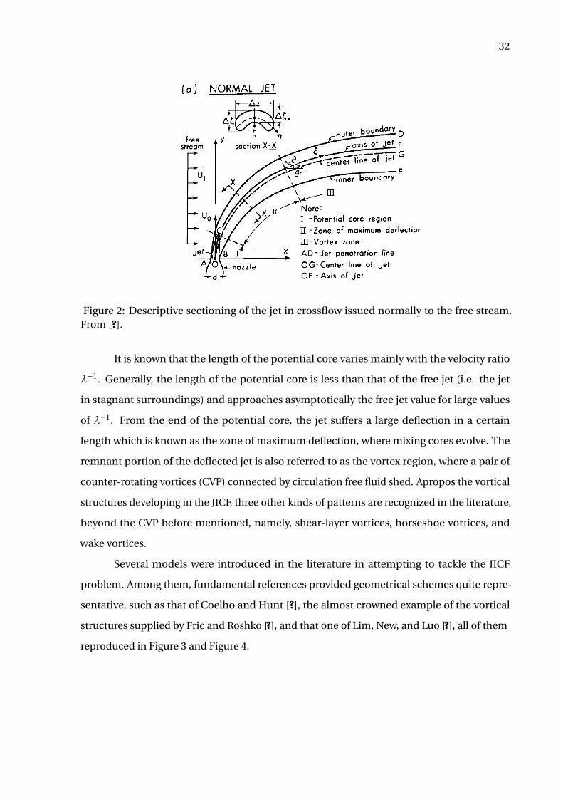
For the physical evaluation pertinent to the JICF, we refer to the presentation by

Rajaratnam [?] diagrammed in Figure 2 as a descriptive sectioning of the jet issued normally

to the free stream. As explained therein, the stagnation pressure exerted by the free stream is

responsible for deflecting the jet. Due to the turbulent mixing developing on the periphery of

the jet, the outer layers lose part of their momentum and hence are easily deflected, bringing

forth a characteristic kidney shape for the jet. As the jet hits the free stream, there is a central

region of relatively shear free flow. This region specified by the lengthOC is generally known

as the potential core region. When the jet-to-crossflow velocity ratio λ−1 = U j

U∞ is relatively

greater than 4, the point C is located directly over the center of the jet. For smaller values, the

point C is pushed downwind.

31

(a) (b)

(c) (d)

Figure 1: Images from internet sites exemplifying physical conditions in which JICF configura-tions are detected: (a) an AV-8B Harrier aircraft during vertical taking-off process (from [?]); (b)atomization of an aircraft engine liquid fuel jet in a crossflow (from [?]); (c) a large plume risingup from a fire on an oil rig in the Gulf of Mexico (from [?]), and (d) gas flow being expelled outto the atmosphere from the big chimney of the Esjberg Power Station, in Denmark (from [?].

32

Figure 2: Descriptive sectioning of the jet in crossflow issued normally to the free stream.From [?].

It is known that the length of the potential core varies mainly with the velocity ratio

λ−1. Generally, the length of the potential core is less than that of the free jet (i.e. the jet

in stagnant surroundings) and approaches asymptotically the free jet value for large values

of λ−1. From the end of the potential core, the jet suffers a large deflection in a certain

length which is known as the zone of maximum deflection, where mixing cores evolve. The

remnant portion of the deflected jet is also referred to as the vortex region, where a pair of

counter-rotating vortices (CVP) connected by circulation free fluid shed. Apropos the vortical

structures developing in the JICF, three other kinds of patterns are recognized in the literature,

beyond the CVP before mentioned, namely, shear-layer vortices, horseshoe vortices, and

wake vortices.

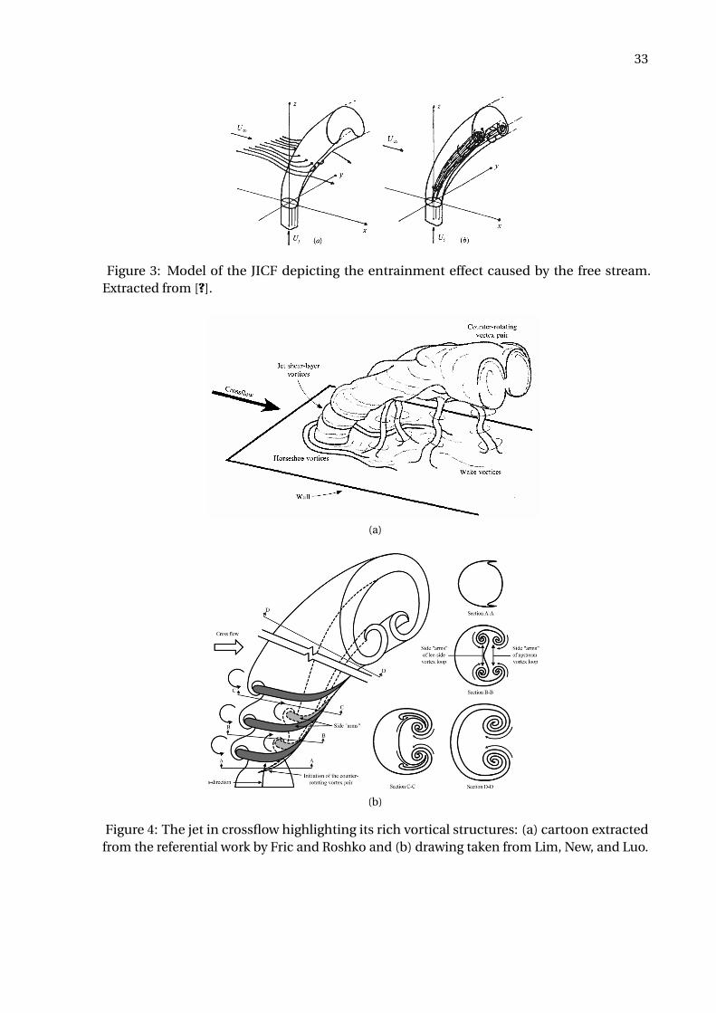
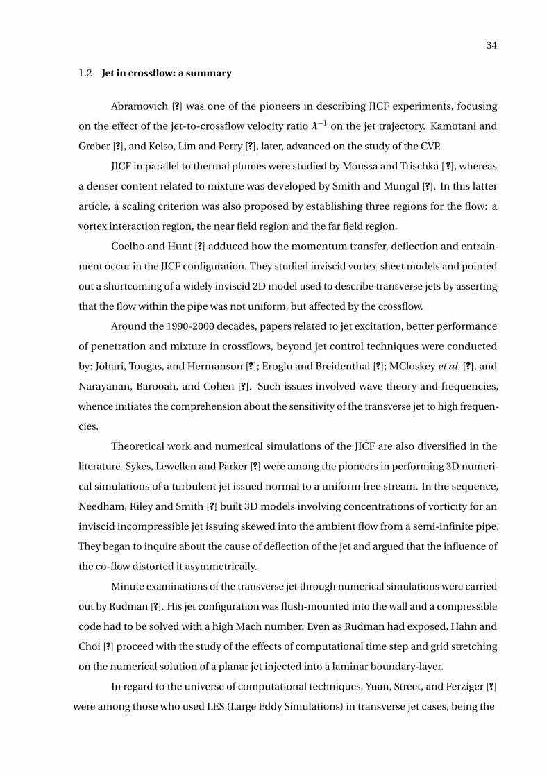
Several models were introduced in the literature in attempting to tackle the JICF

problem. Among them, fundamental references provided geometrical schemes quite repre-

sentative, such as that of Coelho and Hunt [?], the almost crowned example of the vortical

structures supplied by Fric and Roshko [?], and that one of Lim, New, and Luo [?], all of them

reproduced in Figure 3 and Figure 4.

33

Figure 3: Model of the JICF depicting the entrainment effect caused by the free stream.Extracted from [?].

(a)

(b)

Figure 4: The jet in crossflow highlighting its rich vortical structures: (a) cartoon extractedfrom the referential work by Fric and Roshko and (b) drawing taken from Lim, New, and Luo.

34

1.2 Jet in crossflow: a summary

Abramovich [?] was one of the pioneers in describing JICF experiments, focusing

on the effect of the jet-to-crossflow velocity ratio λ−1 on the jet trajectory. Kamotani and

Greber [?], and Kelso, Lim and Perry [?], later, advanced on the study of the CVP.

JICF in parallel to thermal plumes were studied by Moussa and Trischka [ ?], whereas

a denser content related to mixture was developed by Smith and Mungal [?]. In this latter

article, a scaling criterion was also proposed by establishing three regions for the flow: a

vortex interaction region, the near field region and the far field region.

Coelho and Hunt [?] adduced how the momentum transfer, deflection and entrain-

ment occur in the JICF configuration. They studied inviscid vortex-sheet models and pointed

out a shortcoming of a widely inviscid 2D model used to describe transverse jets by asserting

that the flow within the pipe was not uniform, but affected by the crossflow.

Around the 1990-2000 decades, papers related to jet excitation, better performance

of penetration and mixture in crossflows, beyond jet control techniques were conducted

by: Johari, Tougas, and Hermanson [?]; Eroglu and Breidenthal [?]; MCloskey et al. [?], and

Narayanan, Barooah, and Cohen [?]. Such issues involved wave theory and frequencies,

whence initiates the comprehension about the sensitivity of the transverse jet to high frequen-

cies.

Theoretical work and numerical simulations of the JICF are also diversified in the

literature. Sykes, Lewellen and Parker [?] were among the pioneers in performing 3D numeri-

cal simulations of a turbulent jet issued normal to a uniform free stream. In the sequence,

Needham, Riley and Smith [?] built 3D models involving concentrations of vorticity for an

inviscid incompressible jet issuing skewed into the ambient flow from a semi-infinite pipe.

They began to inquire about the cause of deflection of the jet and argued that the influence of

the co-flow distorted it asymmetrically.

Minute examinations of the transverse jet through numerical simulations were carried

out by Rudman [?]. His jet configuration was flush-mounted into the wall and a compressible

code had to be solved with a high Mach number. Even as Rudman had exposed, Hahn and

Choi [?] proceed with the study of the effects of computational time step and grid stretching

on the numerical solution of a planar jet injected into a laminar boundary-layer.

In regard to the universe of computational techniques, Yuan, Street, and Ferziger [?]

were among those who used LES (Large Eddy Simulations) in transverse jet cases, being the

35

first researchers to deal with and solve the problem of the turbulent boundary-layer appearing

in the jet flush-mounted into a wall. Not long ago, Muppidi and Mahesh [?] used DNS (Direct

Numerical Simulations) to study the near field of incompressible round jets in crossflow

with the goal of obtaining improved correlations for transverse jet trajectories. Additionally,

Keimasi, and Taeibi-Rahni [?] came up with techniques based on RANS (Reynolds-Averaged

Navier Stokes) equations for the 3D turbulent flow of square jets injected perpendicularly into

a crossflow handling several different turbulence models.

Special contents about JICF are found in Karagozian, Cortelezzi and Soldati [?], in a

seemingly ceremonial paper by [?], describing a fifty years history about the transverse jet as

well as in meticulous synopses organized by Karagozian [?], [?] and Mahesh [?].

1.3 Selected research milestone

JICF research is plenteous; hence, it is infeasible and impractical to build a full and

unfailing milestone that wraps each issue in a whole. For this reason, this section will cover a

compendium of selected references.

1.3.1 Issues on linear stability

Liquid sheets, stability analysis for inviscid jets and instabilities in viscous jets are

issues covered in Lin’s book [?], in which we will be anchored to single out important remarks

bis in idem. Despite its literary worth, other good references about shear flows such as the

books by Chandrasekhar [?] and by Schmid and Henningson [?] should be appreciated, though

this latter lacks in text about jets. Huerre and Monkewitz [?] is one of the most known papers

on local and global instabilities, where spatially developing open shear flows are carefully

reviewed.

Batchelor and Gill [?] considered temporally growing disturbances to perform a LSA

of the parallel free jet and were followed by Michalke [?], who obtained Strouhal numbers

for different momentum thickness of the free jet – the Strouhal number gives a sight of

the sensitiveness of open shear flows to perturbations and noises and it is defined by St =fr e f Lr e f /Ur e f . Michalke’s results relied on a hyperbolic-tangent velocity profile widely known

in literature. In others papers [?], [?], [?] he examined the instability mechanism occurring in

mixing layers and concluded that spatially growing disturbances were responsible for it.

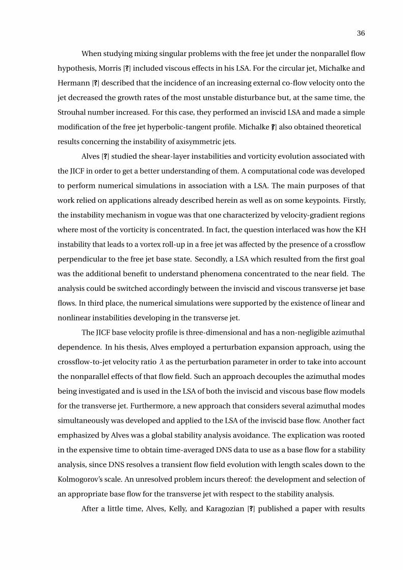
36

When studying mixing singular problems with the free jet under the nonparallel flow

hypothesis, Morris [?] included viscous effects in his LSA. For the circular jet, Michalke and

Hermann [?] described that the incidence of an increasing external co-flow velocity onto the

jet decreased the growth rates of the most unstable disturbance but, at the same time, the

Strouhal number increased. For this case, they performed an inviscid LSA and made a simple

modification of the free jet hyperbolic-tangent profile. Michalke [?] also obtained theoretical

results concerning the instability of axisymmetric jets.

Alves [?] studied the shear-layer instabilities and vorticity evolution associated with

the JICF in order to get a better understanding of them. A computational code was developed

to perform numerical simulations in association with a LSA. The main purposes of that

work relied on applications already described herein as well as on some keypoints. Firstly,

the instability mechanism in vogue was that one characterized by velocity-gradient regions

where most of the vorticity is concentrated. In fact, the question interlaced was how the KH

instability that leads to a vortex roll-up in a free jet was affected by the presence of a crossflow

perpendicular to the free jet base state. Secondly, a LSA which resulted from the first goal

was the additional benefit to understand phenomena concentrated to the near field. The

analysis could be switched accordingly between the inviscid and viscous transverse jet base

flows. In third place, the numerical simulations were supported by the existence of linear and

nonlinear instabilities developing in the transverse jet.

The JICF base velocity profile is three-dimensional and has a non-negligible azimuthal

dependence. In his thesis, Alves employed a perturbation expansion approach, using the

crossflow-to-jet velocity ratio λ as the perturbation parameter in order to take into account

the nonparallel effects of that flow field. Such an approach decouples the azimuthal modes

being investigated and is used in the LSA of both the inviscid and viscous base flow models

for the transverse jet. Furthermore, a new approach that considers several azimuthal modes

simultaneously was developed and applied to the LSA of the inviscid base flow. Another fact

emphasized by Alves was a global stability analysis avoidance. The explication was rooted

in the expensive time to obtain time-averaged DNS data to use as a base flow for a stability

analysis, since DNS resolves a transient flow field evolution with length scales down to the

Kolmogorov’s scale. An unresolved problem incurs thereof: the development and selection of

an appropriate base flow for the transverse jet with respect to the stability analysis.

After a little time, Alves, Kelly, and Karagozian [?] published a paper with results

37

supplied by the stability analysis of the inviscid transverse jet, in which both the jet and

co-flow had the same density. A correction was made in the solution of Coelho and Hunt [ ?]

therein because of an error found in one of the second-order kinematic conditions derived by

the authors. Through this correction, the main conclusions of Alves were that positive and

negative helical modes for the transverse jet had slightly different growth rates, implying a

lack of symmetry for the KH instability arising in the transverse jet. Such an approach was

affirmed to be the first mathematical verification that even low-level crossflows can produce

weak asymmetries in the transverse jet.

In a two-piece paper series, Megerian et al. [?] and Alves et al. [?] showed both experi-

mental and theoretical studies upon the transverse jet. Megerian’s study provided a detailed

exploration of the near field shear-layer instabilities associated with the transverse jet. Jet

injection from nozzles which are flush as well as elevated with respect to the tunnel wall

were explored experimentally for jet-to-crossflow velocity ratios λ−1 in the range 1 ≤λ−1 ≤ 10

and with jet Reynolds numbers of 2000 and 3000. The results indicated that the nature of

the transverse jet instability is significantly different than that of the free jet, and that the

instability changes in character as the crossflow velocity is increased. They proposed ex-

planations for the differences previously observed in transverse jets controlled by strong

forcing in order to improve techniques for the transverse jet penetration control, mixing, and

spread. On the other hand, Alves presented a local LSA for the subinterval λ−1 > 4 using two

different base flows for the transverse jet and predicting the maximum spatial growth rate

for the disturbances through a expansion in powers of λ. This way, the free jet results could

be reached as λ−1 →∞. His results matched accordingly to Megerian’s experiments, thus

suggesting that the convective instability occurs in ratios above 4 and that the instability is

strengthened as λ−1 is decreased. Consistency of his findings with experiments provided

powerful evidence of the dominance of the convectively unstable axisymmetric mode, at least

in the regime λ−1 > 4.

Still considering the expansion in λ, Kelly and Alves [?] reached a uniformly valid

asymptotic solution for the transverse jet. This exercise was accompanied by a LSA in which

the inviscid vortex sheet analysis of Coelho and Hunt was extended so including asymptotic

analysis of the viscous shear layers that formed along the boundaries of the jet. The instability

that gives rise to the near field vortices after developing an asymptotic solution for the three-

dimensional base flow was investigated and its validity for large values of the Reynolds number

38

and small λ was pointed out. By using asymptotic methods, they derived a solution of the NS

equations valid under some conditions for the transverse jet near field. This achievement led

to a more accurate description of the basic flow.

Until now the citations were entwined in the sense of a local stability analysis. Some

contributions on global stability analysis, in turn, are mentioned forth. Bagheri et al. [?],

at first glance, went ahead in taking up a simulation-based global stability analysis of the

viscous three-dimensional JICF considering a steady exact solution to the NS equations, which

showed that the JICF is characterized by self-sustained global oscillations for a jet-to-crossflow

velocity ratio of 3. By suppressing global instabilities by selective frequency damping, they

asserted that the JICF is, in fact, globally unstable and must be placed into this category of

flows. They verified that not only the most unstable global modes with high frequencies

are compact and represent localized wave packets on the CVP, but also that the existence of

global eigenmodes justifies the global stability approach as an appropriate tool to describe

the inherent and dominant dynamics of the JICF.

Davitian et al. [?] studied the transition of the transverse jet shear layer to global

instability in the near field by quantifying the growth of disturbances at several locations along

and about the jet shear layer. Moreover, frequency tracking and response of the transverse jet

to very strong single-mode forcing were applied. It was evidenced that the flush transverse

jet’s near field shear layer becomes globally unstable when λ−1 is within or below a critical

range near 3. According to the authors, this work is characterized as a support tool to improve

strategies for the transverse jet control, since this field has been widely developed.

Ilak et al. [?] published a brief comment on the DNS of a jet in crossflow at low values of

the jet-to-crossflow velocity ratioλ−1, in which they mention the observation of hairpin-like

vortices. A part of this paper is sustained by results from Schlatter’s et al.work [?]. In the latter,

the jet is studied numerically by considering the maximum velocity of the parabolic profile.

Their modelling imposed an inhomogeneous boundary condition at the crossflow wall and

the results showed that two fundamental frequencies – a high one and another low one –

are present in the flow tied to self-sustained oscillations. They used nonlinear DNS, modal

decomposition into global linear eigenmodes, and proper orthogonal decompostion modes.

In a recent publication, Ilak et al. [?] analyzed a bifurcation found from DNS at low

values of the jet-to-crossflow velocity ratio λ−1, precisely occurring at λ−1 = 0.675. As λ−1

increased, it was showed that the flow evolved from simple periodic vortex shedding (a

39

limit cycle) to more complicated quasi-periodic behaviour before coming into turbulence.

Additionally, a LSA was also performed to predict qualitative data about the dynamics of the

nonlinear effects.

1.3.2 Other references

New, Lim and Luo [?] reported the results of an experimental investigation on the

effects of jet velocity profiles on the flow field of a round JICF using laser-induced fluorescence

and digital particle-image velocimetry techniques (DPIV). Though top hat and parabolic jet

velocity profiles with the mass ratios ranging from 2.3 to 5.8 were considered, in the case of the

shear-layer associated to a parabolic profile of JICF, there was an increase in jet penetration

and a reduction in the near-field entrainment of crossflow fluid.

DNS was used by Muppidi and Mahesh [?] to study a round turbulent jet in a laminar

crossflow. Turbulent kinetic energy budgets were computed for this flow and it was shown

that the near field is far from a state of turbulence. Additionally, it was observed in the near

field that the peak of kinetic energy production was close to the leading edge, while the peak

dissipation was observed toward the trailing edge of the jet. Velocity and turbulent intensity

profiles from the simulation were also compared to some profiles obtained from experiments,

and a good agreement was exhibited. Emphatic points in that treatise was the observation

that past the jet exit, the flow is not close to established canonical flows on which most models

appear to be based.

One year later, Muppidi and Mahesh [?] used DNS to study passive scalar transport

and mixing in a round turbulent jet, in a laminar crossflow. In this case, the Schmidt number

rose up naturally as a nondimensional parameter. The scalar field was used to compute

entrainment of the crossflow fluid by the jet. It was shown that the bulk of this entrainment

occurs on the downstream side of the jet and the simulations were used to comment on the

applicability of the gradient-diffusion hypothesis to compute passive scalar mixing in the flow

field.

Denev et al. [?] followed a similar path using DNS for the flow with transport of passive

scalars and chemical reactions when studying phenomena and chemical reactions in a JICF.

Instantaneous mixing of structures and laminar to turbulent flow transition were compared

to experimental data with good agreement.

Many others fields of application of JICF have been provided with scientific research

40

in the recent years, which are out of scope of this thesis. However, some references to further

contents are listed here: pulsed jets are discussed by Muldoon et al. [?], Sau and Mahesh [?] and

Coussement et al. [?]; jet penetration and injection into subsonic and supersonic crossflow

are studied by Lee et al. [?] and Rana, Thornber and Drikakis [?], respectively; applications like

oil flare stacks, pollutant dispersion, soot emissions and flame stabilization are cited by Grout

et al. [?] and Marr et al. [?]; finally, acoustic excitation and atomization are topics related by

Hsu and Huang [?] and Herrmann [?].

1.4 Instability and breakup in two-fluid jets

This section is devoted to bring forth the overall differences among the physical

mechanisms encompassing gas-liquid and liquid-liquid jet configurations by emphasizing

the drop formation stage in order to narrow the review to the purposes of this thesis. The

physics of jets in its entirety is widely discussed by [?], whose major points relate to small

perturbations, breakup, spray formation and non-Newtonian effects.

Several studies about jet instabilities found in literature have their fundamentals upon

gas-liquid configurations unlike a minor parcel dedicated to liquid-liquid interfaces. The

historical development of the LSA applied to liquid jets issued into another immiscible liquid

starts from Tomotika [?], who has extended the inviscid LSA previously done by Rayleigh [ ?].

Although the explanation of Rayleigh pointed that the two main causes of jet instabilities

were the operation of the capillary force, whose effect is to render the jet an unstable form of

equilibrium and favour its disintegration into detached drops, and those due to the dynamical

character of the jet, his investigations were concentrated in liquids issued into calm air.

Tomotika’s equation, in turn, was a surmise to guide newer findings, among which

Meister and Scheele’s [?], [?], who have developed a drop formation theory through experimen-

tal studies with 15 liquid-liquid systems and determined the jet length from which breakup

occurs. Later, Kitamura [?] found experimentally that the Tomotika’s theory described pre-

cisely the size of the droplets when the surrounding fluid and the main fluid moved with the

same velocity. Attempts to include the relative motion of both the liquids in the LSA were

conducted by Bright [?] and [?], for instance.

These pioneer studies about the stability of free jets followed the traditional approach

41

that defines the disturbances of the jet interface η by

η= ae i (kx−ωt ), (1.1)

where x is the axial direction. Such form is initialized over the liquid surface as a result of

pressure fluctuations. Weber [?], for example, solved the NS equation for a viscous liquid jet

to obtain a characteristic equation which found the most unstable dimensionless growth rate

and wave number being, respectively

ℜω∗ = 1

2(1+3Oh1)and k∗ = 1√

2(1+3Oh1), (1.2)

where Oh1 is the Ohnesorge number of the dispersed phase. The Ohnesorge number relates

the rate between viscous forces to inertial and surface tension forces and it is written as

Oh =µr e f /√ρr e f σr e f Lr e f , or, in a different view, as Oh =p

W e/Re.

Because of its unstable behaviour, a jet cannot escape the fate of breakup, which takes

place in two major regimes, viz. the period of large drop formation and the spray formation.

The rupture of a continuous jet in drops is motivated by a couple of applications where it

occurs, such as in combustion chambers, bioprocesses, chemical emulsions, and ink jet

printing. In microfluidic devices, particularly, one resorts to crossflow T-junction geometries

for lubrication, enhanced mixture, among others, for which dripping regimes are intended.

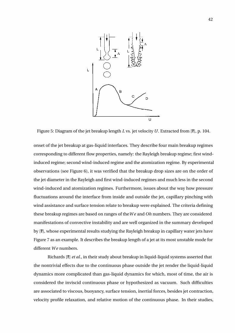
The breakup stages in a gas-liquid pair are explored in Figure 5. The distance elapsed

from the jet’s launching station until the first drop pinches off is called intact length, or

breakup length. Then, as the jet’s velocity increases, the intact length tends to achieve a

maximum value from which drops are formed. This point lies on somewhere between the

points A and B, whereas the quasi-linear uprise marked by the points before A indicates the

dripping, end of dripping and jet formation stages. Such sudden changes subsist until drops

whose radii measure almost twice the jet’s emerge. Between the points B and C, the drops

have their radii equivalent to the jet’s. Beyond the point C, droplets strip off the surface,

thereby shaping a locally atomized regime. As the depth of surface dripping renders deeper,

the average droplet radius become smaller so that the jet achieves the completely atomized

regime after the point D, i.e. the spray regime. At this regime, the droplets’ radius decreases

with the inlet jet velocity.

Lin and Reitz [?] wrote a review focused on the physical mechanisms that cause the

42

Figure 5: Diagram of the jet breakup length L vs. jet velocity U . Extracted from [?], p. 104.

onset of the jet breakup at gas-liquid interfaces. They describe four main breakup regimes

corresponding to different flow properties, namely: the Rayleigh breakup regime; first wind-

induced regime; second wind-induced regime and the atomization regime. By experimental

observations (see Figure 6), it was verified that the breakup drop sizes are on the order of

the jet diameter in the Rayleigh and first wind-induced regimes and much less in the second

wind-induced and atomization regimes. Furthermore, issues about the way how pressure

fluctuations around the interface from inside and outside the jet, capillary pinching with

wind assistance and surface tension relate to breakup were explained. The criteria defining

these breakup regimes are based on ranges of theW e and Oh numbers. They are considered

manifestations of convective instability and are well organized in the summary developed

by [?], whose experimental results studying the Rayleigh breakup in capillary water jets have

Figure 7 as an example. It describes the breakup length of a jet at its most unstable mode for

different W e numbers.

Richards [?] et al., in their study about breakup in liquid-liquid systems asserted that

the nontrivial effects due to the continuous phase outside the jet render the liquid-liquid

dynamics more complicated than gas-liquid dynamics for which, most of time, the air is

considered the inviscid continuous phase or hypothesized as vacuum. Such difficulties

are associated to viscous, buoyancy, surface tension, inertial forces, besides jet contraction,

velocity profile relaxation, and relative motion of the continuous phase. In their studies,

43

Figure 6: Experimental observation of the four breakup regimes occurring after the issuingof a round liquid jet in stagnant gas: a) Rayleigh breakup; b) first wind-induced regime; c)second wind-induced regime; d) atomization regime. Extracted from [?].

Figure 7: Breakup of a capillary water jet at the most unstable mode. Taken from [?], p. 46.

laminar flow, constant properties (e.g. viscosity, density, surface tension) and axisymmetric

disturbances formed the set of hypotheses. The VOF model was applied to predict the jet

length, shape, size of formed droplets through numerical simulations and comparisons with

experimental data were done as well. Following a similar approach based on VOF, Hommaet

al. [?] studied breakup modes for a liquid jet injected into another immiscible liquid. They

found good accordance by contrasting experimental data with their numerical code and

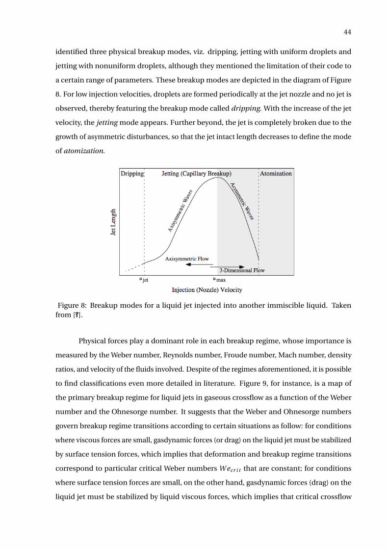
44

identified three physical breakup modes, viz. dripping, jetting with uniform droplets and

jetting with nonuniform droplets, although they mentioned the limitation of their code to

a certain range of parameters. These breakup modes are depicted in the diagram of Figure

8. For low injection velocities, droplets are formed periodically at the jet nozzle and no jet is

observed, thereby featuring the breakup mode called dripping. With the increase of the jet

velocity, the jetting mode appears. Further beyond, the jet is completely broken due to the

growth of asymmetric disturbances, so that the jet intact length decreases to define the mode

of atomization.

Figure 8: Breakup modes for a liquid jet injected into another immiscible liquid. Takenfrom [?].

Physical forces play a dominant role in each breakup regime, whose importance is

measured by the Weber number, Reynolds number, Froude number, Mach number, density

ratios, and velocity of the fluids involved. Despite of the regimes aforementioned, it is possible

to find classifications even more detailed in literature. Figure 9, for instance, is a map of

the primary breakup regime for liquid jets in gaseous crossflow as a function of the Weber

number and the Ohnesorge number. It suggests that the Weber and Ohnesorge numbers

govern breakup regime transitions according to certain situations as follow: for conditions

where viscous forces are small, gasdynamic forces (or drag) on the liquid jet must be stabilized

by surface tension forces, which implies that deformation and breakup regime transitions

correspond to particular critical Weber numbers W ecr i t that are constant; for conditions

where surface tension forces are small, on the other hand, gasdynamic forces (drag) on the

liquid jet must be stabilized by liquid viscous forces, which implies that critical crossflow

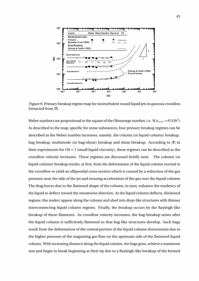
45

Figure 9: Primary breakup regime map for nonturbulent round liquid jets in gaseous crossflow.Extracted from [?].

Weber numbers are proportional to the square of the Ohnesorge number, i.e. W ecr i t =O (Oh2).

As described in the map, specific for some substances, four primary breakup regimes can be

described as the Weber number increases, namely: the column (or liquid-column) breakup,

bag breakup, multimode (or bag/shear) breakup and shear breakup. According to [?] in

their experiments for Oh < 1 (small liquid viscosity), these regimes can be described as the

crossflow velocity increases. These regimes are discussed briefly next. The column (or

liquid-column) breakup results, at first, from the deformation of the liquid column normal to

the crossflow to yield an ellipsoidal cross section which is caused by a reduction of the gas

pressure near the side of the jet and ensuing acceleration of the gas over the liquid column.

The drag forces due to the flattened shape of the column, in turn, enhance the tendency of

the liquid to deflect toward the streamwise direction. As the liquid column deflects, thickened

regions (the nodes) appear along the column and shed into drop-like structures with thinner

interconnecting liquid column regions. Finally, the breakup occurs by the Rayleigh-like

breakup of these filaments. As crossflow velocity increases, the bag-breakup arises after

the liquid column is sufficiently flattened so that bag-like structures develop. Such bags

result from the deformation of the central portion of the liquid column downstream due to

the higher pressure of the stagnating gas flow on the upstream side of the flattened liquid

column. With increasing distance along the liquid column, the bags grow, achieve a maximum

size and begin to break beginning at their tip due to a Rayleigh-like breakup of the formed

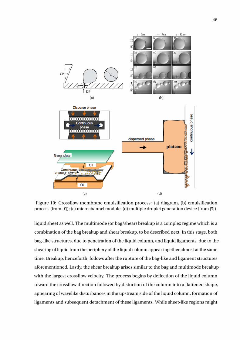
46

(a) (b)

(c) (d)

Figure 10: Crossflow membrane emulsification process: (a) diagram, (b) emulsificationprocess (from [?]); (c) microchannel module; (d) multiple droplet generation device (from [?]).

liquid sheet as well. The multimode (or bag/shear) breakup is a complex regime which is a

combination of the bag breakup and shear breakup, to be described next. In this stage, both

bag-like structures, due to penetration of the liquid column, and liquid ligaments, due to the

shearing of liquid from the periphery of the liquid column appear together almost at the same

time. Breakup, henceforth, follows after the rupture of the bag-like and ligament structures

aforementioned. Lastly, the shear breakup arises similar to the bag and multimode breakup

with the largest crossflow velocity. The process begins by deflection of the liquid column

toward the crossflow direction followed by distortion of the column into a flattened shape,

appearing of wavelike disturbances in the upstream side of the liquid column, formation of

ligaments and subsequent detachment of these ligaments. While sheet-like regions might

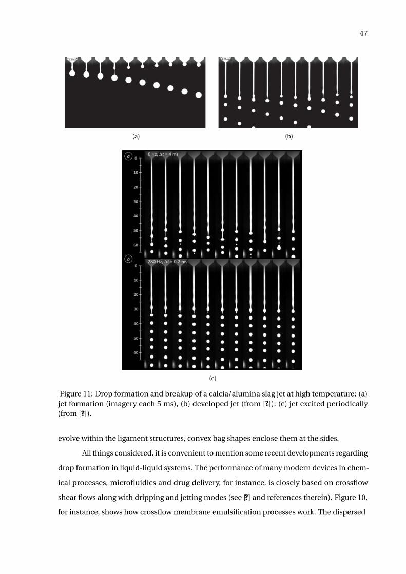
47

(a) (b)

(c)

Figure 11: Drop formation and breakup of a calcia/alumina slag jet at high temperature: (a)jet formation (imagery each 5 ms), (b) developed jet (from [?]); (c) jet excited periodically(from [?]).

evolve within the ligament structures, convex bag shapes enclose them at the sides.

All things considered, it is convenient to mention some recent developments regarding

drop formation in liquid-liquid systems. The performance of many modern devices in chem-

ical processes, microfluidics and drug delivery, for instance, is closely based on crossflow

shear flows along with dripping and jetting modes (see [?] and references therein). Figure 10,

for instance, shows how crossflow membrane emulsification processes work. The dispersed

48

phase (DP) is introduced in the continuous phase (CP) by pressure through a membrane

containing one or more pores. In turn, it is driven by the crossflow over the membrane’s

surface. The capillary breakup of jets of molten oxides (slags) at high temperatures rely on the

investigation of metal production, steelmaking processes and high-precision solder printing

technology. Figure 11 is an example of the formation and breakup of calcia/alumina slag jets.

1.5 Purposes of this thesis

Under the motivational aspects previously reviewed, the contribution of this thesis

relies on the numerical simulation of liquid-liquid dynamics, particularly focused on the drop

regime and its purposes are:

• to use an Arbitrary Lagrangian-Eulerian Finite Element Method two-phase flow code to

simulate a nonturbulent liquid jet in crossflow by considering surface tension effects,

• to apply a unit cell-based model that resorts to periodic boundary conditions along

with the moving frame reference technique to follow the jet, and

• to perform an analysis of the flow hydrodynamics in the primary breakup zone of drop

formation based on experimental liquid-liquid pairs.

49

2 TWO-PHASE FLOW MODELLING: TOOL SUITE AND OVERVIEW

This thesis encompasses many different attributes as regards computational modelling.

By this reason, the gist of this chapter is to accommodate an all-in excerpt about basilar

concepts that will be used along the forthcoming chapters. Any order of preference is taken

into account herein since each topic is viewed independently when converging to a self-

content framework. Section 2.1 centers around the ALE description of movement, an useful

tool to deal with flows whose interfaces are highly mobile; Section 2.2, in turn, revises some

important advances in two-phase flow modelling along the years organizing a brief history of

well-known numerical methods; sequentially, Section 2.3 discourses to some extent about the

physicochemical behaviour of interfaces. Lastly, Section 2.4 brings up a few procedures of

CAD design, pre-processing, and setting of FE meshes.

2.1 Arbitrary Lagrangian-Eulerian: a hybrid movement description

Roots of the ALE methodology stem from pioneer studies like Hirt’s [?] and Chan’s [?].

Nonetheless the second author proposed a generalized technique to manipulate sharp in-

terfaces in incompressible flows, the treatment of free-surface flows and material interfaces

through ALE methods continued to be envisioned by many others. Löhner [?], for instance,

points out some modern examples of interactions occurring between fluids and rigid bodies,

such as off-shore structures submerged in water, military torpedoes launched in the atmo-

sphere, and rapid trains slithering through the air while entering tunnels. Generally, wetted

bodies partially or totally submerged as well as deformable surfaces fall into the class of the

best examples.

In the Eulerian description, an observer watches with time what happens at a fixed

point in space and around it while fluid particles pass over that locus. On the other hand, in

the Lagrangian description an observer is attached to a particle and travels with it undergoing

all the changes concomitantly as the time elapses. Under a computational point of view,

both descriptions can be used to deal with several physical problems and the reasons to

opt between them should be based on suitability criteria because of their advantages and

drawbacks. Next, a brief analysis of their attributes concerning the mixed ALE description will

be done. We will follow substantially the writings by [?] and [?], although [?] is enlightening

as a further reference and [?] a more recent text which discusses generalizaties of moving

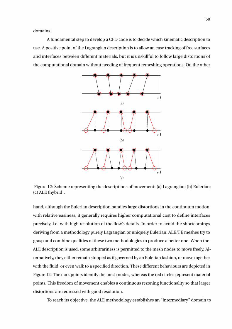
50

domains.

A fundamental step to develop a CFD code is to decide which kinematic description to

use. A positive point of the Lagrangian description is to allow an easy tracking of free surfaces

and interfaces between different materials, but it is unskillful to follow large distortions of

the computational domain without needing of frequent remeshing operations. On the other

t

(a)

t

(b)

t

(c)

Figure 12: Scheme representing the descriptions of movement: (a) Lagrangian; (b) Eulerian;(c) ALE (hybrid).

hand, although the Eulerian description handles large distortions in the continuum motion

with relative easiness, it generally requires higher computational cost to define interfaces

precisely, i.e. with high resolution of the flow’s details. In order to avoid the shortcomings

deriving from a methodology purely Lagrangian or uniquely Eulerian, ALE/FE meshes try to

grasp and combine qualities of these two methodologies to produce a better one. When the

ALE description is used, some arbitrariness is permitted to the mesh nodes to move freely. Al-

ternatively, they either remain stopped as if governed by an Eulerian fashion, or move together

with the fluid, or even walk to a specified direction. These different behaviours are depicted in

Figure 12. The dark points identify the mesh nodes, whereas the red circles represent material

points. This freedom of movement enables a continuous rezoning functionality so that larger

distortions are redressed with good resolution.

To reach its objective, the ALE methodology establishes an “intermediary” domain to

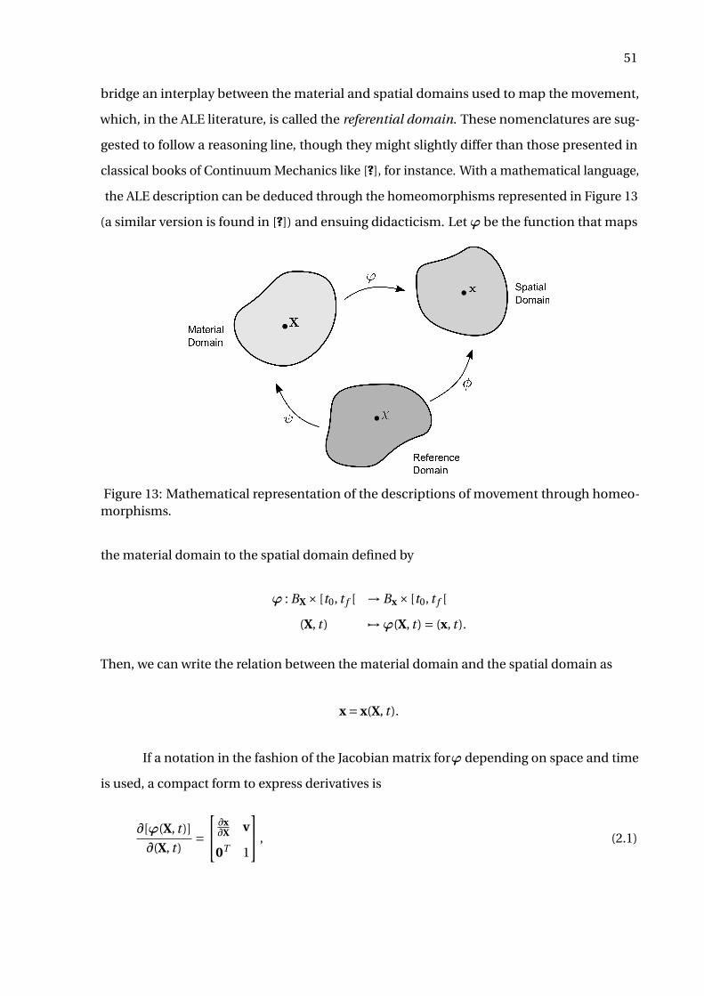
51

bridge an interplay between the material and spatial domains used to map the movement,

which, in the ALE literature, is called the referential domain. These nomenclatures are sug-

gested to follow a reasoning line, though they might slightly differ than those presented in

classical books of Continuum Mechanics like [?], for instance. With a mathematical language,

the ALE description can be deduced through the homeomorphisms represented in Figure 13

(a similar version is found in [?]) and ensuing didacticism. Letϕ be the function that maps

Reference

Domain

Spatial

Domain

Material

Domain

Figure 13: Mathematical representation of the descriptions of movement through homeo-morphisms.

the material domain to the spatial domain defined by

ϕ : BX × [t0, t f [ → Bx × [t0, t f [

(X, t ) 7→ϕ(X, t ) = (x, t ).

Then, we can write the relation between the material domain and the spatial domain as

x = x(X, t ).

If a notation in the fashion of the Jacobian matrix forϕ depending on space and time

is used, a compact form to express derivatives is

∂[ϕ(X, t )]

∂(X, t )=

∂x∂X v

0T 1

, (2.1)

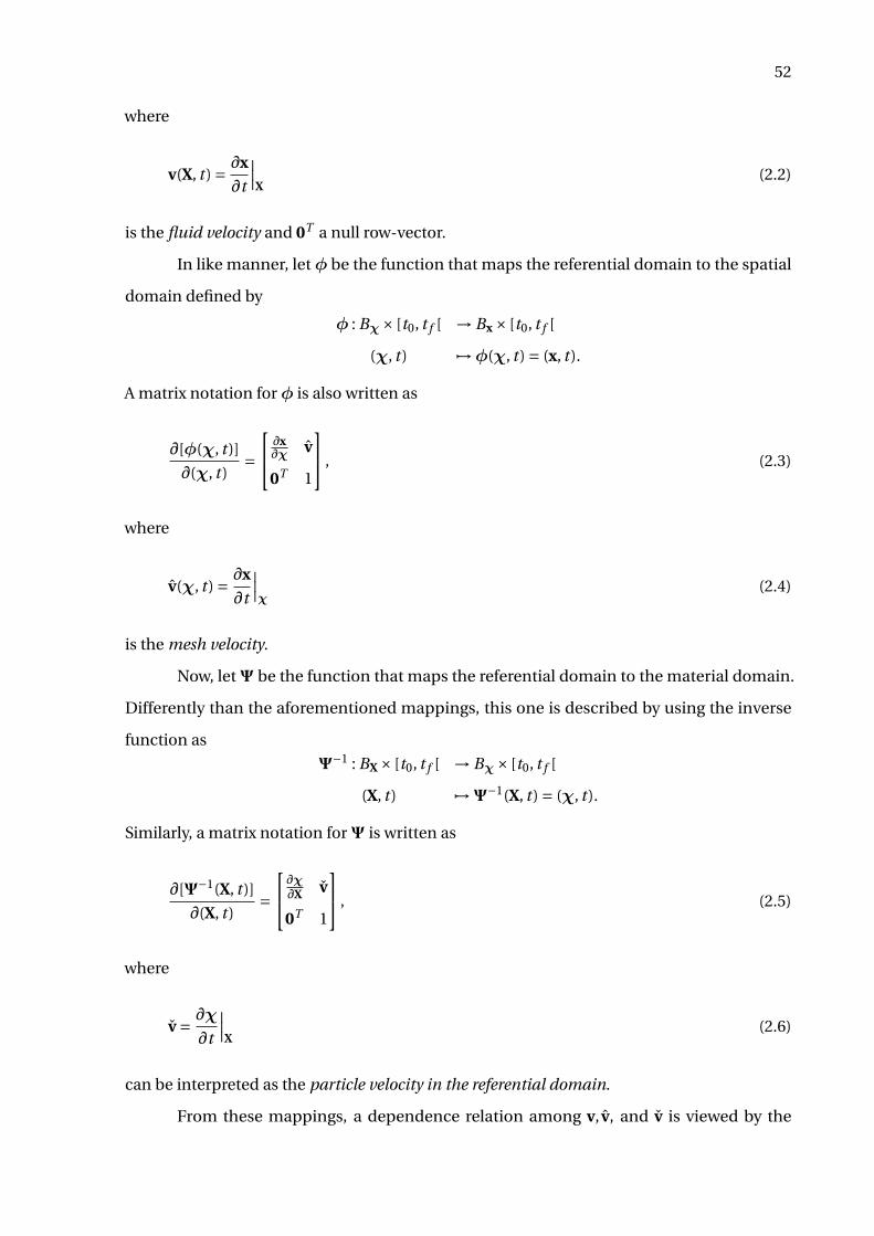
52

where

v(X, t ) = ∂x

∂t

∣∣∣X

(2.2)

is the fluid velocity and 0T a null row-vector.

In like manner, letφ be the function that maps the referential domain to the spatial

domain defined by

φ : Bχ× [t0, t f [ → Bx × [t0, t f [

(χ, t ) 7→φ(χ, t ) = (x, t ).

A matrix notation forφ is also written as

∂[φ(χ, t )]

∂(χ, t )=

∂x∂χ v

0T 1

, (2.3)

where

v(χ, t ) = ∂x

∂t

∣∣∣χ

(2.4)

is the mesh velocity.

Now, letΨ be the function that maps the referential domain to the material domain.

Differently than the aforementioned mappings, this one is described by using the inverse

function as

Ψ−1 : BX × [t0, t f [ → Bχ× [t0, t f [

(X, t ) 7→Ψ−1(X, t ) = (χ, t ).

Similarly, a matrix notation forΨ is written as

∂[Ψ−1(X, t )]

∂(X, t )=

∂χ∂X v

0T 1

, (2.5)

where

v = ∂χ

∂t

∣∣∣X

(2.6)

can be interpreted as the particle velocity in the referential domain.

From these mappings, a dependence relation among v, v, and v is viewed by the

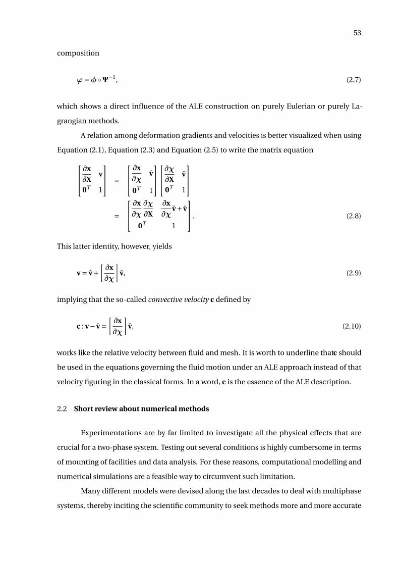
53

composition

ϕ=φΨ−1, (2.7)

which shows a direct influence of the ALE construction on purely Eulerian or purely La-

grangian methods.

A relation among deformation gradients and velocities is better visualized when using

Equation (2.1), Equation (2.3) and Equation (2.5) to write the matrix equation∂x

∂Xv

0T 1

=

∂x

∂χv

0T 1

∂χ∂X

v

0T 1

=

∂x

∂χ

∂χ

∂X

∂x

∂χv+ v

0T 1

. (2.8)

This latter identity, however, yields

v = v+[∂x

∂χ

]v, (2.9)

implying that the so-called convective velocity c defined by

c : v− v =[∂x

∂χ

]v, (2.10)

works like the relative velocity between fluid and mesh. It is worth to underline thatc should

be used in the equations governing the fluid motion under an ALE approach instead of that

velocity figuring in the classical forms. In a word, c is the essence of the ALE description.

2.2 Short review about numerical methods

Experimentations are by far limited to investigate all the physical effects that are

crucial for a two-phase system. Testing out several conditions is highly cumbersome in terms

of mounting of facilities and data analysis. For these reasons, computational modelling and

numerical simulations are a feasible way to circumvent such limitation.

Many different models were devised along the last decades to deal with multiphase

systems, thereby inciting the scientific community to seek methods more and more accurate

54

and capable of capturing the complex dynamics that springs out from these systems. Owing

to their difficult modelling, the hypothesis of homogeneity is predominantly held even in

the most promising methods. A brief history on the main developments concerning the

computational modelling of multiphase flows based on [?] is given hereafter with particular

emphasis to two-phase flows in which mobile interfaces play an important role. A point often

overlooked to be noticed here is the slight difference between themultifluid and multiphase

concepts. While the former is linked to the notion of different fluids, the latter is affixed to

the idea of a same fluid, but with different phases. In other words, while a system of kind

nitrogen-water is a multifluid one, a system vapour-water falls into a multiphase scope.

Boundary integral techniques started up from the 1950’s as tools to simulate the Stokes

flow and inviscid potential flows, whereby, later, multiphase flow simulations multiplied.

Water waves, evolution of KH and RT instabilities, generation of bubbles and droplets due to

coalescence, for example, are some cases to which these methods were applied. Even after

five decades, some authors continued to use this approach, as reviewed by [?].

As integral techniques evolved, the MAC method appeared with the contribution of [?].

In the MAC method the fluid is identified by marker particles distributed all over the fluid

region and the governing equations solved on a regular grid that covers both the fluid-filled

part and the empty part of the domain. From the MAC method, new methods arose in the

course of time. Replacing the marker particles with a marker function was the fundamental

idea to create the VOF method, which began to be widely disclosed after [?]. The advection

of the marker function, however, was a problem recognized due to the numerical diffusion

resulting from working with cell-based averaging. Although the representation of the fluid

interface per cell was improved, the accuracy of surface tension computation remained a

problem to be tackled.

In 1992, the CSF model introduced by [?] was the ground-breaking method found to

perform the calculation of surface tension, when they showed that the curvature as well as

the surface tension could be computed by taking the divergence of the discrete version of the

marker function. Next, [?] developed a conservative form of the CSF model. In the sequence,

improvements and extensions of the VOF were developed by [?], [?], and [?], to cite only a few

articles.

New approaches derived from the MAC and VOF models appeared in the decade of

1990. Unverdi and Tryggvason [?] introduced the front-tracking method in which the interface

55

was marked by connected marker points used to advect the material properties of the interface

and compute the surface tension. This method succeeded to a large set of problems. At the

same epoch, other methods came into sight, namely: the LS method by [?] (see also [?] for an

extended review), soon promulgated by [?]; the CIP method by [?], and the phase-field method

by [?], also explained in more details by [?] and reviewed by [?]. In the LS method, the interface

is identified with the zero contour of a continuous level-set function. The material properties

of the flow are reconstructed thereof through a marker function constructed from the level-set

function. This approach opposes to the VOF’s, in which a discontinuous marker function is

advected with the flow. Differently, the CIP method seeks to describe the transition at the

interface by a cubic polynomial. The phase-field method modifies the governing equations so

that the region between the fluids can be described by a thermodynamically consistent way.

As seen, many methods were devised to face the numerical difficulties arising in the

multiphase universe. In spite of their characteristics, the so-called “one-fluid” formulation

has been being featured in modern codes because of its ability to treat the different fluids or

phases as a unique domain, a reason why it is also employed in this thesis. With this in mind,

it was preferred to postpone the discussion of this topic in order to introduce it, especially, on

the pages devoted to the equations roster in Section 3.1.

2.3 Interface and surface tension

The very thin region created when two phases of matter come into contact is called

interface. To be maintained, we should suppose that both the phases have different properties,

which, at molecular level, work oppositely one another to retain the physical equilibrium.

By considering the three states of the matter – plasma interfaces are not discussed here

–, the possible types of interfaces are: gas-liquid, gas-solid, liquid-liquid, liquid-solid and

solid-solid. Owing to the proposals of this thesis, we will shorten the essay to comment on

fluids only. According to Adamson [?], a general prerequisite for the stable existence of an

interface between two phases is that the free energy of formation of the interface be positive.

Otherwise, the interface would be expanded and dispersed, thereby leading the phases to mix.

In turn, any change provoked by one phase is felt by the other while they are separated by the

interface. As an illustration, Figure 14 (adapted from [?]) clarifies the molecular imbalance

observed near an arbitrary interface of a gas-liquid system. The color gradient in the interstice

between the shaded stems is an analogy to the density jump at the interface, as it would occur

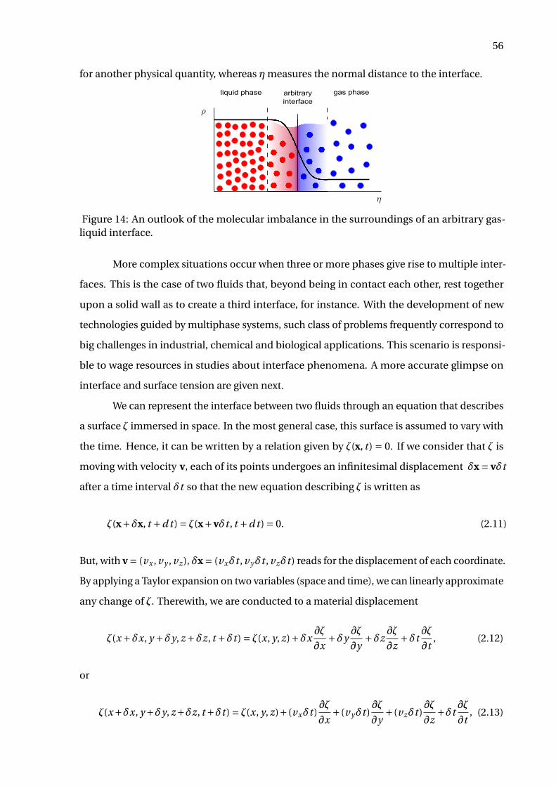
56

for another physical quantity, whereas η measures the normal distance to the interface.

gas phaseliquid phase arbitrary

interface

Figure 14: An outlook of the molecular imbalance in the surroundings of an arbitrary gas-liquid interface.

More complex situations occur when three or more phases give rise to multiple inter-

faces. This is the case of two fluids that, beyond being in contact each other, rest together

upon a solid wall as to create a third interface, for instance. With the development of new

technologies guided by multiphase systems, such class of problems frequently correspond to

big challenges in industrial, chemical and biological applications. This scenario is responsi-

ble to wage resources in studies about interface phenomena. A more accurate glimpse on

interface and surface tension are given next.

We can represent the interface between two fluids through an equation that describes

a surface ζ immersed in space. In the most general case, this surface is assumed to vary with

the time. Hence, it can be written by a relation given by ζ(x, t) = 0. If we consider that ζ is

moving with velocity v, each of its points undergoes an infinitesimal displacement δx = vδt

after a time interval δt so that the new equation describing ζ is written as

ζ(x+δx, t +d t ) = ζ(x+vδt , t +d t ) = 0. (2.11)

But, with v = (vx , vy , vz ), δx = (vxδt , vyδt , vzδt ) reads for the displacement of each coordinate.

By applying a Taylor expansion on two variables (space and time), we can linearly approximate

any change of ζ. Therewith, we are conducted to a material displacement

ζ(x +δx, y +δy, z +δz, t +δt ) = ζ(x, y, z)+δx∂ζ

∂x+δy

∂ζ

∂y+δz

∂ζ

∂z+δt

∂ζ

∂t, (2.12)

or

ζ(x+δx, y +δy, z+δz, t +δt ) = ζ(x, y, z)+(vxδt )∂ζ

∂x+(vyδt )

∂ζ

∂y+(vzδt )

∂ζ

∂z+δt

∂ζ

∂t, (2.13)

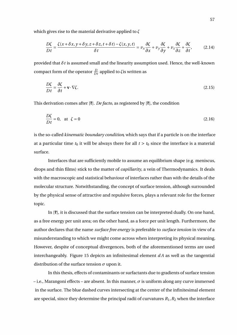
57

which gives rise to the material derivative applied to ζ

Dζ

Dt= ζ(x +δx, y +δy, z +δz, t +δt )−ζ(x, y, t )

δt= vx

∂ζ

∂x+ vy

∂ζ

∂y+ vz

∂ζ

∂z+ ∂ζ

∂t, (2.14)

provided that δt is assumed small and the linearity assumption used. Hence, the well-known

compact form of the operator DDt applied to ζis written as

Dζ

Dt= ∂ζ

∂t+v ·∇ζ. (2.15)

This derivation comes after [?]. De facto, as registered by [?], the condition

Dζ

Dt= 0, at ζ= 0 (2.16)

is the so-called kinematic boundary condition, which says that if a particle is on the interface

at a particular time t0 it will be always there for all t > t0 since the interface is a material

surface.

Interfaces that are sufficiently mobile to assume an equilibrium shape (e.g. meniscus,

drops and thin films) stick to the matter of capillarity, a vein of Thermodynamics. It deals

with the macroscopic and statistical behaviour of interfaces rather than with the details of the

molecular structure. Notwithstanding, the concept of surface tension, although surrounded

by the physical sense of attractive and repulsive forces, plays a relevant role for the former

topic.

In [?], it is discussed that the surface tension can be interpreted dually. On one hand,

as a free energy per unit area; on the other hand, as a force per unit length. Furthermore, the

author declares that the name surface free energy is preferable to surface tension in view of a

misunderstanding to which we might come across when interpreting its physical meaning.

However, despite of conceptual divergences, both of the aforementioned terms are used

interchangeably. Figure 15 depicts an infinitesimal element d A as well as the tangential

distribution of the surface tension σ upon it.

In this thesis, effects of contaminants or surfactants due to gradients of surface tension

– i.e., Marangoni effects – are absent. In this manner, σ is uniform along any curve immersed

in the surface. The blue dashed curves intersecting at the center of the infinitesimal element

are special, since they determine the principal radii of curvatures R1,R2 when the interface

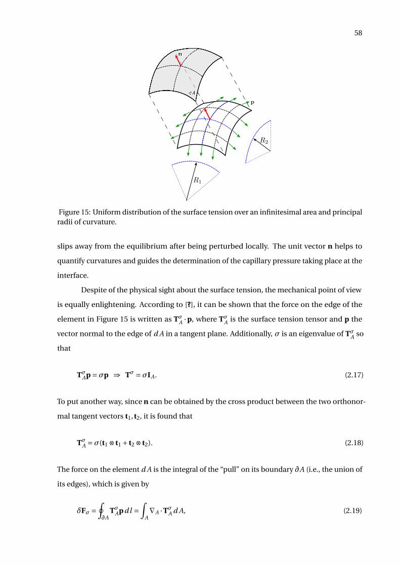
58

Figure 15: Uniform distribution of the surface tension over an infinitesimal area and principalradii of curvature.

slips away from the equilibrium after being perturbed locally. The unit vector n helps to

quantify curvatures and guides the determination of the capillary pressure taking place at the

interface.

Despite of the physical sight about the surface tension, the mechanical point of view

is equally enlightening. According to [?], it can be shown that the force on the edge of the

element in Figure 15 is written as TσA ·p, where TσA is the surface tension tensor and p the

vector normal to the edge of d A in a tangent plane. Additionally, σ is an eigenvalue of TσA so

that

TσAp =σp ⇒ Tσ =σIA. (2.17)

To put another way, since n can be obtained by the cross product between the two orthonor-

mal tangent vectors t1,t2, it is found that

TσA =σ(t1 ⊗ t1 + t2 ⊗ t2). (2.18)

The force on the element d A is the integral of the “pull” on its boundary ∂A (i.e., the union of

its edges), which is given by

δFσ =∮∂A

TσApdl =∫

A∇A ·TσA d A, (2.19)

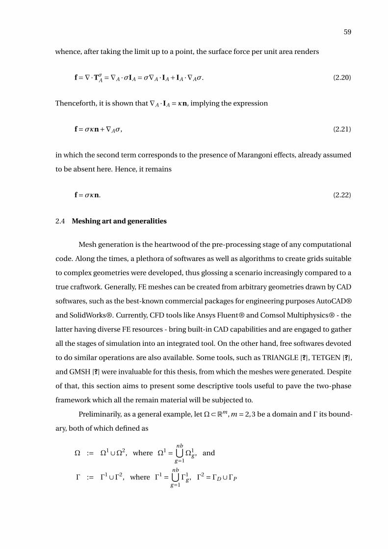
59

whence, after taking the limit up to a point, the surface force per unit area renders

f =∇·TσA =∇A ·σIA =σ∇A · IA + IA ·∇Aσ. (2.20)

Thenceforth, it is shown that ∇A · IA = κn, implying the expression

f =σκn+∇Aσ, (2.21)

in which the second term corresponds to the presence of Marangoni effects, already assumed

to be absent here. Hence, it remains

f =σκn. (2.22)

2.4 Meshing art and generalities

Mesh generation is the heartwood of the pre-processing stage of any computational

code. Along the times, a plethora of softwares as well as algorithms to create grids suitable

to complex geometries were developed, thus glossing a scenario increasingly compared to a

true craftwork. Generally, FE meshes can be created from arbitrary geometries drawn by CAD

softwares, such as the best-known commercial packages for engineering purposes AutoCAD®

and SolidWorks®. Currently, CFD tools like Ansys Fluent® and Comsol Multiphysics® - the

latter having diverse FE resources - bring built-in CAD capabilities and are engaged to gather

all the stages of simulation into an integrated tool. On the other hand, free softwares devoted

to do similar operations are also available. Some tools, such as TRIANGLE [?], TETGEN [?],

and GMSH [?] were invaluable for this thesis, from which the meshes were generated. Despite

of that, this section aims to present some descriptive tools useful to pave the two-phase

framework which all the remain material will be subjected to.

Preliminarily, as a general example, letΩ⊂Rm ,m = 2,3 be a domain and Γ its bound-

ary, both of which defined as

Ω := Ω1 ∪Ω2, where Ω1 =nb⋃

g=1Ω1

g , and

Γ := Γ1 ∪Γ2, where Γ1 =nb⋃

g=1Γ1

g , Γ2 = ΓD ∪ΓP

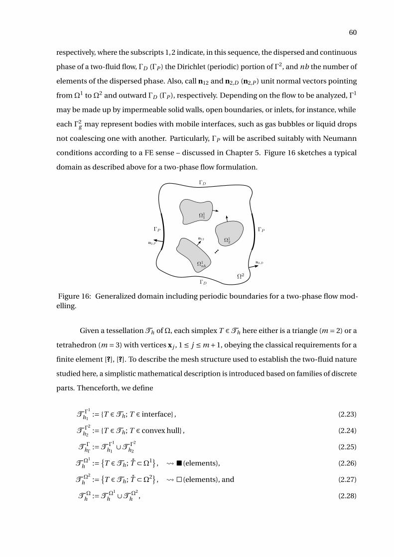
60

respectively, where the subscripts 1,2 indicate, in this sequence, the dispersed and continuous

phase of a two-fluid flow, ΓD (ΓP ) the Dirichlet (periodic) portion of Γ2, and nb the number of

elements of the dispersed phase. Also, call n12 and n2,D (n2,P ) unit normal vectors pointing

fromΩ1 toΩ2 and outward ΓD (ΓP ), respectively. Depending on the flow to be analyzed, Γ1

may be made up by impermeable solid walls, open boundaries, or inlets, for instance, while

each Γ2g may represent bodies with mobile interfaces, such as gas bubbles or liquid drops

not coalescing one with another. Particularly, ΓP will be ascribed suitably with Neumann

conditions according to a FE sense – discussed in Chapter 5. Figure 16 sketches a typical

domain as described above for a two-phase flow formulation.

Figure 16: Generalized domain including periodic boundaries for a two-phase flow mod-elling.

Given a tessellation Th ofΩ, each simplex T ∈Th here either is a triangle (m = 2) or a

tetrahedron (m = 3) with vertices x j , 1 ≤ j ≤ m +1, obeying the classical requirements for a

finite element [?], [?]. To describe the mesh structure used to establish the two-fluid nature

studied here, a simplistic mathematical description is introduced based on families of discrete

parts. Thenceforth, we define

T Γ1

h1:= T ∈Th ; T ∈ interface , (2.23)

T Γ2

h2:= T ∈Th ; T ∈ convex hull , (2.24)

T ΓhΓ

:=T Γ1

h1∪T Γ2

h2(2.25)

T Ω1

h := T ∈Th ; T ⊂Ω1 , (elements), (2.26)

T Ω2

h := T ∈Th ; T ⊂Ω2 , ä (elements), and (2.27)

T Ωh :=T Ω1

h ∪T Ω2

h , (2.28)

61

as mesh subsets. The symbol “ ” is used in Figure 17 for a graphical representation of

element families sharing an interface in a two-dimensional mesh. Despite of these mathe-

matical definitions, the computational mesh is stored into two data structures only, viz. the

area/volume mesh T Ωh , which accounts for an interior discretization and the line/surface mesh

T ΓhΓ

, which discretizes convex hulls and interfaces. Different levels of adaptive refinement h,

h1, h2 can be chosen separately for volumes, interfaces and boundaries according to the flow

conditions.

Since an interface is traced by edges or faces of the own mesh elements, a sharp

thickness is achieved satisfactorily. Therefore, this construction evinces a kind of front-

tracking method in which such an interface is identified by evaluating a nodal Heaviside

function H(x) over the elements belonging to T Γ1

h1. As pointed out by [?], it turns out that the

abrupt transition of a property φ across the interface can be smoothed with by means of the

interpolation

φ(x) =φ1H(x)+φ2(1−H(x)), ∀x of T ∈Th , φi =φ|Ωi , i = 1,2. (2.29)

Besides, we set forth

H(x j ) :=

0, if x j ∈T Ω2

h ∪T Γ2

h2

0.5, if x j ∈T Γ1

h1

1, if x j ∈T Ω1

h .

(2.30)

for the nodal evaluation. Figure 17 is an overview of elements comprising a neighbourhood of

interface highlighting the effect of the interpolation given by 2.29.

Figure 17: Mesh elements comprising the region around the discrete interface between thefluids and effect of transition caused by interpolation with the Heaviside function.

All things considered, the meshing process for the desired two-phase flow configu-

62

ration is now illustrated in Figure 18 in order to single out how the elements are connected

in such a way to create zero-thickness interfaces. The model encompasses three spherical

bodies (e.g. bubbles, or drops) dispersed into a medium that is confined inside a truncated

microchannel. Such a setup is suitable to study, for instance, the dynamics of bubbles in

microscale devices, the breakup and pre-atomization regimes ocurring in liquid jets as well

as the study of bubble interaction under PBC as will be reported later in Chapter 5. In the

same figure, at the top, the quarter of the cylindrical geometry is depicted after the cut by

two mutually perpendicular planes to the axis of revolution. As can be seen by the plotting

of the Heaviside function H(x), the whole domain as well as the interface locus are well

represented by the mesh elements. At the bottom, the overview of the entire surfaces is drawn.

An additional example for a model of a long capsule-shaped bubble typically encountered

in two-phase slug flow regimes is depicted in Figure 19, where H(x) plays the role as marker

function.

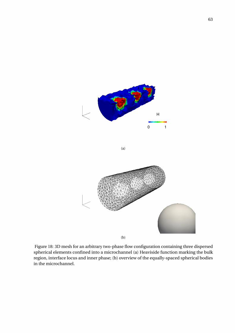
63

1

H

0

(a)

(b)

Figure 18: 3D mesh for an arbitrary two-phase flow configuration containing three dispersedspherical elements confined into a microchannel (a) Heaviside function marking the bulkregion, interface locus and inner phase; (b) overview of the equally-spaced spherical bodiesin the microchannel.

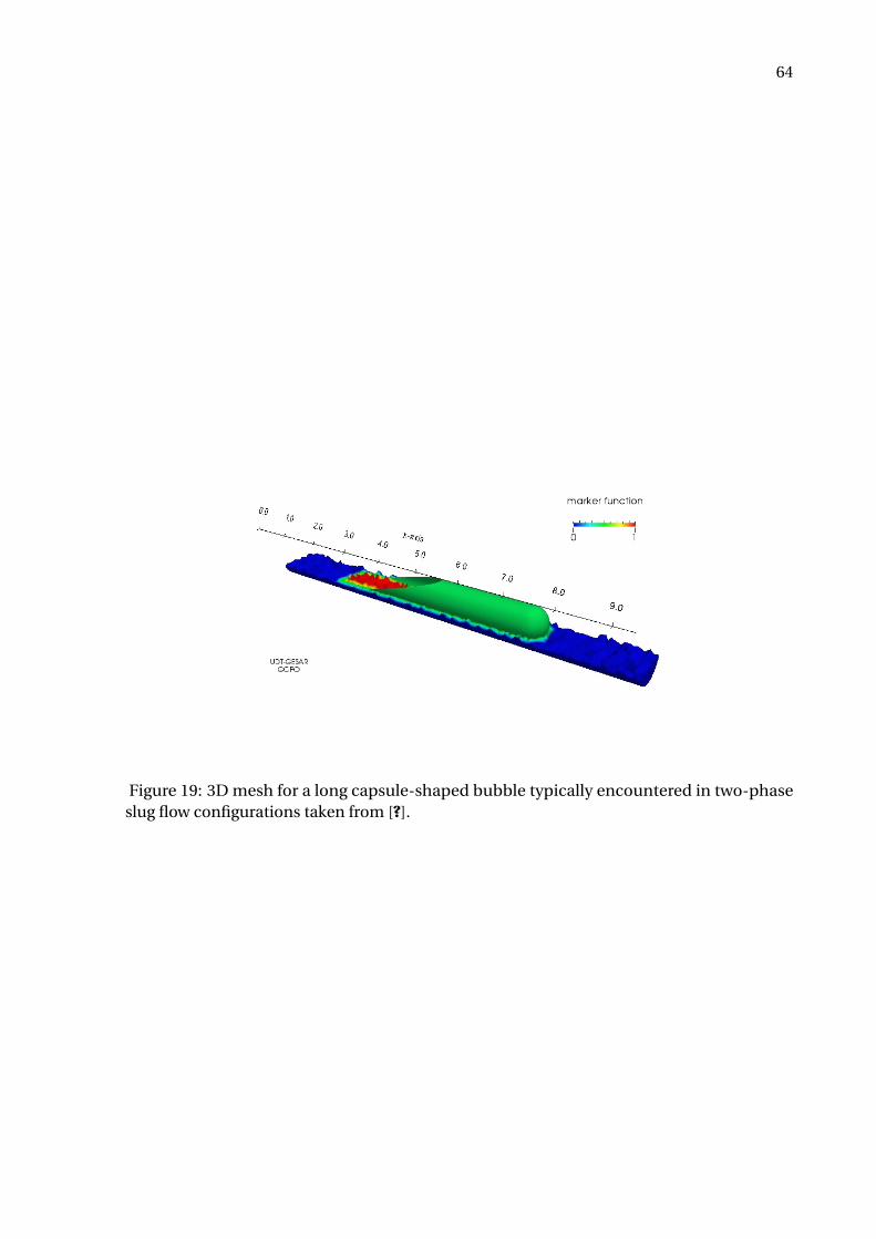
64

Figure 19: 3D mesh for a long capsule-shaped bubble typically encountered in two-phaseslug flow configurations taken from [?].

65

3 GOVERNING EQUATIONS

3.1 Principles

Conservation laws have utter relevance before any thorough study because they gather

a set of fundamental hypotheses that drive the behaviour of a physical system. This section

presents these main conservation laws and the equations governing the movement of fluids

according to the Continuum Mechanics [?]. Integral forms are the starting point in head

to a more suitable set of partial differential equations. A summarized writing, however, is

preferred instead of a detailed scrutiny upon each principle.

3.1.1 Mass conservation

The terminology body is used to specify any limited portion of space with mass m. If

we call such body B , ρt its density associated with the time, then,

m(B) =∫

Bρt dV. (3.1)

Moreover, let ∂B be the boundary of B , n a unit normal vector pointing outward and v the

velocity field of the fluid. By invoking the Divergence Theorem, it holds the equation

∫B∇· (ρv)dV =

∫∂Bρv ·nd A. (3.2)

For each point x ∈ B at a particular time t , we define

∫B

∂

∂tρ(x, t )dV = d

d t

∫Bρ(x, t )dV. (3.3)

By combining Equations (3.2) and (3.3), we write the Principle of Mass Conservation for a

control volume as

d

d t

∫Bρ(x, t )dV =−

∫∂Bρ(x, t )v(x, t ) ·n(x)d A. (3.4)

66

To put another way, Equation (3.4) declares that the mass production rate inside B is numeri-

cally equal to the net mass flux flowing out its boundary. Furthermore,

∂ρ

∂t+∇· (ρv) = 0, (3.5)

holds and it is the Continuity Equation. By using the vectorial identity ∇· (ρv) = v ·∇ρ+ρ∇·v ,

Equation (3.5) is recast to

∂ρ

∂t+v ·∇ρ+ρ(∇·v ) = 0. (3.6)

A simplified version of the continuity equation is obtained when one assumes that

the density is constant in time, thus evoking the incompressibility hypothesis DρDt = 0. Conse-

quently, Equation (3.6) is reduced to the kinematic restriction

∇·v = 0, (3.7)

3.1.2 Linear momentum

When a body B moves over a continuum, interactions among its particles as well as

between B and its surroundings can take place as distinct manifestations of forces. This

system of forces acting upon B can be written, in turn, as a pair (s,b) of functions, such that

s : N ×X −→Rm b : X −→Rm

s(n,x, t), for n ∈ N , x ∈ X at the time t are called surface forces, whereas b(x, t) are named

body forces. By assuming that the state of stress at a point x∂ ∈ ∂B is given by the symmetric

tensor Tx∂ , the total surface force on B is given by

∫∂B

Tx∂ ·nd A, (3.8)

for n unitary placed at x∂ and pointing outward B . Furthermore, since b acts upon the interior

of B , the body forces summed up correspond to

∫B

bdV. (3.9)

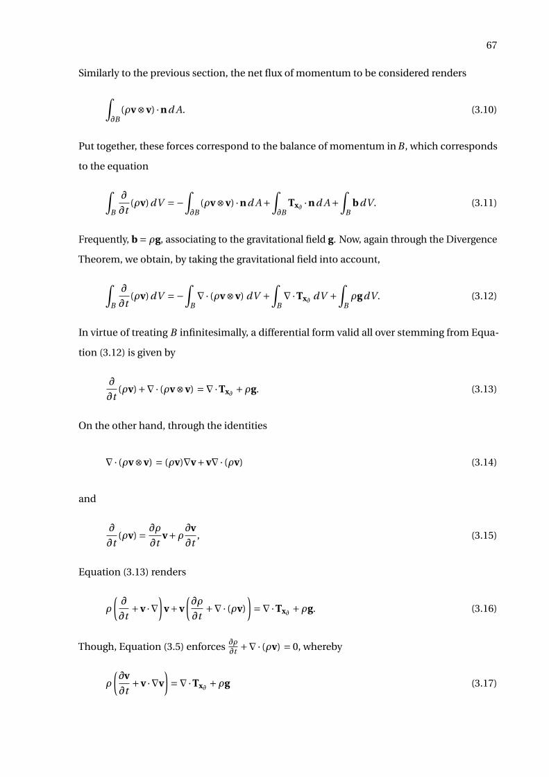
67

Similarly to the previous section, the net flux of momentum to be considered renders

∫∂B

(ρv⊗v) ·nd A. (3.10)

Put together, these forces correspond to the balance of momentum in B , which corresponds

to the equation

∫B

∂

∂t(ρv)dV =−

∫∂B

(ρv⊗v) ·nd A+∫∂B

Tx∂ ·nd A+∫

BbdV. (3.11)

Frequently, b = ρg, associating to the gravitational field g. Now, again through the Divergence

Theorem, we obtain, by taking the gravitational field into account,

∫B

∂

∂t(ρv)dV =−

∫B∇· (ρv⊗v) dV +

∫B∇·Tx∂ dV +

∫BρgdV. (3.12)

In virtue of treating B infinitesimally, a differential form valid all over stemming from Equa-

tion (3.12) is given by

∂

∂t(ρv)+∇· (ρv⊗v) =∇·Tx∂ +ρg. (3.13)

On the other hand, through the identities

∇· (ρv⊗v) = (ρv)∇v+v∇· (ρv) (3.14)

and

∂

∂t(ρv) = ∂ρ

∂tv+ρ∂v

∂t, (3.15)

Equation (3.13) renders

ρ

(∂

∂t+v ·∇

)v+v

(∂ρ

∂t+∇· (ρv)

)=∇·Tx∂ +ρg. (3.16)

Though, Equation (3.5) enforces ∂ρ∂t +∇· (ρv) = 0, whereby

ρ

(∂v

∂t+v ·∇v

)=∇·Tx∂ +ρg (3.17)

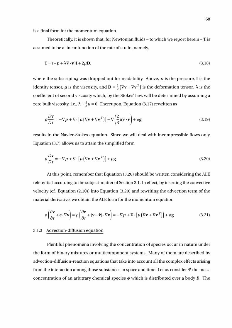
68

is a final form for the momentum equation.

Theoretically, it is shown that, for Newtonian fluids – to which we report herein –,T is

assumed to be a linear function of the rate of strain, namely,

T = (−p +λ∇·v )I+2µD, (3.18)

where the subscript x∂ was dropped out for readability. Above, p is the pressure, I is the

identity tensor, µ is the viscosity, and D = 12

(∇v +∇v T)

is the deformation tensor. λ is the

coefficient of second viscosity which, by the Stokes’ law, will be determined by assuming a

zero bulk viscosity, i.e., λ+ 23µ= 0. Thereupon, Equation (3.17) rewritten as

ρDv

Dt=−∇p +∇· [µ(∇v +∇v T )]−∇

(2

3µ∇·v

)+ρg (3.19)

results in the Navier-Stokes equation. Since we will deal with incompressible flows only,

Equation (3.7) allows us to attain the simplified form

ρDv

Dt=−∇p +∇· [µ(∇v +∇v T )]+ρg (3.20)

At this point, remember that Equation (3.20) should be written considering the ALE

referential according to the subject-matter of Section 2.1. In effect, by inserting the convective

velocity (cf. Equation (2.10)) into Equation (3.20) and rewriting the advection term of the

material derivative, we obtain the ALE form for the momentum equation

ρ

(∂v

∂t+c ·∇v

)= ρ

(∂v

∂t+ (v− v) ·∇v

)=−∇p +∇· [µ(∇v +∇v T )]+ρg (3.21)

3.1.3 Advection-diffusion equation

Plentiful phenomena involving the concentration of species occur in nature under

the form of binary mixtures or multicomponent systems. Many of them are described by

advection-diffusion-reaction equations that take into account all the complex effects arising

from the interaction among those substances in space and time. Let us considerΨ the mass

concentration of an arbitrary chemical species φ which is distributed over a body B . The

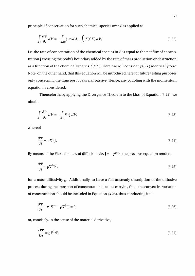
69

principle of conservation for such chemical species over B is applied as

∫B

∂Ψ

∂tdV =−

∫∂B

j ·nd A+∫

Bf (C K )dV , (3.22)

i.e. the rate of concentration of the chemical species in B is equal to the net flux of concen-

tration j crossing the body’s boundary added by the rate of mass production or destruction

as a function of the chemical kinetics f (C K ). Here, we will consider f (C K ) identically zero.

Note, on the other hand, that this equation will be introduced here for future testing purposes

only concerning the transport of a scalar passive. Hence, any coupling with the momentum

equation is considered.

Thenceforth, by applying the Divergence Theorem to the l.h.s. of Equation (3.22), we

obtain

∫B

∂Ψ

∂tdV =−

∫B∇· j dV , (3.23)

whereof

∂Ψ

∂t=−∇· j . (3.24)

By means of the Fick’s first law of diffusion, viz. j =−%∇Ψ, the previous equation renders

∂Ψ

∂t−%∇2Ψ , (3.25)

for a mass diffusivity %. Additionally, to have a full unsteady description of the diffusive

process during the transport of concentration due to a carrying fluid, the convective variation

of concentration should be included in Equation (3.25), thus conducting it to

∂Ψ

∂t+v ·∇Ψ−%∇2Ψ= 0, (3.26)

or, concisely, in the sense of the material derivative,

DΨ

Dt= %∇2Ψ. (3.27)

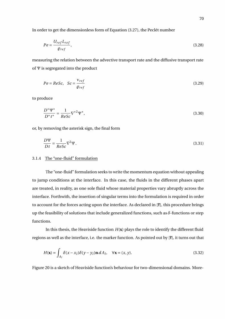
70

In order to get the dimensionless form of Equation (3.27), the Peclét number

Pe = Ur e f Lr e f

%r e f, (3.28)

measuring the relation between the advective transport rate and the diffusive transport rate

ofΨ is segregated into the product

Pe = ReSc, Sc = νr e f

%r e f(3.29)

to produce

D∗Ψ∗

D∗t∗= 1

ReSc∇∗2

Ψ∗, (3.30)

or, by removing the asterisk sign, the final form

DΨ

Dt= 1

ReSc∇2Ψ . (3.31)

3.1.4 The “one-fluid” formulation

The “one-fluid” formulation seeks to write the momentum equation without appealing

to jump conditions at the interface. In this case, the fluids in the different phases apart

are treated, in reality, as one sole fluid whose material properties vary abruptly across the

interface. Forthwith, the insertion of singular terms into the formulation is required in order

to account for the forces acting upon the interface. As declared in [?], this procedure brings

up the feasibility of solutions that include generalized functions, such asδ-functions or step

functions.

In this thesis, the Heaviside function H(x) plays the role to identify the different fluid

regions as well as the interface, i.e. the marker function. As pointed out by [?], it turns out that

H(x) =∫

AI

δ(x −xI )δ(y − yI )nd AI , ∀x = (x, y). (3.32)

Figure 20 is a sketch of Heaviside function’s behaviour for two-dimensional domains. More-

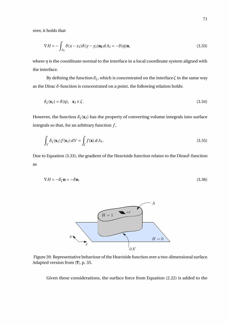
71

over, it holds that

∇H =−∫

AI

δ(x −xI )δ(y − yI )nI d AI =−δ(η)n, (3.33)

where η is the coordinate normal to the interface in a local coordinate system aligned with

the interface.

By defining the function δζ, which is concentrated on the interface ζ in the same way

as the Dirac δ-function is concentrated on a point, the following relation holds:

δζ(xI ) = δ(η), xI ∈ ζ. (3.34)

However, the function δζ(xI ) has the property of converting volume integrals into surface

integrals so that, for an arbitrary function f ,

∫Vδζ(xI ) f (xI )dV =

∫ζ

f (x)d AI . (3.35)

Due to Equation (3.33), the gradient of the Heaviside function relates to the Diracδ-function

as

∇H =−δζn =−δn. (3.36)

Figure 20: Representative behaviour of the Heaviside function over a two-dimensional surface.Adapted version from [?], p. 35.

Given these considerations, the surface force from Equation (2.22) is added to the

72

integral form through

fζδζ =σκnδζ, (3.37)

whereby, the form

f =σκ∇H (3.38)

gathering the effects of a sharp interface immersed in a arbitrary volume leads to

ρ

(∂v

∂t+ (v− v) ·∇v

)=−∇p +∇· [µ(∇v +∇v T )]+ρg+ f. (3.39)

In view of the CSF model introduced by Brackbill et al. [?], the additional surface force term

appended to Equation (3.21) is distributed throughout the volume as a body force.

Additionally, following the standard steps to establish dimensionless quantities (cf. [?]),

Equation (3.39) carried to a normalized and dimensionless domain renders

ρ∗(∂v∗

∂t+ (v∗− v∗) ·∇∗v∗

)=−∇p ∗+ 1

Re∇∗ ·

[µ∗

(∇∗v∗+∇∗v∗T

)]+ 1

F r 2ρ∗g∗+ 1

W ef∗, (3.40)

with the dimensionless groups

Re = Ur e f Lr e f

νr e f, F r = Ur e f√

gr e f Lr e f, W e =

ρr e f Lr e f U 2r e f

σr e f. (3.41)

The latter variables are measures of reference, whereas the asterisk sign identify the dimen-

sionless quantities that, without losing the generality, can, henceforth, be dropped out from

the equation when referred.

Recalling that the divergence constraint in Equation (3.7) takes the dimensionless

form

∇∗v∗ = 0, (3.42)

after dropping out the asterisk, Equations (3.40) and (3.42) form the set of dimensionless

governing equations to be solved for given initial and boundary conditions that set up a

well-posed problem. In a reduced form, the set of partial differential equations which we stick

73

to is given by

B1(v, p, f; v,ρ,µ,g) := ρ Dv

Dt+∇p − 1

Re∇· [µ(∇v+∇vT )]− 1

F r 2ρg− 1

W ef = 0 (3.43a)

B2(v) :=∇·v = 0, (3.43b)

B3(Ψ) := DΨ

Dt− 1

ReSc∇2Ψ = 0, (3.43c)

with

Dv

Dt=

(∂v

∂t+ (v− v) ·∇v

), (3.44)

so as to compact posterior algebrisms.

3.2 Applied methods

3.2.1 Projection method

Projection methods for incompressible flows have been applied since the late 1960’s,

when pioneer treatises grounded on time splitting techniques appeared [ ?], [?]. When these

methods are applied to the Navier-Stokes equations, their gist unveils the interpretation of

the equations as projections that lie on the Helmholtz-Hodge decomposition [?] (also known

as Ladyzenhskaya theorem [?]), which is stated by the following theorem:

Theorem 3.2.1 (Helmholtz-Hodge decomposition) A given vector field w is uniquely decom-

posed in a bounded domainΩwith smooth boundary ∂Ω as

w = v+∇φ, (3.45)

where φ is a scalar field and v a vector field such that ∇·v = 0 and v ·n = 0, i.e., for any vector n

normal to ∂Ω, v is parallel to ∂Ω.

Through this decomposition, velocity and pressure are uncoupled and elliptic equa-

tions are solved at each discrete time step. A organized review of projection methods given by

Guermond et al. [?] separates them into three major classes: pressure-correction methods,

velocity-correction methods, and the consistent splitting methods. In this thesis, in evocation

to the third ensemble, a canonical splitting method based on exact LU factorization in two

74

blocks coined by Lee et al. [?] as of “type D” is used to tackle the coupling. Before exposing this

particular choice, a few words about generalities of the projection method will be imparted

next underpinned by Gresho and Sani’s description (cf. [?], Section 3.16.6).

Awhile, we will write the incompressible Navier-Stokes equations in the traditional

pressure-velocity version for single-phase flows as

∂v

∂t+∇p = d (3.46)

d ≡ ν∇2v +g−v ·∇v . (3.47)

Then, from the incompressibility constraint, one verifies that

∇·v ⇒∇2p =∇·d . (3.48)

Such Poisson-like equation implies

p = (∇2 )−1∇·d (3.49)

∇p =∇(∇2 )−1∇·d , (3.50)

which, in turn, renders Equation (3.46) into

∂v

∂t= d−∇p (3.51)

= d−∇(∇2 )−1∇·d , (3.52)

= [I−∇(∇2 )−1∇· ]d, (3.53)

(3.54)

Now, two orthogonal projection operators leaping out from the latter equation can be identi-

fied, viz.

P≡ I−∇(∇2 )−1∇· (3.55)

Q≡ I−P, (3.56)

(3.57)

75

so that the projection-like form of the primary Navier-Stokes equations turns into

∂v

∂t=Pd(v) (3.58)

= d(v)−∇p (3.59)

= d(v)−Qd(v) (3.60)

with Equations (3.58) and (3.59) delivering the interpretation that the operator P removes the

gradient part of d to reveal its divergence-free part - the acceleration. Insofar that one shows

the validity of

∇·P = 0 (3.61)

∇×Q = 0, (3.62)

the complete argument for the projection is sustained by the orthogonal decomposition

d =Pd+Qd, (3.63)

i.e, whileP projects d onto the null space of divergent andPd is its divergence-free component,

Q projects d onto the null space of curl and Qd is its curl-free component.

To summarize, the recipe to obtain the solution v is stated as follows: guess ∇p;

subtract it from f(v); integrate the result for some length of time coherent to the former guess,

and project the final result to the divergence-free subspace. If the guess is perfect, then the

divergence-free solution is readily attained; otherwise, a spurious divergence is obtained. In

other words, given an incompressible velocity field at an initial time, say t = 0, that satisfies

the boundary conditions imposed, the following steps should be performed:

i) Guess ∇p(x, t ) for t ≥ 0;

ii) Solve the momentum equations alone, with ∇p(x, t ) acting as another given body force up

to a “projection time” t = tm at which an appropriate norm of ∇·v#(x, tm) reaches some

acceptable maximum value, where v#(x, tm) is an intermediary velocity not satisfying the

divergence-free constraint;

iii) Project v#(x, tm) onto the nearest divergence-free subspace to obtain v(x, tm) =Pv#(x, tm)

and retain v(x, tm) as the Navier-Stokes velocity, thus finishing one projection cycle.

76

iv) Restart from the first step.

Because of the uncertainty and fallibility of the guesses, such projection-based methods

generally have a considerable degree of sofistication to retrieve the divergence-free solution

for the equations. However, several of the proposed techniques not always admit a favourable

computational implementation, thus falling back into numerical struggles to deal with the

paramount problem of the coupling.

3.2.2 Semi-Lagrangian method

The Semi-Lagrangian method gained renown with applications turned to meteorolog-

ical predictions and climatic phenomena, as seen in [?] and [?]. Having an intrinsic property

of allowing numerical simulations managed by long time steps, its benefits to public safety,

environment, and economy can be readily recognized. Accurate climatic predictions, for

instance, may support urgent decision makings in prospective scenarios of natural disasters,

thus helping to mitigate eventual damages, restrain severe losses, and secure an entire popu-

lation. Historical background and a general review about the method’s development in the

ambit of the Meteorology is found in [?] and [?].

Aside from its original field, the use of the SL method in other scientific areas had

already been advocated [?], so that different names were coined to express it, such as Method

of Characteristics and Method Eulerian-Lagrangian [?]. Concerning its infusion into the finite

element’s ground, pristine contributions blossomed from [?], at which a numerical algorithm

to solve the advection-diffusion equation was intended.

The basis of the SL method focuses on a backward-in-time integration whereby the

fluid particle trajectories are tracked with the time and can be explained by opting for an

advection problem defined on the setΩ×τ, with τ=L−1⋃n=0

[nt , (n+1)t ] being the union of time in-

tervals. If x ∈Ω is a spatial position through which the particle χ travels and X(τ)nt ≤τ≤(n+1)t

is the solution of the differential equation

dX(τ)

dτ= v [X(τ),τ] , (3.64)

then X(τ) is the trajectory traced by the particle χ within the time range [nt , (n + 1)t ] -

77

elsewhere t n , t n+1 - and also a characteristic of the compact equation

∂Φ

∂τ+v ·∇Φ=F , (3.65)

forΦ= (Φ1,Φ2, . . . ,ΦN ), the vector of N fluid variables, and F = (F1(Φ),F2(Φ), . . . ,FN (Φ)), the

vector of N source terms.

With x and t being parameters for the trajectory, we writeX(τ) =X(x, t ;τ). By defining

x# =X(x,nt ;τ) as the position occupied by the particle at the instant τ= nt and xa =X(x, (n+1)t ;τ) as the position occupied by the particle at the instant τ= (n +1)t , the goal of the SL

method is achieved when the point xd , an approximation to the true departure point x#, is

found after integrating Equation (3.65) backward-in-time. Precisely, the determination ofxd

obeys a relation such that

(xd ,nt ;τ) ≈ (x#,nt ;τ) = (xa , (n +1)t ;τ)−∫ (n+1)t

ntv(X(x,τ))dτ, (3.66)

i.e., the observed particle reposes exactly on the site xa at the time τ= (n +1)t . Furthermore,

it holds (e.g., see Eq. 4 of [?])

Φ(xa , (n +1)t ;τ) =Φ(xd ,nt ;τ)+∫X

(dx−vdτ) ·∇Φ+∫XFdτ. (3.67)

Over the years, the numerical development of the SL method spreaded variably. The

first approximations for the trajectories, however, were based on simple straight lines. There-

after, high-order time-splitting schemes arose [?] [?]. In this thesis, the material derivative in

the form of Equation (3.65) is approximated by

DΦ

Dτ= ∂Φ

∂τ+v ·∇Φ≈ Φ(xa , (n +1)t ;τ)−Φ(xd ,nt ;τ)

∆t, (3.68)

where ∆t is the time step. In such format, the gradient ∇Φ is suppressed on the computa-

tions, meaning that the temporal rate of change plus the convective rate of change occur

instantaneously in a combined effect. In turn, xd is obtained through

(xd ;τ) = (xa ;τ)−α.

Here,α depends on a known velocity at a previous time step which is computed through the

78

linear approximation

α=∆τc(xa ,nt ;τ) =∆τ(v− v)(xa ,nt ;τ). (3.69)

Generally, such approximations result in departure points that do not match any mesh point.

Therefore,Φ(xd ,nt ;τ) must be calculated by means of some interpolation. For these reasons,

trajectory integration and interpolation are the constitutive elements of any SL scheme [?].

With the increasing development of high-order methods, theoretical error analyses as well

as optimization factor reports related to SL methods were published, of which a known

expression for the order of the advection average error of the method was derived, namely,

O

(∆t r + ∆xp+1

∆t

),

where r and p here stand for the order of trajectory integration and of interpolation, respec-

tively [?].

Although this study is based on an ALE context, the SL methodology might seem

abstruse due to its peculiarities. On the one hand, the location of the departure point through

the backwards calculation Equation (3.69) uses the relative velocity c for the advective re-

gression so as to gather both the Lagrangian and Eulerian effects as desired. On the other

hand, the velocity interpolated near the foot of the trajectory carries a purely Lagrangian

contribution that feeds back the iterative process of the computational code within each

time step only. In other words, one observes the existence of an abstract mesh which distorts

at each discrete time interval. Figure 21, adapted from [?] enlightens these events inside a

spatio-temporal context over a two-dimensional triangular mesh that disregards, for clarity,

the mesh movement caused by interference of the ALE dynamics. (T hX , (n +1)t ) and (T h

X ,nt )

represent two “slices” of the same triangulation at the two time instants analyzed.

The Eulerian mesh is drawn in thick borders, which keeps fixed along the time. The

Lagrangian mesh, on the other hand, is formed when the isolated points that spread over

the Eulerian mesh are joint by abstract edges, as seen through the gray-filled portion drawn

on the same plane where the Eulerian mesh lies on. Additionally, the long-dashed lines

starting from the points over the Lagrangian mesh at the instant τ = nt and arriving at

the points of the Eulerian mesh at the time τ = (n +1)t represent the particle trajectories.

Among them, the trajectory X(τ), leaving x# and arriving at xa is highlighted. The isolated

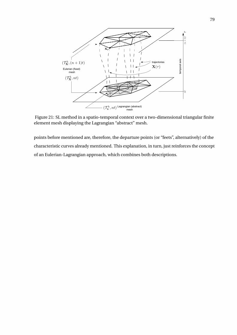
79

tem

po

ral a

xis

trajectories

Lagrangian (abstract)

mesh

Eulerian (fixed)

mesh

Figure 21: SL method in a spatio-temporal context over a two-dimensional triangular finiteelement mesh displaying the Lagrangian “abstract” mesh.

points before mentioned are, therefore, the departure points (or “feets”, alternatively) of the

characteristic curves already mentioned. This explanation, in turn, just reinforces the concept

of an Eulerian-Lagrangian approach, which combines both descriptions.

80

4 FINITE ELEMENT PROCEDURES IN TWO-PHASE FLOWS

The purpose of this chapter is to discourse about theoretical and computational

aspects of the FEM with special attention to the gas-liquid two-phase flow dynamics and

to concepts related to this thesis. A few considerations on the historical background of the

method, however, give occasion to divert out from the Fluid Dynamics momentarily for a

better clarification. This is, in turn, the object of the opening section, which has by progression

a series of theoretical topics studied in developing the FEM. The part of the text corresponding

to more applied contents comes soon after in the sequel.

4.1 Historiography and theory of the classical FEM

From the birth of the FEM as numerical method to solve partial differential equations,

the Engineering follows its remarkable uprise until the present time by recognizing it as a

robust tool capable to branch in many different facets. In reality, the term FEM was coined by

Prof. Ray W. Clough in the 1960’s after a premature version before known as Direct Stiffness

Method, although exist arguments favourable to the FEM’s creation dating back the Leibniz’s

ages between the XVII and XVIII centuries, when the variational methods were being devel-

oped. From these early times, the tied union with the Mathematics elevated the scientific

community to sovereign levels of rigour and formalism while clothing the FEM in a solid

armour. On the other hand, this process caused a bifurcation in the sense of how to interpret

the FEM, dissociating the mathematical current from the physical one. While the former was

used to see the FEM under a structural/mechanical basis, the latter accustomed the eyes

to see the FEM as a functional/variational problem, both of which getting the same results.

The analogy of dividing a domain in smaller pieces called “elements”, for instance, is not as

complete as the mathematical definition, which requires further attention.

In 1943, Courant presented the so-called Courant element, which is the fundamental

element formed by a triangle equipped with linear piecewise functions. Afterwards, many

others arose as byproducts of compositions, such as the family of Hermite elements, Argyris

elements and Crouzeix-Raviart elements, all of them derived from a triangular geometry, but

differing by the set of degrees of freedom. In this case, they consider nodal evaluations of

either only functions, or functions and directional derivatives, or still functions and higher

order derivatives. Figure 22, adapted from [?], illustrates a couple of elements. The arrows in

81

the Argyris element symbolize the normal derivative evaluated at the midpoints of the edges.

Similar ideas extend to other dimensions and geometries, producing new elements.

function

first derivative

second derivative

Figure 22: Different two-dimensional compositions: the Courant element, the Hermiteelement, the quintic Argyris triangle and the nonconforming linear Crouzeix-Raviart triangle(arranged from left to right/top to bottom).

Although the mathematics of FEM flowed independently also with considerable ad-

vancements in a functional scope concerning minimization problems and variational forms

as previously authored by Ritz and Galerkin in 1910’s decade, problems of the structural

mechanics boosted the FE research after the period of the II World War, whose interests

turned to aircraft engineering, and later, with contributions of renowned corporations, such

as IBM, NASA and Boeing. This time was essential to promote the known literature written by

Zienkiewicz [?] as well as the ascension of the sovietic influence worldwide with Friedrichs,

Petrov and Galerkin’s legacy.

In the 1970’s, several mathematical books about FEM appeared, including the Strang

& Fix’s classical book [?]. From this moment on, the most classical FEM acquired variants,

such as: the Generalized FEM (GFEM) [?], [?], which uses not only polynomial spaces as base

functions; the hp-FEM, which combines adaptive refinementh with polynomial orders p [?];

and the Extended FEM (XFEM), which embeds discontinuous functions to enrich spaces

of GFEM [?]. In addition to such an variants, the formulations currently known as SUPG

(Streamline-Upwind Petrov-Galerkin) [?], GLS (Galerkin-Least Squares) [?] and PSPG (Pressure-

Stabilized Petrov-Galerkin) play a fundamental role in the development of stabilized methods

in FE history for both compressible and incompressible dynamics. The so-called PFEM

(Particle-Finite Element Method) [?] and NEFEM (NURBS-enhanced finite element method) [?]

also correspond to different branches in the series of FE methods hitherto.

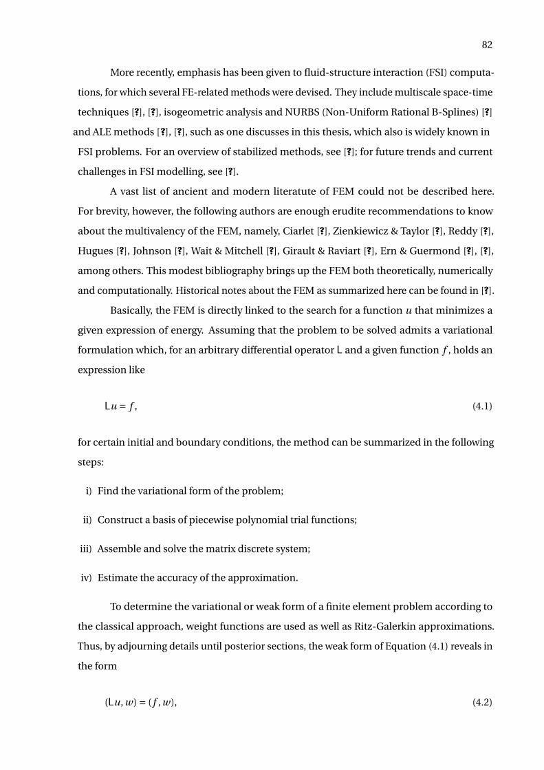
82

More recently, emphasis has been given to fluid-structure interaction (FSI) computa-

tions, for which several FE-related methods were devised. They include multiscale space-time

techniques [?], [?], isogeometric analysis and NURBS (Non-Uniform Rational B-Splines) [?]

and ALE methods [?], [?], such as one discusses in this thesis, which also is widely known in

FSI problems. For an overview of stabilized methods, see [?]; for future trends and current

challenges in FSI modelling, see [?].

A vast list of ancient and modern literatute of FEM could not be described here.

For brevity, however, the following authors are enough erudite recommendations to know

about the multivalency of the FEM, namely, Ciarlet [?], Zienkiewicz & Taylor [?], Reddy [?],

Hugues [?], Johnson [?], Wait & Mitchell [?], Girault & Raviart [?], Ern & Guermond [?], [?],

among others. This modest bibliography brings up the FEM both theoretically, numerically

and computationally. Historical notes about the FEM as summarized here can be found in [?].

Basically, the FEM is directly linked to the search for a function u that minimizes a

given expression of energy. Assuming that the problem to be solved admits a variational

formulation which, for an arbitrary differential operator L and a given function f , holds an

expression like

Lu = f , (4.1)

for certain initial and boundary conditions, the method can be summarized in the following

steps:

i) Find the variational form of the problem;

ii) Construct a basis of piecewise polynomial trial functions;

iii) Assemble and solve the matrix discrete system;

iv) Estimate the accuracy of the approximation.

To determine the variational or weak form of a finite element problem according to

the classical approach, weight functions are used as well as Ritz-Galerkin approximations.

Thus, by adjourning details until posterior sections, the weak form of Equation (4.1) reveals in

the form

(Lu, w) = ( f , w), (4.2)

83

for a given weight function w and operations of inner products (·, ·) well defined. Thenceforth,

function spaces are created to set forth approximationsu ≈ uh , f ≈ fh , so that Equation (4.2)

is written as

(Luh , wh) = ( fh , wh). (4.3)

Such discretized bilinear forms, in turn, are conducted to a n-dimensional matrix equation in

the form

Luh = b, (4.4)

of which uh = L−1b ∈Rm is the solution. Since u would be, indeed, the vector storing the exact

values of the solution evaluated pointwise on the discrete domain, the accuracy of the final

result must be estimated through an error expression as

e = ||u−uh ||, (4.5)

where e can have different norm-based definitions.

4.2 FEM for incompressible two-phase flows

The list of procedures discussed so far presented the fundamental FEM techniques

usually handled in Engineering as a whole. It matters now focusing on the FEM contribution

to the field of incompressible two-phase flows, in preparation to the contents to be discussed

in the rest of this chapter. Meanwhile, it is instructive to recall the classical definition of a

finite element (e.g., see [?], p. 19, or [?], p. 78).

Definition 4.2.1 (Finite element) Let

i) T ⊆ Rm be a compact, connected, Lipschitz subset with nonempty interior (the element

domain);

ii) P be a vector space of functions ϕ : T → Rm for some positive integer m (typically

m <= 3) (the shape functions);

iii) Y = ς1,ς2, . . . ,ςι is a basis for P′, the dual set of P (the nodal variables).

Then, (T,P ,Y ) is called a finite element.

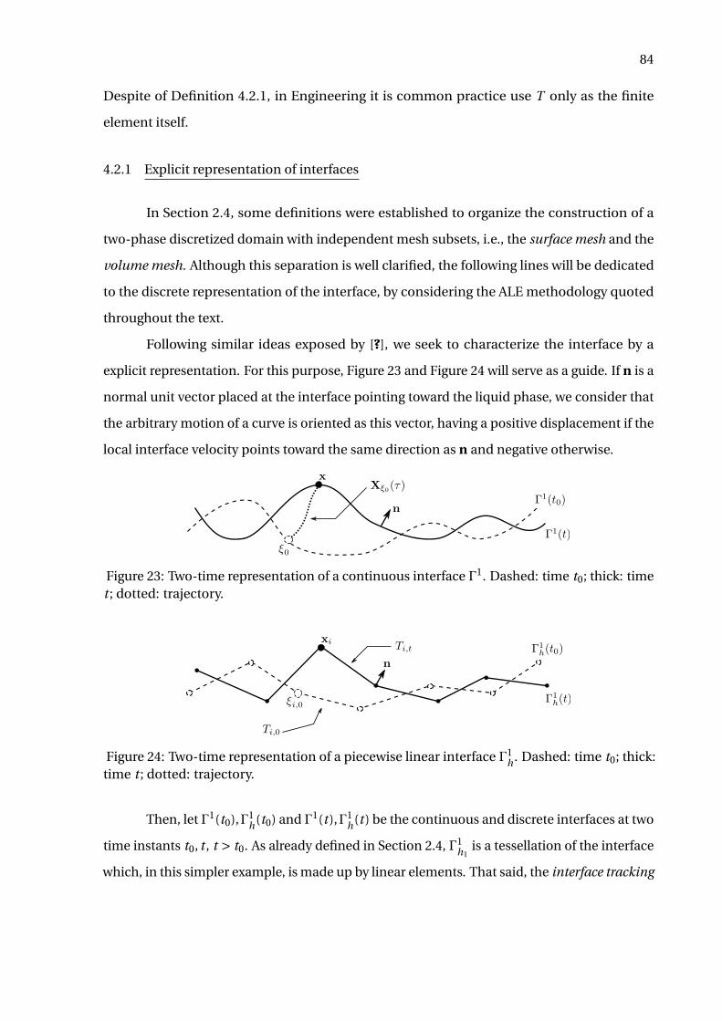
84

Despite of Definition 4.2.1, in Engineering it is common practice use T only as the finite

element itself.

4.2.1 Explicit representation of interfaces

In Section 2.4, some definitions were established to organize the construction of a

two-phase discretized domain with independent mesh subsets, i.e., the surface mesh and the

volume mesh. Although this separation is well clarified, the following lines will be dedicated

to the discrete representation of the interface, by considering the ALE methodology quoted

throughout the text.

Following similar ideas exposed by [?], we seek to characterize the interface by a

explicit representation. For this purpose, Figure 23 and Figure 24 will serve as a guide. If n is a

normal unit vector placed at the interface pointing toward the liquid phase, we consider that

the arbitrary motion of a curve is oriented as this vector, having a positive displacement if the

local interface velocity points toward the same direction as n and negative otherwise.

Figure 23: Two-time representation of a continuous interface Γ1. Dashed: time t0; thick: timet ; dotted: trajectory.

Figure 24: Two-time representation of a piecewise linear interface Γ1h . Dashed: time t0; thick:

time t ; dotted: trajectory.

Then, let Γ1(t0),Γ1h(t0) and Γ1(t ),Γ1

h(t ) be the continuous and discrete interfaces at two

time instants t0, t , t > t0. As already defined in Section 2.4, Γ1h1

is a tessellation of the interface

which, in this simpler example, is made up by linear elements. That said, the interface tracking

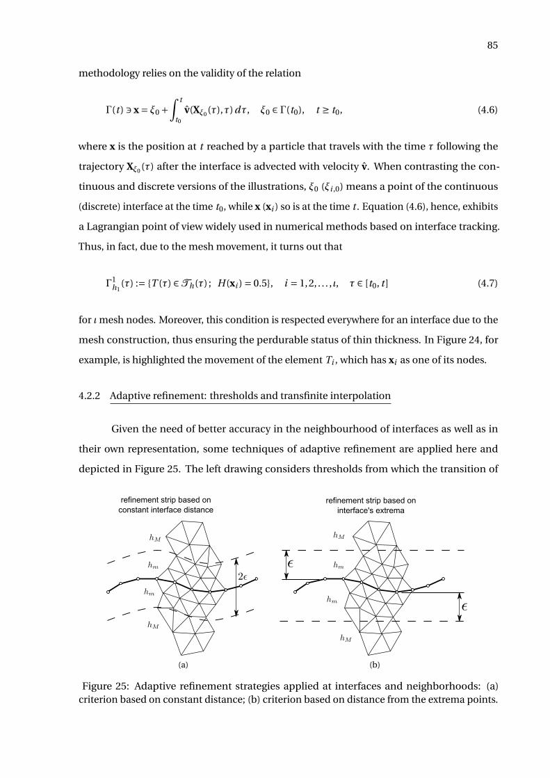
85

methodology relies on the validity of the relation

Γ(t ) 3 x = ξ0 +∫ t

t0

v(Xξ0 (τ),τ)dτ, ξ0 ∈ Γ(t0), t ≥ t0, (4.6)

where x is the position at t reached by a particle that travels with the time τ following the

trajectory Xξ0 (τ) after the interface is advected with velocity v. When contrasting the con-

tinuous and discrete versions of the illustrations, ξ0 (ξi ,0) means a point of the continuous

(discrete) interface at the time t0, while x (xi ) so is at the time t . Equation (4.6), hence, exhibits

a Lagrangian point of view widely used in numerical methods based on interface tracking.

Thus, in fact, due to the mesh movement, it turns out that

Γ1h1

(τ) := T (τ) ∈Th(τ) ; H(xi ) = 0.5, i = 1,2, . . . , ι, τ ∈ [t0, t ] (4.7)

for ι mesh nodes. Moreover, this condition is respected everywhere for an interface due to the

mesh construction, thus ensuring the perdurable status of thin thickness. In Figure 24, for

example, is highlighted the movement of the element Ti , which has xi as one of its nodes.

4.2.2 Adaptive refinement: thresholds and transfinite interpolation

Given the need of better accuracy in the neighbourhood of interfaces as well as in

their own representation, some techniques of adaptive refinement are applied here and

depicted in Figure 25. The left drawing considers thresholds from which the transition of

refinement strip based on

constant interface distance

(a)

refinement strip based on

interface's extrema

(b)

Figure 25: Adaptive refinement strategies applied at interfaces and neighborhoods: (a)criterion based on constant distance; (b) criterion based on distance from the extrema points.

86

characteristic size of the elements belonging to T Ωh takes place. They are determined by

fixing an user-defined distance ε that establishes the neighborhood Nε[Γh], which encircles

a certain topological region of space (e.g. a strip in 2D; a tube, or sphere, in 3D). On the

other hand, the right drawing uses the extrema points of a wambled interface to establish

thresholds further above of the maximum absolute or further below of the minimum absolute.

In a generalized way, we can write

hT = hm , if T ∈ Nε[Γh]

hM , if T ∉ Nε[Γh],

where h is a mean element size. That is to say, hm < hM .

In addition to thresholds, transfinite meshing can be applied for the interfaces through

a denser distribution of nodes as depicted in the drawing at right. However, differently

than the previous strategy, which can be recalled during the simulation and parametrized

over again, this method is used in the pre-processing stage simultaneously with the mesh

construction. Together with the first technique, such an approach provide a wide range of

adaptive refinement for the control parameter h relative to the interface mesh.

4.3 Variational formulation of the governing equations

4.3.1 Primitive variables

Pioneer researches introducing a variational (or weak) form of the incompressible

Navier-Stokes arose some decades ago for the single-phase universe [ ?]. On the other hand,

extensions to two-phase flows based on FE are more juvenile not only by the epoch, but also

because of variants arising from the different ways wherewith methods deal with interfaces

and curvatures (see, e.g., [?], [?], [?], [?]). The approach used here follows the same derivation

for the single-phase dynamics exposed in [?] plus the two-phase increments introduced in [?].

Therefore, most of the algebraic details will be omitted.

A recipe to obtain the weak formulation sought is given in [?] as regards as the In-

tegrated Method, which, sealed with the approach of weighted residual, is summarized as

follows: to multiply the governing equations by arbitrary test functions; to integrate them

over the domain; to apply partial integration, if necessary, and finally to impose the boundary

conditions. Above all, let us define some necessary functional settings onΩ=Ω1 ∪Ω2.

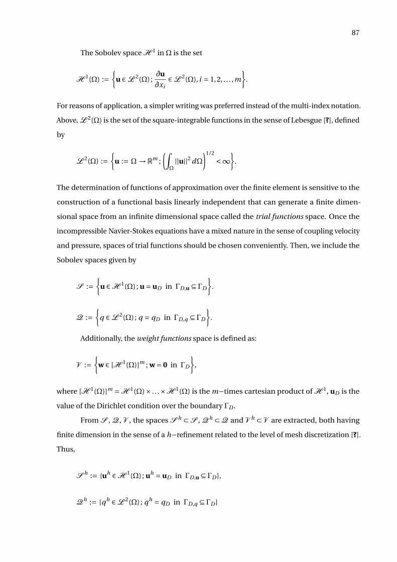
87

The Sobolev space H 1 inΩ is the set

H 1(Ω) :=

u ∈L 2(Ω) ;∂u

∂xi∈L 2(Ω), i = 1,2, . . . ,m

.

For reasons of application, a simpler writing was preferred instead of the multi-index notation.

Above, L 2(Ω) is the set of the square-integrable functions in the sense of Lebesgue [?], defined

by

L 2(Ω) :=

u := Ω→Rm ;

(∫Ω||u||2 dΩ

)1/2

<∞

.

The determination of functions of approximation over the finite element is sensitive to the

construction of a functional basis linearly independent that can generate a finite dimen-

sional space from an infinite dimensional space called the trial functions space. Once the

incompressible Navier-Stokes equations have a mixed nature in the sense of coupling velocity

and pressure, spaces of trial functions should be chosen conveniently. Then, we include the

Sobolev spaces given by

S :=

u ∈H 1(Ω) ; u = uD in ΓD,u ⊆ ΓD

.

Q :=

q ∈L 2(Ω) ; q = qD in ΓD,q ⊆ ΓD

.

Additionally, the weight functions space is defined as:

V :=

w ∈ [H 1(Ω)]m ; w = 0 in ΓD

,

where [H 1(Ω)]m =H 1(Ω)× . . .×H 1(Ω) is the m−times cartesian product of H 1, uD is the

value of the Dirichlet condition over the boundary ΓD .

From S , Q, V , the spaces S h ⊂ S , Qh ⊂ Q and V h ⊂ V are extracted, both having

finite dimension in the sense of a h−refinement related to the level of mesh discretization [?].

Thus,

S h := uh ∈H 1(Ω) ; uh = uD in ΓD,u ⊆ ΓD ,

Qh := qh ∈L 2(Ω) ; qh = qD in ΓD,q ⊆ ΓD

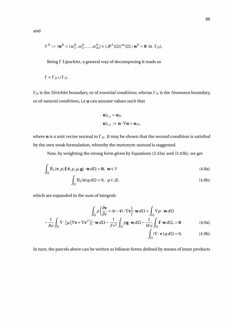
88

and

V h := wh = (w h1 , w h

2 , . . . , w hm) ∈ [H 1(Ω)]m(Ω) ; wh = 0 in ΓD ,

Being Γ Lipschitz, a general way of decomposing it reads as

Γ= ΓD ∪ΓN .

ΓD is the Dirichlet boundary, or of essential conditions, wheras ΓN is the Neumann boundary,

or of natural conditions, i.e u can assume values such that

u|ΓD = uD

u|ΓN := n ·∇u = uN ,

where n is a unit vector normal to ΓN . It may be shown that the second condition is satisfied

by the own weak formulation, whereby the metonym natural is suggested.

Now, by weighting the strong form given by Equations (3.43a) and (3.43b), we get

∫ΩB1(v, p, f; v,ρ,µ,g) ·wdΩ= 0, w ∈ V (4.8a)∫

ΩB2(v)q dΩ= 0, q ∈Q, (4.8b)

which are expanded in the sum of integrals

∫Ωρ

(∂v

∂t+ (v− v) ·∇v

)·wdΩ+

∫Ω∇p ·wdΩ

− 1

Re

∫Ω∇· [µ(∇v+∇vT )] ·wdΩ− 1

F r 2

∫Ωρg ·wdΩ− 1

W e

∫Ω

f ·wdΩ, = 0 (4.9a)∫Ω

(∇·v )q dΩ= 0. (4.9b)

In turn, the parcels above can be written as bilinear forms defined by means of inner products

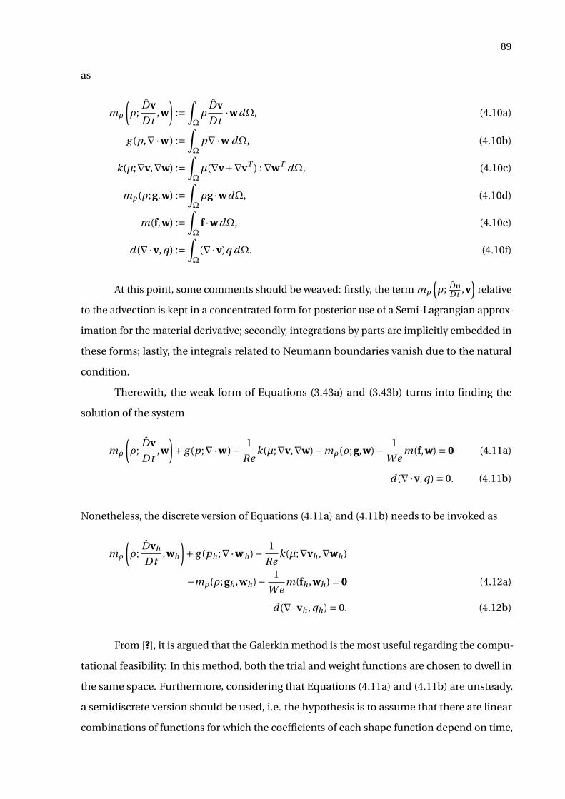
89

as

mρ

(ρ;

Dv

Dt,w

):=

∫Ωρ

Dv

Dt·wdΩ, (4.10a)

g (p,∇·w ) :=∫Ω

p∇·w dΩ, (4.10b)

k(µ;∇v,∇w) :=∫Ωµ(∇v+∇vT ) : ∇wT dΩ, (4.10c)

mρ(ρ;g,w) :=∫Ωρg ·wdΩ, (4.10d)

m(f,w) :=∫Ω

f ·wdΩ, (4.10e)

d(∇·v, q) :=∫Ω

(∇·v)q dΩ. (4.10f)

At this point, some comments should be weaved: firstly, the term mρ

(ρ; Du

Dt ,v)

relative

to the advection is kept in a concentrated form for posterior use of a Semi-Lagrangian approx-

imation for the material derivative; secondly, integrations by parts are implicitly embedded in

these forms; lastly, the integrals related to Neumann boundaries vanish due to the natural

condition.

Therewith, the weak form of Equations (3.43a) and (3.43b) turns into finding the

solution of the system

mρ

(ρ;

Dv

Dt,w

)+ g (p;∇·w )− 1

Rek(µ;∇v,∇w)−mρ(ρ;g,w)− 1

W em(f,w) = 0 (4.11a)

d(∇·v, q) = 0. (4.11b)

Nonetheless, the discrete version of Equations (4.11a) and (4.11b) needs to be invoked as

mρ

(ρ;

Dvh

Dt,wh

)+ g (ph ;∇·w h)− 1

Rek(µ;∇vh ,∇wh)

−mρ(ρ;gh ,wh)− 1

W em(fh ,wh) = 0 (4.12a)

d(∇·vh , qh) = 0. (4.12b)

From [?], it is argued that the Galerkin method is the most useful regarding the compu-

tational feasibility. In this method, both the trial and weight functions are chosen to dwell in

the same space. Furthermore, considering that Equations (4.11a) and (4.11b) are unsteady,

a semidiscrete version should be used, i.e. the hypothesis is to assume that there are linear

combinations of functions for which the coefficients of each shape function depend on time,

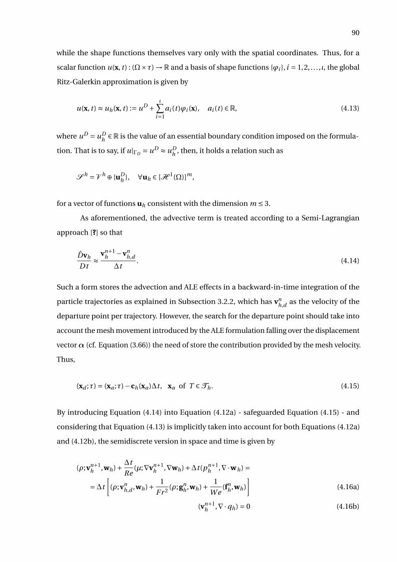
90

while the shape functions themselves vary only with the spatial coordinates. Thus, for a

scalar function u(x, t ) : (Ω×τ) →R and a basis of shape functions ϕi , i = 1,2, . . . , ι, the global

Ritz-Galerkin approximation is given by

u(x, t ) ≈ uh(x, t ) := uD +ι∑

i=1ai (t )ϕi (x), ai (t ) ∈R, (4.13)

where uD = uDh ∈R is the value of an essential boundary condition imposed on the formula-

tion. That is to say, if u|ΓD = uD ≈ uDh , then, it holds a relation such as

S h = V h ⊕ uDh , ∀uh ∈ [H 1(Ω)]m ,

for a vector of functions uh consistent with the dimension m ≤ 3.

As aforementioned, the advective term is treated according to a Semi-Lagrangian

approach [?] so that

Dvh

Dt≈

vn+1h −vn

h,d

∆t. (4.14)

Such a form stores the advection and ALE effects in a backward-in-time integration of the

particle trajectories as explained in Subsection 3.2.2, which has vnh,d as the velocity of the

departure point per trajectory. However, the search for the departure point should take into

account the mesh movement introduced by the ALE formulation falling over the displacement

vectorα (cf. Equation (3.66)) the need of store the contribution provided by the mesh velocity.

Thus,

(xd ;τ) = (xa ;τ)−ch(xa)∆t , xa of T ∈Th . (4.15)

By introducing Equation (4.14) into Equation (4.12a) - safeguarded Equation (4.15) - and

considering that Equation (4.13) is implicitly taken into account for both Equations (4.12a)

and (4.12b), the semidiscrete version in space and time is given by

(ρ;vn+1h ,wh)+ ∆t

Re(µ;∇vn+1

h ,∇wh)+∆t (pn+1h ,∇·w h) =

=∆t

[(ρ;vn

h,d ,wh)+ 1

F r 2(ρ;gn

h ,wh)+ 1

W e(fn

h ,wh)

](4.16a)

(vn+1h ,∇·qh) = 0 (4.16b)

91

Since Equations (4.16a) and (4.16b) are bilinear forms already discretized, the intro-

duction of a suitable finite element space and ensuing assembling mounting at element-level

produces matrices such that, in the respective order, these equations render

Mρvn+1 + ∆t

ReKvn+1 +∆tGpn+1 =∆t

[Mρvn

d + 1

F r 2Mρgn + 1

W eMfn

](4.17a)

Dvn+1 = 0 (4.17b)

Concisely, we can write B = Mρ+ ∆t

ReK and arrange the equations to give

B ∆tG

D 0

vn+1

pn+1

=rn

0

+bc1

bc2

(4.18)

with rn =∆t

[Mρvn

d + 1

F r 2Mρgn + 1

W eMfn

],

where bc1,bc2 are vectors accounting for Dirichlet boundary conditions of velocity and

pressure respectively, if any. Recalling that the interfacial force is given by Equation (3.38),

in order to obtain its discrete version to accompany the W e number, the following matrix

equation is written

Mfn =ΣGhn, (4.19)

where Σ = σκ(x j )I is a diagonal matrix storing the surface tension and curvature effects

distributed for all the mesh nodes and hn the discrete vector of the Heaviside function.

Consequently, the vector rn in Equation (4.18) takes the form

rn =∆t

[Mρvn

d + 1

F r 2Mρgn + 1

W eM−1

L ΣGhn]

,

now containing the inverse lumped matrix M−1L .

Taking advantage of the discussion in Subsection 3.2.1, the governing equations are

now viewed under a projection-like fully discretized format appropriate to the resulting

process derived from the FE intervention,

MN SvN S = bN S , (4.20)

92

with

MN S =B −∆tG

D 0

; vN S =vn+1

pn+1

; bN S =rn

0

+bc1

bc2

, (4.21)

whence comes out the following exact LU factorization of MN S based on lumping process of

the mass matrix Mρ (cf. [?]):

B 0

D ∆tDM−1ρ,LG

I −∆tM−1ρ,LG

0 I

vn+1

pn+1

=rn

0

+bc1

bc2

, (4.22)

The lumping technique minimizes the computational cost of inverting Mρ.

Following the straightforward LU scheme, the solution of Equation (4.22) is bipartite.

Firstly, the system

B 0

D ∆tDM−1ρ,LG

v#

pn+1

= b1

bc2

; b1 = rn +bc1 (4.23)

for the intermediary velocity v# and the pressure pn+1 is solved. Chang et al. [?] reports that

the error due to the splitting process affecting this classic fractional step method is reduced if

a unique matrix – in this case, M−1ρ,L –, is interspersed in the LU scheme. The shortcoming for

the velocity field is corrected posteriorly. Secondly, the system

I −∆tM−1ρ,LG

0 I

vn+1

pn+1

= v#

pn+1

(4.24)

is solved to find the actual values of the fields.

From Equations (4.23) and (4.24), the following routine of calculations can be posed:

Solve Bv# = b1; (4.25)

Solve Epn+1 = b2; with E =∆tDM−1ρ G; b2 = bc2 −Dv#; (4.26)

Correct vn+1 = v# +∆tM−1ρ Gpn+1. (4.27)

However, Anjos [?] generalizes the correction of the intermediary velocity field when gravity

forces and interfacial forces are assumed in the modelling of two-phase flows. The incremental

93

term e, which comes into the correction equation determines a substep for the projection

method resulting in

v#cor r = v# +∆te(g, f,F r,W e) (4.28)

and its form depends on the forces g, f, the F r and W e numbers as well as on the nature of

the flow. For pure single-phase flows without the introduction of the pressure gradient term

(discussed in the next chapter), v#cor r reduces to v#.

4.3.2 Fluid variables

To obtain a variational form for the advection-diffusion equation liable to model the

transport of variables immersed in a carrying fluid, we proceed similarly to the previous essay.

Then, we begin by introducing the Sobolev space

R :=

r ∈L 2(Ω) ; r = 0inΓD

of weight functions. Therefrom, the finite space Rh ⊂ R. In turn, we weight the Equa-

tion (3.31) to have

∫Ω

DΨ

Dtr dV = 1

ReSc

∫Ω∇2Ψr dV , r ∈R. (4.29)

Then, by analogous reasoning, the bilinear forms coming after using Equation (4.13) for u =Ψin the weighted global formulation Equation (4.29) via Galerkin produce the discrete equation

mΨ

(DΨh

Dt,rh

)+ 1

ReSckΨ(%;∇Ψh ,∇rh) = 0, (4.30)

whereof

mΨ

(Ψn+1

h ,rh)+ ∆t

ReSckΨ(%;∇Ψn+1

h ,∇rh) =∆tmΨ(Ψnh,d ,rh,P ). (4.31)

By writing the matrix form, we have

MΨΨn+1 + ∆t

ReScKΨΨ

n+1 =∆tMΨΨnd , (4.32)

94

or, with BΨ = MΨ+ ∆tReSc KΨ, the form

BΨΨn+1 = rn

Ψ+bcΨ, (4.33)

for

rnΨ =∆tMΨΨ

nd (4.34)

and bcΨ a vector containing Dirichlet boundary conditions. Along with Equation (4.18),

Equation (4.33), form a system of FE-based ordinary equations as

Bvn+1 +∆tGpn+1= rn +bc1

Dvn+1= 0+bc2

BΨΨn+1= rnΨ+bcΨ

(4.35)

with a group of generalized discrete initial and boundary conditions

vi ,0= v0,

p j ,0= p0,

Ψ j ,0=Ψ0

vi |Γ2D∨N

= vΓ2

D∨N

p j |Γ2D∨N

= pΓ2

D∨N

Ψ j |Γ2D∨N

=ΨΓ2

D∨N

(4.36)

for i = 1,2, . . . , ιv ; j = 1,2, . . . , ιs whose discrete solution for each unknown DOF over the mesh

is the triple (v,p,Ψ). Here, two remarks are enriching: i) Dirichlet or Neumann boundaries

can be chosen provided that they are consistently imposed; ii) dim(v) = 3ιv , whereas dim(p) =dim(Ψ) = ιs .

4.3.3 The stable MINI element 3D

The Navier-Stokes equations belong to a mixed universe, so that a FE space that

deals with the coupling velocity/pressure is required. Moreover, stability criteria need to be

satisfied for such space. To attire and complete the theoretical development of Section 4.3,

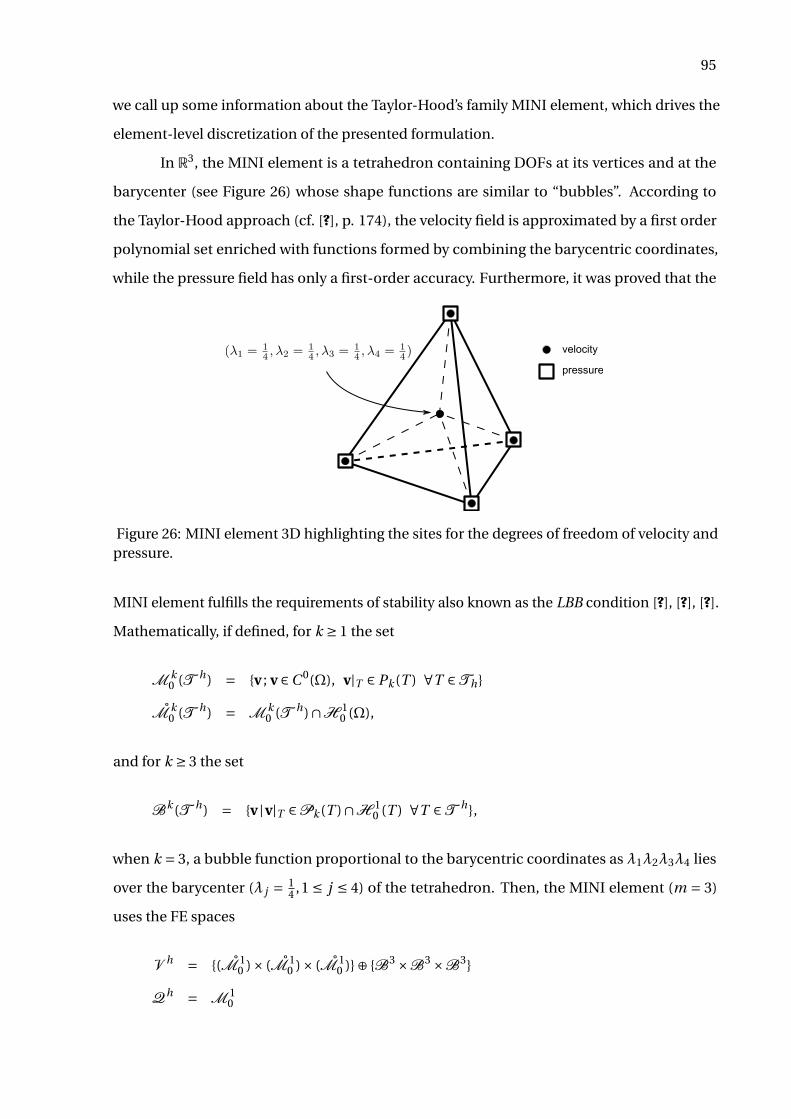
95

we call up some information about the Taylor-Hood’s family MINI element, which drives the

element-level discretization of the presented formulation.

In R3, the MINI element is a tetrahedron containing DOFs at its vertices and at the

barycenter (see Figure 26) whose shape functions are similar to “bubbles”. According to

the Taylor-Hood approach (cf. [?], p. 174), the velocity field is approximated by a first order

polynomial set enriched with functions formed by combining the barycentric coordinates,

while the pressure field has only a first-order accuracy. Furthermore, it was proved that the

velocity

pressure

Figure 26: MINI element 3D highlighting the sites for the degrees of freedom of velocity andpressure.

MINI element fulfills the requirements of stability also known as the LBB condition [?], [?], [?].

Mathematically, if defined, for k ≥ 1 the set

M k0 (T h) = v ; v ∈C 0(Ω), v|T ∈ Pk (T ) ∀T ∈Th

M k0 (T h) = M k

0 (T h)∩H 10 (Ω),

and for k ≥ 3 the set

Bk (T h) = v |v|T ∈Pk (T )∩H 10 (T ) ∀T ∈T h,

when k = 3, a bubble function proportional to the barycentric coordinates as λ1λ2λ3λ4 lies

over the barycenter (λ j = 14 ,1 ≤ j ≤ 4) of the tetrahedron. Then, the MINI element (m = 3)

uses the FE spaces

V h = (M 10 )× (M 1

0 )× (M 10 )⊕ B3 ×B3 ×B3

Qh = M 10

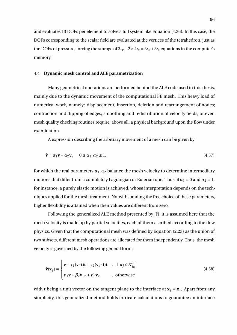
96

and evaluates 13 DOFs per element to solve a full system like Equation (4.36). In this case, the

DOFs corresponding to the scalar field are evaluated at the vertices of the tetrahedron, just as

the DOFs of pressure, forcing the storage of 3ιv +2×4ιs = 3ιv +8ιs equations in the computer’s

memory.

4.4 Dynamic mesh control and ALE parametrization

Many geometrical operations are performed behind the ALE code used in this thesis,

mainly due to the dynamic movement of the computational FE mesh. This heavy load of

numerical work, namely: displacement, insertion, deletion and rearrangement of nodes;

contraction and flipping of edges; smoothing and redistribution of velocity fields, or even

mesh quality checking routines require, above all, a physical background upon the flow under

examination.

A expression describing the arbitrary movement of a mesh can be given by

v =α1v+α2ve , 0 ≤α1,α2 ≤ 1, (4.37)

for which the real parameters α1,α2 balance the mesh velocity to determine intermediary

motions that differ from a completely Lagrangian or Eulerian one. Thus, ifα1 = 0 and α2 = 1,

for instance, a purely elastic motion is achieved, whose interpretation depends on the tech-

niques applied for the mesh treatment. Notwithstanding the free choice of these parameters,

higher flexibility is attained when their values are different from zero.

Following the generalized ALE method presented by [?], it is assumed here that the

mesh velocity is made up by partial velocities, each of them ascribed according to the flow

physics. Given that the computational mesh was defined by Equation (2.23) as the union of

two subsets, different mesh operations are allocated for them independently. Thus, the mesh

velocity is governed by the following general form:

v(x j ) =

v−γ1(v · t)t+γ2(ve · t)t , if x j ∈T Γ1

h1

β1v+β2vI ;ε+β3ve , otherwise(4.38)

with t being a unit vector on the tangent plane to the interface at x j = xI . Apart from any

simplicity, this generalized method holds intricate calculations to guarantee an interface

97

representation highly accurate through nodal scattering. As seen, Equation (4.38) works

differently for the mesh subsets. Therefore, a brief description of how each parcel interferes

on the scheme is serviceable (cf. [?], ch. 6).

By analyzing the first condition, for interface nodes, we note that v is made up by the

fluid velocity, the tangential component of the fluid velocity and the tangential component of

the elastic velocity. More precisely, once the decomposition

vI = (v · t)t+ (v ·n)n ⇒ (4.39)

vI ,n = vI − (v · t)t, (4.40)

is valid for any interface node, it turns out that the parameter γ1 is associated to the reduction

of the tangent interface nodal velocity on the flow so that the two first terms of this condition

are combined into one effect, viz. of allowing that the interface moves in the normal direction

with higher relaxation. Oppositely, γ2 is the parameter responsible for the intensity of mesh

smoothing driven by the elastic velocity ve .

On the other hand, the second condition, for volumetric nodes, aggregates compo-

nents depending on the fluid velocity, the elastic velocity and the additional smoothing

velocity vI ;ε resulting from the contribution of the interface neighbourhood ε, which we will

name “neighbourhood-based velocity”. In turn, it turns out that β1 controls the Lagrangian

motion of the volume mesh, whereasβ2,β3 manage the intensity of mesh smoothing driven

by the neighbourhood-based velocity vI ;ε, and the elastic velocity, respectively.

4.4.1 Dynamic control techniques

In this thesis, a scheme of Laplacian smoothing is used to relocate the mesh nodes

and achieve qualitative elements through volume restriction and aspect ratio control. By con-

sidering S(i ) the “star” of the node i (elements sharing i as a common vertex), the technique

for relocation of points is given by

xi → xi :=#S∑

j∈S(i )

wi j (x j −xi ), wi j = l−1i j , (4.41)

meaning that xi moves to the new position xi within each remeshing operation. Additionally,

li j is the length of the edge joining the central node i to each node j encircling it at the star as

98

displayed in Figure 27.

Figure 27: Representations of the star S(i ) of the node i : 2D version at left and 3D versionwith the tangent plane θ at right.

Both the elastic velocity ve and the neighbourhood-based velocity vI ;ε play a remark-

able role as mesh smoothing appliances. While the former is obtained from an approximation

via uniform motion within each discrete time ∆t , the latter is computed through the arith-

metic mean among the neighbour’s velocities which are immersed into the continuous phase,

thus taking the near-field dynamics into account for the interface motion. Sequentially, they

are defined, for each node i as

ve (i ) = 1

∆t

#S∑j∈S(i )

l−1i j (x j −xi ) (4.42)

vI ;ε(i ) = 1

#S

#S∑j∈S(i )

v j (4.43)

4.4.2 Geometrical operations and remeshing appliances

To gauge harsh topological changes that an interface may undergo in virtue of the

hydrodynamics, geometrical operations are performed over the elements of the discrete

interface. Among the various appliances of the ALE/FE method discussed here, which are

intended to preserve the mesh quality as best as possible, the main operations deserving

particular attention are: node insertion (Υ+), node deletion (Υ−), edge contraction (Ξ³) and

edge flipping (ΞG) as depicted in Figure 28. For each case, a minimal patch of elements is

used as model. Such operations, symbolized by Υ+, Υ−, Ξ³ and ΞG can be interpreted as

functions whose arguments are nodes and/or edges of the interface discrete mesh. In 3D

simulations, many topological complications may arise at element-level due to inaccuracies

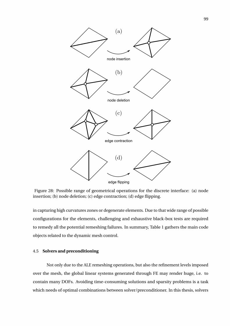
99

node insertion

node deletion

edge contraction

edge flipping

Figure 28: Possible range of geometrical operations for the discrete interface: (a) nodeinsertion; (b) node deletion; (c) edge contraction; (d) edge flipping.

in capturing high curvatures zones or degenerate elements. Due to that wide range of possible

configurations for the elements, challenging and exhaustive black-box tests are required

to remedy all the potential remeshing failures. In summary, Table 1 gathers the main code

objects related to the dynamic mesh control.

4.5 Solvers and preconditioning

Not only due to the ALE remeshing operations, but also the refinement levels imposed

over the mesh, the global linear systems generated through FE may render huge, i.e. to

contain many DOFs. Avoiding time-consuming solutions and sparsity problems is a task

which needs of optimal combinations between solver/preconditioner. In this thesis, solvers

100

Symbol Description

β1 pure Lagrangian motion controlβ2 neighbourhood-based velocity smoothingβ3 elastic-based velocity Laplacian smoothingγ1 tangent interface velocity magnitude controlγ2 elastic-based velocity and mesh qualityΥ+ node insertion operatorΥ− node deletion operatorΞ³ edge contraction operatorΞG edge flipping operator

Table 1: ALE meshing parameters for surface operations.

and preconditioners based on Krylov spaces from the PETSC library [?] were used. Although

a comparative study was not performed to find the better combination, better results were

achieved by using Pre-Conjugated Gradient (PCG) solvers together with Incomplete Cholesky

(ICC) or Incomplete LU (ILU) preconditioners.

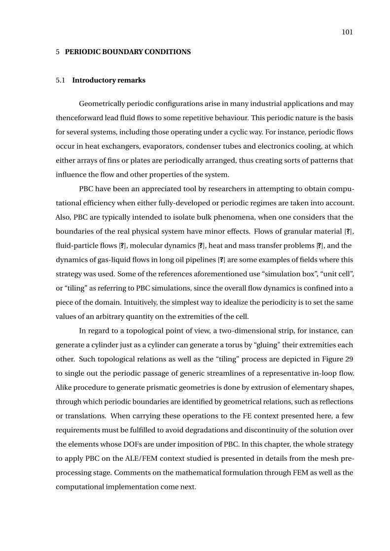
101

5 PERIODIC BOUNDARY CONDITIONS

5.1 Introductory remarks

Geometrically periodic configurations arise in many industrial applications and may

thenceforward lead fluid flows to some repetitive behaviour. This periodic nature is the basis

for several systems, including those operating under a cyclic way. For instance, periodic flows

occur in heat exchangers, evaporators, condenser tubes and electronics cooling, at which

either arrays of fins or plates are periodically arranged, thus creating sorts of patterns that

influence the flow and other properties of the system.

PBC have been an appreciated tool by researchers in attempting to obtain compu-

tational efficiency when either fully-developed or periodic regimes are taken into account.

Also, PBC are typically intended to isolate bulk phenomena, when one considers that the

boundaries of the real physical system have minor effects. Flows of granular material [?],

fluid-particle flows [?], molecular dynamics [?], heat and mass transfer problems [?], and the

dynamics of gas-liquid flows in long oil pipelines [?] are some examples of fields where this

strategy was used. Some of the references aforementioned use “simulation box”, “unit cell”,

or “tiling” as referring to PBC simulations, since the overall flow dynamics is confined into a

piece of the domain. Intuitively, the simplest way to idealize the periodicity is to set the same

values of an arbitrary quantity on the extremities of the cell.

In regard to a topological point of view, a two-dimensional strip, for instance, can

generate a cylinder just as a cylinder can generate a torus by “gluing" their extremities each

other. Such topological relations as well as the “tiling” process are depicted in Figure 29

to single out the periodic passage of generic streamlines of a representative in-loop flow.

Alike procedure to generate prismatic geometries is done by extrusion of elementary shapes,

through which periodic boundaries are identified by geometrical relations, such as reflections

or translations. When carrying these operations to the FE context presented here, a few

requirements must be fulfilled to avoid degradations and discontinuity of the solution over

the elements whose DOFs are under imposition of PBC. In this chapter, the whole strategy

to apply PBC on the ALE/FEM context studied is presented in details from the mesh pre-

processing stage. Comments on the mathematical formulation through FEM as well as the

computational implementation come next.

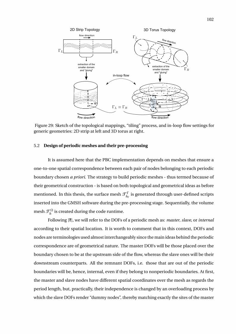
102

flow direction

extraction of the

smaller domain

and "gluing"

flow direction

2D Strip Topology

flow direction

extraction of the

smaller domain

and "gluing"

flow direction

3D Torus Topology

in-loop flow

Figure 29: Sketch of the topological mappings, “tiling” process, and in-loop flow settings forgeneric geometries: 2D strip at left and 3D torus at right.

5.2 Design of periodic meshes and their pre-processing

It is assumed here that the PBC implementation depends on meshes that ensure a

one-to-one spatial correspondence between each pair of nodes belonging to each periodic

boundary chosen a priori. The strategy to build periodic meshes - thus termed because of

their geometrical construction - is based on both topological and geometrical ideas as before

mentioned. In this thesis, the surface mesh T ΓhΓ

is generated through user-defined scripts

inserted into the GMSH software during the pre-processing stage. Sequentially, the volume

mesh T Ωh is created during the code runtime.

Following [?], we will refer to the DOFs of a periodic mesh as: master, slave, or internal

according to their spatial location. It is worth to comment that in this context, DOFs and

nodes are terminologies used almost interchangeably since the main ideas behind the periodic

correspondence are of geometrical nature. The master DOFs will be those placed over the

boundary chosen to be at the upstream side of the flow, whereas the slave ones will be their

downstream counterparts. All the remnant DOFs, i.e. those that are out of the periodic

boundaries will be, hence, internal, even if they belong to nonperiodic boundaries. At first,

the master and slave nodes have different spatial coordinates over the mesh as regards the

period length, but, practically, their independence is changed by an overloading process by

which the slave DOFs render “dummy nodes”, thereby matching exactly the sites of the master

103

DOFs. This numerical artifice eliminates the slave DOFs fictitiously to favour the periodic

simulation. Figure 30 (see a two-dimensional version in [?]) sketches the three-dimensional

geometrical rudiments to establish the PBC in the FEM. For this specific example, let ΓL , ΓR

be the master and slave periodic boundaries, respectively, and consider xL = (xL , yL , zL) ∈ ΓL ,

xR = (xR , yR , zR ) ∈ ΓR to be the master and slave nodes holding the DOFs of interest. For ι

nodes of discretization, the sequences

(xL ; ι) := xL,1,xL,2, . . . ,xL,ι

(xR ; ι) := xR,1,xR,2, . . . ,xR,ι

define the geometrical periodicity of the mesh if

xR = xL +LP eP (5.1)

for each pair of nodes.

periodic copy

process

flow direction

Figure 30: Geometrical sketch of the PBC implementation for a 3D periodic finite elementmesh.

In consequence of the geometrical identification, we achieve conformity between the

elements sharing the periodic boundaries. For a better view of this, letΩeL,1 andΩe

R,1 be the

1-ring neighbours of ΓL and ΓR , respectively, where the definition of “k-rings” here is adapted

from that used by [?] to establish the pairing between the two families of periodic elements.

In this case, the entity shared with each periodic element is the boundary surface itself. In

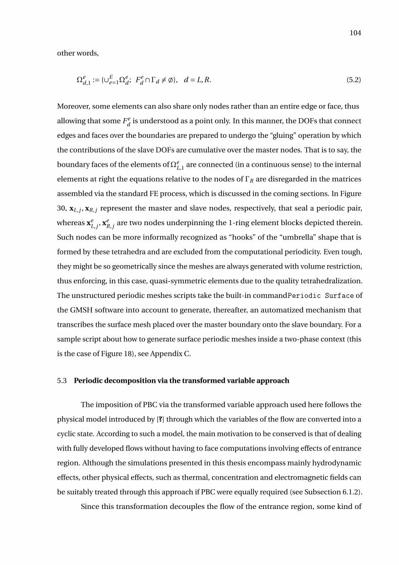
104

other words,

Ωed ,1 := ∪E

e=1Ωed ; F e

d ∩Γd 6= ;, d = L,R. (5.2)

Moreover, some elements can also share only nodes rather than an entire edge or face, thus

allowing that some F ed is understood as a point only. In this manner, the DOFs that connect

edges and faces over the boundaries are prepared to undergo the “gluing” operation by which

the contributions of the slave DOFs are cumulative over the master nodes. That is to say, the

boundary faces of the elements ofΩeL,1 are connected (in a continuous sense) to the internal

elements at right the equations relative to the nodes of ΓR are disregarded in the matrices

assembled via the standard FE process, which is discussed in the coming sections. In Figure

30, xL, j , xR, j represent the master and slave nodes, respectively, that seal a periodic pair,

whereas xeL, j , xe

R, j are two nodes underpinning the 1-ring element blocks depicted therein.

Such nodes can be more informally recognized as “hooks” of the “umbrella” shape that is

formed by these tetrahedra and are excluded from the computational periodicity. Even tough,

they might be so geometrically since the meshes are always generated with volume restriction,

thus enforcing, in this case, quasi-symmetric elements due to the quality tetrahedralization.

The unstructured periodic meshes scripts take the built-in commandPeriodic Surface of

the GMSH software into account to generate, thereafter, an automatized mechanism that

transcribes the surface mesh placed over the master boundary onto the slave boundary. For a

sample script about how to generate surface periodic meshes inside a two-phase context (this

is the case of Figure 18), see Appendix C.

5.3 Periodic decomposition via the transformed variable approach

The imposition of PBC via the transformed variable approach used here follows the

physical model introduced by [?] through which the variables of the flow are converted into a

cyclic state. According to such a model, the main motivation to be conserved is that of dealing

with fully developed flows without having to face computations involving effects of entrance

region. Although the simulations presented in this thesis encompass mainly hydrodynamic

effects, other physical effects, such as thermal, concentration and electromagnetic fields can

be suitably treated through this approach if PBC were equally required (see Subsection 6.1.2).

Since this transformation decouples the flow of the entrance region, some kind of

105

forcing term should be included in the model to compensate the fictitious in-loop domain

enforced by the periodicity. As suggested by [?], velocity and pressure should be treated

differently in the fully developed regime. While the velocity field obeys a relation of kind

v|ΓL = v|ΓR (5.3)

at the extremities of the periodic cell, the pressure drop is periodic along the cell length,

instead of the pressure field itself. For this reason, the approximation

∂p

∂(x ·eP )≈ ∆p

LP= p|ΓR

−p|ΓL

LP=β (5.4)

used for a fluid flowing along the direction eP inside a cell of period LP , describes the periodic

pressure drop by means of a constant gradient. In this manner, β can be interpreted as a

mass flow producer and taken to characterize a decomposition of the pressure field p of the

momentum equation as

p =−β(x ·eP )+ p, (5.5)

where p is related to the local motions of the flow, so that holds

p|ΓL= p|ΓR

. (5.6)

As suggested by [?], [?], p is said to be a reduced pressure. With this formulation, the prescrip-

tion of a pressure gradient is expected, as opposed to a mass flow, or inflow condition. Despite

of this interpretation valid for channel flows, for instance, the physical sense of β can take on

other facets.

On the other hand, we should bear in mind that Equation (5.5) evokes the hypothesis

on unidirectional fully-developed flow and might be the simplest way to settle a forcing term

for the periodic problem given the linear pressure drop. Furthermore,β as above is a dimen-

sional value. To be introduced in the dimensionless momentum equation, some suitable

form should be found (cf. [?], [?]). Depending on the physical situation to be simulated, β

may work as a body force acting on the fluid flow. This is the case, for instance, in a Poiseuille

starting flow (cf. Sec. 4 of [?]). For now, by choosing reference quantities for the Equation (5.5),

106

we will assume that one of its possible representative dimensionless forms is

p

ρr e f U 2r e f

=− βLr e f

ρr e f U 2r e f

(x ·eP )

Lr e f+ p

ρr e f U 2r e f

⇒ p∗ =−β∗(x∗ ·e∗P )+ p∗, (5.7)

whose asterisk can be dropped out to have consistency with Equations (3.40) and (3.42).

Therewith, the dimensionless pressure gradient term is given by

β∗ = βLr e f

ρr e f U 2r e f

=(

β

ρr e f U 2r e f

)Lr e f . (5.8)

Since the term inside parentheses is the Euler number, we will associate β∗ with this dimen-

sionless group by defining

β∗ := Euβ∗ , (5.9)

and calling Euβ∗ an Euler number associated to the pressure gradient.

After dropping out the asterisk and inserting Equation (5.7) into Equation (3.43a), the

momentum equation takes on the form

B1,P (v, p, f; v,ρ,µ,g) := ρ(∂v

∂t+ (v− v) ·∇v

)−Euβe1 +∇p

− 1

Re∇· [µ(∇v+∇vT )]− 1

F r 2ρg− 1

W ef = 0 (5.10)

being now p the unknown to be determined.

The periodic boundary conditions resulting therefrom are

v|ΓL = v|ΓR (5.11)

nL ·∇v|ΓL =−nR ·∇v|ΓR (5.12)

p|ΓL = p|ΓR (5.13)

nL ·∇p|ΓL =−nR ·∇p|ΓR . (5.14)

These relations express the need for continuity over the periodic boundaries and assure that

the primitive variables are identical both in the inlet and outlet, thus closing the connection

loop, i.e. the fluid should leave the domain just as it comes in. In the FEM context, the

Neumann conditions play a relevant role during the assembling process of the elemental

107

matrices modified for PBC which is explained in the next section. Comini et al. [?] underlined

that the normal derivative can be prescribed as zero or nonzero, depending if orthogonal or

skew incoming flow is desired, but the second case is not examined here.

5.4 FE/PBC implementation

Different methodologies are available to impose PBC through a FE approach both

in periodic and non-periodic meshes [?], [?], [?], [?], [?], [?]. Generally, they encompass the

enforcement of nodal connectivity through auxiliary lists during the assembling process of

the FE global system matrices as well as operations to suppress or sum rows and columns in

the global matrices. In this thesis, we have opted by the second strategy, which will be detailed

through the next sections.

5.4.1 Variational formulation in periodic domains

Analogous ideas to those presented in Section 4.3 are reused here to set forth a periodic

variational formulation for the governing equations. We start by putting together the forms

defined in Equations (5.10), (3.43b) and (3.43c) in the system

B1,P (v, p, f; v,ρ,µ,g)= 0

B2(v)= 0

B3(Ψ)= 0.

(5.15)

Next, define the following weight function spaces:

VP := w ∈H 1P (Ω); ∇·v = 0,v(x) = v(x+LP eP ), x ∈ ΓL

QP := q ∈L 2P (Ω); q(x) = q(x+LP eP ), x ∈ ΓL

RP := r ∈L 2P (Ω); r (x) = r (x+LP eP ), x ∈ ΓL.

These spaces gather periodic functions used to comply with a variationally consistent formu-

lation of FE with PBC (cf. [?], [?]). Thenceforward, except for the addition of periodic weight

functions (vP , qP , rP ) ∈ (VP ,QP ,RP ) in the weak form equations (cf. Equations (4.29), (4.8a)

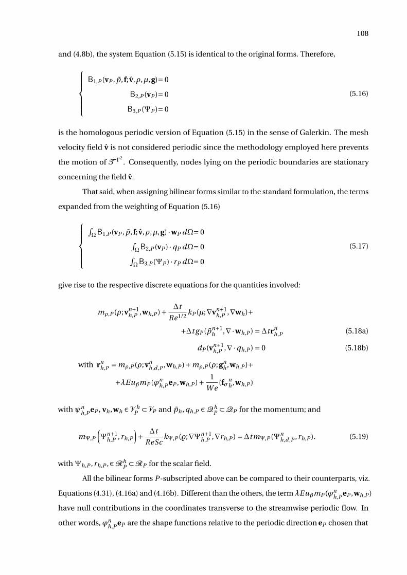
108

and (4.8b), the system Equation (5.15) is identical to the original forms. Therefore,

B1,P (vP , p, f; v,ρ,µ,g)= 0

B2,P (vP )= 0

B3,P (ΨP )= 0

(5.16)

is the homologous periodic version of Equation (5.15) in the sense of Galerkin. The mesh

velocity field v is not considered periodic since the methodology employed here prevents

the motion of T Γ2. Consequently, nodes lying on the periodic boundaries are stationary

concerning the field v.

That said, when assigning bilinear forms similar to the standard formulation, the terms

expanded from the weighting of Equation (5.16)

∫ΩB1,P (vP , p, f; v,ρ,µ,g) ·wP dΩ= 0∫

ΩB2,P (vP ) ·qP dΩ= 0∫ΩB3,P (ΨP ) · rP dΩ= 0

(5.17)

give rise to the respective discrete equations for the quantities involved:

mρ,P (ρ;vn+1h,P ,wh,P )+ ∆t

Re1/2kP (µ;∇vn+1

h,P ,∇wh)+

+∆t gP (pn+1h ,∇·wh,P ) =∆trn

h,P (5.18a)

dP (vn+1h,P ,∇·qh,P ) = 0 (5.18b)

with rnh,P = mρ,P (ρ;vn

h,d ,P ,wh,P )+mρ,P (ρ;gnh ,wh,P )+

+λEuβmP (ϕnh,P eP ,wh,P )+ 1

W e(fσ

nh ,wh,P )

with ψnh,P eP , vh ,wh ∈ V h

P ⊂ VP and ph , qh,P ∈QhP ⊂QP for the momentum; and

mΨ,P

(Ψn+1

h,P ,rh,P

)+ ∆t

ReSckΨ,P (%;∇Ψn+1

h,P ,∇rh,P ) =∆tmΨ,P (Ψnh,d ,P ,rh,P ). (5.19)

withΨh,P ,rh,P ,∈RhP ⊂RP for the scalar field.

All the bilinear forms P-subscripted above can be compared to their counterparts, viz.

Equations (4.31), (4.16a) and (4.16b). Different than the others, the termλEuβmP (ϕnh,P eP ,wh,P )

have null contributions in the coordinates transverse to the streamwise periodic flow. In

other words,ϕnh,P eP are the shape functions relative to the periodic direction eP chosen that

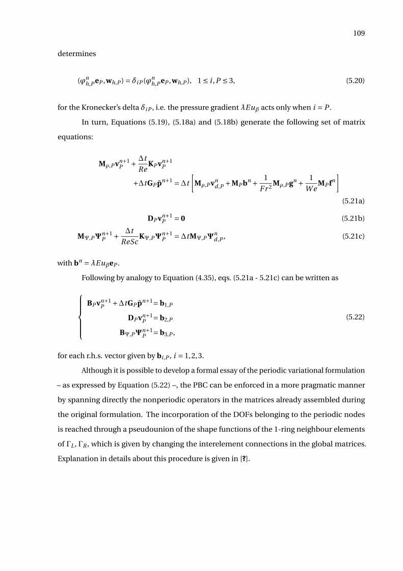
109

determines

(ϕnh,P eP ,wh,P ) = δi P (ϕn

h,P eP ,wh,P ), 1 ≤ i ,P ≤ 3, (5.20)

for the Kronecker’s delta δi P , i.e. the pressure gradient λEuβ acts only when i = P .

In turn, Equations (5.19), (5.18a) and (5.18b) generate the following set of matrix

equations:

Mρ,P vn+1P + ∆t

ReKP vn+1

P

+∆tGP pn+1 =∆t

[Mρ,P vn

d ,P +MP bn + 1

F r 2Mρ,P gn + 1

W eMP fn

](5.21a)

DP vn+1P = 0 (5.21b)

MΨ,PΨn+1P + ∆t

ReScKΨ,PΨ

n+1P =∆tMΨ,PΨ

nd ,P , (5.21c)

with bn =λEuβeP .

Following by analogy to Equation (4.35), eqs. (5.21a - 5.21c) can be written as

BP vn+1

P +∆tGP pn+1= b1,P

DP vn+1P = b2,P

BΨ,PΨn+1P = b3,P ,

(5.22)

for each r.h.s. vector given by bi ,P , i = 1,2,3.

Although it is possible to develop a formal essay of the periodic variational formulation

– as expressed by Equation (5.22) –, the PBC can be enforced in a more pragmatic manner

by spanning directly the nonperiodic operators in the matrices already assembled during

the original formulation. The incorporation of the DOFs belonging to the periodic nodes

is reached through a pseudounion of the shape functions of the 1-ring neighbour elements

of ΓL , ΓR , which is given by changing the interelement connections in the global matrices.

Explanation in details about this procedure is given in [?].

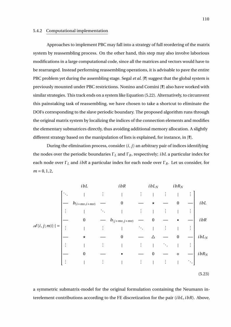
110

5.4.2 Computational implementation

Approaches to implement PBC may fall into a strategy of full reordering of the matrix

system by reassembling process. On the other hand, this step may also involve laborious

modifications in a large computational code, since all the matrices and vectors would have to

be rearranged. Instead performing reassembling operations, it is advisable to pave the entire

PBC problem yet during the assembling stage. Segal et al. [?] suggest that the global system is

previously mounted under PBC restrictions. Nonino and Comini [?] also have worked with

similar strategies. This track ends on a system like Equation (5.22). Alternatively, to circumvent

this painstaking task of reassembling, we have chosen to take a shortcut to eliminate the

DOFs corresponding to the slave periodic boundary. The proposed algorithm runs through

the original matrix system by localizing the indices of the connection elements and modifies

the elementary submatrices directly, thus avoiding additional memory allocation. A slightly

different strategy based on the manipulation of lists is explained, for instance, in [?].

During the elimination process, consider (i , j ) an arbitrary pair of indices identifying

the nodes over the periodic boundaries ΓL and ΓR , respectively; i bL a particular index for

each node over ΓL and i bR a particular index for each node over ΓR . Let us consider, for

m = 0,1,2,

A (i , j ;m)[·] =

i bL i bR i bLN i bRN

. . . | ... | ... | ... | ...

b(i+mυ,i+mυ) 0 ? 0 i bL... | . . . | ... | ... | ...

0 b( j+mυ, j+mυ) 0 • i bR... | ... | . . . | ... | ...

? 0 4 0 i bLN

... | ... | ... | . . . | ...

0 • 0 ¦ i bRN

... | ... | ... | ... | . . .

(5.23)

a symmetric submatrix-model for the original formulation containing the Neumann in-

terelement contributions according to the FE discretization for the pair (i bL, i bR). Above,

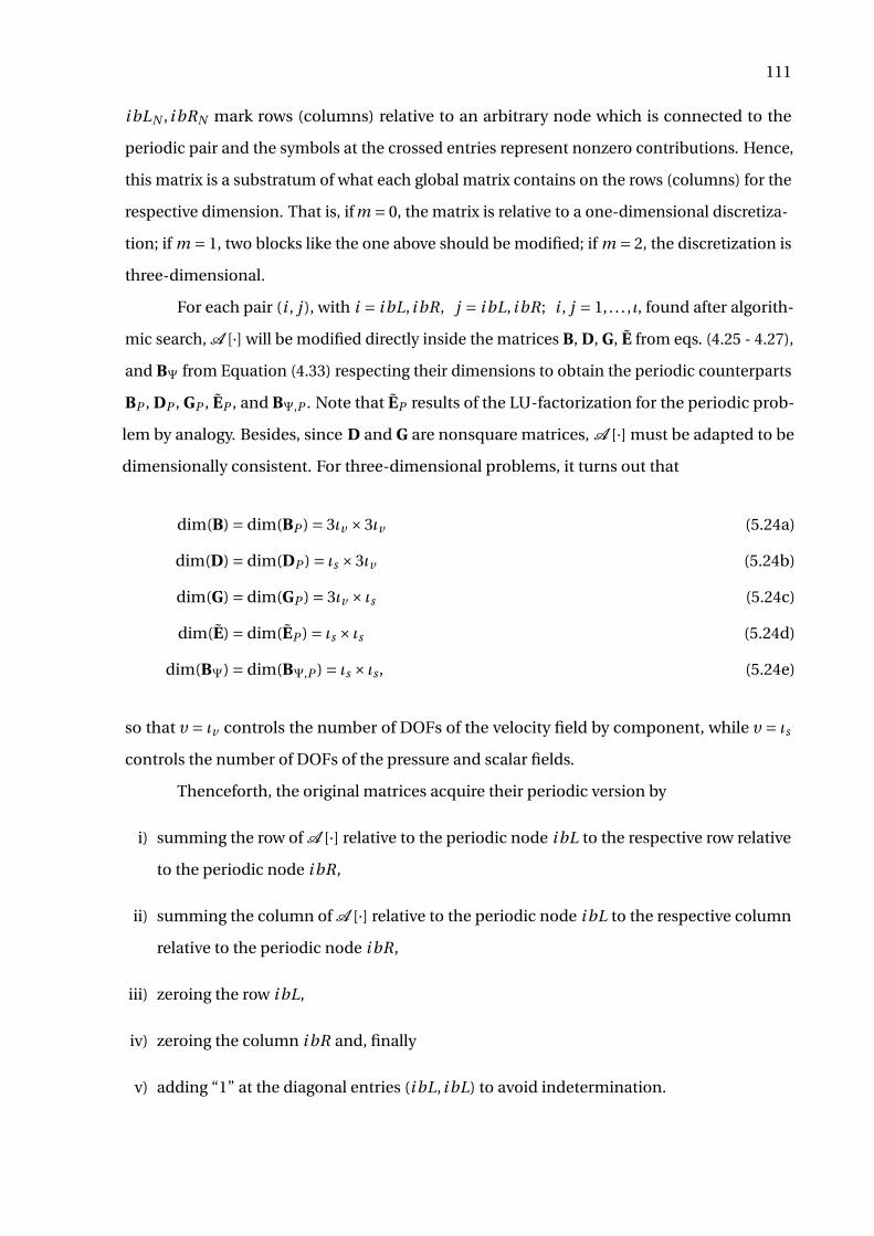
111

i bLN , i bRN mark rows (columns) relative to an arbitrary node which is connected to the

periodic pair and the symbols at the crossed entries represent nonzero contributions. Hence,

this matrix is a substratum of what each global matrix contains on the rows (columns) for the

respective dimension. That is, if m = 0, the matrix is relative to a one-dimensional discretiza-

tion; if m = 1, two blocks like the one above should be modified; if m = 2, the discretization is

three-dimensional.

For each pair (i , j ), with i = i bL, i bR, j = i bL, i bR; i , j = 1, . . . , ι, found after algorith-

mic search, A [·] will be modified directly inside the matrices B, D, G, E from eqs. (4.25 - 4.27),

and BΨ from Equation (4.33) respecting their dimensions to obtain the periodic counterparts

BP , DP , GP , EP , and BΨ,P . Note that EP results of the LU-factorization for the periodic prob-

lem by analogy. Besides, since D and G are nonsquare matrices, A [·] must be adapted to be

dimensionally consistent. For three-dimensional problems, it turns out that

dim(B) = dim(BP ) = 3ιv ×3ιv (5.24a)

dim(D) = dim(DP ) = ιs ×3ιv (5.24b)

dim(G) = dim(GP ) = 3ιv × ιs (5.24c)

dim(E) = dim(EP ) = ιs × ιs (5.24d)

dim(BΨ) = dim(BΨ,P ) = ιs × ιs , (5.24e)

so that υ= ιv controls the number of DOFs of the velocity field by component, while υ= ιscontrols the number of DOFs of the pressure and scalar fields.

Thenceforth, the original matrices acquire their periodic version by

i) summing the row of A [·] relative to the periodic node i bL to the respective row relative

to the periodic node i bR,

ii) summing the column of A [·] relative to the periodic node i bL to the respective column

relative to the periodic node i bR,

iii) zeroing the row i bL,

iv) zeroing the column i bR and, finally

v) adding “1” at the diagonal entries (i bL, i bL) to avoid indetermination.

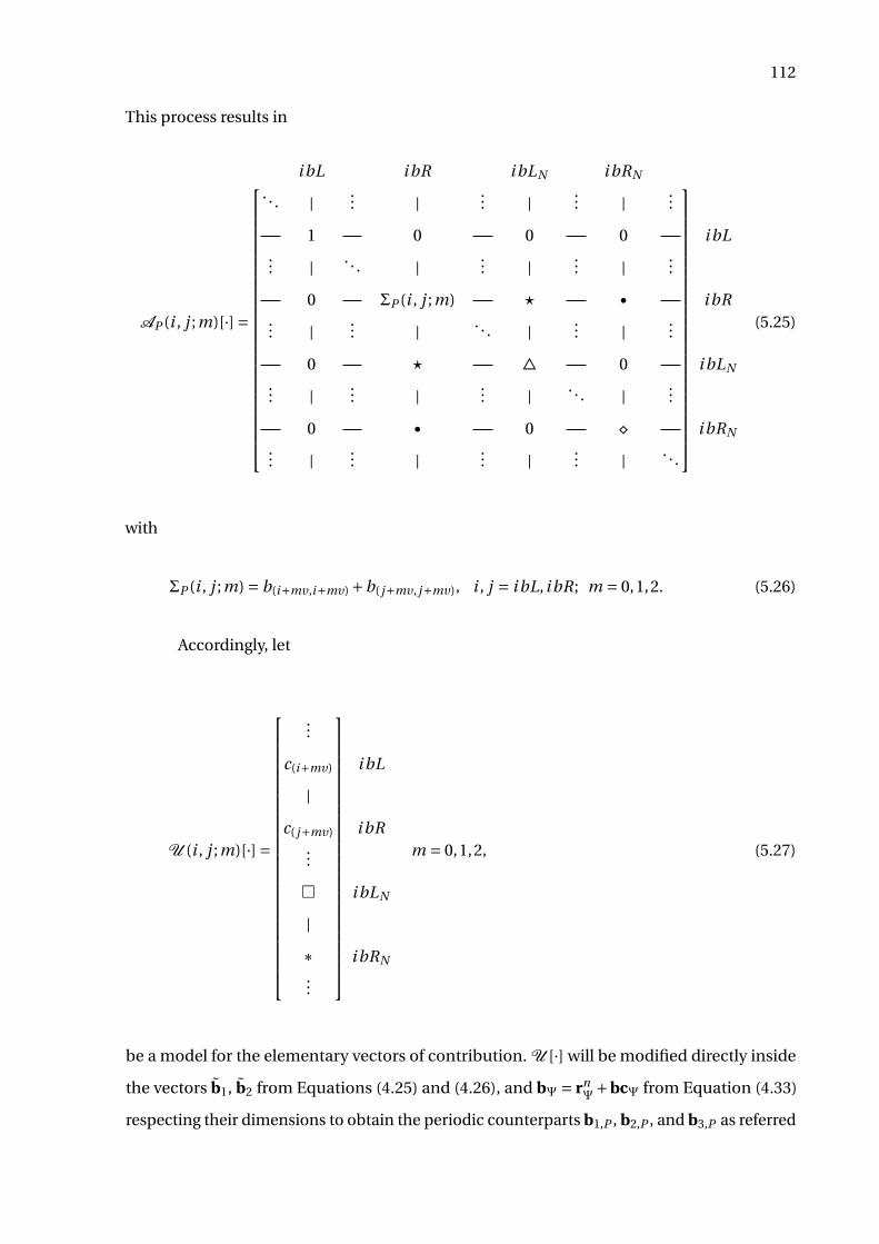
112

This process results in

AP (i , j ;m)[·] =

i bL i bR i bLN i bRN

. . . | ... | ... | ... | ...

1 0 0 0 i bL... | . . . | ... | ... | ...

0 ΣP (i , j ;m) ? • i bR... | ... | . . . | ... | ...

0 ? 4 0 i bLN

... | ... | ... | . . . | ...

0 • 0 ¦ i bRN

... | ... | ... | ... | . . .

(5.25)

with

ΣP (i , j ;m) = b(i+mυ,i+mυ) +b( j+mυ, j+mυ), i , j = i bL, i bR; m = 0,1,2. (5.26)

Accordingly, let

U (i , j ;m)[·] =

...

c(i+mυ) i bL

|c( j+mυ) i bR

...

i bLN

|∗ i bRN

...

m = 0,1,2, (5.27)

be a model for the elementary vectors of contribution. U [·] will be modified directly inside

the vectors b1, b2 from Equations (4.25) and (4.26), and bΨ = rnΨ+bcΨ from Equation (4.33)

respecting their dimensions to obtain the periodic counterparts b1,P , b2,P , and b3,P as referred

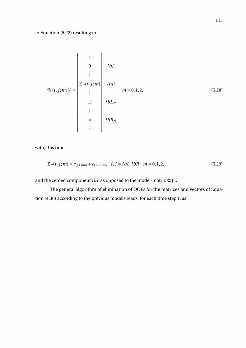
113

in Equation (5.22) resulting in

U (i , j ;m)[·] =

...

0 i bL

|ΣP (i , j ;m) i bR

...

i bLN

|∗ i bRN

...

m = 0,1,2, (5.28)

with, this time,

ΣP (i , j ;m) = c(i+mυ) + c( j+mυ), i , j = i bL, i bR; m = 0,1,2, (5.29)

and the zeroed component i bL as opposed to the model-matrix U [·].The general algorithm of elimination of DOFs for the matrices and vectors of Equa-

tion (4.36) according to the previous models reads, for each time step t , as:

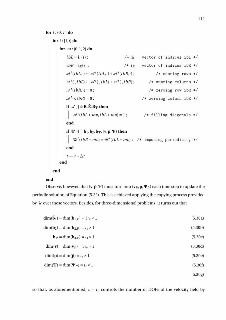
114

for t : (0,T ] do

for i : [1, ι] do

for m : 0,1,2 do

i bL = iL(i ) ; /* iL: vector of indices ibL */

i bR = iR (i ) ; /* iR: vector of indices ibR */

A t (i bL, ·) ←A t (i bL, ·)+A t (i bR, ·) ; /* summing rows */

A t (·, i bL) ←A t (·, i bL)+A t (·, i bR) ; /* summing columns */

A t (i bR, ·) = 0 ; /* zeroing row ibR */

A t (·, i bR) = 0 ; /* zeroing column ibR */

if A [·] .= B, E,BΨ then

A t (i bL+mυ, i bL+mυ) = 1 ; /* filling diagonals */

end

if U [·] .= b1, b2,bΨ, (v, p,Ψ) then

U t (i bR +mυ) =U t (i bL+mυ) ; /* imposing periodicity */

end

t ← t +∆t

end

end

end

Observe, however, that (v, p,Ψ) must turn into (vP , p,ΨP ) each time step to update the

periodic solution of Equation (5.22). This is achieved applying the copying process provided

by U over these vectors. Besides, for three-dimensional problems, it turns out that

dim(b1) = dim(b1,P ) = 3ιv ×1 (5.30a)

dim(b2) = dim(b2,P ) = ιs ×1 (5.30b)

bΨ = dim(b3,P ) = ιs ×1 (5.30c)

dim(v) = dim(vP ) = 3ιv ×1 (5.30d)

dim(p) = dim(p) = ιs ×1 (5.30e)

dim(Ψ) = dim(ΨP ) = ιs ×1 (5.30f)

(5.30g)

so that, as aforementioned, υ = ιv controls the number of DOFs of the velocity field by

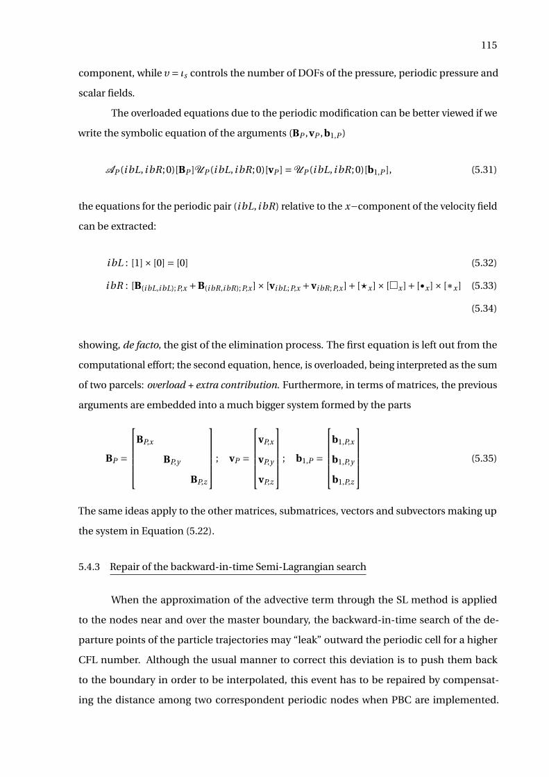
115

component, while υ= ιs controls the number of DOFs of the pressure, periodic pressure and

scalar fields.

The overloaded equations due to the periodic modification can be better viewed if we

write the symbolic equation of the arguments (BP ,vP ,b1,P )

AP (i bL, i bR;0)[BP ]UP (i bL, i bR;0)[vP ] =UP (i bL, i bR;0)[b1,P ], (5.31)

the equations for the periodic pair (i bL, i bR) relative to the x−component of the velocity field

can be extracted:

i bL : [1]× [0] = [0] (5.32)

i bR : [B(i bL,i bL);P,x +B(i bR,i bR);P,x]× [vi bL;P,x +vi bR;P,x]+ [?x]× [x]+ [•x]× [∗x] (5.33)

(5.34)

showing, de facto, the gist of the elimination process. The first equation is left out from the

computational effort; the second equation, hence, is overloaded, being interpreted as the sum

of two parcels: overload + extra contribution. Furthermore, in terms of matrices, the previous

arguments are embedded into a much bigger system formed by the parts

BP =

BP,x

BP,y

BP,z

; vP =

vP,x

vP,y

vP,z

; b1,P =

b1,P,x

b1,P,y

b1,P,z

(5.35)

The same ideas apply to the other matrices, submatrices, vectors and subvectors making up

the system in Equation (5.22).

5.4.3 Repair of the backward-in-time Semi-Lagrangian search

When the approximation of the advective term through the SL method is applied

to the nodes near and over the master boundary, the backward-in-time search of the de-

parture points of the particle trajectories may “leak” outward the periodic cell for a higher

CFL number. Although the usual manner to correct this deviation is to push them back

to the boundary in order to be interpolated, this event has to be repaired by compensat-

ing the distance among two correspondent periodic nodes when PBC are implemented.

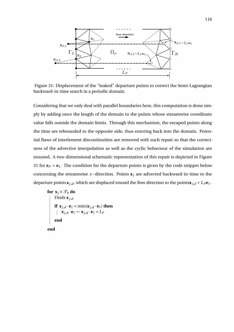
116

flow direction

Figure 31: Displacement of the “leaked” departure points to correct the Semi-Lagrangianbackward-in-time search in a periodic domain.

Considering that we only deal with parallel boundaries here, this computation is done sim-

ply by adding once the length of the domain to the points whose streamwise coordinate

value falls outside the domain limits. Through this mechanism, the escaped points along

the time are rebounded to the opposite side, thus entering back into the domain. Poten-

tial flaws of interlement discontinuities are removed with such repair so that the correct-

ness of the advective interpolation as well as the cyclic behaviour of the simulation are

ensured. A two-dimensional schematic representation of this repair is depicted in Figure

31 for eP = e1. The condition for the departure points is given by the code snippet below

concerning the streamwise x−direction. Points x j are advected backward-in-time to the

departure points x j ,d , which are displaced toward the flow direction to the pointsx j ,d +LP e1.

for x j ∈Th doFinds x j ,d

if x j ,d ·e1 < minx j ,d ·e1 thenx j ,d ·e1 ← x j ,d ·e1 +LP

end

end

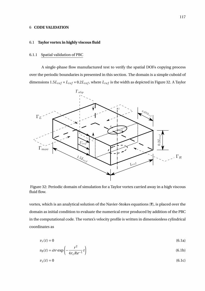
117

6 CODE VALIDATION

6.1 Taylor vortex in highly viscous fluid

6.1.1 Spatial validation of PBC

A single-phase flow manufactured test to verify the spatial DOFs copying process

over the periodic boundaries is presented in this section. The domain is a simple cuboid of

dimensions 1.5Lr e f ×Lr e f ×0.2Lr e f , where Lr e f is the width as depicted in Figure 32. A Taylor

Figure 32: Periodic domain of simulation for a Taylor vortex carried away in a high viscousfluid flow.

vortex, which is an analytical solution of the Navier-Stokes equations [?], is placed over the

domain as initial condition to evaluate the numerical error produced by addition of the PBC

in the computational code. The vortex’s velocity profile is written in dimensionless cylindrical

coordinates as

vr (t ) = 0 (6.1a)

vθ(t ) =$r exp

(− r 2

4rc Re−1t

)(6.1b)

vz(t ) = 0 (6.1c)

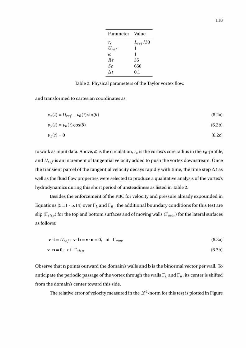
118

Parameter Value

rc Lr e f /30Ur e f 1$ 1Re 35Sc 650∆t 0.1

Table 2: Physical parameters of the Taylor vortex flow.

and transformed to cartesian coordinates as

vx(t ) =Ur e f − vθ(t )sin(θ) (6.2a)

vy (t ) = vθ(t )cos(θ) (6.2b)

vz(t ) = 0 (6.2c)

to work as input data. Above,$ is the circulation, rc is the vortex’s core radius in the vθ-profile,

and Ur e f is an increment of tangential velocity added to push the vortex downstream. Once

the transient parcel of the tangential velocity decays rapidly with time, the time step ∆t as

well as the fluid flow properties were selected to produce a qualitative analysis of the vortex’s

hydrodynamics during this short period of unsteadiness as listed in Table 2.

Besides the enforcement of the PBC for velocity and pressure already expounded in

Equations (5.11 - 5.14) over ΓL and ΓR , the additional boundary conditions for this test are

slip (Γsl i p ) for the top and bottom surfaces and of moving walls (Γmov ) for the lateral surfaces

as follows:

v · t =Ur e f ; v ·b = v ·n = 0, at Γmov (6.3a)

v ·n = 0, at Γsl i p (6.3b)

Observe that n points outward the domain’s walls and b is the binormal vector per wall. To

anticipate the periodic passage of the vortex through the walls ΓL and ΓR , its center is shifted

from the domain’s center toward this side.

The relative error of velocity measured in the L 2-norm for this test is plotted in Figure

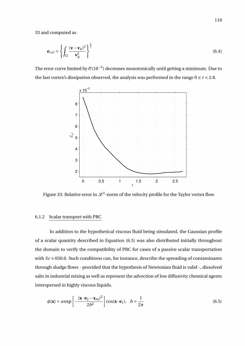
119

33 and computed as

er el =∫

Ω

(v−vh)2

v2h

12

(6.4)

The error curve limited by O (10−3) decreases monotonically until getting a minimum. Due to

the fast vortex’s dissipation observed, the analysis was performed in the range 0 ≤ t < 2.8.

0 0.5 1 1.5 2 2.5

2

3

4

5

6

7

8

x 10−3

t

Egl

Figure 33: Relative error in L 2-norm of the velocity profile for the Taylor vortex flow.

6.1.2 Scalar transport with PBC

In addition to the hypothetical viscous fluid being simulated, the Gaussian profile

of a scalar quantity described in Equation (6.5) was also distributed initially throughout

the domain to verify the compatibility of PBC for cases of a passive scalar transportation

with Sc ≈ 650.0. Such conditions can, for instance, describe the spreading of contaminants

through sludge flows - provided that the hypothesis of Newtonian fluid is valid -, dissolved

salts in industrial mixing as well as represent the advection of low diffusivity chemical agents

interspersed in highly viscous liquids.

φ(x) = a exp

[− (x ·e2 −xm)2

2b2

]cos(x ·e1), b = 1

2π(6.5)

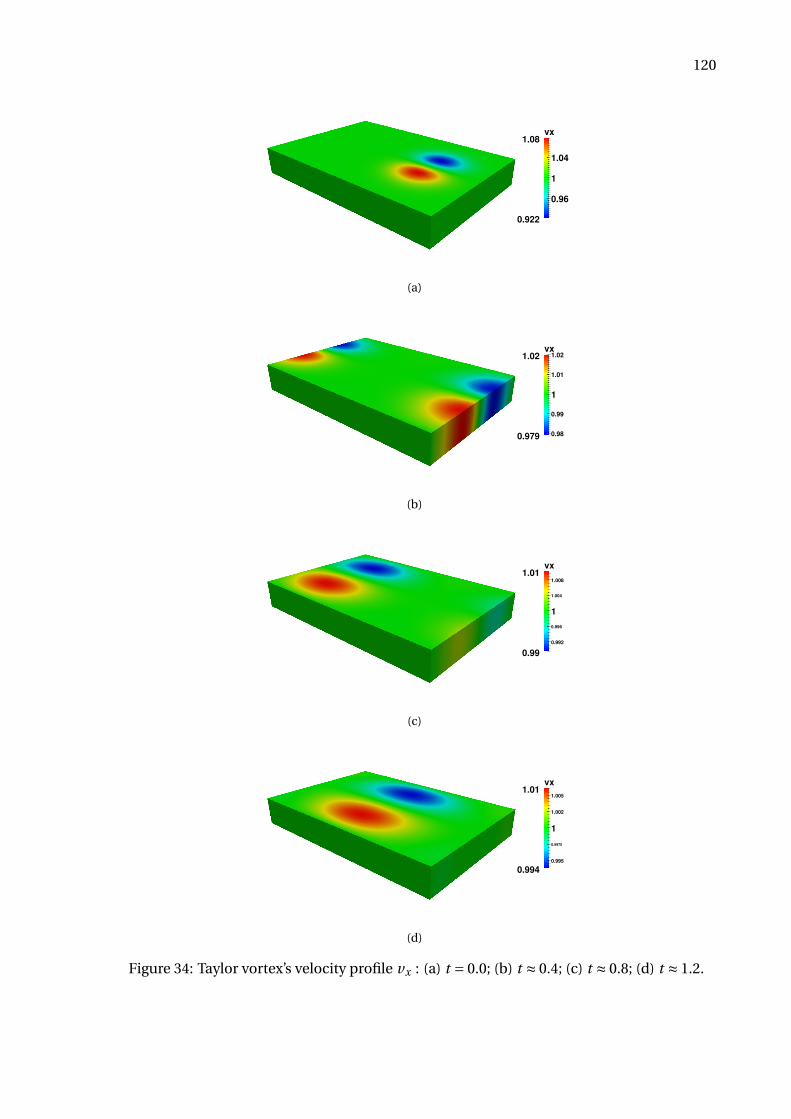
120

0.96

1

1.04

vx

0.922

1.08

(a)

0.98

0.99

1

1.01

1.02vx

0.979

1.02

(b)

0.992

0.996

1

1.004

1.008

vx

0.99

1.01

(c)

1.01

0.995

0.9975

1

1.002

1.005

vx

0.994

(d)

Figure 34: Taylor vortex’s velocity profile vx : (a) t = 0.0; (b) t ≈ 0.4; (c) t ≈ 0.8; (d) t ≈ 1.2.

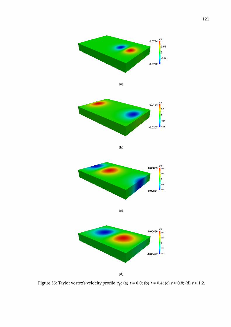
121

-0.04

0

0.04

vy

-0.0772

0.0764

(a)

-0.02

-0.01

0

0.01

vy

-0.0207

0.0184

(b)

-0.008

-0.004

0

0.004

0.008

vy

-0.00851

0.00839

(c)

0.00466

-0.004

-0.002

0

0.002

0.004

vy

-0.00427

(d)

Figure 35: Taylor vortex’s velocity profile vy : (a) t = 0.0; (b) t ≈ 0.4; (c) t ≈ 0.8; (d) t ≈ 1.2.

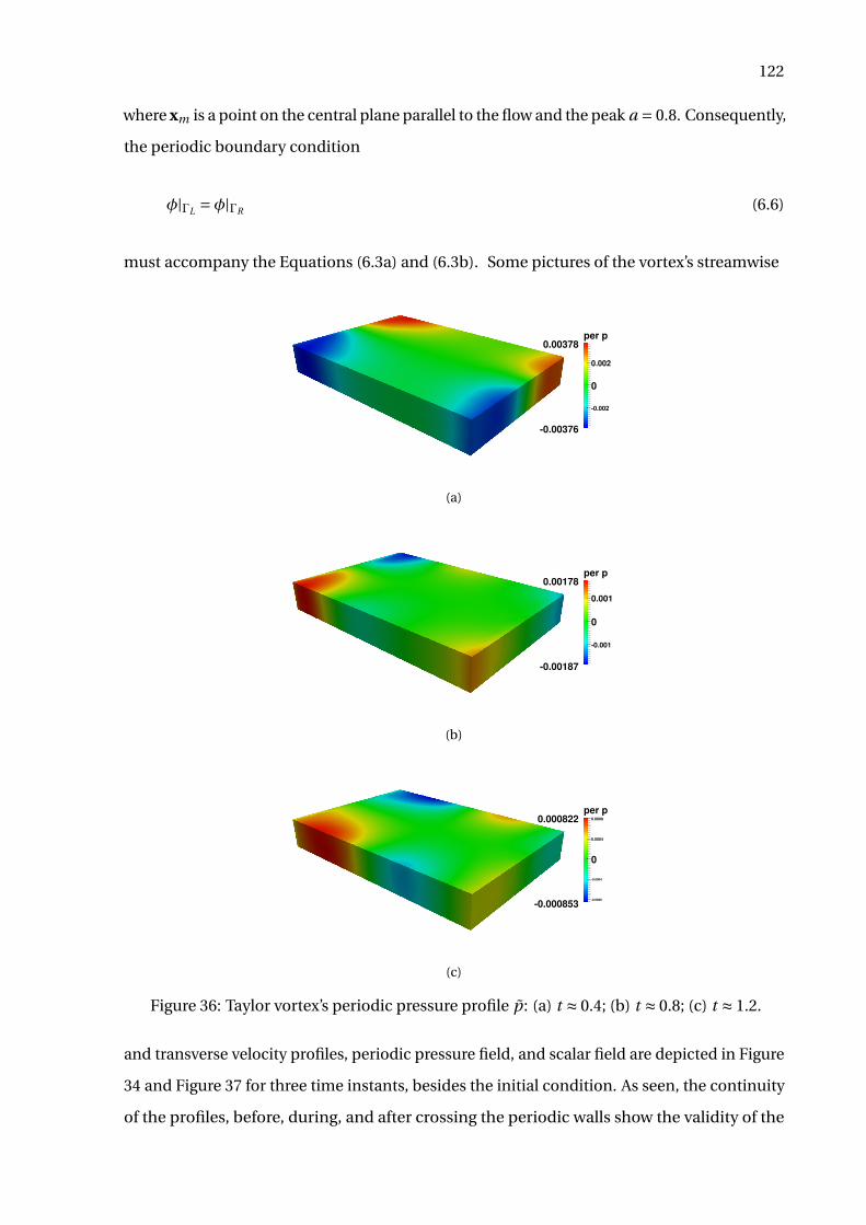
122

where xm is a point on the central plane parallel to the flow and the peak a = 0.8. Consequently,

the periodic boundary condition

φ|ΓL =φ|ΓR (6.6)

must accompany the Equations (6.3a) and (6.3b). Some pictures of the vortex’s streamwise

-0.002

0

0.002

per p

-0.00376

0.00378

(a)

-0.001

0

0.001

per p

-0.00187

0.00178

(b)

-0.0008

-0.0004

0

0.0004

0.0008

per p

-0.000853

0.000822

(c)

Figure 36: Taylor vortex’s periodic pressure profile p: (a) t ≈ 0.4; (b) t ≈ 0.8; (c) t ≈ 1.2.

and transverse velocity profiles, periodic pressure field, and scalar field are depicted in Figure

34 and Figure 37 for three time instants, besides the initial condition. As seen, the continuity

of the profiles, before, during, and after crossing the periodic walls show the validity of the

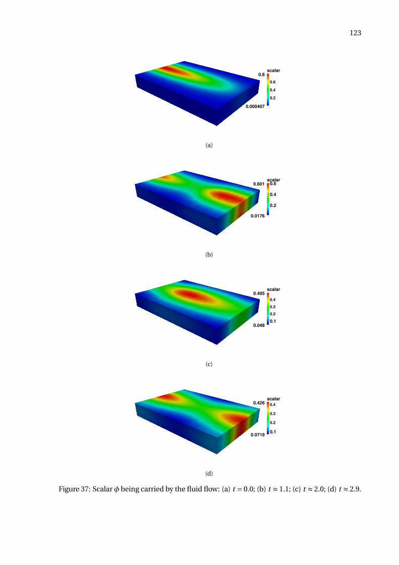
123

0.8

0.2

0.4

0.6

scalar

0.000407

(a)

0.2

0.4

0.6scalar

0.0176

0.601

(b)

0.495

0.1

0.2

0.3

0.4

scalar

0.048

(c)

0.426

0.1

0.2

0.3

0.4

scalar

0.0719

(d)

Figure 37: Scalar φ being carried by the fluid flow: (a) t = 0.0; (b) t ≈ 1.1; (c) t ≈ 2.0; (d) t ≈ 2.9.

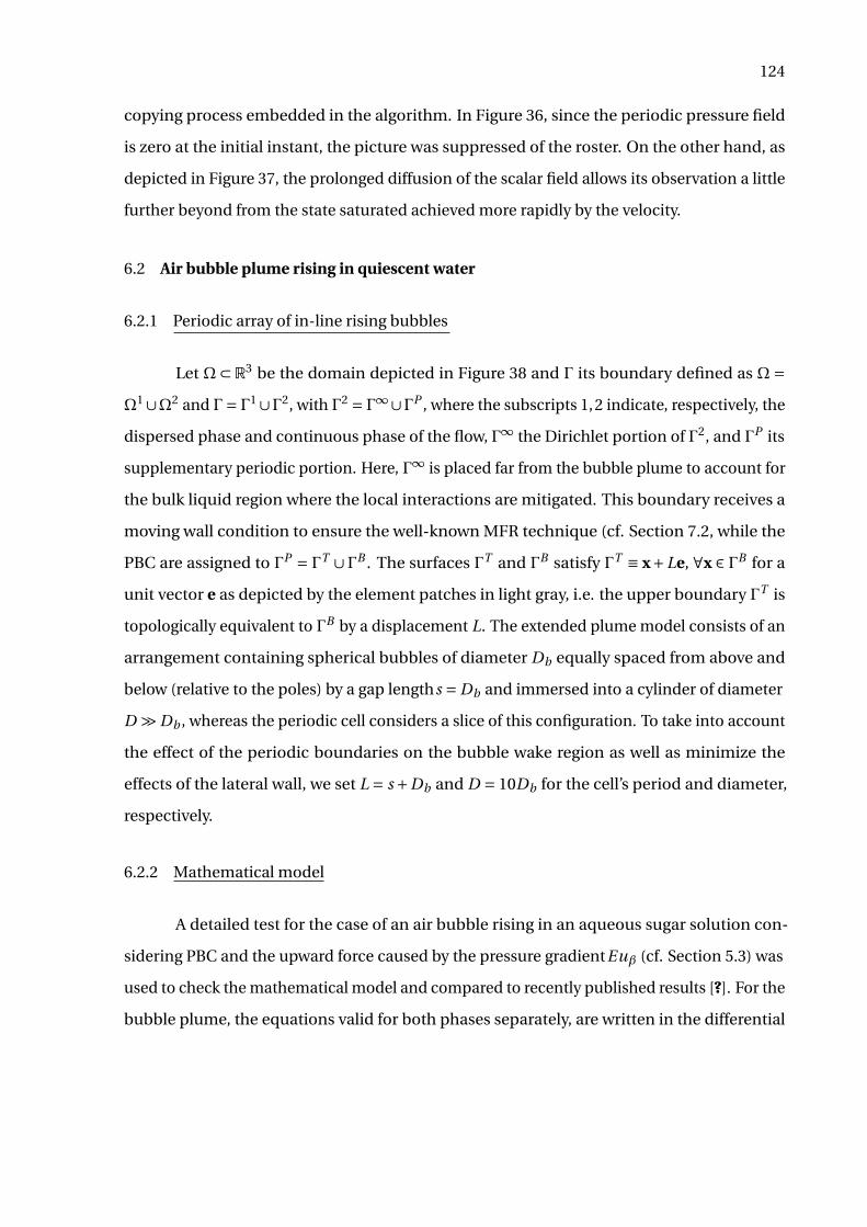
124

copying process embedded in the algorithm. In Figure 36, since the periodic pressure field

is zero at the initial instant, the picture was suppressed of the roster. On the other hand, as

depicted in Figure 37, the prolonged diffusion of the scalar field allows its observation a little

further beyond from the state saturated achieved more rapidly by the velocity.

6.2 Air bubble plume rising in quiescent water

6.2.1 Periodic array of in-line rising bubbles

Let Ω ⊂ R3 be the domain depicted in Figure 38 and Γ its boundary defined as Ω =Ω1∪Ω2 and Γ= Γ1∪Γ2, with Γ2 = Γ∞∪ΓP , where the subscripts 1,2 indicate, respectively, the

dispersed phase and continuous phase of the flow, Γ∞ the Dirichlet portion of Γ2, and ΓP its

supplementary periodic portion. Here, Γ∞ is placed far from the bubble plume to account for

the bulk liquid region where the local interactions are mitigated. This boundary receives a

moving wall condition to ensure the well-known MFR technique (cf. Section 7.2, while the

PBC are assigned to ΓP = ΓT ∪ΓB . The surfaces ΓT and ΓB satisfy ΓT ≡ x+Le, ∀x ∈ ΓB for a

unit vector e as depicted by the element patches in light gray, i.e. the upper boundary ΓT is

topologically equivalent to ΓB by a displacement L. The extended plume model consists of an

arrangement containing spherical bubbles of diameter Db equally spaced from above and

below (relative to the poles) by a gap lengths = Db and immersed into a cylinder of diameter

D À Db , whereas the periodic cell considers a slice of this configuration. To take into account

the effect of the periodic boundaries on the bubble wake region as well as minimize the

effects of the lateral wall, we set L = s +Db and D = 10Db for the cell’s period and diameter,

respectively.

6.2.2 Mathematical model

A detailed test for the case of an air bubble rising in an aqueous sugar solution con-

sidering PBC and the upward force caused by the pressure gradientEuβ (cf. Section 5.3) was

used to check the mathematical model and compared to recently published results [?]. For the

bubble plume, the equations valid for both phases separately, are written in the differential

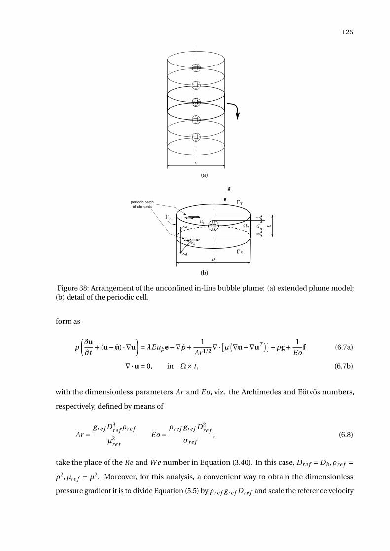
125

(a)

periodic patch

of elements

(b)

Figure 38: Arrangement of the unconfined in-line bubble plume: (a) extended plume model;(b) detail of the periodic cell.

form as

ρ

(∂u

∂t+ (u− u) ·∇u

)=λEuβe−∇p + 1

Ar 1/2∇· [µ(∇u+∇uT )]+ρg+ 1

Eof (6.7a)

∇·u = 0, in Ω× t , (6.7b)

with the dimensionless parameters Ar and Eo, viz. the Archimedes and Eötvös numbers,

respectively, defined by means of

Ar =gr e f D3

r e f ρr e f

µ2r e f

Eo =ρr e f gr e f D2

r e f

σr e f, (6.8)

take the place of the Re and W e number in Equation (3.40). In this case, Dr e f = Db ,ρr e f =ρ2,µr e f = µ2. Moreover, for this analysis, a convenient way to obtain the dimensionless

pressure gradient it is to divide Equation (5.5) by ρr e f gr e f Dr e f and scale the reference velocity

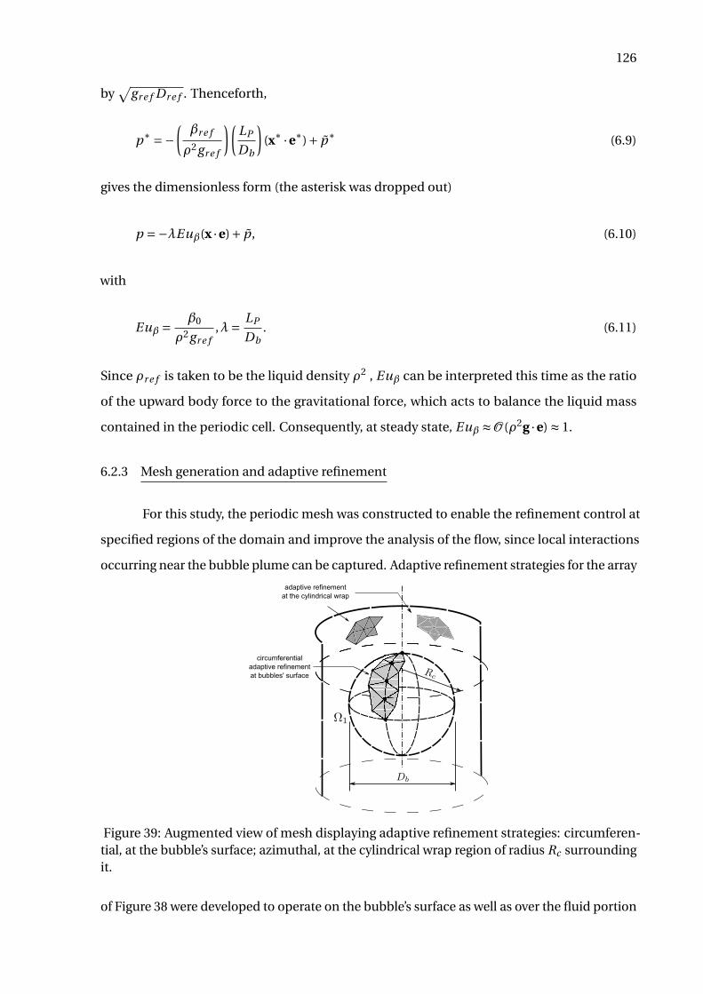
126

by√

gr e f Dr e f . Thenceforth,

p∗ =−(βr e f

ρ2gr e f

)(LP

Db

)(x∗ ·e∗)+ p∗ (6.9)

gives the dimensionless form (the asterisk was dropped out)

p =−λEuβ(x ·e)+ p, (6.10)

with

Euβ =β0

ρ2gr e f,λ= LP

Db. (6.11)

Since ρr e f is taken to be the liquid density ρ2 , Euβ can be interpreted this time as the ratio

of the upward body force to the gravitational force, which acts to balance the liquid mass

contained in the periodic cell. Consequently, at steady state, Euβ ≈O (ρ2g ·e) ≈ 1.

6.2.3 Mesh generation and adaptive refinement

For this study, the periodic mesh was constructed to enable the refinement control at

specified regions of the domain and improve the analysis of the flow, since local interactions

occurring near the bubble plume can be captured. Adaptive refinement strategies for the array

adaptive refinement

at the cylindrical wrap

circumferential

adaptive refinement

at bubbles' surface

Figure 39: Augmented view of mesh displaying adaptive refinement strategies: circumferen-tial, at the bubble’s surface; azimuthal, at the cylindrical wrap region of radius Rc surroundingit.

of Figure 38 were developed to operate on the bubble’s surface as well as over the fluid portion

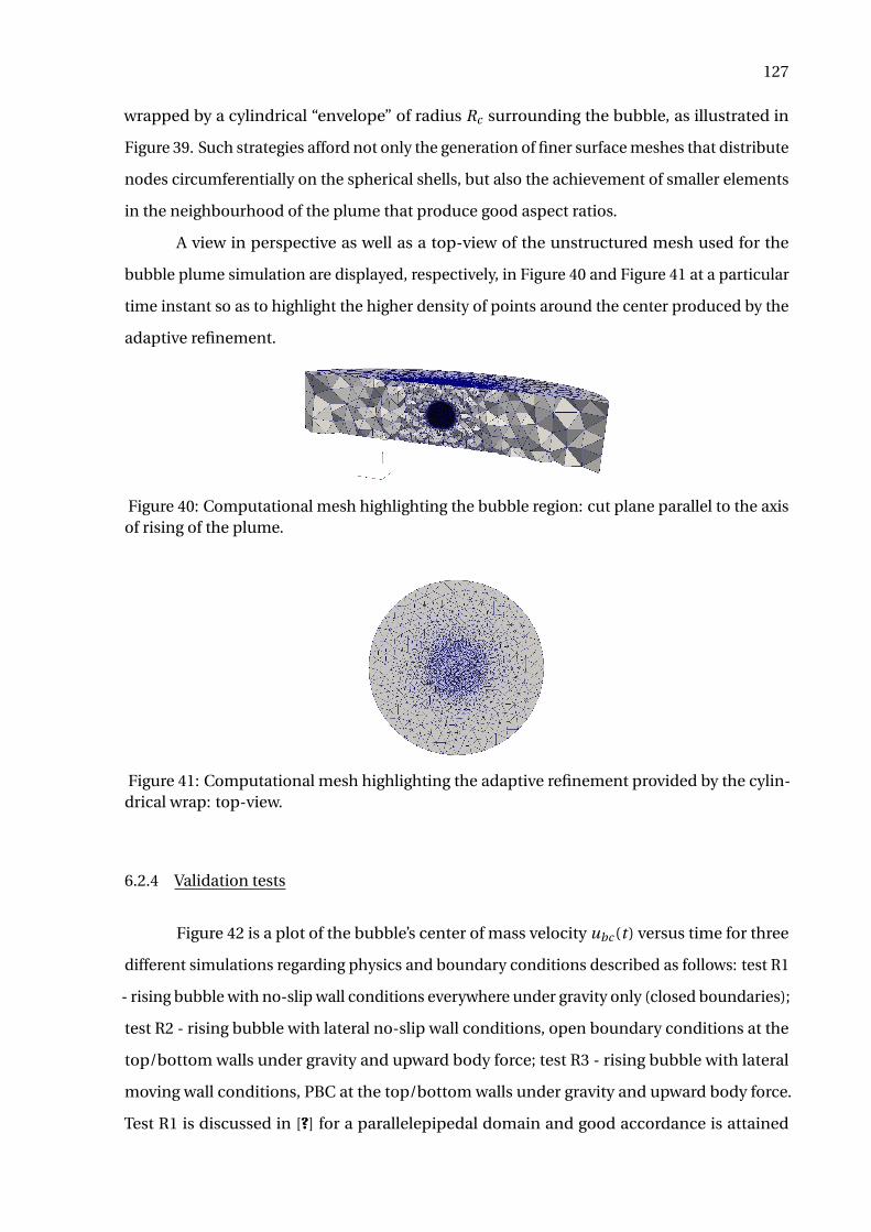
127

wrapped by a cylindrical “envelope” of radius Rc surrounding the bubble, as illustrated in

Figure 39. Such strategies afford not only the generation of finer surface meshes that distribute

nodes circumferentially on the spherical shells, but also the achievement of smaller elements

in the neighbourhood of the plume that produce good aspect ratios.

A view in perspective as well as a top-view of the unstructured mesh used for the

bubble plume simulation are displayed, respectively, in Figure 40 and Figure 41 at a particular

time instant so as to highlight the higher density of points around the center produced by the

adaptive refinement.

Figure 40: Computational mesh highlighting the bubble region: cut plane parallel to the axisof rising of the plume.

Figure 41: Computational mesh highlighting the adaptive refinement provided by the cylin-drical wrap: top-view.

6.2.4 Validation tests

Figure 42 is a plot of the bubble’s center of mass velocity ubc (t ) versus time for three

different simulations regarding physics and boundary conditions described as follows: test R1

- rising bubble with no-slip wall conditions everywhere under gravity only (closed boundaries);

test R2 - rising bubble with lateral no-slip wall conditions, open boundary conditions at the

top/bottom walls under gravity and upward body force; test R3 - rising bubble with lateral

moving wall conditions, PBC at the top/bottom walls under gravity and upward body force.

Test R1 is discussed in [?] for a parallelepipedal domain and good accordance is attained

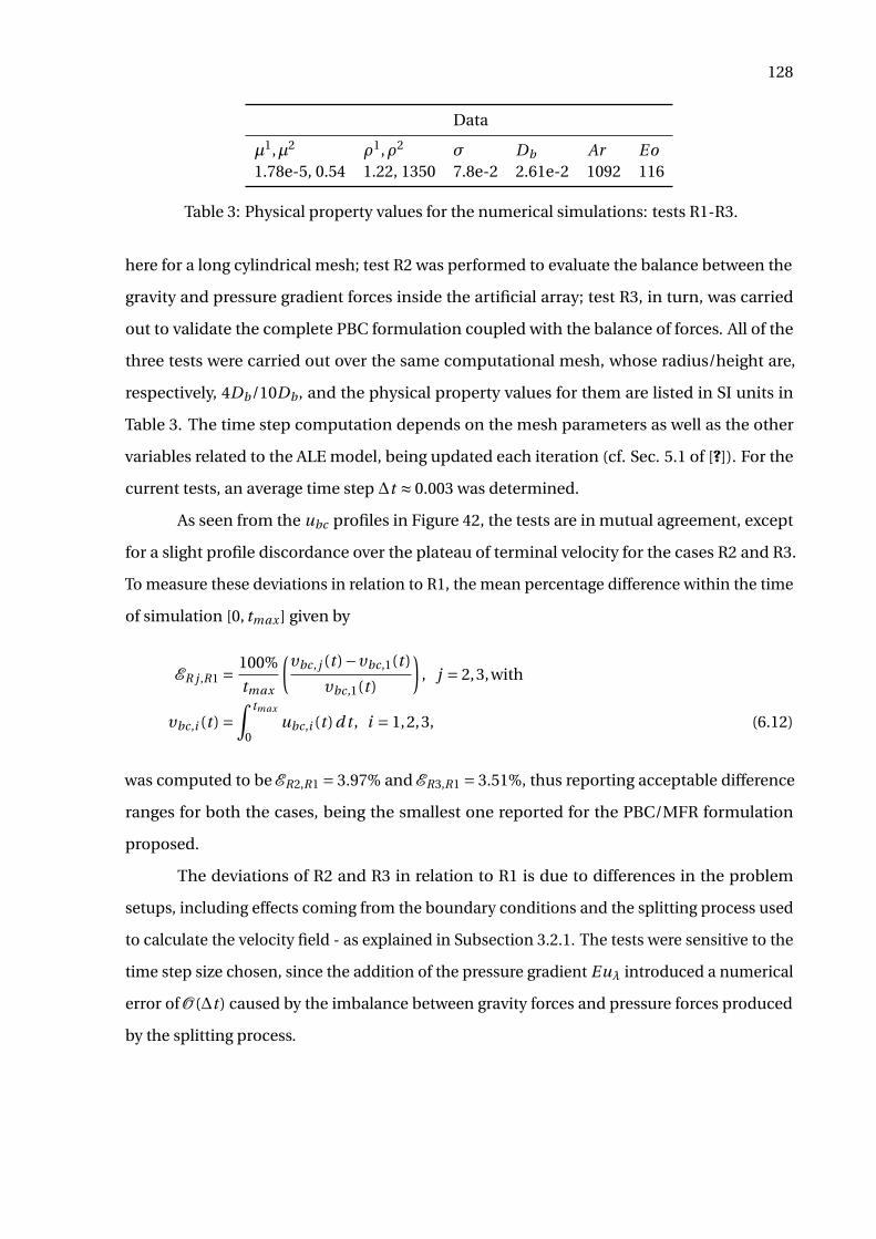
128

Data

µ1,µ2 ρ1,ρ2 σ Db Ar Eo1.78e-5, 0.54 1.22, 1350 7.8e-2 2.61e-2 1092 116

Table 3: Physical property values for the numerical simulations: tests R1-R3.

here for a long cylindrical mesh; test R2 was performed to evaluate the balance between the

gravity and pressure gradient forces inside the artificial array; test R3, in turn, was carried

out to validate the complete PBC formulation coupled with the balance of forces. All of the

three tests were carried out over the same computational mesh, whose radius/height are,

respectively, 4Db/10Db , and the physical property values for them are listed in SI units in

Table 3. The time step computation depends on the mesh parameters as well as the other

variables related to the ALE model, being updated each iteration (cf. Sec. 5.1 of [?]). For the

current tests, an average time step ∆t ≈ 0.003 was determined.

As seen from the ubc profiles in Figure 42, the tests are in mutual agreement, except

for a slight profile discordance over the plateau of terminal velocity for the cases R2 and R3.

To measure these deviations in relation to R1, the mean percentage difference within the time

of simulation [0, tmax] given by

ER j ,R1 = 100%

tmax

(υbc, j (t )−υbc,1(t )

υbc,1(t )

), j = 2,3,with

υbc,i (t ) =∫ tmax

0ubc,i (t )d t , i = 1,2,3, (6.12)

was computed to be ER2,R1 = 3.97% and ER3,R1 = 3.51%, thus reporting acceptable difference

ranges for both the cases, being the smallest one reported for the PBC/MFR formulation

proposed.

The deviations of R2 and R3 in relation to R1 is due to differences in the problem

setups, including effects coming from the boundary conditions and the splitting process used

to calculate the velocity field - as explained in Subsection 3.2.1. The tests were sensitive to the

time step size chosen, since the addition of the pressure gradient Euλ introduced a numerical

error of O (∆t ) caused by the imbalance between gravity forces and pressure forces produced

by the splitting process.

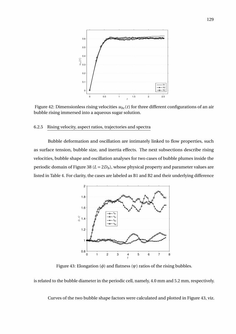
129

0 0.5 1 1.5 2 2.5

0

0.1

0.2

0.3

0.4

0.5

0.6

t

ubc(t)

R1

R2

R3

Figure 42: Dimensionless rising velocities ubc (t ) for three different configurations of an airbubble rising immersed into a aqueous sugar solution.

6.2.5 Rising velocity, aspect ratios, trajectories and spectra

Bubble deformation and oscillation are intimately linked to flow properties, such

as surface tension, bubble size, and inertia effects. The next subsections describe rising

velocities, bubble shape and oscillation analyses for two cases of bubble plumes inside the

periodic domain of Figure 38 (L = 2Db), whose physical property and parameter values are

listed in Table 4. For clarity, the cases are labeled as B1 and B2 and their underlying difference

0 1 2 3 4 5 6 7 8

0.8

1

1.2

1.4

1.6

1.8

2

t

φ,ψ

φB1

ψB1

φB2

ψB2

Figure 43: Elongation (φ) and flatness (ψ) ratios of the rising bubbles.

is related to the bubble diameter in the periodic cell, namely, 4.0 mm and 5.2 mm, respectively.

Curves of the two bubble shape factors were calculated and plotted in Figure 43, viz.

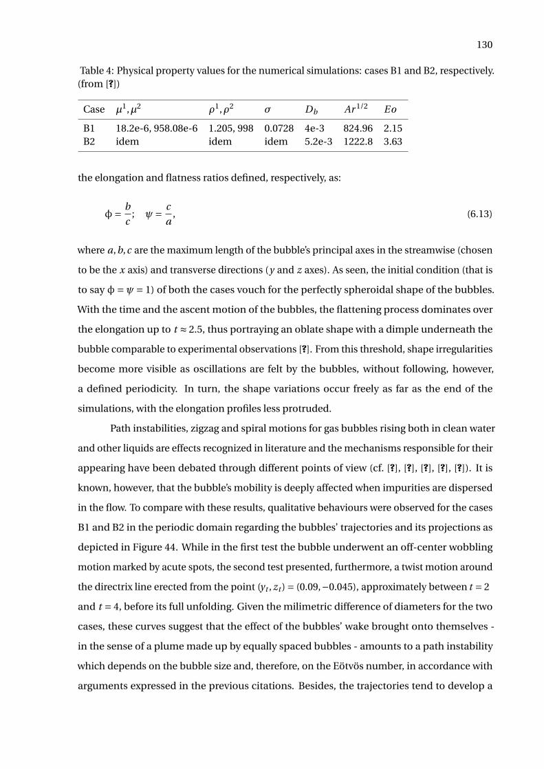
130

Table 4: Physical property values for the numerical simulations: cases B1 and B2, respectively.(from [?])

Case µ1,µ2 ρ1,ρ2 σ Db Ar 1/2 Eo

B1 18.2e-6, 958.08e-6 1.205, 998 0.0728 4e-3 824.96 2.15B2 idem idem idem 5.2e-3 1222.8 3.63

the elongation and flatness ratios defined, respectively, as:

φ= b

c; ψ= c

a, (6.13)

where a,b,c are the maximum length of the bubble’s principal axes in the streamwise (chosen

to be the x axis) and transverse directions (y and z axes). As seen, the initial condition (that is

to say φ=ψ= 1) of both the cases vouch for the perfectly spheroidal shape of the bubbles.

With the time and the ascent motion of the bubbles, the flattening process dominates over

the elongation up to t ≈ 2.5, thus portraying an oblate shape with a dimple underneath the

bubble comparable to experimental observations [?]. From this threshold, shape irregularities

become more visible as oscillations are felt by the bubbles, without following, however,

a defined periodicity. In turn, the shape variations occur freely as far as the end of the

simulations, with the elongation profiles less protruded.

Path instabilities, zigzag and spiral motions for gas bubbles rising both in clean water

and other liquids are effects recognized in literature and the mechanisms responsible for their

appearing have been debated through different points of view (cf. [?], [?], [?], [?], [?]). It is

known, however, that the bubble’s mobility is deeply affected when impurities are dispersed

in the flow. To compare with these results, qualitative behaviours were observed for the cases

B1 and B2 in the periodic domain regarding the bubbles’ trajectories and its projections as

depicted in Figure 44. While in the first test the bubble underwent an off-center wobbling

motion marked by acute spots, the second test presented, furthermore, a twist motion around

the directrix line erected from the point (yt , zt ) = (0.09,−0.045), approximately between t = 2

and t = 4, before its full unfolding. Given the milimetric difference of diameters for the two

cases, these curves suggest that the effect of the bubbles’ wake brought onto themselves -

in the sense of a plume made up by equally spaced bubbles - amounts to a path instability

which depends on the bubble size and, therefore, on the Eötvös number, in accordance with

arguments expressed in the previous citations. Besides, the trajectories tend to develop a

131

−0.2

0

0.2

0.4

−0.5

0

0.5

0

2

4

6

8

yz

xref

path−B1

path−B2

(a)

−0.5 0 0.5−0.05

0

0.05

0.1

0.15

0.2

0.25

0.3

0.35

0.4

z

y

proj−B1

proj−B2

(b)

Figure 44: Bubbles’ spatial motion relative to the reference frame moving upwards alongwith the center of mass (xr e f coordinate): (a) path and directrix line of the twist emergedin case B2 (in red); (b) projection of the paths over the y z− and the directrix’s base point(yt , zt ) = (0.09,−0.045) (in red).

seemingly chaotic path.

In attempting to quantify the harmonic modes involved in the oscillatory motion

of the bubbles, a spectral analysis based on the fast Fourier transform (FFT) of the signals

φ j (t ),ψ j (t ), j = 1,2, was performed. The spectral analysis considered only data on the range

given by tS = [2.5, tmax], thus disregarding the initial evolution stage. FFT-based spectra of

magnitude of disturbance energy computed through the expression

|F F TB j [F (t )]| = F F T [F (t )]F F T [F (t )];

F (t ) =φ j (t ),ψ j (t ), j = 1,2, (6.14)

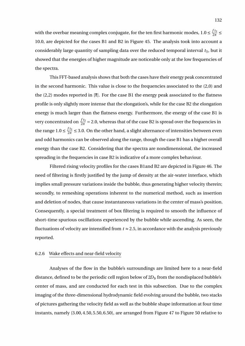
132

with the overbar meaning complex conjugate, for the ten first harmonic modes, 1.0 ≤ f tS2π ≤

10.0, are depicted for the cases B1 and B2 in Figure 45. The analysis took into account a

considerably large quantity of sampling data over the reduced temporal interval tS , but it

showed that the energies of higher magnitude are noticeable only at the low frequencies of

the spectra.

This FFT-based analysis shows that both the cases have their energy peak concentrated

in the second harmonic. This value is close to the frequencies associated to the (2,0) and

the (2,2) modes reported in [?]. For the case B1 the energy peak associated to the flatness

profile is only slightly more intense that the elongation’s, while for the case B2 the elongation

energy is much larger than the flatness energy. Furthermore, the energy of the case B1 is

very concentrated on f tS2π = 2.0, whereas that of the case B2 is spread over the frequencies in

the range 1.0 ≤ f tS2π ≤ 3.0. On the other hand, a slight alternance of intensities between even

and odd harmonics can be observed along the range, though the case B1 has a higher overall

energy than the case B2. Considering that the spectra are nondimensional, the increased

spreading in the frequencies in case B2 is indicative of a more complex behaviour.

Filtered rising velocity profiles for the cases B1and B2 are depicted in Figure 46. The

need of filtering is firstly justified by the jump of density at the air-water interface, which

implies small pressure variations inside the bubble, thus generating higher velocity therein;

secondly, to remeshing operations inherent to the numerical method, such as insertion

and deletion of nodes, that cause instantaneous variations in the center of mass’s position.

Consequently, a special treatment of box filtering is required to smooth the influence of

short-time spurious oscillations experienced by the bubble while ascending. As seen, the

fluctuations of velocity are intensified from t ≈ 2.5, in accordance with the analysis previously

reported.

6.2.6 Wake effects and near-field velocity

Analyses of the flow in the bubble’s surroundings are limited here to a near-field

distance, defined to be the periodic cell region below of 2Db from the nondisplaced bubble’s

center of mass, and are conducted for each test in this subsection. Due to the complex

imaging of the three-dimensional hydrodynamic field evolving around the bubble, two stacks

of pictures gathering the velocity field as well as the bubble shape information at four time

instants, namely 3.00,4.50,5.50,6.50, are arranged from Figure 47 to Figure 50 relative to

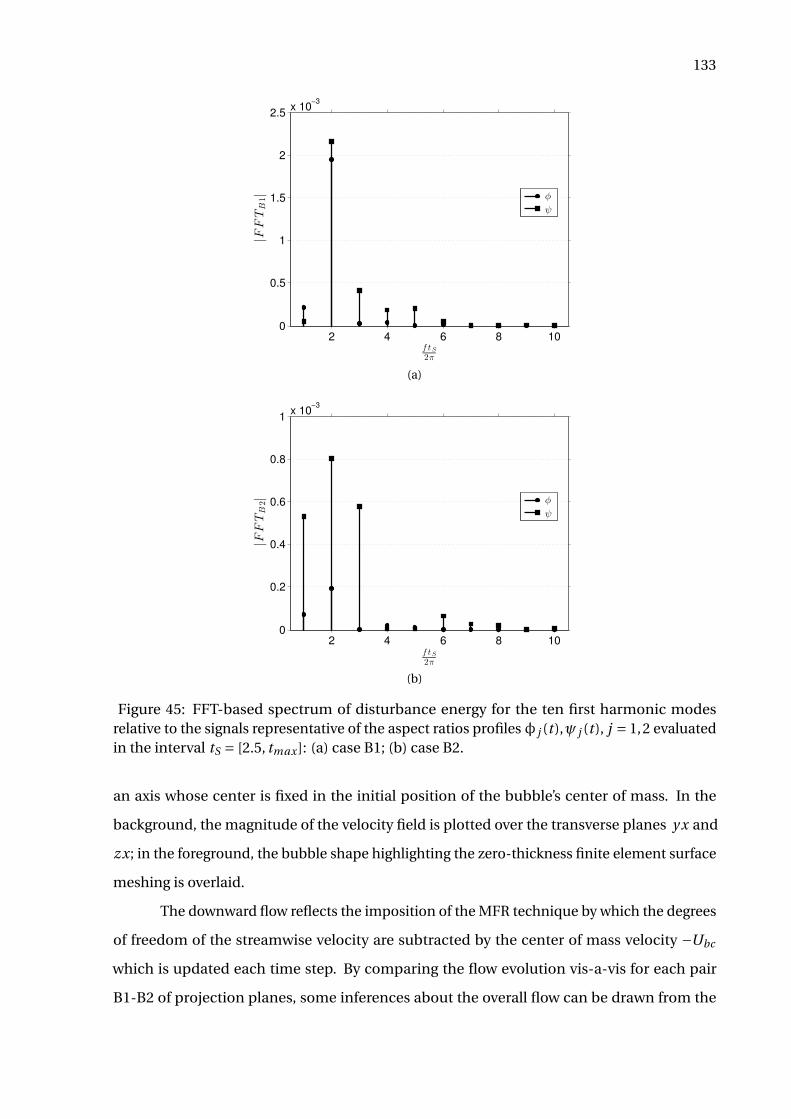
133

2 4 6 8 100

0.5

1

1.5

2

2.5x 10

−3

f t S

2π

|FFTB1|

φ

ψ

(a)

2 4 6 8 100

0.2

0.4

0.6

0.8

1x 10

−3

f t S

2π

|FFTB2|

φ

ψ

(b)

Figure 45: FFT-based spectrum of disturbance energy for the ten first harmonic modesrelative to the signals representative of the aspect ratios profiles φ j (t ),ψ j (t ), j = 1,2 evaluatedin the interval tS = [2.5, tmax]: (a) case B1; (b) case B2.

an axis whose center is fixed in the initial position of the bubble’s center of mass. In the

background, the magnitude of the velocity field is plotted over the transverse planes y x and

zx; in the foreground, the bubble shape highlighting the zero-thickness finite element surface

meshing is overlaid.

The downward flow reflects the imposition of the MFR technique by which the degrees

of freedom of the streamwise velocity are subtracted by the center of mass velocity −Ubc

which is updated each time step. By comparing the flow evolution vis-a-vis for each pair

B1-B2 of projection planes, some inferences about the overall flow can be drawn from the

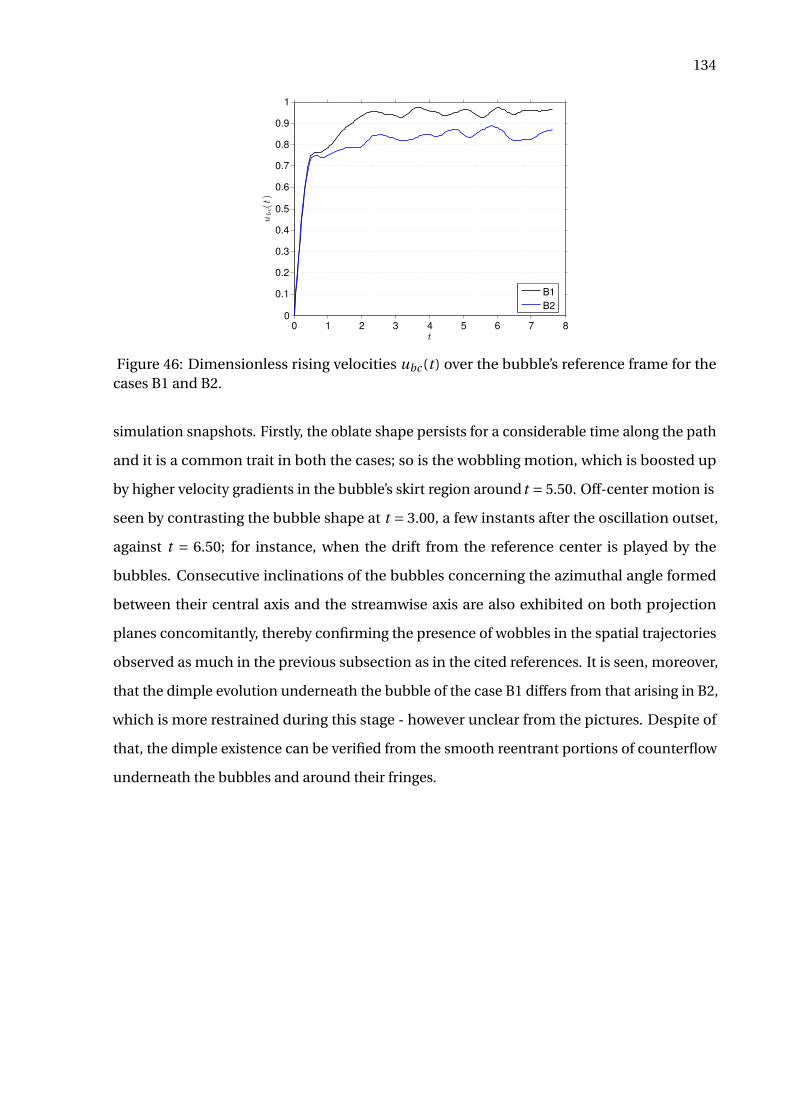
134

0 1 2 3 4 5 6 7 8

0

0.1

0.2

0.3

0.4

0.5

0.6

0.7

0.8

0.9

1

t

ubc(t)

B1

B2

Figure 46: Dimensionless rising velocities ubc (t) over the bubble’s reference frame for thecases B1 and B2.

simulation snapshots. Firstly, the oblate shape persists for a considerable time along the path

and it is a common trait in both the cases; so is the wobbling motion, which is boosted up

by higher velocity gradients in the bubble’s skirt region around t = 5.50. Off-center motion is

seen by contrasting the bubble shape at t = 3.00, a few instants after the oscillation outset,

against t = 6.50; for instance, when the drift from the reference center is played by the

bubbles. Consecutive inclinations of the bubbles concerning the azimuthal angle formed

between their central axis and the streamwise axis are also exhibited on both projection

planes concomitantly, thereby confirming the presence of wobbles in the spatial trajectories

observed as much in the previous subsection as in the cited references. It is seen, moreover,

that the dimple evolution underneath the bubble of the case B1 differs from that arising in B2,

which is more restrained during this stage - however unclear from the pictures. Despite of

that, the dimple existence can be verified from the smooth reentrant portions of counterflow

underneath the bubbles and around their fringes.

135

1.0

velocity

0.18

1.77

t = 6.50

(a)

1.0

velocity

0.19

1.96

t = 5.50

(b)

1.0

velocity

0.13

1.81

t = 4.50

(c)

1.0

velocity

0.08

1.98

t = 3.00

(d)

Figure 47: Velocity field and bubble shape for the case B1: plane y x; (a) t = 3.00, (b) t = 4.50,(c) t = 5.50, (d) t = 6.50.

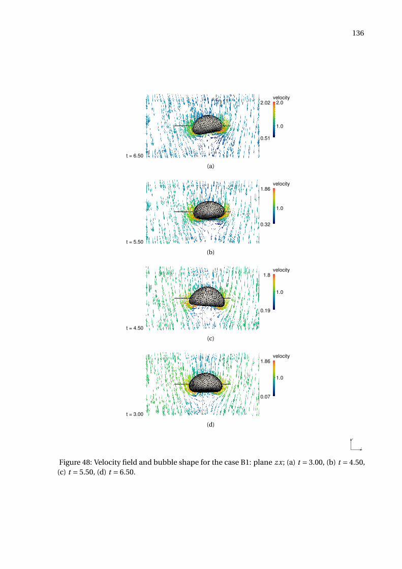
136

t = 6.50

1.0

2.0velocity

0.51

2.02

(a)

1.0

velocity

0.32

1.86

t = 5.50

(b)

1.0

velocity

0.19

1.8

t = 4.50

(c)

1.0

velocity

0.07

1.86

t = 3.00

(d)

Figure 48: Velocity field and bubble shape for the case B1: plane zx; (a) t = 3.00, (b) t = 4.50,(c) t = 5.50, (d) t = 6.50.

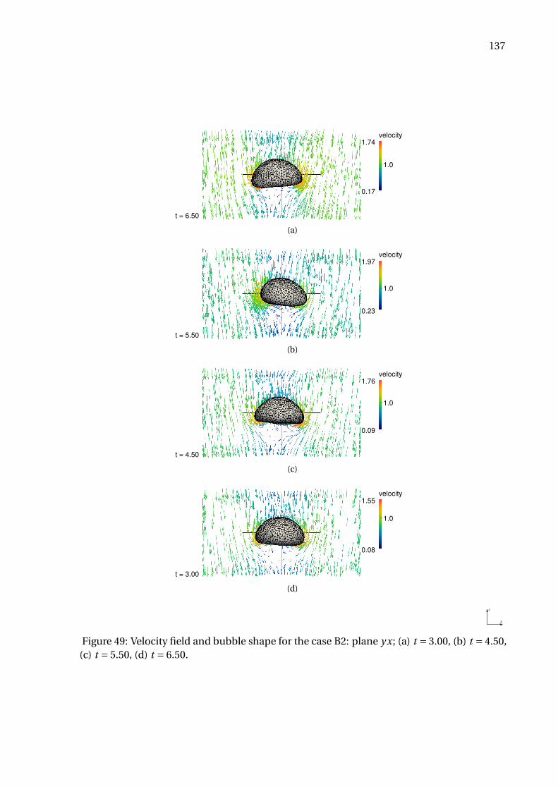
137

1.0

velocity

0.17

1.74

t = 6.50

(a)

1.0

velocity

0.23

1.97

t = 5.50

(b)

1.0

velocity

0.09

1.76

t = 4.50

(c)

1.0

velocity

0.08

1.55

t = 3.00

(d)

Figure 49: Velocity field and bubble shape for the case B2: plane y x; (a) t = 3.00, (b) t = 4.50,(c) t = 5.50, (d) t = 6.50.

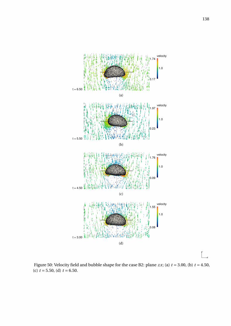
138

1.0

velocity

0.17

1.74

t = 6.50

(a)

1.0

velocity

0.23

1.97

t = 5.50

(b)

1.0

velocity

0.09

1.76

t = 4.50

(c)

1.0

velocity

0.08

1.55

t = 3.00

(d)

Figure 50: Velocity field and bubble shape for the case B2: plane zx; (a) t = 3.00, (b) t = 4.50,(c) t = 5.50, (d) t = 6.50.

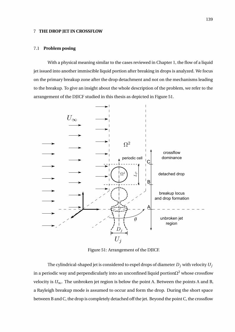
139

7 THE DROP JET IN CROSSFLOW

7.1 Problem posing

With a physical meaning similar to the cases reviewed in Chapter 1, the flow of a liquid

jet issued into another immiscible liquid portion after breaking in drops is analyzed. We focus

on the primary breakup zone after the drop detachment and not on the mechanisms leading

to the breakup. To give an insight about the whole description of the problem, we refer to the

arrangement of the DJICF studied in this thesis as depicted in Figure 51.

unbroken jet

region

A

B

C

breakup locus

and drop formation

detached drop

crossflow

dominanceperiodic cell

Figure 51: Arrangement of the DJICF.

The cylindrical-shaped jet is considered to expel drops of diameter D j with velocity U j

in a periodic way and perpendicularly into an unconfined liquid portionΩ2 whose crossflow

velocity is U∞. The unbroken jet region is below the point A. Between the points A and B,

a Rayleigh breakup mode is assumed to occur and form the drop. During the short space

between B and C, the drop is completely detached off the jet. Beyond the point C, the crossflow

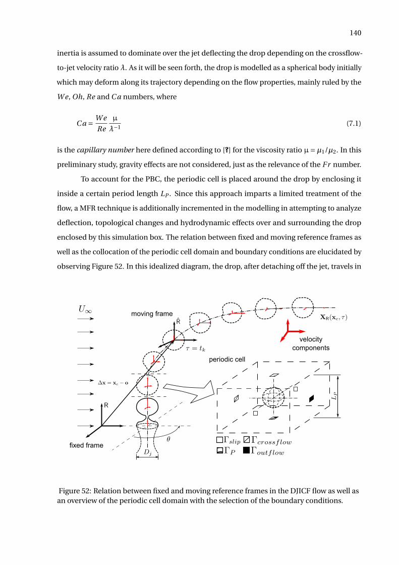
140

inertia is assumed to dominate over the jet deflecting the drop depending on the crossflow-

to-jet velocity ratio λ. As it will be seen forth, the drop is modelled as a spherical body initially

which may deform along its trajectory depending on the flow properties, mainly ruled by the

W e, Oh, Re and C a numbers, where

C a = W e

Re

µ

λ−1(7.1)

is the capillary number here defined according to [?] for the viscosity ratio µ=µ1/µ2. In this

preliminary study, gravity effects are not considered, just as the relevance of the F r number.

To account for the PBC, the periodic cell is placed around the drop by enclosing it

inside a certain period length LP . Since this approach imparts a limited treatment of the

flow, a MFR technique is additionally incremented in the modelling in attempting to analyze

deflection, topological changes and hydrodynamic effects over and surrounding the drop

enclosed by this simulation box. The relation between fixed and moving reference frames as

well as the collocation of the periodic cell domain and boundary conditions are elucidated by

observing Figure 52. In this idealized diagram, the drop, after detaching off the jet, travels in

moving frame

fixed frame

velocity components

periodic cell

Figure 52: Relation between fixed and moving reference frames in the DJICF flow as well asan overview of the periodic cell domain with the selection of the boundary conditions.

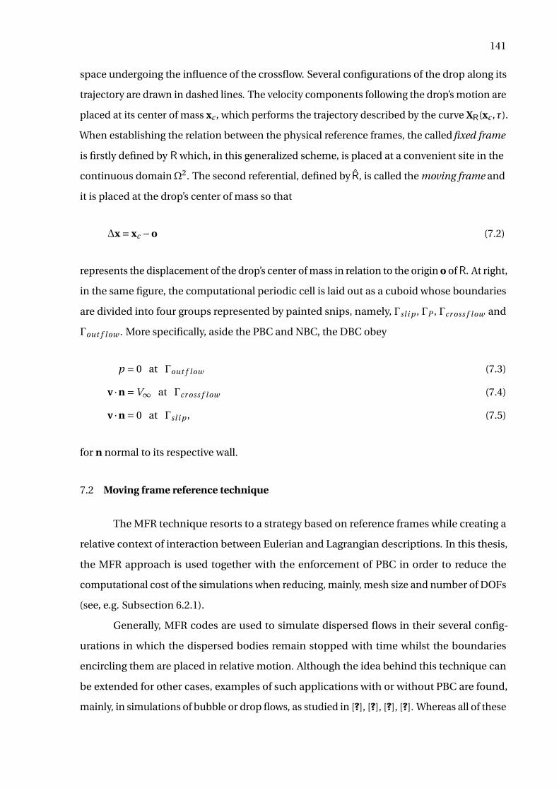
141

space undergoing the influence of the crossflow. Several configurations of the drop along its

trajectory are drawn in dashed lines. The velocity components following the drop’s motion are

placed at its center of mass xc , which performs the trajectory described by the curve XR(xc ,τ).

When establishing the relation between the physical reference frames, the called fixed frame

is firstly defined by R which, in this generalized scheme, is placed at a convenient site in the

continuous domainΩ2. The second referential, defined by R, is called the moving frame and

it is placed at the drop’s center of mass so that

∆x = xc −o (7.2)

represents the displacement of the drop’s center of mass in relation to the origin o ofR. At right,

in the same figure, the computational periodic cell is laid out as a cuboid whose boundaries

are divided into four groups represented by painted snips, namely, Γsl i p , ΓP , Γcr oss f low and

Γout f l ow . More specifically, aside the PBC and NBC, the DBC obey

p = 0 at Γout f low (7.3)

v ·n =V∞ at Γcr oss f l ow (7.4)

v ·n = 0 at Γsl i p , (7.5)

for n normal to its respective wall.

7.2 Moving frame reference technique

The MFR technique resorts to a strategy based on reference frames while creating a

relative context of interaction between Eulerian and Lagrangian descriptions. In this thesis,

the MFR approach is used together with the enforcement of PBC in order to reduce the

computational cost of the simulations when reducing, mainly, mesh size and number of DOFs

(see, e.g. Subsection 6.2.1).

Generally, MFR codes are used to simulate dispersed flows in their several config-

urations in which the dispersed bodies remain stopped with time whilst the boundaries

encircling them are placed in relative motion. Although the idea behind this technique can

be extended for other cases, examples of such applications with or without PBC are found,

mainly, in simulations of bubble or drop flows, as studied in [?], [?], [?], [?]. Whereas all of these

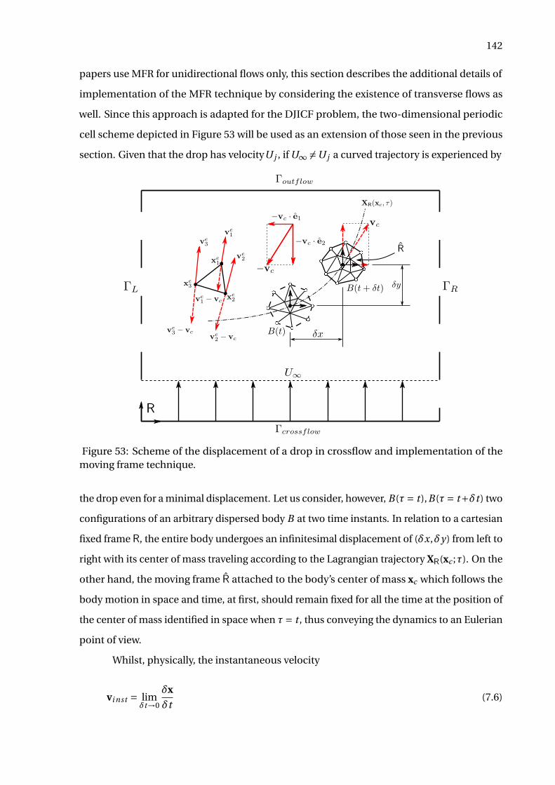
142

papers use MFR for unidirectional flows only, this section describes the additional details of

implementation of the MFR technique by considering the existence of transverse flows as

well. Since this approach is adapted for the DJICF problem, the two-dimensional periodic

cell scheme depicted in Figure 53 will be used as an extension of those seen in the previous

section. Given that the drop has velocityU j , if U∞ 6=U j a curved trajectory is experienced by

Figure 53: Scheme of the displacement of a drop in crossflow and implementation of themoving frame technique.

the drop even for a minimal displacement. Let us consider, however, B(τ= t ),B(τ= t+δt ) two

configurations of an arbitrary dispersed body B at two time instants. In relation to a cartesian

fixed frame R, the entire body undergoes an infinitesimal displacement of (δx,δy) from left to

right with its center of mass traveling according to the Lagrangian trajectory XR(xc ;τ). On the

other hand, the moving frame R attached to the body’s center of mass xc which follows the

body motion in space and time, at first, should remain fixed for all the time at the position of

the center of mass identified in space when τ= t , thus conveying the dynamics to an Eulerian

point of view.

Whilst, physically, the instantaneous velocity

vi nst = limδt→0

δx

δt(7.6)

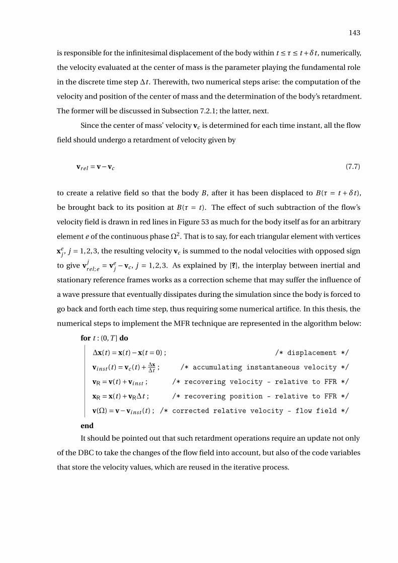
143

is responsible for the infinitesimal displacement of the body within t ≤ τ≤ t +δt , numerically,

the velocity evaluated at the center of mass is the parameter playing the fundamental role

in the discrete time step ∆t . Therewith, two numerical steps arise: the computation of the

velocity and position of the center of mass and the determination of the body’s retardment.

The former will be discussed in Subsection 7.2.1; the latter, next.

Since the center of mass’ velocity vc is determined for each time instant, all the flow

field should undergo a retardment of velocity given by

vr el = v−vc (7.7)

to create a relative field so that the body B , after it has been displaced to B(τ = t + δt),

be brought back to its position at B(τ = t). The effect of such subtraction of the flow’s

velocity field is drawn in red lines in Figure 53 as much for the body itself as for an arbitrary

element e of the continuous phaseΩ2. That is to say, for each triangular element with vertices

xej , j = 1,2,3, the resulting velocity vc is summed to the nodal velocities with opposed sign

to give v jr el ;e = ve

j − vc , j = 1,2,3. As explained by [?], the interplay between inertial and

stationary reference frames works as a correction scheme that may suffer the influence of

a wave pressure that eventually dissipates during the simulation since the body is forced to

go back and forth each time step, thus requiring some numerical artifice. In this thesis, the

numerical steps to implement the MFR technique are represented in the algorithm below:

for t : (0,T ] do

∆x(t ) = x(t )−x(t = 0) ; /* displacement */

vi nst (t ) = vc (t )+ ∆x∆t ; /* accumulating instantaneous velocity */

vR = v(t )+vi nst ; /* recovering velocity - relative to FFR */

xR = x(t )+vR∆t ; /* recovering position - relative to FFR */

v(Ω) = v−vi nst (t ) ; /* corrected relative velocity - flow field */

end

It should be pointed out that such retardment operations require an update not only

of the DBC to take the changes of the flow field into account, but also of the code variables

that store the velocity values, which are reused in the iterative process.

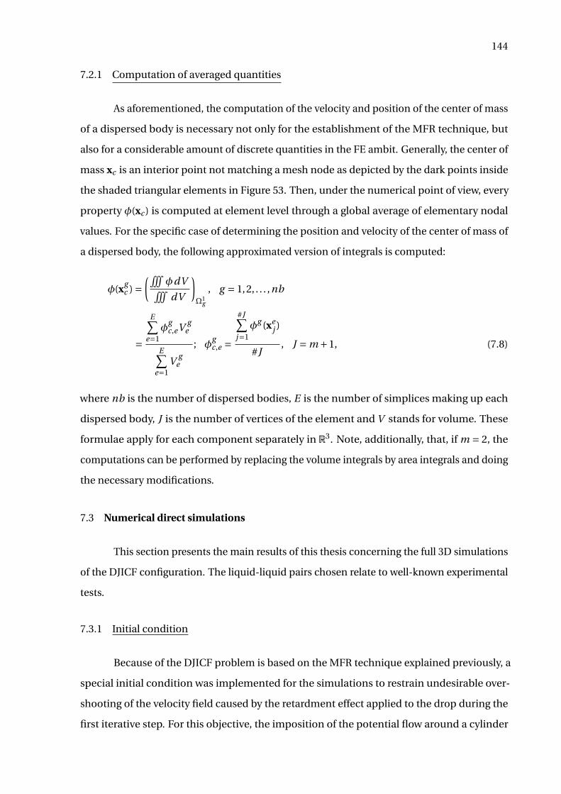
144

7.2.1 Computation of averaged quantities

As aforementioned, the computation of the velocity and position of the center of mass

of a dispersed body is necessary not only for the establishment of the MFR technique, but

also for a considerable amount of discrete quantities in the FE ambit. Generally, the center of

mass xc is an interior point not matching a mesh node as depicted by the dark points inside

the shaded triangular elements in Figure 53. Then, under the numerical point of view, every

property φ(xc ) is computed at element level through a global average of elementary nodal

values. For the specific case of determining the position and velocity of the center of mass of

a dispersed body, the following approximated version of integrals is computed:

φ(xgc ) =

(ÐφdVÐ

dV

)Ω1

g

, g = 1,2, . . . ,nb

=

E∑e=1

φgc,eV g

e

E∑e=1

V ge

; φgc,e =

#J∑j=1

φg (xej )

#J, J = m +1, (7.8)

where nb is the number of dispersed bodies, E is the number of simplices making up each

dispersed body, J is the number of vertices of the element and V stands for volume. These

formulae apply for each component separately in R3. Note, additionally, that, if m = 2, the

computations can be performed by replacing the volume integrals by area integrals and doing

the necessary modifications.

7.3 Numerical direct simulations

This section presents the main results of this thesis concerning the full 3D simulations

of the DJICF configuration. The liquid-liquid pairs chosen relate to well-known experimental

tests.

7.3.1 Initial condition

Because of the DJICF problem is based on the MFR technique explained previously, a

special initial condition was implemented for the simulations to restrain undesirable over-

shooting of the velocity field caused by the retardment effect applied to the drop during the

first iterative step. For this objective, the imposition of the potential flow around a cylinder

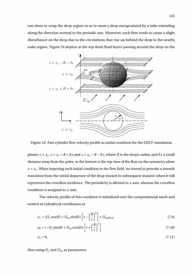
145

was done to wrap the drop region so as to seem a drop encapsulated by a tube extending

along the direction normal to the periodic one. Moreover, such flow tends to cause a slight

disturbance on the drop due to the circulations that rise up behind the drop in the nearby

wake region. Figure 54 depicts at the top three fluid layers passing around the drop on the

Figure 54: Past cylinder flow velocity profile as initial condition for the DJICF simulation.

planes z = zc , z = zc +R +δz and z = zc −R −δz, where R is the drop’s radius and δz a small

distance away from the poles; at the bottom is the top view of the flow on the symmetry plane

z = zc . When imposing such initial condition to the flow field, we intend to provoke a smooth

transition from the initial departure of the drop toward its subsequent instants when it will

experience the crossflow incidence. The periodicity is allotted to x-axis, whereas the crossflow

condition is assigned to y-axis.

The velocity profile of this condition is initialized over the computational mesh and

written in cylindrical coordinates as

vr = (U j cos(θ)+U∞ sin(θ))

[1−

(R

r

)2]+Uadded (7.9)

vθ = (−U j sin(θ)+U∞ cos(θ))

[1+

(R

r

)2](7.10)

vz = 0, (7.11)

thus using U j and U∞ as parameters.

146

At this point, it should be explained that Uadded =U j is added to the original profile

to compensate the difference which will be deduced of the flow immediately afterwards the

simulation begin because of the MFR calculation (see the algorithm in Section 7.2) that retards

the drop’s motion.

7.3.2 Study of DJICF cases: hydrodynamics and discussion

Two different pairs of immiscible liquids relating to experiments performed, respec-

tively, by Meister and Scheele [?] (also reproduced by [?]) for a water/n-heptane interface

and by Webster and Longmire [?] (see p. 226) for a water-glycerin/Dow Corning sylicon-oil

interface make up the next simulations, whose physical parameters are presented in Table

5 and Table 6. For convenience, the labels MS and WL will be used as abbreviations of the

references cited above to designate the numerical tests. Additionally, two other parameters

will determine the simulations, namely the ratio λ and the periodic cell’s length LP . Hence,

the different configurations of tests chosen are expressed by a triple of parameters as

(Re f ,λ,LP ), for Re f = MS, WL; λ= 1.0, 1.5, 2.0 and LP = 1.5, 3.0, 5.0. (7.12)

While different values of LP seek to analyze the effect of the PBC by considering different

spacing between drops (in the sense of the imposed periodicity), small values of λ seek to

add a weak effect to the crossflow so as to ensure small disturbances in the surroundings of

the drop and preserve the periodicity with less tendency to deflection. The cuboid-shaped

meshes used in the simulations, which differ one another by the length LP , are depicted in

Figure 55 clipped along the axis of periodicity.

The analysis of the simulations starts from the velocity field vR(t) = (uc , vc , wc )(t),

whose component profiles are organized for each configuration from Figure 56 to Figure 61 as

the ratio λ. By observing the curves of uc and vc , it is noticeable that uc decays monotonically

from U j = 1.0 - the dimensionless jet velocity - at the initial instant to zero in the far-field

Data

µ ρ D j Re W e2.43 1.45 0.68 1851 2.20

Table 5: Parameters of simulation according to the experiment no. 5 of Meister and Scheele [?].

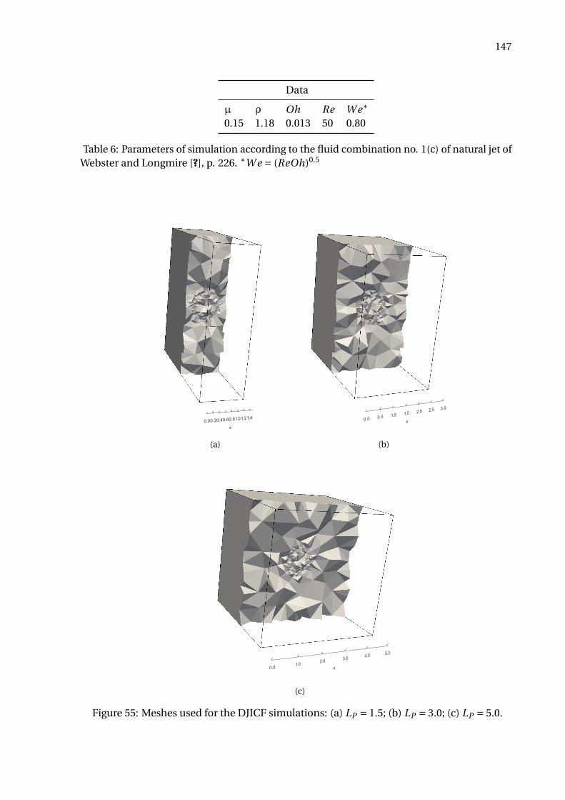
147

Data

µ ρ Oh Re W e∗

0.15 1.18 0.013 50 0.80

Table 6: Parameters of simulation according to the fluid combination no. 1(c) of natural jet ofWebster and Longmire [?], p. 226. ∗W e = (ReOh)0.5

(a) (b)

(c)

Figure 55: Meshes used for the DJICF simulations: (a) LP = 1.5; (b) LP = 3.0; (c) LP = 5.0.

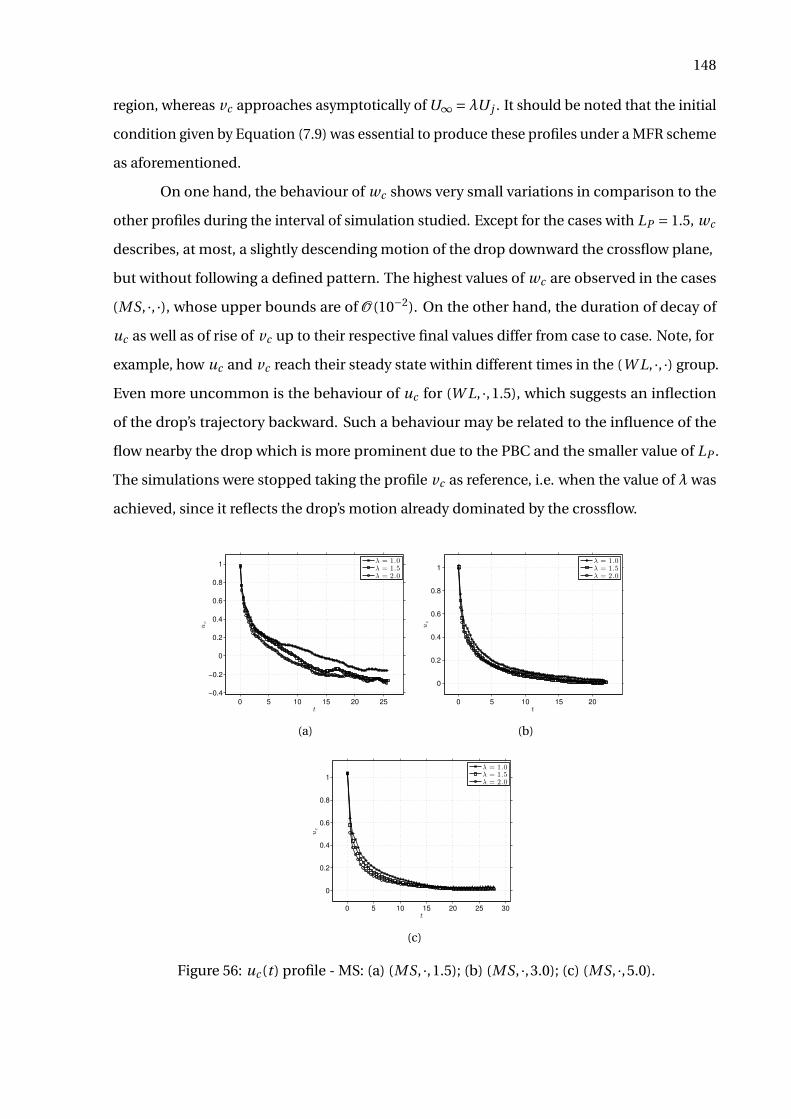
148

region, whereas vc approaches asymptotically of U∞ =λU j . It should be noted that the initial

condition given by Equation (7.9) was essential to produce these profiles under a MFR scheme

as aforementioned.

On one hand, the behaviour of wc shows very small variations in comparison to the

other profiles during the interval of simulation studied. Except for the cases with LP = 1.5, wc

describes, at most, a slightly descending motion of the drop downward the crossflow plane,

but without following a defined pattern. The highest values of wc are observed in the cases

(MS, ·, ·), whose upper bounds are of O (10−2). On the other hand, the duration of decay of

uc as well as of rise of vc up to their respective final values differ from case to case. Note, for

example, how uc and vc reach their steady state within different times in the (W L, ·, ·) group.

Even more uncommon is the behaviour of uc for (W L, ·,1.5), which suggests an inflection

of the drop’s trajectory backward. Such a behaviour may be related to the influence of the

flow nearby the drop which is more prominent due to the PBC and the smaller value of LP .

The simulations were stopped taking the profile vc as reference, i.e. when the value of λ was

achieved, since it reflects the drop’s motion already dominated by the crossflow.

0 5 10 15 20 25

−0.4

−0.2

0

0.2

0.4

0.6

0.8

1

t

uc

λ = 1.0λ = 1.5λ = 2.0

(a)

0 5 10 15 20

0

0.2

0.4

0.6

0.8

1

t

uc

λ = 1.0λ = 1.5λ = 2.0

(b)

0 5 10 15 20 25 30

0

0.2

0.4

0.6

0.8

1

t

uc

λ = 1.0λ = 1.5λ = 2.0

(c)

Figure 56: uc (t ) profile - MS: (a) (MS, ·,1.5); (b) (MS, ·,3.0); (c) (MS, ·,5.0).

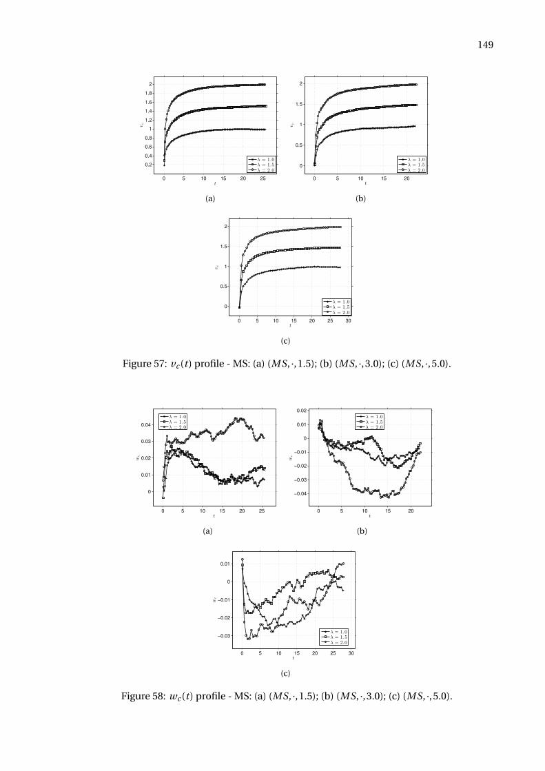
149

0 5 10 15 20 25

0.2

0.4

0.6

0.8

1

1.2

1.4

1.6

1.8

2

t

vc

λ = 1.0λ = 1.5λ = 2.0

(a)

0 5 10 15 20

0

0.5

1

1.5

2

t

vc

λ = 1.0λ = 1.5λ = 2.0

(b)

0 5 10 15 20 25 30

0

0.5

1

1.5

2

t

vc

λ = 1.0λ = 1.5λ = 2.0

(c)

Figure 57: vc (t ) profile - MS: (a) (MS, ·,1.5); (b) (MS, ·,3.0); (c) (MS, ·,5.0).

0 5 10 15 20 25

0

0.01

0.02

0.03

0.04

t

wc

λ = 1.0λ = 1.5λ = 2.0

(a)

0 5 10 15 20

−0.04

−0.03

−0.02

−0.01

0

0.01

0.02

t

wc

λ = 1.0λ = 1.5λ = 2.0

(b)

0 5 10 15 20 25 30

−0.03

−0.02

−0.01

0

0.01

t

wc

λ = 1.0λ = 1.5λ = 2.0

(c)

Figure 58: wc (t ) profile - MS: (a) (MS, ·,1.5); (b) (MS, ·,3.0); (c) (MS, ·,5.0).

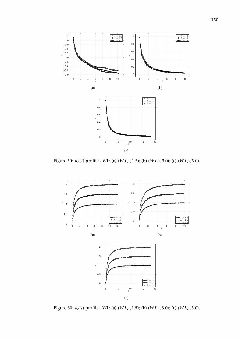
150

0 2 4 6 8 10 12

−0.8

−0.6

−0.4

−0.2

0

0.2

0.4

0.6

0.8

1

t

uc

λ = 1.0λ = 1.5λ = 2.0

(a)

0 2 4 6 8 10

0

0.2

0.4

0.6

0.8

1

t

uc

λ = 1.0λ = 1.5λ = 2.0

(b)

0 5 10 15 20

0

0.2

0.4

0.6

0.8

1

t

uc

λ = 1.0λ = 1.5λ = 2.0

(c)

Figure 59: uc (t ) profile - WL: (a) (W L, ·,1.5); (b) (W L, ·,3.0); (c) (W L, ·,5.0).

0 2 4 6 8 10 12

0

0.5

1

1.5

2

t

vc

λ = 1.0λ = 1.5λ = 2.0

(a)

0 2 4 6 8 10

0

0.5

1

1.5

2

t

vc

λ = 1.0λ = 1.5λ = 2.0

(b)

0 5 10 15 20

0

0.5

1

1.5

2

t

vc

λ = 1.0λ = 1.5λ = 2.0

(c)

Figure 60: vc (t ) profile - WL: (a) (W L, ·,1.5); (b) (W L, ·,3.0); (c) (W L, ·,5.0).

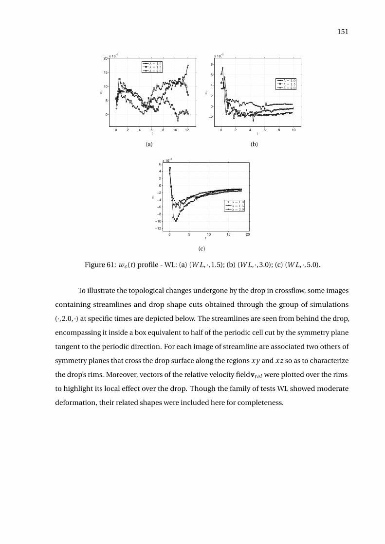
151

0 2 4 6 8 10 12

0

5

10

15

20x 10

−3

t

wc

λ = 1.0λ = 1.5λ = 2.0

(a)

0 2 4 6 8 10

−2

0

2

4

6

8

x 10−3

t

wc

λ = 1.0λ = 1.5λ = 2.0

(b)

0 5 10 15 20

−12

−10

−8

−6

−4

−2

0

2

4

6

x 10−3

t

wc

λ = 1.0λ = 1.5λ = 2.0

(c)

Figure 61: wc (t ) profile - WL: (a) (W L, ·,1.5); (b) (W L, ·,3.0); (c) (W L, ·,5.0).

To illustrate the topological changes undergone by the drop in crossflow, some images

containing streamlines and drop shape cuts obtained through the group of simulations

(·,2.0, ·) at specific times are depicted below. The streamlines are seen from behind the drop,

encompassing it inside a box equivalent to half of the periodic cell cut by the symmetry plane

tangent to the periodic direction. For each image of streamline are associated two others of

symmetry planes that cross the drop surface along the regions x y and xz so as to characterize

the drop’s rims. Moreover, vectors of the relative velocity fieldvr el were plotted over the rims

to highlight its local effect over the drop. Though the family of tests WL showed moderate

deformation, their related shapes were included here for completeness.

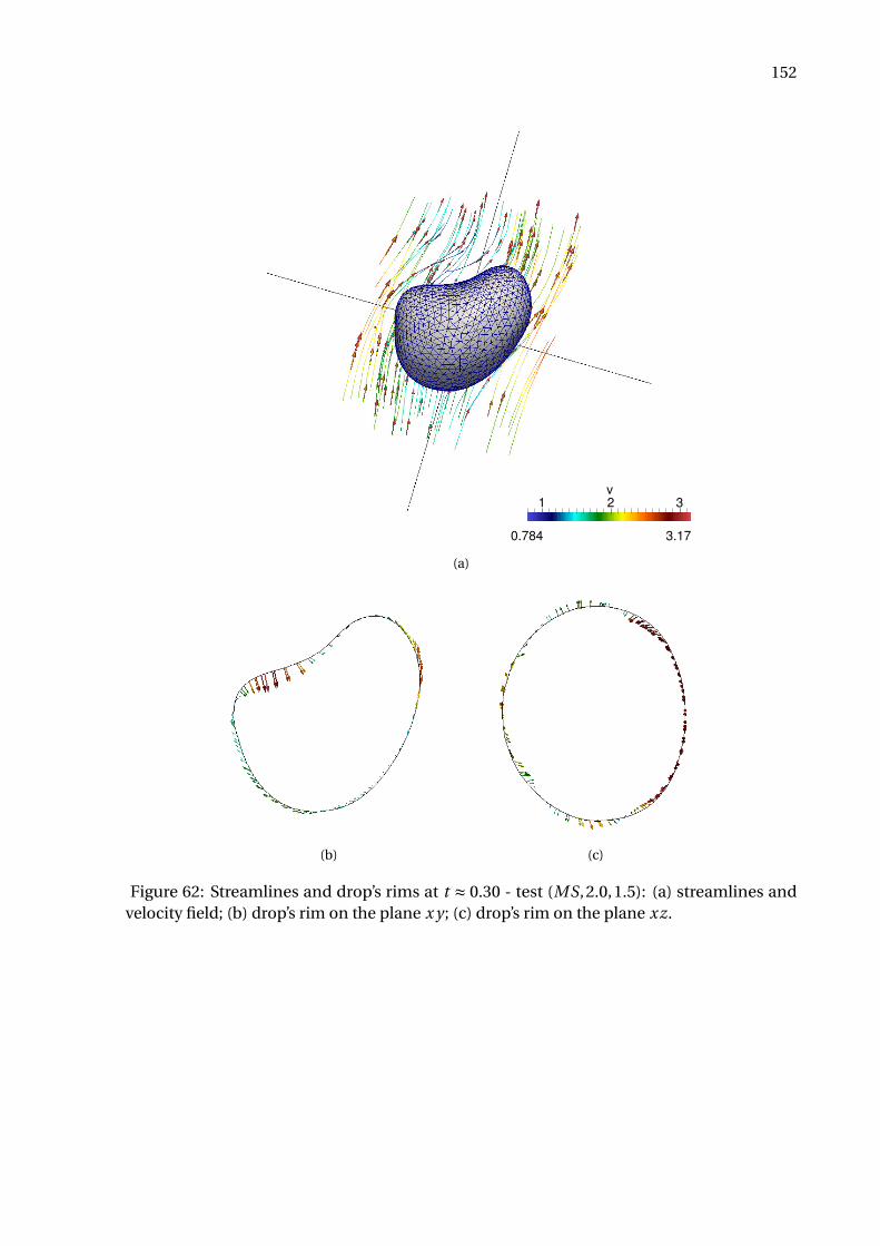
152

3.17

1 2 3

v

0.784

(a)

(b) (c)

Figure 62: Streamlines and drop’s rims at t ≈ 0.30 - test (MS,2.0,1.5): (a) streamlines andvelocity field; (b) drop’s rim on the plane x y ; (c) drop’s rim on the plane xz.

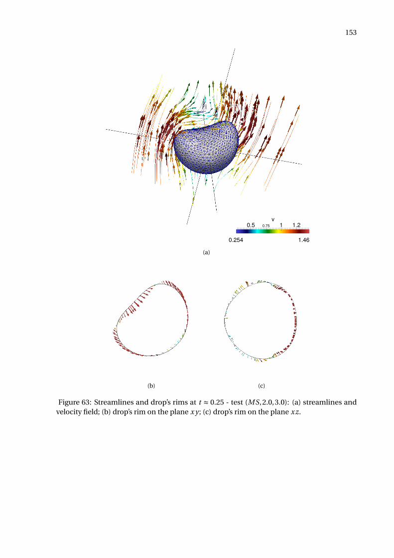
153

0.5 0.75 1 1.2

v

0.254 1.46

(a)

(b) (c)


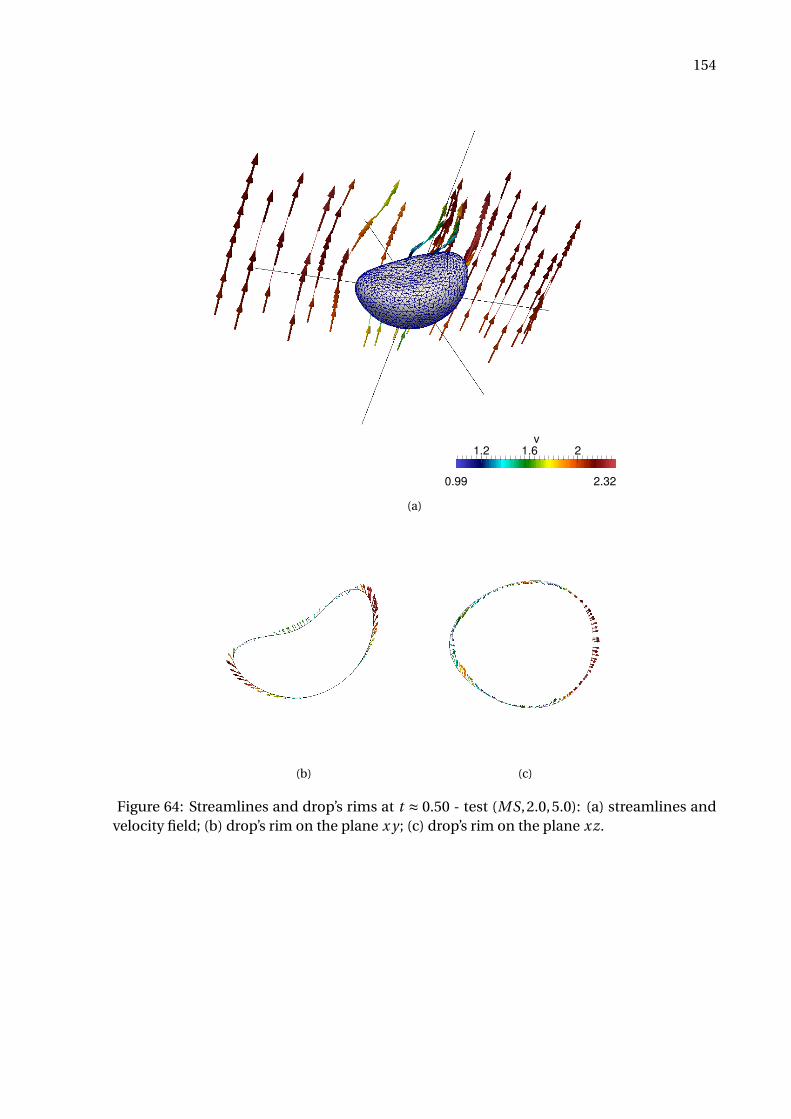
154

1.2 1.6 2

v

0.99 2.32

(a)

(b) (c)


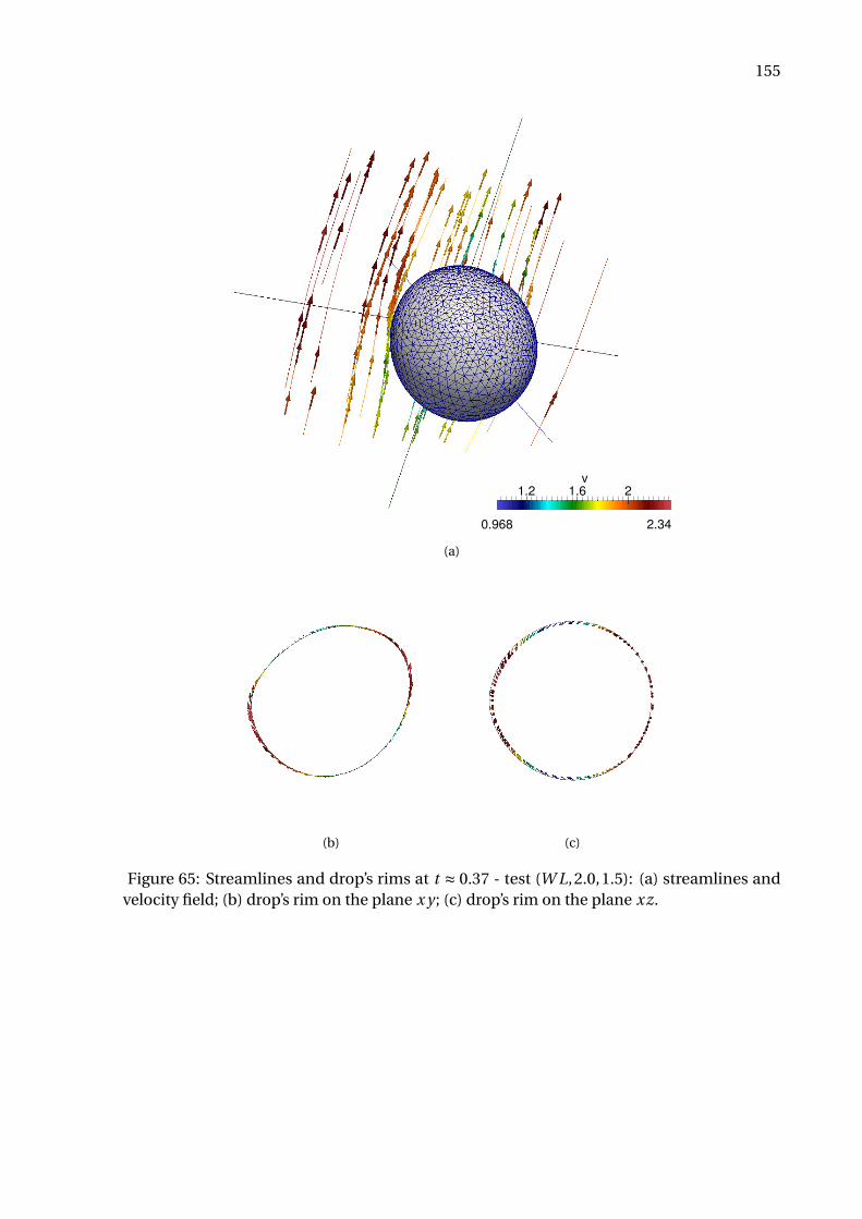
155

1.2 1.6 2

v

0.968 2.34

(a)

(b) (c)

Figure 65: Streamlines and drop’s rims at t ≈ 0.37 - test (W L,2.0,1.5): (a) streamlines andvelocity field; (b) drop’s rim on the plane x y ; (c) drop’s rim on the plane xz.

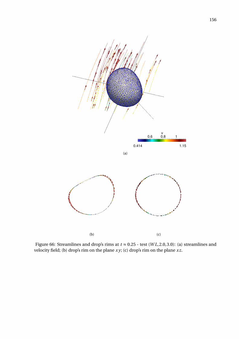
156

0.6 0.8 1

v

0.414 1.15

(a)

(b) (c)


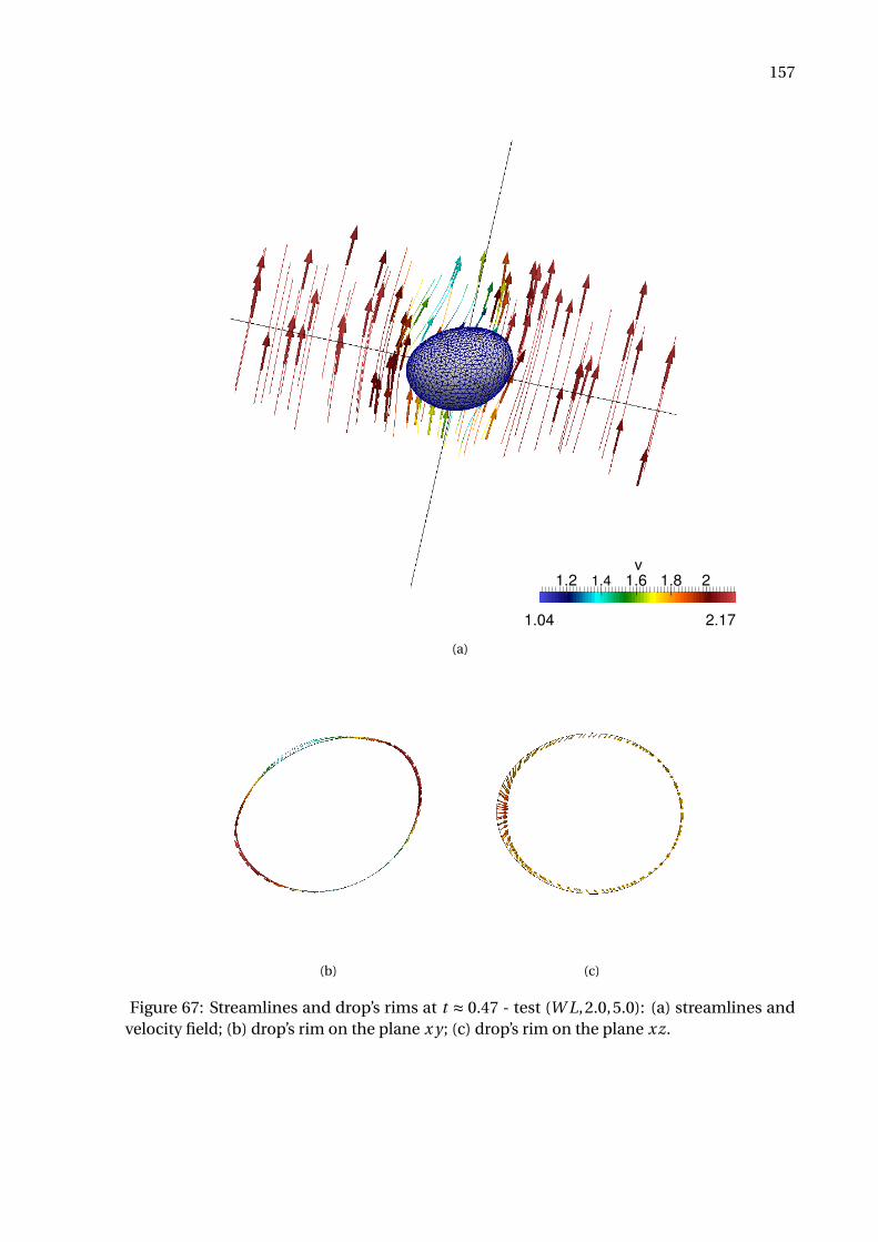
157

1.2 1.4 1.6 1.8 2

v

1.04 2.17

(a)

(b) (c)


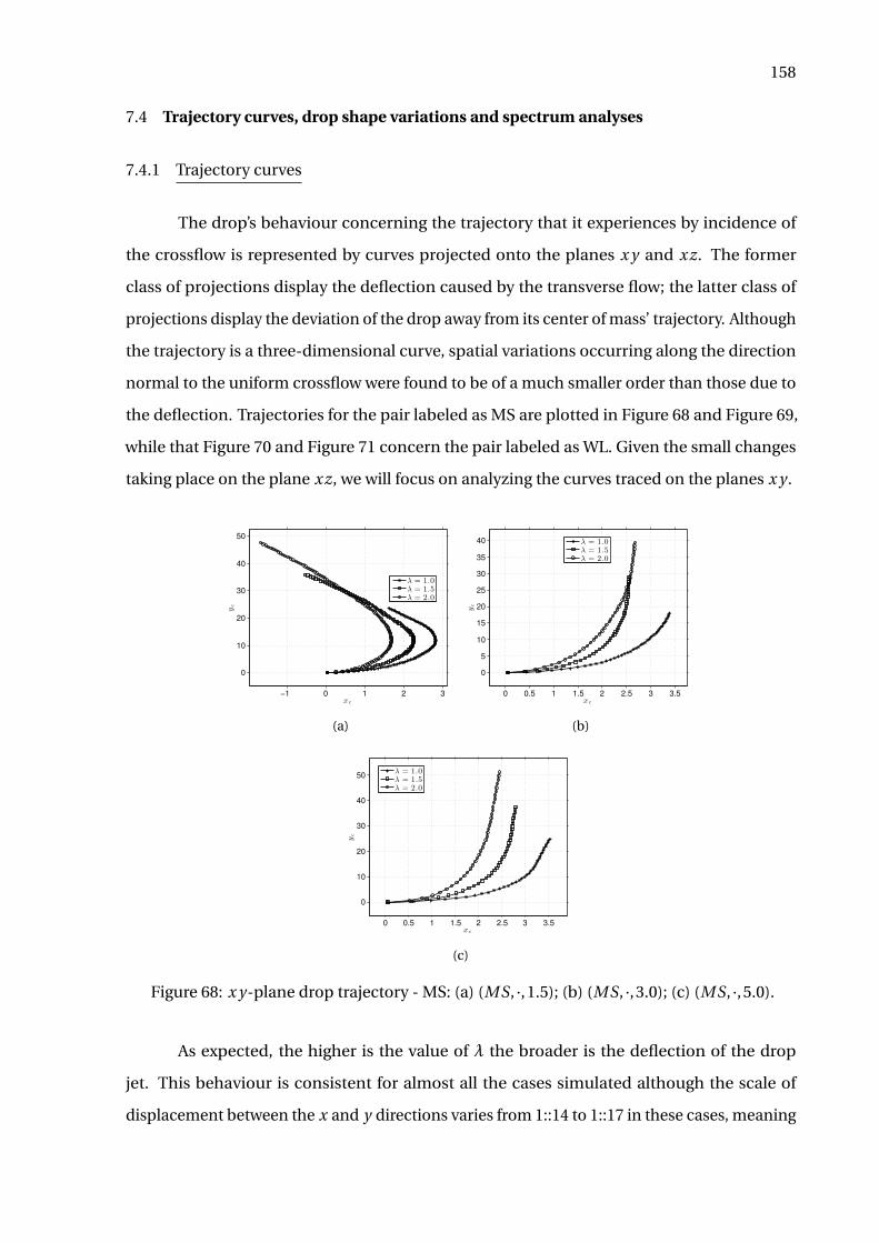
158

7.4 Trajectory curves, drop shape variations and spectrum analyses

7.4.1 Trajectory curves

The drop’s behaviour concerning the trajectory that it experiences by incidence of

the crossflow is represented by curves projected onto the planes x y and xz. The former

class of projections display the deflection caused by the transverse flow; the latter class of

projections display the deviation of the drop away from its center of mass’ trajectory. Although

the trajectory is a three-dimensional curve, spatial variations occurring along the direction

normal to the uniform crossflow were found to be of a much smaller order than those due to

the deflection. Trajectories for the pair labeled as MS are plotted in Figure 68 and Figure 69,

while that Figure 70 and Figure 71 concern the pair labeled as WL. Given the small changes

taking place on the plane xz, we will focus on analyzing the curves traced on the planes x y .

−1 0 1 2 3

0

10

20

30

40

50

x c

yc

λ = 1.0λ = 1.5λ = 2.0

(a)

0 0.5 1 1.5 2 2.5 3 3.5

0

5

10

15

20

25

30

35

40

x c

yc

λ = 1.0λ = 1.5λ = 2.0

(b)

0 0.5 1 1.5 2 2.5 3 3.5

0

10

20

30

40

50

x c

yc

λ = 1.0λ = 1.5λ = 2.0

(c)

Figure 68: x y-plane drop trajectory - MS: (a) (MS, ·,1.5); (b) (MS, ·,3.0); (c) (MS, ·,5.0).

As expected, the higher is the value of λ the broader is the deflection of the drop

jet. This behaviour is consistent for almost all the cases simulated although the scale of

displacement between the x and y directions varies from 1::14 to 1::17 in these cases, meaning

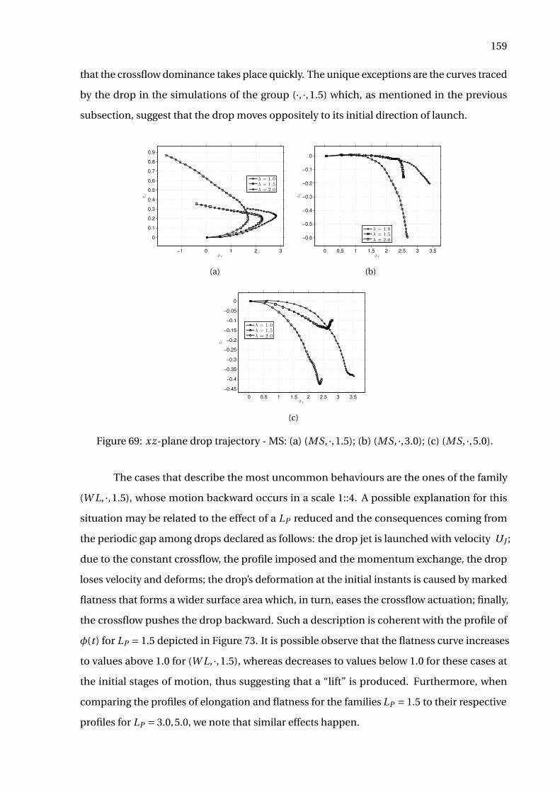
159

that the crossflow dominance takes place quickly. The unique exceptions are the curves traced

by the drop in the simulations of the group (·, ·,1.5) which, as mentioned in the previous

subsection, suggest that the drop moves oppositely to its initial direction of launch.

−1 0 1 2 3

0

0.1

0.2

0.3

0.4

0.5

0.6

0.7

0.8

0.9

x c

zc

λ = 1.0λ = 1.5λ = 2.0

(a)

0 0.5 1 1.5 2 2.5 3 3.5

−0.6

−0.5

−0.4

−0.3

−0.2

−0.1

0

x c

zc

λ = 1.0λ = 1.5λ = 2.0

(b)

0 0.5 1 1.5 2 2.5 3 3.5

−0.45

−0.4

−0.35

−0.3

−0.25

−0.2

−0.15

−0.1

−0.05

0

x c

zc

λ = 1.0λ = 1.5λ = 2.0

(c)

Figure 69: xz-plane drop trajectory - MS: (a) (MS, ·,1.5); (b) (MS, ·,3.0); (c) (MS, ·,5.0).

The cases that describe the most uncommon behaviours are the ones of the family

(W L, ·,1.5), whose motion backward occurs in a scale 1::4. A possible explanation for this

situation may be related to the effect of a LP reduced and the consequences coming from

the periodic gap among drops declared as follows: the drop jet is launched with velocity UJ ;

due to the constant crossflow, the profile imposed and the momentum exchange, the drop

loses velocity and deforms; the drop’s deformation at the initial instants is caused by marked

flatness that forms a wider surface area which, in turn, eases the crossflow actuation; finally,

the crossflow pushes the drop backward. Such a description is coherent with the profile of

φ(t ) for LP = 1.5 depicted in Figure 73. It is possible observe that the flatness curve increases

to values above 1.0 for (W L, ·,1.5), whereas decreases to values below 1.0 for these cases at

the initial stages of motion, thus suggesting that a “lift” is produced. Furthermore, when

comparing the profiles of elongation and flatness for the families LP = 1.5 to their respective

profiles for LP = 3.0,5.0, we note that similar effects happen.

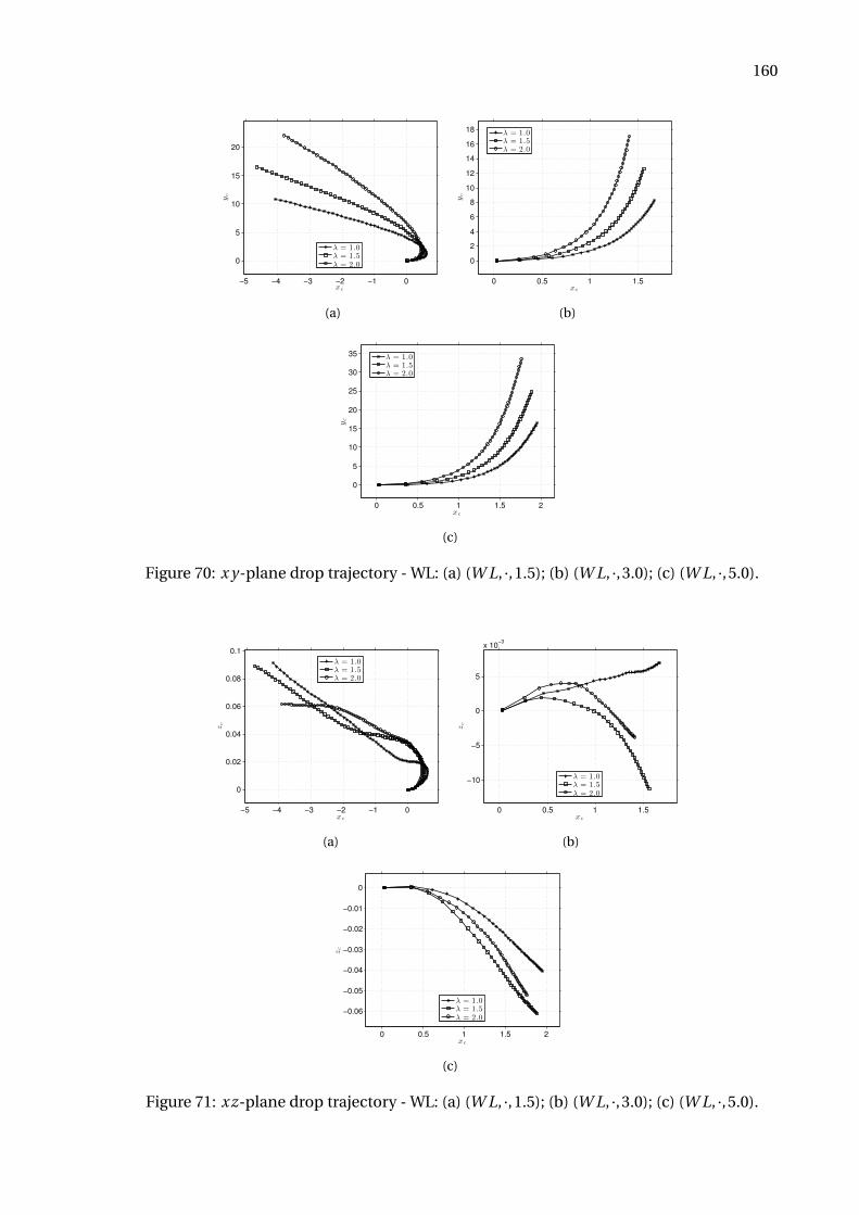
160

−5 −4 −3 −2 −1 0

0

5

10

15

20

x c

yc

λ = 1.0λ = 1.5λ = 2.0

(a)

0 0.5 1 1.5

0

2

4

6

8

10

12

14

16

18

x c

yc

λ = 1.0λ = 1.5λ = 2.0

(b)

0 0.5 1 1.5 2

0

5

10

15

20

25

30

35

x c

yc

λ = 1.0λ = 1.5λ = 2.0

(c)

Figure 70: x y-plane drop trajectory - WL: (a) (W L, ·,1.5); (b) (W L, ·,3.0); (c) (W L, ·,5.0).

−5 −4 −3 −2 −1 0

0

0.02

0.04

0.06

0.08

0.1

x c

zc

λ = 1.0λ = 1.5λ = 2.0

(a)

0 0.5 1 1.5

−10

−5

0

5

x 10−3

x c

zc

λ = 1.0λ = 1.5λ = 2.0

(b)

0 0.5 1 1.5 2

−0.06

−0.05

−0.04

−0.03

−0.02

−0.01

0

x c

zc

λ = 1.0λ = 1.5λ = 2.0

(c)

Figure 71: xz-plane drop trajectory - WL: (a) (W L, ·,1.5); (b) (W L, ·,3.0); (c) (W L, ·,5.0).

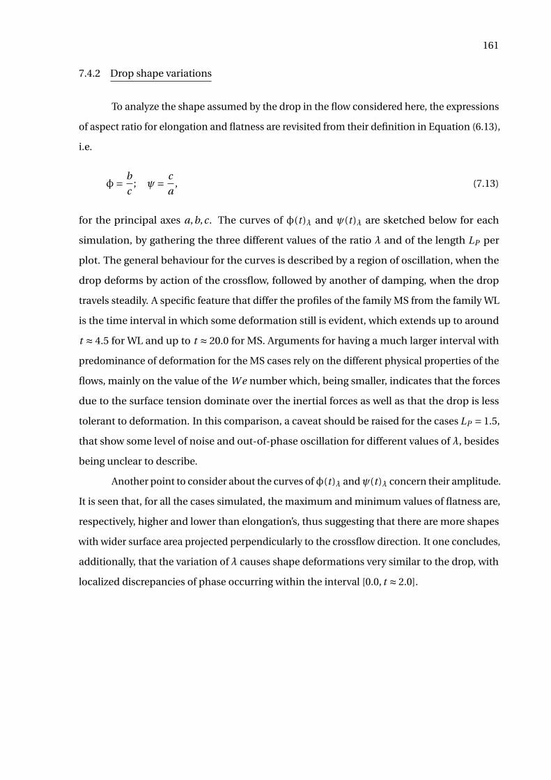
161

7.4.2 Drop shape variations

To analyze the shape assumed by the drop in the flow considered here, the expressions

of aspect ratio for elongation and flatness are revisited from their definition in Equation (6.13),

i.e.

φ= b

c; ψ= c

a, (7.13)

for the principal axes a,b,c. The curves of φ(t)λ and ψ(t)λ are sketched below for each

simulation, by gathering the three different values of the ratio λ and of the length LP per

plot. The general behaviour for the curves is described by a region of oscillation, when the

drop deforms by action of the crossflow, followed by another of damping, when the drop

travels steadily. A specific feature that differ the profiles of the family MS from the family WL

is the time interval in which some deformation still is evident, which extends up to around

t ≈ 4.5 for WL and up to t ≈ 20.0 for MS. Arguments for having a much larger interval with

predominance of deformation for the MS cases rely on the different physical properties of the

flows, mainly on the value of the W e number which, being smaller, indicates that the forces

due to the surface tension dominate over the inertial forces as well as that the drop is less

tolerant to deformation. In this comparison, a caveat should be raised for the cases LP = 1.5,

that show some level of noise and out-of-phase oscillation for different values of λ, besides

being unclear to describe.

Another point to consider about the curves ofφ(t )λ andψ(t )λ concern their amplitude.

It is seen that, for all the cases simulated, the maximum and minimum values of flatness are,

respectively, higher and lower than elongation’s, thus suggesting that there are more shapes

with wider surface area projected perpendicularly to the crossflow direction. It one concludes,

additionally, that the variation of λ causes shape deformations very similar to the drop, with

localized discrepancies of phase occurring within the interval [0.0, t ≈ 2.0].

162

0 5 10 15 20 25

0.9

0.92

0.94

0.96

0.98

1

1.02

1.04

1.06

t

φ(t) (

MS,·,L

P=1.5

)

φλ= 1.0

φλ= 1.5

φλ= 2.0

(a)

0 5 10 15 20 25

0.85

0.9

0.95

1

1.05

1.1

1.15

t

ψ(t) (

MS,·,L

P=1.5

)

φλ= 1.0

φλ= 1.5

φλ= 2.0

(b)

Figure 72: Drop shape variation - (MS, ·,1.5): (a) φ(t ); (b) ψ(t ).

0 5 10 15 20

0.85

0.9

0.95

1

1.05

1.1

1.15

1.2

t

φ(t) (

MS,·,L

P=3.0

)

φλ= 1.0

φλ= 1.5

φλ= 2.0

(a)

0 5 10 15 20

0.6

0.7

0.8

0.9

1

1.1

1.2

1.3

t

ψ(t) (

MS,·,L

P=3.0

)

φλ= 1.0

φλ= 1.5

φλ= 2.0

(b)


0 5 10 15 20

0.85

0.9

0.95

1

1.05

1.1

1.15

1.2

t

φ(t) (

MS,·,L

P=5.0

)

φλ= 1.0

φλ= 1.5

φλ= 2.0

(a)

0 5 10 15 20

0.6

0.7

0.8

0.9

1

1.1

1.2

1.3

t

ψ(t) (

MS,·,L

P=5.0

)

φλ= 1.0

φλ= 1.5

φλ= 2.0

(b)


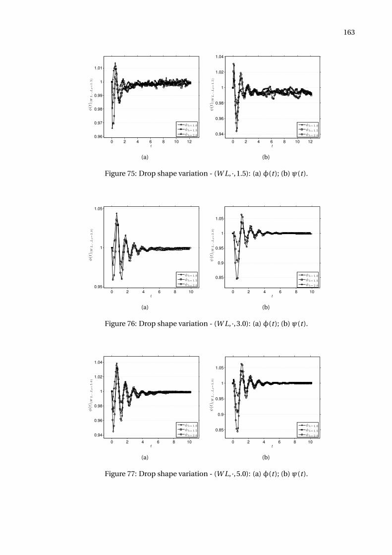
163

0 2 4 6 8 10 12

0.96

0.97

0.98

0.99

1

1.01

t

φ(t) (

WL,·,L

P=1.5

)

φλ= 1.0

φλ= 1.5

φλ= 2.0

(a)

0 2 4 6 8 10 12

0.94

0.96

0.98

1

1.02

1.04

t

ψ(t) (

WL,·,L

P=1.5

)

φλ= 1.0

φλ= 1.5

φλ= 2.0

(b)

Figure 75: Drop shape variation - (W L, ·,1.5): (a) φ(t ); (b) ψ(t ).

0 2 4 6 8 10

0.95

1

1.05

t

φ(t) (

WL,·,L

P=3.0

)

φλ= 1.0

φλ= 1.5

φλ= 2.0

(a)

0 2 4 6 8 10

0.85

0.9

0.95

1

1.05

t

ψ(t) (

WL,·,L

P=3.0

)

φλ= 1.0

φλ= 1.5

φλ= 2.0

(b)


0 2 4 6 8 10

0.94

0.96

0.98

1

1.02

1.04

t

φ(t) (

WL,·,L

P=5.0

)

φλ= 1.0

φλ= 1.5

φλ= 2.0

(a)

0 2 4 6 8 10

0.85

0.9

0.95

1

1.05

t

ψ(t) (

WL,·,L

P=5.0

)

φλ= 1.0

φλ= 1.5

φλ= 2.0

(b)


164

7.4.3 Spectrum analyses

From this point on, spectrum analyses for the DJICF configurations studied are pre-

sented. The input signals for the FFT calculation correspond to the curves φ(t )λ and ψ(t )λ,

which evince disturbances affecting the drop. FFT-based spectra for elongation and flatness

are plotted in the figures below separated according to the values of λ. Inasmuch as the

spectrum of magnitude of such a disturbances is expressed as given by Equation (6.14), it is

convenient to introduce in the following discussion the values given by

Eφλ= max|F F T [φ(t )λ]| and Eψλ

= max|F F T [ψ(t )λ]|, (7.14)

which represent, respectively, the maximum disturbance energy achieved with the slight

wobbling of the drop relative to the profiles of elongation and flatness, whereas

f ∗φ and f ∗

ψ (7.15)

are dimensionless vibration frequencies (or harmonic modes) associated to each of these

profiles within a sampling range tS . The choice of tS , however, was done by truncating the

whole time of the simulations into the regions where the small disturbances were more active,

thus restraining the interval of analysis. Besides, only the 10 first modes are plotted for each

simulation. Spectra for the group MS are plotted from Figure 78 followed by spectra for the

group WL plotted from Figure 81.

Table 7 lists the maximum energy values along with their respective most amplified

modes associated to φ(t )λ and ψ(t )λ for the testing configurations (Re f ,λ,LP ). Furthermore,

note that

EF (t ) = max(ℜF F T [F (t )]2 +ℑF F T [F (t )]2)0.5

, F (t ) =φ(t )λ,ψ(t )λ (7.16)

evokes the maximum value in modulus of complex modes associated to the shape ratios.

A point to be emphasized is that the output of F F T [F (t )] requires that the sampling

time range tS be uniform. Since the selection of the time step ∆t may be different for each

simulation and vary after remeshing operations (cf. Sec. 5.1 of [?]), tS must be modified so

165

2 4 6 8 100

0.2

0.4

0.6

0.8

1

1.2

1.4x 10

−4

f ∗

|FFT(·)|

(M

S,1

.0,1

.5)

φλ=1 . 0

ψλ=1 . 0

(a)

2 4 6 8 10

0

1

2

x 10−4

f ∗

|FFT(·)|

(M

S,1

.5,1

.5)

φλ=1 . 5

ψλ=1 . 5

(b)

2 4 6 8 10

0

1

2

3

4

5

6x 10

−4

f ∗

|FFT(·)|

(M

S,2

.0,1

.5)

φλ=2 . 0

ψλ=2 . 0

(c)

Figure 78: FFT-based spectrum: (a) (MS,1.0,1.5); (b) (MS,1.5,1.5); (c) (MS,2.0,1.5).

that this uniformity be ensured. For that objective, the average time step

∆t = (∆t )n

N= (t n+1 − t n)

N; n = 0,1, . . . N −1 (7.17)

and the function interp1 from MATLAB® were used to build a new discrete vector tS equally

spaced from the original one. The sampling ranges specified for each case as well as the

approximated thresholds from which the disturbances are attenuated are organized in Table

8.

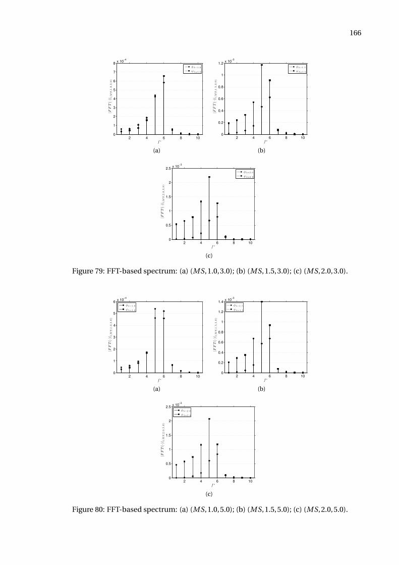
166

2 4 6 8 10

0

1

2

3

4

5

6

7

8x 10

−4

f ∗

|FFT(·)|

(M

S,1

.0,3

.0)

φλ=1 . 0

ψλ=1 . 0

(a)

2 4 6 8 100

0.2

0.4

0.6

0.8

1

1.2x 10

−3

f ∗

|FFT(·)|

(M

S,1

.5,3

.0)

φλ=1 . 5

ψλ=1 . 5

(b)

2 4 6 8 100

0.5

1

1.5

2

2.5x 10

−3

f ∗

|FFT(·)|

(M

S,2

.0,3

.0)

φλ=2 . 0

ψλ=2 . 0

(c)


2 4 6 8 10

0

1

2

3

4

5

6x 10

−4

f ∗

|FFT(·)|

(M

S,1

.0,5

.0)

φλ=1 . 0

ψλ=1 . 0

(a)

2 4 6 8 100

0.2

0.4

0.6

0.8

1

1.2

1.4x 10

−3

f ∗

|FFT(·)|

(M

S,1

.5,5

.0)

φλ=1 . 5

ψλ=1 . 5

(b)

2 4 6 8 100

0.5

1

1.5

2

2.5x 10

−3

f ∗

|FFT(·)|

(M

S,2

.0,5

.0)

φλ=2 . 0

ψλ=2 . 0

(c)


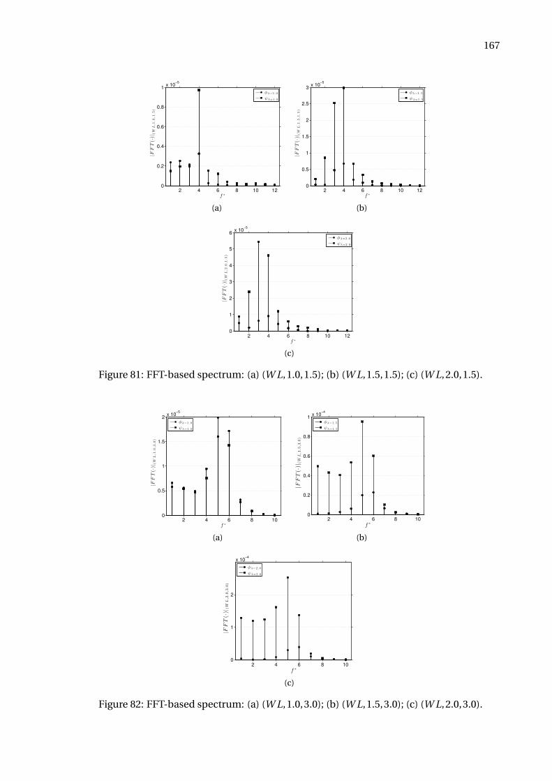
167

2 4 6 8 10 120

0.2

0.4

0.6

0.8

1x 10

−5

f ∗

|FFT(·)|

(W

L,1

.0,1

.5)

φλ=1 . 0

ψλ=1 . 0

(a)

2 4 6 8 10 120

0.5

1

1.5

2

2.5

3x 10

−5

f ∗

|FFT(·)|

(W

L,1

.5,1

.5)

φλ=1 . 5

ψλ=1 . 5

(b)

2 4 6 8 10 12

0

1

2

3

4

5

6x 10

−5

f ∗

|FFT(·)|

(W

L,2

.0,1

.5)

φλ=2 . 0

ψλ=2 . 0

(c)

Figure 81: FFT-based spectrum: (a) (W L,1.0,1.5); (b) (W L,1.5,1.5); (c) (W L,2.0,1.5).

2 4 6 8 100

0.5

1

1.5

2x 10

−5

f ∗

|FFT(·)|

(W

L,1

.0,3

.0)

φλ=1 . 0

ψλ=1 . 0

(a)

2 4 6 8 100

0.2

0.4

0.6

0.8

1x 10

−4

f ∗

|FFT(·)|

(WL,1.5,3.0)

φλ=1 . 5

ψλ=1 . 5

(b)

2 4 6 8 10

0

1

2

x 10−4

f ∗

|FFT(·)|

(WL,2.0,3.0)

φλ=2 . 0

ψλ=2 . 0

(c)


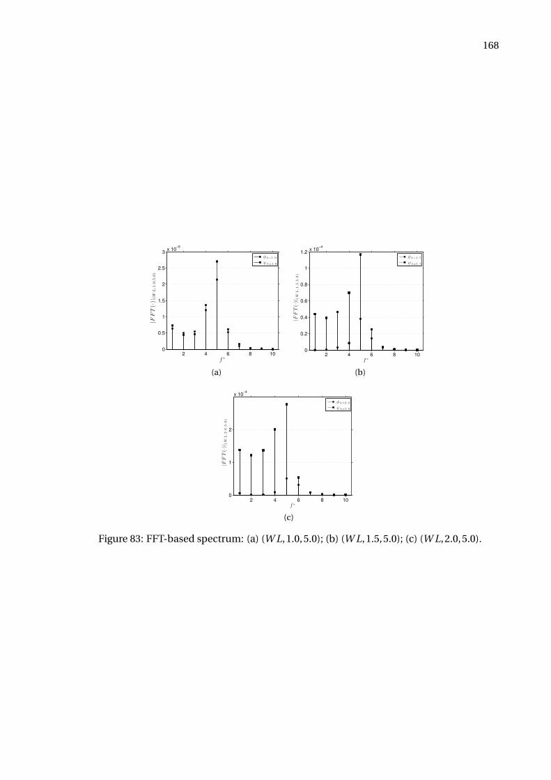
168

2 4 6 8 100

0.5

1

1.5

2

2.5

3x 10

−5

f ∗

|FFT(·)|

(W

L,1.0,5.0)

φλ=1 . 0

ψλ=1 . 0

(a)

2 4 6 8 100

0.2

0.4

0.6

0.8

1

1.2x 10

−4

f ∗

|FFT(·)|

(W

L,1

.5,5

.0)

φλ=1 . 5

ψλ=1 . 5

(b)

2 4 6 8 10

0

1

2

x 10−4

f ∗

|FFT(·)|

(W

L,2

.0,5

.0)

φλ=2 . 0

ψλ=2 . 0

(c)


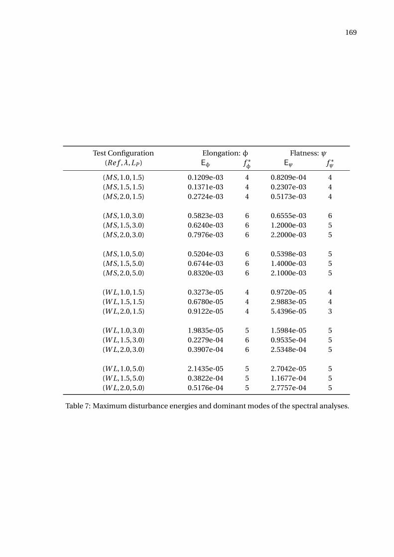
169

Test Configuration Elongation: φ Flatness: ψ(Re f ,λ,LP ) Eφ f ∗

φEψ f ∗

ψ

(MS,1.0,1.5) 0.1209e-03 4 0.8209e-04 4(MS,1.5,1.5) 0.1371e-03 4 0.2307e-03 4(MS,2.0,1.5) 0.2724e-03 4 0.5173e-03 4

(MS,1.0,3.0) 0.5823e-03 6 0.6555e-03 6(MS,1.5,3.0) 0.6240e-03 6 1.2000e-03 5(MS,2.0,3.0) 0.7976e-03 6 2.2000e-03 5

(MS,1.0,5.0) 0.5204e-03 6 0.5398e-03 5(MS,1.5,5.0) 0.6744e-03 6 1.4000e-03 5(MS,2.0,5.0) 0.8320e-03 6 2.1000e-03 5

(W L,1.0,1.5) 0.3273e-05 4 0.9720e-05 4(W L,1.5,1.5) 0.6780e-05 4 2.9883e-05 4(W L,2.0,1.5) 0.9122e-05 4 5.4396e-05 3

(W L,1.0,3.0) 1.9835e-05 5 1.5984e-05 5(W L,1.5,3.0) 0.2279e-04 6 0.9535e-04 5(W L,2.0,3.0) 0.3907e-04 6 2.5348e-04 5

(W L,1.0,5.0) 2.1435e-05 5 2.7042e-05 5(W L,1.5,5.0) 0.3822e-04 5 1.1677e-04 5(W L,2.0,5.0) 0.5176e-04 5 2.7757e-04 5

Table 7: Maximum disturbance energies and dominant modes of the spectral analyses.

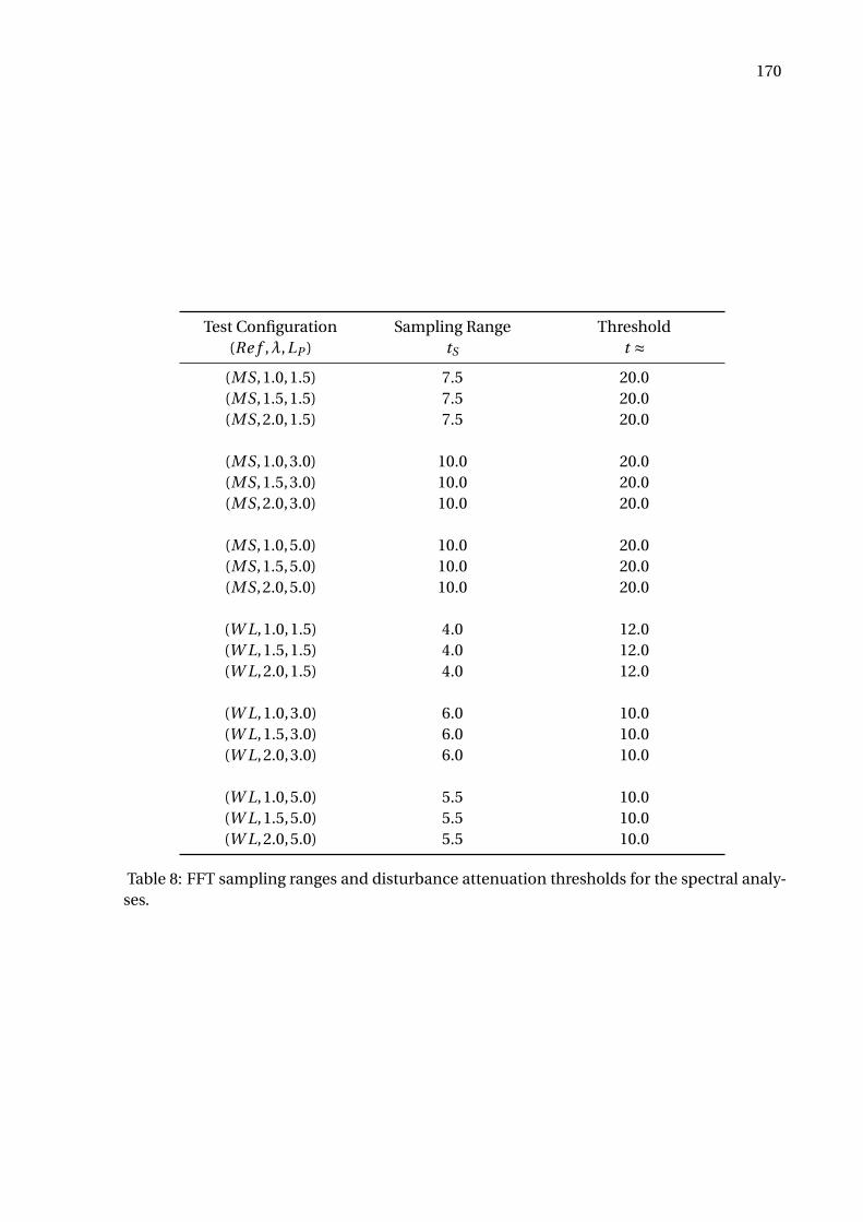
170

Test Configuration Sampling Range Threshold(Re f ,λ,LP ) tS t ≈

(MS,1.0,1.5) 7.5 20.0(MS,1.5,1.5) 7.5 20.0(MS,2.0,1.5) 7.5 20.0

(MS,1.0,3.0) 10.0 20.0(MS,1.5,3.0) 10.0 20.0(MS,2.0,3.0) 10.0 20.0

(MS,1.0,5.0) 10.0 20.0(MS,1.5,5.0) 10.0 20.0(MS,2.0,5.0) 10.0 20.0

(W L,1.0,1.5) 4.0 12.0(W L,1.5,1.5) 4.0 12.0(W L,2.0,1.5) 4.0 12.0

(W L,1.0,3.0) 6.0 10.0(W L,1.5,3.0) 6.0 10.0(W L,2.0,3.0) 6.0 10.0

(W L,1.0,5.0) 5.5 10.0(W L,1.5,5.0) 5.5 10.0(W L,2.0,5.0) 5.5 10.0

Table 8: FFT sampling ranges and disturbance attenuation thresholds for the spectral analy-ses.

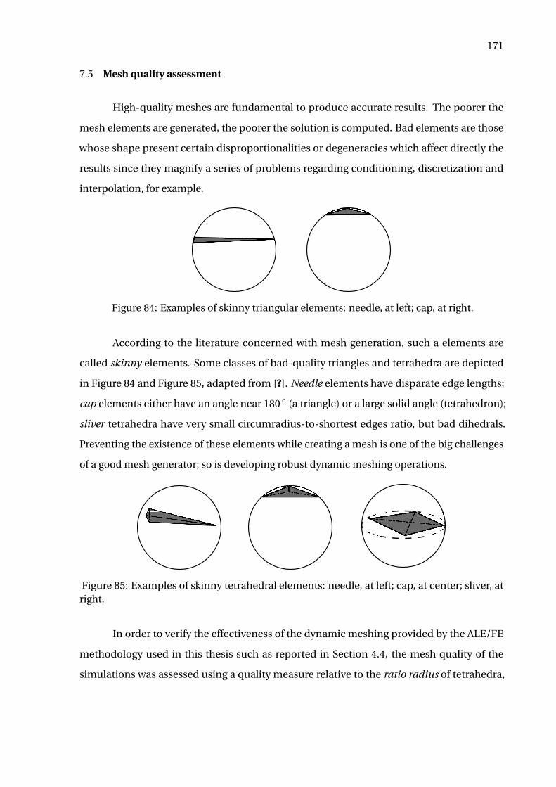
171

7.5 Mesh quality assessment

High-quality meshes are fundamental to produce accurate results. The poorer the

mesh elements are generated, the poorer the solution is computed. Bad elements are those

whose shape present certain disproportionalities or degeneracies which affect directly the

results since they magnify a series of problems regarding conditioning, discretization and

interpolation, for example.

Figure 84: Examples of skinny triangular elements: needle, at left; cap, at right.

According to the literature concerned with mesh generation, such a elements are

called skinny elements. Some classes of bad-quality triangles and tetrahedra are depicted

in Figure 84 and Figure 85, adapted from [?]. Needle elements have disparate edge lengths;

cap elements either have an angle near 180 (a triangle) or a large solid angle (tetrahedron);

sliver tetrahedra have very small circumradius-to-shortest edges ratio, but bad dihedrals.

Preventing the existence of these elements while creating a mesh is one of the big challenges

of a good mesh generator; so is developing robust dynamic meshing operations.

Figure 85: Examples of skinny tetrahedral elements: needle, at left; cap, at center; sliver, atright.

In order to verify the effectiveness of the dynamic meshing provided by the ALE/FE

methodology used in this thesis such as reported in Section 4.4, the mesh quality of the

simulations was assessed using a quality measure relative to the ratio radius of tetrahedra,

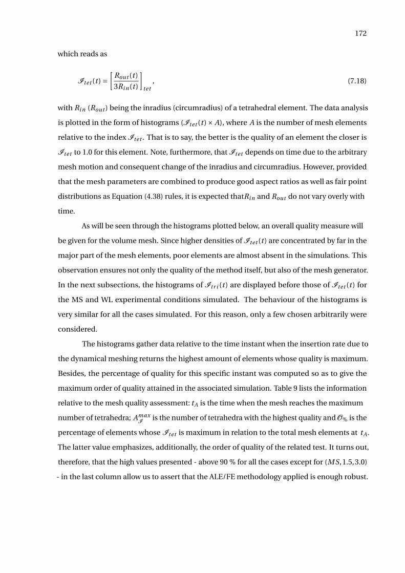
172

which reads as

Itet (t ) =[

Rout (t )

3Ri n(t )

]tet

, (7.18)

with Ri n (Rout ) being the inradius (circumradius) of a tetrahedral element. The data analysis

is plotted in the form of histograms (Itet (t)× A), where A is the number of mesh elements

relative to the index Itet . That is to say, the better is the quality of an element the closer is

Itet to 1.0 for this element. Note, furthermore, that Itet depends on time due to the arbitrary

mesh motion and consequent change of the inradius and circumradius. However, provided

that the mesh parameters are combined to produce good aspect ratios as well as fair point

distributions as Equation (4.38) rules, it is expected thatRi n and Rout do not vary overly with

time.

As will be seen through the histograms plotted below, an overall quality measure will

be given for the volume mesh. Since higher densities of Itet (t ) are concentrated by far in the

major part of the mesh elements, poor elements are almost absent in the simulations. This

observation ensures not only the quality of the method itself, but also of the mesh generator.

In the next subsections, the histograms of Itr i (t) are displayed before those of Itet (t) for

the MS and WL experimental conditions simulated. The behaviour of the histograms is

very similar for all the cases simulated. For this reason, only a few chosen arbitrarily were

considered.

The histograms gather data relative to the time instant when the insertion rate due to

the dynamical meshing returns the highest amount of elements whose quality is maximum.

Besides, the percentage of quality for this specific instant was computed so as to give the

maximum order of quality attained in the associated simulation. Table 9 lists the information

relative to the mesh quality assessment: tA is the time when the mesh reaches the maximum

number of tetrahedra; AmaxI

is the number of tetrahedra with the highest quality and O% is the

percentage of elements whose Itet is maximum in relation to the total mesh elements at tA.

The latter value emphasizes, additionally, the order of quality of the related test. It turns out,

therefore, that the high values presented - above 90 % for all the cases except for (MS,1.5,3.0)

- in the last column allow us to assert that the ALE/FE methodology applied is enough robust.

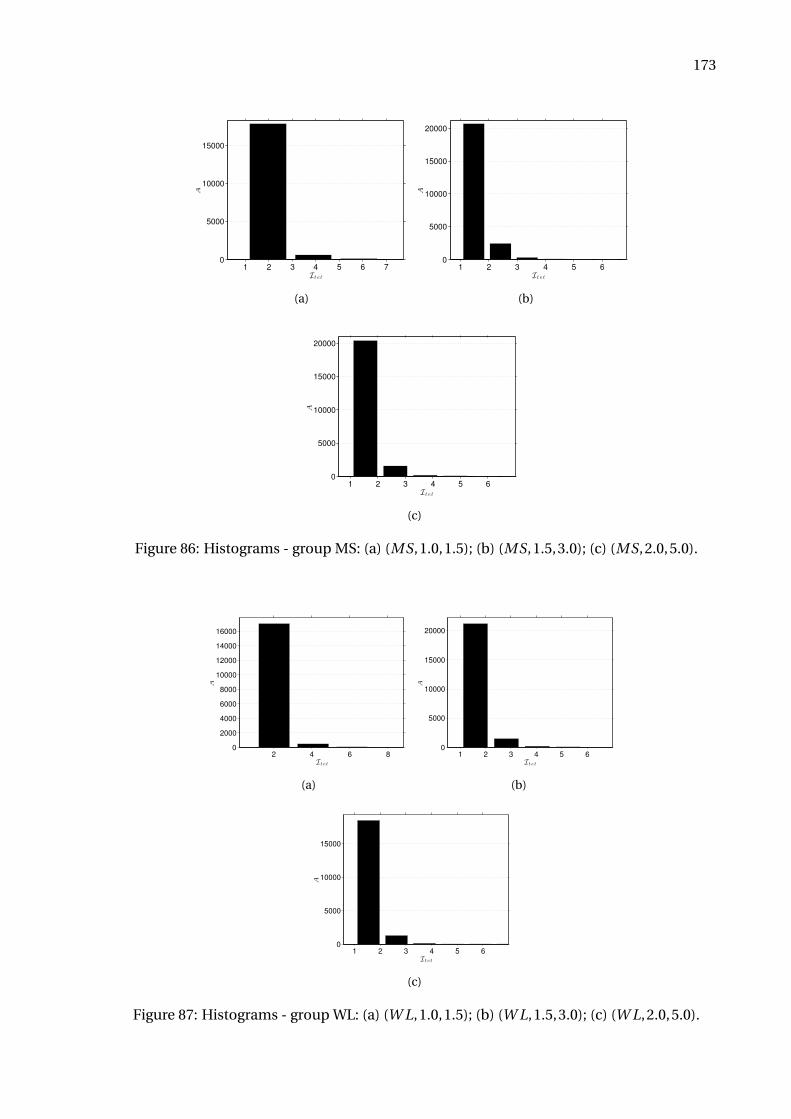
173

1 2 3 4 5 6 70

5000

10000

15000

It et

A

(a)

1 2 3 4 5 60

5000

10000

15000

20000

It et

A

(b)

1 2 3 4 5 60

5000

10000

15000

20000

It et

A

(c)

Figure 86: Histograms - group MS: (a) (MS,1.0,1.5); (b) (MS,1.5,3.0); (c) (MS,2.0,5.0).

2 4 6 80

2000

4000

6000

8000

10000

12000

14000

16000

It et

A

(a)

1 2 3 4 5 60

5000

10000

15000

20000

It et

A

(b)

1 2 3 4 5 60

5000

10000

15000

It et

A

(c)

Figure 87: Histograms - group WL: (a) (W L,1.0,1.5); (b) (W L,1.5,3.0); (c) (W L,2.0,5.0).

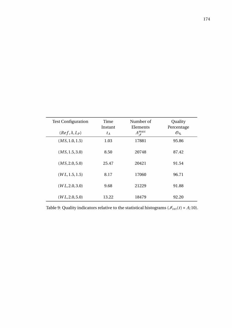
174

Test Configuration TimeInstant

Number ofElements

QualityPercentage

(Re f ,λ,LP ) tA AmaxI

O%

(MS,1.0,1.5) 1.03 17881 95.86

(MS,1.5,3.0) 8.50 20748 87.42

(MS,2.0,5.0) 25.47 20421 91.54

(W L,1.5,1.5) 8.17 17060 96.71

(W L,2.0,3.0) 9.68 21229 91.88

(W L,2.0,5.0) 13.22 18479 92.20

Table 9: Quality indicators relative to the statistical histograms (Itet (t )× A;10).

175

CONCLUSION

This thesis studied the numerical modeling of a particular flow featured by the influ-

ence of a crossflow over drops that detach off a continuous jet taking into account a periodic

approach. The basis for this research was inspired in the well-known canonical flow of a jet in

crossflow, which was dealt with in a nonturbulent scope. Given the large amount of research

concerned with strong jet-to-crossflow ratios as well as with vortical structures shedding

through gas-liquid mixtures, this study took a different path when investigating weak cross-

flow ratios in liquid-liquid interfaces. Assumptions were established concerning the focus on

the jet’s primary breakup zone and the inclusion of periodic boundary conditions into the

model. Nevertheless, the computational structure as well as the ideas behind the numerical

algorithms demonstrated to be a promising tool in studying other two-phase flow regimes

pictured by dispersed bubbles and drops.

In Chapter 2, we addressed the fundamental aspects of the ALE description, introduced

a short review on numerical methods available to model two-phase flows, and discussed a

few topics of the mechanics with interfaces, such as the jump of properties near an interface

and the existence of surface tension. Finally, we established a mathematical description

of the meshing structures applied in the computational code used in this thesis to provide

organization of the content and resources for better theoretical outlines.

Basic principles used in CFD, governing equations, and the one-fluid formulation

were introduced in Chapter 3, by emphasizing the inclusion of the volumetric representation

of the surface tension force into the momentum equation and how a marker function is

implemented to identify the different fluids or phases making up the flow. Additionally,

selected information about the semi-lagrangian method and the projection method were

given.

Chapter 4 along with Chapter 5 provided the detailed description of the FE formulation

applied to two-phase flows as used in this thesis, by integrating the variational approach to

include periodic boundary conditions into this set. Moreover, they explained the peculiarities

of the operational tools that make up this methodology, subsequently applied to validation

tests in Chapter 6 that certified the implementations.

The drop jet in crossflow investigated with details in Chapter 7, starting from the

configuration of a very particular testing setup for studying different fluid-fluid cases. A

176

technique based on a moving-frame reference were extended to deal with transverse flows.

Despite of using only two fluid pairs of known experimental applicability, several data could

be extracted from combinations of parameters defining the jet-to-crossflow ratio and the

periodic cell’s length, such as analyses of hydrodynamics, drop shape, spectrum and mesh

quality so promoting a handful of computational and statistical information fairly complete

as regarding the intended goals of this thesis.

Generally, the ALE/FE methodology employed here gathers many advantages since

it provides a generalized form to control the mesh motion, besides aggregating functions

that enable versatile dynamic meshing operations, such as node addition, node deletion,

mesh smoothing and refinement, which ensure a sophisticated level of adaptivity for different

flow behaviours. To enforce the usability of the tools developed with this work, analyses

of two-fluid configurations under experimental conditions were performed. Qualitative

comparisons about the hydrodynamics of bubble and drops immersed in fluids commonly

mentioned in literature as well as some contributions about shape factors and energy spectra

were presented.

By considering the overall set of technicalities employed in this thesis, a not exhaustive

list of issues can be arranged, of which specific problems may derive. Some directions for

future work are the following.

• Development of high-order methods: as issues relating to numerical accuracy, not only

the interpolation through the semi-lagrangian method needs an upgrade from its linear

capability, but also the projection method applied, which requires better accuracy.

• Algorithm improvement for PBC: although the matrix operations required to enforce

the PBC over rows and columns follow a computational approach known as CSR (Com-

pressed Sparse Row), which stores only the nonzero entries of the matrices in order to

escape memory allocation due to the sparsity, this methodology lacks of improvement

for column operations. The strategy was implemented for square matrices and well

applied for symmetric matrices while taking advantage of the symmetry to produce

more compact loops. Nonsquare matrices, however, are not optimized as to column

loops. Furthermore, the computation time for PBC operations also require additional

observation.

177

• Selection of boundary conditions: the methodology presented here combines PBC, DBC,

and NBC set by selection of boundary physical groups tagged at the pre-processing level.

While the posing of the problems are well defined in regard to the mathematical point of

view, their numerical resolution might be intricate when defining consistent boundary

conditions. Running tests showed that the choice among pairs solver-preconditioner

may render dependent on the problem. Intersection points, viz. corner points, which

share different boundaries worth careful attention and better strategies to select priori-

ties should be achieved.

• Multidimensional periodicity: in this thesis, the periodicity was applied only in one

direction. Although this capability enables the simulation of several flows of practical

interest, other situations in which multidimensional periodicity occurs need to be

covered. The alternative way is to extend the mesh generation for more complex

surfaces, obtained by translation or rotation, for instance, and suit the computational

code to receive such extra functionality.

• Handling of topological changes: the modelling of physical phenomena associated to

the topological changes of dispersed bodies in two-phase configurations, such as acute

deformations, breakup and coalescence is not completely solved in the current code.

Besides requiring the reordering of the data structures responsible to save the mesh

data, such a capability should be assessed so that the physical interactions among the

dispersed bodies are respected. Flows whose hydrodynamic effects are complex (e.g.

approaching velocity, film thinning and rupture in bubble coalescence) represent a

path to be unveiled.

• Coupling of physical mechanisms: diabatic flows inside the scope of heat and mass

transfer dynamics together with multidimensional periodicity are a goal to be achieved,

since modern applications encompassing two-phase flow regimes, such as bubbly

and slug flows, have a big quota of interest in thermo-mechanical applications where

ubiquitous temperature variations and heat transfer processes reign.

• Parallel computing: advancing toward data parallelism as well as evaluating the perfor-

mance of the numerical code across a multi-core stage represents another potential

learning curve regarding the current code.

178

• Curvature and capillary pressure modelling: the curvature computation follows a geo-

metrical idea which is based on the Frenet’s relations. Although the results obtained

until now are satisfactory for a class of dispersed flows, namely bubbles and drops,

other flow regimes, such as annular and jet flows require additional attention because

of their prolonged interfaces. Since they may have instabilities, localized high-curvature

zones may be generated by peaked nodes that cause unavoidable bad-shaped elements.

Therefore, new alternatives for interpolation and capture of numerically uncontrollable

curvatures should be developed. Additionally, advancements in the coupling with PBC

are necessary as regards the computation of curvature over the periodic faces over

which interface points overlap.

• Marangoni effects: flows subject to Marangoni effects generated by surface tension

gradients due to the influence of either contaminants or surfactants as well as reactive

flows represent another field of study opened to the numerical code used in this thesis.

• Multifluid interaction: all cases dealt with here take a two-fluid/two-phase flow condi-

tion. Although the interaction of too many dispersed elements can be studied in these

conditions, the codification required to include three or more substances should be

implemented. Surely, this further step will open up several opportunities of study.

• Extensions for the drop jet configuration: the inclusion of gravity is an incremental

effect to be considered in the future. Another point to be considered sticks to the

imposition of the initial condition of the jet. It is known that disturbances emerge from

a drop that detaches off a unbroken liquid jet, which may propagate with the drop’s

motion. Therefore, the survey on an initial condition that considers such a effects is

deserves additional study. Concerning the periodic spacing of drops, a condition similar

to a “multipole flow” formed by sources and sinks interposed in-line may help to resolve

the flow in the gaps between trailing and leading drops whilst also resorts to a disturbed

flow around the drops.

To conclude, it should be emphasized that has been arising not only many variants of

the classical FEM along the recent decades, but also many opportunities for newer applica-

tions. Incompressible two-phase flows, strictly, represent an important portion of this whole

and so will be the ongoing tools intended to develop FEM codes. ALE/FEM methods have

gained immeasurable proportions in fluid-structure interaction problems, from which other

179

front-end creative solutions may appear and be adapted for different situations. Moreover,

with the ascension of FE-based commercial codes, the state-of-art in developing scientific

MCFD codes with robust and uncomplicated programming languages in this field will may

be able to become a prosper research line.

180

APPENDIX A - Code Flowcharts

This appendix gathers overview flowcharts of the FE-based in-house code used in this

thesis concerning the three basic macro stages of any software turned to Computational Fluid

Dynamics as well as a very simple UML partial diagram of the main C++ classes involved in

the PBC programming.

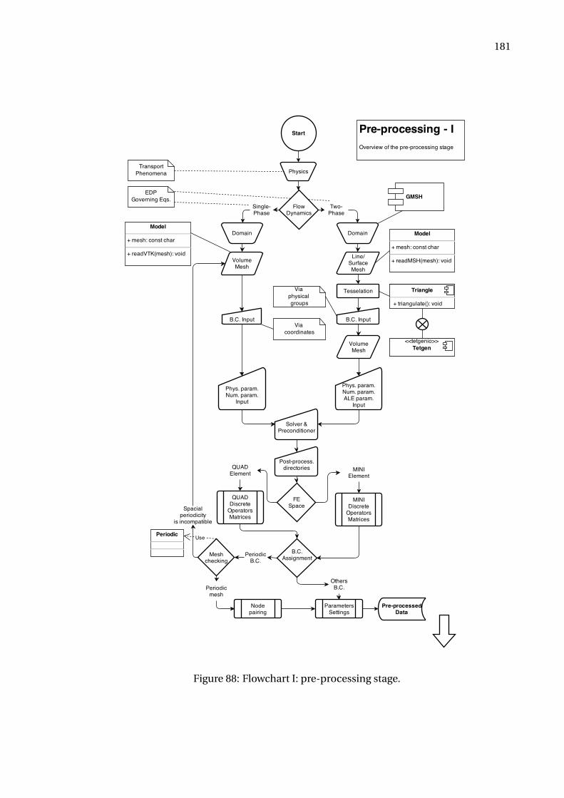
181

Figure 88: Flowchart I: pre-processing stage.

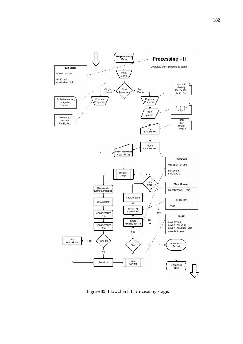
182

Figure 89: Flowchart II: processing stage.

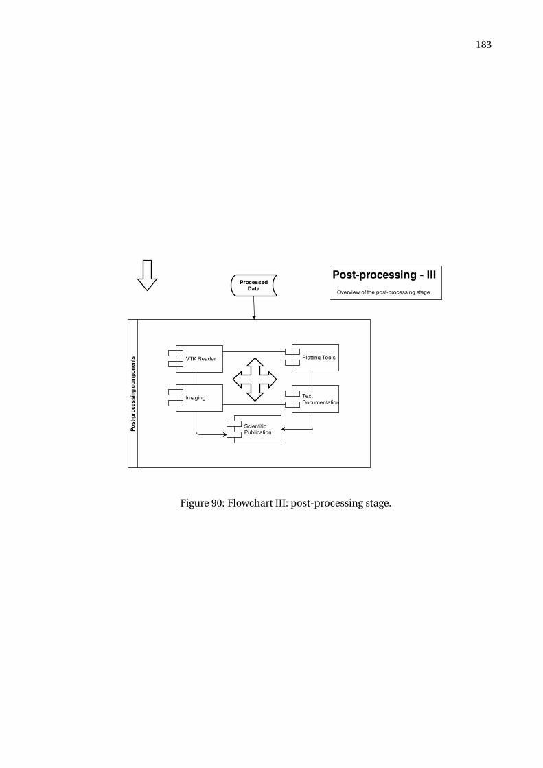
183

Figure 90: Flowchart III: post-processing stage.

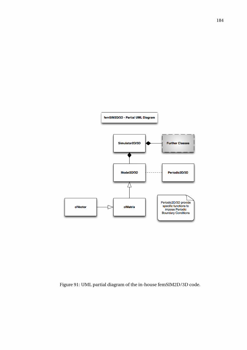
184

Figure 91: UML partial diagram of the in-house femSIM2D/3D code.

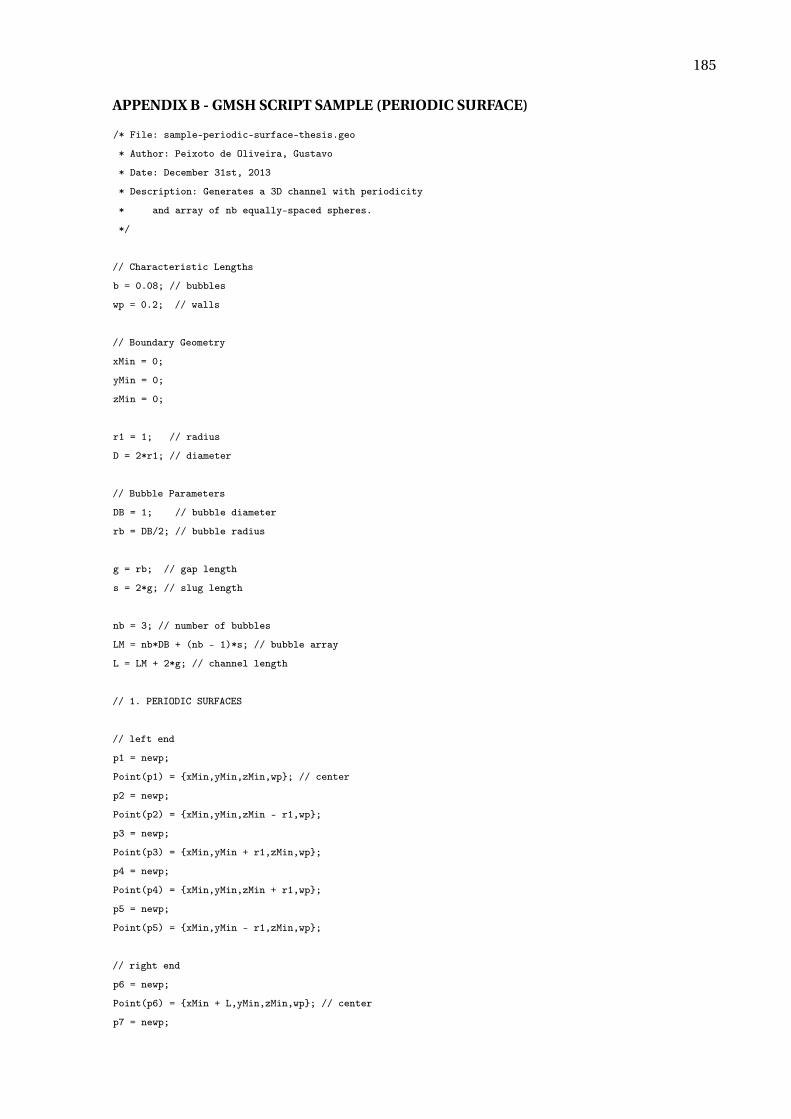
185

APPENDIX B - GMSH SCRIPT SAMPLE (PERIODIC SURFACE)

/* File: sample-periodic-surface-thesis.geo

* Author: Peixoto de Oliveira, Gustavo

* Date: December 31st, 2013

* Description: Generates a 3D channel with periodicity

* and array of nb equally-spaced spheres.

*/

// Characteristic Lengths

b = 0.08; // bubbles

wp = 0.2; // walls

// Boundary Geometry

xMin = 0;

yMin = 0;

zMin = 0;

r1 = 1; // radius

D = 2*r1; // diameter

// Bubble Parameters

DB = 1; // bubble diameter

rb = DB/2; // bubble radius

g = rb; // gap length

s = 2*g; // slug length

nb = 3; // number of bubbles

LM = nb*DB + (nb - 1)*s; // bubble array

L = LM + 2*g; // channel length

// 1. PERIODIC SURFACES

// left end

p1 = newp;

Point(p1) = xMin,yMin,zMin,wp; // center

p2 = newp;

Point(p2) = xMin,yMin,zMin - r1,wp;

p3 = newp;

Point(p3) = xMin,yMin + r1,zMin,wp;

p4 = newp;

Point(p4) = xMin,yMin,zMin + r1,wp;

p5 = newp;

Point(p5) = xMin,yMin - r1,zMin,wp;

// right end

p6 = newp;

Point(p6) = xMin + L,yMin,zMin,wp; // center

p7 = newp;

186

Point(p7) = xMin + L,yMin,zMin - r1,wp;

p8 = newp;

Point(p8) = xMin + L,yMin + r1,zMin,wp;

p9 = newp;

Point(p9) = xMin + L,yMin,zMin + r1,wp;

p10 = newp;

Point(p10) = xMin + L,yMin - r1,zMin,wp;

/* --- BUILDING CIRCLES --- */

// left end

c1 = newc;

Circle(c1) = p2,p1,p3;

c2 = newc;


c3 = newc;


c4 = newc;


// right end

c5 = newc;


c6 = newc;


c7 = newc;


c8 = newc;


/* --- BUILDING EXTERNAL LINES --- */

l1 = newl;

Line(l1) = p2,p7;

l2 = newl;

Line(l2) = p3,p8;

l3 = newl;

Line(l3) = p4,p9;

l4 = newl;

Line(l4) = p5,p10;

// 2. INTERNAL DOMAIN - BUBBLES

// Origin

x0 = xMin;

y0 = yMin;

z0 = zMin;

For i In 1:nb // BEGIN LOOP

// --- spherical bubble points

187

pp9 = newp;

Point(pp9) = x0 + g + rb + (i - 1)*(DB + s), y0, z0, b;

pp10 = newp;

Point(pp10) = x0 + g + rb + (i - 1)*(DB + s), y0, z0 - rb, b;

pp11 = newp;

Point(pp11) = x0 + g + rb + (i - 1)*(DB + s), y0 + rb, z0, b;

pp12 = newp;

Point(pp12) = x0 + g + rb + (i - 1)*(DB + s), y0, z0 + rb, b;

pp13 = newp;

Point(pp13) = x0 + g + rb + (i - 1)*(DB + s), y0 - rb, z0, b;

pp14 = newp;

Point(pp14) = x0 + g + (i - 1)*(DB + s), y0, z0, b;

pp15 = newp;

Point(pp15) = x0 + g + DB + (i - 1)*(DB + s), y0, z0, b;

// --- BUILDING CIRCLES ---

// x-normal meridian

cc11 = newc;

Circle(cc11) = pp12,pp9,pp11;

cc12 = newc;


cc13 = newc;


cc14 = newc;


// z-normal meridian

cc15 = newc;


cc16 = newc;


cc17 = newc;


cc18 = newc;


// --- DISCRETIZATION (THETA) CIRCLES ---

nt2 = 14; // number of theta points per quarter of circle (total around circle is 4*nt)

//Transfinite Linecc11,cc12,cc13,cc14,cc15,cc16,cc17,cc18 = nt2 Using Bump 1;

// BUBBLES’ SURFACES

// reference: central axis is X-positive and theta counterclockwise

// 0:Pi/2

lb21 = newl;

Line Loop(lb21) = cc12,cc13,-cc16,-cc15;

sb21 = news;

188

Ruled Surface(sb21) = lb21;

// Pi/2:Pi

lb22 = newl;

Line Loop(lb22) = -cc18,-cc17,-cc13,-cc12;

sb22 = news;


// Pi:3*Pi/2

lb23 = newl;

Line Loop(lb23) = -cc11,-cc14,cc17,cc18;

sb23 = news;


// 3*Pi/2:2*Pi

lb24 = newl;

Line Loop(lb24) = cc15,cc16,cc14,cc11;

sb24 = news;


Printf("Generating dispersed body %g...",i);

Printf("Data bubble: %g",i);

Printf("Bubble’s ruled surface - 0:Pi/2 = %g",sb21);

Printf("Bubble’s ruled surface - Pi/2:Pi = %g",sb22);

Printf("Bubble’s ruled surface - Pi:1.5*Pi = %g",sb23);

Printf("Bubble’s ruled surface - 1.5*Pi:2*Pi = %g",sb24);

// DISPERSED PHYSICAL SURFACES

Physical Surface(Sprintf("Dispersed%g",i)) = sb21,sb22,sb23,sb24;

EndFor

// 4. BUILDING EXTERNAL SURFACES

// left end

ll15 = newl;

Line Loop(ll15) = -c4,-c3,-c2,-c1;

s1 = news;

Plane Surface(s1) = ll15;

// right end

ll16 = newl;

Line Loop(ll16) = c5,c6,c7,c8;

s2 = news;

Plane Surface(s2) = ll16;

// channel’s surfaces

ll17 = newl;

189

Line Loop(ll17) = -l1,c1,l2,-c5;

s3 = news;

Ruled Surface(s3) = ll17;

ll18 = newl;


s4 = news;


ll19 = newl;


s5 = news;


ll20 = newl;


s6 = news;


// --- PERIODIC SURFACES MESHING s1 - Master :: s2 - Slave

Periodic Surface s1 c1,c2,c3,c4 = s2 c5,c6,c7,c8;

// 5. BOUNDARY PHYSICAL SURFACES

Physical Surface("PeriodicLeftBoundary") = s1;

Physical Surface("PeriodicRightBoundary") = s2;

Physical Surface("NoSlipBoundary") = s3,s4,s5,s6;

/* End of script */

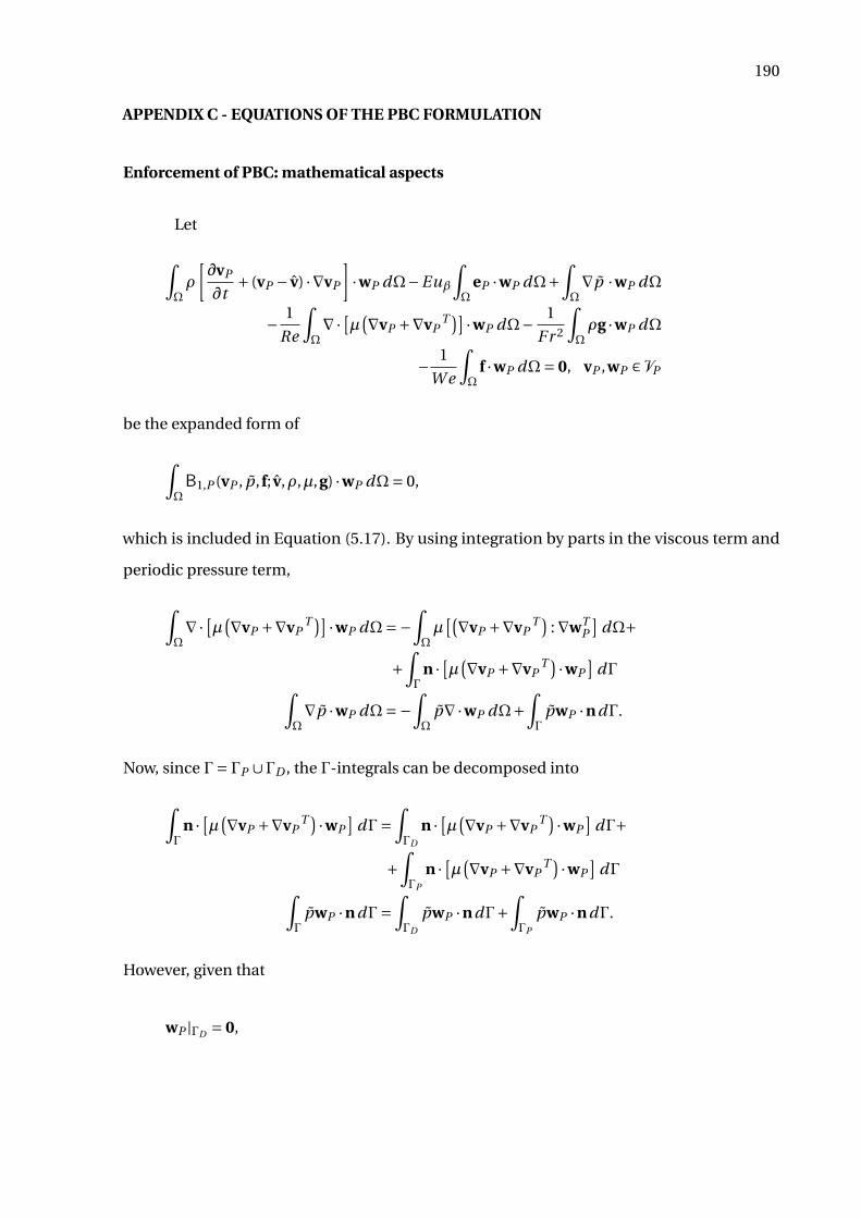
190

APPENDIX C - EQUATIONS OF THE PBC FORMULATION

Enforcement of PBC: mathematical aspects

Let

∫Ωρ

[∂vP

∂t+ (vP − v) ·∇vP

]·wP dΩ−Euβ

∫Ω

eP ·wP dΩ+∫Ω∇p ·wP dΩ

− 1

Re

∫Ω∇· [µ(∇vP +∇vP

T )] ·wP dΩ− 1

F r 2

∫Ωρg ·wP dΩ

− 1

W e

∫Ω

f ·wP dΩ= 0, vP ,wP ∈ VP

be the expanded form of

∫ΩB1,P (vP , p, f; v,ρ,µ,g) ·wP dΩ= 0,

which is included in Equation (5.17). By using integration by parts in the viscous term and

periodic pressure term,

∫Ω∇· [µ(∇vP +∇vP

T )] ·wP dΩ=−∫Ωµ

[(∇vP +∇vPT )

: ∇wTP

]dΩ+

+∫Γ

n · [µ(∇vP +∇vPT ) ·wP

]dΓ∫

Ω∇p ·wP dΩ=−

∫Ω

p∇·wP dΩ+∫Γ

pwP ·ndΓ.

Now, since Γ= ΓP ∪ΓD , the Γ-integrals can be decomposed into

∫Γ


]dΓ=

∫ΓD


]dΓ+

+∫ΓP


]dΓ∫

ΓpwP ·ndΓ=

∫ΓD

pwP ·ndΓ+∫ΓP

pwP ·ndΓ.

However, given that

wP |ΓD = 0,

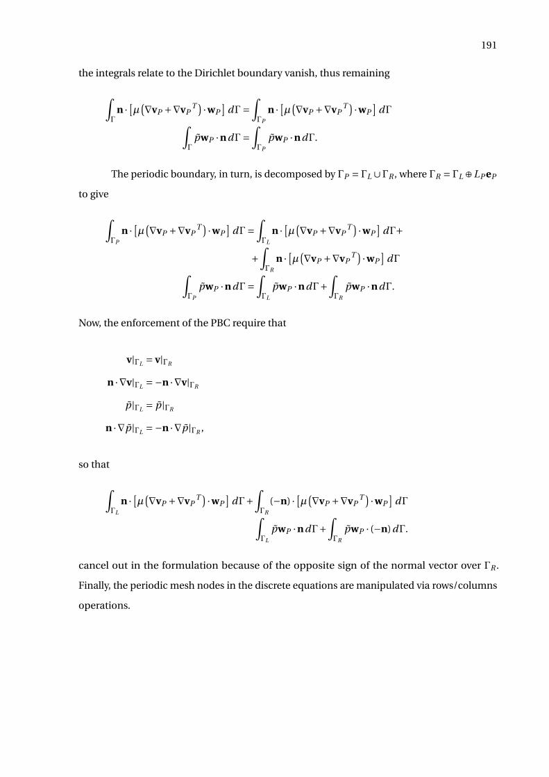
191

the integrals relate to the Dirichlet boundary vanish, thus remaining

∫Γ


]dΓ=

∫ΓP


]dΓ∫

ΓpwP ·ndΓ=

∫ΓP

pwP ·ndΓ.

The periodic boundary, in turn, is decomposed by ΓP = ΓL ∪ΓR , where ΓR = ΓL ⊕LP eP

to give

∫ΓP


]dΓ=

∫ΓL


]dΓ+

+∫ΓR


]dΓ∫

ΓP

pwP ·ndΓ=∫ΓL

pwP ·ndΓ+∫ΓR

pwP ·ndΓ.

Now, the enforcement of the PBC require that

v|ΓL = v|ΓR

n ·∇v|ΓL =−n ·∇v|ΓR

p|ΓL = p|ΓR

n ·∇p|ΓL =−n ·∇p|ΓR ,

so that

∫ΓL


]dΓ+

∫ΓR

(−n) · [µ(∇vP +∇vPT ) ·wP

]dΓ∫

ΓL

pwP ·ndΓ+∫ΓR

pwP · (−n)dΓ.

cancel out in the formulation because of the opposite sign of the normal vector over ΓR .

Finally, the periodic mesh nodes in the discrete equations are manipulated via rows/columns

operations.

192

APPENDIX E - CURVATURE AND FRENET’S FRAME

Curvature

Curvature is a scalar function κ(s) that associates a real number to each point of a

parametrized curve in s by a real interval like a ≤ s ≤ b. From the Differential Geometry [?], one

ascertains that the curvature measures “how much the curve is bending at the parametrized

point”. This quantity is well understood by comparing it to the role played by a derivative of

the velocity vector at a point of a trajectory. However, the concept of curvature extends to

smooth surfaces where it turns into a much more intricate matter. For a general surface ζ,

κ(s) should satisfy some properties. The most intuitive are:

• k is a smooth map;

• a point with an open neighbourhood contained in a plane has zero curvature;

• if p,q ∈ ζ are points such that p has a neighbourhood that forms a sharp peak higher

than a neighbourhood of q, then κ(p) > κ(q).

Frenet Frame

When we consider a curve in R3 parameterized in s by a real interval like a ≤ s ≤ b,

three vectors are essential to give information about the curve, namely, the normal vector

n(s), the tangent vector t(s) and the binormal vector b(s). This latter vector only makes sense

in R3, since is defined by

b = t×n. (7.19)

t,n,b form an orthonormal basis to R3, which, indeed, is called the Frenet frame.

Calculation of curvature for one-dimensional interfaces

Another relevant characteristic of the method used here concerns to the computation

of the curvature κ, which depends on geometrical operations performed over interface ele-

ments. With the insertion of the CSF model [?] to estimate the interfacial force that goes along

with the Equation (3.39), an accurate retrieval of the curvature is needed. In order to spare

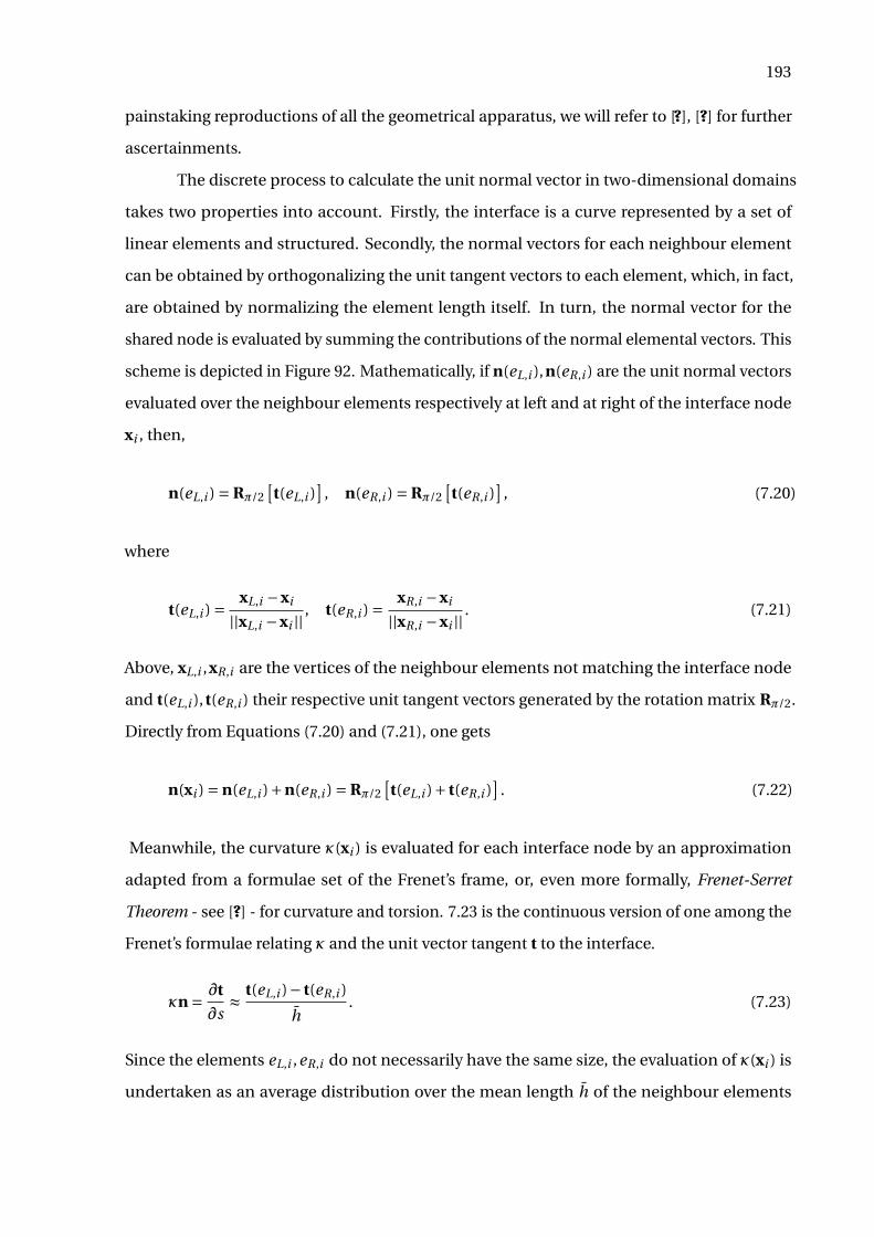
193

painstaking reproductions of all the geometrical apparatus, we will refer to [?], [?] for further

ascertainments.

The discrete process to calculate the unit normal vector in two-dimensional domains

takes two properties into account. Firstly, the interface is a curve represented by a set of

linear elements and structured. Secondly, the normal vectors for each neighbour element

can be obtained by orthogonalizing the unit tangent vectors to each element, which, in fact,

are obtained by normalizing the element length itself. In turn, the normal vector for the

shared node is evaluated by summing the contributions of the normal elemental vectors. This

scheme is depicted in Figure 92. Mathematically, if n(eL,i ),n(eR,i ) are the unit normal vectors

evaluated over the neighbour elements respectively at left and at right of the interface node

xi , then,

n(eL,i ) = Rπ/2[t(eL,i )

], n(eR,i ) = Rπ/2

[t(eR,i )

], (7.20)

where

t(eL,i ) = xL,i −xi

||xL,i −xi ||, t(eR,i ) = xR,i −xi

||xR,i −xi ||. (7.21)

Above, xL,i ,xR,i are the vertices of the neighbour elements not matching the interface node

and t(eL,i ),t(eR,i ) their respective unit tangent vectors generated by the rotation matrix Rπ/2.

Directly from Equations (7.20) and (7.21), one gets

n(xi ) = n(eL,i )+n(eR,i ) = Rπ/2[t(eL,i )+ t(eR,i )

]. (7.22)

Meanwhile, the curvature κ(xi ) is evaluated for each interface node by an approximation

adapted from a formulae set of the Frenet’s frame, or, even more formally, Frenet-Serret

Theorem - see [?] - for curvature and torsion. 7.23 is the continuous version of one among the

Frenet’s formulae relating κ and the unit vector tangent t to the interface.

κn = ∂t

∂s≈ t(eL,i )− t(eR,i )

h. (7.23)

Since the elements eL,i ,eR,i do not necessarily have the same size, the evaluation of κ(xi ) is

undertaken as an average distribution over the mean length h of the neighbour elements

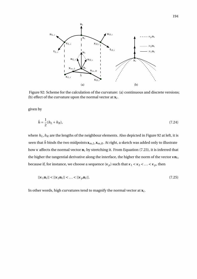
194

(a) (b)

Figure 92: Scheme for the calculation of the curvature: (a) continuous and discrete versions;(b) effect of the curvature upon the normal vector at xi .

given by

h = 1

2(hL +hR ), (7.24)

where hL ,hR are the lengths of the neighbour elements. Also depicted in Figure 92 at left, it is

seen that h binds the two midpoints xm,L ,xm,R . At right, a sketch was added only to illustrate

how κ affects the normal vector ni by stretching it. From Equation (7.23), it is inferred that

the higher the tangential derivative along the interface, the higher the norm of the vector κni ,

because if, for instance, we choose a sequence (κp ) such that κ1 < κ2 < . . . < κp , then

||κ1ni || < ||κ2ni || < . . . < ||κp ni ||. (7.25)

In other words, high curvatures tend to magnify the normal vector at xi .

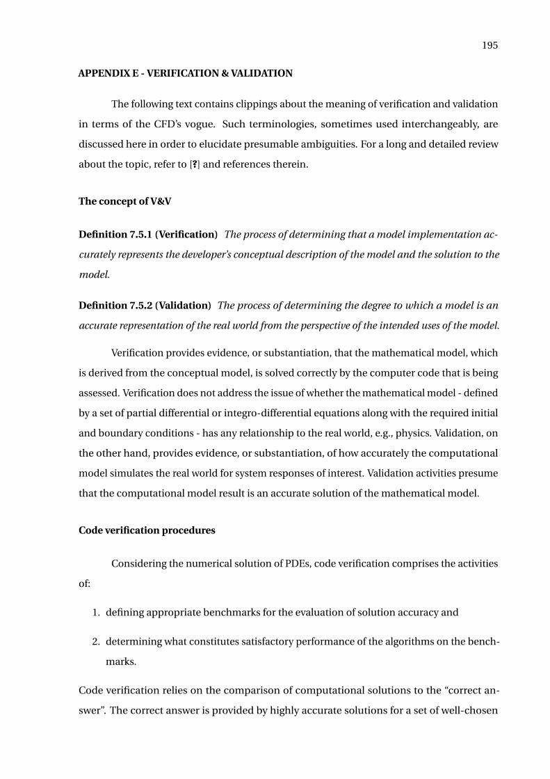
195

APPENDIX E - VERIFICATION & VALIDATION

The following text contains clippings about the meaning of verification and validation

in terms of the CFD’s vogue. Such terminologies, sometimes used interchangeably, are

discussed here in order to elucidate presumable ambiguities. For a long and detailed review

about the topic, refer to [?] and references therein.

The concept of V&V

Definition 7.5.1 (Verification) The process of determining that a model implementation ac-

curately represents the developer’s conceptual description of the model and the solution to the

model.

Definition 7.5.2 (Validation) The process of determining the degree to which a model is an

accurate representation of the real world from the perspective of the intended uses of the model.

Verification provides evidence, or substantiation, that the mathematical model, which

is derived from the conceptual model, is solved correctly by the computer code that is being

assessed. Verification does not address the issue of whether the mathematical model - defined

by a set of partial differential or integro-differential equations along with the required initial

and boundary conditions - has any relationship to the real world, e.g., physics. Validation, on

the other hand, provides evidence, or substantiation, of how accurately the computational

model simulates the real world for system responses of interest. Validation activities presume

that the computational model result is an accurate solution of the mathematical model.

Code verification procedures

Considering the numerical solution of PDEs, code verification comprises the activities

of:

1. defining appropriate benchmarks for the evaluation of solution accuracy and

2. determining what constitutes satisfactory performance of the algorithms on the bench-

marks.

Code verification relies on the comparison of computational solutions to the “correct an-

swer”. The correct answer is provided by highly accurate solutions for a set of well-chosen

196

Figure 93: Example of a process of verification to detect errors in codes. Extracted from [?].

benchmarks, and this answer can only be known in a relatively small number of isolated cases.

These cases therefore assume a very important role in code verification and should be care-

fully formalized in test plans that describe how the code will be verified. In code verification,

the key feature to determine is the observed, or demonstrated, order of convergence using

multiple numerical solutions. An exampled of method that uses exact or highly accurate

solutions to the PDEs to detect numerical algorithm deficiencies and programming errors is

illustrated in Figure 93.

The mathematical model is the general model for the application of interest, whereas

the exact and highly accurate solutions to the PDEs are special-case solutions of the mathe-

matical model. For these special cases, benchmark solutions can be computed. Four types of

highly accurate solutions (from highest to lowest) are recognized:

1. manufactured solutions;

2. analytical solutions;

3. highly accurate numerical solutions to the ODEs and

4. highly accurate numerical solutions to the PDEs.

More specifically, analytical solutions are closed-form solutions to special cases of the PDEs

defined in the mathematical model, commonly represented by infinite series, complex in-

tegrals, and asymptotic expansions. However, the most significant practical shortcoming of

197

classical analytical solutions is that they exist only for very simplified physics, material prop-

erties, and geometries. Therefore, it is indispensable to use the same modelling assumptions

for both the benchmark solution and the code being tested.

198

APPENDIX F - VITA

Gustavo Charles Peixoto de Oliveira was born March 31st, 1987 in Barra do Piraí, Rio

de Janeiro, Brazil. He received his Licentiate degree in Mathematics from Federal Fluminense

University/CECIERJ in 2008. Decided to pursuit an academic career more inclined to applied

contexts, moved to the Engineering’s atrium, whereby received his M.Sc. degree in Metallurgy

and Materials Engineering from Federal University of Rio de Janeiro in 2011 with a two-years

grant provided by the governmental Brazilian funding agency CNPq. Meanwhile, he began to

work with CFD tools to investigate the hydrodynamic stability of rotating flows occurring in

electrochemical cells. He started his Ph.D. trail still in 2011, was a one-year internship Ph.D.

visitor at Ecole Polytechnique Fédérale de Lausanne, Switzerland, during 2013, specifically at

LTCM - Laboratoire de Transfert de Chaleur et de Masse, supported by the Science Without

Borders Program (CNPq/Brazil). There, he worked with gas-liquid two-phase flow dynamics.

Back to Brazil, he received the degree of D.Sc. in Mechanical Engineering in 2015 from State

University of Rio de Janeiro, also sponsored by the Brazilian agency CAPES with a four-years

integral scholarship.

199

APPENDIX G - PUBLICATIONS

? OLIVEIRA, G. P., ANJOS, G. R., PONTES, J., MANGIAVACCHI, N., THOME, J.R. ALE/finite

element modeling of an unconfined bubble plume in periodic domain: bubble shape and

oscillation analysis, accepted for publication in the Journal of the Brazilian Society of

Mechanical Sciences and Engineering, 2015.

? PONTES, J., MANGIAVACCHI, N., ANJOS, G. R., LUCENA, R., GAONA, C. M., OLIVEIRA,

G. P., FERREIRA, D. A Survey of Results Concerning Steady Solutions and the Stability

of a Class of Rotating Flows. Proceedings of the 3rd Conference of Computational

interdisciplinary Sciences, Asunción, Paraguay, 2014.

? OLIVEIRA, G.P., MANGIAVACCHI, N., ANJOS, G., PONTES, J., THOME, J.R. Comparative

CFD Simulations of Gas Transport in Slug Flow from Periodic Arrays with Single or

Multiple Bubbles. Proceedings of the 3rd Conference of Computational interdisciplinary

Sciences, Asunción, Paraguay, 2014.

? OLIVEIRA, G.C.P., ANJOS, G., PONTES, J., MANGIAVACCHI, N. Finite Element Analysis

of Pressure-Driven Laminar Flow Inside Periodically Staggered Arrays. Proceedings of

the VII Brazilian National Congress of Mechanical Engineering, Belém, Brazil, 2014.

? OLIVEIRA, G.C.P., MANGIAVACCHI, N., ANJOS, G., THOME, J.R.Numerical Simulation

of a Periodic Array of Bubbles, MecÃ¡nica Computacional, v. XXXII, 1813-1824, 2013.

? OLIVEIRA, G.C.P., MANGIAVACCHI, N., ANJOS, G., THOME, J.R. Topological Remeshing

and Locally Supported Smoothing for Bubble Coalescence in Two-Phase Flows. Proceed-

ings of the 22nd International Congress of Mechanical Engineering, Ribeirão Preto,

Brazil, 2013.

? MORAES, E.L.S., OLIVEIRA, G.C.P., ANJOS, G., MANGIAVACCHI, N., PONTES, J. Semi-

Lagrangian Algorithms for Second Order for the Study of Hydrodynamics of Electro-

chemical Cells. Proceedings of the 14th Brazilian Congress of Thermal Sciences and

Engineering, Rio de Janeiro, Brazil, 2012.

? OLIVEIRA, G.C.P., MANGIAVACCHI, N., PONTES, J. Semi-Lagrangian High-Order 3D

Interpolation: Survey on a Finite Element Z-Type Operator. Proceedings of the 14th

Brazilian Congress of Thermal Sciences and Engineering, Rio de Janeiro, Brazil, 2012.

200

? OLIVEIRA, G.C.P., MANGIAVACCHI, N., PONTES, J. High-Order Interpolation Applied to

the Modeling of Advective Transport for Incompressible Flows. Congress of Computa-

tional and Applied Mathematics- CMAC/NE, Natal, Brazil, 2012.

? OLIVEIRA, G.C.P, Hydrodynamic Stability in Electrochemical Cells Through the Finite

Element Method, M.Sc. dissertation, Federal University of Rio de Janeiro, Brazil, 2011.

? OLIVEIRA, G.C.P., MANGIAVACCHI, N., PONTES, J. A Semi-Lagrangian Scheme for Fluid

Flow Simulations with a Zienkiewicz-Type Finite Element Interpolation. Proceedings of

the 21st International Congress of Mechanical Engineering, Natal, Brazil, 2011.

drop jet in crossflow: ale/fem simulations and interfacial...

Documents