diversidade de aranhas (araneae-arachnida) em …© do... · natureza em geral e animais em...
TRANSCRIPT

i
INSTITUTO NACIONAL DE PESQUISAS DA AMAZÔNIA
PROGRAMA DE PÓS-GRADUAÇÃO EM ECOLOGIA
DIVERSIDADE DE ARANHAS (ARANEAE-ARACHNIDA) EM DOIS
GRADIENTES ALTITUDINAIS NA AMAZÔNIA, AMAZONAS, BRASIL
ANDRÉ DO AMARAL NOGUEIRA
Manaus, Amazonas
Junho de 2011

i
ANDRÉ DO AMARAL NOGUEIRA
DIVERSIDADE DE ARANHAS (ARANEAE-ARACHNIDA) EM DOIS
GRADIENTES ALTITUDINAIS NA AMAZÔNIA, AMAZONAS, BRASIL
ORIENTADOR: DR. EDUARDO MARTINS VENTICINQUE
Co-orientador: Dr. Antonio Domingos Brescovit
Tese apresentada à Coordenação do Programa
de Pós-Graduação do Instituto Nacional de
Pesquisas da Amazônia como parte dos
requisitos para obtenção do titulo de Doutor em
Biologia (Ecologia)
Manaus, Amazonas
Junho de 2011
ii
Bancas examinadoras
Banca avaliadora do trabalho escrito – Avaliadores e parecer
Dra. Carla Rodrigues Ribas (UFLA, Brasil)- Aprovada
Dr. Felipe Rego (UFMA, Brasil) – Aprovado - Aprovada
Dr. Nathan Sanders (Univ. Tennessee, EUA) – Aprovada com correções
Dr. Robert K. Colwell (Univ. Connecticut, EUA) – Aprovada
Dr. Gonçalo Ferraz (INPA/PDBFF, Brasil) – Reprovada
Banca examinadora da defesa oral – Avaliadores e parecer
Dr. Willian Ernest Magnusson (INPA, Brasil) – Aprovada
Dr. Pedro Ivo Simões (INPA, Brasil) – Aprovada
Dr. Thierry Ray Jehlen Gasnier (UFAM, Brasil) – Aprovada

iii
Sinopse:
Nesse trabalho nós estudamos a distribuição altitudinal da comunidade de aranhas
amostrada no Pico da Neblina (AM - Brasil). Nós descrevemos e analisamos os padrões
de riqueza e diversidade beta ao longo do gradiente e testamos o seu ajuste à hipóteses
biogeográficas relacionadas ao tema. Também descrevemos oito espécies novas do
gênero Chrysometa e discutimos a sua biogeografia.
Palavras-chave: Aracnologia, montanhas, macroecologia, Amazônia, gradientes
ambientais, biodiversidade.
N778 Nogueira, Andre do Amaral Diversidade de aranhas (Arachnida-Araneae) em dois gradientes altitudinais na Amazônia, Amazonas, Brasil / Andre do Amaral Nogueira.---
Manaus : [s.n.], 2011. xv, 243 f. : il. color.
Tese (doutorado)-- INPA, Manaus, 2011 Orientador : Eduardo Martins Venticinque Co-orientador : Antônio Domingos Brescovit
Área de concentração : Ecologia de Comunidades
1. Aracnologia. 2. Biodiversidade. 3. Ecologia de comunidades. 4. Neblina, Pico (AM). I. Título.
CDD 19. ed. 595.47

iv
Dedico esta tese à minha filha Gabriela, uma fonte constante
de motivação, alegria e orgulho.
Também dedico à minha mãe Maria Lúcia, e à minha avó,
Maria José, grandes incentivadoras do meu interesse pela
natureza em geral e animais em particular.

v
Agradecimentos
Esse trabalho jamais teria sido realizado sem a ajuda de muitas pessoas e instituições que listo
a partir de agora. Tentarei ser breve, mas é improvável que consiga.
Começo pelo meu orientador, Eduardo Venticinque, o Dadão, ao qual sou agradecido
por vários motivos, da sugestão do tema da pesquisa até as conversas sobre biologia em geral
e aranhas em particular. Sua postura sempre calma e bem humorada também foi muito
importante em alguns momentos difíceis ao longo desse período. Também agradeço meu co-
orientador, Antonio Brescovit, por tudo que aprendi sobre aranhas com ele até hoje, pelas
parcerias em trabalhos e nos campos de futebol.
As viagens de coleta que realizei para esse doutorado foram alguns dos pontos mais
marcantes e agradáveis dessa jornada acadêmica, e por elas sou grato à muitas pessoas.
Agradeço, portanto, aos meus coletores, Ricardo Braga-Neto, o Saci, que participou da
expedição à Serra do Tapirapecó exibindo notável dedicação (pegou até malária!), e Nancy
Lo-Man-Hung e David Candiani, não menos dedicados, (mas sem malária) que coletaram
comigo no Pico da Neblina, a expedição mais bem sucedida (e trabalhosa) realizada durante
esse doutorado. Um muito obrigado mesmo à vocês pelo empenho, não é fácil largar tudo por
dois meses só para ajudar um colega. Agradeço também aos mateiros e demais auxiliares de
campo dessas duas viagens, Domingos e Jorge, no Tapirapecó, e Waldir “Chouriman”
Pereira, Mário e Tomé, pelo trabalho duro e por passarem um pouco de sua experiência e
conhecimento sobre a mata.
Sou também grato à Rodrigo Loyola Dias, por ter liderado à expedição à Serra do
Tapirapecó e também por atender diversos pedidos de ajuda e informações sobre as áreas de
estudo. Agradeço também à Vinicius Carvalho e Lucéia Bonora, pelo grande auxílio na
preparação da expedição para o Pico da Neblina, terreno conhecido dos dois. Ainda sobre as
viagens tenho que agradecer o IBAMA (em especial a equipe da sede do PARNA Pico da
Neblina em São Gabriel da Cachoeira) e a FUNAI, pelas licenças de coleta e autorização para
ingresso em Terra Indigena, o 5° BIS – Batalhão de Infantaria da Selva – de São Gabriel da
Cachoeira e o 5° PEF – Pelotão Especial de Fronteira Maturacá – pelo apoio logístico na
expedição ao Pico da Neblina, à AYRCA (Associação Yanomami do Rio Cauaburis e
Afluentes) e às comunidades Yanomami dos rios Marari, Ariabú e Maturacá, que gentilmente
nos acolheram em suas terras.

vi
A identificação das aranhas coletadas nessas expedições demandou um pequeno
batalhão de taxonomistas e especialistas, aos quais sou imensamente grato. Identifico-os a
seguir, assim como o grupo de sua especialidade: Lina Almeida (Amaurobiidae), David
Candiani e Alexandre Bonaldo (Corinnidae), Daniele Polotow (Ctenidae), Nancy Lo-Man-
Hung (Hahniidae), Rafael Lemos (Linyphiidae), Flávio Yamamoto, Rafael Indicatti e Dr.
Silvia Lucas (Mygalomorphae), Adalberto Santos (Oxyopidae and Pisauridae, Synotaxidae),
Éwerton Machado (Pholcidae), Gustavo Ruiz (Salticidae), Cristina Rheims (Scytodidae and
Sparassidae), João Barbosa (Chrysometa) Erica Buckup and Maria Aparecida Marques
(Theridiidae), Estevam Silva (Trechaleidae). E o Antonio Brescovit também, claro, que
conferiu boa parte do material.
Esse parágrafo será dedicado à agradecer aos colegas de laboratório, e será grande,
uma vez que participei de vários. Primeiro não poderia esquecer os colegas do meu antigo e
marcante laboratório, o LAL. Ricardo Pinto-da-Rocha, Cibele (valeu pelas referências, Ciba!),
Teté (bela figura, Teta!), MBS (valeu pela hospedagem.), Pudim, Sabrina, Zé (formação
clássica), Patrão, Alipío, José, Vivinha (mais ou menos novas aquisições), obrigado pela
agradável e instrutiva convivência nesses anos todos de aracnologia. Ao longo do doutorado,
quando em São Paulo, instalei-me no Instituto Butantan, onde passei parte desses quatro anos
de maneira igualmente agradável e instrutiva. Agradecendo aos numerosos colegas, em ordem
aleatória e tentando não esquecer ninguém, valeu Cris, Dani, Lina, Priscila, Matilde, Camila,
Vanessa, Ju, Tati, Andria, Dr. Irene, Dr. Silvia, Denise, Kelly, Rafa (valeu pelas fotos, Rafa),
Japa (igualmente, Japa), Gustavo, Mamilo (grande co-autor, o rei das Chrysometa), Pãozinho,
Igor, Claudião, Jaú, Cidão, Tulipas, Hilton, Danilo, Gandhi (valeu pelas ajudas de fim de
tese), Paulão, Samuel, Pica-Pau, Carteiro, Robin, Tárik, Babenco, além de outros que já se
foram e dos muitos que por lá passaram...e, infelizmente, não tenho como não deixar uma
nota de pesar ao lembrar do nosso saudoso Laboratório de Artrópodes, destruído no trágico
incêndio de 2010...tempos bons que não voltarão mais....agora temos que encher de aranhas a
nova coleção...
Por fim agradeço aos colegas de laboratório do INPA, com quem não convivi tanto
quanto gostaria, mas o bastante para avaliar o tempo de convivência como agradável e
instrutivo. São eles, entre outros, Brunão, Maíra, Carine, Rosinha, Duka, Fernanda, Gabi...
Continuando no norte, agradeço todos os que me auxiliaram em minhas estadias
amazônicas. Começo pelos numerosos anfitriões que me receberam nas diversas vezes que

vii
estive aqui: Saci, Gabi, Minduim, Thayná, Dé e Catá, Flávia, obrigado por terem facilitado
imensamente minha vida, me fornecendo abrigo, colchão e até ventilador. Isso sem falar na
companhia e amizade, que tornaram todas as minhas estadias manauaras memoráveis. Valeu
gente. Também sou muito grato aos amigos e colegas velhos e novos aí de Manaus, Bogão,
Manô, Ana, Regiane, Erika, Pardal e Ana e filho, Tropico, Angelita, Fumaça, Rato, Alemão e
muitos outros e outras e também todos os colegas da turma de mestrado/doutorado de 2008,
com os quais passei um semestre dos mais instrutivos e agradáveis. Agradeço também ao
curador de invertebrados do INPA Dr. Henrique Augusto, e aos professores da Ecologia, no
geral gostei bastante das aulas. Agradeço também à Claudia, Flávia Costa, Beverly, Rosi e
demais funcionários da PPGEco.
Voltando rapidamente ao tema anfitriões, inesperadamente tive que passar um
tempinho em Natal no fim do doutorado, quando fui então abrigado por Guiga, Dri e Phoeve,
aos quais expressos aqui meus mais sinceros agradecimentos. Foi bem legal, apesar da rotina
massacrante Agradeço também os professores Carlos e Márcio, pela hospitalidade em seu
laboratório na UFRN.
Começando a finalizar, agradeço a outros colegas aracnólogos, como Rodrigo Pirata,
Adalberto, Sidclay e Janael, que me ajudaram de distintas maneiras, além da Prof. Eudóxia,
que me iniciou na aracnologia. Passando para o terreno mais pessoal, agradeço aos amigos de
escola e da biologia (aliás, valeu Matinas pela tese), meus dois principais círculos de amizade,
além de amigos avulsos de outras procedências...mas não resisto e tenho que destacar o
pessoal do futebol de terça e do de quinta (o futebatradiça), pois jogar bola é muito bom, e
ainda mais na companhia de amigos. Agradeço à Aline pela imensa ajuda nesse fim de tese
em várias tarefas, e, muito mais importante, pela companhia, paciência e carinho nesses
últimos meses...
Passando enfim para a família, agradeço à minha filha Gabriela, meu xodó, e à sua
mãe, Marisa, e todo o pessoal de Garça, por cuidarem dela e pelos divertidos fins de semana.
Agradeço meu pai Dalmo, irmãos Paula e Fernando, e avó Cida, por todo o apoio e carinho de
uma vida inteira. À minha mãe Maria Lúcia e avó Maria José, que infelizmente não poderão
ver o trabalho final, mas que certamente estariam felizes e orgulhosas por mim, como sempre
estive delas Finalizo agradecendo aos que financiaram isso tudo, que foram o CNPq, pela
bolsa de doutorado, uma bolsa BECA, do IEB/Fundação Moore e um auxílio da WCS,
utilizados nas expedições de campo.

viii
Resumo
Montanhas devem representar o exemplo mais evidente da influencia do ambiente sobre as
comunidades bióticas. Neste trabalho nós estudamos a distribuição altitudinal de uma
comunidade de aranhas no Pico da Neblina (AM - Brasil). Realizamos a amostragem em seis
altitudes, 100 m, 400 m, 860 m, 2000 m e 2400 m, sendo que em cada altitude três locais
foram amostrados. Os métodos de coleta empregados foram guarda-chuva entomológico
(unidade amostral = 20 batidas), de dia, e procura ativa (unidade amostral = 1 h de procura), à
noite. O número de amostras por altitude foi 54, sendo metade de cada método, o que leva a
um total de 324 amostras. No total nós coletamos 3140 aranhas adultas que foram divididas
em 528 morfoespécies, de 39 famílias. A maioria das espécies é rara, e 197 (37%) foram
representadas por apenas um indivíduo. A riqueza por altitude variou de 224 (a 100 m) a 24 (a
2400 m) espécies e apresentou uma relação negativa com a altitude, diminuindo de maneira
monotônica. O padrão observado não se ajustou ao modelo gerado pelo Efeito do Domínio
Central (MDE em inglês), que prevê uma maior concentração de espécies nas partes mais
centrais do gradiente. Nossos dados também não sustentaram o Efeito Rapoport, que prevê
uma relação positiva entre altitude e amplitude da distribuição altitudinal das espécies. Essas
duas variáveis não estiveram relacionadas, e a maioria das espécies (333 espécies ou 63%) só
foi registrada em uma das altitudes. Apenas 25 espécies (5%) tiveram uma amplitude grande,
ocorrendo em mais da metade do gradiente. A distribuição dos indivíduos ao longo da área de
ocorrência das espécies variou de maneira específica e não se ajustou à hipóteses de efeito
resgate para a maioria da comunidade, teoricamente responsável pelo Efeito Rapoport. A
composição das espécies apresentou uma grande variação ao longo do gradiente e mesmo
entre as áreas amostradas em cada altitude. A beta diversidade calculada para o total do
gradiente altitudinal foi de 3,45 o que significa que a araneofauna do Pico da Neblina
compreende três e meia comunidades distintas. Esse resultado parece ser sustentado por uma
ordenação (NMDS), que aponta a formação de três grupos principais, um formado pelas três
primeiras altitudes, um formado pelas duas últimas, e a quarta altitude (1550 m) aparece numa
posição intermediária entre os dois grupos. Esse resultado mostra que a comunidade de
aranhas não se encaixa na divisão altitudinal proposta para a região do Escudo das Guianas,
onde se insere a área de estudo. A dominância observada na comunidade de aranhas de cada
altitude aumentou drasticamente nas duas últimas altitudes. Por fim nós descrevemos oito
espécies novas do gênero Chrysometa (Tetragnatidae), sete delas coletadas no Pico da
Neblina e uma delas oriunda de outra montanha amostrada na região, a Serra do Tapirapecó
(AM). A diversidade do gênero obtida no Pico da Neblina foi muito alta (12 espécies e 336
indivíduos), e a riqueza e sobretudo a abundância e importância relativa do gênero
aumentaram junto com a altitude. Na Serra do Tapirapecó o gênero teve presença mais
modesta (4 espécies e 40 indivíduos), o que pode ser atribuído à menor altitude dos locais
amostrados nessa última. A análise dos padrões de distribuição altitudinal nos locais de estudo
e em uma escala maior (verificada com o auxílio da literatura) indica que o gênero atinge sua
maior diversidade em locais de grande altitude, e que as espécies desses locais tendem a ter
uma distribuição mais restrita que as de locais mais baixos.

ix
Abstract
Spider (Arachnida-Araneae) diversity at two amazonian altitudinal gradients,
Amazonas, Brazil
Mountains probably represent the most obvious example of environmental influence on biotic
communities. In this work we studied the altitudinal distribution of a spider community at the
Pico da Neblina (AM-Brazil). We sampled six altitudes, 100 m, 400 m, 860 m, 2000 m e 2400
m, and in each of them three sites were investigated. Spiders were sampled with a beating tray
(sampling unit = 20 beating events), during the day, and through active search (sampling unit
= one hour of search), during the night. We obtained 54 samples by altitude, half with each
method, totaling 324 samples for the whole gradient. We collected 3140 spiders, sorted to 528
morphospecies, from 39 families. Most species are rare, and 197 (37%) were represented by
just one individual. Richness by altitude ranged from 224 (at 100 m) to 24 (at 2400 m) species
and presented a negative relation with altitude, decreasing in a monotonic way. The observed
pattern presented a poor fit with that generated by the mid-domain effect (MDE), which
predicts higher richness at intermediate altitudes. Our data didn’t support a Rapoport effect
either, which predicts a positive relation between altitude and altitudinal range size. These two
variables were not related to each other and most species (333 species or 63%) were recorded
at just one altitude. Only 25 species (25%) presented a large range, encompassing more than
half of the altitudinal gradient. The distribution of individuals along the range of each species
varied in a specific way, which is not in accordance with hypothesis based on rescue effects to
explain the occurrence of Rapoport effect. The composition of species presented a great
variation along the gradient and even for the sampling sites within each altitude. Beta
diversity calculated for the whole gradient was 3,45, which means that the spider fauna from
the Pico da Neblina includes three and a half different communities. The result of a NMDS
seems to support this result as it present three main groups, one composed by the three first
altitudes, another by the two highest altitudes and the fourth altitude (1550 m) situated in an
intermediate position between the two groups. This result does not support the altitudinal
division proposed for the Guaiana region, where our study site is located. Dominance pattern
drastically increased at the two last altitudes. Finally, we described eight new species of the
genus Chrysometa (Tetragnathidae), seven from the Pico da Neblina and one from another
mountain sampled in the region, the Serra do Tapirapecó (AM). Diversity obtained at the Pico
da Neblina was very high (12 species and 336 individuals) and its richness and especially
abundance and relative importance increased with altitude. At the Serra do Tapirapecó the
diversity of the genus was much lower (4 species and 40 individuals), which can imputed to
the smaller altitude of the localities sampled there. The analysis of the pattern of altitudinal
distribution at the study areas and in a larger scale (based on the literature), indicates that the
genus reaches its maximum diversity at high altitude sites, and that species from highlands
tend to have a narrower distribution than species from lowlands.

x
Sumário
Folha de rosto .............................................................................................................i
Bancas examinadoras.......................................................................................ii
Ficha catalográfica ......................................................................................................iii
Sinopse............................................................................................................. ......... .iii
Dedicatória .................................................................................................................iv
Agradecimentos ..........................................................................................................v
Resumo .......................................................................................................................viii
Abstract ......................................................................................................................ix
Sumário ......................................................................................................................x
Lista de tabelas ...........................................................................................................xiii
Lista de figuras ...........................................................................................................xv
1 – Introdução geral......................................................................................... ....1
1.1 – Diversidade biológica em gradientes altitudinais,
MDE e Rapoport......................................................................................................1
1.2 – As aranhas.............................................................................................................4
1.3 – O Pico da Neblina.................................................................................................7
2 – Objetivos gerais ..................................................................................................10
Artigo 1 .................................................................................................................. 12
Araneae, Pico da Neblina, state of Amazonas, Brazil
Resumo ....................................................................................................... 14
Introdução ................................................................................................... 14
Materiais e métodos ..................................................................................... 16
Resultados e discussão ................................................................................. 18

xi
Literatura citada ........................................................................................... 23
Tabelas ........................................................................................................ 27
Figuras ........................................................................................................ 49
Artigo 2 .................................................................................................................. 53
Spiders (Arachnida-Araneae) from the Pico da Neblina (AM-Brazil).
Richness patterns along an Amazonian altitudinal gradient,
with a test of MDE and Rapoport effect.
Resumo ....................................................................................................... 55
Introdução ................................................................................................... 56
Materiais e métodos ..................................................................................... 60
Resultados ................................................................................................... 66
Discussão .................................................................................................... 69
Conclusões .................................................................................................. 77
Referências .................................................................................................. 78
Tabelas ........................................................................................................ 86
Figuras ........................................................................................................ 88
Artigo 3 .................................................................................................................. 93
Beta diversity along altitudinal gradients: a study on the composition of
the spider community from the Pico da Neblina (AM, Brazil), and on its
congruence with regional altitudinal zonation.
Sumário ....................................................................................................... 95

xii
Introdução ................................................................................................... 97
Materiais e métodos ............................ 100
Resultados ................................................................................................. 106
Discussão .................................................................................................. 110
Conclusão .................................................................................................. 120
Referências ................................................................................................ 121
Tabelas ...................................................................................................... 131
Figuras ...................................................................................................... 150
Artigo 4 ................................................................................................................ 154
The spider genus Chrysometa (Araneae, Tetragnathidae) from the Pico da Neblina and
Serra do Tapirapecó mountains (Amazonas, Brazil): new species, new records,
diversity and distribution along two altitudinal gradients.
Resumo ..................................................................................................... 156
Introdução ................................................................................................. 157
Materiais e métodos ................................................................................... 158
Taxonomia ................................................................................................ 162
Distribuição altitudinal e diversidade ......................................................... 174
Referências ................................................................................................ 182
Tabelas ...................................................................................................... 187
Figuras ...................................................................................................... 191
3 – Síntese ............................................................................................................ 199

xiii
Referências bibliográficas....................................................................................... 202 .
Lista de tabelas
Artigo 1
Tabela 1 – Lista de espécies de aranha coletadas no Pico da Neblina...................... 27
Tabela 2 – Riqueza e abundância, absolutas e proporcionais, por família............... 46
Tabela 3 – Inventários de araneofauna realizados na Amazônia.............................. 48
Artigo 2
Tabela 1 – Abundância e medidas de riqueza das comunidades de aranha por
altitude...................................................................................................................... 86
Tabela 2 – Resultados da regressão linear múltipla entre a riqueza e as variáveis
preditoras.................................................................................................................. 87
Artigo 3
Tabela 1 – Coordenadas das 18 áreas de amostragem e medidas de diversidade alfa e beta
para as 18 áreas amostradas e para as seis altitudes............................................. 131
Tabela 2 – Matriz de similaridade e proporção de espécies compartilhadas entre as 18 áreas
amostradas............................................................................................................ 132
Tabela 3 – Matriz de similaridade e proporção de espécies compartilhadas entre as seis
altitudes amostradas............................................................................................. 133
Tabela 4 – Matriz de diversidade beta (D) da comunidade de aranhas amostrada nas seis
altitudes............................................................................................................... 134
Tabela 5 – Resultados dos testes de Mantel e Mantel parcial............................. 135
xiv
Tabela 6 – Resultados da análise de espécies indicadoras para as três divisões do
gradiente................................................................................................................... 136
Tabela 7 – Resultados da análise de espécies indicadoras por família para a três divisões do
gradiente................................................................................................................... 137
Material suplementar do Artigo 3
Tabela 1 – Resultados da análise de espécies indicadoras para a partição do gradiente em duas
metades, inferior e superior...................................................................................... 138
Tabela 2 – Resultados da análise de espécies indicadoras para a partição do gradiente em três
partes, de acordo com a divisão da Região das Guianas..............................................142
Tabela 3 – Resultados da análise de espécies indicadoras para a partição do gradiente em seis
partes, por altitude..................................................................................................... 146
Artigo 4
Tabela 1 – Distribuição altitudinal das espécies de Chrysometa coletadas no Pico da
Neblina...................................................................................................................... 187
Tabela 2 – Distribuição altitudinal das espécies de Chrysometa coletadas na Serra do
Tapirapecó................................................................................................................ 189
Tabela 3 – Inventários de araneofauna neotropicais. Diversidade geral de aranhas e do gênero
Chrysometa.............................................................................................................. 190

xv
Lista de figuras
Artigo 1
Figura 1 – Área de estudo...................................................................................... 49
Figura 2 – Vegetação das seis altitudes amostradas.............................................. 50
Figura 3 – Aranhas coletadas no Pico da Neblina.................................................. 51
Figura 4 – Aranhas coletadas no Pico da Neblina.................................................. 52
Artigo 2
Figura 1 – Área de estudo....................................................................................... 88
Figura 2 – Riqueza observada, interpolada, rarefeita e abundância por altitude....89
Figura 3 – Curvas de rarefação para cada altitude.................................................. 89
Figura 4 – Riqueza observada e prevista de acordo com o Efeito do Domínio Central (MDE,
em inglês) para espécies, gêneros e famílias.......................................................... 90
Figura 5 – Distribuição de frequências do tamanho da amplitude altitudinal das espécies, e
amplitude da distribuição altitudinal e ponto médio ponderado (WAM) para cada
espécie..................................................................................................................... 91
Figura 6 – Relação entre altitude e amplitude altitudinal da área de distribuição
(Rapoport)............................................................................................................... 92
Figura 7 – Relação entre ponto médio altitudinal e ponto médio ponderado......... 92
Artigo 3
Figura 1 – Área de estudo..................................................................................... 147
Figura 2 – Curvas de abundância da comunidade para cada altitude................... 148

xvi
Figura 3 – Correlações entre similaridade de Bray-Curtis, diversidade beta, distância
geográfica e diferença altitudinal (Teste de Mantel parcial).............................. 149
Figura 4 – NMDS realizada para a comunidade, para as 18 áreas amostradas. 150
Artigo 4
Figura 1 – Área de estudo................................................................................... 192
Figura 2 – Ilustração da genitália de Chrysometa nubigena............................... 193
Figura 3 – Ilustração da genitália de Chrysometa saci....................................... 194
Figura 4 – Ilustração da genitália de Chrysometa waikoxi................................. 195
Figura 5 – Ilustração da genitália de Chrysometa petrarsierwaldae.................. 196
Figura 6 – Ilustração da genitália de Chrysometa lomanhungae, C. yanomami e C.
santosi.................................................................................................................. 197
Figura 7 – Ilustração da genitália de Chrysometa candianii e C. minuta............ 198

1
INTRODUÇÃO GERAL
DIVERSIDADE BIOLÓGICA EM GRADIENTES ALTITUDINAIS, EFEITO DO DOMÍNIO CENTRAL E
RAPOPORT
Montanhas devem representar o exemplo mais evidente da influencia do ambiente
sobre as comunidades bióticas. As drásticas mudanças observadas na fauna e flora em espaços
relativamente pequenos, que podem ser percorridos em algumas horas, sempre chamaram a
atenção das pessoas interessadas em observar e compreender o mundo natural. A primeira
descrição da divisão da vegetação em zonas ao longo de um gradiente altitudinal foi feita por
Joseph Pitton de Tournefort, após a escalada do Monte Ararat, na Armênia, no começo do
século XVIII (Papavero et al., 1997). Esse autor também associou as mudanças observadas na
flora ao longo da escalada com as observadas na flora da Europa partindo-se da Itália até a
Noruega, tornando-se o primeiro a associar o gradiente altitudinal ao latitudinal.
Suas observações, aliadas ao que na época pareciam ser outras evidências (como a de
que o nível das águas vinha baixando desde o começo da criação), forneceram a base para
Lineu (1744) criar o “Discurso sobre o aumento da terra habitável”, a primeira grande
hipótese biogeográfica moderna (Papavero et al., 1997). O Éden, onde habitavam todas as
formas de vida que haviam sido criadas por Deus, devia ser uma grande montanha em uma
zona equatorial, comportando todos os ecossistemas conhecidos, ao longo do qual se
distribuiriam todas as espécies de acordo com suas adaptações. Conforme baixava o nível das
águas, as espécies foram se dispersando e se distribuindo no globo de acordo com suas
preferências climáticas.
Um raciocínio semelhante foi defendido por Willdenow (1805, apud Papavero et al.
1997) para explicar a distribuição geográfica das espécies de plantas no mundo. Porém, de
maneira um pouco mais realista, ele supôs que as plantas teriam se originado em várias
montanhas ao redor do mundo, ao invés de apenas uma, o que explicaria as diferentes regiões
fitogeográficas. O mesmo autor também fez a ligação fundamental entre clima e tipo de
vegetação (Lomolino, 2001). Ainda no começo do século XIX, a sucessão de comunidades
vegetais ao longo do gradiente altitudinal e seu paralelo com as observadas ao longo do

2
gradiente latitudinal foram novamente abordados, dessa vez com inédita precisão e
detalhamento por Humboldt, durante a ascensão do Monte Chimborazo, imponente vulcão
equatoriano (6.310 m). O autor também formalizou a relação entre a distribuição das plantas
com características físicas do ambiente, como temperatura (vonHumboldt, 1807, apud
Papavero et al. 1997).
As montanhas permaneceram como fonte de inspiração e como laboratório natural
para vários tipos de trabalhos relacionados à ecologia e biogeografia (Lomolino, 2001). As
montanhas Siskiyou e Santa Catalina, nos Estados Unidos, serviram de palco para trabalhos
pioneiros sobre diversidade beta (Whittaker, 1960 e 1965). Outro trabalho influente que pode
ser citado teorizou sobre os efeitos de montanhas como barreira à dispersão, e previu que
estes seriam mais importantes em áreas tropicais devido à menor tolerância a variações
ambientais de suas espécies, uma conseqüência do clima marcado por menor sazonalidade
(Janzen, 1967). Ecossistemas montanos também foram usados para testar várias outras teorias
ecológicas, como biogeografia de ilhas (Vuillemier, 1970; Brown, 1971), a Lei de Bergman
(Brehm e Fiedler, 2004), e a hipótese do gradiente de stress, relacionada à facilitação
(interações positivas entre plantas) (Callaway et al., 2002).
Por fim, montanhas também merecem um lugar de destaque na biologia simplesmente
por sua notável riqueza de espécies. Regiões montanas, em particular as localizadas nos
trópicos, constituem o ambiente que apresenta o maior número de espécies no planeta (Orme
et al., 2005; Rahbek, 2005), uma consequência dos importantes gradientes ambientais a elas
associados. Essa grande variabilidade ambiental em espaços relativamente pequenos também
é responsável por outras características da maioria das biotas montanas, como distribuição
restrita de suas espécies, elevado grau de endemismo e altas taxas de substituição de espécies
(Jetz et al., 2004; Berry e Riina, 2005; Melo et al., 2009).
Em função disso as montanhas parecem uma escolha natural para testar hipóteses
biogeográficas relacionadas à distribuição de espécies, como é o caso de duas teorias
relativamente recentes, a hipótese das restrições geométricas (Colwell e Lee, 2000), ou efeito
do domínio central (MDE, em inglês), e a Lei de Rapoport (Stevens, 1989). Ambos foram
originalmente relacionados ao gradiente latitudinal, mas rapidamente gradientes altitudinais
também passaram a ser utilizados para testar essas teorias, o que seria importante para
verificar a alegada universalidade dessas propostas.

3
A Lei de Rapoport foi proposta como uma possível explicação para o gradiente
latitudinal de riqueza de espécies. A Lei de Rapoport é uma relação positiva entre latitude e
amplitude latitudinal da área de distribuição, e foi nomeada em homenagem à Eduardo
Rapoport, ornitólogo argentino que relatou pela primeira vez esse padrão (Rapoport, 1975).
Stevens hipotetizou que isso seria causado pela maior tolerância climática das espécies que
ocorrem em altas latitudes, o que seria uma conseqüência da importante variação sazonal que
se observa nessas regiões, enquanto nos trópicos, de maneira inversa, as espécies estão
habituadas a uma variação mínima dos fatores climáticos. Uma conseqüência disso seria um
aumento da riqueza das comunidades de latitudes mais baixas devido à migração de espécies
tolerantes de latitudes maiores, enquanto o contrário não seria possível, devido à incapacidade
de espécies tropicais de expandir sua área de distribuição de maneira significativa. Essa
migração assimétrica seria a responsável pelas diferenças em riqueza ao longo do gradiente
latitudinal.
Com base nessas idéias intuitivas e em alguns exemplos que obviamente
corroboravam suas idéias, seu trabalho suscitou muito interesse (Stevens, 1989), e o mesmo
autor defendeu que elas se aplicaram também a qualquer tipo de gradiente natural, como o
altitudinal ou o batimétrico (Stevens, 1992 e 1996). No entanto, a maioria das pesquisas se
concentrou na validade e universalidade da própria Lei de Rapoport, isto é, uma relação
positiva entre tamanho da amplitude da área de distribuição e o gradiente geográfico, do que
na sua influência sobre padrões de riqueza, rapidamente descartada por falta de evidências
(Rhode, 1993).
Um dos trabalhos que refutou o papel da Lei de Rapoport como responsável pela
ocorrência de gradiente de riqueza de espécies deu origem à outra teoria mencionada, a das
restrições geométricas (Colwell e Hurtt, 1994). Os autores mostraram através de simulações,
que a disposição aleatória da amplitude de áreas de distribuição (a partir de dados empíricos)
em domínios fechados, isto é, com limites físicos assumidos como intransponíveis pelas
espécies, necessariamente leva à uma maior sobreposição de espécies na parte central do
gradiente. Esse resultado foi chamado de Efeito do Domínio Central (MDE, sigla em inglês),
e foi possível constatar que os padrões resultantes eram muito semelhantes aos obtidos em
vários trabalhos empíricos realizados em gradientes naturais (Rahbek, 1995), o que levou os
autores a propor que as restrições geométricas tinham um papel central na geração desses
padrões, ou que, ao menos, não podiam ser descartadas (Colwell e Lees, 2000). Ao enfatizar
que os padrões de riqueza de comunidades poderiam ser explicados prescindindo de qualquer

4
variável ambiental ou ecológica, os autores despertaram uma grande atenção por parte da
comunidade científica da área, que estimulou a realização de um grande número de estudos.
Quase duas décadas, e muita polêmica depois (Gaston et al., 1998; Ribas e
Schoereder, 2006; Colwell et al., 2005; Zapata et al., 2005; entre muitos outros), essas teorias
continuam sendo testadas e investigadas e ainda não há consenso a respeito de suas validades.
Já parece claro que ambas são menos universais do que se sustentava previamente, sendo que
inclusive já se propôs o rebaixamento da Lei de Rapoport para “Efeito Rapoport” (Blackburn
e Gaston, 1996). No entanto, trabalhos recentes ainda encontram evidências em seu favor
(Dunn et al., 2007; McCain, 2009a), ainda que talvez restritas a condições específicas.
De qualquer maneira, o grande número de trabalhos recentes relacionados a esses
temas, assim como a maior abrangência de grupos investigados, proporcionou um aumento
significativo no conhecimento dos padrões de riqueza ao longo de gradientes altitudinais. Ao
contrário do que se acreditava inicialmente, quedas monotônicas de riqueza com o aumento
de altitude não representam um resultado universal. Outros padrões, como a existência de um
platô de alta diversidade em baixas altitudes, e principalmente picos de riqueza em altitudes
intermediárias são igualmente ou até mais freqüentes, dependendo do grupo de estudo e de
outros fatores (Rahbek, 2005; McCain, 2007; 2009b).
Neste trabalho, vamos estudar os padrões de riqueza, diversidade e composição de
uma comunidade de aranhas em um gradiente altitudinal na Amazônia.
AS ARANHAS
Não seria exagero ou parcialidade afirmar que as aranhas (Araneae-Arachnida)
fascinam a humanidade desde o começo dos tempos. Isso é atestado pelas inúmeras
referências à esses animais em diversas culturas, como o mito grego de Arachne, o geoglifo
representando uma aranha em Nazcar, a dança da Tarantela na Itália e o papel central das
aranhas na mitologia de várias culturas indígenas das Américas (Silva, 1999). As aranhas
permaneceram como tema de vários tipos de manifestações culturais mais modernas, como
filmes e até mesmo história em quadrinhos (“o Homem-aranha”). Por fim, sua popularidade
também é atestada pela existência de numerosos sítios de internet, documentários e livros
destinados a crianças e ao publico leigo em geral que tem as aranhas como tema.

5
Um motivo óbvio para esse interesse certamente está ligado ao fato que aranhas são
animais potencialmente perigosos. No entanto, embora a grande maioria das aranhas seja
peçonhenta, apenas uma pequena fração delas possui veneno forte o bastante para causar
acidentes graves (Foelix, 1996), e a fatalidade em humanos é extremamente rara (Isbister et
al., 2005). Isso não é, todavia, o bastante para tranquilizar a maioria das pessoas, e as aranhas
devem representar um dos grupos mais temidos (injustamente, na maior parte dos casos),
tanto que o medo de aranhas é uma das fobias mais comuns (Bourdon et al., 1988). Outra
razão para esse interesse (e medo), é que, ao contrário de outros animais perigosos ou
interessantes de alguma maneira, as aranhas estão entre os animais mais familiares ao homem,
sendo muito comuns e conspícuas mesmo em ambientes urbanos.
Essa presença ubíqua é um bom exemplo da capacidade de adaptação do grupo. As
aranhas estão presentes em todos os continentes, com exceção dos pólos, e ocorrem em
virtualmente todo tipo de ecossistema terrestre, além de uma espécie que ocupa ambientes
dulciaquícolas, vivendo em abrigos de seda construídos debaixo d’água (Foelix, 1996). Um
dos prováveis motivos da distribuição ampla do grupo é sua notável capacidade de dispersão.
O método mais eficiente é conhecido como balonismo, no qual a aranha é transportada
passivamente pelo ar suspensa por fios de seda (Bell et al., 2005). A eficiência desse
mecanismo pode ser atestada não só por relatos anedóticos registrando a presença de aranhas
flutuantes em navios a quilômetros da costa (Foelix, 1996), como também pelo fato de que as
aranhas estão entre os primeiros colonizadores de ilhas (Edwards e Thornthon, 2001). Por
fim, a vagilidade do grupo também pode ser inferida em função do grande tamanho da área de
distribuição de muitas espécies. Várias espécies neotropicais da família Araneidae, por
exemplo, ocupam desde a América Central ou mesmo o sul dos estados Unidos até o sudeste
do Brasil ou a Argentina, como Araneus guttatus, Alpaida truncata e Cyclosa caroli (Levi,
1988, 1991 e 1999).
Além de sua ampla distribuição, as aranhas também costumam estar representadas por
um grande número de espécies e indivíduos, tratando-se de um grupo muito diverso.
Atualmente são conhecidas mais de 41.000 espécies agrupadas em 109 famílias (Platnick,
2010), mas o fato de que centenas de espécies novas continuam a ser descritas por ano
(Platnick, 2010) indica que essa quantidade ainda parece longe do numero efetivo de espécies
existentes. Assim como muitos outros grupos, as aranhas atingem sua diversidade máxima em
florestas tropicais, onde milhares de exemplares e centenas de espécies podem ser obtidos em

6
um período de coleta relativamente curto (Coddington et al., 2009), de alguns dias a poucas
semanas, dependendo da quantidade de coletores.
No entanto, a riqueza de aranhas é grande o bastante para dificultar estimativas
precisas em ambientes produtivos. A riqueza observada em inventários realizados em
florestas tropicais costuma variar entre 200 a mais de 500 espécies (Silva e Coddington, 1996;
Bonaldo et al., 2009, Coddington et al., 2009), embora mais de 1.100 espécies já tenham sido
registradas em um levantamento realizado na Amazônia Peruana (Silva, 1996). A variação
pode ser creditada a vários fatores, como esforço amostral e metodologia empregada, além de
diferenças devidas a características particulares das áreas de estudo. Boa parte da variação
também pode ser devida simplesmente ao fato de que as comunidades de aranhas estão sendo
sistematicamente sub-amostradas, e recentemente foi proposto que a grande proporção de
singletons (espécies representadas por apenas um indivíduo) observadas nessas comunidades
(de 30 a 50%) seria um indício dessa situação (Coddington et al., 2009).
Ainda assim, podemos considerar que inventários que apresentem esforço amostral
considerável (alguns milhares de indivíduos) consigam obter uma parcela significativa da
comunidade. Algumas evidências disto seriam o número expressivo de famílias obtidas,
muitas vezes próximo do total de famílias conhecidas para a região amostrada (Silva, 1996;
Bonaldo et al., 2009) e a relativa constância da importância proporcional das principais
famílias. Outro ponto positivo relativo à coleta de aranhas é que os métodos de coleta mais
comuns são relativamente simples e baratos (coletas manuais, guarda-chuva entomológico,
armadilhas de queda) (Álvarez et al., 2004).
Todas as aranhas são carnívoras. Sua dieta é constituída majoritariamente por insetos,
mas outros artŕopodes, como miriápodes e isópodes, também fazem parte deste espectro, bem
como as próprias aranhas (Foelix, 2011). Mais raramente, pequenos vertebrados podem ser
predados por aranhas de grande porte (McCormick e Polis, 1982). A maioria das espécies, no
entanto, tem insetos como principal item alimentar, e alguns trabalhos já mostraram que elas
podem ter um impacto importante sobre suas populações (Turnbull, 1973), o que lhes confere
uma inquestionável importância ecológica.
Apesar dessa aparente homogeneidade relativa à alimentação, as aranhas exibem uma
grande diversidade de estratégias para obter suas presas, desde a procura ativa e a emboscada
até aquele que é o aspecto mais característico das aranhas, o emprego de diversos tipos de
armadilhas de seda, as teias. O tipo de forrageio das espécies, comumente divididas em

7
guildas (Höfer e Brescovit, 2001; Dias et al., 2010), também varia em função de aspectos
como período de atividade e estrato e microhabitats ocupados. Já foi proposto que a estrutura
da vegetação é uma das variáveis mais importantes para as comunidades de aranhas,
sobretudo para as construtoras de teias (Hatley e MacMahon, 1980; Robinson, 1981;
Greenstone, 1984; Halaj et al., 1998), e dessa maneira mudanças na composição podem ser
relacionadas à mudanças no ambiente. Caçadoras ativas de solo da família Ctenidae também
já foram utilizadas como objeto para monitoramentos de fauna em estudos sobre perturbações
e fragmentação, sendo que ao menos parte das espécies respondeu aos fatores analisados
(Jocqué et al., 2005; Rego et al., 2007).
Em suma, por conta de sua diversidade, importância ecológica e diversidade de nichos
e relação com o meio ambiente as comunidades de aranhas parecem constituir um interessante
modelo para estudos ecológicos e biogeográficos. Nesse trabalho vamos analisar a
distribuição altitudinal da comunidade de aranhas do Pico da Neblina, nossa área de estudo.
O PICO DA NEBLINA
O Pico da Neblina, com 2.994 m (IBGE 2010), é a montanha mais alta do Brasil, além
de ser o ponto mais alto da América do Sul fora da cordilheira dos Andes (Willard et al.,
1991). Localizado no norte do estado do Amazonas (00°48’07”N e 66°00’40”W), fica a
poucos quilômetros da fronteira com a Venezuela, e está inserido em duas áreas sobrepostas,
o Parque Nacional do Pico da Neblina (2.260.344 ha) e a Terra Indígena Yanomami
(9.665.000 ha)
O Pico da Neblina faz parte do Escudo das Guianas, um dos locais de origem
geológica mais antiga da terra. As camadas mais basais são formadas por rochas ígneas e
graníticas e datam de 3.6 – 0.8 bilhões de anos (província geológica do Craton Guianês). No
período entre 1.6 -1 bilhão de anos, esse embasamento granítico foi coberto por sucessivas
camadas de areia que deram origem a uma cobertura sedimentar de arenito (província
geológica do Grupo Roraima) que podia atingir até alguns quilômetros de espessura (Huber et
al., 1995). A total ausência de fósseis nessas rochas também atesta sua origem Pré-Cambriana
(McDiarmid et al., 2005). Por fim, o escudo das guianas também conta com rochas intrusivas,
granitos e diábases, de origem mais recente (Paleozóico e Mesozóico) (Huber, 1995).

8
O aspecto mais característico da região é a sua topografia singular, na qual se
destacam os tepuis, montanhas de arenito de formato tabular, com escarpas verticais e topo
achatado. Os tepuis podem alcançar mais de 2.500 m de altitude, se elevando abruptamente da
matriz de terras baixas cobertas por um mosaico de florestas e savanas. As paisagens
impressionantes e a aparência isolada dos tepuis inspiraram o famoso romance “O mundo
perdido”, de sir Arthur Conan Doyle (1912).
Os tepuis são o resultado de sucessivos períodos de soerguimento do embasamento
granítico e de sua cobertura sedimentar de arenito, que ocorreram desde o Cambriano até o
Terciário (McDiarmid et al., 2005). A região também passou por um intenso processo
erosivo iniciado no Cretáceo, que conferiu aos tepuis seu aspecto característico. Embora o
maciço da Neblina, onde se localiza o Pico da Neblina, seja formado por arenito e possua
extensos planaltos de altitude, ele não apresenta o formato típico dos tepuis.
A região pode ser dividida em três grandes conjuntos fisiográficos, as terras baixas
(lowlands), até 500 m de altitude e clima macrotérmico (médias anuais de temperatura >
24°C), as terras médias (uplands) com altitudes entre 500 e 1.500 m e clima submesotérmico
(24° -18°C), e as terras altas (highlands), acima de 1.500 m de altitude e climas mesotérmico
(18°-12°C) e submicrotérmico, em suas porções mais altas (12°-8°C) (Huber, 1995). Na
região de estudo, a média anual de pluviosidade situa-se entre 2.500-3.000 mm/ano e a
umidade relativa do ar entre 85-90%. A pluviosidade aumenta com a altitude até cerca de
1.800 m, quando então é substituída por uma neblina constante, o que eleva a umidade
relativa a até quase 100% (RADAM, 1978).
De maneira geral, a vegetação da região parece se ajustar à divisão fisiográfica
proposta. Na área de estudo as terras baixas são cobertas por florestas ombrófilas densas, que
vão sendo substituídas por florestas montanas nas altitudes intermediárias. De uma maneira
geral, há uma diminuição na biomassa e porte das árvores, especialmente em áreas de
declividade acentuada, devido à solos mais rasos (Pires e Prance, 1985). No Pico da Neblina,
as florestas estendem-se até quase 2.000 m de altitude, quando são substituídas por formações
mais abertas. Esse tipo de vegetação herbácea e de aspecto tundricóide possui várias espécies
com característica xeromórficas, devido ao solo raso e rochoso (Radam, 1978). Entre as
espécies características dessas formações detacam-se espécies das famílias Rapateacea,
Bromeliacea e Theacea, entre outras (Berry e Riina, 2005).

9
As terras altas da região do Escudo das Guianas formam uma província biogeográfica
descontínua, chamada de Pantepuí , termo cunhado por Mayr e Phelps (1967) (Berry et al.,
1995). A flora desses ambientes de grande altitude é renomada por sua diversidade e elevado
grau de endemismo. Ela representa 17% do total de espécies de plantas vasculares conhecidas
para o Escudo das Guianas, embora o Pantepui ocupe apenas 0,5% do total da área. Cerca de
42% dessa flora é endêmica do Pantepui, sendo que 25% tem sua distribuição restrita à apenas
uma montanha. O Maciço da Neblina se destaca nesse conjunto, uma vez que apresenta a
segunda maior riqueza entre todas essas formações montanhosas, com 690 espécies, e o maior
número de espécies endêmicas, com 132 espécies (Berry e Riina, 2005). O grau de
endemismo e o antigo confinamento da flora no topo dos tepuis fizeram com que ela fosse
considerada como relictual. No entanto, essa visão tradicional vem sendo reavaliada em
função de novas evidências, que indicam a ocorrência de migração vertical e contanto entre
floras de diferentes tepuis e até mesmo com a de terras mais baixas, devido as variações
climáticas do Quaternário (Rull, 2004).
A fauna da região é bem menos conhecida. Um inventário da avifauna do Maciço da
Neblina revelou um número de espécies muito pequeno em relação ao observado para
altitudes equivalentes nos Andes (Willard et al., 1991). Os autores atribuíram esse resultado à
menor produtividade dos solos mais arenosos característicos da região e ao maior isolamento
das áreas de altitude do Pantepui, quando comparadas às extensas montanhas andinas. Isso
parece especialmente verdade para o Maciço da Neblina, uma das montanhas mais isoladas do
Escudo das Guianas, localizada na extremidade sul do Pantepui. A herpetofauna do Escudo
das Guianas também é relativamente bem conhecida e apresenta alto grau de endemismo. O
maciço da Neblina apresenta a maior riqueza entre as montanhas amostradas, embora ainda
possa ser considerada como mal amostrada, a exemplo do resto da região (McDiarmid e
Donelly, 2005).
Concluindo, o estudo da fauna dos gradientes altitudinais do maciço da Neblina parece
ser muito proveitoso devido à peculiar biogeografia da região, assim como importante, em
razão do conhecimento ainda incipiente sobre a maior parte da sua fauna. Além disso, a
localização remota do Pico da Neblina, que só foi descoberto em 1953 (Maguire, 1955),
assegura um grau de preservação excepcional, mesmo para as terras baixas no pé da
montanha, uma característica infelizmente incomum na maioria dos estudos sobre gradientes
altitudinais (Nogués-Bravo et al., 2008).

10
OBJETIVOS
O objetivo deste trabalho é estudar a distribuição das espécies de aranhas ao longo do
gradiente altitudinal no Pico da Neblina. Apresentamos abaixo os objetivos específicos e em
quais capítulos da tese eles são abordados. No último capítulo nós também apresentamos
dados sobre outra montanha amostrada na região, a Serra do Tapirapecó.
Capítulo 1 – Lista de espécies
- Apresentar a lista de famílias e espécies de aranhas coletadas no Pico da Neblina.
- Breve discussão sobre a composição no nível famíliar, com comentários sobre
espécies pouco abundantes.
- Compar a riqueza obtida com a de outros inventários de aranhas realizados na
Amazônia.
Capítulo 2 – Riqueza, Efeito do Domínio Central (MDE) e Rapoport
- Descrever o padrão de riqueza das aranhas ao longo do gradiente.
- Testar a relação do padrão observado com duas variáveis preditoras: altitude e a
riqueza prevista pelo MDE (Mid-Domain-Effect, ou Efeito do Dominio Central), também
conhecida como Hipótese das Limitações Geométricas.
- Verificar a relação entre amplitude altitudinal da área de distribuição das espécies e
altitude, de maneira a testar o Efeito Rapoport, que prevê uma relação positiva entre essas
variáveis.
- Verificar a ocorrência de um efeito resgate, o mecanismo teoricamente responsável
pelo Efeito Rapoport.
Capítulo 3 – Padrões de diversidade beta

11
- Descrever os padrões de diversidade beta ao longo do gradiente e entre os locais
amostrados em cada altitude.
- Verificar se o padrão encontrado está de acordo com a divisão altitudinal proposta
para a região da área de estudo
- Descrever os padrões de dominância das comunidades das diferentes altitudes.
- Identificar espécies associadas à diferentes altitudes ou faixas altitudinais, testando o
ajuste das espécies à diferentes divisões altitudinais.
Capítulo 4 – Distribuição altitudinal do gênero Chrysometa (Tetragnathidae) e descrição
de espécies novas
- Descrever o padrão de distribuição altitudinal das espécies do gênero Chrysometa ao
longo do gradiente no Pico da Neblina e na Serra do Tapirapecó.
- Comparar a diversidade do grupo na área de estudo com a relatada em outros
inventários de arenofauna na região tropical.
- Descrever oito espécies novas desse gênero, o macho de uma espécie conhecida
apenas pela fêmea, e novos registros para outras espécies.

12
CAPÍTULO 1
Nogueira, A.A., Venticinque, E.M., Brescovit, A.D.,
Lo-Man-Hung, N.F. & Candiani, D.F. List of species of
spiders (Arachnida, Araneae) from the Pico da Neblina,
state of Amazonas, Brazil. Manuscrito em preparação
para Checklist.

13
Artigo 1
A ser submetido à revista Check List
LS
Araneae, Pico da Neblina, state of Amazonas, Brazil
List of species of spiders (Arachnida, Araneae) from the Pico da Neblina, state of Amazonas,
Brazil
ANDRÉ A. NOGUEIRA1*
, EDUARDO M. VENTICINQUE1,2
, ANTONIO D. BRESCOVIT
3, NANCY F.
LO-MAN-HUNG4 & DAVID F. CANDIANI
5
1Instituto Nacional de Pesquisas da Amazônia, INPA, Programa de Pós-Graduação em
Ecologia. Avenida André Araújo, 2936, Aleixo, CEP 69011-970, Cx. Postal 478, Manaus,
AM, Brazil.

14
2Universidade Federal do Amazonas – WCS Brasil – Wildlife Conservation Society. Prédio
Sauim de Coleira, ICB-UFAM, Estrada do Contorno 3000, CEP-69077-000, Manaus, AM,
Brazil.
3Laboratório de Artrópodes, Instituto Butantan. Av. Vital Brazil 1500, 05503-900, São Paulo,
SP, Brazil.
4Museu de Ciências e Tecnologia da Pontifícia Universidade Católica do Rio Grande do Sul,
Laboratório de Aracnologia, Av. Ipiranga, 6681, Prédio 40, Sala 125, Partenon, CEP 90619-
900, Porto Alegre, RS, Brazil.
5Museu Paraense Emílio Goeldi, Laboratório de Aracnologia, Av. Perimetral 1901, CEP
66077-530, Terra Firme, Belém, Pa, Brazil.
* Corresponding author. Email: [email protected]
ABSTRACT
We present a list of species of spiders collected at the Pico da Neblina, the highest mountain
in Brazil (Amazonas, Brazil). We sampled at six altitudes (100, 400, 860, 1,550, 2,000 and
2,400 m.a.s.l.), through manual active search, during the night and with a beating tray, during
the day. We obtained a total of 3,140 adult individuals, which were assigned to 528 species,
from 39 families. The most species rich families were Theridiidae (108 species), Araneidae
(97 species) and Salticidae (60 species). Most species were rarely collected, accounting for an
average of 0.19% of the total abundance. We briefly compare our results with those from
other spider surveys in the Amazon basin.
15
INTRODUCTION
Spiders (Araneae, Arachnida) are a remarkable group under many aspects. Conspicuous
animals even in urban environments, they represent the most familiar arachnid order and
usually arouse intense reactions from the general public, from the care of tarantula pet owners
to the exaggerated fear of aracnophobics. All spiders are predators (with one single exception
– Meehan et al. 2009), near the top of the invertebrate food chain (Coddington et al. 1991)
and most feed mainly on insects (Turnbull 1973), which gives them an unquestionable
ecological importance. Present in all terrestrial ecosystems (except for the Antarctic
continent), they are a very diverse taxon, with more than 41,000 species currently described
(Platnick 2011), which probably represent only a fraction of the effective number of species
(roughly estimated at up to 170,000 species, Coddington and Levi 1991). Spiders can also be
locally very diverse and abundant, especially in tropical forests, where hundreds of species
and thousands of individuals can be gathered in relatively short periods (Coddington et al.
2009).
Spider surveys, especially short term expeditions, may result in incomplete sampling
of the community, as suggested by the high proportion of rare species usually observed
(Coddington et al. 2009). However, they still provide valuable information on the diversity
and composition of spider communities, and usually also lead to the discovery of new species,
as well as to a better knowledge on the distribution of known species, especially in poorly
sampled regions.
Although the Amazon basin has been the focus of some spiders surveys, the region
can still be considered undersampled, given its immense extent (Höfer and Brescovit 2001;
Brescovit et al. 2002) and diversity of habitats. Most species lists are from Terra Firme forests
(Borges and Brescovit 1996; Höfer and Brescovit 2001; Bonaldo et al. 2009a) and flooded
16
forests (Borges and Brescovit 1996; Silva 1996; Höfer 1997; Rego et al. 2009). Other surveys
sampled a larger number of environments, such as different forests types and open formations
(Silva and Coddington 1996; Ricetti and Bonaldo 2008). Some studies have investigated the
diversity of spiders from some Andean localities (Coddington et al. 1991 - Bolivia, Silva
1992 - Peru), but no species list was provided, which means that Amazonian montane spider
fauna have been completely overlooked so far.
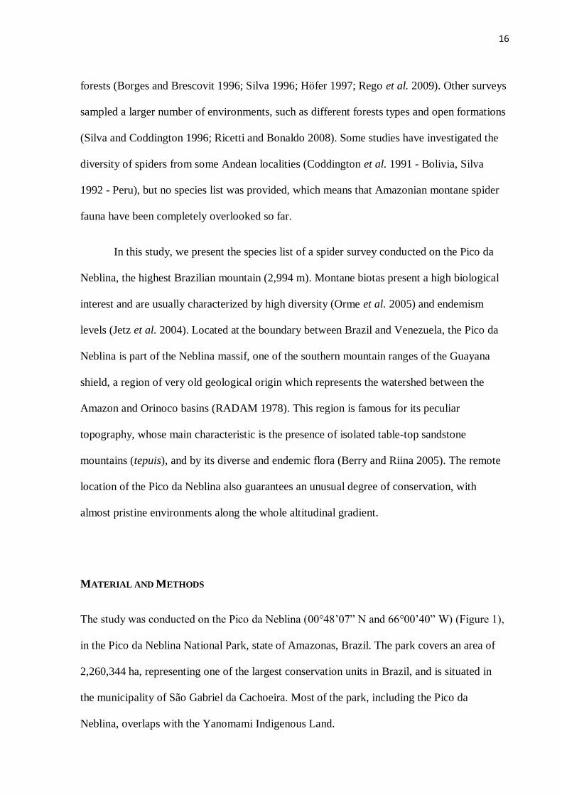
In this study, we present the species list of a spider survey conducted on the Pico da
Neblina, the highest Brazilian mountain (2,994 m). Montane biotas present a high biological
interest and are usually characterized by high diversity (Orme et al. 2005) and endemism
levels (Jetz et al. 2004). Located at the boundary between Brazil and Venezuela, the Pico da
Neblina is part of the Neblina massif, one of the southern mountain ranges of the Guayana
shield, a region of very old geological origin which represents the watershed between the
Amazon and Orinoco basins (RADAM 1978). This region is famous for its peculiar
topography, whose main characteristic is the presence of isolated table-top sandstone
mountains (tepuis), and by its diverse and endemic flora (Berry and Riina 2005). The remote
location of the Pico da Neblina also guarantees an unusual degree of conservation, with
almost pristine environments along the whole altitudinal gradient.
MATERIAL AND METHODS
The study was conducted on the Pico da Neblina (00°48’07” N and 66°00’40” W) (Figure 1),
in the Pico da Neblina National Park, state of Amazonas, Brazil. The park covers an area of
2,260,344 ha, representing one of the largest conservation units in Brazil, and is situated in
the municipality of São Gabriel da Cachoeira. Most of the park, including the Pico da
Neblina, overlaps with the Yanomami Indigenous Land.

17
The Neblina massif is mainly composed of sandstones and is characterized by
extensive high-altitude plateaus, although it does not possess the tipical tepui shape. The
climate of the region is tropical humid and varies little through the year. According to a
division proposed for the Guayana region, the study area can be divided in three main
physiographic units according to temperature and altitude. Lowlands, up to 500 m with
macrothermic climate (> 24°C annual average), uplands from 500 to 1,500 m with
submesothermic climate (18° - 24°C), and highlands from 1,500 to 2,994 m, with
mesothermic (18° - 12°C) and submicrothermic climate (8° - 12°C) (Huber 1995). The annual
average rainfall in the lowlands of the Pico da Neblina, is 3,000 mm/year, without a distinct
dry season, and the humidity is about 85-90% (RADAM 1978). Rainfall increases with
altitude until around 1800 m, being gradually replaced by a constant mist, and the average
humidity reaches almost 100% (RADAM 1978).
Vegetation of the lowlands is composed of tall evergreen forest. Uplands are covered
by montane forests, which present decreasing biomass and tree size, especially when declivity
is accentuated and soils shallow (Pires and Prance 1985). In the highlands, forests are
replaced by more open types of vegetation, such as high altitude scrublands and broad-leaf
meadows, which grow on organic-peat soils and on rocky substrates. Forests formations occur
up to almost to 2,000 m, and their high altitude formations stand out for their diversity and
endemism (Berry et al. 1995). Species from the families Bromeliacea and Rapateacea are
among the most characteristics elements of this flora. Detailed information on the geology
and vegetation of the region can be found in Berry et al. (1995) and Berry and Riina (2005)
(Figure 2).
We collected spiders with two methods, beating tray and manual active search. In the
first method the understory vegetation was sampled during the day (08:00 to 11:00 h) through
the beating of leaves, branches, vines and other parts of the vegetation with a stick, while
18
holding a 1 m2 tray under it. The spiders falling into the tray are collected, and the sampling
unit consisted of 20 of those beating events, in different plants, along a 30 m long transect. In
the second method, employed at night (19:30 to 23:00) spiders from the forest floor and from
the understory were directly collected with the help of tweezers and/or plastic vials. The
sampling unit represents one hour of search along an approximate area of 300 m2 (30 x 10 m).
This method represents a fusion of the methods “looking up” and “looking down”
(Coddington et al. 1991). All spiders collected were fixed in 70% ethanol.
Sampling was carried out by three collectors at six altitudes, 100, 400, 860, 1550,
2000 and 2400 m (Figure 1). At each altitude we investigated three different sites about 100 m
apart from each other. At each site we obtained 18 samples, 9 diurnal and 9 nocturnal, which
represent a total of 54 samples for each altitude (27 of each method) and a final count of 324
samples (162 of each method). The sampling expedition occurred from 22 September 2007 to
13 October 2007, a period with lesser rainfall.
We only identified adult spiders, since allocation of juveniles to species based on
morphology is usually impractical. Specimens were sorted into morphospecies, usually by the
first author, and then identified to the lowest taxonomic level by specialists. Voucher
specimens are deposited in the collection of the Instituto Nacional de Pesquisas da Amazônia,
Manaus (INPA) and duplicates are deposited in the Instituto Butantan, São Paulo (IBSP) and
the Museu Paraense Emílio Goeldi, Belém (MPEG). The material was collected under the
license IBAMA-SISBIO 10560–1.
We compared our results with those obtained in other spider surveys from the Amazon
basin. We excluded studies that focused on only a subset of the community, or a specific kind
of habitat, such as bark.

19
RESULTS AND DISCUSSION
We obtained 3,140 adult spiders (35% of the total number of spiders sampled), representing
528 species from 39 families (Table 1, Figures 3 and 4). The families in which the most
species were collected were Theridiidae, Araneidae and Salticidae, with 110 (20% of total
richness), 97 (18%) and 60 (11%) species (Table 2). Most of the spiders collected were from
14 families: Anyphaenidae, Araneidae, Corinnidae, Ctenidae, Linyphiidae, Mimetidae,
Pholcidae, Salticidae, Sparassidae, Tetragnathidae, Theridiidae, Theridiosomatidae,
Thomisidae and Uloboridae. Those families were the most species rich and abundant in the
samples, and were represented by at least 10 species and 52 individuals. Together, they
account for 89% of total richness and 93% of spiders collected. Fewer species of the
remaining 27 families were collected, although some species , such as Architis tenuis Simon
1898 (Pisauridae, 27 individuals), Amaloxenops sp. (Hahniidae, 25 individuals) and
Orchestina sp. (Oonopidae, 27 individuals) were relatively abundant in samples (Table 2).
Those results are similar to those obtained in other surveys in the Amazon basin
(Table 3). Species richness reported ranges from 102 to 1,140 species, but in most localities
sampled the number of species was around 500. Comparisons must be made with care, as
those results are directly influenced by many factors, such as sampling effort (which can be
estimated from the number of individuals obtained), sampling methods, type of environment
and number of different localities sampled. For example, the fact that our sampling sites were
scattered along an important altitudinal gradient increased the richness, as turnover rates are
higher in strong environmental gradients, such as those represented by mountains (Melo et al.
2009). However, the number of species and families reported at the Pico da Neblina is large,
considering that only two sampling methods were employed, while most of the other surveys
included additional methods, which increeases the coverage of the study. For example, the
litter fauna, usually investigated with pitfall traps, winckler funnels or litter search, was only

20
superficially assessed at the Pico da Neblina. The collecting of specimens from families, such
as Anapidae, Hahniidae, Ochyroceratidae, Symphytognathidae and Oonopidae was
occasional, and the diversity of those families at the Pico da Neblina is certainly
underrepresented.
The presence and relative abundance of families showed little variation among
collections from diferent surveys, indicating that the diversity patterns at the higher taxonomic
level of family are well established. The families Araneidae, Salticidae and Theridiidae
contained most species in collections from all the studies considered, and the 14 above most
common families were recorded in all of those surveys, with few exceptions (families
Pholcidae and Linyphiidae were absent from the lists of Ricetti and Bonaldo 2008 and Rego
et al. 2009, respectively). In fact, most of the families reported in our study, such as
Deinopidae, Lycosidae, Oonopidae, Pisauridae and Scytodidae, are also present in all or at
least most of these studies, but usually represented by few species and individuals.
Nonetheless, characteristics of the habitats may influence the relative contribution of different
families. In the flooded forest, the relative abundance of the families associated with water
bodies, such as Pisauridae and Trechaleidae (Höfer and Brescovit 2001; Bonaldo et al. 2009a)
increases, although their richness remains moderate (Borges and Brescovit 1996; Rego et al.
2009).
Most species were rarely collected. Most (389 - 73%) were represented by up to five
individuals, of which 197 (37% of total richness) were represented by just one individual in
collections. Each species accounted, on average, for only 0.19% of total abundance. This low
abundance in samples seems to be characteristic of very diverse tropical spider communities
(Silva 1996), and is evidence of undersampling. The two most abundant species, with 137
(4.3% of the total abundance) and 96 (3.1%) individuals were new species collected at high

21
altitude from the genus Chrysometa, C. petrasierwaldae Nogueira et al. 2011 and C.
nubigena Nogueira et al.2011.
Only 27.8% of the morphospecies could be identified to species. A similarly low
taxonomic resolution level is shared with other surveys (Silva 1996; Bonaldo et al. 2009a;
Rego et al. 2009), with the exception of the study conducted at the Reserva Ducke (RFAD)
(Höfer and Brescovit 2001), which presents a much higher proportion of identified species
(55%). The better resolution for this area may be a consequence of its proximity to Manaus,
ensuring an unparalleled accessibility to researchers in comparison with the others areas
sampled, which turn the RFAD one of the most studied localities of the Amazon basin.
Moreover, sampling performed by Höfer and Brescovit (2001) were also accompanied by
taxonomic studies, including the description of new species, and as a consequence the RFAD
is the type locality of 38 species of spiders (Bonaldo et al. 2009b). Finally, the species list of
the RFAD is not only the product of sampling over many years, but also from records of the
literature, which means that all species added by this method are necessarily identified to
species.
Nine species collected during this expedition were new to science and have already
been described, one from the genus Architis (Santos and Nogueira 2008), one from the genus
Syntrechalea (Silva and Lise 2010) and seven from the genus Chrysometa (Nogueira et al.
2011). However, the list presented in this study certainly harbors several other new species. It
must be kept in mind that the low level of taxonomic resolution of this list is partially a
consequence of the lack, or unavailability, of taxonomic experts for several of these families
and genera. It is reasonable to suppose that most of the species which could not be identified
to species are undescribed species, although they may have already been collected in other
Amazonian localities. Morphospecies from genera, such as like Eustala, Dipoena and
Tmarus, are reported in almost every survey cited in this study, and at present it is not

22
possible to know the proportion of widespread or endemic species among then. The survey
encountered individuals from several poorly known groups. The specimens of Rhytidiculos
sp. represent the second record of this monotypic genus for Brazil, and the first of a female
(R. Indicatti, pers. com.). Also, the morphospecies Drymusa sp. belongs to the rare family
Drymusidae (15 species) and is probably a new species (Brescovit, pers. com.). Known from
only nine species until recently, none from Brazil, five species have been described since
2004 from surveys in the Brazilian Amazon (Brescovit et al. 2004; Bonaldo et al. 2006). This
is further evidence of the still incipient knowledge of Brazilian-Amazonian arachnids and
reinforces the fundamental importance of faunal surveys, especially in remote regions that
have not yet been sampled, which represent most of the Amazon basin.
ACKNOWLEDGMENTS
We are grateful to the following specialists for the determination of the material: Lina
Almeida (Amaurobiidae), Alexandre Bonaldo (Corinnidae), Daniele Polotow (Ctenidae),
Nancy Lo-Man-Hung (Hahniidae), Rafael Lemos (Linyphiidae), Flávio Yamamoto, Rafael
Indicatti and Silvia Lucas (Mygalomorphae), Adalberto Santos (Oxyopidae, Pisauridae and
Synotaxidae), Éwerton Machado (Pholcidae), Gustavo Ruiz (Salticidae), Cristina Rheims
(Scytodidae and Sparassidae), João Barbosa (Chrysometa) Erica Buckup and Maria Aparecida
Marques (Theridiidae), and Estevam Silva (Trechaleidae). We are also indebted to Tomé,
Mário and Waldir “Chouriman” Pereira, for their invaluable help in the field. The first author
also thanks the PPGEco-INPA, the 5°PEF Maturacá, a frontier squad from the Brazilian army,
the IBAMA/ICMBio and PARNA Pico da Neblina for the collecting licence, and FUNAI and
the Ayrca, a local Yanomami association, for receiving use at the Yanomami Indigenous
Land. A.A. Nogueira was supported by a doctoral fellowship from “Conselho Nacional de
Desenvolvimento Científico e Tecnológico (CNPq)”, a BECA-IEB/Moore Foundation

23
(B/2007/01/BDP/01) fellowship and a grant from Wildlife Conservation Society (WCS). A.D.
Brescovit was supported by CNPq, # 300169/1996-5.
LITERATURE CITED
Berry, P. E., O. Huber and B. K Holst, 1995. Introduction.; p. 161-191 In P. E. Berry, B. K.
Holst & K. Yatskievych, (ed.). Flora of the Venezuelan Guayana. St. Louis: Missouri
Botanical Garden Press.
Berry, P.E. and R. Riina. 2005. Insights into the diversity of the Pantepui flora and the
biogeographic complexity of the Guayana Shield. Biologiske Skrifter 55:145–167.
Bonaldo, A. B., L. S Carvalho, R. Pinto-da-Rocha, A.L. Tourinho, L. T. Miglio, D. F.
Candiani, N. F. Lo Man Hung, N. Abrahim, B. V. B Rodrigues, A. D Brescovit, R. Saturnino,
N. C. Bastos, S. C Dias, B. J. F. J. M. B. Silva, Pereira-Filho, C.A. Rheims, S. M. Lucas, D.
Polotow, G. R. S. Ruiz and R. P. Indicatti. 2009a. Inventário e História Natural dos
Aracnídeos da Floresta Nacional de Caxiuanã, Pará, Brasil; p. 545-588 In Lisboa, P. L. B.
(org.). Caxiuanã: desafios para a conservação de uma Floresta Nacinal da Amazônia,
Belém: Museu Paraense Emílio Goeldi.
Bonaldo, A. B., A. D. Brescovit, H. Höfer, T. R. Gasnier and A. A. Lise. 2009b. A
araneofauna (Arachnida, Araneae) da Reserva Florestal Ducke, Manaus, Amazonas, Brasil; p.
201-222 In C. R. V. Fonseca, C. Magalhães, J. A. Rafael and E. Franklin. (Org.). A Fauna
de Artrópodes da Reserva Florestal Ducke. Estado atual do conhecimento taxonômico e
biológico. 1 ed. Manaus: INPA.
Bonaldo, A.B., C.A. Rheims and A.D. Brescovit. 2006. Four new species of Drymusa Simon
(Araneae, Drymusidae) from Brazilian Oriental Amazonia. Revista Brasileira de Zoologia,
Curitiba 23 (2): 455–359.

24
Borges, S. H. and A. D. Brescovit. 1996. Inventário preliminar da aracnofauna (ARANEAE)
de duas localidades na amazônia ocidental. Boletim do Museu Paraense Emílio Goeldi, série
Zoologia 12(1): 9-21.
Brescovit A.D., A.B. Bonaldo and C.A. Rheims. 2004. A new species of Drymusa Simon,
1891 (Araneae, Drymusidae) from Brazil. Zootaxa 697: 1–5.
Coddington J. and H. Levi. 1991. Systematics and evolution of spiders (Araneae). Annual
Review of Ecology and Systematics 22: 565-592.
Coddington, J.A., I Agnarsson, J.A Miller, M. Kuntner and G. Hormiga. 2009.
Undersampling bias: the null hypothesis for singleton species in tropical arthropod surveys.
Journal of Animal Ecology 78: 573–584.
Coddington, J.A.; C.E. Griswold; D. Silva-D’ávila; E. Peñaranda and S.F. Larcher. 1991.
Designing and testing sampling protocols to estimate biodiversity in tropical ecosystems; p.
44-60 In Dudley, E.C. (ed.). The unity of evolutionary biology: proceedings of the Fourth
International Congress of Systematic and Evolutionary Biology. Portland: Dioscorides Press.
Höfer, H. 1997. The spider communities. P. 373-343. In: Junk, W.J. (org). The Central
Amazon Floodplain. Berlin: Springer-Verlag.
Höfer, H. and A. D. Brescovit. 2001. Species and guild structure of a Neotropical spider assemblage
(Araneae) from Reserva Ducke, Amazonas, Brazil. Andrias 15: 99-119.
Huber, O. 1995. Geographical and physical features; p. 1─ 61In P. E. Berry, B. K. Holst and
K. Yatskievych (ed.). Flora of the Venezuelan Guayana, I. Introduction. St. Louis: Missouri
Botanical Garden Press.
Jetz, W., C. Rahbek and R.C.Colwell. 2004. The coincidence of rarity and richness and the
potential signature of history in centres of endemism. Ecology Letters 7: 1180–1191.

25
Melo, A. S., T. F. L. V. B. Rangel and J. A. F. Diniz-Filho. 2009. Environmental drivers of
beta-diversity patterns in New-World birds and mammals. Ecography 32: 226–236.
Meehan, C.J., E.J. Olson, M.W. Reudink, T.K. Kyser and R. L. Curry. 2009. Herbivory in a
spider through exploitation of an ant-plant mutualism. Current Biology 19(19): R892-893.
Nogueira, A.A., J. P.P. Pena-Barbosa, E.M. Venticinque and A.D. Brescovit. 2011.
The spider genus Chrysometa (Araneae, Tetragnathidae) from the Pico da
Neblina and Serra do Tapirapecó mountains (Amazonas, Brazil): new species,
new records, diversity and distribution along two altitudinal gradients. Zootaxa 2772: 33-51.
Orme, C.D.L., R.G. Davies, M. Burgess, F Eigenbrod, N.Pickup and V.A. Olson 2005. Global
hotspots of species richness are not congruent with endemism or threat. Nature 436:1016–
1019.
Pires, J.M. and T.G. Prance. 1985. The vegetation types of the Brazilian Amazon. p:109-145.
In G.T. Prance and T.E. Lovejoy (ed). Key environments: Amazonia. Oxford: Pergamon
Press.
Platnick, N. I. 2011. The world spider catalog, version 11.5. American Museum of Natural
History, online at http://research.amnh.org/entomology/spiders/catalog/index.html
RADAM. 1978. Folha NA19:. Pico da Neblina. Rio de Janeiro: Ministério das Minas e
Energia.
Rego, F.N.A.A., E. M. Venticinque, A. D. Brescovit, C. A. Rheims and A. L. K. M. Albernaz.
2009. A contribution to the knowledge of the spider fauna (Arachnida: Araneae) of the
floodplain forests of the main Amazon River channel. Revista Ibérica de Aracnologia 97: 85-
96.

26
Ricetti, J. and A. B. Bonaldo. 2008. Diversidade e estimativas de riqueza de aranhas em
quatro fitofisionomias na Serra do Cachimbo, Pará, Brasil. Iheringia 98(1): 88-99.
Santos, A. J. and A. A. Nogueira. Three new species, new records and notes on the nursery-
web spider genus Architis in Brazil (Araneae: Pisauridae). Zootaxa 1815: 51-61.
Silva, D. 1992. Observations on the diversity and distribution of the spiders of peruvian
montane forests. Memorias del Museo de Historia Naturales 21: 31-37.
Silva, D. 1996. Species composition and community structure of peruvian rainforest spiders:
A case study from a seasonally inundated forest along the Samiria river. Revue suisse de
Zoologie 597-610.
Silva, D. and J. A.Coddington. 1996. Spiders of Pakitza (Madre de Dios, Perú): species
richness and notes on community structure; p. 253-311 In D. E. Wilson & A. Sandoval (ed.).
Manu-The biodiversity of Southeastern Perú. Washington: Smithsonian Institution Press.
Silva, E.L.C. and A. A. Lise 2010. Two new species and new records of Syntrechalea
(Araneae: Lycosoidea: Trechaleidae) from Brazil. Zoologia 27(3): 408–412.
Turnbull, A.L. 1973. Ecology of the true spiders (Araneomorphae). Annual Review of
Entomology 18: 305-348

27
TABLES
TABLE 1 – List of spider species collected at six altitudes at the Pico da Neblina (AM, Brazil).
We present the abundance by altitude, total abundance, and relative abundance (abundance of
each species in relation to total abundance) for each species.
*species described after specimens obtained in this study
Family Altitudes sampled (m) Total
Species 100 400 860 1.550 2.000 2.400 Abundance
%
Abundance
Amaurobiidae
Amaurobiidae sp.
2
2 0,06
Retiro sp.1
4
4 0,13
Retiro sp.2
1
1 0,03
Anapidae
Anapidae sp.
1
1 0,03
Pseudanapis sp. 2
2 0,06
Anyphaenidae
Anyphenoides aff. xiboreninho
3
3 0,10
Anyphenoides sp.
4 25 29 0,92
Arachosia sp.1
1 3 4 0,13
Arachosia sp.2
1
1 0,03
Bromelina oliola Brescovit, 1993
2
2 0,06
Josa sp.1
12 12 0,38
Josa sp.2
4
4 0,13
Katissa sp.1
1 1 2 0,06
Patrera sp.1
13
13 0,41
Patrera sp.2 2
2 0,06
Patrera sp.3 1 1
2 0,06

28
Patrera sp.4
1 1
2 0,06
Patrera sp.5
2
2 0,06
Patrera sp.6
1
1 0,03
Patrera sp.7 1
1 0,03
Patrera sp.8
1 1 0,03
Patrera sp.9
1
1 0,03
Patrera sp.10 1
2
3 0,10
Wulfila modesta Chickering, 1937
2
2 0,06
Wulfila sp.1
1
1 0,03
Wulfila sp.2
1
1 0,03
Anyphaenidae sp.1 3
3 0,10
Anyphaenidae sp.2
2 2 1 3 8 0,25
Araneidae
Acacesia benigna Glueck, 1994 2
2 0,06
Alpaida antonio Levi, 1988
1
1 0,03
Alpaida negro Levi, 1988 1 1 2
4 0,13
Alpaida septemmammata (O. P.-Cambridge, 1889) 1
1 0,03
Alpaida truncata (Keyserling, 1865) 4 1 3
8 0,25
Alpaida aff. cuyabeno
11 1
12 0,38
Alpaida aff. delicata 9
11
20 0,64
Alpaida aff. iquitos 1
1 0,03
Alpaida sp.1
12
12 0,38
Alpaida sp.2 1 1
2 0,06
Araneus bogotensis (Keyserling, 1864)
1 15 6 22 0,70
Araneus guttatus (Keyserling, 1865)
1
1 0,03
Aspidolasius branicki (Taczanowski, 1879) 1
1 0,03
Bertrana elinguis (Keyserling, 1883) 4
4 0,13
Bertrana sp. 1
1 0,03
Cyclosa caroli (Hentz, 1850)
3 1
4 0,13
Cyclosa fililineata Hingston, 1932 4
1 2
7 0,22

29
Cyclosa inca Levi, 1999 7
3 1
11 0,35
Cyclosa rubronigra Caporiacco, 1947 2
2
4 0,13
Cyclosa tapetifaciens Hingston, 1932 12 1
13 0,41
Cyclosa vieirae Levi, 1999
2
2 0,06
Dubiepeira lamolina Levi, 1991 1
1 0,03
Eriophora fuliginea (C. L. Koch, 1838) 1
1
2 0,06
Eriophora nephiloides (O. P.-Cambridge, 1889) 1 1
2 0,06
Eustala sp.1
22 16
38 1,21
Eustala sp.2 9 1 2
6
18 0,57
Eustala sp.3
5 2
7 0,22
Eustala sp.4 1
5
6 0,19
Eustala sp.5 1 2 3
6 0,19
Eustala sp.6 1 1 1
3 0,10
Eustala sp.7
2 1
3 0,10
Eustala sp.8
1
1 0,03
Eustala sp.9
1
1 0,03
Eustala sp.10
1
1 0,03
Eustala sp.11
6 7
13 0,41
Eustala sp.12
5
5 0,16
Eustala sp.13
2
2 0,06
Eustala sp.14 2
2 0,06
Eustala sp.15 1
1 0,03
Hypognatha aff. putumayo 12 9 2
23 0,73
Kaira altiventer O. P.-Cambridge, 1889
1 1
2 0,06
Mangora amacayacu Levi, 2007 1 2 6
9 0,29
Mangora apaporis Levi, 2007
1 2
3 0,10
Mangora bovis Levi 2007
7
7 0,22
Mangora aff. acre 1
4 15
20 0,64
Mangora sp.1 3
3 0,10
Mangora sp.2 2
2 0,06

30
Mangora uraricoera Levi, 2007
1 2
3 0,10
Manogea porracea (C. L. Koch, 1838)
4
4 0,13
Melychiopharis cynips Simon, 1895
1
1 0,03
Metazygia ducke Levi, 1995 1
1 0,03
Metazygia enabla Levi, 1995 1 1 7
9 0,29
Metazygia laticeps (O. P.-Cambridge, 1889)
2
2 0,06
Metazygia yucumo Levi, 1995
1
1 0,03
Micrathena clypeata (Walckenaer, 1805) 24 3 1
28 0,89
Micrathena cyanospina (Lucas, 1835)
7
7 0,22
Micrathena embira Levi, 1985 1
1 0,03
Micrathena exilinae Levi, 1985 15
15 0,48
Micrathena flaveola (C. L. Koch, 1839)
1
1 0,03
Micrathena kirbyi (Perty, 1833) 9 6
15 0,48
Micrathena pungens (Walckenaer, 1841) 3 1
4 0,13
Micrathena spinosa (Linnaeus, 1758)
2
2 0,06
Micrathena triangularis (C. L. Koch, 1836) 2 6 7 3
18 0,57
Micrathena triangularispinosa (De Geer, 1778) 5
7
12 0,38
Micrathena vigorsi (Perty, 1833) 4 1 2
7 0,22
Micrathena sp.1 4 2 11
17 0,54
Micrathena sp.2 4
4 0,13
Micrepeira fowleri Levi, 1995 1
1 0,03
Micrepeira hoeferi Levi, 1995 1 1
2 0,06
Ocrepeira bispinosa (Mello-Leitão, 1945)
1 1
2 0,06
Ocrepeira covillei Levi, 1993 4 2 1
7 0,22
Ocrepeira sp.1
1
1 0,03
Ocrepeira sp.2
1
1 0,03
Parawixia hypocrita (O. P.-Cambridge, 1889) 2 2
4 0,13
Parawixia kochi (Taczanowski, 1873) 1 2 1
4 0,13
Parawixia monticola (Keyserling, 1892)
1 1
2 0,06
Parawixia rimosa (Keyserling, 1892)
3 3
6 0,19

31
Parawixia tomba Levi, 1992
1
1 0,03
Parawixia velutina (Taczanowski, 1878) 2
1
3 0,10
Pronous nigripes Caporiacco, 1947
6
6 0,19
Rubrepeira rubronigra (Mello-Leitão, 1939)
1
1 0,03
Scoloderus sp. 3 2
5 0,16
Spilasma duodecinguttata Keyserling, 1879
1
1 0,03
Spintharidius rhomboidalis Simon, 1893
1
1 0,03
Taczanowskia striata Keyserling, 1879 1 1
2 0,06
Testudinaria quadripunctata Taczanowski, 1879
1 3
4 0,13
Verrucosa sp.
1
1 0,03
Wagneriana atuna Levi, 1991
1
1 0,03
Wagneriana pakitza Levi, 1991 1
1
2 0,06
Wagneriana aff. neblina 1
1 0,03
Wagneriana aff. silvae 1
1
2 0,06
Wagneriana sp.1 3 1 4
8 0,25
Wagneriana sp.2
5
5 0,16
Wagneriana sp.3
4
4 0,13
Wagneriana sp.4
3 6
9 0,29
Araneidae sp.1 1
1 0,03
Araneidae sp.2
1
1 0,03
Clubionidae
Elaver sp.1 1 1
2 0,06
Elaver sp.2 2
2 0,06
Corinnidae
Castianeira rubicunda Keyserling, 1879
1
1 0,03
Corinna ducke Bonaldo, 2000 10 4 7 2
23 0,73
Corinna gr. capito sp.
1
1 0,03
Corinna gr. ducke sp.1
1
1 0,03
Corinna gr. ducke sp.2
8 7
15 0,48
Corinna gr. ducke sp.3
14 2
16 0,51

32
Corinna gr. ducke sp.4
1
1 0,03
Corinna gr. ducke sp.5
1
1 0,03
Falconina sp.
1 1
2 0,06
Methesis sp. 1
1 0,03
Myrmecium sp.1 1
1 0,03
Myrmecium sp.2 4
4 0,13
Myrmecium sp.3 3 1 2
6 0,19
Myrmecotypus sp. 1 1
2 0,06
Parachemmis hassleri (Gertsch, 1942)
4
4 0,13
Parachemmis sp.1
1
1 0,03
Parachemmis sp.2 1
1 0,03
Simonestus sp. 1
1 0,03
Stethorragus archangelus Bonaldo & Brescovit,
1994
1
1 0,03
Stethorragus duide Gertsch, 1942
1 1
2 0,06
Trachelas sp.1 1
1 0,03
Trachelas sp.2 2
2 0,06
Tupirina aff. trilineata
1
2
3 0,10
gen. aff. apochinomma
1
1 0,03
Corinnidae sp.
2 2 0,06
Ctenidae
Ancylometes rufus (Walckenaer, 1837) 1
1 0,03
Centroctenus auberti (Caporiacco, 1954) 5 1 1
7 0,22
Centroctenus sp.1
1
1 0,03
Centroctenus sp.2
2
2 0,06
Ctenus amphora Mello-Leitão, 1930 11 51 11
73 2,32
Ctenus inaja Höfer, Brescovit & Gasnier, 1994 1
1 0,03
Ctenus villasboasi Mello-Leitão, 1949 6 2 24 3
35 1,11
Ctenus aff. satanas
2 12
14 0,45
Ctenus sp.1
11
11 0,35

33
Ctenus sp.2 6 2 17
25 0,80
Ctenus sp.3
4
4 0,13
Enoploctenus aff. comosus 1
1 0,03
Enoploctenus sp.1
1
1 0,03
Enoploctenus sp.2
1
1 0,03
Enoploctenus sp.3
1
1 0,03
Gephyroctenus portovelho Polotow & Brescovit,
2008 1 2
3 0,10
Phoneutria fera Perty, 1833 1
1 0,03
Ctenidae sp.1
1
1 0,03
Ctenidae sp.2
1 1 2 0,06
Ctenidae sp.3
4
4 0,13
Ctenizidae
Ummidia sp.
1
1 0,03
Cyrtaucheniidae
Rhytidicolus sp.
1
1 0,03
Deinopidae
Deinops sp.1 1 2 6
9 0,29
Deinops sp.2
2
2 0,06
Dipluridae
Diplura sp.
2
2 0,06
Linothele sp.
1
1 0,03
Masteria sp. 1
1 0,03
Drymusidae
Drymusa sp.
1
1 0,03
Gnaphosidae
Zimiromus sp.
2
2 0,06
Hahniidae
Amoloxenops sp.
25
25 0,80
Hersiliidae

34
Ypipuera vittata (Simon, 1887) 2
2 0,06
Linyphiidae
Dubiaranea caeca Millidge, 1991
5 1 6 0,19
Dubiareanea margaritata Millidge, 1991
5 14
19 0,61
Dubiaranea sp.1
7
7 0,22
Dubiaranea sp.2
2
2 0,06
Dubiaranea sp.3
1
1 0,03
Dubiaranea sp.4
3
3 0,10
Dubiaranea sp.5
1
1 0,03
Exocora sp.
2
2 0,06
Novafrontina uncata (F. O. P.-Cambridge, 1902)
1
1 0,03
Sphecozone crassa (Millidge, 1991)
9 7
16 0,51
Lycosidae
Aglaoctenus castaneus (Mello-Leitão, 1942) 6 4 2
12 0,38
Mimetidae
Ero sp.1
6
6 0,19
Ero sp.2
9 9 0,29
Ero sp.3
1
1 0,03
Ero sp.4
1
1 0,03
Ero sp.5
1
1 0,03
Ero sp.6
5 2 2
9 0,29
Ero sp.7 3 2
5 0,16
Ero sp.8
1
1 0,03
Ero sp.9
1
1 0,03
Ero sp.10
1
1 0,03
Gelanor sp.1
8
8 0,25
Gelanor sp.2
6
6 0,19
Gelanor sp.3 1 1
2 0,06
Gelanor sp.4 1
1 0,03
Mysmenidae

35
Mysmenopsis sp. 1
1 0,03
Mysmenidae sp.
1 1
2 0,06
Nephilidae
Nephila clavipes (Linnaeus, 1767) 2
1
3 0,10
Oonopidae
Gamasomorpha sp.
1
1 0,03
Neoxyphinus sp.
1
1 0,03
Oonops sp.
1
1 0,03
Orchestina sp.
3 1 1 22
27 0,86
Oonopidae sp. 1
1 0,03
Oxyopidae
Hamataliwa sp.1 1
1 0,03
Hamataliwa sp.2
1
1 0,03
Schaenicoscelis guianensis Caporiacco, 1947
2
2 0,06
Pholcidae
Carapoia sp.
31 37
68 2,17
Litoporus aff. uncatus
3 7
10 0,32
Mecoloesthus aff. taino
1
1 0,03
Mesabolivar aurantiacus (Mello-Leitão, 1930) 3 10 67
80 2,55
Mesabolivar eberhardi Huber, 2000
3
3 0,10
Mesabolivar aff. aurantiacus
12 8
20 0,64
Mesabolivar aff. huambisa 2
2
4 0,13
Mesabolivar aff. pseudoblechroscelis 3 3 3
9 0,29
Mesabolivar sp.1 2 3
5 0,16
Mesabolivar sp.2
1 2 1 4 0,13
Metagonia mariguitarensis (González-Sponga,
1998)
5
5 0,16
Metagonia sp.1
2
2 0,06
Metagonia sp.2 2 1
3 0,10
Priscula cf. trauma
11 14
4 29 0,92

36
Wanauana sp.
2
2 0,06
Pholcidae sp. 1
1 1
3 0,10
Pisauridae
Architis neblina Santos & Nogueira, 2008 8
8 0,25
Architis tenuis Simon, 1898 18 9
27 0,86
Thaumasia sp.1 3
3 0,10
Thaumasia sp.2
1
1 0,03
Prodidomidae
Prodidomidae sp.
1
1 0,03
Salticidae
Alcmena sp. 1
1 0,03
Amycus sp.1 1
1 0,03
Amycus sp.2 4 3
7 0,22
Beata sp.
1
1 0,03
Breda sp. 1
1 0,03
Corythalia sp. 1
1
1 0,03
Corythalia sp. 2
1
1 0,03
Corythalia sp. 3
2
2 0,06
Cotinusa sp.1
5
5 0,16
Cotinusa sp.2
1
1 0,03
Cylistella sp.1 2
1
3 0,10
Cylistella sp.2
1
1 0,03
Cylistella sp.3
1
1 0,03
Dendryphantinae sp.
2
2 0,06
Erica sp.
2
2 0,06
Euophryinae sp.1 2 2 1
5 0,16
Euophryinae sp.2
1
1
2 0,06
Euophryinae sp.3
5 2 7 0,22
Euophryinae sp.4
1 12
13 0,41
Euophryinae sp.5
1
1 0,03

37
Euophryinae sp.6
1
1 0,03
Euophryinae sp.7
1 1
2 0,06
Euophryinae sp.8 1
1 0,03
Euophryinae sp.9 3
3 0,10
Euophryinae sp.10
1
1 0,03
Euophryinae sp.11
2
2 0,06
Fluda sp.1 3
1
4 0,13
Fluda sp.2
1 1
2 0,06
Freyinae sp.1 2
2 0,06
Hypaeus sp.1 1
1 0,03
Hypaeus sp.2 4
4 0,13
Hypaeus sp.3 1
1 0,03
Hypaeus sp.4
3
3 0,10
Hypaeus sp.5
1
1 0,03
Itata sp. 2
2 0,06
Kalcerrytus sp. 2 1
3 0,10
Lyssomanes sp.1 2
2 0,06
Lyssomanes sp.2 1 2 3
6 0,19
Lyssomanes sp.3 5
5 0,16
Lyssomanes sp.4 1
3
4 0,13
Lyssomanes sp.5
1
1 0,03
Lyssomanes sp.6
1
1 0,03
Mago sp.1 2 8 3
13 0,41
Mago sp.2
3 1 1
5 0,16
Mago sp.3
1
1 0,03
Mago sp.4 1 2
3 0,10
Mago sp.5
1
1 2 0,06
Noegus sp.1 8
1
9 0,29
Noegus sp.2
6 4
10 0,32
Noegus sp.3
2
2 0,06

38
Noegus sp.4
3
3 0,10
Noegus sp.5 4
4 0,13
Noegus sp.6 5
5 0,16
Noegus sp.7 1 5
6 0,19
Psecas sp.
1
1 0,03
Ramboia sp.
1
1 0,03
Scopocira sp. 6 3 1 1
11 0,35
Synemosyna sp.
2
2 0,06
Thiodina sp.
1
1 0,03
cf Zuniga
1
1 0,03
Scytodidae
Scytodes auricula Rheims & Brescovit, 2000
5 1
6 0,19
Scytodes balbina Rheims & Brescovit, 2000
4 13
17 0,54
Scytodes lineatipes Taczanowski, 1874 1
1 0,03
Selenopidae
Selenops sp. 1 1
2 0,06
Senoculidae
Senoculus caniliculatus F. O. P.-Cambridge, 1902
1
1
2 0,06
Senoculus ruficapillus (Simon, 1880) 4
4 0,13
Senoculus aff. iricolor
1
1 0,03
Senoculus sp.
1 7
8 0,25
Sparassidae
Olios velox
1
1 0,03
Olios sp.
1
1 0,03
Pseudosparianthis ravida Simon, 1897 3 3 1
7 0,22
Sparianthis sp. 2 1
3 0,10
Sparassidae sp.1 16 29 18
63 2,01
Sparassidae sp.2
23 2
25 0,80
Sparassidae sp.3 5 3
8 0,25
Sparassidae sp.4
1
1 0,03

39
Sparassidae sp.5 1
1 0,03
Sparassidae sp.6
1
1 0,03
Symphytognathidae
Symphytognatha sp.1
1
1 0,03
Symphytognatha sp.2
1 1 0,03
Synotaxidae
Synotaxus brescoviti Santos & Rheims, 2005 1
1 0,03
Synotaxus waiwai Agnarsson, 2003
1
1 0,03
Tetragnathidae
Azilia histrio Simon, 1895 2 2 4
8 0,25
Azilia sp.1 5
5 0,16
Azilia sp.2
1
1 0,03
Azilia sp.3
2 2 0,06
Chrysometa boraceia Levi, 1986
6
6 0,19
Chrysometa candianii*
3
3 0,10
Chrysometa guttata (Keyserling, 1881)
4
4 0,13
Chrysometa lomanhungae*
2 1 3 0,10
Chrysometa minuta (Keyserling, 1883) 1 2 4
7 0,22
Chrysometa nubigena*
62 34 96 3,06
Chrysometa opulenta (Keyserling, 1881)
1 4 29
34 1,08
Chrysometa petrasierwaldae*
137 137 4,36
Chrysometa santosi*
1
1 0,03
Chrysometa waikoxi*
41
41 1,31
Chrysometa yanomami*
3
3 0,10
Chrysometa sp.
1
1 0,03
Cyrtognatha sp.1
1
1 0,03
Cyrtognatha sp.2 1
1 0,03
Dolicognatha sp.1 1
1
2 0,06
Dolicognatha sp.2 1
1 0,03
Dolicognatha sp.3 1
1 0,03

40
Dolicognatha sp.4 2
2 0,06
Homalometa sp.
4 2
6 0,19
Leucauge sp.1 12
12 0,38
Leucauge sp.2
2 3
5 0,16
Leucauge sp.3 4
4 0,13
Leucauge sp.4
1 2
3 0,10
Leucauge sp.5
4 2
6 0,19
Leucauge sp.6 5 1
6 0,19
Leucauge sp.7
2
2 0,06
Leucauge sp.8
2 2 0,06
Theraphosidae
Avicularia sp.
1
1 0,03
Ephebopus uatuman Lucas, Silva & Bertani, 1992 3 2
5 0,16
Hapalopus sp. 2 1
3 0,10
Ischnocolinae sp.
1
1 0,03
Theraphosa blondi (Latreille, 1804)
1
1 0,03
Theraphosinae sp.1 1
1 0,03
Theridiidae
Achaearanea dea Buckup & Marques, 2006
8
8 0,25
Achaearanea hierogliphica (Mello-Leitão, 1940) 1
1
2 0,06
Achaearanea nigrovittata (Keyserling, 1884) 2 1
3 0,10
Achaearanea tingo Levi, 1963
1
1 0,03
Achaearenea trapezoidalis (Taczanowski, 1873)
1 1
2 0,06
Ameridion sp.1 1
2 1
4 0,13
Anelosimus domingo Levi, 1963
46
46 1,46
Anelosimus eximius (Keyserling, 1884) 12 7
19 0,61
Ariamnes attenuatus O. P.-Cambridge, 1881 4
2
6 0,19
Cerocida ducke Marques & Buckup, 1989 1
1 0,03
Chrosiothes sp.1 8
8 0,25
Chrosiothes sp.2
1
1 0,03

41
Chrosiothes sp.3 1
1 0,03
Chrysso questona Levi, 1962
3
3 0,10
Chrysso sp.1 2
2 0,06
Chrysso sp.2
7
7 0,22
Chrysso sp.3 1
1 0,03
Chrysso sp.4 1
1 0,03
Cryptachaea bellula (Keyserling, 1891)
1
1 0,03
Cryptachaea hirta (Taczanowski, 1873)
1
1 0,03
Cryptachaea maraca (Buckup & Marques, 1991)
2
2 0,06
Cryptachaea schneirlai (Levi, 1959) 1
1 0,03
Cryptachaea taeniata (Keyserling, 1884)
28 8
36 1,15
Cryptachaea sp.1
1 1
2 0,06
Cryptachaea sp.2
4
4 0,13
Cryptachaea sp.3
1 3
4 0,13
Cryptachaea sp.4
1
1 0,03
Cryptachaea sp.5
1
1 0,03
Cryptachaea sp.6
1
1 0,03
Cryptachaea sp.7 3
3 0,10
Dipoena anas Levi, 1963 1
1 0,03
Dipoena duodecimpunctata Chickering, 1943 1
3 14
18 0,57
Dipoena militaris Chickering, 1943
2
2 0,06
Dipoena rubella (Keyserling, 1884)
6
8 2 3 19 0,61
Dipoena tiro Levi, 1963
1
1 0,03
Dipoena sp.1 2 5
6 1
14 0,45
Dipoena sp.2
3 1
4 0,13
Dipoena sp.3 2
2 0,06
Dipoena sp.4 1
1 0,03
Dipoena sp.5 1
1 0,03
Dipoena sp.6 2 2
4 0,13
Dipoena sp.7
1
1 0,03

42
Dipoena sp.8
1 1
2 0,06
Dipoena sp.9
2
2 0,06
Dipoena sp.10
1
1 0,03
Dipoena sp.11
3
3 0,10
Dipoena sp.12
1
1 0,03
Dipoena sp.13
1
1 0,03
Dipoenata balboae (Chickering, 1943)
8
8 0,25
Echinotheridion levii Ramírez & González, 1999 4
4 0,13
Emertonella taczanowskii (Keyserling, 1886)
2
2 0,06
Episinus bicruciatus (Simon, 1895)
1
1 0,03
Episinus malachinus (Simon, 1895)
2
2 0,06
Episinus nebulosus (Simon, 1895)
23
23 0,73
Episinus salobrensis (Simon, 1895) 11 1
1
13 0,41
Episinus sp.1
18
18 0,57
Episinus sp.2 6
6 0,19
Episinus sp.3
1
1 0,03
Episinus sp.4
30
30 0,96
Episinus sp.5 12
12 0,38
Episinus sp.6 1
1 0,03
Episinus sp.7
1 6
7 0,22
Episinus sp.8 1 2
3 0,10
Exalbidion sexmaculatus (Keyserling, 1884)
1
1 0,03
Exalbidion sp.1
1
1 0,03
Exalbidion sp.2
1
1 0,03
Faiditus amplifrons (O. P.-Cambridge, 1880) 21
21 0,67
Faiditus atopus (Chamberlin & Ivie, 1936)
5
5 0,16
Faiditus convolutus (Exline & Levi, 1962) 9
9 0,29
Faiditus sp.1
1
1 0,03
Faiditus sp.2
3 1
4 0,13
Faiditus sp.3 1
1 0,03

43
Faiditus sp.4
5
5 0,16
Faiditus sp.5 3
1
4 0,13
Faiditus sp.6 2
1
3 0,10
Faiditus sp.7
1
1 0,03
Faiditus sp.8
2 4
6 0,19
Helvibis sp.1 9 1
10 0,32
Phoroncidia moyobamba Levi, 1964
2
4
6 0,19
Phoroncidia sp.1
2 1
3 0,10
Phycossoma altum (Keyserling, 1886) 1
1 0,03
Phycossoma sp.1 1
2 4 7 0,22
Rhomphaea metaltissima Soares & Camargo, 1948
1 5
6 0,19
Rhomphaea sp.1 2
2 0,06
Spintharus sp.1
13
13 0,41
Spintharus sp.2 1 10 13 7
31 0,99
Steatoda moesta
1
1 0,03
Stemmops servus 1
1 0,03
Styposis sp.1
6 4
10 0,32
Styposis sp.2
1
1 0,03
Tekellina sp.1
2
2 0,06
Theridion fungosum Keyserling, 1886
2 9 4
15 0,48
Theridion incertissimum (Caporiacco, 1954)
2
2 0,06
Theridion longipedatum Roewer, 1942
33 8
41 1,31
Theridion plaumanni Levi, 1963
1
1 0,03
Theridion sp.1
2 1 3 0,10
Theridion sp.2 1 1
2 0,06
Theridion sp.3
3
3 0,10
Theridion sp.4
1
1 0,03
Theridion sp.5 1
1 0,03
Theridion sp.6
1
1
2 0,06
Theridion sp.7
3
3 0,10

44
Thymoites sp.1
1
1 0,03
Tidarren haemorrhoidale (Bertkau, 1880)
1
1 0,03
Twaitesia bracteata (Exline, 1950) 1 3 2
6 0,19
Wamba sp.1
3
3 0,10
Wamba sp.2
1
1 0,03
Theridiidae sp.1
1
1 0,03
Theridiosomatidae
Chthonos sp.1 1 2
1
4 0,13
Chthonos sp.2 1 1
2 0,06
Chthonos sp.3
1 1
2 0,06
Naatlo fauna (Simon, 1897)
12 38
50 1,59
Naatlo splendida (Taczanowski, 1879) 2 1 3
6 0,19
Naatlo sp.1 7
7 0,22
Naatlo sp.2 9 2 10
21 0,67
Ogulnius sp.1 1
1 0,03
Ogulnius sp.2
1
1 0,03
Theridiossoma sp.1 4 2 1
7 0,22
Theridiossoma sp.2 1
1 0,03
Theridiossoma sp.3
1
1 0,03
Theridiossoma sp.4
1
1 0,03
Theridiosomatidae sp.1
1
1 0,03
Theridiosomatidae sp.2 1
1 0,03
Thomisidae
Acentroscelus sp.
4
4 0,13
Bucranium taurifrons O. P.-Cambridge, 1881
2
2 0,06
Deltocleta sp.
1
1 0,03
Epicadus sp.1 2 1
3 0,10
Epicadus sp.2
2
2 0,06
Onocolus sp. 2
2 0,06
Titidius sp. 2
1
3 0,10

45
Tmarus sp.1 5 1
5
11 0,35
Tmarus sp.2
3
3 0,10
Tmarus sp.3
1
1 0,03
Tmarus sp.4 1
1 0,03
Tmarus sp.5
1
1 0,03
Tmarus sp.6 1
1 0,03
Tmarus sp.7 1
1 0,03
Tmarus sp.8 1
1 0,03
Tmarus sp.9
1
1 0,03
Tmarus sp.10
1
1 0,03
Tmarus sp.11 5 5 3
13 0,41
Thomisidae sp.1
1
1 0,03
Thomisidae sp.2 1
1 0,03
Trechaleidae
Syntrechalea neblina* 1
1 0,03
Syntrechalea sp.
1
1 0,03
Trechalea syntrechaloides (Mello-Leitão, 1941) 3
3 0,10
Uloboridae
Ariston sp.
1
1 0,03
Conifaber sp.1 3 2
5 0,16
Conifaber sp.2
1
1 0,03
Conifaber sp.3
1
1 0,03
Miagrammopes sp.1
26
26 0,83
Miagrammopes sp.2 7 2
9 0,29
Miagrammopes sp.3 1 2
3 0,10
Miagrammopes sp.4 1 4
5 0,16
Miagrammopes sp.5
2
2 0,06
Miagrammopes sp.6 1 3
4 0,13
Philoponella republicana (Simon, 1891) 4
4 5
13 0,41
Philoponella sp.1 3 2 5
10 0,32

46
Philoponella sp.2
4
4 0,13
Philoponella sp.3
1
1 0,03
Uloborus sp.1 7
7 0,22
Uloborus sp.2 8 6 4
18 0,57
Uloborus sp.3
1
1 0,03
Uloborus sp.4
4
4 0,13
Uloborus sp.5 3 1
4 0,13
Uloborus sp.6 1
1 0,03
Uloborus sp.7 2 6 5
13 0,41
Uloboridae sp.1 1
1 0,03
Uloboridae sp.2 1 1 0,03
TABLE 2 – Species richness, abundance, and proportional species richness and abundance by
family of spider collected at the six altitudes (100, 400, 860, 1550, 2000 and 2400 m) at the
Pico da Neblina (AM, Brazil).
Family Richness % richness Abundance % abundance
Amaurobiidae 3 0.57 7 0.22
Anapidae 2 0.38 3 0.10
Anyphaenidae 23 4.36 100 3.18
Araneidae 97 18.37 555 17.68
Clubionidae 2 0.38 4 0.13
Corinnidae 25 4.73 94 2.99
Ctenidae 20 3.79 189 6.02
Ctenizidae 1 0.19 1 0.03
Cyrtaucheniidae 1 0.19 1 0.03

47
Deinopidae 2 0.38 11 0.35
Dipluridae 3 0.57 4 0.13
Drymusidae 1 0.19 1 0.03
Gnaphosidae 1 0.19 2 0.06
Hahniidae 1 0.19 25 0.80
Hersiliidae 1 0.19 2 0.06
Linyphiidae 10 1.89 58 1.85
Lycosidae 1 0.19 12 0.38
Mimetidae 14 2.65 52 1.66
Mysmenidae 2 0.38 3 0.10
Nephilidae 1 0.19 3 0.10
Oonopidae 5 0.95 31 0.99
Oxyopidae 3 0.57 4 0.13
Pholcidae 16 3.03 248 7.90
Pisauridae 4 0.76 39 1.24
Prodidomidae 1 0.19 1 0.03
Salticidae 60 11.36 190 6.05
Scytodidae 3 0.57 24 0.76
Selenopidae 1 0.19 2 0.06
Senoculidae 4 0.76 15 0.48
Sparassidae 10 1.89 111 3.54
Symphytognathidae 2 0.38 2 0.06
Synotaxidae 2 0.38 2 0.06
Tetragnathidae 31 5.87 406 12.93
Theraphosidae 6 1.14 12 0.38

48
Theridiidae 108 20.45 626 19.94
Theridiosomatidae 15 2.84 106 3.38
Thomisidae 20 3.79 54 1.72
Trechaleidae 3 0.57 5 0.16
Uloboridae 23 4.36 135 4.30
Total 528 100 3,140 100
TABLE 3. Amazonian spider inventories. Authors and year of the study, locality, environment,
sampling methods, families and species richness, and abundance. n.i. - no information
available. Methods: NMAS – nocturnal manual active searching, DMAS – diurnal manual
active searching, BT – beating tray, SN – sweeping net, PIT – pitfall trap, LIT – litter
searching, W – winckler extractor, FOG – fogging, GE – ground eclector, TE – trunk eclector,
LITERAT – information from literature.
Richness
Study Localitiy Environment Sampling methods Families Species Abundance
Borges & Brescovit 1996
Mamirauá and Tefé, AM, Brazil
Flooded and terra firme forest NMAS, BT 22 102 649
Silva 1996 Samiria, Peru Flooded Forest NMAS, DMAS, FOG
39 1140 5895
Silva & Coddington 1996
Paktiza, Peru Seven forest types NMAS, DMAS, BT 32 498 2616
Höfer & Brescovit 2001 RF Adolpho Ducke, AM, Brazil
Terra firme Forest NMAS, BT, FOG, PIT, LIT, GE, TE, LITERAT
52 506 n.i.
Ricetti & Bonaldo 2008 Serra do Cachimbo, PA, Brazil
Open rainforest, riparian forest, arboreal savanna, white sand vegetation
NMAS, BT, SN, LIT
37 427 2750
Bonaldo et al. 2009 FLONA de Caxiuanã, PA, Brazil
Terra firme Forest NMAS, BT, SN, PIT, W
42 591 4768
Rego et al. 2009 AM and PA, Brazil Flooded Forest NMAS, BT 34 384 4142
Present study PARNA Pico da Neblina
AM, Brazil
Terra firme forest, montane
forest and high altitude formations
NMAS, BT 39 528 3140

49
FIGURES
FIGURE 1 – Study area. A) South America; B) Northern South America (rectangle of map A
enlarged). The mountain range at the left of the map represents the northern part of the Andes,
and the mountainous region in the center of the map is the Guayana Shield, showing the study
area in its southern part. Dotted yellow line represents the equator; C) Closer view of the
study area (rectangle of map B enlarged), the Pico da Neblina. Letters represent the altitudes
sampled: A – 100 m, B – 400 m, C – 860 m, D – 1,550 m, E – 2,000 m, F – 2,400 m.

50
FIGURE 2 – Aspect of the vegetation at the altitudes sampled at the Pico da Neblina: A – 100
m; B – 400 m; C – 860 m; D – 1,550 m; E – 2,000 m and F – 2,400 m. Photos by André
Nogueira.

51
FIGURE 3 – Spiders present on the list: A – Avicularia sp. (Theraphosidae); B – Ummidia sp.
(Cyrtauchenidae); C – Aglaoctenus sp. (Lycosidae), immature; D – Mesabolivar sp.
(Pholcidae); E – Ancylometes sp. (Ctenidae); F - Rhomphaea sp. (Theridiidae). Specimens
photographed are not from the Pico da Neblina. Photos A, C, E and F by Flávio Yamamoto, B
by Rafael Indicatti and D by Eduardo Fernandez.

52
FIGURE 4 – Spiders recorded at the Pico da Neblina. Species of the family Araneidae. A –
Micrathena clypeata; B – Micrathena embira; C – Micrathena pungens; D – Micrathena
cyanospina; E – Eriophora nephiloides; F – Micrathena spinosa. Specimens photographed
are not from the Pico da Neblina. Photos A, B, C, E and F by Flávio Yamamoto and D by
Rafael Indicatti.

53
CAPÍTULO 2
Nogueira, A.A., Venticinque, E.M. & Brescovit, A.D.
Spider (Arachnida-Araneae) richness patterns along an
Amazonian altitudinal gradient, with a test of the Mid-
Domain Effect and Rapoport Effect. Manuscrito em
preparação para Journal of Biogeography.

54
Artigo 2
A ser submetido à revista Journal of Biogeography
Original article
SPIDERS (ARACHNIDA - ARANEAE) RICHNESS PATTERN ALONG AN
AMAZONIAN ALTITUDINAL GRADIENT, WITH A TEST OF THE MID-DOMAIN
EFFECT AND RAPOPORT EFFECT.
ANDRÉ A. NOGUEIRA1, EDUARDO M. VENTICINQUE
1,2 & ANTONIO
D. BRESCOVIT
3
1 Instituto Nacional de Pesquisas da Amazônia, INPA, Programa de Pós – Graduação em
Ecologia.. Avenida André Araújo, 2936, Aleixo, CEP 69011-970, Cx. Postal 478, Manaus,
AM, Brazil. E-mail: [email protected], [email protected]
2Universidade Federal do Amazonas - WCS Brasil - Wildlife Conservation Society. Prédio
Sauim de Coleira, ICB-UFAM, Estrada do Contorno 3000. CEP-69077-000, Manaus, AM,
Brasil.
3Laboratório de Artrópodes, Instituto Butantan. Av. Vital Brazil 1500, CEP 05503-900, São
Paulo, SP, Brazil. E-mail: [email protected]

55
ABSTRACT
Aim
Our aim was to document the distribution of spider species richness along an altitudinal
gradient in Brazilian Amazonia, and to test the influence of MDE (Mid-Domain Effect) on the
observed pattern. We also investigated the occurrence of a Rapoport effect in our community.
Finally, we studied the distribution of abundance along the range for each species to test the
rescue hypothesis (Rapoport rescue effect and Alternative rescue effect) proposed to explain
the Rapoport effect.
Location
Pico da Neblina, Amazonas state, Brazil.
Methods
We sampled spiders at six different altitudes with a beating tray, during the day, and though
manual active searching, during the night. We used our data to generate a richness pattern
expected by the MDE, using the null model RangeModel (Colwell 2008). The relation of
richness with altitude and the richness estimated by the MDE was evaluated through a
multiple regression analysis, while the relation of range size and altitudinal midpoint
(Rapoport effect) was verified through a simple OLS regression. To investigate the rescue
effect hypotheses we verified the distribution of abundance within the range of the species,
assuming that large deviations from the range center indicate the occurrence of a rescue
effect..
Results
We obtained 3140 adult spiders, which were sorted to 528 species from 197 genera and 39
families. Richness declined continuosly with increasing altitudealong, while the fit with the

56
MDE richness estimates was very weak and not significant. Range size was not related to
altitude, i. e., no Rapoport effect. Finally, the abundance distribution within each species
range varied more specifically, which prevented the occurrence of a rescue effect at the
community level.
Main Conclusions
The richness decreased monotonically along the gradient. The influence of geometric
constraints was extremely low, a consequence of characteristics of our community, as small
range size of most species, and of the inadequacy of altitudinal gradient (at least those from
humid tropical sites) to test geometric constraints hypothesis. Species with short and medium
range were located at all altitudes, preventing a significant relation between range size and
altitude. The distribution of abundance within a species range varied specifically and do not
support a rescue effects hypothesis.
Keywords
Arachnology, geometric constraints, mountain ecology, environmental gradients, biodiversity,
Amazonia, Guayana shield, rescue effect.
INTRODUCTION
Altitudinal gradients have always attracted the attention of scientists, from eighteenth and
nineteenth century naturalists to modern ecologists and biogeographers. Partially relegated for
a certain period (Lomolino, 2001), the study of altitudinal gradients has been experiencing a
recovery of interest, especially during the last decade, with richness patterns being
increasingly well documented, for a larger range of taxa and environments (e.g. Brehm et al.,
2003, Rahbek 2005, McCain, 2005, 2009b, 2010; Dunn et al., 2006; Grau et al., 2007; Liew
et al., 2010). Richness usually decreases with altitude, either monotonically, or after low

57
altitude plateau of high richness, but it may also present a unimodal pattern, peaking at mid
altitudes, which is frequently observed (Rahbek, 2005).
In the last decade, two new biogeographical theories became a recurring subject for empirical
studies on altitudinal gradients, the mid-domain effect (MDE) (Colwell & Lees, 2000a) and
Rapoport’s rule (Stevens, 1989). MDE represented a new and original approach to explain
peaks of species richness at mid altitudes (or latitude, or any other gradient), based on what
was described as the geometric constraints on the placement of species ranges in a bounded
domain. The authors demonstrated through simulations that the reshuffling of species range
inside a domain delimited by hard boundaries (i. e., limits from which no species can expand
its range) results in a larger overlap of species ranges around the center of the domain,
producing a richness distribution pattern very similar to those observed in some empirical
studies.
By explaining observed patterns while dispensing the influence of any ecological or
environmental gradients, the MDE aroused a lot of interest and has been the subject of a
thorough scrutiny (Colwell et al., 2005, Romdal et al., 2005, Zapata et al., 2005, Storch et al.,
2006). Criticisms range from the methodologies employed to test it to its assumptions (Laurie
& Silander, 2002, Zapata et al., 2003, Hawkins et al., 2005, Currie & Kerr, 2008), but recent
studies still advocate its validity as an explanatory hypothesis for certain gradients in species
richness (Carranza et al., 2008, Grytnes et al., 2008, VanDerWal et al., 2008), although
maybe restricted to some limited situations (Dunn et al., 2007).
Rapoport’s rule is a positive relation between range size and latitude and was proposed as an
explanation for latitudinal gradients of species richness (Stevens, 1989). It was hypothesized
that species from higher latitude have broader environmental tolerance, due to greater climatic
variation, and thus could expand their range at lower latitudes, increasing the local richness at

58
these latitudes. But the opposite would not be possible, due to the narrow environmental
tolerance of species from lower latitudes. Stevens (1989) also proposed that the large range
expansion observed for high latitude species would happen through a rescue effect (Brown &
Kodric-Brown, 1977), i. e. the maintenance of populations at unsuitable places through a
continuous migration of individuals from source populations located at places with more
adequate conditions for its existence.
Rapoport’s rule was later extended to altitudinal and bathymetric gradients (Stevens, 1992,
1996) and also raised an intense debate on its validity, causes and consequences. Although the
support to the role of Rapoport’s rule as a driver of species richness gradient is very weak
(Rhode, 1996; Colwell & Lees, 2000; Willig et al., 2003; Bhattarai & Vetaas, 2006), the
positive association between range size and latitude/altitude/depth was actually detected in
several studies (Stevens, 1992; Fleishman et al., 1998; Fortes & Absalão, 2004; Brehm et al.,
2007; Chettri et al., 2010). Nonetheless, since a considerable number of studies failed to
observe this relation its universality was called into question, which led Blackburn & Gaston
(1996) state that the humbler term “effect” would be more appropriate to describe this
phenomenon.
The Rapoport rescue effect has been much less investigated, although it was proposed as the
mechanism responsible for the Rapoport effect (Stevens, 1989). The only study that directly
tried to verify Steven’s prediction, by investigating the relative abundance of species at each
altitude, revealed a pattern opposite to what could be expected by the theory. Large ranged
species were more abundant at lower altitudes and expanded their range upwards (Almeida-
Neto et al., 2006), which the authors called the “alternative rescue effect”.
In this study, we investigated a spider community along an altitudinal gradient in Brazilian
Amazonia.

59
There is little information about spiders along altitudinal gradients. Most of the few
studies about spiders along altitudinal gradients are from temperate localities, usually for a
subset (guilds or families) of the spider community (Otto & Svensson, 1982; Bosmans et al.,
1986; Olson, 1994; Russel-Smith & Stork, 1994; Chatzaki et al., 2005), and most reported a
mid altitudinal richness peak. Only Chatzaki et al. (2005) tested, and supported a Rapoport
effect, in a study on the family Gnaphosidae at Cretan mountains, but Otto & Svensson
(1982) also reported larger altitudinal ranges for species from higher altitudes.
Given the enormous literature available on species richness patterns on altitudinal gradients
spiders are clearly underrepresented, if we consider their high diversity (> 40,000 species –
Platnick, 2010) and ecological importance as a top invertebrate predator (Coddington et al.,
1991). Our focal group is understory and forest floor spiders.
Our study site also offers a high biological interest, since the Pico da Neblina (AM - Brazil) is
the highest mountain in Brazil, and is renowned for its botanical diversity and endemism
levels (Berry & Riina, 2005), while its fauna is much lesser– known (but see Willard et al.,
1991 and McDiarmid & Donnelly, 2005). Moreover, it is located in a remote area still mainly
covered by forest at a very large scale, which guarantees an unusual conservation level even
at lower altitudes, rarely observed in studies on altitudinal gradients (Nogués-Bravo et al.,
2008).
Our aims are: 1 - to record the pattern of spider species distribution along the altitudinal
gradient at the Pico da Neblina and to assess the relation of this pattern with altitude and with
MDE predictions; 2 - to test for the occurrence of a Rapoport effect and 3 - to investigate the
existence of a rescue effect.

60
MATERIALS AND METHODS
Study area
The study was carried out at the Pico da Neblina (00°48’07” N e 66°00’40” W) (Fig. 1), the
highest Brazilian mountain with 2,994 m.a.s.l. (IBGE, 2004). Situated in the municipality of
São Gabriel da Cachoeira, north of the Amazonas state, Brazil, the study site belongs to the
Pico da Neblina National Park, with 2,260,344 ha, and also to the Yanomami Indigenous
Land, which overlaps with the National Park. The Pico da Neblina lies within a mountainous
region that represents the boundary between Brazil and Venezuela (RADAM, 1978). It is also
one of the southern components of the Guayana Region, a region of very old geological origin
(mostly Precambrian rocks) famous for its sandstone mountains with vertical cliffs and table
tops, the tepuis (Steyermark, 1986), as well as for its diverse and endemic biota (Rull, 2005).
Although the Pico da Neblina is also formed by sandstone rocks and harbours extensive high
altitude plateaus (2,000 to 2,400 m), it does not present the typical tepui shape.
According to a division proposed for the Guayana region, the study area can be divided in
three main physiographic units according to the temperature and altitude. Lowlands, up to 500
m and macrothermic climate (> 24°C annual average); uplands, from 500 to 1,500 m and
submesothermic climate (18° - 24°C); and highlands, from 1,500 to 2,994, with mesothermic
(12° - 18°C) and submicrothermic climate (8° - 12°C) (Huber, 1995, Nogués & Rull, 2007).
At the Pico da Neblina, the annual average rainfall in the lowlands is 3,000 mm/year, without
a dry season, and the humidity is about 85-90% (RADAM, 1978). Rainfall increases with
altitude until around 1800 m, being gradually replaced by a constant mist, and the average
humidity reaches almost 100% (RADAM, 1978).
Vegetation in the lowlands is composed by a tall, evergreen forest. Uplands are covered by
montane forests, which present decreasing biomass and tree size, especially when declivity is

61
accentuated, leading to shallower soils (Pires & Prance, 1985). In the highlands, forests are
replaced by more open types of vegetation like high altitude scrublands and broad leave
meadows, which grow on organic peat soils and on rocky substrates. At the Neblina, forests
formation occurs up almost to 2,000 m, and their high altitude formations stand out for their
diversity and endemism (Berry & Riina, 2005). Species from the families Bromeliacea,
Rapateacea and Theacea are among the most characteristics elements of this flora. Detailed
information on the geology and vegetation of the region can be found at Berry et al. (1995)
and Berry & Riina (2005).
Sampling and identification
Spiders were collected with two traditional methods in spider inventories (Coddington et al.,
1991): beating tray and manual active search. In the first method the understory vegetation is
sampled through the beating of leaves, branches, vines and other parts of the vegetation with a
stick, while holding a 1 m2 tray under it. The spiders falling in the tray are collected, and the
sampling unit consisted of 20 of those beating events, in different plants, along a 30 m long
transect. In the second method spiders from the forest floor and from the understory are
directly collected with the help of tweezers and/or plastic vials. The sampling unit represents
one hour of search along an approximate area of 300 m2 (30 x 10 m). The first method was
employed during the day, from 08.00 h to 11.00 h, and the second at night from 19.30 h to
23.00 h. All spiders collected with both methods were immediately fixed in 70% ethanol.
Sampling was carried out by three collectors at six altitudes, 100, 400, 860, 1550, 2000 and
2400 m. At each altitude we investigated three sites, about 100 m apart from each other. We
obtained a total of 54 samples by altitude (27 of each method) resulting in a final count of 324
samples (162 of each method) for the Pico da Neblina. We also measure temperature at each
sampling site, at the beginning and at the end of nocturnal sampled. The sampling expedition

62
occurred from 22 September 2007 to 13 October 2007, the local “dry season”. We identified
only adult spiders. Specimens were sorted into morphospecies usually by the first author and
then identified until the lowest taxonomic level by specialists. Voucher specimens are
deposited at the collection of the Instituto Nacional de Pesquisas da Amazônia (INPA), at
Manaus (AM), and duplicates are deposited at the Instituto Butantan (IBSP), São Paulo (SP)
and at the Museu Paraense Emílio Goeldi (MPEG), Belém (PA).
Richness measures
In this study, we will refer to the number of species captured in our samples as species
richness, and the number of specimens captured in our samples as abundance, although we are
aware that the results of our sampling represent only an estimation of the real richness and
abundance of the community. The species richness for each altitude was calculated as the total
number of species collected in the three sites at each altitude, pooling data from both
sampling methods. We interpolated richness estimates in all analysis, for all taxonomic levels.
Interpolation assumes that a species occurs in all altitudes between its maximum and
minimum altitudinal record, and represents a common procedure in studies on species
richness on altitudinal gradients (Stevens, 1992; Sanders, 2002; Almeida-Neto et al., 2006;
Bhattarai & Veetas, 2006; Grau et al., 2007). It is based on the assumption that the sampling
of biological communities is usually incomplete, which is certain for a community of tropical
arthropods (Coddington et al., 2009), and that altitudinal ranges are continuous. So we believe
that the increase in richness provided by the interpolation represents a realistic contribution to
our data, although it may enhance or even create mid-altitude peaks (Grytnes & Vetaas,
2002). We also compare interpolated richness with other richness measures calculated for
each altitude: observed richness, rarefied richness (individual based rarefaction) and
exponential Shannon-Wiener index, or numbers equivalents (D). Rarefied richness was
selected because it is independent of sample size (Brehm, 2003), and D was selected as a

63
measure of diversity, which take into account the relative abundance of species. Its use over
raw diversity indices has been recommended for allowing a more intuitive interpretation (Jost,
2006), as it possess the doubling propriety (Hill, 1973), i. e. if two equal sized, completely
distinct communities with a diversity D = X are combined, their diversity will be D = 2X. We
also generated rarefactions curves for each altitude. Their comparison provides valuable
information on the richness pattern along the gradient, even when they fail to reach an
asymptote (Gotelli & Colwell, 2001). Finally, we also calculated the proportion of singletons
(species represented by a single individual) for each altitude. Shannon-Wiener index values
were obtained with the software PAST (Hammer et al., 2001) and rarefaction richness values
and curves were obtained with the software Estimates (Colwell, 2009).
Geometric constraints
We used the software RangeModel (Colwell, 2006) to estimate the richness of spider
communities along a one dimensional gradient under the assumption of geometric constraints.
This null model places the empirical altitudinal ranges of each species randomly along the
gradient, without replacement, and richness at each sampling site is counted. This procedure
was repeated 1000 times, without replacement, and the mean estimated richness and its 95%
confidence intervals were calculated. Species recorded in just one altitude represent a
problem, since their range is restricted to a single point, the altitude in which its was recorded.
This decreases drastically the chance of those species being recorded during the
randomization process, leading to an underestimation of richness. A simple solution is to
expand the altitudinal range of the species upslope and downsolpe (Bhattarai & Veetas, 2006;
Brehm et al., 2007), usually to half the distance from the nearest sampling site. In our study,
however, the distance between our sampling sites was too uneven to allow this procedure. To
overcome this problem, we used the discrete domain model, developed by Dunn et al. (2006)
available at RangeModel. In the discrete model the domain is divided into discrete, ordered

64
sampling points, and each empirical species range encompasses the distance from the first to
the last sampling point where that species was recorded. Additional information required is
the ‘fill’, which is the number of sites at wich each species was actually recorded. To perform
the analysis, we just filled the gaps in the fill input data to represent complete interpolation.
The discrete model may be less realistic, since different distances among sampling sites are
artificially standardized. Moreover, probably in order to avoid this situation, it was
recommended for use with datasets gathered at evenly or approximately evenly sampling sites
(Dunn et al., 2006; Colwell, 2008). However, by this approach we were able to obtain
simulations without missing any record and, more important, we believe that we maintained
the main principle of geometric constraints models, which is to randomize observed ranges
along a bounded domain.
Analyzes
We analyzed the variation in interpolated species richness along the gradient through an
ordinary least squares (OLS) multiple regression with mean richness estimates predicted by a
MDE simulation and altitude as explanatory variables. We used the AICc (small sample
corrected Akaike Information Criterion) to select the best model. We used altitude as an
environmental variable because it is usually strongly correlated with other environmental
factors, as temperature and vegetation type (Dunn et al., 2007), and could be used as a
surrogate for environmental variation along the gradient (Bateman et al., 2010). The
temperature measured at our sampling sites was indeed closely related to altitude (R2 = 0.99,
p < 0.001). We tested this relationship for richness at the species, genus and family level.
Geometric constraints are stronger on large ranged taxa (Colwell & Lees, 2000; Dunn et al.,
2006), so we expect that MDE predictions will present a better fit with increasingly higher
taxonomic levels, since the range of the analyzed taxa will greatly increase, especially at the
family level. We analyzed the residuals of the regression through Moran’s I correlogram to

65
assess the occurrence of spatial autocorrelation, but no significant trend was found, which
allowed us to keep our analysis design with OLS regression (Diniz-Filho et al., 2003). The
analysis was performed with SAM software (Rangel et al., 2010).
Rapoport effect was investigated with an OLS regression between recorded range size and the
altitudinal midpoint of each species. We calculated the range as the difference between upper
and lower altitudinal limits, and the midpoint was the average altitude between the range
extremities, i. e., a geometric midpoint. We added 200 m to each ranges, since otherwise
species recorded at just one altitude would have an altitudinal range of 0, which is not very
realistic. However, this approximation does not have any influence in the analyses, unlike
what is observed in the geometric constraints simulations for this study. We also tested the
Rapoport effect for a subset of the community based on a minium abundance criterion. Most
species from our dataset are rare, represented by just a few individuals. They thus have a large
probability of being recorded in just one altitude (which is certain in the case of singletons),
but this may be simply due to undersampling rather than a genuine narrow distribution. Thus,
we removed all singletons and doubletons to perform another OLS regression between range
size and midpoint for the species represented by at least three individuals (243 species or 46%
of total richness), an arbitrary criterion. This allows us to keep in the analysis species present
in just one altitude, but whose distribution is more reliable due to the larger number of
individuals.
We investigated the occurrence of a rescue effect by the following procedure. First we
calculated the weighted average midpoint (WAM) (Almeida-Neto et al., 2006) for each
species. The WAM is obtained by multiplying the number of individuals present at each
altitude by the corresponding altitude, summing up those products from all altitudes and
dividing it by the total abundance of the species. Assuming that a species attains its maximum
abundance in optimal environmental conditions (Whitaker, 1967; Brown, 1984) the WAM

66
can represent more accurately the actual altitudinal preference of a species than the midpoint.
Then we checked the relation between the midpoint and the WAM through an OLS regression
with the midpoint as independent variable. We inspected the graph and considered that any
species placed outside of the 95% CI of its WAM presented a significant rescue effect, i. e.,
its WAM presented a significant deviation from its midpoint. We included only species with
large ranges (defined here as those present in at least four altitudes), since both Rapoport and
Alternative rescue effect are attributed to large range species.
Finally, we present the RSFD (range size frequency distribution) and the altitudinal range
profile of the community. We produced the RSFD by plotting the range size of each species,
ordered by range size. In the altitudinal range profile, species are represented by their range
and WAM and are ordered by their WAM in an increasing manner. Due to the large number
of species, we divided the altitudinal range profile in three groups, according to the range size:
short (present at just one altitude), medium (two to three altitudes), and large (four to six
altitudes).
RESULTS
Richness pattern and sampling completeness
We obtained a total of 3140 adult spiders, which were sorted to 528 morphospecies,
representing 196 genera and 39 families. A complete list is presented in Nogueira et al. (in
preparation. Chap.1).
The species richness of spiders decreased along the gradient. The decrease was monotonic
and was observed for all four richness and diversity measures employed (Table 1). While the
observed and rarefied richness and D showed a more or less gradual decline, the interpolation
greatly increased the number of species of the second altitude (400 m), which became only

67
slightly lower than the richness of the first altitude (Fig. 2). The remaining richness measures
declined monotonically. Abundance also decreased along the gradient but the decline was not
monotonic. Notably, the second altitude presented a relatively low number of individuals.
Nonetheless, abundance remained quite high until the fourth altitude (1550 m), and then
presented a steep decrease, although remaining similar between the two highest altitudes.
Rarefaction curves for each altitude (Fig. 3) indicated that sampling was incomplete, and none
of them reached an asymptote. The two first altitudes (100 and 400 m), the most species rich,
possess a very similar profile and presents the steeper curves, the two following altitudes (860
and 1550 m) present a gradual decline in its inclination, indicating less diverse communities
than those of lower altitudes. The two highest altitudes (2000 and 2400 m) had a low, similar
number of individuals, but the rarefactions curves revealed a different richness pattern, with a
much steeper curve for the 2000 m spider community, while that from the 2400 m almost
reached an asymptote. This difference is also reflected in the proportion of singletons (Table
1). The lowest proportion was recorded at 2400 m (37, %), while at 2000 m 50.7% of species
were singletons, the second highest record. This value is very similar to those observed at the
two lowest, species rich altitudes. However, the most meaningful information provided by the
accumulation curves is that the gradual decline in species richness with increasing altitude,
observed in all richness measures, is not dependent on sampling effort. Even at abundances
lower than 257, the limit used for rarefaction (vertical bar in Fig. 3), the relative position of
the curves is maintained. Thus, although our data are certainly undersampled, we believe that
the differences in species richness along the gradient reported in our study reflect a real
pattern.
Richness at higher taxonomic levels presented a similar pattern to that observed for species,
with decreasing richness along the gradient, but there is an inversion between the two first
altitudes, and a slightly higher number of genus and families is found at 400 m than at 100 m.

68
This is an effect of interpolation, which had already greatly increased species richness at the
second altitude, although not enough to overcome richness at 100 m. It indicates that the
broader distribution of genus and families along the gradient, based on a increasingly higher
number of individuals enhance the possibility of interpolation, in addition to reduce the
differences in richness along the gradient, which make the decrease in richness less steep than
that observed for specific level.
Richness predictors – MDE and altitude
The variation of spider species richness across the gradient (Fig. 4) was largely related to
altitude, negatively, and the contribution of MDE to the observed pattern was negligible
(Table 2). The Altitude model was able to explain 97.9% of the variation, with the lowest
AICc. The MDE model had an extremely weak and non-significant fit with spider species
richness. Altitude was also selected as the best model for genus and family richness, but the
explained variation decrease with increasing taxonomic level, although remaining quite large
(Table 2).
RSFD and Rapoport effect
Most of the species (63%) had small ranges, occurring in just one altitude (Fig. 5), while only
25 species, 5% of the total, had large ranges, encompassing at least half of the domain. The
decrease in species number with increasing altitude for the three range sizes is visible in the
range profile (Fig. 5). Small range species peaked at the first altitude (100 m), and maintained
a relatively high number of species until the fourth altitude (1550 m). With increasing range
size it is possible to see that the richness of mid altitude sites is largely determined by species
from low altitudes. There is little overlap between species from the upper half of the gradient
and those from the much more diverse lower part.

69
The test of the Rapoport effect showed that range size was not related to altitude (R2 =
0.003, p = 0.189). The triangular pattern observed at Fig. 6 show that the largest ranges are
situated at the center of the domain, and they decrease towards the gradient edges. The
relation between range size and altitude performed for the 243 species represented by at least
three individuals were also very weak and not significant (R2 < 0.001, p = 0.666).
Abundance distribution along the range
The WAM and the midpoint presented a significant positive relation (R2 = 0.473, p < 0.001).
The WAM of almost half (12) of the 25 large range species presented a significant deviation
from its midpoint (Fig. 7). Among them, seven had a WAM smaller than the midpoint
(upwards range expansion) and five had a WAM larger than the midpoint (downwards range
expansion).
DISCUSSION
Our study revealed that spider species richness declined monotonically along the altitudinal
gradient at the Pico da Neblina. The negative relation with altitude and the lack of any
apparent influence of the MDE on richness patterns indicates that the distribution of the
species along the gradient is not due to random processes, and lower altitudes represent a
more favorable environment for most species.
Spider species richness at altitudinal gradients
Our results differ from most information available on spiders at altitudinal gradients.
However, differences in important factors, as sampling design, climate or target group
demand a cautious approach when comparing the results. Some studies were performed on
tropical mountains, but focused only on a subset of the community, like orb-weavers
(Ferreira-Ojeda & Flórez-D., 2007) or canopy spiders (Russel-Smith & Stork, 1994), or, in

70
one case, on the fauna of an irrigated rice ecosystem (Sebastian et al., 2005). Moreover, they
were not designed a priori to investigate altitudinal trends in a detailed manner, sampling as
few as three altitudes or presenting very unbalanced designs, biased towards low altitude sites.
As a consequence the high variability observed in the results, reporting a richness peak from
the lowest, mid and even highest altitudes sampled, may be difficult to interpret.
More detailed studies reported a richness peak at mid-altitude sites. Some of them
focused on litter-dwelling spider (Otto & Svensson, 1982; McCoy, 1990; Olson, 1994) and
this pattern was suggested to be a indirect consequence of optimal environmental conditions
at those altitudes for herbivorous arthropods (Olson, 1994), since precipitation often peaks at
mid-altitudes (McCain, 2007). Mid-altitude richness peak are also characteristics of studies
from temperate localities (Otto & Svensson, 1982, Bosmans et al., 1986, Chatzaki et al.,
2005) which may indicate a different and more tolerant response of the temperate fauna to the
decrease in temperature than that of the tropical fauna from our study, or to be a reflex of the
greater environmental zonation at tropical mountains (Wiens & Graham, 2005; Ghalambor,
2006; McCain, 2009b). Additionally, the lower richness at lower altitudes may also be a
consequence of human disturbance (McCoy, 1990, Chatzaki et al., 2005), a problem already
highlighted in others studies (Wolda, 1987; Sanders, 2002; McCain, 2009a and references
therein). Finally, mid-altitude richness peak could, of course, be due to geometric constraints,
but this seems unlikely, as is exposed above.
Geometric constraints and richness predictors
The accumulation of information in the literature and its organization in recent reviews has
challenged the importance of geometric constraints as a driver of richness patterns.
Performance of MDE models as richness predictors has proved poor in several situation for
several taxa (reviews in McCain, 2007a, b, 2009a; Currie & Kerr, 2008), and seems to be

71
restricted to certain situations. Basically, the importance of geometric constraints increases at
biome and regional levels (Jetz & Rahbek, 2001; Bellwood et al., 2005; Dunn et al., 2007; but
see Rangel & Diniz-Filho, 2005) and for large ranged species (Colwell et al., 2004; Dunn et
al., 2007, VanDerWal et al., 2008).
Altitudinal gradients may also be especially inadequate to test MDE predictions. First, altitude
is more closely related to area and temperature than latitude (Dunn et al., 2007). Moreover,
environmental changes along altitudinal gradients are notoriously steep, exhibiting drastic
changes over relatively small spatial scales, which may reduce average range size and, as a
consequence, the influence of geometric constraints (Colwell et al., 2009). Finally, and more
important, the very essence of geometric constraints theories, a domain delimited by hard
boundaries, may be very questionable for altitudinal gradients. Lower limits of altitudinal
domains, unless located at the sea border or small islands, actually lack any evident
geographic barrier. Mountains from arid localities present a sharp climatic transition from dry
lowlands to more humid places at mountain slopes, which may represent an environmental
barrier at the base of the gradient. However, in mountains from humid, tropical localities, as
the Pico da Neblina, the base is covered by the very same lowland forest that surrounds the
gradient (in our case in a very large scale), what was termed as a “soft” (and ineffective)
barrier (Colwell & Hurtt, 1994). Moreover, while simulations clearly show that richness
effectively decrease at the border of domains delimited by hard boundaries (Colwell & Hurtt,
1994; Grytnes & Vetaas, 2002; Rangel & Diniz-Filho, 2005), models assuming soft
boundaries at the gradient base with an underlying decreasing richness trend generates a
pattern of monotonic decrease very similar to that observed in our study (Colwell & Hurtt,
1994 – hybrid model; Grytnes & Vetaas, 2002 – model III).
The application and effectiveness of the assumption of hard boundaries had already been
scrutinized in several aspects (Laurie & Silander, 2002; Zapata et al., 2005), but critics didn’t
72
include the asymmetry of boundaries in altitude gradients, although this characteristic was
already highlighted when geometric constraints models were presented (Colwell & Hurtt,
1994). Curiously, it hasn’t been much take into account since then and is not usually
mentioned as one of the causes of poor performance of MDE models when richness decreases
along the gradient (Almeida-Neto et al., 2006; Sanders et al., 2007; Liew et al., 2010;
McCain, 2010; but see Chettri et al., 2010). Given the above exposed, the lack of fit of MDE
with our data, obtained from a small range community species (average range represents only
15% of domain size) on an altitudinal gradient on a local scale seems perfectly logical, and
geometric constraints can be discarded as a meaningful driver of species richness pattern for
our community.
Richness at higher taxonomic levels presented a small, low altitude, unimodal richness peak,
due to interpolation. It indicates that the broader distribution of genus and families along the
gradient, based on a increasingly higher number of individuals enhances the possibility of
interpolation, in addition to reducing the differences in richness along the gradient, which
makes the decrease in richness less steep than that observed for species level.
Concerning geometric constraints, it is possible to see in Fig. 4 a gradual approach to the
MDE prediction as taxonomic levels increase, although the relation remains small and not
significant. This is a consequence of the great increase in range size (mean average range size
in relation to domain size: genus – 29.1%, family – 55.1%) but it is also a final evidence of
the lack of influence of geometric constraints on our richness patterns, given the already
mentioned positive relation between range size and fit to MDE predictions. This is an
unequivocal evidence of the influence of some strong environmental or historical gradient on
our community.

73
Actually, our data indicates an intimate relation with temperature, the only environmental
factor that continuously decline with altitude (McCain, 2007b, and references therein). The
importance of climatic factors has obviously already been explored in numerous studies and
its influence on altitudinal gradients was synthesized in the climate model proposed by
McCain (2007b). Based on water availability and temperature, it predicts richness peaks at
mid-altitudes in mountains located at arid environments and decreasing richness at mountains
from wet environments, which was corroborated by our study. Temperature was also exerted
the most positive influence on ant species richness (Sanders et al., 2007).
Needless to say, richness patterns are a product of the combined influence of several factors
and other hypothesis are also in accordance with the observed pattern and offer theoretic
support for our results, as for example species-area relationship (SAR). One of the oldest
patterns reported by ecologists (Hawkins, 2001), SAR predicts a positive relation between
area size and richness (Rosenzweig, 1995), and has often be used as an explanatory factor
with several positive results. However, recent studies failed to find significant area effects for
several taxa at altitudinal gradients (Fu et al., 2006; Kluge et al., 2006; McCain, 2007a,
2009a, 2010; Beck & Chey, 2008), and SAR also seems to have a larger influence on richness
patterns at regional rather than at local scales (Lomolino, 2001; McCain, 2005; Romdal &
Grytnes, 2007). This suggests that an eventual bias in our data due to area effects is probably
not very important.
Finally, our results may also represent an example of tropical niche conservatism (Wiens &
Donoghue, 2004). This recent and comprehensive hypothesis includes evolutionary history to
explain biogeographical patterns, and is based on the principle of niche conservatism, which
predicts that “for a given group of organisms, habitats that are radically different from the
ancestral niche will have more limited richness because of the inability of most lineages to
colonize them.” Proposed as an explanation to the latitudinal gradient of species richness,

74
based on the assumption that most clades had a tropical origin, this hypothesis seems
perfectly suited to our study. Although it could only effectively be demonstrated through a
phylogenetic approach, the isolation of the mountains of the Guayana region from other
mountain range (Fig. 1) leaves no alternative to a colonization of montane environments by
tropical ancestors. Thus, the attractiveness of this hypothesis lies in the fact that it is in
accordance with our observed pattern and also provides a theoretical basis for the mechanistic
cause of the richness decrease, i. e. the negative relation between spider richness and
temperature.
Rapoport effect, rescue effect and RSFD
Our data didn’t support a Rapoport effect, as range size was not related to altitude. The
triangular pattern of our data is a product of the geometric constraints on range size (Colwell
& Hurtt, 1994). As range size increases it has fewer possibilities of location and is constrained
to have its midpoint near the center of the domain. This pattern will necessarily arise
whenever large ranges encompass the whole domain. As a consequence, a Rapoport effect
may only be possible in the absence (or occurrence in a proportionally very small number) of
short or/and medium range species at higher and even mid altitudes, or when ranges are small
in relation to the domain, which reduces the geometric restrictions on their location.
Evidences of Rapoport effect at altitudinal gradient are variable. As observed in relation to its
application on the latitudinal gradient (Gaston et al., 1998; Ribas & Schoereder, 2006), a
considerable number of studies failed to find a significant positive relation between range size
and altitude (Vetaas & Grytnes, 2002; Grau et al., 2007; Liews et al., 2010), which reinforces
the impression that it is not a general pattern. Other works, in contrast, presents evidences in
its support (Fleishman et al., 1998; Sanders, 2002; McCain, 2009b), including the only study
that verified its occurrence for spiders, more precisely, for ground dwelling spiders of the

75
family Gnaphosidae in Cretan mountain ranges (Chatzaki et al., 2005). The authors attributed
the results to the high environmental tolerance of this family, as several species, most of them
from lowlands, occupied a large portion of the gradient. At the Pico da Neblina, on the other
hand, most of the spiders had small ranges. This may reflect intrinsic differences between
communities from tropical and temperate environments (although it is observed that
Gnaphosidae seems particularly tolerant) and also may offer evidence of higher biological
zonation on tropical mountains than on temperate ones. This would lead to narrower
altitudinal ranges for tropical species, an old theory (Janzen, 1967) that has recently received
empirical support (Ghalambour et al., 2006; McCain, 2009b).
The only study that assessed Rapoport effect for tropical arachnids investigated the altitudinal
distribution of harvestman (Opiliones) from mountains of the Brazilian Atlantic coastal forest
(Almeida-Neto et al., 2006), with positive results. Most of the large range species were from
low altitudes, but, as their range encompassed most of the domain they also presented most of
the highest midpoints, which produced the positive relation between range size and altitude.
At the Pico da Neblina, most of the large range species were also present at low altitudes
(only four of the 25 large ranged species were not recorded at the first altitude), but an
important number of short and medium range species were recorded at all altitudes,
preventing a Rapoport effect. Logically, the different result may reflect differences in the
biology of spiders and harvestman, such as dispersal capacity, notoriously poor for the latter
group (Mestre & Pinto-da-Rocha, 2004; Pinto-da-Rocha et al., 2005), among many other
factors that vary between the studies. But we can further hypothesized that the lower height of
mountains sampled at the Atlantic Forests (gradient extent of 950 m, against 2400 m for the
Pico da Neblina) allowed a proportionally larger range expansion from lowland species as
well as preventing, with few exceptions, the existence of high altitude specialists (Almeida-
Neto et al., 2006).

76
Although almost half of the large range species presented an important range expansion based
on the form of individual abundance patterns, interpreted as an evidence of rescue effect, the
number of species expanding their range donwards and upwards was similar. This suggests a
more specific variation in the response of species to the environmental changes along the
altitudinal gradient, instead of a rescue effect at the community level, as predicted by both
rescue hypotheses. This result contrasts with those observed for harvestman of the Atlantic
forest (Almeida-Neto et al., 2006) and Gnaphosidae from Crete (Chatzaki et al., 2005). In
both cases results signaled a predominant upwards range expansion (alternative rescue effect),
which may be a consequence of the fact that most of these communities were formed by
lowland species, as mentioned above.
There were no important downwards range expansions either, as expected by a Rapoport
rescue effect. Nonetheless, daily temperature variations at high altitude tropical sites can be
comparable to seasonal temperature variations at higher latitudes (Ghalambour et al., 2006;
McCain, 2009b), characterizing the environmental conditions theoretically responsible for the
occurrence of Rapoport rescue effect as well as Rapoport effect itself. In our case, a
characteristic of our study area may have prevented the occurrence of these phenomena.
Forest formations that occupy the gradient up until around 1800 m are abruptly replaced by
open formations from 2000 m, representing a very different kind of environment. This may
lead to a higher degree of specialization of the spider fauna from these habitats (2000 and
2400 m), as they may be thus unable to expand their range significantly to lower, forested
altitudes. An evidence of this is that most of the species with medium and large range present
at the high altitude sites are more abundant at lower altitudes. If true, it may offer evidence
that broader thermal tolerance does not necessarily leads to a broad environmental tolerance
in a more general way. Instead, broader climatic tolerance could have evolved at the cost of

77
competitive ability to face species from lower altitudes (Ghalambor et al., 2006), or it could
represent just another requirement to the specialization for these high altitude formations.
Although our data supported neither Rapoport effect nor a strong rescue effect, positive
results observed in other studies and the evidence that high altitude environments demands a
broad thermal tolerances indicates that theories based on rescue effects should be tested more
often, as they may clarify the mechanisms responsible for Rapoport effect. We suggest that
the calculation of the weighted altitudinal midpoint (WAM) (Almeida-Neto et al., 2006) may
represent a useful and easily accessible tool for this purpose, as abundance data can be easily
obtained in studies based on sampling at different altitudes.
CONCLUSIONS
Our study represents the most complete spider inventory performed along an altitudinal
gradient on a tropical mountain. Richness declined monotonically with increasing altitude,
suggesting a strong positive relation with temperature, while the influence of geometric
constraints was extremely low. We claim that our results seems in accordance with the current
state of knowledge on richness patterns along altitudinal gradients, and the poor performance
of MDE models is a consequence of the inadequacy of altitudinal gradients (at least at humid
tropical sites) to test geometric constraints hypothesis, which also seem to be supported by the
literature. Our data didn’t corroborate a Rapoport effect either. Actually, most of the species
with large ranges were mainly located from low to mid altitudes, but any significant relation
between range size and altitude was prevented by the fact that medium and small range
species, the vast majority of our community, occurred in all altitudes. Finally, we couldn’t
observe any strong rescue effect at the community level, which means that the direction of
range expansion varied more specifically, and was not related to range size or altitude. By
focusing on an important albeit little studied group, our study represents a contribution to the

78
knowledge of species richness distribution along altitudinal gradient, which is important to
test the universality of the models proposed to predict and explain richness patterns observed
in mountains.
ACKNOWLEDGMENTS
We are grateful to Tomé, Mário, Waldir “Chouriman” Pereira, Nancy Lo-Man-Hung
and David Candiani, for their invaluable help in the field. The first author also thanks the
PPGEco-INPA, the 5°PEF Maturacá, a frontier squad from the Brazilian army for the logistic
help, the IBAMA/ICMBio and PARNA Pico da Neblina for the collecting licence (Ibama-
Sisbio 10560–1), and FUNAI and the Ayrca, a local Yanomami association, for receiving us
at the Yanomami Indigenous Land. A.A. Nogueira was supported by a doctoral fellowship
from “Conselho Nacional de Desenvolvimento Científico e Tecnológico (CNPq)”, a BECA-
IEB/Moore Foundation (B/2007/01/BDP/01) fellowship and a grant from Wildlife
Conservation Society (WCS). A.D. Brescovit was supported by CNPq, # 300169/1996-5.
REFERENCES
Almeida-Neto, M., Machado, G., Pinto-da-Rocha, R. & Giaretta, A.A. (2006) Harvestman
(Arachnida: Opiliones) species distribution along three Neotropical elevational gradients: an
alternative rescue effect to explain Rapoport’s rule? Journal of Biogeography, 33, 361–375.
Bateman, B.L., Kutt, A.S., Vanderduys, E.P. & Kemp, J.P. (2010) Small-mammal species
richness and abundance along a tropical altitudinal gradient: an Australian example. Journal
of Tropical Ecology, 26, 139–149
Beck, J. & Chey, V.K. (2008) Explaining the elevational diversity pattern of geometrid moths
from Borneo: a test of five hypotheses. Journal of Biogeography, 35, 1452–1464
Bellwood, D. R., Hughes, T. P., Connolly, S. R. & Tanner, J. (2005) Environmental and
geometric constraints on Indo-Pacific coral reef biodiversity. Ecology Letters, 8, 643–651.
Berry, P. E. & Riina, R. (2005) Insights into the diversity of the Pantepui flora and the
biogeographic complexity of the Guayana Shield. Biological. Skrif., 55, 145–167.

79
Berry, P.E., Huber, O. & Holst, B.K. (1995) Introduction. Floristic analysis and
phytogeography. Flora of the Venezuelan Guayana (ed. by Berry, P.E., Holst, B.K.,
Yatskievych, K.). pp. 161–191. Missouri Botanical Garden Press, St Louis, MO.
Bhattarai, K.R. & Vetaas, O.R. (2006) Can Rapoport’s rule explain tree species richness along
the Himalayan elevational gradient, Nepal? Diversity and Distribution, 12, 373–378.
Blackburn, T.M. & Gaston, K.J. (1996) Spatial patterns in the geographical range sizes of bird
species in the New World. Philosophical Transactions of the Royal Society B-Biological
Science, 351, 897–912.kwell Publishing Ltd
Bosmans, R., Maelfait, J.P. & De Kimpe, A. (1986) Analysis of the spider communities in an
altitudinal gradient in the French and Spanish Pyrenees. Bulletin of the British Arachnological
Society, 7, 69–76.
Brehm, G., Colwell, R.K. & Kluge, J. (2007) The role of environment and mid-domain effect
on moth species along a tropical elevational gradient. Global Ecology and Biogeography, 16,
205–219.
Brehm, G., Süssenbach, D. & Fiedler, K. (2003) Unique elevational diversity patterns of
geometrid moths in an Andean montane rainforest. Ecography, 26, 356–366.
Brown, J.H. (1984) On the relationship between abundance and distribution of species.
American Naturalist, 124, 255-279.
Brown, J.H. & Kodric-Brown, A. (1977) Turnover rates in insular Biogeogr: effect of
immigration on extinction. Ecology, 58, 445-449.
Cardelús, C., Colwell, R. K. & Watkins Jr., J. E. (2006) Vascular epiphyte distribution
patterns: explaining the mid-elevation richness peak. Journal of Ecology, 94, 144-156.
Carranza, A., Colwell, R.K. & Rangel, T.F.L.V.B. (2008) Distribution of megabenthic
gastropods along environmental gradients: the mid-domain effect and beyond. Marine
Ecology-Progress Series, 367, 193-202.
Chatzaki, M., Lymberakis, P., Markakis, G. & Mylonas, M. (2005) The distribution of ground
spiders (Araneae, Gnaphosidae) along the altitudinal gradient of Crete, Greece: species
richness, activity and altitudinal range. Journal of Biogeography, 32, 813–831.
Chettri, B., Bhupathy, S. & Acharya, B.K. (2010) Distribution pattern of reptiles along an
eastern Himalayan elevation gradient, India. Acta Oecologica, 36, 16–22
Coddington, J.A., Agnarsson, I., Miller, J.A., Kuntner, M. & Hormiga, G. (2009)
Undersampling bias: the null hypothesis for singleton species in tropical arthropod surveys.
Journal of Animal Ecology, 78, 573–584.
Coddington, J.A., Griswold, C.E., Silva, D. & Larcher, L. (1991) Designing and testing
sampling protocols to estimate biodiversity in tropical ecosystems. The Unity of Evolutionary
Biology: Proceedings of the Fourth International Congress of Systematic and Evolutionary
Biology, Dioscorides Press, Portland, Oregon. p. 44–60.

80
Colwell, R. K. (2006) Range Model A Monte Carlo simulation tool for assessing geometric
constraints on species richness. Version 5. User's Guide and application.
(http://viceroy.eeb.uconn.edu/rangemodel).
Colwell, R. K. (2008) RangeModel: Tools for exploring and assessing geometric constraints
on species richness (the mid-domain effect) along transects. Ecography, 31, 4-7.
Colwell, R. K. (2009) EstimateS: Statistical estimation of species richness and shared species
from samples. Version 8.2. User's Guide and application. (http://purl.oclc.org/estimates).
Colwell, R. K., Rahbek, C. & Gotelli, N. J. (2004) The middomain effect and species richness
patterns; What have we learned so far? American Naturalist, 163, E1–E23.
Colwell, R. K., Rahbek, C. & Gotelli, N. J. (2005) The middomain effect: there’s a baby in
the bathwater. American Naturalist, 166, 149–154.
Colwell, R.K., Gotelli, N.J., Rahbek, C., Entsminger, G.L., Farrell, C. & Graves, G.R. (2009)
Peaks, plateaus, canyons, and craters: the complex geometry of simple mid-domain effect
models. Evolutionary Ecology Research, 11, 355–370.
Colwell, R.K. & Hurtt, G.C. (1994) Nonbiological gradients in species richness and a
spurious Rapoport effect. American Naturalist, 144, 570–595.
Colwell, R.K. & Lees, D.C. (2000) The mid-domain effect: geometric constraints on the
geography of species richness. Trends in Ecology and Evolution, 15, 70–76.
Currie, D.J. & Kerr, J.T. (2008) Tests of the mid-domain hypothesis: review of the evidence.
Ecological Monographs, 78(1): 3-18.
Diniz-Filho, J. A. F.;. Bini, L. M. & Hawkins, B. A.. (2003) Spatial autocorrelation and red
herrings in geographical ecology. Global Ecology and Biogeography, 12,53–64.
Dunn, R. R., Colwell, R. K. & Nilsson, C. (2006) The river domain: Why are there more
species halfway up the river? Ecography, 29, 251–259.
Dunn, R.R., McCain, C.M. & Sanders, N.J. (2007) When does diversity fit null model
predictions? Scale and range size mediate the mid-domain effect. Global Ecology and
Biogeography, 16, 305–312.
Ferreira-Ojeda, L. & Florez-Daza, E. (2007) Arañas orbitelares (Araneae: Orbiculariae) em
tres formaciones vegetales de la Sierra Nevada de Santa Marta (Magdalena, Colombia).
Revista Ibérica de Aracnologia, 16, 3-16.
Fleishman, E., Austin, G.T. & Weiss, A.D. (1998) An empirical test of Rapoport’s rule:
elevational gradients in montane butterfly communities. Ecology, 79, 2482–2493.
Fortes R.R. & Absalão, R.S. (2004) The applicability of Rapoport’s rule to the marine
molluscs of the Americas. Journal of Biogeography, 31, 1909–1916.

81
Fu, C., Hua, X., Li, J., Chang, Z., Pu, Z. & Chen, J. (2006) Elevational patterns of frog
species richness and endemic richness in the Hengduan Mountains, China: geometric
constraints, area and climate effects. Ecography, 29, 919-927.
Ghalambor, C.K., Huey, R.B., Martin, P.R., Tewksbury, J.J. & Wang, G. (2006) Are
mountain passes higher in the tropics? Janzens hypothesis revisited. Integr. Comparative
Biology, 46, 5–17.
Gotelli, N. & Colwell, R. K. (2001) Quantifying biodiversity: Procedures and pitfalls in the
measurement and comparison of species richness. Ecology Letters, 4, 379-391.
Grau, O., Grytnes, J.A. & Birks, H.J.B. (2007) A comparison of altitudinal species richness
patterns of bryophytes with other plant groups in Nepal, Central Himalaya. Journal of
Biogeography, 34, 1907–1915.
Grytnes, J.A., Beaman J.H., Romdal, T.S. & Rahbek., C. (2008) The mid-domain effect
matters: simulation analyses of range-size distribution data from Mount Kinabalu, Borneo
Journal of Biogeography, 35, 2138–2147.
Grytnes, J.A. & Vetaas, O.R. (2002) Species richness and altitude: a comparison between null
models and interpolated plant species richness along the Himalayan altitudinal gradient,
Nepal. American Naturalist, 159, 294–304.
Hammer, O., Harper, D.A.T. & Ryan, P. D. (2001) PAST: Paleontological Statistics Software
Package for Education and Data Analysis. Palaeontological Electronica, 4(1): 9pp.
Hawkins, B. A. (2001) Ecology’s oldest pattern? Trends in Ecology and Evolution, 16, 470.
Hawkins, B. A., Diniz-Filho, J. A. F. & Weis, A. E. (2005) The middomain effect and
diversity gradients: is there anything to learn? American Naturalist, 166, E140–E143.
Hill, M. O. (1973) Diversity and evenness: a unifying notation and its consequences. Ecology,
54, 427-432.
Höfer, H. & Brescovit, A.D. (2001) Species and guild structure of a Neotropical spider
assemblage (Araneae) from Reserva Ducke, Amazonas, Brazil. Andrias, 15, 99-119.
Huber, O. (1995) Vegetation. In: Berry, P.E., Holst, B.K., Yatskievych, K. (Eds). Flora of
the Venezuelan Guayana. Missouri Botanical Garden Press, St. Louis, p. 67─160.
Janzen, D.H. (1967) Why mountain passes are higher in the tropics? American Naturalist,
101, 233–249.
Janzen, D.H., Ataroff, M., Farinas, M., Reyes, S., Rincon, N., Soler, A., Soriano, P. & Vera,
M. (1976) Changes in the arthropod community along an elevational transect in the
Venezuelan Andes. Biotropica, 8, 193–203.
Jetz, W. & Rahbek, C. (2001) Geometric constraints explain much of the species richness
pattern in African birds. Proceddings of the National Academy of Sciences (USA), 98, 5661–
5666.

82
Jost, L. (2006) Entropy and diversity. Oikos, 113, 363-375.
Kluge, J., Kessler, M. & Dunn, R. R. (2006) What drives elevational patterns of diversity? A
test of geometric constraints, climate and species pool effects for pteridophytes on an
elevational gradient in Costa Rica. Global Ecology and Biogeography, 15, 358–371.
Laurie, H. & Silander, J. A. J. (2002) Geometric constraints and spatial patterns of species
richness: critique of rangebased models. Diversity and Distribution, 8, 351–364.
Liew, T.S., Schilthuizen, M. & Bin Laki, M. (2010) The determinants of land snail diversity
along a tropical elevational gradient: insularity, geometry and niches. Journal of
Biogeography, 37 (6): 1071–1078.
Lomolino, M.V. (2001) Elevation gradients of species-density: historical and prospective
views. Global Ecology and Biogeography, 10, 3–13.
McCain, C.M. (2005) Elevational gradients in diversity of small mammals. Ecology, 86, 366–
372.
McCain, C.M. (2007a) Area and mammalian elevational diversity. Ecology, 88, 76–86.
McCain, C.M. (2007b) Could temperature and water availability drive elevational species
richness patterns? A global case study for bats. Global Ecology and Biogeography, 16, 1–13.
McCain, C.M. (2009a) Global analysis of bird elevational diversity. Global Ecology and
Biogeography, 18, 346–360.
McCain, C.M. (2009b) Vertebrate range sizes indicate that mountains may be higher in the
tropics. Ecology Letters, 12, 550–560
McCain, C.M. (2010) Global analysis of reptile elevational diversity. Global Ecology and
Biogeography, 19, 541 -553.
McCoy, E.D. (1990) The distribution of insects along elevational gradients. Oikos, 58, 313–
322.
McDiarmid, R. W. & Donnelly, M. A., (2005) Herpetofauna of the Guyana Highlands:
Amphibians and Reptiles of the Lost World. Ecology and Evolution in the Tropics - A
Herpetological Perspective. (ed. by Donnelly, M. A., Crother, B. I. ;Guyer, C.;Wake, M.
H. ; White, M. E ). 584 pp. The Univestity of Chicago Press. Chicago, EUA..
Moreno, R.A., Rivadeneira, M.M., Hernández C.E., Sampértegui, S. & Rozbaczylo, N. (2008)
Do Rapoport’s rule, the mid-domain effect or the source–sink hypotheses predict bathymetric
patterns of polychaete richness on the Pacific coast of South America? Global Ecology and
Biogeography, 17, 415–423.
Nogue´s-Bravo, D., Araújo M. B., Romdal, T. & Rahbek, C. (2008) Scale effects and human
impact on the elevational species richness gradients. Nature, 453, 216-220.
Olson, D.M. (1994) The distribution of leaf litter invertebrates along a Neotropical altitudinal
gradient. Journal of Tropical Ecology, 10, 129–150.

83
Otto, C., Svensson, B.S. (1982) Structure of communities of ground-living spiders along
altitudinal gradients. Holarctic Ecoogy.,ogy, 35–47.
Pires, J.M. & Prance, T.G. 1985. The vegetation types of the Brazilian Amazon. In: Prance,
G.T., Lovejoy, T.E. (Eds.). Key environments: Amazonia. Pergamon Press. Oxford. p:109-
145.
Platnick, N.I. (2010) The world spider catalog, version 11.0. American Museum of Natural
History (http://research.amnh.org/entomology/spiders/catalog/index.html).
RADAM. (1978) Folha NA19. Pico da Neblina. Ministério das Minas e Energia. Rio de
Janeiro.
Rahbek, C. (2005) The role of spatial scale and the perception of large-scale species-richness
patterns. Ecology Letters, 8, 224– 239.
Rangel, T.F.L.V.B., Diniz-Filho, J. A.F. & Bini, L.M. (2010) SAM: a comprehensive
application of spatial analyses in ecology. Ecography, 33, 46-50.
Rangel, T.F.L.V.B. & Diniz-Filho, J.A.F. (2005) Neutral community dynamics, the mid-
domain effect and spatial patterns in species richness. Ecology Letters, 8, 783–790.
Ribas, C. R. & Schoereder, J. H. (2006) Is the Rapoport effect widespread? Null models
revisited. Global Ecology and Biogeography, 15, 614–624.
Rohde, K. (1996) Rapoport’s rule is a local phenomenon and cannot explain latitudinal
gradients in species diversity. Biodiversity Letters, 3, 10–13.
Rohde, K., Heap, M. & Heap, D. (1993) Rapoport’s rule does not apply to marine teleosts and
cannot explain latitudinal gradients in species richness. American Naturalist, 142, 1–16.
Romdal, T.S., Colwell, R.K. & Rahbek, C. (2005) The influence of band sum area, domain
extent, and range sizes on the latitudinal mid-domain effect. Ecology, 86, 235–244.
Romdal, T.S. & Grytnes, J.A. (2007) An indirect area effect on elevational species richness
patterns. Ecography, 30, 440-448.
Rosenzweig, M.L. (1995) Species diversity in space and time. Cambridge University Press,
Cambridge.
Rull, V. (2005) Biotic diversification in the Guayana Highlands, a proposal. Journal of
Biogeography, 32, 921–927.
Russel-Smith .H. & Stork, N.E. (1994) Abundance and diversity of spiders from the canopy
of tropical rainforests with particular reference to Sulawesi. Indonesia. Journal of Tropical
Ecology, 10, 545-558.
Sanders, N.J. (2002) Elevational gradients in ant species richness: area, geometry, and
Rapoport’s rule. Ecography, 25, 25–32.

84
Sanders, N.J., Lessard, J.P., Fitzpatrick, M.C. & Dunn, R.R. (2007) Temperature, but not
productivity or geometry, predicts elevational diversity gradients in ants across spatial grains.
Global Ecology and Biogeography, 16, 640 -649.
Scharff, N., Coddington, J.A., Griswold, C.E., Hormiga, G. & Bjorn, P.D.P. (2003) When to
quit? Estimating spider species richness in a northern European deciduos forest. Journal of
Arachnology, 31, 246-273.
Sebastian, P.A., Mathew, M.J., Beevi, S.P., Joseph, J. & Biju, C.R. (2005) The spider fauna of
the irrigated rice ecosystems in Central Kerala, India, across different elevational ranges.
Journal of Arachnology, 33,247–255.
Stevens, G.C. (1989) The latitudinal gradient in geographical range: how so many species
coexist in the tropics. American Naturalist, 133, 240–256.
Stevens, G.C. (1992) The elevational gradient in altitudinal range: an extension of Rapoport’s
latitudinal rule to altitude. American Naturalist, 140, 893–911.
Stevens, G.C. (1996) Extending Rapoport’s rule to marine fishes. Journal of Biogeography,
23, 149–154.
Steyermark, J.A. (1986) Speciation and endemism in the flora of the Venezuelan tepuis. High-
altitude tropical Biogeogr. (Ed. by F. Vuilleumier and M. Monasterio), Oxford University
Press, Oxford. p. 317–373.
Storch, D.;Davies, R.G., Zajicek, S., Orme, C.D.L., Olson, V., Thomas, G.H.;Ding, T.S.,
Rasmussen, P.C., Ridgely, R.S., Bennett, P.M., Blackburn, T.M., Owens, I.P.F. & Gaston,
K.J. (2006) Energy, range dynamics and global species richness patterns: reconciling mid-
domain effects and environmental determinants of avian diversity. Ecology Letters, 9, 1308–
1320.
Turnbull, A.L. (1973) Ecology of the true spiders (Araneomorphae). Annual Review of
Entomology, 18, 305-348.
VanDerWal, J., Murphy, H.T. & Lovett-Doust, J. (2008) Three-dimensional mid-domain
predictions: geometric constraints in North American amphibian, bird, mammal and tree
species richness patterns. Ecography, 31, 435-449.
Watkins, Jr., J.E., Cardelus, C., Moran, R. & Colwell, R. K. (2006) Diversity and distribution
of ferns along an elevational gradient in Costa Rica. American Journal of Botany, 93, 73-83.
Whittaker, R.H. (1967) Gradient analysis of vegetation. Biological Review, 42, 207-264.
Wiens, J.J. & Donoghue, M.J. (2004) Historical Biogeography, ecology and species richness.
Trends in Ecology and Evolution, 19, 639–644.
Wiens, J.J. & Graham, C.H. (2005) Niche conservatism: integrating evolution, ecology, and
conservation biology. Annual Review of Ecology Evolution and Systematics, 36, 519–539.
Willard, D.E., Foster, M.S., Barrowclough, G.F., Dickerman,R.W., Cannell, P.F., Coats, S.L.,
Cracraft, J.L. & O'Neill, J.P. (1991) The Birds of Cerro de la Neblina. Fieldiana, 65, 1-80.

85
Willig, M.R., Kaufman, D.M. & Stevens, R.D. (2003) Latitudinal gradients of biodiversity:
pattern, process, scale and synthesis. Annual Review of Ecology Evolution and Systematics,
34, 273–309.
Wolda, H. (1987) Altitude, habitat and tropical insect diversity. Biological Journal of the
Linnean Society, 30, 313-323.
Zapata, F. A., Gaston, K. J. & Chown, S. L. (2005) The middomain effect revisited. American
Naturalist, 166, 144–148.
Zapata, F.A., Gaston, K.J. & Chown, S.L. (2003) Mid-domain models of species richness
gradients: assumptions, methods and evidence. Journal of Animal Ecology, 72, 677–690.
BIOSKETCH
André A. Nogueira is a PhD student from the INPA (Instituto Nacional de Pesquisas da
Amazônia). His main interest is the ecology of arachnid, especially spiders, communities,
with a focus on the distribution patterns of the species and their relation with natural
gradients.
Eduardo M. Venticinque is a professor at the Universidade Federal do Rio Grande do Norte.
In the past 20 years he has been working with Amazon biodiversity conservation.
Antonio D. Brescovit is a Scientific Researcher from the Laboratório de Artrópodes of the
Instituto Butantan. He works with taxonomy and systematic of Neotropical spiders, mainly
with Dionychia and Haplogynae.

86
TABLES
Table 1 - Abundance and richness measures by altitude. For species we present the
observed richness (S obs), interpolated richness (S int), numbers equivalents (D),
rarefied richness (Raref) and proportion of singletons (% singl). For genera and families
we present observed and interpolated richness.
Species Genera Families
Altitude N S obs S int D Raref % singl S obs S int S obs S int
100 687 224 224 142.74 129 48.21 116 116 30 30
400 591 194 223 98.59 117 51.03 107 125 29 32
860 713 171 185 82.02 100 43.86 87 96 25 28
1550 597 115 120 61.68 79 41.74 71 79 23 25
2000 295 69 71 26.31 63 50.72 45 49 17 18
2400 257 24 24 6.10 24 37.50 22 22 11 11
Total 3140 528 37,31 196 39

87
Table 2 - Results of the multiple regression performed between spider richness and
three explanatory models, altitude, richness estimated by the MDE simulations, and
Altitude + MDE. We present the Akaike Information criterion (AICc), Delta AICc,
coefficient of determination and probability in F test for the three models to the specifc,
generic and familiar level. Models are ordered according to the AICc.
Model AICc Delta AICc R2
p
Species Altitude 63,676 0.979 < 0.001
MDE + Altitude 80.318 16.642 0.998 < 0.001
MDE 86.847 23.171 0.022 0.777
Genus Altitude 61.148 0.941 0.001
MDE 77.811 16.664 0.05 0.669
MDE + Altitude 84.061 22.913 0.982 0.002
Family Altitude 46.069 0.883 0.005
MDE 58.176 12.107 0.117 0.507
MDE + Altitude 62.588 16.52 0.988 1

88
FIGURES
Fig. 1 - Study area. . A) South America; B) Northern South America (rectangle of map
A enlarged). The mountain range at the left of the map represents the northern part of
the Andes, and the mountainous region in the center of the map is the Guayana Shield,
showing the study area in its southern part. The dotted yellow line represents the
equator; C) Closer view of the study area (rectangle of map B enlarged), the Pico da
Neblina. Letters represent the altitudes sampled: A - 100 m, B - 400 m, C - 860 m, D -
1,550 m, E - 2,000 m, F - 2,400 m.

89
Figure 2 - Abundance, observed, interpolated and rarefied species richness of spiders at
six altitudes at the Pico da Neblina (AM – Brazil).
Figure 3 - Individual-based rarefaction curves of spider species richness for each of the
six altitudes sampled at the Pico da Neblina (AM-Brazil). The vertical bar indicates the
minimun abundance used for the calculation of the rarefied richness.

90
Figure 4 - Observed richness (closed circles) and mean richness estimated by the MDE
(open circles) based on 1000 randomization, with 95% confidence intervals (grey lines).
Data include all the spiders sampled at Pico da Neblina (AM - Brazil).

91
Figure 5 - Range size frequency distribution (RSFD) of the spider community sampled
at Pico da Neblina (AM - Brazil), and range profile of the species for three range size
categories. Species in the RSFD graphic are represented by points and are ordered by
increasing range size. Ranges are represented by vertical bars in graphs A, B and C, and
their WAMs (weighted average midpoints) are represented by closed circles. Species are
ordered according to the values of their WAMs and then by range size. Dotted lines at
graphs A, B and C represent the six altitudes sampled.

92
Figure 6 - Relationship between range size and altitudinal midpoint, for all species of
spiders sampled at the Pico da Neblina (AM - Brazil). Each point represents a species,
and several species are overlapping. The dotted lines indicate the three range size
categories, and we also present the number of species from each category.
Figure 7 – Relation between the midpoint and the WAM for the 25 species of spiders
with large ranges. Curved lines are the 95% confidence interval.

93
CAPÍTULO 3
Nogueira, A.A., Venticinque, E.M. & Brescovit, A.D. Beta diversity along an altitudinal
gradient: spider community composition and its congruence with regional altitudinal
zonation. Manuscrito em preparação para Journal of Animal Ecology.

94
Artigo 3
A ser submetido à revista Journal of Animal Ecology
Beta diversity along an altitudinal gradient: spider community composition and
its congruence with regional altitudinal zonation
ANDRÉ A. NOGUEIRA1, EDUARDO M. VENTICINQUE
1,2 & ANTONIO
D. BRESCOVIT
3
1 Instituto Nacional de Pesquisas da Amazônia, INPA, Programa de Pós-Graduação em
Ecologia. Avenida André Araújo, 2936, Aleixo, CEP 69011-970, Cx. Postal 478, Manaus,
AM, Brazil.E-mail: [email protected], [email protected]
2Universidade Federal do Amazonas – WCS Brasil – Wildlife Conservation Society. Prédio
Sauim de Coleira, ICB-UFAM, Estrada do Contorno 3000. CEP-69077-000
3Laboratório de Artrópodes, Instituto Butantan. Av. Vital Brazil 1500, 05503-900, São Paulo,
SP, Brazil. E-mail: [email protected]

95
Summary
1 – Beta diversity is expected to be high along altitudinal gradients. Composition of biotic
communities may change gradually or present more abrupt changes at some specific points,
usually corresponding to important environmental transitions.
2 – We studied a spider community at the Pico da Neblina, an Amazonian mountain which is
one of the southern components of the Guayana region. We sampled at six altitudes and
investigated whether if the patterns of beta diversity correspond to the altitudinal division
proposed for the region, between lowlands (up to 500 m), uplands (500 m to 1,500 m) and
highlands (> 1,500 m).
3 – Patterns of dominance increased with altitude along the gradient, especially at the two
highest altitudes, indicating that changes in composition may be accompanied by changes in
species abundance distribution.
4 – Beta diversity recorded was very high, which can partly attributed to the rarity of most
species, but there were differences in the rate of compositional changes along the gradient.
5 – Analysis of similarity revealed significant differences between the faunas from lowlands,
uplands and highlands, although the two first were relatively similar.
6 – Non-metric Multidimensional Scaling ordination indicates a separation of the community
in three main groups. One is composed by the three lower altitudes and represents a lowland
fauna that extends up to 860 m. The two highest also form a distinct group, while the fourth
altitude, 1,550 m, occupies an isolated and intermediate position. Other measures of
compositional change, such as beta diversity and similarity indices, agree with this pattern,
which is not in accordance with the altitudinal division proposed to the region.

96
7 – Species indicator analysis was performed for three different altitudinal partitions of the
gradient. The most refined partition, by altitude, presented the largest number of indicator
species, due to methodological questions and also to the limited distribution of our species.
However, results concerning the rougher partitions of the gradient (lower and upper half, and
lowlands, uplands and highlands) also support a common lowland fauna for the three first
altitudes, representing another evidence of the non adjustment of the spider community to the
altitudinal division proposed for the Guayana region.
Key-words: Araneae, elevation, Pantepui, biodiversity, community ecology, species turnover,
Arachnida

97
INTRODUCTION
Biotic communities present a great variation in the identity of species that occur at a given
site. Even environments with roughly similar number of species, such as lowland Amazon
forests (Gentry 1988) and premontane rainforests (García-López et al. 2010), usually present
important differences in their species composition. This “extent of change in community
composition, or degree of community differentiation, in relation to a complex-gradient of
environment…” has been termed beta diversity (Whittaker 1960). It represents, along with
alpha diversity (local diversity), one of the two components of the overall diversity (gamma
diversity) of a given region or area under study.
Changes in composition among different sites may be attributed to several factors,
from neutral processes, as stochastic and spatial factors (Hubbel 2001), to changes in
environmental conditions, resulting in habitat specialization. In this latter case, changes in
composition are expected to be higher, especially for steep environmental gradients, such as
altitudinal gradients (Soininen, McDonald & Hillebrand 2007). Altitudinal gradients are
notorious for encompassing drastic differences in climatic conditions over relatively short
distances (Lomolino 2001), thus it is no surprise that the highest records of beta diversity are
observed in regions with important altitudinal variation (Barthlott, Lauer & Placke 1996,
Melo, Rangel & Diniz-Filho 2009).
There is evidence of a gradual compositional change along altitudinal gradients
(Whittaker 1960, Lieberman et al. 1996, Vázquez & Gvinish 1998, Brehm, Homeier &
Fiedler 2003), instead of important and localized discontinuities at a specific point. This could

98
be attributed to the fact that some important environmental factors, such as temperature,
decline continuously with altitude (Ghalambour et al. 2006, McCain 2009). However, there
are some empirical examples of more abrupt changes within altitudinal gradients (Paterson et
al. 1998, Jankowski et al. 2009), an evidence of a well defined altitudinal zonation of biotic
communities. There is also theoretical support to expect that this phenomenon is more
pronounced at tropical localities (Janzen 1967).
In this study we quantify the beta diversity component of a spider community at an
altitudinal gradient in Amazonia. Spiders possess an unquestionable ecological importance,
due to their high abundance and diversity (> 41.000 species described – Platnick 2010),
especially in tropical forests, and to their role as top predators of the invertebrate food chain
(Coddington et al. 1991). However, the study of spider communities has essentially focused
on alpha diversity (Silva & Coddington 1996, Höfer & Brescovit 2001, Scharff et al. 2003,
Bonaldo et al. 2009). Changes in composition between different sites are sometimes assessed
through ordinations or other techniques (Pearce et al. 2004, Lo-Man-Hung et al. 2008, Pinto-
Leite, Guerreiro & Brazil 2008), but few studies have explicitly investigated beta diversity
patterns along a full gradient or at larger scales (Kapoor 2008, Jiménez-Valverde et al. 2010).
Differences in composition have been addressed by some of the few studies on spider
communities along altitudinal gradient, but results are not very conclusive so far. This is
probably due to the low number of altitudes sampled and to unbalanced sampling designs that
may confound spatial and altitudinal effects, as often sites with greater similarity were also
much closer together (Otto & Svensson 1982, Russel-Smith & Stork 1994, Ferreira-Ojeda &
Flórez-D. 2007). The two most detailed studies on the theme were conducted at
Mediterranean localities. In the Pyrénées (Bosmans, Malfait & De Kimpe 1986) the most
important changes in composition were observed between the fauna of forested and that of
non forested habitats, while on Crete (Chatzaki et al. 2005) composition gradually changed

99
along the gradient up to the highest altitude sampled, which exhibited a very different
community. The authors signal that this pattern was not always consistent with the greatest
environmental changes observed at the gradient.
Our study site presents some distinct discontinuities ruptures at certain altitudes. We
sampled the Pico da Neblina (2,994 m), the highest Brazilian mountain, as well as highest
place in South America outside the Andes (Willard et al. 1991). It is part of the Neblina
massif, one of the southern components of the Guayana region. This region is famous for its
remote location, old geological origin (mostly Precambrian rocks) and especially for its
peculiar topography characterized by the Tepuis, isolated table top sandstone mountains with
almost vertical cliffs (Huber 1995). A physiographical division based on altitude and
temperature proposed for the region distinguished three main units, lowlands (up to 500 m, >
24°C annual average), uplands (from 500 to 1,500 m, 18° - 24°C) and highlands (> 1,500 m,
8° - 18°C) (Huber 1995), and the altitudinal distribution of the vegetation seems to support
this division (Huber 1995, Berry & Riina 2005, Rull & Nogué 2007).
Accordingly, our main interest in this study is to verify the patterns of beta diversity of
the spider community along the altitudinal gradient, and to assess if they are in accordance
with the altitudinal division proposed for the Guayana region. We also measure and discuss
beta diversity between different sampling sites at the same altitudes and patterns of
dominance and community structure along the gradient, as there is evidence of a larger
dominance at higher altitudes (Janzen 1976, Vázquez & Givnish 1998, Ferreira-Ojeda &
Florez 2007). Finally, we use species indicator analysis (SIA) to identify the degree of
associations of the species with different altitudes or altitudinal zones, which may represent
an additional test of the fit of our data to the altitudinal division proposed for the region.

100
MATERIAL AND METHODS
Study area
The study was conducted at the Pico da Neblina (00°48’07” N e 66°00’40” W). It belongs to
the Pico da Neblina National Park (municipality of São Gabriel da Cachoeira, state of
Amazonas, Brazil), one of the largest conservations units in Brazil (2,260,344.15 ha), and also
to the Yanomami Indigenous Land, with which the Park overlaps. The Pico da Neblina lies in
a mountain region which represents the watershed between the Amazon and Orenoco basins,
as well as the boundary between Brazil and Venezuela (RADAM 1978).
As mentioned above, the Pico da Neblina is part of one of the southern and more
isolated mountain components of the Guayana region (Figure 1), and is characterized by
extensive high altitude plateaus (2,000 to 2,400 m), although it does not present the typical
tepui shape (Huber 1995). The annual average rainfall at lowlands is 3,000 mm/year, without
a dry season, and the humidity is about 85-90% (RADAM 1978). Rainfall increases with
altitude until around 1800 m, being gradually replaced by a constant mist, and the average
humidity reaches almost 100% (RADAM 1978).
Vegetation in the lowlands is composed by a tall, evergreen forest, and uplands are
covered by montane forests, which present decreasing biomass and tree size, especially when
declivity is accentuated, leading to shallower soils (Pires & Prance 1985). In the highlands,
forests are replaced by more open types of vegetation like high altitude scrublands and broad
leave meadows, which grow on organic peat soils and on rocky substrates. At the Neblina,
forests formation occurs almost up to 2,000 m, and above that altitude their high altitude
formations stand out for their diversity and endemism (Berry & Riina 2005). Species from the
families Bromeliacea, Rapateacea and Theacea are among the most characteristics elements
of this flora. The flora of the region, especially from high altitudes is renowned for its high
diversity and endemism (Berry & Riina 2005). High endemism levels have also been

101
observed for the herpetofauna (McDiarmid & Donnely 2005), one of the few animal groups
studied in more detail. Detailed information on the geology and vegetation of the region can
be found in Berry Huber & Holst (1995) and Berry & Riina (2005).
Sampling methods
Spiders were collected with two traditional methods in spider inventories (Coddington
et al. 1991), beating tray and manual active search. In the first method the understory
vegetation is sampled through the beating of leaves, branches, vines and other parts of the
vegetation with a stick, while holding a 1 m2 tray under it. The spiders falling in the tray are
collected, and the sampling unit consisted of 20 of those beating events, in different plants,
along a 30 m long transect. In the second method spiders from the forest floor and from the
understory are directly collected with the help of tweezers and/or plastic vials. The sampling
unit represents one hour of search along an approximate area of 300 m2 (30 x 10 m). The first
method was employed during the day, from 8:00 to 11:00 h, and the second at night from
19:30 to 23:00 h. All spiders collected with both methods were immediately fixed in 70%
ethanol.
Sampling was carried out by three collectors at six altitudes, 100, 400, 860, 1550,
2000 and 2400 m. At each altitude we investigated three sites, about 100 m apart from each
other. We obtained a total of 54 samples by altitude (27 of each method) resulting in a final
count of 324 samples (162 of each method) for the Pico da Neblina. We also measure
temperature at each sampling site, at the beginning and at the end of nocturnal sampled. The
sampling expedition occurred from 22 September 2007 to 13 October 2007, the local “dry
season”. We only identified adult spiders. Specimens were sorted into morphospecies usually
by the first author and then identified until the lowest taxonomic level by specialists. Voucher
specimens are deposited at the collection of the Instituto Nacional de Pesquisas da Amazônia

102
(INPA), at Manaus (AM), and duplicates are deposited at the Instituto Butantan (IBSP), São
Paulo (SP) and at the Museu Paraense Emílio Goeldi (MPEG), Belém (PA).
Analyses
For each sampled site and for each altitude (considering the pooled data from the three
sites by altitude) we calculated and present the following parameters: species richness,
abundance, diversity, dominance and proportion of singletons. In this study, we will refer to
the number of species captured in our samples as species richness, and the number of
specimens captured in our samples as abundance, although we are aware that the results of
our sampling represent only an estimation of the real richness and abundance of the
community.
As a diversity measure we used the exponential of the Shannon-Wiener Index, also
known as “numbers equivalent” or “effective number of species” of a given community. It
represents the number of equally likely elements needed to produce the value of the diversity
index. The use of numbers equivalents (D) over raw diversity indexes has been recommended
(Jost 2006) as this transformation allows a more intuitive interpretation. Unlike raw diversity
indexes, which are non linear, numbers equivalents possess the doubling propriety (Hill
1973), i.e. if two completely distinct communities of equal size with a diversity D = X are
combined, their diversity will be D = 2X (Jost 2006). Finally, it is convenient to stress the
importance of using a measure of diversity that take into account species abundance. Changes
in relative abundances can be as perceptible as changes in species composition and their study
allow a more accurate picture of the community than just species richness, for which
dominant and rare species, often represented by just one individual, are give the same weight
(Jost 2006, 2007). To measure the dominance we used the Berger-Parker index (Berger &
Parker 1970), which is based on the proportional abundance of the single most dominant

103
species. Dominance patterns by altitude were also assessed by the visual inspections of rank
abundance plots. The proportion of singletons refers to the number of species represented by
just one individual in a given site or altitude, regardless of the species total abundance. We
also present the proportional distribution of absolute singletons, i.e., species represented by
just one individual considering the total inventory, by altitude, in relation to the total number
of singletons.
We calculated the beta diversity for three levels: among the three sampling sites within
the same altitudes; between different altitudes, pooling the communities at each altitude and
generating a distance matrix; and for the total inventory, including all altitudes. We use a beta
diversity based on the numbers equivalents (D), where beta D = gamma D/alpha D (Jost
2007). This procedure allows obtaining independent alpha and beta components, a logical
principle often violated by traditional diversity indices (Jost 2007). The alpha is calculated as
the sum of the weighted Shannon-Wiener index of each community (sites or altitudes), and
the weight represents the proportional abundance of each community in relation to the pooled
abundance of all communities being compared. Gamma diversity is obtained by simply
calculating the Shannon-Wiener index for the pooled community in question. After we
obtained the alpha and gamma diversity, we convert them to its equivalent numbers (D
gamma and D alpha) to calculated the beta diversity, which is expressed in number of
communities, ranging from 1 (when all communities compared are identical) to N, which is
the total number of communities being compared, when they are all completely different (Jost
2007). In our case, the maximum possible beta diversity, N may be two, for pairwise
comparisons between different altitudes, three, for comparisons within altitudes, or six,
considering the six altitudes of the whole gradient.
We used the Bray-Curtis index of similarity to generate a distance matrix for the 18
sampling sites and for the six altitudes sampled. We also constructed a matrix based on the

104
proportion of species shared (in relation to the total richness for the pair of sites or altitudes)
between the 18 sampling sites and the six altitudes. We used the Bray Curtis matrix (18
sampling sites) to perform a NMDS (Kruskal 1964) and checked the stress, a measure of the
fit between the final solution of the analysis and the original distance matrix of the
community. This ordination technique has already been positively evaluated (Fasham 1977,
Kenkel & Orlóci 1986), even for dealing with species rich and undersampled communities
(Brehm & Fiedler 2004).
To assess the relation between beta diversity, similarity, spatial distance and altitude
we generated distances matrices of those parameters for the six altitudes and performed partial
Mantel tests, based on 10,000 permutations for each test (α = 0.05). Partial Mantel tests,
through the Pearson correlation coefficient, assess the relation between two distances
matrices, while controlling for the effect of a third matrix (Smouse, Long & Sokal 1986). We
related the two similarity indices between each other and to the two distance measures (spatial
and altitude), successively controlling for space and altitude, and also without a control factor.
We followed an approach suggested by Legendre (2000) and performed the permutation on
the residuals of a null model assuming the absence of effect of the third factor in a partial
regression.
To verify if the changes in composition are in accordance with the division proposed
for the Guayana region we performed an analysis of similarity (ANOSIM), a non parametric
permutation procedure to test for significant differences in composition among differently
grouped sampling units (Clarke 1993). We compared the fauna of three altitudinal groups,
Lowlands (100 m and 400 m), Uplands (860 m and 1,550 m) and Highlands (2,000 m and
2,400 m). To measure the similarity we used the Bray-Curtis index. Significance levels were
adjusted by a Bonferroni correction.

105
Finally, we used species indicator analysis (SIA) (Dufrêne & Legendre 1997) to verify
the association of the 157 most abundant species (represented by at least five individuals)
with the different altitudes. SIA calculates an indicator value (IV) based on the frequency and
abundance with which a species occur at the sites of a given category, and then tests if the IV
differs significantly from random based on a Monte Carlo permutation (n=1000). The higher
the frequency and exclusivity of distribution in a given category, the higher will be IV of a
species, which ranges from 0 (absence of a category) to 100 (present in all sites of a category).
SIA have the advantages that they treat each species independently and to allow the
comparison of the adequacy of the data to different typologies of the categories being
compared, through the sum of species indicator values (Dufrêne & Legendre 1997).
We analyzed the distribution of species under three different partitions of the gradient,
which ranged from a coarser to a more refined altitudinal typology. This represents another
approach to check the adjustement of our community with the altitudinal division proposed
for the region. The first partition split the gradient in two categories, Lower Half (100 m, 400
m and 860 m) and Upper Half (1,550 m, 2,000 m and 2,400 m). The second, based on the
division proposed for the Guayana region, considered three categories, Lowlands (100 m and
400 m), Uplands (860 m and 1,550 m) and Highlands (2,000 m and ). In the last partition we
considered each altitude as a category. The presence of the species was verified at every
sampling site at each altitude.
We used the software EstimateS (Colwell 2009) to obtain the number of shared
species, and the software PAST (Hammer, Harper & Ryan 2001) to calculate the Bray Curtis
similarity, Shannon-Wiener and Berger Parker Indexes, and also to perform the ANOSIM.
The NMDS was performed with the R program (R Development Core Team 2006), and the
Partial Mantel with the software PASSAGE (Rosenberg 2001). We ran the ISA with the
software PC-ORD (McCune & Mefford 1999).

106
RESULTS
We obtained 3,140 adult spiders, which were assigned to 528 morphospecies from 39
families. A complete list of the species collected at the Pico da Neblina is presented in
Nogueira et al. (in preparation. Cap.1).
Diversity and dominance
Richness, diversity and proportion of absolute singletons decreased with increasing altitude
(Table 1), while the abundance and proportion of singletons by altitude showed a more
variable pattern (Table 1). Dominance increased with altitude, although not monotonically.
Notably, dominance sharply increases in the two highest altitudes, especially the last one, at
2,400 m, where the single most dominant species accounted for more than 50% of the total
abundance (Table 1 and Figure 2). Each altitude presented different dominant species,
although some of them were among the most abundant in more than one altitude, as
Sparassidae sp.1 (Sparassidae), at 100 and 400 m, Carapoia sp (Pholcidae), at 400 m and 860
m, and Chrysometa nubigena Nogueira et al. 2011 (Tetragnathidae), at 2000 m and 2400 m.
The most striking taxonomic pattern related to the abundance distribution is related to the
genus Chrysometa, and its positive association with altitude. The dominant species from the
three highest altitudes sampled belong to this genus, and two of them, Chrysometa
petrasierwaldae Nogueira et al. 2011 (137 ind.) and C. nubigena (96 ind.), were the most
abundant of the whole inventory.
Beta diversity
Beta diversity within altitudes, computed between the three sampled sites from each altitude,
varied from 1.21 to 1.54 (Table 1). The highest beta diversity was recorded at the two lowest

107
altitudes, while the lowest diversity was from the highest altitude, at 2,400 m, which indicates
a more homogeneous spider community at that altitude. This variation in the beta diversity is
also detectable in the similarity and shared species matrix (Table 2). The similarity among
sampling sites from the same altitude is higher for altitudes which presented lower beta
diversity, such as 1,550 m and 2,400 m, while the opposite trend can be observed for the two
lowest altitudes.
Results concerning the composition of spider communities along the gradient reveal
important changes between altitudes, which may occur abruptly at certain places. The mean
similarity among the gradient was low, ranging from 0.35 to 0 between sampling sites from
different altitudes (Table 2) and from 0.33 to 0.002 between the pooled communities of
different altitudes (Table 3). The percentage of shared species accompanied this variation,
ranging from 20.7% to 0% in the case of sampling sites from different altitudes and from
26.7% to 0.4%, for the pooled community of different altitudes. Beta diversity between
different altitudes varied from 1.45 to 1.90 (Table 4), with an average value of 1.73. These
large values indicate an impressive complementarity of communities between different
altitudes, considering that the maximum beta diversity possible when comparing two sites is
2. It is convenient to observe that the values may be similar to those observed in the
comparisons between sites within the same altitude, but it indicates a higher beta diversity, as
we are now comparing two instead of three areas. Consequently, a value of 1.50 represents an
increase of 50% in the total diversity when the two sites are pooled.
The Mantel partial test showed that the beta diversity and Bray Curtis similarity
indexes were highly related, even when controlled for space or altitude (Table 5 and Figure
3). Both indexes were related to altitude in a significant way, as similarity decreased and beta
diversity increased with increasing altitudinal difference between the altitudes sampled,

108
although the relation was stronger with similarity. The relation with differences in spatial
distances, on the other way, was not significant for either index (Table 5).
The NMDS (Stress 5.97) indicates that changes in composition are not continuous
along the gradient (Figure 4). Along the first axis, which accounted for 58% of total variation,
it is possible to observe two main groups of sites, one formed by the three lowest altitudes,
and the other by the two highest altitudes sampled. The fourth altitude, at 1550, is fairly
isolated from both groups and occupies an intermediate position. The disposition along the
second axis (20% of total variation), which opposes the sites at 1,550 m from the remaining
sites, also indicates a closer proximity of the communities from different altitudes within the
low altitude group, when compared with the two altitudes from the second group. It also
indicates a closer similarity of the sites at 1,550 m with those at 860 m and 2,000, their
nearest neighbors.
This pattern can also be perceived simply by the inspection of the similarity/shared
species matrix, which expose a sudden drop in similarity/shared species from the 860 m to the
1550 m altitude, for sampling sites or just altitudes (Tables 2 and 3, respectively). The
similarity between adjacent altitudes, observed in the outer diagonal of Table 3 also shows
that the lowest similarities and proportion of shared species involves the community from
1550 m. The distinctness of the fauna from this altitude is confirmed by the beta diversity
matrix, as it is associated to the highest values observed. The similarity and beta diversity
matrix also indicates a relatively high similarity (and corresponding lower beta diversity)
among the three lower altitudes and among the two highest, although for the latter the fauna
seems to be a little less homogeneous. Finally, the beta diversity calculated for the whole
gradient at the Pico da Neblina was 3.45, which means that the pooled spider communities
from the six altitudes sampled could be roughly divided into three and a half different
communities.

109
The ANOSIM revealed significant differences in the composition of spiders
communities at the Pico da Neblina (R = 0.8362, p < 0.001). The comparison performed
between the three groups of altitudes – lowlands, uplands and highlands – also indicated
significant differences between all of them (p < 0.01 for all comparisons). The magnitude of
the relation was very high when comparing the highlands with the lower groups (R = 1 with
lowlands an R = 0.94 with uplands), but considerably smaller for the lowlands in relation to
the uplands (R = 0.55).
Species indicator analysis
Of the 157 species represented by at least five individuals, 100 were assigned as
indicators for at least one of the three partitions proposed for the data. Table 6 summarizes the
number of indicator species for each category in each partition. The division by altitude
yielded the largest number of indicator species, mean Indicator Value and number of species
with an Indicator Value of 100. For the two coarser partitions, Lower and Upper half and
Guayana region, the absolute and proportional number of indicator species was higher for the
lower parts of the gradients, while for the more refined separation by altitude there is a larger
proportional number of indicator species for the three highest altitudes. Eleven species were
assigned as indicators for the three different partitions and the categories Lower Half,
Lowlands and 100 m were the most frequent combination (n=6). Among the 35 species
selected as indicators for two partitions, the main combination of categories were Lower Half
and Lowlands (n=10), Uplands and 1550 m (n=8), and Uplands and 860 m (n=6). The sum of
IV was much higher (Table 6) for the partition by altitude, while the Lower and Upper Half
partition had a slightly higher total IV than the Guayana region partition.
The distribution of indicator species by families (Table 7) is positively related to its
richness, and the strength of the relation increases with increasing refinement of the partition

110
of the data (Lower and Upper half, R2 = 0.565, p < 0.01; Guayana region, R
2 = 0.717, p <
0.01; Altitude, R2 = 0.962, p < 0.01). The families Anyphaenidae and Tetragnathidae showed
the most consistent association with higher altitude environments, for the three partitions,
while for some other families only the partition by altitude reveal some indicator species.
Lowest and medium altitudes were characterized by indicator species representing a larger
number of families, amongst which stands out Araneidae and Ctenidae. Salticidae and
Theridiidae, two other species rich families, are only represented by a relativly important
number of indicator species (especially the former) when data are partitioned by altitude.
Some genera presented an important number of indicator species (considering together
the three data partitions), such as Chrysometa (Tetragnathidae, 5 indicator species),
Micrathena (Araneidae, 4 ind. spp) and Ctenus (Ctenidae, 4 ind. spp) but its representation
varied according to the type of partition. The number of indicator species of Micrathena, for
example, decreased with increasing refinement of the partition, while the genus Chrysometa
showed the opposite trend, indicating a narrower distribution for most of its species. A similar
situation is observed for species from the genera Mangora (Araneidae), Episinus and Faiditus
(Theridiidae), which were only representative for the partition by altitudes. A complete list of
indicators species is presented as supporting information.
DISCUSSION
Diversity and dominance
The drastic increase in dominance above 1,550 m shows that elevation acts not only on the
number and the identity of species of a community, but also on the distribution of species
abundance, which indicates a different sort of influence of the environmental gradient on the
biotic community. The fewer and mostly different species from higher altitudes also partition
the total abundance in a much more uneven way.

111
An increasing dominance level at higher altitudes has already been observed for other
groups (Janzen et al. 1976, Vazquez & Givnish 1998, Choi & An 2010), including spiders
(Chatzaki et al. 2005, Ferreira-Ojeda & Flórez-D 2007). This pattern could represent an
example of the positive relation between evenness of community species abundance and
productivity (McGill et al. 2007), assuming a negative relation between altitude and
productivity, or other related climatic factors as temperatures and rainfall (McCain 2007,
2009). Evenness can be also positively related with habitat structure (Hurlbert 2004), which
also applies to our study, as forests are structurally more complex than more open types of
vegetation, such as those from the highest altitudes sampled. This seems to be a parallelism
between altitudinal and latitudinal gradients, and, effectively, rank abundance plots of spider
communities from tropical and temperate sites (Scharff et al. 2003, Nogueira, Pinto-da-Rocha
& Brescovit 2006, Lo-Man-Hung et al. 2008) resemble those presented in this study for lower
and higher altitudes. However, the causes of the relation between productivity and dominance
are still far from clear (McGill et al. 2007), and are beyond the scope of our study.
The dominance of the genus Chrysometa at high altitudes had already been observed
at the Colombian Andes (Ferreira-Ojeda & Flórez-D 2007), and is also discussed in Levi
(1986) and Nogueira et al. (2011). It is interesting to observe that the dominance of this genus
with increasing altitude in our study is not due to a single species with a particular adaptation,
but to three different species, which indicates that this affinity with high altitudes
environments represents a widespread characteristic within this genus. This pattern is also
perceivable at larger scales by the high diversity of Chrysometa observed at the Andes
paramos (Levi 1986).
Beta diversity
112
The changes in composition of the spider communities along the gradient have been large, but
it was possible to see that those changes were more intense at some specific altitudes. This
indicates the occurrence of an altitudinal zonation for the spider community of the Pico da
Neblina.
Nonetheless, the patterns of compositional changes observed along the gradient do not
seem to fit the altitudinal division proposed for the Guayana region, in lowlands, uplands and
highlands, despite the significant differences found between these categories by the ANOSIM.
The main differences between the altitudinal division tested and the changes in
composition observed in our data are related to the uplands categories. The third altitude
sampled (860 m) is more similar to the lower sites, from the lowland category, than with the
other altitude (1,550 m) in the upland category, as displayed in the NMDS. The two altitudes
from the upland categories are in fact quite different, as can be observed in the similarities and
beta diversity matrices. This can also explain the relatively low R obtained in the ANOSIM
when comparing the lowland and upland categories, as the fauna from the third altitude would
increase the similarity of the fauna between the two categories. This indicates that the upland
category is heterogeneous and represents an inadequate altitudinal division for the spider
fauna.
Instead, results show that a mainly lowland fauna extends up until the third altitude, at
860 m, and the next altitude, at 1,550 m represents a compositional rupture, although it is still
covered by forests. But important differences in composition are not surprising if we consider
that forest formations at these altitudes, classified as upper montane (1,500 – 2000 m)
(Hubber 1995) exhibit important differences in composition and structure in relation to a
lowland Terra Firme forest, and that the cooler temperatures at those at those altitudes also
represent a meaningful environmental change for a lowland spider. However, it is also
important to note that the abrupt difference in similarity may be due to the large distance

113
which separates it from the lower site, at 860 m. This corresponds to the largest gap in our
gradient and it certainly increased the dissimilarity of the faunas, as the Mantel show a
significant relation between similarity and altitudinal difference. Eventually, the sampling of
an intermediate altitude (at 1,200 m, for example) could turn the compositional differences
more gradual.
The fauna from the 1,550 m is not very similar with that from higher altitudes either,
even with its upper neighbor, at 2,000 m. This is not a surprise, given the drastic differences
in climatic factors and vegetation, which assume an open physiognomy. The structure of the
vegetation is indeed considered as one of the most important environmental factors for spider
communities (Robinson, 1981; Greenstone, 1984; Halaj, Ross & Moldenke 1998), and may
have a large influence on the composition of the communities (Toti, Coyle & Miler 2000,
Nogueira, Pinto-da-Rocha & Brescovit 2006, Lo-Man-Hung et al. 2008). The distinction of
the highland spider community may also reflect the distinction of the flora of these altitudes,
reputed by its endemism (Huber 1995, Berry & Riina 2005) and peculiar formations.
Although the fauna from the two high altitude sites presented an relatively large beta
diversity, larger than that observed among the three lowest altitudes, they were nevertheless
much more similar among then than with the fauna from any other altitude. The dominance
pattern of the highlands fauna is another character that distinguished it from the lower sites,
while the fauna from the fourth altitude, at 1,550, represent again an intermediate condition.
The coincidence of significant ruptures in composition and main vegetation types has
already been reported for other studies performed at altitudinal gradients (Bosmans, Maelfait
& De Kimpe 1986, Davis, Scholtz & Chon 1999, Bach, Kessler & Gradstein 2007, Wu, Yang
& Yang 2010). In other cases, however, changes were more gradual (Brehm, Homeier &
Fiedler 2003) or were not directly associated to predominant patterns of the vegetation, as
observed for ground-dwelling spiders (Chatzaki et al. 2005). In this later study conducted at
114
Cretan mountains, the highest compositional change were observed above the timberline, and
separated the community from the summit to those from lower sites, which presents a gradual
dissimilarity with altitude among them. The authors observed that for families more
dependent on the vegetation than their studied group, as web builders and vegetation hunters
the timberline represented a more abrupt compositional transition.
We can conclude that the altitudinal division proposed for the Guayana region does
not fit well with our data because communities from lowlands extend higher than expected.
The spiders from the highlands sites effectively represent a distinct compositional group and
the changes from forested sites to open vegetation coincide with the largest ruptures observed
across our gradient. Finally, the isolation of the fourth altitude from the lower sites may
represent the existence of a different, more exclusively montane fauna, but may also be due to
a sampling effect (large distance between sites).
Results of the SIA furnish additional evidence regarding the low fit of the differences
in spider composition and the altitudinal division proposed for the Guayana region. There are
more indicator species of a “larger” lowland (42 species), composed by the three first
altitudes, than for the lowland defined for the Guayana region, comprising only the 100 m and
400 m altitudes (22 species). This suggests the existence of a well defined community with
common distributional limits, and also seems to reproduce the pattern displayed by the
NMDS, in which the three lower sites are clearly associated.
Nevertheless, changes in composition have been considerably large all along the
gradient. Beta diversity usually increases with altitudinal variation (Barthlott, Lauer & Placke
1996, Melo, Rangel & Diniz-Filho 2009), which seems a logical consequence of the
important environmental gradients associated. Beta diversity also presents a negative relation
with the scale of the study (Mac Nally et al. 2001, Soininen, McDonald & Hillebrand 2007)
and at local scales, as in our study, a great variation in composition is expected.

115
However, high beta diversity may also be a consequence of undersampling (Colwell &
Coddington 1994, Jiménez-Valverde et al. 2010). The differences in composition among
communities formed by several rare species, such as ours, may be simply due to the fact that
rare species are not collected more often and in more sites by chance. Our inventories shows
signs of undersampling, as is usually the case in tropical arthropod inventories (Coddington et
al. 2009) and the simple fact that 37% of our species were singletons (Nogueira et al. in
preparation-cap.2) already guarantee a considerable level of dissimilarity. So, undersampling
is probably responsible by at least part of the compositional changes observed in our study,
especially for those within altitudes, for which no large environmental differences are
expected.
Beta diversity among sites within the same altitude seemed to roughly decrease with
altitude, except for an inversion between the fourth (1,550 m) and fifth (2,000 m) altitudes.
Similar results have already been reported for vascular plants (Vazquez & Givnish 1998) and
birds (Jankowski et al. 2009). This represents an evidence of a more homogeneous fauna at
higher altitudes, but the reasons are not clear, and may be dependent on a biological
characteristic of those communities. However, they also may be simply a consequence of a
smaller species pool coupled with a smaller proportion of rare species, which reduces
variation at random while sampling the community, resulting in more similar samples.
Finally, we think it is opportune to make a few remarks on the beta diversity measure
used in our study (beta D, based on equivalent numbers – Jost 2007). By weighting the
communities based on their size, results produced by beta D may be a little different than
those obtained by more traditional methods of assessing similarity. For example, the
communities from altitudes 100 m and 2,400 m share only one species but have lower beta
diversity than the pair 100 m – 1,550 m, with 17 species in common and a much more similar
species abundance distribution (Beta D values of 1.79 and 1.90, respectively). This result

116
may sound counter intuitive and is different from those obtained by the Bray-Curtis Index and
proportion of shared species, which indicates a gradual decrease along the gradient. However
beta D estimates in fact how many communities, a measure of diversity at the community
level, are represented in a pair or pool of sites being compared. So, in relation to the fauna
from the first altitude (100 m), the addition of a community of 115 species as that sampled at
1,550 m, with many exclusive species, will represent a larger contribution for the overall
diversity than the addition of the 24 species from the 2,400 m community, even if the first
combination share more species.
Thus, beta D is capable of capturing in a more accurate way the total sum of
diversities of a given number of sites than similarity or shared species measures, and this
quality may be useful for studies or conservation purposes, if the goal is to protect the
maximum of diversity. In other cases, however, a community may represent a particular
interest regardless of its size and in this situation beta D may not be the most adequate
measure of similarity to be employed, as it may obscure less divers but more unique
communities. In these cases beta D could be combined with other, more direct measure of
composition, as proportion of shared species.
Species and families association with altitudes
Several species were selected as indicators, and the indicator values (IV) reported are larger
then usually observed in other studies (Bakker 2008, Pinzon & Spencer 2010) or suggested as
an evidence of a strong indicator value (> 25, Dufrêne & Legendre 1987). This may reflect a
great affinity of spider species with a given altitude or altitudinal zone, but we also believe
that this may be partly consequence of the low number of sites by category (from three to
nine) in our study. As the analysis is based on the frequency of occurrences in a given
category, our sampling design probably had an influence on the large IV observed. The

117
fidelity of a species to a category, i.e. no or few specimens occurring outside of it, also result
in large IVs, and was probably also influenced by another characteristic of our study. In this
case, the environmental steepness of the altitudinal gradient probably restrained the
distribution of species along the gradient by chance, diminishing the chance of a penalization
on its IV, as well as the occurrence of inconsistent indicators (sensu Bakker 2008).
The partition of the gradient by altitude yielded the largest number and proportion of
indicator species, the highest total as well as average IV and much more indicator species
with a IV = 100. But, given the methodological reasons exposed above, it is logical that more
detailed partitions will result in a larger number of indicator species with stronger associations
with its sites of occurrence. This is also probably a consequence of the restricted distribution
of most of our species, as 28% of the species used in the analysis were present in just one
altitude. This aggregate distribution, however, may indeed represent a biological characteristic
of our community, as many of these species confined to a single altitude were relatively
abundant (including the most abundant species of the inventory, Chrysometa petrasierwaldae,
with 137 individuals), and thus their exclusive distribution cannot be imputed to rarity.
Similar patterns, with species occurring in only a small fraction of a gradient are often
observed in studies performed in mountains (epiphytes - Cárdelus et al. 2006, ferns – Watkins
et al. 2006, reptiles - Chettri et al. 2010, land snails - Liew et al. 2010). This constitutes an
evidence of the important environmental changes observed across those gradients, which are
stronger in tropical mountains, due to the narrower climatic tolerance of tropical biotas when
compared with temperate ones (Janzen 1967, Ghalambor et al. 2006, McCain 2009). In other
words, methodological issues probably enhanced the number and intensity of response of
indicator species, but their altitudinal distribution ultimately reflects their environmental
adaptation. Although dispersion may be a crucial factor related to species distribution, a study
conducted in a regional scale with spiders couldn’t find any significant pattern related to

118
dispersal capacity (Jiménez-Valverde et al. 2010), which suggests that at local scales, such as
in our study it probably doesn’t represent a limiting factor for the colonization of the different
parts of the gradient, unlike environmental constraints. Climatic factors, especially
temperature are obvious candidates among the most important environmental variables at
altitudinal gradients (McCain 2007b, Sanders 2007), and a study on the distribution of moths
along an altitudinal transect at the Andes indicated temperature as “the main driving force
behind species turnover rates” (Brehm, Homeier & Fiedler 2003).
The distribution of indicator species among families furnishes the identity of the main
components of the faunas from each altitude. The lowlands are dominated by species from
several families, the main contributors being Ctenidae, Pholcidae, Sparassidae, Uloboridae,
and especially Araneidae. All of those families and several others contributed with indicator
species for the three partitions, which indicates that even within families the range of
altitudinal distribution presents a great variation. It is worth mentioning that the proportion of
indicator species by partition is very unbalanced for some families, as Salticidae and
Theridiidae, whose species designed as indicators are concentrated in the more refined
partition by altitude. It may indicate that species from these families are characterized by short
altitudinal ranges and more specific habitat requirements.
Species selected as indicators of the upper half of the gradient should represent the
portion of the lowland fauna with a broader distribution, responsible for the pattern observed
at the NMDS and other similarity measures. Some of the species with higher IV, as Ctenus
amphora Mello-Leitão, 1930 (Ctenidae), Mesabolivar aurantiacus (Mello-Leitão, 1930) (Pholcidae),
Corinna ducke Bonaldo, 2000 (Corinnidae), Architis tenuis Simon, 1898 (Pisauridade) and
Micrathena clypeata (Walckenaer 1805) (Araneidae) are widespread in Terra Firme forest and
are usually recorded in spider inventories through the Amazon basin (Höfer & Brescovit
2001, Bonaldo et al. 2009, Bonaldo & Dias 2010). Some of those species presented higher

119
IVs in other partitions, as Micrathena clypeata, with a more concentrated distribution at 100
m, resulting in a higher IV for this category from the partition by altitude. There are also
many morphospecies among indicators, signaling that even species not previously described
can be locally widespread, although it also reflects the still insufficient taxonomic resolution
of tropical spider diversity (Bonaldo et al. 2009).
Species designed as indicators of the higher altitudes, considering the categories from
the three partitions (Upper half, Highlands, 2,000 m and 2,400 m), belonged to only 10
families. All of those species were web builders or hunters occupying the vegetation, which
signals the absence of ground dwelling spider, as the Ctenidae, as significant components of
these environments. Even families usually associated to the ground or leaf litter, as Hahniidae
and Oonopidae (Höfer & Brescovit 2001), were represented by species occurring on the
vegetation at 2,000 m (pers. comm.). The family Anyphaenidae, with four species and two
species of the genus Chrysometa were the most characteristic elements of that fauna.
The dominance of the orb weaver genus Chrysometa at higher altitudes, mentioned
above and discussed in Nogueira (et al. 2011) contrasted with the distribution of species of
Araneidae, the most species rich orb weaver family. The altitudinal replacement among these
groups have already been noticed at the Colombian Andes (Ferreira-Ojeda & Flórez-D 2007
and references), and constitutes an evidence that flying insects, the target of this kind of web
(Turnbull 1973), are still an available resource at higher altitudes. This suggests that
Chrysometa species can tolerate climatic conditions that represent a constraint to Araneidae
species distribution. Araneus bogotensis (Keyserling, 1864) (Araneidae) constitute a notable
exception, as it was selected as an indicator of high altitude sites for the three partitions. This
species possess a widespread although disjoint distribution, occurring also at the Andes and at
mountain ranges at southeastern Brazil (Levi 1991), indicating its strong association with high
altitude environments.

120
Finally, the fauna of fourth altitude sampled, at 1,500 m presented the highest
proportion of indicator species (36% of total species from that altitudes) and the second
highest average IV for the altitude partition. This restricted community, enlarged by species
coming from lower and upper altitudes resulted in the isolated and intermediate position of
this altitude at the NMDS and other compositional measures.
CONCLUSIONS
The spider fauna found at lowlands and highlands at the Pico da Neblina was distinguished by
compositional similarity and dominance patterns, which increased along the gradient,
especially from 2,000 m. Changes in beta diversity varied among the gradient. The three first
altitudes were considerably similar and shared several species. The two highest altitudes also
formed a distinct community, much more similar among them than with any other altitude.
The fourth altitude, at 1,500 m, represented an intermediate fauna between those groups,
although also composed by several exclusive species. This pattern is not in accordance with
the division proposed for the Guayana region due to an extension of the lowland fauna in our
study up to almost 900 m, against the limit of 500 m, observed for the vegetation. The
highlands, in the other hand, harbors a species poor but very different spider fauna, and our
data support the distinction and biological interest of the highlands of the Guayana region.
ACKNOWLEDGMENTS
We are grateful to Tomé, Mário, Waldir “Chouriman” Pereira, Nancy Lo-Man-Hung
and David Candiani, for their invaluable help in the field. The first author also thanks the
PPGEco-INPA, the 5°PEF Maturacá, a frontier squad from the Brazilian army for the logistic
help, the IBAMA/ICMBio and PARNA Pico da Neblina for the collecting licence (Ibama-
Sisbio 10560–1), and FUNAI and the Ayrca, a local Yanomami association, for receiving us

121
at the Yanomami Indigenous Land. A.A. Nogueira was supported by a doctoral fellowship
from “Conselho Nacional de Desenvolvimento Científico e Tecnológico (CNPq)”, a BECA-
IEB/Moore Foundation (B/2007/01/BDP/01) fellowship and a grant from Wildlife
Conservation Society (WCS). A.D. Brescovit was supported by CNPq, # 300169/1996-5.
REFERENCES
Bach, K. M., Kessler & Gradstein, S. R. (2007) A simulation approach to determine
statistical significance of species turnover peaks in a species-rich tropical cloud forest.
Diversity and Distributions, 13, 863–870
Barthlott, W., Lauer, W. & Placke, A. (1996) Global distribution of species diversity in
vascular plants: towards a world map of phytodiversity. Erdkunde 50, 317–327.
Berger, W.H. & Parker, F.L. (1970) Diversity of planktonic foraminifera in deep-sea
sediments. Science 168,1345–134
Berry, P. E. & Riina, R. (2005) Insights into the diversity of the Pantepui flora and the
biogeographic complexity of the Guayana Shield. Biological Skrif., 55, 145–167.
Berry, P.E., Huber, O. & Holst, B.K. (1995) Introduction. Floristic analysis and
phytogeography. Flora of the Venezuelan Guayana. (eds. Berry, P.E., Holst, B.K.
&Yatskievych, K.) Vol 1. p. 161–191. Missouri Botanical Garden Press, St Louis, MO.
Bonaldo, A. B., Carvalho, L. S., Pinto-da-Rocha, R., Tourinho, A. L., Miglio, L. T., Candiani,
D. F., Lo Man Hung, N. F., Abrahim, N., Rodrigues, B. V. B., Brescovit, A. D., Saturnino, R.,
Bastos, N. C., Dias, S. C., Silva, B. J. F., Pereira-Filho, J. M. B., Rheims, C.A., Lucas, S. M.,
Polotow, D., Ruiz, G. R. S. & Indicatti, R. P. (2009). Inventário e História Natural dos
Aracnídeos da Floresta Nacional de Caxiuanã, Pará, Brasil. In: Lisboa, P. L. B. (Org.)

122
Caxiuanã: desafios para a conservação de uma Floresta Nacinal da Amazônia, Museu
Paraense Emílio Goeldi, Belém, pp. 545-588.
Bosmans, R., Maelfait, J.P. & De Kimpe, A. (1986) Analysis of the spider communities in an
altitudinal gradient in the French and Spanish Pyrenees. Bulletin of the British Arachnological
Society, 7, 69–76.
Bonaldo, A.B. & Dias, S.C. (2010). A structured inventory of spiders (Arachnida, Araneae) in
natural and artificial forest gaps at Porto Urucu, western Brazilian Amazonia. Acta
Amazonica, 40, 357-372.
Brehm, G., Homeier, J. & Fiedler, K. (2003) Beta diversity of geometrid moths (Lepidoptera:
Geometridae) in an Andean montane rainforest. Diversity and Distribution, 9, 351–366.
Brehm, G., Süssenbach, D. & Fiedler, K. (2004) Unique elevational diversity patterns of
geometrid moths in an Andean montane rainforest. Journal of Tropical Ecology, 20, 165–172.
Cardelús, C., Colwell, R. K., Watkins Jr.; J. E. (2006). Vascular epiphyte distribution
patterns: explaining the mid-elevation richness peak. Journal of Ecology, 94, 144-156.
Chatzaki, M., Lymberakis, P., Markakis, G. & Mylonas, M. (2005) The distribution of ground
spiders (Araneae, Gnaphosidae) along the altitudinal gradient of Crete, Greece: species
richness, activity and altitudinal range. Journal of Biogeography 32, 813–831.
Chettri, B., Bhupathy, S., & Acharya, B.K. 2010. Distribution pattern of reptiles along an
eastern Himalayan elevation gradient, India. Acta Oecologica, 36, 16–22
Choi, S. W. & Jeong-Seop, N.A. (2010) Altitudinal distribution of moths (Lepidoptera) in Mt.
Jirisan National Park, South Korea. European. Journal of Entomology, 107, 229–245.
Clarke, K. R. (1993). Non-parametric multivariate analyses of changes in community
structure. Australian Journal of Ecology, 18, 117– 143.

123
Coddington, J.A., Agnarsson, I., Miller, J.A., Kuntner, M. & Hormiga, G. (2009)
Undersampling bias: the null hypothesis for singleton species in tropical arthropod surveys.
Journal of Animal Ecology, 78, 573–584
Coddington, J.A., Griswold, C.E., Silva, D., Larcher, L. (1991) Designing and testing
sampling protocols to estimate biodiversity in tropical ecosystems. The Unity of Evolutionary
Biology: Proceedings of the Fourth International Congress of Systematic and Evolutionary
Biology, Dioscorides Press, Portland, Oregon. p. 44–60.
Colwell, R. K. (2009) EstimateS: Statistical estimation of species richness and shared species
from samples. Version 8.2. User's Guide and application. (http://purl.oclc.org/estimates).
Acesso: 11/(2010)
Colwell, R.K. & Coddington, J.A. (1994) Estimating terrestrial biodiversity through
extrapolation. Philosophical Transactions of the Royal Society, London B, 345, 101–118.
Davis, A.L.V., Scholtz, C.H. & Chown, S.L. (1999) Species turnover, community boundaries
and biogeographical composition of dung beetle assemblages across an altitudinal gradient in
South Africa. Journal of Biogeography, 26, 1039–1055.
Dufrêne, M. & Legendre, P. (1997) Species assemblages and indicator species: the need for a
fl exible asymetrical approach. Ecological Monographs, 67, 345–366.
Fasham, M.J.R. (1977) A comparison of nometric multidimentsional scaling, principal
components and reciprocal averaging for the ordination of simulated coenoclines, and
coenoplanes. Ecology 58, 551-561.
Ferreira-Ojeda, L. & Florez-Daza, E. (2007) Arañas orbitelares (Araneae: Orbiculariae) em
tres formaciones vegetales de la Sierra Nevada de Santa Marta (Magdalena, Colombia).
Revista Ibérica de Aracnologia, 16, 3-16.

124
García-López A., Micó, E., Numa, C & Galante, E. (2010) Spatiotemporal Variation of
Scarab Beetle Assemblages (Coleoptera: Scarabaeidae: Dynastinae, Melolonthinae,
Rutelinae) in the Premontane Rain Forest in Costa Rica: A Question of Scale. Annals of the
American Entomological Society 103, 956-964.
Gentry, A.H. (1988) Changes in plant community diversity and floristic composition on
environmental and geographical gradients. Annals of the Missouri Botanical Garden, 75, 1–
34.
Ghalambor, C.K., Huey, R.B., Martin, P.R., Tewksbury, J.J. & Wang, G. (2006) Are
mountain passes higher in the tropics? Janzens hypothesis revisited. Integr. Comparative
Biology, 46, 5–17.
Greenstone, M.H. (1984) Determinants of web spider species diversity: vegetation structural
diversity vs. prey availability. Oecologia, 62, 299 – 304.
Halaj, J., Ross, D.W. & Moldenke, A. R. (1998) Habitat structure and prey availability as
predictors of the abundance and community.
Hammer, O., Harper, D.A.T. & Ryan, P. D. (2001) PAST: Paleontological Statistics Software
Package for Education and Data Analysis. Palaeontological Electronica 4(1), 9pp.
Höfer, H. & Brescovit, A.D. (2001) Species and guild structure of a Neotropical spider
assemblage (Araneae) from Reserva Ducke, Amazonas, Brazil. Andrias, 15, 99-119.
Hubbell, S.P. (2001) The Unified Neutral Theory of Biodiversity and Biogeography.
Monographs in Population Biology 32. Princeton University Press, Princeton, NJ.
Huber, O. (1995) Geographical and physical features. Flora of the Venezuelan Guayana.
(eds. Berry, P.E., Holst, B.K. & Yatskievych, K.). p. 1-60.Missouri Botanical Garden Press,
St. Louis,

125
Hurlbert, A. H. (2004) Species–energy relationships and habitat complexity in bird
communities. Ecology Letters, 7, 714–720
Jankowski, J.E., Ciecka, A.L., Meyer, N.Y. & Rabenold, K.N (2009) Beta diversity along
environmental gradients: implications of habitat specialization in tropical montane landscapes
Journal of Animal Ecology, 78, 315–327
Janzen, D.H. (1967) Why mountain passes are higher in the tropics? American Naturalist,
101: 233–249.
Janzen, D.H., Ataroff, M., Farinas, M., Reyes, S., Rincon, N., Soler, A., Soriano, P., Vera, M.
1976.Changes in the arthropod community along an elevational transect in the Venezuelan
Andes. Biotropica, 8, 193–203.
Jill , E. Jankowski, A., Ciecka, C., Meyer , N. Y. & Rabenold, K. N. (2009) Beta diversity
along environmental gradients: implications of habitat specialization in tropical montane
landscapes. Journal of Animal Ecology 2009, 78 , 315–327
Jiménez-Valverde, A., Baselga, A.S., Melic, A. & Txasko, N . (2010) Climate and regional
beta-diversity gradients in spiders: dispersal capacity has nothing to say? Insect Conservation
and Diversity , 3, 51–60.
Jost, L. (2007) Partitioning diversity into independent alpha and beta components. Ecology
88, 2427-2439.
Kapoor V. (2008) Effects of rainforest fragmentation and shade-coffee plantations on spider
communities in the Western Ghats, India. Jornal of Insect Conservation, 12, 53–68
Kenkel, N. C. & Orlóci, L. (1986) Applying metric and nonmetric multidimensional scaling
to ecological studies: some new results. Ecology, 67,919–928.
Kruskal J.B. (1964) Nonmetric multidimensional scaling: a numerical method. Psychometrika
29, 115-129.

126
Levi, H.W. (1986) The Neotropical orb-weaver genera Chrysometa and Homalometa
(Araneae: Tetragnathidae). Bulletin of the Museum of Comparative Zoology., Harvard
University, 151, 91–215.
Levi, H.W. (1991) The neotropical and mexican species of the orb-weaver
genera Araneus, Dubiepeira, and Aculepeira (Araneae: Araneidae). Bulletim of the Museum
of Comparative Zoology, 152, 167-315.
Lieberman, D., Lieberman, M., Peralta, R. & Hartshorn, G.S. (1996) Tropical forest structure
and composition on a largescale altitudinal gradient in Costa Rica. Journal of Ecology, 84,
137–152.
Liew, T.S., Schilthuizen, M., Bin & Laki, M. (2010). The determinants of land snail diversity
along a tropical elevational gradient: insularity, geometry and niches. Journal of
Biogeography, 37, 1071–1078.
Lo-Man-H., N. F., Gardner, T. A., Ribeiro-Júnior, M.A., Barlow, J. & Bonaldo, A.L. (2008)
The value of primary, secondary, and plantation forests for Neotropical epigeic arachnids. The
Journal of Arachnology 36, 394–401.
Lomolino, M.K. (2001) Elevation gradients of species-density: historical and prospective
views. Global Ecology and Biogeography, 10, 3-13.
MacNally, R., Fleishman, E., Bulluck, L.P. & Betrus, C.J. (2004) Comparative influence of
spatial scale on beta diversity within regional assemblages of birds and butterflies. Journal of
Biogeography, 31, 917–929.
McCain, C.M. (2005) Elevational gradients in diversity of small mammals. Ecology, 86: 366–
372.
McCain, C.M. (2007a) Area and mammalian elevational diversity. Ecology, 88: 76–86.

127
McCain, C.M. (2007b) Could temperature and water availability drive elevational species
richness patterns? A global case study for bats. Global Ecologu and Biogeography, 16, 1–13.
McCain, C.M. (2009) Vertebrate range sizes indicate that mountains may be higher in the
tropics. Ecology Letters, 12, 550–560
McCune, B. & Mefford, M.J. (1999) PC-ORD: Multivariate Analysis of Ecological Data.
Version 5·12. MjM Software, Gleneden Beach, OR, USA.
McDiarmid, R. W. & Donnelly, M. A. (2005) Herpetofauna of the Guyana Highlands:
Amphibians and Reptiles of the Lost World. Ecology and Evolution in the Tropics - A
Herpetological Perspective. (eds. Donnelly, M. A., Crother, B. I.,Guyer, C., Wake, M. H. &
White, M. E.). 584 pp. The Univestity of Chicago Press. Chicago, EUA.
McGill, B. J., Etienne, R. S., Gray, J. S., Alonso, D., Anderson, M. J., Benecha, H. K.,
Dornelas, M., Enquist, B. J., Green, J. L., He F., Hurlbert, A. H., Magurran, A. E., Marquet,
P. A. & White E. P. (2007) Species abundance distributions: moving beyond single prediction
theories to integration within an ecological framework. Ecology Letters, 10, 995–1015
Melo, A. S., Rangel, T. F. L. V. B. & Diniz-Filho. J. A.F. (2009) Environmental drivers of
beta-diversity patterns in New-World birds and mammals. Ecography, 32, 226–236.
Nogueira, A. A., Pinto-da-Rocha, R. & Brescovit, A. D. (2006) Comunidade de aranhas
orbitelas (Arachnida-Araneae) na região da Reserva Florestal do Morro Grande, Cotia, São
Paulo, Brasil. Biota Neotropica, 6(2), 1-24.
Otto, C. & Svensson, B.S. (1982) Structure of communities of ground-living spiders along
altitudinal gradients. Holarctic Ecology, 5, 35–47.
Patterson, B.D., Stotz, D.F., Solari, S. & Fitzpatrick, J.W. (1998) Contrasting patterns of
elevational zonation for birds and mammals in the Andes of southeastern Peru. Journal of
Biogeography, 25, 593–607.

128
Pearce, J.L., Venier, L.A., Eccles, G., Pedlar, J., McKenney, D. (2004) Influence of habitat
and microhabitat on epigeal spider (Araneae) assemblages in four stand types. Biodiversity
and Conservation, 13, 1305–1334.
Pinto-Leite, C.M., Guerrero,A.C.& Brazil, T.K. (2008) Non-random patterns of spider species
composition in an Atlantic rainforest. The Journal of Arachnology 36,448–452.
Pires, J.M. & Prance, T.G. (1985) The vegetation types of the Brazilian Amazon. Key
environments: Amazonia. (eds. Prance, G.T., Lovejoy, T.E.). p:109-145.Pergamon Press.
Oxford.
Platnick, N.I. (2010) The world spider catalog, version 11.0. American Museum of Natural
History (http://research.amnh.org/entomology/spiders/catalog/index.html). Acesso: 10/(2010)
RADAM. (1978) Folha NA19. Pico da Neblina. Ministério das Minas e Energia. Rio de
Janeiro.
Robinson, J.V. (1981) The effect of architectural variation in habitat on a spider community: an
experimental fiel study. Ecology. 62 (1), 73-80.
Rosenberg, M. S. (2001) PASSAGE. Pattern Analysis, Spatial Statistics, and Geographic
Exegesis. Version 1.0. Department of Biology, Arizona State University, Tempe, AZ.
Rull, V. & Nogué S. (2007) Potential migration routes and barriers for vascular plants of the
Neotropical Guyana Highlands during the Quaternary. Journal of Biogeography, 4, 1327–
1341.
Russel-Smith .H. & Stork, N.E. (1994) Abundance and diversity of spiders from the canopy
of tropical rainforests with particular reference to Sulawesi. Indonesia. Journal of Tropical
Ecology, 10, 545-558.
129
Sanders, N.J., Lessard, J.P., Fitzpatrick, M.C. & Dunn, R.R. (2007) Temperature, but not
productivity or geometry, predicts elevational diversity gradients in ants across spatial grains.
Global Ecology and Biogeography, 16, 640 -649.
Scharff, N., Coddington, J.A., Griswold, C.E., Hormiga, G. & Bjorn, P.D.P. (2003) When to
quit? Estimating spider species richness in a northern European deciduos forest. Journal of
Arachnology, 31, 246-273.
Silva, D. & Coddington, J. A. (1996) Spiders of Pakitza (Madre de Dios, Perú): species
richness and notes on community structure. Manu-The biodiversity of Southeastern Perú.
(eds. Wilson, D. E. & Sandoval, A.) pp- 253-311. Smithsonian Institution Press, Washington,
Smouse, P.E., Long, J.C. & Sokal, R.R. (1986) Multiple regression and correlation extensions
of the Mantel test of matrix correspondence. Systematic Zoology, 35, 627–632.
Soininen, J., McDonald, R. & Hillebrand, H. (2007a) The distance decay of similarity in
ecological communities. Ecography, 30, 3–12.
Toti, D.S., Coyle, F.A. & Miller, J.A. (2000) A structured inventory of Appalachian grass
bald and heath bald spider asemlages and a test of species richness estimator performance.
Journal of Arachnology, 28, 329-345.
Turnbull, A.L. (1973) Ecology of the true spiders (Araneomorphae). Annual Revue of
Entomology, 18, 305-348.
Vazquez, J. A. and Givnish, T. J. (1998) Altitudinal gradients in tropical forest composition,
structure, and diversity in the Sierra de Manantla´n. Journal of Ecology, 86, 999-1020.
Watkins, Jr., J.E., Cardelus, C., Colwell, R. K. & Moran, C. (2006). Diversity and distribution
of ferns along an elevational gradient in Costa Rica. American Journal of Botany, 93, 73-83.

130
Whittaker, R. H. (1960) Vegetation of the Siskiyou Mountains, Oregon and California.
Ecological Monography, 30, 279-338.
Willard, D.E., Foster, M.S., Barrowclough, G.F., Dickerman,R.W., Cannell, P.F., Coats, S.L.,
Cracraft, J.L. & O'Neill, J.P. (1991) The Birds of Cerro de la Neblina. Fieldiana, 65, 1-80.
Wu, F., Yang, X. J., & Yang, J. X. (2010) Additive diversity partitioning as a guide to
regional montane reserve design in Asia: an example from Yunnan Province, China. Diversity
and Distributions, 16, 1022–1033.

131
TABLES
Table 1 – Geographical coordinates of the sampling sites and diversity measures of the spider community from the Pico da Neblina (AM, Brazil). S - richness,
N - individuals, D - exponential Shannon-wiener or numbers equivalent, β alt - beta diversity within altitudes, % singl - proportion of singletons, BP dom -
Berger-Parker dominance index, S (%S) - richness and proportional richness, N(%N) - abundance and proportional abundance, %singl/S alt - proportion of
singletons in relation to the richness of each altitude, % singl/ tot singl - proportion of singletons in relation to total number of singletons.
Results for sampling sites
Results for altitudes
% singl/ % singl/
Sampling sites Latitude Longitude S N D (sampling site) β alt % singl BP dom S (% S) N (% N)
D (altitude) S alt tot singl BP dom
100-1 00°39'51.51"N 65°56'14.67"W 113 216 90.11
58.4 0.04
100-2 00°39'56.30"N 65°56'07.72"W 131 230 101.90 1.54 66.4 0.05
224 (42.4) 688 (21.9) 142.74 48.21 32.49 0.03
100-3 00°40'01.88"N 65°56'08.34"W 121 242 87.01 65.3 0.05
400-1 00°41'46.78"N 65°55'37.45"W 96 191 65.56
65.6 0.08
400-2 00°41'54.96"N 65°55'40.44"W 93 207 61.56 1.53 59.1 0.07
194 (36.7) 590 (18.8) 98.59 51.03 24.87 0.09
400-3 00°41'47.68"N 65°55'42.24"W 105 192 66.09 75.2 0.12
860-1 00°44'58.95"N 65°58'10.56"W 85 196 53.95
54.1 0.11
860-2 00°44'59.89"N 65°58'20.60"W 100 288 56.43 1.44 54.0 0.10
171 (32.4) 713 (22.7) 82.02 43.86 16.75 0.09
860-3 00°45'02.05"N 65°58'15.96"W 98 229 60.28 61.2 0.12
1550-1 00°47'14.74"N 65°59'58.70"W 70 184 48.67
47.1 0.09
1550-2 00°47'06.39"N 66°00'02.41"W 73 219 53.62 1.33 42.5 0.06
115 (21.8) 597 (19) 61.68 41.74 14.21 0.07
1550-3 00°47'11.50"N 65°59'56.07"W 61 194 37.71 49.2 0.08
2000-1 00°47'26.01"N 66°01'23.52"W 30 95 16.96
50.0 0.18
2000-2 00°47'15.82"N 66°01'25.21"W 33 88 16.89 1.42 57.6 0.25
69 (13.1) 295 (9.4) 26.31 50.72 10.66 0.21
2000-3 00°47'18.31"N 66°01'17.50"W 40 112 21.63 55.0 0.27
2400-1 00°48'15.30"N 66°00'45.18"W 15 85 5.10
26.7 0.61 2400-2 00°48'07.74"N 66°00'40.71"W 12 73 5.09 1.21 58.3 0.38
24 (4.5) 257 (8.2) 6.10 37.5 1.02 0.53
2400-3 00°48'03.42"N 66°00'40.39"W 14 99 5.00 35.7 0.58

132
Table 2 – Matrix of distance based on the similarity of the spider community of the 18 sites sampled at the Pico da Neblina (AM, Brazil). Bray-
Curtis similarity index is presented at the lower side of the middle diagonal, and the proportional number (in relation to pooled abundance of the
pair) number of shared species is on the upper side of the middle diagonal. Similarity and proportional shared species values within altitudes are
shaded in gray.
100-1 100-2 100-3 400-1 400-2 400-3 860-1 860-2 860-3 1550-1 1550-2 1550-3 2000-1 2000-2 2000-3 2400-1 2400-2 2400-3
100-1 35.6 32.2 15.5 14.4 13.5 15.1 13.3 13.4 2.8 2.2 2.4 0.0 2.1 1.3 0 0 0
100-2 0.46
34.8 15.8 13.1 16.3 12.5 13.8 14.5 4.7 4.6 4.3 0.6 1.9 0.6 0 0.7 0.7
100-3 0.42 0.46
16.7 16.3 16.5 13.8 10.0 12.9 3.2 2.1 2.2 0.0 0.7 1.3 0 0 0
400-1 0.18 0.19 0.24
25.2 28.0 20.7 18.8 15.5 3.1 4.3 5.4 1.6 1.6 1.5 0.9 0.9 0
400-2 0.21 0.18 0.24 0.49
27.7 21.1 20.6 16.5 3.8 5.7 5.5 1.7 1.6 1.5 0.9 1.0 0
400-3 0.17 0.24 0.23 0.44 0.45
18.0 17.1 15.3 2.9 4.7 2.5 0.7 2.2 1.4 0 0 0
860-1 0.19 0.17 0.19 0.33 0.34 0.27
34.1 35.6 6.2 9.7 10.6 0.9 0.9 0.8 1.0 0 1.0
860-2 0.16 0.16 0.14 0.26 0.29 0.25 0.47
34.7 10.4 10.2 9.5 0.0 0.8 2.2 0.9 0.9 1.8
860-3 0.17 0.17 0.15 0.24 0.22 0.21 0.51 0.46
8.4 9.6 12.8 1.6 1.6 2.2 0.9 0.9 1.8
1550-1 0.04 0.04 0.03 0.04 0.05 0.05 0.09 0.12 0.13
43.0 33.7 7.5 7.3 8.9 3.7 2.5 3.7
1550-2 0.02 0.04 0.03 0.04 0.06 0.04 0.11 0.12 0.12 0.58
44.1 8.4 8.2 6.6 2.3 2.4 1.2
1550-3 0.02 0.04 0.02 0.05 0.04 0.03 0.11 0.09 0.10 0.51 0.58
9.6 8.0 7.4 2.7 2.8 2.7
2000-1 0 0.01 0.00 0.01 0.01 0.01 0.01 0.00 0.01 0.08 0.11 0.08
28.6 25.0 9.8 10.5 12.8
2000-2 0.02 0.03 0.02 0.01 0.01 0.02 0.01 0.01 0.01 0.08 0.12 0.07 0.55
25.9 9.1 9.8 9.3
2000-3 0.01 0.02 0.02 0.01 0.01 0.01 0.01 0.02 0.02 0.11 0.10 0.08 0.43 0.52
12.2 13.0 14.9
2400-1 0 0 0 0.01 0.01 0.00 0.01 0.02 0.02 0.04 0.03 0.02 0.08 0.08 0.10
35.0 38.1
2400-2 0 0.01 0 0.01 0.01 0.00 0.00 0.01 0.01 0.02 0.01 0.01 0.15 0.31 0.35 0.54
44.4
2400-3 0 0.01 0 0 0 0 0.01 0.01 0.01 0.02 0.01 0.02 0.14 0.13 0.16 0.74 0.57

133
Table 3 – Matrix of distance for the spider community sampled at 6 altitudes at the Pico da
Neblina (AM, Brazil). Bray-Curtis similarity index is presented at the lower side of the
middle diagonal, and the proportional number of shared species (in relation to pooled
abundance of the pair) is on the upper side of the middle diagonal. Comparisons between
adjacent altitudes are shaded in gray.
100 400 860 1550 2000 2400
100
26.7 20.1 5.3 2.1 0.4
400 0.30
24.6 5.8 1.5 0.5
860 0.23 0.33
13.0 2.6 1.0
1550 0.05 0.06 0.14
12.2 4.5
2000 0.02 0.02 0.02 0.12
17.7
2400 0.002 0.01 0.01 0.03 0.21

134
Table 4 – Matrix of beta diversity expressed in numbers equivalents (D beta) of the spider
community sampled at six altitudes at the Pico da Neblina (AM, Brazil). Comparisons between
adjacent altitudes are shaded in gray.
100 400 860 1550 2000
400 1.50
860 1.60 1.45
1550 1.90 1.89 1.71
2000 1.80 1.85 1.80 1.65
2400 1.79 1.84 1.76 1.79 1.62

135
Table 5 – Results of Mantel and partial Mantel tests performed for the spider community from
the Pico da Neblina (AM, Brazil). Comparison – matrix being compared; control - matrix
controlled or partial factor; R – Pearson correlation coefficient; P – significance level of the
result. BCS - Bray Curtis Similarity index
Comparsion Control R P
(Partial)
β diversity x BCS space -0.896 0.0051
β diversity x BCS altitude -0.824 0.0018
β diversity x BCS -0.921 0.002
β diversity x
Altitude
space 0.554 0.0507
β diversity x
Altitude
0.727 0.0102
β diversity x Space 0.576 0.0532
BCS x Altitude space -0.829 0.0028
BCS x Altitude -0.797 0.0014
BCS x Space -0.494 0.0964

136
Table 6 – Number of indicator species of spiders, designated by the species indicator analysis,
for the three partitions of the gradient, at the Pico da Neblina (AM, Brazil): Lower and Upper
half; Guayana region and Altitudes. IS -number of species assigned as significant (p < 0.05)
indicators; S - total richness of the category;% IS – proportional number of indicator species
in relation to richness of categories; aver IV – average indicator value; IV 100 - species with
indicator value of 100; Total IV – sum of indicator values for the each partition.
Partition Category IS S % IS Aver IV IV 100 Total IV
Lower and LH 42 110 38.2 68 3
upper half UH 6 62 9.7 64.9 0
Total 48 157 30.6 68.2 3 3272.6
Guayana region Lowlands 22 96 22.9 72.1 1
Uplands 15 103 14.6 78.8 1
Higlands 3 24 12.5 92.9 1
Total 40 157 25.5 75.9 3 3034.5
Altitudes 100 21 72 29.2 89.2 12
400 9 72 12.5 82.3 4
860 12 80 15.0 80.5 3
1550 19 52 36.5 90.9 9
2000 6 20 30.0 81.7 2
2400 4 12 33.3 96.6 3
Total 71 157 45.2 87.1 33 6183.1

137
Table 7 – Results of species indicator analysis by families. Number of indicator species of
spiders for the three partitions of the gradient at the Pico da Neblina (AM, Brazil), by
families. Categories: Partition 1, LH – lower half, UH – upper half; Partition 2, L – lowlands,
U – uplands, H – highlands. IS – indicator species; S – richness of the families considering
only species included in the analysis (at least five individuals).
Partition 1
Partition 2 Partition 3
Family
Category
Category
Category
IS (S) LH UH IS (S) L U H IS (S) 100 400 860 1550 2000 2400
Anyphaenidae 1 (4)
1 1 (4)
1 3 (4)
1
2
Araneidae 13 (35) 12 1 7 (35) 5 1 1 14 (35) 4 4 3 2 1
Corinnidae 2 (4) 2
1 (4)
1
1 (4)
1
Ctenidae 4 (6) 4
4 (6) 2 2
4 (6)
2 1 1
Deinopidae 1 (1) 1
1 (1)
1
Hahniidae
1 (1)
1
Linyphiidae 1 (4)
1 1 (4)
1
2 (4)
1 1
Lycosidae 1 (1) 1
1 (1) 1
Mimetidae
3 (6)
2
1
Oonopidae
1 (1)
1
Pholcidae 4 (8) 4
4 (8) 2 2
3 (8)
1 2
Pisauridae 1 (2) 1
1 (2) 1
2 (2) 2
Salticidae 3 (15) 3
2 (15) 1 1
5 (15) 2 1
1 1
Scytodidae
1 (2)
1
1 (2)
1
Senoculidae
1 (1)
1
1 (1)
1
Sparassidae 3 (4) 3
3 (4) 3
2 (4) 1
1
Tetragnathidae 3 (13) 2 1 3 (13)
2 1 6 (13) 2
2 1 1
Theridiidae 3 (32) 2 1 5 (32) 2 3
15 (32) 6 1 3 5
Theridiosomatidae 3 (5) 2 1 1 (5) 1
3 (5) 2
1
Thomisidae 1 (2) 1 1 (2) 1
Uloboridae 4 (9) 4 3 (9) 3 3 (9) 2 1

138
SUPORTING INFORMATION
Table 1 – Result of the species indicator analysis performed for the spider community at the
Pico da Neblina (AM, Brazil), for the first partition of the gradient, Lower and Upper half.
Shaded species are significant indicators. IV – indicator value, p – level of significance.
Categories: LH – lower half, UH – upper half.
Lower and Upper half
Family Species Category IV p
Ctenidae Ctenus amphora LH 100 0.001
Pholcidae Mesabolivar aurantiacus LH 100 0.001
Sparassidae Sparassidae sp.1 LH 100 0.001
Araneidae Hypognatha aff. putumayo LH 88.9 0.001
Pholcidae Mesabolivar aff. pseudoblechroscelis LH 88.9 0.001
Uloboridae Uloborus sp.2 LH 88.9 0.001
Uloboridae Uloborus sp.7 LH 77.8 0.002
Uloboridae Philoponella sp.1 LH 88.9 0.003
Corinnidae Corinna ducke LH 81.2 0.005
Thomisidae Tmarus sp.13 LH 77.8 0.005
Ctenidae Ctenus sp.2 LH 66.7 0.008
Sparassidae Pseudosparianthis ravida LH 66.7 0.008
Theridiosomatidae Naatlo sp.2 LH 77.8 0.01
Deinopidae Deinops sp.1 LH 66.7 0.01
Salticidae Mago sp.1 LH 66.7 0.01
Tetragnathidae Azilia histrio LH 66.7 0.01
Araneidae Mangora amacayacu LH 66.7 0.011
Pisauridae Architis tenuis LH 66.7 0.011
Araneidae Wagneriana sp.1 LH 66.7 0.012
Araneidae Micrathena clypeata LH 66.7 0.013
Theridiosomatidae Theridiossoma sp.1 LH 66.7 0.013
Araneidae Eustala sp.1 LH 66.7 0.014
Araneidae Eustala sp.11 LH 66.7 0.014
Araneidae Wagneriana sp.4 LH 66.7 0.014
Pholcidae Carapoia sp. LH 66.7 0.014
Araneidae Ocrepeira covillei LH 55.6 0.026

139
Ctenidae Ctenus villasboasi LH 71.1 0.028
Corinnidae Corinna gr. ducke sp.2 LH 55.6 0.028
Araneidae Micrathena kirbyi LH 55.6 0.029
Araneidae Alpaida truncata LH 55.6 0.029
Araneidae Micrathena triangularis LH 64.8 0.03
Ctenidae Centroctenus alberti LH 55.6 0.03
Sparassidae Sparassidae sp.3 LH 55.6 0.03
Lycosidae Aglaoctenus castaneus LH 55.6 0.032
Uloboridae Miagrammopes sp.2 LH 55.6 0.032
Araneidae Metazygia enabla LH 55.6 0.034
Tetragnathidae Chrysometa minuta LH 55.6 0.034
Theridiidae Spintharus sp.2 LH 60.2 0.036
Salticidae Lyssomanes sp.2 LH 55.6 0.036
Pholcidae Litoporus aff. uncatus LH 55.6 0.038
Theridiidae Ariamnes attenuatus LH 55.6 0.038
Salticidae Scopocira sp.1 LH 60.6 0.04
Araneidae Araneus bogotensis UH 77.8 0.003
Tetragnathidae Chrysometa sp.1 UH 66.7 0.01
Theridiidae Theridion longipedatum UH 66.7 0.011
Theridiosomatidae Naatlo fauna UH 66.7 0.011
Linyphiidae Sphecozone crassa UH 55.6 0.025
Anyphaenidae Anyphenoides sp. UH 55.6 0.035
Araneidae Eustala sp.5 LH 44.4 0.063
Araneidae Micrathena vigorsi LH 44.4 0.075
Araneidae Cyclosa tapetifaciens LH 44.4 0.076
Araneidae Micrathena sp.1 LH 44.4 0.077
Theridiidae Twaitesia bracteata LH 44.4 0.078
Araneidae Alpaida aff. delicata LH 44.4 0.079
Araneidae Alpaida aff. cuyabeno LH 44.4 0.079
Corinnidae Myrmecium sp.3 LH 44.4 0.079
Salticidae Euophryinae sp.1 LH 44.4 0.079
Theridiidae Helvibis sp.1 LH 44.4 0.081
Uloboridae Conifaber sp.1 LH 44.4 0.083
Theridiosomatidae Naatlo splendida LH 44.4 0.085
Araneidae Micrathena triangularispinosa LH 44.4 0.086
Pholcidae Mesabolivar sp.1 LH 44.4 0.088
Salticidae Noegus sp.2 LH 44.4 0.094
Theridiidae Faiditus sp.9 LH 44.4 0.094
Araneidae Cyclosa inca LH 50.5 0.096
Araneidae Eustala sp.2 LH 44.4 0.159
Theridiidae Episinus salobrensis LH 41 0.182
Araneidae Micrathena exilinae LH 33.3 0.191
Pisauridae Architis neblina LH 33.3 0.191
Salticidae Faiditus amplifrons LH 33.3 0.191
Salticidae Noegus sp.6 LH 33.3 0.191
Tetragnathidae Leucauge sp.1 LH 33.3 0.191

140
Tetragnathidae Azilia sp.1 LH 33.3 0.191
Theridiidae Episinus sp.5 LH 33.3 0.191
Theridiidae Faiditus convolutus LH 33.3 0.191
Theridiidae Chrosiothes sp.1 LH 33.3 0.191
Theridiidae Episinus sp.7 LH 33.3 0.191
Theridiidae Episinus sp.2 LH 33.3 0.191
Theridiosomatidae Naatlo sp.1 LH 33.3 0.191
Uloboridae Uloborus sp.1 LH 33.3 0.191
Mimetidae Ero sp.7 LH 33.3 0.193
Araneidae Mangora bovis LH 33.3 0.2
Araneidae Wagneriana sp.2 LH 33.3 0.2
Ctenidae Ctenus sp.1 LH 33.3 0.2
Tetragnathidae Leucauge sp.6 LH 33.3 0.2
Theridiidae Episinus sp.4 LH 33.3 0.2
Scytodidae Scytodes auricula LH 33.3 0.201
Salticidae Noegus sp.1 LH 33.3 0.203
Salticidae Amycus sp.2 LH 33.3 0.208
Araneidae Eustala sp.3 LH 33.3 0.212
Araneidae Eustala sp.4 LH 33.3 0.212
Salticidae Noegus sp.7 LH 33.3 0.213
Araneidae Scoloderus sp. LH 33.3 0.22
Linyphiidae Dubiaranea sp.1 LH 33.3 0.221
Theridiidae Anelosimus domingo LH 33.3 0.221
Theridiidae Faiditus atopus LH 33.3 0.221
Araneidae Cyclosa fililineata LH 31.7 0.285
Mimetidae Ero sp.6 LH 34.6 0.313
Corinnidae Corinna gr. ducke sp.3 LH 29.2 0.331
Salticidae Lyssomanes sp.3 LH 22.2 0.454
Uloboridae Miagrammopes sp.4 LH 22.2 0.456
Theridiidae Anelosimus eximius LH 22.2 0.463
Theraphosidae Ephebopus uatumam LH 22.2 0.469
Theridiidae Chrysso sp.2 LH 22.2 0.482
Theridiidae Faiditus sp.5 LH 22.2 0.482
Araneidae Pronous nigripes LH 22.2 0.486
Araneidae Micrathena cyanospina LH 22.2 0.501
Theridiidae Cryptachaea taeniata LH 25.9 0.571
Thomisidae Tmarus sp.1 LH 24.2 0.614
Theridiidae Dipoena sp.1 LH 27.8 0.923
Uloboridae Philoponella republicana LH 13.7 1
Pholcidae Mesabolivar aff. aurantiacus LH 13.3 1
Tetragnathidae Leucauge sp.5 LH 7.4 1
Theridiidae Dipoena rubella UH 53.2 0.067
Tetragnathidae Homalometa sp. UH 44.4 0.073
Araneidae Parawixia rimosa UH 44.4 0.08
Theridiidae Styposis sp.1 UH 44.4 0.08
Sparassidae Sparassidae sp.2 UH 44.4 0.081

141
Theridiidae Theridion fungosum UH 48.1 0.095
Salticidae Euophryinae sp.3 UH 33.3 0.186
Linyphiidae Dubiaranea caeca UH 33.3 0.196
Hahniidae Amoloxenops sp. UH 33.3 0.202
Salticidae Cotinusa sp.1 UH 33.3 0.202
Anyphaenidae Patrera sp.1 UH 33.3 0.211
Araneidae Alpaida sp.1 UH 33.3 0.211
Mimetidae Gelanor sp.1 UH 33.3 0.211
Mimetidae Ero sp.1 UH 33.3 0.211
Tetragnathidae Chrysometa sp.7 UH 33.3 0.211
Theridiidae Episinus nebulosus UH 33.3 0.211
Theridiidae Spintharus sp.1 UH 33.3 0.211
Theridiidae Dipoenata balboae UH 33.3 0.211
Uloboridae Miagrammopes sp.1 UH 33.3 0.211
Salticidae Euophryinae sp.4 UH 30.8 0.211
Anyphaenidae Josa sp.1 UH 33.3 0.225
Mimetidae Ero sp.2 UH 33.3 0.225
Tetragnathidae Chrysometa sp.2 UH 33.3 0.225
Ctenidae Ctenus aff. satanas UH 28.6 0.309
Oonopidae Orchestina sp. UH 37.9 0.329
Anyphaenidae Anyphaenidae sp.2 UH 33.3 0.337
Theridiidae Phycossoma sp.1 UH 28.6 0.349
Senoculidae Senoculus sp. UH 29.2 0.353
Linyphiidae Dubiareanea margaritata UH 24.6 0.421
Pholcidae Priscula cf. taruma UH 34.5 0.424
Scytodidae Scytodes balbina UH 25.5 0.431
Theridiidae Episinus sp.1 UH 22.2 0.453
Mimetidae Gelanor sp.2 UH 22.2 0.459
Pholcidae Metagonia maritaguariensis UH 22.2 0.459
Tetragnathidae Chrysometa boraceia UH 22.2 0.459
Theridiidae Achaearanea dea UH 22.2 0.459
Araneidae Eustala sp.12 UH 22.2 0.47
Araneidae Mangora aff. Acre UH 25 0.564
Tetragnathidae Chrysometa opulenta UH 28.4 0.622
Theridiidae Dipoena duodecimpunctata UH 25.9 0.638
Theridiidae Rhomphaea metaltissima UH 18.5 0.736
Theridiidae Phoroncidia moyobamba UH 14.8 1
Tetragnathidae Leucauge sp.2 UH 13.3 1
Salticidae Mago sp.2 UH 8.9 1

142
Table 2 – Result of the species indicator analysis performed for the spider community at the
Pico da Neblina (AM, Brazil), for the second partition of the gradient, Guayana region.
Shaded species are significant indicators. IV – indicator value; p – level of significance.
Categories: L – lowlands, U – uplands, H – highlands.
Guayana region
Family Species Category IV P
Pisauridae Architis tenuis L 100 0.001
Araneidae Hypognatha aff. putumayo L 91.3 0.001
Uloboridae Uloborus sp.2 L 77.8 0.002
Ctenidae Ctenus amphora L 84.9 0.003
Sparassidae Sparassidae sp.3 L 83.3 0.003
Uloboridae Miagrammopes sp.2 L 83.3 0.003
Sparassidae Sparassidae sp.1 L 71.4 0.003
Araneidae Micrathena clypeata L 80.4 0.004
Araneidae Micrathena kirbyi L 83.3 0.006
Sparassidae Pseudosparianthis ravida L 71.4 0.008
Theridiosomatidae Theridiossoma sp.1 L 71.4 0.008
Pholcidae Mesabolivar sp.1 L 66.7 0.015
Uloboridae Conifaber sp.1 L 66.7 0.016
Salticidae Scopocira sp.1 L 68.2 0.017
Araneidae Cyclosa tapetifaciens L 66.7 0.017
Theridiidae Helvibis sp.1 L 66.7 0.018
Thomisidae Tmarus sp.13 L 64.1 0.024
Lycosidae Aglaoctenus castaneus L 55.6 0.03
Theridiidae Episinus salobrensis L 61.5 0.04
Araneidae Ocrepeira covillei L 57.1 0.046
Ctenidae Centroctenus alberti L 57.1 0.05
Pholcidae Mesabolivar aff. pseudoblechroscelis L 55.6 0.05
Theridiidae Cryptachaea taeniata U 100 0.001
Tetragnathidae Chrysometa opulenta U 97.1 0.001
Theridiidae Dipoena duodecimpunctata U 94.4 0.001
Pholcidae Priscula cf. taruma U 86.2 0.001
Ctenidae Ctenus aff. satanas U 83.3 0.002

143
Linyphiidae Dubiareanea margaritata U 83.3 0.003
Corinnidae Corinna gr. ducke sp.3 U 83.3 0.004
Araneidae Mangora aff. acre U 79.2 0.004
Pholcidae Mesabolivar aff. aurantiacus U 66.7 0.009
Ctenidae Ctenus villasboasi U 77.1 0.01
Salticidae Euophryinae sp.4 U 66.7 0.011
Senoculidae Senoculus sp. U 66.7 0.011
Scytodidae Scytodes balbina U 66.7 0.013
Tetragnathidae Leucauge sp.2 U 66.7 0.014
Theridiidae Spintharus sp.2 U 53.8 0.043
Tetragnathidae Chrysometa sp.1 H 100 0.001
Araneidae Araneus bogotensis H 95.5 0.001
Anyphaenidae Anyphenoides sp. H 83.3 0.007
Salticidae Mago sp.1 L 51.3 0.051
Corinnidae Corinna ducke L 50.7 0.058
Mimetidae Ero sp.7 L 50 0.06
Salticidae Noegus sp.7 L 50 0.067
Araneidae Micrathena exilinae L 50 0.071
Pisauridae Architis neblina L 50 0.071
Salticidae Faiditus amplifrons L 50 0.071
Salticidae Noegus sp.6 L 50 0.071
Tetragnathidae Leucauge sp.1 L 50 0.071
Tetragnathidae Azilia sp.1 L 50 0.071
Theridiidae Episinus sp.5 L 50 0.071
Theridiidae Faiditus convolutus L 50 0.071
Theridiidae Chrosiothes sp.1 L 50 0.071
Theridiidae Episinus sp.2 L 50 0.071
Theridiosomatidae Naatlo sp.1 L 50 0.071
Uloboridae Uloborus sp.1 L 50 0.071
Araneidae Mangora bovis L 50 0.072
Araneidae Wagneriana sp.2 L 50 0.072
Ctenidae Ctenus sp.1 L 50 0.072
Theridiidae Episinus sp.4 L 50 0.072
Araneidae Alpaida aff. cuyabeno L 45.8 0.072
Tetragnathidae Leucauge sp.6 L 50 0.074
Salticidae Amycus sp.2 L 50 0.075
Araneidae Scoloderus sp. L 50 0.079
Uloboridae Philoponella sp.1 L 41.7 0.085
Theridiidae Dipoena sp.1 L 41.7 0.167
Thomisidae Tmarus sp.1 L 36.4 0.18
Salticidae Euophryinae sp.1 L 40 0.181
Uloboridae Uloborus sp.7 L 41 0.243
Araneidae Eustala sp.2 L 37 0.248
Corinnidae Myrmecium sp.3 L 33.3 0.251
Theridiidae Twaitesia bracteata L 33.3 0.251
Araneidae Micrathena vigorsi L 35.7 0.256

144
Araneidae Eustala sp.5 L 25 0.267
Araneidae Eustala sp.1 L 28.9 0.268
Theraphosidae Ephebopus uatumam L 33.3 0.281
Salticidae Lyssomanes sp.3 L 33.3 0.292
Araneidae Pronous nigripes L 33.3 0.294
Scytodidae Scytodes auricula L 27.8 0.312
Uloboridae Miagrammopes sp.4 L 33.3 0.316
Theridiidae Anelosimus eximius L 33.3 0.317
Theridiosomatidae Naatlo sp.2 L 34.9 0.334
Araneidae Alpaida truncata L 31.2 0.339
Theridiidae Ariamnes attenuatus L 33.3 0.347
Araneidae Cyclosa fililineata L 28.6 0.463
Araneidae Cyclosa inca L 31.8 0.48
Salticidae Noegus sp.1 L 29.6 0.509
Salticidae Lyssomanes sp.2 L 25 0.536
Araneidae Eustala sp.3 L 23.8 0.548
Araneidae Alpaida aff. delicata L 22.5 0.568
Araneidae Wagneriana sp.1 L 25 0.693
Tetragnathidae Azilia histrio L 25 0.723
Salticidae Noegus sp.2 L 20 0.727
Theridiosomatidae Naatlo splendida L 16.7 0.926
Uloboridae Philoponella republicana U 46.2 0.053
Anyphaenidae Patrera sp.1 U 50 0.062
Araneidae Alpaida sp.1 U 50 0.062
Mimetidae Gelanor sp.1 U 50 0.062
Mimetidae Ero sp.1 U 50 0.062
Tetragnathidae Chrysometa sp.7 U 50 0.062
Theridiidae Episinus nebulosus U 50 0.062
Theridiidae Spintharus sp.1 U 50 0.062
Theridiidae Dipoenata balboae U 50 0.062
Uloboridae Miagrammopes sp.1 U 50 0.062
Theridiidae Rhomphaea metaltissima U 50 0.075
Linyphiidae Dubiaranea sp.1 U 50 0.091
Theridiidae Anelosimus domingo U 50 0.091
Theridiidae Faiditus atopus U 50 0.091
Araneidae Micrathena triangularis U 46.3 0.117
Sparassidae Sparassidae sp.2 U 46 0.122
Theridiidae Theridion longipedatum U 40.2 0.145
Pholcidae Litoporus aff. uncatus U 35 0.203
Araneidae Wagneriana sp.4 U 33.3 0.204
Araneidae Metazygia enabla U 38.9 0.205
Theridiidae Theridion fungosum U 36.7 0.211
Tetragnathidae Leucauge sp.5 U 33.3 0.275
Theridiidae Chrysso sp.2 U 33.3 0.282
Theridiidae Faiditus sp.5 U 33.3 0.282
Pholcidae Mesabolivar aurantiacus U 41.9 0.291

145
Theridiidae Episinus sp.1 U 33.3 0.294
Deinopidae Deinops sp.1 U 33.3 0.302
Mimetidae Gelanor sp.2 U 33.3 0.302
Pholcidae Metagonia maritaguariensis U 33.3 0.302
Tetragnathidae Chrysometa boraceia U 33.3 0.302
Theridiidae Achaearanea dea U 33.3 0.302
Araneidae Micrathena cyanospina U 33.3 0.308
Mimetidae Ero sp.6 U 29.6 0.308
Araneidae Mangora amacayacu U 33.3 0.312
Theridiidae Episinus sp.7 U 28.6 0.313
Ctenidae Ctenus sp.2 U 34 0.376
Pholcidae Carapoia sp. U 27.2 0.417
Tetragnathidae Chrysometa minuta U 28.6 0.46
Corinnidae Corinna gr. ducke sp.2 U 23.3 0.471
Araneidae Eustala sp.11 U 26.9 0.483
Salticidae Mago sp.2 U 26.7 0.515
Araneidae Eustala sp.4 U 27.8 0.53
Araneidae Micrathena sp.1 U 21.6 0.584
Anyphaenidae Anyphaenidae sp.2 U 25 0.71
Tetragnathidae Homalometa sp. U 22.2 0.724
Araneidae Micrathena triangularispinosa U 19.4 0.739
Theridiidae Phoroncidia moyobamba U 22.2 0.744
Theridiidae Styposis sp.1 U 20 0.754
Theridiidae Faiditus sp.9 U 22.2 0.763
Araneidae Parawixia rimosa U 16.7 0.905
Theridiidae Dipoena rubella U 21.1 0.949
Anyphaenidae Josa sp.1 H 50 0.071
Linyphiidae Dubiaranea caeca H 50 0.071
Mimetidae Ero sp.2 H 50 0.071
Tetragnathidae Chrysometa sp.2 H 50 0.071
Hahniidae Amoloxenops sp. H 50 0.09
Salticidae Euophryinae sp.3 H 50 0.09
Salticidae Cotinusa sp.1 H 50 0.09
Theridiidae Phycossoma sp.1 H 42.9 0.13
Oonopidae Orchestina sp. H 40.7 0.191
Theridiosomatidae Naatlo fauna H 38 0.212
Araneidae Eustala sp.12 H 33.3 0.309
Linyphiidae Sphecozone crassa H 21.9 0.514

146
Table 3 – Result of the species indicator analysis performed for the spider community at the
Pico da Neblina (AM, Brazil), for the third partition of the gradient, by Altitude. Shaded
species are significant indicators. IV – indicator value, p – level of significance. The numbers
in the category column represent the altitudes.
Altitude
Family Species Category IV P
Salticidae Faiditus amplifrons 100 100 0.006
Araneidae Micrathena exilinae 100 100 0.006
Theridiidae Episinus sp.5 100 100 0.006
Tetragnathidae Leucauge sp.1 100 100 0.006
Theridiidae Faiditus convolutus 100 100 0.006
Pisauridae Architis neblina 100 100 0.006
Theridiidae Chrosiothes sp.1 100 100 0.006
Theridiosomatidae Naatlo sp.1 100 100 0.006
Uloboridae Uloborus sp.1 100 100 0.006
Theridiidae Episinus sp.2 100 100 0.006
Tetragnathidae Azilia sp.1 100 100 0.006
Salticidae Noegus sp.6 100 100 0.006
Araneidae Cyclosa tapetifaciens 100 92.3 0.006
Theridiidae Helvibis sp.1 100 90 0.006
Araneidae Micrathena clypeata 100 85.7 0.012
Theridiidae Episinus salobrensis 100 84.6 0.018
Pisauridae Architis tenuis 100 66.7 0.018
Uloboridae Miagrammopes sp.2 100 77.8 0.022
Araneidae Ocrepeira covillei 100 57.1 0.035
Sparassidae Sparassidae sp.3 100 62.5 0.036
Theridiosomatidae Theridiossoma sp.1 100 57.1 0.047
Ctenidae Ctenus amphora 400 69.9 0.001
Theridiidae Episinus sp.4 400 100 0.003
Ctenidae Ctenus sp.1 400 100 0.003
Araneidae Mangora bovis 400 100 0.003
Araneidae Wagneriana sp.2 400 100 0.003
Araneidae Alpaida aff. Cuyabeno 400 91.7 0.003
Araneidae Eustala sp.1 400 57.9 0.013

147
Pholcidae Mesabolivar sp.1 400 60 0.026
Salticidae Mago sp.1 400 61.5 0.035
Corinnidae Corinna gr. ducke sp.3 860 87.5 0.005
Pholcidae Mesabolivar aurantiacus 860 83.7 0.009
Theridiidae Anelosimus domingo 860 100 0.01
Linyphiidae Dubiaranea sp.1 860 100 0.01
Theridiidae Faiditus atopus 860 100 0.01
Araneidae Wagneriana sp.4 860 66.7 0.01
Theridiidae Cryptachaea taeniata 860 77.8 0.019
Araneidae Metazygia enabla 860 77.8 0.023
Ctenidae Ctenus villasboasi 860 68.6 0.027
Pholcidae Litoporus aff. Uncatus 860 70 0.029
Araneidae Mangora amacayacu 860 66.7 0.033
Deinopidae Deinops sp.1 860 66.7 0.035
Ctenidae Ctenus aff. Satanás 1550 85.7 0.002
Tetragnathidae Chrysometa sp.7 1550 100 0.011
Uloboridae Miagrammopes sp.1 1550 100 0.011
Theridiidae Episinus nebulosus 1550 100 0.011
Anyphaenidae Patrera sp.1 1550 100 0.011
Theridiidae Spintharus sp.1 1550 100 0.011
Araneidae Alpaida sp.1 1550 100 0.011
Theridiidae Dipoenata balboae 1550 100 0.011
Mimetidae Gelanor sp.1 1550 100 0.011
Mimetidae Ero sp.1 1550 100 0.011
Salticidae Euophryinae sp.4 1550 92.3 0.011
Tetragnathidae Chrysometa opulenta 1550 85.3 0.011
Theridiidae Theridion longipedatum 1550 80.5 0.011
Theridiidae Dipoena duodecimpunctata 1550 77.8 0.011
Araneidae Mangora aff. acre 1550 75 0.014
Linyphiidae Dubiareanea margaritata 1550 73.7 0.016
Senoculidae Senoculus sp. 1550 87.5 0.02
Sparassidae Sparassidae sp.2 1550 92 0.024
Scytodidae Scytodes balbina 1550 76.5 0.033
Hahniidae Amoloxenops sp. 2000 100 0.003
Salticidae Cotinusa sp.1 2000 100 0.003
Oonopidae Orchestina sp. 2000 81.5 0.003
Araneidae Araneus bogotensis 2000 68.2 0.01
Theridiosomatidae Naatlo fauna 2000 76 0.016
Tetragnathidae Chrysometa sp.1 2000 64.6 0.039
Tetragnathidae Chrysometa sp.2 2400 100 0.011
Anyphaenidae Josa sp.1 2400 100 0.011
Mimetidae Ero sp.2 2400 100 0.011
Anyphaenidae Anyphenoides sp. 2400 86.2 0.011
Araneidae Eustala sp.2 100 50 0.052
Ctenidae Centroctenus alberti 100 71.4 0.054
Theridiidae Ariamnes attenuatus 100 66.7 0.054
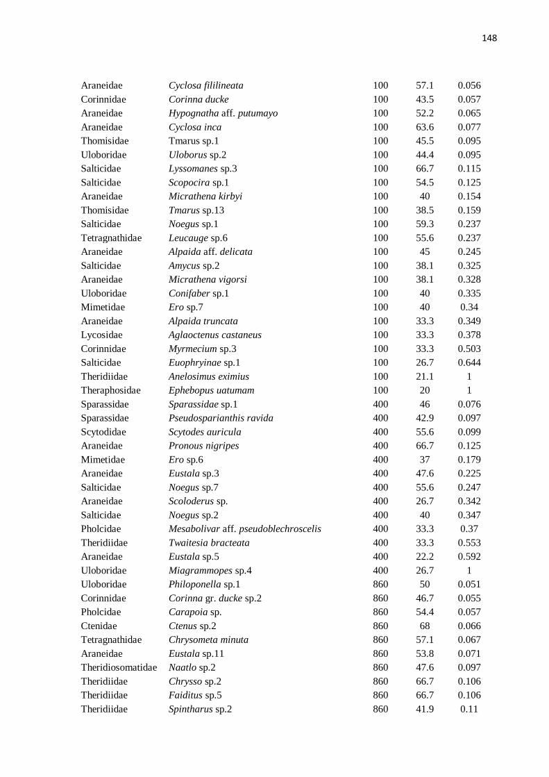
148
Araneidae Cyclosa fililineata 100 57.1 0.056
Corinnidae Corinna ducke 100 43.5 0.057
Araneidae Hypognatha aff. putumayo 100 52.2 0.065
Araneidae Cyclosa inca 100 63.6 0.077
Thomisidae Tmarus sp.1 100 45.5 0.095
Uloboridae Uloborus sp.2 100 44.4 0.095
Salticidae Lyssomanes sp.3 100 66.7 0.115
Salticidae Scopocira sp.1 100 54.5 0.125
Araneidae Micrathena kirbyi 100 40 0.154
Thomisidae Tmarus sp.13 100 38.5 0.159
Salticidae Noegus sp.1 100 59.3 0.237
Tetragnathidae Leucauge sp.6 100 55.6 0.237
Araneidae Alpaida aff. delicata 100 45 0.245
Salticidae Amycus sp.2 100 38.1 0.325
Araneidae Micrathena vigorsi 100 38.1 0.328
Uloboridae Conifaber sp.1 100 40 0.335
Mimetidae Ero sp.7 100 40 0.34
Araneidae Alpaida truncata 100 33.3 0.349
Lycosidae Aglaoctenus castaneus 100 33.3 0.378
Corinnidae Myrmecium sp.3 100 33.3 0.503
Salticidae Euophryinae sp.1 100 26.7 0.644
Theridiidae Anelosimus eximius 100 21.1 1
Theraphosidae Ephebopus uatumam 100 20 1
Sparassidae Sparassidae sp.1 400 46 0.076
Sparassidae Pseudosparianthis ravida 400 42.9 0.097
Scytodidae Scytodes auricula 400 55.6 0.099
Araneidae Pronous nigripes 400 66.7 0.125
Mimetidae Ero sp.6 400 37 0.179
Araneidae Eustala sp.3 400 47.6 0.225
Salticidae Noegus sp.7 400 55.6 0.247
Araneidae Scoloderus sp. 400 26.7 0.342
Salticidae Noegus sp.2 400 40 0.347
Pholcidae Mesabolivar aff. pseudoblechroscelis 400 33.3 0.37
Theridiidae Twaitesia bracteata 400 33.3 0.553
Araneidae Eustala sp.5 400 22.2 0.592
Uloboridae Miagrammopes sp.4 400 26.7 1
Uloboridae Philoponella sp.1 860 50 0.051
Corinnidae Corinna gr. ducke sp.2 860 46.7 0.055
Pholcidae Carapoia sp. 860 54.4 0.057
Ctenidae Ctenus sp.2 860 68 0.066
Tetragnathidae Chrysometa minuta 860 57.1 0.067
Araneidae Eustala sp.11 860 53.8 0.071
Theridiosomatidae Naatlo sp.2 860 47.6 0.097
Theridiidae Chrysso sp.2 860 66.7 0.106
Theridiidae Faiditus sp.5 860 66.7 0.106
Theridiidae Spintharus sp.2 860 41.9 0.11

149
Theridiidae Episinus sp.7 860 57.1 0.116
Araneidae Wagneriana sp.1 860 50 0.123
Araneidae Micrathena cyanospina 860 66.7 0.133
Tetragnathidae Azilia histrio 860 50 0.133
Uloboridae Uloborus sp.7 860 38.5 0.175
Araneidae Micrathena triangularis 860 38.9 0.221
Araneidae Eustala sp.4 860 55.6 0.233
Araneidae Micrathena sp.1 860 43.1 0.238
Theridiidae Faiditus sp.9 860 44.4 0.331
Pholcidae Mesabolivar aff. aurantiacus 860 40 0.345
Araneidae Micrathena triangularispinosa 860 38.9 0.359
Salticidae Lyssomanes sp.2 860 33.3 0.473
Theridiosomatidae Naatlo splendida 860 33.3 0.503
Tetragnathidae Leucauge sp.5 860 22.2 1
Salticidae Mago sp.2 860 20 1
Theridiidae Dipoena sp.1 1550 42.9 0.083
Pholcidae Priscula cf. taruma 1550 48.3 0.094
Theridiidae Episinus sp.1 1550 66.7 0.106
Theridiidae Achaearanea dea 1550 66.7 0.125
Tetragnathidae Chrysometa boraceia 1550 66.7 0.125
Mimetidae Gelanor sp.2 1550 66.7 0.125
Pholcidae Metagonia maritaguariensis 1550 66.7 0.125
Theridiidae Dipoena rubella 1550 42.1 0.14
Uloboridae Philoponella republicana 1550 38.5 0.162
Theridiidae Theridion fungosum 1550 40 0.201
Theridiidae Rhomphaea metaltissima 1550 55.6 0.23
Theridiidae Phoroncidia moyobamba 1550 44.4 0.309
Theridiidae Styposis sp.1 1550 40 0.316
Tetragnathidae Homalometa sp. 1550 44.4 0.333
Tetragnathidae Leucauge sp.2 1550 40 0.34
Araneidae Parawixia rimosa 1550 33.3 0.53
Linyphiidae Sphecozone crassa 2000 43.7 0.075
Araneidae Eustala sp.12 2000 66.7 0.106
Linyphiidae Dubiaranea caeca 2000 55.6 0.106
Salticidae Euophryinae sp.3 2000 47.6 0.221
Theridiidae Phycossoma sp.1 2400 38.1 0.346
Anyphaenidae Anyphaenidae sp.2 2400 25 0.764

150
FIGURES
Fig. 1. Study area. A) South America; B) Northern South America (rectangle of map A
enlarged). The mountain range at the left of the map represents the northern part of the Andes,
and the mountainous region in the center of the map is the Guayana Shield, showing the study
area in its southern part, and dotted yellow line represents the equator; C) Closer view of the
study area (rectangle of map B enlarged), the Pico da Neblina. Letters represent the altitudes
sampled: A – 100 m, B – 400 m, C – 860 m, D – 1,550 m, E – 2,000 m, F – 2,400 m.

151
Fig. 2. Rank abundance plot of the spider community for each altitude. Species are ordered by
decreasing abundance.

152
Fig. 3. Results of the partial Mantel test. a) Relation between altitudinal difference and beta
diversity, controlled by spatial distance; b) Relation between altitude and Bray Curtis
similarity index, controlled by spatial distance; c) Relation between Bray Curtis similarity
index and beta diversity, controlled by spatial distance; d) Relation between Bray Curtis
similarity index and beta diversity, controlled by altitudinal difference.

153
Fig. 4. Graphic representation of the first two axes of a NMDS performed for all species of
spiders at the 18 sites sampled, in six different altitudes. First axis explained 58% of total
variation and second axis 20% Stress = 5,97.

154
CAPÍTULO 4
Nogueira, A.A., Barbosa, J.P.P.P., Venticinque, E.M. & Brescovit, A.D. 2011. The spider
genus Chrysometa (Araneae, Tetragnathidae) from the Pico da Neblina and Serra do
Tapirapecó mountains (Amazonas, Brazil): new species, new records, diversity and
distribution along two altitudinal gradients. Zootaxa. 2772: 33-51.

155
Artigo 4
Submetido à revista Zootaxa
The spider genus Chrysometa (Araneae, Tetragnathidae) from the Pico da Neblina and
Serra do Tapirapecó mountains (Amazonas, Brazil): new species, new records, diversity
and distribution along two altitudinal gradients
ANDRÉ A. NOGUEIRA1, JOÃO P.P. PENA-BARBOSA
2,3, EDUARDO M. VENTICINQUE
1,4 &
ANTONIO D. BRESCOVIT
2
1 Instituto Nacional de Pesquisas da Amazônia, INPA, Programa de Pós-Graduação em
Ecologia. Avenida André Araújo, 2936, Aleixo, CEP 69011-970, Cx. Postal 478, Manaus,
AM, Brazil.E-mail: [email protected], [email protected]
2Laboratório de Artrópodes, Instituto Butantan. Av. Vital Brazil 1500, CEP 05503-900, São
Paulo, SP, Brazil. E-mail: [email protected], [email protected]
3Pós-graduação em Zoologia, Instituto de Biociências, Universidade de São Paulo, São
Paulo, SP, Brazil.
4 Universidade Federal do Amazonas – WCS Brasil – Wildlife Conservation Society. Prédio
Sauim de Coleira, ICB-UFAM, Estrada do Contorno 3000, CEP69077-000, Manaus, AM,
Brazil.

156
Abstract
Eight new species of the spider genus Chrysometa Simon, 1894 (Araneae, Tetragnathidae) are
described and illustrated. Chrysometa nubigena n. sp., C. waikoxi n. sp., C. petrasierwaldae
n. sp., C. santosi n. sp., C. yanomami n. sp., C. candianii n. sp., C. lomanhungae n. sp., and
C. saci n. sp. Those species were collected in a study on the diversity of spider communities
along altitudinal gradients in Brazilian Amazonia. C. saci was captured at the Serra do
Tapirapecó (Barcelos), while all the other species are from the Pico da Neblina (São Gabriel
da Cachoeira), the highest mountain in Brazil. We provide new records for C. boraceia, C.
flava, C. guttata, C. minuta and C. opulenta, and we describe the male of C. minuta for the
first time. We also present the first results on the diversity and altitudinal distribution of the
species of Chrysometa at the Pico da Neblina and Serra do Tapirapecó. We sampled the first
locality at six different elevations, and obtained 336 specimens distributed in 12 species.
Richness and abundance, as well as relative importance peaked at the highest sites sampled
(2,000 and 2,400 m). The three most abundant species showed a segregated distribution,
being dominant or exclusively distributed in different altitudes. At the Serra do Tapirapecó,
sampling at four different elevations up to 1200 m, we only obtained 40 individuals divided in
four species, and there was no clear relation to altitude. Most of the new species were found at
mid and high altitude sites, while species from lower altitude sites represented widespread
species. The comparison with other neotropical spiders inventories highlights the high
diversity recorded at Pico da Neblina, which could be assigned to the large environmental
variation covered in this work and to the sampling of high-altitude environments. Inventories
in the Andean region and other information in the literature also seem to support the
association of Chrysometa with high altitude environments.
Key words: spiders, taxonomy, biodiversity, Araneoidea, orbweavers, Neotropical region

157
Introduction
Spiders from the genus Chrysometa Simon, 1895 are neotropical orb-weavers of the
family Tetragnathidae. The genus was proposed by Simon in 1894 for a specimen described
by Keyserling (1863) as Tetragnatha tenuipes. Levi (1986) examined the specimen and
concluded that it was not C. tenuipes, but a new species, designated as Chrysometa eugeni.
Levi (1986) also considered Capichameta Soares and Camargo, 1955, and Pseudometa
F.O.P.-Cambridge, 1903, to be junior synonyms of Chrysometa.
Adults of most Chrysometa species are small (from 3 to 5 mm) and have an oval
abdomen, with silver or white spots and dark pigmentation. Males have longer legs, but
slightly smaller bodies than females (Levi 1986). In his revision on the genus, Levi (1986)
indicates as the most characteristic features of Chrysometa males the presence of a terminal
apophysis on the bulb and of an apophysis at the dorsal face of the cymbium of the palp. For
females, the diagnostic characters are a flat epigynum, usually without projections, and also
fertilization ducts in most species more sclerotized than the connecting ducts. A recent
hypothesis on the phylogeny of Tetragnathidae (Álvarez-Padilla, 2007) supported the
monophyly of the genus, but since Chrysometa was represented by only six species a larger
taxon sample is necessary to confirm this result. In this latter study the monophyly of
Chrysometa was supported by three female synapomorphies: long fertilization ducts (1),
following a straight path (2), from an anterior origin (3).
There are currently 130 species of Chrysometa, distributed from Mexico to Chile,
including some Caribbean islands (Platnick, 2010). The most peculiar feature of their
distribution is the apparent association of several species with high altitude environments.
Nevertheless several species may occur in low elevation sites, always in forests; their
diversity increases with increasing elevation, reaching its maximum at and above timberline
(Levi 1986). Not surprisingly, the Andean region harbors the largest number of species. Levi

158
(1986) also noticed that the group was unexpectedly rich in higher altitudes, and that several
species are known after a single individual, which suggests that their distribution is still
poorly known and that several species remains to be discovered.
In this work we describe eight new species of Chrysometa from two mountains in
Brazilian Amazonia, the Serra do Tapirapecó and the Pico da Neblina, both located on the
northern border of the state of Amazonas. We also provide new records for species already
described, and describe for the first time the male of C. minuta (Keyserling), 1883. Finally,
we document, and comment on, the diversity and distribution of Chrysometa at the sampled
sites, and compare our results to those of other Neotropical spider inventories. The results
presented here are part of a study about spider communities in altitudinal gradients (Nogueira
et al., in preparation – cap.2).
Material and Methods
Study area
The Serra do Tapirapecó (1°17’N, 64º39W) and the Pico da Neblina (00°46’N e
66º00’W) are located in Yanomami Indigenous Land and Pico da Neblina National Park
(overlapping with Yanomani Indigenous Land), respectively. Both areas are located on the
northern border of the Brazilian state of Amazonas (Fig. 1), a mountain region located at the
boundary between Brazil and Venezuela, as well as the watershed between the Orinoco and
Amazonas basins (RADAM 1978). These formations are in the southern part of the Guyana
Shield, a region of very old geological origin (mostly from the Precambrian, ranging from 3.6
to 1.6 billion years ago), and whose main characteristic is the presence of sandstone
mountains, with vertical cliffs and table tops, known as “tepuis” (Huber 1995a). The Serra do
Tapirapecó is basically constituted by granitic rocks, and reaches its highest altitude at the
Pico do Tamacuari, with an altitude of 2,400 m. The Pico da Neblina (2,994 m). Is the highest

159
Brazilian mountain, as well as the highest place in South America outside the Andes. Mainly
formed by sandstone rocks, the Neblina massif is also characterized by extensive high-altitude
plateaus (2,000 - 2,400 m). although it does not have the typical tepui shape (Huber 1995a).
The climate of the region is tropical humid, with an annual average rainfall 3,000
mm/year, an average temperature of 25°C, 85-90% humidity and little variation through the
year. Both rainfall and humidity increase with the elevation, while the temperature decreases.
In the highlands (> 1,800 m) the rainfall decreases and is replaced by a constant mist, with
humidity reaching almost 100%. In those altitudes, temperature can drop to an average of 10°
in the coolest month (RADAM 1978).
Vegetation of the lowlands is mainly composed by a tall, evergreen forest, gradually
replaced by submontane (400 to 800 m), montane (800 to 1,500 m) and upper-montane forest
(1,500 to 2,000 m) (Huber 1995b). Higher elevations have more open types of vegetation,
such as high-altitude meadows and grasslands. Those formations are composed of a highly
endemic flora (Berry et al. 1995), with several species with sclerophyllous characteristics.
Some species of Rapateacea and Bromeliaceae dominate these communities, which are also
characterized by the presence of several species of Eriocaulaceae, Xyridaceae and Cyperaceae
(Huber 1995b).
The Pico da Neblina will be referred to as Neblina and the Serra do Tapirapecó as
Tapirapecó throughout this paper.
Collecting methods and sampling design
Spiders were collected using a beating tray during the day and manually during the
night. The sample unit of the first method corresponds to the investigation, with a beating
tray, of 20 small trees, or shrubs, or other components of the vegetation. The sample unit of

160
the second method correspond to one hour of searching along a 30 m long transect. All
spiders collected using these two methods were preserved in 70% ethanol.
At Neblina we sampled at six different altitudes , 100, 400, 860, 1,550, 2,000 and
2,400 m, and at each altitude we investigated three different sites. In each site the sampling
effort corresponded to nine diurnal and nine nocturnal samples, which resulted in 54 samples
at each elevation (27 diurnal and 27 nocturnal). The final count for Neblina was 324 samples
(162 diurnal and 162 nocturnal). At the Tapirapecó we only sampled four altitudes, 180, 400,
800 and 1,200 m. Sampling effort was lower in this expedition, with 6 diurnal and 6 nocturnal
samples by site, which correspond to 18 of each method by altitude; although in the last two
elevations sampling could not be completed, resulting in 16 nocturnal samples at 800 and 12
at 1,200 m. To complete these samplings or even to collect in higher altitudes was impossible
due to a malaria outbreak among the expedition members. We sampled Tapirapecó in
September/October 2006, and Neblina in September/October 2007, during the period
corresponding to the regional “dry” season.
We calculated the altitudinal weighted average midpoint (WAM) (Almeida-Neto et al.
2006) for the Chrysometa communities. This parameter is obtained by multiplying the
number of individuals found in each altitude by the corresponding elevation. Those values are
summed up, and divided by the total abundance. Assuming that a species reaches its
maximum abundance in optimal environmental conditions, we consider that this method may
represent in an accurate manner the actual altitudinal preference of the species along the
gradient. We calculated the WAM for each species and also for all species together, but for
the two data sets (Neblina and Tapirapecó) separately. Finally we also calculated the relative
importance of the genus Chrysometa, which is the ratio of Chrysometa abundance and
richness in relation to those parameters for the whole spider community (unpublished data).

161
However, for the Tapirapecó dataset we only investigated the relative abundance, since we
did not identified the others spiders captured there, and so we could not assess the total
richness (528 species and 3140 individuals at the Neblina and 1623 individuals at the
Tapirapecó, unpublished data).
We compared our results with those of 19 other Neotropical spider inventories (Table
3). We selected only those that also used manual active searching as a sampling method,
since this was by far the most efficient method to capture Chrysometa specimens, obtaining
91% of the individuals collected at Neblina and 95% collected at Tapirapecó.
We recorded in the inventory results an additional new species found at Pico da
Neblina. This species is not described here because the only specimen available was lost
during the tragic fire that destroyed most of the Instituto Butantan’s arachnological collection
in May 2010. This species will be referred to as Chrysometa sp.
The specimens examined in this study are deposited in the following collections
(abbreviations and curators in parenthesis): Instituto Nacional de Pesquisas da Amazônia,
Amazonas (INPA, A. Henriques), Instituto Butantan, São Paulo (IBSP, I. Knysak) and Museu
Paraense Emílio Goeldi, Pará (MPEG, A. B. Bonaldo).
The material was examined and illustrated on a stereomicroscope Olympus SZX12 equipped
with a camera lucida. The description format follows Levi (1986) and all measurements are in
millimetres.
The following abbreviations used in the text and figures follow Levi (1986) and
Álvarez-Padilla et al. (2009): C, conductor; CA, cymbial apophysis; CD, copulatory duct;
CEBP, ecto-basal cymbial process; CEMP, ecto-median cymbial process; CMP, cymbial
membranous projection; CO, copulatory openings; E, embolous; H, hematodocha; LP, lateral
plates; LwP, lower prong of paracymbium; MEA, “metine” embolic apophysis; ML, median

162
lobe; MP, median plate; Sp, spermatheca; St, septum; P, paracymbium; PT; paracymbium
tips; T, tibia; Te, tegulum; UpP, upper prong of paracymbium.
Taxonomy
Family Tetragnathidae Menge, 1866
Genus Chrysometa Simon, 1895
Chrysometa nubigena new species
Figures 2A-E
Type material. Holotype: Male from Pico da Neblina (2,000m), São Gabriel da Cachoeira,
(00°46'N 66º00'W), Amazonas, Brazil, X.2007, A.A. Nogueira et al. coll. (INPA-AR 6144).
Paratypes: six males and seven females from the same locality and date (INPA-AR 6145 (1
male), 6146 (1 male) 6147 (1 female), 6148 (1 female), 6149 (1 female); IBSP 160448 (1
male), 160451 (1 female), 160453 (1 male), 160474 (1 female); MPEG 15666 (1 female),
15667 (1 female), 15668 (1 male), 15672 (1 male)).
Additional Material examined: Brazil: Amazonas: São Gabriel da Cachoeira, Pico da
Neblina, (0°46'N 66º00'W), 31 males and 53 females, X.2007, A.A. Nogueira et al., coll.
(INPA-AR 6191-6220; IBSP 160449, 160450, 160452, 160454, 160455; MPEG 15669-
15671, 15673).
Etymology. The specific epithet is a Latin word that means “born on the clouds”, since this
species was only collected at high altitudes at the Pico da Neblina, a place constantly covered
by mist, a characteristic which gave the mountain its name (“peak of the mist”).
Diagnosis. Males of C. nubigena differ from all other species of the genus by the long
cymbial apophysis with a small hump near the tip; paracymbium with thin lower prong in

163
ventral view (Fig. 2A); cymbial membranous projection posteriorly curved rounded tip in
ventral view (Figs. 2A), being subtriangular in retrolateral view (Fig. 2B).
Females of C. nubigena differ from all other species by the posteriorly pointed “V”-shaped
projection of the median lobe over the lateral plates, and the oval-shaped copulatory openings,
on ventral view (Fig. 2C). On posterior view, epiginal lateral plates with anteriorly projected
rounded tip; median plate right behind the lateral plates, creating two arches (Fig. 2D).
Description.
Male (holotype). Carapace yellow; Sternum, chelicerae, labium and endites brown. Legs
yellow. Dorsum of the abdomen grey, with some transversal black lines. Sides with some
white to silver spots. Venter black, with two white spots. Spinnerets black. Total length 2.6;
Carapace 1.2 long, 1.1 wide. Leg I length: femur 2.4; patella+tibia 2.8; metatarsus 2.1; tarsus
0.9. Patella+tibia II 1.5; III 0.8; IV 1.0. Palp: Paracymbium “M”-shaped, with upper prong
more enlarged and shorter than lower prong, on ventral view (Fig. 2A); and 'metine' embolic
apophysis curved on apical region (Fig. 2A).
Female (paratype, INPA-AR 6147). Colour as in male. Total length 3.4; carapace 1.3 long,
1.1 wide. Leg I length: femur 1.3; patella+tibia 1.9; metatarsus 1.8; tarsus 0.7. Patella+tibia II
1.4; III 0.6; IV 1.1. Epigynum: Spermatechae apical, with copulatory ducts right below (Fig.
2E).
Distribution. Only known from the type locality.
Chrysometa saci new species
Figures 3A-E
Type material. Holotype: Male from Serra do Tapirapecó (1,200m), Barcelos (1°17'N
64º39'W), Amazonas, Brazil, X.2006, A.A. Nogueira & R. Braga-Neto coll. (INPA-AR
6156).

164
Paratypes: one male and six females from the same locality and date (INPA-AR 6157 (1
female), 6268 (2 females); IBSP 160490 (1 female), 160491 (1 male), 160492 (1 female),
160493 (1 female)).
Etymology. The species epithet is taken as a noun in apposition honoring mycologist Ricardo
Braga-Neto, nicknamed “Saci”, for his help in the field throughout the Serra do Tapirapecó
expedition.
Diagnosis. Males of C. saci differ from all other species of the genus by the paracymbial
lower prong well developed, extending away from the palp in ventral direction (ventral and
retrolateral views) (Figs. 3A, B); and the paracymbium with the paracymbial tip pointed
retrolaterally with a horn shape, on ventral and retrolateral views (Fig. 3A, B). Males of C.
saci are similar to C. cambara Levi, 1986, figs.: 622, 623.
Females of C. saci differ from all other species by the vessel-shaped septum, with the
posterior half membranous, on ventral view (Fig. 3C). The membranous area is partially
covered by the lateral plates, creating a median groove with two humps on each side, on
ventral and posterior views (Figs. 3C, D). Females of C. saci are similar to C. chica Levi,
1986, figs.: 382-385.
Description.
Male (holotype). Carapace yellow, with cephalic region brown; Sternum, chelicerae, labium
and endites brown. Legs yellow, with many dark spots. Dorsum of the abdomen grey, with
white spots and some transversal black lines. Venter grey with a black longitudinal line on
middle. Spinnerets grey. Total length 4.8; Carapace 2.4 long, 2.2 wide. Leg I length: femur
5.4; patella+tibia 6.7; metatarsus 6.1; tarsus 1.7. Patella+tibia II 4.5; III 1.8; IV 3.0. Palp:
Ecto-median cymbial process pointed ventrally, ecto-basal cymbial apophysis pointed
retrolaterally (Fig. 3B).

165
Female (paratype, IBSP 160490). Colour as in male, with the venter of abdomen with a
black, longitudial line on center with white spots around. Total length 6.3; Carapace 2.3 long,
2.0 wide. Leg I length: femur 3.3; Patella+tibia 4.0; metatarsus 3.0; tarsus 1.1. Patella+tibia II
3.1; III 1.5; IV 2.4. Epigynum: internally with spermathecae apical, with copulation ducts
coiled and basal openings of the ducts, near the septum (Fig. 3E).
Distribution. Only known from the type locality.
Chrysometa waikoxi new species
Figures 4A-E
Type material. Holotype: Male from Pico da Neblina (1,550m), São Gabriel da Cachoeira,
(0°46'N 66º00'W), Amazonas, Brazil, X.2007, A.A. Nogueira et al. coll. (INPA-AR 6159).
Paratypes: four males and six females from the same locality and date (INPA-AR 6160 (1
female), 6161 (1 female), 6162 (1 female), 6163 (1 female); IBSP 160466 (1 female), 160467
(1 male), 160470 (1 male), 160471 (1 female); MPEG 15682 (1 male), 15684 (1 female)).
Additional material examined. Brazil: Amazonas: São Gabriel da Cachoeira, Pico da
Neblina, (0°46'N 66º00'W), three males and 27 females, X.2007, A.A. Nogueira et al., coll.
(INPA-AR 6269-6278; IBSP 160468, 160469, 160472, 160477; MPEG 15683).
Etymology. The species epithet is taken from the Yanomami word for spider, a noun in
apposition, and represents a tribute to the Yanomami people, since the places sampled in our
expeditions are located at the Yanomami Indigenous Land, and also for the help received in
the field from some members of the tribe.
Diagnosis. Males of Chrysometa waikoxi differs from all other species of the genus by a
projection on the middle of the cymbial apophysis turned posteriorly, and the tip turned to the
ventral, on ventral and retrolateral views (Figs. 4A, B); and the conical cymbial membranous

166
projection (Figs. 4A, B). Males of C. waikoxi are similar to C. alajuela Levi, 1986, figs.: 716,
717 and C. harmata (Bryant) on Levi, 1986, fig.: 58.
Females of C. waikoxi differ from other species by the curved shape of the anterior edge of
the copulatory opening, producing a curved projection on each side, on ventral view (Fig.
4C). Females of C. waikoxi are similar to C. troya Levi, 1986, figs.: 413-416.
Description.
Male (holotype). Carapace yellow, with a longitudinal black line on the thoracic region;
sternum, chelicerae, labium and endites brown. Legs yellow, with black spots. Dorsum of the
abdomen grey, with transverse black lines. Sides with some white to silver spots. Venter
black, with two white spots. Spinnerets black. Total length 2.5; Carapace 1.1 long, 0.9 wide.
Leg I length: femur 2.5; patella+tibia 3.0; metatarsus 3.0; tarsus 0.8. Patella+tibia II 1.6; III
0.6; IV 1.0. Palp: Paracymbium “M”-shaped in ventral view, with the lower prong with the
same size of the upper prong (Fig. 4A).
Female (paratype, INPA-AR 6161). Colour as in male. Total length 3.1; Carapace 1.2 long,
1.0 wide. Leg I length: femur 2.2; patella+tibia 2.3; metatarsus 1.8; tarsus 0.6. Patella+tibia II
1.5; III 0.6; IV 1.1. Epigynum: Lateral plates subrectangular in shape; copulatory openings
subtriangular(Fig. 4D). Spermathecae apical with copulatory ducts right below (Fig. 4E).
Distribution. Only known from the type locality.
Chrysometa petrasierwaldae new species
Figures 5A-E
Type material. Holotype: Male from Pico da Neblina, São Gabriel da Cachoeira, (0°46'N
66º00'W), Amazonas, Brazil, X. 2007, A.A. Nogueira et al. coll. (INPA-AR 6150).
Paratype: six males and seven females from the same locality and date (INPA-AR 6151 (1
female), 6152 (1 female), 6153 (1 male), 6154 (1 male), 6155 (1 female); IBSP 160456 (1
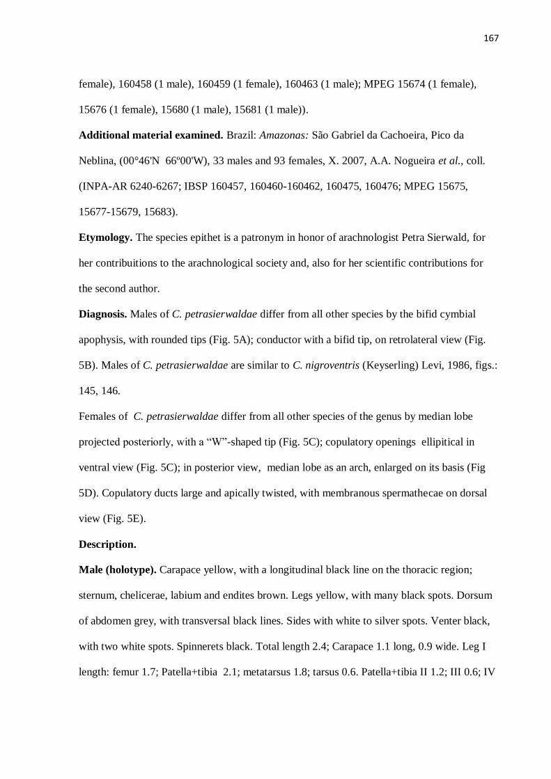
167
female), 160458 (1 male), 160459 (1 female), 160463 (1 male); MPEG 15674 (1 female),
15676 (1 female), 15680 (1 male), 15681 (1 male)).
Additional material examined. Brazil: Amazonas: São Gabriel da Cachoeira, Pico da
Neblina, (00°46'N 66º00'W), 33 males and 93 females, X. 2007, A.A. Nogueira et al., coll.
(INPA-AR 6240-6267; IBSP 160457, 160460-160462, 160475, 160476; MPEG 15675,
15677-15679, 15683).
Etymology. The species epithet is a patronym in honor of arachnologist Petra Sierwald, for
her contribuitions to the arachnological society and, also for her scientific contributions for
the second author.
Diagnosis. Males of C. petrasierwaldae differ from all other species by the bifid cymbial
apophysis, with rounded tips (Fig. 5A); conductor with a bifid tip, on retrolateral view (Fig.
5B). Males of C. petrasierwaldae are similar to C. nigroventris (Keyserling) Levi, 1986, figs.:
145, 146.
Females of C. petrasierwaldae differ from all other species of the genus by median lobe
projected posteriorly, with a “W”-shaped tip (Fig. 5C); copulatory openings ellipitical in
ventral view (Fig. 5C); in posterior view, median lobe as an arch, enlarged on its basis (Fig
5D). Copulatory ducts large and apically twisted, with membranous spermathecae on dorsal
view (Fig. 5E).
Description.
Male (holotype). Carapace yellow, with a longitudinal black line on the thoracic region;
sternum, chelicerae, labium and endites brown. Legs yellow, with many black spots. Dorsum
of abdomen grey, with transversal black lines. Sides with white to silver spots. Venter black,
with two white spots. Spinnerets black. Total length 2.4; Carapace 1.1 long, 0.9 wide. Leg I
length: femur 1.7; Patella+tibia 2.1; metatarsus 1.8; tarsus 0.6. Patella+tibia II 1.2; III 0.6; IV

168
1.0. Palp. Paracymbium subrectangular, with a cymbial membranous projection not so
pronunciated as observed in C. waikoxi (Fig. 5A).
Female (paratype, INPA-AR 6151). Carapace yellow, with a single shield-shaped black spot
on cephalic region. Chelicerae yellow. Labium, endites and sternum brown. Dorsum of
abdomen grey with white spots and transversal black lines. Venter grey with two white spots.
Total length 2.6; Carapace 1.0 long, 0.9 wide. Leg I length: femur 1.5; patella+tibia 1.8;
metatarsus 1.3; tarsus 0.6. Patella+tibia II 1.1; III 0.6; IV 0.9. Epigynum: Lateral plates
subrectangular (Fig. 5D); copulatory openings right below the median lobe, internally with
copulatory ducts large and apically twisted; spermathecae as two hyaline balloons (Fig. 5E).
Distribution. Only known from the type locality.
Chrysometa lomanhungae new species
Figures 6A-C
Type material. Holotype: Female from Pico da Neblina (2,000m), São Gabriel da Cachoeira
(00°46'N 66º00'W), Amazonas, Brazil, X.2007, A.A. Nogueira et al. coll. (INPA-AR 6142).
Paratypes: two females from the same locality and date (INPA-AR 6143 (1 female); IBSP
160465 (1 female)).
Etymology. The species epithet is a patronym in honor of arachnologist Nancy Lo Man
Hung, recognising her help through the Pico da Neblina sampling expedition.
Diagnosis. Females of Chrysometa lomanhungae are similar to C. obscura (Bryant) in the
large size of the copulatory openings (Levi, 1986, fig: 249), but differ by the septum covered
by two humps of the median lobe (Fig. 6A), the presence of two pointed distal tips on the
lateral plates, on posterior view (Fig. 6B). Females of C. nubigena are similar to C. obscura
(Bryant) Levi, 1986, figs.: 247-250.
Description.

169
Male. Unknown.
Female (holotype). Carapace yellow; sternum, chelicerae, labium and endites brown. Legs
yellow, with brown annuli. Dorsum of abdomen grey, with white spots and transversal black
lines. Venter grey with two white spots. Spinnerets grey. Total length 4.6; Carapace 2.0 long,
1.5 wide. Leg I length: femur 4.0; patella+tibia 4.6; metatarsus 3.9; tarsus 1.3. patella+tibia II
2.9 III 1.4; IV 2.0. Epigynum: internally with spermathecae globose and copulatory ducts
opening near the septum (Fig. 6C).
Distribution. Only known from the type locality.
Chrysometa yanomami new species
Figures 6D-F
Type material. Holotype: Female from Pico da Neblina (2,000m), São Gabriel da Cachoeira,
(00°46'N 66º00'W), Amazonas, Brazil, X.2007, A.A. Nogueira et al., coll. (INPA-AR 6140).
Paratype: two females from the same locality and date (INPA-AR 6141 (1 female); IBSP
160473 (1 female)).
Etymology. The specific epithet, a noun in apposition, is a tribute to the Yanomami people
since the places sampled in our expeditions are located on the Yanomami Indigenous Land,
and in gratitude for the help received in the field from some members of the tribe.
Diagnosis. Females of C. yanomami differ from all other species of the genus by the “T”-
shaped median plate on posterior view (Fig. 6E). Females of C. yanomami are similar to C.
satulla (Keyserling) Levi, 1986, figs.: 175-179 and also similar to C. machala Levi, 1986,
figs.: 515-518.
Description.
Male. Unknown.
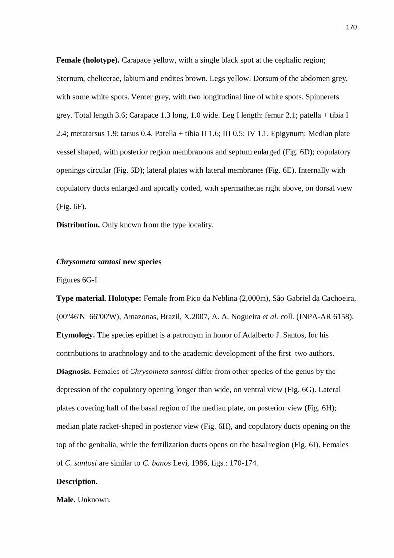
170
Female (holotype). Carapace yellow, with a single black spot at the cephalic region;
Sternum, chelicerae, labium and endites brown. Legs yellow. Dorsum of the abdomen grey,
with some white spots. Venter grey, with two longitudinal line of white spots. Spinnerets
grey. Total length 3.6; Carapace 1.3 long, 1.0 wide. Leg I length: femur 2.1; patella + tibia I
2.4; metatarsus 1.9; tarsus 0.4. Patella + tibia II 1.6; III 0.5; IV 1.1. Epigynum: Median plate
vessel shaped, with posterior region membranous and septum enlarged (Fig. 6D); copulatory
openings circular (Fig. 6D); lateral plates with lateral membranes (Fig. 6E). Internally with
copulatory ducts enlarged and apically coiled, with spermathecae right above, on dorsal view
(Fig. 6F).
Distribution. Only known from the type locality.
Chrysometa santosi new species
Figures 6G-I
Type material. Holotype: Female from Pico da Neblina (2,000m), São Gabriel da Cachoeira,
(00°46'N 66º00'W), Amazonas, Brazil, X.2007, A. A. Nogueira et al. coll. (INPA-AR 6158).
Etymology. The species epithet is a patronym in honor of Adalberto J. Santos, for his
contributions to arachnology and to the academic development of the first two authors.
Diagnosis. Females of Chrysometa santosi differ from other species of the genus by the
depression of the copulatory opening longer than wide, on ventral view (Fig. 6G). Lateral
plates covering half of the basal region of the median plate, on posterior view (Fig. 6H);
median plate racket-shaped in posterior view (Fig. 6H), and copulatory ducts opening on the
top of the genitalia, while the fertilization ducts opens on the basal region (Fig. 6I). Females
of C. santosi are similar to C. banos Levi, 1986, figs.: 170-174.
Description.
Male. Unknown.

171
Female (holotype). Carapace yellow, with cephalic region brown; sternum, chelicerae,
labium and endites brown. Legs yellow, with brown rings. Dorsum of abdomen grey, with
some white spots and some black transversal lines. Venter grey. Spinnerets yellow. Total
length 7.4; Carapace 2.8 long, 2.1 wide. Leg I length: femur 4.4; patella + tibia 5.5;
metatarsus 4.7; tarsus 1.5. Patella+tibia II 3.6; III 1.2; IV 2.3. Epigynum: Lateral copulatory
ducts enlarged averagely (Fig. 6H).
Distribution. Only known from the type locality.
Chrysometa candianii new species
Figures 7A, B
Type material. Holotype: Male from Pico da Neblina (860m), São Gabriel da Cachoeira,
(0°46'N 66º00'W), Amazonas, Brazil, X.2007, A.A. Nogueira et al. coll. (INPA-AR 6138).
Paratype: two males from the same locality and date (INPA-AR 6139 (1 male); IBSP 160464
(1 male)).
Etymology. The species epithet is a patronym in honor of the arachnologist David Candiani,
in gratitude for his help in the field through the Pico da Neblina expedition.
Diagnosis. Males of Chrysometa candianii differs from all other species of the genus by the
lower prong of paracymbium with three projections, on retrolateral views (Fig. 7B), with the
distance between the tips longer than the size of the tips (Fig. 7B); and by a basal projection
of the ecto-median cymbial apophysis, like a lobe of an ear (Fig. 7B). Males of C. candianii
are similar to C. guttata (Keyserling) Levi, 1986, figs.: 559, 560.
Description.
Male (holotype). Carapace, sternum, chelicerae, labium, endites and legs yellow. Dorsum of
abdomen grey, with white spots. Venter grey. Spinnerets grey. Total length 3.8; Carapace 2.0
long, 1.6 wide. Leg I length: femur 3.4; patella+tibia 3.9; metatarsus 3.4; tarsus 1.1. Patella +

172
tibia II 3.0; III 1.2; IV 2.0. Palp: tegulum with a prolateral projection (Fig. 7A), upper prong
of paracymbium with a retrolateral depression (Fig. 7A), and lower prong trifid, median tip
longer than others (Fig. 7B). Cymbial membranous projection ventrally directed (Figs. 7A,
B). ecto-basal cymbial apophysis curved and pointed ventrally (Figs. 7A, B).
Female. Unknown.
Distribution. Only known from the type locality.
Chrysometa minuta (Keyserling, 1883)
Figures 7C, D
Meta minuta Keyserling, 1883: 206, pl. 15, fig. 100 (Holotype female from “Province
Amazonas”, Brazil deposited in Hope Entomological Collection, Oxford, not examined).
Argyroepeira minuta: Keyserling, 1893: 321, pl. 16, fig. 236.
Chrysometa minuta: Levi, 1986: 168, figs. 435-440, Platnick, 2010.
Material examined. Brazil: Amazonas: Barcelos, Serra do Tapirapecó, (1°17'N, 64º39'W), 1
male and 4 females, X.2006, A.A. Nogueira & R. Braga-Neto coll. (INPA-AR 6181 (1
female), 6182 (1 male), 6183 (1 female), 6184 (1 male), 6185 (1 female); IBSP 160441 (1
female)); São Gabriel da Cachoeira, Pico da Neblina, (00°46'N 66º00'W), 4 females, X.2007,
A.A. Nogueira et al. coll. (INPA-AR 6187 (1 female), 6188 (1 female), 6189 (1 female), 6190
(1 female)).
Diagnosis. Males of Chrysometa minuta are similar to C. cebolleta Levi, 1986 (figs. 547-551)
by the “L”-shaped paracymbial apophysis on retrolateral view and a ventral pointed ecto-
basal cymbial process, on ventral and retrolateral views. They differ from C. cebolleta males
the cymbial apophysis folded ventrally on ventral view (Fig. 7C), and curved on retrolateral

173
view (Fig. 7D). The lower prong of paracymbium has a basal hump (Figs. 7C, D), not
observed on C. cebolleta.
Description.
Male (INPA-AR 6182). Carapace, sternum, labium, endites and legs yellow. Chelicerae
brown. Dorsum of abdomen grey, with some white spots and two sets of black transversal
lines, with nine lines each one. Venter grey. Spinnerets grey. Total length 3.4; Carapace 1.6
long, 1.3 wide. Leg I length: femur 2.5; patella+tibia 2.7; metatarsus 2.4; tarsus 0.8.
Patella+tibia II 2.1; III 0.9; IV 1.5. Palp: paracymbium with external face covered with
bristles; lower prong of paracymbium with a lateral groove (Fig. 7D).
Note. Males are matched to females collected in the same place based on similarities of size
and body colour pattern. Seven females and four males were found in the same altitudes (400
and 800 m.a.s.l., Table 2) at the Tapirapecó, and in one case they were collected together,
during a nocturnal sample.
Female. See Levi (1986: 168).
New records
Chrysometa boraceia Levi, 1986
Material examined. Brazil: Amazonas: São Gabriel da Cachoeira, Pico da Neblina, (00°46'N
66º00'W), 2 males and 4 females, X.2007, A.A. Nogueira et al. coll. (INPA-AR 6164, 6165;
IBSP 160437, 160438).
Chrysometa flava (O. P.-Cambridge, 1894)
Material examined. Brazil: Amazonas: Barcelos, Serra do Tapirapecó, (1°17'N, 64º39'W), 2
females, X.2006, A.A. Nogueira & R. Braga-Neto coll. (INPA-AR 6166; IBSP 160478).

174
Chrysometa guttata (Keyserling, 1881)
Material examined. Brazil: Amazonas: Barcelos, Serra do Tapirapecó, (1°17'N, 64º39'W), 7
males and 12 females, X.2006, A.A. Nogueira & R. Braga-Neto coll. (INPA-AR 6167-6175,
6180; IBSP 160479-160484); São Gabriel da Cachoeira, Pico da Neblina, (00°46'N
66º00'W), 2 males and 4 females, X.2007, A.A. Nogueira et al. coll. (INPA-AR 6176-6179;
IBSP 160439, 160440).
Chrysometa minuta (Keyserling, 1883)
Material examined. Brazil: Amazonas: Barcelos, Serra do Tapirapecó, (1°17’N, 64º39W), 4
males and 7 females, X.2006, A.A. Nogueira & R. Braga-Neto coll. (INPA-AR 6181-6186;
IBSP 160485-160489); São Gabriel da Cachoeira, Pico da Neblina, (00°46'N 66º00'W), 7
females, X.2007, A.A. Nogueira et al. coll. (INPA-AR 6187-6190; IBSP 160441, 160443).
Chrysometa opulenta (Keyserling, 1881)
Material examined. Brazil: Amazonas: São Gabriel da Cachoeira, Pico da Neblina, (00°46'N
66º00'W), 4 males and 30 females, X.2007, A.A. Nogueira et al. coll. (INPA-AR 6221-6239;
IBSP 160444-160447).
ALTITUDINAL DISTRIBUTION AND DIVERSITY
Results
The two expeditions yielded 376 adult specimens of Chrysometa, belonging to 14
species, but each produced very different results. The fauna of Neblina was very diverse and
abundant, with 336 specimens distributed in 12 species (Table 1), eight of them new. At
Tapirapecó we obtained 40 specimens of four species of Chrysometa , one of them new. Only
two species, C. guttata and C. minuta were collected at both localities (Table 2).

175
At Neblina the richness and abundance of Chrysometa species increased along the altitudinal
gradient. Richness peaked at 2,000 m, with five species, and abundance at 2.400 m, with 172
individuals (Table 1). The WAM (weighted average midpoint) of each of the 12 species
ranged from 620 to 2,400 m, and the WAM for all species combined was 2,032 m. The
relative importance of the genus also presented a sharp increase along the gradient, especially
the abundance (Table 1), indicating that Chrysometa are more associated with high altitude
environments than are most other spider groups.
Most species were recorded at just one altitude, and those that were present at more
than one usually showed an aggregate distribution, with most individuals concentrated at one
altitude (Table 1). The three most abundant species (81% of the total abundance) were
distributed in a rather exclusionary way, with C. petrasierwaldae n. sp., being dominant at
2400 m, C. nubigena sp. nov. at 2000 m, and C. waikoxi n. sp. at 1,550 m. At this last
altitude, however, dominance was shared with a slightly less abundant species, C. opulenta.
The remaining species were much rarer, representing at most 2% of the total abundance of the
genus (Table 1).
Chrysometa distribution at Tapirapecó presented a different pattern. The four species
were more evenly distributed among the four altitudes investigated. The WAM of the four
species varied from 459 to 1,200 m, and the WAM from all species combined was 633 m. The
relative importance of the genus was also very low at all sampled altitudes, not exceeding 4%
of the total abundance (Table 2).
Discussion
The results seem to confirm the association of Chrysometa with high altitude, a
characteristic already pointed out by Levi (1986) in his revision. But our data set, based on
standardized sampling along an altitudinal gradient, combined with information available in

176
the literature, allows us to assess in a more detailed manner the influence of altitude in the
composition and diversity of Chrysometa communities.
- Diversity
The 12 species of Chrysometa recorded at Neblina represent the highest richness yet
reported for this genus in a single locality, since the fauna recorded in other neotropical
inventories range from none to ten species (Table 3). This result seems to confirm the high
diversity of the Neblina massif, a fact already highlighted in floristic surveys (Berry et al.
1995), but we also believe that our sampling design was especially effective to capture
specimens of this genus, for the following reasons. First, we sampled six different altitudes
along a 2300 m gradient, which represent a greater environmental variation than that present
in most other studies. Table 1 shows that the number of species by altitude varied from one, at
100 m, to five, at 2000 m, and that most species were recorded at just a few altitudes, which
means that their distribution presented little overlap, and, as a consequence, a high species
turnover. If we had sampled just one or two altitudes we would have missed species, the
number of species recorded at our study site would be much lower and similar to the richness
reported in other inventories (usually between 1 to 3 species). Second, we sampled high
altitude environments, where Chrysometa are expected to reach its maximum diversity (Levi
1986), which was indeed confirmed by our results. Only four species were present in the
lower half of our gradient (at 100, 400 and 860 m), against nine in the upper half (1550, 2000
and 2400 m). Moreover, the highest values of richness and abundance are reached in the last
two altitudes (2000 and 2400 m), characterized by more open types of vegetation, which is
again in agreement with observations made by Levi (1986), who claimed that the genus
attained its maximum diversity “…at and above timberline”.

177
The association of Chrysometa with high altitude environments also becomes evident
by two parameters presented in Table 1, the WAM and the relative importance of the genus.
The WAM of two thirds of our species is located in the second half of our gradient. The four
remaining species were distributed in mid altitudes, ranging from 600 to 1400 m. i.e. not a
single species occurred preferably at low altitude sites. Also, the increase in the relative
importance in species richness and especially of the abundance of Chrysometa with
increasing elevation highlights that this distribution pattern represents a characteristic of this
genus, different from the pattern exhibited from most other spiders groups. The analysis of the
nineteen Neotropical inventories (Table 3) seems to support our results. Chrysometa reaches
its highest richness, abundance and relative importance in studies conducted in Andean
localities. It must be noted that most of those studies (Table 3 - Andes) were restricted to orb-
weavers while most of the studies from other regions (Table 3 - remaining regions) include all
spider groups, which automatically decrease the relative importance of Chrysometa. However,
the differences observed in abundance make it clear that Chrysometa are more common at the
Andes, especially at high altitudes. Chrysometa also reach a significant diversity and
abundance at RF Morro Grande, at southeastern Brazil, a place of intermediate altitude
covered by montane Atlantic forest. At low altitude sites the genus, when recorded, presented
a low abundance and relative importance, even in sites with considerable richness, like
Pakitza, in Peru, with six species (Silva & Coddington 1996). Five species were recorded at
the Reserva Florestal Adolpho Ducke. Located near Manaus, Brazil (Höfer & Brescovit
2001), it was sampled in many occasions with several methods, but data on the abundance of
the spiders is not available (Table 3).
The much lower richness obtained at Tapirapecó could seem unexpected as those
localities are relatively close (about 140 km ) and belong to the same mountain range, but this
is probably a consequence of the fact that in this case we sampled only the lower half of the

178
gradient. The highest altitude investigated was at 1200 m and all the sampled sites were
covered by forests, at most montane. In this sense, the results of the Tapirapecó expeditions
are in fact quite similar to the ones from the Neblina at corresponding altitudes. Although at
Neblina Chrysometa were already abundant at 1550 m, an altitude still covered by forests, this
formation is classified as upper-montane forest (Huber 1995b) and have some significant
differences from montane forests in its physiognomy as well as in abiotic factors, mainly
temperature. We measured this variable every sampling night, and the average temperature at
1550 m is closer to that one found at the open sites, at 2000 m and 2400 m (16.3°±0.5,
14.2°±0.5 and 11.8°±1, respectively) than to the average temperature of the lower sites
(25.5°±0.6, 23°±1 and 21.5°±0.3 for 100 m, 400 m and 860 m, respectively).
Species distribution at the study site
Besides the high diversity, the fauna of Chrysometa from the Neblina is remarkable
for the distribution of its species along the altitudinal gradient. The community seems to be
structured by this variable, presenting important changes in its composition in different
altitudes (Table 1). It should be taken into account that great differences in composition could
be expected since most species are present in just one altitude. But most species are rare,
represented by one or just a few individuals, and so their presence or absence in a sample
should not be considered very informative. However, the fact that the four most abundant
species also occur exclusively, or predominantly, at just a single altitude is an evidence of its
strong influence on Chrysometa communities, and also that those species have different
environmental/climatic preferences.
The greatest discontinuity observed in the composition separates the species occurring
from low to mid altitude, up to 1,550 m, from species occurring above, at 2,000 and 2,400 m,

179
since no species is shared between those two elevational groups. This pattern seems correlated
to the greatest environmental discontinuity observed at our gradient. Forest formations that
occur from 100 to 1550 m are replaced above this by open formations, which not only differ
in their floristic composition and physiognomy, but also in their environmental conditions,
notably the lower temperature. Another striking characteristic of the Chrysometa from
Neblina is the segregated distribution of the three most abundant species (Table 1), which
resembles a classical example of spatial niche separation.
Unlike the results from Neblina, at Tapirapecó we couldn’t observe any clear
influence of altitude on the composition of the community, with the possible exception of C.
saci n. sp., which occurred exclusively at 1,200 m. Maybe the environmental differences
between the four sites sampled at this locality, which corresponded only to half of the gradient
sampled at Neblina, were not large enough to produce important shifts in species
composition.
Species distribution at the regional level
Mountain biotic communities are reputed to present at their upper parts a high degree
of speciation and endemism (Brown 2001, Lomolino 2001, Vetaas & Grytnes 2003), and the
species of Chrysometa from the Neblina seem to provide a good example of this
phenomenon. Almost all the new species found at Neblina are from the upper half of the
mountain, i.e, from 1,500 m to above, while the four previously known species occur from the
first to the fourth altitude (100-1,550 m).
The apparent endemism of the species here described may be due to the fact that the
spider fauna from the Amazon is still poorly known, and only a few areas have been
intensively sampled (Silva & Coddington 1996, Höfer & Brescovit 2001, Ricetti & Bonaldo
2008, Bonaldo et al. 2009). However, we believe that the Chrysometa fauna from high
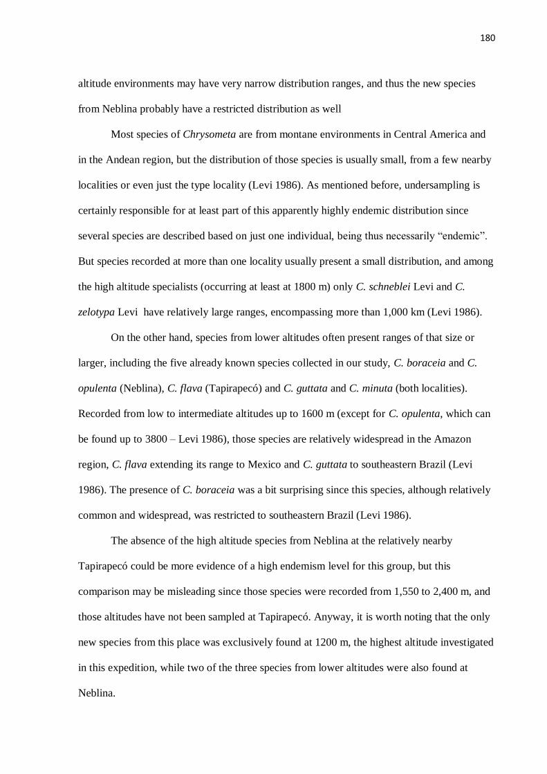
180
altitude environments may have very narrow distribution ranges, and thus the new species
from Neblina probably have a restricted distribution as well
Most species of Chrysometa are from montane environments in Central America and
in the Andean region, but the distribution of those species is usually small, from a few nearby
localities or even just the type locality (Levi 1986). As mentioned before, undersampling is
certainly responsible for at least part of this apparently highly endemic distribution since
several species are described based on just one individual, being thus necessarily “endemic”.
But species recorded at more than one locality usually present a small distribution, and among
the high altitude specialists (occurring at least at 1800 m) only C. schneblei Levi and C.
zelotypa Levi have relatively large ranges, encompassing more than 1,000 km (Levi 1986).
On the other hand, species from lower altitudes often present ranges of that size or
larger, including the five already known species collected in our study, C. boraceia and C.
opulenta (Neblina), C. flava (Tapirapecó) and C. guttata and C. minuta (both localities).
Recorded from low to intermediate altitudes up to 1600 m (except for C. opulenta, which can
be found up to 3800 – Levi 1986), those species are relatively widespread in the Amazon
region, C. flava extending its range to Mexico and C. guttata to southeastern Brazil (Levi
1986). The presence of C. boraceia was a bit surprising since this species, although relatively
common and widespread, was restricted to southeastern Brazil (Levi 1986).
The absence of the high altitude species from Neblina at the relatively nearby
Tapirapecó could be more evidence of a high endemism level for this group, but this
comparison may be misleading since those species were recorded from 1,550 to 2,400 m, and
those altitudes have not been sampled at Tapirapecó. Anyway, it is worth noting that the only
new species from this place was exclusively found at 1200 m, the highest altitude investigated
in this expedition, while two of the three species from lower altitudes were also found at
Neblina.

181
The pattern reported in our work indicates that Chrysometa communities along
altitudinal gradients are characterized by widespread species occupying low and intermediate
altitudes, replaced by small-ranged, possibly endemic species at higher altitudes. As
documented above, the distribution of other species of the genus suggests that this pattern
may be common for Chrysometa communities in mountain regions.
Similar patterns are relatively common for taxa whose distributions encompass
mountain regions (birds - Bates & Zink 1994, Fjeldsa & Rahbek 2006, beetles - Cook 2002,
Escobar et al. 2006, and butterflies - Hall 2005), and quite a few hypotheses have been
proposed or even tested to explain the origin of mountain biota. Hypotheses proposed range
from colonization process through long distance dispersal (Lobo & Halffter 2000, Escobar et
al. 2006) to passive transportation to higher altitudes by mountain uplifts (Hall 2005, Ribas et
al. 2007), with speciation being a consequence of the isolation of higher altitude populations,
either by migration or simply by vicariance. It is also worth noting that the high diversity of
Chrysometa at high altitude environments, with several sympatric species is unusual and at
least partly in disagreement with both models, which predict a smaller richness at higher
altitudes (colonization model), or an allopatric distribution of high altitude species (passive
transportation and vicariance model). But, once again, those questions cannot be assessed
with distributional data, and a phylogenetic approach would be necessary to accordingly
unveil the evolutionary history of the genus as well as the process responsible for the
observed distribution of Chrysometa. Anyway, it seems to reinforce the fact that the genus
posses a great affinity to high altitude environments, probably based on a higher tolerance to
colder climates, an unusual feature for most neotropical spiders.
As a final remark, we can note that the large number of new species reported in our
study, as well as the fact that only two species of Chrysometa were previously known for the
Guayana Shield highlights that the spider fauna from this region is extremely undersampled.

182
Renowned for the high degree of endemism of its flora (Berry et al. 1995), the peculiar
geography of the Guayana Shield, with several high altitude habitats (the tepuis and other
mountain ranges) isolated from each other by lowland forests and savanna, seems especially
suitable to harbor a very diverse and endemic fauna of Chrysometa, and new expeditions will
certainly provide several new species of this interesting genus.
Acknowledgments
We are grateful to Adalberto Santos and Charles Griswold for their relevant comments
on early versions of the manuscript. We are also indebted to Ricardo Braga-Neto, Nancy Lo-
Man-Hung and David Candiani, for their invaluable help in the field. The first author is
grateful to Humberto Yamaguti, for his help preparing the study area map, and to Aline
Benetti, for help with the literature. The first author also thanks the PPGEco-INPA, the 5°PEF
Maturacá, a frontier squad from the Brazilian army, the IBAMA/ICMBio and PARNA Pico
da Neblina for the collecting license, and FUNAI and the Ayrca, a local Yanomami
association, for receiving use at the Yanomami Indigenous Land. A.A. Nogueira was
supported by a doctoral fellowship from “Conselho Nacional de Desenvolvimento Científico
e Tecnológico (CNPq)”, a BECA-IEB/Moore Foundation (B/2007/01/BDP/01) fellowship
and a grant from World Conservation Society (WCS). Fernando Alvarez-Padilla, Alexandre
B. Bonaldo and Gustavo Hormiga made valuable comments and correction to an earlier
version of this paper.
References
Almeida-Neto, A., Machado, G., Pinto-da-Rocha, R. & Giaretta, A.A. (2006) Harvestman
(Arachnida:Opiliones) species distribution along three Neotropical elevational gradients: an
alternative rescue effect to explain Rapoport’s rule? Journal of Biogeography, 33, 361-375.

183
Alvarez-Padilla, F. (2007) Systematics of the spider genus Metabus O. P.-Cambridge, 1899
(Araneoidea: Tetragnathidae) with additions to the tetragnathid fauna of Chile and comments
on the phylogeny of Tetragnathidae. Zoological Journal of the Linnean Society, 151, 285–
335.
Álvarez-Padilla, F., Dimitrov, D., Giribet, G., Hormiga, G. (2009). Phylogenetic relationships
of the spider family Tetragnathidae (Araneae, Araneoidea) based on morphological and DNA
sequence data. Cladistics, 25, 109-146.
Avalos, G., Damborsky, M. P., Bar, M. E., Oscherov E. B. & Porcel, E. (2009) Composición
de la fauna de Araneae (Arachnida) de la Reserva provincial Iberá, Corrientes, Argentina.
Revista de Biología Tropical, 57 (1-2), 339-351.
Baldissera, R., Ganade, G. & Fontoura, S. B. (2004) Web spider community response along
an edge between pastures and Araucaria forest. Biological Conservation, 118, 403-409.
Bates, J. M. & Zink, R. M. (1994) Evolution into the Andes: molecular evidence for species
relationships in the genus Leptopogon. Auk, 111, 507–515.
Berry, P. E., Huber, O. & Holst, B. K. (1995) Introduction. In: Berry, P. E., Holst, B. K. &
Yatskievych, K. (Eds.) Flora of the Venezuelan Guayana, 1, Missouri Botanical Garden
Press, St. Louis, 161-191.
Blanco-Vargas, E., Amat-Garcia, G. D. & Florez-Dáza, E. (2003) Araneofauna orbitelar
(Araneae: Orbiculariae) de los Andes de Colombia: comunidades en habitats bajo
regeneración. Revista Ibérica de Aracnología, 7, 189-203.
Bonaldo, A. B., Carvalho, L. S., Pinto-da-Rocha, R., Tourinho, A. L., Miglio, L. T., Candiani,
D. F., Lo Man Hung, N. F., Abrahim, N., Rodrigues, B. V. B., Brescovit, A. D., Saturnino, R.,
Bastos, N. C., Dias, S. C., Silva, B. J. F., Pereira-Filho, J. M. B., Rheims, C.A., Lucas, S. M.,
Polotow, D., Ruiz, G. R. S. & Indicatti, R. P. (2009) Inventário e História Natural dos
Aracnídeos da Floresta Nacional de Caxiuanã, Pará, Brasil. In: Lisboa, P. L. B. (Org.)
Caxiuanã: desafios para a conservação de uma Floresta Nacinal da Amazônia, Museu
Paraense Emílio Goeldi, Belém, 545-588.
Borges, S. H. & Brescovit, A. D. (1996) Inventário preliminar da aracnofauna (ARANEAE)
de duas localidades na amazônia ocidental. Boletim do Museu Paraense Emílio Goeldi, série
Zoologia, 12(1), 9-21.
Brescovit, A. D., Bertani, R., Pinto-da-Rocha, R. & Rheims, C. A. (2004) Aracnídeos da
Estação Ecológica Juréia–Itatins: inventário preliminar e história natural. In: Marques, O. A.
V. & Duleba, W. (Eds.) Estação Ecológica Juréia-Itatins: Ambiente físico, flora e fauna.
Holos, Ribeirão Preto, 198-221.
Brown, J. (2001) Mammals on mountainsides: elevational patterns of diversity. Global
Ecology and Biogeography, 10, 101–109.
Cook, J. (2002) A revision of the neotropical genus Cryptocanthon Balthasar (Coleoptera:
Scarabaeidae: Scarabaeinae). The Coleopterist Society Monographs, Patricia Vaurie Series
56, 1–96.

184
Dias, S. C., Brescovit, A. D., Couto E. C. G. & Martins C. F. (2006) Species richness and
seasonality of spiders (Arachnida, Araneae) in an urban Atlantic Forest fragment in
Northeastern Brazil. Urban Ecosystems 9, 323–335.
Escobar, F., Lobo, J. M. & Halffter, G. (2006) Assessing the origin of Neotropical mountains
dung beetle assemblages (Scarabaeidae: Scarabaeinae): the comparative influence of vertical
and horizontal colonization. Journal of Biogeography, 33, 1793-1803.
Fjeldsa, J. & Rahbek, C. (2006) Diversification of tanagers, a species rich bird group, from
lowlands to montane regions of South America. Integrative and Comparative Biology, 46 (1),
72-81.
Ferreira-Ojeda, l. & Florez-Daza, E. (2007) Arañas orbitelares (Araneae: Orbiculariae) em
tres formaciones vegetales de la Sierra Nevada de Santa Marta (Magdalena, Colombia).
Revista Ibérica de Aracnología,16, 3-16
Ferreira-Ojeda, L., Florez-Daza, E. & Sabogal-Gonzalez, A. (2009) Bosque húmedo
subtropical de La Sierra Nevada de Santa Marta (Magdalena, Colombia). Caldasia 31(2),
381-391.
Hall, J. P. W. (2005) Montane speciation patterns in Ithomiola butterflies (Lepidoptera:
Riodinidae): are they consistently moving up in the world? Proceedings of the Royal Society
B, 272, 2457–2466.
Höfer, H. & Brescovit, A. D. (2001) Species and guild structure of a Neotropical spider assemblage (Araneae) from Reserva Ducke, Amazonas, Brazil. Andrias, 15, 99-119.
Huber, O. (1995a) Geographical and physical features. In: Berry, P. E., Holst, B. K. &
Yatskievych, K. (Eds.) Flora of the Venezuelan Guayana, I. Introduction. Missouri Botanical
Garden Press, St. Louis, 1─ 61.
Huber, O. (1995b) Vegetation. In: Berry, P.E., Holst, B.K. & Yatskievych, K. (Eds) Flora of
the Venezuelan Guayana, I. Introduction. Missouri Botanical Garden Press, St. Louis, pp.
67─160.
Keyserling, E. (1863) Beschreibungen neuer Spinnen. Verhandlungen der Zoologisch-
Botanischen Gesellschaft in Wien, 13, 369-382.
Levi, H.W. (1986) The Neotropical orb-weaver genera Chrysometa and Homalometa
(Araneae: Tetragnathidae). Bulletin of the Museum of Comparative Zoology, Harvard
University, 151, 91–215.
Lobo, J. M. & Halffter, G. (2000) Biogeographical and ecological factors affecting the
altitudinal variation of mountainous communities of coprophagous beetles (Coleoptera,
Scarabaeoidea): a comparative study. Annals of the Entomological Society of America, 93,
115–126.
Lomolino, M.K. (2001) Elevation gradients of species-density: historical and prospective
views. Global Ecology and Biogeography, 10: 3-13.

185
Moritz, C., Patton, J. L., Schneider, C. J. & Smith, T. B. (2000) Diversification of rainforest
faunas: an integrated molecular approach. Annual Review of Ecology and Systematics, 31,
533–563.
Nogueira, A. A., Pinto-da-Rocha, R., & Brescovit, A. D. (2006) Comunidade de aranhas
orbitelas (Arachnida-Araneae) na região da Reserva Florestal do Morro Grande, Cotia, São
Paulo, Brasil. Biota Neotropica, 6(2), 1-24.
Peres, M. C. L., Silva, J. M. C. & Brescovit, A. D. (2007) The influence of treefall gaps on
the distribution of web-building and ground hunter spiders in an Atlantic Forest remnant,
northeastern Brazil. Studies on Neotropical Fauna and Environment, 42(1), 49–60.
Platnick, N. I. (2010) The world spider catalog, version 10.5. American Museum of Natural
History. Available from: http://research.amnh.org/entomology/spiders/catalog/index.html
Podgaiski, L. R., Ott, R., Rodriguez, E. N. L., Buckup, E. H. & Marquez, M. A. L. (2007)
Araneofauna (Arachnida: Araneae) do Parque Estadual do Turvo, Rio Grande do Sul, Brasil.
Biota Neotropica, 7(2).
RADAM (1978) Folha NA19. Pico da Neblina. Ministério das Minas e Energia. Rio de
Janeiro.
Raizer, J., Japyassu, H. F., Indicatti, R. P. & Brescovit, A. D. (2005) Comunidade de aranhas
(Arachnida, Aranea) do Pantanal do Norte (Mato Grosso, Brasil) e sua similaridade com a
araneofauna amazônica. Biota Neotropica, 5(1a).
Rego, F. N. A. A., Venticinque, E. M., Brescovit, A.D., Rheims, C. A. & Albernaz, A. L. K.
M. (2009) A contribution to the knowledge of the spider fauna (Arachnida: Araneae) of the
floodplain forests of the main Amazon River channel. Revista Ibérica de Aracnologia 97, 85-
96.
Ribas, C. C., Moyle, R. G. , Miyaki, C. Y. & Cracaft, J. (2007) The assembly of montane
biotas: linking Andean tectonics and climatic oscillations to independent regimes of
diversification in Pionus parrots. Proceedings of the Royal Society B, 274, 2399–2408.
Ricetti, J. & Bonaldo, A. B. (2008) Diversidade e estimativas de riqueza de aranhas em quatro
fitofisionomias na Serra do Cachimbo, Pará, Brasil. Iheringia, v. 98(1), 88-99.
Romo, M. I. & Florez-Daza, E. (2009) Comunidad de arañas orbitelares (Araneae:
Orbiculariae) asociada al bosque altoandino Del santuário Flora y Fauna Galeras, Nariño,
Colombia. Boletín Científico Museo de Historia Natural, 13 (1), 114 - 126
Silva, D. & Coddington, J. A. (1996) Spiders of Pakitza (Madre de Dios, Perú): species
richness and notes on community structure. In: Wilson, D. E. & Sandoval, A. (Eds.) Manu-
The biodiversity of Southeastern Perú. Smithsonian Institution Press, Washington, 253-311.
Simkova, A., Gelnar, M. & Sasal, P. (2001) Aggregation of congeneric parasites
(Monogenea: Dactylogyrus). Parasitology, 123, 599-607.

186
Simon, E. (1895) Histoire naturelle des araignées. Paris, 1: 761-1084
Valencia, J. C. & Florez-Daza, E. (2007) Arañas tejedoras: uso de difeentes microhábitats em
um bosque andino de Colombia. Revista Ibérica de Aracnologia, 14, 39-48.
Veetas, O. R. & Grytnes, J. A. (2002) Distribution of vascular plants species richness and
endemic richness along the Himalayan elevation gradient in Nepal. Global Ecology and
Biogeography, 11, 291–301.

187
Tables
Altitude (m.a.s.l.) 100 400 860 1550 2000 2400 Total by specie and WAM N° altitudes
relative abudance(%) m.a.s.l. present
Species Chrysometa petrasierwaldae sp.nov. 137 137 (40.8) 2400 1
Chrysometa nubigena sp.nov. 62 34 96 (28.6) 2142 2
Chrysometa lomanhungae sp.nov. 2 1 3 (0.9) 2133 2
Chrysometa sp. sp.nov. 1 1 (0.3) 2000 1
Chrysometa santosi sp.nov. 1 1 (0.3) 2000 1
Chrysometa ericclaptoni sp.nov. 3 3 (0.9) 2000 1
Chrysometa waikoxi sp.nov. 41 41 (12.2) 1550 1
Chrysometa Boracéia 6 6 (1.8) 1550 1
Chrysometa opulenta 1 4 29 34 (10.1) 1435 3
Chrysometa guttata 4 4 (1.2) 860 1
Chrysometa candianii sp.nov. 3 3 (0.9) 860 1
Chrysometa minuta 1 2 4 7 (2.1) 620 3
Total by altitude
Abundance 1 3 15 76 69 172 336
Richness 1 2 4 3 5 3 12 mean WAM
Relative importance (%)
Chrysometa 2032
Abundance 0.15 0.51 2.10 12.54 23.39 66.93 10.67 All spiders 765
Richness 0.61 0.71 2.29 3.45 9.09 15.00 2.52
Table 1. Chrysometa species from the Pico da Neblina. Distribution of species in six altitudes, weighted average altitudinal midpoint (WAM)
and number of altitudes in which each species were recorded. We also present the relative abundance of each species in relation to the total
abundance of the genus, and the relative importance of the richness and abundance of the genus in relation to the total spider richness and

188
abundance (unpublished data), for each altitude. Species have been ordered in decreasing way based in their WAM. In the lower right corner we
also present the mean WAM of the genus and the WAM of the total spider community (unpublished data).

189
Table 2. Chrysometa species from the Serra do Tapirapecó. Distribution of species in four
altitudes, weighetd average altitudinal midpoint (WAM) and number of altitudes in which
each species were recorded. We also present the relative abundance of each species in relation
to the total abundance of the genus, and the relative importance of the abundance of the genus
in relation to the total spider abundance (unpublished data), for each altitude. Species have
been ordered in decreasing way based in their WAM. In the lower right corner we also present
the mean WAM of the genus
Altitude (m .a .s .l.) 1 8 0 4 0 0 8 0 0 1 2 0 0 Tota l by WAM N° a ltitudes
s pec ie pres ent
S pec ies 8 8 1 2 0 0 1
C hry s om e ta m inuta 7 4 1 1 5 4 5 2
C hry s om e ta flav a 1 1 2 4 9 0 2
C hry s om e ta guttata 4 1 1 3 1 1 9 4 5 9 4
Tota l by a ltitude
Abunda nce 5 1 8 8 9 4 0
R ichnes s 2 2 3 2 4 m ea n WAM
R ela tive im porta nce (% ) C hry s om e ta 6 3 3
Abunda nce 0 ,9 5 4 ,0 1 2 ,5 6 2 ,6 8 2 ,4 6
C hry s om e ta s ac ii n. s p.

190
Chrysometa
Study Localitiy Environment N° sites
sampled
Altitude (m.a.s.l.) Sampling methods * Focal group N of
adults
Richness Abundance (% of
total abundance)
Andes
Blanco-Vargas et al. 2003 EED El Rasgón Santander,
Colombia
oak and riparian, Andean forests 2 High (2200-2400) NMAS, DMAS Orb-weavers 2608 10 357 (13.7)
Ferreira-Ojeda & Florez 2007 Sierra Nevada de Santa Marta,
Magdalena, Colombia
Tropical very dry forest,
Subtropical humid forest,
Subtropical very humid forest
3 Low to
intermediate (100,
900 and 1300)
NMAS, BT, SN Orb-weavers 1755 3 145 (8.3)
Valencia & Florez-Daza 2007 PNN Chingaza, Cundinamarca,
Colombia
Andean upper-montane forest 1 High (3130) NMAS, EMAS, BT,
SN
Web-spiders 1354 1 352 (26)
Ferreira-Ojeda et al. 2009 Sierra Nevada de Santa Marta,
Magdalena, Colombia
Subtropical humid forest 1 Intermediate (900) NMAS, DMAS, BT,
SN
Orb-weavers 496 1 49 (9.9)
Romo & Florez 2009 SFFG, Nariño, Colombia Forest, Shrubs, Grasslands 3 High (3320-3470) NMAS, DMAS Orb-weavers 453 4 288 (63.6)
Amazon Lowlands
Borges & Brescovit 1996 Mamirauá and Tefé, AM, Brazil Flooded and Terra Firme forest 2 Low NMAS, BT All spiders 649 none none
Silva & Coddington 1996 Paktiza, Peru Seven forest types 7 Low (356) NMAS, DMAS, BT Understory
spiders
2616 6 15 (0.6)
Höfer & Brescovit 2001 RF Adolpho Ducke, AM, Brazil Terra Firme Forest n.i. Low (80-140) NMAS, BT, FOG, PIT,
LIT, GE, TE,
LITERAT
All spiders n.i. 5 n.i.
Ricetti & Bonaldo 2008 Serra do Cachimbo, PA, Brazil Open rainforest, Riparian forest,
Arboreal savanna, White sand
vegetation
4 Intermediate (700) NMAS, BT, SN, LIT All spiders 2750 none none
Bonaldo et al. 2009 FLONA de Caxiuanã, PA, Brazil Terra Firme Forest 14 low (<100) NMAS, BT, SN, PIT,
W
All spiders 4768 1 1 (0.02)
Rego et al. 2009 AM and PA, Brazil Flooded Forest 26 low (<100) NMAS, BT All spiders 4142 none none
South and southeastern Brazil
Northern Argentina
Baldissera et al. 2004 FN São Francisco de Paula, RS,
Brazil
Pasture, border and Araucaria
forest
1 Low DMAS Web-spiders 836 1 3 (0.4)
Brescovit et al. 2004 ESEC Juréia, SP, Brazil Coastal Atlantic Forest 3 Low NMAS, BT, PIT, LIT All spiders n.i. 3 n.i.
Nogueira et al. 2006 RF Morro Grande, SP, Brazil Mature and secondary, Montane
Atlantic forest
16 Intermediate (850-
1100)
NMAS Orb-weavers 3148 6 351 (11.1)
Podgaiski et al. 2007 PE do Turvo, RS, Brazil Subtropical decidous, Atlantic
Forest
2 Low NMAS, BT, PIT, W All spiders 2946 2 37 (1.2)
Avalos et al. 2009 Iberá province reserve,
Corrientes, Argentina
Grassland, Hygrophilous
woodland
3 Low NMAS, BT, SN, PIT,
LIT
All spiders 3808 2 n.i.
Central and northeastern Brazil
Raizer et al. 2005 North Pantanal, MT, Brazil Riparian forest, Secondary forest 6 Low NMAS, BT All spiders 601 2 2 (0.3)
Dias et al. 2006 Mata do Buraquinho, PB, Brazil Atlantic Forest 1 Low NMAS, BT, PIT All spiders 1681 1 n.i.
Peres et al. 2007 RESEC Dois Irmãos, PE, Brazil Atlantic forest, Treefall gaps 1 Low DMAS, PIT All spiders 1996 2 3 (0.1)

191
Table 3. Neotropical spider inventories. Authors and year of the study, locality, environment, number and altitude of sites sampled, collecting
methods, focal group, total spider abundance, and richness and abundance of Chrysometa. In brackets we present the relative abundance of the
genus in relation with total abundance. n.i. No information available. *Methods: NMAS – nocturnal manual active searching, DMAS – diurnal
manual active searching, EMAS – manual active searching on epyphytics, BT – beating tray, SN – sweeping net, PIT – pitfall trap, LIT – litter
searching, W – Winkler extractor, FOG – canopy fogging, GE – ground eclector, TE – trunk eclector, LITERAT – information from literature.

192
Figures
FIGURES 1. Study area. A) South America; B) Northern South America (rectangle of map A
enlarged). The mountain range at the left of the map represents the northern part of the
Andes, and the mountainous region in the center of the map is the Guayana Shield,
showing the study area in its southern part; C) Closer view of the study area (rectangle
of map B enlarged), showing the two sampled sites, the Pico da Neblina (red circle)
and the Serra do Tapirapecó (blue triangule). The white line represents the boundary
between Brazil and Venezuela.

193
FIGURES 2A-E. Chrysometa nubigena n. sp. A. Male palpus, ventral view. B. Same,
retrolateral view. C. Epigynum, ventral view. D. Same, posterior view. E. Same, dorsal
view. Scale bars: AB, 0.3 mm; CDE, 0.1 mm.

194
FIGURES 3A-E. Chrysometa saci n. sp. A. Male palpus, ventral view. B. Same, retrolateral
view. C. Epigynum, ventral view. D. Same, posterior view. E. Same, dorsal view. Scale
bars: AB, 0.3 mm; CDE, 0.5 mm.

195
FIGURES 4A-E. Chrysometa waikoxi n. sp. A. Male palpus, ventral view. B. Same,
retrolateral view. C. Epigynum, ventral view. D. Same, posterior view. E. Same, dorsal
view. Scale bars: AB, 0.3 mm; CDE, 0.1 mm.

196
FIGURES 5A-E. Chrysometa petrasierwaldae n. sp. A. Male palpus, ventral view. B. Same,
retrolateral view. C. Epigynum, ventral view. D. Same, posterior view. E. Same, dorsal
view. Scale bars: AB, 0.3 mm; CDE, 0.1 mm.
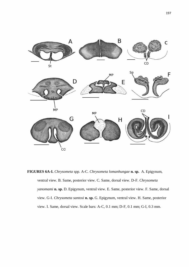
197
FIGURES 6A-I. Chrysometa spp. A-C. Chrysometa lomanhungae n. sp. A. Epigynum,
ventral view. B. Same, posterior view. C. Same, dorsal view. D-F. Chrysometa
yanomami n. sp. D. Epigynum, ventral view. E. Same, posterior view. F. Same, dorsal
view. G-I. Chrysometa santosi n. sp. G. Epigynum, ventral view. H. Same, posterior
view. I. Same, dorsal view. Scale bars: A-C, 0.1 mm; D-F, 0.1 mm; G-I, 0.3 mm.

198
FIGURES 7A-D. Chrysometa spp. AB. Chrysometa candianii n. sp. A. Male palpus, ventral
view. B. Same, retrolateral view. CD. Chrysometa minuta (Keyserling). C. Male
palpus, ventral view. D. Same, retrolateral view. Scale bars: AB, 0.5mm; CD, 0.5 mm.

199
SÍNTESE
O nosso estudo representa a pesquisa mais completa realizada sobre a distribuição de
aranhas ao longo de um gradiente altitudinal tropical, devido ao número de altitudes
amostradas, ao esforço amostral, e à abrangência do grupo estudado, uma vez que
trabalhamos com toda a fauna de solo e subosque, o que inclui a maioria das espécies de
aranha.
Os nossos resultados apresentaram algumas características já observadas em trabalhos
similares com outros grupos taxonômicos e que são consideradas típicas de faunas montanas,
como uma grande diversidade alfa e beta ao longo do gradiente. Em outros casos, nossos
resultados revelaram padrões inesperados, e todas as hipóteses testadas baseadas em teorias
biogeográficas, como o Efeito do Domínio Central e o Efeito Rapoport foram refutadas. Outro
achado que pode ser considerado surpreendente foi que, ao menos em alguns casos, as
mudanças na composição da fauna de aranhas ao longo do gradiente não estiveram
diretamente relacionadas às mudanças observadas na vegetação.
De maneira sintética, nosso trabalho aponta como principais características da
comunidade de aranhas amostrada no Pico da Neblina uma grande riqueza e diversidade. E,
no que diz respeito à distribuição das espécies e indivíduos ao longo do gradienete, o principal
resultado foi a relação negativa entre esses parâmetros da comunidade e a altitude.
A queda monotônica da riqueza com a altitude esteve longe de se ajustar ao previsto
pela Hipótese das Restrições Geométricas (Efeito do Domínio Central), que espera uma maior
riqueza nas partes intermediárias do gradiente. Isso também representa um padrão encontrado
recorrentemente na literatura, o que inclui os principais trabalhos realizados até então com
aranhas ao longo de gradientes altitudinais. No entanto, acreditamos que nossos resultados
podem ser mais representativos da distribuição altitudinal de aranhas devido à sua maior
abrangência taxonômica e desenho amostral mais detalhado. Também é necessário comentar
que alguns dos trabalhos sobre aranhas mencionados acima foram realizados em ambientes
temperados, o que também pode explicar a diferença em relação aos nossos resultados,
obtidos em uma localidade tropical.
Nossos resultados também se ajustam a um modelo climático altitudinal que ressalta a
importância do ambiente no padrão altitudinal da distribuição da riqueza. De acordo com esse
modelo, em montanhas localizadas em locais úmidos, como no caso do presente estudo,

200
espera-se uma diminuição gradual da riqueza com o aumento da altitude. Embora o modelo
tenha sido baseado nos resultados de um grande número de trabalhos com vertebrados, o
ajuste com nossos dados mostra que ele pode ser mais abrangente.
Uma outra característica marcante da comunidade por nós amostrada foi a pequena
distribuição altitudinal da maioria das espécies, que só foi encontrada em uma ou duas
altitudes. Consideramos que essa distribuição restrita foi diretamente responsável por uma
série de resultados do trabalho, uma vez que as distribuições previstas tanto pela Hipótese das
Restrições Geométricas quanto pelo Efeito Rapoport parecem ocorrer com maior freqüência
em comunidades cujas espécies possuam em média uma maior área de distribuição.
A pequena distribuição das espécies também teve como conseqüência grandes
mudanças na composição, como pôde ser observado nos altos valores de diversidade beta.
Como gradientes altitudinais representam gradientes acentuados, com mudanças ambientais
importantes em distâncias relativamente pequenas, biotas amostradas em gradientes
altitudinais realmente costumam apresentar grandes mudanças na composição.
O agrupamento das altitudes amostradas em função da composição de sua fauna de
aranhas revelou três grupos principais, um de locais mais baixos que incluía as três primeiras
altitudes, um formado pelas duas localidades mais altas, e a quarta altitude ficou disposta em
uma posição isolada e intermediária entre esses dois grupos. Esse resultado não está
totalmente de acordo com a divisão altitudinal proposta para a região da área de estudo, uma
vez que nossa comunidade de áreas baixas distribui-se além do limite proposto.
Por fim, o gênero Chrysometa, estudado em maior detalhe, forneceu alguns exemplos
dos padrões mais gerais relatados ao longo do trabalho. A maioria das espécies teve
distribuições restritas ao longo do gradiente, e pudemos observar mudanças importantes na
composição. Os maiores valores de diversidade beta estiveram relacionados à maior ruptura
ambiental existente no gradiente, entre a quarta e a quinta altitude, quando se passa de
ambientes florestais para formações vegetais mais abertas.
A análise da distribuição altitudinal desse gênero, no local de estudo e também em
uma escala maior, com o auxílio da literatura, indicam que as espécies que ocorrem em maior
altitude possuem uma distribuição mais restrita que as espécies de locais mais baixos. Isso
sugere um maior grau de endemismo para as espécies da parte superior do gradiente, um
padrão já ressaltado para outros grupos estudados em ambientes montanos. A teoria também

201
prevê maiores taxas de especiação no alto de gradientes altitudinais, e, embora nossos dados
não permitam testar essa afirmação diretamente, nós efetivamente coletamos um grande
número de espécies novas desse gênero, e a maioria delas estava nas partes mais altas da
montanha.
Em suma, nosso trabalho revelou uma comunidade rica e diversa, e bastante sensível
as mudanças do gradiente. A grande diversidade beta indica que a maioria das espécies está
adpatada à uma faixa restrita e específica do gradiente, sendo que a quantidade de espécies
que consegue ocupar as partes mais altas da montanhas vai caindo gradualmente.

202
REFERÊNCIAS BIBLIOGRÁFICAS
Albernaz, A. L. K. M. 2009. A contribution to the knowledge of the spider fauna (Arachnida:
Araneae) of the floodplain forests of the main Amazon River channel. Rev. Ibérica Aracnol.
97: 85-96.
Almeida-Neto, M.; Machado, G.; Pinto-da-Rocha, R.; Giaretta, A.A. 2006. Harvestman
(Arachnida: Opiliones) species distribution along three Neotropical elevational gradients: an
alternative rescue effect to explain Rapoport’s rule? J. Biogeogr.; 33: 361–375.
Álvares, E. S. S. E, Machado, O.; Azevedo C. S. De-Maria, M.. 2004. Composition of the
spider assemblage in a urban forest reserve in Southeastern Brazil and evalution of a two
sampling method protocols of species richness estimates. Rev. Ibérica Aracnol.; 10: 185-194.
Alvarez-Padilla, F. 2007. Systematics of the spider genus Metabus O. P.-Cambridge, 1899
(Araneoidea: Tetragnathidae) with additions to the tetragnathid fauna of Chile and comments
on the phylogeny of Tetragnathidae. Zool. J. Linn. Soc. 151: 285–335.
Álvarez-Padilla, F.; Dimitrov, D.; Giribet, G.; Hormiga, G. 2009. Phylogenetic relationships
of the spider family Tetragnathidae (Araneae, Araneoidea) based on morphological and DNA
sequence data. Cladistics, 25: 109-146.
Avalos, G.; Damborsky, M. P.; Bar, M. E.; Oscherov E. B.; Porcel, E. 2009. Composición de
la fauna de Araneae (Arachnida) de la Reserva provincial Iberá, Corrientes, Argentina. Rev.
Biol. Trop.; 57 (1-2): 339-351.
Bach, K.; Kessler, M.; Gradstein, S.R. 2007. A simulation approach to determine statistical
significance of species turnover peaks in a species-rich tropical cloud forest.Diversity
Distrib.; 13: 863–870
Baldissera, R.; Ganade, G.; Fontoura, S. B. 2004. Web spider community response along an
edge between pastures and Araucaria forest. Biol. Conserv. 118: 403-409.
Barthlott, W.; Lauer, W.; Placke, A. 1996. Global distribution of species diversity in vascular
plants: towards a world map of phytodiversity. Erdkunde, 50: 317–327.
Bateman, B.L.; Kutt, A.S.; Vanderduys, E.P.; Kemp, J.P. 2010. Small-mammal species
richness and abundance along a tropical altitudinal gradient: an Australian example. J. Trop.
Ecol.; 26: 139–149

203
Bates, J. M.; Zink, R. M. 1994. Evolution into the Andes: molecular evidence for species
relationships in the genus Leptopogon. Auk, 111: 507–515.
Beck, J.; Chey, V.K. 2008. Explaining the elevational diversity pattern of geometrid moths
from Borneo: a test of five hypotheses. J. Biogeogr.; 35: 1452–1464
Bellwood, D. R.; Hughes, T. P.; Connolly, S. R.; Tanner, J. 2005. Environmental and
geometric constraints on Indo-Pacific coral reef biodiversity. Ecol. Lett.; 8: 643–651.
Berger, W.H.; Parker, F.L. 1970. Diversity of planktonic foraminifera in deep-sea sediments.
Science 168:1345–134
Berry, P. E.; Riina, R. 2005. Insights into the diversity of the Pantepui flora and the
biogeographic complexity of the Guayana Shield. Biol. Skrif.; 55: 145–167.
Berry, P.E.; Huber, O.; Holst, B.K. 1995. Introduction. In: Berry, P.E.; Holst, B.K.;
Yatskievych, K. (Eds.) Floristic analysis and phytogeography. Flora of the Venezuelan
Guayana.; Vol 1. Missouri Botanical Garden Press, St Louis, MO. p. 161–191.
Bhattarai, K.R.; Vetaas, O.R.; 2006. Can Rapoport’s rule explain tree species richness along
the Himalayan elevational gradient, Nepal? Divers. Distrib. 12: 373–378.
Blackburn, T.M.; Gaston, K.J. 1996. Spatial patterns in the geographical range sizes of bird
species in the New World. Phil. Trans. Royal Society (Series B), 351: 897–912.kwell
Publishing Ltd
Blanco-Vargas, E.; Amat-Garcia, G. D.; Florez-Dáza, E. 2003. Araneofauna orbitelar
(Araneae: Orbiculariae) de los Andes de Colombia: comunidades en habitats bajo
regeneración. Rev. Ibérica Aracnol. 7: 189-203.
Bonaldo, A. B.; Carvalho, L. S.; Pinto-da-Rocha, R.; Tourinho, A. L.; Miglio, L. T.;
Candiani, D. F.; Lo Man Hung, N. F.; Abrahim, N.; Rodrigues, B. V. B.; Brescovit, A. D.;
Saturnino, R.; Bastos, N. C.; Dias, S. C.; Silva, B. J. F.; Pereira-Filho, J. M. B.; Rheims, C.A.;
Lucas, S. M.; Polotow, D.; Ruiz, G. R. S.; Indicatti, R. P. 2009. Inventário e História Natural
dos Aracnídeos da Floresta Nacional de Caxiuanã, Pará, Brasil. In: Lisboa, P. L. B. (Org.)
Caxiuanã: desafios para a conservação de uma Floresta Nacinal da Amazônia, Museu
Paraense Emílio Goeldi, Belém, pp. 545-588.
Bonaldo, A.B.; Dias, S.C. 2010. A structured inventory of spiders (Arachnida, Araneae) in
natural and artificial forest gaps at Porto Urucu. Western Br. Amazonia. 40(2): 357-372.

204
Bonaldo, A.B.; Rheims, C.A.; Brescovit, A.D. 2006. Four new species of Drymusa Simon
(Araneae, Drymusidae) from Brazilian Oriental Amazonia. Rev. Br. Zool. 23 (2): 455–359.
Borges, S. H.; Brescovit, A. D. 1996. Inventário preliminar da aracnofauna (ARANEAE) de
duas localidades na amazônia ocidental. Bol. M. Paraense Emílio Goeldi, série Zoologia,
12(1): 9-21.
Bosmans, R.; Maelfait, J.P.; De Kimpe, A. 1986. Analysis of the spider communities in an
altitudinal gradient in the French and Spanish Pyrenees. Bull British Arachnol. Soc.; 7: 69–76.
Bourdon, K.H.; Boyd, J.H.; Era, D.S.; Burns, B.J.; Thompson, J.W.; Locke, B.Z. 1988
Gender differences in phobias: results of the ECA community survey. J. Anxiety
Disorders.2(3):227–241.
Brehm, G.; Colwell, R.K.; Kluge, J. 2007. The role of environment and mid-domain effect on
moth species along a tropical elevational gradient. Global Ecol. Biogeogr, 16: 205–219.
Brehm, G.; Homeier, J. Fiedler, K. 2003. Beta diversity of geometrid moths (Lepidoptera:
Geometridae) in an Andean montane rainforest. Div. Distr., 9: 351–366.
Brehm, G.; Süssenbach, D.; Fiedler, K. 2003. Unique elevational diversity patterns of
geometrid moths in an Andean montane rainforest. Ecography, 26: 356–366.
Brehm, G.; Süssenbach, D.; Fiedler, K. 2004. Unique elevational diversity patterns of
geometrid moths in an Andean montane rainforest. J. Trop. Ecol., 20: 165–172.
Brescovit A.D.; Bonaldo, A.B.; Rheims, C.A. 2004. A new species of Drymusa Simon, 1891
(Araneae, Drymusidae) from Brazil. Zootaxa 697: 1–5.
Brescovit, A. D.; Bertani, R.; Pinto-da-Rocha, R.; Rheims, C. A. 2004. Aracnídeos da Estação
Ecológica Juréia–Itatins: inventário preliminar e história natural. In: Marques, O. A. V.;
Duleba, W. (Eds.) Estação Ecológica Juréia-Itatins: Ambiente físico, flora e fauna. Holos,
Ribeirão Preto, 198-221.
Brown, J.H 2001. Mammals on mountainsides: elevational patterns of diversity. Global Ecol.
Biogeogr.10: 101–109.
Brown, J.H. 1984. On the relationship between abundance and distribution of species. Am.
Nat.; 124: 255-279.
Brown, J.H.; Kodric-Brown, A. 1977. Turnover rates in insular Biogeogr: effect of
immigration on extinction. Ecology, 58: 445-449.

205
Callaway, R. M.; Brooker, R. W.; Choler, P.; Kikvidze, Z.; Lortiek, C. J.; Michalet, R.;
Paolini, L.; Pugnaireq, F. I.; Newingham, B.; Aschehoug, E.T.; Armasq, C.; Kikodze, D.;
Cook, B. J. 2002. Positive interactions among alpine plants increase with stress. Nature, 417:
844-848.
Cardelús, C.; Colwell, R. K.; Watkins Jr.; J. E. 2006. Vascular epiphyte distribution patterns:
explaining the mid-elevation richness peak. J. Ecology, 94: 144-156.
Carranza, A.; Colwell, R.K.; Rangel, T.F.L.V.B. 2008. Distribution of megabenthic
gastropods along environmental gradients: the mid-domain effect and beyond. Mar Ecol-Prog
Ser.; 367: 193-202.
Chatzaki, M.; Lymberakis, P.; Markakis, G.; Mylonas, M. 2005. The distribution of ground
spiders (Araneae, Gnaphosidae) along the altitudinal gradient of Crete, Greece: species
richness, activity and altitudinal range. J. Biogeogr, 32: 813–831.
Chettri, B.; Bhupathy, S.; Acharya, B.K. 2010. Distribution pattern of reptiles along an
eastern Himalayan elevation gradient, India. Acta Oecol.; 36: 16–22
Choi, S. W.; Jeong-Seop, N.A. 2010. Altitudinal distribution of moths (Lepidoptera) in Mt.
Jirisan National Park, South Korea. Eur. J. Entomol. 107: 229–245
Clarke, K. R. 1993. Non-parametric multivariate analyses of changes in community structure.
A. J. Ecol. 18:117– 143.
Coddington J.; Levi. H. 1991. Systematics and evolution of spiders (Araneae). Ann. Rev Ecol.
Syst. 22: 565-592.
Coddington, J.A.; Agnarsson, I.; Miller, J.A.; Kuntner, M.; Hormiga, G. 2009. Undersampling
bias: the null hypothesis for singleton species in tropical arthropod surveys. J. Anim. Ecol.;
78: 573–584
Coddington, J.A.; Griswold, C.E.; Silva, D.; Larcher, L. 1991. Designing and testing
sampling protocols to estimate biodiversity in tropical ecosystems. The Unity of Evolutionary
Biology: Proceedings of the Fourth International Congress of Systematic and Evolutionary
Biology, Dioscorides Press, Portland, Oregon. p. 44–60.
Colwell, R. K. 2006. RangeModel A Monte Carlo simulation tool for assessing geometric
constraints on species richness. Version 5. User's Guide and application.
(http://viceroy.eeb.uconn.edu/rangemodel). Acesso: 11/2010.

206
Colwell, R. K. 2008. RangeModel: Tools for exploring and assessing geometric constraints on
species richness (the mid-domain effect) along transects. Ecography, 31: 4-7.
Colwell, R. K. 2009. EstimateS: Statistical estimation of species richness and shared species
from samples. Version 8.2. User's Guide and application. (http://purl.oclc.org/estimates).
Acesso: 11/2010.
Colwell, R. K.; Rahbek, C.; Gotelli, N. J. 2004. The middomain effect and species richness
patterns; What have we learned so far? Am. Nat.; 163: E1–E23.
Colwell, R.K.; Coddington, J.A. 1994. Estimating terrestrial biodiversity through
extrapolation. Phil. Trans. Royal Soc., B, 345: 101–118.
Colwell, R.K.; Gotelli, N.J.; Rahbek, C.; Entsminger, G.L.; Farrell, C.; Graves, G.R. 2009.
Peaks, plateaus, canyons, and craters: the complex geometry of simple mid-domain effect
models. Evol. Ecol. Res.; 11: 355–370.
Colwell, R.K.; Hurtt, G.C. 1994. Nonbiological gradients in species richness and a spurious
Rapoport effect. Am. Nat.; 144: 570–595.
Colwell, R.K.; Lees, D.C. 2000. The mid-domain effect: geometric constraints on the
geography of species richness. Trends Ecol. Evol.; 15: 70–76.
Cook, J. 2002. A revision of the neotropical genus Cryptocanthon Balthasar (Coleoptera:
Scarabaeidae: Scarabaeinae). The Coleopterist Society Monographs, Patricia Vaurie Series
56: 1–96.
Currie, D.J.; Kerr, J.T. 2008. Tests of the mid-domain hypothesis: review of the evidence.
Ecol. Monogr.; 78(1): 3-18.
Davis, A.L.V.; Scholtz, C.H. Chown, S.L. 1999. Species turnover, community boundaries
and biogeographical composition of dung beetle assemblages across an altitudinal gradient in
South Africa. J. Biogeogr, 26: 1039–1055.
Deza, M.; Andia, J.M. 2009. Diversity and species richness of the family Araneidae
(Arachnida, Araneae) in Cicra (Madre de Dios – Peru). Ecología Aplicada, 8(2): 81-90.
Dias, S. C.; Brescovit, A. D.; Couto E. C. G.; Martins C. F. 2006. Species richness and
seasonality of spiders (Arachnida, Araneae) in an urban Atlantic Forest fragment in
Northeastern Brazil. Urban Ecos. 9: 323–335.

207
Diniz-Filho, J. A. F.;. Bini, L. M; Hawkins, B. A.. 2003. Spatial autocorrelation and red
herrings in geographical ecology. Global Ecol. Biogeogr, 12:53–64.
Doyle, A.C. 1912. The Lost World. Hodder Stoughton, New York.
Dufrêne, M.; Legendre, P. 1997. Species assemblages and indicator species: the need for a fl
exible asymetrical approach. Ecol. Monogr. 67: 345–366.
Dunn, R. R.; Colwell, R. K.; Nilsson, C. 2006. The river domain: Why are there more species
halfway up the river? Ecography, 29: 251–259.
Dunn, R.R.; McCain, C.M.; Sanders, N.J. 2007. When does diversity fit null model
predictions? Scale and range size mediate the mid-domain effect. Global Ecol. Biogeogr, 16:
305–312.
Edwards, J.S.; Thornton, W.B. 2001. Colonization of an island volcano, Long Island, Papua
New Guinea, and an emergent island, Motmot, in its caldera lake. VI. The pioneer arthropod
community of Motmot. J. Biogeog.; 28: 1379–1388.
Escobar, F.; Lobo, J. M.; Halffter, G. 2006. Assessing the origin of Neotropical mountains
dung beetle assemblages (Scarabaeidae: Scarabaeinae): the comparative influence of vertical
and horizontal colonization. J. Biogeogr.33: 1793-1803.
Fasham, M.J.R. 1977. A comparison of nometric multidimentsional scaling, principal
components and reciprocal averaging for the ordination of simulated coenoclines, and
coenoplanes. Ecology 58: 551-561
Ferreira-Ojeda, L.; Florez-Daza, E. 2007. Arañas orbitelares (Araneae: Orbiculariae) em tres
formaciones vegetales de la Sierra Nevada de Santa Marta (Magdalena, Colombia). Rev.
Ibérica Aracnol.; 16: 3-16.
Ferreira-Ojeda, L.; Florez-Daza, E.; Sabogal-Gonzalez, A. 2009. Bosque húmedo subtropical
de La Sierra Nevada de Santa Marta (Magdalena, Colombia). Caldasia 31(2): 381-391.
Fjeldsa, J.; Rahbek, C. 2006. Diversification of tanagers, a species rich bird group, from
lowlands to montane regions of South America. Integrative and Comparative Biology, 46 (1):
72-81.
Fleishman, E.; Austin, G.T.; Weiss, A.D. 1998. An empirical test of Rapoport’s rule:
elevational gradients in montane butterfly communities. Ecology, 79: 2482–2493.
Foelix, R.F. 1996. Biology of spiders. Oxford University Press, Oxford.

208
Fortes R.R.; Absalão, R.S. 2004. The applicability of Rapoport’s rule to the marine molluscs
of the Americas. J. Biogeogr, 31: 1909–1916.
Fu, C.; Hua, X.; Li, J.; Chang, Z.; Pu, Z.; Chen, J. 2006. Elevational patterns of frog species
richness and endemic richness in the Hengduan Mountains, China: geometric constraints, area
and climate effects. Ecography, 29: 919-927.
García-López A.; Micó, E.;Numa, C.; Galante, E. 2010. Spatiotemporal Variation of Scarab
Beetle Assemblages (Coleoptera: Scarabaeidae: Dynastinae, Melolonthinae, Rutelinae) in the
Premontane Rain Forest in Costa Rica: A Question of Scale. Ann. Entomol. Soc. Am. 103(6):
956-964.
Gaston, K.J.; Blackburn, T.M.; Spicer, J.I. 1998. Rapoport’s rule: time for an epitaph? Trends
Ecol. Evol.n, 13: 70–74.
Gentry, A.H. 1988. Changes in plant community diversity and floristic composition on
environmental and geographical gradients. Ann,.Missouri Bot. G., 75: 1–34.
Ghalambor, C.K.; Huey, R.B.; Martin, P.R.; Tewksbury, J.J.; Wang, G. 2006. Are mountain
passes higher in the tropics? Janzens hypothesis revisited. Integr. Comp. Biol.; 46: 5–17.
Gotelli, N.; Colwell, R. K. 2001. Quantifying biodiversity: Procedures and pitfalls in the
measurement and comparison of species richness. Ecol. Lett.; 4: 379-391.
Grau, O.; Grytnes, J.A.; Birks, H.J.B. 2007. A comparison of altitudinal species richness
patterns of bryophytes with other plant groups in Nepal, Central Himalaya. J. Biogeogr.; 34:
1907–1915.
Greenstone, M.H. 1984. Determinants of web spider species diversity: vegetation structural
diversity vs. prey availability. Oecologia, 62: 299 – 304.
Grytnes, J.A.; Beaman J.H.; Romdal, T.S.; Rahbek.; C. 2008. The mid-domain effect matters:
simulation analyses of range-size distribution data from Mount Kinabalu, Borneo J. Biogeogr,
35: 2138–2147.
Grytnes, J.A.; Vetaas, O.R. 2002. Species richness and altitude: a comparison between null
models and interpolated plant species richness along the Himalayan altitudinal gradient,
Nepal. Am. Nat.; 159: 294–304.
Halaj, J.; Ross, D.W.; Moldenke, A. R. 1998. Habitat structure and prey availability as
predictors of the abundance and community.

209
Hall, J. P. W. 2005. Montane speciation patterns in Ithomiola butterflies (Lepidoptera:
Riodinidae): are they consistently moving up in the world? P. Roy. Soc. B, 272: 2457–2466.
Hammer, O.; Harper, D.A.T.; Ryan, P. D. 2001. PAST: Paleontological Statistics Software
Package for Education and Data Analysis. Palaeontol Electronica 4(1): 9pp.
Hatley, C.L.; MacMahon, J.A. 1980. Spider community organization: seasonal variation and
the role of vegetation architecture. Envir. Entomol. 9: 632-639.
Hawkins, B. A. 2001. Ecology’s oldest pattern? Trends Ecol. Evol.; 16: 470.
Hawkins, B. A.; Diniz-Filho, J. A. F.; Weis, A. E. 2005. The middomain effect and diversity
gradients: is there anything to learn? Am. Nat.; 166: E140–E143.
Hill, M. O. 1973. Diversity and evenness: a unifying notation and its consequences. Ecology,
54: 427-432.
Höfer, H.; Brescovit, A.D. 2001. Species and guild structure of a Neotropical spider
assemblage (Araneae) from Reserva Ducke, Amazonas, Brazil. Andrias, 15: 99-119.
Höfer, H.; Brescovit, A.D.; Gasnier, T. 1994. The wandering spiders of the genus Ctenus
(Ctenidae, Araneae) of Reserva Ducke, a rainforest reserve in central Amazonia. Andrias
13:81–98.
Hubbell, S.P. 2001. The Unified Neutral Theory of Biodiversity and Biogeography.
Monographs in Population Biology 32. Princeton University Press, Princeton, NJ.
Huber, O. 1995. Geographical and physical features. In: Berry, P.E.; Holst, B.K.;
Yatskievych, K. (Eds). Flora of the Venezuelan Guayana. Missouri Botanical Garden Press,
St. Louis, p. 1-60.
Huber, O. 1995. Vegetation. In: Berry, P.E.; Holst, B.K.; Yatskievych, K. (Eds). Flora of the
Venezuelan Guayana. Missouri Botanical Garden Press, St. Louis, p. 67─160.
Huber, O. 1995a. Geographical and physical features. In: Berry, P. E.; Holst, B. K.;
Yatskievych, K. (Eds.) Flora of the Venezuelan Guayana, I. Introduction. Missouri Botanical
Garden Press, St. Louis, pp. 1─ 61.
Huber, O. 1995b. Vegetation. In: Berry, P.E.; Holst, B.K.; Yatskievych, K. (Eds) Flora of the
Venezuelan Guayana, I. Introduction. Missouri Botanical Garden Press, St. Louis, pp.
67─160.

210
Hurlbert, A.H. 2004. Species–energy relationships and habitat complexity in bird
communities. Ecol. Lett., 7: 714–720
IBGE, 2010. Instituto Brasileiro de geografia e Estatística. In: http://www.ibge.gov.br
Jankowski, J.E.; Ciecka, A.L.; Meyer, N.Y. & Rabenold, K.N (2009) Beta diversity along
environmental gradients: implications of habitat specialization in tropical montane landscapes
J. Anim. Ecol.; 78: 315–327
Janzen, D.H. 1967. Why mountain passes are higher in the tropics? Am. Nat.; 101: 233–249.
Janzen, D.H.; Ataroff, M.; Farinas, M.; Reyes, S.; Rincon, N.; Soler, A.; Soriano, P.; Vera, M.
1976.Changes in the arthropod community along an elevational transect in the Venezuelan
Andes. Biotropica, 8: 193–203.
Jetz, W.; Rahbek, C. 2001. Geometric constraints explain much of the species richness pattern
in African birds. Proc. Nat. Ac. Sciences (USA), 98: 5661–5666.
Jetz, W.; Rahbek, C.;.Colwell, R.C. 2004. The coincidence of rarity and richness and the
potential signature of history in centres of endemism. Ecol. Lett. 7: 1180–1191.
Jill, E.; Jankowski, A. L.; Ciecka, N.; Meyer, Y.; Rabenold, K.N. 2009. Beta diversity along
environmental gradients: implications of habitat specialization in tropical montane
landscapes. J. An. Ecol. 78 , 315–327
Jiménez-Valverde, A.; Baselga, A.S.; Melic, A.; Txasko, N . 2010. Climate and regional beta-
diversity gradients in spiders: dispersal capacity has nothing to say? Insect Conserv. Div. 3:
51–60
Jocqué, R,; Samu, F.; Bird, T. 2005. Density of spiders (Araneae: Ctenidae) in Ivory Coast
rainforests. J. Zool.; Lond266: 105–110
Jost, L. 2006. Entropy and diversity. Oikos, 113: 363-375.
Jost, L. 2007. Partitioning diversity into independent alpha and beta components. _ Ecology
88: 2427-2439.
Kapoor, V. 2008. Effects of rainforest fragmentation and shade-coffee plantations on spider
communities in the Western Ghats, India. J Insect Conserv, 12:53–68
Kenkel, N. C. Orloci, L. 1986. Applying metric and nonmetric multidimensional scaling to
Ecol. studies: some new results. Ecology 67:919–928.

211
Keyserling, E. 1863; Beschreibungen neuer Spinnen. Verhandlungen der Zoologisch-
Botanischen Gesellschaft in Wien, 13: 369-382.
Kluge, J.; Kessler, M.; Dunn, R. R. 2006. What drives elevational patterns of diversity? A test
of geometric constraints, climate and species pool effects for pteridophytes on an elevational
gradient in Costa Rica. Global Ecol. Biogeogr, 15: 358–371.
Koleff, P. 2003a. Measuring beta diversity for presence and absence data. J. Anim. Ecol. 72:
367_382.
Kruskal J.B. 1964. Nonmetric multidimensional scaling: a numerical method. Psychometrika
29: 115-129.
Laurie, H.; Silander, J. A. J. 2002. Geometric constraints and spatial patterns of species
richness: critique of rangebased models. Divers. Distrib.; 8: 351–364.
Levi, H.W. 1986. The Neotropical orb-weaver genera Chrysometa and Homalometa
(Araneae: Tetragnathidae). B. M. Comp. Zool.; Harvard University, 151: 91–215.
Levi, H.W. 1988. The neotropical orb-weaving spiders of the genus Alpaida (Araneae:
Araneidae). Bull. Mus. Comp. Zool. 151: 365-487.
Levi, H.W. 1991. The neotropical and mexican species of the orb-weaver
genera Araneus, Dubiepeira, and Aculepeira (Araneae: Araneidae). Bull. Mus. Comp. Zool.
152: 167-315.
Levi, H.W. 1999. The neotropical and mexican orb weavers of the genera Cyclosa and
Allocyclosa (Araneae: Araneidae). Bull. Mus. Comp. Zool. 155: 299-379.
Levi, H.W. 1992. Spiders of the orb-weaver genus Parawixia in America (Araneae:
Araneidae). Bull. Mus. Comp. Zool. 153: 1-46.
Lieberman, D.; Lieberman, M.; Peralta, R. Hartshorn, G.S. 1996. Tropical forest structure
and composition on a largescale altitudinal gradient in Costa Rica. J. of Ecology, 84: 137–
152.
Liew, T.S.; Schilthuizen, M.; Bin Laki, M. 2010. The determinants of land snail diversity
along a tropical elevational gradient: insularity, geometry and niches. J. Biogeogr, 37 (6):
1071–1078.

212
Lobo, J. M.; Halffter, G. 2000. Biogeographical and Ecol. factors affecting the altitudinal
variation of mountainous communities of coprophagous beetles (Coleoptera, Scarabaeoidea):
a comparative study. Ann. Entomol. Soc. Am. 93: 115–126.
Lo-Man-Hung,N. F.; Gardner, T.B.; Ribeiro-Júnior, M.A.:Barlow, J.; Bonaldo, A.B.. 2008.
The value of primary, secondary, and plantation forests for Neotropical epigeic arachnids. J.
Arachnol. 36:394–401
Lomolino, M.K. 2001. Elevation gradients of species-density: historical and prospective
views. Global Ecol. Biogeogr.10: 3-13.
MacNally, R.; Fleishman, E.; Bulluck, L.P. Betrus, C.J. 2004. Comparative influence of
spatial scale on beta diversity within regional assemblages of birds and butterflies. J.
Biogeogr, 31: 917–929.
Maguire, B. 1955. Cerro de la Neblina, Amazonas, Venezuela: A newly discovered sandstone
mountain. Geogr. Rev.; 45: 27-51.
Manhart, C. 1994. Spiders on bark in a tropical rainforest (Panguana, Peru). St. N. Fauna
Environ. 29(1): 49-53.
McCain, C.M. 2005. Elevational gradients in diversity of small mammals. Ecology, 86: 366–
372.
McCain, C.M. 2007a. Area and mammalian elevational diversity. Ecology, 88: 76–86.
McCain, C.M. 2007b. Could temperature and water availability drive elevational species
richness patterns? A global case study for bats. Global Ecol. Biogeogr.; 16: 1–13.
McCain, C.M. 2009a. Global analysis of bird elevational diversity. Global Ecol. Biogeogr.;
18: 346–360.
McCain, C.M. 2009b. Vertebrate range sizes indicate that mountains may be higher in the
tropics. Ecol. Lett.; 12: 550–560
McCain, C.M. 2010. Global analysis of reptile elevational diversity. Global Ecol. Biogeogr.;
19: 541 -553.
McCormick, S.; Polis, G. A. 1982. Arthropods that prey on vertebrates. Biol. Rev. Cambridge
Phil. Soc. 57:29‐58.
McCoy, E.D. 1990. The distribution of insects along elevational gradients. Oikos, 58: 313–
322.

213
McCune, B.; Mefford, M.J. 1999. PC-ORD: Multivariate Analysis of Ecol. Data. Version
5·12. MjM Software, Gleneden Beach, OR, USA.
McDiarmid, R. W.; Donnelly, M. A. 2005. Herpetofauna of the Guyana Highlands:
Amphibians and Reptiles of the Lost World. In: Donnelly, M. A.; Crother, B. I.;Guyer, C.;
Wake, M. H.; White, M. E. (Eds.). Ecology and Evolution in the Tropics - A Herpetological
Perspective. The Univestity of Chicago Press. Chicago, EUA. 584 pp.
McGill, B. J.; Etienne, R. S.; Gray, J. S.; Alonso, D.; Anderson, M. J.; Benecha, H. K.;
Dornelas, M.; Enquist, B. J.; Green, J. L.; He F.; Hurlbert, A. H.; Magurran, A. E.; Marquet,
P. A.; White E. P. 2007. Species abundance distributions: moving beyond single prediction
theories to integration within an Ecol. framework. Ecol. Lett, 10, 995–1015.
Melo, A. S.; Rangel, T. F. L. V. B.; Diniz-Filho. J. A.F. 2009. Environmental drivers of beta-
diversity patterns in New-World birds and mammals. Ecography, 32: 226–236.
Moreno, R.A.; Rivadeneira, M.M.; Hernández C.E.; Sampértegui, S.; Rozbaczylo, N. 2008.
Do Rapoport’s rule, the mid-domain effect or the source–sink hypotheses predict bathymetric
patterns of polychaete richness on the Pacific coast of South America? Global Ecol.
Biogeogr.; 17: 415–423.
Moritz, C.; Patton, J. L.; Schneider, C. J.; Smith, T. B. 2000. Diversification of rainforest
faunas: an integrated molecular approach. Annu. Rev. Ecol. Syst.; 31: 533–563.
Nogue´s-Bravo, D.; Araújo M. B.; Romdal, T.; Rahbek, C. 2008. Scale effects and human
impact on the elevational species richness gradients. Nature, 453: 216-220.
Nogueira, A. A.; Pinto-da-Rocha, R.; Brescovit, A. D. 2006. Comunidade de aranhas
orbitelas (Arachnida-Araneae) na região da Reserva Florestal do Morro Grande, Cotia, São
Paulo, Brasil. Biota Neotropica, 6(2): 1-24.
Olson, D.M. 1994. The distribution of leaf litter invertebrates along a Neotropical altitudinal
gradient. J. Trop. Ecol.; 10: 129–150.
Orme, C.D.L.; Davies, R.G.; Burgess, M.; Eigenbrod, F.; Pickup, N.; Olson, V.A. 2005.
Global hotspots of species richness are not congruent with endemism or threat. Nature,
436:1016–1019.
Otto, C.; Svensson, B.S. 1982. Structure of communities of ground-living spiders along
altitudinal gradients. Holarctic Ecol.; 5: 35–47.

214
Patterson, B.D.; Stotz, D.F.; Solari, S.; Fitzpatrick, J.W. 1998. Contrasting patterns of
elevational zonation for birds and mammals in the Andes of southeastern Peru. J. Biogeogr,
25: 593–607.
Pearce, J.L.; Venier, L.A.; Eccles, G.; Pedlar, J.; McKenney, D. 2004. Influence of habitat and
microhabitat on epigeal spider (Araneae) assemblages in four stand types. Biodivers. Conserv.
13: 1305–1334.
Peres, M. C. L.; Silva, J. M. C.; Brescovit, A. D. 2007. The influence of treefall gaps on the
distribution of web-building and ground hunter spiders in an Atlantic Forest remnant,
northeastern Brazil. Stud Neotrop. Fauna E.; 42(1): 49–60.
Pinto-da-Rocha, R.; Bragagnolo, C.; DaSilva, M.B. 2005. Faunistic similarity and historic
biogeography of the harvestmen of southern and southeastern Atlantic Rain Forest of Brazil. J
Arachnol, 33(2): 290-299.
Pinto-Leite, C. M.; Guerrero, A.C.; Brazil, T.K. 2008. Non-random patterns of spider species
composition in an Atlantic rainforest. J. Arachnol. 36:448–452
Pires, J.M.; Prance, T.G. 1985. The vegetation types of the Brazilian Amazon. In: Prance,
G.T.; Lovejoy, T.E. (Eds.). Key environments: Amazonia. Pergamon Press. Oxford. p:109-
145.
Platnick, N.I. 2010. The world spider catalog, version 11.0. American Museum of Natural
History (http://research.amnh.org/entomology/spiders/catalog/index.html). Acesso: 10/2010.
Podgaiski, L. R.; Ott, R.; Rodriguez, E. N. L.; Buckup, E. H.; Marquez, M. A. L. 2007.
Araneofauna (Arachnida: Araneae) do Parque Estadual do Turvo, Rio Grande do Sul, Brasil.
Biota Neotropica, 7(2).
RADAM. 1978. Folha NA19. Pico da Neblina. Ministério das Minas e Energia. Rio de
Janeiro.
Rahbek, C. 2005. The role of spatial scale and the perception of large-scale species-richness
patterns. Ecol. Lett.; 8: 224– 239.
Raizer, J.; Japyassu, H. F.; Indicatti, R. P.; Brescovit, A. D. 2005. Comunidade de aranhas
(Arachnida, Aranea) do Pantanal do Norte (Mato Grosso, Brasil) e sua similaridade com a
araneofauna amazônica. Biota Neotropica, 5(1a).

215
Rangel, T.F.L.V.B.; Diniz-Filho, J. A.F.; Bini, L.M. 2010. SAM: a comprehensive
application of spatial analyses in ecology. Ecography, 33: 46-50.
Rangel, T.F.L.V.B.; Diniz-Filho, J.A.F. 2005. Neutral community dynamics, the mid-domain
effect and spatial patterns in species richness. Ecol. Lett.; 8: 783–790.
Rapoport, E. H. 1975. Areografia: estrategias geograficas de las especies. Fondo de Cultura
Economica, Mexico.
Rego, F, N. A. A.; Venticinque, E. M.; A. D. Brescovit. 2007. Effects of forest fragmentation
on fourCtenus spider populations (Araneae: Ctenidae) in central Amazonia, Brazil. Stud.
Neotrop. Fauna E.; 42(2): 137–144.
Rego, F.N.A.A.; Venticinque, E.M.; Brescovit, A.D.; Rheims, C.A.; Albernaz, A.L.K.M.
2009. A contribution to the knowledge of the spider fauna (Arachnida: Araneae) of the
floodplain forests of the main Amazon River channel. Rev. Ibérica Aracnol. 97: 85-96.
Ribas, C. C.; Moyle, R. G. , Miyaki, C. Y.; Cracaft, J. 2007. The assembly of montane biotas:
linking Andean tectonics and climatic oscillations to independent regimes of diversification in
Pionus parrots. P. Roy. Soc. B, 274:2399–2408.
Ribas, C. R.; Schoereder, J. H. 2006. Is the Rapoport effect widespread? Null models
revisited. Global Ecol. Biogeogr.; 15: 614–624.
Ricetti, J.; Bonaldo, A. B. 2008. Diversidade e estimativas de riqueza de aranhas em quatro
fitofisionomias na Serra do Cachimbo, Pará, Brasil. Iheringia, 98(1): 88-99.
Robinson, J.V. 1981. The effect of architectural variation in habitat on a spider community:
an experimental fiel study. Ecology. 62 (1): 73-80.
Rohde, K. 1996. Rapoport’s rule is a local phenomenon and cannot explain latitudinal
gradients in species diversity. Biodivers. Lett.; 3: 10–13.
Rohde, K.; Heap, M.; Heap, D. 1993. Rapoport’s rule does not apply to marine teleosts and
cannot explain latitudinal gradients in species richness. Am. Nat.; 142: 1–16.
Romdal, T.S.; Grytnes, J.A. 2007. An indirect area effect on elevational species richness
pattern.s Ecography, 30: 440-448.
Romdal, T.S.; Colwell, R.K.; Rahbek, C. 2005. The influence of band sum area, domain
extent, and range sizes on the latitudinal mid-domain effect. Ecology, 86: 235–244.

216
Romo, M. I.; Florez-Daza, E. 2009. Comunidad de arañas orbitelares (Araneae: Orbiculariae)
asociada al bosque altoandino Del santuário Flora y Fauna Galeras, Nariño, Colombia. Boletín
Científico Museo de Historia Natural, 13 (1): 114 – 126.
Rosenberg, M. S. 2001. PASSAGE. Pattern Analysis, Spatial Statistics, and Geographic
Exegesis. Version 1.0. Department of Biology, Arizona State University, Tempe, AZ.
Rosenzweig, M.L. 1995. Species diversity in space and time. Cambridge University Press,
Cambridge.
Rull, V. 2004. An evaluation of the Lost World and the vertical displacement hypotheses in
the Chimant´a massif, Venezuelan Guayana. Global Ecol. Biogeogr. 13: 141–148.
Rull, V. 2005. Biotic diversification in the Guayana Highlands, a proposal. J. Biogeogr. 32:
921–927.
Rull, V.; Nogué S. 2007. Potential migration routes and barriers for vascular plants of the
Neotropical Guyana Highlands during the Quaternary. J. Biogeogr.34: 1327–1341.
Russel-Smith .H.; Stork, N.E. 1994. Abundance and diversity of spiders from the canopy of
tropical rainforests with particular reference to Sulawesi. Indonesia. J. Trop. Ecol.; 10: 545-
558.
Sanders, N.J. 2002. Elevational gradients in ant species richness: area, geometry, and
Rapoport’s rule. Ecography, 25: 25–32.
Sanders, N.J.; Lessard, J.P.; Fitzpatrick, M.C.; Dunn, R.R. 2007.Temperature, but not
productivity or geometry, predicts elevational diversity gradients in ants across spatial grains.
Global Ecol. Biogeogr.; 16: 640 -649.
Santos, A. J.; Nogueira, A. A. 2010. Three new species, new records and notes on the
nursery-web spider genus Architis in Brazil (Araneae: Pisauridae). Zootaxa, 1815: 51-61.
sbister, G.K.; White, J.; Currie, B.J.; Bush, S.P.; Vetter, R.S.; Warrel, D.A. 2005. Spider
bites: addressing mythology and poor evidence. A. J. Trop. Medicine Hygiene, 72(4):361-
367.
Scharff, N.; Coddington, J.A.; Griswold, C.E.; Hormiga, G.; Bjorn, P.D.P. 2003. When to
quit? Estimating spider species richness in a northern European deciduos forest. J. Arachnol.
31: 246-273.
217
Scharff, N.; Coddington, J.A.; Griswold, C.E.; Hormiga, G.; Bjorn, P.D.P. 2003. When to
quit? Estimating spider species richness in a northern European deciduos forest. J. Arachnol.
31: 246-273.
Sebastian, P.A.; Mathew, M.J.; Beevi, S.P.; Joseph, J.; Biju, C.R. 2005.The spider fauna of
the irrigated rice ecosystems in Central Kerala, India, across different elevational ranges. J.
Arachnol.; 33:247–255.
Silva, D. 1996. Species composition and community structure of peruvian rainforest spiders:
A case study from a seasonally inundated foresta long the Samiria river. Revue suisse de
Zoologie 597-610.
Silva, D.; Coddington, J. A. 1996. Spiders of Pakitza (Madre de Dios, Perú): species richness
and notes on community structure. In: Wilson, D. E.; Sandoval, A. (Eds.) Manu-The
biodiversity of Southeastern Perú. Smithsonian Institution Press, Washington, 253-311.
Silva, E.L.C.; Lise, A.A. 2010. Two new species and new records of Syntrechalea (Araneae:
Lycosoidea: Trechaleidae) from Brazil. Zoologia 27(3): 408–412.
Silva, W.A. 1999. Lendas e mitos dos índios brasileiros. São Paulo: FTD.
Simkova, A.; Gelnar, M.; Sasal, P. 2001. Aggregation of congeneric parasites (Monogenea:
Dactylogyrus). Parasitology, 123: 599-607.
Simon, E. 1895. Histoire naturelle des araignées. Paris, 1: 761-1084
Smouse, P.E.; Long, J.C.; Sokal, R.R .1986. Multiple regression and correlation extensions of
the Mantel test of matrix correspondence. Syst. Zool, 35: 627–632.
Soininen, J.; McDonald, R.; Hillebrand, H. 2007a. The distance decay of similarity in Ecol.
communities. Ecography, 30: 3–12.
Stevens, G.C. 1989. The latitudinal gradient in geographical range: how so many species
coexist in the tropics. Am. Nat.; 133: 240–256.
Stevens, G.C. 1992. The elevational gradient in altitudinal range: an extension of Rapoport’s
latitudinal rule to altitude. Am. Nat.; 140: 893–911.
Stevens, G.C. 1996. Extending Rapoport’s rule to marine fishes. J. Biogeogr.; 23: 149–154.
Steyermark, J.A. 1986. Speciation and endemism in the flora of the Venezuelan tepuis. High-
altitude tropical Biogeogr. F. Vuilleumier and M. Monasterio (Eds.), Oxford University
Press, Oxford. p. 317–373.

218
Storch, D.;Davies, R.G.; Zajicek, S.; Orme, C.D.L.; Olson, V.; Thomas, G.H.;Ding, T.S.;
Rasmussen, P.C.; Ridgely, R.S.; Bennett, P.M.; Blackburn, T.M.; Owens, I.P.F.; Gaston, K.J.
2006. Energy, range dynamics and global species richness patterns: reconciling mid-domain
effects and environmental determinants of avian diversity. Ecol. Lett.; 9: 1308–1320.
Toti, D.S.; Coyle, F.A.; Miller, J.A. 2000. A structured inventory of Appalachian grass bald
and heath bald spider asemlages and a test of species richness estimator performance. J.
Arachnol. 28: 329-345.
Turnbull, A.L. 1973. Ecology of the true spiders (Araneomorphae). Ann. Rev. Ent.; 18: 305-
348.
Valencia, J. C.; Florez-Daza, E. 2007. Arañas tejedoras: uso de difeentes microhábitats em um
bosque andino de Colombia. Rev. Ibérica Aracnol.14: 39-48.
VanDerWal, J.; Murphy, H.T.; Lovett-Doust, J. 2008. Three-dimensional mid-domain
predictions: geometric constraints in North American amphibian, bird, mammal and tree
species richness patterns. Ecography, 31: 435-449.
Vazquez, J. A. ; Givnish, T. J. 1998. Altitudinal gradients in tropical forest composition,
structure, and diversity in the Sierra de Manantla´n. J. Ecol. 86: 999-1020.
Veetas, O. R.; Grytnes, J. A. 2002. Distribution of vascular plants species richness and
endemic richness along the Himalayan elevation gradient in Nepal. Global Ecol. Biogeogr.11:
291–301.
von Humboldt A.1807. Essai sur la geographie de plantes. Paris
von Linnaeus, C. 1743. On the growth of the habitable earth. Select Dissetations from the
Amoenitates Academicae, I. London.
Vuilleumier, F. 1970. Insular biogeography in continental regions. Am.Nat. 104: 373 – 383.
Watkins, Jr.; J.E.; Cardelus, C.; Moran, R.; Colwell, R. K. 2006. Diversity and distribution of
ferns along an elevational gradient in Costa Rica. Am. J. Bot.; 93: 73-83.
Whittaker, R. H. 1960. Vegetation of the Siskiyou Mountains, Oregon and California. Ecol.
Monogr. 30: 279-338.
Whittaker, R. H.; Niering, W.A. 1965. Vegetation of the Santa Catalina Montains, Arizona: A
gradient analysis of the South Slope. Ecology, 46(4): 429-452.
Whittaker, R.H. 1967. Gradient analysis of vegetation. Biol. Rev.; 42: 207-264.

219
Wiens, J.J.; Donoghue, M.J. 2004. Historical Biogeogr, ecology and species richness. Trends
Ecol. Evol.; 19: 639–644.
Wiens, J.J.; Graham, C.H. 2005. Niche conservatism: integrating evolution, ecology, and
conservation biology. Annu. Rev. Ecol. Evol. S.; 36: 519–539.
Willard, D.E.; Foster, M.S.; Barrowclough, G.F.; Dickerman,R.W.; Cannell, P.F.; Coats, S.L.;
Cracraft, J.L.; O'Neill, J.P. 1991. The Birds of Cerro de la Neblina. Fieldiana, 65: 1-80.
Willdenow, K.L. 1805. The principles of botany and vegetable physiology. Blackwood,
Cadell and Davies, London.
Willig, M.R.; Kaufman, D.M.; Stevens, R.D. 2003. Latitudinal gradients of biodiversity:
pattern, process, scale and synthesis. . Annu. Rev. Ecol. Evol. S.; 34: 273–309.
Wolda, H. 1987. Altitude, habitat and tropical insect diversity. Biol. J. Linn. Soc.; 30: 313-
323.
Wu, F.; Yang, X. J.; Yang, J. X. 2010. Additive diversity partitioning as a guide to regional
montane reserve design in Asia: an example from Yunnan Province, China. Diversity Distrib
,16: 1022–1033
Zapata, F. A.; Gaston, K. J.; Chown, S. L. 2005. The middomain effect revisited. Am. Nat.;
166: E144–E148.
Zapata, F.A.; Gaston, K.J.; Chown, S.L. 2003. Mid-domain models of species richness
gradients: assumptions, methods and evidence. J. Anim. Ecol.; 72: 677–690.

220
Apêndice 1 – Ata da aula de qualificação
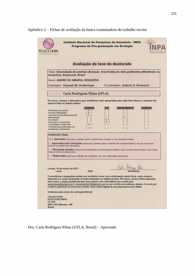
221
Apêndice 2 – Fichas de avaliação da banca examinadora do trabalho escrito
Dra. Carla Rodrigues Ribas (UFLA, Brasil) – Aprovada

222
Dr. Felipe Rego (UFMA, Brasil) – Aprovada

223
Dr. Nathan Sanders (Univ. Tenessee, EUA) – Aprovada com correções

224
Dr. Robert K. Colwell (Univ. Connecticut, EUA) – Aprovada

225
Dr. Gonçalo Ferraz (INPA/PDBFF, Brasil) – Reprovada

226
Apêndice 3 – Ata da defesa presencial