br phd dissertation
TRANSCRIPT
8/8/2019 BR PhD Dissertation
http://slidepdf.com/reader/full/br-phd-dissertation 1/248

8/8/2019 BR PhD Dissertation
http://slidepdf.com/reader/full/br-phd-dissertation 2/248
Copyright
Bart Raeymaekers, 2007
All rights reserved
8/8/2019 BR PhD Dissertation
http://slidepdf.com/reader/full/br-phd-dissertation 3/248
iii
The Dissertation of Bart Raeymaekers is approved, and it is acceptable in
quality and form for publication on microfilm:
____________________________________
____________________________________
____________________________________
____________________________________
Co-Chair
____________________________________
Chair
University of California, San Diego
2007
8/8/2019 BR PhD Dissertation
http://slidepdf.com/reader/full/br-phd-dissertation 4/248
iv
TABLE OF CONTENTS
Signature page................................................................................................................ iii
Table of Contents ........................................................................................................... iv
List of Symbols .............................................................................................................. ix
List of Figures ............................................................................................................ xviii
List of Tables ............................................................................................................. xxiv
Acknowledgments....................................................................................................... xxv
Vita…....................................................................................................................... xxviii
Publications................................................................................................................ xxix
Abstract ...................................................................................................................... xxxi
1. Introduction................................................................................................................. 1
1.1 Application and standards........................................................................................ 1
1.2 Working principle .................................................................................................... 3
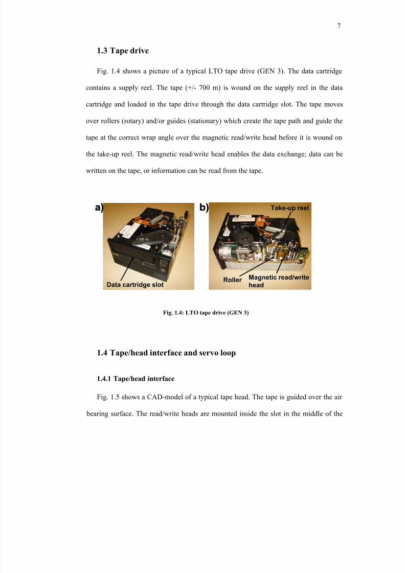
1.3 Tape drive ................................................................................................................ 7
1.4 Tape/head interface and servo loop.......................................................................... 7
1.4.1 Tape/head interface .............................................................................................. 7
1.4.2 Servo loop ............................................................................................................ 9
1.5 Channel and format................................................................................................ 11
1.6 Tape media............................................................................................................. 13
1.6.1 Recording density .............................................................................................. 13
1.6.2 Metal particulate versus metal evaporated tape ................................................. 15
1.7 Lateral tape motion ................................................................................................ 17
1.7.1 Definition ........................................................................................................... 17
1.7.2 Measurement...................................................................................................... 20
1.7.3 Sources of LTM ................................................................................................. 23
1.8 Dissertation outline ................................................................................................ 24
1.9 References.............................................................................................................. 25
8/8/2019 BR PhD Dissertation
http://slidepdf.com/reader/full/br-phd-dissertation 5/248
v
2. Non-contact tape tension measurement and correlation of lateral tape
motion and tape tension transients ................................................................................ 29
2.1 Introduction............................................................................................................ 29
2.2 Tension sensor........................................................................................................ 32
2.3 “Artificial” disturbance .......................................................................................... 33
2.4 Results.................................................................................................................... 34
2.5 Natural disturbance ................................................................................................ 38
2.6 Dependence of LTM on tension transient frequency............................................. 40
2.7 Discussion .............................................................................................................. 42
2.8 Conclusion ............................................................................................................. 48
2.9 Acknowledgements................................................................................................ 48
2.10 References............................................................................................................ 49
3. Characterization of tape edge contact with acoustic emission.................................. 51
3.1 Introduction............................................................................................................ 51
3.2 Acoustic emission .................................................................................................. 52
3.3 Calibration.............................................................................................................. 53
3.4 Detection of tape/flange contact............................................................................. 56
3.5 Impact between tape edge and flange .................................................................... 61
3.5 Discussion .............................................................................................................. 71
3.6 Conclusion ............................................................................................................. 72
3.7 Acknowledgements................................................................................................ 73
3.8 References.............................................................................................................. 73
4. Lateral motion of an axially moving tape on a cylindrical guide surface................. 75
4.1 Introduction............................................................................................................ 75
4.2 Theoretical study.................................................................................................... 77
4.3 Numerical solution................................................................................................. 81
4.3.1 Discretization ..................................................................................................... 81
4.3.2 Tape path and boundary conditions ................................................................... 83

8/8/2019 BR PhD Dissertation
http://slidepdf.com/reader/full/br-phd-dissertation 6/248
vi
4.4 Experimental validation and effect of bending stiffness........................................ 86
4.4.1 Apparatus ........................................................................................................... 86
4.4.2 Experimental results........................................................................................... 87
4.4.3 Tape versus string: the effect of bending stiffness............................................. 88
4.5 Effect of a guide in the tape path ........................................................................... 91
4.6 Discussion ............................................................................................................ 101
4.7 Conclusion ........................................................................................................... 103
4.8 Acknowledgements.............................................................................................. 104
4.9 Appendix.............................................................................................................. 104
4.10 References.......................................................................................................... 106
5. The influence of operating and design parameters on the magnetic
tape/guide friction coefficient ..................................................................................... 108
5.1 Introduction.......................................................................................................... 108
5.2 Theoretical model ................................................................................................ 111
5.2.1 Load sharing..................................................................................................... 111
5.2.2 Friction model .................................................................................................. 114
5.3 Experimental set-up ............................................................................................. 119
5.3.1 Apparatus ......................................................................................................... 119
5.3.2 Test specimens ................................................................................................. 121
5.3.3 Test procedure.................................................................................................. 123
5.4 Results and discussion ......................................................................................... 124
5.4.1 Theoretical results ............................................................................................ 124
5.4.2 Experimental results......................................................................................... 129
5.4.3 Model validation .............................................................................................. 134
5.5 Conclusion ........................................................................................................... 138
5.6 Acknowledgements.............................................................................................. 140
5.7 Appendix.............................................................................................................. 140
5.8 References............................................................................................................ 141
8/8/2019 BR PhD Dissertation
http://slidepdf.com/reader/full/br-phd-dissertation 7/248
vii
6. Enhancing tribological performance of the magnetic tape/guide interface by
laser surface texturing ................................................................................................. 144
6.1 Introduction.......................................................................................................... 144
6.2 Laser surface texturing......................................................................................... 145
6.3 Experimental set-up ............................................................................................. 147
6.3.1 Apparatus ......................................................................................................... 147
6.3.2 Test specimens ................................................................................................. 147
6.3.3 Test procedure.................................................................................................. 152
6.4 Experimental results and discussion .................................................................... 153
6.4.1 Metal particulate tape...................................................................................... 153
6.4.2 Metal evaporated tape ...................................................................................... 155
6.4.3 Tape/guide spacing........................................................................................... 159
6.5 Conclusion of the experimental analysis ............................................................. 161
6.6 Theoretical model ................................................................................................ 161
6.7 Results and discussion ......................................................................................... 167
6.7.1 Air bearing pressure......................................................................................... 167
6.7.2 Optimization of dimple geometry .................................................................... 169
6.7.3 Friction ............................................................................................................. 175
6.7.4 Numerical example .......................................................................................... 181
6.7.5 Transition speed estimation.............................................................................. 183
6.7.6 Discussion ........................................................................................................ 185
6.8 Conclusion ........................................................................................................... 186
6.9 Acknowledgements.............................................................................................. 187
6.10 References.......................................................................................................... 188
7. Design of a dual stage actuator tape head with high bandwidth track-
following capability .................................................................................................... 191
7.1 Introduction.......................................................................................................... 191
7.2 Concept of the dual-stage actuator head .............................................................. 193
7.3 Piezo-electricity.................................................................................................... 194

8/8/2019 BR PhD Dissertation
http://slidepdf.com/reader/full/br-phd-dissertation 8/248
viii
7.3.1 Principle ........................................................................................................... 194
7.3.2 Constitutive equation ....................................................................................... 195
7.4 Design of dual-stage actuator tape head............................................................... 197
7.5 Dynamics ............................................................................................................. 198
7.5.1 Static response.................................................................................................. 198
7.5.2 Dynamic response ............................................................................................ 200
7.6 Modeling of the frequency response function...................................................... 207
7.7 Conclusion ........................................................................................................... 209
7.8 Appendix.............................................................................................................. 209
7.9 References............................................................................................................ 210
8. Summary ................................................................................................................. 213
8/8/2019 BR PhD Dissertation
http://slidepdf.com/reader/full/br-phd-dissertation 9/248
ix
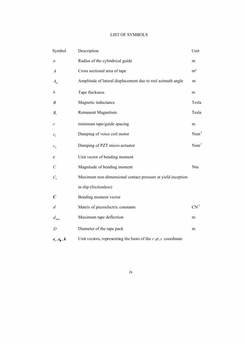
LIST OF SYMBOLS
Symbol Description Unit
a Radius of the cylindrical guide m
A Cross sectional area of tape m²
az A Amplitude of lateral displacement due to reel azimuth angle m
b Tape thickness m
B Magnetic inductance Tesla
r B Remanent Magnetism Tesla
c minimum tape/guide spacing m
1c Damping of voice coil motor Nsm
-1
2c Damping of PZT micro-actuator Nsm-1
c Unit vector of bending moment
C Magnitude of bending moment Nm
C ν Maximum non-dimensional contact pressure at yield inception
in slip (frictionless)
C Bending moment vector
d Matrix of piezoelectric constants CN-1
maxd Maximum tape deflection m
D Diameter of the tape pack m
, ,r e e k ϕ
Unit vectors, representing the basis of the , ,r z ϕ coordinate
8/8/2019 BR PhD Dissertation
http://slidepdf.com/reader/full/br-phd-dissertation 10/248
x
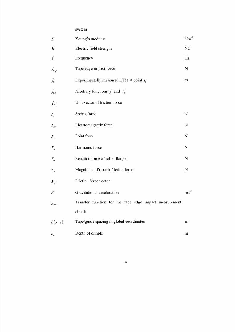
system
E Young’s modulus Nm-2
E Electric field strength NC-1
f Frequency Hz
imp f Tape edge impact force N
0 f Experimentally measured LTM at point 0 s m
1,2 f Arbitrary functions 1 f and 2 f
f f Unit vector of friction force
s F Spring force N
em F Electromagnetic force N
p F Point force N
a F Harmonic force N
0 F Reaction force of roller flange N
f F Magnitude of (local) friction force N
f F Friction force vector
g Gravitational acceleration ms-2
imp g Transfer function for the tape edge impact measurement
circuit
( ),h x y Tape/guide spacing in global coordinates m
ph Depth of dimple m
8/8/2019 BR PhD Dissertation
http://slidepdf.com/reader/full/br-phd-dissertation 11/248
xi
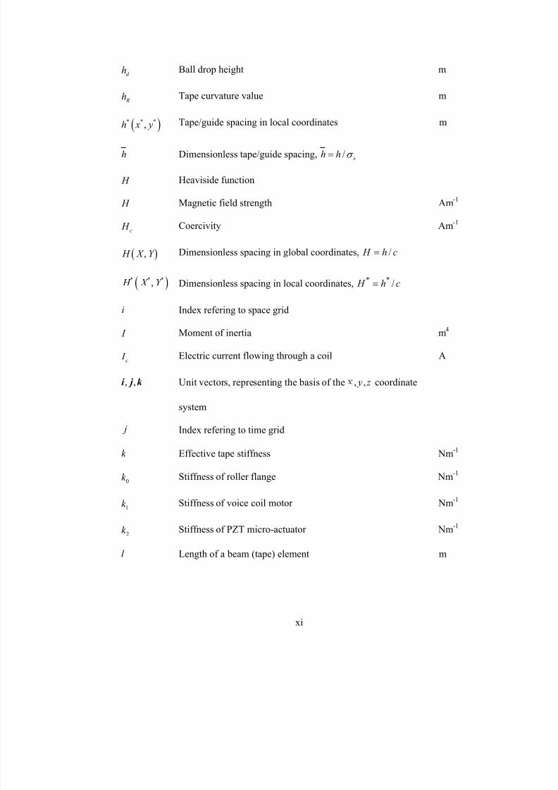
d h Ball drop height m
Rh Tape curvature value m
( )* * *
,h x y Tape/guide spacing in local coordinates m
h Dimensionless tape/guide spacing, / sh h σ =
H Heaviside function
H Magnetic field strength Am-1
c H Coercivity Am-1
( ), H X Y Dimensionless spacing in global coordinates, ch H /=
( )* * *, H X Y Dimensionless spacing in local coordinates, ch H /**=
i Index refering to space grid
I Moment of inertia m4
c I Electric current flowing through a coil A
, ,i j k Unit vectors, representing the basis of the , , y z coordinate
system
j Index refering to time grid
k Effective tape stiffness Nm-1
0k Stiffness of roller flange Nm
-1
1k Stiffness of voice coil motor Nm
-1
2k Stiffness of PZT micro-actuator Nm-1
l Length of a beam (tape) element m
8/8/2019 BR PhD Dissertation
http://slidepdf.com/reader/full/br-phd-dissertation 12/248
xii
cl Length of the coil m
L Position of flange m
C L Critical normal load at yield inception under frictional contact N
C L Normalized critical normal load at yield inception under
frictional contact, /C C C L L P =
1l Length along the tape centerline between 0
s and 1 s m
2l Length along the tape centerline between 1 s and 2 s m
3l Length along the tape centerline between 2 s and 3 s m
m Mass kg
0m , 2m , 4m Spectral moments of the surface roughness
M Position vector, describing the position of a point on the
centerline of the tape
n Number of contacting asperities
n Unit vector of normal force
N Magnitude of normal force, maximum tape/guide contact load
in the absence of any air bearing support
N
c N Number of windings on the coil
asp N Load portion carried by the contacting asperities N
aspdN Increment of load portion carried by the contacting asperities N
N Normal force vector
8/8/2019 BR PhD Dissertation
http://slidepdf.com/reader/full/br-phd-dissertation 13/248
xiii
( ), x y Air bearing pressure Nm-2
a Atmospheric pressure Nm-2
avg Average air bearing pressure Nm-2
( ), P X Y Dimensionless air bearing pressure, a p p P /=
asp P Normal load on one asperity N
C P Critical normal load at yield inception in slip (frictionless) N
P ∗ Dimensionless load on one asperity, / C P P L∗=
r Radius of the asperity tip m
1r Imaginary cell half length m
pr Dimple radius m
corr r Cross-correlation coefficient
R Radius of curvature m
s Laplace transform parameter
s Spatial coordinate along the tape centerline m
0 s Startpoint of the domain
1 s Point where the tape first contacts the guide
2 s Point where the tape comes off the guide
3 s Endpoint of the domain
ds Length of infinitesimal tape element m
s∆ Spatial grid stepsize m
8/8/2019 BR PhD Dissertation
http://slidepdf.com/reader/full/br-phd-dissertation 14/248
xiv
S Tape edge contact area m²
pS Dimple area density
E S Compliance matrix m²N-1
t Time s
t ∆ Time stepsize s
t Unit vector of tape tension
T Magnitude of (local) tape tension N
1T “Tight-side” tension N
2T “Slack-side” tension N
dT Infinitesimal tape tension change N
T ∆ Tape tension change N
T Tape tension vector
1u Actuation force of voice coil motor N
2u Actuation force of PZT micro-actuator N
U Tape speed ms-1
v Output voltage of acoustic emission sensor V
cv Induced voltage V
v Unit vector of shear force
V Magnitude of shear force N
V Shear force vector
w Width of tape m
8/8/2019 BR PhD Dissertation
http://slidepdf.com/reader/full/br-phd-dissertation 15/248
xv
, , y z Cartesian coordinate system
, ,r z ϕ Cylindrical coordinate system
, y Global coordinates m
sh y Position of the servo head m
st y Position of the servo track m
edge y Position of the tape edge m
var y Servo track variability m
* , * y Local coordinates m
X , Y Dimensionless global coordinates, pr x X /= , pr yY /=
* X , *Y Dimensionless local coordinate, pr x X /**= , pr yY /**
=
Y Yield strength Nm-2
α Angular coordinate RAD
d α Increment of angular coordinate RAD
az α Reel azimuth angle RAD
*α Spacing at which head/tape contact begins m
β Asperity load factor
* β Pressure required force zero spacing between the head and the
tape
Nm-2
γ Over-relaxation parameter
Γ Local non-dimensional tape tension (= * P ) /asp C P LΓ =
8/8/2019 BR PhD Dissertation
http://slidepdf.com/reader/full/br-phd-dissertation 16/248
xvi
2Γ Dimensionless “slack-side” tension
δ Dimensionless minimum tape/guide spacing, / 2 pc r δ =
ε Dimple aspect ratio, / 2 p ph r ε =
ε Strain vector
ζ Amplitude ratio
η Asperity density
θ Wrap angle RAD
λ Flow parameter, 3 / 2a p aU r pλ µ =
aλ Mean free path of air under atmospheric conditions m
µ (Isotropic) friction coefficient
aµ Air viscosity Nm-2
s
ϕ µ Friction coefficient in the circumferential direction
z µ Friction coefficient in the z-direction
ν Poisson’s ratio
ν Ratio of the friction coefficients in the circumferential and
vertical direction, / z ϕ ν µ µ =
ρ Tape density kgm-3
σ Stress, Stress wave Nm-2
σ Stress vector
sσ Standard deviation of asperity summit heights distribution m
8/8/2019 BR PhD Dissertation
http://slidepdf.com/reader/full/br-phd-dissertation 17/248
xvii
τ Variable of integration
τ Shear stress Nm-2
Φ Magnetic flux Wb
ψ Plasticity index
ψ Slope of tape with respect to a plane perpendicular to the z-
axis
RAD
ω Rotational frequency RADs-1
C ω Critical interference of a single asperity at yield inception
nω Natural frequency of tape element Hz
r ω Rotational frequency of tape reel Hz
8/8/2019 BR PhD Dissertation
http://slidepdf.com/reader/full/br-phd-dissertation 18/248
xviii
LIST OF FIGURES
Fig. 1.1: Magnetic tape recording: a) helical scan recording and b) linear
recording ......................................................................................................................... 1
Fig. 1.2: Magnetic hysteresis loop .................................................................................. 3
Fig. 1.3: Principle of magnetic tape recording................................................................ 6
Fig. 1.4: LTO tape drive (GEN 3)................................................................................... 7
Fig. 1.5: LTO tape head .................................................................................................. 8
Fig. 1.6: a) Detail of the air bearing surface and b) Read/write head module
(source: IBM).................................................................................................................. 9
Fig. 1.7: Enlarged view of data and servo track on a tape (source: IBM) ,
made visible by magnetic force microscopy (MFM).................................................... 10
Fig. 1.8: LTO tape structure.......................................................................................... 11
Fig. 1.9: LTO sub data band structure .......................................................................... 12
Fig. 1.10: LTO sub data band structure......................................................................... 13
Fig. 1.11: Evolution of the areal density....................................................................... 14
Fig. 1.12: Metal particulate tape ................................................................................... 16
Fig. 1.13: Metal evaporated tape................................................................................... 17
Fig. 1.14: LTM measurement a) fotonic edge sensor, b) PES signal and c)
magnetic signal.............................................................................................................. 22
Fig. 2.1: Lateral Tape Motion versus time.................................................................... 29
Fig. 2.2: Non-contact tape tension measurement a) Smith and Sievers and b)
Imaino ........................................................................................................................... 31
Fig. 2.3: Divergence of light beam as a result of a) tension T1 and b) tension
T2 ............................................................................................................................... 33
Fig. 2.4: Typical calibration curve ................................................................................ 33
Fig. 2.5: Schematic of test-set up .............................................................................................................................35
Fig. 2.6: LTM and tension, artificial disturbance.......................................................... 36
8/8/2019 BR PhD Dissertation
http://slidepdf.com/reader/full/br-phd-dissertation 19/248
xix
Fig. 2.7: Artificial disturbance, absolute values ...........................................................................................38
Fig. 2.8: Tension and LTM, natural disturbance........................................................... 39
Fig. 2.9: Natural disturbance, absolute values................................................................................................40
Fig. 2.10: Frequency study with an artificial disturbance............................................. 41
Fig. 2.11: Frequency study with a natural disturbance ................................................. 42
Fig. 2.12: Tape curvature ................................................................................................................................................43
Fig. 2.13: Tape motion as a result of tension transients................................................ 44
Fig. 2.14: Tape segment ................................................................................................ 45
Fig. 2.15: Non-uniform stress distribution ........................................................................................................46
Fig. 3.1: “Ball drop method” calibration procedure...................................................... 54
Fig. 3.2: Impact force calibration curve ..............................................................................................................55
Fig. 3.3: Experimental set-up........................................................................................ 56
Fig. 3.4: a) LTM, b) 1 kHz high pass filtered LTM and c) rms impact force,
versus time .................................................................................................................... 57
Fig. 3.5: a) rms impact force versus time b) time frequency analysis of LTM............. 58
Fig. 3.6: a) Experimentally measured average impact force versus supply reel
tape pack size, for a nominal tape tension of 1 N (solid lines) and 2 N (dashed
lines) and for different tape speeds ............................................................................... 59
Fig. 3.7: Tape reel misalignment................................................................................... 60
Fig. 3.8: a) Physical model and b) mathematical model............................................... 62
Fig. 3.9: a) Effective tape stiffness and b) belt-wrap force........................................... 65
Fig. 3.10: a) Axial run-out of supply reel for different pack diameters........................ 66
Fig. 3.11: Simulated average impact force versus supply reel tape pack size,
for a nominal tape tension of 1 N (solid lines) and 2 N (dashed lines) and for
different tape speeds...................................................................................................... 68
Fig. 3.12: Fig. 3.12: Simulated average impact force versus supply reel tape
pack size, for different values of Tsin( θ /2) and for a tape speed of a) 4 m/s, b)
8 m/s and c) 12 m/s ....................................................................................................... 70
8/8/2019 BR PhD Dissertation
http://slidepdf.com/reader/full/br-phd-dissertation 20/248
xx
Fig. 4.1: Tape on a cylindrical guide............................................................................. 78
Fig. 4.2: Experimental apparatus to measure LTM on a cylindrical guide................... 86
Fig. 4.3: Comparison of experimental measurements and numerical
predictions in the midspan of the cylindrical guide a) in time domain and b) in
frequency domain.......................................................................................................... 87
Fig. 4.4: Frequency spectrum for a tape and a string.................................................... 88
Fig. 4.5: Typical trajectory for tape and string for a guide with a) radius of
100 mm and b) radius of 10 mm. The friction coefficient is zµ = µ = 0.2ϕ .................. 89
Fig. 4.6: Maximum deviation from straightness for a) a guide with radius 100 mm and
b) a guide with radius 10 mm ( 0s = 20 µm and 3s = 0 µm, zµ = µ = 0.2ϕ ) .................. 90
Fig. 4.7: Amplitude ratio............................................................................................... 92
Fig. 4.8: Influence of the guide radius on the amplitude ratio as a function of
frequency....................................................................................................................... 93
Fig. 4.9: Influence of the wrap angle on the amplitude ratio as a function of
frequency....................................................................................................................... 94
Fig. 4.10: Influence of friction coefficient on amplitude ratio as a function of frequency
a) for a guide of radius 10 mm and b) for a guide of radius 100 mm ........................... 95
Fig. 4.11: Influence of tape speed on amplitude ratio as a function of
frequency....................................................................................................................... 97
Fig. 4.12: Influence of nominal tension on amplitude ratio as a function of frequency
a) for a guide of radius 10 mm and b) for a guide of radius 100 mm ........................... 99
Fig. 4.13: Influence of tape thickness on amplitude ratio as a function of
frequency..................................................................................................................... 100
Fig. 4.A1: Shear force ................................................................................................. 106
Fig. 5.1: Free body diagram of a tape element............................................................ 113
Fig. 5.2: Asperity load factor β versus dimensionless tape spacing h ........................ 119
8/8/2019 BR PhD Dissertation
http://slidepdf.com/reader/full/br-phd-dissertation 21/248
xxi
Fig. 5.3: Experimental set-up...................................................................................... 120
Fig. 5.4: Calculated minimum spacing versus tape speed for different guide radii at a
nominal tape tension of 1 N ........................................................................................ 124
Fig. 5.5: 2/T T versus α for different values of 2Γ .................................................... 127
Fig. 5.6: Friction coefficient versus 2Γ for different wrap angles.............................. 128
Fig. 5.7: Average friction coefficient versus speed for C1 (MP/Ceramic) combination
at different nominal tape tensions and for a guide radius of a) 15 mm, b) 10
mm, c) 7.5 mm ............................................................................................................ 130
Fig. 5.8: Average friction coefficient versus guide radius for C1 (MP/Cermamic)
combination at different nominal tape tensions and a tape speed of 6 m/s................. 132
Fig. 5.9: Average friction coefficient versus speed for ME and MP tapes and a ceramic
guide with a radius of 15 mm at a tape tension of 0.1 N .......................................... 134
Fig. 5.10: Experimental and theoretical results for the average friction
coefficient versus tape speed a) for MP tape and anodized (C3) and ceramic
(C1) guides with radius of 15 mm at a tape tension of 1 N and b) for MP tape
and a ceramic guide with radius of 7.5 mm at tape tensions of 1 N and 0.5 N........... 136
Fig. 5.11: Experimental and theoretical results for the average friction
coefficient versus guide radius for a ceramic guide and MP tape at 1 N tape
tension ......................................................................................................................... 138
Fig. 6.1: Tape moving over a laser surface textured guide ......................................... 148
Fig. 6.2: Geometry of the dimples .............................................................................. 149
Fig. 6.3: White light interferometer image of dimpled surface................................... 150
Fig. 6.4: Average friction coefficient versus speed for a tape tension of 1 N,
wrap angle of 90 degrees and for a guide radius of 10 mm for combinations
C2, C4, C6 and C8 ...................................................................................................... 154
8/8/2019 BR PhD Dissertation
http://slidepdf.com/reader/full/br-phd-dissertation 22/248
8/8/2019 BR PhD Dissertation
http://slidepdf.com/reader/full/br-phd-dissertation 23/248
xxiii
Fig. 7.2: Principle of piezo-electricity a) expansion and b) contraction as a result of an
applied voltage (potential difference) ......................................................................... 194
Fig. 7.3: Application of piezoelectricity ..................................................................... 196
Fig. 7.4: Mechanical design of dual-stage actuator tape head a) isometric view,
b) side view, c) isometric view of prototype and d) side view of prototype............... 197
Fig. 7.5: Static response of a) PZT micro-actuator and b) voice coil motor.............. 199
Fig. 7.6: Simplified mechanical model of the dual-stage actuator head ..................... 200
Fig. 7.7: FRF of the simplified mechanical model of the dual stage actuator
head ............................................................................................................................ 202
Fig. 7.8: Experimental set-up to determine the frequency response function............. 203
Fig. 7.9: Frequency response function; input =1
u , output =1
y ................................. 204
Fig. 7.10: Frequency response function; input = 1u , output = 2 y .............................. 205
Fig. 7.11: Frequency response function; input = 2u , output = 1 y .............................. 206
Fig. 7.12: Frequency response function; input = 2u , output = 2 y .............................. 206
Fig. 7.13: Frequency response function; experimental (solid line), model
(dashed line) ................................................................................................................ 207
Fig. 7.14: PZT micro-actuator response; experimental (solid line), model
(dashed line) ................................................................................................................ 208
Fig. 7.A1: Chirp function............................................................................................ 211
8/8/2019 BR PhD Dissertation
http://slidepdf.com/reader/full/br-phd-dissertation 24/248
xxiv
LIST OF TABLES
Table 1.1: Linear Tape Open key numbers................................................................... 14
Table 1.2: Lateral tape motion versus cut-off frequency .............................................. 18
Table 5.1: Surface characteristics of the test specimens............................................. 122
Table 5.2: Typical values for the asperity load factor β for tape/guide combinations
C1 (MP/ceramic) and C3 (MP/anodized) at different tap tension T2 and guide
radius ........................................................................................................................... 126
Table 6.1: Surface characteristics of the test specimens............................................. 151
Table 6.2: Range of the dimensional and dimensionless parameters.......................... 170
8/8/2019 BR PhD Dissertation
http://slidepdf.com/reader/full/br-phd-dissertation 25/248
xxv
ACKNOWLEDGEMENTS
First of all, I would like to thank my advisor Professor Frank E. Talke for his
continuous support and advice, which significantly contributed to the successful
completion of this dissertation. Professor Talke encouraged me to pursue a Ph.D., and I
could not have imagined having a better advisor and mentor. Professor Talke has been
more than just a Ph.D. advisor and for that I would like to express my special gratitude
and thanks.
Next, I would like to thank Dr. Ryan Taylor for introducing me into magnetic tape
technology. His effort and helpfulness definitely gave me a head-start on my research
project. Furthermore, I want to express my gratitude to the faculty and students I have
worked with over the course of my Ph.D. study at the University of California, San
Diego. In particular Maik Duwensee, Aravind Murthy, Ralf Brunner, John Xu, Paul
Yoon and Yu-Chen Wu, who helped in various aspects of my research. Special thanks
to Professor Raymond de Callafon and Matthew Graham for the valuable discussions
and help on the design of the dual stage actuator head.
I also would like to express my appreciation to machinist Jack Philhower and to
electronics-wizard Ray Descoteaux, who helped me with the realization of
experimental set-ups, and to Betty Manoulian and Iris Villanueva for the help with
administrative matters.
8/8/2019 BR PhD Dissertation
http://slidepdf.com/reader/full/br-phd-dissertation 26/248
xxvi
Furthermore, I wish to thank Professor Izhak Etsion from the Israel Institute of
Technology in Haifa, Israel. I very much admire his dedication, patience and drive. I
appreciate his help and advice inside as well as outside the lab. The help of Professor
Etsion’s company Surface Technologies Ltd. in providing laser surface texturing is also
greatly acknowledged.
Finally I would like to thank my parents Wim Raeymaekers and Luce
Vanderhauwaert who persistently supported me mentally and financially throughout
my study career and also encouraged my move to the U.S.A.
Chapter 2, in part, is a reprint of the material as it appears in “Non-Contact Tape
Tension Measurement and Correlation of Lateral Tape Motion and Tape Tension
Transients”, Raeymaekers B., Taylor R.J., Talke F.E., Microsystem Technologies,
2006. The dissertation author was the primary investigator and author of this paper.
Chapter 3, in part, is a reprint of the material as it appears in “Characterization of
Tape Edge Contact Force with Acoustic Emission”, Raeymaekers B., Talke F.E.,
Journal of Vibration and Acoustics Transactions of the ASME, 2007. The dissertation
author was the primary investigator and author of this paper.
Chapter 4, in part, is a reprint of the material as it appears in “Lateral Motion of an
Axially Moving Tape on a Cylindrical Guide Surface”, Raeymaekers B., Talke F.E.,
8/8/2019 BR PhD Dissertation
http://slidepdf.com/reader/full/br-phd-dissertation 27/248
xxvii
Journal of Applied Mechanics Transactions of the ASME, 2007. The dissertation
author was the primary investigator and author of this paper.
Chapter 4, in part, has been submitted for publication in “Attenuation of Lateral
Tape Motion Due to Frictional Interaction with a Cylindrical Guide”, Raeymaekers B.,
Talke F.E., Tribology International, 2007. The dissertation author was the primary
investigator and author of this paper.
Chapter 5, in part, is a reprint of the material as it appears in “The Influence of
Operating and Design Parameters on the Magnetic Tape/Guide Friction Coefficient”,
Raeymaekers B., Etsion I., Talke F.E., Tribology Letters, 2007. The dissertation author
was the primary investigator and author of this paper.
Chapter 6, in part, is a reprint of the material as it appears in “Enhancing the
Tribological Performance of the Magnetic Tape/Guide Interface by Laser Surface
Texturing”, Raeymaekers B., Etsion I., Talke F.E., Tribology Letters, 2007. The
dissertation author was the primary investigator and author of this paper.
Chapter 6, in part, has been submitted for publication in “A Model for Magnetic
Tape/Guide Friction Reduction by Laser Surface Texturing”, Raeymaekers B., Etsion I.,
Talke F.E., Tribology Letters, 2007. The dissertation author was the primary
investigator and author of this paper.
8/8/2019 BR PhD Dissertation
http://slidepdf.com/reader/full/br-phd-dissertation 28/248
xxviii
VITA
2002 Industrieel Ingenieur Electromechanica (ing.), Katholieke Hogeschool St.Lieven, Ghent, Belgium
2004 Burgerlijk Ingenieur Werktuigkunde-Electrotechniek (ir.), Vrije
Universiteit Brussel, Brussels, Belgium
2004 Belgian American Educational Foundation Fellow and Francqui
Foundation Fellow
2004-2007 Research Assistant and Teaching Assistant, University of California, SanDiego, USA
2005 Master of Science, University of California, San Diego, USA
2007 Doctor of Philosophy, University of California, San Diego, USA
8/8/2019 BR PhD Dissertation
http://slidepdf.com/reader/full/br-phd-dissertation 29/248
xxix
PUBLICATIONS
Journal Papers:
A1. Raeymaekers B, Taylor RJ, Talke FE, 2006, Non-Contact Tape TensionMeasurement and Correlation of Lateral Tape Motion and Tape Tension Transients;
Microsystem Technologies, Vol. 12(4), pp. 814 - 821
A2. Raeymaekers B, Etsion I, Talke FE, 2007, The Influence of Operating and DesignParameters on the Magnetic Tape/Guide Friction Coefficient; Tribology Letters, Vol.
25(2), pp. 161 - 171
A3. Raeymaekers B, Etsion I, Talke FE, 2007, Enhancing Tribological Performance of
the Magnetic Tape/Guide Interface by Laser Surface Texturing; Tribology Letters, Vol.27(1), pp. 89 - 95
A4. Raeymaekers B, Talke FE, 2007, Lateral Motion of an Axially Moving Tape on a
Cylindrical Guide Surface; Journal of Applied Mechanics T ASME, in press
A5. Raeymaekers B, Talke FE, 2007, Characterization of Tape Edge Contact with
Acoustic Emission; Journal of Vibration and Acoustics T ASME , in press
A6. Raeymaekers B, Etsion I, Talke FE, 2007, A Model for Magnetic Tape/Guide
Friction Reduction by Laser Surface Texturing; Tribology Letters, in press
A7. Raeymaekers B, Talke FE, 2007, Attenuation of Lateral Tape Motion Due to
Frictional Interaction with a Cylindrical Guide; submitted to Tribology International ,under review
A8. Raeymaekers B, Lee DE, Talke FE, 2007, A Study of the Brush/Rotor Interface of
a Homopolar Motor using Acoustic Emission; submitted to Tribology International ,under review
A9. Raeymaekers B, Graham MR, de Callafon RA, Talke FE, 2007, Design of a DualStage Actuator Tape Head with High-Bandwidth Track Following Capability; to be
submitted to IEEE T Magnetics
A10. Raeymaekers B, Talke FE, 2007, Measurement and Sources of Lateral Tape
Motion: A Review; to be submitted to Journal of Tribology T ASME
8/8/2019 BR PhD Dissertation
http://slidepdf.com/reader/full/br-phd-dissertation 30/248
xxx
Conference Papers:
B1. Raeymaekers B, Taylor RJ, Talke FE, Correlation of Lateral Tape Motion and
Tape Tension Transients; Proceedings of Information Storage and Processing Systems
(ISPS) Conference, Santa Clara, CA (USA), 28-29 June 2005
B2. Raeymaekers B, Talke FE, The Use of Acoustic Emission for Detection of Tape
Edge Contact; Proceedings of Micromechatronics for Information and Precision
Equipment (MIPE) Conference, Santa Clara, CA (USA), 21-23 June 2006
B3. Raeymaekers B, Etsion I, Talke FE, Influence of Operation Conditions on
Tape/Guide Friction; Proceedings of ASME/STLE International Joint Tribology
Conference, San Antonio, TX (USA), 23-25 October 2006
B4. Raeymaekers B, Talke FE, The Effect of Friction between a Cylindrical Guide and
Magnetic Tape on Lateral Tape Motion; Proceedings of AUSTRIB 06 Conference,
Brisbane, Australia, 3-6 December 2006
B5. Lee DE, Raeymaekers B, Talke FE, In-Situ Monitoring of the Brush/Rotor
Interface in a Homopolar Motor with Acoustic Emission; Proceedings of AUSTRIB 06
Conference, Brisbane, Australia, 3-6 December 2006
B6. Raeymaekers B, Graham MR, de Callafon RA, Talke FE, Design of a Dual Stage
Actuator Tape Head with High-Bandwidth Track Following Capability; Proceedings of
Information Storage and Processing Systems (ISPS) Conference, Santa Clara, CA
(USA), 18-20 June 2007
B7. Raeymaekers B, Etsion I, Talke FE, Reducing the Magnetic Tape/Guide FrictionCoefficient by Laser Surface Texturing: Experimental Analysis; Proceedings of
ASME/STLE International Joint Tribology Conference, San Diego, CA (USA), 22-24
October 2007
B8. Raeymaekers B, Etsion I, Talke FE, A Model for the Magnetic Tape/Guide
Interface with Laser Surface Texturing; Proceedings of ASME/STLE International
Joint Tribology Conference, San Diego, CA (USA), 22-24 October 2007
Patents:
C1. Raeymaekers B, Etsion I, Talke FE, Tape Guiding System and Method, US
Provisional Patent #60/909,832
C2. Raeymaekers B, Talke FE, New Tape Drive Head Design, US Provisional Patent
#60/916,485
8/8/2019 BR PhD Dissertation
http://slidepdf.com/reader/full/br-phd-dissertation 31/248
xxxi
ABSTRACT OF THE DISSERTATION
Sliding Contacts and the Dynamics of Magnetic Tape Transport
by
Bart Raeymaekers
Doctor of Philosophy in Engineering Sciences (Mechanical Engineering)
University of California, San Diego, 2007
Professor Frank E. Talke, Chair
Professor David J. Benson, Co-Chair
Lateral tape motion (LTM) is the motion of a tape perpendicular to the tape
transport direction. It is a problem in magnetic tape recording technology that limits the
track density on a tape. To reduce LTM, it is important to characterize the main sources
of LTM in tape transports. In this dissertation, the effect of tape edge contact as well as
tape tension transients on LTM is investigated. An optical non-contact tension sensor is
developed and a correlation between LTM and tension transients is observed.
Additionally, a method based on acoustic emission is established to measure tape edge
contact. Tape edge contact is observed to cause high frequency LTM, and the
magnitude of the impact is shown to be function of the tape pack size.
8/8/2019 BR PhD Dissertation
http://slidepdf.com/reader/full/br-phd-dissertation 32/248
xxxii
The dynamics of a tape as it moves over a cylindrical guide are studied theoretically
and validated experimentally. Good agreement between theory and experiments is
observed. In the experimental analysis, the tape/guide friction coefficient is observed to
be function of different operating and design parameters. A model for the friction
coefficient between a tape and a cylindrical guide is presented and evaluated with
experimental data.
Finally, the use of laser surface texturing (LST) for improved tape guiding is
proposed and investigated both experimentally and numerically. LST guides are
observed to create an air bearing at low tape speeds and thus reduce the transition speed
between boundary lubrication and full fluid lubrication. Additionally, the design of a
dual stage actuator tape head for increased bandwidth track-following is introduced, as
a means to enable increased track density on a tape for future high performance tape
drives.
8/8/2019 BR PhD Dissertation
http://slidepdf.com/reader/full/br-phd-dissertation 33/248
1
1. Introduction
1.1 Application and standards
Although magnetic tape recording might seem an old-fashioned technique in the
present day storage market dominated by hard disk drives, it is still very much used.
Magnetic tape has kept its leadership position in terms of cost per gigabyte with respect
to other storage media and therefore remains the primary choice for backup/restore and
mass data storage applications. Hundreds or thousands of tape cartridges can be
arranged in automated tape libraries to provide fast data access. In addition, it is more
reliable to archive data on magnetic tape than on any of its competitors [1.1]. Typically,
data can be stored for up to 30 years on a magnetic tape, provided that the ideal
temperature and humidity is maintained.
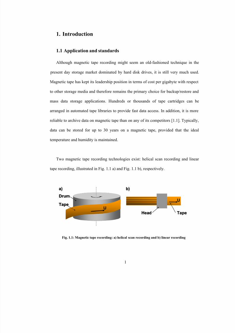
Two magnetic tape recording technologies exist: helical scan recording and linear
tape recording, illustrated in Fig. 1.1 a) and Fig. 1.1 b), respectively.
Drum
TapeU
Tape
U
Head
a) b)
Drum
TapeU
Tape
U
Head
a) b)
Fig. 1.1: Magnetic tape recording: a) helical scan recording and b) linear recording
8/8/2019 BR PhD Dissertation
http://slidepdf.com/reader/full/br-phd-dissertation 34/248
2
In helical scan recording, the recording heads are mounted on a cylindrical drum,
which rotates under a specific azimuth angle relative to the tape. The tracks on the
magnetic tape are written under the same azimuth angle as the read/write heads are
oriented. Helical scan technology was primarily used in video recorders (VCR). Mass
data storage and back-up/restore applications, on the other hand, mainly use linear tape
recording technology. The research presented in this dissertation is concerned with
linear tape recording systems. More specifically, it addresses mechanics and design
problems of tape drives operating under the Linear Tape Open (LTO) format, a standard
that was introduced in 1998 [1.2].
Currently, the two main standards in linear tape recording are Quantum’s (Super)
Digital Linear Tape ((S)DLT) and the Linear Tape Open (LTO) format, introduced in
1998 by an industry consortium that consisted of IBM, Hewlett-Packard (HP) and
Seagate (now Quantum). A rather small player in the linear tape recording market is
Sony’s Advanced Intelligent Tape (AIT).
LTO is a so-called “open format”, meaning that users have the choice of multiple
sources of tape drives and media cartridges [1.2]. The compatibility between the
different products and generations (back-compatibility) of the LTO-technology is
guaranteed. Currently, two types of the LTO format are commercially available. LTO-
Accelis provides fast data-access but does not give high storage capacity. LTO-Ultrium,
on the other hand, provides high storage capacity but comes with slow data access time.
The LTO format exists in three generations: GEN 1 offers tape cartridges with a
8/8/2019 BR PhD Dissertation
http://slidepdf.com/reader/full/br-phd-dissertation 35/248
3
capacity of 100 Gigabyte (GB), GEN 2 offers cartridges with a capacity of 200 GB and
GEN 3, which was first released in 2005, comes with a cartridge capacity of 400 GB.
LTO tape cartridges allow a 2:1 data compression, which virtually doubles the storage
capacity of a cartridge.
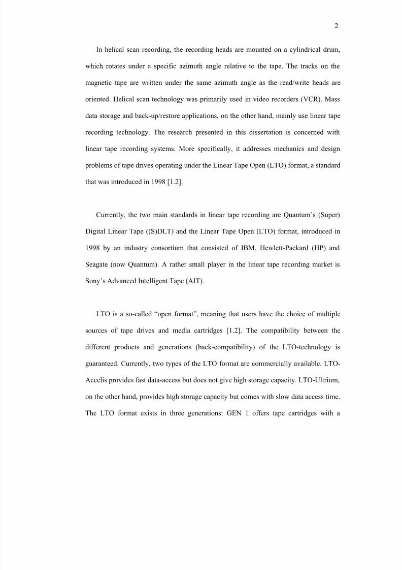
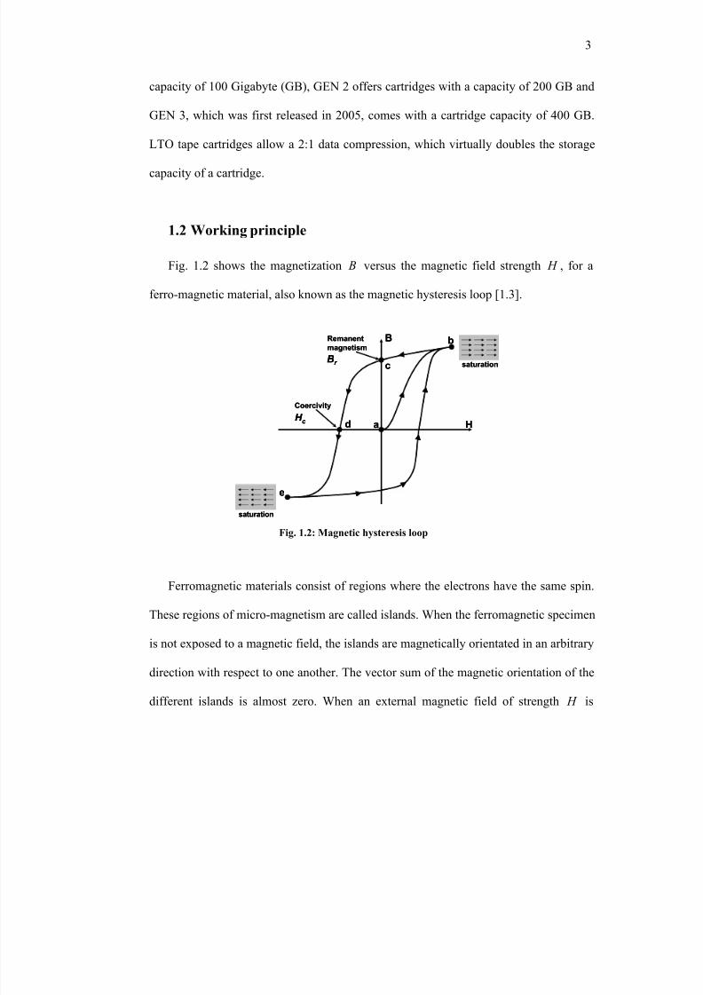
1.2 Working principle
Fig. 1.2 shows the magnetization B versus the magnetic field strength H , for a
ferro-magnetic material, also known as the magnetic hysteresis loop [1.3].
B
Ha
b
c
d
e
saturation
saturation
Remanent
magnetism
Coercivity
Br
H c
B
Ha
b
c
d
e
saturation
saturation
Remanent
magnetism
Coercivity
Br
H c
Ferromagnetic materials consist of regions where the electrons have the same spin.
These regions of micro-magnetism are called islands. When the ferromagnetic specimen
is not exposed to a magnetic field, the islands are magnetically orientated in an arbitrary
direction with respect to one another. The vector sum of the magnetic orientation of the
different islands is almost zero. When an external magnetic field of strength H is
Fig. 1.2: Magnetic hysteresis loop
8/8/2019 BR PhD Dissertation
http://slidepdf.com/reader/full/br-phd-dissertation 36/248
4
applied on the ferromagnetic specimen, the islands align with the direction of the
applied magnetic field. Starting at point a in Fig. 1.2 and increasing the magnetic field
strength H , the islands of the ferromagnetic specimen align with the applied magnetic
field until saturation is reached (point b in Fig. 1.2). Maximum magnetization is now
obtained since all magnetic islands are lined up with one another, i.e., the magnetization
vectors of the individual islands point in the same direction. After reducing the external
magnetic field strength to zero (point b to c in Fig. 1.2), the specimen remains
magnetized. A permanent magnet has been built, characterized by a distinct
magnetization r B , the so-called “remanent magnetism”. It is the remanent magnetism
that enables magnetic storage.
Applying an external magnetic field of increasing strength, but in the opposite
direction of the previously applied field (point d to e in Fig. 1.2), results in an alignment
of the islands with the applied field, until a new saturation point is reached (point e in
Fig. 1.2). Now, all islands are aligned with one another in the opposite sense compared
to point b. Again increasing the field strength in the original direction until saturation is
reached (point b in Fig. 1.2) closes the “magnetic hysteresis loop”. The negative field
strength c H , which results in zero magnetization, is called coercivity (point d in Fig.
1.2). The coercivity is therefore the magnitude of the magnetic field that needs to be
applied to neutralize the remanent magnetism r B . Hence, in magnetic recording the
coercivity could be thought of as a measure of archival capability of the magnetic
medium.
8/8/2019 BR PhD Dissertation
http://slidepdf.com/reader/full/br-phd-dissertation 37/248
5
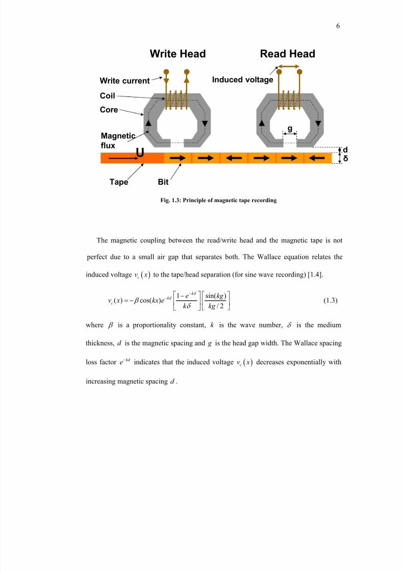
Fig. 1.3 illustrates the working principle of magnetic tape recording. A coil with c N
windings of total length cl is wound around a magnetic core. A write current c I flows
through the coil and creates a magnetic field of strength H given by
c c
c
N I H
l = (1.1)
A so-called fringe field is created perpendicular to this magnetic field of strength H , in
the plane of the magnetic tape. This fringe field magnetizes the ferromagnetic coating of
the tape and, thus, a bit can be recorded. By creating a relative motion between the tape
and the write head, a bit stream can be recorded on the magnetic tape. This recording
process is referred to as “inductive recording”. When moving the inductive head over a
previously recorded bit pattern, the magnetization will induce a voltage in the coil
according to Faraday’s law:
c c
d v N
dt
Φ= − (1.2)
where cv is the induced voltage and Φ is the magnetic flux. t represents the time.
Hence, the previously recorded bit pattern can be reproduced by the read head.
A magneto-resistive (MR) read head consists of a small stripe of permalloy, which
changes its resistance in the vicinity of a magnetic field, depending on the strength and
direction of the field. Hence, a previously recorded bit pattern can be reproduced by
monitoring the resistance change of the permalloy in the MR head. An MR head detects
weaker magnetic signals and thus allows for smaller bits, or equivalently, higher storage
density, and is faster than an inductive recording head.
8/8/2019 BR PhD Dissertation
http://slidepdf.com/reader/full/br-phd-dissertation 38/248
6
U
Write Head Read Head
Write current Induced voltage
Core
Tape Bit
Magnetic
flux
Coil
g
dδ
The magnetic coupling between the read/write head and the magnetic tape is not
perfect due to a small air gap that separates both. The Wallace equation relates the
induced voltage ( )cv x to the tape/head separation (for sine wave recording) [1.4].
1 sin( )( ) cos( )
/ 2
k kd
c
e kg v x kx e
k kg
δ
β δ
−− −
= −
(1.3)
where β is a proportionality constant, k is the wave number, δ is the medium
thickness, d is the magnetic spacing and g is the head gap width. The Wallace spacing
loss factor kd e− indicates that the induced voltage ( )cv x decreases exponentially with
increasing magnetic spacing d .
Fig. 1.3: Principle of magnetic tape recording
8/8/2019 BR PhD Dissertation
http://slidepdf.com/reader/full/br-phd-dissertation 39/248
8/8/2019 BR PhD Dissertation
http://slidepdf.com/reader/full/br-phd-dissertation 40/248
8
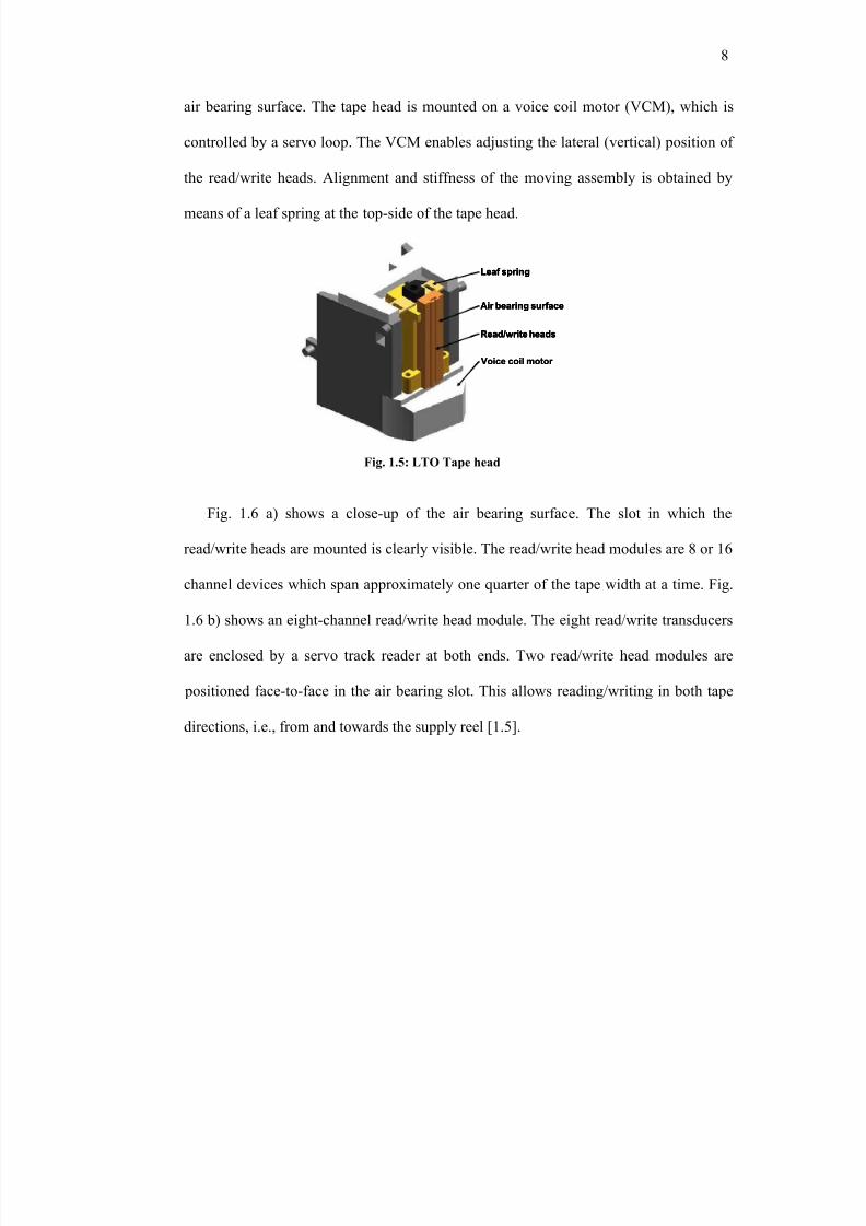
air bearing surface. The tape head is mounted on a voice coil motor (VCM), which is
controlled by a servo loop. The VCM enables adjusting the lateral (vertical) position of
the read/write heads. Alignment and stiffness of the moving assembly is obtained by
means of a leaf spring at the top-side of the tape head.
Voice coil motor
Air bearing surface
Read/write heads
Leaf spring
Voice coil motor
Air bearing surface
Read/write heads
Leaf spring
Air bearing surface
Read/write heads
Leaf spring
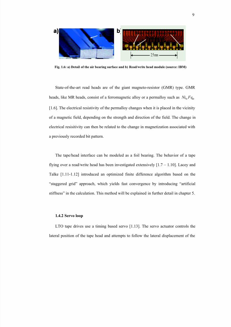
Fig. 1.6 a) shows a close-up of the air bearing surface. The slot in which the
read/write heads are mounted is clearly visible. The read/write head modules are 8 or 16
channel devices which span approximately one quarter of the tape width at a time. Fig.
1.6 b) shows an eight-channel read/write head module. The eight read/write transducers
are enclosed by a servo track reader at both ends. Two read/write head modules are
positioned face-to-face in the air bearing slot. This allows reading/writing in both tape
directions, i.e., from and towards the supply reel [1.5].
Fig. 1.5: LTO Tape head
8/8/2019 BR PhD Dissertation
http://slidepdf.com/reader/full/br-phd-dissertation 41/248
9
a) b) Read head
Write head
Servo headSlot
a) b)a) b) Read head
Write head
Servo headSlot
State-of-the-art read heads are of the giant magneto-resistor (GMR) type. GMR
heads, like MR heads, consist of a ferromagnetic alloy or a permalloy such as 20 80 Ni Fe
[1.6]. The electrical resistivity of the permalloy changes when it is placed in the vicinity
of a magnetic field, depending on the strength and direction of the field. The change in
electrical resisitivity can then be related to the change in magnetization associated with
a previously recorded bit pattern.
The tape/head interface can be modeled as a foil bearing. The behavior of a tape
flying over a read/write head has been investigated extensively [1.7 – 1.10]. Lacey and
Talke [1.11-1.12] introduced an optimized finite difference algorithm based on the
“staggered grid” approach, which yields fast convergence by introducing “artificial
stiffness” in the calculation. This method will be explained in further detail in chapter 5.
1.4.2 Servo loop
LTO tape drives use a timing based servo [1.13]. The servo actuator controls the
lateral position of the tape head and attempts to follow the lateral displacement of the
Fig. 1.6: a) Detail of the air bearing surface and b) Read/write head module (source: IBM)
8/8/2019 BR PhD Dissertation
http://slidepdf.com/reader/full/br-phd-dissertation 42/248
10
tape (see 1.7 Lateral tape motion). The servo controller receives the necessary
information about the lateral position of the tape from servo data and positions the
read/write head accordingly. The servo information is written on the tape as servo tracks
located between regular data tracks. If the tape moves laterally with a frequency higher
than the servo actuator bandwidth, the lateral movement cannot be followed by the
actuator and read/write errors may occur.
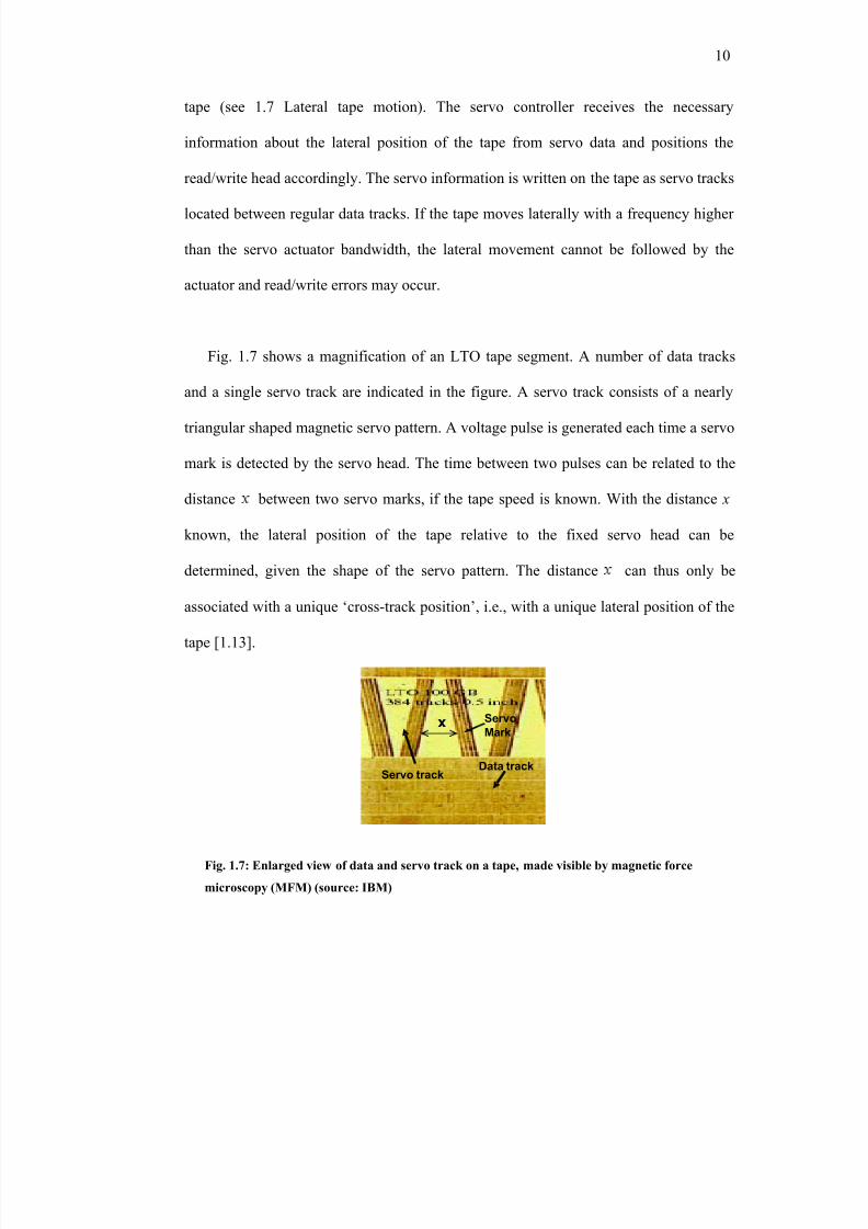
Fig. 1.7 shows a magnification of an LTO tape segment. A number of data tracks
and a single servo track are indicated in the figure. A servo track consists of a nearly
triangular shaped magnetic servo pattern. A voltage pulse is generated each time a servo
mark is detected by the servo head. The time between two pulses can be related to the
distance between two servo marks, if the tape speed is known. With the distance x
known, the lateral position of the tape relative to the fixed servo head can be
determined, given the shape of the servo pattern. The distance can thus only be
associated with a unique ‘cross-track position’, i.e., with a unique lateral position of the
tape [1.13].
xServo
Mark
Servo trackData track
x Servo
Mark
Servo trackData track
Fig. 1.7: Enlarged view of data and servo track on a tape, made visible by magnetic force
microscopy (MFM) (source: IBM)
8/8/2019 BR PhD Dissertation
http://slidepdf.com/reader/full/br-phd-dissertation 43/248
11
1.5 Channel and format
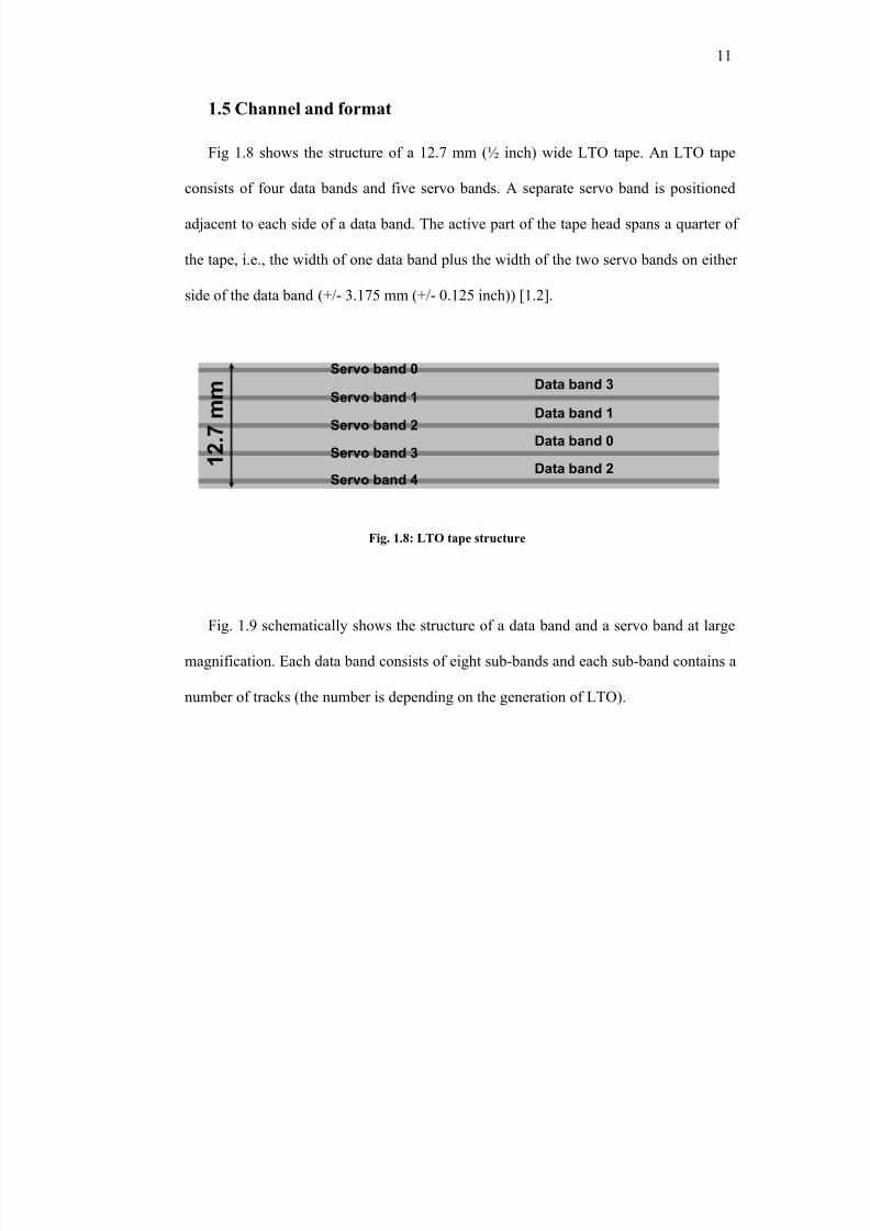
Fig 1.8 shows the structure of a 12.7 mm (½ inch) wide LTO tape. An LTO tape
consists of four data bands and five servo bands. A separate servo band is positioned
adjacent to each side of a data band. The active part of the tape head spans a quarter of
the tape, i.e., the width of one data band plus the width of the two servo bands on either
side of the data band (+/- 3.175 mm (+/- 0.125 inch)) [1.2].
Data band 1
Data band 3
Data band 0
Data band 2
Servo band 0
Servo band 1
Servo band 2
Servo band 3
Servo band 4
1 2 . 7 m m Data band 1
Data band 3
Data band 0
Data band 2
Servo band 0
Servo band 1
Servo band 2
Servo band 3
Servo band 4
1 2 . 7 m m
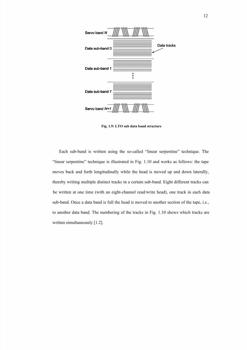
Fig. 1.9 schematically shows the structure of a data band and a servo band at large
magnification. Each data band consists of eight sub-bands and each sub-band contains a
number of tracks (the number is depending on the generation of LTO).
Fig. 1.8: LTO tape structure
8/8/2019 BR PhD Dissertation
http://slidepdf.com/reader/full/br-phd-dissertation 44/248
12
Servo band N
Servo band N+1
Data sub-band 0
Data sub-band 1
Data sub-band 7
Data tracks
Servo band N
Servo band N+1
Data sub-band 0
Data sub-band 1
Data sub-band 7
Servo band N
Servo band N+1
Data sub-band 0
Data sub-band 1
Data sub-band 7
Data tracks
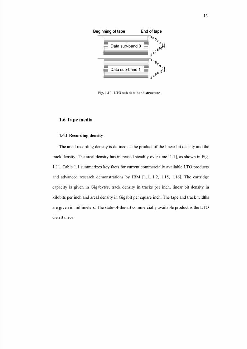
Each sub-band is written using the so-called “linear serpentine” technique. The
“linear serpentine” technique is illustrated in Fig. 1.10 and works as follows: the tape
moves back and forth longitudinally while the head is moved up and down laterally,
thereby writing multiple distinct tracks in a certain sub-band. Eight different tracks can
be written at one time (with an eight-channel read/write head), one track in each data
sub-band. Once a data band is full the head is moved to another section of the tape, i.e.,
to another data band. The numbering of the tracks in Fig. 1.10 shows which tracks are
written simultaneously [1.2].
Fig. 1.9: LTO sub data band structure
8/8/2019 BR PhD Dissertation
http://slidepdf.com/reader/full/br-phd-dissertation 45/248
13
Data sub-band 0
Beginning of tape End of tape
1 3 57
91112108
6
2
4
3 57
91112108
64
1
2
Data sub-band 1
Data sub-band 0
Beginning of tape End of tape
1 3 57
91112108
6
2
4
3 57
91112108
64
1
2
Data sub-band 1
1.6 Tape media
1.6.1 Recording density
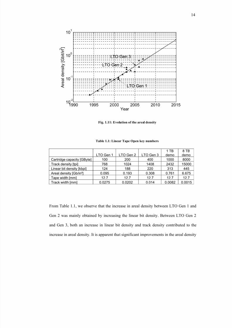
The areal recording density is defined as the product of the linear bit density and the
track density. The areal density has increased steadily over time [1.1], as shown in Fig.
1.11. Table 1.1 summarizes key facts for current commercially available LTO products
and advanced research demonstrations by IBM [1.1, 1.2, 1.15, 1.16]. The cartridge
capacity is given in Gigabytes, track density in tracks per inch, linear bit density in
kilobits per inch and areal density in Gigabit per square inch. The tape and track widths
are given in millimeters. The state-of-the-art commercially available product is the LTO
Gen 3 drive.
Fig. 1.10: LTO sub data band structure
8/8/2019 BR PhD Dissertation
http://slidepdf.com/reader/full/br-phd-dissertation 46/248
14
1990 1995 2000 2005 2010 201510
-2
10-1
100
101
Year
A r e a l d e n s i t y [ G b i t / i n 2 ]
LTO Gen 1
LTO Gen 2
LTO Gen 3
From Table 1.1, we observe that the increase in areal density between LTO Gen 1 and
Gen 2 was mainly obtained by increasing the linear bit density. Between LTO Gen 2
and Gen 3, both an increase in linear bit density and track density contributed to the
increase in areal density. It is apparent that significant improvements in the areal density
LTO Gen 1 LTO Gen 2 LTO Gen 31 TBdemo
8 TBdemo
Cartridge capacity [GByte] 100 200 400 1000 8000
Track density [tpi] 768 1024 1408 2432 15000
Linear bit density [kbpi] 124 188 220 313 445
Areal density [Gb/in²] 0.095 0.193 0.308 0.761 6.675
Tape width [mm] 12.7 12.7 12.7 12.7 12.7
Track width [mm] 0.0275 0.0202 0.014 0.0082 0.0015
Fig. 1.11: Evolution of the areal density
Table 1.1: Linear Tape Open key numbers
8/8/2019 BR PhD Dissertation
http://slidepdf.com/reader/full/br-phd-dissertation 47/248
15
could be made by increasing the track density even further, as shown by both the 1
Terabyte (TB) and 8 TB demonstrations by IBM Research [1.14, 1.15]. However,
increasing the track density is restricted by the tape mechanics as the flexible medium
moves through the tape path.
It is important to increase the areal density without reducing the signal to noise ratio
(SNR). In other words, the grain size of tape media should be decreased as the
recording density is increased. In this case, the number of particles per bit, which
determines the SNR, remains constant while the area per bit decreases. A substantial
effort has been devoted to achieving a smaller grain size and a higher packing density of
the grains for traditional metal particulate (MP) coated media [1.17 - 1.20].
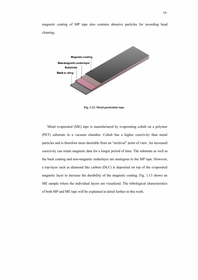
1.6.2 Metal particulate versus metal evaporated tape
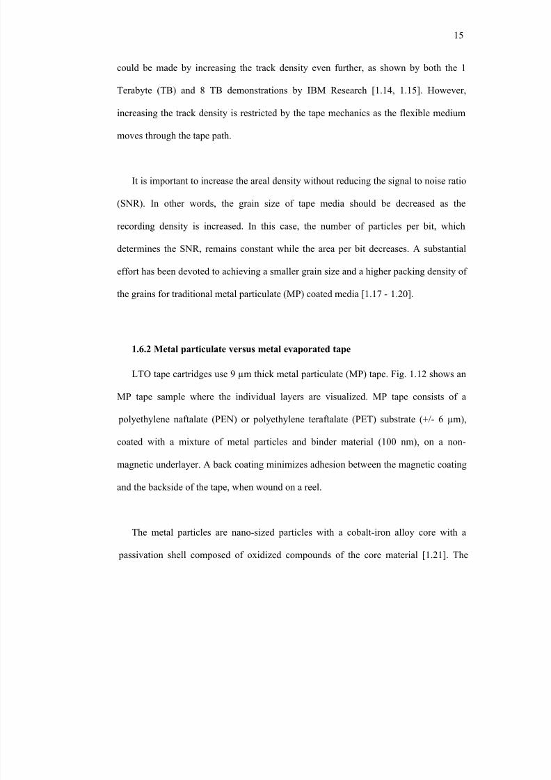
LTO tape cartridges use 9 µm thick metal particulate (MP) tape. Fig. 1.12 shows an
MP tape sample where the individual layers are visualized. MP tape consists of a
polyethylene naftalate (PEN) or polyethylene teraftalate (PET) substrate (+/- 6 µm),
coated with a mixture of metal particles and binder material (100 nm), on a non-
magnetic underlayer. A back coating minimizes adhesion between the magnetic coating
and the backside of the tape, when wound on a reel.
The metal particles are nano-sized particles with a cobalt-iron alloy core with a
passivation shell composed of oxidized compounds of the core material [1.21]. The
8/8/2019 BR PhD Dissertation
http://slidepdf.com/reader/full/br-phd-dissertation 48/248
16
magnetic coating of MP tape also contains abrasive particles for recording head
cleaning.
Back coating
Substrate
Non-magnetic underlayer
Magnetic coating
Back coating
Substrate
Non-magnetic underlayer
Magnetic coating
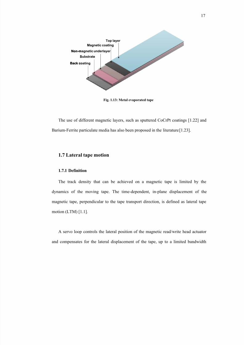
Metal evaporated (ME) tape is manufactured by evaporating cobalt on a polymer
(PET) substrate in a vacuum chamber. Cobalt has a higher coercivity than metal
particles and is therefore more desirable from an “archival” point of view. An increased
coercivity can retain magnetic data for a longer period of time. The substrate as well as
the back coating and non-magnetic underlayer are analogous to the MP tape. However,
a top-layer such as diamond like carbon (DLC) is deposited on top of the evaporated
magnetic layer to increase the durability of the magnetic coating. Fig. 1.13 shows an
ME sample where the individual layers are visualized. The tribological characteristics
of both MP and ME tape will be explained in detail further in this work.
Fig. 1.12: Metal particulate tape
8/8/2019 BR PhD Dissertation
http://slidepdf.com/reader/full/br-phd-dissertation 49/248
17
Back coating
Substrate
Non-magnetic underlayer
Magnetic coating
Top layer
Back coating
Substrate
Non-magnetic underlayer
Magnetic coating
Top layer
The use of different magnetic layers, such as sputtered CoCrPt coatings [1.22] and
Barium-Ferrite particulate media has also been proposed in the literature [1.23].
1.7 Lateral tape motion
1.7.1 Definition
The track density that can be achieved on a magnetic tape is limited by the
dynamics of the moving tape. The time-dependent, in-plane displacement of the
magnetic tape, perpendicular to the tape transport direction, is defined as lateral tape
motion (LTM) [1.1].
A servo loop controls the lateral position of the magnetic read/write head actuator
and compensates for the lateral displacement of the tape, up to a limited bandwidth
Fig. 1.13: Metal evaporated tape
8/8/2019 BR PhD Dissertation
http://slidepdf.com/reader/full/br-phd-dissertation 50/248
18
[1.15]. The bandwidth of the actuator is mainly limited by the actuator mass and
available power [1.1]. LTM with a frequency higher than the bandwidth of the servo
actuator (typical cut-off frequency = 0.75-1 kHz) [1.24] is generally referred to as high
frequency LTM and can cause track misregistration between the read/write head and a
previously written track. Hence, LTM limits the maximum track (recording) density
that can be achieved [1.14, 1.24, 1.25]. It is generally observed that a lateral
displacement on the order of ten percent of the width of a track causes read/write errors
[1.26]. This implies that for the state-of-the-art LTO Gen 3 drive, three times the
standard deviation ( 3σ ) of the high frequency LTM must be smaller than 1.4 µm (some
sources even report on using 6σ [1.1]). For the case of the 8 TB demo, 3σ of the high
frequency LTM must even be smaller than 0.15 µm.
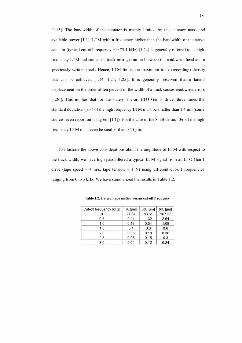
To illustrate the above considerations about the amplitude of LTM with respect to
the track width, we have high pass filtered a typical LTM signal from an LTO Gen 1
drive (tape speed = 4 m/s, tape tension = 1 N) using different cut-off frequencies
ranging from 0 to 3 kHz. We have summarized the results in Table 1.2.
Cut-off frequency [kHz] σs [µm] 3σs [µm] 6σs [µm]
0 27.87 83.61 167.22
0.5 0.44 1.32 2.641.0 0.18 0.54 1.08
1.5 0.1 0.3 0.6
2.0 0.06 0.18 0.36
2.5 0.05 0.15 0.3
3.0 0.04 0.12 0.24
Table 1.2: Lateral tape motion versus cut-off frequency
8/8/2019 BR PhD Dissertation
http://slidepdf.com/reader/full/br-phd-dissertation 51/248
19
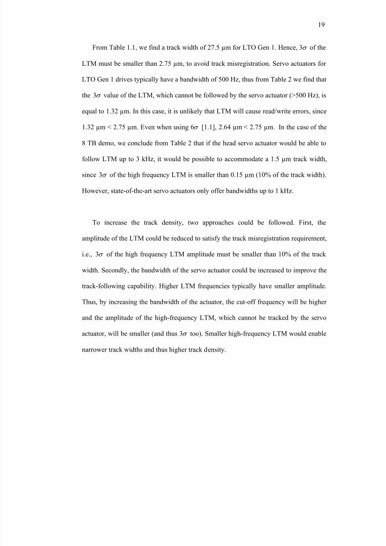
From Table 1.1, we find a track width of 27.5 µm for LTO Gen 1. Hence, 3σ of the
LTM must be smaller than 2.75 µm, to avoid track misregistration. Servo actuators for
LTO Gen 1 drives typically have a bandwidth of 500 Hz, thus from Table 2 we find that
the 3σ value of the LTM, which cannot be followed by the servo actuator (>500 Hz), is
equal to 1.32 µm. In this case, it is unlikely that LTM will cause read/write errors, since
1.32 µm < 2.75 µm. Even when using 6σ [1.1], 2.64 µm < 2.75 µm. In the case of the
8 TB demo, we conclude from Table 2 that if the head servo actuator would be able to
follow LTM up to 3 kHz, it would be possible to accommodate a 1.5 µm track width,
since 3σ of the high frequency LTM is smaller than 0.15 µm (10% of the track width).
However, state-of-the-art servo actuators only offer bandwidths up to 1 kHz.
To increase the track density, two approaches could be followed. First, the
amplitude of the LTM could be reduced to satisfy the track misregistration requirement,
i.e., 3σ of the high frequency LTM amplitude must be smaller than 10% of the track
width. Secondly, the bandwidth of the servo actuator could be increased to improve the
track-following capability. Higher LTM frequencies typically have smaller amplitude.
Thus, by increasing the bandwidth of the actuator, the cut-off frequency will be higher
and the amplitude of the high-frequency LTM, which cannot be tracked by the servo
actuator, will be smaller (and thus 3σ too). Smaller high-frequency LTM would enable
narrower track widths and thus higher track density.

8/8/2019 BR PhD Dissertation
http://slidepdf.com/reader/full/br-phd-dissertation 52/248
20
1.7.2 Measurement
A number of different methods to measure the lateral displacement of magnetic tape
has been reported in the literature. The most common method to measure LTM is the
use of an optical edge probe [1.25, 1.27]. Fig. 1.14 a) illustrates the concept of the
optical edge probe. A light beam emitted through light transmitting fibers is deflected
90 degrees by a prism. The path of the light beam is partially obstructed by the tape,
before the remaining light is again deflected into the receiving fibers by a second prism.
The amount of light “seen” by the receiving fibers is thus a measure for the lateral
position of the tape [1.28].
A similar method has been reported using infrared light instead of light in the visible
light range [1.29, 1.30]. This method uses an optical switch, which is much cheaper
than an optical edge probe. These optical techniques are easily applicable, allow LTM
measurements at any position along the tape path and yield repeatable results. Both
optical techniques, however, incorporate the imperfections of the tape edge in the
measured LTM signal. Factory slit tape edge is not perfectly straight [1.31]. The edge
has local imperfections such as cracks and tears, which may grow in time as a result of
tape edge wear. Hence, a small part of the measured LTM is due to the imperfectly slit
tape edge. However, most imperfections are smaller than the lateral displacement of the
tape and therefore the optical methods still yield reliable results.
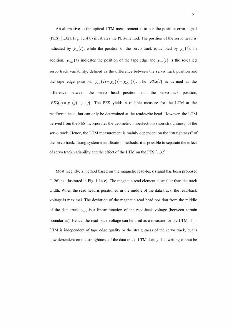
8/8/2019 BR PhD Dissertation
http://slidepdf.com/reader/full/br-phd-dissertation 53/248
21
An alternative to the optical LTM measurement is to use the position error signal
(PES) [1.32]. Fig. 1.14 b) illustrates the PES-method. The position of the servo head is
indicated by ( ) sh y t , while the position of the servo track is denoted by ( ) st y t . In
addition, ( )edge y t indicates the position of the tape edge and ( )var y t is the so-called
servo track variability, defined as the difference between the servo track position and
the tape edge position, ( ) ( ) ( )var st edge y t y t y t = − . The ( ) PES t is defined as the
difference between the servo head position and the servo-track position,
( ) ( ) ( ) sh st PES t y t y t = − . The PES yields a reliable measure for the LTM at the
read/write head, but can only be determined at the read/write head. However, the LTM
derived from the PES incorporates the geometric imperfections (non-straightness) of the
servo track. Hence, the LTM measurement is mainly dependent on the “straightness” of
the servo track. Using system identification methods, it is possible to separate the effect
of servo track variability and the effect of the LTM on the PES [1.32].
Most recently, a method based on the magnetic read-back signal has been proposed
[1.26] as illustrated in Fig. 1.14 c). The magnetic read element is smaller than the track
width. When the read head is positioned in the middle of the data track, the read-back
voltage is maximal. The deviation of the magnetic read head position from the middle
of the data track m y , is a linear function of the read-back voltage (between certain
boundaries). Hence, the read-back voltage can be used as a measure for the LTM. This
LTM is independent of tape edge quality or the straightness of the servo track, but is
now dependent on the straightness of the data track. LTM during data writing cannot be
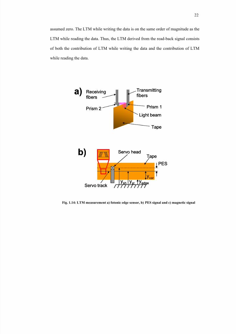
8/8/2019 BR PhD Dissertation
http://slidepdf.com/reader/full/br-phd-dissertation 54/248
22
assumed zero. The LTM while writing the data is on the same order of magnitude as the
LTM while reading the data. Thus, the LTM derived from the read-back signal consists
of both the contribution of LTM while writing the data and the contribution of LTM
while reading the data.
Tape
Transmitting
fibersReceiving
fibers
Prism 2 Prism 1
Light beam
a)
Tape
Transmitting
fibersReceiving
fibers
Prism 2 Prism 1
Light beam
a)
b)
ysh
yvar
PES
TapeServo head
Servo trackyst yedge
b)
ysh
yvar
PES
TapeServo head
Servo trackyst yedge
Fig. 1.14: LTM measurement a) fotonic edge sensor, b) PES signal and c) magnetic signal
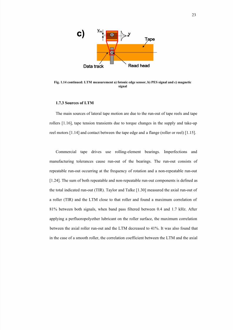
8/8/2019 BR PhD Dissertation
http://slidepdf.com/reader/full/br-phd-dissertation 55/248
23
c)
Read head
v
Tape
Data track
ymc)
Read head
v
Tape
Data track Read head
v
Tape
Data track
ym
1.7.3 Sources of LTM
The main sources of lateral tape motion are due to the run-out of tape reels and tape
rollers [1.16], tape tension transients due to torque changes in the supply and take-up
reel motors [1.14] and contact between the tape edge and a flange (roller or reel) [1.15].
Commercial tape drives use rolling-element bearings. Imperfections and
manufacturing tolerances cause run-out of the bearings. The run-out consists of
repeatable run-out occurring at the frequency of rotation and a non-repeatable run-out
[1.24]. The sum of both repeatable and non-repeatable run-out components is defined as
the total indicated run-out (TIR). Taylor and Talke [1.30] measured the axial run-out of
a roller (TIR) and the LTM close to that roller and found a maximum correlation of
81% between both signals, when band pass filtered between 0.4 and 1.7 kHz. After
applying a perfluoropolyether lubricant on the roller surface, the maximum correlation
between the axial roller run-out and the LTM decreased to 41%. It was also found that
in the case of a smooth roller, the correlation coefficient between the LTM and the axial
Fig. 1.14 continued: LTM measurement a) fotonic edge sensor, b) PES signal and c) magnetic
signal
8/8/2019 BR PhD Dissertation
http://slidepdf.com/reader/full/br-phd-dissertation 56/248
24
run-out measurement was lower than in the case of a grooved roller. Grooved rollers
eliminate the air bearing (hydrodynamic lubrication) and therefore increase the
frictional interaction between the roller and the tape. These experimental results suggest
that frictional coupling between tape and roller in combination with axial roller run-out,
significantly contributes to LTM. The two other main LTM sources, as mentioned
above, will be discussed in detail in chapter 2 and 3 of this dissertation.
1.8 Dissertation outline
This dissertation consists of three parts, each of which containing two chapters. The
first part (chapters 2 and 3) of the dissertation deals in detail with two primary sources
of lateral tape motion, namely tape tension transients and tape edge contact. The second
part (chapters 4 and 5) investigates the fundamentals of the dynamics of the magnetic
tape and the frictional interaction of the tape with a cylindrical guide. The final part
(chapters 6 and 7) presents improvements, which can be implemented to reduce lateral
tape motion in tape drives and lead to an increase in track density.
Chapter 2 presents the design of a non-contact, optical tension sensor. The sensor
was then used to investigate the effect of tape tension transients on LTM. Chapter 3
shows how LTM is affected by tape edge contact. A novel approach based on acoustic
emission was used to measure impacts between a moving tape and the flange of a tape
guide. After calibrating the acoustic emission signal, the impact force between tape and
flange was determined. The influence of tape drive operating conditions as well as
8/8/2019 BR PhD Dissertation
http://slidepdf.com/reader/full/br-phd-dissertation 57/248
25
design parameters on tape edge contact was studied. A one dimensional model was
developed to predict the magnitude of tape/flange impact. The model fits the
experimental data well.
Since a tape translates over tape drive components (such as cylindrical guides), it is
crucial to understand the dynamics of the tape as well as the frictional interaction
between a polymeric tape and a metal guide. Chapter 4 is concerned with the mechanics
of lateral motion of an axially moving tape on a cylindrical guide surface. The effects of
lateral bending stiffness and friction force are studied and the attenuation of lateral tape
motion as a function of the guide radius and friction coefficient is determined. Chapter
5 introduces a model for the friction coefficient between a tape and a guide. The model
allows the investigation of the effect of various parameters such as sliding speed, tape
tension, surface roughness, material properties and guide and tape geometry on the
magnetic tape/guide friction coefficient. The friction coefficient between a guide and a
tape sample is also determined from experimental measurements as a function of these
various parameters.
Chapter 6 presents a novel approach to tape guide design by using micro-textured
guides. The micro-texture enhances the formation of an air bearing and hence reduces
the friction coefficient and the transition speed between boundary lubrication and
hydrodynamic lubrication. Chapter 7 analyses the design of a dual-stage actuator tape
head with an increased bandwidth compared to state-of-the-art tape heads. A prototype
was built and a dual-stage servo controller was developed.
8/8/2019 BR PhD Dissertation
http://slidepdf.com/reader/full/br-phd-dissertation 58/248
8/8/2019 BR PhD Dissertation
http://slidepdf.com/reader/full/br-phd-dissertation 59/248
27
[1.15] IBM Research Press Resources, 2006, IBM Researchers Set World Record in
Magnetic Tape Data Density, http://domino.watson.ibm.com
[1.16] Dee RH, 2006, Magnetic Tape: The Challenge of Reaching Hard Disk Drive
Data Densities on Flexible Media, MRS Bulletin, Vol. 31, pp. 404 - 408
[1.17] Sharrock MP, 2000, Recent Advances in Metal Particulate Recording Media:
Toward the Ultimate Particle, IEEE T. Mag., Vol. 36(5), pp. 2420 - 2425
[1.18] Sekiguchi N, Kawakami K, Ozue T, Yamaga M, Onodera S, 2005, Examination
of Newly Developed Metal Particle Media for >3 Gb/in² Recording in GMR-Based
Tape Systems, IEEE T. Mag., Vol. 41(10), pp. 3235 - 3237
[1.19] Inaba H, Ejiri K, Masaki K, Kitahara T, 1998, Development of an Advanced
Metal Particulate Tape, IEEE T. Mag., Vol. 34(4), pp. 1666 - 1668
[1.20] Richter HJ, Veitch RJ, 1996, MP Tape for High Density Digital Recording, J.Mag. Mag. Mat., Vol. 155, pp. 80 - 82
[1.21] Personal communication
[1.22] Lee HS, Laughlin DE, Bain JA, 2003, Recording Properties of CoCrPt TapeMedia Sputter-Deposited at Room Temperature on Polymeric Substrates, J. Appl.
Phys., Vol. 93(10), pp. 7783 - 7785
[1.23] Nagata T, Harasawa T, Oyanagi M, Abe N, Saito S, 2006, A Recording Density
Study of Advanced Barium-Ferrite Particulate Tape, IEEE T. Mag., Vol. 42(10), pp.
2312 - 2314
[1.24] Richards DB, Sharrock MP, 1998, Key Issues in the Design of Magnetic Tape for Linear Systems of High Track Density, IEEE T. Mag., Vol. 34(4), pp. 1878 - 1882
[1.25] Taylor RJ, Strahle P, Stahl J, Talke FE, 2000, Measurement of Cross-Track
Motion of Magnetic Tapes, J. Info. Storage Proc. Syst., Vol. 2, pp. 255 - 261
[1.26] Alfano AD, Bhushan B, 2006, New Technique for Monitoring Lateral Tape
Motion Using a Magnetic Signal, Microsyst. Technol., Vol. 12, pp. 565 - 570
[1.27] Goldade AV, Bhushan B, 2003, Measurement and Origin of Edge Damage in aLinear Tape Drive, Tribol. Lett., Vol. 14, pp. 167 - 180
[1.28] MTI-2000 Fotonic Sensor Instruction Manual, 2000, Mechanical Technology
Inc. (Latham, NY, USA)

8/8/2019 BR PhD Dissertation
http://slidepdf.com/reader/full/br-phd-dissertation 60/248
28
[1.29] Raeymaekers B, Taylor RJ, Talke FE, 2006, Non-Contact Tape Tension
Measurement and Correlation of Lateral Tape Motion and Tape Tension Transients,Microsyst. Technol., Vol. 12(4), pp. 814 - 821
[1.30] Taylor RJ, Talke FE, 2005, Investigation of Roller Interactions with Flexible
Tape Medium, Tribol. Int., Vol. 38, pp. 599 - 605
[1.31] Goldade AV, Bhushan B, 2004, Tape Edge Study in a Linear Tape Drive with
Single Flanged Guides, J. Mag. Mag. Mat., Vol 271, pp. 409 - 430
[1.32] Jose J, Taylor RJ, de Callafon RA, Talke FE, 2005, Characterization of Lateral
Tape Motion and Disturbances in the Servo Position Error Signal of a Linear TapeDrive, Tribol. Int., Vol. 38, pp. 625 - 632
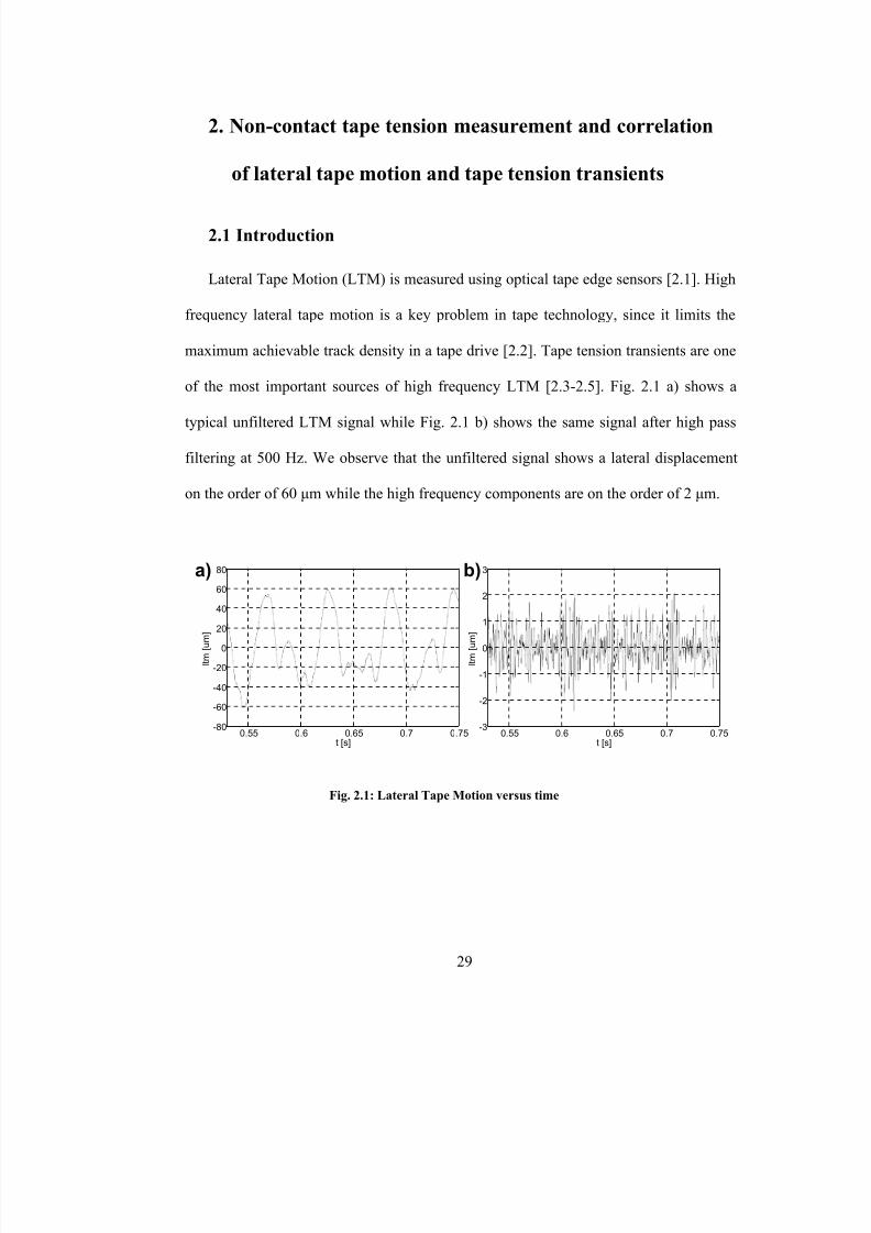
8/8/2019 BR PhD Dissertation
http://slidepdf.com/reader/full/br-phd-dissertation 61/248
29
2. Non-contact tape tension measurement and correlation
of lateral tape motion and tape tension transients
2.1 Introduction
Lateral Tape Motion (LTM) is measured using optical tape edge sensors [2.1]. High
frequency lateral tape motion is a key problem in tape technology, since it limits the
maximum achievable track density in a tape drive [2.2]. Tape tension transients are one
of the most important sources of high frequency LTM [2.3-2.5]. Fig. 2.1 a) shows a
typical unfiltered LTM signal while Fig. 2.1 b) shows the same signal after high pass
filtering at 500 Hz. We observe that the unfiltered signal shows a lateral displacement
on the order of 60 µm while the high frequency components are on the order of 2 µm.
0.55 0.6 0.65 0.7 0.75-80
-60
-40
-20
0
20
40
60
80
t [s]
l t m [ u
m ]
0.55 0.6 0.65 0.7 0.75-3
-2
-1
0
1
2
3
t [s]
l t m [ u
m ]
a) b)
0.55 0.6 0.65 0.7 0.75-80
-60
-40
-20
0
20
40
60
80
t [s]
l t m [ u
m ]
0.55 0.6 0.65 0.7 0.75-3
-2
-1
0
1
2
3
t [s]
l t m [ u
m ]
a) b)
Fig. 2.1: Lateral Tape Motion versus time
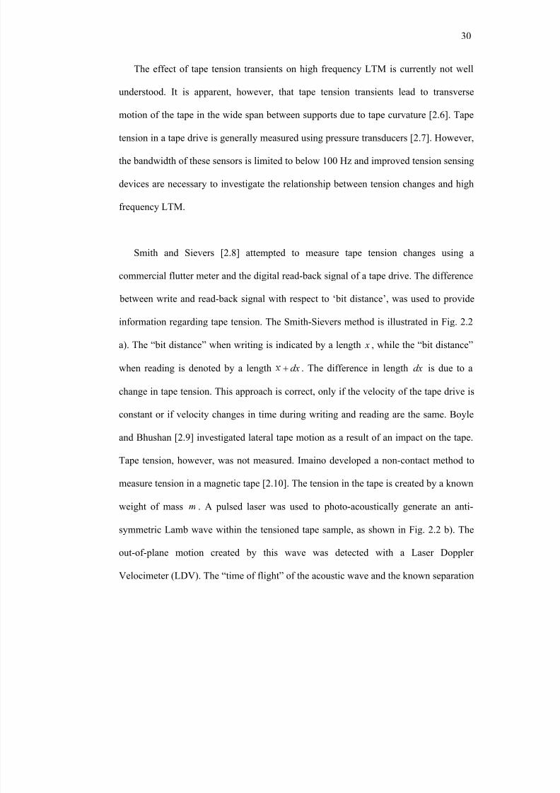
8/8/2019 BR PhD Dissertation
http://slidepdf.com/reader/full/br-phd-dissertation 62/248
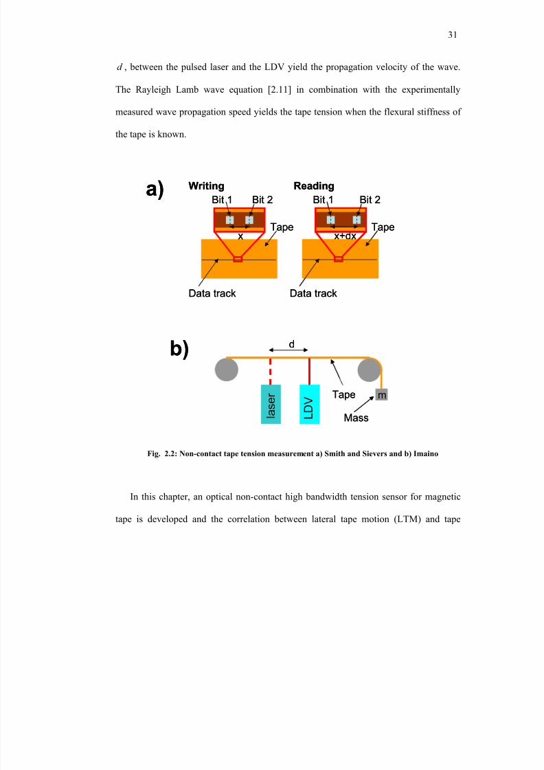
8/8/2019 BR PhD Dissertation
http://slidepdf.com/reader/full/br-phd-dissertation 63/248
31
d , between the pulsed laser and the LDV yield the propagation velocity of the wave.
The Rayleigh Lamb wave equation [2.11] in combination with the experimentally
measured wave propagation speed yields the tape tension when the flexural stiffness of
the tape is known.
a)
Tape
Data track
x
Bit 1 Bit 2
Tape
Data track
x+dx
Bit 1 Bit 2
Writing Readinga)
Tape
Data track
x
Bit 1 Bit 2
Tape
Data track
x+dx
Bit 1 Bit 2
Writing Reading
b)
m
l a s e r
L D V
Tape
Mass
db)
m
l a s e r
L D V
Tape
Mass
d
In this chapter, an optical non-contact high bandwidth tension sensor for magnetic
tape is developed and the correlation between lateral tape motion (LTM) and tape
Fig. 2.2: Non-contact tape tension measurement a) Smith and Sievers and b) Imaino
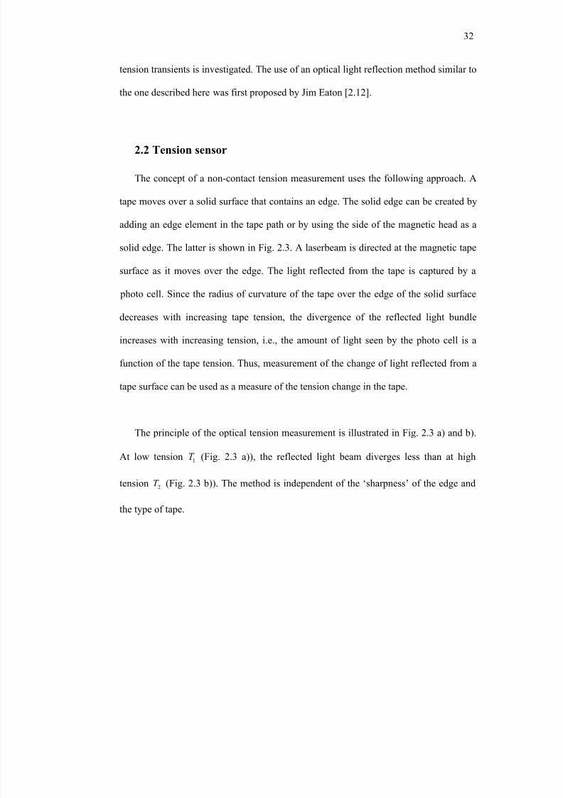
8/8/2019 BR PhD Dissertation
http://slidepdf.com/reader/full/br-phd-dissertation 64/248
32
tension transients is investigated. The use of an optical light reflection method similar to
the one described here was first proposed by Jim Eaton [2.12].
2.2 Tension sensor
The concept of a non-contact tension measurement uses the following approach. A
tape moves over a solid surface that contains an edge. The solid edge can be created by
adding an edge element in the tape path or by using the side of the magnetic head as a
solid edge. The latter is shown in Fig. 2.3. A laserbeam is directed at the magnetic tape
surface as it moves over the edge. The light reflected from the tape is captured by a
photo cell. Since the radius of curvature of the tape over the edge of the solid surface
decreases with increasing tape tension, the divergence of the reflected light bundle
increases with increasing tension, i.e., the amount of light seen by the photo cell is a
function of the tape tension. Thus, measurement of the change of light reflected from a
tape surface can be used as a measure of the tension change in the tape.
The principle of the optical tension measurement is illustrated in Fig. 2.3 a) and b).
At low tension 1T (Fig. 2.3 a)), the reflected light beam diverges less than at high
tension 2T (Fig. 2.3 b)). The method is independent of the ‘sharpness’ of the edge and
the type of tape.
8/8/2019 BR PhD Dissertation
http://slidepdf.com/reader/full/br-phd-dissertation 65/248
33
Laser
Tape
Tape head
T2
T2Laser
Photo
diode
Tape head
Tape
T1
T1
a) b)
Photo
diode
Laser
Tape
Tape head
T2
T2Laser
Photo
diode
Tape head
Tape
T1
T1
a) b)
Photo
diode
A typical calibration curve of the photo cell voltage versus the tape tension is shown
in Fig. 2.4. The entire tension deviation range encountered in a tape drive is contained
within the linear range of calibration. The sensor has to be calibrated for each type of
tape due to different reflectivity of each tape and for each magnetic read/write head due
to variation in the head contour.
0.8 0.9 1 1.1 1.2 1.30.63
0.635
0.64
0.645
0.65
0.655
0.66
Tension [N]
P h o t o c e l l v o l t a g e [ V ]
Fig. 2.3 a) Divergence of the light beam as a result of a) tension T1 and b) tension T2
Fig. 2.4 Typical calibration curve
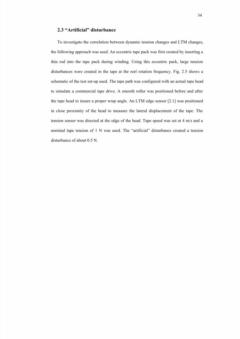
8/8/2019 BR PhD Dissertation
http://slidepdf.com/reader/full/br-phd-dissertation 66/248
34
2.3 “Artificial” disturbance
To investigate the correlation between dynamic tension changes and LTM changes,
the following approach was used. An eccentric tape pack was first created by inserting a
thin rod into the tape pack during winding. Using this eccentric pack, large tension
disturbances were created in the tape at the reel rotation frequency. Fig. 2.5 shows a
schematic of the test set-up used. The tape path was configured with an actual tape head
to simulate a commercial tape drive. A smooth roller was positioned before and after
the tape head to insure a proper wrap angle. An LTM edge sensor [2.1] was positioned
in close proximity of the head to measure the lateral displacement of the tape. The
tension sensor was directed at the edge of the head. Tape speed was set at 4 m/s and a
nominal tape tension of 1 N was used. The “artificial” disturbance created a tension
disturbance of about 0.5 N.
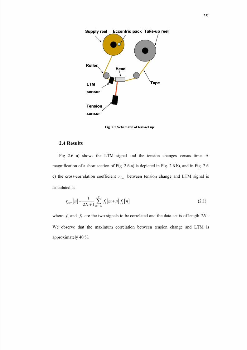
8/8/2019 BR PhD Dissertation
http://slidepdf.com/reader/full/br-phd-dissertation 67/248
35
LTM
sensor
Tension
sensor
Head
Supply reel
Roller
Tape
Eccentric pack Take-up reel
LTM
sensor
Tension
sensor
Head
Supply reel
Roller
Tape
Eccentric pack Take-up reel
2.4 Results
Fig 2.6 a) shows the LTM signal and the tension changes versus time. A
magnification of a short section of Fig. 2.6 a) is depicted in Fig. 2.6 b), and in Fig. 2.6
c) the cross-correlation coefficient corr r between tension change and LTM signal is
calculated as
[ ] [ ] [ ]1 2
1
2 1
N
corr
m N
r n f m n f n N =−
= ++
∑ (2.1)
where 1 f and 2 f are the two signals to be correlated and the data set is of length 2 N .
We observe that the maximum correlation between tension change and LTM is
approximately 40 %.
Fig. 2.5 Schematic of test-set up
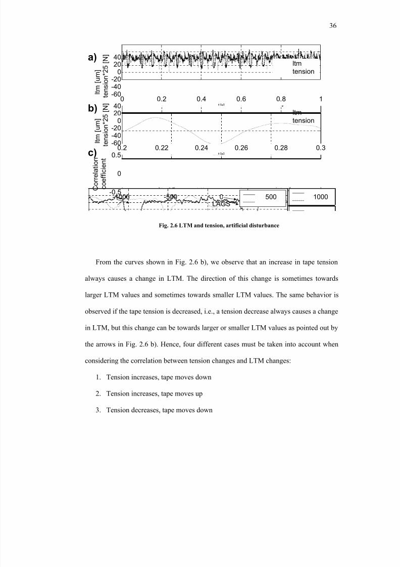
8/8/2019 BR PhD Dissertation
http://slidepdf.com/reader/full/br-phd-dissertation 68/248
36
0 0.2 0.4 0.6 0.8 1-60-40-20
02040
t [s]
l t m
[ u m ]
t e n
s i o n * 2 5 [ N ]
0.2 0.22 0.24 0.26 0.28 0.3-60-40-20
02040
t [s]
l t m [ u
m ]
t e n s i o n * 2 5 [ N ]
-1000 -500 0 500 1000-0.5
0
0.5
LAGS
C o r
r e l a t i o n
c o e
f f i c i e n t
ltm
tension
ltm
tension
a)
b)
c)
0 0.2 0.4 0.6 0.8 1-60-40-20
02040
t [s]
l t m
[ u m ]
t e n
s i o n * 2 5 [ N ]
0.2 0.22 0.24 0.26 0.28 0.3-60-40-20
02040
t [s]
l t m [ u
m ]
t e n s i o n * 2 5 [ N ]
-1000 -500 0 500 1000-0.5
0
0.5
LAGS
C o r
r e l a t i o n
c o e
f f i c i e n t
ltm
tension
ltm
tension
a)
b)
c)
From the curves shown in Fig. 2.6 b), we observe that an increase in tape tension
always causes a change in LTM. The direction of this change is sometimes towards
larger LTM values and sometimes towards smaller LTM values. The same behavior is
observed if the tape tension is decreased, i.e., a tension decrease always causes a change
in LTM, but this change can be towards larger or smaller LTM values as pointed out by
the arrows in Fig. 2.6 b). Hence, four different cases must be taken into account when
considering the correlation between tension changes and LTM changes:
1. Tension increases, tape moves down
2. Tension increases, tape moves up
3. Tension decreases, tape moves down
Fig. 2.6 LTM and tension, artificial disturbance
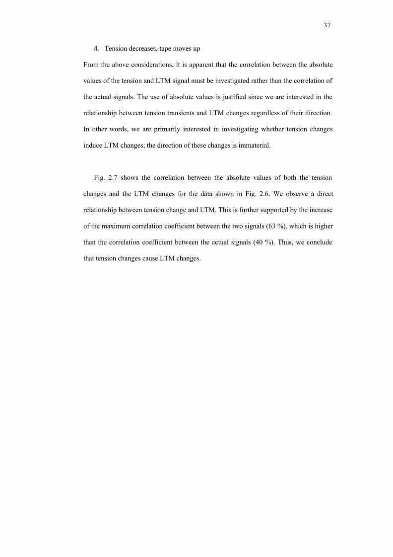
8/8/2019 BR PhD Dissertation
http://slidepdf.com/reader/full/br-phd-dissertation 69/248
37
4. Tension decreases, tape moves up
From the above considerations, it is apparent that the correlation between the absolute
values of the tension and LTM signal must be investigated rather than the correlation of
the actual signals. The use of absolute values is justified since we are interested in the
relationship between tension transients and LTM changes regardless of their direction.
In other words, we are primarily interested in investigating whether tension changes
induce LTM changes; the direction of these changes is immaterial.
Fig. 2.7 shows the correlation between the absolute values of both the tension
changes and the LTM changes for the data shown in Fig. 2.6. We observe a direct
relationship between tension change and LTM. This is further supported by the increase
of the maximum correlation coefficient between the two signals (63 %), which is higher
than the correlation coefficient between the actual signals (40 %). Thus, we conclude
that tension changes cause LTM changes.
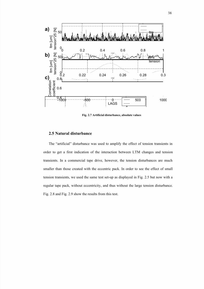
8/8/2019 BR PhD Dissertation
http://slidepdf.com/reader/full/br-phd-dissertation 70/248
38
0 0.2 0.4 0.6 0.8 10
50
t [s]
l t m [ u
m ]
t e n
s i o n * 2 5 [ N ]
ltm
tension
0.2 0.22 0.24 0.26 0.28 0.30
50
t [s]
l t m [ u
m ]
t e n s i o n * 2 5 [ N ]
ltm
tension
-1000 -500 0 500 10000.4
0.6
0.8
LAGS
C o r r e l a t i o n
c o e f f i c i e n t
a)
b)
c)
0 0.2 0.4 0.6 0.8 10
50
t [s]
l t m [ u
m ]
t e n
s i o n * 2 5 [ N ]
ltm
tension
0.2 0.22 0.24 0.26 0.28 0.30
50
t [s]
l t m [ u
m ]
t e n s i o n * 2 5 [ N ]
ltm
tension
-1000 -500 0 500 10000.4
0.6
0.8
LAGS
C o r r e l a t i o n
c o e f f i c i e n t
a)
b)
c)
2.5 Natural disturbance
The “artificial” disturbance was used to amplify the effect of tension transients in
order to get a first indication of the interaction between LTM changes and tension
transients. In a commercial tape drive, however, the tension disturbances are much
smaller than those created with the eccentric pack. In order to see the effect of small
tension transients, we used the same test set-up as displayed in Fig. 2.5 but now with a
regular tape pack, without eccentricity, and thus without the large tension disturbance.
Fig. 2.8 and Fig. 2.9 show the results from this test.
Fig. 2.7 Artificial disturbance, absolute values
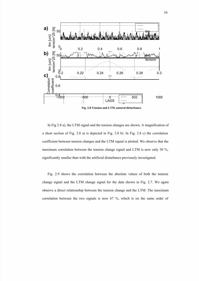
8/8/2019 BR PhD Dissertation
http://slidepdf.com/reader/full/br-phd-dissertation 71/248
39
0 0.2 0.4 0.6 0.8 10
50
t [s]
l t m [ u
m ]
t e n
s i o n * 2 5 [ N ]
ltm
tension
0.2 0.22 0.24 0.26 0.28 0.30
50
t [s]
l t m [ u
m ]
t e n s i o n * 2 5 [ N ]
ltm
tension
-1000 -500 0 500 10000.4
0.6
0.8
LAGS
C o r r e l a t i o n
c o e f f i c i e n t
a)
b)
c)
0 0.2 0.4 0.6 0.8 10
50
t [s]
l t m [ u
m ]
t e n
s i o n * 2 5 [ N ]
ltm
tension
0.2 0.22 0.24 0.26 0.28 0.30
50
t [s]
l t m [ u
m ]
t e n s i o n * 2 5 [ N ]
ltm
tension
-1000 -500 0 500 10000.4
0.6
0.8
LAGS
C o r r e l a t i o n
c o e f f i c i e n t
a)
b)
c)
In Fig 2.8 a), the LTM signal and the tension changes are shown. A magnification of
a short section of Fig. 2.8 a) is depicted in Fig. 2.8 b). In Fig. 2.8 c) the correlation
coefficient between tension changes and the LTM signal is plotted. We observe that the
maximum correlation between the tension change signal and LTM is now only 30 %,
significantly smaller than with the artificial disturbance previously investigated.
Fig. 2.9 shows the correlation between the absolute values of both the tension
change signal and the LTM change signal for the data shown in Fig. 2.7. We again
observe a direct relationship between the tension change and the LTM. The maximum
correlation between the two signals is now 67 %, which is on the same order of
Fig. 2.8 Tension and LTM, natural disturbance
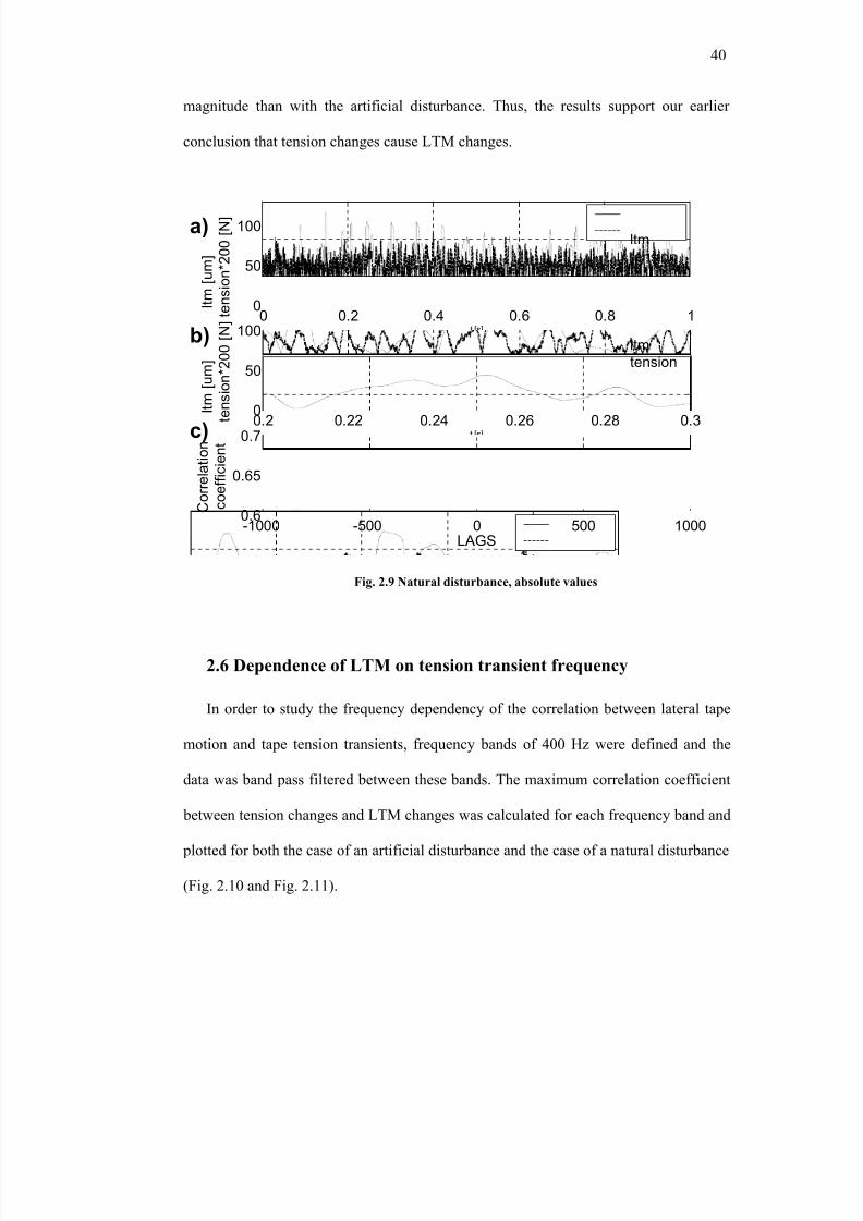
8/8/2019 BR PhD Dissertation
http://slidepdf.com/reader/full/br-phd-dissertation 72/248
40
magnitude than with the artificial disturbance. Thus, the results support our earlier
conclusion that tension changes cause LTM changes.
0 0.2 0.4 0.6 0.8 10
50
100
t [s]
l t m [ u
m ]
t e n s i o n * 2 0 0 [ N ]
ltm
tension
0.2 0.22 0.24 0.26 0.28 0.30
50
100
t [s]
l t m
[ u m ]
t e n s i o n * 2 0 0 [ N ]
ltm
tension
-1000 -500 0 500 10000.6
0.65
0.7
LAGS
C o r r e l a t i o n
c o e f f i c i e n t
a)
b)
c)
0 0.2 0.4 0.6 0.8 10
50
100
t [s]
l t m [ u
m ]
t e n s i o n * 2 0 0 [ N ]
ltm
tension
0.2 0.22 0.24 0.26 0.28 0.30
50
100
t [s]
l t m
[ u m ]
t e n s i o n * 2 0 0 [ N ]
ltm
tension
-1000 -500 0 500 10000.6
0.65
0.7
LAGS
C o r r e l a t i o n
c o e f f i c i e n t
a)
b)
c)
2.6 Dependence of LTM on tension transient frequency
In order to study the frequency dependency of the correlation between lateral tape
motion and tape tension transients, frequency bands of 400 Hz were defined and the
data was band pass filtered between these bands. The maximum correlation coefficient
between tension changes and LTM changes was calculated for each frequency band and
plotted for both the case of an artificial disturbance and the case of a natural disturbance
(Fig. 2.10 and Fig. 2.11).
Fig. 2.9 Natural disturbance, absolute values
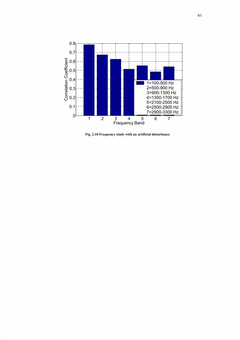
8/8/2019 BR PhD Dissertation
http://slidepdf.com/reader/full/br-phd-dissertation 73/248
41
1 2 3 4 5 6 70
0.1
0.2
0.3
0.4
0.5
0.6
0.7
0.8
Frequency Band
C o r r e l a t i o n C o e f f i c i e n t
1=100-500 Hz2=500-900 Hz3=900-1300 Hz4=1300-1700 Hz5=2100-2500 Hz
6=2500-2900 Hz7=2900-3300 Hz
Fig. 2.10 Frequency study with an artificial disturbance
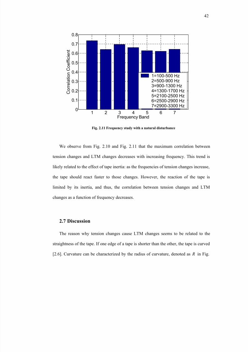
8/8/2019 BR PhD Dissertation
http://slidepdf.com/reader/full/br-phd-dissertation 74/248
42
1 2 3 4 5 6 70
0.1
0.2
0.3
0.4
0.5
0.6
0.7
0.8
Frequency Band
C o r r e l a t i o n C o e f f i c i e n t
1=100-500 Hz2=500-900 Hz3=900-1300 Hz4=1300-1700 Hz5=2100-2500 Hz6=2500-2900 Hz7=2900-3300 Hz
We observe from Fig. 2.10 and Fig. 2.11 that the maximum correlation between
tension changes and LTM changes decreases with increasing frequency. This trend is
likely related to the effect of tape inertia: as the frequencies of tension changes increase,
the tape should react faster to those changes. However, the reaction of the tape is
limited by its inertia, and thus, the correlation between tension changes and LTM
changes as a function of frequency decreases.
2.7 Discussion
The reason why tension changes cause LTM changes seems to be related to the
straightness of the tape. If one edge of a tape is shorter than the other, the tape is curved
[2.6]. Curvature can be characterized by the radius of curvature, denoted as R in Fig.
Fig. 2.11 Frequency study with a natural disturbance
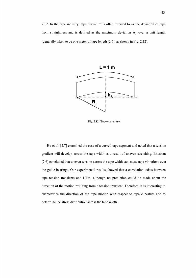
8/8/2019 BR PhD Dissertation
http://slidepdf.com/reader/full/br-phd-dissertation 75/248
43
2.12. In the tape industry, tape curvature is often referred to as the deviation of tape
from straightness and is defined as the maximum deviation Rh over a unit length
(generally taken to be one meter of tape length [2.6], as shown in Fig. 2.12).
L = 1 m
R
hR
L = 1 m
R
hR
Hu et al. [2.7] examined the case of a curved tape segment and noted that a tension
gradient will develop across the tape width as a result of uneven stretching. Bhushan
[2.6] concluded that uneven tension across the tape width can cause tape vibrations over
the guide bearings. Our experimental results showed that a correlation exists between
tape tension transients and LTM, although no prediction could be made about the
direction of the motion resulting from a tension transient. Therefore, it is interesting to
characterize the direction of the tape motion with respect to tape curvature and to
determine the stress distribution across the tape width.
Fig. 2.12: Tape curvature
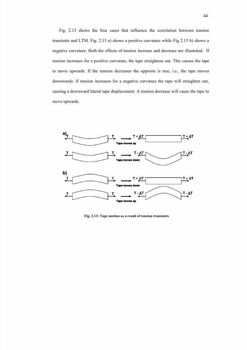
8/8/2019 BR PhD Dissertation
http://slidepdf.com/reader/full/br-phd-dissertation 76/248
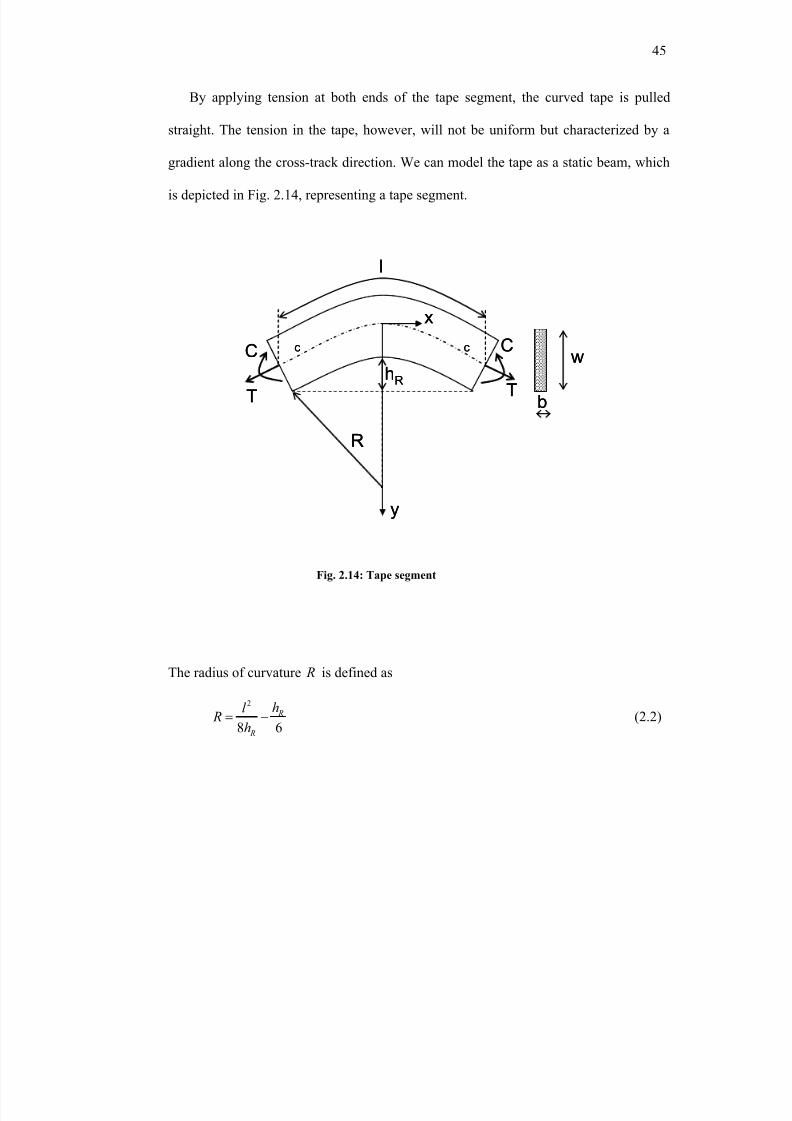
8/8/2019 BR PhD Dissertation
http://slidepdf.com/reader/full/br-phd-dissertation 77/248
45
By applying tension at both ends of the tape segment, the curved tape is pulled
straight. The tension in the tape, however, will not be uniform but characterized by a
gradient along the cross-track direction. We can model the tape as a static beam, which
is depicted in Fig. 2.14, representing a tape segment.
hR
R
TT
C
C
l
b
w
y
x
c c
hR
R
TT
C
C
l
b
w
y
x
c c
The radius of curvature R is defined as
2
8 6
R
R
hl
R h= − (2.2)
Fig. 2.14: Tape segment
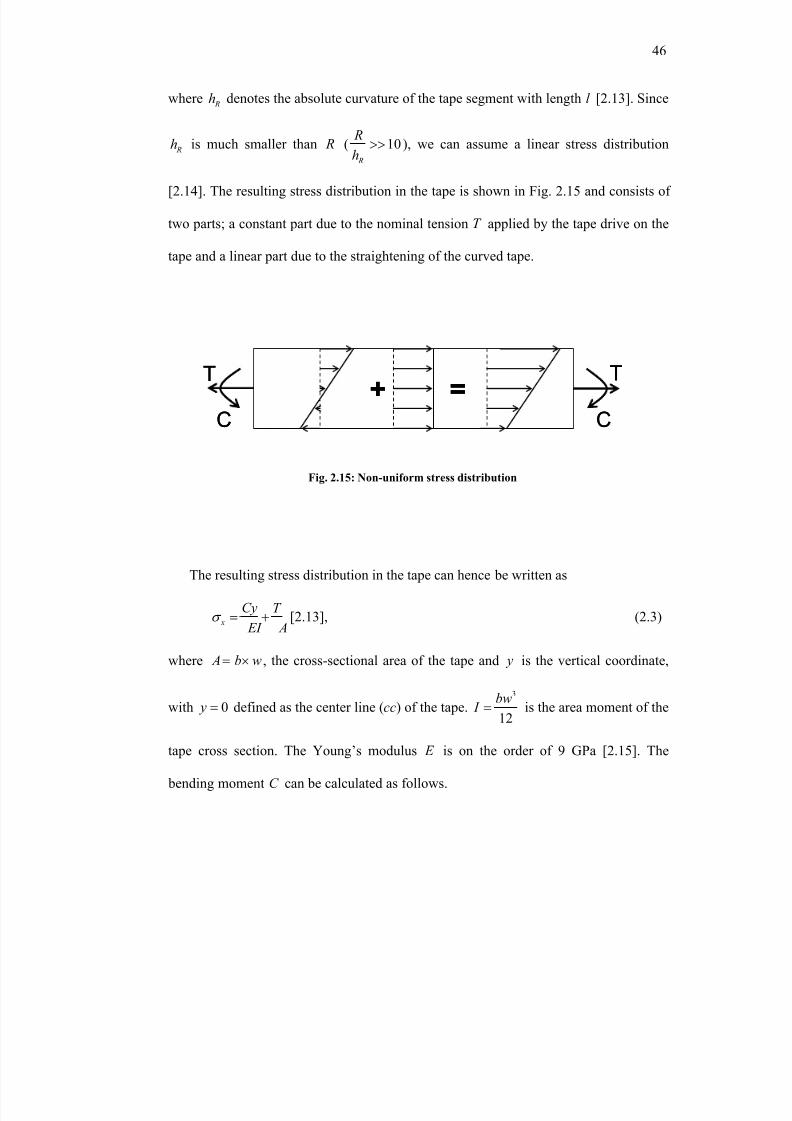
8/8/2019 BR PhD Dissertation
http://slidepdf.com/reader/full/br-phd-dissertation 78/248
46
where Rh denotes the absolute curvature of the tape segment with length l [2.13]. Since
Rh is much smaller than R ( 10 R
R
h>> ), we can assume a linear stress distribution
[2.14]. The resulting stress distribution in the tape is shown in Fig. 2.15 and consists of
two parts; a constant part due to the nominal tension T applied by the tape drive on the
tape and a linear part due to the straightening of the curved tape.
+ =TT
CC
+ =TT
CC
The resulting stress distribution in the tape can hence be written as
x
Cy T
EI Aσ = + [2.13], (2.3)
where A b w= × , the cross-sectional area of the tape and y is the vertical coordinate,
with 0 y = defined as the center line (cc) of the tape.3
12
bw I = is the area moment of the
tape cross section. The Young’s modulus E is on the order of 9 GPa [2.15]. The
bending moment C can be calculated as follows.
Fig. 2.15: Non-uniform stress distribution
8/8/2019 BR PhD Dissertation
http://slidepdf.com/reader/full/br-phd-dissertation 79/248
47
2
2
w
x
w
C ydAσ
−
= ∫ (2.4)
2
0
2
w
R
T C bh dy
A= ∫ (2.5)
where x
T
Aσ = and
R y h= if we assume the curvature to be constant in the lateral
direction. Solving (2.5) and substituting the result in (2.3) finally yields the resulting
stress distribution as a function of y :
R x
Th y T
EI Aσ = + (2.6)
Once the curvature of the tape is known along the length of the tape ( Rh ), the
direction of the lateral tape displacement (direction of LTM) can be obtained from Fig.
13. The resulting stress distribution can be calculated from (2.6).
As new tape systems are developed, thinner tapes would allow an increase in the
tape windings per cartridge, and therefore a greater capacity per cartridge. However,
thinner tapes require increased attention to the stress distribution and the inherent
parameters governing the bending stiffness and system tension considerations. If the
same nominal tension T would be applied to thinner tape, the internal stresses would
increase. The second factor in eq. (2.6) would increase because the cross-sectional area
A becomes smaller. Additionally, since I will decrease, the bending stiffness EI will
decrease and the first factor in eq. (2.6) will increase too. Making tape thinner thus
8/8/2019 BR PhD Dissertation
http://slidepdf.com/reader/full/br-phd-dissertation 80/248
48
affects both the constant and the linear part of the stress distribution along the tape
width. It is thus apparent that tension transients and LTM will become increasingly
important in future high performance tape drives.
2.8 Conclusion
A non-contact optical method was implemented to measure tape tension and study
the effect of tension changes on lateral tape motion. Based on our experimental results,
the following conclusions can be drawn:
1. The measurement of the change in reflected light intensity from a tape surface
due to a tension variation is a viable method to study the effect of tension
change on LTM.
2. A sound correlation exists between the absolute values of tension change and the
lateral tape displacement signal.
3. Tape curvature from the slitting process coupled with tension changes from the
drive system causes lateral motion of the tape.
2.9 Acknowledgements
Chapter 2, in part, is a reprint of the material as it appears in “Non-Contact Tape
Tension Measurement and Correlation of Lateral Tape Motion and Tape Tension
Transients”, Raeymaekers B., Taylor R.J., Talke F.E., Microsystem Technologies,
2006. The dissertation author was the primary investigator and author of this paper.
8/8/2019 BR PhD Dissertation
http://slidepdf.com/reader/full/br-phd-dissertation 81/248

8/8/2019 BR PhD Dissertation
http://slidepdf.com/reader/full/br-phd-dissertation 82/248
50
[2.15] Bhushan B, Tao Z, 2004, Mechanical, Hygroscopic, and Thermal Properties of Metal Particle and Metal Evaporated Tapes and Their Individual Layers, J. Appl.
Polymer Sci. Vol. 92, pp. 1319 - 1345
8/8/2019 BR PhD Dissertation
http://slidepdf.com/reader/full/br-phd-dissertation 83/248
51
3. Characterization of tape edge contact with acoustic
emission
3.1 Introduction
Tape edge contact is one of the primary sources of lateral tape motion (LTM).
Researchers in the past have investigated various aspects related to tape edge contact.
Lakshmikumaran and Wickert studied edge buckling of imperfectly guided webs and
developed a “free sliding” model and an “edge guided” model for web buckling [3.1].
Wang, Taylor and Talke investigated the relationship between LTM and tape edge wear
by applying a force on the tape edge using a tapered cantilever spring from a hard disk
drive suspension [3.2]. They concluded that tape wear increases with increasing tape
edge contact force. Doyle experimentally determined the contact force during the
transverse impact of plates using strain gauges. This technique is not applicable,
however, when dealing with thin magnetic tape [3.3]. The effect of tape edge contact on
edge quality and tape wear has also been studied. Goldade and Bhushan found that tape
edge contact can damage the tape edge, creates debris and negatively affects tape
guiding [3.4, 3.5]. Bhushan, Hinteregger and Rogers optimized edge guiding
mechanisms by decreasing friction and improving thermal conductivity and hence
reducing the guiding forces [3.6]. Taylor and Talke examined contact between magnetic
tape and a reel and studied the effect of tape edge contact on LTM. They also
investigated the cause of the so-called stack-shift phenomenon and its relationship to
LTM [3.7]. Little published information exists regarding the magnitude of contact
8/8/2019 BR PhD Dissertation
http://slidepdf.com/reader/full/br-phd-dissertation 84/248
52
forces during tape edge/flange contact. Since tape edge wear and LTM are related to the
magnitude of the tape edge contact force [3.2, 3.7], this information is desirable for the
design of future high performance tape drives. This chapter tries to fill the above gap
and focuses on the characterization and quantification of tape edge contact between a
tape edge and the flange of a roller by means of acoustic emission (AE) techniques.
3.2 Acoustic emission
On a micro-scale, deformation is characterized by dislocations. The movement of
dislocations generates transient elastic stress waves, referred to as acoustic emission
(AE) [3.8]. Elastic stress waves propagate from a source as plane or spherical waves.
The stress waves are picked up by the AE sensor and converted into a voltage
proportional to the magnitude of the AE energy [3.9]. In this investigation, an AE
sensor is used as a flange instead of an actual flange on a roller. When the tape makes
contact with the flange which is replaced by the sensor, a voltage is generated. This
voltage is analyzed and used as an indicator of the type and strength of contact
occurring as a function of design parameters of the tape edge/roller flange interface.
The impact force ( )imp f t can be calculated from the stress σ in the tape/flange
contact area S by
( )imp
S
f t dS σ = ∫ (3.1)
8/8/2019 BR PhD Dissertation
http://slidepdf.com/reader/full/br-phd-dissertation 85/248
53
The output voltage ( )v t of the AE sensor can be related to the impact force ( )imp f t by
the convolution
( ) ( ) ( )0
t
imp impv t g t f d τ τ τ = −∫ (3.2)
where g is the transfer function and τ is the variable of integration. Calculating the
Laplace transform from eq. (3.2) yields
( ) ( ) ( )*imp impV G F ω ω ω = (3.3)
where ( )V ω is the output voltage, ( )G ω is the transfer function, ( )imp F ω is the impact
force and ω represents the frequency. After rearranging eq. (3.3), we obtain
( )( )
( )imp
imp
V F
G
ω ω
ω = (3.4)
If ( )impG ω is known in eq. (3.4), ( )imp F ω can be calculated from ( )V ω . In order to
find the transfer function ( )impG ω , calibration of the AE sensor is necessary.
3.3 Calibration
To determine the magnitude of the contact force between the tape edge and a flange,
the AE sensor was first calibrated by means of the “ball drop method” [3.10]. This
method has been used previously for the analysis of slider/disk impacts in hard disk
drive research [3.11, 3.12]. Fig. 3.1 illustrates the calibration procedure. A steel ball is
dropped from different heights d h on a load cell which measures the impact force
during contact (Fig. 3.1 a)). Next, a steel ball is dropped from different heights d h on
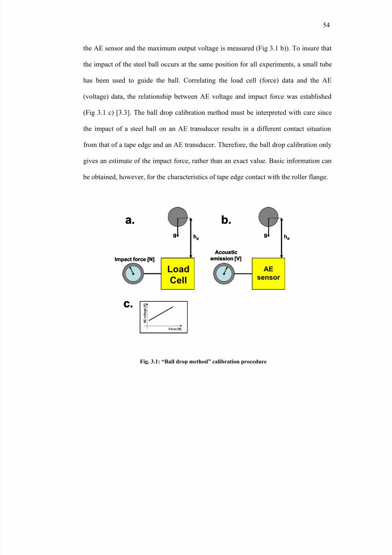
8/8/2019 BR PhD Dissertation
http://slidepdf.com/reader/full/br-phd-dissertation 86/248
54
the AE sensor and the maximum output voltage is measured (Fig 3.1 b)). To insure that
the impact of the steel ball occurs at the same position for all experiments, a small tube
has been used to guide the ball. Correlating the load cell (force) data and the AE
(voltage) data, the relationship between AE voltage and impact force was established
(Fig 3.1 c) [3.3]. The ball drop calibration method must be interpreted with care since
the impact of a steel ball on an AE transducer results in a different contact situation
from that of a tape edge and an AE transducer. Therefore, the ball drop calibration only
gives an estimate of the impact force, rather than an exact value. Basic information can
be obtained, however, for the characteristics of tape edge contact with the roller flange.
g
LoadCell
Impact force [N]
hdg
AEsensor
Acoustic
emission [V]
hd
a. b.
c.
Force [N]
A E
v o l t a g e [ V ]
g
LoadCell
Impact force [N]
hdg
AEsensor
Acoustic
emission [V]
hd
a. b.
c.
Force [N]
A E
v o l t a g e [ V ]
Fig. 3.1: “Ball drop method” calibration procedure
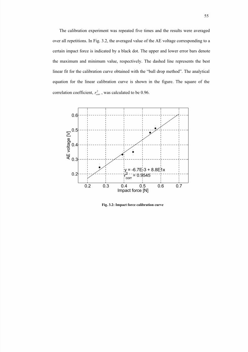
8/8/2019 BR PhD Dissertation
http://slidepdf.com/reader/full/br-phd-dissertation 87/248
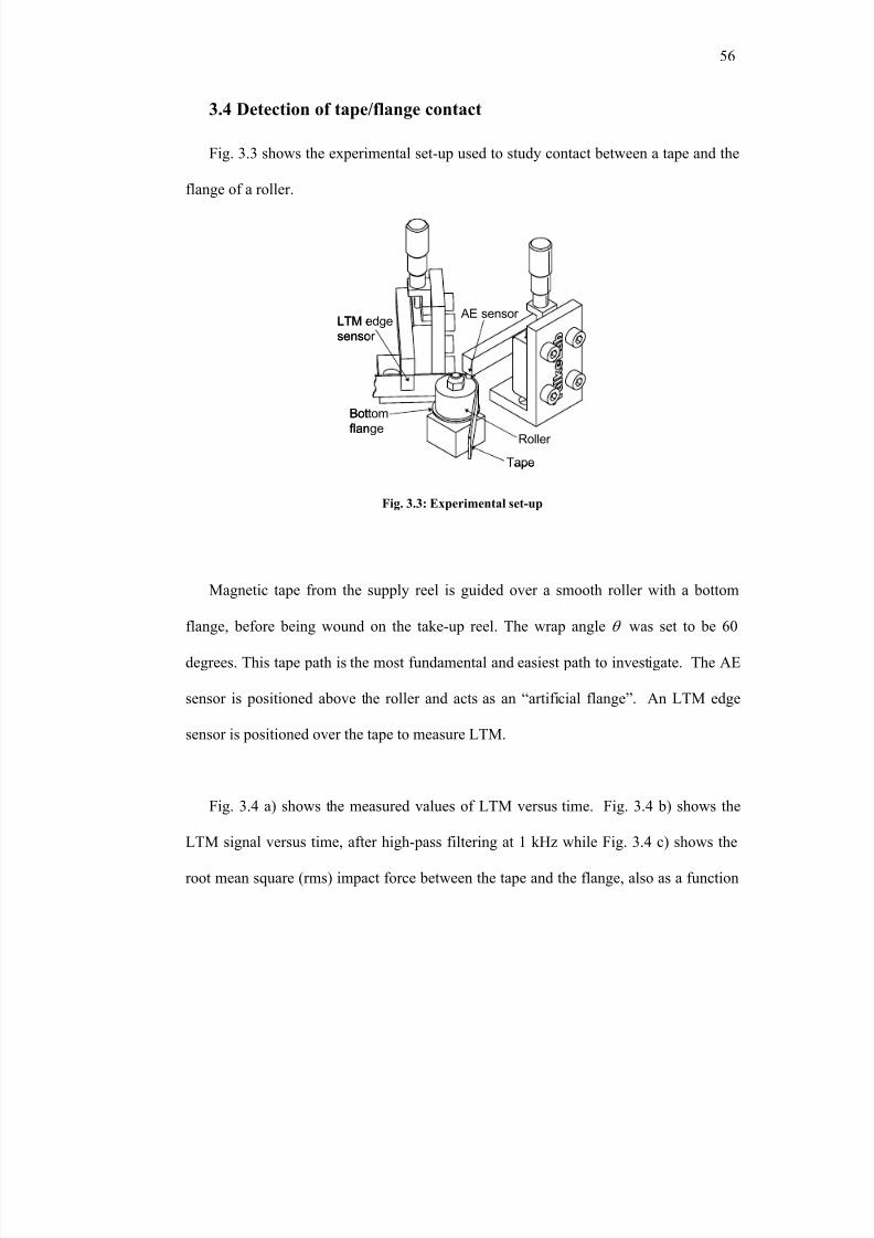
8/8/2019 BR PhD Dissertation
http://slidepdf.com/reader/full/br-phd-dissertation 88/248
56
3.4 Detection of tape/flange contact
Fig. 3.3 shows the experimental set-up used to study contact between a tape and the
flange of a roller.
Tape
Roller
AE sensor LTM edge
sensor
Bottom
flange
Tape
Roller
AE sensor LTM edge
sensor
Bottom
flange
Magnetic tape from the supply reel is guided over a smooth roller with a bottom
flange, before being wound on the take-up reel. The wrap angle θ was set to be 60
degrees. This tape path is the most fundamental and easiest path to investigate. The AE
sensor is positioned above the roller and acts as an “artificial flange”. An LTM edge
sensor is positioned over the tape to measure LTM.
Fig. 3.4 a) shows the measured values of LTM versus time. Fig. 3.4 b) shows the
LTM signal versus time, after high-pass filtering at 1 kHz while Fig. 3.4 c) shows the
root mean square (rms) impact force between the tape and the flange, also as a function
Fig. 3.3: Experimental set-up
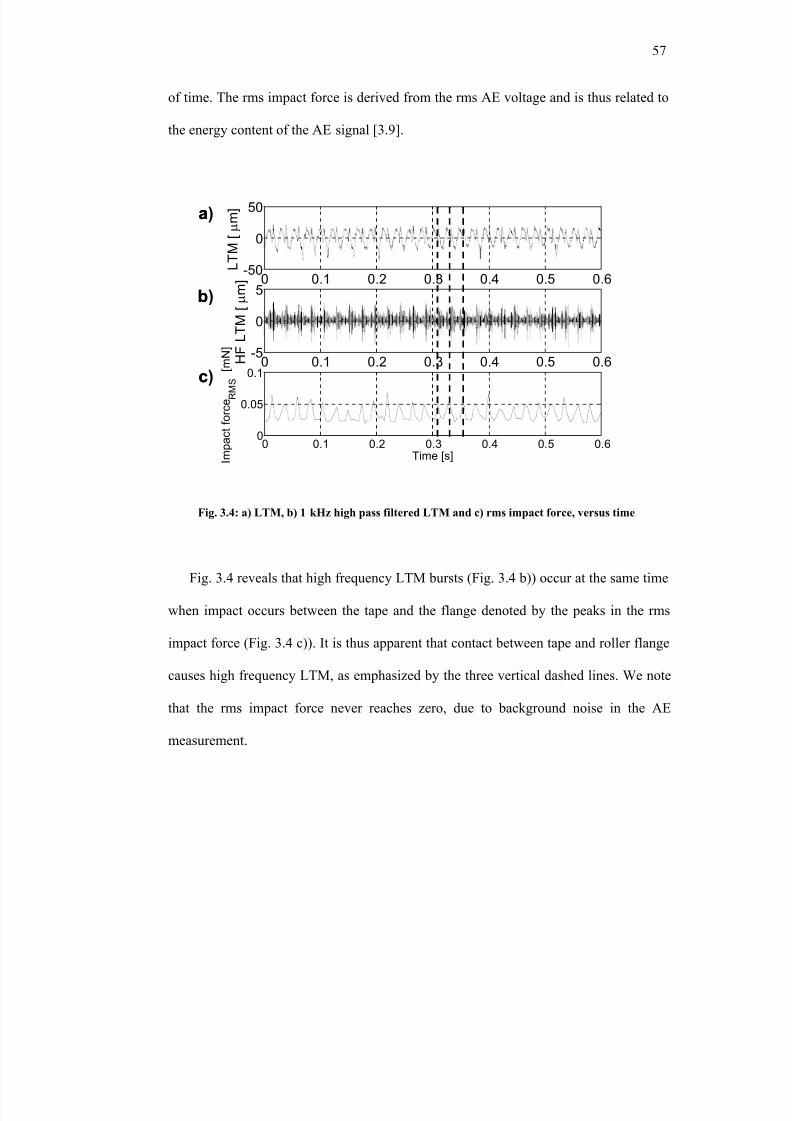
8/8/2019 BR PhD Dissertation
http://slidepdf.com/reader/full/br-phd-dissertation 89/248
57
of time. The rms impact force is derived from the rms AE voltage and is thus related to
the energy content of the AE signal [3.9].
0 0.1 0.2 0.3 0.4 0.5 0.6-50
0
50
L T M [
µ m ]
0 0.1 0.2 0.3 0.4 0.5 0.6-5
0
5
H
F L T M [
µ m ]
0 0.1 0.2 0.3 0.4 0.5 0.60
0.05
0.1
Time [s] I m p a c t f o r c e R M S
[ m N ]
a)
b)
c)
0 0.1 0.2 0.3 0.4 0.5 0.6-50
0
50
L T M [
µ m ]
0 0.1 0.2 0.3 0.4 0.5 0.6-5
0
5
H
F L T M [
µ m ]
0 0.1 0.2 0.3 0.4 0.5 0.60
0.05
0.1
Time [s] I m p a c t f o r c e R M S
[ m N ]
a)
b)
c)
Fig. 3.4 reveals that high frequency LTM bursts (Fig. 3.4 b)) occur at the same time
when impact occurs between the tape and the flange denoted by the peaks in the rms
impact force (Fig. 3.4 c)). It is thus apparent that contact between tape and roller flange
causes high frequency LTM, as emphasized by the three vertical dashed lines. We note
that the rms impact force never reaches zero, due to background noise in the AE
measurement.
Fig. 3.4: a) LTM, b) 1 kHz high pass filtered LTM and c) rms impact force, versus time
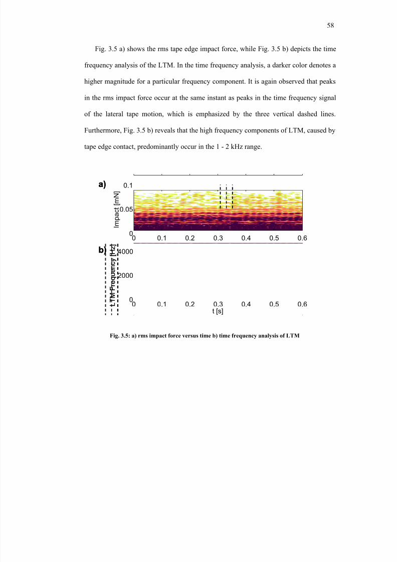
8/8/2019 BR PhD Dissertation
http://slidepdf.com/reader/full/br-phd-dissertation 90/248
58
Fig. 3.5 a) shows the rms tape edge impact force, while Fig. 3.5 b) depicts the time
frequency analysis of the LTM. In the time frequency analysis, a darker color denotes a
higher magnitude for a particular frequency component. It is again observed that peaks
in the rms impact force occur at the same instant as peaks in the time frequency signal
of the lateral tape motion, which is emphasized by the three vertical dashed lines.
Furthermore, Fig. 3.5 b) reveals that the high frequency components of LTM, caused by
tape edge contact, predominantly occur in the 1 - 2 kHz range.
0 0.1 0.2 0.3 0.4 0.5 0.60
0.05
0.1
I m p a c t [ m N ]
t [s] L T M F
r e q u e
n c y [ H z ]
0 0.1 0.2 0.3 0.4 0.5 0.60
2000
4000
a)
b)
0 0.1 0.2 0.3 0.4 0.5 0.60
0.05
0.1
I m p a c t [ m N ]
t [s] L T M F
r e q u e
n c y [ H z ]
0 0.1 0.2 0.3 0.4 0.5 0.60
2000
4000
a)
b)
0 0.1 0.2 0.3 0.4 0.5 0.60
0.05
0.1
I m p a c t [ m N ]
t [s] L T M F
r e q u e
n c y [ H z ]
0 0.1 0.2 0.3 0.4 0.5 0.60
2000
4000
a)
b)
Fig. 3.5: a) rms impact force versus time b) time frequency analysis of LTM
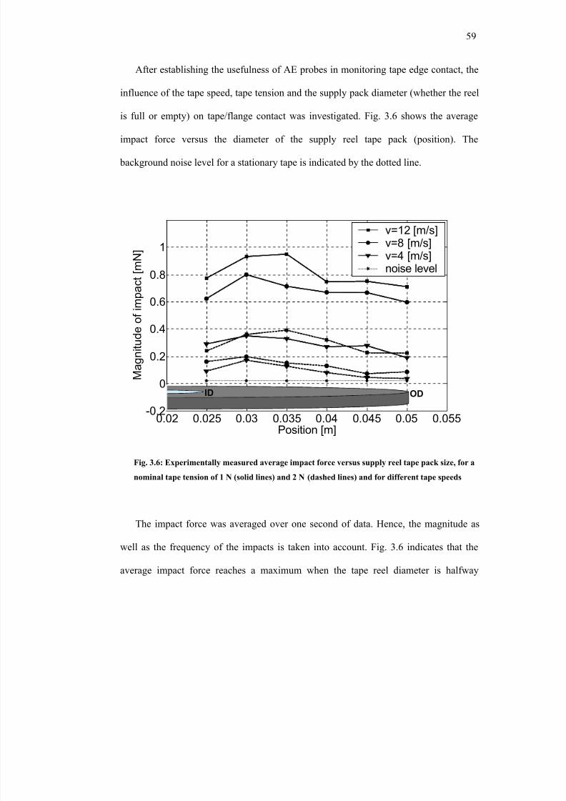
8/8/2019 BR PhD Dissertation
http://slidepdf.com/reader/full/br-phd-dissertation 91/248
59
After establishing the usefulness of AE probes in monitoring tape edge contact, the
influence of the tape speed, tape tension and the supply pack diameter (whether the reel
is full or empty) on tape/flange contact was investigated. Fig. 3.6 shows the average
impact force versus the diameter of the supply reel tape pack (position). The
background noise level for a stationary tape is indicated by the dotted line.
0.02 0.025 0.03 0.035 0.04 0.045 0.05 0.055-0.2
0
0.2
0.4
0.6
0.8
1
Position [m]
M a g n i t u d e o f i m p a c t [ m N
]
v=12 [m/s]v=8 [m/s]
v=4 [m/s]noise level
ID OD
0.02 0.025 0.03 0.035 0.04 0.045 0.05 0.055-0.2
0
0.2
0.4
0.6
0.8
1
Position [m]
M a g n i t u d e o f i m p a c t [ m N
]
v=12 [m/s]v=8 [m/s]
v=4 [m/s]noise level
ID OD
The impact force was averaged over one second of data. Hence, the magnitude as
well as the frequency of the impacts is taken into account. Fig. 3.6 indicates that the
average impact force reaches a maximum when the tape reel diameter is halfway
Fig. 3.6: Experimentally measured average impact force versus supply reel tape pack size, for a
nominal tape tension of 1 N (solid lines) and 2 N (dashed lines) and for different tape speeds
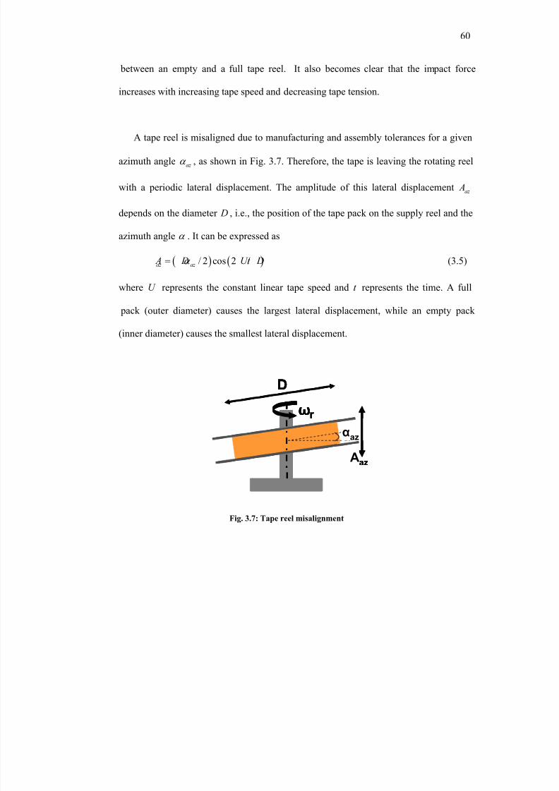
8/8/2019 BR PhD Dissertation
http://slidepdf.com/reader/full/br-phd-dissertation 92/248
60
between an empty and a full tape reel. It also becomes clear that the impact force
increases with increasing tape speed and decreasing tape tension.
A tape reel is misaligned due to manufacturing and assembly tolerances for a given
azimuth angle az α , as shown in Fig. 3.7. Therefore, the tape is leaving the rotating reel
with a periodic lateral displacement. The amplitude of this lateral displacement az A
depends on the diameter D , i.e., the position of the tape pack on the supply reel and the
azimuth angle α . It can be expressed as
( ) ( )/ 2 cos 2 /az az A D Ut Dα = (3.5)
where U represents the constant linear tape speed and t represents the time. A full
pack (outer diameter) causes the largest lateral displacement, while an empty pack
(inner diameter) causes the smallest lateral displacement.
α
A
ω
D
α
A
ω
D
r
αaz
Aaz
α
A
ω
D
α
A
ω
D
r
αaz
Aaz
Fig. 3.7: Tape reel misalignment
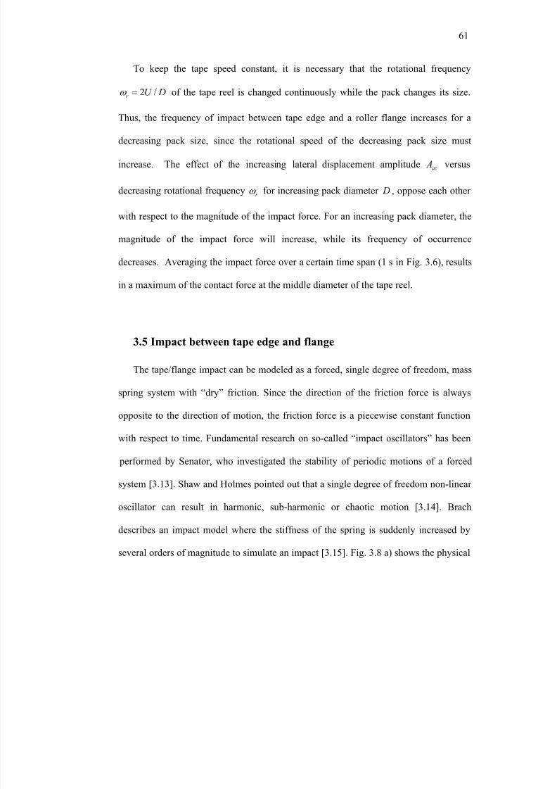
8/8/2019 BR PhD Dissertation
http://slidepdf.com/reader/full/br-phd-dissertation 93/248
61
To keep the tape speed constant, it is necessary that the rotational frequency
2 /r U Dω = of the tape reel is changed continuously while the pack changes its size.
Thus, the frequency of impact between tape edge and a roller flange increases for a
decreasing pack size, since the rotational speed of the decreasing pack size must
increase. The effect of the increasing lateral displacement amplitude az A versus
decreasing rotational frequency r ω for increasing pack diameter D , oppose each other
with respect to the magnitude of the impact force. For an increasing pack diameter, the
magnitude of the impact force will increase, while its frequency of occurrence
decreases. Averaging the impact force over a certain time span (1 s in Fig. 3.6), results
in a maximum of the contact force at the middle diameter of the tape reel.
3.5 Impact between tape edge and flange
The tape/flange impact can be modeled as a forced, single degree of freedom, mass
spring system with “dry” friction. Since the direction of the friction force is always
opposite to the direction of motion, the friction force is a piecewise constant function
with respect to time. Fundamental research on so-called “impact oscillators” has been
performed by Senator, who investigated the stability of periodic motions of a forced
system [3.13]. Shaw and Holmes pointed out that a single degree of freedom non-linear
oscillator can result in harmonic, sub-harmonic or chaotic motion [3.14]. Brach
describes an impact model where the stiffness of the spring is suddenly increased by
several orders of magnitude to simulate an impact [3.15]. Fig. 3.8 a) shows the physical
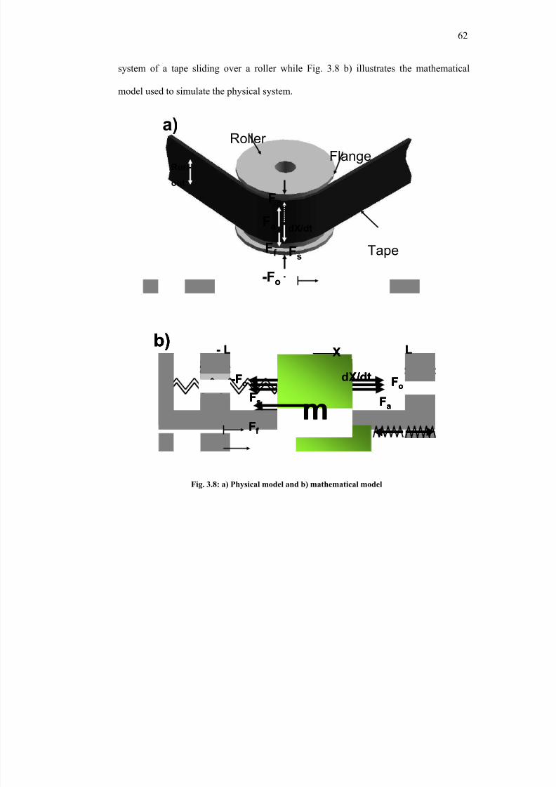
8/8/2019 BR PhD Dissertation
http://slidepdf.com/reader/full/br-phd-dissertation 94/248
62
system of a tape sliding over a roller while Fig. 3.8 b) illustrates the mathematical
model used to simulate the physical system.
Fa
FsFf
Fo
Tape
Roller
Flange
dX/dt
a)
-Fo
Run-
out
Fa
FsFf
Fo
Tape
Roller
Flange
dX/dt
a)
-Fo
Run-
out
m
X
FaFs
Ff
-Fo Fo
b)
dX/dt
L- L
m
X
FaFs
Ff
-Fo Fo
b)
dX/dt
mm
X
FaFs
Ff
-Fo Fo
b)
dX/dt
L- L
Fig. 3.8: a) Physical model and b) mathematical model
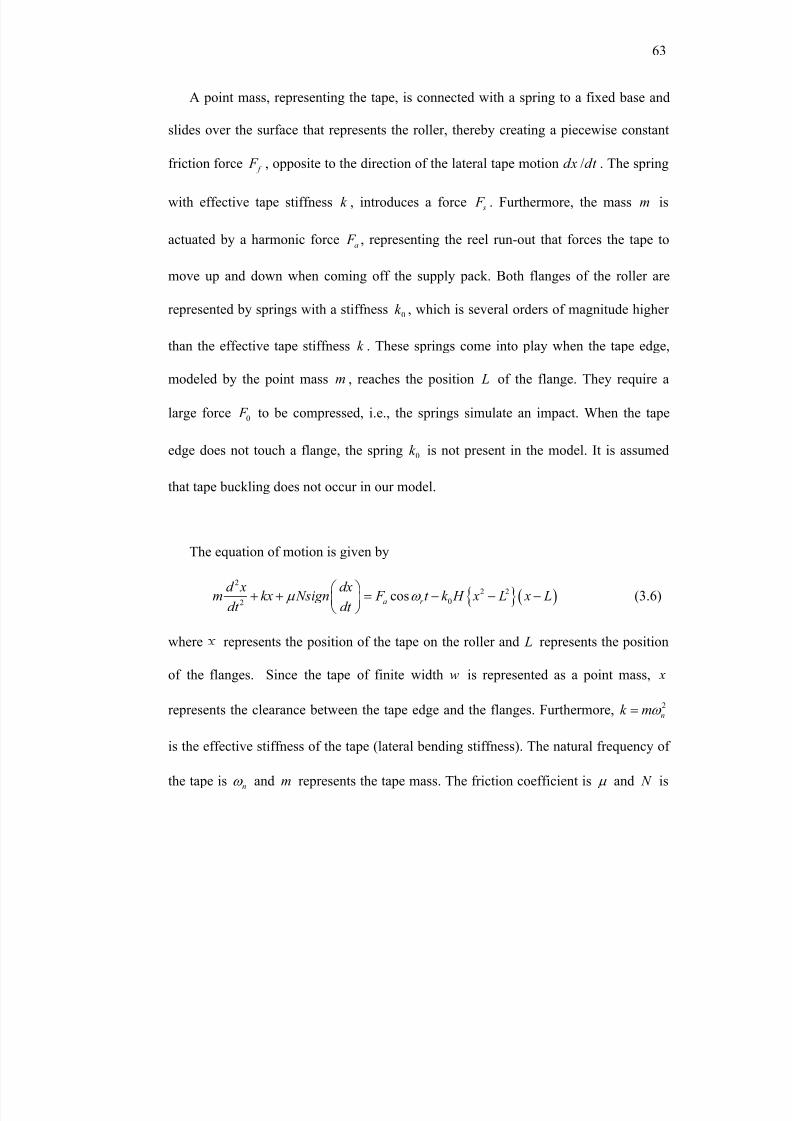
8/8/2019 BR PhD Dissertation
http://slidepdf.com/reader/full/br-phd-dissertation 95/248
63
A point mass, representing the tape, is connected with a spring to a fixed base and
slides over the surface that represents the roller, thereby creating a piecewise constant
friction force f F , opposite to the direction of the lateral tape motion /dx dt . The spring
with effective tape stiffness k , introduces a force s F . Furthermore, the mass m is
actuated by a harmonic force a F , representing the reel run-out that forces the tape to
move up and down when coming off the supply pack. Both flanges of the roller are
represented by springs with a stiffness 0k , which is several orders of magnitude higher
than the effective tape stiffness k . These springs come into play when the tape edge,
modeled by the point mass m , reaches the position L of the flange. They require a
large force 0 F to be compressed, i.e., the springs simulate an impact. When the tape
edge does not touch a flange, the spring 0k is not present in the model. It is assumed
that tape buckling does not occur in our model.
The equation of motion is given by
{ }( )2
2 2
02cosa r
d x dxm kx Nsign F t k H x L x L
dt dt µ ω
+ + = − − −
(3.6)
where represents the position of the tape on the roller and L represents the position
of the flanges. Since the tape of finite width w is represented as a point mass, x
represents the clearance between the tape edge and the flanges. Furthermore, 2
n
k mω =
is the effective stiffness of the tape (lateral bending stiffness). The natural frequency of
the tape is nω and m represents the tape mass. The friction coefficient is µ and N is
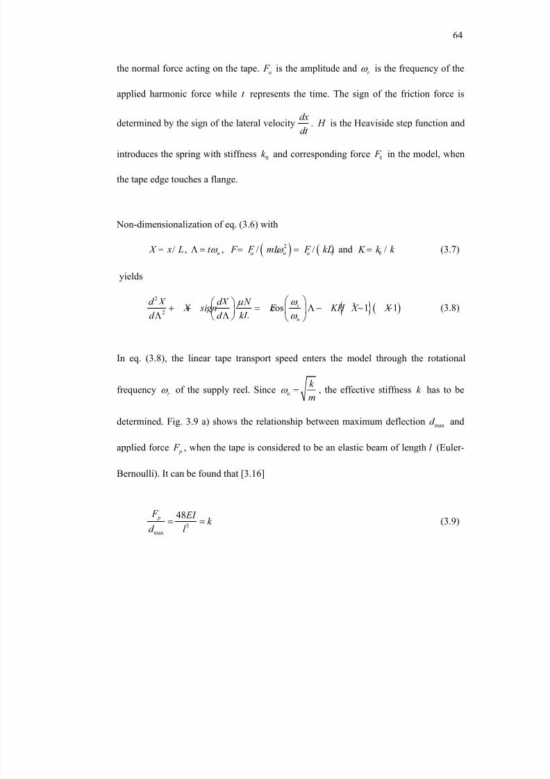
8/8/2019 BR PhD Dissertation
http://slidepdf.com/reader/full/br-phd-dissertation 96/248
64
the normal force acting on the tape. a F is the amplitude and r ω is the frequency of the
applied harmonic force while t represents the time. The sign of the friction force is
determined by the sign of the lateral velocity
dx
dt . H is the Heaviside step function and
introduces the spring with stiffness 0k and corresponding force 0 F in the model, when
the tape edge touches a flange.
Non-dimensionalization of eq. (3.6) with
/ X x L= , nt ω Λ = , ( ) ( )2
/ /a n a F F mL F kLω = = and 0 / K k k = (3.7)
yields
{ }( )2
2
2cos 1 1r
n
d X dX N X sign F KH X X
d d kL
ω µ
ω
+ + = Λ − − −
Λ Λ (3.8)
In eq. (3.8), the linear tape transport speed enters the model through the rotational
frequency r ω of the supply reel. Since n
k
mω = , the effective stiffness k has to be
determined. Fig. 3.9 a) shows the relationship between maximum deflection maxd and
applied force p F , when the tape is considered to be an elastic beam of length l (Euler-
Bernoulli). It can be found that [3.16]
3
max
48 p F EI k
d l = = (3.9)
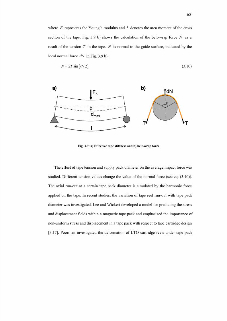
8/8/2019 BR PhD Dissertation
http://slidepdf.com/reader/full/br-phd-dissertation 97/248
65
where E represents the Young’s modulus and I denotes the area moment of the cross
section of the tape. Fig. 3.9 b) shows the calculation of the belt-wrap force N as a
result of the tension T in the tape. N is normal to the guide surface, indicated by the
local normal force dN in Fig. 3.9 b).
( )2 sin / 2 N T θ = (3.10)
dmax
l
Fp
T T
θ
dNa) b)
dmax
l
Fp
T T
θ
dNa) b)
The effect of tape tension and supply pack diameter on the average impact force was
studied. Different tension values change the value of the normal force (see eq. (3.10)).
The axial run-out at a certain tape pack diameter is simulated by the harmonic force
applied on the tape. In recent studies, the variation of tape reel run-out with tape pack
diameter was investigated. Lee and Wickert developed a model for predicting the stress
and displacement fields within a magnetic tape pack and emphasized the importance of
non-uniform stress and displacement in a tape pack with respect to tape cartridge design
[3.17]. Poorman investigated the deformation of LTO cartridge reels under tape pack
Fig. 3.9: a) Effective tape stiffness and b) belt-wrap force
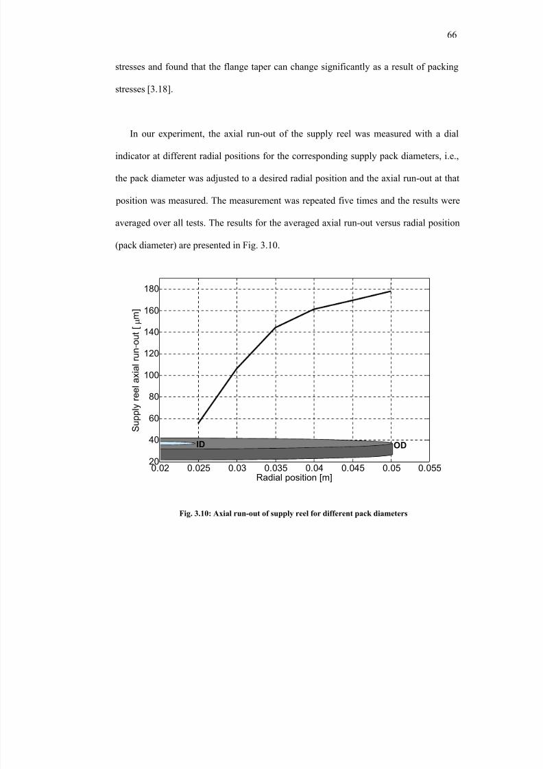
8/8/2019 BR PhD Dissertation
http://slidepdf.com/reader/full/br-phd-dissertation 98/248
66
stresses and found that the flange taper can change significantly as a result of packing
stresses [3.18].
In our experiment, the axial run-out of the supply reel was measured with a dial
indicator at different radial positions for the corresponding supply pack diameters, i.e.,
the pack diameter was adjusted to a desired radial position and the axial run-out at that
position was measured. The measurement was repeated five times and the results were
averaged over all tests. The results for the averaged axial run-out versus radial position
(pack diameter) are presented in Fig. 3.10.
0.02 0.025 0.03 0.035 0.04 0.045 0.05 0.05520
40
60
80
100
120
140
160
180
Radial position [m]
S u p p l y r e e l a x i a
l r u n - o u t [ µ m ]
ID OD
0.02 0.025 0.03 0.035 0.04 0.045 0.05 0.05520
40
60
80
100
120
140
160
180
Radial position [m]
S u p p l y r e e l a x i a
l r u n - o u t [ µ m ]
ID OD
Fig. 3.10: Axial run-out of supply reel for different pack diameters
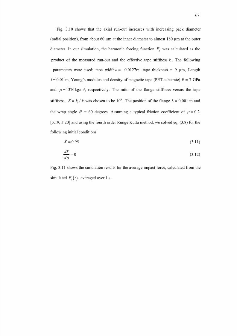
8/8/2019 BR PhD Dissertation
http://slidepdf.com/reader/full/br-phd-dissertation 99/248
67
Fig. 3.10 shows that the axial run-out increases with increasing pack diameter
(radial position), from about 60 µm at the inner diameter to almost 180 µm at the outer
diameter. In our simulation, the harmonic forcing function a F was calculated as the
product of the measured run-out and the effective tape stiffness k . The following
parameters were used: tape width 0.0127w = m, tape thickness = 9 µm, Length
0.01l = m, Young’s modulus and density of magnetic tape (PET substrate) 7 E = GPa
and 1370 ρ = kg/m³, respectively. The ratio of the flange stiffness versus the tape
stiffness, 0 / K k k = was chosen to be 410 . The position of the flange 0.001 L = m and
the wrap angle θ = 60 degrees. Assuming a typical friction coefficient of 0.2µ =
[3.19, 3.20] and using the fourth order Runge Kutta method, we solved eq. (3.8) for the
following initial conditions:
0.95 X = (3.11)
0dX
d =
Λ(3.12)
Fig. 3.11 shows the simulation results for the average impact force, calculated from the
simulated ( )0 F t , averaged over 1 s.
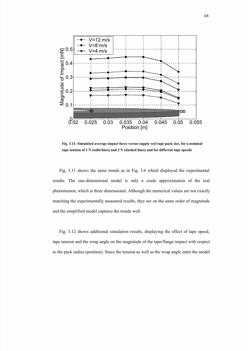
8/8/2019 BR PhD Dissertation
http://slidepdf.com/reader/full/br-phd-dissertation 100/248
68
0.02 0.025 0.03 0.035 0.04 0.045 0.05 0.0550
0.1
0.2
0.3
0.4
0.5
Position [m]
M a g n i t u d e o f I m p a c t [ m
N ]
V=12 m/sV=8 m/sV=4 m/s
ID OD
0.02 0.025 0.03 0.035 0.04 0.045 0.05 0.0550
0.1
0.2
0.3
0.4
0.5
Position [m]
M a g n i t u d e o f I m p a c t [ m
N ]
V=12 m/sV=8 m/sV=4 m/s
ID OD
Fig. 3.11 shows the same trends as in Fig. 3.6 which displayed the experimental
results. The one-dimensional model is only a crude approximation of the real
phenomenon, which is three dimensional. Although the numerical values are not exactly
matching the experimentally measured results, they are on the same order of magnitude
and the simplified model captures the trends well.
Fig. 3.12 shows additional simulation results, displaying the effect of tape speed,
tape tension and the wrap angle on the magnitude of the tape/flange impact with respect
to the pack radius (position). Since the tension as well as the wrap angle enter the model
Fig. 3.11: Simulated average impact force versus supply reel tape pack size, for a nominal
tape tension of 1 N (solid lines) and 2 N (dashed lines) and for different tape speeds
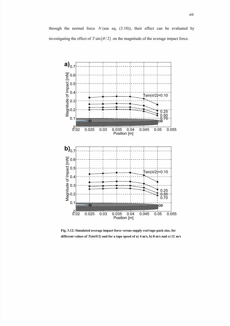
8/8/2019 BR PhD Dissertation
http://slidepdf.com/reader/full/br-phd-dissertation 101/248
69
through the normal force N (see eq. (3.10)), their effect can be evaluated by
investigating the effect of ( )sin / 2T θ on the magnitude of the average impact force.
0.02 0.025 0.03 0.035 0.04 0.045 0.05 0.0550
0.1
0.2
0.3
0.4
0.5
0.6
0.7
Position [m]
M a g n i t u
d e o f I m p a c t [ m N ]
Tsin(θ/2)=0.10
0.250.500.70
ID OD
a)
0.02 0.025 0.03 0.035 0.04 0.045 0.05 0.0550
0.1
0.2
0.3
0.4
0.5
0.6
0.7
Position [m]
M a g n i t u
d e o f I m p a c t [ m N ]
Tsin(θ/2)=0.10
0.250.500.70
ID OD
a)
0.02 0.025 0.03 0.035 0.04 0.045 0.05 0.0550
0.1
0.2
0.3
0.4
0.5
0.6
0.7
Position [m]
M a g n i t u d e o f I m p a c t [ m N ]
Tsin(θ/2)=0.10
0.250.500.70
ID OD
b)
Fig. 3.12: Simulated average impact force versus supply reel tape pack size, for
different values of Tsin( θ /2) and for a tape speed of a) 4 m/s, b) 8 m/s and c) 12 m/s
8/8/2019 BR PhD Dissertation
http://slidepdf.com/reader/full/br-phd-dissertation 102/248
70
0.02 0.025 0.03 0.035 0.04 0.045 0.05 0.0550
0.1
0.2
0.3
0.4
0.5
0.6
0.7
Position [m]
M a g n i t u d e o f I m p a c t [ m N ]
Tsin(θ/2)=0.10
0.25
0.500.70
Tsin(θ/2)=0.10
0.25
0.500.70
Tsin(θ/2)=0.10
0.25
0.500.70
Tsin(θ/2)=0.10
0.25
0.500.70
Tsin(θ/2)=0.10
0.25
0.500.70
Tsin(θ/2)=0.10
0.25
0.500.70
ID OD
c)
We observe from Fig. 3.12 that increasing ( )sin / 2T θ reduces the impact force
between roller flange and tape. Increasing( )
sin / 2T θ implies increasing the tape
tension T or the wrap angle θ . The average impact force is higher for increasing tape
speeds. In addition, Fig. 3.12 reveals that regardless of the tape speed, the impact for
( )sin / 2 0.1T θ = is almost double the value for ( )sin / 2 0.7T θ = . This result is
especially interesting when considering reduced nominal tape tension to accommodate
thinner tapes. On the other hand, increasing the wrap angle decreases the average
impact force, but also increases the contact surface between tape and roller and the
friction that acts on the tape will increase accordingly. Friction will dissipate energy and
hence, the average magnitude of the impact between tape and flange will be smaller.
Fig. 3.12 continued: Simulated average impact force versus supply reel tape pack size,
for different values of Tsin( θ /2) and for a tape speed of a) 4 m/s, b) 8 m/s and c) 12 m/s
8/8/2019 BR PhD Dissertation
http://slidepdf.com/reader/full/br-phd-dissertation 103/248
71
Fig. 3.12 also illustrates that increasing tape speed increases the average magnitude of
the impact. However, the effect of speed appears to be less than the effect of
( )sin / 2T θ . The combination of low tension and small wrap angle will yield the
highest average impact forces. This effect is amplified for increasing tape speeds.
Increasing tension and wrap angle, on the other hand, decreases the magnitude of the
tape/flange contact.
3.5 Discussion
Tape edge contact is a significant problem in achieving track densities beyond 40
tracks/mm (1000 tracks per inch (tpi)). Impacts between tape and roller or guide flanges
induce LTM in the 1-2 KHz frequency range in the tape path. This is the frequency
range beyond the bandwidth of the head servo actuator, i.e., the servo system is
incapable of following such high frequency lateral vibrations of the tape which can lead
to track misregistration.
As tape manufacturers tend to use thinner tape to increase the volumetric storage
density of a tape cartridge, the problem of tape edge contact might manifest itself more.
It was observed that lower nominal tape tensions result in increasingly more severe tape
flange impacts. Thinner tape implies the use of a lower nominal tension since the stress
in the tape has to remain constant. Hence, thinner tape might yield more severe tape
edge contact. This conclusion is in agreement with eq. (3.9). If the tape becomes
8/8/2019 BR PhD Dissertation
http://slidepdf.com/reader/full/br-phd-dissertation 104/248
72
thinner, the moment of inertia I decreases and the effective stiffness constant in the
simulation becomes smaller, resulting in more severe impact.
Higher storage densities also imply higher data transfer rates. Thus, higher tape
speeds will be necessary in future tape drive designs. Hence, LTM originated from tape
flange contact will gain in importance since we found out that tape speed will increase
the average magnitude of the tape flange impact drastically.
3.6 Conclusion
From our investigation it can be concluded that:
1. Acoustic emission is a useful technique to monitor and characterize tape edge
contact.
2. Tape edge contact induces undesirable high frequency lateral tape motion,
predominantly in the 1 – 2 kHz region.
3. The maximum of impact force between the flange of a roller and a tape edge
was observed to occur for a half full tape reel.
4. The magnitude of the impact force increases for increasing tape speed and
decreases for increasing tension.
5. The magnitude of the impact force decreases for increasing wrap angles as a
result of the increased friction due to the increased contact surface between tape
and roller.
8/8/2019 BR PhD Dissertation
http://slidepdf.com/reader/full/br-phd-dissertation 105/248
73
6. Although the one-dimensional “impact oscillator” model simplifies the tape
flange contact problem drastically, it predicts the influence of operating and
design parameters on tape/flange impact well.
3.7 Acknowledgements
Chapter 3, in part, is a reprint of the material as it appears in “Characterization of
Tape Edge Contact Force with Acoustic Emission”, Raeymaekers B., Talke F.E.,
Journal of Vibration and Acoustics Transactions of the ASME, 2007. The dissertation
author was the primary investigator and author of this paper.
3.8 References
[3.1] Lakshmikumaran AV, Wickert JA, 1998, Edge Buckling of Imperfectly GuidedWebs, J. Vib. Acoust. T. ASME, Vol. 120, pp. 346 - 352
[3.2] Wang JH, Taylor RJ, Talke FE, 2003, Lateral Motion and Edge Wear of MagneticTapes, Trib. Int., Vol. 36, pp. 423 - 431
[3.3] Doyle JF, 1987, Determining the Contact Force During the Transverse Impact of
Plates, Exp. Mech., Vol. 21(1), pp. 68 - 72
[3.4] Goldade AV, Bhushan B, 2004, Tape Edge Study in a Linear Tape Drive with
Single-Flanged Guides, J. Mag. Mag. Mat., Vol. 271, pp. 409 - 430
[3.5] Goldade AV, Bhushan B, 2003, Measurement and Origin of Tape Edge Damage
in a Linear Tape Drive, Tribol. lett., Vol. 14(3), pp. 167 - 180
[3.6] Bhushan B, Hinteregger HF, Rogers AEE, 1994, Thermal Considerations for the
Edge Guiding of Thin Magnetic Tape in a Longitudinal Tape Transport, Wear, Vol.
171, pp. 179 - 193
[3.7] Taylor RJ, Talke FE, 2005, High Frequency Lateral Tape Motion and the
Dynamics of Tape Edge Contact, Microsyst. Technol., Vol. 11, pp. 1166 - 1170
8/8/2019 BR PhD Dissertation
http://slidepdf.com/reader/full/br-phd-dissertation 106/248
74
[3.8] Yan T, Jones BE, 2000, Traceability of Acoustic Emission Measurements Using
Energy Calibration Methods, Meas. Sci. and Technol., Vol. 11, pp. L9 - L12
[3.9] Clough RB, 1987, The Energetics of Acoustic Emission Source Characterization,
Materials Evaluation, Vol. 45, pp. 556 - 563
[3.10] Hsu NN, Breckenridge FR, 1981, Characterization and Calibration of Acoustic
Emission Sensors, Materials Evaluation, Vol. 39, pp. 60 - 68
[3.11] Knigge B, Talke FE, 2000, Contact Measurement Using Acoustic Emission
Analysis and System Identification Methods, Tribol. Int., Vol. 33, pp. 639 - 646
[3.12] Matsumoto M, Iida A, Hamaguchi T, 1993, Measurement of Slider/Disk
Collision Forces Using Acoustic Emission Source Wave Analysis, Tribol. T., Vol.
36(4), pp. 736 - 740
[3.13] Senator M, 1970, Existence and Stability of Periodic Motions of a Harmonically
Forced Impacting System, J. Acoust. Soc. Am., Vol. 47(5) (part 2), pp. 1390 - 1397
[3.14] Shaw SW, Holmes PJ, 1983, A Periodically Forced Piecewise Linear Oscillator,
J. Sound Vibr., Vol. 90(1), pp. 129 - 155
[3.15] Brach RM, 1991, Mechanical Impact Dynamics – Rigid Body Collisions, John
Wiley & sons, New York
[3.16] Popov EG, 1999, Engineering Mechanics of Solids, Prentice Hall, Upper Saddle
River
[3.17] Lee YM, Wickert JA, 2002, Width-Wise Variation of Magnetic Tape Pack
Stresses, J. Appl. Mech. T. ASME, Vol. 69, pp. 358 - 369
[3.18] Poorman P, 2005, LTO Cartridge Reel Deflection Under Tape Packing Stresses,
Microsyst. Technol., Vol. 11, pp. 1154 - 1157
[3.19] Broese van Groenou A, 1991, Tribology of Magnetic Storage Systems: a Short
Review, J. Mag. Mag. Mat., Vol. 95, pp. 289 - 312
[3.20] Raeymaekers B, Etsion I, Talke FE, 2007, The Influence of Operating andDesign Parameters on the Magnetic Tape/Guide Friction Coefficient, Tribol. Lett. Vol.
25(2), pp. 161-171
8/8/2019 BR PhD Dissertation
http://slidepdf.com/reader/full/br-phd-dissertation 107/248
75
4. Lateral motion of an axially moving tape on a cylindrical
guide surface
4.1 Introduction
In commercial tape drives and tape manufacturing equipment, tape is guided over
rollers and guides which interact with the tape surface through frictional contact.
Rollers and guides in tape drives are typically small in diameter, on the order of tens of
mm, due to stringent space constraints in a tape drive. On the other hand, rollers and
guides in tape manufacturing process equipment can be much larger in diameter, since
spatial constraints are less important.
Several researchers have studied the dynamic behavior and vibrations of a moving
web between rollers. Swope and Ames [4.1] characterized and analyzed the oscillation
of a string that is being wound on a bobbin. In their analysis, they assumed a perfectly
flexible string without lateral bending stiffness and derived and solved the governing
equations. Norwood [4.2] studied the shape of a tape positioned over a magnetic head.
He investigated tape structural properties and pointed out the importance of bending
stiffness in modeling the head/tape interface. Shelton and Reid [4.3] studied the lateral
dynamics of a moving web and derived the differential equations for the lateral dynamic
motion of a massless, moving web [4.4]. Wickert and Mote [4.5] studied the vibration
and stability of an axially moving continuum with the equations of motion cast in a
canonical state space form. Young and Reid [4.6] investigated the lateral and
8/8/2019 BR PhD Dissertation
http://slidepdf.com/reader/full/br-phd-dissertation 108/248
76
longitudinal motion of a moving web and concluded that the lateral and longitudinal
web dynamics are critical with respect to web edge alignment. Lee and Mote [4.7]
investigated the transverse motion of a translating tensioned Euler-Bernoulli beam
moving at constant velocity between two supports using a fourth order model. Garziero
and Amabili [4.8] studied the effect of damping on the lateral vibration of an axially
moving tape. The tape was modeled as a string, i.e., bending stiffness was neglected and
only the lateral vibrations were investigated. Benson [4.9] used Euler-Bernoulli beam
theory to predict the lateral motion of a long warped web that is transported between
two rollers. Yerashunas et al. [4.10] modeled a web as a viscoelastic beam under axial
tension. This model treats the web position between rollers as a function of both space
and time. However, the lateral displacement of the web guided over a roller was not
investigated.
The effect of guides on the lateral tape motion in a tape path has been studied by
only a few researchers. Ono [4.10] described the lateral displacement of an axially
moving string on a cylindrical guide surface. Bending stiffness was not included in his
model. He showed that the lateral motion is governed by a second order differential
equation similar to that for one dimensional heat flow. More recently, O’Reilly and
Varadi [4.11] studied the dynamics of a closed loop of inextensible string which is
undergoing an axial motion and of which one point is in contact with a singular supply
of momentum. Taylor and Talke [4.12] investigated the interactions between rollers and
flexible tape and showed that friction between the tape and the roller affects the lateral
displacement of tape.
8/8/2019 BR PhD Dissertation
http://slidepdf.com/reader/full/br-phd-dissertation 109/248
77
In this chapter the lateral motion of magnetic tape as it moves over a stationary
guide has been studied. The effect of bending stiffness has been included, since the area
moment of the tape for the transverse direction is very large. Bending stiffness is the
major difference between a simplified string model and an actual magnetic tape. In
addition, the effect of tape/guide friction and guide radius on the attenuation of lateral
tape motion has been studied. Finally, the difference in the tape path for a string and a
tape as a function of bending stiffness is evaluated.
4.2 Theoretical study
The area moment of a tape bent around the r e direction is very large compared to
the area moment for bending around the k -axis. Thus, shear forces must be taken into
account in describing the lateral bending stiffness of the tape. In Fig. 4.1, a section of
tape is shown as it moves over a cylindrical guide surface. Vector M denotes the
position of a point on the centerline of the tape between boundary points 1 s and 2 s in a
fixed cylindrical coordinate system r z ϕ with unit vectors , ,r e e k ϕ
.
We made the following simplifying assumptions:
1) The magnitude of the friction force is proportional to the normal force, f F N µ = .
2) The lateral tape motion is sufficiently small so that only the first-order terms of the
lateral displacement and its derivatives with respect to space or time must be retained.
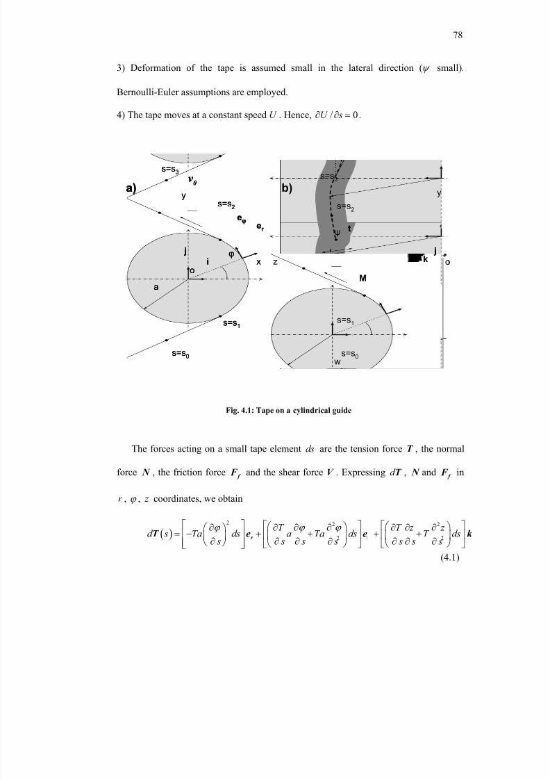
8/8/2019 BR PhD Dissertation
http://slidepdf.com/reader/full/br-phd-dissertation 110/248
78
3) Deformation of the tape is assumed small in the lateral direction (ψ small).
Bernoulli-Euler assumptions are employed.
4) The tape moves at a constant speed U . Hence, / 0U s∂ ∂ = .
a
i j φ
x
y
er
s=s1
s=s2
0v
eφ
okz
w
s=s1
s=s2
ψt
M
y
j
o
a) b)s=s
3
s=s3
s=s0
s=s0
a
i j φ
x
y
er
s=s1
s=s2
0v
eφ
okz
w
s=s1
s=s2
ψt
M
y
j
o
a) b)s=s
3
s=s3
s=s0
s=s0
The forces acting on a small tape element ds are the tension force T , the normal
force N , the friction force f F and the shear force V . Expressing d T , N and
f F in
r , ϕ , z coordinates, we obtain
( )2 2 2
2 2
T T z z d s Ta ds a Ta ds T ds
s s s s s s s
ϕ ϕ ϕ ∂ ∂ ∂ ∂ ∂ ∂ ∂ = − + + + +
∂ ∂ ∂ ∂ ∂ ∂ ∂ r T e e k
ϕ
(4.1)
Fig. 4.1: Tape on a cylindrical guide
8/8/2019 BR PhD Dissertation
http://slidepdf.com/reader/full/br-phd-dissertation 111/248
79
N = r N e , and (4.2)
z
Na N z z U U
U t s U t sϕ
ϕ ϕ µ µ
∂ ∂ ∂ ∂ = − + − + ∂ ∂ ∂ ∂
f F e k
ϕ(4.3)
In addition d V can be shown to be (appendix)
( )5 4 3
5 4 32
z z z z d s EI ds EI ds EI a ds
s s s s s s s
ϕ ϕ ϕ ∂ ∂ ∂ ∂ ∂ ∂ ∂ = − − +
∂ ∂ ∂ ∂ ∂ ∂ ∂ r V e e k
ϕ
(4.4)
Using equilibrium of forces, we have
2
2d wds d d dt
ρ = + + + f M T F N V (4.5)
Introducing (4.1), (4.2), (4.3) and (4.4) in (4.5), we obtain the following equations for
ther
e , eϕ
and k directions:
r e direction:
2 2
2
2 4
4
2wds a aU aU t s t s
z TA ds N EI ds
s s s
ϕ ϕ ϕ ϕ ρ
ϕ ϕ
∂ ∂ ∂ ∂ + +
∂ ∂ ∂ ∂
∂ ∂ ∂ = − +
∂ ∂ ∂
(4.6)
eϕ
direction:
2 2 22
2 2
2 5
2 5
2
2
U wds a aU a aU
t t s s t s
T z a Ta ds a aU EI ds
s s s U t s sϕ
ϕ ϕ ϕ ϕ ρ
ϕ ϕ ϕ ϕ µ
∂ ∂ ∂ ∂ ∂+ + +
∂ ∂ ∂ ∂ ∂ ∂
∂ ∂ ∂ ∂ ∂ ∂ = + − + + ∂ ∂ ∂ ∂ ∂ ∂
N (4.7)
and k direction:
8/8/2019 BR PhD Dissertation
http://slidepdf.com/reader/full/br-phd-dissertation 112/248
80
2 2 22
2 2
2 3
2 3
2
z
z z z z U wds U U
t t s s s t
T z z N z z z z T ds U EIa ds
s s s U t s s s s s
ρ
ϕ ϕ µ
∂ ∂ ∂ ∂ ∂+ + +
∂ ∂ ∂ ∂ ∂ ∂
∂ ∂ ∂ ∂ ∂ ∂ ∂ ∂ ∂ = + − + − +
∂ ∂ ∂ ∂ ∂ ∂ ∂ ∂ ∂
(4.8)
Substituting (4.6) in (4.8), (4.7) in (4.8), and since U is constant, the local stress
change in the tape is negligible and the LTM is sufficiently small, we can assume that
2
20
t t
ϕ ϕ ∂ ∂= =
∂ ∂,
( )2
2sin 1
a
s ds
ϕ ψ ψ
∂ ∂= − <<
∂, sin 1
z
sψ
∂= <<
∂,
( )cos 1
a
s
ϕ ψ
∂= ≅
∂. We can
neglect the inertia terms2
wU ρ versus the tension T for a typical 9 µm thick magnetic
tape (Mylar-PET) with 0.012 ρ = kg/m², 12.7w = mm and a typical tape transport speed
4U = m/s and tension 1T = N. Hence, we obtain the equation of motion of an axially
moving tape on a cylindrical guide surface as
( )4 2
4 21 0 z z T T z z z z
EI T s s a s Ua t
µ µ ν
∂ ∂ ∂ ∂− + − − − =
∂ ∂ ∂ ∂(4.9)
/ z ϕ ν µ µ = is the ratio of the friction coefficients in the circumferential and vertical
direction, respectively. In eq. (4.9), the fourth order derivative represents the bending
stiffness of the tape. If the bending stiffness is neglected, i.e., 0 I = , eq. (4.9) becomes
identical to the equation of motion for a string derived by Ono [4.10]. Furthermore, if
z ϕ µ µ = , eq. (4.9) becomes
4 2
4 20 z T z z z
EI T s s Ua t
µ ∂ ∂ ∂− + − =
∂ ∂ ∂, (4.10)
8/8/2019 BR PhD Dissertation
http://slidepdf.com/reader/full/br-phd-dissertation 113/248
8/8/2019 BR PhD Dissertation
http://slidepdf.com/reader/full/br-phd-dissertation 114/248
82
To solve equation (4.12), an implicit Euler finite difference scheme is implemented
with central discretization in space and forward discretization in time [4.13, 4.14]. Eq.
(4.12) thus becomes
1 1 1 1 1 1 1 1
2 1 1 2 1 1
4 2
1 1 1
1 1
4 6 4 2
02
j j j j j j j j
i i i i i i i i
j j j j
i i i i
z z z z z z z z A B
s s
z z z z C D
s t
+ + + + + + + ++ + − − + −
+ + ++ −
− + − + − ++
∆ ∆
− −+ + =
∆ ∆
(4.17)
where s∆ is the grid stepsize in space, and t ∆ is the grid stepsize in time. The indices
i and j refer to space and time, respectively. Rearranging the terms in equation (4.17)
gives
1 1 1
2 14 4 2 4 2
1 1
1 24 2 4
4 6 2
2
4
2
j j j
i i i
j j j
i i i
A A B C A B D z z z
s s s s s s t
A B C A D z z z
s s s s t
+ + ++ +
+ +− −
− + + + + − +
∆ ∆ ∆ ∆ ∆ ∆ ∆
− + + − + =
∆ ∆ ∆ ∆ ∆
(4.18)
In eq. (4.18), all terms on the left hand side are unknown, while the terms on the right
hand side are known. Eq. (4.18) can be stated in matrix form as
[ ][ ] [ ]G = z b , (4.19)
where [ ]G is a penta-diagonal matrix. The elements of the [ ]G matrix from are given
by
8/8/2019 BR PhD Dissertation
http://slidepdf.com/reader/full/br-phd-dissertation 115/248
83
, 2 4
, 1 4 2
, 4 2
, 1 4 2
, 2 4
4
2
6 2
4
2
i i
i i
i i
i i
i i
AG
s
A B C G
s s s
A B DG s s t
A B C G
s s s
AG
s
−
−
+
+
=∆
−= + −
∆ ∆ ∆
= − +∆ ∆ ∆
−= + +
∆ ∆ ∆
=∆
(4.20)
The corresponding elements of the [ ]b vector are given by
1 j j
i i
D
b z t
+ =∆ (4.21)
4.3.2 Tape path and boundary conditions
As illustrated in Fig. 4.1, the tape makes contact with the cylindrical guide at point
1 s and comes off the cylindrical guide at point 2 s . We assume that the tape is wound on
a reel with zero run-out at 3 s , i.e., 3( , ) 0 z s t = . At 0 s , the lateral displacement ( )0 f t is
assumed to be known from experimental measurements, i.e., ( )0 0( , ) z s t f t = . In
addition we postulate that the tape moves like a rigid body between 0 s and 1 s and 2 s
and 3 s , where it is not supported by the guide. The distances 1 2 s s and 3 4 s s are taken
much shorter than the distance 2 3 s s .
Thus,
( )( )( )1
1 0 1
1
( ) ( ) ( ) s s
z s z s f t z sl
−= + − for 0 1 s s s≤ ≤ (4.22)
8/8/2019 BR PhD Dissertation
http://slidepdf.com/reader/full/br-phd-dissertation 116/248
84
( )3
2
3
( ) ( ) s s
z s z sl
−= for 2 3 s s s≤ ≤ (4.23)
where 1l is the length of the tape between 0 s and 1 s and 3l is the length of the tape
between 2 s and 3 s , respectively.
The solution of eq. (4.9) for the domain 1 s 2 s requires four boundary conditions, two
at 1 s s= and two at 2 s s= . Since the displacement of the tape is known at 0 s s= and
since we assume that the tape moves as a rigid body in the regions 0 1 s s s≤ ≤ and
2 3 s s s≤ ≤ , the slope of the tape at 1 s s= must be equal to the slope at 0 s s= and the
slope of the tape at 2 s s= must be equal to the slope at 3 s s= . Thus,
( )( )1 0 0 z
l z f t s
∂− − =
∂at 1 s s= , and (4.24)
3 0 z
l z s
∂+ =
∂at 2 s s= (4.25)
In addition, the curvature at 1 s and 2 s has to be zero to insure a smooth tape path, i.e.,
1 2
2
2
,
0S S
z
s
∂=
∂(4.26)
Eq. (4.18) and (4.26) yield
8/8/2019 BR PhD Dissertation
http://slidepdf.com/reader/full/br-phd-dissertation 117/248
85
1 1
1 1
1 1
1 1
1, 3 4
1, 2 4 2
1, 1 4 2
1, 4 2
4
2
5 2
2
2
s s
s s
s s
s s
AG
s
A B C G
s s s
A B DG s s t
A B C G
s s s
+ +
+ +
+ +
+
=∆
−= + +
∆ ∆ ∆
= − +∆ ∆ ∆
−= + −
∆ ∆ ∆
(4.27)
and the term on the right hand side becomes
1 1
1
1 1
j j
s s
Db z
t
++ +=
∆(4.28)
Applying the above boundary condition (4.26) at point 2 s , we find the following result
with the help of eq. (4.18)
2 2
2 2
2 2
2 2
1, 4 2
1, 1 4 2
1, 2 4 2
1, 3 4
2
2
5 2
4
2
s s
s s
s s
s s
A B C G
s s s
A B DG s s t
A B C G
s s s
AG
s
−
− −
− −
− −
−= + +
∆ ∆ ∆
= − +∆ ∆ ∆
−= + −
∆ ∆ ∆
=∆
(4.29)
The corresponding term on the right hand side becomes
2 2
1
1 1
j j
s s
Db z
t
+− −=
∆(4.30)
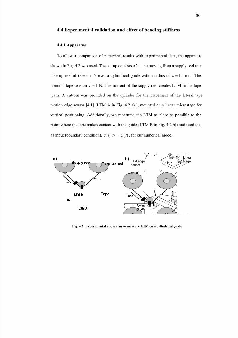
8/8/2019 BR PhD Dissertation
http://slidepdf.com/reader/full/br-phd-dissertation 118/248
86
4.4 Experimental validation and effect of bending stiffness
4.4.1 Apparatus
To allow a comparison of numerical results with experimental data, the apparatus
shown in Fig. 4.2 was used. The set-up consists of a tape moving from a supply reel to a
take-up reel at 4U = m/s over a cylindrical guide with a radius of 10a = mm. The
nominal tape tension 1T = N. The run-out of the supply reel creates LTM in the tape
path. A cut-out was provided on the cylinder for the placement of the lateral tape
motion edge sensor [4.1] (LTM A in Fig. 4.2 a) ), mounted on a linear microstage for
vertical positioning. Additionally, we measured the LTM as close as possible to the
point where the tape makes contact with the guide (LTM B in Fig. 4.2 b)) and used this
as input (boundary condition), ( )0 0( , ) z s t f t = , for our numerical model.
Tape
Cylindrical
guide
LTM edgesensor
Cut-out
Linear
stage
Tape
Cylindrical
guide
LTM edgesensor
Cut-out
Linear
stage
a) b)Supply reel Take-up reel
Tape
v0
LTM B
LTM A
Supply reel Take-up reel
Tape
v0
LTM B
LTM A
Supply reel Take-up reel
Tape
v0
LTM B
LTM A
Tape
Cylindrical
guide
LTM edgesensor
Cut-out
Linear
stage
Tape
Cylindrical
guide
LTM edgesensor
Cut-out
Linear
stage
a) b)Supply reel Take-up reel
Tape
v0
LTM B
LTM A
Supply reel Take-up reel
Tape
v0
LTM B
LTM A
Supply reel Take-up reel
Tape
v0
LTM B
LTM A
Fig. 4.2: Experimental apparatus to measure LTM on a cylindrical guide
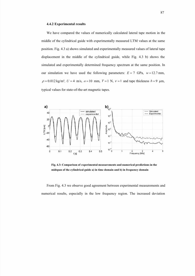
8/8/2019 BR PhD Dissertation
http://slidepdf.com/reader/full/br-phd-dissertation 119/248
87
4.4.2 Experimental results
We have compared the values of numerically calculated lateral tape motion in the
middle of the cylindrical guide with experimentally measured LTM values at the same
position. Fig. 4.3 a) shows simulated and experimentally measured values of lateral tape
displacement in the middle of the cylindrical guide, while Fig. 4.3 b) shows the
simulated and experimentally determined frequency spectrum at the same position. In
our simulation we have used the following parameters: 7 E = GPa, 12.7w = mm,
0.012 ρ = kg/m², 4U = m/s, 10a = mm, 1T = N, 1ν = and tape thickness 9b = µm,
typical values for state-of-the-art magnetic tapes.
a) b)a) b)
From Fig. 4.3 we observe good agreement between experimental measurements and
numerical results, especially in the low frequency region. The increased deviation
Fig. 4.3: Comparison of experimental measurements and numerical predictions in the
midspan of the cylindrical guide a) in time domain and b) in frequency domain
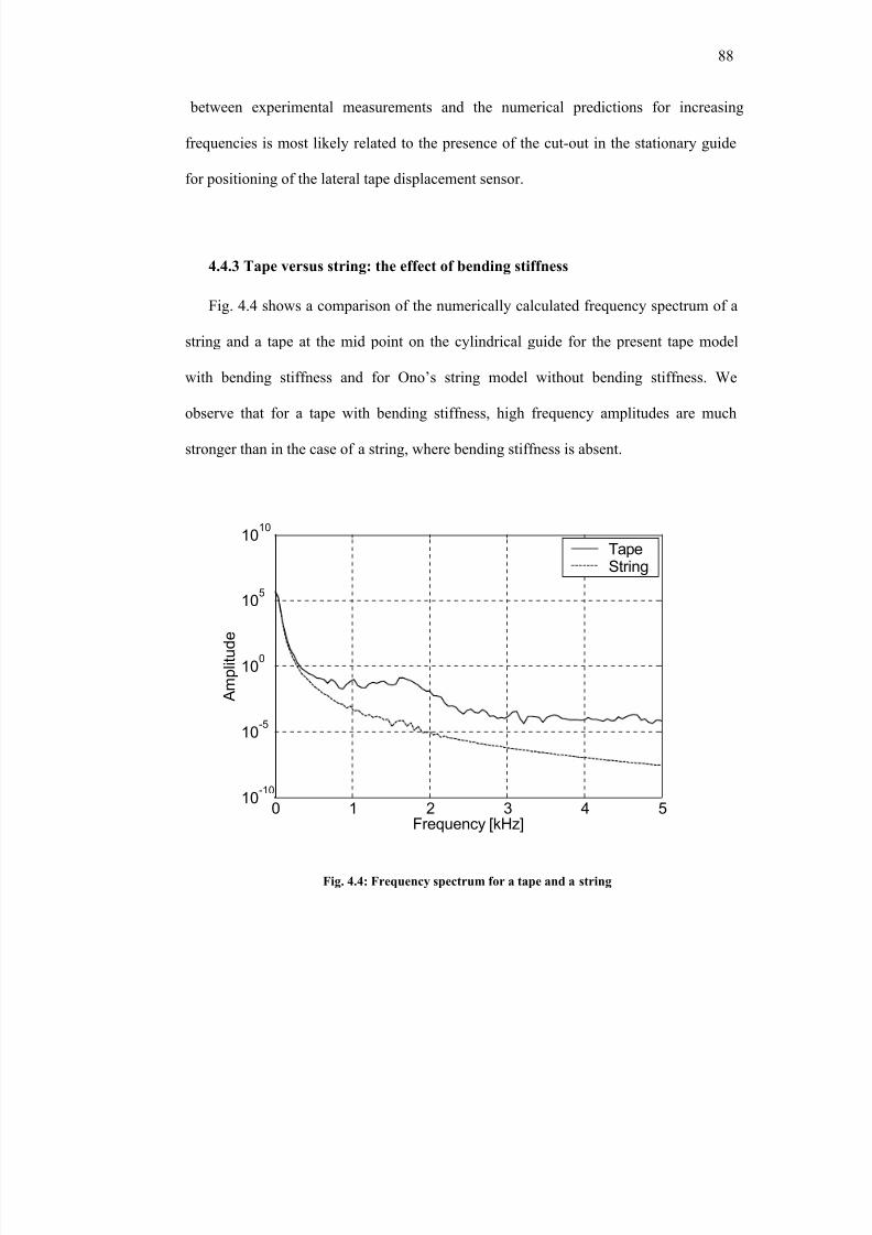
8/8/2019 BR PhD Dissertation
http://slidepdf.com/reader/full/br-phd-dissertation 120/248
88
between experimental measurements and the numerical predictions for increasing
frequencies is most likely related to the presence of the cut-out in the stationary guide
for positioning of the lateral tape displacement sensor.
4.4.3 Tape versus string: the effect of bending stiffness
Fig. 4.4 shows a comparison of the numerically calculated frequency spectrum of a
string and a tape at the mid point on the cylindrical guide for the present tape model
with bending stiffness and for Ono’s string model without bending stiffness. We
observe that for a tape with bending stiffness, high frequency amplitudes are much
stronger than in the case of a string, where bending stiffness is absent.
0 1 2 3 4 510-10
10-5
100
105
1010
Frequency [kHz]
A m p l i t u d e
TapeString
Fig. 4.4: Frequency spectrum for a tape and a string
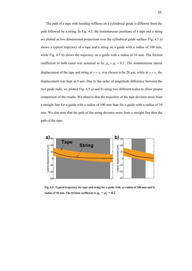
8/8/2019 BR PhD Dissertation
http://slidepdf.com/reader/full/br-phd-dissertation 121/248
89
The path of a tape with bending stiffness on a cylindrical guide is different from the
path followed by a string. In Fig. 4.5, the instantaneous positions of a tape and a string
are plotted as two dimensional projections over the cylindrical guide surface. Fig. 4.5 a)
shows a typical trajectory of a tape and a string on a guide with a radius of 100 mm,
while Fig. 4.5 b) shows the trajectory on a guide with a radius of 10 mm. The friction
coefficient in both cases was assumed to be 0.2 z ϕ µ µ = = . The instanteneous lateral
displacement of the tape and string at0 s s= was chosen to be 20 µm, while at
3 s s= the
displacement was kept at 0 µm. Due to the order of magnitude difference between the
two guide radii, we plotted Fig. 4.5 a) and b) using two different scales to allow proper
comparison of the results. We observe that the trajectory of the tape deviates more from
a straight line for a guide with a radius of 100 mm than for a guide with a radius of 10
mm. We also note that the path of the string deviates more from a straight line than the
path of the tape.
-60
-40
-20
0
20
40
60
L a t e r a l d i s p l a c e m e n t [ µ m ]
-60
-40
-20
0
20
40
60
L a t e r a l d i s p l a c e m e n t [ µ m ]
a) b)Tape
String
-60
-40
-20
0
20
40
60
L a t e r a l d i s p l a c e m e n t [ µ m ]
-60
-40
-20
0
20
40
60
L a t e r a l d i s p l a c e m e n t [ µ m ]
a) b)Tape
String
-60
-40
-20
0
20
40
60
L a t e r a l d i s p l a c e m e n t [ µ m ]
-60
-40
-20
0
20
40
60
L a t e r a l d i s p l a c e m e n t [ µ m ]
a) b)Tape
String
Fig. 4.5: Typical trajectory for tape and string for a guide with a) radius of 100 mm and b)
radius of 10 mm. The friction coefficient is µ = µ = 0.2ϕ
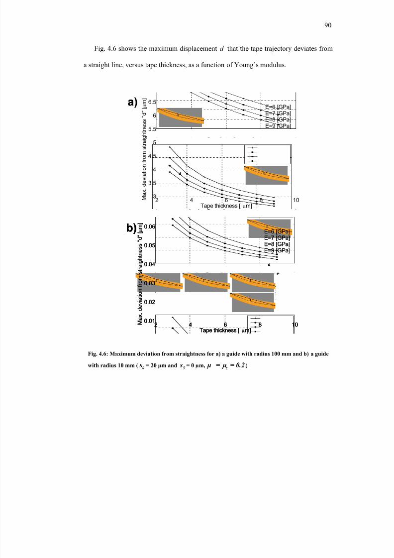
8/8/2019 BR PhD Dissertation
http://slidepdf.com/reader/full/br-phd-dissertation 122/248
90
Fig. 4.6 shows the maximum displacement d that the tape trajectory deviates from
a straight line, versus tape thickness, as a function of Young’s modulus.
2 4 6 8 103
3.5
4
4.5
5
5.5
6
6.5
M a x .
d e v
i a t i o n f r o m s
t r a i g h t n e s s " d " [ µ m ]
Tape thickness [ µm]
E=6 [GPa]E=7 [GPa]E=8 [GPa]E=9 [GPa]
a)
dd
2 4 6 8 103
3.5
4
4.5
5
5.5
6
6.5
M a x .
d e v
i a t i o n f r o m s
t r a i g h t n e s s " d " [ µ m ]
Tape thickness [ µm]
E=6 [GPa]E=7 [GPa]E=8 [GPa]E=9 [GPa]
a)
dd
2 4 6 8 100.01
0.02
0.03
0.04
0.05
0.06
M a x .
d e v i a t i o n f r o m s
t r a i g h t n e s s " d " [ µ m ]
Tape thickness [ µm]
E=6 [GPa]E=7 [GPa]E=8 [GPa]E=9 [GPa]
b)
dd
2 4 6 8 100.01
0.02
0.03
0.04
0.05
0.06
M a x .
d e v i a t i o n f r o m s
t r a i g h t n e s s " d " [ µ m ]
Tape thickness [ µm]
E=6 [GPa]E=7 [GPa]E=8 [GPa]E=9 [GPa]
b)
2 4 6 8 100.01
0.02
0.03
0.04
0.05
0.06
M a x .
d e v i a t i o n f r o m s
t r a i g h t n e s s " d " [ µ m ]
Tape thickness [ µm]
E=6 [GPa]E=7 [GPa]E=8 [GPa]E=9 [GPa]
b)
dd
Fig. 4.6: Maximum deviation from straightness for a) a guide with radius 100 mm and b) a guide
with radius 10 mm (0
s = 20 µm and3
s = 0 µm, z
µ = µ = 0.2ϕ
)
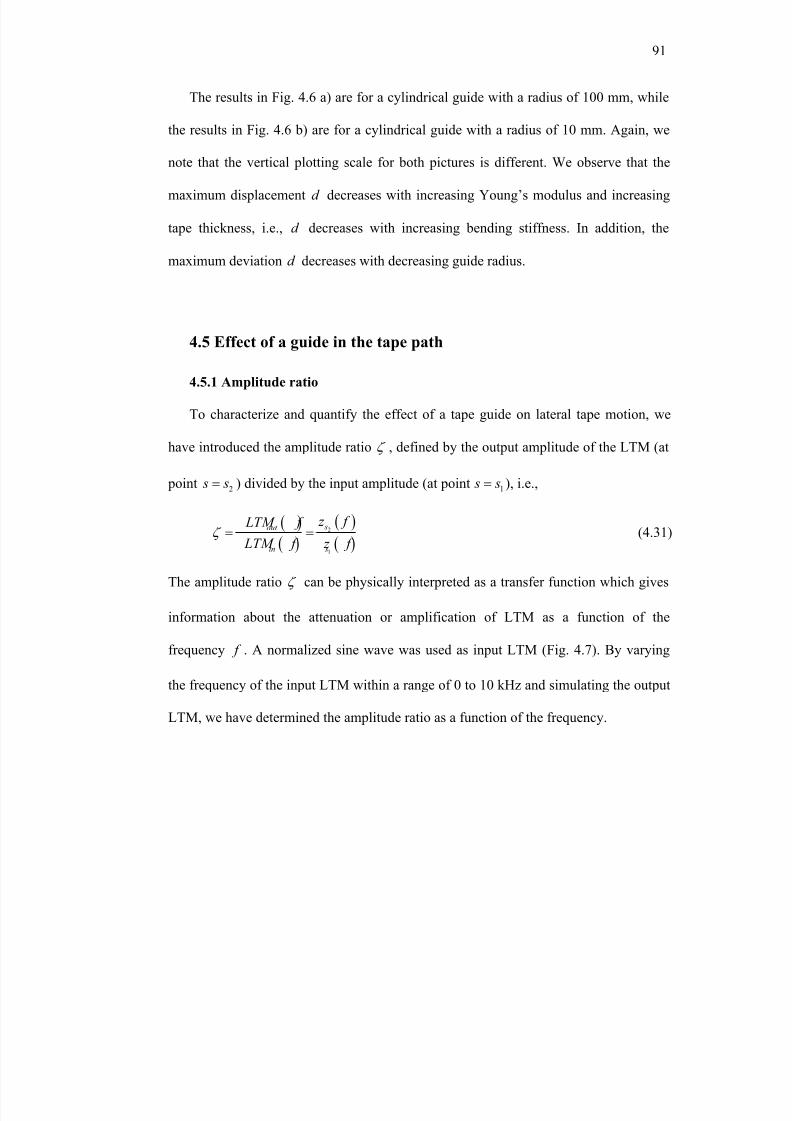
8/8/2019 BR PhD Dissertation
http://slidepdf.com/reader/full/br-phd-dissertation 123/248
91
The results in Fig. 4.6 a) are for a cylindrical guide with a radius of 100 mm, while
the results in Fig. 4.6 b) are for a cylindrical guide with a radius of 10 mm. Again, we
note that the vertical plotting scale for both pictures is different. We observe that the
maximum displacement d decreases with increasing Young’s modulus and increasing
tape thickness, i.e., d decreases with increasing bending stiffness. In addition, the
maximum deviation d decreases with decreasing guide radius.
4.5 Effect of a guide in the tape path
4.5.1 Amplitude ratio
To characterize and quantify the effect of a tape guide on lateral tape motion, we
have introduced the amplitude ratio ζ , defined by the output amplitude of the LTM (at
point 2 s s= ) divided by the input amplitude (at point 1 s s= ), i.e.,
( )
( )
( )
( )2
1
sout
in s
z f LTM f
LTM f z f ζ = =
(4.31)
The amplitude ratio ζ can be physically interpreted as a transfer function which gives
information about the attenuation or amplification of LTM as a function of the
frequency f . A normalized sine wave was used as input LTM (Fig. 4.7). By varying
the frequency of the input LTM within a range of 0 to 10 kHz and simulating the output
LTM, we have determined the amplitude ratio as a function of the frequency.
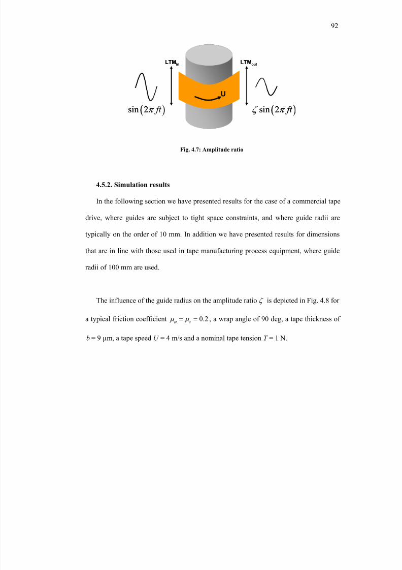
8/8/2019 BR PhD Dissertation
http://slidepdf.com/reader/full/br-phd-dissertation 124/248
92
LTMin LTMout
U
( )sin 2 ft π ( )sin 2 ft ζ π
LTMin LTMout
U
( )sin 2 ft π ( )sin 2 ft ζ π
4.5.2. Simulation results
In the following section we have presented results for the case of a commercial tape
drive, where guides are subject to tight space constraints, and where guide radii are
typically on the order of 10 mm. In addition we have presented results for dimensions
that are in line with those used in tape manufacturing process equipment, where guide
radii of 100 mm are used.
The influence of the guide radius on the amplitude ratio ζ is depicted in Fig. 4.8 for
a typical friction coefficient 0.2 z ϕ µ µ = = , a wrap angle of 90 deg, a tape thickness of
b = 9 µm, a tape speed U = 4 m/s and a nominal tape tension T = 1 N.
Fig. 4.7: Amplitude ratio
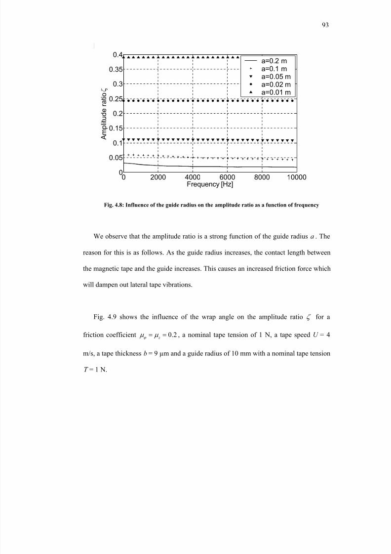
8/8/2019 BR PhD Dissertation
http://slidepdf.com/reader/full/br-phd-dissertation 125/248
93
0 2000 4000 6000 8000 100000
0.05
0.1
0.15
0.2
0.25
0.3
0.35
0.4
Frequency [Hz]
A m p l i t u d e r a t i o ζ
a=0.2 ma=0.1 ma=0.05 ma=0.02 ma=0.01 m
We observe that the amplitude ratio is a strong function of the guide radius a . The
reason for this is as follows. As the guide radius increases, the contact length between
the magnetic tape and the guide increases. This causes an increased friction force which
will dampen out lateral tape vibrations.
Fig. 4.9 shows the influence of the wrap angle on the amplitude ratio ζ for a
friction coefficient 0.2 z ϕ µ µ = = , a nominal tape tension of 1 N, a tape speed U = 4
m/s, a tape thickness b = 9 µm and a guide radius of 10 mm with a nominal tape tension
T = 1 N.
Fig. 4.8: Influence of the guide radius on the amplitude ratio as a function of frequency
8/8/2019 BR PhD Dissertation
http://slidepdf.com/reader/full/br-phd-dissertation 126/248
94
0 2000 4000 6000 8000 100000
0.2
0.4
0.6
0.8
1
Frequency [Hz]
A m p l i t u d e r a t i o ζ
10 deg30 deg60 deg90 deg
We observe that the amplitude ratio decreases with increasing wrap angle.
Physically, the effect of increasing the wrap angle is similar to increasing the guide
radius. Both parameters affect the tape/guide contact length. An increased contact
length yields an increased friction and thus reduced LTM.
Fig. 4.10 shows the influence of the friction coefficient on the amplitude ratio ζ a)
for a guide radius of 10 mm and b) for a guide radius of 100 mm. A wrap angle of 90
deg was maintained together with a nominal tape tension T = 1 N, a tape speed U = 4
m/s, a tape thickness b = 9 µm and a friction coefficient 0.2 z ϕ µ µ = = .
Fig. 4.9: Influence of the wrap angle on the amplitude ratio as a function of frequency
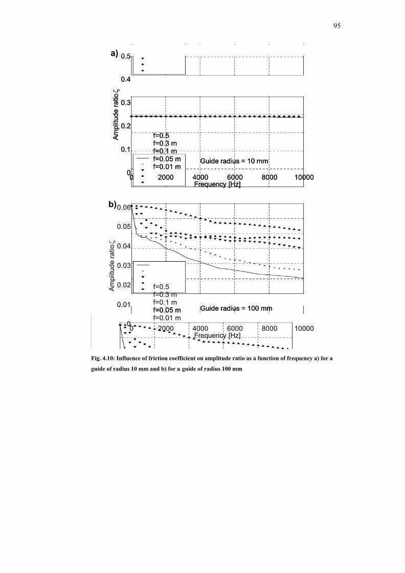
8/8/2019 BR PhD Dissertation
http://slidepdf.com/reader/full/br-phd-dissertation 127/248
95
0 2000 4000 6000 8000 100000
0.1
0.2
0.3
0.4
0.5
Frequency [Hz]
A m p l i t u d e r a t i o ζ
Guide radius = 10 mm
f=0.5f=0.3 mf=0.1 mf=0.05 mf=0.01 m
a)
0 2000 4000 6000 8000 100000
0.1
0.2
0.3
0.4
0.5
Frequency [Hz]
A m p l i t u d e r a t i o ζ
Guide radius = 10 mm
f=0.5f=0.3 mf=0.1 mf=0.05 mf=0.01 m
a)
0 2000 4000 6000 8000 100000
0.01
0.02
0.03
0.04
0.05
0.06
Frequency [Hz]
A m p l i t u d e r a t i o ζ
Guide radius = 100 mm
f=0.5f=0.3 mf=0.1 mf=0.05 mf=0.01 m
b)
0 2000 4000 6000 8000 100000
0.01
0.02
0.03
0.04
0.05
0.06
Frequency [Hz]
A m p l i t u d e r a t i o ζ
Guide radius = 100 mm
f=0.5f=0.3 mf=0.1 mf=0.05 mf=0.01 m
b)
Fig. 4.10: Influence of friction coefficient on amplitude ratio as a function of frequency a) for a
guide of radius 10 mm and b) for a guide of radius 100 mm
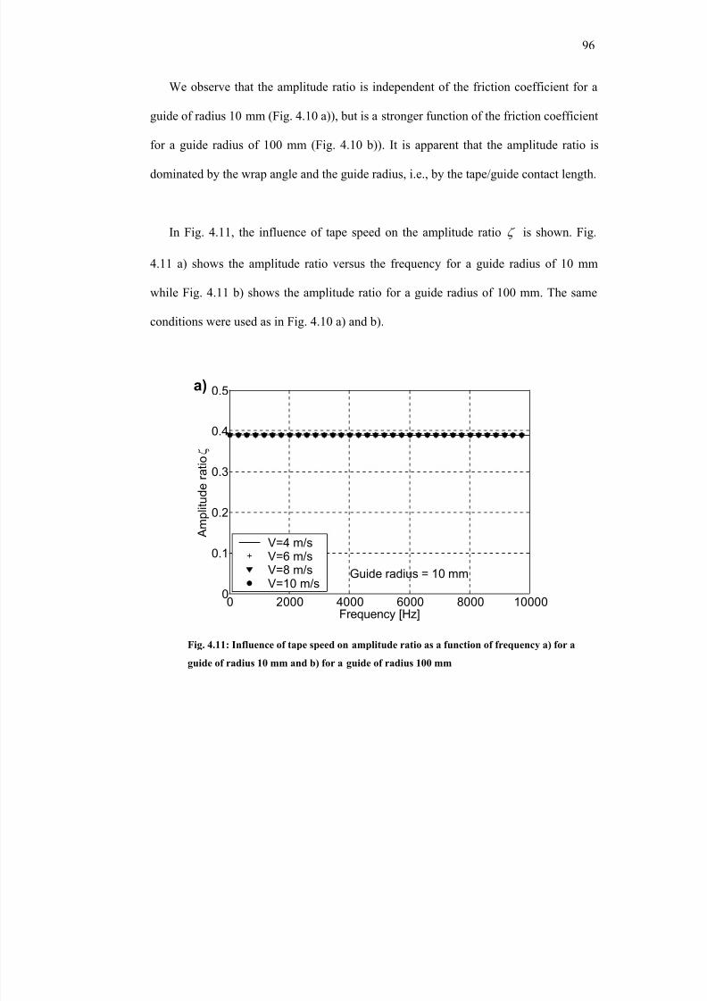
8/8/2019 BR PhD Dissertation
http://slidepdf.com/reader/full/br-phd-dissertation 128/248
96
We observe that the amplitude ratio is independent of the friction coefficient for a
guide of radius 10 mm (Fig. 4.10 a)), but is a stronger function of the friction coefficient
for a guide radius of 100 mm (Fig. 4.10 b)). It is apparent that the amplitude ratio is
dominated by the wrap angle and the guide radius, i.e., by the tape/guide contact length.
In Fig. 4.11, the influence of tape speed on the amplitude ratio ζ is shown. Fig.
4.11 a) shows the amplitude ratio versus the frequency for a guide radius of 10 mm
while Fig. 4.11 b) shows the amplitude ratio for a guide radius of 100 mm. The same
conditions were used as in Fig. 4.10 a) and b).
0 2000 4000 6000 8000 100000
0.1
0.2
0.3
0.4
0.5
Frequency [Hz]
A m p l i t u d e r a t i o ζ
Guide radius = 10 mm
V=4 m/sV=6 m/sV=8 m/sV=10 m/s
a)
Fig. 4.11: Influence of tape speed on amplitude ratio as a function of frequency a) for a
guide of radius 10 mm and b) for a guide of radius 100 mm
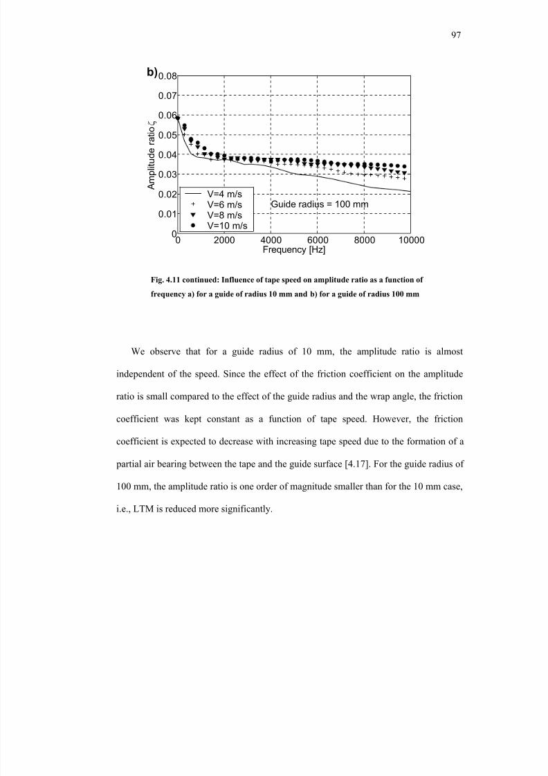
8/8/2019 BR PhD Dissertation
http://slidepdf.com/reader/full/br-phd-dissertation 129/248
97
0 2000 4000 6000 8000 100000
0.01
0.02
0.03
0.04
0.05
0.06
0.07
0.08
Frequency [Hz]
A m p l i t u d e r a t i o ζ
Guide radius = 100 mmV=4 m/sV=6 m/sV=8 m/sV=10 m/s
b)
0 2000 4000 6000 8000 100000
0.01
0.02
0.03
0.04
0.05
0.06
0.07
0.08
Frequency [Hz]
A m p l i t u d e r a t i o ζ
Guide radius = 100 mmV=4 m/sV=6 m/sV=8 m/sV=10 m/s
b)
We observe that for a guide radius of 10 mm, the amplitude ratio is almost
independent of the speed. Since the effect of the friction coefficient on the amplitude
ratio is small compared to the effect of the guide radius and the wrap angle, the friction
coefficient was kept constant as a function of tape speed. However, the friction
coefficient is expected to decrease with increasing tape speed due to the formation of a
partial air bearing between the tape and the guide surface [4.17]. For the guide radius of
100 mm, the amplitude ratio is one order of magnitude smaller than for the 10 mm case,
i.e., LTM is reduced more significantly.
Fig. 4.11 continued: Influence of tape speed on amplitude ratio as a function of
frequency a) for a guide of radius 10 mm and b) for a guide of radius 100 mm
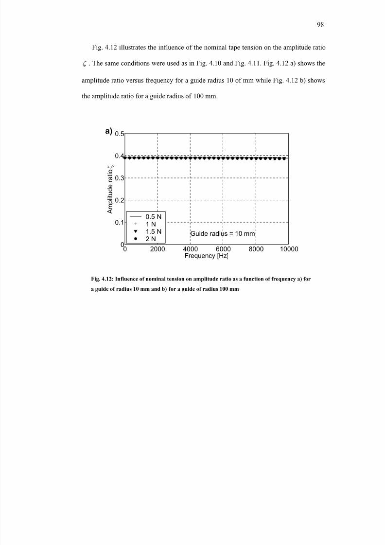
8/8/2019 BR PhD Dissertation
http://slidepdf.com/reader/full/br-phd-dissertation 130/248
98
Fig. 4.12 illustrates the influence of the nominal tape tension on the amplitude ratio
ζ . The same conditions were used as in Fig. 4.10 and Fig. 4.11. Fig. 4.12 a) shows the
amplitude ratio versus frequency for a guide radius 10 of mm while Fig. 4.12 b) shows
the amplitude ratio for a guide radius of 100 mm.
0 2000 4000 6000 8000 100000
0.1
0.2
0.3
0.4
0.5
Frequency [Hz]
A m p l i t u d e r a t i o ζ
Guide radius = 10 mm
0.5 N1 N1.5 N2 N
a)
0 2000 4000 6000 8000 100000
0.1
0.2
0.3
0.4
0.5
Frequency [Hz]
A m p l i t u d e r a t i o ζ
Guide radius = 10 mm
0.5 N1 N1.5 N2 N
a)
Fig. 4.12: Influence of nominal tension on amplitude ratio as a function of frequency a) for
a guide of radius 10 mm and b) for a guide of radius 100 mm
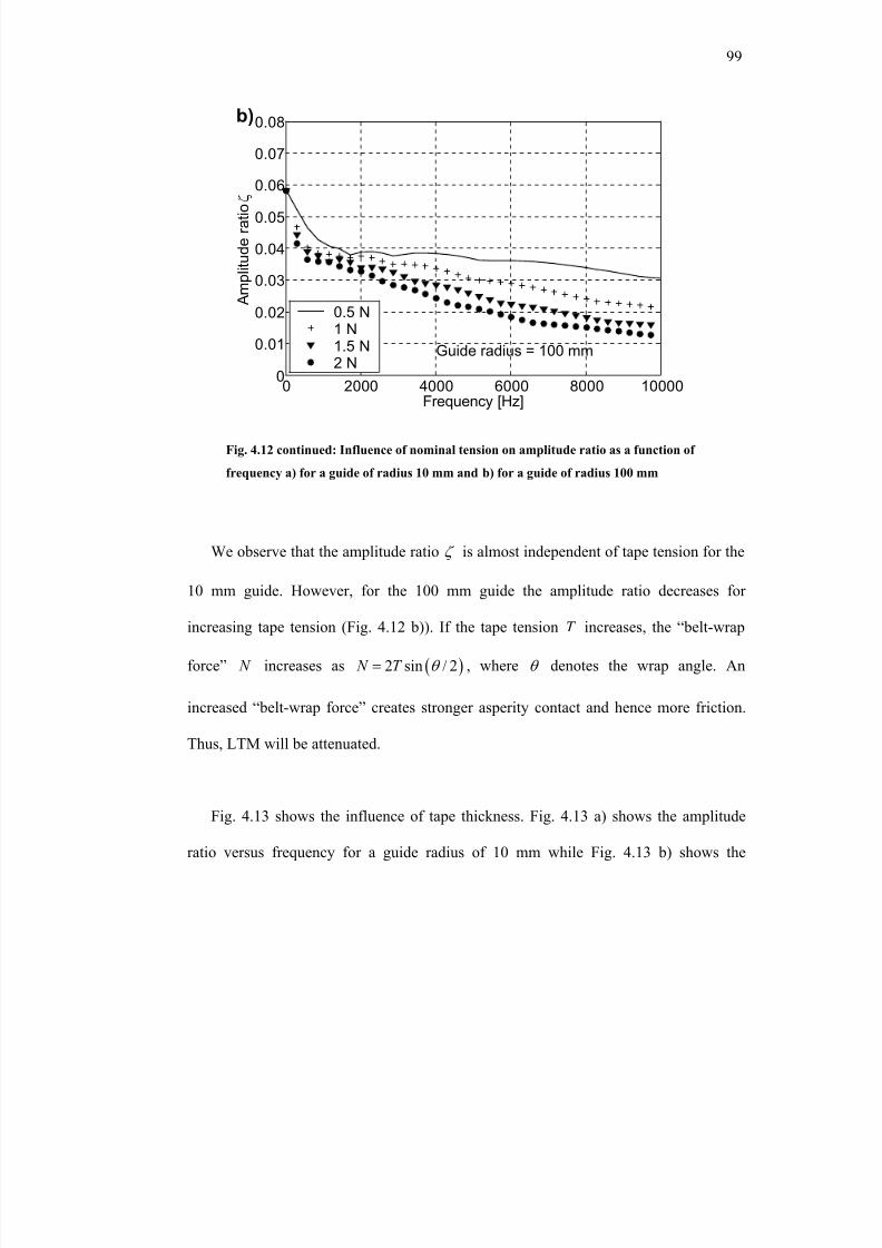
8/8/2019 BR PhD Dissertation
http://slidepdf.com/reader/full/br-phd-dissertation 131/248
99
0 2000 4000 6000 8000 100000
0.01
0.02
0.03
0.04
0.05
0.06
0.07
0.08
Frequency [Hz]
A m p l i t u d e r a t i o ζ
Guide radius = 100 mm
0.5 N1 N1.5 N2 N
b)
0 2000 4000 6000 8000 100000
0.01
0.02
0.03
0.04
0.05
0.06
0.07
0.08
Frequency [Hz]
A m p l i t u d e r a t i o ζ
Guide radius = 100 mm
0.5 N1 N1.5 N2 N
b)
We observe that the amplitude ratio ζ is almost independent of tape tension for the
10 mm guide. However, for the 100 mm guide the amplitude ratio decreases for
increasing tape tension (Fig. 4.12 b)). If the tape tension T increases, the “belt-wrap
force” N increases as ( )2 sin / 2 N T θ = , where θ denotes the wrap angle. An
increased “belt-wrap force” creates stronger asperity contact and hence more friction.
Thus, LTM will be attenuated.
Fig. 4.13 shows the influence of tape thickness. Fig. 4.13 a) shows the amplitude
ratio versus frequency for a guide radius of 10 mm while Fig. 4.13 b) shows the
Fig. 4.12 continued: Influence of nominal tension on amplitude ratio as a function of
frequency a) for a guide of radius 10 mm and b) for a guide of radius 100 mm
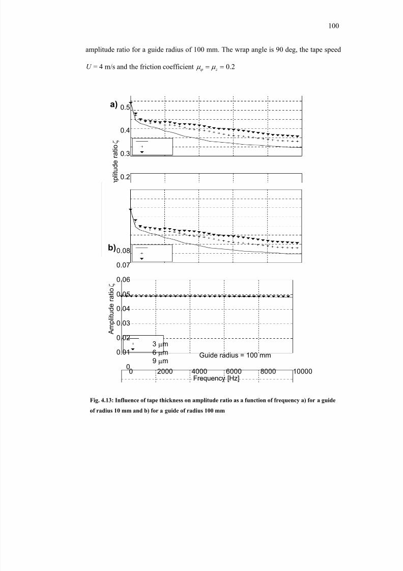
8/8/2019 BR PhD Dissertation
http://slidepdf.com/reader/full/br-phd-dissertation 132/248
100
amplitude ratio for a guide radius of 100 mm. The wrap angle is 90 deg, the tape speed
U = 4 m/s and the friction coefficient 0.2 z ϕ µ µ = =
0 2000 4000 6000 8000 100000
0.1
0.2
0.3
0.4
0.5
Frequency [Hz]
A m
p l i t u d e r a t i o ζ
Guide radius = 10 mm
3 µm
6 µm
9 µm
a)
0 2000 4000 6000 8000 100000
0.1
0.2
0.3
0.4
0.5
Frequency [Hz]
A m
p l i t u d e r a t i o ζ
Guide radius = 10 mm
3 µm
6 µm
9 µm
a)
0 2000 4000 6000 8000 100000
0.01
0.02
0.03
0.04
0.05
0.06
0.07
0.08
Frequency [Hz]
A m p l i t u d e r a t i o ζ
Guide radius = 100 mm
3 µm
6 µm
9 µm
b)
0 2000 4000 6000 8000 100000
0.01
0.02
0.03
0.04
0.05
0.06
0.07
0.08
Frequency [Hz]
A m p l i t u d e r a t i o ζ
Guide radius = 100 mm
3 µm
6 µm
9 µm
b)
Fig. 4.13: Influence of tape thickness on amplitude ratio as a function of frequency a) for a guide
of radius 10 mm and b) for a guide of radius 100 mm
8/8/2019 BR PhD Dissertation
http://slidepdf.com/reader/full/br-phd-dissertation 133/248
101
Similar to the previous results, we observe that the amplitude ratio is nearly independent
of the tape thickness for the 10 mm radius guide, while it decreases with decreasing
thickness for the 100 mm guide radius.
4.6 Discussion
We have observed that the amplitude ratio ζ is inversely proportional to the
tape/guide friction coefficient z ϕ
µ µ µ = = , the wrap angle θ , the nominal tape tension
T and the guide radius a , and proportional to the tape speed U and tape thickness b .
Hence, the amplitude ratio ζ can be defined in terms of tape design parameters as
Ub A
aT ζ
µθ = , (4.32)
where A is a proportionality constant.
It is apparent that an increase in the guide diameter or wrap angle increases the
contact length and friction force. This, in turn, attenuates the LTM more strongly. In the
case of commercial tape drives, the guide diameter cannot be increased arbitrarily due
to space constraints. In tape manufacturing process equipment, where spatial constraints
are less critical, there is greater design freedom to increase the diameter of the guides,
which would reduce LTM. However, increased friction force due to increased contact
length may lead to increased tape wear, and the balance between those effects must be
found.
8/8/2019 BR PhD Dissertation
http://slidepdf.com/reader/full/br-phd-dissertation 134/248
102
The tape industry is moving towards using thinner tapes to increase the volumetric
storage density of a tape cartridge. Thinner tapes require lower tape tension to keep the
stress in the tape constant. Increased storage density also calls for higher data rates
(higher tape speeds). Our results show that the tape speed U , the tape thickness b , the
nominal tape tension T and the friction coefficient z ϕ
µ µ µ = = have only a secondary
effect on the amplitude ratio for small guide diameters.
The present tape model with bending stiffness can be used to study damping and
minimization of lateral tape motion. Lateral tape motion above 1 kHz cannot be
followed by the servo system of the magnetic read/write head. When the amplitude of
high frequency lateral tape motion is larger than 10 % of the track width, read/write
errors are likely to occur. Thus, reducing high frequency tape motion before it reaches
the head is desirable since it would allow narrower tracks, resulting in a higher track
density and increasing the storage capacity of magnetic tape.
From the results presented it is clear that LTM can be reduced by positioning guides
in the tape path before the tape passes over the read/write head. The guides would serve
as “mechanical LTM-filters”. Furthermore, reducing LTM during the tape slitting
process would produce tapes with improved edge quality, i.e., straighter edges.
The tape model with bending stiffness also has an important application in the tape
slitting process where lateral tape displacement has to be minimized in order to
8/8/2019 BR PhD Dissertation
http://slidepdf.com/reader/full/br-phd-dissertation 135/248
103
manufacture tapes with sufficiently “straight” edges. Straight edges are important for
tape edge guiding [4.18, 4.19] and for servo track writing, and thus of primary concern
in the tape manufacturing process. If the radius of the guides that transport the tape is
increased, the amplitude of the LTM is attenuated more strongly and the edge quality of
the tape produced during the slitting process should be improved. Thus, optimization of
the tape path by increasing the diameter of the guides should be considered in tape
slitting machines to improve the quality of future tapes.
4.7 Conclusion
The results obtained in this paper show that:
1. Bending stiffness is an important parameter in describing the lateral
displacement of a tape on a cylindrical guide surface. When modeling a tape,
shear forces have to be included to account for the bending stiffness.
2. The effect of a cylindrical guide in the tape path can be characterized by the
amplitude ratio of output and input lateral tape displacement. The amplitude
ratio mainly depends on the contact length between tape and guide surface, i.e.,
the guide radius and the wrap angle. An increase in the guide radius of the tape
guide or an increase in the wrap angle between the guide surface and the tape
improves the damping of both low and high LTM frequencies. The nominal tape
tension, friction coefficient, tape thickness and tape speed also affect the
amplitude ratio; however their influence is negligible with respect to the
influence of the guide radius and the wrap angle.
8/8/2019 BR PhD Dissertation
http://slidepdf.com/reader/full/br-phd-dissertation 136/248
104
3. The bending stiffness of the tape affects its trajectory over the cylindrical guide.
As the bending stiffness increases, the tape trajectory deviates less from a
straight line.
4. The tape model with bending stiffness can be used to study the design and
optimization of the tape path in a tape drive and in the tape manufacturing
process.
4.8 Acknowledgements
Chapter 4, in part, is a reprint of the material as it appears in “Lateral Motion of an
Axially Moving Tape on a Cylindrical Guide Surface”, Raeymaekers B., Talke F.E.,
Journal of Applied Mechanics Transactions of the ASME, 2007. The dissertation author
was the primary investigator and author of this paper.
Chapter 4, in part, has been submitted for publication in “Attenuation of Lateral
Tape Motion Due to Frictional Interaction with a Cylindrical Guide”, Raeymaekers B.,
Talke F.E., Tribology International, 2007. The dissertation author was the primary
investigator and author of this paper.
4.9 Appendix
Fig. A1 shows the the tension and shear force vectors with respect to the
, ,r z ϕ coordinate system.
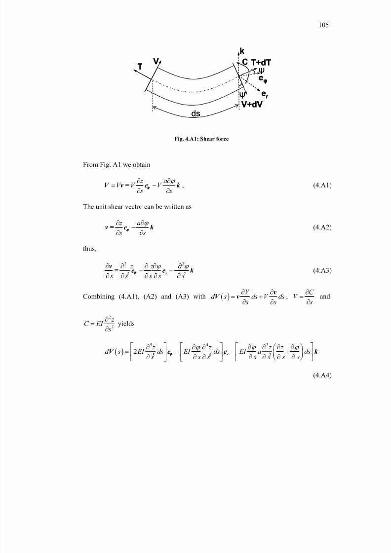
8/8/2019 BR PhD Dissertation
http://slidepdf.com/reader/full/br-phd-dissertation 137/248
105
k
ψ
ψ
V+dV
T+dT
eφ
C
er
ds
VT
k
ψ
ψ
V+dV
T+dT
eφ
C
er
ds
VT
From Fig. A1 we obtain
z aV V V
s s
ϕ ∂ ∂= −∂ ∂
V v = e k ϕ
, (4.A1)
The unit shear vector can be written as
z a
s s
ϕ ∂ ∂−
∂ ∂v = e k
ϕ(4.A2)
thus,
2 2
2 2 z z a
s s s s sϕ ϕ ∂ ∂ ∂ ∂ ∂− −
∂ ∂ ∂ ∂ ∂r
v = e e k ϕ
(4.A3)
Combining (4.A1), (A2) and (A3) with ( )V
d s ds V ds s s
∂ ∂= +
∂ ∂
vV v ,
C V
s
∂=
∂and
2
2
z C EI
s
∂=
∂yields
( )
5 4 3
5 4 32
z z z z
d s EI ds EI ds EI a ds s s s s s s s
ϕ ϕ ϕ ∂ ∂ ∂ ∂ ∂ ∂ ∂ = − − +
∂ ∂ ∂ ∂ ∂ ∂ ∂ r V e e k ϕ
(4.A4)
Fig. 4.A1: Shear force
8/8/2019 BR PhD Dissertation
http://slidepdf.com/reader/full/br-phd-dissertation 138/248
106
4.10 References
[4.1] Swope RD, Ames WF, 1963, Vibrations of a Moving Threadline, J. Franklin
Institute, Vol. 275, pp. 36 - 55
[4.2] Norwood RE, 1969, Effects of Bending Stiffness in Magnetic Tape, IBM J. Res. &
Dev., Vol. 13( 2), pp. 205 - 208
[4.3] Shelton JJ, Reid KN, 1971, Lateral Dynamics of an Idealized Moving Web, J.Dyn., Syst., Meas. and Control T. ASME, Vol. 3, pp. 187 - 192
[4.4] Shelton JJ, Reid KN, 1971, Lateral Dynamics of a Real Moving Web, J. Dyn.,
Syst., Meas. and Control T. ASME, Vol. 3, pp. 180 - 186
[4.5] Wickert JA, Mote CD, 1990, Classical Vibration Analysis of Axially Moving
Continua, J. Appl. Mech. T. ASME, Vol. 57, pp. 738 - 744
[4.6] Young GE, Reid KN, 1993, Lateral and Longitudinal Dynamic Behavior and
Control of Moving Webs, J. Dyn., Syst., Meas. and Control T. ASME, Vol. 115, pp.309 - 317
[4.7] Lee S, Mote Jr. CD, 1999, Wave Characteristics and Vibration Control of Translating Beams by Optimal Boundary Damping, J. Appl. Mech. T. ASME, Vol. 121,
pp. 18 - 25
[4.8] Garziera R, Amabili M, 2000, Damping Effect of Winding on the LateralVibration of Axially Moving Tapes, J. Vib. Acoust. T. ASME, Vol. 122, pp. 49 - 53
[4.9] Benson RC, 2002, Lateral Dynamics of a Moving Web with GeometricalImperfection, J. Dyn., Syst., Meas. and Control T. ASME, Vol. 124, pp. 25 - 34
[4.10] Yerashunas JB, Alexis De Abreu-Garcia A, Hartley T, 2003, Control of LateralMotion in Moving Webs, IEEE T. Contr. Syst. T., Vol. 11, pp. 684 - 693
[4.11] Ono K, 1979, Lateral Motion of an Axially Moving String on a Cylindrical
Guide Surface, J. Appl. Mech. T. ASME, Vol. 46, pp. 905 - 912
[4.12] Taylor RJ, Talke FE, 2005, Investigation of Roller Interactions with Flexible
Tape Medium, Tribol. Int., Vol. 38, pp. 599 - 605
[4.13] Pozrikidis C, 1998, Numerical Computation in Science and Engineering, Oxford
University Press, New York/Oxford
8/8/2019 BR PhD Dissertation
http://slidepdf.com/reader/full/br-phd-dissertation 139/248
107
[4.14] Hirsch C, 1988, Numerical Computation of Internal and External Flows, Vol. 1
Fundamentals of Numerical Discretization, John Wiley and Sons, New York
[4.15] Berry BS, Pritchet WC, 1988, Elastic and Viscoelastic Behavior of a MagneticRecording Tape, IBM J. Res. & Dev., Vol. 32(5), pp. 682 - 694
[4.16] Bhushan B, Tao Z, 2004, Mechanical, Hygroscopic, and Thermal Properties of Metal Particle and Metal Evaporated Tapes and Their Individual Layers, J. Appl.
Polymer Science, Vol. 92, pp. 1319 - 1345
[4.17] Raeymaekers B, Etsion I, Talke FE, 2007, The Influence of Design and
Operating Parameters on the Magnetic Tape/Guide Friction Coefficient, Tribol. Lett.,
Vol. 25(2), pp. 161 - 171
[4.18] Bhushan B, Hinteregger HF, Rogers AEE, 1994, Thermal Considerations for the
Edge Guiding of Thin Magnetic Tape in a Longitudinal Tape Transport, Wear, Vol.
171, pp. 179 – 193
[4.19] Taylor RJ, Talke FE, 2005, High Frequency Lateral Tape Motion and the
Dynamics of Tape Edge Contact, Microsyst. Technol., Vol. 11, pp. 1166 - 1170
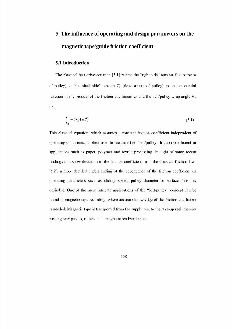
8/8/2019 BR PhD Dissertation
http://slidepdf.com/reader/full/br-phd-dissertation 140/248
108
5. The influence of operating and design parameters on the
magnetic tape/guide friction coefficient
5.1 Introduction
The classical belt drive equation [5.1] relates the “tight-side” tension 1T (upstream
of pulley) to the “slack-side” tension 2T (downstream of pulley) as an exponential
function of the product of the friction coefficient µ and the belt/pulley wrap angle θ ,
i.e.,
( )1
2
expT
T µθ = (5.1)
This classical equation, which assumes a constant friction coefficient independent of
operating conditions, is often used to measure the “belt/pulley” friction coefficient in
applications such as paper, polymer and textile processing. In light of some recent
findings that show deviation of the friction coefficient from the classical friction laws
[5.2], a more detailed understanding of the dependence of the friction coefficient on
operating parameters such as sliding speed, pulley diameter or surface finish is
desirable. One of the most intricate applications of the “belt/pulley” concept can be
found in magnetic tape recording, where accurate knowledge of the friction coefficient
is needed. Magnetic tape is transported from the supply reel to the take-up reel, thereby
passing over guides, rollers and a magnetic read/write head.
8/8/2019 BR PhD Dissertation
http://slidepdf.com/reader/full/br-phd-dissertation 141/248
8/8/2019 BR PhD Dissertation
http://slidepdf.com/reader/full/br-phd-dissertation 142/248
110
showed that lateral tape motion is a function of the tape/roller friction coefficient.
Bhushan [5.8] investigated the friction coefficient between a magnetic tape and a guide
and concluded that the friction coefficient depends on the guide radius and the nominal
tape tension, but is independent of the wrap angle and the speed. In [5.8], operational
parameters were used that are not within the range of parameters used in state-of-the-art
high performance tape drives. Thus, a more detailed study is desirable.
The friction coefficient at the tape/guide interface is a strong function of speed. This
speed dependence is caused by the formation of a partial air bearing at the tape/guide
interface which leads to a reduction in the contact load between tape and guide. The air
bearing causes “load sharing”, i.e., the tape is partially supported by contacting
asperities and partially supported by the pressure in the air bearing. This reduces the
friction coefficient significantly. At high tape speeds, a self-acting air bearing is created
between the tape and the guide and hence, very low friction coefficients are observed
for this regime. At low tape speeds, boundary lubrication exists and the interactions
between the magnetic tape and the guide are dominated by asperity contact. A transition
region exists between high and low tape speeds where air bearing effects coexist with
partial asperity contact. Lacey and Talke [5.9] studied the hydrodynamic flying and the
transition region effects for the case of a magnetic head in a tape drive.
Current tape friction models [5.8] rely mostly on eq. (5.1) and hence, neglect the
effects of tape speed, partial hydrodynamic lubrication, surface characteristics, material
properties and guide dimensions. No published papers appear to be available that
8/8/2019 BR PhD Dissertation
http://slidepdf.com/reader/full/br-phd-dissertation 143/248
111
consider the effect of these parameters on the coefficient of friction between a tape and
a guide. It is the purpose of this chapter to bridge this gap and present a model that
includes the effects of operation and design parameters on the friction coefficient
between a tape and a guide.
5.2 Theoretical model
There are two problems involved in developing a friction model for the tape/guide
interface. These are: a) partial air bearing formation and “load sharing”, and b)
modeling of the friction contributed by the contacting asperities.
5.2.1 Load sharing
Fig. 5.1 a) shows a tape element of width w in contact with a cylindrical guide of
radius a . The relative linear velocity between tape and guide is aω , as shown in the
figure. The local tape tension is denoted by T while dT is the increment in tape tension
due to the local friction force f F that resists the sliding of the tape. As shown in Fig.
5.1 b), the angular coordinate is denoted by α and the wrap angle by θ . The tape
tension results in a normal load which is partially supported by the air bearing pressure
and partially by asperity contact. It is justifiable to assume that contacts between tape
and guide are absent if the spacing 3 sh σ ≥ , where sσ is the standard deviation of
asperity summit heights distribution [5.10].
8/8/2019 BR PhD Dissertation
http://slidepdf.com/reader/full/br-phd-dissertation 144/248
112
In the case of hydrodynamic lubrication between a perfectly smooth tape and guide,
the spacing can be obtained from the steady-state, one-dimensional, compressible
Reynolds equation with first order rarefaction effects [5.9]:
( )3 26 6a a a
d dp dp d ph p h U ph
dx dx dx dxλ µ
+ =
(5.2)
In eq. (5.2), aµ represents the air viscosity, aλ is the mean free path of air under
atmospheric conditions, a p is the atmospheric pressure, x denotes the length
coordinate along the tape/guide interface, ( ) x is the air bearing pressure and ( )h x is
the spacing between the magnetic tape and the guide. In the case of rough surfaces, the
mean through the surface is generally used to denote the effective spacing.
Alternatively, Patir and Cheng [5.10] introduced averaging procedures ending in
pressure flow and shear flow terms.
Lacey and Talke [5.9] presented an empirical expression relating the load carried by
contacting asperities to the spacing at the head/tape interface. This expression depends
on two parameters *α and * β . The parameter *α represents the spacing at which
head/tape contact begins. Hence, according to [5.10], *α is equivalent to 3 sσ in our
model. The parameter * β represents the pressure required to force zero spacing
between the head and the tape.
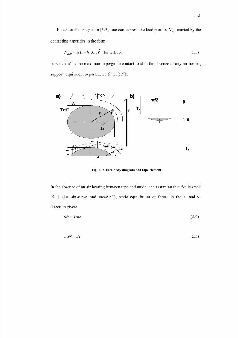
8/8/2019 BR PhD Dissertation
http://slidepdf.com/reader/full/br-phd-dissertation 145/248
113
Based on the analysis in [5.9], one can express the load portion asp N carried by the
contacting asperities in the form:
2
)31( sasp h N N σ −=
, for 3 sh σ ≤
(5.3)
in which N is the maximum tape/guide contact load in the absence of any air bearing
support (equivalent to parameter * β in [5.9]).
b)a)
W
z
x
y
TT+dTFf
dN
a
dα
o
ω
α
π /2
T2
T1
θ
α
π /2
T2
T1
θπ /2
T2
T1
θ
b)a)
W
z
x
y
TT+dTFf
dN
a
dα
o
ω
W
z
x
y
TT+dTFf
dN
a
dα
o
ω
α
π /2
T2
T1
θ
α
π /2
T2
T1
θπ /2
T2
T1
θ
In the absence of an air bearing between tape and guide, and assuming that d α is small
[5.1], (i.e. sinα α ≅ and cos 1α ≅ ), static equilibrium of forces in the z- and y-
direction gives:
dN Td α = (5.4)
dN dT µ = (5.5)
Fig. 5.1: Free body diagram of a tape element
8/8/2019 BR PhD Dissertation
http://slidepdf.com/reader/full/br-phd-dissertation 146/248
114
Assuming that the friction coefficient is constant, one obtains eq. (5.1). This
classical equation represents a simplified situation of the tape/guide interface, since it
neglects the effects of surface characteristics, material properties and guide dimensions
on the friction coefficient. In the following, a more realistic model will be developed in
which these neglected effects will be included.
5.2.2 Friction model
Several friction models of rough surfaces have been proposed in the past [5.11-
5.15]. Recently, Brizmer et al. [5.16] proposed a new model for the static friction
coefficient for a single deformable asperity in contact with a rigid flat based on the
assumption that the contact interface is under stick condition (frictional contact). They
obtained numerical results for the friction coefficient µ which they presented in the
form
( )( )0.35
0.27coth 0.27 P µ ∗= (5.6)
where the non-dimensional load P ∗ on one asperity has the form /asp C P P L∗ = . Here
asp P is the normal load on one asperity and C L is its critical normal load at yield
inception under frictional contact, given by [5.17]
C C C L L P = (5.7)
where
( )28.88 10.13 0.089C L ν ν = − + (5.8)
8/8/2019 BR PhD Dissertation
http://slidepdf.com/reader/full/br-phd-dissertation 147/248
115
and
( )23
3 216
C
Y P C Y r
E ν
π ν
= −
(5.9)
In eq. (5.9), C P (see Ref. [5.17]) is the critical normal load in slip (frictionless), r is the
radius of the asperity tip. The material properties Y , E and ν are the yield strength,
Young’s modulus, and Poisson’s ratio, respectively, of the deformable asperity and
1.234 1.256C ν ν = + .
To apply eq. (5.6) to the case of the tape/guide interface, the following simplifying
assumptions are made:
1. The effects of the various relevant parameters such as tape tension, guide radius,
surface roughness and material properties on the dynamic friction between tape and
guide are similar as on the static friction. Hence, eq. (5.6) can be used for a
qualitative evaluation of these effects. This assumption is justifiable based on
experimental observations reported in the literature [5.18].
2. The tape is assumed "rigid" so that local elastic deformations of the tape can be
neglected. In addition, the tape is assumed to conform to the guide.
3. The contact of two rough surfaces as in the tape/guide case can be modeled by an
equivalent rough surface in contact with a perfectly smooth one [5.19].
8/8/2019 BR PhD Dissertation
http://slidepdf.com/reader/full/br-phd-dissertation 148/248
116
4. The actual load on each individual asperity can be approximated by an average local
asperity load.
Assuming a Gaussian distribution of asperity heights [5.20], one can show that the
number of contacting asperities, n , over a tape section of angular extent d α is given by
[5.21]
* 2 *exp[ 0.5( ) ] [1 ( 0.5 )]22 h
wad wad n z dz erf h
η α η α
π
∞= − = −∫ (5.10)
where η represents the asperity density and / s
h h σ = is a dimensionless spacing. Using
eqs. (5.2), (5.3) and (5.9), we can express the average local load per asperity
/asp asp P dN n= as
2( ) 2(1 / 3)
[1 ( 0.5 )]asp
T h P
wa erf h
α
η
−=
−(5.11)
In non-dimensional quantities, eq. (5.11) can be written as:
2( ) 2(1 / 3)
[1 ( 0.5 )]c
T h
waL erf h
α
η
−Γ =
−(5.12)
whereasp
C
P
LΓ = is a local dimensionless tape tension, which is identical to the parameter
* P in eq. (5.6). Hence, eq. (5.6) can be re-written as:
0.350.27 coth(0.27 )µ = Γ (5.13)
Finally, from eqs. (5.4), (5.5), (5.12) and (5.13) one obtains:
( )
( ) ( )( )0.350.27
coth 0.27
d d
α α
α
Γ=
Γ Γ(5.14)
8/8/2019 BR PhD Dissertation
http://slidepdf.com/reader/full/br-phd-dissertation 149/248
117
Eq. (5.14) is a non-linear ordinary differential equation which yields a solution of the
form: ( )2 2/ , f α Γ Γ = Γ , (5.15)
where
2
22
2(1 / 3)
[1 ( 0.5 )]c
T h
waL erf hη
−Γ =
−(5.16)
is the initial condition. Since in eq. (5.15) the normalization factor is the same in the
nominator as in the denominator, it can also be expressed as
( )2 2/ ,T T f α = Γ , (5.17)
For a given wrap angle α θ = , eq. (5.17) provides the ratio 1 2/T T which can be used in
eq. (5.1) to determine an average friction coefficient that now depends on 2Γ . Hence,
this friction coefficient incorporates the tape speed (through the tape/guide spacing), the
surface characteristics, the material properties and the guide geometry (see eq. (5.16)).
In order to relate the initial condition 2Γ to a rough surface with many asperities
rather than to a single asperity, we assume that each asperity in a tape section of angular
extent d α carries the same average local load (see assumption 4). The critical
interference C ω at yield inception of a single asperity was defined in [5.17] as
( )2
21
2C
Y C r
E ν
π ν ω
− =
(5.18)
Hence, from this C ω and eqs. (5.6) and (5.8) one can obtain the relationship
2
3C C C L L C Yr ν
π ω = (5.19)
8/8/2019 BR PhD Dissertation
http://slidepdf.com/reader/full/br-phd-dissertation 150/248
118
The plasticity index ψ of contacting rough surfaces contact can be written [5.19] as
1/ 2
s
C
σ ψ
ω
=
(5.20)
Substituting C L from eq. (5.19) in eq. (5.16) and using eq. (5.20) we finally obtain
2 2
22
3 (1 / 3)
[1 ( 0.5 )]c s
T h
waL C Y r erf hν
ψ
π η σ
−Γ =
−(5.21)
Eq. (5.21) reveals that the plasticity index ψ , which is proportional to ( )( )1/ 2
/ / s E Y r σ ,
has a significant effect on the solution of eq. (5.14) and hence on the average friction
coefficient. In addition, the material properties ν and Y as well as the guide radius a
and the tape speed, which from the analysis of [5.22] determines h , have also an effect
on the friction coefficient. While the trend of the effects of material properties and
guide radius on 2Γ can easily be seen in eq. (5.21), the effect of tape speed is more
complex. To determine this relationship we define an "asperity load factor" of the form:
2(1 / 3)
[1 ( 0.5 )]
h
erf h β −=
−(5.22)
The variation of β as a function of h is illustrated in Fig. 5.2, showing a maximum
for β around 2.2h ≈ . Since hydrodynamic flying occurs at 3h ≥ , our model predicts
that the asperity load factor reaches a maximum somewhat before flying inception. The
model also predicts (as will be shown in the discussion of Fig. 5.5) that the friction
coefficient becomes very small and independent of 2Γ if β and thus 2
Γ approaches
zero.
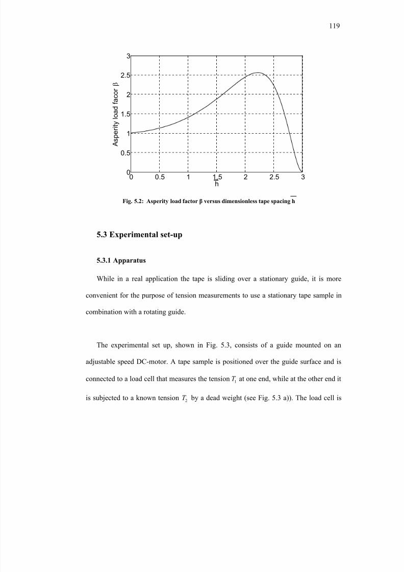
8/8/2019 BR PhD Dissertation
http://slidepdf.com/reader/full/br-phd-dissertation 151/248
119
0 0.5 1 1.5 2 2.5 30
0.5
1
1.5
2
2.5
3
h
A s p e r i t y l o a d f a c o r β
0 0.5 1 1.5 2 2.5 30
0.5
1
1.5
2
2.5
3
h
A s p e r i t y l o a d f a c o r β
5.3 Experimental set-up
5.3.1 Apparatus
While in a real application the tape is sliding over a stationary guide, it is more
convenient for the purpose of tension measurements to use a stationary tape sample in
combination with a rotating guide.
The experimental set up, shown in Fig. 5.3, consists of a guide mounted on an
adjustable speed DC-motor. A tape sample is positioned over the guide surface and is
connected to a load cell that measures the tension 1T at one end, while at the other end it
is subjected to a known tension 2T by a dead weight (see Fig. 5.3 a)). The load cell is
Fig. 5.2: Asperity load factor β versus dimensionless tape spacing h
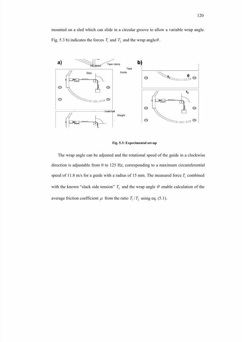
8/8/2019 BR PhD Dissertation
http://slidepdf.com/reader/full/br-phd-dissertation 152/248
120
mounted on a sled which can slide in a circular groove to allow a variable wrap angle.
Fig. 5.3 b) indicates the forces 1T and 2T and the wrap angleθ .
TapeDC Motor
Sled
Tape clamp
Load cell
Weight
Guide
a) b)
T1
T2
θ
TapeDC Motor
Sled
Tape clamp
Load cell
Weight
Guide
a)Tape
DC Motor
Sled
Tape clamp
Load cell
Weight
Guide
a) b)
T1
T2
θ
b)
T1
T2
θ
The wrap angle can be adjusted and the rotational speed of the guide in a clockwise
direction is adjustable from 0 to 125 Hz, corresponding to a maximum circumferential
speed of 11.8 m/s for a guide with a radius of 15 mm. The measured force 1T combined
with the known “slack side tension” 2T and the wrap angle θ enable calculation of the
average friction coefficient µ from the ratio 1 2/T T using eq. (5.1).
Fig. 5.3: Experimental set-up
8/8/2019 BR PhD Dissertation
http://slidepdf.com/reader/full/br-phd-dissertation 153/248
121
5.3.2 Test specimens
Commercially available metal particulate (MP) tape and metal evaporated (ME)
magnetic tape was used for the tests. MP tape consists of a polymer substrate, coated
with a mixture of metal particles and binder material. The magnetic coating of MP tape
also contains abrasive particles for recording head cleaning. ME tape is manufactured
by evaporating cobalt on a polymeric substrate in a vacuum chamber.
Two types of aluminum guides with radii of 7.5 mm, 10 mm and 15 mm were used.
In one case, a ceramic coating was applied and in the other case an anodizing heat
treatment was used. AFM scans of the guides revealed that the surface roughness is
isotropic.
Table 5.1 shows the average asperity tip radius r , the asperity density η , the
standard deviation of asperity summit heights sσ , the ratio / s r σ and the product sr η σ
for the individual tape samples and guides. The equivalent roughness parameters for
two contacting rough surfaces are also shown for three tape/guide combinations. These
combinations are: MP tape and a ceramic guide (C1), ME tape and a ceramic guide (C2)
and MP tape in combination with an anodized guide (C3).
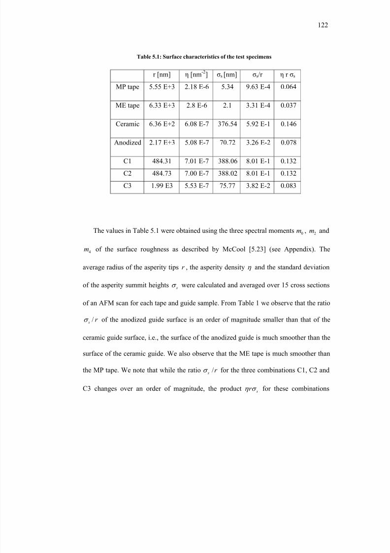
8/8/2019 BR PhD Dissertation
http://slidepdf.com/reader/full/br-phd-dissertation 154/248
122
r [nm] η [nm-2
] σs [nm] σs/r η r σs
MP tape 5.55 E+3 2.18 E-6 5.34 9.63 E-4 0.064
ME tape 6.33 E+3 2.8 E-6 2.1 3.31 E-4 0.037
Ceramic 6.36 E+2 6.08 E-7 376.54 5.92 E-1 0.146
Anodized 2.17 E+3 5.08 E-7 70.72 3.26 E-2 0.078
C1 484.31 7.01 E-7 388.06 8.01 E-1 0.132
C2 484.73 7.00 E-7 388.02 8.01 E-1 0.132
C3 1.99 E3 5.53 E-7 75.77 3.82 E-2 0.083
The values in Table 5.1 were obtained using the three spectral moments 0m , 2m and
4m of the surface roughness as described by McCool [5.23] (see Appendix). The
average radius of the asperity tips r , the asperity density η and the standard deviation
of the asperity summit heights sσ were calculated and averaged over 15 cross sections
of an AFM scan for each tape and guide sample. From Table 1 we observe that the ratio
/ s r σ of the anodized guide surface is an order of magnitude smaller than that of the
ceramic guide surface, i.e., the surface of the anodized guide is much smoother than the
surface of the ceramic guide. We also observe that the ME tape is much smoother than
the MP tape. We note that while the ratio / s r σ for the three combinations C1, C2 and
C3 changes over an order of magnitude, the product sr η σ for these combinations
Table 5.1: Surface characteristics of the test specimens
8/8/2019 BR PhD Dissertation
http://slidepdf.com/reader/full/br-phd-dissertation 155/248
123
changes much less. Hence, 2Γ (see eq. 5.20) is less sensitive to the dimensionless
parameter sr η σ in the tested combinations.
5.3.3 Test procedure
Tape specimens of 0.1 m length were cut out of commercially available tape reels.
For each test a new tape specimen was connected to the load cell through a tape clamp
on one end and a 0.5 N dead weight on its other end (Fig. 5.3 a)). The tape specimen
was run-in for five minutes at a rotational speed 16ω =
Hz. Following this run-in
procedure, the “tight side tension” 1T was measured for stepwise increments of guide
rotational speeds up to 125 Hz and was stored on a PC for further processing. The
“slack-side” tension 2T was then adjusted by adding weight, while keeping the DC-
motor running. The measurements of 1T were taken for the same range of speeds. This
procedure was repeated up to a maximum slack-side tension2
1.2T = N. The test series
for each of the three combinations C1, C2 and C3 were repeated three times with a new
tape specimen for each test. The calculated friction coefficient for each test was
averaged over the three repetitions.
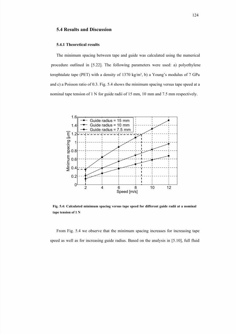
8/8/2019 BR PhD Dissertation
http://slidepdf.com/reader/full/br-phd-dissertation 156/248
124
5.4 Results and Discussion
5.4.1 Theoretical results
The minimum spacing between tape and guide was calculated using the numerical
procedure outlined in [5.22]. The following parameters were used: a) polyethylene
terephtalate tape (PET) with a density of 1370 kg/m³, b) a Young’s modulus of 7 GPa
and c) a Poisson ratio of 0.3. Fig. 5.4 shows the minimum spacing versus tape speed at a
nominal tape tension of 1 N for guide radii of 15 mm, 10 mm and 7.5 mm respectively.
2 4 6 8 10 120
0.2
0.4
0.6
0.8
1
1.2
1.4
1.6
Speed [m/s]
M i n i m u m s
p a c i n g [ µ m ]
Guide radius = 15 mmGuide radius = 10 mmGuide radius = 7.5 mm
2 4 6 8 10 120
0.2
0.4
0.6
0.8
1
1.2
1.4
1.6
Speed [m/s]
M i n i m u m s
p a c i n g [ µ m ]
Guide radius = 15 mmGuide radius = 10 mmGuide radius = 7.5 mm
From Fig. 5.4 we observe that the minimum spacing increases for increasing tape
speed as well as for increasing guide radius. Based on the analysis in [5.10], full fluid
Fig. 5.4: Calculated minimum spacing versus tape speed for different guide radii at a nominal
tape tension of 1 N
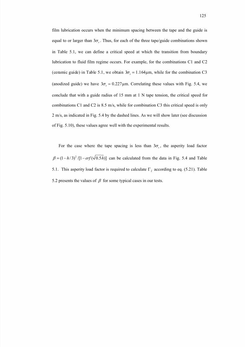
8/8/2019 BR PhD Dissertation
http://slidepdf.com/reader/full/br-phd-dissertation 157/248
125
film lubrication occurs when the minimum spacing between the tape and the guide is
equal to or larger than 3 sσ . Thus, for each of the three tape/guide combinations shown
in Table 5.1, we can define a critical speed at which the transition from boundary
lubrication to fluid film regime occurs. For example, for the combinations C1 and C2
(ceramic guide) in Table 5.1, we obtain 3 1.164 sσ = µm, while for the combination C3
(anodized guide) we have 3 0.227 sσ = µm. Correlating these values with Fig. 5.4, we
conclude that with a guide radius of 15 mm at 1 N tape tension, the critical speed for
combinations C1 and C2 is 8.5 m/s, while for combination C3 this critical speed is only
2 m/s, as indicated in Fig. 5.4 by the dashed lines. As we will show later (see discussion
of Fig. 5.10), these values agree well with the experimental results.
For the case where the tape spacing is less than 3 sσ , the asperity load factor
2(1 / 3) /[1 ( 0.5 )]h erf h β = − − can be calculated from the data in Fig. 5.4 and Table
5.1. This asperity load factor is required to calculate 2Γ according to eq. (5.21). Table
5.2 presents the values of β for some typical cases in our tests.
8/8/2019 BR PhD Dissertation
http://slidepdf.com/reader/full/br-phd-dissertation 158/248
126
Speed [m/s] 2 4 6 8 10 12
C1, T2=1 N, a=15 mm 1.347 2.057 2.547 0.583 0.004 0.004
C3, T2=1 N, a=15 mm 0.004 0.004 0.004 0.004 0.004 0.004
C1, T2=1 N, a=7.5 mm 1.073 1.201 1.378 1.6 1.863 2.152
C3, T2=1 N, a=7.5 mm 2.195 0.004 0.004 0.004 0.004 0.004
C1, T2=0.5N, a=7.5mm 1.179 1.532 2.038 2.507 2.231 0.22
C3, T2=0.5N, a=7.5mm 0.004 0.004 0.004 0.004 0.004 0.004
Eq. (5.14) was integrated numerically using the fourth order Runge Kutta method to
obtain the ratio 2/ ΓΓ or, equivalently, 2/T T , according to eq. (5.15) or (5.17). Fig. 5.5
shows the results as 2/T T versus the angular coordinate α for different initial
conditions 2Γ (see eq. 5.17). We point out that the tape speed, surface characteristics,
mechanical properties and guide geometry are all included (see eq. 5.21) in the model.
Table 5.2: Typical values for the asperity load factor β for tape/guide combinations C1
(MP/ceramic) and C3 (MP/anodized) at different tap tension T2 and guide radius a
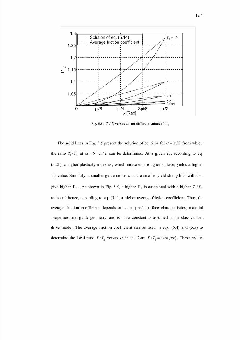
8/8/2019 BR PhD Dissertation
http://slidepdf.com/reader/full/br-phd-dissertation 159/248
127
0 pi/8 pi/4 3pi/8 pi/21
1.05
1.1
1.15
1.2
1.25
1.3Γ
2= 10
1
0.1
0.010.0010.001
α [Rad]
T / T 2
Solution of eq. (5.14)Average friction coefficient
The solid lines in Fig. 5.5 present the solution of eq. 5.14 for / 2θ π = from which
the ratio 1 2/T T at / 2α θ π = = can be determined. At a given 2T , according to eq.
(5.21), a higher plasticity index ψ , which indicates a rougher surface, yields a higher
2Γ value. Similarly, a smaller guide radius a and a smaller yield strength Y will also
give higher 2Γ . As shown in Fig. 5.5, a higher 2
Γ is associated with a higher 1 2/T T
ratio and hence, according to eq. (5.1), a higher average friction coefficient. Thus, the
average friction coefficient depends on tape speed, surface characteristics, material
properties, and guide geometry, and is not a constant as assumed in the classical belt
drive model. The average friction coefficient can be used in eqs. (5.4) and (5.5) to
determine the local ratio 2/T T versus α in the form ( )2/ expT T µα = . These results
Fig. 5.5: 2/T T versus α for different values of 2Γ
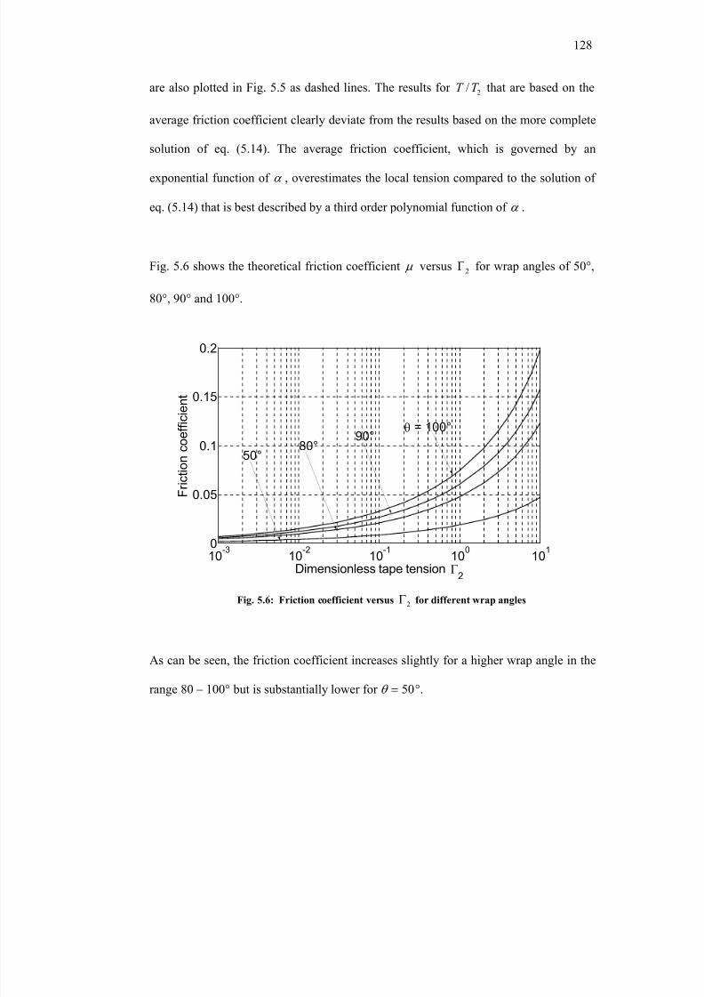
8/8/2019 BR PhD Dissertation
http://slidepdf.com/reader/full/br-phd-dissertation 160/248
128
are also plotted in Fig. 5.5 as dashed lines. The results for 2/T T that are based on the
average friction coefficient clearly deviate from the results based on the more complete
solution of eq. (5.14). The average friction coefficient, which is governed by an
exponential function of α , overestimates the local tension compared to the solution of
eq. (5.14) that is best described by a third order polynomial function of α .
Fig. 5.6 shows the theoretical friction coefficient µ versus 2Γ for wrap angles of 50°,
80°, 90° and 100°.
10-3
10-2
10-1
100
101
0
0.05
0.1
0.15
0.2
Dimensionless tape tension Γ2
F r i c
t i o n c o e f f i c i e n t
50°80°
90°θ = 100°
As can be seen, the friction coefficient increases slightly for a higher wrap angle in the
range 80 – 100° but is substantially lower for 50θ = °.
Fig. 5.6: Friction coefficient versus 2Γ for different wrap angles
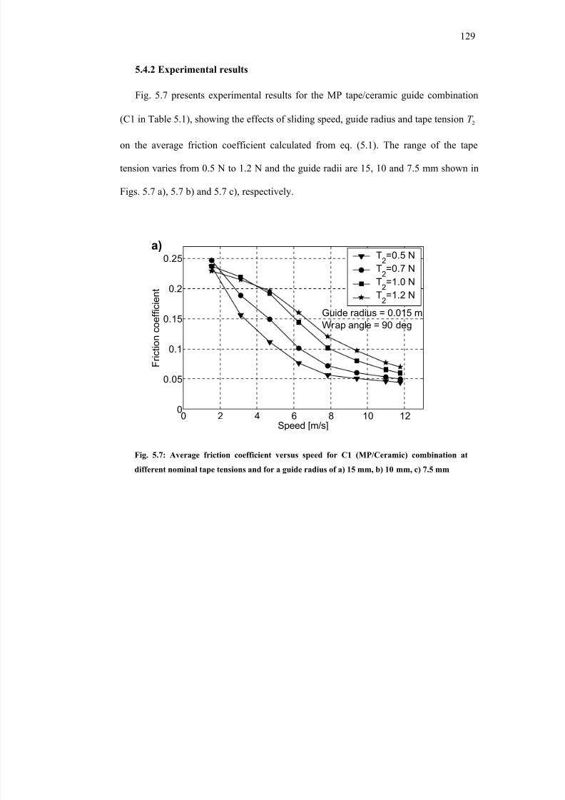
8/8/2019 BR PhD Dissertation
http://slidepdf.com/reader/full/br-phd-dissertation 161/248
129
5.4.2 Experimental results
Fig. 5.7 presents experimental results for the MP tape/ceramic guide combination
(C1 in Table 5.1), showing the effects of sliding speed, guide radius and tape tension 2T
on the average friction coefficient calculated from eq. (5.1). The range of the tape
tension varies from 0.5 N to 1.2 N and the guide radii are 15, 10 and 7.5 mm shown in
Figs. 5.7 a), 5.7 b) and 5.7 c), respectively.
0 2 4 6 8 10 120
0.05
0.1
0.15
0.2
0.25
Speed [m/s]
F r i c t i o n c o e f f i c i e n t
Guide radius = 0.015 m
Wrap angle = 90 deg
T2=0.5 NT
2=0.7 N
T2=1.0 N
T2=1.2 N
a)
0 2 4 6 8 10 120
0.05
0.1
0.15
0.2
0.25
Speed [m/s]
F r i c t i o n c o e f f i c i e n t
Guide radius = 0.015 m
Wrap angle = 90 deg
T2=0.5 NT
2=0.7 N
T2=1.0 N
T2=1.2 N
a)
Fig. 5.7: Average friction coefficient versus speed for C1 (MP/Ceramic) combination at
different nominal tape tensions and for a guide radius of a) 15 mm, b) 10 mm, c) 7.5 mm
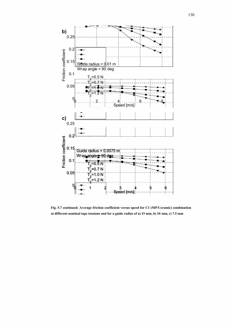
8/8/2019 BR PhD Dissertation
http://slidepdf.com/reader/full/br-phd-dissertation 162/248
130
0 2 4 6 80
0.05
0.1
0.15
0.2
0.25
Speed [m/s]
F r i c t i o n c o e f f i c i e n
t
Guide radius = 0.01 m
Wrap angle = 90 deg
T2=0.5 N
T2=0.7 N
T2=1.0 N
T2=1.2 N
b)
0 2 4 6 80
0.05
0.1
0.15
0.2
0.25
Speed [m/s]
F r i c t i o n c o e f f i c i e n
t
Guide radius = 0.01 m
Wrap angle = 90 deg
T2=0.5 N
T2=0.7 N
T2=1.0 N
T2=1.2 N
b)
0 1 2 3 4 5 60
0.05
0.1
0.15
0.2
0.25
Speed [m/s]
F r i c t i o n c o e f f i c i e n t
Guide radius = 0.0075 m
Wrap angle = 90 deg
T2=0.5 N
T2=0.7 N
T2=1.0 N
T2=1.2 N
c)
0 1 2 3 4 5 60
0.05
0.1
0.15
0.2
0.25
Speed [m/s]
F r i c t i o n c o e f f i c i e n t
Guide radius = 0.0075 m
Wrap angle = 90 deg
T2=0.5 N
T2=0.7 N
T2=1.0 N
T2=1.2 N
c)
Fig. 5.7 continued: Average friction coefficient versus speed for C1 (MP/Ceramic) combination
at different nominal tape tensions and for a guide radius of a) 15 mm, b) 10 mm, c) 7.5 mm
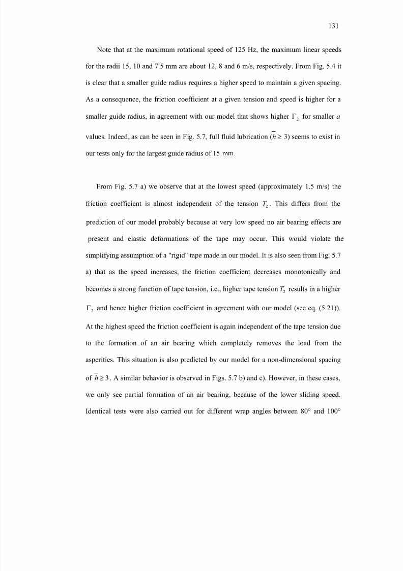
8/8/2019 BR PhD Dissertation
http://slidepdf.com/reader/full/br-phd-dissertation 163/248
131
Note that at the maximum rotational speed of 125 Hz, the maximum linear speeds
for the radii 15, 10 and 7.5 mm are about 12, 8 and 6 m/s, respectively. From Fig. 5.4 it
is clear that a smaller guide radius requires a higher speed to maintain a given spacing.
As a consequence, the friction coefficient at a given tension and speed is higher for a
smaller guide radius, in agreement with our model that shows higher 2Γ for smaller a
values. Indeed, as can be seen in Fig. 5.7, full fluid lubrication ( 3h ≥ ) seems to exist in
our tests only for the largest guide radius of 15 mm.
From Fig. 5.7 a) we observe that at the lowest speed (approximately 1.5 m/s) the
friction coefficient is almost independent of the tension 2T . This differs from the
prediction of our model probably because at very low speed no air bearing effects are
present and elastic deformations of the tape may occur. This would violate the
simplifying assumption of a "rigid" tape made in our model. It is also seen from Fig. 5.7
a) that as the speed increases, the friction coefficient decreases monotonically and
becomes a strong function of tape tension, i.e., higher tape tension 2T results in a higher
2Γ and hence higher friction coefficient in agreement with our model (see eq. (5.21)).
At the highest speed the friction coefficient is again independent of the tape tension due
to the formation of an air bearing which completely removes the load from the
asperities. This situation is also predicted by our model for a non-dimensional spacing
of 3h ≥ . A similar behavior is observed in Figs. 5.7 b) and c). However, in these cases,
we only see partial formation of an air bearing, because of the lower sliding speed.
Identical tests were also carried out for different wrap angles between 80° and 100°
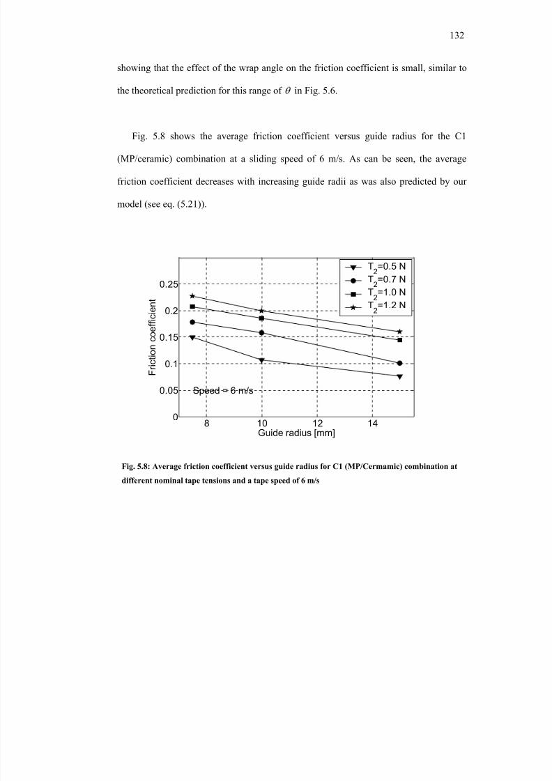
8/8/2019 BR PhD Dissertation
http://slidepdf.com/reader/full/br-phd-dissertation 164/248
8/8/2019 BR PhD Dissertation
http://slidepdf.com/reader/full/br-phd-dissertation 165/248
133
In order to increase the recording density, tape manufacturers use metal evaporated
(ME) tape, consisting of a high coercivity cobalt film, evaporated on the tape substrate
in a vacuum chamber, as described already in chapter 1. Hempstock and Sullivan [5.24]
studied the durability and signal performance of ME and MP tapes and concluded that
MP tape exhibits far greater durability than ME tape. In another study Hempstock and
Sullivan [5.25] identified the mechanical failure mechanism of ME tape as a form of
delamination wear. Bijker et al. [5.26] discussed the use of wear protective coatings
such as diamond like carbon (DLC) and a so-called super protective layer (SPL) to
potentially improve the wear characteristics of ME tape. They concluded that protective
coatings need further development to withstand abrasive wear.
The rotating guide of our test set-up stalled due to high stiction when attempting to
test the ME tape over the full operating range (speed and tension) which was previously
used with MP tape. Hence, in order to overcome the higher stiction tendency inherent to
ME tape [5.4], and allow comparison with MP tape, a test was performed for both
media using a low tape tension of 0.1 N in combination with an 80 degree wrap angle
and a guide radius of 15 mm. Fig. 5.9 presents the comparison between the ME and MP
tapes showing very similar values of friction coefficient over the entire speed range.
From Table 5.1 we observe that although the ME tape has a / s r σ value that is three
times lower than that of the MP tape, the equivalent / s r σ values for the combinations
C1 (MP tape and ceramic guide) and C2 (ME tape and ceramic guide), and their
corresponding plasticity index values, are almost identical. Hence, as can be seen from
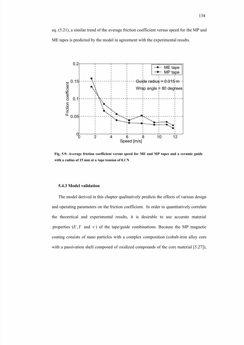
8/8/2019 BR PhD Dissertation
http://slidepdf.com/reader/full/br-phd-dissertation 166/248
134
eq. (5.21), a similar trend of the average friction coefficient versus speed for the MP and
ME tapes is predicted by the model in agreement with the experimental results.
0 2 4 6 8 10 120
0.05
0.1
0.15
0.2
Speed [m/s]
F r i c
t i o n c o e f f i c i e n t Guide radius = 0.015 m
Wrap angle = 80 degrees
ME tapeMP tape
5.4.3 Model validation
The model derived in this chapter qualitatively predicts the effects of various design
and operating parameters on the friction coefficient. In order to quantitatively correlate
the theoretical and experimental results, it is desirable to use accurate material
properties ( E ,Y and ν ) of the tape/guide combinations. Because the MP magnetic
coating consists of nano particles with a complex composition (cobalt-iron alloy core
with a passivation shell composed of oxidized compounds of the core material [5.27]),
Fig. 5.9: Average friction coefficient versus speed for ME and MP tapes and a ceramic guide
with a radius of 15 mm at a tape tension of 0.1 N
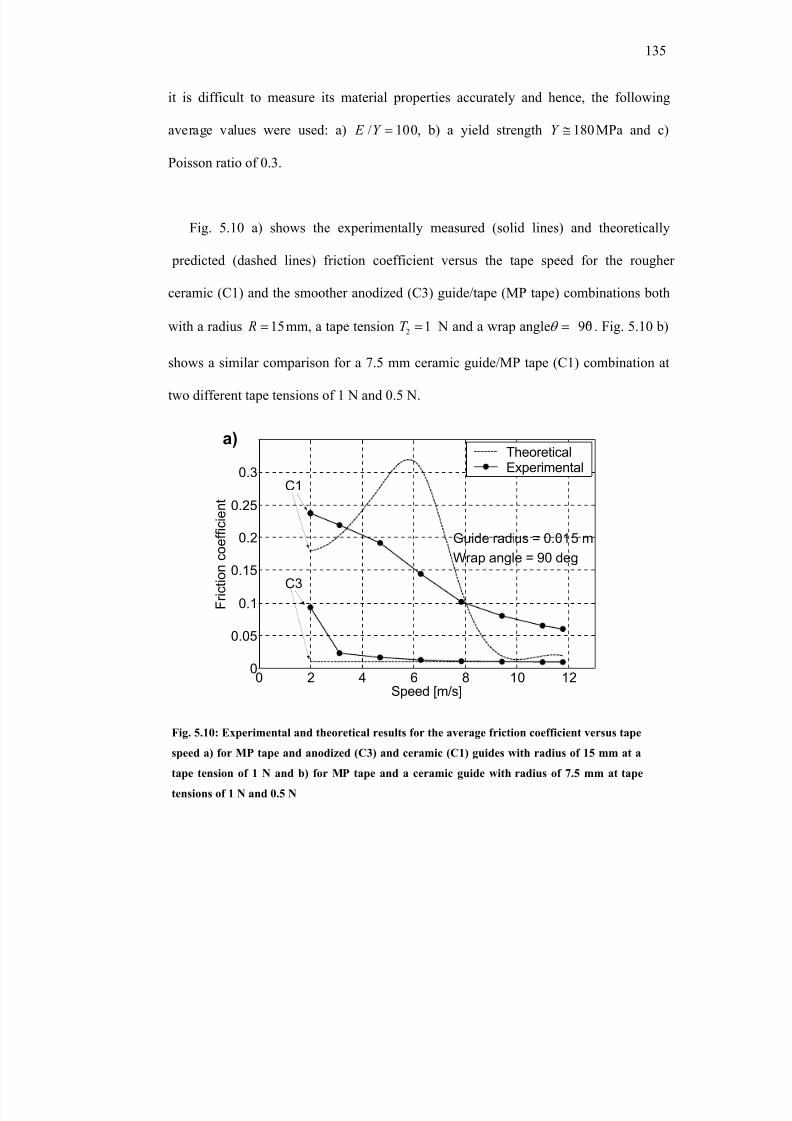
8/8/2019 BR PhD Dissertation
http://slidepdf.com/reader/full/br-phd-dissertation 167/248
135
it is difficult to measure its material properties accurately and hence, the following
average values were used: a) / 100 E Y = , b) a yield strength 180Y ≅ MPa and c)
Poisson ratio of 0.3.
Fig. 5.10 a) shows the experimentally measured (solid lines) and theoretically
predicted (dashed lines) friction coefficient versus the tape speed for the rougher
ceramic (C1) and the smoother anodized (C3) guide/tape (MP tape) combinations both
with a radius 15 R = mm, a tape tension 2 1T = N and a wrap angle 90θ = ° . Fig. 5.10 b)
shows a similar comparison for a 7.5 mm ceramic guide/MP tape (C1) combination at
two different tape tensions of 1 N and 0.5 N.
0 2 4 6 8 10 120
0.05
0.1
0.15
0.2
0.25
0.3C1
C3
Speed [m/s]
F r i c t i o n c o e f f i c i e n t
Guide radius = 0.015 mWrap angle = 90 deg
TheoreticalExperimental
a)
0 2 4 6 8 10 120
0.05
0.1
0.15
0.2
0.25
0.3C1
C3
Speed [m/s]
F r i c t i o n c o e f f i c i e n t
Guide radius = 0.015 mWrap angle = 90 deg
TheoreticalExperimental
a)
Fig. 5.10: Experimental and theoretical results for the average friction coefficient versus tape
speed a) for MP tape and anodized (C3) and ceramic (C1) guides with radius of 15 mm at a
tape tension of 1 N and b) for MP tape and a ceramic guide with radius of 7.5 mm at tape
tensions of 1 N and 0.5 N
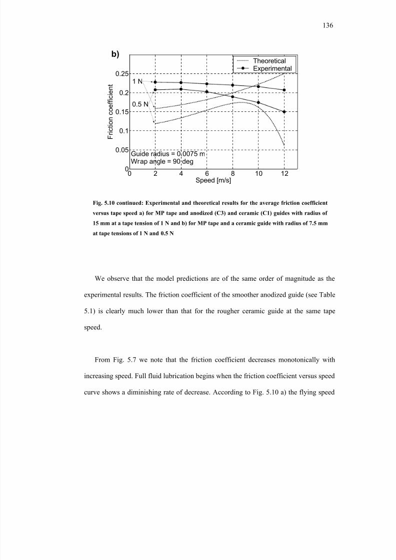
8/8/2019 BR PhD Dissertation
http://slidepdf.com/reader/full/br-phd-dissertation 168/248
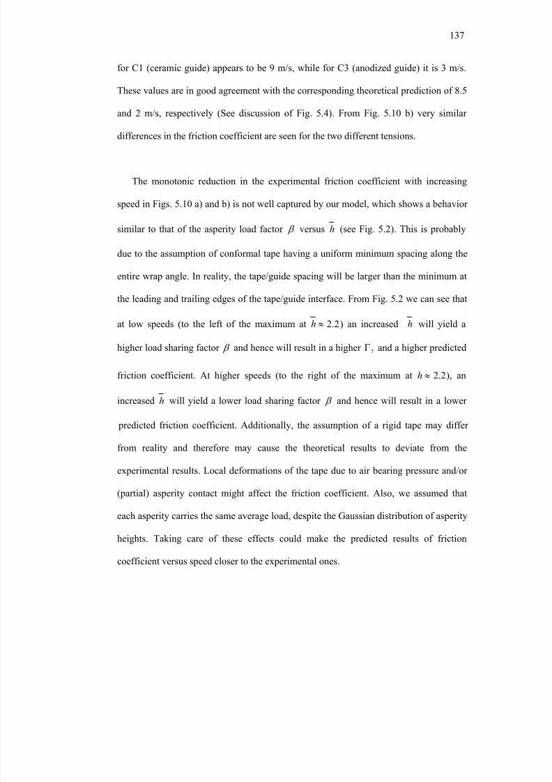
8/8/2019 BR PhD Dissertation
http://slidepdf.com/reader/full/br-phd-dissertation 169/248
137
for C1 (ceramic guide) appears to be 9 m/s, while for C3 (anodized guide) it is 3 m/s.
These values are in good agreement with the corresponding theoretical prediction of 8.5
and 2 m/s, respectively (See discussion of Fig. 5.4). From Fig. 5.10 b) very similar
differences in the friction coefficient are seen for the two different tensions.
The monotonic reduction in the experimental friction coefficient with increasing
speed in Figs. 5.10 a) and b) is not well captured by our model, which shows a behavior
similar to that of the asperity load factor β versus h (see Fig. 5.2). This is probably
due to the assumption of conformal tape having a uniform minimum spacing along the
entire wrap angle. In reality, the tape/guide spacing will be larger than the minimum at
the leading and trailing edges of the tape/guide interface. From Fig. 5.2 we can see that
at low speeds (to the left of the maximum at 2.2h ≈ ) an increased h will yield a
higher load sharing factor β and hence will result in a higher 2Γ and a higher predicted
friction coefficient. At higher speeds (to the right of the maximum at 2.2h ≈ ), an
increased h will yield a lower load sharing factor β and hence will result in a lower
predicted friction coefficient. Additionally, the assumption of a rigid tape may differ
from reality and therefore may cause the theoretical results to deviate from the
experimental results. Local deformations of the tape due to air bearing pressure and/or
(partial) asperity contact might affect the friction coefficient. Also, we assumed that
each asperity carries the same average load, despite the Gaussian distribution of asperity
heights. Taking care of these effects could make the predicted results of friction
coefficient versus speed closer to the experimental ones.
8/8/2019 BR PhD Dissertation
http://slidepdf.com/reader/full/br-phd-dissertation 170/248
138
Fig. 5.11 compares theoretical predictions (dashed line) and experimental results
(solid line) of the effect of the guide radius on the friction coefficient for a tape tension
of 1 N and a ceramic guide/MP tape (C1) combination. As can be seen the agreement
between the model and experiments is fairly good.
8 10 12 14 160
0.05
0.1
0.15
0.2
Guide radius [mm]
F r i c t i o n
c o e f f i c i e n t
Speed = 6 m/s
Tape tension = 1 N TheoreticalExperimental
5.5 Conclusion
A model was developed that predicts the local tape tension along the circumference
of the tape/guide interface, based on a local friction coefficient model for a single
contacting asperity. The model provides an average friction coefficient for different
Fig. 5.11: Experimental and theoretical results for the average friction coefficient versus guide
radius for a ceramic guide and MP tape at 1 N tape tension
8/8/2019 BR PhD Dissertation
http://slidepdf.com/reader/full/br-phd-dissertation 171/248
139
tape/guide combinations taking into account the effects of tape sliding speed, tape and
guide surface characteristics, material properties and guide dimensions. An
experimental set-up was implemented to measure the average friction. Good agreement
was found between theoretical predictions and the experimental results for moderate
tape speeds where an air bearing coexists with partial asperity contact. The main
conclusions of the present study are:
1. The classical belt drive equation that relies on a constant friction coefficient can
be significantly improved to include such effects as sliding speed, surface
roughness, material propertied and guide and tape geometry.
2. The plasticity index ψ , which is proportional to ( )( )1/ 2
/ / s E Y r σ , has a
significant effect on the average friction coefficient. A higher ψ value yields
higher friction coefficients. The material properties ν and Y as well as the
guide radius a also affect the friction coefficient.
3.
The speed at the transition from boundary lubrication to full fluid film regime
can be predicted from surface characteristics and from tape/guide flying height
simulations. This speed is higher for rougher surfaces and smaller guide radii.
4. The average friction coefficient shows only a small dependence on the wrap
angle, over the 80° - 100° range. However, it increases substantially for
increasing dimensionless tape tension 2Γ , especially at high values of this
parameter.
5. The average friction coefficient decreases for increasing speed and decreasing
tape tension 2T .
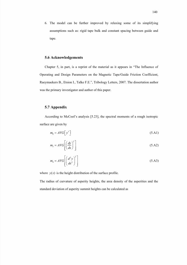
8/8/2019 BR PhD Dissertation
http://slidepdf.com/reader/full/br-phd-dissertation 172/248
140
6. The model can be further improved by relaxing some of its simplifying
assumptions such as: rigid tape bulk and constant spacing between guide and
tape.
5.6 Acknowledgements
Chapter 5, in part, is a reprint of the material as it appears in “The Influence of
Operating and Design Parameters on the Magnetic Tape/Guide Friction Coefficient,
Raeymaekers B., Etsion I., Talke F.E.”, Tribology Letters, 2007. The dissertation author
was the primary investigator and author of this paper.
5.7 Appendix
According to McCool’s analysis [5.23], the spectral moments of a rough isotropic
surface are given by
2
0m AVG y = (5.A1)
2
2
dym AVG
dx
=
(5.A2)
22
4 2
d ym AVG
dx
=
(5.A3)
where ( ) y x is the height distribution of the surface profile.
The radius of curvature of asperity heights, the area density of the asperities and the
standard deviation of asperity summit heights can be calculated as
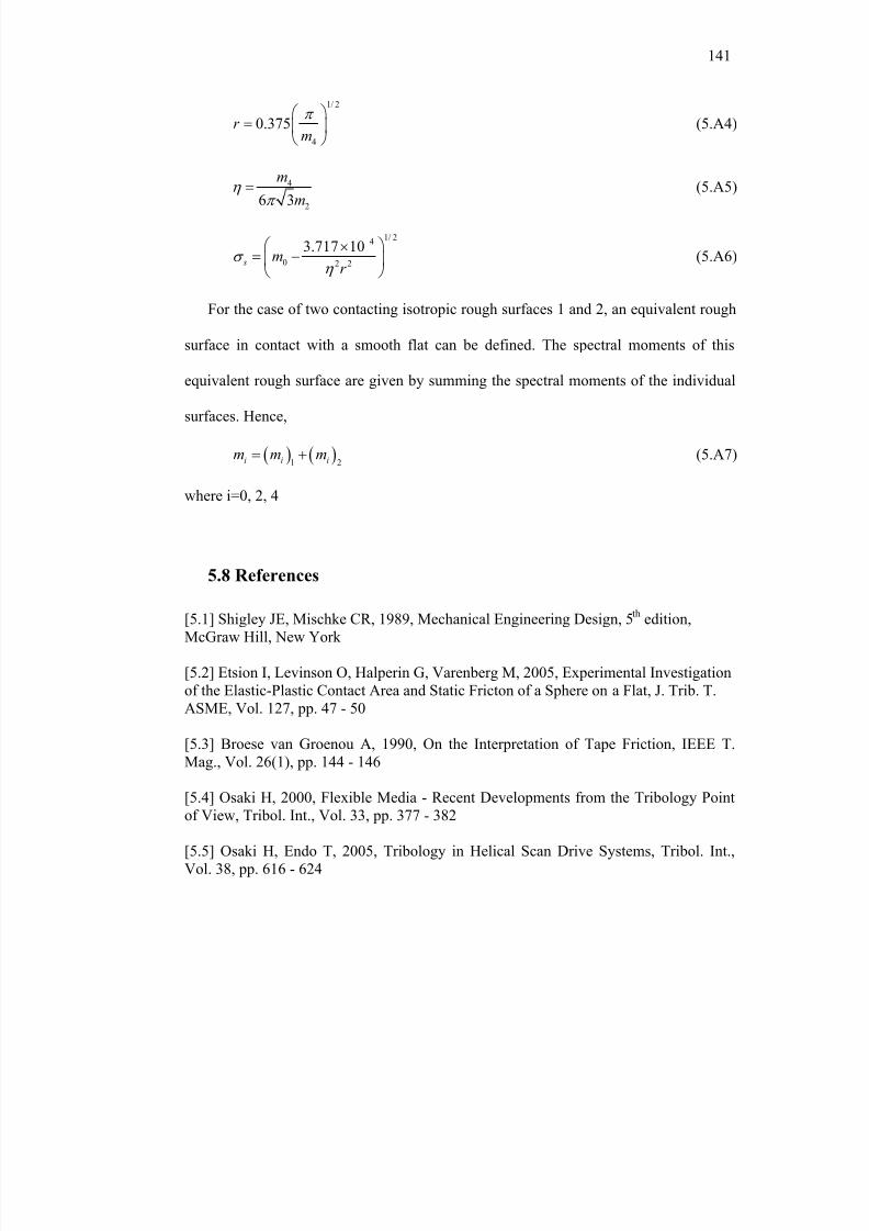
8/8/2019 BR PhD Dissertation
http://slidepdf.com/reader/full/br-phd-dissertation 173/248
141
1/ 2
4
0.375r m
π =
(5.A4)
4
26 3
m
mη
π = (5.A5)
1/ 24
0 2 2
3.717 10 s m
r σ
η
− ×= −
(5.A6)
For the case of two contacting isotropic rough surfaces 1 and 2, an equivalent rough
surface in contact with a smooth flat can be defined. The spectral moments of this
equivalent rough surface are given by summing the spectral moments of the individual
surfaces. Hence,
( ) ( )1 2i i im m m= + (5.A7)
where i=0, 2, 4
5.8 References
[5.1] Shigley JE, Mischke CR, 1989, Mechanical Engineering Design, 5th
edition,
McGraw Hill, New York
[5.2] Etsion I, Levinson O, Halperin G, Varenberg M, 2005, Experimental Investigation
of the Elastic-Plastic Contact Area and Static Fricton of a Sphere on a Flat, J. Trib. T.
ASME, Vol. 127, pp. 47 - 50
[5.3] Broese van Groenou A, 1990, On the Interpretation of Tape Friction, IEEE T.
Mag., Vol. 26(1), pp. 144 - 146
[5.4] Osaki H, 2000, Flexible Media - Recent Developments from the Tribology Point
of View, Tribol. Int., Vol. 33, pp. 377 - 382
[5.5] Osaki H, Endo T, 2005, Tribology in Helical Scan Drive Systems, Tribol. Int.,
Vol. 38, pp. 616 - 624
8/8/2019 BR PhD Dissertation
http://slidepdf.com/reader/full/br-phd-dissertation 174/248
142
[5.6] Panda SP, Engelmann AP, 2003, Control and Operation of Reel-To-Reel TapeDrives without Tension Transducer, Microsyst. Technol., Vol. 10, pp. 53 - 59
[5.7] Taylor R, Talke FE, 2005, Investigation of Roller Interactions with Flexible TapeMedium, Tribol. Int., Vol. 38, pp. 599 - 605
[5.8] Bhushan B, 1984, Influence of Test Parameters on the Measurement of theCoefficient of Friction of Magnetic Tapes, Wear, Vol. 93, pp. 81 - 99
[5.9] Lacey C, Talke FE, 1992, Measurement and Simulation of Partial Contact at theHead/Tape Interface, J. Trib. T. ASME, Vol. 114, pp. 646 - 652
[5.10] Patir N, Cheng HS, 1978, Average Flow Model for Determining Effects of 3-
Dimensional Roughness on Partial Hydrodynamic Lubrication, J. Lubr. Technol. T.ASME, Vol. 100(1), pp. 12 - 17
[5.11] Chang WR, Etsion I, Bogy DB, 1988, Static Friction Coefficient for MetallicRough Surfaces, J. Trib. T. ASME, Vol. 110(1), pp. 57 - 63
[5.12] Tworzydlo WW, Cecot W, Oden JT, Yew CH, 1998, Computational Micro- andMacroscopic Models of Contact and Friction: Formulation, Approach and Applications,
Wear, Vol. 220(2), pp. 113 – 140
[5.13] Amassad A, Shillor M, Sofonea M, 1999, A Quasistatic Contact Problem for an
Elastic Perfectly Plastic Body with Tresca’s Friction, Nonlinear Anal.-Theor., Vol. 35,
pp. 95 - 109
[5.14] Alexandrov S, Richmond O, 2001, Couette Flows of Rigid/Plastic Solids:Analytical Examples of the Interaction of Constitutive and Frictional Laws, Int. J.Mech. Sci., Vol. 43, pp. 653 - 665
[5.15] Kogut L and Etsion I, 2004, A Static Friction Model for Elastic-PlasticContacting Rough Surfaces, J. Trib. ASME, Vol. 126, pp. 34 - 40
[5.16] Brizmer V, Kligerman Y, Etsion I, 2007, Elastic-Plastic Contact under Combined Normal and Tangential Loading, Tribol. Lett., Vol. 25, pp. 61 - 70
[5.17] Brizmer V, Kligerman Y, Etsion I, 2006, The Effect of Contact Conditions and
Material Properties on the Elasticity Terminus of a Spherical Contact, Int. J. Sol. Str.,Vol. 43, pp. 5736 - 5749
[5.18] Rabinowicz E, 1965, Friction and Wear of Materials, J Wiley and sons, NewYork
8/8/2019 BR PhD Dissertation
http://slidepdf.com/reader/full/br-phd-dissertation 175/248
143
[5.19] Greenwood JA, Williamson JBP, 1966, Contact of Nominally Flat Surfaces,Proceedings of the Royal Society of London Series A – Mathematical and Physical
Sciences, Vol. 295 (1442), pp. 300 - 319
[5.20] Greenwood JA, Tripp JH, 1967, Elastic Contact of Rough Spheres, J. Appl.
Mech. T. ASME, Vol. 34(1), pp. 153 - 159
[5.21] Kogut L and Etsion I, 2003, A Finite Element Based Elastic-Plastic Model for
the Contact of Rough Surfaces, Tribol. T., Vol. 46, pp. 383 - 390
[5.22] Lacey C, Talke FE, 1990, A Tightly Coupled Numerical Foil Bearing Solution,
IEEE T. Mag., Vol. 26(6), pp. 3039 - 3043
[5.23] McCool JI, 1987, Relating Profile Instrument Measurements to the FunctionalPerformance of Rough Surfaces, J. Trib. T. ASME, Vol. 109, pp. 264 - 270
[5.24] Hempstock MS, Sullivan JL, 1996, The Durability and Signal Performance of Metal Evaporated and Metal Particle Tape, IEEE T. Mag., Vol. 32(5), pp. 3723 - 3725
[5.25] Hempstock MS, Sullivan JL, 1996, A Study of the Mechanical and MagneticPerformance of Metal Evaporated Tape, J. Mag. Mag. Mat., Vol. 155, pp. 323 - 328
[5.26] Bijker MD, Draaisma EA, Eisenberg M, Jansen J, Persat N, Sourty E, 2000,Future Directions in Advanced Digital Recording Technology, Tribol. Int., Vol. 33, pp.
383 - 390
[5.27] Personal communication
8/8/2019 BR PhD Dissertation
http://slidepdf.com/reader/full/br-phd-dissertation 176/248
144
6. Enhancing tribological performance of the magnetic
tape/guide interface by laser surface texturing
6.1 Introduction
Air-lubricated foil bearings are used in a variety of applications such as
turbomachinery, journal bearings, dentistry equipment, etc. [6.1-6.3]. One of the most
intricate applications of air-lubricated foil bearings can be found in magnetic tape drives
[6.4], where a magnetic tape moves over a read/write head and tape drive components
such as guides (stationary) and rollers (rotating). Friction is an important parameter in
designing a tape transport for a commercial high performance tape drive. The overall
friction force between tape and tape drive components determines the torque needed by
the motor to drive the tape and affects the wear of the tape. Metal particulate (MP) tape
is widely used in commercial tape recording systems since the tribological performance
of the magnetically superior metal evaporated (ME) tape is inferior to that of MP tape.
Although friction between tape and tape drive components was observed to
attenuate lateral tape motion [6.5-6.8], it is well known that tape drives with pressurized
air bearing guides instead of rotating guides exhibit significantly lower LTM than tape
drives with rotating guides [6.9]. Elimination of rotating tape drive components
suppresses lateral tape motion due to run-out of those components. However,
pressurized air bearing guides require an external compressor which is an obstacle for
commercialization of this type of tape drive.
8/8/2019 BR PhD Dissertation
http://slidepdf.com/reader/full/br-phd-dissertation 177/248
145
Based on the above information, it is therefore desirable to create an efficient self
acting air bearing between the tape and the guide, thereby eliminating the need for an
external compressor, while still benefiting from a low friction air bearing. In a recent
study [6.10] (see also chapter 5), it was observed that for a tape tension of 1 N, a tape
speed of at least 8 m/s was needed to achieve full fluid lubrication and hence, a low
friction coefficient. This chapter explores the possibility of creating an efficient low
speed air bearing between a magnetic tape and a cylindrical guide, thereby reducing the
transition speed between boundary lubrication and full fluid lubrication regime, and
thus expanding the speed range of low friction. We use a novel approach to tape guide
design by using laser surface texturing (LST) of the guide surface. We have compared
the tribological performance of the laser surface textured guide with various non-
textured guides, thereby showing the benefits of textured guide surfaces.
6.2 Laser surface texturing
Laser surface texturing (LST) is a well established technique to create micro
dimples on the surface of tribological components. These dimples act as micro-
hydrodynamic bearings, thereby creating a local pressure increase between the sliding
surfaces. This, in turn, increases the load carrying capacity for such bearings and
reduces the friction coefficient for a constant load. The laser surface texturing technique
has been successfully used in a number of applications, as, for instance, in the
manufacturing of metal rolling cylinders with well-defined surface roughness [6.11] or
the fabrication of laser bumps in the landing zone of a hard disk drive to facilitate
8/8/2019 BR PhD Dissertation
http://slidepdf.com/reader/full/br-phd-dissertation 178/248
146
contact start/stop of the magnetic head [6.12]. It was, however, not until 1996 that LST
was used in conventional lubrication situations as a method to reduce friction and
optimize lubrication [6.13]. LST creates spherically shaped dimples on the surface by
means of a material ablation process with a pulsed laser [6.14] and has now successfully
been applied in reducing friction in various applications such as piston rings,
mechanical seals and hydrodynamic seals [6.15-6.17]. The dimples also allow
conducting heat from sliding interfaces and trapping of abrasive wear particles [6.18].
Hydrodynamic gas seals [6.19] and hard disk drive technology [6.20] are applications
that are most relevant to the application of LST of the tape/guide interface.
No published investigations seem to exist about magnetic tape guide design in
general or texturing of magnetic tape drive components in particular. This chapter fills
this gap and investigates LST of magnetic tape guide surfaces in order to lower the
transition speed between boundary lubrication and full fluid lubrication. This, in turn,
reduces tape/guide friction and stiction, provides lower tape/guide wear and would
potentially allow the use of ME tape by enhancing its tribological performance.
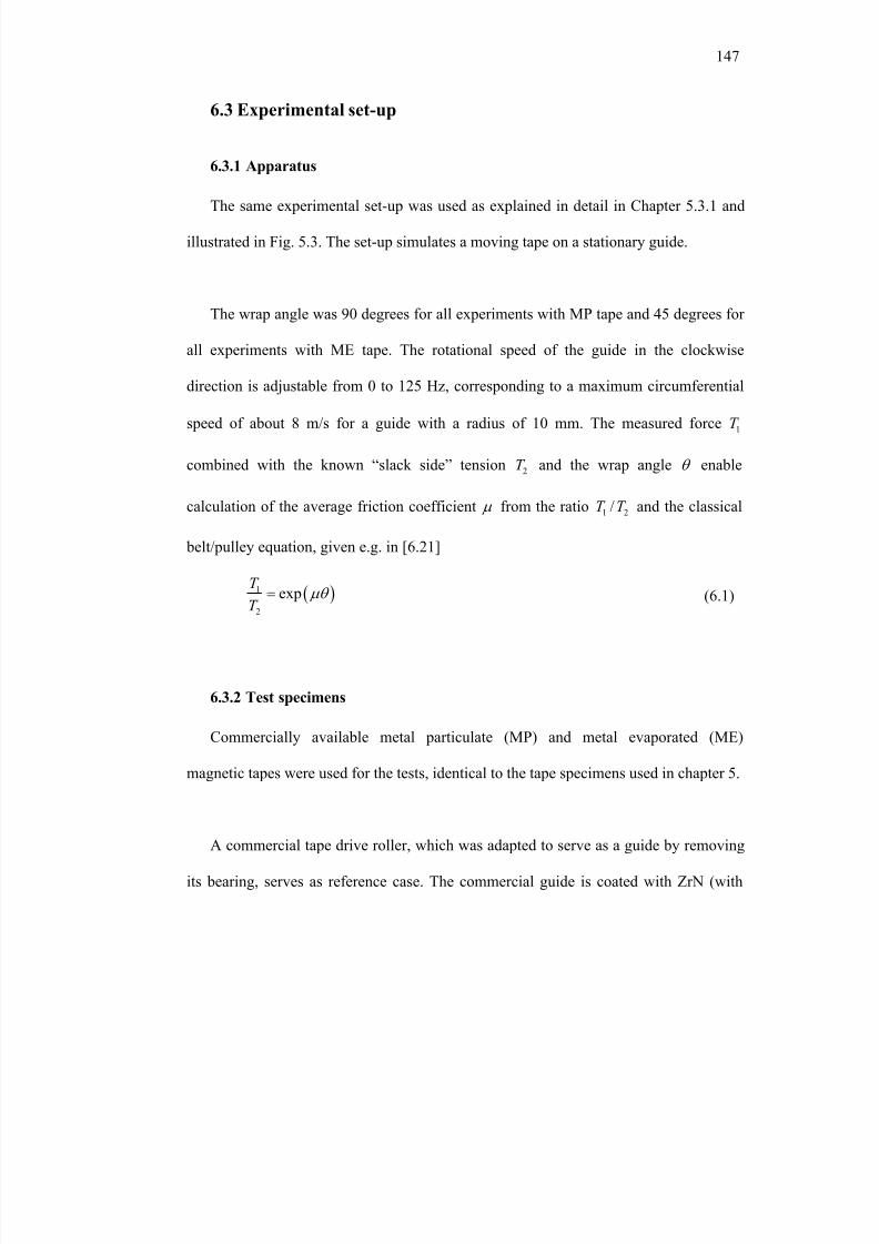
8/8/2019 BR PhD Dissertation
http://slidepdf.com/reader/full/br-phd-dissertation 179/248
147
6.3 Experimental set-up
6.3.1 Apparatus
The same experimental set-up was used as explained in detail in Chapter 5.3.1 and
illustrated in Fig. 5.3. The set-up simulates a moving tape on a stationary guide.
The wrap angle was 90 degrees for all experiments with MP tape and 45 degrees for
all experiments with ME tape. The rotational speed of the guide in the clockwise
direction is adjustable from 0 to 125 Hz, corresponding to a maximum circumferential
speed of about 8 m/s for a guide with a radius of 10 mm. The measured force 1T
combined with the known “slack side” tension 2T and the wrap angle θ enable
calculation of the average friction coefficient µ from the ratio 1 2/T T and the classical
belt/pulley equation, given e.g. in [6.21]
( )1
2exp
T
T µθ = (6.1)
6.3.2 Test specimens
Commercially available metal particulate (MP) and metal evaporated (ME)
magnetic tapes were used for the tests, identical to the tape specimens used in chapter 5.
A commercial tape drive roller, which was adapted to serve as a guide by removing
its bearing, serves as reference case. The commercial guide is coated with ZrN (with
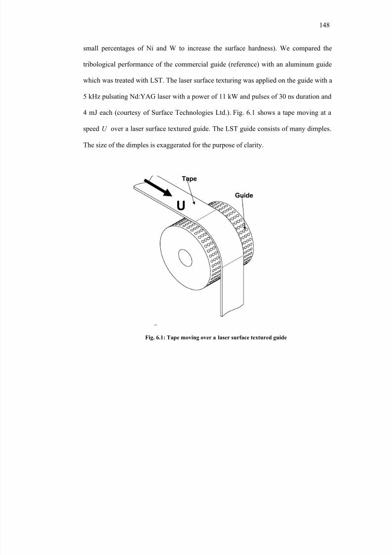
8/8/2019 BR PhD Dissertation
http://slidepdf.com/reader/full/br-phd-dissertation 180/248
148
small percentages of Ni and W to increase the surface hardness). We compared the
tribological performance of the commercial guide (reference) with an aluminum guide
which was treated with LST. The laser surface texturing was applied on the guide with a
5 kHz pulsating Nd:YAG laser with a power of 11 kW and pulses of 30 ns duration and
4 mJ each (courtesy of Surface Technologies Ltd.). Fig. 6.1 shows a tape moving at a
speed U over a laser surface textured guide. The LST guide consists of many dimples.
The size of the dimples is exaggerated for the purpose of clarity.
Guide
Tape
UGuide
Tape
Guide
Tape
U
Fig. 6.1: Tape moving over a laser surface textured guide
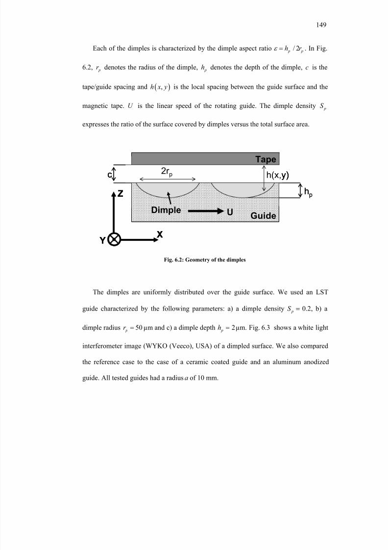
8/8/2019 BR PhD Dissertation
http://slidepdf.com/reader/full/br-phd-dissertation 181/248
149
Each of the dimples is characterized by the dimple aspect ratio / 2 p ph r ε = . In Fig.
6.2, pr denotes the radius of the dimple, ph denotes the depth of the dimple, c is the
tape/guide spacing and ( ),h x y is the local spacing between the guide surface and the
magnetic tape. U is the linear speed of the rotating guide. The dimple density pS
expresses the ratio of the surface covered by dimples versus the total surface area.
hp
2r pc
U GuideDimple
Tape
X
Z
Y
h(x,y)
hp
2r pc
U GuideDimple
Tape
X
Z
Y
h(x,y)2r
pc
U GuideDimple
Tape
X
Z
Y
h(x,y)
The dimples are uniformly distributed over the guide surface. We used an LST
guide characterized by the following parameters: a) a dimple density 0.2 pS = , b) a
dimple radius 50 pr = µm and c) a dimple depth 2 ph = µm. Fig. 6.3 shows a white light
interferometer image (WYKO (Veeco), USA) of a dimpled surface. We also compared
the reference case to the case of a ceramic coated guide and an aluminum anodized
guide. All tested guides had a radius a of 10 mm.
Fig. 6.2: Geometry of the dimples
8/8/2019 BR PhD Dissertation
http://slidepdf.com/reader/full/br-phd-dissertation 182/248
150
3.8 mm
5.1mm
3.8 mm
5.1mm
Atomic force microscopy (AFM) scans were used to determine the surface
roughness of the different guides. The measurements showed that the surface roughness
of the guides is isotropic. Hence, the Greenwood-Williamson approach can be used to
describe their surface roughness [6.22].
Table 6.1 presents the average asperity tip radius r , the asperity density η , the
standard deviation of asperity summit heights sσ , the ratio / s r σ and the dimensionless
roughness parameter sr η σ for the individual tape samples and guides. The equivalent
roughness parameters for two contacting rough surfaces [6.23] are also shown for eight
different tape/guide combinations. These combinations are: a) ME tape in combination
with the commercial tape drive guide (C1), b) MP tape in combination with the
commercial tape drive guide (C2), c) ME tape in combination with a ceramic guide
(C3), d) MP tape in combination with a ceramic guide (C4), e) ME tape and an
Fig. 6.3: White light interferometer image of dimpled surface
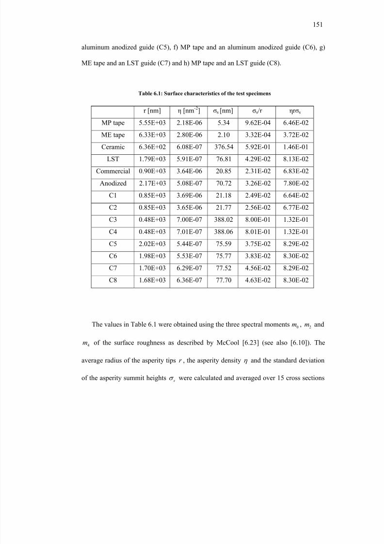
8/8/2019 BR PhD Dissertation
http://slidepdf.com/reader/full/br-phd-dissertation 183/248
151
aluminum anodized guide (C5), f) MP tape and an aluminum anodized guide (C6), g)
ME tape and an LST guide (C7) and h) MP tape and an LST guide (C8).
r [nm] η [nm-2] σs [nm] σs/r ηr σs
MP tape 5.55E+03 2.18E-06 5.34 9.62E-04 6.46E-02
ME tape 6.33E+03 2.80E-06 2.10 3.32E-04 3.72E-02
Ceramic 6.36E+02 6.08E-07 376.54 5.92E-01 1.46E-01
LST 1.79E+03 5.91E-07 76.81 4.29E-02 8.13E-02
Commercial 0.90E+03 3.64E-06 20.85 2.31E-02 6.83E-02Anodized 2.17E+03 5.08E-07 70.72 3.26E-02 7.80E-02
C1 0.85E+03 3.69E-06 21.18 2.49E-02 6.64E-02
C2 0.85E+03 3.65E-06 21.77 2.56E-02 6.77E-02
C3 0.48E+03 7.00E-07 388.02 8.00E-01 1.32E-01
C4 0.48E+03 7.01E-07 388.06 8.01E-01 1.32E-01
C5 2.02E+03 5.44E-07 75.59 3.75E-02 8.29E-02
C6 1.98E+03 5.53E-07 75.77 3.83E-02 8.30E-02
C7 1.70E+03 6.29E-07 77.52 4.56E-02 8.29E-02
C8 1.68E+03 6.36E-07 77.70 4.63E-02 8.30E-02
The values in Table 6.1 were obtained using the three spectral moments 0m , 2m and
4m of the surface roughness as described by McCool [6.23] (see also [6.10]). The
average radius of the asperity tips r , the asperity density η and the standard deviation
of the asperity summit heights sσ were calculated and averaged over 15 cross sections
Table 6.1: Surface characteristics of the test specimens
8/8/2019 BR PhD Dissertation
http://slidepdf.com/reader/full/br-phd-dissertation 184/248
152
of an AFM scan. From Table 6.1 we observe that the ratio / s r σ for the commercial
guide, the anodized guide and the LST guide is an order of magnitude smaller than for
the ceramic guide, i.e., the surfaces of the commercial guide, the anodized guide and the
LST guide are much smoother than the surface of the ceramic guide. We also observe
that the ME tape is much smoother than the MP tape since its / s
r σ value is only one
third of the other material combinations.
6.3.3 Test procedure
Exactly the same test procedure as discussed in chapter 5.3.3 was adopted for the
experimental results described underneath. However, we did not apply the run-in
procedure for the ME tape specimens, to avoid damage of the fragile magnetic coating
by tape/guide contact. In addition, the “tight side” tension 1T was measured for stepwise
decrements of rotational speeds from 125 Hz down to 16 Hz. Thus, any damage of the
coating at the lowest speed does not affect the measurements at higher speeds. These
test series were repeated three times for each of the eight combinations C1 - C8, with a
new tape specimen for each test. The calculated friction coefficient for each test was
averaged over its three repetitions.
8/8/2019 BR PhD Dissertation
http://slidepdf.com/reader/full/br-phd-dissertation 185/248
153
6.4 Experimental Results and Discussion
6.4.1 Metal particulate tape
Fig. 6.4 summarizes the results for the experiments with MP tape. These
experiments include the commercial guide (C2), ceramic guide (C4), anodized guide
(C6) and LST guide (C8), all with a guide radius of 10 mm. We have varied the
nominal tape tension between 0.5 N and 1.2 N and observed similar behavior in terms
of friction coefficient versus tape speed for all cases in that range. However, we
observed that the friction coefficient increased with increasing tape tension, in
agreement with the results in [10]. In this chapter, we only show results for a tape
tension of 1 N, since this is the most commonly used nominal tape tension in state-of-
the-art high performance tape drives. Fig. 6.4 shows the effect of sliding speed on the
magnetic tape/guide friction coefficient calculated from eq. (1) for a wrap angle, θ , of
90 degrees.
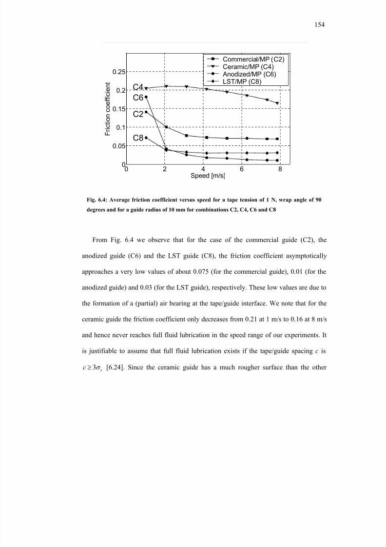
8/8/2019 BR PhD Dissertation
http://slidepdf.com/reader/full/br-phd-dissertation 186/248
154
0 2 4 6 80
0.05
0.1
0.15
0.2
0.25
Speed [m/s]
F r i c t i o n c o e f f i c i e n
t
Commercial/MP (C2)Ceramic/MP (C4)Anodized/MP (C6)LST/MP (C8)
C4C6
C2
C8
0 2 4 6 80
0.05
0.1
0.15
0.2
0.25
Speed [m/s]
F r i c t i o n c o e f f i c i e n
t
Commercial/MP (C2)Ceramic/MP (C4)Anodized/MP (C6)LST/MP (C8)
C4C6
C2
C8
From Fig. 6.4 we observe that for the case of the commercial guide (C2), the
anodized guide (C6) and the LST guide (C8), the friction coefficient asymptotically
approaches a very low values of about 0.075 (for the commercial guide), 0.01 (for the
anodized guide) and 0.03 (for the LST guide), respectively. These low values are due to
the formation of a (partial) air bearing at the tape/guide interface. We note that for the
ceramic guide the friction coefficient only decreases from 0.21 at 1 m/s to 0.16 at 8 m/s
and hence never reaches full fluid lubrication in the speed range of our experiments. It
is justifiable to assume that full fluid lubrication exists if the tape/guide spacing c is
3 sc σ ≥ [6.24]. Since the ceramic guide has a much rougher surface than the other
Fig. 6.4: Average friction coefficient versus speed for a tape tension of 1 N, wrap angle of 90
degrees and for a guide radius of 10 mm for combinations C2, C4, C6 and C8
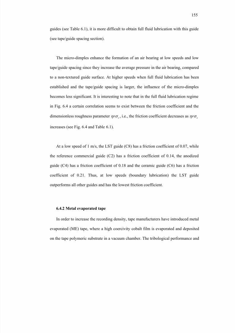
8/8/2019 BR PhD Dissertation
http://slidepdf.com/reader/full/br-phd-dissertation 187/248
155
guides (see Table 6.1), it is more difficult to obtain full fluid lubrication with this guide
(see tape/guide spacing section).
The micro-dimples enhance the formation of an air bearing at low speeds and low
tape/guide spacing since they increase the average pressure in the air bearing, compared
to a non-textured guide surface. At higher speeds when full fluid lubrication has been
established and the tape/guide spacing is larger, the influence of the micro-dimples
becomes less significant. It is interesting to note that in the full fluid lubrication regime
in Fig. 6.4 a certain correlation seems to exist between the friction coefficient and the
dimensionless roughness parameter s
r η σ , i.e., the friction coefficient decreases as s
r η σ
increases (see Fig. 6.4 and Table 6.1).
At a low speed of 1 m/s, the LST guide (C8) has a friction coefficient of 0.07, while
the reference commercial guide (C2) has a friction coefficient of 0.14, the anodized
guide (C4) has a friction coefficient of 0.18 and the ceramic guide (C6) has a friction
coefficient of 0.21. Thus, at low speeds (boundary lubrication) the LST guide
outperforms all other guides and has the lowest friction coefficient.
6.4.2 Metal evaporated tape
In order to increase the recording density, tape manufacturers have introduced metal
evaporated (ME) tape, where a high coercivity cobalt film is evaporated and deposited
on the tape polymeric substrate in a vacuum chamber. The tribological performance and
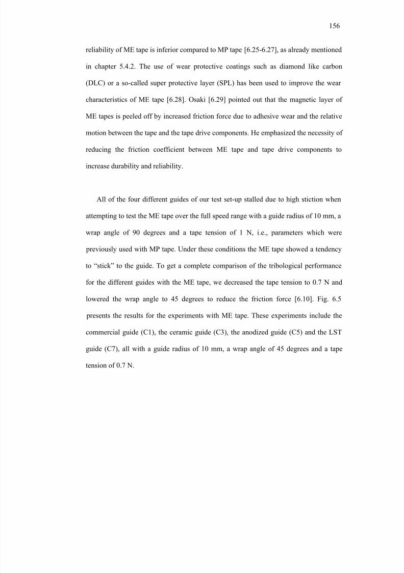
8/8/2019 BR PhD Dissertation
http://slidepdf.com/reader/full/br-phd-dissertation 188/248
156
reliability of ME tape is inferior compared to MP tape [6.25-6.27], as already mentioned
in chapter 5.4.2. The use of wear protective coatings such as diamond like carbon
(DLC) or a so-called super protective layer (SPL) has been used to improve the wear
characteristics of ME tape [6.28]. Osaki [6.29] pointed out that the magnetic layer of
ME tapes is peeled off by increased friction force due to adhesive wear and the relative
motion between the tape and the tape drive components. He emphasized the necessity of
reducing the friction coefficient between ME tape and tape drive components to
increase durability and reliability.
All of the four different guides of our test set-up stalled due to high stiction when
attempting to test the ME tape over the full speed range with a guide radius of 10 mm, a
wrap angle of 90 degrees and a tape tension of 1 N, i.e., parameters which were
previously used with MP tape. Under these conditions the ME tape showed a tendency
to “stick” to the guide. To get a complete comparison of the tribological performance
for the different guides with the ME tape, we decreased the tape tension to 0.7 N and
lowered the wrap angle to 45 degrees to reduce the friction force [6.10]. Fig. 6.5
presents the results for the experiments with ME tape. These experiments include the
commercial guide (C1), the ceramic guide (C3), the anodized guide (C5) and the LST
guide (C7), all with a guide radius of 10 mm, a wrap angle of 45 degrees and a tape
tension of 0.7 N.
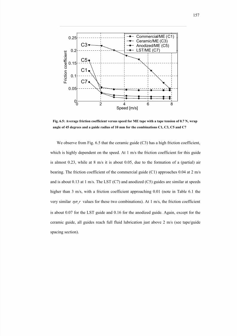
8/8/2019 BR PhD Dissertation
http://slidepdf.com/reader/full/br-phd-dissertation 189/248
157
0 2 4 6 80
0.05
0.1
0.15
0.2
0.25
Speed [m/s]
F r i c t i o n c o e f f i c i e n
t
Commercial/ME (C1)Ceramic/ME (C3)Anodized/ME (C5)LST/ME (C7)
C3
C5
C1
C7
0 2 4 6 80
0.05
0.1
0.15
0.2
0.25
Speed [m/s]
F r i c t i o n c o e f f i c i e n
t
Commercial/ME (C1)Ceramic/ME (C3)Anodized/ME (C5)LST/ME (C7)
C3
C5
C1
C7
We observe from Fig. 6.5 that the ceramic guide (C3) has a high friction coefficient,
which is highly dependent on the speed. At 1 m/s the friction coefficient for this guide
is almost 0.23, while at 8 m/s it is about 0.05, due to the formation of a (partial) air
bearing. The friction coefficient of the commercial guide (C1) approaches 0.04 at 2 m/s
and is about 0.13 at 1 m/s. The LST (C7) and anodized (C5) guides are similar at speeds
higher than 3 m/s, with a friction coefficient approaching 0.01 (note in Table 6.1 the
very similar sr ησ values for these two combinations). At 1 m/s, the friction coefficient
is about 0.07 for the LST guide and 0.16 for the anodized guide. Again, except for the
ceramic guide, all guides reach full fluid lubrication just above 2 m/s (see tape/guide
spacing section).
Fig. 6.5: Average friction coefficient versus speed for ME tape with a tape tension of 0.7 N, wrap
angle of 45 degrees and a guide radius of 10 mm for the combinations C1, C3, C5 and C7
8/8/2019 BR PhD Dissertation
http://slidepdf.com/reader/full/br-phd-dissertation 190/248
158
Fig. 6.5 (guides with ME tape) and Fig. 6.4 (guides with MP tape) reveal the same
trend. The ceramic guide has the highest friction coefficient and its friction coefficient
is highly dependent on speed. The commercial guide has a slightly higher friction
coefficient in the full fluid lubrication regime than the anodized and the LST guides,
which may again be explained by lower roughness parameter sr ησ of the commercial
guide with respect to the anodized and LST guides (see Table 6.1). In the boundary
lubrication regime, the LST guide yields a remarkably low friction coefficient because
of its dimpled surface and increased air bearing pressure. This very promising result
indicates that the use of ME tape in high performance commercial tape drives could
possibly be facilitated with the use of LST guides in the tape path.
The friction coefficient of the LST guide depends less on speed than any of the
other tested guides. This is true for both ME and MP tapes. This phenomenon is highly
desirable in commercial tape drives since the interaction of the magnetic tape with other
tape drive components does not change while the drive is ramping up to operational
speed or ramping down to standstill. Hence, the number of start/stop cycles would not
affect the wear of the tape, since the friction coefficient is independent of the speed. It
should be noted, however, that a direct comparison between Fig. 6.4 and Fig. 6.5 must
be made with care since the experiments of Fig. 6.5 were conducted under modified
conditions (45 degrees wrap angle and 0.7 N tape tension), i.e., stiction effects were
eliminated by reducing the friction force between tape and guide.
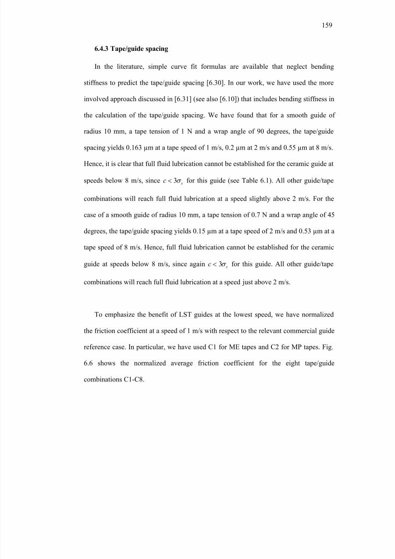
8/8/2019 BR PhD Dissertation
http://slidepdf.com/reader/full/br-phd-dissertation 191/248
159
6.4.3 Tape/guide spacing
In the literature, simple curve fit formulas are available that neglect bending
stiffness to predict the tape/guide spacing [6.30]. In our work, we have used the more
involved approach discussed in [6.31] (see also [6.10]) that includes bending stiffness in
the calculation of the tape/guide spacing. We have found that for a smooth guide of
radius 10 mm, a tape tension of 1 N and a wrap angle of 90 degrees, the tape/guide
spacing yields 0.163 µm at a tape speed of 1 m/s, 0.2 µm at 2 m/s and 0.55 µm at 8 m/s.
Hence, it is clear that full fluid lubrication cannot be established for the ceramic guide at
speeds below 8 m/s, since 3 sc σ < for this guide (see Table 6.1). All other guide/tape
combinations will reach full fluid lubrication at a speed slightly above 2 m/s. For the
case of a smooth guide of radius 10 mm, a tape tension of 0.7 N and a wrap angle of 45
degrees, the tape/guide spacing yields 0.15 µm at a tape speed of 2 m/s and 0.53 µm at a
tape speed of 8 m/s. Hence, full fluid lubrication cannot be established for the ceramic
guide at speeds below 8 m/s, since again 3 sc σ < for this guide. All other guide/tape
combinations will reach full fluid lubrication at a speed just above 2 m/s.
To emphasize the benefit of LST guides at the lowest speed, we have normalized
the friction coefficient at a speed of 1 m/s with respect to the relevant commercial guide
reference case. In particular, we have used C1 for ME tapes and C2 for MP tapes. Fig.
6.6 shows the normalized average friction coefficient for the eight tape/guide
combinations C1-C8.
8/8/2019 BR PhD Dissertation
http://slidepdf.com/reader/full/br-phd-dissertation 192/248
160
C1 C3 C5 C7 C2 C4 C6 C80
0.5
1
1.5
2
2.5
N o r m a l i z e d a v e r a g e f r i c t i o n
c o e f f i c i e n t
ME tape
wrap angle = 45°
tape tension = 0.7 N
MP tape
wrap angle = 90°
tape tension = 1 N
It was pointed out earlier that the ME and MP experiments are not directly
comparable due to their different test parameters. However, we observe clearly that the
combinations of LST guide and ME and MP tape, C7 and C8, respectively, yield the
lowest friction coefficient of all combinations at a speed of 1 m/s. Compared to the
reference case C1, the LST case C7 lowers the friction coefficient by 40 %. Compared
to the reference case C2, the LST case C8 provides a 50 % lower friction coefficient.
The anodized and ceramic guides yield higher friction coefficients than their respective
reference case at 1 m/s for both ME and MP tapes.
Fig. 6.6: Normalized average friction coefficient for ME and MP tapes with the different guides
at a speed of 1 m/s
8/8/2019 BR PhD Dissertation
http://slidepdf.com/reader/full/br-phd-dissertation 193/248
161
6.5 Conclusion of the experimental analysis
1. Laser Surface Textured (LST) guides reduce the friction coefficient between
tape and guide, compared to tested commercial and ceramic guides.
2. LST reduces the influence of speed on the friction coefficient. The critical
speed where boundary lubrication regime changes into full fluid lubrication
decreases significantly for LST guides.
3. Metal evaporated (ME) tape was used successfully in combination with an
LST guide at a nominal tape tension of 0.7 N, and wrap angle of 45 degrees
even at a tape speed as low as 1 m/s. At this low speed the ME tape tends to
“stick” to all other guides (anodized, commercial and ceramic).
6.6 Theoretical model
To better understand the effect of a textured guide surface on the tribological
performance of the tape/guide interface, we have simulated the pressure distribution
between the tape and the guide surface for a column of ten dimples. We made the
following assumptions:
1. The tape is considered rigid. Local elastic deformations of the tape are
neglected. This assumption implies that no elasto-hydrodynamic effects are
taken into account.
2. The tape is assumed to be conformal to the guide [6.30]. This case is identical to
a parallel slider bearing. One-dimensional foil bearing simulations [6.31] show
8/8/2019 BR PhD Dissertation
http://slidepdf.com/reader/full/br-phd-dissertation 194/248
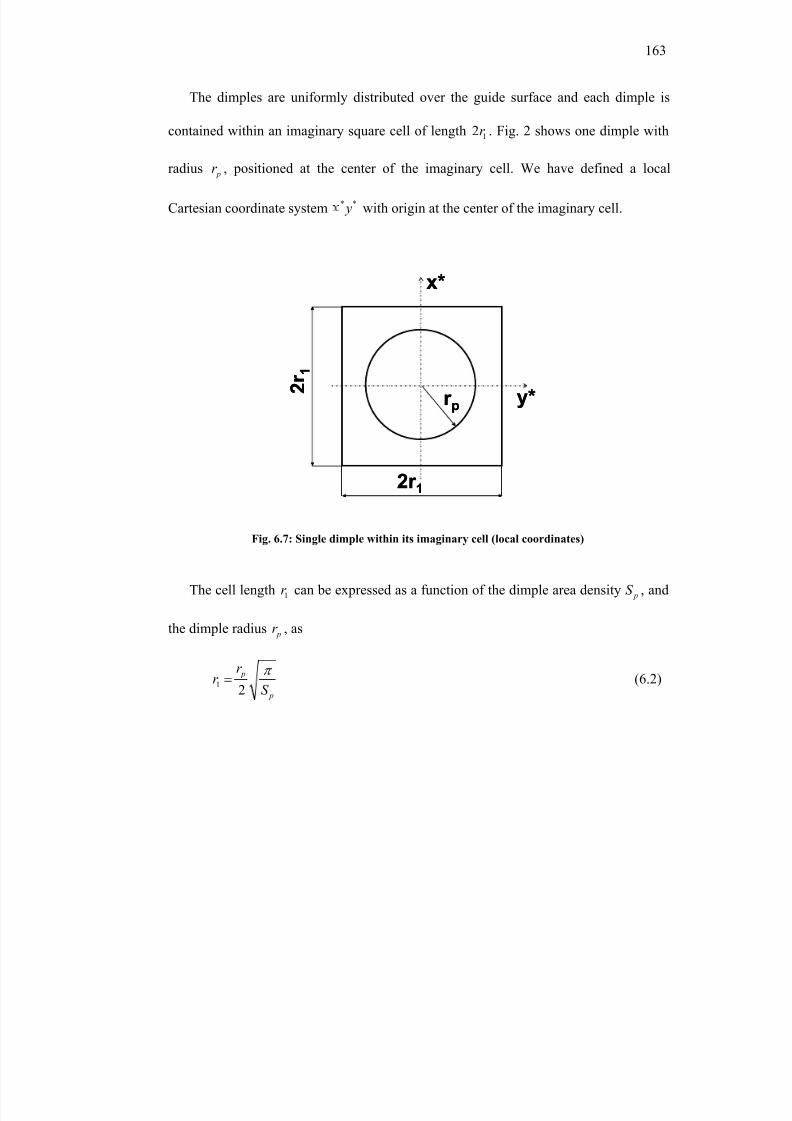
8/8/2019 BR PhD Dissertation
http://slidepdf.com/reader/full/br-phd-dissertation 195/248
163
The dimples are uniformly distributed over the guide surface and each dimple is
contained within an imaginary square cell of length 12r . Fig. 2 shows one dimple with
radius pr , positioned at the center of the imaginary cell. We have defined a local
Cartesian coordinate system * * y with origin at the center of the imaginary cell.
x*
y*
2r 1
2 r 1
r p
x*
y*
2r 1
2 r 1
r p
The cell length 1r can be expressed as a function of the dimple area density pS , and
the dimple radius pr , as
12
p
p
r r
S
π = (6.2)
Fig. 6.7: Single dimple within its imaginary cell (local coordinates)
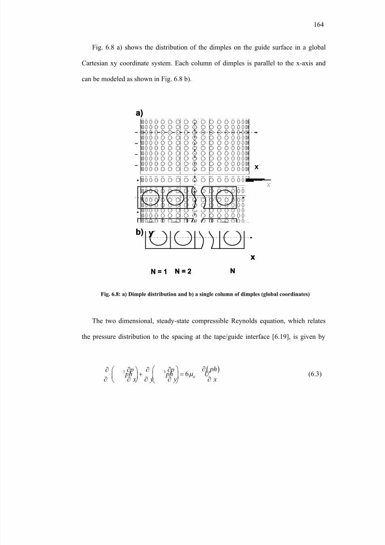
8/8/2019 BR PhD Dissertation
http://slidepdf.com/reader/full/br-phd-dissertation 196/248
164
Fig. 6.8 a) shows the distribution of the dimples on the guide surface in a global
Cartesian xy coordinate system. Each column of dimples is parallel to the x-axis and
can be modeled as shown in Fig. 6.8 b).
y
x
y
x
a)
b) y
x
N = 1 N = 2 N
y
x
y
x
a)
b) y
x
N = 1 N = 2 N
The two dimensional, steady-state compressible Reynolds equation, which relates
the pressure distribution to the spacing at the tape/guide interface [6.19], is given by
( )3 3 6 a
ph p p ph ph U
x y y xµ
∂ ∂ ∂ ∂ ∂ + =
∂ ∂ ∂ ∂ ∂ (6.3)
Fig. 6.8: a) Dimple distribution and b) a single column of dimples (global coordinates)
8/8/2019 BR PhD Dissertation
http://slidepdf.com/reader/full/br-phd-dissertation 197/248
165
where and y represent coordinates in a global Cartesian coordinate system, ( ), p x y
is the air bearing pressure,aµ is the dynamic viscosity of air and ( ),h x y is the
clearance between tape and guide. Because the tape/guide spacing is much larger than
the mean free path of air, rarefaction effects are neglected.
For the analysis of the textured surface, it is convenient to introduce the following
non-dimensional expressions:
p
X r
= , p
yY
r = ,
( )
( ),,
a
p x y P X Y
p= ,
( )
( ),,
h x y H X Y
c= , (6.4)
where X and Y denote the non-dimensional (global) coordinates, and P and H
denote the non-dimensional pressure and spacing, respectively. The normalizing
pressure a p is the atmospheric pressure. The dimensionless local spacing * H as a
function of the dimensionless local coordinates * *, X Y for one cell shown in Fig. 6.2 is
given by [6.32]:
( )* * *, 1 H X Y = , for *2 *2 1 X Y + >
( ) ( )2
* * * *2 *2
2
1 1 1, 1
2 8 4 8 2 H X Y X Y
ε ε
δ εδ δ εδ δ
= + + − + − −
, for *2 *2 1 X Y + ≤
(6.5)
where / 2 p p
h r ε = is the aspect ratio of the dimple and / 2 p
c r δ = is the dimensionless
tape/guide minimum spacing.
8/8/2019 BR PhD Dissertation
http://slidepdf.com/reader/full/br-phd-dissertation 198/248
166
To create a column of dimples of identical shape (see Fig. 6.8 b)), we expand the
dimensionless height distribution for a single cell, ( )* * *, H X Y , to a column of 10 N =
cells by repeating the height distribution for a single cell for each cell in the column.
The dimensionless Reynolds equation in the global coordinate system can then be
expressed as
( )3 3
2
PH P P PH PH
X X Y Y X
λ
δ
∂∂ ∂ ∂ ∂ + =
∂ ∂ ∂ ∂ ∂ (6.6)
where 3 / 2a p aU r pλ µ = and / 2 pc r δ = .
The following boundary conditions are assumed. The pressure is atmospheric at the
inlet and outlet of the tape/guide interface. In addition, the pressure is periodic in the
direction perpendicular to the air flow (Y-direction). Multiple columns of dimples next
to one another will yield a periodic pressure distribution. The period is defined by the
size of the imaginary cell ( 12r ). The boundary conditions can be expressed as
( 0, ) 1 P X Y = =
12( , ) 1
p
r P X N Y
r = = (6.7)
1 1( , ) ( , ) 0 p p
r r P P X Y X Y
Y r Y r
∂ ∂= − = = =
∂ ∂
where N is the number of cells in a column (see Fig. 6.8 b)). Eq. (6.6) can be solved
for the pressure distribution if the dimensionless spacing ( ), H X Y and the
dimensionless parameters λ , δ and ε are specified. A “staggered grid” finite
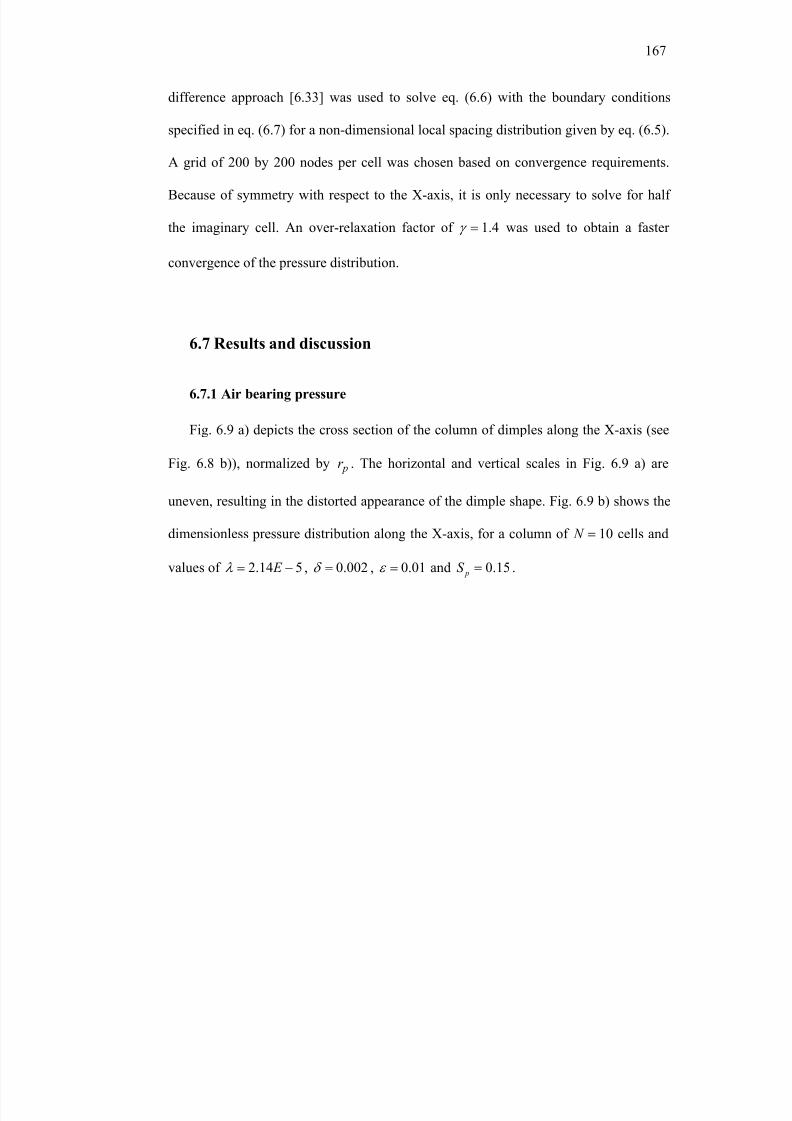
8/8/2019 BR PhD Dissertation
http://slidepdf.com/reader/full/br-phd-dissertation 199/248
167
difference approach [6.33] was used to solve eq. (6.6) with the boundary conditions
specified in eq. (6.7) for a non-dimensional local spacing distribution given by eq. (6.5).
A grid of 200 by 200 nodes per cell was chosen based on convergence requirements.
Because of symmetry with respect to the X-axis, it is only necessary to solve for half
the imaginary cell. An over-relaxation factor of 1.4γ = was used to obtain a faster
convergence of the pressure distribution.
6.7 Results and discussion
6.7.1 Air bearing pressure
Fig. 6.9 a) depicts the cross section of the column of dimples along the X-axis (see
Fig. 6.8 b)), normalized by pr . The horizontal and vertical scales in Fig. 6.9 a) are
uneven, resulting in the distorted appearance of the dimple shape. Fig. 6.9 b) shows the
dimensionless pressure distribution along the X-axis, for a column of 10 N =
cells and
values of 2.14 5 E λ = − , 0.002δ = , 0.01ε = and 0.15 pS = .
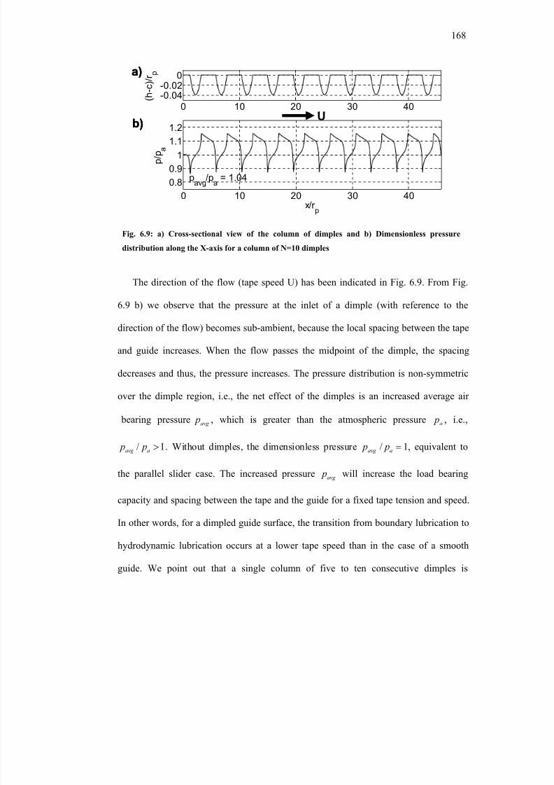
8/8/2019 BR PhD Dissertation
http://slidepdf.com/reader/full/br-phd-dissertation 200/248
168
0 10 20 30 40
0.8
0.9
1
1.1
1.2
p / p
a
pavg
/pa
= 1.04
x/r p
0 10 20 30 40
-0.04-0.02
0
( h - c ) / r
pa)
b)
U
0 10 20 30 40
0.8
0.9
1
1.1
1.2
p / p
a
pavg
/pa
= 1.04
x/r p
0 10 20 30 40
-0.04-0.02
0
( h - c ) / r
pa)
b)
0 10 20 30 40
0.8
0.9
1
1.1
1.2
p / p
a
pavg
/pa
= 1.04
x/r p
0 10 20 30 40
-0.04-0.02
0
( h - c ) / r
pa)
b)
U
The direction of the flow (tape speed U) has been indicated in Fig. 6.9. From Fig.
6.9 b) we observe that the pressure at the inlet of a dimple (with reference to the
direction of the flow) becomes sub-ambient, because the local spacing between the tape
and guide increases. When the flow passes the midpoint of the dimple, the spacing
decreases and thus, the pressure increases. The pressure distribution is non-symmetric
over the dimple region, i.e., the net effect of the dimples is an increased average air
bearing pressure avg p , which is greater than the atmospheric pressure a p , i.e.,
/ 1avg a p p > . Without dimples, the dimensionless pressure / 1avg a p p = , equivalent to
the parallel slider case. The increased pressure avg p will increase the load bearing
capacity and spacing between the tape and the guide for a fixed tape tension and speed.
In other words, for a dimpled guide surface, the transition from boundary lubrication to
hydrodynamic lubrication occurs at a lower tape speed than in the case of a smooth
guide. We point out that a single column of five to ten consecutive dimples is
Fig. 6.9: a) Cross-sectional view of the column of dimples and b) Dimensionless pressure
distribution along the X-axis for a column of N=10 dimples
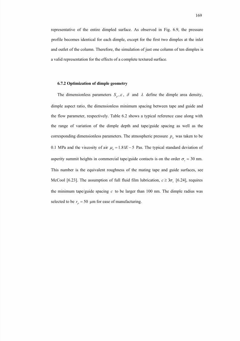
8/8/2019 BR PhD Dissertation
http://slidepdf.com/reader/full/br-phd-dissertation 201/248
169
representative of the entire dimpled surface. As observed in Fig. 6.9, the pressure
profile becomes identical for each dimple, except for the first two dimples at the inlet
and outlet of the column. Therefore, the simulation of just one column of ten dimples is
a valid representation for the effects of a complete textured surface.
6.7.2 Optimization of dimple geometry
The dimensionless parameters pS , ε , δ and λ define the dimple area density,
dimple aspect ratio, the dimensionless minimum spacing between tape and guide and
the flow parameter, respectively. Table 6.2 shows a typical reference case along with
the range of variation of the dimple depth and tape/guide spacing as well as the
corresponding dimensionless parameters. The atmospheric pressure a p was taken to be
0.1 MPa and the viscosity of air 1.81 5a E µ = − Pas. The typical standard deviation of
asperity summit heights in commercial tape/guide contacts is on the order 30 sσ = nm.
This number is the equivalent roughness of the mating tape and guide surfaces, see
McCool [6.23]. The assumption of full fluid film lubrication, 3 sc σ ≥ [6.24], requires
the minimum tape/guide spacing c to be larger than 100 nm. The dimple radius was
selected to be 50 pr = µm for ease of manufacturing.
8/8/2019 BR PhD Dissertation
http://slidepdf.com/reader/full/br-phd-dissertation 202/248
170
Parameter Minimum Reference Maximum
h p [µm] 0.3 1 5
c [nm] 100 200 400
ε 0.003 0.01 0.05
δ 0.001 0.002 0.004
λ 5E-06 2E-05 3E-05
In the following, we use our model to numerically investigate how these parameters
can be chosen to yield the highest possible average air bearing pressure between the
conformal tape and the guide. A maximized average air bearing pressure will yield the
highest load carrying capacity and hence, the highest tape/guide spacing for a given tape
tension.
Fig. 6.10 shows the dimensionless average air bearing pressure /avg a p p versus the
dimple density pS for different values of the dimple aspect ratio ε and for the reference
values 0.002δ = and 2 5 E λ = − .
Table 6.2: Range of the dimensional and dimensionless parameters
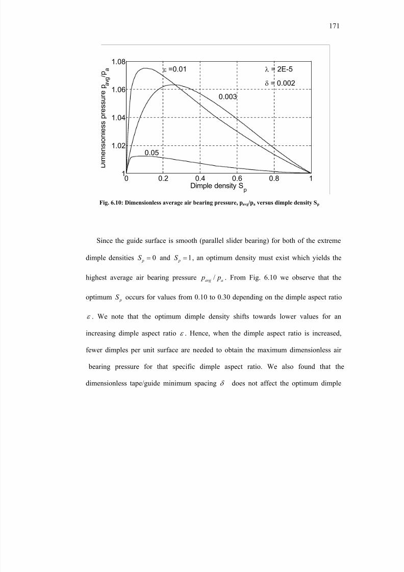
8/8/2019 BR PhD Dissertation
http://slidepdf.com/reader/full/br-phd-dissertation 203/248
171
0 0.2 0.4 0.6 0.8 11
1.02
1.04
1.06
1.08
Dimple density Sp
D i m e n s i o n l e s s p r e s s u r e
p a v g
/ p a λ = 2E-5
δ = 0.002
0.05
ε =0.01
0.003
Since the guide surface is smooth (parallel slider bearing) for both of the extreme
dimple densities 0 pS = and 1 pS = , an optimum density must exist which yields the
highest average air bearing pressure /avg a p p . From Fig. 6.10 we observe that the
optimum pS occurs for values from 0.10 to 0.30 depending on the dimple aspect ratio
ε . We note that the optimum dimple density shifts towards lower values for an
increasing dimple aspect ratio ε . Hence, when the dimple aspect ratio is increased,
fewer dimples per unit surface are needed to obtain the maximum dimensionless air
bearing pressure for that specific dimple aspect ratio. We also found that the
dimensionless tape/guide minimum spacing δ does not affect the optimum dimple
Fig. 6.10: Dimensionless average air bearing pressure, pavg/pa versus dimple density Sp
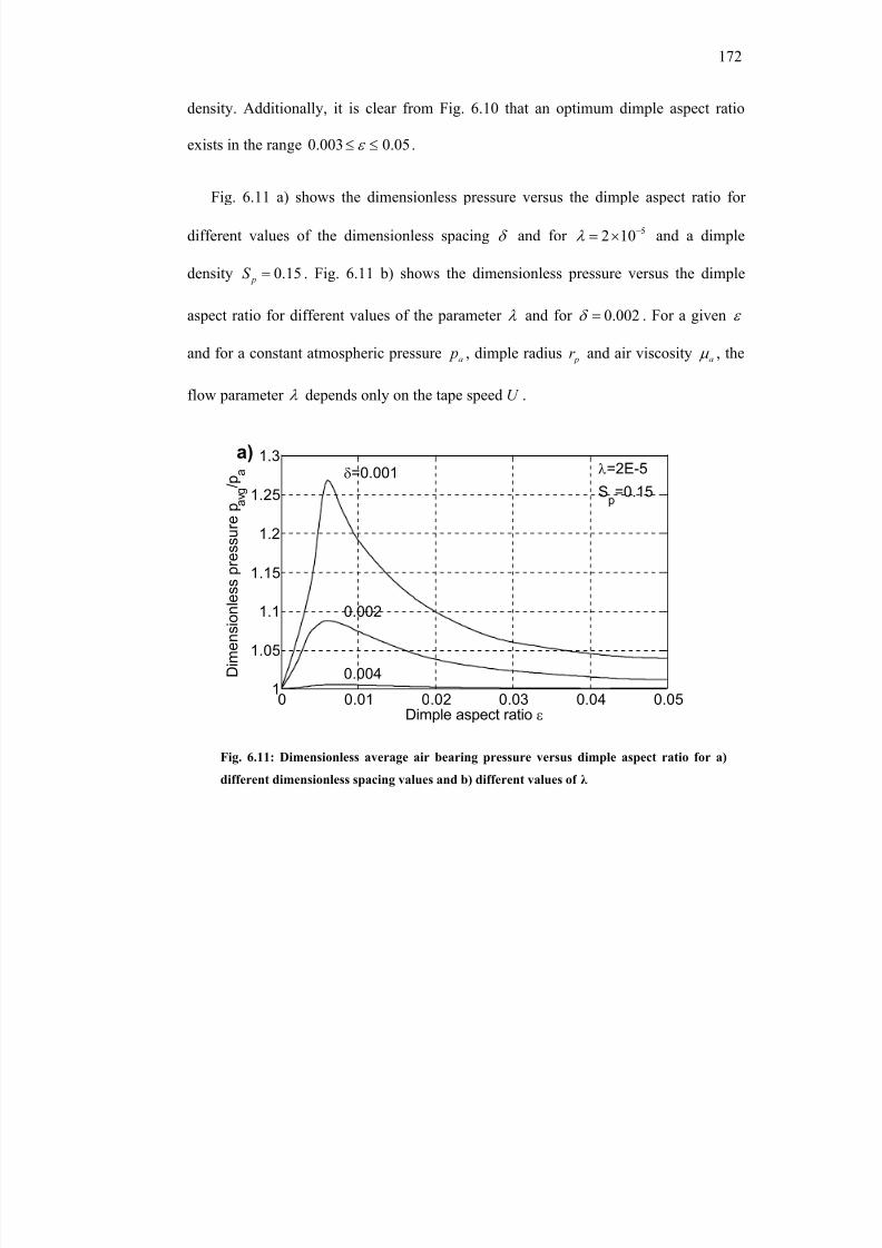
8/8/2019 BR PhD Dissertation
http://slidepdf.com/reader/full/br-phd-dissertation 204/248
172
density. Additionally, it is clear from Fig. 6.10 that an optimum dimple aspect ratio
exists in the range 0.003 0.05ε ≤ ≤ .
Fig. 6.11 a) shows the dimensionless pressure versus the dimple aspect ratio for
different values of the dimensionless spacing δ and for 52 10λ −= × and a dimple
density 0.15 pS = . Fig. 6.11 b) shows the dimensionless pressure versus the dimple
aspect ratio for different values of the parameter λ and for 0.002δ = . For a given ε
and for a constant atmospheric pressure a p , dimple radius pr and air viscosity aµ , the
flow parameter λ depends only on the tape speed U .
0 0.01 0.02 0.03 0.04 0.051
1.05
1.1
1.15
1.2
1.25
1.3
0.004
δ=0.001
0.002
λ=2E-5
Sp=0.15
Dimple aspect ratio ε
D i m e n s i o n l e
s s p r e s s u r e p a v g
/ p a
a)
0 0.01 0.02 0.03 0.04 0.051
1.05
1.1
1.15
1.2
1.25
1.3
0.004
δ=0.001
0.002
λ=2E-5
Sp=0.15
Dimple aspect ratio ε
D i m e n s i o n l e
s s p r e s s u r e p a v g
/ p a
a)
Fig. 6.11: Dimensionless average air bearing pressure versus dimple aspect ratio for a)
different dimensionless spacing values and b) different values of λ
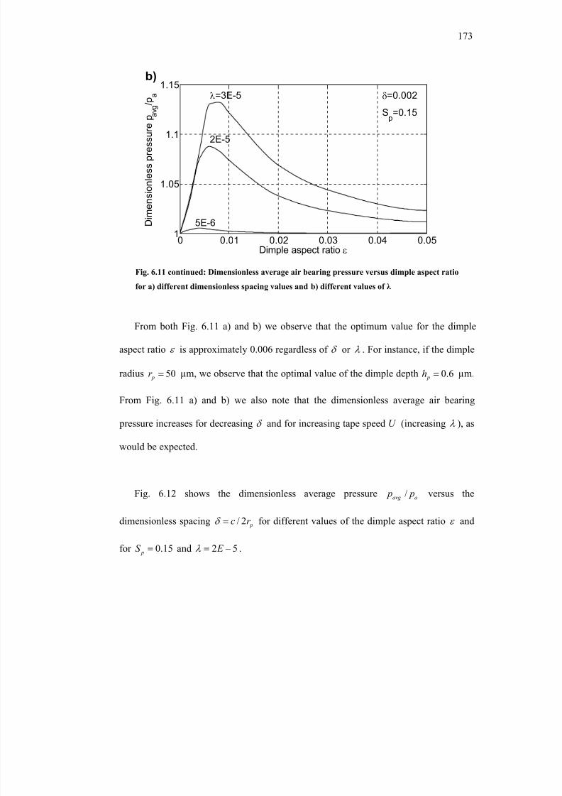
8/8/2019 BR PhD Dissertation
http://slidepdf.com/reader/full/br-phd-dissertation 205/248
173
0 0.01 0.02 0.03 0.04 0.051
1.05
1.1
1.15
5E-6
λ=3E-5
2E-5
δ=0.002
Sp=0.15
Dimple aspect ratio ε
D i m e n s i o n l e s s p r e s s u r e
p a v g
/ p a
b)
0 0.01 0.02 0.03 0.04 0.051
1.05
1.1
1.15
5E-6
λ=3E-5
2E-5
δ=0.002
Sp=0.15
Dimple aspect ratio ε
D i m e n s i o n l e s s p r e s s u r e
p a v g
/ p a
b)
From both Fig. 6.11 a) and b) we observe that the optimum value for the dimple
aspect ratio ε is approximately 0.006 regardless of δ or λ . For instance, if the dimple
radius 50 pr = µm, we observe that the optimal value of the dimple depth 0.6 ph = µm.
From Fig. 6.11 a) and b) we also note that the dimensionless average air bearing
pressure increases for decreasing δ and for increasing tape speed U (increasing λ ), as
would be expected.
Fig. 6.12 shows the dimensionless average pressure /avg a p p versus the
dimensionless spacing / 2 pc r δ = for different values of the dimple aspect ratio ε and
for 0.15 pS = and 2 5 E λ = − .
Fig. 6.11 continued: Dimensionless average air bearing pressure versus dimple aspect ratio
for a) different dimensionless spacing values and b) different values of λ
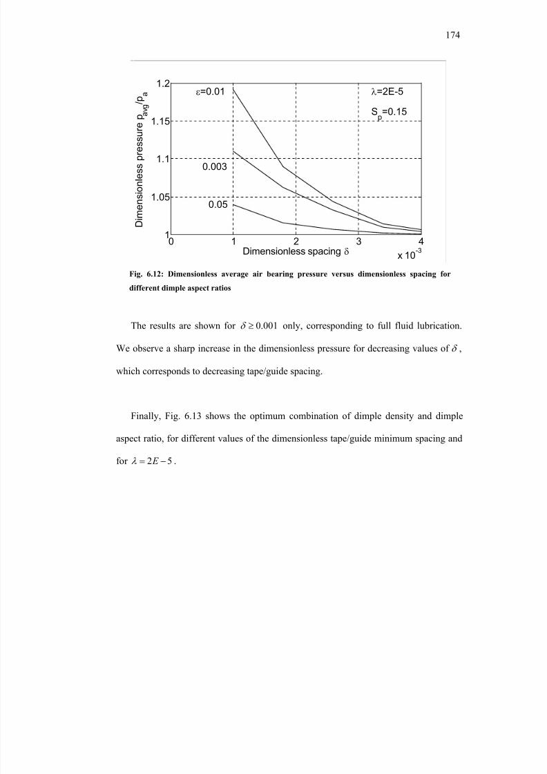
8/8/2019 BR PhD Dissertation
http://slidepdf.com/reader/full/br-phd-dissertation 206/248
174
0 1 2 3 4
x 10-3
1
1.05
1.1
1.15
1.2
0.05
ε=0.01
0.003
λ=2E-5
Sp=0.15
Dimensionless spacing δ
D i m e n s i o n l e s s p r e s s u r e
p a v g
/ p a
The results are shown for 0.001δ ≥ only, corresponding to full fluid lubrication.
We observe a sharp increase in the dimensionless pressure for decreasing values of δ ,
which corresponds to decreasing tape/guide spacing.
Finally, Fig. 6.13 shows the optimum combination of dimple density and dimple
aspect ratio, for different values of the dimensionless tape/guide minimum spacing and
for 2 5 E λ = − .
Fig. 6.12: Dimensionless average air bearing pressure versus dimensionless spacing for
different dimple aspect ratios
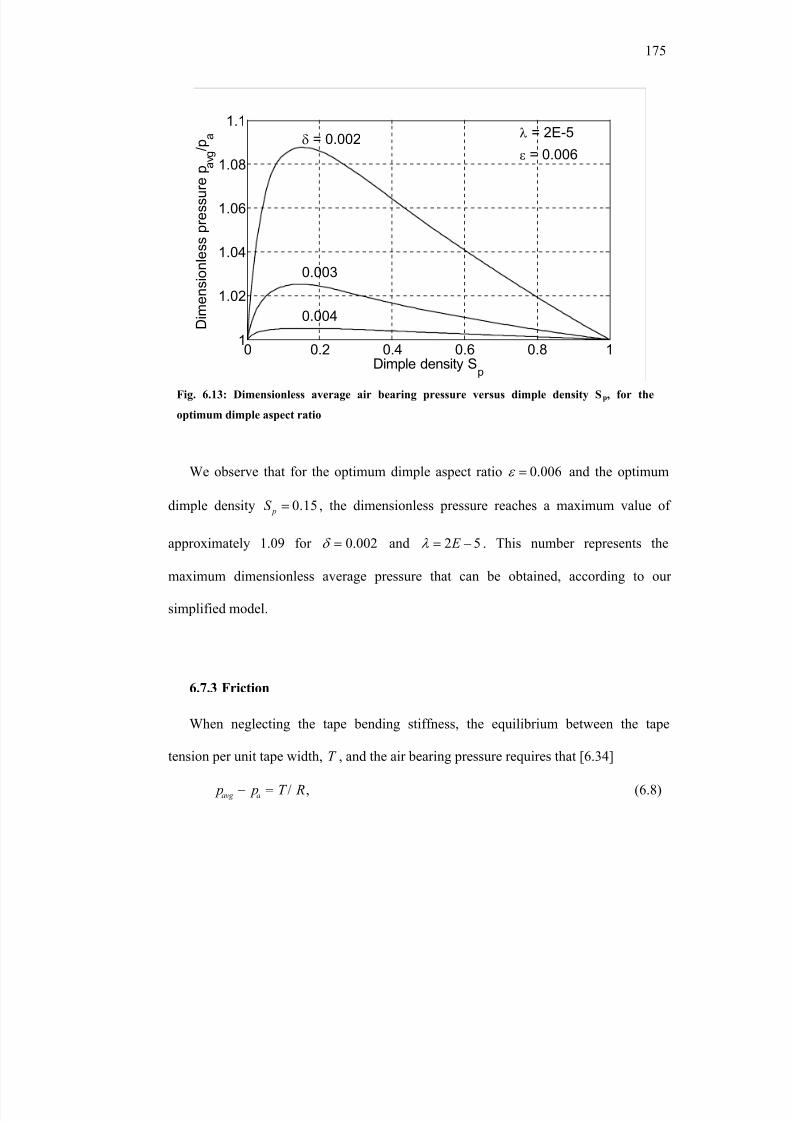
8/8/2019 BR PhD Dissertation
http://slidepdf.com/reader/full/br-phd-dissertation 207/248
175
0 0.2 0.4 0.6 0.8 11
1.02
1.04
1.06
1.08
1.1
Dimple density Sp
D i m e n s i o n l e s s p r e s s u r e
p a v g
/ p a λ = 2E-5
ε = 0.006δ = 0.002
0.003
0.004
We observe that for the optimum dimple aspect ratio 0.006ε = and the optimum
dimple density 0.15 pS = , the dimensionless pressure reaches a maximum value of
approximately 1.09 for 0.002δ = and 2 5 E λ = − . This number represents the
maximum dimensionless average pressure that can be obtained, according to our
simplified model.
6.7.3 Friction
When neglecting the tape bending stiffness, the equilibrium between the tape
tension per unit tape width, T , and the air bearing pressure requires that [6.34]
/avg a p p T R− = , (6.8)
Fig. 6.13: Dimensionless average air bearing pressure versus dimple density Sp, for the
optimum dimple aspect ratio
8/8/2019 BR PhD Dissertation
http://slidepdf.com/reader/full/br-phd-dissertation 208/248
176
for a guide with radius R . Non-dimensionalizing eq. (6.8) with the atmospheric
pressure a p yields
( )/ 1 /avg a a p p T p R− = (6.9)
Fig. 6.14 shows the dimensionless tape/guide spacing δ versus the dimple aspect
ratio ε for different values of the dimensionless tape tension ( )/ aT p R (dimple density
0.15 pS = and flow parameter 2 5 E λ = − ). The results shown in Fig. 6.14 were
obtained from ( )/avg a p p f δ =
curves as shown in Fig. 6.12. The intersection of these
curves with horizontal lines for /avg a p p = constant yields values of δ for each ε -
curve. The dimensionless average air bearing pressure was then converted to a
dimensionless tape tension by eq. (6.9). To obtain Fig. 6.14, we considered more values
of ε than displayed in Fig. 6.12.
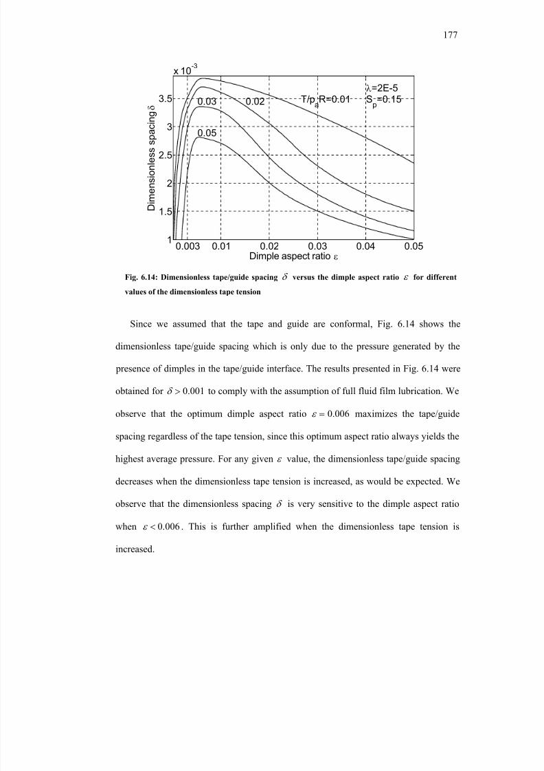
8/8/2019 BR PhD Dissertation
http://slidepdf.com/reader/full/br-phd-dissertation 209/248
177
0.003 0.01 0.02 0.03 0.04 0.051
1.5
2
2.5
3
3.5
x 10-3
Dimple aspect ratio ε
D i m e n s i o n l e s s s p a c i n g δ
T/paR=0.010.020.03
0.05
λ=2E-5S
p=0.15
Since we assumed that the tape and guide are conformal, Fig. 6.14 shows the
dimensionless tape/guide spacing which is only due to the pressure generated by the
presence of dimples in the tape/guide interface. The results presented in Fig. 6.14 were
obtained for 0.001δ > to comply with the assumption of full fluid film lubrication. We
observe that the optimum dimple aspect ratio 0.006ε = maximizes the tape/guide
spacing regardless of the tape tension, since this optimum aspect ratio always yields the
highest average pressure. For any given ε value, the dimensionless tape/guide spacing
decreases when the dimensionless tape tension is increased, as would be expected. We
observe that the dimensionless spacing δ is very sensitive to the dimple aspect ratio
when 006.0<ε . This is further amplified when the dimensionless tape tension is
increased.
Fig. 6.14: Dimensionless tape/guide spacing δ versus the dimple aspect ratio ε for different
values of the dimensionless tape tension
8/8/2019 BR PhD Dissertation
http://slidepdf.com/reader/full/br-phd-dissertation 210/248
178
The average shear stress in the air bearing, which is a measure of the air friction, can
be expressed as
/a eqU cτ µ = (6.10)
where τ is the shear stress, aµ is the air viscosity and U is the tape speed. The spacing
eqc is an equivalent tape/guide spacing that takes into account the dimple depth [6.19]
and can be determined as
eq eqc c h= + (6.11)
In eq. (6.11), eqh can be obtained by dividing the volume of a dimple by the surface
area of its imaginary square cell. Hence,
( )2 2
23
6
p p
eq p p
p
h S h h r
r = + (6.12)
Non-dimensionalizing eq. (6.11) with 2 pr yields
)
4
3(
3
2 2 ++= ε ε δ δ peq S (6.13)
which, for 05.0≤ε , can be approximated by
2/ peq S ε δ δ += (6.14)
If ( ) f τ δ = and ( ) f δ ε = are known (see Eqs. (6.10) – (6.14) and Fig. 6.14), one can
determine the relationship between the shear stress τ and the dimple aspect ratio ε . Eq.
(6.10) can be re-written in terms of eqδ as
2
a
p eq
U
r
µ τ
δ = (6.15)
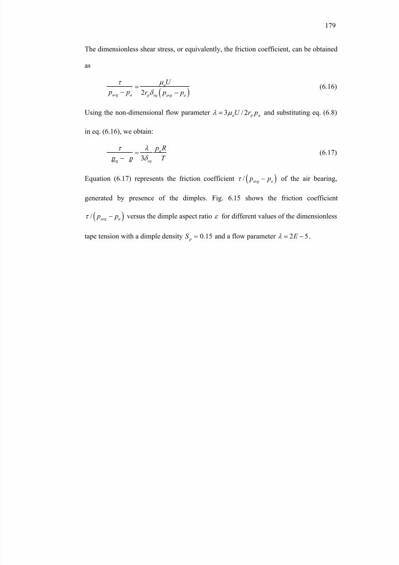
8/8/2019 BR PhD Dissertation
http://slidepdf.com/reader/full/br-phd-dissertation 211/248
179
The dimensionless shear stress, or equivalently, the friction coefficient, can be obtained
as
( )2
a
avg a p eq avg a
U
p p r p p
µ τ
δ =
− −(6.16)
Using the non-dimensional flow parameter a pa pr U 2/3µ λ = and substituting eq. (6.8)
in eq. (6.16), we obtain:
3
a
avg a eq
p R
p p T
τ λ
δ =
−(6.17)
Equation (6.17) represents the friction coefficient ( )/ avg a p pτ − of the air bearing,
generated by presence of the dimples. Fig. 6.15 shows the friction coefficient
( )/ avg a p pτ − versus the dimple aspect ratio ε for different values of the dimensionless
tape tension with a dimple density 0.15 pS = and a flow parameter 52 −= E λ .
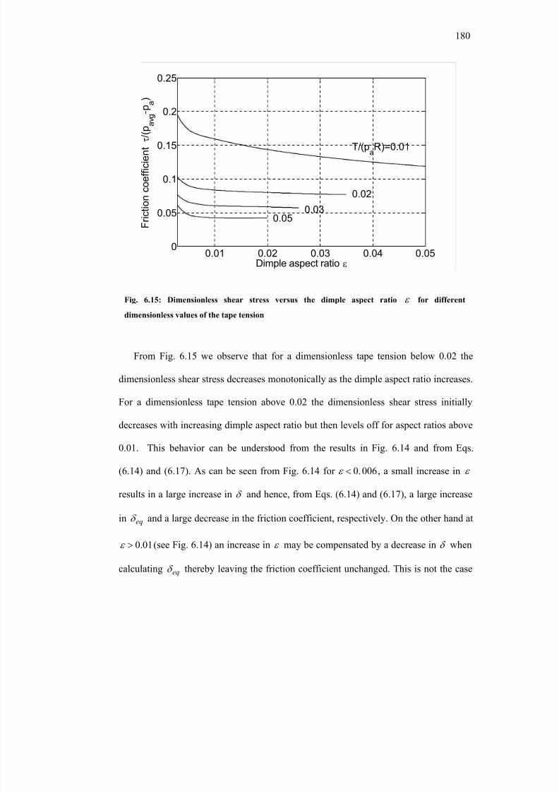
8/8/2019 BR PhD Dissertation
http://slidepdf.com/reader/full/br-phd-dissertation 212/248
180
0.01 0.02 0.03 0.04 0.050
0.05
0.1
0.15
0.2
0.25
Dimple aspect ratio ε
F r i c t i o n c o e f f i c i e n t τ / ( p
a v g
- p a
)
T/(paR)=0.01
0.02
0.030.05
From Fig. 6.15 we observe that for a dimensionless tape tension below 0.02 the
dimensionless shear stress decreases monotonically as the dimple aspect ratio increases.
For a dimensionless tape tension above 0.02 the dimensionless shear stress initially
decreases with increasing dimple aspect ratio but then levels off for aspect ratios above
0.01. This behavior can be understood from the results in Fig. 6.14 and from Eqs.
(6.14) and (6.17). As can be seen from Fig. 6.14 for 006.0<ε , a small increase in ε
results in a large increase in δ and hence, from Eqs. (6.14) and (6.17), a large increase
in eqδ and a large decrease in the friction coefficient, respectively. On the other hand at
01.0>ε (see Fig. 6.14) an increase in ε may be compensated by a decrease in δ when
calculating eqδ thereby leaving the friction coefficient unchanged. This is not the case
Fig. 6.15: Dimensionless shear stress versus the dimple aspect ratio ε for different
dimensionless values of the tape tension
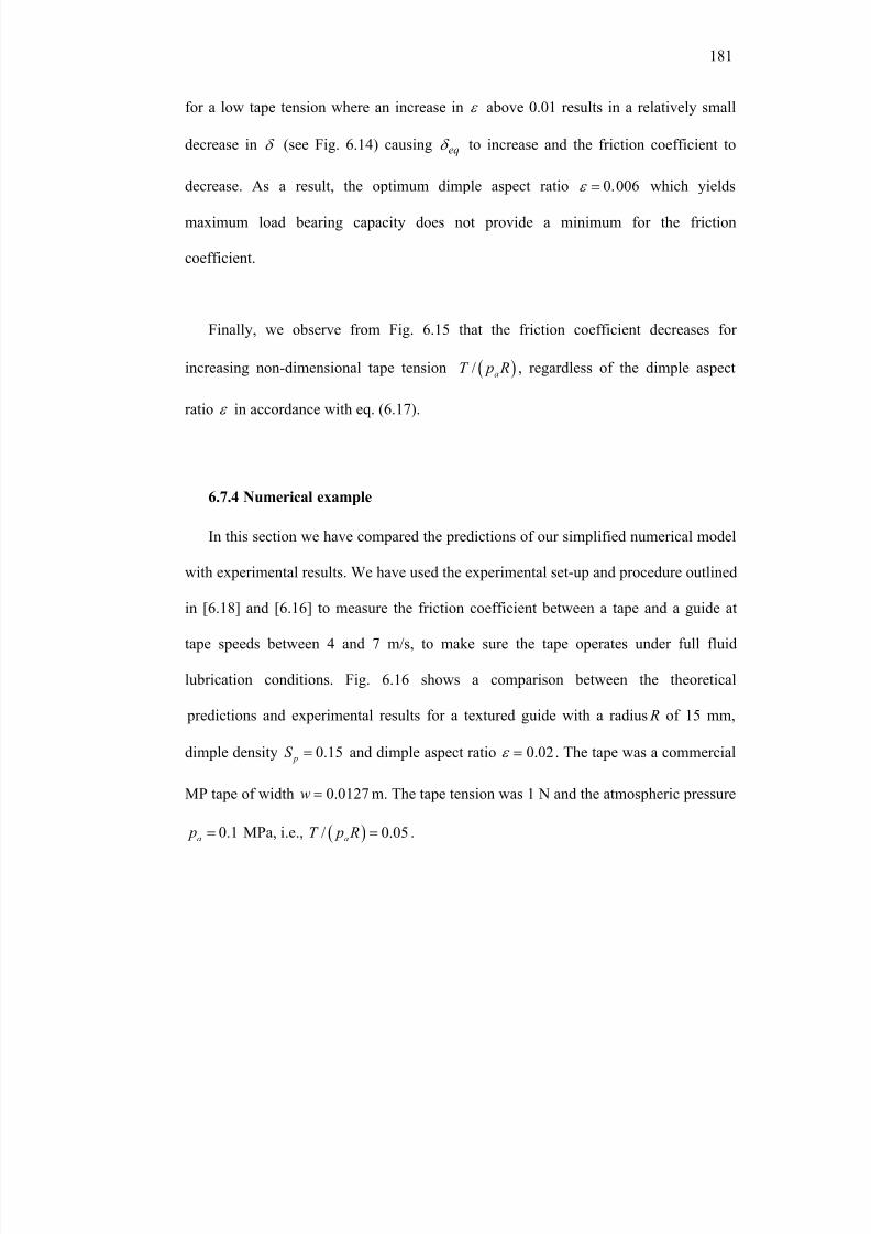
8/8/2019 BR PhD Dissertation
http://slidepdf.com/reader/full/br-phd-dissertation 213/248
181
for a low tape tension where an increase in ε above 0.01 results in a relatively small
decrease in δ (see Fig. 6.14) causing eqδ to increase and the friction coefficient to
decrease.
As a result, the optimum dimple aspect ratio 006.0=ε which yields
maximum load bearing capacity does not provide a minimum for the friction
coefficient.
Finally, we observe from Fig. 6.15 that the friction coefficient decreases for
increasing non-dimensional tape tension ( )/ aT p R , regardless of the dimple aspect
ratio ε in accordance with eq. (6.17).
6.7.4 Numerical example
In this section we have compared the predictions of our simplified numerical model
with experimental results. We have used the experimental set-up and procedure outlined
in [6.18] and [6.16] to measure the friction coefficient between a tape and a guide at
tape speeds between 4 and 7 m/s, to make sure the tape operates under full fluid
lubrication conditions. Fig. 6.16 shows a comparison between the theoretical
predictions and experimental results for a textured guide with a radius R of 15 mm,
dimple density 0.15 pS = and dimple aspect ratio 0.02ε = . The tape was a commercial
MP tape of width 0.0127w = m. The tape tension was 1 N and the atmospheric pressure
0.1a
p = MPa, i.e., ( )/ 0.05aT p R = .
8/8/2019 BR PhD Dissertation
http://slidepdf.com/reader/full/br-phd-dissertation 214/248
182
3 4 5 6 7 80
0.01
0.02
0.03
0.04
0.05
0.06
0.07
F r i c t i o n c o e f f i c i e n
t
Tape speed [m/s]
Sp=0.15
ε=0.02
Theoretical model
Experimental
The theoretical model is in good agreement with experimental measurements. In the
full fluid lubrication regime, the friction coefficient increases slightly for increasing
tape speed as predicted qualitatively by the Stribeck curve. The experimental results
show that the friction coefficients predicted by the model are of the same order as the
experimental results. We note that the values for the theoretical results are higher than
those for the experimental results. This is likely due to the simplifying assumption of a
conformal and “rigid” tape. A converging channel at the leading edge would create a
higher average pressure and thus a higher load bearing capacity. This would result in
lower friction coefficients, which would improve the agreement between the theoretical
model and experimentally obtained friction coefficients.
Fig. 6.16: Friction coefficient versus tape speed for an LST guide of radius 15 mm, Sp=0.15 and
ε=0.02
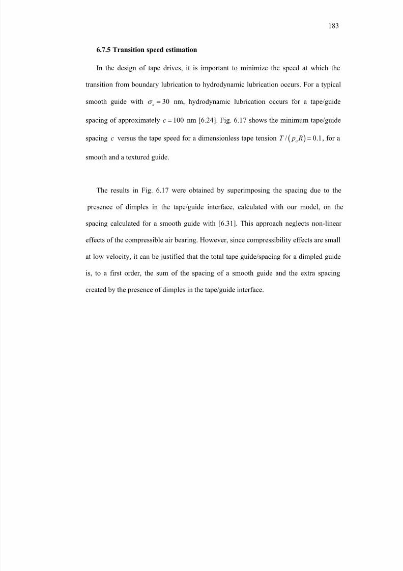
8/8/2019 BR PhD Dissertation
http://slidepdf.com/reader/full/br-phd-dissertation 215/248
183
6.7.5 Transition speed estimation
In the design of tape drives, it is important to minimize the speed at which the
transition from boundary lubrication to hydrodynamic lubrication occurs. For a typical
smooth guide with 30 s
σ = nm, hydrodynamic lubrication occurs for a tape/guide
spacing of approximately 100c = nm [6.24]. Fig. 6.17 shows the minimum tape/guide
spacing c versus the tape speed for a dimensionless tape tension ( )/ 0.1aT p R = , for a
smooth and a textured guide.
The results in Fig. 6.17 were obtained by superimposing the spacing due to the
presence of dimples in the tape/guide interface, calculated with our model, on the
spacing calculated for a smooth guide with [6.31]. This approach neglects non-linear
effects of the compressible air bearing. However, since compressibility effects are small
at low velocity, it can be justified that the total tape guide/spacing for a dimpled guide
is, to a first order, the sum of the spacing of a smooth guide and the extra spacing
created by the presence of dimples in the tape/guide interface.
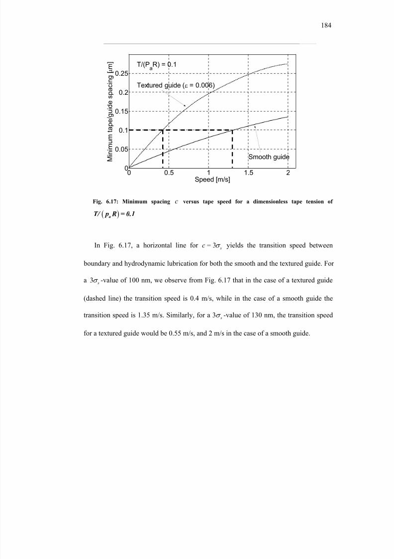
8/8/2019 BR PhD Dissertation
http://slidepdf.com/reader/full/br-phd-dissertation 216/248
184
0 0.5 1 1.5 20
0.05
0.1
0.15
0.2
0.25
Speed [m/s]
M i n i m u m t a
p e / g u i d e s p a
c i n g [ µ m ]
Textured guide (ε = 0.006)
Smooth guide
T/(PaR) = 0.1
In Fig. 6.17, a horizontal line for 3 s
c σ = yields the transition speed between
boundary and hydrodynamic lubrication for both the smooth and the textured guide. For
a 3 sσ -value of 100 nm, we observe from Fig. 6.17 that in the case of a textured guide
(dashed line) the transition speed is 0.4 m/s, while in the case of a smooth guide the
transition speed is 1.35 m/s. Similarly, for a 3 sσ -value of 130 nm, the transition speed
for a textured guide would be 0.55 m/s, and 2 m/s in the case of a smooth guide.
Fig. 6.17: Minimum spacing c versus tape speed for a dimensionless tape tension of
( )aT/ p R = 0.1
8/8/2019 BR PhD Dissertation
http://slidepdf.com/reader/full/br-phd-dissertation 217/248
185
6.7.6 Discussion
Our model predicts that dimpled guides feature a significantly lower transition
speed between boundary lubrication and hydrodynamic lubrication than smooth guides.
Using dimpled guides (stationary) in commercial tape drives instead of the currently
used smooth rollers (rotating), would potentially yield improvements in terms of tape
transport and lateral tape motion. Furthermore, tape wear, which is a problem of
considerable interest in tape drives with smooth stationary guides, will also be reduced
due to the lower transition speed.
Additionally, dimpled guides would potentially enable the wide-spread introduction
of metal evaporated (ME) tape. ME tape is desirable from a magnetics point of view,
since the cobalt magnetic layer has a higher coercivity than the currently used metal
particulate (MP) tape. Hence, ME tape would allow an increase in storage density,
compared to MP tape. The tribological performance of ME tape, however, is
problematic compared to MP tape, especially at low tape speeds, where surface contact
occurs between the tape and the guide surface [6.10, 6.25-6.26]. Dimpled guide surfaces
create a higher air bearing pressure compared to smooth guides and, thus, increase the
flying height at low speeds. This would improve the tribological performance of ME
tape.
Our model neglects elasto-hydrodynamic effects. However, for low tape speeds
corresponding to the transition from boundary to hydrodynamic lubrication, the bearing
8/8/2019 BR PhD Dissertation
http://slidepdf.com/reader/full/br-phd-dissertation 218/248
186
number is small and thus the compressibility effects of the air bearing are less
prominent, i.e., it is justifiable to approximate the compressible air bearing by an
incompressible one.
Including elasto-hydrodynamic effects in the model would yield a more accurate
solution than our current model but would require a substantially larger numerical
effort. For a full-size simulation of the complete tape/dimpled guide interface we
calculate the following scenario. Assuming a guide with a radius of 10 mm, a dimple
density of 0.2 and a dimple radius of 50 µm, in combination with a 12.7 mm wide tape
and a wrap angle of 90 degrees, we calculate that the tape/guide interface contains
approximately 20,000 dimples. To fully capture the pressure gradient created over a
dimple, a grid of 200 by 200 nodes per dimple (imaginary cell) is needed. Hence, 800
million nodes would be required to simulate the complete tape/guide interface. A
numerical problem of this size poses a challenge to present day computer hardware and
requires long simulation times, if it is at all solvable.
6.8 Conclusion
• The optimum dimple density was found to be between 0.1 and 0.3, depending on
the dimple aspect ratio. A greater dimple aspect ratio will reduce the optimum
dimple density. The tape/guide minimum spacing does not affect the optimum
dimple density.
8/8/2019 BR PhD Dissertation
http://slidepdf.com/reader/full/br-phd-dissertation 219/248
187
• The optimum dimple aspect ratio for maximum average air bearing pressure was
found to be 0.006, almost independent of the dimensionless tape/guide spacing
δ and the flow factor λ .
• The friction coefficient decreases monotonically with increasing dimple aspect
ratio. Our simplified model shows good qualitative agreement with experimental
results.
• The transition speed between boundary and hydrodynamic lubrication is reduced
for a dimpled guide compared to a smooth guide.
• Improvements to the present model can be obtained by including the elasto-
hydrodynamic effects.
6.9 Acknowledgements
Chapter 6, in part, is a reprint of the material as it appears in “Enhancing the
Tribological Performance of the Magnetic Tape/Guide Interface by Laser Surface
Texturing”, Raeymaekers B., Etsion I., Talke F.E., Tribology Letters, 2007. The
dissertation author was the primary investigator and author of this paper.
Chapter 6, in part, has been submitted for publication in “A Model for Magnetic
Tape/Guide Friction Reduction by Laser Surface Texturing”, Raeymaekers B., Etsion I.,
Talke F.E., Tribology Letters, 2007. The dissertation author was the primary
investigator and author of this paper.
8/8/2019 BR PhD Dissertation
http://slidepdf.com/reader/full/br-phd-dissertation 220/248
188
6.10 References
[6.1] Peng ZC, Khonsari MM, 2004, Hydrodynamic Analysis of Compliant Foil
Bearings with Compressible Air Flow, J. Trib. T. ASME, Vol. 126, pp. 542 - 546
[6.2] Peng ZC, Khonsari MM, 2004, On the Limiting Load-Carrying Capacity of Foil
Bearings, J. Trib. T. ASME, Vol. 126, pp. 817 - 818
[6.3] Fields S, 2004, Foil Air Bearing Takes Flight, Tribol. Lubr. Technol., Vol. 60(4), pp. 29 - 33
[6.4] Baugh E, Talke FE, 1996, The Head Tape Interface: A Critical Review and RecentResults, Tribol. T., Vol. 39(2), pp. 306 - 313
[6.5] Richards DB, Sharrock MP, 1998, Key Issues in the Design of Magnetic Tape for Linear Systems of High Track Density, IEEE T. Mag., Vol. 34(4), pp. 1878 - 1882
[6.6] Taylor RJ, Talke FE, 2005, Investigation of Roller Interactions with Flexible Tape
Medium, Tribol. Int., Vol. 38, pp. 599 - 605
[6.7] Raeymaekers B, Talke FE, 2007, Lateral Motion of an Axially Moving Tape on a
Cylindrical Guide Surface, J. Appl. Mech. T. ASME (in press)
[6.8] Ono K, 1979, Lateral Motion of an Axially Moving String on a Cylindrical Guide
Surface, J. Appl. Mech. T. ASME, Vol. 46, pp. 905 - 912
[6.9] Taylor RJ, Strahle P, Stahl J, Talke FE, 2000, Measurement of Cross-Track
Motion of Magnetic Tapes, J. Info. Storage Proc. Syst., Vol. 2, pp. 255 - 261
[6.10] Raeymaekers B, Etsion I, Talke FE, 2007, The Influence of Design and
Operating Parameters on the Magnetic Tape/Guide Friction Coefficient, Tribol. Lett.,
Vol. 25(2), pp. 161 - 171
[6.11] Crahay J, Bragard A, 1983, Gravure de la Rugosité des Cylindres de Laminoir
par Impulsions Laser, Revue de Métallurgie CIT, pp. 393 - 401
[6.12] Ranjan R, Lambeth DN, Tromel M, Li Y, 1991, Laser Texturing for Low-Flying-
Height Media, J. Appl. Phys., Vol. 69(8), pp. 5745 - 5747
[6.13] Etsion I, Burstein L, 1996, A Model for Mechanical Seals with Regular
Microsurface Structure, Tribol. T., Vol. 39(3), pp. 667 - 683
[6.14] Scott DA, Brandt M, Dorien-Brown B, Valentine B, De P, 1993, Laser
Modification of Metal Surfaces, Opt. Laser Eng., Vol. 18, pp. 1 - 13
8/8/2019 BR PhD Dissertation
http://slidepdf.com/reader/full/br-phd-dissertation 221/248
189
[6.15] Etsion I, 2004, Improving Tribological Performance of Mechanical Components
by Laser Surface Texturing, Tribol. Lett., Vol. 17(4), pp. 733 - 737
[6.16] Etsion I, 2005, State of the Art in Laser Surface Texturing, J. Trib. T. ASME,
Vol. 127, pp. 248 - 253
[6.17] Duffet G, Sallamand P, Vannes AB, 2003, Improvement in Friction by cw Nd:YAG Laser Surface Treatment on Cast Iron Cylindrical Bore, Appl. Surf. Sci., Vol.
205, pp. 289 - 296
[6.18] Erdemir A, 2005, Review of Engineered Tribological Interfaces for Improved
Boundary Lubrication, Tribol. Int., Vol. 38, pp. 249 - 256
[6.19] Kligerman Y, Etsion I, 2001, Analysis of the Hydrodynamic Effects in a Surface
Textured Circumferential Gas Seal, Tribol. T., Vol. 44(3), pp. 472 - 478
[6.20] Tan AH, Cheng SW, 2006, A Novel Textured Design for Hard Disk DriveTribology Improvement, Tribol. Int., Vol. 39, pp. 506 - 511
[6.21] Shigley JE, Mischke CR, 1989, Mechanical Engineering Design, 5th
edition,McGraw Hill, New York
[6.22] Greenwood JA, Williamson JBP, 1966, Contact of Nominally Flat Surfaces,Proceedings of the Royal Society of London Series A – Mathematical and Physical
Sciences, Vol. 295 (1442), pp. 300 - 319
[6.23] McCool JI, 1987, Relating Profile Instrument Measurements to the Functional
Performance of Rough Surfaces, J. Trib. T. ASME, Vol. 109, pp. 264 – 270
[6.24] Patir N, Cheng HS, 1978, Average Flow Model for Determining Effects of 3-
Dimensional Roughness on Partial Hydrodynamic Lubrication, J. Lubr. Technol. T.ASME, Vol. 100(1), pp. 12-17
[6.25] Hempstock MS, Sullivan JL, 1996, The Durability and Signal Performance of
Metal Evaporated and Metal Particle Tape, IEEE T. Mag., Vol. 32(5), pp. 3723 - 3725
[6.26] Hempstock MS, Sullivan JL, 1996, A Study of the Mechanical and Magnetic
Performance of Metal Evaporated Tape, J. Mag. Mag. Mat., Vol. 155, pp. 323 - 328
[6.27] Patton ST, Bhushan B, 1999, Origins of Friction and Wear of the Thin Metallic
Layer of Metal Evaporated Magnetic Tape, Wear, Vol. 224, pp. 126 - 140
[6.28] Bijker MD, Draaisma EA, Eisenberg M, Jansen J, Persat N, Sourty E, 2000,
Future Directions in Advanced Digital Recording Technology, Tribol. Int., Vol. 33, pp.383 - 390

8/8/2019 BR PhD Dissertation
http://slidepdf.com/reader/full/br-phd-dissertation 222/248
190
[6.29] Osaki H, 2003, Recent Research of Tape/Drive Tribology, Tribol. Int., Vol. 36,
pp. 349 - 360
[6.30] Hashimoto H, Okajima M, 2006, Theoretical and Experimental Investigations
Into Spacing Characteristics Between Roller and Three Types of Webs With Different
Permeabilities, J. Trib. T. ASME, Vol. 128, pp. 267 - 274
[6.31] Lacey C, Talke FE, 1990, A Tightly Coupled Numerical Foil Bearing Solution,
IEEE T. Mag., Vol. 26(6), pp. 3039 - 3043
[6.33] Hirsch C, 1988, Numerical Computation of Internal and External Flows, Vol.1, J.
Wiley and Sons, New York
[6.34] Eshel A, Elrod HG, 1965, The Theory of the Infinitely Wide, Perfectly Flexible,
Self-Acting Foil Bearing, J. Basic Eng. T. ASME, Vol. 87, pp. 831 - 836
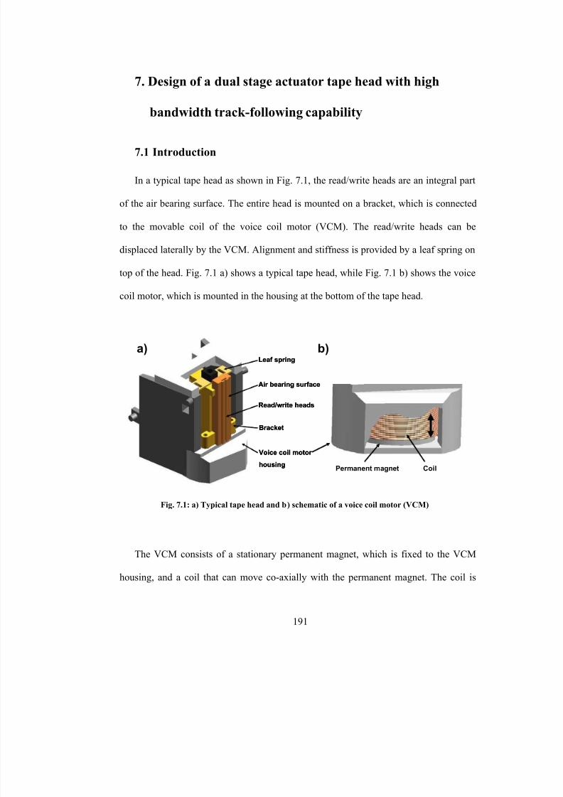
8/8/2019 BR PhD Dissertation
http://slidepdf.com/reader/full/br-phd-dissertation 223/248
191
7. Design of a dual stage actuator tape head with high
bandwidth track-following capability
7.1 Introduction
In a typical tape head as shown in Fig. 7.1, the read/write heads are an integral part
of the air bearing surface. The entire head is mounted on a bracket, which is connected
to the movable coil of the voice coil motor (VCM). The read/write heads can be
displaced laterally by the VCM. Alignment and stiffness is provided by a leaf spring on
top of the head. Fig. 7.1 a) shows a typical tape head, while Fig. 7.1 b) shows the voice
coil motor, which is mounted in the housing at the bottom of the tape head.
Voice coil motor
housing
Air bearing surface
Read/write heads
Leaf spring
Bracket
Voice coil motor
housing
Air bearing surface
Read/write heads
Leaf spring
Bracket
a) b)
Permanent magnet Coil
The VCM consists of a stationary permanent magnet, which is fixed to the VCM
housing, and a coil that can move co-axially with the permanent magnet. The coil is
Fig. 7.1: a) Typical tape head and b) schematic of a voice coil motor (VCM)
8/8/2019 BR PhD Dissertation
http://slidepdf.com/reader/full/br-phd-dissertation 224/248
192
connected to the bracket. The lateral position of the coil in the VCM (and thus the
read/write heads) is determined by the electromagnetic force em F acting on the coil,
given by
( )em c c F B I l = × (7.1)
where B is the magnetic inductance of the permanent magnet, c I is the electric current
flowing through the coil and cl is the length of the coil. Hence, the magnitude of the
current c I determines the lateral position of the coil in the VCM.
The lateral position of the head is controlled by a servo loop. During lateral tape
displacement, an error signal from the servo head is generated and the head is moved by
the VCM to avoid track misregistration. However, the bandwidth of the VCM is
limited, mainly due to mass and available power. LTM frequencies higher than the
bandwidth of the servo actuator, generally referred to as high frequency LTM, cannot
be followed by the servo actuator. State-of-the-art tape head actuators have a bandwidth
on the order of 750 – 1000 Hz.
7.2 Concept of the dual stage actuator head
The concept of a dual stage actuator was first introduced in hard disk drive (HDD)
technology about 15 years ago. Mori et al. introduced a piezo (PZT) based rotary micro-
actuator at the suspension level [7.1]. The VCM is used as a “coarse actuator”, while the
PZT is used as a “fine actuator”. Different types of micro-actuator designs have been
8/8/2019 BR PhD Dissertation
http://slidepdf.com/reader/full/br-phd-dissertation 225/248
193
proposed in the literature. Koganezawa et al. devised a micro-actuator that operates at
the suspension level of a HDD but uses a flexural cross-shaped spring [7.2]. Instead of
using a “stacked”-PZT, they used shear-mode PZT crystals [7.3]. Evans and Griesbach
presented a piezoelectric micro-actuator design that takes into account
manufacturability and economical considerations [7.4]. They modeled the dynamics of
their design and presented two voltage drivers that can be used to drive the actuator.
Nakamura et al. introduced a push-pull multi-layered piggyback PZT actuator that
operates at the suspension level [7.5]. Their design features a high stroke, combined
with a low voltage.
While most designs are PZT-based, some researchers also attempted to manufacture
electrostatic micro-actuators. Fan et al. implemented a micro-actuator that operates at
the slider level instead of the suspension level [7.6]. A more in-depth analysis of the
design proposed by Fan et al. was presented in [7.7] by Hirano et. al. Horsley et al. used
parallel-plate capacitive electrodes to generate an electrostatic force, which was used to
drive an actuator [7.8]. Finally, the design of an electromagnetic micro-actuator was
investigated by Tang et al. [7.9].
This chapter presents the design of a dual stage actuator tape head. We attempt to
increase the bandwidth of the servo loop by introducing a piezo crystal (PZT) micro-
actuator. This micro-actuator serves as a fine-tuning mechanism that can follow high
frequency LTM (> 1 kHz) but is limited in its stroke. Increased servo bandwidth would
allow an increase in track density, since track misregistration will be reduced. The main
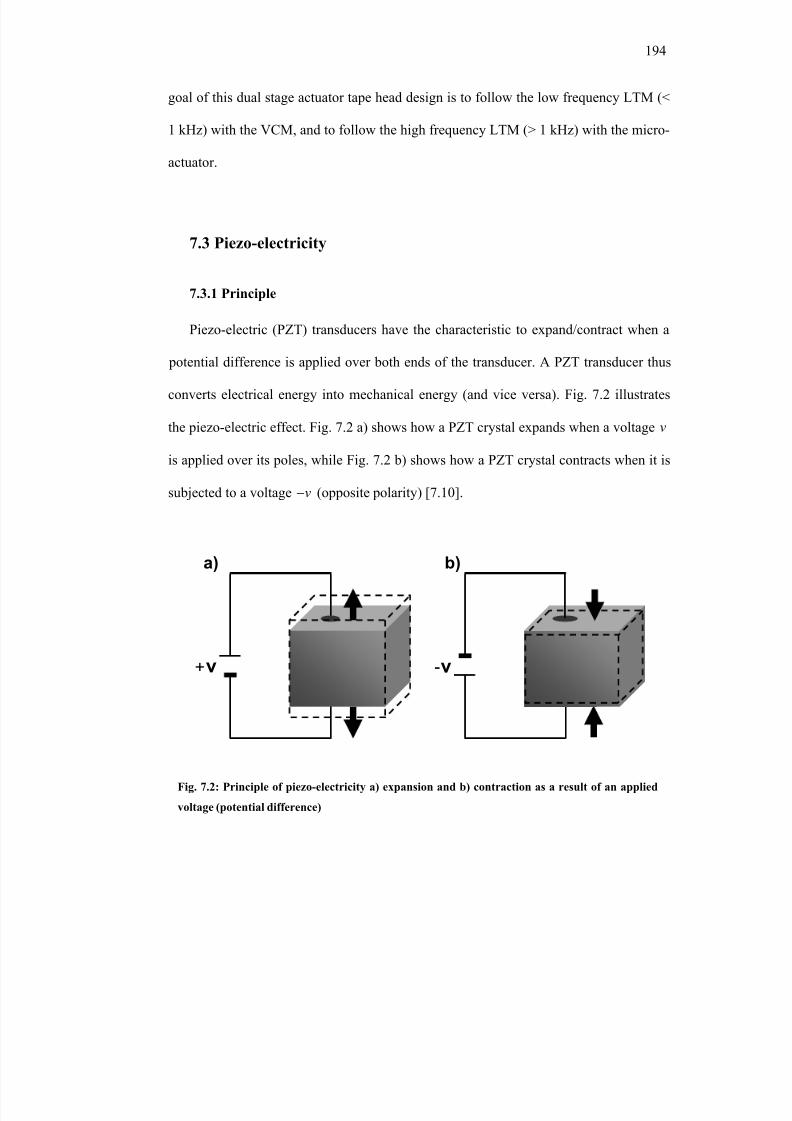
8/8/2019 BR PhD Dissertation
http://slidepdf.com/reader/full/br-phd-dissertation 226/248
194
goal of this dual stage actuator tape head design is to follow the low frequency LTM (<
1 kHz) with the VCM, and to follow the high frequency LTM (> 1 kHz) with the micro-
actuator.
7.3 Piezo-electricity
7.3.1 Principle
Piezo-electric (PZT) transducers have the characteristic to expand/contract when a
potential difference is applied over both ends of the transducer. A PZT transducer thus
converts electrical energy into mechanical energy (and vice versa). Fig. 7.2 illustrates
the piezo-electric effect. Fig. 7.2 a) shows how a PZT crystal expands when a voltage v
is applied over its poles, while Fig. 7.2 b) shows how a PZT crystal contracts when it is
subjected to a voltage v− (opposite polarity) [7.10].
a) b)
vv+ -
Fig. 7.2: Principle of piezo-electricity a) expansion and b) contraction as a result of an applied
voltage (potential difference)
8/8/2019 BR PhD Dissertation
http://slidepdf.com/reader/full/br-phd-dissertation 227/248
195
Among materials that exhibit the piezo-electric effect are quartz and ceramics with
perovskite or tungsten-bronze structures ( 3 BaTiO , 3SrTiO , ( ) 3 Pb ZrTi O ,...) [7.11, 7.12].
7.3.2 Constitutive equation
The constitutive equation that relates the strain ε of the PZT transducer to the
applied electric field E is given by [7.13]
E
i ij j ki k S d E ε σ = + (7.2)
i, j = 1…6 and k = 1…3. ε is the strain tensor, E
S is the compliance matrix at constant
electric field strength [m²/N], σ is the stress tensor [N/m²], d is the matrix with
piezoelectric constants of the PZT transducer [C/N] and E is the strength of the electric
field [N/C].
Assuming that the material is poled along axis 3, and taking into consideration that
piezoelectric material is transverse isotropic, i.e., it exhibits the same properties in the
plane but different properties in the direction normal to this plane, eq. (7.2) can be
written as
( )
11 12 131 1 31
12 11 132 2 31
13 13 333 3 33
444 4 15
445 5 15
6 611 12
0 0 0 0 0
0 0 0 0 0
0 0 0 0 0
0 0 0 0 0 0 0
0 0 0 0 0 0 0
0 0 00 0 0 0 0 2
E E E
E E E
E E E
E
E
E E
S S S d
S S S d
S S S d
S d
S d
S S
ε σ
ε σ
ε σ
ε σ
ε σ
ε σ
= +
−
1
2
3
E
E E
(7.3)
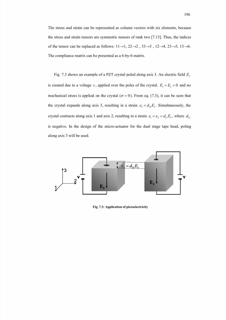
8/8/2019 BR PhD Dissertation
http://slidepdf.com/reader/full/br-phd-dissertation 228/248
196
The stress and strain can be represented as column vectors with six elements, because
the stress and strain tensors are symmetric tensors of rank two [7.13]. Thus, the indices
of the tensor can be replaced as follows: 11→1, 22→2 , 33→3 , 12→4, 23→5, 13→6.
The compliance matrix can be presented as a 6-by-6 matrix.
Fig. 7.3 shows an example of a PZT crystal poled along axis 3. An electric field 3 E
is created due to a voltage v , applied over the poles of the crystal. 1 2 0 E E = = and no
mechanical stress is applied on the crystal ( 0σ = ). From eq. (7.3), it can be seen that
the crystal expands along axis 3, resulting in a strain 3 33 3d E ε = . Simultaneously, the
crystal contracts along axis 1 and axis 2, resulting in a strain 1 2 13 3d E ε ε = = , where 13d
is negative. In the design of the micro-actuator for the dual stage tape head, poling
along axis 3 will be used.
3
2
1
v
3 33 3d E ε =
E3
v
E3
3
2
1
v
3 33 3d E ε =
E3
v
E3
Fig. 7.3: Application of piezoelectricity
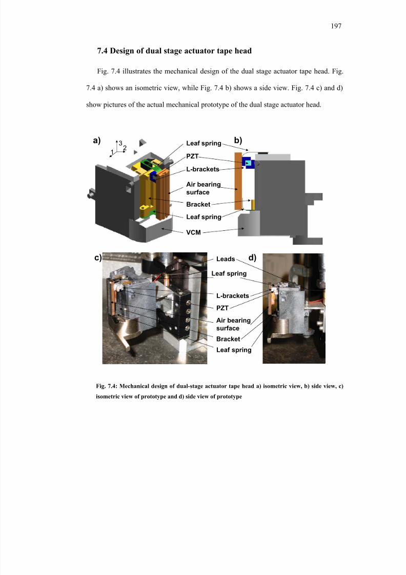
8/8/2019 BR PhD Dissertation
http://slidepdf.com/reader/full/br-phd-dissertation 229/248
197
7.4 Design of dual stage actuator tape head
Fig. 7.4 illustrates the mechanical design of the dual stage actuator tape head. Fig.
7.4 a) shows an isometric view, while Fig. 7.4 b) shows a side view. Fig. 7.4 c) and d)
show pictures of the actual mechanical prototype of the dual stage actuator head.
Air bearingsurface
VCM
PZT
Leaf spring
Leaf spring
L-brackets
Bracket
a) b)32
1
Leads
Leaf spring
Leaf spring
L-brackets
PZT
Air bearing
surface
c) d)
Bracket
Fig. 7.4: Mechanical design of dual-stage actuator tape head a) isometric view, b) side view, c)
isometric view of prototype and d) side view of prototype
8/8/2019 BR PhD Dissertation
http://slidepdf.com/reader/full/br-phd-dissertation 230/248
198
The design is based on a commercial tape head, shown in Fig. 7.1 a). Two L-
brackets, which encapsulate a PZT transducer, form the micro-actuator which drives the
second stage of the dual stage actuator tape head. The L-brackets are attached to the
tape head bracket and the air bearing surface, respectively. Two leaf springs at the top
and bottom of the air bearing surface provide alignment and stiffness. The leaf springs
are flexible with respect to bending around axis 1 (see Fig. 7.4 a)), but inhibit bending
around axis 2 and axis 3. Therefore, warping and torsion of the air bearing surface is
minimized. The PZT is a 2 x 2 x 2 mm stacked crystal (type PL022 from Physik
Instrumente (PI)).
7.5 Dynamics
7.5.1 Static response
Fig. 7.5 a) shows the displacement versus voltage of the PZT micro-actuator, while
Fig. 7.5 b) shows displacement versus voltage of the VCM. We observe that the PZT
micro-actuator exhibits a linear response with a small hysteresis. Hysteresis is caused
by crystalline polarization effects and molecular effects within the piezoelectric material
[7.13]. The use of a closed-loop control system allows accounting for the hysteresis
during dynamic operation [7.13]. From Fig. 7.5 b) we observe that the VCM has a
linear range between 0 and 2 Volts. Higher voltages lead to saturation of the VCM. As
can be seen from Fig. 7.5 b), the displacement-voltage curve levels off for voltages
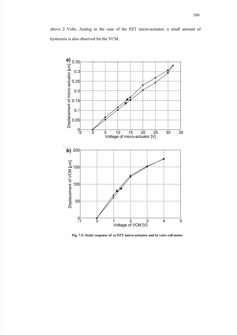
8/8/2019 BR PhD Dissertation
http://slidepdf.com/reader/full/br-phd-dissertation 231/248
199
above 2 Volts. Analog to the case of the PZT micro-actuator, a small amount of
hysteresis is also observed for the VCM.
-5 0 5 10 15 20 25 30 350
0.05
0.1
0.15
0.2
0.25
0.3
0.35
Voltage of micro-actuator [V]
D i s p l a c e m e n t o f m i c r o - a c t u a t o r [ µ m ]a)
-1 0 1 2 3 4 50
50
100
150
200
Voltage of VCM [V]
D i s p l a c e m e n t o f V C M [ µ
m ]
b)
Fig. 7.5: Static response of a) PZT micro-actuator and b) voice coil motor
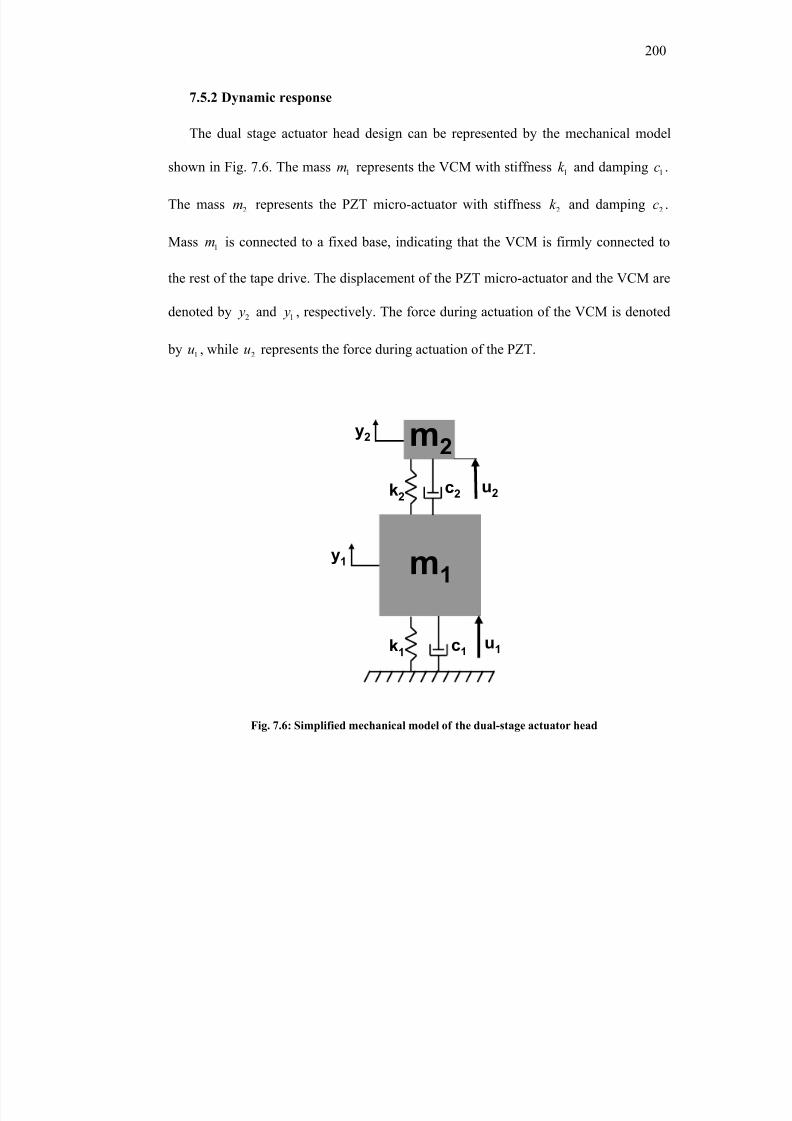
8/8/2019 BR PhD Dissertation
http://slidepdf.com/reader/full/br-phd-dissertation 232/248
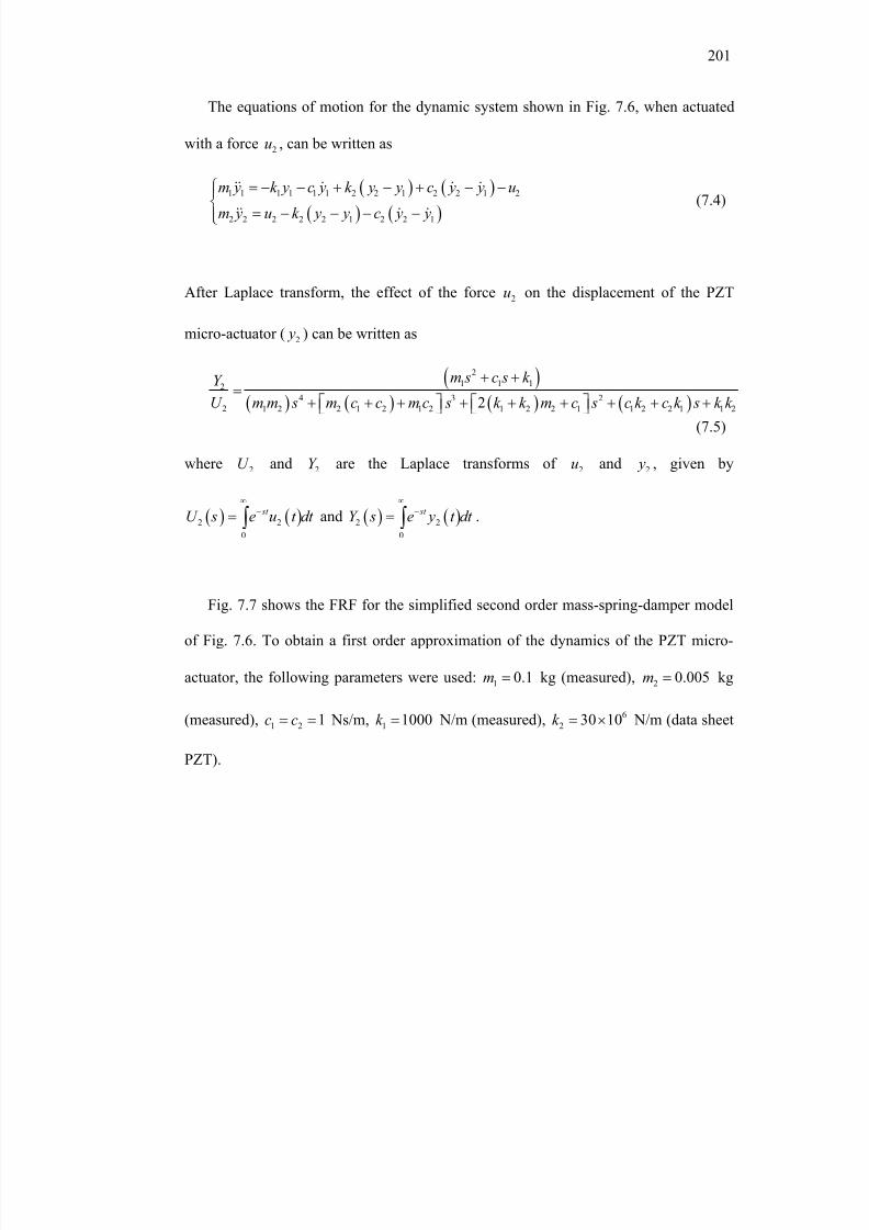
8/8/2019 BR PhD Dissertation
http://slidepdf.com/reader/full/br-phd-dissertation 233/248
201
The equations of motion for the dynamic system shown in Fig. 7.6, when actuated
with a force 2u , can be written as
( ) ( )( ) ( )1 1 1 1 1 1 2 2 1 2 2 1 2
2 2 2 2 2 1 2 2 1
m y k y c y k y y c y y u
m y u k y y c y y
= − − + − + − − = − − − −
(7.4)
After Laplace transform, the effect of the force 2u on the displacement of the PZT
micro-actuator ( 2 y ) can be written as
( )( ) ( ) ( ) ( )
2
1 1 12
4 3 2
2 1 2 2 1 2 1 2 1 2 2 1 1 2 2 1 1 22
m s c s k Y
U m m s m c c m c s k k m c s c k c k s k k
+ +
= + + + + + + + + + (7.5)
where 2U and 2Y are the Laplace transforms of 2u and 2 y , given by
( ) ( )2 2
0
st U s e u t dt
∞−= ∫ and ( ) ( )2 2
0
st Y s e y t dt
∞−= ∫ .
Fig. 7.7 shows the FRF for the simplified second order mass-spring-damper model
of Fig. 7.6. To obtain a first order approximation of the dynamics of the PZT micro-
actuator, the following parameters were used: 1 0.1m = kg (measured), 2 0.005m = kg
(measured), 1 2 1c c= = Ns/m, 1 1000k = N/m (measured), 6
2 30 10k = × N/m (data sheet
PZT).
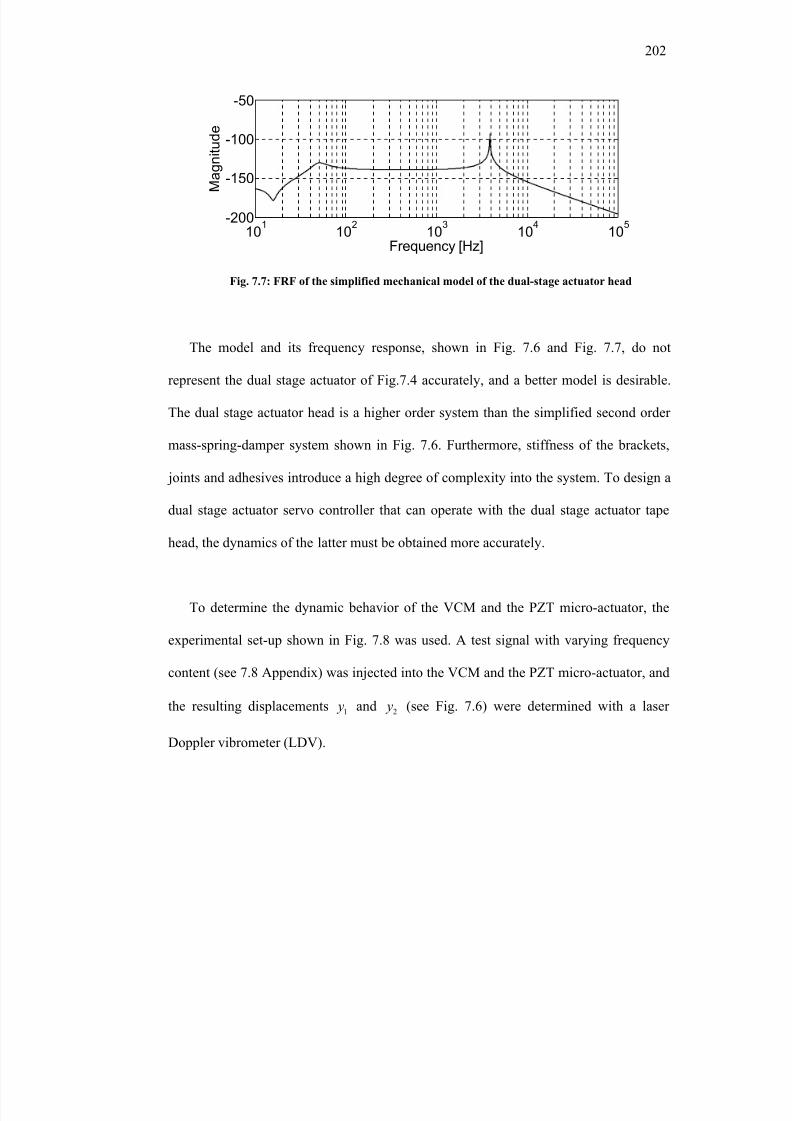
8/8/2019 BR PhD Dissertation
http://slidepdf.com/reader/full/br-phd-dissertation 234/248
202
101
102
103
104
105
-200
-150
-100
-50
M a
g n i t u d e
Frequency [Hz]
The model and its frequency response, shown in Fig. 7.6 and Fig. 7.7, do not
represent the dual stage actuator of Fig.7.4 accurately, and a better model is desirable.
The dual stage actuator head is a higher order system than the simplified second order
mass-spring-damper system shown in Fig. 7.6. Furthermore, stiffness of the brackets,
joints and adhesives introduce a high degree of complexity into the system. To design a
dual stage actuator servo controller that can operate with the dual stage actuator tape
head, the dynamics of the latter must be obtained more accurately.
To determine the dynamic behavior of the VCM and the PZT micro-actuator, the
experimental set-up shown in Fig. 7.8 was used. A test signal with varying frequency
content (see 7.8 Appendix) was injected into the VCM and the PZT micro-actuator, and
the resulting displacements 1 y and 2 y (see Fig. 7.6) were determined with a laser
Doppler vibrometer (LDV).
Fig. 7.7: FRF of the simplified mechanical model of the dual-stage actuator head
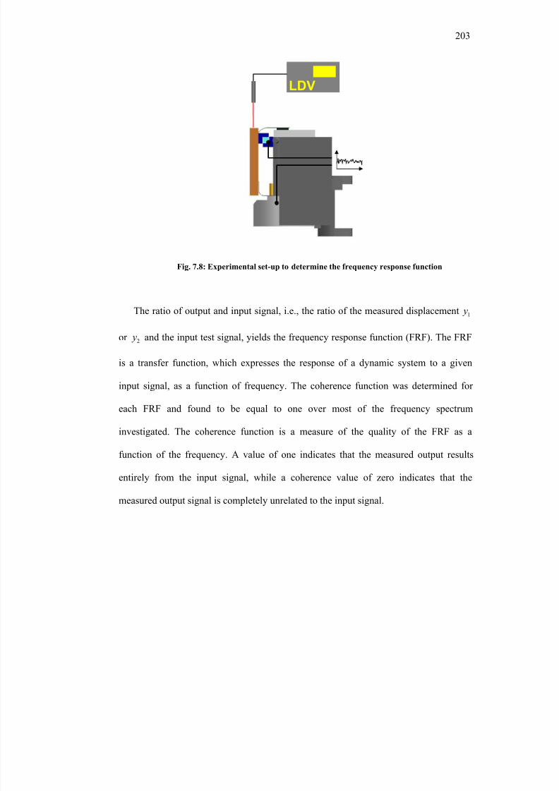
8/8/2019 BR PhD Dissertation
http://slidepdf.com/reader/full/br-phd-dissertation 235/248
203
LDVLDV
The ratio of output and input signal, i.e., the ratio of the measured displacement 1 y
or 2 y and the input test signal, yields the frequency response function (FRF). The FRF
is a transfer function, which expresses the response of a dynamic system to a given
input signal, as a function of frequency. The coherence function was determined for
each FRF and found to be equal to one over most of the frequency spectrum
investigated. The coherence function is a measure of the quality of the FRF as a
function of the frequency. A value of one indicates that the measured output results
entirely from the input signal, while a coherence value of zero indicates that the
measured output signal is completely unrelated to the input signal.
Fig. 7.8: Experimental set-up to determine the frequency response function
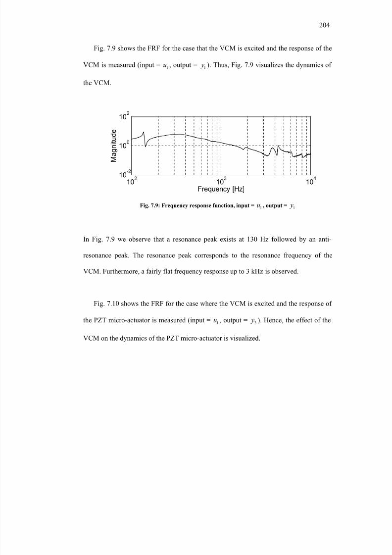
8/8/2019 BR PhD Dissertation
http://slidepdf.com/reader/full/br-phd-dissertation 236/248
204
Fig. 7.9 shows the FRF for the case that the VCM is excited and the response of the
VCM is measured (input = 1u , output = 1 y ). Thus, Fig. 7.9 visualizes the dynamics of
the VCM.
102 103 10410
-2
100
102
Frequency [Hz]
M a g n i t u d e
In Fig. 7.9 we observe that a resonance peak exists at 130 Hz followed by an anti-
resonance peak. The resonance peak corresponds to the resonance frequency of the
VCM. Furthermore, a fairly flat frequency response up to 3 kHz is observed.
Fig. 7.10 shows the FRF for the case where the VCM is excited and the response of
the PZT micro-actuator is measured (input = 1u , output = 2 y ). Hence, the effect of the
VCM on the dynamics of the PZT micro-actuator is visualized.
Fig. 7.9: Frequency response function, input =1u , output =
1 y
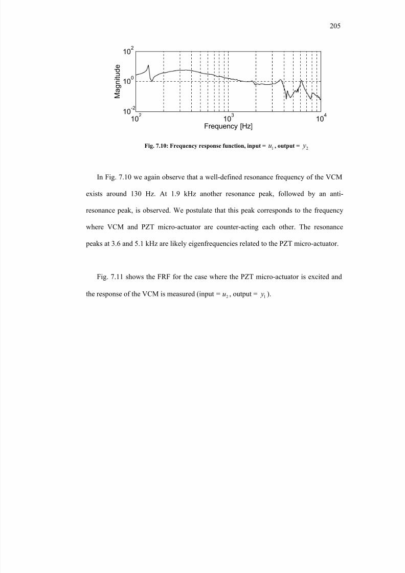
8/8/2019 BR PhD Dissertation
http://slidepdf.com/reader/full/br-phd-dissertation 237/248
205
102
103
104
10-2
100
102
Frequency [Hz]
M a
g n i t u d e
In Fig. 7.10 we again observe that a well-defined resonance frequency of the VCM
exists around 130 Hz. At 1.9 kHz another resonance peak, followed by an anti-
resonance peak, is observed. We postulate that this peak corresponds to the frequency
where VCM and PZT micro-actuator are counter-acting each other. The resonance
peaks at 3.6 and 5.1 kHz are likely eigenfrequencies related to the PZT micro-actuator.
Fig. 7.11 shows the FRF for the case where the PZT micro-actuator is excited and
the response of the VCM is measured (input = 2u , output = 1 y ).
Fig. 7.10: Frequency response function, input =1u , output =
2 y
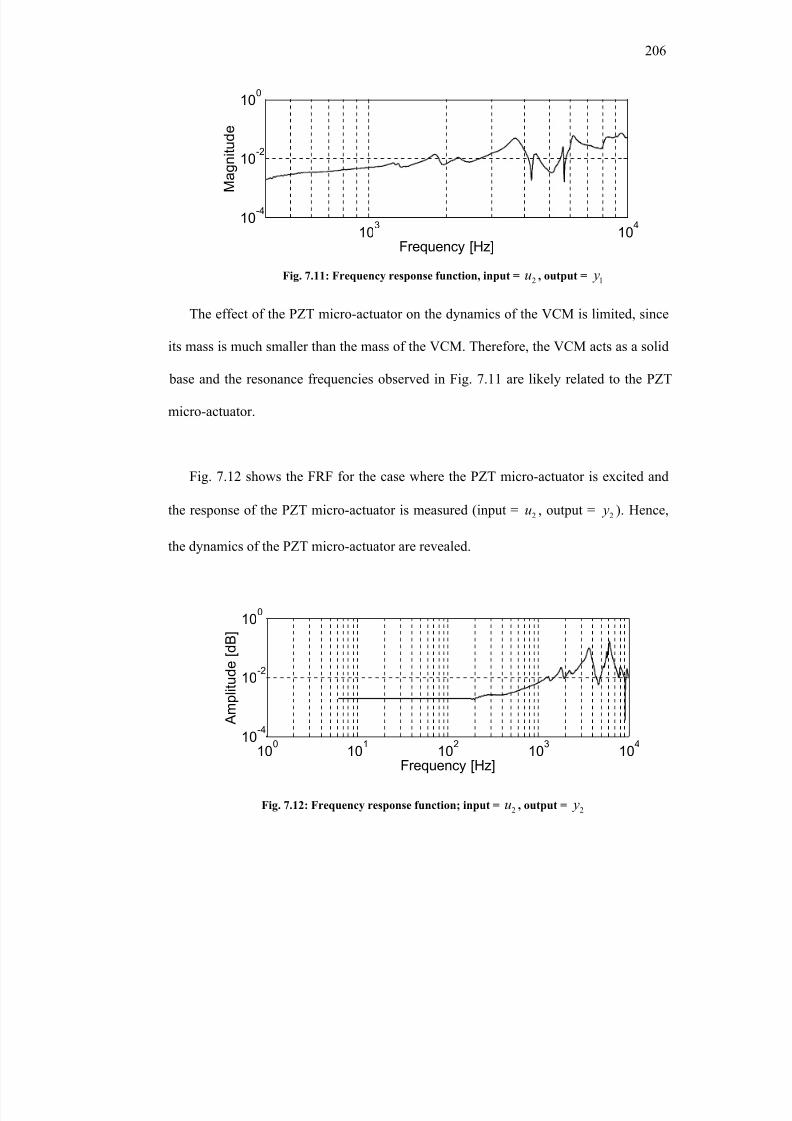
8/8/2019 BR PhD Dissertation
http://slidepdf.com/reader/full/br-phd-dissertation 238/248
206
103
104
10-4
10-2
100
Frequency [Hz]
M a
g n i t u d e
The effect of the PZT micro-actuator on the dynamics of the VCM is limited, since
its mass is much smaller than the mass of the VCM. Therefore, the VCM acts as a solid
base and the resonance frequencies observed in Fig. 7.11 are likely related to the PZT
micro-actuator.
Fig. 7.12 shows the FRF for the case where the PZT micro-actuator is excited and
the response of the PZT micro-actuator is measured (input = 2u , output = 2 y ). Hence,
the dynamics of the PZT micro-actuator are revealed.
100
101
102
103
104
10-4
10-2
100
A
m p l i t u d e [ d B ]
Frequency [Hz]
Fig. 7.12: Frequency response function; input =2u , output =
2 y
Fig. 7.11: Frequency response function, input = 2u , output = 1 y
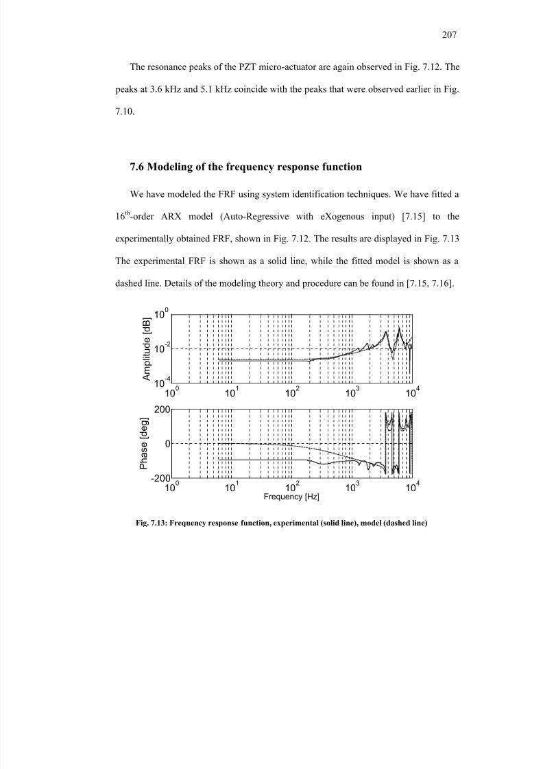
8/8/2019 BR PhD Dissertation
http://slidepdf.com/reader/full/br-phd-dissertation 239/248
207
The resonance peaks of the PZT micro-actuator are again observed in Fig. 7.12. The
peaks at 3.6 kHz and 5.1 kHz coincide with the peaks that were observed earlier in Fig.
7.10.
7.6 Modeling of the frequency response function
We have modeled the FRF using system identification techniques. We have fitted a
16th
-order ARX model (Auto-Regressive with eXogenous input) [7.15] to the
experimentally obtained FRF, shown in Fig. 7.12. The results are displayed in Fig. 7.13
The experimental FRF is shown as a solid line, while the fitted model is shown as a
dashed line. Details of the modeling theory and procedure can be found in [7.15, 7.16].
100
101
102
103
104
10-4
10-2
100
A m
p l i t u d e [ d B ]
100
101
102
103
104
-200
0
200
Frequency [Hz]
P h a s e [ d e g ]
Fig. 7.13: Frequency response function, experimental (solid line), model (dashed line)
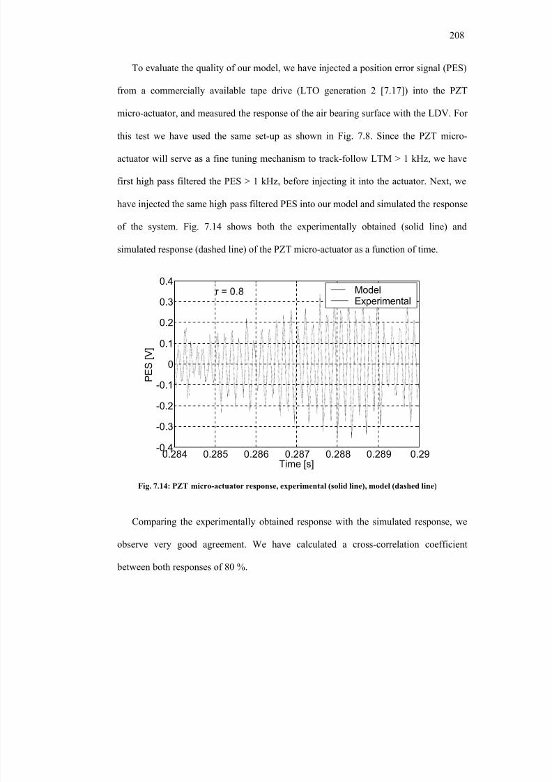
8/8/2019 BR PhD Dissertation
http://slidepdf.com/reader/full/br-phd-dissertation 240/248
8/8/2019 BR PhD Dissertation
http://slidepdf.com/reader/full/br-phd-dissertation 241/248
209
7.7 Conclusion
We have implemented the mechanical design of a dual stage actuator tape head for
high-bandwidth track-following. The new dual stage actuator tape head promises a
significant increase in track density for future high-performance tape drives. We have
developed a model based on system identification techniques. Good agreement between
the model and the experimental results for the dynamic performance of the new actuator
was observed.
The design presented in this chapter is purely a mechanical design. The next step
would be to include servo- and read/write capability. This requires the cables to be re-
routed around the PZT. The final step would be to redesign the injection molded parts
of the tape head, in order to accommodate the PZT, and to enable integration in a
commercial tape drive.
7.8 Appendix
A test signal with varying frequency content is generally referred to as a chirp
signal. In a linear chirp signal, the instantaneous frequency ( )c f t varies linearly with
time, i.e., ( ) ,0c c c f t f k t = + . ,0c f is the starting frequency at 0t = and ck is the rate of
frequency increase [7.14]. A chirp function is particularly interesting to determine a
frequency response function of a system since the signal can contain all desired
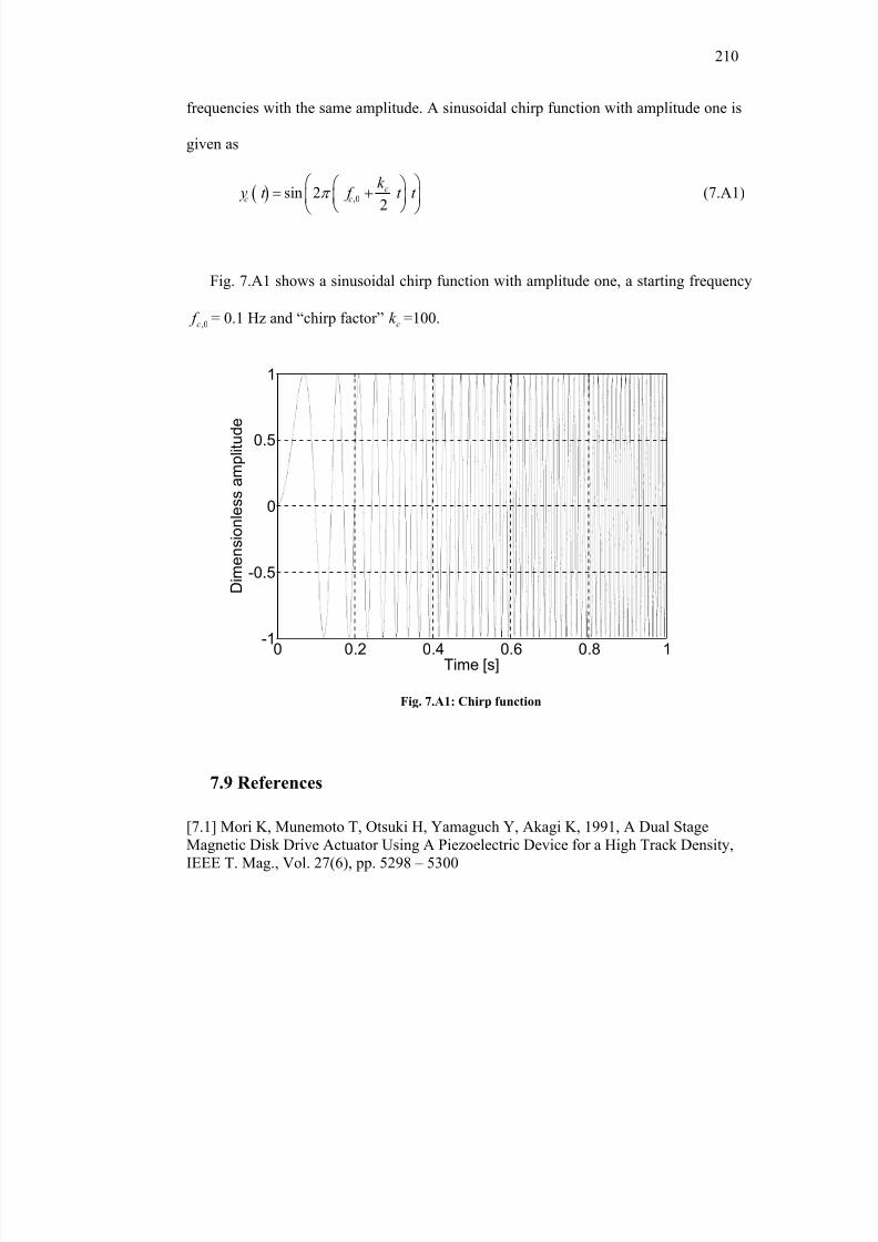
8/8/2019 BR PhD Dissertation
http://slidepdf.com/reader/full/br-phd-dissertation 242/248
210
frequencies with the same amplitude. A sinusoidal chirp function with amplitude one is
given as
( ) ,0sin 2 2
c
c c
k
y t f t t π
= + (7.A1)
Fig. 7.A1 shows a sinusoidal chirp function with amplitude one, a starting frequency
,0c f = 0.1 Hz and “chirp factor” ck =100.
0 0.2 0.4 0.6 0.8 1-1
-0.5
0
0.5
1
D i m e n s i o n l e s s a m p l i t u d e
Time [s]
7.9 References
[7.1] Mori K, Munemoto T, Otsuki H, Yamaguch Y, Akagi K, 1991, A Dual Stage
Magnetic Disk Drive Actuator Using A Piezoelectric Device for a High Track Density,
IEEE T. Mag., Vol. 27(6), pp. 5298 – 5300
Fig. 7.A1: Chirp function
8/8/2019 BR PhD Dissertation
http://slidepdf.com/reader/full/br-phd-dissertation 243/248
211
[7.2] Koganezawa S, Takaishi Y, Mizoshita Y, Uematsu Y, Yamada T, Hasegawa S,Ueno T, 1996, A Flexural Piggyback Mill-Actuator for Over 5 Gbit/in.² Density
Magnetic Recording, IEEE T. Mag., Vol. 32(5), pp. 3908 – 3910
[7.3] Hirano T, Fan LS, Lee WY, Hong J, Imaino W, Pattanaik S, Chan S, Webb P,
HorowitzR, Aggarwal S, Horsley D, 1998, High-Bandwidth High-Accuracy RotaryMicroactuators for Magnetic Hard Disk Drive Tracking Servos, IEEE/ASME T. Mech.,Vol. 3(3), pp. 156 – 165
[7.4] Koganezawa S, Uematsu Y, Yamada T, 1999, Dual Stage Actuator System for Magnetic Disk Drives Using a Shear Mode Piezoelectric Microactuator, IEEE T. Mag.,
Vol. 35(2), pp. 988 – 992
[7.5] Nakamura S, Numasato H, Kobayashi M, Naniwa I, 2002, A Push-Pull Multi-Layered Piggyback PZT Actuator, Microsyst. Technol., Vol. 8, pp. 149 – 154
[7.6] Fan LS, Ottesen HH, Reiley TC, Wood RW, 1995, Magnetic Recording HeadPositioning at Very High Track Densities Using a Microactuator-Based, Two-Stage
Servo System, IEEE T. Ind. Electr., Vol. 42(3), pp. 222 – 233
[7.7] Evans RB, Griesbach JS, 1999, Piezoelectric Microactuator for Dual Stage
Control, IEEE T. Mag., Vol. 35(2), pp. 977 – 982
[7.8] Horsley DA, Wongkomet N, Horowitz R, Pisano AP, 1999, Precision Positioning
Using a Microfabricated Electrostatic Actuator, IEEE T. Mag., Vol. 35(2), pp. 993 –
999
[7.9] Tang W, Temesvary V, Miller R, Desai A, Tai YC, Miu D, 1995, SiliconMicromachined Electromagnetic Microactuators for Rigid Disk Drives, IEEE T. Mag.,Vol. 31(6), pp. 2964 – 2966
[7.10] Sashida T, Kenjo T, 1993, An Introduction to Ultrasonic Motors, CalarendonPress, Oxford
[7.11] Uchino K, 1997, Piezoelectric Actuators and Ultrasonic Motors, Kluwer Academic Publishers, Boston/Dordrecht/London
[7.12] Ikeda T, 1990, Fundamentals of Piezoelectricity, Oxford University Press,
Oxford/New York/Tokio
[7.13] Moheimani SOR, Fleming AJ, 2006, Piezoelectric Transducers for Vibration
Control and Damping, Springer Verlag, London
[7.14] Proakis JG, Manolakis DG, 1988, Introduction to Digital Signal Processing,
McMillan Publishing Company, New York

8/8/2019 BR PhD Dissertation
http://slidepdf.com/reader/full/br-phd-dissertation 244/248
212
[7.15] van den Bosch PPJ, van der Klauw AC, 1994, Modeling, Identification and
Simulation of Dynamical Systems, CRC Press, Boca Raton
[7.16] Claes M, 2006, Frequency Domain Weighted Subspace Identification With
Application To a Tape Servo System, Master Thesis, University of California SanDiego
[7.17] Jacquette GA, 2003, LTO: A Better Format for Mid-Range Tape, IBM J. Res. &
Dev., Vol. 47( 4), pp. 429 - 444
8/8/2019 BR PhD Dissertation
http://slidepdf.com/reader/full/br-phd-dissertation 245/248
213
8. Summary
In this dissertation, an experimental and theoretical analysis of sliding contacts and
dynamics of tape transports has been presented. Dynamics of tape transports are
important since lateral vibrations of the magnetic tape, generally referred to as lateral
tape motion (LTM), limit the track density on a tape.
Tape tension transients and tape edge contact contribute significantly to lateral tape
motion in tape transports. An optical non-contact tape tension sensor was implemented
and used to characterize tape tension transients during tape drive operation. Good
correlation between tape tension transients and LTM was found. Furthermore, a new
method to measure tape edge contact force, based on acoustic emission, has been
introduced. After calibrating the acoustic emission (AE) probe, it was used as an
“artificial flange”, to measure impact force. The AE sensor was fixed just above a roller
in a tape drive, thereby replacing the original flange. Using this method, it was observed
that tape edge contact creates LTM, especially in the 1-2 kHz frequency range.
Additionally, tape edge impact force was observed to be most severe for a half full tape
pack. A simplified one-dimensional impact oscillator model was shown to predict tape
edge contact well.
In this dissertation, the dynamic behavior of a tape as it moves over a cylindrical
guide has been investigated theoretically as well as experimentally. The equation of
motion was derived and solved numerically. The model was then validated with
8/8/2019 BR PhD Dissertation
http://slidepdf.com/reader/full/br-phd-dissertation 246/248
214
experimental data. Good agreement between the model and the experiments was found
in the time domain as well as in the frequency domain. Using this model, we have
investigated the effect of bending stiffness on tape dynamics. In addition, the influence
of operating parameters on LTM was studied, as the tape moves over a cylindrical
guide. The tape/guide contact length, which is function of the wrap angle and the guide
radius, was found to have a major influence on LTM, while the influence of tape
tension, friction coefficient and tape thickness appeared to be less significant.
When the tape is in contact with tape drive components such as a cylindrical guide,
the tape dynamics are related to frictional interaction between the tape and the guide
surface. Therefore, a model for the dynamic friction coefficient between the polymeric
tape and a metallic cylindrical guide was proposed. The model extends the well-known
“belt-drive” equation and introduces the effects of operating and design parameters on
the tape/guide friction coefficient. Both load sharing and asperity contact effects were
taken into account. The theoretical predictions of the model showed good agreement
with experimental measurements of the tape/guide friction coefficient.
The last part of the dissertation focuses on improvements that can be made to tape
transport design in order to yield lower LTM and thus improved tape transport. First,
the idea of laser surface textured (LST) guides was presented. The surface of LST
guides are covered with micro-dimples which enhance the formation of an air bearing,
compared to smooth guides. Enhanced air bearing formation was shown to reduce the
transition speed between boundary lubrication and hydrodynamic lubrication. The
8/8/2019 BR PhD Dissertation
http://slidepdf.com/reader/full/br-phd-dissertation 247/248
215
friction coefficient was found to be almost independent of the tape speed, when using
LST guides. This is very beneficial to avoid tape wear during start/stop of a tape drive
and provides stability to the tape drive operation. The effect of LST on the friction
coefficient was investigated experimentally as well as numerically.
Another improvement that can be made in commercial tape drives is the
introduction of a dual stage actuator head. The tape head, actuated by a voice coil motor
(VCM), and controlled by a servo loop, attempts to follow the lateral tape motion. To
improve the bandwidth of the servo controller, the implementation of a second stage
actuator, based on a piezo crystal, was proposed. The main idea is that the VCM stage
follows the low frequency LTM (< 1 kHz), while the second stage follows the high
frequency LTM (> 1 kHz). The second stage moves only the air bearing surface with
the read/write heads while the VCM actuates the whole tape head mass. Hence, only a
small mass needs to be actuated by the second stage. This increases the bandwidth. A
prototype of a dual stage actuator head was built and tested. The dynamics of the newly
proposed dual stage actuator head was investigated and captured in a mathematical
model. The dynamics of the model showed good agreement with experimental
observations. The prototype promises excellent performance in following high
frequency LTM up to 2.5 kHz, which represents a bandwidth expansion of at least 1.5
kHz compared to current state-of-the-art commercial tape drive heads.
As track density needs to be increased to accommodate higher recording densities,
LTM needs to be reduced. A thorough understanding of sliding contacts and friction is
8/8/2019 BR PhD Dissertation
http://slidepdf.com/reader/full/br-phd-dissertation 248/248
216
essential in achieving this goal; improved guiding technologies need to be developed. A
novel idea could be “active guiding”, where a guide is controlled by a servo actuator
and can be tilted to “steer” the tape laterally, thereby counter-acting the LTM. Also, the
effect of the laterally actuated tape head on the LTM in the tape path, due to frictional