an overview of digital terrain models

II Simpósio Brasileiro de Geomática Presidente Prudente - SP, 24-27 de julho de 2007V Colóquio Brasileiro de Ciências Geodésicas ISSN 1981-6251, p. 091-099

AN OVERVIEW OF DIGITAL TERRAIN MODELS

PH.D. CANDIDATE SILVANE KAROLINE SILVA PAIXÃO

PROFª DRª DARKA MIOC PROFª DRª. SUE NICHOLS

University of New Brunswick – UNB

Department of Geodesy and Geomatic Engineering {silvane.paixao, mioc, nichols}@unb.ca

RESUMO – O fundamental objetivo do modelo digital do terreno (MDT) é a acurável representação da superfície. Para isso, é necessário que haja algoritmos eficientes e precisos para gerar essas superfícies com a massa de dados adquiridos. Alguns interpoladores serão discutidos nesse artigo. Mas o foco será a modelagem pelo GRID e TIN. Essa explicação será dada em formato de aplicações e comparações. Os convencionais métodos de visualização geralmente requerem tempo e muitos possuem limitação de análises. O sistema de visualização interativa (IVS), esta nova tecnologia de visualização tridimensional, mantém o mais próximo contato entre o usuário e o sistema, com maior capacidade e velocidade. Mapas digitais do terreno, elementos vetoriais gráficos e imagens de satélites, entre outros podem ser superposto e analisados em uma única cena. Este artigo mostrará algumas funcionalidades dos softwares Fledemaus, criado pela IVS3D e do HIPS and SIPS desenvolvido pela CARIS. Estes softwares permite a ação do usuário em tempo real, com interação 3D da tela com complexas cenas e com alta resolução, de modo a facilitar a extração de informações e a combinação de dados. ABSTRACT - The fundamental aim of a digital terrain model (DTM) is to represent a surface accurately, such that elevations can be estimated for any given location. It is, therefore, necessary to have efficient and precise algorithms for the computation of surface elevations between given points. Interpolation techniques are addressed in this paper. The focus will be on GRID and TIN models. Some applications will also be explained and compared. Conventional visualization methods often require significant processing time, which limits high-throughput analysis. Interactive visualization systems (IVS), the new 3D visualization technologies, maintain a closed loop between the user and the system and, thus, need to be very fast. Objects such as digital terrain maps, point clouds, lines, polygons, satellite imagery, etc. can all be loaded and analyzed in a single scene. The software explored in this paper is Fledermaus, managed by IVS3D, and HIPS and SIPS, developed by CARIS. These pieces of software allow users to have a real-time and interactive 3D display. Very large and complex scenes can be seen in high resolution. Through combined data, users can rapidly gain insight and extract more information.

1 INTRODUCTION

Terrain data is usually compiled from survey point elevation, from contour lines, digitized from existing maps, or from photographic points and/or line registration (BERNHARDSEN, 1999). The digital representation of the terrain surface is called either a digital terrain model (DTM) or digital elevation model (DEM). Essentially, DTMs comprise various arrangements of individual points in x-y-z coordinates, computing new spot height from the originals (BERNHARDSEN, 1999).

Often, DEMs are used to calculate slope and aspect depending on data quality. With a DTM certain

applications are possible, such as drainage feature identification, geomorphological characterization, viewshed analyses and radio wave propagation modeling (HEARNSHAW and UNWIN, 1994).

To construct the DTM interpolation methods have to be considered. The result depends on the accuracy of the data input and the choice of the interpolation method. Some of these interpolation methods and their surface representation are described in this paper.

Recently, technologies have improved 3D DTM visualization. Interactive visualization systems provide a realistic 3D. These models are useful for evaluation, design and training in virtual environments, such as those

S. Paixão; D. Mioc and S. Nichols

II Simpósio Brasileiro de Geomática Presidente Prudente - SP, 24-27 de julho de 2007V Colóquio Brasileiro de Ciências Geodésicas

found in architectural and mechanical CAD flight simulation and virtual reality (BILIRIS et al., 1996).

By adding interactivity to a visualization system, the understanding of the relationships and patterns within the spatial data can be improved (SIMONETTI, 2003). Applications of the interactive 3D visualization are unlimited. It is applied in 3D exploration of ocean floor surfaces, planning for submarine cable routes, and simulating complex climate data sets. There are also applications in a wide range of fields, including environmental impact assessment, mining, geology, and planning for dredging.


This paper will illustrate the performance of the

software Fledermaus, developed by IVS3D and the software HIPS and SIPS developed by CARIS.

2 DIGITAL TERRAIN MODELS 2.1 Regular Grid Model

In the grid model terrain relief is described by the

array of vertical coordinates of points. The points are located in a regular grid (VANÍČKOVÁ, L. and VANÍČEK, 2005). According to Bernhardsen (1999) in this model the elevation is assumed constant within each cell of the grid. The size of cells is constant in a model, so areas with a greater variation of terrain may be described less accurately than those with less variation. Elevation values are stored in a matrix and the contiguity between points is expressed through the column and row (see Figure 1).

Figure 1 – Regular grid sampling pattern

Chrisman (1997) states that the simplest definition of interpolation involves a process to determine the value of a continuous attribute at some location intermediate between known points.

A conventional distinction between interpolation

methods is between global and local approaches. Global techniques seek to fit a surface model using all known data points simultaneously, whereas local interpolators focus on specific regions of the data plane at one time (MARTIN, 1996).

According to Druck et al. (2004) kriging is

considered a statistic method with local and global effects, because it uses many estimation techniques. Surface prediction is based on modeling the structure of the spatial correlation.

The most commonly used interpolation method for a regular grid DEM is the patchwise polynomial interpolation. The general form of this equation (1) for surface representation is (KIDNER et al., 1999): hi=a00 + a10x+a01y+ a20x2 + a11xy+ a02y2+ a30x3+a21 x2y+ a12xy2 + a03y3+ a31 x3y+ a22 x2y2+ a13 xy3+ a32 x3y2+ a23 x2y3+ a33 x3y3+…. am n xmyn

(1) Where:

hi is the height of an individual point i, x and y are its rectangular coordinates of I; a00, a10, a01, …, amn are the coefficients of the polynomial. Since the coordinates of each vertex are known,

the values of the polynomial coefficients can be determined from the set of simultaneous equations that are set up, one for each point. For any given point with known coordinates x, y, the corresponding elevation can be determined by a substitution into this equation 1 (KIDNER et al., 1999). 2.1.1 Global Interpolation: Kriging

Kriging was originally developed as a geostatistical interpolation technique that considers both the distance and the degree of variation between known data points when estimating values in unknown areas (ANON., 2007a). The basic premise of this interpolation is that every unknown point can be estimated by the weighted sum of the known points (KERRY and HAWICK, 1998; ANON., 2007a).

Bernhardsen (1999) states that Kriging is based on the theory that the same pattern of variation can be observed at all locations and uses a mathematical function to model the spatial variation in values within the input sample points. This interpolation rests on the assumptions of regionalized variable theory, that the spatial variation of a variable can be expressed in terms of a structure component, a random spatially correlated component, and a random error term (MARTIN, 1996).

Kriging is similar to Inverse Distance Weighted

interpolation (IDW) in that it weights the surrounding measured values to derive a prediction for unmeasured location. The general equation (2) for both interpolators is formed as a weighted sum of the data (ANON., 2007b):

(2)

Where: Z (Si) is the measured value at the ith location; λi is an unknown weight for the measured value at the ith location; N is the number of measured value.



In IDW, the weights, λi depend solely on the distance to the prediction location. However, in Kriging, the weights are based on the distance between the measured points, the predicted location, and on overall spatial arrangement among the measured points and their values.

In the IDW method, the rate of correlations and

similarities between neighbors is proportional to the distance between them. It can be defined as a distance reverse function of every point from neighboring points. Equation 3 defines the IDW (ZIARY and SAFARI, 2007):

(3) Where:

Z (Si) is the measured value at the ith location; d1 is the distance of sample point to estimated point; N is a coefficient that determines weigh based on a distance.

Generally the estimation of an unknown point only

takes a limited range of the known values into consideration. The reason for this is that known values at a great distance from the unknown point are unlikely to be of great benefit to the accuracy of the estimate (KERRY and HAWICK, 1998).

2.1.2 - Local Interpolation: Bilinear

Normally, Bilinear interpolation like bi-cubic interpolation are used when a data has a regular grid or when it is desired to create a new grid from an existed one (NAMIKAWA et al., 2003).

Bilinear interpolation determines the output cell

value with a weighted distance average of the four nearest input cell centers (Figure 2). This method is appropriate for continuous data, but not for discrete data because values are averaged, and hence the cell values may be altered (ANON., 2007d). Kidner et al. (1999) define bilinear interpolation as calculated by equation 4 according to Figure 2.

hi=a00 + a10x+a01y+a11xy Where:

a00= h1 (4a) a10= h2-h1 (4b)

a01= h3-h1 (4c) a11= h1-h2-h3+h4 (4d)

Figure 2 – Bilinear calculation in Grid based (KIDNER et al., 1999)

This method is computationaly faster than the bi-

cubic interpolation, with the disadvantage that it produces surfaces which are a little smoothed. It can be used when a soft appearance of the surface it is not needed (NAMIKAWA et al., 2003).

d

-N

1x

d-N

1

Li at al. (2005) describe interpolation on a

triangular facet. This can also be done in similar way to grid based bilinear interpolation. See equation 5 and Figure 3.

Zp = Z1+(Z2 - Z1) x (Xp – X1) / (X2 – X1) (5)

Where:

Z1 = ZA+(ZB - ZA) X (X1 – XA) / (XB – XA) (5a) Z2 = ZA+(ZC - ZA) X (X2 – XA) / (XC – XA) (5b)

A

p 1 2 B C Figure 3 - Bilinear calculation in triangle based (LI et al., 2005) 2.2 TIN Model

A Triangulated Irregular Network (TIN) is a surface representation composed of a network of triangles derived from irregularly spaced point data (Figure 4). The Z values enable the facets of each triangle to be visualized as a three-dimensional surface, making for a striking and efficient representation of a landscape (ANON., 2007c)

(4)

Figure 4 – TIN sampling pattern Each triangle in a TIN connects three neighboring

points so that the plane of the triangle fits the surface sufficiently (MARTIN, 1996). The inclination of the


Shojaee et al. (2006) enumerate the follow properties of Delaunay triangulation:

terrain is assumed to be constant within each triangle; however the area of each triangle may vary. In a TIN model the more the terrain varies, the smaller are the areas represented (BERNHARDSEN, 1999).

• Local empty-circle property: the circum-circle of any triangle in Delaunay triangulation does not contain the vertex of the other triangle in its interior;

TIN models can be stored numerically as random points and break lines. A break line connects a set of random points in such a way that a triangle’s sides do not cross the break line (SARKKILA, 2007).

• Max-min angle property: the diagonal of tetrahedral maximizes the minimum of the six internal angles associated with each of the two possible triangulations of a tetrahedral;

• Uniqueness: there is a unique Delaunay triangulation from a set of points; A Voronoi Diagram is a geometric structure that

represents proximity information for a set of points or objects. A Voronoi Diagram represents the regions of a plane that are closer to a particular point in the plane than to any other point as shown in Figure 6 (OKABE et al., 1992).

• Boundary property: external edges of Delaunay triangulation make the convex hull of the point set.

Okabe et al. (1992) and Li et al. (2005) define some algorithms for constructing the Voronoi diagram:

• Naive Method: This is used to generate many samples of Voronoi polygons to obtain statistical data such as distribution of the number of edges per polygon. The output does not include explicit information about the topological structure of the diagram;

With the Delaunay triangulation, any point will fall into one specific triangle. One of the vertices of the triangle will be the closest point, if the triangulation used is the Delaunay method (CHRISMAN, 1997). An advantage of the Delaunay Triangulation is that the resulting triangulation network is independent of the start point (LI et al., 2005). • Walking Method: Voronoi vertices and edges are

constructed one by one in the order in which a traveler walks along the edges of the diagram;

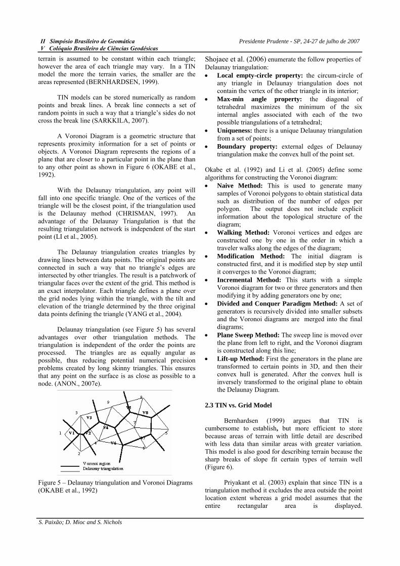
The Delaunay triangulation creates triangles by drawing lines between data points. The original points are connected in such a way that no triangle’s edges are intersected by other triangles. The result is a patchwork of triangular faces over the extent of the grid. This method is an exact interpolator. Each triangle defines a plane over the grid nodes lying within the triangle, with the tilt and elevation of the triangle determined by the three original data points defining the triangle (YANG et al., 2004).

• Modification Method: The initial diagram is constructed first, and it is modified step by step until it converges to the Voronoi diagram;

• Incremental Method: This starts with a simple Voronoi diagram for two or three generators and then modifying it by adding generators one by one;

• Divided and Conquer Paradigm Method: A set of generators is recursively divided into smaller subsets and the Voronoi diagrams are merged into the final diagrams;

Delaunay triangulation (see Figure 5) has several

advantages over other triangulation methods. The triangulation is independent of the order the points are processed. The triangles are as equally angular as possible, thus reducing potential numerical precision problems created by long skinny triangles. This ensures that any point on the surface is as close as possible to a node. (ANON., 2007e).

• Plane Sweep Method: The sweep line is moved over the plane from left to right, and the Voronoi diagram is constructed along this line;

• Lift-up Method: First the generators in the plane are transformed to certain points in 3D, and then their convex hull is generated. After the convex hull is inversely transformed to the original plane to obtain the Delaunay Diagram.

2.3 TIN vs. Grid Model

Bernhardsen (1999) argues that TIN is cumbersome to establish, but more efficient to store because areas of terrain with little detail are described with less data than similar areas with greater variation. This model is also good for describing terrain because the sharp breaks of slope fit certain types of terrain well (Figure 6).

Priyakant et al. (2003) explain that since TIN is a triangulation method it excludes the area outside the point location extent whereas a grid model assumes that the entire rectangular area is displayed.

Figure 5 – Delaunay triangulation and Voronoi Diagrams (OKABE et al., 1992)




(a) (b) Figure 6 – Terrain relief representation of (a) grid and (b) TIN surface (PRIYAKANT et al., 2003)

One advantage of grid models is that the

mathematical processing is easy, but the disadvantage is the inaccuracy. The problem with a grid model is that it can not accurately describe surface points which do not coincide with grid points. This could be improved with a denser grid, but would lead to excessively large files with redundant data (SARKKILA, 2007).

According to Chrisman (1997) grids can model

flow reasonably efficiently. If cells are processed from highest elevation downward, the drainage accumulation can occur without needing to model it as a topological network.

Slope degrees and directions are useful in

simulations of precipitation runoff and in defining drainage areas, as Bernhardsen (1999) has cited. TIN,

which comprise sloping triangular surfaces, are ideal for simulating terrain surface conditions. Chrisman (1997) also adds that a TIN can handle both overland and channel flow. The triangles cover the whole area and can route flow from areas downhill unambiguously.

TIN are also fully represent the subtle elevation

differences required identifying the peaks and valleys in an elevation surface (BERNHARDSEN, 1999). Because population density and census tracts have irregular distribution, TIN has also been used to create the surface (CHRISMAN, 1997).

On the other hand, a grid is useful for weather

maps, e.g. identifying temperature and barometric pressure gradients. The impact of forest harvest on scenic beauty, FM radio transmissions, border control and many other intervisibility applications also use grid methods. The geometry of visibility along a line of sight is simple and strongly dependent on the choice of the height of the observer (CHRISMAN, 1997).

Chrisman (1997) describes others examples of grid model, such as accumulated cost surfaces which maximize routes, travel time and transportation, and cost surface construction that better locate natural gas, water or sewerage pipelines.

Table 1 shows a summary of each model and

attributes (NAMIKAWA et al., 2003; OKABE et al., 1992 and ROTTENSTEINER, 2001).

Table 1- Comparison of Grid and TIN Model

Grid Model TIN Model Spatial Distri-

bution Regular. Corner points at the grid are estimated. Irregular. Corners points at the grid

belong to the data.

Storage

Grid intersections may be stored as a matrix in which both their location and topological relationship are defined implicitly. It is necessary to store only the Z values.

Topological relationships of the facets of a TIN must be explicitly stored.

Point density

Fixed due to the matrix structure. Usually, a trade-off between storage capacities and precision is sought. Highest or lowest points are rarely sampled, since they are not likely to fall directly on the sample grid.

Variable because the original data points are used. TINs can include the highest/ lowest points.

Robustness Robust estimation procedures can be applied. Problems appear with inhomogeneous point distributions

Problems due to the non-uniqueness of the ordering criterion.

Smoothing

Since the generation algorithm is based on least squares adjustment, grid based methods perform smoothing. There is inability to use various grid sizes to reflect areas of different complexity of relief.

Difficult to achieve because the original data points are used. Can increase sampling in zones of high relief.



Applicability

Restrictions due to the 2.5D characteristics. Simple algorithms can be found for many tasks. Problems representing surfaces with accentuated local variations.

More general than grid based methods, but also restricted. More difficult algorithms are required. It better represents inhomogeneous surfaces with accented local variations.

3 DTM VIZUALIZATION 3.1 Contour Lines

An isoline is a closed loop of a contour that becomes an isolated polygon. These isolated polygons never cross over one other. A collection of contours is therefore created by a regular spacing of discrete intervals. A linear interpolation proportions the value between contours values as shown in Figure 7 (CHRISMAN, 1997).

Grid point elevations are interpolated from the

elevations at the intersection of the original data lines and the lines of the grid. In this case grid points on either side of the contours lines are identified (BERNHARDSEN, 1999). The TIN implies linear interpolation between the vertices of the triangles. To produce contours, there is still a tracing stage, and usually a step to smooth the linear sections into a more conventional curved form (CHRISMAN, 1997).

Figure 7 – Linear interpolation between adjacent contour lines (from CHRISMAN, 1997)

Some constrains about flat terrain are observed by

Chrisman (1997) in the Figure 8. In flat terrain, the next contour can be far away, so that triangles may connect points along a single contour. The resulting triangulation produces large areas with absolutely flat terrain (see Figure 8, case a). Additionally, where contours are

closely spaced, the power of a TIN comes from building a triangle that crosses many contours lines (see Figure 8, case b).

(Case b) In steep areas, contours

are closed and too any triangles are genetrated.

In flat areas, triangles may connect points along single contour. Area should be above the contour level.

Acsatrawn

Figure 8 – Fitting triangles to contours (from HR1997) 3.2 Animation Techniques for DTM visualiza

Interactive visualization systems displaya three-dimensional model as seen from a observer's viewpoint under control by a user. are rendered smoothly and quickly enough, an real-time exploration of a virtual environmeachieved as the simulated observer moves thmodel (BILIRIS et al., 1996).

To have a better understanding of

visualization systems the following charactedescribed (LOKUGE and ISHIZAKI, 1995): • Reactive display: The system provides us

responsive visual environment. It means thuser specifies a query, the display reacts into reflect the input request.

• Conversational interaction: The useinformation seeking dialogue as a minteraction enables a continuous exploratiinformation space.

• Context preservation: The system manotion of current state and presents the information within this context. This prefrom getting lost in the complex informatio

Linear interpolation assigns an elevation value between the two adjacent contours, based on the distance between them and the point in question.

Interpolation fline of steepest descent; easy to locate with dense contours.

ollows

nterpolation

wo

Somewhere in here is a pass, linear iwill misbehave, because the tadjacent contours are of same value.

Away from contours lines, the local trend is not easy to determine.

(Case a) In flat areas, matchinpoints aredifficult to locate

g

A TIN triangulatiopeaks and course across contour lines.

m

djacent ontours are of me value, so iangles will ppear flat, hen they are ot.

ISMAN,

tion

images of simulated If images illusion of nt can be rough the

interactive ristics are

ers with a at when a real time

of an odel of

on of the

intains a requested vents one n space.

n works from lines, cutting



• Visual clarity: Dynamic use of various visual design techniques proposed is integrated to enhance the clarity of the display by reducing users' cognitive load.

• Adaptive knowledge base: The knowledge base can be customized for specific user preferences.

Simonetti (2003) enumerates several goals that can

be achieved through visualization, such as: • Explore available data at various levels of detail; • Accomplish a greater sense of engagement with data; • Give users a better understanding of data; • Discover details, relations and patterns within the

data through exploration.

User are allowed to modify the presentation of the data, such as changing the coloring, transparency, viewpoint, and so on, with a quick response time to their actions (SIMONETTI, 2003).

Through the interactive graphical user interface,

we can look at the fluid surface pressures, check the velocity vector field, change the viewing angle, adjust boats' respective locations, add floating objects, and apply some other controls and manipulations for interactive visualization (CHEN et al., 1996).

In terrain visualization, “fly-through” and “walk-

through” are the most common animation technique. The animated image sequence is produced in an order of space, by moving the viewpoint along a certain track. They are explained by Li et al (2005): • Fly-through – provides a continuous bird’s eye view

to the landscape. The viewpoint can be moved in any direction in the 3D space;

• Walk-through – special case of fly-through, the walk-through mimics the human view while walking. The viewpoint is low and its movement in vertical direction is restricted.

Two software packages for visualization originated

at the University of New Brunswick. Fledermaus software developed by Interactive Visualization Systems - IVS3D, and HIPS and SIPS software made by CARIS.

According to Mahoney (2006) Fledermaus software, provides users with a powerful tool for interactive 3D visualization, data preparation, analysis and presentation. Fledermaus allows users to have a real-time interactive 3D display. Very large data sets (10s to 100s of megabytes) and complex scenes can be seen in high resolution. Several data sets can be combined such as: multi-beam, LIDAR, magnetic and gravity or any tri-dimensional data. The flow chart shown in Figure 9 summarizes the input, process and output of the Fledermaus software.

Figure 9 – Flowchart of the processing capability of the Fledermaus software

A resultant 3D visualization of the Fledermaus is seen at the Figure 10.

Figure 10 - A digital terrain map of the Arctic Ocean (from IVS 3D, 2007)

CARIS Hips and Sips software have been used in hydrographic charting, cable and pipeline routing, mine counter measures, side scan search and recovery, geophysical exploration, and management of fisheries. It has high reliability and usability of the cleaned bathymetric data (CARIS, 2007).


Some features of the CARIS Hips and Sips software is demonstrated by the flowchart in the Figure 11.


Figure 11 – Flowchart of the HIPS and SIPS software input, process and output (adapted by CARIS, 2007)

A 3D visualization of the CARIS Hips and Sips is illustrated in the Figure 12.

Figure 12 - A digital terrain map of Africa (from CARIS, 2007)

4 CONCLUSIONS

The accuracy of a DTM depends on the accuracy of its source data and on the model resolution. This is why no one interpolation method is considered the best. All of them depended on what you want to represent. Different kinds of errors and uncertainties can be introduced by interpolating points or fitting surfaces.

The interpolation methods can be classified as

deterministic with local effect (this means each point at the surface is estimated by interpolation with the closest point clouds such as IDW); as determined with global effect (the variation occurs in large scale, local variability do not have effect, such as Trend surface); and as statistical with local and global effect (each point at the surface is estimated by interpolation of closest point, e.g. by using a statistic estimator, like Kriging).

The interactive visualization system is part of

virtual reality. The idea of animation techniques is not relatively new. But the efforts to have a complex and large data (which could be overlapped into a unique scene with high resolution) and interacted by users have been technologically improved.

ACKNOWLEDGEMENT

This research has been supported by the Canadian International Development Agency (CIDA) and Agência Brasileira de Cooperação (ABC) under the National Geospatial Framework Project (PIGN).

REFERENCES ANONYMOUS. Printing Kriging Interpolation. In Lazarus elte hu. Available in: <http://lazarus.elte.hu/hun/digkonyv/havas/mellekl/vm25/vma07.pdf>. Access: 12 March 2007a. _______Kriging. In Using ArcGIS Spatial Analyst Tutorial. Available in:<http://www.geog.ucsb.edu/~ta176/g176b/lab5/kriging_spatial_analyst.pdf >. Access: 17 March 2007b. _______3-D Visualization. In Using ArcGIS Spatial Analyst Tutorial. Available in:<http://www.geog.ucsb.edu/~ta176/g176b/lab6/Lab 6 - Geography 176B.html>. Access: 17 March 2007c. _______Raster Spatial Analysis – Specific Theory. Available in:<http://www.sli.unimelb.edu.au/gisweb/RSAModule/RSATheory.pdf>. Access: 17 March 2007d.

http://lazarus.elte.hu/hun/digkonyv/havas/mellekl/vm25/vma07.pdf

http://lazarus.elte.hu/hun/digkonyv/havas/mellekl/vm25/vma07.pdf

http://www.geog.ucsb.edu/~ta176/g176b/lab5/kriging_spatial_analyst.pdf

http://www.geog.ucsb.edu/~ta176/g176b/lab5/kriging_spatial_analyst.pdf

http://www.geog.ucsb.edu/~ta176/g176b/lab6/Lab 6 - Geography 176B.html

http://www.geog.ucsb.edu/~ta176/g176b/lab6/Lab 6 - Geography 176B.html

http://www.sli.unimelb.edu.au/gisweb/RSAModule/RSATheory.pdf

http://www.sli.unimelb.edu.au/gisweb/RSAModule/RSATheory.pdf



_______Triangulated Irregular Network. Available in:<hppt://www.ian-ko.com/resources/triangulated_irregular_network.htm>Access: 16 March 2007e. BERNHARDSEN, T. Geographic information system: an introduction. John Wiley & Sons Inc, 1999. BILIRIS, A., FUNKHOUSER, T.A., O'CONNELL, W., PANAGOS, E. BeSS: Storage Support for Interactive Visualization Systems. In ACM SIGMOD 96 Int'l Conference on Management of Data, 1996, p 556. CARIS. Available in:<http://www.caris.com.>. Access: 20 March 2007. (2007). CHEN, J. X., SIMON H. D. and RINE D. Interactive visualization and computational steering in visual supercomputing. In IEEE Computational Science and Engineering, Vol. 3, No. 4, Dec. 1996, pp. 13 - 17. CHRISMAN, N.R. Exploring geographic information system. John Wiley & Sons Inc, 1997. DRUCK, S.; CARVALHO, M.S.; CÂMARA, G.; MONTEIRO, A.V.M. (eds) "Análise Espacial de Dados Geográficos". ISBN:85-7383-260-6.Brasília, EMBRAPA, 2004. HEARNSHAW, H.M; UNWIN, D. Visualization in Geographic Information Systems. John Wiley & Sons Inc, 1994. KERRY, K.E.; HAWICK, K.A. Kriging Interpolation on High-Performance Computers. Technical Report DHPC-035. Department of Computer Science, University of Adelaide, Australia, 1998. KIDNER, D.; DOREY, M.; SMITH, D. What's the point? Interpolation and extrapolation with a regular grid DEM. In IV International Conference on GeoComputation, Mary Washington College, Fredericksburg, VA, USA, 1999. IVS3D. Available in:<http://www.IVS.com.> Access: 12 March 2007. (2007).

LI, Z.; ZHU, Q.; GOLD, C. Digital terrain modeling: principles and methodology. CRC Press. 2005.

LOKUGE, I.; ISHIZAKI, S. GeoSpace: An Interactive Visualization System for Exploring Complex Information Spaces. Chi’95 Proceedings paper, 1995. MAHONEY, C. IVS 3D wins the 2006 “global business of the year” award. Award presented at the InfoXchange 2006 Conference, 2006. MARTIN, D. Geographic Information System:

Socioeconomic applications. Second edition. Routledge, 1996. NAMIKAWA, L.M.; FELGUEIRAS,C.A.; MURA, J.C., ROSIM, S.; LOPES, E.S. Modelagem numérica de terreno e aplicações. INPE-9900-PUD/129, 2003. OKABE, A.; BOOTS,B.; SUGIHARA,K. Spatial Tessellations: Concepts and applications of Voronoi Diagrams. John Wiley & Sons Inc, 1992. PRIYAKANT, N.K.V.; RAO, L.I.M.; SINGH, A.N. Surface approximation of Point Data using different Interpolation Techniques – A GIS approach. (2003). Available in:< http://gisdevelopment.net/technology/survey/techgp0009pf.htm.> Access: 10 March 2007. ROTTENSTEINER F. Semi-automatic extraction of buildings based on hybrid adjustment using 3D surface models and management of building data. Ph.D Thesis. Vienna University of Technology, Faculty of Science and Informatics, 2001. Available in:<http://www.ipf.tuwien.ac.at/fr/buildings/diss/node30.html>Access: 11 March 2007. SARKKILA, J. Digital terrain modeling for flood analysis and impact. assessment in emergency action planning. Available in:http://www.ymparisto.fi/download.asp?contentid=16873&lan=en .Access: 12 March 2007. SHOJAEE, D.; HELALI, H.; ALESHEIKH, A.A. Triangulation for surface modelling. In Ninth International Symposium on the 3D analyses of Human movement. (2006). Available in:<http://www.univ- valenciennes.fr/congres/3D2006/Abstracts/159-Shojaee.pdf. > Access: 12 March 2007. SIMONETTI, D.G. Interactive Visualization of Biomedical Data (2003). Available in:< www.science.uva.nl/research/scs/papers/archive/Gavidia-Simonetti2003a.pdf .> Access: 12 March 2007. VANÍČKOVÁ, L.; VANÍČEK, T. Making Plate Digital Terrain Model. In International Symposium Gis…Ostrava 2005: By interoperability to mobility. ČVUT, Praha, 2005. YANG C.S.; KAO S. P.; LEE F. B.; HUNG P. Stwelve different interpolation methods: a case study of surfer 8.0. In XX ISPRS Congress, Istanbul, Turkey, 2004. ZIARY,Y; SAFARI, H. Comparison Methods Interpolation: IDW and Kriging in Make of Map Land Price. Strategic Integration of Surveying Services. FIG Working Week 2007. Hong Kong SAR, China, 13-17 May 2007.

http://www.ian-ko.com/resources/triangulated_irregular_network.htm

http://www.ian-ko.com/resources/triangulated_irregular_network.htm

http://www.ivs.com/

http://www.ipf.tuwien.ac.at/fr/buildings/diss/node30.html

http://www.ipf.tuwien.ac.at/fr/buildings/diss/node30.html

http://www.ymparisto.fi/download.asp?contentid=16873&lan=en

http://www.ymparisto.fi/download.asp?contentid=16873&lan=en

http://www.science.uva.nl/research/scs/papers/archive/Gavidia-Simonetti2003a.pdf

http://www.science.uva.nl/research/scs/papers/archive/Gavidia-Simonetti2003a.pdf

an overview of digital terrain models

Documents