UNIVERSIDADE TECNICA DE LISBOA

INSTITUTO SUPERIOR TECNICO

OIL SPILL DETECTION

USING SAR IMAGES

Sonia Antunes Pelizzari

(Licenciada)

Dissertacao para obtencao do Grau de Doutor em

Engenharia Electrotecnica e de Computadores

Orientador: Doutor Jose Manuel Bioucas Dias

Juri

Presidente Presidente do Conselho Cientıfico do IST

Vogais Doutor Paulo Alexandre Carapinha Marques

Doutor Jorge dos Santos Salvador Marques

Doutor Mario Alexandre Teles de Figueiredo

Doutor Jose Manuel Bioucas Dias

Doutor Andre Ribeiro da Silva de Almeida Marcal

Fevereiro 2011

Resumo:

A presente dissertação descreve uma metodologia para a detecção automática de derrames de

hidrocarbonetos no oceano, utilizando imagens de Radar de Abertura Sintética (SAR) e foi

desenvolvida no contexto do projecto ‘‘Detecção de Derrames de Hidrocarbonetos Utilizando Dados

ASAR/MERIS’’, financiado em parte pela Fundação para a Ciência e Tecnologia e em parte pela

Agência Espacial Europeia.

O trabalho inclui o desenvolvimento e teste de uma série de algoritmos de segmentação e

classificação, bem como a avaliação do seu desempenho numa base de dados de derrames, criada

utilizando imagens SAR adquiridas sobre a Europa pelo satélite Envisat.

Os métodos de segmentação seguem uma abordagem bayesiana e utilizam um ‘‘prior’’

logístico multi-nível. A sua utilidade para segmentar assinaturas de SAR em geral e de derrames em

particular é demonstrada. A possibilidade de utilizar os algoritmos noutro tipo de dados,

nomeadamente imagens espectrais de média resolução é também ilustrada.

São testados diferentes classificadores e feita uma comparação dos resultados obtidos. A

classificação inclui procedimentos de selecção de características, sendo consideradas duas

aproximações diversas: selecção por filtragem e embebida.

A metodologia apresentada foi desenvolvida tendo como foco a sua aplicabilidade

operacional, em estreita colaboração com a indústria espacial nacional.

Palavras-chave:

SAR, derrame, hidrocarboneto, segmentação, classificação, abordagem bayesiana

Abstract:

The present thesis describes a methodology for automatic detection of oil spills in the ocean

using “Synthetic Aperture Radar” (SAR) images and was part of a project named ‘’Oil Slick

Surveillance Using ASAR/MERIS Data’’, supported by the Portuguese “Fundação para a Ciência e

Tecnologia’’ and by the European Space Agency.

A number of segmentation and classification algorithms is developed and tested and a

complete processing chain is evaluated over an oil spill database, created on basis of a sample of SAR

images over Europe, from the Envisat satellite.

The segmentation methods are developed under a Bayesian framework adopting a multi-level

logistic prior. Their capability for segmenting SAR signatures in general and oil spills in particular is

demonstrated. Furthermore, the possibility of using the proposed algorithms for other image types, like

“Medium Resolution Imaging Spectrometer Instrument” (MERIS) images, is also illustrated.

Regarding the classification, a number of different classifiers are tested and a comparison

among the delivered results for oil spill detection is given. The classification includes feature selection

and two approaches are exploited: filter and embedded selection.

The presented methodology was developed with a focus on its operational applicability and in

close cooperation with the national space industry.

Key Words:

SAR, oil, spill, segmentation, classification, Bayesian approach

I would like to dedicate this work to my family, which has given me their

full support for the duration of this PhD: to my husband and children for

their understanding, and especially to my parents, who encouraged me to

continue my education and who demonstrated to me throughout their

lives, the importance of hard work.

I would also like to dedicate this work to my grandmother, who regretted

so much the fact that she did not have the chance to finish primary school.

She was one of the most intelligent persons I have ever known.

i

Acknowledgements

The author wishes to express her gratitude to her supervisor, Prof. Dr.

Jose Bioucas Dias, who helped and offered invaluable assistance, support

and guidance. The author would also like to acknowledge V. Kolmogorov

for the max-flow code made available to be used in the Graph-Cut and

α-Expansion segmentation techniques and S. Kumar for the Loopy Belief

Propagation code used for computing the two-node beliefs in the Loopy-β-

Estimation EM algorithm.

The author would also like to convey thanks to the European Space Agency

and “Fundacao para a Ciencia e Tecnologia” for partially supporting the

work, as well as to the Edisoft S.A. company for the provided data and

cooperation.

Furthermore, my gratitude for the advices and suggestions from Dr. Attilio

Gambardella, in the classification part of this work.

Finally a special thank also to the thousands of individuals who have coded

for the LaTeX project for free. It is due to their efforts that we can generate

professionally typeset PDFs now.

ii

Contents

List of Figures vii

List of Tables xi

1 Introduction 1

1.1 Problem Statement . . . . . . . . . . . . . . . . . . . . . . . . . . . . . . 1

1.2 State-of-the-Art . . . . . . . . . . . . . . . . . . . . . . . . . . . . . . . . 7

1.3 Aims and Contributions . . . . . . . . . . . . . . . . . . . . . . . . . . . 16

1.4 Thesis Structure . . . . . . . . . . . . . . . . . . . . . . . . . . . . . . . 18

2 Data and Methodology 19

2.1 SAR data . . . . . . . . . . . . . . . . . . . . . . . . . . . . . . . . . . . 19

2.2 SAR missions and products . . . . . . . . . . . . . . . . . . . . . . . . . 23

2.2.1 SAR Sensing of the Ocean . . . . . . . . . . . . . . . . . . . . . . 27

2.3 Data Set . . . . . . . . . . . . . . . . . . . . . . . . . . . . . . . . . . . . 30

2.3.1 Data Set for Segmentation . . . . . . . . . . . . . . . . . . . . . . 30

2.3.2 Data Set for Classification . . . . . . . . . . . . . . . . . . . . . . 31

2.4 Methodology . . . . . . . . . . . . . . . . . . . . . . . . . . . . . . . . . 39

2.4.1 Process Chain . . . . . . . . . . . . . . . . . . . . . . . . . . . . 39

2.4.2 Extracted Features . . . . . . . . . . . . . . . . . . . . . . . . . . 42

3 Segmentation 47

3.1 Introduction . . . . . . . . . . . . . . . . . . . . . . . . . . . . . . . . . . 47

3.2 Problem Formulation . . . . . . . . . . . . . . . . . . . . . . . . . . . . . 48

3.2.1 Bayesian Approach . . . . . . . . . . . . . . . . . . . . . . . . . . 48

3.2.2 Observation Model . . . . . . . . . . . . . . . . . . . . . . . . . . 49

iii

CONTENTS

3.2.3 Prior . . . . . . . . . . . . . . . . . . . . . . . . . . . . . . . . . . 50

3.2.4 Maximum a Posteriori Estimate . . . . . . . . . . . . . . . . . . 51

3.2.5 Energy Minimization . . . . . . . . . . . . . . . . . . . . . . . . . 52

3.3 EM Algorithm for Fitting a Mixture of Gamma Densities . . . . . . . . 53

3.4 Estimation of Parameter β . . . . . . . . . . . . . . . . . . . . . . . . . 55

3.4.1 Least Squares Fit . . . . . . . . . . . . . . . . . . . . . . . . . . . 55

3.4.2 Coding Method . . . . . . . . . . . . . . . . . . . . . . . . . . . . 56

3.4.3 Loopy-β-Estimation . . . . . . . . . . . . . . . . . . . . . . . . . 56

3.4.4 A few Remarks about the Vector of Parametres φ . . . . . . . . 59

3.5 Supervised Segmentation . . . . . . . . . . . . . . . . . . . . . . . . . . 59

3.6 Unsupervised Segmentation . . . . . . . . . . . . . . . . . . . . . . . . . 60

3.7 Results . . . . . . . . . . . . . . . . . . . . . . . . . . . . . . . . . . . . . 61

3.7.1 Simulations . . . . . . . . . . . . . . . . . . . . . . . . . . . . . . 62

3.7.1.1 Segmentation Results with Gamma Data Term . . . . . 62

3.7.1.2 EM Algorithm for Gamma Mixture . . . . . . . . . . . 65

3.7.2 Real Images . . . . . . . . . . . . . . . . . . . . . . . . . . . . . . 65

3.7.2.1 Segmentation of an ERS-1 image using Algorithm-1 . . 71

3.7.2.2 Segmentation of MERIS/ASAR pair using Algorithm-1 72

3.7.2.3 Segmentation of an ERS-1 image using Algorithm-2 and

-3 . . . . . . . . . . . . . . . . . . . . . . . . . . . . . . 73

3.7.2.4 Segmentation of an Envisat ASAR IM image using Algorithm-

2 and -3 . . . . . . . . . . . . . . . . . . . . . . . . . . . 77

3.7.2.5 Segmentation of an Envisat ASAR WSM image using

Algorithm-3 . . . . . . . . . . . . . . . . . . . . . . . . 78

3.7.2.6 Computational Complexity . . . . . . . . . . . . . . . . 84

4 Classification 85

4.1 Lookalikes: an Overview . . . . . . . . . . . . . . . . . . . . . . . . . . . 85

4.2 Classification Methods . . . . . . . . . . . . . . . . . . . . . . . . . . . . 88

4.2.1 AP1 . . . . . . . . . . . . . . . . . . . . . . . . . . . . . . . . . . 91

4.2.2 AP2 . . . . . . . . . . . . . . . . . . . . . . . . . . . . . . . . . . 96

4.3 Experimental Results . . . . . . . . . . . . . . . . . . . . . . . . . . . . . 97

4.3.1 Examples of Extracted Features . . . . . . . . . . . . . . . . . . 97

iv

CONTENTS

4.3.2 AP1 . . . . . . . . . . . . . . . . . . . . . . . . . . . . . . . . . . 99

4.3.2.1 With Wind . . . . . . . . . . . . . . . . . . . . . . . . . 101

4.3.2.2 Without Wind . . . . . . . . . . . . . . . . . . . . . . . 103

4.3.3 AP2 . . . . . . . . . . . . . . . . . . . . . . . . . . . . . . . . . . 103

4.3.3.1 With Wind . . . . . . . . . . . . . . . . . . . . . . . . . 106

4.3.3.2 Without Wind . . . . . . . . . . . . . . . . . . . . . . . 106

5 Conclusions 111

5.1 Conclusions on Proposed Methodology for Oil Spill Detection . . . . . . 111

5.2 Perspectives on Oil Spill Detection . . . . . . . . . . . . . . . . . . . . . 113

6 Acronyms 115

Bibliography 117

v

CONTENTS

vi

List of Figures

1.1 Oil spill detection principle . . . . . . . . . . . . . . . . . . . . . . . . . 2

1.2 Example of oil spill signature in a SAR image . . . . . . . . . . . . . . . 5

1.3 Wind shelter effect in Envisat ASAR WSM image . . . . . . . . . . . . 5

1.4 Correlation MERIS/SAR signatures . . . . . . . . . . . . . . . . . . . . 6

1.5 Oil spill detection: block structure . . . . . . . . . . . . . . . . . . . . . 8

1.6 Confusion matrix . . . . . . . . . . . . . . . . . . . . . . . . . . . . . . . 10

1.7 European funded projects related to oil spill detection . . . . . . . . . . 15

2.1 Frequency bands used in radar systems . . . . . . . . . . . . . . . . . . . 20

2.2 Side looking geometry . . . . . . . . . . . . . . . . . . . . . . . . . . . . 22

2.3 Concept of real aperture versus synthetic aperture radar . . . . . . . . . 22

2.4 Side looking geometry (cont.) . . . . . . . . . . . . . . . . . . . . . . . . 23

2.5 Envisat satellite and SAR antenna . . . . . . . . . . . . . . . . . . . . . 24

2.6 polarisation modes . . . . . . . . . . . . . . . . . . . . . . . . . . . . . . 24

2.7 Envisat modes for oil spill detection . . . . . . . . . . . . . . . . . . . . 25

2.8 Relevant SAR missions . . . . . . . . . . . . . . . . . . . . . . . . . . . . 26

2.9 Bragg scattering . . . . . . . . . . . . . . . . . . . . . . . . . . . . . . . 28

2.10 Two-scale approximation theory . . . . . . . . . . . . . . . . . . . . . . 29

2.11 GUI of EOLI-SA . . . . . . . . . . . . . . . . . . . . . . . . . . . . . . . 31

2.12 Location of SAR images used for classification . . . . . . . . . . . . . . . 34

2.13 Example of SAR wind field . . . . . . . . . . . . . . . . . . . . . . . . . 35

2.14 Wind sample data from the Portuguese Meteorological Institute. . . . . 37

2.15 MS Access database for classification . . . . . . . . . . . . . . . . . . . . 38

2.16 Envisat ASAR WSM 1P image from the Prestige accident . . . . . . . . 41

2.17 Landmask application to Prestige image . . . . . . . . . . . . . . . . . . 42

vii

LIST OF FIGURES

3.1 8-pixel-neighbourhood and cliques . . . . . . . . . . . . . . . . . . . . . 51

3.2 Lattice representing the pairwise MRF. . . . . . . . . . . . . . . . . . . 58

3.3 Results: different segmentations for image with Gamma data term . . . 63

3.4 OA for images generated using a Gamma data term, with increasing σ

values . . . . . . . . . . . . . . . . . . . . . . . . . . . . . . . . . . . . . 64

3.5 Results: Gamma data term . . . . . . . . . . . . . . . . . . . . . . . . . 66

3.6 Segmentation results for Image A . . . . . . . . . . . . . . . . . . . . . . 67

3.7 Segmentation results for Image B . . . . . . . . . . . . . . . . . . . . . . 68

3.8 Simulated SAR image . . . . . . . . . . . . . . . . . . . . . . . . . . . . 68

3.9 Probability functions used to simulate SAR image . . . . . . . . . . . . 69

3.10 True and estimated class densities for oil . . . . . . . . . . . . . . . . . . 69

3.11 True and estimated class densities for oil . . . . . . . . . . . . . . . . . . 70

3.12 Segmentation of ERS-1 image . . . . . . . . . . . . . . . . . . . . . . . . 71

3.13 Quicklook of MERIS/ASAR pair with oil spill . . . . . . . . . . . . . . . 72

3.14 MERIS image segmentation using Algorithm-1 . . . . . . . . . . . . . . 73

3.15 ASAR image segmentation with Algorithm-1 . . . . . . . . . . . . . . . 74

3.16 ERS-1 image from the Sicily Channel, Italy . . . . . . . . . . . . . . . . 74

3.17 Closer look to the sub-scenes of the ERS-1 image . . . . . . . . . . . . . 75

3.18 Fitting of a mixture of Gammas in an ERS-1 image . . . . . . . . . . . 75

3.19 Segmentation of ERS-1 subscene using Algorithm-3 . . . . . . . . . . . 76

3.20 Class Parameters Estimation for Algorithm-2. . . . . . . . . . . . . . . . 76

3.21 Segmentation of ERS-1 subscene using Algorithm-2 . . . . . . . . . . . . 77

3.22 Segmentation of ERS-1 subscene containing oil, with β = 0. . . . . . . . 77

3.23 ASAR image segmentation using Algorithm-2 and Algorithm-3 . . . . . 78

3.24 Prestige: location of the ASAR Envisat image . . . . . . . . . . . . . . . 79

3.25 Prestige: full resolution image . . . . . . . . . . . . . . . . . . . . . . . . 80

3.26 Prestige: segmentation results applying Algorithm-3 . . . . . . . . . . . 81

3.27 Zoom to one tile of the Prestige ASAR image . . . . . . . . . . . . . . . 82

3.28 Prestige: results of applying EM Gamma mixture estimation . . . . . . 82

3.29 Prestige: histogram and superimposed estimated Gamma mixture . . . 83

3.30 Prestige: segmentation results applying Algorithm-3 with 3 classes . . . 83

3.31 Prestige: segmentation results (cont.) . . . . . . . . . . . . . . . . . . . 84

viii

LIST OF FIGURES

4.1 SAR image containing bathymetry signatures . . . . . . . . . . . . . . . 86

4.2 Physical origin of the bathymetry structures . . . . . . . . . . . . . . . . 87

4.3 SAR image containing upwelling signature . . . . . . . . . . . . . . . . . 87

4.4 Chlorophyll and SST images correlating with SAR . . . . . . . . . . . . 89

4.5 Biogenic slicks in SAR image . . . . . . . . . . . . . . . . . . . . . . . . 90

4.6 Main steps undertaken in the Classification . . . . . . . . . . . . . . . . 95

4.7 Histogram of Lenght To Width Ratio values . . . . . . . . . . . . . . . . 97

4.8 Oil Slick: LWR example . . . . . . . . . . . . . . . . . . . . . . . . . . . 98

4.9 Lookalike: LWR example . . . . . . . . . . . . . . . . . . . . . . . . . . 98

4.10 Histogram of Intensity Standard Deviation Ratio values . . . . . . . . . 99

4.11 Oil Slick: ISDR example . . . . . . . . . . . . . . . . . . . . . . . . . . . 100

4.12 Lookalike: ISDR example . . . . . . . . . . . . . . . . . . . . . . . . . . 100

4.13 Histogram of wind values . . . . . . . . . . . . . . . . . . . . . . . . . . 101

4.14 OA-test for LOGC classifier using wind information . . . . . . . . . . . 102

4.15 OA-test for LDC classifier using wind information . . . . . . . . . . . . 102

4.16 OA-test for LOGC classifier with no wind . . . . . . . . . . . . . . . . . 103

4.17 OA-test for LDC classifier with no wind . . . . . . . . . . . . . . . . . . 105

4.18 OA-test and OA-train from SLMR with wind . . . . . . . . . . . . . . . 107

4.19 OA-oil and OA-lookalike from SLMR with wind . . . . . . . . . . . . . . 108

4.20 OA-falsePositives and OA-falseNegatives from SLMR with wind . . . . . 108

4.21 Risk versus regularization, with wind . . . . . . . . . . . . . . . . . . . . 109

4.22 Number of Relevant Features versus regularization, with wind . . . . . . 109

4.23 SMLR: result details . . . . . . . . . . . . . . . . . . . . . . . . . . . . . 110

ix

LIST OF FIGURES

x

List of Tables

1.1 Summary of classification techniques proposed in the literature. . . . . . 11

1.2 Further remarks on classification techniques. . . . . . . . . . . . . . . . . 12

2.1 Data Set for Segmentation-Part I. . . . . . . . . . . . . . . . . . . . . . 32

2.2 Data Set for Segmentation-Part II. . . . . . . . . . . . . . . . . . . . . . 33

4.1 Classification Results for AP1 with wind information . . . . . . . . . . . 101

4.2 AP1 Best Result . . . . . . . . . . . . . . . . . . . . . . . . . . . . . . . 104

4.3 Classification Results for AP1 without wind information . . . . . . . . . 105

4.4 AP2 Best Result . . . . . . . . . . . . . . . . . . . . . . . . . . . . . . . 107

xi

LIST OF TABLES

xii

1

Introduction

1.1 Problem Statement

This PhD work was developed in the framework of the “Oil Slick Surveillance Using

ASAR/MERIS Data” project, supported by the European Space Agency (ESA) under

the grant ESA/C1:2422 and by the Portuguese “Fundacao para a Ciencia e Tecnologia”

(FCT) under the grant PDCTE/CPS/49967/2003. The project, in the area of remote

sensing oriented for ocean monitoring, is under the coordination of Prof. Jose Bioucas

Dias. Its main scope is the realization of an automatic detector of oil spills using

“Synthetic Aperture Radar” (SAR) and “Medium Resolution Imaging Spectrometer

Instrument” (MERIS) images, acquired on board of the European satellite Envisat.

Hereby, a methodology for automatic detection using SAR images is proposed. The

thesis was conducted in close cooperation with a private enterprise, the Portuguese

Edisoft S.A., in the space industry field, and the accomplished results are directly

applicable by the company in its operational marine activities/services.

The use of SAR data for oceanography is a well-established technique and encom-

passes applications for wave, wind and currents retrieval, as well as for ice, vessel and

pollution detection [1], [2]). In fact, a wide number of oceanic and atmospheric phe-

nomena become visible on SAR images as they are associated with a variable surface

current. This current modulates the sea surface roughness and thus the Normalized

Radar Cross Section (NRCS) giving rise to typical signatures and making this type

of data very appealing for oceanography. Among these phenomena are gravity waves,

convective cells, oceanic internal waves, current and coastal fronts, eddies, upwelling

1

1. INTRODUCTION

Figure 1.1: Oil spill detection principle using SAR images.

Top Image: no wind → almost no energy reflected back to the satellite → black images;

in this example wind is ≈ 1.5 m/s.

Middle Image: calm winds → oil spill detectable → gray images; in this example wind is

≈ 8 m/s.

Bottom Image: rough winds → more reflection energy returns to the satellite → very

bright images, no oil signature; in this example wind is ≈ between 20 and 40 m/s (Katrina

hurricane, copyright ESA).

2

1.1 Problem Statement

processes, ship wakes and oil pollution [3].

In the context of pollution, oil spills have been and continue to be of utmost rele-

vance. In fact, these events are one of the main causes of marine and coastal pollution

and can be the result of naval accidents or of illegal tank cleaning, although the release

of oil may be legal under certain conditions. One institution providing statistics for oil

spilt quantities as well as information on major oil spills is the International Tanker

Owners Pollution Federation Limited (ITOPF). Although the reports indicate a down-

ward trend in the quantity of spilled oil, it should be taken into consideration that the

vast majority of spills are small (i.e. less than 7 tonnes) and data on numbers and

amounts is incomplete due to the inconsistent reporting of smaller incidents worldwide

[4].

The Portuguese ocean waters are an example of a high risk area due to the great

extension of its Exclusive Economic Zone (EEZ) and to the dense ship traffic passing

very close to the coast and islands of the country. The need for remote sensing based

oil spill monitoring systems was dramatically illustrated during the Prestige accident,

where Portugal was involved in the pollution monitoring and combating actions. In

special SAR has then proven to be a very effective monitoring tool due to its day-

and-night and all-weather imaging capabilities. Moreover, when SAR sensors are on

board of a satellite, larger coverage and higher revisit times can also be achieved, when

compared for example with airborne systems. Other accidents that have occurred in

the Portuguese EEZ or in near proximity were the following: Urquiola in 1976 in La

Coruna, Spain; Jakob Maersk in 1975 in Oporto [4]; Cercal in 1994 in Oporto [5] and

CPValour in 2005 in Azores [6].

Currently, the European Union (EU) is offering an oil spill monitoring operational

system routinely to the European member states and to Norway and Iceland, through

the European Maritime Safety Agency (EMSA) (see http://www.emsa.europa.eu/).

This agency is tasked to contribute to the enhancement of the overall maritime safety

system within the EU. The service for oil pollution detection is called CleanSeaNet

(CSN) and has been in operation since April 2007. It should be considered in the

context of the European program “Global Monitoring for Environment and Security”

(GMES), in the marine environment component. The service is based on Envisat

and Radarsat-1 and -2 (satellites developed by the Canadian Space Agency (CSA) in

collaboration with MDA) images, although SAR data from other satellites can also be

3

1. INTRODUCTION

used in emergency situations. The detection itself is outsourced to the industry, and is

based on semi-automatic procedures, that need the intervention of an human operator

[7]. Other operational services for oil spill detection exist, like the one provided by the

the Canada Center for Remote Sensing based on the Ocean Monitoring Workstation

(OMW) [8]. Furthermore the importance of this issue is well illustrated by the number

of recent and ongoing ESA, European, and national funded projects related to the

theme (see Section 1.2).

The detection process using SAR images exploits the well-known effect of Bragg

scattering of the microwave radiation coming from the sensor mechanisms and inciding

on the ocean surface [1]. Envisat and Radarsat satellites operate in C-Band. For this

band, the radiation ( ≈ 5.6cm) interacts with the so-called short gravity ocean waves

(wave lengths in the range of 5-7 cm) that are generated by winds blowing over the

ocean surface. As consequence of this phenomena, oil spills appear as dark patches

in SAR images, under appropriate wind conditions [1]. Figure 1.1 shows the oil spill

physical detection principle and Figure 1.2 provides an example of an oil signature on a

SAR image. We note that other existing SAR systems use radiation from other bands

like the X-Band (ex: TerraSAR-X and Cosmo-SkyMed) and the L-Band (ex: ALOS).

Unfortunately, a number of oceanic and atmospheric phenomena with different ori-

gins also produce very similar dark signatures on SAR images, making the detection a

complex process and very particular to each concrete ocean region. These phenomena

are denominated “lookalikes” and give raise to false alarms [2]. Figures 1.3 and Fig-

ure 1.4 provide two examples. A way for better discrimination of lookalikes is to use

auxiliary information such as meteorological and oceanic data, like wind and wave, as

well as static data layers like bathymetry and electronic nautical charts. Also the fu-

sion with other data types (optical or multispectral), like MERIS images, from Envisat

and Moderate Resolution Imaging Spectroradiometer(MODIS) images, from the Terra

(EOS AM) and Aqua (EOS PM) satellites, in sun-glint conditions, can in principle be

an aid. In the practice however, and in special for operational services, they are not

useful due to cloud coverage and low co-location with SAR acquisitions [9].

Due to the intrinsic complexity of the process, in current operational oil spill detec-

tion services, the ultimate discrimination between oil spill and lookalike is left to the

responsibility of experienced operators, thus involving a certain degree of subjectivity.

4

1.1 Problem Statement

Figure 1.2: Example of oil spill signature in a SAR image. A ship traveling northward

(bright spot at the end of the dark line) discharging oil can be seen. The oil trail is more

than 80 km long and disperses in time becoming wider. This is an ERS-1 scene, acquired

on the 20th May 1994 at 14:20 UTCover the Pacific Ocean (from [1]).

Figure 1.3: In this image, the large dark patches are due to the wind shelter effect behind

the islands. This is a part of an Envisat ASAR WSM scene acquired on the 7th June 2009

at 22:59 over the Canary Islands (courtesy from Edisoft).

5

1. INTRODUCTION

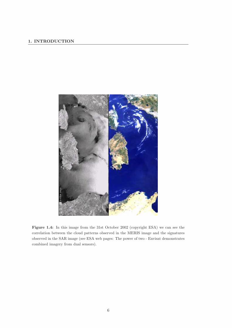
Figure 1.4: In this image from the 31st October 2002 (copyright ESA) we can see the

correlation between the cloud patterns observed in the MERIS image and the signatures

observed in the SAR image (see ESA web pages: The power of two - Envisat demonstrates

combined imagery from dual sensors).

6

1.2 State-of-the-Art

The operators are aided by graphical tools for selecting the possible oil spills and sup-

port their decision in internal guidelines [7]. The guidelines normally consist in a set

of empirical rules that evaluate geometrical and intensity features of the patch (like

contrast) and auxiliary information (like wind speed) and other contextual information

(like vessels or coast proximity). Nevertheless, often operators have to use their “feel-

ing” in complicate scenarios, or unobvious situations, to take a decision if they should

report a dark patch as oil spill or not. The process usually also foresees the assignment

of a confidence level to the detection.

When considering most existing and proposed oil spill detection systems, normally

their processing chain shares a common pipeline structure (see Figure 1.5), differing

in the steps undertaken inside each block (example, see [10]). The main blocks in

the chain are usually the segmentation and the classification. The segmentation step

computes a set of regions defining an image partition, where the features of each region,

for example the gray levels, are similar in some sense. The classification then focus

on the regions with lower backscattering, often using a number of features extracted

from these regions including shape, moments, scale parameters, etc. based on which a

decision on whether the region corresponds to oil or lookalike is taken.

Although this paradigm seems to be very well established in the field of oil spill

detection, some few examples of systems deviating from this structure also exist like

for example kernel-based anomaly detectors [11]. Other important typical steps in the

chain are the initial pre-processing of data, that may include radiometric normalization

and the landmasking. Procedures included in these steps will be later described in

detail.

1.2 State-of-the-Art

There have been so far many approaches to the problem of oil spill detection using

SAR images. We stress that although SAR data actually contain intensity and phase

information, for the special purpose of oil spill detection most proposed methodologies

only take intensity into account. Furthermore, although most SAR sensor mechanisms

allow the acquisition of dual or even multi-polarisation data, most studies on this sub-

ject have been conducted on single-polarisation data. This was in part due to the fact

that this type of imagery was more easily available because of planning and acquisition

7

1. INTRODUCTION

Figure 1.5: Common block structure of most proposed oil spill detection methodologies.

constrains of the SAR instruments. Single polarisation images are also typically char-

acterized by higher radiometric resolution [12]. On the other hand, with the arrival of

satellites like Radarsat-2, Terrasar-X and Cosmoskymed, multipolarisation techniques

are becoming more relevant. In Sub-section 5.2 we provide some references to up-

to-date improvements in the field of oil spill detection methodologies, including also

techniques using multi-polarisation data. Finally, a list and summary of the main Eu-

ropean funded projects that are directly related with oil spill detection is also given at

the end of this section.

A review of SAR segmentation techniques for oil spill detection can be found in

[13]. Most approaches to the problem of oil spill segmentation are built on off-the-shelf

segmentation algorithms such as the adaptive image thresholding and the hysteresis

thresholding. Entropy methods based on the Maximum Descriptive Length (MDL)

and wavelet based approaches have also been proposed. Another recently proposed

segmentation methodology applies Hidden Markov Chains (HMC) to a multiscale rep-

resentation of the original image [14]. Hereby the wavelet coefficients are statistical

characterized by the Pearson system and by the the generalized Gaussian family. When

other SAR products are available, for example polarimetric data, other methods have

been described in the literature, like constant false alarm rate filters [15].

An example of an elaborated adaptive thresholding technique is provided by [13].

In this method, an image pyramid is created by averaging pixels in the original image.

8

1.2 State-of-the-Art

From the original image, the next level in the pyramid is created with half the pixel

size of the original image. A threshold is then computed for each level based on local

estimates of the roughness of the surrounding sea and on a look-up table containing

experimental values obtained from a training data set.

Hysteresis thresholding has been used as the base for detecting oil slicks in [16]. The

method includes two steps: applying a so-called Directional Hysteresis Thresholding

(DHT) and performing the fusion of the DHT responses using a Bayesian operator.

The MDL technique, which basically consists in applying information theory in order

to find the image description which has the lowest complexity, has been applied in [17]

to segment speckled SAR images, namely those containing oil slicks. This segmentation

method describes the image as a polygonal grid and determines the number of regions

and the location of the nodes that delimit the regions. The two-dimensional wavelet

transform, used as a bandpass filter to separate processes at different scales, has also

been adopted to oil slick detection in the framework of an algorithm for automated

detection and tracking of mesoscale features from satellite imagery. [18]. In spite of the

existence of so many different segmentation techniques, in practice only some of them

have been applied and tested in the framework of a complete detection process, as we

shall see in the remaining of this subsection.

Regarding classification, we refer the recent publications [19] and [20] providing

an extensive and deep review on the different used methodologies and correspondent

results. The classifiers are evaluated as part of a detection process, in association with

a specific segmentation method. In these reviews in fact (and in the relevant literature

in general) the reported performance is the one of the whole detection system, including

segmentation and classification, and there are not surveys that assess the classification

performance per se, discoupling it from the remaining of the chain. Table 1 and Table

2 give an overview of the different classification methods (in the context of a specific

detection process) used in oil spill detection that are referred to in the literature. In

order to provide a performance measure of the classifier, which is then also considered

by extension to be the performance of the whole detection system, normally two Overall

Accuracies (OA) are used in the literature: the oil spill detection rate (OA-oil) and the

lookalike detection rate (OA-lookalike). Occasionally, the total accuracy (OA-test) is

also mentioned. These accuracies are defined by the following expressions, which make

9

1. INTRODUCTION

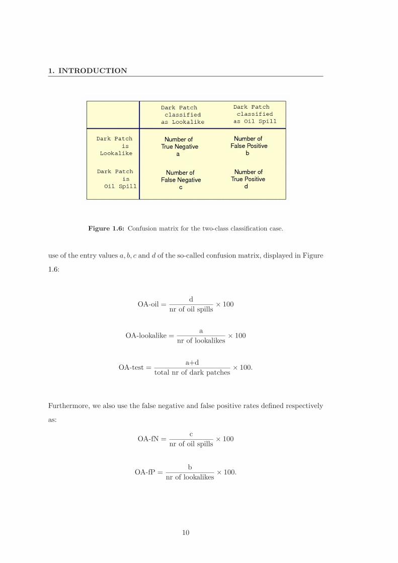
Figure 1.6: Confusion matrix for the two-class classification case.

use of the entry values a, b, c and d of the so-called confusion matrix, displayed in Figure

1.6:

OA-oil =d

nr of oil spills× 100

OA-lookalike =a

nr of lookalikes× 100

OA-test =a+d

total nr of dark patches× 100.

Furthermore, we also use the false negative and false positive rates defined respectively

as:

OA-fN =c

nr of oil spills× 100

OA-fP =b

nr of lookalikes× 100.

10

1.2

Sta

te-o

f-the-A

rt

Table 1.1: Summary of classification techniques proposed in the literature.

Author Proposed Technique Data Set Size OA oil(%) OA lookalike(%)

Espedal and Walh [21] Direct analysis + wind history Three case studies NA NA

Kubat et al. [22] Neural network 41 oil spills + 896 lookalikes 76 86

Solberg et al. [10] Statistical modeling with 71 oil spills + 6980 lookalikes 94 99

rule-based approach

Solberg et al. [23] [10] + sensor specific rules 37 oil spills + 12110 lookalikes 78 99

Del Frate et al. [24] MLP neural network 71 oil spills + 68 lookalikes 82 90

Del Frate et al. [25] [24] + adding wind to network input 111 oil spills + 78 lookalikes NA NA

Del Frate et al. [26] same approach as in [25] 20 dark areas NA NA

Fiscella et al. [27] Mahalanobis classifier 80 oil spills + 43 lookalikes 92 51

Fiscella et al. [27] Compound probability classifier 80 oil spills + 43 lookalikes 85 67

Marghany [28] Textural analysis NA NA NA

Nirchio et al. [29] Fisher discriminant analysis 153 oil spills + 237 lookalikes 74 NA

Nirchio et al. [30] Fisher discriminant analysis 714 images (not clear NA NA

how many dark areas)

Girard-Arduin et al. [31] Ocean backscatter model NA NA

Keramitsloglou et al. [32] Fuzzi logic classifier 28 images 88 NA

Topouzelis et al. [33] Multi-scale segmentation + neural network 69 oil spills + 90 lookalikes 91 87

Topouzelis et al. [34] Combination of neural networks 69 oil spills + 90 lookalikes 85 84

and genetic algorithms

Stathakis et al. [35] Genetic algorithm 69 oil spill + 90 lookalikes 81 88

Gambardella et al. [20] one-class linear programming method X-Band: 16 oil spills + 40 lookalikes 98 99

ERS-SLC: 43 oil spills + 110 lookalikes

11

1.

INT

RO

DU

CT

ION

Table 1.2: Further remarks on classification techniques.

Author Image Type Remarks

Espedal and Walh [21] ERS PRI procedure was foreseen for visual inspection by an operator

method is thus not appropriate for automatization

wind analysis requires too much time

Kubat et al. [22] ERS PRI and Radarsat (not clear which type) no wind information usage

Solberg et al. [10] ERS-PRI method incorporates wind information

and information about vessel/platform proximity

Solberg et al. [23] ASAR-WS and Radarsat (not clear which type) experimental results only given for ASAR-WS in detail

For Radarsat only % of detections of verified oil slicks was provided

Del Frate et al. ERS-PRI no wind information used

Del Frate et al. [25] ERS-PRI use wind, 3 dark patches out of 60 have been misclassified

Del Frate et al. [26] ASAR IM OA-test is 85%, data set very small

result indicative of algorithm independence from sensor

Fiscella et al. [27] ERS-PRI Author considered a third class: uncertain.

Due to this third class it is not very clear how to

compute performance of algorithm

wind information not used

Marghany [28] Radarsat Fine Mode indicative study that showed that texture entropy, energy and

homogeneity features provided good detection of oil spills

Nirchio et al. [29] ERS-PRI no wind information has been used for the classification

Nirchio et al. [30] ASA-WSM and ASA-IM algorithms from [29] have been

redesigned for Envisat images and an appropriate

incidence angle compensation angle has been applied

overall accuracies have not been given, only mentioned they

were similar to those for ERS-PRI images

Girard-Arduin et al. [31] ASA-WSM only one image was used, as a test case

Keramitsloglou et al. [32] ERS-PRI no wind information used

Topouzelis et al. [33] ERS-PRI no wind information used

Topouzelis et al. [34] ERS-PRI no wind information used

feature selection using genetic algorithms

Stathakis et al. [35] ERS-PRI

Gambardella et al. [20] ERS-SLC and X-Band airborne images feature selection performed

no wind information used

different one and two-class standard classifiers tested and compared

12

1.2 State-of-the-Art

Although all approaches have surely contributed to the advance of the state-of-the-

art in oil spill detection, there are still a number of aspects that can be improved or

remain open in this issue, in special in what concerns the operational application of

the proposed algorithms. The following conclusions can be drawn by analyzing the

state-of-the-art in oil spill detection:

1. Most of the so far proposed methodologies are not completely automatic. In

special the segmentation part often requires the specification or tuning of some

kind of parameter, on the algorithm itself or as part of the post-processing of the

segmentation results before they are further provided to the Classifier.

2. Most of the so far proposed Classifiers have been designed for one special type

of SAR images - ERS (a satellite developed by ESA) PRI or ASAR IM, with

≈ 30 m resolution, 100 × 100 km swath - and experimental results are available

for databases of those images. On the other hand, images with other properties

in coverage and resolution, namely Envisat ASAR Wide Swath (WS) with ≈ 150

m resolution and 400 × 400 km swath, have proven to be more adequate for

operational purposes.

3. Even though some of the methods have been adapted to Envisat ASAR WS

images, the correspondent experimental tests have been carried on a very small

dataset, only for preliminary assessment.

4. All the algorithms use features extracted from the dark patches or from its con-

text, but only a few authors [34] and [20] have made an effort to evaluate the effec-

tiveness of the selected features for the classification task. In all the other cases,

the feature set has been chosen empirically. Even those authors who adopted

feature selection, used an initial feature set that missed some of the features

proposed in the literature.

5. Many of the proposed methodologies are not completely automated or are too

complex.

6. Only a fraction of the methods use wind information directly, although it is an

evidence that wind strongly influences oil spill detection.

13

1. INTRODUCTION

7. Because the training and evaluation data sets are different for every author, in

size and content, it is very difficult to compare the obtained results. One example

is the case when oil spills included in a database often occurred near oil platforms

or ships. In this scenario a classification method that uses a context feature like

“distance to the nearest bright object”, results in accuracies that are surely higher

than without such a feature.

For concluding the state-of-the-art survey, a list of the main European projects

related to Oil Spill Detection using SAR data is given in Figure 1.7.

14

1.2

Sta

te-o

f-the-A

rt

Figure 1.7: Main European funded projects related with Oil Spill Detection using SAR images.

15

1. INTRODUCTION

1.3 Aims and Contributions

In this work, we explore the possibility of using automatic segmentation and classi-

fication techniques for operational oil spill detection. By adopting a fully automated

process, we aim at obtaining a method free of subjectivity and less time consuming.

We conducted experiments on different SAR image types but finally focused on ASAR

Wide Swath images, which are currently one of the main input products for operational

services due to its coverage properties.

We approached oil spill segmentation using a Bayesian framework and a “Multi-

Level Logistic” (MLL) [36] prior. Several methods in the same vein have been proposed

since the seminal work of Geman and Geman [37], see e.g., [38]. Applications of these

ideas in the segmentation of SAR images can be found, e.g., in [39], [40], [41].

The main contributions of this work to the state-of-art in oil spill segmentation are

the following:

• the development of a “Expectation Maximization” (EM) [42] algorithm to esti-

mate the parameters of a mixture of a pre-defined number of Gamma distribu-

tions, in order to model the intensities in a SAR image.

• the development of an EM algorithm called “Loopy-β-Estimation”, using “Belief

Propagation” (BP) [43] to estimate the smoothness parameter in the “Markov

Random Field” (MRF) [36] used as prior in our framework.

• the application of recent graph-cut techniques for solving the energy minimization

problem that arises from the followed Bayesian methodology.

• the design of supervised and unsupervised algorithms for oil spill segmentation

supported on the referred tools.

The images used for testing the segmentation algorithms mainly came from the

FCT/ESA funded project OILSAR.

We then explore different classification methods for oil spill detection using Envisat

ASAR WS Images. The classification was then evaluated as part of a complete detection

system. For this purpose, a database of oil spills and lookalikes extracted from these

type of images, has been built. The used images are from the CSN service and the

dark patch extraction was based on the detection CSN reports, produced by Edisofts’

16

1.3 Aims and Contributions

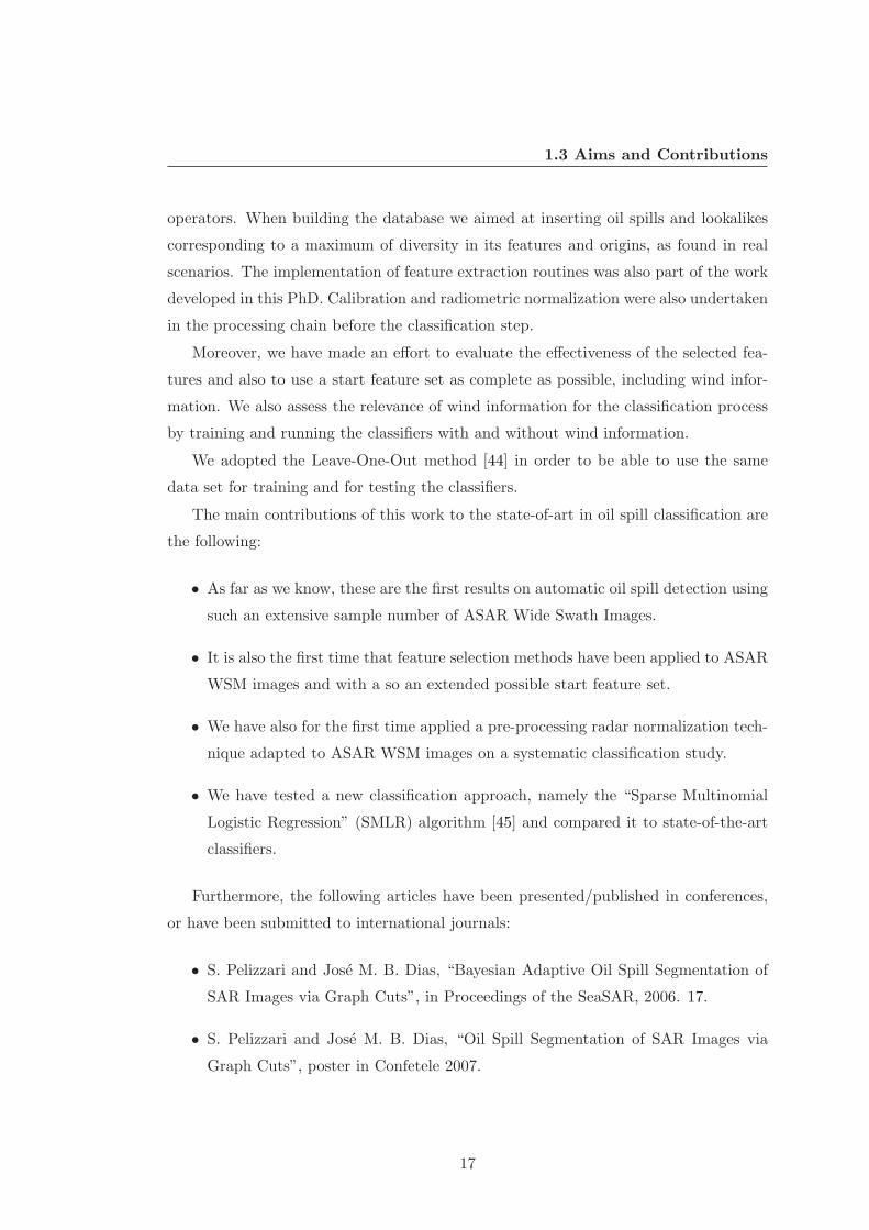
operators. When building the database we aimed at inserting oil spills and lookalikes

corresponding to a maximum of diversity in its features and origins, as found in real

scenarios. The implementation of feature extraction routines was also part of the work

developed in this PhD. Calibration and radiometric normalization were also undertaken

in the processing chain before the classification step.

Moreover, we have made an effort to evaluate the effectiveness of the selected fea-

tures and also to use a start feature set as complete as possible, including wind infor-

mation. We also assess the relevance of wind information for the classification process

by training and running the classifiers with and without wind information.

We adopted the Leave-One-Out method [44] in order to be able to use the same

data set for training and for testing the classifiers.

The main contributions of this work to the state-of-art in oil spill classification are

the following:

• As far as we know, these are the first results on automatic oil spill detection using

such an extensive sample number of ASAR Wide Swath Images.

• It is also the first time that feature selection methods have been applied to ASAR

WSM images and with a so an extended possible start feature set.

• We have also for the first time applied a pre-processing radar normalization tech-

nique adapted to ASAR WSM images on a systematic classification study.

• We have tested a new classification approach, namely the “Sparse Multinomial

Logistic Regression” (SMLR) algorithm [45] and compared it to state-of-the-art

classifiers.

Furthermore, the following articles have been presented/published in conferences,

or have been submitted to international journals:

• S. Pelizzari and Jose M. B. Dias, “Bayesian Adaptive Oil Spill Segmentation of

SAR Images via Graph Cuts”, in Proceedings of the SeaSAR, 2006. 17.

• S. Pelizzari and Jose M. B. Dias, “Oil Spill Segmentation of SAR Images via

Graph Cuts”, poster in Confetele 2007.

17

1. INTRODUCTION

• S. Pelizzari and Jose M. B. Dias, “Bayesian Oil Spill Segmentation of SAR Images

via Graph Cuts”, in Proceedings of the IbPRIA, 2007, vol. 2, pp. 637644. 18.

• S. Pelizzari and Jose M. B. Dias, “Oil Spill Segmentation of SAR Images via

Graph Cuts”, in Proceedings of the IGARSS, 2007, pp. 1318 1321. 18.

• S. Pelizzari and Jose M. B. Dias, “Bayesian Oil Spill Segmentation of SAR Im-

ages”, IEEE Transactions on Geoscience and Remote Sensing, submitted.

• S. Pelizzari and Jose M. B. Dias, “Operational Automatic Classification of Oil

Spills in ASAR WSM Images”, International Journal of Remote Sensing, submit-

ted.

1.4 Thesis Structure

The contents of this thesis are organized in the following way: Section 1 provides

an introduction to the considered problem, containing a review of the state-of-the-art

in oil spill detection, with a mention to relevant research European projects in this

field. The aims and contributions of the work are also stated; Section 2 focus on

the description of the used data and methodology, giving also a brief introduction to

the SAR sensing mechanism and available sensors. The proposed complete processing

chain is also depicted and the features used in the classification step are listed. Section 3

contains the theoretical basis and formulation of the proposed segmentation algorithms,

as well as significative results when they have been applied to SAR data. One example

of the use with MERIS data is also showed as an indication of the possibility of applying

the techniques to a broader range of data types. In Section 4 the results of the different

classification approaches are given. Moreover, the section also contains an a brief

description with examples of some typical lookalike sources. Finally, Section 5 gives

the conclusions and highlights important issues for future improvement in oil spill

detection techniques. The thesis also contains an acronym list and bibliography.

18

2

Data and Methodology

The main data type used in this work are SAR images from ESA missions ERS-1, ERS-

2, and Envisat. For demonstrating the applicability of the segmentation algorithms to

other type of data, one MERIS image from Envisat was also used.

This section contains a brief introduction to SAR in general and a description of

the SAR missions and products relevant for oceanography, with special emphasis on

the missions related related with the PhD. After that, the used data set is listed and

an overall picture of the applied methodology is provided.

2.1 SAR data

A synthetic aperture radar, or SAR, is a coherent radar system that generates high-

resolution remote sensing imagery by means of advanced signal processing techniques.

Active radar systems illuminate the scene with their own electro-magnetic energy by

transmitting a pulse and then record the strength and travel-time of the returned

signals. This allows the range (or distance) of the reflecting objects to be determined

[46]. SAR usually operates in the microwave portion of the electromagnetic spectrum,

ranging from 1mm to 1 meter (300GHz to 300 MHz) [47], (see Figure 2.1).

SAR systems can be mounted on board of aircrafts or satellites and have a side-

looking geometry as illustrated in Figure 2.2 and 2.4.

Most satellites, including ERS-1, ERS-2, and Envisat, are right-side looking. Figure

2.5 depicts the Envisat satellite, which carries a number of instruments on board, among

which there is the Advanced SAR (ASAR) instrument, which main element is a 1.3×10

19

2. DATA AND METHODOLOGY

ERS-1 and 2 and Envisat 5.3 GHz

Figure 2.1: Frequency bands used in radar systems (from [47]). Consider that f = c/λ,

where f is the frequency, c is the light speed (3 × 108ms−1) and λ is the wavelength.

m length antenna, and the MERIS instrument. The satellite is orbiting the earth every

hundred minutes, in a near-Earth polar orbit (800 km mean altitude) and moving at

a velocity of more than seven kilometers per second. Signal processing of SAR data

uses magnitude and phase of the received signals over successive pulses from elements

of a synthetic aperture to create an image. The radar antenna beam illuminates the

ground to the right side of the satellite and due to the satellite motion and the along-

track (azimuth) beam width of the antenna, each target element only stays inside the

illumination beam for a short time.

As part of the on-ground processing, the complex echo signals received during this

time are added coherently, making use of the Doppler history of the radar echoes.

Within the wide antenna beam, returns from features in the area ahead of the platform

will have upshifted, or higher, frequencies resulting from the Doppler effect. Conversely,

returns from features behind the platform will have downshifted, or lower, frequencies.

Returns from features near the centerline of the beam width (the so-called zero-Doppler

line) will experience no frequency shift. This process is equivalent to having a long

antenna (so called synthetic aperture) illuminating the target. The synthetic aperture

Ls is equal to the distance the satellite traveled during the integration time. This is

the area on the ground covered by a single transmitted electromagnetic pulse, known

as the radar footprint. The result is an increase in azimuthal resolution in the final

20

2.1 SAR data

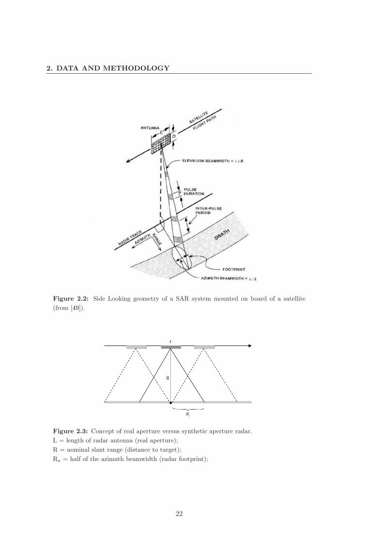
image, despite a physically (real) small antenna [46]. To understand this, consider that

the azimuth resolution ρa is proportional to the expression given in 2.1

ρa ∝ λR

L, (2.1)

where L is the length of the radar antenna, R is the nominal slant range and λ is the

radar wavelength (see Figure 2.3). When the real aperture is substituted by a synthetic

aperture Ls = 2Ra, where Ra is half of the azimuth beamwidth, then the new azimuth

resolution ρ′

a is given by expression 2.2

ρ′

a =λR

2Ra=

L

2. (2.2)

It would take a conventional antenna of length 2Ls to obtain the same resolution without

SAR processing[48].

In the case of Envisat, ERS-1, and ERS-2, the radar footprint is on the order of

8.5 km long in the along-track (azimuth) direction. The nominal real-aperture reso-

lution would be 4.25 km, which is very poor. By assembling a synthetic aperture as

described before, the azimuth resolution is increased approximately a thousand times,

when compared to the real aperture radar, providing a synthetic aperture of about 10

km and an improved resolution of circa 5 m. Note, however, that in the practice several

“looks” are averaged to improve the quality of the amplitude image [46], so that the

final azimuth resolution is about 25 m.

Regarding the across-track or range resolution, this is a function of the transmitted

radar bandwidth, which is inversely proportional to the pulse duration. In SAR sys-

tems, pulse compression techniques are used to improve the performance taking into

account the instrument peak power capability. The use of a so-called matched filter and

of a wide-band (e.g. a chirp) allows the lower intensity, and thus lower power require-

ments. The used illuminating signal is a sinusoidal wave that increases in frequency

linearly with the time, a so-called chirp, and the matched filter avoids the overlapping

in time of records coming from adjacent points. The filter delays the different compo-

nents of the recorded echo signal by a determined value so that they are all compressed

into a short spike [51].

From this brief description of the main steps in SAR signal processing, it should be

clear that the involved algorithms are heavy and complex. The fully description of SAR

21

2. DATA AND METHODOLOGY

Figure 2.2: Side Looking geometry of a SAR system mounted on board of a satellite

(from [49]).

Figure 2.3: Concept of real aperture versus synthetic aperture radar.

L = length of radar antenna (real aperture);

R = nominal slant range (distance to target);

Ra = half of the azimuth beamwidth (radar footprint);

22

2.2 SAR missions and products

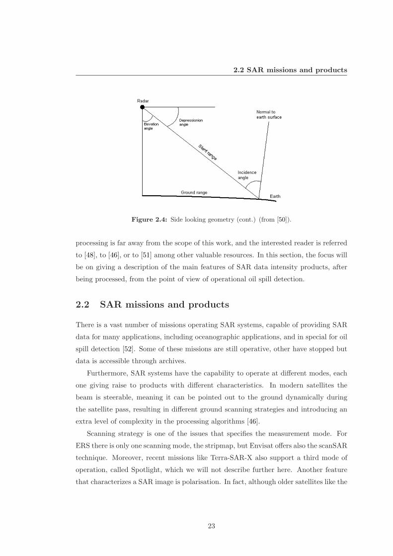
Figure 2.4: Side looking geometry (cont.) (from [50]).

processing is far away from the scope of this work, and the interested reader is referred

to [48], to [46], or to [51] among other valuable resources. In this section, the focus will

be on giving a description of the main features of SAR data intensity products, after

being processed, from the point of view of operational oil spill detection.

2.2 SAR missions and products

There is a vast number of missions operating SAR systems, capable of providing SAR

data for many applications, including oceanographic applications, and in special for oil

spill detection [52]. Some of these missions are still operative, other have stopped but

data is accessible through archives.

Furthermore, SAR systems have the capability to operate at different modes, each

one giving raise to products with different characteristics. In modern satellites the

beam is steerable, meaning it can be pointed out to the ground dynamically during

the satellite pass, resulting in different ground scanning strategies and introducing an

extra level of complexity in the processing algorithms [46].

Scanning strategy is one of the issues that specifies the measurement mode. For

ERS there is only one scanning mode, the stripmap, but Envisat offers also the scanSAR

technique. Moreover, recent missions like Terra-SAR-X also support a third mode of

operation, called Spotlight, which we will not describe further here. Another feature

that characterizes a SAR image is polarisation. In fact, although older satellites like the

23

2. DATA AND METHODOLOGY

Figure 2.5: Picture of Envisat satellite and of the SAR antenna that is on board the

satellite, as main part of the ASAR instrument.It is an active phased array antenna, which

allows independent control of the phase and amplitude of the transmitted radiators from

different regions of the antenna surface, (ESA copyright).

ERS generation and Radarsat-1 are only operated with radiation at a fixed polarisation

(vertical and horizontal polarisation, respectively), modern satellites have the possibil-

ity to transmit and/or received in with different polarisation types and even alternate

between them. Figure 2.6 provides a closer look to these different possibilities in SAR.

Still other factors that distinguish measurement modes can be data rate (implying that

data may be subsampled on board of the satellite), and dimensions and information

content.

(a) (b) (c)

Figure 2.6: (a) VV-Like polarisation: Vertical Transmission/Vertical Reception,(b) HH-

Like polarisation: Horizontal Transmission/Horizontal Reception and (c) VH-Cross polar-

isation: Vertical Transmission/Horizontal Reception (from [46]).

24

2.2 SAR missions and products

Image Mode Wide Swath Mode

Figure 2.7: Envisat modes for oil spill detection: Image Mode- uses stripmap technique,

VV or HH polarisation, 30 m resolution, 100km swath, incidence angle selectable; Wide

Swath- uses scanSAR technique, VV or HH polarisation, 150 m resolution, see [46].

In general, the different modes of operation of an imaging system give raise to

data acquired with different swaths, incidence angles (defined as the angle), resolution

and polarisation. Furthermore, there is a trade-off between coverage and geometric

resolution, implying that higher swaths have lower resolutions. Different SAR systems

also have different revisit capabilities, depending on the orbiting parameters and give

raise to data with different quality.

In respect to the missions that have been used in this PhD, ERS missions were

carrying a so-called Active Microwave Instrument (AMI), this combined the functions

of a SAR and a wind scatterometer (SCATT). When operating as a SAR sensor, it

could be in two measurement modes: Image Mode and Wave Mode. In Image Mode,

the instrument acquires highly detailed images of a 100 km wide strip, in Wave Mode

it continuously provides information on the direction and shape of ocean wave patterns

[53]. Envisat represented an evolution of the measurement capabilities, offering five

distinct measurement modes: Image mode (IM), Alternating Polarisation mode (AP),

Wide Swath mode (WS), Global Monitoring mode (GM) and Wave mode (WV). IM,

AP, and WS modes are designated as high rate modes, and have a downlink rate of 100

25

2. DATA AND METHODOLOGY

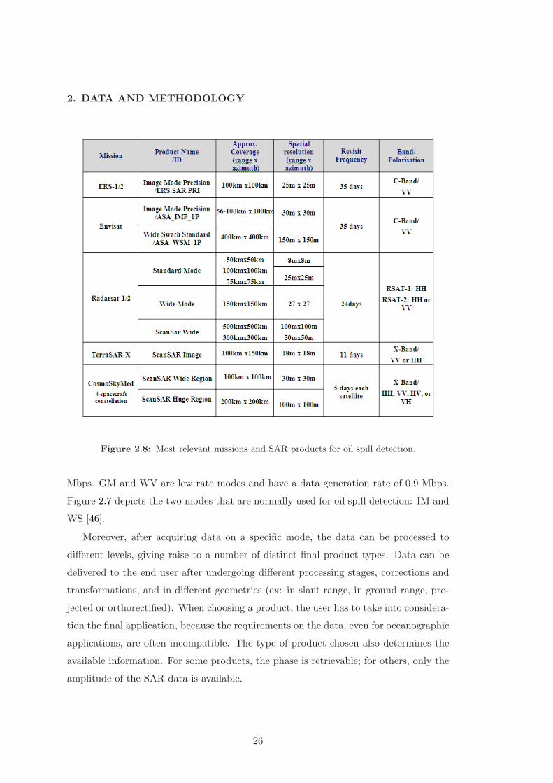
Figure 2.8: Most relevant missions and SAR products for oil spill detection.

Mbps. GM and WV are low rate modes and have a data generation rate of 0.9 Mbps.

Figure 2.7 depicts the two modes that are normally used for oil spill detection: IM and

WS [46].

Moreover, after acquiring data on a specific mode, the data can be processed to

different levels, giving raise to a number of distinct final product types. Data can be

delivered to the end user after undergoing different processing stages, corrections and

transformations, and in different geometries (ex: in slant range, in ground range, pro-

jected or orthorectified). When choosing a product, the user has to take into considera-

tion the final application, because the requirements on the data, even for oceanographic

applications, are often incompatible. The type of product chosen also determines the

available information. For some products, the phase is retrievable; for others, only the

amplitude of the SAR data is available.

26

2.2 SAR missions and products

For operational oil spill detection, the following requirements are recommendable

(see for example [11]):

• Wavelength: C-Band, X-Band and Ku-Band have shown the greatest contrast oil

slick/water. The C-Band seems to be the most suitable frequency.

• Incidence Angle: small (steep) incidence angles are preferably, due to the stronger

Bragg scattering at those angles.

• polarisation: it has been experimentally demonstrated, using artificial slicks, that

VV polarisation seems to be most suitable for C-Band.

• High revisit time.

• Wide Coverage: wide swath modes, acquired using the scanSAR principle, provide

the best trade-off between spatial resolution and monitored area.

The requirement of wide coverage is to be understood in the context of a routine

monitoring system. In fact, in case of an emergency, where an oil spill has already been

identified and one wants to continue targeting it, high resolution images, which imply

narrower swaths, are also adequate.

We note that some of the requirements are in conflict with other ocean applications,

like vessel and ice detection. In this case, HH polarisation and high (incidence angles)

have proved to be more effective.

Figure 2.8 shows a list depicting the main SAR missions currently available, with

some of the product’s specifications.

2.2.1 SAR Sensing of the Ocean

The pixels in a SAR image are backscatter measurements that are associated with the

interaction of the radiation with the target/material. In order to interpret the image,

we have, thus, to understand these physical processes. In general, many factors affect

the strength of a radar signal backscattered from a given material, for a given incident

wave power, from which we highlight the following:

• the radar-target distance

• the incident power

27

2. DATA AND METHODOLOGY

Figure 2.9: Bragg scattering of SAR radiation on the ocean surface, see see [46].

28

2.2 SAR missions and products

Figure 2.10: Two-scale approximation theory of longer/shorter wave interaction in the

ocean (from [1]).

• the roughness of the material (rougher => higher backscatter => brighter image).

• the dielectric constant of the material (wetter => higher).

• the local incidence angle α (smaller => high).

• the radar wavelength and polarisation.

• the shape and orientation of the materials.

• the terrain geometry.

In SAR sensing of the ocean, the primary scattering mechanism, when the incidence

angle ranges between 20 and 45, is the Bragg resonance Mechanism [11] (see Figure

2.9 ). When the radar wavelength, λ, projected onto the surface matches a periodic

structure on the surface, there is a resonance effect causing a strong backscatter termed

Bragg scattering. This means that the most important factor affecting the backscatter

return is the surface roughness on the scales of the Bragg waves (the ones meeting the

Bragg resonance condition). For C-Band radar, these are the so-called short gravity

waves (wave lengths in the range of 5-7 cm) that are generated by winds blowing over

the ocean surface [50]. The amplitude of the Bragg waves can mainly be modulated

by the local wind speed and direction with respect to the line-of-sight direction of the

radar antenna, and by longer gravity waves. The interaction of short and long ocean

waves and how these interactions affect the radar backscattering is referred to as the

two-scale approximation” and can be visualized in Figure 2.10 [50].

29

2. DATA AND METHODOLOGY

As a consequence of these interactions, although the SAR “sees” only the “Bragg

waves”, these waves can be modulated by a large number of upper ocean and atmo-

spheric boundary layer phenomena. This is the reason why lookalikes become visible

in SAR images.

In Section 4.1, examples of some relevant lookalikes are given.

2.3 Data Set

The data used in this PhD can be divided in two main groups: the data set used for

developing and testing the segmentation algorithms and the data set used for developing

and testing the classification.

2.3.1 Data Set for Segmentation

The image data set used to develop the segmentation algorithms was ordered in the

framework of the already referred “Oil Slick Surveillance Using ASAR/MERIS Data”

project.

In order to identify the relevant images, a survey was undertaken. Images have

been identified from relevant research articles, tutorials, and project websites, as well

as from public available oil spill databases. The following references were considered

reliable sources for selecting the data set and for getting background information on

the scenario:

• ESA oil slick earth watching web pages [5]: collection of oil spill case studies

around the world.

• MDA pages [54]: collection of use cases for SAR applications.

• NOAA tutorial [1]: a SAR tutorial sponsored by the NOAA/NESDIS.

• Oceanides database [55]: oil spill database that was built in the context of the

Oceanides project, by the Joint Research Center.

• Tropical and subtropical ocean viewed by ERS SAR [3]: website illustrating range

of oceanic and atmospheric phenomena visible in SAR.

30

2.3 Data Set

Figure 2.11: GUI of EOLI-SA (ESA copyright).

• Cearac web page [56]: oil spill database from the “Coastal Environmental Assess-

ment Regional Activity Centre” (CEARAC), which is part of the regional seas

program of the “United Nations Environment Program” (UNEP).

After being identified, images have been ordered using the “Earth Observation

Link Stand Alone” (EOLI-SA) application, from ESA. This is a java client for Earth

Observation Catalogue and Ordering Services for browsing the metadata and preview

Earth Observation (EO) data acquired by ESA (ERS and Envisat) and many third

part satellite missions, like Landsat, IKONOS, ALOS, SPOT, JERS, and Terra/Aqua.

This application can be downloaded for free from http://eoli.esa.int/geteolisa.

Because many images in the literature are not fully identified, the process of ordering

was oft complicated and needed visual screening of quicklooks and further investiga-

tions.

2.3.2 Data Set for Classification

The part of this PhD regarding the evaluation of different classification approaches has

been performed in cooperation with Edisoft S.A, a private Portuguese company. This

31

2.

DA

TA

AN

DM

ET

HO

DO

LO

GY

Table 2.1: Data Set for Segmentation-Part I.

Description Product Type Identification Comment Reference Source

Cercal accident in Douro plume ERS-1 SLCI Date: 04-Oct-1994 Acquired two days after ESA oil slick

Orbit: 16838 the accident at the Leixoes harbor Earth Watching web pages

Frame: 2781

Prestige accident in Galicia ASA WSM 1P Date: 17-Nov-2002 most popular SAR image Sample data from ESA

Orbit: 3741 documenting the Prestige accident

Prestige accident in Galicia ERS-2 SLCI Date: 16-Dec-2002 effect on Spanish coast International Charter

Orbit: 40028 Space and Major Disasters

Frame: 2727

Prestige accident in Galicia ASA WSM 1P Date: 16-Dec-2002 effect on Spanish coast International Charter

Orbit: 4156 Space and Major Disasters

Acquisition between Cyprus MER FR 2P Date: 19-Jul-2004 There is a ASAR image of Oceanides database

and Lebanon Orbit: 11785 the same date and place

Track: 208

Acquisition between Cyprus ASA IMP 1P Date: 19-Jul-2004 There is a MERIS image of Oceanides database

and Lebanon Orbit: 12471 the same date and place

Frame: 2943

ASA WSM 1P Date: 01-Jun-2004 Oceanides database

Orbit: 11792

Gotland Island case ASA WSM 1P Date: 09-May-2005 97-kilometer oil slick ESA oil slick

Orbit: 16687 of unknown source Earth Watching web pages

Sicily Channel case ERS-1 SLCI Date: 30-Jan-1992 ship wake, natural film ESA oil slick

Orbit: 2828 and current features also present Earth Watching web pages

Philippines ASA WSM 1P Date: 24-Aug-2006 oil spill from a sunken tanker spread ESA oil slick

Orbit: 23432 threatening rich fishing grounds Earth Watching web pages

Time: 01:44:31

North Sea ERS-1 SLCI Date: 30-Oct-1994 suspicious slicks in in article [21]

Orbit: 17211 Norwegian and British platforms

Frame: 2367

Mediterranean Sea northwest ERS-1 SLCI Date: 01-Jun-1992 in proceedings [57]

of Port Said Orbit: 4589

Frame: 2961

Coast of Lebanon ASA IMP 1P Date: 21-Jul-2006 spill due to air strikes MDA web pages

Orbit: 22949 that on July 13 and 15 2006 hit the

Time: 07:49:03 oil-fueled power plant of Jiyeh

led power plant of Jiyeh

32

2.3

Data

Set

Table 2.2: Data Set for Segmentation-Part II.

Description Product Type Identification Comment Reference Source

Yellow Sea ERS-2 SLC Date: 05-Jul 2003 contains also ships, internal waves a Cearac web page

Orbit: 42900 and low wind features

Frame: 2979

Japan/East Sea ERS-1 SLC Date: 08-Nov 1993 biogenic and man-made slicks Cearac web page

Orbit: 12100

Frame: 2763

Korea/Ulleung ASA WSM 1P Date: 14-Apr 2004 oil slicks and biogenic films Cearac web page

Orbit: 11093 building eddies configurations

ASA WSM 1P Date: 14-Apr 2004 contains 2 oil spills Cearac web page

Orbit: 11093

northwestern Japan-East Sea ASA WSM Date: 16-Oct 2003 contains 2 oil spills Cearac web page

Orbit: 8502

Southeast coast of Sicily ERS-1 SLC Date: 26-May 1994 contains 2 oil spills and many lookalikes NOAA tutorial

Orbit: 14957

Frame: 2871

Coast of Malaysia ERS-2 SLC Date: 4-Apr 1997 oil pollution in busy shipping lane NOAA tutorial

Orbit: 10221 busy shipping lane

Frame: 3519

Indian Ocean ERS-2 SLC Date: 6-Apr 1999 “feathered structure” NOAA tutorial

Orbit: 20700 of an oil trail

Frame: 3393

South China Sea ERS-1 SLC Date: 15-Apr 1996 Tropical and subtropical

Orbit: 24841 ocean viewed by ERS SAR

Frame: 3555

South China Sea ERS-2 SLC Date: 13-Jul 1997 Tropical and subtropical

Orbit: 11652 ocean viewed by ERS SAR

Frame: 3483

33

2. DATA AND METHODOLOGY

Figure 2.12: Location (footprints) of the 17 SAR images used for classification.

is a software development and services company with a space department under which

in recent years a number of different projects oriented to ocean remote sensing are

running. In particular, Edisoft has taken part in the MARCOAST project, referred to

in Figure 1.7, and is one of the service providers of the EMSA CSN service as described

at the beginning of this thesis.

Edisoft has a group of well trained oil spill detection operators and is responsible for

the management and operation of a dual-mission Station: the ESA Tracking Station

and EDISOFTs Earth Observation Station at Santa Maria, in Azores. The company

has established an agreement with the “Instituto de Telecomunicacoes”, under which

SAR images have been provided, as well as the oil detection results and associated

auxiliary data, for the scope of evaluating our automatic classification approaches. A

total of 17 Envisat ASAR WSM 1P images have been provided, covering a number

of different European coastal areas: Portugal, Spain, Italy, France, Cyprus, Turkey,

Greece, Germany, Sweden, Denmark, and United Kingdom.

The images have been analyzed by experienced oil spill detection operators, which

identified 70 oil spills, 8 of which have been verified and confirmed in-situ. Furthermore,

70 lookalikes have also been identified in the scenes and used to build a database

containing a total of 140 dark spots (70 oil spills + 70 lookalikes). Figure 2.12 gives

34

2.3 Data Set

Figure 2.13: Example of wind field retrieved from SAR by SARTool (CLS/BOOST

copyright).

an overview of the location of the images. Images have been acquired over different

geographical areas, aiming at developing a classifier as general as possible and not tuned

to specific sources of lookalikes. In fact, an effort was made to include lookalikes with

different oceanographic and atmospheric origins, thus related to diverse SAR signatures.

In Section 4.1, an overview of the different sources of lookalikes is given. The choice

of the oil spills has also been done keeping in mind that there are different types of

signatures [10] depending on their origin and environmental actors, and ensuring that

all these types were present in the database.

Although some of the images contain verified oil spills, for others no validation was

available, so that the operator’s analysis was considered as ground-truth. The opera-

35

2. DATA AND METHODOLOGY

tors’ analysis was documented in form of a report, containing the center coordinates

of the dark patches that had been considered to be oil spills, as well as the confidence

assigned to this assessment and some descriptive features regarding the shape, edges,

contrast, and homogeneity of the spill surroundings, for corroborating their decision.

We have then segmented the images using Algorithm-1, introduced in Section 3.5,

and have considered the dark patches as oil or as lookalike, for building the training

data set, based on the operator’s evaluation. We assumed that any dark signature on

the image that was not reported as an oil spill was considered to be a lookalike.

Furthermore, we also had access to wind estimations retrieved from each one of

the SAR images. For extracting this information, the company is running a software

tool called SARTool, from the Boost company, now integrated within the French CLS

company. The tool is an IDL-based GUI which enables to read, visualize and process

any type of path-oriented SAR images. The advantage of using SAR retrieved wind

is the higher spatial resolution when compared to meteorological models or scatterom-

eter data. Moreover, also meteorological data were delivered for the data set. The

meteorological data were generated by models run by the “Portuguese Meteorological

Institute”. In the following, a list of the used data for classification is given:

• SAR data: 17 ASA WSM 1P images covering different parts of the European

waters.

• SAR retrieved wind: the SAR wind retrievals are based on the combined use of

CMOD-IFREMER2 [58] and HIRLAM [59]. CMOD-IFREMER2 is an inversion

empirical algorithm to estimate wind speed from calibrated data (σ0) and needs

an initial wind direction as input. This initial wind estimation is given by the

HIRLAM model. HIRLAM provides wind fields with accuracy of about 2 m/s

and +/- 10 degrees. The final derived wind field products have a 2 km spatial

resolution but also depend on the model errors. Validation analysis indicate a

resulting root mean square (rms) error of the SAR derived wind speed of about

2.0 m/s in speed and 27◦ in direction for ASAR wide swath. The files are provided

in “Network Common Data Form” (NetCDF) format [60]. Figure 2.13 shows an

example of an wind field retrieved from SAR by SARTool.

• meteorological wind: EDISOFT oil spill detection chain obtains daily wind infor-

mation from the Portuguese Meteo Office (http://www.meteo.pt). Wind speed

36

2.3 Data Set

Figure 2.14: Wind sample data from the Portuguese Meteorological Institute.

and direction predictions at 10 meters are generated once a day by an ECMWF

model with a 0.25◦ spatial resolution in latitude and longitude. The temporal

resolution is 3 hours, and the forecast range is 24 hours. Figure 2.14 shows an

example of generated wind field data. Edisoft provided wind model data inter-

polated to the image acquisition times, for each data set.

• meteorological wave: EDISOFT also obtains daily wave information from the

Portuguese Meteo Office. The used model is the MAR3G that provides sea-state

data: significant wave height, mean wave direction, and mean wave period. It is

a deep-water model that applies a Mercator cartographic projection on the North

Atlantic zone with a special resolution of 1◦ in latitude and longitude. The model

is run four times daily and generates one prediction with a forecast range of 12

hours. Edisoft provided wave model data interpolated to the image acquisition

times, for each data set.

• oil spill detection reports: the reports provided by Edisoft contain the result of

the semiautomatic analysis done by the operator. In summary the information

delivered for each oil spill are: center coordinates, confidence, region affected,

area, width, length, slick orientation, possible source coordinates, model wind

and wave values, SAR wind values, and slick visual evaluation of the geometry,

contrast and surroundings characteristics.

• validation information: for some of the spills (≈ 15%), we also had validation

37

2. DATA AND METHODOLOGY

Figure 2.15: Database: an MS Access database was built, containing the extracted

features and other information of interest obtained from meteorological data sources and

from the operators’ and validation reports.

information, like in-situ verified lengths and widths of the detections. Although

we injected this data into the database with the final scope of incorporating this

evidence in the algorithms, we have not used it in this work.

SAR retrieved wind, meteorological wind and meteorological wave are denominated

here after ancillary data.

For each image, relevant information has been stored in an MS-Access database

developed during the PhD. The database contained metadata regarding the images

and information for each oil spill and lookalike retrieved from the data set provided by

Edisoft (ancillary data and report). Apart from the information provided by Edisoft,

we also stored there on a later stage the results of the Feature Extraction step, which

we will explain in detail in the next section. Figure 2.15 depicts the data types that

have been stored in the developed database. The database has been used for managing

all the information needed for training and testing the classification algorithms.

38

2.4 Methodology

For each oil spill and lookalike, ancillary data, information contained in the reports,

and validation information have been stored. In fact, although in our tested classifi-

cation methods we only used the wind speed and the matlab calculated features, we

think the rest of the information can be of interest in the future for other approaches

or improvements.

2.4 Methodology

We have followed in general the common pipeline structure depicted in Figure 1.5. For

testing the segmentation approaches, we have performed the first 2 steps: Image Pre-

processing and LandMasking. For testing the classifiers, we applied the whole chain.

In the following, we give more details on the steps undertaken. The segmentation

and classification steps, as they are the core of this work, are described in dedicated

sections in the remaining of this text.

2.4.1 Process Chain

We have adopted a processing chain following the typical structure of an oil spill de-

tector, as as already described and depicted in Figure 1.5.

1. Image Preprocessing Two preprocessing steps have been undertaken: the im-

ages have first been calibrated in order to retrieve the radar backscattering (σ0)

and then an incidence angle compensation technique has been applied.

For retrieving σ0 we have used a free available ESA provided software called

BEST (http://earth. esa.int/services/best/). This is a collection of executable

software tools that has been developed to facilitate the use of ESA SAR data.

At the end of this PhD, a new, more advanced, free toolbox for SAR data pro-

cessing has been made available by ESA: NEST. The acronym stands for Next

ESA SAR Toolbox. Among many improvements in comparison to BEST, the tool

allows the visualization and processing of third part SAR data, like Radarsat and

TerraSAR-X data. The use of calibrated data was important due to the fact

that we are using some features based on the digital values of the pixels. For

doing so, the digital values have to be comparable and relate to the same physi-

cal parameter. The BEST calibration routine implements the steps described by

39

2. DATA AND METHODOLOGY

ESA in the document [61]. To perform a precise absolute image calibration and

derive the radar backscattering coefficient for the type of products we are using,

detected ground range products, a detailed knowledge of the local slope (i.e. lo-

cal incidence angle) would be in fact required. Since this information is usually

not available at the processing time, a “flat terrai” is assumed during processing

(based on the ellipsoid WSG84) and the final intensity image is therefore propor-

tional to the radar brightness of the illuminated scene. The processing is basically

a division by a constant and a multiplication by the sinus of the incidence angle.

The relationship between the value of the image pixels (DN), the radar brightness

(β0) and the radar backscattering coefficient (σ0) can be written as given in the

following equation [61]:

DN2 = Kβ0 = Kσ0

sin(α)= Cte(α)σ0 (2.3)

where α is the incidence angle, K is denominated “absolute calibration constant”

and Cte is a constant depending on α.

K is derived -in the ASAR case- from measurements over precision transponders.

This factor is dependent on the processor and product type, and might change

between different beams for the same product type.

On the other hand, we also had the need to compensate the incidence angle

effect on the σ0 value itself, from the point of view of the scattering physical

mechanism associated with the oil presence. For this we adopted a technique

described in [30]. In this work, the author refers that due to the wide extension

of the ASAR WS image swath, the scattering mechanism is mixed: for small

incidence angles the specular mechanism is stronger and for higher incidence

angles the Bragg mechanism dominates. In absence of an analytic expression

for the radar backscattering, the authors derived an exponential fit directly from

data. It is this exponential fit that we applied in this work.

2. Landmasking For the landmasking, the freely available coastline data from the

“Global Self-Consistent High-Resolution Shoreline Database” (GSHHS) [62], in

its higher resolution mode and shapefile format, has been imported into matlab

and used to mask the land. GSHHS is developed and maintained by the University

40

2.4 Methodology

Figure 2.16: Envisat ASAR WSM 1P image acquired on the 11th November 2002 from

the Prestige accident. This is a sample data from ESA and is freely downloadable from

ESA’s site. The displayed yellow rectangle is used for demonstrating the landmasking, in

Figure 2.17.

of Hawai and by the NOAA Laboratory for Satellite Altimetry. Figure 2.17 which

is a zoom of Figure 2.16 gives an idea of the resolution of the used coastline. We

note that this data set does not take into account very small islands or rocks

but this is in fact worst for automatic vessel detection algorithms. What is more

problematic for oil spill detection are sandbanks, due to its “dark appearance”

that makes them typically lookalikes, and these are also not described in the

coastline. In order to get information on sandbanks, and bathymetry in general,

the so-called Electronic Nautical Charts (ENCs) may be used. ENCs contain

other relevant information for oil spill detection, like vessel traffic separation

schemes, which may be used to develop risk maps for oil spill detection. ENCs

must be updated because some of the information they contain, like for example

sandbank location, is dynamical. This information is particularly important for

zones with low bathimetry, where the tide effect is stronger. Dark patches from

sandbanks have been included in the training data set we used for the classification

algorithms.

41

2. DATA AND METHODOLOGY

Figure 2.17: Zoom of the Prestige Envisat image, showing the effect of applying a land-

mask based on the GSHHS coastline.

3. Segmentation We have applied one of the algorithms developed in this work,

namely Algorithm-1, described in detail in Section 3.5. This algorithm has been

chosen only due to practical reasons, as it is the fastest of the proposed segmen-

tation methods.

4. Feature Extraction We have developed and run different matlab routines in

order to calculate a number of features, both from the dark patch as also from

a 150x150 pixel window from the surroundings. The complete list of extracted

features is given in detail bellow, Section 2.4.2. The features have then been

stored in the database, together with other complementary information.

5. Classification In the classification step, we have run all the classifiers described

in detail in Section 4.2.

2.4.2 Extracted Features

A total of 35 features have been considered for classification. An attempt was made to

extract as many features as possible from those referred in the state-of-the-art literature

(see Section 1.2).

These features have all been extracted from the segmented dark patch, except for the

wind information, which was overtaken from the ancillary data or from the operators

reports. The used features can be divided in four main groups: geometrical, backscatter,

texture and ancillary data features.

42

2.4 Methodology

1. Geometrical Features:

• Area (A)

• Perimeter (P)

• Complexity (C), defined as

C :=P

2√πA

.

This feature will take a small numerical value for regions with simple

geometry and larger values for complex geometrical regions.

• Length (L): sum of skeleton edges (obtained by Delaunay triangulation),

that build the main line.

• Width (W): mean value of Delaunay triangles which are crossed by main

line.

• Length To Width Ratio (LWR), defined as

LWR :=L

W.

• Compactness (Comp), defined as

Comp :=LW

A.

• First Invariant Planar Moment (FIPM), defined as

FIPM :=1

n2

n∑

i=1

[(xi − xc)

2 + (yi − yc)2]

with

xc :=1

n

n∑

i=1

xi , yc =1

n

n∑

i=1

yi,

and n the number of points in the dark patch contour.

• Ellipse-Length (EL): value of main axe of an ellipse fitted to the data.

• Ellipse-Width (EW): value of minor axe of an ellipse fitted to the data.

• Ellipse-Asymetry (EA), defined as

EA := 1 − EW

EL.

43

2. DATA AND METHODOLOGY

• Form Factor (FF): represents the dispersion of the dark patch pixels from

its longitudinal axis, when a line is fitted; it is calculated as norm of

residuals after line fit to the dark patch pixels.

• Spreading (S): this feature is derived from the principal component

analysis of the vectors whose components are the coordinates of the pixels

belonging to the dark patch (see [24] for details). Feature S will be low for

long and thin objects and high for objects closer to a circular shape.

2. Backscatter Features:

• Inside Slick Radar Backcatter (µobj)

• Inside Slick Standard Deviation (σobj)

• Outside Slick Radar Backscatter (µsce)

• Outside Slick Standard Deviation (σsce)

• Intensity Ratio (µobj

µsce)

• Intensity Standard Deviation Ratio (σobj

σsce)

• Intensity Standard Deviation Ratio Inside (ISRI), defined as

ISRI :=µobj

σobj.

• Intensity Standard Deviation Ratio Outside (ISRO), defined as

ISRO :=µsce

σsce.

• ISRI ISRO Ratio

• Min Slick Value (MinObj)

• Max Slick Value (MaxObj)

• Max Contrast (ConMax): difference (in dB) between the background mean

value and the lowest value inside the object, defined as

ConMax := µsce − MinObj.

• Mean Contrast (ConMe): difference (in dB) between the background mean

value and the object mean value, defined as

ConMe := µsce − µobj .

44

2.4 Methodology

• Max Gradient (GMax): maximum value (in dB) of border gradient

magnitude, calculated using Sobel operator.

• Mean Gradient (GMe): mean border gradient magnitude (in dB).

• Gradient Standard Deviation (GSd): standard deviation (in dB) of the

border gradient magnitudes.

3. Texture Features:

Texture is a combination of repeated patterns with a regular frequency and

texture analysis has often proved to be effective for oil spill classification (see

[28], [20] and [34]). We have used gray level co-occurrence matrices (GLCM) to

specify texture measures (see [63]) and have used the following measures:

• GLCM Homogeneity

• GLCM Contrast

• GLCM Entropy

• GLCM Correlation

• GLCM Dissimilarity

4. Ancillary Data Features:

• Wind Speed

A fifth group, of so-called context features, is also referred to in the literature, but

was not used by us. This group includes features like:

• Distance from land

• Distance to large dark areas

• Distance to next bright spot (vessel, platform)

• Number of bright spots nearby

• Number of dark Objects in the vicinity

45

2. DATA AND METHODOLOGY

We note that many of the extracted features are related to the same slick character-

istics and are correlated. For example the features “Spreading”, “Compactness” and

“LengthToWidthRatio”, both describe how long and thin objects are. In the same way,

the features “First Invariant Planar Moment”, “Form Factor” and “Ellipse Assimetry”

can all be considered to give an indication to the general shape of the object. In our

work we wanted to examine as much of the features referred to in the literature as

possible.

As a remark, it is important to say that all features have been standardized before

being further used in the classification step. This is necessary because features can have

different scales although they refer to comparable objects [64]. Consider for instance,

a pattern x = [x1, x2] where x1 is a width measured in meters and x2 is a height

measured in centimeters. Both can be compared, added or subtracted but it would be

unreasonable to do it before appropriate normalization. We have used the following

classical centering and scaling procedure of the data : x normi = (xi − µi)/σi, where

µi and σi are the mean and the standard deviation of feature xi over the training

examples.

46

3

Segmentation

3.1 Introduction

In the following, we present algorithms that have been developed for the segmentation of

dark signatures in oceanic SAR images, following a Bayesian approach. The algorithms

have been developed aiming at oil spill detection but, as we will also show at the end of

the chapter, they can also be used to segment other type of signatures, and also more

than one type of signatures at the same time. The adopted technique uses as data

model a finite Gamma mixture, with a given predefined number of components, for

modeling each class density. In fact, this density is well suited to filtered intensity SAR

images as shown, e.g., in [65], [66]. By using a mixture of densities, we aim at describing

the continuous backscattering variability that may be observed in the SAR sea data.

Moreover, a mixture is able to describe densities presenting more than one maximum,

as it is the case of oceanic multi-look SAR images histograms. This cannot be achieved

by none of the statistical models for SAR intensities proposed in the literature, like for

example any of the Pearson distributions [67].

In this work, we propose two supervised and one unsupervised algorithms. In

the supervised algorithms, the user manually selects a region containing pixels from

the dark signature of interest and a region containing water pixels. These regions

should be statistically representative and can be made up of non-connected parts. The

unsupervised algorithm is an improvement of the supervised ones and is completely

automatic.

To estimate the parameters of the class conditional densities, a new EM method

47

3. SEGMENTATION

was developed. Details are described in Section 3.3. When segmenting small sub-scenes

of the image, a simplified data model with only one Gamma function per class can be

used.

The prior used to impose local homogeneity is a multi-level logistic (MLL) model

Markov random field (MRF) [36], with 2nd order neighborhood. To infer the prior

smoothness parameter controling the degree of scene homogeneity, we develop an EM

algorithm that uses loopy believe propagation (LBP) [43]. We have also exploited

different classic estimation methods, namely the least squares fit (LSF) and the coding

method (CD) (see [36] for details) for comparison.

To infer the labels, we adopt the maximum a posterior (MAP) criterion, which we

implement efficiently and exactly with graph-cut techniques [68].

Although the segmentation of oceanic dark patches is typically based on the assump-

tion of two classes, we have generalized the problem to an optional number of classes.

The underlying integer optimization problem is now attacked with the graph-cut based

α-Expansion algorithm [69].

To evaluate the accuracy of the proposed algorithms, different simulations address-

ing both the referred Gamma model as well as intensity images corrupted with Gaussian

noise have been carried out for error rate assessment.

The algorithms have also been applied to real SAR images containing well docu-

mented oil spills. For doing so, the scenes are divided in tiles and segmented individ-

ually. Moreover, the described Bayesian algorithm may be also applied to other type

of data, like the case of MERIS images. To do so, only the data model needs to be

adapted to the data.

3.2 Problem Formulation

3.2.1 Bayesian Approach

Let L := {1, . . . , c} be a set of c classes and P := {1, 2, . . . , N} be the set of N pixels

(sites) where measurements y := {y1, y2, . . . , yN}, the SAR intensities, are available. A

labeling x := {x1, x2, . . . xN} is a mapping from P to L, i.e., it assigns to each pixel

p ∈ P a label xp ∈ L. Any labeling x can be uniquely represented by a partition of image

pixels P := {Pl|l ∈ L}, where Pl = {p ∈ P|xp = l} is the subset of pixels to which the

label l has been assigned. Since there is an one-to-one correspondence between labelings

48

3.2 Problem Formulation

x and partitions P , we use these notions interchangeably. By applying a segmentation

algorithm to the image y, we get x := {x1, x2 . . . xN}, where xi is the inferred label for

the pixel i ∈ P.

3.2.2 Observation Model

In our problem formulation, we assume conditional independence of the measurements

given the labels, i.e.,

p(y|x) =N∏

i=1

p(yi|xi) =c∏

l=1

∏

i∈Pl

p(yi|φl), (3.1)

where p(·|φl) is the density corresponding to class l and φl the correspondent vector of

parameters. The adopted density is a finite Gamma mixture given by

p(yi|φl) :=K∑

s=1

αls p(yi|θl

s), (3.2)

where K is the number of Gamma modes in the mixture, i indexes the pixel, θls is the

vector of parameters of the Gamma mode s and class l, and αls is the a priori probability

of mode s. We denote θl := (θl1, . . . , θ

lK), αl :=

(αl

1, . . . , αlK

), and φl := (αl, θl).

Given that p(yi|θls) is Gamma distributed, we have then

p(yi|θl

s

):=

(λls)

als

Γ (als)y

als−1

i exp(−λl

syi

), yi ≥ 0, (3.3)

where θls :=

(al

s, λls

). The mean and variance of a random variable with the density

(3.3) is, respectively, als/λ

ls and al

s/(λls)

2.

The mixture parameters θl are estimated from the data by applying the EM Gamma

mixture estimation algorithm described in Section 3.3. The procedure is the same both

for the supervised and for the unsupervised approaches.

We now make a brief comment on our choice of the Gamma mixture for modeling

the observation densities. Under the assumption of fully developed speckle, the complex

radar amplitude is zero-mean circular Gaussian distributed [70]. The average intensity

computed over a number of independent random variables with the same density is,

thus, Gamma distributed. It happens, however, that in sea SAR imaging one or more

of the above assumptions may fail, rendering the Gamma density a poor model for

SAR intensity [14]. A line of attack to obtain better models is to use more flexible

49

3. SEGMENTATION

parametric families, such as the Pearson System [67], [66]. However, in our problem

each class density exhibits much more variability than that of accommodated by the

the Pearson System. We have very often, for example, multi-modal densities. We

should resort, therefore, to a mixture of Pearson System densities, what would lead

to complex learning procedures. We have experimentally observed, however, that the

Gamma mixture yields very good fittings for real SAR histograms, obtained with a

moderately complex learning algorithm. For this reason, we have adopted the Gamma

mixture model.

When applying the described Bayesian algorithm to MERIS images, we only need

to replace the data model p(yi|θl) by a multivariate Gaussian density given by:

p(yi|θl) :=1

(2π)N/2 |∑l|1/2

exp

(−1

2(yi − µl)

T∑

l

−1(yi − µl)

)(3.4)

In definition 3.4, yi := [yi1, yiN ] are the values of the MERIS channels (N = 13,

for level 2 processing) and θl = [µl,∑

l] are the data model parameters. For the

MERIS segmentation described in this work, the model parameters have been learned

in a supervised way by defining regions representing the classes and computing ML

estimators.

3.2.3 Prior

A second assumption we are making is of a local smoothness of the labels in a statistical

sense. It is more likely to have neighboring sites with the same label than the other way

around. We model this local smoothness with a second order MRF, more specifically,

by an MLL model (Ising model in the case of two classes [36]). The Markov property

states that

p (xi| xj , j ∈ P) = p (xi| xj , j ∈ Ni) , (3.5)

where Ni is the set of neighbors of site i [36] (see Figure 3.1). If p (xi| xj , j ∈ Ni) > 0,

then the Hammersley-Cliffords Theorem states that p(x) has the form of the Gibbs

distribution

p (x) =1

Zexp−U(x), (3.6)

where Z is the so called partition function and U is the energy function

U (x) =∑

cl∈C

Vcl (x) , (3.7)

50

3.2 Problem Formulation

Figure 3.1: 8-pixel-neighbourhood (light green) of pixel i (dark green), with four

2-pixel-cliques represented as blue ellipses.

where C is the set of cliques and Vcl (x) is the clique potential defined over clique cl. In

this work, we have pair-wise cliques defined on a second-order neighborhood (8 pixels).

That is, C = {(i, j) : i ∈ Nj , j ∈ Ni, i > j}.In these conditions, the MLL clique potentials, in the isotropic case, are given by

Vcl (xr, xs) = −βδ (xr − xs) , (3.8)

where r, s ∈ cl, δ(x) := I0(x) is the indicator function of set {0}, and parameter β > 0

controls the degree of scene homogeneity.

3.2.4 Maximum a Posteriori Estimate

The posterior of the labeling given the observed data is

p (x|y) ∝ p (y|x) p (x) . (3.9)

In order to infer x, we adopt the MAP criterion. This amounts to maximize the

posterior density of the labeling given the observed data:

x = arg maxx

p (x|y) , (3.10)

51

3. SEGMENTATION

and is equivalent to minimize the negative logarithm of (3.9). In this sense, we may

rewrite the problem in the following way:

x = arg minxE(x1, . . . , xn), (3.11)

where

E (x1, . . . , xN ) = − log p(x|y) + cte, (3.12)

and cte denotes an irrelevant constant. From equation (3.9), we have

E (x1, . . . , xN ) =N∑

p=1

Ei (xi) +∑

i,j∈cl

Ei,j (xi, xj) , (3.13)

with

Ei (xi) = − log p (yi|xi) (3.14)

Ei,j(xi, xj) = −βδ(xi − xj). (3.15)

3.2.5 Energy Minimization

As already stated, we are concerned with the minimization of E (x1, . . . xN ) given by

(3.13), which we term energy. For two classes, (i.e., c = 2), the global minimum of

E (x1, . . . xN ) can be computed exactly by applying the graph-cut algorithm described

in [68]. This is a consequence of energy being graph-representable, i.e., Ei,j (0, 0) +

Ei,j (1, 1) ≤ Ei,j (0, 1) + Ei,j (1, 0) (for details see [68]). For more than two classes,

the solution of (3.10) can be approximately computed by the α-Expansion technique

[69], also based on graph-cut concepts. This algorithm finds the local minimum of the

energy within a known factor of the global minimum.

We now give a brief description of the α-Expansion algorithm. Given a label α, a

move from a partition P (with correspondent labeling x) to a new partition P ′ (with

correspondent labeling x′) is called an α-Expansion if Pα ⊂ P ′

α and P ′

l ⊂ Pl for any

label l 6= α. In other words, an α-Expansion move allows any set of image pixels to

change their label to α. The algorithm cycles through the labels in P in some fixed or

random order and finds the lowest α-Expansion move from the current labeling. If the

expansion move has lower energy than the current labeling, then it becomes the current

labeling. The algorithm terminates when no α-Expansion move exist corresponding to

a local minimum of the energy.

52

3.3 EM Algorithm for Fitting a Mixture of Gamma Densities

3.3 EM Algorithm for Fitting a Mixture of Gamma Den-

sities

As stated in the main text of this work, when segmenting real SAR images, the adopted

data model for each class is a finite Gamma mixture. For completely defining the data

model for each class (for lightness of the notation we have dropped the class index),

we need to estimate 2K Gamma parameters, θ = (θ1, . . . , θK), with θs = (as, λs), and

K a priori probabilities α = (α1, . . . , αK)). We infer φ = (α, θ) by computing its ML

estimate from a training set. The ML estimate is computed via an EM algorithm

[42]. Fitting a Gamma mixture is addressed in [71]. However, the authors consider

N -look SAR images meaning that the underlying random variables are the average of

N independent and identically distributed exponential random variables, thus, having

a Gamma density but with just one parameter free; if the mean is µ, then the variance

is given by µ2/N . We estimate both the mean and the variance for each Gamma distri-

bution in the mixture, rendering the algorithm more adaptable to real measurements.

The key point in the EM technique is the introduction of the so called missing

data z, such that p (y|φ) =∫p (y, z|φ) dz and p (y, z|φ) is easier to manipulate than

p (y|φ). In the particular case of a mixture of densities, we will use as missing data a

random variable, zi, per site, with distribution p(zi = s) = αs. The missing variables

are interpretable as the probability that the s-th Gamma mode is selected at pixel i.

The EM algorithm alternates between two steps: the E-step computes the conditional

expectation of the logarithm of the complete a posteriori probability function, with

respect to the missing variables, based on the actual parameter value. The M-step

updates the values of the parameters, by maximizing the expression obtained in the

E-step with respect to each parameter on turn, i.e.,

E-step : Q(φ;φt

)= E

{log p (y, z|φ) |y, φt

}(3.16)

M-step : φt+1 = arg maxφQ(φ;φt

)(3.17)

Denoting

wtsi = P

(zi = s|yi, φ

t)

(3.18)

53

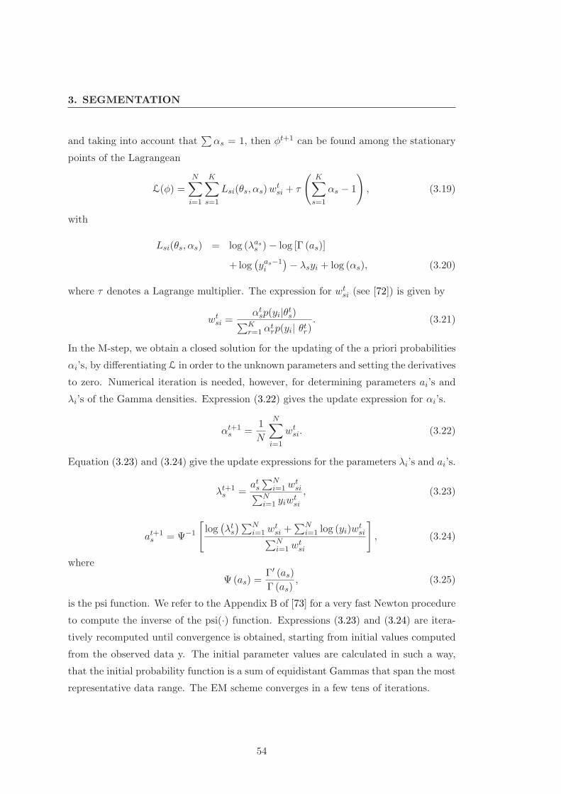
3. SEGMENTATION

and taking into account that∑αs = 1, then φt+1 can be found among the stationary

points of the Lagrangean

L(φ) =N∑

i=1

K∑

s=1

Lsi(θs, αs)wtsi + τ

(K∑

s=1

αs − 1

), (3.19)

with

Lsi(θs, αs) = log (λass ) − log [Γ (as)]

+ log(yas−1

i

)− λsyi + log (αs), (3.20)

where τ denotes a Lagrange multiplier. The expression for wtsi (see [72]) is given by

wtsi =

αtsp(yi|θt

s)∑Kr=1 α

trp(yi| θt

r). (3.21)

In the M-step, we obtain a closed solution for the updating of the a priori probabilities

αi’s, by differentiating L in order to the unknown parameters and setting the derivatives

to zero. Numerical iteration is needed, however, for determining parameters ai’s and

λi’s of the Gamma densities. Expression (3.22) gives the update expression for αi’s.

αt+1s =

1

N

N∑

i=1

wtsi. (3.22)

Equation (3.23) and (3.24) give the update expressions for the parameters λi’s and ai’s.

λt+1s =

ats

∑Ni=1w

tsi∑N

i=1 yiwtsi

, (3.23)

at+1s = Ψ−1

[log(λt

s

)∑Ni=1w

tsi +

∑Ni=1 log (yi)w

tsi∑N

i=1wtsi

], (3.24)

where

Ψ (as) =Γ′ (as)

Γ (as), (3.25)

is the psi function. We refer to the Appendix B of [73] for a very fast Newton procedure

to compute the inverse of the psi(·) function. Expressions (3.23) and (3.24) are itera-

tively recomputed until convergence is obtained, starting from initial values computed

from the observed data y. The initial parameter values are calculated in such a way,

that the initial probability function is a sum of equidistant Gammas that span the most

representative data range. The EM scheme converges in a few tens of iterations.

54

3.4 Estimation of Parameter β

3.4 Estimation of Parameter β

In this work, we consider three different techniques to determine the smoothness pa-

rameter β: a new EM method hereafter introduced that uses loopy belief propagation

(LBP) and the classical LSF and CD methods. Because LSF and CD assume the exis-

tence of labeled data, we have conceived an iterative labeling-estimation scheme, which

alternates between a labeling step and an estimation step until the convergence of β is

attained. On the contrary, the EM estimation algorithm, that we have called “Loopy-

β-Estimation”, is a one-shot technique. In the following sections, we briefly review the

LSF and CD methods and provide a detailed description of the Loopy-β-Estimation

method. In this section, the class parameters φ := (φ1, φ2, . . . , φc) are assumed known.

3.4.1 Least Squares Fit

This procedure for parameter estimation in MRF, described in detail in [36], is based

in the following equation that holds for the MLL model, for every pixel p, with neigh-

borhood Np, and for every label pair xp, x′

p ∈ L :

β[n (xp) − n

(x′p)]

= log

(p(xp|xNp

, y)

p(x′p|xNp

, y))

−(Ep(x′p)− Ep (xp)

), (3.26)

where n(xp) is the number of pixels in the set Np with the same label as xp and

xNp:= {xi, i ∈ Np}. We use histograms to estimate the joint probabilities p

(xp|xNp

, y)

and p(x′p|xNp

, y)

in (3.26): assuming that there are a total of M distinct 3x3 blocks in

the image lattice with a given label configuration xNp, then we take

p(xp|xNp

, y)

=H(xp|xNp

, y)

M, (3.27)

where H(xp|xNp

, y)

is the number of times that a particular 3x3 configuration(xp|xNp

, y)

occurs. The expression is then evaluated for a number of distinct combinations of xp, x′

p

and xNpin order to obtain an over-determined linear system of equations that is solved

in order to β.

55

3. SEGMENTATION

3.4.2 Coding Method

In this method the key idea (see [36]) is to partition the set P into sets P(k), called

codings, such that no two sites in one P(k) are neighbors. In the present work, the

neighborhood Np is of 2nd order thus yielding four codings. As the pixels in P(k) are

not neighbors, the variables associated with these pixels, given the labels at all other

pixels, are mutually independent under the Markovian assumption. The following

simple product is thus obtained for the likelihood:

p(k) (x|β, y) =∏

p∈P(k)

p(xp|xNp

, β, y), (3.28)

Maximizing (3.28) in order to β gives the coding estimate β(k). Although it is not

clear how to combine the results optimally, the arithmetic average, as suggested in [36],

is an intuitive scheme that was adopted in this work.

3.4.3 Loopy-β-Estimation

We are seeking βML = arg maxβ p(y|β), the ML estimate of the smoothness parameter

β. Based on the fact that the marginal density p (y|β), the so-called evidence, is a sum

over the missing labels x, i.e.,

p (y|β) ≡∑

x

p (y, x|β)

=∑

x

p (y|x) p (x|β) , (3.29)

we develop an EM algorithm [42] for the ML estimation of the parameter β. The EM

algorithm alternates between two steps: the E-step computes the conditional expec-

tation of the logarithm of the complete a posteriori probability function, with respect

to the missing variables, based on the actual parameter value; the M-step updates the

value of the parameter, by maximizing the expression obtained in the E-step with re-

spect to that parameter. We now derive the E-step and the M-step.

56

3.4 Estimation of Parameter β

E-step:

Q(β;βt) = E[log p(y, x|β)|y, βt] (3.30)

= E[log p(y|x)|y, βt] (3.31)

+E[log p(x|β)|y, βt]. (3.32)

Recalling that the MLL prior is given by

p (x| β) =1

Z (β)exp

β∑

i,j∈cl

δ (xi − xj)

, (3.33)

with

Z (β) =∑

x

exp

β∑

i,j∈cl

δ (xi − xj)

, (3.34)

we obtain, up to an irrelevant constant,

Q (β;βt) = − log Z (β) + β∑

i,j∈cl

E [δ (xi − xj) | y, βt] . (3.35)

M-step:

βt+1 = arg maxβQ (β, βt) . (3.36)

The stationary points of Q are the solution of

∂Q

∂β= −∂ log [Z (β)]

∂β(3.37)

+∑

i,j∈cl

∑

xi,xj∈L

δ (xi − xj)p (xi, xj | y, βt)) = 0.

By introducing expression (3.34) into (3.37) and if we consider that δ (xi − xj) takes

non-zero values only for equal labels, we obtain

∂Q

∂β=∑

i,j∈cl

c∑

k=1

p (xi = k, xj = k| y, βt)

− p (xi = k, xj = k| βt) = 0. (3.38)

Since computing exact marginal distributions is infeasible in our case, we replace

them by pseudo-marginals using BP. This approach has been successfully applied in

problems of approximate parameter learning in discriminative fields [74]. BP is an

efficient iterative algorithm in which local messages are passed in graphical models.

57

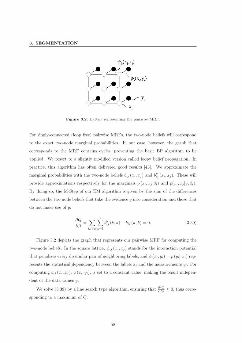
3. SEGMENTATION

Figure 3.2: Lattice representing the pairwise MRF.

For singly-connected (loop free) pairwise MRFs, the two-node beliefs will correspond

to the exact two-node marginal probabilities. In our case, however, the graph that

corresponds to the MRF contains cycles, preventing the basic BP algorithm to be

applied. We resort to a slightly modified version called loopy belief propagation. In

practice, this algorithm has often delivered good results [43]. We approximate the

marginal probabilities with the two-node beliefs bij (xi, xj) and byij (xi, xj). These will

provide approximations respectively for the marginals p (xi, xj |βt) and p(xi, xj |y, βt).

By doing so, the M-Step of our EM algorithm is given by the sum of the differences

between the two node beliefs that take the evidence y into consideration and those that

do not make use of y:

∂Q

∂β=∑

i,j∈cl

c∑

k=1

byij (k, k) − bij (k, k) = 0. (3.39)

Figure 3.2 depicts the graph that represents our pairwise MRF for computing the

two-node beliefs. In the square lattice, ψij (xi, xj) stands for the interaction potential

that penalizes every dissimilar pair of neighboring labels, and φ (xi, yi) = p (yi| xi) rep-

resents the statistical dependency between the labels xi and the measurements yi. For

computing bij (xi, xj), φ (xi, yi), is set to a constant value, making the result indepen-

dent of the data values y.

We solve (3.39) by a line search type algorithm, ensuring that ∂2Q∂2β

≤ 0, thus corre-

sponding to a maximum of Q.

58

3.5 Supervised Segmentation

3.4.4 A few Remarks about the Vector of Parametres φ

In the previous section, we have considered that the class parameter vector φ is known

and only the smoothness parameter β is to be inferred. However, still using the beliefs

computed by LBP, the vector φ could have been inferred simultaneously with β by

including in the Q function the additive term (3.31) corresponding to the class densities.

We would have obtained

Q(φ;φt, βt) = E[log p(y|x)|y, φt, βt]

=N∑

i=1

c∑

l=1

log p(yi|φl)p(xi = l|y, φt, βt),

where the probabilities p(xi = l|y, φt, βt) are given by the LPB method. The M-step

would consist then in two decoupled maximizations; one with respect to β and another

with respect to φ. This approach is, however, beyond the scope of this work. Never-

theless, we present in Section 3.6 an unsupervised algorithm, which is suboptimal but

faster than the LBP based EM algorithm aimed at the inference of both the parameters

β and φ.

An alternative to the proposed EM scheme based on LPB is using Monte Carlo

techniques to cope with the difficulty in computing the E-step and the partition func-

tion Z [75], [76], [77]. Supported on the performance of the LBP, we believe, however,

that the EM scheme based on LPB is, for the present problem, much more faster than

the Monte Carlo based techniques.

3.5 Supervised Segmentation

In this section, we introduce two supervised algorithms aimed at the segmentation of sea

SAR images. In both algorithms, the first step is the estimation of the class parameters

used in the data model. This is done by asking the user to define representative regions

of interest (ROI) in the image. Once the regions are defined, different approaches may

be followed: if a Gamma mixture is assumed for the observed data, as in the case

of SAR images, the EM class parameters estimation algorithm described in Section

3.3 is applied to infer the class conditional densities. If we are segmenting small sub-

scenes and the radar range spreading loss has been compensated in the underlying SAR

images, one single Gamma function per class often provides a good modeling for the

59

3. SEGMENTATION

SAR intensities. In this case, a common ML Gamma estimator is used instead of the

EM procedure. After this step, the data model is considered to be known and is used

thereafter.

The pseudo-code for two supervised algorithms is presented in Algorithm-1 and

Algorithm-2. Algorithm-1 is of generalized likelihood type [78] implementing an itera-

tive labeling scheme with two steps being performed alternately: the β-Estimation and

the segmentation. Algorithm-2 is a one-shot procedure that performs β-Estimation

using the Loopy β-Estimation method described in Section 3.4.3.

Algorithm 1 Supervised Segmentation Using LSF/CD β-Estimation

Require: Initial parameter β = β0 and estimated class parameters φ

1: Compute eLabel = Ep(xp) for every pixel p using φ

2: while∣∣∣∆β

∣∣∣ ≤ δ or nrIterations < NrIterationsMax do

3: Compute x = α-Expansion(β, eLabel)

4: Compute β = β-Estimation(x, eLabel) {LSF or CD}.5: end while

6: return(x, β

)

Algorithm 2 Supervised Segmentation Using Loopy-β-Estimation

Require: estimated class parameters φ

1: Compute eLabel = Ep(xp) for every pixel p using φ

2: Compute β = Loopy-β-Estimation(eLabel)

3: Compute x = GraphCut-Segmentation(β, eLabel)

4: return(x, β

)

3.6 Unsupervised Segmentation

The unsupervised method, stated in “Algorithm-3” is an improvement of the supervised

algorithms described in the previous sections. The main difference is that the data

model is not considered to be known but is also iteratively estimated along with the

smoothness parameter and the segmentation. The scheme needs a rough initialization

of the data model parameters. We computed this initialization by fitting an EM Gamma

mixture to the complete data.

60

3.7 Results

As our EM algorithm automatically eliminates unnecessary modes, we start with

an overestimate of K, the number of modes in the mixtures. In our experiments with

real data, the maximum number of modes we got was four.

Then, different strategies are possible. In the experiments reported in the next

section, when considering c = 2 classes, we have assigned the mode with a lower mean

value to one of the classes and the remaining modes to the other class.

In each iteration, we compute the ML estimate of the vector φ based on the previous

segmentation, compute the new segmentation, and finally the new value of β. The

algorithm may use any of the three β−parameter estimation methods and is applicable

to an optional number of classes. The algorithm stops when both the parameter β and

the class parameters φ converge to stable values.

Algorithm 3 Unsupervised Segmentation

Require: arbitrary parameter β = β0, initial class parameters φ = φ0 (EM Gamma

Mixture Estimation)

1: Compute eLabel0 =Ep(xp) for every pixel p, using φ0

2: Compute initial labeling

x = x0 = α-Expansion(β0, eLabel0)

3: for stop criterium is not met do

4: Compute φ =ML-Estimation(x)

5: Compute eLabel = Ep(xp) for every pixel p, using φ

6: Compute x = α-Expansion(β, eLabel)

7: Compute β = β-Estimation(x, eLabel) {use LSF, CD or Loopy}.8: end for

9: return(x, β, φ

)

3.7 Results

This section presents results of applying the proposed methodology to simulated and

real SAR images, as well as some considerations regarding time complexity of the

algorithms.

61

3. SEGMENTATION

3.7.1 Simulations

We have performed simulations corresponding to Gamma data terms with two classes,

and evaluated the overall accuracies of the obtained segmentations using Algorithms-1,

-2 and -3. We also illustrate in detail the EM Gamma mixture estimation algorithm,

by applying it to an example of simulated data.

3.7.1.1 Segmentation Results with Gamma Data Term

In order to compare the performance of the three proposed methods, we have tested

Algorithms 1, 2 and 3 on simulated data generated accordingly to the model defined

in 3.2. We used two classes (c = 2), and one Gamma mode (K = 1) for each class.

Figure 3.3 (a) represents the image of the classes. The parameters of the Gamma mode

for each class, θ1 = (a1, λ1) and θ2 = (a2, λ2), where chosen in order to obtain a mean

value of µ1 = 5 and µ2 = 9, respectively (with µ = a/λ as described in Section 3.2.2).

Then, the parameters were changed a number of times, generating a set of simulated

data, in order to increase the difficulty of the segmentation process. The parameters

were changed in a way that the mean values remained the same, but the variances

σ2 = a/(λ2) were successively increased. We applied Algorithm-1,with LSF and CD

methods, Algorithm-2, and Algorithm-3 with Loopy-β-Estimation to each simulated

data. Furthermore, for comparison, the images were also segmented tuning the beta

value manually, and for the case that no prior was used (β = 0). Figure 3.3 shows the

segmentation results obtained for the specific simulated data with a value of σ = 2.6.

As we can see from the β = 0 result, this is a hard problem, on which LSF and CD

fails the inner structures, but Loopy-β-Estimation provides better results, both in the

supervised as in the unsupervised approach. This behavior is further confirmed by

the results in Figure 3.4. The graphic depicts the OA’s obtained with the six different

segmentation processes referred above, when applied to the set of simulated data. Each

simulated data corresponds to a different σ value.

We have also tested the proposed algorithms in images generated by adding Gamma

noise to a ground-truth similar to an oil patch (see Figure 3.5). Two images, Image

A and Image B, with the histograms depicted in Figure 3.5, corresponding to different

segmentation difficulty levels are segmented. The best segmentation possible in this

framework, achieved by tuning the β value manually, and the segmentation obtained

62

3.7 Results

Figure 3.3: Image of the classes, and results of different segmentation processes, for an

image generated using a Gamma data term with one mode for each class. The parameters

of the Gamma modes, θ1 = (a1 = 3.695, λ1 = 0.739) and θ2 = (a2 = 11.982, λ2 = 1.331),

where chosen in order to obtain µ1 = 5, µ2 = 9, and σ1 = σ2 = 2.6. Notice the good

performance of Algorithm-2 and Algorithm-3, implementing the Loopy-β-Estimation.

63

3. SEGMENTATION

1.6 1.8 2 2.2 2.4 2.6 2.8 3

75

80

85

90

95

100

OA TMOA LEOA CDOA LSFOA NPOA UNS

OA

(%

)

σ

Figure 3.4: OA for images generated using a Gamma data term, with increasing σ

values: TM := for β tuned manually; LE := Algorithm 2, using Loopy Estimation; LSF

:= Algorithm-1 using LSF; CD := Algorithm-1 using CD, NP := no prior and UNS :=

Algorithm-3 using Loopy Estimation.

64

3.7 Results

with no prior information (setting β = 0) are also displayed for comparison. Figure 3.6

shows the results obtained for Image A and Figure 3.7 the results obtained for Image B.

For Image A, the segmented images using Algorithm-1, with CD and with LSF, are not

shown, as they are almost equal to the image segmented with Algorithm-2. For Image

B, Algorithm 3 has not provided good results and the segmentation is not displayed.

The bad performance of Algorithm-3 in this case is caused by a poor initialization

of the class parameters, due to the complete overlapping from the oil and the water

histograms.

3.7.1.2 EM Algorithm for Gamma Mixture

In this subsection, we illustrate the behavior of the EM algorithm designed to infer

Gamma mixtures. For details on the theoretical issues, we refer to Section 3.3. In

Figure 3.8, we can see the ground-truth used for simulating the image and the generated

image, according to the densities shown in Figure 3.9. The two classes, oil and water

have been modeled respectively by a mixture of two Gamma functions (K = 2) and a

mixture of three Gamma functions (K = 3). For this particular case, we have selected a

“Region of Interest” (ROI) containing 178 pixels for representing the water and a ROI

containing 142 pixels for representing the oil. After 20 iterations of the EM algorithm,

we obtained the approximations for the probability distributions depicted in Figure

3.10 and Figure 3.11. The obtained results are quite reasonable having in mind the low

number of samples used.

3.7.2 Real Images

We first illustrate the application of Algorithm-1 in two different scenarios, both re-

garding the segmentation of more than two classes in marine images. In the first

scenario, the scene covers several oil platforms in the Norwegian and British sector of

the North Sea, and we could segment the oil spill, the water and the platform. In the

second scenario the algorithm has been applied to a pair of simultaneously acquired

Envisat MERIS/ASAR images containing an oil spill, and a third class, related to high

concentrations of chlorophyll could also be identified.

We have then tested the proposed methodology with three real SAR images for

the special purpose of oil spill detection. For this type of application, an unsupervised

65

3. SEGMENTATION

100 200 300 400 500 600

50

100

150

200

250

0 5 10 15 20 250

0.05

0.1

0.15

0.2

0.25

0.3

0 5 10 15 20 25 300

0.05

0.1

0.15

0.2

0.25

0.3

100 200 300 400 500 600

50

100

150

200

250

100 200 300 400 500 600

50

100

150

200

250

(d)

(b) (c)

(a)

(e)

oil

water

oil

water

Figure 3.5: Gamma data term: (a) Image of classes, (b) Histogram of Image A, with one

mode (K = 1), (c) Histogram of Image B, with one mode (K = 1), (d) Image A, (e) Image

B with superimposed delimiting line, for better visualization.

66

3.7 Results

Segmentation for beta = 0 Segmentation for best beta tuned manually

β = 0 ΟΑ = 80.34% β = 0.67 ΟΑ = 99.79%

(a) (b)

(c)

0.5 0.55 0.6 0.65 0.7 0.75

0

2000

4000

6000

8000

10000

Q

βd

d

βloopy

= 0.685 OA = 99.78%β

(d)

100 200 300 400 500 600

50

100

150

200

250

= 0.62 OA = 99.60%β

(e)

Figure 3.6: Segmentation results for Image A: (a) No prior information, (b) β value tuned

manually, (c) Segmentation using Algorithm-3 with Loopy-β-Estimation, (d) Segmentation

using Algorithm-2 (Algorithm-1 provided the same results with only 0.1% difference in OA),

(e) graph depicting the β estimation in Algorithm-2.

67

3. SEGMENTATION

Segmentation for beta = 0 Segmentation for best beta tuned manually

0.5 0.55 0.6 0.65 0.7 0.75

0

2000

4000

6000

8000

10000

Segmentation using LSF Segmentation using CD

β= 0 ΟΑ = 54.73%(a)

β = 0.67 ΟΑ = 99.36% (b)

(c)βloopy = 0.685 OA = 99.21%β

(d)

(e) (f)= 0.13 OA = 77.5%β = 1.1 OA = 98.7%β

Q

βd

d

Figure 3.7: Segmentation results for Image B: (a) No prior information, (b) β value

tuned manually, (c) graph depicting β estimation using Algorithm-2, (d) Segmentation

using Algorithm-2, (e) Segmentation using Algorithm-1 with LSF and (f) Segmentation

using Algorithm-1 with CD.

(a) (b)

Figure 3.8: (a) Image of the classes used for simulating an oil spill. Black represents oil

and white water; (b)Simulated SAR image.

68

3.7 Results

0 20 40 60 80 100 120 140 160 1800

0.005

0.01

0.015

0.02

0.025

0.03

0.035

class1: oilclass2: waterclass1 gen dataclass2 gen data

Figure 3.9: Probability functions used to generate the simulated image depicted in Figure

3.8 (b), with superimposed histogram of generated data set. A three modes (K = 3)

function for water and two modes (K = 2) function for oil was used.

0 20 40 60 80 100 120 140 160 1800

0.005

0.01

0.015

0.02

0.025

true pdf class 0estimative

Figure 3.10: True and estimated class densities for oil, when using a ROI of 142 samples.

69

3. SEGMENTATION

0 20 40 60 80 100 120 140 160 1800

0.002

0.004

0.006

0.008

0.01

0.012

0.014

0.016

0.018

true pdf class 1estimative

Figure 3.11: True and estimated class densities for water, when using a ROI of 178

samples.

algorithm is more indicated, and so we decided to apply Algorithm-3. Because Loopy

Estimation has proven to be an effective method in the simulations, we have chosen

Algorithm-3 with Loopy Estimation. Nevertheless, in order to have a comparison, the

unsupervised approach versus the supervised approach, we also applied Algorithm-2

to two of the images. In oil spill detection, the number of classes is typically set to

c = 2, although more classes can be considered if we are interested in distinguishing

other phenomena occurring at the same time in the region of interest. The application

of the algorithms is straightforward: the key idea, like in most state-of-the-art oil

spill detection methods (see for example [13]), is to partition the image in tiles and

run the algorithm separately for each part. This step is preceded by the application

of a landmask to the image, what can be done using external coastline information

or by adopting some coastline self-extraction procedure. After the segmentation of

each tile, a procedure for grouping patches detected on the tile borders should be

carried on. Another possibility to increase segmentation coherency in the borders is

to define overlapping tiles or to force continuity to some degree on the estimated class

and/or smoothness parameters from one tile to the next. Nevertheless, at the moment

we are not doing this and these are considered future possible improvements to our

methodology. We segmented oil spills contained in three different scenes, described in

the following subsections.

70

3.7 Results

Figure 3.12: (a) ERS-1 image: intensity values (b) Segmentation with LS; (c) Segmen-

tation using “Adaptive Thresholding” followed by morphological operations (as described

in [23]) (d) Segmentation with CD.

3.7.2.1 Segmentation of an ERS-1 image using Algorithm-1

We segmented a real ERS-1 SAR image fragment (frame 2367, orbit 17211) that has

been acquired on the 30th October 1994 over the North Sea. A class has been assigned

to “oil”, a class to “water” and a class to “platform” and then the class parameters

have been learned using the supervised method described in [3]. Figure 3.12 displays

the obtained results after applying Algorithm-1.

The image has also been segmented by applying the method described in [23] for

comparison. Following the described method, an image pyramid of two levels was

created and the threshold was set adaptively based on the PMR value calculated in

a local window of 100 pixels x 100 pixels. After the thresholding, and following the

methodology proposed in [23], morphological operators have been applied in order to

remove segmented patches with area less than 50 pixels.

71

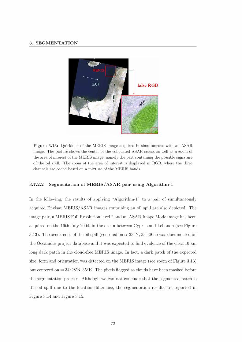
3. SEGMENTATION

Figure 3.13: Quicklook of the MERIS image acquired in simultaneous with an ASAR

image. The picture shows the center of the collocated ASAR scene, as well as a zoom of

the area of interest of the MERIS image, namely the part containing the possible signature

of the oil spill. The zoom of the area of interest is displayed in RGB, where the three

channels are coded based on a mixture of the MERIS bands.

3.7.2.2 Segmentation of MERIS/ASAR pair using Algorithm-1

In the following, the results of applying “Algorithm-1” to a pair of simultaneously

acquired Envisat MERIS/ASAR images containing an oil spill are also depicted. The

image pair, a MERIS Full Resolution level 2 and an ASAR Image Mode image has been

acquired on the 19th July 2004, in the ocean between Cyprus and Lebanon (see Figure

3.13). The occurrence of the oil spill (centered on ≈ 33◦N, 33◦39’E) was documented on

the Oceanides project database and it was expected to find evidence of the circa 10 km

long dark patch in the cloud-free MERIS image. In fact, a dark patch of the expected

size, form and orientation was detected on the MERIS image (see zoom of Figure 3.13)

but centered on ≈ 34◦28’N, 35◦E. The pixels flagged as clouds have been masked before

the segmentation process. Although we can not conclude that the segmented patch is

the oil spill due to the location difference, the segmentation results are reported in

Figure 3.14 and Figure 3.15.

72

3.7 Results

algae?

water

oil?

Figure 3.14: MERIS image segmentation using Algorithm-1 using multivariate Gaussian

distribution as data model.

3.7.2.3 Segmentation of an ERS-1 image using Algorithm-2 and -3

We have segmented part of an ERS-1 image from the Sicily Channel, Italy, that has

been acquired on the 30th January of 1992. This image is referred in the ESA web

pages regarding oil slicks http://earth.esa.int/ew/oil_slicks/ and contains three

oil slicks, along with information regarding wind direction and intensity and existence

of ships, ship wakes, natural oil films and currents.

Figure 3.16 provides a quicklook of the scene with two squares superimposed: the

larger representing the part to be segmented and the smaller representing a part used

for wind estimation. Figure 3.17 provides zooms of the referred squares. By applying

the Radon Transform [79] to the smaller square, a rough estimation of the direction has

been calculated and is depicted in the image. The direction was consistent with the mea-

sured value reported in the url site and is at the origin of the well-known “feathering”

effect that can be observed in this linear spill. We have computed the backscattering

values of the image, by performing calibration using the ESA provided BEST software

(http://earth.esa.int/services/best/) and then applied Algorithm-3 with Loopy-

73

3. SEGMENTATION

Figure 3.15: ASAR image segmentation with Algorithm 1 using Gamma mixture data

model.

Figure 3.16: ERS-1 image from the Sicily Channel, Italy, acquired on the 30th January

1992. The smaller and larger squares are sub-scenes that have been used respectively to

estimate the wind direction and to apply our algorithm.

74

3.7 Results

(a) (b)

Figure 3.17: Closer look to the sub-scenes of the ERS-1 image. Part (a) is used for wind

direction estimation; the estimated direction has been overlapped as a green arrow. Part

(b) contains an oil spill. The colored regions correspond to the ROI’s selected for class

parameter estimation in the supervised algorithm.

0.4 0.5 0.6 0.7 0.8 0.9 10

0.5

1

1.5

2

2.5

3

3.5

4

4.5

Figure 3.18: Fitting of a mixture of Gammas to the data from the red square in the

ERS-1 image.

β-Estimation. The result of the Gamma mixture estimation, in the initialisation of the

algorithm, is depicted in Figure 3.18. After only three iterations, both the class pa-

rameters and the smoothness parameter have converged. A β value equal to 1.4 was

estimated. The segmentation is displayed in Figure 3.19. We also applied Algorithm-2:

we selected two ROI’s (160 pixels for water and 77 for oil) in the image (shown in Fig-

ure 3.17) and computed ML Gamma Estimators for the two classes (see Figure 3.20).

We then applied the algorithm and obtained an estimated β value equal to 1.44. The

segmentation result is given in Figure 3.21 and is similar to the result obtained with

Algorithm-3.

For comparison, we also provide the segmentation obtained with no prior (corre-

75

3. SEGMENTATION

Figure 3.19: Segmentation of ERS-1 subscene containing oil with β = 1.4, estimated

using Algorithm-3 with the Loopy-β-Estimation method.

50 100 150 200 250 3000

0.005

0.01

0.015

0.02

0.025

0.03Oil Gamma Distribution Estimation

Water Gamma Distribution Estimation

Oil HistogramWater Histogram

Figure 3.20: Class Parameters Estimation for Algorithm-2.

76

3.7 Results

Figure 3.21: Segmentation of ERS-1 subscene containing oil with β = 1.44, estimated

using Algorithm-2.

Figure 3.22: Segmentation of ERS-1 subscene containing oil, with β = 0.

sponding to β = 0) in Figure 3.22. In practice, the estimated value has proved to

deliver a good segmentation. When lower β values were used, the result was noisier

and for higher β values, the details of the spill disappeared.

3.7.2.4 Segmentation of an Envisat ASAR IM image using Algorithm-2

and -3

We have also applied Algorithm-2 and Algorithm-3 to the same ASAR Image Mode

image used in Section 3.7.2.2 After six iterations, we achieved convergence of the β and

θ values. The segmentation result is given in Figure 3.23, corresponding to a estimated

β = 1.83. The unsupervised segmentation result is compared with the one provided

by Algorithm-2, where the user provided ROI’s for water and for oil that were used to

77

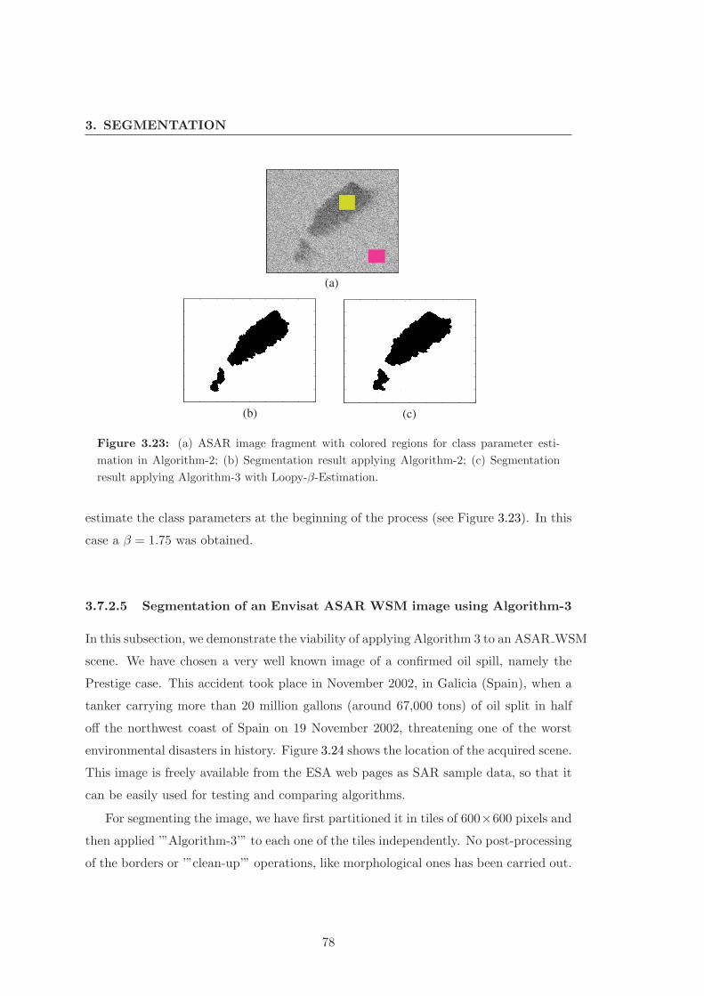
3. SEGMENTATION

(a)

(b) (c)

Figure 3.23: (a) ASAR image fragment with colored regions for class parameter esti-

mation in Algorithm-2; (b) Segmentation result applying Algorithm-2; (c) Segmentation

result applying Algorithm-3 with Loopy-β-Estimation.

estimate the class parameters at the beginning of the process (see Figure 3.23). In this

case a β = 1.75 was obtained.

3.7.2.5 Segmentation of an Envisat ASAR WSM image using Algorithm-3

In this subsection, we demonstrate the viability of applying Algorithm 3 to an ASAR WSM

scene. We have chosen a very well known image of a confirmed oil spill, namely the

Prestige case. This accident took place in November 2002, in Galicia (Spain), when a

tanker carrying more than 20 million gallons (around 67,000 tons) of oil split in half

off the northwest coast of Spain on 19 November 2002, threatening one of the worst

environmental disasters in history. Figure 3.24 shows the location of the acquired scene.

This image is freely available from the ESA web pages as SAR sample data, so that it

can be easily used for testing and comparing algorithms.

For segmenting the image, we have first partitioned it in tiles of 600×600 pixels and

then applied ’”Algorithm-3’” to each one of the tiles independently. No post-processing

of the borders or ’”clean-up’” operations, like morphological ones has been carried out.

78

3.7 Results

Figure 3.24: Location of the ASAR Envisat image acquired on the 17th of November

2002 during the Prestige accident in Galicia.

Figure 3.25 shows the most representative part of the ASAR image that has been

segmented, namely the part containing the oil spill, and Figure 3.26 shows the concate-

nation of the segmentation results. As we can see, they are in general very good, with

only a discrepancy on the border between some of the tiles.

For initializing the algorithm, the EM Gamma mixture estimation procedure was

applied with four modes (K = 4). In fact this number is sufficient to provide a good

fitting of the intensity data of the SAR image. On the other hand, our EM algorithm

allows us to start with a higher mode number, and decreases this number automatically.

We depict the results of this fitting on one of the tiles( depicted in Figure 3.27), by

showing the histogram of the referred tile with the superimposed estimated Gamma

mixture (see Figure 3.28 (a)). As we have explained, the mode corresponding to the

lower mean value is assigned to the oil class and the others to the water class, providing

an initialization to the class parameters. The estimations of these parameters are

actualized along the algorithm and, after nine iterations, we obtain the distributions

shown in Figure 3.28 (b).

To fully demonstrate the possibilities of our algorithm, we again run it on the

chosen tile, but this time setting the number of classes to c = 3. By doing so, we

hope to be able to segment a third ambiguous zone, corresponding to intermediate

radiometry levels and probably due to atmospheric conditions originating a front. In

this case we choose to fit a Gamma mixture of c modes to the data for initializing the

79

3. SEGMENTATION

Figure 3.25: Display of the ASA WSM full resolution image of the Prestige accident.

80

3.7 Results

200 400 600 800 1000 1200 1400 1600 1800

500

1000

1500

2000

Figure 3.26: Display of the segmentation results of applying Algorithm 3 with Loopy-β-

Estimation to Figure 3.25.

81

3. SEGMENTATION

Figure 3.27: Zoom to one of the bottom tiles in which the Prestige ASAR image was

divided. This tile has been chosen to provide further details on the algorithm steps.

0 0.1 0.2 0.3 0.4 0.5 0.6 0.7 0.8 0.9 10

0.5

1

1.5

2

2.5

3

0 0.05 0.1 0.15 0.2 0.25 0.3 0.35 0 0.1 0.2 0.3 0.4 0.5 0.6 0.7 0.8 0.9

(a)

(b)

Figure 3.28: Results of applying the EM Gamma mixture estimation procedure to the tile

depicted in Figure 3.27: (a) Histogram of the data values (normalized) with superimposed

estimated Gamma mixture; (b) Distributions corresponding to the oil class (left) and water

class (right) after nine iterations of Algorithm 3: Histogram and superimposed fitting.

82

3.7 Results

100 200 300 400 500 600 7000

0.5

1

1.5

2

2.5

3

3.5

4

4.5

5x 10

−3

data histogramgamma 1gamma 2gamma 3gamma mixture

Figure 3.29: Histogram of the data values (normalised) with superimposed estimated

Gamma mixture when the number of classes is set to c = 3.

Figure 3.30: Display of the initial segmentation result of applying Algorithm 3 with

Loopy-β-Estimation and three classes to the bottom left tile of Figure 17.

class parameters, as depicted in Figure 3.29. With this initialization, the first obtained

segmentation using Algorithm 3 is displayed in Figure 3.30. After only nine iterations,

all parameters have already converged to the segmentation given in Figure 3.31. When

comparing this segmentation with the one provided by a state-of-the-art algorithm,

namely by multiscale HMC model in [14], we consider to have obtained a very good

result.

83

3. SEGMENTATION

Figure 3.31: Display of the final segmentation result, after nine iterations, of applying

Algorithm 3 with Loopy-β-Estimation and three classes to the bottom left tile of Figure

17.

3.7.2.6 Computational Complexity

The proposed algorithms display, in practical cases, a computational complexity of

O(N), with N being the number of pixels in the image. In fact, the most time-consuming

steps in the algorithms are the α-Expansion and Graph-Cut segmentation routines

[68]. These use the max-flow code implementation referred in [80] that has complexity

O(n2.5) in the worst-case, however, in most situations is O(N). Both Algorithm 1

and Algorithm 3 converge in few iterations and, as an example, for images of the

dimension used in the first simulation (64x64) (see 3.7.1.1), only a few seconds are

needed to run the algorithms. For a 600x600 pixel tile, like those in the Prestige

example in 3.7.2.5, Algorithm 3 is taking ≈ 1 minute, but this time performance could

be improved by a more efficient implementation of our procedure, namely by improving

the implementation of the Loopy-β-Estimation and by migrating our matlab code fully

to C-code.

84

4

Classification

4.1 Lookalikes: an Overview

As it was already referred to at the beginning of this text, there is a number of oceano-

graphic and atmospheric phenomena that gives rise to dark signatures in SAR images

that may very easily be mistaken with oil spill signatures. In this section, we provide

some examples of those phenomena. The given list is in no way complete and only

some main types of lookalikes are described here. For a deeper and more complete view

on this topic, see [3] and [2].

One important aspect of lookalikes is that they are normally local phenomena,

related to local features like existing currents or orography. They are often also seasonal,

like algae blooms, or ice. In the following, four examples of lookalikes, along a brief

explanation of the causes why they are visible in SAR images, is given. One phenomena

associated with false positives is bathymetry. They are typically associated with clear

lines of high and low backscatter forming tails after the obstacle, if the depth change is

abrupt.The origin are currents (usually tidal current), which flow over bottom features

like sand banks, causing modulation of surface currents; the Bragg waves pass through

these currents and change their amplitudes (illustrated by Figure 4.1 and by Figure

4.2).

Intertidal zones and sandbanks are also characterized by homogeneous dark areas,

oft strips of intertidal mud or sand flat. They appear along shallow coastal areas and

river mouths and are observed at low tide (see also Figure 4.1).

Upwelling phenomena also appear as dark area in SAR images. Its origin is colder

85

4. CLASSIFICATION

Figure 4.1: SAR image containing bathymetry signatures, see [1]. This is an ERS-1 image

acquired on the 8th July 1995, showing the Subei Shoal off the coast of China (north of

Shanghai). The dark areas are the sea areas that have fallen dry during ebb tide.

86

4.1 Lookalikes: an Overview

Figure 4.2: Physical explanation of the signature origin of bathymetry structures, see [1].

Figure 4.3: SAR image containing upwelling signature around St. Martin island group.

The image is an ASAR WSM acquisition from the 4th of May 2007 at 10:46 (courtesy of

Edisoft).

87

4. CLASSIFICATION

water from deeper water columns ascending to the sea surface. Under certain condi-

tions, water of the upper layer moves away from the coast in either hemisphere and is

replaced by water upwelling from below this layer. This typically occurs during Sum-

mer in the North and also in the Spring and Autumn for further south. The affected

area usually has a larger concentration of nutrients and high biological productivity

implying that the amount of surface active substances secreted by marine plants and

animals, which float to the sea surface and create there a surface film, are greatly

enhanced. Figures 4.3 and 4.4 show an example of an upwelling

As a last example, a case of natural films is displayed in Figure 4.5 can also com-

pletely hamper the usability of a SAR image for oil spill detection.

4.2 Classification Methods

In the following, we are mostly using the same notation as in [45]. Our goal is to leverage

a set of n training samples in order to design a classifier that is capable of distinguishing

between m classes on the basis of an input vector x, where x = [x1, ..., xd]T ∈ Rd are

simply the d dark patch features. By using the “Leave-One-Out”method, we remove

one item at a time from the n + 1 element dataset and use the remaining n elements

for training the classifier. In our case the dataset contains 140 elements (n = 140),

we have just two classes (m = 2), and d = 35 features when wind is considered and

d = 34 when not. We adopt the common technique of representing the class labels using

a “1-of-m” encoding vector y = [y(1), y(2), ..., y(m)] such that yi = 1 if x corresponds

to an example belonging to class i and yi = 0 otherwise. The n training samples

that we use in each cycle of the “Leave-One-Out”can thus be represented as a set of

training data D = [(x1, y1), ..., (xn, yn)]. In each cycle of the “Leave-One-Out”, after

training the classifier using the data D, we test the classifier in the remaining item.

The classification results are the mean values of all performed tests.

In this work we have exploited two different approaches:

• Approach 1 (AP1): Apply a feature selection method first and then test different

classifiers using the selected features.

• Approach 2 (AP2): Apply a method where feature selection and classification

are performed side-by-side, namely the so called Sparse Multinomial Logistic

88

4.2 Classification Methods

Figure 4.4: Chlorophyll and Sea Surface Temperature (SST) images correlating with

SAR signatures (image from the Multi View for UK Waters, from the Plymouth Marine

Laboratory).

89

4. CLASSIFICATION

Figure 4.5: SAR image of the area of the Baltic, see [1]. The sea is partially covered with

biogenic slicks that are abundant at this time of the year because of the spring plankton

bloom.

90

4.2 Classification Methods

Regression (SMLR), (see [45]).

The feature selection step is important because many of the features we have com-

puted are redundant or strong correlated. On the other hand, due to the limited number

of samples in our database, using too many features would ultimately cause a decrease

of performance due to overfitting.

Feature selection methods essentially divide into wrappers, filters, and embedded

methods. Wrappers utilize the learning algorithm of interest as a black box to score

subsets of variable according to their predictive power. Filters select subsets of variables

as a pre-processing step, independently of the chosen classifier. Embedded methods

perform variable selection in the process of training and are usually specific to given

learning algorithm (see [81]). Following these definitions we can see that AP1 uses a

filter and AP2 an embedded type selection.

We have tested the two approaches in two different scenarios: with and without

wind information. By doing so, we intended to assess the true relevance of wind for the

classification process. In fact, wind is not always available or its resolution or accuracy

is not adequate. Especially in the case of lookalikes, which often occur near the coast,

wind speed models do not provide good estimates and SAR extracted values must be

taken into consideration with some reserve. Considering these operational constraints,

it is of interest to have a quantitative analysis of the importance of wind availability

for this problem.

4.2.1 AP1

In AP1, we have tested two different suboptimal feature selection algorithms: the For-

ward Feature Selection (FFS) (see [81]) method and the Backward Feature Selection

(BFS) (see [81]) method. The choice of using suboptimal algorithms was taken consid-

ering the computational effort. In a forward selection method one starts with an empty

set and progressively adds features yielding to the improvement of a performance index.

In a backward elimination procedure one starts with all the features and progressively

eliminates the least useful ones.

Both procedures are reasonably fast and robust against overfitting and provide

nested feature subsets. However, as we shall see, they may lead to different subsets

and, depending on the application and the objectives, one approach may be preferred

91

4. CLASSIFICATION

over the other one. In particular backward elimination procedures may yield better

performances but at the expense of possibly larger feature sets. However if the feature

set is reduced too much, the performance may degrade abruptly [64]. In this work,

we have used the matlab toolbox PRTools (see http://www.prtools.org/), that pro-

vides FFS and BFS routines. The evaluation criteria was the sum of the Mahalanobis

distances. After the feature selection, we used standard classifiers provided also by

PRTools. We have tested the following:

1. Logistic regression (LOGC)

2. Linear Bayes Normal Classifier (LDC)

3. Quadratic Bayes Normal Classifier (QDC)

4. K-Nearest Neighbor Classifier (KNNC)

5. Parzen Windows (PARZENC)

6. Support Vector Machine (SVMC) with a Gaussian Kernel

Logistic regression is adequate when we have a dependent variable y which takes

binary values, which is also our case in this work (1:= oil, 0:= lookalike). We then

assume that y follows a binomial distribution (y ∼ Bin(p, n)), where p is the probability

of success (being oil) and n is the number of trials (number of dark patches/samples).

The mean value of y is np, and if we normalize the variable it is simply p, taking values

between 0 and 1.

The model in logistic regression proposes that we use as dependent variable the

logarithm of the odds ratio (so-called logits). Odds are defined as Odd := p/(1 − p),

and logits are given by expression

logit(p) = ln

(p

1 − p

), (4.1)

and they are modeled as a linear function of the zi, the set of explanatory variables

(the features), that might inform the final probability:

logit(p) = a+ βz, (4.2)

92

4.2 Classification Methods

where a is called the intercept, β = (β1, β2, . . .) are called the regression coefficients,

z = (z1, . . .) is the vector of the features zi and where p = Pr(y = 1|z).The logit is then converted into a probability using the following expression (the

logistic function):

p =elogit

1 + elogit. (4.3)

The logistic model automatically assures that p is bounded by 0 and 1, which is

not the case with normal linear regression. The parameters of the model are a and β

and can be obtained for example using Ridge Regression. We used the implementation

of the PRTools. An interpretation of the coefficients, in the case of a dichotomous

explanatory variable (zj is 0 or 1), is that odds for group with zj = 1 are exp(βj)

higher, other parameters being equal.

The classifiers used in this work referred to as LDC and QDC are common used

Bayesian classifiers. They are based on the prerequisites that we can quantify as a cost

the “damage” involved when an object is wrongly classified. A second prerequisite,

when using Bayesian classifiers, is that the expectation of this cost can be used as an

optimization criteria. The cost function is in our case, where we have two classes, a

2x2 matrix C(c, ck), where c is the class and can take the values c1 and c2.

It can be demonstrated [82] that the expectation of the cost that the classifier

assigns a class ci to a measurement vector z (containing the features) which actually

corresponds to an object with true class ck, is

R(ci|z) =K∑

k=1

C(ci|ck)P(ck|z), (4.4)

where K is the number of classes and P(ck|z) is the posterior probability. This ex-

pression is called the conditional risk and by averaging it over all possible all possible

measurements we obtain the overall risk, which we would like to minimize in this ap-

proach.

As a conclusion, a Bayesian classifier assigns a class cBayes(z) to a measurement

vector z, such that

cBayes(z) = argminc∈ L{R(c|z)} . (4.5)

93

4. CLASSIFICATION

The linear and quadratic classifiers used result from further assumptions:

• a uniform cost function is defined, where a unit cost is assumed when an object

is misclassified, and zero cost when the classification is correct;

• the conditional probability densities p(z|ck) are modeled as Gaussian functions.

With the above two assumptions, the classifier is called a quadratic classifier and if

we make a further simplification that the covariance matrices in the Gaussian functions

are class independent the classifier is called linear.

The K-Nearest Neighbor algorithm is the simplest approach for two-class classi-

fication. It is a non-parametric model, which classifies a sample by assigning it the

label most frequently represented among the K nearest samples. It uses directly the

training set without explicitly estimating probability densities. For classifying a new

sample, a distance function is needed to determine which K members of the training

set are closest to it. Once the K-nearest training instances have been found, their class

assignments are used to predict the class for the new instance, by a majority vote. It

can be shown that the performance of the K-NNR approximates the optimum as K

increases, but this asymptotic optimality only holds true if the training set is dense.

In practice, the demand on the size of the training set is very high, implying increased

computational complexity. A suitable choice is to make K proportional to√

Nk, where

Nk is the number of samples belonging to class k [82].

Parzen windows classification is a technique for nonparametric density estimation,

which can also be used for classification. It can be regarded as a generalization of

the k-nearest neighbor technique. The basic idea is that the knowledge gained by the

observation of sample zi is represented by a function h centered at zi (the so-called

kernel of the estimator) and with an influence restricted to a small vicinity. This

function represents the contribution of the observation data zi to the estimative of the

conditional probability p(z|c = ck). For obtaining the final estimate, all contributions

for all training data are summed together [82]. The kernel can be regarded as an

interpolation function that interpolates between the samples of the data set. With

Gaussian kernels, the weight decreases exponentially with the square of the distance,

so far away points are practically irrelevant. The width σh of the Guassian function

94

4.2 Classification Methods

Figure 4.6: This image depicts the main steps undertaken in the Classification, as well

as the algorithms and toolbox used.

determines the relative weighting of near and far points and it can be chosen smaller as

the number of training samples increases. A classification based on Parzen estimation

implies first the determination of the σh value. Then, for each sample z in the test set

the density for each class is computed:

p(z|ck) =1

Nk

∑

zj∈Tk

1

σNh

√(2π)N

exp(−‖z − zj‖2

2σ2h

), (4.6)

where N is the number of features and Tk are the subsets into which we partition the

labeled training set Ts, each one containing Nk samples, all belonging to class ck. The

sample is assigned to the class with maximal posterior probability:

c = ck with k = argmaxi=1,...,K

{p (z|ci) P (ci)

}(4.7)

Please refer to [82] for more details on the classifiers and to the documentation of

PRTools [83] for details on the implementation.

95

4. CLASSIFICATION

4.2.2 AP2

The SMLR algorithm is based on multinomial logistic regression and adopts a Laplacian

sparsity-promoting prior in order to learn a classifier that incorporates weighted sums

of basis functions and results in better generalization capability. Under a multinomial

logistic regression model (see [45]), the probability that x belongs to class i is written

as

P(yi = 1|x,w

)=

exp(w(i)T

x)∑m

j=1(w(j)T x)

, (4.8)

for i ∈ 1, ...,m, where wi is the weight vector corresponding to class i and the superscript

T denotes vector/matrix transpose. In our case, because we just have two classes

the regression is called logistic regression. The weight vector are estimated from the

training data D. To perform maximum likelihood (ML) estimation of w, we would

simply maximize the log-likelihood function:

l(w) =n∑

j=1

log P(yjxj , w) =n∑

j=1

[m∑

i=1

y(i)j w(i)T

xj − logm∑

i=1

exp(wiT xj)

]. (4.9)

On the other hand, l(w) can be made arbitrarily large when the training data

is separable, so that we adopt a maximum a posteriori (MAP) estimate, following a

Bayesian framework. We introduce a sparsity-promoter Laplacian prior,

p(w) ∝ exp(−λ‖w‖1), (4.10)

where ‖w‖1 :=∑

l |wl| denotes the l1 norm, and maximize the posterior distribution

instead:

wMAP = arg maxwL(w) = arg maxw[l(w) + log p(w)]. (4.11)

For estimating w, a bound optimization algorithm, described in [45] in detail is used.

When applying SMLR, the Laplacian prior forces w to zero or close to zero for many

of the entries, resulting in an intrinsic feature selection mechanism. The parameter λ

is called regularization parameter and by increasing its value, more components from

w tend to zero.

96

4.3 Experimental Results

Figure 4.7: Histogram of Lenght To Width Ratio values; Red=oil, blue=lookalikes.

4.3 Experimental Results

4.3.1 Examples of Extracted Features

In this subsection we illustrate the physical meaning of some relevant features, providing

examples from the used data set. One interesting example is the “Lenght To Width

Ratio” (LWR), as many of the detected oil spills originate from discharges of moving

vessels, presenting a linear shape. In the empirical guidelines provided to oil spill

detection operators, linear shape is considered a strong indication of oil spill. Figure

4.7 depicts the histogramm of the LWR values calculated for the data set used in the

classification. Figure 4.8 and Figure 4.9 present examples of two dark patches, one oil

spill and one lookalike respectively, with very different LWR values.

Another characteristic, which is also used by the operators as an important indi-

cation of an oil spill is the so-called “homogeneity of the surroundings”. Guidelines to

operators state that an homogeneous area around the dark patch increases the proba-

bility that it is an oil spill. One feature which is correlated with this is the “Intensity

Standard Deviation Ratio” (ISDR). Figure 4.10 depicts the histogramm of the ISDR

values calculated for the data set used in the classification. Figure 4.11 and Figure 4.12

97

4. CLASSIFICATION

Figure 4.8: Example of oil slick from ongoing discharge of moving vessel, with LWR=118

(Length=30.74 km, Width=0.26 km).

Figure 4.9: Red square: Example of lookalike with LWR=2.7 (Length=3.02 km, Width

= 1.1 km).

98

4.3 Experimental Results

Figure 4.10: Histogram of Intensity Standard Deviation Ratio values; Red=oil,

blue=lookalikes.

present examples of two dark patches, one oil spill and one lookalike respectively, with

very different ISDR values.

A common reason for inhomogeneous surroundings is the presence of natural films,

which disappear by medium to high wind speed. This associated with the fact that low

wind areas are also typicall lookalikes, explains why lookalikes are oft linked with low

wind speeds, as we can see from Figure 4.13 a certain number of lookalikes are indeed

associated with low wind areas.

When the wind is not used as feature, the minimum intensity value of the dark

patch (MinObj) is also a good descriminator of lookalikes due to low wind areas.

4.3.2 AP1

We have run the feature selection methods BFS and FFS varying the selected feature

set size from 1 to the maximum value (35 when using wind, 34 when not using wind)

and applied a number of different classifiers, as described in subsection 4.2.1.

99

4. CLASSIFICATION

Figure 4.11: Example of oil slick with with ISDR=3.17, corresponding to a very homo-

geneous surrounding.

Figure 4.12: Example of lookalike with ISDR= 0.33, corresponding to an inhomogeneous

surrounding.

100

4.3 Experimental Results

Figure 4.13: Histogram of wind values associated with the lookalikes and oil spills of the

data set used for classification; Red=oil, blue=lookalikes.

Table 4.1: Classification Results for AP1 with wind information

Classifier BFS FFS

LOGC OA-test = 96.1 NrFeat = 11 OA-test = 93.1 NrFeat = 9

LDC OA-test = 97.0 NrFeat = 15 OA-test = 94.1 NrFeat = 19

QDC OA-test = 93.1 NrFeat = 5 OA-test = 93.1 NrFeat = 15

KNNC OA-test = 92.2 NrFeat = 3 OA-test = 91.2 NrFeat = 14

PARZENC OA-test = 92.2 NrFeat = 3 OA-test = 91.2 NrFeat = 5

SVMC OA-test = 93.1 NrFeat = 9 OA-test = 92.2 NrFeat = 13

4.3.2.1 With Wind

Table 4.1 provides an overview of the obtained results, when wind speed is also used

as feature. For the two feature selection methods and for each classifier, the maximum

obtained OA-test and the correspondent respective number of selected features is given.

For LOGC and LDC classifiers, the results can be visualised in more detail in Figure

4.14 and Figure 4.15.

From Table 4.1, we can see that a good classification method could be LOGC with

11 features given by BSF feature selection, or LDC with 15 features also given by BSF.

The corresponding features for this two methods are given in Table 4.2 , where they

are ranked by relevance.

101

4. CLASSIFICATION

0 5 10 15 20 25 30 3555

60

65

70

75

80

85

90

95

100

BFS: LOGCFFS: LOGC

Nr of Selected Features

OA_test

Figure 4.14: Evolution of OA-test with the number of selected features for LOGC clas-

sifier using wind information. Comparison between the BSF and FFS feature selection

methods.

0 5 10 15 20 25 30 3550

55

60

65

70

75

80

85

90

95

100

Nr of Selected Features

OA_test

BFS: LDCFFS: LDC

Figure 4.15: Evolution of OA-test with the number of selected features for LDC classifier

using wind information. Comparison between the BSF and FFS feature selection methods.

102

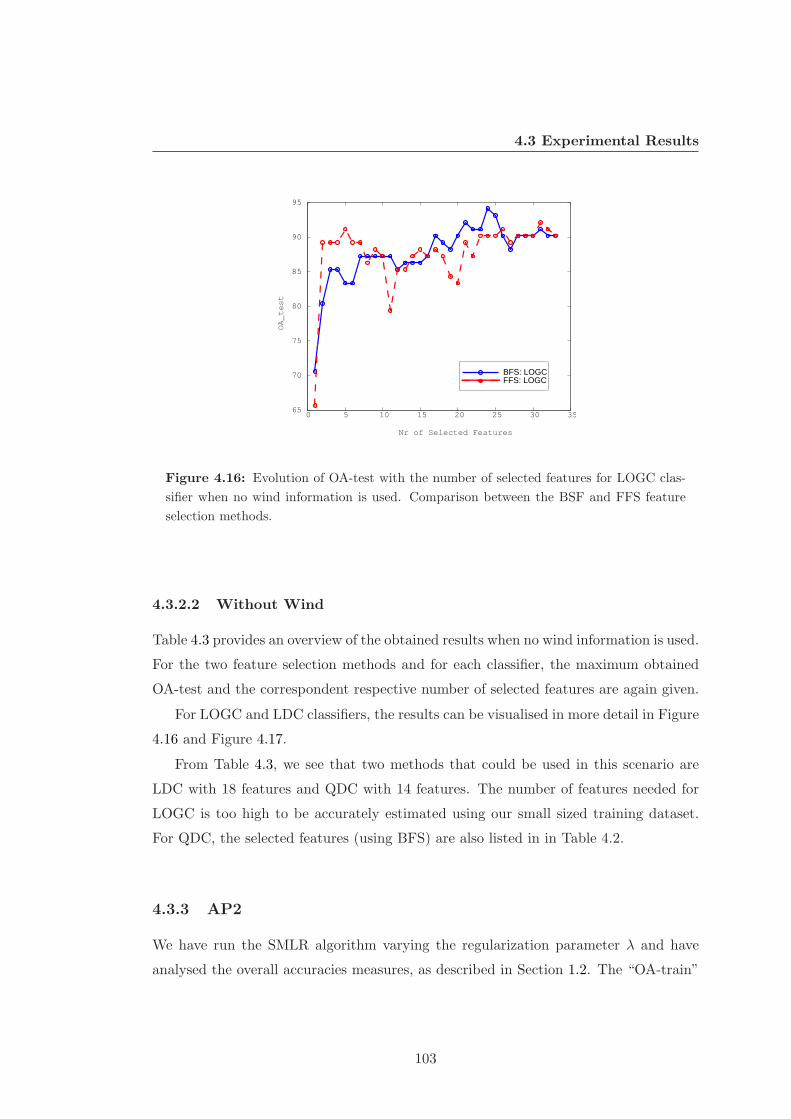
4.3 Experimental Results

0 5 10 15 20 25 30 3565

70

75

80

85

90

95

Nr of Selected Features

OA_test

BFS: LOGCFFS: LOGC

Figure 4.16: Evolution of OA-test with the number of selected features for LOGC clas-

sifier when no wind information is used. Comparison between the BSF and FFS feature

selection methods.

4.3.2.2 Without Wind

Table 4.3 provides an overview of the obtained results when no wind information is used.

For the two feature selection methods and for each classifier, the maximum obtained

OA-test and the correspondent respective number of selected features are again given.

For LOGC and LDC classifiers, the results can be visualised in more detail in Figure

4.16 and Figure 4.17.

From Table 4.3, we see that two methods that could be used in this scenario are

LDC with 18 features and QDC with 14 features. The number of features needed for

LOGC is too high to be accurately estimated using our small sized training dataset.

For QDC, the selected features (using BFS) are also listed in in Table 4.2.

4.3.3 AP2

We have run the SMLR algorithm varying the regularization parameter λ and have

analysed the overall accuracies measures, as described in Section 1.2. The “OA-train”

103

4.

CLA

SSIF

ICA

TIO

N

Table 4.2: AP1 Best Results: Features selected for LOGC, LDC and QDC - ranked by relevance.

For LOGC (with wind) For LDC (with wind) For QDC (without wind)

Max Slick Value Perimeter Min Slick Value

Inside Slick Radar Backcatter Max Slick Value Max Slick Value

Max Contrast Outside Slick Radar Backscatter Intensity Standard Deviation Ratio

Width Max Contrast Width

Length To Width Ratio GLCM Homogeneity Ellipse-Asymmetry

Wind Speed Width GLCM Correlation

Perimeter Length To Width Ratio GLCM Dissimilarity

ISRI ISRO Ratio Wind Speed ISRI ISRO Ratio

Max Gradient ISRI ISRO Ratio GLCM Contrast

Inside Slick Standard Deviation Max Gradient GLCM Entropy

Gradient Standard Deviation Mean Gradient Mean Gradient

Gradient Standard Deviation Outside Slick Radar Backscatter

Inside Slick Standard Deviation Perimeter

Form Factor Length To Width Ratio

GLCM Dissimilarity

104

4.3 Experimental Results

Table 4.3: Classification Results for AP1 without wind information

Classifier BFS FFS

LOGC OA-test = 94.1 NrFeat = 24 OA-test = 92.2 NrFeat = 31

LDC OA-test = 91.2 NrFeat = 18 OA-test = 91.2 NrFeat = 29

QDC OA-test = 93.1 NrFeat = 14 OA-test = 89.2 NrFeat = 19

KNNC OA-test = 91.2 NrFeat = 31 OA-test = 92.1 NrFeat = 20

PARZENC OA-test = 90.2 NrFeat = 11 OA-test = 91.2 NrFeat = 5

SVMC OA-test = 92.2 NrFeat = 28 OA-test = 94.1 NrFeat = 30

0 5 10 15 20 25 30 3560

65

70

75

80

85

90

95

Nr of Selected Features

OA_test

BFS: LDCFFS: LDC

Figure 4.17: Evolution of OA-test with the number of selected features for LDC classifier

when no wind information is used. Comparison between the BSF and FFS feature selection

methods.

105

4. CLASSIFICATION

value has been calculated using the same mathematical expression as “OA-test”, but

over the training data set instead of over the test elements.

4.3.3.1 With Wind

The algorithm was first applied using all the 35 features,including the wind speed. As

we can see from Figure 4.18, we obtain a maximal OA-test value of 93.1 for a parameter

value of λ ≈ 0.42. Figures 4.19 and 4.20 show also the evolution of the values “OA-oil”,

“OA-lookalike”, “OA-falsePositives” and “OA-falseNegatives” with the regularization

parameter. As we can see from Figure 4.21, the value λ = 0.42 is also assigned to the

minimal value of the Bayesian risk, given by expression 4.12, where we are considering

the cost function for false positives and false negatives to be the same.

We can also confirm our expectation that an increasing value of λ results in more

weight values wi set to 0, and though to a reduced number of features relevant for the

classification process. Figure 4.22 shows this aspect and we see that the value λ = 0.42

corresponds to 13 relevant weights. This means that only 13 of the estimated weights

wi take values considerably different from 0, as we can see from Figure 4.23, which

shows the estimated w for one particular, representative Leave-One-Out cycle of the

SLMR algorithm. The image also shows the histogram of the expression xTw, where

we can see the clear separation of the two classes, with just a small overlap, accounting

for the false positives and negatives. The selected features, ranked by relevance, are

listed in Table 4.4.

Risk =OA-fN +OA-fP

2(4.12)

4.3.3.2 Without Wind

We repeated the AP2 procedure but without using the wind feature. The obtained

results were very similar to those obtained using wind information: the regularization

parameter corresponding to the best OA-test = 92.2 was λ = 0.44, with 15 relevant

features. The selected features,ranked by relevance, are also listed in Table 4.4

106

4.3 Experimental Results

Table 4.4: AP2 Best Results: Features selected for SLMR - ranked by relevance.

For SLMR (with wind) For SLMR (without wind)

Min Slick Value Compactness

Width Min Slick Value

Ellipse-Width Width

Compactness Ellipse-Width

Wind Speed ISRI ISRO Ratio

Length To Width Ratio Inside Slick Radar Backcatter

ISRI ISRO Ratio Outside Slick Standard Deviation

Intensity Standard Deviation Ratio Mean Gradient

Mean Gradient Length To Width Ratio

Complexity GLCM Entropy

Outside Slick Standard Deviation Area

GLCM Entropy Complexity

Area Gradient Standard Deviation

Intensity Standard Deviation Ratio

GLCM Correlation

0 2 4 6 8 10 12 14 16 18 200.86

0.88

0.9

0.92

0.94

0.96

0.98

1

OA_trainOA_test

0 0.5 1 1.5

0.88

0.9

0.92

0.94

0.96

0.98

OA_trainOA_test

Regularization Parameter λ

Ove

rall

Accu

racy

Zoom of figure

Figure 4.18: OA-test and OA-train from SLMR algorithm versus regularization param-

eter, when wind information is used.

107

4. CLASSIFICATION

0 2 4 6 8 10 12 14 16 18 200.75

0.8

0.85

0.9

0.95

1

Regularization Parameter λ

OA_oilOA_lookalike

0 0.5 1 1.5

0.86

0.88

0.9

0.92

0.94

0.96

0.98

1

OAoilOAlookalike

Zoom of figure

Overa

ll A

ccura

cy

Figure 4.19: OA-oil and OA-lookalike from SLMR algorithm versus regularization pa-

rameter, when wind information is used.

0 2 4 6 8 10 12 14 16 18 20

0

0.05

0.1

0.15

0.2

0.25

0 0.5 1 1.5

0.02

0.04

0.06

0.08

0.1

0.12

0.14

0.16

OAfalsePositivesOAfalseNegatives

Regularization Parameter λ

Overa

ll A

ccura

cy

OA_falsePosOA_falseNeg

Zoom of figure

Figure 4.20: OA-falsePositives and OA-falseNegatives from SLMR algorithm versus reg-

ularization parameter, when wind information is used.

108

4.3 Experimental Results

0 2 4 6 8 10 12 14 16 18 20

0.07

0.08

0.09

0.1

0.11

0.12

0.13

Ris

k

Regularization Parameter λ

0 0.5 1 1.50.06

0.07

0.08

0.09

0.1

0.11

0.12

0.13

Zoom of figure

Figure 4.21: Risk versus regularization parameter, when wind information is used.

0 2 4 6 8 10 12 14 16 18 206

8

10

12

14

16

18

20

22

24

26

Nr

of re

levant w

eig

ths (

wi~

=0)

0 0.5 1 1.512

14

16

18

20

22

24

26

Regularization Parameter λ

Zoom of figure

Figure 4.22: Number of Relevant Features (wi 6= 0) versus regularization parameter,

when wind information is used.

109

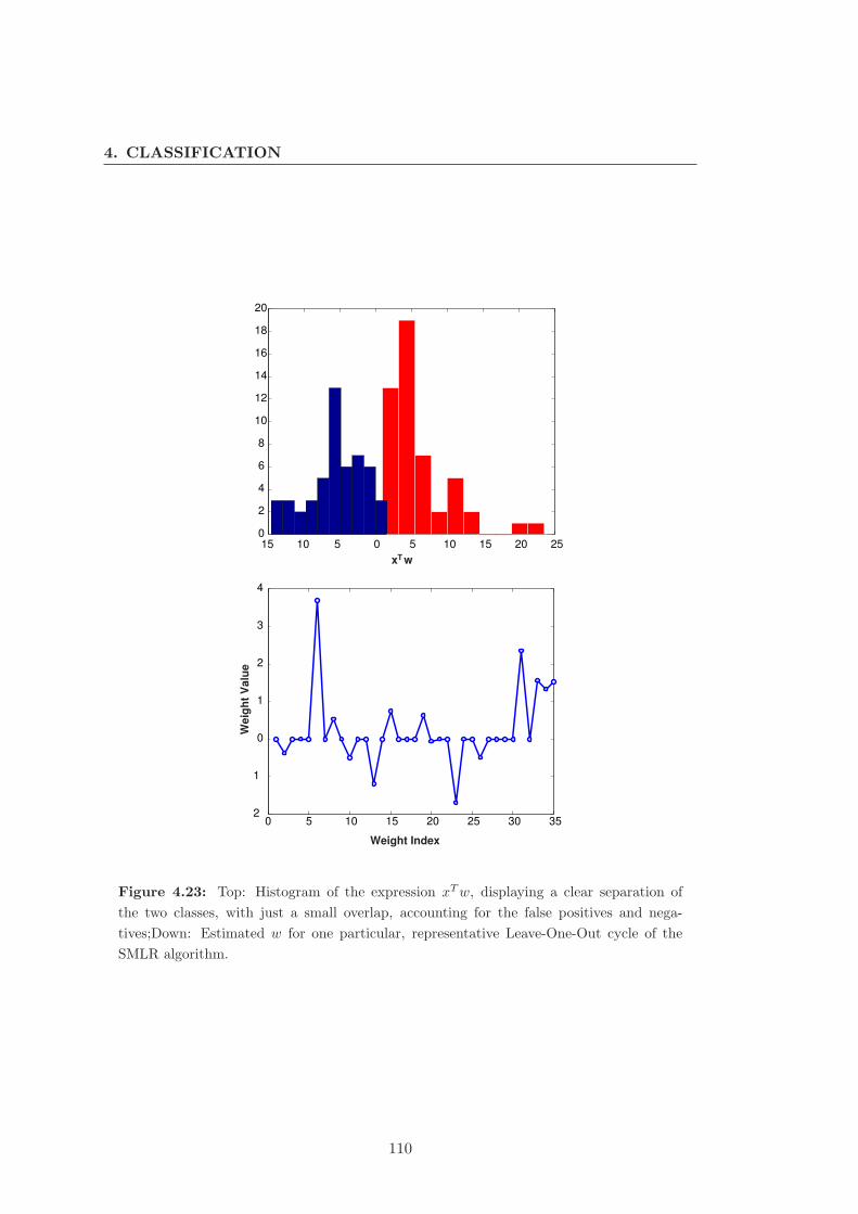
4. CLASSIFICATION

15 10 5 0 5 10 15 20 250

2

4

6

8

10

12

14

16

18

20

0 5 10 15 20 25 30 352

1

0

1

2

3

4

x wT

Weight Index

Weig

ht

Valu

e

Figure 4.23: Top: Histogram of the expression xTw, displaying a clear separation of

the two classes, with just a small overlap, accounting for the false positives and nega-

tives;Down: Estimated w for one particular, representative Leave-One-Out cycle of the

SMLR algorithm.

110

5

Conclusions

5.1 Conclusions on Proposed Methodology for Oil Spill

Detection

In what concerns the segmentation step, the results of applying the proposed methodol-

ogy to simulated images with Gamma data models and to real SAR data are promising.

The developed EM Gamma mixture estimation algorithm, when incorporated into the

proposed segmentation algorithms, has proved to be an efficient tool for data modeling

in SAR intensity images.

With the supervised algorithms, high OA accuracies have been achieved even for

simulated images with high levels of noise. In general the Bayesian approach has

resulted in an OA increase in the segmentation process between 10 and 15%, when

compared to the segmentation using no prior information. Hereby, Algorithm 1 with

LSF and Algorithm 1 with CD methods provided similar results, with a performance

close to that obtained by setting the β value manually. On the other hand, the LSF es-

timation procedure seems to become less reliable for noisier images. When compared to

Algorithm 2, using Loopy-β-Estimation, we see that this last method allways provides

equal or better results, outcoming Algorithm 1. Another advantage of Algorithm 2 is

that it is usually faster than Algorithm 1, being a one-shot process. Both algorithms,

by introducing prior information into the segmentation process, increase the OA signif-

icantly. As a conclusion, Algorithm 2 should be preferred to Algorithm 1, when using

a supervised method for oceanic SAR images segmentation.

111

5. CONCLUSIONS

Algorithm 3, totally unsupervised, has been conceived as an improvement to Al-

gorithm 1 and 2. When testing it on simulated data the obtained results were very

good, although slightly worst than the supervised ones, as expected. In general, after a

few iterations, the class and smoothness parameters converge to stable and meaningful

values. By applying Algorithm 3 to real images containing documented oil spills, the

segmentation has been considered successful. We could segment both linear and patch

type oil spills. Furthermore, the applicability of the method to segment whole scenes,

as well as to segment more than two classes, has also been demonstrated in a well

known image from the Prestige accident. As a conclusion, we believe the presented

methods are suitable to be used for segmenting oceanic SAR images. In particular for

oil spill detection, Algorithm 3 seems to be a suitable method.

Based on observations that oil spills in the ocean are often dragged by the wind

and align more or less perpendicular to its direction, an interesting future issue is

the incorporation of wind information into our segmentation algorithms. By adopting

anisotropic MRF in the prior, we intend to reflect this directional dependency of the

clique potentials. In the practice, the smoothness parameter β is no longer considered

to be a constant value but is clique-dependent according to the wind direction and/or

velocity. For estimating the wind profile from the SAR data, state-of-the-art algorithms

are used. We have run promising simulations, are currently testing this extension on

real data, and expect to obtain interesting results on a near future.

We have tested two different approaches for automatic classification of dark patches

in SAR images. For training and testing our algorithms we have first built a 140 dark

patch database containing oil spills and lookalikes detected by experienced operators

in the framework of the CSN service from EMSA. The used SAR images were from the

Envisat satellite, and were of the type Wide Swath. In both approaches we assessed the

problem of feature selection: by adopting standard feature selection methods, namely

the BFS and the FFS, and then applying standard classifiers and by testing a new

algorithm called SMLR, which performs feature selection and classification in parallel.

From our results we can draw mainly the following conclusions:

• C1: The AP1 approach delivered the best results, with the highest accuracy

corresponding to the LDC and LOGC methods using BFS feature selection (re-

spectively 97.0% and 96.1%).

112

5.2 Perspectives on Oil Spill Detection

• C2: BFS delivered always better results than FFS for this particular classification

problem.

• C3: The AP2 approach resulted in slightly lower accuracies than AP1 (93.1 in-

stead of 97.0), for a similar number of features, but seemed to be more robust

against the absence of wind information. In fact, removing the wind feature only

resulted in a decrease of ≈ 1% in the accuracy, and only in an increase of two

more features in the final selected features set.

• C4: Wind Speed information used as feature seems to be a value-adding element in

classification of oil spills using SAR images. Its use increased accuracy by ≈ 4%.

In special the AP1 approach, when no wind information was used, required a

much higher number of features to obtain comparable results to those when wind

information was used.

• C5: We believe there is a clear evidence that automatic classification could be an

option to the current semi-automatic procedure used in CSN for Envisat ASAR

Wide Swath SAR images.

Although we believe to have obtained very good results when compared to the

state-of-the-art in this matter, we recognize the limitation due to the reduced size of

our database. In special the analysis regarding the wind relevance for the classification

process using AP1 approach should be repeated with more data. In fact, the feature

number size required for AP1 without wind was probably too high to be correctly

learned from the training dataset. As a main conclusion, we outline that linear classifiers

have achieved the best results, indicating that the classes in this problem are linearly

separable when using the proposed feature space.

5.2 Perspectives on Oil Spill Detection

Based on the results obtained in this work, we consider that a completely automated

operational oil spill detection chain is viable. On the other hand, if other ancillary

information is available, a number of possible improvements can be implemented in

order to improve the base methodology proposed in this thesis. Especially the use of

vessel traffic information could greatly enhance the oil spill detection accuracy. This

113

5. CONCLUSIONS

could be possible both by adding derived features (like the distance to closest vessel)

or by generating so-called risk maps, based on vessel traffic density, that could be

incorporated as prior information in the classification methods.

One vessel traffic information source that can provide valuable ancillary data for

oil spill detection is the Automatic Identification System (AIS). This is a short range

coastal tracking system, operating on the VHF Radio range, used on ships and by Vessel

Traffic Services (VTS) for identifying and locating vessels by electronically exchanging

data with other nearby ships and VTS stations. Information content of AIS messages

include unique identification, position, course, and speed. This information may also

be delivered via satellite, in order to overcome the constrain that AIS messages can

only be received if vessels are within 40 NM of the AIS network.

Another possible source of vessel information is the Long range identification and

tracking (LRIT) system, which was established as an international system on 19 May

2006 by the International Maritime Organization (IMO), is satellite based and also

overcomes many limitations of the AIS system, including security issues and coverage

limitations.

Furthermore, very recent researches indicate that the use of dual and multipolar-

isation data for discriminating between oil spills and lookalikes could be a promising

technique. Pointing in this direction, there is the work in [84] where a methodology

using the so called co-polar phase difference for distinguishing oil spills from biogenic

lookalikes was described and demonstrated using TerraSAR-X dual polarisation data.

114

6

Acronyms

ASAR Advanced Synthetic Aperture Radar

AMI Active Microwave Instrument

AP Alternating Polarisation

BP Belief Propagation

CSA Canadian Space Agency

CSN CleanSeaNet

DHT Directional Hysteresis Thresholding

EEZ Exclusive Economic Zone

EM Expectation Maximization

EMSA European Maritime Safety Agency

ENC Electronic Nautical Charts

EO Earth Observation

EOLI-SA Earth Observation Link Stand Alone

ESA European Space Agency

EU European Union

115

6. ACRONYMS

FCT Fundacao para a Ciencia e Tecnologia

GM Global Monitoring

GMES Global Monitoring for Environment and Security

GSHHS Global Self-Consistent High-Resolution Shoreline Database

HMC Hidden Markov Chains

IM Image

ITOPF International Tanker Owners Pollution Federation Limited

MERIS Medium Resolution Imaging Spectrometer Instrument

MDL Maximum Descriptive Length

MODIS Moderate Resolution Imaging Spectroradiometer

MRF Markov Random Fields

NEST Next ESA SAR Toolbox

NRCS Normalized Radar Cross Section

OA Overall Accuracy

OMW Ocean Monitoring Workstation

ROI Region Of Interest

SAR Synthetic Aperture Radar

SST Sea Surface Temperature

WV Wave

WS Wide Swath

116

Bibliography

[1] C. R. Jackson and J. R. Apel, Synthetic Aperture Radar Marine User’s Manual,

Commerce Dept NOAA, 2005. 1, 4, 5, 29, 30, 86, 87, 90

[2] SAR Ocean Feature Catalogue, ESA, October 1994. 1, 4, 85

[3] W. Alpers, “The tropical and subtropical ocean viewed by ers sar,” last modified

(2009), available at http://earth.esa.int/applications/ERS-SARtropical. 3,

30, 85

[4] Oil Tanker Spill Statistics:2009, ITOPF, 2009. 3

[5] ESA, “Esa oil slick earth watching,” available at http://earth.esa.int/ew. 3,

30

[6] Report on the investigation of the grounding of the vessel CP Valour in Baia da

Praia do Norte, Faial, Azores, MAIB, December 2005. 3

[7] KSAT, “Satellite detection and identification of possible oil spills,” available at

http://www.ksat.no/Downloads/Oil-spill-example.pdf. 4, 7

[8] SATLANTIC, “Ocean monitoring workstation,” available at

http://www.satlantic.com. 4

[9] X. Li et al., “Oil spill response utilizing sar imagery in the gulf of mexico,” in

Proceedings of the SeaSAR, 2010. 4

[10] R. Solberg A. Solberg, G. Storvik and E. Volden, “Automatic detection of oil spills

in ers sar images,” IEEE Transactions on Geoscience and Remote Sensing, vol.

37, no. 4, July 1999. 7, 11, 12, 35

117

BIBLIOGRAPHY

[11] G. Mercier and F. Girard-Ardhuin, “Partially supervised oil-slick detection by

SAR imagery using kernel expansion,” IEEE Transactions on Geoscience and

Remote Sensing, vol. 44, no. 10, pp. 2839–2846, February 2006. 7, 27, 29

[12] R. Barstow, “Envisat-1 products specification-asar products specification,” ESA

publications, vol. 8, August 2007. 8

[13] C. Brekke and A. Solberg, “Oil spill detection by satellite remote sensing,” Remote

Sensing of Environment, vol. 95, pp. 1–13, 2005. 8, 70

[14] S. Derrode and G. Mercier, “Unsupervised multiscale oil slick segmentation from

SAR images using a vector hmc model,” Pattern Recognition, vol. 40, pp. 1135–

1147, 2007. 8, 49, 83

[15] A. Gambardella M. Migliaccio and M. Tranfaglia, “SAR polarimetry to observe

oil spills,” IEEE Transactions on Geoscience and Remote Sensing, vol. 45, no. 2,

pp. 506–511, February 2007. 8

[16] T. Kanaa et al., “Detection of oil slick signatures in SAR images by fusion of

hysteresis thresholding responses,” in Proceedings of IGARSS, 2003, vol. 4, pp.

2750–2752. 9

[17] P. Refregier F. Galland and O. Germain, “Synthetic aperture radar oil spill seg-

mentation by stochastic complexity minimization,” IEEE Geoscience and Remote

Sensing Letters, vol. 1, no. 4, 2004. 9

[18] S. Y. Wu and A. K. Liu, “Towards an automated ocean feature detection, extrac-

tion and classification scheme for SAR imagery,” International Journal Remote

Sensing, vol. 24, no. 5, pp. 935–951, 2003. 9

[19] K. Topouzelis, “Oil spill detection by sar images: Dark formation detection, feature

extraction and classification algorithms,” Sensors, , no. 8, October 2008. 9

[20] M. Migliaccio A. Gambardella, G. Giacinto and A. Montali, “One-class classi-

fication for oil spill detection,” Pattern Anal Applic, July 2009. 9, 11, 12, 13,

45

118

BIBLIOGRAPHY

[21] H. Espedal and T. Wahl, “Satellite sar oil spill detection using wind history

information,” International Journal of Remote Sensing, vol. 20, no. 1, pp. 49–65,

1999. 11, 12, 32

[22] R. Holte M. Kubat and S. Matwin, “Machine learning for the detection of oil spills

in satellite radar images,” Machine Learning, vol. 30, no. 3, pp. 195–215, 1998.

11, 12

[23] C. Brekke A. Solberg and P. Husøy, “Oil spill detection in radarsat and envisat

sar images,” IEEE Transactions on Geoscience and Remote Sensing, vol. 45, no.

3, pp. 746–755, March 2007. 11, 12, 71

[24] J. Lichtenegger F. Del Frate, A. Petrocchi and G. Calabresi, “Neural networks

for oil spill detection using ers-sar data,” IEEE Transactions on Geoscience and

Remote Sensing, vol. 38, no. 5, pp. 2282–2287, September 2000. 11, 44

[25] F. Del Frate and L. Salvatori, “Oil spill detection by means of neural networks

algorithms: a sensitivity analysis,” in Proceedings of IGARSS 2004, 2004. 11, 12

[26] F. Del Frate E. Angiuli and L. Salvatori, “Neural networks for oil spill detection

using ers and envisat imagery,” in Proceedings of SeaSAR 2006, 2006. 11, 12

[27] et al. B. Fiscella, A. Giancaspro, “Oil spill detection using marine sar images,”

International Journal of Remote Sensing, vol. 21, no. 18, pp. 35613566, 2000. 11,

12

[28] M. Marghany, “Radarsat automatic algorithms for detecting oil spill pollution,”

International Journal of Applied Earth Observation and Geoinformation, vol. 3,

pp. 191196, 2001. 11, 12, 45

[29] A. Giancaspro W. Biamino E. Parisato R. Ravera F. Nirchio, M. Sorgente and

P. Trivero, “Automatic detection of oil spills from sar images,” International

Journal of Remote Sensing, vol. 26, no. 6, pp. 11571174, March 2005. 11, 12

[30] F. Nirchio et al., “A generalised algorithm for oil spill detection on ers and envisat

sar images,” in Proceedings of Envisat Symposium 2007, 2007. 11, 12, 40

119

BIBLIOGRAPHY

[31] F. Collard F. Girard-Ardhuin, G. Mercier and R. Garello, “Operational oil-slick

characterization by sar imagery and synergistic data,” IEEE Journal of Oceanic

Engineerin, vol. 30, no. 3, pp. 487495, July 2005. 11, 12

[32] C. Cartalis I. Keramitsloglou and C. Kiranoudis, “Automatic identification of oil

spills on satellite images,” Environmental Modelling and Software, vol. 21, pp.

640652, 2006. 11, 12

[33] P. Pavlakis K. Topouzelis, V. Karathanassi and D. Rokos, “Detection and dis-

crimination between oil spills and look-alike phenomena through neural networks,”

Journal of Photogrammetry and Remote Sensing, vol. 62, pp. 264–270, 2007. 11,

12

[34] D. Stathakis K. Topouzelis and V. Karathanassi, “Investigation of genetic al-

gorithms contribution to feature selection for oil spill detection,” International

Journal of Remote Sensing, vol. 30, no. 3, February 2009. 11, 12, 13, 45

[35] K. Topouzelis D. Stathakis and V. Karathanassi, “Large-scale feature selection

using evolved neural networks,” Proceedings of SPIE, vol. 65, 2006. 11, 12

[36] S.Z.Li, Markov Random Field Modeling in Computer Vision, Springer-Verlag,

Tokyo, 1995. 16, 48, 50, 55, 56

[37] S. Geman and D. Geman, “Stochastic relaxation, Gibbs distributions and the

Bayesian restoration of images,” IEEE Trans. Patt. Analysis and Mach. Intel.,

vol. PAMI-6, no. 6, pp. 721–741, 1984. 16

[38] S. YuE M. Berthod, Z. Kato and J. Zerubia, “Bayesian image classification using

Markov random fields,” Image and Vision Computing, vol. 14, pp. 285–295, 1996.

16

[39] H. Derin P. Kelly and K.D.Hartt, “Adaptive segmentation of speckled images using

a hierarchical random field model,” IEEE Transactions on Acoustics, Speech, and

Signal Processing, vol. 36, no. 10, pp. 1628–1641, 1988. 16

[40] G. Vezina H. Derin, P. Kelly and S.G.Labitt, “Modeling and segmentation of

speckled images using complex data,” IEEE Transactions on Geoscience and

Remote Sensing, vol. 28, no. 1, pp. 76–87, 1990. 16

120

BIBLIOGRAPHY

[41] P.C.Smits and S.G.Dellepiane, “Synthetic aperture radar image segmentation by

a detail preserving Markov random field approach,” IEEE Transactions on Geo-

science and Remote Sensing, vol. 35, no. 4, pp. 844–857, 1997. 16

[42] N. Laird A. Dempster and D. Rubin, “Maximum likelihood estimation from in-

complete data via the EM algorithm,” Journal of the Royal Statistical Society B,

vol. 39, pp. 1–38, 1977. 16, 53, 56

[43] W. Freeman J. Yedidia and Y. Weiss, “Understanding belief propagation and and

its generalizations,” in Proceedings of International Joint Conference on Artificial

Intelligence, 2001. 16, 48, 58

[44] C. M. Bishop, Neural Networks for Pattern Recognition, Oxford University Press,

1995. 17

[45] M. Figueiredo B. Krishnapuram, L. Carin and A. Hartemink, “Sparse multinomial

logistic regression: fast algorithms and generalization bounds,” IEEE Transactions

on Pattern Analysis and Machine Intelligence, vol. 27, no. 6, June 2005. 17, 88,

91, 96

[46] ESA, ASAR Product Handbook, February 2007. 19, 21, 23, 24, 25, 26, 28

[47] Thuy Le Toan, Advanced Training Course on Land Remote Sensing, September

2007. 19, 20

[48] I. Cumming and F. Wong, Digital Processing of Synthetic Aperture Radar Data,

Artech House, Noorwood, MA, 2005. 21, 23

[49] C. Olmsted, Alaska SAR Facility Scientific SAR User’s Guide, July 1993. 22

[50] J. Johannessen and V. Kerbaol, Ocean Remote Sensing Training Course 2006-

ASAR Principles/Applications, September 2006. 23, 29

[51] Canada Centre for Remote Sensing/Natural Resources Canada, “Educational re-

sources for radar remote sensing,” available at http://geogratis.cgdi.gc.ca/.

21, 23

[52] T. Lillesand, Remote Sensing and Image Interpretation, John Wiley and Sons,

2004. 23

121

BIBLIOGRAPHY

[53] ERS-1 System, ESA, September 1992. 25

[54] MDA, “Essential information solutions: Feature items,” available at

http://gs.mdacorporation.com/news/. 30

[55] JRC, “Oceanides database,” available at http://oceanides.jrc.cec.eu.int/.

30

[56] NOWPAP CEARAC, “Oil spill monitoring by remote sensing,” available at

http://cearac.nowpap.org/project/index.html. 31

[57] W. Alpers, “Remote sensing of oil spills,” in Proceedings of the symposium Mar-

itime Disaster Management, 2002. 32

[58] T. Elfouhaily K. Katsaros Y. Quilfen, B. Chapron and J. Tournadre, “Observation

of tropical cyclones by high resolution scatterometry,” Journal of Geophysical

Research, vol. 103, pp. 77677786, 1998. 36

[59] Unden et al, HIRLAM-5 Scientific Documentation, HIRLAM-5 Project, Norrkop-

ing, Sweden, December 2002. 36

[60] Unidata, “Netcdf documentation,” available at

http://www.unidata.ucar.edu/software/netcdf/index.html. 36

[61] B. Rosich and P. Meadows, Absolute Calibration of ASAR Level 1 products gen-

erated with PF-ASAR, ESA publications, October 2004. 40

[62] P. Wessel and W. Smith, “A global self-consistent, hierarchical, high-resolution

shoreline database,” Journal of Geophysical Research, vol. 101, pp. 8741–8743,

1996. 40

[63] Mryka Hall-Beyer, “The glcm tutorial home page,” available at

http://www.fp.ucalgary.ca/mhallbey/tutorial.htm. 45

[64] I. Guyon et al., Feature Extraction: Foundations and Applications, Springer, 2006.

46, 92

[65] T. Silva J. B. Dias and J. Leit ao, “Adaptive restoration of speckled SAR images

using a compound random Markov field,” in Proceedings of ICIP, 1998, vol. 2, pp.

79–83. 47

122

BIBLIOGRAPHY

[66] R. Garello Y. Delignon and A. Hillion, “Statistical modelling of ocean SAR im-

ages,” IEEE Proc.-Radar, Sonar Navigation, vol. 144, no. 6, pp. 348–354, Decem-

ber 1997. 47, 50

[67] N. Johnson and S. Kotz, Distributions in Statistics: Continuous Univariate Dis-

tributions, Wiley Interscience, 1969. 47, 50

[68] V. Kolmogorov and R. Zabih, “What energy functions can be minimized via graph

cuts?,” IEEE Transactions on Pattern Analysis and Machine Intelligence, vol. 26,

no. 2, pp. 147–159, February 2004. 48, 52, 84

[69] Y. Boykov, O. Veksler, and R. Zabih, “Fast approximate energy minimization via

graph cuts,” IEEE Transactions on Pattern Analysis and Machine Intelligence,

vol. 23, no. 11, pp. 1222–1239, 2001. 48, 52

[70] J. Goodman, Introduction to Fourier Optics, McGraw Hill, Boston, 1996. 49

[71] S. Wang Q. Jiang A. E. Zaart, D. Ziou and G. B. Benie, “SAR images segmentation

using mixture of Gamma distributions,” in Proceedings of Vision Interface, 1999.

53

[72] G. McLachlanand and D. Peel, Finite Mixture Models, John Wiley and Sons, New

York, 2000. 54

[73] Jose M. Nascimento, Unsupervised Hyperspectral Unmixing, Ph.D. thesis, Instituto

Superior Tecnico, 2006. 54

[74] S. Kumar, J. August, and M. Hebert, “Discontinuity preserving surface recon-

struction through global optimization,” in EMMCVPR, LNCS, 2005, vol. 3757,

pp. 153–168. 57

[75] M. Ibanez and A. Simo, “Parametric estimation in Markov random fiels image

modeling with imperfect observations. a comparative study,” vol. 24, pp. 2377–

2389, 2003. 59

[76] L. Younes, “Parametric inference for imperfectly observed Gibbsian fields and

some comments on Chalmond’s EM Gibbsian algorithm,” Probability Theory and

Related Fields, vol. 82, pp. 625–645, 1989. 59

123

BIBLIOGRAPHY

[77] L. Younes, “Parametric inference for imperfectly observed Gibbsian fields and some

comments on Chalmond’s EM Gibbsian algorithm,” in Proc. Stochastic Models,

Statistical Methods and Algorithms in Image Analysis, P. Barone and A. Frigessi,

Eds., Berlin, Germany, 1991, vol. 47 of Lecture Notes in Statistics, pp. 240–258,

Springer. 59

[78] S. Lakshamanan and H. Derin, “Simultaneous parameter estimation and seg-

mentation of gibbd random fields using simulated annealing,” IEEE Trans. Patt.

Analysis and Mach. Intel., vol. 11, pp. 793–813, 1989. 60

[79] S. Deans, The Radon Transform and Some of Its Applications, Wiley, New York.

73

[80] Y. Boykov and V. Kolmogorov, “An experimental comparison of min-cut/max-

flow algorithms for energy minimization in vision,” IEEE Transactions on Pattern

Analysis and Machine Intelligence, vol. 26, no. 9, pp. 1124–1137, 2004. 84

[81] I. Guyon and A. Elisseeff, “An introduction to variable and feature selection,”

Journal of Machine Learning Research, vol. 3, pp. 1157–1182, 2003. 91

[82] F. van der Heijden et al., Classification, Parameter Estimation and State Estima-

tion, Wiley, West Sussex, 2004. 93, 94, 95

[83] R. Duin et al., “Prtools4, a matlab toolbox for pattern recognition,” available at

http://http://www.prtools.org/files/PRTools4.1.pdf, 2007. 95

[84] F. Nunziata D. Velotto, M. Migliaccio and S. Lehner, “On the terrasar-x dual-

mode for oil slick observation,” in Proceedings of the SeaSAR, 2010. 114

124