mestrado bolonha em tecnologias biomédicas introdução à … · introdução à engenharia...

Introdução à Engenharia Biomédica, MTBiom, 2014/2015

Mestrado Bolonha em Tecnologias Biomédicas

Introdução à Engenharia Biomédica

IST – FMUL,

2014-2015

Spaces


Linear Spaces

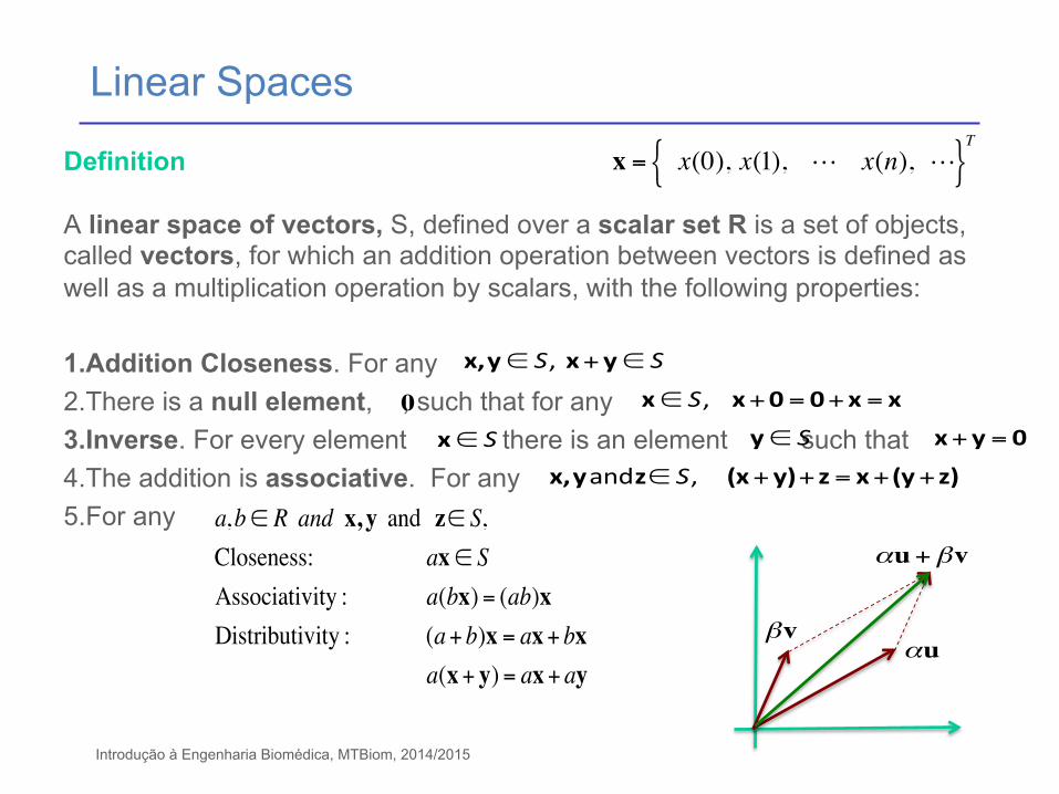
Definition A linear space of vectors, S, defined over a scalar set R is a set of objects, called vectors, for which an addition operation between vectors is defined as well as a multiplication operation by scalars, with the following properties: 1. Addition Closeness. For any 2. There is a null element, , such that for any 3. Inverse. For every element there is an element such that 4. The addition is associative. For any 5. For any

x,y∈ S, x+y∈ S

0 x∈ S, x+0 = 0+x = x

x∈ S y∈ S x+y = 0

x,yandz∈ S, (x+y)+z = x+ (y+z)

a,b∈ R and x, y and z∈ S,Closeness: ax ∈ SAssociativity : a(bx) = (ab)xDistributivity : (a+ b)x = ax+ bx

a(x+ y) = ax+ ayαu

βv

αu+βv

x = x(0), x(1), ! x(n), !{ }T


Vectors and Matrices

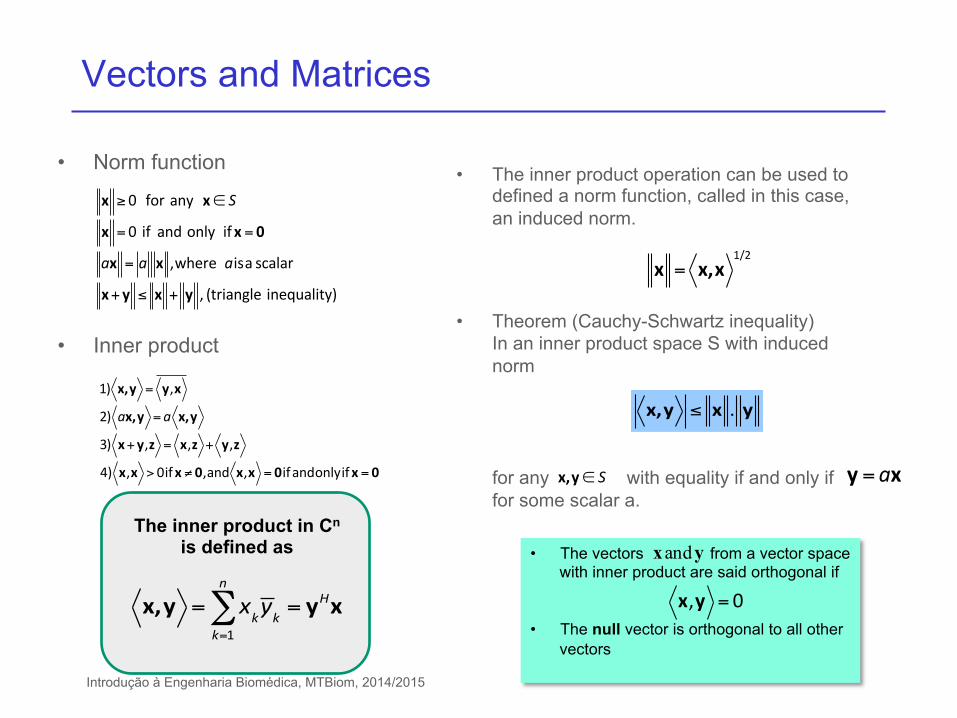
•  Norm function

•  Inner product

x ≥ 0""for"any""x∈ S

x = 0"if and only ifx = 0

ax = a x ,where aisa scalar

x+y ≤ x + y , (triangle inequality)

1) x,y = y,x

2) ax,y =a x,y

3) x+y,z = x,z + y,z

4) x,x > 0ifx ≠ 0,and x,x = 0ifandonlyifx = 0

•  The inner product operation can be used to defined a norm function, called in this case, an induced norm.

•  Theorem (Cauchy-Schwartz inequality) In an inner product space S with induced norm for any with equality if and only if for some scalar a.

x = x,x1/2

x,y ≤ x . y

x,y∈ S y =ax

•  The vectors from a vector space with inner product are said orthogonal if

•  The null vector is orthogonal to all other vectors

yxand

x,y = 0x,y = xkykk=1

n

∑ = yHx

The inner product in Cn is defined as


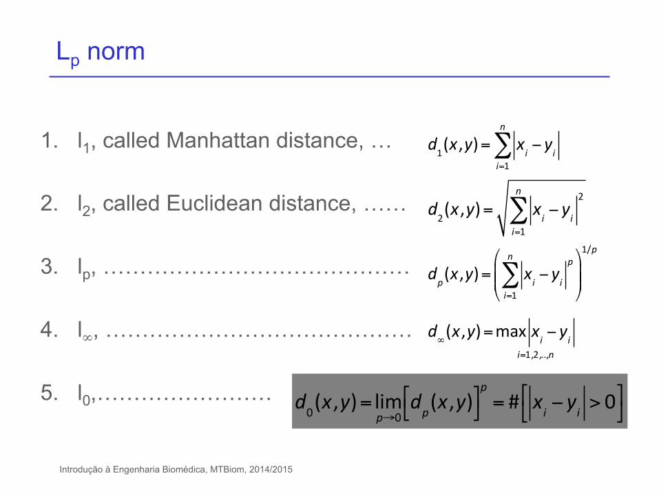
Lp norm

1.  l1, called Manhattan distance, …

2.  l2, called Euclidean distance, ……

3.  lp, ……………………………………

4.  l∞, ……………………………………

5.  l0,……………………

d1(x,y)= xi − yii=1

n

∑

d2(x,y)= xi − yi2

i=1

n

∑

dp(x,y)= xi − yip

i=1

n

∑#

$%%

&

'((

1/p

d∞(x,y)=max xi − yi

i=1,2,..,n

d0(x,y)= limp→0dp(x,y)"#

$%p= # xi − yi > 0

"#

$%


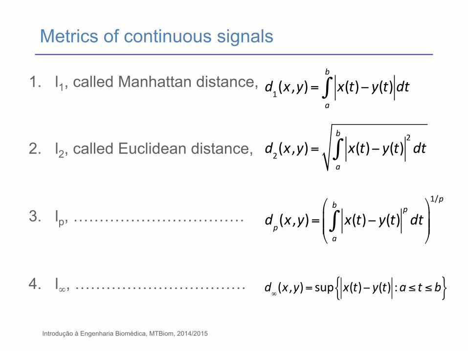
Metrics of continuous signals

1.  l1, called Manhattan distance,

2.  l2, called Euclidean distance,

3.  lp, ……………………………

4.  l∞, ……………………………

d1(x,y)= x(t)− y(t) dta

b

∫

d2(x,y)= x(t)− y(t)2dt

a

b

∫

dp(x,y)= x(t)− y(t)pdt

a

b

∫#

$%%

&

'((

1/p

d∞(x,y)= sup x(t)− y(t) :a ≤ t ≤ b{ }


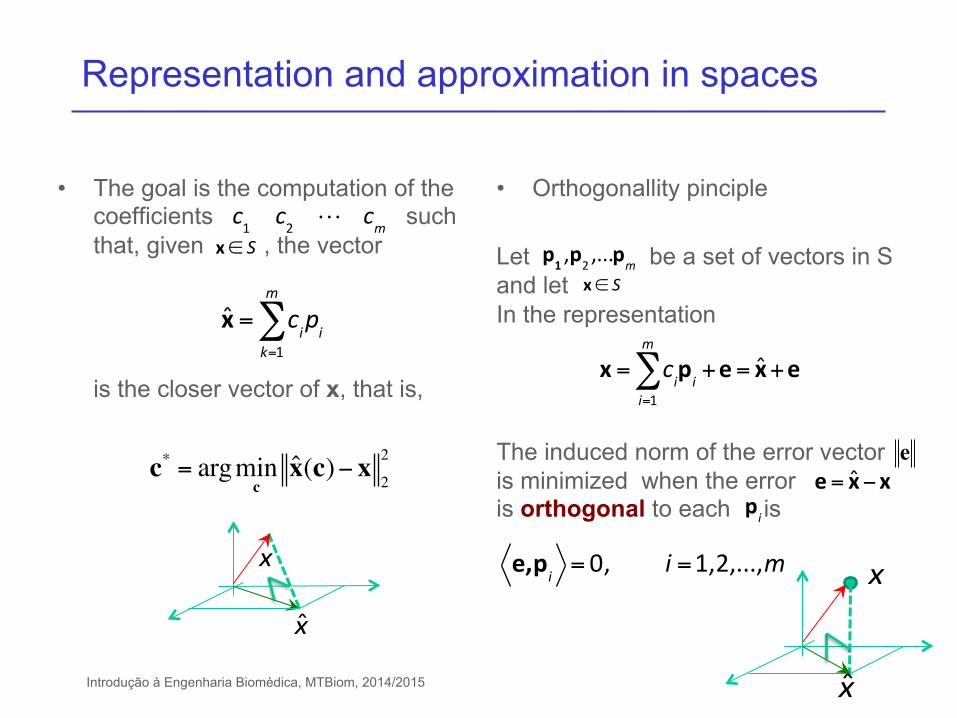
Representation and approximation in spaces

•  The goal is the computation of the coefficients such that, given , the vector is the closer vector of x, that is,

•  Orthogonallity pinciple

Let be a set of vectors in S and let In the representation The induced norm of the error vector is minimized when the error is orthogonal to each is

c1 c2 cmx∈ S

x̂ = cipik=1

m

∑

c* = argmincx̂(c)− x

2

2

x̂

x

x = cipii=1

m

∑ +e= x̂+e

p1 ,p2 ,...pmx∈ S

ee= x̂−x

pi

e,pi = 0, i =1,2,...,m

x̂

x


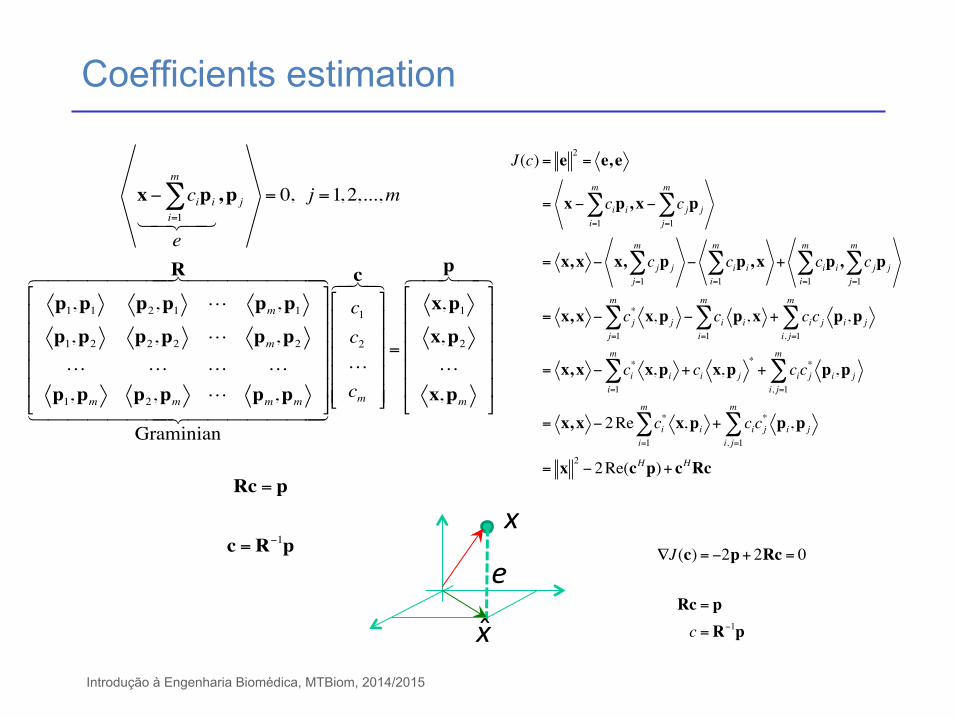
Coefficients estimation

J(c) = e 2= e, e

= x− cipii=1

m

∑ , x− cjp jj=1

m

∑

= x, x − x, cjp jj=1

m

∑ − cipii=1

m

∑ , x + cipii=1

m

∑ , cjp jj=1

m

∑

= x, x − cj* x,p j

j=1

m

∑ − ci pi,xi=1

m

∑ + cicj pi,p ji, j=1

m

∑

= x, x − ci* x,pi + ci x,p j

*

i=1

m

∑ + cicj* pi,p j

i, j=1

m

∑

= x, x − 2Re ci* x,pi

i=1

m

∑ + cicj* pi,p j

i, j=1

m

∑

= x 2− 2Re(cHp)+ cHRc

x− cipii=1

m

∑

e! "# $#

, p j = 0, j =1,2,...,m

p1,p1 p2,p1 % pm,p1p1,p2 p2,p2 % pm,p2% % % %p1,pm p2,pm % pm,pm

#

$

%%%%%

&

'

(((((

Graminian! "####### $#######

R& '####### (#######

c1c2%cm

#

$

%%%%%

&

'

(((((

c&'(

=

x,p1x,p2%x,pm

#

$

%%%%%

&

'

(((((

p& '# (#

Rc = p

c =R−1p

x̂

x

e∇J(c) = −2p+ 2Rc = 0

Rc = pc =R−1p


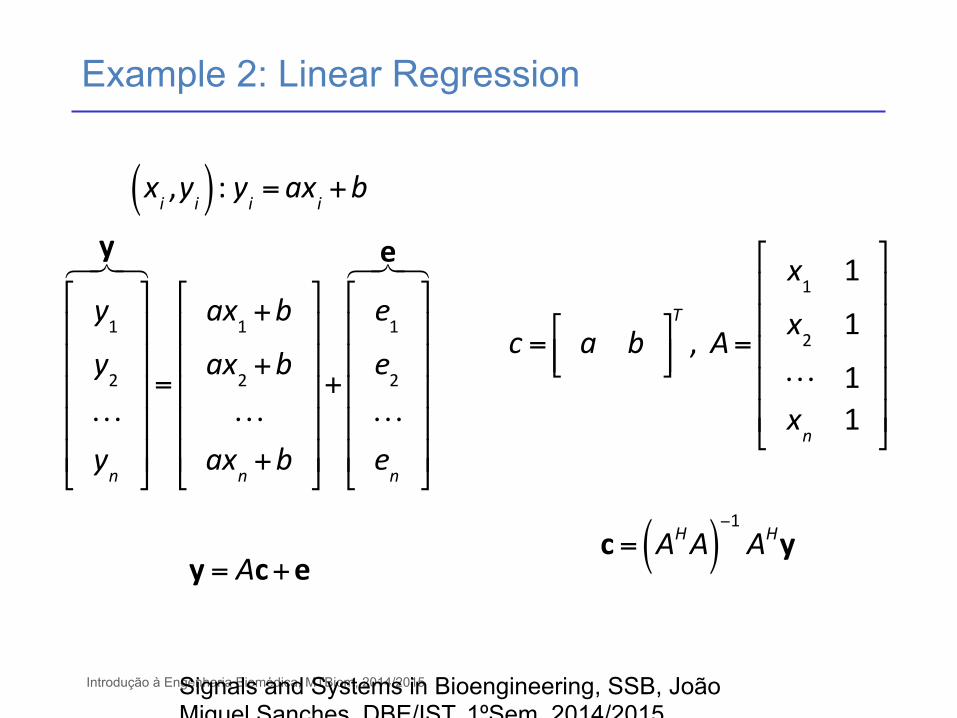
Example 2: Linear Regression

xi ,yi( ) : yi =axi +b

y1y2yn

!

"

#####

$

%

&&&&&

y

=

ax1 +b

ax2 +b

axn +b

!

"

#####

$

%

&&&&&

+

e1e2en

!

"

#####

$

%

&&&&&

e

y = Ac+e

c = a b!"#

$%&T

, A=

x1 1

x2 1

1xn 1

!

"

#####

$

%

&&&&&

c = AHA( )−1AHy

Signals and Systems in Bioengineering, SSB, João Miguel Sanches, DBE/IST, 1ºSem, 2014/2015


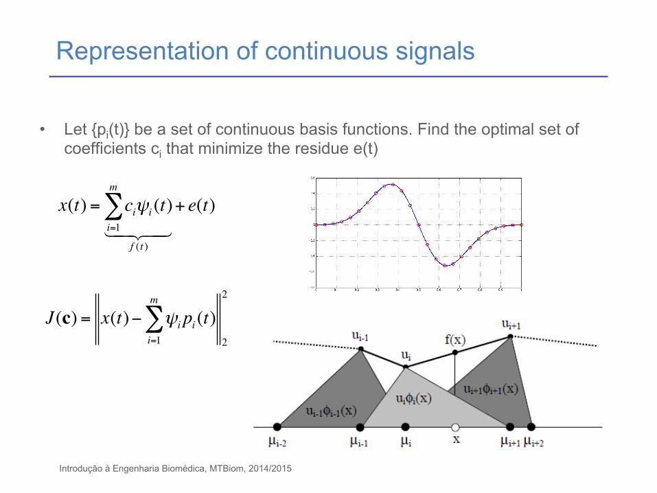
Representation of continuous signals

•  Let {pi(t)} be a set of continuous basis functions. Find the optimal set of coefficients ci that minimize the residue e(t)

x(t) = ciψi (t)i=1

m

∑f (t )

!"# $#+ e(t)

J(c) = x(t)− ψi pi (t)i=1

m

∑2

2


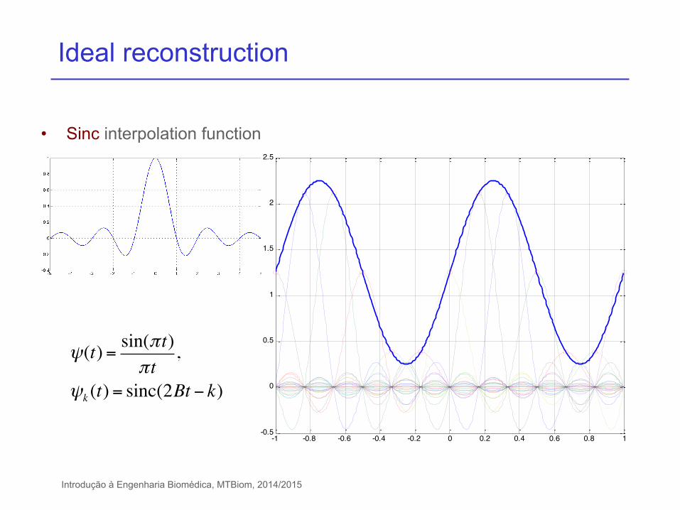
Ideal reconstruction

•  Sinc interpolation function

ψ(t) = sin(π t)π t

,

ψk (t) = sinc(2Bt − k)

-1 -0.8 -0.6 -0.4 -0.2 0 0.2 0.4 0.6 0.8 1-0.5

0

0.5

1

1.5

2

2.5

mestrado bolonha em tecnologias biomédicas introdução à … · introdução à engenharia...

Documents