aeroelastic analysis of aircraft wings - …€¦ · congresso de m etodos num ericos em engenharia...

Congresso de Metodos Numericos em Engenharia 2015Lisboa, 29 de Junho a 2 de Julho 2015

c©APMTAC, Portugal 2015

AEROELASTIC ANALYSIS OF AIRCRAFT WINGS

Andre S. Cardeira†, Andre C. Marta‡

CCTAE, IDMEC, Instituto Superior Tecnico, Universidade de LisboaAv. Rovisco Pais 1, 1049-001 Lisboa, Portugal

† [email protected] ‡ [email protected]

Keywords: Aeroelasticity, Panel method, Fluid-structure interaction, Finite elementmethod, Flutter, Divergence velocity.

Abstract. Aeroelasticity phenomena involve the study of the interaction between aero-dynamic, inertial, and elastic forces (dynamic aeroelasticity). Modern aircraft structures,using more and more lightweight flexible composite materials, make the aeroelastic studyan extremely important aspect in aircraft design. Flutter is a dynamic aeroelastic insta-bility characterized by sustained oscillation of structure arising from interaction betweenthose three forces acting on the body. The present work aims to study the flutter behavioron three-dimensional subsonic aircraft wings, using a computationally efficient method.For that, a computational aeroelasticity design framework is created using a custom devel-oped panel method for the fluid flow analysis and a commercial software for the structuralanalysis. A validation of the flow solver is made using wind tunnel data, while the struc-tural solver is verified using available tests. The coupling of the two domains is madeusing an adequate time discretization scheme. The results are presented for a referencewing. Following the wing baseline analysis, a parametric study under flutter conditionsis performed, revealing some physically expected correlations: i) increasing the freestreamvelocity leads to higher vibration amplitude, whereas the frequency remains unchanged; ii)moving the wing spars aft or forward, causing the twist center to move away from theaerodynamic center, leads to instability; iii) decreasing the material density (weight) leadsto higher flutter frequency and amplitude; iv) increasing the material stiffness (Youngmodulus) leads to higher frequency and smaller amplitude flutter. It is concluded thatthe framework shows very good agreement to the theoretical influences of the parametersstudied. Despite the simplification of the fluid flow, which was assumed to be potential,this method proves to be a very useful tool in aircraft preliminary design.

1 INTRODUCTION

Structural analyses constitute a crucial part in aircraft design. Since the primordials ofthe aviation history, it was stated that the success of the air vehicle is dependent on astructure capable of withstanding the several loads encountered in flight and a strongpropulsion system. Moreover, both components should be as light as possible.

1

A. S. Cardeira and A. C. Marta

Aeroelastic phenomena in modern high-speed aircraft have profound upon the design ofstructural members and also upon mass distribution, lifting surface planforms and controlsystem design [1]. Accurate computational aeroelastic tests can be applied in early stagesof the design phase. By increasing the accuracy and feasibility of computational tools,one can decrease the number of experimental tests needed, which largely reduces thedesign costs. Also, applications of the aeroelastic phenomena are found in several otherdisciplines.A general (but complete) definition is the one from [2]:The science of aeroelasticity encompasses those physical processes and problems that resultfrom the interaction between elasto-mechanical systems and the surrounding airflow.To help visualizing the context of the term, a representation (firstly suggested in [11]) intriangle is used, presented in Figure 1.

Dynamic Aeroelasticity

Inertial Forces(Dynamics)

Aerodynamic Forces(Fluid Mechanics)

Elastic Forces(Solid Mechanics)

StructuralDynamics

Flight Dynamics

Static Aeroelasticity

Figure 1: Collar triangle.

By pairing two of the three corners of the triangle, one can identify other importantdisciplines. For example,

• aerodynamics + dynamics = aerodynamic stability;

• dynamics + solid mechanics = structural dynamics;

• aerodynamics + solid mechanics = static aeroelasticity.

In some sense, all these technical fields may be considered special cases of aeroelasticity.However, for dynamic aeroelastic effects to occur, all three forces are required.

2


Flutter has perhaps the most far-reaching effects on high-speed aircraft [1]. The classicaltype of flutter is associated with potential flow and usually, involves coupling of two ormore degrees of freedom (DOF). The nonclassical type of flutter may involve separatedflow, turbulence and stalling conditions.The object of study is the aircraft wing. The main structural parts are the spars, ribs,stringers and the skin (see Figure 2). Then, accordingly to the application, one can changetheir materials, quantity, location and geometry.

Figure 2: Illustration of the interior of an aircraft wing [8].

A simplified structure is used with only two spars and a skin. The skin will then bethicker to compensate the absence of stringers and the spars can be moved forward andbackward to manipulate the torsional characteristics of the wing.The objectives of this work are then to review the actual models and methods to computeaeroelastic calculations, state the governing equations and its acceptable approximations,and to apply some of these methods to perform aeroelastic studies of aircraft wings.For these studies, an available tool for computational structural mechanics (CSM) analysisis employed, while the computational fluid dynamics (CFD) for aerodynamics and thecoupling tools are to be created and merged in a computational program. The final resultis an aeroelastic design framework for subsonic aircraft wings.

2 BACKGROUND

For the aeroelastic design framework, three domains of theory are treated: structural,fluid flow and fluid-structure coupling.

2.1 Structural Approach

The transient dynamic equilibrium equation is, for a linear structure,

M~u+ C~u+K~u = ~F , (1)

where M represents the structural mass matrix, C the structural damping matrix, K thestructural stiffness matrix, ~u the nodal acceleration vector, ~u the nodal velocity vector, ~uthe nodal displacement vector and ~F the applied load vector.

3


In this work, the structural computations are made in the commercial software ANSYSParametric Design Language (APDL). It has available two time integration schemes [3],being the most commonly used the implicit Newmark method, which applied to Equa-tion (1) gives

~un+1 (a0M + a1C +K) = ~F+

M(a0~un + a2~un + a3~un

)+

C(a1~un + a4~un + a5~un

) , (2)

where

a0 =1

α∆t2, a1 =

δ

α∆t,

a2 =1

α∆t, a3 =

1

2α− 1,

a4 =δ

α− 1, a5 =

∆t

2

(δ

α− 2

),

a6 = ∆t (1− δ) , a7 = δ∆t .

As documented in [3], this scheme is unconditionally stable for

α ≥ 1

4

(1

2+ δ

)2

, δ ≥ 1

2,

1

2+ δ + α > 0 , (3)

where α and δ are the Newmark integration parameters and are related to the amplitudedecay factor γ by α = 1

4(1 + γ)2 and δ = 1

2+ γ.

Three methods are available in APDL to solve Equation (2): the full, reduced and modesuperposition. The full method simply solves Equation (2) with no additional assump-tions, while the reduced forbids the use of pressure loads and the mode superposition hasno element damping matrices. So, the full method is the one used for this task.All the model will be constructed with SHELL181 elements. It is a four-node quadrilateralbi-linear element with six DOF at each node: translations in the x, y, and z directionsand rotations about the x, y and z-axes.

2.2 Aerodynamic Approach

For the aerodynamic calculations, the Potential Flow Model is here applied. It is obtainedassuming that the flow is inviscid, irrotational and isentropic. Compressible effects areout of the scope of this work, so the fluid is also assumed incompressible. With theseassumptions, the governing equation is

∇ · ~V = ∇ · (∇ · Φ) = ∇2Φ = 0 , (4)

4


where Φ(x, y, z) is the velocity potential. Equation (4) is a linear differential equationknown as Laplace equation. It was extensively studied and it has many possible analyticalsolutions. Also, because it is linear, the principle of superposition applies. This meansthat if Φ1, Φ2, ..., Φn are solutions of the Laplace equation, then

Φ =n∑k=1

ckΦk (5)

is also a solution for it (ck are arbitrary constants).The boundary conditions for this problem are the impermeability condition (zero normalvelocity on a body) and the far field condition (the disturbance created by the motionshould vanish far from the body).The solutions in evidence here are the Source

Φ = − σ

4π |~r − ~r0|(6)

and the Doublet

Φ =µ

4π

∂

∂n

1

|~r − ~r0|, (7)

where σ and ν are the source and doublet strength, respectively.The pressure computation is made using the Bernoulli equation for inviscid incompressibleirrotational flow,

E +p

ρ+V 2

2+∂Φ

∂t= C(t) , (8)

where E is the gravitational potential, p pressure, ρ density and V velocity. This meansthat at a certain time t1, the quantity at the left-hand side of Equation (8) must beequal throughout the field. Particularly, one can compare any point of the field with areference point. If this reference condition is chosen such that E = 0 (no body forces)and Φ∞ = const., then the pressure coefficient Cp at any point can be calculated from

Cp =p− p∞0.5ρV 2

∞= 1− V 2

V 2∞− 2

V 2∞

∂Φ

∂t, (9)

where the subscript ∞ denotes far-field conditions. The integration over time demandsa time discretization method. Since the goal is to obtain the pressure coefficient at thetime t + ∆t, an implicit method is required. The simpler and still largely used option isthe Backward Euler method [4], which applied to Equation (9) yields

Ct+∆tp = 1− (V t+∆t)2

V 2∞

− 2

V 2∞

(Φt+∆t − Φt

∆t

), (10)

which is first order accurate. A second order accurate possibility is the Crank-Nicholsonmethod [4].

5


From here, a panel method was built based on the formulation from [5] using constantquadrilateral sources and doublets. The Dirichlet boundary condition results in the form

1

4π

∫body+wake

µ~n · ∇(

1

r

)dS−

1

4π

∫body

σ

(1

r

)dS = 0

. (11)

The body surface is now discretized into N surface panels and the wake is modeled usingNW panels. This problem is then reduced to a set of linear algebraic equations

N∑k=1

Ckµk +

NW∑l=1

Clµl +N∑k=1

Bkσk = 0 , (12)

where for each collocation point the summation of the influences of all k body panels andl wake panels is needed. Since the singularity elements have constant strength in eachpanel, the integrals depend only on the geometry.For Equation (11) to be valid and from the definition of the source strength σ, it comesan additional condition that

σ = ~n · ~V∞. (13)

This way, the third term in Equation (12) is calculated and can be moved to the right-handside.The influence from the wake comes from the linear Kutta condition

µW = µU − µL, (14)

where µU and µL are the upper and lower surface doublet strengths at the trailing edgeand µW is constant along the wake (in a steady problem).In an unsteady case, the wake shape is obtained using a time-stepping method. Hereinthe wake is directly related to the motion, being convected with ~V∞ at each time step.

2.3 Fluid-Structure Coupling

The coupling between fluid and structural domains is normally referred as Fluid-StructureInteraction (FSI). The range of FSI models can be divided in two categories: strongly-coupled (or monolithic) and loosely-coupled (or staggered). A monolithic approach wouldbe for this case, to merge Equations (1) and (9) and to integrate over time.The other option is a staggered procedure. For a given time step, such an algorithmtypically involves the solution of the fluid mechanics with the velocity boundary condi-tions coming from the previous step, followed by the solution of the structural mechanicsequations with the updated fluid interface load, and followed by the mesh movement withthe new structure displacement. The basic algorithm is the so called Conventional Serial

6


Staggered (CSS) procedure [6]. It is graphically depicted in Figure 3, where ~U denotes the

structure state vector (nodal displacement and velocity), ~W denotes the fluid state vector(in the case of a complete fluid discretization), ~p designates the fluid pressure, n standsfor the nth time station, and the equalities shown at the top hold on the fluid/structureinterface boundary.

~Wn~Wn+1

~Wn+2 ...

~Un~Un+1

~Un+2 ...

1 ~un

2

4

3 ~pn+1 5 ~un+1

6

7 ~pn+2

8

Fluid

Structure

~xn = ~un−1 ~xn+1 = ~un ~xn+2 = ~un+1

Figure 3: The Conventional Serial Staggered (CSS) scheme.

A similar procedure was also presented in [6], the Improved Serial Staggered (ISS), whichuses the structural velocity and calculates the fluid states at the middle of each time step.

3 IMPLEMENTATION

First, some verification tests were made using APDL Verification Manual. Then, anaircraft wing was used to make a mesh convergence test, using four different meshes:16×10, 32×20, 64×40 and 128×80. These numbers represent the number of panels of theskin in the form chordwise× spanwise.The wing has NACA 0010 airfoil and an aspect ratio ÆR = 4. Two spars are introducedinside the skin at 30% and 70% chord distance from the leading edge (Figure 4). Thematerial used has Young modulus E = 200 GPa, Poisson ratio ν = 0.3 and thickness of10 mm for all surfaces.

Figure 4: Static test using a wing with two nodal loads of 5000N (mesh 128×80).

Table 1 contains a summary of the results. The displacement values are the maximumvalues for each case. A deviation of the results is calculated in relation to the finer mesh.A mesh having 32×20 panels proves to be a good approximation and still cheap in termsof computational cost.

7


Mesh Displacement [mm] Deviation

16×10 -5.387 4.1%32×20 -5.219 0.8%64×40 -5.186 0.2%128×80 -5.177 0.0%

Table 1: Mesh study for the wing steady test.

3.1 Panel Method Validation

In order to get into the panel methods particularities, four computer programs werecreated: 2DS (two-dimensional steady), 2DU (two-dimensional unsteady), 3DS (three-dimensional steady) and 3DU (three-dimensional unsteady), all coded in MATLAB. The2DS also uses constant doublets and sources but punctual singularities. It was validatedusing a Karman-Trefftz airfoil, which has exact solution for potential flow. The 2DU wassimply the same program with the time-stepping wake convection.The 3DS, which is more important for this work, was validated with wind tunnel dataand verified with a similar panel method program (called here 3DBalt) both documentedin [7].

0 0.5 1

−3

−2

−1

0

1

x/c

Cp

yb/2=0.211

3DBalt3DSExp.

0 0.5 1

−3

−2

−1

0

1

x/c

yb/2=0.611

0 0.5 1

−3

−2

−1

0

1

x/c

yb/2=0.961

(a) Pressure distributions for the α = 8.5◦

0 0.5 1

−1

−0.5

0

0.5

1

x/c

yb/2=0.611

0 0.5 1

−1

−0.5

0

0.5

1

x/c

Cp

yb/2=0.211

0 0.5 1

−1

−0.5

0

0.5

1

x/c

yb/2=0.961

(b) Pressure distributions for the α = 2.5◦

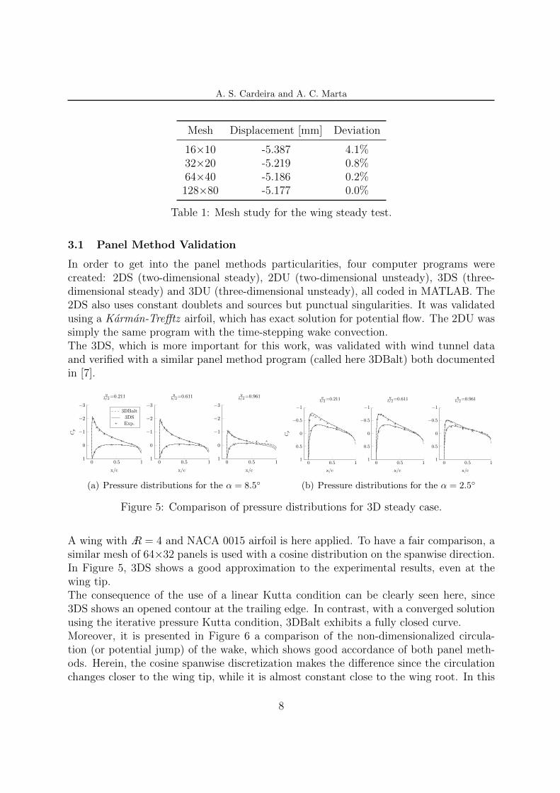
Figure 5: Comparison of pressure distributions for 3D steady case.

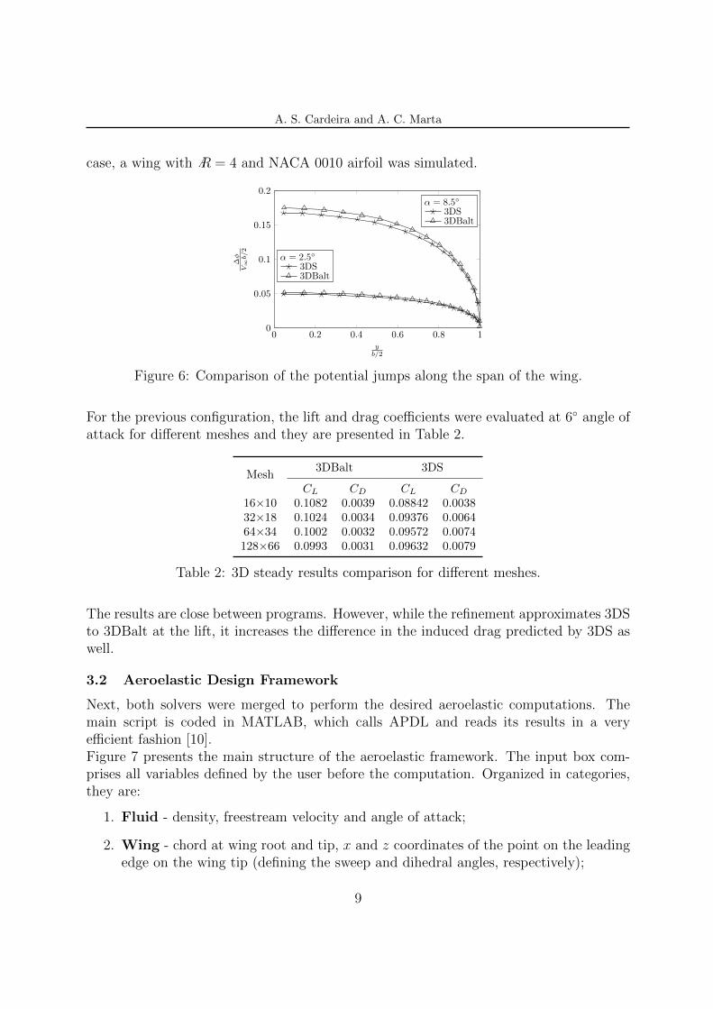
A wing with ÆR = 4 and NACA 0015 airfoil is here applied. To have a fair comparison, asimilar mesh of 64×32 panels is used with a cosine distribution on the spanwise direction.In Figure 5, 3DS shows a good approximation to the experimental results, even at thewing tip.The consequence of the use of a linear Kutta condition can be clearly seen here, since3DS shows an opened contour at the trailing edge. In contrast, with a converged solutionusing the iterative pressure Kutta condition, 3DBalt exhibits a fully closed curve.Moreover, it is presented in Figure 6 a comparison of the non-dimensionalized circula-tion (or potential jump) of the wake, which shows good accordance of both panel meth-ods. Herein, the cosine spanwise discretization makes the difference since the circulationchanges closer to the wing tip, while it is almost constant close to the wing root. In this

8


case, a wing with ÆR = 4 and NACA 0010 airfoil was simulated.

0 0.2 0.4 0.6 0.8 10

0.05

0.1

0.15

0.2

yb/2

∆φ

V∞b/2

α = 2.5◦3DS3DBalt

α = 8.5◦3DS3DBalt

Figure 6: Comparison of the potential jumps along the span of the wing.

For the previous configuration, the lift and drag coefficients were evaluated at 6◦ angle ofattack for different meshes and they are presented in Table 2.

Mesh3DBalt 3DS

CL CD CL CD

16×10 0.1082 0.0039 0.08842 0.003832×18 0.1024 0.0034 0.09376 0.006464×34 0.1002 0.0032 0.09572 0.0074128×66 0.0993 0.0031 0.09632 0.0079

Table 2: 3D steady results comparison for different meshes.

The results are close between programs. However, while the refinement approximates 3DSto 3DBalt at the lift, it increases the difference in the induced drag predicted by 3DS aswell.

3.2 Aeroelastic Design Framework

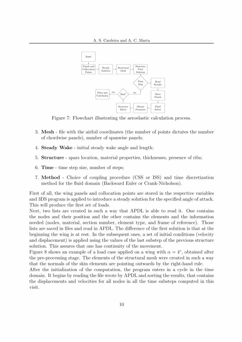
Next, both solvers were merged to perform the desired aeroelastic computations. Themain script is coded in MATLAB, which calls APDL and reads its results in a veryefficient fashion [10].Figure 7 presents the main structure of the aeroelastic framework. The input box com-prises all variables defined by the user before the computation. Organized in categories,they are:

1. Fluid - density, freestream velocity and angle of attack;

2. Wing - chord at wing root and tip, x and z coordinates of the point on the leadingedge on the wing tip (defining the sweep and dihedral angles, respectively);

9


Input

Panels andCollocation

Points

SteadySolution

StructuralMesh

StructureFirst

Solution

TimeStep

ReadResults

MovePanels

FluidSolver

ObtainPressures

StructureSolver

End?Plots andConclusion

noyes

Figure 7: Flowchart illustrating the aeroelastic calculation process.

3. Mesh - file with the airfoil coordinates (the number of points dictates the numberof chordwise panels), number of spanwise panels;

4. Steady Wake - initial steady wake angle and length;

5. Structure - spars location, material properties, thicknesses, presence of ribs;

6. Time - time step size, number of steps;

7. Method - Choice of coupling procedure (CSS or ISS) and time discretizationmethod for the fluid domain (Backward Euler or Crank-Nicholson).

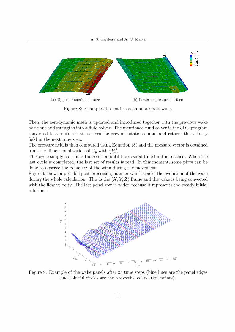
First of all, the wing panels and collocation points are stored in the respective variablesand 3DS program is applied to introduce a steady solution for the specified angle of attack.This will produce the first set of loads.Next, two lists are created in such a way that APDL is able to read it. One containsthe nodes and their position and the other contains the elements and the informationneeded (nodes, material, section number, element type, and frame of reference). Thoselists are saved in files and read in APDL. The difference of the first solution is that at thebeginning the wing is at rest. In the subsequent ones, a set of initial conditions (velocityand displacement) is applied using the values of the last substep of the previous structuresolution. This assures that one has continuity of the movement.Figure 8 shows an example of a load case applied on a wing with α = 4◦, obtained afterthe pre-processing stage. The elements of the structural mesh were created in such a waythat the normals of the skin elements are pointing outwards by the right-hand rule.After the initialization of the computation, the program enters in a cycle in the timedomain. It begins by reading the file wrote by APDL and sorting the results, that containsthe displacements and velocities for all nodes in all the time substeps computed in thisvisit.

10


(a) Upper or suction surface (b) Lower or pressure surface

Figure 8: Example of a load case on an aircraft wing.

Then, the aerodynamic mesh is updated and introduced together with the previous wakepositions and strengths into a fluid solver. The mentioned fluid solver is the 3DU programconverted to a routine that receives the previous state as input and returns the velocityfield in the next time step.The pressure field is then computed using Equation (8) and the pressure vector is obtainedfrom the dimensionalization of Cp with ρ

2V 2∞.

This cycle simply continues the solution until the desired time limit is reached. When thelast cycle is completed, the last set of results is read. In this moment, some plots can bedone to observe the behavior of the wing during the movement.Figure 9 shows a possible post-processing manner which tracks the evolution of the wakeduring the whole calculation. This is the (X, Y, Z) frame and the wake is being convectedwith the flow velocity. The last panel row is wider because it represents the steady initialsolution.

0 20 40 60 80 100 120 140 160 180 200 220 240

0

2

4

6

8−2

0

2

4

6

8

10

12

14

16

18

X [m]

Y [m]

Z[m

]

Figure 9: Example of the wake panels after 25 time steps (blue lines are the panel edgesand colorful circles are the respective collocation points).

11


4 RESULTS

After having the framework finished, several initial tests were made to reduce the rangeof input options and have a set of results with physical sense and computationally cheap.One first study is here presented, which is called the Reference Case (RC). Later, severalinput parameters will be changed and their influence discussed, using the comparison withthe RC.

4.1 Reference Case

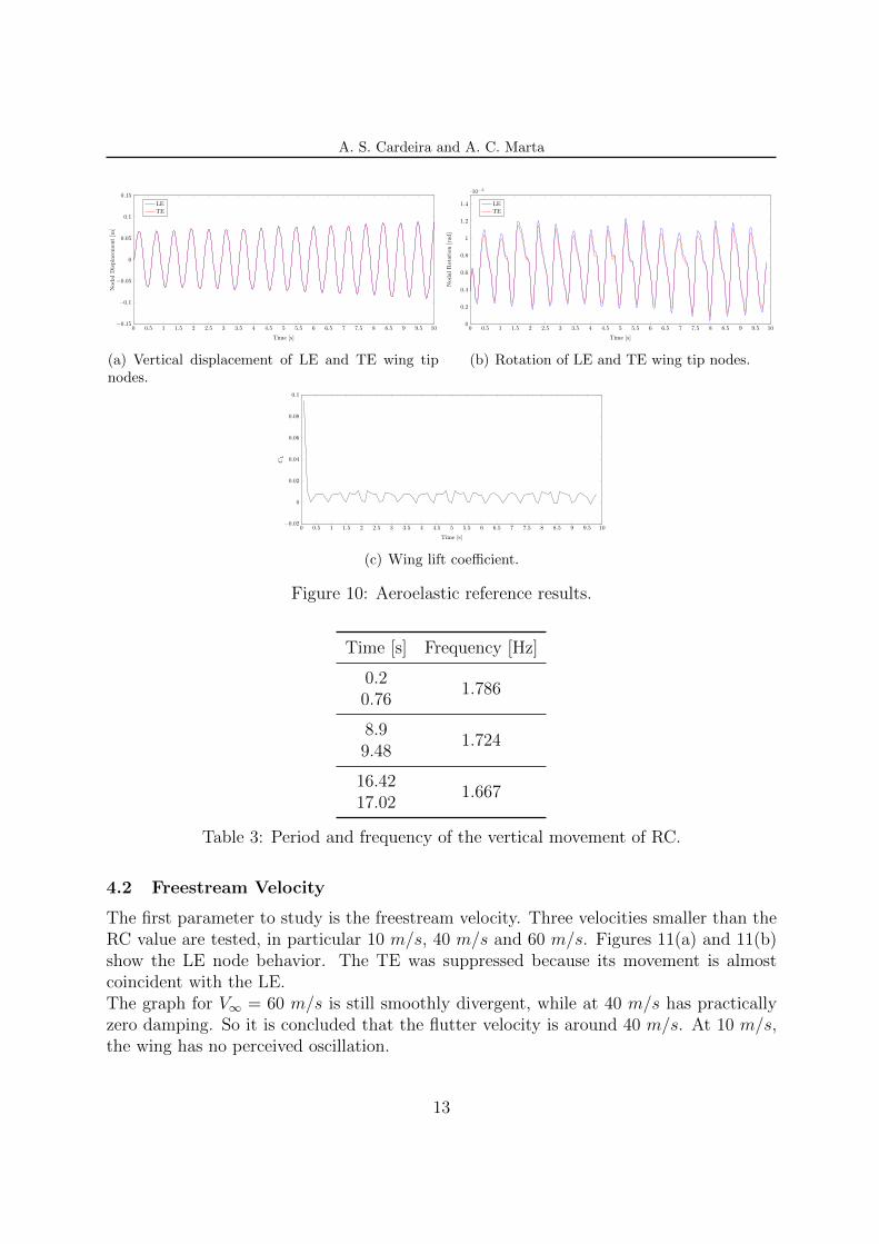
The same input values used in the APDL static test from Section 3 are applied here, usinga 64×30 mesh, ÆR = 15, NACA 0010 airfoil, two spars at 30% and 70% chordwise locationand the wing being rectangular with c = 1 m and no ribs. Moreover, the CSS procedureis applied using Backward Euler for the pressure time integration and Newmark in APDLfor the structural time discretization.The fluid density is assumed to be ρ = 1 kg/m3 corresponding to an altitude of 1371 mat standard atmosphere conditions (considering a temperature offset of 20 ◦C), the angleof attack is α = 4◦ and the fluid freestream velocity V∞ = 75 m/s. The initial wake angleis the angle of attack and its length is three time the wing span. The time step is set to0.1 s.To track the wing movement, the vertical displacement and the spanwise rotation of twonodes at the wing tip, one at the leading edge (LE) another at the trailing edge (TE), areplotted in Figure 10(a).The nodal trajectory of both nodes is almost coincident so the torsion is very low. Thisis confirmed by Figure 10(b) that shows a maximal rotation of 2 · 10−3 rad which meansroughly 0.1◦. The rotational movement has the same period of the vertical displacement.When one is at the minimum displacement, it corresponds to the maximum rotation(positive rotation around Y is using the right-hand rule, from Z towards X axis, also callednose-up) and vice-versa. So, the torsional movement seams to be damping the bendingmovement. However, the increase of the wing maximal displacement shows clearly thatthis velocity is already higher than the flutter velocity.Using the peak values, the movement period and frequency are easily obtained. To obtaina consistent value, three values were used at the beginning, middle and end of the move-ment. The results are summarized in Table 3. Like it was expected, the frequency of themovement is nearly constant during all computation. If one counts the total number ofpeaks and divides by the respective time, the frequency obtained is 1.7 Hz, so that provesthe constancy of the movement.Figure 10(c) shows the evolution of the lift coefficient with the time. After the initialsteady solution, the variation is not very significant, being however possible to see theoscillation caused by the wing movement, which varies with approximately the samefrequency as the nodal displacement from Figure 10(a). Furthermore, lift positive peakscorrespond to rotation positive peaks, which is physically correct.

12


0 0.5 1 1.5 2 2.5 3 3.5 4 4.5 5 5.5 6 6.5 7 7.5 8 8.5 9 9.5 10−0.15

−0.1

−0.05

0

0.05

0.1

0.15

Time [s]

Nodal

Displacement[m

]

LETE

(a) Vertical displacement of LE and TE wing tipnodes.

0 0.5 1 1.5 2 2.5 3 3.5 4 4.5 5 5.5 6 6.5 7 7.5 8 8.5 9 9.5 100

0.2

0.4

0.6

0.8

1

1.2

1.4

·10−3

Time [s]

Nodal

Rotation

[rad]

LETE

(b) Rotation of LE and TE wing tip nodes.

0 0.5 1 1.5 2 2.5 3 3.5 4 4.5 5 5.5 6 6.5 7 7.5 8 8.5 9 9.5 10−0.02

0

0.02

0.04

0.06

0.08

0.1

Time [s]

CL

(c) Wing lift coefficient.

Figure 10: Aeroelastic reference results.

Time [s] Frequency [Hz]

0.21.786

0.76

8.91.724

9.48

16.421.667

17.02

Table 3: Period and frequency of the vertical movement of RC.

4.2 Freestream Velocity

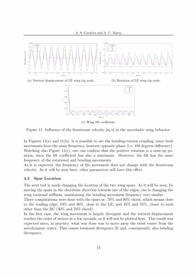
The first parameter to study is the freestream velocity. Three velocities smaller than theRC value are tested, in particular 10 m/s, 40 m/s and 60 m/s. Figures 11(a) and 11(b)show the LE node behavior. The TE was suppressed because its movement is almostcoincident with the LE.The graph for V∞ = 60 m/s is still smoothly divergent, while at 40 m/s has practicallyzero damping. So it is concluded that the flutter velocity is around 40 m/s. At 10 m/s,the wing has no perceived oscillation.

13


0 0.5 1 1.5 2 2.5 3 3.5 4 4.5 5 5.5 6−8

−6

−4

−2

0

2

4

6

8·10−2

Time [s]

Nodal

Displacement[m

]

75 (RC)604010

(a) Vertical displacement of LE wing tip node.

0 0.5 1 1.5 2 2.5 3 3.5 4 4.5 5 5.5 6−0.5

0

0.5

1

1.5

2·10−3

Time [s]

Nodal

Rotation[rad]

75 (RC)604010

(b) Rotation of LE wing tip node.

0 0.5 1 1.5 2 2.5 3 3.5 4 4.5 5 5.5 60

0.02

0.04

0.06

0.08

0.1

Time [s]

CL

75 (RC)604010


Figure 11: Influence of the freestream velocity [m/s] in the aeroelastic wing behavior.

In Figures 11(a) and 11(b), it is possible to see the bending-torsion coupling, since bothmovements have the same frequency, however opposite phase (i.e. 180 degrees difference).Watching also Figure 11(c), one can confirm that the positive rotation is a nose-up po-sition, since the lift coefficient has also a maximum. Moreover, the lift has the samefrequency of the rotational and bending movements.As it is expected, the frequency of the movement does not change with the freestreamvelocity. As it will be seen later, other parameters will have this effect.

4.3 Spar Location

The next test is made changing the location of the two wing spars. As it will be seen, bymoving the spars in the chordwise direction towards one of the edges, one is changing thewing torsional stiffness, maintaining the bending movement frequency very similar.Three computations were done with the spars at: 70% and 90% chord, which means closeto the trailing edge; 10% and 30%, close to the LE; and 45% and 55%, closer to eachother than the RC (30% and 70% chord).In the first case, the wing movement is largely divergent and the vertical displacementreaches the order of meters in a few seconds, so it will not be plotted here. This result wasexpected since, in practice, what was done was to move away the twist center from theaerodynamic center. This causes torsional divergence [8] and, consequently, also bendingdivergence.

14


0 0.5 1 1.5 2 2.5 3 3.5 4 4.5 5 5.5 6 6.5 7 7.5 8−0.1

−0.08

−0.06

−0.04

−0.02

0

0.02

0.04

0.06

0.08

0.1

Time [s]

Nodal

displacement[m

]

0.3 and 0.7 (RC) LE TE

0.1 and 0.3 LE TE

0.45 and 0.55 LE TE


0 0.5 1 1.5 2 2.5 3 3.5 4 4.5 5 5.5 6 6.5 7

−2

−1

0

1

2

·10−2

Time [s]

Nodal

Rotation[rad

]

0.3 and 0.7 (RC)0.1 and 0.30.45 and 0.55


0 0.5 1 1.5 2 2.5 3 3.5 4 4.5 5 5.5 6 6.5 7 7.5 80

0.02

0.04

0.06

0.08

0.1

Time [s]

CL

0.3 and 0.7 (RC)0.1 and 0.30.45 and 0.55


Figure 12: Influence of the spars location (measured in chords) in the aeroelastic wingbehavior.

Figure 12 shows the results for the other cases compared with the RC. Figure 12(a)confirms that the bending frequency was not affected. However, by placing the spars closerto each other at the wing center, the flutter velocity increased and the nodal maximumvertical displacement is decreasing very slowly in this case.The lift coefficient is also not significantly affected, maintaining also the frequency ac-cordingly to the displacement.The big difference is the torsional movement when the spars are pushed towards the LE,which places the center of twist ahead of the aerodynamic center. As it can be seen inFigures 12(a) and 12(b), the bending movement is still similar but a torsional divergencewith higher frequency appears.

4.4 Skin Density

The next two parameters to change are related to material constants. The materialchanges in the spars did not affect significantly the wing dynamic behavior, so only thechanges in the skin are presented here.Herein, the influence of the density is investigated, which will have influence on thestructural mass matrix M . Equation (1) shows that M influences the inertial forces,since it is multiplied by the acceleration vector ~u. So, the higher the density, the higherthe inertial forces.

15


0 0.5 1 1.5 2 2.5 3 3.5 4 4.5 5 5.5 6 6.5 7−0.1

−0.05

0

0.05

0.1

0.15

Time [s]

Nodal

displacement[m

]

5000

7800 (RC)10000


0 0.5 1 1.5 2 2.5 3 3.5 4 4.5 5 5.5 6 6.5 70

0.2

0.4

0.6

0.8

1

1.2

1.4

·10−3

Time [s]

Nodal

Rotation[rad]

5000

7800 (RC)10000


0 0.5 1 1.5 2 2.5 3 3.5 4 4.5 5 5.5 6 6.5 70

0.02

0.04

0.06

0.08

0.1

Time [s]

CL

5000

7800 (RC)10000


Figure 13: Influence of the skin density [kg/m3] in the aeroelastic wing behavior.

In Figure 13(a), one can immediately see that the density influences mainly the fre-quency of the vertical movement. The higher the material density, the smaller the flutterfrequency, as expected from basic principles of mechanical vibrations (f ∝

√(k/m)).

Table 4 summarizes the frequency calculation for three computations, corresponding tothe RC and a less and a more dense material.

Density [kg/m3] Frequency [Hz]

5000 2.107800 1.7210000 1.54

Table 4: Frequency of the vertical movement for changing material density.

Figure 13(a) also shows that reducing density also helps the wing to diverge, since thepeak values increase in comparison with the RC. In reverse, the heavier wing has moreinertia causing the amplitude of the oscillations to be smaller.Figures 13(b) and 13(c) basically show accordance to 13(a) in terms of the frequency, likeit was expected.

16


4.5 Skin Young Modulus

Next, the influence of the elasticity or Young modulus E will be tested. Increasing Emakes the material more stiff, while decreasing makes it more elastic. Having the referencevalue of 200 GPa, two more computations were made for 100 and 300 GPa.The results are clear in Figure 14. As soon as one decreases the Young modulus, bothbending and torsion amplitudes will increase, likewise the period. In this specific case,the increase to 300 GPa also transforms the movement to convergent, since the ampli-tude is decreasing with the time. These results corroborate once again the principles ofmechanical vibrations since frequency f is proportional to stiffness k as f ∝

√(k/m)

The lift coefficient does not suffer a significant change, besides the frequency which is inaccordance with Figures 14(a) and 14(b).

0 0.5 1 1.5 2 2.5 3 3.5 4 4.5 5 5.5 6−0.15

−0.1

−0.05

0

0.05

0.1

0.15

Time [s]

Nodal

Displacement[m

]

100

200 (RC)300


0 0.5 1 1.5 2 2.5 3 3.5 4 4.5 5 5.5 60

0.5

1

1.5

2

2.5

3·10−3

Time [s]

Nodal

Rotation[rad

]

100

200 (RC)300


0 0.5 1 1.5 2 2.5 3 3.5 4 4.5 5 5.5 60

0.02

0.04

0.06

0.08

0.1

Time [s]

CL

100

200 (RC)300


Figure 14: Influence of the skin Young modulus [GPa] in the aeroelastic wing behavior.

5 CONCLUSIONS

An aeroelastic design framework was presented for the study of aircraft wings. It iscomposed by three main parts: the structure solver APDL, the fluid solver a panel methodcoded in MATLAB and a coupling procedure also in MATLAB which controls the othertwo parts.The fluid solver was fully developed in MATLAB, going from the steady two-dimensionalto the unsteady three dimensional problem, being the two-dimensional case validated with

17


exact results from the potential theory and the three-dimensional validated with windtunnel tests. Furthermore, the results were also compared with another panel methodprogram presented in [7] and with XFOIL.The mesh nodes and elements, the material constants, the section types and thickness,the loads and the initial conditions are saved to files by MATLAB and then read fromAPDL, which, in turn, writes the nodal displacements, velocities and rotations to anotherfiles. This method proved to be very efficient and reliable.The FSI normally generates some issues like the transfer of loads and displacements, theframe of reference and the added mass. The first two were very simplified, since the fluidsolver used made it possible to use the same grid in both domains, having only left theLoad Lumping issue, which was proved to be accurate. The latter just influences caseswhen the fluid and structure densities are comparable (for instance blood flows insideveins), which is not the case in aircraft applications.The aeroelastic framework created starts with a fluid steady solution for the values inputby the user. Then, it generates the structural mesh which remains the same during all thecomputation. After the first structural solution, a time cycle starts performing a definednumber of cycles with the same time step for both fluid and structure solver. The latterhas however the possibility to have substeps to track the body movement more precisely.In dynamic aeroelasticity, it is usual to calculate the flutter velocity. Therefore thatwas the first parameter to vary and the results show that it is possible to calculate anapproximate flutter velocity for an aircraft wing. The other tests showed that the sparposition changes the wing center of twist, the sweep angle changes the coupling betweenthe bending and torsion movements, the skin density influences the inertial forces andconsequently the period and amplitude of the bending movements, as well as the Youngmodulus which influences the material stiffness or elasticity.Future work will be pursued in shape or topology optimization using the aeroelastic anal-ysis framework here developed and presented. Tackling problems of flutter speed maxi-mization of an aircraft wing with constraints in weight is something of utmost importancein very high performance aircrafts.

ACKNOWLEDGMENTS

We want to express our gratitude to Professor Luıs Eca for his pertinent and helpfuladvices and Doctor Joao Baltazar for kindly providing his PhD thesis and results used inthe validation of the aerodynamic calculations.

REFERENCES

[1] R. L. Bisplinghoff, H. Ashley and R. L. Halfman, Aeroelasticity, Dover Publications,Inc., First ed. (1996).

[2] E. H. Hirschel, H. Prem and G. Madelung, Aeronautical Research in Germany FromLilienthal until Today, Springer-Verlag, First ed. (2004).

18


[3] ANSYS, Inc., Theory Reference for the Mechanical APDL and Mechanical Applica-tions, Release 13.0 (2010).

[4] C. Hirsch, Numerical Computation of Internal and External Flows, Vol. I,Butterworth-Heinemann, Second ed. (2007).

[5] J. Katz and A. Plotkin, Low-Speed Aerodynamics, Cambridge University Press, Cam-bridge Aerospace Series N. 13, Second ed. (2001).

[6] C. Farhat and M. Lesoinne, Two efficient staggered algorithms for the serial andparallel solution of three–dimensional nonlinear transient aeroelastic problems, Com-puter Methods in Applied Mechanics and Engineering, Vol. 182, N. 3-4, pp. 499-515,(2000).

[7] J. Baltazar, On the modelling of the potential flow about wings and marine propellersusing a boundary element method, Instituto Superior Tecnico (IST), PhD dissertation(2008).

[8] T. H. G. Megson, Aircraft Structures for Engineering Students, Butterworth-Heinemann, Fourth ed. (2007).

[9] Brian Maskew, Program VSAERO Theory Document, NASA (1987), Contractor Re-port n. 4023.

[10] MathWorks, Use Matlab Editor to Write and Run Ansys Program, March 2011,http://www.mathworks.com/matlabcentral/fileexchange/30887-use-matlab-editor-to-write-and-run-ansys-program.

[11] A. R. Collar, The First Fifty Years of Aeroelasticity, Aerospace, Vol. 5, N. 2, pp.12-20, (1978).

[12] Ramji Kamakoti and Wei Shyy, Fluid–structure interaction for aeroelastic applica-tions, Progress in Aerospace Sciences, Vol. 40, N. 8, pp. 535 - 558, (2004).

19

aeroelastic analysis of aircraft wings - …€¦ · congresso de m etodos num ericos em engenharia...

Documents