wider working paper 2018/136 · for the years 1995, 2003, 2009, and 2015. pnad is a rural and urban...

WIDER Working Paper 2018/136

Fiscal redistribution in Brazil

Dynamic microsimulation, 2003–15

Marcelo Neri,1,* Rozane Siqueira,2 José Ricardo Nogueira,2 and Manuel Osorio3

October 2018

1 Fundação Getulio Vargas (FGV) Social and FGV Escola de Pós-Graduação em Economia (EPGE), Rio de Janeiro, Brazil; 2 Department of Economics, Universidade Federal de Pernambuco (UFPE), Recife, Brazil; 3 FGV Social, Rio de Janeiro, Brazil; * corresponding author: [email protected].

This study has been prepared within the UNU-WIDER project on ‘Inequality in the Giants’.

Copyright © UNU-WIDER 2018

Information and requests: [email protected]

ISSN 1798-7237 ISBN 978-92-9256-578-7

Typescript prepared by Ayesha Chari.

The United Nations University World Institute for Development Economics Research provides economic analysis and policy advice with the aim of promoting sustainable and equitable development. The Institute began operations in 1985 in Helsinki, Finland, as the first research and training centre of the United Nations University. Today it is a unique blend of think tank, research institute, and UN agency—providing a range of services from policy advice to governments as well as freely available original research.

The Institute is funded through income from an endowment fund with additional contributions to its work programme from Finland, Sweden, and the United Kingdom as well as earmarked contributions for specific projects from a variety of donors.

Katajanokanlaituri 6 B, 00160 Helsinki, Finland

The views expressed in this paper are those of the author(s), and do not necessarily reflect the views of the Institute or the United Nations University, nor the programme/project donors.

Abstract: This paper assesses causes and consequences of fiscal redistribution in Brazil. The framework proposed allows evaluating in an integrated manner the impacts of government-sponsored actions in inequality and mean income changes on social welfare, addressing both static and dynamic implications. To the best of our knowledge, this is the first microsimulation attempt to gauge actual fiscal policy redistribution changes over time in Brazil. The study develops an empirical methodology that allows consistent comparisons among the years 1995, 2003, 2009, and 2015. We focus on disposable income changes between 2003 and 2015. In this period, the Gini index-based social welfare grew 4.86 per cent per year; that is, higher than the growth rates associated with both initial income (4.36 per cent) and final income (4.47 per cent), but not with gross income (4.91 per cent). The results suggest that official cash transfers accelerated the growth of social welfare while direct and indirect tax changes operated in the opposite direction. The model outcomes allow assessing the role played by specific fiscal instruments among various taxes and cash transfer programmes. The family grant programme was the best-targeted action in the 2003–15 period. Its contribution to the rise of social welfare is 2.7 times the contribution to the rise of mean income. If one compares family grant poverty impacts with the second best targeted cash transfer programme, each monetary unit spent generated a 119.73 per cent higher impact.

Keywords: fiscal redistribution, income inequality, taxes and transfers JEL classification: C63, H23, I32, I38

Acknowledgements: The preliminary results of this study were presented at the international conference ‘Income redistribution and the role of tax–benefit systems in Latin America’ held in Quito, Ecuador, on 5–6 July 2018, and at conferences held in Helsinki and Natal. The authors are grateful for the comments provided at the conferences. This paper will be presented at the National Meeting of Brazilian Economists (Associação Nacional dos Centros de Pós-Graduação em Economia, ANPEC) in Rio de Janeiro, 2018. Manuel Osorio acknowledges the financial support provided by the Applied Knowledge and Research Network (Rede de Pesquisa e Conhecimento Aplicado) from Fundação Getulio Vargas (FGV).

mailto:[email protected]

https://www.wider.unu.edu/node/28447

1

1 Introduction

After decades of the Gini coefficient sticking around 0.60, income inequality in Brazil declined every year from 2001 to 2014, to a Gini of 0.52. However, most recent data indicate some reversion in this trend (Neri 2017). The objective of this study is to shed some light on the role of fiscal policy in determining inequality trends in Brazil. To this purpose, we estimate the redistributive effects of the fiscal system in the period 1995–2015 using Brazilian household surveys for 1995, 2003, 2009, and 2015 and microsimulation techniques, besides public tax and spending accounts.

The main contribution of this paper is to cover changes that occurred in two decades of fiscal policy by using household data and fiscal rules. A recent study released by the Brazilian Ministry of Finance, Seae/MF (2017), analyses the redistributive effect of fiscal policy in Brazil using household data for 2015. Previous works that also assess the distributional incidence of the Brazilian tax and benefit system are Siqueira et al. (2001), Silveira et al. (2013), and Higgins and Pereira (2013).1 These papers focus on the fiscal redistribution in specific points in time. To the best of our knowledge, there is no previous study providing a systematic analysis of the actual impact of Brazilian fiscal policy over time. This allows us to improve the understanding of the nature of inequality changes found in practice.

The analysis will be based mainly on the annual National Sample Household Survey (Pesquisa Nacional por Amostra de Domicílios, PNAD), combined with a tax–benefit microsimulation model, since PNAD provides no information on taxes paid by households or on some relevant transfers. For the four selected years, the analysis includes cash transfers and direct taxation. For the years for which there is complementary data from consumer expenditure surveys available, indirect taxation will also be taken into account.

The paper is organized in seven other sections as follows: Section 2 describes the methodology and data used to estimate the redistributive effects of the fiscal policies considered in this study. Section 3 sets an empirical portrait for 2015 Brazilian household income distribution and available fiscal ingredients in terms of quintiles. Section 4 plots and analyses the concentration curves of different income types, taxes, and cash transfers. Section 5 develops a framework that links mean income, inequality measured by the Gini index, and respective social welfare measured in levels and changes. It also derives static and dynamic targeting efficiency indicators. Section 6 applies the framework developed in Section 5 to per capita disposable income for 2003, 2015, and changes observed between these two years. Section 7 applies a poverty analysis including robustness tests, and the assessment of social benefits per fiscal unit spent of the main Brazilian anti-poverty programmes. The main conclusions are in Section 8, followed by Appendices A and B.

2 Methodology and data

To assess the net redistributive effect of the government’s fiscal policy, one needs to consider a number of policy instruments, in the form of both benefits received and taxes paid by households. In this study, the incidence of cash benefits and taxes on households is estimated by combining micro data from nationally representative household surveys and a tax–benefit microsimulation

1 For a broader Latin-American approach of this issue, also see Barreix (2017).

2

model. The microsimulation model is needed since the available data does not provide information on the payment of taxes by households and on most social benefits received by them.

2.1 Data sources

The basic data set used in the model was built using source household micro data from PNAD for the years 1995, 2003, 2009, and 2015. PNAD is a rural and urban household survey carried out by the Brazilian Institute of Geography and Statistics (Instituto Nacional de Geografia e Estatística, IBGE), covering all Brazilian regions, except, for the years 1995 and 2003, the rural area of the northern region. PNAD provides detailed information on socio-demographic characteristics, labour market status, and income variables relevant for calculating household’s benefit entitlements and direct tax liabilities.

As PNAD does not contain household expenditure data, and this information is needed to simulate the distributional effect of indirect taxes, the two nationally representative expenditure surveys carried out in the period were used, the Family Budget Survey (Pesquisa de Orçamentos Familiares, POF) for 2002–03 and for 2008–09, also produced by IBGE. Appendix Table B1 details the main characteristics of the PNAD and POF surveys.

2.2 Constructing the model data set

Before simulating taxes and cash benefits, the following adjustments are implemented to the original PNAD income data. First, individual incomes reported as ignored in PNAD are imputed a zero value. This procedure is adopted for practical reasons, as it must be repeated for the four PNADs used in this study.2

Second, where public pensions and formal labour incomes are reported in PNAD with a value less than the official minimum wage, the value reported is adjusted to the minimum value guaranteed by law (the official minimum wage).

Third, the ‘thirteenth wage’ and ‘holidays bonus’, which are payments from the employer to which all formal workers are entitled by law, are simulated and imputed to PNAD micro data, since these incomes are not captured by PNAD. The ‘thirteenth wage’ is an extra monthly wage warrant to formal employees, on an annual basis. The ‘holidays bonus’ is an extra payment received by formal employees when on official holidays, with a value equal to 30 per cent of their monthly wage.

2.2 Simulation strategy

A tax–benefit microsimulation model is a computational programme that applies the legal rules of each tax and cash benefit to nationally representative micro data sets in order to calculate the amounts of taxes paid and transfers received by each individual and household. In this study, the aim is to simulate the Brazilian tax–benefit system as close as possible to the legal rules, given the available data. However, in the event of significant discrepancies between the simulated results and the official statistics (usually due to leakages or evasion), the simulations are adjusted to better

2 In 2015, for example, the total number of ignored income cases for the weighted sample was 1,945,847, which amounts to 0.8 per cent of total cases for which the income variable is applicable. Among those with ignored income, 50.7 per cent refer to individuals reported as head of the household.

3

adhere to the official data.3 This section briefly describes the simulation strategies. A more detailed description on the programmes and their simulation procedure is provided in Appendix B.

Cash transfers

The cash benefits considered in this study are: public pensions; three benefits paid only to formal workers, namely, unemployment benefit, family wage, and wage bonus; and two non-contributory means-tested benefits, the poor elderly/disability benefit, and the conditional cash transfer programme Bolsa Família (family grant). The family grant is simulated only for the years 2009 and 2015. In 2003, the conditional cash transfer programme in force was the Bolsa Escola (school grant), which is then simulated for that year. In 1995, there was no conditional cash transfer to poor households.

Among these social benefits, PNAD’s original data set provides direct information only for public pensions.4 The other five transfers programmes have to be simulated. As mentioned, this is done by applying the legal rules of the programmes to each individual or household in PNAD. However, in a few instances, a substitute for the legal rule is used to ensure better adherence of the simulated results to administrative data. For example, in simulating the poor elderly/disability benefit, the income used by the model to test eligibility is the income of the elderly individual only, instead of total household income (as in the legal rule). This procedure is a quite good proxy to what happens in practice.

Direct taxes

The direct taxes simulated by the model are employees’ social security contributions and personal income tax. Social security contribution is simulated only for the individual who declared in PNAD to contribute to social security (both the general regime for private sector employees and the specific regimes for public sector employees, at the federal, state, or municipal level).

Personal income tax is simulated taking into consideration that individuals may choose to file either a simplified form or a complete form. In the first case, a standard deduction is applied. In the complete form, individuals have to report all deductible payments. The model assumes that individuals choose the option that maximizes their disposable income. It is also assumed that spouses and dependent persons earning up to the income exemption limit are pulled together with the head of the family, their incomes being taxed jointly.

The tax allowances built into the model are those for dependent person expenses, medical expenses, educational expenses, and social security contributions. Since PNAD does not include information on household expenditure, the health spending-related allowance built into personal income tax is imputed using average monetary values, for 17 income groups, calculated by the Brazilian tax authority for 2015 (see Secretaria da Receita Federal 2017). On the other hand, the education expense-related allowance is simulated on the assumption that each taxpayer benefits from the maximum allowable amount.

3 The microsimulation model used in this study is the Brazilian Household Microsimulation System (BRAHMS), which was developed by the Public Economics Research Group, Department of Economics, Universidade Federal de Pernambuco, Recife, Brazil. For more details on its construction, see Immervoll et al. (2009) and Appendices A and B of the present paper. 4 Concerning public pensions, only the ‘annual bonus’, which is an extra monthly pension received annually by pensioners, is simulated and imputed to the micro database used by the model.

4

Indirect taxes

The amount of indirect taxes paid by each household is calculated using POF’s expenditure data. In the estimation, we make use of effective tax rates obtained using the input–output method proposed by Scutella (2002), which takes account taxation of inputs, tax evasion, and subsidies.

The average tax burden for each of the 20 income groups is then estimated from the POF-based data and imputed to the PNAD-based micro data set. For PNAD 2003, the estimates are those derived from POF 2002–03. For PNAD 2009 and PNAD 2015, the estimates imputed are from POF 2008–09. Thus, it is assumed that the level and distribution of the tax burden among households did not change between 2009 and 2015.

The tax burden is calculated with respect to household income. However, in cases where income is lower than expenditure, the burden is estimated as a proportion of expenditure. This is to avoid overestimating the tax burden faced by households in the lower end of the income distribution, since the incomes of these households are substantially underreported in POF.5

2.3 Stages of redistribution

This study breaks down the process through which the fiscal policy affects the distribution of income among households into four stages. Initial income derives from private sources, which is observed before transfers from the government and the deduction of taxes. Cash transfers are added to initial income to obtain gross income. Personal income tax and employees’ social security contributions are deducted from gross income to give disposable income. Indirect taxes are then deducted from disposable income to compute final income. Figure 1 schematically presents this process.

Figure 1: Stages in the redistribution of income

Source: Authors’ compilation.

5 Indeed, for some households in the poorest fifth of the population, the tax burden would be above a 100 per cent if estimated with respect to the income reported in the Pesquisa de Orçamentos Familiares (POF, family budget survey). It should be highlighted that, on average, 52 per cent of the expenditure of households in the poorest quintile is allocated to food and rent, which are the expenditure categories with the lowest effective tax rates (17 and 6 per cent, respectively).

INITIAL INCOME (income from employment and

from other private sources)

GROSS INCOME

DISPOSABLE INCOME

FINAL INCOME

CASH TRANSFERS (public pensions and other cash benefits)

DIRECT TAXES (personal income tax and

social security contribution)

INDIRECT TAXES

5

3 Results for 2015 portrait: per capita household income

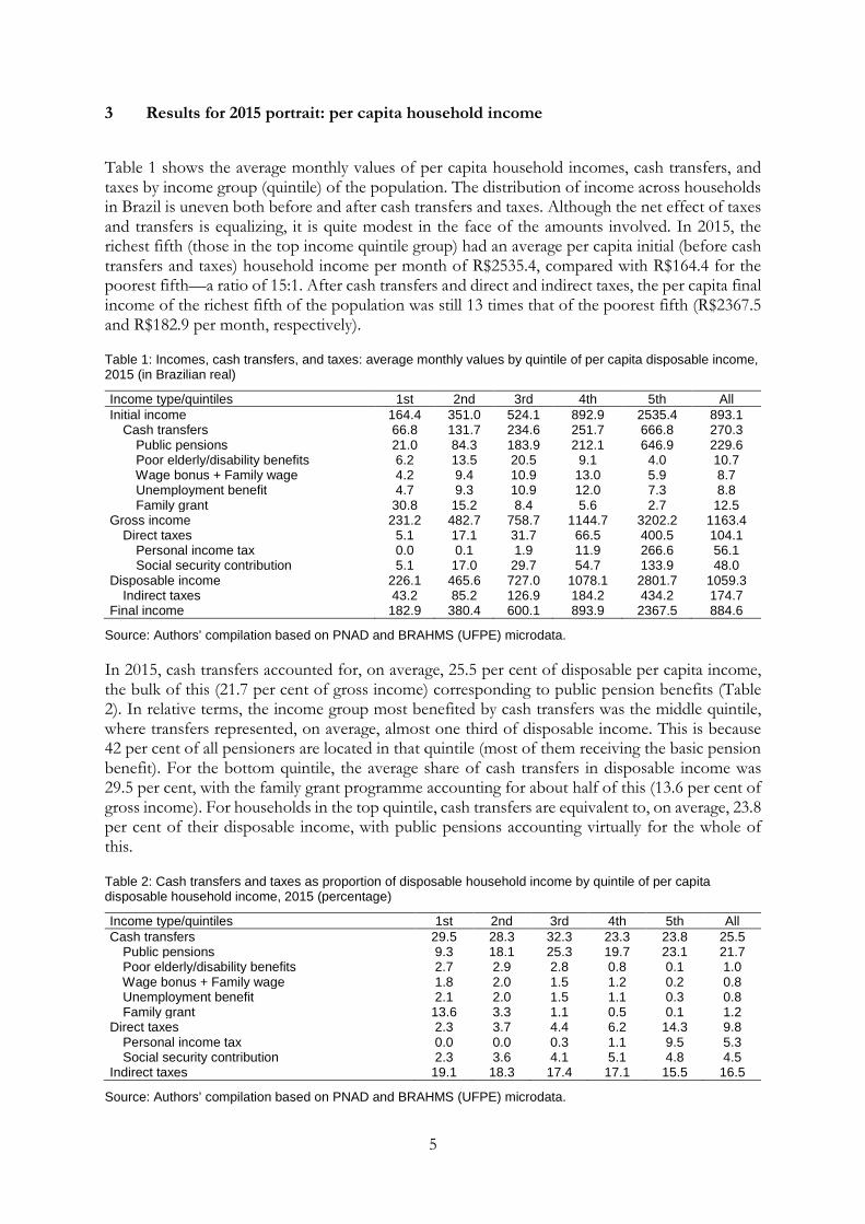
Table 1 shows the average monthly values of per capita household incomes, cash transfers, and taxes by income group (quintile) of the population. The distribution of income across households in Brazil is uneven both before and after cash transfers and taxes. Although the net effect of taxes and transfers is equalizing, it is quite modest in the face of the amounts involved. In 2015, the richest fifth (those in the top income quintile group) had an average per capita initial (before cash transfers and taxes) household income per month of R$2535.4, compared with R$164.4 for the poorest fifth—a ratio of 15:1. After cash transfers and direct and indirect taxes, the per capita final income of the richest fifth of the population was still 13 times that of the poorest fifth (R$2367.5 and R$182.9 per month, respectively).

Table 1: Incomes, cash transfers, and taxes: average monthly values by quintile of per capita disposable income, 2015 (in Brazilian real)

Income type/quintiles 1st 2nd 3rd 4th 5th All Initial income 164.4 351.0 524.1 892.9 2535.4 893.1 Cash transfers 66.8 131.7 234.6 251.7 666.8 270.3 Public pensions 21.0 84.3 183.9 212.1 646.9 229.6 Poor elderly/disability benefits 6.2 13.5 20.5 9.1 4.0 10.7 Wage bonus + Family wage 4.2 9.4 10.9 13.0 5.9 8.7 Unemployment benefit 4.7 9.3 10.9 12.0 7.3 8.8 Family grant 30.8 15.2 8.4 5.6 2.7 12.5 Gross income 231.2 482.7 758.7 1144.7 3202.2 1163.4 Direct taxes 5.1 17.1 31.7 66.5 400.5 104.1 Personal income tax 0.0 0.1 1.9 11.9 266.6 56.1 Social security contribution 5.1 17.0 29.7 54.7 133.9 48.0 Disposable income 226.1 465.6 727.0 1078.1 2801.7 1059.3 Indirect taxes 43.2 85.2 126.9 184.2 434.2 174.7 Final income 182.9 380.4 600.1 893.9 2367.5 884.6

Source: Authors’ compilation based on PNAD and BRAHMS (UFPE) microdata.

In 2015, cash transfers accounted for, on average, 25.5 per cent of disposable per capita income, the bulk of this (21.7 per cent of gross income) corresponding to public pension benefits (Table 2). In relative terms, the income group most benefited by cash transfers was the middle quintile, where transfers represented, on average, almost one third of disposable income. This is because 42 per cent of all pensioners are located in that quintile (most of them receiving the basic pension benefit). For the bottom quintile, the average share of cash transfers in disposable income was 29.5 per cent, with the family grant programme accounting for about half of this (13.6 per cent of gross income). For households in the top quintile, cash transfers are equivalent to, on average, 23.8 per cent of their disposable income, with public pensions accounting virtually for the whole of this.

Table 2: Cash transfers and taxes as proportion of disposable household income by quintile of per capita disposable household income, 2015 (percentage)

Income type/quintiles 1st 2nd 3rd 4th 5th All Cash transfers 29.5 28.3 32.3 23.3 23.8 25.5 Public pensions 9.3 18.1 25.3 19.7 23.1 21.7 Poor elderly/disability benefits 2.7 2.9 2.8 0.8 0.1 1.0 Wage bonus + Family wage 1.8 2.0 1.5 1.2 0.2 0.8 Unemployment benefit 2.1 2.0 1.5 1.1 0.3 0.8 Family grant 13.6 3.3 1.1 0.5 0.1 1.2 Direct taxes 2.3 3.7 4.4 6.2 14.3 9.8 Personal income tax 0.0 0.0 0.3 1.1 9.5 5.3 Social security contribution 2.3 3.6 4.1 5.1 4.8 4.5 Indirect taxes 19.1 18.3 17.4 17.1 15.5 16.5


6

Direct taxes, on average, represented 9.8 per cent of disposable household income, in 2015. For households in the top quintile, direct taxes corresponded to, on average, 14.3 per cent of their disposable income. The majority of this (9.5 per cent of disposable income) was paid in personal income tax. The average tax burden for households in the bottom quintile, by contrast, was 2.3 per cent of their disposable income, comprising only social security contributions. In fact, personal income tax represents a significant proportion of income only for households in the top quintile. Indirect taxes represented, on average, 16.5 per cent of disposable household income in 2015. Households in the bottom quintile paid the equivalent of 19.1 per cent of their disposable income in indirect taxes, while the top quintile paid, on average, 15.5 per cent of their disposable income.

The effect of taxes and transfers on income inequality can be assessed by calculating the Gini coefficient for each measure of income.6 In 2015, Brazil’s Gini of initial income was estimated at 0.591. The difference between this index and the Gini of gross income was 8.9 percentage points, which represents the equalizing effect of cash transfers. In the same year, direct taxes led to a further reduction in the Gini coefficient of 2.35 percentage points. By contrast, when indirect taxes were deducted from disposable income, they acted to increase inequality by 0.7 percentage point. Thus, in 2015, the overall net effect of cash transfers and direct and indirect taxes was to reduce the Gini coefficient by 10.5 percentage points (or 17.8 per cent).

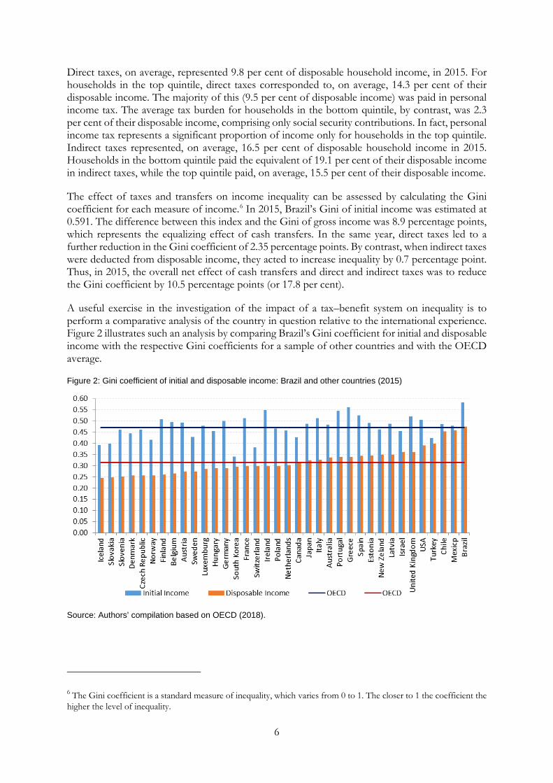
A useful exercise in the investigation of the impact of a tax–benefit system on inequality is to perform a comparative analysis of the country in question relative to the international experience. Figure 2 illustrates such an analysis by comparing Brazil’s Gini coefficient for initial and disposable income with the respective Gini coefficients for a sample of other countries and with the OECD average.

Figure 2: Gini coefficient of initial and disposable income: Brazil and other countries (2015)

Source: Authors’ compilation based on OECD (2018).

6 The Gini coefficient is a standard measure of inequality, which varies from 0 to 1. The closer to 1 the coefficient the higher the level of inequality.

7

4 Concentration curves

The concentration curves are a representation that bears similarities with the Lorenz curve. While the latter refers to the distribution of a single variable throughout the population, the former are constructed from the distribution of two variables in the population. In fact, the Lorenz curve can be understood as a particular case of the concentration curve where the variable used in the ordering of the population and the output variable coincides. Similarly, the correspondence between the Gini index and the Lorenz curve also appears in the relationship between the concentration curve and the concentration index. One key difference is that the Gini varies between 0 and 1 whereas the concentration index varies between −1 and 1. If a certain attribute is better targeted to the poor—for example, conditional cash transfers—then the indicator is negative.

The set of results based on the microsimulation data generated by the project covers the years 1995, 2003, 2009, and 2015. First, we assess the 2015 inequality portrait alone, through concentration curves for the different income types and related fiscal ingredients ordered by disposable incomes.7 We start with the former in Figure 3.

Figure 3: Concentration curves of income types ordered by disposable income (2015)


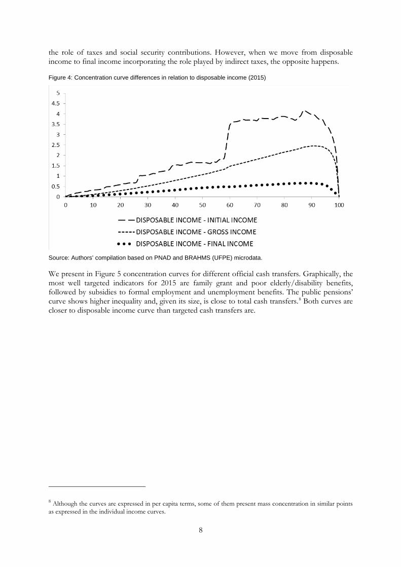
In order to see more clearly, we plot the differences of the concentration curves with respect to the disposable income Lorenz curve (Figure 4). As we move from initial market income to gross income incorporating the role of transfers, inequality falls. The same happens when we incorporate

7 In the income ordering, we used the disposable income concept to fit the comparisons with other countries in the project. The same type of tabulations were also performed for gross incomes and final incomes, everything for three different periods (2003–15, 2003–09, and 2009–15). We will focus on the whole period of 12 years.

8

the role of taxes and social security contributions. However, when we move from disposable income to final income incorporating the role played by indirect taxes, the opposite happens.

Figure 4: Concentration curve differences in relation to disposable income (2015)


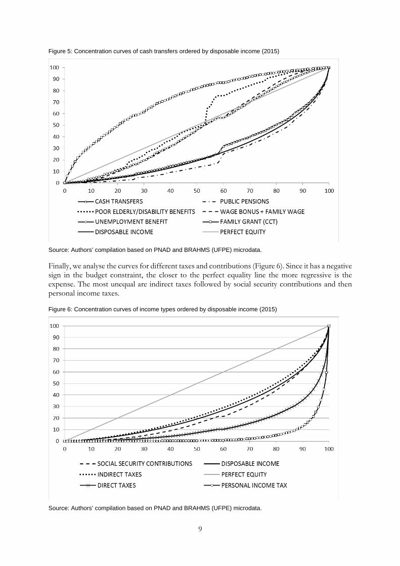
We present in Figure 5 concentration curves for different official cash transfers. Graphically, the most well targeted indicators for 2015 are family grant and poor elderly/disability benefits, followed by subsidies to formal employment and unemployment benefits. The public pensions’ curve shows higher inequality and, given its size, is close to total cash transfers.8 Both curves are closer to disposable income curve than targeted cash transfers are.

8 Although the curves are expressed in per capita terms, some of them present mass concentration in similar points as expressed in the individual income curves.

9

Figure 5: Concentration curves of cash transfers ordered by disposable income (2015)


Finally, we analyse the curves for different taxes and contributions (Figure 6). Since it has a negative sign in the budget constraint, the closer to the perfect equality line the more regressive is the expense. The most unequal are indirect taxes followed by social security contributions and then personal income taxes.

Figure 6: Concentration curves of income types ordered by disposable income (2015)


10

Figure 7 presents the evolution of the concentration curve of the family grant programme in 2003, 2009, and 2015. As the programme expanded it became somewhat less targeted9 but as we have seen previously it was still more inclusive than other social programmes in the final year of 2015.

Figure 7: Concentration curves for the family grant programme ordered by disposable income


The concentration curve allows evaluation of how progressive different fiscal ingredients are in isolation. However, we will build an integrated framework of the static and dynamic impacts of these components. Section 5 presents a framework to measure the social impacts of taxes and transfers that will be applied to Brazilian data. One advantage of this approach is to address these dimensions both in levels and in growth rates.

5 How progressive are incomes, transfers, and taxes? A framework

5.1 Portrait

We depart from Atkinson’s (2007) seminal contribution of decomposing social welfare into mean and inequality components applied by Amartya Sen to the case of the Gini—the most popular inequality index.

𝑊𝑊 = 𝜇𝜇(1 − 𝐺𝐺) = 𝜇𝜇𝜇𝜇 (1)

where G is the Gini index, which is a relative measure of inequality, and E=(1−G) is a measure of equity in income.

Taking logarithm of both sides of Equation (1) gives

9 There is no inequality dominance between years since the concentration curves cross.

11

ln(𝑊𝑊) = ln(𝜇𝜇) + ln(𝜇𝜇) (2)

which on taking the first difference gives

𝛾𝛾∗ = 𝛾𝛾 + 𝑔𝑔 (3)

where γ*=∆ln(W) is the growth rate of social welfare W, γ=∆ln(µ) is the growth rate of average income of the society, and g=∆ln(E) is the social welfare growth rate, which will be positive (negative) if growth is pro-poor (anti-poor).

Taxes and transfers

Suppose households draw their income from k sources with total per capita income x such that

𝜇𝜇 = ∑ 𝜇𝜇𝑖𝑖𝑘𝑘𝑖𝑖=1 (4)

This equation can be used to estimate the contributions of each income source (component) to average income of the population. The percentage contribution of the ith income source or taxes to the total average income is 100×µi/µ.

Similarly, we can calculate the mean social welfare of the ith income source from Equation (4) as

𝑊𝑊 = ∑ 𝑊𝑊𝑖𝑖𝑘𝑘𝑖𝑖=1 (5)

This equation provides the contribution of each income component to total social welfare. The percentage contribution of the ith income source to total social welfare is 100×Wi/W.

The mean social welfare of the ith income component in Equation (5) can also be written as

𝑊𝑊𝑖𝑖 = 𝜇𝜇𝑖𝑖(1 − 𝐶𝐶𝑖𝑖) = 𝜇𝜇𝑖𝑖𝜇𝜇𝑖𝑖 (6)

where Ci is the concentration index of the ith income component.

The concentration index Ci informs how the ith income component is distributed across income ranges. The concentration index lies between −1 and +1. Suppose the ith income component is the income received by beneficiaries of the family grant programme, then if the concentration index is 0, then all individuals in the society are equal beneficiaries; if Ci=−1, then the poorest person receives all the benefits of the programme and if Ci=+1, then the richest person receives all the benefits. The concentration index is a measure of inequity of an income component. Therefore, a measure of equity of the ith income component is defined as Ei=(1−Ci). So, the larger the value of Ei the more equitable will be the ith income component. Ei equals 1 if all individuals enjoy the same ith component income. This could be the benchmark: as such, the ith component is equitably (inequitably) distributed if Ei is greater (less) than 1.

Substituting Equations (4) and (6) into Equation (5) gives

𝜇𝜇 = ∑ 𝜇𝜇𝑖𝑖𝜇𝜇𝜇𝜇𝑖𝑖𝑘𝑘

𝑖𝑖=1 (7)

which shows that equity in total income is a weighted average of equity in each income component where weights are proportional to the shares of income components in the mean income.

12

Taking logarithms and first differences of both sides of Equation (6) gives

∆ ln(𝑊𝑊𝑖𝑖) = ∆ ln(𝜇𝜇𝑖𝑖) + ∆ ln(𝜇𝜇𝑖𝑖) (8)

where 𝛾𝛾𝑖𝑖∗=∆ln(W), γi=∆ln(µi), and gi=∆ln(Ei)

which gives

𝛾𝛾𝑖𝑖∗ = 𝛾𝛾𝑖𝑖 + 𝑔𝑔𝑖𝑖 (9)

which shows that growth rate of social welfare for the ith component is a sum of the two growth rates: (1) growth rate of the mean of the ith income component and (2) growth of the equity index of the income component. We define the growth of the ith income component as pro-poor (anti-poor) if the equity index of the ith income component increases (decreases). Thus, the ith component is pro-poor (anti-poor) if there is a gain (loss) in growth rate of welfare of the ith income component.

5.2 Fiscal determinants of social welfare growth

This section presents a methodology to calculate the contribution of various income sources to the total pro-poor growth rate. For instance, we discuss how much different social welfare programmes contribute to the total pro-poor growth of income.10

Suppose µt is the mean of per capita income in year t and µit is the mean of the ith income component in year t. Then based on Equation (4) we have

𝜇𝜇𝑡𝑡 = ∑ 𝜇𝜇𝑖𝑖𝑡𝑡𝑘𝑘𝑖𝑖=1 (10)

It can be shown that

∆ ln(𝜇𝜇𝑡𝑡) ~ 12∑ �𝜇𝜇𝑖𝑖(𝑡𝑡−1)

𝜇𝜇(𝑡𝑡−1)+ 𝜇𝜇𝑖𝑖𝑡𝑡

𝜇𝜇𝑡𝑡�𝑘𝑘

𝑖𝑖=1 ∆ ln(𝜇𝜇𝑖𝑖𝑡𝑡) (11)

which shows that the growth rate of per capita mean income is the weighted average of the growth rates of individual income components—the weights being proportional to the average of income shares in each period. This equation informs the magnitude of the contribution of each income component to the growth rate of per capita mean (average standard of living).

Suppose Wt is the social welfare in year t and Wit is the social welfare of the ith income component, then based on Equation (10) we have

𝑊𝑊𝑡𝑡 = ∑ 𝑊𝑊𝑖𝑖𝑡𝑡𝑘𝑘𝑖𝑖=1 (12)

Then, it can be shown that

∆ ln(𝑊𝑊𝑡𝑡) ~ 12∑ �𝑊𝑊𝑖𝑖(𝑡𝑡−1)

𝑊𝑊(𝑡𝑡−1)+ 𝑊𝑊𝑖𝑖𝑡𝑡

𝑊𝑊𝑡𝑡�𝑘𝑘

𝑖𝑖=1 ∆ ln(𝑊𝑊𝑖𝑖𝑡𝑡) (13)

10 Kakwani et al. (2010) develop a dynamic analysis framework using another social welfare function.

13

which shows that the growth rate of social welfare is the weighted average of the growth rates of social welfare of individual income components—the weights being proportional to the average of social welfare shares in each period. Equation (13) informs the magnitude of contribution of each income component to the growth rate of social welfare.

𝑔𝑔𝑡𝑡 = ∆ ln(𝑊𝑊𝑡𝑡) − ∆ ln(𝜇𝜇𝑡𝑡) (14)

which in view of Equations (16) and (18) gives the contribution of each income component to the pro-poor growth rate of per capita total income.

5.3 Targeting indicator

The small contribution of the family grant programme to inequality reduction does not imply that the programme is not well targeted to lower-income families. Policy-making will benefit from determining the targeting efficiency of various income sources, which income sources contribute more to social welfare and by how much. An income source can be said to be well targeted to lower-income families if it contributes more to social welfare relative to its contribution to income. This motivates us to propose a new index:

𝜑𝜑𝑖𝑖 = 𝑊𝑊𝑖𝑖𝜇𝜇𝑊𝑊𝜇𝜇𝑖𝑖

= 𝐸𝐸𝑖𝑖𝐸𝐸

(15)

where Ei=(1−Ci) is a measure of equity of the ith income component and E=(1−G) is a measure of equity of total income.

If ϕi is greater than 1, controlling for the income share, the ith income source contributes more to social welfare. This index is like a targeting index informing how well a particular income source is targeted to the lower-income families. The targeting indicator for total income is 1, which is the benchmark. An index value greater than 1 implies that the particular income source benefits the lower-income families more than the average. The larger the value of index, the greater the targeting efficiency.

This same measure of Equation (15) can also be analysed in a dynamic fashion comparing changes in social welfare and changes in the fiscal cost associated with it.

6 Measuring the social welfare impacts of taxes and transfers over time (2003–15)

6.1 Social welfare static decompositions

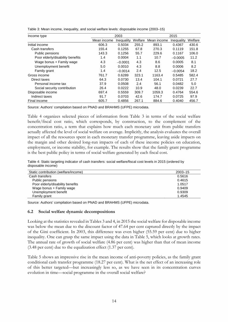
Following the methodology developed in Section 5, Table 3 presents mean income, inequality,11 and social welfare levels associated with different income types and respective fiscal ingredients between them ordered by disposable income. This methodology allows us to map the contribution of different taxes and transfers into disposable income-based mean, inequality, and social welfare.

11 A product between the concentration index of the income type times its share in the mean disposable income.

14

Table 3: Mean income, inequality, and social welfare levels: disposable income (2003–15)

Income type 2003 2015 Mean income Inequality Welfare Mean income Inequality Welfare

Initial income 606.3 0.5034 255.2 893.1 0.4367 430.6 Cash transfers 155.4 0.1255 67.8 270.3 0.1119 151.8 Public pensions 143.3 0.1256 55.7 229.6 0.1167 106.0 Poor elderly/disability benefits 1.4 0.0004 1.1 10.7 −0.0005 11.2 Wage bonus + Family wage 4.3 −0.0001 4.3 8.6 0.0005 8.1 Unemployment benefit 5.0 0.0010 4.3 8.8 0.0006 8.2 Family grant 1.4 −0.0014 2.4 12.5 −0.0054 18.2 Gross income 761.7 0.6289 323.1 1163.4 0.5485 582.4 Direct taxes 64.3 0.0730 13.4 104.1 0.0721 27.7 Personal income tax 37.9 0.0508 2.4 56.1 0.0482 5.0 Social security contribution 26.4 0.0222 10.9 48.0 0.0239 22.7 Disposable income 697.4 0.5559 309.7 1059.3 0.4764 554.6 Indirect taxes 91.7 0.0703 42.6 174.7 0.0725 97.9 Final income 605.7 0.4856 267.1 884.6 0.4040 456.7


Table 4 organizes selected pieces of information from Table 3 in terms of the social welfare benefit/fiscal cost ratio, which corresponds, by construction, to the complement of the concentration ratio, a term that explains how much each monetary unit from public transfers actually affected the level of social welfare on average. Implicitly, the analysis evaluates the overall impact of all the resources spent in each monetary transfer programme, leaving aside impacts on the margin and other desired long-run impacts of each of these income policies on education, employment, or income stability, for example. The results show that the family grant programme is the best public policy in terms of social welfare generated by each fiscal cost.

Table 4: Static targeting indicator of cash transfers: social welfare/fiscal cost levels in 2015 (ordered by disposable income)

Static contribution (welfare/income) 2003–15 Cash transfers 0.5616 Public pensions 0.4615 Poor elderly/disability benefits 1.0517 Wage bonus + Family wage 0.9409 Unemployment benefit 0.9309 Family grant 1.4545


6.2 Social welfare dynamic decompositions

Looking at the statistics revealed in Tables 3 and 4, in 2015 the social welfare for disposable income was below the mean due to the discount factor of 47.64 per cent captured directly by the impact of the Gini coefficient. In 2003, this difference was even higher (55.59 per cent) due to higher inequality. One can grasp the same impact using the data in Table 5, which looks at growth rates. The annual rate of growth of social welfare (4.86 per cent) was higher than that of mean income (3.48 per cent) due to the equalization effect (1.37 per cent).

Table 5 shows an impressive rise in the mean income of anti-poverty policies, as the family grant conditional cash transfer programme (18.27 per cent). What is the net effect of an increasing role of this better targeted—but increasingly less so, as we have seen in its concentration curves evolution in time—social programme in the overall social welfare?

15

Table 5: Income, equality, and social welfare: annual growth rates by disposable income (2003–15)

Income type 2003–15 (Annual) Mean income Equality Welfare

Initial income 0.0323 0.0113 0.0436 Cash transfers 0.0461 0.0210 0.0671 Public pensions 0.0393 0.0143 0.0536 Poor elderly/disability benefits 0.1681 0.0238 0.1919 Wage bonus + Family wage 0.0587 −0.0060 0.0527 Unemployment benefit 0.0478 0.0066 0.0544 Family grant 0.1827 −0.0137 0.1690 Gross income 0.0353 0.0138 0.0491 Direct taxes 0.0402 0.0206 0.0608 Personal income tax 0.0328 0.0267 0.0595 Social security contribution 0.0499 0.0112 0.0611 Disposable income 0.0348 0.0137 0.0486 Indirect taxes 0.0537 0.0156 0.0693 Final income 0.0316 0.0132 0.0447


Although Table 5 is useful, if one is interested in capturing the role of each ingredient, one should also take into account the weights of these ingredients. The main advantage of the decomposition methodology explored here is to allow moving directly from the levels of each component to its contribution to social welfare rates of change. Incorporating not only its growth but also its weight in each income type, we deconstruct the whole effect into smaller components associated with private incomes, public transfers, and taxes. Each of these components of the social welfare impact can be further decomposed into its respective mean and inequality drivers (Table 6).

The period between 2003 and 2015 verified a decrease in inequality and an increase in the mean income and the social welfare of the population for all the different income types and their components. The data ordered by disposable income disclosed that inequality explained 28.4 per cent while mean income explained the remainder 71.6 per cent of an annual social welfare growth of 4.86 per cent in that period.

Table 6: Income, equality, and social welfare growth: contribution by component by disposable income (2003–15)

Income type 2003–15 (Annual) Mean income Equality Welfare

Initial income 0.0276 0.0072 0.0349 Cash transfers 0.0110 0.0055 0.0165 Public pensions 0.0083 0.0016 0.0099 Poor elderly/disability benefits 0.0010 0.0013 0.0023 Wage bonus + Family wage 0.0004 0.0003 0.0008 Unemployment benefit 0.0004 0.0004 0.0008 Family grant 0.0013 0.0022 0.0034 Gross income 0.0387 0.0127 0.0514 Direct taxes 0.0038 −0.0010 0.0028 Personal income tax 0.0018 −0.0013 0.0005 Social security contribution 0.0021 0.0003 0.0023 Disposable income 0.0348 0.0137 0.0486 Indirect taxes 0.0080 0.0029 0.0109 Final income 0.0269 0.0108 0.0377


Finally, Table 7 presents a list of cash transfer policies to measure each relative contribution to social welfare growth in comparison with their relative contribution to income increase during the same period. The results show that the family grant programme—the main income policy designed for poverty alleviation in Brazil—is indeed the one better targeted to the poor, since its contribution to the rise of social welfare is 2.7 times its contribution to the rise of mean income.

16

Table 7: Dynamic targeting indicator of cash transfers: social welfare/fiscal cost growth, relative contribution based on disposable income (2003–15)

Relative contribution to growth (welfare/income) 2003–15 Cash transfers 1.4993 Public pensions 1.1979 Poor elderly/disability benefits 2.2494 Wage bonus + Family wage 1.7982 Unemployment benefit 2.1069 Family grant 2.7148


7 Poverty impacts

Brazil adopted an official extreme poverty line around US$1.25 using older purchasing power parity (PPP) which is perhaps too low for the Brazilian level of income. We perform different exercises using different international poverty lines, recently raised from the use of the new PPP estimates (Table 8).

Table 8: Proportion of poor (P0) and poverty gap (P1) for disposable income and different poverty lines (2003 and 2015)

2003 2015 P0 P1 P0 P1

Poverty–CPS line 25.7 10.9 7.7 2.4 Poverty–US$1.25 new PPP line 7.2 3.4 1.4 0.1 Poverty–US$1.9 new PPP line 13.4 5.7 3.0 0.8 Poverty–US$3.2 new PPP line 27.2 11.7 8.4 2.7 Poverty–US$4 new PPP line 35.5 15.5 12.5 4.3 Poverty–US$5.5 new PPP line 47.5 22.6 21.2 7.7


The first poverty-related contribution of this work is to analyse the impacts of inequality on poverty changes using our microsimulation framework of fiscal instances. The fall of poverty in percentage points increases with the level of the poverty line used, which is not surprising because poverty levels are also necessarily higher. However, the proportional variation is monotonically higher for higher poverty aversion coefficients (i.e. P1 over P0) and for lower poverty lines ranging from −95.91 per cent to −65.92 per cent in the case of the poverty gap (P1). Using as a benchmark the intermediary US$3.2 a day line the fall in the 2003–15 period amounted to −18.8 percentage points or a reduction of 69 per cent. This means that poverty fell nearly twice more than expected in the United Nations’ first Millennium Development Goals in less than half of the period.

We apply a standard Ravallion–Datt decomposition into growth and inequality components to assess their relative roles initially using disposable income (Table 9). The most important dimension analysed here is the relative share of poverty fall explained by inequality that falls monotonically in the case of P1 as the poverty line rises, ranging from 65.44 to 40 per cent of total poverty fall. In the case of our intermediary US$3.2 a day line 43 per cent of total P1 fall was explained by the inequality component—almost a middle path driven by both distributive and growth dimensions.

17

Table 9: Poverty variation between 2003 and 2015 for disposable income

Inequality−Effect (%) Growth−Effect (%) Total (p.p.) P0–disposable income Poverty–CPS line 38.51 61.49 −18.0 Poverty–US$1.25 47.07 52.93 −5.8 Poverty–US$1.9 40.35 59.65 −10.4 Poverty–US$3.2 38.06 61.94 −18.8 Poverty–US$4 38.66 61.34 −23.0 Poverty–US$5.5 37.50 62.50 −26.3 P1 (disposable income) Poverty–CPS line 43.46 56.54 −8.4 Poverty–US$1.25 65.44 34.56 −3.2 Poverty–US$1.9 52.79 47.21 −4.9 Poverty–US$3.2 42.94 57.06 −8.9 Poverty–US$4 41.56 58.44 −11.3 Poverty–US$5.5 40.00 60.00 −14.9


7.1 Efficiency of anti-poverty programmes

We also developed an index to assess pro-poor policies as the ratio between the social gains obtained with how a specific programme impacts poverty over its fiscal cost, ordered by a particular income type in a specific moment in time. We define social gains as the negative variation of poverty in percentage points due to the impacts of the programme and we define its fiscal cost as the programme’s participation in the mean income. Thus, Equation (16) would be written as follows:

𝛹𝛹𝑝𝑝𝑖𝑖 = −∆𝑃𝑃𝜇𝜇𝑡𝑡𝜇𝜇𝑝𝑝𝑖𝑖𝑡𝑡

= − �𝑃𝑃𝜇𝜇𝑡𝑡− 𝑃𝑃′𝜇𝜇𝑡𝑡�𝜇𝜇𝑝𝑝𝑖𝑖𝑡𝑡

(16)

where ∆Pµt is the difference between the actual poverty level (𝑃𝑃) in comparison with a hypothetical scenario of poverty (𝑃𝑃′) where a specific programme p was not implemented and µpit is the mean income of this programme. Either µp, P, P′ are defined in relation to a specific income component, for example, disposable income. Consequently, the mean income of the programme p can also be interpreted as the difference in the mean income of the specific income type due to the existence of this programme. Therefore, Ψi can be interpreted as the ratio between the relative participation of the programme p in poverty and its relative participation in the mean income. The negative symbol in Equation (16) also implies that the larger the value of the index, the greater the targeting efficiency.

Next, we simulate statically for 2015 the benefit of fall in poverty associated with each government’s cost of different anti-poverty programmes. We compare the impacts of family grant and poor elderly/disability benefits by comparing the scenarios of poverty with and without these programmes (Table 10).

18

Table 10: Poverty scenarios if the main poverty alleviation policies did not exist (2015)

Disposable per capita income: poverty levels (2015′)

No family grant No poor elderly/disability benefits

P0 P1 P0 P1 Poverty–CPS line 9.6 4.4 8.9 3.2 Poverty–US$1.25 new PPP line 3.4 2.0 2.1 0.6 Poverty–US$1.9 new PPP line 5.2 2.8 3.9 1.3 Poverty–US$3.2 new PPP line 10.3 4.7 9.6 3.5 Poverty–US$4 new PPP line 14.5 6.2 13.8 5.1 Poverty–US$5.5 new PPP line 22.6 9.6 22.6 8.7


The key statistic is the net benefit in terms of fall in poverty per monetary unit spent as in Table 11. Except for the highest poverty line, the social benefit is higher for the family grant programme for all poverty lines and poverty measures considered. In our benchmark (P1 with the intermediary line), this ratio is 119.73 per cent higher for the family grant programme (Campello and Neri 2013; Peci and Neri 2017).

Table 11: Poverty comparison: reality versus scenarios if main poverty alleviation policies did not exist (2015)

Disposable income: 2015 vs 2015′ Family grant (social benefit/fiscal cost)

Poor elderly/disability benefit (social benefit/fiscal cost)

P0 P1 P0 P1 Poverty–CPS line 0.15 0.16 0.11 0.07 Poverty–US$1.25 new PPP line 0.16 0.15 0.06 0.04 Poverty–US$1.9 new PPP line 0.17 0.16 0.08 0.05 Poverty–US$3.2 new PPP line 0.16 0.16 0.12 0.07 Poverty–US$4 new PPP line 0.16 0.15 0.12 0.08 Poverty–US$5.5 new PPP line 0.11 0.15 0.13 0.09


8 Conclusion

This paper assesses fiscal redistribution in Brazil between 2003 and 2015. The framework proposed evaluates in an integrated manner causes and consequences of inequality in terms of social welfare and poverty both in levels and changes over time.

The paper develops, describes, and applies an empirical methodology, including the source of micro data used, Brazilian institutional features, data adjustments made, simulation procedures adopted, and the results thereupon generated. This paper had the initial objective of providing a report on the procedures adopted in the ongoing work concerning the fiscal redistributive impact of the Brazilian tax–benefit system. This work necessarily involves methodological decisions made in order to be able to model the system as closely as possible to its actual operation. It is thus important to be clear about the steps followed to generate the information used in the analysis.

The general approach delineated here is applied to each of the four years covered in this study (1995, 2003, 2009, and 2015) to allow a compatible comparative analysis for the period considered. We compare different income types but focus here on derived per capita disposable income changes between 2003 and 2015. Another contribution of this paper is to simulate an income type that is not readily available in Brazilian household surveys. Around 28.2 per cent of per capita disposable Gini index-based social welfare measure changes are due to a pure fall in inequality while the remainder is due to mean growth. Our results also suggest that official cash transfers accelerated the growth of social welfare while direct and indirect taxes changes played the opposite role. The analysis of the role played by specific fiscal instruments among various taxes and cash

19

transfer programmes shows that the family grant programme was the better targeted action in the 2003–15 period using both social welfare and poverty criteria.

References

Atkinson, A.B., and T. Piketty (eds.) (2007). Top Incomes Over the Twentieth Century: A Contrast Between European and English-Speaking Countries. Oxford: Oxford University Press.

Barreix, A., J.C. Benítez, and M. Pecho (2017). ‘Revisiting Personal Income Tax in Latin America: Evolution and Impact’. OECD Development Centre Working Paper 338. Paris: OECD Publishing. Available at: http://www.oecd.org/officialdocuments/publicdisplaydocument pdf/?cote=DEV/DOC/WKP(2017)4&docLanguage=En (accessed October 2018).

Campello, T., and M.C. Neri (2013). Programa Bolsa Família: uma década de inclusão e cidadania [Family Grant Programme: A Decade of Inclusion and Citizenship (1st edition, vol.1, 494pp). Brazil: IPEA. Available at: http://www.ipea.gov.br/portal/index.php?option=com_content&view= article&id=20408 (accessed September 2018).

Higgins, S., and C. Pereira (2013). ‘The Effects of Brazil’s High Taxation and Social Spending on the Distribution of Household Spending’. CEQ Working Paper 7. New Orleans, LA: Tulane University. Available at: http://commitmentoequity.org/publications-ceqworkingpapers/ (accessed September 2018).

IBGE (2008). ‘Matriz de insumo-produto: Brasil: 2000/2005’ [‘Brazilian Input–Output Matrix: 2000/2005’] [in Portuguese]. Rio de Janeiro: Série Contas Nacionais.

IBGE (2016). ‘Matriz de insumo-produto: Brasil: 2010’ [‘Brazilian Input–Output Matrix: 2010’] [in Portuguese]. Rio de Janeiro: Série Contas Nacionais.

Immervoll, H., H. Levy, J.R.B. Nogueira, C. O’Donoghue, and R.B. Siqueira (2009). ‘The Impact of Brazil’s Tax-Benefit System on Inequality and Poverty’. In S. Klasen and F. Nowak-Lehmann (eds.), Poverty, Inequality, and Policy in Latin America (pp. 271–301). Cambridge, MA: MIT Press.

Kakwani, N. (1977). ‘Measurement of Tax Progressivity: An International Comparison’. The Economic Journal, 87(345): 71–80.

Kakwani, N., M.C. Neri, and H. Son (2010). ‘Linkages Between Pro-Poor Growth, Social Programs and Labor Market: The Recent Brazilian Experience’. World Development, 38(6): 881–94.

Neri, M.C. (2017). ‘Evolução Social, Superação da Crise e os Programas de Transferência de Renda’ [‘Social Evolution, Overcoming the Crisis and Cash Transfers’] [in Portuguese]. Série IDP Eventos, Gilmar Ferreira Mendes e Paulo Gustavo Gonet Branco (org.), Escola de Administração de Brasília/IDP, April. Available at: https://www.cps.fgv.br/cps/bd/ ARTIGO-EVOLUCAO-SOCIAL-SUPERACAO-DA-CRISE-E-OS-PROGRAMAS-DE-TRANSFERENCIA-DE-RENDA-MARCELO-NERI-FGV-SOCIAL.pdf (accessed October 2018).

OECD (2018). OECD Income Distribution Database (IDD): Gini, Poverty, Methods and Concepts. Available at: http://www.oecd.org/social/income-distribution-database.htm (accessed 2 May 2018).

Peci, A., and M.C. Neri (2017). Revista Brasileira de Administração Pública [Brazilian Journal of Public Administration]. Special Issue on Public Policies on Fighting Poverty. Available at:

http://www.oecd.org/officialdocuments/publicdisplaydocumentpdf/?cote=DEV/DOC/WKP(2017)4&docLanguage=En

http://www.oecd.org/officialdocuments/publicdisplaydocumentpdf/?cote=DEV/DOC/WKP(2017)4&docLanguage=En

https://www.cps.fgv.br/cps/bd/%0bARTIGO-EVOLUCAO-SOCIAL-SUPERACAO-DA-CRISE-E-OS-PROGRAMAS-DE-TRANSFERENCIA-DE-RENDA-MARCELO-NERI-FGV-SOCIAL.pdf



http://www.oecd.org/social/income-distribution-database.htm

20

http://www.scielo.br/pdf/rap/v51n2/en_0034-7612-rap-51-02-22017.pdf (accessed September 2018).

Scutella, R. (2002). ‘The final incidence of Australian indirect taxes’. Australian Economic Review, 32(4), 349–68.

Seae/MF (2017). Efeito Redistributivo da Política Fiscal no Brasil [Redistributive Effect of the Tax Policy in Brazil] [in Portuguese]. Brazil: Secretaria de Acompanhamento Econômico, Ministério da Fazenda. Available at: http://www.fazenda.gov.br/centrais-de-conteudos/publicacoes/boletim-de-avaliacao-de-politicas-publicas/arquivos/2017/efeito_redistributivo_12_2017.pdf/view (accessed October 2018).

Secretaria da Receita Federal (2017). Grandes Número IRPF – Ano Calendário 2015, Exercício 2016 [Personal Income Tax Data. Data collected in the year 2015, work released in 2016] [in Portuguese] Brazil. Available at: http://idg.receita.fazenda.gov.br/dados/receitadata/ estudos-e-tributarios-e-aduaneiros/estudos-e-estatisticas/11-08-2014-grandes-numeros-dirpf/relatorio-gn-irpf-2015.pdf (accessed September 2018).

Silveira, F.G., F. Rezende, J.R. Afonso, and J. Ferreira (2013). ‘Fiscal Equity: Distributional Impacts of Taxation and Social Spending in Brazil’. Working Paper 115. Brazil: International Policy Centre for Inclusive Growth. Available at: http://www.ipc-undp.org/pub/IPCWorkingPaper115.pdf (accessed October 2018).

Siqueira, R.B. de, J.R. Nogueira, and E.S. Souza (2001). ‘A Incidência Final dos Impostos Indiretos no Brasil: Efeitos da Tributação de Insumos’ [‘The Final Incidence of Indirect Taxes in Brazil: Effects of Input Taxation’] [in Portuguese]. Revista Brasileira de Economia, 55(4): 513–44.

http://www.scielo.br/pdf/rap/v51n2/en_0034-7612-rap-51-02-22017.pdf

http://www.fazenda.gov.br/centrais-de-conteudos/publicacoes/boletim-de-avaliacao-de-politicas-publicas/arquivos/2017/efeito_redistributivo_12_2017.pdf/view

http://www.fazenda.gov.br/centrais-de-conteudos/publicacoes/boletim-de-avaliacao-de-politicas-publicas/arquivos/2017/efeito_redistributivo_12_2017.pdf/view

http://www.ipc-undp.org/pub/IPCWorkingPaper115.pdf

http://www.ipc-undp.org/pub/IPCWorkingPaper115.pdf

21

Appendix A: Changes in income inequality over time (1995–2015)

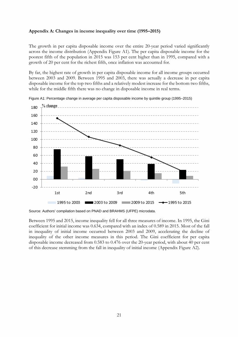
The growth in per capita disposable income over the entire 20-year period varied significantly across the income distribution (Appendix Figure A1). The per capita disposable income for the poorest fifth of the population in 2015 was 153 per cent higher than in 1995, compared with a growth of 20 per cent for the richest fifth, once inflation was accounted for.

By far, the highest rate of growth in per capita disposable income for all income groups occurred between 2003 and 2009. Between 1995 and 2003, there was actually a decrease in per capita disposable income for the top two fifths and a relatively modest increase for the bottom two fifths, while for the middle fifth there was no change in disposable income in real terms.

Figure A1: Percentage change in average per capita disposable income by quintile group (1995–2015)


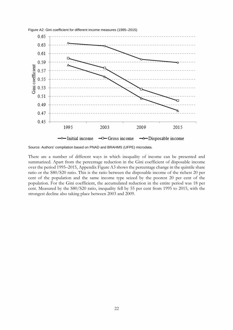
Between 1995 and 2015, income inequality fell for all three measures of income. In 1995, the Gini coefficient for initial income was 0.634, compared with an index of 0.589 in 2015. Most of the fall in inequality of initial income occurred between 2003 and 2009, accelerating the decline of inequality of the other income measures in this period. The Gini coefficient for per capita disposable income decreased from 0.583 to 0.476 over the 20-year period, with about 40 per cent of this decrease stemming from the fall in inequality of initial income (Appendix Figure A2).

22

Figure A2: Gini coefficient for different income measures (1995–2015)


There are a number of different ways in which inequality of income can be presented and summarized. Apart from the percentage reduction in the Gini coefficient of disposable income over the period 1995–2015, Appendix Figure A3 shows the percentage change in the quintile share ratio or the S80/S20 ratio. This is the ratio between the disposable income of the richest 20 per cent of the population and the same income type seized by the poorest 20 per cent of the population. For the Gini coefficient, the accumulated reduction in the entire period was 18 per cent. Measured by the S80/S20 ratio, inequality fell by 55 per cent from 1995 to 2015, with the strongest decline also taking place between 2003 and 2009.

23

Figure A3: Reduction in Gini coefficient and S80/S20 ratio for per capita disposable income (1995–2015)


The impact of cash benefits and direct taxes on income inequality between 1995 and 2015 is shown in Appendix Figure A4. Over this period, the absolute reduction in the Gini coefficient caused by cash benefits increased sharply, from 3.5 percentage points in 1995 to 8.9 percentage points in 2015. The impact of direct taxes in reducing income inequality also increased in the period, but much less, from 1.6 percentage points to 2.4 percentage points reduction in Gini.

Figure A4: Change in Gini coefficient because of cash transfer and direct taxes (1995–2015)

Source: Authors’ compilation based on PNAD and BRAHMS (UFPE) microdata

The redistributive impact of taxes and benefits depends on two factors: the size of the tax or transfer relative to total household income (referred to as average rate) and the progressivity of the

24

tax or transfer. A tax is considered progressive when the tax burden increases with income; similarly, cash benefits are progressive if they account for a larger share of the income of low-income groups than of high-income groups.

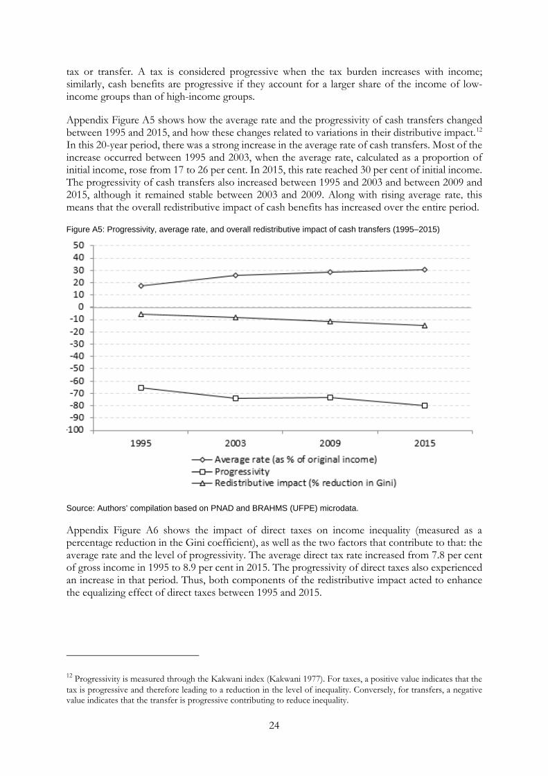
Appendix Figure A5 shows how the average rate and the progressivity of cash transfers changed between 1995 and 2015, and how these changes related to variations in their distributive impact.12

In this 20-year period, there was a strong increase in the average rate of cash transfers. Most of the increase occurred between 1995 and 2003, when the average rate, calculated as a proportion of initial income, rose from 17 to 26 per cent. In 2015, this rate reached 30 per cent of initial income. The progressivity of cash transfers also increased between 1995 and 2003 and between 2009 and 2015, although it remained stable between 2003 and 2009. Along with rising average rate, this means that the overall redistributive impact of cash benefits has increased over the entire period.

Figure A5: Progressivity, average rate, and overall redistributive impact of cash transfers (1995–2015)


Appendix Figure A6 shows the impact of direct taxes on income inequality (measured as a percentage reduction in the Gini coefficient), as well as the two factors that contribute to that: the average rate and the level of progressivity. The average direct tax rate increased from 7.8 per cent of gross income in 1995 to 8.9 per cent in 2015. The progressivity of direct taxes also experienced an increase in that period. Thus, both components of the redistributive impact acted to enhance the equalizing effect of direct taxes between 1995 and 2015.

12 Progressivity is measured through the Kakwani index (Kakwani 1977). For taxes, a positive value indicates that the tax is progressive and therefore leading to a reduction in the level of inequality. Conversely, for transfers, a negative value indicates that the transfer is progressive contributing to reduce inequality.

25

Figure A6: Progressivity, average rate, and overall redistributive impact of direct taxes (1995–2015)


26

Appendix B: The Brazilian Household Microsimulations System (BRAHMS)

Simulation of the Brazilian tax–benefit system in the present study was carried out using BRAHMS, a microsimulation model developed and updated by the Public Economics Research Group, Department of Economics, Universidade Federal de Pernambuco (UFPE), Recife, Brazil.

BRAHMS encodes the Brazilian tax–benefit’s legal rules and allows the assessment of the effects of cash transfers, social security contributions, personal income tax, and indirect taxes on household incomes.

BRAHMS applies the tax–benefit system’s policy rules to nationally representative micro data of individuals, families, and households. It calculates taxes and benefits taking into account characteristics of the individual/family/household in the data. The model’s main output is the calculation of different definitions of income at the individual and household level.

This appendix presents the main features of the BRAHMS version used to generate the results presented in the present study. First, we give an overview of the model’s data set. Then, we present the legal rules that determine eligibility to social benefits and liability to taxes, describing how they are simulated.

B1 Data set transformations

The basic data set used in the model was built using source household micro data from the National Sample Household Survey (Pesquisa Nacional por Amostra de Domicílios, PNAD) for the years 1995, 2003, 2009, and 2015. PNAD is a rural and urban household survey carried out by the Brazilian Institute of Geography and Statistics (Instituto Nacional de Geografia e Estatística, IBGE), covering all Brazilian regions, except, for the years 1995 and 2003, the rural area of the northern region.

As PNAD does not contain expenditure data, and this information is needed to simulate the effect of indirect taxes, a separate survey, the Family Budget Survey (Pesquisa de Orçamentos Familiares, POF), for the periods 2002–03 and 2008–09, also produced by IBGE, was used. Both POF’s waves used cover all Brazilian regions. Appendix Table B1 lists the main characteristics of the PNAD and POF surveys.

27

Table B1: Description of Brazilian household surveys

Original name Pesquisa Nacional por Amostra de Domicílios (PNAD)

Pesquisa de Orçamentos Familiares (POF)

Provider Instituto Nacional de Geografia e Estatística (IBGE)

Instituto Nacional de Geografia e Estatística (IBGE)

Year of collection 1995, 2003, 2009, 2015 2002–03, 2008–09 Conducted Annually At about a five-year interval Publication It is published one year after

collection It is published one year after collection

Period of collection September of previous year to September of current year

May of first year to May of second year

Income/expenditure reference period

Month (the survey registers income for the reference month of collection, September)

The survey registers expenditure for four reference periods: the last 12 months, the last three months, the last month, and the last week, as from the date the household is interviewed

Sampling Three-stage, probabilistic sampling, stratified by municipal and households levels

Two-stage sampling, stratified by geographical and household levels

Main unit of assessment Household Household Coverage National, permanent private

households; does not cover individuals not living in households (e.g. homeless)

National, permanent private households; does not cover individuals not living in households (e.g. homeless)

Other coverage The survey is also representative at the state level, urban and rural levels, regional level, and metropolitan areas level

The survey is also representative at the state level, urban and rural levels, regional level, and metropolitan areas level

Source: Authors’ compilation based on IBGE data.

Despite the main unit of analysis of the model being the household, the Brazilian data set displays socio-economic and demographic information, separately, for all individuals in the sample. It is so because most social benefits and taxes have the individual as the legal unit. An aggregation is then performed for each household, using the sample weights, over its individual members, to get the household total.

Incomes reported in PNAD are gross of taxes. They incorporate only incomes regularly received by individuals, on a monthly basis. Thus, benefits as the unemployment benefit, holiday bonus, and the ‘thirteenth wage’ are not included. On the other hand, the family wage benefit is included in the reported incomes.

There are three sources of labour income: main job, secondary job, and other jobs. For simulations requiring information about formal labour status, only incomes from main and secondary jobs are considered since this information is absent for other jobs. For simulations requiring information about contribution to social security, all three sources of income are used.

Some adjustments were adopted during the construction of the Brazilian data set from the original PNAD data, including:

(i) Some individual incomes are reported as ignored in PNAD. The decision taken was to impute a zero value for such cases.

(ii) Some public pension incomes are reported in PNAD with a value less than the official minimum wage. The decision taken was to impute the official minimum value (equal to the official minimum wage) for these cases.

28

(iii) Some formal labour incomes (employees formally registered and statutory civil and military public servants) are reported in PNAD with a value less than the official minimum wage. The decision taken was to impute the official minimum value for these cases.

(iv) In PNAD, there is a variable that assigns to every individual a ‘condition’ within the household/family. For example, the individual may be the head of the household/family, a spouse, a child, or a relative. Individuals assigned with the condition ‘boarder’ or ‘domestic employee’ were retained in the final data only when they are reported as head of some household/family. All the others were withdrawn because they do not constitute a member of any household/family in the data set.

(v) In the computation of family/household income, only the incomes of the head of the household, the spouse, children aged 10 years old or more, other relatives aged 10 years old or more, and agregados are included. The incomes of individuals with condition in the family/household as boarder, domestic employee, and relative of domestic employee are excluded. This is the usual procedure adopted in the Brazilian surveys.

B2 Social benefits overview

Only cash benefits are modelled. Benefits are simulated under the assumption that all entitled individuals/families actually receive them; that is, we ignore non-take-up. However, where necessary, adjustments are made in the modelling of the benefits in order to take account of some targeting problems and to approximate the simulated results to the aggregate official data. Public pensions are not simulated, being taken directly from the PNAD’s original data set, but are adjusted according to adjustment procedure (ii) cited in the previous Section B1.

We present in Appendix Figure B1 an overview of the main cash transfer programmes incorporated into the microsimulation exercised performed on PNAD microdata.

Figure B1: Brazilian main income policies scheme

Source: Authors’ compilation.

29

(1) Family wage

This is a means-tested benefit paid to formal employees or pensioners with children aged up to 14 years or disabled. For each dependent child the person receives a pre-determined amount, which depends on the salary/pension income bracket in which the employee or pensioner is included. The unit of assessment is the individual, and both fathers and mothers can claim the benefit for the same child.

For lack of information in PNAD, we cannot verify the disability status of individuals. Therefore, the model only uses the age of children and individual income to select those eligible for the benefit. The benefit is calculated for the main and secondary jobs, and then summed up to get the total value of the benefit. For other jobs it is not possible to simulate the benefit for lack of information about job status (formal or not) in PNAD.

The model first calculates the number of dependent children for each household using the definition of dependent children as those classified as son or daughter and being up to 14 years old. Then, the model verifies the job status of spouses in order to select only those in formal employment.

The recipients’ monthly wage or pension must fall in one of two thresholds for which the benefit applies. The value of the benefit is defined by the number of dependent children times the per child value of the benefit for each income threshold. The benefit is simulated for 1995, 2003, 2009, and 2015. In 2015, domestic workers became eligible for the benefit, but only after October. The simulation for this year, as for the other years in the sample, are made excluding these workers.

(2) Wage bonus

This is a benefit paid to those formal workers who receive up to two minimum wages, are registered in one of the social savings programmes (Programa de Integração Social or Programa de Formação do Patrimônio do Servidor Público, better known as PIS/PASEP) run by the government, and who worked for at least 30 days in the previous year. In practice, it works as a ‘fourteenth wage’ paid to low-income workers.

Given that in PNAD there is no information about enrolment in the social savings programmes, this condition is not included in the benefit simulation. Instead, the simulation uses an age restriction (23 years or more) in order to exclude those who are likely to be trainees (aged between 16 and 18 years), who are not entitled to the benefit. The difference between 23 years and 18 years would be equivalent to the enrolment time restriction. The unit of assessment is the individual.

The benefit is calculated both for the principal job and for the second job, but not for any other job the individual may have due to lack of job status (formal or not) in the PNAD data set. The amount of the benefit is equal to one minimum wage. The benefit is simulated for 1995, 2003, 2009, and 2015.

(3) Unemployment benefit

This is an income-related benefit paid to those formal workers who are unemployed. A person can receive from three to five instalments, depending on the number of months worked in the period of 36 months before being unemployed. The unit of assessment is the individual.

As PNAD contains information only for a period of 12 months before an individual is unemployed, the condition of number of months previously worked is checked only for that time

30

period, and not for the legal period of 36 months. Due to this information restriction, the benefit is also simulated under the assumption that all beneficiaries receive five instalments. This assumption produced a better adherence between simulation results and administrative data. The model selects those who are reported to have received unemployment benefit and then calculates the amount received. The benefit differs among three income tiers. The source of income included in the income assessment is labour income.

The V9066 and V084 variables are used to identify who received the benefit. For the V9066 variable, in particular, the current wage is used as a proxy for the wage received in the previous job (this information is not available in PNAD). Regarding the V9084 variable, there is no available information about current or previous wage. The benefit is then simulated under the assumption that everybody received all five insurance instalments, with every instalment equal to the mean of the official benefit value in the respective year.

The amount of the benefit, which cannot be less than one minimum wage, is calculated using the parameter values legally determined. For those in the first income tier, their income is multiplied by 0.8. For those in the second income tier, their income up to the first tier limit is multiplied by 0.8 and the extra income is multiplied by 0.5. For those in the third income tier, the amount of the benefit is a fixed amount. The benefit is simulated for 1995, 2003, 2009, and 2015.

(4) Social security

Social security is the main component of social income in Brazil, second only to labour earnings among all other sources collected by PNAD. The major portion of benefits is made of transfers not explicitly linked with past contributions. Still, the beneficiaries of social security do get public subsidies because the volume of transfers exceeds the volume of contributions, especially lower and public sector-related ones. With respect to the former, there is a link with minimum wage policy, which according to the Brazilian 1988 Constitution sets the floor to these benefits. In addition, the purchasing power of all social security benefits is protected against inflation on a yearly basis, although the Constitution does not make explicit the specific price index that adjusts nominal benefits. Social security also has a rural retirement programme for those that can testify at least 15 years of economic activity in a rural area and are at least 60 years old. It is a non-contributory programme entirely consisting of a subsidy to the beneficiaries, and the benefit offered is equal to the value of a minimum wage.

(5) Annual bonus

This benefit is paid to all retired person receiving a public pension in the form of an extra monthly pension annually. The unit of assessment is the individual. The model simulates the benefit for all those individuals who are reported to receive a pension benefit. The amount of the benefit is equal to the value of the state pension received by the individual. The benefit is simulated for 1995, 2003, 2009, and 2015.

(6) Conditional cash transfers

Until 2003, Brazil had implemented four major cash transfer programmes (i) Bolsa Escola, (ii) Fome Zero, (iii) Bolsa Alimentação, and (iv) Vale Gás. Bolsa Escola was an income grant for primary education. Fome Zero and Bolsa Alimentação provided income grants related to food security while Vale Gás helped poor households buy cooking gas. Bolsa Família or the family grant programme took shape in 2003, early in the first term of Brazilian President Luiz Inácio Lula da Silva. It was established out of a merger of the four major conditional cash transfer programmes. The benefits of the family grant programme require that kids in poor families fill a series of conditions such as

31

prenatal care for pregnant women, vaccination for children between 0 and 6 years of age, matriculation and minimum attendance in schools for those between 6 and 15 years of age. After 2008, a similar benefit was created for teenagers between 16 and 17 years of age. In all cases, mothers are the main recipient of these cash transfers (91 per cent of the cases) under the assumption that they are more altruistic, increasing the probabilities that the resources reach the children. It has now become a popular programme benefiting about 50 million people.

(6.1) School grant (Bolsa Escola): A cash benefit paid to poor families, conditioned to children’s school attendance. The unit of assessment is the family. The model first calculates the number of dependent children aged up to 14 years. Income assessment was made based on per capita family income, defined as total family income (sum of all sources of income reported in PNAD) divided by the number of members of the family. The benefit was paid to all families considered to be poor (per capita family income equal or less than half of the minimum wage) and with children up to 14 years of age. The amount of the benefit was defined per children (R$15), and each family received a maximum of three variable benefits, corresponding to up to three children. The benefit is simulated for 2003. Thereafter, it was replaced by the family grant programme.

(6.2) Family grant (Bolsa Família): A conditional cash benefit paid to poor families, conditioned to children’s school attendance and vaccination, to mother’s prenatal examinations, and the use of other social services. The model simulates the benefit without conditioning it to vaccination, prenatal examinations, and use of social services, for lack of this information in PNAD. The unit of assessment is the family. The model first calculates the number of dependent children aged up to 15 years, and then the number of dependent children aged between 16 and 17 years. This is necessary since the benefit attributes different values for these two groups of dependents. Income assessment is made on the basis of per capita family income, defined as total family income (sum of all sources of income reported in PNAD) divided by the number of members of the family. The benefit is composed of two parts. The first, called basic benefit, is independent of presence of children in the family, being target to all families considered to be extremely poor (per capita family income equal or less than an officially set threshold) and its amount is equal to a fixed value. The second part, called variable benefit, is paid to all families considered to be poor (per capita family income equal or less than twice the threshold for the basic benefit) and with children up to 15 years of age. Additionally, there is also a variable benefit grant to families with adolescents (16 and 17 years of age). The amount of the variable benefit is defined per child, with an upper limit applied to the number of children and adolescents to be considered in the computation of the benefit. For 2015 only, there is an additional third part, paid to families that, after having received the first two parts, still have per capita family income equal or less than the officially set poverty threshold. The amount paid corresponds to the difference between the official threshold and the per capita family income. The benefit is simulated for 2009 and 2015.

(7) Old age and disability lifelong income

This is a means-tested benefit paid to those aged more than 70 years or to those who are unable to work because of a disability. To be eligible, family per capita income must not be more than 60 per cent of the minimum wage and the person cannot be receiving any other social benefit. However, the model considers only individual income to assess eligibility to the benefit, since this resulted in a better fit with administrative data. The unit of assessment is the individual. The amount of the benefit is one minimum wage. The benefit is simulated for 1995. From 1996 onwards, this benefit was replaced by the poor elderly/disability benefit.

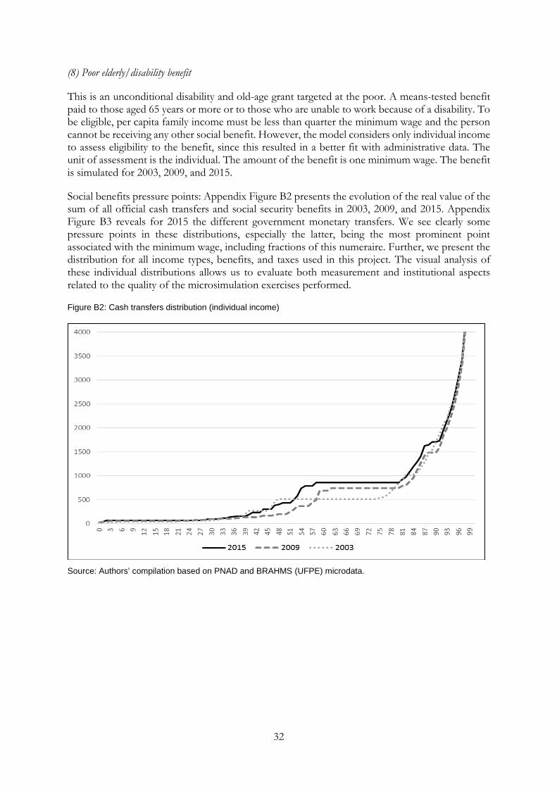
32

(8) Poor elderly/disability benefit

This is an unconditional disability and old-age grant targeted at the poor. A means-tested benefit paid to those aged 65 years or more or to those who are unable to work because of a disability. To be eligible, per capita family income must be less than quarter the minimum wage and the person cannot be receiving any other social benefit. However, the model considers only individual income to assess eligibility to the benefit, since this resulted in a better fit with administrative data. The unit of assessment is the individual. The amount of the benefit is one minimum wage. The benefit is simulated for 2003, 2009, and 2015.

Social benefits pressure points: Appendix Figure B2 presents the evolution of the real value of the sum of all official cash transfers and social security benefits in 2003, 2009, and 2015. Appendix Figure B3 reveals for 2015 the different government monetary transfers. We see clearly some pressure points in these distributions, especially the latter, being the most prominent point associated with the minimum wage, including fractions of this numeraire. Further, we present the distribution for all income types, benefits, and taxes used in this project. The visual analysis of these individual distributions allows us to evaluate both measurement and institutional aspects related to the quality of the microsimulation exercises performed.

Figure B2: Cash transfers distribution (individual income)


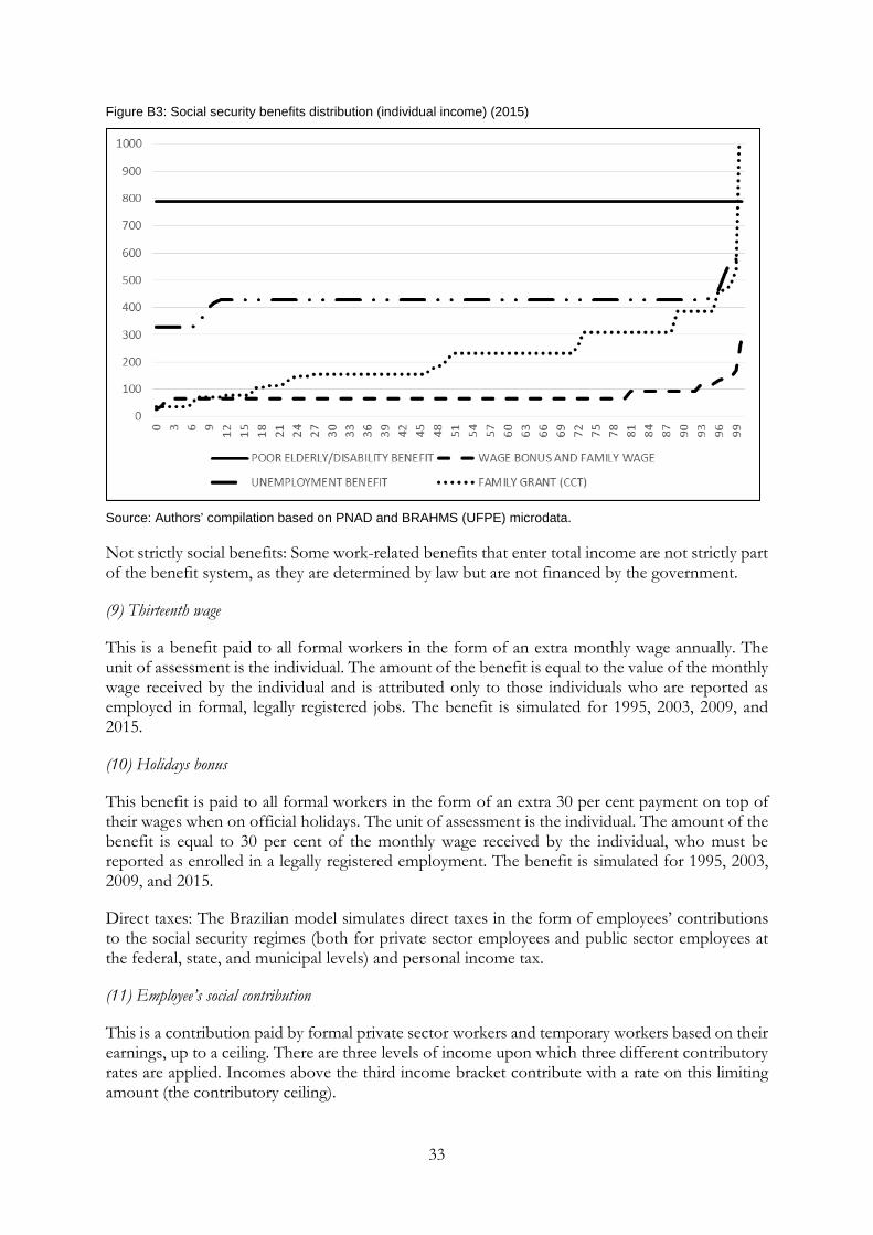
33

Figure B3: Social security benefits distribution (individual income) (2015)


Not strictly social benefits: Some work-related benefits that enter total income are not strictly part of the benefit system, as they are determined by law but are not financed by the government.

(9) Thirteenth wage

This is a benefit paid to all formal workers in the form of an extra monthly wage annually. The unit of assessment is the individual. The amount of the benefit is equal to the value of the monthly wage received by the individual and is attributed only to those individuals who are reported as employed in formal, legally registered jobs. The benefit is simulated for 1995, 2003, 2009, and 2015.

(10) Holidays bonus

This benefit is paid to all formal workers in the form of an extra 30 per cent payment on top of their wages when on official holidays. The unit of assessment is the individual. The amount of the benefit is equal to 30 per cent of the monthly wage received by the individual, who must be reported as enrolled in a legally registered employment. The benefit is simulated for 1995, 2003, 2009, and 2015.

Direct taxes: The Brazilian model simulates direct taxes in the form of employees’ contributions to the social security regimes (both for private sector employees and public sector employees at the federal, state, and municipal levels) and personal income tax.

(11) Employee’s social contribution

This is a contribution paid by formal private sector workers and temporary workers based on their earnings, up to a ceiling. There are three levels of income upon which three different contributory rates are applied. Incomes above the third income bracket contribute with a rate on this limiting amount (the contributory ceiling).

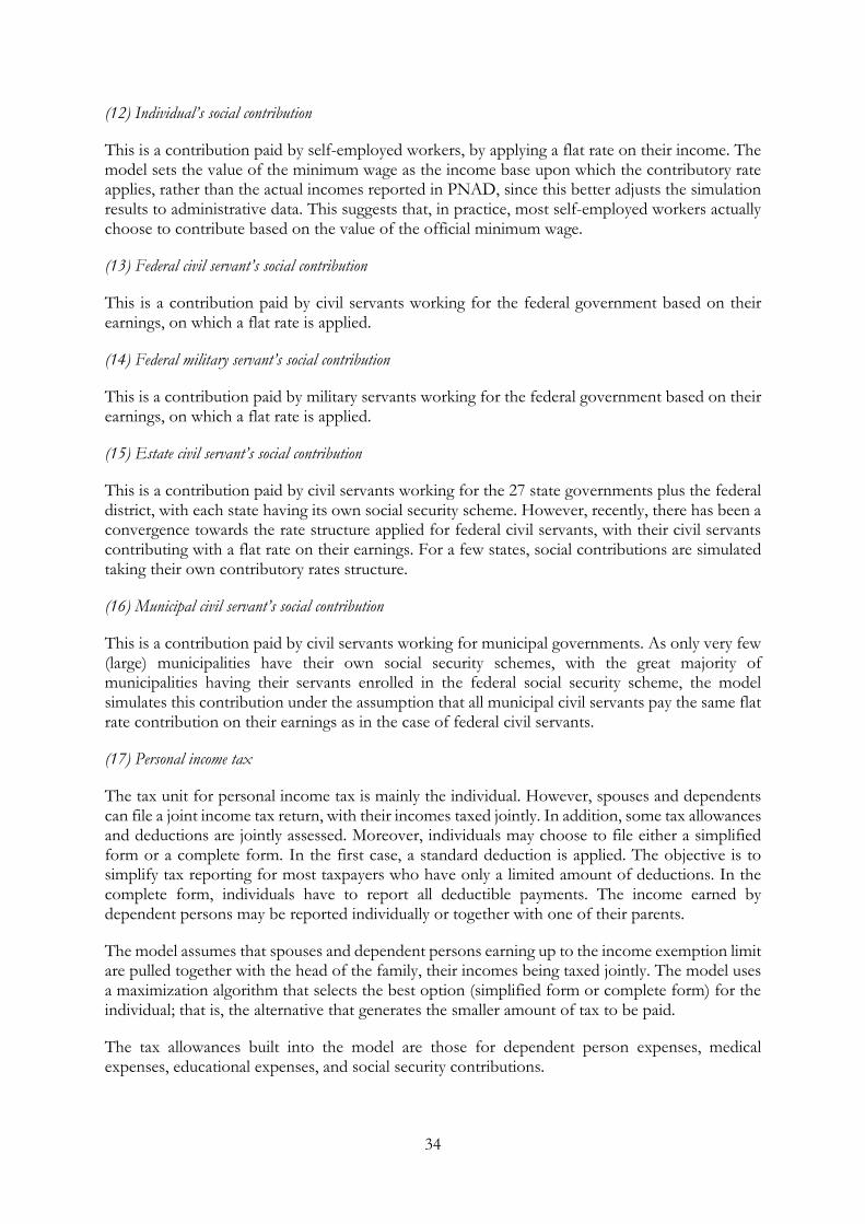
34

(12) Individual’s social contribution

This is a contribution paid by self-employed workers, by applying a flat rate on their income. The model sets the value of the minimum wage as the income base upon which the contributory rate applies, rather than the actual incomes reported in PNAD, since this better adjusts the simulation results to administrative data. This suggests that, in practice, most self-employed workers actually choose to contribute based on the value of the official minimum wage.

(13) Federal civil servant’s social contribution

This is a contribution paid by civil servants working for the federal government based on their earnings, on which a flat rate is applied.

(14) Federal military servant’s social contribution

This is a contribution paid by military servants working for the federal government based on their earnings, on which a flat rate is applied.

(15) Estate civil servant’s social contribution

This is a contribution paid by civil servants working for the 27 state governments plus the federal district, with each state having its own social security scheme. However, recently, there has been a convergence towards the rate structure applied for federal civil servants, with their civil servants contributing with a flat rate on their earnings. For a few states, social contributions are simulated taking their own contributory rates structure.

(16) Municipal civil servant’s social contribution

This is a contribution paid by civil servants working for municipal governments. As only very few (large) municipalities have their own social security schemes, with the great majority of municipalities having their servants enrolled in the federal social security scheme, the model simulates this contribution under the assumption that all municipal civil servants pay the same flat rate contribution on their earnings as in the case of federal civil servants.

(17) Personal income tax

The tax unit for personal income tax is mainly the individual. However, spouses and dependents can file a joint income tax return, with their incomes taxed jointly. In addition, some tax allowances and deductions are jointly assessed. Moreover, individuals may choose to file either a simplified form or a complete form. In the first case, a standard deduction is applied. The objective is to simplify tax reporting for most taxpayers who have only a limited amount of deductions. In the complete form, individuals have to report all deductible payments. The income earned by dependent persons may be reported individually or together with one of their parents.

The model assumes that spouses and dependent persons earning up to the income exemption limit are pulled together with the head of the family, their incomes being taxed jointly. The model uses a maximization algorithm that selects the best option (simplified form or complete form) for the individual; that is, the alternative that generates the smaller amount of tax to be paid.

The tax allowances built into the model are those for dependent person expenses, medical expenses, educational expenses, and social security contributions.

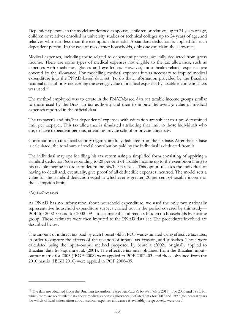
35

Dependent persons in the model are defined as spouses, children or relatives up to 21 years of age, children or relatives enrolled in university studies or technical colleges up to 24 years of age, and relatives who earn less than the exemption threshold. A standard deduction is applied for each dependent person. In the case of two-earner households, only one can claim the allowance.

Medical expenses, including those related to dependent persons, are fully deducted from gross income. There are some types of medical expenses not eligible to the tax allowance, such as expenses with medicines, glasses and eye lenses. However, most health-related expenses are covered by the allowance. For modelling medical expenses it was necessary to impute medical expenditure into the PNAD-based data set. To do that, information provided by the Brazilian national tax authority concerning the average value of medical expenses by taxable income brackets was used.13

The method employed was to create in the PNAD-based data set taxable income groups similar to those used by the Brazilian tax authority and then to impute the average value of medical expenses reported in the official data.

The taxpayer’s and his/her dependents’ expenses with education are subject to a pre-determined limit per taxpayer. This tax allowance is simulated attributing that limit to those individuals who are, or have dependent persons, attending private school or private university.

Contributions to the social security regimes are fully deducted from the tax base. After the tax base is calculated, the total sum of social contribution paid by the individual is deducted from it.

The individual may opt for filing his tax return using a simplified form consisting of applying a standard deduction (corresponding to 20 per cent of taxable income up to the exemption limit) to his taxable income in order to determine his/her tax base. This option releases the individual of having to detail and, eventually, give proof of all deductible expenses incurred. The model sets a value for the standard deduction equal to whichever is greater, 20 per cent of taxable income or the exemption limit.

(18) Indirect taxes

As PNAD has no information about household expenditure, we used the only two nationally representative household expenditure surveys carried out in the period covered by this study—POF for 2002–03 and for 2008–09—to estimate the indirect tax burden on households by income group. Those estimates were then imputed to the PNAD data set. The procedures involved are described below.

The amount of indirect tax paid by each household in POF was estimated using effective tax rates, in order to capture the effects of the taxation of inputs, tax evasion, and subsidies. These were calculated using the input–output method proposed by Scutella (2002), originally applied to Brazilian data by Siqueira et al. (2001). The effective tax rates obtained from the Brazilian input–output matrix for 2005 (IBGE 2008) were applied to POF 2002–03, and those obtained from the 2010 matrix (IBGE 2016) were applied to POF 2008–09.

13 The data are obtained from the Brazilian tax authority (see Secretaria da Receita Federal 2017). For 2003 and 1995, for which there are no detailed data about medical expenses allowance, deflated data for 2007 and 1999 (the nearest years for which official information about medical expenses allowance is available), respectively, were used.

36

The next step is to calculate the indirect tax burden faced by each household, defined by the amount of indirect taxes paid as a proportion of income. The total household income in POF was the income type more similar to the incomes reported in PNAD.14 However, for households for which income was lower than expenditure, the tax burden was estimated as a proportion of expenditure. This is to avoid the problem of overestimation of the tax burden in the lower end of the income distribution, which occurs because the incomes of the poorest households are strongly underreported in POF.15

Finally, the average indirect tax burden for 20 income groups was calculated from POF-based data, and then imputed in the PNAD-based data. Thus, an additional assumption adopted in estimating the indirect tax burden in this study is that its level and distribution did not change significantly in the time period between POF 2008–09 and PNAD 2015 (Appendix Figure B4).

Figure B4: Individual distributions of cash transfers, taxes, and income types

14 Income reported in PNAD is essentially monetary, whereas income reported in POF includes non-monetary components (especially the value of imputed rent for those owner-occupied households. To make PNAD and POF incomes compatible, imputed rent (which is not included in the PNAD income) was deducted from household income in the POF-based data set. 15 Indeed, for some households in the poorest fifth of the population, the tax burden would be above 100 percentage if estimated with respect to the income reported in POF. It should be highlighted that, on average, 52 per cent of the expenditure of households in the poorest quintile is allocated to food and rent (17 and 6 per cent, respectively), which are the expenditure categories with the lowest effective tax rates.

POOR ELDERLY/DISABILITY BENEFIT WAGE BONUS AND FAMILY WAGE

UNEMPLOYMENT BENEFIT FAMILY GRANT (CCT)

0

100

200

300

400

500

600

700

800

900

1000

0 4 8 12 16 20 24 28 32 36 40 44 48 52 56 60 64 68 72 76 80 84 88 92 96 100

2015 2009 2003

0

20

40

60

80

100

120

140

160

180

200

0 4 8 12 16 20 24 28 32 36 40 44 48 52 56 60 64 68 72 76 80 84 88 92 96 100

2015 2009 2003 1995

0

100

200

300

400

500

600

700

800

900

1000

0 4 8 12 16 20 24 28 32 36 40 44 48 52 56 60 64 68 72 76 80 84 88 92 96 100

2015 2009 2003 1995

0

50

100

150

200

250

300

350

400

450

500

0 4 8 12 16 20 24 28 32 36 40 44 48 52 56 60 64 68 72 76 80 84 88 92 96 100

2015 2009 2003

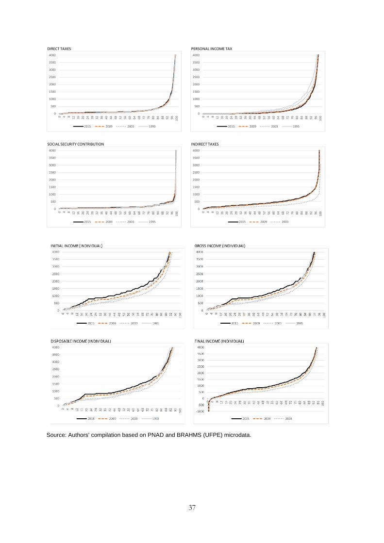
37


DIRECT TAXES PERSONAL INCOME TAX

SOCIAL SECURITY CONTRIBUTION INDIRECT TAXES

0

500

1000

1500

2000

2500

3000

3500

40000 4 8 12 16 20 24 28 32 36 40 44 48 52 56 60 64 68 72 76 80 84 88 92 96 100

2015 2009 2003 1995

0

500

1000

1500

2000

2500

3000

3500

4000

0 4 8 12 16 20 24 28 32 36 40 44 48 52 56 60 64 68 72 76 80 84 88 92 96 100

2015 2009 2003 1995

0

500

1000

1500

2000

2500

3000

3500

4000

0 4 8 12 16 20 24 28 32 36 40 44 48 52 56 60 64 68 72 76 80 84 88 92 96 100

2015 2009 2003 1995

0

500

1000

1500

2000

2500

3000

3500

4000

0 4 8 12 16 20 24 28 32 36 40 44 48 52 56 60 64 68 72 76 80 84 88 92 96 100

2015 2009 2003

wider working paper 2018/136 · for the years 1995, 2003, 2009, and 2015. pnad is a rural and urban...

Documents