trabalho_austrália
TRANSCRIPT

7/27/2019 Trabalho_Austrália
http://slidepdf.com/reader/full/trabalhoaustralia 1/174
South East Queensland ResidentialEnd Use Study: Final Report
Cara Beal and Rodney A. Stewart
November 2011
Urban Water Security Research AllianceTechnical Report No. 47

7/27/2019 Trabalho_Austrália
http://slidepdf.com/reader/full/trabalhoaustralia 2/174
Urban Water Security Research Alliance Technical Report ISSN 1836-5566 (Online)Urban Water Security Research Alliance Technical Report ISSN 1836-5558 (Print)
The Urban Water Security Research Alliance (UWSRA) is a $50 million partnership over five years between the
Queensland Government, CSIRO’s Water for a Healthy Country Flagship, Griffith University and The
University of Queensland. The Alliance has been formed to address South East Queensland's emerging urban
water issues with a focus on water security and recycling. The program will bring new research capacity to South
East Queensland tailored to tackling existing and anticipated future issues to inform the implementation of the
Water Strategy.
For more information about the:
UWSRA - visit http://www.urbanwateralliance.org.au/
Queensland Government - visit http://www.qld.gov.au/
Water for a Healthy Country Flagship - visit www.csiro.au/org/HealthyCountry.html
The University of Queensland - visit http://www.uq.edu.au/
Griffith University - visit http://www.griffith.edu.au/
Enquiries should be addressed to:
The Urban Water Security Research Alliance Project Leader – Rodney StewartPO Box 15087 Griffith School of Engineering and SWRCCITY EAST QLD 4002 Griffith University
GOLD COAST QLD 9726Ph: 07-3247 3005 Ph: 07-5552 8778Email: [email protected] Email: [email protected]
Authors: Griffith University, Griffith School of Engineering and Smart Water Research Centre
Beal, C.D. and Stewart, R.A. (2011). South East Queensland Residential End Use Study: Final Report . Urban
Water Security Research Alliance Technical Report No. 47.
Copyright
© 2011 GU. To the extent permitted by law, all rights are reserved and no part of this publication covered by
copyright may be reproduced or copied in any form or by any means except with the written permission of GU.
Disclaimer
The partners in the UWSRA advise that the information contained in this publication comprises general
statements based on scientific research and does not warrant or represent the accuracy, currency and
completeness of any information or material in this publication. The reader is advised and needs to be aware that
such information may be incomplete or unable to be used in any specific situation. No action shall be made inreliance on that information without seeking prior expert professional, scientific and technical advice. To the
extent permitted by law, UWSRA (including its Partner’s employees and consultants) excludes all liability to
any person for any consequences, including but not limited to all losses, damages, costs, expenses and any other
compensation, arising directly or indirectly from using this publication (in part or in whole) and any information
or material contained in it.
Cover Image:
Image depicts the mixed method approach used in the South East Queensland Residential End Use Study
© GU

7/27/2019 Trabalho_Austrália
http://slidepdf.com/reader/full/trabalhoaustralia 3/174
ACKNOWLEDGEMENTS
This research was undertaken as part of the South East Queensland Urban Water Security ResearchAlliance, a scientific collaboration between the Queensland Government, CSIRO, The University of Queensland and Griffith University.
The authors would like to acknowledge the efforts of Griffith University's eResearch Services Groupin the development of the Smart Meter Information Portal that was integral in the gathering,management and visualisation of the remote smart meter data used in this research.
Particular thanks also go to:
The Systematic Social Analysis Team (Dr Kelly Fielding, Dr Anneliese Spinks,Dr Aditi Mankad from CSIRO and Dr Sally Russell from Griffith University);
Gold Coast Water (formerly Allconnex Water);
Queensland Urban Utilities;
Unitywater;
Rachelle Willis (Western Power); and
Dr Andrew Huang, Lisa Stewart, Byron Carragher, Christopher Bennett, Erasmo Rey,James Maitland, Reza Talebpour, Timothy Bourke, Edoardo Bertone (Griffith University).
South East Queensland Residential End Use Study: Final Report Page i

7/27/2019 Trabalho_Austrália
http://slidepdf.com/reader/full/trabalhoaustralia 4/174
FOREWORD
Water is fundamental to our quality of life, to economic growth and to the environment. With its booming economy and growing population, Australia's South East Queensland (SEQ) region facesincreasing pressure on its water resources. These pressures are compounded by the impact of climate
variability and accelerating climate change.
The Urban Water Security Research Alliance, through targeted, multidisciplinary research initiatives,has been formed to address the region’s emerging urban water issues.
As the largest regionally focused urban water research program in Australia, the Alliance is focused onwater security and recycling, but will align research where appropriate with other water research
programs such as those of other SEQ water agencies, CSIRO’s Water for a Healthy Country NationalResearch Flagship, Water Quality Research Australia, eWater CRC and the Water ServicesAssociation of Australia (WSAA).
The Alliance is a partnership between the Queensland Government, CSIRO’s Water for a HealthyCountry National Research Flagship, The University of Queensland and Griffith University. It bringsnew research capacity to SEQ, tailored to tackling existing and anticipated future risks, assumptionsand uncertainties facing water supply strategy. It is a $50 million partnership over five years.
Alliance research is examining fundamental issues necessary to deliver the region's water needs,including:
ensuring the reliability and safety of recycled water systems. advising on infrastructure and technology for the recycling of wastewater and stormwater. building scientific knowledge into the management of health and safety risks in the water supply
system.
increasing community confidence in the future of water supply.
This report is part of a series summarising the output from the Urban Water Security ResearchAlliance. All reports and additional information about the Alliance can be found athttp://www.urbanwateralliance.org.au/about.html.
Chris Davis
Chair, Urban Water Security Research Alliance
South East Queensland Residential End Use Study: Final Report Page ii

7/27/2019 Trabalho_Austrália
http://slidepdf.com/reader/full/trabalhoaustralia 5/174
CONTENTS
Acknowledgements .................................................................................................................i
Foreword .................................................................................................................................ii
Executive Summary................................................................................................................1
1. Introduction ...................................................................................................................6
1.1. Introduction and Scope........................................................................................................6
1.2. Research Objectives............................................................................................................6
1.3. Method Overview.................................................................................................................7
1.4. Report Structure...................................................................................................................7
2. Background and Literature Review .............................................................................9
2.1. Introduction and Project Justification...................................................................................9
2.2. Overview of IUWM and End Use Studies............................................................................9
2.2.1. Introduction........................ ....................................................... ........................................ 9
2.2.2. End Use Studies to Inform Water Demand Managers.............. ........................................ 9
2.3. Water Conservation Management Strategies....................................................................10
2.3.1. Introduction........................ ....................................................... ...................................... 10
2.3.2. Water Use Efficient Technologies............................................. ...................................... 10
2.3.3. Socio-Demographic Influences of Water Use........................................................... ...... 11
2.3.4. Water-Energy Nexus Overview ......................................................... ............................. 12
2.4. Residential Water End Use Monitoring Approaches .........................................................12
2.4.1. Introduction........................ ....................................................... ...................................... 12
2.4.2. Typical End Use Approaches .............................................................. ........................... 12
2.4.3. Advanced End Use Measurement ........................................................... ....................... 13
2.5. Typical Residential End Uses............................................................................................13
2.6. Summary............................................................................................................................16
3. Research Method ........................................................................................................17
3.1. Sample Selection Process.................................................................................................17
3.2. Sampling Regime and Challenges to Sample Size...........................................................18
3.2.1. Winter and Summer Samples................. ................................................................ ........ 18
3.2.2. Impacts of the January 2011 Flooding................................................ ............................ 18
3.3. End Use Measurement Approach......................................................................................19
3.3.1. Instrumentation for Data Capture ....................................................... ............................ 20
3.3.2. Data Transfer and Storage ........................................................... .................................. 21
3.3.3. Data Analysis.............................................. ............................................................ ........ 21
3.3.4. Household Stock Audits and Water Diaries....................................................... ............. 22
4. Situational Context ......................................................................................................23
4.1. Characteristics of Study Areas ..........................................................................................23
4.1.1. General Description....................................................... ................................................. 23
4.1.2. Climate Data for SEQREUS Analysis Period.................................................................. 23
4.2. Characteristics of Participating Households......................................................................25
5. Descriptive Statist ics ..................................................................................................26
5.1. Calculation of Household and Per Capita Water End Uses ..............................................26
5.2. Distribution and Variability of Water Consumption End Uses ...........................................26
5.3. Winter 2010 End Use Event Statistics...............................................................................31
5.3.1. Introduction........................ ....................................................... ...................................... 31
5.3.2. End Use Event Frequencies................................................................ ........................... 31
5.3.3. End Use Event Mean Volumes............................ ........................................................... 32
5.3.4. Shower End Use Event Flow Rates.......................................... ...................................... 34
5.3.5. Shower End Use Event Durations ....................................................... ........................... 34
South East Queensland Residential End Use Study: Final Report Page iii

7/27/2019 Trabalho_Austrália
http://slidepdf.com/reader/full/trabalhoaustralia 6/174
6. End Use Results and Discussion ..............................................................................35
6.1. Winter 2010 Results...........................................................................................................35
6.1.1. Sample Size ....................................................... ............................................................ 35
6.1.2. Overall Water Consumption Trends ............................................................... ................ 35
6.1.3. Regional Water Consumption.................... ................................................................ ..... 38
6.2. Summer 2010-2011 Analysis.............................................................................................436.2.1. Sample Size ....................................................... ............................................................ 43
6.2.2. Water Consumption for Each Summer Sampling Period................................................ 45
6.2.3. Overall Water Consumption Trends .............................................................. ................. 47
6.2.4. Regional Water Consumption................... ................................................................ ...... 49
6.2.5. Summary of Summer 2010-11 Results........................ ................................................... 53
6.3. Winter 2011 Results...........................................................................................................53
6.3.1. Sample Size ....................................................... ............................................................ 53
6.3.2. Overall Water Consumption Trends ............................................................... ................ 53
6.3.3. ‘Rebounding’ Water Consumption? ................................................................ ................ 55
6.3.4. Regional Water Consumption.................... ................................................................ ..... 56
6.3.5. Summary of Winter 2011 End Use Results ............................................................... ..... 59
6.4. Summer 2011 Results .......................................................................................................596.4.1. Sample Size ....................................................... ............................................................ 59
6.4.2. Overall Water Consumption Trends ............................................................... ................ 60
6.4.3. Regional Water Consumption.................... ................................................................ ..... 61
6.5. Autumn 2012 Results.........................................................................................................64
6.5.1. Sample Size ....................................................... ............................................................ 64
6.5.2. Overall Water Consumption Trends ............................................................... ................ 64
6.5.3. Regional Water Consumption.................... ................................................................ ..... 66
6.6. Winter versus Summer SEQREUS Data...........................................................................69
7. Average and Peak Water Consumption Analys is .....................................................71
7.1. Introduction ........................................................................................................................71
7.2. Timeline Breakdown of Consumption Activity ...................................................................71
7.3. Diurnal Breakdown of Peak Demand.................................................................................71
7.3.1. Peaking Factors and End Use Analysis................................... ....................................... 73
7.3.2. Influence of Climate on Total Household Consumption.................................................. 74
7.4. Future Trends in Peak Demand.........................................................................................75
7.5. Conclusions .......................................................................................................................76
8. End Use Diurnal Pattern Analys is .............................................................................77
8.1. Introduction ........................................................................................................................77
8.2. Combined End Use Pattern Analysis.................................................................................77
8.3. Overall SEQ Pattern Analysis............................................................................................79
8.4. Average Peak Day Total Consumption..............................................................................81
8.5. Regional Pattern Analysis..................................................................................................82
8.5.1. Gold Coast.................................................. ........................................................... ......... 82
8.5.2. Brisbane ....................................................... .................................................................. 83
8.5.3. Ipswich ................................................... ........................................................... ............. 83
8.5.4. Sunshine Coast ...................................................... ........................................................ 84
8.5.5. Diurnal Relationships between End Uses................... .................................................... 85
9. SEQREUS End Use Comparisons with Other Studies .............................................87
9.1. Use of Winter 2010 for Detailed Analysis ..........................................................................87
9.2. End Use Data Comparisons ..............................................................................................87
10. Stock Effic iency Influence on Water Use..................................................................9010.1. Introduction ........................................................................................................................90
10.2. Clothes Washing Machines ...............................................................................................90
10.3. Shower Fixtures.................................................................................................................91
South East Queensland Residential End Use Study: Final Report Page iv

7/27/2019 Trabalho_Austrália
http://slidepdf.com/reader/full/trabalhoaustralia 7/174
South East Queensland Residential End Use Study: Final Report Page v
10.4. Taps...................................................................................................................................93
10.5. Dishwasher ........................................................................................................................94
10.6. Rainwater Tanks................................................................................................................95
11. Stock Effic iency Influence on Peak Demand ............................................................97
11.1. Introduction ........................................................................................................................97
11.2. Overview of Methods.........................................................................................................97
11.3. Conclusions .......................................................................................................................99
12. Socio-Demographic Influences on Water End Uses ..............................................101
12.1. Introduction ......................................................................................................................101
12.2. Household Income and Occupation.................................................................................101
12.3. Household Size and Composition....................................................................................103
12.4. Specific End Uses and Socio-Demographic Influences ..................................................105
12.4.1. Shower .................................................... ........................................................ ............. 105
12.4.2. Clothes Washer ........................................................ .................................................... 106
12.4.3. Tap and Toilet.............................................. ........................................................ ......... 107
13. Perceived Versus Actual Household Water Usage ................................................108
13.1. Introduction ......................................................................................................................108
13.2. Overview of Methods.......................................................................................................108
13.3. Results and Discussion ...................................................................................................108
13.3.1. Actual versus Perceived Household Water Consumption ............................................ 108
13.4. Socio-Demographic Trends.............................................................................................109
13.5. Household Water Appliance/Fixture and Perceived Water Use......................................110
13.6. Attitudes and Beliefs of Respondents..............................................................................111
13.7. Summary and Relevance of Findings..............................................................................112
14. Clustering Water Consumption Flow Rates............................................................113
14.1. Introduction ......................................................................................................................113
14.2. Overview of Methods used to Determining Qs ................................................................113
14.3. Results and Discussion ...................................................................................................113
15. Energy Demand from Water End Uses ....................................................................116
15.1. Introduction ......................................................................................................................116
15.2. Overview of Methods.......................................................................................................116
15.3. Calculating Energy Demand and Carbon Emissions.......................................................116
15.3.1. Determining Energy Consumption from End Use Data ................................................ 116
15.3.2. Determining Carbon Emissions from Water End Uses ................................................. 117
15.4. Optimising Water and Energy Efficient Strategies...........................................................118
15.5. Results and Discussion ...................................................................................................11915.5.1. Water and Energy Consumption for Residential End Uses .......................................... 119
15.5.2. Carbon Emissions from Energy-Related Water End Uses ........................................... 124
15.5.3. Energy Intensity Comparisons between End Use Appliances and Fixtures ................. 124
15.5.4. Impact of Intervention Scenarios on Water, Energy and Carbon Emissions ................ 125
15.6. Conclusions .....................................................................................................................129
16. Conclusions and Policy Considerations.................................................................130
Appendix A ..........................................................................................................................133
Copy of Household Stock Efficiency and Water Audit ............................................................... ............... 133
Appendix B ..........................................................................................................................138
Copy of Water Diary ......................................................... ........................................................................ 138
Appendix C..........................................................................................................................139
SEQREUS Winter 2010 End Use Frequency Distributions....................................................................... 139
References ..........................................................................................................................159

7/27/2019 Trabalho_Austrália
http://slidepdf.com/reader/full/trabalhoaustralia 8/174
LIST OF FIGURES
Figure 1: Average water end use consumption sourced from recent Australian studies. ............................... 15
Figure 2: Comparison of indoor water end uses from three Australian water end use studies. ...................... 16
Figure 3: Examples of unsuitable water meter boxes. ........................................................... ......................... 17
Figure 4: Example of poor condition of equipment following water inundation. .............................................. 18Figure 5: A before and after photograph of a Brisbane suburb impacted in January 2011 floods. ................. 19
Figure 6: Schematic flow of processes in the mixed method approach for the SEQREUS. ........................... 19
Figure 7: Measurement and data storage equipment. ......................................................... ........................... 20
Figure 8: Preparation and final installation of meter and loggers........................ ............................................ 20
Figure 9: Example of Trace Wizard® template.................................................... ........................................... 21
Figure 10: Example of information summary page for the household stock audit. ........................................... 22
Figure 11: Regions examined in SEQREUS. Inset: location of SEQ..................................................... ........... 23
Figure 12: Rainfall and maximum temperature during the three flow trace measurement periods. .................. 24
Figure 13: Frequency and cumulative distribution curves for clothes washer end use. .................................... 27
Figure 14: Frequency and cumulative distribution curves for toilet end use. .................................................... 27
Figure 15: Frequency and cumulative distribution curves for shower end use. ................................................ 28
Figure 16: Frequency and cumulative distribution curves for tap end use....... ................................................. 28
Figure 17: Frequency and cumulative distribution curves for dishwasher end use............................... ............ 29Figure 18: Frequency and cumulative distribution curves for bathtub end use................................................. 29
Figure 19: Frequency and cumulative distribution curves for leak end use. ..................................................... 30
Figure 20: Frequency and cumulative distribution curves for irrigation end use. .............................................. 30
Figure 21: Average daily per capita end use winter 2010 breakdown for all SEQ regions. .............................. 35
Figure 22: Comparison of all SEQ winter 2010 water use with SEQEUS total average. .................................. 36
Figure 23: Household per capita winter 2010 consumption (L/p/d) activity break down. .................................. 37
Figure 24: Distribution of water consumption for winter 2010 irrigation end uses........................... .................. 38
Figure 25: Breakdown of average winter 2010 end uses for each region.................. ....................................... 39
Figure 26: Average percentage of total consumption for each winter 2010 end use. ....................................... 39
Figure 27: Break down of average winter 2010 end uses for the Gold Coast................................................ ... 40
Figure 28: Break down of average winter 2010 end uses for Brisbane. ....................................................... .... 41
Figure 29: Break down of average winter 2010 end uses for Ipswich............................................................ ... 42Figure 30: Standard deviation for individual winter 2010 end uses across the regions: comparing
variance.......... ............................................................ ..................................................................... 42
Figure 31: Break down of average winter 2010 end uses for the Sunshine Coast. .......................................... 43
Figure 32: Cumulative and frequency probability trends for the summer end use period. ................................ 44
Figure 33: Break down of average end uses for summer read 1. ........................................................ ............. 45
Figure 34: Break down of average end uses for summer read 2................................................ ...................... 45
Figure 35: Break down of average end uses for summer read 3................................................. ..................... 46
Figure 36: Average end use consumption across the three summer reads........................................... ........... 46
Figure 37: Average daily per capita summer water end use breakdown for all SEQ regions. .......................... 47
Figure 38: Comparison of all SEQ summer 2010-11 water use with SEQREUS total average. ....................... 48
Figure 39: Household per capita summer consumption (L/p/d) activity break down............................. ............ 48
Figure 40: Distribution of water consumption for summer 2010-11 irrigation end uses. ................................... 49
Figure 41: Break down of average summer end uses for each region. ............................................................ 50
Figure 42: Average percentage of total summer water consumption for each end use. ................................... 50
Figure 43: Break down of average summer end uses for the Gold Coast. ....................................................... 51
Figure 44: Break down of average summer end uses for Brisbane.............................................................. .... 51
Figure 45: Break down of average summer end uses for Ipswich. ........................................................... ........ 52
Figure 46: Break down of average summer end uses for the Sunshine Coast................................................. 53
Figure 47: Average daily per capita water end use winter 2011 breakdown for all SEQ regions
analysed. ......................................................... ........................................................... ..................... 54
Figure 48: Household per capita winter 2011 consumption (L/p/d) activity break down. .................................. 54
Figure 49: Comparison of all SEQ winter 2011 water use with SEQREUS total average................................. 55
Figure 50: Breakdown of average winter 2011 end uses....................................... ........................................... 56
Figure 51: Average percentage of total winter 2011 water consumption. ......................................................... 56
Figure 52: Break down of average winter 2011 end uses for the Gold Coast................................................... 57Figure 53: Break down of average winter 2011 end uses for Brisbane. ................................................ ........... 58
Figure 54: Break down of average winter 2011 end uses for Ipswich..................................................... .......... 58
Figure 55: Break down of average winter 2011 end uses for the Sunshine Coast. .......................................... 59
South East Queensland Residential End Use Study: Final Report Page vi

7/27/2019 Trabalho_Austrália
http://slidepdf.com/reader/full/trabalhoaustralia 9/174
Figure 56: Average daily per capita water end use summer 2011 breakdown for all SEQ regions
analysed. ........................................................ ........................................................... ...................... 60
Figure 57: Household per capita summer 2011 consumption (L/p/d) activity break down..... ........................... 61
Figure 58: Breakdown of average summer 2011 end uses. .................................................... ......................... 61
Figure 59: Average percentage of total summer 2011 water consumption..................................................... .. 62
Figure 60: Break down of average summer 2011 end uses for the Gold Coast. .............................................. 62
Figure 61: Break down of average summer 2011 end uses for Brisbane......................................................... 63Figure 62: Break down of average summer 2011 end uses for Ipswich. .......................................................... 63
Figure 63: Break down of average summer 2011 end uses for the Sunshine Coast. ....................................... 64
Figure 64: Average daily per capita water end use autumn 2012 breakdown for all SEQ regions
analysed. ............................................................ ............................................................................. 65
Figure 65: Household per capita autumn 2012 consumption (L/p/d) activity break down........... ...................... 65
Figure 66: Breakdown of average autumn 2012 end uses. ........................................................ ...................... 66
Figure 67: Average percentage of total autumn 2012 water consumption........................................................ 66
Figure 68: Break down of average autumn 2012 end uses for the Gold Coast. ............................................... 67
Figure 69: Break down of average autumn 2012 end uses for Brisbane. ......................................................... 67
Figure 70: Break down of average autumn 2012 end uses for Ipswich. ........................................................... 68
Figure 71: Break down of average autumn 2012 end uses for the Sunshine Coast. ........................................ 68
Figure 72: Break down of average winter and summer end uses for SEQ combined....................................... 69Figure 73: Break down of average winter and summer end uses for each region. ........................................... 70
Figure 74: Timeline for total water consumption showing (i) water use breakdown in L/p/d and (ii)
average daily diurnal water use (L/p/h/d) for the selected peak demand days of (a) 30/12/10,
(b) 07/01/11, (c) 10/04/11, and (d) 02/07/11 and (e) baseline data for winter 2010, (f)
summer 2010-11, (g) winter 2011. .......................................................... ........................................ 72
Figure 75: Breakdown of (a) average daily total water consumption (LHS) and PD:AD ratio (RHS) and
(b) frequency distributions for combined SEQ sample peaking factors. .......................................... 73
Figure 76: Relative proportion of average hourly end-use PHPD/PHAD ratios for morning and afternoon
peak hours..................................................... ........................................................... ....................... 74
Figure 77: Timeline of average monthly climate data and daily household water consumption. ...................... 75
Figure 78: Average winter 2010 daily diurnal pattern analysis for combined SEQ sample... ............................ 77
Figure 79: Average summer 2010-11 daily diurnal pattern analysis for combined SEQ sample. ..................... 78
Figure 80: Average winter 2011 daily diurnal pattern analysis for combined SEQ sample... ............................ 79
Figure 81: Cumulative average daily diurnal pattern analysis – SEQ sample (all regions)................ ............... 80
Figure 82: Average daily diurnal peak water use – Average for all regions, winter 2010.................................. 81
Figure 83: Average daily diurnal pattern analysis - Gold Coast sample. .......................................................... 82
Figure 84: Average daily diurnal pattern analysis - Brisbane Region. .............................................................. 83
Figure 85: Average daily diurnal pattern analysis - Ipswich Region..................................................... ............. 84
Figure 86: Average daily diurnal pattern analysis - Sunshine Coast Region. ................................................... 85
Figure 87: Average diurnal relationship between end uses. ................................................... .......................... 86
Figure 88: Comparison of average end uses for Willis PhD study of Gold Coast homes. ................................ 87
Figure 89: Comparison of average end use consumption between SEQREUS data and other end use
studies. .................................................... ........................................................ ................................ 88
Figure 90: Daily household clothes washer efficiency cluster comparisons. .................................................... 91
Figure 91: Daily household shower fixture efficiency cluster comparisons. ...................................................... 92Figure 92: Daily household tap fixture efficiency cluster comparisons................................................. ............. 93
Figure 93: Daily household dish washer efficiency cluster comparisons. ...................................................... ... 95
Figure 94: Comparisons between homes with and without a RWT. .............................................................. ... 95
Figure 95: Irrigation consumption for households with and without a RWT. ..................................................... 96
Figure 96: Averaged SEQ Irrigation consumption for households with and without a RWT. ............................ 96
Figure 97: Household efficiency frequency and cumulative distributions............................................ .............. 97
Figure 98: Average day diurnal demand pattern comparison for household clusters of greater than or
equal to and less than a three star rating. ................................................................ ....................... 98
Figure 99: Average day diurnal pattern comparison of 50 least and 50 most efficient households. ................. 99
Figure 100: Relationship between water use and various socio-demographic factors. .................................... 101
Figure 101: Relationship between income category and household consumption. .......................................... 102
Figure 102: Relationship between employment status and household consumption. ...................................... 103
Figure 103: Water consumption efficiency on per capita and per household basis. ......................................... 104
Figure 104: Per capita water consumption for different household compositions. ............................................ 104
Figure 105: Per household consumption for different household compositions......................................... ....... 105
Figure 106: Relationship between shower consumption and socio-demographic factors................................. 106
South East Queensland Residential End Use Study: Final Report Page vii

7/27/2019 Trabalho_Austrália
http://slidepdf.com/reader/full/trabalhoaustralia 10/174
South East Queensland Residential End Use Study: Final Report Page viii
Figure 107: Relationship between clothes washer consumption and household composition.......................... 106
Figure 108: Relationship between tap consumption and household composition. ........................................... 107
Figure 109: Relationship between tap consumption and household composition. ........................................... 107
Figure 110: Comparisons of (a) per capita and (b) per household actual daily water use across self-
reported water use groups........................................ ........................................................... .......... 109
Figure 111: Characteristics of water efficient household stock. ............................................................ ............ 111
Figure 112: Average water consumption and cumulative water consumption (L/hh/d)..................................... 115Figure 113: Average proportion and cumulative proportion of total water consumption (%)............................. 115
Figure 114: Average proportion of total water consumption (%)......................................... .............................. 115
Figure 115: Average annual end use breakdown for water consumption (kL/p/y). ........................................... 119
Figure 116: Average annual end use breakdown for water consumption (kL/p/y). ........................................... 121
Figure 117: Average energy consumption and carbon emissions from clothes washing machines. ................ 123
Figure 118: Average energy intensities for water-related energy in SEQREUS homes. .................................. 125
Figure 119: Cumulative impact of various water-efficient intervention scenarios on annual household
water consumption. .................................................... ................................................................... 125
Figure 120: Cumulative impact of various water-efficient intervention scenarios on annual household
energy consumption. .................................................. ................................................................... 127
Figure 121: Cumulative carbon emission savings by replacing an existing EC HWS with a SEB HWS +
efficient stock...................... ........................................................... ................................................ 127
LIST OF TABLES
Table 1: Summary of the Home WaterWise Rebate Scheme July 2006-December 20081........................... 11
Table 2: Summary of reported water end use studies. .......................................................... ........................ 14
Table 3: Criteria for sample selection of SEQREUS households. ................................................... .............. 17
Table 4: Sample size details for the three winter and summer end use reads. ............................................. 18
Table 5: Statistics for household stock audit and water dairy responses. ..................................................... 22
Table 6: Climate data for four regions during the specific periods of flow trace analysis1............................. 23
Table 7: General characteristics of monitored households in SEQREUS. .................................................... 25
Table 8: Descriptive statistics for SEQREUS Winter 2010 data. ................................................... ................ 26
Table 9: Gold Coast Winter End Use Event Frequency Statistics. .......................................................... ...... 31
Table 10: Brisbane Winter End Use Event Frequency Statistics ...................................................... ............... 31
Table 11: Ipswich Winter End Use Event Frequency Statistics ......................................................... .............. 32
Table 12: Sunshine Coast Winter End Use Event Frequency Statistics.......................................................... 32
Table 13: Gold Coast Winter Mean Volume of End Use Event Statistics. ....................................................... 32
Table 14: Brisbane Winter Mean Volume of End Use Event Statistics........ .................................................... 33
Table 15: Ipswich Winter Mean Volume of End Use Event Statistics. ............................................................. 33
Table 16: Sunshine Coast Winter Mean Volume of End Use Event Statistics.................................... ............. 33
Table 17: Winter Shower End Use Event Flow Rate Statistics.......................... .............................................. 34
Table 18: Winter Shower Event Duration Statistics. ..................................................... ................................... 34
Table 19: Comparison of average total water use (L/p/d) for dwellings in SEQ. ............................................. 40
Table 20: General characteristics of monitored households in SEQREUS. .................................................... 60
Table 21: Clothes washer efficiency comparisons................................................. .......................................... 90
Table 22: Showerhead efficiency cluster comparisons............................................... ..................................... 92Table 23: Tap efficiency cluster comparisons. ....................................................... ......................................... 93
Table 24: Dishwasher efficiency cluster comparisons. .......................................................... .......................... 94
Table 25: Household efficiency rating clusters – descriptive statistics. ........................................................... 98
Table 26: Characteristics of self-reporting groups. ............................................................ ............................ 110
Table 27: Comparison of high, medium, and low water user groups on psycho-social questions. ................ 111
Table 28: SEQ average water usage and cumulative proportion of consumption (n = 213).......................... 114
Table 29: Summary of calculations used to determine the specific energy consumption from water use
appliances and fixtures................. ............................................................ ..................................... 117
Table 30: Number of washing machines for each HWS, water connection and wash cycle category. .......... 117
Table 31: Energy intensity values and GHG emission conversion factors used for calculating GHG
emission savings for hot water systems. ............................................................ ........................... 118
Table 32: Intervention scenarios using water and energy efficient technology.............................................. 118
Table 33: Key assumptions for each intervention scenario shown in Table 31. ............................................ 119
Table 34: Descriptive statistics for energy consumption and carbon emissions from energy-related
residential water end uses in average household................................ .......................................... 122
Table 35: Individual savings from various water and energy efficient scenarios. .......................................... 128

7/27/2019 Trabalho_Austrália
http://slidepdf.com/reader/full/trabalhoaustralia 11/174
EXECUTIVE SUMMARY
Water end use analysis using high resolution smart meters and loggers is becoming increasingly popular to measure and assess the residential water consumption in urban areas of Australia. Previousend use studies in Australia have demonstrated that per capita and per household water consumption
can vary considerably as a result of a number of factors, including socio-demographics, climate andhousehold water appliance stock efficiency.
The primary aim of this study was to quantify and characterise mains water end uses in a sample of 252 residential dwellings located within South East Queensland (SEQ). This report presents themethodology, results and discussion on the end use analysis for three monitoring periods over winter 2010, summer 2010-11 and winter 2011. This report forms part of the Reducing Water Grid Demandresearch theme for the Urban Water Security Research Alliance.
METHODOLOGY
A mixed method approach was used, combining high resolution water meters, remote data transfer
loggers, household water appliance audits and a self-reported household water use diary. A sub-sample for the SEQ Residential End Use Study (SEQREUS) project was generated from the larger Demand Management study which involved the completion of a questionnaire by over 1,500 homesacross SEQ. From this sampling pool, a smaller sub-sample of homes in each study region consentedto participate in the SEQREUS project.
A representative sample of received data was extracted from the database and disaggregated into allend use events associated with the sampled residential households. A water fixture/appliance stock survey on the study sample was conducted in order to qualify how householders interact with suchstock. In addition to the stock survey, each household was asked to complete a water diary where asmany internal and external water use events as possible were recorded over a seven-day period. TraceWizard® software was used in conjunction with water audits and water diaries to analyse anddisaggregate consumption into the following end use event categories: toilets, taps, leaks, irrigation,shower, clothes washer, bathtub and dishwasher.
Three separate water end use analysis periods occurred during the SEQREUS. The first read wasconducted in winter 2010 from 14th June to the 28th June. The second read was taken in the summer 2010-11 between 1st December 2010 and 21st February 2011. To capture the range of water consumption activities and fluctuations over the Christmas and school holiday period, three separatetwo-week reads were conducted with the average end use consumption from the three taken as thesummer reading. The final two-week period of analysis occurred in winter 2011 from the 1
stJune to
the 15th
June.
The sample sizes for each monitoring period were n=252, n=219 and n=110 for winter 2010, summer 2010-11 and winter 2011, respectively.
RESULTS
Winter 2010 Analysis
A total of 252 homes were analysed for mains water end uses. This comprised 87 in the Gold Coast,61 in Brisbane, 67 in the Sunshine Coast and 37 in Ipswich. The SEQ sample average total water consumption of 370.7 litres per household per day (L/hh/d) was recorded during the period of analysis(i.e. winter 2010). This represented a per capita average of 145.3 litres per person per day (L/p/d). Thiswas only slightly below the Queensland Water Commission (QWC) reported figure of 154 L/p/ddetermined from bulk meter data.
The water end use breakdown on a per capita basis indicated that, on average, shower 42.7 L/p/d
(29%), tap 27.5 L/p/d (19%) and clothes washer 31 L/p/d (21%) comprised the bulk of the water consumption. Almost 70% (approximately 100 L/p/d) of total consumption was attributed to thesethree activities. Of note, irrigation made up less than 5% of average total consumption.
South East Queensland Residential End Use Study: Final Report Page 1
7/27/2019 Trabalho_Austrália
http://slidepdf.com/reader/full/trabalhoaustralia 12/174
Properties located in the Sunshine Coast consumed the most water per capita (171 L/p/d) and per home (472 L/hh/d). Householders in Ipswich were clearly the most conservative water consumers,using an average of 111 L/p/d (305 L/hh/d). Brisbane and Gold Coast had similar average per capitaand household total water usage recorded at 144 and 141 L/p/d and 331 and 348 L/hh/d, respectively.The end uses which varied markedly between regions were showers, leaks, and irrigation.
Summer 2010-11 Analysis
The extremely wet summer conditions in SEQ, the sixth wettest on record, strongly influenced the pattern and volume of water consumption over the summer reads. An average total water consumptionof 311.3 L/hh/d was recorded during the combined periods of analysis. This represented a per capitaaverage of 125.3 L/p/d.
The main contributors to this total were again shower at 36.2 L/p/d (or 29%), tap at 27.4 L/p/d (or 22%), clothes washer at 26.5 L/p/d (or 21%) and toilet use at 23 L/p/d (or 18.4%).
Irrigation, which is typically elevated for summer, was only 4.8 L/p/d, representing less than 4% of theaverage total water consumption. Irrigation was generally not required in the region during the 2010-11 summer months due to lower than average temperatures and the very high rainfall experienced in
late spring and most of summer.
Winter 2011 Analysis
An average total water consumption of 415.6 L/hh/d was recorded during the winter 2011 period of analysis. This represented a per capita average of 144.9 L/p/d.
The average total water consumption of 144.9 L/p/d compares well with the QWC reported per capitawater use of 148 L/p/d for the same period. Both the SEQREUS and QWC-based water use averagesfell well below the Permanent Water Conservation Measures (PWCM) target of 200 L/p/d.
The absence, or slow return of a ‘rebound’ effect, i.e. the return to pre-restrictions water consumption,may be driven by a number of factors both at a technical and social level. It is hypothesised that the
introduction of new legislation, water restrictions, effective Target 140 campaigning, monetaryassistance for retrofitting water efficient technology and a prolonged threat to the water supply, haveresulted in a prolonged, if not potentially permanent, change in the behaviour of SEQ residents towardwater consumption. Outdoor consumption reduced significantly during the regions’ drought period
prior to the SEQREUS study and has not yet substantially risen from such low levels. This can beconfirmed with more longitudinal data covering summer seasons having more typical temperature andrainfall patterns.
Peak Day Demand Analysis
The Peak Day (PD) to Average Day (AD) ratio (PD/AD) ranged from 1.22 (Ipswich, May 2010) to 1.7(Brisbane, July 2011). PD/AD factors between 1.2 and 1.4 occurred at the greatest frequency.
PD to AD ratios between 1-1.5 were primarily driven by greater clothes washer and shower use.However, as the PD:AD ratio increased above 1.5, demand was driven largely by external water usage(i.e. lawn and garden irrigation). Peak hour ratios (i.e. PHPD:PHAD) ranged from 1.3 to 3.0 for thefour peak demand days. At the end-use level, the individual end-use category PHPD:PHAD ratioswere in the range of 0.7 – 3.3 for all end-uses, with the exception of external or irrigation. The ratio for this latter end-use category was typically very high, at over 10 times the average irrigation demand.
Comparisons with historically-based, but currently used, peaking factors used for network distributionmodelling suggests that the degree and frequency of high peaking factors are lower now, due to thehigh penetration of water-efficient technology and growing water conservation awareness byconsumers. This could translate into smaller diameter trunk mains in future infrastructure planning.
South East Queensland Residential End Use Study: Final Report Page 2

7/27/2019 Trabalho_Austrália
http://slidepdf.com/reader/full/trabalhoaustralia 13/174
Average Daily Diurnal Patterns
For each of the winter 2010, summer 2010-11 and winter 2011 read periods, there were twinconsumption peaks in the morning and afternoon water use events. Shower, clothes washer and tapscontributed the bulk of the water use activity at these peak times.
The morning peaks were typically higher than evening peaks for both the winter and summer reads,although the summer peak use was more prolonged or ‘flattened’, particularly in the afternoon.
Irrigation use appeared to occur throughout the day across both seasons, demonstrating a conflict withcurrent water restrictions and awareness messages that recommend outdoor watering in early morningand late afternoon.
As a result of the leak intervention programme after winter 2010, leaks have reduced significantly inall regions and were consistently low throughout the day, showing little diurnal variation.
End Use Comparisons with Other Studies
Results suggest that the data obtained from the winter 2010 and winter 2011 periods of analysis
compared well with other estimations of household water consumption.Due to the extreme rainfall and flooding that occurred in the summer 2010-11 recording period, thisdata is not considered overly representative of average water consumption values for the sub-tropicalSEQ climate and was therefore not used for comparisons with other studies or for detailed dataanalysis. Indoor end use values are comparable but irrigation, which is often much higher in summer,was much lower due to the prolonged rain and flooding.
Impacts of Household Stock Efficiency on Water Consumption
Clothes washing machines with a star rating ≥ 4 used significantly less (p<0.05) water than ≤ 2 star machines. This equated to a potential savings of 8.8 kL/hh (or 29%) per year.
Estimated annual savings from front loading washing machines equated to 10.6 kL/hh annually or
around 36%. The penetration of front loaders is likely to have increased sharply in the last three to fiveyears due to the rebates offered in Queensland to install water efficient (typically front loading)machines.
There was a significant reduction ( p<0.05) in shower water demand from high (AAA star) efficiencyheads compared to low (A star) or poor (standard/old) efficiency clusters.
Replacing the old style showerhead with any star rated shower head would significantly ( p<0.05)reduce water consumption by a minimum of 28 kL (or 75%) per year.
There were significant differences ( p<0.05) between all three tap efficiency clusters, and replacing anold style tap with a ≥ 3 star tap fitting can save 12.9 kL/hh or 65% annually.
Efficient dishwashers (e.g. 3.5+ star rating) used significantly less ( p<0.05) water at a mean of 4.4 L/hh/d, compared to the average 9.2 L/hh/d from the inefficient dishwasher cluster.
Obvious increases in per capita irrigation by homes without a rainwater tank (RWT) were apparent for Ipswich and the Sunshine Coast, although this tendency did not appear for the Gold Coast andBrisbane.
Notwithstanding the overall low irrigation consumption for all samples across all regions, the resultsgenerally demonstrate that there are some mains water savings to be made by the installation of non-internally plumbed RWT.
Highly efficient water appliances and fixtures not only contribute to reduced use of potable water supplies but also lower the average day peak hour demand from which water supply infrastructure isdesigned.
Water-efficient homes were found to have a reduced average peak hourly consumption of between2.47 L/p/h/d (19.29%) and 3.52 L/p/h/d (18.56%). Both of these water demand reductions werestatistically significant at p < 0.01.
South East Queensland Residential End Use Study: Final Report Page 3

7/27/2019 Trabalho_Austrália
http://slidepdf.com/reader/full/trabalhoaustralia 14/174
Impacts of Household Socio-Demographics on Water Consumption
Higher income households consumed more water on average per day than lower income homes. Theend uses that contributed most to the increased consumption were shower, clothes washer, dishwasher and bath.
There was a trend for households with small families, with an older average age of residents and nochildren to consume less water per household on average.
At an average total of 354 L/hh/d, households with either full and/or part-time residents consumedsignificantly more ( p>0.05) water than those homes with retired and/or pensioned residents(253 L/hh/d).
Typically, water consumption will be higher for large homes with large families as the demand for water is obviously greater and there are a higher number of water fixtures and appliances. However,larger families are typically more water efficient on a per capita basis than single person families.
In terms of perceived water use clusters, a clear pattern emerged from the results which showed thatself-reported high water users typically consumed less (130 L/p/d) than both the self-reported medium(156 L/p/d) and low (143 L/p/d) water users on a per capita basis.
Results indicate a trend that higher income, larger, younger and more educated households tend toinstall efficiency appliances which may not always be sufficient in reducing water consumption if curtailment actions are not present.
Clustering Water Consumption Flow Rates
The SEQREUS data was used to determine the volume of water passing through the meter at differentflow rate intervals in order to allow better modelling of meter accuracy and non-registration levels.
There were three main ‘clusters’ of flow rate range categories. The first 11 categories were between0 to ≤ 100 L/hr and contributed 10% of the total consumption. The end uses associated with such lowflows were mainly leaks, internal tap use, dishwasher, and some low-flow toilet, shower and clothes
washing events.The middle nine categories (100 ≤ 1,000 L/hr) contributed 80% of the total consumption. The end useswere typically shower, clothes washing, full flush toilet use, external tap use, and irrigation.
The last nine categories (1,000 < 1,800 L/hr) contributed 10% of the total consumption. The end usesassociated with high flow rates included shower, clothes washing, external tap use, irrigation anduncommon water usage (e.g. service break leaks).
Water-Energy-Greenhouse Gas Nexus
Preliminary analysis was undertaken to determine the energy requirements and resultant greenhousegas emissions from residential water use appliances and fixtures (e.g. shower, tap, clothes washer anddishwasher).
There were two major components to the methods: (1) determining water, energy and carbonemissions from measured water end uses; and (2) calculating the optimal combination of interventionsolutions (e.g. cost effective energy-efficient options) to reduce carbon emissions from water end uses.
The major energy end use was shower with 748 kilowatt hours per person per year (kWh/p/y) (or 61%of total energy consumption) and tap with 330 kWh/p/y (or 27%). Clothes washers comprised only 4%(54 kWh/p/y) of the total energy consumption, which was less than dishwashers at 7% or 82 kWh/p/y.
Results demonstrated that replacing an electric HWS with a solar HWS can achieve up to a 43%reduction in energy demand and carbon emissions. Low-flow shower heads can reduce total householdenergy consumption (via reducing hot water demand) by 19%.
Understanding the linkages between residential water and energy consumption can inform buildingcodes and improve the sustainability of future urban planning.
South East Queensland Residential End Use Study: Final Report Page 4

7/27/2019 Trabalho_Austrália
http://slidepdf.com/reader/full/trabalhoaustralia 15/174
South East Queensland Residential End Use Study: Final Report Page 5
WATER DEMAND MANAGEMENT KEY POINTS FORSTAKEHOLDERS
- There is still some degree of non-compliant irrigation between 10 am and 4 pm, particularly for homes in the Sunshine and Gold Coasts.
- Leaking toilets were more widespread than previously reported, however intervention programmes can be very effective at reducing these leaks as was shown in the summer andwinter 2011 monitoring. Rapid post-meter leakage management is one of the key benefits of smart metering systems.
- Water efficient fittings for showers and taps are an excellent least-cost water demandmanagement option for conserving water, confirming previous studies.
- Installing efficient taps, clothes washers and showers is a significant area for reducing averageday peak hour demand.
- Changing to efficient washing machines and low-flow shower heads significantly reduceshousehold consumption. Diurnal patterns indicate that, by encouraging a shift in clothes washer operation from morning to evening, like the existing habit for dishwashers, would substantiallyreduce the average morning peak demand.
-
Results consistently highlight the importance of sustained targeting of water consumption behaviour, particularly shower and tap use, as well as encouraging installation of water-efficientmeasures.
- Families with young children are high water consumers on a household basis and this is a targetarea for sustained water conservation management. Single person households, while having ahigh per capita consumption, typically do not contribute to the peak day demand periods.

7/27/2019 Trabalho_Austrália
http://slidepdf.com/reader/full/trabalhoaustralia 16/174
1. INTRODUCTION
1.1. Introduct ion and Scope
Water security is becoming one of Australia’s greatest issues of concern. Many regions of Australia
are facing a severe drought after years of continued lower than average rainfall. South EastQueensland (SEQ) has just come through one of its most severe and protracted droughts on record.For this reason, as well as the addition of high population growth and strong economic development,water and its use must be managed very carefully. In an attempt to improve water security, manygovernment authorities have imposed a number of water restrictions and water saving measures toensure the conscious use of water across the residential, commercial and industrial sectors. Moreover,due to greater social awareness, people are beginning to value water as a precious resource. Behaviour and attitudes toward both potable and recycled water have forever changed, thus requiring renewedunderstanding of the link between these factors and water end use.
The SEQ Residential End Use Study (SEQREUS) project provides residential water consumption enduse break downs at particular points in time. These data can feed into water demand models to forecast
supply requirements. Moreover, the analysis of end use data along with stock survey and questionnairedata reveals the predictors (i.e. household demographics, washing machine efficiency, etc.) of water demand for different end uses (i.e. shower, washing machine, etc.), thus enabling the government andwater businesses to target those end uses which can be reduced when required, through targetedcommunication strategies, rebate programs, etc. The report also explores average diurnal patterns of consumption, peak and average day demand ratios and the environmental implications of water useappliances in terms of energy demand and carbon emissions.
The research reported herein has the following scope:
Sampling region covers Gold Coast, Brisbane, Ipswich and Sunshine Coast local authority boundaries.
Measured end use data was collected for two consecutive week periods in winter 2010 (June
2010), summer 2010-11 (December 2010 to February 2011) and winter 2011 (June 2011). Residential end use data was measured on owner-occupied, single, detached dwellings (one
water meter present only) with no internally plumbed rainwater tanks.
1.2. Research Objectives
The primary aim of the study is to quantify and characterise mains water end uses in a sample of 250single detached dwellings across SEQ. Specific objectives for the study are:
to calculate both the household and per capita water consumption volumes of each participatinghousehold for the majority of water end use categories (e.g. shower, washing machine, tap, etc.)from households in the study regions;
to undertake a comparative analysis of water end uses between different household demographiccategories within the study regions;
to undertake a comparative analysis of water end uses of sampled households with previous enduse studies;
to develop average day diurnal pattern curves and explore peak hour flow rates and the end usesunderpinning them;
to assess the influence of household appliance/fixture efficiency on water end use consumption; to assess the influence of stock efficiency on peak demand; to identify any disparities between actual and perceived household water consumption;
to categorise the volume passed through the water meter for different flow rates; and
to explore the energy demand and greenhouse gas emissions from water end useappliances and fixtures.
South East Queensland Residential End Use Study: Final Report Page 6

7/27/2019 Trabalho_Austrália
http://slidepdf.com/reader/full/trabalhoaustralia 17/174
1.3. Method Overview
Households from four local authority boundaries located in the south-east corner of Queensland,Australia, took part in a water use survey (n = 1,750). Participants for the SEQREUS study (n = 252)were selected from the larger pool of survey participants who consented to be contacted to take part in
future research.A mixed method, advanced water end use measurement approach was followed in order to obtain andanalyse water use data. This incorporated physical measurement of water use via smart meters withsubsequent remote transfer of high resolution data and documentation of water use appliances and
behaviours. Responses from the household water use survey were used to investigate the psycho-socialvariables of water consumption.
Upon completion of recruitment, standard council residential water meters were replaced withmodified Actaris CTS-5 water meters. These ‘smart’ meters measure flow to a resolution of 72 pulses/litre or a pulse every 0.014 litre (L). The smart meters were connected to Aegis Data Cellseries R-CZ21002 data loggers. The loggers were programmed to record pulse counts at five secondintervals. Data was wirelessly transferred to a central computer and stored in a database for subsequent
analysis (Figure 1). A representative sample of received data was extracted from the database anddisaggregated into all end use events associated with the sampled residential households using theTrace Wizard® software (Aquacraft 2010).
Concomitantly with meter and logger installation, a water fixture/appliance stock survey wasconducted at each participating home in order to investigate how householders interact with suchstock. By completing the stock survey, the householder provided information on typical flow rates of taps and showers, the number and degree of water-efficient appliances and the typical water consumption behaviours of the householders. In addition to the stock survey, each household wasasked to complete a water diary where as many internal and external water use events as possible wererecorded over a seven-day period. This facilitated the disaggregation of trace flows from each homeand also provided a valuable snapshot of the daily water consumption habits within each home.
1.4. Report Structure
This report is compromises 16 chapters, each will be briefly summarised below:
Chapters 1 and 2 introduce the study and discuss the background and relevant literature pertaining to integrated urban water management, conservation management strategies andresidential water end use monitoring.
Chapter 3 provides details of the methods employed to measure, analysis and assess the data.This includes discussion of sample selection, sampling regime and challenges faced during thestudy which impacted on sample size. The qualitative components of the research methods arealso addressed; such as water diaries, household stock audits and the water use questionnairefrom the CSIRO Systematic Social Analysis project.
Chapter 4 provides a situational context to the study such as the location and generalcharacteristics and climate data of the study areas. This chapter also presents socio-demographicinformation on the participating households, such as average age, occupancy, income status andeducation level.
Chapter 5 provides the descriptive statistics for each study region including distribution andvariability of water end uses and winter 2010 end use event statistics (e.g. frequencies, meanvolumes, flow rates and event durations. This information can be used as input parameters for water demand forecasting models.
Chapter 6 presents all the water end use consumption results for each region and SEQ as anaverage for winter 2010, summer 2010-11 and winter 2011. A comparison of winter andsummer end use results is also discussed.
In Chapter 7, the timeline breakdown of consumption activity is presented along with ananalysis of peak water use and the end uses contributing to peak demand. This chapter provideda useful overview of peak day/average day factors which can be used as a guideline on the typeof range of peaking factors that could be expected from SEQ residential properties. A full
South East Queensland Residential End Use Study: Final Report Page 7

7/27/2019 Trabalho_Austrália
http://slidepdf.com/reader/full/trabalhoaustralia 18/174
South East Queensland Residential End Use Study: Final Report Page 8
description of this study will be available from the forthcoming article: Beal, C.D., and Stewart,R.A., (2012) Identifying residential water end uses underpinning peak day and hour demand. Journal of Water Resources Planning and Management (under review).
In Chapter 8, end use diurnal patterns are examined for each region and each sampling period.Peak daily usage and the contributing end uses are identified and discussed. Average peak day
total consumption is compared between sampling periods. A brief discussion on the diurnalrelationships between end uses is also presented.
Chapter 9 provides a comparative analysis of SEQREUS end use results with other end usestudies recently conducted in Queensland, Victoria, Western Australia and New Zealand. Thischapter also presents a discussion on the relatively homogeneity of indoor end uses bothtemporally and spatially.
In Chapter 10, the impacts of household stock efficiency on water use are examined. Astatistical analysis of the differences between total household consumption and clothes washingmachines, dish washers, showers and taps of varying water-efficiency (star ratings) is presented.
Chapter 11 examines the impacts of water-efficient stock on peak diurnal patterns anddemonstrates the significant reductions to peak hourly demand from household clusters with
high efficiency ratings. A full description of the study and outcomes is available from thearticle: Carragher, BJ., Stewart, RA. and Beal, CD., (2012) Quantifying the influence of residential water appliance efficiency on average day diurnal demand patterns at an end uselevel: A precursor to optimised water service infrastructure planning. Resource Conservation
and Recycling, 62, 81-90.
Chapter 12 presents a discussion on the socio-demographic influences on water end useconsumption. This chapter examines the impact of factors such as employment status,household income category, family size and composition on total water consumption. Theinfluence of specific socio-demographic factors such as the number of young children, number of teenagers and gender on water end uses such as shower and clothes washers are also
presented.
In Chapter 13, the perceived water use versus actual water use is discussed based on the
questionnaire section that asked participants to nominate whether they thought their householdwas a high, medium or low water user. A number of psycho-social factors are examined to see if they influenced the disparity between actual and perceived water use. A full description of thestudy and outcomes will be available from the forthcoming article: Beal, C.D., Stewart, R.A.and Fielding, K. (2011) A novel mixed method smart metering approach to reconcilingdifferences between perceived and actual residential end use water consumption, Journal of
Cleaner Production, doi:10.1016/j.jclepro.2011.09.007.
Clustering of water consumption flow rates is presented in Chapter 14. This chapter provides anoverview of methods and some results and discussion on the different flow rate categories (e.g.0 to < 100 litres per hour) that contribute to total consumption. Determining the starting or minimum registration level can allow for a better understanding of post-meter residential water
leakage and the non-registration of meters. Chapter 15 explores the energy demand from water end use appliances and fixtures, and
calculates the associated greenhouse gas emissions from their operation. An overview of themethods for these calculations is provided along with energy and water savings estimationsfrom intervention scenarios such as solar hot water system substation, low-flow shower headsand reduced water temperature. A full description of the study and outcomes is available fromthe article: Beal, C.D., Stewart, R.A. and Bertone, E. (2012) Evaluating the energy and carbonreductions resulting from resource-efficient household stock. Energy and Buildings,DOI 10.1016/j.enbuild.2012.08.004.
Finally, Chapter 16 provides a number of conclusions and policy considerations that haveevolved from the SEQREUS. This section highlights the key results from the report and
presents some suggestions that may be useful to inform future policy directions for demandmanagers and water distributors.
A full reference list is provided at the end of the report, along with some appendices to themethods section (Chapter 3) and descriptive statistics (Chapter 5).
7/27/2019 Trabalho_Austrália
http://slidepdf.com/reader/full/trabalhoaustralia 19/174
2. BACKGROUND AND LITERATURE REVIEW
2.1. Introduction and Project Justification
Over 750,000 new dwellings are forecast for SEQ to house the expected increase in population from
2.8 to 4.4 million people in 2032 (DIP 2009). The combination of enforced water restrictions and Stateand local government rebate programmes for water efficient fixtures and rainwater tanks have resultedin a large reduction in household water use in SEQ.
Despite the successful outcome for SEQ administering authorities, the demand management approachto reduce water consumption necessitated a ‘reactionary’ approach rather than a proactive approachand highlighted the need for more detailed information on how the water is proportioned inhouseholds and how this may change both spatially and temporally across SEQ. Thus, thedisaggregation of residential water end use should be considered as a critical first step in thedevelopment of relevant and successful water policy. More specifically, end use data can facilitate theidentification of correlations between water behaviours and key demographical subsets within a
population (e.g. income, age, gender and family composition). This information can inform
government and water business demand management policy, water rebate program effectiveness andhouseholders’ response to changed water policy. Measured end use data across seasons and regions isthe foundation for water consumption predictions and the development of demand forecasting/water distribution network models (e.g. Blokker et al., 2010). This study aims to address the research gap byway of generating a high resolution data registry of water end uses, and using such a database toexplore the relationships and influences of residential water consumption from a bottom up approach.
2.2. Overview of IUWM and End Use Studies
2.2.1. Introduction
Water security remains one of Australia’s greatest issues of concern as many urban and rural regionsare facing a severe drought after years of continued lower than average rainfall. In 2009, South EastQueensland (SEQ) emerged from one of its most harsh and protracted droughts on record. Thevariability of rainfall in the region, combined with high population growth and strong economicdevelopment, means that effective integrated water management is critical. This has involvedintegrated urban water management (IUWM) strategies from both the demand and supply
perspectives. In an attempt to improve water security, many government authorities in Australia haveimposed water restrictions and water saving measures to manage demand and ensure the conscious useof water across the residential, commercial and industrial sectors. Both in Australia andinternationally, recent research suggests that attitudes and behaviour toward potable water supplieshave changed due to greater social awareness and increasingly widespread exposure to droughtconditions; people are beginning to genuinely value water as a precious resource (Jones et al., 2011,Jorgensen et al., 2009). For example, the combination of state and local government rebate
programmes for water efficient fixtures and rainwater tanks and enforced water restrictions haveresulted in a large reduction in household water use in SEQ (Beal et al., 2011; Willis et al., 2010a;Queensland Water Commission [QWC], 2010a). Internationally, the success of demand managementstrategies such as pricing, restrictions and water conservation education have been shown to havevariable effects on changing the public perception on water consumption (Arbues et al., 2010;Olmstead and Stavins, 2009; Nieswiadomy, 1992).
2.2.2. End Use Studies to Inform Water Demand Managers
The shift in public perception towards water requires renewed understanding of the relationships between the end use and the end users of residential water. Furthermore, despite successful demandmanagement outcomes, approaches by many regulating authorities to reduce water consumption are
often reactionary rather than proactive (Farrelly and Brown, 2011; Kennedy, 2010; Rendwick andArchibald, 1998). Although there are many examples of proactive water demand managementapproaches emerging (e.g. Domènech and Saurí, 2011; Farelly and Brown, 2011; Inman and Jeffrey,2006), the often reactionary policies to reduce water demand in a time of potential supply crisis
South East Queensland Residential End Use Study: Final Report Page 9

7/27/2019 Trabalho_Austrália
http://slidepdf.com/reader/full/trabalhoaustralia 20/174
highlights the need for more detailed information at the “coalface”. For example, information on howthe water is proportioned in households and how this may change both spatially and temporally acrossany given region would provide good insight for demand managers about which local regions totarget. To this end, Chang et al. (2010) examined spatial variations of residential water consumption inOregon and conclude that such a dataset would greatly enhance the development of urban water
policies in regions of limited water resources. Blokker et al. (2010) suggest that measuring end usedata across seasons and regions is the foundation for water consumption predictions and thedevelopment of demand forecasting/water distribution network models. Similarly, Arbués et al. (2003)and White and Fane (2002) emphasise the need for such basic building blocks in the creation of effective demand side management policy. Empirical end use data is essential for validating water useforecasting models such as presented by Blokker et al. (2010), Chu et al. (2009) and Druckman et al.(2008). Thus, the disaggregation of residential water end use is a critical first step in the developmentof relevant and successful water policy. A number of end use studies have been conducted both inAustralia (e.g. Water Corporation, 2011; Beal et al., 2011; Willis et al., 2011a; Willis et al., 2010a;Roberts, 2005; Loh and Coghlan, 2003) and internationally (e.g. Heinrich, 2008; De Oreo et al.,1996).
2.3. Water Conservation Management Strategies
2.3.1. Introduction
There are two key demand side approaches to residential water conservation management that aretypically adopted by water managers: targeting behavioural change and promoting the use of water useefficient (WUE) technology (e.g. low-flow shower roses, WUE washing machines and dishwashers).The success of each method is variable as water consumption patterns and behaviours are highlyvaried amongst households due to the influencing factors of climate, socio-demographics, house size,family composition, water appliances, cultural and personal practices (Russell and Fielding, 2010;Juárez-Nájera et al., 2010; Arbués et al., 2003; Loh and Coghlan, 2003).
2.3.2. Water Use Efficient TechnologiesThe development of WUE devices such as low-flow shower roses, dual flush toilets and tap flowregulators has led to ongoing water savings within households (Willis et al., 2011b) Several studieshave been undertaken to determine the relative water savings attributed to the installation of engineering water conservation fixtures and appliances (Fidar, 2010; Millock and Nauges, 2010;Mayer et al., 2004). The replacement of high water consuming household appliances and fixtures withthose of engineered water efficiency has resulted in indoor water consumption savings up to 50%(Mayer et al., 2004). A variety of water-saving devices are available on today’s market which attemptto reduce water end use consumption. Such devices include AAA or 4+ star-rated shower roses, dualflush toilets (3/4.5 L/flush), water pressure limiting devices and tap aerators. With respect to showers,the trend of lower shower consumption volumes with more efficient devices has previously beenestablished by Willis et al. (2011b), Fidar et al. (2010) and Mayer et al. (2004). In Australia, the Water Efficient Labelling Scheme (WELS) has provided a framework for standardising the technical
performance of household appliances and fixtures (see website http://www.waterrating.gov.au/).
There is increasing popularity for local and state government authorities to offer rebates for retrofittingWUE technology (i.e. low-flow shower heads and tap aerators) into the home (Turner et al., 2007;England, 2009). In Queensland, programmes such as the Home and Garden WaterWise RebateScheme (HGWRS) and, more recently, ClimateSmart initiatives, have become commonplace. TheHGWRS precipitated a significant increase in the penetration of such technology into the home whereover 224,000 households in Queensland utilised the service during its operation (July 2006 toDecember 2008), resulting in an estimated water savings of around 14 ML/y (Walton and Holmes,2009). The relevant water efficient rebate data is presented in Table 1 which shows that the penetrationof water efficient clothes washers (41% of total) was substantially higher than dual flush toilets (7%)
and low-flow shower heads (6%). This is because the latter two devices have been available in themarket for some time now.
South East Queensland Residential End Use Study: Final Report Page 10

7/27/2019 Trabalho_Austrália
http://slidepdf.com/reader/full/trabalhoaustralia 21/174
Table 1: Summary of the Home WaterWise Rebate Scheme July 2006-December 20081.
Product RequiredStandard of
Product
Rebate Amoun t Number of ProductsRebated
Estimated Savingsper Device
(kL/appliance/year)
Total EstimatedSavings per
Product (ML/year)
Rainwater tank –external use*
Minimum3,000 L
Up to $1,000 for purchase and
installation
240,069 10 4,801
Rainwater tank –internallyplumbed laundry&/or toilet
Minimum3,000 L
Up to $1,500 17,025 70 1,191
Clothes washingmachine
≥4 star $200 234,846 20 4,696
Dual flush toilet ≥3 star $150 per suite 42,166 17.9 1,509
Showerhead ≥3 star ½ purchase costup to $30 per showerhead
35,107 18 1,263
1 taken from Walton and Holmes (2009).
Of perhaps the most significance in terms of recent local water management policy is the update to theQueensland Development Code (QDC) which now requires all new houses in SEQ to substitute 70 kL
per year savings from mains water supply (MP4.2, DIP, 2007). One option to meet this requirement isto ensure rainwater tanks are used for toilet flushing, laundry and outdoor use (DIP, 2007). Another
part of the QDC (MP4.1 Sustainable Housing) stipulates all new developments must install water useefficient devices such as: AAA/*** or higher rated shower roses; dual flush toilets; and water pressurelimiting devices that restrict maximum water pressure (e.g. tap aerators, trigger hoses) (DIP, 2007). Asstated earlier, there is strong evidence to demonstrate the success of these WUE devices and the role of end use studies are central to this goal. Section 10 presents a detailed analysis on the impacts of water-efficient devices on total and end use consumption. Research also suggests that technology needs to bematched with consumer behavioural changes to successfully reduce water consumption over the longterm (Russell and Fielding, 2010). This is now discussed in more detail in the below section.
2.3.3. Socio-Demographic Influences of Water Use
As the end use of water is influenced by a number of subjective or manual water use practices within ahousehold (e.g. length of shower, height of bath and frequency of tap use), surveys or questionnairesare key components of any end use study. End use data in combination with such socio-demographicinformation can facilitate the identification of correlations between water behaviours and keydemographical subsets within a population (e.g. income, age, gender and family composition).
Effective and relevant implementation of demand management and water conservation strategies isstrongly underpinned by an understanding and knowledge of how consumers perceive and use their water (Jones et al., 2010; Jorgensen et al., 2009). There have been many studies that have identified
the drivers of water consumption and conservation. Jorgensen et al. (2009) and Russell and Fielding(2010) both present detailed overviews of the literature in this field. Direct drivers include climate,household characteristics (e.g. size, composition, income), regulatory environment (e.g. rebates,incentives, restrictions), personal characteristics (e.g. intention and knowledge on water conservation)and property characteristics (e.g. garden size, pool, house age) (Jorgensen et al., 2009; Corral-Verdugo
and Frías-Armenta, 2006; Gregory and Di Leo, 2003). Indirect drivers relate more to the personal
characteristics (subjective norm, attitude), environmental and water conservation values, socio-economic status, and a sense of trust and fairness to institutions and other consumers (Russell andFielding 2010; Jorgensen et al., 2009; Corral-Verdugo et al., 2002; Syme et al., 1990-1991).
In Australia, there is growing evidence to suggest that residential consumers’ attitudes to water conservation have become more positive and this change in attitudes is paralleled by behavioural shifts
in water use (Beal et al., 2011; Willis et al., 2011c; Millock and Nauges, 2010; Willis et al., 2010a).Despite the growing awareness of the need for water conservation amongst the public, studies haveshown that householders’ perceptions of their water use are often not well matched with their actualwater use (Millock and Nuages, 2010; Corral-Verdugo and Frías-Armenta, 2006; Hamilton, 1985).
South East Queensland Residential End Use Study: Final Report Page 11

7/27/2019 Trabalho_Austrália
http://slidepdf.com/reader/full/trabalhoaustralia 22/174
The mismatch between water use perceptions and outcomes is one that echoes the low correspondencethat is often found between attitudes and behaviour (Kraus, 1995; Dolnicar and Hurlimann, 2010).Kantola et al. (1984), for example, showed that peoples’ self-reported attitudes toward energyconservation and their actual energy consumption differed and observed that people reduce thedissonance between attitudes and behaviour by bolstering or reaffirming their initial attitude (Kantolaet al., 1984). Others describe the differences between beliefs and actual behaviour as more of aconflict between good intentions and difficulties in actually acting on them (Anker-Nilssen, 2003).The key socio-demographical influences on water consumption are discussed in Section 13.
2.3.4. Water-Energy Nexus Overview
It is becoming increasingly accepted that the simultaneous management of water and energy efficiencyis essential in addressing the future management of climate change adaptation strategies (Fidar et al.,2010; Solomon et al., 2007; Gleick et al., 2010). The conflict between water use and associated energyconsumption is often referred to as the water-energy nexus. This is particularly relevant in an urbancontext as studies continue to demonstrate the significant role that the urban resident plays inconsuming water and energy resources (Kenway et al., 2011; Lenzen and Peters, 2010; Kenway et al.,2008; Cheng, 2002; Koomey et al., 1995). Managing such interconnected resources has significant
implications on the savings (or production) of greenhouse gas emissions (Kenway et al., 2011; Goldenet al., 2010; Clarke et al., 2009). As Fidar et al. (2010) and Maas (2009) observe, managing water demand through water efficient technology and behavioural changes has strong implications for reducing greenhouse gas emissions as well as conserving potable water supplies. This argument
becomes stronger when one considers the acceleration of economic development and the subsequentrise in living standards in some developing countries (Pakula and Stamminger, 2010; Pachauri, 2004).Thus, it should be recognised that the link between water and energy use is inescapable and needs to
be considered in managing future sustainable development.
The association between water end use residential appliances and fixtures and energy is brieflyexplored later in this report (Section 14).
2.4. Residential Water End Use Monitoring Approaches
2.4.1. Introduction
Water consumption does not always follow a normal distribution, as the high water users can stronglyskew results. Similarly, water consumption patterns and behaviours are highly varied amongsthouseholds based on socio-demographics, house size, climate, family composition, water appliances,cultural practices and climate, to name just a few factors. As the end use of water is influenced by anumber of subjective factors within a household, surveys or questionnaires are a key component of any end use study, regardless of technology used. Where resources are limited, often householdsurveys on water use behaviours are the only basis for reporting end uses (e.g. Sivakumaran andAramaki, 2010). The following sections describe the two tiers of end use measurements based on the
sophistication of the metering and data capture technology.
2.4.2. Typical End Use Approaches
Most end use studies have a mixed method approach that uses some level of technology with the datacapture together with household surveys and/or existing statistical information sourced from variousdocuments (e.g. census data, council billing data, previous reports). In some instances, residentialwater demand and end use volumes are predicted using a variety of data. For example, Blokker et al. (2010) simulated residential demand with a stochastic end use model. In this study, the water end usetypes were compiled from data; frequency of water fixture/appliance use was retrieved from previoushousehold water surveys and intensity of use was determined from water use surveys and technicalinformation from the stock appliance manufacturers. However, this approach can lead to inaccuracies,
particularly for subjective end uses such as showers and taps. Additionally, reported appliance flowrates from manufacturers are not always the same as actual measured flow rates, as was found byMead and Aravinthan (2009). Therefore, disaggregating end uses from actual long term measurementand analysis is considered the most robust and accurate approach.
South East Queensland Residential End Use Study: Final Report Page 12

7/27/2019 Trabalho_Austrália
http://slidepdf.com/reader/full/trabalhoaustralia 23/174
South East Queensland Residential End Use Study: Final Report Page 13
2.4.3. Advanced End Use Measurement
Advanced end use measurement encompasses a range of attributes associated with all components of an end use study, and is not just limited to improved data capture. Advances in methods for datacapture, transfer, storage and analysis have improved the resolution of water volume data and madetransfer and collection of data substantially more time efficient. Giurco et al. (2008) considers ‘smart
metering’ to have the following key elements: real time monitoring, high resolution interval metering(≥ 10 seconds), automated water meter reading (e.g. drive by, GPRS) and access to data from theinternet.
Willis et al. (2009a) used a mixed method approach of high resolution water meters (0.014 L/pulse),10 second interval data logging and detailed household stock inventories to measure and characterisethe end uses of 151 dwellings on the Gold Coast. With this level of detail, sophisticated statisticalanalysis and water demand modelling can be performed with a much higher degree of certainty andfewer (often critical) assumptions embedded within the results. Indeed, Arbués et al. (2003) argue thatwater pricing modelling, particularly when incorporating time-of-use-tariffs, will only really be usefulif a high level of detailed data input data is used.
Data transfer has also improved in recent times, enabling stored data from the loggers to be transferred
remotely from the site. Such examples include drive-by technology where data is uploaded whiledriving past the metered property (e.g. Britton et al., 2009) or data is sent wirelessly via a GPRSsystem (i.e. email) from the loggers to an external office computer (e.g. Mead and Aravinthan, 2009).
Information on the social and behavioural aspects of metered properties, along with an audit of water appliance and fixtures, is absolutely essential for trace flow analysis (Athuraliya et al., 2008; White et
al., 2004). Software such as Trace Wizard® has provided a key link between measured data and enduse disaggregation (DeOreo and Mayer, 1999). However, without a stock inventory and informationon water use behaviour/patterns for each dwelling it would be more difficult to create accurate end usetemplates. Ultimately, a diary should be kept for a week or more, recording the time and nature of asmany water events as possible at the metered dwelling. Retrospective analysis could then identify thewater event with the trace flow and match the end use type. Having the benefit of a water diary is not
always possible and it requires a high level of commitment from the participants. Nevertheless, thiswas part of the advanced end use measurement approach for the SEQREUS study and has, to date, hadan excellent return rate from the participants. Others such as O’Toole et al. (2009) and Wutich (2009)have also observed self-reported water usage via diaries can be more accurate than verbal estimationsduring interviews, especially for some end uses such as toilets (O’Toole et al., 2009).
2.5. Typical Residential End Uses
A summary of recent end use studies outlining methods and selected results is presented in Table 2. InAustralia, there have been only a few end use studies using a combination of metering technology,household surveys and end use software (i.e. Trace Wizard®) (Table 2). There are two frequentlycited studies which have been conducted earlier; one in Perth (Loh and Coghlan, 2003) which has now
been updated (Water Corporation, 2011) and the other in Melbourne (Roberts, 2005) which also hassome updated publications (e.g. Gato-Trinidad et al., 2011). Willis et al. (2010a, 2010b, 2011a,2011b) have reported more recently on water end uses from 151 dwellings in a development serviced
by dual reticulated supplies (recycled water and mains water). Mead and Aravinthan (2009) reportedon a small study of 10 residential properties in Toowoomba, west of Brisbane, Queensland.Internationally, several studies have been conducted in the United States of America (Mayer et al.,2004; DeOreo et al., 2001) as well as a recent study in New Zealand (Heinrich, 2008). Water end usestudies are becoming more mainstream and many more are being planned internationally.

7/27/2019 Trabalho_Austrália
http://slidepdf.com/reader/full/trabalhoaustralia 24/174

7/27/2019 Trabalho_Austrália
http://slidepdf.com/reader/full/trabalhoaustralia 25/174
End uses of water in residential households include showers, clothes washers, toilets, indoor taps,leakages, and outdoor irrigation (Mayer and DeOreo, 1999). Average daily end use consumption per capita for the four most recent Australian studies is presented in Figure 1 (error bars represent standarddeviation). Bathroom (toilet, shower) and laundry activities generally place the greatest residentialindoor demand on potable water with a combined daily usage averaging around 95 litres per person(L/p). At an average of nearly 40 L/p/d, cumulative tap usage throughout the day may not be evidentto individual users and could be a significant area to target in future demand management initiatives.
ToiletShower /
bath
Clothes
washer
Dish
washerTaps Leaks Indoor Outdoor
Series1 23.5 46.2 32.5 2.3 35.3 8.3 145.3 39.6
0
20
40
60
80
100
120
140
160
180
A v e r a g e p e r c a p i t a c
o n s u m p t i o n ( L / p / d a y ) Sources:
Willis et al (2009)
Mead and Aravinthan (2009)
Heinrich (2007)
Roberts (2005)
Loh & Coghlan (2003)
Figure 1: Average water end use consumption sourced from recent Australian studies.
Notwithstanding the inherent differences in household occupancy rates between studies, the volume of water end use varies, often substantially, between research categories and regions (Figures 1 and 2).
Not surprisingly, the water appliances that have fixed water volumes and cycles (dishwasher, clotheswasher, toilets) have less variation per person than the water fixtures that are manually operated byindividuals (taps). In this instance, the household survey and water diaries would play a strong role inaccurately categorising the ‘manual’ water events and assist in teasing out the simultaneous events in atrace flow analysis.
Variation between studies can be driven by outdoor end uses (e.g. irrigation) as shown in Figure 1where the standard deviation is ±39.6 L/p/d. Irrigation itself is typically a result of region specific
factors such as climate, plant species, restriction regime and garden size (Water Corporation, 2011;Roberts, 2005). End use consumption can also vary within studies, particularly when doing acomparative analysis of seasons, i.e. winter versus summer (e.g. Heinrich, 2007; Roberts, 2005;AWWA, 1998). Outdoor irrigation can be relatively easy to detect in a flow pattern where anautomatic irrigation system is used or a continuous flow rate through a standard hose nozzle for anextended period (i.e. 30 minutes). However, sporadic irrigation events with trigger nozzle hoses aresignificantly more difficult to accurately disaggregate using a single meter and Trace Wizard®approach.
Leaks are an important end use that is often overlooked by consumers if they are not visually evident.Post-meter leakage can account for up to 10% of total water consumption in the residential sector where a small number of homes can account for a large percentage of consumption. For example,
Britton et al. (2009) found that 2% of the meters accounted for 24% of the night time consumption. The contribution of leaks can also vary across households and regions, where the range is 2% to 8% of the total indoor water usage (Figure 2).
South East Queensland Residential End Use Study: Final Report Page 15

7/27/2019 Trabalho_Austrália
http://slidepdf.com/reader/full/trabalhoaustralia 26/174
Figure 2: Comparison of indoor water end uses from three Australian water end use studies.
2.6. Summary
Water end use analysis using high resolution smart meters and loggers are becoming increasingly popular to measure and assess the residential water consumption in urban areas of Australia. Previousend use studies in Australia have demonstrated that per capita and per household water consumptioncan vary considerably as a result of a number of factors, including socio-demographics, climate andhousehold water appliance stock efficiency. This current study aims to explore these influencing
factors across four regions in SEQ as detailed in the following sections.
South East Queensland Residential End Use Study: Final Report Page 16

7/27/2019 Trabalho_Austrália
http://slidepdf.com/reader/full/trabalhoaustralia 27/174
3. RESEARCH METHOD
3.1. Sample Selection Process
A sub-sample for the SEQREUS project was generated from the larger Systematic Social Analysis
(SSA) demand management study, which involved the completion of a questionnaire by over 1,500homes across SEQ. From this pool, a smaller sub-sample of homes in each study region consented tothe SEQREUS project. A desktop filtering and quality control process was applied to each of thehouseholds that consented to be a part of the SEQREUS. Each property was visually inspected prior to
being selected for the final sample. Key criteria for sample selection are listed in Table 3. At this stage,there was no requirement for entering the potential participants’ property. Properties identified ashaving an internally plumbed rainwater tank or alternative supply source were not included in thisstudy. The study sought to target just mains-only supplied detached dwellings which make up themajority of residential stock in the region at present. Knowledge on household occupancy and familycharacteristics was extracted from the SSA household survey response database.
Table 3: Criteria for sample selection of SEQREUS households.
Criteria Comment / Justification for Criteria
Consented to end use study Ethical Clearance requirement for all collaborating research partners.
Residential single, detacheddwelling
Required to have a single residential water meter specific only to the property beingmetered in order to capture single household data.
No internally plumbed rainwater tank. Rainwater tank for externaluse permitted.
Toilet and/or laundry end uses would be sourced from the rain tank and thus could notbe measured by mains water meter. All internal end uses needed to be measured inthis study. Rainwater tanks used predominantly for external use only (i.e. not plumbedin to household) were accepted and this fact documented in the water audit to allowirrigation comparisons.
Water meters accessible andreadily replaced with SmartMeters and associated loggers.
Water meters need to be replaced with minimum disturbance to property. Datatransfer requires clear signal. Concrete lid may reduce reception. In summary, the sitewas reviewed to ensure that it was fit-for-purpose for equipment installations and data
collection reliability.Owner-occupied household Due to consent reasons and that water bills are payed for by the home owner (i.e.
landlord), only home owners have been included in the study. Also, rental householdsare typically transient and can move every 6-12 months, thus not providing a goodsample for seasonal comparisons.
After the initial desktop sample selection process, each home and water meter box was inspectedvisually during field observations to ensure compliance with criteria in Table 3. Examples of non-compliant or unsuitable water meter boxes are shown in Figure 3. Unsuitable water meter boxes weretypically related to poor access (e.g. Figure 3a) or concrete encased meters/meter boxes (e.g.Figure 3b). In a few cases, particularly in the Ipswich City Council area, mains water pipe diameterswere of an unsuitable size for the meters.
(c)
Figure 3: Examples of unsuitable water meter boxes.
South East Queensland Residential End Use Study: Final Report Page 17

7/27/2019 Trabalho_Austrália
http://slidepdf.com/reader/full/trabalhoaustralia 28/174
3.2. Sampl ing Regime and Challenges to Sample Size
3.2.1. Winter and Summer Samples
Three separate water end use analysis reads occurred during the SEQREUS. The first read was
conducted in winter 2010 from 14
th
June to the 28
th
June. The second read was taken in the summer 2010-11 between 1st December 2010 and 21st February 2011. To capture the range of water consumption activities and fluctuations over this Christmas and school holiday period, three separatetwo-week reads were conducted with the average end use consumption from the three taken as thesummer reading. These three dates were Read 1 from 1 st December to the 14th December, Read 2 fromthe 24th December to the 6th January, and Read 3 from the 6th February to the 22nd February 2011. Thefinal two-week period of analysis occurred in winter 2011 from the 1 st June to the 15th June. Thesample sizes for each monitoring period were n=252, n=219 and n=110 for winter 2010, summer 2010-11 and winter 2011, respectively. Table 4 presents a breakdown of sample sizes and water consumption distributions for each of the three monitoring periods.
Table 4: Sample size details for the three winter and summer end use reads.
Total No. Number < 25 L/p/d Number < 100 L/p/dSampleSize
Winter 2010
Summer 2010-11
Winter 2011
Winter 2010
Summer 2010-11
Winter 2011
Winter 2010
Summer 2010-11
Winter 2011
Gold Coast 87 68 33 0 4 0 26 29 12
Brisbane 61 64 26 0 4 1 15 32 8
Ipswich 37 31 12 1 2 0 17 15 4
SunshineCoast
67 56 39 0 2 2 15 18 15
All regions 252 219 110 1 12 3 73 94 39
3.2.2. Impacts of the January 2011 FloodingDuring the heavy and sustained rainfall which occurred in late December / January 2011, andsubsequent flooding, there has been prolonged inundation of these meter boxes, particularly in theBrisbane, Gold Coast and Ipswich regions. Consequently, considerable damage to about 54 metersand/or data loggers has occurred. Some examples of the inundation of meter boxes following thesustained rainfall over summer 2010-11 are shown in Figure 4. Unfortunately, several of the
participants of the SEQREUS were inundated throughout their properties, including residents in theBrisbane suburb of Fairfield, as shown in Figure 5.
As a result of January flood the fleet of loggers was considerably reduced for the summer analysis period, as shown by data in Table 4. Further, ongoing damage such as rusted wiring was incurred bymany more water meters. This led to a severe reduction in operable loggers and meters for the winter
2011 period of analysis (Table 4).
(a) Sand build-up in meter box. (b) Flooded meter box.
Figure 4: Example of poor condition of equipment following water inundation.
South East Queensland Residential End Use Study: Final Report Page 18

7/27/2019 Trabalho_Austrália
http://slidepdf.com/reader/full/trabalhoaustralia 29/174
Note: Source ABC News website (2011).
Figure 5: A before and after photograph of a Brisbane suburb impacted in January 2011 floods.
3.3. End Use Measurement Approach
The relationship between smart metering equipment, household stock inventory surveys and flow traceanalysis is shown in Figure 6. Essentially, a mixed method approach was used to obtain and analysewater use data:
Physical measurement of water use via smart meters with subsequent remote transfer of highresolution data; and
Documentation of water use behaviours and compilation of water appliance stock via individualhousehold audits and self-reported water use diaries.
1
Note: 1 Conducted by CSIRO/UQ Systematic Social Analysis (SSA) project.
Figure 6: Schematic flow of processes in the mixed method approach for the SEQREUS.
South East Queensland Residential End Use Study: Final Report Page 19
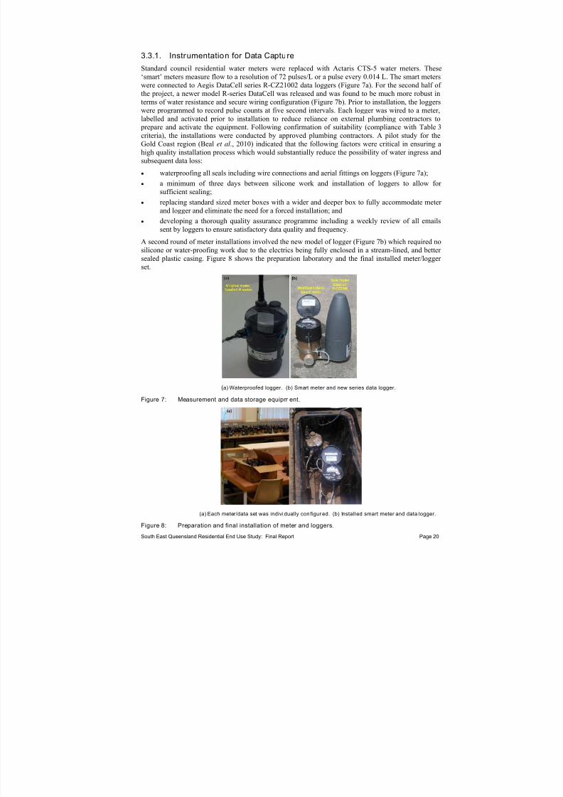
7/27/2019 Trabalho_Austrália
http://slidepdf.com/reader/full/trabalhoaustralia 30/174
3.3.1. Instrumentation for Data Capture
Standard council residential water meters were replaced with Actaris CTS-5 water meters. These‘smart’ meters measure flow to a resolution of 72 pulses/L or a pulse every 0.014 L. The smart meterswere connected to Aegis DataCell series R-CZ21002 data loggers (Figure 7a). For the second half of the project, a newer model R-series DataCell was released and was found to be much more robust interms of water resistance and secure wiring configuration (Figure 7b). Prior to installation, the loggerswere programmed to record pulse counts at five second intervals. Each logger was wired to a meter,labelled and activated prior to installation to reduce reliance on external plumbing contractors to
prepare and activate the equipment. Following confirmation of suitability (compliance with Table 3criteria), the installations were conducted by approved plumbing contractors. A pilot study for theGold Coast region (Beal et al., 2010) indicated that the following factors were critical in ensuring ahigh quality installation process which would substantially reduce the possibility of water ingress andsubsequent data loss:
waterproofing all seals including wire connections and aerial fittings on loggers (Figure 7a);
a minimum of three days between silicone work and installation of loggers to allow for sufficient sealing;
replacing standard sized meter boxes with a wider and deeper box to fully accommodate meter and logger and eliminate the need for a forced installation; and
developing a thorough quality assurance programme including a weekly review of all emailssent by loggers to ensure satisfactory data quality and frequency.
A second round of meter installations involved the new model of logger (Figure 7b) which required nosilicone or water-proofing work due to the electrics being fully enclosed in a stream-lined, and better sealed plastic casing. Figure 8 shows the preparation laboratory and the final installed meter/logger set.
(a) Waterproofed logger. (b) Smart meter and new series data logger.
Figure 7: Measurement and data storage equipment.
(a) Each meter/data set was indivi dually con figur ed. (b) Installed smart meter and data logger.
Figure 8: Preparation and final installation of meter and loggers.
South East Queensland Residential End Use Study: Final Report Page 20
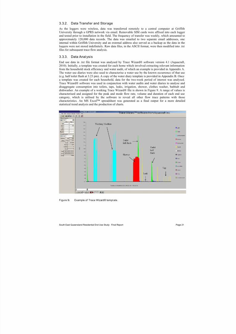
7/27/2019 Trabalho_Austrália
http://slidepdf.com/reader/full/trabalhoaustralia 31/174
3.3.2. Data Transfer and Storage
As the loggers were wireless, data was transferred remotely to a central computer at GriffithUniversity through a GPRS network via email. Removable SIM cards were affixed into each logger and tested prior to installation in the field. The frequency of transfer was weekly, which amounted toapproximately 120,000 data records. The data was emailed to two separate email addresses, oneinternal within Griffith University and an external address also served as a backup as the data in theloggers were not stored indefinitely. Raw data files, in the ASCII format, were then modified into .txtfiles for subsequent trace flow analysis.
3.3.3. Data Analysis
End use data in .txt file format was analysed by Trace Wizard® software version 4.1 (Aquacraft,2010). Initially, a template was created for each home which involved extracting relevant informationfrom the household stock efficiency and water audit, of which an example is provided in Appendix A.The water use diaries were also used to characterise a water use by the known occurrence of that use(e.g. half toilet flush at 3.23 pm). A copy of the water diary template is provided in Appendix B. Oncea template was created for each household, data for the two-week period of interest was analysed.
Trace Wizard® software was used in conjunction with water audits and water diaries to analyse anddisaggregate consumption into toilets, taps, leaks, irrigation, shower, clothes washer, bathtub anddishwasher. An example of a working Trace Wizard® file is shown in Figure 9. A range of values ischaracterised and assigned for the peak and mode flow rate, volume and duration of each end usecategory, which is utilised by the software to reveal all other flow trace patterns with thosecharacteristics. An MS Excel™ spreadsheet was generated as a final output for a more detailedstatistical trend analysis and the production of charts.
Figure 9: Example of Trace Wizard® template.
South East Queensland Residential End Use Study: Final Report Page 21

7/27/2019 Trabalho_Austrália
http://slidepdf.com/reader/full/trabalhoaustralia 32/174
3.3.4. Household Stock Audi ts and Water Diaries
Household water appliance stock audits and self-reported water diaries were used to help identify flowtrace patterns for each household. At the time of the house visit to conduct the water audit, a water diary was left with the participant to fill out over a seven-day period (i.e. five weekdays and twoweekend days) at a timeframe suitable for them (e.g. this could take three weeks to complete as longas a week’s worth of water use events were recorded as best as possible). Overall, 274 household stock audits were conducted out of a possible 289, representing 95% of the SEQREUS sample. A
breakdown of audits for each region is shown in Table 5. A range of information was recorded duringthe audit with a summary page (Figure 10) available to expedite the template building process for theTrace Wizard® analysis.
Figure 10: Example of information summary page for the household stock audit.
Also shown in Table 5 is the response rate for completion and return of the water diaries. Overall, 239water diaries were conducted out of a possible 289, representing 83% of the SEQREUS sample. Thisis an impressive response rate given the somewhat onerous nature of this voluntary task. Responserates for such voluntary tasks are typically reported at between 30 and 60% (Baruch and Brooks, 2008;
Lynn, 2001) thus it was an excellent opportunity to gather another viewpoint on the water useactivities of each home. This information was also used as a general gauge on the proportion of hotand cold tap usage in the home. This information is not readily available in the literature and while it issubjective and would likely not capture all tap usage, it still provides a useful guide to proportion hotand cold water tap use when calculating water and energy demand from hot water systems (this isdiscussed in more detail in Section 15).
Table 5: Statistics for household stock audit and water dairy responses.
Region Household Stock Audi ts
Household Water UseDiaries (Self-Completed)
Gold Coast 82 (97%) 76 (89%)
Brisbane 80 (94%) 67 (79%)
Ipswich 36 (88%) 32 (78%)
Sunshine Coast 76 (97%) 64 (82%)
Overall 274 (95%) 239 (83%)
South East Queensland Residential End Use Study: Final Report Page 22
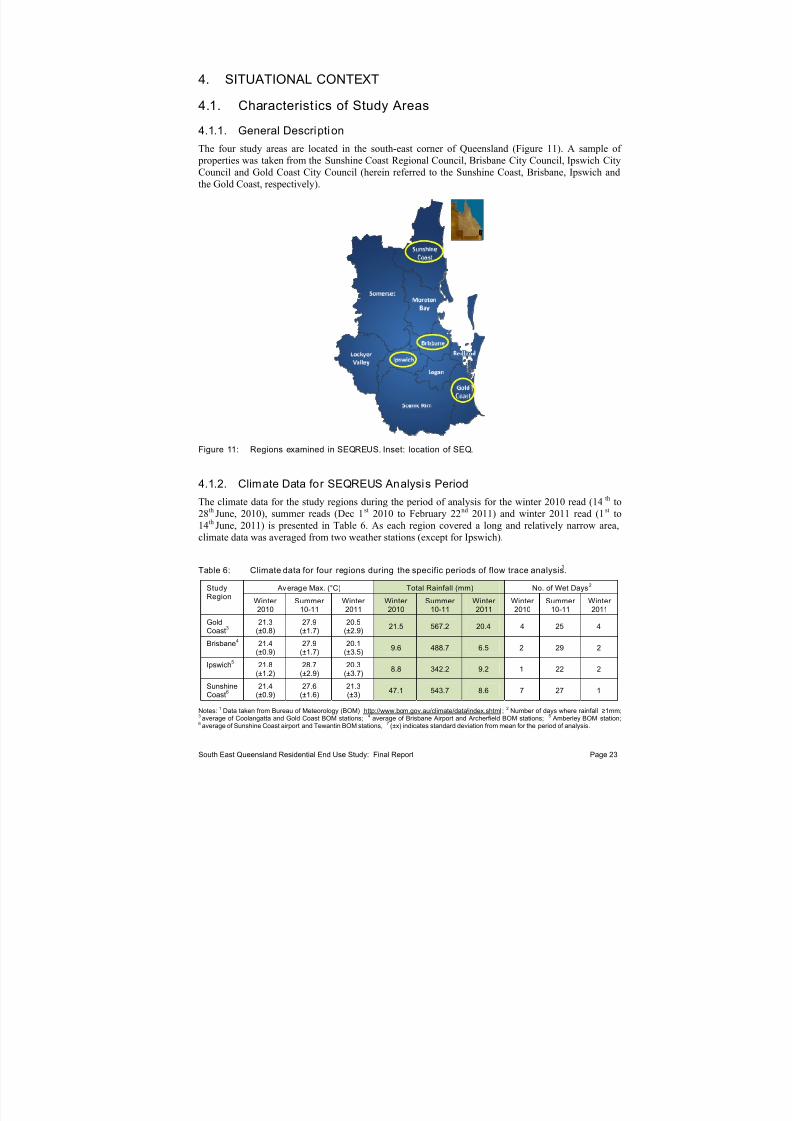
7/27/2019 Trabalho_Austrália
http://slidepdf.com/reader/full/trabalhoaustralia 33/174
4. SITUATIONAL CONTEXT
4.1. Characterist ics of Study Areas
4.1.1. General Description
The four study areas are located in the south-east corner of Queensland (Figure 11). A sample of properties was taken from the Sunshine Coast Regional Council, Brisbane City Council, Ipswich CityCouncil and Gold Coast City Council (herein referred to the Sunshine Coast, Brisbane, Ipswich andthe Gold Coast, respectively).
Figure 11: Regions examined in SEQREUS. Inset: location of SEQ.
4.1.2. Climate Data for SEQREUS Analysis Period
The climate data for the study regions during the period of analysis for the winter 2010 read (14 th to28th June, 2010), summer reads (Dec 1st 2010 to February 22nd 2011) and winter 2011 read (1st to14th June, 2011) is presented in Table 6. As each region covered a long and relatively narrow area,climate data was averaged from two weather stations (except for Ipswich).
Table 6: Climate data for four regions during the specific periods of flow trace analysis1.
Average Max. (°C) Total Rainfall (mm) No. of Wet Days2 Study
RegionWinter 2010
Summer 10-11
Winter 2011
Winter 2010
Summer 10-11
Winter 2011
Winter 2010
Summer 10-11
Winter 2011
GoldCoast
3
21.3(±0.8)
27.9(±1.7)
20.5(±2.9)
21.5 567.2 20.4 4 25 4
Brisbane4
21.4(±0.9)
27.9(±1.7)
20.1(±3.5)
9.6 488.7 6.5 2 29 2
Ipswich5 21.8
(±1.2)28.7
(±2.9)20.3
(±3.7)8.8 342.2 9.2 1 22 2
Sunshine
Coast6
21.4
(±0.9)
27.6
(±1.6)
21.3
(±3) 47.1 543.7 8.6 7 27 1
Notes: 1 Data taken from Bureau of Meteorology (BOM) http://www.bom.gov.au/climate/data/index.shtml; 2 Number of days where rainfall ≥1mm;3 average of Coolangatta and Gold Coast BOM stations; 4 average of Brisbane Airport and Archerfield BOM stations; 5 Amberley BOM station;6 average of Sunshine Coast airport and Tewantin BOM stations, 7 (±x) indicates standard deviation from mean for the period of analysis.
South East Queensland Residential End Use Study: Final Report Page 23

7/27/2019 Trabalho_Austrália
http://slidepdf.com/reader/full/trabalhoaustralia 34/174
Both winter and summer minimum and maximum temperatures were generally average, althoughrainfall was significantly above average for the summer read period as shown in Figure 12.Temperature values were generally typical for the winter and summer periods, although the wetsummer appeared to reduce temperatures below the long-term average for most regions during thestudy (Figure 12). The key features to note in Figure 12 are the climate data preceding and occurringduring the two week periods of analysis (highlighted in green). Rainfall and temperatures during thesetimes were likely to strongly influence outdoor water consumption in particular and also be acontributing factor to peak demand.
0
5
10
15
20
25
30
35
0
100
200
300
400
500
600
A v e r a g e t e m p e r a t u r e ( ° C )
A v e
r a g e r a i n f a l l ( m m )
2010‐2011 rainfall Long term rainfall 2010‐2011 tempe ra tu re Lo ng term temperature
GOLD
COAST
0
5
10
15
20
25
30
35
0
50
100
150
200
250
A
v e r a g e t e m p e r a t u r e ( ° C )
A v e r a g e r a i n f a l l ( m m )
BRISBANE
0
5
10
15
20
25
30
35
0
50
100
150
200
250
300
350
400
A v e r a g e t e m p e r a t u r e ( ° C )
A v e r a g e r a i n f a l l ( m m )
IPSWICH
0
5
10
15
20
25
30
35
0
100
200
300
400
500
600
Jan‐
2010
Feb
M ar Apr M ay Jun J ul Aug Sep Oct Nov Dec J an‐
2011
Feb M ar Apr M ay Jun J ul Aug Sep
A v e r a g e t e m p e r a t u r e ( ° C )
A v e r a g e r a i n f a l l ( m m )
Month
SUNSHINE
COAST
WINTER 2010 SUMMER 2010‐11 WINTER 2011
Figure 12: Rainfall and maximum temperature during the three flow trace measurement periods.
South East Queensland Residential End Use Study: Final Report Page 24

7/27/2019 Trabalho_Austrália
http://slidepdf.com/reader/full/trabalhoaustralia 35/174
4.2. Characterist ics of Participating Households
Some general characteristics of the participating households within each region are shown in Table 7.The average number of people per household was relatively consistent across all regions for all threemeasurement periods, with the Sunshine Coast having the lowest average occupancy of 2.5 people per
household, and the Gold Coast region having the highest average of 2.9 occupants. The percentage of households occupied by two or less people was greater in the Sunshine Coast (average of 56%) andGold Coast (49%) compared to the generally larger households in Ipswich (53%) and Brisbane (43%).These percentages reflect the older demographic of the Sunshine Coast and Gold Coast regions, whichwas also typified by the older age of children for these regions (Table 7).
Table 7: General characterist ics of moni tored households in SEQREUS.
Notes: 1 data presented are averages, 2 this is based on known household occupancies at the time of the initial household water audit and alsoincludes any updates to occupancies which were collated in March this year. This does not include any visitors or absent residents. 3 incomecategories: 1 = <$30,000, 2 = $30,000 – $59,000, 3 = $60,000 – $89,999, 4 = $90,000 - $119,999, 5 = $120,000 - $149,999, 6 = ≥ $150,000, 7 =prefer not to respond. 4 education categories are PS = primary school, HS = high school, T = trade/TAFE, U = university (includes post graduate).
South East Queensland Residential End Use Study: Final Report Page 25

7/27/2019 Trabalho_Austrália
http://slidepdf.com/reader/full/trabalhoaustralia 36/174
5. DESCRIPTIVE STATISTICS
5.1. Calculation of Household and Per Capita Water End Uses
The average per household water use (L/hh/d) has been calculated by taking an average of all theindividual per household water use data measured from each home. Similarly, the average per capitawater use of litres per person per day (L/p/d) was calculated by taking the arithmetic mean of all theindividual per capita data calculated from each home. This calculation was completed for each regionand the total sample. For reporting the overall average per capita figure, an average was taken from allthe individual per capita data across all regions (e.g. winter 2010 average from n=252 individual data
points) using known household occupancy for each home. This method provides an accurate picture of the average per capita and household usage of the analysed sample and is a preferred method whenaccurate household level data is available, as is the case in the SEQREUS (Arbués et al., 2003). Itmeans that the per capita (L/p/d) data can be used as the basic building block for all further calculations as it can be compared with other reported end use studies and provide estimates for urbanwater consumption for similar cities of varying household occupancy.
However, readers should note that overall average per capita end use values for a region (or for thetotal sample) and the equivalent household end use values are not interchangeable using an averageregion or total sample household occupancy scaling factor. This is due to the creation of a newcomposite per capita statistical distribution for each water end use when dividing each household’sconsumption by its occupancy. This per capita end use distribution varies from the householddistribution, especially for those end uses which are not normally distributed (e.g. leaks, irrigation,dishwasher, bathtub) as shown in Figures 13 to 20.
The other method for calculating regional or total sample per capita water end use can be to take thesum of individual household usage and divide by the sum of the number of occupants. Note that thismethod will give a slightly different number to the method described above, i.e. the individual L/p/ddataset has a different distribution to the sum of all data divided by sum of all occupants. Nonetheless,
readers may opt to calculate per capita end uses this way, by dividing the reported household end use break down by the average sample size for that particular region or the total sample.
5.2. Distribution and Variabili ty of Water Consumption End Uses
Water consumption can vary substantially within and between sample populations. As a result of thisvariability, and hence high standard deviation of data points from the mean, the water consumptionrange does not always follow a statistically normal distribution. In terms of water end useconsumption, this holds true for certain end uses such as leaks and irrigation where there is typicallyhigh variation within a sample. This variation can be seen in Table 8 where the standard deviation isconsiderably greater than the average for leaks, dishwasher, bath tub and irrigation. Each of these enduses are characterised by being optional or low occurrence end uses.
Table 8: Descripti ve statist ics for SEQREUS Winter 2010 data.
Statistic
LeakL/p/d
ToiletL/p/d
ClothesWasher
L/p/d
Shower L/p/d
DishWasher
L/p/d
TapL/p/d
BathtubL/p/d
IrrigationL/p/d
TotalL/p/d
Average 9.0 23.9 30.9 42.7 2.5 27.5 1.8 7.0 145.3
Standarddeviation 37.8 15.7 26.8 33.3 4.7 16.6 7.2 15.1 86.7
Firstquartile 0.5 14.3 12.8 21.9 0.0 15.5 0.0 0.0 92.8
Median 1.3 20.7 25.2 34.2 1.2 24.1 0.0 0.0 124.3
Thirdquartile 4.0 29.2 40.1 53.3 3.7 36.0 0.0 6.1 168.9
South East Queensland Residential End Use Study: Final Report Page 26
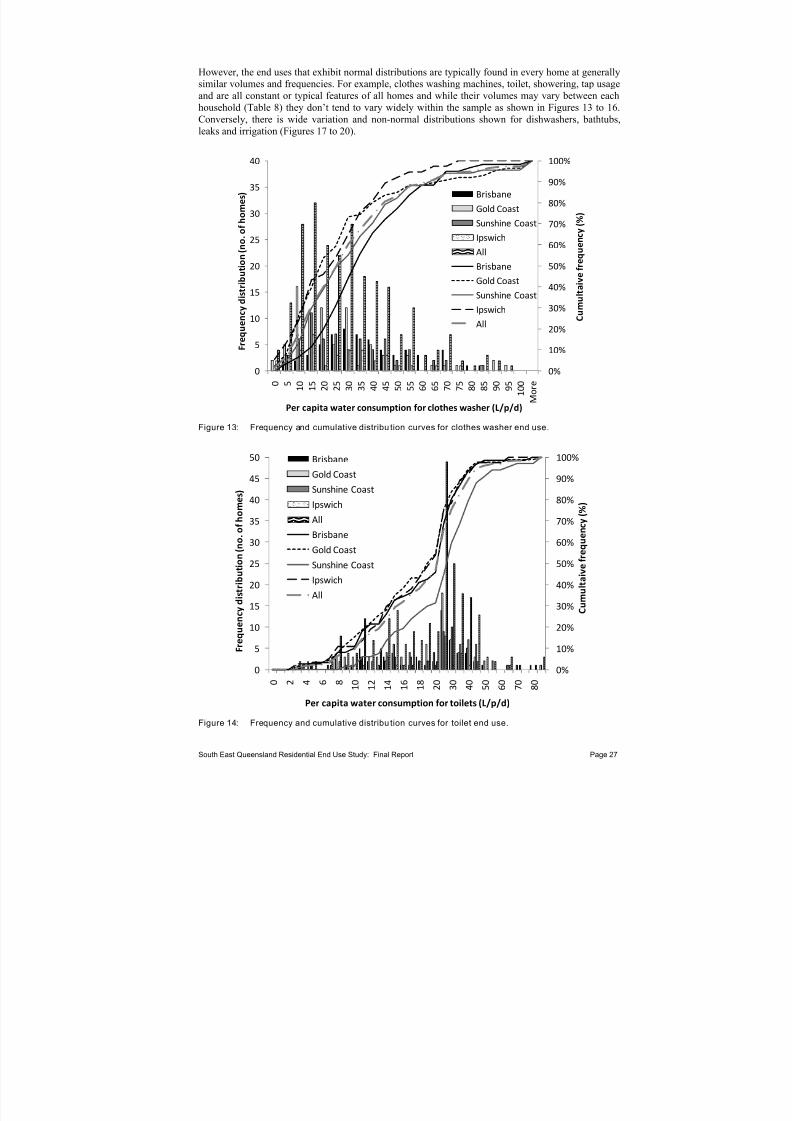
7/27/2019 Trabalho_Austrália
http://slidepdf.com/reader/full/trabalhoaustralia 37/174
However, the end uses that exhibit normal distributions are typically found in every home at generallysimilar volumes and frequencies. For example, clothes washing machines, toilet, showering, tap usageand are all constant or typical features of all homes and while their volumes may vary between eachhousehold (Table 8) they don’t tend to vary widely within the sample as shown in Figures 13 to 16.Conversely, there is wide variation and non-normal distributions shown for dishwashers, bathtubs,leaks and irrigation (Figures 17 to 20).
0%
10%
20%
30%
40%
50%
60%
70%
80%
90%
100%
0
5
10
15
20
25
30
35
40
0 5 1 0
1 5
2 0
2 5
3 0
3 5
4 0
4 5
5 0
5 5
6 0
6 5
7 0
7 5
8 0
8 5
9 0
9 5
1 0 0
M o r e
C u m u l t a i v e
f r e q u e n c y ( % )
F r e q u e n c y d i s t r i b u t i o n ( n o . o f h o m e s )
Per capita water consumption for clothes washer (L/p/d)
Brisbane
Gold Coast
Sunshine Coast
Ipswich
All
Brisbane
Gold Coast
Sunshine Coast
Ipswich
All
Figure 13: Frequency and cumulative distribu tion curves for clothes washer end use.
0%
10%
20%
30%
40%
50%
60%
70%
80%
90%
100%
0
5
10
15
20
25
30
35
40
45
50
0 2 4 6 8 1 0
1 2
1 4
1 6
1 8
2 0
3 0
4 0
5 0
6 0
7 0
8 0
C u m u l t a i v e f r e
q u e n c y ( % )
F r e q u e n c y d i s t r i b u t i o n ( n o . o
f h o m e s )
Per capita water consumption for toilets (L/p/d)
Brisbane
Gold Coast
Sunshine Coast
Ipswich
All
Brisbane
Gold
CoastSunshine Coast
Ipswich
All
Figure 14: Frequency and cumulative distribu tion curves for toilet end use.
South East Queensland Residential End Use Study: Final Report Page 27

7/27/2019 Trabalho_Austrália
http://slidepdf.com/reader/full/trabalhoaustralia 38/174
0%
10%
20%
30%
40%
50%
60%
70%
80%
90%
100%
0
5
10
15
20
25
30
0 5 1 0
1 5
2 0
2 5
3 0
3 5
4 0
4 5
5 0
5 5
6 0
6 5
7 0
7 5
8 0
8 5
9 0
9 5
1 0 0
M o r e
C u m u l t a i v e f r e q u e n c y ( % )
F r e q u e n c y d i s t r i b u t i o n ( n o . o
f h o m e s )
Per capita water consumption for shower L/p/d)
Brisbane
Gold Coast
Sunshine Coast
Ipswich
All
Brisbane
Gold Coast
Sunshine Coast
Ipswich
All
Figure 15: Frequency and cumulative distribu tion curves for shower end use.
0%
10%
20%
30%
40%
50%
60%
70%
80%
90%
100%
0
5
10
15
20
25
30
2 6 1 0
1 4
1 8
2 2
2 6
3 0
3 4
3 8
4 2
4 6
5 0
5 4
5 8
M o r e
C u m u l t
a i v e f r e q u e n c y ( % )
F r e q u e n c y d i s t r i b u t i o n ( n o . o
f h o m e s )
Per capita water consumption for tap (L/p/d)
Brisbane
Gold Coast
Sunshine Coast
Ipswich
All
Brisbane
Gold Coast
Sunshine Coast
Ipswich
All
Figure 16: Frequency and cumulative distribu tion curves for tap end use.
South East Queensland Residential End Use Study: Final Report Page 28
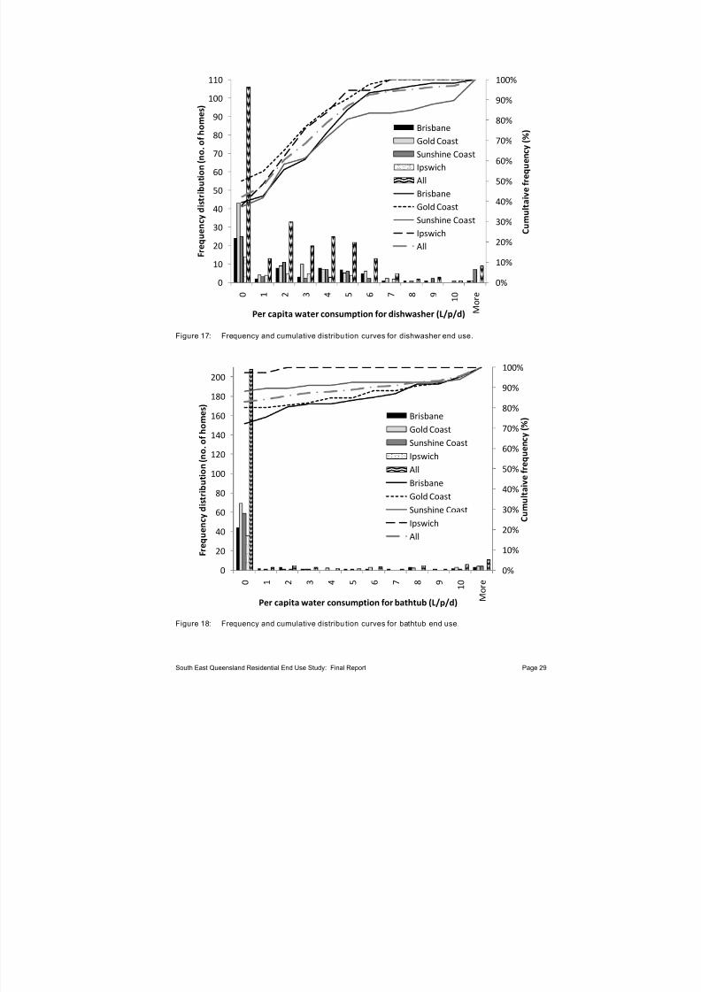
7/27/2019 Trabalho_Austrália
http://slidepdf.com/reader/full/trabalhoaustralia 39/174
0%
10%
20%
30%
40%
50%
60%
70%
80%
90%
100%
0
10
20
30
40
50
60
70
80
90
100
110
0 1 2 3 4 5 6 7 8 9 1 0
M o r e
C u m u l t a i v e f r e q u e n c y ( % )
F r e q u e n c y d i s t r i b u t i o n ( n o . o
f h o m
e s )
Per capita water consumption for dishwasher (L/p/d)
Brisbane
Gold Coast
Sunshine Coast
Ipswich
All
Brisbane
Gold Coast
Sunshine Coast
Ipswich
All
Figure 17: Frequency and cumulative distribu tion curves for dishwasher end use.
0%
10%
20%
30%
40%
50%
60%
70%
80%
90%
100%
0
20
40
60
80
100
120
140
160
180
200
0 1 2 3 4 5 6 7 8 9 1 0
M o r e
C u m u l t a
i v e f r e q u e n c y ( % )
F r e q u e n c y d i s t r i b
u t i o n ( n o . o
f h o m e s )
Per capita water consumption for bathtub (L/p/d)
Brisbane
Gold Coast
Sunshine Coast
Ipswich
All
Brisbane
Gold Coast
Sunshine Coast
Ipswich
All
Figure 18: Frequency and cumulative distribu tion curves for bathtub end use.
South East Queensland Residential End Use Study: Final Report Page 29

7/27/2019 Trabalho_Austrália
http://slidepdf.com/reader/full/trabalhoaustralia 40/174
0%
10%
20%
30%
40%
50%
60%
70%
80%
90%
100%
0
10
20
30
40
50
60
70
80
90
100
110
1 2 3 4 5 6 7 8 9 1 0
1 1
1 2
1 3
1 4
1 5
1 6
1 7
1 8
1 9
2 0
M o r e
C u m u l t a i v e f r e q u e n c y ( % )
F r e q u e n c y d i s t r i b u t i o n ( n o . o
f h o m e s )
Per capita water consumption for leaks (L/p/d)
Brisbane
Gold Coast
Sunshine Coast
Ipswich
All
Brisbane
Gold Coast
Sunshine Coast
Ipswich
All
Figure 19: Frequency and cumulative distribut ion curves for leak end use.
0%
10%
20%
30%
40%
50%
60%
70%
80%
90%
100%
0
10
20
30
40
50
60
70
80
90
100
110
0 1 2 3 4 5 6 7 8 9 1 0
1 1
1 2
1 3
1 4
1 5
1 6
1 7
1 8
1 9
2 0
2 5
3 0
3 5
4 0
M o r e
C u m u l t a i v e
f r e q u e n c y ( % )
F r e q u e n c y d i s t r i b u t i o
n ( n o . o
f h o m e s )
Per capita water consumption for irrigation (L/p/d)
Brisbane
Gold Coast
Sunshine Coast
Ipswich
AllBrisbane
Gold Coast
Sunshine Coast
Ipswich
All
Figure 20: Frequency and cumulative distribut ion curves for irrigation end use.
South East Queensland Residential End Use Study: Final Report Page 30

7/27/2019 Trabalho_Austrália
http://slidepdf.com/reader/full/trabalhoaustralia 41/174
5.3. Winter 2010 End Use Event Statistics
5.3.1. Introduction
The following subsections present descriptive statistics on end use event frequencies, flow rates, mean
volumes and durations. The data from winter 2010 has been used as it represents results from thelargest sample size from the three reads throughout the SEQREUS. Therefore, it is considered themost robust in terms of representing the greatest variation in household characteristics, thus thestrongest dataset in terms of statistical significance and cross regional variations. Additionally, theclimate for the winter 2010 was reasonably representative of the long term averages (temperature andrainfall) for that sampling period. These justifications for primarily using the winter 2010 dataset ismaintained throughout this document when reporting and discussing specific aspects of the SEQREUSresults. Note that some parts of the tables are shaded grey. Due to the small sample size (dishwasher end use) or excessively high values (clothes washer end use), the numbers have been omitted.
5.3.2. End Use Event Frequencies
Tables 9, 10, 11 and 12 present end use event frequency statistics for winter 2010 for the Gold Coast,Brisbane, Ipswich and the Sunshine Coast, respectively.
Table 9: Gold Coast Winter End Use Event Frequency Statist ics.
Frequency (events/day)Statistics
Half Flush Full Flush Tap Shower Bath Dishwasher Clothes Washer Irrigation
Mean 4.49 3.86 40.64 1.84 0.10 0.37 0.54 0.33
Std. 3.25 2.69 19.63 1.20 0.23 0.42 0.34 0.28
Skewness 0.83 1.25 0.77 1.55 2.48 1.28 0.30 0.94
Kurtosis 0.43 1.96 0.37 3.63 5.95 1.23 -0.84 0.43
1st Quartile 1.75 1.86 25.14 1.00 0.00 0.00 0.29 0.21
2nd
Quartile 4.07 3.39 38.21 1.61 0.00 0.21 0.50 0.24
3rd
Quartile 6.57 5.23 51.82 2.64 0.00 0.64 0.73 0.51
4th
Quartile 14.07 12.93 93.29 6.37 1.00 1.57 1.21 1.14
Table 10: Brisbane Winter End Use Event Frequency Statistics.
Frequency (events/day)Statistics
Half Flush Full Flush Tap Shower Bath Dishwasher Clothes Washer Irrigation
Mean 4.87 4.21 58.70 2.13 0.13 0.55 0.71 0.12
Std. 3.97 2.68 33.42 1.99 0.28 0.68 0.56 0.19
Skewness 1.67 1.29 1.13 5.11 2.12 1.94 2.93 1.94
Kurtosis 3.99 1.67 1.90 33.79 3.36 5.15 14.28 3.68
1st
Quartile 2.64 2.54 34.93 1.21 0.00 0.00 0.36 0.00
2nd
Quartile 4.25 3.50 51.36 1.93 0.00 0.43 0.64 0.00
3rd
Quartile 6.00 4.71 80.14 2.57 0.00 0.86 1.00 0.21
4th
Quartile 21.21 13.36 175.14 15.46 1.14 3.21 3.79 0.79
South East Queensland Residential End Use Study: Final Report Page 31

7/27/2019 Trabalho_Austrália
http://slidepdf.com/reader/full/trabalhoaustralia 42/174
Table 11: Ipswich Winter End Use Event Frequency Statist ics.
Frequency (events/day)Statistics
Half Flush Full Flush Tap Shower Bath Dishwasher Clothes Washer Irrigation
Mean 6.14 3.58 46.66 2.11 0.01 0.67 0.56 0.05
Std. 4.21 2.77 27.69 1.43 0.05 1.05 0.54 0.15
Skewness 0.89 1.59 1.11 0.91 5.92 2.25 2.43 3.98
Kurtosis 0.76 3.17 1.52 0.50 35.00 4.93 9.14 17.97
1st Quartile 2.44 1.54 22.43 1.00 0.00 0.00 0.21 0.00
2nd
Quartile 5.50 2.83 45.29 1.79 0.00 0.21 0.50 0.00
3rd
Quartile 8.78 4.70 56.89 3.07 0.00 0.86 0.81 0.00
4th Quartile 18.71 13.14 131.33 6.07 0.31 4.07 2.86 0.78
Table 12: Sunshine Coast Winter End Use Event Frequency Statist ics.
Frequency (events/day)Statistics
Half Flush Full Flush Tap Shower Bath Dishwasher Clothes Washer Irrigation
Mean 6.51 4.76 49.33 1.82 0.05 0.58 0.72 0.07
Std. 4.05 2.92 21.27 1.02 0.17 0.83 0.57 0.11
Skewness 0.50 1.08 0.16 0.74 3.65 2.59 2.78 1.10
Kurtosis -0.50 0.81 -0.84 0.79 13.63 8.94 11.18 -0.07
1st
Quartile 3.43 2.75 31.86 1.07 0.00 0.00 0.39 0.00
2nd Quartile 6.21 4.00 47.43 1.71 0.00 0.36 0.64 0.00
3rd
Quartile 9.01 5.96 65.86 2.46 0.00 0.86 0.89 0.21
4th
Quartile 16.93 13.14 93.64 5.21 0.93 4.57 3.57 0.43
5.3.3. End Use Event Mean Volumes
Tables 13, 14, 15 and 16 present end use mean volume statistics for winter 2010 for the Gold Coast,Brisbane, Ipswich and the Sunshine Coast, respectively.
Table 13: Gold Coast Winter Mean Volume of End Use Event Statist ics.
Mean Volume of End Use Event (L/event)Statistics
Half Flush Full Flush Tap Dishwasher Clothes Washer
Mean 4.12 8.00 1.98 4.26 106.88
Std. 1.37 2.15 0.54 9.55 77.51
Skewness 0.14 1.50 0.08 5.44 0.87
Kurtosis 2.36 2.57 -0.16 33.08 0.32
1st Quartile 3.53 6.68 1.57 0.00 50.06
2nd Quartile 3.97 7.58 1.91 2.12 88.56
3rd
Quartile 4.70 8.92 2.38 5.33 148.80
4th Quartile 8.25 14.85 3.31
Note:1
shaded cells in table represent values that were not considered accurate due to the small sample size in this cluster.
South East Queensland Residential End Use Study: Final Report Page 32
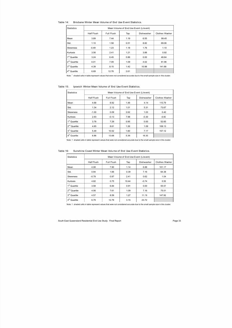
7/27/2019 Trabalho_Austrália
http://slidepdf.com/reader/full/trabalhoaustralia 43/174
Table 14: Brisbane Winter Mean Volume of End Use Event Statist ics.
Mean Volume of End Use Event (L/event)Statistics
Half Flush Full Flush Tap Dishwasher Clothes Washer
Mean 3.89 7.44 1.19 6.55 99.45
Std. 1.10 1.58 0.51 8.82 69.06
Skewness -0.49 1.23 1.18 1.76 1.10
Kurtosis 3.56 2.41 1.21 3.88 0.92
1st Quartile 3.24 6.45 0.86 0.00 48.84
2nd
Quartile 4.01 7.09 1.09 4.02 81.96
3rd
Quartile 4.39 8.15 1.42 10.98 141.68
4th Quartile 6.69 12.78 2.61
Note:1
shaded cells in table represent values that were not considered accurate due to the small sample size in this cluster.
Table 15: Ipswich Winter Mean Volume of End Use Event Statist ics.
Mean Volume of End Use Event (L/event)Statistics
Half Flush Full Flush Tap Dishwasher Clothes Washer
Mean 4.68 8.92 1.48 4.14 113.79
Std. 1.34 2.12 1.01 5.31 73.67
Skewness -1.00 0.09 2.62 1.03 0.40
Kurtosis 2.93 -0.13 7.98 -0.30 -0.60
1st
Quartile 3.78 7.29 0.95 0.00 52.65
2nd
Quartile 4.65 8.61 1.26 1.09 108.13
3rd
Quartile 5.49 10.52 1.60 7.17 157.12
4th
Quartile 6.86 13.68 5.39 16.30
Note: 1 shaded cells in table represent values that were not considered accurate due to the small sample size in this cluster.
Table 16: Sunshine Coast Winter Mean Volume of End Use Event Statist ics.
Mean Volume of End Use Event (L/event)Statistics
Half Flush Full Flush Tap Dishwasher Clothes Washer
Mean 4.08 7.90 1.14 6.88 101.17
Std. 0.94 1.66 0.39 7.16 64.38
Skewness -0.78 0.97 2.41 0.62 1.04
Kurtosis 4.82 0.75 10.44 -0.74 0.59
1st
Quartile 3.58 6.84 0.91 0.00 55.57
2nd Quartile 4.06 7.61 1.09 7.16 75.01
3rd Quartile 4.57 8.59 1.27 11.19 147.92
4th
Quartile 6.79 12.79 3.15 23.72
Note: 1 shaded cells in table represent values that were not considered accurate due to the small sample size in this cluster.
South East Queensland Residential End Use Study: Final Report Page 33

7/27/2019 Trabalho_Austrália
http://slidepdf.com/reader/full/trabalhoaustralia 44/174
South East Queensland Residential End Use Study: Final Report Page 34
5.3.4. Shower End Use Event Flow Rates
Table 17 presents shower end use event flow rate statistics for winter 2010 for the Gold Coast,Brisbane, Ipswich and the Sunshine Coast.
Table 17: Winter Shower End Use Event Flow Rate Statist ics.
Shower Event Flow Rate (L/min)Statistics
Gold Coast Bris bane Ipswich Sunshine Coast
Mean 7.79 7.82 7.71 8.49
Standard Deviation 2.21 3.18 3.15 2.73
Skewness 0.43 2.32 0.07 1.29
Kurtosis 1.80 8.20 1.73 2.23
1st
Quartile 6.97 6.41 6.32 7.07
2nd
Quartile 7.67 7.51 7.35 7.69
3rd
Quartile 8.57 8.13 8.83 9.58
4th
Quartile 14.21 21.03 15.74 17.96
5.3.5. Shower End Use Event Durations
Table 18 presents shower end use event duration statistics for winter 2010 for the Gold Coast,Brisbane, Ipswich and the Sunshine Coast.
Table 18: Winter Shower Event Duration Statist ics.
Shower Event Duration (min)Statistics
Gold Coast Bris bane Ipswich Sunshine Coast
Mean 5.72 5.72 5.79 6.45
Standard Deviation 2.22 2.22 2.25 2.72
Skewness 1.23 1.23 0.94 0.87
Kurtosis 2.07 2.07 1.48 0.86
1st
Quartile 3.83 3.83 4.17 4.43
2nd
Quartile 5.52 5.52 5.52 6.00
3rd
Quartile 6.67 6.67 7.13 8.33
4th
Quartile 13.33 13.33 13.49 15.38

7/27/2019 Trabalho_Austrália
http://slidepdf.com/reader/full/trabalhoaustralia 45/174
6. END USE RESULTS AND DISCUSSION
6.1. Winter 2010 Results
6.1.1. Sample Size
For the winter 2010 sample, 252 homes were analysed for mains water end uses. This comprised 87 inthe Gold Coast, 61 in Brisbane, 67 in Sunshine Coast and 37 in Ipswich. The total representsapproximately 80% of the initial target sample of 320 homes (80 per region). A number of factorsinfluenced the lower than expected sample including: logger failures predominantly due to moistureingress; poor meter to logger data transfer; unsuitable existing meters (i.e. in a few cases atypicaldiameter of existing meters could not fit the larger diameter smart meters); aged service pipe (i.e . changing meters may affect the integrity of the corroded pipeline and meter outlets); and some lastminute cancellations of participants. In Ipswich in particular, there were many water meters that werenot suitable due to location, different sized connections or age of service pipe. Finally, there were twohomes that had not had their water audits completed as they were overseas for a long period. Most of
these factors were unpredictable and unavoidable.
The winter 2010 SEQREUS sample is a good representation of SEQ households with a strong mix of family types, income categories and household occupancies. Additionally, results suggest that the dataobtained from this study compares well with other estimations of household consumption (i.e. weeklyreports from QWC). This is discussed in more detail in subsequent sections of this report.
6.1.2. Overall Water Consumption Trends
An average total water consumption of 370.7 litres per household per day (L/hh/d) was recordedduring the period of analysis. This represented a per capita average of 145.3 L/p/d (Figure 21).
Figure 21: Average daily per capita end use winter 2010 breakdown for all SEQ regions.
South East Queensland Residential End Use Study: Final Report Page 35

7/27/2019 Trabalho_Austrália
http://slidepdf.com/reader/full/trabalhoaustralia 46/174
In comparison, for the same period, the QWC reported a per capita water use of 154 L/p/d (QWC,2010). The relatively small difference between the SEQREUS and QWC averages is due to a range of sampling factors including: (1) slight disparity in sample characteristics; (2) biases encountered whenrecruiting consenting households to a research study (e.g. very high water consumers unlikely toconsent); and (3) assumptions embedded in the QWC calculations for per capita water consumption.In terms of the last point, the residential per capita water usage for SEQ is calculated based on bulk water use over a weekly period and as such there is an inherent assumption that a certain percentage of
businesses are included within this bulk water measurement. Bulk water derived per capita demand areinherently inaccurate as they rely on a range of assumptions on system leakage, business usage,
population, to name a few. Additionally, there will be some bias in the SEQREUS sample due to thesmaller size of the sample compared with the QWC database and the possibility of a slightoverrepresentation of low water consumers due to their involvement in this study. Nonetheless, thecloseness of the top-down (i.e. QWC reported value) and bottom-up (SEQREUS reported value)reported values provide confidence in both data sets.
Both the SEQREUS and QWC-based water use averages fell well below the Permanent Water Conservation Measures (PWCM) target of 200 L/p/d as recommended by the State government
(Figure 22). Furthermore, the average water consumption for the regions monitored were roughlyequivalent to the water use achieved during enforced high and medium-level water restrictions. This isan encouraging indication that there is some long-term behavioural shift in residential consumers aswater use remains generally low regardless of the drought ‘breaking’, water supply dams in SEQrecording over 90% capacity, and a relaxation on external water usage.
0
50
100
150
200
250
300
350
J a n
‐ 0 5
A p r ‐
0 5
J u l ‐ 0 5
O c t ‐
0 5
J a n
‐ 0 6
A p r ‐
0 6
J u l ‐ 0 6
O c t ‐
0 6
J a n
‐ 0 7
A p r ‐
0 7
J u l ‐ 0 7
O c t ‐
0 7
J a n
‐ 0 8
A p r ‐
0 8
J u l ‐ 0 8
O c t ‐
0 8
J a n
‐ 0 9
A p r ‐
0 9
J u l ‐ 0 9
O c t ‐
0 9
J a n
‐ 1 0
A p r ‐
1 0
J u l ‐ 1 0
A
v e r a g e m o n t h l y p e r c a p i t a w a t e r u s e
( L / p / d )
Time (months)
QWC water use
SEQREUS
145 L/p/d
N o r e s t r i c t i o n s
Level
1
Level
2
Level
3
Level
4
Level
5
Level
6
High
Level
Medium
Level
PWCM
Target 140 L/p/dTarget 170
L/p/d
Target 200 L/p/d
Figure 22: Comparison of all SEQ winter 2010 water use with SEQEUS total average.
End use break down on a per capita basis indicated that, on average, shower 42.7 L/p/d (29.4%), tap27.5 L/p/d (19%) and clothes washer 31 L/p/d (21.4%) comprised the bulk of the water consumption
(Figure 21). Almost 70% (approximately 100 L/p/d) of total consumption was attributed to these threeactivities. Toilet use added an additional 23.7 L/p/d (16.3%) to the total per capita water consumption.
South East Queensland Residential End Use Study: Final Report Page 36

7/27/2019 Trabalho_Austrália
http://slidepdf.com/reader/full/trabalhoaustralia 47/174
Interestingly, water consumption for irrigation and general outdoor purposes was found to be low, atan average of only 7 L/p/d, which is less than 5% of total consumption (Figure 21). This low irrigationvalue indicates that the very high restrictions incurred in 2006 and 2007, may have had a lastinginfluence on the way people view their lawn and gardens.
The individual household per capita water consumption activity break down is shown in Figure 23.
Water end use breakdowns varied substantially across (and within) the regions examined. Thisvariation is a reflection of several factors, including family size and composition, socio-demographicfactors and climate. In all homes measured, there was water use from toilet, clothes washer, taps andshowers. The remaining end uses analysed, namely leaks, dishwasher, irrigation and bath tub, werereported in some but not all of the homes.
0
100
200
300
400
500
600
700
H
o u s e h o l d W a t e r C o n s u m p t i o
n ( L / p / d )
Household ID
Irrigation Bath Tap
Dish Washer Shower Clothes Washer
Toilet Leak
Figure 23: Household per capita winter 2010 consumption (L/p/d) activity break down.
Typically, the homes that used the most water had a disproportionately high contribution fromirrigation. This is shown by the strong correlation observed between total household water use andirrigation (Figure 24). The frequency distribution for irrigation (Figure 24) indicates that half thehomes monitored did not register any irrigation use during the period of analysis. The lack of irrigation could be attributed to the winter season where outdoor watering is usually lower than in the
hotter summer climate. Additionally, as discussed previously, there may be a tendency for lower external watering to occur due to the change in behaviours as a result of the water restrictions adheredto during the relatively recent drought period. However, 20% of the homes that did irrigate (or usewater for external purposes) contributed to over 80% of total irrigation water use at an average of 30 L/p/d. This pareto effect has been observed in other residential water use studies (Willis et al.,2009b; Turner et al., 2009) and is a good example of why water restriction policy targets outdoor useto reduce residential demand (Barrett et al., 2009; Inman and Jeffrey, 2006; Kenney et al., 2008).
South East Queensland Residential End Use Study: Final Report Page 37
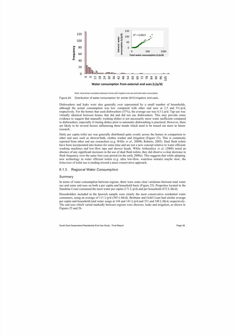
7/27/2019 Trabalho_Austrália
http://slidepdf.com/reader/full/trabalhoaustralia 48/174
0
20
40
60
80
100
120
0 6 1 2
1 8
2 4
3 0
3 6
4 2
4 8
5 4
6 0
6 6
7 2
7 8
8 4
9 0
9 6
1 0 5
F r e q u e n c y
Water consumption
from
external
end
uses
(L/p/d)
R² = 0.8927
0
50
100
150
0 500 1000 E x t r e n a l w
a t e r
c o n s u m p t i o n ( L / p / d )
Total water consumption (L/p/d)
Note: Inset shows correlation between homes with irrigation end use and total water consumption.
Figure 24: Distribution of water consumption for winter 2010 irrigation end uses.
Dishwashers and leaks were also generally over represented by a small number of households,although the actual consumption was low compared with other end uses at 2.5 and 9 L/p/d,respectively. For the homes that used dishwashers (57%), the average use was 4.3 L/p/d. Tap use wasvirtually identical between homes that did and did not use dishwashers. This may provide someevidence to suggest that manually washing dishes is not necessarily more water inefficient comparedto dishwashers, especially if rinsing dishes prior to automatic dishwashing is practised. However, thereare likely to be several factors influencing these trends which need to be teased out more in futureresearch.
Daily per capita toilet use was generally distributed quite evenly across the homes in comparison toother end uses such as shower/bath, clothes washer and irrigation (Figure 23). This is commonlyreported from other end use researchers (e.g. Willis et al., 2009b; Roberts, 2005). Dual flush toiletshave been incorporated into homes for some time and are not a new concept relative to water efficientwashing machines and low-flow taps and shower heads. While Arthuraliya et al. (2008) noted anabsence of any significant increases in the use of dual flush toilets, they did observe a clear decrease inflush frequency over the same four-year period (in the early 2000s). This suggests that while adoptingnew technology in water efficient toilets (e.g. ultra low-flow, waterless urinals) maybe slow, thebehaviour of toilet use is tending toward a more conservative approach.
6.1.3. Regional Water Consumption
Summary
In terms of water consumption between regions, there were some clear variations between total water use and some end uses on both a per capita and household basis (Figure 25). Properties located in theSunshine Coast consumed the most water per capita (171 L/p/d) and per household (472 L/hh/d).
Householders included in the Ipswich sample were clearly the most conservative residential water consumers, using an average of 111 L/p/d (305 L/hh/d). Brisbane and Gold Coast had similar average
per capita and household total water usage at 144 and 141 L/p/d and 331 and 348 L/hh/d, respectively.The end uses which varied markedly between regions were showers, leaks and irrigation, as shown in
Figures 25 and 26.
South East Queensland Residential End Use Study: Final Report Page 38

7/27/2019 Trabalho_Austrália
http://slidepdf.com/reader/full/trabalhoaustralia 49/174
(a) Per capita end use break down (L/p/d). (b) Per household end use break down (L/hh/d).
Figure 25: Breakdown of average winter 2010 end uses for each region.
Figure 26: Average percentage of total consumption for each winter 2010 end use.
Average total per capita water use for the period of analysis reported by the QWC (2010) is presented below, together with the totals from the SEQREUS (Table 19). It can be seen from this table that thereare some disparities between the two datasets. The reasons for the differences have been brieflydiscussed above. The method of calculation (underlying assumption of commercial/residential water use split) and the coarser bulk water demand data that is used by the QWC may slightly overestimateresidential water use in SEQ. Conversely, the SEQREUS data may slightly underestimate averagewater use in SEQ due to possible biases in the sample, including: household occupancy rates; expectedlow representation of the very high water uses; and the lack of inclusion of multi-unit dwellings. Thesedwelling types are not included in the present study. Additionally, it has been observed that
householders are more likely to use less water if they are aware of being monitored (e.g. Stewart et al.,2010) and this may be occurring to some extent in this study. It is anticipated that this phenomenonwill play less of a role as the awareness diminishes. Notwithstanding the differences, the trend for Ipswich to use less water and the Sunshine Coast to use more water has been captured in both datasets.Furthermore, Brisbane averages are very similar, with only a 4 L/p/d difference over the period.
B ri sba ne Gol d CoastSunshine
CoastIpswich
Irrigation 7.2 9.4 6.8 1.7
Bathtub 1.8 1.9 2.9 0.0
Tap 22.7 34.2 26.6 23.0
Dish washer 2.3 1.6 4.2 1.4
Shower 38.6 40.9 51.1 36.3
Clothes Washer 35.8 27.9 34.0 24.5
Toilet 22.0 20.6 31.1 21.4
Leak 13.3 4.3 14.1 2.9
0
25
50
75
100
125
150
175
P E R C
A P I T A
A v e r a g e w a t e r c o n s u m p t i o n
( L /
p / d )
144
171
111
141
(a)
B ri sba ne Gold CoastSunshine
CoastIpswich
Irrigation 14.4 19.6 11.0 6.8
Bathtub 5.7 2.0 8.6 0.2
Tap 52.9 82.5 66.0 56.4
Dish washer 7 4.3 9.3 5.2
Shower 94.8 104.2 155.8 107.0
Clothes Washer 89.9 66.9 99.9 64.1
Toilet 49.9 48.6 80.9 57.3
Leak 16.7 16.4 40.8 8.4
0
50
100
150
200
250
300
350
400
450
500
P E R H O U
S E H O L D
A v e r a g e w a t e r c o n s u m p t i o n
( L / h h / d )
331
472
305
348
(b)
Brisbane Gold Coast Sunshine Coast Ipswich
Irrigation 5.0 6.7 4.0 1.5
Bathtub 1.2 1.4 1.7 0.0
Tap 15.8 24.3 15.6 20.7
Dish washer 1.6 1.1 2.5 1.3
Shower 26.9 29.0 29.9 32.6
Clothes Washer 24.9 19.8 19.9 22.0
Toilet 15.3 14.6 18.2 19.2
Leak 9.3 3.1 8.2 2.6
0
25
50
75
100
A v e r a g e p e r c e n t a g e o f t o t a l
w a t e r c
o n s u m p t i o n ( % )
South East Queensland Residential End Use Study: Final Report Page 39

7/27/2019 Trabalho_Austrália
http://slidepdf.com/reader/full/trabalhoaustralia 50/174
Table 19: Comparison of average total water use (L/p/d) for dwellings in SEQ.
Data Source Gold Coast Br isbane Ipswich Sunshine Coast
QWC 18th June 183 138 138 189
QWC 25th June 180 142 142 185
QWC period average 182 140 140 187
SEQREUS 14 to 24th June 141 144 111 171
In terms of irrigation, properties located in the Gold Coast used slightly, but not significantly, morethan the other regions. This is interesting as this region, along with the Sunshine Coast, received themost rainfall during the period of analysis (Table 6). Ipswich used the least water for irrigation yet hadthe driest weather of all regions during June (Table 6). Some conclusions may be drawn from thisobservation. After recent wet periods, residents may feel less restricted or guilty in using water toirrigate the garden. However, it should be noted that the average irrigation volumes and total volumesin general are substantially lower than those from a decade earlier.
Temperature rather than rainfall may be a stronger trigger for irrigation and this will be measured andreported on with the summer end use analysis results (December 2010). The garden size of homes in
the Sunshine and Gold Coasts may be generally larger than those of Ipswich and Brisbane, thus usingmore water, although this information is not able to be readily determined at this stage. Soil textureand moisture holding capacity of soils will also determine the frequency and volume of irrigation. Soilcharacteristics vary across SEQ, however the predominant upper horizon soils (e.g. Kurosols) in theBrisbane and Ipswich regions and the sandy coastal soils typically have a low moisture holdingcapacity. Soils in the elevated regions (e.g. Red Ferrosols) in the coastal councils have a slightlyhigher capacity. Finally, the increased use of stored rainwater from tanks for external purposes mayalso contribute to the lower irrigation end uses from mains water. This final point is explored more inSection 10.
Gold Coast
Properties in the Gold Coast recorded an average total water consumption of 347.5 L/hh/d or 140.8 L/p/d (Figure 27a), ranging from 26 L/p/d to 549 L/p/d (Figure 27b). End use break down on a
per capita basis indicates that, on average, shower (29%), tap (24%) and clothes washer (20%)comprised the bulk of the water consumption (Figure 27a).
(a) Per capita end use break down (L/p/d) (b) Per capita end use break down (L/p/d) by household0
100
200
300
400
500
600
H o u s e h o l d W a t e r C o
n s u m p t i o n ( L / p / d )
Household ID
Irrigation
Bathtub
Tap
Dishwasher
Shower
Clothes
Washer
Toilet
Leak
(b)Leak
4.3 L (3%)
Toilet 20.6 L
(15%)
Clothes
Washer
27.9 L (20%)
Shower
40.9 L (29%)Dish
washer
1.6 L (1%)
Tap 34.2 L
(24%)
Bathtub
1.9 L (1%)Irrigation
9.4 L
(7%)
Total average = 140.8 L/p/d
(a)
(a) Per capita end use break down (L/p/d). (b) Per capita end use break down (L/p/d) by household.
Figure 27: Break down of average winter 2010 end uses for the Gold Coast.
South East Queensland Residential End Use Study: Final Report Page 40

7/27/2019 Trabalho_Austrália
http://slidepdf.com/reader/full/trabalhoaustralia 51/174
Irrigation contributed an average of 9.4 L/p/d or 7% of total water use. The homes that used the mostwater had a disproportionately high contribution from irrigation (Figure 27b). This is consistent acrossall regions examined. Water used for clothes washing and showers was markedly varied across thesample and may reflect the mix of household types (single, family, pensioners) that were present inthis region. Data from Table 7 suggests that both small and large families with young children were
fairly evenly represented compared to the other regions.
Brisbane
Average household consumption in Brisbane was 331.4 L/hh/d, resulting in a per capita consumptionaverage of 143.8 L/p/d (Figure 28). End use break down on a per capita basis indicates that, onceagain, shower (26.9%), clothes washer (24.9%) and tap (15.8%) comprised the bulk of the water consumption (Figure 28a), contributing over 65% (97 L/p/d) of daily usage. There was an association
between the number of young children in the home and clothes washing and showering. The Brisbanesample had the youngest average age of children (2.7 years) and the highest consumption for water resulting from clothes washing (Figure 26).
The Brisbane total amount of daily per capita usage attributed to leaks was the second highest across
the regions at 13.3 L/p/d representing 9.3% of total household water use (Figure 26 and Figure 28a).However, this result was skewed by extraordinarily high leak usage attributed to two homes, with onehousehold showing average daily consumption from leaks at over 500 L/p/d (Figure 28b). For theaverage householder, the percentage attributed to leaks was much less at 4.4 L/p/d (3% of total water use). It is necessary to include these high leak homes as they are not outliers, rather they represent asmall number of homes (usually 3-5% of dwelling stock) having very high leakage rates and this istypical of a ‘normal’ sample of households (Britton et al., 2009).
Irrigation in the Brisbane region was 5% of total daily usage, or 7.2 L/p/d. This figure was over-represented in some households (Figure 28b). It was noted during the analysis that people whoreported that they irrigate their gardens usually did so using a constant and medium flow rate with theevent lasting between 15 minutes to one hour on average.
Leak 13.3
L/p/d
(9.3%)
Toilet 22 Lp/d
(15.3%)
Clothes
Washer 35.8
L/p/d (24.9%)Shower 38.6
L/p d (26.9%)
Dish
washer
2.3 L/p/d
(1.6%)
Tap 22.7 L/p/d
(15.8%)
Bathtub 1.8
L/p/d (1.2%)
Irrigation
7.2 L/p/d
(5%)
Total average = 143.8 L/p/d
(a)
0
100
200
300
400
500
600
700
H o u s e h o l d W a t e r C o n s u m p t i o n ( L / p / d )
Household ID
Irrigation
Bathtub
Tap
Dishwasher
Shower
Clothes
Washer
Toilet
Leak
(b)
(a) Per capita end use break down (L/p/d). (b) Per capita end use break down (L/p/d) by household.
Figure 28: Break down of average winter 2010 end uses for Brisbane.
Ipswich
The period of analysis in the Ipswich region showed an average household consumption of 305.4 L/hh/day. This resulted in a low per capita figure of 111.2 L/p/d (Figure 29a), nearly half of the
QWC Permanent Water Conservation Measures target of 200 L/p/d. Per capita total water use rangedfrom 283 to 20 L/p/d (Figure 29b). The low per capita use (20 L/p/d) measured for one home was aresult of frequent absences of the sole occupant of the property.
South East Queensland Residential End Use Study: Final Report Page 41
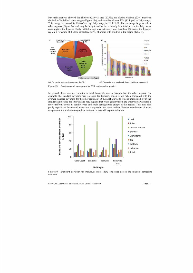
7/27/2019 Trabalho_Austrália
http://slidepdf.com/reader/full/trabalhoaustralia 52/174
Per capita analysis showed that showers (32.6%), taps (20.7%) and clothes washers (22%) made upthe bulk of individual water usages (Figure 29a), and contributed over 75% (81 L/p/d) of daily usage.Toilet usage accounted for 19% of average daily usage, or 21.5 L/p/d; this percentage is greater thanother regions (Figure 26) and may be heightened by the relatively low total per capita daily water consumption for Ipswich. Daily bathtub usage was extremely low, less than 1% across the Ipswichregion; a reflection of the low percentage (21%) of homes with children in the region (Table 7).
(a) Per capita end use break down (L/p/d). (b) Per capita end use break down (L/p/d) by household.
Figure 29: Break down of average winter 2010 end uses for Ipswich.
In general, there was less variation in total household use in Ipswich than the other regions. For example, the standard deviation was 46 L/p/d for Ipswich, which is low when compared with theaverage standard deviation for the other regions of 90 L/p/d (Figure 30). This is unexpected given the
smaller sample size for Ipswich and may suggest that water conservation and water use awareness ismore uniform across all family types and socio-demographic groups in this region. This may also
partly explain the low overall water use compared to the other regions. Further examination of water use patterns and socio-demographics in future reports will explore this more.
0
20
40
60
80
100
Gold Coast Brisbane Ipswich Sunshine
Coast
S t a n d a r d d e v i a t i o n
f r o m t h e m e a n
( L / p / d )
SEQ Region
Leak
Toilet
Clothes Washer
Shower
Dishwasher
Tap
Bathtub
Irrigation
Total
Figure 30: Standard deviation for individual winter 2010 end uses across the regions: comparing
variance.
South East Queensland Residential End Use Study: Final Report Page 42

7/27/2019 Trabalho_Austrália
http://slidepdf.com/reader/full/trabalhoaustralia 53/174
Sunshine Coast
The Sunshine Coast residents consumed the highest volumes of water for all regions, with an averagehousehold consumption of 472.2 L/hh/day, equating to an average daily per capita consumption of 170.8 L/p/d (Figure 31a). The biggest indoor water usages were attributed to showers 51.1 L/p/d
(29.9%), clothes washers 34 L/p/d (19.9%) and toilets 31.1 L/p/d (18.2%), which together resulted indaily consumption of 116 L/person, or 67% of total daily per capita usage.
The Sunshine Coast sample had the oldest average age for children (10 years) and highest percentageof pensioners and retired residents (Table 7). There was more likely to be greater occupancy during theday in this region than compared to regions that had a lower daytime occupancy rate (e.g. Brisbanedemographic are more likely to be working and attending school).
(a) Per capita end use break down (L/p/d). (b) Per capita end use break down (L/p/d) by househol d.
Figure 31: Break down of average winter 2010 end uses for the Sunshine Coast.
During the analysis, it was regularly observed that the homes that were occupied by older residentstended to use more water for showers and toilets. This is confirmed by the high shower usage andrelatively elevated toilet usage observed in Figure 26. Water loss attributed to leaks was the highest of all the regions at 14.1 L/p/d, with a small number of households having elevated leakage rates(Figure 31b). However, in terms of percentages, leaks were lower than reported from Brisbanehouseholds (Figure 26).
6.2. Summer 2010-2011 Analysis
6.2.1. Sample Size
Summer water usage during the Christmas and New Year period has the potential to be lesshomogenous than winter water usage. There will be a proportion of families that will vacate their homes during this period. Conversely, there will also be a proportion of homes that have one or morevisitors to stay and thus increasing the water usage and occupancy. Additionally, the extended schoolholiday break and traditional work leave also occurs throughout summer (typically mid-December tomid-late January. On the basis of occupancy and water consumption variability, more than onesummer read was taken to capture a more accurate water usage profile over the summer in SEQ. Thus,three separate data downloads and flow trace analyses took place across the summer period 2010-2011. This approach ensured that a representative snapshot of household water consumption
behaviours and trends were captured during the school holiday prior to Christmas (Read 1), theChristmas and New Year period (Read 2) and the ‘business as usual’ school and working weeks in lateFebruary (Read 3). The frequency and cumulative distributions are presented for each of the three
periods in Figure 32a-c.
South East Queensland Residential End Use Study: Final Report Page 43

7/27/2019 Trabalho_Austrália
http://slidepdf.com/reader/full/trabalhoaustralia 54/174
0
10
20
30
40
5060
70
80
90
100
0
2
4
6
8
10
12
5 2 5
4 5
6 5
8 5
1 0 5
1 2 5
1 4 5
1 6 5
1 8 5
2 0 5
2 2 5
2 4 5
2 6 5
2 8 5
3 0 5
3 2 5
3 4 5
6 0 0
C u m u l a t i v e p r o
b a b i l i t y
d i s t r i b u t i o n o f w a
t e r u s e ( % )
F r e q u e n c y d i s t r i b u t i o n
o f w a t e r u s e
Water consumption (L/p/d)
Frequency distribution (LHS)
Cumulative distribution (RHS)
(a) Summer read 1: Dec 1st ‐ 14th, 2010 (n=96)
(a) Summer Read 1.
010
20
30
40
50
60
70
80
90
100
0
2
4
6
8
10
12
5 2 5
4 5
6 5
8 5
1 0 5
1 2 5
1 4 5
1 6 5
1 8 5
2 0 5
2 2 5
2 4 5
2 6 5
2 8 5
3 0 5
3 2 5
3 4 5
6 0 0
C u m u l a t i v e p r o b a b i l i t y
d
i s t r i b u t i o n o f w a t e r u s e ( % )
F r e q u e n c y d i s t r i b u t i o n o f w a t e r u s e
Water consumption (L/p/d)
Frequency distribution (LHS)
Cumulative distribution (RHS)
(b) Summer read 2: Dec 24th 2010 ‐ Jan 6th 2011 (n=82)
(b) Summer Read 2.
0
10
20
30
40
50
6070
80
90
100
0
2
4
6
8
10
12
5 2 5
4 5
6 5
8 5
1 0 5
1 2 5
1 4 5
1 6 5
1 8 5
2 0 5
2 2 5
2 4 5
2 6 5
2 8 5
3 0 5
3 2 5
3 4 5
6 0 0
C u m u l a t i v e p r o b a b i l i t y
d i s t r i b u t i o n o f w a t e r
u s e ( % )
F r e q u e n c y d i s t r i b u t i o n o f w a t e r u s e
Water consumption (L/p/d)
Frequency distribution (LHS)
Cumulative distribution
(RHS)
(c) Summer read 3: Feb 6th ‐ 22nd, 2011 (n=41)
(c) Summer Read 3.
Figure 32: Cumulative and frequency probability trends for the summer end use period.
South East Queensland Residential End Use Study: Final Report Page 44

7/27/2019 Trabalho_Austrália
http://slidepdf.com/reader/full/trabalhoaustralia 55/174
The sample sizes for the summer analyses were 96 for Read 1, 82 for Read 2, and 41 for Read 3(Figure 32). There are two main reasons for the lower sample size than winter 2010. Firstly, due to theunusually high rainfall events in SEQ, a number of data loggers were submerged for extended periodsof time in the subterranean meter boxes in many of the homes in the Brisbane, Ipswich and Gold Coastareas. This caused an elevated incidence of water ingress to the older model loggers in particular,rendering them unworkable. Secondly, due to the flood events of early January, 2011 in Brisbane andIpswich, several homes were fully or partially inundated which resulted in permanent withdrawal of these participants from the study.
6.2.2. Water Consumption for Each Summer Sampling Period
The breakdown of water end use consumption for each of the three summer reads is shown in Figures33 to 35. The extremely wet summer conditions in SEQ, the sixth wettest on record, stronglyinfluenced the pattern and volume of water consumption over the three summer reads. Total per capitaaverages ranged narrowly between 118 L/p/d (Figure 35c), 126.8 L/p/d (Figure 33a) and 127.2 L/p/d(Figure 34b). Total household averages had an even narrower range of 315.6 L/hh/d (Figure 34a) to318.2 L/hh/d (Figure 35a).
(a) Per capita end use break down (L/p/d). (b) Per capita end use break down (L/p/d) by household.
Figure 33: Break down of average end uses for summer read 1.
Leak
4.5 L/p/d
(3.5%)
Toilet
23.8 L/p/d
(18.7%)
Clothes
Washer
24.6 L/p/d
(19.4%)Shower
37.6 L/p/d
(29.6%)
Dish
washer
1.6 L/p/d
(1.3%)
Tap
29.7 L/p/d
(23.4%)
Bath
1.9 L/p/d
(1.5%)
Irrigation
3.5 L/p/d
(2.7%)
Total average
127.2 L/p/d
(315.6 L/hh/d)
(a) Read 2
0
100
200
300
400
500
600
700
800
900
H o u s e h o l d w a t e r c o n s u m p t i o n ( L / p / d )
Household ID
Irrigation
Bathtub
Tap
Dishwasher
Shower
Clothes Washer
Toilet
Leak
(b) Read 2
(a) Per capita end use break down (L/p/d). (b) Per capita end use break down (L/p/d) by household.
Figure 34: Break down of average end uses for summer read 2.
South East Queensland Residential End Use Study: Final Report Page 45

7/27/2019 Trabalho_Austrália
http://slidepdf.com/reader/full/trabalhoaustralia 56/174
Leak
3.9 L/p/d
(3.3%)
Toilet
19.7
L/p/d
(16.7%)
Clothes
Washer
27.2 L/p/d
(23%)Shower
35.8 L/p/d
(30.4%)
Dish
washer
1.8 L/p/d
(1.5%)
Tap23.9 L/p/d
(20.2%)
Bath
1.2 L/p/d
(1%)
Irrigation
4.6 L/p/d
(3.9%)
Total average 118 L/p/d
(318.2 L/hh/d)
(a) Read 3
0
50
100
150
200
250
300
350
400
450
H o u s e h o l d w a t e r c o n s u m p t i o n (
L / p / d )
Household ID
Irrigation
Bathtub
Tap
Dishwasher
ShowerClothes Washer
Toilet
Leak
(b) Read 3
(a) Per capita end use break down (L/p/d). (b) Per capita end use break down (L/p/d) by household.
Figure 35: Break down of average end uses for summer read 3.
Per capita breakdown by household showed a strong pareto distribution where only 1 or 2 of thehomes contributed substantially to the overall total. This was particularly notable for Read 1(Figure 33b), where irrigation for one home comprised 46% of the overall irrigation for that period,and Read 2 (Figure 34b) where tap usage was high.
A comparative analysis of the three summer reads for per capita and per household consumption isdisplayed in Figure 36.
Read 1 Read 2 Read 3 Read 1 Read 2 Read 3
Per capita (L/p/d) Per household (L/hh/d)
Irrigation 6.0 3.5 4.6 10.4 7.7 17.1
Bathtub 1.3 1.9 1.2 5.0 5.4 3.4
Tap 26.9 29.7 23.9 65.1 74.2 62.1
Dish washer 2.1 1.6 1.8 5.4 4.7 5.1
Shower 35.0 37.6 35.8 95.4 92.9 102.0
Clothes Washer 27.7 24.6 27.2 70.1 62.7 66.4
Toilet 24.0 23.8 19.7 58.6 58.3 50.9
Leak 3.7 4.5 3.9 7.5 9.7 11.2
0
50
100
150
200
250
300
350
A v e r a g e w a t e r
c o n s u m p t i o n ( L i t r e s )
Figure 36: Average end use consumption across the three summer reads.
South East Queensland Residential End Use Study: Final Report Page 46

7/27/2019 Trabalho_Austrália
http://slidepdf.com/reader/full/trabalhoaustralia 57/174
The volume of end uses are generally homogenous across the three sampling periods, although for Read 2 which included the occurrence of Christmas and New Year, showed a higher tap usage andlower clothes washer usage. Read 3, during the hottest month of February revealed irrigation to bearound 50 to 100% greater than the two previous reads (Figure 36.). The assumption that temperaturewould play a role in this increase in irrigation is confirmed by the climate data presented in Figure 11,which shows an increase in temperature and sharp decrease in rainfall during the third summer read
period across all four council regions.
6.2.3. Overall Water Consumption Trends
An average total water consumption of 311.3 litres per household per day (L/hh/d) was recordedduring the combined periods of analysis. This represented a per capita average of 125.3 L/p/d(Figure 37). The main contributors to this total were again shower at 36.2 L/p/d (28.9%), tap at27.4 L/p/d (21.9%), clothes washer at 26.5 L/p/d (21.1%) and toilet use at 23 L/p/d (18.4%).Surprisingly for the summer period, irrigation was only 4.8 L/p/d, representing less than 4% of theaverage total water consumption (Figure 37). The other end uses of leaks, bath and dish washer represented 3.2% (4 L/p/d), 1.2% (1.5 L/p/d) and 1.5% (1.9 L/p/d) of the average total, respectively.
Figure 37: Average daily per capita summer water end use breakdown for all SEQ regions.
In general, summer end uses and total consumption were lower than expected for all regions and did
not reflect the state government (QWC) records which reported average usage for the SEQ region between the periods of recording at 154 L/p/d compared to the SEQREUS figure of 125 L/p/d(Figure 38).There are several explanations for this reduced summer usage observed in this study.Firstly, the above average rainfall experienced in 2010/11, Queensland’s 6th wettest summer on record,clearly resulted in very low outdoor use (irrigation) - the end use which is inherently higher in summer - thus it is the main end use which typically drives the increase in total consumption over summer (Willis et al., 2011a; Russell and Fielding, 2010; Roberts, 2005). Secondly, the aligned CSIROsystematic social analysis project conducted an intervention study on a sample which included 80SEQREUS homes, resulting in significant reductions in water use, and consequently changedconsumption behaviour. As part of the intervention process, homes with high leakage rates werealerted to such, with resultant leakage rates reduction following maintenance. Additionally, as for thewinter measurements, there will be some bias in the SEQREUS sample due to the smaller size of the
sample compared with the QWC database and the possibility of a slight overrepresentation of lowwater consumers due to their involvement in this study. Due to these factors, greater care needs to betaken when applying the summer end use results towards water practice and policy actions.
South East Queensland Residential End Use Study: Final Report Page 47

7/27/2019 Trabalho_Austrália
http://slidepdf.com/reader/full/trabalhoaustralia 58/174
Figure 38: Comparison of all SEQ summer 2010-11 water use with SEQREUS total average.
The household per capita water consumption activity break down is shown in Figure 39. As for winter 2010, in all homes measured there was water use from toilet, clothes washer, taps and showers. The
remaining end uses analysed: leaks, dishwasher, irrigation and bath tub, were reported in some but notall of the homes. Similarly to winter 2010 results, a pareto-type distribution was observed where lessthan 3% of the homes contributed to over 10% of the total water usage (Figure 39). Extreme water usage for two homes (e.g. 785 and 655 L/p/d) which represented between five and six times theaverage, were driven not only by irrigation end use, but also by tap and shower.
0
100
200
300
400
500
600
700
800
H o u s e h o l d w a t e r c o n s u m p t i o
n ( L / p / d )
Household ID
Irrigation Bath Tap Dishwasher
Shower Clothes Washer Toilet Leak
Figure 39: Household per capita summer consumption (L/p/d) activity break down.
South East Queensland Residential End Use Study: Final Report Page 48

7/27/2019 Trabalho_Austrália
http://slidepdf.com/reader/full/trabalhoaustralia 59/174
In terms of irrigation, only two homes had a disproportionately high contribution from irrigation. Thisis shown by the strong correlation observed between total household water use and irrigation(Figure 40). The frequency distribution for irrigation (Figure 40) indicates that almost 60% of thehomes monitored did not register any irrigation use during the summer period. As mentioned
previously, this lack of irrigation is most likely a result of the unusually wet weather occurring duringthe period of analysis (Figure 12). In these conditions, there was no requirement for irrigation at all.As identified in the previous section, when irrigation did occur, it was during the hotter temperaturesof mid-February (Read 3) than December or January as shown in Figure 37. Under thesecircumstances, it is difficult to gauge the level of irrigation rebound from the 2006 – 2008 SEQdrought where severe outdoor water restrictions resulted in significant reductions in irrigation, andmarked changes in consumer attitudes to outdoor watering and lawn/garden appearance (Walton andHume, 2011; Russell and Fielding, 2010). While under normal or average rainfall conditions, onewould expect a level of rebound behaviour (e.g. return to elevated outdoor water use during summer months), but this is difficult to establish from this summer 2010-11 dataset and future reporting aimsto capture water use during more ‘typical’ summer climatic conditions.
0
20
40
60
80
100
120
140
2 6 10 14 18 22 26 30 34 38 45 150 250
F r e q u e n c y
Water consumption from irrigation (L/p/d)
R² = 0.6505
0
100
200
300
0 500 1000 I r r i g a t i o n w a t e r
c o n s u m p t i o n ( L / p / d )
Total water consumption (L/p/d)
Inset shows correlation between homes with irrigation end use and total water consumption.
Figure 40: Distribution of water consumption for summer 2010-11 irrigation end uses.
6.2.4. Regional Water Consumption
Summary
In terms of water consumption between regions, there were some variations between total water useand some end uses on both a per capita and household basis (Figure 41). Properties located in theSunshine Coast consumed the most water per capita (148.7 L/p/d) although Gold Coast propertiesconsumed the most per home (347.1 L/hh/d). However, there was less variation in summer water enduse break downs across (and within) the regions examined compared with the winter 2010 data(Figure 25). This reduction in end use variation between regions may be due to the consistent and
prolonged rainfall during the summer period compared to a relatively more varied regional rainfallduring the winter 2010 period (Table 7 and Figure 12). The end uses which varied markedly betweenregions were showers, clothes washer and irrigation, as shown in Figures 41 and 42. On a percentageof average total water consumption, shower, tap and clothes washer again comprised the bulk of thewater usage (Figure 42).
South East Queensland Residential End Use Study: Final Report Page 49

7/27/2019 Trabalho_Austrália
http://slidepdf.com/reader/full/trabalhoaustralia 60/174
Gold Coast Brisbane IpswichSunshine
Coast
Irrigation 4.8 2.7 1.2 9.1
Bathtub 1.6 1.5 0.0 2.1
Tap 26.8 25.9 23.7 31.5
Dishwasher 1.7 1.7 1.0 2.7
Shower 35.1 34.1 30.6 42.6
Clothes Washer 22.6 27.8 25.4 30.3
Toilet 20.6 20.3 26.7 27.2
Leak 5.4 3.8 3.1 3.2
0
20
40
60
80
100
120
140
160
P E R C
A P I T A
A v e r a g e w a t e r c o
n s u m p t i o n ( L / p / d )
118.7
148.7
111.6117.7
(a)
Gold Coast Bri sbane IpswichSunshine
Coast
Irrigation 15.0 5.2 3.9 15.4
Bathtub 6.5 4.5 0.0 6.0
Tap 75.4 67.7 60.2 62.9
Dishwasher 5.4 5.7 3.2 5.1
Shower 107.7 85.6 85.8 98.2
Clothes Washer 65.6 71.7 63.5 64.3
Toilet 58.2 50.3 66.4 58.0
Leak 13.4 7.6 7.1 6.4
0
50
100
150
200
250
300
350
400
P E R H O U
S E H O L D
A v e r a g e w a t e r c o n s u m p t i o n ( L / h h / d )
347.1316.2
290.1298.3
(b)
(a) Per capita end use break down (L/p/d). (b) Per household end use break down (L/hh/d).
Figure 41: Break down of average summer end uses for each region .
(a) Per capita end use break down. (b) Per household end use break down.
Figure 42: Average percentage of total summer water consumption for each end use.
Gold Coast
Properties in the Gold Coast recorded an average total water consumption of 347.1 L/hh/d or 118.8 L/p/d (Figure 43a), ranging from 32 L/p/d to 277 L/p/d (Figure 43b). End use break down on a
per capita basis indicates that, on average, shower (29.6%), tap (22.6%) and clothes washer (19%)comprised the bulk of the water consumption (Figure 43a). Irrigation contributed an average of 4.8 L/p/d or only 4.1% of total water use. The homes that used the most water generally haddisproportionately high contribution from tap, clothes washer or shower use (Figure 43b). All end useswere very varied across the sample. As for the winter 2010 sample, this variation is likely to reflect themix of household types that were present, as shown in data from Table 7, which suggests that bothsmaller (older) families and larger (younger) families were fairly evenly represented in this region.
South East Queensland Residential End Use Study: Final Report Page 50

7/27/2019 Trabalho_Austrália
http://slidepdf.com/reader/full/trabalhoaustralia 61/174
(a) Per capita end use break down (L/p/d). (b) Per capita end use break down (L/p/d) by household.
Figure 43: Break down of average summer end uses for the Gold Coast.
Brisbane
Average household consumption in Brisbane was 298.3 L/hh/d, resulting in a per capita consumptionaverage of 117.7 L/p/d (Figure 44). End use break down on a per capita basis indicates that shower (29%), clothes washer (23.6 %) and tap (22%) comprised the bulk of the water consumption(Figure 44a), contributing about 75% (88 L/p/d) of daily usage. Excessive shower use in one home(364 L/p/d) resulted in a skewed usage distribution as shown in Figure 44b. This particular home hadonly a single resident, although as the analysis occurred during the Christmas and New Year period(Read 2), it is probable that there were a number of extra visitors in the home.
Irrigation end usage is extremely low for what would be expected during an Australian summer.
Roberts (2005) observed a peak in irrigation in the summer evening months in Melbourne. Morelocally on the Gold Coast, Willis et al. (2011a) reported a summer irrigation volume of 21.9 L/p/d for single reticulated homes compared to a winter irrigation volume of 13.9 L/p/d. However, for thisSEQREUS, data shows that irrigation is frugal, at 2.7 L/p/d (or 2% of total) for Brisbane (and evenless, 1.1% for Ipswich). A driving influence for this would be the extreme rainfall and subsequentsevere localised flooding in the Brisbane and Ipswich regions (see Figure 5) which inundated hundredsof homes in these areas, negating the need for irrigation for some time (Thompson et al., 2011).
Leak 3.8 L/p/d
(3.2%)
Toilet 20.3
L/p/d
(17.2%)
Clothes
Washer
27.8 L/p/d
(23.6%)
Shower
34.1 L/p/d
(29%)
Dish
washer
1.7 L/p/d
(1.4%)
Tap 25.9 L/p/d
(22%)
Bath
1.5 L/p/d
(1.3%)
Irrigation
2.7 L/p/d
(2.3%)
Total average
117.7 L/p/d0
100
200
300
400
500
600
700
800
900
H o u s e h o l d w a t e r c o n s u m p t i o n ( L / p / d )
Household ID
Irrigation Bathtub
Tap Dishwasher
Shower Clothes
WasherToilet Leak
(a) Per capita end use break down (L/p/d). (b) Per capita end use break down (L/p/d) by household.
Figure 44: Break down of average summer end uses for Brisbane.
South East Queensland Residential End Use Study: Final Report Page 51

7/27/2019 Trabalho_Austrália
http://slidepdf.com/reader/full/trabalhoaustralia 62/174
Ipswich
The period of analysis in the Ipswich region showed an average household consumption of 290.1 L/hh/day. This resulted in a low per capita figure of 111.6 L/p/d (Figure 45a), nearly half of theQWC Permanent Water Conservation Measures target of 200 L/p/d. Per capita total water use rangedfrom 211 to 43 L/p/d (Figure 45b). Per capita and per household toilet use for Ipswich was noticeably
higher than the other regions at almost 27 L/p/d (or 24%). The reasons for this are not obvious giventhat high toilet use is often associated with older residents, of which Sunshine Coast has the highest
percentage, or younger residents, of which Brisbane has the highest percentage (Table 7). Oneexplanation may be the residents of homes in the Read 1 and Read 2 groups (School, holidays,Christmas and New Year) had a higher number of visitors and children in the home. This hypothesis issomewhat supported by the fact that the Read 1 and 2 toilet average was 29 L/p/d and the Read 3average for toilet use was lower at 21 L/p/d. Also, there were a higher numbers of homes in thesegroups (1 and 2) with school age families. This is one example of the importance of having alongitudinal dataset when examining water end use consumption as household water demand can varysubstantially depending on occupancy, situational context and climate.
Leak 3.1
L/p/d
(2.7%)
Toilet 26.7
L/p/d
(23.9%)
Clothes
Washer
25.4L/p/d
(22.8%)
Shower
30.6 L/p/d
(27.4%)
Dish
washer
1 L/p/d
(0.9%)
Tap 23.7 L/p/d
(21.2%)
Bath 1.6 L/p/d
(1.4%)
Irrigation
1.2 L/p/d
(1.1%)
Total average
111.6 L/p/d0
50
100
150
200
250
H o u s e h o l d w a t e r c o n s u m p t i o n ( L / p / d )
Household ID
Irrigation Bathtub
Tap Dishwasher
Shower Clothes Washer
Toilet Leak
(a) Per capita end use break down (L/p/d). (b) Per capita end use break down (L/p/d) by household.
Figure 45: Break down of average summer end uses for Ipswich.
Sunshine Coast
The Sunshine Coast residents consumed the highest volume of water, for all regions measured, with anaverage household consumption of 316.2 L/hh/day, equating to an average daily per capita
consumption of 148.7 L/p/d (Figure 46). The biggest indoor water usages were attributed to showers42.6 L/p/d (28.7%), clothes washers 30.3 L/p/d (20.4%) and taps 31.5 L/p/d (21.2%), which together resulted in daily consumption of 104 L/person, or 70% of total daily per capita usage. Irrigation,9.1 L/p/d (or just over 6% of the total) was the highest for all regions. This is consistent with thewinter 2010 findings, with one explanation being that since the Sunshine Coast was not subjected tothe same stringent outdoor watering restrictions as the other three regions, there is a generally morerelaxed attitude to outdoor water use. Additionally, the higher number of ‘stay at home’ occupants(pensioners/retirees) in the Sunshine Coast sample would also influence higher irrigation/outdoor watering activities during the day. Dual income working couples and families that are more prevalentin the other regions would have limited time for outdoor gardening endeavours.
Consistent with the winter 2010 dataset, the Sunshine Coast sample had the greatest water consumption of the four regions across the summer period. As mentioned before, the Sunshine Coast
sample had the oldest average age for children (10 years) and highest percentage of pensioners andretired residents (47%) (Table 7). While these family typologies would push the average dailyoccupancy rates up compared to other regions, it is also likely that other factors were at play in
South East Queensland Residential End Use Study: Final Report Page 52

7/27/2019 Trabalho_Austrália
http://slidepdf.com/reader/full/trabalhoaustralia 63/174
influencing the high consumption totals compared with other regions over summer. This will bediscussed in more detail in the next section, but briefly, the Sunshine Coast total householdconsumption clearly peaked over the summer period with a concomitant reduction in water consumption in Ipswich, Brisbane and the Gold Coast. This may suggest that over the school holidaysand Christmas season there was an over-representation of occupants/visitors in the Sunshine Coastsample. It is not unexpected or unusual for the Sunshine Coast region to support high numbers of
people during these times (it is acknowledged though, that the same could be argued for the GoldCoast region).
(a) Per capita end use break down (L/p/d). (b) Per capita end use break down (L/p/d) by household.
Figure 46: Break down of average summer end uses for the Sunshine Coast.
6.2.5. Summary of Summer 2010-11 ResultsIn summary, summer 2010-11 average water consumption was atypically low at an average of around125 L/p/d, or 311 L/hh/d (Figure 37). A number of factors have impacted on the summer water usageincluding extreme wet weather over the summer season, a change in consumption behaviour resultingfrom an aligned research intervention, and an awareness and subsequent reduction in leakage rates for many homes. As a result of this low consumption, the summer end use data are not considered trulyrepresentative of SEQ summer water consumption activity and it is strongly recommended that thesefigures are used with extreme caution when applying towards any water planning or policy purposes.
6.3. Winter 2011 Results
6.3.1. Sample SizeFor winter 2011, 110 homes were analysed for mains water end uses. This comprised 33 in the GoldCoast, 26 in Brisbane, 12 in Ipswich and 39 in the Sunshine Coast. A number of factors influenced thelow sample, predominantly the large number of loggers, and to a lesser extent water meters, which
permanently failed as a result of water ingress from the summer rains and floods. Additionally, manyof the meters and loggers required some general maintenance in order to continue logging; givenconstrained project funding towards the end of the project, such required servicing was not possible atthe time of data download and analysis.
6.3.2. Overall Water Consumption Trends
An average total water consumption of 415.6 L/hh/d was recorded during the winter 2011 period of
analysis. This represented a per capita average of 144.9 L/p/d (Figure 47). The main contributors tothis total were shower 49.9 L/p/d (34.4%), clothes washer 31.8 (21.9%), tap 25.1 L/p/d (17.3%), andtoilet use 24.4 L/p/d (16.9%).
South East Queensland Residential End Use Study: Final Report Page 53

7/27/2019 Trabalho_Austrália
http://slidepdf.com/reader/full/trabalhoaustralia 64/174
Figure 47: Average daily per capita water end use winter 2011 breakdown for all SEQ regions analysed.
The household per capita water consumption activity break down is shown in Figure 48. Typically,water end use varied substantially across, and within, all the regions. Again, a small percentage of homes contributed to the peak consumption observed in Figure 48. That is, four homes (3.6% of winter 2011 sample) recorded a per capita usage of greater than 500 L/p/d and this represents over 14% of the total water measured during this period. In terms of low water consumption, around 35.4%
of homes recorded per capita use < 100 L which is slightly more than the previous winter figure of 29% (Table 4). Irrigation was slightly higher than the previous summer period at nearly 7 L/p/d (4%),although it is the same as the winter 2010 use. This is a reasonable observation as the volume andfrequency of rainfall was very similar during both winter analyses, with the exception of the SunshineCoast (Figure 12 and Table 6). The other end uses of leaks, dishwasher and bath represented 2%(3.1 L/p/d), 1.5% (2.2 L/p/d) and 1% (1.9 L/p/d) of the average total consumption, respectively(Figure 47). Further comparisons of winter end use data will be made in Section 8.
0
100
200
300
400
500
600
700
H o u s e h o l d w a t e r c o n s u m p t i o n ( L
/ p / d )
Household ID
Irrigation Bathtub Tap Dishwasher Shower Clothes Washer Toilet Leak
Figure 48: Household per capita winter 2011 consumption (L/p/d) activity break down.
South East Queensland Residential End Use Study: Final Report Page 54

7/27/2019 Trabalho_Austrália
http://slidepdf.com/reader/full/trabalhoaustralia 65/174
6.3.3. ‘Rebounding’ Water Consumption?
The average total water consumption of 144.9 L/p/d compares well with the QWC reported per capitawater use of 148 L/p/d for the same period (QWC, 2011). Both the SEQREUS and QWC-based water use averages fell well below the Permanent Water Conservation Measures (PWCM) target of 200 L/p/d (Figure 49). This continues to demonstrate the slow rebound effect from the drought drivenwater restrictions and demand management strategies in 2006-7 that saw a reduction of the average per capita water consumption from around 300 L/p/d to as low as 120 L/p/d.
N o r e s t r i c t i o n s
Level
1
Level
2
Level
3
Level
4
Level
5
Level
6High
Level
Medium
LevelPWCM
Target 140 L/p/d
Target 170L/p/d
Target 200 L/p/d
SEQREUS
Winter 2010
145.3 L/p/d
SEQREUS
Summer 2010-11
125.3 L/p/d
SEQREUS
Winter 2011
144.9 L/p/d
0
50
100
150
200
250
300
350
J a n
‐ 0 5
A p r ‐ 0 5
J u l ‐ 0 5
O c t ‐ 0 5
J a n
‐ 0 6
A p r ‐ 0 6
J u l ‐ 0 6
O c t ‐ 0 6
J a n
‐ 0 7
A p r ‐ 0 7
J u l ‐ 0 7
O c t ‐ 0 7
J a n
‐ 0 8
A p r ‐ 0 8
J u l ‐ 0 8
O c t ‐ 0 8
J a n
‐ 0 9
A p r ‐ 0 9
J u l ‐ 0 9
O c t ‐ 0 9
J a n
‐ 1 0
A p r ‐ 1 0
J u l ‐ 1 0
O c t ‐ 1 0
J a n
‐ 1 1
A p r ‐ 1 1
J u l ‐ 1 1
O c t ‐ 1 1
A v e r a g e m o n t h l y p e r c a p i t
a w a t e r u s e ( L / p / d )
Time (months)
Queensland Water Commission
reported water use
Figure 49: Comparison of all SEQ winter 2011 water use with SEQREUS total average.
The absence or slow return of a ‘rebound’ effect, i.e. the rapid return to pre-restrictions water consumption, may be driven by a number of factors both at a technical and social level. Technically,the introduction of water use efficient technology such as low-flow showerheads, low water useclothes washers and dishwashers and low-flow tap fittings has had a significant impact on residentialwater consumption. This will be explored in detail in subsequent sections of this report. The
penetration of this water efficient technology has been facilitated by a number of grants and rebateinitiatives such as the Home WaterWise Program and Rainwater Tank Rebate Scheme by the StateGovernment as part of their demand management strategies to reduce water consumption during thedrought in SEQ. Another important policy strategy to reduce residential water demand was the updateof the Queensland Development Code (QDC) to mandate the installation of water use efficient
technology into all new dwellings in Queensland from January 1 2007 (DIP, 2007). The “Target 140” programme was introduced by QWC to appeal more to the behavioural and attitudinal side of residential water consumers. This was aimed at changing behaviours to try, collectively, to reduce theSEQ per capita water usage down to 140 L/p/d. This, combined with severe outdoor water restrictions,was believed to trigger a significant behavioural and attitudinal shift to the need for frequent outdoor watering and a ‘green and lush’ garden appearance (Willis et al., 2011c; Walton and Hume, 2011;Russell and Fielding, 2010). Furthermore, the recent rise of water prices in SEQ would likely to havehad a small influence, particularly on discretionary usage such as outdoor water use (e.g. car washing).Therefore, the introduction of new legislation, water restrictions and price increases, effective Target140 campaigning, monetary assistance for retrofitting water efficient technology and a prolongedthreat to the water supply resulted in a potentially permanent change in the behaviour of SEQ residentstoward water consumption.
More longitudinal data (i.e. an average rainfall summer) will be required to fully capture the absenceor presence of a rebound in consumption back to the 200+ L/p/d usage, although there is a belief thatconsumption is unlikely to rebound to the pre drought usage of 300+ L/p/d due to the above mentionedfactors (e.g. Walton and Hume, 2011).
South East Queensland Residential End Use Study: Final Report Page 55

7/27/2019 Trabalho_Austrália
http://slidepdf.com/reader/full/trabalhoaustralia 66/174
6.3.4. Regional Water Consumption
Summary
In terms of water consumption comparisons between regions, Figure 50 shows that homes located inthe Sunshine Coast continued to consume the most water per capita (158 L/p/d) and per home(494 L/hh/d). Householders in the Ipswich sample continued to consume the least water, using anaverage of 111 L/p/d (296 L/hh/d). Gold Coast and Brisbane again had similar average per capita andhousehold total water usage at 142 and 146 L/p/d and 390 and 398 L/hh/d, respectively.
Gold
CoastBrisbane Ipswich
Sunshine
Coast
Irrigation 5.2 2.5 0.3 12.8
Bathtub 3.9 2.7 0.0 0.1
Tap 25.1 28.5 19.6 24.5
Dishwasher 2.6 1.3 1.0 2.8
Shower 47.0 51.8 34.5 55.8
Clothes Washer 29.0 38.2 26.2 31.5
Toilet 25.8 19.9 24.9 26.2
Leak 2.9 1.1 4.0 4.2
0
20
40
60
80
100
120
140
160
180
P E R C A P I T A
A v e
r a g e w a t e r c o n s u m p t i o n
( L / p / d )
(a)
142
158
111
146
Gold
CoastBrisbane Ipswich
Sunshine
Coast
Irrigation 8.0 15.3 0.9 29.7
Bathtub 4.8 11.9 0.0 0.7
Tap 72.8 73.0 51.5 72.1
Dishwasher 4.1 5.8 3.3 8.7
Shower 138.6 128.4 99.7 193.8
Clothes Washer 102.2 80.7 65.0 96.4
Toilet 56.3 73.0 66.7 79.4
Leak 3.0 9.4 8.7 12.9
0
100
200
300
400
500
P E R H O U S E H O L D
A v e r a g e w a t e r c o n s u m p t i o n
( L / h h / d )
(b)
390
494
296
398
(a) Per capita end use break down (L/p/d). (b) Per household end use break down (L/hh/d).
Figure 50: Breakdown of average winter 2011 end uses.
The end uses which varied markedly between regions were showers, clothes washers and irrigation, asshown in Figure 51. Toilet use, which typically has a relatively stable contribution of around 15 to20% of total household consumption, is observed to be comparatively heterogeneous across regionsfor the winter 2011 period (Figure 51). While toilet event flow patterns are quite characteristic andreadily discernible, this heterogeneity may be a function of pattern analysis subjectivity which can leadto some inconsistencies in end use identification (Mayer and DeOreo, 1999).
(a) Per capita end use break down. (b) Per household end use break down.
Figure 51: Average percentage of total winter 2011 water consumption.
South East Queensland Residential End Use Study: Final Report Page 56

7/27/2019 Trabalho_Austrália
http://slidepdf.com/reader/full/trabalhoaustralia 67/174
Gold Coast
Properties in the Gold Coast recorded an average total water consumption in winter 2011 of 389.7 L/hh/d or 141.5 L/p/d (Figure 52a), ranging from 51.5 L/p/d to 371 L/p/d (Figure 52b). End use
break down on a per capita basis indicates that, on average, shower (33.3%), clothes washer (20.5%)tap (17.7%) and toilet (18.2%) comprised the bulk of the water consumption (Figure 52a). Irrigation
contributed an average of 5.2 L/p/d or less than 4% of total water use. The homes that used the mostwater did not have a disproportionately high contribution from irrigation as can often be the case(Willis et al., 2011b), but rather shower and tap use (Figure 52b). Bath end use of 3.9 L/p/d (2.7%)represented the highest contribution of all regions and was overrepresented in 10% of the homes,which contributed 56% of the total bath end use consumption (Figure 52b). This, and the high clotheswashing and shower activity may reflect the high proportion of families with children < 17 years(52%) in the Gold Coast winter sample (Table 7).
0
50
100
150
200
250
300
350
400
H o u s e h o l d w a t e r c o n s u m p t i o n
( L / p / d )
Household ID
Irrigation Bathtub
Tap Dishwasher
Shower Clothes washer
Toilet Leak
(b)
(a) Per capita end use break down (L/p/d). (b) Per capita end use break down (L/p/d) by household.
Figure 52: Break down of average winter 2011 end uses for the Gold Coast.
Brisbane
Average household consumption in Brisbane was 397.6 L/hh/d, resulting in a per capita consumptionaverage of 146.1 L/p/d (Figure 53). End use break down on a per capita basis indicates that shower (35.5%), clothes washer (26.1%) and tap (19.5%) comprised an substantial majority of the water consumption (Figure 53a), contributing over 81% (118.5 L/p/d) of daily usage. As with the winter 2010 breakdown, the explanation for this relationship may lie with the demographics of the Brisbanesample that had over 45% of the households with children < 17 years and one of the youngest averagefamilies with children averaging less than six years (Table 7). High tap, clothes washing and shower
consumption are all commonly associated with families with children. Supporting this argument is the bath tub usage for this sample, which, at 2.7 L/p/d, is the second highest consumption across theregions and is an end use that is also closely associated with young families (Willis et al., 2011b;Roberts, 2005).
Leakage rates are low for Brisbane at 0.8 L/p/d, or just over 1% of the total (Figure 53). As mentionedearlier, the intervention study conducted by CSIRO which is aligned to the SEQREUS, notified homeswhich had elevated leaks identified in their winter 2010 flow trace analysis. For Brisbane, leaks weremeasured at 13.3 L/p/d, with two houses in particular positively skewing the data (Figure 28b). Thus,once these two homes addressed their major leaks, leakage rates were likely to substantially reduce.The low sample size the Brisbane winter 2011 is also likely to minimise the chances of detecting newsignificant leaks (e.g. service pipe breaks) given that only 33 homes were able to be measured.
South East Queensland Residential End Use Study: Final Report Page 57

7/27/2019 Trabalho_Austrália
http://slidepdf.com/reader/full/trabalhoaustralia 68/174
(a) Per capita end use break down (L/p/d). (b) Per capita end use break down (L/p/d) by household.
Figure 53: Break down of average winter 2011 end uses for Brisbane.
Ipswich
The period of analysis in the Ipswich region showed an average household consumption of 295.8 L/hh/day. This resulted in a per capita figure of 110.5 L/p/d (Figure 54a). Per capita total water use had a comparatively narrow range from 74 to 139 L/p/d (Figure 54b). Due to the low sample size(n=12 homes), the authors are reluctant to draw too many conclusions from the data, although the totalvolumes and end use breakdowns are consistent with the previous summer and winter 2010 data. Onenotable observation is the virtual absence of irrigation activity, with only 0.1% attributable to the totalconsumption.
0
20
40
60
80
100
120
140
160
H o u s e h o l d w a t e r c o n s u m p t i o n
( L / p / d )
Household ID
Irrigation Bathtub
Tap DishwasherShower Clothes washer
Toilet Leak
(b)
(a) Per capita end use break down (L/p/d). (b) Per capita end use break down (L/p/d) by household.
Figure 54: Break down of average winter 2011 end uses for Ipswich.
Sunshine Coast
At n=39, the number of households was the highest of all regions for the winter 2011 sampling period(Table 4). Sunshine Coast residents again consumed the highest volumes of water for all regionsduring the winter of 2011, with an average household consumption of 493.8 L/hh/d, equating to anaverage daily per capita consumption of 158 L/p/d (Figure 55a). The main contributors to this totalwere showers 53.8 L/p/d (35.3%) and clothes washer 31.5 L/p/d (20%). Toilets and taps represented16.6% and 15.5% of the total respectively. Average per capita consumption ranged markedly from 18
up to 620 L/p/d (Figure 55b). The breakdown of end uses by household demonstrates an over representation of clothes washer, irrigation and shower use in several of the homes which would beresponsible for pushing up the average totals for those end uses (Figure 55b).
South East Queensland Residential End Use Study: Final Report Page 58

7/27/2019 Trabalho_Austrália
http://slidepdf.com/reader/full/trabalhoaustralia 69/174
0
100
200
300
400
500
600
700
H o u s e h o l d w a t e r c o n s u m p t i o n
( L / p / d )
Household ID
Irrigation Bathtub
Tap Dishwasher
Shower Clothes washer
Toilet Leak
(b)
(a) Per capita end use break down (L/p/d). (b) Per capita end use break down (L/p/d) by househol d.
Figure 55: Break down of average winter 2011 end uses for the Sunshine Coast.
6.3.5. Summary of Winter 2011 End Use Results
The average winter 2011 consumption totals were similar to the winter 2010 results. The SunshineCoast average was around 20 L/p/d lower than the previous winter for that region. Average totals werewell aligned with the estimated SEQ per capita average, suggesting that despite the small sample size(n=110), the winter household water consumption was reasonably represented in these homes.Additionally, this further illustrates the typically homogenous nature of residential (indoor) water consumption. Shower, tap, clothes washer and toilet consistently contributed the greatest to totalindoor use with a generally narrow range of variation within each end across the regions and seasons.
Irrigation continued to be the main fluctuating end use which is consistent with other end use studies.
6.4. Summer 2011 Results
6.4.1. Sample Size
Despite the limited sample size, end-use analysis was undertaken for 1st
to 14th
December 2011(summer) and 1
stto 14
thMarch 2012 (autumn) to explore whether some rebound effect was occurring
for SEQ. Additionally, the aligned SSA intervention study conducted by CSIRO required at least onemore dataset to fully establish their conclusions from their intervention study (Fielding et al., in prep).A substantial number of the meters and loggers required some general maintenance in order tocontinue logging; given constrained project funding towards the end of the project, such required
servicing was not possible at the time of data download and analysis, as explained in section 6.3.1.While the results for these two additional read periods are presented herein, there is no additionalanalysis of data arising from these two latest measurement periods in summer 2011 and autumn 2012in any other sections of this report. The results presented in section 6.4 and 6.5 are briefly discussed
but no analysis is undertaken due to the small sample sizes and associated potential misrepresentationof actual consumption patterns during these periods.
For summer 2011, 93 homes were analysed for mains water end uses. This comprised 28 in the GoldCoast, 21 in Brisbane, 9 in Ipswich and 35 in the Sunshine Coast. The general characteristics of theadditional sampling periods are presented in Table 20.
South East Queensland Residential End Use Study: Final Report Page 59
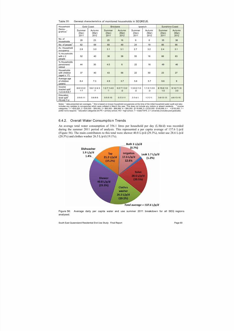
7/27/2019 Trabalho_Austrália
http://slidepdf.com/reader/full/trabalhoaustralia 70/174
Table 20: General characterist ics of moni tored households in SEQREUS.
Gold Coast Brisbane Ipswich Sunshine CoastHouseholdDemo-grahics
1 Summer (Dec)2011
Autumn(Mar)2012
Summer (Dec)2011
Autumn(Mar)2012
Summer (Dec)2011
Autumn(Mar)2012
Summer (Dec)2011
Autumn(Mar)2012
No. of
households 28 23 25 16 9 6 35 38
No. of people2
82 69 65 49 24 19 85 95
Av. Householdoccupancy
2.8 3.0 3.1 3.1 2.7 3.2 2.4 3.1
% Householdswith ≤ 2people
52 40 38 38 55 16 66 63
% Householdspensioners/retired
44 30 4.5 6 22 16 49 46
Householdswith children(aged ≤ 17)
37 40 43 56 22 50 23 27
Average age
of children(years) 8.4 7.3 4.9 3.7 5.6 5.7 9.6 9
Incomebracket split
3
1:2:3:4:5:6:7
6:6:3:3:2:1:2
5:6:1:2:4:3:2
1:2:7:1:4:0:2
0:2:7:1:3:2:0
1:3:0:2:1:0:0
1:1:0:1:2:0:0
8:15:6:1:0:1:0
9:14:7:1:0:3:0
Educationlevel split
4
PS:HS:T:U0:9:5:11 0:6:8:9 0:5:5:10 0:2:3:11 2:2:4:1 1:2:2:1 3:6:13:13 4:6:13:15
Notes:1
data presented are averages,2
this is based on known household occupancies at the time of the initial household water audit and alsoincludes any updates to occupancies which were collated in March this year. This does not include any visitors or absent residents.
3income
categories: 1 = <$30,000, 2 = $30,000 – $59,000, 3 = $60,000 – $89,999, 4 = $90,000 - $119,999, 5 = $120,000 - $149,999, 6 = ≥ $150,000, 7 =prefer not to respond. 4 education categories are PS = primary school, HS = high school, T = trade/TAFE, U = university (includes post graduate).
6.4.2. Overall Water Consumption Trends
An average total water consumption of 356.1 litres per household per day (L/hh/d) was recordedduring the summer 2011 period of analysis. This represented a per capita average of 137.6 L/p/d(Figure 56). The main contributors to this total were shower 40.8 L/p/d (29.3%), toilet use 28.6 L/p/d(20.5%) and clothes washer 26.5 L/p/d (19.1%).
Figure 56: Average daily per capita water end use summer 2011 breakdown for all SEQ regions
analysed.
South East Queensland Residential End Use Study: Final Report Page 60
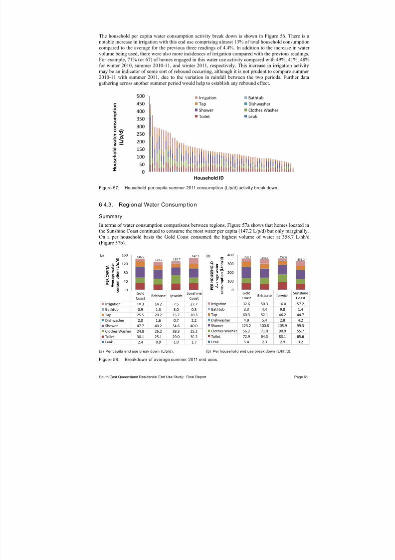
7/27/2019 Trabalho_Austrália
http://slidepdf.com/reader/full/trabalhoaustralia 71/174
The household per capita water consumption activity break down is shown in Figure 56. There is anotable increase in irrigation with this end use comprising almost 13% of total household consumptioncompared to the average for the previous three readings of 4.4%. In addition to the increase in water volume being used, there were also more incidences of irrigation compared with the previous readings.For example, 71% (or 67) of homes engaged in this water use activity compared with 49%, 41%, 48%for winter 2010, summer 2010-11, and winter 2011, respectively. This increase in irrigation activitymay be an indicator of some sort of rebound occurring, although it is not prudent to compare summer 2010-11 with summer 2011, due to the variation in rainfall between the two periods. Further datagathering across another summer period would help to establish any rebound effect.
0
50
100
150
200
250
300
350
400
450
500
H o u s e h o l d w a t e r c o n s u m p t i o n
( L / p
/ d )
Household ID
Irrigation Bathtub
Tap Dishwasher
Shower Clothes Washer
Toilet Leak
Figure 57: Household per capita summer 2011 consumption (L/p/d) activity break down.
6.4.3. Regional Water ConsumptionSummary
In terms of water consumption comparisons between regions, Figure 57a shows that homes located inthe Sunshine Coast continued to consume the most water per capita (147.2 L/p/d) but only marginally.On a per household basis the Gold Coast consumed the highest volume of water at 358.7 L/hh/d(Figure 57b).
Gold
CoastBrisbane Ipswich
Sunshine
Coast
Irrigation 10.3 14.2 7.5 27.2
Bathtub 0.9 1.3 3.0 0.3
Tap 25.5 20.2 15.7 20.3
Dishwasher 2.0 1.6 0.7 2.2
Shower 47.7 40.2 34.6 40.0
Clothes Washer 24.8 26.2 39.3 25.2
Toilet 30.1 25.1 29.0 30.2
Leak 2.4 0.9 1.0 1.7
0
40
80
120
160
P E R C
A P I T A
A v e r a g
e w a t e r
c o n s u m p t
i o n ( L / p / d ) 146.5 147.2
130.7129.7
(a)
Gold
CoastBrisbane Ipswich
Sunshine
Coast
Irrigation 32.6 50.3 16.0 57.2
Bathtub 3.3 4.4 9.8 1.4
Tap 60.3 52.1 46.2 44.7
Dishwasher 4.9 5.4 2.8 4.2
Shower 123.2 100.8 105.9 99.3
Clothes Washer 56.2 71.0 90.9 55.7
Toilet 72.9 64.3 83.1 65.6
Leak 5.4 2.3 2.9 3.2
0
100
200
300
400
P E R H O U
S E H O L D
A v e r a g e w a t e r
c o n s u m p t i o n ( L / h h / d ) 358.7
331.2357.6350.5
(b)
(a) Per capita end use break down (L/p/d). (b) Per household end use break down (L/hh/d).
Figure 58: Breakdown of average summer 2011 end uses.
South East Queensland Residential End Use Study: Final Report Page 61

7/27/2019 Trabalho_Austrália
http://slidepdf.com/reader/full/trabalhoaustralia 72/174
The end uses which varied markedly between regions were clothes washers and irrigation, as shown inFigure 58. Toilet use, which typically has a relatively stable contribution of around 15 to 20% of totalhousehold consumption, is observed to be comparatively heterogeneous across regions for the summer 2011 period (Figure 58).
Gold
CoastBrisbane Ipswich
Sunshine
Coast
Irrigation 7.0 10.9 5.7 18.5
Bathtub 0.6 1.0 2.3 0.2
Tap 17.4 15.6 12.0 13.8
Dishwasher 1.4 1.2 0.6 1.5
Shower 32.6 31.0 26.5 27.2
Clothes Washer 16.9 20.2 30.0 17.1
Toilet 20.6 19.4 22.2 20.5
Leak 1.6 0.7 0.7 1.2
0
25
50
75
100
P E R C A P I T A
A v e r a g e p e r c e n t o f t o t a l
h o u s e h o l d w a t e r u s e ( %
)(a)
Gold
CoastBrisbane Ipswich
Sunshine
Coast
Irrigation 9.1 14.4 4.5 17.3
Bathtub 0.9 1.2 2.7 0.4
Tap 16.8 14.9 12.9 13.5
Dishwasher 1.4 1.5 0.8 1.3
Shower 34.4 28.8 29.6 30.0
Clothes Washer 15.7 20.3 25.4 16.8
Toilet 20.3 18.4 23.2 19.8
Leak 1.5 0.7 0.8 1.0
0
25
50
75
100
P E R H O U S E H O L D
A v e r a g e p e r c e n t o f t o t a
l
h o u s e h o l d w a t e r u s e ( %
)(b)
(a) Per capita end use break down. (b) Per household end use break down.
Figure 59: Average percentage of total summer 2011 water consumption.
Gold Coast
Properties in the Gold Coast recorded an average total water consumption in summer 2011 of 358.7 L/hh/d or 146.5 L/p/d (Figure 59a), ranging from 47.8 L/p/d to 444.3 L/p/d (Figure 59b). End
use break down on a per capita basis indicates that, on average, shower (33.3%), clothes washer (20.5%) tap (17.7%) and toilet (18.2%) comprised the bulk of the water consumption (Figure 59a).Irrigation contributed an average of 5.2 L/p/d or 4% of total water use.
(a) Per capita end use break down (L/p/d). (b) Per capita end use break down (L/p/d) by household.
Figure 60: Break down of average summer 2011 end uses for the Gold Coast.
South East Queensland Residential End Use Study: Final Report Page 62

7/27/2019 Trabalho_Austrália
http://slidepdf.com/reader/full/trabalhoaustralia 73/174
Brisbane
Average household consumption in Brisbane was 350.5 L/hh/d, resulting in a per capita consumptionaverage of 129.7 L/p/d (Figure 60). The average irrigation consumption of 14.2L/p/d was skewed byone household that was believed to have been filling a pool.
(a) Per capita end use break down (L/p/d). (b) Per capita end use break down (L/p/d) by household.
Figure 61: Break down of average summer 2011 end uses for Brisbane.
Ipswich
The period of analysis in the Ipswich region showed an average household consumption of 357.6 L/hh/day. This resulted in a per capita figure of 130.7 L/p/d (Figure 61a). Due to the low sample
size (n=9 homes), the authors are reluctant to draw too many conclusions from the data.
(a) Per capita end use break down (L/p/d). (b) Per capita end use break down (L/p/d) by household.
Figure 62: Break down of average summer 2011 end uses for Ipswich.
South East Queensland Residential End Use Study: Final Report Page 63

7/27/2019 Trabalho_Austrália
http://slidepdf.com/reader/full/trabalhoaustralia 74/174
Sunshine Coast
At n=35, the number of households was the highest of all regions for the summer 2011 sampling period (Table 4). The Sunshine Coast residents while consuming the highest volumes of water per capita for all regions during the summer of 2011, at an average of 147.2 L/p/d, it had a comparatively
low per household water consumption of 331.2 L/hh/d (Figure 62). Irrigation is quire elevated for theSunshine Coast compared to the other regions, and the other sampling periods.
(a) Per capita end use break down (L/p/d). (b) Per capita end use break down (L/p/d) by househol d.
Figure 63: Break down of average summer 2011 end uses for the Sunshine Coast.
6.5. Autumn 2012 Results
6.5.1. Sample Size
For autumn (March) 2012, 83 homes were analysed for mains water end uses. This comprised 23 inthe Gold Coast, 16 in Brisbane, 6 in Ipswich and 38 in the Sunshine Coast. Again, many of the metersand loggers required some general maintenance in order to continue logging; given constrained projectfunding towards the end of the project, such required servicing was not possible at the time of datadownload and analysis, as explained in section 6.4.1. The general characteristics of the additionalsampling periods are presented in Table 20.
6.5.2. Overall Water Consumption Trends
An average total water consumption of 378.5 litres per household per day (L/hh/d) was recorded
during the summer 2011 period of analysis. This represented a per capita average of 144.4 L/p/d(Figure 64). The main contributors to this total were shower 39.2 L/p/d (27.3%), clothes washer 29.0 L/p/d (20.2%), toilet use 25.2 L/p/d (17.6%) and irrigation 24 L/p/d (16.7%).
South East Queensland Residential End Use Study: Final Report Page 64
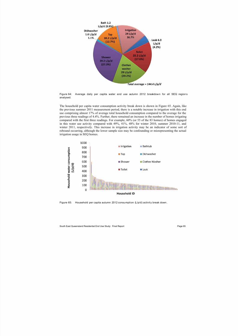
7/27/2019 Trabalho_Austrália
http://slidepdf.com/reader/full/trabalhoaustralia 75/174
Figure 64: Average daily per capita water end use autumn 2012 breakdown for all SEQ regions
analysed.
The household per capita water consumption activity break down is shown in Figure 65. Again, likethe previous summer 2011 measurement period, there is a notable increase in irrigation with this enduse comprising almost 17% of average total household consumption compared to the average for the
previous three readings of 4.4%. Further, there remained an increase in the number of homes irrigatingcompared with the first three readings. For example, 60% (or 55 of the 83 homes) of homes engaged
in this water use activity compared with 49%, 41%, 48% for winter 2010, summer 2010-11, andwinter 2011, respectively. This increase in irrigation activity may be an indicator of some sort of rebound occurring, although the lower sample size may be confounding or misrepresenting the actualirrigation usage in SEQ homes.
Figure 65: Household per capita autumn 2012 consumption (L/p/d) activit y break down.
South East Queensland Residential End Use Study: Final Report Page 65
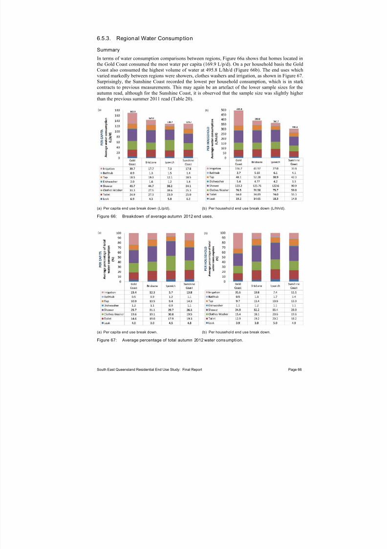
7/27/2019 Trabalho_Austrália
http://slidepdf.com/reader/full/trabalhoaustralia 76/174
6.5.3. Regional Water Consumption
Summary
In terms of water consumption comparisons between regions, Figure 66a shows that homes located inthe Gold Coast consumed the most water per capita (169.9 L/p/d). On a per household basis the GoldCoast also consumed the highest volume of water at 495.8 L/hh/d (Figure 66b). The end uses whichvaried markedly between regions were showers, clothes washers and irrigation, as shown in Figure 67.Surprisingly, the Sunshine Coast recorded the lowest per household consumption, which is in stark contracts to previous measurements. This may again be an artefact of the lower sample sizes for theautumn read, although for the Sunshine Coast, it is observed that the sample size was slightly higher than the previous summer 2011 read (Table 20).
(a) Per capita end use break down (L/p/d). (b) Per household end use break down (L/hh/d).
Figure 66: Breakdown of average autumn 2012 end uses.
(a) Per capita end use break down. (b) Per household end use break down.
Figure 67: Average percentage of total autumn 2012 water consumption.
South East Queensland Residential End Use Study: Final Report Page 66

7/27/2019 Trabalho_Austrália
http://slidepdf.com/reader/full/trabalhoaustralia 77/174
Gold Coast
Properties in the Gold Coast recorded an average total water consumption in autumn 2012 of 495.8 L/hh/d or 169.9 L/p/d (Figure 68a). The breakdown of end-uses per household indicates that anextreme high irrigation event (~900 L/p/d) at one home has skewed the total average consumptionfigures (Figure 68b). Apart from irrigation, other key end uses contributing to the total average were
ranging from 47.8 L/p/d to 444.3 L/p/d (Figure 59b). End use break down on a per capita basisindicates that, on average, shower (25.7%), clothes washer (19.6%), and toilet (14.6%).
(a) Per capita end use break down (L/p/d). (b) Per capita end use break down (L/p/d) by househol d.
Figure 68: Break down of average autumn 2012 end uses for the Gold Coast.
Brisbane
Average household consumption in Brisbane was 390.0 L/hh/d, resulting in a per capita consumptionaverage of 143.6 L/p/d (Figure 69). Shower use was a significant component of total average use,comprising over 30% or 44.7 L/p/d of consumption. Irrigation occurred in 60% of homes, at anaverage of 28.8 L/p/d for these particular homes. Overall, average irrigation consumption in all homeswas 17.7 L/p/d (12.3%).
(a) Per capita end use break down (L/p/d). (b) Per capita end use break down (L/p/d) by household.
Figure 69: Break down of average autumn 2012 end uses for Brisbane.
South East Queensland Residential End Use Study: Final Report Page 67

7/27/2019 Trabalho_Austrália
http://slidepdf.com/reader/full/trabalhoaustralia 78/174
Ipswich
The period of analysis in the Ipswich region showed an average household consumption of 366.7 L/hh/day. This resulted in a per capita figure of 127.8 L/p/d (Figure 70a). Due to the very lowsample size (n=6 homes), the authors are reluctant to draw too many conclusions from the data.
(a) Per capita end use break down (L/p/d). (b) Per capita end use break down (L/p/d) by househol d.
Figure 70: Break down of average autumn 2012 end uses for Ipswich.
Sunshine Coast
At n=38, the number of households was the highest of all regions for the autumn 2012 sampling period(Table 20). The Sunshine Coast residents, while consuming the highest volumes of water per capitafor all regions during the summer of 2011, at an average of 127.9 L/p/d, it had a comparatively low per household water consumption of 304.4 L/hh/d (Figure 71). Irrigation is quire elevated for the SunshineCoast compared to the other regions, and other sampling periods. Irrigation occurred in 70% of thehomes, at an average of 25.7 L/p/d.
(a) Per capita end use break down (L/p/d). (b) Per capita end use break down (L/p/d) by househol d.
Figure 71: Break down of average autumn 2012 end uses for the Sunshine Coast.
South East Queensland Residential End Use Study: Final Report Page 68

7/27/2019 Trabalho_Austrália
http://slidepdf.com/reader/full/trabalhoaustralia 79/174
6.6. Winter versus Summer SEQREUS Data
Average end use consumption breakdowns are shown for each period of analysis for the averageacross all regions (Figure 72) and individual regions (Figure 73). As has been identified previously,summer 2010-11 average consumption is lower than both winter reads due to the extreme weather
events and CSIRO/UQ intervention study which encouraged frugal water use, which appeared to have been particularly effective for shower and clothes washing activities. Leaks have also beensubstantially reduced as a result of communications to homeowners that were identified as havingexcessive leaks (Figure 72). The impacts on the intervention study will presented and discussed indetail in a separate technical report (Gardner et al., forthcoming).
(a) Average per capita breakdown.
(b) Percentage of total water consumption.
Figure 72: Break down of average winter and summer end uses for SEQ combined.
South East Queensland Residential End Use Study: Final Report Page 69

7/27/2019 Trabalho_Austrália
http://slidepdf.com/reader/full/trabalhoaustralia 80/174
With the exception of leaks and shower usage, average end use consumption for both winter periodswere very similar. On a percentage basis, end use breakdowns across all seasons were quite similar with the exception of shower use in the winter 2011 sample which may be biased by the smaller sample size. Therefore, while the summer 2010-11 volumetric averages are lower, the end use
percentages of total consumption are reasonably comparable, and it is expected that this would be thecase for indoor water use more so than outdoor water use for a typical (more average rainfall) summer.
Looking at the regional breakdowns, it is clear that Gold Coast and Brisbane were mainly responsiblefor the upward shift in shower end use consumption (Figure 73a, 73b). Collectively, for the winter 2011 analysis, households in these two regions had the highest percentage of families with children≤ 17 years old. This may be reflected in the higher shower use and slightly higher bath end use also.The influence of household typology and socio-demographics are discussed in detail in Section 11.
Average end use breakdowns for Ipswich are very stable across the seasons, despite the reducedsample sizes, particularly for the final winter 2011 read (n=12). As there is very little irrigation for many of the Ipswich households, essentially it is the indoor end uses that are being compared inFigure 73c. The Ipswich sample provides a good example of a low level of fluctuation between indoor end uses which have been reported elsewhere (e.g. Willis et al., 2011a; DeOreo et al., 2004; Jacobs
and Haarhoff, 2004). The homogeneity in indoor end uses further emphasises the strong influence thatirrigation can have on total household demand and thus the value of supplementing irrigation water sources such as rainwater tanks and greywater systems.
Winter 2010 Summer 2010‐11 Winter 2011
Irrigation 7.2 2.7 2.5
Bathtub 1.8 1.5 2.7Tap 22.7 25.9 28.5
Dishwasher 2.3 1.7 1.3
Shower 38.4 34.5 51.8
Clothes washer 35.7 27.9 38.2
Toilet 21.9 20.3 19.9
Leak 13.3 3.8 1.1
0
20
40
60
80
100
120
140
160
A v e r a g e d a i l y p e r c a p i t a
w a t e r c o n s u m p t i o n ( L / p / d )(a)
Winter 2010 Summer 2010‐11 Winter 2011
Irrigation 10.7 4.9 5.2
Bathtub 1.9 1.7 3.9Tap 33.7 25.4 25.1
Dishwasher 1.9 1.7 2.6
Shower 40.2 34.7 47.0
Clothes washer 28.2 22.0 29.0
Toilet 20.4 19.6 25.8
Leak 4.6 4.6 2.9
0
20
40
60
80
100
120
140
160
A v e r a g e d a i l y p e r c a p i t a
w a t e r c o n s u m p t i o n ( L / p / d )(b)
(a) Gold Coast seasonal comparison. (b) Brisbane seasonal comparis on.
Winter 2010 Summer 2010‐11 Winter 2011
Irrigation 1.7 1.2 0.3
Bathtub 0.1 0.0 0.0
Tap 23.2 23.7 19.6
Dishwasher 1.5 1.0 1.0
Shower 36.3 30.5 34.5
Clothes washer 24.9 25.4 26.2
Toilet 21.3 26.7 24.9
Leak 2.8 3.1 4.0
0
20
40
60
80
100
120
A v e r a g e d a i l y p e r c a p i t a
w a t e r c o n s u m
p t i o n ( L / p / d )(c)
Winter 2010 Summer 2010‐11 Winter 2011
Irrigation 6.8 9.1 12.8
Bathtub 2.9 2.1 0.1
Tap 25.8 31.5 24.5
Dishwasher 4.2 2.7 2.8
Shower 50.7 42.6 55.8
Clothes washer 33.3 30.3 31.5
Toilet 30.2 27.2 26.2
Leak 14.0 3.2 4.2
0
20
40
6080
100
120
140
160
180
A v e r a g e d a
i l y p e r c a p i t a
w a t e r c o n s u m p t i o n ( L / p / d )(d)
(c) Ipswich seasonal comparison. (d) Sunshine Coast seasonal comparis on.
Figure 73: Break down of average winter and summer end uses for each region .
South East Queensland Residential End Use Study: Final Report Page 70

7/27/2019 Trabalho_Austrália
http://slidepdf.com/reader/full/trabalhoaustralia 81/174

7/27/2019 Trabalho_Austrália
http://slidepdf.com/reader/full/trabalhoaustralia 82/174
100
200
300
400
500
600
700
800
A v e r a g
e d a i l y h o u s e h o l d w a t e r c o n s u m p t i o n
( L / h h / d )
Time (months)
Average daily total consumption in SEQ
Average consumption
across
the
measured
period
PD/AD
1.5PD/AD
1.2
PD/AD
1.7
(a)30/12/10 10/04/11
(c) (d)(i)
(ii)
(i)
(ii)
(i)
(ii)
PD/AD
1.3
07/01/11
(b)(i)
(ii)
(e)(i)
(ii)
14 – 28 June
Winter, 2010
TOIL 34
CW
42SHOW
58
TAP 27
EX
13
0
4
8
12
16
1 3 5 7 9 1 1 13 15 17 19 21 23
A v e r a g e d a i l y d i u r n a l
c o n s u m p t i o n ( L / p / h / d )
Hour of day
EXBATH
TAP
SHOW
CW
TOIL
0
5
10
15
20
25
1 3 5 7 9 11 13 15 17 19 21 23
A v e r a g e d a i l y d i u r n a l
c o n s u m p t i o n ( L / p / h / d )
Hour of day
EX
BATH
TAP
SHOW
CW
TOIL
0
4
8
12
16
20
1 3 5 7 9 1 1 1 3 1 5 1 7 1 9 2 1 2 3
A v e r a g e d a i l y d i u r n a l
c o n s u m p t i o n ( L / p / h / d )
Hour of day
EXTAP
SHOW
CW
TOIL
LEAK
TOIL 34
CW
57
SHOW
41
TAP 23
EX
12
TOIL
24
CW
31SHOW
43
TAP 28
0
2
4
6
8
10
12
14
1 3 5 7 9 1 1 13 15 17 19 21 23
A v e r a g e d a i l y d
i u r n a l
c o n s u m p t i o n ( L / p / h / d )
Hour of day
EX
BATH
TAP
DWSHOW
CW
TOIL
LEAK
TOIL
37
CW
56
SHOW
61
TAP
24
(f)(i)
1 Dec – 22 Feb
Summer 2010‐11 (g)(i)
(ii)
1– 14 June
Winter 2011
0
10
20
30
40
1
A v e r a g e d a i l y d i u r n a l
c o n s u m p t i o n ( L / p / h / d )
0
2
4
68
10
12
14
1 3 5 7 9 1 1 13 15 17 19 21 23
A v e r a g e d a i l y
d i u r n a l
c o n s u m p t i o n ( L / p / h / d )
Hour of day
EX BATH TAP DW
SHOW CW TOIL Leak
0
2
4
68
10
12
14
1 3 5 7 9 11 13 15 17 19 21 23
A v e r a g e d a i l y d
i u r n a l
c o n s u m p t i o n ( L / p / h / d )
Hour of day
EX BATH TAP DW
SHOW CW TOIL Leak
(ii)
TOIL
24
CW
32SHOW
50
TAP
25
L
4
TOIL
23
CW
27SHOW
36
TAP
27
EX
5
Notes: EX = external, TOIL = toilet, CW = clothes washer, SHOW = shower, DW = dishwasher, L = leak.
Figure 74: Timeline for total water consumpt ion show ing (i) water use breakdown in L/p/d and (ii) average daily diurnal watedays of (a) 30/12/10, (b) 07/01/11, (c) 10/04/11, and (d) 02/07/11 and (e) baseline data fo r winter 2010, (f) summer 2010-11, (g) win
South East Queensland Residential End Use Study: Final Report

7/27/2019 Trabalho_Austrália
http://slidepdf.com/reader/full/trabalhoaustralia 83/174
One other important characteristic of the peak day diurnal patterns is the timing of the external water use activities. In SEQ, where the data was sourced from, there is a current restriction on irrigation
between 10 am and 4 pm. The results demonstrate a degree of non-compliance during this timeframeand further, this practice appeared to have increased rather than decreased over the 18-monthmonitoring period, judging by the consumption timeline shown in Figure 74.
7.3.1. Peaking Factors and End Use Analysis
The peaking factor (PF) is the ratio of the maximum flow to the average daily flow in a water system.Peaking factors for peak day (e.g. PD/AD) and peak hour (e.g. PHPD/PHAD) are the basis for designing mains water supply infrastructure. A peaking factor over one indicates high water volumes,with potential capacity constraints if the supply pipes are not of sufficient diameter.
Peak Day Factors
A breakdown of average daily total water consumption showing the peaking factor trend for combinedSEQ sample is shown in Figure 75. Less than a third of the data had peaking factors over one, thusextreme usage from a small number of days, primarily driven by irrigation/external use, is likely to
dictate the average peaking factor of any given region. The relative frequency distribution of PD/ADof each month is shown in Figure 75b (inset) where it can be observed that PD/AD factors between 0.8and 1.4 occurred with the greatest frequency. The four peak demand days selected had increasing peak day factors of 1.3, 1.5, 1.6 and 1.7 (Figure 74). These values lie within the lower end of the rangereported for local guidelines, of 1.5 to 2.3 (DERM, 2010); and well within the ranges reportedelsewhere in the literature (Van Zyl et al., 2011, Surendran et al., 2005).
0
0.5
1
1.5
2
2.5
0
100
200
300
400
500
600
700
800
1 50 99 148 197 246 295 344 393 442 491 540
P e a k i n g f a c t o r ( P D / s t u d y A D )
T o t a l
d a i l y h o u s e h o l d c o n s u m p t i o n ( L / h h / d )
Number of days of data
Average consumption (left)
Median average consumption (left)
Peaking factor (right)
(a)
0.6‐0.7 0.7‐0.8 0.8‐0.9 0.9‐1.0 1.0‐1.2 1.2‐1.4 1.4‐1.6 1.6‐1.8
RF 0 0.007 0.136 0.358 0.397 0.081 0.011 0.005
CF 0 0.007 0.143 0.501 0.898 0.979 0.989 0.995
0
0.2
0.4
0.6
0.8
1
0
0.1
0.2
0.3
0.4
C u m u l a t i v e f r e q u e n c y C F )
R e l a t i v e f r
e q u e n c y ( R F )
(b)
Figure 75: Breakdown of (a) average daily total water consumption (LHS) and PD:AD ratio (RHS) and(b) frequency distr ibutions for combined SEQ sample peaking factors.
Peak Hour Factors
The peak hour in average day (PHAD) values (i.e. morning and evening peak hour in average day)were derived from an average of the three periods of analysis: winter 2010, summer 2010-11 andwinter 2011. The peak hour in peak day (PHPD) values were taken from each of the four peak day end
use diurnal demand patterns. As expected, the hourly peaking factors are higher than the daily factors.Hourly peaking factors ranged from 1.7 to 3.0 in the morning and 1.3 to 2.8 in the afternoon(Figure 76). Notably, they are lower than the range of Queensland government reported values (i.e. 3.6to 5.0), although other researchers have reported similar ranges to those observed in this study (e.g.Shvarster et al., 1993; WSAA, 2002).
South East Queensland Residential End Use Study: Final Report Page 73

7/27/2019 Trabalho_Austrália
http://slidepdf.com/reader/full/trabalhoaustralia 84/174
0.0
0.5
1.0
1.5
2.0
2.5
3.0
3.5
AM PM AM PM AM PM AM PM
30/12/10 7/01/11 10/04/11 2/07/11
A v e r a g e P H P D / P H A D p e a k i n g f a c t o r s
Time
External Bath Tap Dish washer
Shower Clothes washer Toilet
1.8
2.8
3.0
2.7
1.81.81.7
1.3
Figure 76: Relative proport ion of average hour ly end-use PHPD/PHAD ratios for morning and afternoonpeak hours.
A breakdown of individual end use peak hour (PHPD/PHAD) factors demonstrates that all end usesare elevated during peak demand days, however, it is clear that external water use events are driving
peak hour use (Figure 76). This is consistent with other findings such as Willis et al. (2011b) whofound a strong association with irrigation and peak morning and afternoon diurnal patterns. Similar results were reported by Roberts (2005) and Heinrich (2007). Other end uses, such as shower and
clothes washer, have also been strongly associated with peak hour and peak day demand (Beal et al.,2011; Willis et al., 2011b).
7.3.2. Influence of Climate on Total Household Consumption
A timeline of average temperature, rainfall and daily total consumption for each month of the study is presented in Figure 77. The four peak days selected for analysis are indicated by the hatched triangleson the water consumption curve. There is a weak relationship between increased temperature and peak demand days, although this is not consistent across the timeline. There is a stronger association
between temperature and total household water consumption for the warmer months, e.g. January toMarch 2010 and November to March 2011. Cole and Stewart (in review) report a strong correlation
between temperature and bulk water demand for the Hervey Bay region of SEQ. Others have alsoobserved this relationship between temperature and residential water consumption (Water Corporation2011; Willis et al., 2011b; Adamowski 2008). Another weak relationship is apparent for low rainfalland increased water demand during the months of April to August 2010 and June to July 2011(Figure 70). It should be noted that the high rainfall events occurring in December 2010 and January2011 contributed to major flooding across SEQ, effectively eliminating the need for irrigation duringthis period.
South East Queensland Residential End Use Study: Final Report Page 74

7/27/2019 Trabalho_Austrália
http://slidepdf.com/reader/full/trabalhoaustralia 85/174
0
5
10
15
20
25
30
35
40
0
50
100
150
200
250
300
350
400
450
A v e r a g e m o n t h l y t e m p e r a t u r e ( C ° )
A v e r a g e m o n t h l y r a i n f a l l ( m m ) a n d a v
e r a g e t o t a l d a i l y
w a t e r c o n s u m p t i o n ( L / h h / d )
Time (months)
Average monthly rainfall (left y‐axis)
Average total daily consumption (left y‐axis)
Peak day in month breakdown shown in Fig. 2
Average monthly temperature (right y‐axis)
Note: Climate data sourced from the Bureau of Meteorology http://www.bom.gov.au/climate/data/index.shtml.using data averaged from the GoldCoast, Brisbane, Sunshine Coast and Ipswich weather stations – see notes from Table 2.
Figure 77: Timeline of average monthly climate data and daily household water consumption.
7.4. Future Trends in Peak Demand
There is wide acknowledgement of the need to adapt to, as well as mitigate for, climate changeimpacts on the urban water systems (Gleick 2003; Polebitski et al., 2011; Short et al., 2012). Direct
climate change impacts, such as changes to rainfall and temperature patterns, may see the past peak water usage period, historically in the summer months (December to February) in sub-tropicalQueensland, shift toward the drier months in winter (June to August). Recent climate modelling inQueensland has shown that shorter but more intense rainfall patterns in the summer, resulting in alonger period of dry weather over the winter months (Queensland Government 2012). The data
presented in this paper demonstrates that peak demand times were not restricted to summer months,occurring throughout the year, including April and July. Prior to the peak water usage day on 02/07/11of 261 L/p/d, there was a period of approximately two weeks with negligible rainfall and low relativehumidity in the SEQ region. These conditions are typical of winter climate in SEQ and it is believedthat the conditions were likely to have prompted the observed sudden increase in the number of irrigation events occurring on that Saturday.
Indirect impacts on urban water systems from climate change include the introduction of resource-efficient planning initiatives (i.e. water conservation and intervention programmes, high density, lowfootprint housing, water-efficient fixtures, internally connected rainwater tanks), borne from climatechange adaptation strategies. Such initiatives have shown to substantially reduce household water consumption (Fidar et al., 2010; Beal et al., 2012; Fielding et al., 2012). For example, while peak daydemand in a SEQ context has been shown to be consistently influenced primarily by external(irrigation) and shower events, this may not necessarily remain the case in the future, due to the high
penetration of water efficient technology and a shift toward more frugal consumer behaviour. Peakingfactors may well be lower now and into the future than say a decade ago where water consumptionwas an average of 300 L/p/d in SEQ. Tsang (2010) found that using the same SEQREUS data used inthis study, peak flow rates were around 15% less than currently estimated values for bulk trunk mainsin the Gold Coast, Queensland; translating into potential lower diameter trunk mains in future
infrastructure planning.
South East Queensland Residential End Use Study: Final Report Page 75
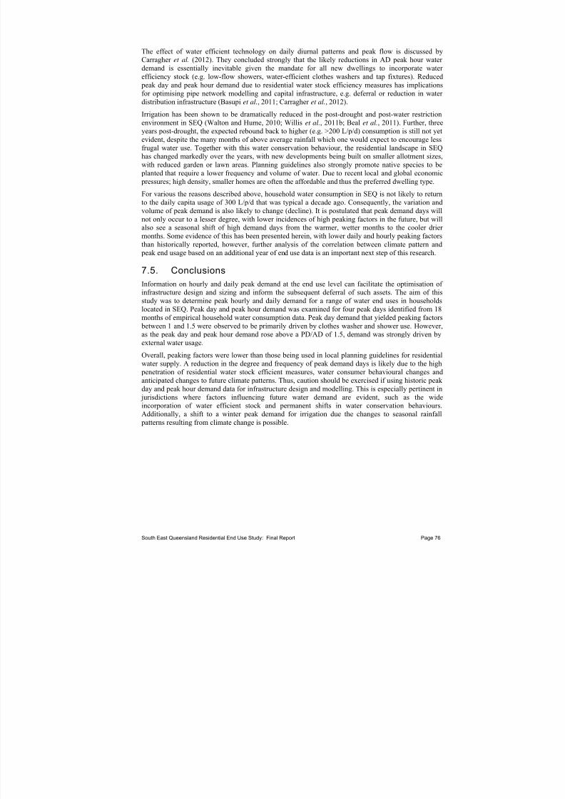
7/27/2019 Trabalho_Austrália
http://slidepdf.com/reader/full/trabalhoaustralia 86/174
South East Queensland Residential End Use Study: Final Report Page 76
The effect of water efficient technology on daily diurnal patterns and peak flow is discussed byCarragher et al. (2012). They concluded strongly that the likely reductions in AD peak hour water demand is essentially inevitable given the mandate for all new dwellings to incorporate water efficiency stock (e.g. low-flow showers, water-efficient clothes washers and tap fixtures). Reduced
peak day and peak hour demand due to residential water stock efficiency measures has implicationsfor optimising pipe network modelling and capital infrastructure, e.g. deferral or reduction in water distribution infrastructure (Basupi et al., 2011; Carragher et al., 2012).
Irrigation has been shown to be dramatically reduced in the post-drought and post-water restrictionenvironment in SEQ (Walton and Hume, 2010; Willis et al., 2011b; Beal et al., 2011). Further, threeyears post-drought, the expected rebound back to higher (e.g. >200 L/p/d) consumption is still not yetevident, despite the many months of above average rainfall which one would expect to encourage lessfrugal water use. Together with this water conservation behaviour, the residential landscape in SEQhas changed markedly over the years, with new developments being built on smaller allotment sizes,with reduced garden or lawn areas. Planning guidelines also strongly promote native species to be
planted that require a lower frequency and volume of water. Due to recent local and global economic pressures; high density, smaller homes are often the affordable and thus the preferred dwelling type.
For various the reasons described above, household water consumption in SEQ is not likely to returnto the daily capita usage of 300 L/p/d that was typical a decade ago. Consequently, the variation andvolume of peak demand is also likely to change (decline). It is postulated that peak demand days willnot only occur to a lesser degree, with lower incidences of high peaking factors in the future, but willalso see a seasonal shift of high demand days from the warmer, wetter months to the cooler drier months. Some evidence of this has been presented herein, with lower daily and hourly peaking factorsthan historically reported, however, further analysis of the correlation between climate pattern and
peak end usage based on an additional year of end use data is an important next step of this research.
7.5. Conclusions
Information on hourly and daily peak demand at the end use level can facilitate the optimisation of infrastructure design and sizing and inform the subsequent deferral of such assets. The aim of thisstudy was to determine peak hourly and daily demand for a range of water end uses in householdslocated in SEQ. Peak day and peak hour demand was examined for four peak days identified from 18months of empirical household water consumption data. Peak day demand that yielded peaking factors
between 1 and 1.5 were observed to be primarily driven by clothes washer and shower use. However,as the peak day and peak hour demand rose above a PD/AD of 1.5, demand was strongly driven byexternal water usage.
Overall, peaking factors were lower than those being used in local planning guidelines for residentialwater supply. A reduction in the degree and frequency of peak demand days is likely due to the high
penetration of residential water stock efficient measures, water consumer behavioural changes andanticipated changes to future climate patterns. Thus, caution should be exercised if using historic peak day and peak hour demand data for infrastructure design and modelling. This is especially pertinent in
jurisdictions where factors influencing future water demand are evident, such as the wideincorporation of water efficient stock and permanent shifts in water conservation behaviours.Additionally, a shift to a winter peak demand for irrigation due the changes to seasonal rainfall
patterns resulting from climate change is possible.
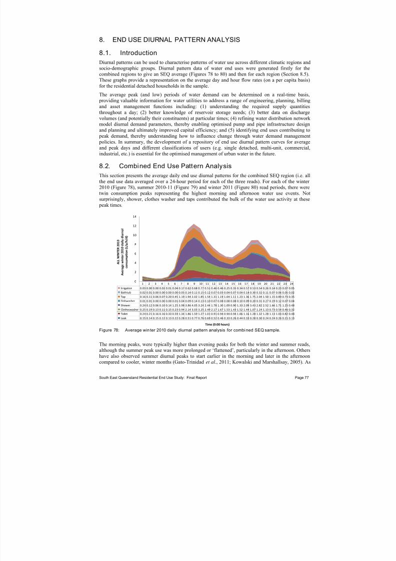
7/27/2019 Trabalho_Austrália
http://slidepdf.com/reader/full/trabalhoaustralia 87/174
8. END USE DIURNAL PATTERN ANALYSIS
8.1. Introduction
Diurnal patterns can be used to characterise patterns of water use across different climatic regions and
socio-demographic groups. Diurnal pattern data of water end uses were generated firstly for thecombined regions to give an SEQ average (Figures 78 to 80) and then for each region (Section 8.5).These graphs provide a representation on the average day and hour flow rates (on a per capita basis)for the residential detached households in the sample.
The average peak (and low) periods of water demand can be determined on a real-time basis, providing valuable information for water utilities to address a range of engineering, planning, billingand asset management functions including: (1) understanding the required supply quantitiesthroughout a day; (2) better knowledge of reservoir storage needs; (3) better data on dischargevolumes (and potentially their constituents) at particular times; (4) refining water distribution network model diurnal demand parameters, thereby enabling optimised pump and pipe infrastructure designand planning and ultimately improved capital efficiency; and (5) identifying end uses contributing to
peak demand, thereby understanding how to influence change through water demand management policies. In summary, the development of a repository of end use diurnal pattern curves for averageand peak days and different classifications of users (e.g. single detached, multi-unit, commercial,industrial, etc.) is essential for the optimised management of urban water in the future.
8.2. Combined End Use Pattern Analysis
This section presents the average daily end use diurnal patterns for the combined SEQ region (i.e. allthe end use data averaged over a 24-hour period for each of the three reads). For each of the winter 2010 (Figure 78), summer 2010-11 (Figure 79) and winter 2011 (Figure 80) read periods, there weretwin consumption peaks representing the highest morning and afternoon water use events. Notsurprisingly, shower, clothes washer and taps contributed the bulk of the water use activity at these
peak times.
1 2 3 4 5 6 7 8 9 10 11 12 13 14 15 16 17 18 19 20 21 22 23 24
Irrigation 0.03 0.00 0.00 0.02 0.01 0.04 0.17 0.62 0.68 0.77 0.51 0.46 0.46 0.25 0.35 0.34 0.57 0.53 0.54 0.26 0.14 0.23 0.07 0.05
Bathtub 0.02 0.01 0.00 0.00 0.00 0.00 0.05 0.14 0.11 0.15 0.12 0.07 0.03 0.04 0.07 0.04 0.14 0.30 0.32 0.11 0.07 0.06 0.05 0.02
Tap 0.16 0.11 0.06 0.07 0.20 0.45 1.19 1.94 2.02 1.85 1.54 1.31 1.19 1.04 1.11 1.23 1.36 1.75 2.04 1.50 1.15 0.89 0.73 0.35
Dishwasher 0.01 0.01 0.00 0.00 0.00 0.01 0.04 0.09 0.14 0.13 0.10 0.07 0.08 0.08 0.08 0.10 0.09 0.20 0.31 0.27 0.19 0.12 0.07 0.04
Shower 0.24 0.12 0.06 0.10 0.14 1.25 3.98 3.86 4.05 3.24 2.44 1.78 1.30 1.09 0.90 1.33 2.09 3.43 2.82 2.52 1.66 1.71 1.25 0.48
Clotheswasher 0.25 0.19 0.13 0.11 0.15 0.23 0.94 2.14 3.03 3.25 2.49 2.17 1.67 1.53 1.43 1.52 1.44 1.07 1.24 1.13 0.73 0.54 0.46 0.32
Toilet 0.24 0.21 0.16 0.16 0.33 0.59 1.34 1.86 1.59 1.27 1.01 0.91 0.94 0.94 0.94 1.06 1.16 1.28 1.32 1.28 1.13 1.03 0.82 0.48
Leak 0.15 0.14 0.15 0.12 0.13 0.22 0.28 0.51 0.77 0.76 0.69 0.52 0.46 0.33 0.26 0.44 0.33 0.28 0.30 0.24 0.24 0.26 0.21 0.13
0
2
4
6
8
10
12
14
A L L W I N T E R 2 0 1 0
A v e r a g e w i n t e r 2 0 1 0 d a i l y d i u r n a l
c o n s u m p t i o n ( L / p / h / d )
Time (0:00 hours) Figure 78: Average win ter 2010 daily diurnal pattern analysis for combined SEQ sample.
The morning peaks, were typically higher than evening peaks for both the winter and summer reads,although the summer peak use was more prolonged or ‘flattened’, particularly in the afternoon. Othershave also observed summer diurnal peaks to start earlier in the morning and later in the afternooncompared to cooler, winter months (Gato-Trinidad et al., 2011; Kowalski and Marshallsay, 2005). As
South East Queensland Residential End Use Study: Final Report Page 77

7/27/2019 Trabalho_Austrália
http://slidepdf.com/reader/full/trabalhoaustralia 88/174
seen in Figure 79, the afternoon peak water use period during summer lasted around three hours between 6.00pm and 8.00pm where irrigation, bath, and shower use was particularly prevalent. The prolonged summer peak observed in the afternoon is likely to be a result of the longer daylight hoursresulting in the extension of outdoor activities and family evening ablutions such as shower/bath. Bathend use is clearly occurring predominantly in the early evenings and is usually associated withyounger families, where filling up the bath before bed time was commonly noted in the water diariesand water audits for many of the participants.
Figure 79: Average summer 2010-11 daily diurnal pattern analysis for combined SEQ sample.
Irrigation use appeared to occur throughout the day across both seasons, demonstrating a conflict withcurrent water restrictions and awareness messages that encourage outdoor watering in early morningand late afternoon. The winter 2010 diurnal pattern suggested that peak irrigation occurred outside therestricted daytime hours (Figure 78). However, this appeared not to be the case for summer 2010-11(Figure 79) and winter 2011 (Figure 80).
Clothes washing events were clearly preferentially occurring in the morning hours between around7.30am and 10.30am. For the winter 2011 diurnal pattern, the peak clothes washing period occurred alittle later from around 8.00am to 11.00am (Figure 80). Willis et al. (2011a) report similar trends with
clothes washing dropping markedly after 10.30am. Conversely, dishwashing water use was most prevalent in the mid to late evening which is again consistent with Willis et al. (2011a) and is wellaligned with self-reported water use activities from participants who tend to fill the dishwasher throughout the day and switch it on before retiring to bed. Should this practice also occur with theclothes washer then a notable reduction in the peak morning water use would be likely. This wouldrequire a shift in people’s habits but would have the added advantage of using off peak energydemand.
Tap use, as with toilet use, was understandably more consistent throughout the day than clothes anddishwashing events, which are only required in discrete intervals. Tap use tended to peak at the usualmorning and afternoon times of 7.00am to 9.30am and 4.00pm to 8.00 pm. For the winter 2010sample, there was a slight peak in leaks occurring in the morning, likely to be associated with tap and
toilet use. However, as a result of the leak intervention programme after winter 2010, leaks reducedsignificantly in all regions and were consistently low throughout the day, showing little diurnalvariation.
South East Queensland Residential End Use Study: Final Report Page 78

7/27/2019 Trabalho_Austrália
http://slidepdf.com/reader/full/trabalhoaustralia 89/174
Figure 80: Average win ter 2011 daily diurnal pattern analysis for combined SEQ sample.
The short, sharp peaks observed for the winter 2011 sample (Figure 80) are a little curious, especiallythe afternoon peak which usually tends to be more flattened and drawn out. One explanation may bethe smaller sample size for this winter period which would emphasise outliers (high end use data
points) at these peak times.
8.3. Overall SEQ Pattern Analysis
The cumulative average daily diurnal patterns are compared for each region in Figure 81. For eachseasonal read, Brisbane, the Gold Coast and Sunshine Coast have the most distinct peaks. Ipswich datademonstrates overall consistently low water consumption with consumption being more evenlydistributed throughout the day irrespective of season. For both winter 2010 (Figure 81a) and winter 2011 (Figure 81c) the afternoon peak water use occurred around 6.00pm for all regions. In contrast,the summer 2010-11 afternoon peak occurred around 8.00pm (less so for Brisbane) (Figure 81b). Thesummer diurnal pattern for most regions also demonstrated a prolonged afternoon peak as discussedearlier. The shift in time and length of the afternoon water consumption peaks have been observed byothers in SEQ (Willis et al., 2011b), elsewhere in Australia (Water Corporation, 2011; Gato-Trinidadet al., 2011) and in the United Kingdom (Kowalski and Marshallsay, 2005).
However unlike the current SEQREUS study, outdoor use was the main contributor to the notablyheightened summer peak in the other studies, suggesting that while all other indoor end use remainrelatively homogenous, the outdoor end uses are responsible for the peaks in average daily water usage. We are not observing this to any great extent for the SEQREUS data, particularly for thesummer of 2010-11.
The presence or absence of daylight savings will also influence the diurnal water use patterns. Gato-Trinidad et al. (2011) report a summer evening peak at 9.00pm in homes located in Melbourne,Victoria, where daylight savings is observed in the summer months. Should daylight savings ever beintroduced in SEQ, it would be likely that one would see a later peak (both in the morning andevening).
South East Queensland Residential End Use Study: Final Report Page 79

7/27/2019 Trabalho_Austrália
http://slidepdf.com/reader/full/trabalhoaustralia 90/174
1 2 3 4 5 6 7 8 9 10 11 12 13 14 15 16 17 18 19 20 21 22 23 24
Brisbane 0.9 0.5 0.3 0.3 0.5 2.4 8.2 11. 12. 12. 9.2 7.6 6.0 6.4 5.1 6.0 7.7 9.0 9.5 8.1 5.5 5.3 3.9 2.2
Sunshine
Coast1.7 1.2 0.7 0.7 1.0 3.0 9.6 12. 14. 14. 11. 8.8 7.8 6.4 6.8 7.9 7.3 10. 10. 8.9 6.5 6.1 5.4 2.8
Gold Coast 1.0 0.7 0.7 0.9 1.4 4.0 8.9 12. 13. 11. 8.4 7.1 5.7 5.6 4.9 6.6 7.6 9.3 9.2 6.7 5.0 4.1 3.3 1.3
Ipswich 0.9 0.9 0.5 0.4 1.1 1.9 6.0 9.1 8.5 9.0 7.8 7.5 4.6 3.8 4.1 4.6 7.1 8.0 6.3 6.4 4.7 4.7 2.4 1.5
0
5
10
15
20
25
30
35
40
45
50
A v e r a g e w i n t e r 2 0 1 0 d a i l y d i u r n a l
c o n s u m p t i o n ( L / p / h / d )
Time (0:00 hours)
(a)
(a) Winter 2010.
1 2 3 4 5 6 7 8 9 10 11 12 13 14 15 16 17 18 19 20 21 22 23 24
Brisbane 0.7 0.3 0.4 0.4 0.6 2.5 5.5 7.4 7.1 6.4 6.1 4.5 3.8 3.4 3.3 3.8 4.5 6.3 6.4 5.1 4.5 3.4 2.2 1.0
Sunshine
Coast 0.9 0.5 0.5 0.3 0.6 3.5 7.6 12. 12. 9.5 6.4 6.4 5.5 5.0 5.2 4.7 5.9 7.3 7.5 6.7 5.3 5.1 4.0 2.4
Gold Coast 0.6 0.4 0.2 0.4 1.1 3.0 8.3 9.3 9.1 7.3 5.6 4.2 4.1 4.1 3.2 4.3 5.5 6.6 7.0 6.4 4.1 3.5 2.3 1.1
Ipswich 1.2 1.0 0.7 0.5 1.1 4.1 5.5 7.2 8.7 6.8 5.5 4.2 4.0 3.4 3.4 3.6 4.9 6.3 6.4 8.4 5.2 3.7 2.1 1.5
0
5
10
15
20
25
30
35
40
45
50
A v e r a g e s u m m e r 2 0 1 0
‐ 1 1 d a i l y d i u r n a l
c o n s u m p t i o n ( L / p / h / d )
Time (0:00 hours)
(b)
(b) Summer 2010-2011.
1 2 3 4 5 6 7 8 9 10 11 12 13 14 15 16 17 18 19 20 21 22 23 24
Brisbane 0.6 0.4 0.2 0.2 0.3 1.4 6.6 7.3 7.3 5.0 5.9 4.6 3.3 3.9 3.2 4.0 5.1 8.8 7.1 5.6 4.2 3.8 2.3 1.2
Sunshine
Coast0.9 0.5 0.2 0.3 0.7 2.8 8.4 11. 10. 8.6 6.9 6.2 4.8 5.6 5.5 3.8 6.4 9.6 8.3 6.5 4.4 4.6 4.2 1.6
Gold Coast 0.5 0.4 0.4 0.9 0.9 3.1 10. 13. 10. 8.6 6.7 5.5 6.0 4.7 4.6 4.1 6.5 10. 8.3 6.3 5.5 3.9 3.2 1.6
Ipswich 2.5 2.9 1.5 1.2 2.0 5.7 5.8 7.2 7.8 6.9 4.7 4.5 4.4 3.1 4.5 4.2 5.5 8.1 6.6 6.2 6.7 4.0 4.2 2.5
0
5
10
15
20
25
30
35
40
45
50
A v e r a g e w i n t e r 2 0 1 1 d a i l y d i u r n a l
c o n s u m p t i o
n ( L / p / h / d )
Time (0:00 hours)
(c)
(c) Winter 2011.
Figure 81: Cumulative average daily diurnal pattern analysis – SEQ sample (all regions).
South East Queensland Residential End Use Study: Final Report Page 80

7/27/2019 Trabalho_Austrália
http://slidepdf.com/reader/full/trabalhoaustralia 91/174
8.4. Average Peak Day Total Consumption
Peak water use data can be used to compare weekdays to weekends, compare seasonal differences(where irrigation is typically greater in the summer) and also to determine peak hourly and dailyconsumption for specific occasions where water demand is extreme. For example, trace analysis can
be conducted on the sample for peak events of the year (such as Boxing Day and Australia Day) whichwill establish a ‘peak hour’ and ‘peak day’ total consumption. This data is critical for many design
parameters for pump and pipe infrastructure modelling, future network distribution planning andtargeted demand management policy. Therefore, using diurnal pattern analysis and determining peak flow rates and times enables the establishment of a repository of patterns to inform design, planningand demand management policy.
The peak water use as an average for all the regions is shown in Figure 82 where the greatestconcentration of water consumption is during the morning, as discussed in the previous sections. For winter 2010, the average maximum peak of 12.4 litres per person per hour per day (L/p/h/d) occurredat 9.00 am and the secondary afternoon peak occurred at 6 pm at an average of approximately9.2 L/p/h/d (Figure 82a). For summer, the peaks are slightly later in both the morning and evening and
are generally flatter than the winter data (Figure 82b). As discussed earlier, water consumption wasatypically low for summer 2010-11, thus the peak consumption volumes of 9.3 L/p/h/d in the morningand 6.8 L/p/h/d in the evening should not be considered representative of this time of year. Winter 2011 afternoon peak was the same as the previous winter at 9.2 L/p/h/d (Figure 82c), but the morning
peak was around 21% lower, at 9.8 L/p/h/d, than in winter 2010. The reason for this may be due to anincreased awareness of water usage resulting from the CSIRO intervention study which translated intoa more even daily proportioning of water use activities. While this cannot be confirmed for other enduses, it certainly appeared to be the case for leaks which clearly contributed to the morning peak for winter 2010 (Figure 78) but not at all to the winter 2011 pattern (Figure 80).
(a) Winter 2010. (b) Summer 2010-2011.
(c) Winter 2011.
Figure 82: Average daily diurnal peak water use – Average for all regions, winter 2010.
South East Queensland Residential End Use Study: Final Report Page 81
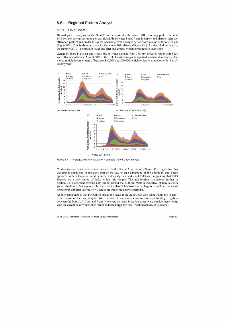
7/27/2019 Trabalho_Austrália
http://slidepdf.com/reader/full/trabalhoaustralia 92/174
8.5. Regional Pattern Analysis
8.5.1. Gold Coast
Diurnal pattern analysis on the Gold Coast demonstrates the winter 2011 morning peak of around
14 litres per person per hour per day (L/p/h/d) between 8 and 9 am is higher and sharper than theafternoon peak of just under 8 L/p/h/d occurring over a longer period from around 5.30 to 7.30 pm(Figure 83a). This is also consistent for the winter 2011 dataset (Figure 83c). As identified previously,the summer 2010-11 peaks are lower and later and generally more prolonged (Figure 83b).
Generally, there is a clear and steady rise in water demand from 3.00 pm onwards which coincideswith after school hours. Almost 50% of the Gold Coast participants reported household incomes in thelow to middle income range of between $30,000 and $90,000, which typically coincides with ‘8-to-5’employment.
0
2
4
6
8
10
12
14
1 2 3 4 5 6 7 8 9 10 11 12 13 14 15 16 17 18 19 20 21 22 23 24
A v e r a g e d a i l y d i u r n a l c o n s u m p t
i o n
( L / p / h / d )
Leak Toilet Clotheswasher
Shower Dishwasher Tap
Bathtub Irrigation
(a)
0
2
4
6
8
10
12
14
1 2 3 4 5 6 7 8 9 10 11 12 13 14 15 16 17 18 19 20 21 22 23 24 A v e r a g e d a i l y d i u r n a l c o n s u m p t i o n
( L / p / h / d )
Leak Toilet Clotheswasher
Shower Dishwasher Tap
Bathtub Irrigation
(b)
(a) Winter 2010 (n=87). (b) Summer 2010-2011 (n=68).
0
2
4
6
8
10
12
14
1 2 3 4 5 6 7 8 9 10 11 12 13 14 15 16 17 18 19 20 21 22 23 24 A v e r a g e d a i l y d i u r n a l c o n s u m p t i o n
( L / p / h / d )
Leak Toilet Clotheswasher
Shower Dishwasher Tap
Bathtub Irrigation
(c)
(c) Winter 2011 (n=33).
Figure 83: Average daily diurnal pattern analysis - Gold Coast sample.
Clothes washer usage is also concentrated in the 8 am-12 pm period (Figure 83), suggesting thatwashing is conducted in the early part of the day to take advantage of the afternoon sun. Thereappeared to be a temporal trend between water usage via leaks and toilet use, suggesting that toiletfixtures are a key source of leaks within this sample. This relationship is explored further inSection 9.6. Consistent evening bath filling around the 5.00 pm mark is indicative of families withyoung children, a fact supported by the statistics that Gold Coast has the largest overall percentage of homes with children (average 44% across the three read analysis periods).
An interesting note is that the bulk of irrigation events in the Gold Coast took place within the 11 am –
5 pm period of the day, despite QWC permanent water restriction measures prohibiting irrigation between the hours of 10 am and 4 pm. However, the peak irrigation times were outside these hours,with the exception of winter 2011 which indicated high daytime irrigation activity (Figure 83c).
South East Queensland Residential End Use Study: Final Report Page 82

7/27/2019 Trabalho_Austrália
http://slidepdf.com/reader/full/trabalhoaustralia 93/174
8.5.2. Brisbane
The diurnal patterns for Brisbane show the typical morning peak and smaller afternoon peak, but alsofor winter 2010, a minor peak in the early afternoon for shower, clothes washer and irrigation(Figure 84a). The Brisbane sample had the second highest number of homes with children and theyoungest average age of children and this may be represented by the early afternoon peak where oneadult and one or more small children are at home during the day. Water demanding activities such asclothes washing and showering are more likely to occur during the day for these people than in themorning or evening where other activities would be occurring (e.g. meal preparation, morning outings,etc).
Compared to the other regions, there is a relatively low trough in the middle of the day for each of thethree periods of analysis. The Brisbane samples all had the lowest percentage of retired/pensioner households but a high percentage of two person households, suggesting that many of the householdswere the younger “double-income-no-kids” type families that would be absent from their homes for asignificant proportion of the day.
0
2
4
6
8
10
12
14
1 2 3 4 5 6 7 8 9 10 11 12 13 14 15 16 17 18 19 20 21 22 23 24
A v e r a g e d a i l y d i u r n a l c o n s u m p t i o n
( L / p / h / d )
Leak Toilet
ClotheswasherShower Dishwasher Tap
Bathtub Irrigation
(a)
0
2
4
6
8
10
12
14
1 2 3 4 5 6 7 8 9 10 11 12 13 14 15 16 17 18 19 20 21 22 23 24 A v e r a g e d a i l y d i u r n a l c o n s u m p t i o n
( L / p / h / d )
Leak Toilet Clotheswasher
Shower Dishwasher Tap
Bathtub Irrigation
(b)
(a) Winter 2010 (n=61). (b) Summer 2010-2011 (n=64).
0
2
4
6
8
10
12
14
1 2 3 4 5 6 7 8 9 10 11 12 13 14 15 16 17 18 19 20 21 22 23 24 A v e r a g e d a i l y d i u r n a l c o n s u m p t i o n
( L / p / h / d )
Leak Toilet Clotheswasher
Shower Dishwasher Tap
Bathtub Irrigation
(c)
(c) Winter 2011 (n=26).
Figure 84: Average daily diurnal pattern analysis - Brisbane Region.
8.5.3. Ipswich
The Ipswich region showed distinct double peaks in the diurnal usage analysis for both morning andthe evening periods for all three periods of analysis (Figure 85). In particular, the peaks contain sharpconcentrations of shower and tap usages. The double peaks suggest that there may be two clear familytypes; a smaller household leaving early and returning later from work, and a larger, younger family
where school age children leave the house later in the mornings and return home earlier in theevenings.
South East Queensland Residential End Use Study: Final Report Page 83

7/27/2019 Trabalho_Austrália
http://slidepdf.com/reader/full/trabalhoaustralia 94/174
0
2
4
6
8
10
12
14
1 2 3 4 5 6 7 8 9 10 11 12 13 14 15 16 17 18 19 20 21 22 23 24
A v e r a g e d a i l y d i u r n a l c o n s u m p t i o n
( L /
p / h / d )
Leak Toilet Clotheswasher
Shower Dishwasher Tap
Bathtub Irrigation
(a)
0
2
4
6
8
10
1 2 3 4 5 6 7 8 9 10 11 12 13 14 15 16 17 18 19 20 21 22 23 24 A v e r a g e d a i l y d i u r n
a l c o n s u m p t i o n
( L / p / h
/ d )
Leak Toilet Clotheswasher
Shower Dishwasher Tap
Bathtub Irrigation
(b)
(a) Winter 2010 (n=37). (b) Summer 2010-2011 (n=31).
0
2
4
6
8
10
1 2 3 4 5 6 7 8 9 10 11 12 13 14 15 16 17 18 19 20 21 22 23 24 A v e r a g e d a i l y d i u r n a l c o n s u m p
t i o n
( L / p / h / d )
Leak Toilet Clotheswasher
Shower Dishwasher Tap
Bathtub Irrigation
(c)
(c) Winter 2011 (n=12).
Figure 85: Average daily diurnal pattern analysis - Ipswich Region.
Ipswich householders with families had relatively young children at an average age of 4.4 years old,suggesting that the children shower earlier at distinctly different times to the adults. About 50% of households in Ipswich had two or fewer occupants. During the trace analysis, it was observed thatthese two-person households were typically younger, and appeared to spend more time away from thehousehold, leaving for work earlier and returning home later. With two distinct family types, there islikely to be a small window of time where the homes are generally unoccupied. This may be areflected by the troughs evident in the middle of the day, particularly for winter 2010 (Figure 85a) andsummer 2010-11 (Figure 85b).
8.5.4. Sunshine CoastDiurnal pattern analysis of the Sunshine Coast region shows two distinct peaks, at 9am and againaround 6pm (Figure 86). The sharp peaks show a high concentration of shower events, whichcorrelates with approximately 69% of households in the region being occupied by two or fewer occupants (Table 7), resulting in less of a time spread than larger households. The analysis also showsa consistent pattern of shower, toilet and tap events throughout the day, which is typical of older families, who tend to remain at home more than younger households. Consistent tap and toilet usagefor the entire day suggests that a large percentage of households see one or more occupants remain athome all day. Leakage rates in the morning peak for winter 2010 were dominated by one home(Figure 86a).
Irrigation rates during the middle period of the day in winter 2011 show a clear departure from the
previous trend for morning or afternoon irrigation and, like Brisbane and the Gold Coast, demonstratea lack of compliance with the watering restrictions applied to SEQ for the middle of the day.
South East Queensland Residential End Use Study: Final Report Page 84

7/27/2019 Trabalho_Austrália
http://slidepdf.com/reader/full/trabalhoaustralia 95/174
0
2
4
68
10
12
14
16
1 2 3 4 5 6 7 8 9 10 11 12 13 14 15 16 17 18 19 20 21 22 23 24
A v e r a g e d a i l y d i u r n a l c o n s u m p t i o n
( L /
p / h / d )
Leak Toilet Clotheswasher
Shower Dishwasher Tap
Bathtub Irrigation
(a)
0
2
4
6
8
10
12
14
16
1 2 3 4 5 6 7 8 9 10 11 12 13 14 15 16 17 18 19 20 21 22 23 24 A v e r a g e d a i l y d i u r n a l c o n s u m p t i o n
( L / p / h
/ d )
Leak Toilet Clotheswasher
Shower Dishwasher Tap
Bathtub Irrigation
(b)
(a) Winter 2010 (n=67). (b) Summer 2010-2011 (n=56).
0
2
4
6
8
10
12
14
16
1 2 3 4 5 6 7 8 9 10 11 12 13 14 15 16 17 18 19 20 21 22 23 24 A v e r a g e d a i l y d i u r n a l c o n s u m
p t i o n
( L / p / h / d )
Leak Toilet Clotheswasher
Shower Dishwasher Tap
Bathtub Irrigation
(c)
(c) Winter 2011 (n=39).
Figure 86: Average daily diurnal pattern analysis - Sunshine Coast Region.
8.5.5. Diurnal Relationships between End Uses
This section briefly explores end uses that are strongly correlated with each other in terms of diurnalusage. The winter end use data from 2010 is being used for reasons explained in section 9.1. As would
be expected, tap and toilet end uses occur around the same time (Figure 87a). Shower use is alsoclosely related to tap and toilet use (Figures 87b and 87d), all of which peak in the mornings. Thisconfirms the belief that the morning ablution ‘rituals’ consume the major proportion of peak water useand occur consistently across all households and regions. Closer examination of the data could revealthat certain household types (i.e. where family members work or attend school regularly) might beoverrepresented in this. Knowledge of this type can greatly assist water demand managers inimplementing strategies to change water use behaviours, which may subsequently shift or flatten the
peak usage times in these households.
Interestingly, the greatest association for leaks was with toilet usage (Figure 87c). There was areasonably strong positive correlation between leaks and toilet water consumption end uses for allregions. During the water audits and trace analysis, it was clear that many of the leaks wereattributable to toilets and in some instances leaks comprised almost 50% of total water use. This is anarea also worthy of further investigation, as, while we may have addressed the low flush dual toiletquestion, it may now be prudent to promote maintenance and inspection on these toilet fixtures.
South East Queensland Residential End Use Study: Final Report Page 85

7/27/2019 Trabalho_Austrália
http://slidepdf.com/reader/full/trabalhoaustralia 96/174
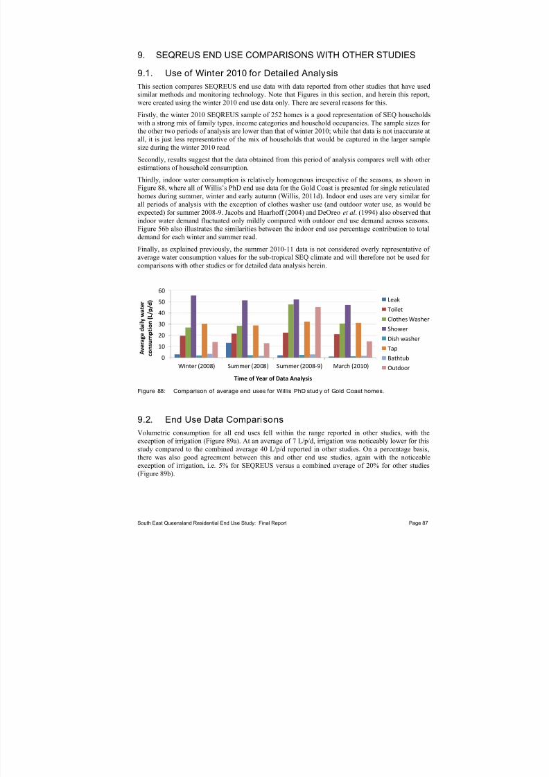
7/27/2019 Trabalho_Austrália
http://slidepdf.com/reader/full/trabalhoaustralia 97/174
9. SEQREUS END USE COMPARISONS WITH OTHER STUDIES
9.1. Use of Winter 2010 for Detailed Analysis
This section compares SEQREUS end use data with data reported from other studies that have used
similar methods and monitoring technology. Note that Figures in this section, and herein this report,were created using the winter 2010 end use data only. There are several reasons for this.
Firstly, the winter 2010 SEQREUS sample of 252 homes is a good representation of SEQ householdswith a strong mix of family types, income categories and household occupancies. The sample sizes for the other two periods of analysis are lower than that of winter 2010; while that data is not inaccurate atall, it is just less representative of the mix of households that would be captured in the larger samplesize during the winter 2010 read.
Secondly, results suggest that the data obtained from this period of analysis compares well with other estimations of household consumption.
Thirdly, indoor water consumption is relatively homogenous irrespective of the seasons, as shown inFigure 88, where all of Willis’s PhD end use data for the Gold Coast is presented for single reticulatedhomes during summer, winter and early autumn (Willis, 2011d). Indoor end uses are very similar for all periods of analysis with the exception of clothes washer use (and outdoor water use, as would beexpected) for summer 2008-9. Jacobs and Haarhoff (2004) and DeOreo et al. (1994) also observed thatindoor water demand fluctuated only mildly compared with outdoor end use demand across seasons.Figure 56b also illustrates the similarities between the indoor end use percentage contribution to totaldemand for each winter and summer read.
Finally, as explained previously, the summer 2010-11 data is not considered overly representative of average water consumption values for the sub-tropical SEQ climate and will therefore not be used for comparisons with other studies or for detailed data analysis herein.
0
10
20
30
40
50
60
Winter (2008) Summer (2008) Summer (2008‐9) March (2010)
A v e r a g e d a i l y w a t e r
c o n s u m p t i o n ( L / p / d )
Time of Year of Data Analysis
Leak
Toilet
Clothes Washer
Shower
Dish washer
Tap
Bathtub
Outdoor
Figure 88: Comparison of average end uses for Willis PhD study of Gold Coast homes.
9.2. End Use Data Comparisons
Volumetric consumption for all end uses fell within the range reported in other studies, with theexception of irrigation (Figure 89a). At an average of 7 L/p/d, irrigation was noticeably lower for thisstudy compared to the combined average 40 L/p/d reported in other studies. On a percentage basis,there was also good agreement between this and other end use studies, again with the noticeableexception of irrigation, i.e. 5% for SEQREUS versus a combined average of 20% for other studies(Figure 89b).
South East Queensland Residential End Use Study: Final Report Page 87

7/27/2019 Trabalho_Austrália
http://slidepdf.com/reader/full/trabalhoaustralia 98/174
ToiletShower /
bath
Clothes
washerDish washer Taps Leaks Irrigation‡
Gold Coast (n=151) 21 50 30 2.2 27 2.1 18.6
Toowoomba (n=10) 14.2 48.7 25.4 2 16.8 0.5 0.5
Melbourne (n=100) 30 49 40 2.7 27 15.9 65
Perth (n=120) 21 33 27 83 100
Auckland (n=50) 31.3 50.4 39.9 2.1 22.7 7.0 13.9
SEQEUS (n=252) 23.7 44.5 31.0 2.5 27.5 9.0 7.0
0
10
20
30
4050
60
70
80
90
100
A v e r a g e p e r c a p i t
a c o n s u m p t i o n
( L / p / d )
Sources:
Willis et al. (2009)
Mead and Aravinthan (2009)
Roberts (2005)
Loh & Coghlan (2003)
Heinrich, M. (2007)
(a)
(a) Average volumetric consumpt ion (L/p/d).
ToiletShower /
bath
Clothes
washerDish washer Taps Leaks Irrigation
Gold Coast (n=151) 13.0 37.0 19.0 1.0 17.0 1.0 12.0
Toowoomba (n=10) 12.3 45.2 22.7 2.1 16.8 0.4 0.3
Melbourne (n=100) 13.0 23.0 19.5 1.0 12.0 6.0 25.0
Perth (n=120) 10.0 16.0 13.0 7.0 54.0
Auckland (n=50) 19.0 30.0 24.0 1.0 14.0 4.0 8.0
SEQEUS (n=252) 16.5 30.5 21.0 2.0 19.0 6.0 5.0
0
10
20
30
40
50
60
A v e r a g e p e r c e n t a g e o f t o t a l
c o n s u m p t i o n ( % )
(b)
(b) Average percentage of total consumption.
Notes: ‡ = Gold Coast study - outdoor mains water use subject to government water restrictions. Toowoomba study - outdoor mains water useprohibited. Yarra Valley Water study - outdoor end use reported for summer only.
Figure 89: Comparison of average end use consumpt ion between SEQREUS data and other end usestudies.
Some discussion on the several factors likely to be influencing the low irrigation volumes observed inthis study was undertaken in earlier sections of this report. A lingering reluctance to use mains water outdoors as a result of the recent drought and an associated strong awareness of water conservation isone underlying factor. Another is related to seasonal factors, including the relatively frequent rainfall(days > 1 mm of rain) in SEQ leading up to the winter 2010 read. This resulted in a much reducedneed to irrigate during winter and summer months to sustain lawns and gardens.
South East Queensland Residential End Use Study: Final Report Page 88

7/27/2019 Trabalho_Austrália
http://slidepdf.com/reader/full/trabalhoaustralia 99/174
South East Queensland Residential End Use Study: Final Report Page 89
As for previous studies, shower usage comprised the bulk of household water use for all regions.Across all regions, a minimum of one quarter of all household water demand was associated with this
practice. This is not unusual and has been reported in other end use studies (Willis et al., 2010b,2011a; Gato-Trinidad et al., 2011; Water Corporation, 2011; Mead and Aravinthan, 2009).
Leakage rates for the SEQREUS are consistent with other studies both on a volumetric and percentage
basis (Figure 89). Leaks are a common occurrence in all households, with a trend typically shown for less leakage to occur from new (< five years old) dwellings (Willis et al., 2009a). For the SEQREUSwinter 2010 sample, leaks ranged from 0.2 to 513 L/p/d. The latter value is an extreme case andsubsequent investigation has revealed that this household has had ongoing issues with leaks on its
property. Very large leaks are usually due to service breaks and can cause the average per capitaleakage volumes in an end use sample to fluctuate significantly. Leakage rates for the subsequentsummer 2010-11 and winter 2011 were substantially reduced as a result of the aligned CSIROintervention study as discussed previously.

7/27/2019 Trabalho_Austrália
http://slidepdf.com/reader/full/trabalhoaustralia 100/174
10. STOCK EFFICIENCY INFLUENCE ON WATER USE
10.1. Introduction
Previous studies have shown associations between water efficient technology and reduced water
demand in homes (Lee et al., 2011; Willis et al., 2011b; Water Corporation, 2011; Heinrich, 2008;Arthuraliya et al., 2008; Mayer et al., 2004). With a combination of financial incentives for retrofittingwater wise technology (i.e. low-flow shower roses, 4+ star rated washing machines) and revised
building codes mandating such fixtures and appliances in new developments in Queensland, there will be an expected reduction in residential water demand. The quantum of this reduction will varydepending on the type of water efficient technology, the number of fixtures within a home, the existingwater demand (i.e. installing water efficient stock in a home of low existing demand will not realisetoo much of a downward shift in use), and family size and composition. This next section explores theimpacts that water efficient household stock can have on water consumption and on peak water demand. As explained earlier, all the analysis was been performed on the winter 2010 dataset.
10.2. Clothes Washing Machines
Water demand associated with clothes washing accounted for over 20% of the average total householdconsumption (Figure 21), and during peak demand days, up to 35% (or 57 L/p/d) (Figure 74e). Thevariation in clothes washing end use consumption between homes is likely a reflection of the differenttypes and models of appliances that are available. The stock surveys undertaken for each homerevealed a variety of water star rating machines and whether they were front or top loading machines.
A breakdown of machine types (star rating vs load type) and their average rate of water consumption is presented in Table 21. There is a clear trend for higher star rating and front loading machines to useless water. Gato-Trinidad et al. (2011) and Willis et al. (2011b) both discussed the variation in end usewater consumption as a result of efficient devices. Willis et al. (2009b, 2011b), Water Corporation(2011) and Fidar et al. (2010) demonstrated that substantial water savings could be made by usinghigh-efficiency washing machines. The high efficiency of the machine relates to the flow rate in litres
per wash (L/wash).
Table 21: Clothes washer efficiency comparisons.
Clothes Washer Efficienc y Clusters Load TypeDescriptor
Low Medium High Front Top Twin Tub
Star rating0 to 2 stars 3 or 3+ stars ≥ 4 stars 85% ≥ 4 stars
24% ≥ 4stars
2 stars
Flow rate category (averageL/wash)
131.3 86.4 67.5 64.8 91.9 127
No. homes in cluster 1
24 55 97 81 112 1
Daily per capita clothes washconsumption (average L/p/d)
31.8 29.8 22.5 19.0 29.9 30.6
Daily household clotheswash consumption (averageL/hh/d)
82.6 77.5 58.4 50.7 79.7 81.5
Annual per capita clotheswash consumption (averagekL/p/y)
11.6 10.9 8.2 6.9 10.9 11.2
Annual household clotheswash consumption (averagekL/hh/y)
30.1 28.3 21.3 18.5 29.1 29.7
Savings (kL/hh/y) comparedto lowest star rating
2
-1.9
(6.2%)8.8
(29.3%)10.6 (36.4%) - -
Notes:1
No. of homes will not be equal to the total Winter 2010 sample size of 252 as not all homes had information on stock efficiency;2 Clothes washing water consumption savings for load type based on the difference between top and front loaders only, due to small samplesize for twin tub (n=1).
South East Queensland Residential End Use Study: Final Report Page 90
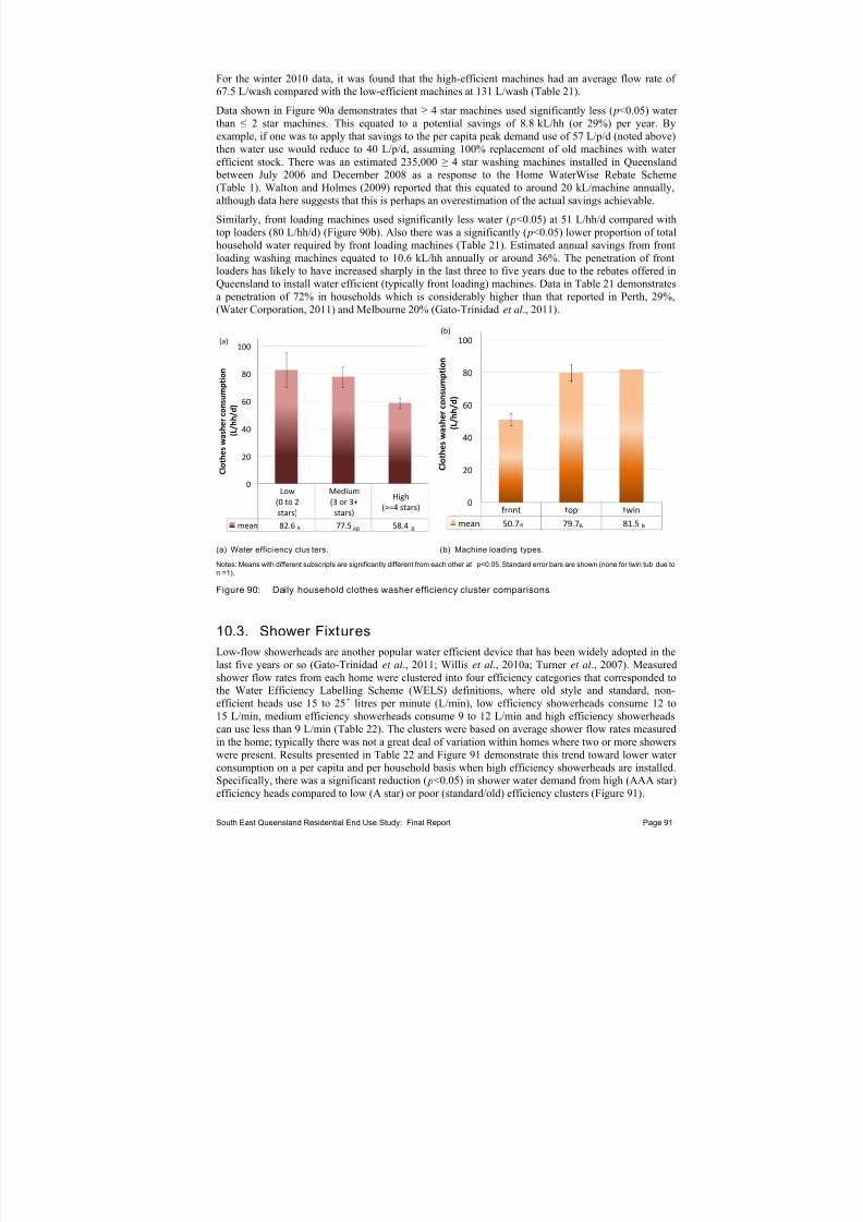
7/27/2019 Trabalho_Austrália
http://slidepdf.com/reader/full/trabalhoaustralia 101/174
For the winter 2010 data, it was found that the high-efficient machines had an average flow rate of 67.5 L/wash compared with the low-efficient machines at 131 L/wash (Table 21).
Data shown in Figure 90a demonstrates that ≥ 4 star machines used significantly less ( p<0.05) water than ≤ 2 star machines. This equated to a potential savings of 8.8 kL/hh (or 29%) per year. Byexample, if one was to apply that savings to the per capita peak demand use of 57 L/p/d (noted above)
then water use would reduce to 40 L/p/d, assuming 100% replacement of old machines with water efficient stock. There was an estimated 235,000 ≥ 4 star washing machines installed in Queensland
between July 2006 and December 2008 as a response to the Home WaterWise Rebate Scheme(Table 1). Walton and Holmes (2009) reported that this equated to around 20 kL/machine annually,although data here suggests that this is perhaps an overestimation of the actual savings achievable.
Similarly, front loading machines used significantly less water ( p<0.05) at 51 L/hh/d compared withtop loaders (80 L/hh/d) (Figure 90b). Also there was a significantly ( p<0.05) lower proportion of totalhousehold water required by front loading machines (Table 21). Estimated annual savings from frontloading washing machines equated to 10.6 kL/hh annually or around 36%. The penetration of frontloaders has likely to have increased sharply in the last three to five years due to the rebates offered inQueensland to install water efficient (typically front loading) machines. Data in Table 21 demonstrates
a penetration of 72% in households which is considerably higher than that reported in Perth, 29%,(Water Corporation, 2011) and Melbourne 20% (Gato-Trinidad et al., 2011).
Low
(0 to 2
stars)
Medium
(3 or 3+
stars)
High
(>=4 stars)
mean 82.6 77.5 58.4
0
20
40
60
80
100
C l o t h e
s w a s h e r c o n s u m p t i o n
( L / h h / d )
A AB B
(a)
front top twin
mean 50.7 79.7 81.5
0
20
40
60
80
100
C l o t h
e s w a s h e r c o n s u m p t i o n
( L / h h / d )
A B B
(b)
(a) Water efficiency clus ters. (b) Machine loading types.
Notes: Means with different subscripts are significantly different from each other at p<0.05. Standard error bars are shown (none for twin tub due ton =1).
Figure 90: Daily household clothes washer efficiency cluster comparisons.
10.3. Shower Fixtures
Low-flow showerheads are another popular water efficient device that has been widely adopted in thelast five years or so (Gato-Trinidad et al., 2011; Willis et al., 2010a; Turner et al., 2007). Measuredshower flow rates from each home were clustered into four efficiency categories that corresponded tothe Water Efficiency Labelling Scheme (WELS) definitions, where old style and standard, non-efficient heads use 15 to 25+ litres per minute (L/min), low efficiency showerheads consume 12 to15 L/min, medium efficiency showerheads consume 9 to 12 L/min and high efficiency showerheadscan use less than 9 L/min (Table 22). The clusters were based on average shower flow rates measuredin the home; typically there was not a great deal of variation within homes where two or more showers
were present. Results presented in Table 22 and Figure 91 demonstrate this trend toward lower water consumption on a per capita and per household basis when high efficiency showerheads are installed.Specifically, there was a significant reduction ( p<0.05) in shower water demand from high (AAA star)efficiency heads compared to low (A star) or poor (standard/old) efficiency clusters (Figure 91).
South East Queensland Residential End Use Study: Final Report Page 91

7/27/2019 Trabalho_Austrália
http://slidepdf.com/reader/full/trabalhoaustralia 102/174
Table 22: Showerhead efficiency cluster comparisons .
Descriptor Showerhead Efficiency Rating Clusters
Poor Low Medium High
Star rating Old style Standard A or 1 star AA or 2 Stars AAA or 3 Stars
Flow rate category (L/min) >21 15 to 21 12 to 15 9 to 12 < 9No. homes in cluster (proportion)
20 36 30 22 13
Daily per capita shower consumption (L/p/d)
37.9 28.5 24.6 15.0 9.4
Daily household shower consumption (L/hh/d)
102.4 76.8 66.4 30.1 25.4
Annual per capita shower consumption (kL/p/y)
13.8 10.4 9.0 5.5 3.4
Annual household shower consumption (kL/hh/y)
37.3 28.0 24.2 14.8 9.3
Savings (kL/hh/y) comparedto poor rated showerhead
-9.3
(25%)13.2
(35.2%)22.6
(60.5%)37.4
(75.1%)
Results demonstrate that replacing the old style showerhead with any star rated showerhead wouldsignificantly ( p<0.05) reduce shower water consumption (Figure 91). This suggests that one can haveexcellent returns for a low technology solution, particularly given the typically high shower end usedemand in homes. For example, replacing standard non-efficient showerheads with high efficiencyshowerheads could provide potential savings of 28 kL (or 75%) per year (Table 22).
AAA or 3
Stars
AA or 2
StarsA or 1 Star Standard Old
mean 25.5 40.4 66.4 76.8 102.4
0
20
40
60
80
100
S h o w e r c o n s u m p t
i o n ( L / h h / d )
A AB CD
C
Notes: Means with different subscripts are significantly different from each other at p<0.05. Standard error bars are shown.
Figure 91: Daily household shower fixture efficiency cluster comparisons.
This may be over representing the potential savings, as the penetration of low-flow showerheads isassumed to be already quite high as a result of the Home WaterWise Rebate Scheme implemented bythe Queensland State Government in recent years (Walton and Homes, 2009), thus the margin for further savings will be less as the technology has already been widely adopted across SEQ. For example, around 54% of the winter 2010 sample had an A star or higher rated showerhead, and datafrom Table 1 shows that over 35,000 homes had ≥ 3 star showerheads installed during the WaterWiserebate scheme (Walton and Homes, 2009). Notwithstanding this, data presented in this report clearlyillustrates the need for ongoing policy and water conservation initiatives to reduce shower consumption, which continues to represent around a third of average total household consumption.
South East Queensland Residential End Use Study: Final Report Page 92

7/27/2019 Trabalho_Austrália
http://slidepdf.com/reader/full/trabalhoaustralia 103/174
10.4. Taps
Tap end use consumption is largely influenced by behaviour and habit, as much of the use is related toa desired fixed volume irrespective of flow rate (e.g. filling up kettles, sinks and buckets). Where tapuse is flow rate dependent, such as rinsing plates, teeth cleaning and washing hands, the attitudes and
habits of the consumer are still paramount in influencing the volume of water used (e.g. turning the tapoff to shave, brush teeth, lightly vs heavily rinse plates). Therefore, replacing high-flow tap fittingswith low-flow devices such as aerators and flow restrictors can be very effective in reducing tap water consumption. Aerators are devices that reduce flow from the tap without reducing water pressure by
breaking up the solid flow of water using air (spreading the flow into many droplets thus increasingthe perceived water pressure). Flow controllers and restrictors physically restrict the diameter of thewater flow path, thus reducing the flow rate through the tap.
Tap fixtures have been categorised into low, medium and high efficiency clusters (Table 23). Anotable feature of Table 23 is the number of low or inefficient tap fixtures (based on flow rate). This issurprising given the penetration rates of the other, more expensive and labour intensive, water efficienttechnologies discussed in Table 1.
Table 23: Tap efficiency cluster comparisons .
Descriptor Tap Fixture Efficiency Clusters
Low Medium High
Star rating Inefficient / old style 1 to 2 stars ≥ 3 stars
Flow rate category (L/min) >16 9 to 16 4.5 to 9
No. homes in cluster (proportion)
127 54 5
Daily per capita tapconsumption (L/p/d)
20.2 15.1 7.0
Daily household tapconsumption (L/hh/d)
54.5 40.6 18.9
Annual per capita tap
consumption (kL/p/y) 7.4 5.5 2.6
Daily household tapconsumption (kL/hh/y)
19.8 14.8 6.9
Water savings compared tolow rated tap
-5
(25.3%)12.9
(65.2%)
Inefficient 1 to 2 Stars 3 to 6 Stars
mean 54.5 40.7 19.0
0
20
40
60
80
100
T a p c o n s u m p
t i o n
( L / h h / d )
A B C
Notes: Means with different subscripts are significantly different from each other at p<0.05. Standard error bars are shown.
Figure 92: Daily household tap fixture efficiency cluster comparisons.
South East Queensland Residential End Use Study: Final Report Page 93

7/27/2019 Trabalho_Austrália
http://slidepdf.com/reader/full/trabalhoaustralia 104/174
There were significant differences (p<0.05) between all three tap efficiency clusters (Figure 92), andreplacing an old style tap with a ≥ 3 star tap fitting can save 12.9 kL/hh or 65% annually (Table 23).They are also often associated with leaks or are fixtures that need to be turned off manually (unlikedishwashers and clothes washers) and a dripping tap can often go undetected after use by smallchildren. These characteristics are important as taps can readily slip ‘under the radar’ in terms of theunnoticed, cumulative contribution to daily total water consumption in a home. Therefore, the
potential savings that can be realised from efficient tap fixtures is also an area of focus for water conservation policy. However, it is assumed that all new residential developments will have a veryhigh penetration of efficient tap fittings as required under the QDC MP 4.1 standards.
10.5. Dishwasher
The WELS Scheme has identified water-efficient dishwashers as potentially saving up to half thewater of average models (WELS 2011). Dishwashing machines were also categorised into water efficiency clusters based on observed litres per place setting (L/place setting) and WELS data.Dishwasher economy and non-economy cycles were also clustered based on the flow rate (L/wash) of each machine (Table 24). Results demonstrate that for the winter 2010 sample, efficient dishwashers(e.g. 3.5+ star rating) used significantly less ( p<0.05) water at a mean of 4.4 L/hh/d, compared to the
average 9.2 L/hh/d from the inefficient dishwasher cluster (Figure 93a).
Table 24: Dishwasher efficiency clus ter comparisons .
Dishwasher EfficiencyClusters
1Dishwasher Cycle Typically Used
by HouseholdDescriptor
Inefficient EfficientEconomy Not
UsedEconomy Used
Star rating / Flow rate category(L/wash)
0 to 3 stars 3.5 to 6 stars >16 L/wash ≤16 L/wash
No. homes in cluster (proportion) 55 53 45 41
Daily per capita dishwasher consumption (L/p/d) 3.1 1.5 2.8 2.2
Daily household dishwasher consumption (L/hh/d)
9.2 4.4 8.2 6.5
Annual per capita dishwasher consumption (kL/p/y)
1.1 0.5 1.0 0.8
Daily household dishwasher consumption (kL/hh/y)
3.3 1.6 3.0 2.4
Savings compared to inefficientmachine/cycle
-1.7
(52%)- 0.62 (20%)
1 Calculated star ratings based on average observed L/ place settings and WELS data.
This equates to a savings of 52% or 1.7 kL/hh annually. By choosing an economy wash cycle, water
consumption can potentially be reduced by 20% (0.6 kL/hh/y) annually (Table 24) although this is nota significant reduction (Figure 93b). Dishwashers are characteristically low water consumers asevidenced in this report and other studies (Willis et al., 2010b; Roberts, 2005), therefore the savingsthat can be achieved from water-efficient dishwashers is not remarkable relative to clothes washers or showerheads. However, the water-efficiency of dishwashers is basically an indirect benefit of machines that were originally designed to reduce energy consumption. That is, energy-efficientdishwashers typically are also water-efficient (WELS, 2011). Thus, households should be encouragedto install such a machine nonetheless. The water-energy nexus will be explored briefly in Section 14.
South East Queensland Residential End Use Study: Final Report Page 94

7/27/2019 Trabalho_Austrália
http://slidepdf.com/reader/full/trabalhoaustralia 105/174
0 to 3 stars 3.5 to 6 stars
mean 9.2 4.4
0
2
4
6
8
10
D i s h w a s h e r c
o n s u m p t i o n
( L / h h
/ d )
A B
(a)
Economy cycle
typically used
Economy cycle
typically not used
mean 6.5 8.2
0
2
4
6
8
10
D i s h w a s h e r c o n s u m p t i o n
( L / h h
/ d )
A A
(b)
(a) Water efficiency clus ters. (b) Wash cycl e selected.
Notes: Means with different subscripts are significantly different from each other at p<0.05. Standard error bars are shown.
Figure 93: Daily household dish washer efficiency cluster comparisons.
10.6. Rainwater Tanks
Following the State and Local Government rebate schemes in the mid to late 2000s, around 240,000homes in Queensland installed a rainwater tank (Walton and Holmes, 2009). In the SEQREUS study,rainwater tanks (RWT) were installed in about 44% (n=22) of Gold Coast homes, 48% (n=29) of Brisbane homes, 65% (n=24) of Ipswich homes and 25% (n=17) of Sunshine Coast homes. None of these RWT were internally connected to any internal water appliance or fixture; that is, rainwater wasonly used externally. Of these homes with a RWT, about 60% of them stated during the water auditthat they typically used their rainwater for outdoor garden watering. Other common uses were car washing and topping up pools.
Figure 94 indicates that, for the winter 2010 results, homes with a RWT had significantly lower ( p<0.05) total water consumption than homes without a RWT. Previous studies indicate that thisreduction would be attributable to the RWT offsetting mains water for irrigation and general externalwater end uses (Willis et al., 2011b; Beal et al., 2011c). However, this trend is not evident here asthere was only a slight positive correlation between irrigation and total end use consumption for allSEQ homes without a RWT, although when assessed on a region by region basis there are obviousincreases in per capita irrigation by homes without a RWT for Ipswich and Sunshine Coast, althoughthis tendency did not appear for the Gold Coast and Brisbane (Figure 95a).
Homes with RWT Homes without RWT
Mean 123.7 146.2
100
120
140
160
T o t a l h o u s e h o l d w a t e r c o n s u m p t i o n
( L / p / d )
A B
Notes: Means with different subscripts are significantly different from each other at p<.05.
Standard error bars are shown.
Figure 94: Comparisons between homes with and without a RWT.
South East Queensland Residential End Use Study: Final Report Page 95

7/27/2019 Trabalho_Austrália
http://slidepdf.com/reader/full/trabalhoaustralia 106/174
Similarly, the proportion of total water consumed for irrigation (or other external uses) for homeswithout a RWT is also higher for Ipswich and the Sunshine Coast (Figure 95b). Although the summer 2010-11 analysis was confounded by extreme rainfall and flooding events, the three analysis periodsare compared in terms of contribution of irrigation to total water consumption for homes with andwithout a RWT (Figure 96). The results show that for the homes with a RWT the proportion of irrigation is higher in winter 2011 than any other time.
0
1
2
3
4
5
6
7
8
9
10
Gold Coast Br isb an e Ip swich Sun sh in e
Coast
A v e r a g e w a t e r c o n s u m e d
f r o m i r r i g a t i o n ( L / p / d )
Homes with RWT
Homes without RWT
(a)
(a) Irrigation end use per capita volume.
0
1
2
3
4
5
6
7
8
Gold Co ast Br isb an e Ipswic h Su nsh in e
Coast
A v e r a g e p e r c e n t a g e o f t o t a l
w a t e r u s e u s e d f o r i r r i g a t i o n ( % )
Homes with RWT
Homes without RWT(b)
(b) Irrigation percentage of total use.
Figure 95: Irrigation consumption for households with and without a RWT.
Figure 96: Averaged SEQ Irrigation consumption for households with and without a RWT.
This may be a result of the consistent rainfall preceding winter, enabling the tanks to have aconsistently high capacity to offset mains water for external uses. As expected, during the warmer months of summer, homes with RWT used less mains water for irrigation compared to those homeswithout RWT. During a survey of SEQ homeowners, Gardiner (2009) identified a group of RWTowners that specifically used their RWT to supplement irrigation during restrictions or dry periods as“restriction compensators”. Typically, these homeowners had tanks that were not internally plumbed.
Other explanations for the significantly lower water use from homes with RWT could be related to thehouseholder attitudes to water consumption and conservation. Gardiner (2009) reported thathouseholders who had installed a RWT voluntarily in SEQ were much more likely to be part of theattitudinal category that practised other water savings strategies such as low-flow showers and who
self-rated their overall water efficiently very highly (e.g. 9 out of a 10 scale). As Gardner and Vieritz(2010) point out, these RWT retrofitters (e.g. non-mandated tank owners) are likely to become anever-decreasing proportion of the population in SEQ and thus their contribution to potable water savings will also lessen.
South East Queensland Residential End Use Study: Final Report Page 96

7/27/2019 Trabalho_Austrália
http://slidepdf.com/reader/full/trabalhoaustralia 107/174
11. STOCK EFFICIENCY INFLUENCE ON PEAK DEMAND
11.1. Introduction
The above sections have clearly shown how water-efficient stock can significantly reduce total
household water consumption. This section will now briefly explore how water-efficient stock canreduce the average day peak hour demand by examining diurnal patterns from homes with and withoutwater-efficient technology. The end uses which drive these reductions in peak demand will beidentified. The relevance of this research relates to future infrastructure and network distributionmodelling which use peaking factors for designing the diameters of the distribution pipes.Optimisation and deferral of water supply infrastructure by using current and representative peak demand data is likely to be of significant interest to water utilities. Moreover, also consideringreductions in peak demand that will result from demand management interventions, when conductingleast-cost water planning assessments, will further enhance the attractiveness of such options.
11.2. Overview of Methods
Household stock efficiency information was obtained from household water audits with efficiencyratings recorded as per the WELS star rating system. The efficiency information included flow rates of showerheads, average flow rates of indoor taps, and the volume of toilet cisterns, in order to establishwater used per flush, star rating and water used per cycle of washing machines and dishwashers. In anattempt to develop a representative composite star rating, reflecting the combined efficiency of theentire household water appliance/fixture stock composition, a weighted classification system wasdesigned and implemented. The overall household efficiency weighting system takes account of boththe contribution of each end use to total consumption and the star rating of the various indoor fixtures/appliances within each household. Although a dishwasher could be allocated a WELS rating,it is such a small component (i.e. < 2%) of overall household water use it is unlikely to discerniblyaffect peak flows and was therefore not included in the composite household star rating. The four
primary end uses accounted for over 87.5% of the total water use within the sample and therefore
would be the significant contributors to average day (AD) peak hour diurnal flows. After each home’soverall efficiency was calculated, a frequency distribution was created in order to classify the range of household composite star rating categories and identify potential efficiency clusters (Figure 97).
0
1
2
3
4
5
O v e
r a l l S t a r R a t i n g
Household ID
Toilet Shower Tap Clothes Washer
(a)
0
0.25
0.5
0.75
1
0
0.02
0.04
0.06
0.08
0.1
0.12
1 .1 1 .4 1. 7 2 2 .3 2 .6 2.9 3. 2 3 .5 3 .8 4 .1 4 .4
C u m u l a t i v e f r e q u e n c y d i s t r i b u t i o n
R e l a t i v e f r e q
u e n c y d i s t r i b u t i o n
Total weighted efficiency rating
Relative Frequency
Cumulative Frequency
(b)
(a) Weighted star rating distribution. (b) Total frequency and cumulative distribution.
Figure 97: Household efficiency frequency and cumulative distribut ions.
South East Queensland Residential End Use Study: Final Report Page 97

7/27/2019 Trabalho_Austrália
http://slidepdf.com/reader/full/trabalhoaustralia 108/174
The base comparison was categorised into two main clusters; homes < 3 stars and homes ≥ 3 stars. Inaddition to the base comparison, 50 of the most efficient and 50 of the least efficient homes were alsoclustered for comparison, as these homes generally represented the upper and lower quartiles of thesample group. These four efficiency clusters became the sample groups from which AD diurnaldemand patterns were developed in order to identify the peak hour demand differences for thesecluster groupings. Some descriptive statistics of each efficiency cluster are presented in Table 25.
Table 25: Household efficiency rating clusters – descriptive statistics.
Efficiency Cluster Number of Homes
Number of People
Average HouseholdOccupancy
Average Composi teStar Rating
All homes 191 508 2.66 2.88
< three star 102 271 2.66 2.40
≥ three star 89 237 2.66 3.43
50 least efficient homes1
50 137 2.74 2.03
50 most efficient homes1
50 138 2.76 3.64
Note: 1 these represent roughly the top and bottom quartiles of the sample with respect to star rating.
In the three-hour peak morning period between 7:00 and 10:00 am, the greater than three star homeshad a average hourly consumption reduction of 2.5 L/p/h/d (19.2%), which was statistically significant( p < 0.01) (Figure 98). Similarly, the 50 most efficient homes produced an average reduction in the
peak morning period (7:00 to 10:00 am) consumption flow rate of 3.5 L/p/h/d (18.5%), which was alsostatistically significant ( p < 0.01) (Figure 99). In the three-hour afternoon peak period between 16:00and 19:00 hours, consumption for the greater than three star efficiency cluster was also statisticallylower ( p < 0.01), at an average of 1.5 L/p/h/d (28.2%), than the less than three star efficiency cluster.The 50 most efficient homes afternoon peak period consumption had reduced by an average flow rateof 1.6 L/p/h/d (18.6%), which was also statistically significant ( p < 0.05).
0.0
2.5
5.0
7.5
10.0
12.5
15.0
A v e r a g e d a i l y d
i u r n a l c o n s u m p t i o n ( L / p / h / d )
Time
Less Than 3 Star Efficiency Greater Than 3 Star Efficiency
Figure 98: Average day diurnal demand pattern comparison for household clusters of greater than or
equal to and less than a three star rating.
South East Queensland Residential End Use Study: Final Report Page 98

7/27/2019 Trabalho_Austrália
http://slidepdf.com/reader/full/trabalhoaustralia 109/174
0.0
2.5
5.0
7.5
10.0
12.5
15.0
A v e r a g e d a i l y d i u r n a l c o n s u m p t i o n ( L / p /
h / d )
Time
50 Least Efficient Homes 50 Most Efficient Homes
Figure 99: Average day diurnal pattern comparison of 50 least and 50 most efficient households .
The AD diurnal pattern for the 50 most efficient homes displayed distinct double peak morning usage(Figure 99). The initial morning peak, with a flow rate of 9.1 L/p/h/d occurred between 6:00 and7:00 am, which was outside the normal peak usage period of 7:00 to 10:00 am displayed in the other AD diurnal patterns. The second morning peak occurred between 9:00 and 10:00 am with a flow rateof 8.5 L/p/h/d. This double peak scenario could be a result of two different types of families within thesample; those smaller working families who leave early for work in the morning and larger familieswith school aged children who tend to leave the home later and use more water in the later part of themorning. Afternoon peak consumption occurred between 18:00 and 19:00 hours with a flow rate of 8.3 L/p/h/d, with considerably more shower use than the 50 least efficient homes. Interestingly, thedifference in morning and afternoon peaks for the 50 most efficient homes is very small whencompared to the other AD diurnal pattern.
Reduced peak demand flow rates have substantial implications to water distribution networks. There is
the potential for significant capital efficiency opportunities derived from the potential for smaller diameter pipe infrastructure in new developments as well as providing a basis for deferring an existingsupply network’s inevitable future upgrade costs. When honing in on the study findings here, whichindicate that stock efficiency measures not only reduce total demand but AD peak hour demand, this
presents the case for widespread review and refinement of diurnal demand parameters often used innetwork modelling studies by engineering consultants. Such refinements are especially necessary post-implementation of large scale water efficiency retrofit programs (e.g. showerhead and toilet retrofit
programs).
11.3. Conclusions
The statistically significant reductions in peak hour demand flow rates reported in this study provide
the necessary evidence for water businesses to explore alternatives to capital intensive upgrades inexisting water supply zones. This study provides empirical evidence that supports the implementationof residential efficient household appliance/fixture retrofit programs, which will effectively reduce the
South East Queensland Residential End Use Study: Final Report Page 99
7/27/2019 Trabalho_Austrália
http://slidepdf.com/reader/full/trabalhoaustralia 110/174
South East Queensland Residential End Use Study: Final Report Page 100
critical peak demand values used in network modelling design, and defer urgent water serviceinfrastructure upgrade requirements. This suggests excellent capital efficiency opportunities for water supply infrastructure, specifically through the deferral of future upgrade costs in existing areas, and the
potential decrease in sizing for new network distribution elements in growing population areas.
As a result of the likelihood of considerably lower peak flows in future developments, particularlywhere development codes mandate the installation of water efficient technology, it is recommendedthat future network modelling tasks completed by engineers incorporate real reductions in futuredemand flow rates as well as reduced network peaking factors as a result of water efficient technology.

7/27/2019 Trabalho_Austrália
http://slidepdf.com/reader/full/trabalhoaustralia 111/174
12. SOCIO-DEMOGRAPHIC INFLUENCES ON WATER END USES
12.1. Introduction
Water consumption has been shown to be influenced by some key socio-demographic factors:
household income, household occupancy and house size (Renwick and Archibald, 1998; Kim et al.,2007; Turner et al., 2009). As part of the Systematic Social Analysis study, an Alliance projectrunning concurrently and in close collaboration with the End Use Study, each participant completed adetailed household water use survey. The Household Water Use Survey (‘the survey’) consisted of 27multi-item questions (totalling 103 items) which were designed to elicit information from participantsabout various aspects of household water use and conservation, as well as standard demographic andhousehold composition data (Spinks et al., forthcoming). Participants were asked questions aboutcurtailment behaviours, that is, their intentions and attitudes toward everyday water saving behavioursand the extent to which they engaged in these behaviours. They were also asked about efficiency
behaviours, that is, their intentions and attitudes toward installing water efficient appliances andwhether they currently had installed these appliances. Other variables included self-identification as awater conserver and the extent to which the household valued and were committed to water
conservation.
The responses of the survey have been used, together with information from the household water auditto explore the effect of several socio-demographic factors on water use for the SEQREUS sample.
12.2. Household Income and Occupation
The relationship between income categories, people per household and total water usage on a per capita basis is demonstrated in Figure 100.
0.0
0.5
1.0
1.5
2.0
2.5
3.0
3.5
0
50
100
150
200
250
300
350
400
450
< 30 30 ‐ 59 60 ‐ 89 >90A
v e r a g e p e o p l e p e r h o u s e h o l d p e r i n c o m e
c a t e g o r y
A v e r a g e t o t a l
h o u s e h o l d c o n u s m p t i o n ( L / h h / d )
Household income category ($ '000)
Per capita water use (left y‐axis)
Average age per income category (years)
Persons per
household
(right
y‐axis)
65504754
Figure 100: Relationship between water use and various socio -demographic factors .
Previous studies such as Kim et al. (2007) and Kenney et al. (2008) have reported higher water consumption per capita for larger, higher-income homes. This is consistent with data presented inFigure 86 where results showed that higher income households consumed more water on average per
day than lower income homes. The end uses that contributed most to the increased consumption wereshower, clothes washer, dishwasher and bath. This is consistent with the nature of end uses that would
be occurring in homes of young children and larger families of a comparatively young average age
South East Queensland Residential End Use Study: Final Report Page 101

7/27/2019 Trabalho_Austrália
http://slidepdf.com/reader/full/trabalhoaustralia 112/174
(e.g. ≤ 50 years). Socio-demographic data presented in Table 7 and Figure 100 clearly show that suchfamilies are associated with higher income households. Conversely, there was a trend for householdswith small families, with an older average age of residents and no children to consume on average lesswater per household.
0
50
100
150
200
250
300
350
400
450
<30 30 ‐ 60 60 ‐ 90 >90
A v e r a g e h o u
s e h o l d w a t e r c o n s u m p t i o n
( L / h h / d )
Household income category ($,000)
Irrigation Bathtub Tap Dishwasher
Shower Clothes washer Toilet Leak
325 318
387
256
Figure 101: Relationship between income category and household consumption.
The influence of employment status on total and end use consumption was explored for householdsfalling into two clusters; respondents who had full or part time employment, and respondents whoidentified as pensioners or retirees (Figure 101). At an average total of 389 L/hh/d, households witheither full and/or part-time residents consumed significantly more ( p>0.05) water than those homeswith retired and/or pensioned residents (243 L/hh/d) (Figure 101a).
The key end uses that are driving the differences were showers, clothes and dishwashers. This isexpected as households with one or more employed residents are more likely to be larger, younger families, driving demand up for washing and bathing practices. Conversely, retired or low incomefamilies in the SEQREUS were typically smaller and older families. However, on a per person basis,the trend does not continue (Figure 101b), although shower and clothes washing remained elevated for the employed group. On balance, per person water consumption did not appear to be influenced byoccupation. A more detailed examination which considers all occupants of the home, rather than thesoul respondent of the survey may reveal more distinct consumption trends.
South East Queensland Residential End Use Study: Final Report Page 102

7/27/2019 Trabalho_Austrália
http://slidepdf.com/reader/full/trabalhoaustralia 113/174
0
50
100
150
200
250
300
350
400
450
Full/part time
employed Pensioners/retired
A v e r a g e h o u s e h o l d w a t e r c o n s u m p t i o n
( L / h h / d )
Occupational status
Irrigation Bathtub Tap
Dishwasher Shower Clothes washer
243
389
(a)
(a) Per household daily water consumption breakdown .
0
20
40
60
80
100
120
140
160
Full/part time employed Pensioners/retired
A v e r a g e h o u s e h o l d w a t e r
c o n s u m p t i o n
( L / p / d )
Occupational status
Irrigation Bathtub Tap
Dishwasher Shower Clothes washer
136133
(b)
(b) Per person daily water consumption breakdown.
Figure 102: Relationship between employment status and household consumption.
12.3. Household Size and Composit ion
There was an expected trend towards higher household water use as occupancy rates increased(Figure 102) as also reported by others (e.g. Turner et al., 2009; Willis et al., 2009a). Typically, water consumption will be higher for large homes with large families as the demand for water is obviouslygreater and there are a higher number of water fixtures and appliances (e.g . 2
+toilets,
2+ bathrooms/showers). Paradoxically, larger families are usually more water efficient on a per capita
basis due to economies of scale (Turner et al., 2009; Russell and Fielding, 2010). This trend isgenerally shown for the SEQREUS sample (Figure 104), although as only a small number of households had an occupancy of 6 or more, the trend is not strongly shown (less reliable) for theselarger families.
South East Queensland Residential End Use Study: Final Report Page 103

7/27/2019 Trabalho_Austrália
http://slidepdf.com/reader/full/trabalhoaustralia 114/174
0
100
200
300
400
500
600
700
800
130
135
140
145
150
155
160
1
(n=41)
2
(n=104)
3
(n=47)
4
(n=36)
>=5
(n=24)
A v e r a g e t o t a l d a i l y p e r h o u s e h o l d u s e
( L / h h / d )
A v e r a g e t o t a l d a i l y p e r c a p i t a u s e ( L / p / d )
People per household
Daily per capita use (left y‐axis)
Daily per household use (right y‐axis)
Figure 103: Water consumption efficiency on per capita and per household basis.
End use comparisons were also made between different household typologies. Households weregrouped into single (1 person), adult household (2 people), small family (e.g. 2 adults and 1 child),medium family (e.g. 2 adults and 2 children) and large family (5 or more people). Comparing trends
between per capita (Figure 104) and per household (Figure 105) again shows that larger families aretypically more water efficient on a per capita basis. Tap and toilet usage in particularly exhibited adownward consumption with increasing family size (Figure 104).
Single family Adult family Small family Medium family Large family
Irrigation 12.7 5.6 3.4 2.7 3.5Bathtub 0.6 1.4 3.5 3.0 0.8
Tap 25.5 22.0 17.1 16.7 11.8
Dishwasher 7.0 10.2 5.6 5.9 6.9
Shower 32.0 27.6 36.5 24.6 28.1
Clothes Washer 26.9 30.9 35.0 28.2 32.7
Toilet 31.6 25.2 21.3 16.4 13.8
Leak 32.5 9.9 11.8 13.2 12.1
0
40
80
120
160
200
A v e r a g e p e r c a p i t a
w a t e r c o m s u m p t i o n ( L / p / d )
Figure 104: Per capita water consumption for di fferent household compositions.
South East Queensland Residential End Use Study: Final Report Page 104

7/27/2019 Trabalho_Austrália
http://slidepdf.com/reader/full/trabalhoaustralia 115/174
Single
household
Adult
householdSmall family Medium family Large family
Irrigation 12.7 11.3 10.1 10.9 15.9
Bathtub 0.6 2.8 10.4 12.1 3.6
Tap 25.5 44.1 51.2 66.8 53.0
Dishwasher 7.0 20.4 16.9 23.4 30.9
Shower 32.0 55.1 109.6 98.6 126.4
Clothes Washer 26.9 61.8 105.0 112.9 147.2
Toilet 31.6 50.4 64.0 65.5 62.0
Leak 32.5 19.7 35.5 52.6 54.3
0
100200
300
400
500
600
A v e r a g e p e r h o u s e h o l d
w a t e r c o m s u m p t i o n ( L / h h / d )
Figure 105: Per household consumption for different household compositions.
The water consumption pattern for a single household shows a relatively even consumption across allend uses with a growing trend for higher clothes washer, shower and tap use as the households becomelarger. Bathtub use is also apparent mainly in the households with families. The high leakage for single households is likely to be influenced by an extreme leak event for one single householdrecorded in Brisbane during the winter 2010 read.
Both per capita and per household end use consumption were volumetrically uniform for single person
homes with a percentage range of total contribution (L/hh/d) being evenly distributed between themain end uses of toilet (16%), clothes washer (14%), shower (16%), tap (13%) and leaks (16%). Thissuggests that targeting water conservation programs for specific end uses for single families is likelyto not be very effective at reducing total consumption, compared to targeting high end uses such as theshower and clothes washer within larger families. Greater savings would be realised by installingefficient water stock devices in the medium to large family cohorts.
12.4. Specif ic End Uses and Socio-Demographic Influences
The key water use contributors of shower, clothes washer, tap and toilet were examined in more detailto see how various socio-demographic features influenced per capita demand for these end uses. Anumber of trends were found, with some being significant at the 95% confidence interval ( p<0.05).
12.4.1. Shower
The presence of one or more teenagers significantly increased the volume of water consumed for showers (Figure 106a). This was also found by Makki et al. (2011) who reported a strong relationship
between teenagers and both shower and total household water consumption. The average age of thesurvey respondent was used as a proxy to represent age category of adult residents of each household.Data in Figure 106b demonstrates that as the average age of the respondent increases, average shower consumption is likely to decrease. Data presented here confirms results from other sections of thisreport and elsewhere (e.g. Willis et al., 2011b; Makki et al., 2011) that targeting shower consumption,
particularly in younger, larger families with teenagers may be a prudent focus for demand managers.Results from Stewart et al. (2011) also suggest that a sustained targeting of shower consumption
behaviour is required in high water use households, as behaviour, rather than technology, may dictatelong term showering practices.
South East Queensland Residential End Use Study: Final Report Page 105

7/27/2019 Trabalho_Austrália
http://slidepdf.com/reader/full/trabalhoaustralia 116/174
0 >=1
mean 36.5 46.6
20
30
40
50
60
A v e r a g
e s h o w e r
w a t e r u s e ( L / p / d )
Number of teenagers
A B
(a)
20 ‐ 40 41 ‐ 60 61 ‐ 70 >70
mean 42.5 40.4 32.4 25.8
0
20
40
60
A v e r a
g e s h o w e r
w a t e r
u s e ( L / p / d )
Average age of survey respondent (years)
A AB
(b)
AB B
(a) Number of teenagers. (b) Household income category.
Notes: Means with different subscripts are significantly different from each other at p<0.05 or lower. Standard error bars are shown.
Figure 106: Relationship between shower consumption and socio-demographic factors.
12.4.2. Clothes Washer
For clothes washer use, some trends were found between increasing household income and higher clothes washing consumption (Figure 107a) which would be expected given that many of the higher income families were also larger and had higher numbers of children. There was also a significantassociation between age of respondent and clothes washing, with average clothes washing water use
being significantly higher in the 20 to 40 year old age group compared with the 61 to 70 and >70 yearsage groups (Figure 107b). Again, the family composition associated with the younger age groups – such as young children and teenagers, may be contributing to the higher clothes washing events in
these family types.
<30 30 ‐ 60 60 ‐ 90 >90
mean 23.7 28.6 29.7 30.7
20
30
40
A
v e r a g e c l o t h e s w a s h
w a t e r u s e ( L / p / d )
Household income category ($ ,000)
A A
(a)
A A
20 ‐ 40 41 ‐ 60 61 ‐ 70 >70
mean 31.3 29.3 22.7 22
20
30
40
A
v e r a g e c l o t h e s w a s h
w a t e r u s e ( L / p / d )
Average age of survey respondent (years)
A AB
(b)
AB B
(a) Household income category. (b) Age of survey respondent.
Notes: Means with different subscripts are significantly different from each other at p<0.05 or lower. Standard error bars are shown.
Figure 107: Relationship between clothes washer consumption and household compositi on.
South East Queensland Residential End Use Study: Final Report Page 106

7/27/2019 Trabalho_Austrália
http://slidepdf.com/reader/full/trabalhoaustralia 117/174
12.4.3. Tap and Toilet
Tap usage was higher in the lower income (Figure 108a) and higher respondent age groups(Figure 108b). These two groups are likely to be at home for longer periods of time during the day(e.g. retirees, pensioners) and thus cumulative tap use throughout the day would be expected to begreater than that of families who are working or away from the home. Willis et al. (2009b) hasreported that retired couples tend to use more water per capita, likely due to medical requirements andincreased toilet flushing. Tap usage is also likely to be associated with such activities. This isconfirmed by data in Figure 109 which shows a significant increase in toilet water use for older respondents and lower income households.
<30 30 ‐ 60 60 ‐ 90 >90
mean 29.4 30 19.7 25.5
10
20
30
40
A v e r a
g e t a p
w a t e r u s
e ( L / p / d )
Household income category ($ ,000)
A B
(a)
ABA
20 ‐ 40 41 ‐ 60 61 ‐ 70 >70
mean 19.3 26.1 33.3 26.3
10
20
30
40
A v e r a g e t a p
w a t e r u s
e ( L / p / d )
Average age of survey respondent (years)
A B
(b)
ABAB
(a) Household income category. (b) Age of surv ey respondent.
Notes: Means with different subscripts are significantly different from each other at p<0.05 or lower. Standard error bars are shown.
Figure 108: Relationship between tap consumption and household composition .
<30 30 ‐ 60 60 ‐ 90 >90
mean 28.2 27.7 18.5 20.8
10
20
30
A v e r a g e t o i l e t
w
a t e r u s e ( L / p / d )
Household income category ($ ,000)
A B
(a)
BA
20 ‐ 40 41 ‐ 60 61 ‐ 70 >70
mean 18.1 24.2 25.2 26.2
10
20
30
A v e r a g e t o i l e t
w
a t e r u s e ( L / p / d )
Average age of survey respondent (years)
A B
(b)
ABB
(a) Household income category. (b) Age of surv ey respondent.
Notes: Means with different subscripts are significantly different from each other at p<0.05 or lower. Standard error bars are shown.
Figure 109: Relationship between tap consumption and household composition .
South East Queensland Residential End Use Study: Final Report Page 107
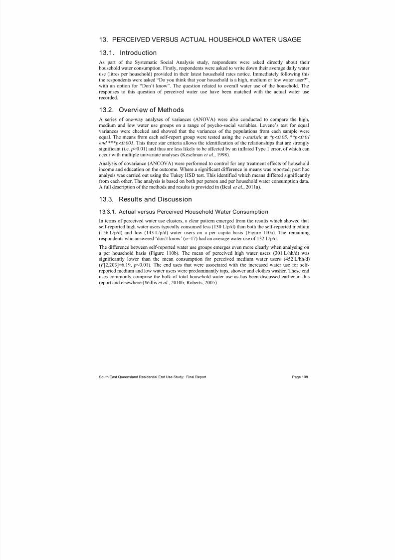
7/27/2019 Trabalho_Austrália
http://slidepdf.com/reader/full/trabalhoaustralia 118/174
13. PERCEIVED VERSUS ACTUAL HOUSEHOLD WATER USAGE
13.1. Introduction
As part of the Systematic Social Analysis study, respondents were asked directly about their
household water consumption. Firstly, respondents were asked to write down their average daily water use (litres per household) provided in their latest household rates notice. Immediately following thisthe respondents were asked “Do you think that your household is a high, medium or low water user?”,with an option for “Don’t know”. The question related to overall water use of the household. Theresponses to this question of perceived water use have been matched with the actual water userecorded.
13.2. Overview of Methods
A series of one-way analyses of variances (ANOVA) were also conducted to compare the high,medium and low water use groups on a range of psycho-social variables. Levene’s test for equalvariances were checked and showed that the variances of the populations from each sample were
equal. The means from each self-report group were tested using the t-statistic at *p<0.05, **p<0.01and *** p<0.001. This three star criteria allows the identification of the relationships that are stronglysignificant (i.e. p>0.01) and thus are less likely to be affected by an inflated Type 1 error, of which canoccur with multiple univariate analyses (Keselman et al., 1998).
Analysis of covariance (ANCOVA) were performed to control for any treatment effects of householdincome and education on the outcome. Where a significant difference in means was reported, post hocanalysis was carried out using the Tukey HSD test. This identified which means differed significantlyfrom each other. The analysis is based on both per person and per household water consumption data.A full description of the methods and results is provided in (Beal et al., 2011a).
13.3. Results and Discussion
13.3.1. Actual versus Perceived Household Water Consumption
In terms of perceived water use clusters, a clear pattern emerged from the results which showed thatself-reported high water users typically consumed less (130 L/p/d) than both the self-reported medium(156 L/p/d) and low (143 L/p/d) water users on a per capita basis (Figure 110a). The remainingrespondents who answered ‘don’t know’ (n=17) had an average water use of 132 L/p/d.
The difference between self-reported water use groups emerges even more clearly when analysing ona per household basis (Figure 110b). The mean of perceived high water users (301 L/hh/d) wassignificantly lower than the mean consumption for perceived medium water users (452 L/hh/d)(F [2,203]=6.19, p<0.01). The end uses that were associated with the increased water use for self-reported medium and low water users were predominantly taps, shower and clothes washer. These end
uses commonly comprise the bulk of total household water use as has been discussed earlier in thisreport and elsewhere (Willis et al., 2010b; Roberts, 2005).
South East Queensland Residential End Use Study: Final Report Page 108
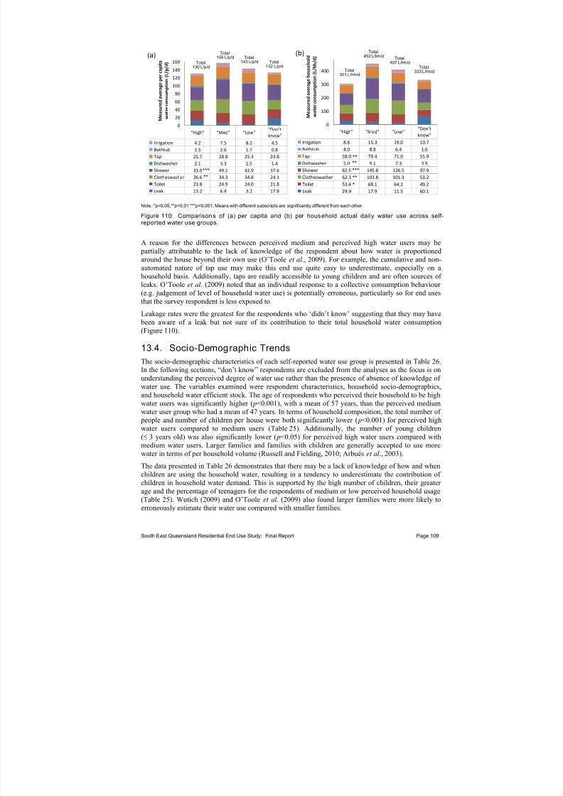
7/27/2019 Trabalho_Austrália
http://slidepdf.com/reader/full/trabalhoaustralia 119/174
"High" "Med" "Low""Don't
know"
Irrigation 4.2 7.5 8.2 4.5
Bathtub 1.5 2.6 1.7 0.8
Tap 25.7 28.8 25.3 24.8
Dishwasher 2.1 3.3 2.5 1.4
Shower 33.0 49.1 42.9 37.6
Clotheswasher 26.6 34.3 34.8 24.1
Toilet 23.8 24.9 24.0 21.8
Leak 13.2 6.4 3.2 17.8
0
20
40
60
80
100
120
140
160
M e a s u r e d a
v e r a g e p e r c a p i t a
w a t e r c o n s
u m p t i o n ( L / p
/ d ) Total
130 L/p/d
Total156 L/p/d
Total132 L/p/d
Total143 L/p/d
(a)
***
**
"High" "Med" "Low""Don't
know"
Irrigation 8.6 15.3 19.0 10.7
Bathtub 4.0 8.8 6.4 1.6
Tap 58.0 79.4 71.0 55.9
Dishwasher 5.0 9.1 7.3 3.9
Shower 82.5 149.8 126.5 97.9
Clotheswasher 62.3 103.8 101.3 53.2
Toilet 53.4 68.1 64.1 49.2
Leak 29.9 17.9 11.5 60.1
0
100
200
300
400
M e a s u r e d
a v e r a g e h o u s e h o l d
w a t e r c o n
s u m p t i o n ( L / h h / d )
Total301 L/hh/d
Total452 L/hh/d
Total333 L/hh/d
Total407 L/hh/d
(b)
**
***
**
**
*
Note. *p<0.05,**p<0.01 ***p<0.001; Means with different subscripts are significantly different from each other.
Figure 110: Comparisons of (a) per capita and (b) per household actual daily water use across self-reported water use groups.
A reason for the differences between perceived medium and perceived high water users may be partially attributable to the lack of knowledge of the respondent about how water is proportionedaround the house beyond their own use (O’Toole et al., 2009). For example, the cumulative and non-automated nature of tap use may make this end use quite easy to underestimate, especially on ahousehold basis. Additionally, taps are readily accessible to young children and are often sources of leaks. O’Toole et al. (2009) noted that an individual response to a collective consumption behaviour
(e.g. judgement of level of household water use) is potentially erroneous, particularly so for end usesthat the survey respondent is less exposed to.
Leakage rates were the greatest for the respondents who ‘didn’t know’ suggesting that they may have been aware of a leak but not sure of its contribution to their total household water consumption(Figure 110).
13.4. Socio-Demographic Trends
The socio-demographic characteristics of each self-reported water use group is presented in Table 26.In the following sections, “don’t know” respondents are excluded from the analyses as the focus is onunderstanding the perceived degree of water use rather than the presence of absence of knowledge of water use. The variables examined were respondent characteristics, household socio-demographics,
and household water efficient stock. The age of respondents who perceived their household to be highwater users was significantly higher ( p<0.001), with a mean of 57 years, than the perceived mediumwater user group who had a mean of 47 years. In terms of household composition, the total number of
people and number of children per house were both significantly lower ( p<0.001) for perceived highwater users compared to medium users (Table 25). Additionally, the number of young children(≤ 3 years old) was also significantly lower ( p<0.05) for perceived high water users compared withmedium water users. Larger families and families with children are generally accepted to use morewater in terms of per household volume (Russell and Fielding, 2010; Arbués et al., 2003).
The data presented in Table 26 demonstrates that there may be a lack of knowledge of how and whenchildren are using the household water, resulting in a tendency to underestimate the contribution of children in household water demand. This is supported by the high number of children, their greater
age and the percentage of teenagers for the respondents of medium or low perceived household usage(Table 25). Wutich (2009) and O’Toole et al. (2009) also found larger families were more likely toerroneously estimate their water use compared with smaller families.
South East Queensland Residential End Use Study: Final Report Page 109

7/27/2019 Trabalho_Austrália
http://slidepdf.com/reader/full/trabalhoaustralia 120/174
Table 26: Characteristics of self-reporting groups.
Self-Reported Water Use Category A,B
CharacteristicDescriptor (values are all means) High
(av.=301)Medium(av.=452)
Low(av.=407)
df C F
Value
Age of respondent 57a (13.7) 47a (12.8) 51ab (14) 2,201 11.51***
Education ratio(%Secondary:%TAFE/trade:%Tertiary)
36:29:35 29:26:45 29:24:47 - -
Respondent
Gender ratio (%male:%female) 46:54 42:58 43:57 - -
People per house 2.3a (1.0) 3.1b (1.3) 2.9
ab (1.1) 2,216 12.48***
Number of children 0.30a (.70) 0.77b
(1.0) 0.50ab
(.09) 2,214 7.41***
Children ≤ 3 years old 0.07a (.25) 0.24b (.49) 0.23ab (.59) 2,216 4.38*
Percentage teenagers (%) 14 30 24 - -
Householdsocio-demographics
IncomeD
57.1a (7.3) 79.4b (7.8) 89b (21) 2,201 9.72***
A Note. *p<0.05, ***p<0.001; Means with different subscripts are significantly different from each other. The standard deviations are italicised inparentheses. B The actual average household water use for each group is reported in L/hh/d in parentheses. C
df = degrees of freedom betweenand within groups. D Estimated from taking the average of the household income category that each respondents selected (Gregory and Di Leo2003), where categories were: 1 = <$30,000, 2 = $30,000 – $59,000, 3 = $60,000 – $89,999, 4 = $90,000 - $119,999, 5 = $120,000 - $149,999,
6 ≥ $150,000.
13.5. Household Water Appliance/Fixture and Perceived Water Use
In terms of water efficient appliances and fixtures, there were some general trends for people whoidentified as medium and low water users to have higher star rated and water efficient clothes washersand lower flow rated showerheads than those who identified as higher water users. The perceivedmedium water user group used a significantly greater ( p<0.05) volume of water in washing machines,higher than the perceived high water user group. The peak shower flow rate was also significantlylower ( p<0.05) for perceived high water users compared with perceived low water users (Figure 111a).
In general, the results in Figure 111 show a trend for the self-nominated medium and low water users
(i.e. higher average income earners as shown in Table 26) to have more water efficient appliances (i.e.higher star rated washing machines) and fixtures (i.e. low-flow rated showerheads). Consistent withthis, research shows that households with higher incomes have a greater tendency to install such water efficient technology (Millock and Nuages, 2010; Olmsetad and Stavins, 2009; Gregory and Di Leo,2003). Alternatively, the presence of water conserving technology may not be enough to alter a user’s
behaviour, as reported by Willis et al. (2010a) who observed that some people continued to have veryhigh volume showers, despite the presence of a recently installed shower alarm. A subsequentlongitudinal study by Stewart et al. (2011) provides evidence that alarming visual display showeringmonitors did not instil a sustained showering behaviour change over the longer term, sincehouseholders often reverted to previous habits.
The results of the current study indicate a trend for higher income, larger, younger and more educated
households to install efficiency appliances, which may not always be sufficient in reducing water consumption if curtailment actions are not also present. Using the same reasoning it could also beargued that lower income earners in older, smaller and less educated households tend towardscurtailment behaviours of water use frugality rather than adoption of potentially expensive and
potentially superfluous (i.e. if a one person household) technology. Gregory and Di Leo (2009) andGilg and Barr (2006) also reported a similar profile of low water users who were older, less educated,
had lower incomes and smaller household sizes.
South East Queensland Residential End Use Study: Final Report Page 110
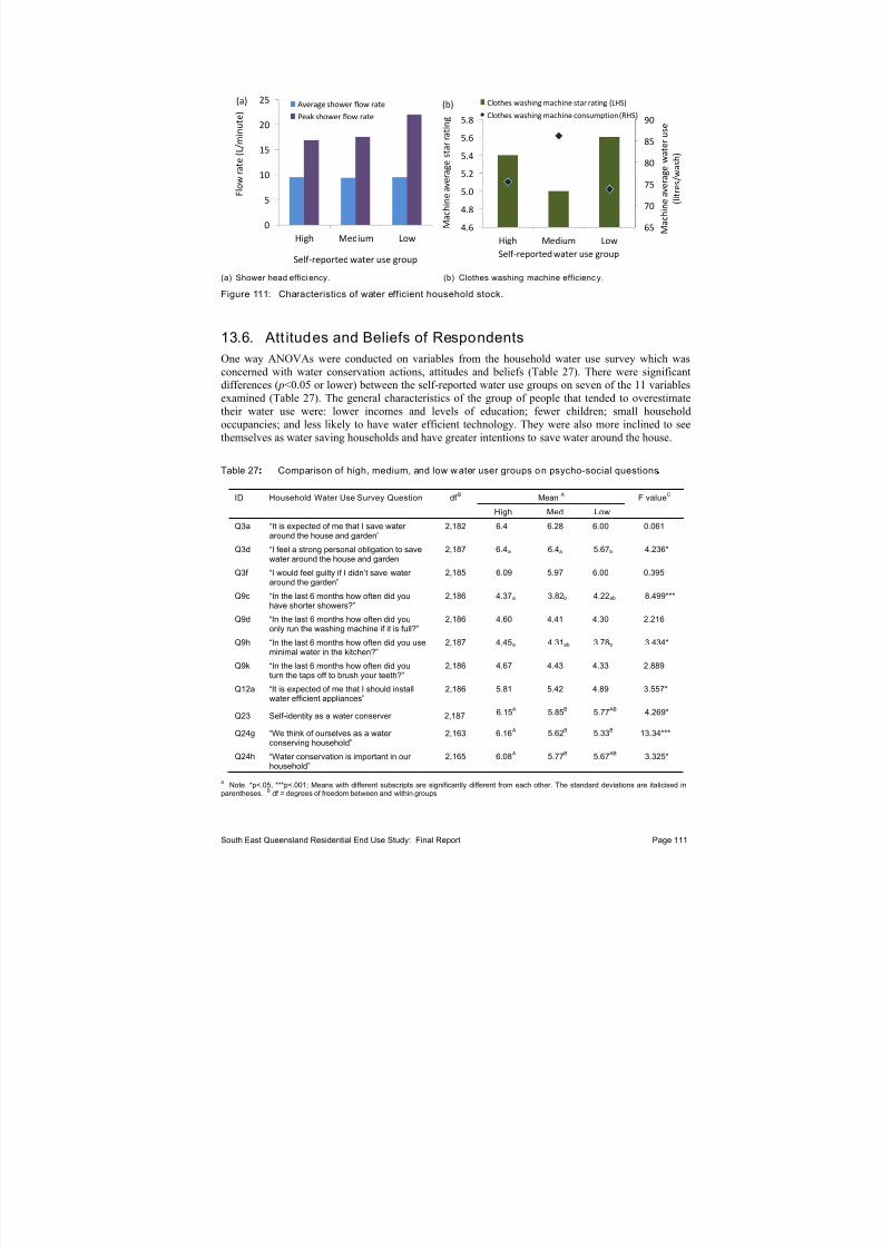
7/27/2019 Trabalho_Austrália
http://slidepdf.com/reader/full/trabalhoaustralia 121/174
0
5
10
15
20
25
High Medium Low
F l o w r a t e ( L / m i n u t e )
Self ‐reported water use group
Average shower flow rate
Peak shower flow rate
(a)
65
70
75
80
85
90
4.6
4.8
5.0
5.2
5.4
5.6
5.8
High Medium Low M a c h
i n e a v e r a g e w a
t e r u s e
( l i t r e s / w a s h )
M a c
h i n e a v e r a g e s
t a r r a
t i n g
Self ‐reported water use group
Clothes washing machine star rating (LHS)
Clothes washing machine consumption (RHS)
(b)
(a) Shower head efficiency. (b) Clothes washing machine efficiency.
Figure 111: Characteristics of water efficient household stock.
13.6. Att itudes and Beliefs of Respondents
One way ANOVAs were conducted on variables from the household water use survey which wasconcerned with water conservation actions, attitudes and beliefs (Table 27). There were significantdifferences ( p<0.05 or lower) between the self-reported water use groups on seven of the 11 variablesexamined (Table 27). The general characteristics of the group of people that tended to overestimatetheir water use were: lower incomes and levels of education; fewer children; small householdoccupancies; and less likely to have water efficient technology. They were also more inclined to seethemselves as water saving households and have greater intentions to save water around the house.
Table 27: Comparison of high, medium, and low w ater user groups on psycho-social questions.
ID Household Water Use Survey Question df B
MeanA
F valueC
High Med Low
Q3a “It is expected of me that I save water around the house and garden”
2,182 6.4 6.28 6.00 0.061
Q3d “I feel a strong personal obligation to savewater around the house and garden
2,187 6.4a 6.4a 5.67b 4.236*
Q3f “I would feel guilty if I didn’t save water around the garden”
2,185 6.09 5.97 6.00 0.395
Q9c “In the last 6 months how often did youhave shorter showers?”
2,186 4.37a 3.82b 4.22ab 8.499***
Q9d “In the last 6 months how often did youonly run the washing machine if it is full?”
2,186 4.60 4.41 4.30 2.216
Q9h “In the last 6 months how often did you useminimal water in the kitchen?”
2,187 4.45a 4.31ab 3.78b 3.434*
Q9k “In the last 6 months how often did youturn the taps off to brush your teeth?”
2,186 4.67 4.43 4.33 2.889
Q12a “It is expected of me that I should installwater efficient appliances”
2,186 5.81 5.42 4.89 3.557*
Q23 Self-identity as a water conserver 2,187 6.15 A 5.85B 5.77 AB 4.269*
Q24g “We think of ourselves as a water conserving household”
2,163 6.16 A 5.62B 5.33B 13.34***
Q24h “Water conservation is important in our household”
2,165 6.08 A
5.77B
5.67 AB
3.325*
A Note. *p<.05, ***p<.001; Means with different subscripts are significantly different from each other. The standard deviations are italicised inparentheses. B df = degrees of freedom between and within groups.
South East Queensland Residential End Use Study: Final Report Page 111

7/27/2019 Trabalho_Austrália
http://slidepdf.com/reader/full/trabalhoaustralia 122/174
Conversely, the characteristics of the group who underestimated their water use were: higher incomes;larger families with young children; and more likely to have more water efficient technology includinglow-flow shower roses and higher star rated washing machines. This group tended to have lower self-identity as water conservers and demonstrated lower intentions to save water around the home. Theways in which this knowledge can inform future water demand management approaches can begrouped into soft or voluntary approaches where citizens are given the choice through education,awareness, incentives, etc., to change their consumption behaviours, or hard polices where mandatorytools such as restrictions are used to reduce demand (Jones et al., 2009).
13.7. Summary and Relevance of Findings
Frequent and high volume water end uses such as clothes washing, showering and tap use wereassociated with the incorrect estimations of household consumption. Households that overestimate or underestimate their water use also differ in their socio-demographic and psycho-social profile,
providing further clues for why the disparity between perceived and actual behaviour arises. This typeof profiling can be used to formulate targeted water policy approaches such as educating citizens ontheir water use through feedback information and community-based social marketing. Heightenedfeedback to consumers on their households’ water consumption will improve their awareness and
understanding of water use and help to encourage future water conservation behaviours.
The over- or under-estimation of water use by householders demonstrates that there cannot beexclusive reliance on individual household attitudes and beliefs to reduce water consumption. In somecases water demand management policy cannot rely solely on individual household attitudes and
beliefs to reduce water consumption. Mandatory or hard measures such as water restrictions or tariff restructure are possibly more reliable in reducing residential demand, although a combination of regulation, efficiency appliances and behaviour change is likely to result in the best outcomes. A fulldiscussion of results and policy implications relating to perceived versus actual (measured) householdwater use can be found in Beal et al. (2011a).
South East Queensland Residential End Use Study: Final Report Page 112

7/27/2019 Trabalho_Austrália
http://slidepdf.com/reader/full/trabalhoaustralia 123/174
14. CLUSTERING WATER CONSUMPTION FLOW RATES
14.1. Introduction
A challenge facing the water industry in optimising water resources available for use by the
community is in the area of water leakage at the household level. Most Australian utilities are requiredto have water meter replacement programs, but there is still limited understanding of meter accuracy
performance with in-situ age, particularly when considering its starting or minimum registration level(Qs or Qstart). Moreover, low flow residential water leakages are often not registered (i.e. Q event<Qstart),and subsequently go undetected, by a typical water businesses aged fleet of conventional water meters.Currently, the entire community pays for this unaccounted water in the fixed and/or variablecomponent of their water charges. This next section summarises the work performed using theSEQREUS data to determine the Qs and to subsequently allow a better understanding of post-meter residential water leakage, adequate meter sizing and the non-registration of meters.
14.2. Overview of Methods used to Determining Qs
In order to categorise flow events, a software application was developed to assimilate data filescontaining household high resolution water consumption into various flow rate (L/hr) categories. Thesoftware was designed to read water usage from the data files (.txt file for each individual householdcovering a two-week period) and collate the water usage within the flow rate category range. Avolume of water (litre per household per day, L/hh/d) for each flow rate category (e.g. < 5 L/hr, 5 ≤ 10 L/hr, up to 1,800+ L/hr; see Table 28) was then created. If the flow rate of a particular event waswithin the flow rate category, then the volume of that event was summed with others that belong tothat category and total data was averaged for number of homes and total number of days of data.Results were then exported to an excel file where tables and charts were produced (i.e. volume in eachflow rate category, per cent of water use in each flow rate category, cumulative volume andcumulative proportion of total consumption). As a note to readers, the smart meter used (i.e. modifiedActaris CT-5) had a starting flow rate of 2 L/hr, so the recorded flows in the < 5 L/hr category do not
accurately capture those very slow drips (< 2 L/hr) that may be occurring in the household.
14.3. Results and Discussion
The average water usage and cumulative proportions of consumption are shown in Table 28. Datafrom this table are also presented graphically for the average and cumulative water consumption(Figure 112) and average and cumulative water use proportions (Figure 113). It is clear that there arethree main ‘clusters’ of flow rate range categories (Table 28):
- Flow rate range category Cluster 1 – this cluster denotes the first 11 categories (0 to ≤ 100 L/hr) and contributes 10% of the total consumption. The lowest four categories (i.e. flowrates ≤ 30 L/hr) comprise 60% (or 19.5 L/hh/d) of the cluster, or 6% of the overall total
consumption. The end uses associated with such low flows were mainly leaks, internal tap use,dishwasher, and some low-flow toilet, shower and clothes washing events.
- Flow rate range category Cluster 2 – this cluster represents the middle nine categories(100 ≤ 1,000 L/hr) and contributes to 80% of the total consumption. In particular, the categories
between 300 ≤ 700 L/hr comprise 57% (or 148.8 L/hh/d) of the cluster, or 45% of the overalltotal consumption. The end uses associated with these flow rates were typically shower, clotheswashing, full flush toilet use, external tap use, and irrigation.
- Flow rate range category Cluster 3 – this cluster denotes the last nine categories(1,000 < 1,800 L/hr) and contributes to 10% of the total consumption. The end uses associatedwith high flow rates included shower, clothes washing, external tap use, irrigation anduncommon water usage (e.g. service break leaks).
South East Queensland Residential End Use Study: Final Report Page 113

7/27/2019 Trabalho_Austrália
http://slidepdf.com/reader/full/trabalhoaustralia 124/174
Table 28: SEQ average water usage and cumulative proportion of consumption (n = 213).
Average FlowRate (L/hr)
Average Flow Rate(L/min)
Volume(L/hh/d)
Proportion of Total
Consumption(%)
CumulativeVolume(L/hh/d)
CumulativeProportion of TotalConsumption (%)
0 ≤ 5 0.0000 ≤ 0.0833 3.97 1.21 3.97 1.21
5 ≤ 10 0.0833 ≤ 0.1667 4.16 1.27 8.13 2.48
10 ≤ 20 0.1667 ≤ 0.3333 6.42 1.96 14.55 4.44
20 ≤ 30 0.3333 ≤ 0.5000 4.93 1.50 19.48 5.94
30 ≤ 40 0.5000 ≤ 0.6667 2.19 0.67 21.68 6.61
40 ≤ 50 0.6667 ≤ 0.8333 1.89 0.58 23.57 7.19
50 ≤ 60 0.8333 ≤ 1.0000 1.69 0.51 25.26 7.71
60 ≤ 70 1.0000 ≤ 1.1667 2.33 0.71 27.59 8.42
70 ≤ 80 1.1667 ≤ 1.3333 2.83 0.86 30.41 9.28
80 ≤ 90 1.3333 ≤ 1.5000 2.03 0.62 32.44 9.90
F l o w r
a t e C a t e g o r y C l u s t e r 1
90 ≤ 100 1.5000 ≤ 1.6667 2.51 0.77 34.96 10.67
100 ≤ 200 1.6667 ≤ 3.3333 15.57 4.75 50.53 15.42
200 ≤ 300 3.3333 ≤ 5.0000 25.15 7.67 75.68 23.09
300 ≤ 400 5.0000 ≤ 6.6667 35.22 10.75 110.90 33.84
400 ≤ 500 6.6667 ≤ 8.3333 54.91 16.75 165.82 50.59
500 ≤ 600 8.3333 ≤ 10.0000 29.31 8.94 195.13 59.53
600 ≤ 700 10.0000 ≤ 11.6667 29.36 8.96 224.48 68.49
700 ≤ 800 11.6667 ≤ 13.3333 23.54 7.18 248.02 75.67
800 ≤ 900 13.3333 ≤ 15.0000 22.33 6.81 270.35 82.49 F l o w R
a t e C a t e g o r y C l u s t e r 2
900 ≤ 1,000 15.0000 ≤ 16.6667 25.49 7.78 295.84 90.26
1,000 ≤ 1,100 16.6667 ≤ 18.3333 9.62 2.94 305.46 93.20
1,100 ≤ 1,200 18.3333 ≤ 20.0000 7.00 2.14 312.46 95.33
1,200 ≤ 1,300 20.0000 ≤ 21.6667 4.70 1.43 317.16 96.77
1,300 ≤ 1,400 21.6667 ≤ 23.3333 3.16 0.97 320.32 97.73
1,400 ≤ 1,500 23.3333 ≤ 25.0000 2.19 0.67 322.51 98.40
1,500 ≤ 1,600 25.0000 ≤ 26.6667 1.03 0.31 323.54 98.71
1,600 ≤ 1,700 26.6667 ≤ 28.3333 0.95 0.29 324.48 99.00
1,700 ≤ 1,800 28.3333 ≤ 30.0000 0.70 0.21 325.19 99.22 F l o w R
a t e C a t e g o r y C l u s t e r 3
> 1,800 > 30.0000 2.53 0.77 327.72 100.00
The data displayed in Figure 114 (pie chart) graphically shows the proportion of flow rate categoriesthat contribute to <100 L/hr or >1,000 L/hr flows. It can be seen from the pie chart that just over 20%of total flow is associated with these extreme low or extreme high flow rate events. In terms of theextremely high flow rates it was determined that these higher values were due to unusual water usagein a few households which elevated these averages, such as a mains service break, using two externaltaps for an extended period in combination, and/or long-term leakage in a few participatinghouseholds.
South East Queensland Residential End Use Study: Final Report Page 114

7/27/2019 Trabalho_Austrália
http://slidepdf.com/reader/full/trabalhoaustralia 125/174
Figure 112: Average water consumption and cumulative water consumption (L/hh/d).
Figure 113: Average proportion and cumulative proportion of total water consumption (%).
0 ‐ <5
1.21%5 ‐ <10
1.27%10 ‐ <20
1.96%20 ‐ <30
1.50%
30 ‐ <40
0.67%
40 ‐ <50
0.58%
50 ‐ <60
0.51%
60 ‐ <70
0.71%
70 ‐ <80
0.86%
80 ‐ <90
0.62%
90 ‐ <100
0.77%
100 ‐ <200
4.75%
200 ‐ <300
7.67%
300 ‐ <400
10.75%
400 ‐ <500
16.76%
500 ‐ <600
8.94%
600 ‐ <700
8.96%
700 ‐ <800
7.18%
800 ‐ <900
6.81%
900 ‐ <1000
7.78%1000 ‐ <1100
2.94%1100 ‐ <1200
2.14%
1200 ‐ <1300
1.43%
1300 ‐
<1400
0.97%
1400 ‐ <1500
0.67%
1500 ‐ <1600
0.31%1600 ‐ <1700
0.29%1700 ‐ <1800
0.21%> 1800
0.77%
Other
20.39%
Figure 114: Average proportion of total water consumption (%).
South East Queensland Residential End Use Study: Final Report Page 115
7/27/2019 Trabalho_Austrália
http://slidepdf.com/reader/full/trabalhoaustralia 126/174
15. ENERGY DEMAND FROM WATER END USES
15.1. Introduction
The conflict between water use and associated energy consumption is often referred to as the water-
energy nexus. This is particularly relevant in an urban context as studies continue to demonstrate thesignificant role that the urban resident plays in consuming water and energy resources (Kenway et al.,2008; Lenzen and Peters, 2010; Kenway et al., 2011). Managing such interconnected resources hassignificant implications on the savings (or production) of greenhouse gas emissions (Kenway et al.,2011; Golden et al., 2010). As Fidar et al. (2010) and Maas (2009) observe, managing water demandthrough water efficient technology and behavioural changes has strong implications for reducinggreenhouse gas emissions as well as conserving potable water supplies. This argument becomesstronger when one considers the acceleration of economic development and subsequent rise in livingstandards in some developing countries (Pakula and Stamminger, 2010).
The following section presents an overview of the methodology and some preliminary results obtainedfrom analysing the energy requirements and resultant greenhouse gas emissions from residential water
use appliances and fixtures (e.g. shower, tap, clothes washer and dishwasher).
15.2. Overview of Methods
There were two major components to the methods: (1) determining water, energy and carbonemissions from measured water end uses; and (2) calculating the optimal combination of interventionsolutions (e.g. cost effective energy-efficient options) to reduce carbon emissions from water end uses.A sub-sample of homes that had energy information captured during the household stock audit fromthe SEQREUS was used to determine the water (and energy) demand, thus, the water consumptionvalues presented in section 15.5 will be slightly different than those reported for the full SEQREUSsample in earlier sections of this report. The sub-sample size was 211 homes; however, the sample waslower (n=189) for clothes washers and dishwashers due to some missing stock appliance data (e.g.information on clothes washer cycle temperatures and dishwasher models).
15.3. Calculating Energy Demand and Carbon Emissions
15.3.1. Determining Energy Consumption from End Use Data
Calculations shown in Table 29 were applied to the measured and published water and energy datadescribed above to predict energy consumption for each end use in each household in the study. Themean, median, standard deviation and 95% confidence intervals are reported for each end use tocharacterise the variation and uncertainties of energy demand data across households and end uses.Units are reported in kilowatt hours per person per year (kWh/p/y). Note that the source of data for calculations were taken from Australian Government (2011, 2010a, 2010b) and Kenway et al. (2008)when not provided directly from household water stock audit.
Clothes washers (CW) are one of the most ubiquitous household appliances in the western world andare in use in an estimated 97% of Australian homes (Paluka and Stamminger, 2010). In calculating theenergy demand from clothes washers, a number of issues need to be considered. Many of the later model machines have a horizontal axis (or are front loading machines) and only have a single, coldwater tap connection to the machine, and thus heat water internally. In contrast, the older models tendto have vertical axis (or are top loading machines); they have a larger capacity and dual water connections (i.e. hot and cold tap connections to the machine). In this configuration, hot water issourced from the external hot water service. As also observed by others, (Willis et al., 2011; Palukaand Stamminger, 2010; Flower, 2009; Kenway et al., 2008), the wide variety of heating, water connection, and loading configurations of clothes washers mean that the water and energy demandscan vary markedly between the machines. The proportion of hot and cold water needs to be
considered, along with a comparison between the energy demand from the internal heating and theenergy demand from the HWS heating.
South East Queensland Residential End Use Study: Final Report Page 116
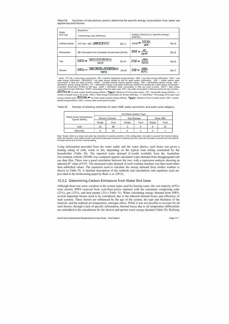
7/27/2019 Trabalho_Austrália
http://slidepdf.com/reader/full/trabalhoaustralia 127/174
Table 29: Summary of calculations used to determine the specific energy consumption from water useappliances and fixtures.
Equations1
Water End Use Total Energy Use (kWh/p/y)
Energy Intensity (or specific energy)(kWh/kL)
Clothes washer TOT EN = ME + [Eq 1] AWSE [Eq 2]
Dishwasher ME information from Australian Government (2010a) [Eq 3]
Tap [Eq 4] [Eq 5]
Shower [Eq 6] [Eq 7]
1where: TOT EN = total energy consumption, ME = machine (appliance) energy demand, HWE = hot water energy (kWh/wash), CWE = cold
water energy (kWh/wash), HWE(HWS) = hot water energy needed by the hot water system (kWh/wash), LpW = clothes washer water consumption in litres per wash (L/wash), AWSE = average washing machine specific energy, DSE = dishwashing specific energy, DSE =dishwasher specific energy (kWh/kL), EC = dishwasher energy consumption (kWh/use) obtained by dividing the overall energy consumption(Australian Government 2010a) by 365 days, LpdW = dishwasher water consumption in litres per cycle (L/cycle), DECt = daily energyconsumption for taps (kWh/day), %HWt = percentage of tap hot water used, TWC = tap water consumption in litres per person per day (L/p/day),
hot water system specific energy (kWh/kL), = efficiency of the hot water system, TSE = tap specific energy (kWh/kL), n =
number of people living in the house, DECs = Daily Energy Consumption for Shower (kWh/day), % HW(HWS)s = Percentage of hot water used
during a shower event, hot water system specific energy (kWh/kL), = efficiency of the hot water system, SSE = shower
specific energy (kWh/kL), SWC = shower water consumption (L/p/day).
Table 30: Number of washing machines for each HWS, water connection and wash cycle category.
Hot Water System Type
Electric Cylinder Gas Storage Solar (EB)Wash Cycle Temperature
Typical SettingSingle Dual Single Dual Single Dual
Cold 23 86 2 8 8 22
Warm/Hot 8 23 0 2 0 7
Note: ‘Single’ refers to a single cold water tap connection to washing machine; in this configuration, hot water is sourced from internal heatingwithin the machine. ‘Dual’ refers to both a cold and hot water tap connection to washing machine, where the hot water is sourced from the externalhot water service and not from internal heating.
Using information provided from the water audits and the water diaries, each home was given aheating rating of cold, warm or hot, depending on the typical load setting nominated by thehouseholder (Table 30). The reported water demand (L/wash) available from the AustralianGovernment website (2010b) was compared against calculated water demand from disaggregated end
use data files. There was a good correlation between the two, with a regression analysis showing anadjusted R
2 value of 0.91. The measured water demand of each washing machine was then used rather than published values. The equations used to calculate the energy demand from clothes washers isshown in Table 29. A detailed description of the methods and calculations and equations used are
provided in the forthcoming paper by Beal et al. (2012).
15.3.2. Determining Carbon Emissions from Water End Uses
Although there was some variation in the system types used for heating water, the vast majority (65%)were electric HWS (sourced from coal-fired power stations) with the remainder comprising solar (21%), gas (12%), and heat pumps (2%) (Table 31). When calculating energy demand from HWS,several important factors need to be considered, due to the inherent thermal losses and efficiency of
such systems. These factors are influenced by the age of the system, the type and thickness of thematerial, and the ambient air temperature, amongst others. While it was not possible to account for allsuch factors, through a lack of specific information, thermal losses due to air temperature differentialsare embedded in the calculations for the shower and tap hot water energy demand (Table 29). Refining
South East Queensland Residential End Use Study: Final Report Page 117

7/27/2019 Trabalho_Austrália
http://slidepdf.com/reader/full/trabalhoaustralia 128/174
South East Queensland Residential End Use Study: Final Report Page 118
the model input parameters, and including the energy demand beyond the operational stage of theappliances/fixtures (e.g. embedded energy and life cycle stages prior to and subsequent to operationalstage) will be the subject of future investigations.
The energy consumption varies with the type of HWS (Table 31), with the highest demand typicallyassociated with the electric cylinder and gas cylinder. The carbon emission conversion factors for the
various energy sources to heat water are also shown in Table 3. An emission factor of 0.138 was usedto determine carbon emissions from an electric boosted solar HWS, based on the assumption of a 10%requirement of electricity boosted heating during periods of insolation. This figure was calculatedfrom historical climate data from the Australian Bureau of Meteorology website (the Brisbane airportweather station) and the value of 8.1 for the average hours of sunshine at that location.
Table 31: Energy intens ity values and GHG emission conversion factors used for calculating GHGemission savings for hot water systems.
HWS Type Number inSample
(% Total)
Energy Intensity(kWh/kL)
1
GHG Emission Factor (kgCO2e/kWh)
Electric 177 (65) 126.80 1.0002
Gas Cylinder 22 (8) 171.23 0.1973
Gas Instant 11 (4) 85.60 0.1973
Solar (electric boosted) 56 (21) 59.19 0.1384
Heat pump 5 (2) 22.095 0.5006
1 Kenway et al. (2008) except heat pump values; 2 Australian Government (2011) assuming 100% supply from coal-fired power station; 3 AustralianGovernment (2011) for natural gas; 4 assumes insufficient insolation for 10% of the year due to cloud cover (i.e. 0.038 (Australian Government2011) + 0.1×1.00), 5 heat pump energy intensity based on coefficient of performance, 6 assumed a 50% reduction in coal-fired electricity generation(Blum et al., 2010, Lund et al., 2004).
15.4. Optimising Water and Energy Efficient Strategies
A number of scenarios were devised to determine the impact on carbon emission reductions fromvarious water and energy-efficient technologies (Table 32). The data from each scenario were basedon the average consumption calculated from SEQREUS homes that met existing sets of classificationconditions. For example, when determining the savings from replacing an electric HWS with a solar (electric boosted) HWS, the average percentage difference between a cluster of homes with solar HWSand with electric only was applied to the base case. The percentage savings from the base casescenario (worst case scenario of no efficient strategies and electric HWS) were calculated bycomparing a range of sequentially applied water and energy efficiency intervention strategies. As aresult, the cumulative reduction in energy consumption can be determined as each new scenario isapplied. Additionally, the savings from each individual scenario was also calculated. Some keyassumptions were made during the development of these scenarios and are outlined in Table 33.
Table 32: Intervention scenarios using water and energy efficient technology.
ScenarioNumber
Intervention Scenario Rationale Snapshot
S1Conversion to energy-efficientsolar HWS
An increasingly popular choice for homeowners in Australia withgovernment rebates offered.
S2 Water-efficient shower heads A very popular, cheap and effective technology (Beal et al., 2011; Willis etal., 2010).
S3S2 + Water-efficient clotheswasher
An increased penetration in Australian households with governmentrebates offered.
S4 S3 + Tap aeratorsCheap and common solution to reducing volume but maintaining flowrate. Recommended in Queensland building codes.
S5 S4 + Shower temperaturereduced to average of 37 C˚
Strategy to reduce hot water demand and heat losses (Flower 2009;Clarke et al., 2009).
S6S5 + Energy-efficientdishwashers (DW)
Increasing penetration in market place based on energy efficiency rather than water efficiency (Stamminger, 2011).

7/27/2019 Trabalho_Austrália
http://slidepdf.com/reader/full/trabalhoaustralia 129/174
Table 33: Key assumptions for each intervent ion scenario shown in Table 31.
ScenarioNumber
Assumptions
S1a) Solar panels with electric-boosted storage system; b) direct replacement of electric HWS; c) long termaverage solar radiation data taken from Brisbane airport and assuming same characteristics across SEQ;d) 38 days or 10% of year with insufficient insolation.
S2a) Substitute high flow shower head with low-flow shower head of flow rate at 0.09 L/s; b) co-efficient of 1.2 applied to compensate for increased duration due to lower flows.
S3a) CW internally heats cold water; b) front load only; c) cold water connection only; d) directly substitutingdual connected front or top load CW.
S4 a) Tap flow rate fixed value of 0.08 L/s (Australian Government, 2011b).
S5a) Original shower temperature set at 40˚C (Flower, 2009); b) existing shower head efficiencies (e.g. lowor high flow roses) remain.
S6a) > 3 star rated machines considered ‘energy-efficient’; b) two efficiency clusters generated fromSEQREUS data: ≤ 3 star and >3 star rated.
15.5. Results and Discussion
15.5.1. Water and Energy Consumpt ion for Residential End Uses
Shower, clothes washer and tap usage comprised the bulk of the average annual water consumption(69% combined) (Figure 115). This represents a total of 33 kilolitres per person per year (kL/p/y) for shower, taps and clothes washer (CW).
Dish
washer 1.2
kL/p/y
(3%)
Clothes
washer
8.9 kL/p/y
(19%)
Taps
9.5 kL/p/y
(20%)
Shower
13.9
kL/p/y
(30%)
Bathtub0.5 kL/p/y
(1%)
Toilet
7.5. kL/p/y
(16%)
Irrigation
2 kL/p/y
(4%)
Leaks
3.2 kL/p/y
(7%)
Figure 115: Average annual end use breakdown for water consumption (kL/p/y).
South East Queensland Residential End Use Study: Final Report Page 119

7/27/2019 Trabalho_Austrália
http://slidepdf.com/reader/full/trabalhoaustralia 130/174
The proportions of annual energy demand and carbon emissions vary quite considerably across thefour main HWS (Figure 116). Dishwasher energy demand and carbon emissions remain constantirrespective of HWS, as 100% of energy requirements are drawn from the electricity grid generatedfrom coal-fired power stations (hence carbon emissions = 1 x energy demand value for Queensland[Australian Government, 2011]). However, the proportion of total energy and carbon emissions for dishwasher operation increases as the coal-fired electric HWS sources are replaced with gas and solar HWS.
Dish
washer*
81.9
kWh/p/y
(5.6%)
Clothes
washer
104
kWh/p/y
(7.1%)
Taps
464
kWh/p/y
(31.8%)
Shower
810
kWh/p/y
(55.5%)
(a) Energy ‐ Electric cylinder (EC) Dish
washer*
81.9
kg
CO2e/p/y
(5.6%)
Clothes
washer
104
kg
CO2e/p/y
(7.1%)
Taps
464 kg
CO2e/p/y
(31.8%)
Shower
810
kg
CO2e/p/y
(55.5%)
(b) Carbon ‐ Electric cylinder (EC)
(a) Average energy demand from EC. (b) Average carbon emissions from EC.
Dish
washer*
81.9
kWh/p/y
(3.4%)
Clothes
washer
364
kWh/p/y
(15.3%)Taps
692
kWh/p/y
(29%)
Shower1246
kWh/p/y
(52.3%)
(c) Energy ‐ Gas cylinder (GC)Dish
washer*
81.9
kg
CO2e/p/y(3.4%)
Clothes
washer
72
kg
CO2e/p/y
(13.5%)
Taps
136 kg
CO2e/p/y
(25.4%)
Shower
245
kg
CO2e/p/y
(45.8%)
(d) Carbon ‐ Gas cylinder (GC)
(c) Average energy demand from GC. (d) Average carbon emissions from GC.
South East Queensland Residential End Use Study: Final Report Page 120

7/27/2019 Trabalho_Austrália
http://slidepdf.com/reader/full/trabalhoaustralia 131/174
Dish
washer
81.9
kWh/p/y
(6.5%)
Clothes
washer
71
kWh/p/y
(5.6%)
Taps
240
kWh/p/y
(19%)
Shower
871
kWh/p/y(68.9%)
(e) Energy ‐ Instant gas (IG)
Dish
washer
81.9
kg
CO2e/p/y
(26%)
Clothes
washer
14
kg
CO2e/p/y
(4.5%)
Taps
47 kg
CO2e/p/y
(15%)
Shower
171 kg
CO2e/p/y
(54.5%)
(f) Carbon ‐ Instant gas (IG)
(e) Average energy demand from IG. (f) Average carbon emissions from IG.
Dish
washer*
81.9
kWh/p/y
(10.3%)
Clothes
washer
125
kWh/p/y
(15.8%)
Taps
234
kWh/p/y
(29.5%)
Shower
351
kWh/p/y
(44.4%)
(g) Energy ‐ Solar electric boosted (SEB)
Dish
washer*
81.9
kg
CO2e/p/y
(45.3%)
Clothes
washer
17
kg
CO2e/p/y
(9.4%)
Taps
34 kg
CO2e/p/y(18.8%)
Shower 48
kg
CO2e/p/y
(26.5%)
(h) Carbon ‐ Solar electric boosted (SEB)
(g) Average energy demand from SEB. (h) Average carbon emissions from SEB.
Note: *Dishwasher energy sourced solely from electricity grid using coal-fired power therefore energy demand and carbon emissions are constantfor the four HWS scenarios.
Figure 116: Average annual end use breakdown for water consumpt ion (kL/p/y).
The energy associated with heating water is, typically, the major influence on household energy use(Kenway et al., 2010; Fidar et al., 2010; Clarke et al., 2009) and, thus, hot water system type must be
accounted for when comparing energy demand across end-uses and households. The descriptivestatistics for the energy consumption for the dishwasher and the hot water components of the shower and tap usage for the four main HWS types of electric cylinder (EC), gas cylinder (GC), instant gas(IG) and electric-boosted solar (SEB), are presented in Table 34.
The results demonstrate that SEB HWS require substantially less grid energy than conventionalelectric hot water systems. Specifically, energy demand can be reduced by an average of 460 kWh/p(or 56%) for shower use and 220 kWh/p (or 57%) for tap use annually if an EC was replaced with anSEB system (Table 34). This degree of energy demand reduction from solar HWS is consistent withother findings (Tsilingiridis and Martinopoulos, 2010; Perry et al., 2008; Crawford et al., 2003). Evengreater energy savings are indicated if using a GC system due to its higher energy intensity than an EC(Table 31).
South East Queensland Residential End Use Study: Final Report Page 121

7/27/2019 Trabalho_Austrália
http://slidepdf.com/reader/full/trabalhoaustralia 132/174
Table 34: Descriptive statistics for energy consumption and carbon emissions from energy-related
residential water end uses in average household.
Shower (Hot Water Component)
Tap(Hot Water Component)
Dishwasher 1
(Machine Operation +Internal Heating )
Hot Water System Statistic
EnergydemandkWh/p/y
Carbonemissions
kg CO2-e/p/y
EnergydemandkWh/p/y
Carbonemissions
kg CO2-e/p/y
EnergydemandkWh/p/y
Carbonemissions
kg CO2-e/p/y
Mean 810.3 810.3 463.8 463.8 81.9 81.9
Median 714.8 714.8 422.5 422.5 73.7 73.7
SD 521.7 521.7 317.6 317.6 71.6 71.6
Electriccylinder
(EC) (coal-fired power)
95% CI 85.2 85.2 51.9 51.9 19.5 19.5
Mean 1246.4 245.4 691.8 136.3
Median 1080.7 212.9 492.8 97.1
SD 624.0 184.7 591.7 116.6Gas cylinder (GC)
95% CI 353.1 109.1 334.8 66
-
Mean 871.5 171.7 239.6 47.2
Median 630.6 124.4 190.8 37.6
SD 937.5 187.4 214.2 42.2
Instant gas(IG)
95% CI 554.0 109.1 126.6 24.9
-
Mean 350.8 48.4 244 33.7
Median 324.7 44.8 215.6 29.8
SD 184.3 25.4 179.5 24.8
Solar 2
(Electricboosted)(SEB)
95% CI 57.1 7.9 56.3 7.8
-
1 Assuming all dishwashers are operated from energy sourced from coal-fired power stations, where carbon emissions factor = 1.0 (DCCEE2011); 2 Assuming electric booster used 10% of the year i.e. carbon emissions factor = 0.138 (0.1 [coal-fired power station] + 0.038 [solar panels]).
As all dishwashers used for the sample heated the water internally, energy consumption originatedsolely from the mains electricity grid. As such, the energy consumption was comparatively low (at anaverage of 82 kWh/p/y) compared to the fixtures reliant on the HWS. The average energy demandfrom showering ranged from 1246 kWh/p/y (GC) to 351 kWh/p/y (SEB) (Table 34).
From the sensitivity analysis, the percentage of hot water consumption was able to determine, moreaccurately, the energy demand more so than the HWS type. This outcome is especially important for demand managers, as shower usage is consistently the greatest proportion of total indoor water consumption in homes. Hence, demand managers need to continuously target both water and energyconsumption. Not unexpectedly, the energy demand for tap usage was lower than for showers, due tothe reduced total water consumption (4.4 kL/p/y less than showers), including a 2% reduction inaverage hot water consumption.
Estimating the energy demand from the clothes washers is a more complex calculation, which requiresconsideration of the various configurations of tap connections, HWS types, and temperature washcycles. Fortunately, the data registry available from the SEQREUS allowed a high level of precision inclustering each of the configurations, although sample size was quite low for some categories (seeTable 30). The average and standard deviations of energy consumption for each of theseconfigurations is displayed in Figure 117a.
South East Queensland Residential End Use Study: Final Report Page 122

7/27/2019 Trabalho_Austrália
http://slidepdf.com/reader/full/trabalhoaustralia 133/174
single dual single dual single dual single dual
Electric Gas cylinder Instant gas Solar (EB)
Cold 17.8 24.9 39.2 31.4 52 27.5 27.7 23.0
Warm/Hot 72.7 478.5 2024.5 256.3 167.8 557.9
1
10
100
1000
10000
A v e r a g e e n e r g y c o n s u m
p t i o n f o r
c l o t h e s w a s h e r s
( k W h / p / y )
(a)
(a) Average energy consumption.
single dual single dual single dual single dual
Electric Gas cylinder Instant gas Solar (EB)
Cold 17.8 24.9 7.7 6.2 10.25 5.43 3.8 3.2
Warm/Hot 72.7 478.5 265.9 50.5 33.0 77.0
1
10
100
1000
A v e r a g e c a r b o n e m i s s i o n s f o r
c l o t h e s w a s h e r s
( k g C O 2 e
/ p / y
)
(b)
(b) Average carbon emissi ons.
Note: error bars represent standard deviation.
Figure 117: Average energy consumption and carbon emissions from clothes washing machines.
The lowest energy demand was from machines using only the cold cycle. The energy demand for thesemachines was based on the published values for each machine, are irrespective of HWS. Once a warmor hot cycle is chosen, with a single or dual connected machine, the energy demand rises. For the
single connection of a warm or hot wash cycle, the energy demand is solely from the machine, onceagain, irrespective of the HWS. However, for the dual connection, that is, the warm/hot wash, the hotwater is sourced from the HWS. As a consequence, the energy demand increases sharply, particularlyfor an EC, 478.5 kWh/p/y, and a GC, 2024.5 kWh/p/y (Figure 117a).
South East Queensland Residential End Use Study: Final Report Page 123

7/27/2019 Trabalho_Austrália
http://slidepdf.com/reader/full/trabalhoaustralia 134/174
15.5.2. Carbon Emissions from Energy-Related Water End Uses
Water-related carbon emissions are also presented for the dishwasher, tap and shower (Table 34) andclothes washers (Fig 118b). The carbon emissions from end uses relying on a solar HWS with electric
booster are based on the assumption that the electric booster would only be required 10% of the year based on average sunny days in the sub-tropical climate for Brisbane. Any extrapolation of thesevalues to regions of lower insolation need to consider greater reliance on the electric booster and thuswould potentially increase the carbon emissions associated with a SEB HWS. Notwithstanding, thereduction in carbon emissions associated with an alternative HWS to electric is clear; whether it be agas or solar based HWS.
In terms of end uses, results demonstrate that appliances that internally heat water are substantiallymore economical in terms of operational energy demand and carbon emissions than those that sourcehot water externally from an electric or gas cylinder. This is exemplified by the results for dishwashersand single connected clothes washers where carbon emissions were an average of 82 (SD± 72) kgCO2-e/p/y and between 3.8 (SD± 1.3) to 73 (SD± 26) kg CO2-e/p/y, respectively.
In comparison, carbon emissions from sourcing hot water from either gas or electric storage cylinders
ranged from 245 (SD± 185) to 810 (SD± 523) kg CO2-e/p/y respectively, for showers and 136 (SD±116) to 464 (SD± 318) kg CO2-e/p/y respectively, for taps (Table 34). The large standard deviationobserved for energy use and subsequent carbon emissions, is a reflection of the inherent variability inwater and energy demand from appliances and fixtures within a household (Frijia et al., 2012; Williset al., 2011; Clarke et al., 2009; Flower et al., 2007).
15.5.3. Energy Intensity Comparisons between End Use Appliances andFixtures
Energy intensity (EI), sometimes referred to as specific energy, is a quantum of the energy per unit of water used, and in this case is expressed in kilowatt hours per kilolitre (kWh/kL). A comparison of EIsis useful as it provides a gauge of the relative energy efficiency for each water end use (Figure 118).Again, end uses which rely on externally heating water clearly have higher EIs than those thatinternally heat water, with the exception of dishwashers which had an EI of 55 (SD± 11) kWh/kL.This suggest that the typical dishwasher is not overly energy-efficient in relation to the amount of water it requires, however due to the low water demand, around 2-3% total average household water consumption, its overall energy demand is reduced.
Clothes washers with dual connection on a warm/hot wash cycle require energy for both heating water and appliance operation. In this study, the EI for these activities were 55.1 (SD± 16) kWh/kL and 3.3(SD± 1) kWh/kL for external heating and operation, respectively. Conversely, for the same warm/hotwash cycle, the single connected clothes washers had an average EI of 4.2 (SD± 3) kWh/kL(Figure 118). That is, the additional energy required to heat the water internally is lower than theenergy required to heat the water via the HWS, which heats larger volumes of water to a greattemperature. The majority of these single connected systems were front loading (or horizontal axis)
machines. The results emphasise the importance of knowing details on clothes washer configurationsin order to produce a representative dataset.
South East Queensland Residential End Use Study: Final Report Page 124

7/27/2019 Trabalho_Austrália
http://slidepdf.com/reader/full/trabalhoaustralia 135/174
0
10
20
30
40
50
60
70
80
C W
( s i n g l e
, c o l d )
C W
( s i n g l e
,
w a r m
/ h o t )
C W
( d u a l , c o l d )
C W
( d u a l ,
w a r m
/ h o t )
D W
T a p s
S h o w e r s
A v e r a g e e n e r g y i n t e n s i t y o f e
n d u s e a c t i v i t y
( k W h / k L )
Water end use appliance/fixture
Energy demand from appliance Energy demand from HWS
Figure 118: Average energy intensities for water-related energy in SEQREUS homes.
15.5.4. Impact of Intervention Scenarios on Water, Energy and CarbonEmissions
Total Household Savings
A number of energy-efficient intervention scenarios were modelled to quantify reductions in carbon
emissions compared with base (worst) case scenario for a household with no water-efficientappliances/fixtures and an electric cylinder HWS. The scenarios described in Tables 31 and 32 weremodelled for shower, tap, clothes washer and dishwasher. Results are shown in Figure 119.
Base case S2 S3 S4
Shower 13.9 8.7 8.7 8.7
DW 9.5 9.5 9.5 6.9
CW 9.0 9.0 6.6 6.6
Taps 1.2 1.2 1.2 1.2
Total 33.6 28.4 26.0 23.4
0
10
20
30
40
A n n u a l
a v e r a g e w a t e r
c o n s u m
p t i o n ( k L / p / y )
Note: Savings are cumulative – see Table 32.
Figure 119: Cumulative impact of various water-efficient intervention scenarios on annual householdwater consumption .
South East Queensland Residential End Use Study: Final Report Page 125

7/27/2019 Trabalho_Austrália
http://slidepdf.com/reader/full/trabalhoaustralia 136/174
Figure 119 shows the annual average water consumption starting with the base case using SEQREUSdata from homes without any of the water-efficient technologies. Cumulative reductions are thenshown as each scenario is applied (i.e. the final row in Figure 119 assumes all the previous scenariosare applied as well as installing a 4 star shower head). Results show that a savings of 10.2 kL/p/y can
be achieved by installing a combination of water-efficient shower, tap and clothes washer stock. Thewater savings from efficient clothes washers are a little lower than reported elsewhere (e.g. Willis et
al., 2011), and may be a function of elevated water usage for a small number of homes with high star-rated machines. Beal et al. (2011b) discuss the phenomenon where people with a high level of water-efficient stock do not necessarily exhibit water conserving behaviours (such as reducing the number of small loads) and this may also have been a factor in the observed lower water savings from homeswith water-efficient clothes washers.
The annual household energy consumption and carbon emission savings was also predicted for variousresource-efficient stock for two groups: (i) no change to an existing electric HWS (Figure 120a); and(ii) replacement of an electric HWs with a solar HWS (SEB) (Figure 120b and Figure 121). Both thesescenarios have been presented to represent older/existing homes with retrofitted resource-efficientindoor stock but an existing EC HWS, and newer homes built under current building codesustainability requirements which would include both resource-efficient stock and an efficient HWS
(in this case a SEB). Knowledge of the savings from both scenarios can assist in the decision makingfor developing future building development codes.
Base case S2 S3 S4 S5 S6
Shower 821 305 305 305 259 259
Taps 464 464 464 291 291 291
CW 252 252 45 45 45 45
DW 82 82 82 82 82 59
Total 1619 1103 896 723 677 654
1
10
100
1000
10000
A n n u a l a v e r a g e e n e
r g y c o n s u m p t i o n
E C H W S ( k
W h / p / y )
(a)
(a) Energy savings from an existing EC HWS + effic ient stock .
South East Queensland Residential End Use Study: Final Report Page 126

7/27/2019 Trabalho_Austrália
http://slidepdf.com/reader/full/trabalhoaustralia 137/174
Base
caseS1 S1 + S2 S1 + S3 S1 + S4 S1 + S5 S1 + S6
Shower 821 345 128 128 128 112 112
Taps 464 244 244 244 151 151 151
CW 252 211 211 28 28 28 28
DW 82 82 82 82 82 82 59
Total 1619 882 665 482 389 373 350
1
10
100
1000
10000
A n n u a l a v e r a g e e n e r g y
c o n s u m p t i o n
S E B H W S ( k W h
/ p / y )
(b)
(b) Energy savings by replacing an existing EC HWS with a SEB HWS + effici ent stock.
Note: Savings are cumulative – see Table 32.
Figure 120: Cumulative impact of various water-efficient intervention scenarios on annual householdenergy consumption .
Base
caseS1 S1 + S2 S1 + S3 S1 + S4 S1 + S5 S1 + S6
Shower 113 48 18 18 18 15 15
Taps 64 34 34 34 21 21 21
CW 35 29 29 4 4 4 4
DW 11 11 11 11 11 11 8
Total 223 122 92 67 54 51 48
1
10
100
1000
A n n u a l a v e r a g e c a r b o n e m i s s i o n s
S
E B H W S ( k g C O 2 e / p / y )
Note: Savings are cumulative – see Table 32.
Figure 121: Cumulative carbon emission savings by replacing an existing EC HWS with a SEB HWS +efficient stock.
South East Queensland Residential End Use Study: Final Report Page 127

7/27/2019 Trabalho_Austrália
http://slidepdf.com/reader/full/trabalhoaustralia 138/174
Results demonstrate that substantial savings to energy (and carbon emissions) can be achieved byretrofitting without replacing an existing EC HWS (Figure 120a). If all intervention scenarios wereadopted, an energy savings of about 965 kWh/p/y (or 60%) may be achieved. This equates to the samevolume of carbon emissions savings due to the emissions factor of 1 for Queensland (AustralianGovernment, 2011). In contrast, average energy and carbon emissions savings from applying the samescenarios to households who also installed a SEB HWS were estimated at 1,269 kWh/p/y (or 78%)(Figure 120b) and 175 kg CO2-e/p/y (Figure 121), respectively.
Savings from Indiv idual Resource-Efficient Stock
Individual volumetric and percentage savings for each resource-efficient scenario were alsodetermined (Table 35). Installing a solar HWS (electric boosted) was the most energy-efficientscenario reducing total household energy savings of around 46% at an equivalent volumetric savingsof 737 kWh/p/y and 102 kg CO2-e/p/y. Results from other studies suggest that this may be aconservative estimation with reductions of up to 60% (Kenway et al., 2008) and 75% (Flower, 2009),however, there are many factors that influence the efficacy of solar HWS which must be consideredwhen comparing energy reductions and subsequent carbon emissions savings. These include climate,type and location of solar cells and storage systems, and method of booster (gas or electric).
In terms of the most optimal solution for reducing both water and energy savings, the installation of alow-flow shower rose is the best water/energy saving combination of all scenarios tested, and also oneof the cheapest. This resulted in a potential total savings of 37% of annual total household water consumption and 63% energy savings (Table 35). Other studies have shown the substantial reductionsto total household water and energy use from low-flow shower heads (Beal et al., 2011a; Willis et al.,2010; Mayer et al., 2004). Locally however, the margin for savings may not be as great as other resource-efficient strategies, such as water-efficient clothes washers, due to the already high
penetration of low-flow shower heads in Australian homes.
Water savings of 27% and energy and carbon emission savings of around 183 kWh/p/y and 25 kgCO2-e/p/y, respectively, (or 87%) were found by installing a water-efficient single connected clotheswashers. Reducing the temperature of the shower hot water from 40 to 37°C also resulted in notable
energy savings of about 13% (Table 35). Replacement of standard dishwashers to low energy usedishwashers reduced energy demand by 23 kWh/p/y, which is an annual savings of about 28% of energy (and carbon) emissions per person.
Table 35: Individual savings from various water and energy efficient scenarios.
Individual Savings – Volumetric Individual Savings – Percentage
Resource-EfficientScenario
Water Consumption
(kL/p/y)
EnergyConsumption
(kWh/p/y)
Carbon Emissions1
(kgCO2-e/p/y)
Water Consumption
(%)
EnergyConsumption
2
(%)
Solar HWS (EB) - 737 102 - 46
Water-efficientshower head
5.2 217 30 37 63
Water-efficientclothes washer
2.4 183 25 27 87
Tap aerators 2.6 93 13 27 38
Shower reduced to37°C
- 16 6 - 13
Energy-efficient dishwasher
- 23 3 - 28
Notes: 1 applicable for conversion to solar HWS (electric-boosted) only as current carbon emissions factor for electricity generated from coal-firedpower stations in Queensland is 1, therefore carbon emission savings if no conversion from EB HWS to SEB HWS will equal the values in theenergy consumption volumetric savings column; 2 carbon emission percentage savings is equivalent to energy consumption percentage savings.
South East Queensland Residential End Use Study: Final Report Page 128

7/27/2019 Trabalho_Austrália
http://slidepdf.com/reader/full/trabalhoaustralia 139/174
Calculations show that by replacing a conventional electric HWS with a SEB HWS, the annual carbonemissions can potentially decrease from an average of 1,618 to 882 kg CO2e/kWh/p/y. However, thisis a slightly simplistic argument, particularly in regard to economic savings – replacing an old electricwith a new solar HWS can be expensive. Calculated payback periods for solar HWS and low-flowshower heads were estimated at 9.6 years and 1.1 years, respectively. This aligns well with other reported values, where a payback period for water-efficient shower devices is between 1 to 1.5 years(Willis et al., 2010) compared to installing a solar HWS which may be around 10 years (Crawford et
al., 2003). Retrofitting old shower heads with low-flow roses is regarded as a cheap and relativelyeasy-to-install solution to reducing both energy and water consumption.
15.6. Conclusions
There is considerable variation and uncertainty in estimating water and energy consumption andgreenhouse gas emissions from water end uses. A major driver of water-related energy is the type of hot water system and percentage of hot water demanded from each end use. Such knowledge wasavailable from over 200 homes for this study and highlighted the reductions in energy demand andcarbon emissions achievable from replacing an electric hot water system with a solar system (withelectrical booster). Further, the energy intensities (or specific energy) from clothes washers vary
widely depending on number of tap connections and temperature of wash cycle. Unsurprisingly, enduses that relied on an externally heated water source, such as showers and hot water tap usage,consumed the most energy and generated the highest carbon emissions annually per capita. The mostoptimal solution for reducing both water and energy saving technology is installing a low-flow shower rose. This resulted in a potential total savings of 37% of annual total household water consumptionand 63% energy savings. Cold tap only connected washing machines were also very effective inreducing energy demand, even if the warm/hot wash temperature cycle was used.
Mandating resource-efficient technologies in building codes, such as tap aerators, low-flow shower heads and solar or instant gas hot water systems, will significantly reduce residential energy demand innew developments. Understanding the linkages between residential water and energy consumption caninform design optimisation and improve the sustainability of future urban planning. For example, in
this study, it was shown that retrofitting homes with simple and cheap water-efficient technologies,even without replacing existing electric storage water heaters, can markedly reduce energy savings dueto the reduction in water consumption. Knowledge of the savings achievable from installing bothefficient water heating system and internal resource-efficient technologies in new homes can assistdecision makers on the optimal solution for future sustainable urban planning.
Limitations of the study relate to the energy consumption values used for generating carbon emissionestimates; only a small pilot sample of HWS was instrumented (water and electricity use). Moreover,theoretical and not empirical appliance energy use data was used (although this is presently common
practice). Accounting for thermal losses from the HWS would also reduce uncertainties in the data.
Ideally, all water appliance or fixture energy consumption and HWS end uses would be based on arepresentative sample of field collected empirical data. This is a primary aim of a forthcoming
research project using 150 homes which will be monitored for energy and water end use consumption.Future work will also focus on the economics of achieving such savings. While installing solar systems have large potential savings in energy and GHG emissions, they are significantly more costlyto install than efficient shower heads. On a least-cost planning basis, the latter option deliversrelatively more savings than the former. Such an assessment will enable the development of a least-cost hierarchy of water and energy saving options for the household.
South East Queensland Residential End Use Study: Final Report Page 129

7/27/2019 Trabalho_Austrália
http://slidepdf.com/reader/full/trabalhoaustralia 140/174
16. CONCLUSIONS AND POLICY CONSIDERATIONS
This section highlights some results from the report that may be useful to inform future policydirections for demand management. The relatively low water consumption of 145 L/p/d reported for
the initial winter 2010 analysis study confirms the anecdotal and government reporting of a shift ingeneral water consumption post drought in SEQ. This may be partly a result of the prolonged water restrictions that have created a behavioural shift in SEQ consumers. Given that the sample was acrossfour regions of varying levels of water restrictions in the recent past (e.g. severe for Brisbane andIpswich, more relaxed for the Gold and Sunshine Coasts), the observed trend of generally lower water consumption is likely to be representative across SEQ. Subsequent summer 2010-11 and winter 2011analysis revealed that average total water consumption remained below 145 L/p/d for SEQ. A number of key points from the report have been summarised below:
- End uses that are always high and that consistently contribute to peak hour and peak daydemand are showers, clothes washers and taps. Sporadic irrigation events can sometimes behighly influential contributors to peak demand.
- Shower use is consistently high across all regions, contributing an average of around 30% of thetotal household consumption. There is a trend toward greater use amongst older, smaller households and younger, larger families. Water efficient showerheads will reduce totalhousehold water use substantially.
- Clothes washing consistently contributed 20% or more of total household water use. Elevatedusage of clothes washers was generally associated with larger and younger families, and theolder age brackets. This may be explained by the lower numbers of water efficient washingmachines that were present in these older households. Conversely, large families with youngchildren tended to have more efficient and updated models, therefore reducing the water demand for this end use.
- Tap use is the third highest water end use and is likely to go “unnoticed” due to the smallvolumes typically being used per each individual tap event. The cumulative and non-automated
nature of tap use may be contributing to its high (19%) proportion of total consumption.Additionally, taps are readily accessible to young children and are often sources of leaks.Therefore, tap use may be an area to target with emphasis on the use of flow regulators andaerators, repairing faulty taps and increasing levels of awareness on the degree to which tap usecontributes to total household water consumption.
- A correlation between toilet use and leak rate diurnal patterns suggests that this may be an areato target in reducing residential demand. The greatest associations between leak and toilets werein the Gold and Sunshine Coasts.
- Leaking toilets were more widespread than previously reported, however intervention programmes can be very effective at reducing these leaks as was shown in the summer andwinter 2011 monitoring.
- There is still some degree of non-compliant irrigation between 10 am and 4 pm, particularly for homes in the Sunshine and Gold Coasts. This practice appears to have increased rather thandecreased over the 18 month monitoring period, suggesting that the average resident is nolonger as aware of the water restrictions in place under the Permanent Water ConservationMeasures. Therefore, it is likely that a new/revised message is needed to increase the awarenessof the current PWCM.
- Diurnal patterns revealed that peak hourly irrigation is occurring outside the restricted times of 10 am to 4 pm, although cumulatively, there is a large proportion of irrigation occurring withinthese hours. Comparisons of winter and summer irrigation patterns will elicit a greater understanding of these trends. Sunshine Coast and Gold Coast householders, who had agenerally older demographic, were the least compliant in terms of irrigation times.
- The morning period (7-9 am) included the highest peak hour demand in all regions for the
average day diurnal pattern curve. Showering and clothes washing contributed to approximatelytwo thirds of this demand, indicating that policies targeting reductions in peak demand for capital efficiency purposes would need to consider these end uses.
South East Queensland Residential End Use Study: Final Report Page 130

7/27/2019 Trabalho_Austrália
http://slidepdf.com/reader/full/trabalhoaustralia 141/174
- Further diurnal pattern analysis during summer periods will better reveal how irrigationcontributes to peak hourly demand on the average day. Also, further analysis will seek todetermine the maximum consumption day (including the peak hour) diurnal pattern curve(usually occurs in Christmas holiday period) to reveal the ratio of this particular maximum day
peak hour to the average day peak hour. Such analysis could serve to help refine existingnetwork models and thus pump and pipe infrastructure planning for a region.
- Reduced peak demand flow rates as a result of the mandated water-efficient technology andinternally plumbed rainwater tanks in all new developments are likely to have substantialimplications to water distribution networks.
- As a result of the likelihood of considerably lower peak flows in future developments, particularly where development codes mandate the installation of water efficient technology, itis recommended that future network modelling tasks completed by engineers incorporate realreductions in future peak demand. There is the potential for significant capital efficiencyopportunities derived from the potential for smaller diameter pipe infrastructure in newdevelopments as well as providing a basis for deferring an existing supply network’s inevitablefuture upgrade costs.
- Water efficient fittings for showers and taps are an excellent least-cost water demand
management option for conserving water, confirming previous studies.- With a combination of financial incentives for retrofitting water wise technology (i.e. low-flow
shower roses, 4+ star rated washing machines) and revised building codes mandating suchfixtures and appliances in new developments in Queensland, there will be an expected reductionin residential water demand. However, data presented in this report clearly illustrates the needfor ongoing policy and water conservation initiatives to reduce shower consumption, whichcontinues to represent around a third of average total household consumption.
- Changing to efficient washing machines and low-flow showerheads significantly reduceshousehold water consumption. Diurnal patterns indicate that by encouraging a shift in clotheswasher operation from morning to evening, like the existing habit for dishwashers, wouldsubstantially reduce the average morning peak demand.
- Families with young children are high water consumers on a household basis; this is a target
area for sustained water conservation management. Single person households, while having ahigh per capita consumption, typically do not contribute to the peak day demand periods.
- Younger aged households were observed to use less water per capita and this may have someinteresting implications for newer developments that are tending toward larger, younger familiese.g. master planned communities.
- Although younger families may, in general, use less water per capita, data presented heredemonstrates that targeting shower consumption, particularly in younger, larger families withteenagers may be a prudent focus for demand managers. Results from this report and elsewhere(e.g. Stewart et al., 2011) also suggest that a sustained targeting of shower consumption
behaviour is required in high water use households, as behaviour, rather than technology, maydictate long term showering practices.
- The disparity between perceived and actual water use behaviour and the over- or
underestimation of water use by householders demonstrates that there cannot be exclusivereliance on individual household attitudes and beliefs to reduce water consumption. Mandatorymeasures such as water restrictions or incentives such as clothes washing machine rebates are
possibly more reliable in reducing residential demand.- Characteristics of groups who overestimate their water use:
o Lower incomes, less children, small household occupancies, less likely to have water efficient technology.
- Characteristics of groups who underestimate their water use:o Higher incomes, larger families with young children, more water efficient technology,
including low-flow shower roses and higher star rated washing machines.- Frequent and high volume water end uses such as clothes washing, showering and tap use were
associated with the incorrect estimations of household consumption.- Heightened feedback to consumers on their households’ water consumption will improve their
awareness and understanding of water use and help to encourage future water conservation behaviours.
South East Queensland Residential End Use Study: Final Report Page 131

7/27/2019 Trabalho_Austrália
http://slidepdf.com/reader/full/trabalhoaustralia 142/174
South East Queensland Residential End Use Study: Final Report Page 132
- Clustered water flow rate intervals revealed that around 10% of flow is ≤ 100 L/hr, which ismainly contributed to leaks and internal tap use. Very low flow leaks are likely not to beregistered by existing water meters.
- End uses associated with high flow rates (1,000 < 1,800 L/hr) included shower, clotheswashing, external tap use, irrigation and uncommon water usage (e.g. service break leaks).These very high flow rates contributed to 10% of the total consumption.
- Results demonstrated that replacing an electric HWS with a solar HWS can achieve up to 43%reduction in energy consumption and carbon emissions.
- Retrofitting homes with simple and cheap water-efficient technologies, even without replacingexisting electric HWS, can markedly reduce energy savings due to the reduction in water consumption.
- A number of different intervention scenarios aimed at shower end usage will be effective inreducing both water and energy demand. The most optimal solution is installing a low-flowshower rose, with potential total savings of 37% of annual total household water consumptionand 63% energy savings. Reducing the temperature of the shower hot water from 40 to 37°Ccan also result in notable energy savings of about 13%.
- Front loading, single tap (cold) connected clothes washers can potentially reduce water and
energy consumption by up to 27% and 87%, respectively.

7/27/2019 Trabalho_Austrália
http://slidepdf.com/reader/full/trabalhoaustralia 143/174
APPENDIX A
Copy of Household Stock Effic iency and Water Audit
SEQ End Use St udy
Household Wat er Audit
Name ………………………………….……………………
Address ………………………………….…………………… (Street)
………………………………….…………………… (Suburb, Postcode)
Cont act No ………………………………….……………………
Dat e of Audit …………………………
INTERVIEW
Occupant details
1. What is the ownership situation of this dwelling?
Own Rent
2. How many years have you lived at this address?
0-5 yrs 5-10 yrs 10-20 yrs 20-30 yrs over 30yrs
3. Please fill in the number of fulltime residents in 2009 in the table below.
(List the number of males or females according to each age group)
Age (years) Male Female
Less than 2 _ _ _ _ _ _
3-12 _ _ _ _ _ _
13-17 _ _ _ _ _ _
18-25 _ _ _ _ _ _
26-44 _ _ _ _ _ _
45-65 _ _ _ _ _ _
Over 65 _ _ _ _ _ _
4. Typically how many adults (18 and over) and children are usually at home?
Adults Children
During week day (9-5pm) _ _ _ _ _ _
Week night _ _ _ _ _ _
Week end _ _ _ _ _ _
5. What best describes your dwelling structure?
Separate house Semi-detached or town house Flat, Unit or Apartment
6. How old is the property?
0-5 yrs 5-10 yrs over 10 yrs
South East Queensland Residential End Use Study: Final Report Page 133

7/27/2019 Trabalho_Austrália
http://slidepdf.com/reader/full/trabalhoaustralia 144/174
7. What type of hot water system do you have? (see photos on page 14)
Electric cylinder Zip heater Solid fuel cylinder
Gas cylinder Instant gas Heat pump
Electric boosted solar Gas boosted solar Solar heat pump Solar panels only
other________ don’t know
What is the size of your solar hot water system (e.g. 250 L)________________
What is the temperature set to?__________________________
8. What type of air conditioner do you have?
None Reverse cycle Refrigerated Evaporative
9. On average, how many hours do you use the air conditioner on a hot day?
Less than 4 hrs 4-8 hrs 8-12 hrs over 12 hours
10. Typically, what time of the day do you use the air conditioner?
Morning Middle / Heat of day Evening Varies
General
1. Do you have any known leak(s)?
Yes No Yes but fixed
If yes, where are/were the leak(s)? __________________________
2. Do you have any dripping tap(s)?
Yes No Don’t know
If yes, where are they located in the house/garden____________________________
3. How do you rate your water usage?
High Medium Low Don’t know
4. How would you rate your household’s average water consumption (litres [L] per person per day)?
Info from User Info from the notice
0-50 L 51-100 L 101-200 L 201-300 L 301-400 L
401-500 L 501-600 L 601-700 L 701-800 L 801-900 L
901-1,000 L over 1,000 L
5. Have you had water efficient fixtures/appliances installed in your home in the last year or so?
Yes No Unsure
If yes, please select from the list
Shower head/s Flow regulators on all taps Kitchen Tap/s only Bathroom tap/s only
Water efficient washing machine water efficient dishwater
Other________________________________________________________________
Kitchen
1. Is food rinsed under a running tap?
Yes, all the time Yes, sometimes No
2. Do you have a separate tap for filtered / purified water? Yes No
3. Do you have an ice maker on the fridge? Yes No
4. Do you have a dishwasher?
Yes No
(c) What is your normal load size? Full Medium Small
(d) Do you select economy cycle? All the time sometimes Never No economy cycle
(e) How many times do you use the dishwasher per week? __________
(f) Do you rinse the dishes before using the dishwasher? YesNo Sometimes
5. How many times are dishes washed by hand per week? __________
6. When hand washing the dishes, do you use a plug in the sink?
Yes No Sometimes
7. What is the average water level filled when a plug is used in the kitchen sink?
¼ full ½ full ¾ full Full
8. Is an insinkerator fitted to the sink?
Yes No
If yes how many times is the insinkerator used per week?________
South East Queensland Residential End Use Study: Final Report Page 134

7/27/2019 Trabalho_Austrália
http://slidepdf.com/reader/full/trabalhoaustralia 145/174
Laundry
1. Do you have a clothes washer?
Yes No
If yes,
(a) How many times do you use the clothes washer per week? __________
(b) What is the clothes washer capacity (kg)? Under 5 kg 5 to 7 kg Over 7 kg Not sure
(c) What is the clothes washer type? Top loading Front loading
Twin tub Other
(d) What is the proportion of laundry done using the clothes washer?
100% 90% 75% 50% 25% 0%
(e) What is the normal washing load size? Full Medium Low
(f) What is the water level normally selected? Full Medium
Low Auto
(g) What is the water temperature normally selected?
Hot Warm Cold
(h) Make______________ Model_____________
2. How many times do you hand wash clothes per week? __________
3. When hand washing, what method do you normally use?
Laundry trough Bucket Bath Bathroom basin
4. What is the average water level of the trough or bucket filled when hand washing?
¼ full ½ full ¾ full Full
General Bathroom Information
1. How many bathrooms do you have? _________
2. How many toilets? _________
3. What time of day would showers normally occur?
Morning Afternoon Evening Morning & evening
Afternoon & evening Morning & afternoon Morning & afternoon & evening4. Are any showers taken away from the home, e.g. at gym, school, work?
Yes No Sometimes
If so, how many times per week?________
5. Is there anyone taking baths? If so a what time of day would baths normally occur?
Morning Afternoon Evening Morning & evening
Afternoon & evening Morning & afternoon Morning & afternoon & evening Exact time?:_____________
Bathroom 1
1. Which of the following best describes this bathroom?
Main Guest Ensuite Children/s
2. How many times is this shower used per week? _________
3. What is the average shower time (for this shower) in minutes? ________minutes
4. Do you have a combined bath and shower?
Yes No Separated Only shower
If yes, do you typically use your bath tub? And how many times per week?
Yes No Times/week_______
If yes, do you typically use the shower or bath taps to fill the bath____________
5. What is the average water level of the bath tub filled when bathing?
¼ full ½ full ¾ full Full
6. What is the type of this toilet?
Single flush Dual flush
7. How many times is the half flush option used per day? _________(total household)
8. How many times is the full flush option used per day? __________(total household)
South East Queensland Residential End Use Study: Final Report Page 135

7/27/2019 Trabalho_Austrália
http://slidepdf.com/reader/full/trabalhoaustralia 146/174
Bathroom 2
1. Which of the following best describes this bathroom?
Main Guest Ensuite Children/s
2. How many times is this shower used per week? _________
3. What is the average shower time in minutes? ________minutes
4. Do you have a combined bath and shower?
Yes No Separated Only shower
If yes, do you typically use the shower or bath taps to fill the bath____________
5. What is the average water level of the bath tub filled when bathing?
¼ full ½ full ¾ full Full
6. How many times is this bath tub used per week? _________
7. What is the type of this toilet?
Single flush Dual flush
Outdoor
1. Do you have a rain water tank?
Yes No
If yes,
(a) What is its approximate volume (in litres)? _____________
(b) Is the rain water tank connected to a pump? Yes No
(c) For what purpose is the rain water used in the home? (multiple items possible)
Garden irrigation Toilet flushing Clothes washer
Other (Specify) ____________________________________________
(d) Is the rain water tank plumbed internally? Yes No
(e) Is the rain water tank topped up by mains supply when empty?
Yes No
If yes, which method? (e.g. auto switch, trickle top up)______________________
Pool and Spa2. Do you have a swimming pool?
Yes No
If yes,
(a) What is its approximate volume (in litres)? _____________(depth x length x width)
(b) When do you refill your pool?
Never All year when needed Summer Winter
(c) How many times per month or per year is your pool refilled? _____________
(d) What is the source of water to refill the pool?
Potable water Rainwater Both
3. Do you have a spa/hot tub?
Yes No
If yes,
(a) What is its approximate volume (in litres)? _____________
(b) How many times per month is your spa/hot tub refilled? _____________
(c) On average how many times a month is it used? _____________
Garden
4. What is your garden type? (can tick more than one option e.g. combination lawn and garden AND garden largely non-native)
All lawn Combination lawn and garden beds Native/Water conserving garden Garden beds largely non-native
Not sure No garden or lawn
Other_______________________________
5. What is the approximate area (in m2) of your garden/s? (refers to lawn/garden or any combination of outdoor vegetation that receiveswatering at some stage or another during the year) __________
6. How many times do you water your garden/lawn per week? ___________
South East Queensland Residential End Use Study: Final Report Page 136

7/27/2019 Trabalho_Austrália
http://slidepdf.com/reader/full/trabalhoaustralia 147/174
7. Please indicate the approximate percentage of the watering method used for your garden in the table below.
Method Percentage in which that method is used (%)
Cans/bucket _ _ _
Hose _ _ _
Drip irrigation _ _ _
Manual sprinkler _ _ _
Automatic sprinkler _ _ _
8. How long does it typically take you to water the garden?
15 mins ½ hr ¾ hr 1 hr 1 ½ hr 2 hr over 2 hr
9. How many outdoor taps do you have? ___________
10. How many cars are washed at home? ___________
11. On average how many times per month would your car(s) be washed? _____________
12. How are car(s) normally washed at home?
Hose only Hose with trigger nozzle Hose & Bucket
Bucket only Trigger hose & bucket Hose with flow controller
Other__________________
13. Do you have a greywater system?
Yes No
If yes,
(a) Please give details of the system (brand, age, type) _________________________________________________________
(b) For what purpose is the greywater used in the home? (multiple items possible)
Garden irrigation Toilet flushing
Other (Specify) _________________________________________________
14. Do you have a private bore?
Yes No
If yes, for what purpose is the borewater used in the home? (multiple items possible)
Garden irrigation Toilet flushing
Other (Specify) ________________________________________________
Comments: ____________________________________________________________________________________________________
______________________________________________________________________________________________________________
Name of Auditor: ________________________________
Signature (with date): ________________________________
SEQ End Use Study - Household Water Audit Technical Data Sheet
Volume(lt) Time(s) Aerator
Flow
Controler Make Model Star AAA Hot Cold
Dishwasher
Tap
K
Clotheswasher
Tap L
Toilet 1 Flush
Toilet 1 (1/2)Flush
Shower 1
Tap B1
Toilet 2 Flush
Toilet 2 (1/2)Flush
Shower 2
Tap B2
Toilet 3 Flush
Toilet 3 (1/2)Flush
Shower 3
Tap B3
Tap
Size W= L= H=
Tap
Size W= L= H=
InletAppliances Rating
Bathroom3
Bathroom2
Bathtub 1
Bathtub 2
Tap Tap add ons
Bathroom1
Laundry
Kitchen
South East Queensland Residential End Use Study: Final Report Page 137
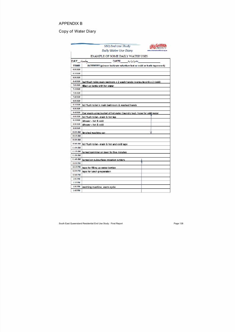
7/27/2019 Trabalho_Austrália
http://slidepdf.com/reader/full/trabalhoaustralia 148/174
APPENDIX B
Copy of Water Diary
South East Queensland Residential End Use Study: Final Report Page 138

7/27/2019 Trabalho_Austrália
http://slidepdf.com/reader/full/trabalhoaustralia 149/174
APPENDIX C
SEQREUS Winter 2010 End Use Frequency Distributions
South East Queensland Residential End Use Study: Final Report Page 139
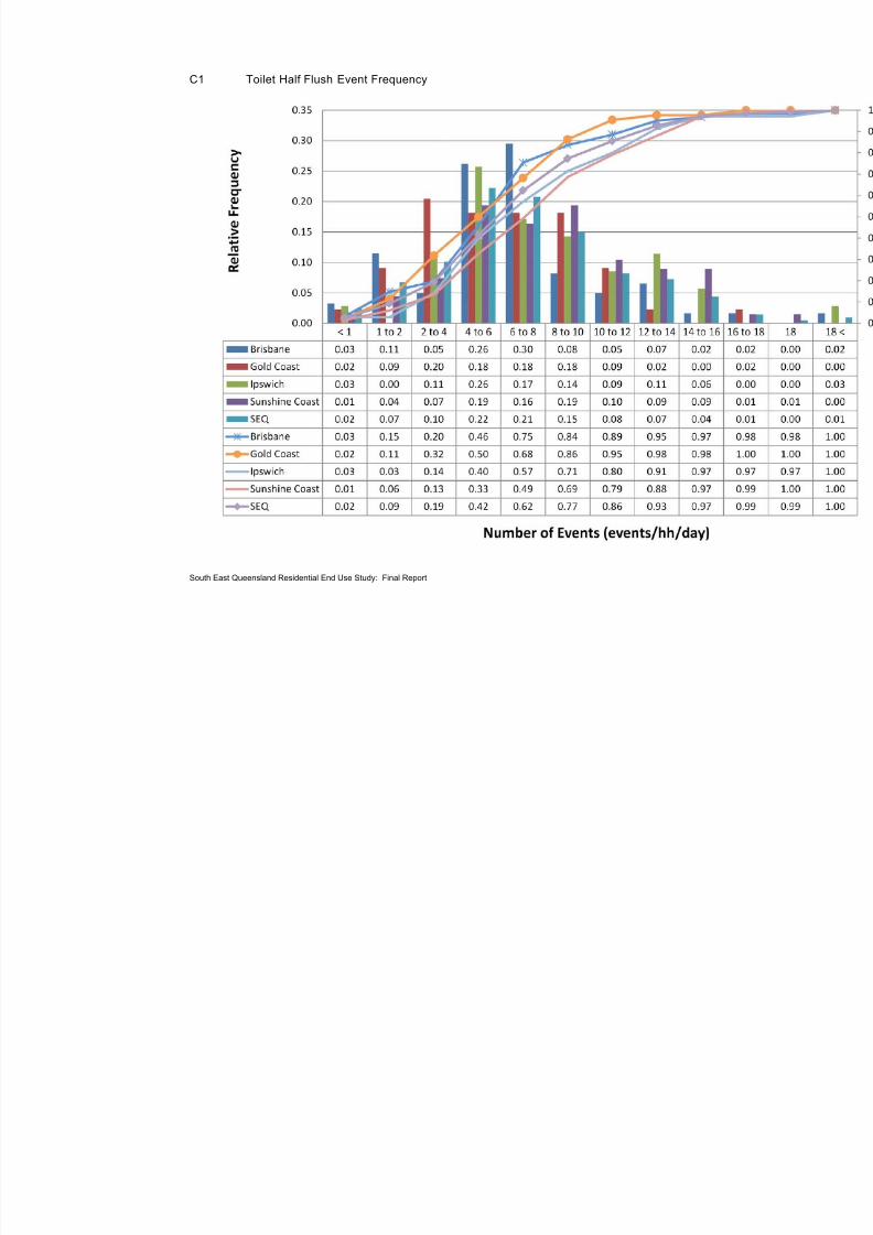
7/27/2019 Trabalho_Austrália
http://slidepdf.com/reader/full/trabalhoaustralia 150/174
C1 Toilet Half Flush Event Frequency
South East Queensland Residential End Use Study: Final Report

7/27/2019 Trabalho_Austrália
http://slidepdf.com/reader/full/trabalhoaustralia 151/174
C2 Toilet Half Flush Event Volume Distribut ion
South East Queensland Residential End Use Study: Final Report

7/27/2019 Trabalho_Austrália
http://slidepdf.com/reader/full/trabalhoaustralia 152/174
C3 Toilet Full Flush Event Frequency
South East Queensland Residential End Use Study: Final Report

7/27/2019 Trabalho_Austrália
http://slidepdf.com/reader/full/trabalhoaustralia 153/174
C4 Toilet Full Flush Event Volume Distribut ion
South East Queensland Residential End Use Study: Final Report

7/27/2019 Trabalho_Austrália
http://slidepdf.com/reader/full/trabalhoaustralia 154/174
C5 Tap Event Frequency
South East Queensland Residential End Use Study: Final Report

7/27/2019 Trabalho_Austrália
http://slidepdf.com/reader/full/trabalhoaustralia 155/174
C6 Tap Event Volume Distribut ion
South East Queensland Residential End Use Study: Final Report
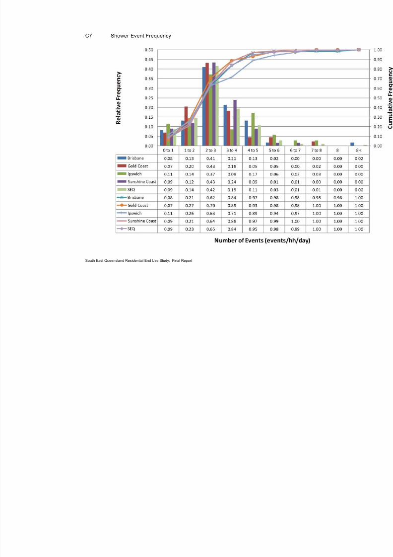
7/27/2019 Trabalho_Austrália
http://slidepdf.com/reader/full/trabalhoaustralia 156/174
C7 Shower Event Frequency
South East Queensland Residential End Use Study: Final Report

7/27/2019 Trabalho_Austrália
http://slidepdf.com/reader/full/trabalhoaustralia 157/174
C8 Shower Event Duration Distribut ion
South East Queensland Residential End Use Study: Final Report

7/27/2019 Trabalho_Austrália
http://slidepdf.com/reader/full/trabalhoaustralia 158/174
C9 Shower Flow Rate Distribut ion
South East Queensland Residential End Use Study: Final Report

7/27/2019 Trabalho_Austrália
http://slidepdf.com/reader/full/trabalhoaustralia 159/174
C10 Bath Event Frequency
South East Queensland Residential End Use Study: Final Report

7/27/2019 Trabalho_Austrália
http://slidepdf.com/reader/full/trabalhoaustralia 160/174
C11 Bath Event Volume Distribut ion
South East Queensland Residential End Use Study: Final Report
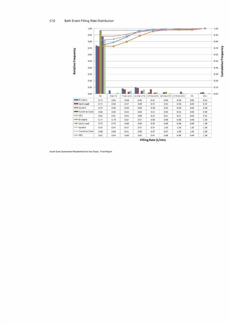
7/27/2019 Trabalho_Austrália
http://slidepdf.com/reader/full/trabalhoaustralia 161/174
C12 Bath Event Filling Rate Distribut ion
South East Queensland Residential End Use Study: Final Report

7/27/2019 Trabalho_Austrália
http://slidepdf.com/reader/full/trabalhoaustralia 162/174
C13 Dishwasher Event Frequency
South East Queensland Residential End Use Study: Final Report

7/27/2019 Trabalho_Austrália
http://slidepdf.com/reader/full/trabalhoaustralia 163/174
C14 Dishwasher Event Volume Distribut ion
South East Queensland Residential End Use Study: Final Report

7/27/2019 Trabalho_Austrália
http://slidepdf.com/reader/full/trabalhoaustralia 164/174
C15 Clothes Washer Event Frequency
South East Queensland Residential End Use Study: Final Report

7/27/2019 Trabalho_Austrália
http://slidepdf.com/reader/full/trabalhoaustralia 165/174
C16 Clothes Washer Event Volume Distribut ion
South East Queensland Residential End Use Study: Final Report

7/27/2019 Trabalho_Austrália
http://slidepdf.com/reader/full/trabalhoaustralia 166/174
C17 Irrigation Event Frequency
South East Queensland Residential End Use Study: Final Report

7/27/2019 Trabalho_Austrália
http://slidepdf.com/reader/full/trabalhoaustralia 167/174
C18 Irrigation Event Duration Distribut ion
South East Queensland Residential End Use Study: Final Report
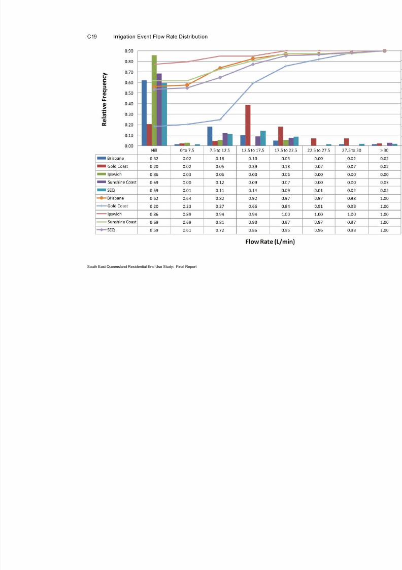
7/27/2019 Trabalho_Austrália
http://slidepdf.com/reader/full/trabalhoaustralia 168/174
7/27/2019 Trabalho_Austrália
http://slidepdf.com/reader/full/trabalhoaustralia 169/174
REFERENCES
ABC News (2011) Brisbane floods: before and after. In ABC News, 17 January 2011,http://www.abc.net.au/news/infographics/qldfloods/beforeafter.htm. Accessed November 17
th, 2011.
Anker-Nilssen, P., 2003. Household energy use and the environment--a conflicting issue. Applied Energy,76(1-3), 189-196.
Aquacraft (2010). Trace Wizard® software version 4.1. 1995-2010 Aquacraft, Inc. Boulder, CO, USA.http://www.aquacraft.com/
Arbués, F., García-Valiñas, M.A. and Martínez-Espiñeira, R. (2003). Estimation of residential water demand: a state-of-the-art review. Journal of Socio-Economics 32: 81-102.
Arbues, F., Villanua, I. and Barberan, R., 2010. Household size and residential water demand: an empiricalapproach. The Australian Journal of Agricultural and Resource Economics 54, 61-80.
Australian Government (2010a). National Greenhouse Accounts (NGA) Factors, prepared by theDepartment of Climate Change and Energy Efficiency, July 2010.
Australian Government (2010b) Water efficiency labeling and standards (WELS) scheme. Commonwealthof Australia website: http://www.waterrating.gov.au/products/index.html. Accessed 10th October
2011.Australian Government (2010c) E3 Equipment, Energy, Efficiency. Commonwealth of Australia website:
http://www.energyrating.gov.au/compare-products/Accessed 10th October 2011.Barrett, G. and Wallace, M. (2009). Characteristics of Australian urban residential water users: implications
for water demand management and whole of the system water accounting framework. Water Policy,11 413:426.
Baruch, Y. and Brooks, C. (2008) Survey response rate levels in and trends in organizational research. Human Relations 61(8), 1139-1160.
Beal, C., Gardner, T., Sharma, A. Barton, R. and Chong, M. (2011c). A Desktop Analysis of Potable Water Savings from Internally Plumbed Rainwater Tanks in South East Qld. Urban Water SecurityResearch Alliance Technical Report No. 26. http://www.urbanwateralliance.org.au/publications/UWSRA-tr26.pdf
Beal, C., Stewart, R., Huang, T., Rey, E., (2011b). SEQ residential end use study. Australian Water
Association Journal, 38(1), 80-84.Beal, C.D., Stewart, R.A. and Bertone, E. (2012) Evaluating the energy and carbon reductions resulting
from resource-efficient household stock. Energy and Buildings, in press,DOI 10.1016/j.enbuild.2012.08.004.
Beal, C.D., Stewart, R.A., Fielding, K. A novel mixed method smart metering approach to reconcilingdifferences between perceived and actual residential end use water consumption, Journal of Cleaner
Production (2011a), doi:10.1016/j.jclepro.2011.09.007.Beal, C.D., Stewart, R.A., Talebpour, R., Huang, A. and Rey, E. (2010). South East Queensland residential
end use study: Pilot study of Gold Coast households . Technical Report for Urban Water SecurityResearch Alliance. Griffith University and Smart Water Research Centre, September, 2010.
Beal, C.D., Stewart, R.A., (2012) Identifying residential water end uses underpinning peak day and hour demand. Journal of Water Resources Planning and Management (under review).
Blokker, E., Vreeburg, J. and van Dijk, J. (2010). Simulating residential water demand with a stochasticend-use model. Journal of Water Resources, Planning and Management 136(1), 19-26.
Carragher, BJ., Stewart, RA. and Beal, CD., (2012) Quantifying the influence of residential water applianceefficiency on average day diurnal demand patterns at an end use level: A precursor to optimisedwater service infrastructure planning. Resource Conservation and Recycling, 62, 81-90.
Chang, H., Parandvash, G. and Shandas, V., 2010. Spatial variations of single-family residential water consumption in Portland, Oregon. Urban Geography 31, 953-972.
Cheng, C.-L. (2002) Study of the inter-relationship between water use and energy conservation for a building. Energy and Buildings 34, 261-266.
Chu, J., Wang, C., Chen, J. and Wang, H. (2009) Agent-based residential water use behavior simulationand policy implications: a case study in Beijing City. Water Resources Management 23, 3267-3295.
Clarke, A., Grant, N. and Thornton, J. (2009) Quantifying the energy and carbon effects of water savings,
Full technical report for Environment Agency and Energy Savings Trust prepared by ElementalSolutions, April 2009, UK.
Cole, G and Stewart, R.A., (2012) Smart meter enabled disaggregation of urban peak water demand: precursor to effective urban water planning. Urban Water Journal, under review.
South East Queensland Residential End Use Study: Final Report Page 159

7/27/2019 Trabalho_Austrália
http://slidepdf.com/reader/full/trabalhoaustralia 170/174
Corral-Verdugo, V., Bechtel, R. and Fraijo-Sing, B. (2002). Environmental beliefs and water conservation:an empirical study. Environmental Psychology, 23:247-257.
Corral-Verdugo, V., Frías-Armenta, M., 2006. Personal normative beliefs, antisocial behavior, andresidential water conservation. Environment and Behavior 38(3), 406-421
DCCEE (2011) Department of Climate Change and Energy Efficiency – National Greenhouse Accounts(NGA) Factors – July 2011. Australian Government website
http://www.climatechange.gov.au/~/media/publications/greenhouse-acctg/national-greenhouse-factors-july-2010-pdf . Accessed 10 September 2011.
DeOreo, W., Heaney, J. and Mayer, P. (1996). Flow trace analysis to assess water use. American Water
Works Association Journal 88(1), 79-90.DERM (2007). Chapter 5: Demand/flow and projections. Planning Guidelines for Water Supply and
Sewerage, Department of Environment and Resource Management. June 2007 revision.DIP (2007) Queensland Development Code. Queensland Government. January 2007.DIP (2009). South East Queensland Regional Plan 2009-2031. Department of Infrastructure and Planning,
Queensland Government. September 2009.Dolnicar, S., Hurlimann, A., 2010. Australian water conservation behaviours and attitudes [online].
Australian Journal of Water Resources, 14, 43-53.Domènech, L., Saurí, D., 2011. A comparative appraisal of the use of rainwater harvesting in single and
multi-family buildings of the Metropolitan Area of Barcelona (Spain): social experience, drinkingwater savings and economic costs. Journal of Cleaner Production 19, 598-608.
Druckman, A., Sinclair, P. and Jackson, T., 2008. A geographically and socio-economically disaggregatedlocal household consumption model for the UK. Journal of Cleaner Production 16, 870-880.
England, P. (2009 ) Managing urban water in Australia: the planned and the unplanned Management of
Environmental Quality: An International Journal 20(5), 592-608.Farrelly, M., Brown, R., 2011. Rethinking urban water management: Experimentation as a way forward?
Global Environmental Change 847, dio:10.1016/j.gloenvcha.2011.1001.1007.Fidar, A., Memon, F. and Butler, D. (2010). Environmental implications of water efficient
microcomponents in residential buildings. Science of the Total Environment, 408, 5828-5835.Fielding, K., Spinks, A., Russell, S. and Mankad, A. (2011) Predictors of Household Water Use in South
East Queensland, in Science Forum and Stakeholder Engagement: Building Linkages,
Collaboration and Science Quality, (eds) D.K., Begbie and S.L., Wakem, Urban Water SecurityResearch Alliance, September 2011, Brisbane, Queensland, pp 25.
Fielding, K., Spinks, A., Russell, S., MCCRea, R, Stewart, R.A., Gardner, J. An experimental test of voluntary strategies to promote urban water demand management. Under review, 2012.
Gardiner, A. (2009) Domestic rainwater tanks: usage and maintenance patterns in South East Queensland. Australian Water Association Journal 36(1), 74-77.
Gardner, T. and Vieritz, A. (2010) The role of rainwater tanks in Australia in the twenty first century. Architectural Science Review 53(1), 107-125.
Gato, S., Jayasuriya, N. and Roberts, P. (2007) Temperature and rainfall thresholds for base use urbanwater demand modelling. Journal of Hydrology 337(3-4), 364-376.
Gato-Trinidad, S., Jayasuriya, N. and Roberts, P. (2011) Understanding urban residential end uses of water.Water Science and Technology 64(1), 36-42.
GHD (2009). Desired Standards of Service Review 2008 Final Report Rev 3. 178/07/01_GHD-10. October,
2009.Gilg, A. and Barr, S. (2006). Behavioural attitudes towards water saving? Evidence from a study of
environmental actions. Ecological Economics, 57: 400-414.Giurco, D., Carrard, N., McFallan, S., Nalbantoglu, M., Inman, M., Thornton, N. and White, S. (2008).
Residential end-use measurement Guidebook: a guide to study design, sampling and technology.Prepared by the Institute for Sustainable Futures, UTS and CSIRO for the Smart Water Fund,Victoria.
Gleick P.H., Adams R.M., Amasino R.M., Anders E., Anderson D.J., Anderson W.W., Anselin L.E., et al.(2010). Climate change and the integrity of science. Science 328:689-690.
Gold Coast Water (2010). May Monthly Summary report – Water Supplied. Gold Coast Water and GoldCoast City Council, June, 2010.
Golden, J., Subramaniana, V., Irizarria, G., Whitec, P. and Meierd, F. (2010) Energy and carbon impact
from residential laundry in the United States. Journal of Integrative Environmental Sciences 7(1),53-73.
South East Queensland Residential End Use Study: Final Report Page 160

7/27/2019 Trabalho_Austrália
http://slidepdf.com/reader/full/trabalhoaustralia 171/174
Gregory, G., Di Leo, M., 2003. Repeated behavior and environmental psychology: the role of personalinvolvement and habit formation in explaining water consumption. Applied Social Psychology 33(6),1261-1296.
Hamilton, L., 1985. Self-reported and actual savings in a water conservation campaign. Environment and
Behavior 17(3), 315-326.Heinrich, M. (2007). Water End Use and Efficiency Project (WEEP) - Final Report. BRANZ Study Report
159, Branz, Judgeford, New Zealand.Hoffman, M., Worthington, A. and Higgs, H. (2006). Urban water demand with fixed volumetric charging
in a large municipality: the case of Brisbane, Australia. The Australian Journal of Agriculture and
Resource Economics 50:347-359.http://www.waterrating.gov.au/products/index.html. Accessed November 24
th, 2011.
Inman, D. and Jeffrey, P. (2006). A review of residential water conservation tool performance andinfluences on implementation effectiveness. Urban Water Journal, Vol 3:3, pp. 127-143.
Jacobs, H. and Haarhoff, J. (2004) Structure and data requirements of an end-use model or residential water demand and return flow. Water SA 30(3), 293-304.
Jones, N., Evangelinos, K., Gaganis, P. and Polyzou, E., 2010. Citizen's perceptions on water conservation policies and the role of social capital. Water Resources Management 25, 509-522.
Jorgensen, B., Graymore, M. and O'Toole, K., 2009. Household water use behavior: an integrated model.
Journal of Environmental Management 91, 227-236.Juárez-Nájera, M., Rivera-Martinez, J., Hafkamp, W., 2010. An explorative socio-physcological model for
determining sustainable behavior: Pilot study in Germany and Mexican Universities. Journal of
Cleaner Production 18, 686-694.Kantola, S.J., Syme, G.J., Campbell, N.A., 1984. Cognitive dissonance and energy conservation. Journal of
Applied Psychology 69(3), 416-421.Kennedy, A., 2010. Using Community-Based Social Marketing Techniques to Enhance Environmental
Regulation. Sustainability, 2(4), 1138-1160Kenney, D.S., Goemans, C., Klein, R.A., Lowrey, J. and Reidy, K. (2008). Residential water demand
management: lessons from Aurora, Colorado. Journal of the American Water resources Association,44 (1):192-207.
Kenway, S., Priestley, A., Cook, S., Seo, S., Inman, M., Gregory, A. and Hall, M. (2008) Energy use in the provision and consumption of urban water in Australia and New Zealand, CSIRO:Water for aHealthy Country National Research Flagship.
Kenway, S.J., Lant, P., Preistly, T., Daniels, P., (2011) The connection between water and energy in cities.Water Science and Technology, 63, 1983-1990.
Keselman, H., Huberty, C., Lix, L., Olejnik, S., Cribbie, R., Donahue, B., Kowalchuk, R., Lowman, L.,Petoskey, M., Keselman, J. and Levin, J., 1998. Statistical practices of educational researchers: ananalysis of their ANOVA, MANOVA, and ANCOVA analyses. Review of Educational Research 68(3), 350-386.
Koomey, J., Dunham, C. and Lutz, J. (1995) The effect of efficient standards on the water use and water-heating energy use in the U.S: A detailed end-use treatment. Energy 20(7), 627-635.
Kowalski, M. and Marshallsay, D. (2005) Using measured microcomponent data to model the impact of water conservation strategies on the diurnal consumption profile. Water Science and
Technology:Water Supply 5(3-4), 145-150.
Kraus, S.J., 1995. Attitudes and the prediction of behaviour: A meta-analysis of the empirical literature.Personal and Social Psychology Bulletin 2: 58-75
Lee, M., Tansel, B. and Balbin, M. (2011) Influence of residential water use efficiency measures onhousehold water demand: A four year longitudinal study. Resources, Conservation and Recycling 56(1), 1-6.
Lenzen, M. and Peters, G.M. (2010) How City Dwellers Affect Their Resource Hinterland. Journal of
Industrial Ecology 14(1), 73-90.Loh, M. and Coghlan, P. (2003). Domestic water use study in Perth, Western Australia 1998 to 2000.
Water Corporation of Western Australia.Lynn, P. (2001) The impact of incentives on response rates to personal interview surveys: Role and
perceptions of interviewers. international Journal of Public Opinion Research 13(3), 326-336.Maas, C. (2009) Greenhouse gas energy co-benefits of water conservation, POLIS Research Report 09-01,
March 2009Makki, A., Stewart, R. and Beal, C. (2011) Revealing the determinants of shower water end use
consumption: enabling better targeted urban water conservation strategies. Journal of Cleaner
Production doi:10.1016/j.jclepro.2011.08.007.
South East Queensland Residential End Use Study: Final Report Page 161

7/27/2019 Trabalho_Austrália
http://slidepdf.com/reader/full/trabalhoaustralia 172/174

7/27/2019 Trabalho_Austrália
http://slidepdf.com/reader/full/trabalhoaustralia 173/174
South East Queensland Residential End Use Study: Final Report Page 163
Turner, A., White, S., Kazaglis, A., Simard, S. (2007) Have we achieved the savings? The importance of evaluations when implementing demand management. Water Science and Technology: Water Supply 7 (5-6):203-210.
van Zyl, J. E., le Gat, Y., Piller, O., and Walski, T. M. (2011). "Impact of Water Demand Parameters on theReliability of Municipal Storage Tanks." J. Water Resour. Plann. Manage. doi:10.1061/(ASCE)WR.1943-5452.0000200.
Walton, A. and Hume, M. (2011) Creating positive habits in water conservation: the case of theQueensland Water Commission and the Target 140 campaign. International Journal of Nonprofit andVoluntary Sector Marketing 16(3), 215-224.
Walton, C. and Holmes, K. (2009) How much water efficiency does $321 million buy?, In Proceedings of
the 5th IWA Specialist Conference 'Efficient 2009' , eds. International Water Association (IWA) andAustralian Water Association, Sydney, Australia.
Water Corporation, (2011) Perth residential water use study 2008/2009, Water Forever, Water Corporation,Western Australia.
WELS (2011) Water Efficiency Labelling Scheme website,White, S., and Fane, S., 2002. Designing cost effective water demand management programs in Australia.
Water Science and Technology 46(6/7), 225-232.White, S., Milne, G. and Riedy, C. (2004). "End use analysis: issues and lessons." Water Science and
Technology: Water Supply 4(3): 57-65.Willis R, Stewart R, Panuwatwanich K, Jones S, A K., 2010a. Alarming visual display monitors affecting
shower end use water and energy conservation in Australian residential households. Resources,
Conservation and Recycling. Vol. 54, pp. 1117 – 1127, 2010:10.1016/j.resconrec.2010.03.004.Willis, R. (2011d) Domestic water end use study: an investigation of the water savings attributed to
demand management strategies and dual reticulated recycled water systems, PhD Thesis, School of Engineering, Griffith University.
Willis, R., Stewart, R.A., Panuwatwanich, K., Capati, B. and Giurco, D. (2009a). Gold Coast DomesticWater End Use Study, Australian Water Association Journal, 36(6): 84-90.
Willis, R., Stewart, R.A., Talebpour, M.R., Mousavinejad, A., Jones, S. and Giurco, D. (2009b). Revealingthe impact of socio-demographic factors and efficient devices on end use water consumption: case of Gold Coast Australia. In Proceedings of the 5th IWA Specialist Conference 'Efficient 2009' , eds.International Water Association (IWA) and Australian Water Association, Sydney, Australia.
Willis, R.M., et al., End use water consumption in households: impact of socio-demographic factors andefficient devices, Journal of Cleaner Production (2011b), doi:10.1016/j.jclepro.2011.08.006
Willis, R.M., Stewart, R.A., Emmonds, S., (2010b) Pimpama-Coomera dual reticulation end use study: pre-commission baseline, context and post-commission end use prediction. Water, Science and
Technology: Water Supply, 10(3), 302-314, doi: 10.2166/ws.2010.104.Willis, R.M., Stewart, R.A., Panuwatwanich, K., Williams, P., Hollingsworth, A., 2011c. Quantifying the
influence of environmental and water conservation attitudes on household end use water consumption. Journal of Environmental Management , 92(8), 1996-2008. ,doi:10.1016/j.jenvman.2011.03.023
Willis, R.M., Stewart, R.A., Williams, P.R., Hacker, C.H., Emmonds, S.C., Capati, G., 2011a. Residential potable and recycled water end uses in a dual reticulated supply system. Desalination, 273(1-3),201-211. doi: 10.1016/j.desal.2011.01.022.
Worthington, A., Higgs, H. and Hoffman, M. (2009). Residential water demand modelling in Queensland,Australia: a comparative panel data approach. Water Policy, 11 427-441.
Wutich, A. (2009). Estimating household water use: a comparison of diary, prompted recall and free recallmethods. Field Methods 21(1):49-6.
Zhou, S.L., McMahon, T.A., Walton, A. and Lewis, J. (2000) Forecasting daily urban water demand: a casestudy of Melbourne. Journal of Hydrology 236(3-4), 153-164.

7/27/2019 Trabalho_Austrália
http://slidepdf.com/reader/full/trabalhoaustralia 174/174