sistemas fracamente ligados de três corpos: moléculas e ... · sistemas fracamente ligados de...
TRANSCRIPT

Universidade de São Paulo Instituto de Física
Sistemas Fracamente Ligados de Três Corpos: Moléculas e Núcleos Exóticos Leves
Marcelo Takeshi Yamashita
Orientador: Prof. Dr.Tobias Frederico
Tese de doutorado apresentada ao Instituto de Física para a o b t e n ç ã o d o t í t u l o d e D o u t o r e m C i ê n c i a s
Banca Examinadora: Profa. Dra. Alinka Lépine-Szily (IFUSP) Prof. Dr. Diógenes Galetti (IFT - UNESP) Prof. Dr. Mahir Saleh Hussein (IFUSP) Prof. Dr. Manuel Máximo Bastos Malheiro de Oliveira (UFF) Prof. Dr. Tobias Frederico (ITA)
São Paulo
2004

FICHA CATALOGRÁFICA Preparada pelo Serviço de Biblioteca e Informação do Instituto de Física da Universidade de São Paulo
Yamashita, Marcelo Takeshi Sistemas Fracamente Ligados de Três Corpos: Moléculas e Núcleos Exóticos Leves. São Paulo - 2004 Tese (Doutoramento) – Universidade de São Paulo Instituto de Física - Depto. de Física Experimental Orientador: Prof. Dr. Tobias Frederico Área de Concentração: Física
Unitermos 1. Núcleos Exóticos;
2. Átomos; 3. Física Teoria – Problemas de poucos corpos USP/IF/SBI-069/2004

i
.
Aos meus pais, Tomie e Takeshi,
aos quais nunca sera demais agradecer,
e a minha companheira Raquel.

ii
.

iii
Agradecimentos
A redacao desta tese utilizando-se a primeira pessoa do plural foi feita
para mostrar que este trabalho constitui o fruto do esforco de muitas pessoas. A
essas pessoas os meus sinceros agradecimentos:
Prof. Tobias Frederico, meu orientador e amigo, que desde o inıcio deste trabalho
teve a paciencia e a dedicacao para ensinar um estudante que estava vindo de uma
area diferente, sem nenhuma experiencia com os calculos que foram feitos nesta tese.
Muito obrigado por ter acreditado em mim.
Ao amigo Prof. Lauro Tomio, por toda ajuda em todas as etapas deste trabalho.
Muito obrigado pelas discussoes, conversas e conselhos em todos os momentos que
precisei.
Ao amigo Prof. Iuda Goldman, pelas conversas e toda ajuda desde o inıcio da minha
carreira cientıfica.
A amiga Tereza Faracini, pelas agradaveis conversas durante o dia.
Aos meus queridos pais, Tomie e Takeshi, obrigado por tudo.
A minha mulher, Raquel, pela compreensao, carinho e apoio durante todo esse tempo.
Ao Laboratorio do Acelerador Linear por ter me cedido um lugar para trabalhar
durante esses quase dez anos.
A Fundacao de Amparo a Pesquisa do Estado de Sao Paulo, FAPESP, pelo apoio
financeiro ao projeto.
Marcelo Takeshi Yamashita

iv
.

v
.
“Observo-me a escrever como nunca me observei a pintar, e descubro o que ha de
fascinante neste acto: na pintura, vem sempre o momento em que o quadro nao
suporta nem mais uma pincelada (mau ou bom, ela ira torna-lo pior), ao passo que
estas linhas podem prolongar-se infinitamente, alinhando parcelas de uma soma que
nunca sera comecada, mas que e, nesse alinhamento, ja trabalho perfeito, ja obra
definitiva porque conhecida. E sobretudo a ideia do prolongamento infinito que me
fascina. Poderei escrever sempre, ate o fim da vida, ao passo que os quadros, fechados
em si mesmos, repelem, sao eles proprios isolados na sua pele, autoritarios, e, tambem
eles, insolentes.”
Jose Saramago, Manual de Pintura e Caligrafia

vi
.
vii
Resumo
Um potencial de dois corpos do tipo δ-Dirac foi utilizado para descrever sistemas fra-
camente ligados de tres corpos. A trajetoria completa dos estados Efimov em funcao
da energia ligacao de dois corpos foi calculada para o caso de tres bosons identicos:
se o subsistema de dois corpos e ligado, conforme a razao entre a energia de ligacao
de dois e tres corpos aumenta, o estado excitado desaparece e um estado virtual cor-
respondente aparece quando a energia do estado fundamental atinge o limiar dado
por 6.9~2/(ma2) (a - comprimento de espalhamento, m - massa do boson). Quando
o subsistema de dois corpos e virtual, o aumento da razao entre as energias faz com
que o estado excitado se transforme em uma ressonancia quando a energia do es-
tado fundamental e 1.1~2/(ma2). Neste ultimo caso as condicoes para a formacao de
moleculas triatomicas no interior de condensados e favorecida, pois a competicao com
dımeros fracamente ligados esta ausente. A energia de ligacao de trımeros com mo-
mento angular total nulo em condensados atomicos foi estimada atraves da correlacao
desta com o coeficiente de recombinacao e com a energia do dımero, ambos conhecidos
experimentalmente em alguns casos. Os tamanhos de moleculas fracamente ligadas
(4He2-X; X≡4He, 6Li, 7Li e 23Na) e de nucleos exoticos leves (6He, 11Li, 14Be e 20C)
tambem foram calculados juntamente com um estudo sistematico do comportamento
dos raios quadraticos medios conforme a interacao dos subsistemas de dois corpos e
variada. Neste ultimo caso a classificacao de um sistema de tres corpos (tipo AAB)
foi completada denominando de Samba a configuracao formada por dois subsistemas
de dois corpos ligados e um virtual. As equacoes subtraıdas para os estados ligados
de quatro bosons tambem foram deduzidas.

viii
Abstract
A pairwise Dirac-δ interaction was used to describe weakly bound three-body sys-
tems. The complete trajectory of an Efimov state as a function of the two-body
energy was calculated for three identical bosons: if the two-body subsystem is bound,
as the ratio of the two- and three-body binding energy grows up, the excited state
disappears and a corresponding virtual state appears when the ground state energy
hits the threshold given by 6.9~2/(ma2) (a - scattering length, m - mass of the bo-
son). When the two-body subsystem is virtual, the increase of the ratio between the
energies turns an excited state into a resonance for a ground state energy greater than
1.1~2/(ma2). This last case may be more favorable for the formation of condensed
trimers in trapped ultracold monoatomic gases as the competition with the weakly
bound dimers is absent. The energy of triatomic molecules with total angular momen-
tum zero inside a condensate was estimated using its correlation with the three-body
recombination coefficient and scattering length, both are known experimentally for
some cases. The sizes of the weakly bound molecules (4He2-X; X≡4He, 6Li, 7Li e
23Na) and the light exotic nuclei (6He, 11Li, 14Be e 20C) were also calculated and
together with a systematic study of the behavior of the root-mean-square distances
as the two-body interaction is changed. In this last case the classification of a three-
body system (AAB type) was completed denoting by Samba the configuration formed
by two two-body subsystems bound and one virtual. The subtracted equations for
the four-boson bound states were also deduced.
Conteudo
1 Introducao 1
2 Equacoes subtraıdas - Formalismo 7
2.1 Revisao das equacoes de Faddeev e notacao . . . . . . . . . . . . . . 7
2.2 Matriz-T para o potencial δ-Dirac . . . . . . . . . . . . . . . . . . . . 12
2.3 Equacao subtraıda para a matriz-T . . . . . . . . . . . . . . . . . . . 15
2.4 Equacoes de Faddeev subtraıdas . . . . . . . . . . . . . . . . . . . . . 18
3 Os estados Efimov - Estados ligados, virtuais e ressonancias 21
4 Moleculas triatomicas fracamente ligadas em armadilhas magneto-
opticas 41
5 Limite de escala para os raios de sistemas fracamente ligados do tipo
AAB 53
5.1 Formalismo . . . . . . . . . . . . . . . . . . . . . . . . . . . . . . . . 54
5.1.1 Equacoes subtraıdas para as funcoes espectadoras . . . . . . . 58
5.2 Esquema de classificacao . . . . . . . . . . . . . . . . . . . . . . . . . 61
x CONTEUDO
5.3 Nucleos exoticos leves . . . . . . . . . . . . . . . . . . . . . . . . . . . 68
5.4 Moleculas triatomicas fracamente ligadas . . . . . . . . . . . . . . . . 73
6 4-corpos 79
6.1 Formalismo . . . . . . . . . . . . . . . . . . . . . . . . . . . . . . . . 79
7 Conclusoes e perspectivas 85
A Coordenadas de Jacobi (3-corpos) 89
B Deducao do fator de forma para o potencial δ-Dirac 91
C Deducao da matriz-T de dois corpos na forma subtraıda 93
D Normalizacao da funcao de onda do estado ligado de dois corpos 95
E Extensao da matriz-T de dois corpos 97
F Calculo dos elementos de matriz das eqs. (5.18) e (5.19) 101
G Calculo dos elementos de matriz das eqs. (6.12) e (6.13) 103
H Anexo dos trabalhos publicados referentes a tese 105
Lista de Tabelas
4.1 Energia de ligacao dos trımeros no interior de condensados . . . . . . 51
5.1 Resultados para os raios quadraticos medios neutron-neutron em nucleos
exoticos . . . . . . . . . . . . . . . . . . . . . . . . . . . . . . . . . . 70
5.2 Raios quadraticos medios para moleculas do tipo AAB . . . . . . . . 76
5.3 Resultados para o raio quadratico medio do atomo em relacao ao CM
do sistema no interior de armadilhas magneto-opticas . . . . . . . . . 77

xii LISTA DE TABELAS

Lista de Figuras
2.1 Coordenadas de Jacobi . . . . . . . . . . . . . . . . . . . . . . . . . . 8
3.1 Extensao da matriz-T de tres corpos para a segunda folha de Riemann
no plano de energia . . . . . . . . . . . . . . . . . . . . . . . . . . . . 27
3.2 Terceira partıcula se aproximando do dımero de energia de ligacao ε2
com uma energia cinetica de 34x2 . . . . . . . . . . . . . . . . . . . . . 27
3.3 Energias dos trımeros ε3, em unidades de µ(3) = 1 em funcao da energia
do estado ligado do dımero ε2 . . . . . . . . . . . . . . . . . . . . . . 32
3.4 Razao da energia do (N + 1)esimo estado ligado ou virtual do trımero,
E(N+1)3 , e da energia do dımero, E2, em funcao da razao da energia do
dımero e do N esimo estado ligado do trımero . . . . . . . . . . . . . . 33
3.5 Energias dos estados ligados e virtuais de tres bosons identicos . . . . 34
3.6 Parte real da energia de ressonancia para tres bosons identicos em
funcao da energia do estado virtual de dois corpos, em unidades de
µ(3) = 1 . . . . . . . . . . . . . . . . . . . . . . . . . . . . . . . . . . 36
3.7 Parte imaginaria da energia de ressonancia para tres bosons identicos
em funcao da energia do estado virtual de dois corpos, em unidades de
µ(3) = 1 . . . . . . . . . . . . . . . . . . . . . . . . . . . . . . . . . . 37

xiv LISTA DE FIGURAS
3.8 Razao da parte real da energia de ressonancia (parte positiva) ou da
energia do estado ligado (parte negativa), E(N)3 , e da energia do estado
ligado, E(N−1)3L para tres bosons identicos em funcao da razao da energia
do estado virtual de dois corpos, E2V , e da energia do estado ligado de
tres corpos, E(N−1)3L . . . . . . . . . . . . . . . . . . . . . . . . . . . . 38
3.9 Razao da parte imaginaria da energia de ressonancia, E(N)3 , e da energia
do estado ligado, E(N−1)3L para tres bosons identicos em funcao da razao
da energia do estado virtual de dois corpos, E2V , e da energia do estado
ligado de tres corpos, E(N−1)3L . . . . . . . . . . . . . . . . . . . . . . . 39
3.10 Trajetoria completa dos estados Efimov . . . . . . . . . . . . . . . . . 40
4.1 Coordenadas de Jacobi . . . . . . . . . . . . . . . . . . . . . . . . . . 43
4.2 Coeficiente adimensional de recombinacao, α, como funcao da razao
das energias de ligacao das moleculas diatomicas e triatomicas . . . . 50
5.1 Orientacao dos momentos. . . . . . . . . . . . . . . . . . . . . . . . . 58
5.2 Esquema de classificacao . . . . . . . . . . . . . . . . . . . . . . . . . 61
5.3 Produtos adimensionais√
〈r2AB〉|E3| e
√
〈r2AA〉|E3| para A = 0.1 e
EAA/E3 = K2AA = 0.1 em funcao de KAB/|KAA| . . . . . . . . . . . . 64
5.4 Produtos adimensionais√
〈r2AB〉|E3| e
√
〈r2AA〉|E3| paraA = 1 e K2
AA =
0.1 em funcao de KAB/|KAA| . . . . . . . . . . . . . . . . . . . . . . 65
5.5 Produtos adimensionais√
〈r2AB〉|E3| e
√
〈r2AA〉|E3| para A = 200 e
K2AA = 0.1 em funcao de KAB/|KAA| . . . . . . . . . . . . . . . . . . 66
5.6 Produtos adimensionais√
〈r2AB〉|E3| e
√
〈r2AA〉|E3| para A = 200 e
EAB/E3 = K2AB = 0.1 em funcao de KAA/|KAB| . . . . . . . . . . . . 67
5.7 Produtos adimensionais√
〈r2Aγ〉|E3| e
√
〈r2γ〉|E3| (γ = A, B) em funcao
da razao entre as massas, A . . . . . . . . . . . . . . . . . . . . . . . 68
LISTA DE FIGURAS xv
5.8 Produtos adimensionais√
〈r2nγ〉|E3| e
√
〈r2γ〉|E3| (γ = n, C) em funcao
da razao entre as massas, A . . . . . . . . . . . . . . . . . . . . . . . 71
5.9 Produtos adimensionais√
〈r2He−He〉S3 e
√
〈r2He〉S3 em funcao da razao
√
E2/E3 . . . . . . . . . . . . . . . . . . . . . . . . . . . . . . . . . . 74
5.10 Resultados para um sistema triatomico do tipo AAB, com γ = A, B.
Produtos adimensionais√
〈r2Aγ〉S3 e
√
〈r2γ〉S3 em funcao da razao entre
as massa A . . . . . . . . . . . . . . . . . . . . . . . . . . . . . . . . 75
6.1 Coordenadas de Jacobi para as amplitudes de Faddeev-Yakubovsky do
tipo K, lado esquerdo, e H, lado direito . . . . . . . . . . . . . . . . . 80
6.2 Orientacao dos momentos . . . . . . . . . . . . . . . . . . . . . . . . 83
A.1 Coordenadas de Jacobi (3-corpos) . . . . . . . . . . . . . . . . . . . . 89
E.1 Extensao da Matriz-T de Dois Corpos para a Segunda Folha de Riemann 97
E.2 Caminho da Integracao utilizado para calcular a eq. (E.3) . . . . . . 99
G.1 Coordenadas de Jacobi para as amplitudes de Faddeev-Yakubovsky . 103

Capıtulo 1
Introducao
Sistemas fracamente ligados formados por tres bosons com momento angular nulo
exibem infinitos estados ligados conforme a energia de dois corpos tende a zero. Esses
estados sao chamados de estados Efimov [1, 2, 3]. Os estados Efimov, fracamente
ligados, possuem uma funcao de onda que se estende muito alem do alcance efetivo
do potencial (r0), ou em outras palavras, o comprimento de espalhamento de dois
corpos, a, e muito maior que r0,ar0 1, justificando a utilizacao de potenciais
do tipo δ-Dirac para a descricao de propriedades desses sistemas. A interacao de
contato, ou alcance-zero, e o limite de potenciais de curto alcance e os observaveis dos
sistemas fısicos nos quais as partıculas apresentam este tipo de interacao dependem
principalmente das escalas fısicas que determinam os comportamentos assintoticos
da funcao de onda. Nesta situacao, aparecem no sistema de tres corpos correlacoes
entre os observaveis que independem do modelo do potencial e, portanto, apresentam
uma universalidade nas predicoes quando as escalas fısicas de dois e tres corpos sao
mantidas fixas. O estudo dos estados Efimov aparece em varios artigos teoricos
[4, 5, 6, 7, 8, 9, 10] tanto no campo da fısica atomica como nuclear, porem ainda nao
se tem uma evidencia muita clara de seu aparecimento em trabalhos experimentais
[3, 11, 12, 13, 14, 15, 16, 17].
A necessidade da adicao de uma escala de tres corpos independente da
escala de dois corpos [18, 19] para descrever um observavel deste sistema esta relacio-

2 1 Introducao
nada fisicamente com a possibilidade de colapso do sistema de tres bosons na onda-S
em tres dimensoes conforme r0 → 0 mantendo-se a energia de dois corpos fixa. Isto
e conhecido como colapso Thomas [20]. Uma questao que ainda continua em aberto
seria se a cada boson adicionado ao sistema haveria tambem a adicao de uma nova
escala fısica independente das outras escalas [18, 19]. No capıtulo 2 nos mostraremos
que fisicamente os efeitos Efimov e Thomas sao equivalentes [21].
A existencia do colapso Thomas introduz ainda, uma divergencia nas equa-
coes para as componentes de Faddeev quando consideramos grandes momentos. Esse
problema pode ser contornado com a introducao de um corte para momentos elevados
[22, 23, 24] ou atraves da utilizacao das equacoes subtraıdas cujo formalismo sera
discutido no capıtulo 2. No capıtulo 3 porem, onde estudamos a trajetoria completa
destes estados conforme variamos a energia de dois corpos, ficara claro que ambos os
metodos sao equivalentes e produzem o mesmo resultado numerico quando a energia
de dois corpos vai para zero (ou o parametro de regularizacao vai para infinito). Ainda
nesse capıtulo nos analisamos a possibilidade de um estado excitado do trımero tornar-
se um estado virtual conforme variamos as escalas fısicas do sistema. Esses resultados
vao alem daqueles calculados na Ref. [15] onde a funcao de escala foi introduzida
somente no contexto dos estados ligados, agora nos estendemos essa funcao para a
segunda folha de Riemann no plano de energia para incluir os estados virtuais que
aparecem conforme a razao entre as energias de ligacao de dois e tres corpos cresce. De
forma a tornarmos completo o estudo da “trajetoria”dos estados Efimov consideramos
nesse capıtulo a situacao onde a energia de dois corpos e virtual, neste caso vemos que
o estado ligado torna-se uma ressonancia conforme a energia de dois corpos aumenta
em modulo. A funcao de escala tambem e estendida para essa regiao.
Atualmente tem se estudado bastante os efeitos de grandes variacoes do
comprimento de espalhamento de dois corpos no interior de armadilhas atomicas de-
vido as mudancas de campos magneticos externos proximos a ressonancia de Feshbach
do sistema atomo-atomo [25, 26, 27, 28, 29, 30]. Essa variacao permite o estudo das
correlacoes entre os observaveis do sistema de tres atomos neutros e a verificacao
da universalidade a qual nos referimos no primeiro paragrafo. Embora ainda nao
1 Introducao 3
se tenha notıcia da formacao de moleculas triatomicas no interior de condensados, a
formacao de algumas moleculas diatomicas como 87Rb2 [31] e 23Na2 [32] ja foi compro-
vada experimentalmente, todavia a dificuldade para a obtencao de trımeros e apenas
experimental ja que teoricamente nao existe nenhum impedimento para a formacao
destas moleculas. No capıtulo 4, atraves da correlacao do coeficiente de recombinacao
de tres corpos com as energias de dois e tres corpos fazemos uma previsao das ener-
gias dos trımeros no interior dos condensados. A recombinacao de tres corpos e o
processo pelo qual dois atomos livres no interior de armadilhas se combinam para
formar um estado ligado (este processo necessita obviamente da participacao de um
terceiro atomo para que o momento total e a energia sejam conservados). Este pro-
cesso contribui para a destruicao de condensados e pode ser medido pelas perdas dos
atomos da armadilha. O comprimento de espalhamento de dois corpos em atomos
aprisionados tambem e conhecido na maioria dos experimentos e esta diretamente re-
lacionado a energia de ligacao de dois corpos. Estas duas informacoes sao suficientes
para estimar a energia dos trımeros. Para interacoes de curto alcance a magnitude
do coeficiente de recombinacao e determinada principalmente pelo comprimento de
espalhamento de dois corpos, porem todos os trabalhos nos quais aparece o coefici-
ente de recombinacao tambem e apresentada a sua dependencia com um parametro
de tres corpos [33, 34, 35], ou seja, a dependencia de uma escala tıpica de tres corpos
ainda continua [18, 19, 25]. A validade da nossa aproximacao e restrita a gases su-
ficientemente diluıdos, pois nossas relacoes de escala sao derivadas de tres partıculas
isoladas. A obtencao de moleculas triatomicas no interior de condensados pode ainda
ser favorecida no contexto das ressonancias (a < 0) calculadas no capıtulo 3. Neste
caso, os principais competidores das moleculas triatomicas - as moleculas diatomicas
- estao ausentes.
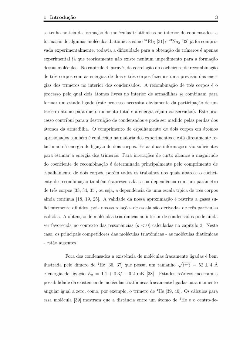
Fora dos condensados a existencia de moleculas fracamente ligadas e bem
ilustrada pelo dımero de 4He [36, 37] que possui um tamanho√
〈r2〉 = 52 ± 4 A
e energia de ligacao E2 = 1.1 + 0.3/ − 0.2 mK [38]. Estudos teoricos mostram a
possibilidade da existencia de moleculas triatomicas fracamente ligadas para momento
angular igual a zero, como, por exemplo, o trımero de 4He [39, 40]. Os calculos para
essa molecula [39] mostram que a distancia entre um atomo de 4He e o centro-de-
4 1 Introducao
massa (C.M.) do trımero varia de 6.4 a 6.5 A para o estado fundamental e de 42.9 a
58.8 A para o estado excitado. A distancia entre dois atomos de 4He varia de 11.0 a
11.1 A para o estado fundamental e de 74.8 a 102.0 A para o estado excitado. Esses
sistemas se estendem para regioes que estao bastante fora do alcance do potencial
e sao essencialmente uma solucao da equacao de Schrodinger livre, justificando a
utilizacao de um potencial de curto-alcance e, conforme veremos no capıtulo 5 - onde
tambem calculamos os raios quadraticos medios para moleculas do tipo 4He-X, onde
X ≡ 4He, 6Li, 7Li e 23Na - o sistema de tres corpos fica completamente definido por
apenas duas escalas fısicas, neste caso as energias de dois e tres corpos.
Uma outra aplicacao bastante interessante do potencial de alcance-zero
pode ser verificada em nucleos exoticos. Estes nucleos, com elevado numero de pro-
tons ou neutrons, localizam-se proximos das linhas de estabilidade e em alguns casos
podem ser aproximados por um sistema de tres corpos composto por um caroco e dois
nucleons fracamente ligados [14, 25, 41, 42]. No capıtulo 5 vamos considerar o caso de
um nucleo composto por um caroco pontual (C) e dois neutrons (n). Nesta situacao
podemos ter quatro tipos de sistemas conforme modificamos a interacao dos subsiste-
mas de dois corpos: Borromean (os pares sao completamente desligados), All-Bound
(os pares sao completamente ligados), Tango [43] (um par e ligado e dois pares sao
desligados) e Samba (dois pares sao ligados e um par e desligado). Faremos calculos
para o 6He (Borromean), 11Li (Borromean), 14Be (Borromean) e 20C (Samba), veremos
que os raios destes sistemas tambem podem ser representados como funcoes de escala
universais escritas em termos de produtos adimensionais. Utilizando essas funcoes de
escala nos podemos seguir o comportamento dos diferentes raios conforme acontece
a transicao entre as diversas possibilidades: iniciando de um sistema Borromean nos
podemos ir para o tipo Samba aumentando a energia de ligacao do par nC mantendo
nn desligado, ou entao para um sistema Tango aumentando a energia de ligacao de nn
mantendo nC desligado. Como os nossos calculos restringem-se a onda-S eles apre-
sentam algumas limitacoes principalmente nos casos onde a interacao do sistema de
dois corpos na onda-P poderia ser considerada importante para a energia de ligacao
de tres corpos (por exemplo, 5He [44] e 10Li [45]). Todavia essa limitacao e redu-
zida levando-se em conta que estamos considerando nos nossos calculos as energias

1 Introducao 5
de ligacao medidas experimentalmente, as quais devem carregar o efeito das ondas
parciais mais elevadas.
Os estudos feitos no contexto de tres bosons podem tambem ser estendidos
para quatro bosons. A questao levantada no primeiro paragrafo sobre a existencia
de novas escalas fısicas adicionadas devido ao aumento do numero de bosons pode
ser estudada no contexto de quatro corpos. Isto pode ser evidenciado calculando-se
a dependencia da energia do estado ligado de quatro bosons com a respectiva escala
introduzida nas equacoes para as amplitudes de Faddeev-Yakubovsky [46] atraves da
subtracao no propagador de quatro corpos (de forma analoga as equacoes subtraıdas
de tres corpos). No capıtulo 6 nos apresentamos essa formulacao.
Em alguns artigos [47] a definicao do sinal dos estados ligados e virtuais
aparece diferente da nossa. Em unidades de ~ = m = 1, onde m e a massa de um dos
constituintes do sistema de tres corpos, temos que a amplitude de espalhamento de
dois corpos na onda-S em termos do momento k e dada por: f0(k) = 1k cot δ0−ik
. Para
baixas energias a expansao de alcance efetivo k cot δ0 = −a−1 + 12r0k
2 + ..., fica igual
a k cot δ0 = −a−1. Assim, f0(k) = 1−a−1−ik
e a−1 = ±√
E2. O estado ligado e dado
pelo sinal positivo e o virtual pelo sinal negativo. Adotamos essa convencao para o
sinal do comprimento de espalhamento em analogia com o caso de um espalhamento
em baixas energias (k ≈ 0) por um poco quadrado (ver, por exemplo, Ref. [48]).
Conforme vamos aumentando a profundidade do poco ocorre o aparecimento de um
estado ligado e o comprimento de espalhamento que era negativo (na ausencia do
estado ligado) torna-se positivo.
Sumarizando: no capıtulo 2 nos mostramos uma das formas de tratar a di-
vergencia nas equacoes de Faddeev para momentos grandes. Neste capıtulo deduzimos
as equacoes subtraıdas onde sao introduzidas as escalas fısicas atraves do propagador
de tres corpos, veremos que os resultados sao independentes do ponto de subtracao
como consequencia da matriz-T satisfazer uma equacao do tipo Callan-Symanzik.
No capıtulo 3 nos estudamos os estados Efimov. Discutimos a equivalencia entre os
efeitos Efimov e Thomas. Fazemos um estudo sistematico das trajetorias desses es-
tados conforme variamos a energia de ligacao de dois corpos (E2). Veremos que um
6 1 Introducao
estado Efimov iniciado em um estado virtual para um valor elevado de E2 (ligado),
passa para um estado ligado conforme diminuımos E2 [7], ate “virar”finalmente uma
ressonancia conforme aumentamos em modulo o valor de E2 (virtual) [49]. Ficara
claro neste capıtulo que os metodos utilizados para a regularizacao da equacao da
funcao espectadora - corte e subtracao - sao equivalentes [7]. No capıtulo 4 relacio-
namos o coeficiente de recombinacao de tres corpos com as energias de dois e tres
corpos, mostramos que ele obedece a uma funcao de escala universal e conseguimos
prever a energia de moleculas triatomicas no interior de condensados [8]. No capıtulo
5 calculamos os tamanhos de algumas moleculas fracamente ligadas [9] e estendemos
o estudo para o caso de nucleos exoticos [10]. Fazemos neste capıtulo um estudo
sistematico dos tamanhos de um sistema de tres corpos generico fracamente ligado
conforme mudamos o tipo de interacao de dois corpos [10]. No capıtulo 6 nos apresen-
tamos a deducao das equacoes para as amplitudes de Faddeev-Yakubovsky na forma
subtraıda. No capıtulo 7 sao apresentadas as conclusoes.

Capıtulo 2
Equacoes subtraıdas - Formalismo
Neste capıtulo descreveremos como sao introduzidas as escalas fısicas nas equacoes
de Faddeev para a matriz de transicao, T . Essas escalas aparecem na forma de uma
subtracao no propagador de tres corpos e excluem a necessidade do uso de um corte
para grandes momentos [18, 19].
O problema da nao unicidade da solucao da equacao de Lippmann-Schwinger
quando consideramos um sistema de tres ou mais corpos foi solucionado em 1960
por L. D. Faddeev [50]. Uma revisao das equacoes de Faddeev para o caso de tres
partıculas sera feita a seguir.
2.1 Revisao das equacoes de Faddeev e notacao
Consideremos a equacao de Schrodinger para uma certa funcao de onda espalhada
Ψ(+) (o sinal (+) indica uma funcao de onda esferica emergente):
(E −H0)Ψ(+) = (vi + vj + vk)Ψ
(+), (2.1)
onde vi, vj e vk sao, respectivamente, os potenciais de interacao entre as partıculas
(j, k), (i, k) e (i, j). O hamiltoniano livre,
8 2 Equacoes subtraıdas - Formalismo
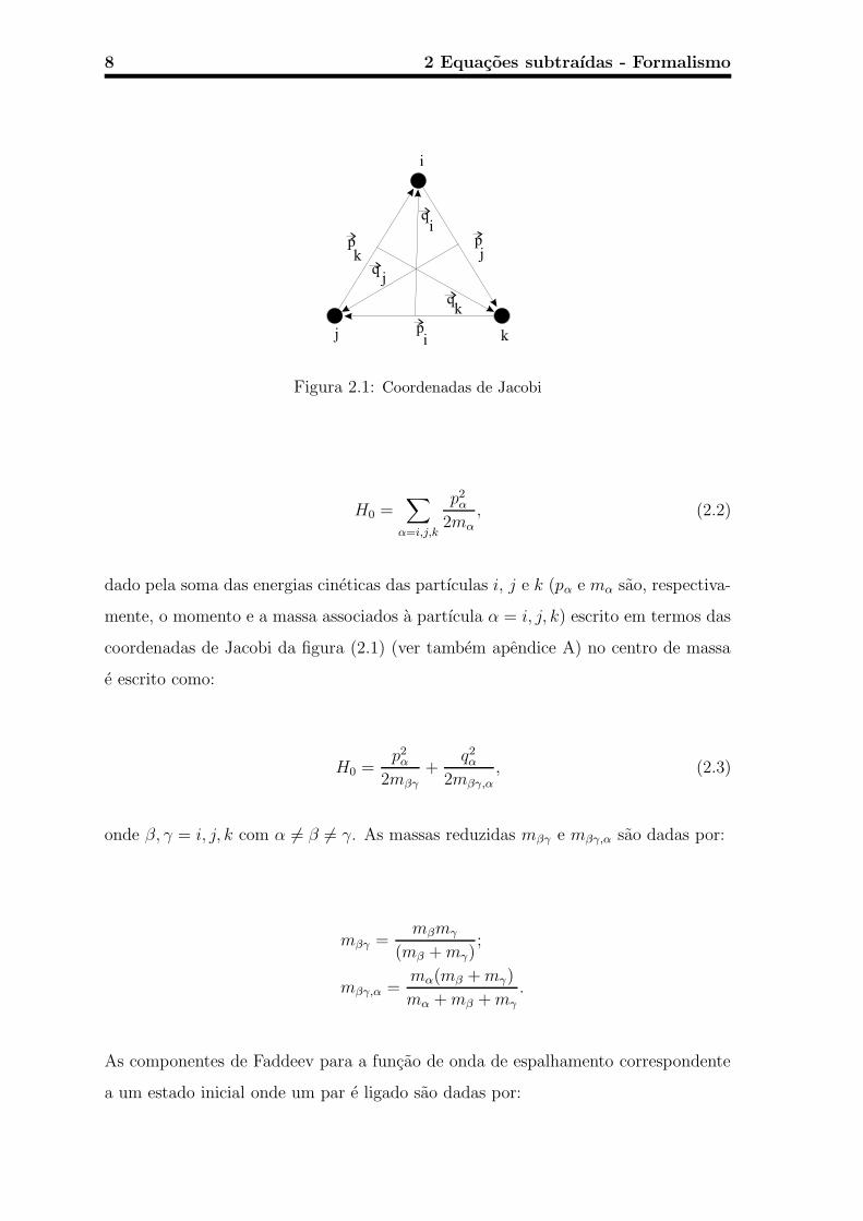
Figura 2.1: Coordenadas de Jacobi
H0 =∑
α=i,j,k
p2α
2mα, (2.2)
dado pela soma das energias cineticas das partıculas i, j e k (pα e mα sao, respectiva-
mente, o momento e a massa associados a partıcula α = i, j, k) escrito em termos das
coordenadas de Jacobi da figura (2.1) (ver tambem apendice A) no centro de massa
e escrito como:
H0 =p2
α
2mβγ+
q2α
2mβγ,α, (2.3)
onde β, γ = i, j, k com α 6= β 6= γ. As massas reduzidas mβγ e mβγ,α sao dadas por:
mβγ =mβmγ
(mβ + mγ);
mβγ,α =mα(mβ + mγ)
mα + mβ + mγ
.
As componentes de Faddeev para a funcao de onda de espalhamento correspondente
a um estado inicial onde um par e ligado sao dadas por:
2.1 Revisao das equacoes de Faddeev e notacao 9
Ψ(+) = G(+)0 (E)(vi + vj + vk)Ψ
(+)
= Ψ(+)i + Ψ
(+)j + Ψ
(+)k , (2.4)
onde G(+)0 = 1
E−H0+iεe o propagador livre de tres corpos e Ψ
(+)α = G
(+)0 (E)vαΨ(+),
α = i, j, k. A funcao Ψ(+)i , por exemplo, pode ser escrita como:
Ψ(+)i = G
(+)0 (E)viΨ
(+), (2.5)
e substituindo Ψ(+), temos que:
Ψ(+)i = G
(+)0 (E)vi(Ψ
(+)i + Ψ
(+)j + Ψ
(+)k ); (2.6)
(1−G(+)0 (E)vi)Ψ
(+)i = G
(+)0 (E)vi(Ψ
(+)j + Ψ
(+)k ). (2.7)
A funcao de onda de espalhamento para a partıcula i e dada somando-se o termo
referente a onda plana:
Ψ(+)i = Φi + (1−G
(+)0 (E)vi)
−1G
(+)0 (E)vi(Ψ
(+)j + Ψ
(+)k ), (2.8)
onde Φi e a “funcao de onda do estado ligado jk ⊗ onda plana i” e e solucao da
equacao homogenea:
(1−G(+)0 (E)vi)Φi = 0;
E =k2
i
2mi
+ Eligjk ,
onde Eligjk e a energia do estado ligado jk e ~ki e o momento associado a partıcula i.
10 2 Equacoes subtraıdas - Formalismo
O operador que multiplica as componentes de Faddeev j e k na eq. (2.8)
pode ainda ser escrito de outra forma, fazendo uso da matriz de transicao de dois
corpos do subsistema j e k (ti):
ti(E) = vi + ti(E)G(+)0 (E)vi = vi + viG
(+)0 (E)ti(E);
G(+)0 (E)ti(E) = G
(+)0 (E)vi + G
(+)0 (E)viG
(+)0 (E)ti(E);
(1−G(+)0 (E)vi)G
(+)0 (E)ti(E) = G
(+)0 (E)vi;
G(+)0 (E)ti(E) = (1−G
(+)0 (E)vi)
−1G
(+)0 (E)vi. (2.9)
O lado direito de (2.9) e exatamente o operador aplicado a Ψ(+)j e Ψ
(+)k na eq. (2.8).
Substituindo (2.9) em (2.8) e escrevendo as componentes j e k que, obviamente, nao
possuem o termo nao homogeneo, temos que:
Ψ(+)i = Φi + G
(+)0 (E)ti(E)[Ψ
(+)j + Ψ
(+)k ];
Ψ(+)j = G
(+)0 (E)tj(E)[Ψ
(+)i + Ψ
(+)k ];
Ψ(+)k = G
(+)0 (E)tk(E)[Ψ
(+)i + Ψ
(+)j ].
(2.10)
Na forma matricial a eq. (2.10) e escrita como:
Ψ(+)i
Ψ(+)j
Ψ(+)k
=
Φi
0
0
+ G(+)0 (E)
0 ti ti
tj 0 tj
tk tk 0
Ψ(+)i
Ψ(+)j
Ψ(+)k
, (2.11)
cuja solucao e dada por:
Ψ(+)i
Ψ(+)j
Ψ(+)k
=
1−G(+)0 (E)
0 ti ti
tj 0 tj
tk tk 0
−1
Φi
0
0
. (2.12)
Desta forma a nao unicidade das solucoes da equacao de Lippmann-Schwinger
para tres corpos e eliminada na eq. (2.12) onde os termos homogeneos sao distintos
2.1 Revisao das equacoes de Faddeev e notacao 11
para cada componente de Faddeev da funcao de onda Ψ. Da mesma forma que es-
crevemos as equacoes para as componentes de Faddeev da funcao de onda, tambem
podemos escrever as componentes de Faddeev para a matriz de transicao T de tres
corpos, dada pela eq. (2.13):
T (z) = V + V G(z)V, (2.13)
onde G(z) = G0(z)+G0(z)T (z)G0(z) = 1z−H
e H sao, respectivamente, o propagador
e o hamiltoniano completo de tres corpos. V = vi+vj+vk e o somatorio dos potenciais
de dois corpos (a notacao utilizada aqui e a mesma da deducao da funcao de onda).
Separando a eq. (2.13) em tres equacoes (α = i, j, k):
Tα = vα + vαG0T, (2.14)
ou ainda na forma matricial:
Ti
Tj
Tk
=
vi
vj
vk
+
vi vi vi
vj vj vj
vk vk vk
G0
Ti
Tj
Tk
. (2.15)
Isolando Ti da eq. (2.15)
(1− viG0)Ti = vi + viG0(Tj + Tk), (2.16)
e multiplicando por (1− viG0)−1 pela esquerda chegamos a equacao para Ti:
Ti = ti + tiG0(Tj + Tk), (2.17)
onde ti = (1− viG0)−1vi e a matriz-T de dois corpos para a componente de Faddeev
i (veja eq. (2.9)).
12 2 Equacoes subtraıdas - Formalismo
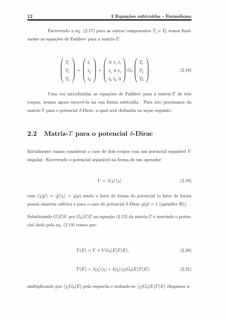
Escrevendo a eq. (2.17) para as outras componentes Tj e Tk temos final-
mente as equacoes de Faddeev para a matriz-T :
Ti
Tj
Tk
=
ti
tj
tk
+
0 ti ti
tj 0 tj
tk tk 0
G0
Ti
Tj
Tk
. (2.18)
Uma vez introduzidas as equacoes de Faddeev para a matriz-T de tres
corpos, iremos agora escreve-la na sua forma subtraıda. Para isto precisamos da
matriz-T para o potencial δ-Dirac, a qual sera deduzida na secao seguinte.
2.2 Matriz-T para o potencial δ-Dirac
Inicialmente vamos considerar o caso de dois corpos com um potencial separavel V
singular. Escrevendo o potencial separavel na forma de um operador
V = λ|χ〉〈χ| (2.19)
com 〈χ|~p 〉 = 〈~p |χ〉 = g(p) sendo o fator de forma do potencial (o fator de forma
possui simetria esferica e para o caso do potencial δ-Dirac g(p) = 1 (apendice B)).
Substituindo G(E)V por G0(E)T na equacao (2.13) da matriz-T e inserindo o poten-
cial dado pela eq. (2.19) temos que:
T (E) = V + V G0(E)T (E), (2.20)
T (E) = λ|χ〉〈χ|+ λ|χ〉〈χ|G0(E)T (E), (2.21)
multiplicando por 〈χ|G0(E) pela esquerda e isolando-se 〈χ|G0(E)T (E) chegamos a:
2.2 Matriz-T para o potencial δ-Dirac 13
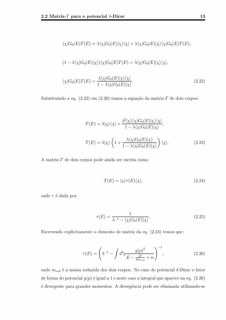
〈χ|G0(E)T (E) = λ〈χ|G0(E)|χ〉〈χ|+ λ〈χ|G0(E)|χ〉〈χ|G0(E)T (E),
(1− λ〈χ|G0(E)|χ〉)〈χ|G0(E)T (E) = λ〈χ|G0(E)|χ〉〈χ|,
〈χ|G0(E)T (E) =λ〈χ|G0(E)|χ〉〈χ|1− λ〈χ|G0(E)|χ〉 . (2.22)
Substituindo a eq. (2.22) em (2.20) temos a equacao da matriz-T de dois corpos:
T (E) = λ|χ〉〈χ|+ λ2|χ〉〈χ|G0(E)|χ〉〈χ|1− λ〈χ|G0(E)|χ〉 ,
T (E) = λ|χ〉(
1 +λ〈χ|G0(E)|χ〉
1− λ〈χ|G0(E)|χ〉
)
〈χ|. (2.23)
A matriz-T de dois corpos pode ainda ser escrita como:
T (E) = |χ〉τ(E)〈χ|, (2.24)
onde τ e dada por:
τ(E) =1
λ−1 − 〈χ|G0(E)|χ〉 . (2.25)
Escrevendo explicitamente o elemento de matriz da eq. (2.24) temos que:
τ(E) =
(
λ−1 −∫
d3pg(p)2
E − p2
2mred+ iε
)−1
, (2.26)
onde mred e a massa reduzida dos dois corpos. No caso do potencial δ-Dirac o fator
de forma do potencial g(p) e igual a 1 e neste caso a integral que aparece na eq. (2.26)
e divergente para grandes momentos. A divergencia pode ser eliminada utilizando-se

14 2 Equacoes subtraıdas - Formalismo
um corte ou atraves da introducao de uma escala fısica (no capıtulo seguinte sera
mostrado que os dois metodos sao equivalentes). A informacao fısica e introduzida
atribuindo-se um valor fısico, λR, para a matriz-T num ponto de subtracao de energia
E = −µ2(2) (o ındice entre parenteses subscrito em µ2 indica que estamos considerando
a escala de 2-corpos), ou seja,
τR(−µ2(2)) = λR(−µ2
(2)). (2.27)
o ındice subscrito R significa renormalizado.
Introduzindo a informacao fısica na eq. (2.26) com o fator de forma do
potencial ja colocado igual a 1, temos que:
τR(−µ2(2)) =
[
λ−1 −∫
d3p1
−µ2(2) −
p2
2mred
]−1
= λR(−µ2(2)),
λ−1 −∫
d3p1
−µ2(2) −
p2
2mred
= λR−1(−µ2
(2)),
λ−1 = λR−1(−µ2
(2)) +
∫
d3p1
−µ2(2) −
p2
2mred
. (2.28)
Substituindo agora o resultado de λ−1 em (2.26) chegamos na forma da equacao
subtraıda:
τ−1R (E) = λR
−1(−µ2(2)) +
∫
d3p
[
1
−µ2(2) −
p2
2mred
− 1
E − p2
2mred+ iε
]
,
(2.29)
τ−1R (E) = λR
−1(−µ2(2)) + (E + µ2
(2))
∫
d3p1
(
−µ2(2) −
p2
2mred
)(
E − p2
2mred+ iε
) .
Agora a integral que aparece em (2.29) e finita. Calculando a integral utilizando o
metodo dos resıduos, substituindo a massa dos dois corpos e substituindo E = k2
2.3 Equacao subtraıda para a matriz-T 15
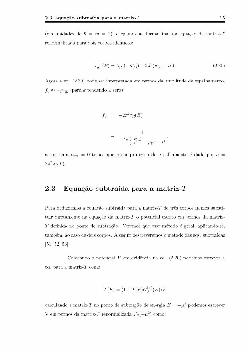
(em unidades de ~ = m = 1), chegamos na forma final da equacao da matriz-T
renormalizada para dois corpos identicos:
τ−1R (E) = λ−1
R (−µ2(2)) + 2π2(µ(2) + ik). (2.30)
Agora a eq. (2.30) pode ser interpretada em termos da amplitude de espalhamento,
f0 ≈ 1− 1
a−ik
(para k tendendo a zero):
f0 = −2π2τR(E)
=1
−λ−1R (−µ2
(2))
2π2 − µ(2) − ik,
assim para µ(2) = 0 temos que o comprimento de espalhamento e dado por a =
2π2λR(0).
2.3 Equacao subtraıda para a matriz-T
Para deduzirmos a equacao subtraıda para a matriz-T de tres corpos iremos substi-
tuir diretamente na equacao da matriz-T o potencial escrito em termos da matriz-
T definida no ponto de subtracao. Veremos que esse metodo e geral, aplicando-se,
tambem, ao caso de dois corpos. A seguir descreveremos o metodo das eqs. subtraıdas
[51, 52, 53].
Colocando o potencial V em evidencia na eq. (2.20) podemos escrever a
eq. para a matriz-T como:
T (E) = (1 + T (E)G(+)0 (E))V,
calculando a matriz-T no ponto de subtracao de energia E = −µ2 podemos escrever
V em termos da matriz-T renormalizada TR(−µ2) como:
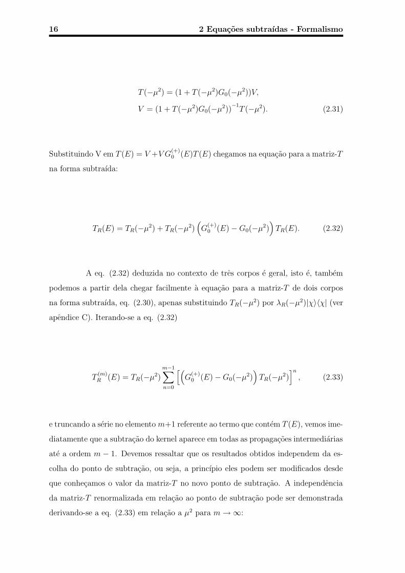
16 2 Equacoes subtraıdas - Formalismo
T (−µ2) = (1 + T (−µ2)G0(−µ2))V,
V = (1 + T (−µ2)G0(−µ2))−1
T (−µ2). (2.31)
Substituindo V em T (E) = V +V G(+)0 (E)T (E) chegamos na equacao para a matriz-T
na forma subtraıda:
TR(E) = TR(−µ2) + TR(−µ2)(
G(+)0 (E)−G0(−µ2)
)
TR(E). (2.32)
A eq. (2.32) deduzida no contexto de tres corpos e geral, isto e, tambem
podemos a partir dela chegar facilmente a equacao para a matriz-T de dois corpos
na forma subtraıda, eq. (2.30), apenas substituindo TR(−µ2) por λR(−µ2)|χ〉〈χ| (verapendice C). Iterando-se a eq. (2.32)
T(m)R (E) = TR(−µ2)
m−1∑
n=0
[(
G(+)0 (E)−G0(−µ2)
)
TR(−µ2)]n
, (2.33)
e truncando a serie no elemento m+1 referente ao termo que contem T (E), vemos ime-
diatamente que a subtracao do kernel aparece em todas as propagacoes intermediarias
ate a ordem m − 1. Devemos ressaltar que os resultados obtidos independem da es-
colha do ponto de subtracao, ou seja, a princıpio eles podem ser modificados desde
que conhecamos o valor da matriz-T no novo ponto de subtracao. A independencia
da matriz-T renormalizada em relacao ao ponto de subtracao pode ser demonstrada
derivando-se a eq. (2.33) em relacao a µ2 para m →∞:

2.3 Equacao subtraıda para a matriz-T 17
d
dµ2TR(E) =
d
dµ2
TR(−µ2)
∞∑
n=0
[(
G(+)0 (E)−G0(−µ2)
)
TR(−µ2)]n
=d
dµ2TR(−µ2) +
d
dµ2TR(−µ2)
(
G(+)0 (E)−G0(−µ2)
)
TR(−µ2)
−TR(−µ2)d
dµ2G0(−µ2)T (−µ2) + TR(−µ2)
(
G(+)0 (E)−G0(−µ2)
) d
dµ2TR(−µ2) + ...
=1
1− TR(−µ2)(
G(+)0 (E)−G0(−µ2)
)
d
dµ2TR(−µ2)− TR(−µ2)
1
(µ2 + H0)2TR(−µ2)
× 1
1−(
G(+)0 (E)−G0(−µ2)
)
TR(−µ2), (2.34)
o termo que aparece entre chaves na eq. (2.34) e obtido substituindo-se E por −µ′2
na eq. (2.32) e depois derivando-a em relacao a µ2 no limite de µ′ → µ:
d
dµ2TR(−µ2)− TR(−µ2)
1
(µ2 + H0)2TR(−µ2) = 0, (2.35)
Assim demonstramos que:
d
dµ2TR(E) = 0. (2.36)
Podemos ainda reescrever a eq. (2.36) como:
µd
dµTR(E) = 0, (2.37)
que e uma equacao do tipo Callan-Symanzik. Desta forma, podemos dizer que a
invariancia da matriz-T renormalizada, TR(E), em relacao ao ponto de subtracao e
consequencia dela satisfazer a uma equacao do tipo Callan-Symanzik [54].
18 2 Equacoes subtraıdas - Formalismo
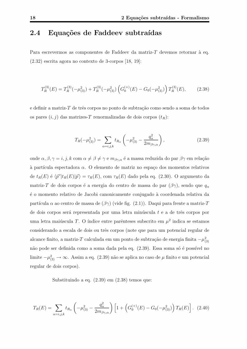
2.4 Equacoes de Faddeev subtraıdas
Para escrevermos as componentes de Faddeev da matriz-T devemos retornar a eq.
(2.32) escrita agora no contexto de 3-corpos [18, 19]:
T(3)R (E) = T
(3)R (−µ2
(3)) + T(3)R (−µ2
(3))(
G(+)0 (E)−G0(−µ2
(3)))
T(3)R (E), (2.38)
e definir a matriz-T de tres corpos no ponto de subtracao como sendo a soma de todos
os pares (i, j) das matrizes-T renormalizadas de dois corpos (tR):
TR(−µ2(3)) =
∑
α=i,j,k
tRα
(
−µ2(3) −
q2α
2mβγ,α
)
, (2.39)
onde α, β, γ = i, j, k com α 6= β 6= γ e mβγ,α e a massa reduzida do par βγ em relacao
a partıcula espectadora α. O elemento de matriz no espaco dos momentos relativos
de tR(E) e 〈~p ′|tR(E)|~p 〉 = τR(E), com τR(E) dado pela eq. (2.30). O argumento da
matriz-T de dois corpos e a energia do centro de massa do par (βγ), sendo que qα
e o momento relativo de Jacobi canonicamente conjugado a coordenada relativa da
partıcula α ao centro de massa de (βγ) (vide fig. (2.1)). Daqui para frente a matriz-T
de dois corpos sera representada por uma letra minuscula t e a de tres corpos por
uma letra maiuscula T . O ındice entre parenteses subscrito em µ2 indica se estamos
considerando a escala de dois ou tres corpos (note que para um potencial regular de
alcance finito, a matriz-T calculada em um ponto de subtracao de energia finita −µ2(3)
nao pode ser definida como a soma dada pela eq. (2.39). Essa soma so e possıvel no
limite −µ2(3) →∞. Assim a eq. (2.39) nao se aplica no caso de µ finito e um potencial
regular de dois corpos).
Substituindo a eq. (2.39) em (2.38) temos que:
TR(E) =∑
α=i,j,k
tRα
(
−µ2(3) −
q2α
2mβγ,α
)
[
1 +(
G(+)0 (E)−G0(−µ2
(3)))
TR(E)]
. (2.40)
2.4 Equacoes de Faddeev subtraıdas 19
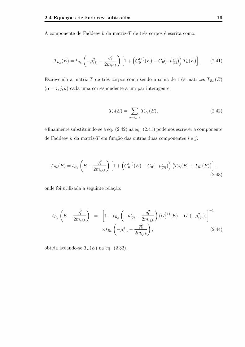
A componente de Faddeev k da matriz-T de tres corpos e escrita como:
TRk(E) = tRk
(
−µ2(3) −
q2k
2mij,k
)
[
1 +(
G(+)0 (E)−G0(−µ2
(3)))
TR(E)]
. (2.41)
Escrevendo a matriz-T de tres corpos como sendo a soma de tres matrizes TRα(E)
(α = i, j, k) cada uma correspondente a um par interagente:
TR(E) =∑
α=i,j,k
TRα(E), (2.42)
e finalmente substituindo-se a eq. (2.42) na eq. (2.41) podemos escrever a componente
de Faddeev k da matriz-T em funcao das outras duas componentes i e j:
TRk(E) = tRk
(
E − q2k
2mij,k
)
[
1 +(
G(+)0 (E)−G0(−µ2
(3)))
(
TRi(E) + TRj
(E))
]
,
(2.43)
onde foi utilizada a seguinte relacao:
tRk
(
E − q2k
2mij,k
)
=
[
1− tRk
(
−µ2(3) −
q2k
2mij,k
)
(G(+)0 (E)−G0(−µ2
(3)))
]−1
×tRk
(
−µ2(3) −
q2k
2mij,k
)
, (2.44)
obtida isolando-se TR(E) na eq. (2.32).

20 2 Equacoes subtraıdas - Formalismo

Capıtulo 3
Os estados Efimov - Estados
ligados, virtuais e ressonancias
Partindo da equacao subtraıda para a matriz-T de tres corpos obtida na secao ante-
rior, podemos deduzir a equacao homogenea para os estados ligados e virtuais de tres
corpos identicos. Nesta secao iremos tambem calcular as energias das ressonancias
no sistema de tres corpos. Mostraremos que partindo-se de uma certa energia para
o estado ligado de dois corpos e diminuindo o seu modulo, um estado virtual de tres
corpos torna-se ligado [7], esse estado ligado torna-se por sua vez uma ressonancia
quando a energia de dois corpos torna-se virtual [49].
Partindo-se da equacao para a matriz-T podemos inserir nela a seguinte
relacao de completeza:
1 =∑
L
|ΦL〉〈ΦL|+∫
d3k|Ψ(+)k 〉〈Ψ(+)
k |, (3.1)
onde |ΦL〉 e |Ψ(+)k 〉 sao, respectivamente, a funcao de onda dos estados ligados e a
funcao de onda de espalhamento das partıculas de momento inicial igual a ~k. Assim,
inserindo a eq. (3.1) na equacao da matriz-T , eq. (2.13) com z = E, temos que:
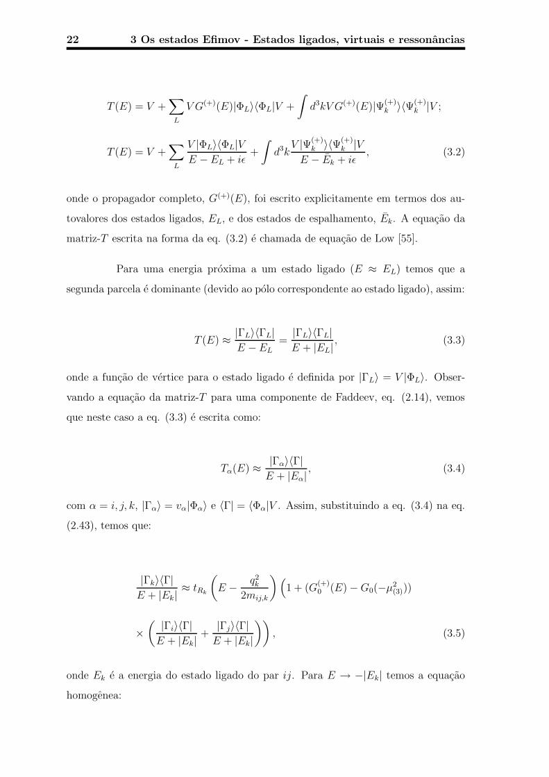
22 3 Os estados Efimov - Estados ligados, virtuais e ressonancias
T (E) = V +∑
L
V G(+)(E)|ΦL〉〈ΦL|V +
∫
d3kV G(+)(E)|Ψ(+)k 〉〈Ψ(+)
k |V ;
T (E) = V +∑
L
V |ΦL〉〈ΦL|VE − EL + iε
+
∫
d3kV |Ψ(+)
k 〉〈Ψ(+)k |V
E − Ek + iε, (3.2)
onde o propagador completo, G(+)(E), foi escrito explicitamente em termos dos au-
tovalores dos estados ligados, EL, e dos estados de espalhamento, Ek. A equacao da
matriz-T escrita na forma da eq. (3.2) e chamada de equacao de Low [55].
Para uma energia proxima a um estado ligado (E ≈ EL) temos que a
segunda parcela e dominante (devido ao polo correspondente ao estado ligado), assim:
T (E) ≈ |ΓL〉〈ΓL|E − EL
=|ΓL〉〈ΓL|E + |EL|
, (3.3)
onde a funcao de vertice para o estado ligado e definida por |ΓL〉 = V |ΦL〉. Obser-
vando a equacao da matriz-T para uma componente de Faddeev, eq. (2.14), vemos
que neste caso a eq. (3.3) e escrita como:
Tα(E) ≈ |Γα〉〈Γ|E + |Eα|
, (3.4)
com α = i, j, k, |Γα〉 = vα|Φα〉 e 〈Γ| = 〈Φα|V . Assim, substituindo a eq. (3.4) na eq.
(2.43), temos que:
|Γk〉〈Γ|E + |Ek|
≈ tRk
(
E − q2k
2mij,k
)
(
1 + (G(+)0 (E)−G0(−µ2
(3)))
×( |Γi〉〈Γ|
E + |Ek|+
|Γj〉〈Γ|E + |Ek|
))
, (3.5)
onde Ek e a energia do estado ligado do par ij. Para E → −|Ek| temos a equacao
homogenea:

3 Os estados Efimov - Estados ligados, virtuais e ressonancias 23
|Γk〉 = tRk
(
E − q2k
2mij,k
)
(G(+)0 (E)−G0(−µ2
(3)))(|Γi〉+ |Γj〉). (3.6)
Escrevendo explicitamente a matriz-T de dois corpos dada pela eq. (2.24)
temos que:
|Γk〉 = |χk〉τ(
E − q2k
2mk(ij)
)
〈χk|(
G(+)0 (E)−G0(−µ2
(3)))
(|Γi〉+ |Γj〉) , (3.7)
onde τ(E2) e o elemento de matriz da matriz-T renormalizada dado pela eq. (2.30).
A partir deste ponto usaremos a notacao τ ≡ τR.
Multiplicando a eq. (3.7) por 〈~pk, ~qk| pela esquerda:
〈~pk, ~qk|Γk〉 = 〈~pk|χk〉τ(
E − q2k
2mij,k
)
〈χk, ~qk|(
G(+)0 (E)−G0(−µ2
(3)))
(|Γi〉+ |Γj〉) ,
(3.8)
e utilizando que 〈~pk, ~qk|Γk〉 = 〈~pk|χk〉〈~qk|fk〉 = fk(~qk) para o potencial δ-Dirac, temos
a equacao homogenea do estado ligado de tres corpos para a componente de Faddeev
k:
fk(~qk) = τ
(
E − q2k
2mij,k
)
〈χk, ~qk|(
G(+)0 (E)−G0(−µ2
(3)))
(|Γi〉+ |Γj〉) , (3.9)
No caso especıfico de tres bosons identicos, as tres funcoes espectadoras
sao identicas:
〈~qi|fi〉 = 〈~qj|fj〉 = 〈~qk|fk〉, (3.10)
e a eq. (3.9) fica entao escrita como:
24 3 Os estados Efimov - Estados ligados, virtuais e ressonancias
fk(~qk) = 2τ
(
E − q2k
2mij,k
)
〈χk, ~qk|(
G(+)0 (E)−G0(−µ2
(3)))
(|χi〉|fi〉) . (3.11)
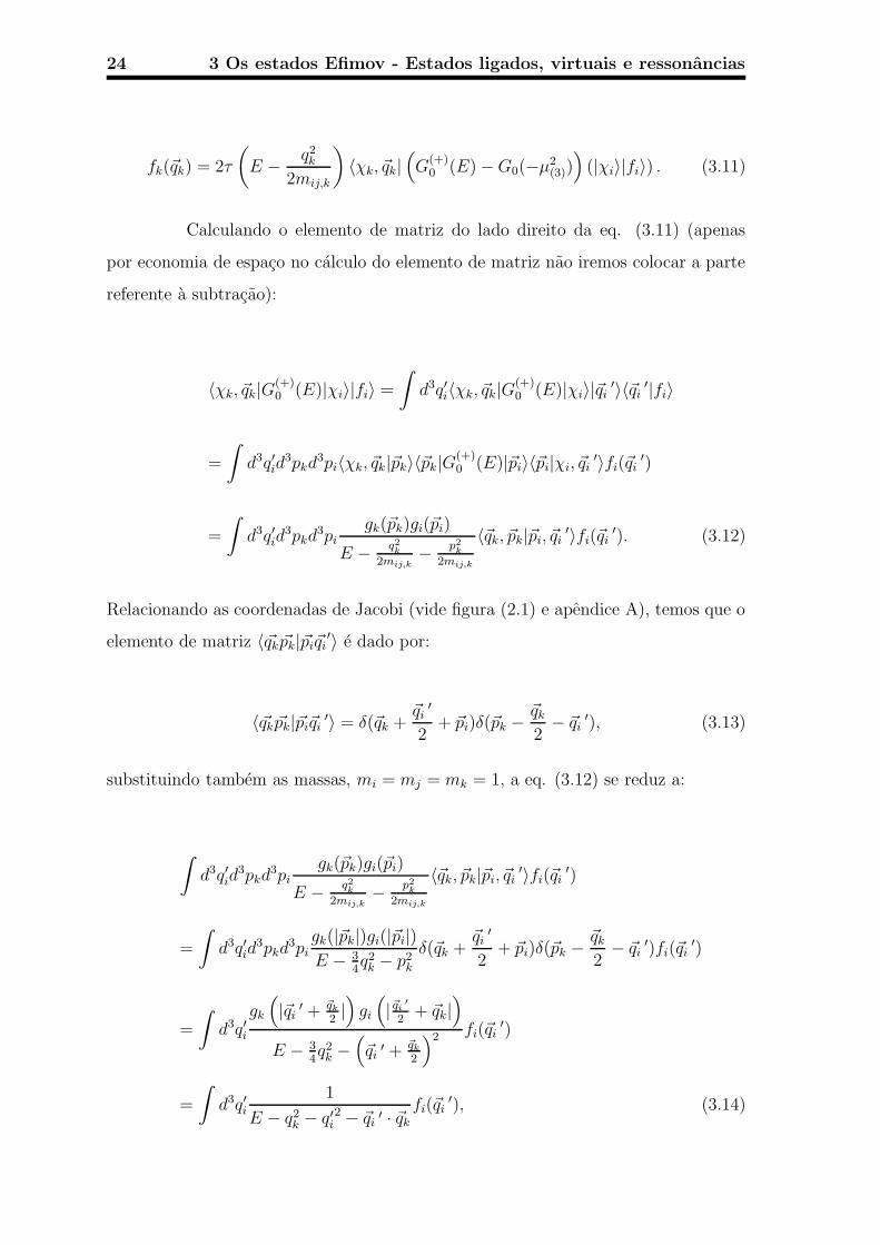
Calculando o elemento de matriz do lado direito da eq. (3.11) (apenas
por economia de espaco no calculo do elemento de matriz nao iremos colocar a parte
referente a subtracao):
〈χk, ~qk|G(+)0 (E)|χi〉|fi〉 =
∫
d3q′i〈χk, ~qk|G(+)0 (E)|χi〉|~qi
′〉〈~qi′|fi〉
=
∫
d3q′id3pkd
3pi〈χk, ~qk|~pk〉〈~pk|G(+)0 (E)|~pi〉〈~pi|χi, ~qi
′〉fi(~qi′)
=
∫
d3q′id3pkd
3pigk(~pk)gi(~pi)
E − q2k
2mij,k− p2
k
2mij,k
〈~qk, ~pk|~pi, ~qi′〉fi(~qi
′). (3.12)
Relacionando as coordenadas de Jacobi (vide figura (2.1) e apendice A), temos que o
elemento de matriz 〈~qk ~pk|~pi~qi′〉 e dado por:
〈~qk ~pk|~pi~qi′〉 = δ(~qk +
~qi′
2+ ~pi)δ(~pk −
~qk
2− ~qi
′), (3.13)
substituindo tambem as massas, mi = mj = mk = 1, a eq. (3.12) se reduz a:
∫
d3q′id3pkd
3pigk(~pk)gi(~pi)
E − q2k
2mij,k− p2
k
2mij,k
〈~qk, ~pk|~pi, ~qi′〉fi(~qi
′)
=
∫
d3q′id3pkd
3pigk(|~pk|)gi(|~pi|)E − 3
4q2k − p2
k
δ(~qk +~qi
′
2+ ~pi)δ(~pk −
~qk
2− ~qi
′)fi(~qi′)
=
∫
d3q′i
gk
(
|~qi′ + ~qk
2|)
gi
(
|~qi′
2+ ~qk|
)
E − 34q2k −
(
~qi′ + ~qk
2
)2 fi(~qi′)
=
∫
d3q′i1
E − q2k − q′i
2 − ~qi′ · ~qk
fi(~qi′), (3.14)

3 Os estados Efimov - Estados ligados, virtuais e ressonancias 25
onde utilizamos que o fator de forma para o potencial δ-Dirac gk = gi = 1. Desta
forma, substituindo o elemento de matriz dado pela eq. (3.14) (note que a parte refe-
rente a subtracao e identica a eq. (3.14) com excecao da energia E que e substituıda
por −µ2(3)) na eq. (3.12), e fazendo q′i ≡ q′ e qk ≡ q, temos a equacao para o estado
ligado de tres bosons identicos:
f(~q ) = 2τ
(
E − 3
4q2
)∫
d3q′
(
1
E − q2 − q′2 − ~q ′ · ~q −1
−µ2(3) − q2 − q′2 − ~q ′ · ~q
)
f(~q ′).
(3.15)
Introduzindo a informacao fısica do estado ligado λ−1R (−µ2
(2)) = 0, onde −µ2(2) e a
energia do estado ligado de dois corpos, na funcao τ dada pela eq. (2.30), temos que:
τ
(
E − 3
4q2
)
=1/2π2
µ(2) −√
−E + 34q2
(3.16)
Escrevendo a eq. (3.15) para a onda-S, temos que:
f(~q) =π−2
µ(2) −√
−E + 34q2
∫
d3q′
(
1
E − q2 − q′2 − ~q ′ · ~q −1
−µ2(3) − q2 − q′2 − ~q ′ · ~q
)
f(~q′).
(3.17)
Esta equacao sem o segundo termo onde aparece µ(3) foi obtida pela primeira vez por
Skorniakov e Ter-Martirosian [56].
Realcando a integracao angular na eq. (3.17), temos que a funcao espec-
tadora na onda-S (que corresponde a funcao de onda de tres bosons com momento
angular orbital total nulo) fica igual a:
f(q) =2/π
µ(2) −√
−E + 34q2
∫ ∞
0
dq′q′2
∫ −1
1
dz
(
1
E − q2 − q′2 − q′qz
− 1
−µ2(3) − q2 − q′2 − q′qz
)
f(q′). (3.18)

26 3 Os estados Efimov - Estados ligados, virtuais e ressonancias
Reescrevendo as variaveis como ε3L = −Eµ2
(3), y = q
µ(3)e x = q′
µ(3)e fazendo µ(3) = 1
temos que:
f(y) =−2/π
±√ε2 −√
ε3L + 34y2
∫ ∞
0
dxx2
∫ −1
1
dz
[
1
ε3L + y2 + x2 + xyz
(3.19)
− 1
1 + y2 + x2 + xyz
]
f(x),
onde substituımosµ(2)
µ(3)por ±√ε2, sendo ε2 a energia de dois corpos, o sinal positivo
refere-se ao estado ligado e o negativo ao estado virtual. ε3L e a energia do estado
ligado de tres corpos em unidades de µ2(3).
A eq. (3.19) utilizada para calcular o estado ligado de tres bosons identicos
tambem sera utilizada para o calculo das ressonancias de tres bosons. Neste caso,
iremos considerar somente as energias dos estados virtuais de dois corpos representado
pelo sinal negativo em frente a√
ε2. Para calcular as ressonancias e suas larguras
iremos utilizar o metodo do desvio de contorno [57, 58]. Neste metodo a continuacao
analıtica para a segunda folha e feita substituindo-se x(y) → xe−iθ(ye−iθ), com 0 <
θ < π/4. Para um angulo θ suficientemente grande a solucao da eq. (3.19) no plano
complexo e encontrada para tg(2θ) > −Im(ε3)/Re(ε3).
Para calcularmos a energia do estado virtual de tres bosons vamos fazer
a extensao analıtica da eq. (3.19) para a segunda folha de Riemann passando pelo
corte do espalhamento elastico (vide figura (3.1)). Na fig. (3.1) esta representada
esquematicamente a energia do sistema ligado de dois corpos, −ε2, e as energias
de tres corpos, −ε3L e −ε3V , no plano de energia. Podemos ver na figura que o
corte do espalhamento elastico define duas folhas de Riemann: na primeira folha
esta localizada a energia para o estado ligado de tres corpos, Re(ε) = −ε3L, e na
segunda folha o estado virtual de tres corpos, Re(ε) = −ε3V [59, 60]. Assim, definindo
h(η) ≡(
ε2 − ε3L − 34y2)
f(η) podemos escrever a eq. (3.19) na primeira folha como:

3 Os estados Efimov - Estados ligados, virtuais e ressonancias 27
Figura 3.1: Extensao da matriz-T de tres corpos para a segunda folha de Riemann no
plano de energia. −ε2 e a energia do estado ligado de dois corpos, −ε3L e a energia do
estado ligado de tres corpos (localizada na primeira folha de Riemann) e −ε3V e a energia
do estado virtual (localizada na segunda folha).
h(y) = − 2
π
(
√ε2 +
√
ε3L +3
4y2
)
∫ ∞
0
dxx2
∫ −1
1
dz
[
1
ε3L + y2 + x2 + xyz
− 1
1 + y2 + x2 + xyz
]
h(x)
ε2 − ε3L − 34x2 + iδ
(3.20)
Podemos notar que o denominador ε2 − ε3L − 34x2 + iδ que aparece sob a
funcao h(x) pode ser interpretado como a funcao de Green do sistema ligado de dois
corpos na presenca de um terceiro corpo se aproximando do centro de massa dos dois
corpos com energia cinetica igual a 34x2, conforme mostra a figura (3.2) (obviamente
essa interpretacao e qualitativa tendo em vista que ε3L e x sao adimensionais):
Figura 3.2: Terceira partıcula se aproximando do dımero de energia de ligacao ε2 com uma
energia cinetica de 34x2.

28 3 Os estados Efimov - Estados ligados, virtuais e ressonancias
A extensao para segunda folha da eq. (3.20) e feita somando-se e sub-
traındo-se o termo referente a descontinuidade da equacao para a segunda folha (para
ilustrar o metodo utilizado no caso de tres corpos, uma deduc.ao detalhada da extensao
da equacao da matriz-T de dois corpos e feita no apendice E):
h2a
(y) = − 2
π
(
±√ε2 +
√
ε3V +3
4y2
)
∫ ∞
0
dxx2
∫ −1
1
dz
[
1
ε3V + y2 + x2 + xyz
− 1
1 + y2 + x2 + xyz
] [
1
ε2 − ε3V − 34x2 + iδ
− 1
ε2 − ε3V − 34x2 − iδ
]
h(x)
(3.21)
− 2
π
(
±√ε2 +
√
ε3V +3
4y2
)
∫ ∞
0
dxx2
∫ −1
1
dz
[
1
ε3V + y2 + x2 + xyz
− 1
1 + y2 + x2 + xyz
]
h(x)
ε2 − ε3V − 34x2 − iδ
.
ε3L foi substitıdo por ε3V somente para distinguirmos as energias ligadas e virtuais de
tres corpos. Calculando a primeira integral utilizando o metodo dos resıduos (vide
apendice E) e substituindo ε2− ε3V ≡ 34κ2 (note que para o caso do estado virtual de
tres corpos κ e definido como κ ≡ −i√
43(ε3V − ε2) ≡ −iκV ) chegamos na forma final
para h2a(y):
h2a
(y) =8
3iκ
(
±√ε2 +
√
ε3V +3
4y2
)
×∫ −1
1
dz
[
1
ε3V + y2 + κ2 + κyz− 1
1 + y2 + κ2 + κyz
]
h(κ)
(3.22)
− 2
π
(
±√ε2 +
√
ε3V +3
4y2
)
∫ ∞
0
dxx2
∫ −1
1
dz
[
1
ε3V + y2 + x2 + xyz
− 1
1 + y2 + x2 + xyz
]
h(x)
ε2 − ε3V − 34x2 − iδ
.
A energia do estado virtual de tres corpos e limitada pelo corte na ampli-
tude de espalhamento elastica que e dado pelo polo da funcao de Green de tres corpos

3 Os estados Efimov - Estados ligados, virtuais e ressonancias 29
no primeiro termo da eq. (3.22),
εcorte + y2 + x2 + xyz = 0, (3.23)
com x = y = −iκcorte. Resolvendo a eq. (3.23) temos que o corte corresponde as
energias que estao contidas no limite de
4
3|ε2| ≤ |εcorte| ≤ 4|ε2|, (3.24)
como a energia do estado virtual deve estar fora do intervalo dado pela eq. (3.24) e
obviamente deve ser maior que |ε2|, concluımos que a energia para o estado virtual
deve ser maior que |ε2| e menor que 43|ε2|.
Os resultados para este capıtulo sao encontrados resolvendo-se as equacoes
subtraıdas (3.19) e (3.22). Os resultados serao comparados com calculos realısticos e
com o resultado da equacao com corte para grandes momentos [21]. A equacao do
estado ligado utilizando o corte para grandes momentos e dada na Ref. [21] (colocare-
mos aqui somente a equacao para o estado ligado para nortear nossa discussao sobre
os estados Efimov, o colapso Thomas e a introducao da funcao de escala. A equacao
para o estado virtual com o corte nos momentos pode ser deduzida da mesma forma
que foi feita a deducao no caso das equacoes subtraıdas):
χ(~y) =−π−2
±√ε2 −√
ε3 + 34y2
∫
d3xθ(1− |~x|)
ε3 + y2 + x2 + ~y · ~xχ(~x), (3.25)
onde o corte, Λ, foi colocado igual a 1 e os momentos e as energias de dois e tres corpos
foram reescalonados como ~p = Λ~x, ~q = Λ~y, E2 = Λ2ε2, e E3 = Λ2ε3. O numero
de estado ligados de tres corpos ε3 = ε(N)3 (N = 0, 1, 2, ...) aumenta infinitamente
conforme ε2 tende a zero e nesse limite satisfaz a razao ε(N)3 /ε
(N+1)3 ≈ 500 [1, 2]. Note
que ε2 tende a zero se a energia de dois corpos, E2, vai para zero (mantendo-se fixo Λ),
ou se o corte Λ vai para infinito (mantendo-se E2 fixa). Este ultimo caso equivale a
30 3 Os estados Efimov - Estados ligados, virtuais e ressonancias
fazermos o alcance do potencial, r0, tender a zero (Λ ∼ r−10 ), nesta situacao o sistema
de tres corpos colapsa, E(0)3 = Λ2ε
(0)3 → ∞. Esse colapso e conhecido como colapso
Thomas do estado fundamental de tres corpos. Assim, podemos ver claramente que os
efeitos Efimov e Thomas sao fisicamente equivalentes e sao dados pelo mesmo limite,
ε2 → 0, estando relacionados apenas por uma transformacao de escala [21].
O conceito de funcao de escala sera introduzido conforme a Ref. [15] e
generalizado para o caso dos estados virtuais. As solucoes da eq. (3.25) sao as “ener-
gias”adimensionais que sao funcoes de ±√ε2: ε(N)3 = ε
(N)3 (±√ε2), assim utilizando o
N esimo estado da energia para obter Λ temos que:
E(N+1)3 = E
(N)3
ε(N+1)3 (ξ)
ε(N)3
, (3.26)
onde ξ ≡ ±√ε2 = ±√
E2(ε(N)3 /E
(N)3 ). Podemos ver na eq. (3.26) que as escalas fısicas
de dois e tres corpos determinam o estado E(N+1)3 , o estado excitado acima de E
(N)3 .
A razao entre as energias escrita conforme a eq. (3.26) nao e ambıgua, pois o limite:
E(N+1)3
E(N)3
= limN→∞
ε(N+1)3 (ξ)
ε(N)3
= F(
±√
E2
E(N)3
)
, (3.27)
existe e define a funcao de escala F (um argumento qualitativo para a existencia desse
limite e dado na Ref. [15]. O termo “limite de escala”e o mesmo que o termo “limit
cycle”discutido por K. Wilson na Ref. [61]). A generalizacao da eq. (3.27) para as
energias do estado virtual de tres corpos e escrita como:
K(√
E2
E(N)3
)
≡ ±
√
√
√
√
E(N+1)3 − E2
E(N)3
= ±
√
√
√
√
ε(N+1)3 − ε2
ε(N)3
. (3.28)
A funcao K tem os seus valores definidos nas duas folhas de Riemann no espaco dos
momentos com origem no ponto onde as energias de dois e tres corpos, ε2 e ε3, sao
iguais. A energia do subsistema de dois corpos foi colocada sempre ligada. Os sinais
positivo e negativo definem, respectivamente, os estados ligados e virtuais de tres

3 Os estados Efimov - Estados ligados, virtuais e ressonancias 31
corpos.
No caso das energias das ressonancias dos tres corpos a funcao de escala e
escrita como (a energia de dois corpos foi colocada sempre virtual):
R(√
ε2
ε3L
)
= ±√
ε3
ε3L, (3.29)
O sinal ± fora dos parenteses indica se estamos considerando uma energia para uma
ressonancia (+) ou um estado ligado (−).
De forma a generalizar as funcoes de escala, podemos dizer que a existencia
de uma escala de tres corpos em sistemas de tres corpos em baixas energias implica
na existencia de uma funcao universal que correlaciona os observaveis de tres corpos
[18, 19, 62]. No limite de escala, ou limit cycle, ela pode ser escrita como:
O (E, E3, E2) = (E3)ηB(
√
E/E3,±√
E2/E3
)
(3.30)
onde O e qualquer observavel do sistema de tres corpos em uma energia E, com
dimensao de energia elevada a potencia η. O sinal ± indica se estamos considerando
um estado ligado ou virtual de dois corpos.
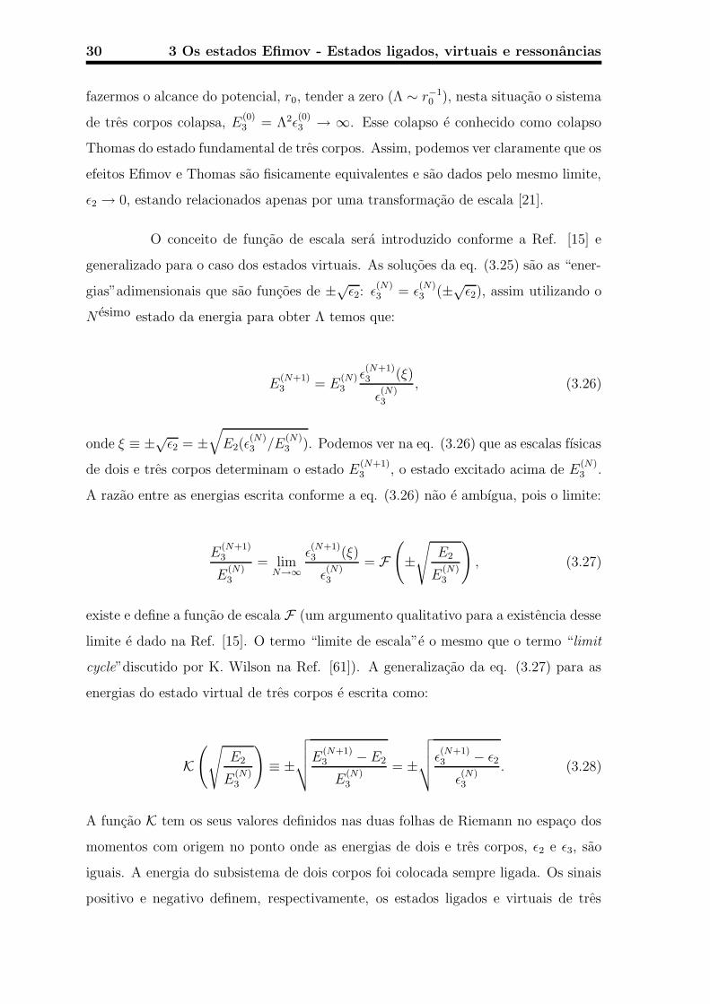
A seguir serao descritos os resultados desta secao. Na fig. (3.3) mostramos
o aparecimento dos estados virtuais e ligados conforme variamos a energia de ligacao
de dois corpos.
Nesta figura mostramos somente os tres primeiros estados ligados, mas
podemos ver claramente que conforme a energia de dois corpos tende a zero um
numero crescente de estados fracamente ligados de Efimov aparece. Na fig. (3.3)
podemos, ainda, ver a natureza dos estados Efimov conforme variamos a energia de
dois corpos: para uma energia ε2 da ordem de 10−1 vemos que existe somente o estado
fundamental ε(0)3L (linha com cruzes). Neste caso, ε2 e muito grande para que exista
o primeiro estado excitado, esse estado encontra-se na segunda folha de Riemann e
corresponde a um estado virtual, representado pelos cırculos. Conforme diminuımos
32 3 Os estados Efimov - Estados ligados, virtuais e ressonancias
Figura 3.3: Energias dos trımeros ε3, em unidades de µ(3) = 1 em funcao da energia
do estado ligado do dımero ε2. O estado fundamental, ε(0)3L , esta representado pela linha
com cruzes, o primeiro estado excitado, ε(1)3L , pela linha com quadrados e o segundo estado
excitado, ε(2)3L , pela linha com losangos. O estados virtuais ε
(1)3V e ε
(2)3V estao representados,
respectivamente, pelos cırculos e triangulos localizados entre os limites definidos pelas linhas
pontilhada, ε3 = 43ε2, e solida ε3 = ε2.
ε2 o estado virtual correspondente ao primeiro estado excitado “sai”da segunda folha
para tornar-se um estado ligado (linha com quadrados). Esse processo se repete
conforme a energia de dois corpos tende a zero. O ponto onde o estado virtual de
tres corpos surge e dado pela seta para baixo, ↓, que comeca no limiar do corte do
espalhamento elastico, ε3 = (4/3)ε2, dado pela linha pontilhada. A seta para cima,
↑, indica o ponto onde o estado virtual torna-se um estado excitado, este emerge da
segunda folha para a primeira em ε3 = ε2 (linha contınua).
Na fig. (3.4) a transicao de um estado virtual para um estado ligado pode
ser vista claramente. Esta figura foi construıda utilizando-se o primeiro e o segundo
estado Efimov. Este resultado praticamente nao difere daquele obtido com o segundo
e o terceiro estado Efimov (nao colocamos na figura).

3 Os estados Efimov - Estados ligados, virtuais e ressonancias 33
0.1 0.3 0.5 0.7
1.2
1.6
2.0
2.4
2.8
E3(N
+1) /E
2
E2/E3
(N)
Figura 3.4: Razao da energia do (N +1)esimo estado ligado ou virtual do trımero, E(N+1)3 ,
e da energia do dımero, E2, em funcao da razao da energia do dımero e do N esimo estado
ligado do trımero. Os estados ligados estao representados pela linha contınua e os virtuais
pela linha tracejada. Resultados para N = 0. Os sımbolos sao resultados de outros calculos
para o trımero de 4He: quadrados vazios (onda-S) e cırculos vazios (ondas-S + D) sao da
Ref. [63] (N = 0), quadrados com cruzes sao da Ref. [64], cırculos com cruzes sao da Ref.
[39], triangulos sao da Ref. [65] e os losangos sao da Ref. [66].
A transicao de um estado ligado (linha contınua) para um estado virtual
(linha tracejada) se da para um valor crıtico de ε2 dado pela razao (E2/E(N)3 ) =
0.145 (correspondente ao ponto indicado pela ↑ na fig. (3.3)). Essa figura sugere
fortemente que os estados Efimov nao devem ser analisados somente em termos dos
valores absolutos de E2 porque o valor crıtico para o aparecimento do estado excitado
(N +1) depende somente da razao (ε2/ε(N)3 ) = E2/E
(N)3 que e independente da escala
absoluta. O estado virtual atinge o limite superior, (4/3)ε2, em (E2/E(N)3 ) = 0.71.
A fig. (3.4) mostra ainda resultados de outros artigos para o caso do trımero de
4He (embora o nosso resultado se aplique a qualquer sistema de tres bosons identicos
que seja fracamente ligado). Podemos ver que todos os pontos coincidem com os
34 3 Os estados Efimov - Estados ligados, virtuais e ressonancias
nossos calculos. Nenhum resultado foi encontrado na regiao dos estados virtuais.
Enfatizamos que a funcao da fig. (3.4) e universal e no limite de escala, todos os
estados Efimov devem obedecer a essa mesma funcao.
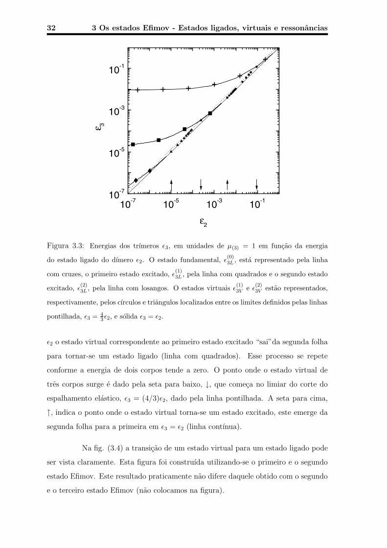
Na fig. (3.5) os resultados sao apresentados de outra maneira. Nesta figura
reproduzimos a curva da Ref. [15] e a estendemos para a regiao do estado virtual. Esta
figura tambem compara os resultados obtidos com o metodo das equacoes subtraıdas,
linha pontilhada, e com o metodo de corte para momentos grandes, eq. (3.25), linha
contınua.
Figura 3.5: Energias dos estados ligados e virtuais de tres bosons identicos. As linhas
pontilhada (subtracao) e contınua (corte) mostram dois metodos para a regularizacao. Os
sımbolos obedecem as mesmas convencoes da fig. (3.4). Na figura mostramos somente os
resultados para N = 0.
A partir de
√
E2/E(N)3 ≈ 0.4 podemos notar que os calculos realısticos
comecam a se distanciar dos nossos calculos devido aos efeitos de alcance do potencial.
A partir de
√
E2/E(N)3 = 0.38 o estado excitado (N + 1) torna-se virtual, este limite
confirma o resultado apresentado nas Refs. [14, 15] e mais recentemente na Ref. [67].
A trajetoria completa dos estado Efimov e descrita agora com os resultados
3 Os estados Efimov - Estados ligados, virtuais e ressonancias 35
das ressonancias. Neste caso a energia de dois corpos e sempre virtual e sera escrita
nos graficos como E2V (ou ε2V ). As energias das ressonancias serao escritas como E3
(ou ε3) e as energias dos estados ligados como E3L (ou ε3L) (o ε e escrito quando as
energias aparecem em unidades de µ(3) = 1).
Na fig. (3.6) estao representadas as energias dos estados ligados e as partes
reais da energia da ressonancia como funcao da energia de dois corpos (em unidades
de µ(3) = 1). Podemos ver na fig. (3.6) que aumentando-se o modulo da energia de
dois corpos o estado ligado torna-se uma ressonancia. A fig. (3.7) mostra a parte
imaginaria das energias da ressonancia.
Os resultados para os estados ligados e ressonancias tambem podem ser
representados na forma de uma funcao de escala universal dependente somente da
razao entre a energia do estado virtual de dois corpos e da energia do estado ligado
de tres corpos:
√
E(N)3 /E
(N−1)3L = R
(√
E2V /E(N−1)3L
)
. (3.31)
Na fig. (3.8) esta representada a parte real da energia da ressonancia (parte
positiva do grafico) e os estados ligados (parte negativa). A linha contınua representa
os resultados para N = 1 e a pontilhada para N = 2. Na fig. (3.9) sao mostrados
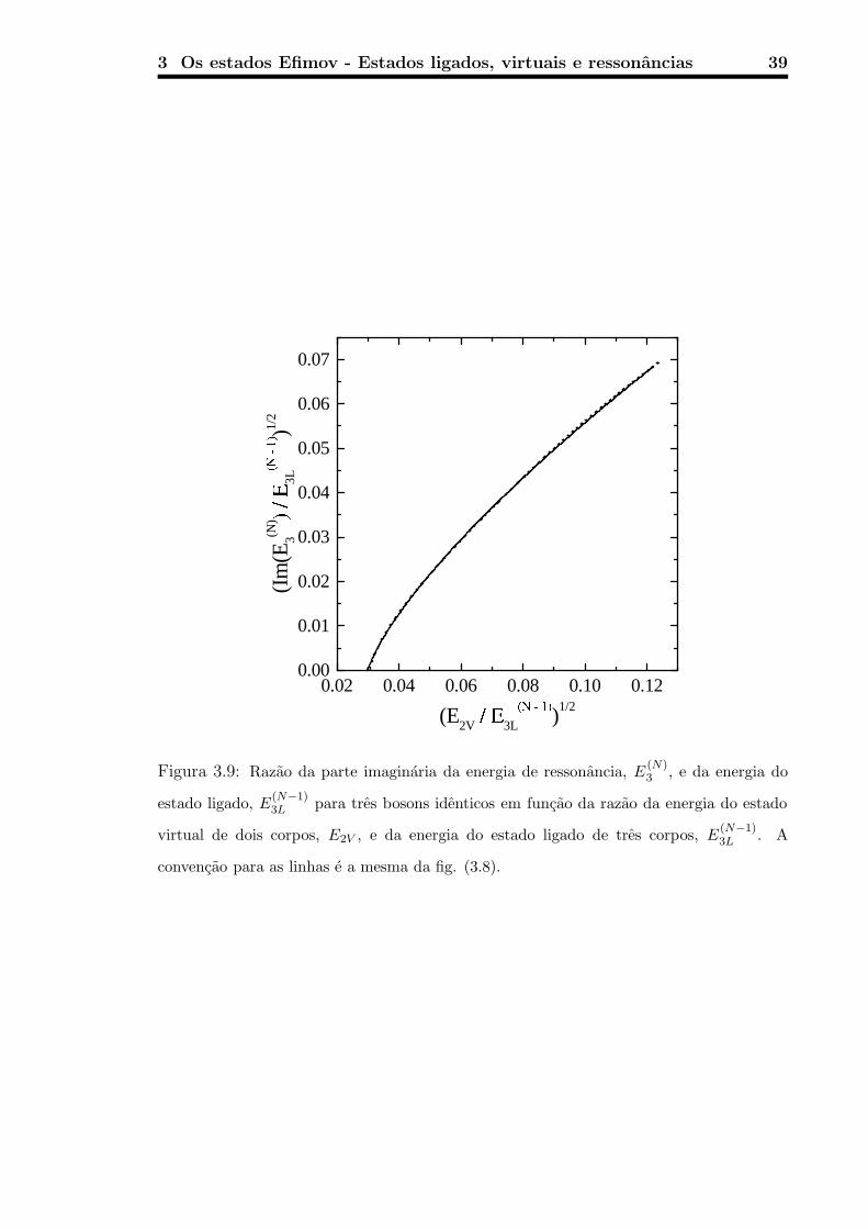
os resultados para a parte imaginaria da energia, a convencao utilizada nesta figura
e a mesma da fig. (3.8). Nestas duas figuras fica claro o limite de escala, ja que,
praticamente, as duas curvas nao apresentam diferenca. O valor crıtico de E2V para
o qual o estados ligados tornam-se ressonancias e dado por E2V ≥ 0.0009E3L, ou em
termos do comprimento de espalhamento a−1 ≤ −0.03√
mE3L/~, onde m e a massa
do boson.
A trajetoria completa dos estados Efimov conforme variamos a razao entre
as energias de dois e tres corpos esta mostrada na fig. (3.10). De fato, podemos notar
que variando a energia de dois corpos nos temos uma transicao contınua da energia
de tres corpos: para uma energia de dois corpos ligada e relativamente grande, os
tres corpos formam um estado virtual; conforme a energia de dois corpos diminui (em

36 3 Os estados Efimov - Estados ligados, virtuais e ressonancias
0.0 1.0x10⁻¹
2.0x10⁻¹
3.0x10⁻¹
-1.0x10⁻¹
-5.0x10⁻²
0.0
5.0x10⁻²
(Re(
ε
(0)
1/2
0.0 5.0x10⁻³
1.0x10⁻²
-4.0x10⁻³
-2.0x10⁻³
0.0
2.0x10⁻³
(Re(
ε 3(1)
1/
2
0.00 1.50x10⁻⁴
3.00x10⁻⁴
4.50x10⁻⁴
-2.0x10⁻⁴
-1.0x10⁻⁴
0.0
1.0x10⁻⁴
(Re(
ε 3(2)
1/
2
(ε2V)1/2
Figura 3.6: Parte real da energia de ressonancia para tres bosons identicos em funcao da
energia do estado virtual de dois corpos, em unidades de µ(3) = 1. Os valores negativos
representam o N esimo estado ligado de tres corpos ε(N)3 que se torna uma ressonancia
conforme aumentamos o modulo de ε2. Os valores positivos de Re(ε(N)3 ) correspondem as
ressonancias. Sao mostrados os resultados para N = 0 (linha contınua), N = 1 (linha
tracejada) e N = 2 (linha pontilhada).
modulo) o estado virtual torna-se ligado; finalmente fazendo a energia de dois corpos
virtual e aumentando o seu valor, o estado ligado torna-se uma ressonancia [7, 49].
No caso de atomos ultrafrios aprisionados, a existencia das ressonancias
de tres corpos no vacuo pode aumentar a possibilidade da existencia de estados liga-
dos de tres corpos no interior de armadilhas, considerando, ainda, a inexistencia de

3 Os estados Efimov - Estados ligados, virtuais e ressonancias 37
10-4
10-3
10-2
10-1
10-5
10-4
10-3
10-2
10-1
ε 3))1/
2
(ε 2V)1/2
Figura 3.7: Parte imaginaria da energia de ressonancia para tres bosons identicos em
funcao da energia do estado virtual de dois corpos, em unidades de µ(3) = 1. As curvas
estao rotuladas da mesma forma que na fig. (3.6).
dımeros ligados que poderiam aparecer como concorrentes dos trımeros. Um calculo
das energias de trımeros no interior de armadilhas magneto-opticas, quando dımeros
formam um estado fracamente ligado [8], sera feito no capıtulo seguinte com base no
coeficiente de recombinacao de tres corpos.

38 3 Os estados Efimov - Estados ligados, virtuais e ressonancias
0.00 0.02 0.04 0.06 0.08 0.10 0.12
-0.04
-0.03
-0.02
-0.01
0.00
0.01
0.02
(Re(
E3(N
)
3L
)1/2
(E2V
3L
)1/2
Figura 3.8: Razao da parte real da energia de ressonancia (parte positiva) ou da energia
do estado ligado (parte negativa), E(N)3 , e da energia do estado ligado, E
(N−1)3L para tres
bosons identicos em funcao da razao da energia do estado virtual de dois corpos, E2V , e da
energia do estado ligado de tres corpos, E(N−1)3L . A linha contınua sao os resultados para
N = 1 e na linha pontilhada para N = 2.
3 Os estados Efimov - Estados ligados, virtuais e ressonancias 39
0.02 0.04 0.06 0.08 0.10 0.120.00
0.01
0.02
0.03
0.04
0.05
0.06
0.07
(Im
(E3(N
)
3L
)1/2
(E2V
3L
)1/2
Figura 3.9: Razao da parte imaginaria da energia de ressonancia, E(N)3 , e da energia do
estado ligado, E(N−1)3L para tres bosons identicos em funcao da razao da energia do estado
virtual de dois corpos, E2V , e da energia do estado ligado de tres corpos, E(N−1)3L . A
convencao para as linhas e a mesma da fig. (3.8).

40 3 Os estados Efimov - Estados ligados, virtuais e ressonancias
-0.15 0.00 0.15 0.30 0.45-0.10
-0.05
0.00
0.05
0.10
IVIII
II I
((E
3(N+1
) -E2
3(N
) )1/2
(E2
3
(N))1/2
Figura 3.10: Razao da energia do (N + 1)esimo estado ligado, virtual ou ressonancia do
trımero, E(N+1)3 , subtraıda da energia do dımero, E2, em funcao da razao da energia do
dımero e do N esimo estado ligado do trımero. Os quadrantes I e II referem-se, respec-
tivamente, aos estados ligados de tres corpos para E2 ligado e virtual, o quadrante III
corresponde as ressonancias para E2 virtual e o quadrante IV aos estados virtuais para E2
ligado. Resultados para N=0.

Capıtulo 4
Moleculas triatomicas fracamente
ligadas em armadilhas
magneto-opticas
Em uma carta escrita a Ehrenfest em dezembro de 1924 Einstein comenta: “A partir
de uma certa temperatura, as moleculas ‘condensam-se’ sem forcas atrativas, isto
e, acumulam-se com velocidade nula. A teoria e atraente, mas havera nela algo de
verdade?”[68]. Essa pergunta, motivada pelo sexto artigo de Bose enviado a Einstein
e posteriormente publicado na revista Zeitschrift fur Physik [69] so foi respondida
aproximadamente 70 anos depois com a obtencao dos condensados de Bose-Einstein
com atomos de 87Rb, em junho de 1995 pelo grupo do JILA [70], e com atomos de
23Na, obtido pelo grupo do MIT [28]. Esse trabalhos deram o Nobel a Eric Cornell,
Wolfgang Ketterle e a Carl E. Wieman em 2001.
Embora a obtencao de um condensado so tenha acontecido em 1995, o
confinamento de atomos em armadilhas magneto-opticas ja havia sido objeto do
premio Nobel de 1997 (Steven Chu, Claude Cohen-Tannoudji e William D. Phillips).
Esse atomos aprisionados podem ter o seu comprimento de espalhamento controlado
variando-se o campo magnetico [71, 72] (efeito Zeeman). O comprimento de espalha-
mento pode ainda tornar-se muito grande proximo a uma ressonancia de Feshbach

424 Moleculas triatomicas fracamente ligadas em armadilhas
magneto-opticas
[73]. A utilizacao da ressonancia de Feshbach para a producao de grandes comprimen-
tos de espalhamento foi demonstrado pela primeira vez em experimentos com atomos
de 23Na [29] e 85Rb [74, 75]. Obviamente os atomos no interior das armadilhas po-
dem se chocar e formar estados ligados. A obtencao de condensados de moleculas
diatomicas ja foi obtido experimentalmente, por exemplo, para os casos 87Rb2 [31],
23Na2 [32, 76] e 133Cs2 [77].
Para que dois atomos em uma armadilha possam se combinar e formar um
estado ligado devemos ter a participacao de um terceiro atomo para que o momento
e a energia sejam conservados. Esse processo e chamado de recombinacao de tres
corpos. Utilizando o conceito de funcao de escala introduzido no capıtulo anterior,
podemos relacionar o coeficiente de recombinacao com as energias dos estados ligados
de dois e tres corpos. Assim, conhecendo-se a energia de dois corpos e o coeficiente de
recombinacao (ambos ja medidos experimentalmente [78, 79, 80, 81]) podemos prever
a energia do estado ligado do trımero no interior de armadilhas [8].
Atualmente, ja foi obtido experimentalmente condensados de moleculas for-
madas por atomos fermionicos (obviamente as moleculas podem ser tratadas como bo-
sons). Moleculas como, por exemplo, 6Li2 possuem um “tempo de vida”relativamente
grande (da ordem de 1 s) [82, 83, 84], outras moleculas como o 40K2 ja possuem uma
“vida”menor (cerca de 10−3 s) [85]. Uma revisao bastante completa sobre a evolucao
da pesquisa em condensados pode ser encontrada na Ref. [86]. Nas Refs. [30, 87, 88]
estao discutidos varios problemas atuais em condensados.
O nosso objetivo neste capıtulo e a predicao das energias de ligacao de
trımeros atomicos a partir dos valores experimentais dos coeficientes de recombinacao
de tres atomos. Desta forma, iremos deduzir a seguir as equacoes relevantes para a
obtencao do coeficiente de recombinacao dentro do modelo de tres corpos com forca de
alcance zero, formulado atraves das equacoes subtraıdas. As coordenadas utilizadas
estao representadas na fig. (4.1) que mostra um sistema inicialmente composto por
tres partıculas livres de massa m, descritas por ondas planas de momento igual a ~k
normalizadas para um volume de quantizacao V:
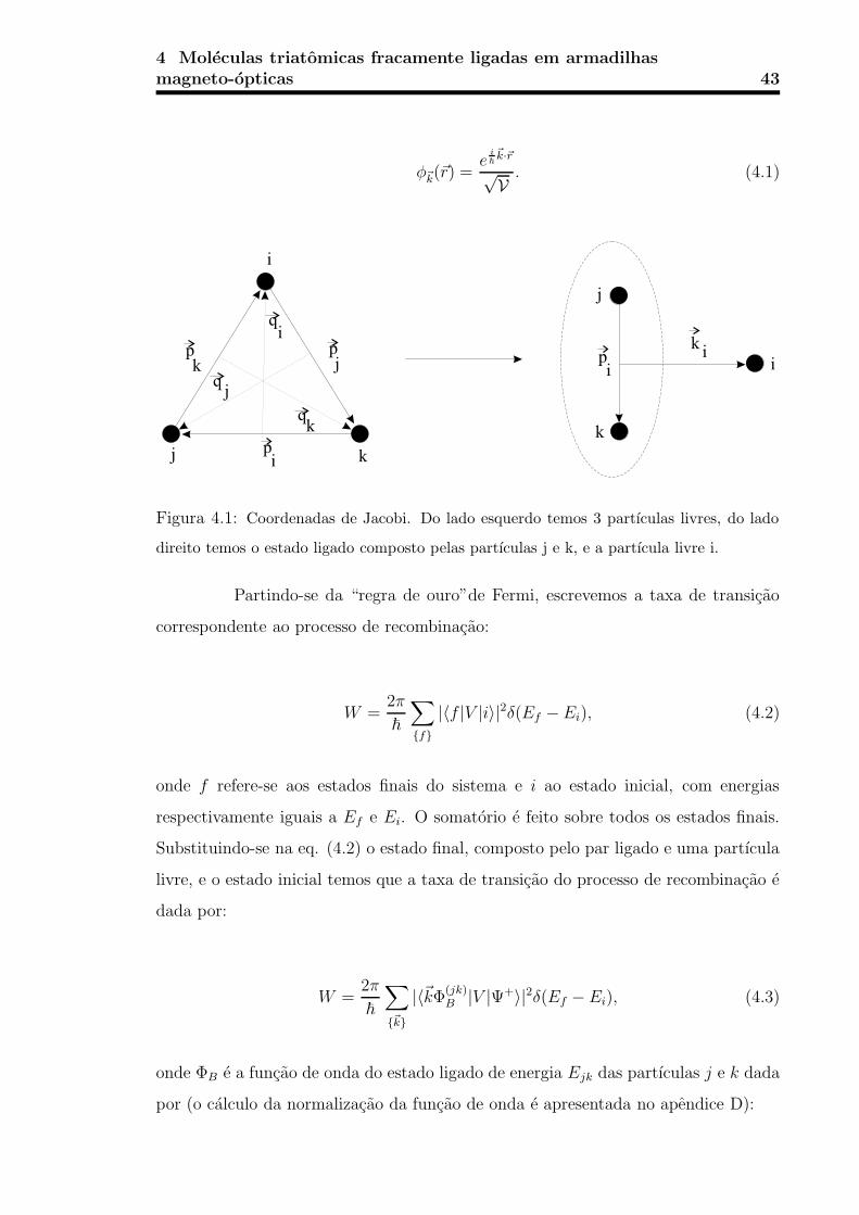
4 Moleculas triatomicas fracamente ligadas em armadilhasmagneto-opticas 43
φ~k(~r) =e
i~
~k·~r√V
. (4.1)
Figura 4.1: Coordenadas de Jacobi. Do lado esquerdo temos 3 partıculas livres, do lado
direito temos o estado ligado composto pelas partıculas j e k, e a partıcula livre i.
Partindo-se da “regra de ouro”de Fermi, escrevemos a taxa de transicao
correspondente ao processo de recombinacao:
W =2π
~
∑
f|〈f |V |i〉|2δ(Ef − Ei), (4.2)
onde f refere-se aos estados finais do sistema e i ao estado inicial, com energias
respectivamente iguais a Ef e Ei. O somatorio e feito sobre todos os estados finais.
Substituindo-se na eq. (4.2) o estado final, composto pelo par ligado e uma partıcula
livre, e o estado inicial temos que a taxa de transicao do processo de recombinacao e
dada por:
W =2π
~
∑
~k
|〈~kΦ(jk)B |V |Ψ+〉|2δ(Ef − Ei), (4.3)
onde ΦB e a funcao de onda do estado ligado de energia Ejk das partıculas j e k dada
por (o calculo da normalizacao da funcao de onda e apresentada no apendice D):

444 Moleculas triatomicas fracamente ligadas em armadilhas
magneto-opticas
〈~p |Φ(jk)B 〉 =
E14jk
π
1
Ejk + p2, (4.4)
e Ψ+ e a funcao de onda de espalhamento completamente simetrica para o estado
inicial de tres bosons livres. A soma da eq. (4.3) pode ser transformada em uma
integral utilizando a forma usual
∑
~k
→ V(2π~)3
∫
d3k.
Assim, reescrevendo a eq. (4.3) na forma integral temos que:
W =2π
~
V(2π~)3
(2π~)9
V3
∫
d3k|〈~kΦB|V |Ψ+〉|2δ(Ef − Ei), (4.5)
onde o fator (2π~)9
V3 e proveniente da normalizacao das funcoes de onda livres |~k〉( (2π~)3/2
√V ) e |Ψ+〉 ( (2π~)3
V ).
A perda do numero de atomos em um condensado devido ao processo de
recombinacao de tres corpos e dada pela seguinte equacao:
dN
dt= −3
N
3
W, (4.6)
onde o fator 3 vem do fato de que a cada processo de recombinacao temos a perda de
tres atomos da armadilha ou do condensado, o outro fator corresponde a combinacao
de N atomos 3 a 3 que aproximando para um valor grande de N da:
dN
dt= −3
N3
3!W. (4.7)
Escrevendo a eq. (4.7) em termos da densidade de atomos η = NV , temos
que:

4 Moleculas triatomicas fracamente ligadas em armadilhasmagneto-opticas 45
dη
dt= −3
η3
3!V2W. (4.8)
Finalmente substituindo-se a eq. (4.6) para W na eq. (4.8) temos a equacao
final para a taxa de perda de atomos no condensado:
dη
dt= − 3
3!K3η
3, (4.9)
onde a equacao para K3 e dada por:
K3 =2π
~(2π~)9
∫
d3k
(2π~)3|Ti→f |2δ(Ef − Ei). (4.10)
A amplitude de transicao 〈~kΦB |V |Ψ+〉 foi chamada de Ti→f . A taxa de recombinacao
de tres atomos no limite da energia do dımero tendendo a zero, eq. (4.9), e dada por
[25, 89]
K3 =~
ma4α, (4.11)
onde α e uma constante adimensional que possui um carater oscilatorio dado por [25]
α = αmax sin2(1.01 ln(a) + δ), (4.12)
sendo δ uma fase que depende da interacao entre os atomos a pequenas distancias.
Para a energia do dımero tendendo a zero essa fase deve ser independente de pequenas
variacoes do potencial desde que a escala de tres corpos esteja fixa, como descrito pela
eq. (3.30).
O elemento de matriz que aparece na eq. (4.10), Ti→f , pode ser escrito em
termos das ondas planas das partıculas livres e das componentes de Faddeev da matriz
de transicao de tres corpos. Escrevendo o potencial V como a soma dos potenciais
de interacao entre os pares de partıculas ik, vj, e ij , vk,
464 Moleculas triatomicas fracamente ligadas em armadilhas
magneto-opticas
Ti→f = 〈~kiΦ(jk)B |vj + vk|Ψ+〉,
e substituindo |Ψ+〉 = |φ0〉 + G0T (E)|φ0〉, onde φ0 e a funcao de onda dos bosons
livres iniciais com momentos nulos, temos que:
〈~kiΦ(jk)B |vj + vk|Ψ+〉 = 〈~kiΦ
(jk)B |vj + vk(|φ0〉+ G0T (E)|φ0〉)
= 〈~kiΦ(jk)B |vj + vk|φ0〉+ 〈~kiΦ
(jk)B |(vj + vk)G0T (E)|φ0〉,
como Tα = vα + vαG0T , eq. (2.14), verificamos que:
Ti→f = 〈~kiΦ(jk)B |vj + vk|Ψ+〉 = 〈~kiΦ
(jk)B |Tj(E) + Tk(E)|φ0〉. (4.13)
A partir deste ponto usaremos unidades tais que ~ = m = 1. Partindo
agora da equacao para a matriz-T de tres corpos na forma subtraıda, eq. (2.43):
TRi(E) = tRi
(E− 3
4q2i )+tRi
(E− 3
4q2i )[G
(+)0 (E)−G0(−µ2
(3))](TRj(E)+TRk
(E)), (4.14)
multiplicando por 〈~qi~pi| pela esquerda e por |~0~0〉 pela direita o elemento de matriz
〈~qi~pi|TRi(0)|~0~0〉 para a componente de Faddeev TRi
(0) e dado por:
〈~qi~pi|TRi(0)|~0~0〉 = 〈~qi~pi|χi〉τ(−3
4q2i )〈χi|~0~0〉
+2〈~qi~pi|χi〉τ(−3
4q2i )〈χi|
[
G(+)0 (0)−G0(−µ2)
]
TRj(0)|~0~0〉, (4.15)
onde foi utilizada a matriz-T de dois corpos para E = 0 dada por tRi(−3
4q2i ) =
|χi〉τ(−34q2i )〈χi|, eqs. (2.24) e (3.16). O fator 2 que aparece na segunda parcela e
4 Moleculas triatomicas fracamente ligadas em armadilhasmagneto-opticas 47
proveniente da igualdade das componentes TRje TRk
. Manipulando a eq. (4.15),
temos que:
〈~qi~pi|TRi(0)|~0~0〉 = 〈~pi|χi〉τ(−3
4q2i )〈χi|~0〉〈~qi|~0〉+ 2〈~pi|χi〉τ(−3
4q2i )
×〈χi, ~qi|[
G(+)0 (0)−G0(−µ2)
]
TRj(0)|~0~0〉
= τ(−3
4q2i )δ(~qi) + 2τ(−3
4q2i )z(~qi), (4.16)
onde utilizamos que o fator de forma 〈~pi|χ〉 do potencial δ-Dirac e igual a 1. A funcao
z(~qi) e dada por:
z(~qi) =
∫
d3pid3pjd
3qj〈~pi~qi|[
G(+)0 (0)−G0(−µ2)
]
|~pj~qj〉〈~pj~qj|TRj(0)|~0~0〉. (4.17)
Substituindo na eq. (4.17) o elemento de matriz dado pela eq. (4.16) temos
que:
z(~qi) =
∫
d3pid3pjd
3qj〈~pi~qi|[
G(+)0 (0)−G0(−µ2)
]
|~pj~qj〉 τ(−3
4q2j )δ(~qj)+2τ(−3
4q2j )z(~qj).
(4.18)
Escrevendo explicitamente os propagadores e fazendo a integracao na pri-
meira parcela da eq. (4.18) e lembrando que 〈~pi~qi|~pj~qj〉 = δ(~qi +~qj
2+~pj)δ(~pi− ~qi
2+~qj),
escrevemos z(~qi) como:
z(~q) = −τ(0)µ2
q2(µ2 + q2)− 2
∫
d3q′τ(−3
4q′
2)
×[
1
E + q2 + q′2 + ~q · ~q ′ −1
µ2 + q2 + q′2 + ~q · ~q ′
]
z(~q ′), (4.19)
484 Moleculas triatomicas fracamente ligadas em armadilhas
magneto-opticas
onde qi e qj foram substituıdos respectivamente por q e q′.
Voltando agora a amplitude de transicao, Ti→f , dada pela eq. (4.13) vamos
substituir a funcao de onda completamente simetrica do estado inicial de tres bosons,
|φ0〉 =1√3
∑
α=i,j,k
|~qα~pα〉, (4.20)
na eq. (4.13):
Ti→f = 2√
3〈~kiΦ(jk)B |TRj
(0)|~0~0〉. (4.21)
Introduzindo∫
d3pj|~pj〉〈~pj|,∫
d3qj|~qj〉〈~qj| e∫
d3pi|~pi〉〈~pi| e notando que
devemos ter Ejk = 34k2
i , podemos escrever Ti→f como:
Ti→f = 2√
3
∫
d3pjd3qjd
3pi
E14jk
π
〈~ki~pi|~pj~qj〉34k2
i + p2i
〈~pj~qj|TRj(0)|~0~0〉, (4.22)
escrevendo o primeiro elemento de matriz em termos das funcoes δ-Dirac dadas pelas
coordenadas de Jacobi e substituindo o segundo elemento de matriz pela eq. (4.16),
podemos escrever a eq. (4.22) da seguinte forma:
Ti→f = 2√
3E
14jk
π
∫
d3pjd3qjd
3pi
δ(~ki +~qj
2+ ~pj)δ(~pi − ~ki
2− ~qj)
34k2
i + p2i
×[
τ(−3
4q2j )δ(~qj) + 2τ(−3
4q2j )z(~qj)
]
. (4.23)
Resolvendo as integrais e escrevendo explicitamente τ a eq. (4.22) fica
igual a (o comprimento de espalhamento, a, e igual a 1√Ejk
):
Ti→f =3√
3a52
4π3+
4
π3a12
∫
d3qjz(~qj)
q2j + k2
i + ~ki · ~qj
1
ki − qj + iε. (4.24)

4 Moleculas triatomicas fracamente ligadas em armadilhasmagneto-opticas 49
Substituindo a eq. (4.24) na eq. (4.10) (tambem em unidades de ~ = m =
1) e fazendo a integracao em k temos que:
K3 =(2π)512
√3
π3a4|1 +
32π
3√
3a3
∫ ∞
0
dqq
kln
(
k2 + q2 + qk
k2 + q2 − qk
)
z(q)
k − q + iε|2, (4.25)
onde os ındices de k e q foram suprimidos. O coeficiente adimensional de recom-
binacao, eq. (4.11), e dado por
α =(2π)512
√3
π3|1 +
32π
3√
3a3
∫ ∞
0
dqq
kln
(
k2 + q2 + qk
k2 + q2 − qk
)
z(q)
k − q + iε|2, (4.26)
Os resultados numericos para o coeficiente de recombinacao sao dados pela
solucao da eq. (4.26) e da eq. integral (4.19). Resolvemos a eq. (4.19) no plano
complexo evitando as singularidades do espalhamento e, em seguida, integramos a
eq. (4.23) no contorno do plano complexo escolhido (q→qeiθ). Este procedimento e
conhecido como metodo do desvio de contorno [90]. Na fig. (4.2) temos os resultados
teoricos de α em funcao da razao√
E2/E3.
Na fig. (4.2) podemos notar claramente a existencia do limite de escala
conforme a energia do estado ligado de dois corpos diminui (e consequentemente
o numero de estados ligados de tres corpos aumenta). O limite de escala ja foi
observado nas figuras anteriores nos casos dos estados virtuais e das ressonancias. O
valor maximo de α ocorre para o limiar E2 = E3 e para (E3/E2)1/2 = 0.38.
As linhas horizontais na figura 4.2, correspondentes aos valores experimen-
tais centrais para o coeficiente de recombinacao, interceptam a curva teorica em dois
pontos indicando a possibilidade da existencia de um trımero no condensado com
energia, E3 ou E ′3, referentes a um estado fracamente ligado. Somente para o caso do
85Rb|2,−2〉, onde o valor para o coeficiente de recombinacao e menor, foi subtraıdo
a contribuicao referente ao estado profundamente ligado, ∼ 1 de acordo com a Ref.
[91]. Os valores em mK para as energias dos trımeros estao contidos nas colunas 6 e
7 da tabela 4.

504 Moleculas triatomicas fracamente ligadas em armadilhas
magneto-opticas
0.4 0.6 0.8 1(E2/E3)
(1/2)
0
20
40
60
80
α
87Rb|1,−1>
23Na|1,−1>
85Rb|2,−2>
Figura 4.2: Coeficiente adimensional de recombinacao, α, como funcao da razao das ener-
gias de ligacao das moleculas diatomicas e triatomicas. Resultados teoricos: cırculos cheios
(um estado ligado de tres atomos), linha cheia (dois estados ligados de tres atomos) e
quadrados cheios (tres estados ligados de tres atomos). As linhas horizontais indicam os
resultados experimentais (valores centrais) para o 23Na, 87Rb e 85Rb apresentados na ta-
bela 4. No caso do 85Rb foi subtraıdo do valor experimental de α a contribuicao do estado
profundamente ligado (≈ 1), conforme calculado na Ref. [91].
A hipotese de formacao dos trımeros no vacuo, no interior de armadilhas,
sera valida somente se tivermos uma quantidade de atomos num cubo de arestas
iguais ao comprimento de espalhamento muito menor do que 1. Essa quantidade
e dada pelo coeficiente de diluicao que aparece na coluna 3 da tabela 4. Podemos
ver que exceto para o 85Rb|2,−2〉 onde o valor 0.5 do coeficiente de diluicao pode
ser considerado como o limite de nossa aproximacao, os outros atomos possuem um
coeficiente muito menor do que 1.

4 Moleculas triatomicas fracamente ligadas em armadilhasmagneto-opticas 51
AZ|F, mF 〉 a(nm) ρa3 αexp E2 (mK) S3(mK) S ′3(mK)
23Na|1,−1〉 2.75 6×10⁻⁵ 42±12 [79] 2.85 4.9 0.21
87Rb|1,−1〉 5.8 1×10⁻⁵ 52±22∗ [78] 0.17 0.39 0.005
87Rb|1,−1〉 5.8 1×10⁻⁴ 41±17† [78] 0.17 0.30 0.013
87Rb|2, 2〉 5.8 4×10⁻⁵ 130±36 [80] 0.17 - -
85Rb|2,−2〉 211.6 0.5 7.84±3.4 [92, 93] 1.3×10⁻⁴ 1.14×10⁻⁴ 3.8×10⁻⁵
Tabela 4.1: Para os atomos AZ|F,mF 〉 (F e mF sao , respectivamente, o spin total e a sua
projecao), dados na coluna 1, apresentamos nas colunas 6 e 7 as energias de ligacao para
os trımeros em relacao ao limiar, S3 ≡ (E3−E2) e S′3 ≡ (E′
3−E2), considerando os valores
centrais para os coeficientes de recombinacao adimensionais αexpt medidos experimental-
mente (dados na coluna 4). O comprimento de espalhamento a, o coeficiente de diluicao
ρa3 e a energia para o estado ligado de dois corpos sao dados, respectivamente, nas colunas
2, 3 e 5. O coeficiente de recombinacao do 87Rb|1,−1〉 para os atomos nao condensados (∗)
e para os condensados (†) foi obtido da Ref. [78].

524 Moleculas triatomicas fracamente ligadas em armadilhas
magneto-opticas
Capıtulo 5
Limite de escala para os raios de
sistemas fracamente ligados do tipo
AAB
Neste capıtulo iniciaremos o estudo dos tamanhos dos sistemas de tres corpos com-
postos por duas partıculas de massas identicas, A, e uma outra partıcula chamada
de B. Calcularemos os raios quadraticos medios de separacao entre A − A, A − B,
A − CM e B − CM (CM e o centro-de-massa do sistema de tres corpos). Na pri-
meira secao mostraremos o formalismo que sera utilizado nas tres secoes seguintes.
Na segunda secao faremos um estudo geral do tamanho dos diversos sistemas que
podem ser formados conforme variamos a energia de dois corpos. Na terceira secao
os raios serao calculados no contexto de nucleos exoticos, neste caso A representara
um neutron e B o caroco do nucleo [10]. Na quarta secao mostraremos que o mesmo
formalismo tambem se aplica muito bem ao caso de moleculas fracamente ligadas,
neste caso A representara um atomo de 4He e B um outro atomo [9].

545 Limite de escala para os raios de sistemas fracamente ligados do tipo
AAB
5.1 Formalismo
Descreveremos nosso sistema de tres corpos utilizando as mesmas coordenadas de
Jacobi da fig. (2.1). As posicoes canonicamente conjugadas ao momento relativo do
centro-de-massa do par, ~q, e do momento do par, ~p, serao chamadas respectivamente
de ~R e ~r, conservando os mesmos ındices dos momentos. Para as deducoes conside-
raremos j ≡ k ≡ A e i ≡ B. Mostraremos de forma detalhada a obtencao do raio
quadratico medio de separacao relativa entre as partıculas j e k, usando o fator de
forma correspondente a transformada de Fourier da densidade de probabilidade como
funcao da distancia relativa. Este procedimento e conveniente, pois obtemos a funcao
de onda diretamente no espaco dos momentos. Como as outras distancias sao obtidas
mudando-se apenas as coordenadas do sistema, elas serao mostradas somente na sua
forma final, sem detalhes da deducao.
O raio quadratico medio de separacao relativa das partıculas j e k e escrito
da forma usual como:
〈r2i 〉 =
∫
d3rir2i ρi(ri), (5.1)
onde ρ e a densidade de probabilidade dada por
ρi(ri) =
∫
d3Ri|〈~ri, ~Ri|Ψ〉|2. (5.2)
Escrevendo a densidade em termos de uma transformada de Fourier no
espaco dos momentos temos que
ρi(ri) =
∫
d3QF (Q2)e−i ~Q·~ri
(2π)3, (5.3)
onde a funcao F (Q2) e dada pela anti-transformada de Fourier da eq. (5.3):
F (Q2) =
∫
d3riei ~Q·~riρi(ri), (5.4)

5.1 Formalismo 55
normalizada para F (0) ≡ 1. Expandindo a exponencial da eq. (5.4) em serie de
Taylor ate segunda ordem e considerando a simetria esferica de ρi, temos que:
〈r2i 〉 ≡ 〈r2
AA〉 = −6dFAA(Q2)
dQ2
∣
∣
∣
∣
Q2=0
. (5.5)
Devemos escrever agora a funcao F (Q2), eq. (5.4), em termos da funcao
de onda do sistema no espaco dos momentos. Substituindo a eq. (5.2) em (5.4) temos
que:
F (Q2) =
∫
d3riei ~Q·~ri
∫
d3Ri|〈~ri, ~Ri|Ψ〉|2
=
∫
d3rid3Rie
i ~Q·~ri〈~ri, ~Ri|Ψ〉〈Ψ|~ri, ~Ri〉
=
∫
d3rid3Rid
3qid3q′id
3pid3p′ie
i( ~Q−~pi+~pi′)·~Riei(~qi−~qi
′)·~ri〈~qi, ~pi|Ψ〉〈~qi′, ~pi
′|Ψ〉
=
∫
d3qid3q′id
3pid3p′iδ(
~Q− ~pi + ~pi′)δ(~qi − ~qi
′)〈~qi, ~pi|Ψ〉〈~qi′, ~pi
′|Ψ〉
=
∫
d3qid3pi〈~qi, ~pi|Ψ〉〈~qi, ~pi + ~Q|Ψ〉
Integrando a funcao δ-Dirac escrevemos o fator de forma FAA(Q2) (partıcula B e a
espectadora) em termos das funcoes de onda do sistema no espaco dos momentos.
Para simetrizarmos os argumentos das funcoes de onda vamos substituir o momento
~pi por ~pi −~Q2.
FAA(Q2) =
∫
d3qid3pi〈~qi, ~pi +
~Q
2|Ψ〉〈~qi, ~pi −
~Q
2|Ψ〉. (5.6)
A equacao de Schrodinger do sistema de tres corpos para um potencial
separavel do tipo vα = λα|χα〉〈χα|, com α = i, j, k (vi, vj e vk sao, respectivamente,
os potenciais de dois corpos de jk, ik e ij) pode ser escrita como:
565 Limite de escala para os raios de sistemas fracamente ligados do tipo
AAB
(H0 +∑
α=i,j,k
λα|χα〉〈χα|)|Ψ〉 = E|Ψ〉 (5.7)
(E −H0)|Ψ〉 =∑
α=i,j,k
λα|χα〉〈χα|Ψ〉, (5.8)
onde H0 e o hamiltoniano livre do sistema.
Utilizando que o fator de forma 〈~pα|χ〉 = 1 para o potencial δ-Dirac, pode-
mos escrever a funcao de onda na base |~qi, ~pi〉 e em termos das funcoes espectadoras
fα(~qα) = λα〈~qαχα|Ψ〉:
〈~qi, ~pi|Ψ〉 =fi(|~qi|) + fj(|~pi − ~qi
2|) + fk(|~pi + ~qi
2|)
|E3|+ H0, (5.9)
onde fi, fj e fk sao, respectivamente, as funcoes espectadoras de B, A e A. E3 e a
energia do estado ligado dos tres corpos. Substituindo a eq. (5.9) na eq. (5.6) temos
a forma final da funcao FAA(Q2) no espaco dos momentos:
FAA(Q2) =
∫
d3qid3pi
(
fi(|~qi|) + fj(|~pi +~Q
2− ~qi
2|) + fk(|~pi +
~Q
2+
~qi
2|))
×
(
fi(|~qi|) + fj(|~pi −~Q2− ~qi
2|) + fk(|~pi −
~Q2
+ ~qi
2|))
(|E3|+ H0)(|E3|+ H ′0)
, (5.10)
onde H0 e H ′0 sao dados por:
H0 =|~pi +
~Q2|2
2mAA
+q2i
2mAA,B
, (5.11)
e
H ′0 =
|~pi −~Q2|2
2mAA
+q2i
2mAA,B
, (5.12)
onde mAA = mA
2e mAA,B = 2mBmA
2mA+mB. De forma analoga podemos escrever as eqs.
(5.5) e (5.6) para 〈r2k〉:
5.1 Formalismo 57
〈r2k〉 ≡ 〈r2
AB〉 = −6dFAB(Q2)
dQ2
∣
∣
∣
∣
Q2=0
. (5.13)
FAB(Q2) =
∫
d3qkd3pk〈~qk, ~pk +
~Q
2|Ψ〉〈~qk, ~pk −
~Q
2|Ψ〉. (5.14)
Lembrando que i, j e k correspondem, respectivamente, as partıculas es-
pectadoras B, A, e A, a funcao de onda na base |~qk, ~pk〉 e dada pela seguinte equacao:
〈~qk, ~pk|Ψ〉 =fi(|~pk − A
A+1~qk|) + fj(|~pk + 1
A+1~qk|) + fk(|~qk|)
|E3|+ p2kA+12A + q2
kA+2
2(A+1)
. (5.15)
onde A = mB/mA e a razao entre as massas das partıculas A e B.
As distancias quadraticas medias de A e de B ao CM do sistema de tres
corpos sao calculadas atraves dos respectivos fatores de forma e sao dadas, respecti-
vamente, por:
〈r2A〉 ≡
(
mA + mB
2mA + mB
)2
〈R2k〉 = −6
(
mA + mB
2mA + mB
)2dFA(Q2)
dQ2
∣
∣
∣
∣
Q2=0
,
(5.16)
FA(Q2) =
∫
d3qd3p〈~qk +~Q
2, ~pk|Ψ〉〈~qk −
~Q
2, ~pk|Ψ〉
e
〈r2B〉 ≡
(
2mA
2mA + mB
)2
〈R2i 〉 = −6
(
2mA
2mA + mB
)2dFB(Q2)
dQ2
∣
∣
∣
∣
Q2=0
,
(5.17)
FB(Q2) =
∫
d3qid3pi〈~qi +
~Q
2, ~pi|Ψ〉〈~qi −
~Q
2, ~pi|Ψ〉.
As integracoes das eqs. para os fatores de forma, F , podem ser reduzidas
para 5 dimensoes, ao inves das 6 dimensoes colocando o momento ~Q paralelo ao eixo
z e ~q no plano xz, (vide fig. (5.1)):

585 Limite de escala para os raios de sistemas fracamente ligados do tipo
AAB
Figura 5.1: Orientacao dos momentos.
Desta forma a integracao dos fatores de forma e feita nas seguintes variaveis
radiais e angulares com os respectivos limites:
∫
d3qd3p ≡ 2π
∫ ∞
0
p2dp
∫ ∞
0
q2dq
∫ π
0
senθpdθp
∫ π
0
senθqdθq
∫ 2π
0
dϕp.
Note que as funcoes de onda dependem somente do angulo relativo entre os momentos
~p, ~q e ~Q, assim, nao ha nenhuma perda de generalizacao ao fixarmos os momentos
segundo a fig. (5.1).
5.1.1 Equacoes subtraıdas para as funcoes espectadoras
A deducao das funcoes espectadoras para o caso onde uma das partıculas e distinta
das outras duas e feita da mesma forma que no capıtulo 3, a mudanca ocorre somente
a partir da eq. (3.10), pois agora, apenas duas funcoes espectadoras sao identicas.
Entao, escrevendo a funcao espectadora para a componente de Faddeev k, temos que:

5.1 Formalismo 59
fk(~qk) = τ
(
E − q2k
2mij,k
)
〈χk, ~qk|(
G(+)0 (E)−G0(−µ2
(3)))
(|χi〉|fi〉+ |χj〉|fj〉) ,
(5.18)
a funcao τ e dada pela eq. (2.25), calculada agora para o caso de duas partıculas de
massas identicas e uma diferente.
A funcao espectadora para a componente de Faddeev i e escrita como (neste
caso as funcoes espectadoras do lado direito j e k sao identicas, |χk〉|fk〉 ≡ |χj〉|fj〉):
fi(~qi) = 2τ
(
E − q2k
2mjk,i
)
〈χi, ~qi|(
G(+)0 (E)−G0(−µ2
(3)))
|χj〉|fj〉. (5.19)
Os elementos de matriz 〈χk~qk|G(+)0 (E)|χi〉|fi〉, 〈χk~qk|G(+)
0 (E)|χj〉|fj〉 que
aparecem na eq. (5.18) e 〈χi~qi|G(+)0 (E)|χj〉|fj〉 da eq. (5.19) serao calculados no
apendice F (obviamente a parte referente a subtracao e identica a menos da energia
E que e substituıda por −µ2(3)).
Substituindo os elementos de matriz dados pelas eqs. (F.1), (F.2) e (F.3)
nas eqs. (5.18) e (5.19) para as funcoes espectadoras, temos que:
fk(~qk) ≡ fA(~qk) = −τA
(
E − q2k(A+ 2)
2(A+ 1)
)
∫
d3q′i
1
E − q2k(A+2)
2(A+1)− (~qi
′+ A
A+1~qk)2(A+1)
2A
− 1
−µ2(3) −
q2k(A+2)
2(A+1)− (~qi
′+ A
A+1~qk)2(A+1)
2A
fB(~qi′) +
∫
d3qj
1
E − q2k(A+2)
2(A+1)− (~qj+
1A+1
~qk)2(A+1)
2A
− 1
−µ2(3) −
q2k(A+2)
2(A+1)− (~qj+
1A+1
~qk)2(A+1)
2A
fA(~qj)
, (5.20)
fi(~qi) ≡ fB(~qi) = −2τB
(
E − q2i (A+ 2)
4A
)
∫
d3qj
[
1
E − q2i (A+2)
4A − (~qj + 12~qi)2
− 1
−µ2(3) −
q2i (A+2)
4A − (~qj + 12~qi)2
fA(~qi)
. (5.21)
605 Limite de escala para os raios de sistemas fracamente ligados do tipo
AAB
As funcoes τA e τB sao calculadas de forma analoga ao caso dos tres bosons
identicos e sao dadas por:
τ−1A
(
E − q2(A+ 2)
(A+ 1)
)
=
(
(A+ 1)
2A
)(3/2)
2π2
±√
EAB −√
|E| − q2(A+ 2)
A+ 1
,
(5.22)
τ−1B
(
E − q2(A+ 2)
4A
)
= 2π2
±√
EAA −√
|E|+ q2(A+ 2)
4A
, (5.23)
onde EAB e EAA sao, respectivamente, as energias de dois corpos de AB e AA. O
sinal positivo refere-se ao estado ligado e o negativo ao virtual.
Finalmente substituindo τA e τB, respectivamente, nas eqs. (5.20) e (5.21)
temos a forma final das equacoes espectadoras em unidades de ~ = mA = µ(3) = 1
com as energias e momentos reescalonados como ε = Eµ2
(3)
, εAA = EAA
µ2(3)
, εAB = EAB
µ2(3)
,
~qk
µ(3)≡ ~qi
µ(3)≡ ~q, ~qi
′
µ(3)≡ ~qj
µ(3)≡ ~k:
fA(~q ) =
(A+ 1
2A
)3/21
π
(√
|ε|+ q2(A+ 2)
2(A+ 1)∓√εAB
)−1∫ ∞
0
k2dk
∫ 1
−1
dy
×[
1
|ε|+ q2 + A+12A k2 + kqy
− 1
1 + q2 + A+12A k2 + kqy
]
fB(~k ) (5.24)
−∫ 1
−1
[
1
|ε|+ (A+1)2A q2 + (A+1)
2A k2 + 1Akqy
− 1
1 + (A+1)2A q2 + (A+1)
2A k2 + 1Akqy
]
fA(~k ).
fB(~q ) =2
π
(√
|ε|+ (A+ 2)
2A q2 ∓√εAA
)−1∫ ∞
0
k2dk
×∫ 1
−1
dy
[
1
|ε|+ (A+1)2A q2 + k2 + kqy
− 1
1 + (A+1)2A q2 + k2 + kqy
]
fA(~k ). (5.25)
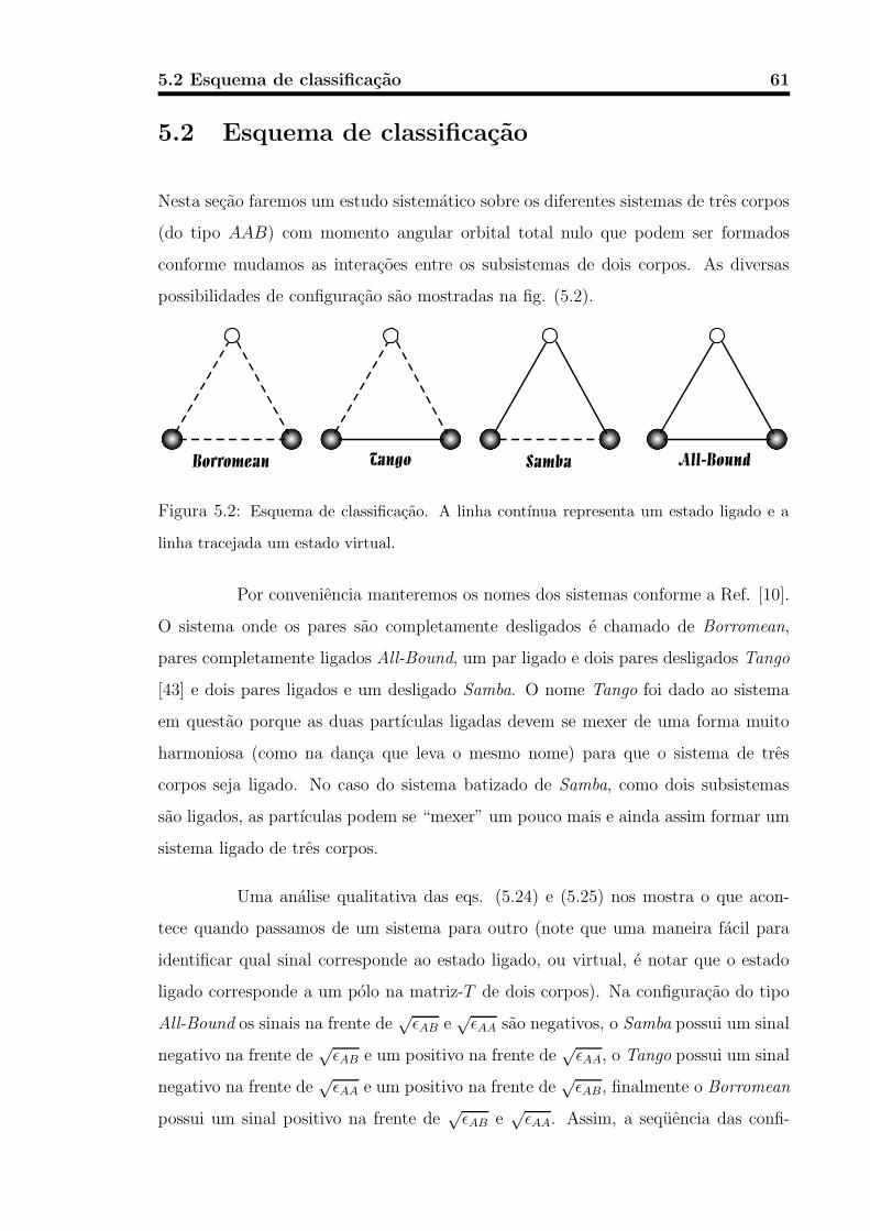
5.2 Esquema de classificacao 61
5.2 Esquema de classificacao
Nesta secao faremos um estudo sistematico sobre os diferentes sistemas de tres corpos
(do tipo AAB) com momento angular orbital total nulo que podem ser formados
conforme mudamos as interacoes entre os subsistemas de dois corpos. As diversas
possibilidades de configuracao sao mostradas na fig. (5.2).
Figura 5.2: Esquema de classificacao. A linha contınua representa um estado ligado e a
linha tracejada um estado virtual.
Por conveniencia manteremos os nomes dos sistemas conforme a Ref. [10].
O sistema onde os pares sao completamente desligados e chamado de Borromean,
pares completamente ligados All-Bound, um par ligado e dois pares desligados Tango
[43] e dois pares ligados e um desligado Samba. O nome Tango foi dado ao sistema
em questao porque as duas partıculas ligadas devem se mexer de uma forma muito
harmoniosa (como na danca que leva o mesmo nome) para que o sistema de tres
corpos seja ligado. No caso do sistema batizado de Samba, como dois subsistemas
sao ligados, as partıculas podem se “mexer” um pouco mais e ainda assim formar um
sistema ligado de tres corpos.
Uma analise qualitativa das eqs. (5.24) e (5.25) nos mostra o que acon-
tece quando passamos de um sistema para outro (note que uma maneira facil para
identificar qual sinal corresponde ao estado ligado, ou virtual, e notar que o estado
ligado corresponde a um polo na matriz-T de dois corpos). Na configuracao do tipo
All-Bound os sinais na frente de√
εAB e√
εAA sao negativos, o Samba possui um sinal
negativo na frente de√
εAB e um positivo na frente de√
εAA, o Tango possui um sinal
negativo na frente de√
εAA e um positivo na frente de√
εAB, finalmente o Borromean
possui um sinal positivo na frente de√
εAB e√
εAA. Assim, a sequencia das confi-
625 Limite de escala para os raios de sistemas fracamente ligados do tipo
AAB
guracoes de acordo com a intensidade efetiva de atracao do kernel fica: All-Bound >
Samba > Tango > Borromean. Essas diferencas entre os kernels se refletem nos tama-
nhos dos sistemas da seguinte maneira (para uma mesma energia de ligacao de tres
corpos): no caso do kernel mais atrativo os constituintes do sistema podem ficar mais
afastados e produzir um sistema ligado, ja com o kernel menos atrativo as partıculas
devem estar mais proximas umas das outras. Obviamente poderıamos raciocinar no
sentido de que quanto maior a atracao mais proximas estariam as partıculas, todavia
veremos atraves dos resultados numericos que isso nao acontece. Desta forma, para
uma mesma energia de ligacao de tres corpos o tamanho dos sistemas deve variar da
seguinte maneira: All-Bound > Samba > Tango > Borromean.
De maneira analoga a eq. (3.30) podemos escrever as funcoes de escala
para o caso de um sistema formado por duas partıculas de massas identicas, AA, e
uma distinta, B. Agora o sistema depende de duas energias de dois corpos e da razao
entre as massas de A e de B. Assim, para um observavel generico O com dimensao
de [energia]η, em uma certa energia E, a funcao de escala D pode ser escrita como:
O (E, E3, EAA, EAB) = (E3)ηD(
√
E/E3,±√
EAA/E3,±√
EAB/E3,A)
, (5.26)
as energias EAγ (γ = A, B) sao sempre negativas. Desta forma a natureza do estado
de dois corpos e dado pelo sinal ±. O sinal + em frente de√
|EAγ| indica um estado
ligado e o − um estado virtual.
De acordo com a eq. (5.26) as funcoes de escala para os raios podem ser
escritas como:
√
〈r2Aγ〉|E3| = RAγ
(
±√
EAA
E3
,±√
EAB
E3
,A)
, (5.27)
√
〈r2γ〉|E3| = RCM
γ
(
±√
EAA
E3
,±√
EAB
E3
,A)
. (5.28)
Os resultados das figuras (5.3) a (5.6) serao mostrados conforme a eq.

5.2 Esquema de classificacao 63
(5.27). Nessas figuras uma das energias do subsistema de dois corpos e fixada em
relacao a energia de tres corpos, a outra energia varia. Para os calculos nos usamos
valores de A iguais a 0.1, 1 e 200. As energias dos subsistemas podem ser ligadas ou
virtuais, desta forma conseguimos analisar as quatro configuracoes mostradas na fig.
(5.2). Introduziremos agora as seguintes definicoes K2AA = EAA/E3 e K2
AB = EAB/E3:
KAA = ±√
EAA/E3
(5.29)
KAB = ±√
EAB/E3
os sinais + e − referem-se, respectivamente, aos estados ligados e virtuais dos subsis-
temas de dois corpos.
Nas figuras (5.3) a (5.6) os resultados sao apresentados em unidades de
~ = mA = 1, assim o produto do raio quadratico medio e da energia de tres corpos e
um adimensional. A energia do subsistema do numerador varia e a do denominador
e mantida fixa segundo uma certa razao com E3.
Na fig. (5.3) superior o raio quadratico medio de AB e mostrado quando
o subsistema AA e ligado (linha tracejada) e virtual (traco-ponto). Do lado direito
da linha vertical contınua passando pelo 0, AB e ligado e do lado esquerdo e virtual.
Na linha tracejada podemos ver o aumento de√
〈r2AB〉|E3| conforme passamos do
sistema Tango para o All-Bound. Na traco-ponto o aumento se da quando passamos
do sistema Borromean para o Samba.
Na fig. (5.3) inferior estao os resultados de√
〈r2AA〉|E3|. Nessa figura, AA
e virtual na linha pontilhada e ligado na contınua. O aumento se da quando passamos
dos sistemas Tango para All-Bound, linha contınua, e Borromean para Samba, linha
pontilhada. Nesse caso vemos uma variacao muito pequena quando o subsistema
AA muda de virtual para ligado, essa diferenca aumenta conforme aumentamos A,
como pode ser visto nas figuras (5.4) e (5.5). Isso pode ser entendido atraves do papel
dominante da partıcula mais leve, B, na interacao de longo alcance entre as partıculas
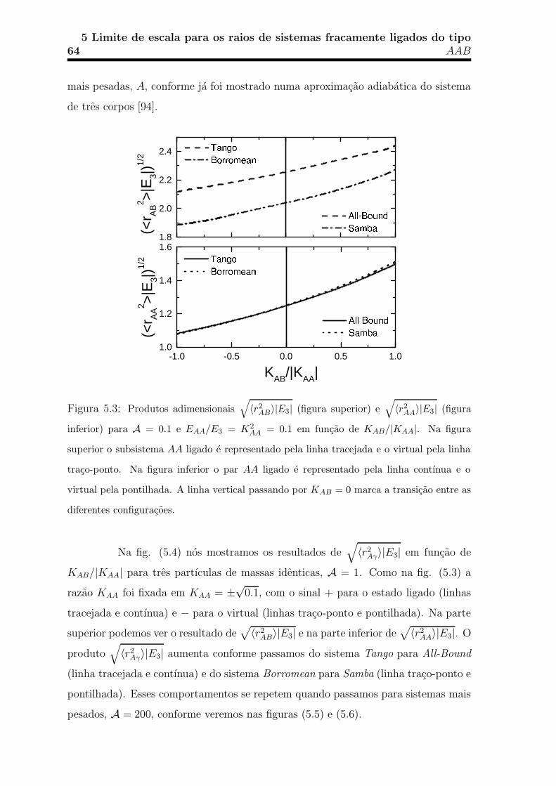
645 Limite de escala para os raios de sistemas fracamente ligados do tipo
AAB
mais pesadas, A, conforme ja foi mostrado numa aproximacao adiabatica do sistema
de tres corpos [94].
-1.0 -0.5 0.0 0.5 1.01.0
1.2
1.4
1.6
KAB/|KAA|
(<r A
A
2 >|E
3|)1/
2
1.8
2.0
2.2
2.4
(<r A
B
2 >|E
3|)1/
2
Figura 5.3: Produtos adimensionais√
〈r2AB〉|E3| (figura superior) e
√
〈r2AA〉|E3| (figura
inferior) para A = 0.1 e EAA/E3 = K2AA = 0.1 em funcao de KAB/|KAA|. Na figura
superior o subsistema AA ligado e representado pela linha tracejada e o virtual pela linha
traco-ponto. Na figura inferior o par AA ligado e representado pela linha contınua e o
virtual pela pontilhada. A linha vertical passando por KAB = 0 marca a transicao entre as
diferentes configuracoes.
Na fig. (5.4) nos mostramos os resultados de√
〈r2Aγ〉|E3| em funcao de
KAB/|KAA| para tres partıculas de massas identicas, A = 1. Como na fig. (5.3) a
razao KAA foi fixada em KAA = ±√
0.1, com o sinal + para o estado ligado (linhas
tracejada e contınua) e − para o virtual (linhas traco-ponto e pontilhada). Na parte
superior podemos ver o resultado de√
〈r2AB〉|E3| e na parte inferior de
√
〈r2AA〉|E3|. O
produto√
〈r2Aγ〉|E3| aumenta conforme passamos do sistema Tango para All-Bound
(linha tracejada e contınua) e do sistema Borromean para Samba (linha traco-ponto e
pontilhada). Esses comportamentos se repetem quando passamos para sistemas mais
pesados, A = 200, conforme veremos nas figuras (5.5) e (5.6).
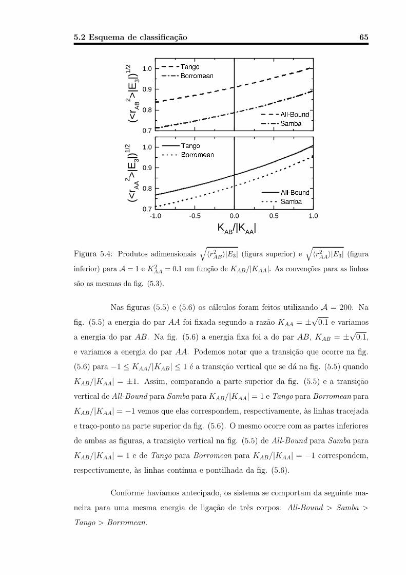
5.2 Esquema de classificacao 65
-1.0 -0.5 0.0 0.5 1.00.7
0.8
0.9
1.0
(<r A
B
2 >|E
3|)1/
2(<
r AA
2 >|E
3|)1/
2
KAB/|KAA|
0.7
0.8
0.9
1.0
Figura 5.4: Produtos adimensionais√
〈r2AB〉|E3| (figura superior) e
√
〈r2AA〉|E3| (figura
inferior) para A = 1 e K2AA = 0.1 em funcao de KAB/|KAA|. As convencoes para as linhas
sao as mesmas da fig. (5.3).
Nas figuras (5.5) e (5.6) os calculos foram feitos utilizando A = 200. Na
fig. (5.5) a energia do par AA foi fixada segundo a razao KAA = ±√
0.1 e variamos
a energia do par AB. Na fig. (5.6) a energia fixa foi a do par AB, KAB = ±√
0.1,
e variamos a energia do par AA. Podemos notar que a transicao que ocorre na fig.
(5.6) para −1 ≤ KAA/|KAB| ≤ 1 e a transicao vertical que se da na fig. (5.5) quando
KAB/|KAA| = ±1. Assim, comparando a parte superior da fig. (5.5) e a transicao
vertical de All-Bound para Samba para KAB/|KAA| = 1 e Tango para Borromean para
KAB/|KAA| = −1 vemos que elas correspondem, respectivamente, as linhas tracejada
e traco-ponto na parte superior da fig. (5.6). O mesmo ocorre com as partes inferiores
de ambas as figuras, a transicao vertical na fig. (5.5) de All-Bound para Samba para
KAB/|KAA| = 1 e de Tango para Borromean para KAB/|KAA| = −1 correspondem,
respectivamente, as linhas contınua e pontilhada da fig. (5.6).
Conforme havıamos antecipado, os sistema se comportam da seguinte ma-
neira para uma mesma energia de ligacao de tres corpos: All-Bound > Samba >
Tango > Borromean.

665 Limite de escala para os raios de sistemas fracamente ligados do tipo
AAB
-1.0 -0.5 0.0 0.5 1.00.7
0.8
0.9
1.0
0.6
0.7
0.8
KAB/|KAA|
(<r A
A
2 >|E
3|)1/
2(<
r AB
2 >|E
3|)1/
2
Figura 5.5: Produtos adimensionais√
〈r2AB〉|E3| (figura superior) e
√
〈r2AA〉|E3| (figura
inferior) para A = 200 e K2AA = 0.1 em funcao de KAB/|KAA|. As convencoes para as
linhas sao as mesmas das figuras (5.3) e (5.4).
Na fig. (5.7) as energias de ligacao de dois corpos foram colocadas iguais a
zero e variamos a razao entre as massas, A. Nessa figura sao mostrados os resultados
para√
〈r2Aγ〉|E3| e
√
〈r2γ〉|E3|.
Na situacao da fig. (5.7) como as energias de dois corpos sao iguais a zero
a unica escala fısica do sistema e a energia de tres corpos e as funcoes de escala dadas
pelas eqs. (5.27) e (5.28) ficam dependentes somente da razao entre as massas das
partıculas e se reduzem a:
√
〈r2Aγ〉|E3| = R′
Aγ(A), (5.30)
√
〈r2γ〉|E3| = R′CM
γ (A). (5.31)
Na fig. (5.7) vemos que as distancias entre as partıculas e das partıculas ao
CM do sistema saturam rapidamente conforme aumentamos A, porem elas divergem

5.2 Esquema de classificacao 67
-1.0 -0.5 0.0 0.5 1.00.7
0.8
0.9
1.0
0.6
0.7
0.8
KAA/|KAB|
(<r A
A
2 >|E
3|)1/
2(<
r AB
2 >|E
3|)1/
2
Figura 5.6: Produtos adimensionais√
〈r2AB〉|E3| (figura superior) e
√
〈r2AA〉|E3| (figura
inferior) para A = 200 e EAB/E3 = K2AB = 0.1 em funcao de KAA/|KAB |. Na figura
superior o subsistema AB ligado e representado pela linha tracejada e o virtual pela linha
traco-ponto. Na figura inferior o par AB ligado e representado pela linha contınua e o
virtual pela pontilhada. A linha vertical passando por KAA = 0 marca a transicao entre as
diferentes configuracoes. Essas linhas representam as transicoes verticais (|KAB | = |KAA|)
nas extremidades da fig. (5.5).
conforme a razao entre as massas tende a zero. A razao para o aumento dos produtos√
〈r2Aγ〉|E3| e
√
〈r2γ〉|E3| e devido ao momento medio do caroco, ∼
√
A|E3|, que
tende a zero fazendo com que o tamanho do sistema, nas unidades escolhidas, cresca
infinitamente. Os resultados tendem a valores finitos apos a multiplicacao por√A.
Devemos tambem chamar a atencao para o fato das distancias de B ao CM tender
a zero e de A ao CM tender a distancia AB conforme A vai para infinito, como
deverıamos esperar.
Nas proximas secoes vamos particularizar o estudo feito sobre os tamanhos
dos sistemas de tres corpos para o caso de nucleos exoticos e moleculas fracamente
ligadas.

685 Limite de escala para os raios de sistemas fracamente ligados do tipo
AAB
0 4 8 12 16 200.0
0.2
0.4
0.6
0.8
1.0
1.2
(<r2 γ>
|E3|)
1/2
(<r2 A
γ>|E
3|)1/
2
A
(b)
(a)
Figura 5.7: Produtos adimensionais√
〈r2Aγ〉|E3| e
√
〈r2γ〉|E3| (γ = A,B) em funcao da
razao entre as massas, A. As energias de dois corpos foram colocadas iguais a zero.
A parte superior da figura, (a), mostra os resultados de√
〈r2AA〉|E3|, linha contınua, e
√
〈r2AB〉|E3|, linha traco-ponto. A parte inferior, (b), mostra os resultados para
√
〈r2A〉|E3|,
linha contınua, e√
〈r2B〉|E3|, linha traco-ponto.
5.3 Nucleos exoticos leves
O estudo de nucleos que estao proximos a linha de estabilidade, mais especificamente
a linha linha de estabilidade de neutrons, revelou estruturas interessantes, como por
exemplo um halo formado pelos neutrons. Esses nucleos, denominados de nucleos
exoticos ou nucleos-halo, tornaram-se objetos de intensas investigacoes da fısica nu-
clear atual. Embora a primeira observacao experimental de um nucleo exotico tıpico
tenha sido feita na segunda metade da decada de 30 (6He [95]) o enfoque atual dado
aos nucleos proximos a fronteira de estabilidade teve inıcio somente ha 15 anos a
partir da observacao do aumento da secao de choque do 11Li em um experimento
de medida da secao de choque de isotopos de Li colidindo com alguns alvos [96, 97]
(a deteccao do 11Li foi feita pela primeira vez em 1966 [98]). O aumento da secao
de choque do 11Li foi interpretado como sendo uma decorrencia da estrutura desse
5.3 Nucleos exoticos leves 69
nucleo, o qual seria formado por um caroco, 9Li, e dois neutrons fracamente liga-
dos [99] (esse aumento foi verificado experimentalmente em 1989 [100]). Revisoes a
respeito de nucleos exoticos podem ser encontradas nas Refs. [25, 101, 102, 103, 104].
O formalismo desenvolvido no inıcio deste capıtulo que foi utilizado de
uma forma generica para um sistema de tres corpos fracamente ligado e composto
por duas partıculas identicas e uma diferente sera utilizado nessa secao para o caso
especıfico de nucleos exoticos leves. Os nucleos exoticos serao tratados aqui como um
sistema de tres corpos constituıdo por um caroco pontual que chamaremos de C e
dois neutrons fracamente ligados provenientes do halo que chamaremos de n. Nesta
secao γ = n, C.
Nossos calculos para os raios quadraticos medios entre os dois neutrons do
halo serao comparados com os resultados experimentais de 6He, 11Li e 14Be proveni-
entes das Refs. [105, 106]. A tabela 5.1 mostra esses resultados.
A fig. (5.8) reproduz os resultados ja apresentados na fig. (5.7) acrescidos
dos pontos experimentais para o 6He, 11Li e 14Be dados na tabela 5.1.
Os pontos experimentais colocados na fig. (5.8) sao meramente ilustrativos
considerando que os subsistemas 5He, 10Li e 13Be tivessem uma energia de ligacao
igual a zero. Conforme podemos ver na fig. (5.8) a utilizacao de uma energia igual a
zero para o 10Li nao nos da um resultado compatıvel com o resultado experimental
para a distancia nn no halo do 11Li, tabela 5.1. Devemos ressaltar o fato de que os
resultados para a energia do estado virtual do 10Li na literatura ainda sao bastante
controversos [108, 109, 110, 111, 112].
Podemos ver na tabela 5.1 que os resultados de√
〈r2nn〉 para o 6He utili-
zando o nosso modelo indicam que o estado virtual do 5He deve possuir uma energia
proxima de zero, ou ate mesmo fracamente ligada, o que nao concorda com os valores
dados na literatura os quais sugerem uma energia bem maior [107, 44]. Essa dis-
crepancia e compreensıvel levando-se em conta que a interacao para n-4He e repulsiva
na onda-S e atrativa na onda P , produzindo, assim, um valor elevado para a energia
do estado virtual do 5He (no nosso modelo o polo da onda-S deveria ficar proximo do
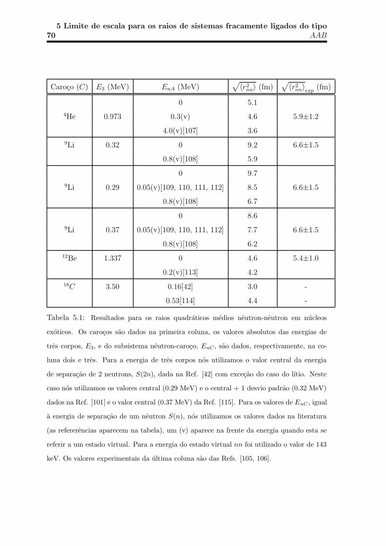
705 Limite de escala para os raios de sistemas fracamente ligados do tipo
AAB
Caroco (C) E3 (MeV) EnA (MeV)√
〈r2nn〉 (fm)
√
〈r2nn〉exp
(fm)
0 5.1
4He 0.973 0.3(v) 4.6 5.9±1.2
4.0(v)[107] 3.6
9Li 0.32 0 9.2 6.6±1.5
0.8(v)[108] 5.9
0 9.7
9Li 0.29 0.05(v)[109, 110, 111, 112] 8.5 6.6±1.5
0.8(v)[108] 6.7
0 8.6
9Li 0.37 0.05(v)[109, 110, 111, 112] 7.7 6.6±1.5
0.8(v)[108] 6.2
12Be 1.337 0 4.6 5.4±1.0
0.2(v)[113] 4.2
18C 3.50 0.16[42] 3.0 -
0.53[114] 4.4 -
Tabela 5.1: Resultados para os raios quadraticos medios neutron-neutron em nucleos
exoticos. Os carocos sao dados na primeira coluna, os valores absolutos das energias de
tres corpos, E3, e do subsistema neutron-caroco, EnC , sao dados, respectivamente, na co-
luna dois e tres. Para a energia de tres corpos nos utilizamos o valor central da energia
de separacao de 2 neutrons, S(2n), dada na Ref. [42] com excecao do caso do lıtio. Neste
caso nos utilizamos os valores central (0.29 MeV) e o central + 1 desvio padrao (0.32 MeV)
dados na Ref. [101] e o valor central (0.37 MeV) da Ref. [115]. Para os valores de EnC , igual
a energia de separacao de um neutron S(n), nos utilizamos os valores dados na literatura
(as refererencias aparecem na tabela), um (v) aparece na frente da energia quando esta se
referir a um estado virtual. Para a energia do estado virtual nn foi utilizado o valor de 143
keV. Os valores experimentais da ultima coluna sao das Refs. [105, 106].

5.3 Nucleos exoticos leves 71
0 4 8 12 16 200.0
0.2
0.4
0.6
0.8
1.0
1.2
11Li
(<r2 γ>
|E3|)
1/2
(<r2 n γ
>|E
3|)1/
2
A
(b)
(a)
14Be6He
Figura 5.8: Produtos adimensionais√
〈r2nγ〉|E3| e
√
〈r2γ〉|E3| (γ = n,C) em funcao da razao
entre as massas, A. As energias de dois corpos foram colocadas iguais a zero. A parte supe-
rior da figura, (a), mostra os resultados de√
〈r2nn〉|E3|, linha contınua, e
√
〈r2nC〉|E3|, linha
traco-ponto. A parte inferior, (b), mostra os resultados para√
〈r2n〉|E3|, linha contınua, e
√
〈r2C〉|E3|, linha traco-ponto. Os cırculos cheios sao os pontos experimentais de
√
〈r2nn〉|E3|
para o 6He, 11Li e 14Be retirados da Ref. [105, 106].
limiar do espalhamento).
Para a energia de ligacao do subsistema n-9Li sabe-se que ambas as ondas,
S e P , sao importantes, um dos motivos que deve explicar o desvio dos nossos resul-
tados com os resultados experimentais. Todavia, no caso do 10Li nossa aproximacao
deve ser um pouco melhor ja que neste caso a interacao na onda-S e atrativa.
Vale ressaltar tambem, que em todos os casos nos estamos considerando
como entrada para os nossos calculos os valores experimentais das energias dos sub-
sistemas de dois corpos. Assim, embora o nosso modelo envolva apenas a onda-S,
nos estamos considerando de forma indireta o efeito das ondas superiores nos nossos
resultados. Os tamanhos dos sistemas tambem sao obtidos da cauda da funcao de
onda que e dominada pela onda-S. Outros fatores que poderiam melhorar os nossos

725 Limite de escala para os raios de sistemas fracamente ligados do tipo
AAB
resultados seriam a inclusao no nosso modelo do princıpio de Pauli e um tamanho
finito para o caroco.
Os raios quadraticos medios sao extraıdos experimentalmente de uma funcao
que fornece uma informacao direta da funcao de onda do halo: a funcao de correlacao
[105, 106]. Essa funcao de correlacao teve origem na astrofısica e foi inicialmente de-
senvolvida por Hanbury-Brown e Twiss na decada de 50 para determinar a dimensao
de objetos astronomicos distantes da Terra [116] (uma revisao sobre esse assunto pode
ser encontrada na Ref. [117]), posteriormente a aplicacao do metodo se estendeu a
outras areas da fısica, como, por exemplo, a fısica nuclear onde a funcao de correlacao
nos fornece informacoes sobre as dimensoes nucleares.
Utilizando a mesma notacao da subsecao 5.1 podemos escrever a funcao
de correlacao, Cnn(~pC), como uma funcao do momento relativo dos neutrons do halo,
~pC , como (embora os neutrons sejam indistinguıveis entre si nos os chamaremos de n
e n′ apenas para facilitar a definicao das coordenadas):
Cnn(~pC) =
∫
d3qC |Φ(~qC , ~pC)|2∫
d3qCρ(~qn′)ρ(~qn), (5.32)
~qn′ ≡ ~pC −~qC
2e ~qn ≡ −~pC −
~qC
2.
A densidade de 1-corpo e dada por:
ρ(~qn′) =
∫
d3qn
∣
∣
∣
∣
Φ
(
−~qn′ − ~qn,~qn′ − ~qn
2
)∣
∣
∣
∣
2
, (5.33)
onde Φ ≡ Φ(~qC , ~pC) e a amplitude de quebra da funcao de onda de tres corpos com
a interacao de estado final (FSI) entre os neutrons.
A FSI e introduzida diretamente no produto escalar Φ ≡ 〈~qC ; ~pC(−)|Ψ〉,
onde o ket |~pC(−)〉 se refere a onda distorcida dos neutrons e e dada pela eq. de
Lippmann-Schwinger. Φ e dada por:

5.4 Moleculas triatomicas fracamente ligadas 73
Φ = Ψ(~qC , ~pC)− 1/(2π2)√Enn + ipC
∫
d3pΨ(~qC , ~p)
p2C − p2 − iε
, (5.34)
onde Enn e a energia do estado virtual de dois neutrons. No futuro prximo pretende-
mos concluir os calculos referentes a eq. (5.34).
5.4 Moleculas triatomicas fracamente ligadas
Veremos nesta secao que o formalismo tambem se aplica muito bem ao caso de
moleculas triatomicas fracamente ligadas. Nesta secao a partıcula A da secao 5.1
representara um atomo de 4He e a partıcula B representara um dos seguintes atomos:
4He, 6Li, 7Li e 23Na.
Na fig. (5.9) sao mostrados os resultados para o caso de um sistema com-
posto por tres atomos de helio, 4He3, na forma de um produto adimensional√
〈r2〉S3,
S3 = E3 − E2, em funcao da razao entre as energias de dois e tres corpos√
E2/E3.
Os calculos realısticos da Ref. [39] tambem estao nesta figura.
Podemos ver na fig. (5.9) que os nossos resultados para o estado fun-
damental (linha contınua) e para o estado excitado (linha tracejada) praticamente
coincidem. Isso mostra a validade do nosso limite de escala quando as energias re-
escalonadas com respeito a µ2 tendem a zero, neste limite os resultados devem ser
os mesmos. Os calculos realısticos mostram um desvio de aproximadamente 20% dos
nossos resultados para o estado fundamental, ja para o estado excitado os dois re-
sultados mostram-se mais proximos. Esse fato pode ser compreendido levando-se em
conta o tamanho dos trımeros. No caso do estado excitado o tamanho do trımero e,
aproximadamente, 10 vezes maior que o estado fundamental correspondente. Desta
forma, a nossa aproximacao e melhor nesse caso onde o tamanho da molecula e muito
maior que o alcance do potencial.
A fig. (5.10) e basicamente igual as figuras (5.7) e (5.8) com a diferenca de
que neste caso os calculos sao feitos para A ≥ 1 e alem do estado fundamental, N = 0

745 Limite de escala para os raios de sistemas fracamente ligados do tipo
AAB
0.0 0.2 0.4 0.6 0.8 1.0
0.4
0.6
0.8
1.0
1.2
(E2/E3)1/2
(<r H
e
2>
S3)
1/2
(<r H
e-H
e
2>
S3)
1/2
Figura 5.9: Produtos adimensionais√
〈r2He−He〉S3 (curvas superiores) e
√
〈r2He〉S3 (curvas
inferiores) em funcao da razao√
E2/E3. 〈r2He−He〉 e a distancia quadratica media entre dois
atomos de 4He, 〈r2He〉 e a distancia de um atomo de 4He ao centro-de-massa do sistema e S3 =
E3−E2. Nossos resultados para o estado fundamental e primeiro estado excitado sao dados,
respectivamente, pela linha contınua e tracejada. Os calculos realısticos retirados da Ref.
[39] para√
〈r2He−He〉S3 sao dados pelos quadrados cheios (estado fundamental) e cırculos
cheios (estado excitado), e para√
〈r2He〉S3 pelos quadrados vazios (estado fundamental) e
cırculos vazios (estado excitado).
(linha contınua), foi incluıdo o primeiro estado excitado, N = 1 (linha tracejada).
Embora a fig. (5.10) esteja inserida no contexto das moleculas ela e bastante geral, por
esse motivo iremos manter a notacao AAB para representar um sistema triatomico.
Conforme podemos ver na fig. (5.10) superior, (a), as curvas saturam
rapidamente. Para A ∼ 3 as curvas assumem o mesmo valor que A → ∞. Fazendo
A → ∞ os calculos dao para 〈r2AA〉 o valor de 0.69/E3 para N = 0 e 0.61/E3 para
N = 1 e para 〈r2AB〉 o valor de 0.45/E3 para N = 0 e 0.40/E3 para N = 1. A parte
inferior da fig. (5.10), (b), mostra os raios quadraticos medios em relacao ao CM
do sistema. Aumentando-se A vemos que 〈r2A〉 e 〈r2
B〉 tendem, respectivamente, a

5.4 Moleculas triatomicas fracamente ligadas 75
0 4 8 12 16 200.0
0.2
0.4
0.6
0.8
(b)
(a)
(<r γ2
>E
3)1/
2(<
r Aγ
2>
E3)
1/2
A
Figura 5.10: Resultados para um sistema triatomico do tipo AAB, com γ = A,B. Produtos
adimensionais√
〈r2Aγ〉S3 (curvas superiores) e
√
〈r2γ〉S3 (curvas inferiores) em funcao da
razao entre as massa A. 〈r2Aγ〉 e a distancia quadratica media entre os atomos A e γ, e 〈r2
γ〉
e a distancia do atomo γ ao CM do sistema. As energias dos subsistemas de dois corpos sao
iguais a zero. Nossos resultados para o estado fundamental sao dados pela linha contınua
(γ = A) e traco-ponto (γ = B), e para o primeiro estado excitado pelas linhas tracejada
(γ = A) e pontilhada (γ = B).
〈r2AB〉 e a 0, como era esperado considerando que a partıcula pesada deve estar no
CM do sistema para A muito grande. Devemos ressaltar o fato de que embora a
razao entre as energias do estado fundamental, N=0, e do estado excitado, N=1, seja
aproximadamente 500 para A = 1 e 300 para A = 10, as variacoes entre as duas
curvas e de apenas 10%.
Na tabela (5.2) nos apresentamos os resultados do raios quadraticos medios
para diferentes moleculas constituıdas de dois atomos de 4He e um outro atomo que
pode ser: 4He, 6Li, 7Li e 23Na. Os raios sao calculados para o estado fundamental e
as energias teoricas E3, EAA e EAB sao retiradas da Ref. [118].
Nosso resultado para 4He3 da como resultado para√
〈r2AA〉 um valor de
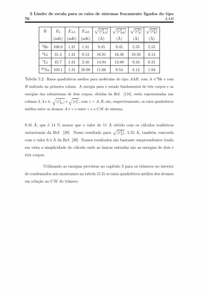
765 Limite de escala para os raios de sistemas fracamente ligados do tipo
AAB
B E3 EAA EAB
√
〈r2AA〉
√
〈r2AB〉
√
〈r2A〉
√
〈r2B〉
(mK) (mK) (mK) (A) (A) (A) (A)
4He 106.0 1.31 1.31 9.45 9.45 5.55 5.55
6Li 31.4 1.31 0.12 16.91 16.38 10.50 8.14
7Li 45.7 1.31 2.16 14.94 13.88 9.34 6.31
23Na 103.1 1.31 28.98 11.66 9.54 8.12 1.94
Tabela 5.2: Raios quadraticos medios para moleculas do tipo AAB, com A ≡4He e com
B indicado na primeira coluna. A energia para o estado fundamental de tres corpos e as
energias dos subsistemas de dois corpos, obtidas da Ref. [118], estao representadas nas
colunas 2, 3 e 4.√
〈r2Aγ〉 e
√
〈r2γ〉, com γ = A,B, sao, respectivamente, os raios quadraticos
medios entre os atomos A e γ e entre γ e o CM do sistema.
9.45 A, que e 14 % menor que o valor de 11 A obtido com os calculos realısticos
variacionais da Ref. [39]. Nosso resultado para√
〈r2A〉, 5.55 A, tambem concorda
com o valor 6.4 A da Ref. [39]. Nossos resultados sao bastante surpreendentes tendo
em vista a simplicidade do calculo onde as unicas entradas sao as energias de dois e
tres corpos.
Utilizando as energias previstas no capıtulo 3 para os trımeros no interior
de condensados nos mostramos na tabela (5.3) os raios quadraticos medios dos atomos
em relacao ao CM do trımero.

5.4 Moleculas triatomicas fracamente ligadas 77
Atomo E2 E3
√
〈r2A〉 E ′
3
√
〈r2A〉′
(mK) (mK) (A) (mK) (A)
23Na|1,−1〉 2.85 7.75 12 3.06 38
87Rb|1,−1〉∗ 0.17 0.56 22 0.175 114
87Rb|1,−1〉† 0.17 0.47 25 0.183 91
85Rb|2,−2〉 1.3× 10⁻⁴ 2.4× 10⁻⁴ 1293 1.7× 10⁻⁴ 1944
Tabela 5.3: Resultados para o raio quadratico medio do atomo em relacao ao CM do sis-
tema no interior de armadilhas magneto-opticas utilizando as energias previstas no capıtulo
3. Os atomos estao identificados na primeira coluna. Para cada energia do dımero, dada na
coluna 2, nos temos duas energia para o trımero, colunas 3 e 5, com os raios correspondentes
dados nas colunas 4 e 6. ∗ atomos nao condensados. † atomos condensados. |F,mF 〉 sao,
respectivamente, o spin total e a sua projecao.

785 Limite de escala para os raios de sistemas fracamente ligados do tipo
AAB
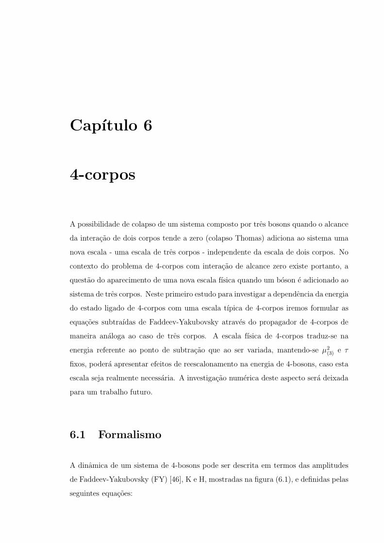
Capıtulo 6
4-corpos
A possibilidade de colapso de um sistema composto por tres bosons quando o alcance
da interacao de dois corpos tende a zero (colapso Thomas) adiciona ao sistema uma
nova escala - uma escala de tres corpos - independente da escala de dois corpos. No
contexto do problema de 4-corpos com interacao de alcance zero existe portanto, a
questao do aparecimento de uma nova escala fısica quando um boson e adicionado ao
sistema de tres corpos. Neste primeiro estudo para investigar a dependencia da energia
do estado ligado de 4-corpos com uma escala tıpica de 4-corpos iremos formular as
equacoes subtraıdas de Faddeev-Yakubovsky atraves do propagador de 4-corpos de
maneira analoga ao caso de tres corpos. A escala fısica de 4-corpos traduz-se na
energia referente ao ponto de subtracao que ao ser variada, mantendo-se µ2(3) e τ
fixos, podera apresentar efeitos de reescalonamento na energia de 4-bosons, caso esta
escala seja realmente necessaria. A investigacao numerica deste aspecto sera deixada
para um trabalho futuro.
6.1 Formalismo
A dinamica de um sistema de 4-bosons pode ser descrita em termos das amplitudes
de Faddeev-Yakubovsky (FY) [46], K e H, mostradas na figura (6.1), e definidas pelas
seguintes equacoes:

80 6 4-corpos
|K lij,k〉 = GijvijG0(vik + vjk)|Ψ〉 (i < j), (6.1)
|Hij,kl〉 = GijvijG0vkl|Ψ〉 (i < j, k < l), (6.2)
onde Gij e o propagador de 4-corpos dado por Gij = (E −H0 − vij) (H0 e a energia
cinetica), vij e o potencial de dois corpos entre as partıculas i e j e G0 e o propagador
livre de 4-corpos. A funcao de onda total do sistema, Ψ, e dada pela soma das 18
amplitudes de FY, 12 delas dada pela eq. (6.1) e 6 pela eq. (6.2). As amplitudes K lij,k
e Hij,kl descrevem, respectivamente, um sistema formado por 3 partıculas ligadas, ijk,
e uma livre, l, e um sistema formado pelos pares ligados, ij e kl.
Figura 6.1: Coordenadas de Jacobi para as amplitudes de Faddeev-Yakubovsky do tipo K,
lado esquerdo, e H, lado direito.
As amplitudes K e H podem ainda ser escritas em termos das amplitudes
de Faddeev como:
|K lij,k〉 = Gijvij(|Fik〉+ |Fjk)〉) (i < j), (6.3)
|Hij,kl〉 = Gijvij|Fkl〉 (i < j, k < l), (6.4)
onde |Fij〉 = G0vij|Ψ〉 e a amplitude de Faddeev que pode tambem ser escrita em
termos das amplitudes K e H da seguinte maneira:
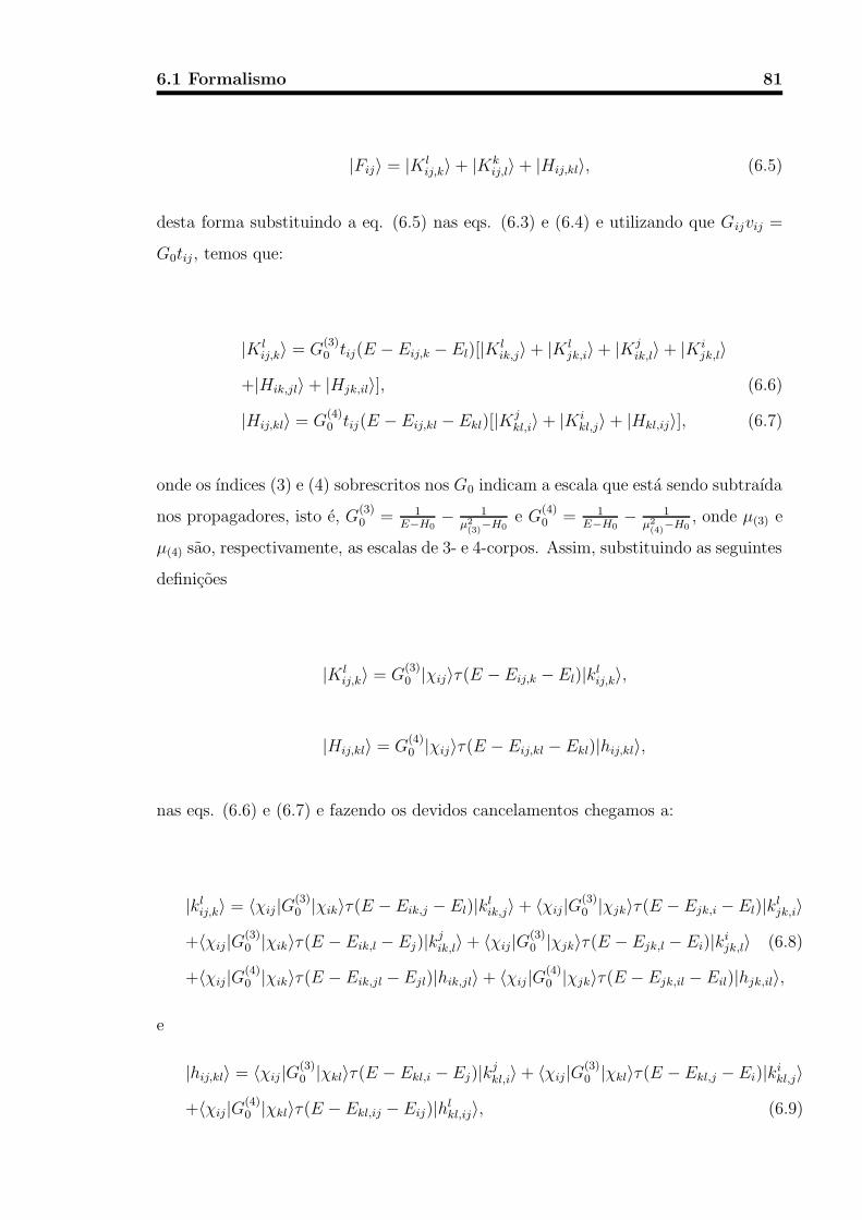
6.1 Formalismo 81
|Fij〉 = |K lij,k〉+ |Kk
ij,l〉+ |Hij,kl〉, (6.5)
desta forma substituindo a eq. (6.5) nas eqs. (6.3) e (6.4) e utilizando que Gijvij =
G0tij, temos que:
|K lij,k〉 = G
(3)0 tij(E − Eij,k − El)[|K l
ik,j〉+ |K ljk,i〉+ |Kj
ik,l〉+ |Kijk,l〉
+|Hik,jl〉+ |Hjk,il〉], (6.6)
|Hij,kl〉 = G(4)0 tij(E − Eij,kl − Ekl)[|Kj
kl,i〉+ |Kikl,j〉+ |Hkl,ij〉], (6.7)
onde os ındices (3) e (4) sobrescritos nos G0 indicam a escala que esta sendo subtraıda
nos propagadores, isto e, G(3)0 = 1
E−H0− 1
µ2(3)−H0
e G(4)0 = 1
E−H0− 1
µ2(4)−H0
, onde µ(3) e
µ(4) sao, respectivamente, as escalas de 3- e 4-corpos. Assim, substituindo as seguintes
definicoes
|K lij,k〉 = G
(3)0 |χij〉τ(E − Eij,k − El)|kl
ij,k〉,
|Hij,kl〉 = G(4)0 |χij〉τ(E − Eij,kl − Ekl)|hij,kl〉,
nas eqs. (6.6) e (6.7) e fazendo os devidos cancelamentos chegamos a:
|klij,k〉 = 〈χij|G(3)
0 |χik〉τ(E − Eik,j − El)|klik,j〉+ 〈χij|G(3)
0 |χjk〉τ(E − Ejk,i − El)|kljk,i〉
+〈χij|G(3)0 |χik〉τ(E − Eik,l − Ej)|kj
ik,l〉+ 〈χij|G(3)0 |χjk〉τ(E − Ejk,l − Ei)|ki
jk,l〉 (6.8)
+〈χij|G(4)0 |χik〉τ(E − Eik,jl − Ejl)|hik,jl〉+ 〈χij|G(4)
0 |χjk〉τ(E − Ejk,il − Eil)|hjk,il〉,
e
|hij,kl〉 = 〈χij|G(3)0 |χkl〉τ(E − Ekl,i − Ej)|kj
kl,i〉+ 〈χij|G(3)0 |χkl〉τ(E − Ekl,j − Ei)|ki
kl,j〉
+〈χij|G(4)0 |χkl〉τ(E − Ekl,ij − Eij)|hl
kl,ij〉, (6.9)

82 6 4-corpos
sendo 〈~qij|χij〉 = g(~qij) = 1 o fator de forma para o potencial δ-Dirac. Igualando os
termos identicos do lado direito da equacao temos que:
|klij,k〉 = 2〈χij|G(3)
0 |χik〉τ(E − Eik,j − El)|klik,j〉+ 2〈χij|G(3)
0 |χik〉τ(E − Eik,l − Ej)|kjik,l〉
+2〈χij|G(4)0 |χik〉τ(E − Eik,jl − Ejl)|hik,jl〉, (6.10)
|hij,kl〉 = 2〈χij|G(3)0 |χkl〉τ(E − Ekl,i − Ej)|kj
kl,i〉+ 〈χij|G(4)0 |χkl〉τ(E − Ekl,ij − Eij)|hkl,ij〉.
(6.11)
Redefinindo τ(E)|k〉 como K e τ(E)|h〉 como H, multiplicando as eqs.
(6.10) e (6.11), respectivamente, por 〈~qij,k; ~ql| e 〈~qij,kl; ~qkl| pela esquerda e inserindo
algumas resolucoes da unidade chegamos a:
〈~qij,k; ~ql|Klij,k〉 = 2τ(E − Eij,k − El)
×
∫
d3qik,jd3q′ld
3qijd3qik
〈~qij; ~qij,k; ~ql|~qik,j; ~ql′; ~qik〉
E − q2ij,k
2mij,k− q2
l
2ml− q2
ij
2mij
〈~qij,k; ~ql′|Kl
ik,j〉
+
∫
d3qik,ld3qjd
3qijd3qik
〈~qij; ~qij,k; ~ql|~qik,l; ~qj; ~qik〉E − q2
ij,k
2mij,k− q2
l
2ml− q2
ij
2mij
〈~qik,l; ~qj|Kjik,l〉
+
∫
d3qik,jld3qjld
3qijd3qik
〈~qij; ~qij,k; ~ql|~qik,jl; ~qjl; ~qik〉E − q2
ij,k
2mij,k− q2
l
2ml− q2
ij
2mij
〈~qik,jl; ~qjl|Hik,jl〉
(6.12)
〈~qij,kl; ~qkl|Hij,kl〉 = 2τ(E − Eij,kl − Ekl)
×
∫
d3qkl,id3qjd
3qijd3q′kl
〈~qij,kl; ~qkl; ~qij|~qkl,i; ~qj; ~qkl′〉
E − q2ij,kl
2mij,kl− q2
kl
2mkl− q2
ij
2mij
〈~qkl,i; ~qj|Kjkl,i〉 (6.13)
+
∫
d3qkl,ijd3qij
′d3qijd3qkl
′ 〈~qij,kl; ~qkl; ~qij|~qkl,ij; ~qij′; ~qkl
′〉E − q2
ij,kl
2mij,kl− q2
kl
2mkl− q2
ij
2mij
〈~qkl,ij; ~qij′|Hj
kl,ij〉
Finalmente podemos escrever as eqs. (6.12) e (6.13) na forma de uma
equacao integral com os momentos orientados conforme a figura 6.2. O calculo do
elementos de matriz das eqs. (6.12) e (6.13) esta no apendice G. Os momentos que
aparecem do lado esquerdo ~qij,k e ~qij,kl foram chamados de ~q e ~ql, respectivamente, e

6.1 Formalismo 83
~qkl foi chamado de ~p. Do lado direito o momento que sobra apos a integracao dos δ’s
foi chamado de ~k.
Figura 6.2: Orientacao dos momentos.
K(q, p) = 2τ(E − 3
4q2 − 2
3p2)
∫
d cos θkd cos θqdφkk2dkK(k, p)
[
1
−|E| − q2 − k2 − 23p2 + qkz
− 1
−1− q2 − k2 − 23p2 + qkz
]
+
∫
d cos θkd cos θqdφkk2dkK(k, 3
√
k2 + p2 − 2pk cos θk)[
1
−|E| − q2 − 709p2 − 9k2 + 16pk cos θk + 8
3pq cos θq − 3kqz
(6.14)
− 1
−1− q2 − 709p2 − 9k2 + 16pk cos θk + 8
3pq cos θq − 3kqz
]
+
∫
d cos θkd cos θqdφkk2dkH(k,
√
k2 +16
9p2 − 8
3pk cos θk)
[
1
−|E| − q2 − 109p2 − k2 − qkz + 4
3pk cos φk + 2
3pq cos θq
−
− 1
−µ2(4) − q2 − 10
9p2 − k2 − qkz + 4
3pk cos φk + 2
3pq cos θq
]
,

84 6 4-corpos
H(q, p) = τ(E − 1
2q2 − p2)
2
∫
d cos θkd cos θqdφkk2dkK(k,
√
4
9k2 + q2 +
4
3kqz)
[
1
−|E| − 34q2 − p2 − k2 − qkz
− 1
−1− 34q2 − p2 − k2 − qkz
]
(6.15)
+
∫
d cos θkd cos θqdφkk2dkH(q, k)
[
1
−|E| − 12q2 − p2 − k2
− 1
−µ2(4) − 1
2q2 − p2 − k2
]
,
onde z = cos θq cos θk + senθqsenθk cos φk. Os propagadores foram escritos explicita-
mente em termos da energia de 4-corpos, E, e dos demais momentos. µ2(4) e o ponto
de subtracao de 4-corpos que em unidades de ~ = m = 1 tem dimensao de energia.
A energia de subtracao de 3-corpos foi colocada igual a 1.
Note que as funcoes espectadoras dependem somente do modulo dos mo-
mentos, uma vez que estamos interessados em estudar o estado fundamental de mo-
mento angular orbital total nulo. A energia de 4-corpos e a solucao do sistema de
eqs. acopladas (6.14) e (6.15).
Uma analise qualitativa das eqs. (6.10) e (6.11) nos permite tirar algumas
conclusoes: a amplitude do tipo k “cai”com a escala de tres corpos µ(3) e a amplitude
do tipo h com a escala de quatro corpos µ(4). Se fixarmos µ(3) = 1 e µ(4) 1, entao
para momentos grandes as eqs. (6.10) e (6.11) ficariam reduzidas a
|klij,k〉 = 2〈χij|G(4)
0 |χik〉τ(E − Eik,jl − Ejl)|hik,jl〉,
|hij,kl〉 = 〈χij|G(4)0 |χkl〉τ(E − Ekl,ij − Eij)|hkl,ij〉,
ou seja, as equacoes se desacoplam e precisamos resolver somente a segunda equacao
que pode possuir infinitas solucoes, desta forma, segundo a nossa analise qualitativa,
a escala de quatro bosons seria realmente nova.

Capıtulo 7
Conclusoes e perspectivas
A utilizacao de um potencial tipo δ-Dirac mostrou-se uma ferramenta muito util para
a descricao de propriedades de sistemas fracamente ligados de tres e quatro corpos
tanto no campo da fısica atomica como da fısica nuclear. Vimos que para potenciais
de curto-alcance a fısica desses sistemas esta contida nas escalas de dois e tres corpos
ou em outras palavras, qualquer observavel desse sistema pode ser representado em
termos de uma funcao de escala universal. Esse limite de escala e atingido quando
a razao entre o comprimento de espalhamento de dois corpos e o alcance efetivo do
potencial tende a infinito. Os calculos, feitos utilizando as equacoes subtraıdas para
a matriz-T, se reduzem aqueles calculados com um corte para grandes momentos
quando o ponto de subtracao vai para infinito [7].
Mostramos o comportamento de um estado Thomas-Efimov excitado con-
forme variamos a energia do subsistema de dois corpos. De fato, se o subsistema de
dois corpos e ligado, conforme aumentamos a razao entre a energia de ligacao de dois
e tres corpos o estado excitado desaparece e um estado virtual correspondente aparece
quando a energia do estado fundamental atinge o limiar dado por 6.9~2/(ma2) [7].
Quando o subsistema de dois corpos e virtual, o aumento da razao entre as energias
faz com que o estado excitado se transforme em uma ressonancia quando a energia
do estado fundamental e 1.1~2/(ma2) [49]. Neste ultimo caso as condicoes para a
formacao de moleculas triatomicas no interior de condensados e favorecida, pois a
86 7 Conclusoes e perspectivas
competicao com dımeros fracamente ligados esta ausente.
O conceito de universalidade, i.e., o reescalonamento dos observaveis, ainda
foi utilizado para escrevermos a dependencia do coeficiente de recombinacao de tres
corpos como uma funcao da razao entre as energias dos dımeros e trımeros atomicos.
Essa funcao tambem tende a uma funcao de escala universal. Utilizando a funcao de
escala e os valores experimentais conhecidos para o comprimento de espalhamento de
dois atomos e o coeficiente de recombinacao de tres atomos, calculamos as energias
de moleculas triatomicas no interior de armadilhas magneto-opticas [8]. A formacao
desses trımeros poderia ainda envolver colisoes de quatro corpos, tipo dımero-dımero
ou um dımero e dois atomos livres.
Finalmente, as funcoes de escala foram utilizadas para descrever os tama-
nhos de moleculas triatomicas fracamente ligadas [9] e nucleos exoticos (aproximados
por um caroco e dois neutrons) [10]. Neste ultimo caso completamos a nomenclatura
denominando de Samba a configuracao de um sistema de tres corpos formado por
dois subsistemas de dois corpos ligados e um virtual. O tamanho desses sistemas,
para uma mesma energia de tres corpos, comporta-se de maneira inesperada ja que
o maior sistema corresponde aquele onde os pares formam estados ligados e o menor
aquele onde os pares nao formam estados ligados.
A questao formulada na introducao sobre o aparecimento de uma nova
escala fısica cada vez que um boson fosse adicionado ao sistema ainda nao foi res-
pondida apesar da formulacao das equacoes de quatro corpos. Todavia, a analise
qualitativa das eqs. (6.10) e (6.11), feita no final do capıtulo referente ao problema
de 4-corpos, indica a introducao de uma nova escala fısica a esse sistema. E claro que
a simplificacao feita deve, ainda, ter um suporte numerico ou uma prova matematica
mais rigorosa.
Como perspectivas continuaremos estudando a dinamica dos sistemas de
tres e quatro corpos utilizando interacoes tipo δ-Dirac juntamente com a formulacao
das equacoes subtraıdas de Faddeev invariantes sob transformacoes do grupo de re-
normalizacao. Um estudo da trajetoria dos estados Efimov sera feita no contexto de

7 Conclusoes e perspectivas 87
sistemas de tres corpos do tipo AAB. Serao feitos calculos das energias de ligacao
de estados excitados, raios quadraticos medios e funcoes de correlacao de dois corpos
em funcao das escalas fısicas de dois e tres corpos no contexto de hipernucleos do
tipo Λ-hipernucleo. Sera investigada a necessidade da introducao de uma nova escala
para o sistema de quatro bosons, independente das escalas de dois e tres corpos, na
regularizacao das equacoes de Faddeev-Yakubovsky em tres dimensoes.

88 7 Conclusoes e perspectivas

Apendice A
Coordenadas de Jacobi (3-corpos)
Figura A.1: Coordenadas de Jacobi
Sejam ~ki +~kj +~kk = 0 os momentos das partıculas em relacao ao centro-de-
massa (C.M.) e mα e vα (α = i, j, k) as suas massas e velocidades, respectivamente.
Temos entao que ~pi e ~qi sao dados por:
~pi =mjmk
mj + mk(~vj − ~vk) =
mk~kj −mj
~kk
mj + mk(A.1)
~qi =mi(mj + mk)
mi + mj + mk
[
~vi −mj~vj + mk~vk
mj + mk
]
= ~ki. (A.2)
Analogamente temos que: ~qj = ~kj e ~qk = ~kk. Assim, relacionando as

90 A Coordenadas de Jacobi (3-corpos)
coordenadas temos que:
~pi =mk~qj −mj~qk
mj + mk(A.3)
~pj =mi~qk −mk~qi
mi + mk
(A.4)
~pk =mj~qi −mi~qj
mi + mj
(A.5)

Apendice B
Deducao do fator de forma para o
potencial δ-Dirac
Demonstraremos a seguir que no caso do potencial δ-Dirac temos que 〈χ|~p 〉 = 〈~p |χ〉 =
g(p) = 1. Sendo ~R um vetor ligando duas partıculas quaisquer, temos que o elemento
de matriz 〈~R′|V |~R〉 para um potencial local V pode ser escrito como:
〈~R′|V |~R〉 = δ(~R′ − ~R)V (~R).
Para o potencial δ-Dirac:
V (~R) ≡ (2π)3λδ(~R),
desta forma substituindo o potencial V ( ~R), temos:
〈~R′|V |~R〉 = (2π)3λδ(~R′ − ~R)δ(~R)
= (2π)3λδ(~R′)δ(~R).

92 B Deducao do fator de forma para o potencial δ-Dirac
Desta forma podemos notar que o potencial δ-Dirac alem de ser local e tambem um
potencial separavel. Escrevendo o elemento de matriz 〈~p′|V |~p〉, temos:
〈~p ′|V |~p 〉 = λ
∫
d3R d3R′ ei~p·~R e−i~p′·~R′ δ( ~R′) δ(~R)
= λg∗(~p ′)g(~p ),
onde g(~p ) =∫
d3R ei~p·~R δ(~R) = 1.
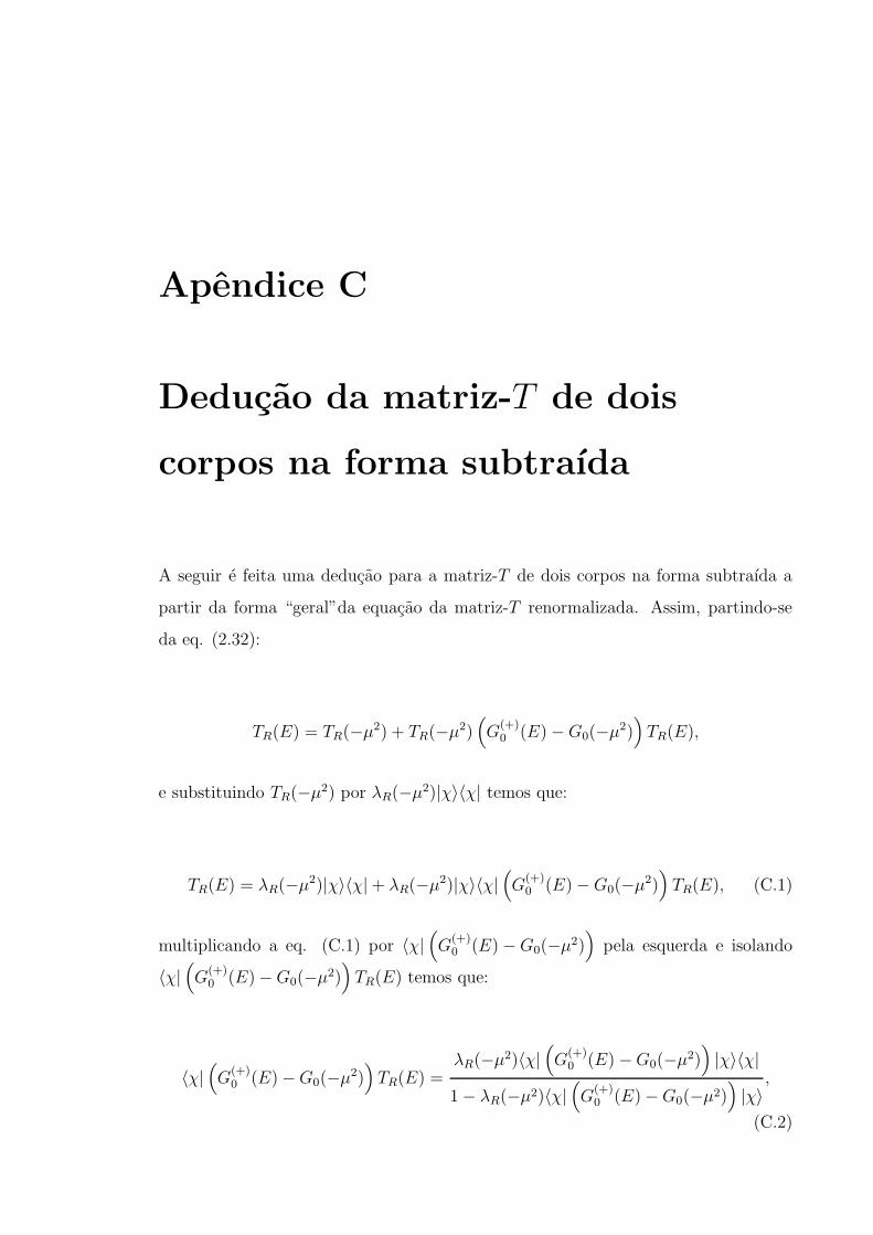
Apendice C
Deducao da matriz-T de dois
corpos na forma subtraıda
A seguir e feita uma deducao para a matriz-T de dois corpos na forma subtraıda a
partir da forma “geral”da equacao da matriz-T renormalizada. Assim, partindo-se
da eq. (2.32):
TR(E) = TR(−µ2) + TR(−µ2)(
G(+)0 (E)−G0(−µ2)
)
TR(E),
e substituindo TR(−µ2) por λR(−µ2)|χ〉〈χ| temos que:
TR(E) = λR(−µ2)|χ〉〈χ|+ λR(−µ2)|χ〉〈χ|(
G(+)0 (E)−G0(−µ2)
)
TR(E), (C.1)
multiplicando a eq. (C.1) por 〈χ|(
G(+)0 (E)−G0(−µ2)
)
pela esquerda e isolando
〈χ|(
G(+)0 (E)−G0(−µ2)
)
TR(E) temos que:
〈χ|(
G(+)0 (E)−G0(−µ2)
)
TR(E) =λR(−µ2)〈χ|
(
G(+)0 (E)−G0(−µ2)
)
|χ〉〈χ|
1− λR(−µ2)〈χ|(
G(+)0 (E)−G0(−µ2)
)
|χ〉,
(C.2)

94 C Deducao da matriz-T de dois corpos na forma subtraıda
substituindo a eq. (C.2) na eq. (C.1) chegamos na matriz-T de dois corpos na forma
subtraıda:
TR(E) = λR(−µ2)|χ〉
1 +λR(−µ2)〈χ|
(
G(+)0 (E)−G0(−µ2)
)
|χ〉〈χ|
1− λR(−µ2)〈χ|(
G(+)0 (E)−G0(−µ2)
)
|χ〉
〈χ|, (C.3)
que e a eq. (2.25) na forma subtraıda.

Apendice D
Normalizacao da funcao de onda
do estado ligado de dois corpos
∫
d3pN2
(E2 + p2)2= 1
−4π∂
∂λ
∫ ∞
0
dpN2
E2 + λp2
∣
∣
∣
∣
λ=1
= 1
−4π∂
∂λ
1
2λ
∫ ∞
−∞dp
N2
(p + i√
E2/λ)(p− i√
E2/λ)= 1
−4π∂
∂λ
N2π
2√
E2λ−1/2= 1
N =E
1/42
π(D.1)

96 D Normalizacao da funcao de onda do estado ligado de dois corpos

Apendice E
Extensao da matriz-T de dois
corpos para a segunda folha de
Riemann
A seguir faremos a extensao da equacao da matriz-T de dois corpos para a segunda
folha de Riemann como mostra a figura (E.1).
Figura E.1: Extensao da Matriz-T de Dois Corpos para a Segunda Folha de Riemann. EL
representa a energia do estado ligado de dois corpos e EV a energia do estado virtual.

98 E Extensao da matriz-T de dois corpos
Escrevendo o elemento de matriz de T na base de momento |~k 〉 e |~p 〉, temos que:
〈~k |T (E)|~p 〉 = 〈~k |V |~p 〉+
∫
d3q〈~k |V |~q 〉〈~q | T (E)
E − q2
2m+ iδ
|~p 〉, (E.1)
onde m e a massa reduzida dos dois corpos. A extensao da eq. (E.1) para a segunda
folha de Riemann e feita somando-se e subtraindo-se a descontinuidade referente ao
corte do espalhamento:
〈~k |T (E)|~p 〉 = 〈~k |V |~p 〉+
∫
d3q〈~k |V |~q 〉[
1
E − q2
2m+ iδ
− 1
E − q2
2m− iδ
]
〈~q |T (E)|~p 〉
+
∫
d3q〈~k |V |~q 〉 1
E − q2
2m− iδ
〈~q |T (E)|~p 〉. (E.2)
Vamos agora calcular a primeira integral:
I =
∫
d3q v(~k, ~q )
[
1
E − q2
2m+ iδ
− 1
E − q2
2m− iδ
]
t(~q, ~p; E), (E.3)
onde: v(~k, ~q ) ≡ 〈~k |V |~q 〉 e t(~q, ~p; E) ≡ 〈~q |T (E)|~p 〉.
I = 2m
∫
dΩq
∫ ∞
0
q2dqv(~k, ~q )
[
1
k2 − q2 + iδ− 1
k2 − q2 − iδ
]
t(~q, ~p; E)
= 2m
∫
dΩq
∫ ∞
0
q2dqv(~k, ~q )
(k + q)
[
1
k − q + iδ− 1
k − q − iδ
]
t(~q, ~p; E)
= −2m
∫
dΩq
∫ ∞
0
q2dqv(~k, ~q )
(k + q)
[
1
q − k + iδ− 1
q − k − iδ
]
t(~q, ~p; E).
onde substituımos k2 = 2mE (em unidades de ~ = 1). Utilizando o teorema dos
resıduos para fazer a integracao, vide figura (E.2):
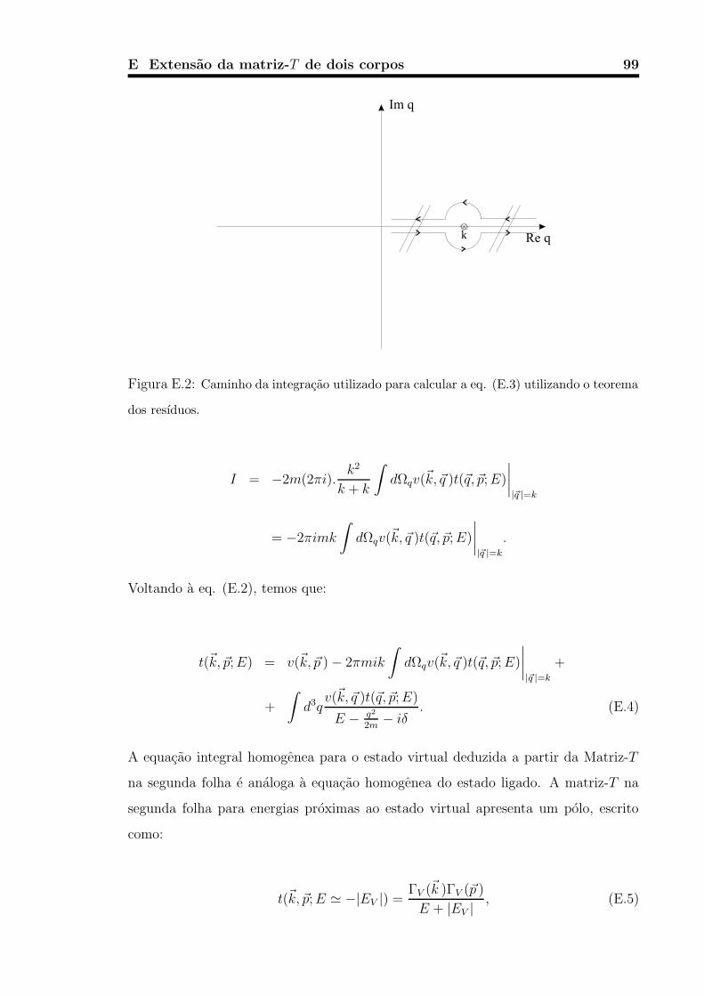
E Extensao da matriz-T de dois corpos 99
Figura E.2: Caminho da integracao utilizado para calcular a eq. (E.3) utilizando o teorema
dos resıduos.
I = −2m(2πi).k2
k + k
∫
dΩqv(~k, ~q )t(~q, ~p; E)
∣
∣
∣
∣
|~q |=k
= −2πimk
∫
dΩqv(~k, ~q )t(~q, ~p; E)
∣
∣
∣
∣
|~q |=k
.
Voltando a eq. (E.2), temos que:
t(~k, ~p; E) = v(~k, ~p )− 2πmik
∫
dΩqv(~k, ~q )t(~q, ~p; E)
∣
∣
∣
∣
|~q |=k
+
+
∫
d3qv(~k, ~q )t(~q, ~p; E)
E − q2
2m− iδ
. (E.4)
A equacao integral homogenea para o estado virtual deduzida a partir da Matriz-T
na segunda folha e analoga a equacao homogenea do estado ligado. A matriz-T na
segunda folha para energias proximas ao estado virtual apresenta um polo, escrito
como:
t(~k, ~p; E ' −|EV |) =ΓV (~k )ΓV (~p )
E + |EV |, (E.5)

100 E Extensao da matriz-T de dois corpos
onde a funcao ΓV e a funcao de vertice do estado virtual e EV a energia do estado
virtual. Assim, para E → −|EV | podemos substituir a eq. (E.5) na eq. (E.4):
ΓV (~k )ΓV (~p )
E + |EV |' −2mπ|kV |
∫
dΩqv(~k, ~q )ΓV (~q )ΓV (~p )
E + |EV |
∣
∣
∣
∣
|~q |=−i|kV |(E.6)
+
∫
d3qv(~k, ~q )1
−|EV | − q2
2m
ΓV (~q )ΓV (~p )
E + |EV |,
para o estado virtual de tres corpos, k = ±i√
2m|E| e definido com o sinal negativo.
Assim temos k = −i√
2m|EV | com kV =√
2m|EV |. Cancelando o termo ΓV (~p )E+|EV | nos
dois lados da eq. (E.6) chegamos finalmente a equacao integral homogenea para o
vertice do EV:
ΓV (~k ) = −2mπ|kV |∫
dΩqv(~k, ~q )ΓV (~q )
∣
∣
∣
∣
|~q |=−i|kV |+
∫
d3qv(~k, ~q )ΓV (~q )
−|EV | − q2
2m
. (E.7)
Podemos calcular de maneira analoga a equacao integral homogenea para o vertice
do EL:
t(~k, ~p; E) ' ΓL(~k )ΓB(~p )
E − EL
;
ΓL(~k )ΓL(~p )
E − EL'∫
d3qv(~k, ~q )
−|EL| − q2
2m
ΓL(~q )Γ(~p )
E − EL;
ΓL(~k ) =
∫
d3qv(~k, ~q )
−|EL| − q2
2m
ΓL(~q ). (E.8)
Comparando as eqs. (E.7) e (E.8) vemos que a segunda parcela da eq.
(E.7) e analoga a eq. (E.7) para o vertice do estado ligado. A existencia, porem,
da primeira parcela na eq. (E.7) faz com que, na pratica, o estado virtual “sinta”o
potencial de uma forma um pouco mais atrativa que para o estado ligado (note que
a primeira parcela e positiva v < 0).
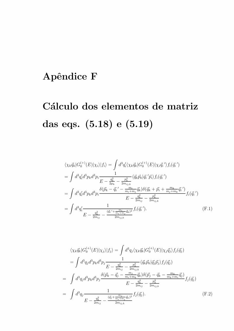
Apendice F
Calculo dos elementos de matriz
das eqs. (5.18) e (5.19)
〈χk~qk|G(+)0 (E)|χi〉|fi〉 =
∫
d3q′i〈χk~qk|G(+)0 (E)|χi~qi
′〉fi(~qi′)
=
∫
d3q′id3pkd
3pi1
E − q2k
2µk− p2
k
2mij,k
〈~qk~pk|~qi′~pi〉fi(~qi
′)
=
∫
d3q′id3pkd
3pi
δ(~pk − ~qi′ − mi
mi+mj~qk)δ(~qk + ~pi + mk
mj+mk~qi
′)
E − q2k
2mij− p2
k
2mij,k
fi(~qi′)
=
∫
d3q′i1
E − q2k
2mij−
(~qi′+
mimi+mj
~qk)2
2mij,k
fi(~qi′). (F.1)
〈χk~qk|G(+)0 (E)|χj〉|fj〉 =
∫
d3qj〈χk~qk|G(+)0 (E)|χj~qj〉fj(~qj)
=
∫
d3qjd3pkd
3pj1
E − q2k
2mij− p2
k
2mij,k
〈~qk~pk|~qj~pj〉fj(~qj)
=
∫
d3qjd3pkd
3pj
δ(~pk − ~qj − mj
mi+mk~qk)δ(~pj − ~qk − mk
mk+mi~qj)
E − q2k
2mij− p2
k
2mij,k
fj(~qj)
=
∫
d3qj1
E − q2k
2mij−
(~qj+mj
mi+mj~qk)2
2mij,k
fj(~qj). (F.2)

102 F Calculo dos elementos de matriz das eqs. (5.18) e (5.19)
〈χi~qk|G(+)0 (E)|χj〉|fj〉 =
∫
d3qj〈χi~qi|G(+)0 (E)|fj~qj〉fj(~qj)
=
∫
d3qjd3pid
3pj1
E − q2i
2mjk− p2
i
2mjk,i
〈~qi~pi|~qj~pj〉fj(~qj)
=
∫
d3qjd3pid
3pj
δ(~pi − ~qj − mj
mj+mk~qi)δ(~qi − ~pj − mi
mk+mi~qj)
E − q2i
2mjk− p2
i
2mjk,i
fj(~qj)
=
∫
d3qj1
E − q2i
2mjk−
(~qj+mj
mj+mk~qi)2
2mjk,i
fj(~qj). (F.3)

Apendice G
Calculo dos elementos de matriz
das eqs. (6.12) e (6.13)
Figura G.1: Coordenadas de Jacobi para as amplitudes de Faddeev-Yakubovsky do tipo
K, lado esquerdo, e H, lado direito.
Sejam ~ki + ~kj + ~kk + ~kk = 0 os momentos das partıculas em relacao ao
centro-de-massa (C.M.) e mα e vα (α = i, j, k, l) as suas massas e velocidades, res-
pectivamente. Podemos escrever os momentos de Jacobi que aparecem na figura em
funcao dos momentos ~k da seguinte maneira:

104 G Calculo dos elementos de matriz das eqs. (6.12) e (6.13)
~ql =ml(mi + mj + mk)
mi + mj + mk + ml
[
~vl −mi~vi + mj~vj + mk~vk
mi + mj + mk
]
= ~kl (G.1)
~qij,k =mk(mi + mj)
mi + mj + mk
[
~vk −mi~vi + mj~vj
mi + mj
]
= ~kk +mk
mi + mj + mk
~kl (G.2)
~qij =mimj
mi + mj
(~vi + ~vj) =mj
~ki −mi~kj
mi + mj
(G.3)
~qij,kl =(mi + mj)(mk + ml)
mi + mj + mk + ml
[
mk~vk + ml~vl
mk + ml
− mi~vi + mj~vj
mi + mj
]
= ~kk + ~kl (G.4)
Os elementos de matriz das eqs. (6.12) e (6.13) estao calculados a seguir.
〈~qij; ~qij,k; ~ql|~qik,j; ~ql′; ~qik〉 = δ(~ql − ~ql
′)δ(~qik −~qij
2+
3
4~qij,k)δ(~qij + ~qik,j −
~qij,k
2). (G.5)
〈~qij; ~qij,k; ~ql|~qik,l; ~qj; ~qik〉 = δ(~qij + ~qj +~qij,k
2+
1
3~ql)δ(~qik,l −
~qj
3− ~ql)
×δ(~qik + ~qij,k +~qj
2+
1
6~ql). (G.6)
〈~qij; ~qij,k; ~ql|~qik,jl; ~qjl; ~qik〉 = δ(~qik +1
2~qik,jl + ~qij,k −
1
3~ql)δ(~qik,jl + ~qij +
1
2~qij,k −
2
3~ql)
×δ(~qjl − ~qik,jl +4
3~ql) (G.7)
〈~qij,kl; ~qkl; ~qij|~qkl,i; ~qj; ~qkl′〉 = δ(~qkl − ~qkl
′)δ(~qij + ~qj +1
2~qij,kl)δ(~qkl,i +
2
3~qj + ~qij,kl).(G.8)
〈~qij,kl; ~qkl; ~qij|~qkl,ij; ~qij′; ~qkl
′〉 = δ(~qkl − ~qkl′)δ(~qij − ~qij
′)δ(~qkl,ij − ~qij,kl). (G.9)

Apendice H
Anexo dos trabalhos publicados
referentes a tese
Os seguintes trabalhos, colocados em ordem cronologica, referem-se aos assuntos tra-
tados nesta tese. Eles estao anexados nas paginas seguintes.
• “Scaling limit of virtual states of triatomic systems”de autoria de M. T. Yamashita,
T. Frederico, A. Delfino e Lauro Tomio, Physical Review A 66, 052702 (2002).
• “Weakly bound atomic trimers in ultracold traps”de autoria de M. T. Yamashita,
T. Frederico, Lauro Tomio and A. Delfino, Physical Review A 68, 033406 (2003).
• “Scaling predictions for radii of weakly bound triatomic molecules”de autoria de
M. T. Yamashita, R. S. Marques de Carvalho, Lauro Tomio e T. Frederico, Physical
Review A 68, 012506 (2003).
• “Radii in weakly-bound light halo nuclei”de autoria de M. T. Yamashita, Lauro
Tomio e T. Frederico, Nuclear Physics A 735, 40 (2004).
• “Triatomic continuum resonances for large negative scattering lengths”de autoria
de F. Bringas, M. T. Yamashita e T. Frederico, Physical Review A 69, 040702(R)
(2004).
• “Radii of weakly bound three-body systems: halo nuclei and molecules”de autoria
106 H Anexo dos trabalhos publicados referentes a tese
de M. T. Yamashita, T. Frederico, R. S. Marques de Carvalho e Lauro Tomio, Nuclear
Physics A 737, S195 (2004).
• “Three-Body Recombination in Ultracold Systems: Prediction of Weakly-Bound
Atomic Trimer Energies”de autoria de L. Tomio, V. S. Filho, M. T. Yamashita, A.
Gammal e T. Frederico, Few-Body Systems 34, 191 (2004).
PHYSICAL REVIEW A 66, 052702 ~2002!
Scaling limit of virtual states of triatomic systems
M. T. Yamashita,1 T. Frederico,2 A. Delfino,3 and Lauro Tomio41Laboratorio do Acelerador Linear, Instituto de Fı´sica, Universidade de Sa˜o Paulo, Caixa Postal 66318, CEP 05315-970,
Sao Paulo, Brazil2Departamento de Fı´sica, Instituto Tecnolo´gico de Aerona´utica, Centro Te´cnico Aeroespacial, 12228-900 Sa˜o Josedos Campos, Brazil
3Departamento de Fı´sica, Universidade Federal Fluminense, 24210-340 Nitero´i, Rio de Janeiro, Brazil4Instituto de Fı´sica Teo´rica, Universidade Estadual Paulista, 01405-900 Sa˜o Paulo, Brazil
~Received 9 March 2002; revised manuscript received 5 June 2002; published 8 November 2002!
For a system with three identical atoms, the dependence of thes-wave virtual state energy on the weaklybound dimer and trimer binding energies is calculated in the form of a universal scaling function. The scalingfunction is obtained from a renormalizable three-body model with a pairwise Dirac-d interaction. The thresh-old condition for the appearance of the trimer virtual state was also discussed.
DOI: 10.1103/PhysRevA.66.052702 PACS number~s!: 11.80.Jy, 03.65.Ge, 21.45.1v, 21.10.Dr
teata
ntta
n
siz--
tivng
to
feu
eviocb
eodysm
odp-
emlen
heteme
anysi-d toat-ue;oes
anyualfngthto-
aac-m
nce
er-sis
rac-
ndes.om-
ap-
t ism
he, ascha-lu-em.gea
I. INTRODUCTION
Weakly bound three-body zero-angular-momentum staappear in a three-boson system, with the number of stgrowing to infinity, condensing at zero energy as the pinteractions are just about to bind two particles in thes wave.These three-body states are known as the Efimov states@1,2#.Their wave functions, loosely bound, extend far beyothose of normal states and dominate the low-energy scaing phenomena in these systems. The Efimov states hbeen studied in a number of model calculations@3–5#, inatomic and nuclear systems, without yet a clear experimesignature of their occurrence@2,6–10#.
Actually, the search of Efimov states in atomic systembecoming more appealing, due to the experimental realtion of Bose-Einstein condensation@11#, and due to the possibility of altering the effective scattering length of the lowenergy atom-atom interaction in the trap, from large negato large positive values crossing the dimer zero-bindienergy value, by using an external magnetic field@12#. Thispossibility of changing the two-body scattering lengthlarge values, as recently shown in Ref.@13#, can alter in anessential way the balance between the nonlinear firstterms of the mean-field description presented in the eqtions that model Bose-Einstein condensed gases@14#. Thiscan certainly open new perspectives for theoretical andperimental investigations related to the many-body behaof condensate systems. Even in systems where the ocrence of an excited bound Efimov state has shown todoubtful or even not possible, as for example, in the cashalo nuclei like20C or 18C ~seen as a core with a halo of twneutrons! @8#, one can verify the occurrence of three-bovirtual states. The physics of these three-body systemrelated to the unusually large size of the wave function copared to the range of the potential. Thus, the detailed formthe short-ranged potential is not important for the three-bobservables@15#, which gives to the system universal proerties, defined by few physical scales@8#. Strictly speaking,in the limit of a zero-range interaction, the three-body systis parametrized by the physical two- and three-body scawhich are identified with the two-body scattering lengths aone three-body binding energy@9,16#. The physical reason
1050-2947/2002/66~5!/052702~7!/$20.00 66 0527
sesir
der-ve
tal
isa-
e-
wa-
x-r
ur-e
of
is-
ofy
s,d
for the sensibility of the three-body binding energy to tinteraction properties comes from the collapse of the sysin the limit of a zero-range force, which is known as thThomas effect@17#.
In the present work, we analyze the possibility thatexcited trimer state becomes a virtual state, when the phcal scales of the system are changed. This is expecteoccur, for example, near the limit when the two-body sctering length goes from large positive to large negative valthe corresponding two-body energy is close to zero and gfrom a bound to a virtual state, with the appearance of mbound and virtual three-body states. The three-body virtstate energy is a pole of theS matrix in the second sheet othe complex energy plane. In a general case, as the streof the two-body potential diminishes, the pole moveswards the first energy sheet to become a bound state@5#.More recently, this behavior of the Efimov state going tovirtual state with the increase of the strength of the intertion has been confirmed in realistic calculation of the heliutrimer @18#. Here, we study another aspect of the emergeof the s-wave virtual state from an Efimov state:it appearswhen the ratio between the dimer and trimer binding engies grows. This approach goes beyond a previous analyof excited three-body bound states with short-range intetions, that was performed in Ref.@9#. In Ref. @9#, a scalingfunction was introduced to analyze the behavior of bouEfimov states when modifying the triatomic physical scalEssentially, we are extending to the second sheet of the cplex energy plane~to include virtual trimer states! a previousinvestigation on a universal scaling mechanism that wasplied to two- and three-body bound states@9,10#. The exten-sion of the scaling function to the second energy sheeperformed by following the Efimov states as they move frobound to virtual, according to the variation of the ratio of tdimer to trimer bound-state energies. On the other handwe present the discussion through a universal scaling menism with the results in dimensionless units, all the concsions apply equally to any low-energy three-boson systFor the regularization and renormalization of the zero-ranmodel, we compare two different approaches: by usingmomentum cutoff parameter@9# and via kernel subtraction@16,19,20#. As the two-body energy goes to zero~or equiva-
©2002 The American Physical Society02-1

ra
tiointhfoerhoetfl
dauoe
O
adenth
erelf
r-r-
-s-t
heysy
e
od
nuc
lues
v
e
heEfi-
ed
as
thearetee-
d
inial
er-ergywo-the
YAMASHITA et al. PHYSICAL REVIEW A 66, 052702 ~2002!
lently the regularization parameter goes to infinity!, we con-clude that the results of both methods do not differ.
The paper is organized as follows. In Sec. II, we geneize the scaling function defined in Ref.@9# to include virtualtrimer states. In this section, we also revise the connecbetween the Thomas and Efimov effects, while introducour notation and the homogeneous integral equation forFaddeev component of the vertex of the wave functionzero-range potential. In Sec. III we present our main numcal results. In the Sec. III A, we present the subtractedmogeneous Faddeev equation that we have used for dmining the trimer bound and virtual states, and we brieexplain how the renormalization method of Refs.@19,20# im-plies in the subtracted three-body equation first formulateRef. @16#. In the Sec. III B, we present our new numericresults for the virtual-state energies, including the previobound-state results and we compare, as well, the resultstained by using the sharp-cutoff and the subtraction schemComparison with other calculations are also discussed.conclusions are summarized in Sec. IV.
II. THOMAS-EFIMOV EFFECT AND THE GENERALIZEDSCALING FUNCTION
In this section, we introduce the generalization of the scing function defined in Ref.@9#, to be used in the seconenergy sheet of the trimer energy. In order clarify this extsion, and to define our notation, we begin by revisingmain findings of Refs.@9,21#.
The two-boson system in the limit of a zero-range intaction has only one physical scale, which one can choosthe scattering lengtha or the energy of the bound or virtuastate. The two-bodys-wave scattering amplitude in units o\5m51 is parametrized as a function of the momentumk,by f (k)5(k cotd02ik)21, where thes-wave phase shiftd0is given byk cotd052a2111
2r0k21•••, and r 0 is the effec-
tive range. Fora.0, the two-body system is bound; othewise, for a,0, it is virtual. A short-range potential is chaacterized byr 0uau21!1 and, in this case,f (k)5(2a21
2 ik)21 and a2156AE2 (1 for bound and2 for virtualstate!.
The three-boson system for,50 in three dimensions collapses whenr 0→0 with a fixed two-body scale, which iknown as the Thomas effect@17#. Thus, the three-body system has a characteristic physical scale independent oftwo-body ones@16#. In one and two space dimensions, tcollapse is absent@15#. In the limit where the binding energof the two-boson system goes to zero, the three-bosontem has an infinite number of bound Efimov states@1# con-densing at zero energy. The Thomas and Efimov effects wshown to be physically equivalent@21#, since in both casesthe ratio between the interaction range and the two-bscattering length goes to zero.
The integral equation for the Faddeev components,f, ofthe three-boson bound-state vertex, for,50, with the zero-range interaction, needs a momentum cutoffL of the orderof r 0
21, due to the Thomas collapse. According to Ref.@21#,using units ofL51, we rescale the momentum variables athe two- and three-body binding energies, respectively, s
05270
l-
ngeri--
er-y
inlsb-s.
ur
l-
-e
-as
he
s-
re
y
dh
that pW 5LxW , qW 5LyW , E25L2e2, andE35L2e3. In this di-mensionless variables, after redefiningf as x(xW )[L3/2f(pW ), we obtain the integral equation@21,7,8#:
x~yW !52p22
6Ae22Ae31 34 yW 2
E d3xu~12uxW u!
e31yW 21xW21yW•xWx~xW !.
~1!
The number of three-body bound states, given by the vaof e3 that satisfies Eq.~1!, grows without limit whene2
decreases to zero;e35e3(N) (N50,1,2, . . . ), with
e3(N)/e3
(N11)'500 @1#. They are the energies of the Efimostates, in units ofL51. But, the limit of e2 going to zerocan be realized either byE2→0 ~with a fixed L) or by L;r 0
21→` ~with E2 fixed!. In this last case, the range of thinteraction is set to zero and the system collapses;E3
(0)
5e3(0)L2→`. This is known as the Thomas collapse of t
three-body ground state. Therefore, the Thomas and themov states are given by the same limite2→0 of Eq.~1!, andare related by a scale transformation@21#.
Now, the concept of the scaling function is introducaccording to Ref.@9#. For a nonvanishinge2, the solutions ofEq. ~1! defines the dimensionless three-body energiesfunctions of 6Ae2; e3
(N)[e3(N)(6Ae2). Using theNth en-
ergy to obtainL, thenL25E3(N)/e3
(N) , and
E3(N11)5E3
(N)e3
(N11)~j!
e3(N)
, ~2!
where j[6Ae256(E2e3(N)/E3
(N))1/2. In Eq. ~2!, the two-and three-body physical scales determineE3
(N11) , the nextexcited state aboveE3
(N) . In Ref. @9#, E3(N) was identified
with the three-body scale, as any stateN works equally wellto set the trimer scale. However, we will be interested intwo most excited three-body states that, in practice, wegoing to identify with the ground- and the first-excited-stain triatomic systems. This identification is unambiguous bcause, withN and N11 being two consecutive excitestates, the limit
E3(N11)
E3(N)
5 limN→`
e3(N11)~j!
e3(N)
5FS 6A E2
E3(N)D ~3!
exists and defines the scaling functionF @8,9#. A qualitativeargument to explain the scaling limit has been providedRef. @9# based on the notion of the long-range potent@1,2,22#.
In the following, we provide the generalization of thscaling function~3!, which is obtained by extending the fomalism to the second sheet of the three-body complex enplane. In the present approach, we only consider the tbody subsystem as bound. For this purpose, we definegeneral scaling functionK, given by
2-2
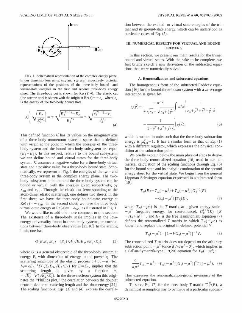
isnequmoduachn
wonb
eyd
nwla
i-le
-
tri-d as
erwe
ua-
qua-ge
ion
on-
ive
onderalorm
ry
the
trac-
anlaner
SCALING LIMIT OF VIRTUAL STATES OF . . . PHYSICAL REVIEW A 66, 052702 ~2002!
KSA E2
E3(N)D [6AE3
(N11)2E2
E3(N)
56Ae3(N11)2e2
e3(N)
.
~4!
This defined functionK has its values on the imaginary axof a three-body momentum space; a space that is defiwith origin at the point in which the energies of the threbody system and the bound two-body subsystem are e(E35E2). In this respect, relative to the bound subsystewe can define bound and virtual states for the three-bsystem.K assumes a negative value for a three-body virtstate and a positive value for a three-body bound state. Smatically, we represent in Fig. 1 the energies of the two- athree-body system in the complex energy plane. The tbody subsystem is bound and the three-body system cabound or virtual, with the energies given, respectively,e3B and e3V . Through the elastic cut~corresponding to theatom-dimer elastic scattering!, one defines two sheets; in thfirst sheet, we have the three-body bound-state energRe(e)52e3B ; in the second sheet, we have the three-bovirtual-state energy at Re(e)52e3V , as illustrated in Fig. 1.
We would like to add one more comment to this sectioThe existence of a three-body scale implies in the loenergy universality found in three-body systems, or corretions between three-body observables@23,16#. In the scalinglimit, one has
O~E,E3 ,E2!5~E3!hA~AE/E3,AE2 /E3!, ~5!
whereO is a general observable of the three-body systemenergyE, with dimension of energy to the powerh. Thescattering amplitude of the elastic processa1bc→a1bc,f 35AE3
21F(AE/E3,AE2 /E3) for E5E2, implies that thescattering length is given by a functiona3
5AE321F(AE2 /E3). In the three-nucleon system this orig
nates the ‘‘Phillips plot,’’ the correlation between the doubneutron-deuteron scattering length and the triton energy@24#.The scaling functions, Eqs.~3! and ~4!, express the correla
FIG. 1. Schematical representation of the complex energy plin our dimensionless units.e3B and e3V are, respectively, pictoriarepresentations of the positions of the three-body bound-virtual-state energies in the first and second three-body ensheet. The three-body cut is shown for Re(e).0. The elastic cut~the narrow one! is shown with the origin at Re(e)52e2, wheree2
is the energy of the two-body bound state.
05270
ed-al,yle-d-be
y
aty
.--
at
t
tion between the excited- or virtual-state energies of themer and its ground-state energy, which can be understooparticular cases of Eq.~5!.
III. NUMERICAL RESULTS FOR VIRTUAL AND BOUNDTRIMERS
In this section, we present our main results for the trimbound and virtual states. With the sake to be complete,first briefly sketch a new derivation of the subtracted eqtions that were numerically solved.
A. Renormalization and subtracted equations
The homogeneous form of the subtracted Faddeev etion @16# for the bound three-boson system with a zero-raninteraction is given by
x~yW !52p22
6Ae22Ae31 34 yW 2
E d3xS 1
e31yW 21xW21yW•xW
21
11yW 21xW21yW•xWD x~xW !, ~6!
which is written in units such that the three-body subtractenergy ism (3)
2 51. It has a similar form as that of Eq.~1!with a different regulator, which expresses the physical cdition at the subtraction point.
We briefly explain below the main physical steps to derthe three-body renormalized equation@16# used in our nu-merical calculation of the scaling functions through Eq.~6!for the bound state and its analytic continuation to the secenergy sheet for the virtual state. We begin from the genLippman-Schwinger equation expressed in a subtracted f@19#:
TR~E!5TR~2m2!1TR~2m2!@G0(1)~E!
2G0~2m2!#TR~E!, ~7!
where TR(2m2) is the T matrix at a given energy scale2m2 ~negative energy, for convenience!, G0
(1)(E)5@E2H01 id#21, andH0 is the free Hamiltonian. Equation~7!defines the renormalizedT matrix in which TR(2m2) isknown and replace the original ill-defined potentialV:
TR~2m2!5@12VG0~2m2!#21V. ~8!
The renormalizedT matrix does not depend on the arbitrasubtraction point2m2 ~oncedV/dm250), which implies ina Callan-Symanzik-type@19,20# equation forTR(2m2):
d
dm2TR~2m2!5TR~2m2!@G0~2m2!#2TR~2m2!. ~9!
This expresses the renormalization-group invariance ofsubtracted equation.
To solve Eq.~7! for the three-bodyT matrix TR(3)(E), a
dynamical assumption has to be made at a particular sub
e,
dgy
2-3

eyinisit
al
t
d
y,n
dts
ay
-
nsl
r
.
as-be
telyto
en-
lo
, ofssed
ob-dycat-
of
ond
e is
ofndmall
en’s
YAMASHITA et al. PHYSICAL REVIEW A 66, 052702 ~2002!
tion point 2m (3)2 , where we assume that the three-bodyT
matrix is equal to the driving term, which is given by thsum of the pairwise two-bodyT matrices. Thus, at the energ2m (3)
2 , it is assumed that the three-body multiple-scatterseries vanishes beyond the driving term. Observe that thnot true for a regular finite-range potential, only in the limof m (3)→`. However, in the scaling limit, in fact, the actuvalue ofm (3) tends to infinity such thatE2 /m (3)
2 goes to zero,as it be will be clear in our numerical calculations.
With our assumption, theT matrix at the subtraction poinm (3) is given by
TR(3)~2m (3)
2 !5(( i j )
TR( i j )(2) S 2m (3)
2 2qk
2
2mk( i j )D , ~10!
where (i , j ,k)5(1,2,3), ~2,3,1!, ~3,1,2!. The summation isperformed over all pairs and the renormalized two-boT-matrix elements for the pair (i j ) are given by
^PW 8uTR(2)(E)uPW &51/@2p2(6AE21 iAE)#. The argument of
the two-bodyT matrix is the center-of-mass pair energwhereqk is the Jacobi relative momentum canonically cojugated to the relative coordinate of the particlek to thecenter of mass of the pair (i j ), and mk( i j ) is the reducedmass.
Using Eqs.~7! and ~10! and after some straightforwarmanipulations, the equations for the Faddeev componenthe T matrix at the bound-state pole give Eq.~6!, which hasa natural momentum scale given bym (3)
2 . In principle,m (3)2
can be varied without changing the content of the theorylong as the three-bodyT matrix at the new subtraction energm (3)
2 is found from the solution of Eq.~9! with the boundarycondition Eq.~10!; and consequently, Eq.~6! should be con-veniently rewritten. In the scaling limit, Eqs.~1! and ~6!produce the same results~as we are going to illustrate numerically!, since they are solved fore2 going to zero, and thedetailed form of the regularization implied in both equatiois not important anymore. However, Eq.~6! has conceptuaand practical advantages over Eq.~1!, namely, it is explicitlyrenormalization-group invariant and also regularized.
To simplify the notation of Eq.~6!, we introduce anothedefinition related to the two-body energy;k2[6Ae2, where1 refers to bound and2 to virtual two-body-state energiesAfter partial-wave projection of Eq.~6!, the s-wave integralequation for the three-boson system is
xs~y!5t~y;e3 ;k2!E0
`
dx x2G~y,x;e3!xs~x!, ~11!
where
t~y;e3 ;k2!522
p FAe313
4y22k2G21
, ~12!
05270
gis
y
-
of
s
G~y,x;e3!5~e321!
3E21
1
dz1
~e31y21x21yxz!~11y21x21yxz!.
~13!
For the,th angular-momentum three-body state, the Thomcollapse is forbidden if,.0; consequently, no regularization is required and the integration over momentum canextended to infinity even in the limitm (3)→`. For,.0, theoriginal Skornyakov and Ter-Martirosian equation@25# iswell defined, and the three-body observables are compledetermined by the two-body physical scale correspondingE2. One finds examples of the disappearance of the depdence on the three-body scale inp-wavevirtual states, for thetrineutron system whenn-n is artificially bound@26,27#, andin three-body halo nuclei~represented as a core with a haof two neutrons! @28#.
The analytic continuation to the second energy sheetthe scattering equations for separable potentials, is discuin detail by Glockle, in Ref.@26#. The particular case of thezero-range three-body model@25# is also given in Ref.@29#.On the second energy sheet, the integral equations aretained by the analytical continuation through the two-boelastic scattering cut corresponding to the atom-dimer stering. The elastic scattering cut comes through the polethe atom-atom elastic scattering amplitude in Eq.~12!. Weperform the analytic continuation of Eq.~11! to the secondenergy sheet. By substituting the spectator functionxs(y) byxs(y)[(e3v2e21 3
4 y2)xs(y), wheree3v is the modulus ofthe virtual-state energy, the resulting equation in the secenergy sheet is given by
xs~y!5 t~y;e3v ;k2!4pk3v
3G~y,2 ik3v ;e3v!xs~2 ik3v!
1 t~y;e3v ;k2!E0
`
dx x2G~y,x;e3v!xs~x!
e3v2e213
4x2
, ~14!
where the on-energy-shell momentum at the virtual stat
k3v[A 43 (e3v2e2), and
t~y;e3v ;k2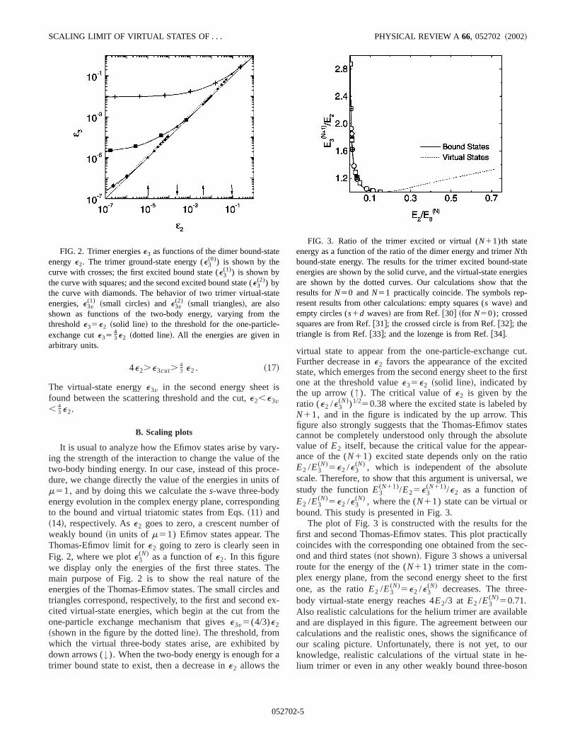
is
rythces
in
oen
hthae
th
ba
cut.dfirst
byis
ateslutear-tiotewe
r
eallyec-l
first-
leour
e ofure-on
te
te
he-
tatergiesthe-
SCALING LIMIT OF VIRTUAL STATES OF . . . PHYSICAL REVIEW A 66, 052702 ~2002!
4e2.e3cut.43 e2 . ~17!
The virtual-state energye3v in the second energy sheetfound between the scattering threshold and the cut,e2,e3v, 4
3 e2.
B. Scaling plots
It is usual to analyze how the Efimov states arise by vaing the strength of the interaction to change the value oftwo-body binding energy. In our case, instead of this produre, we change directly the value of the energies in unitm51, and by doing this we calculate thes-wave three-bodyenergy evolution in the complex energy plane, correspondto the bound and virtual triatomic states from Eqs.~11! and~14!, respectively. Ase2 goes to zero, a crescent numberweakly bound~in units of m51) Efimov states appear. ThThomas-Efimov limit fore2 going to zero is clearly seen iFig. 2, where we plote3
(N) as a function ofe2. In this figurewe display only the energies of the first three states. Tmain purpose of Fig. 2 is to show the real nature ofenergies of the Thomas-Efimov states. The small circlestriangles correspond, respectively, to the first and secondcited virtual-state energies, which begin at the cut fromone-particle exchange mechanism that givese3v5(4/3)e2~shown in the figure by the dotted line!. The threshold, fromwhich the virtual three-body states arise, are exhibiteddown arrows (↓). When the two-body energy is enough fortrimer bound state to exist, then a decrease ine2 allows the
FIG. 2. Trimer energiese3 as functions of the dimer bound-staenergye2. The trimer ground-state energy (e3
(0)) is shown by thecurve with crosses; the first excited bound state (e3
(1)) is shown bythe curve with squares; and the second excited bound state (e3
(2)) bythe curve with diamonds. The behavior of two trimer virtual-staenergies,e3v
(1) ~small circles! and e3v(2) ~small triangles!, are also
shown as functions of the two-body energy, varying from tthresholde35e2 ~solid line! to the threshold for the one-particleexchange cute35
43 e2 ~dotted line!. All the energies are given in
arbitrary units.
05270
-e-
of
g
f
eendx-e
y
virtual state to appear from the one-particle-exchangeFurther decrease ine2 favors the appearance of the excitestate, which emerges from the second energy sheet to theone at the threshold valuee35e2 ~solid line!, indicated bythe up arrow (↑). The critical value ofe2 is given by theratio (e2 /e3
(N))1/250.38 where the excited state is labeledN11, and in the figure is indicated by the up arrow. Thfigure also strongly suggests that the Thomas-Efimov stcannot be completely understood only through the absovalue ofE2 itself, because the critical value for the appeance of the (N11) excited state depends only on the raE2 /E3
(N)5e2 /e3(N) , which is independent of the absolu
scale. Therefore, to show that this argument is universal,study the functionE3
(N11)/E25e3(N11)/e2 as a function of
E2 /E3(N)5e2 /e3
(N) , where the (N11) state can be virtual obound. This study is presented in Fig. 3.
The plot of Fig. 3 is constructed with the results for thfirst and second Thomas-Efimov states. This plot practiccoincides with the corresponding one obtained from the sond and third states~not shown!. Figure 3 shows a universaroute for the energy of the (N11) trimer state in the com-plex energy plane, from the second energy sheet to theone, as the ratioE2 /E3
(N)5e2 /e3(N) decreases. The three
body virtual-state energy reaches 4E2/3 at E2 /E3(N)50.71.
Also realistic calculations for the helium trimer are availaband are displayed in this figure. The agreement betweencalculations and the realistic ones, shows the significancour scaling picture. Unfortunately, there is not yet, to oknowledge, realistic calculations of the virtual state in hlium trimer or even in any other weakly bound three-bos
FIG. 3. Ratio of the trimer excited or virtual (N11)th stateenergy as a function of the ratio of the dimer energy and trimerNthbound-state energy. The results for the trimer excited bound-senergies are shown by the solid curve, and the virtual-state eneare shown by the dotted curves. Our calculations show thatresults forN50 andN51 practically coincide. The symbols represent results from other calculations: empty squares (s wave! andempty circles (s1d waves! are from Ref.@30# ~for N50); crossedsquares are from Ref.@31#; the crossed circle is from Ref.@32#; thetriangle is from Ref.@33#; and the lozenge is from Ref.@34#.
2-5
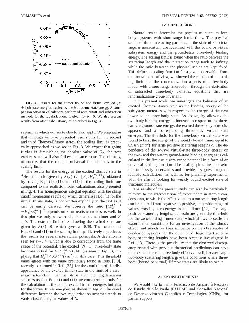
sizotiin
isth
i
nta
it
e
si
te
rotiorlsas
w-icalotalal
dingtheity,ed.omal-dyion
anthenextheee-dis-tatewasl to
ncal-anfulidets,
of
arlyn-
gthof
oldheov
oftwo-d inp-
averge
ee-
l
-tiot
YAMASHITA et al. PHYSICAL REVIEW A 66, 052702 ~2002!
system, in which our route should also apply. We emphathat although we have presented results only for the secand third Thomas-Efimov states, the scaling limit is praccally approached as we see in Fig. 3. We expect that gofurther in diminishing the absolute value ofE2, the newexcited states will also follow the same route. The claimof course, that the route is universal for all states inscaling limit.
The results for the energy of the excited Efimov state4He3 molecule given byK(z) (z5@E2 /E3
(N)#1/2), obtainedby solving Eqs.~1!, ~11!, and ~14! in the scaling limit, arecompared to the realistic model calculations also presein Fig. 4. The homogeneous integral equation with the shcutoff momentum regulator, which generalizes Eq.~1! for thevirtual trimer state, is not written explicitly in the text ascan be easily derived. We observe the ratio@(E3
(N11)
2E2)/E3(N)#1/2 depends onz for realistic models as well. In
this plot we only show results for a bound dimer andN50. The extreme limit ofz allowing the excited state argiven by K(z)50, which givesz50.38. The solution ofEqs.~1! and~11! in the scaling limit qualitatively reproducethe results for several interatomic potentials. A deviationseen forz'0.4, which is due to corrections from the finirange of the potential. The excited (N11) three-body statebecomes virtual forE2 /E3
(N).0.145~as seen in Fig. 3!, im-plying that E3
(N),6.9\2/(ma2) in this case. This thresholdvalue agrees with the value previously found in Refs.@8,9#,recently confirmed in Ref.@35#, for the condition of the dis-appearance of the excited trimer state in the limit of a zerange interaction. Let us stress that the regularizaschemes used in Eqs.~1! and~11! are consistent not only fothe calculation of the bound excited trimer energies but afor the virtual trimer energies, as shown in Fig. 4. The smdifference between the two regularization schemes tendvanish fast for higher values ofN.
FIG. 4. Results for the trimer bound and virtual excited (N11)th state energies, scaled by theNth bound-state energy. A comparison between calculations performed with cutoff and subtracmethods for the regularizations is given forN50. We also presenresults from other calculations, as described in Fig. 3.
05270
end-g
,e
n
edrp
s
-n
ollto
IV. CONCLUSIONS
Natural scales determine the physics of quantum febody systems with short-range interactions. The physscales of three interacting particles, in the state of zero tangular momentum, are identified with the bound or virtusubsystem energy and the ground-state three-body binenergy. The scaling limit is found when the ratio betweenscattering length and the interaction range tends to infinwhile the ratio between the physical scales are kept fixThis defines a scaling function for a given observable. Frthe formal point of view, we showed the relation of the scing limit and the renormalization aspects of a few-bomodel with a zero-range interaction, through the derivatof subtracted three-bodyT-matrix equations that arerenormalization-group invariant.
In the present work, we investigate the behavior ofexcited Thomas-Efimov state as the binding energy ofsubsystem increases with respect to the energy of thelower bound three-body state. As shown, by allowing ttwo-body binding energy to increase in respect to the thrparticle ground-state energy, the excited three-body stateappears, and a corresponding three-body virtual semerges. The threshold for the three-body virtual statefound to be at the energy of the weakly bound trimer equa6.9\2/(ma2) for large positive scattering lengthsa. The de-pendence of thes-wave virtual-state three-body energy othe two- and three-atom ground-state binding energies isculated in the limit of a zero-range potential in a form ofuniversal scaling function. The scaling plots are an usetool to classify observables and provide first guess to gurealistic calculations, as well as for planning experimenwith the aim of looking for weakly bound excited statetriatomic molecules.
The results of the present study can also be particulrelevant to the interpretation of experiments in atomic codensation, in which the effective atom-atom scattering lencan be altered from negative to positive, in a wide rangevalues crossing zero-energy bound dimer@12#. For largepositive scattering lengths, our estimate gives the threshfor the zero-binding trimer state, which allows to settle texperimental conditions for an investigation of the Efimeffect, and search for their influence on the observablescondensed systems. On the other hand, large negativebody scattering lengths have been recently investigateRef. @13#. There is the possibility that the observed discreancy related with previous theoretical predictions can htheir explanations in three-body effects as well, because latwo-body scattering lengths give the conditions where thrbody ~bound or virtual! Efimov states are likely to occur.
ACKNOWLEDGMENTS
We would like to thank Fundac¸ao de Amparo a` Pesquisado Estado de Sa˜o Paulo~FAPESP! and Conselho Nacionade Desenvolvimento Cientı´fico e Tecnolo´gico ~CNPq! forpartial support.
n
2-6
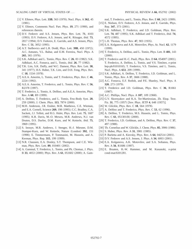
ys
A
v.
.
an
n
M
A.
ie
ys
ys.
v.
.
. A
r.
s.
s.
nt
SCALING LIMIT OF VIRTUAL STATES OF . . . PHYSICAL REVIEW A 66, 052702 ~2002!
@1# V. Efimov, Phys. Lett.33B, 563~1970!; Nucl. Phys. A362, 45~1981!.
@2# V. Efimov, Comments Nucl. Part. Phys.19, 271 ~1990!, andreferences therein.
@3# D.V. Fedorov and A.S. Jensen, Phys. Rev. Lett.71, 4103~1993!; D.V. Fedorov, A.S. Jensen, and K. Riisager,ibid. 73,2817~1994!; D.V. Fedorov, E. Garrido, and A.S. Jensen, PhRev. C51, 3052~1995!.
@4# A.T. Stelbovics and L.R. Dodd, Phys. Lett.39B, 450 ~1972!;A.C. Antunes, V.L. Baltar, and E.M. Ferreira, Nucl. Phys.265, 365 ~1976!.
@5# S.K. Adhikari and L. Tomio, Phys. Rev. C26, 83 ~1982!; S.K.Adhikari, A.C. Fonseca, and L. Tomio,ibid. 26, 77 ~1982!.
@6# T.K. Lim, S.K. Duffy, and W.C. Damest, Phys. Rev. Lett.38,341 ~1977!; H.S. Huber, T.K. Lim, and D.H. Feng, Phys. ReC 18, 1534~1978!.
@7# A.E.A. Amorim, L. Tomio, and T. Frederico, Phys. Rev. C46,2224 ~1992!.
@8# A.E.A. Amorim, T. Frederico, and L. Tomio, Phys. Rev. C56,R2378~1997!.
@9# T. Frederico, L. Tomio, A. Delfino, and A.E.A. Amorim, PhysRev. A60, R9 ~1999!.
@10# A. Delfino, T. Frederico, and L. Tomio, Few-Body Syst.28,259 ~2000!; J. Chem. Phys.113, 7874~2000!.
@11# M.H. Anderson, J.R. Ensher, M.R. Matthews, C.E. Wiemand E.A. Cornell, Science269, 198~1995!; C.C. Bradley, C.A.Sackett, J.J. Tollett, and R.G. Hulet, Phys. Rev. Lett.75, 1687~1995!; K.B. Davis, M.-O. Mewes, M.R. Andrews, N.J. vaDruten, D.S. Durfee, D.M. Kurn, and W. Ketterle,ibid. 75,3969 ~1995!.
@12# S. Inouye, M.R. Andrews, J. Stenger, H.-J. Miesner, D.Stamper-Kurn, and W. Ketterle, Nature~London! 392, 151~1998!; E. Timmermans, P. Tommasini, M. Hussein, andKerman, Phys. Rep.315, 199 ~1999!.
@13# N.R. Claussen, E.A. Donley, S.T. Thompson, and C.E. Wman, Phys. Rev. Lett.89, 010401~2002!.
@14# A. Gammal, T. Frederico, L. Tomio, and Ph. Chomaz, J. PhB 33, 4053~2000!; Phys. Rev. A61, 051602~2000!; A. Gam-
05270
.
,
.
-
.
mal, T. Frederico, and L. Tomio, Phys. Rev. E60, 2421~1999!.@15# E. Nielsen, D.V. Fedorov, A.S. Jensen, and E. Garrido, Ph
Rep.347, 373 ~2001!.@16# S.K. Adhikari, T. Frederico, and I.D. Goldman, Phys. Re
Lett. 74, 487 ~1995!; S.K. Adhikari and T. Frederico,ibid. 74,4572 ~1995!.
@17# L.H. Thomas, Phys. Rev.47, 903 ~1935!.@18# E.A. Kolganova and A.K. Motovilov, Phys. At. Nucl.62, 1179
~1999!.@19# T. Frederico, A. Delfino, and L. Tomio, Phys. Lett. B481, 143
~2000!.@20# T. Frederico and H.-C. Pauli, Phys. Rev. D64, 054007~2001!;
T. Frederico, A. Delfino, L. Tomio, and V.S. Timo´teo, e-printhep-ph/01010165; T. Frederico, V.S. Timo´teo, and L. Tomio,Nucl. Phys. A653, 209 ~1999!.
@21# S.K. Adhikari, A. Delfino, T. Frederico, I.D. Goldman, and LTomio, Phys. Rev. A37, 3666~1988!.
@22# A.C. Fonseca, E.F. Redish, and P.E. Shanley, Nucl. Phys320, 273 ~1979!.
@23# T. Frederico and I.D. Goldman, Phys. Rev. C36, R1661~1987!.
@24# A.C. Phillips, Nucl. Phys. A107, 109 ~1968!.@25# G.V. Skornyakov and K.A. Ter-Martirosian, Zh. Eksp. Teo
Fiz. 31, 775 ~1957! @Sov. Phys. JETP4, 648 ~1957!#.@26# W. Glockle, Phys. Rev. C18, 564 ~1978!.@27# A. Delfino and T. Frederico, Phys. Rev. C53, 62 ~1996!.@28# A. Delfino, T. Frederico, M.S. Hussein, and L. Tomio, Phy
Rev. C61, 051301~R! ~2000!.@29# T. Frederico, I.D. Goldman, and A. Delfino, Phys. Rev. C37,
497 ~1988!.@30# Th. Cornelius and W. Glo¨ckle, J. Chem. Phys.85, 3906~1986!.@31# S. Huber, Phys. Rev. A31, 3981~1985!.@32# P. Barletta and A. Kievsky, Phys. Rev. A64, 042514~2001!.@33# D.V. Fedorov and A.S. Jensen, J. Phys. A34, 6003~2001!.@34# E.A. Kolganova, A.K. Motovilov, and S.A. Sofianos, Phy
Rev. A56, R1686~1997!.@35# E. Braaten, H.-W. Hammer, and M. Kusunoki, e-pri
cond-mat/0201281.
2-7

PHYSICAL REVIEW A 68, 033406 ~2003!
Weakly bound atomic trimers in ultracold traps
M. T. Yamashita,1 T. Frederico,2 Lauro Tomio,3 and A. Delfino41Laboratorio do Acelerador Linear, Instituto de Fı´sica da USP, 05315-970 Sa˜o Paulo, Brazil
2Departamento de Fı´sica, Instituto Tecnolo´gico de Aerona´utica, Centro Te´cnico Aeroespacial, 12228-900 Sa˜o Josedos Campos, Brazil3Instituto de Fı´sica Teo´rica, Universidade Estadual Paulista, 01405-900 Sa˜o Paulo, Brazil
4Instituto de Fı´sica, Universidade Federal Fluminense, 24210-900 Nitero´i, Rio de Janeiro, Brazil~Received 13 March 2003; published 15 September 2003!
The experimental three-atom recombination coefficients of the atomic states23NauF51,mF521&,87RbuF51,mF521&, and85RbuF52,mF522&, together with the corresponding two-body scattering lengths,allow predictions of the trimer bound-state energies for such systems in a trap. The recombination parameter isgiven as a function of the weakly bound trimer energies, which are in the interval 1,m(a/\)2E3,6.9 forlarge positive scattering lengthsa. The contribution of a deep-bound state to our prediction, in the case of85RbuF52,mF522&, for a particular trap, is shown to be relatively small.
DOI: 10.1103/PhysRevA.68.033406 PACS number~s!: 32.80.Pj, 36.40.2c, 34.10.1x
f-o
e
d-inouape
misdil
a, cindthb
reetlit
amnestod
tethri
ta
e incan
lyd for
isentonsheeter
rcor-t, inness
ofvia
-
the-intoonver,ndthe
es,n-
ct
ectdythan
r
re-
if-
The formation of molecules in ultracold atomic traps ofers new and exciting possibilities to study the dynamicscondensates@1#. The formation of rubidium molecules87Rb2
in a bosonic condensate was reported, which allowed to msure its binding energy with unprecedented accuracy@2#. Ul-tracold sodium molecules23Na2 have also been formethrough photoassociation@3#. However, nothing has been reported till now about the formation of molecular trimerscold traps. The first information, one is led to ask, is abthe magnitude of the binding energy of trimers in a cold trTwo-body scattering lengths of trapped atoms are wknown in several cases, as well as their closely related dibinding energy. In the limit of large scattering lengths, itnecessary to know in addition one low-energy three-boobservable to predict any other one. In this case, the detaform of the two-body interaction is not important@4,5#. Therecombination rate of three atoms in the ultracold limit, mesured by atomic losses in trapped condensed systemssupply the necessary information to estimate the trimer bing energy. For short-range interactions, the magnitude ofrecombination rate of three atoms is mainly determinedthe two-body scattering lengtha @6#. However, it is importantto remark that a dependence on one typical low-energy thbody scale@4,5# still remains. Indeed, it is gratifying to notthat all the works on three-body recombination, consistenpresent a dependence on a three-body parameter in addto the scattering length@7–9#.
The aim of the present work is to report on how one cobtain the trimer binding energy of a trapped atomic systefrom the three-body recombination rate and the correspoing two-body scattering length. For this purpose, we usscale independent approach valid in the limit of large potive scattering lengths~or when the interaction range goeszero!, obtained from a renormalized zero-range three-botheory @4#, which relates the recombination rate, the scating length, and the trimer binding energy. Consideringexperimental values of the recombination rates and scattelengths given in Refs.@10–13#, the method is applied topredict the trimer binding energies of23NauF51,mF521&, 87RbuF51,mF521&, and 85RbuF52,mF522&,where uF,mF& is the respective hyperfine states of the to
1050-2947/2003/68~3!/033406~5!/$20.00 68 0334
f
a-
t.ller
yed
-an-ey
e-
y,ion
n,
d-ai-
yr-eng
l
spin F. We note that the bound states considered here arfact high-lying resonances, not true bound states, as theydecay into lower-lying channels.
The validity of our approach is restricted to sufficientdiluted gases, because all the scaling relations are derivethree isolated particles. Also, when the scattering lengthtuned via external field in a trap, the parameters are differfrom the vacuum values, and consequently, our predictionly apply to that particular experimental conditions. For ttrapped gases that we are analyzing, the diluteness paramra3 ~wherer is the gas density! should not be much largethan one, otherwise one needs to consider higher-orderrelations between the particles. Indeed, we observe thageneral, for the analyzed condensed systems, the diluteparameter is much smaller than one. Even in the case85Rb, where the considered scattering length is obtainedFeshbach resonance techniques@13#, the diluteness parameter is about 1/2.
Another relevant remark, pointed out in Ref.@14#, is thatthe recombination into deep-bound states can affect theoretical results that are based on calculation of this rateshallow states alone. This additive contribution dependsone more constant, beyond the three-body scale. Howethe fitted contribution of the recombination into deep-boustates is fortunately much smaller than the contribution ofshallow bound state, as found in the case of85Rb @14#. Suchan evidence supports our estimation of trimer energiwhen a.0, that are obtained by only considering the cotribution of recombination rates into the shallow state.
The values ofa are usually defined as large with respeto the effective ranger 0, such thata/r 0@1. The low-energythree-boson system presents, in this limit, the Efimov eff@15#, where an infinite number of weakly bound three-bostates appears. The size of such states are much largerthe effective range. The limita/r 0→` can be realized eitheby a→` with r 0 kept constant or byr 0→0 with a constant.In the last case, the limit of a zero-range interaction corsponds to the Thomas bound-state collapse@16#. In this re-spect, the Efimov and Thomas limits are equivalent or dferent aspects of the same physics@17#. The Thomas-Efimovconnection is also reviewed in Ref.@5#. In the limit a/r 0
©2003 The American Physical Society06-1

eca
bgb
foee
eo
at
thde
of
n
Thp
avin
1/
.
a
rg
as
re-
tify-e-s; it
ion
n
e
ve-ach
ge-l-
YAMASHITA et al. PHYSICAL REVIEW A 68, 033406 ~2003!
→`, the details of the interaction for the low-energy threbody system are contained in one typical three-body sand the two-body scattering length~or the dimer bound-stateenergyE2); they are enough to determine all three-body oservables@4#. Considering, for example, the trimer bindinenergyE3 as the three-body scale, any three-body observaO3 that has dimension of (energy)b, in the limit of r 0→0,can be expressed as
O35E2bF2~E2 /E3!5E3
bF3~E2 /E3!. ~1!
The dimensional factor in the above equation is chosenconvenience asE2 or E3. The scaling function in each casis F2 or F3. The existence of the scaling limit for zero-ranginteractions was verified in Refs.@18,19#. In practice, such alimit is approached by the excited state of the atomic trimobtained in realistic calculations, allowing as well the theretical interpretation of those excited states as Efimov st@19#. Here, we observe that the binding energyE3 refers tothe magnitude of the total energy of the bound system;binding energy with respect to the two-body threshold isfined asS3[E32E2.
The rate of three free bosons to recombine, formingdimer and one remaining particle, is given in the limitzero energy, by the recombination coefficient@5,6#
K35\
ma4a, ~2!
wherea is a dimensionless parameter andm is the mass ofthe atom. Whena.0, the recombination parametera oscil-lates between zero and a maximum value, which is a fution of a, as shown in Refs.@7# (a<68.4), @8# (a<65), and@9# (a<67.9). With amplitudeamax and phased, we canwrite it as @5#
[email protected] ln~a!1d#, ~3!
whered depends on the interaction at short distances.physics at short distances, in the three-boson system, isrametrized by one typical three-body scale, which we hchosen as the unknown trimer binding energy. So, by usthe general scaling given by Eq.~1!, one can explicitly ex-press the functional dependence ofa as a[a(AE2 /E3),considering that for large scattering lengths we havea5AmE2 /\2. To exemplify the scaling form ofa, we canrewrite Eq.~3! such that theAE2 /E3 dependence is explicitTherefore,
a5amaxsin2F21.01 lnAE2
E31DSAE2
E3D G , ~4!
whereD(AE2 /E3)5d21.01 ln(AmE3 /\2). Our next task isthe calculation of the scaling function by using the renormized subtracted Faddeev equations@4#.
The three-boson recombination coefficient at zero eneis derived from the Fermi’s golden rule as
03340
-le
-
le
r
r-es
e-
a
c-
ea-eg
l-
y
K352p
\~2p\!9E d3p
~2p\!3uTi→fu2dS 3
4mp22E2D , ~5!
whereTi→f is the transition amplitude between the initial~i!and final ~f! momentum states, which are normalizedplane waves: rWupW &5exp@2i(pW/\)•rW#/(2p\)3/2. The numberof atomsN in the condensed state decreases, due to thecombination process, as
1
N
dN
dt52
3
3!K3r2. ~6!
For each recombination process three atoms are lost, jusing the factor 3 in the numerator. The factor 3! in the dnominator appears only in case of condensed systemcounts for the number of triples in such a state@11#.
Considering the symmetrized scattering wave functfor the initial state of three free particles,uF0&5(1/A3)( i 51
3 uqW i ,pW i&, we obtain the transition amplitude, iterms of the Faddeev components of the three-bodyT matrixTi(E), as
Ti→f5^kW iFb( jk)u@Tj~E!1Tk~E!#uF0&, ~7!
where (i , j ,k)5(1,2,3) are cyclic permutations, andE@53qi
2/(4m)1pi2/m53ki
2/(4m)2E2# is the energy of the
scattering state.qW i is the Jacobi relative momentum of thparticle i with respect to the center of mass of particlesj andk, pW i is the relative momentum ofj with respect tok, andkW iis the relative momentum of the free particlei in the finalstate.uFb
( jk)& is the normalized two-body bound-state wafunction of the pairjk. The calculation of the Faddeev components is performed with the use of the subtracted approgiven in Ref.@4#, such that
Ti~E!5t i S E23qi
2
4m D $11@G01~E!2G0~Em!#
3@Tj~E!1Tk~E!#%, ~8!
whereEm[2m2/m is the subtraction energy scale withm aconstant in momentum units. It is possible to varym withoutchanging the physics of the theory as long as the inhomoneous term of Eq.~8! is modified according to the renormaization group equations@20#. t i is the two-bodyt matrix forthe subsystem of particles (jk). For E50 and zero-rangepotential the corresponding matrix elements are given by@4#
K pW 8UtS 23q2
4m D UpW L 5tS 23q2
4m D51
mA3p2
1
k2q1 i e,
~9!
wherek[A4mE2/3. From Eqs.~8! and ~9!, and forE50,the matrix elements ofTi are given by
^qW i pW i uTi~0!u0W 0W &5t~0!d~qW i !12t@23qi2/~4m!#h~qi !,
~10!
6-2

in
rm
are
it
o-
nse,
ecal-eshentedthehenll
of-
arstates, denoted byE3 andE38 , consistent with these values.
mi
-
at
WEAKLY BOUND ATOMIC TRIMERS IN ULTRACOLD TRAPS PHYSICAL REVIEW A68, 033406 ~2003!
where thes wave functionh(q) is the solution of
h~q!52m2
A3p2kq2~m21q2!2
4
A3pE
0
`dq8
q
q8h~q8!
k2q81 i e
3 lnS q21q821qq8
q21q822qq8
m21q21q822qq8
m21q21q821qq8D . ~11!
The normalized two-body bound-state wave function,the zero-range model, to be introduced in Eq.~7!, is given by
^pW uFb&51
pA\
a
1
~\/a!21p2. ~12!
By considering the above equations, we obtain the final foof the recombination parameter:
FIG. 1. The dimensionless recombination parametera as afunction of the ratio between the binding energies of the diatoand triatomic molecules. Theoretical results: full circles~one tri-atomic bound state!, solid line~two triatomic bound states!, and fullsquares~three triatomic states!. The lines indicate the center of experimental data, given in Table I, for23Na, 87Rb, and85Rb. In caseof 85Rb we subtracted the contribution of the deep-bound stwhich was reported in Ref.@14#.
03340
a58~2p!8m2
3A3S \
aD 5
uT i→ f u2
56A3~8p!2U1116p\2
3a2 E0
`
dqq h~q!
k2q1 ie
3 lnS k21q21qk
k21q22qkD U2
. ~13!
The numerical results for the recombination parameterobtained from the solution of Eq.~11!, for different values ofm. When m→`, the results approach the scaling lim@18,19#. Therefore, the theoretical results fora are shown inFig. 1 as a function of the ratioAE2 /E3. The calculationswere performed in dimensionless units, such that all the mmentum variables were rescaled in units ofm ~in otherwords,m51 in our calculations!. So, the two-atom bindingenergy is decreased with respect to this scale. In that sethe Thomas-Efimov states appear forE2 /Em going towardszero, which is equivalent of havingE2 fixed andm→`. Theparametera, shown in Fig. 1, is obtained as a function of thmost excited trimer state. We have performed numericalculations with at most three Efimov states. The full circlshow the results when only one bound state exists. WE2 /Em allows two Efimov states, the results are represenby the solid curve, which is plotted against the energy ofexcited state. With full squares we represent the results wE2 /Em allows three Efimov states. The scaling limit is weapproached in our calculations. The maximuma occurs atthe threshold (E35E2) and when (E3 /E2)1/250.38@19#. So,according to this figure one obtains that 1,m(a/\)2E3,6.9, a range consistent with Refs.@18,19,21#. The scalinglimit for a has been obtained in Refs.@7,9#, but withoutreference to the weakly bound triatomic molecular state.
In Fig. 1, we represent with horizontal lines the centerexperimental values ofa, as given in Table I, for the hyperfine states23Nau1,21&, 87Rbu1,21&, and 85Rbu2,22&. Us-ing the measured values ofaexpt one obtains, from the uni-versal scaling plot, two weakly bound triatomic molecul
c
e,
nth
s
TABLE I. For the atomic speciesAZuF,mF&, given in the first column, we present in the sixth and sevecolumns our predicted trimer binding energies, with respect to the threshold,S3[(E32E2) and S38[(E382E2), considering the central values of the experimental dimensionless recombination parameteraexpt
~given in the fourth column!. It is also shown that the corresponding two-body scattering lengthsa ~secondcolumn!, the diluteness parametersra3 ~third column!, and the dimer binding energiesE2 ~fifth column!. For87Rbu1,21&, the recombination process was obtained in Ref.@11# for noncondensed (* ) and condensed (†)trapped atoms.
AZuF,mF& a ~nm! ra3 aexpt E2 ~mK! S3 ~mK! S38 ~mK!
23Nau1,21& 2.75 631025 42612 @10# 2.85 4.9 0.2187Rbu1,21& 5.8 131025 52622* @11# 0.17 0.39 0.00587Rbu1,21& 5.8 131024 41617† @11# 0.17 0.30 0.01387Rbu2,2& 5.8 431025 130636 @12# 0.1785Rbu2,22& 211.6 0.5 7.8463.4 @1,13# 1.331024 1.1431024 3.831025
6-3

ngthsi
o
it
al
-
nuc
so
ve
ie
oofo
esinw
thraun
so-on-isa-
ingn ofthe
o aora-f aof
talringtri-ibu-
to
nearot
el-h.
sedas
tri--
is
e
YAMASHITA et al. PHYSICAL REVIEW A 68, 033406 ~2003!
Considering the center of experimental values ofa, our pre-dicted values forE3 and E38 are given in Table I in mil-likelvin. We are also giving in the table the correspondiknown values of the scattering lengths. The range forpredicted values can be easily estimated from Fig. 1, conering the corresponding errorbars inaexpt. See also Ref.@22#, for a recent experiment with ultracold thermal gas133Csu3,3&, where the obtained values ofamax, consideringtheir systematic error limits, are in good agreement wtheory.
One observe that the trap diluteness parameter is smthan one in all the cases. For85Rbu2,22&, we study a casecorresponding to K3'3.561.5310223 cm6/s, extractedfrom Fig. 2~c! of Ref. @13#, measured in an ultracold noncondensed gas with external fieldB5156 G. This value ofBcorresponds toa54000a0 (a0 is the Bohr radius! ~seeClaussenet al. @1#!. As the resulting value ofa is quite smallfor 85Rbu2,22&, one should expect a more significant cotribution from the deep-bound state. Thus, we found instrtive to subtract such a contribution fromaexpt, which isabout 1m, as found in Ref.@14#. However, the resultingeffect in the determination of the trimer energy is notdramatic, as seen in Fig. 1. The experimental value ofa for87Rbu2,2& does not appear in the figure, as it is well abothe maximum. By increasing the value ofa from 5.8 nm to6.8 nm we can make the experimental value consistent wour scaling limit approach. We also point out that the trimcan only supportE3 or E38 , not both simultaneously@19#.
In our predictions for the trimer’s energies, except f85Rb, we have disregarded the possible much smaller ctribution of the recombination rate into deep-bound statesa.0, considering only recombinations into shallow statWhen the recombination into deep-bound states is takenaccount, the curve in Fig. 1 is moved upward by an unknoamount. But, using the value found in Ref.@14#, this contri-bution is hardly going to affect the extracted values fortrimer’s binding energies, given in Table I. It seems natuthat if one were to measure the recombination rate as a f
ie
in
v
y
ys
e
03340
ed-
f
h
ler
--
thr
rn-r.ton
elc-
tion of an applied magnetic field, leading to a Feshbach renance, one perhaps could be able to fix this additional ctribution and determine the trimer binding energy. Thadditional contribution may help to explain part of the mesured value ofa for 87Rbu2,2&.
In summary, in the present work, we derived the scaldependence of the recombination parameter as a functiothe ratio between the energies of the atomic dimer andmost excited trimer states. The scaling function tends tuniversal function in the limit of zero-range interactioninfinite scattering length. The maximum of the recombintion rate comes at the threshold for the appearance obound triatomic molecule. In the cases of diluted gases23Nau1,21&, 87Rbu1,21&, and 85Rbu2,22&, we use thescaling function, with the corresponding known experimenvalues of the recombination rates and two-atom scattelengths, to predict the binding energies of weakly boundmers in ultracold traps. We stress that the possible contrtion of a deep-bound state in our predictions is expectedbe relatively small, as verified for85Rbu2,22&, in a particu-lar trap. We also note that for85Rbu2,22& the dilutenessparameter is about 0.5, a value that may be consideredthe limit of validity of the present approach, which does ninclude higher-order correlations between the particles.
Finally, we would like to remark that, at a first sight, oncould think that formation of trimers requires four-body colisions, which are very unlikely unless the density is higHowever, the recent experimental results given in Ref.@1#indicate formation of molecules in the trap, as also discusin Ref. @23#. Therefore, other collision processes suchdimer-dimer or dimer and two atoms could also lead tomer formations, enhancing the possibility of producing trimers in a trapped ultracold gas.
We thank V. S. Filho and A. Gammal for discussions. Thwork was partially supported by Fundac¸ao de Amparo a` Pes-quisa do Estado de Sa˜o Paulo and Conselho Nacional dDesenvolvimento Cientı´fico e Tecnolo´gico.
ett.
e,
-
an,
.
@1# N.R. Claussen, E.A. Donley, S.T. Thompson, and C.E. Wman, Phys. Rev. Lett.89, 010401~2002!; E.A. Donley, N.R.Claussen, S.T. Thompson, and C.E. Wieman, Nature~London!417, 529 ~2002!.
@2# R.H. Wynar, R.S. Freeland, D.J. Han, C. Ryu, and D.J. Hezen, Science287, 1016~2000!.
@3# C. McKenzieet al., Phys. Rev. Lett.88, 120403~2001!.@4# S.K. Adhikari, T. Frederico, and I.D. Goldman, Phys. Re
Lett. 74, 487 ~1995!; S.K. Adhikari and T. Frederico,ibid. 74,4572 ~1995!.
@5# E. Nielsen, D.V. Fedorov, A.S. Jensen, and E. Garrido, PhRep.347, 373 ~2001!.
@6# P.O. Fedichev, M.W. Reynolds, and G.V. Shlyapnikov, PhRev. Lett.77, 2921~1996!.
@7# E. Nielsen and J.H. Macek, Phys. Rev. Lett.83, 1566~1999!.@8# B.D. Esry, C.H. Greene, and J.P. Burke, Jr., Phys. Rev. L
83, 1751~1999!.
-
-
.
s.
.
tt.
@9# P.F. Bedaque, E. Braaten, and H.-W. Hammer, Phys. Rev. L85, 908 ~2000!.
@10# D.M. Stamper-Kurn, M.R. Andrews, A.P. Chikkatur, S. InouyH.-J. Miesner, J. Stenger, and W. Ketterle, Phys. Rev. Lett.80,2027 ~1998!.
@11# E.A. Burt, R.W. Ghrist, C.J. Myatt, M.J. Holland, E.A. Cornell, and C.E. Wieman, Phys. Rev. Lett.79, 337 ~1997!.
@12# J. Soding et al., Appl. Phys. B: Lasers Opt.B69, 257 ~1999!.@13# J.L. Roberts, N.R. Claussen, S.L. Cornish, and C.E. Wiem
Phys. Rev. Lett.85, 728 ~2000!.@14# E. Braaten and H.-W. Hammer, Phys. Rev. Lett.87, 160407
~2001!.@15# V. Efimov, Phys. Lett. B33, 563~1970!; Comments Nucl. Part.
Phys.19, 271 ~1990!.@16# L.H. Thomas, Phys. Rev.47, 903 ~1935!.@17# S.K. Adhikari, A. Delfino, T. Frederico, I.D. Goldman, and L
Tomio, Phys. Rev. A37, 3666 ~1988!; S.K. Adhikari, A.
6-4
.,
n,
,
WEAKLY BOUND ATOMIC TRIMERS IN ULTRACOLD TRAPS PHYSICAL REVIEW A68, 033406 ~2003!
Delfino, T. Frederico, and L. Tomio,ibid. 47, 1093~1993!.@18# A.E.A. Amorim, T. Frederico, and L. Tomio, Phys. Rev. C56,
R2378~1997!.@19# T. Frederico, L. Tomio, A. Delfino, and A.E.A. Amorim, Phys
Rev. A60, R9 ~1999!; A. Delfino, T. Frederico, and L. TomioFew-Body Syst.28, 259 ~2000!; J. Chem. Phys.113, 7874~2000!.
@20# T. Frederico, A. Delfino, and L. Tomio, Phys. Lett. B481, 143
03340
~2000!.@21# The given limit was also recently confirmed in E. Braate
H.-W. Hammer, and M. Kusunoki, Phys. Rev. A67, 022505~2003!.
@22# T. Weber, J. Herbig, M. Mark, H.-C. Naegerl, and R. Grimme-print Physics/0304052.
@23# T. Kohler, T. Gasenzer, and K. Burnett, Phys. Rev. A67,013601~2003!.
6-5

PHYSICAL REVIEW A 68, 012506 ~2003!
Scaling predictions for radii of weakly bound triatomic molecules
M. T. YamashitaLaboratorio do Acelerador Linear, Instituto de Fı´sica, Universidade de Sa˜o Paulo, Caixa Postal 66318, CEP 05315-970,
Sao Paulo, Brazil
R. S. Marques de Carvalho and Lauro TomioInstituto de Fı´sica Teo´rica, Universidade Estadual Paulista, 01405-900, Sa˜o Paulo, Brazil
T. FredericoDepartamento de Fı´sica, Instituto Tecnolo´gico de Aerona´utica, Centro Te´cnico Aeroespacial, 12228-900, Sa˜o Josedos Campos, Brazil
~Received 8 March 2003; published 16 July 2003!
The mean-square radii of the molecules4He3 , 4He226Li, 4He227Li, and 4He2223Na are calculated usinga three-body model with contact interactions. They are obtained from a universal scaling function calculatedwithin a renormalized scheme for three particles interacting through pairwise Dirac-d interaction. The root-mean-square distance between two atoms of massmA in a triatomic molecule are estimated to be of the orderof CA\2/@mA(E32E2)#, whereE2 is the dimer andE3 is the trimer binding energies, andC is a constant~varying from;0.6 to;1), which depends on the ratio betweenE2 andE3. Considering previous estimatesfor the trimer energies, we also predict the sizes of rubidium and sodium trimers in atomic traps.
DOI: 10.1103/PhysRevA.68.012506 PACS number~s!: 31.50.2x, 34.10.1x, 36.40.2c
emb
amu
do
rgb
ic
e
m
,t.icthea
l-y
eu
-
r-r
e oflly
efewt ofen-
tythe
-ys-ol-geof
e-ion
nl
gere-
he
is-at-
les
ion
I. INTRODUCTION
Weakly bound molecules are large size quantum systin which the atoms have an appreciable probability tofound much beyond the interaction range, and at the stime tiny changes in the potential parameters can prodhuge effects in the properties of these states@1#. The bestillustration of such systems is the experimentally found4He2
dimer @2#, with A^r 2&55264 Å and binding energyE251.110.3/20.2 mK @3#. Other examples of weakly bounmolecules are found through the experimental realizationBose-Einstein condensation~BEC! @4#, where the possibilityto change the effective scattering length of the low-eneatom-atom interaction in the trap to large positive valuesusing an external magnetic field@4,5# can produce very largedimers. In fact, weakly bound molecules in ultracold atomtraps were reported in Ref.@6#. The binding energy of the87Rb2 dimer formed in a Bose-Einstein condensate was msured with unprecedented accuracy@7#. Ultracold Na2 mol-ecules have also been formed through photoassociation@8#.One should note that in the limit of an infinite atom-atoscattering length tuned by the Feshbach resonances intrap, in principle the Efimov condition@9# can be achievedin which an infinite number of weakly bound trimers exisThe formation of weakly bound trimers in ultracold atomsystems have not been reported till now, but recentlyrecombination coefficient rate was used to predict trimbinding energies of some specific atomic species thatbeing studied in atomic traps@10#.
Theoretically it is possible to exist weakly bound moecules of zero-angular momentum states in triatomic stems, as for example, in the extensively studied4He trimersystem~see, e.g., Ref.@11# and therein!. These molecules arspecial due to the large spatial size, which spreads out mbeyond the potential range@11,12#. In such trimer, the calculations of the mean-square distance of each4He atom to the
1050-2947/2003/68~1!/012506~7!/$20.00 68 0125
see
ce
f
yy
a-
the
erre
s-
ch
corresponding center of mass~c.m.! have been performed fothe ground and excited states@11,12#, and also for the meansquare interatomic distance@11#. These sizes are of the ordeof 5 –10 Å for the ground state of the4He3 molecule, and ofabout 50–90 Å for the excited Efimov state@11#. Therefore,the system heals through the regions that are well outsidthe potential range, in which the wave function is essentiaa solution of the free Schro¨dinger equation, and where thphysical properties of the bound system is defined by aphysical scales. For example, the dimensionless producthe mean-square interatom distance with the separationergy of one atom from the trimer is not far from the uni@11# in the ground and also in the excited states, despitelarge difference between such energiesE3
(0)/E3(1)'50 (E3
(n)
is the binding energy of thenth trimer state!. So, as alreadydiscussed in Refs.@13–16#, we should note that quite naturally the binding energy is the scale that dominates the phics of the trimer. One should remember as well that the clapse of the three-body system in the limit of a zero-ranforce @17# makes the three-body energy one of the scalesthe system, beyond the two-body energy@13#.
The calculation of the low-energy properties of the threbody system can be performed with a renormalizatscheme applied to three-body equations withs wave zero-range pairwise potential@13,18#. In this approach, one cafix the three-body ground-state~the three-body physicascale! and the two-body scattering lengths@13#. Conse-quently, all the detailed information about the short-ranforce, beyond the low-energy two-body observables, aretained in only one three-body physical information in tlimit of zero-range interaction.
In the present work, we first study the mean-square dtances of one atom to the c.m. system and between twooms in the ground and excited states of triatomic molecuof type 4He22X, where X[ 4He, 6Li, 7Li, and 23Na.Next, using trimer energies derived from the recombinat
©2003 The American Physical Society06-1

dni aob
ea
rathoica
diy
entr
arne
utot
on
a
orrehe
ns
emsnlo
dcor-rgy
e,sign
athe
is
ody
of
ed
yestrep-
y
be
fear
YAMASHITA et al. PHYSICAL REVIEW A 68, 012506 ~2003!
coefficient rates@10#, we make estimates of the corresponing sizes of rubidium and sodium trimers. We introduce acalculate scaling functions that describe the different radifunctions of the physical scales of the triatomic systemtained in the limit of a zero-range interaction. In this way, ware generalizing the concept of scaling function, which wpreviously introduced in Refs.@15# and @18# to study thebehavior of bound and excited virtual Efimov states@9# interms of triatomic physical scales.
The scaling function depends only on dimensionlesstios of the binding energies of two and three atoms, andratio of masses of the different atoms. In that sense our cclusions apply equally well to any other low-energy triatomsystem. The validity condition for the scaling relations is ththe interaction range must be small compared to particletances, which is the case for weakly bound three-body stems.
The paper is organized as follows. In Sec. II, we presthe Faddeev equations for the spectator functions for aatomic system with two equal particlesa and a third oneb,and the form factors from which the different mean-squradii are obtained. Also in this section we discuss the gealization of the scaling function defined in Refs.@15,18# todescribe the different radii. In Sec. III, we present our nmerical results for the mean-square distances of one awith respect to the c.m. system and between two atoms inground and excited states of triatomic molecules. Our cclusions are summarized in Sec. IV.
II. RENORMALIZED THREE-BODY MODELAND FORM FACTORS
In this section, we introduce the generalization of the scing function defined in Refs.@15# and @18#, to be used toobtain the different radii. We write down the coupled renmalized equations for the spectator functions and the expsions for the form factors, which allow the calculation of tdifferent mean-square distances.
A. Subtracted Faddeev equations
Throughout this paper we use units such that\5ma51. For a54He, \2/m4He512.12 K Å2. After partial waveprojection, thes-wave coupled subtracted integral equatiofor two identical particlesa and a third oneb, are given by
xaa~y!52taa~y;e3!E0
`
dxx
yG1~y,x;e3!xab~x!, ~1!
xab~y!5tab~y;e3!E0
`
dxx
y@G1~x,y;e3!xaa~x!
1AG2~y,x;e3!xab~x!#, ~2!
taa~y;e3
oaldaie
wla
ones
od
yre
nd
tivitr
re-
are
in
SCALING PREDICTIONS FOR RADII OF WEAKLY . . . PHYSICAL REVIEW A68, 012506 ~2003!
when the subtraction point energy is written as a functionE3 and, consequently, the three-body quantities naturscale with E3. Finally, the scaling functions are obtainewhen the dimensionless product of physical quantitieswritten as a function of the ratios between two-body energandE3.
B. Scaling functions for the radii
The existence of a three-body scale implies in the loenergy universality found in three-body systems, or corretions between three-body observables@13,22#. In the scalinglimit @14,18#, one has
O~E,E3 ,Eaa ,Eab!~E3!2h
5A~AE/E3,AEaa /E3,AEab /E3,A!, ~7!
whereO is a general observable of the three-body systemenergyE, with dimension of energy to the powerh. In thepresent paper we discuss only the situation that we havebound subsystems (aab); however, the analysis could beasily extended to other three-body halo systems such aBorromean, tango, and (aba) systems.
In the case of the mean-square separation distances,^r g2&
with g5a or b, i.e, the distance of the atomg to the c.m.,and^r ag
2 &, i.e, the distance between the atomsa andg, thescaling functions are of the form
A^r g2&S35Rg~Aeaa /e3,Aeab /e3,A! ~8!
and
A^r ag2 &S35Rag~Aeaa /e3,Aeab /e3,A!, ~9!
whereS3 is the smallest separation energy of the three-bsystem, i.e.,S35min(E32Eaa ,E32Eab). Two particular situ-ations are worth mentioning, one is the case of trimer stems (A51), where the above scaling functions aboveduce to
A^r g2&S35Rg~Ae2 /e3! ~10!
and
A^r aa2 &S35Rag~Ae2 /e3!. ~11!
The other special situation is found foreag50 where thedimensionless product of the square radii and triatomic biing energy depend only on the mass ratio:
A^r g2&E35Rg~A! ~12!
and
A^r ag2 &E35Rag~A!. ~13!
C. Form factors
The mean-square radii are calculated from the derivaof the Fourier transform of the respective matter density wrespect to the square of the momentum transfer. The Fou
01250
fly
res
--
at
ly
the
y
s--
-
ehier
transform of the one- and two-body densities define thespective form factors,Fb(q2) andFag(q2), as a function ofthe dimensionless momentum transferqW . For the mean-square radius of the particleg (5a or b) to c.m., we have
^r g2&526S 12
mg
2ma1mbD 2UdFg~q2!
dq2 Uq250
, ~14!
where
Fa~q2!5E d3yd3zCabS yW1qW
2,zW DCabS yW2
qW
2,zW D ,
Fb~q2!5E d3yd3zCaaS yW1qW
2,zW DCaaS yW2
qW
2,zW D .
~15!
For the mean-square distance between the particlesa andg,we have
^r ag2 &526
dFag~q2!
dq2 Uq250
, ~16!
where
Fag~q2!5E d3yd3zCagS yW ,zW1qW
2DCagS yW ,zW2
qW
2D .
~17!
The above triatomic wave functions in momentum spacegiven in terms of the spectator functionsxag :
Caa~yW ,zW !5S 1
e31A12
4AyW 21zW2
21
11A12
4AyW 21zW2D
3Fxaa~ uyW u!1xabS UzW2yW
2U D 1xabS UzW1
yW
2U D G ,
~18!
Cab~yW ,zW !5S 1
e31A11
2AzW21
A12
2~A11!yW 2
21
11A11
2AzW21
A12
2~A11!yW 2D
3FxaaS UzW2AyW
A11U D
1xab~ uyW u!1xabS UzW1yW
A11U D G ,
wherezW is the relative momentum of the pair andyW is therelative momentum of the spectator particle to the pairunits of m (3)51. Note that the subindices ofC in Eq. ~18!
6-3

th
oeu
heia
ing
hedtevo
tiokiolyeen
uldionthehan
f a
omtesthe
ult.of
rgerore,te,
notia-
cts
-
of
y,-
YAMASHITA et al. PHYSICAL REVIEW A 68, 012506 ~2003!
just denote the pair of Jacobi relative momenta usedevaluate the wave function. Forag with g5a or b, one hasthe relative momentum betweena and g and the relativemomentum of the third particle to the center of mass ofsystemag.
III. RESULTS FOR TRIATOMIC RADII
Our analysis has considered some particular three-bmolecular systems, in which the three-body ground-stateergy and the corresponding energies of the two-body ssystem are known theoretically for4He trimer @11#, 4He226Li, 4He227Li, and 4He2223Na @23#. In Ref. @11#, theauthors have considered realistic two-body interactions; tresults for the ground and excited state radii are approprfor our purpose of comparing with the present scalapproach.
The ground and excited Efimov state energies of the4He3molecule were extensively studied in the scaling approacRefs. @15,18#, with the results that are in very good agrement with realistic calculations. This leads us to concluthat other details~beyond the dimer and trimer ground-staenergies! presented in the realistic interactions, which habeen used, are quite irrelevant to the existence of Efimstates. These features validates a universal scaling funcrelating the trimer ground state, the dimer, and the weabound excited three-body energy state. Realistic calculatfor the excited states of4He trimer approaches reasonabwell the scaling limit@15,18#, which suggests to investigatthe scaling limit of other observables such as the differradii defined in Eqs.~14! and ~16!. The conditions for the
FIG. 1. The dimensionless productsA^r a2&S3 ~lower curves! and
A^r aa2 &S3 ~upper curves! as functions ofAE2 /E3. Our results for
the ground state and first excited state are shown, respectivelsolid and dashed lines. Realistic calculations from Ref.@11#, forA^r a
2&S3, are given by empty squares~ground state! and emptycircles ~excited state!, and, forA^r aa
2 &S3, by full squares~groundstate! and full circles~excited state!.
01250
to
e
dyn-b-
irte
of-e
evn,
lyns
t
validity of the present approach are that the atoms shohave a very shallow and short-ranged two-body interactand the binding energy close to 0, i.e., the ratio betweeninteraction range and dimer size should be much smaller t1. These are indeed the cases we are considering.
The results for the radii of4He3 molecule in the groundand excited states are shown in Fig. 1, in the form oscaling plot. The dimensionless productsA^r a
2&S3 andA^r aa
2 &S3 as functions ofAE2 /E3 are shown in the figureand compared to the realistic calculations, obtained frRef. @11#. Our calculations for the ground and excited staare practically the same, which would be the case ifenergies with respect tom2 are, in fact, going to 0, i.e., thescaling limit. The results forA^r a
2&S3 andA^r aa2 &S3 for the
excited state are in good agreement with the realistic resHowever, for the ground state the results show a deviationabout 20%. The excited state size is about ten times lathan the corresponding size of the ground state. Therefthe scaling limit is better approached in the excited stawhich is much larger than the interaction range, which isstrictly valid for the ground state, and consequently devtions in the scaling plot are stronger for this state.
In Fig. 2, the results for the dimensionless produA^r aa
2 &E3, A^r ab2 &E3, and A^r g
2&E3, as functions ofA5mb /ma , for Eaa5Eab50 are shown. We perform calculations for the ground (N50) and excited (N51) states, asindicated in the figure. One observes in the upper frameFig. 2 that the results almost saturate aboveA'3 to thevalues found in the limit ofA5`. The calculations forA5` give for ^r aa
2 & the values of 0.69/E3 for N50 and
by
FIG. 2. For the triatomicaab system, withg[a, b, it isshown the dimensionless productsA^r ag
2 &E3 @upper~a! plots# andA^r g
2&E3 @lower ~b! plots#, as functions ofA[mb /ma , in the limitEaa5Eab50. A^r g
2& is the root-mean-square distance of particlegfrom the center of mass, andA^r ag
2 & is the root-mean-square distance between the particlesa and g. The results for the groundstate (N50) are shown by the solid line (g5a) and dot-dashedline (g5b), and, for the excited state (N51), by the dashed line(g5a) and dotted line (g5b).
6-4
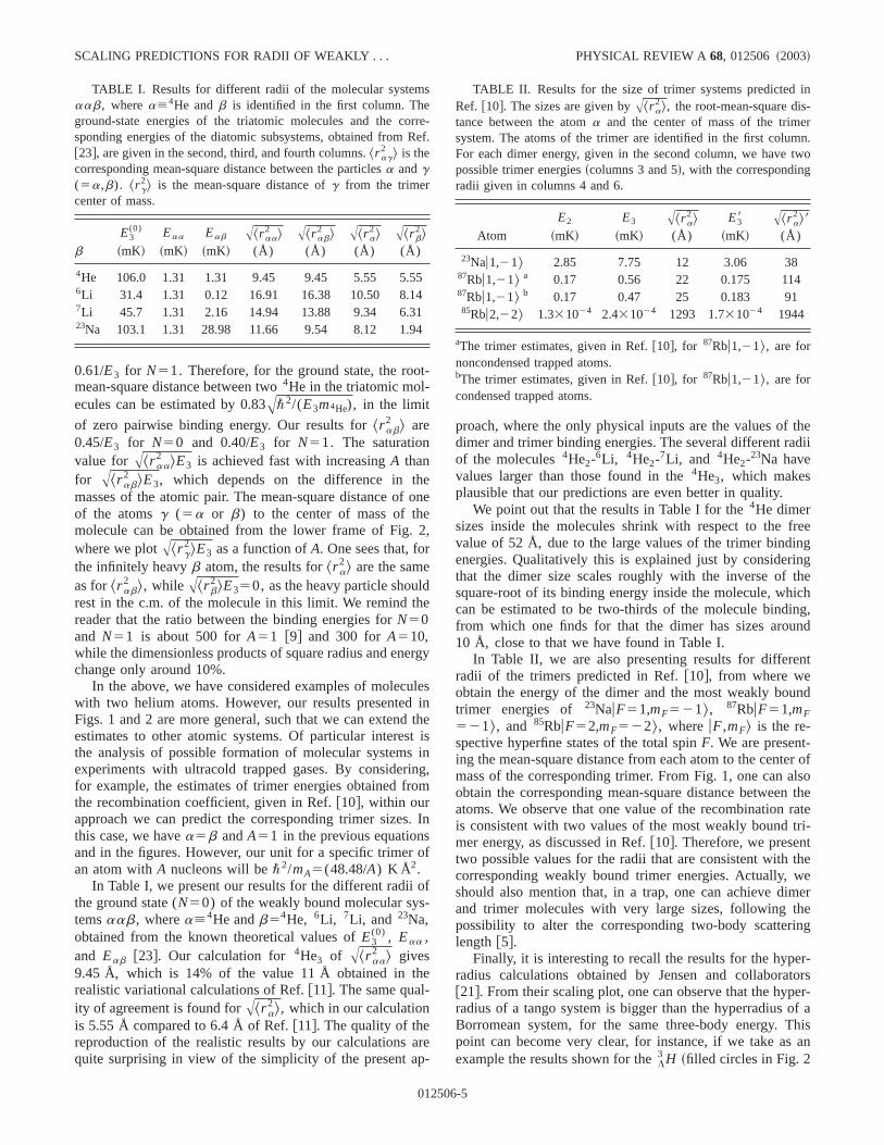
t-
eo
e2
r
de
er
ulit
ti
ino
.so
o-
e
arp-
thedii
reengingtheichng,nd
nt
nd
er oflsothe
ratetri-tthewemere
ng
r-torser-
of ahisan
s
rrR
in-rn.
two
SCALING PREDICTIONS FOR RADII OF WEAKLY . . . PHYSICAL REVIEW A68, 012506 ~2003!
0.61/E3 for N51. Therefore, for the ground state, the roomean-square distance between two4He in the triatomic mol-ecules can be estimated by 0.83A\2/(E3m4He), in the limit
of zero pairwise binding energy. Our results for^r ab2 & are
0.45/E3 for N50 and 0.40/E3 for N51. The saturationvalue forA^r aa
2 &E3 is achieved fast with increasingA thanfor A^r ab
2 &E3, which depends on the difference in thmasses of the atomic pair. The mean-square distance ofof the atomsg (5a or b) to the center of mass of thmolecule can be obtained from the lower frame of Fig.where we plotA^r g
2&E3 as a function ofA. One sees that, fothe infinitely heavyb atom, the results forr a
2& are the sameas for^r ab
2 &, whileA^r b2&E350, as the heavy particle shoul
rest in the c.m. of the molecule in this limit. We remind threader that the ratio between the binding energies forN50and N51 is about 500 forA51 @9# and 300 forA510,while the dimensionless products of square radius and enchange only around 10%.
In the above, we have considered examples of molecwith two helium atoms. However, our results presentedFigs. 1 and 2 are more general, such that we can extendestimates to other atomic systems. Of particular interesthe analysis of possible formation of molecular systemsexperiments with ultracold trapped gases. By considerfor example, the estimates of trimer energies obtained frthe recombination coefficient, given in Ref.@10#, within ourapproach we can predict the corresponding trimer sizesthis case, we havea5b andA51 in the previous equationand in the figures. However, our unit for a specific trimeran atom withA nucleons will be\2/mA5(48.48/A) K Å2.
In Table I, we present our results for the different radiithe ground state (N50) of the weakly bound molecular systemsaab, wherea[4He andb54He, 6Li, 7Li, and 23Na,obtained from the known theoretical values ofE3
(0) , Eaa ,and Eab @23#. Our calculation for 4He3 of A^r aa
2 & gives9.45 Å, which is 14% of the value 11 Å obtained in threalistic variational calculations of Ref.@11#. The same qual-ity of agreement is found forA^r a
2&, which in our calculationis 5.55 Å compared to 6.4 Å of Ref.@11#. The quality of thereproduction of the realistic results by our calculationsquite surprising in view of the simplicity of the present a
TABLE I. Results for different radii of the molecular systemaab, wherea[4He andb is identified in the first column. Theground-state energies of the triatomic molecules and the cosponding energies of the diatomic subsystems, obtained from@23#, are given in the second, third, and fourth columns.^r ag
2 & is thecorresponding mean-square distance between the particlesa andg(5a,b). ^r g
2& is the mean-square distance ofg from the trimercenter of mass.
E3(0) Eaa Eab A^r aa
2 & A^r ab2 & A^r a
2& A^r b2&
b ~mK! ~mK! ~mK! (Å) (Å) (Å) (Å)
4He 106.0 1.31 1.31 9.45 9.45 5.55 5.556Li 31.4 1.31 0.12 16.91 16.38 10.50 8.147Li 45.7 1.31 2.16 14.94 13.88 9.34 6.3123Na 103.1 1.31 28.98 11.66 9.54 8.12 1.94
01250
ne
,
gy
esnheisng,m
In
f
f
e
proach, where the only physical inputs are the values ofdimer and trimer binding energies. The several different raof the molecules4He2-6Li, 4He2-7Li, and 4He2-23Na havevalues larger than those found in the4He3, which makesplausible that our predictions are even better in quality.
We point out that the results in Table I for the4He dimersizes inside the molecules shrink with respect to the fvalue of 52 Å, due to the large values of the trimer bindienergies. Qualitatively this is explained just by considerthat the dimer size scales roughly with the inverse ofsquare-root of its binding energy inside the molecule, whcan be estimated to be two-thirds of the molecule bindifrom which one finds for that the dimer has sizes arou10 Å, close to that we have found in Table I.
In Table II, we are also presenting results for differeradii of the trimers predicted in Ref.@10#, from where weobtain the energy of the dimer and the most weakly boutrimer energies of 23NauF51,mF521&, 87RbuF51,mF521&, and 85RbuF52,mF522&, whereuF,mF& is the re-spective hyperfine states of the total spinF. We are present-ing the mean-square distance from each atom to the centmass of the corresponding trimer. From Fig. 1, one can aobtain the corresponding mean-square distance betweenatoms. We observe that one value of the recombinationis consistent with two values of the most weakly boundmer energy, as discussed in Ref.@10#. Therefore, we presentwo possible values for the radii that are consistent withcorresponding weakly bound trimer energies. Actually,should also mention that, in a trap, one can achieve diand trimer molecules with very large sizes, following thpossibility to alter the corresponding two-body scatterilength @5#.
Finally, it is interesting to recall the results for the hyperadius calculations obtained by Jensen and collabora@21#. From their scaling plot, one can observe that the hypradius of a tango system is bigger than the hyperradiusBorromean system, for the same three-body energy. Tpoint can become very clear, for instance, if we take asexample the results shown for theL
3 H ~filled circles in Fig. 2
e-ef.
TABLE II. Results for the size of trimer systems predictedRef. @10#. The sizes are given byA^r a
2&, the root-mean-square distance between the atoma and the center of mass of the trimesystem. The atoms of the trimer are identified in the first columFor each dimer energy, given in the second column, we havepossible trimer energies~columns 3 and 5!, with the correspondingradii given in columns 4 and 6.
E2 E3 A^r a2& E38 A^r a
2&8Atom ~mK! ~mK! (Å) ~mK! (Å)
23Nau1,21& 2.85 7.75 12 3.06 3887Rbu1,21& a 0.17 0.56 22 0.175 11487Rbu1,21& b 0.17 0.47 25 0.183 9185Rbu2,22& 1.331024 2.431024 1293 1.731024 1944
aThe trimer estimates, given in Ref.@10#, for 87Rbu1,21&, are fornoncondensed trapped atoms.bThe trimer estimates, given in Ref.@10#, for 87Rbu1,21&, are forcondensed trapped atoms.
6-5

b
seo
sy
dhenebr
tapl
triba
iottatdi
a
theste
nor-asesom-ten-delthis
byhe
%.of
luesforer-
iesn--tter
s-ibil-ediumhat-
nto
YAMASHITA et al. PHYSICAL REVIEW A 68, 012506 ~2003!
of Ref. @21#! and estimate the dimensionless product of oservables, r2&mB/\2 ~product of thex axis andy axis inFig. 2 of Ref.@21#, wherer is the hyperradius andB is thethree-body binding energy!. When going from the tango tothe Borromean configuration, this product will decreaTherefore, if one keeps the same binding energy, the Bromean system would be more compact than the tangotem. Extending this analysis to (aba) halos, where (a2a) is virtual and (ab) is bound, and also to all-bounpairs (aab), one should expect that the sizes increase wgoing from the Borromean states to halos with all-bousubsystems, while keeping the three-body energy fixWithin our approach, the scaling relations are expected tofollowed in all the cases, in the limit of a zero-range inteaction. The Borromean halo~the less attractive system!, inorder to have the same three-body energy as a tango sshould be more compact in agreement with the scalingof Ref. @21#. In a realistic case, our scheme is expectedproduce better results in the all-bound case, when compasystems with the same three-body energies. This occurscause the all-bound case would have the most extended wfunction; consequently, the range of the potential, in relatto the size, would have the smallest value, satisfying bethe validity condition for the scaling relations, which is ththe interaction range must be small compared to particletances.
IV. CONCLUSIONS
The mean-square radii of the triatomic molecules4He3 ,4He2–6Li, 4He2–7Li, and 4He2–23Na are calculated usingrenormalized three-body model with a pairwise Dirac-d in-teraction, having as physical inputs only the values ofbinding energies of the diatomic and triatomic moleculPresently, we have considered molecular three-body sys
e
.
an
n
M
A.
ie
01250
-
.r-s-
ndd.e
-
te,otonge-ve
ner
s-
e.ms
with bound subsystems, due to the available data. The remalized zero-range model can also be applied to the cwhere at least one of the subsystems is virtual. When cparing systems with the same three-body energies and potial ranges, the validity of the renormalized zero-range mois expected to be better in the all-bound case, becausecase corresponds to the most extended wave function.
The validity of the present framework is substantiatedthe agreement of our results for the different radii with trealistic potential model calculations of Ref.@11# for 4He3ground and excited states, which are within about 14These results are quite surprising in view of the simplicitythe approach, where only the physical inputs are the vaof diatomic and triatomic binding energies. We predictedthe first time, as far as we know, the values of several diffent radii for 4He2–6Li, 4He2–7Li, and 4He2–23Na mol-ecules, from the theoretical values of the binding energcalculated in Ref.@23#. These other molecules are, in geeral, larger than the4He-trimer, indicating that our radii predictions for these triatomic ground states can be even bein quality than those found for4He3.
In view of the actual relevance of ultracold atomic sytems that are being experimentally studied, and the possity to observe the formation of molecular systems in trappcondensates, we also present results for the sizes of rubidand sodium trimers, considering the binding energies twere recently estimated@10# from the analysis of the corresponding three-body recombination coefficients.
ACKNOWLEDGMENTS
We would like to thank Fundac¸ao de Amparo a` Pesquisado Estado de Sa˜o Paulo~FAPESP! for partial support. L.T.and T.F. also thank Conselho Nacional de DesenvolvimeCientıfico e Tecnolo´gico ~CNPq! partial support.
in-
s.
v.
.
@1# E. Nielsen, D.V. Fedorov, A.S. Jensen, E. Garrido, Phys. R347, 373 ~2001!.
@2# W. Schollkopf and J.P. Toennies, Science266, 1345 ~1994!;K.T. Tang, J.P. Toennies, and C.L. Liu, Phys. Rev. Lett.74,1546 ~1995!.
@3# R.E. Grisenti, W. Scho¨llkopf, J.P. Toennies, G.C. Hegerfeldt, TKohler, and M. Stoll, Phys. Rev. Lett.85, 2284~2000!.
@4# M.H. Anderson, J.R. Ensher, M.R. Matthews, C.E. Wiemand E.A. Cornell, Science269, 198~1995!; C.C. Bradley, C.A.Sackett, J.J. Tollet, and R.G. Hulet, Phys. Rev. Lett.75, 1687~1995!; K.B. Davis, M.-O. Mewes, M.R. Andrews, N.J. vaDruten, D.S. Durfee, D.M. Kurn, and W. Ketterle,ibid. 75,3969 ~1995!.
@5# S. Inouye, M.R. Andrews, J. Stenger, H.-J. Miesner, D.Stamper-Kurn, and W. Ketterle, Nature~London! 392, 151~1998!; E. Timmermans, P. Tommasini, M. Hussein, andKerman, Phys. Rep.315, 199 ~1999!.
@6# N.R. Claussen, E.A. Donley, S.T. Thompson, and C.E. Wman, Phys. Rev. Lett.89, 010401~2002!; E.A. Donley, N.R.Claussen, S.T. Thompson, and C.E. Wieman, Nature~London!417, 529 ~2002!.
p.
,
.
-
@7# R.H. Wynar, R.S. Freeland, D.J. Han, C. Ryu, and D.J. Hezen, Science287, 1016~2000!.
@8# C. Mckenzieet al., Phys. Rev. Lett.88, 120403~2001!.@9# V. Efimov, Phys. Lett. B33, 563~1970!; Nucl. Phys. A362, 45
~1981!; V. Efimov, Comments Nucl. Part. Phys.19, 271~1990!, and references therein.
@10# M. T. Yamashita, T. Frederico, A. Delfino, and L. Tomio, PhyRev. A ~to be published!, e-print cond-mat/0206317.
@11# P. Barletta and A. Kievsky, Phys. Rev. A64, 042514~2001!.@12# V. Roudnev and S. Yakovlev, Chem. Phys. Lett.328, 97
~2000!.@13# S.K. Adhikari, T. Frederico, and I.D. Goldman, Phys. Re
Lett. 74, 487 ~1995!; S.K. Adhikari and T. Frederico,ibid. 74,4572 ~1995!.
@14# A.E.A. Amorim, L. Tomio, and T. Frederico, Phys. Rev. C56,R2378~1997!.
@15# T. Frederico, A. Delfino, A.E.A. Amorim, and L. Tomio, PhysRev. A60, R9 ~1999!.
@16# A. Delfino, T. Frederico, and L. Tomio, Few-Body Syst.28,259 ~2000!; J. Chem. Phys.113, 7874~2000!.
6-6

s.
-
ro-
SCALING PREDICTIONS FOR RADII OF WEAKLY . . . PHYSICAL REVIEW A68, 012506 ~2003!
@17# L.H. Thomas, Phys. Rev.47, 903 ~1935!.@18# M.T. Yamashita, T. Frederico, A. Delfino, and L. Tomio, Phy
Rev. A66, 052702~2002!.@19# M.V. Zhukov, B.V. Danilin, D.V. Fedorov, J.M. Bang, I.J. Th
ompson, and J. Vaagen, Phys. Rep.231, 151 ~1993!.@20# F. Robichaux, Phys. Rev. A60, 1706~1999!.
01250
@21# A.S. Jensen, K. Riisager, D.V. Fedorov, and E. Garrido, Euphys. Lett.61, 320 ~2003!.
@22# T. Frederico and I.D. Goldman, Phys. Rev. C36, R1661~1987!.
@23# J. Yuan and C.D. Lin, J. Phys. B31, L637 ~1998!.
6-7
e
4
-bound-range
o of theulationse in the
thereticalents ofn, theusefullarge
despiteith a
Nuclear Physics A 735 (2004) 40–54
www.elsevier.com/locate/np
Radii in weakly-bound light halo nuclei
M.T. Yamashitaa, Lauro Tomiob,∗, T. Fredericoc
a Laboratório do Acelerador Linear, Instituto de Física, Universidade de São Paulo, C.P. 66318,CEP 05315-970, São Paulo, Brazil
b Instituto de Física Teórica, Universidade Estadual Paulista, Rua Pamplona, 145, Bela Vista,01405-900, São Paulo, Brazil
c Departamento de Física, Instituto Tecnológico de Aeronáutica, Centro Técnico Aeroespacial,12228-900, São José dos Campos, Brazil
Received 24 December 2003; received in revised form 2 February 2004; accepted 3 February 200
Abstract
A systematic study of the root-mean-square distance between the constituents of weaklynuclei consisting of two halo neutrons and a core is performed using a renormalized zeromodel. The radii are obtained from a universal scaling function that depends on the mass ratineutron and the core, as well as on the nature of the subsystems, bound or virtual. Our calcare qualitatively consistent with recent data for the neutron–neutron root-mean-square distanchalo of11Li and 14Be nuclei. 2004 Published by Elsevier B.V.
PACS: 27.20.+n; 21.60.-n; 21.45.+v
1. Introduction
Light exotic-nuclei with one or two weakly bound neutrons in their halo offeropportunity to study large systems at small nuclear density. (A review on the theoapproaches and characteristics of halo nuclei can be found in Ref. [1].) The constituthe halo have a high probability to be found much beyond the interaction range. Theconcept of a short-range interaction between the particles and its implications arein understanding the few-body physics of the halo. The quantum description of suchand weakly bound systems are universal and can be defined by few physical scalesthe range and details of the pairwise interaction [2]. The particular halo-nuclei, w
* Corresponding author.E-mail address: [email protected] (L. Tomio).
0375-9474/$ – see front matter 2004 Published by Elsevier B.V.doi:10.1016/j.nuclphysa.2004.02.003
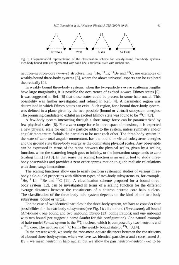
ystems.
fxplored
s.i. Thiswas
ystem,ergies.
ed bypectedand/ortem in
nergieservablescalingo zeroree-
lations
three-mple,ree-erentucleus.-body
er four
dle
and
tituents
M.T. Yamashita et al. / Nuclear Physics A 735 (2004) 40–54 41
Fig. 1. Diagrammatical representation of the classification scheme for weakly-bound three-body sTwo-body bound state are represented with solid line, and virtual state with dashed line.
neutron–neutron–core (n–n–c) structure, like6He, 11Li, 14Be and20C, are examples oweakly-bound three-body systems [3], where the above universal aspects can be etheoretically [4].
In weakly bound three-body systems, when the two-particles-wave scattering lengthhave large magnitudes, it is possible the occurrence of exciteds-wave Efimov states [5]It was suggested in Ref. [6] that these states could be present in some halo nuclepossibility was further investigated and refined in Ref. [4]. A parametric regiondetermined in which Efimov states can exist. Such region, for a bound three-body swas defined in a plane given by the two possible (bound or virtual) subsystem enThe promising candidate to exhibit an excited Efimov state was found to be20C [4,7].
A few-body system interacting through a short range force can be parameterizfew physical scales [8]. For a zero-range force in three-space dimensions, it is exa new physical scale for each new particle added to the system, unless symmetryangular momentum forbids the particles to be near each other. The three-body systhe state of zero total angular momentum, has the bound or virtual subsystems eand the ground state three-body energy as the dominating physical scales. Any obscan be expressed in terms of the ratios between the physical scales, given by afunction, when the scattering length goes to infinity, or the interaction range tends t(scaling limit) [9,10]. In that sense the scaling function is an useful tool to study thbody observables and provides a zero order approximation to guide realistic calcuwith short-range interactions.
The scaling functions allow one to easily perform systematic studies of variousbody halo-nuclei properties with different types of two-body subsystems as, for exa6He, 11Li, 14Be and 20C [11]. A classification scheme proposed for a bound thbody system [12], can be investigated in terms of a scaling function for the diffaverage distances between the constituents of a neutron–neutron–core halo nThe classification of the three-body halo system depends on the kind of the twosubsystems, bound or virtual.
For the case of two identical particles in the three-body system, we have to considpossibilities for the two-body subsystems (see Fig. 1): all unbound (Borromean); all bound(All-Bound); one bound and two unbound (Tango [13] configuration); and one unbounwith two bound (we suggest a nameSamba for this configuration). One natural exampof halo-nucleiSamba system is the20C nucleus, which is composed by two-neutronsa 18C core. The neutron and18C forms the weakly bound state of19C [3,14].
In the present work, we study the root-mean-square distances between the cons
of a bound three-body system, where we have two identical particlesn and a core namedA.By n we mean neutron in halo nuclei, but we allow the pair neutron–neutron (nn) to be
radii inviousw theem to
,
of the
stem
hehat, innt
be]).
affectg theigherhe tail
hichrticles,also
iscuss-mean-n 5.
pledwith auationsd
42 M.T. Yamashita et al. / Nuclear Physics A 735 (2004) 40–54
bound in order to cover all the configurations presented above. We represent thea scaling plot in terms of a dimensionless product, extending to halo nuclei a preapplication that was done for molecules [15]. Using these scaling plots we can follobehavior of the different radii when it happens a transition between one kind of systanother one. Starting from theBorromean case (all unbound), we can go to theSamba caseby increasing the binding energy of the pairnA (keepingnn unbound); and to theTangocase by increasing the binding energy of the pairnn (keepingnA unbound). In particularwe calculate the mean square distance between the two neutrons in6He, 11Li and 14Be(which have been measured recently [16]) from the known bound or virtual energiessubsystems and the two-neutron separation energy.
The calculation of the scaling function for the different radii of the three-body syis performed with a renormalization scheme applied to three-body equations withs-wavezero-range pairwise potential, which makes use of subtracted equations [8,17].
As our approach is restricted tos-wave two-body interactions, some limitations in tapplication of our analysis are expected. The argument has the origin in the fact tsome cases, the two-body subsystem interaction inp-wave is considered to be importafor the three-body binding. The examples are6He [18], known to be bound by thep-waveinteraction inn–4He; and11Li, where bothp- ands-waves might be relevant to descrithe ground state of the unbound subsystem10Li (see discussion and references in [19However, as pointed out in Ref. [20] (in a discussion related to11Li), one should alsonoticed that even the three-body wave function withs-wavenn correlation producesground state of the halo nuclei with two or more shell-model configurations. The eof the aboves-wave restriction is also reduced due to the fact that we are considerinexperimental energies in our approach, which implicitly are carrying the effect of hpartial waves in the interaction. Another aspect is that the radius are obtained from tof the wave-function, which is dominated by thes-wave.
The paper is organized as follows. In Section 2, we present our formalism, wcontains the subtracted method to treat the Faddeev equations with two identical paleading to the form factors from which we obtain the different mean-square radii. Wegive a brief discussion of the scaling functions to describe the radii. In Section 3, we dthe classification scheme. In Section 4, we present our numerical results for the rootsquare distances between the particles. Our conclusions are summarized in Sectio
2. Formalism
In the next subsection, we consider the formalism given in Refs. [15,17] for couchannels to calculate the three-body wave functions and the possible different radiizero-range pairwise interaction. We solve the homogeneous three-body Faddeev eqfor a system with two identical particlesα and a third oneβ in a renormalized subtracte
form, which allows one to obtain the observables as a function of the two and three-bodyscales of the system. The corresponding masses of the particlesα andβ aremα andmβ .
deevyumy. Afterdeev
bodyenergy
cal
nless
dy
ring
e
M.T. Yamashita et al. / Nuclear Physics A 735 (2004) 40–54 43
2.1. Subtracted Faddeev equations
Next, we follow the model presented in Refs. [15,17] for the subtracted Fadequations, and consider units such thath = 1 andmα = 1. For the subtraction energthat is required in the model, we chooseµ2
(3). In this case, all the energies and momentvariables are rescaled to dimensionless variables considering this subtraction energpartial wave projection, thes-wave coupled subtracted integral equations for the Fadspectator functionsχαα andχαβ , are given by:
χαα(y)= 2ταα(y; ε3)
∞∫0
dxx
yG1(y, x; ε3)χαβ(x), (1)
χαβ(y)= ταβ(y; ε3)
∞∫0
dxx
y
[G1(x, y; ε3)χαα(x)+AG2(y, x; ε3)χαβ(x)
], (2)
ταα(y; ε3)≡ 1
π
[√ε3 + CA1 y2 ∓ √
εαα]−1
, (3)
ταβ(y; ε3)≡ 1
π
(CA2 )3/2
[√ε3 + C(A+1)
2 y2 ∓ √εαβ ]
, (4)
G1(y, x; ε3)≡ log(ε3 + x2 + xy)+ CA2 y2
(ε3 + x2 − xy)+ CA2 y2− log
(1+ x2 + xy)+ CA2 y2
(1+ x2 − xy)+ CA2 y2, (5)
G2(y, x; ε3)≡ log(ε3 + xy/A)+ CA2 (y2 + x2)
(ε3 − xy/A)+ CA2 (y2 + x2)− log
(1+ xy/A)+ CA2 (y2 + x2)
(1− xy/A)+ CA2 (y2 + x2),
(6)
where we are defining the mass ratio and the constant mass factors by
A ≡ mβ
mα
, CAj=1,2 ≡(j
4+ 1
2A
). (7)
The plus and minus signs in Eqs. (3) and (4) refer to virtual and bound two-subsystems, respectively. In the equations above, the dimensionless three-bodyε3 and the two-body energies (εαα and εαβ ), are related to the corresponding physiquantities byε3 ≡ −E3/µ
2(3), εαα ≡ −Eαα/µ
2(3), andεαβ ≡ −Eαβ/µ
2(3). The three-body
physical quantities can be written in terms of a scaling function, i.e., the dimensioproduct of the observable and some power of the three-body binding energyE3, when thevalue ofµ2
(3) is determined from the known value ofE3 and consequently the three-boquantities are naturally a function ofE3 and the ratiosEαα/E3 andEαβ/E3. Note that weare using the same symbolA for the mass ratio as well as for the core label, considethat, in an–n–core nucleus we have the core consisting ofA nucleons andA can alsobe identified with the mass ratio (mβ = Amn, mα = mn). However, our expression can bgenerally applied for non-integer values ofA.
For large scattering lengths, the details of the interaction are unimportant to describefew-body systems, as the short-range informations, beyond the two-body scattering

nergyinding, thewrittenf many
l
dy
undin thel-s
al).
sntum
ndices
le
44 M.T. Yamashita et al. / Nuclear Physics A 735 (2004) 40–54
lengths, are carried out by one typical three-body scale. Therefore, the low-eobservables present a scaling behavior quite universal with the three-body benergy [8,21]. In the limit of infinite scattering lengths or zero range interactionsfunction which represents a given correlation between two three-body observables,in terms of scaled variables, converges to a single curve, despite the existence oother Efimov states.
For a three-body system with binding energyE3, in thescaling limit [4,17], one generathree-body physical observableO, with dimension of energy to the powerη, at a particularenergyE, can be written as a functionF of the ratios between the two and three-boenergies, such that
O(E,E3,Eαα,Eαβ)= (E3)ηF
(√E
E3,±
√Eαα
E3,±
√Eαβ
E3,A
). (8)
The two-body energiesEαγ (γ = α,β), are negative quantities, corresponding to boor virtual states. The nature of such two-body state, bound or virtual, is revealedmomentum space, such that we have a bound state when
√|Eαβ | is positive and a virtuastate when
√|Eαβ | is negative. So, in Eq. (8), the signs+ or− mean a bound or virtual twobody subsystem, respectively. The different radii of the boundααβ system are functiondefined from the Eq. (8) withE =E3, which depend on the mass ratio,A, the ratios of thetwo and three-body energies and the kind of subsystem interactions (bound or virtu
2.2. Radii calculation
The Faddeev components of the wave-function for theααβ system are written in termof the spectator functions, obtained from the solution of Eqs. (1) and (2) in momespace:
Ψαα(y, z)=(
1
ε3 + CA1 y2 + z2− 1
1+ CA1 y2 + z2
)
×[χαα
(|y|) + χαβ
(∣∣∣∣z− y2
∣∣∣∣)
+ χαβ
(∣∣∣∣z+ y2
∣∣∣∣)]
, (9)
Ψαβ(y, z)=(
1
ε3 + CA2 z2 + CA+12 y2
− 1
1+ CA2 z2 + CA+12 y2
)
×[χαα
(∣∣∣∣z− AyA+ 1
∣∣∣∣)
+ χαβ(|y|) + χαβ
(∣∣∣∣z+ yA+ 1
∣∣∣∣)]
,
whereCAj is defined in Eq. (7). The Faddeev components are denoted by the sub-iof the interacting pair. Representing the pair byαγ with γ = α or β , one has thatz is therelative momentum betweenα andγ and y is the relative momentum of the third partic
to the center-of-mass of the systemαγ . For the halo nuclei the notation isα = n andβ isthe core represented byA.
quareatter
square
ntum
and thedy
articles
or theever,stems
M.T. Yamashita et al. / Nuclear Physics A 735 (2004) 40–54 45
The momentum component of the total wave-function,
ΨAnn′ = Ψnn′ +ΨAn +ΨAn′ , (10)
is symmetrical by the exchange between the neutrons,n andn′, while the antisymmetryis given by the singlet spin-component (not explicitly shown). The different mean-sradii are calculated from the derivative of the Fourier transform of the respective mdensity in respect to the square of the momentum transfer. The relative mean-distances between the halo neutrons and between the neutron and the core (γ = n,A)are obtained from the expression
⟨r2nγ
⟩ = −6dFnγ (q
2)
dq2
∣∣∣∣q2=0
, (11)
where
Fnγ
(q2) =
∫d3y d3zΨAnn′
(y, z+ q
2
)ΨAnn′
(y, z− q
2
)(12)
is the Fourier transform of the two-body densities, which is a function of the mometransferq (given in units ofµ(3)). The relative momentum betweenn andγ is z± q/2 andthe relative momentum of the third particle to the center-of-mass ofnγ is y.
Analogous equations can be found for the mean square distances of the neutroncore to the center-of-mass system (〈r2〉γ ), in terms of the Fourier transform of the one-bodensity.
2.3. Scaling functions for the radii
The scaling functions for the mean-square separation distances between the pin the three-body system can be written according to Eq. (8) withE ≡ E3. The scalingfunctions for the radii are written as:
√⟨r2nγ
⟩|E3| =Rnγ
(±
√Enn
E3,±
√EnA
E3,A
), (13)
√⟨r2γ
⟩|E3| =Rcmγ
(±
√Enn
E3,±
√EnA
E3,A
). (14)
To study the different types of three-body systems, the general scaling function fradii given by Eqs. (13) and (14) will be studied in the configurations of Fig. 1. Howone noticeable situation occurs when the Efimov limit is reached, for which the subsyenergies vanishes, and√⟨
r2nγ
⟩|E3| =Rnγ (A),
√⟨r2γ
⟩|E3| = Rcmγ (A), (15)
depends only on the mass ratioA (γ = n,A). Curiously, this configuration containssimultaneously all types shown in Fig. 1.

twostemally in
tativeof the
bilities.ergiesign
ve4), the,odyll havein the
ourseits one
uationtheill be
itativef the
(10)tron–
-bodyusefulules
d formy verys long-body
46 M.T. Yamashita et al. / Nuclear Physics A 735 (2004) 40–54
3. Classification scheme: qualitative properties
A discussion of a classification scheme for a bound three-body system, withidentical particles, is given in Ref. [12], according to the nature of the subsyinteractions, which can present a bound or virtual state, as depicted diagrammaticFig. 1.
The different possibilities of three-body systems are reflected in the qualiproperties of the dynamics as given by the coupled equations (1) and (2) in termsstrength of the attractive kernel of these equations. Let us describe all these possiTheBorromean case corresponds to positive signs in front of the square-root of the enof the subsystems in both Eqs. (3) and (4). ATango three-body system has a negative sonly in front of
√εαα in Eq. (3), with positive sign in front of
√εαβ in Eq. (4). For a
Samba configuration of the three-body system, a minus sign appears multiplying√εαβ in
Eq. (4), while a plus sign multiplies√εαα in Eq. (3). The All-Bound system has negati
signs in Eqs. (3) and (4). As a consequence of the differences in Eqs. (3) and (weakest attractive kernel in Eqs. (1) and (2) is given by aBorromean three-body systemfollowed by theTango, Samba andAll-Bound systems. Therefore, once fixed a three-bbinding energy, the system for which the kernel presents the weakest attraction withe smallest configuration. So, the size of the corresponding system will increasefollowing order:Borromean, Tango, Samba andAll-Bound. TheAll-Bound configurationhas the biggest size among all, for a given three-body binding energy. One of chas to remind that the sizes are expected to increase when the binding energy hscattering threshold. Therefore, for nonvanishing three-body binding energy this sitdoes not happen only in theBorromean case. In this sense, it is physically sensible thatBorromean case corresponds to the smallest configuration size. This observation wexplored in our numerical calculations. In this respect, we are showing the quantdetailed implication to the different radii of weakly-bound three-body systems oclassification scheme proposed in Ref. [12].
4. Numerical results for the radii: scaling plots
We present numerical results for the different possible radii forBorromean, Tango,Samba andAll-Bound three-body configurations obtained from the wave-function, Eq.derived from the solution of Eqs. (1) and (2). In particular, we give results for the neuneutron (nn) average distance in the three-body halo nuclei,6He,11Li, 14Be,20C.
It is interesting to present results in a general scaled form in terms of scaled twobinding energies and mass ratio, as given by Eqs. (13) and (14), which turns to befor the prediction of the several radii in different situations for weakly bound molecup to light halo-nuclei. Our calculations present results independent on the detaileof the interactions in a weakly bound three-body system. It means that they applwell to halo nuclei and weakly bound molecules. The present approach is valid aas the interactions within the three-body system are of short range while the two
energies are close to zero, i.e., the ratio between the interaction range and the modulus ofthe scattering lengths should be somewhat less than 1. These are indeed the cases we are
e for
e havetion ofse.nces,
of
moretszerolowell
t it
dn–coree
M.T. Yamashita et al. / Nuclear Physics A 735 (2004) 40–54 47
Fig. 2. Dimensionless products√
〈r2nγ 〉|E3| and
√〈r2γ 〉|E3| (γ = n,A) as a function ofA for zero two-body
energies. Results for: (a)√
〈r2nn〉|E3| (upper solid line) and
√〈r2nA
〉|E3| (upper dot-dashed line); (b)√
〈r2n〉|E3|
(lower solid curve) and√
〈r2A〉|E3| (lower dot-dashed curve). The experimental data, obtained from [16], ar√
〈r2nn〉|E3|.
considering. We present results only for the ground state of the three-body system. Wshown that the scaling function for the radii is indeed approached even for a calculathe ground state in our subtraction scheme [15], which will be enough for our purpo
In Fig. 2, we show the results of the scaling function for the mean square dista√〈r2nγ 〉 and
√〈r2γ 〉 with γ = n or A (see Eq. (15)) which are shown as a function
A for Enγ = 0. The comparison with experimental results of√〈r2
nn〉 [16], for the 6He,14Be and11Li is just for illustrative purpose, considering the hypothetical cases that5He,13Be and10Li would have virtual states close to zero energy. Such hypothesis isrealistic in case of14Be, while for the6He and11Li are not so. As shown by our resulfor 11Li, given in Table 1, the assumption of a virtual state with energy close to(|EnA| 0.05 MeV [20]) for 10Li lead to an averagenn separation distance (in the haof 11Li) not compatible with the corresponding experimental result. Given that it isdocumented the difficulty in studying the10Li [19], we can consider
√〈r2nn〉 [16] as one of
our inputs to predict the virtual state of then–9Li system. In this case, we conclude thacannot be smaller than∼ 0.1 MeV.
In this case (Enγ = 0) the only physical scale isE3 and the scaling plots will depensolely onA. The average separation distance between the neutrons and the neutrotends naturally to a constant for largeA, while it diverges forA tending towards zero. Th
reason for the unbound increase of the products〈r2nn〉|E3| and 〈r2nA〉|E3| for smallA is
due to the average momentum of the core which tends to zero (∼ √A|E3|) extending the

,
ing
s forre given-s
alues
ome they seen
othernd or
res,
tem
onless
48 M.T. Yamashita et al. / Nuclear Physics A 735 (2004) 40–54
Table 1Results of the neutron–neutron root-mean-square radii in halo nuclei. The cores (A) are given in the first columnthe absolute values of the three-body ground state energiesE3 are given in the second column. For−E3,which is equal to the two-neutron separation energyS(2n), we consider the center value of the correspondenergies given in Ref. [3], except for lithium. In case of lithium we consider for−E3 the maximum (0.32MeV) and the center value (0.29 MeV) given in Ref. [22]. In the third column we give our input value−EnA, considering several values, covering the values suggested in the literature (the references atogether with the corresponding number). For bound two-body subsystemnA, we have−EnA equal to the oneneutron separation energyS(n). The virtual states are indicated by (v), and thenn virtual state energy is taken a−143 keV. The experimental values, in the last column, are obtained from Marqués et al. (2000) [16].
Core (A) −E3 (MeV) −EnA (MeV)√
〈r2nn〉 (fm)
√〈r2nn〉
exp(fm)
4He 0.973 0 (v) 5.10.3 (v) 4.6 5.9±1.24.0 [23] (v) 3.6
9Li 0.32 0 (v) 9.2 6.6±1.50.8 [24] (v) 5.9
9Li 0.29 0 (v) 9.70.05 [20,25,26] (v) 8.5 6.6±1.50.8 [24] (v) 6.7
12Be 1.337 0 (v) 4.6 5.4±1.00.2[27] (v) 4.2
18C 3.50 0.16 [3] 3.0 –0.53 [14] 4.4 –
system to infinity. We have checked that the results shown in Fig. 2 tends to finite vafter multiplication by
√A (one has to remember that we are using units ofmn = 1).
The average distance of the neutron to the center of mass system tends to becrelative distance to the core, when the core mass grows to infinity. This fact is clearlin Fig. 2 with the lower solid line approaching the upper dot-dashed one whenA 10.Also, one sees that the core distance to the center of mass vanishes with growingA as itshould be.
In Figs. 3–6, we show results for√〈r2
nn〉|E3| and√
〈r2nA〉|E3|, when one of the
subsystem energies is fixed in respect to the three-body binding energy, while theone varies. We use values ofA equal to 0.1, 1 and 200. The subsystems can be bouvirtual and therefore all configurations are covered, i.e., we show results forBorromean,Tango, Samba andAll-Bound-type systems. Anticipating the presentation of these figuin general we find that, the radii increase in the following orderBorromean, Tango, SambaandAll-Bound for a given three-body energy and fixedA. In our analysis below, we fixeitherEnn/E3 = 0.1 orEnA/E3 = 0.1 which can correspond to bound or virtual subsysenergies. In the next, we also consider the definitionsEnA/E3 ≡K2
nA andEnn/E3 ≡ K2nn
(for both bound or virtual-state energies), such that
KnA = ±√EnA/E3 and Knn = ±√
Enn/E3. (16)
The+ (−) sign refers to bound (virtual) state. One should also note that, the dimensi
quantitiesKnn andKnA are directly related to poles in the imaginary axis of the respectivetwo-body momentum space.
ns
M.T. Yamashita et al. / Nuclear Physics A 735 (2004) 40–54 49
Fig. 3. Dimensionless products√
〈r2nA
〉|E3| (upper frame) and√
〈r2nn〉|E3| (lower frame) forA = 0.1 and
Enn/E3 = K2nn = 0.1 as a function ofKnA/|Knn|. In the upper frame, a boundnn pair is represented with
dashed line; and a virtualnn pair with dot-dashed line. In the lower frame, a boundnn pair is represented withsolid line; and a virtualnn pair with dotted line. The transition between the configurations occurs whenKnA = 0(represented by the vertical line).
Fig. 4. Dimensionless products√
〈r2nA
〉|E3| (upper frame) and√
〈r2nn〉|E3| (lower frame) forA = 1 and
K2nn = 0.1 as a function ofKnA/|Knn|. The convention of the lines is the same as given in Fig. 3.
In Fig. 3, we present calculations of thenA andnn root-mean-square radius as functio√
of KnA/|Knn|. Such average radius, multiplied by|E3|, are scaled to dimensionlessquantities. We considerA = 0.1 andEnn/E3 = 0.1 fixed, corresponding to bound (Knn =
.
ions
50 M.T. Yamashita et al. / Nuclear Physics A 735 (2004) 40–54
Fig. 5. Dimensionless products√
〈r2nA
〉|E3| (upper frame) and√
〈r2nn〉|E3| (lower frame) forA = 200 and
Enn/E3 = 0.1 as a function ofKnA/|Knn|. The convention of the lines is the same as given in Figs. 3 and 4
Fig. 6. Dimensionless products√
〈r2nA
〉|E3| (upper frame) and√
〈r2nn〉|E3| (lower frame) forA = 200 and
EnA/E3 = 0.1 as a function ofKnn/|KnA|. In the upper we represent the case of a boundnA pair with dashedline; and the case of a virtualnA pair with dot-dashed line. In the lower frame we represent the boundnA pairwith solid line and the virtualnA pair with dotted line. The lines of this figure correspond to the vertical transitrepresented in Fig. 5 in both extreme sides where|KnA| = |Knn|.
√0.1 ) or virtual (Knn = −√
0.1 ) subsystems. In this case, the mass of the particlen is
much heavier than the “core”, which does not happen in halo nuclei. However, we considerthis case for the sake of general interest. In thex-axis, the positive (negative) values of
ndot-
ct
nis
baaseminantes,
mass
r
es
e same
ore with
ted
f
pond
n fromand,he
thatsition
om
M.T. Yamashita et al. / Nuclear Physics A 735 (2004) 40–54 51
KnA/|Knn| correspond to bound (virtual)nA states. In the upper frame, the averagenA
radius is shown for a boundnn pair (dashed line) and for a virtualnn pair (dot-dashed
line). So, the dashed line shows that the value of√
〈r2nA〉|E3| increases with the transitio
from Tango to All-Bound configuration. In the other possibility, represented by the
dashed line (nn in a virtual state), the value of√
〈r2nA〉|E3| increases from the most compa
Borromean configuration (KnA negative) to theSamba-type configuration (KnA positive).In the lower frame of Fig. 3, we also show that
√〈r2nn〉|E3| increases with the transitio
from Tango to All-Bound andBorromean to Samba configurations. We observe, in thcase, a small sensitivity onKnn, when going from−√
0.1 (dotted line) to√
0.1 (solidline), with
√〈r2nn〉|E3| having practically the same value for the All-Bound and Sam
configurations; and also for the Tango and Borromean configurations. As we increA,this sensitivity increases, as one can see in Figs. 4 and 5. We interpret this as the dorole played by a light particle in the long-range interaction between two heavy particln,as already shown in an adiabatical approximation of the three-body system [28].
In Fig. 4, we show the radii for the ground state of the three-body system with theratioA = 1. As in Fig. 3, we fixedKnn = ±√
0.1, corresponding to bound (+) or virtual
(−) subsystems. The same behavior found in Fig. 3 for√
〈r2nA〉|E3| is found in the uppe
frame of Fig. 4 forA = 1, i.e., the configurations for which thenn pair is virtual (dot-dashed line) are smaller than the ones that have thenn pair bound (dashed line). Besidthat, the configuration increases in size when the system changes from aBorromean toa Samba type and when it changes from aTango to anAll-Bound type. ForA = 1, themean square distance between the two-neutrons (lower frame of Fig. 4) exhibits th
qualitative behavior as found for√
〈r2nA〉|E3| when the configuration type is modified f
a fixed three-body energy. These conclusions are still valid for a heavy core particlA = 200, as one can verify in Fig. 5. It is worthwhile to mention that
√〈r2nn〉|E3| attains its
asymptotic value fast with the increase ofA consistently with the calculations presenin Fig. 2 forEnn = EnA = 0. (Compare the results forA = 1 andA = 200 in the lowerframes of Figs. 4 and 5.)
In correspondence with Fig. 5, for the same mass ratioA = 200, in the last set osystematic calculations we consider in Fig. 6 the energy of the subsystemnA fixedin relation toE3, with KnA = ±√
0.1, corresponding to bound (+) or virtual (−) nA
subsystem. In this case, the ratioKnn/|KnA| is changed from−1 to +1, such that thetransitions of configurations from the left side to the right side of this figure corresto the vertical transitions in the extreme side of Fig. 5 (when|KnA| = |Knn| = √
0.1). So,comparing the upper frames of Figs. 5 and 6, we observe that the vertical transitioAll-Bound to Samba configuration in Fig. 5 corresponds to the dashed line of Fig. 6;the vertical transition fromTango to Borromean configuration in Fig. 5 corresponds to tdot-dashed line of Fig. 6. In the lower frames of both figures, similarly we observethe vertical transitions of Fig. 5 correspond to the lines represented in Fig. 6: the tranfrom Samba to All-Bound configuration is given by the solid line; and the transition fr
Borromean to Tango configuration given by the dotted line. In general, one can observethat the three-body bound state has a smaller size when thenA pair forms a virtual state
is for
or thental
preferith the
e
ies of
er, as
tion of
eis last
ring
rtially
the
gura-
Paulithree-
ave afree
52 M.T. Yamashita et al. / Nuclear Physics A 735 (2004) 40–54
(see in each frame of Fig. 6, where the upper line is for bound and the lower linevirtual nA pair).
The calculations of the average distances of the neutrons in the halo of6He,11Li, 14Beand20C are shown in Table 1 and compared with the available experimental data. Finput, we have consideredEnn = −0.143 MeV and the center of the available experimevalues ofE3 andEnA. For the cases that we have unbound virtualnA systems, theEnA
input values are taken from several recent theoretical and experimental analysis; weto keep at least two possible values in order to verify the consistency of the model wexperimental data.
Within the possible limitations of our approach, by comparing our results for thnn
mean-square radius with the experimental ones, which are known in the cases of6He,11Liand14Be, as given in Table 1, one can also predict the corresponding virtual energthenA subsystem.
In the particular case of6He, the comparison between the experimentalnn mean-squareradius with our result is pointing out to a virtual energy close to zero forn–4He, whichis not supported by the quite large values given in the literature [18,23]. Howevdiscussed in [18,23], the interaction forn−4He is attractive inp-wave and repulsive ins-wave producing a large value for the energy of the virtual state, such that a deviaour calculation from the experimental result is expected (in our model thes-wave polesshould be near the scattering thresholds). For the binding of11Li, it is also known thatbothp- ands-waves are important in the subsystemn–9Li. This fact can also explain somdeviations of our results when compared with experimental ones. However, in thcase, our approach can be more reliable based on the fact that:
(i) the s-waven–9Li interaction is attractive and it has a virtual state near the scatteregion;
(ii) we are considering the experimental energies for the inputs, such that we are pataking into account the effect of higher partial waves in the interactions;
(iii) the radius is obtained from the tail of the wave-function, which is dominated bys-wave;
(iv) as noted in Ref. [20], even the three-body wave function withs-wavenn correlationproduces a ground state of the halo nuclei with two or more shell-model confitions.
One should also expect that other effects like the finite size of the core andprinciple, missing in our model, could affect the average relative distances, if thebody wave function would overlap appreciably with the core. At least for11Li this is notexpected due to the small binding. It is of notice that indeed the halo neutrons hlarge probability to be in a region in which the wave function is an eigenstate of theHamiltonian, and thus dominated by few asymptotic scales.
5. Conclusions
The mean-square radii of a light halo-nuclei modelled as a three-body system (twoneutronsn and a coreA) are calculated using a renormalized three-body model with
utsenergy
alfoundutronsed. Thedering,
e
valueo thewavend tos near
ions are
ilable
oposedlyzing
s-root ofare fouround:
me-bodynd.
easilyirtual
e-bodyturns
w that
limits
M.T. Yamashita et al. / Nuclear Physics A 735 (2004) 40–54 53
a pairwise Dirac-δ interaction, which works with a minimal number of physical inpdirectly related to observables. These physical scales are the two-neutron separationS(2n)= −E3, and thenn andn–cores-wave scattering lengths.
The existent data for11Li and 14Be compare qualitatively well with our theoreticresults, which means that the neutrons of the halo have a large probability to beoutside the interaction range. Therefore the low-energy properties of these halo neare, to a large extend, model independent as long as few physical input scales are fixmodel provides a good insight into the three-body structure of halo nuclei, even consisome of its limitations. We pointed out that the model is restricted tos-wave subsystemswith small energies for the bound or virtual states. So, the model is not suitable for th6He,since thes-wave virtual state energy of5He is quite large (−4 MeV). There is non–corep-wave interaction, although some of its physics is effectively included through theof the two-neutron separation energy, which is an input for our radii calculations. Alsfinite size of the core and consequently the antisymmetrization of the total nuclearfunction, are both missing in our model. However, as the three-body halo nuclei tebe more and more weakly bound with subsystems that have bound or virtual statethe scattering threshold, our approach becomes adequated and the above limitatsoftened. The results indicate that the model is reasonable for11Li and14Be.
As an example of application to other halo-nuclei system, considering the avaenergies, we have also estimated thenn root-mean-square radius for then–n–18C system.
We have also studied in detail the consequences of the classification scheme prin Ref. [12] for weakly bound three-body systems. This study was performed ana
the dimensionless products√
〈r2nA〉|E3| and
√〈r2nn〉|E3| in terms of scaling function
depending on the dimensionless product of the scattering lengths and the squarethe neutron–neutron separation energy. In the cases we have addressed, theredifferent types of a three-body system when we allow the neutron–neutronpair to be bBorromean (only virtual two-body subsystems),Tango (nn bound andnA virtual), Samba(nn virtual andnA bound) andAll-Bound (only bound two-body subsystems). The naSamba was introduced to refer to a system quite stable because it has two bound twosubsystem than theTango type, so it can “shake” a little bit more and continue to be bou
The qualitative properties of the different possibilities of three-body systems areunderstood in terms of the effective attraction in the model: when a pair has a vstate the effective interaction is weaker than when the pair is bound. Thus, a thresystem has to shrink to keep the binding energy unchanged if a pair which is boundto be virtual. We have illustrated through several examples this property, which sho
dimensionless sizes√
〈r2nA〉|E3| and
√〈r2nn〉|E3| increase fromBorromean, Tango, Samba
and toAll-Bound configurations. Of course the size is expected to increase beyondwhen a nonvanishing three-body energy hits a scattering threshold, with theBorromean
configuration being the only exception. In spite of that, we conclude that even far from thethreshold situation, the configuration sizes increase as we pointed out.
Pauloelho
1993)
-body
.
54 M.T. Yamashita et al. / Nuclear Physics A 735 (2004) 40–54
Acknowledgements
We would like to thank Fundação de Amparo à Pesquisa do Estado de São(FAPESP) for partial support. LT and TF also thank partial support from ConsNacional de Desenvolvimento Científico e Tecnológico (CNPq).
References
[1] M.V. Zhukov, B.V. Danilin, D.V. Fedorov, J.M. Bang, I.J. Thompson, J.S. Vaagen, Phys. Rep. 231 (151.
[2] E. Nielsen, D.V. Fedorov, A.S. Jensen, E. Garrido, Phys. Rep. 347 (2001) 373.[3] G. Audi, A.H. Wapstra, Nucl. Phys. A 595 (1995) 409.[4] A.E.A. Amorim, T. Frederico, L. Tomio, Phys. Rev. C 56 (1997) R2378.[5] V. Efimov, Phys. Lett. B 33 (1970) 563.[6] D.V. Fedorov, A.S. Jensen, K. Riisager, Phys. Rev. Lett. 73 (1994) 2817.[7] I. Mazumdar, V. Arora, V.S. Bhasin, Phys. Rev. C 61 (2000) 051303.[8] S.K. Adhikari, T. Frederico, I.D. Goldman, Phys. Rev. Lett. 74 (1995) 487;
S.K. Adhikari, T. Frederico, Phys. Rev. Lett. 74 (1995) 4572.[9] T. Frederico, L. Tomio, A. Delfino, A.E.A. Amorim, Phys. Rev. A 60 (1999) R9.
[10] S.K. Adhikari, A. Delfino, T. Frederico, I.D. Goldman, L. Tomio, Phys. Rev. A 37 (1988) 3666.[11] M.T. Yamashita, T. Frederico, R.S. Marques de Carvalho, L. Tomio, Radii of weakly bound three
systems: halo nuclei and molecules, nucl-th/0308072, Nucl. Phys. A, in press.[12] A.S. Jensen, K. Riisager, D.V. Fedorov, E. Garrido, Europhys. Lett. 61 (2003) 320.[13] F. Robicheaux, Phys. Rev. A 60 (1999) 1706.[14] T. Nakamura, et al., Phys. Rev. Lett. 83 (1999) 1112.[15] M.T. Yamashita, R.S. Marques de Carvalho, L. Tomio, T. Frederico, Phys. Rev. A 68 (2003) 012506[16] F.M. Marqués, et al., Phys. Lett. B 476 (2000) 219;
F.M. Marqués, et al., Phys. Rev. C 64 (2001) 061301.[17] M.T. Yamashita, T. Frederico, A. Delfino, L. Tomio, Phys. Rev. A 66 (2002) 052702.[18] D.C. Zheng, et al., Phys. Rev. C 48 (1993) 1083.[19] J.A. Caggiano, et al., Phys. Rev. C 60 (1999) 064322.[20] M. Zinser, et al., Phys. Rev. Lett. 75 (1995) 1719;
M. Zinser, et al., Nucl. Phys. A 619 (1997) 151.[21] T. Frederico, I.D. Goldman, Phys. Rev. C 36 (1987) R1661.[22] I. Tanihata, J. Phys. G 22 (1996) 157.[23] F. Ajzenberg-Selove, Nucl. Phys. A 490 (1988) 1.[24] K.H. Wilcox, et al., Phys. Lett. B 59 (1975) 142.[25] F. Barranco, P.F. Bortignon, R.A. Broglia, G. Colo, E. Vigezzi, Eur. Phys. J. A 11 (2001) 385.[26] M. Thoennessen, et al., Phys. Rev. C 59 (1999) 111.
[27] M. Thoennessen, S. Yokoyama, P.G. Hansen, Phys. Rev. C 63 (2001) 014308.[28] A.C. Fonseca, E.F. Redish, P.E. Shanley, Nucl. Phys. A 320 (1979) 273.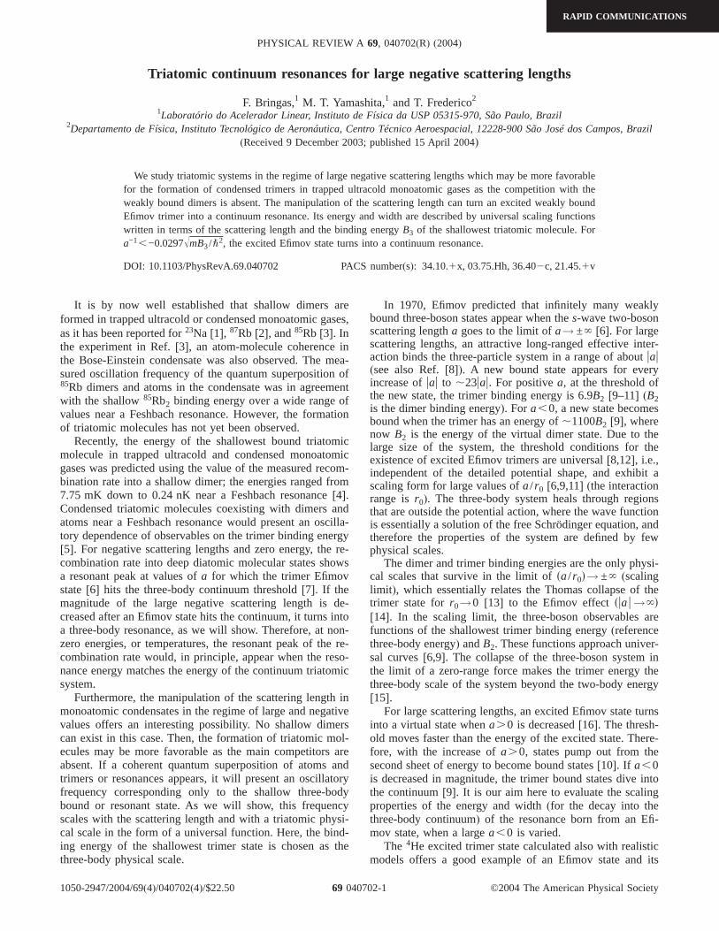
Triatomic continuum resonances for large negative scattering lengths
F. Bringas,1 M. T. Yamashita,1 and T. Frederico21Laboratório do Acelerador Linear, Instituto de Física da USP 05315-970, São Paulo, Brazil
2Departamento de Física, Instituto Tecnológico de Aeronáutica, Centro Técnico Aeroespacial, 12228-900 São José dos Campos, Brazil(Received 9 December 2003; published 15 April 2004)
We study triatomic systems in the regime of large negative scattering lengths which may be more favorablefor the formation of condensed trimers in trapped ultracold monoatomic gases as the competition with theweakly bound dimers is absent. The manipulation of the scattering length can turn an excited weakly boundEfimov trimer into a continuum resonance. Its energy and width are described by universal scaling functionswritten in terms of the scattering length and the binding energyB3 of the shallowest triatomic molecule. Fora−1,−0.0297ÎmB3/"2, the excited Efimov state turns into a continuum resonance.
DOI: 10.1103/PhysRevA.69.040702 PACS number(s): 34.10.1x, 03.75.Hh, 36.402c, 21.45.1v
It is by now well established that shallow dimers areformed in trapped ultracold or condensed monoatomic gases,as it has been reported for23Na [1], 87Rb [2], and85Rb [3]. Inthe experiment in Ref.[3], an atom-molecule coherence inthe Bose-Einstein condensate was also observed. The mea-sured oscillation frequency of the quantum superposition of85Rb dimers and atoms in the condensate was in agreementwith the shallow85Rb2 binding energy over a wide range ofvalues near a Feshbach resonance. However, the formationof triatomic molecules has not yet been observed.
Recently, the energy of the shallowest bound triatomicmolecule in trapped ultracold and condensed monoatomicgases was predicted using the value of the measured recom-bination rate into a shallow dimer; the energies ranged from7.75 mK down to 0.24 nK near a Feshbach resonance[4].Condensed triatomic molecules coexisting with dimers andatoms near a Feshbach resonance would present an oscilla-tory dependence of observables on the trimer binding energy[5]. For negative scattering lengths and zero energy, the re-combination rate into deep diatomic molecular states showsa resonant peak at values ofa for which the trimer Efimovstate[6] hits the three-body continuum threshold[7]. If themagnitude of the large negative scattering length is de-creased after an Efimov state hits the continuum, it turns intoa three-body resonance, as we will show. Therefore, at non-zero energies, or temperatures, the resonant peak of the re-combination rate would, in principle, appear when the reso-nance energy matches the energy of the continuum triatomicsystem.
Furthermore, the manipulation of the scattering length inmonoatomic condensates in the regime of large and negativevalues offers an interesting possibility. No shallow dimerscan exist in this case. Then, the formation of triatomic mol-ecules may be more favorable as the main competitors areabsent. If a coherent quantum superposition of atoms andtrimers or resonances appears, it will present an oscillatoryfrequency corresponding only to the shallow three-bodybound or resonant state. As we will show, this frequencyscales with the scattering length and with a triatomic physi-cal scale in the form of a universal function. Here, the bind-ing energy of the shallowest trimer state is chosen as thethree-body physical scale.
In 1970, Efimov predicted that infinitely many weaklybound three-boson states appear when thes-wave two-bosonscattering lengtha goes to the limit ofa→ ±` [6]. For largescattering lengths, an attractive long-ranged effective inter-action binds the three-particle system in a range of aboutuau(see also Ref.[8]). A new bound state appears for everyincrease ofuau to ,23uau. For positivea, at the threshold ofthe new state, the trimer binding energy is 6.9B2 [9–11] (B2is the dimer binding energy). For a,0, a new state becomesbound when the trimer has an energy of,1100B2 [9], wherenow B2 is the energy of the virtual dimer state. Due to thelarge size of the system, the threshold conditions for theexistence of excited Efimov trimers are universal[8,12], i.e.,independent of the detailed potential shape, and exhibit ascaling form for large values ofa/ r0 [6,9,11] (the interactionrange isr0). The three-body system heals through regionsthat are outside the potential action, where the wave functionis essentially a solution of the free Schrödinger equation, andtherefore the properties of the system are defined by fewphysical scales.
The dimer and trimer binding energies are the only physi-cal scales that survive in the limit ofsa/ r0d→ ±` (scalinglimit ), which essentially relates the Thomas collapse of thetrimer state forr0→0 [13] to the Efimov effectsuau →`d[14]. In the scaling limit, the three-boson observables arefunctions of the shallowest trimer binding energy(referencethree-body energy) andB2. These functions approach univer-sal curves[6,9]. The collapse of the three-boson system inthe limit of a zero-range force makes the trimer energy thethree-body scale of the system beyond the two-body energy[15].
For large scattering lengths, an excited Efimov state turnsinto a virtual state whena.0 is decreased[16]. The thresh-old moves faster than the energy of the excited state. There-fore, with the increase ofa.0, states pump out from thesecond sheet of energy to become bound states[10]. If a,0is decreased in magnitude, the trimer bound states dive intothe continuum[9]. It is our aim here to evaluate the scalingproperties of the energy and width(for the decay into thethree-body continuum) of the resonance born from an Efi-mov state, when a largea,0 is varied.
The 4He excited trimer state calculated also with realisticmodels offers a good example of an Efimov state and its
PHYSICAL REVIEW A 69, 040702(R) (2004)
RAPID COMMUNICATIONS
1050-2947/2004/69(4)/040702(4)/$22.50 ©2004 The American Physical Society69 040702-1

universal scaling properties with the shallow dimer and tri-mer binding energies[9,11]. These molecules are special dueto the large spatial size which spreads out much beyond therange of the potential[17,18]. The 4He-4He root-mean-square distances in4He3 for the ground and excited states[17,19] are of the order of 5 to 10Å and of about 50 to 90Å,respectively. The product of the mean-square interatom dis-tance with the separation energy of one atom from the trimerin units of "=m=1 (m is the atom mass) is about 1 in theground and the excited states[17,19], while the ratio of thebinding energiesB3
s0d /B3s1d<500 [6] (B3
sNd is the binding en-ergy of theNth trimer state).
In the present work we calculate the three-boson reso-nance energy and width for the decay into continuum statesfor large and negative scattering lengths. In this case it isjustifiable to use a Dirac-d potential. We solve subtractedhomogeneous equations defined within a renormalizationscheme applied to a three-body system interacting withs-wave zero-range pairwise potentials[10,15]. We presentthe results for the energies and widths in the form of a uni-versal scaling function[9], which gives the trajectory of thethree-body energy in the complex plane as a function of theshallow two-body virtual state energy. We show that a reso-nance becomes an excited trimer Efimov state when the largea,0 is decreased. We go beyond Ref.[10], where it wasfound the dependence of the virtual three-boson state energyon a.0 originated from an Efimov state which entered intothe second energy sheet.
One can fix the energy of one three-body bound state(thethree-body physical scale), and the two-body scatteringlength and get other observables. All the detailed informationabout the short-range force, beyond the low-energy two-bodyobservables, is retained in only one three-body physical in-formation in the limit of zero-range interaction. The exis-tence of a three-body scale implies in the low energy univer-sality found in three-body systems, or correlations betweenthree-body observables[20,15]. In the scaling limit[9,10],one has
OsE,B3,B2dsB3d−h = FsÎE/B3, ± ÎB2/B3d, s1d
whereO is a general observable of the three-body system atan energyE, with dimension of energy to the powerh. Thisequation means that any observable of the system can berepresented by a function that depends only on one three-and one two-body scales. The three-body scale is brought bythe reference energyB3 sbinding energyd of the shallowesttrimer state. The ± sign denotes positive or negative scatter-ing lengths. In the case of the energies of a resonance, of anexcited or virtual trimer state, instead of Eq.s1d, the scalingfunction is written as
E3 = B3 Es±ÎB2/B3d. s2d
sThroughout this paper, we use units such that"=m=1,wherem is the mass of the atom.d
After partial-wave projection, thes-wave subtracted inte-gral equation for three identical bosons is given by[10]
xsqd = 4ptsjdE0
`
dq8q82E−1
1
dyxsq8d
3 S 1
E3 − q2 − q82 − qq8y−
1
− m2 − q2 − q82 − qq8yD ,
s3d
wherej=E3− 34q2, m is the subtraction point, andt is given
by
t−1sjd = − 2p2ÎB2 − 4pjE0
` dp
j − p2 . s4d
HereB2 is the dimer virtual state energy.fFor positive valuesof the real part ofE3, Eqs. s3d and s4d are analytically ex-tended to the second energy sheet, as we discuss below.g
Throughout this work we perform calculations only con-sidering a,0 for a virtual dimer state. We use a contourdeformation method to calculate the resonance energy andwidth [21]. The homogeneous equation(3) is analyticallycontinued to the second sheet of energy by makingqsq8d→qe−iusq8e−iud with 0,u,p /4. For large enoughu, thesolution of Eq.(3) in the complex energy plane is found fortan s2ud.−Im sE3d /Re sE3d.
In the limit of a virtual dimer energy tending to zero, aninfinite number of Efimov states appears from the solution ofEq. (3) for negativeE3s=−B3d. The Nth Efimov state hasbinding energy given byB3
sNd with N=0 indicating theground state obtained from Eq.(3). When theNth Efimovstate turns into a resonance its complex energy is denoted byE3
sNd. In Fig. 1 the real part of the complex energies is shown,in units ofm=1, for the first three states obtained by solvingnumerically Eq.(3). In the figure, the values offRe sE3dg1/2
for the first three resonances are described by the positivepart of the plot. The curves representE3
s0d (solid line), E3s1d
(dashed line), andE3s2d (dotted line), i.e., the complex ener-
gies of the first three states of Eq.(3). Note that the subtrac-tion present in Eq.(3) regularizes it, and the Thomas collapseis avoided. WhenB2 is decreased, the resonance turns into abound state and the negative part of the plot gives the ener-gies of the groundsB3
s0dd, first sB3s1dd, and secondsB3
s2dd boundtrimer states. One realizes that the form of the curves is verysimilar which indicates that the functionE of Eq. (2) does notdepend on the state, which will be confirmed later on in thescaling plot of Fig. 3. The values ofÎB2 in units of m=1 atwhich the Efimov state becomes unbound are 0.066, 0.0028,and 0.000 13 for the ground, first, and second states, respec-tively. The ratios s0.066/0.0028d2<s0.0028/0.00013d2
,500 are practically independent of the state, in agreementwith the scaling limit implied by Eq.(2). It is curious that thereal part of the resonance energy tends to zero for largeenoughB2, while the width is nonzero.
In Fig. 2 the results for the imaginary part of the reso-nance complex energy are shown as a function ofB2 in unitsof m=1. The solid, dashed, and dotted lines are, respectively,the corresponding imaginary parts ofE3
s0d, E3s1d, andE3
s2d. Thethreshold values ofB2 for which the resonant state becomesbound are clearly seen in the figure and the resonance width
BRINGAS, YAMASHITA, AND FREDERICO PHYSICAL REVIEW A69, 040702(R) (2004)
RAPID COMMUNICATIONS
040702-2
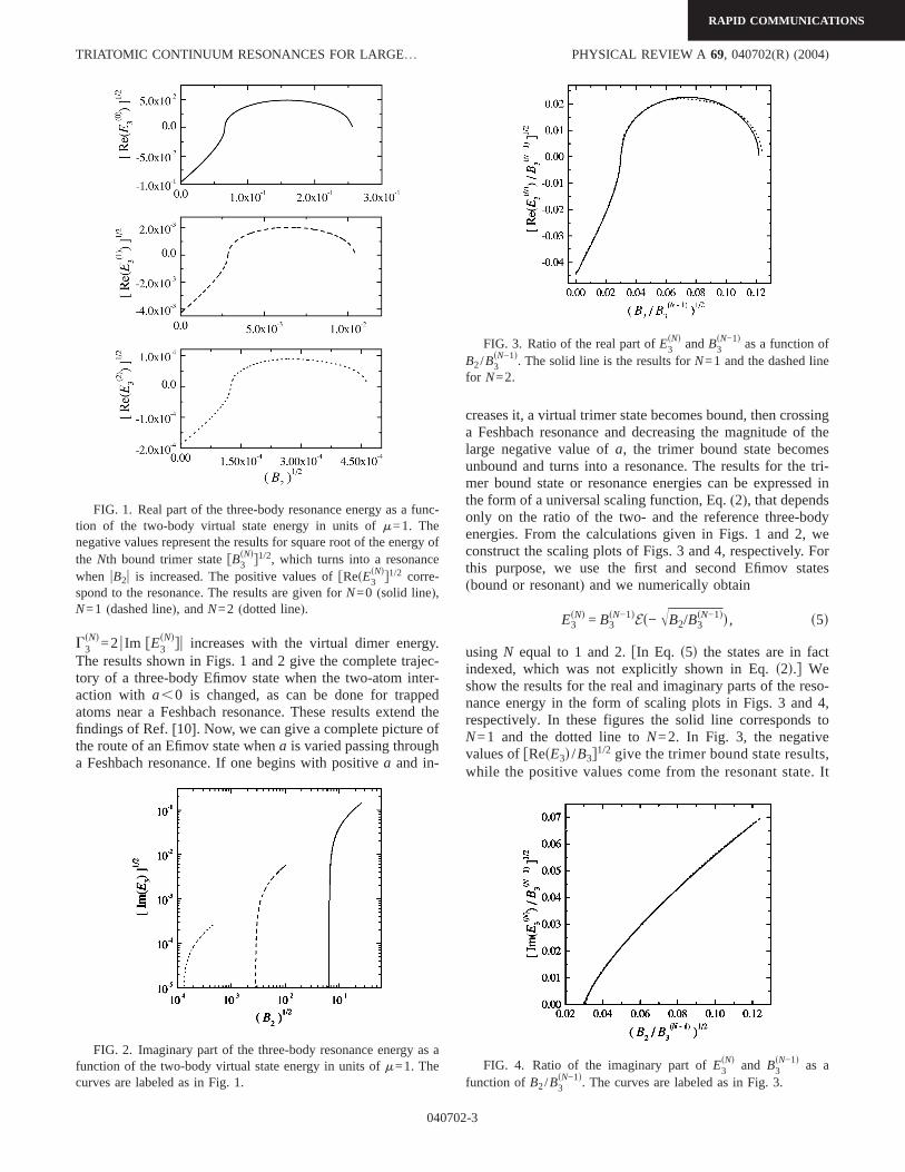
G3sNd=2u Im fE3
sNdgu increases with the virtual dimer energy.The results shown in Figs. 1 and 2 give the complete trajec-tory of a three-body Efimov state when the two-atom inter-action with a,0 is changed, as can be done for trappedatoms near a Feshbach resonance. These results extend thefindings of Ref.[10]. Now, we can give a complete picture ofthe route of an Efimov state whena is varied passing througha Feshbach resonance. If one begins with positivea and in-
creases it, a virtual trimer state becomes bound, then crossinga Feshbach resonance and decreasing the magnitude of thelarge negative value ofa, the trimer bound state becomesunbound and turns into a resonance. The results for the tri-mer bound state or resonance energies can be expressed inthe form of a universal scaling function, Eq.(2), that dependsonly on the ratio of the two- and the reference three-bodyenergies. From the calculations given in Figs. 1 and 2, weconstruct the scaling plots of Figs. 3 and 4, respectively. Forthis purpose, we use the first and second Efimov states(bound or resonant) and we numerically obtain
E3sNd = B3
sN−1dEs− ÎB2/B3sN−1dd, s5d
using N equal to 1 and 2.fIn Eq. s5d the states are in factindexed, which was not explicitly shown in Eq.s2d.g Weshow the results for the real and imaginary parts of the reso-nance energy in the form of scaling plots in Figs. 3 and 4,respectively. In these figures the solid line corresponds toN=1 and the dotted line toN=2. In Fig. 3, the negativevalues offResE3d /B3g1/2 give the trimer bound state results,while the positive values come from the resonant state. It
FIG. 1. Real part of the three-body resonance energy as a func-tion of the two-body virtual state energy in units ofm=1. Thenegative values represent the results for square root of the energy ofthe Nth bound trimer statefB3
sNdg1/2, which turns into a resonancewhen uB2u is increased. The positive values offResE3
sNdg1/2 corre-spond to the resonance. The results are given forN=0 (solid line),N=1 (dashed line), andN=2 (dotted line).
FIG. 2. Imaginary part of the three-body resonance energy as afunction of the two-body virtual state energy in units ofm=1. Thecurves are labeled as in Fig. 1.
FIG. 3. Ratio of the real part ofE3sNd andB3
sN−1d as a function ofB2/B3
sN−1d. The solid line is the results forN=1 and the dashed linefor N=2.
FIG. 4. Ratio of the imaginary part ofE3sNd and B3
sN−1d as afunction of B2/B3
sN−1d. The curves are labeled as in Fig. 3.
TRIATOMIC CONTINUUM RESONANCES FOR LARGE… PHYSICAL REVIEW A 69, 040702(R) (2004)
RAPID COMMUNICATIONS
040702-3
is clear that a universal curve for the scaling functionEs−ÎB2/B3d is approached as the results forN=1 and 2practically overlap. The imaginary part of the resonanceenergy in Fig. 4 appears for the dimer virtual state energyB2ù0.000 882B3, where the excited Efimov bound stateturns into the resonance. Our results extend the scalingfunction EsÎB2/B3d sbound dimer statesd obtained previ-ously in Refs.f9,10g to negative values of the argumentand for the trimer resonance region.
In conclusion, we have obtained the trajectory of an Efi-mov state when the two-atom interaction crosses a Feshbachresonance, in the form of a scaling function. The value of theresonance energy and width depends only on the dimerbound or virtual energy and the shallowest trimer bindingenergy. The route of an Efimov state whena is varied pass-ing through a Feshbach resonance can be summarized asfollows: beginning from a large positivea and increasing it
further, a virtual trimer state becomes bound and then aftercrossing a Feshbach resonance and decreasing the magnitudeof the large negative value ofa, the trimer bound state be-comes unbound and turns into a resonance, fora−1,−0.0297ÎmB3/"2, where B3 is the binding energy of theshallowest trimer state. In this respect, the study of trappedBose-Einstein condensates near a Feshbach resonance can befruitful not only to reveal the properties of an interactingcoherent quantum state under extreme conditions, but couldalso give new insights into the few-body physics underlyingthe curious phenomenon of Efimov resonant states.
We would like to thank Professor Y. Koike from HoseiUniversity for a helpful discussion. We thank the Brazilianagencies FAPESP(Fundação de Amparo a Pesquisa do Es-tado de São Paulo) and CNPq(Conselho Nacional de Desen-volvimento Científico e Tecnológico) for financial support.
[1] C. Mckenzieet al., Phys. Rev. Lett.88, 120403(2002).[2] R. H. Wynar, R. S. Freeland, D. J. Han, C. Ryu, and D. J.
Heinzen, Science287, 1016(2000).[3] N. R. Claussen, E. A. Donley, S. T. Thompson, and C. E.
Wieman, Phys. Rev. Lett.89, 010401(2002); E. A. Donley, N.R. Claussen, S. T. Thompson, and C. E. Wieman, Nature(London) 417, 529 (2002).
[4] M. T. Yamashita, T. Frederico, A. Delfino, and L. Tomio, Phys.Rev. A 68, 033406(2003).
[5] E. Braaten, H.-W. Hammer, and M. Kusunoki, Phys. Rev. Lett.90, 170402(2003).
[6] V. Efimov, Phys. Lett.33B, 563 (1970); Nucl. Phys. A 362,45 (1981); V. Efimov, Comments Nucl. Part. Phys.19, 271(1990), and references therein.
[7] E. Braaten and H.-W. Hammer, Phys. Rev. Lett.87, 160407(2001).
[8] E. Nielsen, D. V. Fedorov, A. S. Jensen, and E. Garrido, Phys.Rep. 347, 373 (2001).
[9] A. E.A. Amorim, T. Frederico, and L. Tomio, Phys. Rev. C56,R2378(1997); T. Frederico, L. Tomio, A. Delfino, and A. E.A.Amorim, Phys. Rev. A60, R9 (1999).
[10] M. T. Yamashita, T. Frederico, A. Delfino, and L. Tomio, Phys.
Rev. A 66, 052702(2002).[11] E. Braaten, H.-W. Hammer, and M. Kusunoki, Phys. Rev. A
67, 022505(2003).[12] A. Delfino, T. Frederico, and L. Tomio, Few-Body Syst.28,
259 (2000); J. Chem. Phys.113, 7874(2000).[13] L. H. Thomas, Phys. Rev.47, 903 (1935).[14] S. K. Adhikari, A. Delfino, T. Frederico, I. D. Goldman, and L.
Tomio, Phys. Rev. A37, 3666(1988).[15] S. K. Adhikari, T. Frederico, and I. D. Goldman, Phys. Rev.
Lett. 74, 487 (1995); S. K. Adhikari and T. Frederico,ibid.74, 4572(1995).
[16] S. K. Adhikari, A. C. Fonseca, and L. Tomio, Phys. Rev. C26,77 (1982); S. K. Adhikari and L. Tomio,ibid. 26, 83 (1982).
[17] P. Barletta and A. Kievsky, Phys. Rev. A64, 042514(2001).[18] V. Roudnev and S. Yakovlev, Chem. Phys. Lett.328, 97
(2000).[19] M. T. Yamashita, R. S. Marques de Carvalho, L. Tomio, and T.
Frederico, Phys. Rev. A68, 012506(2003).[20] T. Frederico and I. D. Goldman, Phys. Rev. C36, 1661(1987).[21] J. Aguilar and J. M. Combes, Commun. Math. Phys.22, 269
(1971); E. Balslev and J. M. Combes,ibid. 22, 280 (1971).
BRINGAS, YAMASHITA, AND FREDERICO PHYSICAL REVIEW A69, 040702(R) (2004)
RAPID COMMUNICATIONS
040702-4

1
Radii of weakly bound three-body systems: halo nuclei and molecules
M.T. Yamashita a, T. Frederico b, R.S. Marques de Carvalho c and Lauro Tomioc
aLaboratorio do Acelerador Linear, Instituto de Fısica, Universidade de Sao Paulo,C.P. 66318, CEP 05315-970, Sao Paulo, Brazil
bDepartamento de Fısica, Instituto Tecnologico de Aeronautica, CTA,C.P. 12228-900, Sao Jose dos Campos, Brazil
cInstituto de Fısica Teorica, Universidade Estadual Paulista,C.P. 01405-900, Sao Paulo, Brazil
A renormalized three-body model with zero-range potential is used to estimate themean-square radii of three-body halo nuclei and molecular systems. The halo nuclei (6He,11Li, 14Be and 20C) are described as point-like inert cores and two neutrons. The molecularsystems, with two helium atoms, are of the type 4He2−X, where X=4He, 6Li, 7Li, or 23Na.The estimations are compared with experimental data and realistic results.
Halo nuclei and weakly bound molecules are quantum systems with very large sizesin which the constituent particles have a large probability to be found much beyondthe interaction range. Under this circumstances, the physical properties of such boundsystems can be defined by few physical scales.
In the present contribution we report results obtained for the root-mean-square radii ofthree-body halo nuclei and molecular systems that are obtained from a universal scaling
function calculated within a renormalized scheme for three particles interacting throughpairwise Dirac-δ potential. In the case where we have the two-body scattering length,a, much greater than the effective range of the potential, r0, (a/r0 1) our zero-rangeapproach is expected to be a good aproximation [1]. In the scaling limit [2,3] all theobservables of the three-body system can be represented by a function that depends onlyon the three- and two-body scales.
Figure 1 and Table 1 show results for halo nuclei systems, where C represents the coreand n the neutron. In Fig. 1, our results (h = mn = 1) are given as functions of themass ratio A ≡ mC/mn, where mC and mn are the masses of the core and the neutron,respectively. r2
γ (γ ≡ C, n) is the mean-square distance from the particle γ to the center-of-mass of the system. r2
nγ is the mean-square distance between the particles n and γ.The results given in Fig. 1 are obtained in the limit where the two-body energies are equalto zero, such that the system have just the three-body energy as a physical scale. Ourformalism is presented in detail in ref. [4], where we show that Fig. 1 applies equally wellto weakly bound molecular systems, as the results are given in terms of dimensionlessquantities.

2
Figure 1. Dimensionless products√
〈r2nγ〉E3 [upper (a) plots] and
√
〈r2γ〉E3 [lower (b)
plots], are given as functions of A ≡ mC/mn, for Enn = EnC = 0. The results for theground-state are shown with solid line (γ = n) and dot-dashed line (γ = C); and, for thefirst excited state, with dashed line (γ = n) and dotted line (γ = C).
We can see in Fig. 1 that, although the ratio between the energies of the ground and thefirst excited states are about few hundreds [5], we have practically no difference betweenour dimensionless curves, supporting the validity of our scaling limit. The experimentalresults for the halo nuclei 6He (4He+n+n) and 14Be (12Be+n+n) are quite consistent withour predictions based on the zero-range calculations. Therefore, our assumption that suchnuclei could be represented by inert cores and two neutrons, interacting through shortrange forces, produces a reasonable description of the average interparticle distances.
In Table 1 we present the results of the neutron-neutron root-mean-square distances,for the halo nuclei C-n-n system 6He, 11Li, 14Be, and 20C. Our results are compared withexperimental values, given in ref. [6]. Although the calculations are in reasonable agree-ment with data, they systematically underestimate the measured values. Analogously, weshow in Table 2 our results, obtained in ref. [4] for weakly-bound three-body molecules. Inthis case, we present results for the root-mean-square distances between the particles andalso the root-mean-square distances of each particle to the center-of-mass of the system.For the 4He3 trimer, our calculations deviate only about 14% from the realistic resultsobtained in ref. [7].
In conclusion, the present model for the weakly bound halo nuclei and molecular sys-tems gives a reasonable description of these systems, validated by the comparison withexperimental data and realistic results.
We would like to thank the partial support from FAPESP and CNPq of Brazil.
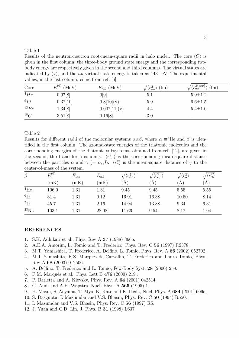
3
Table 1Results of the neutron-neutron root-mean-square radii in halo nuclei. The core (C) isgiven in the first column, the three-body ground state energy and the corresponding two-body energy are respectively given in the second and third columns. The virtual states areindicated by (v), and the nn virtual state energy is taken as 143 keV. The experimentalvalues, in the last column, come from ref. [6].
Core E(0)3 (MeV) EnC (MeV)
√
〈r2nn〉 (fm)
√
〈r2expnn 〉 (fm)
4He 0.97[8] 0[9] 5.1 5.9±1.29Li 0.32[10] 0.8[10](v) 5.9 6.6±1.512Be 1.34[8] 0.002[11](v) 4.4 5.4±1.018C 3.51[8] 0.16[8] 3.0 -
Table 2Results for different radii of the molecular systems ααβ, where α ≡4He and β is iden-tified in the first column. The ground-state energies of the triatomic molecules and thecorresponding energies of the diatomic subsystems, obtained from ref. [12], are given inthe second, third and forth columns. 〈r2
αγ〉 is the corresponding mean-square distancebetween the particles α and γ (= α, β). 〈r2
γ〉 is the mean-square distance of γ to thecenter-of-mass of the system.
β E(0)3 Eαα Eαβ
√
〈r2αα〉
√
〈r2αβ〉
√
〈r2α〉
√
〈r2β〉
(mK) (mK) (mK) (A) (A) (A) (A)4He 106.0 1.31 1.31 9.45 9.45 5.55 5.556Li 31.4 1.31 0.12 16.91 16.38 10.50 8.147Li 45.7 1.31 2.16 14.94 13.88 9.34 6.3123Na 103.1 1.31 28.98 11.66 9.54 8.12 1.94
REFERENCES
1. S.K. Adhikari et al., Phys. Rev A 37 (1988) 3666.2. A.E.A. Amorim, L. Tomio and T. Frederico, Phys. Rev. C 56 (1997) R2378.3. M.T. Yamashita, T. Frederico, A. Delfino, L. Tomio, Phys. Rev. A 66 (2002) 052702.4. M.T Yamashita, R.S. Marques de Carvalho, T. Frederico and Lauro Tomio, Phys.
Rev A 68 (2003) 012506.5. A. Delfino, T. Frederico and L. Tomio, Few-Body Syst. 28 (2000) 259.6. F.M. Marques et al., Phys. Lett B 476 (2000) 219 .7. P. Barletta and A. Kievsky, Phys. Rev. A 64 (2001) 042514.8. G. Audi and A.H. Wapstra, Nucl. Phys. A 565 (1995) 1.9. H. Masui, S. Aoyama, T. Myo, K. Kato and K. Ikeda, Nucl. Phys. A 684 (2001) 609c.10. S. Dasgupta, I. Mazumdar and V.S. Bhasin, Phys. Rev. C 50 (1994) R550.11. I. Mazumdar and V.S. Bhasin, Phys. Rev. C 56 (1997) R5.12. J. Yuan and C.D. Lin, J. Phys. B 31 (1998) L637.

Few-Body Systems 34, 191–196 (2004)
DOI 10.1007/s00601-004-0038-2
Three-Body Recombination in Ultracold
Systems: Prediction of Weakly-Bound
Atomic Trimer Energies
L. Tomio1, V. S. Filho1, M. T. Yamashita2, A. Gammal2, and T. Frederico3
1 Instituto de Fısica Teoorica, Universidade Estadual Paulista,
01405-900 S~aao Paulo, Brasil2 Laboratoorio do Acelerador Linear, Instituto de Fısica da USP,
05315-970 S~aao Paulo, Brasil3 Departamento de Fısica, Instituto Tecnoloogico de Aeronautica, CTA,
12228-900 S~aao Josee dos Campos, Brasil
Received October 14, 2003; accepted November 11, 2003
Published online May 24, 2004; # Springer-Verlag 2004
Abstract. The three-body recombination coefficient of an ultracold atomicsystem, together with the corresponding two-body scattering length a, allowus to predict the energy E3 of the shallow trimer bound state, using a universalscaling function. The production of dimers in trapped Bose-Einstein con-densates, from three-body recombination processes, in the regime of shortmagnetic pulses near a Feshbach resonance, is also studied in line with theexperimental observation.
1 Introduction
The interaction among neutral atoms is equivalent to a range zero in the limit ofa ! 1. For identical bosonic atoms, either the Efimov effect [1] or the Thomascollapse [2] can happen when the ratio between a and the range goes to infinity.This is the scaling limit, where the three-boson properties can be determined justby two scales: the dimer binding energy (or virtual dimer energy) and the shallowtrimer binding energy [3].
Recently, Bose-Einstein condensation (BEC) has been obtained with trappedultra-cold atomic gases. Losses of atoms in BEC can occur due to three-atom re-combination processes, which are measured in several cases: 23NajF ¼ 1;mF ¼ 1i
Article based on the presentation by L. Tomio at the Third Workshop on the Dynamics and Structure
of Critically Stable Quantum Few-Body Systems, Trento, Italy, September 2003

[4], 87RbjF ¼ 1;mF ¼ 1i [5, 6], and 85RbjF ¼ 2;mF ¼ 2i [7, 8]. The value ofthe three-body recombination coefficient, together with the corresponding two-body scattering length, allow us to predict the energy of the shallow trimer boundstate, as described in Sect. 2.
Another aspect related to the three-body recombination process, supported byexperimental observations, is a possible enhancement due to quantum coherence(laser effect), which may happen in a special situation of fast changes of a. In Sect.3, we discuss the dynamics of BEC related to this aspect of the three-body recom-bination process. Our conclusions are summarized in Sect. 4.
2 Weakly Bound Atomic Trimer Energies
It was shown by some of us, in ref. [9], how to obtain the trimer binding energies ofan atomic system from the three-body recombination rate and the correspondingtwo-body scattering length. A universal scaling function which gives the depend-ence of the recombination parameter as a function of the weakly bound trimerenergy (E3) is calculated within a renormalized scheme for three particles inter-acting through pairwise Dirac-delta interaction [9]. For atoms with mass m and forlarge a, E3 is shown to be in the interval 1<mða=hÞ2
E3 < 6:9. The contribution ofa deep-bound state to the prediction, in the case of 85RbjF ¼ 2;mF ¼ 2i for aparticular trap, is shown to be relatively small. Also, using the predicted energies ofthe triatomic molecules in ultra-cold traps, the sizes of the trimers 23Naj1;1i and87Rbj1;1i can be estimated. In this case, a scaling function gives the mean-squareradii as a function of E3 and a. The root-mean-square distance between two atoms
in a triatomic molecule is estimated to be 0:8ffiffiffiffiffiffiffiffiffiffiffiffiffiffiffiffiffiffiffiffiffiffiffiffiffiffiffiffiffiffiffiffiffiffih2=ðmðE3 E2ÞÞ
q, where E2 is the
dimer binding energy [10].The rate of three free bosons to recombine, forming a dimer and one remaining
particle, is given in the limit of zero energy, by the recombination coefficient[11, 12]
K3 ¼ h
ma4; ð1Þ
where is a dimensionless parameter. When a> 0, the recombination parameter oscillates between zero and a maximum value as a function of a, as shown in refs.[13] ( 68:4), [14] ( 65), and [15] ( 67:9).
By using a general scaling procedure, it is shown in ref. [9] that one can expressthe functional dependence of in terms of the two- and three-body energies,
ffiffiffiffiffiffiffiffiffiffiffiffiffiE2=E3
p , considering that for large scattering lengths one has 1=a ¼ffiffiffiffiffiffiffiffiffiffiffiffiffiffiffi
mE2=h2
q. Such scaling form of is derived in detail in ref. [9], using results
presented in ref. [11]. It is given by
¼ max sin2
1:01 ln
ffiffiffiffiffiE2
E3
rþ D
ffiffiffiffiffiE2
E3
r ; ð2Þ
where D, a function of the ratio E2=E3, depends on the interaction at short dis-tances, which defines E3.
192 L. Tomio et al.

Next, considering the calculation of the scaling function, with the subtractedform of the Faddeev equations [16], and considering the relation between thetransition matrix elements and the three-body recombination coefficient at zeroenergy, the functional dependence of was derived in terms of the ratio E2=E3
(see Fig. 1 of ref. [9]). The scaling limit is well approached in the calculations, withthe maximum occurring near the atom-dimer threshold (E3 E2) and whenðE3=E2Þ1=2 0:38 [3], such that between two consecutive maxima of we have1<mða=hÞ2
E3 < 6:9.Using the experimental values expt, for a few atomic species AZjF;mFi, one
can obtain two possible values of the weakly bound triatomic molecular states thatare consistent with the universal scaling plot that was derived. In Table 1, thepredicted trimer binding energies, in respect to the threshold, S3 ðE3 E2Þand S03 ðE0
3 E2Þ, are given in milliKelvins. We consider the central values ofthe experimental dimensionless recombination parameters.
3 Coherent Dimer Formation
One should note that the three-body recombination coefficient was derived in theprevious section considering very dilute systems and considering that the two-bodyinteraction is kept fixed. Another interesting possibility may happen in a specialsituation when we have fast changes of the two-body scattering length a. In thiscase, the three-body recombination process may be enhanced due to quantumcoherence. The remaining atoms and dimers are produced in a single state and,due to the symmetrization of the full wave-function, the recombination processwhich happens in this background is enhanced (laser effect).
Supporting this possibility, it was observed [8] an isotropic burst of relativelyhot 85Rb atoms with temperature of about 150 nK, when a fast magnetic pulse neara Feshbach resonance increases the scattering length up to 4000 a0. The maximumvalue of a gives a lower bound for the temperature of the remaining atoms about75 nK consistent with the experiment. In line with the experimental observation,we make an attempt to describe the remaining number of condensed atoms afterthe pulse, within a mean field description. For that, we consider that: (i) shallowdimers, with their centre-of-mass in s-wave, are formed (the temperature of theatoms in the burst is consistent with weakly bound dimers and not deeply bound
Table 1. For the atomic species AZjF;mFi, the predicted trimer binding energies with
respect to the atom-dimer threshold are shown in the 4th and 5th columns. expt and E2
are, respectively, given in the 2nd and 3rd column. For 87Rbj1;1i, the recombination
process was obtained in ref. [5] for noncondensed () and condensed (y) trapped atoms
AZjF;mFi expt E2 (mK) S3 (mK) S03 (mK)
23Naj1;1i 42 12 [4] 2.85 4.9 0.2187Rbj1;1i 52 22 [5] 0.17 0.39 0.00587Rbj1;1i 41 17y [5] 0.17 0.30 0.01387Rbj2; 2i 130 36 [6] 0.17 – –85Rbj2;2i 7.84 3.4 [7, 8] 1.3 104 1.14 104 3.8 105
Three-Body Recombination in Ultracold Systems 193
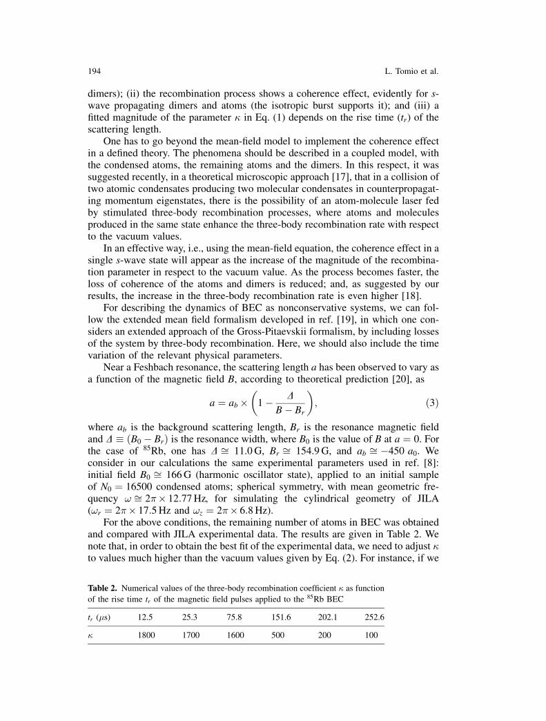
dimers); (ii) the recombination process shows a coherence effect, evidently for s-wave propagating dimers and atoms (the isotropic burst supports it); and (iii) afitted magnitude of the parameter in Eq. (1) depends on the rise time (tr) of thescattering length.
One has to go beyond the mean-field model to implement the coherence effectin a defined theory. The phenomena should be described in a coupled model, withthe condensed atoms, the remaining atoms and the dimers. In this respect, it wassuggested recently, in a theoretical microscopic approach [17], that in a collision oftwo atomic condensates producing two molecular condensates in counterpropagat-ing momentum eigenstates, there is the possibility of an atom-molecule laser fedby stimulated three-body recombination processes, where atoms and moleculesproduced in the same state enhance the three-body recombination rate with respectto the vacuum values.
In an effective way, i.e., using the mean-field equation, the coherence effect in asingle s-wave state will appear as the increase of the magnitude of the recombina-tion parameter in respect to the vacuum value. As the process becomes faster, theloss of coherence of the atoms and dimers is reduced; and, as suggested by ourresults, the increase in the three-body recombination rate is even higher [18].
For describing the dynamics of BEC as nonconservative systems, we can fol-low the extended mean field formalism developed in ref. [19], in which one con-siders an extended approach of the Gross-Pitaevskii formalism, by including lossesof the system by three-body recombination. Here, we should also include the timevariation of the relevant physical parameters.
Near a Feshbach resonance, the scattering length a has been observed to vary asa function of the magnetic field B, according to theoretical prediction [20], as
a ¼ ab
1 DB Br
; ð3Þ
where ab is the background scattering length, Br is the resonance magnetic fieldand D ðB0 BrÞ is the resonance width, where B0 is the value of B at a ¼ 0. Forthe case of 85Rb, one has D ffi 11.0 G, Br ffi 154.9 G, and ab ffi 450 a0. Weconsider in our calculations the same experimental parameters used in ref. [8]:initial field B0 ffi 166 G (harmonic oscillator state), applied to an initial sampleof N0 ¼ 16500 condensed atoms; spherical symmetry, with mean geometric fre-quency ! ffi 2 12:77 Hz, for simulating the cylindrical geometry of JILA(!r ¼ 2 17:5 Hz and !z ¼ 2 6:8 Hz).
For the above conditions, the remaining number of atoms in BEC was obtainedand compared with JILA experimental data. The results are given in Table 2. Wenote that, in order to obtain the best fit of the experimental data, we need to adjust to values much higher than the vacuum values given by Eq. (2). For instance, if we
Table 2. Numerical values of the three-body recombination coefficient as function
of the rise time tr of the magnetic field pulses applied to the 85Rb BEC
tr (s) 12.5 25.3 75.8 151.6 202.1 252.6
1800 1700 1600 500 200 100
194 L. Tomio et al.

consider the rise time of the magnetic field pulses lower than 100 ms, we have1000 . . 2000. However, decreases while tr increases, such that 100 fortr of the order of 250 ms. In this case, slowing the rise time, we note that approaches the predicted interval 0 . 68.
The phenomenon of enhancement in the magnitude of the three-body recom-bination coefficient gives an indication that a laser-like effect may be occurring inthe experiment of ref. [8]. Our picture suggests that for very short time scales (timeranges varying from 0 up to 100 ms) the three-body recombination processes pro-duce shallow dimers and a third atom (burst effect) in many-boson states.
The coherent production of shallow dimers occurs for very short rise times anddisappears for longer ones, producing the strange effect reported in ref. [8], of adecreasing dissipation from the condensate for long rise times. This effect isbrought to the mean-field calculation by the enhanced values of as a functionof tr, which can be approximately given by the parametrization
ðtrÞ ¼ 2300 exp ð0:01!trÞ: ð4Þ
Such parametrization is convenient to study the remaining number of atoms in 85RbBEC as a function of the scaled rise time of the applied magnetic pulse, for fixedhold times, with the parameters considered in ref. [8] (where the magnetic fieldduring the hold time is Bh ¼ 156.7 G). The results of our model calculation describethe observed behavior of the remaining number of atoms (see Fig. 3 of ref. [18]).
4 Conclusions
In the present communication, we report recent results that we have obtained byconsidering the three-body recombination processes in ultracold or condensedatomic gases. From the experimental values of the recombination coefficienttogether with the corresponding two-body scattering length, we are able to predictenergies of the shallow trimer bound state for a few atomic systems. To obtain thescaling function corresponding to the dependence of the dimensionless recombina-tion parameter with the shallow trimer binding energy, we use a zero-range modelwhich is valid for large scattering lengths. We point out that, at least, one experi-mental result for 87Rbj2; 2i is outside the interval of theoretical vacuum values of, which may indicate that some particular physics is present in that experiment.
We also observe that, when considering the special situation of fast variations ofthe two-body scattering length, near a Feshbach resonance, the experimental resultscan be put consistent with a mean-field description, if one allows a strong enhance-ment of the three-body recombination process motivated by possible quantumcoherence phenomena in the production of dimers (laser effect). However, certainlyone has to go beyond the mean-field description with only condensed atoms, to beable to implement the coherence effect in a defined way. Such a mean-field theoryshould describe simultaneously the dynamics of the condensed atoms, the remain-ing atoms and the dimers, which is within the scope of a future investigation.
Acknowledgement. This work was supported by Fundac~aao de Amparo aa Pesquisa do Estado de S~aao
Paulo and Conselho Nacional de Desenvolvimento Cientıfico e Tecnoloogico.
Three-Body Recombination in Ultracold Systems 195

References
1. Efimov, V.: Phys. Lett. B33, 563 (1970)
2. Thomas, L. H.: Phys. Rev. 47, 903 (1935)
3. Frederico, T., Tomio, L., Delfino, A., Amorim, A. E. A.: Phys. Rev. A60, R9 (1999)
4. Stamper-Kurn, D. M., et al.: Phys. Rev. Lett. 80, 2027 (1998)
5. Burt, E. A., et al.: Phys. Rev. Lett. 79, 337 (1997)
6. S€ooding, J., et al.: Appl. Phys. B69, 257 (1999)
7. Roberts, J. L., Claussen, N. R., Cornish, S. L., Wieman, C. E.: Phys. Rev. Lett. 85, 728 (2000)
8. Claussen, N. R., Donley, E. A., Thompson, S. T., Wieman, C. E.: Phys. Rev. Lett. 89, 010401
(2002)
9. Yamashita, M. T., Frederico, T., Tomio, L., Delfino, A.: Phys. Rev. A68, 033406 (2003)
10. Yamashita, M. T., Marques de Carvalho, R. S., Tomio, L., Frederico, T.: Phys. Rev. A68, 012506
(2003)
11. Nielsen, E., Fedorov, D. V., Jensen, A. S., Garrido, E.: Phys. Rep. 347, 373 (2001), and references
therein
12. Fedichev, P. O., Reynolds, M. W., Shlyapnikov, G. V.: Phys. Rev. Lett. 77, 2921 (1996)
13. Nielsen, E., Macek, J. H.: Phys. Rev. Lett. 83, 1566 (1999)
14. Esry, B. D., Greene, C. H., Burke Jr., J. P.: Phys. Rev. Lett. 83, 1751 (1999)
15. Bedaque, P. J., Braaten, E., Hammer, H.-W.: Phys. Rev. Lett. 85, 908 (2000)
16. Adhikari, S. K., Frederico, T., Goldman, I. D.: Phys. Rev. Lett. 74, 487 (1995); Adhikari, S. K.,
Frederico, T.: Phys. Rev. Lett. 74, 4572 (1995)
17. Borca, B., Dunn, J. W., Kokoouline, V., Greene, C. H.: Phys. Rev. Lett. 91, 070404 (2003)
18. Filho, V. S., Tomio, L., Gammal, A., Frederico, T.: Preprint cond-mat 0306218
19. Filho, V. S., Abdullaev, F. Kh., Gammal, A., Tomio, L.: Phys. Rev. A63, 053603 (2001)
20. Moerdijk, A. J., Verhaar, B. J., Axelsson, A.: Phys. Rev. A51, 4852 (1995)
196 L. Tomio et al.

Bibliografia
[1] V. Efimov. Phys. Lett. B33, 563 (1970).
[2] V. Efimov. Nucl. Phys. A362, 45 (1981).
[3] V. Efimov. Comments Nucl. Part. Phys. 19, 271 (1990).
[4] D. V. Fedorov e A. S. Jensen. Phys. Rev. Lett. 71, 4103 (1993).
[5] D. V. Fedorov, A. S. Jensen e K. Riisager. Phys. Rev. Lett. 73, 2817 (1994).
[6] D. V. Fedorov, E. Garrido e A. S. Jensen. Phys. Rev. C51, 3052 (1995).
[7] M. T. Yamashita, T. Frederico, A. Delfino e Lauro Tomio. Phys. Rev. A66,
052702 (2002).
[8] M. T. Yamashita, T. Frederico, A. Delfino e Lauro Tomio. Phys. Rev. A68,
033406 (2003).
[9] M. T. Yamashita, R.S. Marques, Lauro Tomio e T. Frederico. Phys. Rev. A68,
012506 (2003).
[10] M. T. Yamashita, Lauro Tomio e T. Frederico. Nucl. Phys. A 735, 40 (2004).
[11] T. K. Lim, S. K. Duffy e W. C. Damest. Phys. Rev. Lett. 38, 341 (1977).
[12] S. Huber, T. K. Lim e D. H. Feng. Phys. Rev. C18, 1534 (1978).
[13] A. E. A. Amorim, L. Tomio e T. Frederico. Phys. Rev. C46, 2224 (1992).
[14] A.E.A. Amorim, T. Frederico e L. Tomio. Phys. Rev. C56, R2378 (1997).

108 BIBLIOGRAFIA
[15] T. Frederico, L. Tomio, A. Delfino e E.A. Amorim. Phys. Rev. A60, R9 (1999).
[16] A. Delfino, T. Frederico e L. Tomio. Few-Body Syst. 28, 259 (2000).
[17] A. Delfino, T. Frederico e L. Tomio. J. Chem. Phys. 113, 7874 (2000).
[18] S.K. Adhikari e T. Frederico. Phys. Rev. Lett. 74, 4572 (1995).
[19] S.K. Adhikari, T. Frederico e I.D. Goldman. Phys. Rev. Lett. 74, 487 (1995).
[20] L. H. Thomas. Phys. Rev. 47, 903 (1935).
[21] S.K. Adhikari, A. Delfino, T. Frederico, I.D. Goldman e L. Tomio. Phys. Rev.
A37, 3666 (1988).
[22] G. S. Danilov. Sov. Phys. JETP 13, 349 (1961).
[23] V. F. Kharchenko. Sov. J. Nucl. Phys. 16, 173 (1973).
[24] E. G. Tkachenko. Phys. Lett. B98, 328 (1981).
[25] E. Nielsen, D.V. Fedorov, A.S. Jensen e E. Garrido. Phys. Rep. 347, 373 (2001).
[26] M. H. Anderson et al. Science 269, 198 (1995).
[27] C. C. Bradley et al. Phys. Rev. Lett. 75, 1687 (1995).
[28] K. B. Davis et al. Phys. Rev. Lett. 75, 3969 (1995).
[29] S. Inouye et al. Nature 392, 151 (1998).
[30] E. Timmermans, P. Tommasini, M. Hussein e A. Kerman. Phys. Rep. 315, 199
(1999).
[31] R. Wynar, R.S. Freeland, D.J. Han, C. Ryu e D.J. Heinzen. Science 287, 1016
(2000).
[32] C. Mckenzie et al. Phys. Rev. Lett. 88, 120403 (2001).
[33] E. Nielsen e J.H. Macek. Phys. Rev. Lett. 83, 1566 (1999).
[34] B.D. Esry, C.H. Greene e Jr. J.P. Burke. Phys. Rev. Lett. 83, 1751 (1999).
BIBLIOGRAFIA 109
[35] P.F. Bedaque, E. Braaten e H.-W Hammer. Phys. Rev Lett. 85, 908 (2000).
[36] W. Schollkopf e J.P. Toennies. Science 266, 1345 (1994).
[37] K.T. Tang, J.P. Toennies e C.L. Yiu. Phys. Rev. Lett. 74, 1546 (1995).
[38] R.E. Grisenti et al. Phys. Rev. Lett. 85, 2284 (2000).
[39] P. Barletta e A. Kievsky. Phys. Rev. A64, 042514 (2001).
[40] V. Roudnev e S. Yakovlev. Chem. Phys. Lett. 328, 97 (2000).
[41] M. V. Zhukov et al. Phys. Rep. 231, 151 (1993).
[42] G. Audi e A. H. Wapstra. Nucl. Phys. A595, 409 (1995).
[43] F. Robicheaux. Phys. Rev. A60, 1706 (1999).
[44] D. C. Zheng et al. Phys. Rev. C48, 1083 (1993).
[45] J. A. Caggiano et al. Phys. Rev. C60, 064322 (1999).
[46] F. Ciesielski. Systeme a quatre corps: etats lies et etats de diffusion par la
resolution numerique des equations de Faddeec-Yakubovski, tese, Universite Jo-
seph Fourier, Grenoble 1997.
[47] A. S. Jensen, K. Riisager, D. V. Fedorov e E. Garrido. Europhys. Lett. 61, 320
(2003).
[48] J.J. Sakurai. Modern Quantum Mechanics - Revised Edition. Addison-Wesley
Publishing Company (1994).
[49] F. Bringas, M. T. Yamashita e T. Frederico. Phys. Rev A69, 040702(R) (2004).
[50] L.D. Faddeev. Soviet Phys. JETP 12, 1014 (1961).
[51] T. Frederico, V. S. Timoteo e L. Tomio. Nucl. Phys. A653, 209 (1999).
[52] T. Frederico, A. Delfino e L. Tomio. Phys. Lett. B481, 143 (2000).
[53] T. Frederico. Hamiltonianas renormalizadas em mecanica quantica, tese de
livre-docencia, Universidade de Sao Paulo, 1998.

110 BIBLIOGRAFIA
[54] S. Weinberg. The Quantum Theory of Fields Vol. II - Modern Applications,
Cambridge University Press 1996.
[55] F. E. Low. Phys. Rev. 97, 1392 (1955).
[56] G.V. Skorniakov e K.A. Ter-Martirosyan. Soviet Phys. JETP 4, 648 (1957).
[57] J. Aguilar e J.M. Combes. Commun. Math. Phys. 22, 269 (1971).
[58] E. Balslev e J. M. Combes. Commun. Math. Phys. 22, 280 (1971).
[59] A. Delfino e W. Glockle. Phys. Rev. C30, 376 (1984).
[60] S.K. Adhikari e L. Tomio. Phys. Rev. C26, 83 (1982).
[61] Kenneth G. Wilson. Phys. Rev. D3, 1818 (1971).
[62] T. Frederico e I.D. Goldman. Phys. Rev. C87, 1661 (1987).
[63] Th. Cornelius e W. Glocke. J. Chem. Phys. 85, 1 (1986).
[64] S. Huber. Phys. Rev. A31, 3981 (1985).
[65] D.V. Fedorov e A.S. Jensen. J. Phys. A34, 6003 (2001).
[66] E.A. Kolganova, A.K. Motovilov e S.A. Sofianos. Phys. Rev. A56, R1686
(1997).
[67] E. Braaten, H.-W. Hammer e M. Kusunoki. Phys. Rev. A67, 022505 (2003).
[68] Abraham Pais. Sutil e o Senhor, A Ciencia e a Vida de Albert Einstein. Editora
Nova Fronteira (1982).
[69] S. N. Bose. Z. Phys. 26, 178 (1924).
[70] M. H. Anderson et al. Science 269, 198 (1995).
[71] E. Tiesinga, A.J. Moerdijk, B.J. Verhaar e H.T.C. Stoof. Phys. Rev. A46,
R1167 (1992).
[72] E. Tiesinga, B.J. Verhaar e H.T.C. Stoof. Phys. Rev. A47, 4114 (1993).
BIBLIOGRAFIA 111
[73] H. Feshbach. Ann. Phys. 19, 287 (1962).
[74] Ph. Courteille et al. Phys. Rev. Lett. 81, 69 (1998).
[75] J. L. Roberts et al. Phys. Rev. Lett. 81, 5109 (1998).
[76] K. Xu et al. Phys. Rev. Lett. 91, 210402 (2003).
[77] J. Herbig et al. Science 301, 1510 (2003).
[78] E.A. Burt et al. Phys. Rev. Lett. 79, 337 (1997).
[79] D.M. Stamper-Kurn et al. Phys. Rev. Lett. 80, 2027 (1998).
[80] J. Soding, D. Guery-Odelin, P. Desbiolles, F. Cheby, H. Inamori e J. Dalibard.
Appl.Phys. B69, 257 (1999).
[81] J. Stenger et al. Phys. Rev. Lett. 82, 2422 (1999).
[82] K. E. Strecker, G. B. Partridge e R. G. Hulet. Phys. Rev. Lett. 91, 080406
(2003).
[83] J. Cubizolles et al. Phys. Rev. Lett. 91, 240401 (2003).
[84] S. Jochim et al. Phys. Rev. Lett. 91, 240402 (2003).
[85] C. A. Regal, C. Ticknor, J. L. Bohn e D. S. Jin. Nature 424, 47 (2003).
[86] W. Ketterle, D. S. Durfee e D. M. Stamper-Kurn. Cond-mat/9904034.
[87] Eric Braaten e H.-W. Hammer. Cond-mat/0410417.
[88] V. I. Yukalov. Cond-mat/0408599.
[89] P.O. Fedichev, M.W. Reynolds e G.V. Shlyapnikov. Phys. Rev. Lett. 77, 2921
(1996).
[90] J.H. Hetherington e L.H. Schick. Phys. Rev. 137, B935 (1965).
[91] E. Braaten e H.-W. Hammer. Phys. Rev. Lett. 87, 160407 (2001).
[92] N. R. Claussen, E. A. Donley, S. T. Thompson e C. E. Wieman. Phys. Rev.
Lett. 89, 010401 (2002).

112 BIBLIOGRAFIA
[93] J.L. Roberts, N.R. Clausen, S.L. Cornish e C.E. Wieman. Phys. Rev. Lett. 85,
728 (2000).
[94] A. C. Fonseca, E. F. Redish e P. E. Shanley. Nucl. Phys. A320, 273 (1979).
[95] T. Bjerge. Nature 138, 400 (1936).
[96] I. Tanihata et al. Phys. Rev. Lett. 55, 2676 (1985).
[97] I. Tanihata et al. Phys. Lett. B160, 380 (1985).
[98] A. M. Poskanzer, S. W. Cosper, E. K. Hyde e J. Cerny. Phys. Rev. Lett. 17,
1271 (1966).
[99] P. G. Hansen e B. Jonson. Europhys. Lett. 4, 409 (1987).
[100] T. Kobayashi et al. Phys. Lett. B232, 51 (1989).
[101] I. Tanihata. J. Phys. G22, 157 (1996).
[102] C. A. Bertulani, L. F. Canto e M. S. Hussein. Phys. Rep. 226, 281 (1993).
[103] Bjorn Jonson. Phys. Rep. 389, 1 (2004).
[104] A. S. Jensen, K. Riisager e D. V. Fedorov. Rev. Mod. Phys. 76, 215 (2004).
[105] F. M. Marques et al. Phys. Lett. B476, 219 (2000).
[106] F. M. Marques et al. Phys. Rev. C64, 061301 (2001).
[107] F. Ajzenberg-Selove. Nucl. Phys. A490, 1 (1988).
[108] K. H. Wilcox et al. Phys. Lett. B59, 142 (1975).
[109] M. Zinser et al. Phys. Rev. Lett. 75, 1719 (1995).
[110] M. Zinser et al. Nucl. Phys. A619, 151 (1997).
[111] F. Barranco et al. Eur. Phys. J. A11, 385 (2001).
[112] M. Thoennessen et al. Phys. Rev. C59, 111 (1999).
[113] M. Thoennessen, S. Yokoyama e P. G. Hansen. Phys. Rev. C63, 014308 (2001).
BIBLIOGRAFIA 113
[114] T. Nakamura et al. Phys. Rev. Lett. 83, 1112 (1999).
[115] D. Lunney. Comunicacao privada.
[116] R. Hanbury-Brown, R. C. Jennison e M. K. Das Gupta. Nature 170, 1061
(1952).
[117] David H. Boal, Claus-Konrad Gelbke e Byron K. Jennings. Rev. Mod. Phys.
62, 553 (1990).
[118] J. Yuan e C.D. Lin. J. Phys. B31, L637 (1998).