1

Phillips Curve in Brazil: an unobserved components approach

Vicente da Gama Machado

1

Marcelo Savino Portugal2

Resumo

Este artigo apresenta estimações da Curva de Phillips para o Brasil, utilizando a abordagem de séries de

tempo com componentes não-observados. A decomposição em tendência, sazonalidade e ciclo permite

interpretações econômicas diretas. De forma diferente de Harvey (2008), incluímos as expectativas de

inflação em uma especificação similar a uma Curva de Phillips novo-Keynesiana híbrida empregando

uma série ainda não-explorada no Brasil, que é o IBC-Br, como proxy para o produto. Em seguida um

modelo multivariado de inflação e produto com componentes não-observados é ajustado, supondo que

ambos seguem ciclos similares. Conclui-se que o regime de metas de inflação no Brasil tem conseguido

reduzir a variância tanto da sazonalidade como do nível da inflação. Além disso, todas as medidas de

atividade econômica empregadas parecem ter respondido cada vez menos à inflação nos anos mais

recentes, embora em alguns casos o intervalo de confiança foi considerável. Tal fato é evidência de um

achatamento da Curva de Phillips no Brasil, tendência também mostrada por Tombini & Alves (2006), o

que significa maiores custos desinflacionários por um lado, mas também menores pressões sobre a

inflação derivadas de crescimento do PIB.

Palavras-chave: Curva de Phillips novo-Keynesiana, Filtro de Kalman, componentes não-observados,

inflação

Área 3: Macroeconomia, Economia Monetária e Finanças

Abstract

This paper presents estimations of the reduced-form Phillips Curve for recent Brazilian data, using a

framework of unobserved components time series models. The decomposition into trend, seasonal and

cycle features offers, through the graphical output, straightforward economic interpretations. Differently

from Harvey (2008), we allow for inflation expectations in a specification similar to a hybrid new

Keynesian Phillips Curve and we also use an unexplored time series, which is the IBC-Br, as a proxy for

GDP. Then, a multivariate unobserved components model of inflation and output is fitted, assuming that

they follow similar cycles. Our findings support the view that Brazilian inflation targeting has been

successful in reducing the variance of both the seasonality and level of the inflation rate. Furthermore,

all measures of economic activity employed seem to have responded progressively less to inflation in

recent years, although in some cases large confidence intervals were found. This provides some

evidence of a flattening of the Phillips Curve in Brazil, a trend also shown by Tombini & Alves (2006),

which translates into higher costs of disinflation on the one hand, but also lower inflationary pressures

derived from output growth, on the other hand.

Keywords: New Keynesian Phillips Curve, Kalman filter, unobserved components, inflation

JEL Classification: C32, E31

1 Central Bank of Brazil and PhD Student at Universidade Federal do Rio Grande do Sul (UFRGS-PPGE).

2 Professor of Economics at Universidade Federal do Rio Grande do Sul (UFRGS-PPGE).

2

1. Introduction

The Phillips curve (PC), ever since the first approaches developed by A. W. Phillips (1958)

and Samuelson & Solow (1960), has been a constant subject of debate in macroeconomics. Its

implicit formulation encompasses an important trade-off between inflation rate and unemployment

rate or alternatively between inflation rate and output gap. Numerous countries use this aggregate

supply relation when formulating and implementing monetary policy, often jointly with an

aggregate demand equation (IS) and an interest rate rule. The PC is also commonly utilized in

inflation forecasting models, as reviewed by Stock & Watson (2008).

In the past few years the new Keynesian PC has become popular in its various forms. The

initial form, mainly attributed to Calvo (1983), consisted of a connection between inflation and real

marginal cost plus an inflation expectation component. The driving force was the observed sticky

price adjustment by some firms. Over time, some changes occurred, often to make up for flaws in

microeconomic (approach to price adjustments), empirical (i.e. persistence of observed inflation,

not contemplated in the original equation) or macroeconomic aspects (under some circumstances,

the coefficient of real marginal cost may be negative, which is economically counterintuitive, as

Rudd & Whelan (2007) mention). Even the widely adopted hybrid new Keynesian PC, which

includes lagged inflation, has not been successful in explaining inflation dynamics in a satisfactory

manner. According to Rudd & Whelan (2007), this occurs whether output gap or labor income is

used as a proxy for real marginal cost. Mavroeidis (2005) assesses a few methodological problems

with estimating forward-looking rational expectations models by GMM. By focusing mainly on the

model proposed by Gali & Gertler (1999), the author concludes that limited information methods,

such as GMM, usually do not account for identifiability conditions. In other words, the

controversies over the econometric approach to the new Keynesian PC, combined with its

theoretical relevance, open up opportunities for different approaches.

Therefore, it is possible to say that, despite some recent renewed interest in the PC,

supported by the new Keynesian literature, the dynamics of the relation between inflation and

economic activity expressed by it is deprived of strong empirical or theoretical foundations. The

efficiency of its estimations for the recent past of the Brazilian economy, as pointed out by Sachsida

et al (2009), is equally fuzzy.

Given the clear-cut empirical difficulties of such an important relation for economic theory

as the PC, in the present study we verify the dynamics of inflation in an estimation with unobserved

components for the Brazilian economy, following to some extent the approach proposed by Harvey

(2008). A simple relationship is established between monthly inflation and output data, in which

inflation is explained by a set of unobserved components (UC), in addition to the usual output gap

and expected inflation terms. The first term is identified from detrended output, also by the UC

method.3 Differently from Harvey (2008), the expectations term is introduced in the PC, bringing

the model closer to a standard hybrid new Keynesian PC. This way, notions about price rigidity and

3 Some authors (Gali & Gertler, 1999 and Schwartzman, 2006 and Sachsida et al, 2009 in the Brazilian case) suggest

that the output gap has not been a significant measure of inflationary pressures in GMM estimations. On the other hand,

measures such as labor income, or unit labor cost are also criticized for they have a countercyclical pattern in the

analysis of U.S. data (Rudd & Whelan, 2007). As in the present study we use a different method from that which is

commonly adopted, we would rather test the output gap, which is an important measure of policy for most central

banks.

3

inflationary inertia are taken into account, but at the same time, we depart from standard

econometric approaches to the PC. The stochastic trend component, modeled as a random walk, is

regarded as core inflation, successfully substituting the lagged term of the hybrid new Keynesian

PC. Thereafter, a multivariate estimation is used, in which output gap is implicitly present in the

output equation, no longer being inserted exogenously, which is an advantage as it precludes the

previous estimation of an additional unobserved component. Put differently, the PC parameters are

found without having to first estimate the output gap.

The aim of the present model is therefore to parsimoniously reproduce the stylized facts of

the relation between inflation and output gap, providing more recent estimates of this important

interaction and its dynamics for Brazil. A further contribution concerns the use of output gap

obtained from detrending Central Bank’s index of economic activity (IBC-Br), still unexplored in

academic works. Notwithstanding the relatively small sample size, interesting conclusions can be

drawn from this series, which leads to some reflection about the contemporaneous evolution of

economic activity in Brazil.4 By also considering time variation of the output gap parameter, which

is new in comparison to Harvey (2008), we also test its linearity for Brazil. Some studies on

developed countries, as the one conducted by Kuttner & Robinson (2008), advocate the recent

flattening of the PC, in the sense that the output gap parameter has become gradually smaller. This

behavior has important macroeconomic implications, as will be discussed later. Moreover, an

analysis of the forecasting power is carried out by comparing our models with a simple forecasting

model in order to test the assumption that Phillips curves may provide good inflation forecasts

(Stock & Watson, 2008).

Much of the literature that focus on the estimation the new Keynesian PC considers the

inflation trend to be stationary, as reviewed by Rudd & Whelan (2007) and Nason & Smith (2008b).

On the other hand, recent works have sought to model Phillips curves with a stochastic inflation

trend, as done in the present study. Lee & Nelson (2007) propose a bivariate specification between

inflation and unemployment, in which inflation trend varies over time. Goodfriend & King (2009)

explain the stochastic behavior of inflation trend based on assumptions about the Central Bank’s

policy.

Dealing more specifically with the PC with unobserved components, Vogel (2008) uses a

modeling strategy that resembles the one utilized in the present study, but instead she regarded the

unemployment gap as a variable of inflationary pressures. Interestingly, her work combines the idea

of Gordon’s (1997) “triangle” model of inflation, in which the NAIRU varies over time, with the

new Keynesian model that focuses on short-term inflation dynamics. Harvey (2008) proposes

decomposing inflation into transitory and permanent components, following the methodology of

structural time series models, described in more detail in Harvey (1989).

With respect to the Brazilian literature on this issue, Sachsida et al (2009) provide a good

survey and propose a regime-switching model to account for time-variation in the PC parameters.

Schwartzman (2006) estimates the PC using industrial capacity utilization data to address the fact

that the output gap is not observable. Fasolo & Portugal (2004) adapt a new Keynesian PC for

4 This index was adopted by the Central Bank of Brazil in 2009, in order to follow up economic activity in a more

tempestive fashion, due to its low occurrence of lags and to its monthly periodicity. According to the Central Bank’s

Inflation Report of March 2010, IBC-Br is considerably attached to the GDP series. Besides new estimations, back-

calculations starting in January 2003 were made and used in the present study.

4

Brazil based on the NAIRU, giving a sharper focus on expectations formation. Some works, such as

Arruda et al (2008) and Correa & Minella (2005), used PC versions to assess their inflation

forecasting power. To our knowledge, there are no Brazilian studies that investigate inflation

dynamics with a primary focus on the decomposition of its factors using permanent and transitory

unobserved components.

The paper is organized into five sections. Section 2 deals with conceptual issues and with

the econometric estimation of the PC with exogenous marginal cost measures. Section 3 presents

the multivariate estimation and its respective results. Section 4 describes some extensions to the

basic model and Section 5 concludes.

2. Phillips curve basic model with unobserved components

The PC proposed in the model partially follows Harvey (2008). The author used a structural

time series approach in which the gap was regarded as explanatory variable in a decomposition of

the inflation rate.

The specification with unobserved components has some advantages over ARMA models.

First, unlike the ARMA specification, the components provide a straightforward economic

interpretation. More importantly, in ARMA specifications, the model’s dynamics relies exclusively

upon the dependent variable, whereas in UC models, the dynamics is constantly inferred by

observations.5

Before moving on to the specification used, some brief comments should be made about

Harvey’s (2008) model and about the adaptations made.

A basic structural6 time series model can be easily represented by:

(1)

where the observed series is decomposed into trend ( , cycle ( , and seasonality ( ,

components, and into an irregular white noise component . In addition to permanent and

transitory components, it is possible to add explanatory variables, as well as structural breaks and

breaks in the slope and outliers, as in a usual regression.

When one includes an output gap term in equation (1), as a measure of inflationary

pressure, there is a Phillips curve similar equation, using unobserved components:

(2)

For Harvey (2008), under some hypotheses, an inflation model with this configuration may

simultaneously capture the backward- and forward-looking ideas of the hybrid new Keynesian PC.7

5 This issue was dealt with by Wongwachara & Minphimai (2009).

6 Models with unobserved components are also known in the literature as structural time series models. See Harvey

(1989). 7 Gali & Gertler (1999) and Christiano, Eichenbaum & Evans (2005) are theoretical references on the treatment of

inflation through the hybrid new Keynesian PC. The differences basically lie in the way prices are adjusted and in their

nominal rigidity.

5

This configuration is based on the following terms explaining current inflation: lagged inflation,

output gap and a future inflation expectation component, i.e.: 8

(3)

In other words, Harvey (2008) focuses on estimating (2), arguing that this formulation

contemplates the notion of a hybrid PC as in (3).

At least with respect to the lagged term, it is reasonable to affirm that it can be successfully

replaced with the specification proposed here. It suffices to observe that a simple model that

combines inflation and output gap :

(4)

can be written as:

(5)

where is an innovation and is a weighted average of past

observations, corrected for the output gap’s effect. If we include cycle and/or seasonality

components in (5), we have the term capturing not only the past trend, but also the

information on lagged inflation rates, appropriately weighted. Economically, this formulation seems

to be more realistic than the PC with a lagged inflation term. In addition, as pointed out by Harvey

(2008), admitting that is stationary in (4), the long-term inflation forecast is the current value of

, i.e., the unobserved term of the structural model becomes a measure of core inflation or

underlying rate of inflation.

In regard to the expectations term, our view is different from that adopted by Harvey (2008),

which turned a hybrid new Keynesian PC, like equation (3), into an equation that relates inflation to

core inflation expectation, to future output gaps expectation and to the current output gap, i.e.,

(6)

In addition to the need to appeal to several simplifying assumptions, this does not fully solve

the problem, that is, it does not allow, in general terms, modeling the past and future effects of

hybrid NKPC as in the equation with unobserved components, or in the present model, equation (4).

The author acknowledges the difficulty in doing so and places little importance on the future term,

citing Rudd & Whelan (2007) and Nason & Smith (2008a).

Unlike Harvey (2008),9 we included the future inflation expectations term in the analysis, as

we consider it to be a crucial element in the modeling of inflation dynamics when price rigidity is

assumed. Furthermore, it is possible to check whether the future term does play a major role for the

8 Nason & Smith (2008b) argue that the hybrid new Keynesian PC is consistent with a variety of price and information

adjustment schemes. Therefore, the focus on reduced-form coefficients, , e , instead of on structural parameters,

simplifies the analysis without interfering in the importance of the result. 9 Vogel (2008) also argues that inflation expectations should not be neglected, citing the difficulty in the identification

of in Harvey (2008) regarding past or future effects.

6

Brazilian data in our model, as highlighted by Sachsida et al (2009).10

There is also a debate on the

appropriate measure of inflation expectations. Nason & Smith (2008b) draw attention to the weak

identification of GMM-based estimates, which strengthen the use of survey data. On the other hand,

some authors highlight the drawback of survey-based forecasting bias, as a sign of agents’ lack of

rationality. However, Araujo & Gaglianone (2010) state that the Focus Bulletin series do not suffer

forecasting bias in the case of expectations over a shorter time horizon (one and three months

ahead). Among the studies that used inflation expectations surveys, Basistha & Nelson (2007), for

instance, adopt an inverse perspective, in which they estimate the output gap using a forward-

looking PC.

As usual, in the empirical literature, one should also consider some real activity variable that

represents the inflationary pressure (or the real marginal cost, as in the original new Keynesian PC).

The most frequent examples include labor income share, deviation of the natural rate of

unemployment or output gap. In the present study, the major focus is on the output gap, measured

by two indicators, the gross domestic product and the IBC-Br series, developed by the Central Bank

of Brazil (CBB). Even though some authors such as Schwartzman (2006) and Sachsida et al (2009)

support series with larger economic information to the detriment of econometrically detrended gap

series, we use the output gap for the following reasons: it is still an important index used by the

Central Bank for monetary policy formulation as an indicative sign of demand pressures on prices.

Secondly, as this is a new method for the analysis of Brazilian data, it should be tested in

comparison to this index, which is widely used in economic theory and practice. Last but not least,

it is expected that with the gradual and larger availability of data after the introduction of the

inflation targeting system, the output gap may become more representative of inflationary pressures

in Brazil. Nonetheless, for the sake of comparison, we reproduced the same estimations with the

monthly industrial capacity utilization (ICU) series.

A large strand of the literature is devoted to the estimation of the output gap series, which is not

directly observed in the economy.11

Since the primary goal is not to explore these techniques, we

opted for the decomposition of the logarithm of output into unobserved trend and cycle

components, also used in Harvey (2008), but closer to what Gerlach & Peng (2006) did.

Simultaneously, we extracted the seasonality of the series with the component :

(7)

(8)

(9)

and the stochastic cycle , which is equivalent to the output gap of the PC in the modeling and

takes on the following form:

(10)

10

According to this model, studies that consider the PC to be nonlinear underestimate the role of the future term in the

Brazilian inflation dynamics. 11

The main paths are: production function approach, which has the advantage of imposing some economic structure,

with information on capital accumulation and on total factor productivity; and the econometric approach, in which the

trend of the real GDP series is identified as the potential output, a good and useful approximation when good

macroeconomic data on capital and labor are not available.

7

where is a damping factor, in the frequency in radians . Error terms and

are normally independently distributed with variances and

. and are mutually

uncorrelated disturbances with 0 mean and common variances

. The dynamics of the

seasonal stochastic component is identical with the one described in equations (14) and (15).

Note that the expression above indicates a smooth trend which, together with a cyclical component,

represents an attractive decomposition for output data, according to Koopman et al (2007). The

trend described in (8) and (9) can be also referred to as integrated random walk.12

The Hodrick-

Prescott (HP) filter is another traditional tool for trend extraction. However, even if the resulting

output gap is similar to the one obtained here, the HP filter tends to be less efficient at the end of the

series, as described by Mise et al (2005).

The estimations carried out begin with a simpler PC (model I), adapted from Harvey (2008),

with the inclusion of interventions in order to capture irregularities in the data:

(11)

where and follow the same dynamics of equations (13) through (15).

With the inclusion of the expectations term, one obtains the proposed PC model, which is

classified as model II, III or IV in the next section, depending on the variable used as measure of

marginal cost:

(12)

, ) (13)

(14)

where each is generated by:

(15)

In the above expression for trigonometric seasonality, is the seasonal frequency

in radians, and are normally independent distributed seasonal disturbances with zero mean

and common variance . To choose the intervention dummy variables we analyzed the

auxiliary residuals, which are smooth estimates of the disturbances of irregular, level and slope

components.13

Equation (12) is also called measurement or observation equation with variables that explain

the observed inflation. Equations (13) through (15) form the state equations that characterize the

dynamics of unobserved variables. Note that the inflation trend is dealt with by using a local level

12

Portugal (1993) performs a similar estimation for annual data from 1920 to 1988, but he first deals with the fixed

output growth rate and then with the stochastic one. In the present model, the difference between both is the term . 13

The inclusion of the cyclical component was also tested, but it was found to incorrectly capture some typical

outlier episodes such as peaks or troughs found in the cycles. A larger amount of years would likely minimize this

problem. Thus, the component was not considered at this estimation stage.

8

approach, compatible with nonstationarity, which is common in the literature. As to seasonality, the

component can be seen as the sum of time-varying trigonometric cycles.

For implementation of the Kalman filter algorithm, basically it is necessary that the model’s

equations be in state-space form, i.e.:

where and

.

Summarizing the basic ideas about the model, it resembles a reduced-form new Keynesian

PC, with future inflation term and output gap as explanatory variables. Nevertheless, it also

captures, to some extent, past inflation behavior by way of the decomposed trend and seasonality

terms, in an attempt to mitigate an empirical deficiency that is commonly referred in the literature.14

2.1 Data and the econometric approach

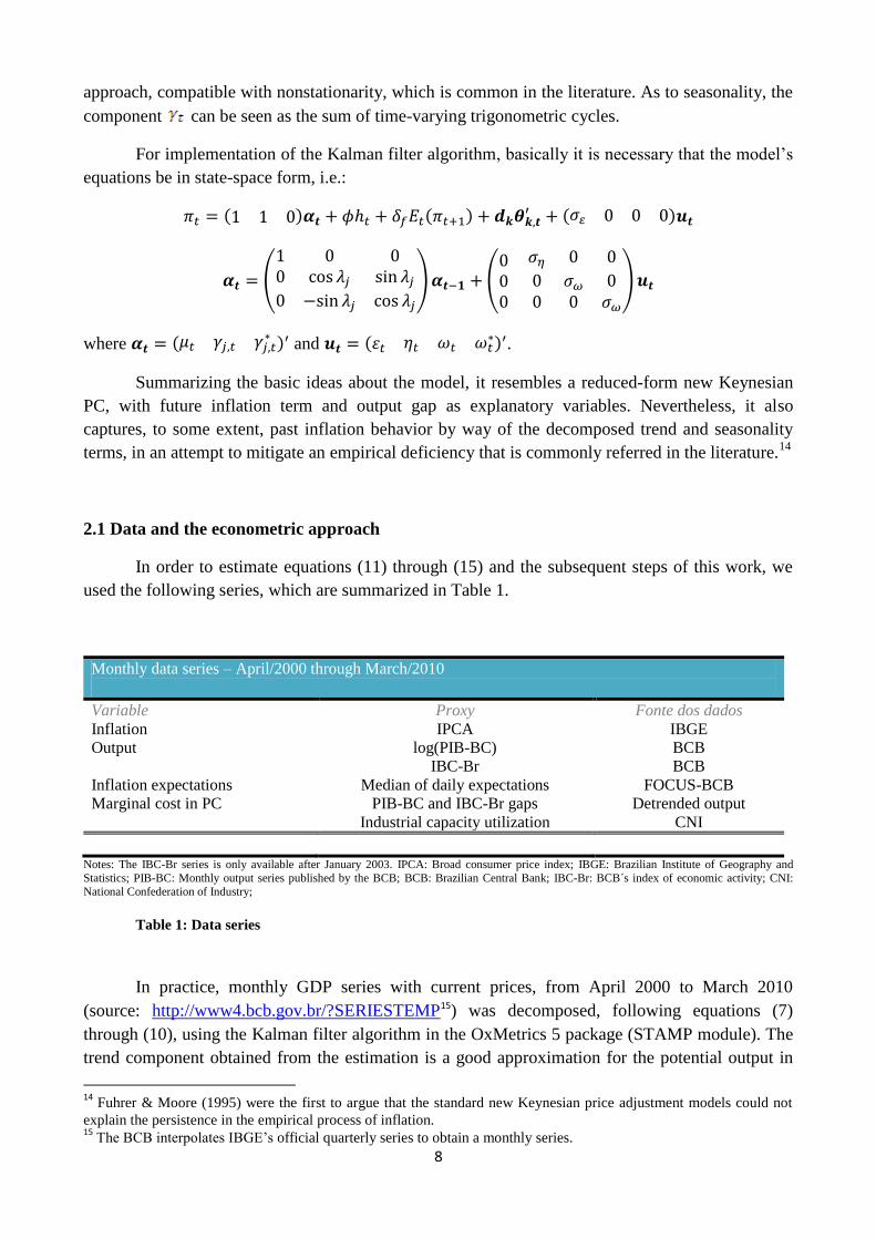
In order to estimate equations (11) through (15) and the subsequent steps of this work, we

used the following series, which are summarized in Table 1.

Monthly data series – April/2000 through March/2010

Variable Proxy Fonte dos dados

Inflation IPCA IBGE

Output log(PIB-BC)

IBC-Br

BCB

BCB

Inflation expectations Median of daily expectations FOCUS-BCB

Marginal cost in PC

PIB-BC and IBC-Br gaps Detrended output

Industrial capacity utilization CNI

Notes: The IBC-Br series is only available after January 2003. IPCA: Broad consumer price index; IBGE: Brazilian Institute of Geography and

Statistics; PIB-BC: Monthly output series published by the BCB; BCB: Brazilian Central Bank; IBC-Br: BCB´s index of economic activity; CNI:

National Confederation of Industry;

Table 1: Data series

In practice, monthly GDP series with current prices, from April 2000 to March 2010

(source: http://www4.bcb.gov.br/?SERIESTEMP15) was decomposed, following equations (7)

through (10), using the Kalman filter algorithm in the OxMetrics 5 package (STAMP module). The

trend component obtained from the estimation is a good approximation for the potential output in

14

Fuhrer & Moore (1995) were the first to argue that the standard new Keynesian price adjustment models could not

explain the persistence in the empirical process of inflation. 15

The BCB interpolates IBGE’s official quarterly series to obtain a monthly series.

9

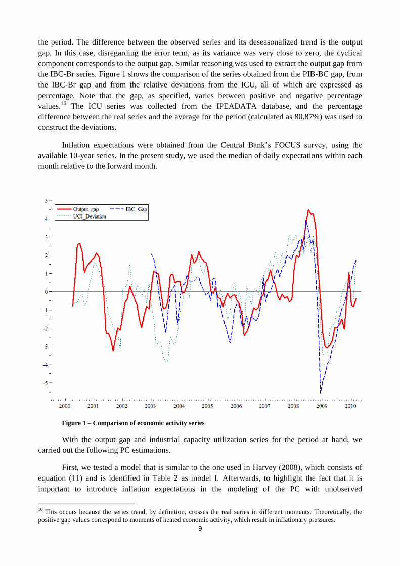
the period. The difference between the observed series and its deseasonalized trend is the output

gap. In this case, disregarding the error term, as its variance was very close to zero, the cyclical

component corresponds to the output gap. Similar reasoning was used to extract the output gap from

the IBC-Br series. Figure 1 shows the comparison of the series obtained from the PIB-BC gap, from

the IBC-Br gap and from the relative deviations from the ICU, all of which are expressed as

percentage. Note that the gap, as specified, varies between positive and negative percentage

values.16

The ICU series was collected from the IPEADATA database, and the percentage

difference between the real series and the average for the period (calculated as 80.87%) was used to

construct the deviations.

Inflation expectations were obtained from the Central Bank’s FOCUS survey, using the

available 10-year series. In the present study, we used the median of daily expectations within each

month relative to the forward month.

Figure 1 – Comparison of economic activity series

With the output gap and industrial capacity utilization series for the period at hand, we

carried out the following PC estimations.

First, we tested a model that is similar to the one used in Harvey (2008), which consists of

equation (11) and is identified in Table 2 as model I. Afterwards, to highlight the fact that it is

important to introduce inflation expectations in the modeling of the PC with unobserved

16

This occurs because the series trend, by definition, crosses the real series in different moments. Theoretically, the

positive gap values correspond to moments of heated economic activity, which result in inflationary pressures.

10

components, we use equation (12). In these first two alternatives, the measure of marginal cost used

is the output gap calculated from the monthly GDP provided by the BCB. The third model concerns

a PC that is identical to equation (12), but with ICU data instead of output gap. Finally, the IV

model consists of the same equation (12) with the difference that the output gap series was

calculated using IBC-Br. Note that, due to some unusual inflation movements, especially between

2002 and 2003, the inclusion of interventions inevitably leads to a better fit.

The evaluation of models follows some fitting and residuals diagnostic statistics. With

respect to fitting, the chief indicators contemplated in the estimation of the output gap and of the PC

were the following: algorithm convergence, forecast error variance decomposition, and log-

likelihood. According to Koopman et al (2007), a good convergence is key to showing that the

model was properly formulated and that, in general, it does not have fitting problems. Prediction

error variance (PEV) is the basic measure of goodness-of-fit which, in steady state, corresponds to

the variance of the one-step-ahead forecast errors. Other diagnostic statistics analyzed include Box-

Ljung’s Q statistics, for the assessment of residuals autocorrelation, and normality (N) and

heteroskedasticity (H) results.

2.2 Results

In the output gap estimation, a “very strong” convergence and a relatively small prediction

error variance were obtained. The recent global financial crisis and the resulting sharp decrease of

both output gap measures and of the deviations in the ICU in the last quarter of 2008 is noteworthy.

Table 2 shows the different models described in Section 2.1, following an increasing order

from the worst to the best fit. In all cases, convergence was again “very strong,” satisfying the

principal modeling criterion proposed by Koopman et al (2007). The prediction error variance

decreased from I to IV, as expected, indicating superior fit of the models (II through IV) that

include inflation expectations. The log-likelihood indicators underscore this conclusion, as they

increased from I to III. In case of model IV, the reduction is more a result of sample size than of the

goodness of fit, given that log-likelihood is an absolute and cumulative indicator.

The traditional coefficient of determination undergoes a slight change in case of seasonal

data, , and measures the relative performance of the specified model in relation to a simple

random walk model with drift and fixed seasonality. Again, the result is better for models II and III.

According to Box-Ljung’s Q statistics, serial correlation of residuals is absent in all models and

significance is lower than 0.1%.

With values lower than one, heteroskedasticity tests indicate that the variance of residuals

decreases slightly over time. Unequivocally, this results from the improvement of the inflation

targeting regime in Brazil, with an increasingly larger convergence of the inflation rate towards the

targets. Even in model IV, with a more recent sample, the pattern is maintained in favor of lower

variances for the more recent months. As to normality, the models clearly succeeded on the test,

based on Doornik-Hansen’s statistic whose critical value at a 5% significance level is 5.99.

11

Model I (Harvey):

0.060 116.82 0.51 22.45 0.27 0.44 - 0.023

[0.42]#

Model II

0.052 123.19 0.58 25.28 0.64 0.63

1.12

[3x10-5]

0.018

[0.47]

Model III

0.052 123.18 0.58 29.98 1.02 0.62

1.13 [2x10-5]

0.019 [0.42]

Model IV

0.030 97.71 0.48 19.17 1.84 0.72

1.19

[0]

0.041

[6x10-5]

Source: Data obtained by the authors Notes: #Values in square brackets: p-value.

The interventions, in order of importance, and respective p-values for models I through III were as follows:

- Outlier in 2002/11. Model I: 1.31 [0]; model II: 1.19 [0]; model III: 1.21 [0] - Level break in 2003/6: Modelo I: -0.81 [8x10-4]; model II: -1.07 [0]; model III: -1.07 [0]

- Outlier in 2003/9: Model I: 0.70 [2x10-4]; model II: 0.65 [2x10-4]; model III: 0.65 [2x10-4]

- Outlier in 2000/8: Model I: 0.64 [0.003]; model II: 0.55 [0.007]; model III: 0.56 [0.007] - Outlier in 2001/10: Model I: 0.34 [0.07]; model II: 0.34 [0.05]; model III: 0.34 [0.06]

In model IV, the resulting interventions were:

- Level break in 2003/3: -0.76 [2x10-5]

- Outlier in 2003/6: -1.15 [1x10-5]

- Outlier in 2005/10: 0.60 [0.001].

Table 2: Phillips Curve estimation results

The slopes of the different Phillips curves – which are the coefficients for output gap and

ICU deviation at the end of the sample – were positive in all cases, but not statistically significant in

case II and III. The same comment made by Tombini & Alves (2006), that smaller coefficients than

most of those described in the literature are due to the monthly frequency of data, applies here. In

regard to the coefficients of inflation expectations, the values showed high statistical significance.

Values are slightly larger than one, suggesting alignment of inflation expectations with the observed

rates.

In brief, test statistics indicate an improvement in the fit when going from an approach

without inflation expectations, as in Harvey (2008), to an approach that includes them. Among

output gap measures of the monthly GDP and the ICU deviations, there is no clear superiority of

fitting. In both cases, coefficients were positive, as recommended by the economic theory, though

not statistically significant. On the other hand, the output gap measure calculated based on the IBC-

Br series was positively correlated with the inflation rate, with a high level of significance, although

the amount of available data is smaller.

12

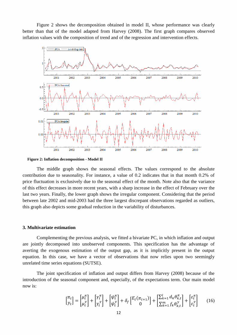
Figure 2 shows the decomposition obtained in model II, whose performance was clearly

better than that of the model adapted from Harvey (2008). The first graph compares observed

inflation values with the composition of trend and of the regression and intervention effects.

Figure 2: Inflation decomposition - Model II

The middle graph shows the seasonal effects. The values correspond to the absolute

contribution due to seasonality. For instance, a value of 0.2 indicates that in that month 0.2% of

price fluctuation is exclusively due to the seasonal effect of the month. Note also that the variance

of this effect decreases in more recent years, with a sharp increase in the effect of February over the

last two years. Finally, the lower graph shows the irregular component. Considering that the period

between late 2002 and mid-2003 had the three largest discrepant observations regarded as outliers,

this graph also depicts some gradual reduction in the variability of disturbances.

3. Multivariate estimation

Complementing the previous analysis, we fitted a bivariate PC, in which inflation and output

are jointly decomposed into unobserved components. This specification has the advantage of

averting the exogenous estimation of the output gap, as it is implicitly present in the output

equation. In this case, we have a vector of observations that now relies upon two seemingly

unrelated time series equations (SUTSE).

The joint specification of inflation and output differs from Harvey (2008) because of the

introduction of the seasonal component and, especially, of the expectations term. Our main model

now is:

(16)

13

where and

represent the sets of outliers considered for the inflation and output series,

respectively.

The link between the series in the SUTSE approach is generally established by the

correlations of errors of one or more components. Following Harvey (2008), it is assumed here that

the cycles have the same autocorrelation function and spectrum. In other words, inflation and output

cycles are modeled as similar cycles. In algebraic terms, supposing

,

(17)

where and are 2 x 1 error vectors, such that

, and is a 2 x 2

covariance matrix and .

The series can also be expressed in state-space form, but now the components are vectors.

As with univariate estimation, the inflation trend component follows a local level model, as in (13),

and the output component conforms to a smooth trend model, as in (8) and (9). Seasonality here is

also stochastic, in order to confirm its variability in the inflation series.

The cyclical component of inflation can be broken down into two independent parts, as

follows:

(18)

where

and

is a cyclical component specific to inflation.

Thus, the inflation equation may be written as:

(19)

Considering that the cycle of the output equation gives a notion about the output gap, as

occurred in Section 2, and that disturbances and

are perfectly correlated, it is possible to

conclude that coefficient corresponds to parameter of the univariate PC, i.e., the slope of the

PC. Therefore, from the correlation matrix of cycles, one obtains .

In the bivariate case, three specifications are tested. Again, an approach similar to that of

Harvey (2008) is compared with the model built above, in which one includes the future inflation

expectations term, as shown in equation (16). Finally, procedures (16) through (19) are repeated

considering the IBC-Br for the series of .

The relevant goodness-of-fit statistics are now a correlation matrix for the prediction error

variance and the log-likelihood. Test statistics already used in the univariate model are also

reproduced in Table 3.

14

3.1 Results

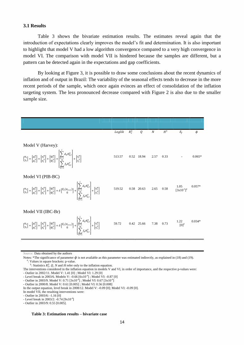
Table 3 shows the bivariate estimation results. The estimates reveal again that the

introduction of expectations clearly improves the model’s fit and determination. It is also important

to highlight that model V had a low algorithm convergence compared to a very high convergence in

model VI. The comparison with model VII is hindered because the samples are different, but a

pattern can be detected again in the expectations and gap coefficients.

By looking at Figure 3, it is possible to draw some conclusions about the recent dynamics of

inflation and of output in Brazil: The variability of the seasonal effects tends to decrease in the more

recent periods of the sample, which once again evinces an effect of consolidation of the inflation

targeting system. The less pronounced decrease compared with Figure 2 is also due to the smaller

sample size.

Model V (Harvey):

513.57 0.52 18.94 2.57 0.33 - 0.065*

Model VI (PIB-BC)

519.52 0.58 20.63 2.65 0.58

1.05

[3x10-5]#

0.057*

Model VII (IBC-Br)

59.72 0.42 25.66 7.38 0.73

1.22 [0]#

0.034*

Source: Data obtained by the authors

Notes: *The significance of parameter is not available as this parameter was estimated indirectly, as explained in (18) and (19). #: Values in square brackets: p-value. : Statistics

, , N and H refer only to the inflation equation. The interventions considered in the inflation equation in models V and VI, in order of importance, and the respective p-values were:

- Outlier in 2002/11. Model V: 1.41 [0] ; Model VI: 1.29 [0] - Level break in 2003/6. Modelo V: -0.66 [6x10-4] ; Model VI: -0.87 [0]

- Outlier in 2003/9. Model V: 0.71 [3x10-4] ; Model VI: 0.67 [3x10-4]

- Outlier in 2000/8. Model V: 0.61 [0.005] ; Model VI: 0.56 [0.008] In the output equation, level break in 2008/12. Model V: -0.09 [0]; Model VI: -0.09 [0].

In model VII, the resulting interventions were:

- Outlier in 2003/6: -1.16 [0] - Level break in 2003/2: -0.74 [9x10-4]

- Outlier in 2003/9: 0.55 [0.005].

Table 3: Estimation results – bivariate case

15

As to the GDP, the seasonal effects were reasonably constant in the sample. On the other

hand, the cyclical component, which gives some notion about the gap, showed a more erratic

behavior, with brisk movements at the end of 2008,17

due to the impact of the U.S. real estate crisis.

Also, note how the modeling of similar cycles allowed for a contemporaneous pattern in both series

close to the U.S. real estate crisis episode.

Note: The IBC-Br is constructed based on the value of 100 in 2002. Inflation is expressed in monthly rates.

Figure 3: Inflation and output (IBC-Br) decomposition – Bivariate model (VII)

4. Extensions

Some analyses were added to the basic models in order to better understand the dynamics of

PC components in the Brazilian case. The first one concerns the flattening of the PC, observed in

studies for some developed countries. As shown by Kuttner & Robinson (2008), parameter of

equation (12), which represents the response of the observed inflation to the output gap, has

decreased in empirical analyses of the United States and Australia. To investigate whether the same

occurs in Brazil, a variant of model IV was tested, in which the output gap coefficient was allowed

to vary over time, i.e., we now have . In this case, a smoothing spline was used, in which the

slope of the PC varies according to:

(20)

17

The behavior of IBC-Br in late 2008 suggests a level break in trend, which was not feasible in practice due to

restrictions on the algorithm and to the relatively small amount of observations.

16

The estimation of this new model is carried out with equations (12) through (15) plus (20),

which is an additional state equation.

The prediction error variance of this estimation, 0.026, was slightly lower than that of model

IV. Results indicate that flattening of the PC has recently been underway in Brazil as well. Figure 4

shows the time evolution of coefficient and the interval of two standard deviations. This result

confirms the importance to consider time-varying parameters in PC estimations, as underscored by

Sachsida et al (2009). In addition, there is an important policy assumption that the potential cost of

disinflation in terms of lost output has increased. On the other hand, increases in economic activity

have been accompanied by gradually smaller inflationary pressures. Tombini & Alves (2006)

highlight that the mere uncertainty caused by the 2002 electoral crisis would have been strong

enough to change the parameters of the reduced-form PC, leading to higher costs of disinflation.

The authors also find evidence of reduction in parameter .

Figure 4: Variation of the IBC-Br’s gap coefficient in the Phillips curve - Model VIII

The modeling proposed in the present study additionally allows assessing the forecasting

power of a PC model by comparing the observed inflation with the one calculated through the

models built by the Kalman filter, based on the minimization of one-step-ahead forecast errors.

Stock & Watson (2008) reviewed works that dealt with forecasting inflation based on some form of

PC and observed that these types of forecast are advantageous in some cases. However, Atkeson &

Ohanian (2001) advocate that these forecasts tend to be worse than those which are based on simple

17

univariate models. Notwithstanding, the widespread use of PC in the literature and the practice with

such forecasts require that their forecasting power be evaluated18

.

In the present study, the last 12 observations were excluded and the one-step-ahead inflation

forecast was estimated for the period between April 2009 and March 2010. The mean squared error

values for each model are shown in Table 4.

Model I II III IV V VI VII Naive

Mean

squared

error:

0.0258 0.0235 0.0215 0.0269 0.0222 0.0208 0.0184 0.0296

Source: Data collected by the authors

Table 4: Mean squared forecast error

Note that the model without expectations had a lower forecasting power than the model with

expectations, corroborating again the argument of the present study. This occurred both in the

univariate and bivariate cases. In the univariate specification, the gap extracted from IBC-Br was

not very successful, but in the bivariate case, it yielded the lowest mean squared error among all

estimations.

It should be underscored that the forecasting power increases in all cases when a

multivariate specification is used. Finally, the mean squared error of a naive inflation model was

calculated. In such a model, expected inflation value is forecasted by its current value, i.e.,

. All analyzed cases of PC outperformed this specification.

5. Conclusions

Given the clear-cut empirical difficulties surrounding the PC and in order to fill a gap in its

investigation in Brazil, the present study assessed inflation dynamics using an estimation with

unobserved components for the Brazilian economy. By modifying Harvey’s (2008) approach,

introducing an inflation expectation term in the PC, the model manages to parsimoniously

reproduce some stylized facts about the relation between inflation and output gap, at least when the

IBC-Br index is used. With the additional advantage of the graphical result, which allows a more

direct economic interpretation of the components, we highlight the variability of the seasonal

component of inflation, even with a sample of relatively few years. The relative reduction in this

18

Araujo & Guillen (2008) test the forecasting power of different PC specifications according to the gap measure used

and conclude that the best performance was obtained by the gap extracted by the multivariate method of unobserved

components.

18

variability in the past years suggests that the inflation targeting system has contributed to reducing

not only the inflation rates, but also their volatility within each year.

The detrended output gap built by the PIB-BC series and the ICU deviation series did not

yield good statistical results for the analyzed PC, even though positive coefficients were always

found. In the case of an output gap extracted from the IBC-Br series, the result was clearly better,

showing that this index, yet not used in academic works, may be of great value in monitoring

Brazilian monetary policy. Such success indicates that the output gap can also be representative in

the Brazilian inflation dynamics, depending on the index used. Previous studies have normally used

quarterly GDP series or the BCB’s monthly series, as the one used here, in model II. In the former

case, the number of observations is too small and, in the latter, the extrapolation of quarterly values

to monthly ones is unlikely to allow capturing the output dynamics. Thus, the output gap results of

the IBC-Br series may again strengthen the crucial relation of the PC for the Brazilian case.

The analysis of the PC slope, represented by parameter , is another important aspect.

Models that considered the fixed coefficient did not provide very accurate values for the analyzed

sample. On the other hand, the analysis of the first extension, despite its poorly accurate results,

indicates that flattening of the PC occurs in Brazil similarly to what is observed in developed

countries, as reported by Kuttner & Robinson (2008). An important implication is that PC

estimations for Brazil for larger periods should take this movement into consideration, otherwise the

output parameter will be overestimated at the end of the sampled period. This reduction in the

impact of deviations of output from its real level on inflation means, ceteris paribus, that increases

in economic activity, would not produce so much inflationary pressure as they used to. However,

the costs of disinflation, in terms of lost output, would tend to increase in this scenario.

Finally, the forecasting power of different models was tested against a simple forecasting

model. All models could outperform it in terms of squared forecast errors for the last 12 months of

the sample.

Some issues, which were not dealt with here and that could be subject of investigation of

future research, include the following: comparison of the performance of the output gap with that of

other measures, such as unit labor cost or deviation from the natural rate of unemployment; another

approach that considers different dynamics of free and administered prices, and even possible

distinctions between tradable and nontradable goods, which concern the exchange rate influence;

and finally, similar estimations for other countries.

As more data become available, it is likely that quarterly samples will have a higher

forecasting power and will be successfully used in similar estimations. In the meantime, the study

showed that IBC-Br can be an important tool for the formulation of monetary policy in Brazil.

References

Arruda, E., R. Ferreira & I. Castelar (2008). Modelos lineares e não lineares da curva de Phillips

para previsão da taxa de inflação no Brasil. Anais do XXXVI Encontro Nacional de Economia.

19

Atkeson, A. & L. Ohanian (2001). Are Phillips Curves useful for forecasting inflation? Federal

Reserve Bank of Minneapolis Quarterly Review 25(1):2-11.

Basistha, A. & C. Nelson (2007). New measures of the output gap based on the forward-looking

New Keynesian Phillips curve. Journal of Monetary Economics, 54(2), 498-511.

Bonomo, M. & R. Brito (2002). Regras monetárias e dinâmica macroeconômica no Brasil: Uma

abordagem de expectativas racionais. Revista Brasileira de Economia 56, 551-589.

Calvo, G. (1983). Staggered prices in a utility maximizing framework. Journal of Monetary

Economics 12, 383-398.

Christiano, L., M. Eichenbaum & C. Evans (2005). Nominal rigidities and the dynamic effects of a

shock to monetary policy. Journal of Political Economy, 113, 1-145.

Correa, A. & A. Minella (2005). Mecanismos não lineares de repasse cambial: um modelo de curva

de Phillips com threshold para o Brasil. Anais do XXXIII Encontro Nacional de Economia.

Fasolo, A. & M. Portugal (2004). Imperfect rationality and inflationary inertia: a new estimation of

the Phillips Curve for Brazil. Estudos Econômicos, 34(4), 725-776.

Gali, J & M. Gertler (1999). Inflation dynamics: A structural econometric analysis. Journal of

Monetary Economics 44, 195-222.

Gerlach, S. & W. Peng (2006). Output gaps and inflation in Mainland China. BIS Working Paper,

194.

Goodfriend, M. & R. King (2009). The great inflation drift. . NBER Working Paper Series. N.

14862.

Gordon, R. (1997). The time-varying NAIRU and its implications for economic policy. Journal of

Economic Perspectives, vol. 11, no. 1, pp. 11 – 32.

Hamilton, C. & W. Gaglianone (2010). Survey-based inflation expectations in Brazil. In: "Monetary

policy and the measurement of inflation: prices, wages and expectations," BIS Papers, Bank for

International Settlements, 49, 107-113.

Harvey, A. (1989). Forecasting, Structural Time Series Models and the Kalman Filter. Cambridge

University Press, Cambridge.

Harvey, A. (2008). Modeling the Phillips Curve with unobserved components. Cambridge

University Working Paper, CWPE 0805.

Koopman, S., A. Harvey, J. Doornik & N. Shephard (2007). STAMP 8. Structural Time Series

Analyser, Modeller and Predictor. Timberlake Consultants, London.

Kuttner, K & T. Robinson (2008). Understanding the flattening Phillips Curve. Research

Discussion Paper RBA, Australia.

Lee, J. & C. Nelson (2007). Expectation horizon and the Phillips curve: The solution to an empirical

puzzle. Journal of Applied Econometrics 22, 161-178.

20

Mavroeidis, S. (2005). Identification issues in forward looking models estimated by GMM, with an

application to the Phillips Curve, Journal of Money Credit and Banking, 37, 421-448.

Mendonça, H. & M. Santos (2006). Credibilidade da política monetária e a previsão do trade-off

entre inflação e desemprego: uma aplicação para o Brasil. Revista Economia, 7(2), p. 293-306.

Mise, E., Kim, T. & P. Newbold (2005). On suboptimality of the Hodrick-Prescott filter at time

series endpoints. Journal of Macroeconomics, 27, 53-67.

Nason, J. & G. Smith (2008a). Identifying the New Keynesian Phillips Curve. Journal of Applied

Econometrics 23(5), 525-551.

Nason, J. & G. Smith (2008b). The New Keynesian Phillips Curve: Lessons from single-equation

econometric estimation. Economic Quarterly 94 (4), 361-395.

Phillips, A. (1958). The relation between unemployment and the rate of change of money wage

rates in the United Kingdom, 1861-1957. Economica, 25, 283-99.

Portugal, M. (1993). Measures of capacity utilization: Brazil, 1920/1988. Análise Econômica 19,

89-102.

Rudd, J. & K. Whelan (2007). Modeling inflation dynamics: A critical review of recent research.

Journal of Money, Credit and Banking. Vol. 39, 155-170.

Sachsida, A. , M. Ribeiro & C. Santos (2009). A Curva de Phillips e a experiência brasileira. Textos

para Discussão IPEA, N. 1429.

Samuelson, P. & R. Solow (1960). Analytical aspects of anti-inflation policy. American Economic

Review, 50, 177-94.

Schwartzman, F. (2006). Estimativa de Curva de Phillips para o Brasil com preços desagregados.

Economia Aplicada. Vol.10, N.1.

Stock, J. & M. Watson (2008). Phillips Curve inflation forecasts. NBER Working Paper Series. N.

14322.

Tombini, A. & S. Alves (2006). The recent Brazilian disinflation process and costs. Banco Central

do Brasil. Working Paper Series, 109.

Vogel, L. (2008). The relationship between the hybrid New Keynesian Phillips Curve and the

NAIRU over time. Macroeconomics and Finance Series 200803, Hamburg University.

Wongwachara, W. & A. Minphimai (2009). Unobserved components models of the Phillips relation

in the ASEAN Economy. Journal of Economics and Management. Vol 5, N.2, 241-256.

Woodford, M (2003). Interest and Prices: Foundations of a Theory of Monetary Policy. Princeton

University Press, Princeton.