natália da costa análise não-standard em equações ... · minimizer. if f satisfies the...
TRANSCRIPT

Universidade de Aveiro 2006
Departamento de Matemática
Natália da Costa Martins
Análise Não-Standard em Equações DiferenciaisOrdinárias e na Teoria dos Pontos Críticos Nonstandard Analysis in Ordinary DifferentialEquations and in Critical Point Theory

Universidade de Aveiro
2006 Departamento de Matemática
Natália da Costa Martins
Análise Não-Standard em Equações DiferenciaisOrdinárias e na Teoria dos Pontos Críticos Nonstandard Analysis in Ordinary DifferentialEquations and in Critical Point Theory
Dissertação apresentada à Universidade de Aveiro para cumprimento dosrequisitos necessários à obtenção do grau de Doutor em Matemática, realizadasob a orientação científica de Vítor Manuel Carvalho das Neves, ProfessorAssociado do Departamento de Matemática da Universidade de Aveiro e co-orientação de Maria João Simões Nunes Borges, Professora Auxiliar do Departamento de Matemática do Instituto Superior Técnico da UniversidadeTécnica de Lisboa. Dissertation submitted to the University of Aveiro in fulfilment of the requirements for the degree of Doctor of Philosophy in Mathematics, under the supervision of Vítor Manuel Carvalho das Neves, Associated Professor at theDepartment of Mathematics of the University of Aveiro and co-supervision of Maria João Simões Nunes Borges, Assistant Professor at the Department of Mathematics of the Instituto Superior Técnico of the Technical University ofLisbon.

o júri
presidente Prof. Doutor Eduardo Anselmo Ferreira da Silva Professor Catedrático da Universidade de Aveiro
Prof. Doutor Vítor Manuel Carvalho das Neves Professor Associado da Universidade de Aveiro (orientador)
Prof. Doutora Maria João Simões Nunes Borges Professora Auxiliar do Instituto Superior Técnico da Universidade Técnica de Lisboa (co-orientadora)
Prof. Doutora Maria do Rosário Grossinho Professora Associada do Instituto Superior de Economia e Gestão da Universidade Técnica de Lisboa
Prof. Doutor Imme Peter van der Berg Professor Associado da Universidade de Évora
Prof. Doutor Delfim Fernando Marado Torres Professor Auxiliar da Universidade de Aveiro

agradecimentos
Ao Professor Vítor Neves, meu orientador, pelo modo como acompanhou todoo trabalho, bem como pela sua amizade e disponibilidade permanente. À Professora Maria João Borges, minha co-orientadora, pela suadisponibilidade e apoio na preparação deste trabalho, assim como pelaamabilidade com que sempre me recebeu na sua instituição. À Universidade de Aveiro, em particular ao Departamento de Matemática e àUnidade de Investigação e Desenvolvimento CEOC, pelas facilidadesproporcionadas durante a elaboração deste trabalho. Ao Projecto POCTI/MAT/41683/2001 da FCT pelo apoio financeiro de algumasdeslocações a congressos e encontros científicos com a minha co-orientadora. A todos os meus colegas e amigos do Departamento de Matemática daUniversidade de Aveiro pela amizade e encorajamento manifestado ao longodestes anos. Gostaria particularmente de agradecer àqueles com quem convividiariamente: Enide, João, Virginia, Liliana, Paula Rama, Cristina, Célia,Anabela, Emília, Isabel Brás, Ricardo Almeida e António Neves. Ao Professor Manfred Wolff (Universidade de Tübingen) e ao Professor JoãoTeixeira (UTL - IST) pela colaboração em algumas etapas deste trabalho. Ao saudoso Professor Sousa Pinto, por me ter incentivado a estudar AnáliseNão-Standard e, principalmente, pela sua amizade. Ao Professor João David Vieira, por me ter incentivado a enveredar pela vidaacadémica. A todos os familiares e amigos pela amizade, apoio e encorajamento quesempre me dedicaram, o que contribuiu decisivamente para ultrapassar osinevitáveis maus momentos. Em particular, agradeço ao Quim e aos nossosfilhos, Inês, Nuno e Miguel, por existirem e me fazerem feliz.
palavras-chave
Análise Não-Standard, Teoria Abstrata dos Pontos Críticos, Problemas deMinimax, Equações Diferenciais Ordinárias.
resumo
Esta dissertação apresenta várias aplicações da Análise Não-Standard àTeoria das Equações Diferenciais Ordinárias e à Teoria dos Pontos Críticos. Relativamente à Teoria das Equações Diferenciais Ordinárias, sãoapresentadas generalizações não-standard de dois resultados importantesdesta teoria, bem como uma nova prova não-standard do Teorema deExistência de Carathéodory e dedução correspondente do Teorema deExistência de Peano. Um dos resultados fundamentais da Teoria dos Pontos Críticos é o Teoremada Passagem da Montanha de Ambrosetti-Rabinowitz. Neste contexto, sãoapresentadas várias provas não-standard deste teorema para funcionaiscoercivos definidos em espaços de Banach reais de dimensão finita, além devárias generalizações não-standard de condições do tipo de Palais-Smale quepermitem a demonstração de novos teoremas. São ainda apresentados doisnovos teoremas da passagem da montanha sem a condição de Palais-Smaleou suas generalizações. Todos estes teoremas permitem obter novosteoremas de três pontos críticos.

keywords
Nonstandard Analysis, Abstract Critical Point Theory, Minimax Problems,Ordinary Differential Equations.
abstract
This dissertation describes several applications of Nonstandard Analysis bothto the Ordinary Differential Equations Theory and to the Critical Point Theory. Two important results of Ordinary Differential Equations Theory are generalizedaccording to Nonstandard Analysis, a new nonstandard proof of Carathéodory'sExistence Theorem is presented wherefrom Peano's Existence Theorem isdeduced. One of the fundamental results of Critical Point Theory is the Mountain PassTheorem of Ambrosetti-Rabinowitz. Several nonstandard proofs of this theoremfor coercive functionals defined in finite dimensional real Banach spaces arepresented together with some nonstandard generalizations of Palais-Smaleconditions that allow the demonstration of new theorems. Two new mountainpass theorems are also proved without using the Palais-Smale condition orgeneralizations thereof. These mountain pass theorems are used to obtain newthree critical points theorems.

Ao Quim,
à Inês, ao Nuno e ao Miguel.

Contents
Symbols iii
1 Introduction 1
1.1 Overview . . . . . . . . . . . . . . . . . . . . . . . . . . . . . . . . . . . . . . . 1
1.2 Contributions . . . . . . . . . . . . . . . . . . . . . . . . . . . . . . . . . . . . . 5
1.2.1 Nonstandard Carathéodory’s Existence Theorem . . . . . . . . . . . . . 6
1.2.2 Nonstandard Palais-Smale conditions . . . . . . . . . . . . . . . . . . . . 6
1.2.3 Theorems with nonstandard Palais-Smale conditions . . . . . . . . . . . 6
1.2.4 Mountain Pass Theorem with a nonstandard Palais-Smale condition . . 6
1.2.5 Mountain Pass Theorems without Palais-Smale conditions . . . . . . . . 6
1.2.6 Nonstandard proofs of the Mountain Pass Theorem of Ambrosetti-Rabinowitz
for coercive functionals defined in finite dimensional real Banach spaces 7
1.2.7 Three Critical Points Theorems with a nonstandard Palais-Smale con-
dition . . . . . . . . . . . . . . . . . . . . . . . . . . . . . . . . . . . . . 7
1.2.8 Three Critical Points Theorems without Palais-Smale conditions . . . . 7
1.3 Organization of the dissertation . . . . . . . . . . . . . . . . . . . . . . . . . . . 8
2 Nonstandard Analysis 11
2.1 Introduction . . . . . . . . . . . . . . . . . . . . . . . . . . . . . . . . . . . . . . 11
2.2 Notation and preliminars in NSA . . . . . . . . . . . . . . . . . . . . . . . . . . 12
2.3 Hyperreal numbers . . . . . . . . . . . . . . . . . . . . . . . . . . . . . . . . . . 16
2.4 Topology . . . . . . . . . . . . . . . . . . . . . . . . . . . . . . . . . . . . . . . 18
2.5 Differentiation . . . . . . . . . . . . . . . . . . . . . . . . . . . . . . . . . . . . . 25
2.6 Loeb integration theory . . . . . . . . . . . . . . . . . . . . . . . . . . . . . . . 26
2.7 Nonstandard discrete derivative . . . . . . . . . . . . . . . . . . . . . . . . . . . 35
i

3 Existence Theorems for ODE’s 37
3.1 Introduction . . . . . . . . . . . . . . . . . . . . . . . . . . . . . . . . . . . . . . 37
3.2 Nonstandard Carathéodory’s Existence Theorem . . . . . . . . . . . . . . . . . 38
3.3 Carathéodory’s Existence Theorem . . . . . . . . . . . . . . . . . . . . . . . . . 39
3.4 Peano’s Existence Theorem . . . . . . . . . . . . . . . . . . . . . . . . . . . . . 42
4 Palais-Smale conditions 45
4.1 Introduction . . . . . . . . . . . . . . . . . . . . . . . . . . . . . . . . . . . . . . 45
4.2 The Palais-Smale condition . . . . . . . . . . . . . . . . . . . . . . . . . . . . . 45
4.3 Nonstandard Palais-Smale conditions . . . . . . . . . . . . . . . . . . . . . . . . 47
4.4 Coercive functionals . . . . . . . . . . . . . . . . . . . . . . . . . . . . . . . . . 55
4.5 Palais-Smale conditions per level . . . . . . . . . . . . . . . . . . . . . . . . . . 60
4.6 Nonstandard Variants of Palais-Smale conditions per level . . . . . . . . . . . . 61
5 Mountain Pass Theorems 65
5.1 Introduction . . . . . . . . . . . . . . . . . . . . . . . . . . . . . . . . . . . . . . 65
5.2 Critical Points and the Quantitative Deformation Lemma . . . . . . . . . . . . 66
5.3 Mountain Pass Theorems in arbitrary real Banach spaces . . . . . . . . . . . . 70
5.4 Obtaining almost critical points in real Hilbert spaces . . . . . . . . . . . . . . 75
5.5 A Mountain Pass Theorem in the finite dimensional case . . . . . . . . . . . . . 80
5.6 Mountain Pass Theorems without Palais-Smale conditions . . . . . . . . . . . . 81
6 Three Critical Points Theorems 85
6.1 Introduction . . . . . . . . . . . . . . . . . . . . . . . . . . . . . . . . . . . . . . 85
6.2 Three Critical Points Theorems with a nonstandard Palais-Smale condition . . 86
6.3 Three Critical Points Theorems without Palais-Smale conditions . . . . . . . . 88
A Peano’s Existence Theorem 93
B Nonstandard proofs of a Mountain Pass Theorem in finite dimension 97
B.0.1 A "normal" proof . . . . . . . . . . . . . . . . . . . . . . . . . . . . . . . 97
B.0.2 A discrete proof . . . . . . . . . . . . . . . . . . . . . . . . . . . . . . . . 101
Bibliography 109
Index 115
ii

Symbols
Basic notation:
:= equality, by definition;
∅ empty set;
N set of natural numbers;
Z set of integer numbers;
Q set of rational numbers;
R set of real numbers;
R+ set of positive real numbers;
R+0 set of nonnegative real numbers;
Rn n-dimensional Euclidean space;
Br(a) open ball centered at a and radius r ∈ R+;
Br(a) closed ball centered at a and radius r ∈ R+;
card(E) cardinality of the set E;
P(E) power set of E;
BA set of all mappings from the set A into the set B;
⋃disjoint union;
iii

f|A restriction of the map f : X → Y to A ⊆ X;
· takes the place of the variable with respect to which the mapping is evaluated;
| · | absolute value function;
‖ · ‖ norm;
· • · inner product;
� end of proof.
Other symbols and pages where they are introduced:
X 12 Y 12�(·) 12 �a 12�R 16 �R0 16�R∞ 16 �Rfin 16�N 17 �N∞ 17
st(x) 17 ◦x 17σX 17 fin(�E) 19
inf(�E) 19 ns(�E) 19
pns(�E) 19 ≈ 19
mon(a) 19 �≈ 19
st(Y ) 19 Lin(E, F ) 25
C1(U, F ) 25 〈·, ·〉 26
L1([a, b]) 39 C([a, b]) 40
K 45 Kc 45
(PS) 46 (PS)c 61
(PS0) 48 (PS0)c 61
(PS1) 48 (PS1)c 61
(PS2) 48 (PS2)c 62
(PS3) 48 (PS3)c 62
(PS4) 48 (PS4)c 62
f c 66 Sα 66
C([0, 1], E) 66 C([0, 1] × E, E) 66
dist(x, S) 66 � 75
C([0, 1], [0, 1]) 75
iv

Chapter 1
Introduction
1.1 Overview
Nonstandard Analysis (NSA) is a coherent and powerful theory developed by Abraham Robin-
son in 1961 [Rob61], which among other things, provides a logical foundation for the use of
infinitesimal numbers in Mathematics. Robinson proved that the set of real numbers, R, may
be made a proper subset of a new set of numbers, which will thus contain infinitesimal num-
bers and infinite numbers and in a sense satisfies the same analytical properties of R; namely,
functions extend naturally with the same properties. This new set is usually denoted by �R
and its elements are called hyperreal numbers or nonstandard real numbers. NSA is also
sometimes referred in the literature to as Infinitesimal Analysis or Robinsonian Analysis.
One of the advantages of NSA is that nonstandard methods may yield shorter and/or intuitive
proofs of classical results. However, nonstandard methods are more than an alternative to
standard methods, since they have provided new results in many fields of Mathematics, such as
Functionals Analysis, Differential Equations, Optimal Control Theory, Probability Theory and
Mathematical Physics. Even more, NSA is an important field of research in their own right;
[ACH97] and [CNOSP95] are collection of articles covering basic NSA as well as advanced
material from many of the areas of Mathematics to which NSA has being applied.
Critical Point Theory (CPT) is also an important subject in Mathematics that has been
widely used in the last decades in many fields of Mathematics, such as Differential Equations,
1

2 Chapter 1. Introduction
Differential Geometry and Global Analysis and also in Physics and Mechanics, where solutions
of many problems are critical points of a suitable energy functional.
CPT rely on methods of classical Mathematics. However, we believe that the application
of nonstandard methods to CPT may both simplify and potentiate the development of new
results.
According to [San93], this theory has its origins in the Calculus of Variations and it had an
increased development after the first quarter of the twentieth century with the works of Morse,
Lusternik and Schnirelmann. In contrast to the Calculus of Variations, where the problems
involve the determination of maxima and minima of functionals, CPT concerns the study of
all types of critical points.
Until the second half of the nineteenth century, the existence of a minimum was taken for
granted if the functional was bounded from below. This situation changed in 1870 when
Weierstrass [Wei] gave an example of a nonnegative functional which did not have a minimum.
The basic idea for finding a minimum of a smooth functional is, in general, simple: if E
is a real Banach space and f : E → R is of class C1 and bounded from below, with a
deformation technique or using Ekeland’s Variational Principle [Eke79], we can construct a
sequence (un)n∈N such that
f(un) → inft∈E
f(t) and f ′(un) → 0.
The main problem is to show that this sequence has an accumulation point which will be a
minimizer. If f satisfies the condition
every sequence (xn)n∈N in E such that (f(xn))n∈N is bounded and f ′(xn) → 0
has a convergent subsequence,
the functional has a minimum. This condition was introduced in 1964 by Palais and Smale
[PS64] and it is known by Palais-Smale condition ((PS) for short). In the beginning, this
condition was received with some caution because several interesting functionals did not sat-
isfy it. Since then, many variants of the Palais-Smale condition have been introduced and
nowadays these Palais-Smale conditions became important compactness conditions in many
critical point theorems. In 1980, H. Brézis, J. Coron and L. Nirenberg introduced the following
generalization of the Palais-Smale condition [BCN80]:
1.1 Overview 3
every sequence (xn)n∈N in E such that f(xn) → c and f ′(xn) → 0 has a
convergent subsequence,
where c is a fixed real number. This Palais-Smale condition of level c ((PS)c for short) is a
compactness condition on the functional f in the sense that the set of critical points of f with
value c,
Kc := {u ∈ E : f ′(u) = 0 ∧ f(u) = c},
is compact.
Saddle points, that is, critical points that are not local extrema, are more difficult to find but
lead to similar compactness problems. Deformation techniques were introduced in 1934 by
Lusternik and Schnirelman [LS34] and can also be applied to functionals f which do not need
to be bounded from below (or above), by characterizing the critical values as a minimax over
a suitable class of sets S:
infA∈S
supx∈A
f(x) := c.
The choice of S must reflect some change in the topology of the sublevel sets
fs := {u ∈ E : f(u) ≤ s}
for s near c.
In the general case, minimax theorems for C1 functionals are obtained as follows:
1. the functional f must satisfy some geometrical condition that relates the value of the
functional over some sets that have some kind of connection between them;
2. use a deformation technique to prove that, for some value c characterized by a minimax
argument, there exists a Palais-Smale sequence of level c, that is, there exists a sequence
(xn)n∈N such that f(xn) → c and f ′(xn) → 0;
3. use a Palais-Smale type compactness condition to prove that c is a critical value of f .
In this work we will present the Quantitative Deformation Lemma for C1 functionals, intro-
duced in 1983 by Willem [Wil83], as an example of a deformation technique. We mention that
there also exists Deformation Lemmas for continuous functionals defined on metric spaces

4 Chapter 1. Introduction
(see, for example, [Cor99]) and even for non continuous functionals (see, [RTK98]). These
results are fundamental for the development of nonsmooth critical point theory.
An important minimax theorem that will be addressed in this dissertation is the Mountain Pass
Theorem [AR73] introduced in 1973 by Ambrosetti and Rabinowitz. This theorem considers
a C1 functional f defined in a real Banach space E that verifies both the (PS) condition and
the following condition
there exist x1, x2 ∈ E and r ∈ R+ such that ‖ x1 −x2 ‖> r and (*)
k0 := max{f(x1), f(x2)} < inf‖y−x1‖=r
f(y).
The Mountain Pass Theorem of Ambrosetti-Rabinowitz shows that there exists a critical
point u different from x1 and x2 and with critical value k1 > k0. Moreover, k1 is the following
minimax value
k1 = infγ∈Γ
maxt∈[0,1]
f(γ(t))
where Γ is the set of all continuous paths joining x1 to x2.
Let us give a geometric interpretation of this theorem; if E = R2 and, for each x, f(x)
represents the altitude of x, then x1 and x2 are two different points that are separated by a
mountain range. For each γ ∈ Γ, the number maxt∈[0,1] f(γ(t)) is the maximum height on
that path and k1 is the infimum of all those maximal heights. In order to go from x1 to x2
one tries to find a mountain pass γ0 ∈ Γ such that
maxt∈[0,1]
f(γ0(t)) = infγ∈Γ
maxt∈[0,1]
f(γ(t)) = k1.
The geometry expressed by condition (*) is called the mountain pass geometry and is the
simplest minimax geometry that leads to a minimax theorem. Using the Quantitative Defor-
mation Lemma and the mountain pass geometry, one can prove that there exists a sequence
(un)n∈N such that
f(un) → k1 and f ′(un) → 0.
Therefore, since f satisfies (PS), then there exists a critical point with value k1. Notice that
only the condition (PS)k1 is needed to conclude that k1 is a critical value as it was pointed
out by Brézis, Coron and Nirenberg in [BCN80], the paper where the condition (PS)k1 was
1.2 Contributions 5
introduced for the first time. This generalization of the Mountain Pass Theorem of Ambrosetti-
Rabinowitz is known as the Mountain Pass Theorem of Brézis-Coron-Nirenberg.
Note that if f does not satisfy (PS)k1 , we cannot guarantee that the smallest value of
maxt∈[0,1] f(γ(t)) exists (see Exemple 5.13).
We notice that the critical point obtained by the Mountain Pass Theorem of Ambrosetti-
Rabinowitz (and by the Mountain Pass Theorem of Brézis-Coron-Nirenberg) is not necessarily
a saddle point, as one might conjecture from the mountain pass geometry. Pucci and Serrin
showed in [PS84] that under certain reasonable hypotheses, the critical point must indeed be a
saddle point. In particular, they proved that if there is only one critical point with the critical
value k1, then it is a saddle point.
From the Mountain Pass Theorem of Ambrosetti-Rabinowitz it follows easily that if f is a C1
functional that satisfies (PS) and has two distinct local minimizers, then f has a third critical
point. This result is known as a Three Critical Points Theorem.
Research activities around Mountain Pass Theorem of Ambrosetti-Rabinowitz have produced
a great variety of generalizations of this theorem. Such generalizations were obtained u-
sing weaker Palais-Smale conditions, weakening the differentiability of the functional and by
adopting more general geometrical conditions than the mountain pass geometry.
Readers interested in the Mountain Pass Theorem of Ambrosetti-Rabinowitz and its genera-
lizations, may refer to [GT01] and [Jab03] for further details.
1.2 Contributions
This dissertation applies for the first time, as far as we know, Nonstandard Analysis to Critical
Point Theory. It also presents a new and general form to prove some important theorems for
ordinary differential equations (ODE’s).
The major contributions of this dissertation are summarized next.

6 Chapter 1. Introduction
1.2.1 Nonstandard Carathéodory’s Existence Theorem
A nonstandard proof of Carathéodory’s Existence Theorem (which avoid Ascoli’s Theorem as
well as Lebesgue’s Dominated Convergence Theorem) is presented wherefrom Peano’s Exis-
tence Theorem is deduced. For this purpose, we use the Loeb integration theory and the
notion of nonstandard discrete derivative. We also obtained a generalization of Carathéodory’s
Existence Theorem, that we called Nonstandard Carathéodory’s Existence Theorem (Theorem
3.1).
1.2.2 Nonstandard Palais-Smale conditions
Nonstandard conditions of Palais-Smale type are presented. Inspired in (PS) and (PS)c
conditions, we obtained several nonstandard variants of these classical conditions that are
weaker than the classical ones, but still sufficient to prove new Mountain Pass Theorems.
1.2.3 Theorems with nonstandard Palais-Smale conditions
We establish some relations between coercivity and our nonstandard Palais-Smale conditions
(Proposition 4.24 and Proposition 5.8). We also obtained a minimizing theorem which is a
generalization of a classical result (Corollary 5.4).
1.2.4 Mountain Pass Theorem with a nonstandard Palais-Smale condition
The nonstandard Palais-Smale conditions per level allow us to prove a Mountain Pass Theorem
which is a generalization of the Mountain Pass Theorem of Brézis-Coron-Nirenberg (Theorem
5.15). We also present the "dual" of this new Mountain Pass Theorem (Theorem 5.18).
1.2.5 Mountain Pass Theorems without Palais-Smale conditions
We proved that, in the finite dimensional case, if we substitute the (PS) condition in the
Mountain Pass Theorem of Ambrosetti-Rabinowitz by
1.2 Contributions 7
there exists s ∈ R+ such that ‖ x2 − x1 ‖< s and if ‖ x − x1 ‖≥ s then
f(x) < k1
we obtain other theorem of mountain pass type (Theorem 5.25).
We also proved a new Mountain Pass Theorem without Palais-Smale conditions (Theorem
5.29) for a functional f defined in a real Hilbert space H that satisfies the condition
∃γ ∈�Γ [ γ(�[0, 1]) ⊆ ns(�H) ∧ maxt∈�[0,1] f(γ(t)) ≈ k1 ].
Notice that these theorems cannot be obtained from the Mountain Pass Theorem of Ambrosetti-
Rabinowitz or generalizations of it, e.g. given in [GT01], since our geometrical conditions do
not imply (PS) or weaker forms of (PS). We also present the "duals" of these new Mountain
Pass Theorems (Theorem 5.28 and Theorem 5.31).
1.2.6 Nonstandard proofs of the Mountain Pass Theorem of Ambrosetti-
Rabinowitz for coercive functionals defined in finite dimensional real
Banach spaces
We present some nonstandard proofs of the Mountain Pass Theorem of Ambrosetti-Rabinowitz
for coercive functionals defined in finite dimensional real Banach spaces without using a De-
formation Lemma. One of the proofs uses a hyperfinite set and is of a discrete type.
1.2.7 Three Critical Points Theorems with a nonstandard Palais-Smale
condition
From the Mountain Pass Theorem with nonstandard Palais-Smale condition and its "dual",
we obtained new Three Critical Points Theorems (Theorem 6.1, Theorem 6.2, Theorem 6.4
and Theorem 6.5).
1.2.8 Three Critical Points Theorems without Palais-Smale conditions
Applying the Mountain Pass Theorems without Palais-Smale conditions and their "duals", we
proved other Three Critical Points Theorems (Theorem 6.7 to Theorem 6.10, Theorem 6.12

8 Chapter 1. Introduction
to Theorem 6.15).
1.3 Organization of the dissertation
We had the concern to guide the exposition in a logical and sequential way. In order to create
a self contained text, we present the contents that we found necessary for the understanding
of this work.
This dissertation is organized in six chapters and two appendixes. The Index, Symbols and
Bibliography refer the reader to terminology, notation and sources thereof.
In Chapter 2 we present a brief introduction to Nonstandard Analysis. We begin this chap-
ter presenting the fundamental results for our almost axiomatic description of Nonstandard
Analysis: the Transfer Principle and the Polysaturation Principle. Then, in the setting of real
normed spaces, we present nonstandard characterizations of some topological concepts. We
also present some nonstandard characterizations of C1 functions defined in real Banach spaces.
A great part of this chapter is dedicated to Loeb integration theory and the relations between
this theory and the Lebesgue integration theory. At the end of this chapter, we introduce the
notion of nonstandard discrete derivative.
In Chapter 3 we present a nonstandard generalization of Carathéodory’s Existence Theorem
and a nonstandard proof of Carathéodory’s Existence Theorem. In the end of this chapter,
we obtain Peano’s Existence Theorem as a corollary of Carathéodory’s Existence Theorem.
We begin Chapter 4 presenting the classical (PS) condition and our nonstandard variants of
(PS). After these definitions, we establish some relations between these nonstandard condi-
tions and (PS). In order to relate coercivity and our nonstandard Palais-Smale conditions, we
present some nonstandard characterizations of coercive functionals. To end this chapter, we
present (PS)c condition, our nonstandard variants of (PS)c and the relations between them.
Chapter 5 contains a (known) proof of a variant of Ekeland’s Variational Principle using the
Quantitative Deformation Lemma. This variational principle and a nonstandard Palais-Smale
condition proves a generalization of a classical minimizing theorem. We proceed by presenting
the famous Mountain Pass Theorem of Ambrosetti-Rabinowitz and one of its generalizations,
1.3 Organization of the dissertation 9
the Mountain Pass Theorem of Brézis-Coron-Nirenberg. Using the Quantitative Deformation
Lemma and a nonstandard Palais-Smale condition, we prove a new generalization of the
Mountain Pass Theorem of Brézis-Coron-Nirenberg. Afterwards, we present a proof of the
Mountain Pass Theorem of Ambrosetti-Rabinowitz for coercive functionals defined in finite
dimensional real Banach spaces without using the Quantitative Deformation Lemma. In
the end of this chapter, we prove two new Mountain Pass Theorems without Palais-Smale
conditions.
In Chapter 6 we prove some variants of Three Critical Points Theorems: Three Critical
Points Theorems without Palais-Smale conditions and Three Critical Points Theorems with a
nonstandard Palais-Smale condition.
In Appendix A we present a nonstandard generalization of Peano’s Existence Theorem and
a (known) nonstandard proof of Peano’s Existence Theorem.
In Appendix B we present other two nonstandard proofs of the Mountain Pass Theorem
of Ambrosetti-Rabinowitz for coercive functionals defined in finite dimensional real Banach
spaces.


Chapter 2
Nonstandard Analysis
2.1 Introduction
The aim of this chapter is to present a short introduction to Nonstandard Analysis. In Section
2.2 and Section 2.3 we will present basic concepts and results about NSA. In Sections 2.4
and 2.5 we will see how NSA makes many mathematical arguments and concepts much easier
than the classical ones. For example, we will see that the nonstandard characterizations of C1
functions (see Theorems 2.37 and 2.38) are much simpler than the classical ones and easier to
work with.
In Section 2.6 we will describe Loeb’s integration theory and its relation with Lebesgue’s
integration theory. We will see that the Lebesgue integral is infinitely close to an appropriate
hyperfinite sum (see Theorem 2.66). Finally, in Section 2.7, we will present the notion of
nonstandard discrete derivative and some of its properties.
In this introduction to NSA we will omit all the proofs and many technical details, because we
do not intend to make a detailed presentation of foundations of NSA, but only to present the
notions and results needed in the next chapters, in order to keep the work more self contained;
specified references are sources for proofs.
11

12 Chapter 2. Nonstandard Analysis
2.2 Notation and preliminars in NSA
In this section we will give an almost axiomatic description of the foundations of NSA.
For other approaches the reader may consult the references [Lin88], [Hen97], [Cut97], [Loe97],
[HL85], [AHKFL86], [SL76] or [Mar97]. Very recent efforts on axiomatization are exhaustively
presented in [KR04].
Most mathematical theory can be formalized in Set Theory. For convenience, we will assume
the existence of atoms, i.e., objects which are not the empty set but have no elements;
however, we will work in the context of Zermelo-Fraenkel Set Theory with the Axiom of
Choice.
In order to present our almost axiomatic approach to NSA, denote by X a set containing
(models of) all mathematical objects of Classical Analysis which one wishes to study, both
as elements and subsets, in case they are sets themselves; namely, X contains the set of real
numbers R, normed linear spaces and all the functionals defined in these spaces. We will
consider that the real numbers are atoms in X . If E is a real Banach space we want to study,
the elements of E will also be consider as atoms. In addition, we will suppose that we have
another set-theoretical structure Y and an injective map
�(·) : X → Y
which satisfies two basic principles: the Transfer Principle and the Polysaturation Prin-
ciple.
For each element a ∈ X , �a ∈ Y will be called the nonstandard extension of a.
For convenience, we will assume that the �(·) mapping is the identity for atoms, that is, if
u ∈ X is an atom, then �u = u. In particular, �r = r for all r ∈ R. Therefore, if X is a set of
atoms, we can write X ⊆�X.
In order to formalize the Transfer Principle and the Polysaturation Principle, we will fix a
formal first order language L that contains the logical symbols:
1. Logical relations: = (equality relation) and ∈ (membership relation);
2. Logical connectives : ¬ (negation), ∧ (conjunction), ∨ (disjunction), =⇒ (implication)

2.2 Notation and preliminars in NSA 13
and ⇐⇒ (equivalence);
3. Quantifier symbols : ∃ (existencial quantifier) and ∀ (universal quantifier);
4. Variable symbols : x, y, v1, v2, · · · , vn, · · · (to be used as variables);
5. Parentheses : ( ) and [ ] (used as usual in mathematics for bracketing).
Also, the language L contain enough constants, relation and function symbols to denote any
element, relation and function of both structures X and Y.
With this alphabet we can write (well formed) formulas in the usual way.
We will always suppose that all the quantifiers that appear in a formula are bounded, that
is, they have the form
∀x[x ∈ a ⇒ ϕ] or ∃x[x ∈ a ∧ ϕ]
where x is a variable, a is a set and ϕ is a formula. These formulas will be abbreviated,
respectively, by
∀x ∈ a [ϕ] and ∃x ∈ a [ϕ].
As usual, a variable x is bounded if it occurs in the scope of a quantifier (∀x or ∃x); x is
free otherwise.
A sentence is a formula without free variables.
We are now able to present the Transfer Principle:
(T): A sentence ϕ(a1, · · · , an) whose only constants are a1, · · · , an is true in Xif and only if ϕ(�a1, · · · ,�an) is true in Y.
We will distinguish important subclasses in Y according to the next definition.
Definition 2.1 If a ∈ Y, then
1. a is called standard if a =�b for some b ∈ X (elements of X are also called standard);
2. a is called internal if a ∈�b for some b ∈ X ;
14 Chapter 2. Nonstandard Analysis
3. a is called external if a is not internal.
We say that a formula φ in L is internal (respectively standard) if all of its constants
denote internal (respectively standard) elements of Y.
The following proposition is consequence of the Transfer Principle.
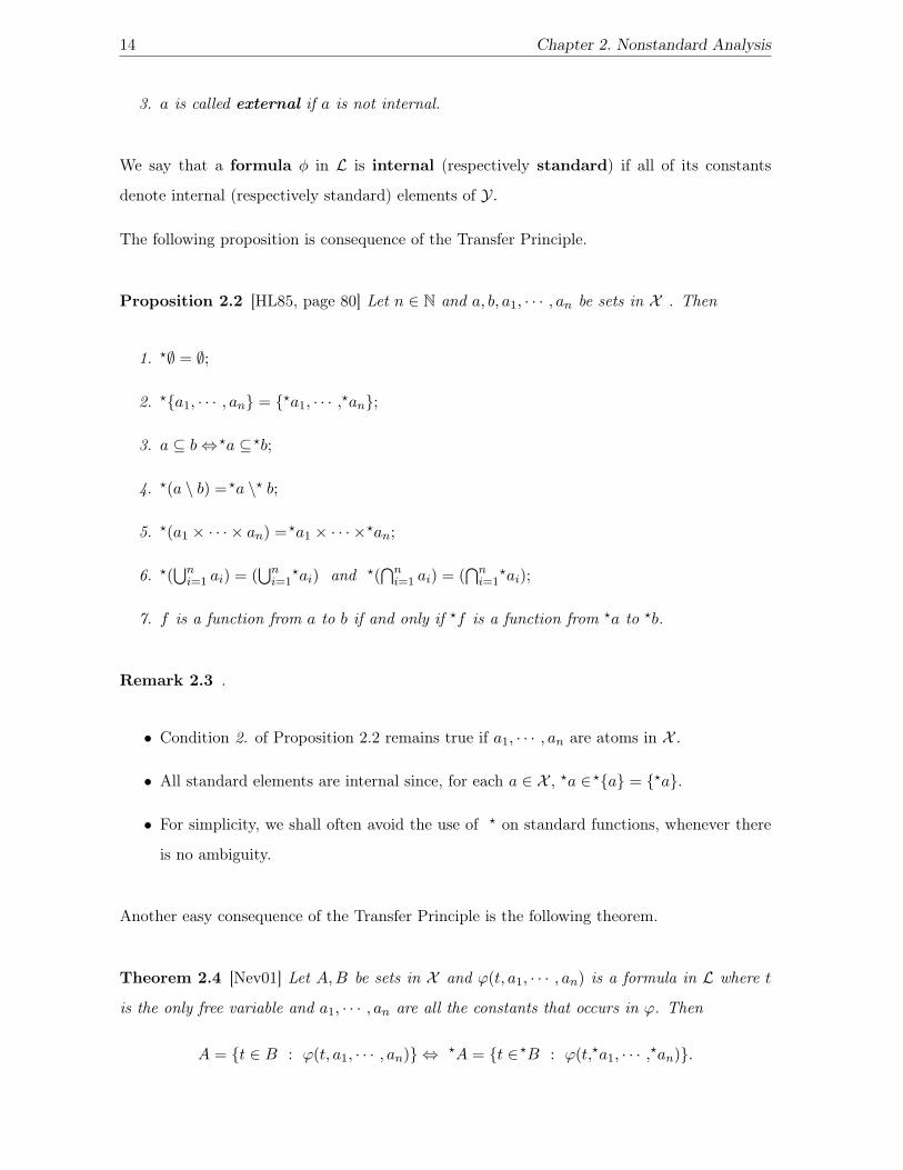
Proposition 2.2 [HL85, page 80] Let n ∈ N and a, b, a1, · · · , an be sets in X . Then
1. �∅ = ∅;
2. �{a1, · · · , an} = {�a1, · · · ,�an};
3. a ⊆ b ⇔�a ⊆�b;
4. �(a \ b) =�a \� b;
5. �(a1 × · · · × an) =�a1 × · · · ×�an;
6. �(⋃n
i=1 ai) = (⋃n
i=1�ai) and �(
⋂ni=1 ai) = (
⋂ni=1
�ai);
7. f is a function from a to b if and only if �f is a function from �a to �b.
Remark 2.3 .
• Condition 2. of Proposition 2.2 remains true if a1, · · · , an are atoms in X .
• All standard elements are internal since, for each a ∈ X , �a ∈�{a} = {�a}.
• For simplicity, we shall often avoid the use of � on standard functions, whenever there
is no ambiguity.
Another easy consequence of the Transfer Principle is the following theorem.
Theorem 2.4 [Nev01] Let A, B be sets in X and ϕ(t, a1, · · · , an) is a formula in L where t
is the only free variable and a1, · · · , an are all the constants that occurs in ϕ. Then
A = {t ∈ B : ϕ(t, a1, · · · , an)} ⇔ �A = {t ∈�B : ϕ(t,�a1, · · · ,�an)}.

2.2 Notation and preliminars in NSA 15
If E is a set, P(E) will denote the set of subsets of E and card(E) the cardinality of E. We
will say that a family C of sets satisfies the finite intersection property if intersections of
finite subfamilies of C are non empty.
The Polysaturation Principle reads as follows,
(P): Let E be a set in X and C be a collection of internal subsets of �E. If Cverifies the finite intersection property and card(C) < card(X ), then C has non
empty intersection.
This is a very strong kind of compactness property ; actually for some applications, such as
the study of Loeb measure theory (Section 2.6), we only need ℵ1-saturation (also called
countable saturation):
ℵ1-saturation: Let E be a set in X and (An)n∈N a sequence of internal subsets
of �E that satisfies the finite intersection property. Then⋂
n∈NAn �= ∅.
In the following theorem we present an alternative formulation of ℵ1-saturation that is very
useful in the construction of Loeb measures.
Theorem 2.5 [Lin88, page 13] Let E be a set in X and (An)n∈N be a sequence of internal
subsets of �E. Then⋃
n∈NAn is internal if and only if there exists k ∈ N such that
⋃n∈N
An =
A1 ∪ · · · ∪ Ak.
The next two theorems are basic tools for distinction of standard, internal and external sets
([Nev01]).
Theorem 2.6 (Internal Definition Principle) Let A be a set in X and φ(x) an internal
formula in L where x is the only free variable. Then the set
B := {x ∈�A : φ(x)}
is internal. Conversely, every internal set can be defined this way.

16 Chapter 2. Nonstandard Analysis
Theorem 2.7 (Standard Definition Principle) Let A be a set in X and φ(x) a standard
formula in L where x is the only free variable. Then the set
B := {x ∈�A : φ(x)}
is standard. Conversely, every standard set can be defined this way.
2.3 Hyperreal numbers
Denote by �R the nonstandard extension of the set of real numbers, R. A simple application of
the Transfer Principle shows that �R is an ordered field under the extension of the operations
+ and ·, and the relation < . The Polysaturation Principle shows that �R is a proper extension
of R.
The elements of �R are called hyperreal numbers or nonstandard real numbers and
are classified the following way, where N denotes the set of natural numbers and | · | is the
extension of the absolute value function to �R.
Definition 2.8 A hyperreal number x is
1. infinitesimal if |x| < 1n for all n ∈ N (the set of infinitesimal hyperreal numbers will be
denoted �R0);
2. finite if |x| < n for some n ∈ N (the set of finite hyperreal numbers will be denoted�Rfin);
3. infinite if it is not finite (the set of infinite hyperreal numbers will be denoted �R∞).
If x ∈�R is infinitesimal we write x ≈ 0. If x, y ∈�R and x−y ≈ 0, we say that x is infinitely
close to y and write x ≈ y.
Remark 2.9 The Transfer Principle implies that every nonempty internal subset of �R that
is bounded above (respectively below) has a supremum (respectively infimum); therefore we
may conclude that the sets �R0, �Rfin and �R∞ are external.

2.3 Hyperreal numbers 17
Next we present an important property of the finite hyperreal numbers ([HL85, pages 26-27]).
Theorem 2.10 (Standard Part Theorem) If x ∈ �Rfin, there exists a unique r ∈ R such
that x ≈ r; r is called the standard part of x and is denoted by st(x) or ◦x. Moreover, for
all x, y ∈�Rfin, st(x+y) = st(x)+st(y), st(xy) = st(x)st(y) and if x ≤ y then st(x) ≤ st(y).
In particular, it follows from the Standard Part Theorem that 0 is the unique infinitesimal
real number.
The nonstandard extension of N, �N , will be called the set of hypernatural numbers and
we will denote by �N∞ the set of infinite hypernatural numbers.
Definition 2.11 If H is a set in Y, then H is hyperfinite if there exists ω ∈ �N and an
internal bijection f : H → {n ∈�N : n ≤ ω}; ω is called the internal cardinality of H.
Denoting PF (E) the set of finite subsets of the set E, it follows that
Proposition 2.12 [HL85, page 89] H is an hyperfinite subset of �E if and only if H ∈�PF (E).
Remark 2.13 Again, the Transfer Principle shows that every hyperfinite set satisfies the
same properties of the finite sets as far as they can be formalized in L. For example,
• every hyperfinite set of hyperreal numbers has a minimum and a maximum element;
• every internal subset of a hyperfinite set is also hyperfinite;
• the collection of all internal subsets of a hyperfinite set is hyperfinite;
• internal images of hyperfinite sets are hyperfinite.
Definition 2.14 If X is a set in X , the standard copy of X is the set
σX := {�x : x ∈ X}.

18 Chapter 2. Nonstandard Analysis
Therefore, σX is the set of all standard elements of �X. Notice that if X is a set of atoms,
then σX = X. It may happen that σX �=�X, as we can see with the next consequence of the
Transfer and Polysaturation Principles ([Nev01]).
Theorem 2.15 (Discretization Principle) For any set X ∈ X , there exists an hyperfinite
set H ∈ Y such thatσX ⊆ H ⊆ �X.
X is infinite if and only if both inclusions are strict.
Other consequences of the Transfer Principle are the Overflow and Underflow Principles des-
cribed below ([Lin88, page 12]).
Theorem 2.16 (Overflow Principle) Let A ⊆ �R be an internal set. If A contains ar-
bitrarily large finite numbers, then A contains an infinite number. If A contains arbitrarily
large positive infinitesimal numbers, then A contains a positive finite number which is not
infinitesimal.
Theorem 2.17 (Underflow Principle) Let A ⊆�R be an internal set. If A contains arbi-
trarily small positive infinite numbers, then A contains a positive finite number. If A contains
arbitrarily small positive non infinitesimal numbers, then A contains a positive infinitesimal
number.
The following is an important consequence of the Polysaturation Principle ([Nev01]).
Theorem 2.18 (Comprehension Principle) Suppose that X and Y are sets in X , A ⊆�X, B ⊆ �Y , card(A) < card(X ) and B is internal. For each f : A → B, there exists an
internal function g : �X → B such that g |A= f.
2.4 Topology
Throughout this section, (E, ‖ · ‖) will denote a real normed space.

2.4 Topology 19
Definition 2.19 If x ∈�E then
1. x is finite if ‖ x ‖∈�Rfin; the set of finite elements of �E shall be denoted fin(�E);
2. x is infinitesimal if ‖ x ‖≈ 0 in �R; denote by inf(�E) the set of infinitesimal elements
of �E and write x ≈ 0 for x ∈ inf(�E);
3. x is near-standard if there exists a ∈ E, called the standard part of x, such that
x−a ≈ 0, and we write x ≈ a; the set of near-standard elements will be denoted ns(�E);
4. x is pre-near-standard if ∀ε ∈ R+ ∃a ∈ E ‖ x− a ‖< ε; the set of pre-near-standard
elements shall be denoted pns(�E).
As usual, if x, y ∈�E are such that x− y ≈ 0, we say that x is infinitely close to y and write
x ≈ y; otherwise, we write x �≈ y.
Definition 2.20 For each a ∈ E, the set
mon(a) := {x ∈�E : x ≈ a}
is called the monad of a.
Theorem 2.21 [HL85, page 114] If a, b ∈ E are such that a �= b, then mon(a)∩mon(b) = ∅.
From the last theorem it makes sense to define the following application
st : ns(�E) → E
x �→ st(x)
called the standard part function, where st(x) is the unique a ∈ E such that a ≈ x. The
notation ◦x for st(x) is often used.
If Y ⊆�E, define
st(Y ) := {st(x) : x ∈ Y ∩ ns(�E)}.
In the sequel we will describe nonstandard characterizations of some topological concepts.

20 Chapter 2. Nonstandard Analysis
Theorem 2.22 [Lin88, pages 52-53] Let (E, ‖ · ‖) be a real normed space and A ⊆ E.
1. A is open if and only if for all a ∈ A, mon(a) ⊆�A;
2. A is closed if and only if st(�A) = A;
3. A ⊆ E is compact if and only if �A ⊆ ns(�E) and st(�A) = A.
Characterizations of some properties of sequences in E are as follows.
Proposition 2.23 [Dav77, pages 91-92] Suppose (xn)n∈N is a sequence in E. Then
1. (xn)n∈N is bounded if and only if ∀n ∈�N∞ xn ∈ fin(�E);
2. (xn)n∈N is a Cauchy sequence if and only if ∀n, m ∈�N∞ xn ≈ xm;
3. (xn)n∈N converges to a ∈ E if and only if ∀n ∈�N∞ xn ≈ a;
4. (xn)n∈N has a convergent subsequence if and only if ∃m ∈�N∞ xm ∈ ns(�E).
From Definition 2.19 it follows that ns(�E) ⊆ fin(�E) ∩ pns(�E). But, in general, ns(�E) �=fin(�E) and ns(�E) �= pns(�E) as we will see in the following result ([Dav77, page 90], [HL85,
page 127]) and Examples 2.25 and 2.26.
Theorem 2.24 Let (E, ‖ · ‖) be a real normed space.
1. E is finite dimensional if and only if fin(�E) = ns(�E);
2. E is complete if and only if ns(�E) = pns(�E).
Example 2.25 Consider the real normed space
X = l1(N) := {(xn)n∈N ∈ RN :∑n∈N
| xn |< ∞}

2.4 Topology 21
where, for each x = (xn)n∈N ∈ X,
‖ x ‖=∑n∈N
| xn | .
Take ω ∈�N∞ and define
g :�N → �R
n �→ gn =
⎧⎨⎩1ω if 1 ≤ n ≤ ω
0 if n > ω.
Since
‖ g ‖=∑n∈�N
| gn |=ω∑
n=1
1ω
= 1
it follows that g ∈ fin(�X). Next we will prove that g �∈ ns(�X). Suppose that there exists
a = (an)n∈N ∈ X such that g ≈ a. Since
‖ g − a ‖≈ 0 ⇔ ∑n∈�N
| gn − an |≈ 0
⇒ ∀n ∈�N gn ≈ an
⇒ ∀n ∈ N an = 0
⇔ ‖ a ‖= 0
and
‖ g − a ‖≥‖ g ‖ − ‖ a ‖= 1
we obtain a contradiction with g ≈ a; hence g �∈ ns(�X).
Example 2.26 .
1. Let Q denote the set of rational numbers, x = (xn)n∈N be a sequence in Q that converges
to some a ∈ R \ Q and ω ∈ �N∞. Since xω ≈ a (Proposition 2.23) and a �∈ Q then
xω �∈ ns(�Q) (Theorem 2.21). On the other hand, xω ∈ pns(�Q), because in any open
interval centered in xω with radius ε ∈ R+ there exists a rational number.
2. Let X = (C([−2, 2]), ‖ · ‖) be the (incomplete) normed space of all continuous real
valued functions defined in [−2, 2] with the norm ‖ · ‖ defined by
‖ f ‖=∫ 2
−2| f(t) | dt (f ∈ C([−2, 2]).

22 Chapter 2. Nonstandard Analysis
Consider the Cauchy sequence (fn)n∈N in X defined by
fn(t) =
⎧⎪⎪⎪⎨⎪⎪⎪⎩0 if −2 ≤ t < − 1
n
n2 t + 1
2 if − 1n ≤ t ≤ 1
n
1 if 1n < t ≤ 2
and g : [−2, 2] → R be such that
g(t) =
⎧⎪⎪⎪⎨⎪⎪⎪⎩0 if −2 ≤ t < 012 if t = 0
1 if 0 < t ≤ 2
.
Observe that, for any ω ∈�N∞,
‖ fω−g ‖=∫ 2
−2| fω(t)−g(t) | dt = 2
∫ 1ω
0
(1 −
(ω
2t +
12
))dt =
∫ 1ω
0(1−ωt)dt =
12ω
≈ 0.
Since g �∈ C([−2, 2]), then fω �∈ ns(�X) (Theorem 2.21).
Next we will show that fω ∈ pns(�X). Notice that, for each n ∈ N,
‖ fω − fn ‖= 2∫ 1
ω
0
(ω
2t − n
2t)
dt + 2∫ 1
n
1ω
(1 − n
2t − 1
2
)dt =
12n
− 12ω
<12n
.
Take ε ∈ R+; choosing m ∈ N such that 12m < ε we have that ‖ fω − fm ‖< ε, and this
shows that fω ∈ pns(�X). Hence, ns(�X) �= pns(�X).
In the following, we will suppose that (F, | · |) is another real normed space.
Definition 2.27 Let g : �E → �F be a function. Then g is said to be S-continuous on a
(possibly external) subset A of its domain if
∀x, y ∈ A [x ≈ y ⇒ g(x) ≈ g(y)].
Some relations between this notion and the usual continuity are the following results.
Theorem 2.28 [HL85, pages 115 and 125] A function f : E → F is
1. continuous on c ∈ E if and only if it is S-continuous in mon(c);

2.4 Topology 23
2. continuous if and only if f is S-continuous in ns(�E);
3. uniformly continuous if and only if f is S-continuous in �E.
In the sequel we present some results that will be very useful in Chapter 3, when we will study
some Existence Theorems for ODE’s.
Theorem 2.29 [Cut97, page 72] If [a, b] ⊆ R, g : �[a, b] → �R is internal and S-continuous
and there exists z ∈�[a, b] such that g(z) is finite, then
1. g(x) is finite for all x ∈�[a, b];
2. the standard function◦g : [a, b] → R
t �→ ◦g(t) := st(g(t))
is continuous.
Remark 2.30 Theorem 2.29 remains true if we substitute �[a, b] by a hyperfinite set X such
that st(X) = [a, b]; in this case, ◦g : [a, b] → R is such that, for each t ∈ [a, b],
◦g(t) := st(g(τ))
for some τ ∈ X satisfying τ ≈ t.
Definition 2.31 Let Y ⊆ �E and g : Y → �R. Then g is S-bounded if there exists L ∈ R
such that for all y ∈ Y ,
| g(y) |≤ L.
Definition 2.32 Let Y ⊆ �E and g : Y → �R. Then g is S-Lipschitzian if there exists
M ∈ R such that for all x, y ∈ Y ,
| g(x) − g(y) |≤ M ‖ x − y ‖ .
24 Chapter 2. Nonstandard Analysis
Definition 2.33 Let Y ⊆�R and g : Y →�R. Then g is S-absolutely continuous if
N∑i=1
|g(bi) − g(ai)| ≈ 0
for every hyperfinite collection
{[a1, b1[, [a2, b2[, · · · , [aN , bN [} (N ∈�N)
(where [a, b[ denotes the set {t ∈ �R : a ≤ t < b} ∩ Y and a, b ∈ Y ) of non overlapping
subintervals of Y such that∑N
i=1(bi − ai) ≈ 0.
The following is easy to prove.
Proposition 2.34 Let Y ⊆�R and g : Y →�R.
1. If g is S-absolutely continuous, then g is S-continuous;
2. If g is S-Lipschitzian, then g is S-absolutely continuous.
Next we present an important result that relates the (nonstandard) notion of S-absolutely
continuity and the (classical) notion of absolutely continuity. We recall that a function f :
[a, b] → R is absolutely continuous on [a, b] if, for any ε ∈ R+, there is a δ ∈ R+ such that
n∑i=1
| f(bi) − f(ai) |< ε
for any disjoint intervals [a1, b1[, · · · , [an, bn[ in [a, b] whose lengths satisfy
n∑i=1
(bi − ai) < δ.
Theorem 2.35 [Tuc93, pages 35-36] Let [a, b] ⊆ R and X a hyperfinite set such that st(X) =
[a, b]. If g : X → �R is internal, S-bounded and S-absolutely continuous function, then the
function ◦g : [a, b] → R defined by◦g(t) := st(g(τ))
where τ ∈ X is such that τ ≈ t, is a standard absolutely continuous function.

2.5 Differentiation 25
2.5 Differentiation
Suppose (E, ‖ · ‖) and (F, | · |) are real Banach spaces and let Lin(E, F ) denote the space of
all continuous linear maps from E to F . Let U be an open subset of E and f : U → F a map.
We say that f : U → F is a C1 function and write f ∈ C1(U, F ), if the Fréchet derivative
f ′ : U → Lin(E, F ) exists at every point a ∈ U and the mapping f ′ is continuous.
The next result follows easily from the nonstandard characterization of limits.
Theorem 2.36 The map f : U → F is Fréchet differentiable if and only if there exists an
application f ′ : U → Lin(E, F ) such that
∀a ∈ U ∀ε ∈ inf(�E) ∃η ∈ inf(�F ) f(a + ε) = f(a) + f ′(a)(ε)+ ‖ ε ‖ η.
Next we present nonstandard characterizations of C1 functions. Denote
ns(�U) := {x ∈�E : x ∈ ns(�E) ∧ st(x) ∈ U}.
Theorem 2.37 [SL76, page 97] Suppose f : U → F is a map. The following conditions are
equivalent:
1. f ∈ C1(U, F );
2. there exists a map f ′ : U → Lin(E, F ) such that
∀a ∈ ns(�U) ∀ε ∈ inf(�E) ∃η ∈ inf(�F ) f(a + ε) = f(a) + f ′(a)(ε)+ ‖ ε ‖ η;
3. there exists a map f ′ : U → Lin(E, F ) such that
∀a ∈ U ∀x, y ∈�E [ x ≈ y ≈ a ⇒∃β ∈ inf(�F ) f(x) − f(y) = f ′(a)(x − y)+ ‖ x − y ‖ β ].
We notice that the only difference between the nonstandard characterization of a Fréchet
differentiable map (Theorem 2.36) and the nonstandard characterization of a C1 map given
in condition 2. of Theorem 2.37, is "only" the set to which a belongs: in the first case, a ∈ U
and in the second case, a ∈ ns(�U).

26 Chapter 2. Nonstandard Analysis
We proceed with other nonstandard characterization of a C1 map (in the sense of Fréchet)
using the weaker notion of Gâteaux-Levy derivative.
Theorem 2.38 [Str78, pages 367-368] Suppose f : U → F is a map. Then f ∈ C1(U, F ) if
and only if there exists a map Df(·) : U → Lin(E, F ) such that
∀a ∈ ns(�U) ∀x ∈ fin(�E) ∀ε ∈�R0 ∃β ∈ inf(�F ) f(a + εx) = f(a) + εDfa(x) + εβ.
Denote by E′ the dual space of E with uniform norm ‖ · ‖ and 〈·, ·〉 the duality pairing
between E′ and E. For later use, we present the following definition.
Definition 2.39 Let f : U → R be Fréchet differentiable and a ∈ �U. Then a is an almost
critical point of f if f ′(a) ≈ 0.
Therefore, a is an almost critical point of f : U → R if ‖ f ′(a) ‖≈ 0, that is,
∀v ∈ fin(�E) 〈f ′(a), v〉 ≈ 0.
2.6 Loeb integration theory
Loeb measures were discovered by Peter Loeb in 1975 ([Loe75]) and they are very important in
many applications of NSA. These measures have appeared in Control Theory, Mathematical
Physics, Mathematical Finance, Functional Analysis and several other fields. In Chapter 3 we
will apply (finite) Loeb measures to ordinary differential equations, namely, we will present a
nonstandard proof of Carathéodory’s Existence Theorem.
For convenience, we will describe only the construction of finite Loeb measures. These mea-
sures are obtained from an internal measure in the way described below. For a more complete
treatment of nonstandard integration theory see [Cut83], [Cut95], [Cut00], [Lin88], [SB86],
[Ros97], [And82], [AHKFL86] or [Mar97], for example.
Suppose that (Ω,A, μ) is a finite internal measure space, that is,
1. Ω is an internal non empty set;

2.6 Loeb integration theory 27
2. A is an internal algebra on Ω (that is, A is internal, A ⊆ P(Ω), Ω ∈ A and A is closed
for complements and finite unions);
3. μ : A →�R is a finite internal finitely additive measure (that is, μ is an internal function
such that μ(Ω) is finite, μ(∅) = 0, μ(A) ≥ 0 for all A ∈ A, and μ(A∪B) = μ(A) + μ(B)
for disjoint A, B ∈ A).
In general, this is not a measure space because A is not a σ-algebra, except in the trivial
case where A is finite. This is a consequence of ℵ1-saturation: if A is infinite, there exists
a countable collection of pairwise disjoint non empty sets (An)n∈N ⊆ A; Theorem 2.5 shows
that⋃
n∈NAn is not internal and, therefore,
⋃n∈N
An �∈ A.
From μ : A →�R we can define the (external) mapping
◦μ : A → R
A �→ ◦μ(A) :=◦(μ(A)).
The Loeb measure generated by μ will be denoted by μL and is a measure defined in a family
of subsets of Ω that contains the internal algebra A and that coincide with ◦μ on A.
Definition 2.40 Let B ⊆ Ω (B not necessarily internal). We say that
1. B is a Loeb null set if for each real ε > 0 there exists an internal set A ∈ A such that
B ⊆ A and μ(A) < ε;
2. B is Loeb measurable if there exists a set A ∈ A such that A�B := (A \B)∪ (B \A)
is Loeb null. Denote the collection of all Loeb measurable sets by L(A);
3. For B ∈ L(A) define
μL(B) :=◦μ(A)
for all A ∈ A such that A�B is Loeb null; μL(B) is called the Loeb measure of B.

28 Chapter 2. Nonstandard Analysis
Remark 2.41 Observe that
• A subset of a Loeb null set is a Loeb null set;
• μL : L(A) → R+0 ;
• ∀A ∈ A μL(A) =◦μ(A).
The next proposition clarifies the term Loeb null set.
Proposition 2.42 [Cut95, page 155] For any B ⊆ Ω, B is a Loeb null set if and only if
B ∈ L(A) and μL(B) = 0.
The next proposition says that a set Y ⊆ Ω is Loeb measurable if it is almost internal in the
sense described below.
Proposition 2.43 [Mar97, pages 47-48] Y ∈ L(A) if and only if there exists C ∈ A and a
Loeb null set N such that Y = C�N.
In [Cut95], [Cut00], [SB86], [AHKFL86] and [Mar97] the reader can find alternative cha-
racterizations of Loeb measurable sets.
Now we present the central theorem in Loeb measure theory.
Theorem 2.44 [Cut95, pages 155-156] L(A) is a σ-algebra, called Loeb σ-algebra, and μL
is a complete σ-additive measure on L(A).
(Ω, L(A), μL) is a measure space, called the Loeb measure space generated by (Ω,A, μ).
Remark 2.45 Note that
• μL acts on sets which may not be standard;
• A countable union of Loeb null sets is a Loeb null set.

2.6 Loeb integration theory 29
Remark 2.46 If μ is not finite, it is also possible to define the (unbounded) Loeb measure
space (Ω, L(A), μL) generated by (Ω,A, μ); see [Lin88] or [Mar97].
In the following we present important examples of Loeb spaces.
Example 2.47 Let (X,L, λ) be a standard measure space and take Ω = �X, A = �L and
μ =�λ. Then (�X, L(�L),� λL) is the Loeb space generated by (�X,�L,�λ).
Example 2.48 Fix N ∈�N∞, define � = 1N and make
T := {k� : k = 0, 1, 2, · · · , N − 1} = {0,1N
,2N
, · · · , 1 − 1N
}. (2.1)
T is usually called hyperfinite time line with increment �. Denoting the set of all internal
subsets of T by A and defining ν : A →�[0, 1] by
ν(A) =card(A)card(T)
=card(A)
N(2.2)
we obtain an internal measure space (T,A, ν) called internal counting measure space
on T. The Loeb space (T, L(A), νL) generated by (T,A, ν) is called the Loeb counting
measure space on T.
Next we will see how the Loeb counting measure space on the hyperfinite time line can be
used to represent the Lebesgue measure space ([0, 1],L, λ).
Theorem 2.49 [Cut00, page 17] Let (T, L(A), νL) be the Loeb counting measure space. A set
A ⊆ [0, 1] is Lebesgue measurable if and only if the set st−1T
(A) defined by
st−1T
(A) := {t ∈ T : ◦t ∈ A}
is Loeb measurable; if this is the case,
λ(A) = νL(st−1T
(A)).
Remark 2.50 Theorem 2.49 is a particular case of a general hyperfinite representation the-
orem due to Anderson ([And82]) that shows that any Radon measure space on a Hausdorff
space can be represented by a hyperfinite Loeb counting measure.

30 Chapter 2. Nonstandard Analysis
We deal now with measurable functions.
Definition 2.51 A function f : Ω → R is Loeb measurable if f is μL-measurable in the
conventional sense, that is, for every open set B ⊆ R, f−1(B) ∈ L(A).
Definition 2.52 An internal function F : Ω → �R is �measurable if F−1(A) ∈ A, for any�open set A ⊆�R (that is, A ∈�O where O denotes the euclidian topology of R).
Connections between these notions are given in the following theorem.
Theorem 2.53 [Cut95, page 166] If F : Ω → �R is internal and �measurable, then the func-
tion◦F : Ω → R
w �→ ◦F (w) :=◦(F (w)).
is Loeb measurable.
Now we present important notions in nonstandard integration theory. As usual in measure
theory, we will write a.a. to mean "almost all".
Definition 2.54 .
1. Let (Ω,A, μ) be an internal measure space and f : Ω → R. An internal �measurable
function F : Ω →�R is called a (one legged) lifting of f if
◦F (w) = f(w) μL − a.a. w ∈ Ω.
Ω �R
R
F
f ◦
2.6 Loeb integration theory 31
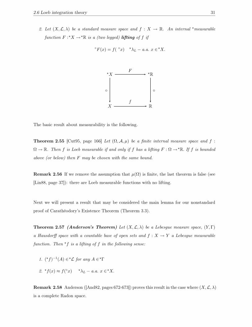
2. Let (X,L, λ) be a standard measure space and f : X → R. An internal �measurable
function F :�X →�R is a (two legged) lifting of f if
◦F (x) = f( ◦x) �λL − a.a. x ∈�X.
�X �R
X R
F
◦
f
◦
The basic result about measurability is the following.
Theorem 2.55 [Cut95, page 166] Let (Ω,A, μ) be a finite internal measure space and f :
Ω → R. Then f is Loeb measurable if and only if f has a lifting F : Ω → �R. If f is bounded
above (or below) then F may be chosen with the same bound.
Remark 2.56 If we remove the assumption that μ(Ω) is finite, the last theorem is false (see
[Lin88, page 37]): there are Loeb measurable functions with no lifting.
Next we will present a result that may be considered the main lemma for our nonstandard
proof of Carathéodory’s Existence Theorem (Theorem 3.3).
Theorem 2.57 (Anderson’s Theorem) Let (X,L, λ) be a Lebesgue measure space, (Y, Γ)
a Hausdorff space with a countable base of open sets and f : X → Y a Lebesgue measurable
function. Then �f is a lifting of f in the following sense:
1. (�f)−1(A) ∈�L for any A ∈�Γ
2. �f(x) ≈ f(◦x) �λL − a.a. x ∈�X.
Remark 2.58 Anderson ([And82, pages 672-673]) proves this result in the case where (X,L, λ)
is a complete Radon space.

32 Chapter 2. Nonstandard Analysis
Loeb measures are classical measures over σ-algebras (with possibly nonstandard elements),
thus Loeb integration theory is simply the classical theory of integration with respect to Loeb
measure: in particular, a Loeb measurable function f : Ω → R is Loeb integrable if f is
integrable in the classical sense with respect to the Loeb measure μL, in which case the Loeb
integral∫Ω fdμL is a real number.
The �integral or internal integral of a �measurable function F : Ω → �R is obtained
applying the Transfer Principle to the classical definition of integral; usually we will write∫Fdμ instead �
∫Fdμ.
Although Theorem 2.53 says that if F : Ω →�R is internal and �measurable, then ◦F is Loeb
measurable and for all x ∈ Ω
F (x) ≈◦F (x),
the equation◦(∫
ΩFdμ
)=∫
Ω
◦FdμL (2.3)
is, in general, false.
Example 2.59 Let (T, L(A), νL) be the Loeb counting measure space. Define the internal�measurable function
F (τ) =
⎧⎨⎩ N if τ = 0
0 if τ ∈T \ {0}where N ∈ �N∞ is the same used in the construction of T. Then
∫T
◦FdνL = 0 (since◦F (τ) = 0 for νL- a.a. τ ∈ T) and∫
T
Fdν =∑τ∈T
F (τ)ν({τ}) =∑τ∈T
F (τ)1N
= 1.
To obtain equality of ◦ (∫Ω Fdμ
)and
∫Ω
◦FdμL we have to restrict the class of �integrable
functions.
Definition 2.60 An internal �measurable function F : Ω →�R is S-integrable if
1.∫Ω | F | dμ is finite;

2.6 Loeb integration theory 33
2. for all A ∈ A such that μ(A) ≈ 0, then∫A | F | dμ ≈ 0.
Remark 2.61 Concerning the last definition,
• Condition 1. is necessary to guarantee that all S-integrable function are �integrable;
• Condition 2. is needed for equality (2.3), because if μ(A) ≈ 0, then μL(A) = 0 and
therefore,∫A
◦ | F | dμL = 0; so∫A | F | dμ must be infinitesimal;
• If μ is not finite we must add an extra condition to Definition 2.60:
3. if A ∈ A and F ≈ 0 on A, then∫A | F | dμ ≈ 0.
Observe that if μ is finite, condition 3. is always satisfied, since F ≈ 0 on A means that
∀ε ∈ R+ ∀x ∈ A | F (x) |< ε
and then, for all ε ∈ R+, ∫A| F | dμ ≤ εμ(A);
since μ(A) is finite, it follows that∫A | F | dμ ≈ 0.
The following is easy to prove.
Proposition 2.62 Let (Ω,A, μ) be a finite internal measure space and F : Ω → �R internal�mensurable. If F is S-bounded, then F is S-integrable.
The following theorem shows that if F : Ω →�R is S-integrable, then equality (2.3) holds.
Theorem 2.63 [Cut95, pages 169-170] Let (Ω,A, μ) an internal measure space and F : Ω →�R an internal �mensurable function. Then the following conditions are equivalent:
1. F is S-integrable;
2. ◦F is Loeb integrable and
◦(∫
AFdμ
)=∫
A
◦FdμL, ∀A ∈ A.
34 Chapter 2. Nonstandard Analysis
The next result relates the Loeb integral of f : Ω → R to the �integral of a lifting of f .
Theorem 2.64 [Cut95, pages 170-171] Let (Ω,A, μ) be an internal measure space and f :
Ω → R a Loeb measurable function. Then the following conditions are equivalent:
1. f is Loeb integrable;
2. f has an internal S-integrable lifting F : Ω →�R and
◦(∫
AFdμ
)=∫
AfdμL, ∀A ∈ A.
The next theorem characterizes nonstandard extensions of Lebesgue integrable functions.
Theorem 2.65 [And82, pages 679-680] Let (Z,L, λ) be a Lebesgue measure space and suppose
that f : Z → R is Lebesgue integrable. Then �f : �Z → �R is S-integrable.
To end this section we will present the following characterization of the Lebesgue integral on
[0, 1]. For f : [0, 1] → R define
f : T → R
τ �→ f(τ) = f(◦τ).
Theorem 2.66 [Mar97, pages 66-68] Let (T, L(A), νL) be the Loeb counting measure space
and ([0, 1],L, λ) the Lebesgue measure space on [0, 1]. The following conditions are equivalent:
1. f : [0, 1] → R is Lebesgue integrable;
2. f : T → R is Loeb integrable;
3. there exists an internal S-integrable function F : T →�R that is a lifting of f .
In this case ∫[0,1]
f(t)dλ(t) =∫
T
f(τ)dνL(τ) = ◦(∫
T
Fdν
)= ◦
(∑τ∈T
F (τ)1N
).

2.7 Nonstandard discrete derivative 35
Remark 2.67 Note that the last theorem defines the Lebesgue integral on [0, 1] as the stan-
dard part of some hyperfinite sum. This is also true for the Lebesgue integral on R (see [SB86]
or [Mar97] for details).
Example 2.68 It may happen that G and F are two liftings of the same Lebesgue integrable
function f : [0, 1] → R but G is S-integrable (then,∫[0,1] f(t)dλ(t) = ◦ (∫
TGdν
)) and F is not
S-integrable. Take F : T →�R defined in Example 2.59 and let G : T →�R be such that
G(τ) =
⎧⎨⎩ 1 if τ = 0
0 if τ ∈T \ {0}.
It is clear that F and G are liftings of the null function defined on [0, 1]. G is S-integrable
because G is S-bounded (Proposition 2.62) but F is not S-integrable because (Theorem 2.63)
1 = ◦(∫
T
Fdν
)�=∫
T
◦FdνL = 0.
2.7 Nonstandard discrete derivative
Let T be the hyperfinite time line with respect to the increment � = 1N and N ∈ �N∞
(see (2.1)). The nonstandard discrete derivative or hyperfinite difference quotient
([Tuc93, page 34]) of an internal function X : T → �R is the function X ′ : T \ {1 −�} → �R
defined by
X ′(t) :=X(t + �) − X(t)
� .
We finish this chapter by presenting the following result that will be used in the next chapter.
Theorem 2.69 [Tuc93, pages 34-35] Let (T,A, ν) be the internal counting measure space and
suppose X : T →�R is an internal function. The following conditions are equivalent:
1. X is S-absolutely continuous;
2.∫A | X ′ | dν =
∑τ∈A | X ′(τ) | � ≈ 0 for all A ∈ A such that ν(A) ≈ 0.


Chapter 3
Existence Theorems for ODE’s
3.1 Introduction
The aim of this chapter is to present a nonstandard generalization of Carathéodory’s Existence
Theorem and also a nonstandard proof of Carathéodory’s Existence Theorem, which avoid
Ascoli’s Theorem as well as Lebesgue’s Dominated Convergence Theorem.
Throughout this chapter we will suppose that N ∈ �N∞ and T is the hyperfinite time line
with respect to the increment � = 1N ,
T := {k� : k = 0, 1, 2, · · · , N − 1} = {0,1N
,2N
, · · · , 1 − 1N
}.
(T,A, ν) will be denote the internal counting measure space (see Example 2.48), that is, A is
the set of all internal subsets of T and
ν : A → �[0, 1]
A �→ ν(A) = card(A)card(T) .
The Loeb space generated by (T,A, ν) will be denoted by (T, L(A), νL). As usual, λ will
represent the Lebesgue measure and �λL the Loeb measure generated by �λ.
37
38 Chapter 3. Existence Theorems for ODE’s
If X : T →�R is an internal function we use the notion X ′ to denote the nonstandard discrete
derivative, that is,
X ′ : T \ {1 −�} → �R
t �→ X ′(t) := X(t+�)−X(t)� .
For classical results in Measure and Integration Theory consult, for example, [Rao87] or
[Coh80].
3.2 Nonstandard Carathéodory’s Existence Theorem
In this section we present a result about internal functions. As we will see, this result is a
generalization of Carathéodory’s Existence Theorem since this classical theorem for ODE’s
is a consequence of the first one.
Theorem 3.1 (Nonstandard Carathéodory’s Existence Theorem) [MNa] Let F : T ×�R → �R be an internal �measurable function. Suppose there exists an internal S-integrable
function M : T →�R such that
∀(τ, x) ∈ T ×� R | F (τ, x) |≤ M(τ).
Then, for each α ∈�R, there exists one and only one internal S-absolutely continuous function
X : T →�R such that ⎧⎨⎩ X ′(τ) = F (τ, X(τ)) (τ ∈ T \ {1 −�})X(0) = α
. (3.1)
If α is finite, then X(T) ⊆�Rfin.
Proof. Define X : T → �R recursively by
X(0) = α
X(t + �) = X(t) + F (t, X(t))� (t ∈ T \ {1 −�}).
X is internal and, by construction, if t = k� ∈ T,
X(t) = α +k−1∑i=0
F (i�, X(i�))�.

3.3 Carathéodory’s Existence Theorem 39
Moreover,
X ′(t) =X(t + �) − X(t)
� = F (t, X(t)) (t ∈ T \ {1 −�}).
Using the definition of the discrete derivative, it is obvious that there exists only one internal
function X : T →�R such that (3.1) holds.
To prove that X is S-absolutely continuous, we will use Theorem 2.69. Take A an internal
subset of T such that ν(A) ≈ 0. Note that
∑τ∈A
| X ′(τ) | � =∑τ∈A
| F (τ, X(τ)) | � ≤∑τ∈A
M(τ)� =∫
AMdν.
Since M is S-integrable,∫A Mdν ≈ 0 and therefore∫
A| X ′ | dν =
∑τ∈A
| X ′(τ) | � ≈ 0
which proves that X is S-absolutely continuous.
Finally, note that, for each τ = k� ∈ T,
| X(τ) − α | = |k−1∑i=0
F (i�, X(i�))� | ≤k−1∑i=0
M(i�)� ≤∫
T
Mdν
and∫
TMdν is finite since M is S-integrable. Hence, if α is finite, X(T) ⊆�Rfin.
3.3 Carathéodory’s Existence Theorem
The next result (see [Rao87, pages 230-240]) gives a characterization of absolutely continuous
functions. As usual, L1([a, b]) denotes the set of all Lebesgue measurable functions f : [a, b] →R such that
∫[a,b] | f |< ∞.
Theorem 3.2 (Fundamental Theorem of Calculus for the Lebesgue integral) A func-
tion f : [a, b] → R is absolutely continuous if and only if f is differentiable almost everywhere
on [a, b], f ′ ∈ L1([a, b]) and
f(x) − f(a) =∫
[a,x]f ′(t)dλ(t) (a ≤ x ≤ b).
40 Chapter 3. Existence Theorems for ODE’s
Next we will present our nonstandard proof of Carathéodory’s Existence Theorem ([MNa]) (a
classical proof of this theorem can be found in [CL55, pages 43-44]). In the following, C([a, b])
denotes the Banach space of all real continuous functions on [a, b] with the norm defined by
‖ f ‖:= maxx∈[a,b] | f(x) | .
Theorem 3.3 (Carathéodory’s Existence Theorem) Suppose that f : [0, 1] × R → R
is Lebesgue measurable, continuous in the second variable and let x0 ∈ R. If there exists a
Lebesgue integrable function m : [0, 1] → R such that
∀(t, x) ∈ [0, 1] × R | f(t, x) |≤ m(t)
then there exists x : [0, 1] → R absolutely continuous such that⎧⎨⎩ x′(t) = f(t, x(t)) a.a. t ∈ [0, 1]
x(0) = x0
. (3.2)
Proof. Since f : [0, 1] × R → R is a Lebesgue measurable function then F = �f |T×�R :
T ×�R → �R is �measurable (with respect to �λ). Theorem 2.65 says that �m : �[0, 1] → �R
is S-integrable and therefore M = �m |T is also S-integrable. Using the Transfer Principle we
conclude that
∀(t, x) ∈�[0, 1] ×�R |�f(t, x) |≤ �m(t)
and then
∀(τ, x) ∈ T ×�R | F (τ, x) |≤ M(τ).
Nonstandard Carathéodory’s Existence Theorem (Theorem 3.1) shows that there exists an
internal S-absolutely continuous X : T →�R such that⎧⎨⎩ X ′(τ) = F (τ, X(τ)) (τ ∈ T \ {1 −�})X(0) = x0
and for all τ = k� ∈ T
X(τ) = x0 +k−1∑i=0
F (i�, X(i�))� ∈�Rfin.
Since X(T) ⊆�Rfin, we can choose r ∈ R+ such that
∀τ ∈ T | X(τ) |≤ r. (3.3)

3.3 Carathéodory’s Existence Theorem 41
Defining x : [0, 1] → R by
x(◦τ) =◦X(τ) (τ ∈ T) (3.4)
we conclude, by Theorem 2.35, that x is absolutely continuous. We will prove that this
function is a solution to the problem (3.2).
Using the definition and continuity of x we have that
X(τ) ≈ x(◦τ) ≈ x(τ) (τ ∈ T).
By hypothesis f is Lebesgue measurable, then the function
f : [0, 1] → C([−r, r])
defined by
f(t)(z) = f(t, z) ((t, z) ∈ [0, 1] × [−r, r])
is also Lebesgue measurable. Taking the uniform topology in C([−r, r]) and using Anderson’s
Theorem (Theorem 2.57) we can conclude that
�f : �[0, 1] →�C([−r, r])
is a lifting of f with respect to the Loeb measure �λL, hence
�f(τ) ≈ f(◦τ) �λL − a.a. τ ∈�[0, 1].
Using the definition of the norm in C([−r, r]) we may conclude that[∀z ∈�[−r, r] �f(τ, z) ≈�f(◦τ, z)
]�λL − a.a. τ ∈�[0, 1]. (3.5)
Since f is continuous in the second variable, we obtain that[∀z ∈�[−r, r] �f(τ, z) ≈ f(◦τ,◦ z)
]�λL − a.a. τ ∈�[0, 1]. (3.6)
As X satisfies (3.3) and (3.4), it follows that
�f(τ, X(τ)) ≈ f(◦τ,◦ X(τ)) = f(◦τ, x(◦τ)) νL − a.a. τ ∈ T
because νL(T) = 1.

42 Chapter 3. Existence Theorems for ODE’s
Hence,
G : T → �R
τ �→ G(τ) =�f(τ, X(τ))
is a lifting of the Lebesgue integrable function
g : [0, 1] → R
t �→ g(t) = f(t, x(t)).
Next we will prove that G is S-integrable. Observe that, for all A ∈ A,∫A| G | dν ≤
∫A
�mdν.
Since �m :�[0, 1] →�R is S-integrable, then∫T
| G | dν ∈�Rfin
and ∫A| G | dν ≈ 0
whenever ν(A) ≈ 0, proving that G is S-integrable.
We may now prove that, for all t ∈ [0, 1],
x(t) = x0 +∫
[0,t]f(s, x(s))dλ(s).
Fix z ∈ [0, 1] and τ = k� ∈ T such that τ ≈ z. Observe that
x(z) = ◦X(τ)
= x0 + ◦(∑k−1
i=0 F (i�, X(i�))�)
= x0 + ◦(∑k−1
i=0 G(i�)�)
= x0 +∫[0,z] g(t)dλ(t) (Theorem 2.66)
= x0 +∫[0,z] f(t, x(t))dλ(t).
Obviously, x(0) = x0. Finally, by Theorem 3.2, we may conclude that x is a solution to the
problem (3.2).
3.4 Peano’s Existence Theorem
Peano’s Existence Theorem is very easily derived from Carathéodory’s Existence Theorem.

3.4 Peano’s Existence Theorem 43
Theorem 3.4 (Peano’s Existence Theorem) Suppose f : [0, 1] × R → R is bounded and
continuous and x0 ∈ R. Then there exists x : [0, 1] → R such that⎧⎨⎩ x′(t) = f(t, x(t))
x(0) = x0
. (3.7)
Proof. Notice that f satisfies all the conditions of Carathéodory’s Existence Theorem
(Theorem 3.3). This theorem says that there exists an absolutely continuous function x :
[0, 1] → R that satisfies the integral equation
x(z) = x0 +∫
[0,z]f(t, x(t))dλ(t) (z ∈ [0, 1]).
Clearly, x(0) = x0. Since f and x are continuous, by the Fundamental Theorem of Calculus
(for the Riemann integral), x is such that
∀t ∈ [0, 1] x′(t) = f(t, x(t)).
Therefore, x : [0, 1] → R satisfies the initial valued problem (3.7).
We included in Appendix A a direct nonstandard proof of Peano’s Existence Theorem. The
reader may compare the nonstandard proofs of Carathéodory’s and Peano’s Existence Theo-
rems.


Chapter 4
Palais-Smale conditions
4.1 Introduction
The aim of this chapter is to present nonstandard versions of the Palais-Smale condition
(Definition 4.1) and the relations between them. We will see that some of them are gene-
ralizations of the classical Palais-Smale condition but still sufficient to prove a new Mountain
Pass Theorem (Theorem 5.15).
Suppose (E, ‖ · ‖) is a real Banach space and f : E → R is Fréchet differentiable. We will
denote by K the set of all critical points of f , that is,
K := {x ∈ E : f ′(x) = 0}
and, for each c ∈ R, Kc will denote the set of all critical points with value c, that is,
Kc := {x ∈ E : f ′(x) = 0 ∧ f(x) = c} = K ∩ f−1({c}).
As usual, C1(E, R) denotes the set of continuously Fréchet differentiable functionals defined
on E.
4.2 The Palais-Smale condition
Many results in Critical Point Theory involve the following condition, originally introduced in
1964 [PS64] by Palais and Smale:
45

46 Chapter 4. Palais-Smale conditions
Definition 4.1 Let E be a real Banach space. We say that f ∈ C1(E, R) satisfies the Palais-
Smale condition ((PS) for short) if for all sequence (un)n∈N in E,
(PS) (f(un))n∈N is bounded and limn→∞ f ′(un) = 0
⇒ (un)n∈N has a convergent subsequence.
The following condition
(PS0) (f(un))n∈N is bounded and limn→∞ f ′(un) = 0
⇒ ∃m ∈�N∞ um ∈ ns(�E)
is a direct translation of (PS) in nonstandard terms.
The following is easy to prove.
Proposition 4.2 Suppose that f ∈ C1(E, R) satisfies (PS). Then
1. For each a, b ∈ R such that a ≤ b,
{u ∈ E : a ≤ f(u) ≤ b ∧ f ′(u) = 0} = f−1([a, b]) ∩ K
is a compact set;
2. If f is bounded, K is a compact set.
Note that
f satisfies (PS) and K is compact �⇒ f is bounded
and
K is compact and f is bounded �⇒ f satisfies (PS)
as can be seen with the following two examples.
4.3 Nonstandard Palais-Smale conditions 47
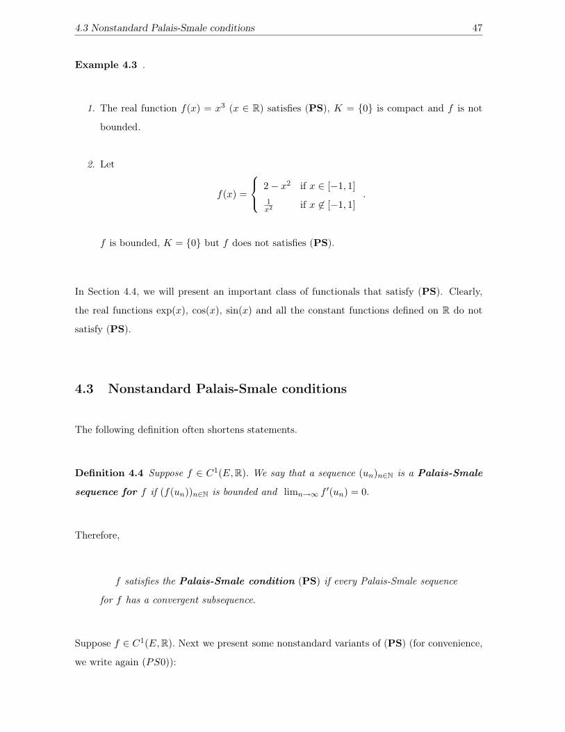
Example 4.3 .
1. The real function f(x) = x3 (x ∈ R) satisfies (PS), K = {0} is compact and f is not
bounded.
2. Let
f(x) =
⎧⎨⎩ 2 − x2 if x ∈ [−1, 1]1x2 if x �∈ [−1, 1]
.
f is bounded, K = {0} but f does not satisfies (PS).
In Section 4.4, we will present an important class of functionals that satisfy (PS). Clearly,
the real functions exp(x), cos(x), sin(x) and all the constant functions defined on R do not
satisfy (PS).
4.3 Nonstandard Palais-Smale conditions
The following definition often shortens statements.
Definition 4.4 Suppose f ∈ C1(E, R). We say that a sequence (un)n∈N is a Palais-Smale
sequence for f if (f(un))n∈N is bounded and limn→∞ f ′(un) = 0.
Therefore,
f satisfies the Palais-Smale condition (PS) if every Palais-Smale sequence
for f has a convergent subsequence.
Suppose f ∈ C1(E, R). Next we present some nonstandard variants of (PS) (for convenience,
we write again (PS0)):

48 Chapter 4. Palais-Smale conditions
(PS0)
(un)n∈N is a Palais-Smale sequence
⇓∃m ∈�N∞ um ∈ ns(�E)
(PS1) f(u) ∈�Rfin ∧ f ′(u) ≈ 0 ⇒ u ∈ ns(�E)
(PS2)
f(u) ∈�Rfin ∧ f ′(u) ≈ 0
⇓u ∈ fin(�E) ∧ st(f(u)) is a critical value of f
(PS3)
(un)n∈N is a Palais-Smale sequence
⇓(un)n∈N is bounded ∧ ∀n ∈�N∞ st(f(un)) is a critical value of f
(PS4)
(un)n∈N is a Palais-Smale sequence
⇓(un)n∈N is bounded ∧ ∃n ∈�N∞ st(f(un)) is a critical value of f
Proposition 4.5 If f ∈ C1(E, R) then
(PS1) ⇔ [f(u) ∈�Rfin ∧ f ′(u) ≈ 0 ⇒ u ∈ ns(�E) ∧ st(f(u)) is a critical value of f ].
Proof. The implication ⇐ is trivial. For the proof of the other implication, suppose that
u ∈�E is such that f(u) ∈�Rfin and f ′(u) ≈ 0. By (PS1), there exists a ∈ E such that u ≈ a
and, therefore, from the continuity of f and f ′ it follows that
f(a) ≈ f(u) and f ′(a) ≈ f ′(u) ≈ 0
too, so that f(a) = st(f(u)) and f(a) is a critical value of f .
Nonstandard versions of (PS) and (PS) itself are related as follows.

4.3 Nonstandard Palais-Smale conditions 49
Theorem 4.6 [MNb] For any real Banach space E we have
(PS1) ⇒ (PS) ⇔ (PS0) ⇒ (PS2) ⇔ (PS3) ⇒ (PS4).
Proof. For the equivalence (PS) ⇔ (PS0) see Definition 4.1 and following remark. Now,
we will prove that (PS1) ⇒ (PS0). Let (un)n∈N be a Palais-Smale sequence. Then, by
Proposition 2.23, for all n ∈�N∞, f(un) ∈�Rfin and f ′(un) ≈ 0; hence, by (PS1),
∀n ∈�N∞ un ∈ ns(�E)
and, therefore,
∃m ∈�N∞ um ∈ ns(�E).
The implication (PS3) ⇒ (PS4) is clear. Summarizing,
(PS1) ⇒ (PS) ⇔ (PS0) and (PS3) ⇒ (PS4)
are true.
Next we will prove that (PS0) ⇒ (PS2). Let u ∈ �E such that f(u) ∈ �Rfin and f ′(u) ≈ 0.
Fix M ∈ R+ such that | f(u) |< M. Suppose u /∈ fin(�E). For each n ∈ N, define the standard
set
Hn := {x ∈ E : | f(x) |< M ∧ ‖ f ′(x) ‖< 1n
∧ ‖ x ‖> n}.
Since, for each n ∈ N,
u ∈�Hn = {x ∈�E : | f(x) |< M ∧ ‖ f ′(x) ‖< 1n
∧ ‖ x ‖> n},
we conclude that �Hn �= ∅ and the Transfer Principle says that Hn �= ∅. For each n ∈ N,
take xn ∈ Hn. Then (xn)n∈N is a Palais-Smale sequence but, for all n ∈ �N∞, xn /∈ fin(�E),
and hence, for all n ∈ �N∞, xn /∈ ns(�E). This is a contradiction with (PS0) and therefore
u ∈ fin(�E). Now we will prove that if f(u) ∈�Rfin and f ′(u) ≈ 0, then st(f(u)) is a critical
value of f . Let α = st(f(u)) and, for each n ∈ N, define
Fn := {x ∈ E : | f(x) |< M ∧ ‖ f ′(x) ‖< 1n
∧ | α − f(x) |< 1n}.
Since, for each n ∈ N,
u ∈�Fn = {x ∈�E : | f(x) |< M ∧ ‖ f ′(x) ‖< 1n
∧ | α − f(x) |< 1n}

50 Chapter 4. Palais-Smale conditions
then, �Fn �= ∅ and therefore Fn �= ∅. For each n ∈ N take xn ∈ Fn. Then (xn)n∈N is a
Palais-Smale sequence and from (PS0) we conclude
∃a ∈ E ∃m ∈�N∞ xm ≈ a.
Since f ∈ C1(E, R),
α ≈ f(xm) ≈ f(a) and 0 ≈ f ′(xm) ≈ f ′(a).
Therefore α = f(a) and f ′(a) = 0; hence (PS0) ⇒ (PS2) is proved.
To prove that (PS2) ⇒ (PS3), let (un)n∈N be a Palais-Smale sequence. Then,
∀n ∈�N∞ [f(un) ∈�Rfin ∧ f ′(un) ≈ 0].
From (PS2) we conclude that
∀n ∈�N∞ [un ∈ fin(�E) ∧ st(f(un)) is a critical value of f ]
thus (un)n∈N is bounded and
∀n ∈�N∞ st(f(un)) is a critical value of f.
Finally we will prove that (PS3) ⇒ (PS2). Let u ∈ �E such that f(u) ∈ �Rfin and f ′(u) ≈ 0
and M ∈ R+ such that | f(u) |< M. If u /∈ fin(�E), we will be able to construct an
unbounded Palais-Smale sequence (xn)n∈N using the sets Hn as in the first part of the proof
of (PS0) ⇒ (PS2), contradicting (PS3). Hence u ∈ fin(�E). We still need to prove that
α = st(f(u)) is a critical value of f . As in the second part of the proof of (PS0) ⇒ (PS2), we
can construct a Palais-Smale sequence (xn)n∈N such that for all n ∈ �N∞, f(xn) ≈ α. From
(PS3) we conclude that for all n ∈�N∞, st(f(xn)) = α is a critical value of f .
More can be said when E is separable:
Theorem 4.7 [MNb] When E is a separable Banach space, (PS) and (PS1) are equivalent;
in other words: if E is a separable Banach space, a C1 functional f : E → R verifies the
Palais-Smale condition if and only if almost critical points where f is finite are near-standard.
Proof. Suppose f satisfies (PS) and u ∈ �E is such that f(u) ∈ �Rfin and f ′(u) ≈ 0. If
u /∈ ns(�E), it follows from Theorem 2.24 that u /∈ pns(�E), that is,
∃ε ∈ R+ ∀y ∈ E ‖ u − y ‖> ε.
4.3 Nonstandard Palais-Smale conditions 51
Let V := {vp : p ∈ N} be dense in E. We will construct a Palais-Smale sequence (xn)n∈N in
E such that for all N ∈�N∞, xN /∈ ns(�E) which contradicts (PS).
Let M ∈ R+ be such that | f(u) |< M . For each n ∈ N, define
Cn := {x ∈ E : | f(x) |< M ∧ ‖ f ′(x) ‖< 1n
∧ ∀p ∈ N [p ≤ n ⇒‖ x − vp ‖> ε]}.
Since, for each n ∈ N, u ∈ �Cn, we conclude that �Cn �= ∅ and therefore Cn �= ∅. For each
n ∈ N, take xn ∈ Cn. Let N ∈ �N∞ and v ∈ E. Since V = E, there exists p0 ∈ N such that
‖ v − vp0 ‖< ε2 . Since
‖ xN − v ‖≥‖ xN − vp0 ‖ − ‖ vp0 − v ‖> ε
2
we conclude that xN /∈ ns(�E) which contradicts (PS).
Next we show that, in the finite dimensional case, all the nonstandard variants of (PS) are
equivalent.
Theorem 4.8 [MNb] If E is finite dimensional
(PS1) ⇔ (PS) ⇔ (PS0) ⇔ (PS2) ⇔ (PS3) ⇔ (PS4).
Proof. It follows easily from the last result that (PS1) ⇔ (PS), since all finite dimensional
Banach spaces are separable. Then, we may conclude that,
(PS1) ⇔ (PS) ⇔ (PS0) ⇒ (PS2) ⇔ (PS3) ⇒ (PS4).
Therefore, we only need to prove that
(PS2) ⇒ (PS1) and (PS4) ⇒ (PS0).
Since E is finite dimensional, fin(�E) = ns(�E) (Theorem 2.24), and consequently (PS2) ⇒(PS1).
To prove that (PS4) ⇒ (PS0), let (un)n∈N be a Palais-Smale sequence. From (PS4), (un)n∈N
is bounded, then
∀n ∈�N∞ [un ∈ fin(�E) = ns(�E)]
and this implies (PS0).

52 Chapter 4. Palais-Smale conditions
Proposition 4.9 Any C1 functional in a real Banach space which verifies (PS4) and admits
a Palais-Smale sequence, has at least one critical point.
Proof. Suppose that (un)n∈N is a Palais-Smale sequence for the functional f ∈ C1(E, R).
Since f verifies (PS4), there exists m ∈ �N∞ such that st(f(um)) is a critical value of f .
Hence, there exists a ∈ E such that f(a) = st(f(um)) and f ′(a) = 0.
Next we present an example which shows that
(PS2) �⇒ (PS1).
Example 4.10 Let H be an infinite dimensional real Hilbert space and define
f : H → R
x �→ f(x) = g(‖ x ‖2 −1)
where g : R → R is given by
g(t) =
⎧⎨⎩ 0 if t ≤ 0
t2 exp− 1t2 if t > 0
.
Observe that g is a C1 function and
g′(t) ≈ 0 ⇔ [t ≤ 0 ∨ t ≈ 0]. (4.1)
Also,
h : H → R
x �→ ‖ x ‖2 −1
is a C1 functional and
∀a ∈ H ∀x ∈ H 〈h′(a), x〉 = 2a • x
where · • · denotes the inner product in H. Therefore, f is a C1 functional. We will prove
that f does not satisfy (PS1) but satisfies (PS2).
By Theorem 2.24 we can take u ∈ �H such that u ∈ fin(�H) \ ns(�H) and ‖ u ‖= 1. Hence,
f(u) = 0 and f ′(u) = 0, which shows that f does not satisfy (PS1).
Note that
v �∈ fin(�H) ⇒ f(v) �∈�Rfin

4.3 Nonstandard Palais-Smale conditions 53
and
f ′(v) ≈ 0 ⇔ ‖ f ′(v) ‖ ≈ 0 ⇔ ∀x ∈ fin(�H) 〈f ′(v), x〉 = (2v • x)g′(‖ v ‖2 −1) ≈ 0 (4.2)
(see the observation after the Definition 2.39).
Next we will prove that
f ′(v) ≈ 0 ⇒ [‖ v ‖≤ 1 ∨ ‖ v ‖≈ 1]. (4.3)
If f ′(v) ≈ 0 and v �= 0, by (4.2) either 2v • v‖v‖ ≈ 0, and thus ‖ v ‖≈ 0, or g′(‖ v ‖2 −1) ≈ 0,
so that, by (4.1), ‖ v ‖≤ 1 or ‖ v ‖≈ 1; in all possible cases (4.3) holds.
Since
[ ‖ v ‖≤ 1 ∨ ‖ v ‖≈ 1 ] ⇒ f(v) ≈ 0
and 0 is a critical value of f , we may conclude that
f(v) ∈�Rfin ∧ f ′(v) ≈ 0 ⇒ v ∈ fin(�H) ∧ st(f(v)) = 0 is a critical value of f
proving that f does satisfy (PS2).
Remark 4.11 We present some consequences of Example 4.10:
1. If we assume H to be separable, Theorem 4.7 shows that
(PS2) �⇒ (PS).
For example, take the separable Hilbert space
H = l2 :=
{(xn)n∈N ∈ RN :
∑n∈N
| xn |2< +∞}
where, for each (xn)n∈N ∈ l2,
‖ (xn)n∈N ‖:=(∑
n∈N
| xn |2) 1
2
.
Let (uj)j∈N be a sequence in l2 such that, for each j ∈ N,
uj = (un)n∈N =
⎧⎨⎩ 0 if n �= j
12 if n = j
.

54 Chapter 4. Palais-Smale conditions
Note that, for each j ∈ N, ‖ uj ‖= 12 , therefore,
∀j ∈ N [ f(uj) = 0 ∧ f ′(uj) = 0 ],
where f is the functional defined on Example 4.10.
Hence, (uj)j∈N is a Palais-Smale sequence. Since (uj)j∈N does not have a convergent
subsequence, f does not satisfy (PS).
2. The fact that f ∈ C1(E, R) and satisfies (PS2), does not imply that the sets
f−1([a, b]) ∩ K (a ≤ b)
are compact (see Proposition 4.2).
We notice that, by Proposition 2.23, condition (PS3) is equivalent to
(un)n∈N is a Palais-Smale sequence
⇓(un)n∈N is bounded ∧ all convergent subsequences of (f(un))n∈N
converge to a critical value of f
and (PS4) is equivalent to
(un)n∈N is a Palais-Smale sequence
⇓(un)n∈N is bounded ∧ there is a subsequence of (f(un))n∈N
which converges to a critical value of f.
Moreover, in the finite dimensional case, these two standard conditions are equivalent.
Remark 4.12 In [AE84] Aubin and Ekeland introduced the following form of the Palais-
Smale condition:
f ∈ C1(E, R) satisfies (WPS) condition on Ω ⊆ E if for every Palais-Smale
sequence (un)n∈N in Ω, there exists x ∈ E such that
lim infn→∞ f(un) ≤ f(x) ≤ lim sup
n→∞f(un) and f ′(x) = 0.

4.4 Coercive functionals 55
In fact, (PS4) condition implies (WPS) on Ω for any Ω ⊆ E. To prove this implication,
suppose that f ∈ C1(E, R) satisfies (PS4) and (un)n∈N is a Palais-Smale sequence in Ω.
Then, there exists a subsequence (f(uσ(n)))n∈N of (f(un))n∈N which converges to a critical
value of f ; hence, there exists x ∈ E such that
limn→∞ f(uσ(n)) = f(x) ∧ f ′(x) = 0.
Since
lim infn→∞ f(xn) ≤ lim
n→∞ f(uσ(n)) ≤ lim supn→∞
f(xn),
then f satisfies (WPS) condition on Ω.
4.4 Coercive functionals
Definition 4.13 The functional f : E → R is called coercive if lim‖x‖→+∞ f(x) = +∞.
In the following, if b �∈ �Rfin and b > 0 we will write b ≈ +∞; b ≈ −∞ means that b �∈ �Rfin
and b < 0.
It is easily seen that
lim‖x‖→+∞
f(x) = +∞ ⇔ ∀x ∈�E [ ‖ x ‖≈ +∞ ⇒ f(x) ≈ +∞ ];
therefore
f : E → R is coercive if and only if ∀x ∈�E [ ‖ x ‖≈ +∞ ⇒ f(x) ≈ +∞ ].
The following is a known result.
Theorem 4.14 If E is a finite dimensional real Banach space and f : E → R is continuous
and coercive, then f has a minimum on E.
Proof. By the Discretization Principle (Theorem 2.15), there exists an hyperfinite set D
such that E ⊆ D ⊆ �E. Therefore f|D : D → �R has a minimum m ∈ �R. Since f is coercive,
m = f(x0) for some x0 ∈ D ∩ fin(�E). Since E is finite dimensional, ns(�E) = fin(�E)

56 Chapter 4. Palais-Smale conditions
(Theorem 2.24) and so x0 ∈ D ∩ ns(�E). Consequently, there exists a ∈ E such that x0 ≈ a
and, since f is continuous, we have f(a) ≈ f(x0) (Theorem 2.28), so that
st(m) = st(f(x0)) = f(a);
but f(x0) = m ≤ f(x), for all x ∈ E, because E ⊆ D, and thus
f(a) = st(m) ≤ st(f(x)) = f(x),
for all x ∈ E, and f(a) is indeed the minimum of f .
If E is an arbitrary real Banach space the conclusion of Theorem 4.14 is false, as can be seen
with the following examples.
Example 4.15 Consider the real Banach space
χ = {u ∈ C([0, 1], R) : u(0) = u(1) = 0}
with the norm
‖ u ‖:= maxt∈[0,1]
| u(t) | .
Let I : χ → R be such that
I(u) =∫ 1
0(u(x) + 1)2dx.
Clearly, I is continuous, coercive and infu∈χ I(u) ≥ 0.
Now we will prove that infu∈χ I(u) = 0. For each n ∈ N and n ≥ 2 define
un(x) =
⎧⎪⎪⎪⎨⎪⎪⎪⎩−2nx if x ∈ [0, 1
2n [
−1 if x ∈ [ 12n , 1 − 1
2n [
2n(x − 1) if x ∈ [1 − 12n , 1]
.
Since each un ∈ χ and
limn→+∞ I(un) = lim
n→+∞
∫ 1
0(un(x) + 1)2(x)dx = 0,
we may conclude that
infu∈χ
I(u) = 0.
However, I has no minimum because I(u) = 0 if and only if u(x) = −1 for all x ∈]0, 1[, and
there is no a continuous function which satisfies this condition and u(0) = u(1) = 0.

4.4 Coercive functionals 57
Now we present a coercive continuous functional that is not even bounded from below.
Example 4.16 Denote by l∞ the set of all bounded sequences of real numbers. Recall that
l∞ is a real Banach space with the norm
‖ x ‖:= supi∈N
| xi |,
where x = (xi)i∈N.
Define B = {ei : i ∈ N} where, for each i ∈ N, ei is the sequence that in the position i is equal
to 1 and is 0 in the other positions. Observe that B is a closed set. Define on B the continuous
function
F1 : B → R where F1(ei) = −i.
From the Tietze-Urysohn Theorem (also called Tietze Extension Theorem) (see [Lan93, page
42]), there exists a continuous function that extends F1; denote this function F1 : l∞ → R.
Take
F2 : l∞ → R such that F2(x) = ‖ x ‖ .
By Urysohn’s Theorem (see [Lan93, page 40]), there exists a continuous function g : R → [0, 1]
such that
g(x) =
⎧⎪⎪⎪⎨⎪⎪⎪⎩1 if | x |≤ 1 ∨ | x |≥ 4
0 if 2 ≤| x |≤ 3
∈ [0, 1] if 1 <| x |< 2 ∨ 3 <| x |< 4
.
If we define G : l∞ → R by
G(x) =
⎧⎨⎩ g(‖ x ‖)F1(x) if ‖ x ‖ < 52
g(‖ x ‖)F2(x) if ‖ x ‖ ≥ 52
we obtain a continuous functional that is coercive. Nevertheless, G is not bounded from below
because
limi→+∞
G(ei) = limi→+∞
g(‖ ei ‖)F1(ei) = limi→+∞
F1(ei) = −∞.
The next result gives us another nonstandard characterization for coercive functionals.

58 Chapter 4. Palais-Smale conditions
Proposition 4.17 A functional f : E → R is coercive if and only if
∀x ∈�E [ ( f(x) ∈�Rfin ∨ f(x) < 0 ) ⇒ x ∈ fin(�E) ]. (4.4)
Proof. Suppose f is coercive and x ∈ �E is such that f(x) ∈ �Rfin or f(x) < 0. Then, x
must be finite, otherwise, since f is coercive, f(x) ≈ +∞, which is a contradiction.
Suppose now that f satisfies (4.4). We must prove that f is coercive; let x ∈�E be such that
‖ x ‖≈ +∞. Since x �∈ fin(�E), by (4.4),
f(x) �∈�Rfin ∧ f(x) ≥ 0
and this means that f(x) ≈ +∞; hence, f is coercive.
In order to show that the implication in (4.4) cannot be an equivalence, we present a coercive
function f : R → R for which
∃x ∈�E [ x ∈ fin(�E) ∧ f(x) ≥ 0 ∧ f(x) �∈�Rfin ].
Example 4.18 Define f : R → R by
f(x) =
⎧⎪⎪⎪⎨⎪⎪⎪⎩1x2 if x ∈ [−1, 1] \ {0}0 if x = 0
x2 if x �∈ [−1, 1]
.
Observe that f is coercive and, for all 0 �= ε ≈ 0, f(ε) ≈ +∞.
If we introduce extra conditions to f we have the following result.
Proposition 4.19 Let E be a finite dimensional real Banach space and f : E → R a conti-
nuous map. The following conditions are equivalent:
1. f is coercive;
2. ∀x ∈�E [ ( f(x) ∈�Rfin ∨ f(x) < 0 ) ⇔ x ∈ fin(�E) ];
3. ∀x ∈�E [ f(x) ≈ +∞ ⇔ x �∈ fin(�E) ].

4.4 Coercive functionals 59
Proof. Obviously 2. ⇔ 3. ⇒ 1. Lets prove that 1. ⇒ 2. Suppose that f is coercive; using
Proposition 4.17, it remains to prove that
∀x ∈�E [ x ∈ fin(�E) ⇒ ( f(x) ∈�Rfin ∨ f(x) < 0 ) ].
Let x ∈ fin(�E); since E is finite dimensional, x ∈ ns(�E) and the continuity of f implies
that f(x) ∈ ns(�R) =�Rfin.
Proposition 4.20 Suppose that E is a finite dimensional real Banach space and f : E → R
is continuous. If f is coercive then
∀x ∈�E [ f(x) ∈�Rfin ⇔ x ∈ ns(�E) ]. (4.5)
Proof. Suppose that E is finite dimensional and f : E → R is continuous and coercive. From
Proposition 4.19 it is obvious that
∀x ∈�E [ f(x) ∈�Rfin ⇒ x ∈ ns(�E) ].
Condition
∀x ∈�E [ x ∈ ns(�E) ⇒ f(x) ∈�Rfin ]
follows easily from the continuity of f .
Remark 4.21 Notice that, even when f is continuous,
(4.5) � f is coercive.
For example, f(x) = x3 (x ∈ R) is continuous, satisfies (4.5) but is not coercive.
If E is finite dimensional, f : E → R is continuous and bounded from below, we have a nicer
characterization of coercive functionals:
Proposition 4.22 Let E be a finite dimensional real Banach space and f : E → R be conti-
nuous and bounded from below. Then, f is coercive if and only if
∀x ∈�E [ f(x) ∈�Rfin ⇔ x ∈ ns(�E) ].

60 Chapter 4. Palais-Smale conditions
Proof. Let E be finite dimensional and f : E → R be continuous and bounded from below.
Using Proposition 4.20 it remains to prove that
(∀x ∈�E [ f(x) ∈�Rfin ⇔ x ∈ ns(�E) ]) ⇒ f is coercive.
Let x ∈ �E be such that ‖ x ‖≈ +∞. Then x �∈ fin(�E) = ns(�E) and, by hypothesis,
f(x) �∈�Rfin. Since f is bounded from below, f(x) ≈ +∞. Thus, f is coercive.
Remark 4.23 Example 4.18 also shows that if we remove the continuity of the functional,
then the conclusion of Proposition 4.22 is false.
Next we will prove that in the finite dimensional case, coercivity is a stronger condition than
(PS1).
Proposition 4.24 If E is a finite dimensional real Banach space and f ∈ C1(E, R) is coer-
cive, then f satisfies (PS1).
Proof. Let u ∈�E be such that f(u) ∈�Rfin and f ′(u) ≈ 0. We must prove that u ∈ ns(�E).
Since f is bounded from below (see Theorem 4.14), the conclusion follows from Proposition
4.22.
Since in the finite dimensional case, (PS) and (PS1) are equivalent, a known proposition
follows:
Proposition 4.25 If E is a finite dimensional real Banach space and f ∈ C1(E, R) is coer-
cive, then f satisfies (PS).
4.5 Palais-Smale conditions per level
In the following we present a weaker compactness condition for C1 functionals introduced in
1980 [BCN80] by Brézis, Coron and Nirenberg. In the survey books [GT01] and [Jab03] the
reader can find more variants of the (PS) condition.

4.6 Nonstandard Variants of Palais-Smale conditions per level 61
Definition 4.26 Suppose f ∈ C1(E, R) and c ∈ R. We say that (un)n∈N is a Palais-Smale
sequence of level c (for f) if
limn→∞ f(un) = c and lim
n→∞ f ′(un) = 0.
f sati sfies the Palais-Smale condition of level c, (PS)c, if every Palais-Smale sequence
of level c has a convergent subsequence.
Remark 4.27 Suppose that f ∈ C1(E, R). Then
1. f satisfies (PS) if and only if f satisfies (PS)c for all c ∈ R;
2. If f satisfies (PS)c, then the set of critical points of value c,
Kc = {x ∈ E : f ′(x) = 0 ∧ f(x) = c}
is compact.
Example 4.28 The function exp(x) : R → R satisfies (PS)c for all c except for c = 0. The
real functions sin(x) and cos(x) defined in R satisfy (PS)c for all c except for c = 1 and
c = −1.
4.6 Nonstandard Variants of Palais-Smale conditions per level
As above, E is a real Banach space, f ∈ C1(E, R) and c ∈ R.
(PS0)c
(un)n∈N is a Palais-Smale sequence of level c
⇓∃m ∈�N∞ um ∈ ns(�E)
(PS1)c f(u) ≈ c ∧ f ′(u) ≈ 0 ⇒ u ∈ ns(�E)
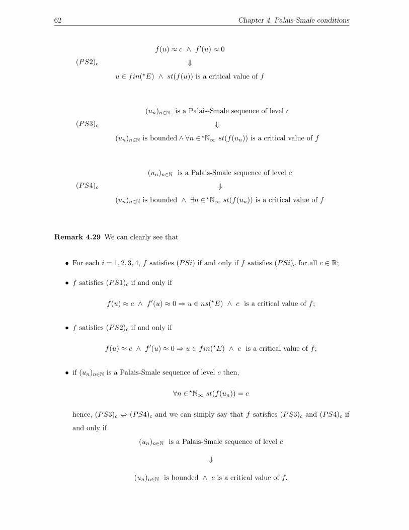
62 Chapter 4. Palais-Smale conditions
(PS2)c
f(u) ≈ c ∧ f ′(u) ≈ 0
⇓u ∈ fin(�E) ∧ st(f(u)) is a critical value of f
(PS3)c
(un)n∈N is a Palais-Smale sequence of level c
⇓(un)n∈N is bounded ∧ ∀n ∈�N∞ st(f(un)) is a critical value of f
(PS4)c
(un)n∈N is a Palais-Smale sequence of level c
⇓(un)n∈N is bounded ∧ ∃n ∈�N∞ st(f(un)) is a critical value of f
Remark 4.29 We can clearly see that
• For each i = 1, 2, 3, 4, f satisfies (PSi) if and only if f satisfies (PSi)c for all c ∈ R;
• f satisfies (PS1)c if and only if
f(u) ≈ c ∧ f ′(u) ≈ 0 ⇒ u ∈ ns(�E) ∧ c is a critical value of f ;
• f satisfies (PS2)c if and only if
f(u) ≈ c ∧ f ′(u) ≈ 0 ⇒ u ∈ fin(�E) ∧ c is a critical value of f ;
• if (un)n∈N is a Palais-Smale sequence of level c then,
∀n ∈�N∞ st(f(un)) = c
hence, (PS3)c ⇔ (PS4)c and we can simply say that f satisfies (PS3)c and (PS4)c if
and only if
(un)n∈N is a Palais-Smale sequence of level c
⇓
(un)n∈N is bounded ∧ c is a critical value of f.

4.6 Nonstandard Variants of Palais-Smale conditions per level 63
The following result establish the relations between the classical (PS)c condition with the
nonstandard variants defined above.
Theorem 4.30 [MNb] For any real Banach space E we have
(PS1)c ⇒ (PS)c ⇔ (PS0)c ⇒ (PS2)c ⇔ (PS3)c ⇔ (PS4)c.
Proof. Clearly
(PS1)c ⇒ (PS)c ⇔ (PS0)c and (PS3)c ⇔ (PS4)c.
For the proof of (PS0)c ⇒ (PS2)c take u ∈ �E such that f(u) ≈ c and f ′(u) ≈ 0. Suppose
u �∈ fin(�E) and for each n ∈ N, let
Yn := {x ∈ E : | f(x) − c |< 1n
∧ ‖ f ′(x) ‖< 1n
∧ ‖ x ‖> n}.
Using the same arguments used in the proof (PS0) ⇒ (PS2) (Theorem 4.6) we can construct
a Palais-Smale sequence (xn)n∈N of level c such that, for all n ∈ �N∞, xn �∈ ns(�E), which
contradicts (PS0)c; therefore, u must be finite. It remains to show that if f(u) ≈ c and
f ′(u) ≈ 0, then c is a critical value of f . For each n ∈ N take
Xn := {x ∈ E : | f(x) − c |< 1n
∧ ‖ f ′(x) ‖< 1n}
and repeat the argument used in the proof (PS0) ⇒ (PS2).
The proof (PS2)c ⇔ (PS3)c is analogous to the proof (PS2) ⇔ (PS3).
Theorem 4.31 [MNb] Let E be a real separable Banach space and f ∈ C1(E, R). Then f
satisfies (PS)c if and only if f satisfies (PS1)c.
Proof. Suppose f satisfies (PS)c and u ∈ �E is such that f(u) ≈ c and f ′(u) ≈ 0. Choose
V := {vp : p ∈ N} dense in E and suppose that u /∈ ns(�E). For each n ∈ N, define
Gn := {x ∈ E : | f(x) − c |< 1n
∧ ‖ f ′(x) ‖< 1n
∧ ∀p ∈ N [p ≤ n ⇒‖ x − vp ‖> ε]}.
In a similar way as we did in the proof of Theorem 4.7, we can construct a Palais-Smale
sequence (xn)n∈N of level c such that, for all n ∈ �N∞, xN �∈ ns(�E); this is a contradiction
with (PS0)c.
The variant of Theorem 4.8 can be easily proved.

64 Chapter 4. Palais-Smale conditions
Theorem 4.32 [MNb] If E has finite dimension, then
(PS1)c ⇔ (PS)c ⇔ (PS0)c ⇔ (PS2)c ⇔ (PS3)c ⇔ (PS4)c.
Remark 4.33 Example 4.10 also shows that condition (PS2)c does generalize (PS)c and
(PS1)c when c = 0.

Chapter 5
Mountain Pass Theorems
5.1 Introduction
The purpose of this chapter is to present
• generalizations of classical results about C1 functionals bounded from below (Corollary
5.4 and Proposition 5.8);
• a Mountain Pass Theorem with a nonstandard Palais-Smale condition (Theorem 5.15)
which is a generalization of classical Mountain Pass Theorems;
• a nonstandard proof of the Mountain Pass Theorem of Ambrosetti-Rabinowitz for coer-
cive functionals defined in finite dimensional real Banach spaces;
• a new Mountain Pass Theorem in finite dimension without Palais-Smale conditions (The-
orem 5.25);
• a new Mountain Pass Theorem without Palais-Smale conditions for functionals defined
in real Hilbert spaces (Theorem 5.29).
In this chapter we will suppose that (E, ‖ · ‖) is a real Banach space and f ∈ C1(E, R). If
a ∈ E and r ∈ R+, we will use the notations Br(a) and Br(a) to denote, respectively, the
open ball and the closed ball centered at a and radius r. Specified references are sources for
proofs.
65

66 Chapter 5. Mountain Pass Theorems
5.2 Critical Points and the Quantitative Deformation Lemma
In the next section we will present two important results in Critical Point Theory: the Moun-
tain Pass Theorem of Ambrosetti-Rabinowitz (Theorem 5.10) and one of its generaliza-
tions, the Mountain Pass Theorem of Brézis-Coron-Nirenberg (Theorem 5.14). Proofs
of these theorems use some form of the Deformation Lemma, a very technical lemma that in-
volves the concept of pseudo-gradient vector field (see [Jab03], [GT01], [Maw02] or [Rab86]); it
can also be proved using Ekeland’s Variational Principle and Von Neumann min-max Theorem
(see [Eke79] and [Fig88]).
The deformation technique was introduced in 1934 by Lusternik and Schnirelman [LS34] and
consists of deforming a given C1 functional outside the set of critical points. In 1983 Willem
proved in [Wil83] the Quantitative Deformation Lemma (see also [Maw02, pages 12-14] or
[Jab03, pages 38-40]) without the (PS) condition; the usual Deformation Lemma (see [Rab86,
pages 82-85]) is proved for functionals that satisfy the (PS) condition.
For S ⊆ E, α ∈ R+ and c ∈ R, we use the following notations
f c := {x ∈ E : f(x) ≤ c} and Sα := {x ∈ E : dist(x, S) ≤ α}
where
dist(x, S) := inf{‖ x − y ‖ : y ∈ S}.
Let us introduce more notation
C([0, 1] × E, E) := {η : [0, 1] × E → E : η is continuous}
and
C([0, 1], E) := {γ : [0, 1] → E : γ is continuous}.
For our purposes, the following version of the Quantitative Deformation Lemma is suffi-
cient.
Lemma 5.1 Let f ∈ C1(E, R), S ⊆ E, c ∈ R, ε, δ ∈ R+ be such that
∀y ∈ f−1([c − 2ε, c + 2ε]) ∩ S2δ ‖ f ′(y) ‖≥ 8ε
δ.
5.2 Critical Points and the Quantitative Deformation Lemma 67
Then there exists η ∈ C([0, 1] × E, E) such that
1. η(t, y) = y if y �∈ f−1([c − 2ε, c + 2ε]) ∩ S2δ;
2. η(1, f c+ε ∩ S) ⊆ f c−ε.
Lemma 5.1 proves the following variant of Ekeland’s Variational Principle [Eke79]:
Theorem 5.2 [Maw02, page 14] Suppose f ∈ C1(E, R) is bounded from below. Let ε ∈ R+
and z ∈ E be such that
f(z) ≤ infx∈E
f(x) + ε.
Then, for any δ ∈ R+, there exists u ∈ E with the following properties:
1. f(u) ≤ infx∈E f(x) + 2ε;
2. ‖ u − z ‖≤ 2δ;
3. ‖ f ′(u) ‖< 8εδ .
Proof. Take S = {z} and c = infx∈E f(x). If we suppose that exists δ ∈ R+ such that
∀y ∈ f−1([c − 2ε, c + 2ε]) ∩ S2δ ‖ f ′(y) ‖≥ 8ε
δ
then, by condition 2. of Lemma 5.1, there exists η ∈ C([0, 1] × E, E) such that
η(1, f c+ε ∩ S) ⊆ f c−ε.
Therefore
f(η(1, z)) ≤ c − ε,
which contradicts the definition of c.
The last theorem shows the following existence result.
Corollary 5.3 Let f ∈ C1(E, R) be bounded from below. Then, there exists u ∈�E such that
f(u) ≈ infx∈E
f(x) and f ′(u) ≈ 0.

68 Chapter 5. Mountain Pass Theorems
Proof. The result follows applying Transfer Principle to Theorem 5.2 and taking 0 < ε ≈ 0
and δ =√
ε.
Clearly, a C1 functional which is bounded from below needs not to have a minimum; a classical
example is the exponential function. But, if the functional satisfies some kind of compactness,
then it has a minimum:
Corollary 5.4 Let f ∈ C1(E, R) be bounded from below. If f satisfies (PS2)c for c =
infx∈E f(x), then c is a minimum of f .
Proof. By Corollary 5.3 there exists u ∈�E such that
f(u) ≈ infx∈E
f(x) = c and f ′(u) ≈ 0.
Since f satisfies (PS2)c, c is a critical value of f ; therefore, c is a minimum of f .
The following result is an easy consequence of the previous corollary.
Corollary 5.5 Let f ∈ C1(E, R) be bounded from above. If f satisfies (PS2)c for c =
supx∈E f(x), then c is a maximum of f .
Proof. Apply Corollary 5.4 to −f .
We recall that, for any real Banach space, we have
(PS)c ⇒ (PS2)c
and
(PS2)c � (PS)c
hence, Corollary 5.4 and Corollary 5.5 are generalizations of the classical results:
Corollary 5.6 Let f ∈ C1(E, R) be bounded from below. If f satisfies (PS)c for c =
infx∈E f(x), then c is a minimum of f .
Corollary 5.7 Let f ∈ C1(E, R) be bounded from above. If f satisfies (PS)c for c =
supx∈E f(x), then c is a maximum of f .

5.2 Critical Points and the Quantitative Deformation Lemma 69
If f : E → R is Fréchet differentiable and f(a) is an extreme value, then a is a critical point
of f ; would it be true that
When H is a hyperfinite set such that E ⊆ H ⊆ �E and f(ω) = minx∈H f(x)
or f(ω) = maxx∈H f(x), then ω is an almost critical point of f?
The answer is no: the function
f(x) = exp(x) + x (x ∈ R)
has a minimum and a maximum on any hyperfinite set H satisfying R ⊆ H ⊆ �R, but
f ′(x) = exp(x) + 1 �≈ 0 therefore, f has no almost critical points.
From Proposition 4.24 and Theorem 4.8 it follows that
If E is a finite dimensional real Banach space and f ∈ C1(E, R) is coercive,
then f satisfies (PS4).
The converse of this result is, in general, not true. For example, the function f(x) = x3
(x ∈ R) satisfies (PS4) but f is not coercive. The next result shows that (PS4) for functionals
bounded from below is a stronger condition than coercivity. Our proof is similar to the one
presented in [MM02, page 5].
Proposition 5.8 Let f ∈ C1(E, R) bounded from below. If f satisfies (PS4), then f is
coercive.
Proof. Suppose that f is not coercive. Then, there exists a sequence (xn)n∈N in E such
that ‖ xn ‖→ +∞ and (f(xn))n∈N is bounded. Let c = infx∈E f(x) and, for each n ∈ N, take
εn = f(xn) − c + 1n and δn = 1
4 ‖ xn ‖. By Theorem 5.2 there exists, for each n ∈ N, un ∈ E
such that
f(un) ≤ 2f(xn) − c +2n
∧ ‖ un − xn ‖≤ 12‖ xn ‖ ∧ ‖ f ′(un) ‖< 32(f(xn) − c + 1
n)‖ xn ‖ .
Thus, (f(un))n∈N is bounded and f ′(un) → 0. Since, for each n ∈ N,
‖ un ‖≥‖ xn ‖ − ‖ un − xn ‖≥ 12‖ xn ‖

70 Chapter 5. Mountain Pass Theorems
(un)n∈N is not bounded, contradicting (PS4).
Recall that, for any real Banach space,
(PS) ⇒ (PS4)
and
(PS4) � (PS),
hence Proposition 5.8 generalizes the following result.
Proposition 5.9 [CLW90] Let f ∈ C1(E, R) be bounded from below. If f satisfies (PS)c
condition for all c ∈ R, then f is coercive.
5.3 Mountain Pass Theorems in arbitrary real Banach spaces
We begin this section presenting the Mountain Pass Theorem of Ambrosetti-Rabinowitz proved
in 1973 [AR73] and frequently used to prove the existence of nontrivial solutions of nonlinear
problems.
Theorem 5.10 (Mountain Pass Theorem of Ambrosetti-Rabinowitz) Let E be a real
Banach space and f ∈ C1(E, R). Suppose that
1. there exist x1, x2 ∈ E and r ∈ R+ such that ‖ x1 − x2 ‖> r and
k0 := max{f(x1), f(x2)} < inf‖y−x1‖=r
f(y);
2. Γ := {γ ∈ C([0, 1], E) : γ(0) = x1 ∧ γ(1) = x2} and k1 := infγ∈Γ maxt∈[0,1] f(γ(t));
3. f satisfies (PS).
Then k1 > k0 and k1 is a critical value of f .
Condition 1. of Theorem 5.10 will be used several times in this work therefore, in order to
shorten statements, we will present the following definition:

5.3 Mountain Pass Theorems in arbitrary real Banach spaces 71
Definition 5.11 Let f ∈ C(E, R) and x1, x2 ∈ E. We say that f satisfies the mountain
pass geometry with respect to x1 and x2 if there exists r ∈ R+ such that
‖ x1 − x2 ‖> r and max{f(x1), f(x2)} < inf‖y−x1‖=r
f(y).
The following result justifies the purpose of the mountain pass geometry.
Proposition 5.12 Let E be a real Banach space, x1, x2 ∈ E and f ∈ C(E, R). Suppose that
1. f satisfies the mountain pass geometry with respect to x1 and x2;
2. Γ := {γ ∈ C([0, 1], E) : γ(0) = x1 ∧ γ(1) = x2}, k0 := max{f(x1), f(x2)} and
k1 := infγ∈Γ maxt∈[0,1] f(γ(t)).
Then k0 < k1 < +∞.
Proof. [Rab86, page 7] Clearly k1 ∈ R, so we are left to prove that k1 > k0. Take r ∈ R+
as in Definition 5.11. Observe that, for each γ ∈ Γ,
γ([0, 1]) ∩ {y ∈ E : ‖ y − x1 ‖= r} �= ∅
and therefore
maxt∈[0,1]
f(γ(t)) ≥ inf‖y−x1‖=r
f(y).
Then
k1 := infγ∈Γ
maxt∈[0,1]
f(γ(t)) ≥ inf‖y−x1‖=r
f(y) > max{f(x1), f(x2)} := k0.
Conditions 1. and 2. of Theorem 5.10 are not enough to imply that k1 is a critical value of f
as we can see with the following example.
Example 5.13 [GT01, page 36] The function f : R2 → R defined by f(x, y) = x2+(x+1)3y2
satisfies the mountain pass geometry with x1 = (0, 0), x2 = (−2, 3) and r = 12 . (0, 0) is a
strict local minimizer and is the only critical point of f . Therefore there is no z ∈ R2 such
that f(z) = k1 > 0 and f ′(z) = 0.
72 Chapter 5. Mountain Pass Theorems
In 1980 Brézis, Coron and Nirenberg obtained in [BCN80] a generalization of the Mountain
Pass Theorem of Ambrosetti-Rabinowitz for functionals satisfying the (PS)k1 condition:
Theorem 5.14 (Mountain Pass Theorem of Brézis-Coron-Nirenberg) Let E be a
real Banach space, x1, x2 ∈ E and f ∈ C1(E, R). Suppose that
1. f satisfies the mountain pass geometry with respect to x1 and x2;
2. Γ := {γ ∈ C([0, 1], E) : γ(0) = x1 ∧ γ(1) = x2} and k1 := infγ∈Γ maxt∈[0,1] f(γ(t));
3. f satisfies (PS)k1 .
Then k1 is a critical value of f .
We now present the following generalization of the Mountain Pass Theorem of Brézis-Coron-
Nirenberg.
Theorem 5.15 (Mountain Pass Theorem with nonstandard Palais-Smale condi-
tion) [MNb] Let E be a real Banach space, x1, x2 ∈ E and f ∈ C1(E, R). Suppose that
1. f satisfies the mountain pass geometry with respect to x1 and x2;
2. Γ := {γ ∈ C([0, 1], E) : γ(0) = x1 ∧ γ(1) = x2} and k1 := infγ∈Γ maxt∈[0,1] f(γ(t));
3. f satisfies (PS2)k1 .
Then k1 is a critical value of f .
The proof of this theorem can be easily obtained from the following consequence of Lemma
5.1 [Maw02, pages 17-18]:
Theorem 5.16 Let E be a real Banach space, x1, x2 ∈ E and f ∈ C1(E, R). Suppose that
1. f satisfies the mountain pass geometry with respect to x1 and x2;
2. Γ := {γ ∈ C([0, 1], E) : γ(0) = x1 ∧ γ(1) = x2} and k1 := infγ∈Γ maxt∈[0,1] f(γ(t)).

5.3 Mountain Pass Theorems in arbitrary real Banach spaces 73
Then, for each ε > 0, δ > 0 and γ ∈ Γ such that
maxt∈[0,1]
f(γ(t)) ≤ k1 + ε,
there exists u ∈ E such that
(i) k1 − 2ε ≤ f(u) ≤ k1 + 2ε;
(ii) dist(u, γ([0, 1])) ≤ 2δ;
(iii) ‖ f ′(u) ‖< 8εδ .
Proof. By hypothesis there exists r ∈ R+ such that ‖ x2 − x1 ‖> r and
k0 := max{f(x1), f(x2)} < inf‖y−x1‖=r
f(y) := b.
We can suppose, without loss of generality, that ε < b−k02 . Then k0 < b − 2ε ≤ k1 − 2ε. Fix
δ > 0 and choose γ ∈ Γ such that maxt∈[0,1] f(γ(t)) ≤ k1 + ε. Let S := γ([0, 1]) and assume
that
∀y ∈ E
[[ k1 − 2ε ≤ f(y) ≤ k1 + 2ε ∧ dist(y, S) ≤ 2δ ] ⇒ ‖ f ′(y) ‖≥ 8ε
δ
].
Then, by Lemma 5.1, there exists η ∈ C([0, 1] × E, E) such that
η(t, y) = y if y �∈ f−1([k1 − 2ε, k1 + 2ε]) ∩ S2δ
and
η(1, fk1+ε ∩ S) ⊆ fk1−ε.
Let β(t) = η(1, γ(t)) for all t ∈ [0, 1]. Observe that β is continuous, β(0) = η(1, x1) = x1
and β(1) = η(1, x2) = x2 (because f(xi) ≤ k0 < k1 − 2ε for i = 1, 2). Hence, β ∈ Γ. Since
maxt∈[0,1] f(γ(t)) ≤ k1 + ε, it follows that
η(1, γ([0, 1])) ⊆ fk1−ε
that is,
f(β([0, 1])) = f(η(1, γ([0, 1]))) ⊆ ] −∞, k1 − ε]
which contradicts the definition of k1 := infγ∈Γ maxt∈[0,1] f(γ(t)).

74 Chapter 5. Mountain Pass Theorems
Corollary 5.17 Let E be a real Banach space, x1, x2 ∈ E and f ∈ C1(E, R). Suppose that
1. f satisfies the mountain pass geometry with respect to x1 and x2;
2. Γ := {γ ∈ C([0, 1], E) : γ(0) = x1 ∧ γ(1) = x2} and k1 := infγ∈Γ maxt∈[0,1] f(γ(t)).
Then, for each γ ∈�Γ such that
maxt∈�[0,1]
f(γ(t)) ≈ k1,
there exists u ∈�E such that
(i) f(u) ≈ k1;
(ii) dist(u, γ(�[0, 1]) ≈ 0;
(iii) f ′(u) ≈ 0.
Proof. Apply the Transfer Principle to Theorem 5.16, take 0 < ε ≈ 0 and δ =√
ε.
Proof. (of Theorem 5.15) Let γ0 ∈�Γ be such that
maxt∈�[0,1]
f(γ0(t)) ≈ k1.
Then, by Corollary 5.17, there exists u ∈ �E such that f(u) ≈ k1 and f ′(u) ≈ 0. Since f
satisfies (PS2)k1 , we may conclude that k1 is a critical value of f .
To finish this section we will obtain the "dual" of Theorem 5.15.
Theorem 5.18 Let E be a real Banach space and f ∈ C1(E, R). Suppose that
1. there exist x1, x2 ∈ E and r ∈ R+ such that ‖ x2 − x1 ‖> r and
k2 := min{f(x1), f(x2)} > sup‖y−x1‖=r
f(y);
2. Γ := {γ ∈ C([0, 1], E) : γ(0) = x1 ∧ γ(1) = x2} and k3 := supγ∈Γ mint∈[0,1] f(γ(t));
3. f satisfies (PS2)k3 .
Then k3 < k2 and k3 is a critical value of f .

5.4 Obtaining almost critical points in real Hilbert spaces 75
Proof. By condition 1. we obtain
−min{f(x1), f(x2)} < − sup‖y−x1‖=r
f(y).
Hence
max{−f(x1),−f(x2)} < inf‖y−x1‖=r
(−f(y))
and therefore −f satisfies the mountain pass geometry with respect to x1 and x2. Since
− supγ∈Γ
mint∈[0,1]
f(γ(t)) = infγ∈Γ
maxt∈[0,1]
(−f(γ(t)))
it follows that
infγ∈Γ
maxt∈[0,1]
(−f(γ(t))) = −k3.
By Proposition 5.12,
−k3 > max{−f(x1),−f(x2)}
then,
−k3 > −min{f(x1), f(x2)} = −k2.
Since −f satisfies (PS2)−k3 , it follows by Theorem 5.15 that −k3 is a critical value of −f .
Therefore, k3 < k2 and k3 is a critical value of f .
5.4 Obtaining almost critical points in real Hilbert spaces
In the following we will suppose that H is a real Hilbert space and U is an open subset of H.
Later on we will need the following lemmas. First define
r � s := r > s ∧ r �≈ s (r, s ∈�R)
and
C([0, 1], [0, 1]) := {δ : [0, 1] → [0, 1] : δ is continuous}
and recall that
ns(�U) := {x ∈�H : x ∈ ns(�H) ∧ st(x) ∈ U}.

76 Chapter 5. Mountain Pass Theorems
Lemma 5.19 [BMN+05] Suppose H is a real Hilbert space with inner product · • · and norm
‖ · ‖ and let U be an open subset of H. Let f ∈ C1(U, R) and x ∈ ns(�U). If f ′(x) �≈ 0, then
for every 0 < ε ≈ 0, the following inequality holds:
f(x − εf ′(x)) < f(x) − ε‖ f ′(x) ‖2
2.
Proof. Suppose x ∈ ns(�U) is such that f ′(x) �≈ 0 and let 0 < ε ≈ 0. For some ι ≈ 0 in �R,
f(x − εf ′(x)) = f(x) − ε[f ′(x) • f ′(x) − ι
](5.1)
= f(x) − ε[‖f ′(x)‖2 − ι
](5.2)
< f(x) − ε‖ f ′(x) ‖2
2. (5.3)
Condition (5.1) is true because f is of class C1 and x ∈ ns(�H) (Theorem 2.37) and condition
(5.3) results from
‖ f ′(x) ‖ � 0 ∧ ‖ f ′(x) ‖2 −ι ≈ ‖ f ′(x) ‖2 >‖ f ′(x) ‖2
2∧ ε > 0
which proves the lemma.
The following lemma can be used to get almost critical points for C1 functionals defined in
real Hilbert spaces.
Lemma 5.20 Let H be a real Hilbert space with inner product · • · and norm ‖ · ‖. Suppose
that f ∈ C1(H, R) satisfies the mountain pass geometry with respect to x1 and x2. Let
Γ := {γ ∈ C([0, 1], H) : γ(0) = x1 ∧ γ(1) = x2}
and
k1 := infγ∈Γ
maxt∈[0,1]
f(γ(t)).
Then
∀γ ∈�Γ[ [
γ(�[0, 1]) ⊆ ns(�H) ∧ maxt∈�[0,1]
f(γ(t)) ≈ k1
]⇒ ∃t0 ∈�[0, 1]
[f(γ(t0)) ≈ k1 ∧ ‖ f ′(γ(t0)) ‖≈ 0
] ].
Proof. [BMN+05] Take γ ∈�Γ such that
γ(�[0, 1]) ⊆ ns(�H) ∧ k2 := maxt∈�[0,1]
f(γ(t)) ≈ k1 (5.4)

5.4 Obtaining almost critical points in real Hilbert spaces 77
and let k0 := max{f(x1), f(x2)}. Then
k0 < k1 ≤ k2 ≈ k1. (5.5)
Define
U := {t ∈�[0, 1] : k1 ≤ f(γ(t)) ≤ k2} (5.6)
and
d := min{‖f ′(γ(t))‖ : t ∈ U}. (5.7)
We claim that d ≈ 0. If not define
V := {t ∈�[0, 1] : ‖f ′(γ(t))‖ >d
2}
and
W := ( �[0, 1] \ V ) ∪ {0, 1}.
Then W and U are �closed, V is �open (in the relative �topology of �[0, 1]) and U ⊆ V .
Moreover,
{0, 1} �⊆ U
since k1 > max{f(γ(0)), f(γ(1))}, and
V �= U
since U �=�[0, 1] and �[0, 1] is �connected.
Hence, by Urysohn’s Theorem and the Transfer Principle, there exists a function u ∈�C([0, 1], [0, 1])
such that
u(W ) = {0} and u(U) = {1}. (5.8)
Choose b such that
0 ≤ 2(k2−k1)d2 < b ≈ 0 (5.9)
and define η :�[0, 1] → [0, b] by
η(t) := bu(t);
let
γη(t) := γ(t) − η(t)f ′(γ(t)).
78 Chapter 5. Mountain Pass Theorems
Since γ(�[0, 1]) ⊆ ns(�H), η(t) ≈ 0 for all t ∈ �[0, 1] and f ′ is continuous, it follows that
γη(�[0, 1]) ⊆ ns(�H). Moreover, γη ∈�Γ, because γη ∈�C([0, 1], H), γη(0) = x1 and γη(1) = x2.
Next we will prove that under these conditions
∀t ∈�[0, 1] f(γη(t)) < k1,
which will be a contradiction to the definition of k1.
If t ∈ W, then
f(γη(t)) = f(γ(t)) < k1,
because η(t) = 0 and t �∈ U .
If t ∈ U , then
f(γη(t)) = f(γ(t) − bf ′(γ(t)))
< f(γ(t)) − b‖ f ′(γ(t)) ‖2
2(by Lemma 5.19)
≤ f(γ(t)) − bd2
2(by (5.7))
< f(γ(t)) − (k2 − k1) (by (5.9))
≤ k1 (by (5.6)).
Finally, if t ∈ V \ U , Lemma 5.19 and the definition of U imply
f(γη(t)) ≤ f(γ(t)) − η(t)‖ f ′(γ(t)) ‖2
2< k1
which, as pointed out above, is a contradiction and we conclude that d must be infinitesimal.
Hence, there exists t0 ∈ U such that ‖ f ′(γ(t0)) ‖≈ 0, that is,
∃t0 ∈�[0, 1] [ f(γ(t0)) ≈ k1 ∧ ‖ f ′(γ(t0)) ‖≈ 0 ],
proving the desired result.
Lemma 5.20 was inspired in a claim that appears in [JLJ98, pages 64-66] about coercive
functionals defined in a finite real Banach space and where x1 and x2 are two strict local
minimizers. As an historical remark, we mention that Courant [Cou50] proved in 1950 the
following theorem:

5.4 Obtaining almost critical points in real Hilbert spaces 79
Suppose that f ∈ C1(Rn, R) is coercive and possesses two distinct strict local
minimizers x1 and x2. Then f possesses a third critical point x3 distinct from x1
and x2, characterized by
f(x3) = infK∈Σ
maxx∈K
f(x),
where
Σ = {K ⊆ Rn : K is compact and connected and x1, x2 ∈ K}.
Moreover, x3 is not a local minimizer.
Notice that, since x1 and x2 are two strict local minimizers, then f satisfies the mountain pass
geometry with respect to x1 and x2. Also note that,
• infK∈Σ maxx∈K f(x) ≤ infγ∈Γ maxt∈[0,1] f(γ(t)), since Γ ⊆ Σ;
• infγ∈Γ maxt∈[0,1] f(γ(t)) ≤ infK∈Σ maxx∈K f(x), because for each K ∈ Σ and ε ∈ R+,
there exists γ ∈ Γ such that K is a uniform ε-neighborhood of γ([0, 1]).
Hence,
infK∈Σ
maxx∈K
f(x) = infγ∈Γ
maxt∈[0,1]
f(γ(t))
and this result of Courant may be considered as an ancestor of the Mountain Pass Theorem
of Ambrosetti-Rabinowitz.
Remark 5.21 We notice that Lemma 5.20 can also be proved using the Quantitative Defor-
mation Lemma, more precisely, Corollary 5.17, because for any γ ∈�Γ such that
γ(�[0, 1]) ⊆ ns(�H) ∧ maxt∈�[0,1]
f(γ(t)) ≈ k1,
there exists, by Corollary 5.17, u ∈�H such that
f(u) ≈ k1 ∧ dist(u, γ(�[0, 1])) ≈ 0 ∧ f ′(u) ≈ 0.
Therefore, there exists t0 ∈�[0, 1] such that u ≈ γ(t0) ∈ ns(�H). Since f and f ′ are continuous,
f(γ(t0)) ≈ k1 ∧ ‖ f ′(γ(t0)) ‖≈ 0
and the lemma is proved.
80 Chapter 5. Mountain Pass Theorems
5.5 A Mountain Pass Theorem in the finite dimensional case
In this section we will use Lemma 5.20 to give a nonstandard proof of the Mountain Pass
Theorem of Ambrosetti-Rabinowitz for the special case where the functional is coercive and
is defined in a finite dimensional real Banach space.
Until the end of this chapter we will suppose that E is a finite dimensional real Banach space.
In Chapter 4 we proved that
If E is a finite dimensional real Banach space and f ∈ C1(E, R) is coercive,
then f satisfies (PS1).
As (PS1) ⇒ (PS) (Theorem 4.6), the following may be derived as a consequence of the
Mountain Pass Theorem of Ambrosetti-Rabinowitz. Nevertheless, we will give a proof which
does not use Palais-Smale conditions but only some properties of the coercive functionals.
Theorem 5.22 (Mountain Pass Theorem - a special case) Let E be a finite dimensional
real Banach space, x1, x2 ∈ E and f ∈ C1(E, R). Suppose that
1. f satisfies the mountain pass geometry with respect to x1 and x2;
2. Γ := {γ ∈ C([0, 1], E) : γ(0) = x1 ∧ γ(1) = x2} and k1 := infγ∈Γ maxt∈[0,1] f(γ(t));
3. f is coercive.
Then k1 is a critical value of f .
Proof. Take γ0 ∈ �Γ such that maxt∈�[0,1] f(γ0(t)) ≈ k1. First of all note that, as f is
coercive,
γ0(�[0, 1]) ⊆ fin(�E)
and since E is finite dimensional,
γ0(�[0, 1]) ⊆ ns(�E).

5.6 Mountain Pass Theorems without Palais-Smale conditions 81
Then, by Lemma 5.20,
∃t0 ∈�[0, 1] [ f(γ0(t0)) ≈ k1 ∧ ‖ f ′(γ0(t0)) ‖≈ 0 ].
The continuity of f and f ′ shows that
f(st(γ0(t0))) = st(f(γ0(t0))) = k1 ∧ f ′(st(γ0(t0))) = st(f ′(γ0(t0))) = 0;
hence k1 is a critical value of f .
In Appendix B we present other nonstandard proofs for this theorem.
Remark 5.23 If the coercivity of the functional is removed, we cannot guarantee that k1 is
a critical value of f , as can be seen with the function f(x, y) = x2 + (x + 1)3y2 of Example
5.13; f is not coercive since for all y ≈ +∞, ‖ (−2, y) ‖≈ +∞ and
f(−2, y) = 4 − y2 ≈ −∞.
The following example shows that the coercivity of the functional is not a necessary condition
for k1 to be a critical value of f .
Example 5.24 Let h(x, y) = sin(x2 + y2) for all (x, y) ∈ R2. Clearly h is C1, satisfies the
mountain pass geometry with respect to (0, 0), (0,√
π) and r =√
π2 , h is not coercive, but
k1 = 1 is a critical value of h.
5.6 Mountain Pass Theorems without Palais-Smale conditions
In this section we will prove two mountain pass type results for functionals that satisfy special
properties. Notice that the following theorems cannot be obtained from the Mountain Pass
Theorem of Ambrosetti-Rabinowitz or generalizations thereof, e.g. given in [GT01], since
conditions 3. of Theorem 5.25 and Theorem 5.29 do not imply (PS) or weaker forms of (PS).
Theorem 5.25 (Mountain Pass Theorem without Palais-Smale conditions in finite
dimension)[Mar05] Let E be a finite dimensional real Banach space, x1, x2 ∈ E and f ∈C1(E, R). Suppose that
82 Chapter 5. Mountain Pass Theorems
1. f satisfies the mountain pass geometry with respect to x1 and x2;
2. Γ := {γ ∈ C([0, 1], E) : γ(0) = x1 ∧ γ(1) = x2} and k1 := infγ∈Γ maxt∈[0,1] f(γ(t));
3. there exists s ∈ R+ such that ‖ x2 − x1 ‖< s and if ‖ x − x1 ‖≥ s then f(x) < k1.
Then k1 is a critical value of f .
Proof. Let γ0 ∈ �Γ be such that k1 ≤ maxt∈�[0,1] f(γ0(t)) ≈ k1. Using condition 3. we
may assume that γ0(�[0, 1]) ⊆ Bs(x1) and, since E is finite dimensional, γ0(�[0, 1]) ⊆ ns(�E).
Therefore, by Lemma 5.20, there exists t0 ∈�[0, 1] such that
f(γ0(t0)) ≈ k1 ∧ ‖ f ′(γ0(t0)) ‖≈ 0.
The continuity of f and f ′ shows that st(γ0(t0)) is a critical point with value k1.
We believe that our Theorem 5.25 is sometimes easier to apply than the Mountain Pass
Theorem of Ambrosetti-Rabinowitz in the n-dimensional case: the third condition of Theorem
5.25 may be simpler to verify than (PS), even for small n. Moreover, there are functionals
which satisfy all the conditions of Theorem 5.25 but do not satisfy (PS).
Example 5.26 The function g(x, y) = (x2+y2+sin(x2+y2))(1−(x2+y2)) for all (x, y) ∈ R2
is C1 and verifies the mountain pass geometry with respect to z1 = (0, 0) and z2 = (1, 0) since
inf‖(x,y)‖= 1
2
g(x, y) > k0 := max{g(z1), g(z2)} = 0.
Since g is not coercive we cannot apply Theorem 5.22. But is easy to prove that
‖ (x, y) ‖≥ 4 ⇒ g(x, y) < 0 < k1
and therefore, by Theorem 5.25, we can conclude that k1 is a critical value of g. We also point
out that checking the (PS) condition may not be an easy task.
Next we present an example of a functional defined in R2 that satisfies all the conditions of
Theorem 5.25 but does not satisfy (PS).

5.6 Mountain Pass Theorems without Palais-Smale conditions 83
Example 5.27 Let h(x, y) = [1 − (x2 + y2)] exp−(x2+y2) arctan(x2 + y2) for all (x, y) ∈ R2.
Clearly h is a C1 functional, h(0, 0) = 0, h(1, 0) = 0,
inf‖(x,y)‖= 1
2
h(x, y) > k0 := max{h(0, 0), h(1, 0)} = 0
and
(x, y) �∈ B2(0, 0) ⇒ h(x, y) < 0.
The function h does not satisfy (PS) condition, since the sequence ((n, n))n∈N is such that
(h(n, n))n∈N is bounded, ∂h∂x(n, n) → 0 and ∂h
∂y (n, n) → 0 but the sequence ((n, n))n∈N does
not contain a convergent subsequence.
We proceed presenting the "dual" of Theorem 5.25.
Theorem 5.28 [Mar05] Let E be a finite dimensional real Banach space and f ∈ C1(E, R).
Suppose that
1. there exist x1, x2 ∈ E and r ∈ R+ such that ‖ x2 − x1 ‖> r and
k2 := min{f(x1), f(x2)} > max‖y−x1‖=r
f(y);
2. Γ := {γ ∈ C([0, 1], E) : γ(0) = x1 ∧ γ(1) = x2} and k3 := supγ∈Γ mint∈[0,1] f(γ(t));
3. there exists s ∈ R+ such that ‖ x2 − x1 ‖< s and if ‖ x − x1 ‖≥ s then f(x) > k3.
Then k3 < k2 and k3 is a critical value of f .
Proof. Apply Theorem 5.25 to −f and use the same arguments used in the proof of Theorem
5.18.
The following theorem is an easy consequence of Lemma 5.20. Note also that Theorem 5.22
follows easily from Theorem 5.29.
Theorem 5.29 (Mountain Pass Theorem without Palais-Smale conditions in Hilbert
spaces) Let H be a real Hilbert space, x1, x2 ∈ H and f ∈ C1(H, R). Suppose that

84 Chapter 5. Mountain Pass Theorems
1. f satisfies the mountain pass geometry with respect to x1 and x2;
2. Γ := {γ ∈ C([0, 1], H) : γ(0) = x1 ∧ γ(1) = x2} and k1 := infγ∈Γ maxt∈[0,1] f(γ(t));
3. ∃γ ∈�Γ [ γ(�[0, 1]) ⊆ ns(�H) ∧ maxt∈�[0,1] f(γ(t)) ≈ k1 ].
Then k1 is a critical value of f .
The following example shows that Theorem 5.29 cannot be obtained from the Mountain Pass
Theorem of Ambrosetti-Rabinowitz.
Example 5.30 Consider the function h of Example 5.27:
h(x, y) = [1 − (x2 + y2)] exp−(x2+y2) arctan(x2 + y2) ((x, y) ∈ R2).
We saw that this function satisfies the mountain pass geometry with respect to (0, 0) and
(1, 0) and
(x, y) �∈ B2(0, 0) ⇒ h(x, y) < 0.
Since k1 > 0, there exists γ ∈�Γ such that
maxt∈�[0,1]
h(γ(t)) ≈ k1 ∧ γ(�[0, 1]) ⊆ B2(0, 0) ⊆ ns(�R2).
Hence, h satisfies all the conditions of Theorem 5.29 but do not satisfy (PS) condition.
To finish this chapter we present the "dual" of Theorem 5.29. Since the proof is obvious we
omit it.
Theorem 5.31 Let H be a real Hilbert space and f ∈ C1(H, R). Suppose that
1. there exist x1, x2 ∈ H and r ∈ R+ such that ‖ x2 − x1 ‖> r and
k2 := min{f(x1), f(x2)} > sup‖y−x1‖=r
f(y);
2. Γ := {γ ∈ C([0, 1], H) : γ(0) = x1 ∧ γ(1) = x2} and k3 := supγ∈Γ mint∈[0,1] f(γ(t));
3. ∃γ ∈�Γ [ γ(�[0, 1]) ⊆ ns(�H) ∧ mint∈�[0,1] f(γ(t)) ≈ k3 ].
Then k3 is a critical value of f .

Chapter 6
Three Critical Points Theorems
6.1 Introduction
The goal of this chapter is to present new variants of Three Critical Points Theorems. Namely,
we will prove
• Three Critical Points Theorems with (PS2)c condition (Theorem 6.1, Theorem 6.2,
Theorem 6.4 and Theorem 6.5);
• Three Critical Points Theorems without Palais-Smale conditions in finite dimensional
spaces (Theorem 6.7, Theorem 6.8, Theorem 6.9 and Theorem 6.10);
• Three Critical Points Theorems without Palais-Smale conditions in real Hilbert spaces
(Theorem 6.12, Theorem 6.13, Theorem 6.14 and Theorem 6.15).
Let us recall some notation used in the last chapter. If E is a real Banach space, f : E → R
a continuous functional and x1 and x2 are two elements of E, we will denote
Γ := {γ ∈ C([0, 1], E) : γ(0) = x1 ∧ γ(1) = x2}
k0 := max{f(x1), f(x2)}
k1 := infγ∈Γ
maxt∈[0,1]
f(γ(t))
k2 := min{f(x1), f(x2)}
85
86 Chapter 6. Three Critical Points Theorems
and
k3 := supγ∈Γ
mint∈[0,1]
f(γ(t)).
6.2 Three Critical Points Theorems with a nonstandard Palais-
Smale condition
The Three Critical Points Theorems presented in this section are obtained from the Mountain
Pass Theorem with nonstandard Palais-Smale condition (Theorem 5.15) and Theorem 5.18.
Theorem 6.1 Let E be a real Banach space and f ∈ C1(E, R). Suppose x1 and x2 are two
distinct strict local minimizers of f ,
k1 := infγ∈Γ
maxt∈[0,1]
f(γ(t))
and f satisfies (PS2)k1 . Then f has a third critical point with value k1.
Proof. Since x1 and x2 are two strict local minimizers, f satisfies the mountain pass
geometry with respect to x1 and x2. Theorem 5.15 shows that k1 is a critical value of f ; since
k1 > k0 := max{f(x1), f(x2)}
there exists another critical point x3 such that f(x3) = k1.
Theorem 6.1 can be generalized in the following sense.
Theorem 6.2 Let E be a real Banach space and f ∈ C1(E, R). Suppose x1 and x2 are two
distinct local minimizers of f ,
k1 := infγ∈Γ
maxt∈[0,1]
f(γ(t))
and f satisfies (PS2)k1 . Then f has (at least) one critical point with value k1 or f has an
infinite number of critical points with value k0 := max{f(x1), f(x2)}.
Proof. Suppose that f(x2) ≤ f(x1) := k0.
6.2 Three Critical Points Theorems with a nonstandard Palais-Smale condition 87
If x1 is a strict local minimizer then, by Theorem 5.15, there exists a third critical point x3
such that
f(x3) = k1 > k0 := max{f(x1), f(x2)}.
If x1 is a non strict local minimizer then, in any neighborhood of x1, there exists y �= x1 such
that f(y) = f(x1) = k0; hence, y is also a local minimizer of f . Since in any real Banach
space every local minimizer (or maximizer) of a Fréchet differentiable functional is a critical
point, we may conclude that f has an infinite number of critical points with value k0.
Next we present a functional that satisfies all the conditions of Theorem 6.2 and for which the
number of critical points with value k0 is (only) countable.
Example 6.3 Consider the function
f(x) =
⎧⎨⎩ x4 sin2( 1x) if x �= 0
0 if x = 0.
Observe that f ≥ 0, f ∈ C1(R, R), f(0) = f( 1π ) = 0 := k0 and f is coercive (hence, f satisfies
(PS2)). Also note that
1. f(x) = 0 ⇔ x ∈ {1
kπ : k ∈ Z \ {0}} ∪ {0} ;
2. 1π is a strict minimizer;
3. 0 is a non strict minimizer.
Therefore, there exists only a countable number of critical points with value k0.
We finish this section with some consequences of Theorem 5.18.
Theorem 6.4 Let E be a real Banach space and f ∈ C1(E, R). Suppose x1 and x2 are two
distinct strict local maximizers of f ,
k3 := supγ∈Γ
mint∈[0,1]
f(γ(t))
and f satisfies (PS2)k3 . Then f has a third critical point with value k3.

88 Chapter 6. Three Critical Points Theorems
Proof. Since f satisfies all the conditions of Theorem 5.18, we may conclude that k3 is a
critical value of f. Since
k3 < k2 := min{f(x1), f(x2)},
there exists another critical point x3 such that f(x3) = k3.
Theorem 6.5 Let E be a real Banach space and f ∈ C1(E, R). Suppose x1 and x2 are two
distinct local maximizers of f ,
k3 := supγ∈Γ
mint∈[0,1]
f(γ(t))
and f satisfies (PS2)k3 . Then f has (at least) one critical point with value k3 or f has an
infinite number of critical points with value k2 := min{f(x1), f(x2)}.
Proof. Apply Theorem 5.18 and use the same arguments used in the proof of Theorem 6.2.
Example 6.6 Let f be the function of Example 6.3, x1 = 0 and x2 = 1π . Thus, −f shows
that, in the conditions of Theorem 6.5, the number of critical points with value k2 = 0 may
be only countable.
6.3 Three Critical Points Theorems without Palais-Smale con-
ditions
The Three Critical Points Theorems proved in this section are obtained from the Mountain
Pass Theorems without Palais-Smale conditions (Theorem 5.25 and Theorem 5.29 ) and their
"duals" (Theorem 5.28 and Theorem 5.31). The proofs are similar to the proofs done in the
last section so we will omit them.
Theorem 6.7 [Mar05] Let E be a finite dimensional real Banach space and f ∈ C1(E, R).
Suppose x1 and x2 are two distinct strict local minimizers of f ,
k1 := infγ∈Γ
maxt∈[0,1]
f(γ(t))

6.3 Three Critical Points Theorems without Palais-Smale conditions 89
and f satisfies the condition
∃s ∈ R+ [ ‖ x2 − x1 ‖< s ∧ ∀x ∈ E ( ‖ x − x1 ‖≥ s ⇒ f(x) < k1 ) ] .
Then f has a third critical point with value k1.
Theorem 6.8 [Mar05] Let E be a finite dimensional real Banach space and f ∈ C1(E, R).
Suppose x1 and x2 are two distinct local minimizers of f ,
k1 := infγ∈Γ
maxt∈[0,1]
f(γ(t))
and f satisfies the condition
∃s ∈ R+ [ ‖ x2 − x1 ‖< s ∧ ∀x ∈ E ( ‖ x − x1 ‖≥ s ⇒ f(x) < k1 ) ] .
Then f has (at least) one critical point with value k1 or f has an infinite number of critical
points with value k0 := max{f(x1), f(x2)}.
Theorem 6.9 [Mar05] Let E be a finite dimensional real Banach space and f ∈ C1(E, R).
Suppose x1 and x2 are two distinct strict local maximizers of f ,
k3 := supγ∈Γ
mint∈[0,1]
f(γ(t))
and f satisfies the condition
∃s ∈ R+ [ ‖ x2 − x1 ‖< s ∧ ∀x ∈ E ( ‖ x − x1 ‖≥ s ⇒ f(x) > k3 ) ] .
Then f has a third critical point with value k3.
Theorem 6.10 [Mar05] Let E be a finite dimensional real Banach space and f ∈ C1(E, R).
Suppose x1 and x2 are two distinct local maximizers of f ,
k3 := supγ∈Γ
mint∈[0,1]
f(γ(t))
and f satisfies the condition
∃s ∈ R+ [ ‖ x2 − x1 ‖< s ∧ ∀x ∈ E ( ‖ x − x1 ‖≥ s ⇒ f(x) > k3 ) ] .
Then f has (at least) one critical point with value k3 or f has an infinite number of critical
points with value k2 := min{f(x1), f(x2)}.

90 Chapter 6. Three Critical Points Theorems
Remark 6.11 It is not difficult to see that there exist functionals that satisfy all the condi-
tions of Theorem 6.8 (respectively, Theorem 6.10) and such that the number of critical points
with value k0 (respectively, k2) is only countable.
Theorem 6.12 Let H be a real Hilbert space and f ∈ C1(H, R). Suppose x1 and x2 are two
distinct strict local minimizers of f ,
k1 := infγ∈Γ
maxt∈[0,1]
f(γ(t))
and f satisfies the condition
∃γ ∈�Γ [ γ(�[0, 1]) ⊆ ns(�H) ∧ maxt∈�[0,1]
f(γ(t)) ≈ k1 ].
Then f has a third critical point with value k1.
Theorem 6.13 Let H be a real Hilbert space and f ∈ C1(H, R). Suppose x1 and x2 are two
distinct local minimizers of f ,
k1 := infγ∈Γ
maxt∈[0,1]
f(γ(t))
and f satisfies the condition
∃γ ∈�Γ [ γ(�[0, 1]) ⊆ ns(�H) ∧ maxt∈�[0,1]
f(γ(t)) ≈ k1 ].
Then f has (at least) one critical point with value k1 or f has an infinite number of critical
points with value k0 := max{f(x1), f(x2)}.
Theorem 6.14 Let H be a real Hilbert space and f ∈ C1(H, R). Suppose x1 and x2 are two
distinct strict local maximizers of f ,
k3 := supγ∈Γ
mint∈[0,1]
f(γ(t))
and f satisfies the condition
∃γ ∈�Γ [ γ(�[0, 1]) ⊆ ns(�H) ∧ mint∈�[0,1]
f(γ(t)) ≈ k3 ].
Then f has a third critical point with value k3.

6.3 Three Critical Points Theorems without Palais-Smale conditions 91
Theorem 6.15 Let H be a real Hilbert space and f ∈ C1(H, R). Suppose x1 and x2 are two
distinct local maximizers of f ,
k3 := supγ∈Γ
mint∈[0,1]
f(γ(t))
and f satisfies the condition
∃γ ∈�Γ [ γ(�[0, 1]) ⊆ ns(�H) ∧ mint∈�[0,1]
f(γ(t)) ≈ k3 ].
Then f has (at least) one critical point with value k3 or f has an infinite number of critical
points with value k2 := min{f(x1), f(x2)}.
The observations in Remark 6.11 are equally applied to Theorem 6.13 and Theorem 6.15.


Appendix A
Peano’s Existence Theorem
Theorem A.1 (Nonstandard Peano’s Existence Theorem) [MNa] Suppose F : T ×�R → �R is internal, S-bounded and α ∈ �R. Then there exists one and only one internal
S-absolutely continuous function X : T →�R such that
⎧⎨⎩ X ′(t) = F (t, X(t)) (t ∈ T \ {1 −�})X(0) = α
. (A.1)
Moreover, if α is finite, then X(T) ⊆�Rfin.
Proof. Define X : T → �R recursively by
X(0) = α
X(t + �) = X(t) + F (t, X(t))� (t ∈ T \ {1 −�}).
X is internal, by construction
X(t) = α +k−1∑i=0
F (i�, X(i�))� (t = k� ∈ T) (A.2)
and
X ′(t) =X(t + �) − X(t)
� = F (t, X(t)) (t ∈ T \ {1 −�}).
93

94 Appendix A. Peano’s Existence Theorem
We will proof that X is S-Lipschitzian. Take M ∈ R such that |F (t, z)| ≤ M for all (t, z) ∈T ×�R. Suppose that s = k1� < k2� = t, for certain k1, k2 ∈ {0, 1, · · · , N − 1}. Then
|X(t) − X(s)| = |k2−1∑i=k1
F (i�, X(i�))�|
≤k2−1∑i=k1
|F (i�, X(i�))|�
≤k2−1∑i=k1
M�
= M(t − s).
Hence,
|X(t) − X(s)| ≤ M |t − s| (s, t ∈ T) (A.3)
and therefore X is S-absolutely continuous (see Proposition 2.34).
The uniqueness of the internal function X : T →�R such that (A.1) holds is obvious.
Using (A.2) we can prove that, for each k = 0, 1, · · · , N − 1
|X(k�) − α| ≤k−1∑i=0
|F (i�, X(i�))|� ≤k−1∑i=0
M� ≤ M
hence, X(T) ⊆ [α − M, α + M ]. If α is finite, we conclude that X(T) ⊆�Rfin.
Next we will present a nonstandard proof of Peano’s Existence Theorem (a classical proof of
this theorem can be found in [CL55], pages 6-7).
Theorem A.2 (Peano’s Existence Theorem) Suppose f : [0, 1] × R → R is bounded and
continuous and x0 ∈ R. Then there exists x : [0, 1] → R such that⎧⎨⎩ x′(t) = f(t, x(t))
x(0) = x0
. (A.4)
Proof. Suppose F = �f|T×�R: T ×�R → �R. F is internal, F (T ×�R) ⊆ �Rfin and for each
τ ∈ T and y ∈�Rfin,◦F (τ, y) = f( ◦τ, ◦y);

95
note that
F (τ, y) = �f(τ, y) ≈ f( ◦τ, ◦y)
because τ ≈ ◦τ ∈ [0, 1], y ≈ ◦y ∈ R and f is continuous.
By Nonstandard Peano’s Existence Theorem (Theorem A.1), there exists an internal
S-absolutely continuous function
X : T →�Rfin
such that ⎧⎨⎩ X ′(τ) = F (τ, X(τ)) (τ ∈ T \ {1 −�})X(0) = x0
.
Define x : [0, 1] → R such that
x(◦τ) = ◦X(τ) (τ ∈ T).
By Theorem 2.35, x is absolutely continuous. Moreover,
x(0) = ◦X(0) = x0,
so that x satisfies the initial condition.
Using the definition and continuity of x we have that
X(τ) ≈ x(◦τ) ≈ x(τ) (τ ∈ T)
and, since f is continuous,
f(τ, X(τ)) ≈ f(τ, x(τ)) ≈ f(◦τ, x(◦τ)) (τ ∈ T).
Hence G : T →�R such that G(τ) = f(τ, X(τ)) is a lifting of the Lebesgue integrable function
g : [0, 1] → R, g(t) = f(t, x(t)).
Moreover, G is S-integrable since, for all A ∈ A,∫A| G | dν ≤
∫A
Mdν = Mν(A)
where M ∈ R is an upper bound of f , and then∫T
| G | dν ≤ M
96 Appendix A. Peano’s Existence Theorem
and ∫A| G | dν ≈ 0
whenever ν(A) ≈ 0.
Next, we will prove that x is a solution to the initial value problem (A.4).
Fix z ∈ [0, 1] and τ = k� ∈ T such that τ ≈ z. Since
x(z) = ◦X(τ)
= x0 + ◦(∑k−1
i=0 F (i�, X(i�))�)
= x0 + ◦(∑k−1
i=0 G(i�)�)
= x0 +∫[0,z] f(t, x(t))dλ(t) (Theorem 2.66)
then, x(0) = x0 and x′(t) = f(t, x(t)) for all t ∈ [0, 1].
The reader can find an alternative nonstandard proof of Peano’s Existence Theorem in [Cut00,
pages 25-26]; in this proof, instead of using the nonstandard discrete derivative, the author
uses an infinitesimal delayed equation.

Appendix B
Nonstandard proofs of a Mountain
Pass Theorem in finite dimension
In this appendix we will present (other) nonstandard proofs of Theorem 5.22:
Theorem B.1 (Mountain Pass Theorem - a special case) Let E be a finite dimensional
real Banach space and f ∈ C1(E, R). Suppose that
1. there exist x1, x2 ∈ E and r ∈ R+ such that ‖ x2 − x1 ‖> r and
k0 := max{f(x1), f(x2)} < min‖y−x1‖=r
f(y);
2. Γ := {γ ∈ C([0, 1], E) : γ(0) = x1 ∧ γ(1) = x2} and k1 := infγ∈Γ maxt∈[0,1] f(γ(t));
3. f is coercive.
Then k1 is a critical value of f .
B.0.1 A "normal" proof
We begin this section proving the following lemma:
97

98 Appendix B. Nonstandard proofs of a Mountain Pass Theorem in finite dimension
Lemma B.2 [BMN+05] Suppose H is a real Hilbert space with inner product · • · and norm
‖ · ‖. Let γ ∈ C([0, 1], H), r ∈ R+ and f ∈ C1(H, R) such that
f ◦ γ is not constant ∧ 0 < r < maxt∈[0,1]
‖f ′(γ(t))‖.
For each function η : [0, 1] → R+0 , define
γη(t) := γ(t) − η(t)f ′(γ(t))
and
Vr := {t ∈ ]0, 1[ : ‖ f ′(γ(t)) ‖> r}.
There exists a function δr ∈ C([0, 1], [0, 1]) such that
δr(0) = δr(1) = 0 (B.1)
∀t ∈ Vr δr(t) > 0 (B.2)
∀t ∈ Vr f(γδr(t)) < f(γ(t)) (B.3)
and for all functions η : [0, 1] → R+0 ,
∀t ∈ [0, 1] [ η(t) ≤ δr(t) ⇒ f(γη(t)) ≤ f(γ(t)) ] . (B.4)
Proof. In the first place we show that there exists εr ∈ ]0, 1] such that for all functions
η : [0, 1] → R+,
∀t ∈ Vr [ η(t) ≤ εr ⇒ f(γη(t)) < f(γ(t)) ] . (B.5)
Note that, since γ([0, 1]) is compact, γ(�[0, 1]) ⊆ ns(�H) (Theorem 2.22), so that condition
(B.5) is verified for any positive infinitesimal εr by Lemma 5.19; by Overflow Principle (The-
orem 2.16), condition (B.5) is indeed satisfied by a real 0 < εr < 1; take such an εr, pick
ν ∈ C([0, 1], [0, 1]) such that
ν(t) =
⎧⎨⎩ 0 if t ∈ [0, 1] \ Vr
∈ ]0, 1] if t ∈ Vr
and define
δr(t) := ν(t)εr (t ∈ [0, 1]).
Therefore, δr : [0, 1] → [0, 1] is continuous, δr(0) = ν(0)εr = 0, δr(1) = ν(1)εr = 0 and, for
each t ∈ Vr, δr(t) > 0. Since, for each t ∈ Vr, δr(t) = ν(t)εr ≤ εr then, by (B.5),
f(γδr(t)) = f(γ(t) − δrf′(γ(t))) < f(γ(t))

99
proving (B.3).
Let η : [0, 1] → R+0 and t ∈ [0, 1] be such that η(t) ≤ δr(t). If η(t) = 0, it is obvious that
f(γη(t)) = f(γ(t)). Observe that, if t �∈ Vr, δr(t) = 0 and, consequently, η(t) = 0. Suppose
then η(t) �= 0 and t ∈ Vr. Since η(t) ≤ δr(t) ≤ εr then, by (B.5), f(γη(t)) < f(γ(t)), proving
(B.4).
Proof. (of Theorem B.1) [BMN+05] Take γ ∈ �Γ such that k2 := maxt∈�[0,1] f(γ(t)) ≈ k1.
Let U, V, W and d as defined in the proof of Lemma 5.20, that is,
U := {t ∈�[0, 1] : k1 ≤ f(γ(t)) ≤ k2},
d := min{‖f ′(γ(t))‖ : t ∈ U},
V := {t ∈�[0, 1] : ‖f ′(γ(t))‖ >d
2}
and
W := ( �[0, 1] \ V ) ∪ {0, 1}.
Suppose d �≈ 0. Fix b such that
0 ≤ 2(k2 − k1)d2
< b ≈ 0
and let δ d2∈�C([0, 1], [0, 1]) be as in Lemma B.2 with r = d
2 . Note that, by (B.1) and (B.2),
δ d2(0) = δ d
2(1) = 0 and ∀t ∈ U δ d
2(t) > 0.
Defineξ :�[0, 1] → [0, b]
t �→ ξ(t) := bδ d2(t)
and observe that
∀t ∈�[0, 1][0 ≤ ξ(t) ≤ min{δ d
2(t), b} ∧ ξ(t) ≈ 0
];
so that, by (B.4) and Transfer Principle,
∀t ∈�[0, 1] f(γξ(t)) ≤ f(γ(t)). (B.6)
Let u ∈�C([0, 1], [0, 1]) be as in (5.8), that is,
u(W ) = {0} and u(U) = {1}.

100 Appendix B. Nonstandard proofs of a Mountain Pass Theorem in finite dimension
Define
δ(t) := max{bu(t), ξ(t)}= b · max{u(t), δ d
2(t)}
and
γδ(t) := γ(t) − δ(t)f ′(γ(t))
for all t ∈�[0, 1].
Since γδ ∈�C([0, 1], E),
δ d2(0) = δ d
2(1) = 0 ∧ u(0) = u(1) = 0
and
γδ(0) = γ(0) − δ(0)f ′(γ(0)) = x1 ∧ γδ(1) = γ(1) − δ(1)f ′(γ(1)) = x2,
it follows that γδ ∈�Γ. Clearly, γδ(�[0, 1]) ⊆ ns(�E).
We claim that
∀t ∈�[0, 1] f(γδ(t)) < k1.
This is certainly true for t ∈ W , because there δ(t) = ξ(t), ξ verifies (B.6) and, as t �∈U, f(γ(t)) < k1; it is also true for t ∈ V \ U because, when this is the case, f ′(γ(t)) �≈ 0 and
f(γ(t)) < k1 therefore, since δ(t) ≈ 0, by Lemma 5.19,
∀t ∈ V \ U f(γδ(t)) ≤ f(γ(t)) < k1.
Now take t ∈ U ; in this case, δ(t) = b, then, by Lemma 5.19 and the definition of b,
f(γδ(t)) = f(γ(t) − bf ′(γ(t))) < f(γ(t)) − b‖ f ′(γ(t)) ‖2
2< k1.
Hence
∀t ∈�[0, 1] f(γδ(t)) < k1,
which contradicts the definition of k1 and therefore d must be infinitesimal. Consequently, k1
is a critical value of f .

101
B.0.2 A discrete proof
Suppose n ∈ N, n ≥ 2, E = Rn and
{e1, e2, · · · , en}
is the usual basis of Rn; if f : Rn → R is differentiable, ∂fu will denote the directional
derivative along the vector u, so that ∂f∂xk
= ∂fek(k = 1, 2, · · · , n).
As usual, BA denotes the set of all mappings from the set A into the set B.
Lemma B.3 [BMN+05] Let f ∈ C1(Rn, R) and define
b : Rn → {1, 2, · · · , n}x �→ b(x) := max
{k = 1, 2, · · · , n :
∣∣∣ ∂f∂xk
(x)∣∣∣ = max
{∣∣∣ ∂f∂xi
(x)∣∣∣ : i = 1, 2, · · · , n
}}.
If a ∈�Rn is such that f ′(a) �≈ 0, then ∂f∂xb(a)
(a) �≈ 0. Furthermore, if
ub(a) =
⎧⎨⎩ −eb(a) if ∂f∂xb(a)
(a) > 0
eb(a) if ∂f∂xb(a)
(a) < 0
then, 0 �≈ ∂fub(a)(a) < 0.
Proof. Suppose that a ∈�Rn is such that f ′(a) �≈ 0. Since
f ′(a) �≈ 0 ⇔‖ f ′(a) ‖�≈ 0 ⇔√( ∂f
∂x1(a)
)2+ · · · +
( ∂f
∂xn(a)
)2 �≈ 0,
there exists i = 1, 2, · · · , n such that ∂f∂xi
(a) �≈ 0 and, consequently, ∂f∂xb(a)
(a) �≈ 0.
The following is easily provable analogously to Lemma 5.19.
Lemma B.4 Let f ∈ C1(Rn, R) and a ∈ ns(�Rn) be such that 0 �≈ ∂fu(a) < 0, where u is a
fixed unitary vector in �Rn. Then,
∀ 0 < h ≈ 0 f(a + hu) < f(a).
In order to simplify the proof of Theorem B.1, we will prove the following equivalent version:

102 Appendix B. Nonstandard proofs of a Mountain Pass Theorem in finite dimension
Theorem B.5 Let E be a finite dimensional real Banach space and f ∈ C1(E, R). Suppose
that
1. there exists e ∈ E and s ∈ R+ such that ‖ e ‖> s and
k0 := max{f(0), f(e)} < min‖x‖=s
f(x);
2. Γ := {γ ∈ C([0, 1], E) : γ(0) = 0 ∧ γ(1) = e} and k1 := infγ∈Γ maxt∈[0,1] f(γ(t));
3. f is coercive.
Then k1 is a critical value of f .
Proof. [BMN+05] Since f is coercive, there exists r ∈ R+ such that ‖ e ‖< r and if ‖ x ‖> r
then f(x) > k1 + 1, therefore we may assume without loss of generality that
∀γ ∈ Γ γ([0, 1]) ⊆ [−r, r]n; (B.7)
fix such an r, pick N ∈ N such that N > r + 1, M ∈�N∞, define
h :=1M
≈ 0
and make
R := �] − N, N [n ∩ h�Zn ={
ai := −N + ih : 0 < i < 2NM ∧ i ∈�N
}n. (B.8)
R is a hyperfinite subset of �Rn and elements xσ ∈ R are of the form (see (B.8) above)
xσ := (xσ(1), · · · , xσ(n))
= (−N + σ(1)h, · · · ,−N + σ(n)h)
where σ ∈ {1, · · · , 2MN − 1}{1,··· ,n}.
If a = (a1, · · · , an) and b = (b1, · · · , bn) are two elements of Rn such that for all i ∈ {1, · · · , n},ai < bi, then we write
[a, b[ := Πni=1[ai, bi[ = [a1, b1[× · · · × [an, bn[.
Let us introduce a bit more of notation:
−→t := (t, · · · , t) (t ∈�R),

103
so that, with some obvious abuse, for some xσe ∈ R
0 ∈ [0,−→h [ ∧ e ∈ [xσe , xσe +
−→h [.
Define
P :={
p(�N) : p ∈�((Rn)N
)∧ p(�N) ⊆ R ∧ p(1) = 0
∧[∃ω ∈�N p(ω) = xσe ∧ ∀n ∈�N [n ≥ ω ⇒ p(n) = xσe ]
]∧[∀i ∈�N ‖ p(i) − p(i + 1) ‖ ≤ √
nh]}
.
Claim 1: P is a hyperfinite set and
c := minp(�N)∈P
maxx∈p(�N)
f(x) (B.9)
is well defined.
Note that R is hyperfinite, say it has card(R) elements; each p(�N) is an internal subset of
R, hence also hyperfinite, and
maxx∈p(�N)
f(x)
is well defined; moreover, P is an internal set of internal parts of R and there cannot be more
than 2card(R) of these, so that P is itself hyperfinite and c is indeed well defined.
Claim 2: c ≈ k1.
Let us see first that
k1 < c ∨ c ≈ k1. (B.10)
Let q(�N) ∈ P be such that c = maxx∈q(�N)
f(x); suppose that ω ∈�N is such that
∀i ∈�N [ i ≥ ω − 1 ⇒ q(i) = xσe ],
fill in linearly between each q(i) and q(i + 1) and between xσe and e, and reparametrize in�[0, 1], i.e., define
γ(t) :=
⎧⎨⎩ q(i) + ω(t − i
ω
) (q(i + 1) − q(i)
)if i
ω ≤ t ≤ i+1ω ∧ 0 ≤ i ≤ ω − 2
xσe + ω(t − ω−1
ω
)(e − xσe) if ω−1
ω ≤ t ≤ 1.

104 Appendix B. Nonstandard proofs of a Mountain Pass Theorem in finite dimension
Note that γ ∈�Γ and
k1 ≤ maxt∈�[0,1]
f(γ(t)) ≈ maxx∈q(�N)
f(x) = c,
so that (B.10) is proven.
Now take ε ∈ ]0, 1], γ ∈ Γ such that
k1 ≤ maxt∈[0,1]
f(γ(t)) < k1 + ε
and recall from (B.7) that
γ([0, 1]) ⊆ [−r, r]n.
Pick Ω ∈�N∞ such that∥∥∥γ ( i + 1Ω
)− γ
(i
Ω
)∥∥∥ < h (0 ≤ i ≤ Ω − 1). (B.11)
With the points γ(
iΩ
), i = 0, 1, · · · , Ω, we will define a function p :�N →�Rn in the following
way: for i ∈ {1, 2, · · · , Ω − 1}, we choose p(i) ∈ R such that
γ
(i − 1
Ω
)∈ [p(i), p(i) +
−→h [
and
p(i) = xσe for all i ≥ Ω.
Observe that indeed
‖p(i + 1) − p(i)‖ ≤ √nh.
It is easily seen from (B.11) and the continuity of f , that
c ≤ maxx∈p(�N)
f(x) ≈ maxt∈�[0,1]
f(γ(t)) < k1 + ε
so that
c < k1 + ε;
this together with (B.10) implies our claim that c ≈ k1.
Note that
∀p ∈�((Rn)N
) [max
x∈p(�N)f(x) ≈ k1 ⇒ p(�N) ⊆�[−r, r]n
].

105
Claim 3: f−1∣∣∣R
(c) contains at least one almost critical point, that is, there exists a ∈ R such
that f(a) = c and f ′(a) ≈ 0.
Suppose this is not the case, that is,
∀x ∈ R [f(x) = c ⇒ f ′(x) �≈ 0
]. (B.12)
Let pmin(�N) ∈ P be such that
maxx∈pmin(�N)
f(x) = minp(�N)∈P
maxx∈p(�N)
f(x) = c.
Note that
[x ∈ pmin(�N) ∧ f(x) = c] ⇒ [x �≈ 0 ∧ x �≈ e]
and let
ν := max{i ∈�N : f(pmin(i)) = c}.
Let us first do an internal partition of f−1(c) ∩ pmin(�N). Define recursively
i1 := min{i ∈�N : f(pmin(i)) = c}i1 := max{j ∈�N : ∀i ∈�N [i1 ≤ i ≤ j ⇒ f(pmin(i)) = c]}
i�+1 := min{i ∈�N : i� < i ∧ f(pmin(i)) = c}i�+1 := max{j ∈�N : ∀i ∈�N [i�+1 ≤ i ≤ j ⇒ f(pmin(i)) = c]}.
Let ω ∈�N be such that
∀i ∈�N [ i ≥ ω ⇒ pmin(i) = xσe ].
For some κ ∈�N,
1 < i1 ≤ i1 < · · · < iκ ≤ iκ = ν < ω.
With
Cj := {pmin(i) : ij ≤ i ≤ ij} (1 ≤ j ≤ κ),
we have
f−1(c) ∩ pmin(�N) =•⋃
1≤j≤κCj := C,

106 Appendix B. Nonstandard proofs of a Mountain Pass Theorem in finite dimension
that is, f−1(c) ∩ pmin(�N) is the disjoint union of the Cj .
For each 1 ≤ j ≤ κ, repartition the Cj the following way using the function b from Lemma
B.3:
mj,1 := max{m ∈�N : ∀i ∈�N [ ij ≤ i ≤ m ⇒ b(pmin(i)) = b(pmin(ij)) ]
}mj,�+1 := max
{m ∈�N : ∀i ∈�N [ mj,� < i ≤ m ⇒ b(pmin(i)) = b(pmin(mj,� + 1)) ]
}
Cj,1 :={pmin(i) : ij ≤ i ≤ mj,1
}Cj,� :=
{pmin(i) : mj,�−1 < i ≤ mj,�
}(� > 1).
For some specific sequence (χj)1≤j≤κ,
1 < i1 ≤ m1,1 < · · · < m1,χ1 = i1 < · · · < iκ ≤ mκ,1 < · · · < mκ,χκ = iκ = ν < ω,
Cj =•⋃
1≤�≤χj
Cj,�
and
f−1(c) ∩ pmin(�N) =•⋃
1≤j≤κ
•⋃1≤�≤χj
Cj,�.
Observe that Cj,� were built so that the function b is constant on each of them. We will see
that under these assumptions a function p−(�N) ∈ P for which max f(p−(�N)) < c may be
built, thus contradicting the definition of c, so that condition (B.12) cannot hold and Claim
3 will be proven.
The procedure consists of two instances:
1. To define a convenient multi-valued internal — at most 1-2 — function P : {1, · · · , ω} →R
(a) P outside C:
P (i) :=
⎧⎪⎪⎪⎪⎪⎪⎪⎪⎪⎨⎪⎪⎪⎪⎪⎪⎪⎪⎪⎩
pmin(i) pmin(i) �∈ C
pmin(ij − 1) + hub(pmin(ij)) i = ij − 1
pmin(ij + 1) + hub(pmin(ij))i = ij + 1
(1 ≤ j ≤ κ)

107
P is 1-2 at the ij − 1 and ij + 1.
(b) P inside C:
i. First step
P (i) := pmin(i) + hub(pmin(i)) if pmin(i) ∈ C (1 ≤ j ≤ κ).
Observe that the distances between consecutive points outside C are simply
not changed because the same happens with the points themselves; note also
that adding one point before the begin and after the end of each Cj as we did
in (a) keeps the passage "into" and "out of" C within the bound√
nh.
Also observe that, by Lemma B.4 and condition (B.12), when 1 ≤ j ≤ κ,
f(pmin(i) + hub(pmin(i))) < c if pmin(i) ∈ Cj
f(pmin(i)) < c if pmin(i) �∈ Cf(pmin(ij − 1) + hub(pmin(ij))) < f(pmin(ij − 1)) < c
f(pmin(ij + 1) + hub(pmin(ij))) < f(pmin(ij + 1)) < c.
ii. Second step.
We must take care of passages from Cj,� to Cj,�+1.
Let pmin(i) := α be the last element of Cj,� and pmin(i + 1) := β the first of
Cj,�+1; it is easily seen that ub(α)⊥ub(β) because the relevant partial derivatives
are S-continuous and non-infinitesimal at α and at β; as their distance is at
most√
nh, α and β are vertices of an interval of the grid R, say I. Define
possibly one more image for one or both of these P (·) by:⎧⎪⎨⎪⎩P (i) = α + hub(β) if ub(β) points to the outside of I
P (i + 1) = β + hub(α) if ub(α) points to the outside of I
.
Note that, by Lemma B.4, α and β cannot be consecutive vertices when
ub(β) = β−α‖β−α‖ or ub(α) = α−β
‖α−β‖ .
Again
f(P (j)) < c (j = i, i + 1)
because of Lemma B.4, the fact that f ′ is S-continuous and (B.12).
2. By means of adequate shifts in i, a function p− may be built from P for which max f(p−(�N)) <
c, an impossibility as mentioned above.

Claim 4: k1 is a critical value of f .
This follows from Claim 2, Claim 3 and the continuity of f and f ′.

Bibliography
[ACH97] Leif O.(ed.) Arkeryd, Nigel J.(ed.) Cutland, and C.Ward (ed.) Henson. Nonstan-
dard analysis: theory and applications. Proceedings of the NATO Advanced Study
Institute on nonstandard analysis and its applications, Edinburgh, UK, June 30–
July 13, 1996. NATO ASI Series. Series C. Mathematical and Physical Sciences.
493. Dordrecht: Kluwer Academic Publishers. xiv, 366 p. , 1997. {1}
[AE84] Jean-Pierre Aubin and Ivar Ekeland. Applied nonlinear analysis. Pure and Ap-
plied Mathematics. A Wiley-Interscience Publication. New York etc.: John Wiley
& Sons. XI, 518 p. , 1984. {54}
[AHKFL86] Sergio Albeverio, Raphael Høegh-Krohn, Jens Erik Fenstad, and Tom Lindstrøm.
Nonstandard methods in stochastic analysis and mathematical physics. Pure and
Applied Mathematics, Vol. 122. Orlando etc.: Academic Press, Inc. (Harcourt
Brace Jovanovich, Publishers). XI, 514 p., 1986. {12,26,28}
[And82] Robert M. Anderson. Star-finite representations of measure spaces. Trans. Am.
Math. Soc., 271:667–687, 1982. {26,29,31,34}
[AR73] Antonio Ambrosetti and Paul H. Rabinowitz. Dual variational methods in critical
point theory and applications. J. Funct. Anal., 14:349–381, 1973. {4,70}
[BCN80] Haïm Brézis, Jean-Michel Coron, and Louis Nirenberg. Free vibrations for a
nonlinear wave equation and a theorem of P. Rabinowitz. Commun. Pure Appl.
Math., 33:667–684, 1980. {2,4,60,72}
[BMN+05] Maria João Borges, Natália Martins, Vítor Neves, João Teixeira, and Manfred
Wolff. Mountain pass theorems without the deformation lemma. i. finite dimen-
109
110 BIBLIOGRAPHY
sional spaces. Technical report, Cadernos de Matemática CM05/I-36, Departa-
mento de Matemática da Universidade de Aveiro, 2005. {76,98,99,101,102}
[CL55] Earl A. Coddington and Norman Levinson. Theory of ordinary differential equa-
tions. New York, Toronto, London: McGill-Hill Book Company, Inc. XII, 429 p.,
1955. {40,94}
[CLW90] L. Caklovic, Shujie Li, and M. Willem. A note on Palais-Smale condition and
coercivity. Differ. Integral Equ., 3(4):799–800, 1990. {70}
[CNOSP95] Nigel J.(ed.) Cutland, Vítor (ed.) Neves, Franco (ed.) Oliveira, and José (ed.)
Sousa-Pinto. Developments in nonstandard mathematics. Proceedings of the in-
ternational colloquium on nonstandard mathematics, held at the University of
Aveiro, Portugal, July 18-22, 1994. Pitman Research Notes in Mathematics Se-
ries. 336. Harlow: Longman. New York, NY: Wiley, 260 p., 1995. {1}
[Coh80] Donald L. Cohn. Measure Theory. Birkhauser Boston 373 p. , 1980. {38}
[Cor99] Jean-Noël Corvellec. Quantitative deformation theorems and critical point theo-
ry. Pac. J. Math., 187(2):263–279, 1999. {4}
[Cou50] Richard Courant. Dirichlet’s principle, conformal mapping and minimal surfaces.
(Pure and Applied Mathematics. A Series of Texts and Monographs. III) New
York: Interscience Publishers, Inc. XIII, 330 p. , 1950. {78}
[Cut83] Nigel J. Cutland. Nonstandard measure theory and its applications. Bull. Lond.
Math. Soc., 15:529–589, 1983. {26}
[Cut95] Nigel Cutland. Loeb measure theory. In Cutland, Nigel J. (ed.) et al., Develop-
ments in nonstandard mathematics. Proceedings of the international colloquium
on nonstandard mathematics, held at the University of Aveiro, Portugal, July
18-22, 1994. Harlow: Longman. Pitman Res. Notes Math. Ser. 336, 151-177 .
1995. {26,28,30,31,33,34}
[Cut97] Nigel J. Cutland. Nonstandard real analysis. In Arkeryd, Leif O. (ed.) et al.,
Nonstandard analysis: theory and applications. Proceedings of the NATO Ad-
vanced Study Institute on nonstandard analysis and its applications, Edinburgh,
BIBLIOGRAPHY 111
UK, June 30–July 13, 1996. Dordrecht: Kluwer Academic Publishers. NATO ASI
Ser., Ser. C, Math. Phys. Sci. 493, 51-76 . 1997. {12,23}
[Cut00] Nigel J. Cutland. Loeb measures in practice: Recent advances. EMS lectures
1997. Lecture Notes in Mathematics. 1751. Berlin: Springer. xi, 122 p. , 2000.{26,28,29,96}
[Dav77] Martin Davis. Applied Nonstandard Analysis. John Wiley & Sons 181 p. , 1977.{20}
[Eke79] Ivar Ekeland. Nonconvex minimization problems. Bull. Am. Math. Soc., New
Ser., 1:443–474, 1979. {2,66,67}
[Fig88] Djairo G. de Figueiredo. Lectures on the ekeland variational principle with ap-
plications and detours. Technical report, International Centre for Theoretical
Physics, Trieste, Italy, 1988. {66}
[GT01] Maria do Rosário Grossinho and Stepan Agop Tersian. An introduction to mini-
max theorems and their applications to differential equations. Nonconvex Opti-
mization and Its Applications. 52. Dordrecht: Kluwer Academic Publishers. xii,
269 p. , 2001. {5,7,60,66,71,81}
[Hen97] C.Ward Henson. Foundations of nonstandard analysis. A gentle introduction to
nonstandard extensions. In Arkeryd, Leif O. (ed.) et al., Nonstandard analysis:
theory and applications. Proceedings of the NATO Advanced Study Institute on
nonstandard analysis and its applications, Edinburgh, UK, June 30–July 13, 1996.
Dordrecht: Kluwer Academic Publishers. NATO ASI Ser., Ser. C, Math. Phys.
Sci. 493, 1-49 . 1997. {12}
[HL85] Albert E. Hurd and Peter A. Loeb. An introduction to nonstandard real ana-
lysis. Pure and Applied Mathematics, 118. Orlando etc.: Academic Press, Inc.
(Harcourt Brace Javanovich, Publishers). XII; 232 p., 1985. {12,14,17,19,20,22}
[Jab03] Youssef Jabri. The mountain pass theorem. Variants, generalizations and some
applications. Encyclopedia of Mathematics and Its Applications 95. Cambridge:
Cambridge University Press. xii, 369 p. , 2003. {5,60,66}

112 BIBLIOGRAPHY
[JLJ98] Jürgen Jost and Xianqing Li-Jost. Calculus of variations. Cambridge Studies
in Advanced Mathematics. 64. Cambridge: Cambridge University Press. xvi, 323
p., 1998. {78}
[KR04] V. Kanovei and Michael Reeken. Nonstandard analysis, axiomatically. Springer
Monographs in Mathematics. Berlin: Springer. xvi, 408 p., 2004. {12}
[Lan93] Serge Lang. Real and functional analysis. 3. ed. Graduate Texts in Mathematics.
142. New York: Springer-Verlag. xiv, 580 p., 1993. {57}
[Lin88] Tom Lindstrøm. An invitation to nonstandard analysis. In Nonstandard analysis
and its applications, Pap. Conf., Hull/UK 1986, Lond. Math. Soc. Stud. Texts
10, 1-105 . 1988. {12,15,18,20,26,29,31}
[Loe75] P. A. Loeb. Conversion from nonstandard to standard measure spaces and appli-
cations in probability theory. Transactions of the American Mathematical Society,
211:113–122, 1975. {26}
[Loe97] Peter A. Loeb. Nonstandard analysis and topology. In Arkeryd, Leif O. (ed.) et
al., Nonstandard analysis: theory and applications. Proceedings of the NATO Ad-
vanced Study Institute on nonstandard analysis and its applications, Edinburgh,
UK, June 30–July 13, 1996. Dordrecht: Kluwer Academic Publishers. NATO ASI
Ser., Ser. C, Math. Phys. Sci. 493, 77-89 . 1997. {12}
[LS34] L. Lusternik and L. Schnirelmann. Méthodes topologiques dans les problèmes
variationnels. I. Pt. Espaces à un nombre fini de dimensions. Traduit du russe
par J. Kravtchenko. Paris: Hermann & Cie. 51 S., 5 Fig. , 1934. {3,66}
[Mar97] Natália Martins. Introdução à Análise Não-Standard e sua Aplicação à Medida e
Integral de Loeb. Master’s thesis, Universidade de Aveiro, 1997. {12,26,28,29,34,35}
[Mar05] Natália Martins. Nonstandard proofs of some critical point theorems, in preprints
of the third junior european meeting on control, optimization, and computa-
tion. Technical report, Cadernos de Matemática CM05/I-04, Departamento de
Matemática da Universidade de Aveiro, 2005. {81,83,88,89}

BIBLIOGRAPHY 113
[Maw02] J. Mawhin. Critical point theory and applications to nonlin-
ear differential equations. Technical report, University of Utah,
(http://www.math.utah.edu/ rudd/minicourse/mawhin.pdf), 2002. {66,67,72}
[MM02] Jorge J. Moré and Todd S. Munson. Computing mountain passes. Tech-
nical report, Argonne National Laboratory, Preprint ANL/MCS-P957-0522,
(htpp://www-unix.mcs.anl.gov/ more//papers/saddle.pdf), 2002. {69}
[MNa] Natália Martins and Vítor Neves. Nonstandard Discrete derivatives and Existence
Theorems for ODEs. Rediconti del Seminário Matemático dell’Università e del
Politecnico di Torino, Special Issue “Control Theory and Stabilization I”, Vol. 63,
4, 383-395, 2005. {38,40,93}
[MNb] Natália Martins and Vítor Neves. Nonstandard Palais-Smale conditions.
Preprints of the Conference on Non Standard Mathematics NSM2004, Depart-
ment of Mathematics, University of Aveiro, July 5-10, 2004 - approved for pu-
blication in January 2006. {49,50,51,63,64,72}
[Nev01] Vítor Neves. Análise não-standard de espaços localmente convexos. Tech-
nical report, Departamento de Matemática da Universidade de Aveiro,
(http://www.mat.ua.pt/vneves/nsa/elc.pdf), 2001. {14,15,18}
[PS64] R.S. Palais and S. Smale. A generalized Morse theory. Bull. Am. Math. Soc.,
70:165–172, 1964. {2,45}
[PS84] Patrizia Pucci and James Serrin. Extensions of the mountain pass theorem. J.
Funct. Anal., 59:185–210, 1984. {5}
[Rab86] Paul H. Rabinowitz. Minimax methods in critical point theory with applications
to differential equations. CBMS Regional Conference, 65, AMS, Providence,
Rhode Island, 1986. {66,71}
[Rao87] M. M. Rao. Measure Theory and Integration. A Wiley-Interscience Publication,
John Wiley & Sons 540 p. , 1987. {38,39}
[Rob61] Abraham Robinson. Non-standard analysis. Nederl. Akad. Wet., Proc., Ser. A,
64:432–440, 1961. {1}

114 BIBLIOGRAPHY
[Ros97] David A. Ross. Loeb measure and probability. In Arkeryd, Leif O. (ed.) et al.,
Nonstandard analysis: theory and applications. Proceedings of the NATO Ad-
vanced Study Institute on nonstandard analysis and its applications, Edinburgh,
UK, June 30–July 13, 1996. Dordrecht: Kluwer Academic Publishers. NATO ASI
Ser., Ser. C, Math. Phys. Sci. 493, 91-120 . 1997. {26}
[RTK98] Nadezhda Ribarska, Tsvetomir Tsachev, and Mikhail Krastanov. The intrinsic
mountain pass principle. Topol. Methods Nonlinear Anal., 12(2):309–322, 1998.{4}
[San93] Luís Sanchez. Métodos da teoria de pontos críticos. Textos de Matemática.
1. Lisboa: Universidade de Lisboa, Faculdade de Ciências, Departamento de
Matemática. 159 p. , 1993. {2}
[SB86] K.D. Stroyan and José Manuel Bayod. Foundations of infinitesimal stochas-
tic analysis. Studies in Logic and the Foundations of Mathematics, Vol. 119.
Amsterdam- New York-Oxford: North-Holland. XII, 478 p. , 1986. {26,28,35}
[SL76] K.D. Stroyan and W.A.J. Luxemburg. Introduction to the theory of infinitesimals.
Pure and Applied Mathematics. 72. New York-San Francisco-London: Academic
Press, a subsidiary of Harcourt Brace Jovanovich, Publishers. XIII, 326 p. , 1976.{12,25}
[Str78] K.D. Stroyan. Infinitesimal calculus on locally convex spaces. I: Fundamentals.
Trans. Am. Math. Soc., 240:363–383, 1978. {26}
[Tuc93] Curtis Tuckey. Nonstandard methods in the calculus of variations. Pitman Re-
search Notes in Mathematics Series. 297. Harlow: Longman Scientific & Techni-
cal. New York: John Wiley & Sons, Inc. xiii, 94 p. , 1993. {24,35}
[Wei] Karl Weierstrass. Über das sogenannte Dirichlet’sche Princip. (Gelesen in der
Königl. Akad. Wiss. 14 Juli 1870). Mathematische Werke von Karl Weierstrass.
2. Band, Abhandlungen II. Berlin, Mayer& Müller 1895. {2}
[Wil83] Michel Willem. Lectures on critical point theory. (Given at the University of
Brasilia in January and February 1983). Louvain-la-Neuve, Belgique: Université
Catholique de Louvain, Institut de Mathématique Pure et Appliquée. 61 p., 1983.{3,66}
Index
(PS0), 46, 48
(PS0)c, 61
(PS1), 48
(PS1)c, 61
(PS2), 48
(PS2)c, 62
(PS3), 48
(PS3)c, 62
(PS4), 48
(PS4)c, 62
C([0, 1], E), 66
C([0, 1], [0, 1]), 75
C([0, 1] × E, E), 66
C([a, b]), 40
C1(U, F ), 25
K, 45
Kc, 45
L1([a, b]), 39
Lin(E, F ), 25
Sα, 66
ℵ1-saturation, 15
≈, 16, 19
· • ·, 76
�, 75
〈·, ·〉, 26
N, 16
R, 1, 12
R+0 , 28
(PS)c, 3, 61
(PS), 2, 46
Br(a), 65
P(E), 15
X , 12
Y, 12
�≈, 19
Br(a), 65
‖ · ‖, 18◦x, 17, 19σX, 17�R, 1, 16�R0, 16�R∞, 16�Rfin, 16�integral, 32�measurable function, 30�(·), 12�N, 17�N∞, 17
card(E), 15
dist(x, S), 66
f c, 66
fin(�E), 19
inf(�E), 19
mon(a), 19
115

116 INDEX
ns(�E), 19
pns(�E), 19
st(Y ), 19
st(x), 17, 19
absolutely continuous function, 24
almost critical point, 26
Anderson’s Theorem, 31
atoms, 12
coercive functional, 55
Comprehension Principle, 18
countable saturation, 15
CPT, 1
critical point, 45
Discretization Principle, 18
Ekeland’s Variational Principle, 67
element
external, 14
internal, 13
standard, 13
finite intersection property, 15
formula
internal, 14
standard, 14
Fundamental Theorem of Calculus for
the Lebesgue integral, 39
hyperfinite difference quotient, 35
hyperfinite set, 17
hyperfinite time line, 29
hypernatural numbers, 17
hyperreal number, 16
finite, 16
infinite, 16
infinitesimal, 16
infinitely close, 16, 19
internal
counting measure space, 29
measure space, 26
internal cardinality, 17
Internal Definition Principle, 15
internal integral, 32
lifting
one legged, 30
two legged, 31
Loeb
σ-algebra, 28
integrable function, 32
integral, 32
measurable function, 30
measurable set, 27
measure, 27
measure space, 28
null set, 27
Loeb counting measure space, 29
monad, 19
mountain pass geometry, 71
Mountain Pass Theorem of Ambrosetti-Rabinowitz,
70
Mountain Pass Theorem of Brézis-Coron-Nirenberg,
72
Mountain Pass Theorem with nonstandard (PS)
condition, 72

INDEX 117
Mountain Pass Theorem without (PS) condi-
tions in finite dimension, 81
Mountain Pass Theorem without (PS) condi-
tions in Hilbert spaces, 83
nonstandard discrete derivative, 35
nonstandard extension, 12
nonstandard real number, 16
NSA, 1
ODE’s, 5
Overflow Principle, 18
Palais-Smale condition, 46
Palais-Smale condition of level c, 61
Palais-Smale sequence, 47
Palais-Smale sequence of level c, 61
Polysaturation Principle, 15
Quantitative Deformation Lemma, 66
S-absolutely continuous, 24
S-bounded, 23
S-continuous, 22
S-integrable function, 32
S-Lipschitzian, 23
sentence, 13
standard copy, 17
Standard Definition Principle, 16
standard part, 17, 19
standard part function, 19
Standard Part Theorem, 17
Three Critical Points Theorems, 85
Transfer Principle, 13
Underflow Principle, 18
variable
bounded, 13
free, 13
vector
finite, 19
infinitesimal, 19
near-standard, 19
pre-near-standard, 19
