ministÉrio da educaÇÃo universidad de la republica
TRANSCRIPT
MINISTÉRIO DA EDUCAÇÃO
UNIVERSIDADE FEDERAL DO RIO GRANDE DO SUL
PROGRAMA DE PÓS-GRADUAÇÃO EM ENGENHARIA MECÂNICA
UNIVERSIDAD DE LA REPUBLICA, URUGUAY
FACULTAD DE INGENIERIA
ESTUDO DA FORMAÇÃO DE GELO DURANTE O ARMAZENAMENTO
A GRANEL DE VEGETAIS CONGELADOS
por
Ana Urquiola Mujica
Dissertação para obtenção do Título de
Mestre em Engenharia Mecânica
Porto Alegre, Março de 2017
ii
ESTUDO DA FORMAÇÃO DE GELO DURANTE O ARMAZENAMENTO
A GRANEL DE VEGETAIS CONGELADOS
por
Ana Urquiola Mujica
Engenheira Industrial Mecânica
Dissertação submetida ao Programa de Pós-Graduação em Engenharia Mecânica, da Escola de
Engenharia da Universidade Federal do Rio Grande do Sul, como parte dos requisitos necessários para
a obtenção do Título de
Mestre em Engenharia
Área de Concentração: Fenômenos de Transporte
Orientador: Prof. Dr. Paulo Smith Schneider
Aprovada por:
Prof. Dr. Cirilo Seppi Bresolin …………………………………………….. DEMEC / UFRGS
Prof. Dr. Pedro Curto ……………………………………………...………. UDELAR/ Uruguai
Prof. Dr. Letícia Jenisch Rodrigues …………………………….………… PROMEC / UFRGS
Prof. Dr. Graciela Álvarez …………………………………...……………… IRSTEA / França
Prof. Dr. Jakson Manfredini Vassoler
Coordenador do PROMEC
Porto Alegre, 21 de Março de 2017

iii
A mi familia y amigos
iv
AGRADECIMENTOS
Agradezco enormemente a la Dra. Graciela Álvarez y al Dr. Paulo Schneider por el
apoyo, el acompañamiento y la dedicación en la dirección mi trabajo de maestría. Agradezco
también a todo el equipo de trabajo del IRSTEA, GPAN, y de la UFRGS quienes me
recibieron muy amablemente y colaboraron en este proyecto.
También agradezco a la Agencia Nacional de Investigación e Innovación, quien me
otorgó la beca que me permitió realizar el presente trabajo, con actividades en Francia, Brasil
y Uruguay.
Finalmente agradezco a la UDELAR y especialmente mis compañeros del IIMPI
quienes me apoyaron en esta etapa.
v
ABSTRACT
A model of heat and mass transfer is proposed in order to predict frost formation into a closed
container filled with frozen vegetables. The physical problem is modeled as a macroporous
media composed by the product itself and the surrounding air. Natural convection air flow is
assumed into the container, who promotes water mass transport. As a first validation, the
model is simulated for several exterior air temperatures, under environmental fluctuations
(boundary conditions). Results of four temperature cycles were compared, varying average air
temperature, amplitude and frequency of oscillation, one by one. As a general result, it is
observed that the product temperature behavior is as expected, and it is directly associated
with frost formation into the container. Frost formation increases with large amplitude of
oscillation, but decreases with higher frequencies and higher mean temperatures. Model
parameters were obtained for two assembling: frozen slices of carrots and air, and frozen extra
thin green beans and air. Parameter definition and evaluation combines literature review,
measurements and numerical simulation. In general, parameters which characterize these
porous media were similar for both products, even though they display different geometries.
The experimental validation is performed for carrot slices with two temperature cycles. The
numerical model is able to predict air velocity field, air and product temperatures, and local
frost formation. Results are validated in respect to a set of independent experimental results
that shown a good agreement. Air flow circulation is as expected due to natural convection.
Product temperature simulated behavior agrees with measurements, and temperature values
differ by less than 12%. Respect to frost formation predictions, the model predicts correctly
the most susceptible regions to frost formation. However, the quantity of frost formed
predicted by the model ( ) is lower than the experimental one ( ),
despite being of the same order of magnitude. The effect of each parameter in the model is
study in order to detect how to improve the model. The most important parameters affecting
total frost formation are effective mass diffusivity and convective heat coefficient into the
storage container. Adjusting these parameters to twice, better results in terms of frost
formation could be obtained ( ).
Keywords: Frozen food; Porous media; Heat and mass transfer; Temperature fluctuation;
Natural convection; Frost formation.

vi
RESUMO
Este trabalho propõe um modelo de transferência de calor e massa para prever a formação de
gelo em um container preenchido com legumes congelados. O problema físico é modelado
como um meio poroso composto pelo próprio produto e o ar em seu entorno. O regime de
convecção natural é assumido dentro do container, o qual promove o transporte de massa.
Como uma primeira validação, o modelo é simulado considerando diferentes temperaturas de
ar externo, causadas por flutuações da vizinhança. Resultados para quatro ciclos de
temperaturas foram comparados, variando separadamente a temperatura média do ar,
amplitude e frequência de oscilação. De modo geral, é observado que a temperatura do
produto se comporta assim como era esperado e este resultado é diretamente associado à
formação de gelo dentro do container. A formação de gelo cresce com uma maior amplitude
de oscilação, porém decresce com um aumento na frequência e na temperatura média. Os
parâmetros do modelo foram obtidos para dois diferentes produtos: fatias de cenouras
congeladas e vagens congeladas, ambos em meio ao ar. As definições de parâmetros são
oriundas de revisão bibliográfica, medições experimentais e simulações numéricas. Os
parâmetros encontrados para a caracterização desses meios porosos foram similares para
ambos os produtos, mesmo eles possuindo diferentes geometrias. A validação experimental
foi feita para as fatias de cenoura considerando dois ciclos de temperatura. O modelo
numérico é capaz de prever o campo de velocidades do ar, as temperaturas do produto e a
formação de gelo local. Os resultados foram validados em relação a um grupo independente
de resultados numéricos, tal comparação apresentou uma boa concordância. A circulação de
ar encontrada é, de fato, devido à convecção natural. O comportamento da temperatura dos
produtos simulados concorda com os valores medidos e os valores de temperaturas diferem
por menos de 12%. Com respeito à formação de gelo, o modelo é capaz de prevê-la
corretamente nas regiões mais suscetíveis a este fenômeno. Porém, a quantidade de gelo
formado prevista pelo modelo (1,56 g/semana) é menor do que a experimental (4,67
g/semana), apesar de serem de mesma ordem de magnitude. O efeito de cada parâmetro no
modelo é estudado visando detectar maneiras de aprimorar o modelo. Foi encontrado que os
parâmetros mais importantes para a formação de gelo total são a difusividade de massa efetiva
e o coeficiente de transferência de calor convectivo dentro do container. Ajustando estes
parâmetros duas vezes foi possível encontrar resultados melhores com respeito à formação de
gelo (3,09 g/semana).
vii
Palavras-chave: Comida congelada; Meio poroso; Transferência de calor e massa; Flutuação
de temperatura; Convecção natural; Formação de gelo.
viii
ÍNDICE
1. INTRODUCTION ...................................................................................................... 1
1.1. Context......................................................................................................................... 1
1.2. Literature Review ........................................................................................................ 2
1.2.1. Transport phenomena in macroporous media ............................................................. 2
1.2.1.1 Natural convection in macroporous media .................................................................. 3
1.2.1.2 Temperature fluctuation effects in frozen products .................................................... 3
1.2.1.3 Frost formation phenomena ........................................................................................ 4
1.3. Objectives .................................................................................................................... 5
1.4. Structure....................................................................................................................... 5
2. AIRFLOW, HEAT AND MASS TRANSFER AND FROST FORMATION
MODELING ............................................................................................................... 6
3. PARAMETERS IDENTIFICATION .................................................................... 28
4. MODEL EXPERIMENTAL VALIDATION ........................................................ 60
5. CONCLUSION ........................................................................................................ 94
5.1. General conclusion and perspectives ......................................................................... 95
BIBLIOGRAPHY .................................................................................................................. 97

ix
LISTA DE FIGURAS
Figure 2.1 Scheme of the geometry used for the model ......................................................... 14
Figure 2.2 Scheme of calculation domain .............................................................................. 15
Figure 2.3 Domain points to evaluate temperature ................................................................ 20
Figure 2.4 Simulation results. Exterior air and product temperatures versus time, for different
exterior air temperature cycles: a. Cycle I. b. Cycle II. c. Cycle III. d. Cycle IV . 22
Figure 2.5 Simulation results, cumulative frost formation versus time for cycles I to IV ..... 24
Figure 3.1 a. Comparison of freezing curves for pure water and an aqueous solutions
containing one solute; b. Schematic illustration of the phase change in a food
product during freezing. From Food Process Engineering [Amara et al., 2004] .. 30
Figure 3.2 Scheme of experimental device used for permeability measure ........................... 35
Figure 3.3 Scheme of experimental device used for conductivity measurement ................... 37
Figure 3.4 Scheme of experimental device used for convective coefficient estimation ........ 38
Figure 3.5 Experimental device used for convective coefficient estimation, for each vegetable
............................................................................................................................... 38
Figure 3.6 Experimental curve from DSC measure, for carrots ............................................. 41
Figure 3.7 Apparent specific heat from Food Process Engineering [Amara et al., 2004] ..... 41
Figure 3.8 Comparison between enthalpy experimental measure and values from [Verboven
et al., 2006] ............................................................................................................ 42
Figure 3.9 Comparison between values obtained from Eq. (3.18) and from the ASHRAE .. 43
Figure 3.10 Experimental device used for permeability measure .......................................... 44
Figure 3.11 Product distribution in the experimental device for permeability measure ........ 45
Figure 3.12 Experimental measures of pressure drop in a carrots bed (length 40 cm) for
different air velocities and its curve fitting ........................................................... 45
Figure 3.13 Experimental measures of pressure drop in a green beans bed (length 31 cm) for
different air velocities and its curve fitting ........................................................... 46
Figure 3.14 Comparison between temperatures measured in experiments 1 (Exp 1) and 2
(Exp 2), for carrot slices ........................................................................................ 47
Figure 3.15 Comparison between experimental and simulated temperatures versus time, for
carrot slices, with ......................................................... 48
Figure 3.16 Mean quadratic error versus equivalent conductivity for carrot bed .................. 49
Figure 3.17 Comparison between experimental and simulated temperatures in the center of
the box (T2) versus time, for carrot slices, with .......... 50
x
Figure 3.18 Comparison between experimental and simulated temperatures in the center of
the box (T2) versus time, for green beans, to determine equivalent conductivity of
the porous media, with . ............................................. 51
Figure 3.19 Experimental temperature measurement of aluminum probe and surrounding air
versus time ............................................................................................................. 53
Figure 3.20 Aluminum probe dimensionless temperature versus time and its curve fitting, for
carrot slices. ........................................................................................................... 53
Figure 3.21 Aluminum probe dimensionless temperature versus time and its curve fitting, for
green beans ............................................................................................................ 55
Figure 4.1 Simulation domain for the numerical simulation of airflow, heat and mass transfer
and frost formation filled with slices of carrots .................................................... 63
Figure 4.2 Scheme of calculation domain of the cylindrical container .................................. 64
Figure 4.3 Experimental workbench built to measure bulk product permeability ................. 69
Figure 4.4 Experimental pressure drops in respect to air velocity in a carrot bed and its linear
fitting ..................................................................................................................... 70
Figure 4.5 Insulated box built to acquire data to calculate the equivalent or effective
conductivity of the bulk of frozen carrots ............................................................. 71
Figure 4.6 Comparison between experimental and simulated temperatures versus time, to
determine equivalent conductivity of the porous media ....................................... 72
Figure 4.7 Experimental device used for convection coefficient measure ............................. 73
Figure 4.8 Air and probe temperatures measured in the experimental device depicted in
Figure 4.5 ............................................................................................................... 74
Figure 4.9 Plastic grids used into the container to measure frost in each region ................... 77
Figure 4.10 Comparison between experimental and simulated temperatures for cycle 1 ...... 79
Figure 4.11 Comparison between experimental measured and simulated temperatures for
cycle 2 .................................................................................................................... 79
Figure 4.12 Experimental values of cumulative frost formation for cycles 1 and 2, experiment
1 ............................................................................................................................. 81
Figure 4.13 Simulation results for cycle 1, 1 hour time simulation: a. Product temperature
( ) and velocity field, b. Rate of frost formation ( ) and velocity
field ........................................................................................................................ 83
Figure 4.14 Simulation results for cycle 1, 2 hours time simulation: a. Product temperature
( ) and velocity field, b. Rate of frost formation ( ) and velocity
field ........................................................................................................................ 83
Figure 4.15 Schematic air circulation into the container: a. Time 1 hour, b. Time 2 hours .. 84
Figure 4.16 Frost concentration after one day (86400 s) of cycle 1 .................... 85
Figure 4.17 Simulated cumulative frost formation during one day, for cycle 1 .................... 86
xi
Figure 4.18 Percentage of frost measure experimentally in each region ............................... 87
Figure 4.19 Effect on product temperature at region A due to model parameter variation, for
Cycle 1 ................................................................................................................... 88
Figure 4.20 Effect on total frost formation due to model parameter variation, for Cycle 1 .. 89

xii
LISTA DE TABELAS
Table 2.1 Parameters used for the model prove ..................................................................... 19
Table 2.2 Temperature cycles for the first model validation ................................................. 20
Table 3.1 Summary of correlations for the equivalent conductivity of a porous media .. 32
Table 3.2 Model parameters and its determination method ................................................... 39
Table 3.3 Vegetables composition and density of each component as a function of
temperature, from [Verboven et al., 2006] ............................................................ 40
Table 3.4 Equivalent conductivities obtained with different correlations, for carrot slices and
green beans ............................................................................................................ 52
Table 3.5 Results of parameters for carrot slices and green beans porous media .................. 56
Table 4.1 Porous media parameters selected for the frost formation modeling of stored
frozen carrots exposed to temperature fluctuations ............................................... 67
Table 4.2 Elements number for different meshes .................................................................. 75
Table 4.3 Results comparison between meshes fine and finer ............................................... 76
Table 4.4 Temperature cycles 1 and 2 .................................................................................... 77
Table 4.5 Maximum difference between experimental and numerical values of temperatures
............................................................................................................................... 80
Table 4.6 Frost formation rate for experiment repetitions ..................................................... 82
Table 4.7 Relative temperature deviation due to parameter variation effect in the model, at
region A for Cycle 1 .............................................................................................. 88
Table 4.8 Relative frost formation deviation due to parameter variation effect in the model,
for Cycle 1 ............................................................................................................. 89
Table 4.9 Comparison in frost formation for different scenarios ........................................... 90

xiii
LISTA DE SÍMBOLOS
Heat transfer surface,
Specific surface of carrots bed,
Water activity
Biot number
Water vapor concentration in air,
Nusselt constant
Water vapor concentration in air, of porous medium
Water (ice) content in frost, of porous medium
Water (ice) content in carrots, of porous medium
Specific heat at constant pressure,
Interior diameter of the plastic container,
Mass dispersion of water vapor in air,
Effective mass diffusivity of water vapor in air,
Molecular mass diffusivity of water vapor in air,
Particle diameter,
Error
Mean quadratic error, %
Forchheimer coefficient
Frost formation,
Function
Grashoff number
xiv
Gravitational acceleration,
Enthalpy,
Convective heat transfer coefficient,
Convective mass transfer coefficient,
Permeability,
Thermal conductivity,
Height of the plastic container,
Lewis number
Molecular mass,
Mass,
Reynolds exponent
Mass generation rate per unit volume,
Nusselt number
Prandlt exponent
Pressure,
Prandlt number
Heat power,
Universal gas constant,
Reynolds number
Skin mass transfer resistance,
Radial position,
Permeablity factor

xv
Temperature,
Initial freezing point,
Time,
Global heat transfer coefficient,
Volume,
Fluid velocity,
Mass fraction
Position,
Variable
Vertical position,
Greek letters
Thermal diffusivity,
Thermal coefficient of volumetric expansion,
Porosity
Relative difference, %
Dynamic viscosity,
Effective dynamic viscosity,
Kinematic viscosity,
Density,
Time constant,
Subscripts
Container region A

xvi
Air
Container region B
Porous bed
Container region C
Carrots
Container region D
Equivalent
Exterior
Fine mesh
Finer mesh
Final
Fluid phase
Frozen product
Water fusion
Green beans
Ice
Product component
Latent
Maximum
Initial
Product
Reference condition
Sensible
xvii
Saturated
Simulation
Solid phase
Water sublimation
Unfrozen
Free water
Container wall

1
1 INTRODUCTION
1.1 Context
Nowadays, there is a world scale effort towards the efficient use of energy and to
reduce carbon emissions, by adapting consume behaviors to renewable energies limitations.
The European project Horizon 20201 states to obtaining “Secure, clean and efficiency energy”
as one of its objectives. The European Union's objective is to increase the share of renewable
energies in energy matrix from 8% in 2014 to 20% in 2020. In this context, the French Agence
de l'Environnement et de la Maitrise de l'Energie (ADEME) offers financial benefits for
industrial consumers that are capable of disconnecting from the energy network. In the other
hand, consumers must be able to adapt then to a more flexible energy matrix, based on
different sources, like solar or wind. When it concerns the food industry, that procedure may
respect a compromise, since energy disconnection leads to temperature fluctuation into the
storage environment, affecting directly product quality, which is an important restriction.
In frozen food industry, products, and in the particular case of vegetables, are stored at
low temperature in cold rooms, packed in box pallets covered with a plastic bag. Storage
duration can range from few months up to one year, before being transfer to small packages,
in order to be commercialized. During long term storage into cold rooms, frozen products are
exposed to air temperature fluctuations that impact product quality, like ice recrystallization,
dehydration, frost formation, etc. Therefore, losses can be expected due to the quality of
temperature management.
Flexifroid2 project, financed by ADEME and carried out by the Institut National de
Recherché en Sciences et Technologies pour l'Environnement et l'Agriculture (IRSTEA) of
France and by the frozen food company Bonduelle S.A., wants to answer two questions:
- Which is the impact of longer or shorter-term periods of energy
disconnection on product quality?
- Does energy disconnection cause a final overconsumption? In which
circumstances?
1https://ec.europa.eu/programmes/horizon2020/
2www.projetflexifroid.fr

2
In this way, the aim of the project is to develop a model to optimize the refrigeration
system operation and to predict product quality in different conditions. Results are seen as a
tool for industry and they can, eventually, help to decide on the disconnection of the power
supply network.
In order to understand the behavior of bulk storage of frozen vegetables, and to avoid
quality losses, it is necessary to analyze multiphysical phenomena involved inside a pallet
box, such as heat transfer, airflow, and frost formation.
Slices of frozen vegetables and the air trapped inside can be modeled as a porous
media. That macroporous domain is submitted to temperature fluctuations of the external air,
caused by the operation of the storage facility refrigerating system. Heat transfer, airflow by
natural convection, and mass transport lead to product dehydration and frost formation inside
the pallet.
Unsteady heating and cooling induced by exterior air fluctuations may produce a non-
uniform field of proprieties on the pallet box. Close to external walls, products and air
temperature would react or respond more rapidly than in the middle of the pallet, due to
thermal inertia. Water from the warmer product is sublimated from hotter regions and then is
deposited and frozen at the surface of cooler product regions, where temperature is lower than
the air dew temperature, and frost formation takes place. As a result, product dehydration and
frost formation are the major quality losses to be avoided, generating changes in product
appearance, color, texture and taste. Moreover, frost deposition generates “blocks” of product-
frost.
A literature review on airflow, heat transfer and frost formation in frozen porous
media is presented.
1.2 Literature review
1.2.1 Transport phenomena in macroporous media
Macroporous media are defined as the porous media in which the ratio of container
diameter to particle diameter is smaller than 10. Under these conditions, the effect of the
container walls and airflow entrance region cannot be neglected [Alvarez et al., 2003, Amara
et al., 2004 and Verboven et al., 2006]. There are several studies supporting the use of heat
and mass transfer models for a porous media, applied to a bulk of food products (macroporous

3
media). A possible approach is direct CFD simulation, which consist on numerically solving
the Navier-Stokes and local energy and mass transfer equations [Verboven et al., 2006 and
Laguerre et al., 2008]. This method is limited as it requires large computational hardware
[Laguerre et al., 2008]. Alternatively, good results are obtained by the porous media
approach, based on space average velocity (Darcy velocity) and different methods developed
for the energy equation, with one and two temperatures models [Rohsenow, 1998].
1.2.1.1 Natural convection in macroporous media
Some of these works were focused on transport phenomena in porous media under
natural convection conditions. In this case, a buoyancy term is add to Darcy equation
(momentum equation), coupled to the energy equation. Laguerre et al., 2008, studied transient
heat transfer by free convection in a packed bed of spheres. They developed a packed bed
approach and compared it to direct CFD simulation. They concluded that both approaches
were in good agreement with experimental values of product and air temperatures. However,
the CFD approach was harder to mesh and required more computational time, but it was able
to predict fluid flow and temperature in details. Beukema et al., 1982, developed a two
dimensional two phase model of temperature and moisture distribution during cooling and
storage of fresh agricultural products in cylindrical containers, under natural convection.
Model results showed good agreement with experimental measures for potatoes. Dona and
Sewart Jr, 1988, applied the porous media approach to solved numerically natural convection
heat transfer inside a cylindrical grain bin filled with stored corn. The effect of container
aspect ratios was also analyzed.
1.2.1.2 Temperature fluctuation effects in frozen products
Constant temperature storage conditions in frozen food cold stores are very difficult to
attain in practice. It is well known that product can display weight losses due to temperature
fluctuation. As a consequence, sublimated water induces changes in food appearance, color,
texture and taste [Poovarodom, Tocci and Mascheroni, 1995, and Campañone et al., 2001].
Studies have shown the effect of temperature fluctuations and temperature heterogeneity on
the quality of the product. For example, Martins et al., 2004, studied the behavior of ascorbic
acid, vitamin C, color and flavor on frozen green beans, and found that thermal fluctuations
are detrimental at higher storage temperatures.

4
Numerous studies show that frozen food weight loss depend on several factors like
freezing method, storage average temperature and amplitude of temperature fluctuation,
relative humidity, packaging, etc. Pham et al., 1982, Pham and Willix, 1985, and Méndez
Bustabad, 1999, studied experimentally the weight loss of lamb, beef and pork frozen
carcasses. Phimolsiripol et al., 2011, worked with frozen bread dough into a polyethylene bag;
they proposed a kinetic, physical and artificial neural network model and compared their
results to experimental measures. Pham and Willix, 1984, developed simple equations to
describe the ratio of desiccation of frozen food, taking into account the dehydrate layer. Pham,
1987, presented equations and graphical methods to predict the maximum possible moisture
change between product and air. Tocci and Mascheroni, 1995, proposed a heat and mass
transfer model for frozen food storage, capable to predict product (spheres) weight loss, based
on an explicit finite difference method. Campaño et al, 2005, proposed a numerical model
solved with implicit finite difference method Campaño et al, 2001, and a simplified analytical
model Campaño et al, 2005, for prediction of weight loss during freezing and storage of
unpacked frozen food, taking into account the changes on the dehydrated layer in the product
surface. All authors agreed in the fact that product weight loss increases at high temperatures,
large amplitudes of fluctuations and low frequencies. They also stated that packaging may
reduce product weight loss. However, none of them studied the posterior frost formation.
1.2.1.3 Frost formation phenomena
Most studies in this area are focused on frost formation in air coolers. In these
conditions, frost layer thickness and density are key parameters, since they affect significantly
the heat transfer rate and airflow through the fins. Some of these studies analyzed the effect of
air relative humidity, air temperature and surface temperature [Cheng et al., 2001, Amini et
al., 2014, Haijie et al., 2014, and Wu et al., 2016].
As a result of this literature review, it was seen that there are few studies in frost
formation in frozen food. Poovarodom studied experimentally the influence of temperature
(averaged, amplitude and frequency of fluctuations) and the role of packing in the storage of
frozen meat. She analyzes the product quality and frost formation into the package for
different storage temperature, amplitudes and frequency of fluctuations. Laguerre and Flick,
2007, studied frost formation on frozen products (packed bed of potato and melon balls)
inside hermetic packages in domestic freezers. They compared the results for four different
insulation packages and two types of refrigerator (different frequency and amplitude of

5
temperature oscillations). They proposed a qualitative model to explain the phenomenon
observed experimentally. Both studies [Poovarodom, Laguerre and Flick, 2007] concluded
that frost formation is higher at high storage temperatures, large amplitudes of fluctuations
and low frequencies. Studies on the modeling of frost formation into a container with frozen
product in conditions of natural convection were not found on the open literature.
1.3 Objectives
The main goal of this work consists on the prediction of frost formation of frozen
product packed on a container submitted to temperature fluctuations under natural convection.
Complementary objectives are:
- Perform an experimental characterization of frost formation.
- Modeling and simulation of heat and mass transfer of the packed frozen
products.
- Experimental validation of the model against measured data from
temperature and frost in different regions of the product container, in two different
temperature cycles.
1.4 Structure
The work is organized in five chapters. The first chapter, Introduction, presents a
general review about frost formation in porous media. Modeling airflow, heat and mass
transfer, and frost formation presents a review of theoretical foundations and literature
review, about modeling airflow in porous media, heat and mass transfer in porous media and
frozen food storage (dehydration and frost formation). A numerical model for a cylindrical
container was proposed, implemented in the software CFD COMSOL and test for simple
cases. Parameters identification presents materials and methods used to measure, calculate
and identified parameters that characterized two porous media: slices of frozen carrots and
frozen green beans. Experimental values were compared between them. Experimental
validation presents materials and methods for the experimental validation and compares
experimental measures and simulation results, for two temperature cycles, with slices of
carrots. Temperature and frost formation were tested and a study of the influence of different
parameters was done.

6
BULK STORAGE OF FROZEN VEGETABLES AS A MACROPOROUS
MEDIA: AIRFLOW, HEAT AND MASS TRANSFER AND FROST
FORMATION MODELING
Abstract
A model of heat and mass transfer is proposed in order to predict frost formation into a closed
container filled with frozen vegetables. The physical problem is modeled as a macroporous
media composed by the product itself and the surrounding air. Natural convection airflow is
assumed into the container, who promotes water mass transport. The model is simulated for
several exterior air temperatures, under environmental fluctuations (boundary conditions).
Results of four temperature cycles were compared, varying average air temperature,
amplitude and frequency of oscillation, one by one. As a general result, it is observed that the
product temperature behavior is as expected, and it is directly associated with frost formation
into the container. The bigger is the change on the product temperature, the bigger is the
amount of frost formation. Frost formation increases with large amplitude of oscillation, but
decreases with higher frequencies and higher mean temperatures.
Key words: modeling heat and mass transfer; temperature fluctuation; natural convection;
CFD simulation; frost formation.

7
Index
1. Transport phenomena in porous media ...................................................................................... 8
1.1. Airflow in a porous media ........................................................................................... 8
1.2. Heat transfer in a porous media ................................................................................. 10
1.2.1. One temperature model ...................................................................................... 10
1.2.2. Two temperatures model .................................................................................... 11
1.3. Mass conservation and frost formation in a porous media ........................................ 12
2. Existing models ........................................................................................................................... 12
3. Proposed numerical model ........................................................................................................ 14
3.1. Problem description ................................................................................................... 14
3.2. Governing equations .................................................................................................. 16
3.2.1. Continuity and Momentum equations ................................................................ 16
3.2.2. Energy ................................................................................................................ 16
3.2.3. Water mass balance ............................................................................................ 17
3.3. Initial conditions ........................................................................................................ 18
3.4. Boundary conditions .................................................................................................. 18
4. Results .......................................................................................................................................... 19
5. Conclusion ................................................................................................................................... 25
Bibliography ........................................................................................................................................ 26
8
1. Transport phenomena in porous media
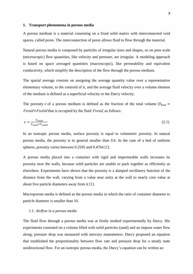
A porous medium is a material consisting on a fixed solid matrix with interconnected void
spaces, called pores. The interconnection of pores allows fluid to flow through the material.
Natural porous media is composed by particles of irregular sizes and shapes, so on pore scale
(microscopic) flow quantities, like velocity and pressure, are irregular. A modeling approach
is based on space averaged quantities (macroscopic), like permeability and equivalent
conductivity, which simplify the description of the flow through the porous medium.
The spatial average consists on assigning the average quantity value over a representative
elementary volume, to the centroid of it, and the average fluid velocity over a volume element
of the medium is defined as a superficial velocity or the Darcy velocity.
The porosity of a porous medium is defined as the fraction of the total volume
+ that is occupied by the fluid , as follows:
(2.1)
In an isotropic porous media, surface porosity is equal to volumetric porosity. In natural
porous media, the porosity is in general smaller than 0.6. In the case of a bed of uniform
spheres, porosity varies between 0.2595 and 0.4764 [1].
A porous media placed into a container with rigid and impermeable walls increases its
porosity near the walls, because solid particles are unable to pack together as efficiently as
elsewhere. Experiments have shown that the porosity is a damped oscillatory function of the
distance from the wall, varying from a value near unity at the wall to nearly core value at
about five particle diameters away from it [1].
Macroporous media is defined as the porous media in which the ratio of container diameter to
particle diameter is smaller than 10.
1.1. Airflow in a porous media
The fluid flow through a porous media was at firstly studied experimentally by Darcy. His
experiments consisted on a column filled with solid particles (sand) and an impose water flow
along; pressure drop was measured with mercury manometers. Darcy proposed an equation
that established the proportionality between flow rate and pressure drop for a steady state
unidirectional flow. For an isotropic porous media, the Darcy’s equation can be written as:

9
(2.2)
Where is the pressure gradient through the porous bed, is the Darcy velocity, defined as
the average of the fluid velocity over the total volume of the porous media, is the dynamic
viscosity of the fluid and is the permeability of the porous media. This last parameter
depends only on the porous media geometry, but not on fluid nature. There are different
equations to determine the permeability of a porous media, according to its geometry. For
example, for a packed bed of spheres, the permeability was related to the porosity and to the
particle diameter ( ) by the following equation.
(2.3)
Where is the particle diameter and is an experimental factor related to particle shape.
Several values between 150 and 199 can be found in literature [1, 2].
The increase in fluid velocities isn’t followed by a linear increase in the flow pressure drop.
Dupuit and Forchheimer proposed to add a quadratic velocity term to Darcy’s equation, to
take into account the drag due to the solids obstacles, which is of the same order than the
linear term. This term can be neglected for small velocities, with Reynolds number of the
order of one or smaller [1]. An extension of the Darcy’s law can be used to consider the
effects of boundary friction, inertia and acceleration. This equation was obtained by analogy
with the Navier-Stokes equation. In [2], a macroscopic momentum equation is proposed for
natural convection in enclosed porous cavities, with Boussinesq approximation, as follows:
(2.4)
(I) (II) (III) (IV) (V) (VI) (VII)
Terms in that last equation stand for: (I) Acceleration term, (II) Inertia term, (III) Pressure
gradient, (VI) Brinkman term, (V) Darcy term, (VI) Gravitational force, (VII) Forchheimer
term.
The Brinkman term (IV) is similar to the Laplacian one in Navier-Stokes, but is the
effective viscosity, which depends on the fluid viscosity and the geometry of the porous
media. In cases of high porosity, it can be assumed that . The empirical coefficient in
Forchheimer term (VII) varies with the porous media nature.

10
1.2. Heat transfer in a porous media
Heat transfer in a porous media depends on the thermal and physical properties of both the
solid and the fluid phase. There are two types of approaches for this phenomenon: the one
temperature model and the two temperature model.
1.2.1. One temperature model
This model is based on the hypothesis that the medium is isotropic, and radiant effects,
viscous dissipation and work done by pressure changes, are negligible. One temperature
model assumes local thermal equilibrium between solid and fluid phases, and it displays good
accuracy whenever temperature differences between solid and fluid phases at pore scale are
much lower than at global scale. When it is subjected to an airflow, heat transfer occurs due to
conduction and convection, and it is characterized by the effective or equivalent thermal
conductivity tensor ( ) and the dispersion tensor ( ). In case of isotropic materials, the
equivalent thermal conductivity tensor is a scalar, placed in the energy equation as follows:
(2.5)
where
(2.6)
The equivalent thermal conductivity is obtained by considering the porous medium as
homogeneous. In case of solid and fluid phases arranged in parallel, it can be defined in a
similar way that the equivalent heat capacity per unit volume of the medium,
Other
correlations for the equivalent conductivity are presented in Chapter III. Parameters
identification, depending on fluid and solid thermal conductivities and porosity.
The thermal dispersion tensor appears in cases of force convection or vigorous natural
convection, to take into account convective heat transfer due to mixing of interstitial fluid at
pore scale. This mixing phenomenon can occur due to the nature of the porous media:
obstructions, recirculation, wall effect and eddies, etc [1]. The dispersion tensor is a complex
function of matrix structure, porosity, and thermal properties of both phases and its
hydrodynamic characteristics [4].
11
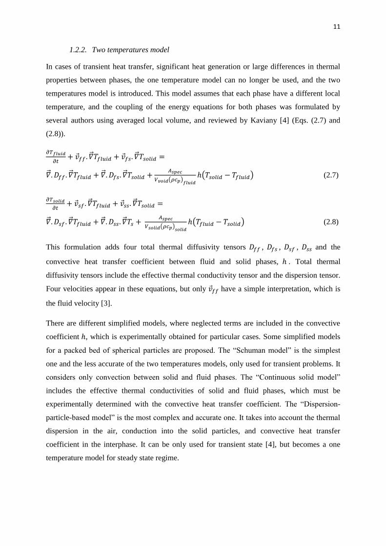
1.2.2. Two temperatures model
In cases of transient heat transfer, significant heat generation or large differences in thermal
properties between phases, the one temperature model can no longer be used, and the two
temperatures model is introduced. This model assumes that each phase have a different local
temperature, and the coupling of the energy equations for both phases was formulated by
several authors using averaged local volume, and reviewed by Kaviany [4] (Eqs. (2.7) and
(2.8)).
(2.7)
(2.8)
This formulation adds four total thermal diffusivity tensors , , , and the
convective heat transfer coefficient between fluid and solid phases, . Total thermal
diffusivity tensors include the effective thermal conductivity tensor and the dispersion tensor.
Four velocities appear in these equations, but only have a simple interpretation, which is
the fluid velocity [3].
There are different simplified models, where neglected terms are included in the convective
coefficient , which is experimentally obtained for particular cases. Some simplified models
for a packed bed of spherical particles are proposed. The “Schuman model” is the simplest
one and the less accurate of the two temperatures models, only used for transient problems. It
considers only convection between solid and fluid phases. The “Continuous solid model”
includes the effective thermal conductivities of solid and fluid phases, which must be
experimentally determined with the convective heat transfer coefficient. The “Dispersion-
particle-based model” is the most complex and accurate one. It takes into account the thermal
dispersion in the air, conduction into the solid particles, and convective heat transfer
coefficient in the interphase. It can be only used for transient state [4], but becomes a one
temperature model for steady state regime.

12
1.3. Mass conservation and frost formation in a porous media
Unlike the case of energy balance equation, mass conservation in a porous media is only
applied for the fluid phase, and can be written as in Eq. (2.9).
(2.9)
Where is the specie concentration, is the Darcy velocity, is the effective mass
diffusivity and is the mass generation per unit volume of this specie. Analog to heat
transfer, the effective mass diffusivity is composed by the molecular diffusivity and the
dispersion mass diffusivity. Mass diffusivity depends on pressure, temperature and
composition of the species mixture.
In order to model mass transfer between fluid and solid phases, it could be consider in the
source term as in Eq. (2.10).
(2.10)
where is the mass transfer convective coefficient, is the specie concentration in the
solid surface and is the specie concentration in the fluid. In cases of forced convection,
the mass transfer coefficient could be obtained from the heat transfer convective coefficient
making use of the Lewis analogy, presented in Eq. (2.11).
with
(2.11)
where is the Prandlt number exponent in the Nusselt equation for these conditions
(geometry, fluid and flux), and varies between 0 and 1. A usual value is 1/3.
2. Existing models
There are several works on heat and mass transfer models for a porous media. Laguerre et al.
[5] studied the transient heat transfer by free convection in a packed bed of spheres, and
developed a dispersed particle based model (including radiation between solid surfaces) and
compared it to direct CFD model and experimental values. Both models were in agreement
with the experimental values. The developed model for a packed bed requires less
computational time than direct CFD, but it does not predict the details of the fluid flow and
temperature at pore scale. Beukema et al. [6] developed a two dimensional two phase model
13
of temperature and moisture distribution during cooling and storage of fresh agricultural
products in cylindrical containers (porous media), subjected to natural convection. The model
results agree with experimental measures with potatoes. Dona and SewartJr [7] studied
numerically heat transfer by natural convection into a cylindrical grain bin which contained
stored corn, with a porous media approach, and analyzed the effect of different container
aspect ratios.
Pham and Willix [8] developed simple equations to describe the ratio of desiccation of frozen
food, taking into account the dehydrate layer. Pham [9] presented equations and graphical
methods to predict the maximum possible moisture change between product and air. Tocci
and Mascheroni [10] proposed a model for heat and mass transfer during the storage of frozen
food, to predict product (spheres) weight loss, using explicit finite difference methods.
Campaño et al. propose a numerical model [11] and a simple analytical model [12] for the
prediction of weight loss during freezing and storage of unpacked frozen food, taking into
account the dehydrated varying layer in the product surface. They compare both, the
numerical and analytical models, to experimental data and among them. Weight loss during
storage depends on the freezing method, because of the mass transfer resistance of the
dehydrate layer. They concluded that the weight loss is lower for lower temperatures, weight
loss increase with air circulation and there is a linear increase of weight loss with relative
humidity [11].
All authors agree to the fact that product weight loss increase with large amplitudes of
fluctuations and low frequencies. In cases where package was used, it was found that it
reduced product weight loss. However any of them studied the posterior frost formation.
Most studies in modeling frost formation were developed for air coolers. In these conditions,
it is important to predict the thickness of the frost layer as well as its density, since these
factors affect significantly the rate of heat transfer and the airflow through the fins. For
example, Wu et al. [13] developed a phase change mass transfer CFD model to predict the
frost layer growth and densification. They concluded that the averaged frost thickness
increased gradually with time, with the growth rate slowing down; and the average frost
density increased with time, with the increases rate getting faster.
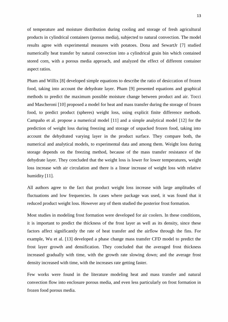
Few works were found in the literature modeling heat and mass transfer and natural
convection flow into enclosure porous media, and even less particularly on frost formation in
frozen food porous media.
14
3. Proposed numerical model
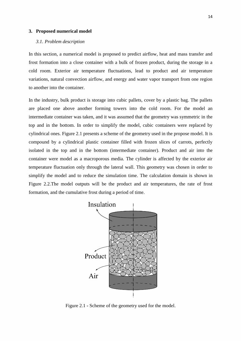
3.1. Problem description
In this section, a numerical model is proposed to predict airflow, heat and mass transfer and
frost formation into a close container with a bulk of frozen product, during the storage in a
cold room. Exterior air temperature fluctuations, lead to product and air temperature
variations, natural convection airflow, and energy and water vapor transport from one region
to another into the container.
In the industry, bulk product is storage into cubic pallets, cover by a plastic bag. The pallets
are placed one above another forming towers into the cold room. For the model an
intermediate container was taken, and it was assumed that the geometry was symmetric in the
top and in the bottom. In order to simplify the model, cubic containers were replaced by
cylindrical ones. Figure 2.1 presents a scheme of the geometry used in the propose model. It is
compound by a cylindrical plastic container filled with frozen slices of carrots, perfectly
isolated in the top and in the bottom (intermediate container). Product and air into the
container were model as a macroporous media. The cylinder is affected by the exterior air
temperature fluctuation only through the lateral wall. This geometry was chosen in order to
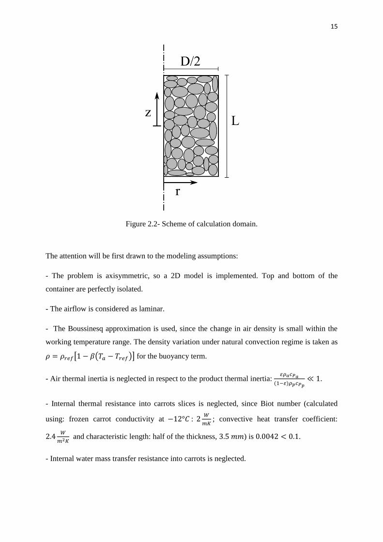
simplify the model and to reduce the simulation time. The calculation domain is shown in
Figure 2.2.The model outputs will be the product and air temperatures, the rate of frost
formation, and the cumulative frost during a period of time.
Figure 2.1 - Scheme of the geometry used for the model.
15
Figure 2.2- Scheme of calculation domain.
The attention will be first drawn to the modeling assumptions:
- The problem is axisymmetric, so a 2D model is implemented. Top and bottom of the
container are perfectly isolated.
- The airflow is considered as laminar.
- The Boussinesq approximation is used, since the change in air density is small within the
working temperature range. The density variation under natural convection regime is taken as
for the buoyancy term.
- Air thermal inertia is neglected in respect to the product thermal inertia:
.
- Internal thermal resistance into carrots slices is neglected, since Biot number (calculated
using: frozen carrot conductivity at :
; convective heat transfer coefficient:
and characteristic length: half of the thickness, ) is .
- Internal water mass transfer resistance into carrots is neglected.

16
- Temperature at the container external lateral wall is known as a function of time, by
measurements.
- Radiation heat transfer is neglected inside the container.
- The dispersion term in the energy equation for the porous medium is neglected, because of
the low fluid velocities.
- Forchheimer term in momentum equation is neglected as the Reynolds number is smaller
than one [1] (simulated air velocity of ; pore diameter ; and air
kinetic viscosity, ).
3.2. Governing equations
The following equations, momentum, energy and mass transfer will be solved according to
the previous assumptions.
3.2.1. Continuity and Momentum equations
Continuity and momentum equations are written for the fluid phase, assuming the Boussinesq
approximation. The momentum equation integrates also the Darcy term for fluid flow in
porous media.
(2.12)
(2.13)
where is the porosity, is the Darcy superficial air velocity into the porous medium, is
the permeability of the porous media and is the thermal coefficient of volumetric expansion.
3.2.2. Energy
Energy equation is written for the air, Eq. (2.14), and for the product, Eq. (2.15). These
equations are coupled by the convective heat transfer between air and product. The specific
surface, , is defined as the total heat transfer surface of product over the bed volume of
porous medium.
(2.14)
17
(2.15)
where is the equivalent conductivity of the carrots bed and is the convective heat
transfer coefficient inside the container (product - air). Last term of Eq. (2.15) takes into
account latent heat of ice sublimation, where and are ice contents in frost and product
per unit volume of porous medium respectively.
3.2.3. Water mass balance
Total water mass balance inside product container is written as follows:
(2.16)
where , is water content in air and is the vapor effective or total mass diffusivity in the
porous media.
Eq. (2.17) describes the frost formation. If water concentration in air is higher than the
saturation limit at product temperature , frost is formed.
(2.17)
Eq. (2.18) describes product dehydration, which occurs when water vapor concentration in air
is smaller than water vapor concentration in air in equilibrium with the product
.
(2.18)
In these equations, is the convective mass transfer coefficient, obtained by Lewis analogy
from the convective heat transfer coefficient, and assuming that the airflow is imposed
externally for one single slice, and it could be consider as forced convection. is the mass
transfer resistance at the vegetable skin, and is the water activity of the product. For peeled
carrots, there is no skin resistance, but this term can be used to take into account the mass
transfer resistance due to the thin layer of dehydrated product near the surface [8, 10, 12, 13].
18
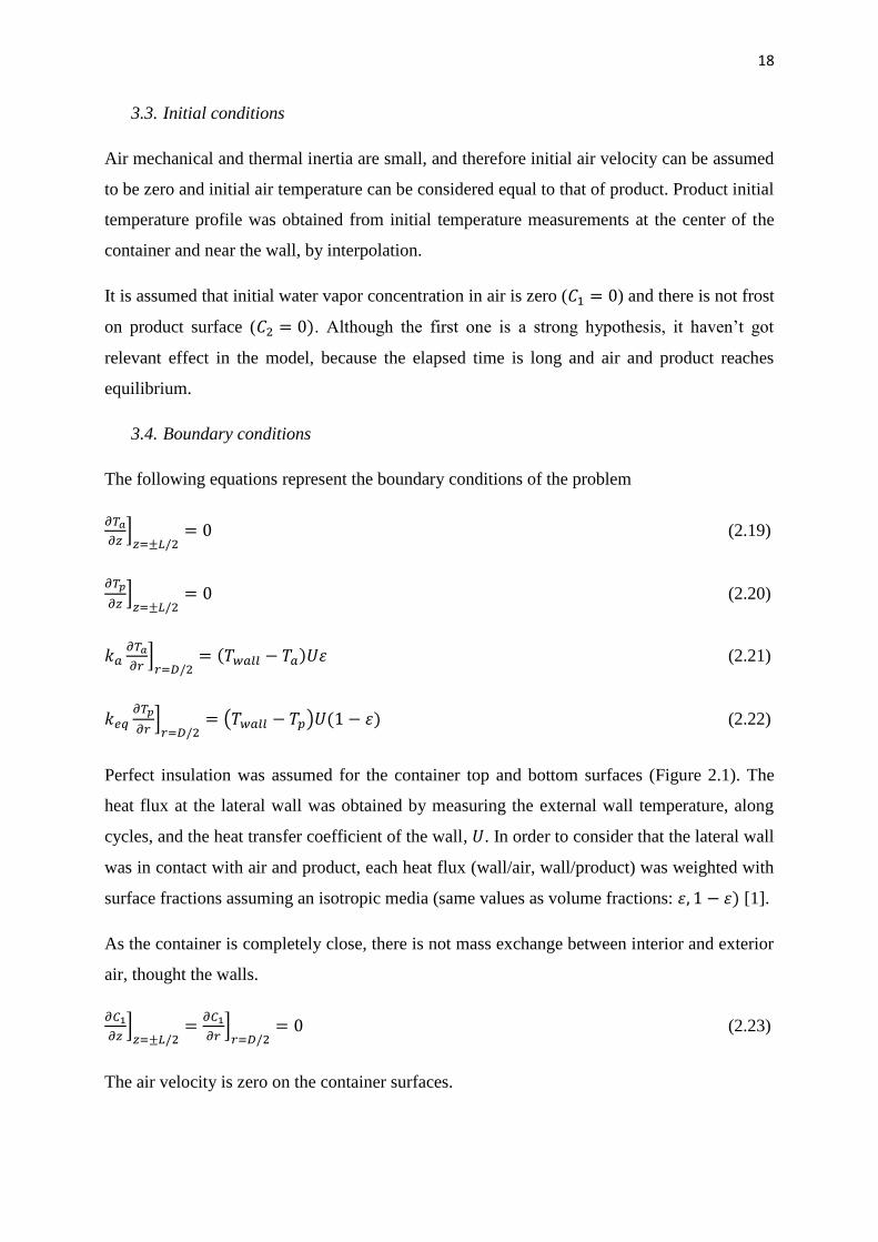
3.3. Initial conditions
Air mechanical and thermal inertia are small, and therefore initial air velocity can be assumed
to be zero and initial air temperature can be considered equal to that of product. Product initial
temperature profile was obtained from initial temperature measurements at the center of the
container and near the wall, by interpolation.
It is assumed that initial water vapor concentration in air is zero ( ) and there is not frost
on product surface ( . Although the first one is a strong hypothesis, it haven’t got
relevant effect in the model, because the elapsed time is long and air and product reaches
equilibrium.
3.4. Boundary conditions
The following equations represent the boundary conditions of the problem
(2.19)
(2.20)
(2.21)
(2.22)
Perfect insulation was assumed for the container top and bottom surfaces (Figure 2.1). The
heat flux at the lateral wall was obtained by measuring the external wall temperature, along
cycles, and the heat transfer coefficient of the wall, . In order to consider that the lateral wall
was in contact with air and product, each heat flux (wall/air, wall/product) was weighted with
surface fractions assuming an isotropic media (same values as volume fractions: [1].
As the container is completely close, there is not mass exchange between interior and exterior
air, thought the walls.
(2.23)
The air velocity is zero on the container surfaces.

19
(2.24)
4. Results
The proposed model was submitted to different operational conditions, by changing the
problem exterior air temperature and initial conditions, and compared to literature results. The
parameter values used for the test presented in Table 2.1, were obtained by different methods
explain in detail in Chapter III. Parameters identification. Simulations were applied to a
cylindrical container of dimensions: diameter and height .
Table 2.1– Parameters used for the model prove
Parameter Symbol Value
Product density
Apparent specific heat Function of
temperature
Porosity
Specific surface
Permeability
Equivalent conductivity
Convective coefficient
Effective mass
diffusivity
The problem was solved using COMSOL ® CFD software running on a Ubuntu 16.04 LTS
computer in a PC Intel® Core ™ i7-6700K CPU @ 4.00GHz with 15.6 GB RAM. COMSOL
automatic meshing “Fine” was used for the discretization of the computational domain.
Physics-controlled mesh discretize on triangular and quadrilateral elements, with refined near
walls (3501 domain elements and 179 boundary elements). The mesh independence was done
for the most complex problem, presented in Chapter IV. Experimental validation, where
“Fine” mesh was adequate.
Four temperature cycles, presented in Table 2.2, were proposed as external input. Simulations
were performed for two hours and a half long period.
20
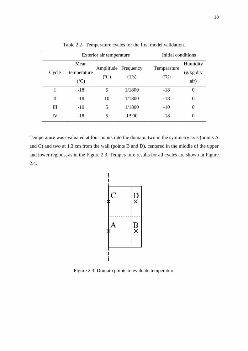
Table 2.2– Temperature cycles for the first model validation.
Exterior air temperature Initial conditions
Cycle
Mean
temperature
(ºC)
Amplitude
(ºC)
Frequency
(1/s)
Temperature
(ºC)
Humidity
(g/kg dry
air)
I -18 5 1/1800
-18 0
II -18 10 1/1800
-18 0
III -10 5 1/1800
-10 0
IV -18 5 1/900 -18 0
Temperature was evaluated at four points into the domain, two in the symmetry axis (points A
and C) and two at 1.3 cm from the wall (points B and D), centered in the middle of the upper
and lower regions, as in the Figure 2.3. Temperature results for all cycles are shown in Figure
2.4.
Figure 2.3–Domain points to evaluate temperature

21
a.
b.
-30,00
-25,00
-20,00
-15,00
-10,00
-5,00
0,00
0 2000 4000 6000 8000 10000
Tem
pe
ratu
re (
ºC)
time (s)
Exterior air A C B D
-30,00
-25,00
-20,00
-15,00
-10,00
-5,00
0,00
0 2000 4000 6000 8000 10000
Tem
pe
ratu
re (
ºC)
time(s)
Exterior air A C B D

22
c.
d.
Figure 2.4 - Simulation results. Exterior air and product temperatures versus time, for
different exterior air temperature cycles: a. Cycle I. b. Cycle II. c. Cycle III. d. Cycle IV.
As can be seen, in all cycles, temperature varies into the domain only in radial direction, so
temperatures in the top and in the bottom are practically the same ( and ).
This means that conduction heat transfer is dominant over natural convection heat transfer, as
was expected, since convective heat transfer coefficient is very low. Another observation is
that with this air temperature cycles, product at the center of the domain is not affected by the
-30,00
-25,00
-20,00
-15,00
-10,00
-5,00
0,00
0 2000 4000 6000 8000 10000
Tem
pe
ratu
re (
ºC)
time(s)
Exterior air A C B D
-30,00
-25,00
-20,00
-15,00
-10,00
-5,00
0,00
0 2000 4000 6000 8000 10000
Tem
pe
ratu
re (
ºC)
time(s)
Exterior air A C B D
23
exterior air temperature fluctuation, so it is practically constant in all cycles. The effect of
thermal inertia is observed in the gap between air and product fluctuations. Results could be
compared by taking the first cycle (I) as the reference one, and changing the mean
temperature, amplitude and frequency of oscillation for the following three proposed cases.
As it was expected, the increases of air temperature fluctuations keeping the same mean
temperature and frequency (comparison cycle I to II), lead to changes of the product
temperature, since there was an increase in the heat transfer rate. Comparing cycles I to III, it
was observed that the increase of the mean temperature, but keeping the same amplitude and
frequency of oscillation, caused the product to decrease its temperatures fluctuation,
becoming practically null. This can be explained by the change in thermal diffusivity, due to
apparent specific heat variation. Using the propose approach for apparent specific heat, and
taking into account that it is assumed a constant density and thermal conductivity of the
product, the thermal diffusivity ranged from at -18ºC to
at -10ºC. In case of frequency increase, with the same mean temperature and
amplitude (comparison between cycles I to IV), product temperature fluctuations decreased,
since there was less time to perform the heat transfer.
The calculation of the total frost formed in the container was obtained from volume
integration in COMSOL, and plotted in Figure 2.5 for all cycles.

24
Figure 2.5-Simulation results, cumulative frost formation versus time for cycles I to IV.
A first observation is that frost formation displayed approximately a linear growth with time,
independently of mean temperature, amplitude and frequency of oscillation of exterior air.
This result was also found experimentally by Phimolsiripol et al. [14] and Pham et al. [15].
However, it is important to recognize that all these parameters have an important effect in
total frost formed. Cycles could be compared, once again, taking cycle I as a reference, with
the aid of temperatures evolution in Figure 2.4. In cycle II, the amplitude of oscillation
increased two times in comparison to cycle I. As the total frost increase twice, it seems to be
directly proportional to oscillation amplitude, as it was found in others works: Phimolsiripol
et al. [14], Poovarodom [16] and Laguerre and Flick [17]. In cycle III, the mean temperature
decrease to -10ºC, and total frost decrease approximately proportionally. It means that the
same temperature fluctuation (amplitude and frequency) have less effect on frost formation at
higher temperatures. This result could be explained by the change in product specific heat,
which increases significantly between -18ºC to -10ºC due to the phase change. Laguerre and
Flick [17] proposed a model that showed that, the higher the thermal inertia, the lower frost
formation. In cycle IV frequencies increased twice respect to cycle I, and total frost formation
0
0,01
0,02
0,03
0,04
0,05
0,06
0,07
0,08
0,09
0 2000 4000 6000 8000 10000
Cu
mu
lati
ve f
rost
fo
rmat
ion
(g)
time (s)
Cycle I
Cycle II
Cycle III
Cycle IV

25
decrease, since product temperature varies less than in cycle I. This result agrees with the one
obtained by Poovarodom [16] and Laguerre and Flick [17]. Finally, it can be said that product
temperature variation had a very important effect on frost formation, increasing with each
other.
5. Conclusion
A model of heat and mass transfer was proposed in order to predict frost formation into a
closed container filled with frozen vegetables. The problem was study as a macroporous
media compose by the product and the surrounding air. Natural convection air flow was
assumed into the container, who promotes water mass transport. The model was developed in
the commercial software CFD COMSOL, and it was test imposing different exterior air
temperature fluctuations (boundary conditions). Results of four temperature cycles were
compared, varying one by one: average temperature, amplitude and frequency of oscillation.
As general result it was observed that product temperature behavior is as expected, and it is
directly associated with frost formation into the container. The bigger the product temperature
variation, the bigger the amount of frost formed. Frost formation increase with large
amplitude of oscillation, but decrease with higher frequencies and mean temperatures.

26
Bibliography
[1] Donald A. Neild and Adrian Bejan, Convection in porous media, Third Edition, Springer
Science + Business Media, Inc., 2006.
[2] Derek B. Ingham and Iaon Pop, Transport phenomena in porous media, Elseiver Science
Ltd., 1998.
[3] S. Ben Amara, Ecoulements et transferts thermiques en convection naturelle dans les
milieux macroporeux alimentaires: Application aux réfrigérateurs ménagers, Thèse doctorant
de l’Institut National de Paris-Grignon, 2005.
[4] Warren M. Rohsenow, James P. Hartnett, Young I. Cho, Handbook of Heat Transfer,
Third Edition, The McGraw-Hill Companies, Inc., 1998.M. Kaviany, Chapter 9: Heat
Transfer in Porous Media
[5] O. Laguerre, S.B. Amara, G. Alvarez, D. Flick, Transient heat transfer by free convection
in a packed bed of spheres/ Comparison between two modelling approaches and experimental
results, Applied Thermal Engineering, 28 (2008) 14-24
[6] K.J. Beukema, S. Bruin, J. Schenk, Heat and mass transfer during cooling and storage of
agricultural products, Chemical Engineering Science, 37 (1982) 291-298
[7] C.L.G. Dona and W.E. Stewart Jr, Numerical analysis of natural convection heat transfer
in stored high moisture corn, Journal of Agricultural Engineering Research 40 (1988) 275-284
[8] Q.T. Pham and J. Willix, A model for food desiccation in frozen storage, Journal of Food
Science, 49 (1984) 1275-1281
9] Q.T. Pham, Moisture transfer due to temperature changes or fluctuations, J. Food Eng. 6
(1987) 33-49
[10] A.M. Tocci, R.H. Mascheroni, Numerical models for the simulation of the simultaneous
heat and mass transfer during food freezing and storage, International Communications of
Heat and Mass Transfer, 22 (1995) 251-260
[11] L.A. Campañone, V.O. Salvadori, R.H. Mascheroni, Weight loss during freezing and
storage of unpackaged foods, Journal of Food Engineering, 47 (2001) 69-79

27
[12] L.A. Campañone, V.O. Salvadori, R.H. Mascheroni, Food freezing simultaneous surface
dehydration: approximate prediction of weight loss during freezing and storage, International
Journal of Heat and Mass Transfer, 48 (2005) 1195-1204
[13] X. Wu, Q. Ma, F. Chu, S. Hu, Phase change mass transfer model for frost growth and
densification, International Journal of Heat an Mass Transfer 96 (2016) 11-19
[14] Y. Phimolsiripol, U. Siripatrawan, D.J. Cleland, Weight loss of frozen bread dough under
isothermal and fluctuating temperature storage conditions, J. Food Eng. 106 (2011) 134-143
[15] Q.T. Pham, J.R. Durbin, J. Willix, Survey of weight loss from lamb in frozen storage,
Revue Internationale du Froid,5 (1982) 337-342
[16] N. Poovarodom, Modification de la qualité des denrées alimentaires surgelées au cours
de leur conservation: le rôle de l’emballage et l’influence de la température de conservation,
Thèse doctorant de l’Université de Technologie de Compiègne
[17] O. Laguerre, D. Flick, Frost formation on frozen products preserved in domestic freezers,
Journal of Food Engineering, 79 (2007) 124-136
28
BULK STORAGE OF FROZEN VEGETABLES MODELED AS A
MACROPOROUS MEDIA: PARAMETERS IDENTIFICATION
Abstract
This chapter deals with the parameter identification of stored frozen vegetables packed on
pallets and submitted to heat and mass transfer phenomena. Products were modeled as a
porous media. Parameters were obtained for two assembling: frozen slices of carrots and air,
and frozen extra thin green beans and air. Parameter definition and evaluation combines
literature review, measurements and numerical simulation. They were classified in three
types, as: the ones that only depend on thermophysical properties (product density and
apparent specific heat), which depends only on the geometry (porosity, specific surface and
permeability) and the ones that depend on both (equivalent conductivity and convective heat
transfer coefficient). In general, parameters which characterize these porous media, were
similar for both products, even though they display different geometries.
Key words: frozen food; macroporous media; vegetables; parameter identification.
29
Index
1. Introduction ……………………...………………………………………………….....................................................30
1.1. Frozen food thermodynamic properties ............................................................................... 30
1.2. Macroporous media characteristics ...................................................................................... 31
2. Materials and methods ...………………………………………………………………............................................33
2.1. Products ................................................................................................................................. 33
2.1.1. Carrot ............................................................................................................................. 33
2.1.2. Green beans .................................................................................................................. 33
2.2. Frozen product properties .................................................................................................... 34
2.2.1. Product density.............................................................................................................. 34
2.2.2. Enthalpy of phase change - Apparent specific heat ...................................................... 34
2.3. Porous media characteristics ................................................................................................ 34
2.3.1. Product bulk porosity .................................................................................................... 34
2.3.2. Specific surface .............................................................................................................. 35
2.3.3. Bulk product permeability ............................................................................................. 35
2.3.4. Equivalent conductivity ................................................................................................. 36
2.3.5. Convective heat transfer coefficient into the porous media ........................................ 37
3. Results ……………...……………………………………………………………………...................................................39
3.1. Frozen product density .......................................................................................................... 40
3.2. Apparent specific heat........................................................................................................... 40
3.3. Product bulk porosity ............................................................................................................ 43
3.4. Specific surface ...................................................................................................................... 43
3.5. Bulk product permeability ..................................................................................................... 44
3.6. Equivalent conductivity ......................................................................................................... 46
3.7. Convective heat transfer coefficient ..................................................................................... 52
4. Conclusion ……………………………………………………………………...………..................................................57
Bibliography .…………………………………………………………………………………………………………………………………...58

30
1. Introduction
1.1. Frozen food thermodynamic properties
Food products, in particular vegetables, are mainly composed by water, around 90% (from
Chapter 9, ASHRAE [1]), and a small fraction of solved solids. The water freezing process
reduces the liquid water fraction, inhibiting microorganism’s growth and enzymatic activity.
Food freezing have two important engineering aspects: the enthalpy change during freezing,
and freezing time, which directly affects the product properties and its quality, in accordance
to the ice crystallization into the product.
In the study of frozen food, the water phase change must be taken into account. The presence
of solved solids in product solution reduces the initial freezing point, in respect to pure water.
This behavior is important since there is not a unique phase change temperature as is shown in
Figure 3.1.a. The scheme in Figure 3.1igure 3.1.b presents the food phase change process.
Over the initial freezing point, the food product is compound by unfrozen water ( ) and
solids ( ). When the initial freezing point ( ) is achieved, a fraction of water becomes ice
( ), and the solution, unfrozen water and solids (mainly sugar), increases its concentration
reducing even more the solution freezing point.
a. b.
Figure 3.1 - a. Comparison of freezing curves for pure water and an aqueous solutions
containing one solute; b. Schematic illustration of the phase change in a food product during
freezing. From Food Process Engineering [2].
The energy embedded on a freezing process was predicted by Eq.(3.1)

31
(3.1)
where is the solid particles sensible enthalpy, is the unfrozen water enthalpy, is
the latent enthalpy and is the ice water sensible enthalpy, defined as follows:
(3.2)
(3.3)
(3.4)
(3.5)
Where and are the mass fraction and specific heat of each phase, and , and are
initial temperature, product initial freezing point and product temperature, respectively.
In terms , and , the mass fractions are temperature functions. Once product
temperature is lower than initial freezing point, and
are temperature functions also.
These temperature dependences and the lack of knowledge about product composition, turns
difficult to calculate enthalpy changes. The enthalpy variation needed to reduce product
temperature under the initial freezing point could be measured by a calorimeter test
(Differential Scanning Calorimetry).
There are different methods to take into account the latent heat in simulations, Pham [3]
review some of them: apparent specific heat method, enthalpy method and quasi-enthalpy
method. In the apparent specific heat method, latent heat is merged with sensible heat to
produce a specific heat curve with a large peak around the freezing point.
1.2. Macroporous media characteristics
A porous medium is a material consisting on a fixed solid matrix with interconnected void
spaces, called pores, whose interconnection allows fluid flow through the material. Porous
media are characterized by geometric parameters as porosity (void fraction), specific
surface (rate of interior solid matrix surface to total volume) and
permeability (hydraulic resistance). Equivalent thermal conductivity
and interior convective heat transfer coefficient depends on thermodynamic
properties of solid and fluid phases and geometric characteristics of the porous medium.
In case of an enclosure porous medias it can be defined the macroporous media as the one in
which the ratio of container characteristic length to particle characteristic length is smaller
than 10.
In natural porous media, the porosity is in general smaller than 0.6. In common porous media
it can vary close to limit values, 0 and 1. In the case of a bed of uniform spheres, porosity
varies between 0.2595 and 0.4764 [4].
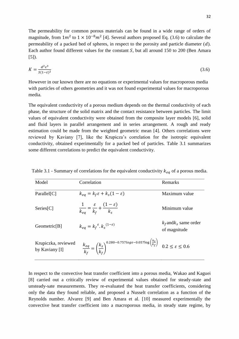
32
The permeability for common porous materials can be found in a wide range of orders of
magnitude, from to [4]. Several authors proposed Eq. (3.6) to calculate the
permeability of a packed bed of spheres, in respect to the porosity and particle diameter ( ).
Each author found different values for the constant , but all around 150 to 200 (Ben Amara
[5]).
(3.6)
However in our known there are no equations or experimental values for macroporous media
with particles of others geometries and it was not found experimental values for macroporous
media.
The equivalent conductivity of a porous medium depends on the thermal conductivity of each
phase, the structure of the solid matrix and the contact resistance between particles. The limit
values of equivalent conductivity were obtained from the composite layer models [6], solid
and fluid layers in parallel arrangement and in series arrangement. A rough and ready
estimation could be made from the weighted geometric mean [4]. Others correlations were
reviewed by Kaviany [7], like the Krupicza’s correlation for the isotropic equivalent
conductivity, obtained experimentally for a packed bed of particles. Table 3.1 summarizes
some different correlations to predict the equivalent conductivity.
Table 3.1 - Summary of correlations for the equivalent conductivity of a porous media.
Model Correlation Remarks
Parallel[C] Maximum value
Series[C]
Minimum value
Geometric[B]
and same order
of magnitude
Krupiczka, reviewed
by Kaviany [I]
In respect to the convective heat transfer coefficient into a porous media, Wakao and Kaguei
[8] carried out a critically review of experimental values obtained for steady-state and
unsteady-sate measurements. They re-evaluated the heat transfer coefficients, considering
only the data they found reliable, and proposed a Nusselt correlation as a function of the
Reynolds number. Alvarez [9] and Ben Amara et al. [10] measured experimentally the
convective heat transfer coefficient into a macroporous media, in steady state regime, by

33
neglecting conduction and radiation between solid particles. They placed a sphere of high
conductivity material into a packed bed of spheres of very small conductivity. An electrical
resistance heated the sphere and temperature was measured by a thermocouple, assuming
uniform temperature. Alvarez [9] established a Nusselt correlation for turbulent flow. Ben.
Amara et al. [10] studied the influence of the operational parameters on the convective
coefficient, and proposed a correlation for Reynolds in the range from 74 to 495 (low
velocities), similar to the one proposed for Wakao and Kaguei.
Ben Amara et al. [10] performed an experimental study of convective heat transfer during
cooling with low air velocity in a stack of objects. They found that for low velocities
(<0.2m/s) radiation and conduction could be of the same order of magnitude as convection.
There were several researches working with porous media, in general with spherical particles.
However, few researches had been carried out the characterization and identification of
macroporous media parameters, even less for confined porous media at very low air velocity.
2. Materials and methods
In this work, the porous media consists on frozen product and air. Properties and parameters
of two porous media were determined by different ways, as it was explained in this section.
2.1. Products
Two types of frozen vegetables were studied: sliced carrots and extra thin green beans. These
were chosen because they were the most susceptible to damage during frozen storage. For all
measures and experiments, products were prepared from fresh vegetables.
2.1.1. Carrot
Frozen slices of carrots were prepared from fresh carrots, peeled, cut, and frozen in a freezer
at temperature of .
Standard dimensions in the industry are diameter between and , and thickness
between and .
A sample of 100 carrot slices was taken to measure their average diameter and thickness, with
the correspondent uncertainties: and respectively.
2.1.2. Green beans
Fresh extra thin green beans were prepared by removing the beans tips and then frozen at
.
Standard dimensions in the industry are diameter between and , and length
between and 120 .
Sample of 50 green beans was taken to measure their average diameter and length, with the
correspondent uncertainties: and respectively.

34
2.2. Frozen product properties
2.2.1. Product density
Frozen product density was difficult to be measure experimentally, since it was not possible to
use water, because it melts the product. For this work, product density was calculated using
Eq. (3.7) and composition data from [1], for food products. Density depends on product
composition and its mass fraction.
(3.7)
where was the mass fraction and the density of each component (water, protein, fat,
carbohydrate and ash). Density of each component and therefore product density depends on
temperature.
2.2.2. Enthalpy of phase change - Apparent specific heat
A Differential Scanning Calorimetry (DSC) analysis of carrots was performed using the
equipment Metter Toledo DSC 822e by a thermo analytical technique in which the difference
in the amount of heat power ( required to increase the temperature of a sample and a
reference, is measured as a function of temperature.
Samples for the calorimetry test were prepared from fresh product. Approximately
sample of product was placed in an aluminum pan, hermetically closed. Sample weight was
recorded and then subjected to the DSC. Measures were made in the temperature range
between and , with a speed of .
Finally, the DSC software returned values of heat power versus temperature. The apparent
specific heat of phase change could be obtained by Eqs. (3.8) and (3.9).
(3.8)
(3.9)
2.3. Porous media characteristics
2.3.1. Product bulk porosity
The porosity of a porous medium was defined as the ratio between air volume and total bed
volume.
(3.10)
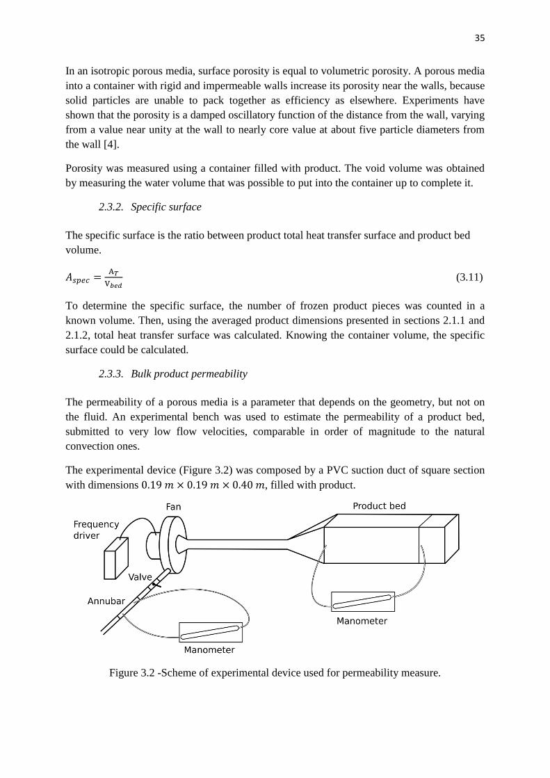
35
In an isotropic porous media, surface porosity is equal to volumetric porosity. A porous media
into a container with rigid and impermeable walls increase its porosity near the walls, because
solid particles are unable to pack together as efficiency as elsewhere. Experiments have
shown that the porosity is a damped oscillatory function of the distance from the wall, varying
from a value near unity at the wall to nearly core value at about five particle diameters from
the wall [4].
Porosity was measured using a container filled with product. The void volume was obtained
by measuring the water volume that was possible to put into the container up to complete it.
2.3.2. Specific surface
The specific surface is the ratio between product total heat transfer surface and product bed
volume.
(3.11)
To determine the specific surface, the number of frozen product pieces was counted in a
known volume. Then, using the averaged product dimensions presented in sections 2.1.1 and
2.1.2, total heat transfer surface was calculated. Knowing the container volume, the specific
surface could be calculated.
2.3.3. Bulk product permeability
The permeability of a porous media is a parameter that depends on the geometry, but not on
the fluid. An experimental bench was used to estimate the permeability of a product bed,
submitted to very low flow velocities, comparable in order of magnitude to the natural
convection ones.
The experimental device (Figure 3.2) was composed by a PVC suction duct of square section
with dimensions , filled with product.
Figure 3.2 -Scheme of experimental device used for permeability measure.
36
The airflow was controlled by a variable frequency drive (SSD Drives 650) connected to the
fan and with a valve installed in the discharge line. An Annubar (AWR-71) connected to an
inclined tube manometer was used to measure airflow, and therefore the superficial velocity
in the suction duct was obtained. The pressure drop in the carrots bed was measure with
another inclined tube manometer. The range of velocities used varied between
and , the same order of magnitude of natural convection ones.
The same method was previously used by Ben Amara [5] to measure product permeability.
The momentum equation for a porous media, assuming the Bousinesq approximation and
incompressible flow is similar to Navier Stokes but adding the Darcy and Forchheimer terms.
(3.12)
Where was the porosity, the permeability and the Forchheimer coefficient. Since the
experimental velocities were very small, the Forchheimer term became negligible in respect to
the Darcy term. The air temperature was the same as the reference one ( ), so the
mass force term could be neglected too. Under these conditions, and assuming steady state
regime, momentum equation was reduced to Darcy's equation, Eq. (3.13). Eq. (3.14) was a
unidirectional version of Darcy’s.
(3.13)
(3.14)
In these conditions, the permeability was determined making use of Eq. (3.14), by measuring
pressure drop through a bulk product bed for different velocities. The experiment was
repeated at least twice for each vegetable.
2.3.4. Equivalent conductivity
In this work the equivalent conductivity of the frozen product bed was identified from
experimental measures, in the absence of convection, with a unidirectional transient pure
conductive model in COMSOL.
A polyurethane box of of thickness in the lateral walls and in the bottom, was use
to contain the product. The interior dimensions were length, width and height, 15,5cm x
10,7cm x 9,5cm respectively. In the top of the box a thin steel plate was placed. Three pieces
of product (slices of carrot or green beans) were fixed exactly at known positions into the box,
at different heights and centered, and connected to thermocouples, as it is shown in Figure
3.3. Product and steel plate temperatures were measured by type T thermocouples
(copper/constantan) connected to a data logger (Pico Technology TC-08) and a computer.
A eutectic substance (PCM) with a phase change temperature of the order of -10ºC was used
to heat up the top surface of the box.
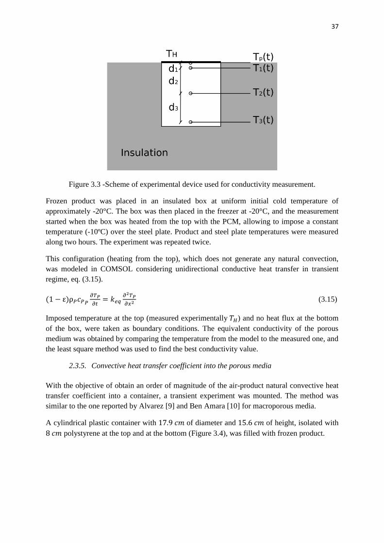
37
Figure 3.3 -Scheme of experimental device used for conductivity measurement.
Frozen product was placed in an insulated box at uniform initial cold temperature of
approximately -20°C. The box was then placed in the freezer at -20°C, and the measurement
started when the box was heated from the top with the PCM, allowing to impose a constant
temperature (-10ºC) over the steel plate. Product and steel plate temperatures were measured
along two hours. The experiment was repeated twice.
This configuration (heating from the top), which does not generate any natural convection,
was modeled in COMSOL considering unidirectional conductive heat transfer in transient
regime, eq. (3.15).
(3.15)
Imposed temperature at the top (measured experimentally ) and no heat flux at the bottom
of the box, were taken as boundary conditions. The equivalent conductivity of the porous
medium was obtained by comparing the temperature from the model to the measured one, and
the least square method was used to find the best conductivity value.
2.3.5. Convective heat transfer coefficient into the porous media
With the objective of obtain an order of magnitude of the air-product natural convective heat
transfer coefficient into a container, a transient experiment was mounted. The method was
similar to the one reported by Alvarez [9] and Ben Amara [10] for macroporous media.
A cylindrical plastic container with of diameter and of height, isolated with
polystyrene at the top and at the bottom (Figure 3.4), was filled with frozen product.

38
Figure 3.4 - Scheme of experimental device used for convective coefficient estimation.
An aluminum probe with dimensions close to the ones of product (diameter and
thickness for carrots; diameter and length for green beans) and
equipped with a type T thermocouple, was introduce into the container with an initial
temperature hotter that the device. The probe was surrounded by isolated objects, such as
polystyrene slices for carrots and hollow plastic tubes for green beans, chose to avoid thermal
contact between the probe and frozen product (Figure 3.4 and Figure 3.5). Under these
conditions, it was assumed that convection was the unique heat transfer phenomenon affecting
the aluminum slice.
Figure 3.5 - Experimental device used for convective coefficient estimation, for each
vegetable.
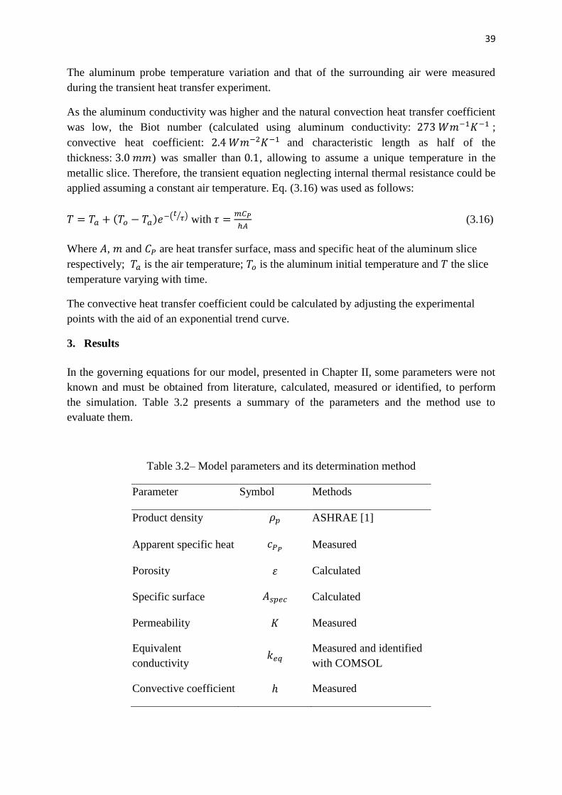
39
The aluminum probe temperature variation and that of the surrounding air were measured
during the transient heat transfer experiment.
As the aluminum conductivity was higher and the natural convection heat transfer coefficient
was low, the Biot number (calculated using aluminum conductivity: ;
convective heat coefficient: and characteristic length as half of the
thickness: ) was smaller than , allowing to assume a unique temperature in the
metallic slice. Therefore, the transient equation neglecting internal thermal resistance could be
applied assuming a constant air temperature. Eq. (3.16) was used as follows:
with
(3.16)
Where , and are heat transfer surface, mass and specific heat of the aluminum slice
respectively; is the air temperature; is the aluminum initial temperature and the slice
temperature varying with time.
The convective heat transfer coefficient could be calculated by adjusting the experimental
points with the aid of an exponential trend curve.
3. Results
In the governing equations for our model, presented in Chapter II, some parameters were not
known and must be obtained from literature, calculated, measured or identified, to perform
the simulation. Table 3.2 presents a summary of the parameters and the method use to
evaluate them.
Table 3.2– Model parameters and its determination method
Parameter Symbol Methods
Product density ASHRAE [1]
Apparent specific heat Measured
Porosity Calculated
Specific surface Calculated
Permeability Measured
Equivalent
conductivity
Measured and identified
with COMSOL
Convective coefficient Measured

40
3.1. Frozen product density
Product density depends on the product composition and its component individual density.
Table 3.3 presents these data from [1]. Water in the product was a combination of ice and
liquid water, depending on product and temperature. To simplify, it was assumed that all
water was in solid phase.
Table 3.3 - Vegetables composition and density of each component as a function of
temperature, from [1].
Components
Carrots
Mass fraction
(%)
Green beans
Mass fraction
(%)
Density
Water (ice)
Protein
Fat
Carbohydrate
Fiber
Ash
Component density varies with temperature. However, for the working range of temperatures
( to ), the calculated values varied slightly, less than 0.2%, so it was assumed a
constant density. By taking as the reference temperature, the carrot density was found
to be and for green beans.
3.2. Apparent specific heat
There was not a unique phase change temperature in food products, since water was not pure,
as it carried dissolved solids. This means that there was a range of temperatures (between
approximately -1ºC and -18ºC) in which coexisted sensible and latent heat. The concept of an
apparent specific heat allows for taking into account these combined phenomena.
Figure 3.6 presents the experimental values of heat power versus temperature, for a
sample. The shape of the curve presents the typical peak in the temperature range of phase
change, similar to the one predicted by the apparent specific heat in Figure 3.7. However, the
initial freezing point did not occur in the expected value, and it was slightly shifted to the
right.

41
Figure 3.6 -Experimental curve from DSC measure, for carrots.
Figure 3.7 - Apparent specific heat from Food Process Engineering [2]
0,00
1,00
2,00
3,00
4,00
5,00
6,00
7,00
8,00
9,00
10,00
-40,00 -30,00 -20,00 -10,00 0,00 10,00 20,00 30,00
Po
we
r (m
W)
Temperature (°C)

42
Phase change enthalpy was obtained by curve fitting, with the aid of Eqs. (3.8) and (3.9),
starting with the initial freezing point ( ) ([2]), as shown in Figure 3.8, with an
enthalpy origin of .
Figure 3.8 -Comparison between enthalpy experimental measure and values from [1].
As it can be seen, in the range of to , there was a similar behavior between
experimental values and the ones from Chapter 9, ASHRAE Handbook [1]. However the
numerical values were a bit different.
The enthalpy balance approach was used in order to predict heat transfer with phase change
and introduced in the numerical model. The apparent specific heat was modeled as in Eq.
(3.17).
(3.17)
where ( ) is the specific heat of completely frozen product, ( ) is
the free water fraction in the product, ( ) is the water latent heat of fusion.
The enthalpy of the product can be written from Eq. (3.18) as
(3.18)
Figure 3.9 presents the comparison between the model, experimental measures and values
from [1], using as an enthalpy origin. The model tried to take into account the
apparent specific heat in a large range of temperatures, even near the initial freezing point.
0,00
5,00
10,00
15,00
20,00
25,00
30,00
35,00
40,00
45,00
-18,00 -16,00 -14,00 -12,00 -10,00 -8,00
Enth
alp
y o
f fr
oze
n c
arro
ts (
kJ/k
g)
Temperature (°C)
ASHRAE
Experimental
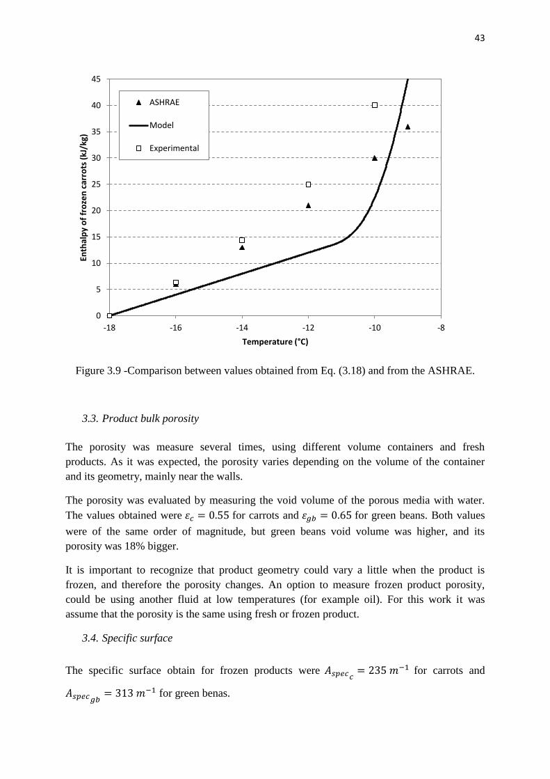
43
Figure 3.9 -Comparison between values obtained from Eq. (3.18) and from the ASHRAE.
3.3. Product bulk porosity
The porosity was measure several times, using different volume containers and fresh
products. As it was expected, the porosity varies depending on the volume of the container
and its geometry, mainly near the walls.
The porosity was evaluated by measuring the void volume of the porous media with water.
The values obtained were for carrots and for green beans. Both values
were of the same order of magnitude, but green beans void volume was higher, and its
porosity was 18% bigger.
It is important to recognize that product geometry could vary a little when the product is
frozen, and therefore the porosity changes. An option to measure frozen product porosity,
could be using another fluid at low temperatures (for example oil). For this work it was
assume that the porosity is the same using fresh or frozen product.
3.4. Specific surface
The specific surface obtain for frozen products were for carrots and
for green benas.
0
5
10
15
20
25
30
35
40
45
-18 -16 -14 -12 -10 -8
Enth
alp
y o
f fr
oze
n c
arro
ts (
kJ/k
g)
Temperature (°C)
ASHRAE
Model
Experimental

44
3.5. Bulk product permeability
As was presented in section 2.33, in order to measure bulk permeability, bulk fresh product
was placed into the square suction duct. A plastic seal was used to avoid air preferential
pathways in particular between the top and the upper wall, as shown in Figure 3.10.
Figure 3.10 - Experimental device used for permeability measure.
As permeability is a geometric parameter, it is important to take into account the geometry
disposition of product in the bed, for example parallel to airflow, cross to airflow or
disorganized. As bulk storage condition was to be represented, product was placed randomly,
as is shown in Figure 3.11.

45
Figure 3.11 – Product distribution in the experimental device for permeability measure.
A fan installed in the suction duct allowed imposing a constant airflow through the product
bulk, with a superficial velocity at the inlet of the duct ranging from
to .
Figure 3.12 and Figure 3.13 show measured pressure drop versus air velocity, for carrots and
green beans respectively. The measures were repeated three times for carrots and two times
for green beans, for the same velocities. In both cases, little data dispersion was noticed.
Figure 3.12 - Experimental measures of pressure drop in a carrots bed (length 40 cm) for
different air velocities and its curve fitting.
0,0
5,0
10,0
15,0
20,0
25,0
30,0
35,0
0,00 0,02 0,04 0,06 0,08 0,10 0,12 0,14
-DP
/L (
Pa/
m)
Velocity (m/s)
Experimental
Linear (Experimental ) -DP/L=256.51v
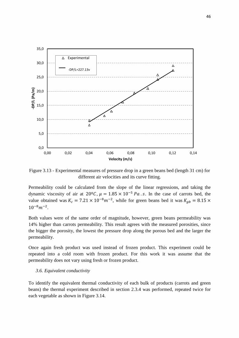
46
Figure 3.13 - Experimental measures of pressure drop in a green beans bed (length 31 cm) for
different air velocities and its curve fitting.
Permeability could be calculated from the slope of the linear regressions, and taking the
dynamic viscosity of air at , . In the case of carrots bed, the
value obtained was , while for green beans bed it was
.
Both values were of the same order of magnitude, however, green beans permeability was
14% higher than carrots permeability. This result agrees with the measured porosities, since
the bigger the porosity, the lowest the pressure drop along the porous bed and the larger the
permeability.
Once again fresh product was used instead of frozen product. This experiment could be
repeated into a cold room with frozen product. For this work it was assume that the
permeability does not vary using fresh or frozen product.
3.6. Equivalent conductivity
To identify the equivalent thermal conductivity of each bulk of products (carrots and green
beans) the thermal experiment described in section 2.3.4 was performed, repeated twice for
each vegetable as shown in Figure 3.14.
0,0
5,0
10,0
15,0
20,0
25,0
30,0
35,0
0,00 0,02 0,04 0,06 0,08 0,10 0,12 0,14
-DP
/L (
Pa/
m)
Velocity (m/s)
Experimental
Linear (Experimental ) -DP/L=227.13v

47
Figure 3.14 - Comparison between temperatures measured in experiments 1 (Exp 1) and 2
(Exp 2), for carrot slices.
A unidirectional conduction model was implemented in COMSOL software, with data from
product density, product specific heat and porosity, calculated earlier in this work.
In order to estimate the range of equivalent conductivity, it was evaluate for the limit
conditions, parallel and series arranged of air and product by using equations from Table 3.1.
The limit values for carrot slices were , and
for green beans.
Simulations were carried out by sweeping the equivalent conductivity in these ranges. Figure
3.15 shows the comparison between experimental measures and simulation results for carrot
slices, for an imposed equivalent conductivity of . As it can be seen,
the general shape of temperature evolution for different positions was similar. However, it
was not possible to adjust all temperatures for the same value of equivalent conductivity. This
was probably due to the porosity variation near the wall, which was not taken into account by
the model since a uniform porosity was assumed for the entire domain. For this reason, only
product temperature in the center of the box ( ) was used for the comparison.
-22,00
-20,00
-18,00
-16,00
-14,00
-12,00
-10,00
-8,00
-6,00
-4,00
0 1000 2000 3000 4000 5000 6000 7000 8000
Tem
pe
ratu
re (
ºC)
time (s)
T1 - Exp 2 T1 - Exp 1 T2 - Exp 2 T2 - Exp 1 T3 - Exp 2 T3 - Exp 1 TH - Exp 2

48
Figure 3.15 - Comparison between experimental and simulated temperatures versus time, for
carrot slices, with
The minimum square method was used to obtain the better adjustment of equivalent
conductivity. The error, , was calculated for each temperature value as in Eq. (3.19), then
the mean quadratic error, , was calculated for each equivalent conductivity and were
plotted in Figure 3.16.
(3.19)
(3.20)
-22,00
-20,00
-18,00
-16,00
-14,00
-12,00
-10,00
-8,00
-6,00
0 1000 2000 3000 4000 5000 6000 7000
Tem
pe
ratu
re (
°C)
time (s)
T3_sim
T2_sim
T1_sim
T3_exp
T2_exp
T1_exp
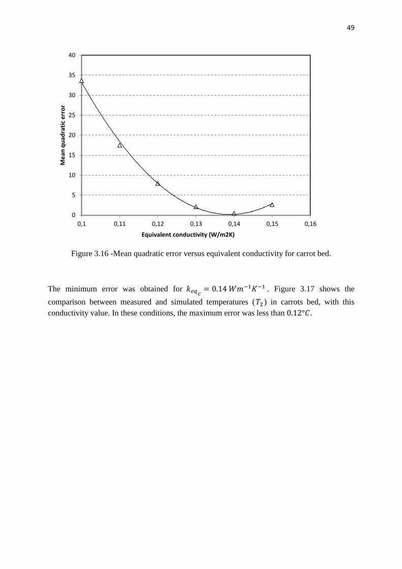
49
Figure 3.16 -Mean quadratic error versus equivalent conductivity for carrot bed.
The minimum error was obtained for . Figure 3.17 shows the
comparison between measured and simulated temperatures ( ) in carrots bed, with this
conductivity value. In these conditions, the maximum error was less than .
0
5
10
15
20
25
30
35
40
0,1 0,11 0,12 0,13 0,14 0,15 0,16
Me
an q
uad
rati
c e
rro
r
Equivalent conductivity (W/m2K)
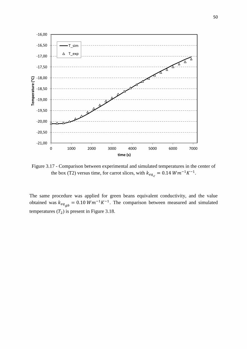
50
Figure 3.17 - Comparison between experimental and simulated temperatures in the center of
the box (T2) versus time, for carrot slices, with .
The same procedure was applied for green beans equivalent conductivity, and the value
obtained was . The comparison between measured and simulated
temperatures ( ) is present in Figure 3.18.
-21,00
-20,50
-20,00
-19,50
-19,00
-18,50
-18,00
-17,50
-17,00
-16,50
-16,00
0 1000 2000 3000 4000 5000 6000 7000
Tem
pe
ratu
re (
°C)
time (s)
T_sim
T_exp

51
Figure 3.18 - Comparison between experimental and simulated temperatures in the center of
the box (T2) versus time, for green beans, with .
The identified values of equivalent conductivity can be validated by comparing to calculated
values by different models. Table 3.4 presents calculated values for carrot slices and green
beans, using air conductivity and product conductivities,
for frozen carrots (from [2]) and for frozen green
beans (calculated form product composition, according to the equation propose in Chapter 9,
ASHRAE Handbook [1]). The difference in products conductivities and porosities explains
that the equivalent conductivity was bigger for carrots bed than for green beans bed.
As it can be seen, the identified equivalent conductivities were into the range established by
parallel and series models. The others correlations also gave results between these limits. The
geometric model gave a good approximation, as an order of magnitude. However, this model
give better results the more similar were fluid and solid conductivities [4]. Using Krupiczka
correlation, the values calculated in both cases were very similar to the experimental ones.
The error, defined as in Eq. (3.21), was 7.1% for carrots and 10% for green beans.
(3.21)
Finally the method proposed to identify the equivalent conductivity of a porous medium was
adequate.
-19,00
-18,50
-18,00
-17,50
-17,00
-16,50
-16,00
-15,50
-15,00
-14,50
-14,00
0 1000 2000 3000 4000 5000 6000 7000 8000
Tem
pe
ratu
re(°
C)
time(s)
T_exp
T_sim
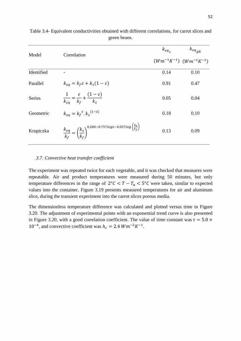
52
Table 3.4- Equivalent conductivities obtained with different correlations, for carrot slices and
green beans.
Model Correlation
Identified - 0.14 0.10
Parallel 0.91 0.47
Series
0.05 0.04
Geometric
0.18 0.10
Krupiczka
0.13 0.09
3.7. Convective heat transfer coefficient
The experiment was repeated twice for each vegetable, and it was checked that measures were
repeatable. Air and product temperatures were measured during 50 minutes, but only
temperature differences in the range of were taken, similar to expected
values into the container. Figure 3.19 presents measured temperatures for air and aluminum
slice, during the transient experiment into the carrot slices porous media.
The dimensionless temperature difference was calculated and plotted versus time in Figure
3.20. The adjustment of experimental points with an exponential trend curve is also presented
in Figure 3.20, with a good correlation coefficient. The value of time constant was
, and convective coefficient was .

53
Figure 3.19– Experimental temperature measurement of aluminum probe and surrounding air
versus time.
Figure 3.20– Aluminum probe dimensionless temperature versus time and its curve fitting, for
carrot slices.
In order to evaluate the experimental convective coefficient obtained for carrot slices, it was
compared to the convective coefficient for a sphere. Assuming the unique phenomena was
-17,00
-16,00
-15,00
-14,00
-13,00
-12,00
-11,00
0 200 400 600 800 1000
Tem
pe
ratu
re (
ºC)
time (s)
Aluminum slice
Air
y = e-0,00050x R² = 0,98773
0
0,1
0,2
0,3
0,4
0,5
0,6
0,7
0,8
0,9
1
0 200 400 600 800 1000 1200
(T(t
)-Ta
)/(T
o-T
a)
time (s)

54
conduction in the air around the sphere (convection was neglected in respect to conduction),
the Nusselt number for a single sphere was , and using the slice diameter as
characteristic length, and the air conductivity ,
the convective coefficient was .
Considering the local natural convection, the correlation proposed by Yuge [11] for heat
transfer between a single sphere and air could be used to obtain an order of magnitude.
(3.22)
Using the temperature difference obtained from the simulation of the order of , diameter
as the characteristic length ( ), and air properties at -15°C (
, and ) the Grashoff was
. Finally the Nusselt number was and the convective heat transfer coefficient
obtained was .
For a bed of spheres, Wakao and Kaguei [8] proposed the following correlation for forced
convection.
(3.23)
In the present experiment, the Reynolds number was of the order of , calculated after a
simulated velocity ), the diameter as a characteristic length
and air kinematic viscosity ( ). The convective heat transfer coefficient
using Eq. (3.23) is .
Ben Amara [10] proposed a correlation obtained for a macroporous media compose by
spheres in cubic arrange, as follows.
(3.24)
This correlation was obtained from an experimental measurement, similar to the one proposed
here, and also similar to the one of Wakao and Kaguei (Eq. (3.19)). The convective heat
transfer coefficient using Eq. (3.24) is .
Despite these correlations were for spheres and in some cases for a single one, the values
obtained were of the same order of magnitude than the experimental one.
The same procedure was repeated with green beans (Figure 3.21) and the time constant was
and convective coefficient was .
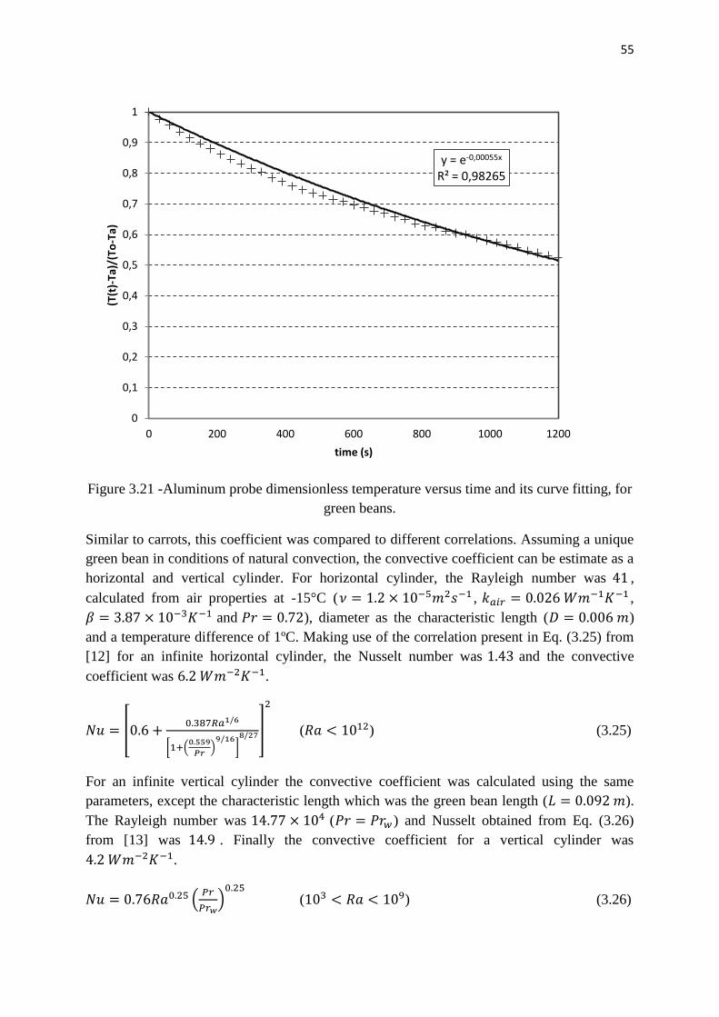
55
Figure 3.21 -Aluminum probe dimensionless temperature versus time and its curve fitting, for
green beans.
Similar to carrots, this coefficient was compared to different correlations. Assuming a unique
green bean in conditions of natural convection, the convective coefficient can be estimate as a
horizontal and vertical cylinder. For horizontal cylinder, the Rayleigh number was ,
calculated from air properties at -15°C ( , ,
and ), diameter as the characteristic length ( )
and a temperature difference of 1ºC. Making use of the correlation present in Eq. (3.25) from
[12] for an infinite horizontal cylinder, the Nusselt number was and the convective
coefficient was .
( ) (3.25)
For an infinite vertical cylinder the convective coefficient was calculated using the same
parameters, except the characteristic length which was the green bean length ( ).
The Rayleigh number was ( ) and Nusselt obtained from Eq. (3.26)
from [13] was . Finally the convective coefficient for a vertical cylinder was
.
( ) (3.26)
y = e-0,00055x R² = 0,98265
0
0,1
0,2
0,3
0,4
0,5
0,6
0,7
0,8
0,9
1
0 200 400 600 800 1000 1200
(T(t
)-Ta
)/(T
o-T
a)
time (s)
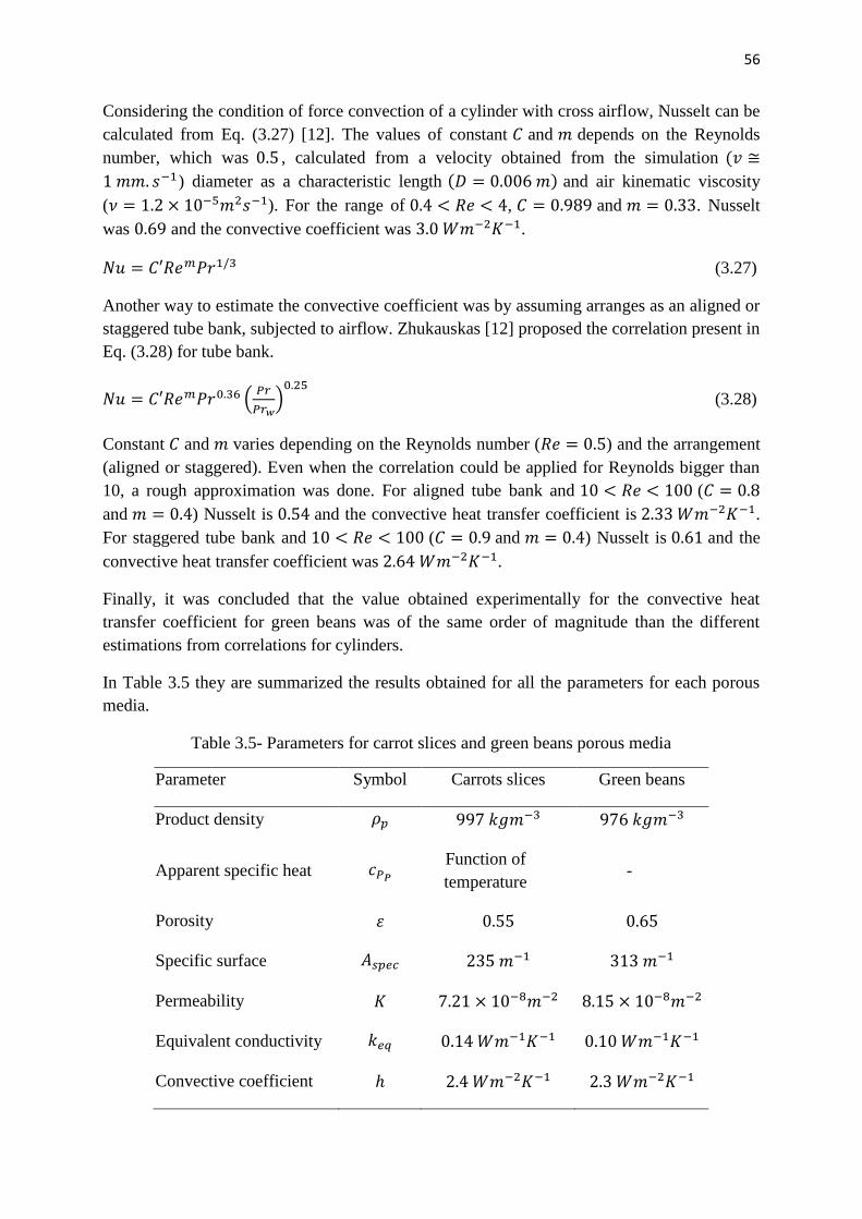
56
Considering the condition of force convection of a cylinder with cross airflow, Nusselt can be
calculated from Eq. (3.27) [12]. The values of constant and depends on the Reynolds
number, which was , calculated from a velocity obtained from the simulation
) diameter as a characteristic length and air kinematic viscosity
( ). For the range of , and . Nusselt
was and the convective coefficient was .
(3.27)
Another way to estimate the convective coefficient was by assuming arranges as an aligned or
staggered tube bank, subjected to airflow. Zhukauskas [12] proposed the correlation present in
Eq. (3.28) for tube bank.
(3.28)
Constant and varies depending on the Reynolds number ( ) and the arrangement
(aligned or staggered). Even when the correlation could be applied for Reynolds bigger than
10, a rough approximation was done. For aligned tube bank and (
and ) Nusselt is and the convective heat transfer coefficient is .
For staggered tube bank and ( and ) Nusselt is and the
convective heat transfer coefficient was .
Finally, it was concluded that the value obtained experimentally for the convective heat
transfer coefficient for green beans was of the same order of magnitude than the different
estimations from correlations for cylinders.
In Table 3.5 they are summarized the results obtained for all the parameters for each porous
media.
Table 3.5- Parameters for carrot slices and green beans porous media
Parameter Symbol Carrots slices Green beans
Product density
Apparent specific heat
Function of
temperature -
Porosity
Specific surface
Permeability
Equivalent conductivity
Convective coefficient

57
4. Conclusion
Parameters can be classified in three types: the ones which depend only on thermophysical
properties (product density and apparent specific heat), which depends only on the geometry
(porosity, specific surface and permeability) and the ones which depends on both (equivalent
conductivity and convective heat transfer coefficient). From the results, summarized in Table
3.5, it can be seen that parameters in the first case, were similar for both vegetables since they
were compose mainly by water (carrots 87.79% and green beans 90.27%). Green beans
density is 2% smaller than carrot density. Pure geometric parameters were of the same order
of magnitude for both porous media, but were a bit bigger for green beans than for carrots. It
was not strange since product geometries were completely different. Green beans porosity
was 18% bigger, specific surface was 33% bigger and permeability was 14% bigger, respect
to carrots. These results appear to be in concordance, since the biggest the porosity, the
biggest the permeability. In case of the last two parameters, equivalent conductivity and
convective heat transfer coefficient, the results were of the same order of magnitude.
However, the equivalent conductivity varied more significantly, since it is directly related
with the geometric appearance. As the porosity is smaller for carrots, there were more
vegetables per bed volume, leading to a higher conductivity, and less air with lower
conductivity. That situation explained the equivalent conductivity augmentation on 28.5%. In
the case of convective coefficient, differences in geometric characteristics appear not to have
a large impact. Fluid (air) and solid phases in porous media have similar thermal properties,
and finally the convective coefficients were practically the same (7% higher for carrots bed).
In general, parameters which characterize these porous media were similar for both products,
even though the different geometries.
58
Bibliography
[1] ASHRAE Handbook—Refrigeration, Chapter 9: Thermal properties of food, 2006.
[2] Dennis R. Heldman and R. Paul Singh, Food Process Engineering, Second Edition, The
Avi Publishing Company, Inc., 1981.
[3] Q.T. Pham, Modelling heat and mass transfer in frozen foods: a review, Int. J.
Refrigeration 29 (2006) 876-888
[4] Donald A. Neild and Adrian Bejan, Convection in porous media, Third Edition, Springer
Science + Business Media, Inc., 2006.
[5] S. Ben Amara, Ecoulements et transferts thermiques en convection naturelle dans les
milieux macroporeux alimentaires: Application aux réfrigérateurs ménagers, Thèse doctorant
de l’Institut National de Paris-Grignon, 2005
[6] Derek B. Ingham and Iaon Pop, Transport phenomena in porous media, Elseiver Science
Ltd., 1998.
[7] Warren M. Rohsenow, James P. Hartnett, Young I. Cho, Handbook of Heat Transfer,
Third Edition, The McGraw-Hill Companies, Inc., 1998.M. Kaviany, Chapter 9: Heat
Transfer in Porous Media
[8] N. Wakao and S. Kaguei, Heat and mass transfer in packed beds, Gordon and Breach
Science Publishers Inc., 1982.
[9] G. Alvarez, Etude de transfert de chaleur et de matière au sein d’un échangeur complexe
de type « palette», Thèse doctorant de l’Ecole National du Génie Rural des Eaux et des Forêts
(Paris), 1992.
[10] S.B. Amara, O. Laguerre, D. Flick, Experimental study of convective heat transfer during
cooling with low air velocity in stack of objects, International Journal of Thermal Sciences 43
(2004) 1213-1221
[11] J.P. Holman, Transferencia de calor, McGraw-Hill Book Company, 1972.
[12] Frank D. Incropera, David, P De Witt, Fundamentos de transferencia de calor, 4ª
Edición, Prentice Hall, Mexico 1999.
[13] M.A. Mijeev, I.M. Mijeeva, Fundamentos de termotransferencia, Mir, 1979.

59
BULK STORAGE OF FROZEN VEGETABLES AS A MACROPOROUS
MEDIA: MODEL EXPERIMENTAL VALIDATION
Abstract
This chapter is dedicated to the experimental validation of the numerical model developed to
predict frost formation during storage of frozen vegetables submitted to external temperature
fluctuations. The numerical model is able to predict air velocity field, air and product
temperatures, and local frost formation. Results are validated in respect to a set of
independent experimental results that shown in general a good agreement. Airflow circulation
is as expected due to natural convection. Product temperature simulated behavior agrees with
measurements, and temperature values differ by less than 12%. Frost formation predicted by
the model was , smaller than the experimental measurement of ,
but still within the same order of magnitude. The model predicted correctly the most
susceptible regions to frost formation. The effect model parameters was analyzed in order to
point out how to improve it. Frost formation is mostly affected by the effective mass
diffusivity and convective heat coefficient within the storage container. Better simulated
results ( )are obtained by the adjustment of these parameters.
Key words: frozen food; macroporous media; heat and mass transfer; temperature
fluctuation; natural convection; frost formation.
60
Index
1. Introduction ................................................................................................................................. 62
2. Numerical modeling ................................................................................................................... 63
2.1. Governing equations .................................................................................................. 65
2.1.1. Momentum ......................................................................................................... 65
2.1.2. Energy ................................................................................................................. 65
2.1.3. Water mass balance ............................................................................................ 65
2.2. Initial conditions ........................................................................................................ 66
2.3. Boundary conditions .................................................................................................. 66
2.4. Parameter identification ............................................................................................. 67
2.4.1. Bulk product porosity ......................................................................................... 68
2.4.2. Specific surface................................................................................................... 68
2.4.3. Product density ................................................................................................... 68
2.4.4. Product specific heat ........................................................................................... 68
2.4.5. Bulk product permeability .................................................................................. 69
2.4.6. Equivalent conductivity ...................................................................................... 70
2.4.7. Convective heat transfer coefficient ................................................................... 72
2.4.8. Heat transfer coefficient across the container wall ............................................. 74
2.4.9. Saturated vapor concentration ............................................................................ 75
2.4.10. Effective mass diffusivity ............................................................................... 75
2.5. Numerical resolution .................................................................................................. 75
3. Materials and methods ............................................................................................................... 76
3.1. Product ....................................................................................................................... 76
3.2. Containers .................................................................................................................. 76
3.3. Freezers ...................................................................................................................... 77
3.4. Temperature cycles .................................................................................................... 77
3.5. Frost formation .......................................................................................................... 78
4. Results .......................................................................................................................................... 78
4.1. Temperature ............................................................................................................... 78
4.2. Frost formation .......................................................................................................... 81
4.2.1. Experimental results ........................................................................................... 81
4.2.2. Simulation results ............................................................................................... 82
4.3. Parametric assessment ............................................................................................... 87

61
5. Conclusion ................................................................................................................................... 90
Bibliography ........................................................................................................................................ 90

62
1. Introduction
In the frozen food industry, in particular for vegetables, products are frozen and bulk stored
into box pallets at low temperature in cold rooms. Storage duration can range from few
months up to one year, before market distribution. During that long-term storage, frozen
products may be exposed to air temperature fluctuations that can impact product quality.
Thereafter, losses can be expected due to a poor management of storage environmental
conditions.
A number of studies in the literature have shown the effect of both, temperature fluctuations
and heterogeneity, on product quality. Quality losses and kinetics degradation such as vitamin
C, color and drip loss are often considered an important issue to be reduced (Martins et al. [1],
Theofania Tsironi et al. [2]).
Frost formation during storage of frozen food is also one of major industrial problems.
Experimental studies (Poovarodom [3]) have been dedicated to analyze the influence of
temperature changes in average, amplitude and frequency of fluctuations. Laguerre and Flick
[4] studied experimentally frost formation on packed bed of potato and melon balls inside
hermetic boxes, stored in domestic freezers. They proposed a qualitative simplified model to
explain the observed phenomena. These models showed that frost was developed whenever
the temperature was low inside the box and/or its fluctuation was also low. They observed
less frost in more insulated boxes, less frost at higher frequency and lower amplitude of
exterior air temperature variation, and less frost for potatoes than for melon balls due to the
lower surface water activity.
Desiccation of frozen food during storage has been studied by several authors [5 - 9], that
generally admit that both, large amplitude of fluctuations and low frequencies, increase
weight loss in product.
Pallet boxes may be heated or cooled due to external air fluctuation along the storage period,
causing the product to change from one position to another inside the pallet, followed by
variations on the pallet inside air temperature. Close to the external walls, product and air
temperature can be submitted to more intense changes than the ones in the core of the pallet,
due to thermal inertia. Water from warmer product is sublimated, transported by the air and
finally deposited at the cooler frozen surfaces, where frost formation occurs.
Few works in literature report natural convection in food stacks. Laguerre et al. [10] studied
the transient heat transfer by free convection in a packed bed of spheres in a refrigerated
cavity. They proposed a porous media approach and compared it with direct CFD method and
experimental measures. The numerical results obtained with both approaches were in good
agreement with the experimental values. CFD approach required more computational time,
and the proposed approach did not predict in detail the fluid flow patterns and temperature at
pore scale. Evaporative mass transfer inside bulks submitted to natural convection was studied
by Beukema et al. [11]. They developed a two dimensional and two phase model (product-air)
to predict temperature and moisture distribution during cooling and bulk storage of fresh

63
agricultural products in a cylindrical container. They validated the proposed model with
experimental values for potatoes during long time periods.
Despite the importance of frost formation during storage of frozen food, there is little work on
the modeling of the coupled phenomena: airflow, heat transfer and mass transfer for bulk of
frozen food porous media under natural convection.
The objective of this chapter is to establish and validate a numerical model able to predict
airflow, heat transfer and frost formation in a cylindrical container filled with bulk frozen
vegetables (slices of carrots) exposed to temperature fluctuations. Parameters were obtained
from literature or by experimental identification, and the model was validated by performing
independent experiments.
2. Numerical modeling
In this section, a numerical model is proposed to predict airflow, heat and mass transfer and
frost formation into a close container with a bulk of frozen product, during the storage in a
cold room. Figure 4.1 depicts the cylindrical container filled with slices of carrots, used in the
proposed model.
Figure 4.1 - Simulation domain for the numerical simulation of airflow, heat and mass
transfer and frost formation filled with slices of carrots.
The container lateral wall was meant to be built with plastic material, and top and bottom
surfaces were perfectly insulated. That imposition, although not physically realistic, may
represent an intermediate sample of frozen products within a pallet tower, placed inside the
cold room.
Product and air inside the container were model as a macroporous media. The container was
submitted to air temperature fluctuation only through the lateral wall. This geometry was
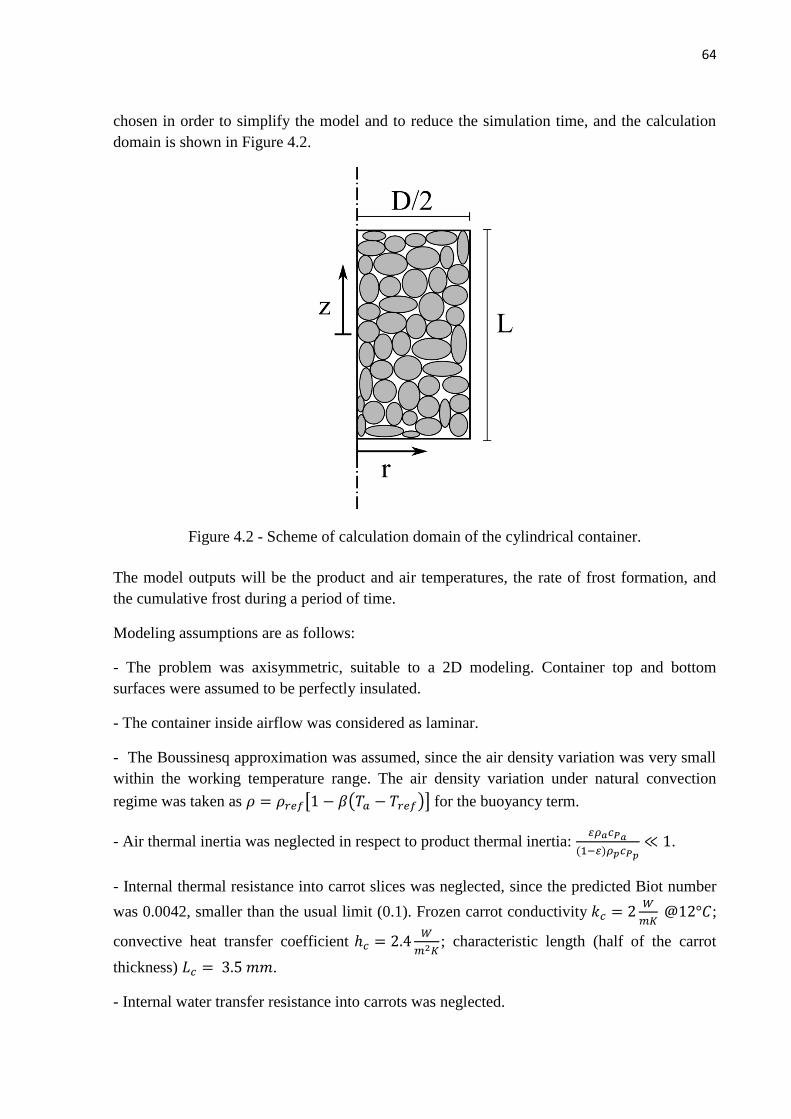
64
chosen in order to simplify the model and to reduce the simulation time, and the calculation
domain is shown in Figure 4.2.
Figure 4.2 - Scheme of calculation domain of the cylindrical container.
The model outputs will be the product and air temperatures, the rate of frost formation, and
the cumulative frost during a period of time.
Modeling assumptions are as follows:
- The problem was axisymmetric, suitable to a 2D modeling. Container top and bottom
surfaces were assumed to be perfectly insulated.
- The container inside airflow was considered as laminar.
- The Boussinesq approximation was assumed, since the air density variation was very small
within the working temperature range. The air density variation under natural convection
regime was taken as for the buoyancy term.
- Air thermal inertia was neglected in respect to product thermal inertia:
.
- Internal thermal resistance into carrot slices was neglected, since the predicted Biot number
was 0.0042, smaller than the usual limit (0.1). Frozen carrot conductivity
;
convective heat transfer coefficient
; characteristic length (half of the carrot
thickness) .
- Internal water transfer resistance into carrots was neglected.
65
- Temperature of the external lateral container wall was known experimentally, as a function
of time.
- Radiation heat transfer was neglected inside the container.
- The dispersion term in the energy equation for the porous medium was neglected.
2.1. Governing equations
The following equations, momentum, energy and mass transfer were solved according to the
previous assumptions.
2.1.1. Momentum
Continuity and momentum equations were used assuming the Boussinesq approximation. The
momentum equation integrates also the Darcy term for fluid flow in porous media.
(4.1)
(4.2)
where is the porosity, the Darcy superficial air velocity into the porous medium, the
porous media permeability and the thermal coefficient of volumetric expansion.
2.1.2. Energy
Energy equation was written for the air, Eq. (4.3), and for the product, Eq. (4.4), and coupled by the
convective heat transfer between them. The specific surface, , was defined as the
total heat transfer surface of carrots over bed volume of porous medium.
(4.3)
(4.4)
where is the equivalent conductivity of carrots bed and the convective heat transfer
coefficient inside the container. Last term of Eq. (4.4) takes into account latent heat of ice
sublimation, where and are ice contents in frost and product per unit volume of porous
medium respectively.
2.1.3. Water mass balance
Total water mass balance inside product container is written as follows,
(4.5)

66
where , is water content in air and is the vapor effective or total mass diffusivity in the
porous media.
Equation (4.6) describes the frost formation.
(4.6)
Frost is formed whenever vapor concentration in air is higher than saturated vapor
concentration at product temperature .
Equation (4.7) describes product dehydration, which occurs when vapor concentration in air is
smaller than vapor concentration in air in equilibrium with the product .
(4.7)
In these equations, was the convective mass transfer coefficient, obtained from the
convective heat transfer coefficient using Lewis analogy. was the mass transfer
resistance of the vegetable skin, and was the water activity of the product. Although there
is not skin resistance on peeled carrots, this term was used to take into account the mass
transfer resistance due to the thin layer of dehydrated product near the surface [5, 9, 12, 13].
2.2. Initial conditions
Mechanical and thermal inertia of air were very small, allowing to assume initial air velocity
to be zero and initial air temperature to be equal to that of the product. Product initial
temperature profile was obtained by data interpolation from initial temperature measurements
at the center of the container and near its wall.
It was assume that air initial vapor concentration was zero ( ) and there was no frost on
product surface ( .
2.3. Boundary conditions
Modeling assumptions declared in the begging of this chapter allowed to write the following
boundary conditions:
(4.8)
(4.9)
(4.10)
(4.11)
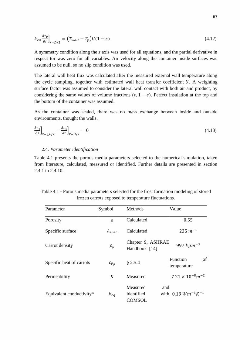
67
(4.12)
A symmetry condition along the z axis was used for all equations, and the partial derivative in
respect to was zero for all variables. Air velocity along the container inside surfaces was
assumed to be null, so no slip condition was used.
The lateral wall heat flux was calculated after the measured external wall temperature along
the cycle sampling, together with estimated wall heat transfer coefficient . A weighting
surface factor was assumed to consider the lateral wall contact with both air and product, by
considering the same values of volume fractions ( . Perfect insulation at the top and
the bottom of the container was assumed.
As the container was sealed, there was no mass exchange between inside and outside
environments, thought the walls.
(4.13)
2.4. Parameter identification
Table 4.1 presents the porous media parameters selected to the numerical simulation, taken
from literature, calculated, measured or identified. Further details are presented in section
2.4.1 to 2.4.10.
Table 4.1 - Porous media parameters selected for the frost formation modeling of stored
frozen carrots exposed to temperature fluctuations.
Parameter Symbol Methods Value
Porosity Calculated
Specific surface Calculated
Carrot density Chapter 9, ASHRAE
Handbook [14]
Specific heat of carrots § 2.5.4
Function of
temperature
Permeability Measured
Equivalent conductivity*
Measured and
identified with
COMSOL
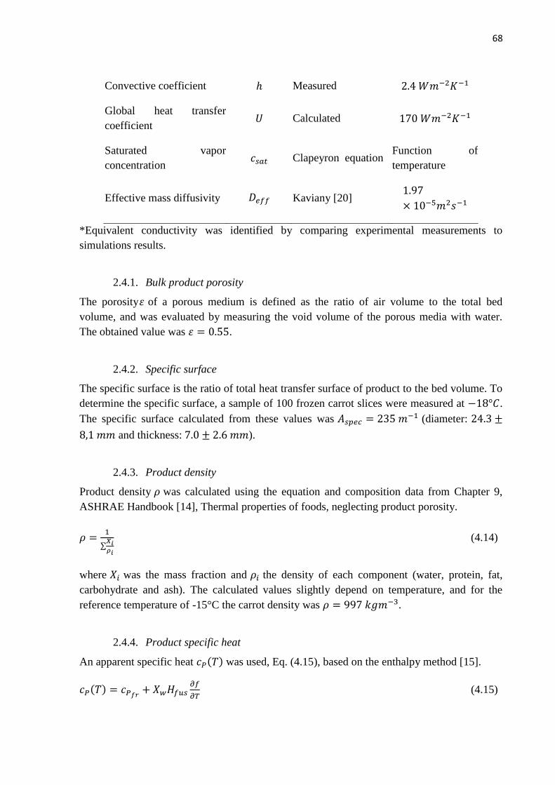
68
Convective coefficient Measured
Global heat transfer
coefficient Calculated
Saturated vapor
concentration Clapeyron equation
Function of
temperature
Effective mass diffusivity Kaviany [20]
*Equivalent conductivity was identified by comparing experimental measurements to
simulations results.
2.4.1. Bulk product porosity
The porosity of a porous medium is defined as the ratio of air volume to the total bed
volume, and was evaluated by measuring the void volume of the porous media with water.
The obtained value was .
2.4.2. Specific surface
The specific surface is the ratio of total heat transfer surface of product to the bed volume. To
determine the specific surface, a sample of 100 frozen carrot slices were measured at .
The specific surface calculated from these values was (diameter:
and thickness: ).
2.4.3. Product density
Product density was calculated using the equation and composition data from Chapter 9,
ASHRAE Handbook [14], Thermal properties of foods, neglecting product porosity.
(4.14)
where was the mass fraction and the density of each component (water, protein, fat,
carbohydrate and ash). The calculated values slightly depend on temperature, and for the
reference temperature of -15°C the carrot density was .
2.4.4. Product specific heat
An apparent specific heat was used, Eq. (4.15), based on the enthalpy method [15].
(4.15)

69
where ( [14]) was the specific heat of a completely frozen product,
( [14]) was the product water content, ( ) was the water latent heat of
fusion. The function varies from 0 (completely frozen) to 1 (unfrozen) within a temperature
range of 10 °C (from to , the initial freezing point [14]).
2.4.5. Bulk product permeability
Bulk product permeability was identified for a one-dimensional flow, using a method
previously reported by Ben Amara [16]. An experimental workbench was built (Figure 4.3)
for that task, where slices of carrots were placed on a square section PVC suction duct
( ).
Figure 4.3 -Experimental workbench built to measure bulk product permeability.
Airflow rate and its superficial velocity were measured at the fan discharge with an Annubar
flow meter (OxitrolAWR-71), connected to an inclined tube manometer. The pressure drop
generated by the bulk product bed (0.4 m in length) was measured with an inclined tube
manometer (+/- 0.1 Pa). Very low velocities were promoted for this experiment, similar in
order of magnitude to the ones under natural convection.
Under these conditions, the momentum equation becomes the Darcy`s equation, assuming
steady state and air at reference temperature ( ).
(4.17)
Air velocity ranged from to and the corresponding pressure drop is
displayed in Figure 4.4.

70
Figure 4.4 - Experimental pressure drops in respect to air velocity in a carrot bed and its linear
fitting.
The permeability calculated from these data was .
2.4.6. Equivalent conductivity
The equivalent or effective conductivity of the bulk of frozen carrots was identified by
solving a one dimensional conduction model, validated experimentally. Frozen carrots were
placed in an insulated box (Figure 4.5) its top wall made of a steel plate.

71
Figure 4.5 - Insulated box built to acquire data to calculate the equivalent or effective
conductivity of the bulk of frozen carrots.
A single type T thermocouple was introduced in the inside of a slice of carrot placed at the
center of the bulk and at the steel plate, and connected to a data logger (Pico Technology TC-
08). The box was kept 24 hours at stable temperature of -20°C and then heated from the top
by a phase change material (-10°C), disposed over the steel plate. Sample temperatures were
recorded along 2 hours.
Top heating allowed for avoiding natural convection inside the box. A one directional and
transient heat conduction model was solved with COMSOL (Eq. 4.18) with adapted boundary
conditions: imposed temperature at the top and no heat flux at the bottom of the box.
(4.18)
Equivalent conductivity was then identified by a least square procedure, comparing
experimental temperatures and simulated ones, shown in Figure 4.6 for the equivalent
conductivity of .
72
Figure 4.6 - Comparison between experimental and simulated temperatures versus time, to
determine equivalent conductivity of the porous media.
Another way to estimate the equivalent conductivity for a porous media is given by the
weighted geometric mean model [17], as follows.
(4.19)
The equivalent conductivity calculated by that last equation was ,
with air conductivity , and frozen carrot conductivity
. The calculated ( ) and identified equivalent ( )
conductivities were of the same order of magnitude.
2.4.7. Convective heat transfer coefficient
A non-stationary method was employed in order to obtain an order of magnitude for the
convective heat transfer coefficient between frozen slices and air inside the bulk of frozen
carrots, similar to the one reported previously by Alvarez [18] and Ben Amara et al. [19], and
depicted in Figure 4.7.
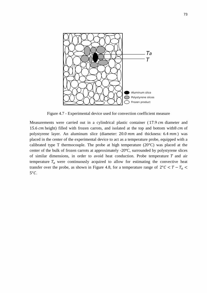
73
Figure 4.7 - Experimental device used for convection coefficient measure
Measurements were carried out in a cylindrical plastic container ( diameter and
height) filled with frozen carrots, and isolated at the top and bottom with of
polystyrene layer. An aluminum slice (diameter: and thickness: ) was
placed in the center of the experimental device to act as a temperature probe, equipped with a
calibrated type T thermocouple. The probe at high temperature (20°C) was placed at the
center of the bulk of frozen carrots at approximately -20ºC, surrounded by polystyrene slices
of similar dimensions, in order to avoid heat conduction. Probe temperature and air
temperature were continuously acquired to allow for estimating the convective heat
transfer over the probe, as shown in Figure 4.8, for a temperature range of
.

74
.
Figure 4.8 - Air and probe temperatures measured in the experimental device depicted in
Figure 4.7.
The probe Biot number was estimated to be less than 0.1 (aluminum
conductivity ; convective heat coefficient and characteristic
length as half of slice thickness, ).Once the probe could be modeled by a lumped
approach, its uniform internal temperature T was expressed as follows, for a constant air
temperature:
with
(4.20)
where , , and are the slice heat transfer surface, mass, specific heat and initial
temperature respectively.
The convective heat transfer coefficient was estimated from that approach, with a value of
.
2.4.8. Heat transfer coefficient across the container wall
This coefficient took into account the conductive thermal resistance of the thick
plastic wall, with thermal conductivity (ploypropylene). The wall heat
transfer coefficient was .
75
2.4.9. Saturated vapor concentration
Saturated vapor concentration was calculated from equation (4.23), assuming the air as an
ideal gas
(4.23)
Saturated vapor pressure was calculated from Clapeyron equation.
(4.24)
The reference values used for pressure and temperature were and
respectively and was the water molar mass.
2.4.10. Effective mass diffusivity
The effective mass diffusivity of the porous media considers the molecular diffusivity
( ) and the dispersion term ( ). The second one appears to takes into account effects of
mass transfer due to hydrodynamic mixing of the interstitial fluid at the pore scale. If Peclet
number defined as in Eq. (4.25) is lower than one, molecular diffusion dominates, and
otherwise mass dispersion cannot be neglected [20].
(4.25)
2.5. Numerical resolution
The set of differential equations was solved with the aid of COMSOL® CFD software
running on a Ubuntu 16.04 LTS computer in a PC Intel® Core ™ i7-6700K CPU @ 4.00GHz
with 15.6 GB RAM. All calculated outputs, including temperatures and water contents, were
performed every 120 seconds, in accordance to the experiment time step.
The discretization of the computational domain was done with COMSOL automatic meshing.
Physics-controlled mesh was employed, which consist on triangular and quadrilateral
elements, with refined near walls. “Fine” and “Finer” meshes were tested for the mesh
independence study. Table 4.2 shows the number of domain and boundary elements for each
mesh.
Table 4.2 - Elements number for different meshes.
Mesh /
Number of elements
Fine Finer
(F) (Fr)
Domain elements 3501 8179

76
Boundary elements 179 351
Table 4.3 presents the maximum difference between the values of temperature ( ) and
frost formed ( ) obtained from the simulation of one day (24 hours) of an impose
temperature cycle (cycle 1presented in section 3.4), with both meshes.
Table 4.3 - Results comparison between meshes fine and finer.
Maximum difference
Temperature 0.092 ºC 0.05%
Frost formed 0.00059 g 0.21%
As it can be seen, the temperature variations were very small in respect to the order of
magnitude of the measured values. The maximum difference in frost formation
represented of the total frost formed during one day. After that, it was assumed that
results were independent of the mesh refinement so a “Fine” mesh was used. The
characteristics of this mesh were: 3233 triangular elements, 268 quadrilateral elements,
minimum element quality 0.121 and average element quality 0.8824.
3. Materials and methods
In order to evaluate the influence of temperature variation on frost formation, containers filled
with frozen carrots were placed sequentially in different freezers.
3.1. Product
This study was carried out using fresh commercial grade carrots. Frozen slices were prepared
out of fresh carrots, peeled, cut, and frozen in a freezer at temperature of -30°C. The averaged
slices dimensions were mentioned in section 2.4.2.
3.2. Containers
Carrots were storage in cylindrical plastic (polypropylene 5) containers of (diameter
; height ; wall thickness ). These containers were insulated
at the top and bottom with thick expanded polystyrene ( ).
Carrotswere disposed in the container into four separated regions (A, B, C, D) made with
semi rigid plastic grids of the same volume (Figure 4.9). These sets up allowed do generate a
central zone separated from a peripheral one; and in two levels, to perform the analysis of
water migration into the container.

77
Figure 4.9 - Plastic grids used into the container to measure frost in each region.
Some carrots slices in the container were equipped with thermocouples, allowing to measure
the temperature at the center of regions A and C, and near to the surface in regions B and D.
Wall and exterior air temperatures were also measure.
3.3. Freezers
Three commercial freezers were used, set to the temperatures of ,
and .
3.4. Temperature cycles
Experiments were carried out with two different air temperature cycles (Table 4.4), which
were performed daily for a two month long period, except for the weekends.
Table 4.4 - Temperature cycles 1 and 2
Cycle Set point 1
(°C)
time 1
(h)
Set point 2
(°C)
time 2
(h)
1 -18.0 23 -5.5 1
2 -18.0 18 -12.8 6
Cycle 1 kept the container in the freezer at and one hour a day it climbed ;
Cycle 2 kept the container in the freezer at the same and six hour a day at .

78
Product, wall and exterior air temperatures were measured for each temperature cycle, using
thermocouples type T (copper/constantan) connected to a data logger (Pico Technology TC-
08) and a computer.
3.5. Frost formation
Frost formation was measured weekly by weight loss for the four regions (A, B, C, D) during
the two month of temperature cycling. To evaluate weight loss, containers were opened in a
low temperature room ( ), and each region was removed separately and was shacked
during 30 seconds to remove the frost formed on carrots surface. Frost was deposited over an
absorbent paper and then it is weighted using a balance of high precision ( ).
The drawbacks of this method are that it may have errors due to several issues, like
environmental influences, handling operation or hysteresis effects due to frost removal on
each measure. On the other hand, this method is extremely simple, cheap and easily
implemented.
4. Results
The cycles 1 and 2 used for the experimental measurements were simulated using the
proposed model and imposing the container wall temperature measure experimentally during
the cycles, as a boundary condition. Results from experiments and simulations were analyzed
and compared to validate the model. A study of the effect of the identified parameters in the
model was done. Finally an estimation of frost formed in real conditions is present.
4.1. Temperature
Product temperatures were measured into the container in the center of each region as
described in section 3. Figure 4.10 and Figure 4.11 shows simulated and measured
temperature evolution over time, for cycles 1 and 2, respectively.

79
Figure 4.10 - Comparison between experimental and simulated temperatures for cycle 1.
Figure 4.11 - Comparison between experimental measured and simulated temperatures for
cycle 2.

80
From the last figures can be observed a good agreement between experimental values and
simulated ones, as they show the same behavior. Nevertheless, simulated temperatures only
vary along the radial direction ( and ). Experimental temperatures show slight
differences between top and bottom of the container. Temperature differences and
varied with time and it was smaller than . This can be explained by differences in
experimental insulation between top and bottom. Indeed the shape of the container lid could
generate a thermal resistance at the upper surface. Despite similar thermal behavior from
simulations and experimental measures, the simulated temperature curves were always
slightly higher than the experimental ones. Table 4.5 presents the maximum deviation
between simulated and measured temperatures for each cycle. The biggest differences were
for cycle 1 and for cycle 2, which represents an error less than 12% and 8%
respectively, respect to experimental temperatures in ºC.
Table 4.5 - Maximum difference between experimental and numerical values of temperatures.
In cycle 1 (Figure 4.10), product near the wall quickly changed its temperature, following the
behavior of the wall temperature. During the first hour, the product was heated from the wall
and its temperature was smaller than the one at the wall. Product temperature increases fast
because of the temperature difference between product and wall. After one hour, when the
container returns to the freezer at , wall temperature decreases and product was hotter
than the wall and there was a heat flux in the opposite direction. Product temperature
decreases slowly because temperature difference between product and wall was smaller than
during the first hour. Product in the center (A, D) changes its temperature more slowly and
there was a delay due to the thermal inertia. Temperature increased during the first two hours
and a half and its temperature increase rate increased with time since temperature difference
between product in the center and in the periphery become bigger. At six hours experimental
values show that practically all the system was in equilibrium.
In cycle 2 (Figure 4.11) the behavior of product temperatures was similar near the wall and in
the center. As time heating the cylinder was bigger and temperature difference between
product and wall was smaller than in cycle 1, the effect of thermal inertia was smaller.
Cycle
(°C)
TA TB TC TD
1 0.98 1.61 0.87 1.39
2 0.94 0.88 1.11 1.13

81
4.2. Frost formation
Different phenomena are involved during frost formation. Completely frozen products consist
of ice and liquid water (bounded water) with high concentration of solved solid. Air and
product temperatures may change when submitted to external air cycles. If vapor
concentration of the surrounding air is lower than saturated vapor concentration at product
surface, ice may sublimate and water vapor is transferred to the air. In that case, the latent
heat needed to sublimate water was provided by the product itself. After that, water vapor was
transferred to the air by diffusion and free convection. Humid air may undergo condensation
by reaching cold surfaces (temperature lower than the air dew point), causing frost formation
to start around the product surfaces. At the beginning of the process, when the product surface
is frost free, nucleation phenomena occur, giving place to the subsequent crystal growth. That
ice crystal deposition increases cycle by cycle.
Phenomena involved can be classified in periodic, like the ones induced by temperature
cycles, or non-periodic, as nucleation that occurs at the beginning of the frost formation
process. As soon as the nucleuses are formed, water vapor condensates and increases the ice
crystal size. Product dehydration is another important non-periodic phenomenon caused by
accumulative product water sublimation along cycle repetition. Water vapor from the
sublimation front diffuses through this layer, up to the surface. Mass transfer resistance
increases with time, reducing the frost formation rate.
4.2.1. Experimental results
Figure 4.12 shows experimental results of the cumulative frost formation into the container
during two months, for cycle 1 and 2.
Figure 4.12 - Experimental values of cumulative frost formation for cycles 1 and 2,
experiment 1.
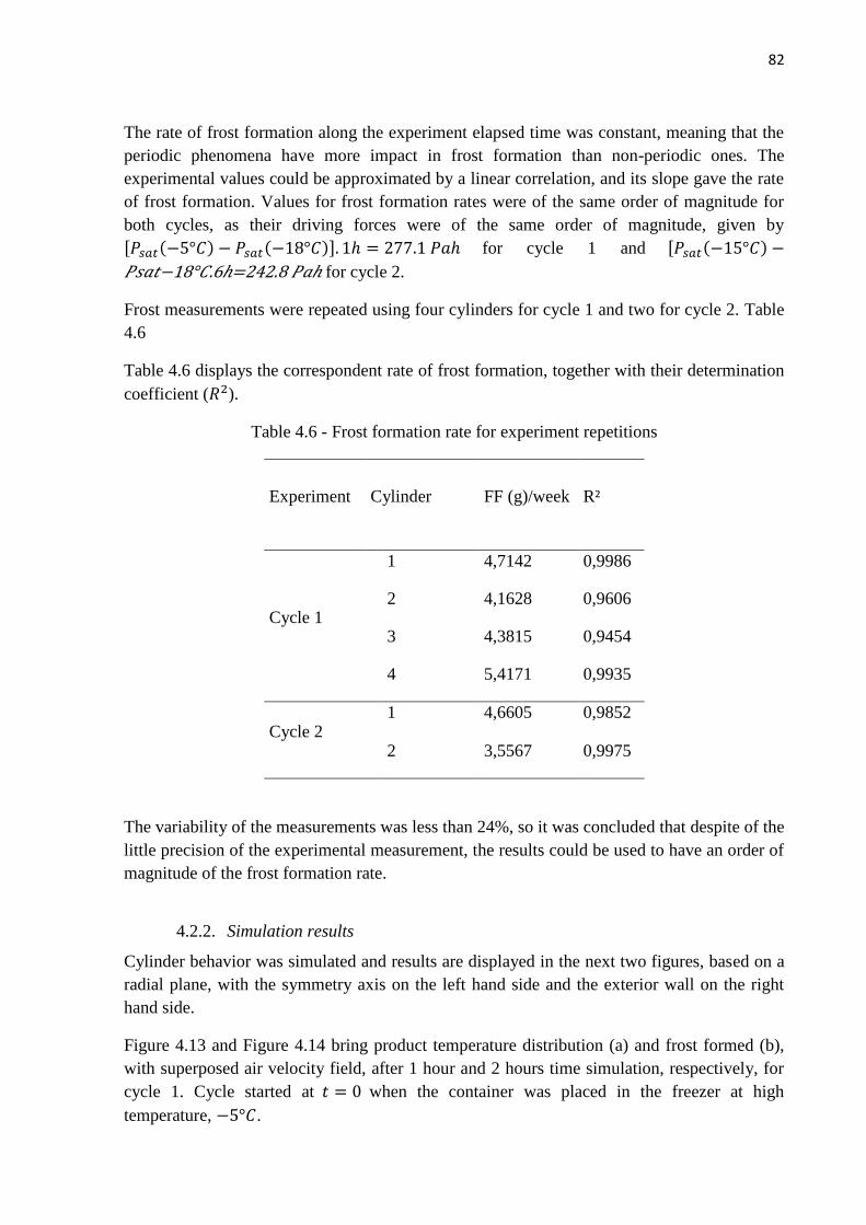
82
The rate of frost formation along the experiment elapsed time was constant, meaning that the
periodic phenomena have more impact in frost formation than non-periodic ones. The
experimental values could be approximated by a linear correlation, and its slope gave the rate
of frost formation. Values for frost formation rates were of the same order of magnitude for
both cycles, as their driving forces were of the same order of magnitude, given by
for cycle 1 and
18° for cycle 2.
Frost measurements were repeated using four cylinders for cycle 1 and two for cycle 2. Table
4.6
Table 4.6 displays the correspondent rate of frost formation, together with their determination
coefficient ( ).
Table 4.6 - Frost formation rate for experiment repetitions
Experiment Cylinder FF (g)/week R²
Cycle 1
1 4,7142 0,9986
2 4,1628 0,9606
3 4,3815 0,9454
4 5,4171 0,9935
Cycle 2 1 4,6605 0,9852
2 3,5567 0,9975
The variability of the measurements was less than 24%, so it was concluded that despite of the
little precision of the experimental measurement, the results could be used to have an order of
magnitude of the frost formation rate.
4.2.2. Simulation results
Cylinder behavior was simulated and results are displayed in the next two figures, based on a
radial plane, with the symmetry axis on the left hand side and the exterior wall on the right
hand side.
Figure 4.13 and Figure 4.14 bring product temperature distribution (a) and frost formed (b),
with superposed air velocity field, after 1 hour and 2 hours time simulation, respectively, for
cycle 1. Cycle started at when the container was placed in the freezer at high
temperature, .

83
a. b.
Figure 4.13 - Simulation results for cycle 1, 1 hour time simulation: a. Product temperature
( ) and velocity field, b. Rate of frost formation ( ) and velocity field.
a. b.
Figure 4.14 -Simulation results for cycle 1, 2 hours time simulation: a. Product temperature
( ) and velocity field, b. Rate of frost formation ( ) and velocity field.
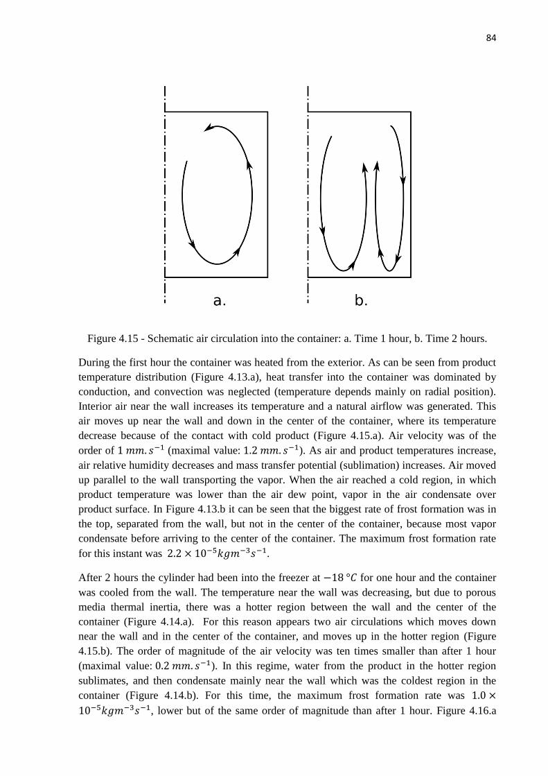
84
Figure 4.15 - Schematic air circulation into the container: a. Time 1 hour, b. Time 2 hours.
During the first hour the container was heated from the exterior. As can be seen from product
temperature distribution (Figure 4.13.a), heat transfer into the container was dominated by
conduction, and convection was neglected (temperature depends mainly on radial position).
Interior air near the wall increases its temperature and a natural airflow was generated. This
air moves up near the wall and down in the center of the container, where its temperature
decrease because of the contact with cold product (Figure 4.15.a). Air velocity was of the
order of (maximal value: ). As air and product temperatures increase,
air relative humidity decreases and mass transfer potential (sublimation) increases. Air moved
up parallel to the wall transporting the vapor. When the air reached a cold region, in which
product temperature was lower than the air dew point, vapor in the air condensate over
product surface. In Figure 4.13.b it can be seen that the biggest rate of frost formation was in
the top, separated from the wall, but not in the center of the container, because most vapor
condensate before arriving to the center of the container. The maximum frost formation rate
for this instant was .
After 2 hours the cylinder had been into the freezer at for one hour and the container
was cooled from the wall. The temperature near the wall was decreasing, but due to porous
media thermal inertia, there was a hotter region between the wall and the center of the
container (Figure 4.14.a). For this reason appears two air circulations which moves down
near the wall and in the center of the container, and moves up in the hotter region (Figure
4.15.b). The order of magnitude of the air velocity was ten times smaller than after 1 hour
(maximal value: ). In this regime, water from the product in the hotter region
sublimates, and then condensate mainly near the wall which was the coldest region in the
container (Figure 4.14.b). For this time, the maximum frost formation rate was
, lower but of the same order of magnitude than after 1 hour. Figure 4.16.a
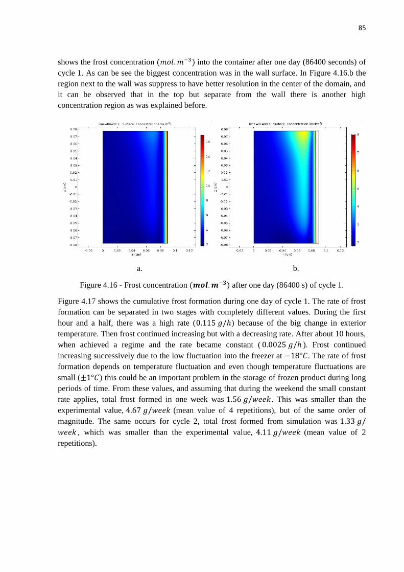
85
shows the frost concentration into the container after one day (86400 seconds) of
cycle 1. As can be see the biggest concentration was in the wall surface. In Figure 4.16.b the
region next to the wall was suppress to have better resolution in the center of the domain, and
it can be observed that in the top but separate from the wall there is another high
concentration region as was explained before.
a. b.
Figure 4.16 - Frost concentration after one day (86400 s) of cycle 1.
Figure 4.17 shows the cumulative frost formation during one day of cycle 1. The rate of frost
formation can be separated in two stages with completely different values. During the first
hour and a half, there was a high rate ( ) because of the big change in exterior
temperature. Then frost continued increasing but with a decreasing rate. After about 10 hours,
when achieved a regime and the rate became constant ( ). Frost continued
increasing successively due to the low fluctuation into the freezer at . The rate of frost
formation depends on temperature fluctuation and even though temperature fluctuations are
small ( this could be an important problem in the storage of frozen product during long
periods of time. From these values, and assuming that during the weekend the small constant
rate applies, total frost formed in one week was . This was smaller than the
experimental value, (mean value of 4 repetitions), but of the same order of
magnitude. The same occurs for cycle 2, total frost formed from simulation was
, which was smaller than the experimental value, (mean value of 2
repetitions).

86
Figure 4.17 - Simulated cumulative frost formation during one day, for cycle 1.
Figure 4.18 presents the averages percentages of frost measured experimentally in each region
for cycle 1. The results were 20% in region A, 23% in region B, 27% in region C and 30% in
region D. Regions in the top had 7% more frost than the ones in the bottom and regions in the
periphery, near the wall, had 3% more frost than regions in the center. So most frost was
formed in region D and the lowest was in region A. This result agrees with simulation results
(Figure 4.16). The regions near the wall had more frost, but the volume is smaller, so total
frost near the wall (regions B and D) was smaller than in region in the top and centered
(region A). Another detail to take into account is that when the product nets were removed to
measure frost, the frost layer next the container wall was detached and it was not quantified.
The model predicted properly the more susceptible zones to frost formation into the container.

87
Figure 4.18 -Percentage of frost measure experimentally in each region.
4.3. Parametric assessment
Model parametric assessment was performed by changing one by one some parameters value
and comparing temperature evolution and frost formation for cycle 1. Selected parameters
were: permeability K, equivalent conductivity keq, convective heat transfer coefficient h
between product and air into the container and effective mass diffusivity , within a range
from half to twice its reference value (Table 4.1).Results for product temperature at region are
presented in Figure 4.19.
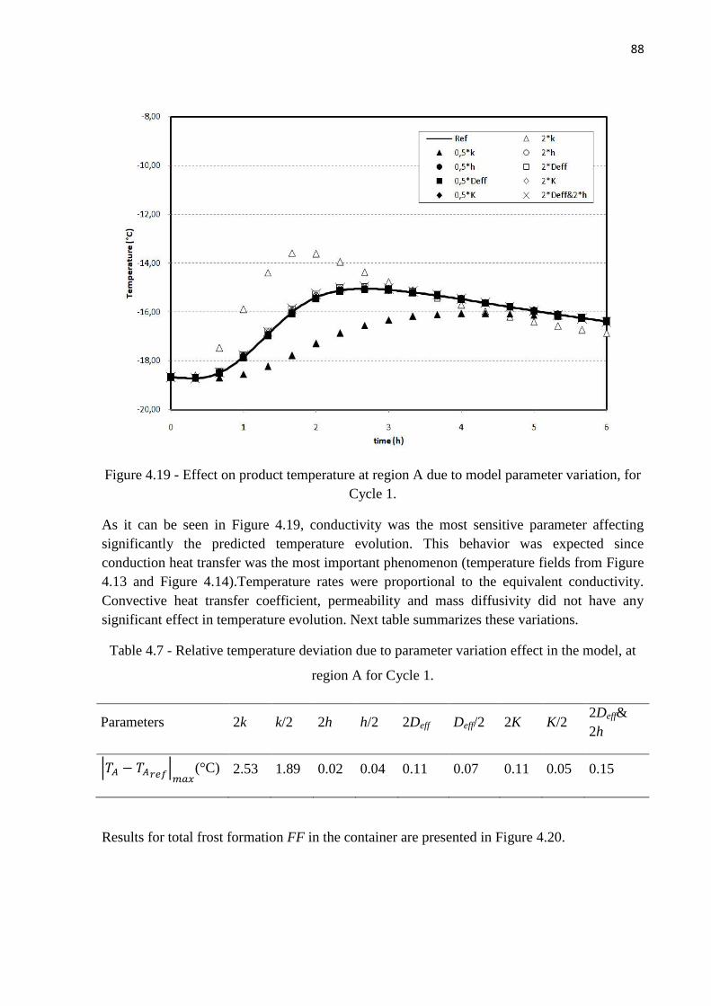
88
Figure 4.19 - Effect on product temperature at region A due to model parameter variation, for
Cycle 1.
As it can be seen in Figure 4.19, conductivity was the most sensitive parameter affecting
significantly the predicted temperature evolution. This behavior was expected since
conduction heat transfer was the most important phenomenon (temperature fields from Figure
4.13 and Figure 4.14).Temperature rates were proportional to the equivalent conductivity.
Convective heat transfer coefficient, permeability and mass diffusivity did not have any
significant effect in temperature evolution. Next table summarizes these variations.
Table 4.7 - Relative temperature deviation due to parameter variation effect in the model, at
region A for Cycle 1.
Parameters 2k k/2 2h h/2 2Deff Deff/2 2K K/2 2Deff&
2h
(°C) 2.53 1.89 0.02 0.04 0.11 0.07 0.11 0.05 0.15
Results for total frost formation FF in the container are presented in Figure 4.20.

89
Figure 4.20 - Effect on total frost formation due to model parameter variation, for Cycle 1.
In contrast to temperature, frost formation evolution depends significantly on all the
parameters, but permeability. Frost formation increased with increasing convective coefficient
or effective mass diffusivity while it decreased with equivalent conductivity of the porous
media. The effect of each parameter was evaluated with the maximum variation defined as in
equation (4.26) and presented in Table 4.8.
(4.26)
Table 4.8 - Relative frost formation deviation due to parameter variation effect in the model,
for Cycle 1
Parameters 2k k/2 2h h/2 2Deff Deff/2 2K K/2 2Deff&2h
(%) 22.80 20.52 26.46 25.00 55.96 38.42 2.26 0.59 99.39
The effective mass diffusivity was the most important parameter, reaching a frost formation
56% higher than the reference value during one day, followed by the convective coefficient
with 26%. Finally, the condition varying both parameters simultaneously to twice of the
reference value led to an increase in the frost formation of approximately twice the reference
value.

90
Table 4.9 brings the comparison of total frost formed during one day of cycle 1, one day of
weekend, and total frost during one week, for each of the selected parameters.
Table 4.9 - Comparison in frost formation for different scenarios
Scenario
Frost (g) / day Frost (g)
/week cycle
day weekend
1 Ref 0.286 0.063 1.557
2 k/2 0.344 0.090 1.902
3 2k 0.222 0.047 1.206
4 h/2 0.223 0.046 1.206
5 2h 0.352 0.085 1.930
6 Deff /2 0.178 0.042 0,976
7 2Deff 0.441 0.091 2.387
8 K/2 0.285 0.063 1.551
9 2K 0.290 0.063 1.577
10 2Deff&2h 0.567 0.126 3.086
Simulation results for all scenarios were smaller than the experimental value of ,
but of the same order of magnitude. As it was discussed before, this model assumes constant
effective mass diffusivity and in the reference case the dispersion term was ignored. On the
other side, the convective heat transfer coefficient, from which the convective mass transfer
coefficient was also deduced, was measured experimentally in one point into the container to
have an order of magnitude, and was assume to be uniform and constant for the model. In this
context, it was reasonable to consider that these values could be twice the reference value.
Scenario 10 brought that condition and the obtained value was similar to the experimental
one.
5. Conclusion
A simpler model of heat and mass transfer for a porous media and in conditions of free
convection was developed. The model predicted product temperatures for different
temperature cycles with deviations smaller than 12% for cycle 1 and 8% for cycle 2 in respect
to experimental measurements. The model was a good tool to identify more susceptible
regions for frost formation into the container. The rate of frost formation from the model

91
( ) was lower than in the experiment ( ), but the order of magnitude
was correct. Some of the identified parameter could be adjusted to obtain better results in
terms of frost formation ( ).
The importance of different parameters in the frost formation prediction was observed
through a sensitivity study, which pointed out the role of the effective mass diffusivity and
convective heat transfer coefficient.

92
Bibliography
[1] R.C. Martins, M.G. Almeida, C.L.M. Silva, The effect of home storage conditions and
packaging materials on quality of frozen green beans, International Journal of Refrigeration,
27 (2004) 850-861
[2] Theofania Tsironi, Efimia Dermesonlouoglou, Maria Giannakourou, Petros Taoukis, Shelf
life modelling of frozen shrimp at variable temperature conditions, LWT – Food Science and
Technology, 42 (2009) 664 - 671
[3] N. Poovarodom, Modification de la qualité des denrées alimentaires surgelées au cours de
leur conservation: le rôle de l’emballage et l’influence de la température de conservation,
Thèse doctorant de l’Université de Technologie de Compiègne
[4] O. Laguerre, D. Flick, Frost formation on frozen products preserved in domestic freezers,
Journal of Food Engineering, 79 (2007) 124-136
[5] Q.T. Pham and J. Willix, A model for food desiccation in frozen storage, Journal of Food
Science, 49 (1984) 1275-1281
[6] Q.T. Pham and J. Willix, Wheight loss from lamb carcasses in frozen storage: influence of
environmental factors, International Journal of Refrigeration8 (1985) 231-235
[7] Q.T. Pham, J.R. Durbin, J. Willix, Survey of weight loss from lamb in frozen storage,
International Journal of Refrigeration, 5 (1982) 337-342
[8] Y. Phimolsiripol, U. Siripatrawan, D.J. Cleland, Weight loss of frozen bread dough under
isothermal and fluctuating temperature storage conditions, Journal of Food Engineering, 106
(2011) 134-143
[9] L.A. Campañone, V.O. Salvadori, R.H. Mascheroni, Weight loss during freezing and
storage of unpackaged foods, Journal of Food Engineering, 47 (2001) 69-79
[10] O. Laguerre, S.B. Amara, G. Alvarez, D. Flick, Transient heat transfer by free
convection in a packed bed of spheres/ Comparison between two modelling approaches and
experimental results, Applied Thermal Engineering, 28 (2008) 14-24
[11] K.J. Beukema, S. Bruin, J. Schenk, Heat and mass transfer during cooling and storage of
agricultural products, Chemical Engineering Science, 37 (1982) 291-298
[12] L.A. Campañone, V.O. Salvadori, R.H. Mascheroni, Food freezing simultaneous surface
dehydration: approximate prediction of weight loss during freezing and storage, International
Journal of Heat and Mass Transfer, 48 (2005) 1195-1204
[13] A.M. Tocci, R.H. Mascheroni, Numerical models for the simulation of the simultaneous
heat and mass transfer during food freezing and storage, International Communications of
Heat and Mass Transfer, 22 (1995) 251-260
[14] ASHRAE Handbook—Refrigeration, Chapter 9: Thermal properties of food, 2006.
93
[15] Q.T. Pham, Modelling heat and mass transfer in frozen foods: a review, International
Journal of Refrigeration, 29 (2006) 876-888
[16] S. Ben Amara, Ecoulements et transferts thermiques en convection naturelle dans les
milieux macroporeux alimentaires: Application aux réfrigérateurs ménagers, Thèse doctorant
de l’Institut National de Paris-Grignon, 2005.
[17] Donald A. Neild and Adrian Bejan, Convection in porous media, Third Edition, Springer
Science + Business Media, Inc., 2006.
[18] G. Alvarez, Etude de transfert de chaleur et de matière au sein d’un échangeur complexe
de type « palette», Thèse doctorant de l’Ecole National du Génie Rural des Eaux et des Forêts
(Paris), 1992.
[19] S.B. Amara, O. Laguerre, D. Flick, Experimental study of convective heat transfer during
cooling with low air velocity in stack of objects, International Journal of Thermal Sciences,
43 (2004) 1213-1221
[20] Warren M. Rohsenow, James P. Hartnett, Young I. Cho, Handbook of Heat Transfer,
Third Edition, The McGraw-Hill Companies, Inc., 1998.M. Kaviany, Chapter 9: Heat
Transfer in Porous Media
94
5 CONCLUSION
A model of heat and mass transfer was proposed in order to predict frost formation
into a closed container filled with frozen vegetables. The problem was study as a macroporous
media compose by the product and the surrounding air. Natural convection air flow was
assumed into the container, who promotes water mass transport. The model was developed in
the commercial software CFD COMSOL, and it was test imposing different exterior air
temperature fluctuations (boundary conditions). Results of four temperature cycles were
compared, varying one by one: average temperature, amplitude and frequency of oscillation.
As general result it was observed that product temperature behavior is as expected, and it is
directly associated with frost formation into the container. The bigger the product temperature
variation, the bigger the amount of frost formed. Frost formation increase with large
amplitude of oscillation, but decrease with higher frequencies and mean temperatures.
Parameters that characterized the porous media were measure and identified for two
porous media: slices of frozen carrots- air, and frozen green beans- air. Parameters can be
classified in three types: the ones that depend only on thermophysical properties (product
density and apparent specific heat), which depends only on the geometry (porosity, specific
surface and permeability) and the ones which depends on both (equivalent conductivity and
convective heat transfer coefficient). From the results, summarized in Table 3.5, it can be seen
that parameters in the first case, were similar for both vegetables since they were compose
mainly by water (carrots 87.79% and green beans 90.27%). Green beans density is 2% smaller
than carrot density. Pure geometric parameters were of the same order of magnitude for both
porous media, but were a bit bigger for green beans than for carrots. It was not strange since
product geometries were completely different. Green beans porosity was 18% bigger, specific
surface was 33% bigger and permeability was 14% bigger, respect to carrots. These results
appear to be in concordance, since the biggest the porosity, the biggest the permeability. In
case of the last two parameters, equivalent conductivity and convective heat transfer
coefficient, the results were of the same order of magnitude. However, the equivalent
conductivity varied more significantly, since it is directly related with the geometric
appearance. As the porosity is smaller for carrots, there were more vegetables per bed volume,
leading to a higher conductivity, and less air with lower conductivity. That situation explained
the equivalent conductivity augmentation on 28.5% In the case of convective coefficient,
differences in geometric characteristics appear not to have a large impact. Fluid (air) and solid

95
phases in porous media have similar thermal properties, and finally the convective
coefficients were practically the same (7% higher for carrots bed). In general, parameters
which characterize these porous media were similar for both products, even though the
different geometries.
A simpler model of heat and mass transfer for a porous media and in conditions of free
convection was developed. The model predicted product temperatures for different
temperature cycles with deviations smaller than 12% for cycle 1 and 8% for cycle 2 in respect
to experimental measurements. The model was a good tool to identify more susceptible
regions for frost formation into the container. The rate of frost formation from the model
( ) was lower than in the experiment ( ), but the order of magnitude
was correct. Some of the identified parameter could be adjusted to obtain better results in
terms of frost formation ( ).
The importance of different parameters in the frost formation prediction was observed
through a sensitivity study, which pointed out the role of the effective mass diffusivity and
convective heat transfer coefficient.
5.1 General conclusion and perspectives
A model was developed to predict frost formation during the storage of a bulk of
frozen vegetables. This model is a first step of the project Flexifroid, in order to create a tool
for the industry to predict frost formation during normal storage conditions, or in cases of
disconnection from the energy supply.
This work would continue in different ways, in direction to a macroscopic study,
improving the model and introducing it into a model of the air flow and heat exchange in the
cold room, or microscopic study, analyzing recrystallization and frost densification.
Some possible lines of work are summarized below:
- Improve the model to consider recrystallization phenomena and frost densification.
- Made a micro tomography in a small scale sample of the porous media, in order to
understand the phenomena involved during the frost formation.
- Validate the model changing to a cubic container (3D model) with real dimensions.
- Implement a reduced model.

96
- Model air flow and heat transfer into the cold room with a stack of pallets in the real
arrangement.
97
BIBLIOGRAPHY
Amara, S.B. Laguerre, O. Flick, D. Experimental study of convective heat transfer
during cooling with low air velocity in stack of objects, International Journal of Thermal
Sciences 43, p. 1213-1221, 2004.
Beukema, K.J. Bruin, S. Schenk, J. Heat and mass transfer during cooling and storage
of agricultural products, Chemical engineering Science 37, p. 291-298, 1982.
Campañone, L.A. Salvadori, V.O. Mascheroni, R.H. Weight loss during freezing and
storage of unpackaged foods, Journal of Food Engineering 47, p. 69-79, 2001.
Campañone, L.A. Salvadori, V.O. Mascheroni, R.H. Food freezing simultaneous
surface dehydration: approximate prediction of weight loss during freezing and storage,
International Journal of Heat and Mass Transfer 48, p. 1195-1204, 2005.
Chin-Hsiang Cheng, Yu-Chieh Cheng, Preditions of frost growth on a cold plate in
atmospheric air, International Communications in Heat and Mass transfer 8, p. 953-962,
2001.
Dona, C.L.G. and Stewart Jr, W.E. Numerical analysis of natural convection heat
transfer instored high moisture corn, Journal of Agricultural Engineering Research 40, p.
275-284, 1988.
Graciela Alvarez, Pierre-Emmanuel Bournet, Denis Flick, Two dimensional
simulation of turbulent flow and transfer through stacked spheres, International Journal of
Heat and Mass Transfer 46, p. 2459-2469, 2003.
Laguerre, O. Amara, S.B. Alvarez, G. Flick, D. Transient heat transfer by free
convection in a packed bed of spheres/ Comparison between two modeling approaches and
experimental results, Applied Thermal Engineering 28, p. 14-24, 2008.
Laguerre, O. Flick, D. Frost formation on frozen products preserved in domestic
freezers, Journal of Food Engineering 79, p. 124-136, 2007.
Martins, R.C. Almeida, M.G. Silva, C.L.M. The effect of home storage conditions and
packing materials on the quality of frozen green beans, International Journal of
Refrigeration 27, p. 850-861, 2004.

98
Méndew Bustabad, O. Weight loss during freezing and storage of frozen meat,
Journal of Food Engineering 41, p. 1-11, 1999.
Mohammad Amini, Ahmad R. Pishevar, Mahmood Yaghoubi, Experimental study of
frost formation on a fin-and-tube heat exchanger by natural convection, International
Journal of Refrigeration 46, p. 37-49, 2014.
Pham, Q. T. Durbin, J. R. and J. Willix, Survey of weight loss from lamb in frozen
storage, Revue Internationale du Froid 5, p. 337-342, 1982.
Pham, Q.T. Moisture transfer due to temperature changes or fluctuations, Journal of
Food Engineering 6, p. 33-49, 1987
Pham, Q.T. and Willix, J. A model for food desiccation in frozen storage, Journal of
Food Science 49, p. 1275-1281, 1984.
Pham, Q.T. and Willix, J. Weight loss from lamb carcasses in frozen storage:
influence of environmental factors, International Journal of Refrigeration 8, p. 231-235,
1985.
Phimolsiripol, Y. Siripatrawan, U. Cleland, D.J. Weight loss of frozen bread dough
under isothermal and fluctuating temperature storage conditions, Journal of Food
Engineering 106, p. 134-143, 2011.
Pieter Verboven, D. Flick, B.M. Nicolai, G. Alvarez, Modelling transport phenomena
in refrigerated food bulks, packages and stacks: basics and advances, International Journal
of Refrigeration 29, p. 985-997, 2006.
Poovarodom, N. Modification de la qualité des denrées alimentaires surgelées au cours
de leur conservation: le rôle de l’emballage et l’influence de la température de conservation,
Thèse doctorant de l’Université de Technologie de Compiègne.
Qin Haijie, li Weizhong, Dong Bo, Zhao Zhihai, Zhu Weiying, Experimental study of
the characteristic of frosting on low-temperatures air cooler, Exprimental Thermal and
Fluid Science 55, p. 106-114, 2014.
99
Tocci, A.M. and Mascheroni, R.H. Numerical models for the simulation of the
simultaneous heat and mass transfer during food freezing and storage, Int. Communications
of Heat and Mass Transfer 22, p. 251-260, 1995.
Warren M. Rohsenow, James P. Hartnett, Young I. Cho, Handbook of Heat
Transfer, Third Edition, The McGraw-Hill Companies, Inc. M. Kaviany, 1998.
Wu, X. Ma, Chu, F. Hu, S. Phase change mass transfer model for frost growth and
densification, International Journal of Heat an Mass Transfer 96, p. 11-19, 2016.