MicroPET Scanner Characterisation

Nuno José Santos Pereira

Dissertação para obtenção do Grau de Mestre em

Engenharia Física Tecnológica

Júri

Presidente: Prof. João Seixas

Orientador: Prof. João Varela

Orientador: Prof. Stefaan Tavernier

Setembro 2008

Resumo

O desenvolvimento de scanners MicroPET, destinados a roedores e pequenos primatas, traz claras

vantagens no estudo clínico destes animais, bem como em testes pré-clínicos de produtos médicos

destinados a humanos. A transferência de tecnologia entre estes e os scanner PET destinados a

humanos é outra mais valia.

No Instituto de Altas Energias da Vrije Universiteit Brussel, um dos membros da Colaboração Crystal

Clear, foi desenvolvido um protótipo de scanner MicroPET - ClearPET1 - tendo em vista a sua comer-

cialização. Este scanner é o objecto de estudo desta tese. Nela é feita a descrição da arquitectura

geral, dos módulos de detecção de radiação, no qual as matrizes phoswich são o elemento central, dos

módulos electrónicos associados à detecção e do sistema de aquisição e tratamento de dados.

Foi experimentalmente determinado o perfil de sensibilidade axial do scanner (ASP); a comparação

dos resultados experimentais com simulações efectuadas na plataforma GATE mostrou que estes estão

em concordância. Um método novo, para o cálculo da fracção de scattered events, com base em ASPs

é apresentado. São igualmente apresentados os resultados da determinação da resolução temporal.

As ferramentas de análise de dados desenvolvidas no âmbito do trabalho experimental desta tese

servirão como base da caracterização do novo protótipo, ClearPET2, em fase de finalização. A realiza-

ção de simulações melhoradas é necessária para compreender alguns aspectos menos claros focados

ao longo da tese.

Palavras-chave:MicroPET, Sensibilidade, Scatter Fraction, Resolução Temporal de Coincidências, GATE

2

Abstract

The development of MicroPET scanners, destined to rodents and small mammals, brings clear adavan-

tages in the clinical study of these animals, as well as in pre-clincal tests of medical prodcuts destinated

to human beings. The technology transfer between these and the human PET scanners is another

advantage.

In the High Energy Institute of the Vrije Universiteit Brussel, one of the members of the Crystal Clear

Colaboration, a MicroPET scanner prototype - ClearPET1 - with the objective of its later commercializa-

tion. This scanner is this thesis’ study object. In it is made the description of the global architecture,

of the detection modules, in which the phoswich matrices are the nuclear element, of the electronic

modules associated with detection and of the data acquisiton and treatment system.

The axial profiles of sensitivity (ASP) were experimentally determined; the comparison between

experimental results and simulations done in the Gate platform, showed the agreement between these.

A new method, to calculate the scattered events fraction based on ASPs is presented. Also the results

of the temporal resolution calculation are presented.

The data analysis tools developed throughout the experimental work part of this thesis will be useful

as a basis for the caractherization of the new prototype, in a final stage: ClearPET2. The realization of

improved simulations is needed to understand some unclear aspects foscued in this thesis.

Key-words:MicroPET, Sensitivity, Scatter Fraction, Coincidence Time Resolution, Gate

3

Contents

1 Introduction 9

2 Positron Emission Tomography 122.1 Positron Emission . . . . . . . . . . . . . . . . . . . . . . . . . . . . . . . . . . . . . . . . 12

2.2 Isotopes . . . . . . . . . . . . . . . . . . . . . . . . . . . . . . . . . . . . . . . . . . . . . . 13

2.3 Photon Interaction . . . . . . . . . . . . . . . . . . . . . . . . . . . . . . . . . . . . . . . . 13

2.3.1 Cross Section and Mean Free Path . . . . . . . . . . . . . . . . . . . . . . . . . . . 14

2.3.2 Compton Scattering . . . . . . . . . . . . . . . . . . . . . . . . . . . . . . . . . . . 15

2.3.3 Photoelectric Effect . . . . . . . . . . . . . . . . . . . . . . . . . . . . . . . . . . . 15

2.4 Photon Detection . . . . . . . . . . . . . . . . . . . . . . . . . . . . . . . . . . . . . . . . . 16

2.4.1 Scintillation Crystals . . . . . . . . . . . . . . . . . . . . . . . . . . . . . . . . . . . 16

2.4.2 Photomultipliers . . . . . . . . . . . . . . . . . . . . . . . . . . . . . . . . . . . . . 17

2.5 Events in PET . . . . . . . . . . . . . . . . . . . . . . . . . . . . . . . . . . . . . . . . . . . 19

2.6 PET Scanner Characteristics . . . . . . . . . . . . . . . . . . . . . . . . . . . . . . . . . . 21

2.6.1 Sensitivity . . . . . . . . . . . . . . . . . . . . . . . . . . . . . . . . . . . . . . . . . 21

2.6.2 Noise Equivalent Count . . . . . . . . . . . . . . . . . . . . . . . . . . . . . . . . . 21

2.6.3 Spatial Resolution . . . . . . . . . . . . . . . . . . . . . . . . . . . . . . . . . . . . 22

2.6.4 Time Resolution . . . . . . . . . . . . . . . . . . . . . . . . . . . . . . . . . . . . . 23

3 ClearPET Scanner 263.1 Scanner Geometry and Architecture . . . . . . . . . . . . . . . . . . . . . . . . . . . . . . 26

3.2 Detection Module . . . . . . . . . . . . . . . . . . . . . . . . . . . . . . . . . . . . . . . . . 27

3.2.1 Scintillation Crystals . . . . . . . . . . . . . . . . . . . . . . . . . . . . . . . . . . . 27

3.2.2 Photo Multipliers . . . . . . . . . . . . . . . . . . . . . . . . . . . . . . . . . . . . . 27

3.2.3 Phoswich Matrix . . . . . . . . . . . . . . . . . . . . . . . . . . . . . . . . . . . . . 28

3.2.4 Cassettes . . . . . . . . . . . . . . . . . . . . . . . . . . . . . . . . . . . . . . . . . 29

3.3 Electronics . . . . . . . . . . . . . . . . . . . . . . . . . . . . . . . . . . . . . . . . . . . . 29

3.4 Data Acquisition (DAQ) . . . . . . . . . . . . . . . . . . . . . . . . . . . . . . . . . . . . . 31

4 Results 344.1 Measurements . . . . . . . . . . . . . . . . . . . . . . . . . . . . . . . . . . . . . . . . . . 34

4.2 Simulation . . . . . . . . . . . . . . . . . . . . . . . . . . . . . . . . . . . . . . . . . . . . . 34

4.3 Sensitivity . . . . . . . . . . . . . . . . . . . . . . . . . . . . . . . . . . . . . . . . . . . . . 35

4.3.1 Full Scanner Sensitivity . . . . . . . . . . . . . . . . . . . . . . . . . . . . . . . . . 35

4.3.2 PMT Singles Rate . . . . . . . . . . . . . . . . . . . . . . . . . . . . . . . . . . . . 36

4.3.3 PMT Pair Coincidence Sensitivity . . . . . . . . . . . . . . . . . . . . . . . . . . . . 39

4

4.3.4 Cassette Pair Coincidences Sensitivity . . . . . . . . . . . . . . . . . . . . . . . . . 41

4.3.5 Full Scanner Sensitivity . . . . . . . . . . . . . . . . . . . . . . . . . . . . . . . . . 42

4.4 Coincidence Time Resolution . . . . . . . . . . . . . . . . . . . . . . . . . . . . . . . . . . 46

5 Conclusions 48

A Simulation 50A.1 General Aspects of GATE . . . . . . . . . . . . . . . . . . . . . . . . . . . . . . . . . . . . 50

A.2 Simulation Structure . . . . . . . . . . . . . . . . . . . . . . . . . . . . . . . . . . . . . . . 50

A.2.1 Geometry . . . . . . . . . . . . . . . . . . . . . . . . . . . . . . . . . . . . . . . . . 50

A.2.2 Physical Processes . . . . . . . . . . . . . . . . . . . . . . . . . . . . . . . . . . . 52

A.2.3 Radioactive Sources . . . . . . . . . . . . . . . . . . . . . . . . . . . . . . . . . . . 52

A.2.4 Digitizing Module . . . . . . . . . . . . . . . . . . . . . . . . . . . . . . . . . . . . . 53

A.2.5 Data Output . . . . . . . . . . . . . . . . . . . . . . . . . . . . . . . . . . . . . . . . 55

B Commercial ClearPET 56

5

List of Figures

2.1 interaction of a photon with an infinitesimal volume with N interaction centres per volume unit . . . 14

2.2 Photon-carbon interaction cross section, in function of the photon’s energy . . . . . . . . . . . . 14

2.3 Compton Scattering between a photon and an electron . . . . . . . . . . . . . . . . . . . . . . . 15

2.4 Generic PMT schematic cross-section . . . . . . . . . . . . . . . . . . . . . . . . . . . . . . . 17

2.5 HAMAMATSU H7546A PhotoMultiplier Tube Cathode Radiant Sensitivity, Sk, and Quantum Effi-

ciency in function of the wavelength of incident photon. Sk is related with Quantum Efficiency by:

Sk = εQλ

1.24. . . . . . . . . . . . . . . . . . . . . . . . . . . . . . . . . . . . . . . . . . . . 18

2.6 137Cs energy spectrum . . . . . . . . . . . . . . . . . . . . . . . . . . . . . . . . . . . . . . . 19

2.7 a)true coincidence; b)scatter coincidence; c)random coincidence . . . . . . . . . . . . . . . . . . 20

2.8 time window method for coincidence sorting; after the first photon is detected a time window of τ

ns is open and another photon is expected in the opposite detector. a) coincidence detected b) no

coincidence detected . . . . . . . . . . . . . . . . . . . . . . . . . . . . . . . . . . . . . . . . 20

2.9 simulated ASP with and without axial shift between cassettes, blue and purple curves respectively . 21

2.10 simulated NEC curve in function of a phantom activity, for a ClearPET scanner prototype . . . . . . 22

2.11 exemplification of parallax error

a) with a layer of crystal, parallax error is p

b) if the layer is subdivided in two, this error b can be reduced . . . . . . . . . . . . . . . . . . . 23

2.12 ClearPET scanner spatial radial resolution. The red and blue curves correspond to measured and

simulated data, respectively . . . . . . . . . . . . . . . . . . . . . . . . . . . . . . . . . . . . 23

2.13 Plot of time difference in coincidences of a test setup for a ClearPET prototype; a Gaussian curve

is fit to the histogram and; the FWHM of the Gaussian curve is the coincidence time resolution . . . 25

3.1 ClearPET1 Scanner . . . . . . . . . . . . . . . . . . . . . . . . . . . . . . . . . . . . . . . . 26

3.2 The scanner geometry is defined in cylindrical coordinates reference frame . . . . . . . . . . . . 27

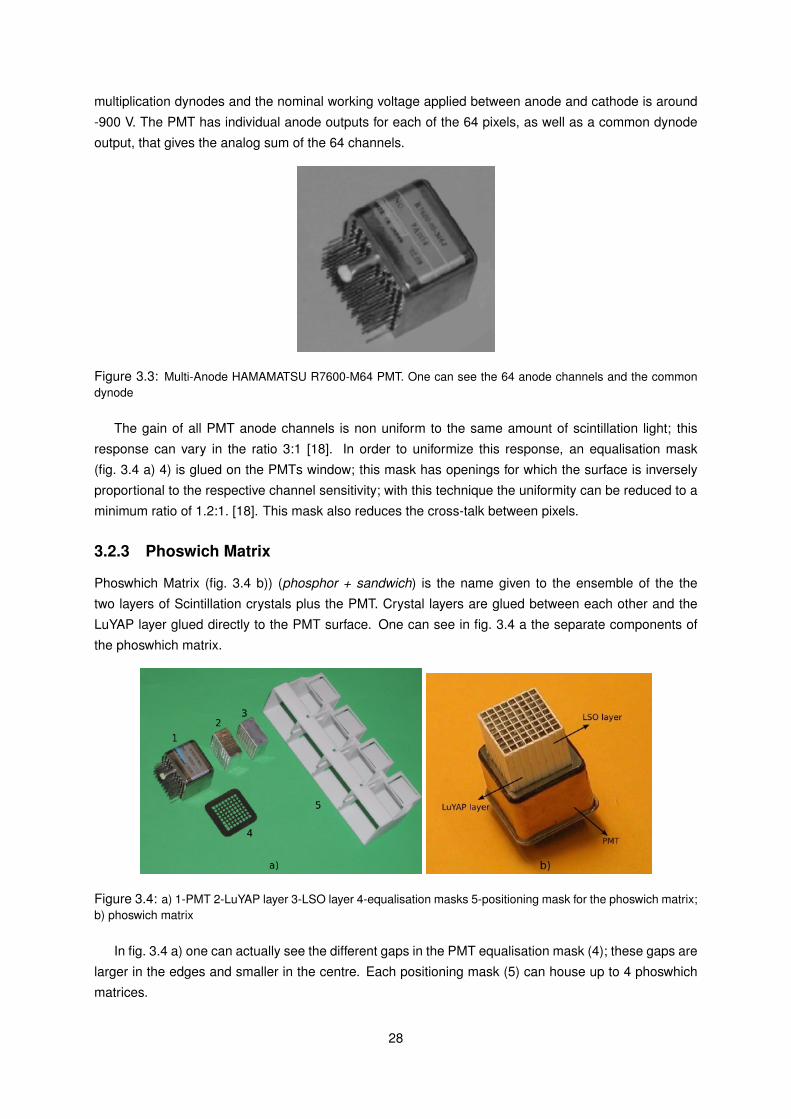
3.3 Multi-Anode HAMAMATSU R7600-M64 PMT. One can see the 64 anode channels and the common

dynode . . . . . . . . . . . . . . . . . . . . . . . . . . . . . . . . . . . . . . . . . . . . . . . 28

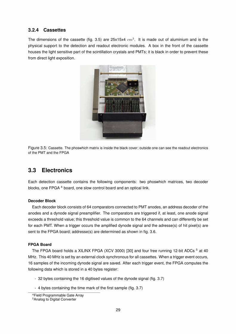
3.4 a) 1-PMT 2-LuYAP layer 3-LSO layer 4-equalisation masks 5-positioning mask for the phoswich

matrix; b) phoswich matrix . . . . . . . . . . . . . . . . . . . . . . . . . . . . . . . . . . . . . 28

3.5 Cassette. The phoswhich matrix is inside the black cover; outside one can see the readout elec-

tronics of the PMT and the FPGA . . . . . . . . . . . . . . . . . . . . . . . . . . . . . . . . . . 29

3.6 when a pulse over threshold level is registered the decoder block searches for the low (blue) high

(red) pixel addresses; four types of events can occur: a)single: low and high pixel addresses are

equal. b) neighbour: low and high pixel addresses are in each others immediate vicinity (direct

or diagonal). c) far: low and high pixels addresses are not equal neither neighbours. d) error of

position: low pixel address is higher than high pixel address . . . . . . . . . . . . . . . . . . . . 30

6

3.7 signal sampling and time mark of the event. the time mark corresponds to the first sampled value

after a trigger occurs. the sampling takes 16 x 25 ns = 400 ns . . . . . . . . . . . . . . . . . . . 30

3.8 Data Acquisition Layout . . . . . . . . . . . . . . . . . . . . . . . . . . . . . . . . . . . . . . . 31

3.9 signal sampling and time mark of the event. the time mark corresponds to the first sampled value

after a trigger occurs. the sampling takes 16 x 25 ns = 400 ns . . . . . . . . . . . . . . . . . . . 32

3.10 distribution of the normalized values of the last pulse sample to the sum of all pulses samples, for

LSO and LuYAP crystals . . . . . . . . . . . . . . . . . . . . . . . . . . . . . . . . . . . . . . 32

4.1 left: simulation of a full ring of 20 cassettes. right: scheme of Cassettes and PMTs numbering.

Cassettes 1 to 4 are diametrically opposing cassettes 11 to 14, respectively; cassette 1 is said to

be the opposite of cassette 11, and so on. Each pair of PMTs in a cassette is labeled as PMT 0 and

PMT 1 . . . . . . . . . . . . . . . . . . . . . . . . . . . . . . . . . . . . . . . . . . . . . . . 35

4.2 PMTs measured singles rate compared with simulation. Left: level 0 PMTs. Right: level 1 PMTs . . 35

4.3 a) singles registered in just one PMT; b) coincidences registered between one pair of specific cas-

settes; c) coincidences registered between any pair of PMT of a pair of opposite cassettes . . . . . 36

4.4 PMTs measured singles rate compared with simulation. Left: level 0 PMTs. Right: level 1 PMTs;

for clearness of visualisation, only one simulated PMT is shown, as simulated single count rate per

PMT is practically equal . . . . . . . . . . . . . . . . . . . . . . . . . . . . . . . . . . . . . . 36

4.5 Measured energy spectrum of all the 16 PMTs . . . . . . . . . . . . . . . . . . . . . . . . . . . 37

4.6 left: determination of PMT 0 of cassette 13 energy resolution. right: determination of a simulated

PMT energy resolution . . . . . . . . . . . . . . . . . . . . . . . . . . . . . . . . . . . . . . . 38

4.7 left: determination of PMT 0 of cassette 13 energy resolution with subtraction of the LSO background 38

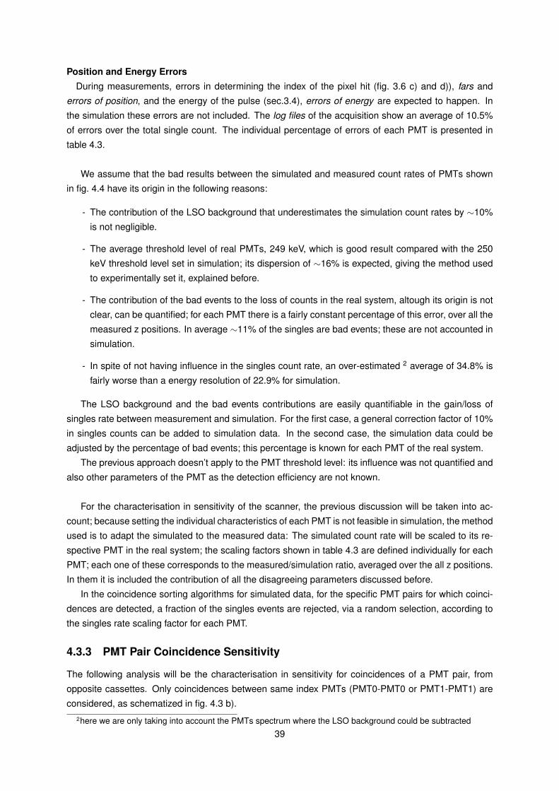
4.8 Simulated and measured sensitivity for PMT pairs. Blue: simulation PMTs index 0. Red: measure-

ment PMTs index 0. Green: simulation PMTs index 1. Black: measurement PMTs index 1 . . . . 40

4.9 Blue: simulated sensitivity profile. Red: measured sensitivity profile; the z position for each one of

the cassette pair plots is corrected for the respective peak deviation shown in table 4.1 . . . . . . . 41

4.10 Blue: simulated sensitivity profile. Red: measured sensitivity profile. The axial position of measured

data is corrected as the average of all the peaks deviations shown in table 4.1 . . . . . . . . . . . 42

4.11 comparison between full scanner and cassette pair sum sensitivity profiles, for measurement and

simulation . . . . . . . . . . . . . . . . . . . . . . . . . . . . . . . . . . . . . . . . . . . . . 43

4.12 left: scattered coincidences contribution to sensitivity; right: scatter fraction . . . . . . . . . . . . 43

4.13 Blue: simulated sensitivity profile. Red: measured sensitivity profile . . . . . . . . . . . . . . . . 44

4.14 For each PMT pair combination of each cassette pair ∆tcoin is plotted; only the points with a Gaus-

sian like shape (blue points) are used to fit a Gaussian distribution; the average of this distribution

is presented as a delay and the FWHM as the time resolution . . . . . . . . . . . . . . . . . . . 46

4.15 Global and crystal layer energy resolutions for each opposite cassette pair; the blue curve refers to

LSO-LSO interactions and the Green curve refers to LuYAP-LuYAP interactions . . . . . . . . . . 47

4.16 full scanner time resolution . . . . . . . . . . . . . . . . . . . . . . . . . . . . . . . . . . . . . 47

A.1 Digitizing module . . . . . . . . . . . . . . . . . . . . . . . . . . . . . . . . . . . . . . . . . . 54

B.1 left: axial profile of sensitivity of the scanner; centre: spatial resolution; coincidence time distribution

and respective time resolution . . . . . . . . . . . . . . . . . . . . . . . . . . . . . . . . . . . 56

B.2 left: coronal view; centre: transversal view; right: sagital view . . . . . . . . . . . . . . . . . . . . 57

7

List of Tables

2.1 main isotopes used in PET and its principal characteristics . . . . . . . . . . . . . . . . . . . . . 13

2.2 list of crystals commonly used in PET systems, and some of their proprieties. An ideal crystal would

have a large light yield like NaI(Tl), a fast decay constant like LSO or LuAP and a small absorption

length like LuAP. Such a crystal doesn’t exist and a compromise between these has to be achieved 17

4.1 Peak deviation is the distance between the measured peak and the simulated peak; the peak-

to-peak ratio is the ratio between the measured and simulated peaks sensitivity values; the total

ratio between measure and simulation doesn’t include the bad data points of cassettes 11 and 12

(sec.4.3.1) . . . . . . . . . . . . . . . . . . . . . . . . . . . . . . . . . . . . . . . . . . . . . 40

4.2 ratios between measured and simulation for the different profile parts. . . . . . . . . . . . . . . . 41

4.3 Real system PMTs characteristics. a): the LSO background could not be fit in the energy spectrum.

b): the photopeak is not completely visible in the energy spectrum . . . . . . . . . . . . . . . . . 45

A.1 geometry definition in GATE . . . . . . . . . . . . . . . . . . . . . . . . . . . . . . . . . . . . 51

8

Chapter 1

Introduction

Since 1970s, Positron Emission Tomography has been used in humans as a clinical diagnosis tech-

nique, specifically in oncology and neurology areas. It allows to trace the spatial distribution of a given

radioactive marker, as a function of metabolism in particular regions of the body. It differs from other

tomography techniques, such as X-Ray or MRI, in the sense that a functional rather than an anatomical

image is obtained. The metabolic modifications usually precede the anatomical ones, so that an ad-

vantage of PET is to detect potential sicknesses, such as cancer metastasis, early enough to allow an

efficient treatment.

Small and medium size mammals, like primates and rodents, have always been used in laboratories

for fundamental disease research or preclinical tests of drugs destined to humans; amongst them, lab

mice, due to the similitude of their genetic expression with humans and to their fast rate of reproduction

and growing, are the most used ones, with a share of 90% [1].

The success of PET scanners in humans naturally led to the interest from pharmaceutical and

biomedical companies in using PET scanners on mice. Another argument that boosted this demand

was the fact that less animals would eventually have to die when using PET in comparison with autora-

diography; this fact comes out as a strong argument for using PET, in the sense that it answers both an

humanitarian and an economic concern.

The existing scanners were not suited to this purpose as their spatial resolution was not adequate to

the animal’s dimensions and also due to practical issues concerning legal impediments on using human

medical devices on mice. Also the price of the scanner is an important factor; the difference in physical

dimensions of an animal dedicated scanner in comparison with an Human one implies that the final price

of the first would be much lower. Due to this in the 90s dedicated small animal PET scanners started to

be developed under the name of microPET.

MicroPET scanners present design challenges relative to human PET scanner, specially concerning

spatial resolution and sensitivity; the smaller dimensions of mice internal organs demand for better

spatial resolution and higher detection efficiency; this demands for new research and development on

detection methods for microPET systems. This parallel development of microPET systems is also clearly

advantageous to the development of human PET scanners.

The Crystal Clear Collaboration (CCC) was set in the 90s in CERN with the aim of developing new

scintillator materials and instrumentation for gamma ray detection, to use in basic research in subatomic

particle physics. In the mid 90s the know-how acquired in this domain started to be used in the devel-

opment of radiation detection methods for biomedical purposes.

A number of sub-projects under the CCC are currently being carried out by the members of the

9

collaboration; one of them consists in developing a prototype for commercialisation of a dedicated small

animal PET scanner : ClearPET. The collaboration succeeded in this particular sub-project and a version

of this scanner is nowadays commercialised by Raytest. The work on this thesis is directed towards one

of these prototypes, built at IIHE-VUB 1 : ClearPET1.

1Inter University Institute for High Energy Physics - Vrije Universiteit Brussel

10

In this thesis, the physical phenomena on which PET techniques rely on will be introduced. An

overlook of positron emission and isotopes will be given. The relevant photon interaction modes: Pho-

toelectric effect and Compton Scattering will be detailed.

As far as the photon detection is concerned, the principal characteristics of scintillation crystals and

Photo Multiplier Tubes (PMTs) will be shown; emphasis will be given to scintillation crystals currently

used in PET techniques and to the general aspects of a PMT.

The general characteristics of PET scanners are presented: the different types of events one expects

to detect. The working characteristics of a PET scanner: sensitivity, noise equivalent count and spatial

and temporal resolutions are introduced.

A major part of this work is dedicated to characterise ClearPET1 Scanner. Its characterisation in-

cludes the general geometry and assemblage of the different parts. The phoswich matrix, composed

by the scintillation crystals and PMTs, and the solutions adopted to overcome the problems in light col-

lection will be detailed. In the electronics module emphasis will be given to the implemented methods

used to treat data from the detection modules. The layout of the Data Acquisition (DAQ) will be pre-

sented; only the major informatics solutions will be presented but the algorithms of data treatment will

be detailed.

The first results of this work will focus on the sensitivity determination of the scanner; throughout the

data analysis simulated and measured data will be systematically compared.

In the second part of results the time resolution of the scanner will be presented.

11

Chapter 2

Positron Emission Tomography

2.1 Positron Emission

Within the beta decay processes family there is the β+ decay which is the physical basis for one of the

imaging techniques used in medicine:Positron Emission Tomography (PET). The positron is one of the

products of the β+ decay; the particle and charge balance reactions are given by eqs. (2.1) and eq. (2.2):

p→ n+ e+ + νe (2.1)

AZN → A

Z−1 N′+ e+ + νe (2.2)

The positron presents the same characteristics, as his anti-particle, the electron, except for its charge,

which is positive; the neutrino does not play any role, as it is an undetectable particle in PET systems.

Positron Interaction in MatterAfter it is emitted, the positron suffers a termalization process, in which its kinetic energy is gradually

lost into the medium; while the termalization process is going on, the positron travels randomly in the

medium until it suffers a pair annihilation.

Pair Annihilation and Photon EmissionAfter termalization is complete, the positron goes into a pair annihilation reaction, i.e., when interacting

with its anti-particle, both annihilate and give rise to the production of photons. Production of a single

photon is forbidden by energy and momentum conservation laws, being the most probable the creation of

two photons (eq. (2.3)), while the production of three photons or more photons are events with extremely

low probabilites [42].

e+ + e− → γ + γ (2.3)

The two emitted photons have an energy of 511 keV and travel in opposite directions. Their angular

deviation is 180o, however, as a possible result of non-zero momentum of positron and electron in the

moment of annihilation, there exists a non-co-linearity in photon trajectories which is represented by a

Gaussian with a full width at half maximum (FWHM) of 0.5o [40]. This non-co-linearity effect may be a

factor of degradation on spatial resolution in PET systems with large diameter [11].

The two emitted photons are the observables on which PET image techniques rely on. To know

which pair of detected photons correspond to a real β+ decay and the subsequent annihilating, will be

further detailed.

12

2.2 Isotopes

PET is a functional technique of medical imaging, i.e., the point is to visualise body regions where

physiological activity, such as blood flow or cell growth is taking place, therefore a positron source is

needed in the specific spot one wants to visualise.

This is achieved with the use of radioactive elements such as 11C, 15O or 18F that undergo β+

decay. These elements are then linked to an organic molecule that plays some role in a given type of

physiological activity. The radioactivity present in this molecule acts then as tracer of this physiological

activity.

The 18F − FDG 1 is one of these carrier molecules and also one of the most commonly used in

oncology; it is a glucose similar molecule which acts as an energy supplier for cell metabolism. This

makes 18F − FDG an ideal tracer to study regions of the body where metabolism is abnormally high,

such as metastasis in cancers.11C is an isotope used to study brain and neurological metabolism, due to its likelihood to link with

neuro-transmitters such as serotonin [2].15O is used to study the kinetics of the transfer of oxygen such as in blood-lung gaseous transfer or

in cell metabolism [4].

All the previously cited radioactive elements have to be produced in particle accelerators like cy-

clotrons. The fact of being short-lived particles makes the physical proximity between the cyclotron and

the examination site important, as well as the rapidity of the chemical processes involved in between the

isotope production and the examination.

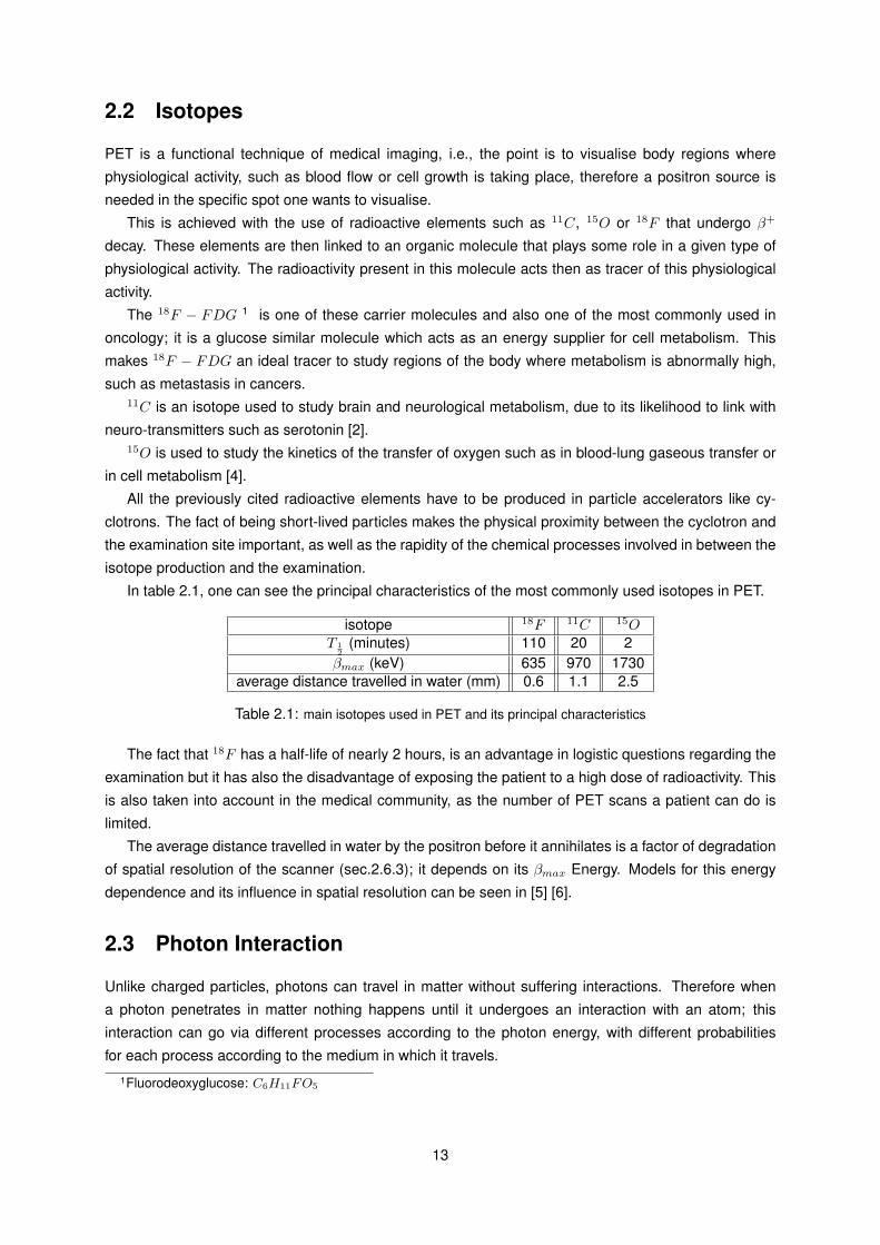
In table 2.1, one can see the principal characteristics of the most commonly used isotopes in PET.

isotope 18F 11C 15OT 1

2(minutes) 110 20 2

βmax (keV) 635 970 1730average distance travelled in water (mm) 0.6 1.1 2.5

Table 2.1: main isotopes used in PET and its principal characteristics

The fact that 18F has a half-life of nearly 2 hours, is an advantage in logistic questions regarding the

examination but it has also the disadvantage of exposing the patient to a high dose of radioactivity. This

is also taken into account in the medical community, as the number of PET scans a patient can do is

limited.

The average distance travelled in water by the positron before it annihilates is a factor of degradation

of spatial resolution of the scanner (sec.2.6.3); it depends on its βmax Energy. Models for this energy

dependence and its influence in spatial resolution can be seen in [5] [6].

2.3 Photon Interaction

Unlike charged particles, photons can travel in matter without suffering interactions. Therefore when

a photon penetrates in matter nothing happens until it undergoes an interaction with an atom; this

interaction can go via different processes according to the photon energy, with different probabilities

for each process according to the medium in which it travels.

1Fluorodeoxyglucose: C6H11FO5

13

2.3.1 Cross Section and Mean Free Path

When a photon travels through matter it has a given probability of interacting with it (fig. 2.1).

Figure 2.1: interaction of a photon with an infinitesimal volume with N interaction centres per volume unit

Considering a particle hitting this target volume, perpendicularly, with infinitesimal thickness dx and

N interaction centres, it is straightforward to see that the probability of interaction is proportional to dx

and N .

There is, however, another factor contributing to this probability: this is defined as cross-section, σ,

and it is dependent on the nature of the interaction. In nuclear and particle physics cross sections have

the dimensions of a surface and the most commonly used unit is the barn (1barn = 10−24cm2).

Therefore, the infinitesimal probability that a particle undergoes an interaction in the infinitesimal

volume mentioned above is given by eq. (2.4)

dW = Ndxσ (2.4)

A cross-section plot for photon-carbon interaction, is shown in fig. 2.2 [12].

Figure 2.2: Photon-carbon interaction cross section, in function of the photon’s energy

The mean free path (mfp) of a particle is defined as being the average distance that a particle travels,

in a given medium, before undergoing the first interaction. The probability of a particle to undergo an

interaction inside a distance x, in a given material is given by eq. (2.5)14

P (x) = 1− e− xλ (2.5)

Where λ is the m.f.p. and it is related with the cross section, given by the eq. (2.6):

λ =1Nσ

(2.6)

One can now see that the mfp. of a particle decreases with increasing density of material (N), and

cross-section σ. The m.f.p. is also commonly referred to as Absorption Length, and is an important

characteristic of scintillation crystals (sec.2.4.1).

2.3.2 Compton Scattering

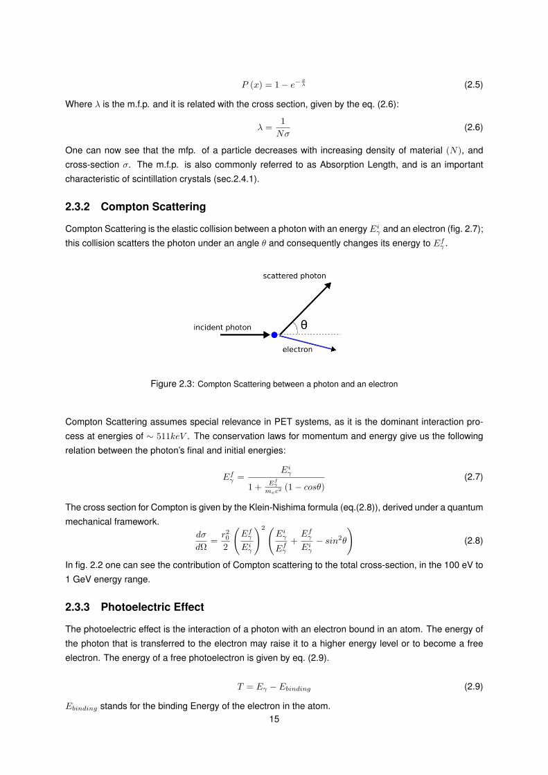
Compton Scattering is the elastic collision between a photon with an energy Eiγ and an electron (fig. 2.7);

this collision scatters the photon under an angle θ and consequently changes its energy to Efγ .

Figure 2.3: Compton Scattering between a photon and an electron

Compton Scattering assumes special relevance in PET systems, as it is the dominant interaction pro-

cess at energies of ∼ 511keV . The conservation laws for momentum and energy give us the following

relation between the photon’s final and initial energies:

Efγ =Eiγ

1 + Efγmec2

(1− cosθ)(2.7)

The cross section for Compton is given by the Klein-Nishima formula (eq.(2.8)), derived under a quantum

mechanical framework.dσ

dΩ=r202

(EfγEiγ

)2(Eiγ

Efγ+EfγEiγ− sin2θ

)(2.8)

In fig. 2.2 one can see the contribution of Compton scattering to the total cross-section, in the 100 eV to

1 GeV energy range.

2.3.3 Photoelectric Effect

The photoelectric effect is the interaction of a photon with an electron bound in an atom. The energy of

the photon that is transferred to the electron may raise it to a higher energy level or to become a free

electron. The energy of a free photoelectron is given by eq. (2.9).

T = Eγ − Ebinding (2.9)

Ebinding stands for the binding Energy of the electron in the atom.15

Photoelectric effect is the dominant interaction at energies of gamma rays less than 100 keV (fig. 2.2).

The energy dependence on cross section is given by eq. (2.10) [13].

σ ∝ Zn

E3.5γ

(2.10)

The coefficient n varies between 4 and 5, and its dependent on the photon energy

2.4 Photon Detection

2.4.1 Scintillation Crystals

Scintillation is the phenomenon that takes place when radiation that travels through a medium excites or

ionises atoms; the atoms returning to their ground state give rise to emission of photons. There are two

groups of scintillators: organic and inorganic. The physics of scintillation won’t be detailed here; focus

will be given to inorganic scintillators.

Inorganic Scintillators, usually ionic crystals , from now on referred to as crystals, have a high Zeff(>

50) and are suitable for X and γ − ray radiation detection. In order to achieve a good performance in

photon detection, some characteristics of crystals have to be taken into account.

- High density, in order to have the highest possible amount of photons interacting in the crystal.

- A large efficiency of produced light, and preferably proportional to the energy of the incoming

radiation. The number of scintillation photons is given by eq. (2.11) [13].

Nsciγ ' ηEγ

2Ebg(2.11)

being Eγ the energy of incoming gamma, Ebg the Energy band-gap of crystal and η the efficiency

of the crystal, which depends on temperature.

- A decay constant τ , significantly lower than rate of incoming photons, in order to achieve a good

temporal resolution.

- Transparency of the crystal to its own scintillation light, allowing it to reach the photodetector win-

dow.

- Compatibility between the spectrum of light emission and the photodetector spectral range; this

range is typically in the visible spectrum : 350 ∼ 700nm.

Some of this characteristics for different commonly use crystals in PET: NaI(Tl) 2 , LSO 3 , LuAP 4 and

LuYAP 5 are summarised in table 2.2 [7] [8].

The fact that LuYAP presents a slow and fast light decay component, will assume special relevance

when discriminating signals from different crystals is necessary (section 3.4 DOI)2Iodine of Sodium doped with Thallium: NaI(T l)3Lutetium Oxyorthosilicat: Lu2SiO54Lutetium Orthoaluminate Perovskite: LuAlO35Lutetium Yttrium Orthoaluminate Perovskite: Lu0.7Y0.3AlO3

16

scintillator crystal NaI(Tl) LSO LuAP LuYAPlight yield relative to NaI(Tl) % 100 75 25 20

18 (80%) 21 (55%)Decay Constant (ns) 230 42181 (20%) 188 (45%)

511keV absorption length (mm) 29.4 11.3 10.5 10.4density (g/cm3) 3.67 7.40 8.34 7.44

Table 2.2: list of crystals commonly used in PET systems, and some of their proprieties. An ideal crystal wouldhave a large light yield like NaI(Tl), a fast decay constant like LSO or LuAP and a small absorption length like LuAP.Such a crystal doesn’t exist and a compromise between these has to be achieved

2.4.2 Photomultipliers

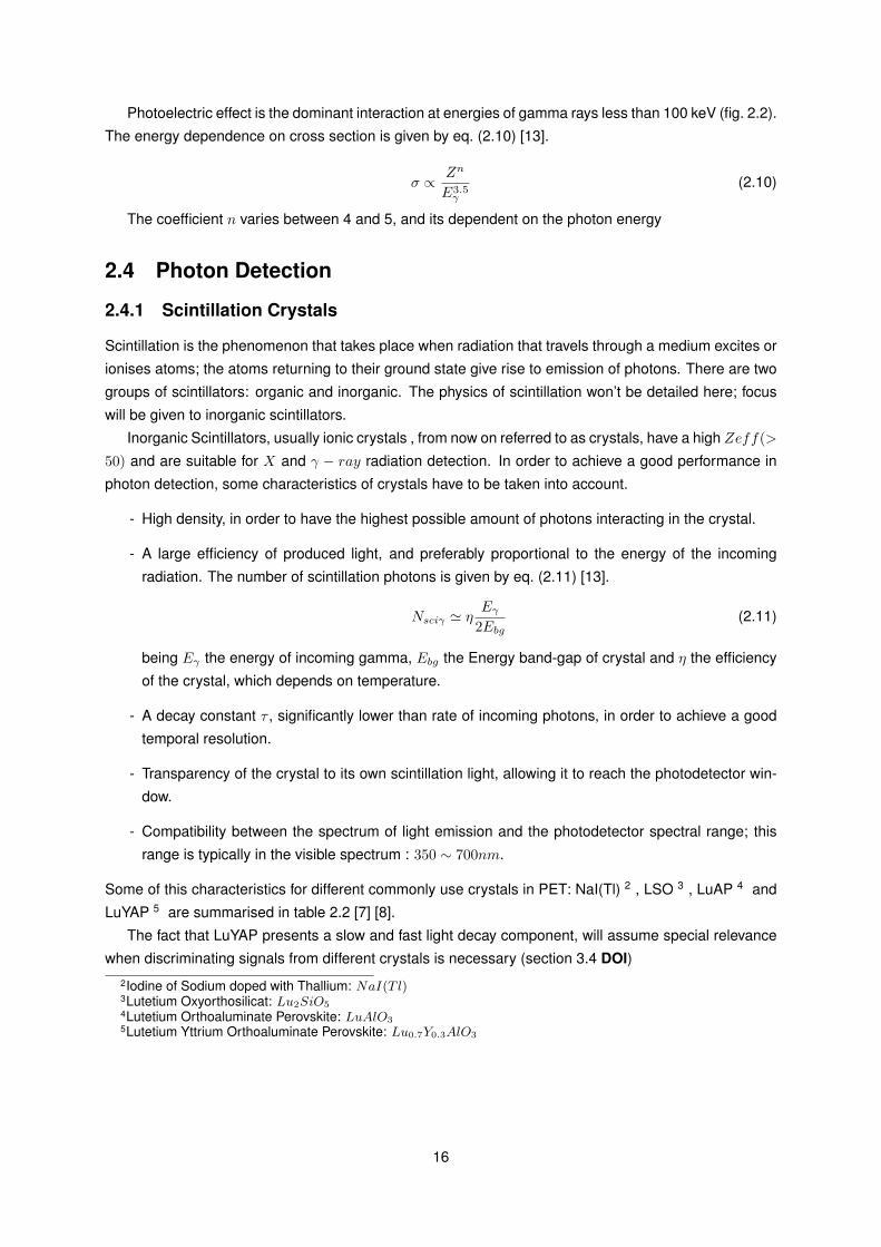
Photomultiplier tubes (PMT), of which we can see a cross section in fig 2.4, are used as scintillation light

detectors. They consist of a vacuum tube with a glass window; in its interior, where vacuum ( 10−4Pa)

has been made, there is, in one end, the photocathode and in the other the anode; in between there are

typically 10 to 15 dynodes; The photocathode is maintained at a large negative potential (∼ −2000V )

while the anode is at ground potential; the potential of each dynode varies between the photocathode

voltage and the anode voltage (0V ) in steps of ∼ −150V .

Figure 2.4: Generic PMT schematic cross-section

Scintillation photons that pass through the PMT windows eject, by photoelectric effect, electrons from

the photocathode. The number of ejected electrons is multiplied in each of the dynodes until they reach

the photoanode; this process is called secondary emission and it happens when the electron hits the

dynodes surface with sufficient energy; the result is the emission of a number of secondary electrons.

As a result of all the secondary electrons charge collected in the anode, an electric signal is produced.

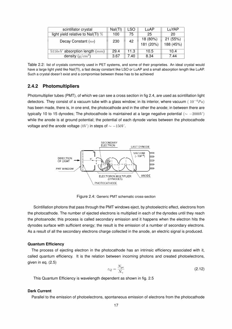
Quantum EfficiencyThe process of ejecting electron in the photocathode has an intrinsic efficiency associated with it,

called quantum efficiency. It is the relation between incoming photons and created photoelectrons,

given in eq. (2.5)

εQ =NpeNγ

(2.12)

This Quantum Efficiency is wavelength dependent as shown in fig. 2.5

Dark CurrentParallel to the emission of photoelectrons, spontaneous emission of electrons from the photocathode

17

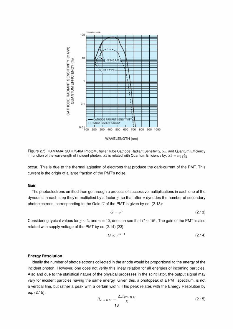
Figure 2.5: HAMAMATSU H7546A PhotoMultiplier Tube Cathode Radiant Sensitivity, Sk, and Quantum Efficiencyin function of the wavelength of incident photon. Sk is related with Quantum Efficiency by: Sk = εQ

λ1.24

occur. This is due to the thermal agitation of electrons that produce the dark-current of the PMT. This

current is the origin of a large fraction of the PMT’s noise.

GainThe photoelectrons emitted then go through a process of successive multiplications in each one of the

dynodes; in each step they’re multiplied by a factor g, so that after n dynodes the number of secondary

photoelectrons, corresponding to the Gain G of the PMT is given by eq. (2.13):

G = gn (2.13)

Considering typical values for g ∼ 3, and n = 12, one can see that G ∼ 106. The gain of the PMT is also

related with supply voltage of the PMT by eq.(2.14) [23]:

G ∝ V n−1 (2.14)

Energy ResolutionIdeally the number of photoelectrons collected in the anode would be proportional to the energy of the

incident photon. However, one does not verify this linear relation for all energies of incoming particles.

Also and due to the statistical nature of the physical processes in the scintillator, the output signal may

vary for incident particles having the same energy. Given this, a photopeak of a PMT spectrum, is not

a vertical line, but rather a peak with a certain width. This peak relates with the Energy Resolution by

eq. (2.15).

RFWHM =∆EFWHM

E(2.15)

18

Where E is the energy of the photopeak and ∆EFWHM , the peak’s width, measured at half of its height.

If the number of incident photoelectrons is large enough, one can admit that the shape of this peak is a

Gaussian with standard deviation σ and mean-value µ, for which the resolution is given by eq. (2.16).

RFWHM ' 2.35σ

µ(2.16)

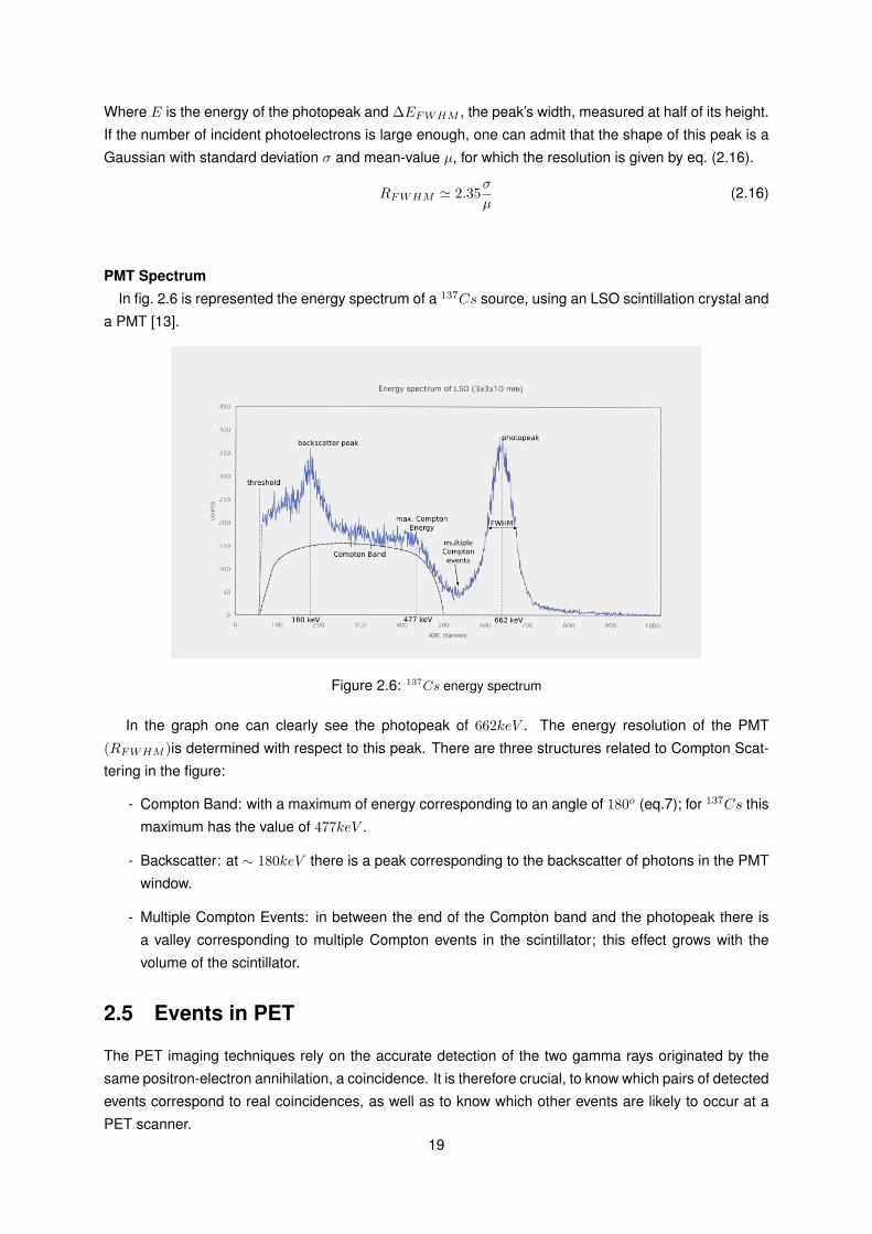
PMT SpectrumIn fig. 2.6 is represented the energy spectrum of a 137Cs source, using an LSO scintillation crystal and

a PMT [13].

Figure 2.6: 137Cs energy spectrum

In the graph one can clearly see the photopeak of 662keV . The energy resolution of the PMT

(RFWHM )is determined with respect to this peak. There are three structures related to Compton Scat-

tering in the figure:

- Compton Band: with a maximum of energy corresponding to an angle of 180o (eq.7); for 137Cs this

maximum has the value of 477keV .

- Backscatter: at ∼ 180keV there is a peak corresponding to the backscatter of photons in the PMT

window.

- Multiple Compton Events: in between the end of the Compton band and the photopeak there is

a valley corresponding to multiple Compton events in the scintillator; this effect grows with the

volume of the scintillator.

2.5 Events in PET

The PET imaging techniques rely on the accurate detection of the two gamma rays originated by the

same positron-electron annihilation, a coincidence. It is therefore crucial, to know which pairs of detected

events correspond to real coincidences, as well as to know which other events are likely to occur at a

PET scanner.19

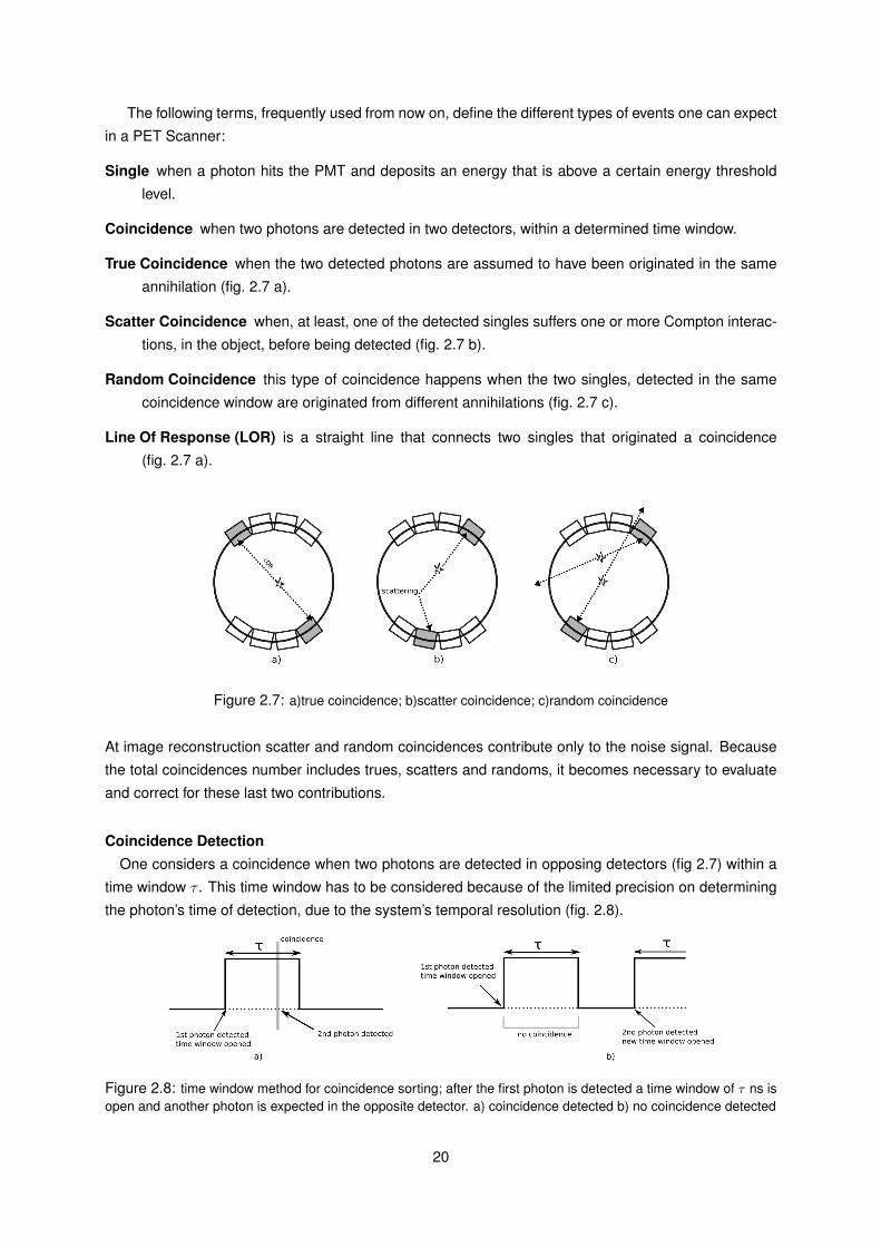
The following terms, frequently used from now on, define the different types of events one can expect

in a PET Scanner:

Single when a photon hits the PMT and deposits an energy that is above a certain energy threshold

level.

Coincidence when two photons are detected in two detectors, within a determined time window.

True Coincidence when the two detected photons are assumed to have been originated in the same

annihilation (fig. 2.7 a).

Scatter Coincidence when, at least, one of the detected singles suffers one or more Compton interac-

tions, in the object, before being detected (fig. 2.7 b).

Random Coincidence this type of coincidence happens when the two singles, detected in the same

coincidence window are originated from different annihilations (fig. 2.7 c).

Line Of Response (LOR) is a straight line that connects two singles that originated a coincidence

(fig. 2.7 a).

Figure 2.7: a)true coincidence; b)scatter coincidence; c)random coincidence

At image reconstruction scatter and random coincidences contribute only to the noise signal. Because

the total coincidences number includes trues, scatters and randoms, it becomes necessary to evaluate

and correct for these last two contributions.

Coincidence DetectionOne considers a coincidence when two photons are detected in opposing detectors (fig 2.7) within a

time window τ . This time window has to be considered because of the limited precision on determining

the photon’s time of detection, due to the system’s temporal resolution (fig. 2.8).

Figure 2.8: time window method for coincidence sorting; after the first photon is detected a time window of τ ns isopen and another photon is expected in the opposite detector. a) coincidence detected b) no coincidence detected

20

The random coincidences are estimated by a delayed time window process In this case a time

window is also open, not immediately after the first photon is detected, but after a delay time d τ ;

the temporal correlation between two events from the same annihilation is then lost and, instead of

detecting a real coincidence, only randoms will be detected; this relies on the assumption that random

coincidences are uniformly distributed in time.

2.6 PET Scanner Characteristics

2.6.1 Sensitivity

The measurement of a scanner’s total sensitivity expresses the ratio between detected coincidences

(Ndetected) and total number of β+ decays that undergo pair annihilation and consequent photon pro-

duction (Nβ+ ) (eq. (2.17)). It is strongly dependent on the scanner geometry as well as on its intrinsic

efficiency of detection.

sensitivity =NdetectedNβ+

(2.17)

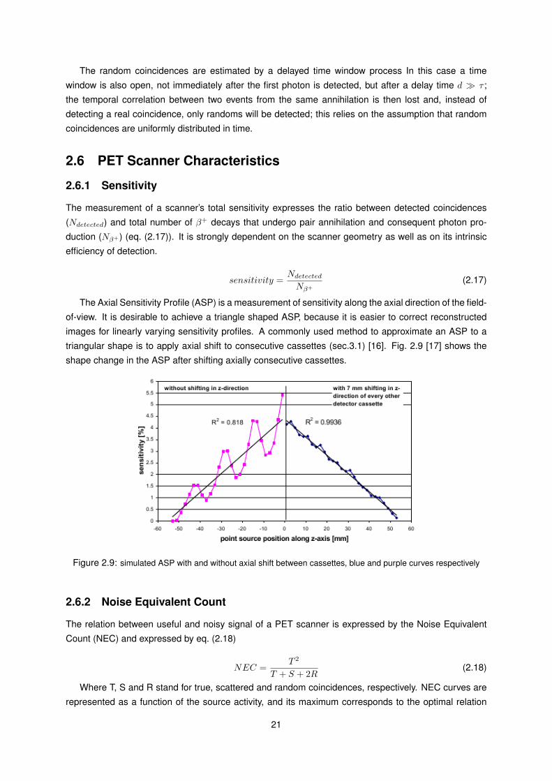
The Axial Sensitivity Profile (ASP) is a measurement of sensitivity along the axial direction of the field-

of-view. It is desirable to achieve a triangle shaped ASP, because it is easier to correct reconstructed

images for linearly varying sensitivity profiles. A commonly used method to approximate an ASP to a

triangular shape is to apply axial shift to consecutive cassettes (sec.3.1) [16]. Fig. 2.9 [17] shows the

shape change in the ASP after shifting axially consecutive cassettes.

Figure 2.9: simulated ASP with and without axial shift between cassettes, blue and purple curves respectively

2.6.2 Noise Equivalent Count

The relation between useful and noisy signal of a PET scanner is expressed by the Noise Equivalent

Count (NEC) and expressed by eq. (2.18)

NEC =T 2

T + S + 2R(2.18)

Where T, S and R stand for true, scattered and random coincidences, respectively. NEC curves are

represented as a function of the source activity, and its maximum corresponds to the optimal relation

21

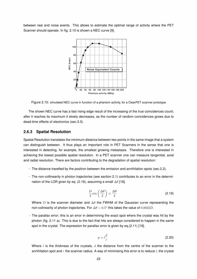
between real and noise events. This allows to estimate the optimal range of activity where the PET

Scanner should operate. In fig. 2.10 is shown a NEC curve [9].

Figure 2.10: simulated NEC curve in function of a phantom activity, for a ClearPET scanner prototype

The shown NEC curve has a fast rising edge result of the increasing of the true coincidences count;

after it reaches its maximum it slowly decreases, as the number of random coincidences grows due to

dead-time effects of electronics (sec.3.3).

2.6.3 Spatial Resolution

Spatial Resolution translates the minimum distance between two points in the same image that a system

can distinguish between. It thus plays an important role in PET Scanners in the sense that one is

interested in detecting, for example, the smallest growing metastasis. Therefore one is interested in

achieving the lowest possible spatial resolution. In a PET scanner one can measure tangential, axial

and radial resolution. There are factors contributing to the degradation of spatial resolution:

- The distance travelled by the positron between the emission and annihilation spots (sec.2.2).

- The non-collinearity in photon trajectories (see section 2.1) contributes to an error in the determi-

nation of the LOR given by eq. (2.19), assuming a small ∆θ [18].

D

2sin

(∆θ2

)' ∆θ

4(2.19)

Where D is the scanner diameter and ∆θ the FWHM of the Gaussian curve representing the

non-colinearity of photon trajectories. For ∆θ ∼ 0.5o this takes the value of 0.0022D.

- The parallax error; this is an error in determining the exact spot where the crystal was hit by the

photon (fig. 2.11 a). This is due to the fact that hits are always considered to happen in the same

spot in the crystal. The expression for parallax error is given by eq.(2.11) [19].

p = ld

r(2.20)

Where l is the thickness of the crystals, d the distance from the centre of the scanner to the

annihilation spot and r the scanner radius. A way of minimising this error is to reduce l, the crystal

22

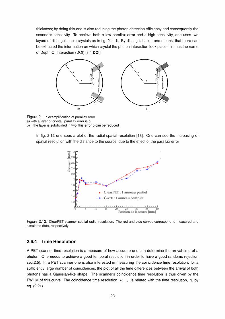
thickness; by doing this one is also reducing the photon detection efficiency and consequently the

scanner’s sensitivity. To achieve both a low parallax error and a high sensitivity, one uses two

layers of distinguishable crystals as in fig. 2.11 b. By distinguishable, one means, that there can

be extracted the information on which crystal the photon interaction took place; this has the name

of Depth Of Interaction (DOI) [3.4 DOI]

Figure 2.11: exemplification of parallax errora) with a layer of crystal, parallax error is pb) if the layer is subdivided in two, this error b can be reduced

In fig. 2.12 one sees a plot of the radial spatial resolution [18]. One can see the increasing of

spatial resolution with the distance to the source, due to the effect of the parallax error

Figure 2.12: ClearPET scanner spatial radial resolution. The red and blue curves correspond to measured andsimulated data, respectively

2.6.4 Time Resolution

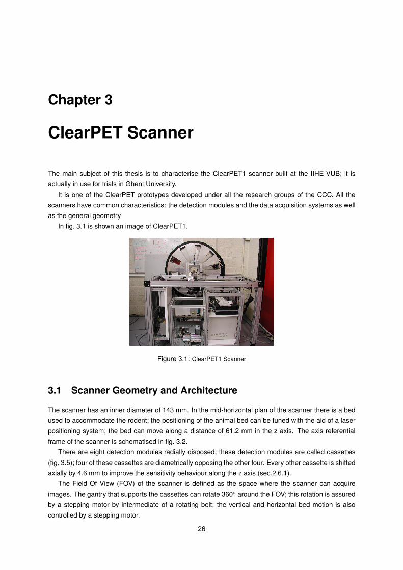
A PET scanner time resolution is a measure of how accurate one can determine the arrival time of a

photon. One needs to achieve a good temporal resolution in order to have a good randoms rejection

sec.2.5). In a PET scanner one is also interested in measuring the coincidence time resolution: for a

sufficiently large number of coincidences, the plot of all the time differences between the arrival of both

photons has a Gaussian-like shape. The scanner’s coincidence time resolution is thus given by the

FWHM of this curve. The coincidence time resolution, Rcoin, is related with the time resolution, R, by

eq. (2.21).

23

Coincidence time resolution =√

2 Time resolution (2.21)

Fig. 2.13 shows a plot of time differences in coincidences [10].

24

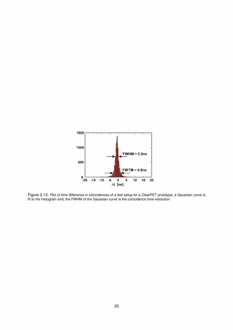
Figure 2.13: Plot of time difference in coincidences of a test setup for a ClearPET prototype; a Gaussian curve isfit to the histogram and; the FWHM of the Gaussian curve is the coincidence time resolution

25

Chapter 3

ClearPET Scanner

The main subject of this thesis is to characterise the ClearPET1 scanner built at the IIHE-VUB; it is

actually in use for trials in Ghent University.

It is one of the ClearPET prototypes developed under all the research groups of the CCC. All the

scanners have common characteristics: the detection modules and the data acquisition systems as well

as the general geometry

In fig. 3.1 is shown an image of ClearPET1.

Figure 3.1: ClearPET1 Scanner

3.1 Scanner Geometry and Architecture

The scanner has an inner diameter of 143 mm. In the mid-horizontal plan of the scanner there is a bed

used to accommodate the rodent; the positioning of the animal bed can be tuned with the aid of a laser

positioning system; the bed can move along a distance of 61.2 mm in the z axis. The axis referential

frame of the scanner is schematised in fig. 3.2.

There are eight detection modules radially disposed; these detection modules are called cassettes

(fig. 3.5); four of these cassettes are diametrically opposing the other four. Every other cassette is shifted

axially by 4.6 mm to improve the sensitivity behaviour along the z axis (sec.2.6.1).

The Field Of View (FOV) of the scanner is defined as the space where the scanner can acquire

images. The gantry that supports the cassettes can rotate 360o around the FOV; this rotation is assured

by a stepping motor by intermediate of a rotating belt; the vertical and horizontal bed motion is also

controlled by a stepping motor.

26

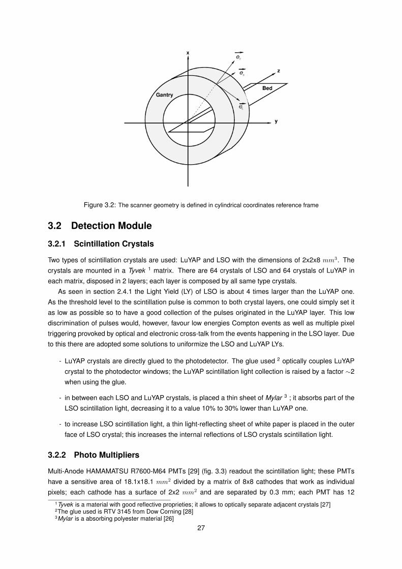
Figure 3.2: The scanner geometry is defined in cylindrical coordinates reference frame

3.2 Detection Module

3.2.1 Scintillation Crystals

Two types of scintillation crystals are used: LuYAP and LSO with the dimensions of 2x2x8 mm3. The

crystals are mounted in a Tyvek 1 matrix. There are 64 crystals of LSO and 64 crystals of LuYAP in

each matrix, disposed in 2 layers; each layer is composed by all same type crystals.

As seen in section 2.4.1 the Light Yield (LY) of LSO is about 4 times larger than the LuYAP one.

As the threshold level to the scintillation pulse is common to both crystal layers, one could simply set it

as low as possible so to have a good collection of the pulses originated in the LuYAP layer. This low

discrimination of pulses would, however, favour low energies Compton events as well as multiple pixel

triggering provoked by optical and electronic cross-talk from the events happening in the LSO layer. Due

to this there are adopted some solutions to uniformize the LSO and LuYAP LYs.

- LuYAP crystals are directly glued to the photodetector. The glue used 2 optically couples LuYAP

crystal to the photodector windows; the LuYAP scintillation light collection is raised by a factor ∼2

when using the glue.

- in between each LSO and LuYAP crystals, is placed a thin sheet of Mylar 3 ; it absorbs part of the

LSO scintillation light, decreasing it to a value 10% to 30% lower than LuYAP one.

- to increase LSO scintillation light, a thin light-reflecting sheet of white paper is placed in the outer

face of LSO crystal; this increases the internal reflections of LSO crystals scintillation light.

3.2.2 Photo Multipliers

Multi-Anode HAMAMATSU R7600-M64 PMTs [29] (fig. 3.3) readout the scintillation light; these PMTs

have a sensitive area of 18.1x18.1 mm2 divided by a matrix of 8x8 cathodes that work as individual

pixels; each cathode has a surface of 2x2 mm2 and are separated by 0.3 mm; each PMT has 121Tyvek is a material with good reflective proprieties; it allows to optically separate adjacent crystals [27]2The glue used is RTV 3145 from Dow Corning [28]3Mylar is a absorbing polyester material [26]

27

multiplication dynodes and the nominal working voltage applied between anode and cathode is around

-900 V. The PMT has individual anode outputs for each of the 64 pixels, as well as a common dynode

output, that gives the analog sum of the 64 channels.

Figure 3.3: Multi-Anode HAMAMATSU R7600-M64 PMT. One can see the 64 anode channels and the commondynode

The gain of all PMT anode channels is non uniform to the same amount of scintillation light; this

response can vary in the ratio 3:1 [18]. In order to uniformize this response, an equalisation mask

(fig. 3.4 a) 4) is glued on the PMTs window; this mask has openings for which the surface is inversely

proportional to the respective channel sensitivity; with this technique the uniformity can be reduced to a

minimum ratio of 1.2:1. [18]. This mask also reduces the cross-talk between pixels.

3.2.3 Phoswich Matrix

Phoswhich Matrix (fig. 3.4 b)) (phosphor + sandwich) is the name given to the ensemble of the the

two layers of Scintillation crystals plus the PMT. Crystal layers are glued between each other and the

LuYAP layer glued directly to the PMT surface. One can see in fig. 3.4 a the separate components of

the phoswhich matrix.

Figure 3.4: a) 1-PMT 2-LuYAP layer 3-LSO layer 4-equalisation masks 5-positioning mask for the phoswich matrix;b) phoswich matrix

In fig. 3.4 a) one can actually see the different gaps in the PMT equalisation mask (4); these gaps are

larger in the edges and smaller in the centre. Each positioning mask (5) can house up to 4 phoswhich

matrices.

28

3.2.4 Cassettes

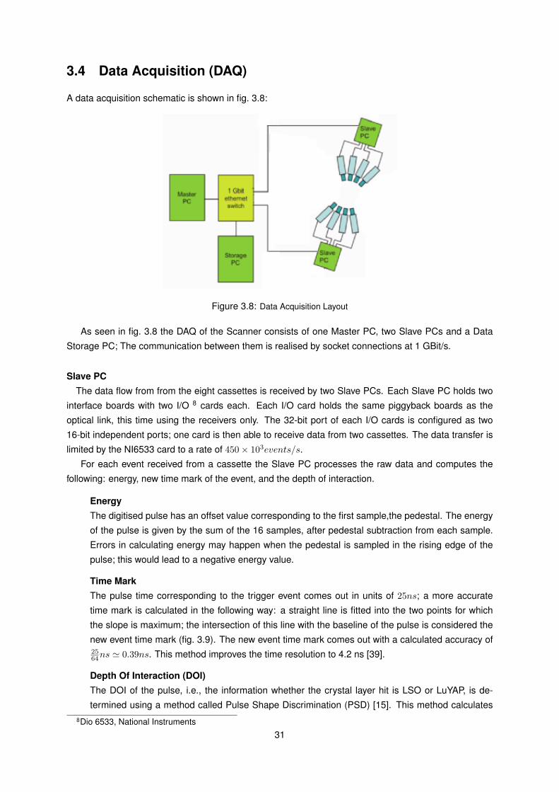
The dimensions of the cassette (fig. 3.5) are 25x15x4 cm3. It is made out of aluminium and is the

physical support to the detection and readout electronic modules. A box in the front of the cassette

houses the light sensitive part of the scintillation crystals and PMTs; it is black in order to prevent these

from direct light exposition.

Figure 3.5: Cassette. The phoswhich matrix is inside the black cover; outside one can see the readout electronicsof the PMT and the FPGA

3.3 Electronics

Each detection cassette contains the following components: two phoswhich matrices, two decoder

blocks, one FPGA 4 board, one slow control board and an optical link.

Decoder BlockEach decoder block consists of 64 comparators connected to PMT anodes, an address decoder of the

anodes and a dynode signal preamplifier. The comparators are triggered if, at least, one anode signal

exceeds a threshold value; this threshold value is common to the 64 channels and can differently be set

for each PMT. When a trigger occurs the amplified dynode signal and the adresse(s) of hit pixel(s) are

sent to the FPGA board; addresse(s) are determined as shown in fig. 3.6.

FPGA BoardThe FPGA board holds a XILINX FPGA (XCV 3000) [30] and four free running 12-bit ADCs 5 at 40

MHz. This 40 MHz is set by an external clock synchronous for all cassettes. When a trigger event occurs,

16 samples of the incoming dynode signal are saved. After each trigger event, the FPGA computes the

following data which is stored in a 40 bytes register:

- 32 bytes containing the 16 digitised values of the dynode signal (fig. 3.7)

- 4 bytes containing the time mark of the first sample (fig. 3.7)

4Field Programmable Gate Array5Analog to Digital Converter

29

Figure 3.6: when a pulse over threshold level is registered the decoder block searches for the low (blue) high (red)pixel addresses; four types of events can occur: a)single: low and high pixel addresses are equal. b) neighbour:low and high pixel addresses are in each others immediate vicinity (direct or diagonal). c) far: low and high pixelsaddresses are not equal neither neighbours. d) error of position: low pixel address is higher than high pixeladdress

- 2+2 bytes with the indexes of the pixels over threshold (fig. 3.6)

The FPGA takes 700 ns to process each trigger event; this time is the biggest contribution to the deadtime of the system. The 40 bytes of data are sent to a Data Acquisition computer via an optical link

interface (next paragraph).

Figure 3.7: signal sampling and time mark of the event. the time mark corresponds to the first sampled value aftera trigger occurs. the sampling takes 16 x 25 ns = 400 ns

Slow Control BoardThe slow control board is situated in the back part of each cassette; it is equipped with an ADuC812 [31]

microcontroller that adjusts High Voltage (HV) and threshold, individually, for each PMT. HVs are gen-

erated by DC-DC converters 6 . HV and threshold settings are received from a Master PC (fig. 3.8), via

a RS232 serial interface. Additionally, the microcontroller monitors the HVs and supply voltages as well

as the temperature given by a sensor placed near the phoswhich matrix.

Optical LinkIn the top of the slow control board is placed a piggyback board with an optical transceiver unit 7 but it

is set to works only as a data transmitter; it sends 16 bits data words to a Slave PC at a rate of 10 MHz.612SMV1000, PICO Electronics, New York [32]7GigaStar ING TRF, inova semiconductors, Munich [33]

30

3.4 Data Acquisition (DAQ)

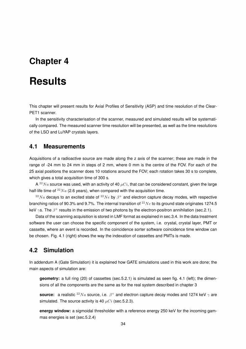
A data acquisition schematic is shown in fig. 3.8:

Figure 3.8: Data Acquisition Layout

As seen in fig. 3.8 the DAQ of the Scanner consists of one Master PC, two Slave PCs and a Data

Storage PC; The communication between them is realised by socket connections at 1 GBit/s.

Slave PCThe data flow from from the eight cassettes is received by two Slave PCs. Each Slave PC holds two

interface boards with two I/O 8 cards each. Each I/O card holds the same piggyback boards as the

optical link, this time using the receivers only. The 32-bit port of each I/O cards is configured as two

16-bit independent ports; one card is then able to receive data from two cassettes. The data transfer is

limited by the NI6533 card to a rate of 450× 103events/s.

For each event received from a cassette the Slave PC processes the raw data and computes the

following: energy, new time mark of the event, and the depth of interaction.

EnergyThe digitised pulse has an offset value corresponding to the first sample,the pedestal. The energy

of the pulse is given by the sum of the 16 samples, after pedestal subtraction from each sample.

Errors in calculating energy may happen when the pedestal is sampled in the rising edge of the

pulse; this would lead to a negative energy value.

Time MarkThe pulse time corresponding to the trigger event comes out in units of 25ns; a more accurate

time mark is calculated in the following way: a straight line is fitted into the two points for which

the slope is maximum; the intersection of this line with the baseline of the pulse is considered the

new event time mark (fig. 3.9). The new event time mark comes out with a calculated accuracy of2564ns ' 0.39ns. This method improves the time resolution to 4.2 ns [39].

Depth Of Interaction (DOI)The DOI of the pulse, i.e., the information whether the crystal layer hit is LSO or LuYAP, is de-

termined using a method called Pulse Shape Discrimination (PSD) [15]. This method calculates8Dio 6533, National Instruments

31

Figure 3.9: signal sampling and time mark of the event. the time mark corresponds to the first sampled value aftera trigger occurs. the sampling takes 16 x 25 ns = 400 ns

the normalised value of the last sample to the sum of all pulses samples as seen in eq. (3.1).

Fig. 3.10 [41] shows the distribution of the x value calculated by eq. (3.1) for LSO and LuYAP

crystals.

x =x16∑16i=1 xi

(3.1)

It is then possible to associate each value of x with the crystal layer where the interaction took

place; this is method is based on the presence of a slow decay component of the light scintillated

by LuYAP crystals (sec 2.4.1). The PSD method has a reliability of > 97% [15].

Figure 3.10: distribution of the normalized values of the last pulse sample to the sum of all pulses samples, forLSO and LuYAP crystals

After the previous calculations are made, for each event, it is checked whether it is or not a valid

event; errors on determining the pixel hit fig. 3.6 and/or the energy value are likely to happen.

Per event, 8 bytes of the previous calculated data are sent to a Data Storage PC; these 8 bytes of

data include: Energy, Time Mark, DOI, Pixel, PMT and Cassette Address; these data is stored in a List

Mode Format (LMF) file [36] [37].

The LMF is a format developed under the CCC, which records events sequentially; data concerning

the scanner characteristics and scanning conditions is stored in a ASCII header file, while data contain-

ing the events information is stored in a binary file.

Master PCThe Master PC is responsible for controlling all the scan processes. It runs a LabView application that

manages a Graphical User Interface (GUI) allowing to control the parameters of the acquisition such as

32

time of acquisition, bed position and gantry rotation. The bed position and the gantry rotation stepping

motors are controlled with a Phytron ZSH-87 Mini Programmable Stepper Motor Controller [35]. In the

Master PC, HV and threshold parameters of the PMTs, are controlled; these settings are sent to the

Slow Control Board via the RS232 serial port. The serial port also provides a reset signal and a 40 MHz

clock, both signals are synchronous to all cassettes.

33

Chapter 4

Results

This chapter will present results for Axial Profiles of Sensitivity (ASP) and time resolution of the Clear-

PET1 scanner.

In the sensitivity characterisation of the scanner, measured and simulated results will be systemati-

cally compared. The measured scanner time resolution will be presented, as well as the time resolutions

of the LSO and LuYAP crystals layers.

4.1 Measurements

Acquisitions of a radioactive source are made along the z axis of the scanner; these are made in the

range of -24 mm to 24 mm in steps of 2 mm, where 0 mm is the centre of the FOV. For each of the

25 axial positions the scanner does 10 rotations around the FOV; each rotation takes 30 s to complete,

which gives a total acquisition time of 300 s.

A 22Na source was used, with an activity of 40 µCi, that can be considered constant, given the large

half-life time of 22Na (2.6 years), when compared with the acquisition time.22Na decays to an excited state of 22Ne by β+ and electron capture decay modes, with respective

branching ratios of 90.3% and 9.7%. The internal transition of 22Ne to its ground state originates 1274.5

keV γs. The β+ results in the emission of two photons by the electron-positron annihilation (sec.2.1).

Data of the scanning acquisition is stored in LMF format as explained in sec.3.4. In the data treatment

software the user can choose the specific component of the system, i.e. crystal, crystal layer, PMT or

cassette, where an event is recorded. In the coincidence sorter software coincidence time window can

be chosen. Fig. 4.1 (right) shows the way the indexation of cassettes and PMTs is made.

4.2 Simulation

In addendum A (Gate Simulation) it is explained how GATE simulations used in this work are done; the

main aspects of simulation are:

geometry: a full ring (20) of cassettes (sec.5.2.1) is simulated as seen fig. 4.1 (left); the dimen-

sions of all the components are the same as for the real system described in chapter 3

source: a realistic 22Na source, i.e. β+ and electron capture decay modes and 1274 keV γ are

simulated. The source activity is 40 µCi (sec.5.2.3).

energy window: a sigmoidal thresholder with a reference energy 250 keV for the incoming gam-

mas energies is set (sec.5.2.4)

34

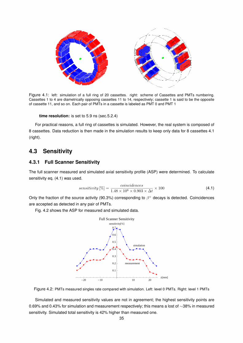
Figure 4.1: left: simulation of a full ring of 20 cassettes. right: scheme of Cassettes and PMTs numbering.Cassettes 1 to 4 are diametrically opposing cassettes 11 to 14, respectively; cassette 1 is said to be the oppositeof cassette 11, and so on. Each pair of PMTs in a cassette is labeled as PMT 0 and PMT 1

time resolution: is set to 5.9 ns (sec.5.2.4)

For practical reasons, a full ring of cassettes is simulated. However, the real system is composed of

8 cassettes. Data reduction is then made in the simulation results to keep only data for 8 cassettes 4.1

(right).

4.3 Sensitivity

4.3.1 Full Scanner Sensitivity

The full scanner measured and simulated axial sensitivity profile (ASP) were determined. To calculate

sensitivity eq. (4.1) was used.

sensitivity [%] =coincidences

1.48× 106 × 0.903×∆t× 100 (4.1)

Only the fraction of the source activity (90.3%) corresponding to β+ decays is detected. Coincidences

are accepted as detected in any pair of PMTs.

Fig. 4.2 shows the ASP for measured and simulated data.

è

è

è

èè

è è èè

è

è

è è

è

è

èè è è è

è

è

è

èè

è

è

è

è

è è èè è

è

è

èè

è

è

è

è èè è è

è

è

è

è

simulation

measurement

-20 -10 10 20z@mmD

0.1

0.2

0.3

0.4

0.5

0.6

0.7

sensitivity@%D

Full Scanner Sensitivity

Figure 4.2: PMTs measured singles rate compared with simulation. Left: level 0 PMTs. Right: level 1 PMTs

Simulated and measured sensitivity values are not in agreement; the highest sensitivity points are

0.69% and 0.43% for simulation and measurement respectively; this means a lost of ∼38% in measured

sensitivity. Simulated total sensitivity is 42% higher than measured one.35

Measured curve also presents an asymmetry relative to the y axis and an asymmetry between the

first four and the last four measured z positions.

This result is clearly not satisfactory and the reasons of the lost/gain in measured/simulated sensitiv-

ity will be analyzed by having a different approach to the the sensitivity characterisation of the scanner.

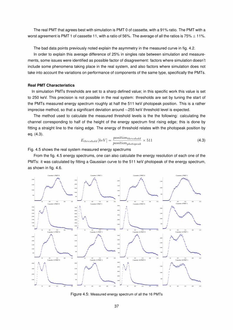
The sensitivity characterisation of the scanner will be realised in a structured way: first, one will

analyse the individual PMT detection efficiency; the sensitivity profiles resulting of coincidences detected

exclusively between PMT pairs will then be presented; the following step is to calculate the sensitivity

profiles for pairs of opposite cassettes. Fig. 4.3 illustrates this approach.

Figure 4.3: a) singles registered in just one PMT; b) coincidences registered between one pair of specific cassettes;c) coincidences registered between any pair of PMT of a pair of opposite cassettes

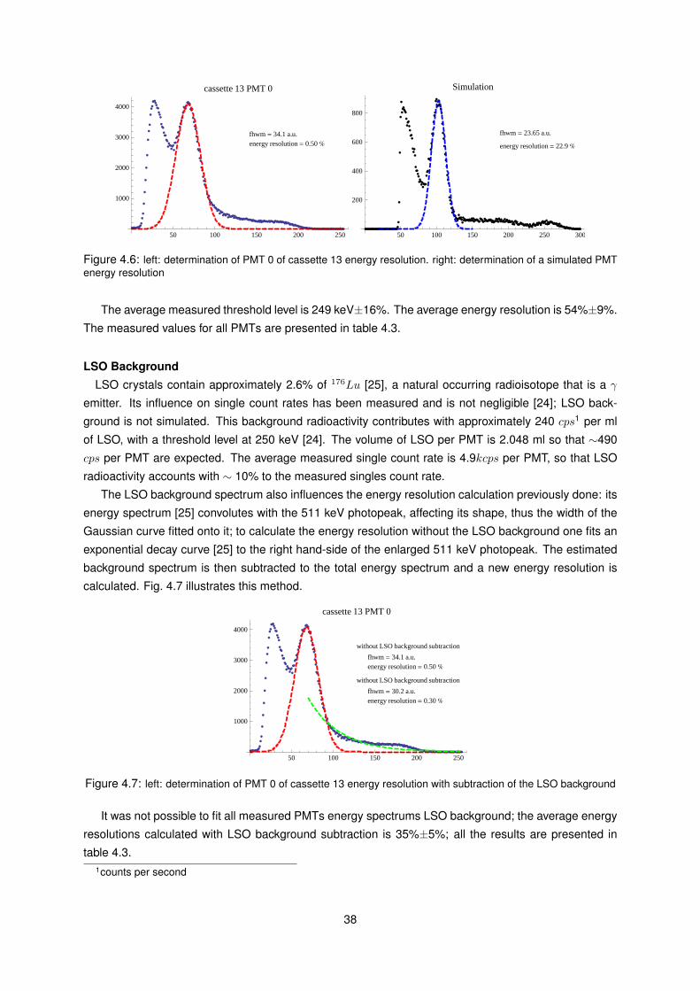
4.3.2 PMT Singles Rate

For each PMT the measured and simulated singles rate were calculated by eq (4.2)

rate[s−1]

=singles

tacquisition(4.2)

Fig. 4.4 shows the singles rates for each PMT along the z axis of the scanner.

ò ò ò ò ò ò ò ò ò ò ò ò ò ò òò ò ò

ò ò ò òò ò ò

è è è è è è è è è è è è è è è è è è è è è è è è è

è è è è è è è è è è è è è è è è è è è è è è è è è

è è è è è è è è è è è è è è è è è è è è è è è è è

è è è è è è è è è è è è è è è è è è è è è è è è è

è è è è è è è è è è è è è è è è è è è è è

è

è è è

è è è è è è è è è è è è è è è è è è è è è

è

è è è

è è è è è è è è è è è è è è è è è è è è è è è è è

è è è è è è è è è è è è è è è è è è è è è è è è è

ò simulationè measurements

-20 -10 0 10 200

2000

4000

6000

8000

singles per second

ò òò ò ò

ò òò ò ò ò ò ò ò ò ò ò ò ò ò ò ò ò ò ò

è è è è è è è è è è è è è è è è è è è è è è è è èè è è è è è è è è è è è è è è è è è è è è è è è è

è è è è è è è è è è è è è è è è è è è è è è è è è

è è è è è è è è è è è è è è è è è è è è è è è è è

è è è è è è è è è è è è è è è è è è è è è

è

è è è

è è è è è è è è è è è è è è è è è è è è è

è

è è è

è è è è è è è è è è è è è è è è è è è è è è è è è

è è è è è è è è è è è è è è è è è è è è è è è è è

ò simulationè measurements

-20 -10 0 10 200

2000

4000

6000

8000

singles per second

Figure 4.4: PMTs measured singles rate compared with simulation. Left: level 0 PMTs. Right: level 1 PMTs; forclearness of visualisation, only one simulated PMT is shown, as simulated single count rate per PMT is practicallyequal

One can see that, for the four PMTs of cassettes 11 and 12, there are bad data points, between 18

mm and 24 mm. Indeed, the log files of the measurement show that between those specific positions,

there are no counts for these four specific PMTs, due to an error in data acquisition.

For each measured PMT the ratio between measured and simulated singles rate was calculated; this

ratio was averaged over all the points of the z axis; results are presented in table 4.3.36

The real PMT that agrees best with simulation is PMT 0 of cassette, with a 91% ratio. The PMT with a

worst agreement is PMT 1 of cassette 11, with a ratio of 56%. The average of all the ratios is 75%± 11%.

The bad data points previously noted explain the asymmetry in the measured curve in fig. 4.2.

In order to explain this average difference of 25% in singles rate between simulation and measure-

ments, some issues were identified as possible factor of disagreement: factors where simulation doesn’t

include some phenomena taking place in the real system, and also factors where simulation does not

take into account the variations on performance of components of the same type, specifically the PMTs.

Real PMT CharacteristicsIn simulation PMTs thresholds are set to a sharp defined value; in this specific work this value is set

to 250 keV. This precision is not possible in the real system: thresholds are set by tuning the start of

the PMTs measured energy spectrum roughly at half the 511 keV photopeak position. This is a rather

imprecise method, so that a significant deviation around ∼255 keV threshold level is expected.

The method used to calculate the measured threshold levels is the the following: calculating the

channel corresponding to half of the height of the energy spectrum first rising edge; this is done by

fitting a straight line to the rising edge. The energy of threshold relates with the photopeak position by

eq. (4.3).

Ethreshold [keV ] =positionthresholdpositionphotopeak

× 511 (4.3)

Fig. 4.5 shows the real system measured energy spectrums

From the fig. 4.5 energy spectrums, one can also calculate the energy resolution of each one of the

PMTs: it was calculated by fitting a Gaussian curve to the 511 keV photopeak of the energy spectrum,

as shown in fig. 4.6.

50 100 150 200 250

500

1000

1500

2000

Cassette 1 PMT 0

50 100 150 200 250

500

1000

1500

2000

2500

Cassette 1 PMT 1

50 100 150 200 250

500

1000

1500

2000

Cassette 2 PMT 0

50 100 150 200 250

500

1000

1500

Cassette 2 PMT 1

50 100 150 200 250

500

1000

1500

2000

2500

3000

3500

Cassette 3 PMT 0

50 100 150 200 250

1000

2000

3000

4000

5000

6000

7000

Cassette 3 PMT 1

50 100 150 200 250

1000

2000

3000

4000

5000Cassette 4 PMT 0

50 100 150 200 250

500

1000

1500

2000

Cassette 4 PMT 1

50 100 150 200 250

500

1000

1500

2000

2500

Cassette 11 PMT 0

50 100 150 200 250

500

1000

1500

2000

Cassette 11 PMT 1

50 100 150 200 250

500

1000

1500

2000

2500

Cassette 12 PMT 0

50 100 150 200 250

500

1000

1500

2000

Cassette 12 PMT 1

50 100 150 200 250

1000

2000

3000

4000

Cassette 13 PMT 0

50 100 150 200 250

500

1000

1500

2000

Cassette 13 PMT 1

50 100 150 200 250

1000

2000

3000

4000

5000

Cassette 14 PMT 0

50 100 150 200 250

500

1000

1500

Cassette 14 PMT 1

Figure 4.5: Measured energy spectrum of all the 16 PMTs

37

fhwm = 34.1 a.u.energy resolution = 0.50 %

50 100 150 200 250

1000

2000

3000

4000

cassette 13 PMT 0

fhwm = 23.65 a.u.

energy resolution = 22.9 %

50 100 150 200 250 300

200

400

600

800

Simulation

Figure 4.6: left: determination of PMT 0 of cassette 13 energy resolution. right: determination of a simulated PMTenergy resolution

The average measured threshold level is 249 keV±16%. The average energy resolution is 54%±9%.

The measured values for all PMTs are presented in table 4.3.

LSO BackgroundLSO crystals contain approximately 2.6% of 176Lu [25], a natural occurring radioisotope that is a γ

emitter. Its influence on single count rates has been measured and is not negligible [24]; LSO back-

ground is not simulated. This background radioactivity contributes with approximately 240 cps1 per ml

of LSO, with a threshold level at 250 keV [24]. The volume of LSO per PMT is 2.048 ml so that ∼490

cps per PMT are expected. The average measured single count rate is 4.9kcps per PMT, so that LSO

radioactivity accounts with ∼ 10% to the measured singles count rate.

The LSO background spectrum also influences the energy resolution calculation previously done: its

energy spectrum [25] convolutes with the 511 keV photopeak, affecting its shape, thus the width of the

Gaussian curve fitted onto it; to calculate the energy resolution without the LSO background one fits an

exponential decay curve [25] to the right hand-side of the enlarged 511 keV photopeak. The estimated

background spectrum is then subtracted to the total energy spectrum and a new energy resolution is

calculated. Fig. 4.7 illustrates this method.

without LSO background subtraction

fhwm = 34.1 a.u.energy resolution = 0.50 %

without LSO background subtraction

fhwm = 30.2 a.u.energy resolution = 0.30 %

50 100 150 200 250

1000

2000

3000

4000

cassette 13 PMT 0

Figure 4.7: left: determination of PMT 0 of cassette 13 energy resolution with subtraction of the LSO background

It was not possible to fit all measured PMTs energy spectrums LSO background; the average energy

resolutions calculated with LSO background subtraction is 35%±5%; all the results are presented in

table 4.3.1counts per second

38

Position and Energy ErrorsDuring measurements, errors in determining the index of the pixel hit (fig. 3.6 c) and d)), fars and

errors of position, and the energy of the pulse (sec.3.4), errors of energy are expected to happen. In

the simulation these errors are not included. The log files of the acquisition show an average of 10.5%

of errors over the total single count. The individual percentage of errors of each PMT is presented in

table 4.3.

We assume that the bad results between the simulated and measured count rates of PMTs shown

in fig. 4.4 have its origin in the following reasons:

- The contribution of the LSO background that underestimates the simulation count rates by ∼10%

is not negligible.

- The average threshold level of real PMTs, 249 keV, which is good result compared with the 250

keV threshold level set in simulation; its dispersion of ∼16% is expected, giving the method used

to experimentally set it, explained before.

- The contribution of the bad events to the loss of counts in the real system, altough its origin is not

clear, can be quantified; for each PMT there is a fairly constant percentage of this error, over all the

measured z positions. In average ∼11% of the singles are bad events; these are not accounted in

simulation.

- In spite of not having influence in the singles count rate, an over-estimated 2 average of 34.8% is

fairly worse than a energy resolution of 22.9% for simulation.

The LSO background and the bad events contributions are easily quantifiable in the gain/loss of

singles rate between measurement and simulation. For the first case, a general correction factor of 10%

in singles counts can be added to simulation data. In the second case, the simulation data could be

adjusted by the percentage of bad events; this percentage is known for each PMT of the real system.

The previous approach doesn’t apply to the PMT threshold level: its influence was not quantified and

also other parameters of the PMT as the detection efficiency are not known.

For the characterisation in sensitivity of the scanner, the previous discussion will be taken into ac-

count; because setting the individual characteristics of each PMT is not feasible in simulation, the method

used is to adapt the simulated to the measured data: The simulated count rate will be scaled to its re-

spective PMT in the real system; the scaling factors shown in table 4.3 are defined individually for each

PMT; each one of these corresponds to the measured/simulation ratio, averaged over the all z positions.

In them it is included the contribution of all the disagreeing parameters discussed before.

In the coincidence sorting algorithms for simulated data, for the specific PMT pairs for which coinci-

dences are detected, a fraction of the singles events are rejected, via a random selection, according to

the singles rate scaling factor for each PMT.

4.3.3 PMT Pair Coincidence Sensitivity

The following analysis will be the characterisation in sensitivity for coincidences of a PMT pair, from

opposite cassettes. Only coincidences between same index PMTs (PMT0-PMT0 or PMT1-PMT1) are

considered, as schematized in fig. 4.3 b).2here we are only taking into account the PMTs spectrum where the LSO background could be subtracted

39

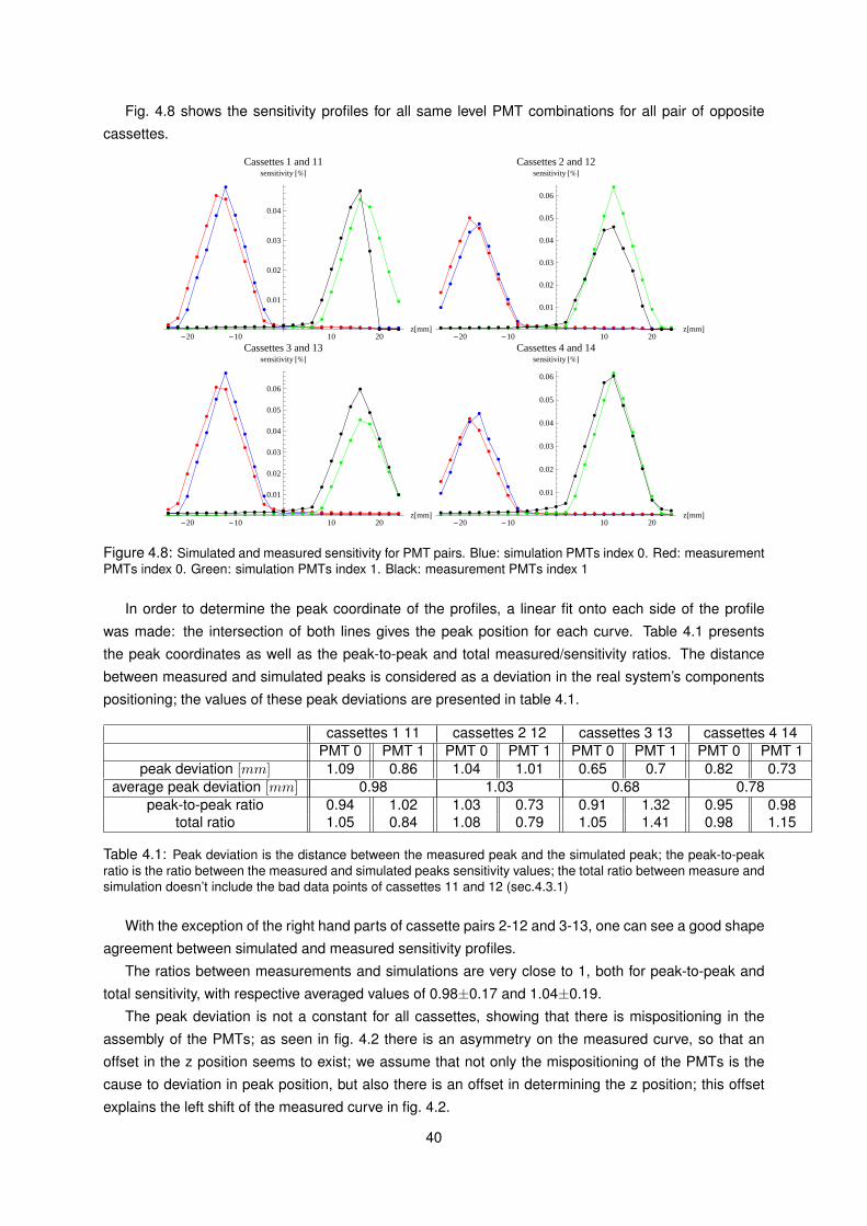
Fig. 4.8 shows the sensitivity profiles for all same level PMT combinations for all pair of opposite

cassettes.

è è

è

è

è

è

è

è

è

è

è

è è è è è è è è è è è è èè

è

è

è

è

èè

è

è

è

èè è è è è è è è è è è è è è

è è è è è è è è è è è è è è è è

è

è

è

è

è

è

è

è

è

è è è è è è è è è è è è è è è è

è

è

è

è

è

è

è è è

-20 -10 10 20z@mmD

0.01

0.02

0.03

0.04

sensitivity @%DCassettes 1 and 11

è

è

è

è

è

è

è

è

è

è è è è è è è è è è è è è è è è

è

è

è

è

è

è

è

è

è è è è è è è è è è è è è è è è èè è è è è è è è è è è è è è

è

è

è

è

è

è

è

è

è

è èè è è è è è è è è è è è èè

è

è

è

èè

è

è

è

è è è

-20 -10 10 20z@mmD

0.01

0.02

0.03

0.04

0.05

0.06

sensitivity @%DCassettes 2 and 12

è è

è

è

è

è

è

è

è

è

è

è è è è è è è è è è è è è è

è

è

è

è

è

èè

è

è

è

è

è è è è è è è è è è è è è èè è è è è è è è è è è è è è è è

è

è

è

è

è

è

è

è

è

è è è è è è è è è è è è è è èè

è

è

è

è

è

è

è

è

è

-20 -10 10 20z@mmD

0.01

0.02

0.03

0.04

0.05

0.06

sensitivity @%DCassettes 3 and 13

è

è

è

è

è

è

è

è

è

è è è è è è è è è è è è è è è è

è

è

è

è

è

è

è

è

è è è è è è è è è è è è è è è è èè è è è è è è è è è è è è è

è

è

è

è

è

è

è

è

è

è èè è è è è è è è è è è èè

è

è

è

è

è

è

è

è

è

è

èè

-20 -10 10 20z@mmD

0.01

0.02

0.03

0.04

0.05

0.06

sensitivity @%DCassettes 4 and 14

Figure 4.8: Simulated and measured sensitivity for PMT pairs. Blue: simulation PMTs index 0. Red: measurementPMTs index 0. Green: simulation PMTs index 1. Black: measurement PMTs index 1

In order to determine the peak coordinate of the profiles, a linear fit onto each side of the profile

was made: the intersection of both lines gives the peak position for each curve. Table 4.1 presents

the peak coordinates as well as the peak-to-peak and total measured/sensitivity ratios. The distance

between measured and simulated peaks is considered as a deviation in the real system’s components

positioning; the values of these peak deviations are presented in table 4.1.

cassettes 1 11 cassettes 2 12 cassettes 3 13 cassettes 4 14PMT 0 PMT 1 PMT 0 PMT 1 PMT 0 PMT 1 PMT 0 PMT 1

peak deviation [mm] 1.09 0.86 1.04 1.01 0.65 0.7 0.82 0.73average peak deviation [mm] 0.98 1.03 0.68 0.78

peak-to-peak ratio 0.94 1.02 1.03 0.73 0.91 1.32 0.95 0.98total ratio 1.05 0.84 1.08 0.79 1.05 1.41 0.98 1.15

Table 4.1: Peak deviation is the distance between the measured peak and the simulated peak; the peak-to-peakratio is the ratio between the measured and simulated peaks sensitivity values; the total ratio between measure andsimulation doesn’t include the bad data points of cassettes 11 and 12 (sec.4.3.1)

With the exception of the right hand parts of cassette pairs 2-12 and 3-13, one can see a good shape

agreement between simulated and measured sensitivity profiles.

The ratios between measurements and simulations are very close to 1, both for peak-to-peak and

total sensitivity, with respective averaged values of 0.98±0.17 and 1.04±0.19.

The peak deviation is not a constant for all cassettes, showing that there is mispositioning in the

assembly of the PMTs; as seen in fig. 4.2 there is an asymmetry on the measured curve, so that an

offset in the z position seems to exist; we assume that not only the mispositioning of the PMTs is the

cause to deviation in peak position, but also there is an offset in determining the z position; this offset

explains the left shift of the measured curve in fig. 4.2.

40

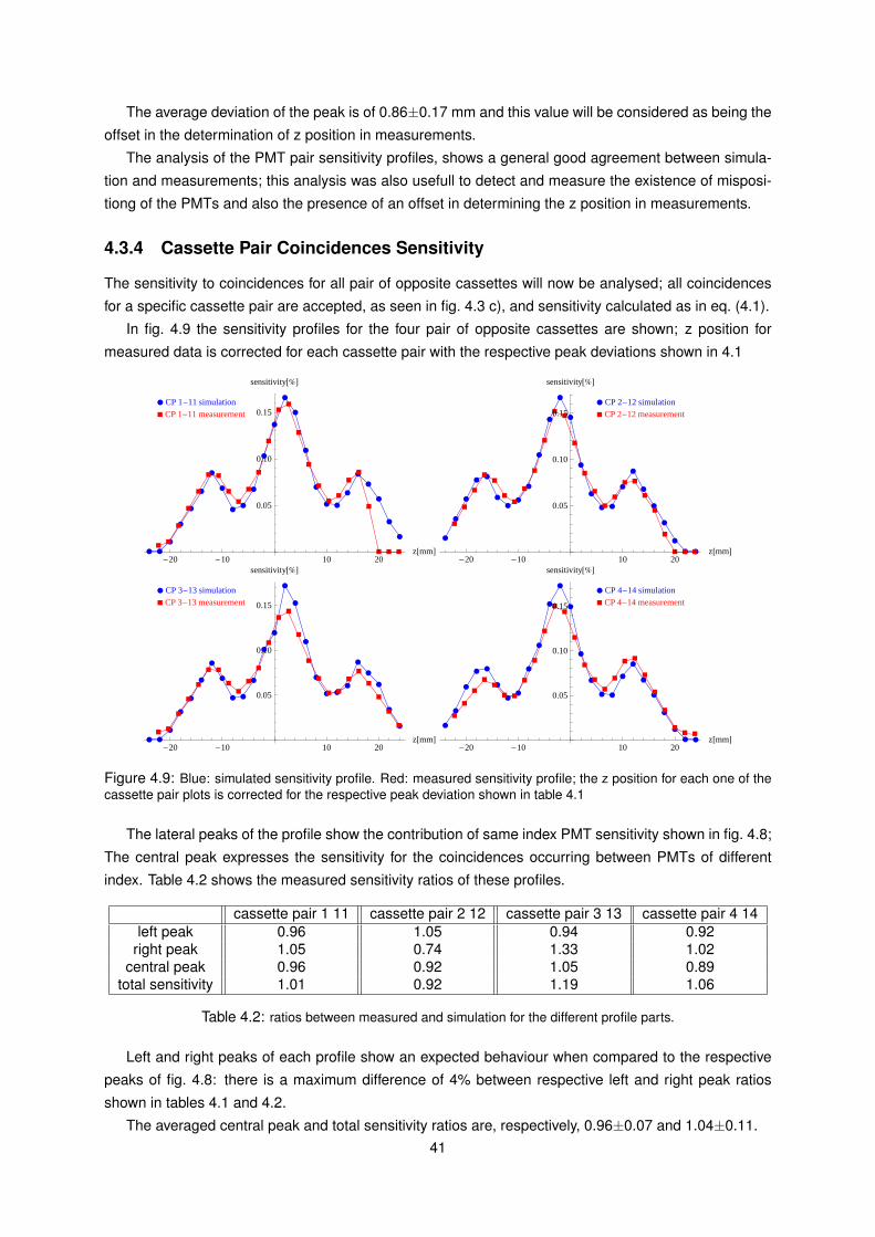
The average deviation of the peak is of 0.86±0.17 mm and this value will be considered as being the

offset in the determination of z position in measurements.

The analysis of the PMT pair sensitivity profiles, shows a general good agreement between simula-

tion and measurements; this analysis was also usefull to detect and measure the existence of misposi-

tiong of the PMTs and also the presence of an offset in determining the z position in measurements.

4.3.4 Cassette Pair Coincidences Sensitivity

The sensitivity to coincidences for all pair of opposite cassettes will now be analysed; all coincidences

for a specific cassette pair are accepted, as seen in fig. 4.3 c), and sensitivity calculated as in eq. (4.1).

In fig. 4.9 the sensitivity profiles for the four pair of opposite cassettes are shown; z position for

measured data is corrected for each cassette pair with the respective peak deviations shown in 4.1

æ æ

æ

æ

æ

æ

æ

æ

ææ

æ

æ

æ

æ

æ

æ

æ

æ æ

æ

æ

æ

æ

æ

æ

àà

à

à

à

à à

à

à

à

à

à

à

à

à

à

à

àà

à

à

à

à à à

æ CP 1-11 simulationà CP 1-11 measurement

-20 -10 10 20z@mmD

0.05

0.10

0.15

sensitivity@%D

æ

æ

æ

ææ

æ

æ

æ

æ

æ

æ

æ

æ

æ

æ

æ æ

æ

æ

æ

æ

æ

æ

æ æ

à

à

à

à

à

à

à

à

à

à

àà

à

à

à

à

à

à à

à

à

à

à à à

æ CP 2-12 simulationà CP 2-12 measurement

-20 -10 10 20z@mmD

0.05

0.10

0.15

sensitivity@%D

æ æ

æ

æ

æ

æ

æ

æ

æ æ

æ

æ

æ

æ

æ

æ

æ

æ æ

æ

æ

æ

æ

æ

æ

àà

à

à

à

à à

à

à

à

à

à

à

à

à

à

à

à à

à

à

à

à

à

à

à CP 3-13 measurementæ CP 3-13 simulation

-20 -10 10 20z@mmD

0.05

0.10

0.15

sensitivity@%D

æ

æ

æ

ææ

æ

ææ

æ

æ

æ

æ

æ

æ

æ

æ æ

æ

æ

æ

æ

æ

æ

æ æ

à

à

à

à

à

à à

à

à

à

à

à

à

à

à

à

à

àà

à

à

à

àà à

à CP 4-14 measurementæ CP 4-14 simulation

-20 -10 10 20z@mmD

0.05

0.10

0.15

sensitivity@%D

Figure 4.9: Blue: simulated sensitivity profile. Red: measured sensitivity profile; the z position for each one of thecassette pair plots is corrected for the respective peak deviation shown in table 4.1

The lateral peaks of the profile show the contribution of same index PMT sensitivity shown in fig. 4.8;

The central peak expresses the sensitivity for the coincidences occurring between PMTs of different

index. Table 4.2 shows the measured sensitivity ratios of these profiles.

cassette pair 1 11 cassette pair 2 12 cassette pair 3 13 cassette pair 4 14left peak 0.96 1.05 0.94 0.92

right peak 1.05 0.74 1.33 1.02central peak 0.96 0.92 1.05 0.89

total sensitivity 1.01 0.92 1.19 1.06

Table 4.2: ratios between measured and simulation for the different profile parts.

Left and right peaks of each profile show an expected behaviour when compared to the respective

peaks of fig. 4.8: there is a maximum difference of 4% between respective left and right peak ratios

shown in tables 4.1 and 4.2.

The averaged central peak and total sensitivity ratios are, respectively, 0.96±0.07 and 1.04±0.11.41

These numbers shows that a consistent agreement in cassette pair sensitivity with the results for

PMT pair sensitivity.

4.3.5 Full Scanner Sensitivity

The sensitivity of the full scanner will now be recalculated as in sec.4.3.1. Results for the simulated and

the measured sensitivity profiles are shown in fig. 4.10.

è

è

è

è

èè è è

è

è

è

è è

è

è

è

è èè è

è

è

è

è

è

è

è

è

è

èè è

èè

è

è

èè

è

è

è

è è

èè

è

è

è

è

è

-20 -10 10 20z@mmD

0.1

0.2

0.3

0.4

sensitivity @%DFull scanner

Figure 4.10: Blue: simulated sensitivity profile. Red: measured sensitivity profile. The axial position of measureddata is corrected as the average of all the peaks deviations shown in table 4.1

A good agreement between measured and simulated total sensitivity is seen, with a measured to

simulation ratio of 96%. The central (z=0 mm) position, corresponding to the point of the scanner’s

maximum sensitivity shows an improvement of the agreement between measurement and simulation,

with ratio of 91%.

Scatter FractionIn sec.2.5 is explained the importance of knowing a scanner’s scatter fraction. There are protocols

used to calculate scatter fractions [38]. In this work a method of estimating scatter fraction using sensi-

tivity profiles will be presented. The following points have to be considered when using this method:

- to calculate a full scanner sensitivity coincidences from all PMT combination are accepted; a frac-

tion of this coincidences are due to scattered events in the scanner’s material, such as the metallic

parts of the rotation gantry, the cassettes and the animal bed.

- the source is positioned at the central line of the scanner (x = 0 y = 0), so that the scattered

coincidences are the ones occurring in non opposite cassette pairs.

- when calculating cassette pair sensitivity, only coincidences from the specific cassette pairs are

accepted.

Taking into account the previous considerations, one concludes that the scattered coincidences are

the difference between coincidences detected for the full scanner’s sensitivity (fig. 4.10) and the sum of

coincidences detected for the cassette pair sensitivity profiles (fig. 4.9).

In fig. 4.11 is shown the full scanner sensitivity profile and the sum of the four individual cassette pair

sensitivity profiles.

The number of scattered coincidences is then the difference between red and blue curves. In fig. 4.12

(left) this difference is expressed in sensitivity; in fig. 4.12 (right) is shown the scatter fraction, defined as

in eq. (4.4).42

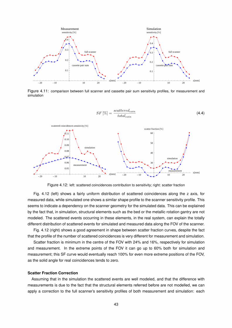
è

è

è

è

èè

è è

è

è

è

è è

è

è

è

è èè è

è

è

è

è

è

è

è

è

è

èè è è

è

è

è

è è

è

è

è

è èè è

è

è

è

è

è

full scanner

cassette pair sum

-20 -10 10 20z@mmD

0.1

0.2

0.3

0.4

sensitivity @%DMeasurement

è

è

è

è

èè è

è è

è

è

èè

è

è

è

è èè è

è

è

è

è

è

è

è

è

è

èè è

èè

è

è

èè

è

è

è

è è

èè

è

è

è

è

è

full scanner

cassette pair sum

-20 -10 10 20z@mmD

0.1

0.2

0.3

0.4

sensitivity @%DSimulation

Figure 4.11: comparison between full scanner and cassette pair sum sensitivity profiles, for measurement andsimulation

SF [%] =scatteredcointotalcoin

(4.4)

è

è

è

è

è

è èè è

è

è

è èè

è

è

èè

è

èè

è

è

è

è

è

èè

èè

èè

èè

èè è è è

èè

èè

èè

èè

èè

è

simulation

measurement

-20 -10 10 20z@mmD

0.05

0.06

0.07

0.08

0.09

0.10

0.11

scattered coincidences sensitivity @%D

è

è

è

è

è è èè

è

èè

è èè

è

è

èè è è

è

è

è

è

è

è

è

è

è

è èè

èè

è

è

è è

è

è

èè

è

è è è

è

è

è

è

simulation

measurement

-20 -10 10 20z@mmD

30

40

50

60

scatter fraction @%D

Figure 4.12: left: scattered coincidences contribution to sensitivity; right: scatter fraction

Fig. 4.12 (left) shows a fairly uniform distribution of scattered coincidences along the z axis, for

measured data, while simulated one shows a similar shape profile to the scanner sensitivity profile. This

seems to indicate a dependency on the scanner geometry for the simulated data. This can be explained

by the fact that, in simulation, structural elements such as the bed or the metallic rotation gantry are not

modeled. The scattered events occurring in these elements, in the real system, can explain the totally

different distribution of scattered events for simulated and measured data along the FOV of the scanner.

Fig. 4.12 (right) shows a good agreement in shape between scatter fraction curves, despite the fact

that the profile of the number of scattered coincidences is very different for measurement and simulation.

Scatter fraction is minimum in the centre of the FOV with 24% and 16%, respectively for simulation

and measurement. In the extreme points of the FOV it can go up to 60% both for simulation and

measurement; this SF curve would eventually reach 100% for even more extreme positions of the FOV,

as the solid angle for real coincidences tends to zero.

Scatter Fraction CorrectionAssuming that in the simulation the scattered events are well modeled, and that the difference with

measurements is due to the fact that the structural elements referred before are not modelled, we can

apply a correction to the full scanner’s sensitivity profiles of both measurement and simulation: each

43

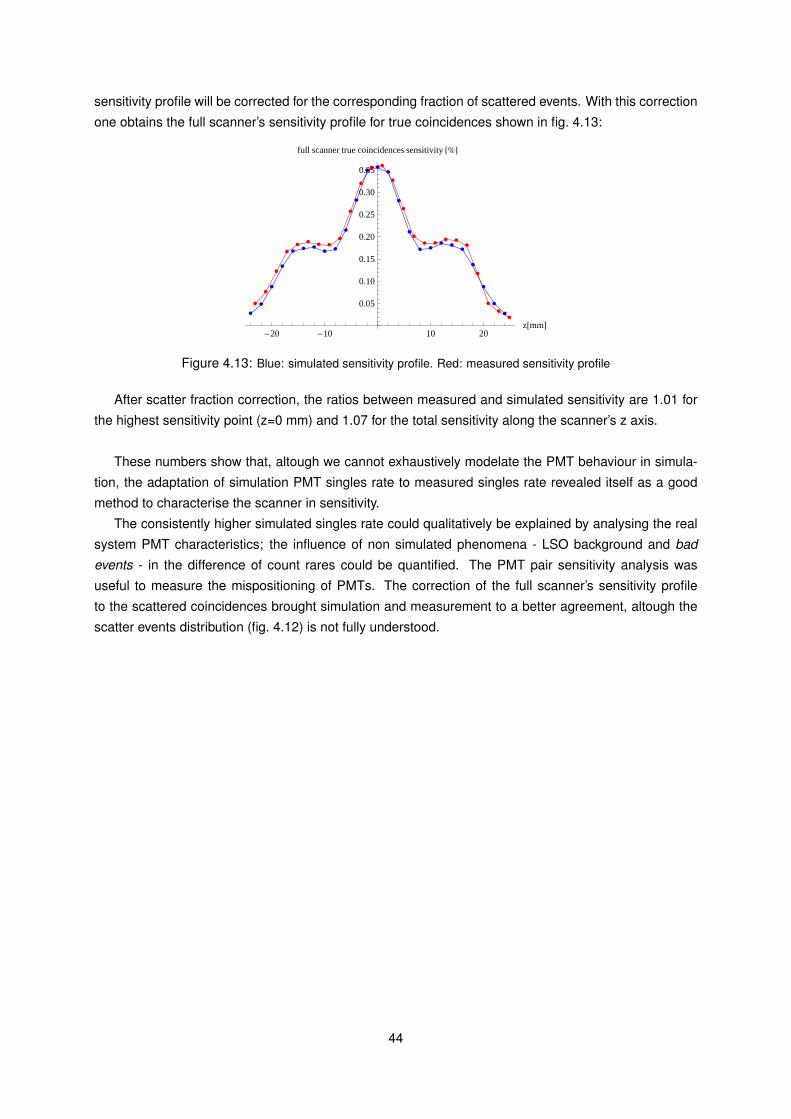
sensitivity profile will be corrected for the corresponding fraction of scattered events. With this correction

one obtains the full scanner’s sensitivity profile for true coincidences shown in fig. 4.13:

è

è

è

è

èè è

èè

è

è

èè

è

è

è

è è

èè

è

è

è

è

è

è

è

è

è

èè

è è

è

è

è

èè

è

è

è

è èè è

è

è

è

è

è

-20 -10 10 20z@mmD

0.05

0.10

0.15

0.20

0.25

0.30

0.35

full scanner true coincidences sensitivity @%D

Figure 4.13: Blue: simulated sensitivity profile. Red: measured sensitivity profile

After scatter fraction correction, the ratios between measured and simulated sensitivity are 1.01 for

the highest sensitivity point (z=0 mm) and 1.07 for the total sensitivity along the scanner’s z axis.

These numbers show that, altough we cannot exhaustively modelate the PMT behaviour in simula-

tion, the adaptation of simulation PMT singles rate to measured singles rate revealed itself as a good

method to characterise the scanner in sensitivity.

The consistently higher simulated singles rate could qualitatively be explained by analysing the real

system PMT characteristics; the influence of non simulated phenomena - LSO background and bad

events - in the difference of count rares could be quantified. The PMT pair sensitivity analysis was

useful to measure the mispositioning of PMTs. The correction of the full scanner’s sensitivity profile

to the scattered coincidences brought simulation and measurement to a better agreement, altough the

scatter events distribution (fig. 4.12) is not fully understood.

44

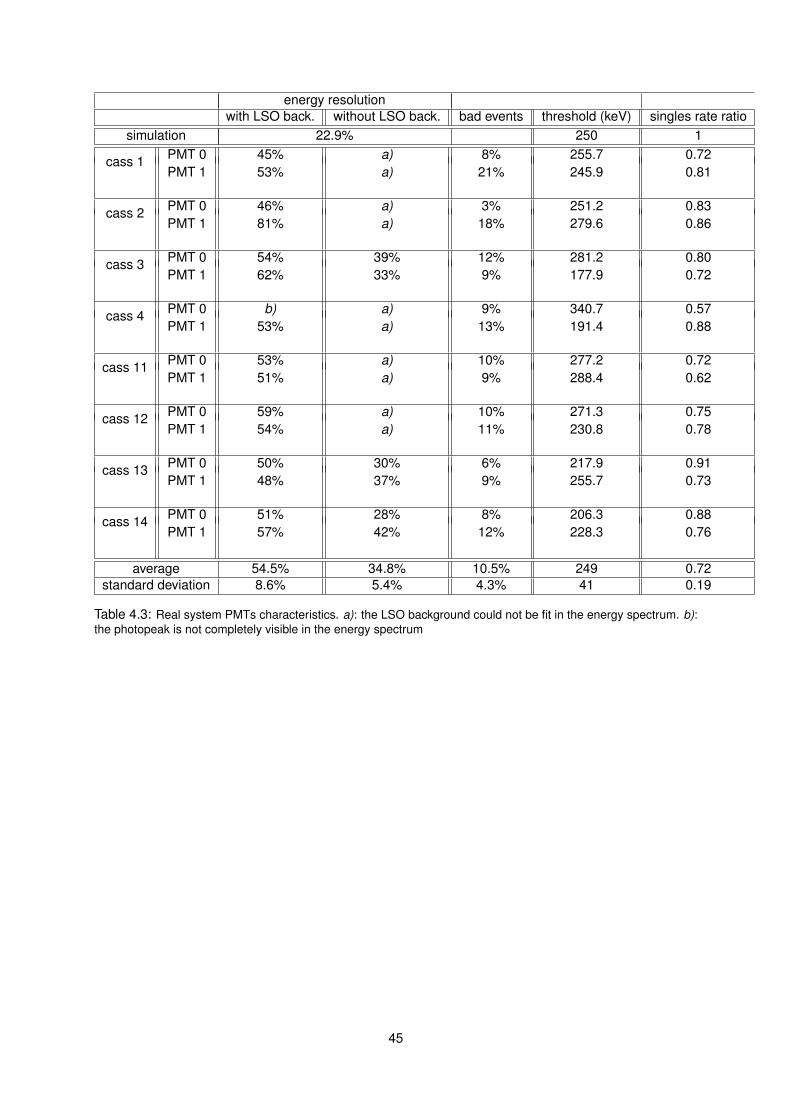
energy resolutionwith LSO back. without LSO back. bad events threshold (keV) singles rate ratio

simulation 22.9% 250 1PMT 0 45% a) 8% 255.7 0.72cass 1PMT 1 53% a) 21% 245.9 0.81

PMT 0 46% a) 3% 251.2 0.83cass 2PMT 1 81% a) 18% 279.6 0.86

PMT 0 54% 39% 12% 281.2 0.80cass 3PMT 1 62% 33% 9% 177.9 0.72

PMT 0 b) a) 9% 340.7 0.57cass 4PMT 1 53% a) 13% 191.4 0.88

PMT 0 53% a) 10% 277.2 0.72cass 11PMT 1 51% a) 9% 288.4 0.62

PMT 0 59% a) 10% 271.3 0.75cass 12PMT 1 54% a) 11% 230.8 0.78

PMT 0 50% 30% 6% 217.9 0.91cass 13PMT 1 48% 37% 9% 255.7 0.73

PMT 0 51% 28% 8% 206.3 0.88cass 14PMT 1 57% 42% 12% 228.3 0.76

average 54.5% 34.8% 10.5% 249 0.72standard deviation 8.6% 5.4% 4.3% 41 0.19

Table 4.3: Real system PMTs characteristics. a): the LSO background could not be fit in the energy spectrum. b):the photopeak is not completely visible in the energy spectrum

45

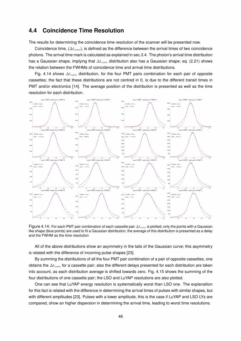
4.4 Coincidence Time Resolution

The results for determining the coincidence time resolution of the scanner will be presented now.

Coincidence time, (∆tcoin), is defined as the difference between the arrival times of two coincidence

photons. The arrival time mark is calculated as explained in sec.3.4. The photon’s arrival time distribution

has a Gaussian shape, implying that ∆tcoin distribution also has a Gaussian shape; eq. (2.21) shows

the relation between the FWHMs of coincidence time and arrival time distributions.

Fig. 4.14 shows ∆tcoin distribution, for the four PMT pairs combination for each pair of opposite

cassettes; the fact that these distributions are not centred in 0, is due to the different transit times in

PMT and/or electronics [14]. The average position of the distribution is presented as well as the time

resolution for each distribution.

FWHM : 4.58 ns

delay : 0.579 ns

10 20 30 40 50

1000

2000

3000

4000

cass 1 PMT 0 and cass 11 PMT 0

FWHM : 4.32 ns

delay : -2.25 ns

10 20 30 40 50

1000

2000

3000

4000cass 1 PMT 0 and cass 11 PMT 1

FWHM : 5.27 ns

delay : 2.36 ns

10 20 30 40 50

1000

2000

3000

4000cass 1 PMT 1 and cass 11 PMT 0

FWHM : 4.55 ns

delay : -0.44 ns

10 20 30 40 50

1000

2000

3000

4000

cass 1 PMT 1 and cass 11 PMT 1

FWHM : 4.56 ns

delay : -0.116 ns

10 20 30 40 50

1000

2000

3000

4000

cass 2 PMT 0 and cass 12 PMT 0

FWHM : 4.83 ns

delay : 0.886 ns

10 20 30 40 50

1000

2000

3000

4000

cass 2 PMT 0 and cass 12 PMT 1

FWHM : 4.86 ns

delay : -0.373 ns

10 20 30 40 50

500

1000

1500

2000

2500

3000

3500

cass 2 PMT 1 and cass 12 PMT 0

FWHM : 5.04 ns

delay : 0.657 ns

10 20 30 40 50

500

1000

1500

2000

2500

3000

3500

cass 2 PMT 1 and cass 12 PMT 1

FWHM : 6.77 ns

delay : 0.748 ns

10 20 30 40 50

500

1000

1500

2000

cass 3 PMT 0 and cass 13 PMT 0

FWHM : 6.15 ns

delay : -1.75 ns

10 20 30 40 50

500

1000

1500

2000

2500

cass 3 PMT 0 and cass 13 PMT 1

FWHM : 7.15 ns

delay : 2.11 ns

10 20 30 40 50

500

1000

1500

2000

2500

3000

cass 3 PMT 1 and cass 13 PMT 0

FWHM : 5.85 ns

delay : -0.423 ns

10 20 30 40 50

500

1000

1500

2000

2500

3000

cass 3 PMT 1 and cass 13 PMT 1

FWHM : 6.79 ns

delay : 1. ns

10 20 30 40 50

500

1000

1500

2000

cass 4 PMT 0 and cass 14 PMT 0

FWHM : 5.22 ns

delay : 1. ns

10 20 30 40 50

500

1000

1500

2000

cass 4 PMT 0 and cass 14 PMT 1

FWHM : 7.78 ns

delay : 1.2 ns

10 20 30 40 50

500

1000

1500

2000

2500

cass 4 PMT 1 and cass 14 PMT 0

FWHM : 5.89 ns

delay : 1.21 ns

10 20 30 40 50

500

1000

1500

2000

2500

3000

3500

cass 4 PMT 1 and cass 14 PMT 1

Figure 4.14: For each PMT pair combination of each cassette pair ∆tcoin is plotted; only the points with a Gaussianlike shape (blue points) are used to fit a Gaussian distribution; the average of this distribution is presented as a delayand the FWHM as the time resolution

All of the above distributions show an asymmetry in the tails of the Gaussian curve; this asymmetry

is related with the difference of incoming pulse shapes [23].

By summing the distributions of all the four PMT pair combination of a pair of opposite cassettes, one

obtains the ∆tcoin for a cassette pair; also the different delays presented for each distribution are taken

into account, as each distribution average is shifted towards zero. Fig. 4.15 shows the summing of the

four distributions of one cassette pair; the LSO and LuYAP resolutions are also plotted.

One can see that LuYAP energy resolution is systematically worst than LSO one. The explanaition

for this fact is related with the difference in determining the arrival times of pulses with similar shapes, but

with different amplitudes [23]. Pulses with a lower amplitude, this is the case if LuYAP and LSO LYs are

compared, show an higher dispersion in determining the arrival time, leading to worst time resolutions.

46

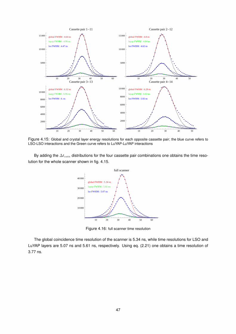
global FWHM : 4.64 ns

lso FWHM : 4.47 ns

luyap FWHM : 4.98 ns

10 20 30 40 50 60

5000

10 000

15 000

Cassette pair 1-11

global FWHM : 4.8 ns

lso FWHM : 4.62 ns

luyap FWHM : 4.84 ns

10 20 30 40 50

5000

10 000

15 000

Cassette pair 2-12

global FWHM : 6.32 ns

lso FWHM : 6. ns

luayp FWHM : 6.96 ns

10 20 30 40 50 60

2000

4000

6000

8000

10 000

Cassette pair 3-13

global FWHM : 6.28 ns

lso FWHM : 5.92 ns

luyap FWHM : 6.63 ns

10 20 30 40 50

2000

4000

6000

8000

10 000

Cassette pair 4-14

Figure 4.15: Global and crystal layer energy resolutions for each opposite cassette pair; the blue curve refers toLSO-LSO interactions and the Green curve refers to LuYAP-LuYAP interactions

By adding the ∆tcoin distributions for the four cassette pair combinations one obtains the time reso-

lution for the whole scanner shown in fig. 4.15.

global FWHM : 5.34 ns

luyap FWHM : 5.61 ns

lso FWHM : 5.07 ns

10 20 30 40 50 60

10 000

20 000

30 000

40 000

full scanner

Figure 4.16: full scanner time resolution

The global coincidence time resolution of the scanner is 5.34 ns, while time resolutions for LSO and

LuYAP layers are 5.07 ns and 5.61 ns, respectively. Using eq. (2.21) one obtains a time resolution of

3.77 ns.

47

Chapter 5

Conclusions

The results obtained for the sensitivity of the scanner can be considered satisfactory. The good agree-

ment between measured data and GATE simulations could be observed for PMT pair, cassette pair and

full scanner sensitivity. The measured and simulated full scanner sensitivity for the highest sensitivity

point were 0.36% and 0.35%, respectively.

Not only the results were satisfactory but, more important, the methods used for characterising the

scanner’s sensitivity lead us to a better understanding of the scanner. One was able to evaluate the

different performances of the nuclear component of the detection system: the phoswhich matrix.

The energy resolutions showed a big deviation relatively to simulation: the best real system energy

resolution was significantly worse than the simulated one, with respective values of 28.1% and 22.9%.

The measured threshold energies of the PMTs were in a good agreement with simulation, with an

average value of 249 keV, while simulated threshold was of 250 keV. The influence of LSO background

was well determined: it contributed not only to an increase in the measured singles count rate, but

it also had influence in the energy resolution determination. In the inverse way, the amount of bad

events contributed to a decrease in the measured count rates; the origin of these errors in the real

system is not clear, but its contribution to the measured singles decrease is well known for each PMT.

A much lower contribution to the measurement/simulation disagreement was detected: small deviations

in the positioning of PMTs were measured, as well as the existence of a systematic error of 0.86 mm in

determining the real position in measurements.

A new method of determining the scatter fraction using sensitivity profiles was presented. The results

show a similar behaviour between measured and simulated scatter fraction. The variation of the SF

between the centre and the extreme positions of the FOV was of 24% to 60% and 16% to 50% for

simulation and measurement, respectively.

All the previously described factors will be useful in future work on the second version of the Clear-

PET; ClearPET2 differs from ClearPET1 in the crystals height and in the number of PMT per cassette:

it will have 8 mm long crystals and 4 PMTs per cassette. In spite of that, the methods used to calculate

PMT energy resolutions and thresholds remain valid in the new scanner.

The future simulations relative to the new scanner can also be improved, taking into account the

issues shown previously and that were not modeled in simulations used in this work.

The measured global time resolution of the scanner is 5.34 ns. The time resolutions of LSO and

LuYAP crystal layers were also calculated and are 5.07 ns and 5.61 ns, respectively; the lower time

resolution of LSO compared to LuYAP was expected, given the difference in the light yield of both

crystals.

48

The time resolution between PMT pairs were also calculated; an unexpected asymmetry in the coin-

cidence time distribution was detected, but its origin was related with the difference in pulse shapes.

49

Appendix A

Simulation

Numerical Simulations are essential tools in Physics. In experimental Physics they allow to estimate the

performance of an experimental device prior to its development; also the posterior comparison between

these and experimental data is an important analysis.

Monte Carlo numerical methods are the basis of GEANT4 simulation algorithms; these model phys-

ical processes based on the statistical nature of these.

The GEANT (GEometry ANd Tracking) community, under the CERN supervising, has been devel-

oping over the last 20 years Monte Carlo tools, specially for High Energy Physics; these tools focus on

modeling the detection systems as well as in the interactions of elementary particles with matter.

Based on the core of a GEANT version, GEANT4, a platform of simulations was created in 2001:

GATE (Geant4 Application for Tomographic Emission); GATE makes use of GATE4 core tables and

libraries to perform simulations of PET and SPECT (Single Proton Emission Computed Tomography)

systems. This chapter will focus on the relevant aspects of GATE related with the simulation part of this

work.

The bibliographic reference used throughout this chapter will be [22].

A.1 General Aspects of GATE

GATE is, like GEANT4, organised in a layer structure:

- the core layer consists of several hundred C++ classes that manage time, geometry or radioactive

sources processes.

- in an intermediate layer, there are classes implementing the core layer ones: they execute specific

geometry operations, like defining volumes or rotation.

- at the user-level layer, one finds a scripting mechanism that makes it possible for the user to

perform and to control a simulation.

Simulations setups may be described interactively, i.e., the user sequentially introduces the parameters

of the simulation or, most commonly, by building up a macro file containing all necessary commands.

A.2 Simulation Structure

A.2.1 Geometry

The definition of a Scanner geometry is made on a hierarchical basis: a world volume is defined by

default and all the other geometric structures are defined as daughters, grand-daughters and so on, of50

itself. Inside the world volume, at its daughter level, a geometry for the scanner has to be defined. There

are several predefined scanner geometries; here one only focus on CylindricalPET.

For a CylindricalPET geometry there are 5 possible daughter levels; these levels and its correspon-

dent physical components are shown in table A.2.1.

depth level name real system equivalent1 rsector cassette2 module PMT3 submodule phoswich matrix4 crystal individual crystal5 layer[i], i = 0, 3 crystal layer index

Table A.1: geometry definition in GATE

One can define the geometry of a Cylindrical PET system by using the following macro commands:

defining the world volume, a cube of 25x25x25cm3

/gate/world/geometry/setXLength 25 cm

...

defining a cylindricalPET system and its dimensions

/gate/world/daughters/name cylindricalPET

/gate/cylindricalPET/geometry/setRmax 105 mm

...

defining an rsector volume; an rsector corresponds to a cassette

/gate/cylindricalPET/daughters/name cassette

inside an rsector volume one defines two daughters of same level; the first one is the creation of a

matrix, which will house the crystal layers

/gate/cassette/daughters/name crystalMatrix

/gate/crystalMatrix/geometry/setXLength 16.0 mm

...

the second is the creation of the PMT structure

/gate/cassette/daughters/name PMT

definition of the two crystal layers, LSO and LuYAP

/gate/crystalMatrix/daughters/name crystal

/gate/crystal/geometry/setXLength 16.0 mm

/gate/crystal/daughters/name LSO

/gate/LSO/geometry/setXLength 8.0 mm

/gate/crystal/daughters/name LuYAP

/gate/LuYAP/geometry/setXLength 8.0 mm

In GATE one only defines a single volume-element for each component (rsector,module, . . . ), so that

it becomes necessary to repeat each one of those elements, according to its spatial distribution. It is

possible to define repeaters of several types, such as a cubic, for the crystal matrix, or linear repeater

for PMTs; to fully reproduce the scanner’s geometry it is thus necessary to repeat its components as

exemplified in the following command lines

rsector repetition in radial symmetry; creation of a ring of 20 detectors.51

/gate/cassette/repeaters/insert ring

/gate/cassette/ring/setRepeatNumber 20

PMT repetition; it is repeated twice for each rsector

/gate/PMT/repeaters/insert linear

/gate/PMT/linear/setRepeatNumber 2

creation of the 8x8 crystal matrix

/gate/crystal/repeaters/insert cubicArray

/gate/crystal/cubicArray/setRepeatNumberY 8

/gate/crystal/cubicArray/setRepeatNumberZ 8

A.2.2 Physical Processes

To setup the physical processes in GATE one makes use of two libraries present in GEANT4:

- standard energy electromagnetic processes (SEP) for Energies above 10keV .

- low energy electromagnetic processes (LEP) for energies below 10keV .

In a ClearPET scanner with typical positron energies of ∼ 101keV (table 2.1), SEP is the library

modelling electron and positron physics. The most important processes are:

- multiple scattering

- ionisation

- bremsstrahlung

- e+e− annihilation

This processes are not user-changeable, as they are already hard-coded in GEANT4 core.

As far as photon interaction is concerned, the user has the possibility to select processes affect-

ing it and the respective energy model (LEP or SEP). These macro lines define the energy model for

Photoelectric, Compton and Rayleigh processes.

/gate/physics/gamma/selectPhotoelectric inactive

/gate/physics/gamma/selectCompton lowenergy

/gate/physics/gamma/selectRayleigh standard

A.2.3 Radioactive Sources

In order to define a source for the system GATE makes use of a GEANT4 library called General Particle

Source (GPS). there are several parameters the user can define:

emitted particle: single particles such as γ, e+ or e−; user can also define a positron emitter source

such as 18F or 11C; there is also implemented a back to back source, where two photons are emit-

ted as if coming from of a e+e− annihilation; this last results in a faster simulation when compared

to a real positron emitting source.

energy: the particle’s energy can be set, for example as monoenergetic particle or with a particular

energy distribution.

emission distribution: it is possible to define the angular span of emission of a particle.

52

shape: user can define several geometrical configurations for the radioactive source: point source, or a

predefined source shape, such as spherical or cylindrical.

activity: user defines the initial activity of the source.

This is the code example of a back to back γ point source with initial activity of 1MBq emmiting isotropi-

cally. The following code lines show how to simulate a 511 keV back-to-back point source and a realistic22Na source, both with 1 MBq of activity.

/gate/source/addSource gamma

/gate/source/gamma/setActivity 1000000 Bq

/gate/source/gamma/setType backtoback

/gate/source/gamma/gps/energytype Mono

/gate/source/gamma/gps/monoenergy 511. keV

/gate/source/gamma/gps/type Point

/gate/source/gamma/gps/angtype iso

/gate/source/addSource Na22

/gate/source/Na22/setActivity 1000000. Bq

/gate/source/Na22/gps/particle ion

/gate/source/Na22/gps/ion 11 22 0 0

/gate/source/Na22/gps/monoenergy 0 eV

/gate/source/Na22/setForcedUnstableFlag true

/gate/source/Na22/setForcedHalfLife 10000000 s

/gate/source/Na22/gps/centre 0. 0. z mm

/gate/source/Na22/gps/angtype iso

/gate/source/Na22/gps/shape Sphere

/gate/source/Na22/gps/radius 0.25 mm

A.2.4 Digitizing Module

Before detailing the architecture of the Digitizing module, it is convenient to explain the chain of events

undergone by a particle in the scanner:

1. a particle is generated, with pre-determined characteristics: energy and momentum

2. steps, corresponding to the distance travelled by the particle between 2 interactions, are succes-

sively applied to the particle.

3. when a step occurs inside a volume element identified as a crystal, one says a hit occurred; when

this happens information about the interaction is recorded. this information includes deposited

energy and particle’s moment.

4. steps 2 and 3 are repeated until the particle goes out of the geometric limits of the detector, or its

energy drops below a certain level. the ensemble of all the steps is called the particle’s track.

5. the energy of a hit is treated throughout a series of components, called digitisers; each transitory

value between two digitisers is called a pulse; in the end of the Digitizing chain a single is produced

as output.

This steps are repeated to all emitted particles giving rise to a list of singles that is stored in an output

file (see section 4.2.5).

A Digitizing chain used in this work’s simulation is schematised in fig. A.1.53

Figure A.1: Digitizing module

adderThe first task of the digitiser is to sum all the hits energies occurring in a single crystal. This is due

to the fact that, in the same crystal, multiple Compton or Photoelectric interactions can occur; because

electronics always readout an integrated signal from a single crystal, all the hit energies have to be

summed. the adder module is set as follows:

/gate/digitiser/Singles/insert adder

readoutWhile the adder module sums the hits within the same crystal volume, the readout module allows to

group signals occurring in volumes with the same depth; if there’s a particle interacting on both crystal

layers, the readout module can sum both signals; for that one needs to specify the depth in which the

signals should be grouped; for the crystal block, which has depth 4 (table A.2.1), the readout module

would be set as follows:

/gate/digitiser/Singles/insert readout

/gate/digitiser/Singles/insert setDepth 4

energy blurringThe energy blurring module simulates the blurring of the energy spectrum of a pulse in the crystal;

this blurring has a Gaussian shape, for which the resolution is given by eq. (2.15). To set this, one has

to introduce the resolution at a certain energy of reference; for an LSO crystal with a resolution of 20%

at 511 keV :

/gate/digitiser/Singles/localBlurring/chooseNewVolume LSO

/gate/digitiser/Singles/localBlurring/LSO/setResolution 0.20

/gate/digitiser/Singles/localBlurring/LSO/setEnergyOfReference 511. keV

thresholder and upholderThe thresholder and upholder module allow to apply an energy window to detected photons; photons

above and below uphold and threshold levels, respectively, are removed.

- the thresholder is modelated by a sigmoidal function as in eq. (A.1):

σ(E) =1

1 + exp(αE−E0

E0

) (A.1)

to set a sigmoidal thresholder at 250 keV , with a percentage of acceptance of 95%, and a param-

eter α = 60, the user has to introduce the follwing commands:

/gate/digitiser/Singles/sigmoidalThresholder/setThreshold 250 keV

/gate/digitiser/Singles/sigmoidalThresholder/setThresholdAlpha 80

/gate/digitiser/Singles/sigmoidalThresholder/setThresholdPerCent 0.95

54

to realise the cut, σ(E) is calculated for a determined energy and compared to a random number

between 0 and 1; if σ(E) is lower than the percentage of acceptance, the photon is removed.

- an upholder that simply removes photons above 750 keV is set in the following way:

/gate/digitiser/upholder/setUphold 750 keV

temporal resolutionThe temporal resolution module works in the same way of the energy blurring module; the difference

is that it applies a Gaussian blurring in the temporal resolution rather than in energy. To set a time

resolution of, for example ,5 ns, the user should introduce the follwing commands:

/gate/digitiser/Singles/insert timeResolution

/gate/digitiser/Singles/timeResolution/setTimeResolution 5 ns

dead timeElectronic readout devices are limited to a maximum rate of events that they can handle; this limitations

implies that for a sufficiently high incoming particle rate, some events are not able to be processed; the

amount of time an event takes to be processed is called dead time; here are two ways of modelling

dead-time: paralysable and non-paralysable [23]. This example shows how to define a non-paralysable

dead time of 1440 ns per cassette.

/gate/digitiser/Singles/deadtime/chooseDTVolume cassette

/gate/digitiser/Singles/deadtime/setDeadTime 1440 ns

/gate/digitiser/Singles/deadtime/setMode nonparalysable

A.2.5 Data Output

GATE allows to choose various formats of data output: ASCII and ROOT that are system independent

formats; LMF, ECAT and Interfile, that were developed for specific systems; the LMF format, already

referred in section 3.4 is the most used one in the simulations of our ClearPET scanner.

Next macro lines show an example of how output can be configured:

/gate/output/ascii/disable

/gate/output/root/disable

/gate/output/lmf1/enable

/gate/output/lmf1/setEnergyBool 1

/gate/output/lmf1/setDetectorIDBool 0

in this example, ASCII and ROOT outputs are disabled and LMF is enabled; for which output format one

can set various options; in this case the user chooses to save the energy of the hit but not the ID of the

detector where the hit occurred

55

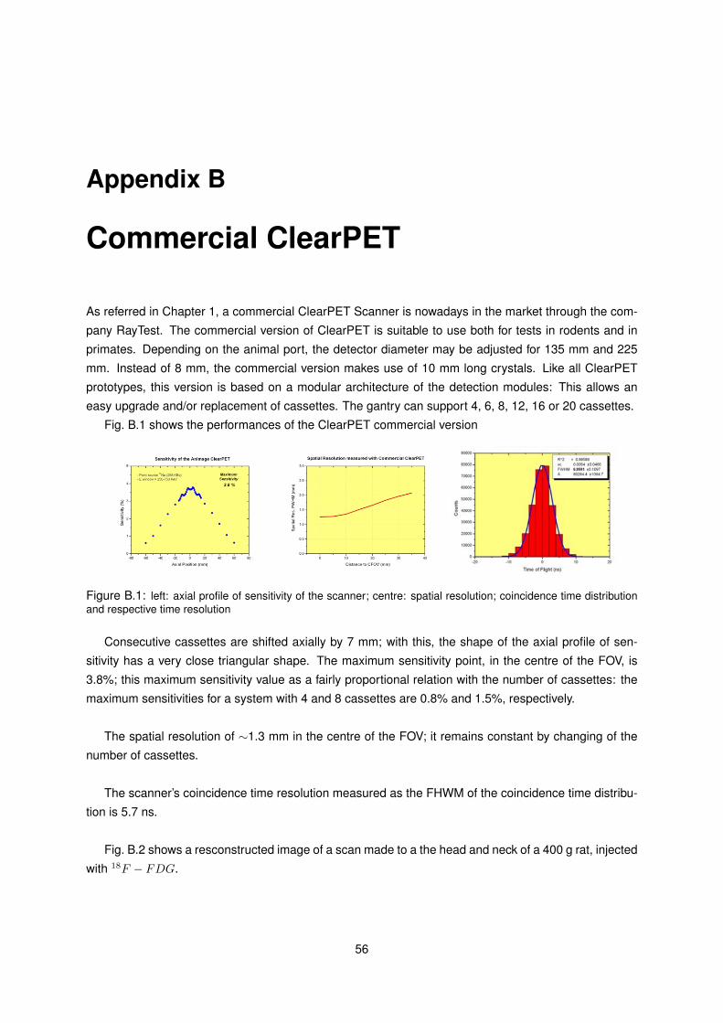
Appendix B

Commercial ClearPET

As referred in Chapter 1, a commercial ClearPET Scanner is nowadays in the market through the com-

pany RayTest. The commercial version of ClearPET is suitable to use both for tests in rodents and in

primates. Depending on the animal port, the detector diameter may be adjusted for 135 mm and 225

mm. Instead of 8 mm, the commercial version makes use of 10 mm long crystals. Like all ClearPET

prototypes, this version is based on a modular architecture of the detection modules: This allows an

easy upgrade and/or replacement of cassettes. The gantry can support 4, 6, 8, 12, 16 or 20 cassettes.

Fig. B.1 shows the performances of the ClearPET commercial version

Figure B.1: left: axial profile of sensitivity of the scanner; centre: spatial resolution; coincidence time distributionand respective time resolution

Consecutive cassettes are shifted axially by 7 mm; with this, the shape of the axial profile of sen-

sitivity has a very close triangular shape. The maximum sensitivity point, in the centre of the FOV, is

3.8%; this maximum sensitivity value as a fairly proportional relation with the number of cassettes: the

maximum sensitivities for a system with 4 and 8 cassettes are 0.8% and 1.5%, respectively.

The spatial resolution of ∼1.3 mm in the centre of the FOV; it remains constant by changing of the

number of cassettes.

The scanner’s coincidence time resolution measured as the FHWM of the coincidence time distribu-

tion is 5.7 ns.

Fig. B.2 shows a resconstructed image of a scan made to a the head and neck of a 400 g rat, injected

with 18F − FDG.

56

Figure B.2: left: coronal view; centre: transversal view; right: sagital view

57

Bibliography

[1] D. Malakof. The rise of the mouse, biomedicine’s model mammal. Science, 288 :248-253, 2000.

[2] Suehiro M. et all. A PET radiotracer for studying serotonin uptake sites : carbon-11-McN-5652Z. The journal of nuclear medicine. 1993, vol. 34, no 1, pp. 120-127

[3] Jarkas N. et all. Carbon-11 HOMADAM: a novel PET radiotracer for imaging serotonin trans-porters. Nuclear Medical Biology. 2005 Apr;32(3):211-24

[4] Wolfgang B. Oxygen-15-Water PET Assessment of Muscular Blood Flow in Peripheral Vascu-lar Disease. The Journal of Nuclear Medicine Vol. 38 No. 1 93-98

[5] Blanco A. Positron Range Effects on the Spatial Resolution of RPC-PET. Nuclear Science

Symposium Conference Record, 2006. IEEE

[6] Levin S. et all. Calculation of positron range and its effect on the fundamental limit of positronemission tomography system spatial resolution. Physical Medical Biology. 44 (1999) 781-799

[7] Daghighiam, F. et all. Evaluation of cerium doped lutetium oxyorthosilicate (LSO)scintillationcrystals for PET. Nuclear Science Symposium and Medical Imaging Conference, 1992

[8] Trummer J. et all. Comparison of LuAP and LuYAP crystal properties from statistically signif-icant batches produced with two different growth methods. Nuclear Instruments and Methods

in Physics Research. Vol. 551, (11 October 2005), pp. 339-351

[9] Simon L. at all. Simulation of time curves in small animal PET using GATE. Nuclear Instruments

and Methods in Physics Research A 527 (2004) 190â194.

[10] Auffray E. et all. The ClearPET project. Nuclear Instruments and Methods in Physics Research A

527 (2004) 171-174.

[11] S. Cherry. The 2006 Henry N. Wagner Lecture: Of Mice and Men (and Positrons)-Advances inPET Imaging Technology. Journal of Nuclear Medicine 2006; vol:47; pp:1735-1745.

[12] Particle Database Group. http://pdg.lbl.gov/pdg.html

[13] S. Tavernier. Measurement Techniques in Nuclear and Particle Physics. VUB 2007

[14] S. Tavernier et all. First Results with the ClearPET Small Animal PET Scanners. Radiation

Detectors for Medical Applications. 2006 Springer

[15] M.Streun et all. Pulse Shape Discrimination of LSO and LuYAP. Scintillators for Depth ofInteraction Detection in PET. IEEE Transactions on Nuclear Science; vol.50, no.3, June 2003

58

[16] U. Heinrichs Auslegung Des Detektorsystems Fur Einen Hochauflosenden Positronen-Emissions-Tomographen Mit Hoher Sensitivitat. Forschungszentrum Julich, Zentralbibliothek,

2003

[17] U. Heinrichs. Design optimization of the PMT-ClearPET prototypes based on simulation stud-ies with GEANT3. 37th Crystal CLear general meeting. CERN 27-28 November 2002

[18] M. Rey. Ãtude du tomographe de haute résolution pour petits animaux Clearpet par la méth-ode de monte Carlo. École Polytechnique Fédérale de Lausanne, 2007

[19] J.B. Mosset. Dèveloppement d’un module de détection phoswich LSO/LuYAP pour le proto-type de caméra à positrons clearpet.École Polytechnique Fédérale de Lausanne, 2006

[20] S.Yamamoto et all. Investigation of single, random and true counts from natural radioactivityin LSO-based clinical PET. Annals of Nuclear Medicine Vol.19, No. 2, 109-114, 2005

[21] S. Kerkhoas-Cavata et all. Modeling electronic processing in GATE. Nuclear Instruments and

Methods in Physics Research A 569 (2006) 330-334

[22] S. Jan et all. GATE: GEANT4 Application for Tomographic Emission: a simulation toolkit forPET and SPECT. http://opengatecollaboration.org. 2006

[23] Knoll G. Radiation Detection and Measurement. John Wiley sons, 1999

[24] S. Yamamoto. Investigation of single, random and true counts from natural radioactivity in LSO-

based clinical PET. Annals of Nuclear Medicine Vol.19, No.2, 109-114, 2005

[25] J.S.Huber et all. Effect of 176Lu background on singles transmission for LSO-based PET Cam-eras. Physical Medical Biology. 47 (2002) 1-7

[26] http://heritage.dupont.com/

[27] http://www2.dupont.com/Tyvek/

[28] DOW CORNING R©3145 RTV MIL-A-46146 Product Information. http://www.dowcorning.com

[29] HAMAMATSU R7600-M64 Datasheet. http://hamamatsu.com

[30] http://www.xilinx.com

[31] http://www.analog.com/en/analog-microcontrollers/ADUC812/products/product.html

[32] http://www.picoelectronics.com

[33] http://www.inova-semiconductors.de

[34] http://www.ni.com

[35] http://phytron.com

[36] M. Krieguer et all. List Mode Format Implementation: scanner geometry description. Univer-

site de Lausanne

[37] C. Morel et all. LMF specifications. Universite de Lausanne

[38] Performance Measurements of Small Animal Positron Emission Tomographs. National Elec-

trical Manufacturers Association. 200859

[39] M. Streun et all. The Data Acquisition System of ClearPET Neuro-a Small Animal PET Scan-ner. IEEE Transactions on Nuclear Science, Vol.53, no.3, June 2006

[40] S. Derenzo. Mathematical removal of positron range blurring in high resolution tomography.

IEEE Transactions on Nuclear Science, Vol.33 pp:565-569, 1986.

[41] O. Devroede. Front End Modules Update. CCC Meeting. Lyon 10-11 March 2004

[42] Suraj N. Gupta. Multiple Photon Production in Electron-Positron Annihilation. Physical Review,

n.96 p.1453, 1954

60