mestre em engenharia civil especializaÇÃo em geotecnia · mestrado integrado em engenharia civil...
TRANSCRIPT

CONSTITUTIVE MODELLING OF SANDS
UNDER UNDRAINED CONDITIONS
BASED ON GENERALIZED PLASTICITY
PREMISES
MIGUEL NUNO SANTIAGO RIBEIRO
Dissertação submetida para satisfação parcial dos requisitos do grau de
MESTRE EM ENGENHARIA CIVIL — ESPECIALIZAÇÃO EM GEOTECNIA
Orientador: Professor Doutor António Joaquim Pereira Viana da
Fonseca
Coorientador: Professora Doutora Laura Tonni
JULHO DE 2014
MESTRADO INTEGRADO EM ENGENHARIA CIVIL 2013/2014
DEPARTAMENTO DE ENGENHARIA CIVIL
Tel. +351-22-508 1901
Fax +351-22-508 1446
Editado por
FACULDADE DE ENGENHARIA DA UNIVERSIDADE DO PORTO
Rua Dr. Roberto Frias
4200-465 PORTO
Portugal
Tel. +351-22-508 1400
Fax +351-22-508 1440
http://www.fe.up.pt
Reproduções parciais deste documento serão autorizadas na condição que seja
mencionado o Autor e feita referência a Mestrado Integrado em Engenharia Civil -
2013/2014 - Departamento de Engenharia Civil, Faculdade de Engenharia da
Universidade do Porto, Porto, Portugal, 2014.
As opiniões e informações incluídas neste documento representam unicamente o
ponto de vista do respetivo Autor, não podendo o Editor aceitar qualquer
responsabilidade legal ou outra em relação a erros ou omissões que possam existir.
Este documento foi produzido a partir de versão eletrónica fornecida pelo respetivo
Autor.

To my Mother and Father
What saves a man is to take a step. Then another step.
It is always the same step, but you have to take it.
Antoine de Saint-Exupéry


Constitutive modelling of sands under undrained conditions based on Generalized Plasticity premises
i
ACKNOWLEDGEMENTS
I would like to express my deep gratitude to the following people, all of them very important during
the period required for the development of this dissertation:
To Professor Laura Tonni, my Italian supervisor, who welcomed me at the Università di
Bologna in the best possible way. The constant guidance, advice and patience have been very
important during these months throughout the development of this work.
To Professor António Viana da Fonseca, my Portuguese supervisor, for all the support and
help during these months.
To my mother and my father for all the support, care and love and for being the most
important persons in my life.
To my family for every moment of joy that they bring to my life.
To my friends, especially the ones who always accompanied me during the last five years. But
also to the ones I met in Italy, with whom I shared probably the most exciting adventure in my
life which was my exchange period in Bologna.

Constitutive modelling of sands under undrained conditions based on Generalized Plasticity premises
ii

Constitutive modelling of sands under undrained conditions based on Generalized Plasticity premises
iii
ABSTRACT
In this work, Generalized Plasticity-based constitutive models, originally developed for the analysis of
sandy soil behaviour, will be calibrated in order to simulate the stress-strain response of granular soils
under undrained conditions.
The research will be based on the large experimental database, including both laboratory and in situ
testing, recently collected by the University of Bologna in a rather restricted area of the village of
Scortichino (Ferrara) where liquefaction and lateral spreading related phenomena were observed after
the earthquake sequence that struck a wide portion of the Po River alluvial plane (Northern Italy) in
May 2012. On the basis of the available data, a detailed geotechnical model of the area was first
defined. Afterwards, a numerical approach will be adopted in order to simulate the behaviour of the
sandy soils found there. A Generalized Plasticity framework (Pastor et al., 1990) will be considered in
the analysis, allowing for the calibration of different constitutive models: the original Pastor &
Zienkiewicz model (1990) but also two newer modified models. These modified models, based on the
original, were designed with the purpose of including a dependency of the model equations on the
state parameter, for example, allowing for a better reproduction of sand behaviour over a wide range
of confining pressures and densities with a single set of constitutive parameters.
The approach is validated by comparing the model predictions with the experimental results of the
undrained triaxial tests considered. Some sensitivity tests will also be executed in order to understand
which are the main advantages and disadvantages of the models considered.
KEYWORDS: Generalized Plasticity, constitutive modelling, sand behaviour, critical state, granular
soils.

Constitutive modelling of sands under undrained conditions based on Generalized Plasticity premises
iv

Constitutive modelling of sands under undrained conditions based on Generalized Plasticity premises
v
RESUMO
Neste trabalho, vários modelos constitutivos baseados na Generalized Plasticity, originalmente criados
para a análise do comportamento de solos arenosos, serão calibrados e aplicados de forma a simular o
comportamento de solos granulares carregados sob condições não drenadas.
A presente dissertação será baseada nos vários dados experimentais, que incluem ensaios de
laboratório e testes in situ, recentemente recolhidos e executados pela Universidade de Bolonha, numa
zona da vila de Scortichino (Ferrara), onde fenómenos associados à liquefação e a escorregamentos
laterais foram observados após a sequência sísmica que atingiu uma extensa parte da planície aluvial
do rio Pó (norte de Itália), em maio de 2012. Tendo por base a informação disponível, um modelo
geotécnico foi inicialmente definido para a zona. De seguida, a base teórica da Generalized Plasticity
(Pastor et al., 1990) será tida em conta para a análise dos solos considerados, permitindo a aplicação e
calibração de diferentes modelos constitutivos: o modelo original de Pastor & Zienkiewicz (1990) mas
também dois modelos mais recentes. Estes, baseados no modelo original, foram pensados como uma
extensão daquele, na qual se atingiu o objetivo de introduzir uma dependência das equações do
modelo em relação ao parâmetro de estado, por exemplo, permitindo assim uma melhor reprodução do
comportamento das areias sob uma vasta gama de pressões de confinamento e densidades.
A aplicação dos modelos é validada ao comparar as previsões daqueles com os dados experimentais
dos ensaios triaxiais não drenados considerados. Também serão realizados alguns testes de
sensibilidade dos modelos no sentido de perceber as suas vantagens e desvantagens.
PALAVRAS-CHAVE: Generalized Plasticity, modelos constitutivos, comportamento das areias, estado
crítico, solos granulares.

Constitutive modelling of sands under undrained conditions based on Generalized Plasticity premises
vi

Constitutive modelling of sands under undrained conditions based on Generalized Plasticity premises
vii
TABLE OF CONTENTS
ACKNOWLEDGEMENTS ............................................................................................................................ i
ABSTRACT .............................................................................................................................. iii
RESUMO ................................................................................................................................................... v
1. INTRODUCTION .............................................................................................................. 1
1.1. PREAMBLE AND OBJECTIVES ......................................................................................................... 1
1.2. ORGANIZATION OF THE DISSERTATION ......................................................................................... 2
2. FRAMEWORK FOR THE STUDY OF SAND BEHAVIOUR ... 3
2.1. INTRODUCTION ................................................................................................................................ 3
2.2. EXPERIMENTAL BEHAVIOUR OF SANDS ......................................................................................... 3
2.2.1. TRIAXIAL TEST ................................................................................................................................. 3
2.2.2. DRAINED BEHAVIOUR OF SANDS ........................................................................................................ 5
2.2.3. UNDRAINED BEHAVIOUR OF SANDS .................................................................................................... 7
2.3. CRITICAL STATE CONCEPTS ........................................................................................................... 8
2.3.1 CRITICAL VOID RATIO ......................................................................................................................... 8
2.3.2 STATE PARAMETER ........................................................................................................................... 9
2.3.3 CRITICAL STATE LINE ....................................................................................................................... 10
2.4. BACKGROUND ON LIQUEFACTION................................................................................................ 11
2.4.1 FLOW LIQUEFACTION ....................................................................................................................... 12
2.4.2 CYCLIC MOBILITY ............................................................................................................................ 14
2.5. DILATANCY .................................................................................................................................... 15
3. CONSTITUTIVE MODELS BASED ON THE GENERALIZED PLASTICITY THEORY ................................................................................................... 19
3.1. INTRODUCTION TO CONSTITUTIVE MODELS ................................................................................. 19
3.2. GENERALIZED PLASTICITY THEORY ............................................................................................ 20
3.3. THE ORIGINAL PASTOR-ZIENKIEWICZ MODEL FOR GRANULAR SOILS ....................................... 23
3.4. THE MODIFIED MODEL OF COLA & TONNI (2006) ....................................................................... 29
3.4.1. STATE-DEPENDENT DILATANCY ...................................................................................................... 29
3.4.2. PLASTIC MODULUS AT CONSTANT STRESS RATIO COMPRESSION ....................................................... 30
3.4.3. GENERAL EQUATION OF THE PLASTIC MODULUS ............................................................................... 31

Constitutive modelling of sands under undrained conditions based on Generalized Plasticity premises
viii
3.4.4. ELASTIC COMPONENTS ................................................................................................................... 32
3.5. THE MODIFIED MODEL OF DIEGO MANZANAL (2008) ................................................................. 33
3.5.1. CRITICAL STATE CONCEPTS TO CONSIDER ....................................................................................... 33
3.5.2. FLOW RULE ................................................................................................................................... 34
3.5.3. LOADING-UNLOADING DIRECTION .................................................................................................... 36
3.5.4. ELASTIC COMPONENTS ................................................................................................................... 36
3.5.5. PLASTIC MODULUS ......................................................................................................................... 37
4. CASE STUDY – THE 2012 EMILIA-ROMAGNA SEISMIC SEQUENCE .............................................................................................................................. 39
4.1. INTRODUCTION .............................................................................................................................. 39
4.2. DESCRIPTION OF THE CASE .......................................................................................................... 39
4.3. MAIN RESULTS OF THE TRIAXIAL TESTS PERFORMED ................................................................ 45
4.3.1. GRANULOMETRIC DISTRIBUTION CURVE AND GENERAL MATERIAL DESCRIPTION ................................. 45
4.3.2. UNDRAINED TRIAXIAL TESTS RESULTS ............................................................................................. 49
4.3.3. CRITICAL STATE PARAMETERS ........................................................................................................ 55
4.3.4. DILATANCY AND ELASTIC COMPONENTS .......................................................................................... 61
4.3.5. PLASTIC MODULUS ......................................................................................................................... 64
4.4. CONCLUSIONS ............................................................................................................................... 64
5.APPLICATION AND CALIBRATION OF THE CONSTITUTIVE MODELS .......................................................................................... 65
5.1. INTRODUCTION .............................................................................................................................. 65
5.2. DRIVER PD .................................................................................................................................... 66
5.3. PASTOR-ZIENKIEWICZ MODEL ...................................................................................................... 68
5.3.1. MODEL PARAMETERS AND THEIR CALIBRATION ................................................................................. 68
5.3.2. SENSITIVITY TEST OF THE PZ MODEL ............................................................................................... 70
5.3.2.1. Elastic components .................................................................................................................. 72
5.3.2.2. Mg parameter ............................................................................................................................ 76
5.3.2.3. Mf parameter ............................................................................................................................. 79
5.3.2.4. H0 parameter ............................................................................................................................ 81
5.3.2.5. β0 parameter ............................................................................................................................. 83
5.3.2.6. β1 parameter ............................................................................................................................. 86
5.3.2.7. αg parameter ............................................................................................................................. 89
5.3.2.8. αf parameter .............................................................................................................................. 90

Constitutive modelling of sands under undrained conditions based on Generalized Plasticity premises
ix
5.3.2.9. Confining pressure ................................................................................................................... 93
5.3.4. PRELIMINARY CONCLUSIONS ABOUT THE ORIGINAL PASTOR-ZIENKIEWICZ MODEL .............................. 95
5.3.5. FINAL CALIBRATION PROCEDURE AND RESULTS ................................................................................ 95
5.3.6. CONCLUSION ................................................................................................................................. 98
5.4. MODIFIED MODEL OF COLA AND TONNI (2006) .......................................................................... 99
5.4.1. MODEL PARAMETERS AND THEIR CALIBRATION ................................................................................. 99
5.4.1.1. Elastic components ................................................................................................................ 100
5.4.1.2. Critical state parameters ........................................................................................................ 102
5.4.1.3. Dilatancy components ............................................................................................................ 102
5.4.1.4. Loading vector parameters..................................................................................................... 108
5.4.1.5. Plastic modulus law ................................................................................................................ 109
5.4.2. FINAL CALIBRATION AND RESULTS ................................................................................................. 111
5.5. MODIFIED MODEL OF MANZANAL (2008) .................................................................................. 117
5.5.1. MODEL PARAMETERS AND THEIR CALIBRATION ............................................................................... 117
5.5.1.1. Elastic components ................................................................................................................ 117
5.5.1.2. Critical state parameters ........................................................................................................ 118
5.5.1.3. Dilatancy components ............................................................................................................ 118
5.5.1.4. Loading vector parameters..................................................................................................... 122
5.5.1.5. Plastic modulus law ................................................................................................................ 122
5.5.2. FINAL CALIBRATION AND RESULTS ................................................................................................. 123
6. CONCLUSIONS ........................................................................................................... 129
6.1. CONCLUSIONS............................................................................................................................. 129
6.2. FUTURE DEVELOPMENTS ............................................................................................................ 129
REFERENCES ...................................................................................................................................... 131
APPENDIX A ......................................................................................................................... 135
A.1 EQUATIONS CONSIDERED IN THE MODEL FOR THE DRAINED TESTS ........................................ 135
A.2 EQUATIONS CONSIDERED IN THE MODEL FOR THE UNDRAINED TESTS .................................... 136

Constitutive modelling of sands under undrained conditions based on Generalized Plasticity premises
x

Constitutive modelling of sands under undrained conditions based on Generalized Plasticity premises
xi
LIST OF FIGURES
Fig. 2.1 - Experimental setup of triaxial test (Bardet, 1997) .................................................................... 4
Fig. 2.2 - Triaxial test: a) compression paths; b) extension paths (Adapted from Manzanal, 2008) ....... 4
Fig. 2.3 – Typical behaviours of a soil subjected to a drained triaxial test: a) in the q - εa space; b) in
the εv - εa space (Adapted from Manzanal, 2008) ................................................................................... 5
Fig. 2.4 - Stress ratio q/p' plotted as a function of the: a) axial strain; b) void ratio (Adapted from
Manzanal, 2008) ...................................................................................................................................... 5
Fig. 2.5 - Void ratio variation plotted as function of the axial strain (Adapted from Manzanal, 2008) ..... 6
Fig. 2.6 - Typical behaviours of a soil subjected to an undrained triaxial test: a) in the q – p’ space; b)
in the q - εa space (Adapted from Manzanal, 2008) ................................................................................ 7
Fig. 2.7 - Pore pressure plotted as a function of axial deformation ......................................................... 7
Fig. 2.8 – Different behaviours of specimens with different initial conditions and under different
drainage conditions: a) e - p’ space; b) e - log(p’) space (Adapted from Kramer, 1996) ........................ 8
Fig. 2.9 - State parameter definition ........................................................................................................ 9
Fig. 2.10 - Critical State Line over a wide range of confining pressures (Been et. al, 1991) ................ 10
Fig. 2.11 - Critical State Line for the Toyoura sand a) semi-Log scale b) scale (Li & Wang,
1998) ..................................................................................................................................................... 11
Fig. 2.12 - Response of loose and saturated sands: a) stress-strain curve; b) effective stress path; c)
excess pore pressure; d) effective confining pressure (Kramer, 1996) ................................................ 12
Fig. 2.13 - Response of specimens with different initial conditions (Kramer, 1996) ............................. 13
Fig. 2.14 - Stress-strain and effective stress curves for the mechanisms of flow liquefaction by cyclic
and monotonic loading (Kramer, 1996) ................................................................................................. 14
Fig. 2.15 - Zone of susceptibility of flow liquefaction (Kramer, 1996) ................................................... 14
Fig. 2.16 - Zone of susceptibility to cyclic mobility ................................................................................ 15
Fig. 2.17 – Normal displacements to the shearing plane: a) inexistent, dilatancy is zero; b) existent,
dilatancy occurs ..................................................................................................................................... 16
Fig. 2.18 - Angle of dilation .................................................................................................................... 16
Fig. 3.1 - Critical Sate Line on the q-p’ space (Laura Tonni, 2002). ..................................................... 25
Fig. 3.2 - a) Yield surface; b) Plastic potential surface (Laura Tonni, 2002). ........................................ 26
Fig. 3.3 - State parameter (adapted from Diego Manzanal, 2008) ....................................................... 34
Fig. 3.4 - Comparison between the original and the state parameter-dependent dilatancy expressions
(Diego Manzanal, 2008). ....................................................................................................................... 35
Fig. 4.1 - Localization of the earthquakes epicentres: a) 20 May 2012; b) 29 May 2012 (USGS, 2012)
............................................................................................................................................................... 40

Constitutive modelling of sands under undrained conditions based on Generalized Plasticity premises
xii
Fig. 4.2 - Aerial view of Scortichino (Gottardi, G., & Tonni, L. (2013). Attività del Gruppo di Lavoro AGI
per lo studio del comportamento e per la messa in sicurezza degli argini. Geotecnica Sismica. Lecture
conducted from Università di Bologna) .................................................................................................. 41
Fig. 4.3 - a); b); c); d) (Gottardi, G., & Tonni, L. (2013). Attività del Gruppo di Lavoro AGI per lo studio
del comportamento e per la messa in sicurezza degli argini. Geotecnica Sismica. Lecture conducted
from Università di Bologna) ................................................................................................................... 41
Fig. 4.4 - a); b); c) (Gottardi, G., & Tonni, L. (2013). Attività del Gruppo di Lavoro AGI per lo studio del
comportamento e per la messa in sicurezza degli argini. Geotecnica Sismica. Lecture conducted from
Università di Bologna) ............................................................................................................................ 42
Fig. 4.5 - Preferential alignments defined for the geotechnical campaign along the riverbank in study
(Gottardi, G., & Tonni, L. (2013). Attività del Gruppo di Lavoro AGI per lo studio del comportamento e
per la messa in sicurezza degli argini. Geotecnica Sismica. Lecture conducted from Università di
Bologna) ................................................................................................................................................ 43
Fig. 4.6 - Geotechnical tests performed in section A (Gottardi, G., & Tonni, L. (2013). Attività del
Gruppo di Lavoro AGI per lo studio del comportamento e per la messa in sicurezza degli argini.
Geotecnica Sismica. Lecture conducted from Università di Bologna) .................................................. 44
Fig. 4.7 - Example of one of the geotechnical models built with reference to the data collected
(Gottardi, G., & Tonni, L. (2013). Attività del Gruppo di Lavoro AGI per lo studio del comportamento e
per la messa in sicurezza degli argini. Geotecnica Sismica. Lecture conducted from Università di
Bologna) ................................................................................................................................................ 44
Fig. 4.8 - Soil gradation curve for the S5-C6 specimens (Università di Napoli, 2013) .......................... 46
Fig. 4.9 - Soil gradation curve for the S4-C6 specimens (Università di Napoli, 2013) .......................... 47
Fig. 4.10 - Soil gradation curve for the S1-C5 specimens (Università di Napoli, 2013) ........................ 48
Fig. 4.11 - Experimental results obtained for deviatoric stress versus axial deformation for different
confining pressures, from the S5-C6 set ............................................................................................... 50
Fig. 4.12 - Experimental results obtained for pore pressure versus axial deformation for different
confining pressures, from the S5-C6 set ............................................................................................... 50
Fig. 4.13 - Experimental results obtained for deviatoric stress versus principal effective stress for
different confining pressures, from the S5-C6 set ................................................................................. 51
Fig. 4.14 - Experimental results obtained for deviatoric stress versus axial deformation for different
confining pressures, from the S4-C6 set ............................................................................................... 52
Fig. 4.15 - Experimental results obtained for pore pressure versus axial deformation for different
confining pressures, from the S4-C6 set ............................................................................................... 52
Fig. 4.16 - Experimental results obtained for deviatoric stress versus principal effective stress for
different confining pressures, from the S4-C6 set ................................................................................. 53
Fig. 4.17 - Experimental results obtained for deviatoric stress versus axial deformation for different
confining pressures, from the S1-C5 set ............................................................................................... 54
Fig. 4.18 - Experimental results obtained for pore pressure versus axial deformation for different
confining pressures, from the S1-C5 set ............................................................................................... 54

Constitutive modelling of sands under undrained conditions based on Generalized Plasticity premises
xiii
Fig. 4.19 - Experimental results obtained for deviatoric stress versus principal effective stress for
different confining pressures, from the S1-C5 set ................................................................................. 55
Fig. 4.20 - Critical State Line slope ....................................................................................................... 56
Fig. 4.21 - Critical State Line in the e-ln(p’) space ................................................................................ 57
Fig. 4.22 - Second try for finding the Critical State Line in the e-ln(p’) space ....................................... 58
Fig. 4.23 - Third try for finding the Critical State Line in the e-ln(p’) space ........................................... 58
Fig. 4.24 - Scheme of the behaviour of a dense specimen ................................................................... 59
Fig. 4.25 - Critical State Line in space ................................................................................. 60
Fig. 4.26 - Second plotting of the Critical State Line in space ............................................. 60
Fig. 4.27 - Dilatancy law considering both elastic components as constants during shear .................. 63
Fig. 4.28 - Dilatancy law considering both elastic components changing during shear ........................ 63
Fig. 4.29 - Plastic Modulus law for every specimen .............................................................................. 64
Fig. 5.1 - User interface of Driver PD .................................................................................................... 67
Fig. 5.2 - First estimate of deviatoric stress versus principal effective stress, for the sensitivity test ... 71
Fig. 5.3 - First estimate of deviatoric stress versus axial deformation, for the sensitivity test .............. 71
Fig. 5.4 - First estimate of pore pressure versus axial deformation, for the sensitivity test .................. 71
Fig. 5.5 - Results obtained for deviatoric stress versus principal effective stress for different K0 values
............................................................................................................................................................... 72
Fig. 5.6 - Results obtained for deviatoric stress versus axial deformation for different K0 values ........ 73
Fig. 5.7 - Results obtained for pore pressure versus axial deformation for different K0 values ............ 73
Fig. 5.8 - Results obtained for plastic modulus versus axial deformation for different K0 values ......... 74
Fig. 5.9 - Results obtained for deviatoric stress versus principal effective stress for different G0 values
............................................................................................................................................................... 74
Fig. 5.10 - Results obtained for deviatoric stress versus axial deformation for different G0 values ...... 75
Fig. 5.11 - Results obtained for pore pressure versus axial deformation for different G0 values .......... 75
Fig. 5.12 - Results obtained for plastic modulus versus axial deformation for different G0 values ....... 76
Fig. 5.13 - Results obtained for deviatoric stress versus principal effective stress for different Mg values
............................................................................................................................................................... 77
Fig. 5.14 - Results obtained for deviatoric stress versus axial deformation for different Mg values...... 77
Fig. 5.15 - Results obtained for pore pressure versus axial deformation for different Mg values ......... 78
Fig. 5.16 - Results obtained for plastic modulus versus axial deformation for different Mg values ....... 78
Fig. 5.17 - Results obtained for deviatoric stress versus principal effective stress for different Mf values
............................................................................................................................................................... 79

Constitutive modelling of sands under undrained conditions based on Generalized Plasticity premises
xiv
Fig. 5.18 - Results obtained for deviatoric stress versus axial deformation for different Mf values ...... 80
Fig. 5.19 - Results obtained for pore pressure versus axial deformation for different Mf values .......... 80
Fig. 5.20 - Results obtained for plastic modulus versus axial deformation for different Mf values ........ 81
Fig. 5.21 - Results obtained for deviatoric stress versus principal effective stress for different H0 values
............................................................................................................................................................... 82
Fig. 5.22 - Results obtained for deviatoric stress versus axial deformation for different H0 values ...... 82
Fig. 5.23 - Results obtained for pore pressure versus axial deformation for different H0 values .......... 83
Fig. 5.24 - Results obtained for plastic modulus versus axial deformation for different H0 values ....... 83
Fig. 5.25 - Results obtained for deviatoric stress versus principal effective stress for different β0 values
............................................................................................................................................................... 84
Fig. 5.26 - Results obtained for deviatoric stress versus axial deformation for different β0 values ....... 85
Fig. 5.27 - Results obtained for pore pressure versus axial deformation for different β0 values ........... 85
Fig. 5.28 - Results obtained for plastic modulus versus axial deformation for different β0 values ........ 86
Fig. 5.29 - Results obtained for deviatoric stress versus principal effective stress for different β1 values
............................................................................................................................................................... 87
Fig. 5.30 - Results obtained for deviatoric stress versus axial deformation for different β1 values ....... 87
Fig. 5.31 - Results obtained for pore pressure versus axial deformation for different β1 values ........... 88
Fig. 5.32 - Results obtained for plastic modulus versus axial deformation for different β1 values ........ 88
Fig. 5. 33 - Results obtained for deviatoric stress versus principal effective stress for different αg values
............................................................................................................................................................... 89
Fig. 5. 34 - Results obtained for deviatoric stress versus axial deformation for different αg values ...... 89
Fig. 5. 35 - Results obtained for pore pressure versus axial deformation for different αg values .......... 90
Fig. 5.36 - Results obtained for dilatancy versus axial deformation for different αg values ................... 90
Fig. 5.37 - Results obtained for deviatoric stress versus principal effective stress for different αf values
............................................................................................................................................................... 91
Fig. 5.38 - Results obtained for deviatoric stress versus axial deformation for different αf values ....... 91
Fig. 5.39 - Results obtained for pore pressure versus axial deformation for different αf values ........... 92
Fig. 5.40 - Results obtained for plastic modulus versus axial deformation for different αf values ......... 92
Fig. 5.41 - Results obtained for deviatoric stress versus principal effective stress for different p0 values
............................................................................................................................................................... 93
Fig. 5.42 - Results obtained for deviatoric stress versus axial deformation for different p0 values ....... 94
Fig. 5.43 - Results obtained for pore pressure versus axial deformation for different p0 values ........... 94
Fig. 5.44 - Results obtained for plastic modulus versus axial deformation for different p0 values ........ 95
Fig. 5.45 - Results of the calibration for the PZ model, deviatoric stress versus principal effective stress
............................................................................................................................................................... 97
Constitutive modelling of sands under undrained conditions based on Generalized Plasticity premises
xv
Fig. 5.46 - Results of the calibration for the PZ model, deviatoric stress versus axial deformation ..... 97
Fig. 5.47 - Results of the calibration for the PZ model, pore pressure versus axial deformation ......... 98
Fig. 5.48 - Results obtained for deviatoric stress versus principal effective stress for different elastic
laws ..................................................................................................................................................... 100
Fig. 5.49 - Results obtained for deviatoric stress versus axial deformation for different elastic laws . 101
Fig. 5.50 - Results obtained for pore pressure versus axial deformation for different elastic laws ..... 101
Fig. 5.51 - Least squares method for the 100 kPa test, considering Dilatancy 1 ................................ 104
Fig. 5.52 - Least squares method for the 100 kPa test, considering Dilatancy 2 ................................ 105
Fig. 5.53 - Least squares method for the 250 kPa test, considering Dilatancy 1 ................................ 106
Fig. 5.54 - Least squares method for the 250 kPa test, considering Dilatancy 2 ................................ 106
Fig. 5.55 - Least squares method for the 300 kPa test, considering Dilatancy 1 ................................ 107
Fig. 5.56 - Least squares method for the 300 kPa test, considering Dilatancy 2 ................................ 108
Fig. 5.57 - Prediction in the space for the 100 kPa test........................................................... 112
Fig. 5.58 - Prediction in the space for the 100 kPa test .......................................................... 112
Fig. 5.59 - Prediction in the space for the 100 kPa test .......................................................... 113
Fig. 5.60 - Prediction in the space for the 250 kPa test........................................................... 113
Fig. 5.61 - Prediction in the space for the 250 kPa test .......................................................... 114
Fig. 5.62 - Prediction in the space for the 100 kPa test ......................................................... 114
Fig. 5.63 - Prediction in the space for the 300 kPa test........................................................... 115
Fig. 5.64 - Prediction in the space for the 300 kPa test .......................................................... 115
Fig. 5.65 - Prediction in the space for the 300 kPa test ......................................................... 116
Fig. 5.66 - Least squares method for the 100 kPa test, considering Dilatancy 1 ................................ 119
Fig. 5.67 - Least squares method for the 100 kPa test, considering Dilatancy 2 ................................ 119
Fig. 5.68 - Least squares method for the 250 kPa test, considering Dilatancy 1 ................................ 120
Fig. 5.69 - Least squares method for the 250 kPa test, considering Dilatancy 2 ................................ 120
Fig. 5.70 - Least squares method for the 300 kPa test, considering Dilatancy 1 ................................ 121
Fig. 5.71 - Least squares method for the 300 kPa test, considering Dilatancy 1 ................................ 121
Fig. 5.72 - Prediction in the space for the 100 kPa test........................................................... 124
Fig. 5.73 - Prediction in the space for the 250 kPa test .......................................................... 124
Fig. 5.74 - Prediction in the space for the 300 kPa test ......................................................... 125
Fig. 5.75 - Prediction in the space for the 250 kPa test........................................................... 125
Fig. 5.76 - Prediction in the space for the 250 kPa test .......................................................... 126
Fig. 5.77 - Prediction in the space for the 250 kPa test ......................................................... 126

Constitutive modelling of sands under undrained conditions based on Generalized Plasticity premises
xvi
Fig. 5.78 - Prediction in the space for the 300 kPa test ........................................................... 127
Fig. 5.79 - Prediction in the space for the 300 kPa test .......................................................... 127
Fig. 5.80 - Prediction in the space for the 300 kPa test .......................................................... 128

Constitutive modelling of sands under undrained conditions based on Generalized Plasticity premises
xvii
LIST OF TABLES
Table 4.1 – Particle size distribution for the S5-C6 specimens (Università di Napoli, 2013) ................ 46
Table 4.2 – General characteristics of the S5-C6 specimens (Università di Napoli, 2013) .................. 46
Table 4.3 - Particle size distribution for the S4-C6 specimens (Università di Napoli, 2013) ................. 47
Table 4.4 - General characteristics of the S4-C6 specimens (Università di Napoli, 2013) ................... 47
Table 4.5 - Particle size distribution for the S1-C5 specimens (Università di Napoli, 2013) ................. 48
Table 4.6 - General characteristics of the S1-C5 specimens (Università di Napoli, 2013) ................... 48
Table 4.7 - Consolidation phase for the S5-C6 tests ............................................................................ 49
Table 4.8 - Consolidation phase for the S4-C6 tests ............................................................................ 51
Table 4.9 - Consolidation phase for the S1-C5 tests ............................................................................ 53
Table 4.10 – Shear and bulk modulus for S5-C6 set ............................................................................ 61
Table 5.1 - Parameters of the original Pastor-Zienkiewicz model ......................................................... 68
Table 5.2 - Initial values for the sensitivity test of the PZ model ........................................................... 70
Table 5.3 - Values of K0 tested for the original PZ model ..................................................................... 72
Table 5.4 - Values of G0 tested for the original PZ model ..................................................................... 72
Table 5.5 - Values of Mg tested for the original PZ model .................................................................... 76
Table 5.6 - Values of Mf tested for the original PZ model ..................................................................... 79
Table 5.7 - Values of H0 tested for the original PZ model .................................................................... 81
Table 5.8 - Values of β0 tested for the original PZ model ..................................................................... 84
Table 5.9 - Values of β1 tested for the original PZ model ..................................................................... 86
Table 5.10 - Values of αg tested for the original PZ model ................................................................... 89
Table 5.11 - Values of αf tested for the original PZ model .................................................................... 91
Table 5.12 - Values of p0 tested for the original PZ model ................................................................... 93
Table 5.13 - Final set of values for PZ model responsible for the simulation of S5-C6 triaxial tests .... 96
Table 5.14 - Parameters of the modified model of Cola and Tonni ...................................................... 99
Table 5.15 - Critical state parameters considered .............................................................................. 102
Table 5.16 - Calibration of m using CSL (A), from Fig. 4.12 ............................................................... 103
Table 5.17 - Calibration of m using CSL (B), from Fig. 4.13 ............................................................... 103
Table 5.18 - Values of d0 found for the 100 kPa test .......................................................................... 105
Table 5.19 - Values of d0 found for the 250 kPa test .......................................................................... 107
Table 5.20 - Values of d0 found for the 300 kPa test .......................................................................... 107
Table 5.21 - Values obtained for cf ..................................................................................................... 109
Table 5.22 - nf calibration for the point where stress state is maximum for CSL (A) .......................... 110
Constitutive modelling of sands under undrained conditions based on Generalized Plasticity premises
xviii
Table 5.23 - nf calibration for the point where stress state is maximum for CSL (B) .......................... 110
Table 5.24 - Model parameters from calibration of Tonni model ......................................................... 111
Table 5.25 - Model parameters of the modified model of Diego Manzanal ......................................... 117
Table 5.26 - Critical state parameters for the modified model of Manzanal ........................................ 118
Table 5.27 - Calibration of m using CSL (C), from Fig. 4.17 ............................................................... 118
Table 5.28 - Calibration of m using CSL (D), from Fig. 4.18 ............................................................... 118
Table 5.29 - Values of d0 found for the 100 kPa test .......................................................................... 120
Table 5.30 - Values of d0 found for the 250 kPa test .......................................................................... 121
Table 5.31 - Values of d0 found for the 300 kPa test .......................................................................... 122
Table 5.32 - β_v calibration for the point where stress state is maximum for CSL (C) ....................... 122
Table 5.33 - β_v calibration for the point where stress state is maximum for CSL (D) ....................... 123
Table 5.34 - Model parameters from calibration of Manzanal model .................................................. 123

Constitutive modelling of sands under undrained conditions based on Generalized Plasticity premises
xix
NOMENCLATURE
Latin characters
Dr – relative density
D10 – diameter correspondent to 10% passing
D10 – diameter correspondent to 10% passing
D10 – diameter correspondent to 10% passing
dg – dilatancy rate
E – Young Modulus
e – void ratio
e0 – initial void ratio
ecs – critical state void ratio
G – Shear modulus
H – Plastic modulus
K – Bulk modulus
M – slope of the critical state line (in q - p’ space)
p’ – principal effective stress
p’0 – confining pressure
q – deviatoric stress
u – pore pressure
Greek characters
εa – axial strain
η – stress ratio
λ – slope of the CSL (in υ-lnp' space)
ν – Poisson’s ratio
Ψ – state parameter
φ – angle of dilation
Φ’ – friction angle
Φc – critical friction angle
Abbreviations and Acronyms
CSL – Critical State Line

Constitutive modelling of sands under undrained conditions based on Generalized Plasticity premises
xx
CVR – Critical Void Ratio Line
FLS – Flow Liquefaction Surface
PTP – Phase Transformation Point
SSL – Steady State Line
Constitutive modelling of sands under undrained conditions based on Generalized Plasticity premises
1
1
INTRODUCTION
1.1. PREAMBLE AND OBJECTIVES
Seismic events may represent a serious hazard to populations and infrastructures. The theme proposed
for this dissertation arises exactly from the seismic activity that struck part of northern Italy, in 2012,
causing substantial damage in numerous villages and cities. As will be presented later in this work,
phenomena related to liquefaction and lateral spreading were identified in some cases as the main
causes for the damage registered. From this statement, the opportunity to study granular soils when
loaded under undrained conditions appeared. This concept is usually taken into account when such
materials are saturated and subjected to quick loading such as the one triggered by an earthquake.
In the other hand, constitutive modelling of material behaviour is one of the most interesting themes of
nowadays engineering. The application of these models to Geotechnical topics has motivated
numerous studies from many researchers around the world. In general words, constitutive approaches
should be able to reproduce the response of materials when subjected to certain loading conditions.
Joining both ideas, the constitutive modelling of sands loaded under undrained conditions certainly
represents an interesting and challenging work for a master thesis. Generalized Plasticity-based
models have, as their biggest advantage, the ability to reproduce the stress-strain behaviour of many
soil types with good accuracy under both monotonic and cyclic loading without requiring an explicit
definition of yield and plastic potential surfaces. The main purpose of this work is to apply
Generalized Plasticity-based model to the granular soils found in Scortichino, one of the Italian
villages where the damage caused by the seismic activity was considerable, trying to simulate the
results of various undrained triaxial tests performed in the laboratory. Firstly, the original Pastor-
Zienkiewicz (PZ) model will be studied and, later, the same study will take place by applying other
more recent models, which incorporate significant changes when compared to the original PZ model,
namely the dependency on the state parameter, now included in the newest model equations.
This work can and should be seen as complementary to several other previous studies in the field of
Generalized Plasticity. Most of those have been focused on the application of the constitutive models
mentioned but to granular soils loaded under drained conditions. This thesis is, then, one of the first
studies that involve the use of the original and modified models based on Generalized Plasticity
premises to sands loaded under undrained conditions. Also, sensitivity tests will be performed along
the work developed, in order to understand the model response to eventual changes in their
parameters, trying to identify its limits, advantages and disadvantages. It is also important to mention
that the numerical software used for the development of this work had only been properly validated for
sands loaded under drained conditions.

Constitutive modelling of sands under undrained conditions based on Generalized Plasticity premises
2
1.2. ORGANIZATION OF THE DISSERTATION
The dissertation here presented is organized in six chapters and one appendix:
In Chapter 1, a general description of the reasons that led to the proposal of such theme for this master
thesis is presented. It is also made an overview about which are the objectives to be fulfilled during the
development of the work, based obviously on the theme proposed and on the experimental data
available.
In Chapter 2, the most relevant concepts concerning the behaviour of granular soils are presented in
detail. Initially, the typical behaviour of this type of material, when subjected to triaxial tests
performed in undrained conditions, is shown. Then, short references to the theoretical frameworks that
dominate, nowadays, most of the studies related to sand behaviour are made. Among those, the critical
state theory arises as one of the most important. A reference to concepts associated with the
liquefaction phenomena, evidently related to the case study that motivated this work, is also made. At
last, concepts concerning dilatancy of sands are presented.
In Chapter 3, the Theory of Generalized Plasticity is presented. Along with the framework described
in Chapter 2, this is the other theoretical tool in which this dissertation is mainly based. The
constitutive models to be applied later were designed with reference to Generalized Plasticity. Hence,
also in this chapter, the first constitutive model based on Generalized Plasticity, originally developed
by Pastor and Zienkiewicz, is presented. Also, the two modified models, proposed by Laura Tonni and
Diego Manzanal, are described, all the changes to the original model being properly explained, already
taking into account some of the concepts previously introduced in Chapter 2.
In Chapter 4, the case study is presented more in detail, the seismic events being described as also
happens with the damages registered. Nevertheless, the major focus of this chapter is to work on the
undrained triaxial tests considered for this thesis. The tests are initially presented and discussed
according to some of the concepts studied in Chapter 2. Later, they will be studied more in detail in
order to obtain some of the necessary parameters for the calibration and application of the constitutive
models.
Chapter 5 deals with the calibration and application of the constitutive models studied, aiming to
reproduce and simulate the undrained triaxial tests taken into account in Chapter 4. Nevertheless, as
already mentioned in the objectives to be achieved during the development of this work, given that it
is one of the first studies to work with these constitutive models under undrained conditions, the
objectives will also be related to the identification of the main difficulties and limitations that these
models present, namely to the original PZ model. Thus, some sensitivity tests will also be conducted,
in order to understand the influence of various parameters on the overall response of the models.
Finally, in Chapter 6, some conclusions are summarized, regarding the development of the work and
the results achieved. Some advice will also be included in order to facilitate further developments in
this field of study.
Appendix A contains the equations in triaxial space introduced in the software code used in Chapter 5,
which distinguishes loading in drained conditions from loading under undrained conditions.

Constitutive modelling of sands under undrained conditions based on Generalized Plasticity premises
3
2 FRAMEWORK FOR THE STUDY OF
SAND BEHAVIOUR
2.1. INTRODUCTION
In order to properly develop or apply a constitutive model to a specific material, it is necessary to
know with a good amount of certainty what will be the behaviour of such material when subjected to
various loading conditions.
The study developed in the context of this thesis will start from the results of undrained triaxial tests
performed on sand specimens from an Italian village, Scortichino, as will be presented in Chapter 4,
where the case study will be explained in detail. Given that, the following chapter will be focused on
the analysis of the stress-strain behaviour of sands in triaxial tests under undrained conditions.
However, the behaviour of sands under drained conditions will also be mentioned, with the purpose of
making it easier to distinguish but also to understand the differences between both scenarios.
Critical State theory concepts will also be discussed, since these represent an important conceptual
framework to understand the behaviour of granular materials.
A background on the liquefaction phenomenon will be presented, after understanding which kind of
behaviour is generally associated with this well-known occurrence in Geotechnical engineering.
Lastly, some references about dilatancy are going to be presented since it represents an important part
of the laws that rule the constitutive models in consideration.
2.2. EXPERIMENTAL BEHAVIOUR OF SANDS
2.2.1. TRIAXIAL TEST
Among the large number of laboratory tests that have been developed for the experimental study of
soils, the triaxial test (see Figure 2.1) is clearly recognized as one of the most useful and reliable used
in this field. In general words, it is suitable for all types of soils and allows for the determination of the
shear strength characteristics or mechanical properties of a given material.
It is usually performed with controlled increases in axial stresses (load control) or axial displacements
(deformation control) and permits the consideration of different drainage conditions (drained or
undrained conditions) and also different loading conditions, namely monotonic or cyclic loading.
These types of tests can also be performed as an extension or a compression test. The differences
between both conditions are related to the trajectories that each test assumes, as evident in Figure 2.2.

Constitutive modelling of sands under undrained conditions based on Generalized Plasticity premises
4
Fig. 2.1 - Experimental setup of triaxial test (Bardet, 1997)
The triaxial test is, first of all, unconsolidated or consolidated, depending on whether the soil specimen
is consolidated or not before being sheared. The consolidation phase has the objective of recreating the
in situ conditions of a soil sample, namely the stress state, by gradually increasing the stresses in the
laboratory.
During the shear phase, which follows the consolidation phase, the specimen is subjected to an
increasing of the stresses, in order to simulate a certain type of loading that would be applied by a
construction or seismic event, for example.
The shear phase can be either drained or undrained, as explained before. The triaxial test is drained
when the drainage valves are open which permits the drainage of the water without changes in pore
pressure. On the other hand, the test is undrained when those valves are closed, not allowing for the
water to drain, creating an excess pore pressure in the sample. In this case, the total and the effective
stresses do not coincide, as opposed to what happens in the drained test.
Fig. 2.2 - Triaxial test: a) compression paths; b) extension paths (Adapted from Manzanal, 2008)
Trixial compression test Trixial extension test

Constitutive modelling of sands under undrained conditions based on Generalized Plasticity premises
5
2.2.2. DRAINED BEHAVIOUR OF SAND
The behaviour of granular materials is known to depend on its loose or dense nature, which in turn
depends both on density and confining pressure (Manzanal et al., 2011). In Figure 2.3, the results of
such dependence are shown, understandable from the different paths in the q - εa and εv - εa spaces that
a soil subjected to a triaxial test assumes, depending on the initial conditions of each specimen tested.
Fig. 2.3 – Typical behaviours of a soil subjected to a drained triaxial test: a) in the q - εa space; b) in the εv - εa
space (Adapted from Manzanal, 2008)
The case designated with number 1 in Figure 2.3, Case 1, corresponds to dense sands. The response of
such soil in the q - εa plot shows a well-marked strength peak and a subsequent decrease of the
deviatoric stress q until it stabilizes for large values of axial strain. The same peak would be less well-
marked if plotted as a function of the stress ratio, as stated in Figure 2.4. The volume changes
observed in such sample indicate a dilatant behaviour, evident from the pronounced volume increase
shown in Figure 2.3b). The same behaviour can be detected in Figure 2.5, by analysing the variation of
the void ratio e during the shear phase, where its marked increase turns out as evident. If, at the
beginning of the test, there are small contractions, soon the void ratio e starts to increase as the axial
deformation accumulates, until a point where no more appreciable volume changes are observed.
Fig. 2.4 - Stress ratio plotted as a function of the: a) axial strain; b) void ratio (Adapted from Manzanal, 2008)
The case indicated as the number 2 in Figure 2.3, Case 2, has a similar behaviour to Case 1 even if
without showing a so well-marked peak in the deviatoric stress q path, a fact that can be associated
with its different initial conditions by being a less dense specimen. As in Case 1, there is very small

Constitutive modelling of sands under undrained conditions based on Generalized Plasticity premises
6
contraction at the beginning of the triaxial test but soon the dilatant response becomes dominant and
the void ratio e starts to evolve towards a similar value to Case 1. From this statement can be
concluded that, for large strains, there are no significant volume variations, even for specimens with
different initial conditions.
Fig. 2.5 - Void ratio variation plotted as function of the axial strain (Manzanal, 2008)
In its turn, Case 3 shows a quite different behaviour due to its loose nature. The deviatoric stress q
increases monotonically along with the axial deformation until it reaches a point where it stabilizes,
usually for large strain. In this case, from the beginning of the test to its end, there is a reduction of the
volume of the specimen, as stated in Figure 2.3. Put differently, that is equivalent to a decrease of the
void ratio e during all the shear phase as shown in Figure 2.5.
In what concerns drained triaxial tests, it is interesting to plot the stress ratio η=q/p’ as a function of
the void ratio e, as has been shown in Figure 2.4b), given that it allows for a more complete analysis of
the stress-strain response and volumetric change of each specimen. Also, it is worth noting the
continuous change of the initial slope in the q - εa space along with the decrease of the void ratio e, as
a result of an increase in density.
One of the most remarkable conclusions that can be taken out from the analysis of the behaviours
outlined above is that, even with different initial conditions, every sample seems to converge to the
same point, defined by Casagrande in 1936 as the critical void ratio ec. Later, in section 2.3, an
overview about critical state concepts will be included.

Constitutive modelling of sands under undrained conditions based on Generalized Plasticity premises
7
2.2.3. UNDRAINED BEHAVIOUR OF SAND
Figure 2.6 shows the different responses of a granular material under different initial conditions,
namely density, when subjected to an undrained triaxial test with the same confining pressure. The
results are plotted in the q - p’ and q - εa spaces.
Fig. 2.6 - Typical behaviour of a soil subjected to an undrained triaxial test: a) in the q – p’ space; b) in the q - εa
space (Adapted from Manzanal, 2008)
Case 1 shows a continuous increase of the deviatoric stress q along with the accumulation of the axial
strain εa until it reaches a stable value, as can be seen in Figure 2.6b). This kind of behaviour is typical
of dense sands when subjected to a triaxial test in undrained conditions. In its turn, in the q - p’ space,
becomes evident the slight decrease of the principal effective stress p’ at the beginning of the test,
rapidly reaching a minimum to then start increasing. The deviatoric stress q, as in the other plot
represented, is continuously increasing.
Figure 2.7 shows the variation of pore pressure. The generation of positive excess pore pressure Δu
means that the sample starts by exhibiting a contractive behaviour until a certain point beyond which it
starts to decline and the dilatant behaviour becomes the dominant one, the excess pore pressures Δu
being now generated as negative. The point where the behaviour changes from contractive to dilatant
in undrained triaxial tests was defined by Ishihara et al. (1975) as the Phase Transformation Point
(PTP).
Fig. 2.7 - Pore pressure plotted as a function of axial deformation (Manzanal, 2008)

Constitutive modelling of sands under undrained conditions based on Generalized Plasticity premises
8
Case 2, in its turn, shows the typical response of a sand with medium to low density. It is observed a
peak in the q - εa space which means that there is an increase of the deviatoric stress q until a certain
point, from where it decreases to a minimum before moving up again, towards a constant value,
obtained at large value of the deformation.
Finally, Case 3 represents the behaviour which is commonly described in the Geotechnical literature
as liquefaction. In the q - εa plot, it is evident the initial increase of the deviatoric stress q, marking a
peak, but soon it starts decreasing continuously, attaining the residual resistance of the material. Along
with this, there is an important generation of positive excess pore pressure, which becomes constant as
can be observed in Figure 2.7.
2.3. CRITICAL STATE CONCEPTS
2.3.1 CRITICAL VOID RATIO
Casagrande, in 1936, performed numerous drained triaxial tests on loose and dense sand specimens.
The results of such tests showed that all the specimens tested at the same effective confining pressure
approached the same density when sheared to large strains (Kramer, 1996). The specimens considered
as loose, due to its initial state, contracted (or densified) during shear while the specimens considered
as dense first contracted but soon began to dilate. Despite these different behaviours, all specimens
tested tended to the same density and continued to shear with constant resistance, at large strain. The
void ratio corresponding to this constant density was called as critical void ratio, ec or ecs.
Casagrande defined the critical void ratio line (CVR) as the one which could be used to differentiate
contractive (initially loose specimens) from dilative (initially dense specimens) behaviour.
In the same work, it was mentioned that a strain-controlled undrained test would cause positive excess
pore pressure in a loose specimen, due to its contractive tendency, and negative excess pore pressure
in a dense specimen, given its dilatant tendency.
All these concepts are summarized in Figure 2.8. The CVR line represents the state toward which any
soil specimen would move at large strains (Kramer, 1996). Under drained conditions, such path is
caused by volume changes while under undrained conditions it is caused by changes in the effective
confining pressure.
Fig. 2.8 – Different behaviours of specimens with different initial conditions and under different drainage
conditions: a) e - p’ space; b) e - log(p’) space (Adapted from Kramer, 1996)

Constitutive modelling of sands under undrained conditions based on Generalized Plasticity premises
9
Given that the CVR marks the boundary between contractive and dilative behaviour, it was also
considered to mark the boundary between soils susceptible or not to liquefaction. In few words, soils
with an initial condition considered loose were considered as susceptible while soils plotted below the
CVR line were classified as non-susceptible to liquefaction.
2.3.2 STATE PARAMETER
As a soil is a material which exists in a range of states, the first requirement is a measure of that state
(Been and Jefferies, 2006). The reference concept for the measurement of the state of sand is the one
that measures the distance of a given sand from the reference state – the critical state. The state
parameter is defined as the distance between the initial void ratio e and the void ratio at the steady
state line ess (or void ratio at the critical state line ecs):
(2.1)
Figure 2.9 allows for a graphical interpretation of the critical state parameter.
Fig. 2.9 - State parameter definition (Kramer, 1996)
When the state parameter is positive, which means a loose sample, the soil exhibits a contractive
behaviour. When it is negative, dilative behaviour will occur (Kramer, 1996).
The state parameter is nowadays fundamental to constitutive models of soil and the critical state
theory has become crucial for understanding soil behaviour.

Constitutive modelling of sands under undrained conditions based on Generalized Plasticity premises
10
2.3.3 CRITICAL STATE LINE
The study of the critical state line CSL for sands over the years can be divided into two different main
points:
Uniqueness of the critical state line;
Shape of the critical state line.
The uniqueness of the CSL for sands has been discussed for several years, namely since the first works
of Castro (1969) about liquefaction, where he proposed the existence of three different lines that
would divide the space into a hardening region, a transitional one and finally a softening region.
Later, the works of Been et al. (1991) and Poulos et al. (1988) support the idea that the critical state
line is unique, by showing that drainage conditions or stress level would not influence the
determination of such line.
In what concerns the shape of the CSL in the space, the work of Been & Jefferies (1985)
considered that the CSL was linear in the plot. However, nowadays it is known that, for a
large range of confining pressures, the CSL in that plot is not linear. Due to the most recent studies in
the field, now can be identified three different slopes in that space as a result of the different pressure
levels to which the materials may be subjected. Some authors identify the abrupt change in the slope
of the CSL as a result of grain crushing at the higher pressures. Many constitutive models use already
a bi-linear model equation for the CSL. This can be observed in Figure 2.10.
Fig. 2.10 - Critical State Line over a wide range of confining pressures (Been et al., 1991)
In logarithmic scale, the changes in the slope of the CSL as a result of the increasing confining
pressures are evident. The changes are dramatic for high confining pressure, namely beyond 2000 kPa.
Another way of representing the critical state line was proposed by Li & Wang (1998), by plotting it in
the ( ) space, where is a parameter that usually is adopted within the range 0,6 to 0,8. This
kind of representation allows for a linear plotting of the CSL and it will not show any change in its
slope even if the grain crushing actually occurs. This can be observed in Figure 2.11, where the
experimental data of the work of Li & Wang (1998) is represented.

Constitutive modelling of sands under undrained conditions based on Generalized Plasticity premises
11
Fig. 2.11 - Critical State Line for the Toyoura sand a) semi-Log scale b) ( ) scale (Li & Wang, 1998)
2.4. BACKGROUND ON LIQUEFACTION
Among the numerous topics in Geotechnical engineering, liquefaction emerges as one of the most
exciting and interesting fields of study. The concept of liquefaction has achieved a particular notoriety
after the earthquakes occurred in Niigata, Japan and Alaska, United States of America, both in 1964.
These seismic events were responsible for several examples of liquefaction-induced damage such as
slope failures, bridge and building foundation failures and flotation of buried structures (Kramer,
1996).
Although it has been intensively studied since that year, liquefaction is responsible for some
misunderstandings. The term has been used to describe various different phenomena even if all of
them are somehow related.
In general terms, liquefaction is a phenomenon related to the decrease of the effective stress associated
with the generation of excess pore pressure. It is a well-known fact that dry cohesionless soils tend to
densify under both monotonic and cyclic loading (Kramer, 1996). However, when a soil of that kind is
saturated, quick loads (such as the ones provoked by a seismic event) will occur under undrained
conditions and the tendency for densification will cause excess pore pressure to increase and effective
stresses do decrease. This happens because drainage is inefficient in rapid loadings preventing pore
water to dissipate. In these conditions, pore pressure will eventually increase enough to a point where
it equals the total stress which basically means that the effective stresses are reduced to zero and the
liquefaction phenomenon is triggered. It occurs normally in granular soils, if saturated, although not
exclusively, and can be started by different loading conditions, from monotonic to cyclic ones.
In Geotechnical bibliography, it became usual to divide liquefaction phenomena into two different
groups: flow liquefaction and cyclic liquefaction. There are the most commonly used terms to describe
the excessive deformation effects that happen as a consequence of the development of excess pore
pressure when a soil is subjected to ground vibration. Both phenomena will be discussed in the
following subsections.
Constitutive modelling of sands under undrained conditions based on Generalized Plasticity premises
12
2.4.1 FLOW LIQUEFACTION
Flow liquefaction occurs when the shear stress required for static equilibrium of a soil mass is greater
than the shear strength of the soil in its liquefied state (Kramer, 1996). It may responsible for
catastrophic consequences when it occurs, termed flow failures. Flow liquefaction can be triggered by
monotonic loading conditions and by cyclic loading conditions. It is important to note that the cyclic
stresses, usually caused by a seismic event, may bring the soil to an unstable state at which the large
deformations produced may be driven by static shear stresses, due to strength drop.
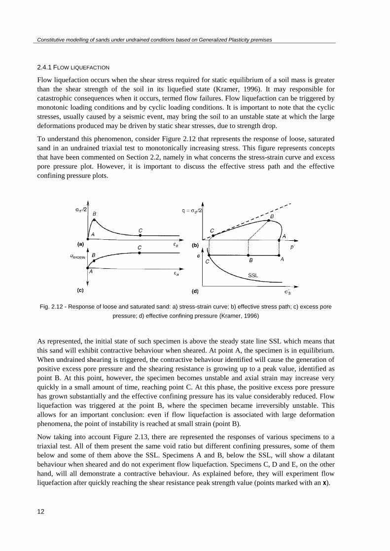
To understand this phenomenon, consider Figure 2.12 that represents the response of loose, saturated
sand in an undrained triaxial test to monotonically increasing stress. This figure represents concepts
that have been commented on Section 2.2, namely in what concerns the stress-strain curve and excess
pore pressure plot. However, it is important to discuss the effective stress path and the effective
confining pressure plots.
Fig. 2.12 - Response of loose and saturated sand: a) stress-strain curve; b) effective stress path; c) excess pore
pressure; d) effective confining pressure (Kramer, 1996)
As represented, the initial state of such specimen is above the steady state line SSL which means that
this sand will exhibit contractive behaviour when sheared. At point A, the specimen is in equilibrium.
When undrained shearing is triggered, the contractive behaviour identified will cause the generation of
positive excess pore pressure and the shearing resistance is growing up to a peak value, identified as
point B. At this point, however, the specimen becomes unstable and axial strain may increase very
quickly in a small amount of time, reaching point C. At this phase, the positive excess pore pressure
has grown substantially and the effective confining pressure has its value considerably reduced. Flow
liquefaction was triggered at the point B, where the specimen became irreversibly unstable. This
allows for an important conclusion: even if flow liquefaction is associated with large deformation
phenomena, the point of instability is reached at small strain (point B).
Now taking into account Figure 2.13, there are represented the responses of various specimens to a
triaxial test. All of them present the same void ratio but different confining pressures, some of them
below and some of them above the SSL. Specimens A and B, below the SSL, will show a dilatant
behaviour when sheared and do not experiment flow liquefaction. Specimens C, D and E, on the other
hand, will all demonstrate a contractive behaviour. As explained before, they will experiment flow
liquefaction after quickly reaching the shear resistance peak strength value (points marked with an x).
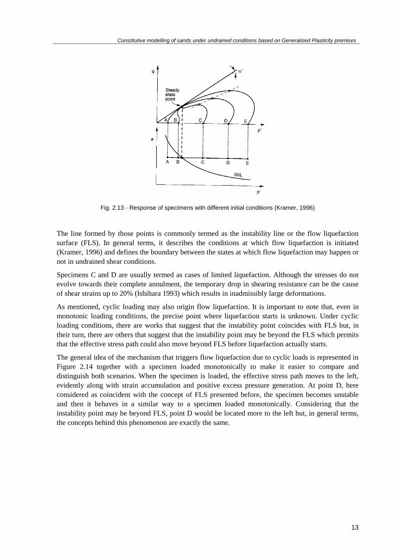
Constitutive modelling of sands under undrained conditions based on Generalized Plasticity premises
13
Fig. 2.13 - Response of specimens with different initial conditions (Kramer, 1996)
The line formed by those points is commonly termed as the instability line or the flow liquefaction
surface (FLS). In general terms, it describes the conditions at which flow liquefaction is initiated
(Kramer, 1996) and defines the boundary between the states at which flow liquefaction may happen or
not in undrained shear conditions.
Specimens C and D are usually termed as cases of limited liquefaction. Although the stresses do not
evolve towards their complete annulment, the temporary drop in shearing resistance can be the cause
of shear strains up to 20% (Ishihara 1993) which results in inadmissibly large deformations.
As mentioned, cyclic loading may also origin flow liquefaction. It is important to note that, even in
monotonic loading conditions, the precise point where liquefaction starts is unknown. Under cyclic
loading conditions, there are works that suggest that the instability point coincides with FLS but, in
their turn, there are others that suggest that the instability point may be beyond the FLS which permits
that the effective stress path could also move beyond FLS before liquefaction actually starts.
The general idea of the mechanism that triggers flow liquefaction due to cyclic loads is represented in
Figure 2.14 together with a specimen loaded monotonically to make it easier to compare and
distinguish both scenarios. When the specimen is loaded, the effective stress path moves to the left,
evidently along with strain accumulation and positive excess pressure generation. At point D, here
considered as coincident with the concept of FLS presented before, the specimen becomes unstable
and then it behaves in a similar way to a specimen loaded monotonically. Considering that the
instability point may be beyond FLS, point D would be located more to the left but, in general terms,
the concepts behind this phenomenon are exactly the same.

Constitutive modelling of sands under undrained conditions based on Generalized Plasticity premises
14
Fig. 2.14 - Stress-strain and effective stress curves for the mechanisms of flow liquefaction for cyclic and
monotonic loading (Kramer, 1996)
After all explanations about flow liquefaction, it is correct to consider that, if the initial conditions of a
given sand fall inside the black zone of Figure 2.15, flow liquefaction will occur if there is any loading
condition capable of bringing the effective stress path to the instability point, commonly plotted in
FLS.
Fig. 2.15 - Zone of susceptibility to flow liquefaction (Kramer, 1996)
2.4.2 CYCLIC MOBILITY
Cyclic mobility may happen when the static shear stress is smaller than the steady-state shear strength
and it is worth mention that it can occur in loose but also in dense sands (Kramer, 1996). It also is
extendable to soils of low to high confining pressures and to initial states above and below the SSL. In
opposition to flow liquefaction, there is no point at which cyclic mobility is actually started giving that
the permanent deformations produced are accumulating incrementally during the development of the
phenomenon.
The magnitude of such deformations depends on the stresses but also on the duration of the cyclic
loading. Evidently, the longer the load is acting, the greater will be the accumulated deformation and
the consequent damage. It is important to note that, even if large permanent strains develop, the sand
does not collapse as happens in flow liquefaction.
Cyclic mobility may happen if the initial conditions of the material fall inside the shaded zone of
Figure 2.16.

Constitutive modelling of sands under undrained conditions based on Generalized Plasticity premises
15
Fig. 2.16 - Zone of susceptibility to cyclic mobility (Kramer, 1996)
One of the most important failure types related to cyclic mobility is lateral spreading. It may be
described as the lateral permanent deformation of a gently sloping site and implicates a large
horizontal displacement of superficial blocks of soil. As a result of pore pressure build up or
liquefaction, lateral spreading is defined as the lateral displacement of moderately or gently sloping
sites subjected to ground motion. During an earthquake, movements of the ground are generated and
such displacements may happen. Its consequences are dramatic and may affect numerous important
structures in urban areas. Also, at the head of a slide, it is usual to find ground fissures that run
perpendicular to the direction of the slope movement.
2.5. DILATANCY
When studying a granular material such as sand, it is known that its behaviour is strictly related to the
changes that occur in its physical structure during the loading phase. In the context of the modelling of
the stress-strain behaviour of soils, the correct description of volume changes becomes fundamental to
properly describe that same behaviour.
In general terms, it is considered that granular soils can dilate or contract (negative dilatancy). Both
classifications are related to concepts presented previously, namely the ones described when
commenting Figure 2.5.
To the property of soils of exhibiting volumetric strain when subjected to shear stresses it is given the
name of dilatancy, which is accepted as positive when the volume of the material increases and
negative when the opposite happens. Thus, when the initial void ratio of a given sand is lower than the
critical void ratio, the material will exhibit positive dilatancy (volume increase). On the other hand,
when the initial void ratio is higher than the critical one, the volume of the material will decrease and
dilatancy will be negative. As also mentioned before, for large strains, all granular materials,
independently of the value of their initial void ratio, tend to the same value - the critical void ratio –
allowing for the conclusion that dilatancy tends to zero.
In other words, dilatancy consists of the volume changes induced by the application of shear stresses
to a certain material (Matos Fernandes, 2011a). It is usually studied in the context of dense sands since
these tend to dilate and enlarge its voids when sheared until failure. The analytical definition of
dilatancy is commonly given by relationship (2.2), as the ratio between volumetric and shear
deformations:

Constitutive modelling of sands under undrained conditions based on Generalized Plasticity premises
16
(2.2)
where,
( ) (2.3)
Also, the existence of dilatancy is explained by the development of displacements normal to the
shearing plane. Otherwise, as represented in Figure 2.17a), dilatancy is zero. In Figure 2.18b),
dilatancy exists during shear.
Fig. 2.17 – Normal displacements to the shearing plane: a) inexistent, dilatancy is zero; b) existent, dilatancy
occurs
Dilatancy is also characterized by the angle of dilation Ψ, which is the local slope of the curve that
plots volumetric strains versus distortions. It is typically determined from triaxial or shear box tests
and can be found from the plot of volumetric strain versus axial strain. However, it is also identifiable
in a scheme similar to Figure 2.17, as the angle formed between the horizontal displacement and the
resultant of total displacements, as shown in Figure 2.18.
Fig. 2.18 - Angle of dilation
For dense sands, the maximum positive value of the angle of dilation coincides with the peak value of
the shear stress. The angle of dilation also controls the amount of plastic volumetric strain developed
during plastic shearing. For sands, it depends on the angle of internal friction. Negative values of the
angle of dilation are acceptable for loose sands.
Although Reynolds (1885) and Taylor (1948) have been the first to develop works about the concepts
of dilatancy, it was Rowe (1962) that brought several improvements to the field. Based on minimum

Constitutive modelling of sands under undrained conditions based on Generalized Plasticity premises
17
rate of internal work assumption, Rowe proposed the following relationship, relating dilatancy to the
principal stress ratio as:
(
) (2.4)
where K is a parameter that depends on the friction angle :
(2.5)
Equation (2.4) was named the stress-dilatancy relation and it has been used as a flow rule in numerous
soil plasticity models, even if subsequently modified.
Using the common expressions for the increments of deformation and stress in the triaxial plane,
Equation (2.2) can also be written as:
( ) ( )
( ) ( ) (2.6)
where η is the stress ratio and K represents the bulk modulus.
At critical state, in triaxial compression, where σ2 = σ3,
(2.7)
( ) ( ) (2.8)
where M represents the slope of the CSL in the plot. Equation (2.6) can be finally rewritten as:
( )
(2.9)
Nowadays, many sand models make use of the state parameter concept, assuming always that the
critical state line in the space is unique. Rowe (1962) also did suggest that the stress-dilatancy
relationship should include a dependency on the sample density and past stress history. Since the state
parameter can represent the sample density and confining pressure, Li and Dafalias (2000) proposed
an improved state dependent dilatancy equation:

Constitutive modelling of sands under undrained conditions based on Generalized Plasticity premises
18
( ) (2.10)
where M can now evolve with state parameter Ψ. This equation is currently one of the most used ones
in this context. Earlier, in 1985, Pastor & Zienkiewicz had proposed the following one:
( ) ( ) (2.11)
where represents a model constant.
Both expressions will be also mentioned later, in Chapter 3, and applied in Chapter 5, where the
calibration of the different constitutive models will take place.

Constitutive modelling of sands under undrained conditions based on Generalized Plasticity premises
19
3
CONSTITUTIVE MODELS BASED ON THE GENERALIZED PLASTICITY
THEORY
3.1. INTRODUCTION TO CONSTITUTIVE MODELS
In general words, a constitutive equation can be defined as the relation between two physical
quantities that is specific to a given material and approximates the response of that material to external
loadings. The constitutive laws are usually formulated by means of mathematical equations that
involve parameters of the material being studied. Put differently, a well-designed constitutive model
provides a mathematical description of the behaviour of a material and should be able to represent the
most important aspects of its response to different loadings.
In the context of Geotechnical analysis, it is expected that the constitutive model is capable of
conveniently describing the mechanical performance of the soil in terms of stress, strain and internal
state, when subjected to external stimuli. Predicting properly the elastic and plastic deformations of
soil should be one of its main concerns.
The need to characterize and describe as best as possible the behaviour of granular soils has led to the
appearance, during the last decades, of numerous types of constitutive models, proposed by
researchers all over the world, given that they represent the basis of every Geotechnical study. Most of
them have been developed in the context of the classical Elastoplasticity theory and are able to
reproduce, with more or less accuracy, the main aspects of sand behaviour, especially when taking into
account monotonic loading conditions. In those models, deformation is usually decomposed into a
recoverable elastic part and an unrecoverable plastic part, which allows them to reproduce some of the
most usual phenomena in sand behaviour.
Now, the increasing complexity of Geotechnical works, as well as the availability of a greater amount
of experimental data, has been stimulating interesting developments in this domain, which are leading
to new constitutive models, anchored on different or modified theoretical formulations. Among the
existing models, those that are based on Generalized Plasticity have been recognized as capable of
successfully reproducing the mechanical behaviour of soils, especially in more complex loading
conditions as cyclic loadings. The constitutive model proposed by Pastor and Zienkiewicz, in 1986,
was the first model based on the concepts of Generalized Plasticity.
In this chapter, a review of Generalized Plasticity theory will be firstly presented. After that, the
original Pastor-Zienkiewicz model and its limitations will be discussed. Thereafter, two different
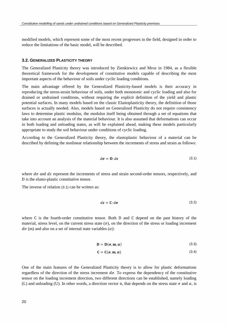
Constitutive modelling of sands under undrained conditions based on Generalized Plasticity premises
20
modified models, which represent some of the most recent progresses in the field, designed in order to
reduce the limitations of the basic model, will be described.
3.2. GENERALIZED PLASTICITY THEORY
The Generalized Plasticity theory was introduced by Zienkiewicz and Mroz in 1984, as a flexible
theoretical framework for the development of constitutive models capable of describing the most
important aspects of the behaviour of soils under cyclic loading conditions.
The main advantage offered by the Generalized Plasticity-based models is their accuracy in
reproducing the stress-strain behaviour of soils, under both monotonic and cyclic loading and also for
drained or undrained conditions, without requiring the explicit definition of the yield and plastic
potential surfaces. In many models based on the classic Elastoplasticity theory, the definition of those
surfaces is actually needed. Also, models based on Generalized Plasticity do not require consistency
laws to determine plastic modulus, the modulus itself being obtained through a set of equations that
take into account an analysis of the material behaviour. It is also assumed that deformations can occur
in both loading and unloading states, as will be explained ahead, making these models particularly
appropriate to study the soil behaviour under conditions of cyclic loading.
According to the Generalized Plasticity theory, the elastoplastic behaviour of a material can be
described by defining the nonlinear relationship between the increments of stress and strain as follows:
(3.1)
where and represent the increments of stress and strain second-order tensors, respectively, and
is the elasto-plastic constitutive tensor.
The inverse of relation (3.1) can be written as:
(3.2)
where is the fourth-order constitutive tensor. Both and depend on the past history of the
material, stress level, on the current stress state ( ), on the direction of the stress or loading increment
(m) and also on a set of internal state variables ( ):
( ) (3.3)
( ) (3.4)
One of the main features of the Generalized Plasticity theory is to allow for plastic deformations
regardless of the direction of the stress increment . To express the dependency of the constitutive
tensor on the loading increment direction, two different directions can be established, namely loading
(L) and unloading (U). In other words, a direction vector , that depends on the stress state and , is
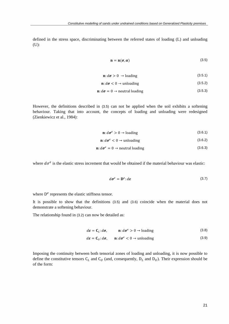
Constitutive modelling of sands under undrained conditions based on Generalized Plasticity premises
21
defined in the stress space, discriminating between the referred states of loading (L) and unloading
(U):
( ) (3.5)
(3.5.1)
(3.5.2)
(3.5.3)
However, the definitions described in (3.5) can not be applied when the soil exhibits a softening
behaviour. Taking that into account, the concepts of loading and unloading were redesigned
(Zienkiewicz et al., 1984):
(3.6.1)
(3.6.2)
(3.6.3)
where is the elastic stress increment that would be obtained if the material behaviour was elastic:
(3.7)
where represents the elastic stiffness tensor.
It is possible to show that the definitions (3.5) and (3.6) coincide when the material does not
demonstrate a softening behaviour.
The relationship found in (3.2) can now be detailed as:
, (3.8)
, (3.9)
Imposing the continuity between both tensorial zones of loading and unloading, it is now possible to
define the constitutive tensors and (and, consequently, and ). Their expression should be
of the form:

Constitutive modelling of sands under undrained conditions based on Generalized Plasticity premises
22
(3.10)
(3.11)
where is the fourth-order tensor that characterizes the elastic behaviour of the material, and
are the unit tensors that define the plastic flow direction in loading (L) or unloading (U),
respectively, and and are two scalar functions that are defined as the loading (L) and unloading
(U) plastic modulus.
From Equations (3.6), (3.8), (3.9), (3.10) and (3.11) it follows that, in the case of neutral loading, the
constitutive tensor expressions provide the same strain increment, a fact that ensures the continuity
between the states of loading and unloading:
(3.12)
In this situation, the material behaviour is elastic and considered to be reversible, given that no plastic
deformations occur.
The total strain increments can now be decomposed into elastic and plastic components:
(3.13)
(3.14)
( ) (3.15)
We arrive at the conclusion that the relationship between total strain and stress increments can be
defined as:
(3.16)
In this way, to fully characterize the material behaviour using a Generalized Plasticity-based model, it
is necessary to provide the following items:
i. The elastic constitutive tensor ;
ii. The unit tensor n that distinguishes loading from unloading conditions;
iii. The unit tensor describing the direction of plastic flow , again in loading and
unloading conditions;
iv. The loading and unloading plastic moduli , in loading and unloading conditions.

Constitutive modelling of sands under undrained conditions based on Generalized Plasticity premises
23
The inversion of the fourth-order tensor results in the equivalent , with ( ) :
(3.17)
3.3. THE ORIGINAL PASTOR-ZIENKIEWICZ MODEL FOR GRANULAR SOILS
The original Pastor-Zienkiewicz model (or the PZ model for short) was the first generalized plasticity-
based model, designed in 1986 by those authors, especially for the analysis of sand and clay
behaviour. It was developed assuming an isotropic material response in both elastic and plastic ranges
and, therefore, the constitutive equations were formulated in terms of the three stress invariants ,
and :
( ) (3.18)
√ (3.19)
(
√
) (3.20)
together with the work-conjugate stress invariants and :
( ) (3.21)
√
| ( )| (3.22)
where:
(3.23)
( ) (3.24)
( ) (9.25)
(3.26)
Constitutive modelling of sands under undrained conditions based on Generalized Plasticity premises
24
In its turn, the formulation of the stress and strain components in the triaxial space is expressed in an
incremental way as:
(
) (3.27)
(
) (3.28)
(3.29)
( ) (3.30)
Beginning with the definition of the elastic stiffness tensor, the PZ model assumes that the material
has a non-linear response, according to the incremental relationships established:
(3.31)
(3.32)
where and are the tangent bulk and shear moduli, respectively, which are assumed to be
dependent on the confining pressure :
(3.33)
(3.34)
being and the elastic bulk and shear moduli at the reference mean effective stress .
On the other hand, the plastic behaviour of the material is expressed by the following equations:
( ) (3.35)
( ) (3.36)
The plastic strain increment, detailed also in Equation (3.15), is characterized by the following aspects:
first of all, the direction of the plastic flow ng. It characterizes the direction in which the plastic strain
will occur by applying a load increment and was obtained as a function of the soil dilatancy .
Considering that the elastic strain component is quite small when compared to the plastic strain
component, the soil dilatancy :
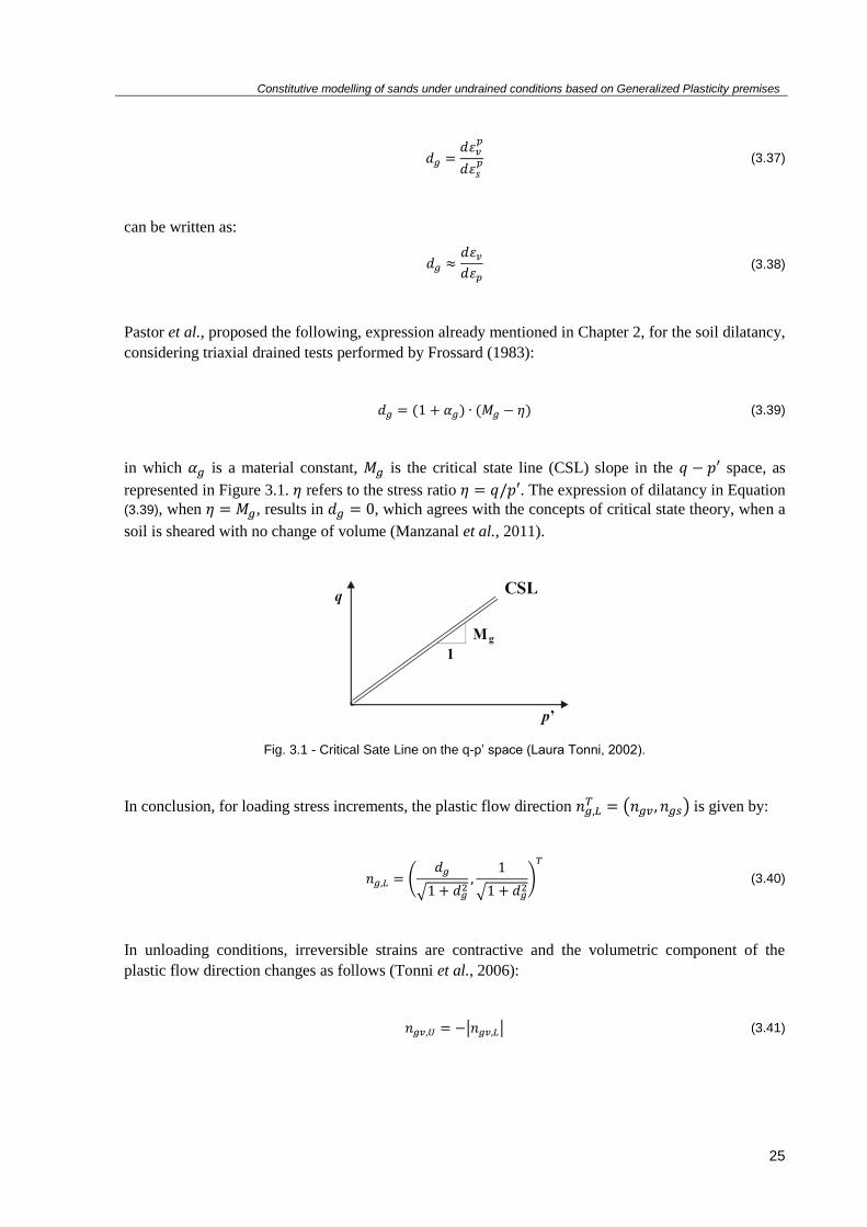
Constitutive modelling of sands under undrained conditions based on Generalized Plasticity premises
25
(3.37)
can be written as:
(3.38)
Pastor et al., proposed the following, expression already mentioned in Chapter 2, for the soil dilatancy,
considering triaxial drained tests performed by Frossard (1983):
( ) ( ) (3.39)
in which is a material constant, is the critical state line (CSL) slope in the space, as
represented in Figure 3.1. refers to the stress ratio . The expression of dilatancy in Equation
(3.39), when , results in , which agrees with the concepts of critical state theory, when a
soil is sheared with no change of volume (Manzanal et al., 2011).
Fig. 3.1 - Critical Sate Line on the q-p’ space (Laura Tonni, 2002).
In conclusion, for loading stress increments, the plastic flow direction ( ) is given by:
(
√
√ )
(3.40)
In unloading conditions, irreversible strains are contractive and the volumetric component of the
plastic flow direction changes as follows (Tonni et al., 2006):
| | (3.41)

Constitutive modelling of sands under undrained conditions based on Generalized Plasticity premises
26
The loading and unloading direction is given by the unit vector n. In the case of granular soils, the
original PZ model assumes a non-associated flow rule so, consequently, .
However, both expressions are similar and the loading direction ( ) can be defined as:
(
√
√
)
(3.42)
where:
( ) ( ) (3.43)
In the case of clays, the associative behaviour can be recovered by choosing and
(Manzanal et al., 2010).
As stated at the beginning of this chapter, there is no need to explicitly define the yield or plastic
potential surfaces when working with constitutive models based on Generalized Plasticity. However,
by integrating and , it is possible to define both surfaces, namely and :
{ (
) [ (
)
]} (3.44)
{ (
) [ (
)
]} (3.45)
where represents the yield surface while represents the plastic potential surface. Figure 3.2 shows
how both surfaces can be graphically represented in the plane, for (a) loose and (b) dense sands.
Fig. 3.2 - a) Yield surface; b) Plastic potential surface (Laura Tonni, 2002).

Constitutive modelling of sands under undrained conditions based on Generalized Plasticity premises
27
The and values included in the previous equations are both dependent on the Lode angle θ, as
suggested by Zienkiewicz et al. (1997):
(3.46)
Lastly, it is still needed to define the plastic modulus. In the basic PZ model, the expression of the
plastic modulus was defined without introducing any hardening law or consistency condition, a fact
that allows for the choice of different expressions for the plastic modulus in loading and unloading
conditions. In loading conditions it assumes the form:
( ) (3.47)
with,
(
)
(3.48)
(
) (3.49)
(
) (3.50)
( ) (3.51)
where is the accumulated deviatoric plastic strain:
∫| | (3.52)
is a multiplying factor related to plastic strains at the beginning of the loading process, defines
an asymmetric cone in the space of stress invariants, which acts like a limit between the admissible
and the impossible states, and and are constitutive parameters, assumed to be constant during the
loading process.
is a decreasing function that reaches zero when the stress ratio reaches the critical state
( ) and then assumes negative values after overcoming the Critical State Line. That implies that
the plastic modulus decreases while the plastic strain increases.

Constitutive modelling of sands under undrained conditions based on Generalized Plasticity premises
28
is also a decreasing function but will always assume positive values, given that it is asymptotic to
zero and characterizes the material behaviour while the deviatoric plastic strain is increasing, avoiding
the plastic modulus to reach zero.
is a function which incorporates material memory:
(
)
(3.53)
[ (
)
]
(3.54)
where a material parameter.
However, another important aspect of the behaviour of granular soils is the material response during
the unloading state, namely, the way how plastic strains develop. The law suggested for the unloading
plastic modulus assumed that there were plastic strains since the beginning of the unloading
process, the expression proposed being of the form:
(
)
|
| (3.55)
|
| (3.56)
where and are constitutive parameters. represents the stress ratio value from which
unloading takes place.
In conclusion, the original PZ model requires the definition of 12 material and constitutive parameters,
which can be calibrated from drained or undrained monotonic triaxial tests or undrained cyclic triaxial
tests. The model is able to reproduce some of the main phenomena of sand behaviour like liquefaction,
cyclic mobility or softening of dense sands. However, one of its important limitations for sands is that
specimens of a given sand with different densities or subjected to different confining pressures require
different sets of parameters to reproduce the behaviour of the material. That is why several studies and
works have been developed during the last years, so that the necessary modifications and corrections
to the constitutive equations can be introduced of the original PZ model, in order to get unified
modelling over a wide range of densities and stress levels.
In the following sections, two different modified versions of the original PZ model will be presented
and discussed.
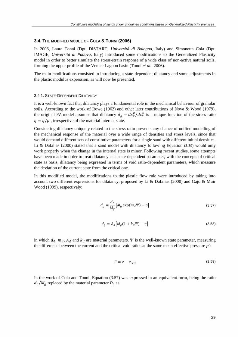
Constitutive modelling of sands under undrained conditions based on Generalized Plasticity premises
29
3.4. THE MODIFIED MODEL OF COLA & TONNI (2006)
In 2006, Laura Tonni (Dpt. DISTART, Università di Bologna, Italy) and Simonetta Cola (Dpt.
IMAGE, Università di Padova, Italy) introduced some modifications to the Generalized Plasticity
model in order to better simulate the stress-strain response of a wide class of non-active natural soils,
forming the upper profile of the Venice Lagoon basin (Tonni et al., 2006).
The main modifications consisted in introducing a state-dependent dilatancy and some adjustments in
the plastic modulus expression, as will now be presented.
3.4.1. STATE-DEPENDENT DILATANCY
It is a well-known fact that dilatancy plays a fundamental role in the mechanical behaviour of granular
soils. According to the work of Rowe (1962) and other later contributions of Nova & Wood (1979),
the original PZ model assumes that dilatancy
is a unique function of the stress ratio
, irrespective of the material internal state.
Considering dilatancy uniquely related to the stress ratio prevents any chance of unified modelling of
the mechanical response of the material over a wide range of densities and stress levels, since that
would demand different sets of constitutive parameters for a single sand with different initial densities.
Li & Dafalias (2000) stated that a sand model with dilatancy following Equation (3.39) would only
work properly when the change in the internal state is minor. Following recent studies, some attempts
have been made in order to treat dilatancy as a state-dependent parameter, with the concepts of critical
state as basis, dilatancy being expressed in terms of void ratio-dependent parameters, which measure
the deviation of the current state from the critical one.
In this modified model, the modifications to the plastic flow rule were introduced by taking into
account two different expressions for dilatancy, proposed by Li & Dafalias (2000) and Gajo & Muir
Wood (1999), respectively:
[ ( ) ] (3.57)
[ ( ) ] (3.58)
in which , , and are material parameters. is the well-known state parameter, measuring
the difference between the current and the critical void ratios at the same mean effective pressure :
(3.59)
In the work of Cola and Tonni, Equation (3.57) was expressed in an equivalent form, being the ratio
replaced by the material parameter as:

Constitutive modelling of sands under undrained conditions based on Generalized Plasticity premises
30
[ ( ) ] (3.60)
Expressions (3.57) and (3.58) were obtained from the original dilatancy expression by introducing a
linear and an exponential dependence on , respectively. With these modifications, it is now possible
to better capture the evolution of sand behaviour due to pressure and density changes, which did not
happen with the original model. Besides, those expressions still guarantee basic premises of Critical
State Soil Mechanics and embed at the same time both picnotropy and barotropy through the state
parameter that changes during the deformation process.
3.4.2. PLASTIC MODULUS AT CONSTANT STRESS RATIO COMPRESSION
There are several constitutive models for granular soils assuming that sands, when compressed at
constant stress ratios not causing crushing of particles, do not experience any plastic deformation.
Such hypothesis implies that in isotropic compression (which is a special case of constant stress ratio
compression), the plastic modulus is infinite as long as the material remains with a “cap” limiting the
elastic behaviour (Tonni et al., 2006). This limitation is actually overcome in the original PZ model,
given that there is no need to introduce any cap in order to allow for plastic deformations in isotropic
compression, since the volumetric plastic strain is inversely proportional to the material parameter ,
as evident from Equations (3.47) to (3.51) when .
In the case of clays, and according to the Cam-Clay Model, plastic deformations happen when the
stress path moves along the normal compression line (NCL) and can be determined as:
(3.61)
where is the initial void ratio, is the slope of the Normal Consolidation Line (NCL) and is the
slope of the unloading-reloading line, both in the space.
For granular soils, Zienkiewicz et al. (1999) observed that could be determined by fitting the
experimental curves or . Pastor et al. (1990) reported estimations of varying between
350 and 16000, with higher values for dense sands. In Tonni (2002), the calibration of by fitting
the curves of three drained triaxial tests gave values equal to 800, 1000 and 2800 for clay (CL),
silt (ML) and sand (SP-SM).
Despite the values seemed to be in agreement with the ones reported in works by Pastor, the procedure
did not appear sufficiently reliable and alternative formulations for isotropic compression were
examined, with particular reference to the works of Pestana & Whittle (1995) and Jefferies & Been
(2000). In fact, the unified approach proposed by Pestana & Whittle (1995) overcomes the limitations
of some constitutive models that assume that soils exhibit irreversible volumetric strains for -constant
paths, also at low pressures: plastic strains gradually increases as long as the distance from the limiting
compression curve (LCC) decreases. In such model, the volumetric plastic strain in isotropic
compression is given by:

Constitutive modelling of sands under undrained conditions based on Generalized Plasticity premises
31
(
)
(10)
where,
(11)
represents a normalized parameter varying from 0 to 1 that takes into account the distance from
LCC. is the octahedral stress on the LCC at the same void ratio. The exponent rules the
compression curve curvature, when it comes close to the LCC: the higher the , the higher the
curvature.
In conclusion, can be formulated as:
( )
(12)
Jefferies & Been (2000) presented an alternative approach on the isotropic compression of sands. It
combines concepts of Critical State Soil Mechanics with the idea there is a single LCC only when the
grain crushing phenomenon becomes prevalent. Based on numerous isotropic compression tests
performed on Erksak sand, the authors proposed that the plastic bulk modulus could be expressed
as follows:
( ) (
) (13)
is the apparent grain crushing pressure in shear, corresponding to a discontinuity of the CSL slope
in the space (Verdugo, 1992). The critical void ratio is proportional to the logarithm of
when and becomes proportional to the mean pressure when .
can be estimated as follows, as coincides with :
(14)
3.4.3. GENERAL EQUATION OF THE PLASTIC MODULUS
Another of the changes introduced in this modified model is the simplified expression of the plastic
modulus in monotonic loading that is proposed. It is expressed as:
(15)

Constitutive modelling of sands under undrained conditions based on Generalized Plasticity premises
32
where the components and
are defined as:
(
) (16)
(17)
being and material constants. C is usually considered equal to 1. represents plastic strains.
In the original PZ model, the plastic modulus components proposed to account for the stiffness
decrease as the shear plastic deformation increases and the critical state is drawing on.
In this version, the “failure” component , that replaces in the original formulation, includes the
idea that, during the distortional process, the sand is aiming to reach the current peak stress ratio,
defined as . According to Equation (3.68), changes with in a way that, for
, results represent dense states and, for , they represent loose sands.
Muir Wood et al. (1994) introduced the concept of a virtual failure stress ratio depending on the
material internal state, idea that was followed by other authors, as Manzari & Dafalias (1997), who
adopted a linear function of the state parameter or Wang et al. (2002), who formulated such
dependence by means of the state pressure index .
In Equation (3.68), the mobilized peak stress was related to the state parameter through the exponential
function defined.
3.4.4. ELASTIC COMPONENTS
According to the basic PZ model, the elastic behaviour of the material is assumed non-linear and the
tangent bulk and shear moduli are defined as stated in Section 3.2. In this modified version, and
according to a method successfully adopted in earlier works, the initial shear modulus can be
estimated from . In its turn, can be determined by the relationship proposed by Hardin &
Drnevich (1972):
( )
( )(
)
(18)
with and being material parameters, determined using an experimental fitting procedure.
In the last equation, represents the material response at very small strain while refers to larger
strain levels, being calculated by reducing by a factor of 2.5, as suggested by Gajo & Muir
Wood (1999).

Constitutive modelling of sands under undrained conditions based on Generalized Plasticity premises
33
3.5. THE MODIFIED MODEL OF DIEGO MANZANAL (2008)
As stated before, the mechanical behaviour of granular soils shows a strong dependence both on
density and confining pressure, for a big range of deformations, from the smallest ones, introduced by
common engineering structures, to the bigger ones, associated to states of failure (Diego Manzanal,
2008).
The purpose of the work developed by Diego Manzanal (Department of Applied Mathematics,
Universidad Politécnica de Madrid, Spain) is to extend the basic constitutive model for sands based
on Generalized Plasticity proposed by Pastor, Zienkiewicz and Chan by modifying some of its features
in order to include a dependency on the state parameter. From the point of view of constitutive
modelling, if the sand dependency on density and confining pressure is not included on the model
relationships, the simulation of the behaviour of the material will require the use of different sets of
constitutive parameters for the same sand under different initial conditions, treating the same material
as a different one if density or confining pressures are not similar (Manzanal et al., 2010). The original
PZ model, presented in Section 3.2, does not include such dependency on its relationships, which can
be considered as one important limitation to its application.
The most important aspect related to the study of the behaviour of granular soils from a unified point
of view is to make clear how the main elements of the model will depend on confining pressure and
void ratio through the state parameters that will be described ahead.
3.5.1. CRITICAL STATE CONCEPTS TO CONSIDER
The critical state parameter is fundamental to understand the behaviour of granular soils, given that it
allows to represent the existing relationship between relative density ( ), void ratio ( ) and confining
pressure ( ). In other words, the state parameter describes the position of the current state on the
space and also the projection of the Critical State Line. It is worth mentioning that the CSL is
accepted as unique for the sands on the plane. On the space, Diego Manzanal considered
the formulation proposed by Li (1997):
(
)
(3.71)
where is the void ratio at the atmospheric pressure, is the slope of the Critical State Line in the
( ) plane, and are the void ratio and the confining pressure at the critical state and
is the atmospheric pressure.
On the plane, the classical form is kept:
(3.72)
Constitutive modelling of sands under undrained conditions based on Generalized Plasticity premises
34
Defining the state parameter as proposed by Been and Jefferies (2006),
(3.73)
but considering the equation that describes the Critical State Line, Manzanal obtained:
(
)
(3.74)
In the following figure, the Critical State Line on the plane ( ) is presented:
Fig. 3.3 - State parameter (adapted from Diego Manzanal, 2008)
The parameter measures the distance between the current state and the critical state, taking into
account the joint effect of density and effective confining pressure. The material states located over the
Critical State Line are considered as loose and, when below it, are considered as dense. Therefore,
positive values of are associated to contractive behaviour while negative values of it are associated
to dilative behaviour.
In the context of the Generalized Plasticity, it is actually possible to reproduce the stress-strain
behaviour of the soil on a unified approach by means of Equation (3.74).
3.5.2. FLOW RULE
The flow rule depends on the relative density of the sand and, therefore, on the state parameter
(Manzanal et al., 2010). It is known that the stress ratio at which the behaviour changes from
contractive to dilative is not constant and depends on the void ratio. For example, in a cyclic drained
triaxial test where sand densifies, the stress ratio at which the behaviour changes from contractive to
dilative varies as soil densifies. Li and Dafalias (2000) showed that dilatancy cannot depend only on

Constitutive modelling of sands under undrained conditions based on Generalized Plasticity premises
35
the stress ratio as proposed by Rowe (1962) since, for a given stress ratio, dilatancy could be of
different signs for dense or loose materials.
It was also found experimentally that dilatancy should be zero not only when reaching the critical state
( , for and ) but also before ( , for and ), this state being
usually referred to as the Phase Transformation State (PTS). Based on that, Li and Dafalias (2000)
proposed the following dilatancy equation:
( ) (3.75)
where,
( ) (3.76)
is the state parameter defined above by Equation (3.73), is the stress ratio, represents the
Critical State Line in space and and are model constants. can be defined as the stress
ratio at the Phase Transformation State, which depends on the state parameter, by means of Equation
(3.76).
Equation (3.76) also demonstrates the existence of a family of stress-dilatancy ( ) curves for
different confining pressures and densities. The following figure, Figure 3.4, shows the variation of the
stress ratio with dilatancy for dense ( ) and loose states ( ), based on Equations (3.75) and
(3.76):
Fig. 3.4 - Comparison between the original and the state parameter-dependent dilatancy expressions (Diego
Manzanal, 2008).
The simple dilatancy law of the original PZ model is also represented. It is observed that it can
characterize reasonably well the behaviour of loose specimens but is much less accurate when treating
denser sands.

Constitutive modelling of sands under undrained conditions based on Generalized Plasticity premises
36
In the end, the direction of the plastic flow is obtained as a function of dilatancy, as in the original
PZ model. The model assumes a non-associated flow rule, the direction vector being expressed like in
the basic model.
3.5.3. LOADING-UNLOADING DIRECTION
Once again, the loading-unloading discriminating tensor will be derived from an expression similar
to the one used to obtain . In this way, an associative flow rule can be recovered if required:
(
√
√
)
(3.77)
where,
( ( ) ) (3.78)
In the original PZ model, Zienkiewicz proposed that the relation between and should be equal
to the sand relative density . In this modified model, the following relationship is
proposed, in order to determine once is known:
(
)
(3.79)
where and are model constants, which can be calibrated based on a curve from undrained
triaxial tests, is a constant equal to 1,8 and is the ratio between the current void ratio and the
void ratio at critical state, which varies between:
(
)
(
)
(3.80)
reaches its lower value when the relation is equal to one and, consequently, the flow is now
associated.
3.5.4. ELASTIC COMPONENTS
The original PZ model takes into account the dependence of the shear and bulk moduli on the
confining pressure, as stated before. In this modified model, the relation proposed by Richard et al.

Constitutive modelling of sands under undrained conditions based on Generalized Plasticity premises
37
(1970) has been chosen, where the shear and bulk moduli depend not only on the confining pressure
but also on the void ratio:
(3.81)
where,
( )
√ (3.82)
( )
√ (3.83)
and are model constants and can be related by the following expression
( )
( ) (3.84)
so the parameters of the model can be the pair and or the pair and .
3.5.5. PLASTIC MODULUS
In the original PZ model, the plastic behaviour of the material is a function of the confining pressure,
being a model constant. Keeping the same structure of the expression proposed for the plastic
modulus of the original model, the necessary modifications were introduced in order to incorporate the
dependency of the plastic modulus on density and confining pressure, expressed as:
√ (3.85)
where,
(
) (3.86)
and are constitutive parameters. By introducing as a function of , the state parameter
defined in the previous section, the capacity of the model for predicting the plastic deformations with a
unique set of constitutive parameters is significantly improved.
When the stress path includes the deviatoric component ( ), the Equation (3.85) is generalized:
√
( ) (3.87)
Constitutive modelling of sands under undrained conditions based on Generalized Plasticity premises
38
where,
( ) (3.88)
( ) ( ) (3.89)
The inclusion of the state parameter in Equations (3.86) and (3.87) allows for considering the
dependency of the peak stress and of the behaviour of the soil after the peak on the initial conditions of
the soil. The expression for the volumetric component of the plastic modulus was also modified to
make it dependent on the state parameter:
[ ] (3.90)
where,
( ) (3.91)
is achieved for loose states while for dense states.
Constitutive modelling of sands under undrained conditions based on Generalized Plasticity premises
39
4 CASE STUDY – THE 2012 EMILIA-ROMAGNA SEISMIC SEQUENCE
4.1. INTRODUCTION
In this chapter, will be described the seismic events that occurred in the region of Emilia-Romagna in
2012 which led to severe damage in numerous Italian cities. It was exactly those events that gave rise
to numerous works in this field, in which this dissertation can also be included.
This chapter will mainly focus on the results of undrained triaxial tests on the Scortichino sand
specimens, performed in order to characterize the behaviour of such material. Also, the most relevant
Geotechnical characteristics of this granular soil will be also listed. The triaxial tests presented in this
chapter have been conducted by laboratory technicians from the Department of Civil Engineering of
the Università degli Studi di Napoli Federico II (Italy).
Besides, those tests will be studied in order to obtain the necessary parameters for the application of
the constitutive approaches studied in Chapter 3. All the calibration procedure, using the data collected
in the following sections, will be then detailed in Chapter 5.
4.2. DESCRIPTION OF THE CASE
From the 20th of May to the 3rd of June of 2012, a series of seismic events occurred in Emilia-
Romagna, a region located in the north of Italy. The most relevant ones took place in May, 20 and
May, 29. Both were responsible for several damages to a number of river banks situated in the
proximity of the earthquake epicentre. In consequence, some buildings and roads built on top of such
river banks were declared unstable and then unsafe (Gottardi et al., 2013).
The first major earthquake struck on 20 May 2012 at 04:03, about 36 kilometres north of the city of
Bologna, registering a 6.1 magnitude, in moment magnitude scale. The second one struck on 29 May
2012 at 09:00, registering a 5.9 magnitude in the same scale.

Constitutive modelling of sands under undrained conditions based on Generalized Plasticity premises
40
Fig. 4.1 - Localization of the earthquakes epicentres: a) 20 May 2012; b) 29 May 2012 (USGS, 2012)
The epicentres of the earthquakes of May 2012 (Figure 4.1) are located in the centre of the Po Valley
(Piadura Padana), between the provinces of Modena and Ferrara. The subsoil of this area consists on
a succession of alluvial horizons a few meters thick of fine (silt and clay) or granular material (mostly
sand), referring to two major depositional cycles: the oldest one, known as Sintema Alluvionale
Emiliano-Romagnolo Inferiore (AEI), which lasted from 650,000 to 450,000 years ago, and the
newest one, known as Sintema Alluvionale Emiliano-Romagnolo Superiore (AES), which has under
450,000 years. This alluvial succession rests on marine and transitional deposits from the Lower to
Middle Pleistocene.
One of the most affected river banks is the Canale Diversivo di Burana, which flows between the
provinces of Modena and Ferrara. This work will focus on the damage occurred on a stretch of such
embankment, where the village of Scortichino, province of Ferrara, is located (Figure 4.2). Such area,
with a total length of about 3 kilometres, hosts more than 400 houses and also commercial and other
productive activities. Some of those buildings and facilities ended up being classified as insecure, due
to the damage suffered. Figures 4.3 and 4.4 illustrate that fact.

Constitutive modelling of sands under undrained conditions based on Generalized Plasticity premises
41
Fig. 4.2 - Aerial view of Scortichino (Gottardi, G., & Tonni, L. (2013). Attività del Gruppo di Lavoro AGI per lo
studio del comportamento e per la messa in sicurezza degli argini. Geotecnica Sismica. Lecture conducted from
Università di Bologna)
Fig. 4.3 - a); b); c); d) (Gottardi, G., & Tonni, L. (2013). Attività del Gruppo di Lavoro AGI per lo studio del
comportamento e per la messa in sicurezza degli argini. Geotecnica Sismica. Lecture conducted from Università
di Bologna)

Constitutive modelling of sands under undrained conditions based on Generalized Plasticity premises
42
Fig. 4.4 - a); b); c) (Gottardi, G., & Tonni, L. (2013). Attività del Gruppo di Lavoro AGI per lo studio del
comportamento e per la messa in sicurezza degli argini. Geotecnica Sismica. Lecture conducted from Università
di Bologna)
Most of the damages reported in the village are related to fractures and cracks in walls of current
buildings and structural damage in retaining walls, associated with the evident fractures in the soil,
parallel to the embankment, that also affected the road that runs longitudinally next to the embankment
itself. Further studies, based on experimental data collected in situ, revealed that nearly all the damage
in that area can be viewed as a consequence of liquefaction phenomena but also lateral spreading
occurrences, both triggered by the seismic events described before.
In order to study and analyse the damage observed after the earthquake, the Emilia-Romagna
authorities and the Italian Geotechnical Association agreed to create a working group (Gruppo di
Lavoro Argini), formed by professors and researchers of numerous Italian universities, that would
focus on the analysis and verification of the seismic response and of the conditions of stability of the
embankments affected by the seismic events, aiming also to understand the causes of the damage
observed and to suggest the necessary mitigation techniques to minimize future earthquakes impact.
To this end, took place an extensive campaign of site investigation, involving in situ and laboratory
tests, in order to develop an accurate geotechnical model of the subsurface of the embankment for a
correct evaluation of its stability conditions in seismic circumstances.
Considering the deformation phenomena observed, it is correct to say that the stretch of the river bank
in question was not affected in the same way in all its extent. Because of that, it was decided to define
four critical areas, where the geotechnical campaign would concentrate and take place. There were
also identified the preferential alignments (sections A to D, in Figure 4.5) along which the on-site tests
would be performed.
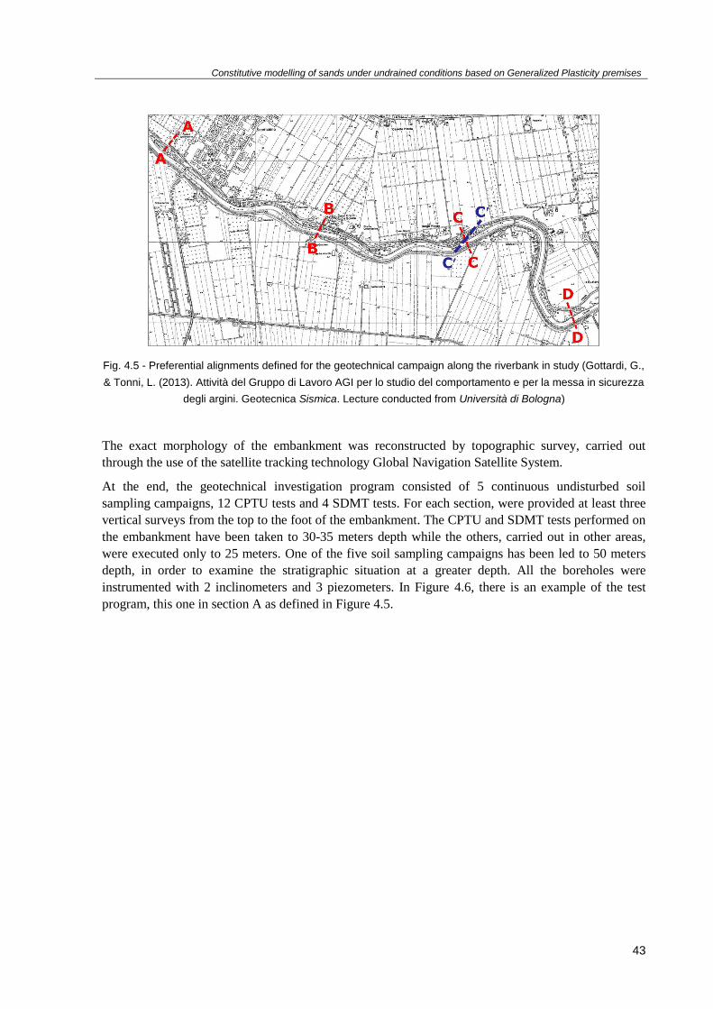
Constitutive modelling of sands under undrained conditions based on Generalized Plasticity premises
43
Fig. 4.5 - Preferential alignments defined for the geotechnical campaign along the riverbank in study (Gottardi, G.,
& Tonni, L. (2013). Attività del Gruppo di Lavoro AGI per lo studio del comportamento e per la messa in sicurezza
degli argini. Geotecnica Sismica. Lecture conducted from Università di Bologna)
The exact morphology of the embankment was reconstructed by topographic survey, carried out
through the use of the satellite tracking technology Global Navigation Satellite System.
At the end, the geotechnical investigation program consisted of 5 continuous undisturbed soil
sampling campaigns, 12 CPTU tests and 4 SDMT tests. For each section, were provided at least three
vertical surveys from the top to the foot of the embankment. The CPTU and SDMT tests performed on
the embankment have been taken to 30-35 meters depth while the others, carried out in other areas,
were executed only to 25 meters. One of the five soil sampling campaigns has been led to 50 meters
depth, in order to examine the stratigraphic situation at a greater depth. All the boreholes were
instrumented with 2 inclinometers and 3 piezometers. In Figure 4.6, there is an example of the test
program, this one in section A as defined in Figure 4.5.

Constitutive modelling of sands under undrained conditions based on Generalized Plasticity premises
44
Fig. 4.6 - Geotechnical tests performed in section A (Gottardi, G., & Tonni, L. (2013). Attività del Gruppo di Lavoro
AGI per lo studio del comportamento e per la messa in sicurezza degli argini. Geotecnica Sismica. Lecture
conducted from Università di Bologna)
The stratigraphic examination revealed a heterogeneous upper layer, of about 9-10 meters thick,
characterized by a succession of sand, silty sand and sandy silts layers. The first 6-7 meters correspond
to the body of the embankment. This stratigraphic horizon was called Unit AR (argine in Italian,
which means river bank), while the lower part corresponds to Unit B. Then, Unit C is constituted by a
layer of clays and silty clays, with a thickness of less than 2 meters. Below, and for the next 40 meters,
there is Unit A, characterized by medium to very coarse sand layers, in which have been also
identified thin layers of clay. In Figure 4.7 there in example of the stratigraphic information collected:
Fig. 4.7 - Example of one of the geotechnical models built with reference to the data collected (Gottardi, G., &
Tonni, L. (2013). Attività del Gruppo di Lavoro AGI per lo studio del comportamento e per la messa in sicurezza
degli argini. Geotecnica Sismica. Lecture conducted from Università di Bologna)
Constitutive modelling of sands under undrained conditions based on Generalized Plasticity premises
45
It is worth mentioning that there is a substantial agreement of the data collected through the
topographic survey with the widely established classifications for soils based on the CPTU and DMT
in situ tests performed. For the CPTU tests, the method of Robertson (2009) was used, which classifies
the different soil types found in terms of its behaviour (SBT, Soil Behaviour Type). For the DMT
tests, the approach adopted is based on the material index, .
On the other hand, the program of laboratory tests performed, including the investigations for the
correct characterization of soils both in static and dynamic loading conditions, consisted of 12
consolidated-undrained triaxial tests (TXCU), 4 direct shear tests (TD), 4 cyclic torsional shear tests
(CTS), 4 resonant column tests (RC) on fine sand and, also, 16 simple cyclic shear tests (CSS) and 5
double-specimen cyclic shear tests (DSDSS) on the coarse sand.
In conclusion, the geotechnical models of the embankment and its foundation were built with
reference to all the results of the in situ and laboratory tests described before.
4.3. MAIN RESULTS OF THE TRIAXIAL TESTS PERFORMED
In this section, the main characteristics and results of the soils tested will be detailed. In the first
subsection, the granulometry and a general material description will be provided. Next, the results
obtained for the stress-strain and pore pressure curves will be presented. Based on those results, the
critical state parameters needed for the calibration and application of the constitutive models presented
in Chapter 3 will be discussed in subsection 4.3.3. In subsection 4.3.4 and 4.3.5, the results of the
dilatancy and plastic modulus laws of the specimens tested will also be detailed, since both represent
also an important part of the calibration work that will be performed later in Chapter 5.
The tests selected for this work were the S5-C6, S4-C6 and S1-C5 sets from the Scortichino
geotechnical investigation. The results presented in the following subsections will be organized by
each set of tests.
4.3.1. GRANULOMETRIC DISTRIBUTION CURVE AND GENERAL MATERIAL DESCRIPTION
Since the constitutive models presented in Chapter 3 were all designed for the simulation of the
behaviour of granular soils, there was the need to select mainly sandy specimens for this work.
The soil gradation curves (Figures 4.8, 4.9 and 4.10) and their respective particle size distribution
tables (Tables 4.1, 4.3 and 4.5) show that all the tests picked for this study refer to sand specimens
(sabbia, in Italian). The remaining tables (Tables 4.2, 4.4 and 4.6) are relative to other general
characteristics of the granular soils tested, such as the depth at which the specimens were collected in
situ.
Also, the relative density Dr is listed. It is important to mention that this value was not actually
experimentally measured but it is just an estimate from the laboratory technicians. This may represent
an additional difficulty in the development of this work since this parameter is important within the
context of the calibration of the constitutive approaches that will be taken into account later.
The total unit, dry unit and solid unit weights are also listed. The effective diameter D60 is also
presented. It represents the grain diameter of the sieve through which 60% of the weight of particles
pass. D30 and D10 have an equivalent meaning to D60. These values may not be important in the

Constitutive modelling of sands under undrained conditions based on Generalized Plasticity premises
46
calibration procedure performed in this work but are presented in order to better describe the
characteristics of the material that is being studied.
The data related to the S5-C6 set of tests is firstly presented, in Figure 4.8 and Table 4.1 and 4.2. This
material is described as a sabbia fine (fine sand). Then, the S4-C6 material is described as a sabbia
medio grossa (medium to coarse sand), whose characteristics can be found in Figure 4.9 and Table 4.3
and 4.4. Lastly, S1-C5 was classified as a sabbia medio fine (fine to medium sand) and its
granulometry and other geotechnical characteristics are listed in Figure 4.10 and Table 4.5 and 4.6.
As an additional note, every figure related to the gradation curves has the watermark “BOZZA”, which
means draft in English, over every image. This happens because the issue of the documents containing
this information has not been totally approved until the moment of conclusion of this dissertation.
Fig. 4.8 - Soil gradation curve for the S5-C6 specimens (Università di Napoli, 2013)
Table 4.1 – Particle size distribution for the S5-C6 specimens (Università di Napoli, 2013)
d (mm) Passing (%)
0.50 100
0.30 99.47
0.15 16.70
0.075 8.54
Table 4.2 – General characteristics of the S5-C6 specimens (Università di Napoli, 2013)
Depth
(m)
γ
(kN/m3)
γd
(kN/m3)
γs
(kN/m3)
D60
(mm)
D30
(mm)
D10
(mm)
Dr
(%)
11.20 – 11.80 18.54 14.35 26.74 0.22 0.18 - 0.40 – 0.60
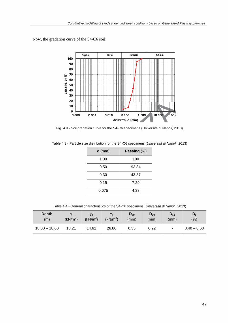
Constitutive modelling of sands under undrained conditions based on Generalized Plasticity premises
47
Now, the gradation curve of the S4-C6 soil:
Fig. 4.9 - Soil gradation curve for the S4-C6 specimens (Università di Napoli, 2013)
Table 4.3 - Particle size distribution for the S4-C6 specimens (Università di Napoli, 2013)
d (mm) Passing (%)
1.00 100
0.50 93.84
0.30 43.37
0.15 7.29
0.075 4.33
Table 4.4 - General characteristics of the S4-C6 specimens (Università di Napoli, 2013)
Depth
(m)
γ
(kN/m3)
γd
(kN/m3)
γs
(kN/m3)
D60
(mm)
D30
(mm)
D10
(mm)
Dr
(%)
18.00 – 18.60 18.21 14.62 26.80 0.35 0.22 - 0.40 – 0.60

Constitutive modelling of sands under undrained conditions based on Generalized Plasticity premises
48
At last, the results obtained for the S1-C5 set of specimens:
Fig. 4.10 - Soil gradation curve for the S1-C5 specimens (Università di Napoli, 2013)
Table 4.5 - Particle size distribution for the S1-C5 specimens (Università di Napoli, 2013)
d (mm) Passing (%)
1.00 100
0.50 94.35
0.30 47.37
0.15 14.27
0.075 7.4
Table 4.6 - General characteristics of the S1-C5 specimens (Università di Napoli, 2013)
Depth
(m)
γ
(kN/m3)
γd
(kN/m3)
γs
(kN/m3)
D60
(mm)
D30
(mm)
D10
(mm)
Dr
(%)
23.00 – 23.60 19.20 15.79 26.70 0.35 0.21 0.10 0.30 – 0.40
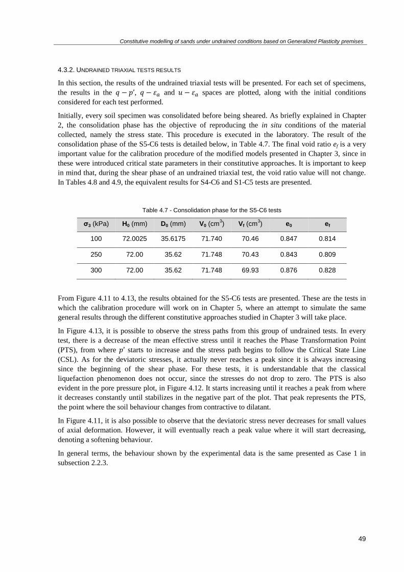
Constitutive modelling of sands under undrained conditions based on Generalized Plasticity premises
49
4.3.2. UNDRAINED TRIAXIAL TESTS RESULTS
In this section, the results of the undrained triaxial tests will be presented. For each set of specimens,
the results in the , and spaces are plotted, along with the initial conditions
considered for each test performed.
Initially, every soil specimen was consolidated before being sheared. As briefly explained in Chapter
2, the consolidation phase has the objective of reproducing the in situ conditions of the material
collected, namely the stress state. This procedure is executed in the laboratory. The result of the
consolidation phase of the S5-C6 tests is detailed below, in Table 4.7. The final void ratio ef is a very
important value for the calibration procedure of the modified models presented in Chapter 3, since in
these were introduced critical state parameters in their constitutive approaches. It is important to keep
in mind that, during the shear phase of an undrained triaxial test, the void ratio value will not change.
In Tables 4.8 and 4.9, the equivalent results for S4-C6 and S1-C5 tests are presented.
Table 4.7 - Consolidation phase for the S5-C6 tests
σ3 (kPa) H0 (mm) D0 (mm) V0 (cm3) Vf (cm
3) e0 ef
100 72.0025 35.6175 71.740 70.46 0.847 0.814
250 72.00 35.62 71.748 70.43 0.843 0.809
300 72.00 35.62 71.748 69.93 0.876 0.828
From Figure 4.11 to 4.13, the results obtained for the S5-C6 tests are presented. These are the tests in
which the calibration procedure will work on in Chapter 5, where an attempt to simulate the same
general results through the different constitutive approaches studied in Chapter 3 will take place.
In Figure 4.13, it is possible to observe the stress paths from this group of undrained tests. In every
test, there is a decrease of the mean effective stress until it reaches the Phase Transformation Point
(PTS), from where starts to increase and the stress path begins to follow the Critical State Line
(CSL). As for the deviatoric stresses, it actually never reaches a peak since it is always increasing
since the beginning of the shear phase. For these tests, it is understandable that the classical
liquefaction phenomenon does not occur, since the stresses do not drop to zero. The PTS is also
evident in the pore pressure plot, in Figure 4.12. It starts increasing until it reaches a peak from where
it decreases constantly until stabilizes in the negative part of the plot. That peak represents the PTS,
the point where the soil behaviour changes from contractive to dilatant.
In Figure 4.11, it is also possible to observe that the deviatoric stress never decreases for small values
of axial deformation. However, it will eventually reach a peak value where it will start decreasing,
denoting a softening behaviour.
In general terms, the behaviour shown by the experimental data is the same presented as Case 1 in
subsection 2.2.3.

Constitutive modelling of sands under undrained conditions based on Generalized Plasticity premises
50
Fig. 4.11 - Experimental results obtained for deviatoric stress versus axial deformation for different confining
pressures, from the S5-C6 set
Fig. 4.12 - Experimental results obtained for pore pressure versus axial deformation for different confining
pressures, from the S5-C6 set
0
200
400
600
800
1000
1200
0,0 5,0 10,0 15,0 20,0 25,0 30,0 35,0
De
viat
ori
c st
ress
, q [
kPa]
Axial deformation, εa (%)
300 kPa
250 kPa
100 kPa
-200
-150
-100
-50
0
50
100
150
0,0 5,0 10,0 15,0 20,0 25,0 30,0 35,0
Po
re p
ress
ure
, u [
kPa]
Axial deformation, εa (%)
300 Kpa
250 kPa
100 kPa

Constitutive modelling of sands under undrained conditions based on Generalized Plasticity premises
51
Fig. 4.13 - Experimental results obtained for deviatoric stress versus principal effective stress for different
confining pressures, from the S5-C6 set
From Figures 4.14 to 4.16, there are the results obtained from the S4-C6 tests and, from Figures 4.17
to 4.19, the results from the S1-C5 set. The comments made for S5-C6 tests are also reproducible for
both sets of tests since the behaviour of the soil is, in general terms, the same. However, it is worth
noting that, in both pore pressure curves, the Phase Transformation Point is not so evident and is not
achieved for the same value of axial deformation for every specimen as in the first group of triaxial
tests. This may represent a difficulty when trying to reproduce these tests through the constitutive
models to be used.
Table 4.8 - Consolidation phase for the S4-C6 tests
σ3 (kPa) H0 (mm) D0 (mm) V0 (cm3) Vf (cm
3) e0 ef
170 72.04 35.79 72.475 71.140 0.787 0.754
300 72.04 35.79 72.475 70.69 0.727 0.684
0
200
400
600
800
1000
1200
0 200 400 600 800 1000 1200
De
viat
ori
c st
ress
, q [
kPa]
Principal effective stress, p' [kPa]
300 kPa
250 kPa
100 kPa

Constitutive modelling of sands under undrained conditions based on Generalized Plasticity premises
52
Fig. 4.14 - Experimental results obtained for deviatoric stress versus axial deformation for different confining
pressures, from the S4-C6 set
Fig. 4.15 - Experimental results obtained for pore pressure versus axial deformation for different confining
pressures, from the S4-C6 set
0
500
1000
1500
2000
2500
0,0 5,0 10,0 15,0 20,0 25,0 30,0 35,0
De
viat
ori
c st
ress
, q [
kPa]
Axial deformation, εa (%)
300 kPa
170 kPa
-500
-450
-400
-350
-300
-250
-200
-150
-100
-50
0
50
100
150
0,0 5,0 10,0 15,0 20,0 25,0 30,0 35,0
Po
re p
ress
ure
, u [
kPa]
Axial deformation, εa (%)
300 kPa
170 kPa
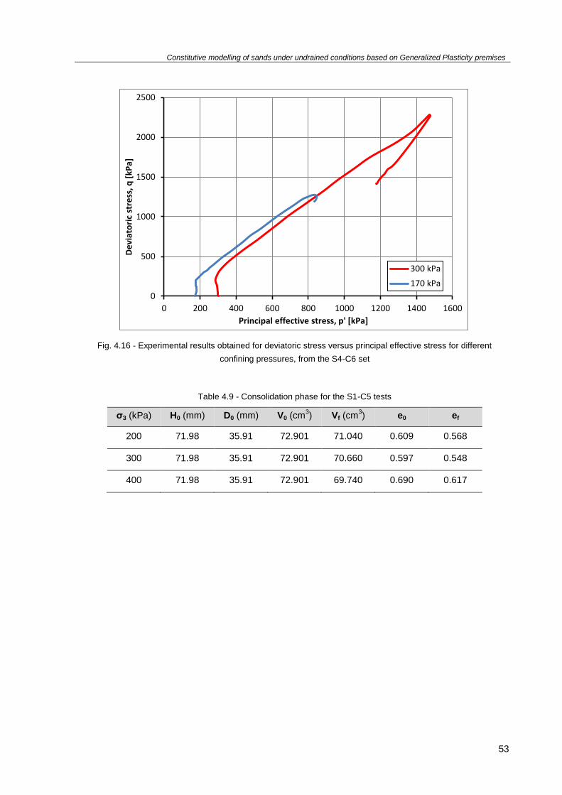
Constitutive modelling of sands under undrained conditions based on Generalized Plasticity premises
53
Fig. 4.16 - Experimental results obtained for deviatoric stress versus principal effective stress for different
confining pressures, from the S4-C6 set
Table 4.9 - Consolidation phase for the S1-C5 tests
σ3 (kPa) H0 (mm) D0 (mm) V0 (cm3) Vf (cm
3) e0 ef
200 71.98 35.91 72.901 71.040 0.609 0.568
300 71.98 35.91 72.901 70.660 0.597 0.548
400 71.98 35.91 72.901 69.740 0.690 0.617
0
500
1000
1500
2000
2500
0 200 400 600 800 1000 1200 1400 1600
De
viat
ori
c st
ress
, q [
kPa]
Principal effective stress, p' [kPa]
300 kPa
170 kPa

Constitutive modelling of sands under undrained conditions based on Generalized Plasticity premises
54
Fig. 4.17 - Experimental results obtained for deviatoric stress versus axial deformation for different confining
pressures, from the S1-C5 set
Fig. 4.18 - Experimental results obtained for pore pressure versus axial deformation for different confining
pressures, from the S1-C5 set
0
500
1000
1500
2000
2500
0 5 10 15 20 25 30 35 40
De
viat
ori
c st
ress
, q [
kPa]
Axial deformation, εa (%)
400 kPa
300 kPa
200 kPa
-500
-450
-400
-350
-300
-250
-200
-150
-100
-50
0
50
100
150
200
0 5 10 15 20 25 30 35 40
Po
re p
ress
ure
, u [
kPa]
Axial deformation, εa (%)
400 kPa
300 Kpa
200 kPa

Constitutive modelling of sands under undrained conditions based on Generalized Plasticity premises
55
Fig. 4.19 - Experimental results obtained for deviatoric stress versus principal effective stress for different
confining pressures, from the S1-C5 set
As a final note, it may be worth mentioning that all the results of the undrained triaxial tests previously
presented have been rebuilt in Excel software from the data provided by the tests sheets, namely the
final height of the specimen Hf (mm), Linear Variable Differential Transformer LVDT (mm), force F
(kg) and pore pressure increments Δu (kg/cm2) and, obviously, using the classical equations that
govern this type of testing. The need to do so was related to the fact that the graphical results of these
tests were not available in an editable file, a fact that could bring additional difficulties to the work
developed within this dissertation.
4.3.3. CRITICAL STATE PARAMETERS
As explained in Chapter 3, the most recent constitutive models based on Generalized Plasticity theory
take into account critical state parameters in their formulation and equations, in opposition to the
original Pastor-Zienkiewicz model which does only includes Mg, a parameter that represents the slope
of the CSL in the space, as explained before. Because of that, is of extreme importance to study
the critical state of the three groups of tests presented in the previous subsection.
Firstly, the Mg parameter is studied. This is a parameter considered as a constant for every constitutive
model that will be applied next, since it represents an intrinsic feature of the granular material studied
in the group of triaxial tests presented earlier. It is found by plotting the final values of the deviatoric
stress and of the mean effective stress of every test considered, which means that each test will
have a single point in that space, representing the pair of values mentioned. Then, the linear trend line
that, intercepting the origin, better fits the values plotted will return the slope of the CSL.
0
500
1000
1500
2000
2500
0 200 400 600 800 1000 1200 1400 1600
De
viat
ori
c st
ress
, q [
kPa]
Principal effective stress, p' [kPa]
400 kPa
300 kPa
200 kPa

Constitutive modelling of sands under undrained conditions based on Generalized Plasticity premises
56
From the value obtained is also possible to find the critical state friction angle, through the following
equation:
(4.19)
where represents the critical state friction angle.
The CSL slope in space can be found in the equation that rules the trend line presented next, in
Figure 4.20:
Fig. 4.20 - Critical State Line slope
Applying now Equation 4.1, it was found a value of 34.84º for the critical state friction angle . The
values for sands generally vary between 26º to 36º, which is a range coherent with the value found.
Although the sand specimens have been collected at different depths and may refer to different sands,
the value obtained usually indicates a well graded material.
Another important item to find is the equation that rules these tests in the ( ) space. The result
obtained is represented in Figure 4.21. The values obtained were found by plotting the void ratio e
values of each test, which can be found in Tables 4.7, 4.8 and 4.9, along with the values of the mean
effective stress previously plotted when studying the CSL slope in space.
It is important to note that none of the tests, as evident in Figures 4.11, 4.14 and 4.17, has been
actually pushed to its critical state. It is expectable that, in the space, the paths of each test tend
y = 1,4113x R² = 0,9633
0
200
400
600
800
1000
1200
1400
1600
1800
0 200 400 600 800 1000 1200
De
viat
ori
c st
ress
, q [
kPa]
Mean effective stress, p' [kPa]
S5-C6
S4-C6
S1-C5

Constitutive modelling of sands under undrained conditions based on Generalized Plasticity premises
57
to the same values, as explained in Chapter 2. So, there was the need to make some assumptions, in
order to find values sufficiently reliable to proceed with this study.
Although the line obtained may actually represent the trend of the values plotted, observing the R2
value obtained in Figure 4.21, it becomes clear that the trend line found does not represent with
sufficient accuracy the CSL in the space considered.
Fig. 4.21 - Critical State Line in the e-ln(p’) space
In order to tackle that issue, that would probably become one of the major shortcomings of the work
developed in this dissertation, particularly in the calibration of the modified models since these take
into account the state parameter Ψ in their formulation, it was tried to obtain other critical state line
equations in the ( ) space by dropping off some of the tests considered with the aim of seeing
what would actually happen.
The results obtained can be found next, in Figure 4.22 and 4.23. In Figure 4.22, the S1-C5 set of tests
was not considered and, in Figure 4.23, only the test performed with a confining pressure of 200 kPa
was not taken into account. The option of not considering the S1-C5 tests may be questionable, since
the S5-C6 represents a fine sand and the S4-C6 is related to a medium to coarse sand. However, the
values obtained for S1-C5 are, at the same time, the ones who are not as well represented by the trend
line obtained before, in Figure 4.21. Also, the set of tests dropped represents the one collected at a
greater depth, a material probably not so relevant within the development of the liquefaction
phenomenon observed.
Although the values of R2 remain difficult to accept, it was decided to move forward with the latest
equations for the CSL found, given that no reliable alternatives to solve this problem were found.
y = -0,156ln(x) + 1,7377 R² = 0,3741
0,00
0,10
0,20
0,30
0,40
0,50
0,60
0,70
0,80
0,90
1,00
1 10 100 1000 10000
Vo
id r
atio
, e
Mean effective stress, p'
S5-C6
S4-C6
S1-C5
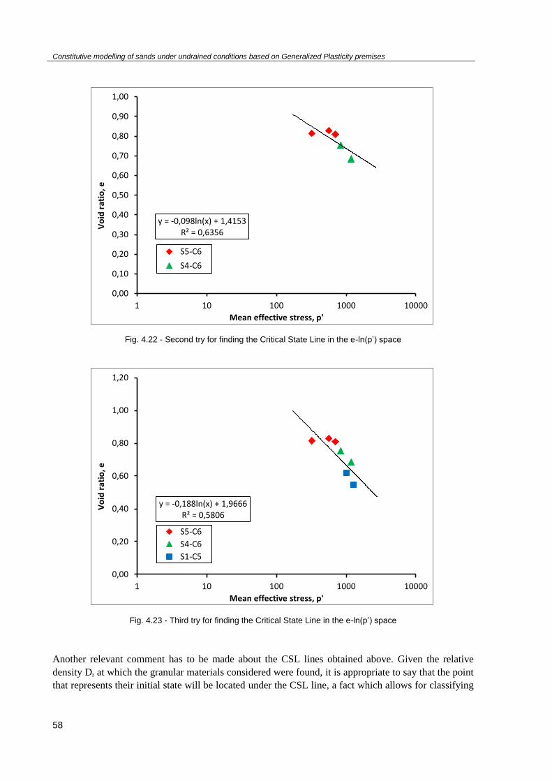
Constitutive modelling of sands under undrained conditions based on Generalized Plasticity premises
58
Fig. 4.22 - Second try for finding the Critical State Line in the e-ln(p’) space
Fig. 4.23 - Third try for finding the Critical State Line in the e-ln(p’) space
Another relevant comment has to be made about the CSL lines obtained above. Given the relative
density Dr at which the granular materials considered were found, it is appropriate to say that the point
that represents their initial state will be located under the CSL line, a fact which allows for classifying
y = -0,098ln(x) + 1,4153 R² = 0,6356
0,00
0,10
0,20
0,30
0,40
0,50
0,60
0,70
0,80
0,90
1,00
1 10 100 1000 10000
Vo
id r
atio
, e
Mean effective stress, p'
S5-C6
S4-C6
y = -0,188ln(x) + 1,9666 R² = 0,5806
0,00
0,20
0,40
0,60
0,80
1,00
1,20
1 10 100 1000 10000
Vo
id r
atio
, e
Mean effective stress, p'
S5-C6
S4-C6
S1-C5
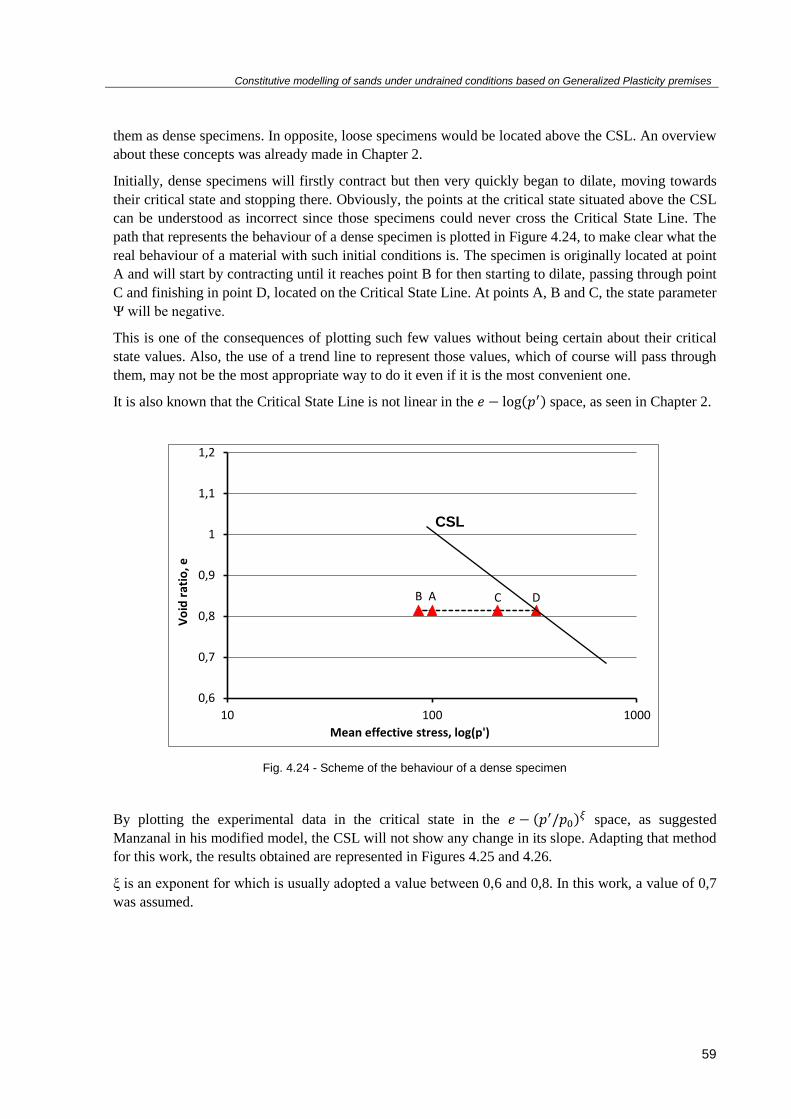
Constitutive modelling of sands under undrained conditions based on Generalized Plasticity premises
59
them as dense specimens. In opposite, loose specimens would be located above the CSL. An overview
about these concepts was already made in Chapter 2.
Initially, dense specimens will firstly contract but then very quickly began to dilate, moving towards
their critical state and stopping there. Obviously, the points at the critical state situated above the CSL
can be understood as incorrect since those specimens could never cross the Critical State Line. The
path that represents the behaviour of a dense specimen is plotted in Figure 4.24, to make clear what the
real behaviour of a material with such initial conditions is. The specimen is originally located at point
A and will start by contracting until it reaches point B for then starting to dilate, passing through point
C and finishing in point D, located on the Critical State Line. At points A, B and C, the state parameter
Ψ will be negative.
This is one of the consequences of plotting such few values without being certain about their critical
state values. Also, the use of a trend line to represent those values, which of course will pass through
them, may not be the most appropriate way to do it even if it is the most convenient one.
It is also known that the Critical State Line is not linear in the ( ) space, as seen in Chapter 2.
Fig. 4.24 - Scheme of the behaviour of a dense specimen
By plotting the experimental data in the critical state in the ( ) space, as suggested
Manzanal in his modified model, the CSL will not show any change in its slope. Adapting that method
for this work, the results obtained are represented in Figures 4.25 and 4.26.
ξ is an exponent for which is usually adopted a value between 0,6 and 0,8. In this work, a value of 0,7
was assumed.
A B C D
0,6
0,7
0,8
0,9
1
1,1
1,2
10 100 1000
Vo
id r
atio
, e
Mean effective stress, log(p')
CSL
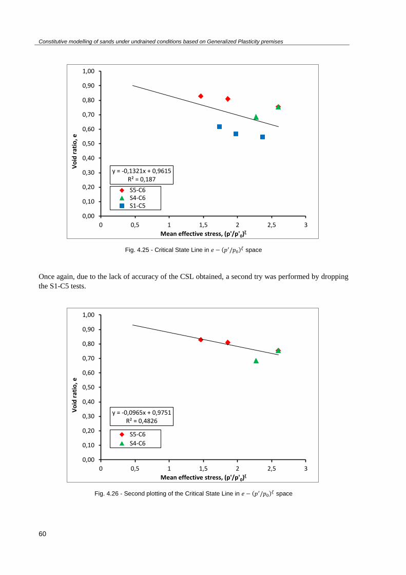
Constitutive modelling of sands under undrained conditions based on Generalized Plasticity premises
60
Fig. 4.25 - Critical State Line in ( ) space
Once again, due to the lack of accuracy of the CSL obtained, a second try was performed by dropping
the S1-C5 tests.
Fig. 4.26 - Second plotting of the Critical State Line in ( ) space
y = -0,1321x + 0,9615 R² = 0,187
0,00
0,10
0,20
0,30
0,40
0,50
0,60
0,70
0,80
0,90
1,00
0 0,5 1 1,5 2 2,5 3
Vo
id r
atio
, e
Mean effective stress, (p'/p'0)ξ
S5-C6S4-C6S1-C5
y = -0,0965x + 0,9751 R² = 0,4826
0,00
0,10
0,20
0,30
0,40
0,50
0,60
0,70
0,80
0,90
1,00
0 0,5 1 1,5 2 2,5 3
Vo
id r
atio
, e
Mean effective stress, (p'/p'0)ξ
S5-C6
S4-C6
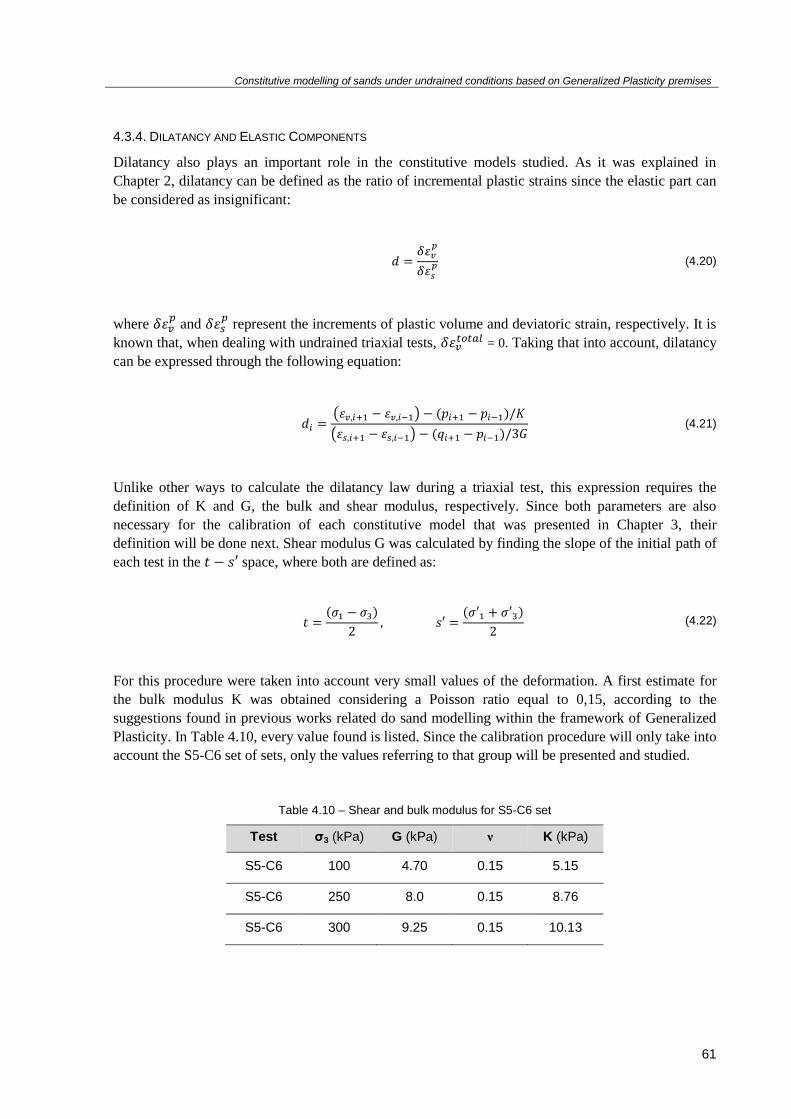
Constitutive modelling of sands under undrained conditions based on Generalized Plasticity premises
61
4.3.4. DILATANCY AND ELASTIC COMPONENTS
Dilatancy also plays an important role in the constitutive models studied. As it was explained in
Chapter 2, dilatancy can be defined as the ratio of incremental plastic strains since the elastic part can
be considered as insignificant:
(4.20)
where
and
represent the increments of plastic volume and deviatoric strain, respectively. It is
known that, when dealing with undrained triaxial tests, = 0. Taking that into account, dilatancy
can be expressed through the following equation:
( ) ( )
( ) ( ) (4.21)
Unlike other ways to calculate the dilatancy law during a triaxial test, this expression requires the
definition of K and G, the bulk and shear modulus, respectively. Since both parameters are also
necessary for the calibration of each constitutive model that was presented in Chapter 3, their
definition will be done next. Shear modulus G was calculated by finding the slope of the initial path of
each test in the space, where both are defined as:
( )
( )
(4.22)
For this procedure were taken into account very small values of the deformation. A first estimate for
the bulk modulus K was obtained considering a Poisson ratio equal to 0,15, according to the
suggestions found in previous works related do sand modelling within the framework of Generalized
Plasticity. In Table 4.10, every value found is listed. Since the calibration procedure will only take into
account the S5-C6 set of sets, only the values referring to that group will be presented and studied.
Table 4.10 – Shear and bulk modulus for S5-C6 set
Test σ3 (kPa) G (kPa) ν K (kPa)
S5-C6 100 4.70 0.15 5.15
S5-C6 250 8.0 0.15 8.76
S5-C6 300 9.25 0.15 10.13
Constitutive modelling of sands under undrained conditions based on Generalized Plasticity premises
62
Despite the values listed above are a result of the experimental data itself, it will be noted that during
the calibration and application of the constitutive models under study, the values referring to the bulk
and shear modulus may change. This may happen because, according to the Generalized Plasticity
theory-based models, the deformations are considered since the beginning as plastic, being the elastic
ones completely disregarded. Given that fact, both elastic components can be the object of an
increment in their own values as a result of the fitting operations that will be described later in Chapter
5.
With the values corresponding to the elastic components found, it is now possible to plot dilatancy as a
function of the axial deformation. Two different laws will be presented. The first one, plotted in Figure
4.27, is obtained considering that the bulk and shear modulus are constant during the shear phase. The
second one, presented in Figure 4.28, considers the tangent bulk and tangent shear modulus, obtained
for every step of the test through Equations 3.33 and 3.34, presented in Chapter 3, and here
represented again:
(4.23)
This obviously means that the elastic components change constantly during the test, since both are
dependent on the current mean effective stress . It was done by calculating, for each value of , the
correspondent value of the bulk and shear modulus and, after it, considering the mean value between
every two consecutive points.
The interest of doing this comparison is related to the possibility of understanding the differences
obtained in the dilatancy law of the material studied taking already into consideration the non-linear
elastic response of the original PZ model, presented in Chapter 2. There are no significant changes in
the maximum value, which remains around the value of -0,5. Despite that, the value of axial
deformation for which the maximum dilatancy is obtained changes considerably, as observed in both
plots.

Constitutive modelling of sands under undrained conditions based on Generalized Plasticity premises
63
Fig. 4.27 - Dilatancy law considering both elastic components as constants during shear
Fig. 4.28 - Dilatancy law considering both elastic components changing during shear
-1
-0,8
-0,6
-0,4
-0,2
0
0,2
0,4
0,6
0,8
1
0,0 5,0 10,0 15,0 20,0 25,0
Dila
tan
cy,
dg
Axial deformation, εa (%)
100 kPa
250 kPa
300 kPa
-1
-0,8
-0,6
-0,4
-0,2
0
0,2
0,4
0,6
0,8
1
0,0 5,0 10,0 15,0 20,0 25,0
Dila
tan
cy,
dg
Axial deformation, εa (%)
100 kPa
250 kPa
300 kPa

Constitutive modelling of sands under undrained conditions based on Generalized Plasticity premises
64
4.3.5. PLASTIC MODULUS
The expressions used for obtaining the Plastic Modulus are probably the most important of the group
of equations that rule the constitutive models in study. They not only take into account almost every
parameter considered within the application of these models but, at the same time, it is probably the
less studied component of the same models, being the one that more problems can bring to the
development of a work like the one presented here. The dilatancy laws considered have been, for
example, much more studied and are understood as more well-established.
The plastic modulus in loading conditions HL is plotted in the space. It can be obtained
through the set of equations that describe the Generalized Plasticity theory, presented in Chapter 3,
considering the experimental data under study, namely the increments of volumetric and shear
deformation.
The values obtained can be found in Figure 4.29, the results being difficult to explain. Consulting
bibliography related to previous work in this field, namely under drained conditions, the plastic
modulus law would decrease in a much smoother and constant way, for small values of deformation,
not presenting an increase at a certain point as these specimens do.
After the calibration procedures, comparisons between the plastic modulus law obtained from the
experimental data and the ones obtained through the constitutive models equations will be performed.
Fig. 4.29 - Plastic Modulus law for every specimen
4.4. CONCLUSIONS
The granular soils found in the village of Scortichino have been subjected to undrained triaxial tests in
order to obtain the mechanical properties of the material. Those tests, along with the analysis that have
been performed, namely the ones related to the critical state, should allow for the calibration of the
constitutive models presented in Chapter 3, that will be next presented in Chapter 5.
-10000
-5000
0
5000
10000
15000
20000
0,0 5,0 10,0 15,0 20,0 25,0 30,0
Pla
stic
Mo
du
lus,
H
Axial deformation, εa (%)
PM 100 kPa
PM 250 kPa
PM 300 kPa

Constitutive modelling of sands under undrained conditions based on Generalized Plasticity premises
65
5 APPLICATION AND CALIBRATION OF THE CONSTITUTIVE MODELS
5.1. INTRODUCTION
In this chapter, the application of the different constitutive models based on Generalized Plasticity
theory, previously presented in Chapter 3, will take place. For each model, the way how every
parameter should be found or calibrated will be described. Besides, a profound sensitivity test to the
PZ model will also be performed with the purpose of allowing for the correct understanding of how
each parameter can influence the global response of the model itself. At the end, a final comparison
between the experimental results, obtained from the undrained triaxial tests performed on Scortichino
sand specimens, and the numerical solution obtained with the application of the constitutive models
will be detailed, aiming for the validation of the appropriateness of the models studied.
The main focus of this chapter is to understand how the different constitutive models and their own
parameters must be manipulated and calibrated in order to reproduce as best as possible the real
behaviour of the material that is being studied, whose main results have been presented in Chapter 4.
The different constitutive models are simulated and based on a programming code, written in the well-
established programming language Visual Basic, and presented in Microsoft Excel software. The code
obviously discriminates every equation needed for the correct application of the original PZ and the
different modified models. This code was originally named as Driver PD and designed as a driver for
the simulation of the drained triaxial tests performed on Venice soils, due to previous works done in
this field. That fact demanded a few changes in the code itself to improve its application to the case
study considered in this thesis, presented in Chapter 4. It is important to note that this will be one of
the first works that will take into account and test the equations that were written for the simulation of
the triaxial tests executed under undrained conditions.
All the process related to the application of the code mentioned above will be described in detail, in
order to make it easier to understand how the calibration of the numerous parameters can be done.
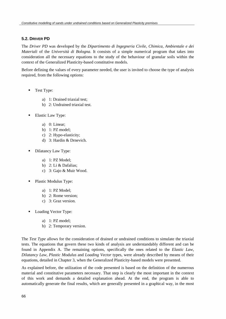
Constitutive modelling of sands under undrained conditions based on Generalized Plasticity premises
66
5.2. DRIVER PD
The Driver PD was developed by the Dipartimento di Ingegneria Civile, Chimica, Ambientale e dei
Materiali of the Università di Bologna. It consists of a simple numerical program that takes into
consideration all the necessary equations to the study of the behaviour of granular soils within the
context of the Generalized Plasticity-based constitutive models.
Before defining the values of every parameter needed, the user is invited to choose the type of analysis
required, from the following options:
Test Type:
a) 1: Drained triaxial test;
b) 2: Undrained triaxial test.
Elastic Law Type:
a) 0: Linear;
b) 1: PZ model;
c) 2: Hypo-elasticity;
d) 3: Hardin & Drnevich.
Dilatancy Law Type:
a) 1: PZ Model;
b) 2: Li & Dafalias;
c) 3: Gajo & Muir Wood.
Plastic Modulus Type:
a) 1: PZ Model;
b) 2: Rome version;
c) 3: Graz version.
Loading Vector Type:
a) 1: PZ model;
b) 2: Temporary version.
The Test Type allows for the consideration of drained or undrained conditions to simulate the triaxial
tests. The equations that govern these two kinds of analysis are understandably different and can be
found in Appendix A. The remaining options, specifically the ones related to the Elastic Law,
Dilatancy Law, Plastic Modulus and Loading Vector types, were already described by means of their
equations, detailed in Chapter 3, when the Generalized Plasticity-based models were presented.
As explained before, the utilization of the code presented is based on the definition of the numerous
material and constitutive parameters necessary. That step is clearly the most important in the context
of this work and demands a detailed explanation ahead. At the end, the program is able to
automatically generate the final results, which are generally presented in a graphical way, in the most
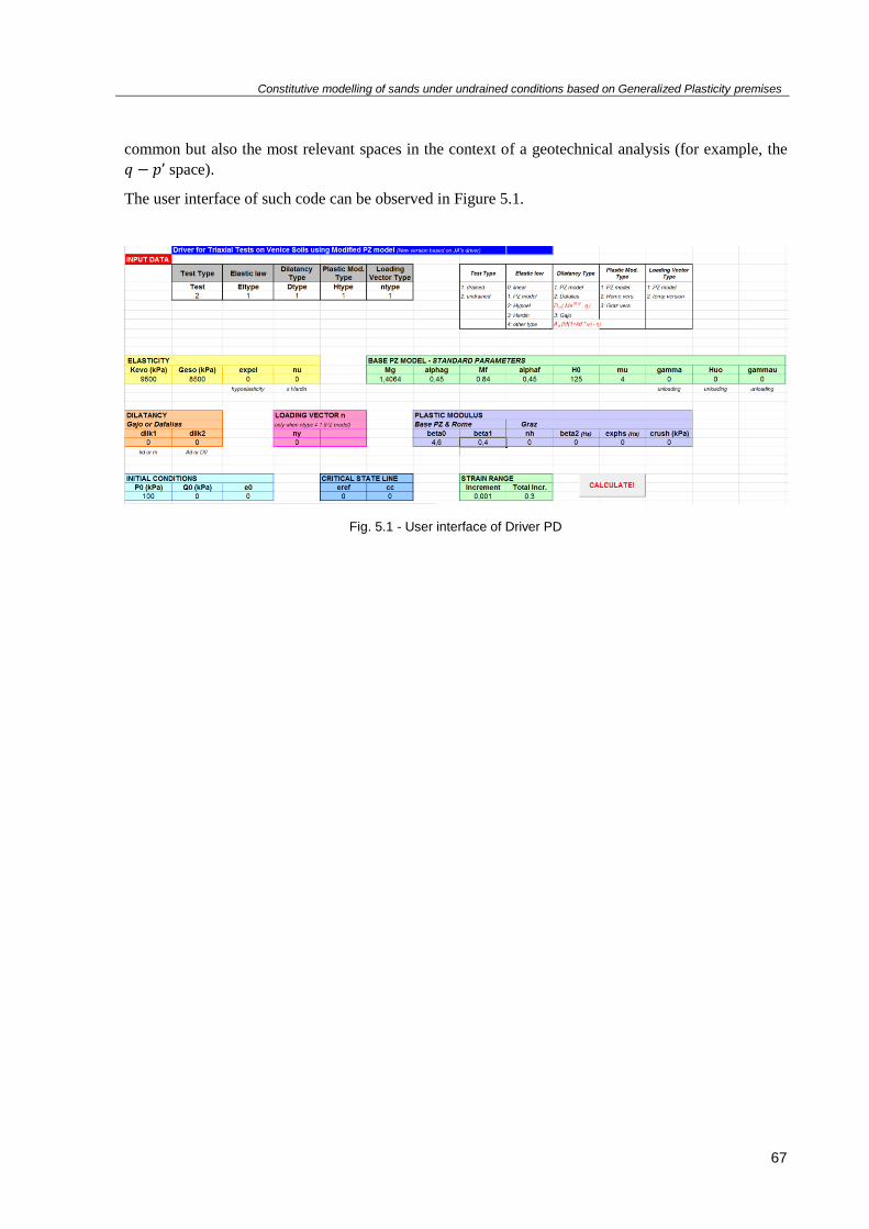
Constitutive modelling of sands under undrained conditions based on Generalized Plasticity premises
67
common but also the most relevant spaces in the context of a geotechnical analysis (for example, the
space).
The user interface of such code can be observed in Figure 5.1.
Fig. 5.1 - User interface of Driver PD

Constitutive modelling of sands under undrained conditions based on Generalized Plasticity premises
68
5.3. PASTOR-ZIENKIEWICZ MODEL
5.3.1. MODEL PARAMETERS AND THEIR CALIBRATION
As explained in Chapter 3, the parameters needed for a simulation using the original Pastor-
Zienkiewicz constitutive model are 12 and are now discriminated in Table 5.1. The process of
calibration of each parameter tabled will be detailed next.
Table 5.1 - Parameters of the original Pastor-Zienkiewicz model
Parameters Description
K0 Bulk modulus (kPa)
G0 Shear modulus (kPa)
Mg Slope of Critical State Line in the space
αg Material constant, slope of the plot
Mf Parameter which is function of relative density and Mg
αf Usually taken equal to αg
H0 Plastic modulus parameter on loading conditions
β0 Model parameter assumed to be constant
β1 Model parameter assumed to be constant
γ Constitutive parameter on loading conditions
Hu0 Plastic modulus parameter on unloading conditions
γu Constitutive parameter on unloading conditions
K0 – the bulk modulus can be obtained by taking into account the initial slope of the curve that
describes the trend of the principal effective stress with respect to the axial deformation .
In the case of an undrained test, as the ones performed in the context of this work, its value
can be adjusted to better reproduce the pore pressure curve when plotted as a function of
the axial strain .
G0 – the shear modulus can be found by considering the slope of the initial part of the curve
that describes the evolution of the deviatoric stress with respect to the axial deformation .
Again, its value can be adjusted to better reproduce the curve of as a function of .
Constitutive modelling of sands under undrained conditions based on Generalized Plasticity premises
69
The bulk modulus can be related to the shear modulus through Theory of Elasticity, by means of the
following equation:
( )
( ) (5.1)
where ν represents the Poisson’s ratio. That way, the parameters of the model may be K0 and G0 but
also G0 and ν.
Mg – the slope of the Critical State Line can be estimated from the experimental graph that
relates the final or critical values of the deviatoric stress with the corresponding ones of the
principal effective stress . The value is obtained by considering the maximum slope of the
line that passes through the origin and better adjusts the values plotted.
αg – this parameter can be determined from the graph where dilatancy dg is plotted as a
function of stress ratio η, using Equation (3.39) (Chapter 3). This parameter is usually
considered equal to 0.45, taking into consideration previous works.
Mf – Pastor and Zienkiewicz (1987) suggested that, as a first estimate, Mf could be obtained
from the following equation, that relates this parameter with Mg but also with the relative
density Dr of the material:
(5.2)
Another way to determine this parameter may be by fitting the stress path in the space,
when studying tests performed under undrained conditions. A third method could also be done
by fitting the critical stress ratio in correspondence to the point where the behaviour of a dense
sand changes to dilatant.
αf – although not explicitly defined, if the value of αf is taken equal to the value of αg, the yield
and plastic potential surfaces have the same shape. So, normally, the value of αf is also
adopted as equal to 0.45.
H0 – this parameter, a multiplying one related to the plastic strains at the beginning of the
loading process, can be determined by executing a fitting operation of the path in or
plot. In case of an undrained test, it also can be determined by fitting the shape of the
stress path in the space.

Constitutive modelling of sands under undrained conditions based on Generalized Plasticity premises
70
β0 – this constitutive parameter can vary between 1.5 and 5. The value recommended from the
works of Laura Tonni (2002) and Diego Manzanal (2008) is 4.2.
β1 – this parameter is taken from the range [0.1; 0.2]. Once again, the recommended value
obtained from the works of the authors mentioned above is 0.2.
Hu0 – this constitutive parameter, related to the unloading plastic modulus, can be obtained
also from a fitting operation that takes into account the slope of the first part of the unloading
curve.
γu – also this constitutive parameter is related to the initial slope of the unloading curve, being
normal to be adopted equal as 2.
γ – this parameter is related to a function which incorporates material memory in a simple
way. Its calibration can be done by considering the initial slope of the reloading path.
The parameters relative to the unloading and reloading paths, Hu0, γu and γ, will not be studied in the
context of this thesis, which means that the calibration procedure will only be required for the first 9
parameters presented before.
Given that some parameters have been and are usually considered as constants in other works, the
calibration process would end up with 5 different parameters to work on: K0, G0, Mg, Mf, and H0.
However, in this work, the influence under undrained conditions of the parameters αg, αf, β0 and β1, the
ones normally taken as constants, will also be studied. To understand as best as possible how these
parameters influence the global response of the PZ model in simulating that type of triaxial tests, a
sensitivity test will be performed in the following subsection.
5.3.2. SENSITIVITY TEST OF THE PZ MODEL
This sensitivity test will be done by changing, under a controlled range of variation, the parameters
needed for the running of the original PZ model. The results will be plotted in the , and
spaces. The differences in the global response of the model will be analysed, in order to
understand how the code works, its advantages and disadvantages, but also to facilitate the choice of
the final set of values that will be responsible for the simulation of the triaxial tests presented in
Chapter 4. To work as a reference, the results of the undrained triaxial test performed under a
confining pressure of 100 kPa, in the set S5-C6, will be plotted next to the numerous tests that will be
run. The tests will start from the following set of values, listed in Table 5.2.
Table 5.2 - Initial values for the sensitivity test of the PZ model
p0 (kPa) K0 (kPa) G0 (kPa) Mg αg Mf αf H0 β0 β1
100 5000 4500 1.4113 0.45 0.86 0.45 150 4.2 0.2

Constitutive modelling of sands under undrained conditions based on Generalized Plasticity premises
71
The results obtained with the parameters detailed in Table 5.2 are presented in Figures 5.2, 5.3 and
5.4, respectively, in the , and spaces.
Fig. 5.2 - First estimate of deviatoric stress versus principal effective stress, for the sensitivity test
Fig. 5.3 - First estimate of deviatoric stress versus axial deformation, for the sensitivity test
Fig. 5.4 - First estimate of pore pressure versus axial deformation, for the sensitivity test
0
100
200
300
400
500
600
0 50 100 150 200 250 300 350
De
viat
ori
c st
ress
, q [
kPa]
Principal effective stress, p' [kPa]
Triaxial test
Prediction
0
100
200
300
400
500
600
0 5 10 15 20 25 30 35
De
viat
ori
c st
ress
, q [
kPa]
Axial deformation, εa (%)
Triaxial test
Prediction
-80
-60
-40
-20
0
20
40
60
80
0 5 10 15 20 25 30 35
Po
re p
ress
ure
, u [
kPa]
Axial deformation, εa (%)
Triaxial test
Prediction

Constitutive modelling of sands under undrained conditions based on Generalized Plasticity premises
72
5.3.2.1. Elastic components
Firstly, this test will focus on understanding how both elastic components may change the initial
response of the model. The first set of graphs, presented in Figures 5.5 to 5.8, is the result of changing
the bulk modulus K0 value, maintaining all the other parameters the same. The values tested are listed
below, in Table 5.3:
Table 5.3 - Values of K0 tested for the original PZ model
Prediction 1, K0
(kPa)
Prediction 2, K0
(kPa)
Prediction 3, K0
(kPa)
Prediction 4, K0
(kPa)
Prediction 5, K0
(kPa)
5000 6500 8500 10000 20000
The same procedure will be repeated with shear modulus G0 but in separate tests, being the values
tested listed in Table 5.4. The results obtained are represented in Figure 5.9 to 5.12.
Table 5.4 - Values of G0 tested for the original PZ model
Prediction 1, G0
(kPa)
Prediction 2, G0
(kPa)
Prediction 3, G0
(kPa)
Prediction 5, G0
(kPa)
Prediction 5, G0
(kPa)
4500 7000 9500 15000 22500
Analysing the following three figures, it becomes evident that the bulk modulus K0 has a certain
influence in the elastic response of the model, for the smaller axial deformations, but not in its global
response, since it does not change dramatically the path for where all the predictions tend to, after the
initial linear response.
Fig. 5.5 - Results obtained for deviatoric stress versus principal effective stress for different K0 values
0
50
100
150
200
0 20 40 60 80 100 120 140 160
De
viat
ori
c st
ress
, q [
kPa]
Principal effective stress, p' [kPa]
Triaxial testK = 5000 kPaK = 6500 kPaK = 8500 kPaK = 10000 kPaK = 20000 kPa

Constitutive modelling of sands under undrained conditions based on Generalized Plasticity premises
73
In the space, Figure 5.6, it is observed that, as long as the bulk modulus value increases, the
length of the linear path of the simulation decreases. However, the slope of such path does not change.
Fig. 5.6 - Results obtained for deviatoric stress versus axial deformation for different K0 values
By increasing the bulk modulus, the model is also anticipating the Phase Transformation Point, where
the soil behaviour changes from contractive to dilatant. That can be observed in Figure 5.5 but also in
Figure 5.7, where the pore pressure peaks of the tests of 5000 kPa and 20000 kPa are considerably
different.
Fig. 5.7 - Results obtained for pore pressure versus axial deformation for different K0 values
0
20
40
60
80
100
0 1 2 3 4 5
De
viat
ori
c st
ress
, q [
kPa]
Axial deformation, εa (%)
Triaxial test
K = 5000 kPa
K = 6500 kPa
K = 8500 kPa
K = 10000 kPa
K = 20000 Kpa
0
20
40
60
80
100
0 2 4 6 8 10
Po
re p
ress
ure
, u [
kPa]
Axial deformation, εa (%)
Triaxial testK = 5000 kPaK = 6500 kPaK = 8500 kPaK = 10000 kPaK = 20000 kPa

Constitutive modelling of sands under undrained conditions based on Generalized Plasticity premises
74
The plastic modulus evolution during the test has also been plotted as a function of the axial
deformation, in Figure 5.8. With a bulk modulus increase, the plastic modulus will decrease sooner
until it reaches a common value for every test. This is explained by the bigger plastic strains that are
generated by the model code, given that the deviatoric stress also decreases as well as the stress ratio
η.
Fig. 5.8 - Results obtained for plastic modulus versus axial deformation for different K0 values
In its turn, the shear modulus G0 has the opposite influence, as noticeable in Figures 5.9 to 5.12.
Raising its value will cause an increase in the slope of the line responsible for the elastic behaviour of
the material.
Fig. 5.9 - Results obtained for deviatoric stress versus principal effective stress for different G0 values
0
5000
10000
15000
20000
25000
30000
0 0,5 1 1,5 2
Pla
stic
Mo
du
lus
Axial deformation, εa (%)
K = 5000 kPa
K = 6500 kPa
K = 8500 kPa
K = 10000 kPa
K = 20000 kPa
0
50
100
150
200
0 20 40 60 80 100 120 140 160
De
viat
ori
c st
ress
, q [
kPa]
Principal effective stress, p' [kPa]
Triaxial test
G = 4500 kPa
G = 7000 kPa
G = 9500 kPa
G = 15000 kPa
G = 22500 kPa

Constitutive modelling of sands under undrained conditions based on Generalized Plasticity premises
75
Fig. 5.10 - Results obtained for deviatoric stress versus axial deformation for different G0 values
In this case, as observed in the space, Figure 5.11, the Phase Transformation Point does not
suffer particular change by increasing the shear modulus.
Fig. 5.11 - Results obtained for pore pressure versus axial deformation for different G0 values
The differences in the plastic modulus, Figure 5.12, are now much more accentuated. It is important to
note that, in the elastic matrix that rules the code equations, the shear modulus value is multiplied by 3
compared to the bulk modulus, which is multiplied by 1, as detailed in Equations (3.31) and (3.32).
0
10
20
30
40
50
60
70
80
90
100
0 1 2 3 4 5
De
viat
ori
c st
ress
, q [
kPa]
Axial deformation, εa (%)
Triaxial test
G = 4500 kPa
G = 7000 kPa
G = 9500 kPa
G = 15000 kPa
G = 22500 kPa
0
20
40
60
80
100
0 2 4 6 8 10
Po
re p
ress
ure
, u [
kPa]
Axial deformation, εa (%)
Triaxial test G = 4500 kPa G = 7000 kPa
G = 9500 kPa G = 15000 kPa G = 22500 kPa

Constitutive modelling of sands under undrained conditions based on Generalized Plasticity premises
76
Fig. 5.12 - Results obtained for plastic modulus versus axial deformation for different G0 values
5.3.2.2. Mg parameter
The sensitivity test continues, now testing different values of Mg, the ones listed in Table 5.5. The
results are plotted in Figures 5.13 to 5.16.
Table 5.5 - Values of Mg tested for the original PZ model
Prediction 1, Mg Prediction 2, Mg Prediction 3, Mg Prediction 4, Mg
1.4113 1.3064 1.15 1.0
Mg, as explained in subsection 5.3.1, is a parameter that can be found experimentally, from the slope
of the line that better adjusts and represents the values plotted. It represents the slope of CSL so its
influence in the model becomes obvious in the space: if a lower value of Mg is chosen, the PZ
model will represent a CSL with a lower slope, what can be observed in Figure 5.13.
However, this parameter is also related to the dilatancy and plastic modulus laws, as detailed in
Equations (3.39) and (3.50) from Chapter 3, a fact that will introduce changes in the deviatoric stress ,
principal effective stress and pore pressure values generated by the model equations, as evident in
Figures 5.14 and 5.15.
It is evident that the influence of this parameter becomes bigger as the axial deformations accumulate,
given the differences in the deviatoric stress plotted or in the evolution of the plastic modulus.
However, this parameter is present in most of the equations that rule the behaviour of this model
which makes it difficult to really understand where this value is more relevant.
0
5 000
10 000
15 000
20 000
25 000
30 000
0 0,5 1 1,5 2
Pla
stic
Mo
du
lus
Axial deformation, εa (%)
G = 4500 kPa
G = 7000 kPa
G = 9500 kPa
G = 15000 kPa
G = 22500 kPa

Constitutive modelling of sands under undrained conditions based on Generalized Plasticity premises
77
Fig. 5.13 - Results obtained for deviatoric stress versus principal effective stress for different Mg values
Fig. 5.14 - Results obtained for deviatoric stress versus axial deformation for different Mg values
0
100
200
300
400
500
600
700
800
900
0 100 200 300 400 500 600 700 800
De
viat
ori
c st
ress
, q [
kPa]
Principal effective stress, p' [kPa]
Triaxial test
Mg = 1,4064
Mg = 1,3064
Mg = 1,15
Mg = 1,0
0
100
200
300
400
500
600
700
800
900
0 5 10 15 20 25 30 35
De
viat
ori
c st
ress
, q [
kPa]
Axial deformation, εa (%)
Triaxial test
Mg = 1,4064
Mg = 1,3064
Mg = 1,15
Mg = 1,0

Constitutive modelling of sands under undrained conditions based on Generalized Plasticity premises
78
Fig. 5.15 - Results obtained for pore pressure versus axial deformation for different Mg values
Fig. 5.16 - Results obtained for plastic modulus versus axial deformation for different Mg values
-300
-250
-200
-150
-100
-50
0
50
100
0 5 10 15 20 25 30 35
Po
re p
ress
ure
, u [
kPa]
Axial deformation, εa (%)
Triaxial test
Mg = 1,4064
Mg = 1,3064
Mg = 1,15
Mg = 1,0
0
5 000
10 000
15 000
20 000
25 000
30 000
0 5 10 15 20 25 30
Pla
stic
Mo
du
lus
Axial deformation, εa (%)
Mg = 1,4064
Mg = 1,3064
Mg = 1,15
Mg = 1,0
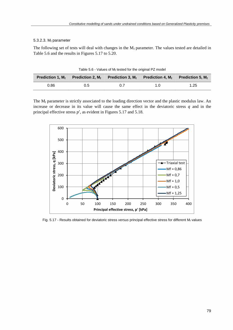
Constitutive modelling of sands under undrained conditions based on Generalized Plasticity premises
79
5.3.2.3. Mf parameter
The following set of tests will deal with changes in the Mf parameter. The values tested are detailed in
Table 5.6 and the results in Figures 5.17 to 5.20.
Table 5.6 - Values of Mf tested for the original PZ model
Prediction 1, Mf Prediction 2, Mf Prediction 3, Mf Prediction 4, Mf Prediction 5, Mf
0.86 0.5 0.7 1.0 1.25
The Mf parameter is strictly associated to the loading direction vector and the plastic modulus law. An
increase or decrease in its value will cause the same effect in the deviatoric stress and in the
principal effective stress , as evident in Figures 5.17 and 5.18.
Fig. 5.17 - Results obtained for deviatoric stress versus principal effective stress for different Mf values
0
100
200
300
400
500
600
0 50 100 150 200 250 300 350 400
De
viat
ori
c st
ress
, q [
kPa]
Principal effective stress, p' [kPa]
Triaxial test
Mf = 0,86
Mf = 0,7
Mf = 1,0
Mf = 0,5
Mf = 1,25

Constitutive modelling of sands under undrained conditions based on Generalized Plasticity premises
80
Fig. 5.18 - Results obtained for deviatoric stress versus axial deformation for different Mf values
Pastor and Zienkiewicz also suggested that Mf should be related to the relative density of the material
studied. It is known that liquefaction phenomenon usually happens to loose sands and, when tested a
value for Mf that would represent a loose state, the code shows up as actually capable of simulating
liquefaction, as represented in Figure 5.17, when both stresses progress towards zero. Also in Figure
5.19 it is possible to see that, for the test that represents liquefaction phenomenon, the pore pressure
never decreases and stabilizes for a constant positive value.
Fig. 5.19 - Results obtained for pore pressure versus axial deformation for different Mf values
0
100
200
300
400
500
600
700
800
900
1000
1100
0 5 10 15 20 25 30 35
De
viat
ori
c st
ress
, q [
kPa]
Axial deformation, εa (%)
Triaxial test
Mf = 0,86
Mf = 0,7
Mf = 1,0
Mf = 0,5
Mf = 1,25
-160
-140
-120
-100
-80
-60
-40
-20
0
20
40
60
80
100
0 5 10 15 20 25 30 35
Po
re p
ress
ure
, u [
kPa]
Axial deformation, εa (%)
Triaxial test
Mf = 0,86
Mf = 0,5
Mf = 0,70
Mf = 1,0
Mf = 1,25

Constitutive modelling of sands under undrained conditions based on Generalized Plasticity premises
81
Fig. 5.20 - Results obtained for plastic modulus versus axial deformation for different Mf values
In the plastic modulus law becomes evident that, by increasing Mf, the material will show a hardening
behaviour every time more accentuated.
5.3.2.4. H0 parameter
Now, H0 is tested. Once again, the values tried are listed below, in Table 5.7, and the results found in
Figures 5.21 to 5.24.
Table 5.7 - Values of H0 tested for the original PZ model
Prediction 1, H0 Prediction 2, H0 Prediction 3, H0 Prediction 4, H0 Prediction 5, H0
150 50 125 175 300
H0, as a constant in the plastic modulus law in loading conditions, affects the results in a similar way
to Mf. The higher this parameter is, the higher will be the stresses generated by the code.
0
5 000
10 000
15 000
20 000
25 000
30 000
0 5 10 15 20 25 30 35
Pla
stic
Mo
du
lus
Axial deformation, εa (%)
Mf = 0,86
Mf = 0,70
Mf = 1,0
Mf = 0,5
Mf = 1,25

Constitutive modelling of sands under undrained conditions based on Generalized Plasticity premises
82
Fig. 5.21 - Results obtained for deviatoric stress versus principal effective stress for different H0 values
Fig. 5.22 - Results obtained for deviatoric stress versus axial deformation for different H0 values
0
100
200
300
400
500
600
0 50 100 150 200 250 300 350 400 450 500
De
viat
ori
c st
ress
, q [
kPa]
Principal effective stress, p' [kPa]
Triaxial test
H0 = 150
H0 = 50
H0 = 125
H0 = 175
H0 = 300
0
100
200
300
400
500
600
0 5 10 15 20 25 30 35
De
viat
ori
c st
ress
, q [
kPa]
Axial deformation, εa (%)
Triaxial test
H0 = 150
H0 = 50
H0 = 125
H0 = 175
H0 = 300

Constitutive modelling of sands under undrained conditions based on Generalized Plasticity premises
83
Fig. 5.23 - Results obtained for pore pressure versus axial deformation for different H0 values
Fig. 5.24 - Results obtained for plastic modulus versus axial deformation for different H0 values
5.3.2.5. β0 parameter
β0 is a constitutive parameter of the plastic modulus law for which is usually adopted the value of 4,2,
taking into account previous works related to the original PZ model. Nevertheless, this sensitivity test
will also study the influence of this parameter in the global response of the model when run under
undrained conditions. The values tested are listed above, in Table 5.8.
-160
-140
-120
-100
-80
-60
-40
-20
0
20
40
60
80
100
0 5 10 15 20 25 30 35
Po
re p
ress
ure
, u [
kPa]
Axial deformation, εa (%)
Triaxial test
H0 = 150
H0 = 50
H0 = 125
H0 = 175
H0 = 300
0
10 000
20 000
30 000
40 000
50 000
60 000
0 5 10 15 20 25 30
Pla
stic
Mo
du
lus
Axial deformation, εa (%)
H0 = 150
H0 = 50
H0 = 125
H0 = 175
H0 = 300

Constitutive modelling of sands under undrained conditions based on Generalized Plasticity premises
84
Table 5.8 - Values of β0 tested for the original PZ model
Prediction 1, β0 Prediction 2, β0 Prediction 3, β0
4.2 1 10
Fig. 5.25 - Results obtained for deviatoric stress versus principal effective stress for different β0 values
As expected, this parameter has a huge influence on the initial values of the plastic modulus graph, as
noticeable in Figure 5.28. However, it loses influence as long as the deformations occur and all the
values tested tend to similar values at a certain point.
From Figures 5.25 to 5.27, it is possible to notice that it also affects the deviatoric stress and the
principal effective stress which is explained by the fact that every increment of and is directly
related to the plastic modulus equations.
0
100
200
300
400
500
600
0 50 100 150 200 250 300 350 400 450 500
De
viat
ori
c st
ress
, q [
kPa]
Principal effective stress, p' [kPa]
Triaxial test
Beta0 = 4,2
Beta0 = 1
Beta0 = 10

Constitutive modelling of sands under undrained conditions based on Generalized Plasticity premises
85
Fig. 5.26 - Results obtained for deviatoric stress versus axial deformation for different β0 values
Fig. 5.27 - Results obtained for pore pressure versus axial deformation for different β0 values
Looking for Equation (3.51) from Chapter 3, it is possible to check how Hs is doubly dependant on β0.
0
100
200
300
400
500
600
0 5 10 15 20 25 30 35
De
viat
ori
c st
ress
, q [
kPa]
Axial deformation, εa (%)
Triaxial test
Beta0 = 4,2
Beta0 = 1
Beta0 = 10
-160
-140
-120
-100
-80
-60
-40
-20
0
20
40
60
80
100
0 5 10 15 20 25 30 35
Po
re p
ress
ure
, u [
kPa]
Axial deformation, εa (%)
Triaxial test
Beta0 = 4,2
Beta0 = 1
Beta0 = 10

Constitutive modelling of sands under undrained conditions based on Generalized Plasticity premises
86
Fig. 5.28 - Results obtained for plastic modulus versus axial deformation for different β0 values
5.3.2.6. β1 parameter
β1 is the other constitutive parameter that works directly in the plastic modulus law. The values tried
are listed above, in Table 5.9, and the results presented in Figures 5.29 to 5.32.
Table 5.9 - Values of β1 tested for the original PZ model
Prediction 1, β1 Prediction 2, β1 Prediction 3, β1
0.2 0.1 0.5
0
5 000
10 000
15 000
20 000
25 000
30 000
35 000
40 000
45 000
50 000
0 2,5 5 7,5 10 12,5 15
Pla
stic
Mo
du
lus
Axial deformation, εa (%)
Beta0 = 10
Beta0 = 4,2
Beta0 = 1

Constitutive modelling of sands under undrained conditions based on Generalized Plasticity premises
87
Fig. 5.29 - Results obtained for deviatoric stress versus principal effective stress for different β1 values
Fig. 5.30 - Results obtained for deviatoric stress versus axial deformation for different β1 values
0
100
200
300
400
500
600
0 50 100 150 200 250 300 350 400 450 500
De
viat
ori
c st
ress
, q [
kPa]
Principal effective stress, p' [kPa]
Triaxial test
Beta1 = 0,2
Beta1 = 0,1
Beta1 = 0,5
0
100
200
300
400
500
600
700
800
900
1000
0 5 10 15 20 25 30 35
De
viat
ori
c st
ress
, q [
kPa]
Axial deformation, εa (%)
Triaxial test
Beta1 = 0,2
Beta1 = 0,1
Beta1 = 0,5

Constitutive modelling of sands under undrained conditions based on Generalized Plasticity premises
88
Fig. 5.31 - Results obtained for pore pressure versus axial deformation for different β1 values
Fig. 5.32 - Results obtained for plastic modulus versus axial deformation for different β1 values
The influence of this parameter is similar to β1. An increase or a decrease in its value will cause the
same effects in the response of the model.
-160
-140
-120
-100
-80
-60
-40
-20
0
20
40
60
80
100
0 5 10 15 20 25 30 35
Po
re p
ress
ure
, u [
kPa]
Axial deformation, εa (%)
Triaxial test
Beta1 = 0,2
Beta1 = 0,1
Beta1 = 0,5
0
5 000
10 000
15 000
20 000
25 000
30 000
35 000
40 000
45 000
50 000
0 5 10 15 20 25 30 35
Po
re p
ress
ure
, u [
kPa]
Axial deformation, εa (%)
Beta1 = 0,5
Beta1 = 0,2
Beta1 = 0,1

Constitutive modelling of sands under undrained conditions based on Generalized Plasticity premises
89
5.3.2.7. αg parameter
On the other hand, αg is a constitutive parameter of the dilatancy law, which is normally adopted as
0,45. The values listed in Table 5.10 are the ones tested.
Table 5.10 - Values of αg tested for the original PZ model
Prediction 1, αg Prediction 2, αg Prediction 3, αg
0.45 0.25 0.9
Fig. 5. 33 - Results obtained for deviatoric stress versus principal effective stress for different αg values
Fig. 5. 34 - Results obtained for deviatoric stress versus axial deformation for different αg values
0
100
200
300
400
500
600
0 50 100 150 200 250 300 350 400 450 500
De
viat
ori
c st
ress
, q [
kPa]
Principal effective stress, p' [kPa]
Triaxial test
alphaG = 0,45
alphaG = 0,25
alphaG = 0,9
0
100
200
300
400
500
600
0 5 10 15 20 25 30 35
De
viat
ori
c st
ress
, q [
kPa]
Axial deformation, εa (%)
Triaxial test
alphaG = 0,45
alphaG = 0,25
alphaG = 0,9
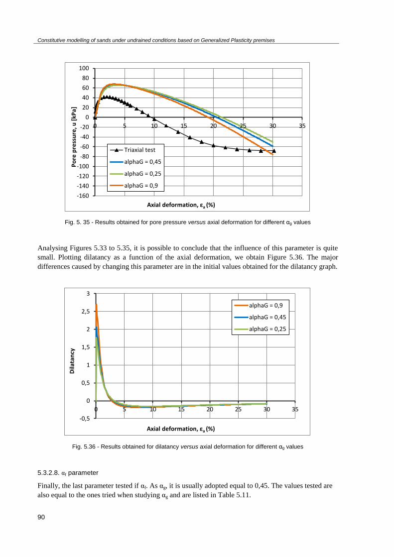
Constitutive modelling of sands under undrained conditions based on Generalized Plasticity premises
90
Fig. 5. 35 - Results obtained for pore pressure versus axial deformation for different αg values
Analysing Figures 5.33 to 5.35, it is possible to conclude that the influence of this parameter is quite
small. Plotting dilatancy as a function of the axial deformation, we obtain Figure 5.36. The major
differences caused by changing this parameter are in the initial values obtained for the dilatancy graph.
Fig. 5.36 - Results obtained for dilatancy versus axial deformation for different αg values
5.3.2.8. αf parameter
Finally, the last parameter tested if αf. As αg, it is usually adopted equal to 0,45. The values tested are
also equal to the ones tried when studying αg and are listed in Table 5.11.
-160
-140
-120
-100
-80
-60
-40
-20
0
20
40
60
80
100
0 5 10 15 20 25 30 35
Po
re p
ress
ure
, u [
kPa]
Axial deformation, εa (%)
Triaxial test
alphaG = 0,45
alphaG = 0,25
alphaG = 0,9
-0,5
0
0,5
1
1,5
2
2,5
3
0 5 10 15 20 25 30 35
Dila
tan
cy
Axial deformation, εa (%)
alphaG = 0,9
alphaG = 0,45
alphaG = 0,25

Constitutive modelling of sands under undrained conditions based on Generalized Plasticity premises
91
Table 5.11 - Values of αf tested for the original PZ model
Prediction 1, αf Prediction 2, αf Prediction 3, αf
0.45 0.25 0.9
Fig. 5.37 - Results obtained for deviatoric stress versus principal effective stress for different αf values
Analysing the space, this is the first parameter that can actually change in such a strong way the
slope of the Critical State Line, as observed in Figure 5.37.
Fig. 5.38 - Results obtained for deviatoric stress versus axial deformation for different αf values
0
100
200
300
400
500
600
0 50 100 150 200 250 300 350 400 450 500
De
viat
ori
c st
ress
, q [
kPa]
Principal effective stress, p' [kPa]
Triaxial test
alphaF = 0,45
alphaF = 0,25
alphaF = 0,9
0
100
200
300
400
500
600
0 5 10 15 20 25 30 35
De
viat
ori
c st
ress
, q [
kPa]
Axial deformation, εa (%)
Triaxial test
alphaF = 0,45
alphaF = 0,25
alphaF = 0,9

Constitutive modelling of sands under undrained conditions based on Generalized Plasticity premises
92
Fig. 5.39 - Results obtained for pore pressure versus axial deformation for different αf values
Fig. 5.40 - Results obtained for plastic modulus versus axial deformation for different αf values
-160
-140
-120
-100
-80
-60
-40
-20
0
20
40
60
80
100
0 5 10 15 20 25 30 35
Po
re p
ress
ure
, u [
kPa]
Axial deformation, εa (%)
Triaxial test
alphaF = 0,45
alphaF = 0,25
alphaF = 0,9
0
5 000
10 000
15 000
20 000
25 000
30 000
0 5 10 15 20 25 30 35
Pla
stic
Mo
du
lus
Axial deformation, εa (%)
alphaF = 0,45
alphaF = 0,25
alphaF = 0,9

Constitutive modelling of sands under undrained conditions based on Generalized Plasticity premises
93
5.3.2.9. Confining pressure
In this subsection, different confining pressures will be tested maintaining every other parameter
constant during the sensitivity test, as Table 5.12 shows. The results obtained are represented in Figure
5.41 to 5.44.
Table 5.12 - Values of p0 tested for the original PZ model
p0 (kPa) K0 (kPa) G0 (kPa) Mg αg Mf αf H0 β0 β1
100 20000 25000 1.4113 0.45 0.6 0.45 75 4.2 0.2
1000 20000 25000 1.4113 0.45 0.6 0.45 75 4.2 0.2
3000 20000 25000 1.4113 0.45 0.6 0.45 75 4.2 0.2
It is possible to observe that all the tests run demonstrate what would be the beginning of the
liquefaction phenomena if triggered since both stresses tend to zero, as evident in Figure 5.41.
Apparently, the model is only able to simulate a material with a strength peak and then a softening
behaviour, as plotted in Figure 5.42, when it is dealing with a behaviour similar to liquefaction. If the
material is purely dilatant or only shows some instability before dilating, as all the experimental data
considered in this work, both stress will end up increasing constantly in the model, this one being
unable to show a softening behaviour at a certain point.
Fig. 5.41 - Results obtained for deviatoric stress versus principal effective stress for different p0 values
0
250
500
750
1000
1250
1500
1750
2000
2250
2500
2750
0 500 1000 1500 2000 2500 3000 3500
De
viat
ori
c st
ress
, q [
kPa]
Principal effective stress, p' [kPa]
p0 = 100 kPa
p0 = 1000 kPa
p0 = 3000 kPa
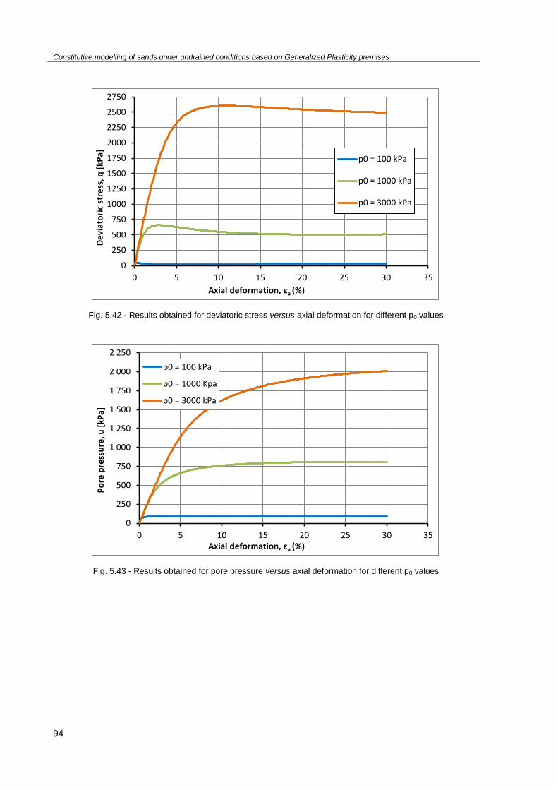
Constitutive modelling of sands under undrained conditions based on Generalized Plasticity premises
94
Fig. 5.42 - Results obtained for deviatoric stress versus axial deformation for different p0 values
Fig. 5.43 - Results obtained for pore pressure versus axial deformation for different p0 values
0
250
500
750
1000
1250
1500
1750
2000
2250
2500
2750
0 5 10 15 20 25 30 35
De
viat
ori
c st
ress
, q [
kPa]
Axial deformation, εa (%)
p0 = 100 kPa
p0 = 1000 kPa
p0 = 3000 kPa
0
250
500
750
1 000
1 250
1 500
1 750
2 000
2 250
0 5 10 15 20 25 30 35
Po
re p
ress
ure
, u [
kPa]
Axial deformation, εa (%)
p0 = 100 kPa
p0 = 1000 Kpa
p0 = 3000 kPa

Constitutive modelling of sands under undrained conditions based on Generalized Plasticity premises
95
Fig. 5.44 - Results obtained for plastic modulus versus axial deformation for different p0 values
5.3.4. PRELIMINARY CONCLUSIONS ABOUT THE ORIGINAL PASTOR-ZIENKIEWICZ MODEL
From the previous results it turns out that some difficulties or limits of the original PZ model became
evident.
Having as reference the experimental data obtained from Scortichino sand, one of the major
shortcomings found was the inability of the model in simulating a softening behaviour for large values
of axial strain unless when liquefaction actually occurs. When liquefaction does not happen, the
deviatoric stress will usually increase indefinitely and the model is incapable of capturing the totality
of the behaviour of the sand studied in this work.
Analysing the pore pressure graphs, it also becomes clear that the model has difficulties in simulating
the behaviour of the experimental data from the triaxial tests. Although for values of deformation up to
10% it is possible to reproduce with some exactitude the general path of the pore pressure curve, when
the excess pore pressure becomes negative, the model will never be capable of simulating the
stabilization of such value, as happens in the experimental data, letting to progress indeterminately
in the negative part of the plot.
In the following subsection, the final calibration of the original PZ model will take place, in order to
simulate as better as possible the behaviour of the triaxial tests studied. Having in mind the problems
referred above, the calibration process will be conducted by trying to reproduce at least the first 10%
to 15% of the behaviour of the material considered.
5.3.5. FINAL CALIBRATION PROCEDURE AND RESULTS
After understanding how the model reacts to the various changes introduced in all the parameters that
require a calibration procedure, in order to make the code able to reproduce and simulate the
undrained triaxial tests presented in Chapter 4, it is now time to present the final set of values that can
reproduce as best as possible the tests mentioned.
0
50 000
100 000
150 000
200 000
250 000
300 000
350 000
400 000
450 000
0 2,5 5 7,5 10
Pla
stic
Mo
du
lus
Axial deformation, εa (%)
p0 = 100 kPa
p0 = 1000 kPa
p0 = 3000 kPa

Constitutive modelling of sands under undrained conditions based on Generalized Plasticity premises
96
The final values are detailed in Table 5.13, found with reference to the calibration procedure described
in subsection 5.3.1.
Table 5.13 - Final set of values for the PZ model responsible for the simulation of S5-C6 triaxial tests
p0 (kPa) K0 (kPa) G0 (kPa) Mg αg Mf αf H0 β0 β1
100 8500 9500 1.4064 0.45 0.84 0.45 125 4.6 0.4
250 12500 12000 1.4064 0.45 0.84 0.45 110 4.5 0.5
300 23000 19500 1.4064 0.45 0.84 0.45 110 4.5 0.5
The values about the confining pressure p0 are constants of each triaxial test of the S5-C6 set. The
elastic components, K0 and G0, as described before, were found by fitting the results of the model to
the experimental ones.
The value of Mg was determined with reference to the experimental data, as described in Chapter 3,
and maintained constant for every test. Also Mf was preserved the same for all the tests. Since it is
related to the relative density of the material, and considering that the material is actually the same,
with a relative density of about 60%, it makes sense to maintain this value equal for all the simulations
even if previous works in this field make reference to changes in this parameter in order to better
reproduce the triaxial tests studied.
H0, β0 and β1 were adjusted individually to every test, in order to simulate at least the general
behaviour of the material of the first 10% of deformation, as explained before.
The results can be found in Figures 5.45 to 5.47.

Constitutive modelling of sands under undrained conditions based on Generalized Plasticity premises
97
Fig. 5.45 - Results of the calibration for the PZ model, deviatoric stress versus principal effective stress
Fig. 5.46 - Results of the calibration for the PZ model, deviatoric stress versus axial deformation
0
100
200
300
400
500
600
700
800
900
1000
1100
0 100 200 300 400 500 600 700 800
De
viat
ori
c st
ress
, q [
kPa]
Principal effective stress, p' [kPa]
300 kPa test
300 kPa prediction
250 kPa test
250 kPa prediction
100 kPa prediction
100 kPa test
0
100
200
300
400
500
600
700
800
900
1000
1100
0,0 5,0 10,0 15,0 20,0 25,0 30,0 35,0
De
viat
ori
c st
ress
, q [
kPa]
Axial deformation, εa (%)
300 kPa test
300 kPa prediction
250 kPa test
250 kPa prediction
100 kPa prediction
100 kPa test
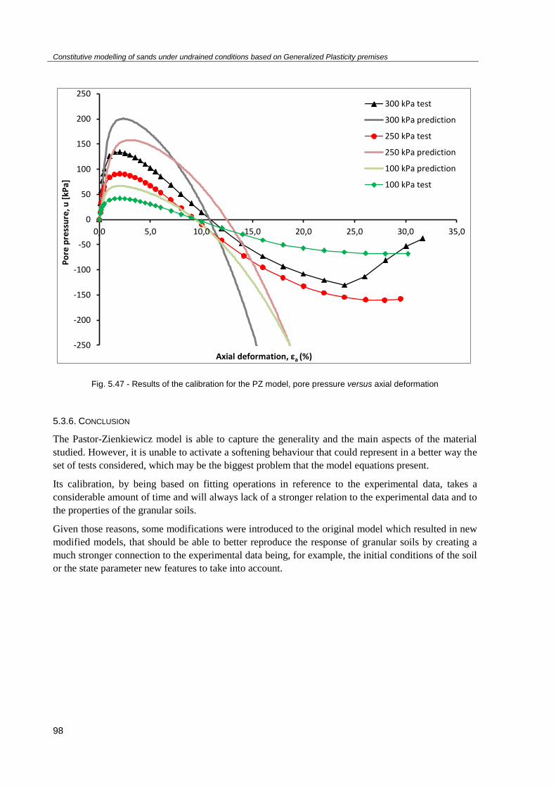
Constitutive modelling of sands under undrained conditions based on Generalized Plasticity premises
98
Fig. 5.47 - Results of the calibration for the PZ model, pore pressure versus axial deformation
5.3.6. CONCLUSION
The Pastor-Zienkiewicz model is able to capture the generality and the main aspects of the material
studied. However, it is unable to activate a softening behaviour that could represent in a better way the
set of tests considered, which may be the biggest problem that the model equations present.
Its calibration, by being based on fitting operations in reference to the experimental data, takes a
considerable amount of time and will always lack of a stronger relation to the experimental data and to
the properties of the granular soils.
Given those reasons, some modifications were introduced to the original model which resulted in new
modified models, that should be able to better reproduce the response of granular soils by creating a
much stronger connection to the experimental data being, for example, the initial conditions of the soil
or the state parameter new features to take into account.
-250
-200
-150
-100
-50
0
50
100
150
200
250
0,0 5,0 10,0 15,0 20,0 25,0 30,0 35,0
Po
re p
ress
ure
, u [
kPa]
Axial deformation, εa (%)
300 kPa test
300 kPa prediction
250 kPa test
250 kPa prediction
100 kPa prediction
100 kPa test

Constitutive modelling of sands under undrained conditions based on Generalized Plasticity premises
99
5.4. MODIFIED MODEL OF COLA AND TONNI (2006)
5.4.1. MODEL PARAMETERS AND THEIR CALIBRATION
As explained in Chapter 3, the modifications in the original Pastor-Zienkiewicz model were
introduced with the objective of permitting the simulation of the behaviour of numerous specimens of
the same granular soil with different initial conditions with a single set of constitutive parameters,
making the generality of this procedure much easier to work with. Aiming that goal, most of the model
parameters have been changed and are now state-dependent, which should allow for a proper
behaviour modelling of sands over a wide range of pressures and densities, now much more based on
the experimental data previously collected.
The modified model of Simonetta Cola and Laura Tonni is the first to be studied in the context of this
thesis. It may be worth noting that the following model has only been developed and tested with the
results of triaxial tests performed in drained conditions and not in the undrained conditions that will be
taken into account in the subsequent subsections.
In Table 5.14, every parameter present in the model and its description is discriminated. Next, the
calibration procedure will be detailed, along with a sensitivity test to the elastic components of the
model in order to understand better how it responds to the choice of different constitutive parameters.
Table 5.14 - Parameters of the modified model of Cola and Tonni (2006)
Parameters Description
K0 Bulk modulus (kPa)
G0 Shear modulus (kPa)
Mg Slope of Critical State Line in the space
λ Slope of Critical State Line in the space
Ψ State parameter
e Void ratio
ec Critical void ratio
D0 Material parameter of dilatancy law
md Material parameter of dilatancy law
αf Material parameter of loading vector
cf Material parameter of loading vector
nf Material constant of plastic modulus law
β Constitutive parameter of Hs* equation
kc Material parameter of H0* equation
σx Apparent grain crushing pressure in shear

Constitutive modelling of sands under undrained conditions based on Generalized Plasticity premises
100
As may be noted, there are 14 different parameters and only the use of K0, G0 and Mg is shared with
the original PZ model. The following subsections will be organized according to the different groups
of equations that rule the code.
5.4.1.1. Elastic components
In this work, the method presented in subsection 3.4.4 from Chapter 3 will not be applied. As
explained, such procedure was successfully applied for drained triaxial tests on Venice soils but is
based on experimental data such as the grain size index, IGS, a kind of information that is not available
for this study in particular. Because of that, K0 and G0 will be estimated as in the original PZ model.
However, other elastic law will also be tested. Previous experimental works suggest that the tangent
shear modulus is better described by a power function of the mean effective stress with an exponent n
smaller than one (Tonni et al., 2008). Following those studies, Ling and Yang (2006) replaced the
elastic law of the original PZ model with an empirical relationship which takes into account the effects
of pressure level but also of void ratio on both elastic components. In this work, a simplified
version will be tested, in which the dependence on the void ratio is not considered:
(
)
(
)
(5.3a, b)
where represents the confining pressure of each test.
A short sensitivity test will be performed next with the purpose of testing the equations described.
Previous works suggest that the exponent n may vary from 0,3 to 0,6. Both equations are going to be
tested together and the results are represented in Figures 5.48 to 5.50.
Fig. 5.48 - Results obtained for deviatoric stress versus principal effective stress for different elastic laws
0
100
200
300
400
500
600
700
0 100 200 300 400 500
De
viat
ori
c st
ress
, q [
kPa]
Principal effective stress, p' [kPa]
PZ model
n = 0,6
n = 0,5
n = 0,4
n = 0,3

Constitutive modelling of sands under undrained conditions based on Generalized Plasticity premises
101
Fig. 5.49 - Results obtained for deviatoric stress versus axial deformation for different elastic laws
Fig. 5.50 - Results obtained for pore pressure versus axial deformation for different elastic laws
The new law tested has the capability to prevent the deviatoric stress to grow in an uncontrolled
way, as evident in Figure 5.49. The value of exponent n to use should be adapted according to the best
fit with reference to the experimental data considered. However, no changes have been noticed in the
elastic part of the behaviour.
Since the objective is now to reproduce the behaviour of granular soils with a single set of constitutive
parameters, there would be no room for changing bulk and shear modulus from test to test, expecting
0
100
200
300
400
500
600
700
0 5 10 15 20 25 30 35
De
viat
ori
c st
ress
, q [
kPa]
Axial deformation, εa (%)
PZ model
n = 0,6
n = 0,5
n = 0,4
n = 0,3
-100
-80
-60
-40
-20
0
20
40
60
80
0 5 10 15 20 25 30 35
Po
re p
ress
ure
, u [
kPa]
Axial deformation, εa (%)
PZ model
n = 0,6
n = 0,5
n = 0,4
n = 0,3
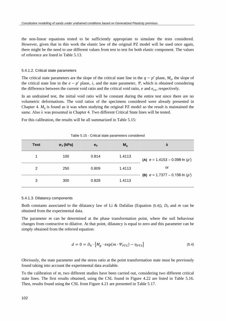
Constitutive modelling of sands under undrained conditions based on Generalized Plasticity premises
102
the non-linear equations tested to be sufficiently appropriate to simulate the tests considered.
However, given that in this work the elastic law of the original PZ model will be used once again,
there might be the need to use different values from test to test for both elastic component. The values
of reference are listed in Table 5.13.
5.4.1.2. Critical state parameters
The critical state parameters are the slope of the critical state line in the plane, Mg, the slope of
the critical state line in the plane, λ, and the state parameter, Ψ, which is obtained considering
the difference between the current void ratio and the critical void ratio, and , respectively.
In an undrained test, the initial void ratio will be constant during the entire test since there are no
volumetric deformations. The void ratios of the specimens considered were already presented in
Chapter 4. Mg is found as it was when studying the original PZ model so the result is maintained the
same. Also λ was presented in Chapter 4. Two different Critical State lines will be tested.
For this calibration, the results will be all summarized in Table 5.15:
Table 5.15 - Critical state parameters considered
Test σ3 (kPa) e0 Mg λ
1 100 0.814 1.4113 (A) e = 1.4153 – 0.098∙ln (p’)
or
(B) e = 1.7377 – 0.156∙ln (p’)
2 250 0.809 1.4113
3 300 0.828 1.4113
5.4.1.3. Dilatancy components
Both constants associated to the dilatancy law of Li & Dafalias (Equation (5.4)), D0 and m can be
obtained from the experimental data.
The parameter m can be determined at the phase transformation point, where the soil behaviour
changes from contractive to dilative. At that point, dilatancy is equal to zero and this parameter can be
simply obtained from the referred equation:
[ ( ) ] (5.4)
Obviously, the state parameter and the stress ratio at the point transformation state must be previously
found taking into account the experimental data available.
To the calibration of m, two different studies have been carried out, considering two different critical
state lines. The first results obtained, using the CSL found in Figure 4.22 are listed in Table 5.16.
Then, results found using the CSL from Figure 4.21 are presented in Table 5.17.

Constitutive modelling of sands under undrained conditions based on Generalized Plasticity premises
103
Table 5.16 - Calibration of m using CSL (A), from Fig. 4.22
Test p’PTP
(kPa)
qPTP
(kPa) ηPTP ePTP ΨPTP m
100 kPa 85.92 74.24 0.864 0.979 -0.165 2.975
250 kPa 205.03 132.51 0.646 0.894 -0.085 9.229
300 kPa 236.77 210.98 0.891 0.880 -0.052 8.924
Table 5.17 - Calibration of m using CSL (B), from Fig. 4.21
Test p’PTP
(kPa)
qPTP
(kPa) ηPTP ePTP ΨPTP m
100 kPa 85.92 74.24 0.864 1.043 -0.229 2.142
250 kPa 205.03 132.51 0.646 0.907 -0.098 7.947
300 kPa 236.77 210.98 0.891 0.885 -0.057 8.091
In triaxial tests performed under undrained conditions, the Phase Transformation Point corresponds to
the point where the principal effective stress is minimum. The deviatoric stress and the void
ratio , returned by the CSL equation, are subsequently obtained. Then, the state parameter is
calculated and the values of m found.
As observed, m varies between 2,975 and 9,229 or between 2,142 and 8,091, which is a quite large
range and may be an additional difficulty when choosing a final value that should be able to represent
all the tests considered. The consideration of two different CSL for this study does not permit, at the
moment, any relevant conclusion. However, it may be important when calibrating D0.
In previous works, mainly dealing with drained triaxial tests, the calibration of D0 was performed by
fitting the curve, a procedure impossible to apply in this work since the tests are undrained and
the volumetric strains null. In order to surpass this problem, the method proposed by Diego Manzanal
for his own model was adopted.
Manzanal considered that d0 is determined supposing that the elastic deformations are small and
negligible which means that the total strains are equal to the plastic ones, when dealing with drained
tests:
(5.5)

Constitutive modelling of sands under undrained conditions based on Generalized Plasticity premises
104
In this work, this procedure will be maintained, considering that the dilatancy law can be expressed as:
[ ( ) ] (5.6)
d0 ends up being calibrated through the method of least squares, with a fitting operation of the
experimental curve and the model curve . Being the residual the difference
between the experimental data and the fitted value provided by the model, the best fit through the least
squares method will minimize the sum of squared residuals.
Different approaches have been tried. The method was used individually for each triaxial test of the
S5-C6 set of specimens. However, the two Critical State Lines, (A) and (B), considered so far have
been tested along with the two different dilatancy laws taken into account in Chapter 4, one
considering the bulk and shear modulus constant and other considering the tangent bulk and shear
modulus, as presented in Figures 4.27 and 4.28. So, put differently, the data provided by the model
was the object of four different fitting operations to the experimental data, firstly with reference to the
dilatancy law that takes into account the initial values of both elastic components, identified as
Dilatancy 1 in the graphs below, and then with reference to the dilatancy law that considers the tangent
values of both elastic components, identified as Dilatancy 2. For each one, the two CSL equations
were tested.
The results found here are presented in Figures 5.51 to 5.56. The values obtained for d0 are listed
below, in Tables 5.18, 5.19 and 5.20.
Fig. 5.51 - Least squares method for the 100 kPa test, considering Dilatancy 1
-0,6
-0,4
-0,2
0
0,2
0,4
0,6
0,8
1
0,0 5,0 10,0 15,0 20,0 25,0 30,0
Dia
ltan
cy,
dg
Axial deformation, εa (%)
CSL (A)
CSL (B)
Dilatancy 1
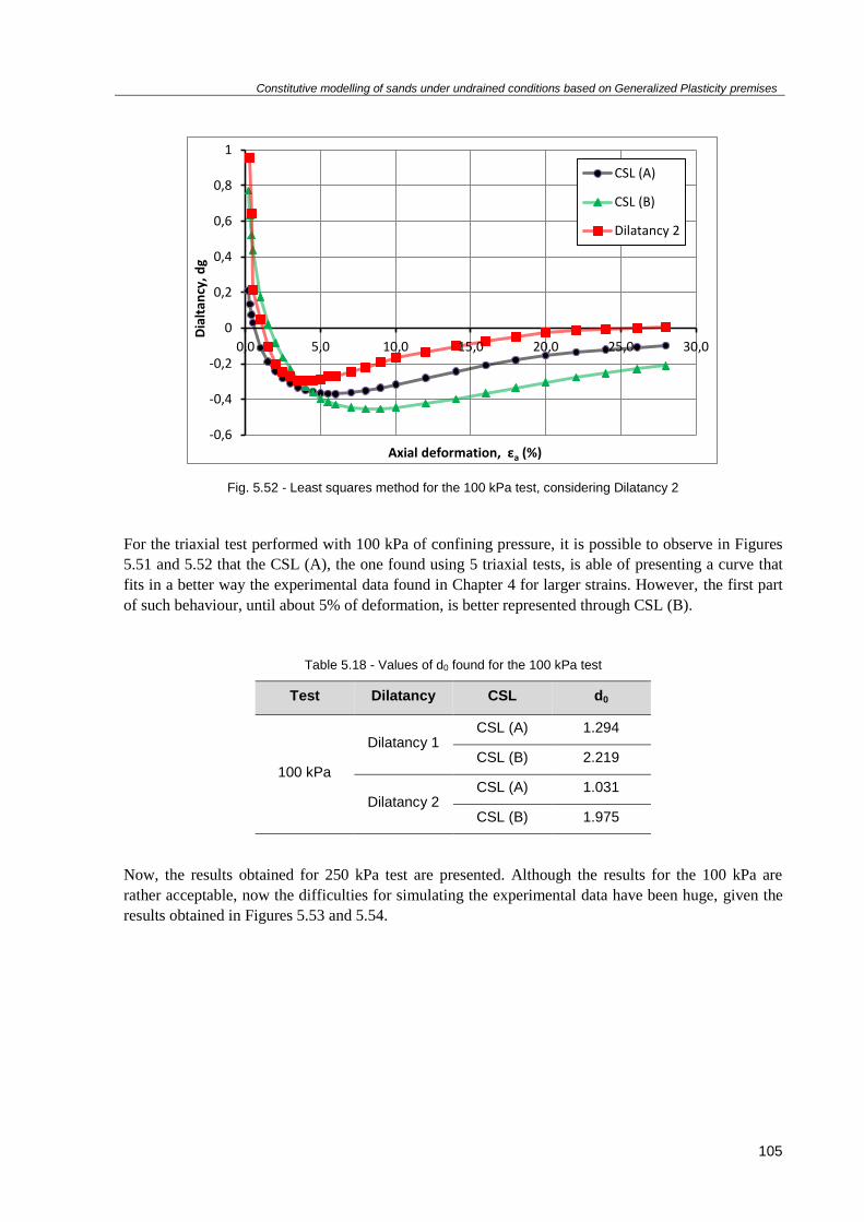
Constitutive modelling of sands under undrained conditions based on Generalized Plasticity premises
105
Fig. 5.52 - Least squares method for the 100 kPa test, considering Dilatancy 2
For the triaxial test performed with 100 kPa of confining pressure, it is possible to observe in Figures
5.51 and 5.52 that the CSL (A), the one found using 5 triaxial tests, is able of presenting a curve that
fits in a better way the experimental data found in Chapter 4 for larger strains. However, the first part
of such behaviour, until about 5% of deformation, is better represented through CSL (B).
Table 5.18 - Values of d0 found for the 100 kPa test
Test Dilatancy CSL d0
100 kPa
Dilatancy 1 CSL (A) 1.294
CSL (B) 2.219
Dilatancy 2 CSL (A) 1.031
CSL (B) 1.975
Now, the results obtained for 250 kPa test are presented. Although the results for the 100 kPa are
rather acceptable, now the difficulties for simulating the experimental data have been huge, given the
results obtained in Figures 5.53 and 5.54.
-0,6
-0,4
-0,2
0
0,2
0,4
0,6
0,8
1
0,0 5,0 10,0 15,0 20,0 25,0 30,0
Dia
ltan
cy,
dg
Axial deformation, εa (%)
CSL (A)
CSL (B)
Dilatancy 2

Constitutive modelling of sands under undrained conditions based on Generalized Plasticity premises
106
Fig. 5.53 - Least squares method for the 250 kPa test, considering Dilatancy 1
Even if the model equation is capable of capturing the shape of the dilatancy law obtained
experimentally, it cannot reproduce well its behaviour. The best results are obtained in Figure 5.54,
where the first 10% of the behaviour can be considered as acceptable. The use of the values obtained,
listed in Table 5.19, may lead to unsatisfactory results when calibrating all the components of the
model to the final simulation.
Fig. 5.54 - Least squares method for the 250 kPa test, considering Dilatancy 2
-0,8
-0,6
-0,4
-0,2
0
0,2
0,4
0,6
0,8
0,0 5,0 10,0 15,0 20,0 25,0 30,0
Dia
ltan
cy,
dg
Axial deformation, εa (%)
CSL (A)
CSL (B)
Dilatancy 1
-0,8
-0,6
-0,4
-0,2
0
0,2
0,4
0,6
0,8
0,0 5,0 10,0 15,0 20,0 25,0 30,0
Dia
ltan
cy,
dg
Axial deformation, εa (%)
CSL (A)
CSL (B)
Dilatancy 2

Constitutive modelling of sands under undrained conditions based on Generalized Plasticity premises
107
Table 5.19 - Values of d0 found for the 250 kPa test
Test Dilatancy CSL d0
250 kPa
Dilatancy 1 CSL (A) 0.289
CSL (B) 1.646
Dilatancy 2 CSL (A) 1.169
CSL (B) 1.643
Finally, the results for the 300 kPa test are now presented. Once again, the model is unable to simulate
the real behaviour of the material studied in terms of dilatancy, as evident in Figures 5.55 and 5.56.
The values obtained are listed in Table 5.20.
Table 5.20 - Values of d0 found for the 300 kPa test
Test Dilatancy CSL d0
300 kPa
Dilatancy 1 CSL (A) 0.885
CSL (B) 0.475
Dilatancy 2 CSL (A) 0.740
CSL (B) 1.407
Fig. 5.55 - Least squares method for the 300 kPa test, considering Dilatancy 1
-1,2
-0,9
-0,6
-0,3
0
0,3
0,6
0,9
1,2
0,0 5,0 10,0 15,0 20,0 25,0 30,0
Dia
ltan
cy,
dg
Axial deformation, εa (%)
CSL (A)
CSL (B)
Dilatancy 1

Constitutive modelling of sands under undrained conditions based on Generalized Plasticity premises
108
Fig. 5.56 - Least squares method for the 300 kPa test, considering Dilatancy 2
As regards parameter m, the small number of tests considered did not allow to explain its oscillations
and range of variation. Such difficulties may be related to its dependence on the state parameter Ψ, a
value calculated having as reference the CSL equations found earlier in this work whose results have
already been discussed in time. Manzanal et al. (2010) points out values for this parameter between 2
and 3,5, when studying Banding, Kurnell and Toyoura sands. However, Tonni et al. (2006) indicate
values from 0,05 to 1,2 when studying fine sands.
In what concerns d0, the problems caused by the lack of a better CSL may in fact be repeated for this
calibration procedure, with the aggravating factor of using for the m parameter values previously
affected by the same inaccurate CSL. Manzanal et al. (2010) indicates values varying between 0,6 and
0,9 while Tonni et al. (2006) refers to values of 0,5 to 1 when studying parameter D0.
5.4.1.4. Loading vector parameters
It has been seen that, according to the original PZ model, the model parameter Mf can be found by
taking into account the initial relative density of the soil Dr. As a consequence, different values of Mf
may be considered when studying a single sand at different initial void ratios (Laura Tonni et al.,
2008). The following expression has been proposed in order to overcome this limitation, trying to
express Mf as a function of the critical state line slope Mg and of the current material internal state, the
latter being defined in terms of the current void ratio e:
( ) [ (
) ] (5.7)
Equation 5.7 requires the void ratio to be less than one. In this work, such condition is respected.
However, the calibration of such parameter is still related to the relative density of the material. Due to
-0,15
-0,1
-0,05
0
0,05
0,1
0,15
0,2
0,0 5,0 10,0 15,0 20,0 25,0 30,0Dia
ltan
cy,
dg
Axial deformation, εa (%)
CSL (A)
CSL (B)
Dilatancy 2

Constitutive modelling of sands under undrained conditions based on Generalized Plasticity premises
109
the lack of a specific test particularly useful for the definition of cf, it seemed to be convenient to look
at the initial value of Mf as:
[
( )] (5.8)
which may be preliminary estimated by using the procedure proposed by Pastor for the original PZ
model. Then, cf is easily calculated. As when Mf was calculated for the original model, a relative
density Dr of 60% will be considered again. Such procedure resulted in the data listed in Table 5.20:
Table 5.21 - Values obtained for cf
Test cf
100 kPa 0.131
250 kPa 0.134
300 kPa 0.129
These results show a short range of variation and a value of about 0,13 will be certainly a good choice.
Tonni et al. (2008) adopts values equal to 0,1 for every test carried out.
It may be important to note that this parameter was not presented in Chapter 3 because it was not part
of the first modified model proposed by the authors, being introduced in later works.
5.4.1.5. Plastic modulus law
Instead of being estimated by fitting experimental results, H0 should be now more reliably calculated,
according to Equation (3.66) from Chapter 3, since here it is not considered a constant anymore and is
dependent on the state parameter, for example. However, there are two parameters that, in this work,
may lack a more sensitive calibration study.
The first of them is the apparent grain crushing pressure σx. As explained, it corresponds to a
discontinuity of the CSL slope in the ( ) space. Previous studies in other granular soils, namely
the ones in Venice soils, show that this parameter may vary between 700 to 1200 kPa. Since there are
no sufficient experimental data in the context of this work to find a reliable value for this parameter,
all the study will continue assuming this value equal to 1000 kPa.
Also kc is a parameter that can be calibrated in a more accurate way. However, it is usually adopted as
equal to 0,3 in other studies and that will also be the value assumed for this calibration study.
The component responsible for failure, Hf, includes the idea that, during the distortional process, sand
is moving towards to achieve the current peak stress ratio, according to Equation (3.68). The model

Constitutive modelling of sands under undrained conditions based on Generalized Plasticity premises
110
parameter nf has been studied when dealing with drained tests, its calibration being performed at the
drained peak stress state, where Hf becomes equal to zero:
(
) (5.9)
where ηp and Ψp are the values of the stress ratio and state parameter at the drained peak stress state,
determined from the experimental data. Although this work deals with undrained tests, this parameter
will be calibrated also for the point where the stress ratio is maximum. The results are presented
in the following tables, 5.22 and 5.23, since both CSL selected were considered once again:
Table 5.22 - nf calibration for the point where stress state is maximum for CSL (A)
Test p’ η MAX
(kPa)
q η MAX
(kPa) η η MAX e η MAX Ψ η MAX nf
100 kPa 265.68 408.18 1.536 0.867 -0.053 1.672
250 kPa 633.08 863.89 1.365 0.731 0.026 0.389
300 kPa 659.56 936.28 1.420 0.725 0.049 -0.090
Table 5.23 - nf calibration for the point where stress state is maximum for CSL (B)
Test p’η MAX
(kPa)
q η MAX
(kPa) η η MAX e η MAX Ψ η MAX nf
100 kPa 265.68 408.18 1.536 0.868 -0.054 1.630
250 kPa 633.08 863.89 1.365 0.783 0.026 1.167
300 kPa 659.56 936.28 1.420 0.779 0.049 -0.191
The triaxial tests relative to 250 and 300 kPa of confining pressure may represent here useless results.
As known, all the tests refer to dense sands and should always present a negative value for the state
parameter Ψ. In Manzanal et al. (2010), values between 0,9 and 1,8 are adopted. Tonni et al. (2008)
indicates a range of variation between 0,35 to 1.
In what concerns the Hs component, which has the role of controlling the way how plastic stiffness
decreases making it smoother or sharper, the exponent β is calibrated by fitting the curve.

Constitutive modelling of sands under undrained conditions based on Generalized Plasticity premises
111
5.4.2. FINAL CALIBRATION AND RESULTS
The final calibration was performed for each test individually. The parameters used are listed in Table
5.24. The results are presented in Figures 5.57 to 5.65.
Table 5.24 - Model parameters from calibration of Tonni model
Parameters 100 kPa 250 kPa 300 kPa
K0 (kPa) 10500 15000 23500
G0 (kPa) 9500 13500 22500
n 0.4 0.4 0.3
Mg 1.41 1.41 1.41
αf 0.45 0.45 0.45
m 2.1 8.1 8.1
d0 0.2 0.11 0.11
cf 0.13 0.13 0.13
nf 0.4 0.25 0.17
β 1 1 1
σx 1000 1000 1000
kc 0.3 0.3 0.3
It is worth noting that, for some of the parameters considered, were adopted values out of range of
variation found during the studies performed in subsection 5.4.3., especially when the results were not
satisfactory at all. The new values were found with reference to the works of Diego Manzanal and
Laura Tonni, where other ranges of variation for some of the parameters have been discussed.
Also, although the final achievement would be finding a unique set of parameters capable of
reproducing the behaviour of the material over a wide range of confining pressures and densities, some
different values had to be chosen during the final calibration of the model, especially in both elastic
components. This probably happens due to the fact of using the same elastic law as the one present in
the original PZ model.

Constitutive modelling of sands under undrained conditions based on Generalized Plasticity premises
112
Fig. 5.57 - Prediction in the space for the 100 kPa test
Fig. 5.58 - Prediction in the space for the 100 kPa test
0
100
200
300
400
500
600
700
800
900
0 100 200 300 400 500 600
De
viat
ori
c st
ress
, q [
kPa]
Mean effective stress, p' [kPa]
LAB S5-C6 100 kPa
TEST S5-C6 100 kPa
0
100
200
300
400
500
600
700
800
900
0,0 5,0 10,0 15,0 20,0 25,0 30,0 35,0
De
viat
ori
c st
ress
, q [
kPa]
Axial deformation, εa (%)
LAB S5-C6 100 kPa
TEST S5-C6 100 kPa

Constitutive modelling of sands under undrained conditions based on Generalized Plasticity premises
113
Fig. 5.59 - Prediction in the space for the 100 kPa test
In what concerns the model predictions for the 100 kPa of confining pressure test (Figures 5.57 to
5.59), the model simulations can match quite well the experimental data for pre-peak deformations, up
to about 17%. However, in the post-peak regime, the model is unable to introduce a softening rate that
could actually fit properly the experimental data considered. Also, the initial part of the behaviour is
overestimated by the model predictions since it does not reproduce the initial instability verified.
Fig. 5.60 - Prediction in the space for the 250 kPa test
-150
-100
-50
0
50
100
0,0 5,0 10,0 15,0 20,0 25,0 30,0 35,0
Po
re p
ress
ure
, u [
kPa]
Axial deformation, εa (%)
LAB S5-C6 100 kPa
TEST S5-C6 100 kPa
0
200
400
600
800
1000
1200
1400
1600
1800
0 200 400 600 800 1000 1200
De
viat
ori
c st
ress
, q [
kPa]
Mean effective stress, p' [kPa]
LAB S5-C6 250 kPa
TEST S5-C6 250 kPa

Constitutive modelling of sands under undrained conditions based on Generalized Plasticity premises
114
Fig. 5.61 - Prediction in the space for the 250 kPa test
Fig. 5.62 - Prediction in the space for the 100 kPa test
For the 250 kPa test, the comments previously made about the 100 kPa can be repeated. The model,
once again, is capable of reproducing with some accuracy the first 17-18% of behaviour, where the
pre-peak regime is dominant. After that, the model cannot introduce the softening behaviour, observed
in the experimental data, in its predictions.
0
200
400
600
800
1000
1200
1400
1600
1800
0,0 5,0 10,0 15,0 20,0 25,0 30,0 35,0
De
viat
ori
c st
ress
, q [
kPa]
Axial deformation, εa (%)
LAB S5-C6 250 kPa
TEST S5-C6 250 kPa
-350
-300
-250
-200
-150
-100
-50
0
50
100
150
0,0 5,0 10,0 15,0 20,0 25,0 30,0 35,0
Po
re p
ress
ure
, u [
kPa]
Axial deformation, εa (%)
LAB S5-C6 250 kPa
TEST S5-C6 250 kPa

Constitutive modelling of sands under undrained conditions based on Generalized Plasticity premises
115
Fig. 5.63 - Prediction in the space for the 300 kPa test
Fig. 5.64 - Prediction in the space for the 300 kPa test
0
200
400
600
800
1000
1200
1400
1600
1800
0 200 400 600 800 1000 1200 1400 1600 1800
De
viat
ori
c st
ress
, q [
kPa]
Mean effective stress, p' [kPa]
LAB S5-C6 300 kPa
TEST S5-C6 300 kPa
0
200
400
600
800
1000
1200
1400
1600
1800
0,0 5,0 10,0 15,0 20,0 25,0 30,0 35,0
De
viat
ori
c st
ress
, q [
kPa]
Axial deformation, εa (%)
LAB S5-C6 300 kPa
TEST S5-C6 300 kPa

Constitutive modelling of sands under undrained conditions based on Generalized Plasticity premises
116
Fig. 5.65 - Prediction in the space for the 300 kPa test
The test of 300 kPa of confining pressure is the one that was worst simulated by the model equations.
Still, the model difficulties pointed out above are evident once again, as expected.
-600
-500
-400
-300
-200
-100
0
100
200
0,0 5,0 10,0 15,0 20,0 25,0 30,0 35,0
Po
re p
ress
ure
, u [
kPa]
Axial deformation, εa (%)
LAB S5-C6 300 kPa
TEST S5-C6 300 kPa

Constitutive modelling of sands under undrained conditions based on Generalized Plasticity premises
117
5.5. MODIFIED MODEL OF MANZANAL (2008)
5.5.1. MODEL PARAMETERS AND THEIR CALIBRATION
In Table 5.25, every parameter present in this model and its description is listed. After that, the
calibration procedure will be presented and detailed.
Table 5.25 - Model parameters of the modified model of Diego Manzanal
Parameters Description
Keso Bulk modulus (kPa)
Gevo Shear modulus (kPa)
Mg Slope of Critical State Line in the space
λ Slope of Critical State Line in the ( ) space
Ψ State parameter
e Void ratio
ec Critical void ratio
d0 Material parameter of the plastic flow law
md Material parameter of the plastic flow law
H’0 Model parameter of the plastic modulus law
β’0 Model parameter of the plastic modulus law
β Model parameter of the plastic modulus law
Hv0 Model parameter of the plastic modulus law
βv Model parameter of the plastic modulus law
5.5.1.1. Elastic components
The elastic constants of this model are determined from laboratory tests. The shear modulus Geso can
be found by fitting the initial slope in the space or through resonant column or bender tests.
Once again, the Poisson’s ratio is related to Kevo through the Equation (3.84). It can be adjusted in
isotropic compression test or by fitting the initial slope in the space, in triaxial tests performed
under drained conditions. The reference values for the final calibration are, again, those which have
been appointed for the calibration of the original PZ model.
Due to difficulties related with the correct functioning of the Driver PD, the expression proposed could
not be used. Once again, the elastic laws of the original PZ model were used.
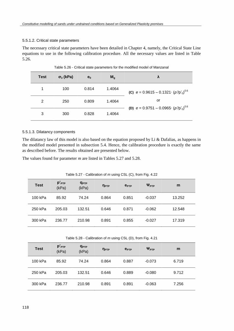
Constitutive modelling of sands under undrained conditions based on Generalized Plasticity premises
118
5.5.1.2. Critical state parameters
The necessary critical state parameters have been detailed in Chapter 4, namely, the Critical State Line
equations to use in the following calibration procedure. All the necessary values are listed in Table
5.26.
Table 5.26 - Critical state parameters for the modified model of Manzanal
Test σ3 (kPa) e0 Mg λ
1 100 0.814 1.4064 (C) e = 0.9615 – 0.1321∙ (p’/p’0)
0.6
or
(D) e = 0.9751 – 0.0965∙ (p’/p’0)0.6
2 250 0.809 1.4064
3 300 0.828 1.4064
5.5.1.3. Dilatancy components
The dilatancy law of this model is also based on the equation proposed by Li & Dafalias, as happens in
the modified model presented in subsection 5.4. Hence, the calibration procedure is exactly the same
as described before. The results obtained are presented below.
The values found for parameter m are listed in Tables 5.27 and 5.28.
Table 5.27 - Calibration of m using CSL (C), from Fig. 4.22
Test p’PTP
(kPa)
qPTP
(kPa) ηPTP ePTP ΨPTP m
100 kPa 85.92 74.24 0.864 0.851 -0.037 13.252
250 kPa 205.03 132.51 0.646 0.871 -0.062 12.548
300 kPa 236.77 210.98 0.891 0.855 -0.027 17.319
Table 5.28 - Calibration of m using CSL (D), from Fig. 4.21
Test p’PTP
(kPa)
qPTP
(kPa) ηPTP ePTP ΨPTP m
100 kPa 85.92 74.24 0.864 0.887 -0.073 6.719
250 kPa 205.03 132.51 0.646 0.889 -0.080 9.712
300 kPa 236.77 210.98 0.891 0.891 -0.063 7.256

Constitutive modelling of sands under undrained conditions based on Generalized Plasticity premises
119
In its turn, the calibration of d0, performed through a fitting operating using the least squares method,
turned out the following results:
Fig. 5.66 - Least squares method for the 100 kPa test, considering Dilatancy 1
Fig. 5.67 - Least squares method for the 100 kPa test, considering Dilatancy 2
-1
-0,5
0
0,5
1
1,5
2
2,5
3
3,5
0,0 5,0 10,0 15,0 20,0 25,0 30,0
Dia
ltan
cy,
dg
Axial deformation, εa (%)
CSL (C)
CSL (D)
Dilatancy 1
-0,6
-0,4
-0,2
0
0,2
0,4
0,6
0,8
1
1,2
0,0 5,0 10,0 15,0 20,0 25,0 30,0
Dia
ltan
cy,
dg
Axial deformation, εa (%)
CSL (C)
CSL (D)
Dilatancy 2

Constitutive modelling of sands under undrained conditions based on Generalized Plasticity premises
120
Table 5.29 - Values of d0 found for the 100 kPa test
Test Dilatancy CSL d0
100 kPa
Dilatancy 1 CSL (C) 0.777
CSL (D) 2.051
Dilatancy 2 CSL (C) 0.048
CSL (D) 1.849
Fig. 5.68 - Least squares method for the 250 kPa test, considering Dilatancy 1
Fig. 5.69 - Least squares method for the 250 kPa test, considering Dilatancy 2
-0,6
-0,4
-0,2
0
0,2
0,4
0,6
0,8
1
0,0 5,0 10,0 15,0 20,0 25,0 30,0
Dia
ltan
cy,
dg
Axial deformation, εa (%)
CSL (C)
CSL (D)
Dilatancy 1
-0,6
-0,4
-0,2
0
0,2
0,4
0,6
0,8
1
1,2
0,00 5,00 10,00 15,00 20,00 25,00 30,00
Dia
ltan
cy,
dg
Axial deformation, εa (%)
CSL (C)
CSL (D)
Dilatancy 2

Constitutive modelling of sands under undrained conditions based on Generalized Plasticity premises
121
Table 5.30 - Values of d0 found for the 250 kPa test
Test Dilatancy CSL d0
250 kPa
Dilatancy 1 CSL (C) 0.351
CSL (D) 2.433
Dilatancy 2 CSL (C) 0.368
CSL (D) 2.221
Fig. 5.70 - Least squares method for the 300 kPa test, considering Dilatancy 1
Fig. 5.71 - Least squares method for the 300 kPa test, considering Dilatancy 1
-1
-0,5
0
0,5
1
1,5
2
2,5
3
0,0 5,0 10,0 15,0 20,0 25,0 30,0 35,0
Dia
ltan
cy,
dg
Axial deformation, εa (%)
CSL (C)
CSL (D)
Dilatancy 1
-1
-0,5
0
0,5
1
1,5
0,0 5,0 10,0 15,0 20,0 25,0 30,0 35,0Dia
ltan
cy,
dg
Axial deformation, εa (%)
CSL (C)
CSL (D)
Dilatancy 2

Constitutive modelling of sands under undrained conditions based on Generalized Plasticity premises
122
Table 5.31 - Values of d0 found for the 300 kPa test
Test Dilatancy CSL d0
300 kPa
Dilatancy 1 CSL (C) 0.114
CSL (D) 3.474
Dilatancy 2 CSL (C) 0.178
CSL (D) 4.360
As expected, the values using CSL (D) are more accurate when trying to fit the experimental data.
5.5.1.4. Loading vector parameters
The method described in subsection 3.5.3 to obtain parameter Mf will not be used in this work. The
calibration method proposed by Manzanal for h1 and h2 is impossible to use in the context of this
thesis, taking into account the experimental data considered.
Instead, considering once a relative density of 60%, Mf will be calculated through the expression
.
5.5.1.5. Plastic modulus law
The parameter βv is calculated also for the point where the stress ratio is maximum, as the
parameter nf in Tonni model.
(
) (5.10)
The results are listed below, in Tables 5.32 and 5.33.
Table 5.32 - calibration for the point where stress state is maximum for CSL (C)
Test p’ η MAX
(kPa)
q η MAX
(kPa) η η MAX e η MAX Ψ η MAX
100 kPa 265.68 408.18 1.536 0.724 0.090 -0.945
250 kPa 633.08 863.89 1.365 0.905 -0.096 -0.352
300 kPa 659.56 936.28 1.420 0.75 0.078 -0.074
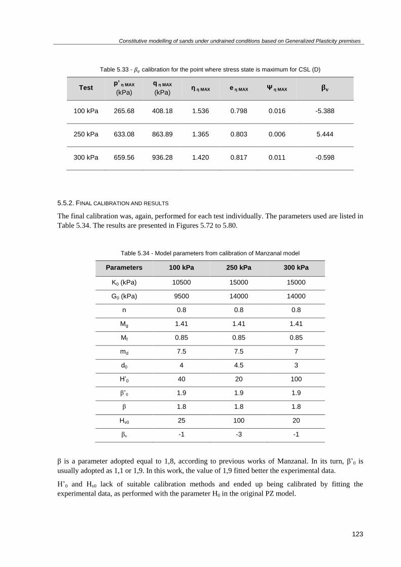
Constitutive modelling of sands under undrained conditions based on Generalized Plasticity premises
123
Table 5.33 - calibration for the point where stress state is maximum for CSL (D)
Test p’ η MAX
(kPa)
q η MAX
(kPa) η η MAX e η MAX Ψ η MAX
100 kPa 265.68 408.18 1.536 0.798 0.016 -5.388
250 kPa 633.08 863.89 1.365 0.803 0.006 5.444
300 kPa 659.56 936.28 1.420 0.817 0.011 -0.598
5.5.2. FINAL CALIBRATION AND RESULTS
The final calibration was, again, performed for each test individually. The parameters used are listed in
Table 5.34. The results are presented in Figures 5.72 to 5.80.
Table 5.34 - Model parameters from calibration of Manzanal model
Parameters 100 kPa 250 kPa 300 kPa
K0 (kPa) 10500 15000 15000
G0 (kPa) 9500 14000 14000
n 0.8 0.8 0.8
Mg 1.41 1.41 1.41
Mf 0.85 0.85 0.85
md 7.5 7.5 7
d0 4 4.5 3
H’0 40 20 100
β’0 1.9 1.9 1.9
β 1.8 1.8 1.8
Hv0 25 100 20
βv -1 -3 -1
β is a parameter adopted equal to 1,8, according to previous works of Manzanal. In its turn, β’0 is
usually adopted as 1,1 or 1,9. In this work, the value of 1,9 fitted better the experimental data.
H’0 and Hv0 lack of suitable calibration methods and ended up being calibrated by fitting the
experimental data, as performed with the parameter H0 in the original PZ model.
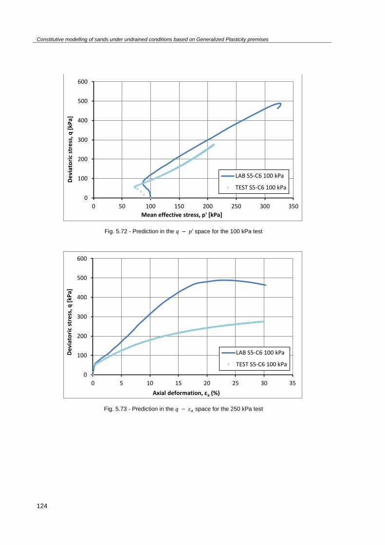
Constitutive modelling of sands under undrained conditions based on Generalized Plasticity premises
124
Fig. 5.72 - Prediction in the space for the 100 kPa test
Fig. 5.73 - Prediction in the space for the 250 kPa test
0
100
200
300
400
500
600
0 50 100 150 200 250 300 350
De
viat
ori
c st
ress
, q [
kPa]
Mean effective stress, p' [kPa]
LAB S5-C6 100 kPa
TEST S5-C6 100 kPa
0
100
200
300
400
500
600
0 5 10 15 20 25 30 35
De
viat
ori
c st
ress
, q [
kPa]
Axial deformation, εa (%)
LAB S5-C6 100 kPa
TEST S5-C6 100 kPa

Constitutive modelling of sands under undrained conditions based on Generalized Plasticity premises
125
Fig. 5.74 - Prediction in the space for the 300 kPa test
From Figures 5.72 to 5.74, the predictions for the 100 kPa test are presented. It is relevant to point out
that this model, as opposite to the one tested before, is able to introduce a softening rate in its
behaviour. However, the results obtained are difficult to accept with optimism since they do not
capture with exactitude the behaviour of the specimens considered.
From Figures 5.75 to 5.77, the results for the 250 kPa test are presented.
Fig. 5.75 - Prediction in the space for the 250 kPa test
-80
-60
-40
-20
0
20
40
60
0 5 10 15 20 25 30 35
Po
re p
ress
ure
, u [
kPa]
Axial deformation, εa (%)
LAB S5-C6 100 kPa
TEST S5-C6 100 kPa
0
100
200
300
400
500
600
700
800
900
1000
0 200 400 600 800
De
viat
ori
c st
ress
, q [
kPa]
Mean effective stress, p' [kPa]
LAB S5-C6 250 kPa
TEST S5-C6 250 kPa

Constitutive modelling of sands under undrained conditions based on Generalized Plasticity premises
126
Fig. 5.76 - Prediction in the space for the 250 kPa test
Comparing to the previous test, the agreement between the predictions and the experimental data is
fairly better. The first 10% of the pore pressure curve are represented with accuracy. The biggest issue
remains the lack of precision of the model when plotting the deviatoric stress versus the axial
deformation.
Fig. 5.77 - Prediction in the space for the 250 kPa test
0
100
200
300
400
500
600
700
800
900
1000
0 5 10 15 20 25 30 35
De
viat
ori
c st
ress
, q [
kPa]
Axial deformation, εa (%)
LAB S5-C6 250 kPa
TEST S5-C6 250 kPa
-200
-150
-100
-50
0
50
100
150
0 5 10 15 20 25 30 35
Po
re p
ress
ure
, u [
kPa]
Axial deformation, εa (%)
LAB S5-C6 250 kPa
TEST S5-C6 250 kPa
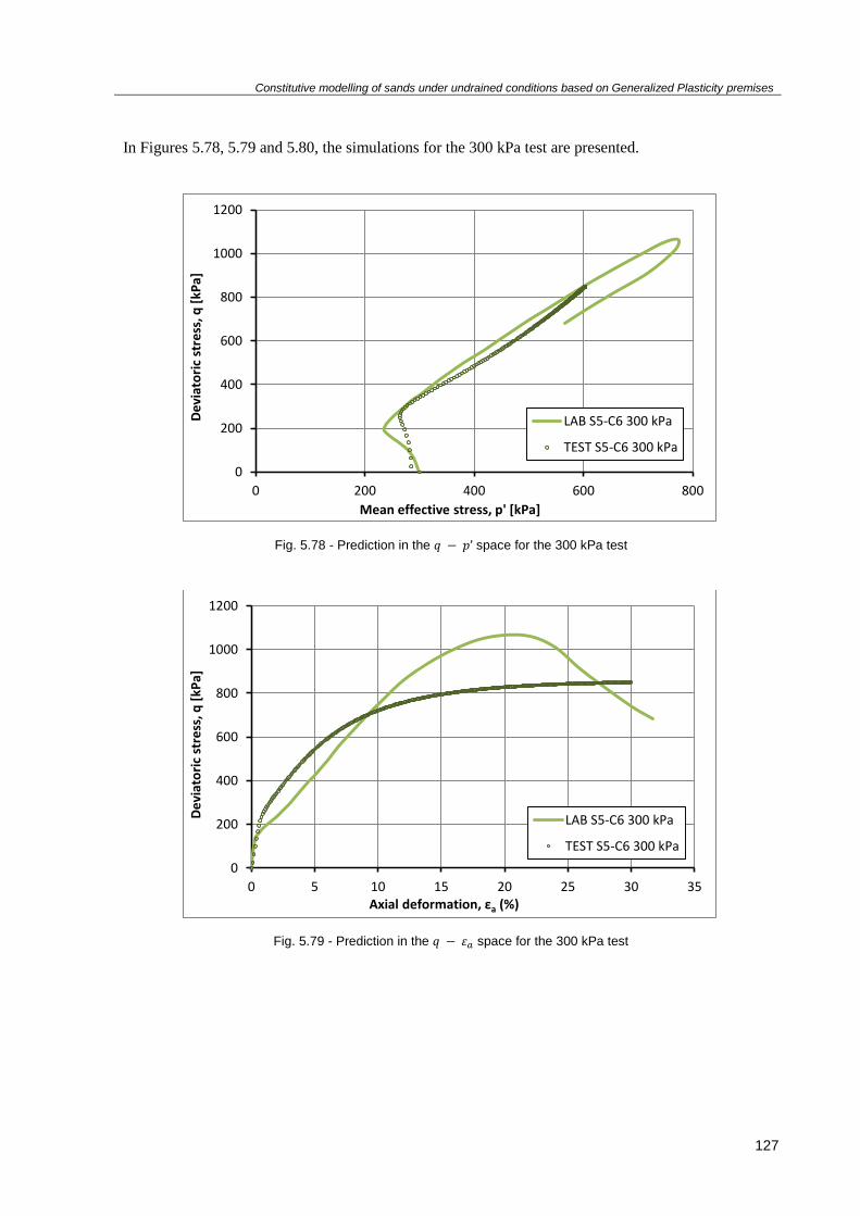
Constitutive modelling of sands under undrained conditions based on Generalized Plasticity premises
127
In Figures 5.78, 5.79 and 5.80, the simulations for the 300 kPa test are presented.
Fig. 5.78 - Prediction in the space for the 300 kPa test
Fig. 5.79 - Prediction in the space for the 300 kPa test
0
200
400
600
800
1000
1200
0 200 400 600 800
De
viat
ori
c st
ress
, q [
kPa]
Mean effective stress, p' [kPa]
LAB S5-C6 300 kPa
TEST S5-C6 300 kPa
0
200
400
600
800
1000
1200
0 5 10 15 20 25 30 35
De
viat
ori
c st
ress
, q [
kPa]
Axial deformation, εa (%)
LAB S5-C6 300 kPa
TEST S5-C6 300 kPa

Constitutive modelling of sands under undrained conditions based on Generalized Plasticity premises
128
Fig. 5.80 - Prediction in the space for the 300 kPa test
In general terms, the model could not capture properly the phase transformation points in the three
tests. It also failed at capturing the strength peak values of the experimental data. One of the biggest
achievements, when compared to the model of Cola and Tonni, is the capability of introducing a
softening behaviour at some point, fitting better the experimental data in a certain way. This is
probably related to the different plastic modulus law in use.
-150
-100
-50
0
50
100
150
0 5 10 15 20 25 30 35
Po
re p
ress
ure
, u [
kPa]
Axial deformation, εa (%)
LAB S5-C6 300 kPa
TEST S5-C6 300 kPa
Constitutive modelling of sands under undrained conditions based on Generalized Plasticity premises
129
6
CONCLUSIONS
6.1. CONCLUSIONS
Although admittedly the models predictions, in some cases, do not adequately capture the behaviour of
the sands subjected to undrained triaxial tests, the original objectives of the work proposed have been
eventually met.
In the beginning, the undrained triaxial tests from Scortichino sand have been properly studied. The
different analyses carried out, namely the ones related to the critical state of the material and to the
dilatancy law, permitted to characterize as best as possible the mechanical response of those materials.
It is recognizable that the use of so few tests turned up as one of the major shortcomings of this work
since it was not possible to properly capture the critical state of the material studied and the
opportunity of finding a reasonable Critical State Line has been lost.
Subsequently, the capability of the original PZ model under undrained conditions was studied. The
main difficulties of the model were pointed out but it is also recognizable that the original PZ model
presents itself as a good basis for the study of sand behaviour. Proceeding from this point, the
modified models have been studied. By integrating in their equations the concepts of the state
parameter and critical state, they proved themselves to be more capable of reproducing properly the
experimental data considered at the beginning of the work here presented. Once again, using so few
tests caused the loss of capacity in understanding in a more proper way if the methods pointed out for
the calibration of the different model parameters are reasonable since the comparison, in most cases,
of three values showed up as inconclusive. It should be noted again that the model of Cola & Tonni
had only been studied for triaxial tests performed under drained conditions, a fact that turns the
previous conclusions as even more important.
However, the improvements achieved with the modified models are relevant and the introduction of
the concepts of critical state revealed to be important to this kind of works.
6.2. FUTURE DEVELOPMENTS
In what concerns the experimental data, it was evident how the lack of a better critical state line has
influenced negatively the results obtained. This fact leads to an obvious conclusion: the quantity (but
also the quality) of the experimental results is very important when dealing with a study like the one
presented here, mostly focused on a constitutive approach validation.

Constitutive modelling of sands under undrained conditions based on Generalized Plasticity premises
130
So, in order to develop in a better way the themes covered here, it would be important to perform more
drained and undrained triaxial tests, creating an experimental database as wide as possible before
introducing more changes or adjustments to the model equations or parameters.
Related to the model itself, the search for more suitable expressions for the loading vector or the
plastic modulus may be one point of much interest to focus on the near future. Also, a continuing
search for a model that would combine better the Generalized Plasticity theory with the Critical State
framework is certainly a challenging objective.
Another important remark would be the integration of Generalized Plasticity constitutive equations
within finite element models.

Constitutive modelling of sands under undrained conditions based on Generalized Plasticity premises
131
REFERENCES
Bardet, J. P. (1997). Experimental Soil Mechanics. Prentice-Hall, Inc., Upper Saddle River, New
Jersey.
Been, K., Jefferies, M. (1985). A state parameter for sand. Géotechnique, 35(2), 99-112.
Been, K., Jefferies, M., Hachey, J. (1991). The critical state of sand. Géotechnique, 41(3), 365-381.
Been, K., Jefferies, M. (2006). Soil Liquefaction – A critical state approach. Taylor & Francis, New
York.
Castro, G. (1969). Liquefaction of Sand. PhD Thesis, Division of Engineering and Applied Physics,
Harvard University.
Ceccato, F. (2009). Modellazione costitutiva dei terreni di Venezia con la Plascitità Generalizzata.
Master Thesis, Facoltà di Ingegneria Università degli Studi di Padova.
Cola, S., Pastor. M and Tonni, L. (2008). Mathematical Modelling of Venetian Sediment Behaviour
Using Generalized Plasticity. International Association for Computer Methods and Advances in
Geomechanics (IACMAG), 1-6 October 2008, Goa, India.
Cola, S., Tonni, L. (2007). Adapting a Generalized Plasticity model to reproduce the stress-strain
response of silty soils forming the Venice lagoon basin. Soil Stress-Strain Behavior: Measurement,
Modeling and Analysis – Geotechnical Symposium in Roma, March 16 & 17, 2006, 743-758,
Springer, Netherlands.
Crespellani, T., Facciorusso, J. (2010). Dinamica dei Terreni – Per le Applicazioni Sismiche. Dario
Flaccovio Editore, Palermo.
Frossard, E. (1983). Une equation d’ecoulement simple pour les materiaux granulaires. Géotechnique,
33(1), 21-29.
Nova, R., Wood, D. M. (1979). A constitutive model for sand in triaxial compression. International
Journal for Numerical and Analytical Methods in Geomechanics. 3, 255-278.
Gottardi, G. (2013). Analisi di Stabilità di un Argine danneggiato dalla sequenza sismica Emiliana del
2012. Bologna.
Gottardi. G, Tonni, L. (2013). Attività del Gruppo di Lavoro AGI per lo studio del comportamento e
per la messa in sicurezza degli argini. Geotecnica Sismica – Corso di Formazione Professionale.
DICAM, Università di Bologna.
Ishihara, K., Tatsuoka, F. and Yasuda, S. (1975). Undrained Deformation and Liquefaction of Sand
Under Cyclic Stresses. Soil and Foundation, 15(1), 29-44.
Ishihara, K. (1993). Liquefaction and Flow Failure During Earthquakes. Géotechnique, 43(3), 351-
415.
Jefferies, M., Been, K. (2000). Implication for critical state from isotropic compression of sand.
Géotechnique, 50(4), 419-429.
Kramer, S. (1996). Geotechnical Earthquake Engineering. Prentice Hall International Series, Upper
Saddle River, New Jersey.
Li, X.S. (1997). Modeling of Dilative Shear Failure. Journal of Geotechnical and Geoenvironmental
Engineering, 123(7), 609-616.

Constitutive modelling of sands under undrained conditions based on Generalized Plasticity premises
132
Li, X.S., Wang, Y. (1998). Linear representation of steady-state line for sand. Journal of Geotechnical
and Geoenvironmental Engineering, 124(12), 1215-1217.
Li, X.S., Dafalias, Y. (2000). Dilatancy for cohesionless soils. Géotechnique, 50(4), 449-460.
Ling H.I., Yang S. (2006). Unified Sand Model Based on the Critical State and Generalized Plasticity.
Journal of Engineering Mechanics, 132 (12), 1380-1391.
Luison, L. (2010). Implementation and Validation of advanced Constitutive Models for the Analysis of
Hydro-Thermo-Mechanical Interactions in Geo-Environmental Engineering Problems. PhD Thesis,
Facoltà di Ingegneria Università degli Studi di Padova.
Manzanal, D. (2008), Modelo Constitutivo basado en la Teoría de la Plasticidad Generalizada con la
Incorporación de Parámetros de Estado para Arenas Saturadas y No Saturadas. PhD Thesis, E. T. S.
de Ingenieros de Caminos, Canales y Puertos, Universidad Politécnica de Madrid.
Manzanal, D., Merodo, J. A. F., Pastor, M (2011). Generalized Plasticity state and parameter-based
model for saturated and unsaturated soils. Part 1: Saturated state. International Journal for Numerical
and Analytical Methods in Geomechanics, 2010, 1347-1362, John Wiley & Sons, Ltd.
Manzari, M., Dafalias, Y. (1997). A critical state two-surface plasticity model for sands.
Géotechnique, 47(2), 255-272.
Matos Fernandes, M. (2011a). Mecânica dos Solos – Conceitos e Princípios Fundamentais. FEUP
Edições, Porto.
Matos Fernandes, M. (2011b). Mecânica dos Solos – Introdução à Engenharia Geotécnica. FEUP
Edições, Porto.
Wood, D. M., Belkheir, K., Liu, D.F. (1994). Strain softening and state parameter for sand modeling.
Géotechnique, 44(2), 335-339.
Nova, R., Wood, D. M. (1979). A constitutive model for sand in triaxial compression. International
Journal for Numerical and Analytical Methods in Geomechanics. 3, 255-278.
Pastor, M., Zienkiewicz, C. C. and Leung, K.H. (1985). Simple Model for Transient Soil Loading in
Earthquake Analysis II: Non-Associative Models for Sands. International Journal for Numerical and
Analytical Methods in Geomechanics, 9, 477-498.
Pastor, M., Zienkiewicz, C. C. (1986). A Generalized Plasticity, Hierarchical Model for Sand under
Monotonic and Cyclic Loading. 2nd International Symposium on Numerical Models in
Geomechanics, Ghent, 131-149.
Pastor, M., Zienkiewicz, C.C., Chan, A.H.C. (1990). Generalized plasticity and the modelling of soil
behavior. International Journal for Numerical and Analytical Methods in Geomechanics, 14, 151-190.
Pestana, J.M., Whittle, A.J. (1995). Compression model of cohesionless soils. Géotechnique, 45(4),
611-631.
Poulos, S. J., Castro, G and France, J. (1988). Liquefaction Evaluation Procedure: Discussion, Journal
of Geotechnical Engineering, 114(2), 251-259.
Ramos, C. (2013). Modelling Sand Instability within the Framework of Critical State Soil Mechanics.
Masther Thesis, Faculdade de Engenharia da Universidade do Porto.
Constitutive modelling of sands under undrained conditions based on Generalized Plasticity premises
133
Reynolds, O. (1885). The dilating of media composed of rigid particles in contact. Philosophical
Magazine, 20, 469-481.
Richard, F.E., Hall, J.R., Woods, R.D. (1970). Vibration of soils and foundations. Prentice-Hall.
Robertson P.K., 2009. Interpretation of cone penetration tests — a unified approach. Canadian
Geotechnical Journal, 46(11), 1337 – 1355.
Rowe, P.W. (1962). The stress-dilatancy relation for static equilibrium of an assembly of particles in
contact. Proceeding of the Royal Society of London, Series A, 500-527.
Taylor, D.W. (1948). Fundamentals of soil mechanics. John Wiley & Sons, New York.
Tonni, L. (2002). Modellazione Numerica del Comportamento di Terreni Granulari con la Plasticità
Generalizzata. PhD Thesis, Politecnico di Torino.
Tonni, L., Cola, S., Pastor. M (2006). A Generalized Plasticity approach for describing the behaviour
of silty soils forming the Venetian lagoon basin. Numerical Methods in Geotechnical Engineering,
2006, 93-99, Taylor & Francis Group, London.
Verdugo, R. (1992). The critical state of sand: reply to discussion. Géotechnique, 42(4), 655-663.
Wang, Z., Dafalias, Y. Li, X. S., Makdisi, F. I. (2002). State Pressure Index for Modeling Sand
Behaviour. Journal of Geotechnical and Geoenvironmental Engineering, 128(6), 511-519.
Yu, M. (2006). Generalized Plasticity. Springer, Berlin.
Zienkiewicz, C. C., Mroz, Z. (1984). Generalized plasticity formulation and applications to
geomechanics. Mechanics of Engineering Materials, C.S. Desai and R.H. Gallagher (eds.), John Wiley
& Sons, 655-679.
Zienkiewicz, C.C., Pande, G.N (1977). Some Useful Forms of Isotropic Yield Surfaces for Soil and
Rock Mechanics. Finite Element in Geomechanics, G. Gudehus (ed.), 179-198.
Zienkiewicz, O.C. Chan, A.H.C., Pastor, M., Schrefler, B.A., Shiomi, T. (1999). Computational
Geomechanics. John Wiley & Sons.

Constitutive modelling of sands under undrained conditions based on Generalized Plasticity premises
134

Constitutive modelling of sands under undrained conditions based on Generalized Plasticity premises
135
APPENDIX A
A.1 EQUATIONS CONSIDERED IN THE MODEL FOR THE DRAINED TESTS
(
) (
) (
) {(
)
[
]} [
] (A.24)
[ ] (A.2)
( )
[ ] (A.3)
(
( ))
(A.4)

Constitutive modelling of sands under undrained conditions based on Generalized Plasticity premises
136
[
]
[
]
[ (
) ]
[ ( ) ]
{
[ (
)]} {
[ ( )]}
(A.5)
[ (
)]
(A.25)
[ ( )] (A.26)
( ) (A.27)
(A.28)
(A.29)
A.2 EQUATIONS CONSIDERED IN THE MODEL FOR THE UNDRAINED TESTS
{
( )
(
)
(A.30)
(
) (
) (A.12)

Constitutive modelling of sands under undrained conditions based on Generalized Plasticity premises
137
(
)
(
)
(A.13)
(
) (A.14)
(
) (
)
(
)
(A.15)
[
(
(
) (
)
(
)
)
]
(A.16)
(
) [(
) ((
) (
))] (A.17)
(
) ((
) (
)) (A.18)
(
) (A.19)
(
)
(A.20)