joana isabel marques avaliação da qualidade ecológica do ...garante por si só uma má qualidade...
TRANSCRIPT

Universidade de Aveiro 2010
Departamento de Biologia
Joana Isabel Marques dos Santos
Avaliação da qualidade ecológica do Rio Mau
Dissertação apresentada à Universidade de Aveiro para cumprimento dos requisitos necessários à obtenção do grau de Mestre em Ecologia, Biodiversidade e Gestão de Ecossistemas, realizada sob a orientação científica do Doutor Bruno Branco Castro, Investigador Auxiliar do CESAM e Departamento de Biologia da Universidade de Aveiro, e da Doutora Catarina Pires Ribeiro Ramos Marques, Bolseira de Pós-Doutoramento do CESAM e Departamento de Biologia da Universidade de Aveiro.

Ao meu Avô Zé, que teria gostado muito de ver chegar este dia…

o júri
presidente Prof. Doutor Fernando José Mendes Gonçalves professor associado com agregação do Depto. de Biologia da Universidade de Aveiro
Doutora Ruth Maria de Oliveira Pereira investigadora auxiliar do CESAM e Depto. de Biologia da Universidade de Aveiro
Doutor Bruno Branco Castro (Orientador) investigador auxiliar do CESAM e Depto. de Biologia da Universidade de Aveiro
Doutor Nelson José Cabaços Abrantes bolseiro de pós-doutoramento do CESAM e Depto. de Ambiente e Ordenamento da Universidade de Aveiro
Doutora Catarina Pires Ribeiro Ramos Marques (Co-orientadora) bolseira de pós-doutoramento do CESAM e Depto. de Biologia da Universidade de Aveiro
agradecimentos
Agradeço ao Professor Doutor Fernando Gonçalves por me ter recebido no seu grupo de trabalho, possibilitando-me desta forma aprender e crescer como bióloga. Obrigada pela simpatia, pela boa-disposição constante e os conselhos que me foi oferecendo ao longo deste ano. Muito obrigada ao Doutor Bruno Castro por toda a disponibilidade, compreensão e paciência com que orientou o meu trabalho e pela preocupação que sempre demonstrou para comigo. Obrigada por ter acreditado que eu era capaz (mesmo quando eu própria duvidei) e por me motivar constantemente a querer aprender mais e fazer sempre o melhor possível. Agradeço por me ter corrigido incansavelmente tentando sempre respeitar a minha opinião. Muito obrigada à Doutora Catarina Marques, que também orientou o meu trabalho de perto ao longo do ano. Agradeço a motivação constante para avançar, a preocupação demonstrada, as sugestões e as críticas construtivas. Agradeço também à Teresa Claro, que me ensinou a identificar macroinvertebrados e que sempre me ajudou quando precisei, sempre. E que além disso me mostrou que é possível encontrar amigos onde pensamos encontrar só trabalho. Obrigada pelo companheirismo genuíno e inabalável e pela motivação constante. Sem ela, teria sido bem mais difícil completar o meu trabalho. Obrigada também à Cláudia Loureiro pela amizade, companhia, pelos conselhos e pela motivação. Agradeço também a todos os colegas do LEADER, que me receberam de braços abertos; obrigada pelas conversas, brincadeiras e momentos sérios. Foi um prazer aprender com todos eles. Um agradecimento especial ao João Carvalho, que me fez um belo mapa da área de estudo, e à Doutora Sara Antunes, pela simpatia e por, de forma desinteressada, ter feito todos os possíveis para que eu tivesse alguns dos meus dados a tempo de os trabalhar. Aos meus amigos mais chegados, que muitas vezes sem saber me dão força para continuar e me permitem manter a sanidade mental. Obrigada pelas palavras de conforto e alento, pela amizade genuína que demonstram a cada dia, com cada gargalhada e cada abraço. Ao meu Pai, à minha Mãe e à Mana, as pessoas mais importantes da minha vida, sem as quais não teria conseguido chegar até aqui. Muito obrigada por tudo quanto me dão. E por fim, a Ele, que deixou muitas pegadas na areia por mim…

palavras-chave
Rio Mau, múltiplos agentes de stress, estado ecológico, Directiva Quadro da Água, comunidade de invertebrados bentónicos, qualidade da água
resumo
O Rio Mau sofre a influência de vários agentes de stress. A poluição das suas águas é particularmente preocupante uma vez que este rio é um tributário do Rio Vouga; ambos são usados para várias actividades, incluindo captação de águas neste último. No entanto, a presença destes agentes de stress não garante por si só uma má qualidade ecológica, uma vez que os rios possuem uma certa capacidade de auto-depuração. O principal objectivo da Directiva Quadro da Água (DQA - Directiva 2000/60/CE, 2000) é a obtenção ou preservação do bom estado ecológico nas massas de água em todos os Estados-Membros da UE. Assim sendo, avaliar o estado ecológico do Rio Mau é necessário no âmbito da DQA. Os programas de biomonitorização, recomendados pela DQA como parte da avaliação ecológica, baseiam-se em bioindicadores, os quais são muito úteis no estudo do efeito de agentes de stress. Os macroinvertebrados bênticos têm sido largamente usados – e são fortemente recomendados – como indicadores biológicos da qualidade ecológica na gestão de rios. Este trabalho pretendeu estudar os efeitos de múltiplos agentes de stress (escorrências de minas abandonadas, efluentes domésticos e escorrências agrícolas) no Rio Mau, através da análise da variação espacial e sazonal das suas comunidades de macroinvertebrados. Foram utilizadas duas abordagens distintas: a) avaliação da qualidade da água, através do uso de índices bióticos e tendo como foco o estado ecológico; b) estudo da estrutura das comunidades, através do uso de análise multivariável para decompor padrões espaciais e temporais e factores explicativos intrínsecos. Foi levada a cabo uma campanha de amostragem anual em seis locais distintos ao longo do rio. Foram usados protocolos e procedimentos padronizados na caracterização biótica e abiótica de cada estação de amostragem. Pontualmente (no espaço e no tempo), foram registados valores elevados de metais no sedimento e nutrientes (mormente fosfatos). Não obstante, a qualidade ecológica do rio foi globalmente boa, apesar de algumas flutuações nos factores abióticos. O uso de índices bióticos, incluindo o IPtIN – resultante de um exercício de intercalibração – revelou uma boa qualidade da água e um estado ecológico excelente. A análise multivariável confirmou que a comunidade de invertebrados bênticos foi bastante homogénea entre épocas do ano e entre estações de amostragem, com algumas excepções. Esta última abordagem permitiu explorar os padrões espaciais e temporais de forma mais detalhada do que os índices bióticos, bem como quantificar a influência dos factores ambientais subjacentes. Apesar da presença de algumas fontes de contaminação, os impactos sobre a comunidade de macroinvertebrados foram negligenciáveis. Em perspectiva, o Rio Mau é, afinal, bom.
keywords
Mau River, multiple stressors, ecological status, Water Framework Directive, benthic invertebrate community, water quality
abstract
Mau River suffers the influence of multiple stressors. Water pollution in this case is particularly worrying because Mau River is a tributary of Vouga River; both rivers are used for several activities, including the domestic consumption water in the latter. However, the presence of these factors alone does not guarantee a poor ecological status, as rivers have some self-depuration capacity. The main goal of the Water Framework Directive (WFD - Directive 2000/60/CE, 2000) is to attain or preserve good ecological quality in waterbodies in all EU Member States. Thus, assessing the ecological status of this river is necessary within the scope of WFD. Biomonitoring programs, recommended by WFD as part of the ecological assessment, rely on bioindicators, which are very useful in the study of the effects of stressors. Benthic macroinvertebrates have been widely used – and are strongly recommended – as biological indicators of water quality in river management. This work aimed to study the effects of multiple stressors (runoff from abandoned mines, domestic effluents and agriculture runoffs) on Mau River, by exploring the seasonal and spatial variation of its benthic macroinvertebrate communities. Two distinct approaches were followed: a) a water quality approach, using biotic indices and focusing on ecological status; b) a community structure approach, using multivariate analyses to decompose spatial and temporal patterns and underlying explanatory factors. A one-year sampling campaign was carried out at six distinct locations along the river continuum. Standard protocols and procedures were used in the abiotic and biotic characterisation of each sampling station. Sporadically (in space and in time), high levels of metals and nutrients (chiefly phosphates) were found in sediment and water samples, respectively. Nevertheless, the overall ecological quality of the river was good, despite some fluctuations in the abiotic framework. The use of biotic indices, including IPtIN – which resulted from an intercalibration exercise – revealed good water quality and a high ecological status. Multivariate analysis confirmed that the benthic invertebrate community is fairly homogeneous among seasons and among sites, with a few exceptions. The latter approach allowed exploring the spatial and seasonal patterns with finer resolution than biotic indices, as well as quantifying the underlying environmental explanatory factors. Despite the presence of some contamination sources, the impacts on the macroinvertebrate community were negligible. Putting it into perspective, Mau River (Bad River, from Portuguese) is, after all, a good one.

Índice Introdução geral
Qualidade da água: perspectiva histórica
Biomonitorização e bioindicadores
Macroinvertebrados bênticos
Metodologias de análise das comunidades de
macroinvertebrados
Objectivos e estrutura da dissertação
3
5
7
8
9
11
Capítulo 1
«Water quality and benthic invertebrate community structure
in Mau River (Sever do Vouga, Portugal)»
Introduction
Materials and Methods
Study area and sampling stations
Sampling strategy and methods
Laboratory analysis
Data analysis: abiotic variables
Data analysis: water quality approach
Data analysis: community structure approach
Results
Abiotic framework
Benthic invertebrates – water quality approach
Benthic invertebrates – community structure approach
Discussion
13
15
17
17
19
19
20
20
22
24
24
29
34
40
Referências bibliográficas
47
Anexos

Introdução geral

5
Ao longo do último século, o rápido crescimento populacional e tudo o que
ele implica (desenvolvimento industrial, expansão das áreas metropolitanas,
necessidade crescente de alimentos e consequente aumento das áreas de
culturas agrícolas) provocou um forte aumento da contaminação e poluição do
meio ambiente, à escala global. O Homem tem reconhecido desde sempre como
seu privilégio poluir o ambiente, seja ele aquático, aéreo ou terrestre. Poluição é
um termo aplicado a qualquer estado ou manifestação ambiental que é prejudicial
ou imprópria para a vida, resultando da falha em atingir ou manter o controlo
sobre as consequências ou efeitos laterais químicos, físicos ou biológicos dos
hábitos sociais, industriais e científicos do ser humano (Collocott & Dobson,
1974).
Os sistemas aquáticos são habitualmente afectados por múltiplos agentes
de stress. As massas de água são frequentemente o receptáculo final dos
contaminantes, sejam estes despejados na água ou no solo, uma vez que a água
desempenha um papel importante no transporte ou evacuação de vários
produtos. Algumas destas substâncias provêm de esgotos domésticos ou
efluentes industriais e agrícolas (Mendes & Oliveira, 2004). Estas substâncias
também se acumulam nos sedimentos das linhas de água (Förstner & Wittmann,
1979, Nascimento, 2003). A passagem e acumulação de contaminantes no
compartimento aquático (coluna de água e sedimento) comprometem a qualidade
geral da água e o estado ecológico do ecossistema.
Qualidade da água: perspectiva histórica
A água é essencial à sobrevivência do Homem e de todos os seres vivos,
daí que a manutenção da sua boa qualidade seja fundamental. No passado, a
avaliação desta qualidade era feita com base apenas na visão, sabor e olfacto
dos examinadores (ver perspectiva histórica de Nunes, 2007). Com a evolução e
introdução de novas técnicas de detecção, foram estabelecidos padrões de
qualidade da água baseados na concentração de elementos ou compostos que
nela poderiam estar presentes, de modo a ser compatível com a sua utilização
para determinados fins (abastecimento público e industrial, preservação da vida
aquática, irrigação, recreação, agricultura, navegação e paisagismo) (Tucci,

6
2002). Num contexto nacional, estes padrões estão definidos nos Decretos-Lei nº
236/98 de 1 de Agosto e 306/2007 de 27 de Agosto.
Esta visão antropocêntrica sobre a água fez com que, até aos finais do
século XX, a legislação portuguesa, assim como a europeia, apenas exigisse que
se fizessem análises físico-químicas (ou microbiológicas, em alguns casos
restritos) à água para determinar a sua aptidão para os vários usos humanos
(rega, aquacultura, consumo, etc.). No caso deste tipo de análise, o
acompanhamento e vigilância são levados a cabo através da recolha periódica de
amostras e análise posterior de uma variedade de parâmetros de carácter físico-
químico. Contudo, esta caracterização do meio aquático é incompleta porque é
pontual no espaço e no tempo. Muitas das descargas nos rios são intermitentes e
produzem picos de concentração química ao longo do rio. Da mesma forma, a
presença de um determinado poluente num curso de água indica uma descarga
do mesmo a montante, mas não indica com precisão a sua fonte. Com a
aprovação da Directiva nº2000/60/CE do Parlamento Europeu e do Conselho, de
23 de Outubro (Directiva Quadro da Água), transposta para a legislação nacional
pela Lei da Água (Lei nº 58/2005 de 29 de Dezembro) e pelo Decreto-Lei
nº77/2006 de 30 de Março, a monitorização dos ecossistemas aquáticos passou a
reger-se por um novo paradigma, que abandona a abordagem clássica da água
como recurso (perspectiva antropocêntrica), centrando-se agora na água como
suporte de ecossistemas (perspectiva ecocêntrica) (INAG, 2008a).
A Directiva Quadro da Água (DQA) estabelece um quadro de acção
comunitária no domínio da política da água e veio assim incumbir todos os
Estados-Membros da União Europeia da protecção, melhoria e recuperação de
todas as massas de água de superfície, com o objectivo final de alcançar um bom
estado ecológico das mesmas. Para que tal seja possível, a DQA recomenda que
seja feita uma monitorização das massas de água segundo parâmetros físico-
químicos, hidromorfológicos e biológicos no sentido de determinar o estado
ecológico das formações aquáticas relativas a situações de referência pré-
estabelecidas. No caso dos rios e lagos, os descritores biológicos são as
comunidades de fitoplâncton (só para os lagos), macrófitos, fitobentos
(diatomáceas), macroinvertebrados bênticos, e fauna piscícola. Uma das razões

7
para a exigência desta monitorização mais alargada deriva do facto de os
métodos biológicos, os quais recorrem à utilização de bioindicadores, serem mais
eficazes na obtenção de pistas sobre situações de poluição contínua e
intermitente e integrar as variações ambientais (Nunes, 2007).
Biomonitorização e bioindicadores
Um bioindicador aplicado à avaliação da qualidade da água pode definir-se
como sendo uma espécie (ou conjunto de espécies) que apresenta requisitos
particulares em relação a uma ou a um conjunto de variáveis físicas ou químicas;
deste modo, a sua presença ou ausência, bem como as alterações na
abundância, morfologia ou comportamento revelam se as condicionantes
ambientais consideradas se encontram ou não nos limites de tolerância dessa
espécie em particular (Rosemberg & Resh, 1993). Deste modo, as comunidades
de organismos sensíveis (que não suportam as novas condições impostas)
comportam-se como intolerantes, verificando-se uma diminuição ou mesmo o
desaparecimento dos seus efectivos. Pelo contrário, as comunidades de
organismos tolerantes não sofrem variações significativas. Se a perturbação
acarretar o desaparecimento dos intolerantes (por fuga ou morte), o espaço e
recursos deixados disponíveis são ocupados por novas ou já existentes
comunidades de organismos tolerantes. Deste modo, as variações na composição
e estrutura das comunidades de organismos vivos dos rios podem interpretar-se
como sinais evidentes de algum tipo de contaminação (Alba-Tercedor, 1996).
Portanto, no contexto do desenvolvimento sustentável e conservação de
ambientes aquáticos, os bioindicadores têm um papel importante na gestão
adequada dos recursos (Gamboa et al., 2008). Em conjunto com informação
físico-química recolhida na água, na atmosfera e no solo, eles permitem
identificar, dentro de uma escala de qualidade, o nível de deterioração ambiental
(Arenas, 1993). Considera-se por isso que um meio aquático apresenta uma boa
qualidade ecológica (vide Directiva 2000/60/CE) quando tem características
naturais que permitam que no seu leito se desenvolvam as comunidades de
organismos que lhe são próprias (Alba-Tercedor, 1996).

8
A monitorização biológica (biomonitorização), através da utilização de
bioindicadores, apresenta várias vantagens (comparativamente à monitorização
química) (Pafkin et al., 1989):
• As comunidades biológicas reflectem a qualidade ecológica geral (i.e.,
integridade química, física e biológica), avaliando portanto o estado
geral do sistema aquático.
• As comunidades biológicas integram os efeitos de diferentes agentes de
stress proporcionando assim uma medida holística do seu impacto
global. As comunidades também integram as variações ao longo do
tempo (visão retrospectiva) e fornecem uma medida ecológica da
flutuação das condições ambientais.
• A monitorização regular das comunidades biológicas é relativamente
económica, particularmente quando comparada com a avaliação da
toxicidade dos poluentes.
• No caso de não haver critérios para impactos ambientais específicos
(ex: impactos sem fonte definível que degradam o ambiente), as
comunidades ecológicas podem ser o único meio prático de avaliação.
• O estado das comunidades ecológicas é de interesse directo para o
público como medida de um ambiente livre de poluição, ao passo que
os resultados das monitorizações químicas não são tão bem
compreendidos e relacionados com o estado do ambiente.
Tanto os métodos biológicos como os químicos desempenham um papel
fundamental para o sucesso de um programa de controlo da poluição. Ambos
devem ser considerados complementares em vez de mutuamente exclusivos
(Pafkin et al., 1989). De acordo com as recomendações da DQA, só assim se
obterá uma visão holística do estado ecológico dos locais, sobretudo quando se
lida com uma contaminação ligeira.
Macroinvertebrados bênticos
De entre a grande variedade de organismos que podem ser usados como
bioindicadores, os macroinvertebrados aquáticos ocupam um lugar de destaque.
9
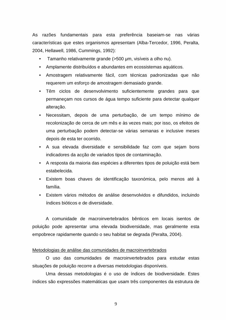
As razões fundamentais para esta preferência baseiam-se nas várias
características que estes organismos apresentam (Alba-Tercedor, 1996, Peralta,
2004, Hellawell, 1986, Cummings, 1992):
• Tamanho relativamente grande (>500 µm, visíveis a olho nu).
• Amplamente distribuídos e abundantes em ecossistemas aquáticos.
• Amostragem relativamente fácil, com técnicas padronizadas que não
requerem um esforço de amostragem demasiado grande.
• Têm ciclos de desenvolvimento suficientemente grandes para que
permaneçam nos cursos de água tempo suficiente para detectar qualquer
alteração.
• Necessitam, depois de uma perturbação, de um tempo mínimo de
recolonização de cerca de um mês e às vezes mais; por isso, os efeitos de
uma perturbação podem detectar-se várias semanas e inclusive meses
depois de esta ter ocorrido.
• A sua elevada diversidade e sensibilidade faz com que sejam bons
indicadores da acção de variados tipos de contaminação.
• A resposta da maioria das espécies a diferentes tipos de poluição está bem
estabelecida.
• Existem boas chaves de identificação taxonómica, pelo menos até à
família.
• Existem vários métodos de análise desenvolvidos e difundidos, incluindo
índices bióticos e de diversidade.
A comunidade de macroinvertebrados bênticos em locais isentos de
poluição pode apresentar uma elevada biodiversidade, mas geralmente esta
empobrece rapidamente quando o seu habitat se degrada (Peralta, 2004).
Metodologias de análise das comunidades de macroinvertebrados
O uso das comunidades de macroinvertebrados para estudar estas
situações de poluição recorre a diversas metodologias disponíveis.
Uma dessas metodologias é o uso de índices de biodiversidade. Estes
índices são expressões matemáticas que usam três componentes da estrutura de

10
uma comunidade, nomeadamente riqueza (número de espécies presente),
equitabilidade (uniformidade na distribuição dos indivíduos nas espécies) e
abundância (número total de organismos presentes), para descrever a resposta
de uma comunidade à qualidade do seu ambiente (Metcalfe-Smith, 1994).
Segundo Neher et al. (1995) os índices de diversidade apresentam pouca ou
nenhuma sensibilidade a mudanças na composição do taxon, embora se mostrem
sensíveis ao declínio do seu número. Geralmente, ecossistemas pobres em
espécies são considerados como tendo uma qualidade aquática degradada
(Kenney et al., 2009). Gray e Delaney (2010) concluíram que os índices de
diversidade medem o stress total e portanto são melhores que os índices bióticos
na detecção da existência de impacto causado por escorrências mineiras ácidas
nos rios, mas baseiam-se num modelo teórico de comunidade não totalmente
apropriado para estudar os efeitos deste agente de stress.
Os índices bióticos também são usados frequentemente em estudos com
macroinvertebrados. Estes costumam ser específicos para um tipo de alteração
ou contaminação e/ou região geográfica, e baseiam-se no conceito de organismo
indicador. Eles permitem uma aferição do estado ecológico de um ecossistema
aquático afectado por um qualquer processo de contaminação (Gamboa et al.,
2008). São especialmente eficazes na avaliação dos efeitos causados por
poluição orgânica; a sua aplicação a outros tipos de poluição ou perturbação pode
ser questionável (Metcalfe-Smith, 1994). No início, desenvolveram-se índices
bióticos para os quais era necessária uma identificação taxonómica dos
macroinvertebrados ao nível do género ou espécie (Róldan, 2003), ou uma
estimativa quantitativa das abundâncias (Alonso & Camargo, 2005); todavia,
comprovou-se que os índices mais práticos (pela sua facilidade de obtenção) são
aqueles em que só são necessários dados qualitativos (presença–ausência) e
uma identificação taxonómica até ao nível da família (Leiva, 2004). Deste modo,
uma amostragem exaustiva pode garantir a colheita dos taxa presentes na área
de estudo (Alba-Tercedor, 1996) e aumentar a fiabilidade do índice aplicado.
Muitos índices têm sido desenvolvidos mas todos assentam em duas premissas
básicas. Primeiro, os diferentes taxa bioindicadores variam na sua tolerância à
poluição. A sua presença ou ausência pode ser usada para estimar o grau de

11
poluição especialmente se houver um ranking de resposta conhecido para os taxa
tolerantes e sensíveis. Segundo, o número de indivíduos presentes varia com a
intensidade da poluição, e a abundância também pode ser incorporada num
índice biótico (Jeffries & Mills, 1996).
A análise multivariável dos dados também é usada com frequência para
analisar comunidades de macroinvertebrados. Este tipo de análise estuda toda a
comunidade, incorporando processos naturais e parâmetros indicadores da
presença de poluição (Jeffries & Mills, 1996). A principal vantagem deste tipo de
análise é a integração de dados multidimensionais com o mínimo possível de
perda de informação, permitindo a detecção de tendências de variabilidade pouco
evidentes nos dados (Rosemberg & Resh, 1993). Ela detecta também padrões
sazonais e espaciais da comunidade.
Num estudo de biodiversidade, o ideal será fazer uma utilização conjunta
de várias métricas de análise das comunidades de macroinvertebrados e conjugá-
las com a análise dos descritores físico-químicos. Desta forma será possível obter
uma visão abrangente dos efeitos dos vários impactos sofridos por determinada
comunidade de macroinvertebrados.
Objectivos e estrutura da dissertação
Este trabalho teve como objectivo avaliar a qualidade ecológica do Rio Mau
(Sever do Vouga), no âmbito da DQA, e poderá constituir uma base para
trabalhos futuros. Para fazer esta avaliação ecológica, estudou-se de que forma
os múltiplos agentes de stress que exercem influência sobre o Rio Mau afectam a
estrutura das comunidades de macroinvertebrados bênticos nele presentes. A
conceptualização teórica e os objectivos específicos do trabalho, assim como as
metodologias usadas, os resultados obtidos e a sua discussão são apresentados
numa secção própria e independente, constituindo o Capítulo 1 da presente
dissertação. Este capítulo é precedido da presente introdução geral, onde a
temática da dissertação é inicialmente abordada e enquadrada, e o objectivo geral
do trabalho é definido.
Capítulo 1
«Water quality and benthic invertebrate community
structure in Mau River (Sever do Vouga, Portugal)»

15
Introduction
The main goal of the Water Framework Directive (WFD - Directive
2000/60/CE, 2000) is to attain or preserve good ecological quality in waterbodies
in all EU Member States, or at least prevent further deterioration of surface and
groundwater. In order to accomplish this, Member States have the obligation of
assessing the ecological status of their waterbodies, through the monitoring of
phytoplankton, phytobenthos, macrophytes, benthic invertebrates, and fish
assemblages. This way, WFD abandons the classic approach of the water as just
a resource (anthropocentric perspective) and instead sees it as ecosystem holder
(ecocentric perspective) (INAG, 2008a).
Mau River, a small mountain river in central Portugal, is located far from
large industrial and housing areas. This could lead us to expect good ecological
status, as it seems to suffer few impacts. However, as most rivers and
waterbodies (see Ormerod et al., 2010 and references therein), it suffers the
influence of multiple stressors (a stressor is a variable that potentially provokes a
measurable biological or ecological response (Statzner & Beche, 2010)). Mau
River potentially suffers impacts from organic and inorganic pollution from
abandoned mines, agriculture and sewage, either on specific locations (near the
dumping places) or along the river continuum. This water pollution is particularly
worrying because Mau River is a tributary of Vouga River and both rivers are used
for fishing and recreational activities (picnic areas, river beaches). Furthermore,
water is captured in Vouga River for human consumption, downstream its
confluence with Mau River.
The wastes from mining activity, containing high metal concentrations,
represent a source of metal contamination for a long time following extraction
(Kelly, 1988, Ferreira da Silva et al., 2009), as in the case of Malhada and Braçal
mines in Mau River. In these mines, prospection of lead and zinc took place for
more than one century until the 1950s, when they were deactivated. The effects of
mine drainage can be summarized as acidity, metal toxicity, metal precipitation
and salinization (Gray, 1997, Gray & Delaney, 2010). Mau River also crosses a
small locality (Silva Escura), where agriculture practices contribute with fertilizer

16
and pesticide inputs. The most common agriculture contaminants in the
hydrographic basin of Caima and Mau Rivers are phosphates, nitrates and
pesticides, which may be composed by metals like Cd, Cu, Pb, As, Zn and Fe
(Nunes, 2007). Thus, agriculture can influence biological quality of the water by
interfering in the nutrient cycles. Besides this, cesspools (individual and collective)
are still common in Silva Escura, also exerting a potentially negative influence on
the ecological quality of Mau River.
However, the presence of these factors alone does not guarantee a poor
ecological status. Loredo et al. (2010) reached the conclusion that mine drainage
and spoil heap leaches show occasionally very acidic conditions, but these
conditions are easily neutralised when polluted waters reach streams or rivers with
enough water flow to dilute the concentration of pollutants. Their work also showed
that, in spite of the past extensive mining activities in Los Rueldos and the
weathering of mine wastes, local streams were not significantly polluted. Even in
the case of severe impacts, it is possible that parts of a stream or river can recover
without mitigation measures. This was observed by Cerqueira et al. (2008) in
Antuã River where, despite the relevance of pollution problems, considerable
water quality improvement was observed in the final stretch of the river, giving
evidence of a great self-depuration capacity.
Assessing the ecological status of this river is necessary within the scope of
WFD. For example, this could lead to the outline of a mitigation plan for this river, if
necessary. Biomonitoring programs, recommended by WFD as part of the
ecological assessment, rely on bioindicators. A bioindicator can be defined as a
species (or group of species) which present specific requests concerning one or
more physical or chemical variables, in a way that changes in presence or
absence, number, morphology or behaviour of that species indicate that the abiotic
variables are in their tolerance limits (Rosemberg & Resh, 1993). Bioindicators are
very effective in obtaining clues about situations of continuous and intermittent
pollution (Nunes, 2007) and they integrate the effects of multiple stressors. Benthic
macroinvertebrates have been widely used – and are strongly recommended – as
biological indicators of water quality in river management (Barbour et al., 1999,
17
Cummings, 1992, INAG, 2008a, Klemm et al., 2002, Tachet et al., 1980, Metcalfe-
Smith, 1994).
This work aimed to study the potential effects of multiple stressors (acid
mine drainage, domestic effluents and agriculture activities) on Mau River, by
accompanying the seasonal and spatial variation of its benthic macroinvertebrate
communities. Two distinct approaches were followed: a) a water quality approach,
using biotic indices and focusing on ecological status; b) a community structure
approach, using multivariate analyses to decompose spatial and temporal patterns
and underlying explanatory factors.
Materials and Methods
Study area and sampling stations
This work focused on Mau River, which presents Braçal and Malhada mines
in its catchment basin, and is located in the vicinities of Sever do Vouga
(40º44'00’’N 8º22'00’’W) – see Figure 1. The main extraction in Braçal and
Malhada mines was galena ore (native lead sulphide), with more accidental
extraction of zinc blende ore and iron pirite ore (Cabral et al., 1889). The distance
between the old mines is less than 1 km. Mau River has an extension of 12.4 km,
beginning in Serra do Salgueiro until Pessegueiro do Vouga, where it meets
Vouga River. The constant occurrence of rocky outcrops makes the water to flow
through a sinuous path creating some waterfalls which oxygenate the water.
18
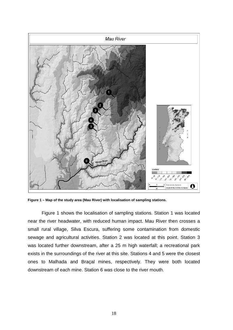
Figure 1 – Map of the study area (Mau River) with l ocalisation of sampling stations.
Figure 1 shows the localisation of sampling stations. Station 1 was located
near the river headwater, with reduced human impact. Mau River then crosses a
small rural village, Silva Escura, suffering some contamination from domestic
sewage and agricultural activities. Station 2 was located at this point. Station 3
was located further downstream, after a 25 m high waterfall; a recreational park
exists in the surroundings of the river at this site. Stations 4 and 5 were the closest
ones to Malhada and Braçal mines, respectively. They were both located
downstream of each mine. Station 6 was close to the river mouth.

19
Riparian vegetation along the river extension is usually tall and dense, with
plants belonging to different families, namely Commelinaceae, Umbelliferae,
Compositae.
Sampling strategy and methods
There were 4 sampling campaigns, which took place in May 2005 (spring),
August 2005 (summer), November 2005 (autumn) and February 2006 (winter). In
all campaigns, all 6 stations (see above) were characterised as described below.
At each station, chemical and physical parameters were measured in situ
using portable testing meters: pH (pH 330 from WTW, Germany), temperature and
conductivity (LF 330 from WTW), and dissolved oxygen (Oxi 315i from WTW). A
1.5 L water sample was collected in plastic bottles for posterior determination of
other parameters (see Laboratory analysis). The section of the river-bed and water
depth were also measured. Water transparency was classified by observation.
Sediment samples were collected from the river-bed at each station into plastic
bags. They were maintained and transported at 4ºC in the dark, and later frozen at
-20ºC until further analysis.
Benthic macroinvertebrates were collected at each station by kick-sampling,
using a standard hand net (500 µm pore size; square frame, 0.33 x 0.33 m). To
assure similar effort among sites and seasons, sampling was performed during 3
min, along 3-4 transects covering the diversity of habitats (margins, aquatic
macrophytes, riffles, main canal) and sediment types (rocks, gravel, sand, etc.).
Following collection, samples were fixed with 4% buffered formalin.
Laboratory analysis
Water samples were filtered through standard glass fiber filters (GF/C type,
pore 1.2 µm); filtrate was used for nutrient analysis and residue was used to
quantify total suspended solids (TSS). Nutrients were analysed following the Hach
test methods for the determination of nitrites (NO2-), nitrates (NO3
-), ammonia
(NH4+), orthophosphates (PO4
3-) and sulphates (SO42-) in water samples. All
analyses followed widely disseminated protocols (A.P.H.A. et al., 1998).

20
Metal analysis was performed for sediment samples. Metal extraction was
performed by mixing them with distilled water in a proportion of 1:2 (w/v). They
were left overnight in an orbital shaker at 200 rpm. On the day after, elutriates
were centrifuged for 15 min at 4000 rpm and the supernatant was filtered by a 45
µm pore filter. Afterwards, the filtrate was acidified to pH<2 with nitric acid 65 %.
Metal concentrations were then determined by inductively coupled plasma mass
spectrometry (ICP-MS) for Al, As, B, Ba, Cd, Cr, Cu, Fe, Mn, Ni, Pb, Sr, V and Zn.
At the laboratory, preserved benthic macroinvertebrate samples were
washed through a 500 µm sieve and organisms were sorted out. After this, they
were stored in 70 % alcohol and identified to the lowest practical taxonomical
level, generally the family (or genus, when possible) using standard keys (Serra et
al., 2009, Tachet et al., 1980, Macan, 1959, Sundermann et al., 2007, Richoux,
1982, Pattée & Gourbault, 1981, Elliott, 1977).
Data analysis: abiotic variables
Physical and chemical parameters and sediment metal concentrations were
analysed using a 2-way ANOVA without replication to explore differences among
sampling sites and among sampling seasons. A significance level (α) of 0.05 was
used. Additionally, principal components analysis (PCA) was used to explore
patterns in the environmental data matrix; physical and chemical parameters and
sediment metal concentrations were analysed individually. PCA is an ordination
technique usually employed in the analysis of multivariate matrices of abiotic data,
since it assumes an underlying linear mathematical model (ter Braak, 1995,
Gauch, 1982). Before running the analysis, the environmental data were
standardized by subtracting the mean from each observation and dividing by the
corresponding standard deviation.
Data analysis: water quality approach
Macroinvertebrate data was analysed using some metrics, including taxa
richness, number of families, Shannon’s diversity index (H’), Pielou’s equitability
index (J’), EPT (Ephemeroptera-Plecoptera-Trichoptera) index, biological water
quality indices IBMWP (Iberian Biological Monitoring Working Party) (Alba-

21
Tercedor & Sánchez-Ortega, 1988, Alba-Tercedor et al., 2002, Jáimez-Cuéllar et
al., 2002) (Table 1) and IASPT (Iberian Average Score per Taxon) (Rodriguez &
Wright, 1987).
Table 1 – Water quality and ecological status class es according to IBMWP (Jáimez-Cuéllar et al., 2002)
IBMWP Water Quality Ecological status
>100 Good. Waters without contamination
or with very subtle contamination. High
61 – 100 Acceptable. Some water
contamination effects are evident. Good
36 – 60 Doubtful. Contaminated waters. Moderate
16 – 35 Critical. Very contaminated waters. Poor
<15 Very critical. Heavily contaminated
waters. Bad
North Invertebrate Portuguese Index (IPtIN) was calculated using the
recommendations given by INAG (2009). This metric resulted from the European
and Portuguese intercalibration exercises (INAG, 2009, Buffagni & Furse, 2006,
Buffagni et al., 2006) and is defined in the European Commission’s Decision
2008/915/CE. It is the weighted sum of some metrics, each normalized using the
quotient between the obtained values and corresponding reference values for
small dimension rivers of northern Portugal, category which Mau River belongs to
(INAG, 2008b).
IPtIN = (0,25 x S) + (0,15 x EPT) + (0,1 x J’ ) + (0,3 x (IASPT - 2)) + (0,2 x log (Sel. ETD + 1) ),
where S stands for richness; EPT is the number of families belonging to orders
Ephemeroptera, Plecoptera, Trichoptera; J’ is Pielou’s equitability index (J’ =
H’/ln(S), with H’ being Shannon’s diversity index); IASPT results from the quotient
between IBMWP and the number of families with IBMWP scores in the sample;
and log (Sel. ETD + 1) stands for the logarithm of the sum of abundances of
organisms belonging to families Heptageniidae, Ephemeridae, Brachycentridae,
Goeridae, Odontoceridae, Limnephilidae, Polycentropodidae, Athericidae, Dixidae,
Dolichopodidae, Empididae, Stratiomyidae (ETD taxa).

22
The final IPtIN value is itself subjected to normalization, by dividing it by the
corresponding reference value for small dimension rivers of northern Portugal
(1.02, as in INAG, 2009). In this way, the final result can be expressed in
Ecological Quality Ratios (EQR), which are associated with different categories of
ecological quality; frontier values to classify small dimension rivers of northern
Portugal are presented in Table 2.
Table 2 – Water ecological status according to EQR o f IPtIN (INAG, 2009).
Tipology EQR (IPtIN) Ecological status
>0.87 High
0.86 – 0.65 Good
0.64 – 0.44 Moderate
0.43 – 0.22 Poor
Small Dimension
Rivers of Northern
Portugal
(N1 ≤ 100 km2)
< 0.22 Bad
Selected metrics were analysed using a 2-way ANOVA without replication
(using SPSS®) to explore differences among sampling sites and among sampling
seasons. A significance level (α) of 0.05 was used.
Data analysis: community structure approach
Benthic invertebrate abundance data were compiled as a multivariate
matrix. Detrended Correspondence Analysis (DCA) was used to analyse gradients
in community structure, including spatial and temporal patterns. DCA is an
improved eigenvector ordination technique based on reciprocal (weighted)
averaging, and is commonly used in community ecology, as it assumes an
underlying unimodal mathematical model (ter Braak, 1995, Gauch, 1982).
Abundances were log-transformed prior to analysis. Downweighting of rare
species was used, and species and sample scores were plotted in a bidimensional
space.
Additionally, redundancy analysis (RDA) was also used to explore seasonal
and spatial gradients in the benthic invertebrate assemblage. RDA is a canonical
ordination technique which constrains the biotic data matrix relatively to the

23
environmental gradients (ter Braak, 1995). As a consequence, it extracts synthetic
gradients from the biotic and environmental matrices, which are quantitatively
represented by arrows in graphical biplots (ter Braak, 1995). The length of the
arrow is relative to the importance of the explanatory variable in the ordination,
and arrow direction indicates positive or negative correlations. RDA is the
extension of PCA (unconstrained form) in the same way as canonical
correspondence analysis (CCA) is the extension of weighted averaging or
(detrended) correspondence analysis (CA or DCA). Ideally, CCA should be used
with species abundance data sets (ter Braak, 1995); however, ter Braak and
Smilauer (1998) recommend the use of RDA when the environmental gradient is
not very pronounced (given by a length of gradient of the first axis of DCA run on
the biotic matrix lower than 4 SD).
Five distinct RDA models were built from the benthic invertebrate data set:
1) sediment metal concentrations as explanatory variables (M); 2) water physical
and chemical parameters as explanatory variables (PC); 3) global model (M+PC);
4) M partialling out PC (as covariable; see ter Braak & Verdonschot, 1995); 5) PC
partialling out M (as covariable). A forward selection procedure (ter Braak &
Verdonschot, 1995) was performed a priori on the sediment metal concentration
and physical and chemical data sets, in order to include only significant
explanatory variables in the model (significance was tested using a Monte Carlo
permutation test; α=0.05). Similarly to DCA, downweighting of rare species was
employed in all analyses. Monte Carlo permutation tests were used to assess the
significance of the relation between macroinvertebrate data and explanatory
variables for each of the above models. The variation partitioning technique
proposed by Borcard et al. (1992) was used to quantify the variation explained by
each of the environmental subsets of explanatory variables (see also Okland &
Eilersten, 1994). To do so, we compared the resulting percentage of variance of
the partial RDAs (as the quotient between the sum of canonical eigenvalues and
total inertia) with that of the global model.
All multivariate analyses were performed using CANOCO software.

24
Results
Abiotic framework
Mau River fluctuated in terms of pH, while exhibiting low nutrient
concentrations, reduced conductivity and reduced TSS (except in February at the
most upstream stations). Dissolved oxygen was equal to or above saturation.
These conditions suggest a river in good condition (Table 3). Overall, Mau River
was fairly homogeneous among sampling stations. With the exception of
conductivity and width, no significant differences were found among sites for
physical and chemical parameters (Table 4). Differences in conductivity reflect the
upstream-downstream gradient, with minima in station 1 and maxima in station 6
(Table 3). The width of the canal varied between 1.8 m in station 1 and 7.7 m in
station 5. Seasonality was observed for pH, dissolved oxygen, temperature,
conductivity, depth, TSS, nitrates, phosphates, and sulfates (see Table 3), since
significant differences were found among sampling seasons (Table 4). The only
exceptions were width, ammonia, and nitrites, which showed no significant
seasonal fluctuations.
The PCA diagram revealed a large scatter of sampling stations (Figure 2),
as a consequence of seasonal variations of the river physico-chemistry (see
above). A noticeable exception was site 1 (S1), whose PCA scores were all
distributed in the bottom left part of the biplot, associating this site with low
conductivity, low concentration of sulfates, high amount of suspended solids (TSS)
and high dissolved oxygen levels. Still, most sites were located in the middle
region of the diagram, corroborating the among site homogeneity shown above.
Stations 5 and 6, in November, formed a distinct cluster, as a result of high
phosphate, nitrite and ammonia levels.

25
Table 3 – Range (min.-max.) of physical and chemica l parameters measured at Mau River between May 2005 and February 2006.
Parameter 1 2 3 4 5 6pH 5.65-8.65 5.91-7.40 5.99-7.83 6.68-7.57 6.85-7.85 6.74-7.61O2 (mg L-1) 8.4-12.4 8.5-13.1 9.1-18.4 11.1-18.4 8.6-13.7 11.2-11.7
Temperature (ºC) 9.4-14.5 10.8-16.3 10.7-16.3 10.1-16.7 9.5-16.5 9.1-18.0Conductivity (µS cm -1) 23.8-33.2 49.0-64.6 44.6-71.1 49.8-77.8 55.2-66.7 58.3-77.3Section width (m) 1.0-2.5 1.5-5.3 3.3-5.7 3.7-5.4 4.9-9.5 3.6-4.0Water depth (m) 0.20-0.40 0.20-0.30 0.20-0.40 0.10-0.40 0.15-0.30 0.10-0.30TSS (mg L -1) 1.34-54.95 2.28-41.24 2.60-5.97 1.38-6.13 0.48-9.89 1.24-4.37Ammonia (mg L -1) 0.00-0.01 0 0.00-0.01 0.00-0.19 0.00-0.28 0.00-0.04Nitrates (mg L -1) 0.07-0.30 0.07-1.20 0.08-1.60 0.08-1.30 0.08-1.40 0.09-1.40Nitrites (mg L -1) 0.00-0.01 0.00-0.01 0.00-0.01 0.00-0.01 0.00-0.01 0.00-0.03Phosphates (mg L-1) 0.12-0.14 0.12-0.37 0.11-0.40 0.15-0.65 0.09-1.06 0.12-0.94
Sulfates (mg L-1) 0.00-6.00 1.00-7.00 0.00-7.00 1.00-12.00 0.00-9.00 6.00-10.00Transparency clear clear clear clear clear clear
Sampling station
Table 4 – Source of variation, degrees of freedom ( df), mean square and p values of 2-way ANOVA without replication applied to several physical and chemical parameters measured in Mau River.
Parameter Source of variation df Mean Square pSite 5 0.100 0.758Season 3 2.21 <0.001Residual 15 0.192Site 5 5.00 0.197Season 3 25.0 0.002Residual 15 2.96Site 5 1.07 0.067Season 3 51.6 <0.001Residual 15 0.407Site 5 664 <0.001Season 3 277 0.002Residual 14 31.9Site 5 14.3 0.001Season 3 1.54 0.448Residual 15 1.65Site 5 0.00300 0.668Season 3 0.0290 0.005Residual 15 0.00400Site 5 136 0.378Season 3 458 0.031Residual 15 118Site 5 0.00400 0.554Season 3 0.00300 0.582Residual 15 0.00500Site 5 0.191 0.060Season 3 2.13 <0.001Residual 15 0.0700
Site 5 3.40 x 10⁻⁵
0.728Season 3 3.80 x 10⁻⁵ 0.615
Residual 15 6.10 x 10⁻⁵
Site 5 0.0420 0.307Season 3 0.286 0.001Residual 15 0.0320Site 5 23.4 0.060Season 3 29.5 0.044Residual 15 8.55
Nitrate
Nitrite
Phosphate
Sulfate
Width
Depth
TSS
Ammonia
pH
O2
Temperature
Conductivity
26
-1.0 1.0
-0.6
1.0
pH
O2Temp
Cond
Width
Depth
TSS
Ammonia
Nitrate
Nitrite
Phosphat
Sulfates
S1_MS1_A
S1_N
S1_F
S2_M
S2_AS2_N
S2_F
S3_M S3_A
S3_N
S3_F
S4_MS4_A
S4_N
S4_F
S5_M
S5_A
S5_N
S5_F
S6_M
S6_A
S6_N
S6_F
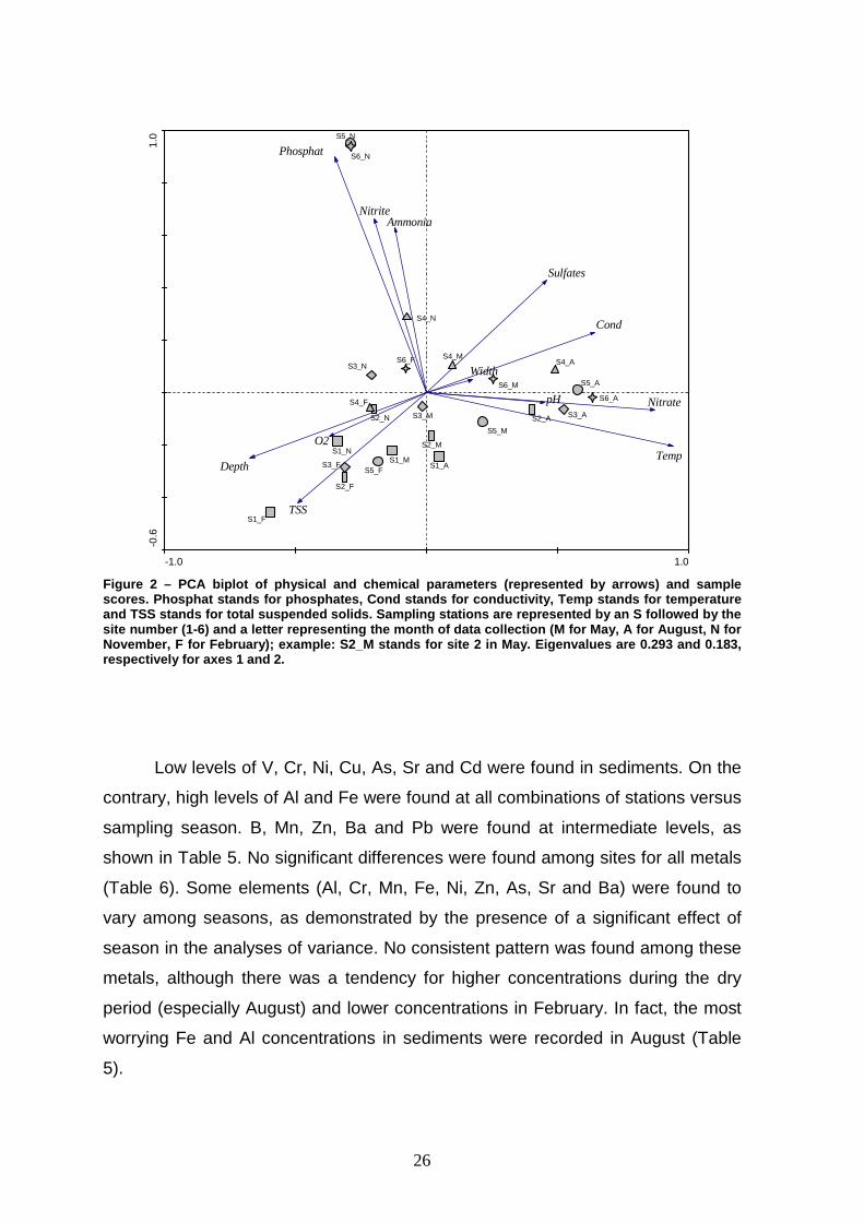
Figure 2 – PCA biplot of physical and chemical param eters (represented by arrows) and sample scores. Phosphat stands for phosphates, Cond stands for conductivity, Temp stands for temperature and TSS stands for total suspended solids. Sampling s tations are represented by an S followed by the site number (1-6) and a letter representing the mon th of data collection (M for May, A for August, N f or November, F for February); example: S2_M stands for site 2 in May. Eigenvalues are 0.293 and 0.183, respectively for axes 1 and 2.
Low levels of V, Cr, Ni, Cu, As, Sr and Cd were found in sediments. On the
contrary, high levels of Al and Fe were found at all combinations of stations versus
sampling season. B, Mn, Zn, Ba and Pb were found at intermediate levels, as
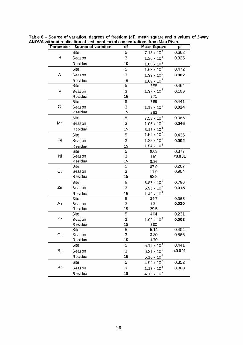
shown in Table 5. No significant differences were found among sites for all metals
(Table 6). Some elements (Al, Cr, Mn, Fe, Ni, Zn, As, Sr and Ba) were found to
vary among seasons, as demonstrated by the presence of a significant effect of
season in the analyses of variance. No consistent pattern was found among these
metals, although there was a tendency for higher concentrations during the dry
period (especially August) and lower concentrations in February. In fact, the most
worrying Fe and Al concentrations in sediments were recorded in August (Table
5).

27
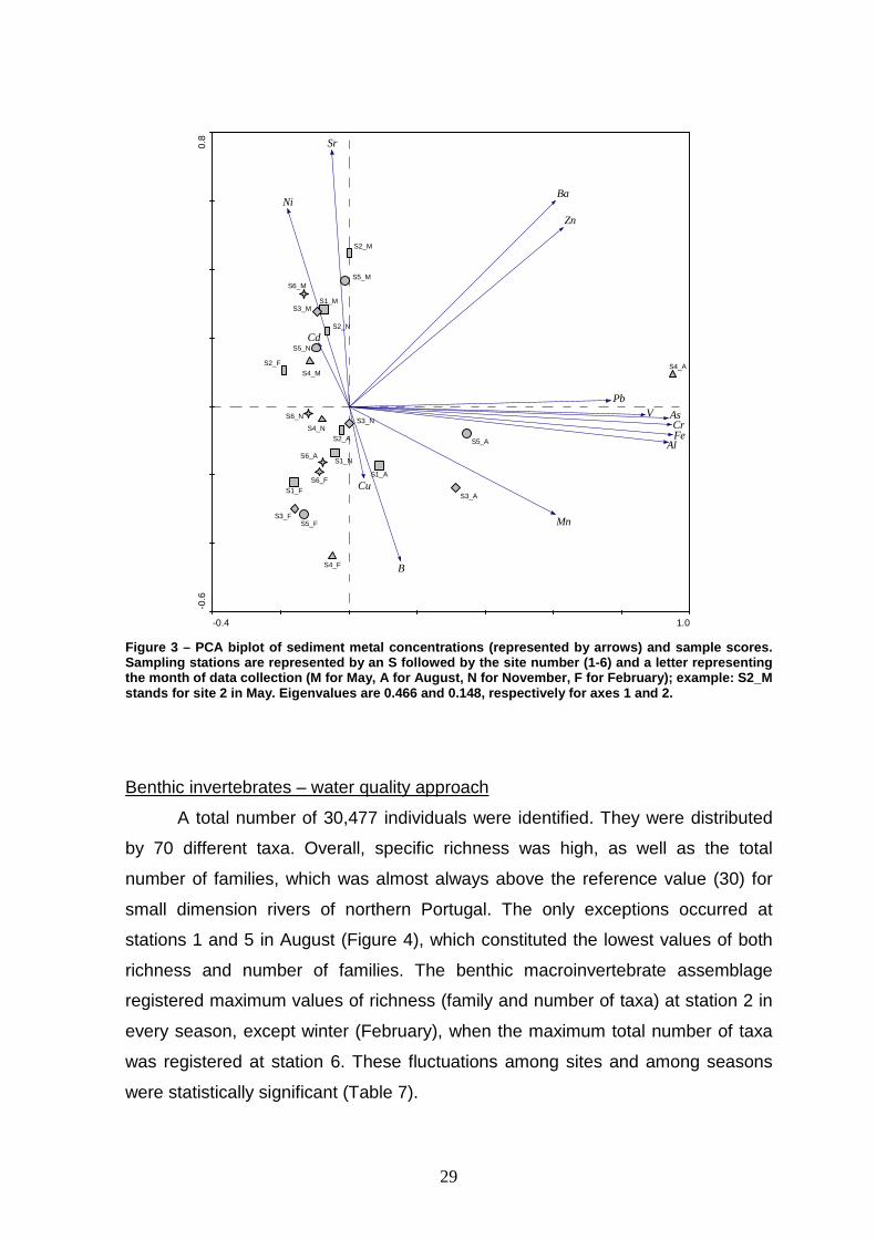
Similarly to physical and chemical parameters, the PCA scores for sampling
stations seem more dependent on seasonality than on a spatial gradient (Figure
3). This is perceptible in the biplot in an apparent gradient from February (bottom
left) to May (top left); November and August samples occupy an intermediate
position. This gradient is associated with Ni and Sr, which increase from February
to May, and B, which decreases from February to May (see Figure 3 and Table 5).
Also, seasonality is evident in August samples, which occupy a position on the
right side of the diagram as a consequence of very high levels of Fe, Al and Pb
(see Figure 3 and Table 5). This is especially noticeable for site 4 (S4).
Table 5 – Range (min.-max.) of sediment metal concentrations (µµµµg Kg -1) measured at Mau River between May 2005 and February 2006.
Metal 1 2 3 4 5 6B <20-482 <20-410 275-1134 103-1216 150-998 41-587Al 456-22926 75.9-16410 589-40434 610-78200 1218-27574 397-5712V 1.36-25.1 <2-7.20 0.954-57.6 1.44-118 <2-5.80 <2-5.13Cr 0.862-21.0 <2-4.80 0.544-39.8 0.960-90.2 2.00-32.0 <2-3.42Mn 59.3-288 22.6-143 85.4-306 33.2-875 32.5-646 40.0-153Fe 296-17502 38.4-13940 488-35402 888-75716 1942-35480 674-7864Ni <20 <20 <20 <20 <20 <20Cu 2.06-22.2 <20 2.11-27.8 <20 <20 <20Zn 5.61-400 <4-377 13.4-316 46.9-546 62.7-344 103-171As 0.400-3.92 1.65-3.84 1.38-11.6 1-30.8 2.23-17.5 1.38-4.60Sr 7.10-46 13.5-83.1 8.03-72.0 14.4-52.0 10.2-56.0 4.28-62.0Cd <2 <2 <2 <2 0.12-10.6 <2Ba 11.9-714 27.3-868 12.0-896 14.1-1310 55.2-818 65.3-628Pb 1.77-21.7 <20-860 8.35-128 64.0-2596 147-2566 5.40-842
Sampling station
28
Table 6 – Source of variation, degrees of freedom ( df), mean square and p values of 2-way ANOVA without replication of sediment metal concent rations from Mau River.
Parameter Source of variation df Mean Square pSite 5 7.13 x 10
4 0.662Season 3 1.36 x 10⁵ 0.325
Residual 15 1.09 x 10⁵
Site 5 1.63 x 10⁸ 0.472
Season 3 1.33 x 10⁹ 0.002Residual 15 1.69 x 10
8
Site 5 558 0.464
Season 3 1.37 x 10³
0.109Residual 15 571Site 5 289 0.441Season 3 1.19 x 10³ 0.024Residual 15 283Site 5 7.53 x 10⁴ 0.086Season 3 1.06 x 10⁵ 0.046Residual 15 3.13 x 10⁴
Site 5 1.59 x 1080.436
Season 3 1.25 x 10⁹
0.002Residual 15 1.54 x 10⁸
Site 5 9.63 0.377Season 3 151 <0.001Residual 15 8.36Site 5 87.9 0.287Season 3 11.9 0.904Residual 15 63.8
Site 5 6.87 x 10³ 0.786
Season 3 6.96 x 10⁴ 0.015Residual 15 1.43 x 10
4
Site 5 34.7 0.365Season 3 131 0.020Residual 15 29.5Site 5 404 0.231Season 3 1.92 x 10³ 0.003Residual 15 260Site 5 5.14 0.404Season 3 3.30 0.566Residual 15 4.70Site 5 5.19 x 10⁴ 0.441
Season 3 6.21 x 10⁵ <0.001Residual 15 5.10 x 10
4
Site 5 4.99 x 10⁵ 0.352
Season 3 1.13 x 10⁶ 0.080
Residual 15 4.12 x 10⁵
Ba
Pb
Zn
As
Sr
Cd
Mn
Fe
Ni
Cu
B
Al
V
Cr
29
-0.4 1.0
-0.6
0.8
B
Al
VCr
Mn
Fe
Ni
Cu
Zn
As
Sr
Cd
Ba
Pb
S1_M
S1_A
S1_N
S1_F
S2_M
S2_A
S2_N
S2_F
S3_M
S3_A
S3_N
S3_F
S4_MS4_A
S4_N
S4_F
S5_M
S5_A
S5_N
S5_F
S6_M
S6_A
S6_N
S6_F
Figure 3 – PCA biplot of sediment metal concentratio ns (represented by arrows) and sample scores. Sampling stations are represented by an S followed by the site number (1-6) and a letter representing the month of data collection (M for May, A for Augu st, N for November, F for February); example: S2_M stands for site 2 in May. Eigenvalues are 0.466 and 0.148, respectively for axes 1 and 2.
Benthic invertebrates – water quality approach
A total number of 30,477 individuals were identified. They were distributed
by 70 different taxa. Overall, specific richness was high, as well as the total
number of families, which was almost always above the reference value (30) for
small dimension rivers of northern Portugal. The only exceptions occurred at
stations 1 and 5 in August (Figure 4), which constituted the lowest values of both
richness and number of families. The benthic macroinvertebrate assemblage
registered maximum values of richness (family and number of taxa) at station 2 in
every season, except winter (February), when the maximum total number of taxa
was registered at station 6. These fluctuations among sites and among seasons
were statistically significant (Table 7).

30
May 2005
0
10
20
30
40
50
60
70
1 2 3 4 5 6
Num
ber
of ta
xa
February 2006
0
10
20
30
40
50
60
70
1 2 3 4 5 6
Num
ber
of ta
xa
November 2005
0
10
20
30
40
50
60
70
1 2 3 4 5 6
Num
ber
of ta
xaAugust 2005
0
10
20
30
40
50
60
70
1 2 3 4 5 6
Num
ber
of ta
xa
Figure 4– Specific richness (grey bars) and number o f families (white bars) for each sampling station in each season. The dashed line marks the reference value for number of families according to INAG (2009). Table 7 – Source of variation, degrees of freedom ( df), mean square and p values of 2-way ANOVA without replication applied to several metrics deri ved from the macroinvertebrate data matrix.
Parameter Source of variation df Mean Square pSite 5 87.5 0.002Season 3 97.8 0.007Residual 15 15.0Site 5 167 0.002Season 3 222 0.014Residual 15 33.9Site 5 0.330 0.512Season 3 0.133 0.129Residual 15 0.149Site 5 0.0150 0.368Season 3 0.0110 0.254Residual 15 0.0100Site 5 8.89 0.065Season 3 22.1 0.392Residual 15 8.32
Site 5 2.06 x 10³ 0.018
Season 3 2.82 x 10³ 0.070Residual 15 715Site 5 0.418 0.511Season 3 0.152 0.103Residual 15 0.170Site 5 0.0230 0.121Season 3 0.0210 0.117Residual 15 0.0100
Families
Richness
Diversity
IPtIN
Equitability
EPT
IBMWP
IASPT

31
Shannon’s diversity index (H’) and Pielou’s equitability index (J’) were both
high for all sampling stations in all seasons. As for richness, their lowest values
were recorded at station 1 in August. Despite these fluctuations, differences
among sites and seasons were not significant (Table 7). Equitability’s values were
always close and sometimes higher than the reference value (0.71) for small
dimension rivers of northern Portugal (Figure 5). Sites 2 and 6 were exceptions to
this, since equitability was lower than the reference value with some consistency.
May 2005
0.0
0.5
1.0
1.5
2.0
2.5
3.0
1 2 3 4 5 6
H'
0.0
0.1
0.2
0.3
0.4
0.5
0.6
0.7
0.8
0.9
J'
August 2005
0.0
0.5
1.0
1.5
2.0
2.5
3.0
1 2 3 4 5 6
H'
0.0
0.1
0.2
0.3
0.4
0.5
0.6
0.7
0.8
0.9
J'
November 2005
0.0
0.5
1.0
1.5
2.0
2.5
3.0
1 2 3 4 5 6
H'
0.0
0.1
0.2
0.3
0.4
0.5
0.6
0.7
0.8
0.9
J'
February 2006
0.0
0.5
1.0
1.5
2.0
2.5
3.0
1 2 3 4 5 6
H'
0.0
0.1
0.2
0.3
0.4
0.5
0.6
0.7
0.8
0.9
J'
Figure 5 – Diversity (H’, grey bars) and equitabili ty (J’, white bars) for each sampling station in ea ch sampling period. The dashed line marks the referenc e value for equitability according to INAG (2009).
EPT taxa were present in all sampling stations. In most of them, the values
were close to or above the reference value for small dimension rivers of northern
Portugal. The most noticeable exceptions were station 1 and 5 in August (Figure
6), following the same pattern as for richness. In fact, station 5 almost always
recorded the lowest EPT value. Still, no significant differences were found
between sites or seasons (Table 7), although in the former case the p-value was
marginal.

32
May 2005
0
5
10
15
20
25
1 2 3 4 5 6
Sampling station
August 2005
0
5
10
15
20
25
1 2 3 4 5 6
Sampling station
November 2005
0
5
10
15
20
25
1 2 3 4 5 6
Sampling station
February 2006
0
5
10
15
20
25
1 2 3 4 5 6
Sampling station
Figure 6 – EPT taxa for each sampling station in each season. The dash ed line marks the reference value for EPT taxa, according to INAG (2009).
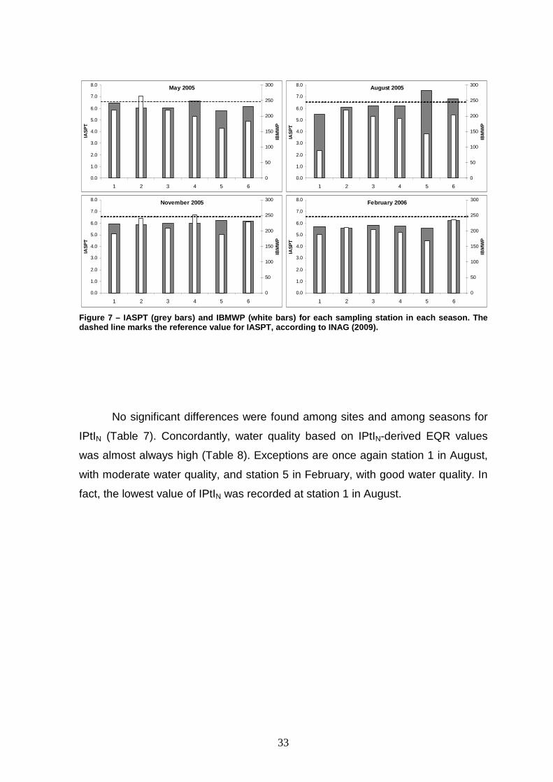
Very high IBMWP values were found in all stations and seasons (Figure 7).
Still, along with richness and number of families, IBMWP registered significant
differences among sites (Table 7). This is probably due to station 5, where this
index was consistently lower than the remaining sites. Also noticeable, and
confirming a tendency already observed previously, is a drastic reduction in the
IBMWP in station 1 in August. This was reflected in the water quality status (good),
which in all other sites was considered to be high, regardless of the season.
IASPT recorded small oscillations among stations and seasons, which were
found to be non significant (Table 7). Globally, all registered values were slightly
lower than the reference value (6.52) for small dimension rivers of northern
Portugal. The only exceptions were stations 5 and 6 in August and 4 in May
(Figure 7).
33
May 2005
0.0
1.0
2.0
3.0
4.0
5.0
6.0
7.0
8.0
1 2 3 4 5 6
IAS
PT
0
50
100
150
200
250
300
IBM
WP
August 2005
0.0
1.0
2.0
3.0
4.0
5.0
6.0
7.0
8.0
1 2 3 4 5 6
IAS
PT
0
50
100
150
200
250
300
IBM
WP
November 2005
0.0
1.0
2.0
3.0
4.0
5.0
6.0
7.0
8.0
1 2 3 4 5 6
IAS
PT
0
50
100
150
200
250
300
IBM
WP
February 2006
0.0
1.0
2.0
3.0
4.0
5.0
6.0
7.0
8.0
1 2 3 4 5 6
IAS
PT
0
50
100
150
200
250
300
IBM
WP
Figure 7 – IASPT (grey bars) and IBMWP (white bars) fo r each sampling station in each season. The dashed line marks the reference value for IASPT, acco rding to INAG (2009).
No significant differences were found among sites and among seasons for
IPtIN (Table 7). Concordantly, water quality based on IPtIN-derived EQR values
was almost always high (Table 8). Exceptions are once again station 1 in August,
with moderate water quality, and station 5 in February, with good water quality. In
fact, the lowest value of IPtIN was recorded at station 1 in August.

34
Table 8 – Ecological status of each sampling station in all four seasons according to IPtI N and respective EQR.
Season Sampling station IPtIN EQR Ecological status1 1.043 1.023 High2 1.21 1.186 High3 1.07 1.049 High4 1.059 1.038 High5 0.936 0.917 High6 0.976 0.957 High1 0.554 0.543 Moderate2 1.041 1.021 High3 0.972 0.953 High4 0.997 0.977 High5 0.892 0.874 High6 1.087 1.065 High1 0.988 0.969 High2 1.04 1.02 High3 1.018 0.998 High4 1.118 1.096 High5 1.017 0.997 High6 1.091 1.07 High1 0.95 0.932 High2 0.967 0.948 High3 0.946 0.928 High4 0.994 0.975 High5 0.869 0.852 Good6 1.037 1.017 High
May 2005
August 2005
November 2005
February 2005
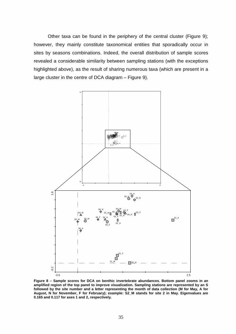
Benthic invertebrates – community structure approach
The length of gradient of the first axis (2.108) of the DCA revealed a modest
gradient in taxa succession. Consequently, a homogeneous distribution of the
sampling stations was observed (Figure 8). Station 1, however, is in the periphery
of the main cluster (see magnified zone – Figure 8). Correspondingly, taxa that
only occur at this site are located in the bottom right quadrant (e.g. Sialis,
Chloroperlidae). Several of these exclusive taxa occur only occasionally and at low
abundances: e.g. Dicranota, Riolus (adults), Helodes (larvae) and Chelifera in
November; Nemouridae Athericidae, Helophorus (adults), Dytiscidae (adults) and
Aselus in May; Lymnaeidae and Mesovelia in August (Figure 9). It therefore
appears that these rare taxa are responsible for the peripheral scores of station 1.
Nevertheless, their position in the DCA diagram is still fairly close to the other
sites.
35
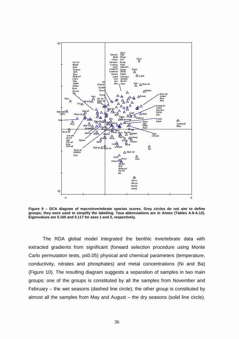
Other taxa can be found in the periphery of the central cluster (Figure 9);
however, they mainly constitute taxonomical entities that sporadically occur in
sites by seasons combinations. Indeed, the overall distribution of sample scores
revealed a considerable similarity between sampling stations (with the exceptions
highlighted above), as the result of sharing numerous taxa (which are present in a
large cluster in the centre of DCA diagram – Figure 9).
-4 8
-68
S1_M
S2_MS3_MS4_MS5_MS6_M S1_AS2_A
S3_A
S4_AS5_A
S6_A
S1_N
S2_NS3_N
S4_N
S5_NS6_N
S1_F
S2_FS3_FS4_F
S5_FS6_F
-0.5 2.5
-0.2
1.6
S1_M
S2_M
S3_M
S4_M
S5_MS6_MS1_A
S2_A
S3_A
S4_A
S5_A
S6_A
S1_N
S2_N
S3_N
S4_N
S5_N
S6_N
S1_F
S2_FS3_F
S4_F
S5_F
S6_F
Figure 8 – Sample scores for DCA on benthic inverteb rate abundances. Bottom panel zooms in an amplified region of the top panel to improve visual ization. Sampling stations are represented by an S followed by the site number and a letter representi ng the month of data collection (M for May, A for August, N for November, F for February); example: S2 _M stands for site 2 in May. Eigenvalues are 0.165 and 0.117 for axes 1 and 2, respectively.
36
-4 8
-68
Dug
Plan
Pol
Tric
Dina l i
Dina
Erpblla
Erpob
Glossnia
Gloss
Enchy
Eistetra
EisenLumbriciLumbricu
Pris t
Naid
Tubif
Pisid
Byth i
Potam Lymna
Lymnaeid
Phys
Ancy
Hidrac
Ase
Dryo ad
Dryo lar
Dyt a d
Dyt lar
Dyt ad2
Dupo ad
Dupo lar
Elm ad
Elm lar
Eso ad
Eso lar
Hydr ad
Hydr ad2
Lim ad1
Lim ad2
Norm ad
Norm lar
Ouli ad
Ouli lar
Rio a d
Rio lar
Elmd lar
Gyr lar
Hel lar
Helo lar
Helop ad
Limnb ad
Hydp ad
Hydc lar
Coleo
Anthom
Athex
Atri
Athe
Blepha
Atr ich
Cera to
Chironu s
Coryn
Diame
Ortho
Tanyp
Chironi
Tanyi
Chiro
Dixa
DixllaDixi
Dolich
Hemer
Chelif
Ata la
Eloe
Hexat
Rhyph
Scler Limo
Dicra
Psycho
Psycho2
Simu
Taba
Tipul
Tipul2
Tipu
Dip t
Btis
Baet
Caen
Ephella
Ep hemell
Ephemra
Ecdy
Epeo
Hepta
Centrop
HabropPa ralep
Lepto
Ephem
Gerr
Meso
Noto
Sai
Aesh
Agr
Cordu
Gomp
Libell
Platyc
Od o
Chloro
Leuc
Amphi
Nem
Proton
Nemae
Per
Perlo
Plec
Bera
Brachy
Calam
Glosso
Goe
Helic
Hydrpsy
Hydrop
Lepid
Leptc
Limnen
Limni
Limnep
Odont
Philo
Polycen
Psych
Rya
Seri
Thre
Tricho
Figure 9 – DCA diagram of macroinvertebrate species scores. Grey circles do not aim to define groups; they were used to simplify the labelling. Taxa abbreviations are in Annex (Tables A.9-A.12). Eigenvalues are 0.165 and 0.117 for axes 1 and 2, re spectively.
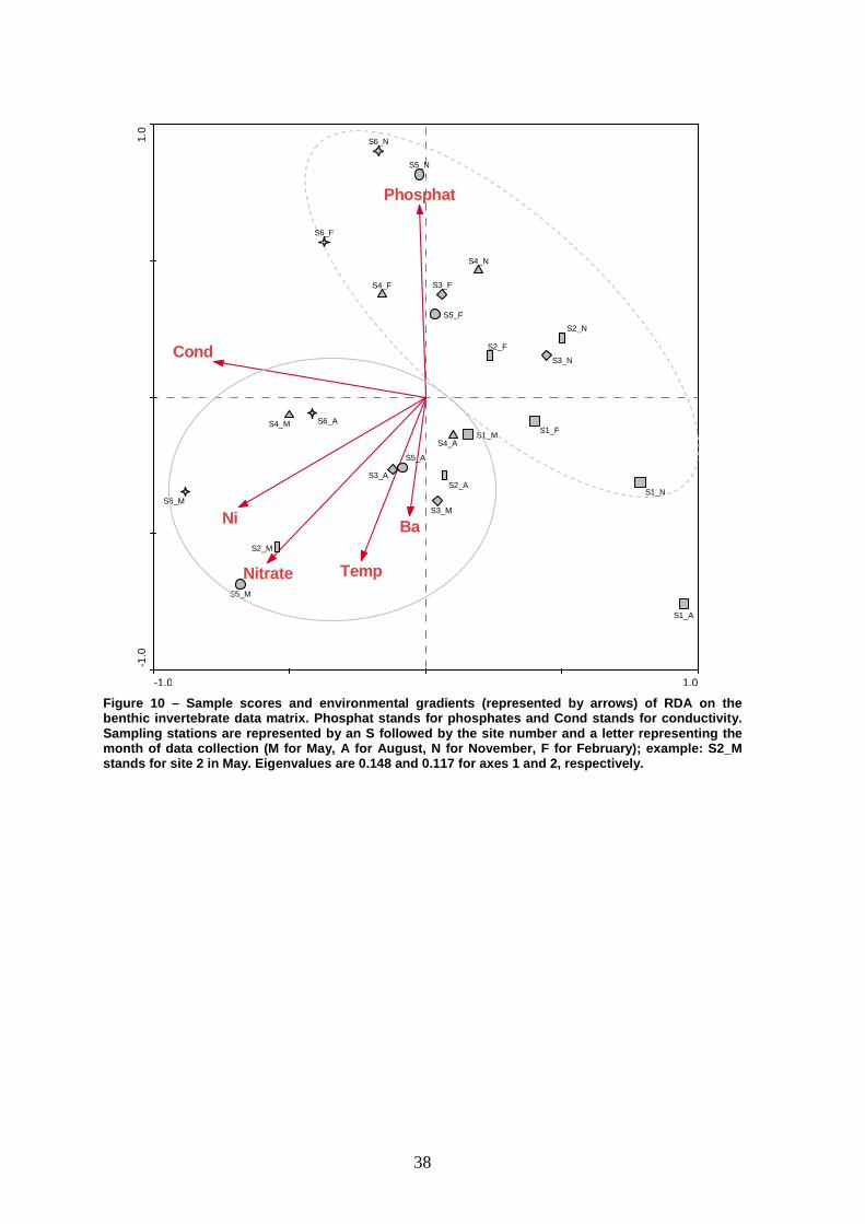
The RDA global model integrated the benthic invertebrate data with
extracted gradients from significant (forward selection procedure using Monte
Carlo permutation tests, p≤0.05) physical and chemical parameters (temperature,
conductivity, nitrates and phosphates) and metal concentrations (Ni and Ba)
(Figure 10). The resulting diagram suggests a separation of samples in two main
groups: one of the groups is constituted by all the samples from November and
February – the wet seasons (dashed line circle); the other group is constituted by
almost all the samples from May and August – the dry seasons (solid line circle).
-6
8 -4
8

37
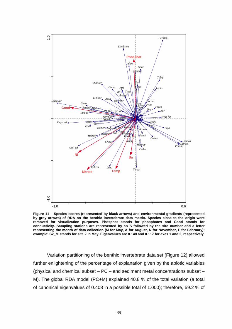
This is consistent with the distribution of species scores (Figure 11), which show
that taxa with higher abundances in November and February occur mostly in the
top right quadrant. Complementarily, taxa that were more abundant in May and
August are consistently found in the bottom left quadrant. Lumbriculidae,
Paraleptophlebia, Psychomiidae, Agrion and Potamopyrgus antipodarum,
constitute good examples of the first cluster (taxa associated with wet seasons).
Hydrocyphon (larvae) is an example of taxa occurring only in November and
February in Mau River. Tanypodinae, Leuctridae, Ephemeroptera, Oulimnius
(adults), Dupophilus (adults) and Elmis (adults) are some examples of taxa
associated with dry seasons. Some taxa are exclusively found during this period,
such as Habrophlebia.
These seasonal differences in the abundance of benthic invertebrates are
responsible for the separation of the two clusters. RDA also allows identifying the
environmental gradients which explain the distribution of taxa (Figure 10). The dry
season group was associated with increasing values of temperature, metals (Ni
and Ba) and nitrates. In opposition, the wet period cluster is mostly associated with
lower values of these variables. Station 1 (especially in August) was located far
from the other sample scores, as previously found in PCA and DCA diagrams.
Beyond the separation of the two clusters, a spatial pattern is apparent
during the wet season that is not perceptible in May and August samples. Thus,
samples belonging to this group form a slight gradient from the most upstream
(bottom right) to the most downstream sampling stations (top left). The position of
the most upstream sites corresponded to lower values of phosphates and
conductivity, whereas the final portion of the gradient (the most downstream
stations) was associated to higher values of phosphates and conductivity (Figure
10).
38
-1.0 1.0
-1.0
1.0
Ni Ba
Temp
Cond
Nitrate
Phosphat
S1_M
S1_A
S1_N
S1_F
S2_M
S2_A
S2_N
S2_F
S3_M
S3_A
S3_N
S3_F
S4_M
S4_A
S4_N
S4_F
S5_M
S5_A
S5_N
S5_F
S6_M
S6_A
S6_N
S6_F
Figure 10 – Sample scores and environmental gradient s (represented by arrows) of RDA on the benthic invertebrate data matrix. Phosphat stands fo r phosphates and Cond stands for conductivity. Sampling stations are represented by an S followed by the site number and a letter representing the month of data collection (M for May, A for August, N for November, F for February); example: S2_M stands for site 2 in May. Eigenvalues are 0.148 and 0.117 for axes 1 and 2, respectively.
39
-1.0 0.6
-1.0
1.0
Dug
Pol
Lumbricu
Naid
Tubif
Potam
Phys
Ancy
Hidrac
Dupo ad
Dupo lar
Elm ad
Elm lar
Eso ad
Eso lar Hydr adLim ad1
Norm lar
Ouli ad
Ouli lar
Gyr lar
Helo lar
Hydc lar
Athex
Atri
Cerato
Chironus
Coryn
Diame
Ortho
Tanyp
Chironi
Tanyi
Chiro
Hemer
Simu
Dipt
Btis Caen
Ephella
Ephemra
Ecdy
Epeo
Hepta
Habrop
Paralep
Lepto
Ephem
Gerr
Sai
Aesh
Agr
Cordu
Gomp
Chloro
Leuc
Amphi
Nem
Proton
Calam
Glosso
HydrpsyLeptc
Limnen
Limni
Philo
Polycen
Psych
Rya
Seri
Thre
Tricho
NiBa
Temp
Cond
Nitrate
Phosphat
Figure 11 – Species scores (represented by black arr ows) and environmental gradients (represented by grey arrows) of RDA on the benthic invertebrate data matrix. Species close to the origin were removed for visualization purposes. Phosphat stands for phosphates and Cond stands for conductivity. Sampling stations are represented by an S followed by the site number and a letter representing the month of data collection (M for Ma y, A for August, N for November, F for February); example: S2_M stands for site 2 in May. Eigenvalues a re 0.148 and 0.117 for axes 1 and 2, respectively.
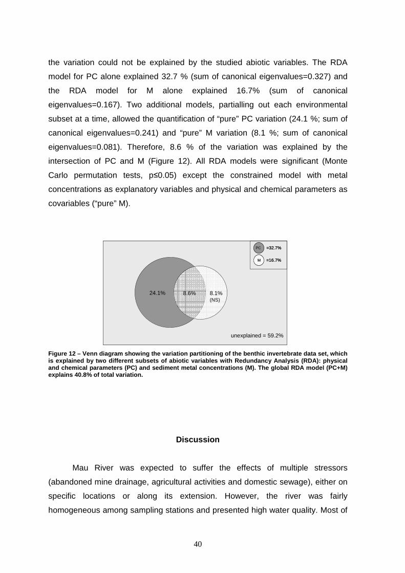
Variation partitioning of the benthic invertebrate data set (Figure 12) allowed
further enlightening of the percentage of explanation given by the abiotic variables
(physical and chemical subset – PC – and sediment metal concentrations subset –
M). The global RDA model (PC+M) explained 40.8 % of the total variation (a total
of canonical eigenvalues of 0.408 in a possible total of 1.000); therefore, 59.2 % of
40
the variation could not be explained by the studied abiotic variables. The RDA
model for PC alone explained 32.7 % (sum of canonical eigenvalues=0.327) and
the RDA model for M alone explained 16.7% (sum of canonical
eigenvalues=0.167). Two additional models, partialling out each environmental
subset at a time, allowed the quantification of “pure” PC variation (24.1 %; sum of
canonical eigenvalues=0.241) and “pure” M variation (8.1 %; sum of canonical
eigenvalues=0.081). Therefore, 8.6 % of the variation was explained by the
intersection of PC and M (Figure 12). All RDA models were significant (Monte
Carlo permutation tests, p≤0.05) except the constrained model with metal
concentrations as explanatory variables and physical and chemical parameters as
covariables (“pure” M).
unexplained = 59.2%
8.1%24.1% 8.6%
=16.7%M
=32.7%PC
(NS)
unexplained = 59.2%
8.1%24.1% 8.6%
=16.7%M =16.7%M
=32.7%PC =32.7%PC
(NS)
Figure 12 – Venn diagram showing the variation parti tioning of the benthic invertebrate data set, which is explained by two different subsets of abiotic va riables with Redundancy Analysis (RDA): physical and chemical parameters (PC) and sediment metal con centrations (M). The global RDA model (PC+M) explains 40.8% of total variation.
Discussion
Mau River was expected to suffer the effects of multiple stressors
(abandoned mine drainage, agricultural activities and domestic sewage), either on
specific locations or along its extension. However, the river was fairly
homogeneous among sampling stations and presented high water quality. Most of
41
the variation in its physico-chemistry and macroinvertebrate assemblage was due
to seasonality. The good condition of the river contradicts expected impacts of
multiple stressors and endorses the idea that this river suffers minor effects from
recent and historical pollution.
Minima and maxima values of physical and chemical parameters were more
or less consistently reached in the same months for all sampling sites (see Table
A.1 to A.4 in the Annex). This marked seasonality was expected, as most of these
parameters depend directly (temperature influences many of them) or indirectly on
the season (e.g. TSS, solids are dragged into the river in larger quantities by more
abundant rainfall in February). Conductivity was also affected by seasonal
changes, which are a consequence of variations in the concentration of dissolved
solids due to the seasonal fluctuations in the amount of water drained by the
hydrologic system (Cerqueira et al., 2008). Local variation (upstream-downstream
conductivity gradient) was also observed and was also expected, as upstream
waters tend to have lower ionic concentrations because they usually are less
polluted; these concentrations tend to increase along the extension of the water
course.
Stations 5 and 6 in November seem to be in some way influenced by
hydrologic drainage containing detergents (which usually contain phosphates) and
sewage, as these sites are associated with higher concentrations of phosphates,
nitrites and ammonia than the other sites. Still, ammonia values are not very high
(Gago & Mana, 2007), even in wet season (November and February). Although
phosphate levels are high, their impact on macroinvertebrate communities was
only slight, as biotic indices for station 5 were depressed but were not markedly
lower than most stations; station 6 communities do not seem to be affected by this
high values of phosphates. Differences between stations 5 and 6 can not be
explained on the basis of phosphates level alone, which may suggest the influence
of other factors (station 5 is located in the vicinity of Braçal mine). Sewage impact
was indeed expected for station 2 (located among the housing areas), but the
analysis does not reflect that. However, Simuliidae was generally more abundant
in this site (see Table A.9 to A.12 in the Annex), and this taxon is positively
influenced by organic enrichment (Wright & Burgin, 2009), thus indicating a subtle

42
impact in the macroinvertebrate community. The dominance of this taxon in station
2 was already reported in a previous study (in 1999-2000; unpublished data from
our team).
No significant differences among sites were found for sediment metal
concentrations, thus confirming the spatial homogeneity of the river and an
unexpected lack of influence from Malhada and Braçal mines. We were expecting
the existence of runoffs or drainage from the abandoned mines, leading to higher
metal concentrations at these sites, which could alter macroinvertebrate
abundance and biomass and reduce taxonomic diversity, as shown in other
studies (e.g. Malmqvist & Hoffsten, 1999). Ephemeroptera and Plecoptera are
considered to be generally sensitive to heavy metals, whereas Trichoptera are
relatively tolerant (Malmqvist & Hoffsten, 1999, Hickey & Golding, 2002). Both
sensitive and tolerant taxa were present in all sampling stations, with high levels of
diversity and equitability. These results were corroborated by the variation
partitioning of the benthic invertebrate data set, which showed that metals explain
a small and non-significant percentage (8.1 %) of the total variation. However,
interactive effects (explaining 8.6 % of total variation) between metals and other
physical and chemical parameters were evident in the seasonal differences within
the river. During low-flow conditions, mine drainage is the least diluted (Besser &
Leib, 1999), as well as the receiving stream itself. This may have happened in
August (higher levels of some metals characteristic to Malhada and Braçal mines
– Pb, Fe) due to warmer temperatures and the reduced rainfall of 2005 (Cerqueira
et al., 2008). Contrarily, the lowest metal concentrations were found in February
(wet season), where rainfall leads to a more abundant water flow and turbulence,
which may resuspend and drag contaminated sediments downstream. Riverbeds
are transitional environments between groundwater and surface water and are
both a sink and source of fine organic and inorganic sediment and associated
pollutants (Jarvie et al., 2005). Still, bioavailability of metals is affected by
numerous factors (e.g. pH, water hardness, and dissolved organic matter) which
may modify toxicity in situ (Hickey & Golding, 2002). Indeed, our study does not
allow us to infer about negative influence of metals on macroinvertebrate
community, even during the dry period, when metal concentrations were higher.
43
Despite this evident seasonality in the variation of physical and chemical
parameters and metal concentrations, macroinvertebrate assemblages did not
seem to be strongly affected by seasons. The exceptions were the number of
families and richness, which were affected by both seasonal and local variation. In
natural stream systems, both living and detrital food bases are processed
continuously, but there is a seasonal shift in the relative importance of autotrophic
production versus detritus loading and processing (Vannote et al., 1980), which
influence macroinvertebrates in a way that could lead to seasonal differences in
biotic indices. Many headwater streams are strongly influenced by the riparian
vegetation, which reduces autotrophic production by shading and contributes with
large amounts of allochthonous detritus (Vannote et al., 1980). In some way,
seasonal variations in Mau River could be explained by this factor, because of
natural fluctuations in the presence and quantity of these materials, depending on
the season, which probably affects invertebrates. Studies on headwater streams
(see Vannote et al., 1980 and references therein) have shown that biological
communities in most habitats can be characterized as forming a temporal
sequence of synchronized species replacement. This could explain the seasonal
variations in number of families and richness and the lack of variation in diversity
and equitability. However, concerning the other biotic indices, these seasonal
fluctuations did not seem to be well marked in Mau River.
Habitat features are very important for the distribution of macroinvertebrates
(Lake, 2000) and streams of lower order may have localized effects of varying
magnitude depending upon the volume and nature of the inputs (Vannote et al.,
1980). Riparian vegetation was relatively dense at stations 3, 4, 5 and 6,
increasing the particle loading to the stream waters, which could be responsible for
the dominance of collector invertebrates, according to Whiles and Dodds (2002).
Chironomidae, Ephemerellidae, Elmidae, Baetidae, Hydropsychidae, Simuliidae,
Leptophlebiidae, Glossosomatidae and Lumbriculidae are some of these dominant
collectors (Barbour et al., 1999) at these stations, repeating what was verified in a
previous study (unpublished data from our team). Despite the river uniformity
along the year, RDA put in evidence that there was a separation of two main
groups, according to the macroinvertebrate community structure: dry season

44
samples and wet season samples. In the latter season, there was a slight gradient
along the river, indicating the progressive replacement of species. However, such
a spatial segregation was not visible in the dry season, when metal concentrations
were highest, especially in station 4. This confirms that metals are not affecting
community structure and suggests that organic enrichment (mainly phosphorus)
may cause spatial heterogeneity. However, it is unclear whether these changes
were due to natural (see above) or anthropogenic influences.
There are no specific indicator species for acid mine drainage in affected
rivers, although oligochaetes and dipterans, and chironomids in particular, are
generally the dominant macroinvertebrate groups found downstream of mine
drainage; on the contrary, ephemeropterans are particularly sensitive to it and are
among the last group to recolonize rivers after contamination (Gray, 1997).
Leptophlebiidae has reputation of being one of the most pollution-sensitive
macroinvertebrate families worldwide (Malmqvist & Hoffsten, 1999, Wright &
Burgin, 2009, Hickey & Golding, 2002). Mayfly (Ephemeroptera) abundance would
generally provide a sensitive measure of the impact of metals on stream
communities (Hickey & Golding, 2002). In Mau River, Leptophlebiidae are
abundant, especially in the wet season, suggesting that Mau River has low
pollution levels. This is supported by the presence in both seasons and most sites
of other taxa recognized as the most sensitive to pollution, such as Chloroperlidae
and Leuctridae (Plecoptera), Paraleptophlebia and Habrophlebia (Ephemeroptera)
and Psychomiidae (Trichoptera). For example, Friberg et al. (2010) confirmed that
Leuctra (Leuctridae) is highly sensitive and a good indicator organism of organic
pollution. Hickey and Golding (2002) found that Potamopyrgus antipodarum is
markedly more sensitive to chronic metal exposures than would be expected
based on laboratory acute and chronic data. Like Leptophlebiidae, this taxon is
also present in Mau River in high abundances in the wet season. In fact, site 5
(located downstream Braçal mine) is the only sampling station with consistently
lower EPT taxa, probably due to the presence of a slightly higher concentration of
metals, although they do not interfere very much in the survivorship of these
invertebrates, keeping the index values above or very near the reference values in
most cases.

45
The general lack of local variation corroborates the idea given by physical
and chemical parameters and macroinvertebrate community that Mau River is in
good ecological condition, being the observed variations due to the variability
provoked by the natural succession of seasons that affect temperature,
conductivity, phosphates, nitrates, and concentrations of Ni and Ba (variables
chosen by multivariate analysis as significant). Apparently, stations 1 and 5 are the
most different from all the others, although this was obvious only in August, when,
of all 24 samples, station 5 scored the second lowest values in richness, number
of families, EPT taxa and IBMWP and station 1 scored the lowest values for all the
indices. According to IPtIN, site 1 in August and site 5 in February are exceptions
to the overall high ecological status, having moderate and good status,
respectively. These differences were also reflected in the multivariate analysis,
when station 1 samples emerged consistently apart from the cluster formed by all
the other samples and invertebrate taxa associated with these locations were also
shown in the periphery of the main cluster. The fact that multiple stressors can act
synergistically has been experimentally demonstrated by some authors (Folt et al.,
1999, Matthaei et al., 2006) and is evident in this work too. The differences in
stations 1 and 5 are probably due to location and natural seasonal variations. Site
1 is the most upstream sampling station, with expected lower anthropogenic
impact. However, there is an inhabited house nearby and riparian vegetation is
occasionally cut to ease passage to upstream, so there may be more
anthropogenic influence than expected for a headwater, leading to a moderate
water quality in August, the worst recorded. It is possible that this result was due to
a localized occasional event with human origin (as in the other seasons water
quality was good and indices values were similar to the other sites) or it could be a
natural reaction to differences in the presence or absence of leaves and other
organic materials. Recent studies (e.g. Feld & Hering, 2007) have identified, using
various multivariate approaches, that macroinvertebrates respond to combinations
of natural environmental factors and anthropogenic pressures.
Mau River was considered to be homogeneous and have a good water
quality, although there may be impacts from the multiple stressors affecting the
river. This was verified both with the biotic indices and community structure

46
approaches, which allowed to identify localized (in space and in time) impacts on
the macroinvertebrate assemblage. Although useful and recommended within the
WFD scope, the use of biotic indices was not as discriminating as the community
structure analysis. The latter approach explored spatial and temporal trends with
finer resolution, allowing a more detailed analysis of the species succession and
quantifying the underlying environmental explanatory factors. Still, both
approaches reveal that impacts are negligible at the Mau River scale, although
contamination occurs at least sporadically. However, the fate of diffuse pollutants
entering rivers depends not only on landscape filtering of diffuse and point sources
but also on “instream” processes that may transform, immobilise or eliminate
diffuse pollutants delivered from land to water (Heathwaite, 2010). More research
is needed to solve remaining uncertainties and pollution sources. Ideally, an
integrated approach including surveys on other biological descriptors
(phytobenthos, macrophytes, fish) and in situ experimental designs, namely
directed for the study of river ecological processes (e.g. leaf litter processing),
should be developed.

Referências bibliográficas
49
A.P.H.A., A.W.W.A. & W.E.F. 1998. Standard methods for the examination of water and wastewater, Washington, American Public Health Association (A.P.H.A.).
ALBA-TERCEDOR, J. 1996. Macroinvertebrados acuaticos y calidad de las aguas de los rios. IV Simposio del Agua en Andalucía (SIAGA), vol. II, 203-213.
ALBA-TERCEDOR, J., JÁIMEZ-CUÉLLAR, P., ÁLVAREZ, M., AVILÉS, J., BONADA, N., CASAS, J., MELLADO, A., ORTEGA, M., PARDO, I., PRAT, N., RIERADEVALL, M., ROBLES, S., SÁINZ-CANTERO, C. E., SÁNCHEZ-ORTEGA, A., SUÁREZ, M. L., TORO, M., VIDAL-ABARCA, M. R., VIVAS, S. & ZAMORA-MUÑOZ, C. 2002. Caracterización del estado ecológico de ríos mediterráneos ibéricos mediante el índice IBMWP (antes BMWP’). Limnetica, 21 (3-4), 175-185.
ALBA-TERCEDOR, J. & SÁNCHEZ-ORTEGA, A. 1988. Un método rápido y simple para evaluar la calidad biológica de las aguas corrientes basado en el de Hellawell (1978). Limnetica, 4, 51-56.
ALONSO, A. & CAMARGO, J. A. 2005. Estado actual y perspectivas en el empleo de la comunidad de macroinvertebrados bentónicos como indicadora del estado ecológico de los Ecossistemas fluviales españoles. Ecossistemas, 1-12.
ARENAS, J. 1993. Macroinvertebrados bentónicos como bioindicadores de la calidad del agua del río Bío Bío, Chile. Tesis de Doctorado, Universidad de Concepción.
BARBOUR, M. T., GERRITSEN, J., SNYDER, B. D. & STRIBLING, J. B. 1999. Rapid Bioassessment Protocols for Use in Streams and Wadeable Rivers: Periphyton, Benthic Macroinvertebrates and Fish, Washington, D.C., U.S. Environmental Protection Agency; Office of Water.
BESSER, J. M. & LEIB, K. J. 1999. Modeling frequency of occurrence of toxic concentrations of zinc and copper in the upper Animas River. In: MORGANWALP, D. W. & BUXTON, H. T. (eds.) U.S. Geological Survey Toxic Substances Hydrology Program - Proceedings of the Technical Meeting. Charlston, South Carolina.
BORCARD, D., LEGENDRE, P. & DRAPEAU, P. 1992. Partialling out the spatial component of ecological variation. Ecology, 73, 1045-1055.
BUFFAGNI, A., ERBA, S., CAZZOLA, M., MURRAY-BLIGH, J., SOSZKA, H. & GENONI, P. 2006. The STAR common metrics approach to the WFD intercalibration process: Full application for small, lowland rivers in three European countries. Hydrobiologia, 566, 379-399.
BUFFAGNI, A. & FURSE, M. 2006. Intercalibration and comparison - major results and conclusions from the STAR project. Hydrobiologia, 566, 357-364.
CABRAL, J. A. C. D. N., MONTEIRO, S. & BARATA, J. A. 1889. Catálogo descriptivo da secção de minas: grupos I e II, Lisboa, Imprensa Nacional.
CERQUEIRA, M. A., SILVA, J. F., MAGALHAES, F. P., SOARES, F. M. & PATO, J. J. 2008. Assessment of water pollution in the Antua River basin (Northwestern Portugal). Environmental Monitoring and Assessment, 142, 325-335.
COLLOCOTT, T. & DOBSON, A. 1974. Chambers Science and Technology Dictionary. Edinburgh: Chambers.
50
CUMMINGS, K. W. 1992. Invertebrates. In: CALOW, P. & PETTS, G. E. (eds.) The Rivers Handbook. Oxford: Blackwell Science Ltd.
ELLIOTT, J. M. 1977. A key to British freshwater Megaloptera and Neuroptera, Ambleside, Freshwater Biological Association.
FELD, C. K. & HERING, D. 2007. Community structure or function: effects of environmental stress on benthic macroinvertebrates at different spatial scales. Freshwater Biology, 52, 1380-1399.
FERREIRA DA SILVA, E., ALMEIDA, S. F. P., NUNES, M. L., LUÍS, A. T., BORG, F., HEDLUND, M., DE SÁ, C. M., PATINHA, C. & TEIXEIRA, P. 2009. Heavy metal pollution downstream the abandoned Coval da Mó mine (Portugal) and associated effects on epilithic diatom communities. Science of The Total Environment, 407, 5620-5636.
FOLT, C. L., CHEN, C. Y., MOORE, M. V. & BURNAFORD, J. 1999. Synergism and antagonism among multiple stressors American Society of Limnology and Oceanography.
FÖRSTNER, U. & WITTMANN, G. T. W. 1979. Metal Pollution in the Aquatic Environment, Berlin, Springer-Verlag.
FRIBERG, N., SKRIVER, J., LARSEN, S. E., PEDERSEN, M. L. & BUFFAGNI, A. 2010. Stream macroinvertebrate occurrence along gradients in organic pollution and eutrophication. Freshwater Biology, 55, 1405-1419.
GAGO, C. & MANA, M. A. C. N. B. D. 2007. Avaliação da Qualidade da Água Superficial na Região do Algarve 2005-2006. PROAlgarve, CCDRAlg, União Europeia.
GAMBOA, M., REYES, R. & ARRIVILLAGA, J. 2008. Macroinvertebrados bentónicos como bioindicadores de salud ambiental. Bol Mal Salud Amb, 48, 109-120.
GAUCH, H. G. 1982. Multivariate analysis in community ecology, New York, Cambridge University Press.
GRAY, N. F. 1997. Environmental impact and remediation of acid mine drainage: A management problem. Environmental Geology, 30, 62-71.
GRAY, N. F. & DELANEY, E. 2010. Measuring community response of bentic macroinvertebrates in an erosional river impacted by acid mine drainage by use of a simple model. Ecological Indicators, 10, 668-675.
HEATHWAITE, A. L. 2010. Multiple stressors on water availability at global to catchment scales: understanding human impact on nutrient cycles to protect water quality and water availability in the long term. Freshwater Biology, 55, 241-257.
HELLAWELL, J. L. 1986. Biological indicators of freshwater pollution and environmental management, London & New York, Elsevier Applied Science Publ.
HICKEY, C. W. & GOLDING, L. A. 2002. Response of macroinvertebrates to copper and zinc in a stream mesocosm. Environmental Toxicology and Chemistry, 21, 1854-1863.
INAG, I. P. 2008a. Manual para a avaliação biológica da qualidade da água em sistemas fluviais segundo a Directiva Quadro da Água - Protocolo de amostragem e análise para os macroinvertebrados bentónicos, Ministério do Ambiente, Ordenamento do Território e do Desenvolvimento Regional.
51
INAG, I. P. 2008b. Tipologia de rios em Portugal Continental no âmbito da implementação da Directiva-Quadro da Água. I – Caracterização abiótica, Ministério do Ambiente, do Ordenamento do Território e do Desenvolvimento Regional.
INAG, I. P. 2009. Critérios para a classificação das massas de água superficiais – rios e albufeiras, Ministério do Ambiente, do Ordenamento do Território e do Desenvolvimento Regional.
JÁIMEZ-CUÉLLAR, P., VIVAS, S., BONADA, N., ROBLES, S., MELLADO, A., ÁLVAREZ, M., AVILÉS, J., CASAS, J., ORTEGA, M., PARDO, I. P., NARCÍS, RIERADEVALL, M., SÁINZ-CANTERO, C. E., SÁNCHEZ-ORTEGA, A., SUÁREZ, M. L., TORO, M., VIDAL-ABARCA, M. R., ZAMORA-MUÑOZ, C. & ALBA-TERCEDOR, J. 2002. Protocolo GUADALMED (PRECE). Limnetica, 21 (3-4), 187-204.
JARVIE, H. P., JÜRGENS, M. D., WILLIAMS, R. J., NEAL, C., DAVIES, J. J. L., BARRETT, C. & WHITE, J. 2005. Role of river bed sediments as sources and sinks of phosphorus across two major eutrophic UK river basins: the Hampshire Avon and Herefordshire Wye. Journal of Hydrology, 304, 51-74.
JEFFRIES, M. & MILLS, D. 1996. Freshwater Ecology: principles and applications, Chichester, John Wiley.
KELLY, M. 1988. Mining and the freshwater environment, London, Elsevier Applied Science.
KENNEY, M. A., SUTTON-GRIER, A. E., SMITH, R. F. & GRESENS, S. E. 2009. Benthic macroinvertebrates as indicators of water quality: the intersection of science and policy. Terrestrial Arthropod Reviews, 2 (2009), 99-128.
KLEMM, D. J., BLOCKSOM, K. A., THOENY, W. T., FULK, F. A., HERLIHY, A. T., KAUFMANN, P. R. & CORMIER, S. M. 2002. Methods development and use of macroinvertebrates as indicators of ecological conditions for streams in the Mid-Atlantic Highlands Region. Environmental Monitoring and Assessment, 78, 169-212.
LAKE, P. S. 2000. Disturbance, Patchiness, and Diversity in Streams. Journal of the North American Benthological Society, 19, 573-592.
LEIVA, J. 2004. Macroinvertebrados bentónicos como bioindicadores de calidad de agua en la Cuenca del estero Peu Peu, Comuna de Lautaro IX, Region de la Araucania. Tesis de Licenciatura en Recursos Naturales, Universidad Católica de Temuco
LOREDO, J., PETIT-DOMINGUEZ, M. D., ORDONEZ, A., GALAN, M. P., FERNANDEZ-MARTINEZ, R., ALVAREZ, R. & RUCANDIO, M. I. 2010. Surface water monitoring in the mercury mining district of Asturias (Spain). Journal of Hazardous Materials, 176, 323-332.
MACAN, T. T. 1959. A guide to freshwater invertebrate animals, London, Longman Group Limited.
MALMQVIST, B. & HOFFSTEN, P. O. 1999. Influence of drainage from old mine deposits on benthic macroinvertebrate communities in central Swedish streams. Wat. Res., 33 (10), 2415-2423.
MATTHAEI, C. D., WELLER, F., KELLY, D. W. & TOWNSEND, C. R. 2006. Impacts of fine sediment addition to tussock, pasture, dairy and deer farming streams in New Zealand. Freshwater Biology, 51, 844-855.

52
MENDES, B. & OLIVEIRA, J. F. S. 2004. Qualidade da água para consumo humano, Lisboa, Lidel Edições Técnicas, Lda.
METCALFE-SMITH, J. L. 1994. Biological Water-Quality Assessment of Rivers: Use of Macroinvertebrate Communities. In: CALOW, P. & PETTS, G. E. (eds.) The Rivers Handbook. Oxford: Blackwell Science Ltd.
NASCIMENTO, M. R. L. 2003. Proposição de valores de referência para concentração de metais e metalóides em sedimentos límnicos e fluviais da bacia hidrográfica do rio Tietê, SP. Tese de Doutorado, Universidade de São Carlos.
NEHER, D. A., PECK, S. L., RAWLINGS, J. O. & CAMPBELL, C. L. 1995. Measures of nematode community structure and sources of variability among and within agricultural fields. Plant and Soil, 170, 167-181.
NUNES, M. L. 2007. Diagnóstico da qualidade ambiental das bacias do rio Mau e Caima: estudo da dinâmica dos processos naturais e antrópicos e definição de zonas vulneráveis. Tese de Doutoramento Tese de Doutoramento, Universidade de Aveiro.
OKLAND, R. H. & EILERSTEN, O. 1994. Canonical correspondence analysis with variation partitioning: some comments and an application. Journal of Vegetation Science, 5, 117-126.
ORMEROD, S. J., DOBSON, M., HILDREW, A. G. & TOWNSEND, C. R. 2010. Multiple stressors in freshwater ecosystems. Freshwater Biology, 55, 1-4.
PAFKIN, J. L., BARBOUR, M. T., PORTER, K. D., GROSS, S. K. & HUGHES, R. M. 1989. Rapid Bioassessment Protocols for Use in Streams and Rivers, Washington, Environmental Protection Agency.
PATTÉE, E. & GOURBAULT, N. 1981. Turbellaries triclades paludicoles (Planaires d'eau douce). Introduction pratique a la systematique des organismes des eaux continentales françaises. Lyon: Bulletin de la societe linneenne de Lyon.
PERALTA, N. R. E. 2004. Levantamento de Invertebrados Bentónicos na Zona de Protecção Especial do Paul do Taipal. Universidade de Aveiro
Instituto de Conservação da Natureza - Reserva Natural do Paul de Arzila. RICHOUX, P. 1982. Coleopteres aquatiques (genres: adultes et larves).
Introduction pratique a la systematique des organismes des eaux continentales françaises. Lyon: Bulletin de la societe linneenne de Lyon.
RODRIGUEZ, P. & WRIGHT, J. F. Year. Biological evaluation of the quality of three Basque water courses. In: Proceedings of the 2nd International Basque Congress, Leioa, Spain, 1987. 223-243.
RÓLDAN, G. 2003. Bioindicación de la calidad del agua en Colombia, Colombia, Editorial Universidad de Antioquia.
ROSEMBERG, D. & RESH, V. 1993. Freshwater biomonitoring and benthic macroinvertebrates. Publicación, 330-354.
SERRA, S., COIMBRA, N. & GRAÇA, M. 2009. Invertebrados de Água Doce. Chave de Identificação das Principais Famílias, Coimbra, Imprensa da Universidade de Coimbra.
STATZNER, B. & BECHE, L. A. 2010. Can biological invertebrate traits resolve effects of multiple stressors on running water ecosystems? Freshwater Biology, 55, 80-119.

53
SUNDERMANN, A., LOHSE, S., BECK, L. A. & HAASE, P. 2007. Key to the larval stages of aquatic true flies (Diptera), based on the operational taxa list for running waters in Germany. Annales De Limnologie-International Journal of Limnology, 43, 61-74.
TACHET, H., BOURNAUD, M. & RICHOUX, P. 1980. Introduction à l'étude des macroinvertébrés des eaux douces. Université Lyon. Association Française de Limnologie.
TER BRAAK, C. J. F. 1995. Ordination. . In: JONGMAN, R. H. G., TER BRAAK, C. J. F. & TONGEREN, O. F. R. (eds.) Data Analysis in Community and Landscape Ecology Cambridge: Cambridge University Press.
TER BRAAK, C. J. F. & SMILAUER, P. 1998. CANOCO Reference Manual and User's Guide to Canoco for Windows: Software for Canonical Community Ordination (version 4). Ithaca, NY, USA, Microcomputer Power.
TER BRAAK, C. J. F. & VERDONSCHOT, P. F. M. 1995. Canonical correspondence analysis and related multivariate methods in aquatic ecology. Aquatic Sciences, 57, 255-289.
TUCCI, C. E. M. 2002. Hidrologia: ciência e aplicação, Porto Alegre, Brasil, UFRGS.
VANNOTE, R. L., MINSHALL, G. W., CUMMINS, K. W., SEDELL, J. R. & CUSHING, C. E. 1980. The River Continuum Concept. Canadian Journal of Fisheries and Aquatic Sciences, 37, 130-137.
WHILES, M. R. & DODDS, W. K. 2002. Relationships between Stream Size, Suspended Particles, and Filter-Feeding Macroinvertebrates in a Great Plains Drainage Network. Journal of Environmental Quality, 31, 1589-1600.
WRIGHT, I. A. & BURGIN, S. 2009. Comparison of Sewage and Coal-Mine Wastes on Stream Macroinvertebrates Within an Otherwise Clean Upland Catchment, Southeastern Australia. Water Air and Soil Pollution, 204, 227-241.

Anexos
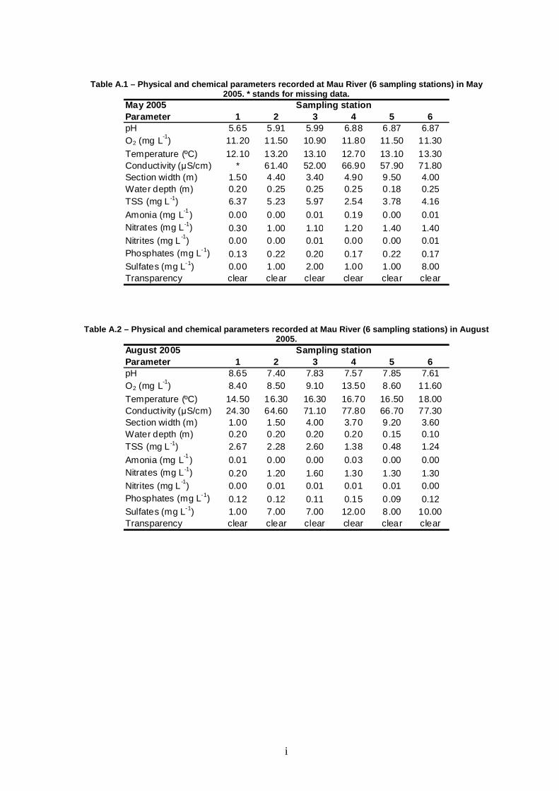
i
Table A.1 – Physical and chemical parameters recorde d at Mau River (6 sampling stations) in May 2005. * stands for missing data.
May 2005Parameter 1 2 3 4 5 6pH 5.65 5.91 5.99 6.88 6.87 6.87O2 (mg L
-1) 11.20 11.50 10.90 11.80 11.50 11.30
Temperature (ºC) 12.10 13.20 13.10 12.70 13.10 13.30Conductivity (µS/cm) * 61.40 52.00 66.90 57.90 71.80Section width (m) 1.50 4.40 3.40 4.90 9.50 4.00Water depth (m) 0.20 0.25 0.25 0.25 0.18 0.25TSS (mg L -1) 6.37 5.23 5.97 2.54 3.78 4.16
Amonia (mg L-1
) 0.00 0.00 0.01 0.19 0.00 0.01Nitrates (mg L -1) 0.30 1.00 1.10 1.20 1.40 1.40Nitrites (mg L
-1) 0.00 0.00 0.01 0.00 0.00 0.01
Phosphates (mg L-1) 0.13 0.22 0.20 0.17 0.22 0.17Sulfates (mg L-1) 0.00 1.00 2.00 1.00 1.00 8.00Transparency clear clear clear clear clear clear
Sampling station
Table A.2 – Physical and chemical parameters recorde d at Mau River (6 sampling stations) in August 2005.
August 2005Parameter 1 2 3 4 5 6pH 8.65 7.40 7.83 7.57 7.85 7.61O2 (mg L
-1) 8.40 8.50 9.10 13.50 8.60 11.60
Temperature (ºC) 14.50 16.30 16.30 16.70 16.50 18.00Conductivity (µS/cm) 24.30 64.60 71.10 77.80 66.70 77.30Section width (m) 1.00 1.50 4.00 3.70 9.20 3.60Water depth (m) 0.20 0.20 0.20 0.20 0.15 0.10TSS (mg L -1) 2.67 2.28 2.60 1.38 0.48 1.24
Amonia (mg L-1
) 0.01 0.00 0.00 0.03 0.00 0.00Nitrates (mg L -1) 0.20 1.20 1.60 1.30 1.30 1.30Nitrites (mg L
-1) 0.00 0.01 0.01 0.01 0.01 0.00
Phosphates (mg L-1) 0.12 0.12 0.11 0.15 0.09 0.12Sulfates (mg L-1) 1.00 7.00 7.00 12.00 8.00 10.00Transparency clear clear clear clear clear clear
Sampling station
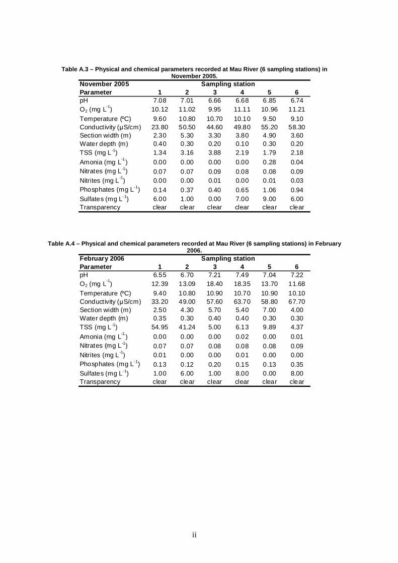
ii
Table A.3 – Physical and chemical parameters recorde d at Mau River (6 sampling stations) in
November 2005. November 2005Parameter 1 2 3 4 5 6pH 7.08 7.01 6.66 6.68 6.85 6.74O2 (mg L
-1) 10.12 11.02 9.95 11.11 10.96 11.21
Temperature (ºC) 9.60 10.80 10.70 10.10 9.50 9.10Conductivity (µS/cm) 23.80 50.50 44.60 49.80 55.20 58.30Section width (m) 2.30 5.30 3.30 3.80 4.90 3.60Water depth (m) 0.40 0.30 0.20 0.10 0.30 0.20TSS (mg L -1) 1.34 3.16 3.88 2.19 1.79 2.18
Amonia (mg L-1
) 0.00 0.00 0.00 0.00 0.28 0.04Nitrates (mg L -1) 0.07 0.07 0.09 0.08 0.08 0.09Nitrites (mg L
-1) 0.00 0.00 0.01 0.00 0.01 0.03
Phosphates (mg L-1) 0.14 0.37 0.40 0.65 1.06 0.94Sulfates (mg L-1) 6.00 1.00 0.00 7.00 9.00 6.00Transparency clear clear clear clear clear clear
Sampling station
Table A.4 – Physical and chemical parameters recorde d at Mau River (6 sampling stations) in February 2006.
February 2006Parameter 1 2 3 4 5 6pH 6.55 6.70 7.21 7.49 7.04 7.22O2 (mg L
-1) 12.39 13.09 18.40 18.35 13.70 11.68
Temperature (ºC) 9.40 10.80 10.90 10.70 10.90 10.10Conductivity (µS/cm) 33.20 49.00 57.60 63.70 58.80 67.70Section width (m) 2.50 4.30 5.70 5.40 7.00 4.00Water depth (m) 0.35 0.30 0.40 0.40 0.30 0.30TSS (mg L -1) 54.95 41.24 5.00 6.13 9.89 4.37
Amonia (mg L-1
) 0.00 0.00 0.00 0.02 0.00 0.01Nitrates (mg L -1) 0.07 0.07 0.08 0.08 0.08 0.09Nitrites (mg L
-1) 0.01 0.00 0.00 0.01 0.00 0.00
Phosphates (mg L-1) 0.13 0.12 0.20 0.15 0.13 0.35Sulfates (mg L-1) 1.00 6.00 1.00 8.00 0.00 8.00Transparency clear clear clear clear clear clear
Sampling station
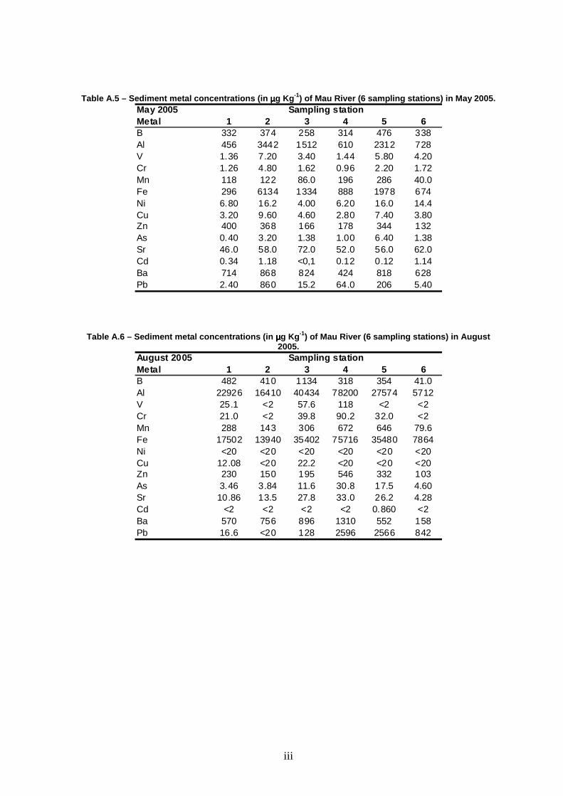
iii
Table A.5 – Sediment metal concentrations (in µµµµg Kg -1) of Mau River (6 sampling stations) in May 2005.
May 2005Metal 1 2 3 4 5 6B 332 374 258 314 476 338Al 456 3442 1512 610 2312 728V 1.36 7.20 3.40 1.44 5.80 4.20Cr 1.26 4.80 1.62 0.96 2.20 1.72Mn 118 122 86.0 196 286 40.0Fe 296 6134 1334 888 1978 674Ni 6.80 16.2 4.00 6.20 16.0 14.4Cu 3.20 9.60 4.60 2.80 7.40 3.80Zn 400 368 166 178 344 132As 0.40 3.20 1.38 1.00 6.40 1.38Sr 46.0 58.0 72.0 52.0 56.0 62.0Cd 0.34 1.18 <0,1 0.12 0.12 1.14Ba 714 868 824 424 818 628Pb 2.40 860 15.2 64.0 206 5.40
Sampling station
Table A.6 – Sediment metal concentrations (in µµµµg Kg -1) of Mau River (6 sampling stations) in August 2005.
August 2005Metal 1 2 3 4 5 6B 482 410 1134 318 354 41.0Al 22926 16410 40434 78200 27574 5712V 25.1 <2 57.6 118 <2 <2Cr 21.0 <2 39.8 90.2 32.0 <2Mn 288 143 306 672 646 79.6Fe 17502 13940 35402 75716 35480 7864Ni <20 <20 <20 <20 <20 <20Cu 12.08 <20 22.2 <20 <20 <20Zn 230 150 195 546 332 103As 3.46 3.84 11.6 30.8 17.5 4.60Sr 10.86 13.5 27.8 33.0 26.2 4.28Cd <2 <2 <2 <2 0.860 <2Ba 570 756 896 1310 552 158Pb 16.6 <20 128 2596 2566 842
Sampling station
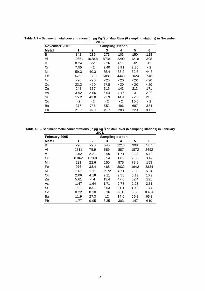
iv
Table A.7 – Sediment metal concentrations (in µµµµg Kg -1) of Mau River (6 sampling stations) in November 2005.
November 2005Metal 1 2 3 4 5 6B 342 236 275 103 150 128Al 10654 1028.8 8734 2290 1218 398V 8.24 <2 9.26 4.53 <2 <2Cr 7.55 <2 9.40 3.91 2.36 <2Mn 59.3 40.3 85.4 33.2 32.5 44.3Fe 4762 1380 5886 4448 2024 748Ni <20 <20 <20 <20 <20 <20Cu 22.2 <20 27.8 <20 <20 <20Zn 248 377 316 143 213 171As 3.92 2.06 6.04 4.17 3 2.90Sr 15.2 43.0 22.9 14.4 22.3 21.6Cd <2 <2 <2 <2 10.6 <2Ba 377 786 552 496 697 384Pb 21.7 <20 49.7 288 220 80.5
Sampling station
Table A.8 – Sediment metal concentrations (in µµµµg Kg -1) of Mau River (6 sampling stations) in February 2006.
February 2005Metal 1 2 3 4 5 6B <20 <20 545 1216 998 587Al 1511 75.9 589 887 1872 2492V 1.52 2.21 0.95 1.71 3.28 5.13Cr 0.862 0.268 0.54 1.09 2.00 3.42Mn 231 22.6 150 875 73.9 153Fe 976 38.4 488 2032 1942 3834Ni 1.61 1.11 0.972 4.71 2.59 5.94Cu 2.06 4.18 2.11 9.58 5.19 10.9Zn 5.61 < 4 13.4 47.0 62.4 121As 1.47 1.64 1.71 2.78 2.23 3.51Sr 7.1 83.1 8.03 21.1 10.2 13.4Cd 0.22 0.10 0.16 0.616 0.30 0.484Ba 11.9 27.3 12 14.0 55.2 65.3Pb 1.77 0.95 8.35 303 147 610
Sampling station
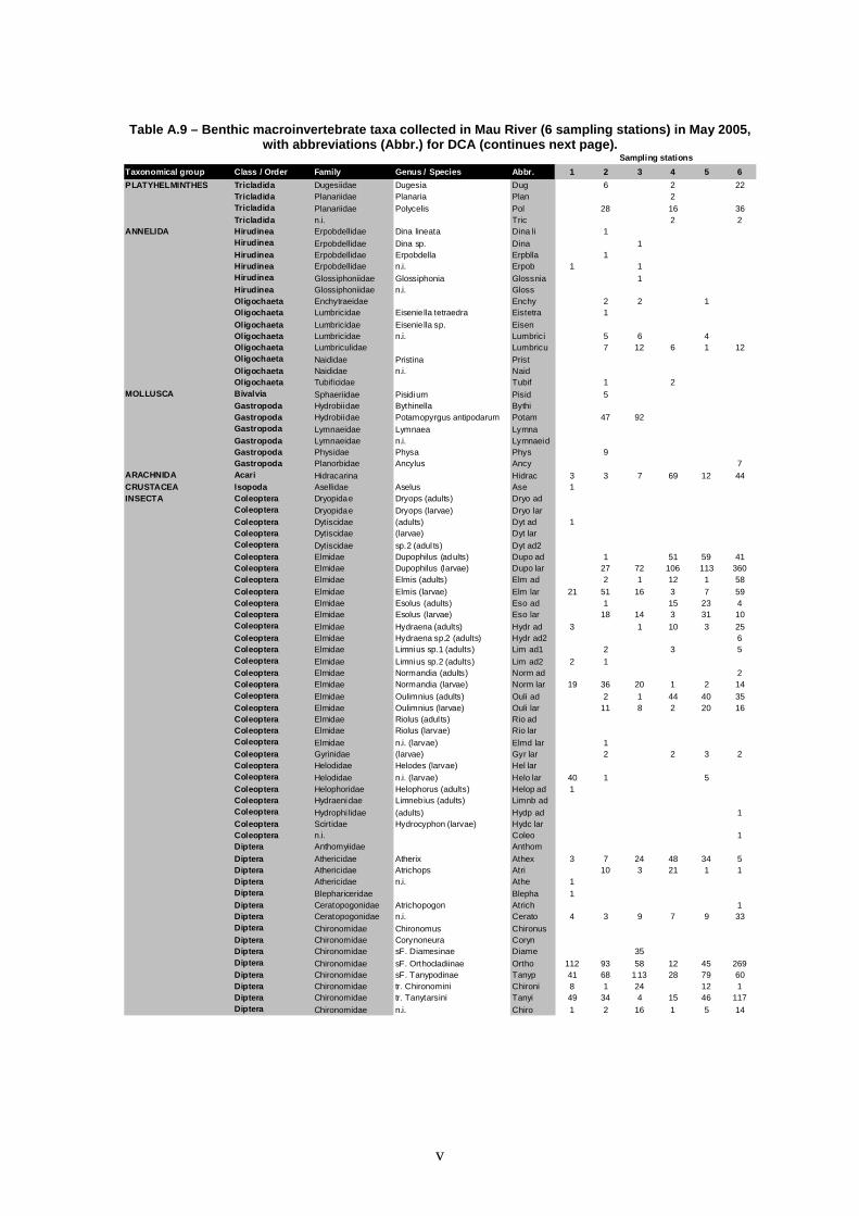
v
Table A.9 – Benthic macroinvertebrate taxa collected in Mau River (6 sampling stations) in Ma y 2005, with abbreviations (Abbr.) for DCA (continues next page).
Taxonomical group Class / Order Family Genus / Species Abbr. 1 2 3 4 5 6
PLATYHELMINTHES Tricladida Dugesiidae Dugesia Dug 6 2 22Tricladida Planariidae Planaria Plan 2Tricladida Planariidae Polycelis Pol 28 16 36Tricladida n.i. Tric 2 2
ANNELIDA Hirudinea Erpobdellidae Dina lineata Dina li 1Hirudinea Erpobdellidae Dina sp. Dina 1Hirudinea Erpobdellidae Erpobdella Erpblla 1Hirudinea Erpobdellidae n.i. Erpob 1 1Hirudinea Glossiphoniidae Glossiphonia Glossnia 1Hirudinea Glossiphoniidae n.i. GlossOligochaeta Enchytraeidae Enchy 2 2 1Oligochaeta Lumbricidae Eiseniella tetraedra Eistetra 1
Oligochaeta Lumbricidae Eiseniella sp. EisenOligochaeta Lumbricidae n.i. Lumbrici 5 6 4Oligochaeta Lumbriculidae Lumbricu 7 12 6 1 12Oligochaeta Naididae Pristina PristOligochaeta Naididae n.i. NaidOligochaeta Tubificidae Tubif 1 2
MOLLUSCA Bivalvia Sphaeriidae Pisidium Pisid 5Gastropoda Hydrobiidae Bythinella BythiGastropoda Hydrobiidae Potamopyrgus antipodarum Potam 47 92Gastropoda Lymnaeidae Lymnaea LymnaGastropoda Lymnaeidae n.i. LymnaeidGastropoda Physidae Physa Phys 9Gastropoda Planorbidae Ancylus Ancy 7
ARACHNIDA Acari Hidracarina Hidrac 3 3 7 69 12 44CRUSTACEA Isopoda Asellidae Aselus Ase 1INSECTA Coleoptera Dryopidae Dryops (adults) Dryo ad
Coleoptera Dryopidae Dryops (larvae) Dryo larColeoptera Dytiscidae (adults) Dyt ad 1Coleoptera Dytiscidae (larvae) Dyt larColeoptera Dytiscidae sp.2 (adul ts) Dyt ad2Coleoptera Elmidae Dupophilus (adults) Dupo ad 1 51 59 41Coleoptera Elmidae Dupophilus (larvae) Dupo lar 27 72 106 113 360Coleoptera Elmidae Elmis (adults) Elm ad 2 1 12 1 58Coleoptera Elmidae Elmis (larvae) Elm lar 21 51 16 3 7 59Coleoptera Elmidae Esolus (adults) Eso ad 1 15 23 4Coleoptera Elmidae Esolus (larvae) Eso lar 18 14 3 31 10Coleoptera Elmidae Hydraena (adults) Hydr ad 3 1 10 3 25Coleoptera Elmidae Hydraena sp.2 (adults) Hydr ad2 6Coleoptera Elmidae Limnius sp.1 (adults) Lim ad1 2 3 5Coleoptera Elmidae Limnius sp.2 (adults) Lim ad2 2 1Coleoptera Elmidae Normandia (adults) Norm ad 2Coleoptera Elmidae Normandia (larvae) Norm lar 19 36 20 1 2 14Coleoptera Elmidae Oulimnius (adults) Ouli ad 2 1 44 40 35Coleoptera Elmidae Oulimnius (larvae) Ouli lar 11 8 2 20 16Coleoptera Elmidae Riolus (adul ts) Rio adColeoptera Elmidae Riolus (larvae) Rio larColeoptera Elmidae n.i. (larvae) Elmd lar 1Coleoptera Gyrinidae (larvae) Gyr lar 2 2 3 2Coleoptera Helodidae Helodes (larvae) Hel larColeoptera Helodidae n.i. (larvae) Helo lar 40 1 5Coleoptera Helophoridae Helophorus (adults) Helop ad 1Coleoptera Hydraenidae Limnebius (adults) Limnb adColeoptera Hydrophi lidae (adults) Hydp ad 1Coleoptera Scirtidae Hydrocyphon (larvae) Hydc larColeoptera n.i. Coleo 1Diptera Anthomyiidae Anthom
Diptera Athericidae Atherix Athex 3 7 24 48 34 5Diptera Athericidae Atrichops Atri 10 3 21 1 1Diptera Athericidae n.i. Athe 1Diptera Blephariceridae Blepha 1Diptera Ceratopogonidae Atrichopogon Atrich 1Diptera Ceratopogonidae n.i. Cerato 4 3 9 7 9 33Diptera Chironomidae Chironomus ChironusDiptera Chironomidae Corynoneura CorynDiptera Chironomidae sF. Diamesinae Diame 35Diptera Chironomidae sF. Orthocladiinae Ortho 112 93 58 12 45 269Diptera Chironomidae sF. Tanypodinae Tanyp 41 68 113 28 79 60Diptera Chironomidae tr. Chironomini Chironi 8 1 24 12 1Diptera Chironomidae tr. Tanytarsini Tanyi 49 34 4 15 46 117Diptera Chironomidae n.i. Chiro 1 2 16 1 5 14
Sampling stations

vi
Taxonomical group Class / Order Family Genus / Species Abbr. 1 2 3 4 5 6
Diptera Dixidae Dixa Dixa 1 1Diptera Dixidae Dixella DixllaDiptera Dixidae n.i. DixiDiptera Dolichopodidae Dolich 5Diptera Empididae sF. Hemerodromiinae Hemer 6 2 10 21 12Diptera Empididae Chelifera ChelifDiptera Empididae sF. Atalantinae Atala 1Diptera Limoniidae Eloeophila EloeDiptera Limoniidae Hexatoma Hexat 1 1Diptera Limoniidae Rhypholophus RhyphDiptera Limoniidae Scleroprocta Scler 1Diptera Limoniidae n.i. Limo 2Diptera Pediciidae Dicranota DicraDiptera Psychodidae Psycho 1Diptera Psychodidae sp. 2 Psycho2Diptera Simuliidae Simu 6 35 3 29 696 46Diptera Tabanidae Taba 1Diptera Tipulidae Tipula TipulDiptera Tipulidae sp2 Tipul2Diptera Tipulidae n.i. Tipu 1Diptera n.i. Dipt 13 11 7 2 1 87Ephemeroptera Baetidae Baetis Btis 7 16 4 16 18 9Ephemeroptera Baetidae n.i. Baet 4 4 10 1 8 3
Ephemeroptera Caenidae Caenis Caen 3 2 1Ephemeroptera Ephemerellidae Ephemerella Ephella 45 171 46 12 144 43Ephemeroptera Ephemerellidae n.i. EphemellEphemeroptera Ephemeridae Ephemera Ephemra 66 42 5Ephemeroptera Heptageniidae Ecdyonurus Ecdy 3Ephemeroptera Heptageniidae Epeorus Epeo 4 36 1 6 31 28Ephemeroptera Heptageniidae n.i. Hepta 3 8 1 4 2Ephemeroptera Leptophlebiidae Centroptilum CentropEphemeroptera Leptophlebiidae Habrophlebia Habrop 8 7 1 1Ephemeroptera Leptophlebiidae Paraleptophleb ia Paralep 7 5 7 6Ephemeroptera Leptophlebiidae n.i. Lepto 17 4 32 3Ephemeroptera n.i. Ephem 24 101 25 4 43 2Heteroptera Gerridae Gerris GerrHeteroptera Mesoveliidae Mesovelia MesoHeteroptera Notonectidae Notonecta NotoMegaloptera Sialidae Sialis Sai 1Odonata Aeshnidae Aesh 2 9 29 2Odonata Calopterygidae Agrion Agr 2 7 2Odonata Cordulegasteridae Cordulegaster Cordu 6 7 5 6 1Odonata Gomphidae Gomp 1 2 27 8Odonata Libellulidae LibellOdonata Platycnemididae Platycnemis PlatycOdonata n.i. Odo 1 1 3
Plecoptera Chloroperlidae Chloro 22 1Plecoptera Leuctridae Leuc 106 173 82 57 46 8Plecoptera Nemouridae Amphinemura AmphiPlecoptera Nemouridae Nemoura NemPlecoptera Nemouridae Protonemura Proton 16 4 5 56 2Plecoptera Nemouridae n.i. Nemae 1Plecoptera Perlidae Perla Per 1Plecoptera Perlodidae PerloPlecoptera n.i. PlecTrichoptera Beraeidae Bera 4 1Trichoptera Brachycentridae Brachy 4 3Trichoptera Calamoceratidae Calam 4Trichoptera Glossosomatidae Glosso 9 13 12 163 285 74Trichoptera Goeridae Goe 1Trichoptera Helicopsychidae HelicTrichoptera Hydropsychidae Hydrpsy 11 18 13 2 6 18Trichoptera Hydroptilidae Hydrop 1Trichoptera Lepidostomatidae Lepid 1Trichoptera Leptoceridae LeptcTrichoptera Limnephilidae sF. Limnephilinae Limnen 28 1Trichoptera Limnephilidae tr. Limnephilini LimniTrichoptera Limnephilidae n.i. Limnep 2 1Trichoptera Odontoceridae Odontocerum Odont
Trichoptera Philopotamidae Philo 13 6 1 1 1Trichoptera Polycentropodidae Polycen 5 4 1 6 4Trichoptera Psychomyiidae Psych 2 4 3Trichoptera Rhyacophilidae Ryacophila Rya 3 19 10 4 4Trichoptera Sericostomatidae Seri 1 9 12 28 2 4Trichoptera Thremmatidae Thremma Thre 39 3 3 1 3Trichoptera n.i. Tricho 1 8 3 1 1 4

vii
Table A.10 – Benthic macroinvertebrates taxa collected in Mau River (6 sampling stations) in Au gust 2005, with abbreviations (Abbr.) for DCA (continues next page).
Taxonomical group Class / Order Family Genus / Species Abbr. 1 2 3 4 5 6
PLATYHELMINTHES Tricladida Dugesiidae Dugesia Dug 10 1 4 14Tricladida Planariidae Planaria PlanTricladida Planariidae Polycelis Pol 308 1 8 28Tricladida n.i. Tric
ANNELIDA Hirudinea Erpobdellidae Dina lineata Dina liHirudinea Erpobdellidae Dina sp. DinaHirudinea Erpobdellidae Erpobdella ErpbllaHirudinea Erpobdellidae n.i. ErpobHirudinea Glossiphoniidae Glossiphonia Glossnia 1Hirudinea Glossiphoniidae n.i. Gloss 1Oligochaeta Enchytraeidae Enchy 2 1Oligochaeta Lumbricidae Eiseniella tetraedra Eistetra 1
Oligochaeta Lumbricidae Eiseniella sp. Eisen 1 4Oligochaeta Lumbricidae n.i. LumbriciOligochaeta Lumbriculidae Lumbricu 7 2 18 1Oligochaeta Naididae Pristina Prist 3Oligochaeta Naididae n.i. Naid 1Oligochaeta Tubificidae Tubif 2 43 1
MOLLUSCA Bivalvia Sphaeriidae Pisidium Pisid 2Gastropoda Hydrobiidae Bythinella BythiGastropoda Hydrobiidae Potamopyrgus antipodarum Potam 89 61Gastropoda Lymnaeidae Lymnaea LymnaGastropoda Lymnaeidae n.i. Lymnaeid 2Gastropoda Physidae Physa Phys 20Gastropoda Planorbidae Ancylus Ancy 1
ARACHNIDA Acari Hidracarina Hidrac 6 3CRUSTACEA Isopoda Asellidae Aselus AseINSECTA Coleoptera Dryopidae Dryops (adults) Dryo ad
Coleoptera Dryopidae Dryops (larvae) Dryo larColeoptera Dytiscidae (adults) Dyt adColeoptera Dytiscidae (larvae) Dyt lar 1 4Coleoptera Dytiscidae sp.2 (adul ts) Dyt ad2 2 2Coleoptera Elmidae Dupophilus (adults) Dupo ad 1 4 3 72Coleoptera Elmidae Dupophilus (larvae) Dupo lar 31 19 46 13 274Coleoptera Elmidae Elmis (adults) Elm ad 2 6 175Coleoptera Elmidae Elmis (larvae) Elm lar 6 2 26 252Coleoptera Elmidae Esolus (adults) Eso ad 1 6Coleoptera Elmidae Esolus (larvae) Eso lar 1 3 5 10 10Coleoptera Elmidae Hydraena (adults) Hydr ad 1 41Coleoptera Elmidae Hydraena sp.2 (adults) Hydr ad2Coleoptera Elmidae Limnius sp.1 (adults) Lim ad1 9Coleoptera Elmidae Limnius sp.2 (adults) Lim ad2Coleoptera Elmidae Normandia (adults) Norm ad 4Coleoptera Elmidae Normandia (larvae) Norm lar 3 12 1 11Coleoptera Elmidae Oulimnius (adults) Ouli ad 1 4 5 84Coleoptera Elmidae Oulimnius (larvae) Ouli lar 1 3 6 15 11Coleoptera Elmidae Riolus (adul ts) Rio adColeoptera Elmidae Riolus (larvae) Rio lar 2Coleoptera Elmidae n.i. (larvae) Elmd larColeoptera Gyrinidae (larvae) Gyr lar 4 4 1Coleoptera Helodidae Helodes (larvae) Hel larColeoptera Helodidae n.i. (larvae) Helo larColeoptera Helophoridae Helophorus (adults) Helop adColeoptera Hydraenidae Limnebius (adults) Limnb adColeoptera Hydrophi lidae (adults) Hydp adColeoptera Scirtidae Hydrocyphon (larvae) Hydc larColeoptera n.i. ColeoDiptera Anthomyiidae Anthom 1
Diptera Athericidae Atherix Athex 15 45 9 4Diptera Athericidae Atrichops Atri 5 3 4Diptera Athericidae n.i. AtheDiptera Blephariceridae BlephaDiptera Ceratopogonidae Atrichopogon Atrich 1Diptera Ceratopogonidae n.i. CeratoDiptera Chironomidae Chironomus Chironus 339Diptera Chironomidae Corynoneura CorynDiptera Chironomidae sF. Diamesinae Diame 9 5Diptera Chironomidae sF. Orthocladiinae Ortho 152 88 30 35 5 28Diptera Chironomidae sF. Tanypodinae Tanyp 128 156 64 80 53 17Diptera Chironomidae tr. Chironomini Chironi 301 113 15 29 41 8Diptera Chironomidae tr. Tanytarsini Tanyi 48 273 42 218 15 39Diptera Chironomidae n.i. Chiro 1 3
Sampling stations
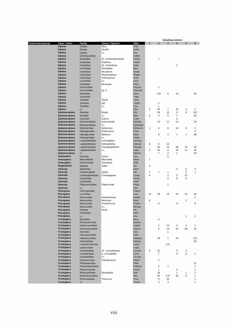
viii
Taxonomical group Class / Order Family Genus / Species Abbr. 1 2 3 4 5 6Diptera Dixidae Dixa DixaDiptera Dixidae Dixella DixllaDiptera Dixidae n.i. DixiDiptera Dolichopodidae DolichDiptera Empididae sF. Hemerodromiinae Hemer 1Diptera Empididae Chelifera ChelifDiptera Empididae sF. Atalantinae Atala 2Diptera Limoniidae Eloeophila EloeDiptera Limoniidae Hexatoma HexatDiptera Limoniidae Rhypholophus RhyphDiptera Limoniidae Scleroprocta SclerDiptera Limoniidae n.i. LimoDiptera Pediciidae Dicranota DicraDiptera Psychodidae Psycho 1Diptera Psychodidae sp. 2 Psycho2Diptera Simuliidae Simu 116 5 16 65Diptera Tabanidae TabaDiptera Tipulidae Tipula TipulDiptera Tipulidae sp2 Tipul2 2Diptera Tipulidae n.i. Tipu 1Diptera n.i. Dipt 5 95 7 20 3 2Ephemeroptera Baetidae Baetis Btis 94 10 8 6 422Ephemeroptera Baetidae n.i. Baet 2 3 5 7 55Ephemeroptera Caenidae Caenis Caen 3Ephemeroptera Ephemerellidae Ephemerella Ephella 27 12 12 18Ephemeroptera Ephemerellidae n.i. EphemellEphemeroptera Ephemeridae Ephemera Ephemra 1 4 6 13 5 2Ephemeroptera Heptageniidae Ecdyonurus Ecdy 3Ephemeroptera Heptageniidae Epeorus Epeo 8 3 1 1 88Ephemeroptera Heptageniidae n.i. HeptaEphemeroptera Leptophlebiidae Centroptilum CentropEphemeroptera Leptophlebiidae Habrophlebia Habrop 8 3 12Ephemeroptera Leptophlebiidae Paraleptophleb ia Paralep 62 10 58 19 52Ephemeroptera Leptophlebiidae n.i. Lepto 3 24 6 23 11 16Ephemeroptera n.i. Ephem 7 2 2 25Heteroptera Gerridae Gerris Gerr 5Heteroptera Mesoveliidae Mesovelia Meso 1Heteroptera Notonectidae Notonecta NotoMegaloptera Sialidae Sialis Sai 5Odonata Aeshnidae Aesh 3 6 4Odonata Calopterygidae Agrion Agr 1 1 1 3 1Odonata Cordulegasteridae Cordulegaster Cordu 4 2 2 37Odonata Gomphidae Gomp 2 5 9Odonata Libellulidae LibellOdonata Platycnemididae Platycnemis Platyc 1
Odonata n.i. OdoPlecoptera Chloroperlidae ChloroPlecoptera Leuctridae Leuc 15 39 19 54 10 83Plecoptera Nemouridae Amphinemura Amphi 2Plecoptera Nemouridae Nemoura Nem 6 1Plecoptera Nemouridae Protonemura Proton 6 17 8Plecoptera Nemouridae n.i. NemaePlecoptera Perlidae Perla PerPlecoptera Perlodidae PerloPlecoptera n.i. Plec 1 2Trichoptera Beraeidae Bera 5Trichoptera Brachycentridae BrachyTrichoptera Calamoceratidae Calam 2 13 4 4 1Trichoptera Glossosomatidae Glosso 5 16 42 85 15Trichoptera Goeridae Goe 1Trichoptera Helicopsychidae HelicTrichoptera Hydropsychidae Hydrpsy 20 1 24 214Trichoptera Hydroptilidae Hydrop 83Trichoptera Lepidostomatidae Lepid 101Trichoptera Leptoceridae LeptcTrichoptera Limnephilidae sF. Limnephilinae Limnen 4 22 5 3Trichoptera Limnephilidae tr. Limnephilini Limni 7 9 3 2Trichoptera Limnephilidae n.i. Limnep
Trichoptera Odontoceridae Odontocerum Odont 2Trichoptera Philopotamidae Philo 11Trichoptera Polycentropodidae Polycen 2 1 2Trichoptera Psychomyiidae Psych 1 3 2Trichoptera Rhyacophilidae Ryacophila Rya 18 1 1 1Trichoptera Sericostomatidae Seri 92 137 50 6 1Trichoptera Thremmatidae Thremma Thre 9 30 2Trichoptera n.i. Tricho 3 3 1
Sampling stations

ix
Table A.11 – Benthic macroinvertebrates taxa collected in Mau River (6 sampling stations) in November 2005, with abbreviations (Abbr.) for DCA ( continues next page).
Taxonomical group Class / Order Family Genus / Species Abbr. 1 2 3 4 5 6
PLATYHELMINTHES Tricladida Dugesiidae Dugesia Dug 13 26Tricladida Planariidae Planaria PlanTricladida Planariidae Polycelis Pol 144 1 9Tricladida n.i. Tric 1
ANNELIDA Hirudinea Erpobdellidae Dina lineata Dina liHirudinea Erpobdellidae Dina sp. DinaHirudinea Erpobdellidae Erpobdella ErpbllaHirudinea Erpobdellidae n.i. ErpobHirudinea Glossiphoniidae Glossiphonia Glossnia 4Hirudinea Glossiphoniidae n.i. GlossOligochaeta Enchytraeidae Enchy 7 4 1 2Oligochaeta Lumbricidae Eiseniella tetraedra Eistetra
Oligochaeta Lumbricidae Eiseniella sp. EisenOligochaeta Lumbricidae n.i. Lumbrici 5 1 1Oligochaeta Lumbriculidae Lumbricu 23 48 7 43 149Oligochaeta Naididae Pristina PristOligochaeta Naididae n.i. Naid 5 1 3 3Oligochaeta Tubificidae Tubif 4 5 6 20 7 2
MOLLUSCA Bivalvia Sphaeriidae Pisidium Pisid 1 1Gastropoda Hydrobiidae Bythinella Bythi 5 1Gastropoda Hydrobiidae Potamopyrgus antipodarum Potam 157 72Gastropoda Lymnaeidae Lymnaea Lymna 2Gastropoda Lymnaeidae n.i. LymnaeidGastropoda Physidae Physa Phys 80 1Gastropoda Planorbidae Ancylus Ancy
ARACHNIDA Acari Hidracarina Hidrac 15CRUSTACEA Isopoda Asellidae Aselus AseINSECTA Coleoptera Dryopidae Dryops (adults) Dryo ad 1
Coleoptera Dryopidae Dryops (larvae) Dryo larColeoptera Dytiscidae (adults) Dyt adColeoptera Dytiscidae (larvae) Dyt larColeoptera Dytiscidae sp.2 (adul ts) Dyt ad2 1Coleoptera Elmidae Dupophilus (adults) Dupo ad 19Coleoptera Elmidae Dupophilus (larvae) Dupo lar 22 14 6 8 176Coleoptera Elmidae Elmis (adults) Elm ad 6 12Coleoptera Elmidae Elmis (larvae) Elm lar 11 21 1 9 3 135Coleoptera Elmidae Esolus (adults) Eso ad 4Coleoptera Elmidae Esolus (larvae) Eso lar 8 1 14 16Coleoptera Elmidae Hydraena (adults) Hydr ad 1 7Coleoptera Elmidae Hydraena sp.2 (adults) Hydr ad2Coleoptera Elmidae Limnius sp.1 (adults) Lim ad1 1 4Coleoptera Elmidae Limnius sp.2 (adults) Lim ad2Coleoptera Elmidae Normandia (adults) Norm adColeoptera Elmidae Normandia (larvae) Norm lar 4 2 4 3 2 13Coleoptera Elmidae Oulimnius (adults) Ouli ad 1Coleoptera Elmidae Oulimnius (larvae) Ouli lar 2 3 3 76 10 143Coleoptera Elmidae Riolus (adul ts) Rio ad 1Coleoptera Elmidae Riolus (larvae) Rio larColeoptera Elmidae n.i. (larvae) Elmd larColeoptera Gyrinidae (larvae) Gyr lar 2 3 2 4Coleoptera Helodidae Helodes (larvae) Hel lar 1Coleoptera Helodidae n.i. (larvae) Helo larColeoptera Helophoridae Helophorus (adults) Helop adColeoptera Hydraenidae Limnebius (adults) Limnb ad 1Coleoptera Hydrophi lidae (adults) Hydp ad 1Coleoptera Scirtidae Hydrocyphon (larvae) Hydc lar 39 1 1Coleoptera n.i. ColeoDiptera Anthomyiidae Anthom
Diptera Athericidae Atherix Athex 1 7 19 7 11Diptera Athericidae Atrichops Atri 2 11 42 26 2Diptera Athericidae n.i. AtheDiptera Blephariceridae BlephaDiptera Ceratopogonidae Atrichopogon AtrichDiptera Ceratopogonidae n.i. Cerato 4 1Diptera Chironomidae Chironomus ChironusDiptera Chironomidae Corynoneura Coryn 2Diptera Chironomidae sF. Diamesinae Diame 7Diptera Chironomidae sF. Orthocladiinae Ortho 171 20 18 81 2 12Diptera Chironomidae sF. Tanypodinae Tanyp 38 17 10 15 14 1Diptera Chironomidae tr. Chironomini Chironi 60 1 2 36 5 3Diptera Chironomidae tr. Tanytarsini Tanyi 201 13 13 202 16 3Diptera Chironomidae n.i. Chiro
Sampling stations

x
Taxonomical group Class / Order Family Genus / Species Abbr. 1 2 3 4 5 6Diptera Dixidae Dixa Dixa 1 1 5 1Diptera Dixidae Dixella Dixlla 6Diptera Dixidae n.i. Dixi 1Diptera Dolichopodidae Dolich 1 1Diptera Empididae sF. Hemerodromiinae Hemer 1 1 3 1Diptera Empididae Chelifera Chelif 3Diptera Empididae sF. Atalantinae Atala 1Diptera Limoniidae Eloeophila Eloe 2Diptera Limoniidae Hexatoma Hexat 1 1Diptera Limoniidae Rhypholophus RhyphDiptera Limoniidae Scleroprocta SclerDiptera Limoniidae n.i. LimoDiptera Pediciidae Dicranota Dicra 1Diptera Psychodidae Psycho 1Diptera Psychodidae sp. 2 Psycho2 2Diptera Simuliidae Simu 105 9 12 2 54Diptera Tabanidae TabaDiptera Tipulidae Tipula Tipul 1 1 1Diptera Tipulidae sp2 Tipul2Diptera Tipulidae n.i. Tipu 1Diptera n.i. Dipt 11 3 1 23 1Ephemeroptera Baetidae Baetis Btis 15 258 50 9 66Ephemeroptera Baetidae n.i. Baet 3 8 4 7 1 8Ephemeroptera Caenidae Caenis Caen 1 14 9Ephemeroptera Ephemerellidae Ephemerella Ephella 25 70 23 7 2 59Ephemeroptera Ephemerellidae n.i. EphemellEphemeroptera Ephemeridae Ephemera Ephemra 2 4 69 39 94 84Ephemeroptera Heptageniidae Ecdyonurus Ecdy 16 1Ephemeroptera Heptageniidae Epeorus Epeo 2 38 4 38Ephemeroptera Heptageniidae n.i. Hepta 1 2Ephemeroptera Leptophlebiidae Centroptilum CentropEphemeroptera Leptophlebiidae Habrophlebia HabropEphemeroptera Leptophlebiidae Paraleptophleb ia Paralep 55 1227 67 132 146 368Ephemeroptera Leptophlebiidae n.i. Lepto 20 88 43 88 33 62Ephemeroptera n.i. EphemHeteroptera Gerridae Gerris Gerr 4 5 3Heteroptera Mesoveliidae Mesovelia MesoHeteroptera Notonectidae Notonecta Noto 1Megaloptera Sialidae Sialis Sai 3 1Odonata Aeshnidae Aesh 3 1 19 6 8Odonata Calopterygidae Agrion Agr 14 5 6 13 3 4Odonata Cordulegasteridae Cordulegaster Cordu 6 3 38 12 3Odonata Gomphidae Gomp 3 3 50 11 6Odonata Libellulidae Libell 1Odonata Platycnemididae Platycnemis Platyc 3
Odonata n.i. OdoPlecoptera Chloroperlidae Chloro 3Plecoptera Leuctridae Leuc 15 1 1 1 6 7Plecoptera Nemouridae Amphinemura Amphi 1 2Plecoptera Nemouridae Nemoura Nem 1 6 1 4Plecoptera Nemouridae Protonemura Proton 36 3 1 1Plecoptera Nemouridae n.i. NemaePlecoptera Perlidae Perla PerPlecoptera Perlodidae PerloPlecoptera n.i. PlecTrichoptera Beraeidae BeraTrichoptera Brachycentridae BrachyTrichoptera Calamoceratidae Calam 3 165 100 32Trichoptera Glossosomatidae Glosso 44 12 97 1 13Trichoptera Goeridae Goe 2 2Trichoptera Helicopsychidae HelicTrichoptera Hydropsychidae Hydrpsy 3 51 8 4 3 37Trichoptera Hydroptilidae Hydrop 6 2 1Trichoptera Lepidostomatidae Lepid 9Trichoptera Leptoceridae Leptc 8 2Trichoptera Limnephilidae sF. Limnephilinae Limnen 44 2 6Trichoptera Limnephilidae tr. Limnephilini Limni 37 40 5Trichoptera Limnephilidae n.i. Limnep
Trichoptera Odontoceridae Odontocerum OdontTrichoptera Philopotamidae Philo 11 33 1 5 4Trichoptera Polycentropodidae Polycen 1 1 3Trichoptera Psychomyiidae Psych 19 5 19 1 1Trichoptera Rhyacophilidae Ryacophila Rya 24 5 1Trichoptera Sericostomatidae Seri 14 29 42 15 71 40Trichoptera Thremmatidae Thremma Thre 14 2 3 2Trichoptera n.i. Tricho 5 1 1 1
Sampling stations
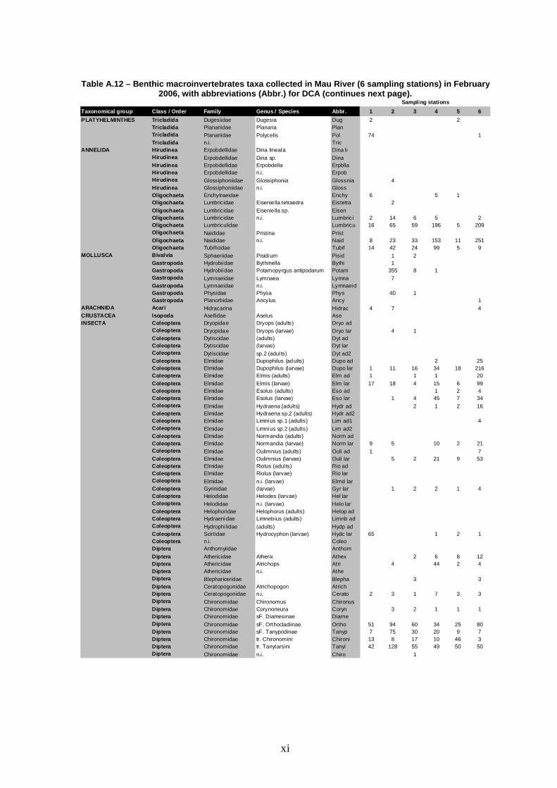
xi
Table A.12 – Benthic macroinvertebrates taxa collected in Mau River (6 sampling stations) in Fe bruary 2006, with abbreviations (Abbr.) for DCA (continues next page).
Taxonomical group Class / Order Family Genus / Species Abbr. 1 2 3 4 5 6
PLATYHELMINTHES Tricladida Dugesiidae Dugesia Dug 2 2Tricladida Planariidae Planaria PlanTricladida Planariidae Polycelis Pol 74 1Tricladida n.i. Tric
ANNELIDA Hirudinea Erpobdellidae Dina lineata Dina liHirudinea Erpobdellidae Dina sp. DinaHirudinea Erpobdellidae Erpobdella ErpbllaHirudinea Erpobdellidae n.i. ErpobHirudinea Glossiphoniidae Glossiphonia Glossnia 4Hirudinea Glossiphoniidae n.i. GlossOligochaeta Enchytraeidae Enchy 6 5 1Oligochaeta Lumbricidae Eiseniella tetraedra Eistetra 2
Oligochaeta Lumbricidae Eiseniella sp. EisenOligochaeta Lumbricidae n.i. Lumbrici 2 14 6 5 2Oligochaeta Lumbriculidae Lumbricu 16 65 59 196 5 209Oligochaeta Naididae Pristina PristOligochaeta Naididae n.i. Naid 8 23 33 153 11 251Oligochaeta Tubificidae Tubif 14 42 24 99 5 9
MOLLUSCA Bivalvia Sphaeriidae Pisidium Pisid 1 2Gastropoda Hydrobiidae Bythinella Bythi 1Gastropoda Hydrobiidae Potamopyrgus antipodarum Potam 355 8 1Gastropoda Lymnaeidae Lymnaea Lymna 7Gastropoda Lymnaeidae n.i. LymnaeidGastropoda Physidae Physa Phys 40 1Gastropoda Planorbidae Ancylus Ancy 1
ARACHNIDA Acari Hidracarina Hidrac 4 7 4CRUSTACEA Isopoda Asellidae Aselus AseINSECTA Coleoptera Dryopidae Dryops (adults) Dryo ad
Coleoptera Dryopidae Dryops (larvae) Dryo lar 4 1Coleoptera Dytiscidae (adults) Dyt adColeoptera Dytiscidae (larvae) Dyt larColeoptera Dytiscidae sp.2 (adul ts) Dyt ad2Coleoptera Elmidae Dupophilus (adults) Dupo ad 2 25Coleoptera Elmidae Dupophilus (larvae) Dupo lar 1 11 16 34 18 216Coleoptera Elmidae Elmis (adults) Elm ad 1 1 1 20Coleoptera Elmidae Elmis (larvae) Elm lar 17 18 4 15 6 99Coleoptera Elmidae Esolus (adults) Eso ad 1 2 4Coleoptera Elmidae Esolus (larvae) Eso lar 1 4 45 7 34Coleoptera Elmidae Hydraena (adults) Hydr ad 2 1 2 16Coleoptera Elmidae Hydraena sp.2 (adults) Hydr ad2Coleoptera Elmidae Limnius sp.1 (adults) Lim ad1 4Coleoptera Elmidae Limnius sp.2 (adults) Lim ad2Coleoptera Elmidae Normandia (adults) Norm adColeoptera Elmidae Normandia (larvae) Norm lar 9 5 10 2 21Coleoptera Elmidae Oulimnius (adults) Ouli ad 1 7Coleoptera Elmidae Oulimnius (larvae) Ouli lar 5 2 21 9 53Coleoptera Elmidae Riolus (adul ts) Rio adColeoptera Elmidae Riolus (larvae) Rio larColeoptera Elmidae n.i. (larvae) Elmd larColeoptera Gyrinidae (larvae) Gyr lar 1 2 2 1 4Coleoptera Helodidae Helodes (larvae) Hel larColeoptera Helodidae n.i. (larvae) Helo larColeoptera Helophoridae Helophorus (adults) Helop adColeoptera Hydraenidae Limnebius (adults) Limnb adColeoptera Hydrophi lidae (adults) Hydp adColeoptera Scirtidae Hydrocyphon (larvae) Hydc lar 65 1 2 1Coleoptera n.i. ColeoDiptera Anthomyiidae Anthom
Diptera Athericidae Atherix Athex 2 6 8 12Diptera Athericidae Atrichops Atri 4 44 2 4Diptera Athericidae n.i. AtheDiptera Blephariceridae Blepha 3 3Diptera Ceratopogonidae Atrichopogon AtrichDiptera Ceratopogonidae n.i. Cerato 2 3 1 7 3 3Diptera Chironomidae Chironomus ChironusDiptera Chironomidae Corynoneura Coryn 3 2 1 1 1Diptera Chironomidae sF. Diamesinae DiameDiptera Chironomidae sF. Orthocladiinae Ortho 51 94 60 34 25 80Diptera Chironomidae sF. Tanypodinae Tanyp 7 75 30 20 9 7Diptera Chironomidae tr. Chironomini Chironi 13 8 17 10 46 3Diptera Chironomidae tr. Tanytarsini Tanyi 42 128 55 49 50 50Diptera Chironomidae n.i. Chiro 1
Sampling stations

xii
Taxonomical group Class / Order Family Genus / Species Abbr. 1 2 3 4 5 6Diptera Dixidae Dixa DixaDiptera Dixidae Dixella DixllaDiptera Dixidae n.i. DixiDiptera Dolichopodidae Dolich 1 2 2 2Diptera Empididae sF. Hemerodromiinae Hemer 3 1 4 8 2Diptera Empididae Chelifera ChelifDiptera Empididae sF. Atalantinae AtalaDiptera Limoniidae Eloeophila Eloe 1Diptera Limoniidae Hexatoma Hexat 2 1Diptera Limoniidae Rhypholophus Rhyph 1Diptera Limoniidae Scleroprocta Scler 1Diptera Limoniidae n.i. Limo 1 1 1Diptera Pediciidae Dicranota DicraDiptera Psychodidae Psycho 1 2Diptera Psychodidae sp. 2 Psycho2Diptera Simuliidae Simu 7 544 22 10 42 86Diptera Tabanidae TabaDiptera Tipulidae Tipula Tipul 1Diptera Tipulidae sp2 Tipul2Diptera Tipulidae n.i. TipuDiptera n.i. Dipt 4 2 7 4 1 16Ephemeroptera Baetidae Baetis Btis 23 116 77 32 37 219Ephemeroptera Baetidae n.i. Baet 14 7 2 12Ephemeroptera Caenidae Caenis Caen 4 1 2 1 12Ephemeroptera Ephemerellidae Ephemerella Ephella 55 106 36 7 19 74Ephemeroptera Ephemerellidae n.i. Ephemell 2Ephemeroptera Ephemeridae Ephemera Ephemra 11 16 48 1 7Ephemeroptera Heptageniidae Ecdyonurus Ecdy 4 1Ephemeroptera Heptageniidae Epeorus Epeo 6 20Ephemeroptera Heptageniidae n.i. HeptaEphemeroptera Leptophlebiidae Centroptilum Centrop 2Ephemeroptera Leptophlebiidae Habrophlebia HabropEphemeroptera Leptophlebiidae Paraleptophleb ia Paralep 21 1001 31 50 61 82Ephemeroptera Leptophlebiidae n.i. Lepto 8 84 4 2 9 13Ephemeroptera n.i. Ephem 1Heteroptera Gerridae Gerris GerrHeteroptera Mesoveliidae Mesovelia MesoHeteroptera Notonectidae Notonecta NotoMegaloptera Sialidae Sialis SaiOdonata Aeshnidae Aesh 2 4 3Odonata Calopterygidae Agrion Agr 3 9 1Odonata Cordulegasteridae Cordulegaster Cordu 7 10 3 11 3 6Odonata Gomphidae Gomp 2 7 34 15Odonata Libellulidae LibellOdonata Platycnemididae Platycnemis Platyc
Odonata n.i. OdoPlecoptera Chloroperlidae Chloro 9Plecoptera Leuctridae Leuc 10 7 18 5 1Plecoptera Nemouridae Amphinemura Amphi 1 3 20Plecoptera Nemouridae Nemoura NemPlecoptera Nemouridae Protonemura Proton 87 6 10 24Plecoptera Nemouridae n.i. NemaePlecoptera Perlidae Perla PerPlecoptera Perlodidae Perlo 3Plecoptera n.i. PlecTrichoptera Beraeidae BeraTrichoptera Brachycentridae BrachyTrichoptera Calamoceratidae Calam 3 1 2 12Trichoptera Glossosomatidae Glosso 71 2 135 73 151 28Trichoptera Goeridae Goe 3Trichoptera Helicopsychidae Helic 60Trichoptera Hydropsychidae Hydrpsy 10 19 13 4 7 19Trichoptera Hydroptilidae Hydrop 14Trichoptera Lepidostomatidae Lepid 4Trichoptera Leptoceridae Leptc 1Trichoptera Limnephilidae sF. Limnephilinae Limnen 13 3Trichoptera Limnephilidae tr. Limnephilini Limni 1Trichoptera Limnephilidae n.i. Limnep 1
Trichoptera Odontoceridae Odontocerum OdontTrichoptera Philopotamidae Philo 27 3 34Trichoptera Polycentropodidae Polycen 2 3 3 3Trichoptera Psychomyiidae Psych 25 3 2 1 8Trichoptera Rhyacophilidae Ryacophila Rya 2 7 5Trichoptera Sericostomatidae Seri 9 31 7 44 11 17Trichoptera Thremmatidae Thremma Thre 3 2 1Trichoptera n.i. Tricho 6 1
Sampling stations