instituto nacional de pesquisas da...
TRANSCRIPT

INSTITUTO NACIONAL DE PESQUISAS DA AMAZÔNIA
Programa de Pós-Graduação em Ecologia
Dinâmica da Ocorrência de Papa-Formigas (Aves: Thamnophilidae) em
uma Parcela de Floresta Primária de Terra Firme
Carlos Eduardo Nader
Manaus, Amazonas
Março, 2011

Carlos Eduardo Nader
Dinâmica da Ocorrência de Papa-Formigas (Aves: Thamnophilidae) em
uma Parcela de Floresta Primária de Terra Firme
Orientador: Gonçalo Ferraz
Dissertação apresentada ao Instituto
Nacional de Pesquisas da Amazônia,
como parte dos requisitos para
obtenção do título de Mestre em
Biologia (Ecologia).
Manaus, Amazonas
Março, 2011

ii
Banca examinadora do trabalho escrito:
Cintia Cornelius – USP
parecer: aprovado
Maja Kajin – UFRJ
parecer: aprovado
Beth Gardner – USGS Patuxent Wildlife Research Center
parecer: não enviado
Banca examinadora da defesa presencial:
Thierry Gasnier – UFAM
parecer: aprovado
Tânia Sanaiotti – INPA
parecer: aprovado
Mario Cohn-Haft – INPA
parecer: aprovado

iii
N135 Nader, Carlos Eduardo Dinâmica da ocorrência de papa-formigas (Aves: Thamnophilidae) em uma parcela de floresta primária de terra firme / Carlos Eduardo Nader.--- Manaus : [s.n.], 2010. xviii, 36 f. Dissertação (mestrado)-- INPA, Manaus, 2010 Orientador : Gonçalo Ferraz Área de concentração : Ecologia 1. Thamnophilidae. 2. Aves – Floresta de terra firme – Amazônia. 3. Dinâmica de populações. 4. Insetívoros. I. Título. CDD 19. ed. 598.8045

iv
Sinopse:
Foi estudada a ocorrência de aves insetívoras em uma parcela de 928-
ha de floresta de terra firme, a aproximadamente 60 km ao norte de
Manaus, levando em conta a detecção imperfeita. Foram estimados
aspectos da dinâmica de ocorrência como crescimento, turnover,
colonização e sobrevivência de manchas, e foram testadas previsões
sobrevariação da dinâmica entre três tipos de espécies: solitárias, de
bando misto, e seguidoras de formigas de correição.
Palavras-chave: insetívoros, Thamnophilidae, ocorrência, detecção,
colonização, turnover, MCMC, Amazônia

v
Dedico a todos aqueles que, desde Wallace e Bates, enfrentam as vicissitudes da Floresta Amazônica no intuito de desvendar um pouco mais sobre esse formidável ecossistema.

vi
Agradecimentos
Aqui dedico meus agradecimentos sinceros, primeiramente, à minha família, que mesmo
nem sempre concordando com os caminhos que tomei, me deu o carinho e o apoio que eu
precisei, resistindo à distância e me incentivando sempre.
À minha namorada, Duna, que nesses seis últimos meses teve que conviver com
apenas uma voz no telefone, mas que esteve ao meu lado mesmo assim e me deu uma
chama para continuar batalhando, sabendo que eu teria sua companhia ao final de tudo.
À minha outra família, Marlos, Jarbas, Pati e Tati (e Anderson), que dividiram um teto
comigo nessa jornada por um longo período, que suportaram minhas manias e meu
eventual mau humor, e me animaram quando eu chegava em casa depois de um dia ruim. E
também àqueles que foram minha família por tempos menores, Luiz, Igor, Arnold, Melina,
Marcelino, Priscila, Igor, Cristian, Mauro e Cíntia, mas que foram igualmente importantes
para completar essa jornada.
A todos aqueles que ajudaram na execução do projeto, dedicando tempo em saídas
de campo ou em escuta de gravações, Angela, Carla, Christian, Gonçalo, João Vitor,
Monica, Mariana, Thiago O., Thiago C. e, principalmente, Claudeir Vargas e Marconi
Cerqueira. Ao Mario Cohn-Haft, pelos conselhos ornitológicos, e à Coleção de Aves do INPA
e Philip Stouffer, pela cessão de vocalizações.
Ao meu orientador Gonçalo Ferraz, que acreditou no meu potencial, me ensinou
muito sobre ecologia e também um pouco sobre a vida, e também subiu e desceu os morros
da trilha M para que esse projeto desse certo.
Ao PDBFF pela estrutura e a seus funcionários, pela organização do rancho, apoio
logístico e manutenção de trilhas e acampamentos, que foram vitais para o bom
funcionamento do projeto.
Ao INPA e ao Programa de Pós Graduação em Ecologia, por manterem um curso em
que pude aprender muito na teoria e na prática.
Ao Smithsonian Tropical Research Institute pelo financiamento do projeto e ao CNPq
pela concessão da bolsa de mestrado.

vii
“A Natureza é uma nuvem mutável, sempre e nunca a mesma.”
Ralph Waldo Emerson

viii
Resumo
Apesar de populações tropicais de aves terem sido consideradas por muito tempo mais estáveis que suas correspondentes de regiões temperadas, sabemos que a variação das chuvas ao longo do ano pode acarretar sazonalidade na disponibilidade de comida e às condições microclimáticas da floresta. Estas mudanças podem afetar as aves, fazendo com que movam-se em busca de recursos. Estudamos parâmetros estáticos e dinâmicos da ocupação de 14 espécies de papa-formigas, comparando o uso do espaço antes e depois da estação chuvosa. Dividimos as espécies em três grupos: solitários (SL), espécies de bando misto (BM) e seguidores de formigas de correição (SF). Nós testamos predições de que SF apresentariam maior variação de locais ocupados que ambos os outros grupos, e que BM apresentariam maior variação que SL. Amostramos vocalizações de papa-formigas em 55 pontos distribuídos regurlamente em 928-ha de floresta primária contínua, logo antes e logo depois da estação chuvosa, empregando pontos de escuta e gravadores autônomos durante as primeiras horas da manhã. Os dados foram analisados, levando em consideração a detecção imperfeita, através de Markov Chain Monte Carlo. Comparações de parâmetros entre grupos indicaram apenas que as probabilidades de detecção de SF são mais baixas que de SL ou BM. A detecção mais baixa de SF indica que possivelmente eles estão menos disponíveis para amostragem devido ao seu maior movimento; considerando também o evidente movimento de P. rufifrons (SF), acreditamos que SF apresentam mais variação que SL e BM. BM de copa aparentemente possuem maior variação que os BM de subosque, visto que estes, tal como SL, não apresentaram evidência de mudanças.

ix
Abstract
Occupancy Dynamics of Antbirds (Aves: Thamnophilidae) in a Primary Terra Firme Forest Plot
Although tropical bird populations were considered for a long time as more stable than their temperate counterparts, it is known that tropical variation in rainfall throughout the year can bring seasonal variations to food availability and changes in microclimatic conditions of the forest, which can possibly affect birds, making them move in search of resources. We studied static and dynamic occupancy parameters between 14 species of antbirds, to compare their use of space before and after the rainy season. We divided them into three groups, according to their social and foraging habits: solitary (SL), mixed-species flock followers (MF) and army-ant followers (AF). We tested predictions that AF would present more variation in location of occupied sites than both groups, and that MF would show more variation than SL. We surveyed vocalizations of antbirds in 55 points distributed evenly in 928-ha of continuous primary forest, just before and just after the rainy season, employing point counts and autonomous recording during early morning. Data were analyzed, accounting for imperfect detection, using Markov Chain Monte Carlo (MCMC). Comparisons of parameters between groups indicated only that detection probabilities of AF are lower than SL and MF. Lower detection of AF possibly indicates that they are less available to detection since they move more; considering also P. rufifrons’ (AF) noticeable changes in occupied sites, we believe that AF show more variation than SL and MF. Canopy MF seem to be more prone to variation than understory MF, since understory MF, along with SL did not show evidence of changes.

x
Sumário
Resumo ................................................................................................................ viii
Abstract ..................................................................................................................ix
Sumário .................................................................................................................. x
Introdução ..............................................................................................................xi
Objetivos .............................................................................................................. xiv
Objetivo geral .................................................................................................... xiv
Objetivo específico ............................................................................................ xiv
ABSTRACT................................................................................................................ 2
METHODS ................................................................................................................ 5
RESULTS................................................................................................................ 13
DISCUSSION ........................................................................................................... 14
ACKNOWLEDGEMENTS ............................................................................................. 18
LITERATURE CITED .................................................................................................. 19
TABLES .................................................................................................................. 22
FIGURES ................................................................................................................ 24
FIGURE LEGENDS .................................................................................................... 28
Conclusão .............................................................................................................xv
Perspectivas ......................................................................................................... xvi
Anexo A............................................................................................................... xvii
Anexo B................................................................................................................ xix
Anexo C ............................................................................................................... xxi
Anexo D ............................................................................................................. xxiii

xi
Introdução
Por muito tempo, acreditou-se que as populações de aves tropicais eram
particularmente estáveis, se comparadas a espécies similares em regiões
temperadas (Klopfer, 1959; MacArthur, 1972). Frequentemente isso foi atribuído à
ausência de variações extremas de temperatura ao longo do ano nos trópicos, e
assim os organismos não necessitariam suportar condições climáticas severas
anualmente. Mantida essa visão, aves tropicais não necessitariam viajar à procura
de melhores condições climáticas ou de forrageio e deveriam viver mais que suas
correspondentes de regiões temperadas (Murray, 1985; Karr et al., 1990).
Entretanto, a variação no regime de chuvas ao longo do ano pode causar
fortes mudanças no ambiente, trazendo modificações na umidade do solo e
influenciando a produção de folhas, flores e frutos (Frankie et al., 1974; Stevenson et
al., 2008). Essas variações sazonais podem afetar a comunidade de artrópodes
(Janzen e Schoener, 1968; Janzen, 1973; Wolda, 1988; Anu et al., 2009), o que, a
seu tempo, pode trazer mudanças às aves (Williams e Middleton, 2008). Karr e
Freemark (1983) investigaram as implicações espaciais e temporais das variações
ambientais sobre as taxas de captura de aves em um Parque Nacional no Panamá,
usando redes de neblina em 4 parcelas de 2-ha, que representavam as diferentes
condições microclimáticas e estrutura da vegetação encontradas em uma área maior
de 2 km2. Seus resultados indicaram que as aves procuraram condições
microclimáticas mais favoráveis dentro da área de estudo ao longo do ano; eles
chamaram atenção especial aos efeitos derivados da perda de habitat, que pode
impactar não apenas espécies especialistas daquele ambiente, mas também
aquelas que podem utilizar ocasionalmente um tipo de ambiente ameaçado durante
períodos críticos de seus ciclos de vida.
A ubiquidade da variação ambiental nos trópicos e a evidência de seus efeitos
sobre as populações animais reforçam a necessidade de entender como os animais
utilizam o espaço ao longo do ano. Neste sentido, tivemos a intenção de estudar a
estabilidade da ocupação de sítios por aves em uma floresta primária de terra firme.
Para alcançar esse objetivo, procuramos espécies de aves que poderiam ser

xii
facilmente amostradas e que compartilhassem uma quantidade de características
devido a sua filogenia próxima, mas que diferissem em relação ao comportamento, o
que hipoteticamente poderia influenciar seus vínculos com sítios em particular ao
longo do tempo. Os Papa-formigas (Thamnophilidae) se mostraram como uma
escolha interessante, pois sua filogenia é bem conhecida (Brumfield et al., 2007) e
porque, apesar de serem aves tipicamente sedentárias, formando casais
monogâmicos que aparentemente defendem seus territórios por todo o ano, eles
demonstram uma variedade de comportamentos que refletem seu uso do espaço.
Um minucioso estudo sobre a estabilidade de territórios de algumas espécies
desta família foi conduzido por Greenberg e Gradwohl (1986). Seus resultados
sugerem que os territórios destas aves permanecem inalterados por longos
períodos. Conduzido no Panamá, o estudo acompanhou quatro espécies de papa-
formigas em uma parcela de 12-ha durante sete anos, com censos anuais sempre
na mesma época do ano. Seus resultados indicaram que os territórios são muitos
estáveis, não mudando de ano para ano. A chegada de novos ocupantes ajudava a
manter a estabilidade do território quando um ou ambos os indivíduos do par
desaparecia. Outro exemplo de uso estável do espaço, desta vez com relação aos
bandos mistos, é o estudo de Jullien e Thiollay (1998) na Guiana Francesa, que
documentou como as medidas de área de vida, tamanho e composição de bando se
mantiveram notavelmente constantes ao longo dos anos. Todavia, nem todos os
estudos sugerem constância: na mesma área de nosso estudo, Stouffer (2007)
estudou 13 espécies de insetívoros terrestres (incluindo dois papa-formigas,
Myrmeciza ferruginea and Myrmornis torquata) por 10 anos em uma área de 100-ha,
entre os meses de março a agosto. Seu estudo indica que aquelas espécies não
mantêm territórios estritamente estáveis. Cerca de 71% dos territórios persistiu de
um ano para outro, sugerindo que há ainda uma necessidade de compreender
melhor as dinâmicas de território e de ocorrência de aves de floresta.
Este trabalho apresenta uma análise da ocorrência de 14 espécies de papa-
formigas em uma área de floresta tropical contínua, com um foco na variação
espacial da ocupação de diferentes sítios ao longo do ano. O objetivo deste estudo é
testar previsões sobre quais grupos de espécies tendem a apresentar mudanças de

xiii
sítios ocupados entre dois momentos do ano, independentemente da identidade dos
indivíduos ou outros processos populacionais. Com essa intenção, dividimos as
espécies alvo em três grupos, de acordo com o comportamento social e de forrageio:
1) espécies que vivem solitárias ou em pares, 2) espécies que acompanham bandos
mistos e 3) espécies que seguem formigas de correição. Considerando os diferentes
hábitos, nossas hipóteses são que espécies solitárias apresentarão menores
alterações de sítios ocupados que espécies de bando misto, e por fim, espécies
seguidoras de formigas demonstrarão maiores alterações que os outros dois grupos,
dado que possivelmente possuem maiores territórios, e cobrem maiores áreas em
busca de comida, possuindo uma territorialidade menos estrita.
Para testar nossas hipóteses, nós amostramos vocalizações de papa-
formigas em uma área de 928-ha de floresta contínua na Amazônia Central
brasileira. Devido à grande abrangência espacial, decidimos basear as análises na
estimativa de ocupação, a probabilidade de que um sítio está ocupado por uma
determinada espécie. Como este método não requer a marcação e recaptura de
indivíduos, ou acompanhamento visual de territórios, ele se mostra mais apropriado
a um estudo em uma área tão ampla. Deste modo, abrimos mão da possibilidade de
inferir sobre indivíduos e sua persistência de territórios, para poder analisar
processos de ocupação espacial em uma escala mais ampla.
Nossas mais importantes variáveis de interesse são dadas pelos
componentes dinâmicos da ocupação; para isso nosso estudo abrange duas
diferentes épocas do ano, antes e depois da mesma estação chuvosa, com a
intenção de detectar mudanças espaciais causadas pela variação sazonal dos
recursos e comportamental (entretanto, essa variação não foi especificada no
estudo). Nosso processo de amostragem, tal como nossa análise de dados, leva em
conta a detecção imperfeita, de modo que nossa estimativa de ocorrência considera
explicitamente que algumas das ocasiões de amostragem podem levar à não
detecção de uma espécie que, de fato, estava presente; deste modo, as estimativas
geradas são facilmente comparáveis entre estudos.

xiv
Objetivos
Objetivo geral
- Estudar a variação espacial da ocorrência em 14 espécies de papa-formigas
divididos em três grupos.
Objetivo específico
- Testar previsões sobre quais grupos apresentam maior variação na ocorrência
baseadas no comportamento social e de forrageio de cada grupo.

xv
Capítulo 1
Nader, C.E. & Ferraz, G. Occupancy Dynamics of
Antbirds (Aves: Thamnophilidae) in a Primary Terra Firme
Forest Plot. Manuscrito em preparação para The Auk

1
OCCUPANCY DYNAMICS OF ANTBIRDS (AVES: THAMNOPHILIDAE) IN A
PRIMARY TERRA FIRME FOREST PLOT
Carlos Nader1,2 and Gonçalo Ferraz1,3,4
1Biological Dynamics of Forest Fragments Project
Instituto Nacional de Pesquisas da Amazônia
Av. André Araújo, 1753
Manaus – AM – Brazil
69011-970
4Corresponding Author

2
ABSTRACT
Although tropical bird populations were considered for a long time as more stable
than their temperate counterparts, it is known that tropical variation in rainfall
throughout the year can bring seasonal variations to food availability and changes in
microclimatic conditions of the forest, which can possibly affect birds, making them
move in search of resources. We studied static and dynamic occupancy parameters
of 14 species of antbirds, to compare their use of space before and after the rainy
season. We divided them into three groups, according to their social and foraging
habits: solitary (SL), mixed-species flock followers (MF) and army-ant followers (AF).
We tested predictions that AF would present more variation in location of occupied
sites than both groups, and that MF would show more variation than SL. We
surveyed vocalizations of antbirds in 55 points distributed evenly in 928-ha of
continuous primary forest, just before and just after the rainy season, employing point
counts and autonomous recording during early morning. Data were analyzed,
accounting for imperfect detection, using Markov Chain Monte Carlo (MCMC).
Comparisons of parameters between groups indicated only that detection
probabilities of AF are lower than SL and MF. Lower detection of AF possibly
indicates that they are less available to detection since they move more; considering
also P. rufifrons’ (AF) noticeable changes in occupied sites, we believe that AF show
more variation than SL and MF. Canopy MF seem to be more prone to variation than
understory MF, since understory MF, along with SL did not show evidence of
changes.
Key words: insectivorous birds, Thamnophilidae, occupancy, detection, patch
survival, turnover, Amazon
TROPICAL POPULATIONS OF BIRDS were believed for a long time to be particularly stable,
compared to their temperate counterparts (Klopfer 1959; MacArthur 1972). A
frequent explanation for this belief was that the tropics do not suffer from extreme
temperature variation throughout the year, so that organisms do not have to bear

3
severe weather conditions yearly. Thus, the traditional view held, tropical birds should
not need to travel in search of better climatic or foraging conditions and they should
live longer than their temperate counterparts (Murray 1985; Karr et al. 1990).
Nevertheless, tropical variation in rainfall throughout the year can cause strong
variation in the environment, bringing changes to soil moisture and influencing the
production of leaf, flowers and fruits (Frankie et al. 1974; Stevenson et al. 2008).
Those seasonal variations can affect the community of arthropods (Janzen and
Schoener 1968; Janzen 1973; Wolda 1988; Anu et al. 2009) which, in turn, can also
bring changes to birds populations (Williams and Middleton 2008). Karr and
Freemark (1983) investigated temporal and spatial implications of environmental
variation upon capture rates of birds in a Panama National Park, using mist-nets in
four 2-ha plots, that represented the different microclimatic conditions and vegetation
structures found in a larger 2 km2 area. Their results indicate that birds tracked most
favorable microclimatic conditions within the area throughout the year, and they call
special attention to the potential for far-reaching effects of habitat loss, impacting not
only specialist species, but also species that may occasionally use one type of
threatened habitat during stressful periods of their life cycle.
The ubiquity of tropical environmental variation and the evidence of its effects
on animal populations reinforce the need for understanding how animals use space
throughout the year. In this sense, we aimed to study the stability of site occupancy
by birds within primary terra firme forest. To accomplish this goal we sought target
birds that could also be easily sampled and shared a number of traits due to shared
phylogeny, but differed with regard to behavioral traits that hypothetically influence
their attachment to particular sites through time. Antbirds (Thamnophilidae) proved
to be a reasonable choice because their phylogeny is well known (Brumfield et al.
2007) and because, despite being typically sedentary birds that form monogamous
pairs and often defend territories throughout the year, they show a variety of
behaviors that reflect upon their use of space (Zimmer and Isler 2003).
A thorough study of territory stability was carried by Greenberg and Gradwohl
(1986). Their results suggested that antbirds have territories that remain in the same
place for long periods. Greenberg and Gradwohl’s study, carried in Panama, tracked

4
four species of antbirds in a 12-ha plot during seven years, with yearly census always
at the same time of year. Their results indicated that territories are very stable, not
changing from year to year. The arrival of new occupants helped to maintain territory
stability when one or both individuals of the pair disappeared. As another example of
stable use of space, this time pertaining to mixed-species flocks, the three-year study
by Jullien and Thiollay (1998) in the French Guiana documented how metrics of
home-range size, flock size and flock composition stayed remarkably constant
through time. Nonetheless, not all studies suggest constancy: in the same area of our
study, Stouffer (2007) studied 13 species of terrestrial insectivorous birds (including
two antbirds, Myrmeciza ferruginea and Myrmornis torquata) for 10 years in a 100-ha
area, through the months of May to August. His study indicates that those species do
not keep strictly stable territories. Around 71% territories persisted from one year to
the next, suggesting the need to improve our understanding of territory dynamics and
occupancy dynamics of forest birds.
This paper presents an analysis of the occupancy of 14 antbirds species in a
continuous tropical forest site, with a particular focus on spatial variation of site
occupancy between different times of the year. Our objective is to test predictions
about which groups of species are most prone to changes in occupied sites between
two times of the year, independently from individual identification or other
populational processes. With that intent, we divided the target species into three
groups, based mainly in their social and foraging behavior: 1) species that live in
couples or solitary (SL), 2) species that accompany mixed-species flocks (MF) and 3)
species that follow army-ant swarms (AF). Considering the different habits, our
hypotheses are that SL will present less alteration in site occupation compared to MF
and, ultimately, that AF will show higher alteration than both other groups, since they
possibly have larger territories, and cover larger areas in search of food, having less
strict territorialities.
To test our hypotheses, we surveyed vocalizations of antbirds in an area of
928-ha of continuous forest in the central Brazilian Amazon. Due to the wide spatial
scale, we decided to base our analyses on the occupancy, the probability that a site
is occupied by a given species. Since this method does not require marking and

5
recapturing individual birds, or visual territory tracking, it proves to be quite
appropriate to work over such a large area. In this way, we forwent the possibility of
infering about individuals and their territory persistency, to analyze the spatial
processes in a wider scale.
Our most important variables of interest were given by the dynamic
components of occupancy; therefore we covered two different times of the year,
before and after one single rainy season, with the intent of detecting spatial changes
caused by seasonal variation of resources and behaviour (although this variation was
not specified in this study). Our sampling process, along with our data analysis,
account for imperfect detection, so that our occupancy estimation method explicitly
considers the possibility that some sampling visits may end in non-detection of a
species that is actually present at a site; thus, estimates generated are easily
comparable between species and studies.
METHODS
Study area. – Fieldwork for this study took place at the Biological Dynamics of Forest
Fragments Project area (BDFFP)(Bierregaard et al. 2001; Laurance et al. 2002),
approximately 60km north of the city of Manaus, Brazil (Fig. 1a). We sampled bird
vocalizations in a 694-ha grid of trails formally denominated reserve 1501, also
known as Km 41. The informal site name derives from its location along ZF3, a dirt
road extending east off Km 64 of highway BR-174 which connects Manaus to
Venezuela. The Km 41 grid (Fig. 1b) spans an area of continuous primary terra firme
forest. The rainy season in the area extends from December to May and the dry
season from June to November, registering an average annual rainfall of 1900-2500
mm. Vegetation is typical of terra firme forest, with a canopy around 30-37m high. Its
understory is relatively open, and gaps due to tree falls are common. The grid
includes streams that form four micro-basins, which flow to the Urubu River, an
affluent of the Amazon River.
Study species. – Antbirds, the focus of our study, are suboscine passerines which
belong to the family Thamnophilidae. Antbirds, as the name suggests, have

6
insectivorous foraging habits even though they do not necessarily include ants in
their diets. Some species of antbirds follow army-ant swarms, feeding upon the
insects that are flushed away by the ants. Some of them follow army-ants
occasionally, like Willisornis poecilinotus or Percnostola rufifrons, but a few others,
like Pithys albifrons and Gymnopithys rufigula, are obligate army-ant followers,
believed to forage exclusively in the company of army ants (Willis and Oniki 1978).
Antbirds may also associate in mixed-species flocks, composed by many
insectivorous species, where they likely gain anti-predator protection with relatively
low competition for resources (Terborgh 1990; Jullien and Thiollay 1998). In mixed
species flocks, some species, called nuclear species, act like flock leaders, as
Thamnomanes caesius and Thamnomanes ardesiacus in our study area (Develey
and Stouffer 2001). A flock is composed of core species that spend all of their time
within the flock, while some other species may participate irregularly (Munn and
Terborgh 1979; Jullien and Thiollay 1998). The number of irregular species may vary;
however, association to the flock is commonly limited to only one pair (and possibly
their offspring) per species (Zimmer and Isler 2003). As it is possible that both mixed-
species flock followers and ant-followers wander longer distances in search of food,
we hypothesize that their dynamic components of occupancy, namely turnover,
colonization and patch survival, are going to indicate less stability than the ones of
solitary species.
Instead of working with all antbirds found at our study site, we chose to
analyze a subset of the species found at the BDFFP. We selected, by field
experience, 14 that were more likely to be commonly found, out of the 26 species
registered in the area (Table 1). These species were divided into three groups: group
1 is composed by the primarily solitary species, which rarely participate in mixed-
species flocks or ant-following groups and tend to hold well-defined territories
throughout the year (SL); group 2 is composed by species that accompany canopy or
understory mixed-species flocks (MF), and group 3 by both regular or obligate ant-
following species (AF). Group membership is based on Cohn-Haft et al. (1997).
Sampling design. – Our sampling consisted on bird vocalizations surveys over 55
sites, regularly distributed over the trail system, in 10 north-south trails (Fig. 1b). We

7
separated every two points by a minimum distance of 400m. We consider it an
appropriate distance to treat them as independent sample points – which guarantees
that no bird will be detected simultaneously in two different points.. Considering each
point as the center of a 400x400-m cell, the total sampled area spans 928 ha.
To study the dynamic components of occupancy, we treated our sampling
scheme as a Pollock robust design (Pollock 1982), having two separate sampling
seasons, or primary occasions, subdivided into several visits to each sampling site
(secondary occasions). Thus we assumed that dynamic changes in occupancy do
not occur within primary occasions, considering their short duration (19 days and 49
days, respectively), but only between primary occasions. The two sampling seasons
took place in November 2008 and in June-July 2009, just before the onset and just
after the end of the rainy season. Because detection during the rainy season is much
lower than during the dry season, this choice of periods increases our chance of
detecting birds. Furthermore, having one season just before and one just after the
rainy period opens the possibility of occupancy changes during the study, not only
due to the considerably longer period between seasons compared to the one
between visits, but also to environmental and life-history changes expected between
the two periods of the year, such as food availability and stage in the reproductive
cycle.
During each season, we conducted a variable number of visits to each site,
ranging from 7 to 25, with a total of 1024 in the first season and 885 in the second.
Visits were short samples of 3 or 5 minutes (point counts or recordings, respectively).
Apart from their duration, visits differ in three important ways that were used as
sampling covariates: the sampling method, the listener, and the time of the day the
sampling started.
We used two different sampling methods: point counts (which accounted for
992 visits) and autonomous recording (917 visits). In the first method an observer
goes to the point at sampling time and records all species seen or heard, in the
second one, the ‘observer’ listens to a recording that was taken by a machine left at
the sampling point ahead of time. In both cases, recognition of bird vocalizations is a
crucial skill and thus we refer to the observer as the ‘listener’ regardless of whether
8
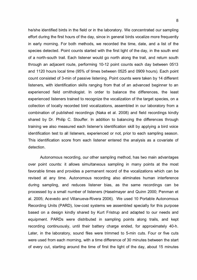
he/she identified birds in the field or in the laboratory. We concentrated our sampling
effort during the first hours of the day, since in general birds vocalize more frequently
in early morning. For both methods, we recorded the time, date, and a list of the
species detected. Point counts started with the first light of the day, in the south end
of a north-south trail. Each listener would go north along the trail, and return south
through an adjacent route, performing 10-12 point counts each day between 0513
and 1120 hours local time (95% of times between 0525 and 0909 hours). Each point
count consisted of 3-min of passive listening. Point counts were taken by 14 different
listeners, with identification skills ranging from that of an advanced beginner to an
experienced field ornithologist. In order to balance the differences, the least
experienced listeners trained to recognize the vocalization of the target species, on a
collection of locally recorded bird vocalizations, assembled in our laboratory from a
combination of published recordings (Naka et al. 2008) and field recordings kindly
shared by Dr. Philip C. Stouffer. In addition to balancing the differences through
training we also measured each listener’s identification skill by applying a bird voice
identification test to all listeners, experienced or not, prior to each sampling season.
This identification score from each listener entered the analysis as a covariate of
detection.
Autonomous recording, our other sampling method, has two main advantages
over point counts: it allows simultaneous sampling in many points at the most
favorable times and provides a permanent record of the vocalizations which can be
revised at any time. Autonomous recording also eliminates human interference
during sampling, and reduces listener bias, as the same recordings can be
processed by a small number of listeners (Haselmayer and Quinn 2000; Penman et
al. 2005; Acevedo and Villanueva-Rivera 2006). We used 10 Portable Autonomous
Recording Units (PARD), low-cost systems we assembled specially for this purpose
based on a design kindly shared by Kurt Fristrup and adapted to our needs and
equipment. PARDs were distributed in sampling points along trails, and kept
recording continuously, until their battery charge ended, for approximately 40-h.
Later, in the laboratory, sound files were trimmed to 5-min cuts. Four or five cuts
were used from each morning, with a time difference of 30 minutes between the start
of every cut, starting around the time of first the light of the day, about 15 minutes

9
before sunrise. If an early morning recording was not available due to late equipment
positioning, we still used cuts up to 1000 hours. Sound cuts were filtered to reduce
the excessive insect noise when needed, decreasing their volume in frequencies of
most cicadas and crickets, ranging from 5 to 8 kHz. All target species vocalizations
are situated in lower frequencies, therefore no data was lost due to filtering. Sound
cuts were then listened to by Marconi C. Cerqueira and Claudeir F. Vargas, which
have respectively 3 and 5 years of field experience in identification of local bird
vocalizations. Even though MCC and CFV have outstanding identification skills, their
identification score was measured and employed in the analysis just as with point
counts. Counting both point counts and autonomous recordings, the total listening
effort was greater than 126 hours, equivalent to the listening time a single person in
the field would carry out in 229 days performing an average of 11 point counts per
day.
The last, but not the least important detection covariate that we measured
during our sampling is time of the day. Time is relevant because different species
tend to vocalize more at different times. However, since changes in vocalization
activity follow circadian rhythms which do not always match legal time, we converted
our time data to minutes after sunrise, based on sunrise data of Manaus published by
the Brazilian government’s National Observatory (euler.on.br/ephemeris). Sampling
visit start times ranged from -38 to 343-min after sunrise, with a median of 68 min.
Ninety five percent of all visits took place between -18 and 198 min after sunrise.
Analysis. – Sampling in ecological research is almost never perfect: when a species
is present at a given site, it may easily go undetected. To account for imperfect
detection, MacKenzie et al. (2002) proposed a model with two levels, taking into
account both the state (if a site is occupied or not) and the sampling process (if a
species is detected at a given site). In this model, multiple visits to each site are used
to estimate both occupancy and detection probability via maximum likelihood.
Cerqueira et al. (in prep.) used this model to test predictions on the occupancy of 10
pairs of bird species, also at the Km 41 grid. The applicability of the MacKenzie et al.
(2002) approach was extended by a multi-season model developed in MacKenzie et

10
al. (2003) which estimates occupancy dynamics parameters: colonization and local
extinction probabilities.
The hierarchical approach employed in both MacKenzie et al. (2002,2003)
models is more fully developed in the Bayesian framework models of Link et al.
(2002), Royle and Kéry (2007) and Royle and Dorazio (2008), which estimate
occupancy and other population biological parameters while taking advantage of the
flexibility of modern computational solutions such as Markov Chain Monte Carlo
(MCMC). The combination of a Bayesian approach and MCMC adds possibilities like
using a priori information, and generating full a posteriori distributions of the main
model parameters or any combination of their values. Besides, MCMC makes it
particularly easy to incorporate spatial components in the analyses, such as, for
example, the inclusion of a covariate that estimates spatial autocorrelation in
occupancy (Royle and Dorazio 2008). At a preliminary stage of our analysis, we ran
single-season occupancy models similar to the ones used by Sberze et al. (2010) to
estimate spatial autocorrelation in occupancy between our sampling sites. Since we
did not find any significant indications that occupancy presented autocorrelation, we
chose not to include it in our analyses, and so we picked a Bayesian formulation of a
multi-season occupancy model from Kéry and Schaub (in prep.) adapted to the
detection variables we felt necessary to best describe the biological aspects of the
species along with the sampling process. Each species was analyzed separately,
and the results from different species were compared later, outside the occupancy
modeling framework.
Our model consists of two levels, describing: 1) the biological state, whether a
cell is occupied or not in a given season; and 2) the sampling process, whether a
species is detected or not, provided it is present at a site in a given season (Fig. 2).
For clarity, we represent the state part of the model in Fig. 2 referring to the two
sampling seasons separately. As we are using a Markovian formulation of occupancy
dynamics, the state of site i in season j depends on the state of site i in season j-1.
This leaves out the first season as not depending on any paste state, as represented
in Figure 2. Considering the biological state, the latent (partially observed) variable z
describes the true occupancy, whether the species is present (zij = 1) at a given site i

11
in season j or not (zij = 0). In the first season (j = 1), zij is drawn from a Bernoulli
distribution with probability ψ1, the occupancy probability for the first season, or the
probability that any given site is occupied at that time. The occupancy probability ψ
can also be interpreted as the proportion of sites that are occupied in a given season,
and ψ1 is that proportion referring to the first season. In the second season, zij also
comes from a Bernoulli draw, but this time the Bernoulli parameter, ψij, is given by:
ψij = zi(j-1) φj-1 + (1 - zi(j-1)) γj-1 (1)
where zi(j-1) φj-1 is the probability that a site that was occupied in the first season (zi(j-1)
= 1) remains occupied (‘survives’) in the second season, and (1 - zi(j-1)) γj-1 is the
probability that a site that was not occupied in season 1 (zi(j-1) = 0) becomes occupied
(colonized) in season 2. We will call the parameter φ as patch survival, as it indicates
the probability that an occupied site (or patch) will remain occupied from one season
to another, while the parameter γ will be called as colonization, since it indicates the
probability that an unoccupied site is colonized.
The detection probability pijk, the probability of detecting a species at site i,
season j and visit k, is given by the logistic function:
logit (pijk) = a0 + a1 time + a2 time2 + a3 score + a4 recorder + a5 (j - 1) (2)
where a0 is an intercept, a1 and a2 are linear and quadratic effects of the time of the
day, respectively, a3 is an effect of the identification score, a4 is an effect of the
autonomous recording technique (in contrast to point count), and a5 is an effect of the
second season, as j – 1 = 0 in the first season. We used both linear and quadratic
effects of time because, although most species vocalize close to sunrise, many
species vocalize most frequently at some time later in the morning. The probability
pijk is conditioned to occupancy, because if the species is not there, the chance to
detect it is zero. This is included in the model in the form of an unconditional
detection probability, µijk, which becomes zero when zij = 0 (species does not occur at
site i and season j), and pijk when zij = 1 (species does occur). The data collected
enters the model as yijk, and is modeled as a Bernoulli draw with probability µijk. From
the main parameters, we also estimated other derivate dynamic parameters. One

12
useful derived dynamic parameter we used, turnover (τ), is the probability that a
random occupied cell in season j was not occupied in previous season (j-1). Turnover
can be interpreted as the proportion of the occupied sites in a given season that were
not occupied in the previous season. It was defined by Royle and Kéry (2007) as:
τj = γj-1 (1 – ψ j-1) / ψj (3)
We also estimated the growth rate (λ), the factor that multiplies the occupancy
from one season to the following one, which is equal to 1 if no changes occurred.
The growth rate is defined by MacKenzie et al. (2003) as:
λj = ψj+1 / ψj (4)
Since we did not have any consistent a priori information about the
populations, we used uninformative priors to all of the parameters. Parameters
describing detection (a0, a1, a2, a3, a4 and a5) had uniform prior distributions between
-10 and 10, and ψ1, φ and γ had uniform distributions between 0 and 1. We estimated
the posterior distribution of parameters using an MCMC with 6,000 interactions in
each of 3 chains, discarding the first 1,000 interactions as a burn-in, and a thinning
rate of 5. Model was fitted by the use of WinBUGS (Lunn et al. 2000) combined to R
(R Development Core Team 2009) by the use of package R2WinBUGS (Sturtz et al.
2005).
We also performed comparisons between mean parameters of different
groups. Since distributions of parameters are unknown, we preferred a non-
parametric test. To accomplish these comparisons we chose a Wilcoxon two-sample
test, also known as Mann-Whitney U-test, also performed in R. All groups were
compared in pairs, SL vs. MF, SL vs. AF, and MF vs. AF. Occupancy and detection
were tested using values from both seasons as different estimates to the same
group. We used linear regressions to estimate variation of turnover and patch
survival in relation to occupancy probabilities, using the average from occupancy
values from both seasons.

13
RESULTS
Most species presented considerably high occupancies, with 12 of the 14 species
presenting mean occupancies higher than 0.5 in both seasons (Fig. 3a and Table 2).
Although most species presented an increase in their mean occupancies from first to
second season, we have no strong evidence of change in occupancy, since the
confidence intervals of the occupancy estimates from different seasons overlapped
for all of them. Comparing the occupancy between the three groups none were
significantly different.
Mean detections of all species were all lower than 0.4, with most of them lying
under 0.25 (Fig. 3b and Table 2). Among the 14 species, 11 present a positive
change in p from the first to the second sampling season. Only two of them though,
M. ferruginea and H. dorsimaculatus, had non-overlapping 95% confidence bounds
on p between seasons. Nevertheless, the effect of the second season on detection
(a5 - Fig. 3c) shows that actually seven species had a significant difference in
detection in second season, six positive and only one negative: C.lineatus.
Comparing mean detections of groups, SL and MF showed no differences between
them; on the other hand, U-test showed differences between detections of SL and AF
(p-value=0.004) and MF and AF (p-value=0.015).
Most species had mean growth rates higher than 1, reflecting the slight
change noticed in occupancy in different seasons (Fig. 3d and Table 2); however, in
accordance to the overlapping confidence bounds of occupancy to all species, none
of the growth rates were different than 1. Mean growth rates were compared but no
differences between any of the groups were detected.
Turnover was generally low, which is not surprising due to the high occupancy
values: if too many sites are occupied, not many occupations can be new (Fig. 3f and
Table 2). Colonization, on the other hand, had considerably high means, but
estimates were generally uninformative, since they had very broad 95% confidence
bounds, covering, in several cases, more than 90% of possible values (Table 2).

14
Comparisons of both turnover and colonization between groups showed no
differences between different social foraging habits.
Patch survival had high values and most confidence bounds were close to one
(Fig. 3e and Table 2). A difference of mean patch survival probabilities can be
noticed in Figure 3e, mainly between SL and AF, although they were not significant
by the U-test.
In Figure 4 we can observe the correlation of turnover and patch survival with
the average occupancy of both seasons. This comes mainly from a mathematical
artifact, but the regression helps us identify which species stray most from the
tendency; thus species that showed higher residuals are identified in Figure 4. C.
lineatus and T. ardesiacus had turnovers higher than generally expected, clearly
presented those values because of the non-significant growth, in the same way that
P. albifrons presented a negative residual due to the non-significant decrease in
occupancy. M. brachyura had a much higher turnover than expected, what indicates
alteration in occupied sites. M. axillaris also had lower turnover than expect, but its
turnover presents broad confidence bounds, covering expected values; this also
explains the higher than expected patch survival for this species; the same happened
to P. albifrons and G. rufigula, but with a patch survival lower than expected. T.
ardesiacus also showed a higher than expected patch survival due to the non-
significant occupancy growth.
DISCUSSION
No significant changes in occupancy probability were detected from one season to
another, leading us to believe that the target species presented a stable proportion of
the grid occupied throughout the period of study. The average patch survival (φ)
across species was 0.83, higher than the survival of territories of 0.71 found by
Stouffer (2007) for a group of species that included 2 antbirds and other 11 terrestrial
insectivores.

15
The generally high occupancy across species agrees with Cohn-Haft et al.
(1997), as they classified all but M. axillaris as common. M. axillaris actually
presented low occupancy in both seasons (0.50 and 0.49, respectively), and along
with M. brachyura (0.45 and 0.56) had the lowest occupancy values of all the target
species. Based on these results, they probably should be classified in the same
abundance class. Surprisingly some species, particularly H. dorsimaculatus, seem to
be present in all sites. The species turnover estimate was expected to be close to
zero, since it is impossible to colonize many new sites when most of them are
already occupied. This mathematical artifact explains most of the correlation between
turnover and survival with occupancy, as seen in Figure 4; this correlation must be
carefully taken into account while examining the dynamic parameters, which can
present unreliable information if analyzed alone. This correlation was also
comparable to the study of Stouffer (2007), which indicated that territory stability was
positively correlated with abundance; although our main parameter estimated was
occupancy, this could be an indication that species which occur more widely are less
inclined to changes in space also in the scale of our study.
Detection was higher in the beginning of the dry season (second sampling
season) than in the end (first sampling season), showing that antbirds are more
conspicuous at this time; that is probably due to November being at the end of a
stressful dry period. Unfortunately, detections were generally low, contributing to
broaden 95% confidence bounds in all biological parameters. Considering the
generally low detection of all species, the use of methods that take the sampling
process into consideration should be seen as an essential step to avoid bias in
parameter estimation.
Only one species, C. lineatus, showed a higher detection in the first sampling
season. That can be evidence of a different behaviour from the other species, which
might also indicate a different reproductive season, due to the vocalization frequency.
Detection was lowest for AF, resulting in high uncertainty about their
occupancy dynamics parameters. On the other hand, the lower detection for this
group suggests that their foraging habits make them cover larger areas in search of
food, and probably are unavailable to be detected at cell central point during most of

16
the time. Still, they are present in most of the grid, since they have high occupancy
probabilities. As a result, the low detection accompanied by the high occupancy, may
be an indication that AF show more alteration in space than SL or MF in each
season, and possibly between seasons.
Drawing comparisons between AF species, we notice that P. rufifrons, an
occasional ant-follower, exceptionally presents a higher detection probability
comparable to most species in the other two groups. Perhaps the high detection
reflects the species’ solitary behavior, as we think that solitary species are more
regularly available for detection in sampling points. That is corroborated by the little
change observed for P. rufifrons in occupancy probability (Fig. 3a), with an estimated
growth rate of 1.04 (0.81-1.34). However, if we evaluate the dynamic parameters, we
find comparatively high turnover and colonization probabilities (0.25 and 0.62,
respectively) with relatively narrow 95% confidence bounds, suggesting that P.
rufifrons has a considerable change in patch occupancy: although we cannot observe
a difference in the number of occupied sites, many occupied sites actually changed
locations. That may occur due to a similar number of newly colonized sites and site
extinctions. The high detection then may be explained as this species being more
conspicuous than other AF. The spatial changes of P. rufifrons, although accounts for
only one species, along with the presumed movement of other AF species, could
point out to the direction that AF present more spatial changes than the other two
groups.
Some SL species showed relatively high values of turnover and colonization
probabilities, namely C. lineatus, T. murinus and C. cinerascens. These values agree
with the non-significant growth in occupancy, but no remarkable changes can be
noticed in the previously occupied sites, since the upper limit of the patch survival
confidence bounds is close to 1 for all SL. These patch survivals values indicate that
solitary species were considerably stable between seasons.
It is interesting to notice the changes with M. brachyura (MF), a species that
also presented a non-significant occupancy growth comparable to the species above.
As a result, we should also expect a high patch survival probability. However, it
presented low patch survival along with high turnover and colonization, what points

17
out to a less stable occupancy. These changes in space might indicate our
hypothesized changes in occupancy of MF which we could not observe in other
members of the group. Possibly this behavior is more evident in canopy mixed-
species flock followers, such as M. brachyura itself, and H. dorsimaculatus. The latter
did not show any changes in space, but that could simply have been obscured by its
occupancy, since the species seems to occur everywhere within the grid.
The three understory MF species, T. ardesiacus, T. caesius and M. axillaris,
presented high patch survival rates, along with low confidence bounds in turnover.
This seems to indicate spatial stability, which agrees with the stable home-range size
of understory mixed-species flocks found by Jullien and Thiollay (1998).
We found that many antbirds we studied are generally stable, which is in
accordance to Greenberg and Gradwohl (1986). However, two species, M. brachyura
(MF) and P. rufifrons (AF) had noticeably high turnover rates along with lower
survival confidence bounds, what indicates a considerable change in occupied sites.
In addition, the low detection probabilities for the three other AF species make us
believe that they use wider ranges in search of food. Although we cannot fully accept
the hypothesis that AF species are more prone to changes in space, we believe that
our results tend to confirm that; further studies are needed. On the other hand, since
only one species of MF had evidence of changes, we then refute the hypothesis that
MF present more changes in occupied sites than SL. Nevertheless, in an inside
comparison between MF, different behavior between them can make us raise
another hypothesis, that canopy MF can present a different use of space than
understory MF, judging from the noticeable changes of M. brachyura and the fact that
H. dorsimaculatus seems to be almost omnipresent, in contrast to the apparent
stability of the understory MF. Thus, we think that AF are more prone to changes in
space than understory MF, as they show estimates more similar to SL; on the other
hand, we cannot don’t have any evidence that AF and canopy MF show any
differences in occupation stability.
Our results indicate that some species which were considered stable in space
actually may have a different use of the forest areas throughout the year.
Understanding the functioning of space use by animals is of vital importance to
18
conservation, and more studies should be directed to it, covering more species,
possibly in a community model. This would be particularly important to less abundant
species, which are more susceptible to population variations. Rare species are
obviously more difficult to sample, and models that take into account the imperfect
detection can be much more accurate than traditional ones, when studying a large
area such as the Km 41 grid. Different sampling methods may also be associated,
since different techniques like point counts and mist-netting may have radically
different detection probabilities for some species, for example P. albifrons, which has
low detection in point counts or recordings, but is commonly caught in mist-nets.
Autonomous recorders or mist-nets used in canopy heights would probably bring
more information about more species and make it possible to investigate further into
the community; those methods could possibly help us understand one of the
questions raised by this study, about the differences of space use between canopy
and understory MF.
ACKNOWLEDGEMENTS
We would like to thank all friends who made this project possible. Fieldwork was
done with the kind help of Angela Midori, Carla Sardelli, Christian Andretti, João Vitor
Silva, Monica Sberze, Mariana Tolentino, Thiago Orsi, Thiago Costa, Claudeir
Vargas e Marconi Cerqueira. The last two also listened to extensive hours of
recordings, and, along with Mario Cohn-Haft, could lend their precious ornithological
knowledge. PDBFF provided the indispensable logistic support, along with camp and
trail maintenance. This study was funded by the Smithsonian Tropical Research
Institute, and by a master´s fellowship offered by the Brazilian government´s National
Council for Scientific and Technological Development (CNPq).

19
LITERATURE CITED
ACEVEDO, M. A., AND L. J. VILLANUEVA-RIVERA. 2006. Using automated digital recording
systems as effective tools for the monitoring of birds and amphibians. Wildlife Society
Bulletin 34:211-214.
ANU, A., T. K. SABU, AND P. J. VINEESH. 2009. Seasonality of litter insects and relationship
with rainfall in a wet evergreen forest in south Western Ghats. Journal of Insect Science 9.
BIERREGAARD, J., R. O., C. GASCON, T. E. LOVEJOY, AND R. C. G. MESQUITA. 2001. The
biological dynamics of forest fragments project - the study site, experimental design, and
research activity. Pages 31-42 in Lessons from Amazonia: the ecology and conservation
of a fragmented forest. Yale University Press, New Haven.
BRUMFIELD, R. T., J. G. TELLO, Z. A. CHEVIRON, M. D. CARLING, N. CROCHET, AND K. V.
ROSENBERG. 2007. Phylogenetic conservatism and antiquity of a tropical specialization:
Army-ant-following in the typical antbirds (Thamnophilidae). Molecular Phylogenetics and
Evolution 45:1-13.
CERQUEIRA, M. C., C. F. VARGAS, C. E. NADER, C. B. ANDRETTI, T. V. COSTA, A. M. F.
PACHECO, M. COHN-HAFT, AND G. FERRAZ. in prep. An occupancy test of rarity and
commonness for central Amazon forest birds.
COHN-HAFT, M., A. WHITTAKER, AND P. C. STOUFFER. 1997. A new look at the "species-poor"
central Amazon: the avifauna north of Manaus, Brazil. Ornithological Monographs 48:205-
235.
DEVELEY, P. F., AND P. C. STOUFFER. 2001. Effects of roads on movements by understory
birds in mixed-species flocks in central Amazonian Brazil. Conservation Biology 15:1416-
1422.
FRANKIE, G. W., H. G. BAKER, AND P. A. OPLER. 1974. Comparative Phenological Studies of
Trees in Tropical Wet and Dry Forests in the Lowlands of Costa Rica. Journal of Ecology
62:881-919.
GREENBERG, R., AND J. GRADWOHL. 1986. Constant Density and Stable Territoriality in Some
Tropical Insectivorous Birds. Oecologia 69:618-625.
HASELMAYER, J., AND J. S. QUINN. 2000. A Comparison of Point Counts and Sound Recording
as Bird Survey Methods in Amazonian Southeast Peru. The Condor 102:887-893.
JANZEN, D. H. 1973. Sweep Samples of Tropical Foliage Insects: Effects of Seasons,
Vegetation Types, Elevation, Time of Day, and Insularity. Ecology 54:687-708.
20
JANZEN, D. H., AND T. W. SCHOENER. 1968. Differences in Insect Abundance and Diversity
Between Wetter and Drier Sites During a Tropical Dry Season. Ecology 49:96-110.
JULLIEN, M., AND J. M. THIOLLAY. 1998. Multi-species territoriality and dynamic of neotropical
forest understorey bird flocks. Journal of Animal Ecology 67:227-252.
KARR, J. R., AND K. E. FREEMARK. 1983. Habitat Selection and Environmental Gradients -
Dynamics in the Stable Tropics. Ecology 64:1481-1494.
KARR, J. R., J. D. NICHOLS, M. K. KLIMKIEWICZ, AND J. D. BRAWN. 1990. Survival rates of birds
of tropical and temperate forests - will the dogma survive? American Naturalist 136:277-
291.
KÉRY, M., AND M. SCHAUB. in prep. Bayesian Population Analysis using WinBUGS.
KLOPFER, P. H. 1959. Environmental determinants of faunal diversity. American Naturalist
93:337-342.
LAURANCE, W. F., T. E. LOVEJOY, H. L. VASCONCELOS, E. M. BRUNA, R. K. DIDHAM, P. C.
STOUFFER, C. GASCON, R. O. BIERREGAARD, S. G. LAURANCE, AND E. SAMPAIO. 2002.
Ecosystem decay of Amazonian forest fragments: a 22-year investigation. Conservation
Biology 16:605-618.
LINK, W. A., E. CAM, J. D. NICHOLS, AND E. G. COOCH. 2002. Of BUGS and birds: Markov
chain Monte Carlo for hierarchical modeling in wildlife research. Journal of Wildlife
Management 66:277-291.
LUNN, D. J., A. THOMAS, N. BEST, AND D. SPIEGELHALTER. 2000. WinBUGS -- a Bayesian
modelling framework: concepts, structure, and extensibility. Statistics and Computing
10:325-337.
MACARTHUR, R. H. 1972. Geographical Ecology: Patterns in the Distribution of Species.
Princeton University Press, New Jersey.
MACKENZIE, D. I., J. D. NICHOLS, J. E. HINES, M. G. KNUTSON, AND A. B. FRANKLIN. 2003.
Estimating site occupancy, colonization, and local extinction when a species is detected
imperfectly. Ecology 84:2200-2207.
MACKENZIE, D. I., J. D. NICHOLS, G. B. LACHMAN, S. DROEGE, J. A. ROYLE, AND C. A.
LANGTIMM. 2002. Estimating site occupancy rates when detection probabilities are less
than one. Ecology 83:2248-2255.
MUNN, C. A., AND J. W. TERBORGH. 1979. Multi-species territoriality in Neotropical Foraging
Flocks. The Condor 81:338-347.
MURRAY, B. G., JR. 1985. Evolution of Clutch Size in Tropical Species of Birds. Ornithological
Monographs 36:505-519.

21
NAKA, L. N., P. C. STOUFFER, M. COHN-HAFT, C. A. MARANTZ, A. WHITTAKER, AND J.
BIERREGAARD, RICHARD O. 2008. CD. Vozes da Amazônia, Vol. 1. – Aves das florestas de
terra firme ao norte de Manaus: Área de endemismo das Guianas. Editora Inpa, Manaus.
PENMAN, T. D., F. L. LEMCKERT, AND M. J. MAHONY. 2005. A cost-benefit analysis of
automated call recorders. Applied Herpetology 2:389-400.
POLLOCK, K. H. 1982. A capture-recapture design robust to unequal probability of capture.
Journal of Wildlife Management 46:752-757.
R DEVELOPMENT CORE TEAM. 2009. R: A Language and Environment for Statistical
Computing. R Foundation for Statistical Computing, Vienna, Austria.
ROYLE, J. A., AND R. M. DORAZIO. 2008. Hierarchical Modeling and Inference in Ecology: The
Analysis of Data from Populations, Metapopulations and Communities. Academic Press,
London.
ROYLE, J. A., AND M. KÉRY. 2007. A Bayesian Space-State Formulation of Dynamic
Occupancy Models. Ecology 88:1813-1823.
SBERZE, M., M. COHN-HAFT, AND G. FERRAZ. 2010. Old growth and secondary forest site
occupancy by nocturnal birds in a neotropical landscape. Animal Conservation 13:3-11.
STEVENSON, P. R., M. C. CASTELLANOS, A. I. CORTES, AND A. LINK. 2008. Flowering patterns in
a seasonal tropical lowland forest in western Amazonia. Biotropica 40:559-567.
STOUFFER, P. C. 2007. Density, territory size, and long-term spatial dynamics of a guild of
terrestrial insectivorous birds near Manaus, Brazil. Auk 124:291-306.
STURTZ, S., U. LIGGES, AND A. GELMAN. 2005. R2WinBUGS: A Package for Running
WinBUGS from R. Journal of Statistical Software 12:1-16.
TERBORGH, J. 1990. Mixed flocks and polyspecific associations: Costs and benefits of mixed
groups to birds and monkeys. American Journal of Primatology 21:87-100.
WILLIAMS, S. E., AND J. MIDDLETON. 2008. Climatic seasonality, resource bottlenecks, and
abundance of rainforest birds: implications for global climate change. Diversity and
Distributions 14:69-77.
WILLIS, E. O., AND Y. ONIKI. 1978. Birds and Army Ants. Ann. Rev. Ecol. Syst. 9:243-263.
WOLDA, H. 1988. Insect seasonality: Why? Annual Review of Ecology and Systematics 19:1-
18.
ZIMMER, K., AND M. ISLER. 2003. Family Thamnophilidae (Typical Antbirds). in Handbook of
the Birds of the World - Volume 8 (Broadbills to Tapaculos) (J. Hoyo, A. Elliott, and D. A.
Christie, Eds.). Lynx Edicions.

22
TABLES
Table 1. List of studied species divided by sociality groups. Adapted from Cohn-Haft
et al. (1997).
Habitata Positionb Socialityc
Group 1 – Solitary species (SL)
Fasciated Antshrike Cymbilaimus lineatus 2,1 M S
Mouse-colored Antshrike Thamnophilus murinus 1,2 M SU
Guianan Warbling-Antbird Hypocnemis cantator 1,2 U S
Gray Antbird Cercomacra cinerascens 1 C S
Ferruginous-backed Antbird Myrmeciza ferruginea 1 T S
Group 2 – Mixed-species flock followers (MF)
Dusky-throated Antshrike Thamnomanes ardesiacus 1 U U
Cinereous Antshrike Thamnomanes caesius 1 UM U
Pygmy Antwren Myrmotherula brachyura 1,2 C C
White-flanked Antwren Myrmotherula axillaris 1,2 M US
Spot-backed Antwren Herpsilochmus dorsimaculatus 1 C C
Group 3 – Ant-following species (AF)
Black-headed Antbird Percnostola rufifrons 1,2 U SA
White-plumed Antbird Pithys albifronsd 1 U A
Rufous-throated Antbird Gymnopithys rufigulad 1 U A
Scale-backed Antbird Willisornis poecilinotus 1 U SA a Habitat: 1 – primary terra firme forest, 2 – secondary forest. b Position: T – terrestrial, U –
understory, M – midstory, C – Canopy. c Sociality: U – accompanies understory mixed-
species flocks, C – accompanies canopy mixed-species flocks, A – army-ant follower, S –
solitary or in pairs. d obligate ant followers.
23
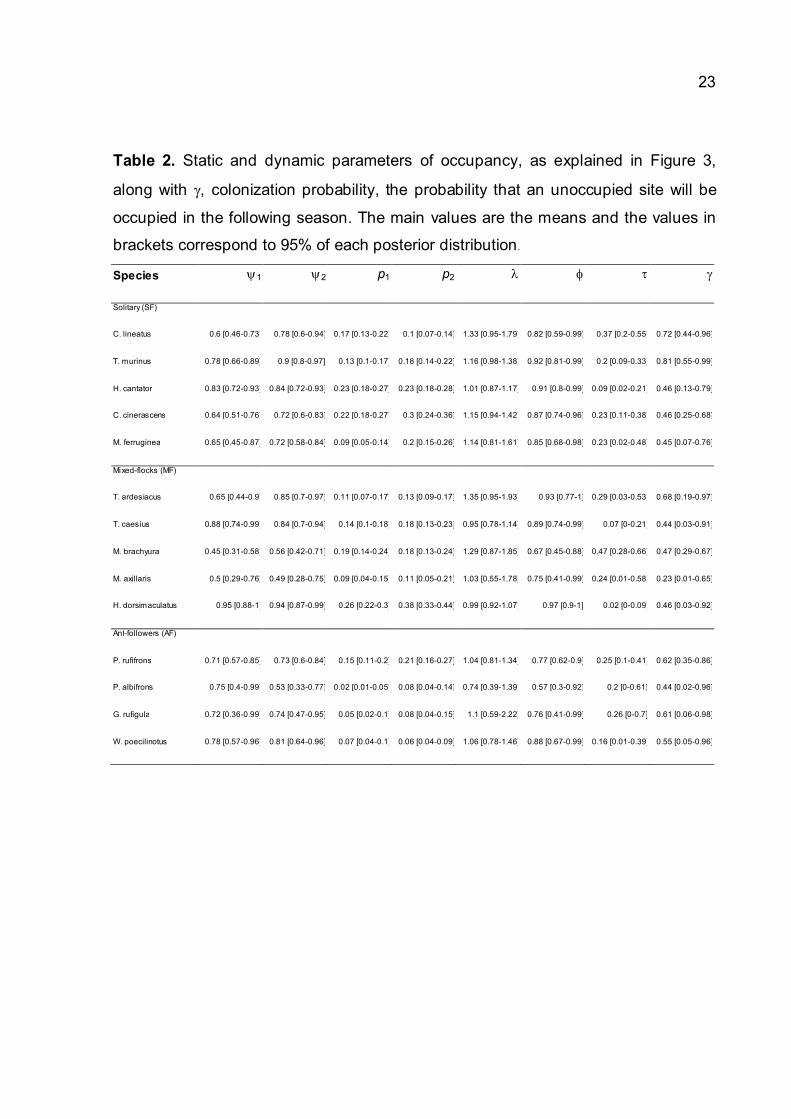
Table 2. Static and dynamic parameters of occupancy, as explained in Figure 3,
along with γ, colonization probability, the probability that an unoccupied site will be
occupied in the following season. The main values are the means and the values in
brackets correspond to 95% of each posterior distribution.
Species ψ1 ψ2 p1 p2 λ φ τ γ
Solitary (SF)
C. lineatus 0.6 [0.46-0.73] 0.78 [0.6-0.94] 0.17 [0.13-0.22] 0.1 [0.07-0.14] 1.33 [0.95-1.79] 0.82 [0.59-0.99] 0.37 [0.2-0.55] 0.72 [0.44-0.96]
T. murinus 0.78 [0.66-0.89] 0.9 [0.8-0.97] 0.13 [0.1-0.17] 0.18 [0.14-0.22] 1.16 [0.98-1.38] 0.92 [0.81-0.99] 0.2 [0.09-0.33] 0.81 [0.55-0.99]
H. cantator 0.83 [0.72-0.93] 0.84 [0.72-0.93] 0.23 [0.18-0.27] 0.23 [0.18-0.28] 1.01 [0.87-1.17] 0.91 [0.8-0.99] 0.09 [0.02-0.21] 0.46 [0.13-0.79]
C. cinerascens 0.64 [0.51-0.76] 0.72 [0.6-0.83] 0.22 [0.18-0.27] 0.3 [0.24-0.36] 1.15 [0.94-1.42] 0.87 [0.74-0.96] 0.23 [0.11-0.38] 0.46 [0.25-0.68]
M. ferruginea 0.65 [0.45-0.87] 0.72 [0.58-0.84] 0.09 [0.05-0.14] 0.2 [0.15-0.26] 1.14 [0.81-1.61] 0.85 [0.68-0.98] 0.23 [0.02-0.48] 0.45 [0.07-0.76]
Mixed-flocks (MF)
T. ardesiacus 0.65 [0.44-0.9] 0.85 [0.7-0.97] 0.11 [0.07-0.17] 0.13 [0.09-0.17] 1.35 [0.95-1.93] 0.93 [0.77-1] 0.29 [0.03-0.53] 0.68 [0.19-0.97]
T. caesius 0.88 [0.74-0.99] 0.84 [0.7-0.94] 0.14 [0.1-0.18] 0.18 [0.13-0.23] 0.95 [0.78-1.14] 0.89 [0.74-0.99] 0.07 [0-0.21] 0.44 [0.03-0.91]
M. brachyura 0.45 [0.31-0.58] 0.56 [0.42-0.71] 0.19 [0.14-0.24] 0.18 [0.13-0.24] 1.29 [0.87-1.85] 0.67 [0.45-0.88] 0.47 [0.28-0.66] 0.47 [0.29-0.67]
M. axillaris 0.5 [0.29-0.76] 0.49 [0.28-0.75] 0.09 [0.04-0.15] 0.11 [0.05-0.21] 1.03 [0.55-1.78] 0.75 [0.41-0.99] 0.24 [0.01-0.58] 0.23 [0.01-0.65]
H. dorsimaculatus 0.95 [0.88-1] 0.94 [0.87-0.99] 0.26 [0.22-0.3] 0.38 [0.33-0.44] 0.99 [0.92-1.07] 0.97 [0.9-1] 0.02 [0-0.09] 0.46 [0.03-0.92]
Ant-followers (AF)
P. rufifrons 0.71 [0.57-0.85] 0.73 [0.6-0.84] 0.15 [0.11-0.2] 0.21 [0.16-0.27] 1.04 [0.81-1.34] 0.77 [0.62-0.9] 0.25 [0.1-0.41] 0.62 [0.35-0.86]
P. albifrons 0.75 [0.4-0.99] 0.53 [0.33-0.77] 0.02 [0.01-0.05] 0.08 [0.04-0.14] 0.74 [0.39-1.39] 0.57 [0.3-0.92] 0.2 [0-0.61] 0.44 [0.02-0.96]
G. rufigula 0.72 [0.36-0.99] 0.74 [0.47-0.95] 0.05 [0.02-0.1] 0.08 [0.04-0.15] 1.1 [0.59-2.22] 0.76 [0.41-0.99] 0.26 [0-0.7] 0.61 [0.06-0.98]
W. poecilinotus 0.78 [0.57-0.96] 0.81 [0.64-0.96] 0.07 [0.04-0.1] 0.06 [0.04-0.09] 1.06 [0.78-1.46] 0.88 [0.67-0.99] 0.16 [0.01-0.39] 0.55 [0.05-0.96]

24
FIGURES
Fig. 1.

25
Fig. 2.

26
Fig. 3.

27
Fig. 4.

28
FIGURE LEGENDS
Fig. 1. BDFFP study area east of BR-174, north of Manaus (a); the black line shows
highway BR-174 and the dotted lines show dirt roads, including road ZF-3, running
east-west through the map. The lower panel (b) shows the trail grid in Km 41;
sampling points are marked with empty circles
Fig. 2. Diagram of dynamic occupancy model in two levels describing the biological
state and the sampling process. The state level is described differently in the first and
second season, as the first season (j = 1) does not depend on any past state.
Symbols in the diagram stand for the following quantities: zij is the partially observed
true presence or absence of species in site i during season j; ψ1 is the probability that
any given site is occupied in season 1; ψij is the probability that site i is occupied in
season j; φj-1, patch ‘survival’ probability is the probability that an occupied site in
season j - 1 is still occupied in season j; γj-1, the colonization probability, is the
probability that an unoccupied site in season j - 1 is occupied in season j; pijk is the
conditional probability of detecting the species at site i, season j and visit k; a0 is the
intercept of the detection part of the model; a1 and a2 are the linear and quadratic
effects of time, respectively; a3 is the effect of the listener identification score on p; a4
is the effect of the use of the autonomous recorder instead of point counts on p; a5 is
the effect of the second season on p; µijk is the unconditional probability of detection;
and yijk is the observation data (detection/non-detection) of given species at site i,
season j and visit k.
Fig. 3. Static and dynamic parameters of occupancy and detection. Circles indicate
means and lines indicate the 95% confidence bounds of posterior distributions: a)
occupancy (ψ), probability that a random site is occupied in each season; b)
detection (p), probability that a species is detected in a point count, with the average
detection score and the average time of day, in each season; c) effect of second
season on detection; d) growth rate (λ), a growth rate of 1 means no changes in
occupancy; e) patch survival (φ), probability that an occupied site will remain

29
occupied in the following season; f) turnover (τ), probability that a random occupied
site was not occupied in previous season.
Fig. 4. Turnover (τ) and patch survival (φ) versus occupancy (ψ) (average of both
seasons). Species identified showed residuals above 10% of the slope.

xv
Conclusão
Encontramos estabilidade para muitas das espécies estudadas, principalmente as
espécies de hábitos solitários e as que participam em bandos mistos de subosque, o
que está de acordo com o estudo de Greenberg e Gradwohl (1986) e Jullien e
Thiollay (1998). No entanto, duas espécies, Myrmotherula brachyura e Percnostola
rufifrons, demonstraram valores altos de turnover, além de limites de confiança mais
baixos de persistência de manchas, o que indica mudanças consideráveis nos sítios
ocupados. Adicionalmente, com exceção de P. rufifrons, os outros seguidores de
correição apresentaram baixas probabilidades de detecção, consideravelmente mais
baixas que todas as outras espécies, o que nos faz crer, devido a sua alta
ocorrência, que dificilmente estão disponíveis para amostragem no ponto central de
um sítio, pois possuem maior movimentação que as outras espécies. Deste modo,
concluímos que, apesar da alta incerteza dos parâmetros dinâmicos dos seguidores
de correição, temos evidência de que este grupo apresenta uma maior
movimentação pela grade, e consequentemente menor estabilidade de ocupação
que os outros. Assim, apesar de não podermos aceitar completamente a hipótese
de que esse grupo possui maior mudança nos sítios ocupados em diferentes épocas
do ano que os outros, temos indícios que apontam nessa direção. Com relação às
espécies de bando misto, como apenas uma espécie deste grupo apresentou
evidências de mudanças, nós refutamos a hipótese de que as espécies solitárias
são mais estáveis que as espécies de bando misto. Todavia, ao fazer uma
comparação entre as espécies de bando misto, seus diferentes hábitos podem nos
fazer levantar uma nova hipótese: que espécies de bandos mistos de copa podem
ter uma maior tendência à instabilidade espacial que aquelas que participam de
bandos mistos de subosque. Isso se deve às perceptíveis mudanças de M.
brachyura e o fato de que Herpsilochmus dorsimaculatus parece ser quase
onipresente na área de estudo, em contraste à aparente estabilidade das espécies
de bando misto de subosque. Deste modo, acreditamos que os seguidores de
correição apresentam maiores alterações no espaço que os bandos mistos de
subosque; entretanto não temos evidência de que os seguidores de correição e as

xvi
espécie de bandos mistos de copa demonstram qualquer diferença nas alterações
no espaço.
Perspectivas
Nossos resultados indicam que algumas espécies que eram consideradas estáveis
no espaço na realidade podem apresentar um uso de diferentes áreas em diferentes
períodos do ano. Entender como funciona o uso do espaço para os animais é de
vital importância para a conservação, e mais estudos deveriam ser direcionados a
isso, abrangendo mais espécies, possivelmente em um modelo de comunidades.
Isso pode ser particularmente importante para espécies menos abundantes, que
consequentemente são mais suscetíveis a variações de população. Espécies mais
raras são obviamente mais difíceis de serem amostradas, e modelos que levam em
consideração a detecção imperfeita podem ser muito mais precisos que os
tradicionais quando estudamos uma área tão ampla quanto a do presente estudo.
Métodos de amostragem diferentes também podem ser associados, já que
diferentes técnicas como pontos de escuta e redes de neblina podem apresentar
probabilidades de detecção completamente distintas para algumas espécies, como
por exemplo para Pithys albifrons, que, como pudemos observar, apresenta baixa
detecção em pontos de escuta ou gravações autônomas, mas é comumente
capturado em redes de neblina. Gravadores autônomos ou redes de neblina
utilizados na copa das árvores também podem contribuir para uma investigação
mais aprofundada da comunidade; esses métodos poderiam por exemplo nos ajudar
a entender uma das questões levantadas por este trabalho, sobre as diferenças do
uso do espaço por espécies de bando misto de subosque e copa.

xvii
Anexo A
Ata da aula de qualificação

xviii

xix
Anexo B
Parecer de avaliador do trabalho escrito - Cintia Cornelius

xx

xxi
Anexo C
Parecer de avaliador do trabalho escrito - Maja Kajin

xxii

xxiii
Anexo D
Ata da defesa presencial com parecer dos avaliadores

xxiv