gesep – gerência de especialistas em sistemas elétricos de
TRANSCRIPT

GESEP – Gerência de Especialistas em Sistemas Elétricos de Potência
Título:
Impacts of photovoltaic plants on the power factor correction: the cat head curve
Autor:
Lucas Soares Gusman
Orientador:
Prof. Dr. Heverton Augusto Pereira
Membros:
M.Sc. Lucas Santana Xavier
Eng. Rodrigo Cássio de Barros
Aprovação:
19 de Outubro de 2018
Lucas Soares Gusman
Impacts of photovoltaic plants on the power
factor correction: the cat head curve
Brasil
2018
Lucas Soares Gusman
Impacts of photovoltaic plants on the power factor
correction: the cat head curve
Universidade Federal de Vicosa
Departamento de Engenharia Eletrica
Curso de Graduacao em Engenharia Eletrica
Heverton Augusto Pereira
Brasil
2018

Dedico este trabalho a todas pessoas que acreditaram em mim,
e que ajudaram a tornar deste sonho, uma realidade.

Agradecimentos
Agradeco a todas que me apoiaram ao longo da conclusao deste sonho. Sou grato
aos meus pais, Silvia e Marcelo, que me apoiaram de toda forma possıvel para que eu
concluısse esta graduacao em busca de uma vida melhor. Agradeco a minha irma Grasielle
e seu marido Alan, os quais tornaram a convivencia em Vicosa uma coisa extremamente
prazerosa e divertida, e os quais eu vou sempre mostrar que podem se orgulhar de mim.
Agradeco tambem a minha namorada Daiane, que sempre me incentivou e me ajudou de
toda forma possıvel a ir alem.
Agradeco ainda a todos os amigos que fiz ao longo destes anos de graduacao,
principalmente pelos meus companheiros de GESEP: Joao Marcus, Dayane, William e
Paulo Junior, os quais eu dividi, literalmente, a maior parte dos meus dias. Gracas aos
mesmos, consegui ir ainda mais longe pela forca e troca de marretas ao longo de todo
curso.
Por fim, agradeco aos meus mestres, todos os professores da UFV e, em especial, os
professores do DEL/UFV que sempre deram o seu melhor para contribuir com parte do seu
conhecimento para os alunos. Particularmente, agradeco ao professor e orientador Heverton
que sempre deu o seu melhor para me inspirar a ser uma pessoa mais dedicada aos trabalhos
dos quais eu faco parte e que me ensinou a sempre ter orgulho do seu proprio trabalho.
Agradeco ao professor Allan, que sempre me apoiou com seu jeito super extrovertido e
com as ideias super interessantes, sendo bem caracterıstico da sua inteligencia.
Sou grato por todo conhecimento ao qual herdei de todas essas pessoas, seja da
parte tecnica ou da parte de valores que levarei para a vida. A todos, meu muito obrigado!

”The superior man is modest in his speech,
but exceeds in his actions.”
(Confucius)

Resumo
Com a crescente utilizacao de usinas fotovoltaicas, principalmente em ambientes industriais
os quais necessitam de grande quantidade de energia eletrica para seu funcionamento,
impactos na distribuicao de energia devem ser pesquisados de forma a obter-se um melhor
entendimento das novas caracterısticas do sistema eletrico. Um fator importante a ser
observado e o fator de potencia, visto que o mesmo possui um limite inferior o qual gera
tarifas extras sob potencia reativa excedente caso esteja abaixo deste limite. Este trabalho
mostra os efeitos do fator de potencia com a instalacao de uma usina fotovoltaica em
determinados perfis industriais e como a correcao deste fator de potencia deve ser realizada
neste caso. Isto deve ser propriamente avaliado visto que o fator de potencia cai para
aproximadamente zero nos pontos onde a potencia ativa liquida e cancelada, causando um
incremento em torno de 80% do banco de capacitores previamente instalado. A potencia
para correcao tem um formato semelhante a uma cabeca de gato, sendo denominado dessa
forma.
Keywords: Potencia Reativa; Usinas Fotovoltaicas; Fator de Potencia; Qualidade de
Energia.
Abstract
With the increasing utilization of photovoltaic plants around the world, some impacts on
the energy distribution must be researched for a better understanding of the system in
general. An important issue is the power factor value, since it has an inferior limit that can
create extras charges on exceeding reactive power if under its determined limit. This paper
works on showing the influence on exceeding reactive power by adding a photovoltaic
plant in different industries and how the power factor correction should be made, since it
falls to almost zero in points where the liquid active power is canceled, therefore causing
an increment of almost 80% of the nominal installed capacitor bank. In fact, the extra
capacitive reactive power has a dynamic profile that reminds a cat head, being called that
way.
Keywords: Reactive Power; Photovoltaic Plants; Power Factor; Energy Quality.

List of Figures
Figure 1 – Electrical brazilian matrix against the world matrix in 2015(EPE, 2016). 12
Figure 2 – The representation of load net active power along a day: the Duck
Chart(ISO, 2016). . . . . . . . . . . . . . . . . . . . . . . . . . . . . . . 14
Figure 3 – Diagram of the industry, PV plant and grid connections. . . . . . . . . 17
Figure 4 – Central inverters produced by ABB(ABB, 2018). . . . . . . . . . . . . 18
Figure 5 – A capacitor bank. (a) Delta connected. (b) Star connected. . . . . . . . 20
Figure 6 – WEG capacitor bank(WEG, 2018). (a) Practical device. (b) Diagram
of contacts. . . . . . . . . . . . . . . . . . . . . . . . . . . . . . . . . . 21
Figure 7 – Effects of the PV plant on power factor compensation. (a) Power trian-
gles changing on time. (b) Demanded capacitive power for correction
(cat-head curve). . . . . . . . . . . . . . . . . . . . . . . . . . . . . . . 23
Figure 8 – Power profiles of the two consumers. . . . . . . . . . . . . . . . . . . . 24
Figure 9 – Adjusted photovoltaic active power profiles. . . . . . . . . . . . . . . . 25
Figure 10 – Power profiles of the two consumers in the presence of a PV plant. . . . 26
Figure 11 – New power factor of both consumers. . . . . . . . . . . . . . . . . . . . 27
Figure 12 – Additional capacitive reactive power for both consumers: the cat head
curve. . . . . . . . . . . . . . . . . . . . . . . . . . . . . . . . . . . . . 28
Figure 13 – 2-tap cat curve for the 0.7 pf industry. . . . . . . . . . . . . . . . . . . 29
Figure 14 – 2 tap cat-head curve for both case studies and their corrected power
factor. . . . . . . . . . . . . . . . . . . . . . . . . . . . . . . . . . . . . 30
List of abbreviations and acronyms
ANEEL Agencia Nacional de Energia Eletrica
EPE Empresa de Pesquisas Energeticas
PV Photovoltaic
GCPS Grid-Connected Photovoltaic Systems
RES Renewable Energy Sources
SEPIC Single-Ended Primary Inductor Converter
MPPT Maximum Power Point Tracking
ISO Independent System Operator
pf Power factor
List of symbols
P Nominal active power of the industry
QL Nominal inductive reactive power of the industry
PP V Active power generated by the PV panels
QP V Capacitive reactive power generated by the PV panel
QC Capacitive reactive power given by the capacitor bank
Pgrid Active power drawn from the grid
Qgrid Reactive power drawn from the grid
XC Capacitive reactance
Vg Line to line RMS voltage
ω Angular frequency of the grid
fg Frequency of the grid
CY Capacitance of the capacitor bank in star connection
C∆ Capacitance of the capacitor bank in delta connection
S Apparent power of the industries
∆QC,max Maximum value of the capacitive power from the cat head curve
∆QC,min Minimum value of the ”belly” created by the cat head curve
∆QC,mean Mean value between ∆QC,max and ∆QC,min

Contents
1 INTRODUCTION . . . . . . . . . . . . . . . . . . . . . . . . . . . . . 12
1.1 Objectives . . . . . . . . . . . . . . . . . . . . . . . . . . . . . . . . . 15
1.2 Text organization . . . . . . . . . . . . . . . . . . . . . . . . . . . . . 15
2 LITERATURE REVIEW . . . . . . . . . . . . . . . . . . . . . . . . . . 17
2.1 An overview of the system . . . . . . . . . . . . . . . . . . . . . . . . 17
2.2 Industrial capacitor banks and power factor correction . . . . . . 18
2.3 Effects of adding a PV plant . . . . . . . . . . . . . . . . . . . . . . . 20
3 METHODOLOGY . . . . . . . . . . . . . . . . . . . . . . . . . . . . . 24
3.1 Case Study . . . . . . . . . . . . . . . . . . . . . . . . . . . . . . . . . 24
4 RESULTS AND DISCUSSION . . . . . . . . . . . . . . . . . . . . . . 27
5 CONCLUSION . . . . . . . . . . . . . . . . . . . . . . . . . . . . . . 31
REFERENCES . . . . . . . . . . . . . . . . . . . . . . . . . . . . . . 33
12
1 Introduction
Nowadays, the distributed generation has been attractive for various economical
interests. Instead of using dispersed generation based on high power plants, each consumer
has the possibility to use various sources for generating energy (such as solar, wind and
thermal power)(DULaU; BICa, 2017). By using the local generated power, it is expected a
reduction in the electricity bill.
In fact, this economy comes from the active power generation, such as by photo-
voltaic panels. By producing an amount of active power, less will be required from the grid
to feed the industry loads and the consumed active power will be reduced to its minimum
value. This causes the electricity bill to fall to the minimum cost possible (that is specified
in the Resolution no414/2010 from ANEEL(ANEEL, 2010)). In three-phase systems, this
minimum value is the cost of 100kWh in a month, for example.
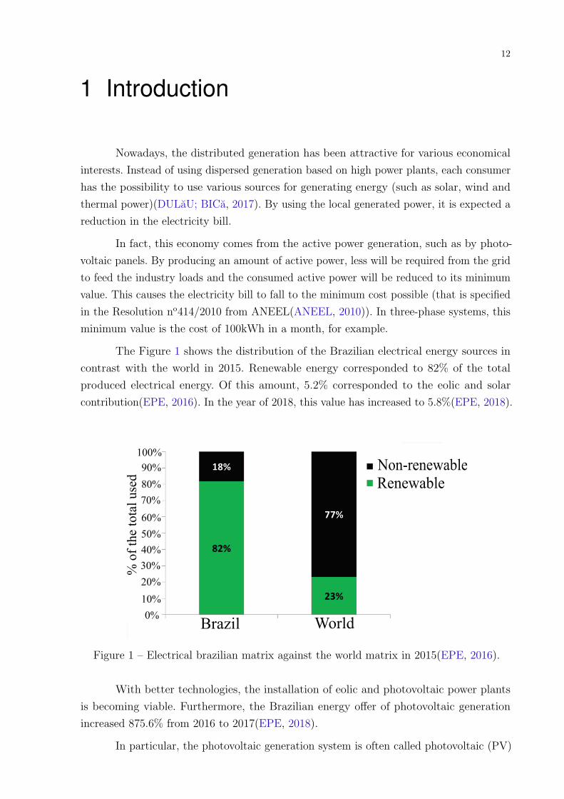
The Figure 1 shows the distribution of the Brazilian electrical energy sources in
contrast with the world in 2015. Renewable energy corresponded to 82% of the total
produced electrical energy. Of this amount, 5.2% corresponded to the eolic and solar
contribution(EPE, 2016). In the year of 2018, this value has increased to 5.8%(EPE, 2018).
% o
f th
e t
ota
l used
Figure 1 – Electrical brazilian matrix against the world matrix in 2015(EPE, 2016).
With better technologies, the installation of eolic and photovoltaic power plants
is becoming viable. Furthermore, the Brazilian energy offer of photovoltaic generation
increased 875.6% from 2016 to 2017(EPE, 2018).
In particular, the photovoltaic generation system is often called photovoltaic (PV)
Chapter 1. Introduction 13
plants for high nominal powers. On the other hand, they are called grid-connected photo-
voltaic systems (GCPS), for medium to low powers. This generation utilizes photovoltaic
cells that generates d.c. voltage when exposed to solar irradiance. They are characterized
by a high initial capital cost and can be utilized in residential and commercial/industrial
places (ISE, 2018).
The technology used in PV panels is actually focused on improve the conversion
(of solar irradiance in electricity) efficiency, reducing the cost per watt and the energy
payback time (the necessary period of time to equal the economy obtained with the initial
capital utilized).These improvements can be achieved with low cost crystalline silicon cells,
which has better conversion efficiency, and it is expected to approximately 26% in the
2020’s. In this scenario, the photovoltaic generation will be even more competitive with
other forms of generation(MANN et al., 2014).
However, the PV panels generate d.c. electricity, which is not suited for the
a.c. voltage grid levels(MANN et al., 2014). It is demanded a system to convert this
energy, to make possible the power injection by the PV plant in the grid, by using power
converters(SINGH; GAUTAM; FULWANI, 2017). This conversion demands an increasing
care about the energy quality(ACKERMANN; ANDERSSON; SoDER, 2001).
In low power cases, the energy produced by the PV panel is commonly regulated
by a d.c.-d.c. converter (such as Buck/Boost converters or more complex and effective
topologies, like a SEPIC converter). Those converters are necessary in order to achieve a
DC-Link bus with higher voltage and to extract the maximum power from the PV panels
through a maximum power point tracking (MPPT) algorithm (PRADHAN; SUBUDHI,
2016).
The d.c. voltages are then exchanged to a.c. voltages by using power inverters
(d.c.-a.c. converters), which have specific control loops to regulate the d.c. bus voltage,
active and reactive power injection and voltage/current levels. Thus, the power generated
by the PV panels can be injected into the grid(WANG; WANG, 2013). In high power
systems, the d.c.-d.c. step can be ignored because there is already an high DC-Link voltage
level and the MPPT algorithm can act directly in the external loop control of the inverter.
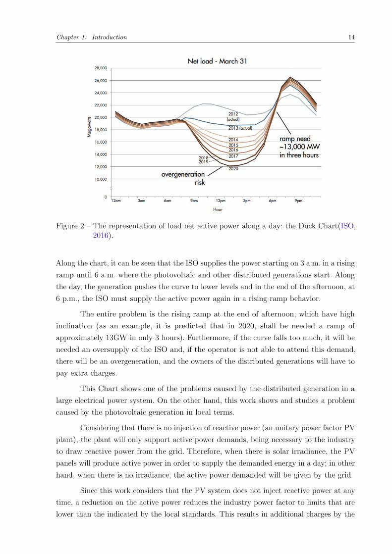
With the increasing utilization of distributed generation, some problems on the
entire electrical grid begin to appear. In fact, a problem rising in electrical power system
is described by the Duck Chart, which can be seen on Figure 2(ISO, 2016). This Chart
represents the net active power delivered, which is the power supplied by the grid minus
the power generated by all distributed generations on analysis. This particular Chart
comes from a day in the city of California.(ISO, 2016)
The Independent System Operator (ISO), that is the operator that controls the
actions and distribution on electrical grids must have attention to the net production.
Chapter 1. Introduction 14
Figure 2 – The representation of load net active power along a day: the Duck Chart(ISO,2016).
Along the chart, it can be seen that the ISO supplies the power starting on 3 a.m. in a rising
ramp until 6 a.m. where the photovoltaic and other distributed generations start. Along
the day, the generation pushes the curve to lower levels and in the end of the afternoon, at
6 p.m., the ISO must supply the active power again in a rising ramp behavior.
The entire problem is the rising ramp at the end of afternoon, which have high
inclination (as an example, it is predicted that in 2020, shall be needed a ramp of
approximately 13GW in only 3 hours). Furthermore, if the curve falls too much, it will be
needed an oversupply of the ISO and, if the operator is not able to attend this demand,
there will be an overgeneration, and the owners of the distributed generations will have to
pay extra charges.
This Chart shows one of the problems caused by the distributed generation in a
large electrical power system. On the other hand, this work shows and studies a problem
caused by the photovoltaic generation in local terms.
Considering that there is no injection of reactive power (an unitary power factor PV
plant), the plant will only support active power demands, being necessary to the industry
to draw reactive power from the grid. Therefore, when there is solar irradiance, the PV
panels will produce active power in order to supply the demanded energy in a day; in other
hand, when there is no irradiance, the active power demanded will be given by the grid.
Since this work considers that the PV system does not inject reactive power at any
time, a reduction on the active power reduces the industry power factor to limits that are
lower than the indicated by the local standards. This results in additional charges by the
Chapter 1. Introduction 15
energy distribution company. In many countries, e.g., Brazil, the power factor must be
over 0.92 inductive (from 6 a.m. to 11 p.m) and 0.92 capacitive (from 0 a.m. to 6 a.m.) to
prevent these charges on exceeding reactive power(ANEEL, 2010).
For instance, there are works related to these aspects. In electrical power systems
in general, capacitor banks are studied as a part of the bus by delivering reactive power
and increasing the voltage levels. The work made on (LONG; OCHOA, 2016) shows the
project of a tapped capacitor bank and a tapped transformer to regulate the voltage levels
on safe limits. The association of control in power factor and voltage level (or Voltage/VAr
control) is greatly studied nowadays. The works on (WANG et al., 2014), (WANDHARE;
AGARWAL, 2014) and (JAHANGIRI; ALIPRANTIS, 2013) show methodologies to find
an optimum utilization of capacitor banks and inverters to make the Voltage/VAr control.
All of these works consider a large system with several bus bars.
When it comes to industrial power plants, there are few works about power factor
impacts due to the installation of PV plants. The work made on (LO; LEE; WU, 2008)
shows the implementation of a control loop to use the inverter as a parallel power factor
corrector, without considering a capacitor bank. Furthermore, in (BANUELOS et al., 2016)
is showed a double loop to use the system to compensate reactive power at night (the
often called multifunctional PV inverter), since there is no active power production in this
period. Also, the work on (LO et al., 2009) shows a power factor correction of the grid
with a switching device to regulate the power supply on a d.c. load with a PV system
operating in parallel.
1.1 Objectives
There are few works in literature that concern about capacitor bank correction for
local industrial RL loads with the presence of a PV power plant. Thus, the contributions
of this work are:
• An overall analysis about the effects of a PV plant on the industry power factor;
• Show the dynamic variations of the additional capacitive reactive power, which is
called here “cat-head curve”;
• Proposing a solution based on tapped capacitor banks.
1.2 Text organization
In chapter 2, a literature review is made to show the schematics of the system,
about power factor corrections and the effects that the PV active power production should

Chapter 1. Introduction 16
cause. Furthermore, in chapter 3, generalized profiles of power consumption are tested as
a case study applying the methodology proposed, theoretically. Also, in chapter 4, the
results about the new demanded capacitive power is explored. Finally, in chapter 5, the
conclusions about this work are discussed.
17
2 Literature Review
2.1 An overview of the system
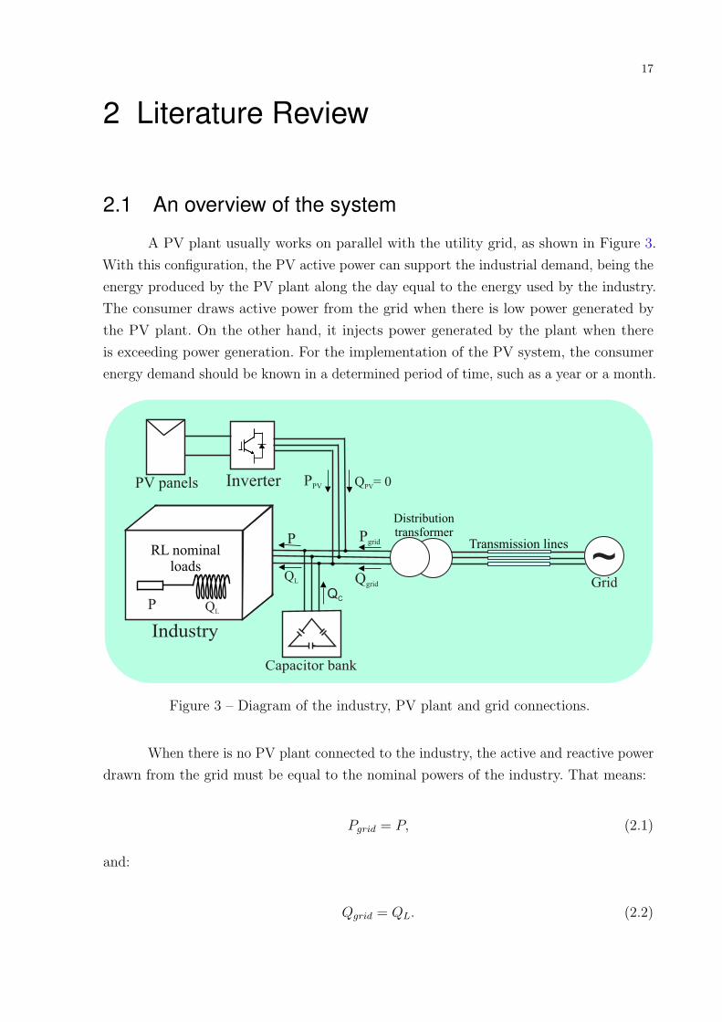
A PV plant usually works on parallel with the utility grid, as shown in Figure 3.
With this configuration, the PV active power can support the industrial demand, being the
energy produced by the PV plant along the day equal to the energy used by the industry.
The consumer draws active power from the grid when there is low power generated by
the PV plant. On the other hand, it injects power generated by the plant when there
is exceeding power generation. For the implementation of the PV system, the consumer
energy demand should be known in a determined period of time, such as a year or a month.
Industry
PV panels Inverter
Capacitor bank
Distributiontransformer
Transmission lines
~Grid
RL nominalloads
Pgrid
Qgrid
PPV Q = 0PV
QC
P QL
P
QL
Figure 3 – Diagram of the industry, PV plant and grid connections.
When there is no PV plant connected to the industry, the active and reactive power
drawn from the grid must be equal to the nominal powers of the industry. That means:
Pgrid = P, (2.1)
and:
Qgrid = QL. (2.2)

Chapter 2. Literature Review 18
The values of P and QL correspond to the nominal load power values, i.e., the
relation of active and reactive power of all equipments in the industry, such as pumps,
motors, etc.
Normally, in the industrial ambient, large inverters are used in a centralized
configuration, which has multi strings inputs and a certain number of MPPTs for maximum
power tracking. Figure 4 shows some types of central inverters produced by ABB.
Figure 4 – Central inverters produced by ABB(ABB, 2018).
2.2 Industrial capacitor banks and power factor correction
As can be seen in Figure 3, there is a capacitor bank which is used in order to
correct the actual power factor of the industry to the limit of 0.92. With the presence of a
capacitor bank, the power factor can be calculated as follows:
pf = cos[
tan−1
(
QL − QC
P
)]
. (2.3)
Chapter 2. Literature Review 19
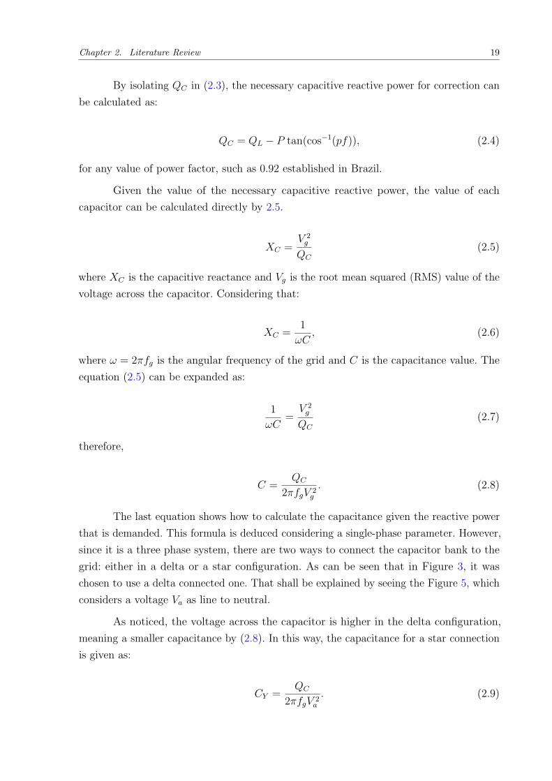
By isolating QC in (2.3), the necessary capacitive reactive power for correction can
be calculated as:
QC = QL − P tan(cos−1(pf)), (2.4)
for any value of power factor, such as 0.92 established in Brazil.
Given the value of the necessary capacitive reactive power, the value of each
capacitor can be calculated directly by 2.5.
XC =V 2
g
QC
(2.5)
where XC is the capacitive reactance and Vg is the root mean squared (RMS) value of the
voltage across the capacitor. Considering that:
XC =1
ωC, (2.6)
where ω = 2πfg is the angular frequency of the grid and C is the capacitance value. The
equation (2.5) can be expanded as:
1
ωC=
V 2g
QC
(2.7)
therefore,
C =QC
2πfgV 2g
. (2.8)
The last equation shows how to calculate the capacitance given the reactive power
that is demanded. This formula is deduced considering a single-phase parameter. However,
since it is a three phase system, there are two ways to connect the capacitor bank to the
grid: either in a delta or a star configuration. As can be seen that in Figure 3, it was
chosen to use a delta connected one. That shall be explained by seeing the Figure 5, which
considers a voltage Va as line to neutral.
As noticed, the voltage across the capacitor is higher in the delta configuration,
meaning a smaller capacitance by (2.8). In this way, the capacitance for a star connection
is given as:
CY =QC
2πfgV 2a
. (2.9)
Chapter 2. Literature Review 20
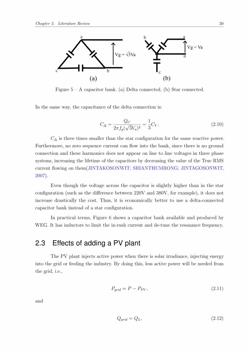
Figure 5 – A capacitor bank. (a) Delta connected. (b) Star connected.
In the same way, the capacitance of the delta connection is:
C∆ =QC
2πfg(√
3Va)2=
1
3CY . (2.10)
C∆ is three times smaller than the star configuration for the same reactive power.
Furthermore, no zero sequence current can flow into the bank, since there is no ground
connection and these harmonics does not appear on line to line voltages in three phase
systems, increasing the lifetime of the capacitors by decreasing the value of the True RMS
current flowing on them(JINTAKOSONWIT; SRIANTHUMRONG; JINTAGOSONWIT,
2007).
Even though the voltage across the capacitor is slightly higher than in the star
configuration (such as the difference between 220V and 380V, for example), it does not
increase drastically the cost. Thus, it is economically better to use a delta-connected
capacitor bank instead of a star configuration.
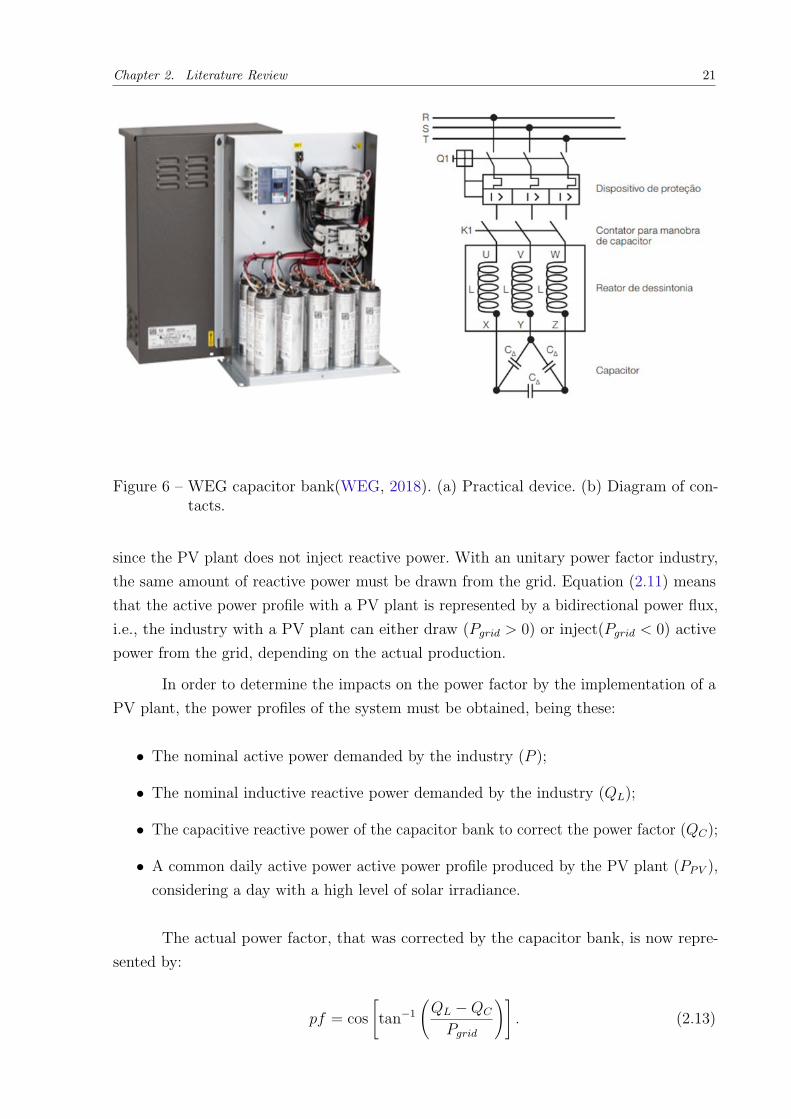
In practical terms, Figure 6 shows a capacitor bank available and produced by
WEG. It has inductors to limit the in-rush current and de-tune the resonance frequency.
2.3 Effects of adding a PV plant
The PV plant injects active power when there is solar irradiance, injecting energy
into the grid or feeding the industry. By doing this, less active power will be needed from
the grid, i.e.,
Pgrid = P − PP V , (2.11)
and
Qgrid = QL, (2.12)
Chapter 2. Literature Review 21
Figure 6 – WEG capacitor bank(WEG, 2018). (a) Practical device. (b) Diagram of con-tacts.
since the PV plant does not inject reactive power. With an unitary power factor industry,
the same amount of reactive power must be drawn from the grid. Equation (2.11) means
that the active power profile with a PV plant is represented by a bidirectional power flux,
i.e., the industry with a PV plant can either draw (Pgrid > 0) or inject(Pgrid < 0) active
power from the grid, depending on the actual production.
In order to determine the impacts on the power factor by the implementation of a
PV plant, the power profiles of the system must be obtained, being these:
• The nominal active power demanded by the industry (P );
• The nominal inductive reactive power demanded by the industry (QL);
• The capacitive reactive power of the capacitor bank to correct the power factor (QC);
• A common daily active power active power profile produced by the PV plant (PP V ),
considering a day with a high level of solar irradiance.
The actual power factor, that was corrected by the capacitor bank, is now repre-
sented by:
pf = cos
[
tan−1
(
QL − QC
Pgrid
)]
. (2.13)
Chapter 2. Literature Review 22
Since Pgrid has lower values than the original active power profile P , it is expected,
by (2.13), that the power factor falls as well. This variable has to remain controlled and,
thus, the reactive capacitive power must be increased. The capacitive power correction
can be made using the expression:
QC,new = QL − |Pgrid| tan(
cos−1 (pf))
, (2.14)
where, given the profiles of the active power P , inductive reactive power QL and the
reference power factor pf , the capacitive reactive power profile can be calculated. Observe
that it is counted the absolute value of the difference between the active power of the load
and the produced power from the PV plant, because negative values for the capacitive
power is not physically significant. The variation of capacitive power can be expressed as
∆QC = QC,new − QC . (2.15)
Expanding the expression in equation (2.15) by using (2.14) and (2.4), it becomes:
∆QC = QL − |Pgrid| tan(
cos−1 (pf))
−(
QL − P tan(
cos−1 (pf)))
. (2.16)
The terms of QL are canceled in (2.16), since the inductive reactive power remains
unchanged with the addition of a unitary power factor PV plant. By simplifying the
expression in (2.16), ∆QC can be represented by:
∆QC = (P − |Pgrid|) tan(
cos−1 (pf))
, (2.17)
which can be expressed as a piecewise function:
∆QC =
PP V tan (cos−1 (pf)) , if P > PP V
(2P − PP V ) tan (cos−1 (pf)) , if P < PP V
(2.18)
The last expression shows a very interesting description of a grid-connected pho-
tovoltaic system that is not often observed. If the active production of the PV plant is
zero, it will be needed no extra capacitive reactive power for power factor correction, i.e.,
there is no change on the previous corrected pf . However, when there is production of
active power, an extra amount of capacitive power will be demanded in order for further
correction.
This last curve expressed in (2.18) is called “cat head curve” in this work, for its
shape. The curve acts like the curve PP V while P − PP V > 0 and has critical values where
the liquid active power (Pgrid) is zero, being necessary the compensation of the entire
Chapter 2. Literature Review 23
reactive inductive power, and that is a risky situation, for the large size of the necessary
extra capacitor bank for correction.
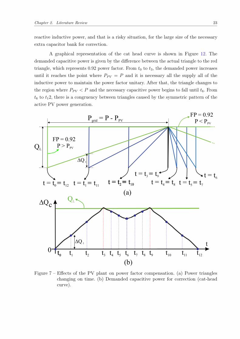
A graphical representation of the cat head curve is shown in Figure 12. The
demanded capacitive power is given by the difference between the actual triangle to the red
triangle, which represents 0.92 power factor. From t0 to t3, the demanded power increases
until it reaches the point where PP V = P and it is necessary all the supply all of the
inductive power to maintain the power factor unitary. After that, the triangle changes to
the region where PP V < P and the necessary capacitive power begins to fall until t6. From
t6 to t12, there is a congruency between triangles caused by the symmetric pattern of the
active PV power generation.
P = P - Pgrid PV
FP = 0.92P > PPV
FP = 0.92P < PPV
c
Figure 7 – Effects of the PV plant on power factor compensation. (a) Power triangleschanging on time. (b) Demanded capacitive power for correction (cat-headcurve).
24
3 Methodology
3.1 Case Study
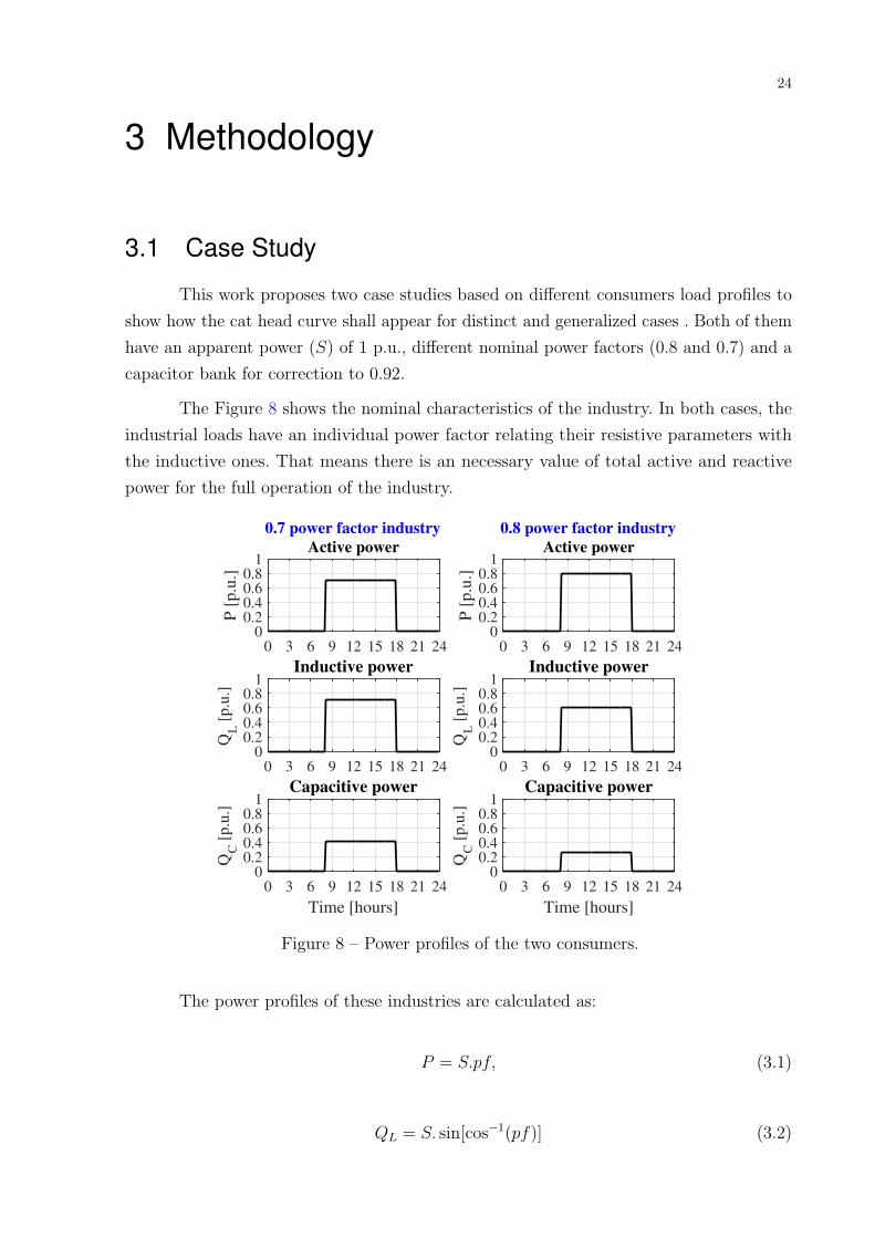
This work proposes two case studies based on different consumers load profiles to
show how the cat head curve shall appear for distinct and generalized cases . Both of them
have an apparent power (S) of 1 p.u., different nominal power factors (0.8 and 0.7) and a
capacitor bank for correction to 0.92.
The Figure 8 shows the nominal characteristics of the industry. In both cases, the
industrial loads have an individual power factor relating their resistive parameters with
the inductive ones. That means there is an necessary value of total active and reactive
power for the full operation of the industry.
0 3 6 9 12 15 18 21 24
P [
p.u
.]
00.20.40.60.8
1
0.7 power factor industry
Active power
0 3 6 9 12 15 18 21 24
QL [
p.u
.]
00.20.40.60.8
1Inductive power
Time [hours]
0 3 6 9 12 15 18 21 24
QC
[p.u
.]
00.20.40.60.8
1Capacitive power
0 3 6 9 12 15 18 21 24
P [
p.u
.]
00.20.40.60.8
1
0.8 power factor industry
Active power
0 3 6 9 12 15 18 21 24
QL [
p.u
.]
00.20.40.60.8
1Inductive power
Time [hours]
0 3 6 9 12 15 18 21 24
QC
[p.u
.]
00.20.40.60.8
1Capacitive power
Figure 8 – Power profiles of the two consumers.
The power profiles of these industries are calculated as:
P = S.pf, (3.1)
QL = S. sin[cos−1(pf)] (3.2)
Chapter 3. Methodology 25
and the capacitive reactive power can be calculated as shown in (2.4).
These profiles represent ideal profiles in industries, being the nominal power (repre-
sented by 1 p.u.) turned on at 8 a.m., kept constant all day long until the system shut
down at 6 p.m.. The nominal power factor represents the installed nominal power of the
consumer (the relation between all reactive power by the active power of the equipments).
With a power factor of 0.7, there is less active power demanded while the inductive
reactive power is increased. This means that the industry needs more capacitive reactive
power in order to regulate the power factor. In other hand, a power factor of 0.8 means
an industry more resistive and less inductive and, thus, less capacitive reactive power is
needed.
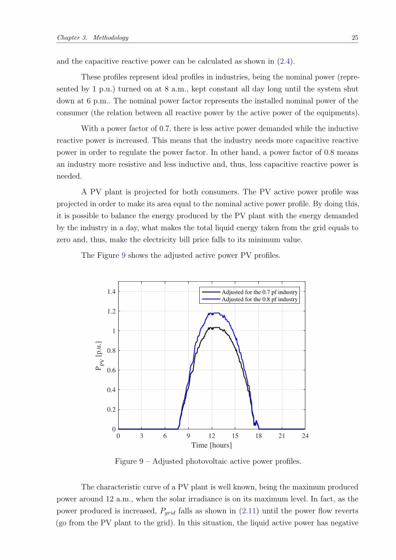
A PV plant is projected for both consumers. The PV active power profile was
projected in order to make its area equal to the nominal active power profile. By doing this,
it is possible to balance the energy produced by the PV plant with the energy demanded
by the industry in a day, what makes the total liquid energy taken from the grid equals to
zero and, thus, make the electricity bill price falls to its minimum value.
The Figure 9 shows the adjusted active power PV profiles.
Time [hours]
0 3 6 9 12 15 18 21 24
PP
V [
p.u
.]
0
0.2
0.4
0.6
0.8
1
1.2
1.4 Adjusted for the 0.7 pf industry
Adjusted for the 0.8 pf industry
Figure 9 – Adjusted photovoltaic active power profiles.
The characteristic curve of a PV plant is well known, being the maximum produced
power around 12 a.m., when the solar irradiance is on its maximum level. In fact, as the
power produced is increased, Pgrid falls as shown in (2.11) until the power flow reverts
(go from the PV plant to the grid). In this situation, the liquid active power has negative
Chapter 3. Methodology 26
values, representing this reverse flow. After the solar irradiance falls at the end of the day,
the liquid active power starts to increase again.
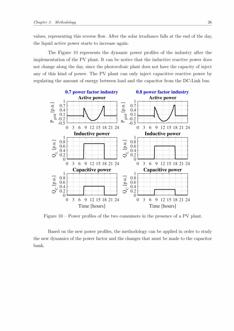
The Figure 10 represents the dynamic power profiles of the industry after the
implementation of the PV plant. It can be notice that the inductive reactive power does
not change along the day, since the photovoltaic plant does not have the capacity of inject
any of this kind of power. The PV plant can only inject capacitive reactive power by
regulating the amount of energy between load and the capacitor from the DC-Link bus.
0 3 6 9 12 15 18 21 24
Pg
rid [
p.u
.]
-0.5-0.20.10.40.7
1
0.7 power factor industry
Active power
0 3 6 9 12 15 18 21 24
QL [
p.u
.]
00.20.40.60.8
1Inductive power
Time [hours]
0 3 6 9 12 15 18 21 24
QC
[p.u
.]
00.20.40.60.8
1Capacitive power
0 3 6 9 12 15 18 21 24P
gri
d [
p.u
.]-0.5-0.20.10.40.7
1
0.8 power factor industry
Active power
0 3 6 9 12 15 18 21 24
QL [
p.u
.]
00.20.40.60.8
1Inductive power
Time [hours]
0 3 6 9 12 15 18 21 24
QC
[p.u
.]
00.20.40.60.8
1Capacitive power
Figure 10 – Power profiles of the two consumers in the presence of a PV plant.
Based on the new power profiles, the methodology can be applied in order to study
the new dynamics of the power factor and the changes that must be made to the capacitor
bank.
27
4 Results and Discussion
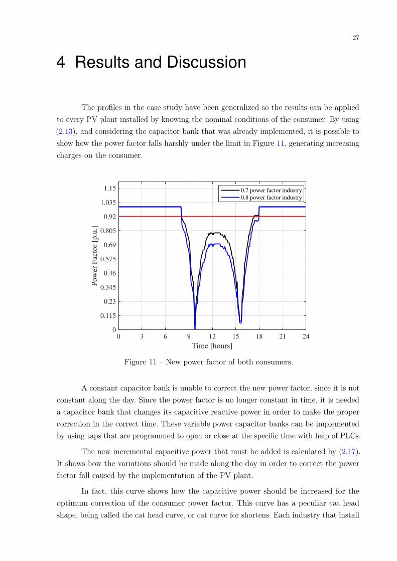
The profiles in the case study have been generalized so the results can be applied
to every PV plant installed by knowing the nominal conditions of the consumer. By using
(2.13), and considering the capacitor bank that was already implemented, it is possible to
show how the power factor falls harshly under the limit in Figure 11, generating increasing
charges on the consumer.
Time [hours]
0 3 6 9 12 15 18 21 24
Po
wer
Fac
tor
[p.u
.]
0
0.115
0.23
0.345
0.46
0.575
0.69
0.805
0.92
1.035
1.15 0.7 power factor industry
0.8 power factor industry
Figure 11 – New power factor of both consumers.
A constant capacitor bank is unable to correct the new power factor, since it is not
constant along the day. Since the power factor is no longer constant in time, it is needed
a capacitor bank that changes its capacitive reactive power in order to make the proper
correction in the correct time. These variable power capacitor banks can be implemented
by using taps that are programmed to open or close at the specific time with help of PLCs.
The new incremental capacitive power that must be added is calculated by (2.17).
It shows how the variations should be made along the day in order to correct the power
factor fall caused by the implementation of the PV plant.
In fact, this curve shows how the capacitive power should be increased for the
optimum correction of the consumer power factor. This curve has a peculiar cat head
shape, being called the cat head curve, or cat curve for shortens. Each industry that install
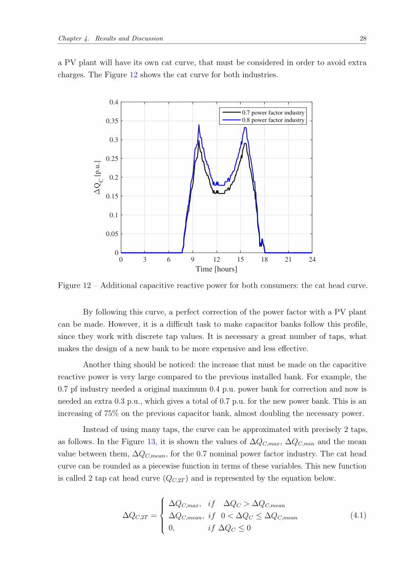
Chapter 4. Results and Discussion 28
a PV plant will have its own cat curve, that must be considered in order to avoid extra
charges. The Figure 12 shows the cat curve for both industries.
Time [hours]
0 3 6 9 12 15 18 21 24
∆Q
C [
p.u
.]
0
0.05
0.1
0.15
0.2
0.25
0.3
0.35
0.4
0.7 power factor industry
0.8 power factor industry
Figure 12 – Additional capacitive reactive power for both consumers: the cat head curve.
By following this curve, a perfect correction of the power factor with a PV plant
can be made. However, it is a difficult task to make capacitor banks follow this profile,
since they work with discrete tap values. It is necessary a great number of taps, what
makes the design of a new bank to be more expensive and less effective.
Another thing should be noticed: the increase that must be made on the capacitive
reactive power is very large compared to the previous installed bank. For example, the
0.7 pf industry needed a original maximum 0.4 p.u. power bank for correction and now is
needed an extra 0.3 p.u., which gives a total of 0.7 p.u. for the new power bank. This is an
increasing of 75% on the previous capacitor bank, almost doubling the necessary power.
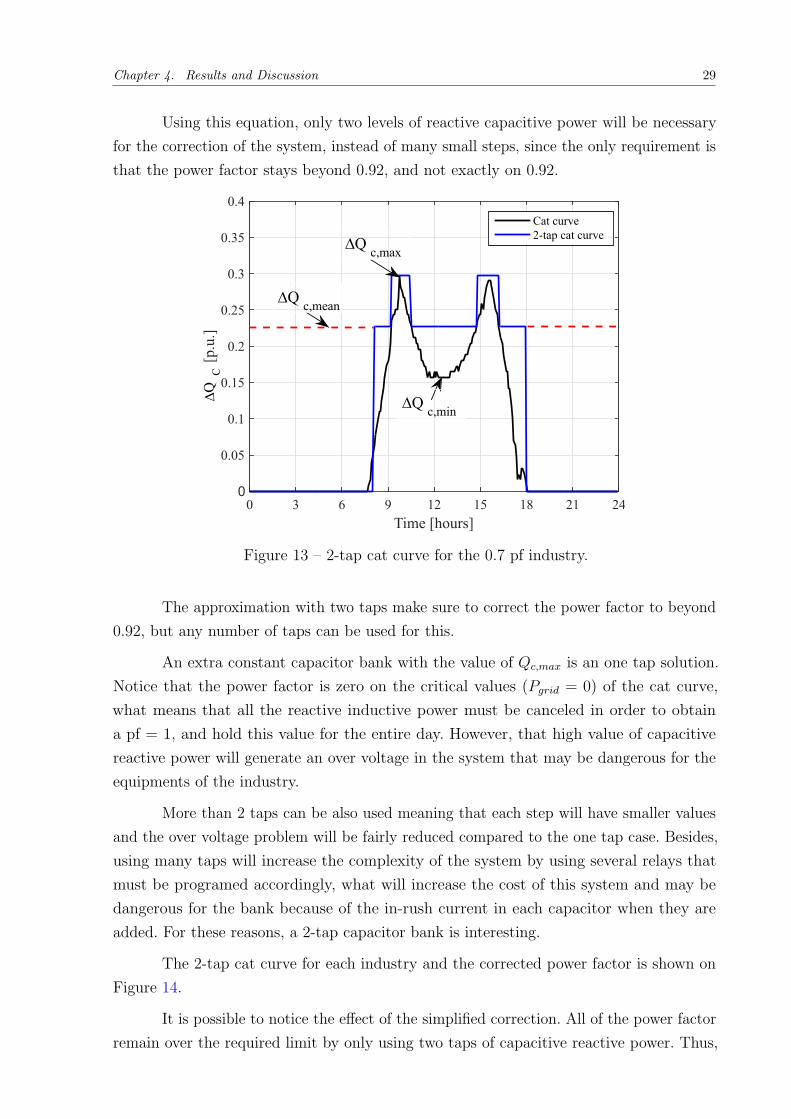
Instead of using many taps, the curve can be approximated with precisely 2 taps,
as follows. In the Figure 13, it is shown the values of ∆QC,max, ∆QC,min and the mean
value between them, ∆QC,mean, for the 0.7 nominal power factor industry. The cat head
curve can be rounded as a piecewise function in terms of these variables. This new function
is called 2 tap cat head curve (QC,2T ) and is represented by the equation below.
∆QC,2T =
∆QC,max, if ∆QC > ∆QC,mean
∆QC,mean, if 0 < ∆QC ≤ ∆QC,mean
0, if ∆QC ≤ 0
(4.1)
Chapter 4. Results and Discussion 29
Using this equation, only two levels of reactive capacitive power will be necessary
for the correction of the system, instead of many small steps, since the only requirement is
that the power factor stays beyond 0.92, and not exactly on 0.92.
Time [hours]
0 3 6 9 12 15 18 21 24
[p.u
.]
0
0.05
0.1
0.15
0.2
0.25
0.3
0.35
0.4∆
QC
Cat curve
2-tap cat curve
∆Qc,min
∆Qc,max
∆Qc,mean
Figure 13 – 2-tap cat curve for the 0.7 pf industry.
The approximation with two taps make sure to correct the power factor to beyond
0.92, but any number of taps can be used for this.
An extra constant capacitor bank with the value of Qc,max is an one tap solution.
Notice that the power factor is zero on the critical values (Pgrid = 0) of the cat curve,
what means that all the reactive inductive power must be canceled in order to obtain
a pf = 1, and hold this value for the entire day. However, that high value of capacitive
reactive power will generate an over voltage in the system that may be dangerous for the
equipments of the industry.
More than 2 taps can be also used meaning that each step will have smaller values
and the over voltage problem will be fairly reduced compared to the one tap case. Besides,
using many taps will increase the complexity of the system by using several relays that
must be programed accordingly, what will increase the cost of this system and may be
dangerous for the bank because of the in-rush current in each capacitor when they are
added. For these reasons, a 2-tap capacitor bank is interesting.
The 2-tap cat curve for each industry and the corrected power factor is shown on
Figure 14.
It is possible to notice the effect of the simplified correction. All of the power factor
remain over the required limit by only using two taps of capacitive reactive power. Thus,
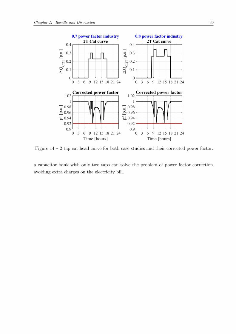
Chapter 4. Results and Discussion 30
0 3 6 9 12 15 18 21 24
∆Q
C,2
T [
p.u
.]
0
0.1
0.2
0.3
0.4
0.7 power factor industry
2T Cat curve
Time [hours]
0 3 6 9 12 15 18 21 24
pf
[p.u
.]
0.9
0.92
0.94
0.96
0.98
1
1.02Corrected power factor
0 3 6 9 12 15 18 21 24
∆Q
C,2
T [
p.u
.]
0
0.1
0.2
0.3
0.4
0.8 power factor industry
2T Cat curve
Time [hours]
0 3 6 9 12 15 18 21 24
pf
[p.u
.]
0.9
0.92
0.94
0.96
0.98
1
1.02Corrected power factor
Figure 14 – 2 tap cat-head curve for both case studies and their corrected power factor.
a capacitor bank with only two taps can solve the problem of power factor correction,
avoiding extra charges on the electricity bill.
31
5 Conclusion
This work made a study on how the inclusion of a PV plant can affect the power
factor of the industries. In fact, with a reduction in the liquid active power of the consumer,
there is a reduction on the power factor that must be solved in order to prevent the charges
on this variable.
It is seen that the capacitive reactive power that must be added have a cat head
shaped curve, in opposition of the constant reactive power that was used for correction.
Thus, a industry that is going to install a photovoltaic plant, must be aware of this
problem, design its own cat head curve and re-design the capacitor bank for an appropriate
correction.
It can yet be analyzed how the reactive power compensation of the inverter can
affect the cat-head curve. With a capacitive power factor, the inverter can decrease the
demand of capacitive power for the curve, making the project of a capacitor bank easier
and less expensive.
Besides, future studies should see the viability of making a good use of both
capacitor bank and inverter, instead of using too much the inverter or designing a large
capacitor bank for correction.

Chapter 5. Conclusion 32
———————————————————-
33
References
ABB. ABB Central inverters @ONLINE. 2018. Disponıvel em: <https://new.abb.com/docs/librariesprovider22/technical-documentation/pvs800-central-inverters-flyer.pdf?sfvrsn=2>. Citado 2 vezes nas paginas 8 and 18.
ACKERMANN, T.; ANDERSSON, G.; SoDER, L. Distributed generation: a definition.Electric Power Systems Research, v. 57, n. 3, p. 195 – 204, 2001. ISSN 0378-7796. Citadona pagina 13.
ANEEL, A. N. de E. E. Resolucao normativa no 414/2010. [S.l.], 2010. Citado 2 vezesnas paginas 12 and 15.
BANUELOS, M. I. F. et al. Passivity-based control for a photovoltaic inverter with powerfactor correction and night operation. IEEE Latin America Transactions, v. 14, n. 8, p.3569–3574, Aug 2016. ISSN 1548-0992. Citado na pagina 15.
DULaU, L. I.; BICa, D. Influence of distributed generators on power systems. ProcediaEngineering, v. 181, p. 791 – 795, 2017. ISSN 1877-7058. Citado na pagina 12.
EPE, E. de pesquisa energetica. Matriz energetica e eletrica. [S.l.], 2016. Citado 2 vezesnas paginas 8 and 12.
EPE, E. de pesquisa energetica. Balanco energetico nacional 2018. [S.l.], 2018. Citado napagina 12.
ISE, F. I. for S. E. S. Photovoltaics Report. [S.l.], 2018. Citado na pagina 13.
ISO, C. What the duck curve tells us about managing a green grid. [S.l.], 2016. Citado 3vezes nas paginas 8, 13, and 14.
JAHANGIRI, P.; ALIPRANTIS, D. C. Distributed volt/var control by pv inverters. IEEETransactions on Power Systems, v. 28, n. 3, p. 3429–3439, Aug 2013. ISSN 0885-8950.Citado na pagina 15.
JINTAKOSONWIT, P.; SRIANTHUMRONG, S.; JINTAGOSONWIT, P. Implementationand performance of an anti-resonance hybrid delta-connected capacitor bank for powerfactor correction. IEEE Transactions on Power Electronics, v. 22, n. 6, p. 2543–2551, Nov2007. ISSN 0885-8993. Citado na pagina 20.
LO, Y. et al. Analysis and design of a photovoltaic system dc connected to the utilitywith a power factor corrector. IEEE Transactions on Industrial Electronics, v. 56, n. 11, p.4354–4362, Nov 2009. ISSN 0278-0046. Citado na pagina 15.
LO, Y. K.; LEE, T. P.; WU, K. H. Grid-connected photovoltaic system with power factorcorrection. IEEE Transactions on Industrial Electronics, v. 55, n. 5, p. 2224–2227, May2008. ISSN 0278-0046. Citado na pagina 15.
LONG, C.; OCHOA, L. F. Voltage control of pv-rich lv networks: Oltc-fitted transformerand capacitor banks. IEEE Transactions on Power Systems, v. 31, n. 5, p. 4016–4025,Sept 2016. ISSN 0885-8950. Citado na pagina 15.

References 34
MANN, S. A. et al. The energy payback time of advanced crystalline silicon pv modulesin 2020: a prospective study. Progress in Photovoltaics: Research and Applications., v. 22,n. 11, p. 1180 – 1194, 2014. ISSN 1099-159X. Citado na pagina 13.
PRADHAN, R.; SUBUDHI, B. Double integral sliding mode mppt control of aphotovoltaic system. IEEE Transactions on Control Systems Technology, v. 24, n. 1, p.285–292, Jan 2016. ISSN 1063-6536. Citado na pagina 13.
SINGH, S.; GAUTAM, A. R.; FULWANI, D. Constant power loads and their effects in dcdistributed power systems: A review. Renewable and Sustainable Energy Reviews, v. 72, p.407 – 421, 2017. ISSN 1364-0321. Citado na pagina 13.
WANDHARE, R. G.; AGARWAL, V. Reactive power capacity enhancement of a pv-gridsystem to increase pv penetration level in smart grid scenario. IEEE Transactions onSmart Grid, v. 5, n. 4, p. 1845–1854, July 2014. ISSN 1949-3053. Citado na pagina 15.
WANG, Y.; WANG, F. Novel three-phase three-level-stacked neutral point clampedgrid-tied solar inverter with a split phase controller. IEEE Transactions on PowerElectronics, v. 28, n. 6, p. 2856–2866, June 2013. ISSN 0885-8993. Citado na pagina 13.
WANG, Z. et al. Inverter-less hybrid voltage/var control for distribution circuits withphotovoltaic generators. IEEE Transactions on Smart Grid, v. 5, n. 6, p. 2718–2728, Nov2014. ISSN 1949-3053. Citado na pagina 15.
WEG. WEG Correcao de fator de potencia @ONLINE.2018. Disponıvel em: <http://ecatalog.weg.net/files/wegnet/WEG-capacitores-para-correcao-do-fator-de-potencia-50009818-catalogo-portugues-br.pdf>. Citado 2 vezes nas paginas 8 and 21.