capítulo 5 astrofísica estelar: o diagrama hr · a classificação se estendia até a letra p. na...

UFABC – NHZ3043 – NOÇÕES DE ASTRONOMIA E COSMOLOGIA – Curso 2016.2 Prof. Germán Lugones

Capítulo 5 Astrofísica estelar: o diagrama HR

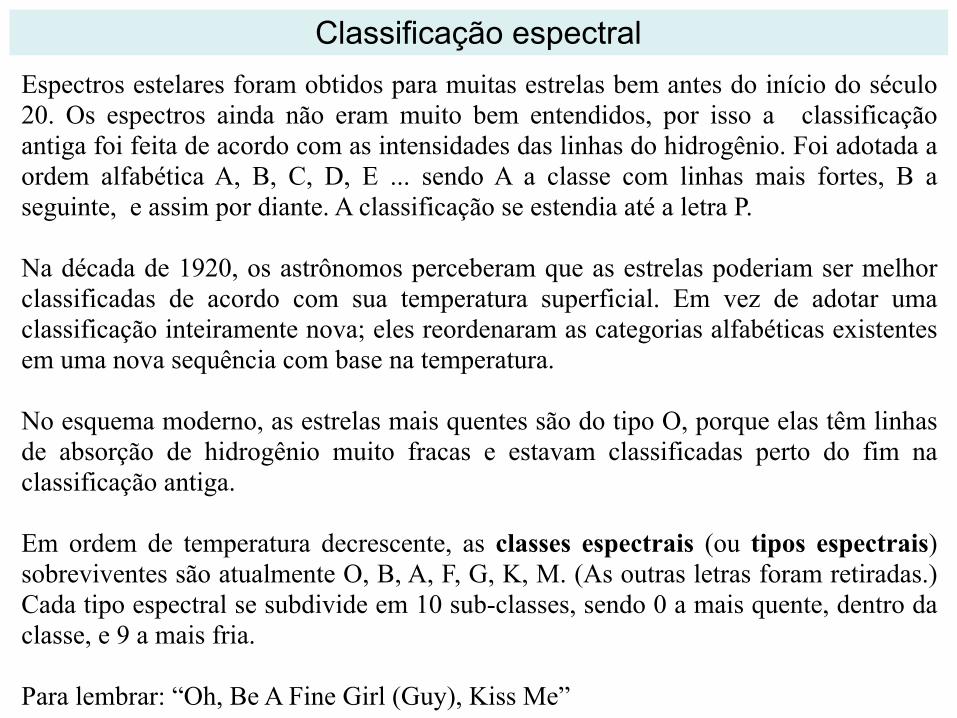
Espectros estelares foram obtidos para muitas estrelas bem antes do início do século 20. Os espectros ainda não eram muito bem entendidos, por isso a classificação antiga foi feita de acordo com as intensidades das linhas do hidrogênio. Foi adotada a ordem alfabética A, B, C, D, E ... sendo A a classe com linhas mais fortes, B a seguinte, e assim por diante. A classificação se estendia até a letra P.

Na década de 1920, os astrônomos perceberam que as estrelas poderiam ser melhor classificadas de acordo com sua temperatura superficial. Em vez de adotar uma classificação inteiramente nova; eles reordenaram as categorias alfabéticas existentes em uma nova sequência com base na temperatura.

No esquema moderno, as estrelas mais quentes são do tipo O, porque elas têm linhas de absorção de hidrogênio muito fracas e estavam classificadas perto do fim na classificação antiga.

Em ordem de temperatura decrescente, as classes espectrais (ou tipos espectrais) sobreviventes são atualmente O, B, A, F, G, K, M. (As outras letras foram retiradas.) Cada tipo espectral se subdivide em 10 sub-classes, sendo 0 a mais quente, dentro da classe, e 9 a mais fria.

Para lembrar: “Oh, Be A Fine Girl (Guy), Kiss Me”

Classificação espectral

432 CHAPTER 17 The Stars

at short wavelengths. Steadily improving interferometric and adaptive-optics techniques have allowed astronomers to construct very-high-resolution stellar images in a small number of cases. Some results show enough detail to show a few surface features, as noted in Figure 17.11(b) for the same star Betelgeuse. (Sec. 5.4 and 5.6)

Once a star’s angular size has been measured, if its distance is also known, we can determine its radius by simple geometry.

(Sec. 1.6) For example, with a distance of 130 pc and an angular diameter of up to 0.045–, Betelgeuse’s maximum radius is 630 times that of the Sun. (We say “maximum radius” here because, as it happens, Betelgeuse is a variable star—its radius and luminosity vary somewhat irregularly, with a period of roughly 6 years.) All told, the sizes of perhaps a few dozen stars have been measured in this way.

Most stars are too distant or too small for such direct measurements to be made. Instead, their sizes must be inferred by indirect means, using

17.4 Stellar SizesMost stars are unresolved points of light in the sky, even when viewed through the largest telescopes. Even so, astronomers can often make quite accurate determinations of their sizes.

Direct and Indirect MeasurementsSome stars are big enough, bright enough, and close enough to allow us to measure their sizes directly. One well-known example is the bright red star Betelgeuse, a prominent member of the constellation Orion (Figure 17.8). As shown in Figure 17.11(a), Betelgeuse is barely large enough to be resolvable by the Hubble Space Telescope

R I V U X G

Size of Jupiter’s orbit(a) (b)

R I V U X G

◀ FIGURE 17.11 Betelgeuse The swollen star Betelgeuse (shown here in false color) is close enough for us to resolve its size directly, along with some surface features thought to be storms similar to those that occur on the Sun. (a) An ultraviolet view of Betelgeuse, as seen by a European camera onboard the Hubble Space Telescope, nearly resolves this huge star. (b) An infrared image, acquired by a three-telescope interferometer in Arizona does better, showing two spots on Betelgeuse’s surface. (ESA/NASA; SAO)

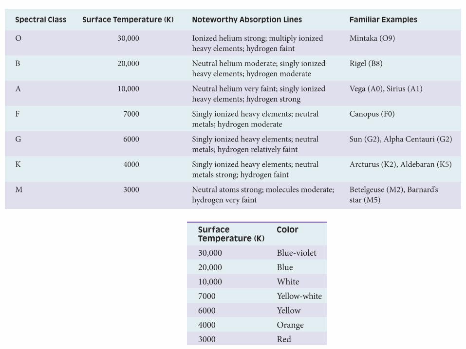
TABLE 17.2 Stellar Spectral Classes

Spectral Class Surface Temperature (K) Noteworthy Absorption Lines Familiar Examples

O 30,000 Ionized helium strong; multiply ionized heavy elements; hydrogen faint

Mintaka (O9)

B 20,000 Neutral helium moderate; singly ionized heavy elements; hydrogen moderate

Rigel (B8)

A 10,000 Neutral helium very faint; singly ionized heavy elements; hydrogen strong

Vega (A0), Sirius (A1)

F 7000 Singly ionized heavy elements; neutral metals; hydrogen moderate

Canopus (F0)

G 6000 Singly ionized heavy elements; neutral metals; hydrogen relatively faint

Sun (G2), Alpha Centauri (G2)

K 4000 Singly ionized heavy elements; neutral metals strong; hydrogen faint

Arcturus (K2), Aldebaran (K5)

M 3000 Neutral atoms strong; molecules moderate; hydrogen very faint

Betelgeuse (M2), Barnard’s star (M5)

SECTION 17.3 Stellar Temperatures 429

Stellar SpectraColor is a useful way to describe a star, but astronomers often use a more detailed scheme to classify stellar properties, incor-porating additional knowledge of stellar physics obtained through spectroscopy. Figure 17.10 compares the spectra of sev-eral different stars, arranged in order of decreasing surface tem-perature (as determined from measurements of their colors). All the spectra extend from 400 to 650 nm, and each shows a series of dark absorption lines superimposed on a background of continuous color, like the spectrum of the Sun. (Sec. 16.3) However, the precise patterns of lines reveal many differences. Some stars display strong lines in the long-wavelength part of the spectrum (to the left in the figure). Other stars have their strongest lines at short wavelengths (to the right). Still others show strong absorption lines spread across the whole visible spectrum. What do these differences tell us?

Although spectral lines of many elements are present with widely varying strengths, the differences among the spec-tra in Figure 17.10 are not due to differences in composition.

drawn through both measured points. To the extent that a star’s spectrum is well approximated as a blackbody, measurements of the B and V fluxes are enough to spec-ify the star’s blackbody curve and thus yield its surface temperature.

Thus, astronomers can estimate a star’s temperature simply by measuring and comparing the amount of light received through different colored filters. As discussed in Chapter 5, this type of non-spectral-line analysis using a standard set of filters is known as photometry.

(Sec. 5.3) Table 17.1 lists, for several prominent stars, the surface temperatures derived by photometric means, along with the color that would be perceived in the absence of filters.

1014

(c)

(b)

B

1000 100

100

1

0.01

10–4

V

3000 K

10,000 K

30,000 K (a)

Infrared Ultraviolet

Frequency (Hz)

Wavelength (nm)

Flux

(arb

itrar

y un

its)

10161015

Temperatures of distant objects can be determined by measuring their radiation.

▲ FIGURE 17.9 Blackbody Curves Star (a) is very hot—30,000 K —so its B (blue) intensity is greater than its V (visual) intensity (as is actually the case for Rigel in Figure 17.8a). Star (b) has roughly equal B and V readings and so appears white, and its temperature is about 10,000 K. Star (c) is red; its V intensity greatly exceeds the B value, and its temperature is 3000 K (much as for Betelgeuse in Figure 17.8a).

Surface Temperature (K)

Color Familiar Examples

30,000 Blue-violet Mintaka (d Orionis)20,000 Blue Rigel10,000 White Vega, Sirius7000 Yellow-white Canopus6000 Yellow Sun, Alpha Centauri4000 Orange Arcturus, Aldebaran3000 Red Betelgeuse, Barnard’s star

TABLE 17.1 Stellar Colors and Temperatures

30,000 K

650 nm 400 nm

O

B

A

F

G

K

M

Many molecules

Oxygen

Oxygen

Iron Calcium

Helium

Helium

Hydrogen

Carbon

IronMagnesiumSodium

20,000 K

10,000 K

7000 K

6000 K

4000 K

3000 K

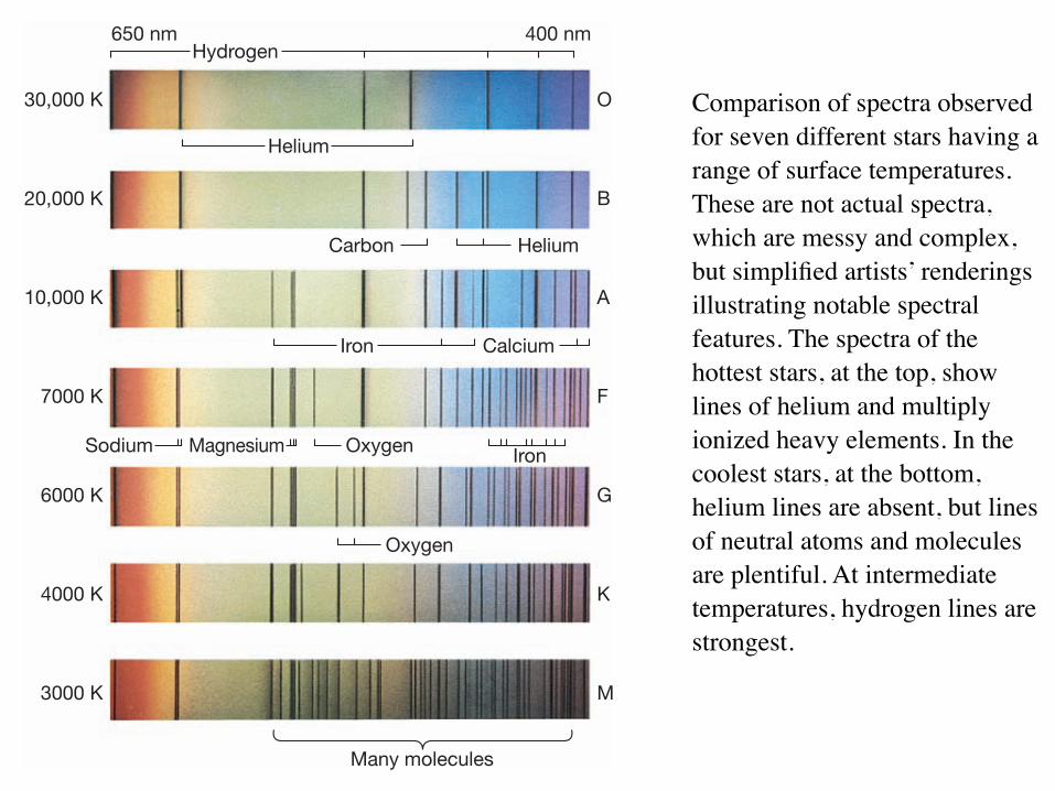
▲ FIGURE 17.10 Stellar Spectra Comparison of spectra observed for seven different stars having a range of surface temperatures. These are not actual spectra, which are messy and complex, but simplified artists’ renderings illustrating notable spectral features. The spectra of the hottest stars, at the top, show lines of helium and multiply ionized heavy elements. In the coolest stars, at the bottom, helium lines are absent, but lines of neutral atoms and molecules are plentiful. At intermediate temperatures, hydrogen lines are strongest.







1014

(c)

(b)

B

1000 100

100

1

0.01

10–4

V

3000 K

10,000 K

30,000 K (a)


Frequency (Hz)

Wavelength (nm)Fl

ux (a

rbitr

ary

units

)

10161015







30,000 K

650 nm 400 nm

O

B

A

F

G

K

M

Many molecules

Oxygen

Oxygen

Iron Calcium

Helium

Helium

Hydrogen

Carbon

IronMagnesiumSodium

20,000 K

10,000 K

7000 K

6000 K

4000 K

3000 K


Comparison of spectra observed for seven different stars having a range of surface temperatures. These are not actual spectra, which are messy and complex, but simplified artists’ renderings illustrating notable spectral features. The spectra of the hottest stars, at the top, show lines of helium and multiply ionized heavy elements. In the coolest stars, at the bottom, helium lines are absent, but lines of neutral atoms and molecules are plentiful. At intermediate temperatures, hydrogen lines are strongest.

212

8. Stellar Spectra

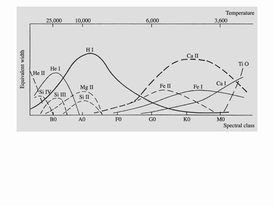
Fig. 8.5. Equivalent widthsof some important spec-tral lines in the variousspectral classes. [Struve, O.(1959): Elementary Astron-omy (Oxford UniversityPress, New York) p. 259]

lines. These lines are due to singly ionized calcium,and the temperature must be just right to remove oneelectron but no more.

The hydrogen Balmer lines Hβ, Hγ and Hδ arestongest in the spectral class A2. These lines corre-spond to transitions to the level the principal quantumnumber of which is n = 2. If the temprature is too highthe hydrogen is ionized and such transitions are notpossible.

8.3 The Yerkes Spectral Classification

The Harvard classification only takes into account theeffect of the temperature on the spectrum. For a moreprecise classification, one also has to take into ac-count the luminosity of the star, since two stars withthe same effective temperature may have widely differ-ent luminosities. A two-dimensional system of spectralclassification was introduced by William W. Morgan,Philip C. Keenan and Edith Kellman of Yerkes Obser-vatory. This system is known as the MKK or Yerkesclassification. (The MK classification is a modified,later version.) The MKK classification is based onthe visual scrutiny of slit spectra with a dispersion of11.5 nm/mm. It is carefully defined on the basis of stan-dard stars and the specification of luminosity criteria.Six different luminosity classes are distinguished:

– Ia most luminous supergiants,– Ib less luminous supergiants,

– II luminous giants,– III normal giants,– IV subgiants,– V main sequence stars (dwarfs).

The luminosity class is determined from spectrallines that depend strongly on the stellar surface gravity,which is closely related to the luminosity. The massesof giants and dwarfs are roughly similar, but the radii ofgiants are much larger than those of dwarfs. Thereforethe gravitational acceleration g = G M/R2 at the surfaceof a giant is much smaller than for a dwarf. In conse-quence, the gas density and pressure in the atmosphereof a giant is much smaller. This gives rise to luminos-ity effects in the stellar spectrum, which can be used todistinguish between stars of different luminosities.

1. For spectral types B–F, the lines of neutral hydrogenare deeper and narrower for stars of higher lumi-nosities. The reason for this is that the metal ionsgive rise to a fluctuating electric field near the hydro-gen atoms. This field leads to shifts in the hydrogenenergy levels (the Stark effect), appearing as a broad-ening of the lines. The effect becomes stronger as thedensity increases. Thus the hydrogen lines are nar-row in absolutely bright stars, and become broaderin main sequence stars and even more so in whitedwarfs (Fig. 8.6).

2. The lines from ionized elements are relativelystronger in high-luminosity stars. This is because thehigher density makes it easier for electrons and ionsto recombine to neutral atoms. On the other hand, the

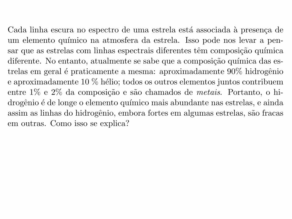
Figura 22.4: Intensidade das linhas espectrais em funcao da temperatura,ou tipo espectral.

22.4.1 A sequencia espectral e a temperatura das estrelas

Cada linha escura no espectro de uma estrela esta associada a presenca deum elemento quımico na atmosfera da estrela. Isso pode nos levar a pen-sar que as estrelas com linhas espectrais diferentes tem composicao quımicadiferente. No entanto, atualmente se sabe que a composicao quımica das es-trelas em geral e praticamente a mesma: aproximadamente 90% hidrogenioe aproximadamente 10 % helio; todos os outros elementos juntos contribuementre 1% e 2% da composicao e sao chamados de metais. Portanto, o hi-drogenio e de longe o elemento quımico mais abundante nas estrelas, e aindaassim as linhas do hidrogenio, embora fortes em algumas estrelas, sao fracasem outras. Como isso se explica?

Na verdade, mais do que a composicao quımica, e a temperatura quedetermina o espectro das estrelas. Consideremos uma linha de Balmer dohidrogenio. Essas linhas se originam em transicoes entre o segundo nıvelde energia do hidrogenio e qualquer outro nıvel acima dele: transicoes denıvel para cima (n2 > 2) resultam em absorcao, transicoes de nıvel parabaixo (n2 = 2) resultam em emissao. Entao, para uma estrela ter linhas deBalmer intensas, ela precisa ter muitos atomos de hidrogenio excitados aonıvel n=2. Isso acontece em estrelas com temperatura em torno de 10 000 K(kT = 0, 86 eV); para temperaturas muito mais baixas, como a do Sol porexemplo, o hidrogenio esta no estado fundamental, e poucas colisoes podemacontecer que sejam energeticas o suficiente para excitar o hidrogenio. Ja emestrelas com temperaturas muito mais altas, o hidrogenio esta quase todo

211

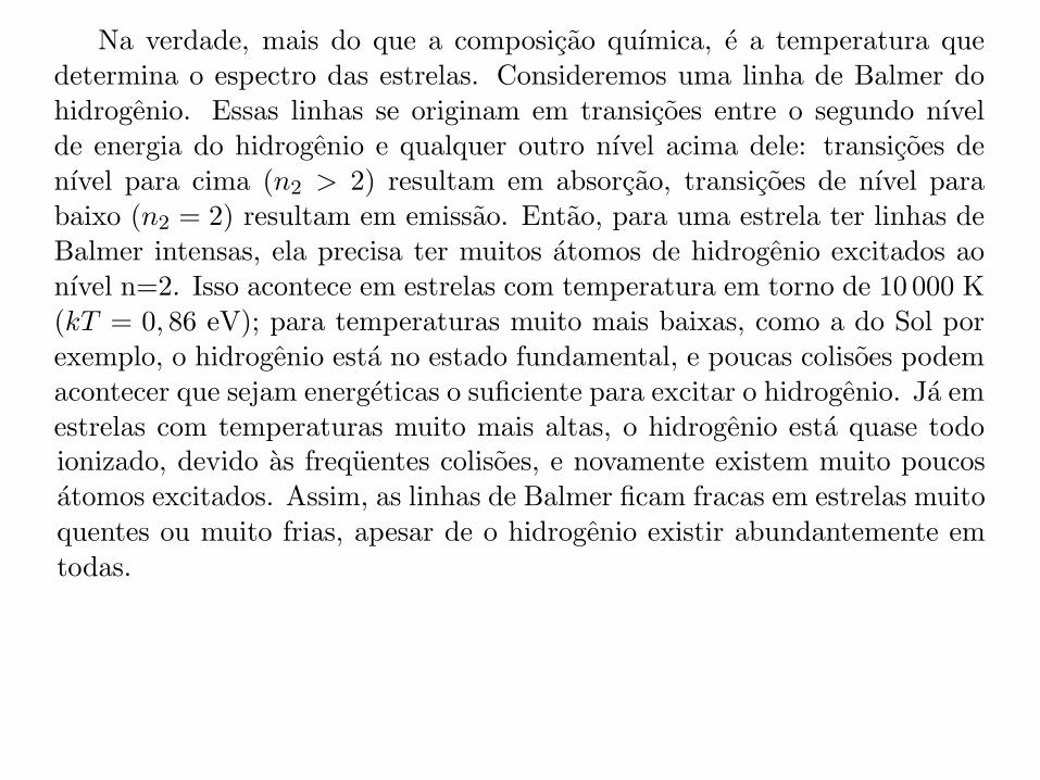
Figura 22.4: Intensidade das linhas espectrais em funcao da temperatura,ou tipo espectral.

22.4.1 A sequencia espectral e a temperatura das estrelas

Cada linha escura no espectro de uma estrela esta associada a presenca deum elemento quımico na atmosfera da estrela. Isso pode nos levar a pen-sar que as estrelas com linhas espectrais diferentes tem composicao quımicadiferente. No entanto, atualmente se sabe que a composicao quımica das es-trelas em geral e praticamente a mesma: aproximadamente 90% hidrogenioe aproximadamente 10 % helio; todos os outros elementos juntos contribuementre 1% e 2% da composicao e sao chamados de metais. Portanto, o hi-drogenio e de longe o elemento quımico mais abundante nas estrelas, e aindaassim as linhas do hidrogenio, embora fortes em algumas estrelas, sao fracasem outras. Como isso se explica?

Na verdade, mais do que a composicao quımica, e a temperatura quedetermina o espectro das estrelas. Consideremos uma linha de Balmer dohidrogenio. Essas linhas se originam em transicoes entre o segundo nıvelde energia do hidrogenio e qualquer outro nıvel acima dele: transicoes denıvel para cima (n2 > 2) resultam em absorcao, transicoes de nıvel parabaixo (n2 = 2) resultam em emissao. Entao, para uma estrela ter linhas deBalmer intensas, ela precisa ter muitos atomos de hidrogenio excitados aonıvel n=2. Isso acontece em estrelas com temperatura em torno de 10 000 K(kT = 0, 86 eV); para temperaturas muito mais baixas, como a do Sol porexemplo, o hidrogenio esta no estado fundamental, e poucas colisoes podemacontecer que sejam energeticas o suficiente para excitar o hidrogenio. Ja emestrelas com temperaturas muito mais altas, o hidrogenio esta quase todo

211ionizado, devido as frequentes colisoes, e novamente existem muito poucosatomos excitados. Assim, as linhas de Balmer ficam fracas em estrelas muitoquentes ou muito frias, apesar de o hidrogenio existir abundantemente emtodas.

22.5 Classificacao de luminosidade

A classificacao espectral de Harvard so leva em conta a temperatura dasestrelas. Considerando que a luminosidade de uma estrela e dada por

L = 4ºR2æT 4ef

vemos que a luminosidade de uma estrela com maior raio e maior, para amesma temperatura. Em 1943, William Wilson Morgan (1906-1994), PhilipChilds Keenan (1908-2000) e Edith Kellman, do Observatorio de Yerkes, in-troduziram as seis diferentes classes de luminosidade, baseados nas largurasde linhas espectrais que sao sensıveis a gravidade superficial:

• Ia - supergigantes superluminosas. Exemplo: Rigel (B8Ia)

• Ib - supergigantes. Exemplo: Betelgeuse (M2Iab)

• II - gigantes luminosas. Exemplo: Antares (MII)

• III - gigantes. Exemplo: Aldebara (K5III)

• IV - subgigantes. Exemplo: Æ Crucis (B1IV)

• V - anas (sequencia principal). Exemplo: Sırius (A1V)

A classe de luminosidade de uma estrela tambem e conhecida pelo seuespectro. Isso e possıvel porque a largura das linhas espectrais dependefortemente da gravidade superficial, que e diretamente relacionada a lumi-nosidade. As massas das gigantes e anas da sequencia principal sao similares,mas o raio das gigantes e muito maior. Como a aceleracao gravitacional edada por g:

g =GM

R2,

ela e muito maior para uma ana do que para uma gigante. Quanto maiora gravidade superficial, maior a pressao e, portanto, maior o numero de co-lisoes entre as partıculas na atmosfera da estrela. As colisoes perturbam osnıveis de energia dos atomos, fazendo com que eles fiquem mais proximos

212







1014

(c)

(b)

B

1000 100

100

1

0.01

10–4

V

3000 K

10,000 K

30,000 K (a)


Frequency (Hz)

Wavelength (nm)

Flux

(arb

itrar

y un

its)

10161015







30,000 K

650 nm 400 nm

O

B

A

F

G

K

M

Many molecules

Oxygen

Oxygen

Iron Calcium

Helium

Helium

Hydrogen

Carbon

IronMagnesiumSodium

20,000 K

10,000 K

7000 K

6000 K

4000 K

3000 K


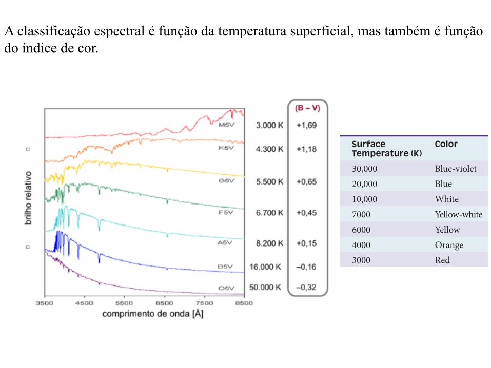
A classificação espectral é função da temperatura superficial, mas também é função do índice de cor.

Classificação de luminosidade

A classificação espectral de Harvard só leva em conta a temperatura das estrelas. Considerando que a luminosidade de uma estrela é dada por

vemos que a luminosidade de uma estrela com maior raio é maior, para a mesma temperatura.

Em 1943, foram introduzidas seis diferentes classes de luminosidade (de Morgan-Keenan), baseadas nas larguras de linhas espectrais que são sensíveis à gravidade superficial:

• Ia - supergigantes superluminosas. Exemplo: Rigel (B8Ia) • Ib - supergigantes. Exemplo: Betelgeuse (M2Iab)• II - gigantes luminosas. Exemplo: Antares (MII)• III - gigantes. Exemplo: Aldebarã (K5III) • IV - subgigantes. Exemplo: α Crucis (B1IV) • V - anãs (sequência principal). Exemplo: Sírius (A1V)

ionizado, devido as frequentes colisoes, e novamente existem muito poucosatomos excitados. Assim, as linhas de Balmer ficam fracas em estrelas muitoquentes ou muito frias, apesar de o hidrogenio existir abundantemente emtodas.



L = 4ºR2æT 4ef









g =GM

R2,


212

A classe de luminosidade de uma estrela pode ser conhecida pelo seu espectro. Isso é possível porque a largura das linhas espectrais depende fortemente da gravidade superficial, que é diretamente relacionada à luminosidade:

‣ A aceleração gravitacional na superfície de uma estrela é dada por g:

‣ Para estrelas de massas iguais, g é muito maior para uma anã do que para uma gigante.

‣ Quanto maior a gravidade superficial, maior a pressão e, portanto, maior o número de colisões entre as partículas na atmosfera da estrela.

‣ As colisões perturbam os níveis de energia dos átomos, fazendo com que eles fiquem mais próximos ou mais afastados entre si do que o normal.

‣ Assim, os átomos perturbados podem absorver fótons de energia e comprimento de onda levemente maior ou menor do que os que os fótons absorvidos nas transições entre níveis não perturbados.

‣ O efeito disso é que as linhas ficam alargadas (alargamento colisional ou de pressão). Portanto, para uma mesma temperatura, quanto menor a estrela, mais alargada será a linha, e vice-versa.

ionizado, devido as frequentes colisoes, e novamente existem muito poucosatomos excitados. Assim, as linhas de Balmer ficam fracas em estrelas muitoquentes ou muito frias, apesar de o hidrogenio existir abundantemente emtodas.



L = 4ºR2æT 4ef









g =GM

R2,


212

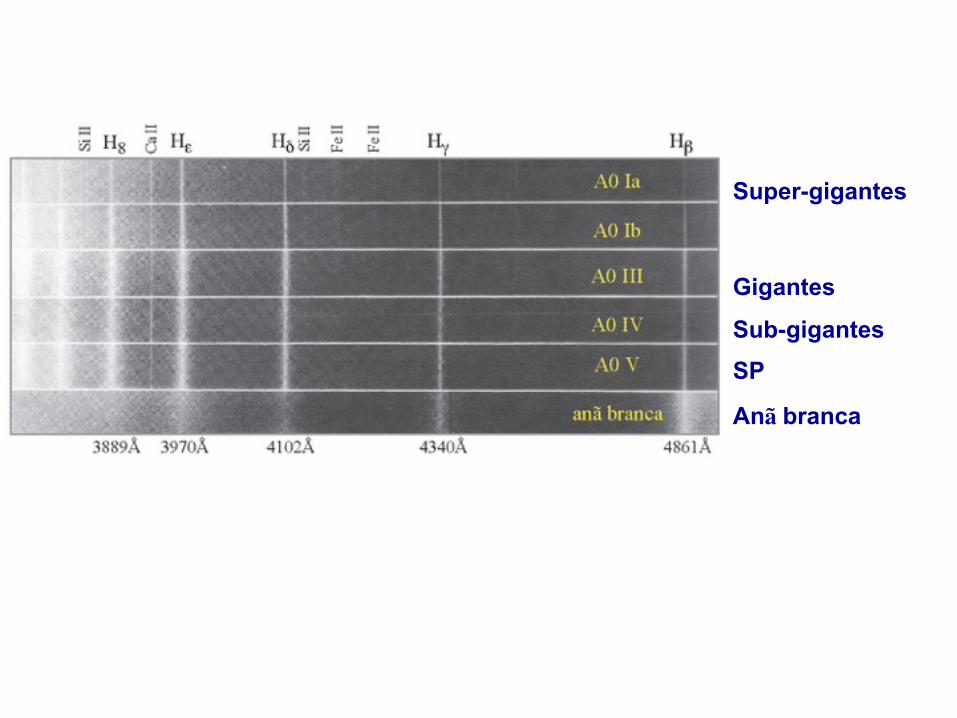
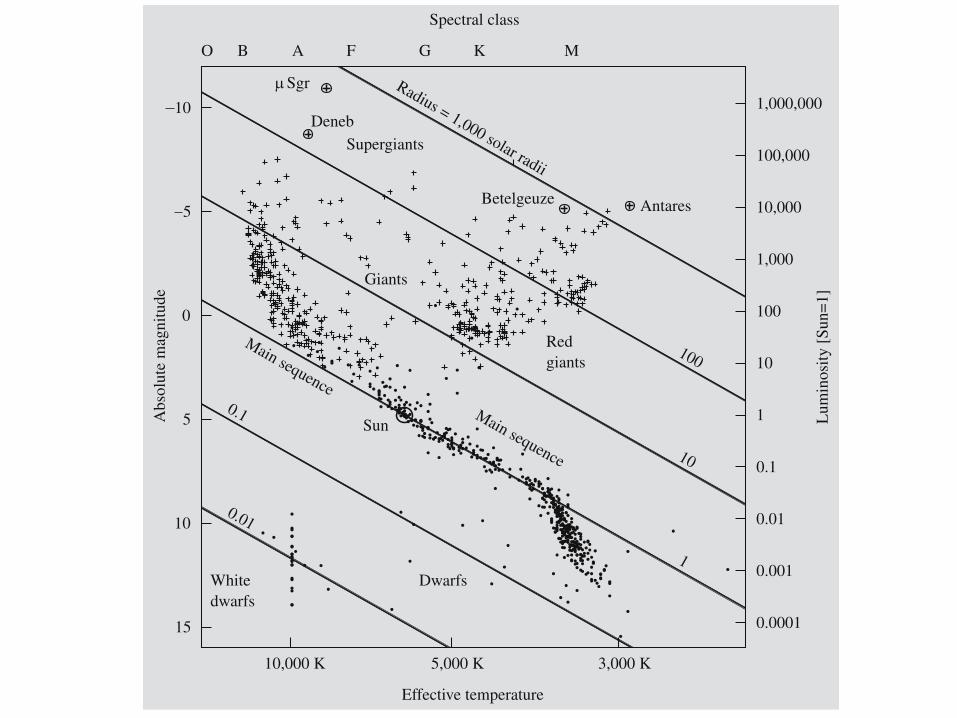
Super-gigantes

Gigantes

Sub-gigantes SP

Anã branca

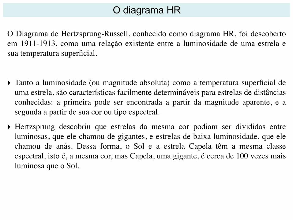
O Diagrama de Hertzsprung-Russell, conhecido como diagrama HR, foi descoberto em 1911-1913, como uma relação existente entre a luminosidade de uma estrela e sua temperatura superficial.

‣ Tanto a luminosidade (ou magnitude absoluta) como a temperatura superficial de uma estrela, são características facilmente determináveis para estrelas de distâncias conhecidas: a primeira pode ser encontrada a partir da magnitude aparente, e a segunda a partir de sua cor ou tipo espectral.

‣ Hertzsprung descobriu que estrelas da mesma cor podiam ser divididas entre luminosas, que ele chamou de gigantes, e estrelas de baixa luminosidade, que ele chamou de anãs. Dessa forma, o Sol e a estrela Capela têm a mesma classe espectral, isto é, a mesma cor, mas Capela, uma gigante, é cerca de 100 vezes mais luminosa que o Sol.

O diagrama HR

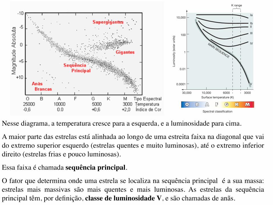
Nesse diagrama, a temperatura cresce para a esquerda, e a luminosidade para cima.

A maior parte das estrelas está alinhada ao longo de uma estreita faixa na diagonal que vai do extremo superior esquerdo (estrelas quentes e muito luminosas), até o extremo inferior direito (estrelas frias e pouco luminosas).

Essa faixa é chamada sequência principal.

O fator que determina onde uma estrela se localiza na sequência principal é a sua massa: estrelas mais massivas são mais quentes e mais luminosas. As estrelas da sequência principal têm, por definição, classe de luminosidade V, e são chamadas de anãs.

SECTION 17.6 Extending the Cosmic Distance Scale 439

normally found in main-sequence stars, the star may be recognized as a K2III giant, with a luminosity 100 times that of the Sun (Figure 17.18a). If the lines are very narrow, the star might instead be classified as a K2Ib supergiant, brighter by a further factor of 40, at 4000 solar luminosities. In each case, knowledge of luminosity classes allows astronomers to identify the object and make an appropriate estimate of its luminosity and hence its distance.

CONCEPT Check

4 Suppose astronomers discover that, due to a calibration error, all distances measured by geometric parallax are 10 percent larger than currently thought. What effect would this finding have on the “standard” main sequence used in spectroscopic parallax?

astronomers can usually tell with a high degree of confi-dence what sort of object it is. Now we have a way of speci-fying a star’s location in the diagram in terms of properties that are measurable by purely spectroscopic means: Spectral type and luminosity class define a star on the H–R diagram just as surely as do temperature and luminosity. The full specification of a star’s spectral properties includes its lumi-nosity class. For example, the Sun, a G2 main-sequence star, is of class G2V, the B8 blue supergiant Rigel is B8Ia, the red dwarf Barnard’s star is M5V, the red supergiant Betelgeuse is M2Ia, and so on.

Consider, for example, a K2-type star (Table 17.4) with a surface temperature of approximately 4500 K. If the widths of the star’s spectral lines tell us that it lies on the main sequence (i.e., it is a K2V star), then its luminosity is about 0.3 times the solar value. If the star’s spectral lines are observed to be narrower than lines

◀ FIGURE 17.18 Luminosity Classes (a) Approximate locations of the standard stellar luminosity classes in the H–R diagram. The widths of absorption lines also provide information on the density of a star’s atmosphere. The denser atmosphere of a main-sequence K-type star has broader lines (c) than a giant star of the same spectral class (b).

KIb-typesupergiant

star

KV-typemain sequence

star

Spectral classification

Surface temperature (K)

(a)

30,000 10,000 6000 3000

0.0001

0.01

1

100

10,000

Lum

inos

ity (s

olar

uni

ts)

Ia

K range

IbII

III

IV

V

MAIN SEQUENCE

(b)

Wavelength430 420 410 nm

(c)

TABLE 17.4 Variation in Stellar Properties within a Spectral Class

Surface Temperature Luminosity Radius Object Example(K) (solar luminosities) (solar radii)

4900 0.3 0.8 K2V main-sequence star P Eridani

4500 110 21 K2III red giant Arcturus

4300 4000 140 K2Ib red supergiant P Pegasi

Um número substancial de estrelas também se concentra acima da sequência principal, na região superior direita (estrelas frias e luminosas). Essas estrelas são chamadas gigantes, e pertencem à classe de luminosidade II ou III.

Bem no topo do diagrama existem algumas estrelas ainda mais luminosas: são chamadas supergigantes, com classe de luminosidade I.



CONCEPT Check





KIb-typesupergiant

star


star



(a)

30,000 10,000 6000 3000

0.0001

0.01

1

100

10,000

Lum

inos

ity (s

olar

uni

ts)

Ia

K range

IbII

III

IV

V

MAIN SEQUENCE

(b)


(c)






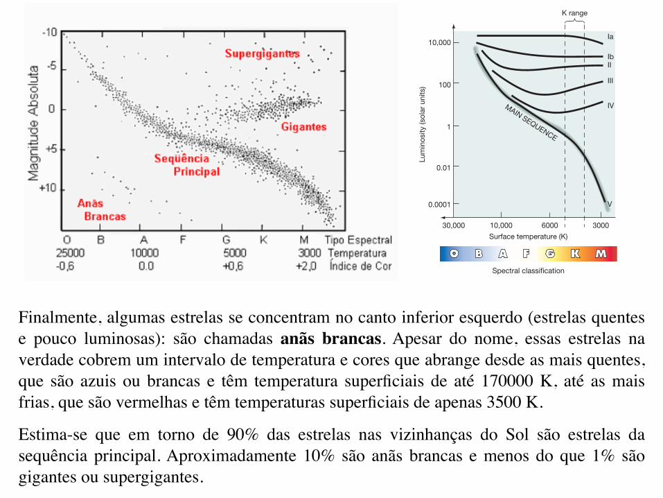
Finalmente, algumas estrelas se concentram no canto inferior esquerdo (estrelas quentes e pouco luminosas): são chamadas anãs brancas. Apesar do nome, essas estrelas na verdade cobrem um intervalo de temperatura e cores que abrange desde as mais quentes, que são azuis ou brancas e têm temperatura superficiais de até 170000 K, até as mais frias, que são vermelhas e têm temperaturas superficiais de apenas 3500 K.

Estima-se que em torno de 90% das estrelas nas vizinhanças do Sol são estrelas da sequência principal. Aproximadamente 10% são anãs brancas e menos do que 1% são gigantes ou supergigantes.



CONCEPT Check





KIb-typesupergiant

star


star



(a)

30,000 10,000 6000 3000

0.0001

0.01

1

100

10,000

Lum

inos

ity (s

olar

uni

ts)

Ia

K range

IbII

III

IV

V

MAIN SEQUENCE

(b)


(c)






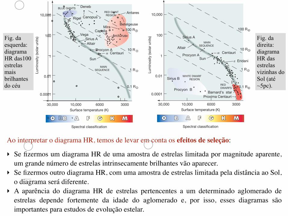
Ao interpretar o diagrama HR, temos de levar em conta os efeitos de seleção:

‣ Se fizermos um diagrama HR de uma amostra de estrelas limitada por magnitude aparente, um grande número de estrelas intrinsecamente brilhantes vão aparecer.

‣ Se fizermos outro diagrama HR, com uma amostra de estrelas limitada pela distância ao Sol, o diagrama será diferente.

‣ A aparência do diagrama HR de estrelas pertencentes a um determinado aglomerado de estrelas depende fortemente da idade do aglomerado e, por isso, esses diagramas são importantes para estudos de evolução estelar.

436 CHAPTER 17 The Stars

AN

IMAT

ION

/VID

EO W

hite

Dw

arfs

in G

lobu

lar

Clus

ter

SELF

-GU

IDED

TU

TOR

IAL

Her

tzsp

rung

–Rus

sell

Dia

gram

If very luminous blue giants are overrepresented in Figure 17.15, low-luminosity red dwarfs are surely under-represented. In fact, no dwarfs appear on the diagram. This absence is not surprising because low-luminosity stars are difficult to observe from Earth. In the 1970s, astronomers began to realize that they had greatly underestimated the number of red dwarfs in our galaxy. As hinted at by the H–R diagram in Figure 17.14, which shows an unbiased sample of stars in the solar neighborhood, red dwarfs are actually the most common type of star in the sky. In fact, they probably account for upward of 80 percent of all stars in the universe. In contrast, O- and B-type supergiants are extremely rare, with only about 1 star in 10,000 falling into these categories.

White Dwarfs and Red GiantsMost stars lie on the main sequence. However, some of the points plotted in Figures 17.13 through 17.15 clearly do not. One such point in Figure 17.13 represents Procyon B, the white dwarf discussed earlier (Section 17.4), with surface tempera-ture 8500 K and luminosity about 0.0006 times the solar value. A few more such faint, hot stars can be seen in Figure 17.14 in the bottom left-hand corner of the H–R diagram. This region, known as the white-dwarf region, is marked on Figure 17.14.

Also shown in Figure 17.13 is Aldebaran (discussed in Section 17.4), whose surface temperature is 4000 K and whose luminosity is some 300 times greater than the Sun’s. Another point represents Betelgeuse (Alpha Orionis), the ninth-brightest star in the sky, a little cooler than Aldebaran, but more than 100 times brighter. The upper right-hand corner of the H–R diagram, where these stars lie (marked on Figure 17.15), is called the red-giant region. No red giants are found within 5 pc of the Sun (Figure 17.14), but many of the brightest stars seen in the sky are in fact red giants (Figure 17.15). Though relatively rare, red giants are so bright that they are visible to great distances. They form a third distinct class of stars on the H–R diagram, very different in their properties from both main-sequence stars and white dwarfs.

The Hipparcos mission (Section 17.1), in addition to determining hundreds of thousands of stellar parallaxes with unprecedented accuracy, also measured the colors and luminosities of more than 2 million stars. Figure 17.16 shows an H–R diagram based on a tiny portion of the enormous Hipparcos dataset. The main-sequence and red-giant regions are clearly evident. Few white dwarfs appear, however, sim-ply because the telescope was limited to observations of rela-tively bright objects—brighter than apparent magnitude 12. Almost no white dwarfs lie close enough to Earth that their magnitudes fall below this limit.

About 90 percent of all stars in our solar neighborhood, and probably a similar percentage elsewhere in the universe, are main-sequence stars. About 9 percent of stars are white dwarfs, and 1 percent are red giants.

Along a constant-radius line, the radius–luminosity–temper-ature relationship implies that

luminosity ∝ temperature4.

By including such lines on our H–R diagrams, we can indicate stellar temperatures, luminosities, and radii on a single plot.

We see a very clear trend as we traverse the main sequence from top to bottom. At one end, the stars are large, hot, and bright. Because of their size and color, they are referred to as blue giants. The very largest are called blue supergiants. At the other end, stars are small, cool, and faint. They are known as red dwarfs. Our Sun lies right in the middle.

Figure 17.15 shows an H–R diagram for a different group of stars—the 100 stars of known distance having the great-est apparent brightness, as seen from Earth. Notice the much larger number of very luminous stars at the upper end of the main sequence than at the lower end. The reason for this excess of blue giants is simple: We can see very luminous stars a long way off. The stars shown in this figure are scattered through a much greater volume of space than those depicted in Figure 17.14, but the sample is heavily biased toward the brightest objects. In fact, of the 20 brightest stars in the sky, only 6 lie within 10 pc of us; the rest are visible, despite their great distances, because of their high luminosities.

▲ FIGURE 17.15 H–R Diagram of Brightest Stars An H–R diagram for the 100 brightest stars in the sky is biased in favor of the most luminous stars—which appear toward the upper left—because we can see them more easily than we can the faintest stars. (Compare with Figure 17.14, which shows only the closest stars.)


Surface temperature (K)30,000 10,000 6000 3000

0.0001

0.01

1

100

10,000

Lum

inos

ity (s

olar

uni

ts)

Rigel

Betelgeuse

Antares

Arcturus

Sun

MAINSEQUENCE

BLUE GIANTSRED GIANT REGION

0.1 R

10 R

100 R

Deneb

Canopus

1 R

MiraCapella

a CentauriProcyon A

Altair

VegaSirius A

SECTION 17.5 The Hertzsprung–Russell Diagram 435

Figure 17.14 shows a more systematic study of stellar properties, covering the 80 or so stars that lie within 5 pc of the Sun. As more points are included in the diagram, the main sequence “fills up,” and the pattern becomes more evi-dent. The vast majority of stars in the immediate vicinity of the Sun lie on the main sequence.

The surface temperatures of main-sequence stars range from about 3000 K (spectral class M) to over 30,000 K (spec-tral class O). This relatively small temperature range—a differ-ence of only a factor of 10—is determined mainly by the rates at which nuclear reactions occur in stellar cores. (Sec. 16.6) In contrast, the observed range in luminosities is very large, cover-ing some eight orders of magnitude (i.e., a factor of 100 million), ranging from 10−4 to 104 times the luminosity of the Sun.

Using the radius–luminosity–temperature relationship (Section 17.4), astronomers find that stellar radii also vary along the main sequence. The faint, red M-type stars at the bottom right of the H–R diagram are only about one-tenth the size of the Sun, whereas the bright, blue O-type stars in the upper left are about 10 times larger than the Sun. The diagonal dashed lines in Figure 17.14 represent constant stel-lar radii, meaning that any star lying on a given line has the same radius, regardless of its luminosity or temperature.

discussion mainly in terms of the more “theoretical” quan-tities, temperature and luminosity, but realize that, for many purposes, color-magnitude and H–R diagrams repre-sent pretty much the same thing.

The Main SequenceThe handful of stars plotted in Figure 17.13 gives little indication of any particular connection between stellar properties. However, as Hertzsprung and Russell plot-ted more and more stellar temperatures and luminosities, they found that a relationship does in fact exist: Stars are not uniformly scattered across the H–R diagram; instead, most are confined to a fairly well-defined band stretching diagonally from the top left (high temperature, high lumi-nosity) to the bottom right (low temperature, low lumi-nosity). In other words, cool stars tend to be faint (less luminous) and hot stars tend to be bright (more lumi-nous). This band of stars spanning the H–R diagram is known as the main sequence.



0.0001

0.01

1

100

10,000

Lum

inos

ity (s

olar

uni

ts) Sirius A

Sun

MAINSEQUENCE

Altair

0.1 R

10 R

e Eridani

1 R

REDDWARFS

WHITE DWARF REGION

Barnard’s starProxima Centauri

Procyon B

Sirius B

100 R

CentauriProcyon A

a

Interactive FIGURE 17.14 H–R Diagram of Nearby Stars Most stars have properties within the long, thin, shaded region of the H–R diagram known as the main sequence. The points plotted here are for stars lying within about 5 pc of

the Sun. Each dashed diagonal line corresponds to a constant stellar radius. (Recall that the symbol “R}” means “solar radius.”)



0.0001

0.01

1

100

10,000

Lum

inos

ity (s

olar

uni

ts)

RigelBetelgeuseAntares

VegaSirius A

Sun

Aldebaran

Arcturus

Capella

Spica A

a Centauri

Sirius B

Procyon BBarnard’s star

Proxima Centauri

Interactive FIGURE 17.13 H–R Diagram of Well-Known Stars A plot of luminosity against surface temperature (or spectral class) is a useful way to compare stars. Plotted here are the data for some stars mentioned earlier in the text. The Sun, which has a luminosity of 1 solar unit and a temperature of

5800 K, is a G-type star. The B-type star Rigel, at top left, has a temperature of about 11,000 K and a luminosity more than 10,000 times that of the Sun. The M-type star Proxima Centauri, at bottom right, has a temperature of about 3000 K and a luminosity less than

110.000 that of the Sun. (See also Overlay 1 of the acetate insert.)

Fig. da esquerda: diagrama HR das100 estrelas mais brilhantes do céu

Fig. da direita: diagrama HR das estrelas vizinhas do Sol (até ~5pc).

Lembremos que: portanto: σπ

= ∗∗ 4

12ef

LT

R

4ef

24 TRL σπ ∗∗ =

( )2*4loglog4log RTL ef σπ+=∗

bxay +⋅=

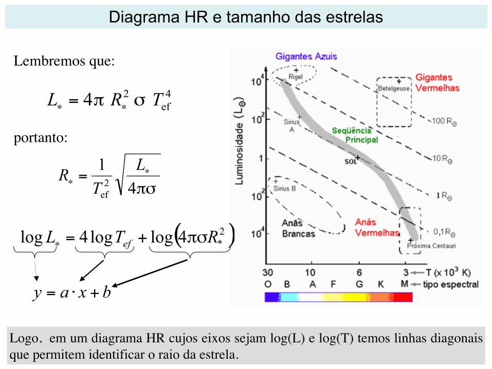
Logo, em um diagrama HR cujos eixos sejam log(L) e log(T) temos linhas diagonais que permitem identificar o raio da estrela.

Diagrama HR e tamanho das estrelas

8.5 The Hertzsprung--Russell Diagram

215lines of titanium, scandium and vanadium oxide arereplaced with oxides of heavier elements, zirconium,yttrium and barium. A large fraction of the S starsare irregular variables. The name of the C stars refersto carbon. The metal oxide lines are almost com-pletely absent in their spectra; instead, various carboncompounds (CN, C2, CH) are strong. The abundanceof carbon relative to oxygen is 4–5 times greater inthe C stars than in normal stars. The C stars aredivided into two groups, hotter R stars and coolerN stars.

Another type of giant stars with abundance anomaliesare the barium stars. The lines of barium, strontium, rareearths and some carbon compounds are strong in theirspectra. Apparently nuclear reaction products have beenmixed up to the surface in these stars.

Fig. 8.8. The Hertzsprung–Russell diagram. Thehorizontal coordinate canbe either the colour indexB − V , obtained directlyfrom observations, or thespectral class. In theoreticalstudies the effective tem-perature Te is commonlyused. These correspondto each other but thedependence varies some-what with luminosity. Thevertical axis gives theabsolute magnitude. Ina (lg(L/L⊙), lg Te) plotthe curves of constant ra-dius are straight lines. Thedensest areas are the mainsequence and the horizon-tal, red giant and asymptoticbranches consisting of gi-ant stars. The supergiantsare scattered above the gi-ants. To the lower left aresome white dwarfs about10 magnitudes below themain sequence. The appar-ently brightest stars (m < 4)are marked with crosses andthe nearest stars (r < 50 ly)with dots. The data are fromthe Hipparcos catalogue

8.5 The Hertzsprung--Russell DiagramAround 1910, Ejnar Hertzsprung and Henry NorrisRussell studied the relation between the absolute mag-nitudes and the spectral types of stars. The diagramshowing these two variables is now known as theHertzsprung–Russell diagram or simply the HR dia-gram (Fig. 8.8). It has turned out to be an important aidin studies of stellar evolution.

In view of the fact that stellar radii, luminosities andsurface temperatures vary widely, one might have ex-pected the stars to be uniformly distributed in the HRdiagram. However, it is found that most stars are lo-cated along a roughly diagonal curve called the mainsequence. The Sun is situated about the middle of themain sequence.

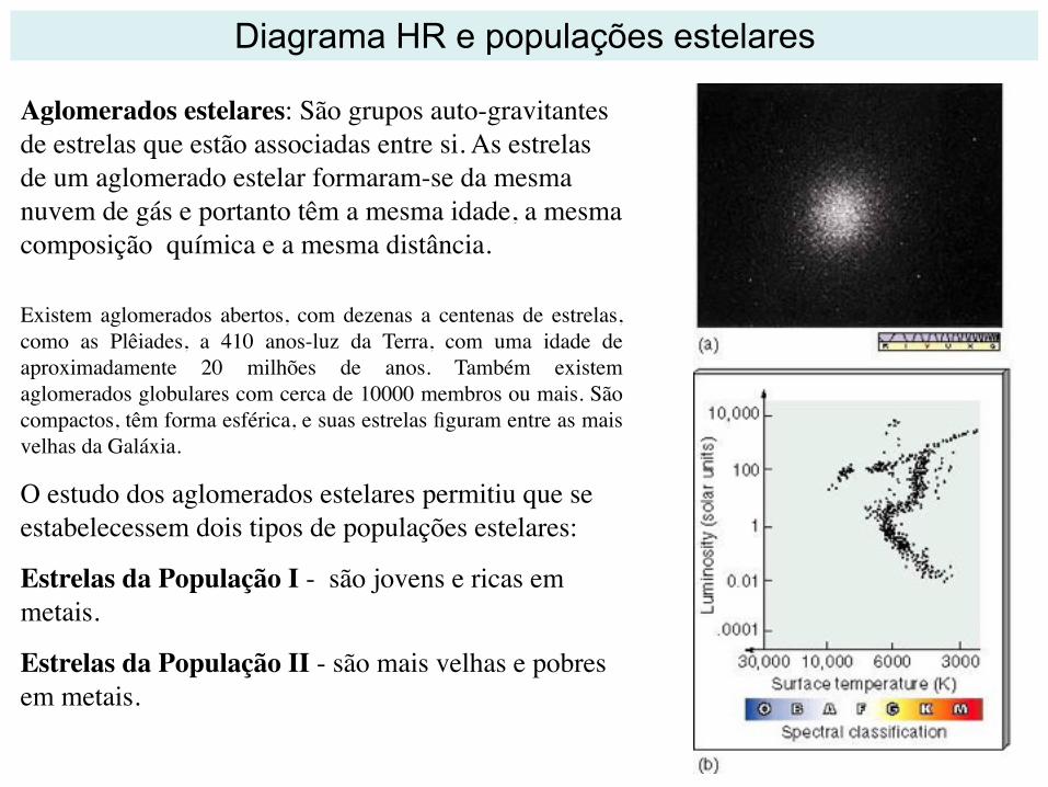
Aglomerados estelares: São grupos auto-gravitantes de estrelas que estão associadas entre si. As estrelas de um aglomerado estelar formaram-se da mesma nuvem de gás e portanto têm a mesma idade, a mesma composição química e a mesma distância.

Existem aglomerados abertos, com dezenas a centenas de estrelas, como as Plêiades, a 410 anos-luz da Terra, com uma idade de aproximadamente 20 milhões de anos. Também existem aglomerados globulares com cerca de 10000 membros ou mais. São compactos, têm forma esférica, e suas estrelas figuram entre as mais velhas da Galáxia.

O estudo dos aglomerados estelares permitiu que se estabelecessem dois tipos de populações estelares:

Estrelas da População I - são jovens e ricas em metais.

Estrelas da População II - são mais velhas e pobres em metais.

Diagrama HR e populações estelares

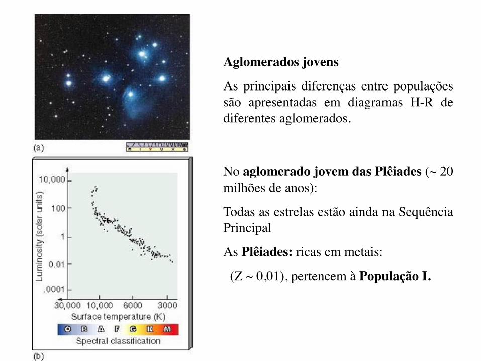
Aglomerados jovens

As principais diferenças entre populações são apresentadas em diagramas H-R de diferentes aglomerados.

No aglomerado jovem das Plêiades (~ 20 milhões de anos):

Todas as estrelas estão ainda na Sequência Principal

As Plêiades: ricas em metais:

(Z ~ 0,01), pertencem à População I.

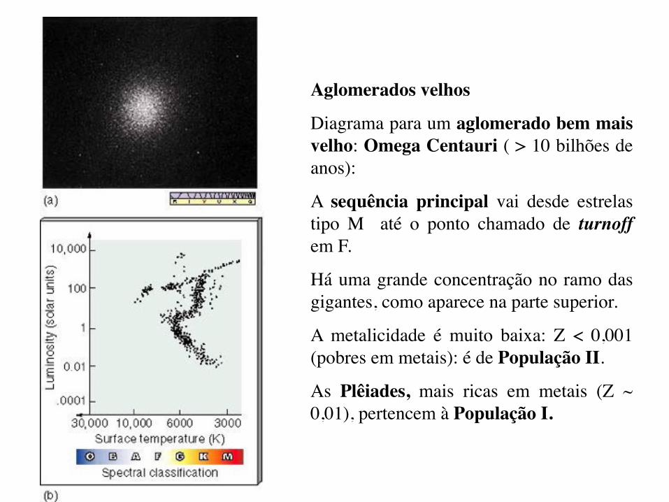
Aglomerados velhos

Diagrama para um aglomerado bem mais velho: Omega Centauri ( > 10 bilhões de anos):

A sequência principal vai desde estrelas tipo M até o ponto chamado de turnoff em F.

Há uma grande concentração no ramo das gigantes, como aparece na parte superior.

A metalicidade é muito baixa: Z < 0,001 (pobres em metais): é de População II.

As Plêiades, mais ricas em metais (Z ~ 0,01), pertencem à População I.

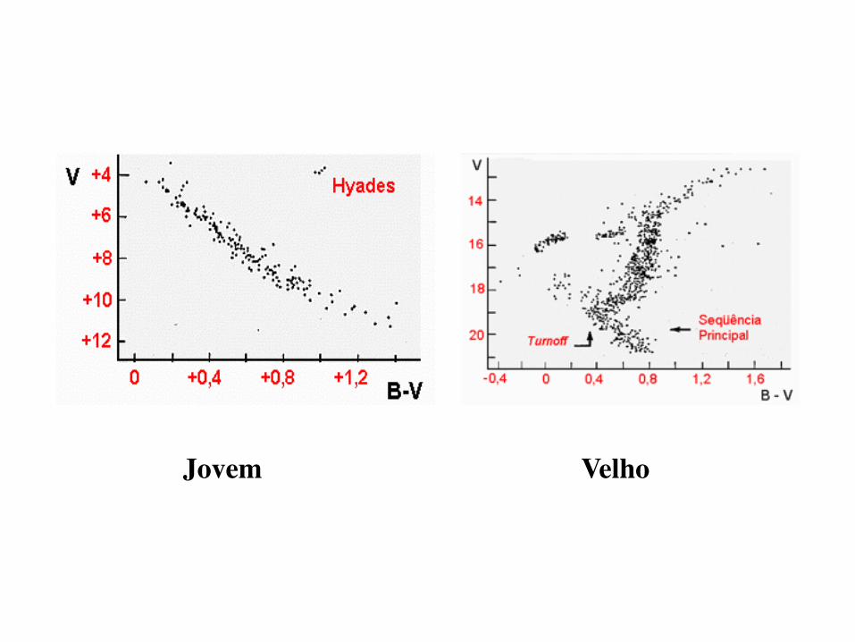
Jovem Velho

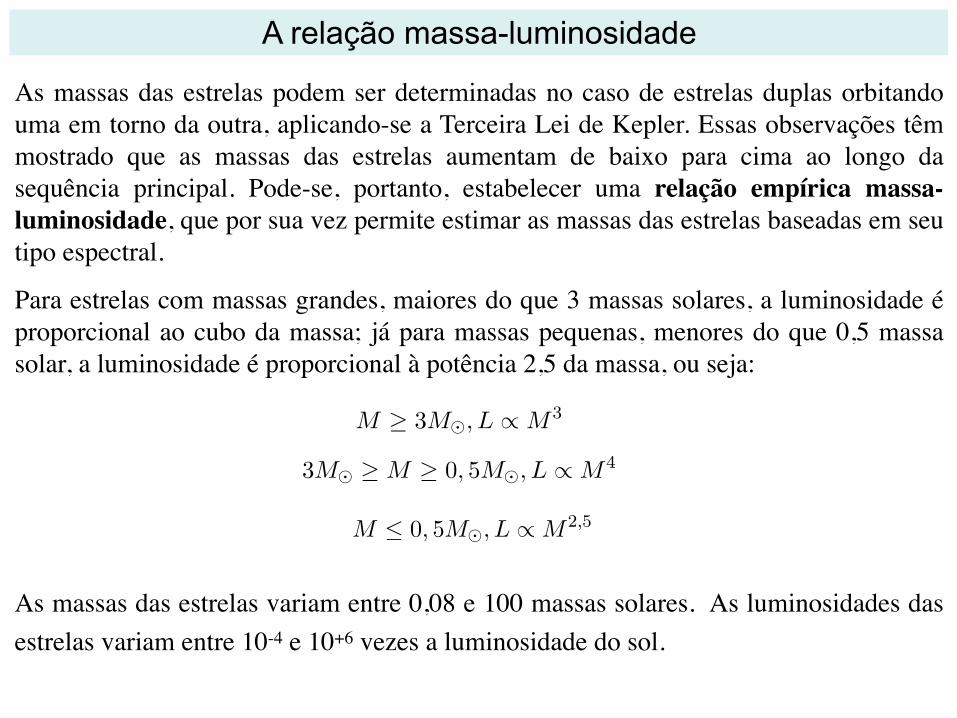
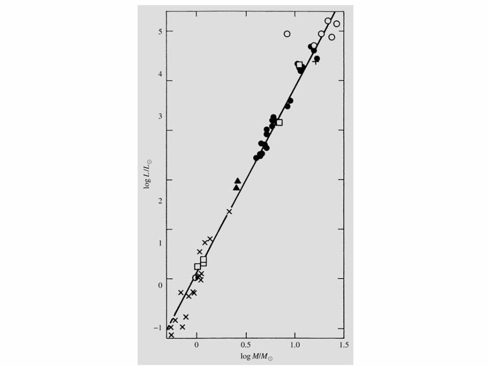
A relação massa-luminosidade

As massas das estrelas podem ser determinadas no caso de estrelas duplas orbitando uma em torno da outra, aplicando-se a Terceira Lei de Kepler. Essas observações têm mostrado que as massas das estrelas aumentam de baixo para cima ao longo da sequência principal. Pode-se, portanto, estabelecer uma relação empírica massa-luminosidade, que por sua vez permite estimar as massas das estrelas baseadas em seu tipo espectral.

Para estrelas com massas grandes, maiores do que 3 massas solares, a luminosidade é proporcional ao cubo da massa; já para massas pequenas, menores do que 0,5 massa solar, a luminosidade é proporcional à potência 2,5 da massa, ou seja:

As massas das estrelas variam entre 0,08 e 100 massas solares. As luminosidades das estrelas variam entre 10-4 e 10+6 vezes a luminosidade do sol.

23.3 Distancias espectroscopicas

Uma das aplicacoes mais importantes do diagrama HR e a determinacao dedistancias estelares. Suponha, por exemplo, que uma determinada estrelatem um espectro que indica que ela esta na sequencia principal e tem tipoespectral G2. Sua luminosidade, entao, pode ser encontrada a partir do dia-grama HR e sera em torno de 1LØ (M = +5). Conhecendo-se sua magnitudeaparente, portanto, sua distancia pode ser conhecida a partir do seu modulode distancia:

(m°M) = °5 + 5 log d °! d = 10(m°M+5)/5

onde (m-M) e o modulo de distancia, em = magnitude aparenteM = magnitude absolutad = distancia em parsecs.Em geral, a classe espectral sozinha nao e suficiente para se conhecer

a luminosidade da estrela de forma unica. E necessario conhecer tambemsua classe de luminosidade. Por exemplo, um estrela de tipo espectral G2pode ter uma luminosidade de 1LØ, se for da sequencia principal, ou de10 LØ (M = 0), se for uma gigante, ou ainda de 100LØ (M = -5), se for umasupergigante.

Essa maneira de se obter as distancias das estrelas, a partir do seu tipoespectral e da sua classe de luminosidade, e chamada metodo das paralaxesespectroscopicas.

23.4 A relacao massa-luminosidade

As massas das estrelas podem ser determinadas no caso de estrelas duplasorbitando uma em torno da outra, aplicando-se a Terceira Lei de Kepler.Essas observacoes tem mostrado que as massas das estrelas aumentam debaixo para cima ao longo da sequencia principal. Pode-se, portanto, esta-belecer uma relacao massa-luminosidade, que por sua vez permite estimaras massas das estrelas baseadas em seu tipo espectral. Para estrelas commassas grandes, maiores do que 3 massas solares, a luminosidade e proporci-onal ao cubo da massa; ja para massas pequenas, menores do que 0,5 massasolar, a luminosidade e proporcional a potencia 2,5 da massa, ou seja:

M ∏ 3MØ, L /M3

3MØ ∏M ∏ 0, 5MØ, L /M4

225M ∑ 0, 5MØ, L /M2,5

As massas das estrelas variam entre 0,08 e 100 massas solares, ao passo queas luminosidades das estrelas variam entre 10°4 e 10+6 vezes a luminosidadedo sol.

23.5 Extremos de luminosidade, raios e densida-des

A relacao entre luminosidade, temperatura e tamanho de uma estrela e dadapela lei de Stefan-Boltzmann, da qual se infere que a luminosidade da estrelae diretamente proporcional ao quadrado de seu raio e a quarta potencia desua temperatura:

L = 4ºR2æT 4ef

onde æ e a constante de Stefan-Boltzmann, e vale æ = 5, 67051£ 10°5 ergscm°2 K°4 s°1.

Essa relacao torna evidente que tanto o raio quanto a temperatura influ-enciam na luminosidade da estrela, embora a temperatura seja mais decisiva.

As estrelas normais tem temperaturas variando entre 3 000 e 30 000 Kaproximadamente (0,5 TØ e 5 TØ), e luminosidades variando entre 10°4LØe 10+6LØ. Como a luminosidade depende de T 4, um fator de apenas 10 emtemperatura resulta em um fator de 10 000 em luminosidade, e consequen-temente a parte substancial das diferencas de luminosidade entre as estrelase devida as diferencas de temperatura entre elas. O fator restante de 106 nointervalo de luminosidades deve-se as diferencas em raios estelares. Estima-se que os raios das estrelas cobrem um intervalo de valores possıveis entre10°2RØ e 10+3RØ, aproximadamente.

No diagrama HR, o raio aumenta do canto inferior esquerdo para o cantosuperior direito.

23.5.1 As estrelas mais luminosas

As estrelas mais massivas que existem sao estrelas azuis com massas deate 100 massas solares. Suas magnitudes absolutas sao em torno de -6 a -8,podendo, em alguns casos raros, chegar a -10

°10+6LØ

¢. Essas estrelas estao

em geral no canto superior esquerdo do diagrama HR e tem tipo espectralO ou B. Sao as estrelas mais luminosas da sequencia principal. A estrelaRigel e 62 000 vezes mais luminosa que o Sol.

226

218

8. Stellar Spectra

Fig. 8.9. Mass–luminosity relation. The picture is based on bi-naries with known masses. Different symbols refer to differentkinds of binaries. (From Böhm-Vitense: Introduction to StellarAstrophysics, Cambridge University Press (1989–1992))

radii several thousand times larger than the Sun. Notincluded in the figure are the compact stars (neutronstars and black holes) with typical radii of a few tens ofkilometres.

Since the stellar radii vary so widely, so do the den-sities of stars. The density of giant stars may be only10−4 kg/m3, whereas the density of white dwarfs isabout 109 kg/m3.

The range of values for stellar effective temper-atures and luminosities can be immediately seen in

the HR diagram. The range of effective temperatureis 2,000–40,000 K, and that of luminosity 10−4–106

L⊙.The rotation of stars appears as a broadening of the

spectral lines. One edge of the stellar disc is approach-ing us, the other edge is receding, and the radiationfrom the edges is Doppler shifted accordingly. Therotational velocity observed in this way is only thecomponent along the line of sight. The true velocityis obtained by dividing with sin i, where i is the an-gle between the line of sight and the rotational axis.A star seen from the direction of the pole will show norotation.

Assuming the axes of rotation to be randomly ori-ented, the distribution of rotational velocities can bestatistically estimated. The hottest stars appear to rotatefaster than the cooler ones. The rotational velocity at theequator varies from 200–250 km/s for O and B stars toabout 20 km/s for spectral type G. In shell stars, therotational velocity may reach 500 km/s.

The chemical composition of the outer layers is de-duced from the strengths of the spectral lines. Aboutthree-fourths of the stellar mass is hydrogen. Heliumcomprises about one-fourth, and the abundance of otherelements is very small. The abundance of heavy ele-ments in young stars (about 2%) is much larger than inold ones, where it is less than 0.02%.

* The Intensity Emergingfrom a Stellar AtmosphereThe intensity of radiation emerging from an atmosphereis given by the expression (5.45), i. e.

Iν(0, θ) =∞!

0

Sν(τν) e−τν sec θ sec θ dτν . (8.2)

If a model atmosphere has been computed, the sourcefunction Sν is known.

An approximate formula for the intensity can be de-rived as follows. Let us expand the source function asa Taylor series about some arbitrary point τ∗, thus

Sν = Sν(τ∗)+ (τν − τ∗)S′

ν(τ∗)+ . . .

where the dash denotes a derivative. With this ex-pression, the integral in (8.2) can be evaluated,

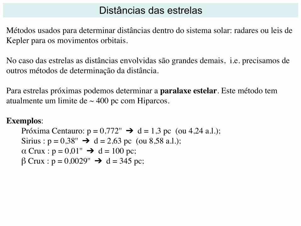
Métodos usados para determinar distâncias dentro do sistema solar: radares ou leis de Kepler para os movimentos orbitais.

No caso das estrelas as distâncias envolvidas são grandes demais, i.e. precisamos de outros métodos de determinação da distância.

Para estrelas próximas podemos determinar a paralaxe estelar. Este método tem atualmente um limite de ~ 400 pc com Hiparcos.

Exemplos:Próxima Centauro: p = 0,772'' ➔ d = 1,3 pc (ou 4,24 a.l.);Sirius : p = 0,38'' ➔ d = 2,63 pc (ou 8,58 a.l.);α Crux : p = 0,01'' ➔ d = 100 pc;β Crux : p = 0,0029'' ➔ d = 345 pc;

Distâncias das estrelas

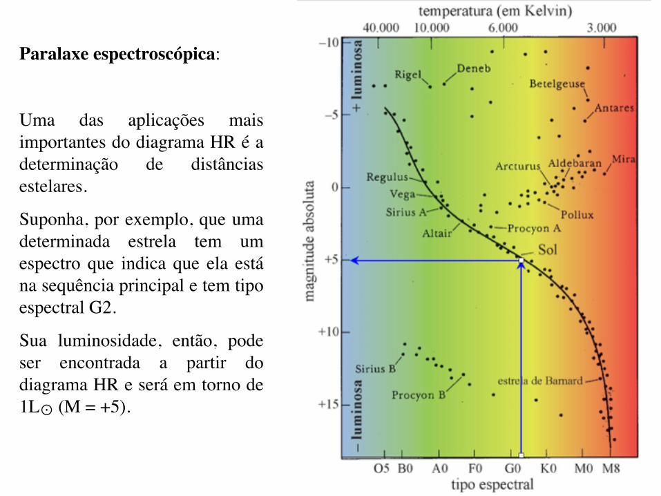
Paralaxe espectroscópica:

Uma das aplicações mais importantes do diagrama HR é a determinação de distâncias estelares.

Suponha, por exemplo, que uma determinada estrela tem um espectro que indica que ela está na sequência principal e tem tipo espectral G2.

Sua luminosidade, então, pode ser encontrada a partir do diagrama HR e será em torno de 1L⊙ (M = +5).

Conhecendo-se sua magnitude aparente, portanto, sua distância pode ser conhecida a partir do seu módulo de distância:

onde (m-M) é o módulo de distância, e

m = magnitude aparente M = magnitude absoluta d = distância em parsecs.

Essa maneira de se obter as distâncias das estrelas, a partir do seu tipo espectral e da sua classe de luminosidade, é chamada método das paralaxes espectroscópicas.

23.3 Distancias espectroscopicas

Uma das aplicacoes mais importantes do diagrama HR e a determinacao dedistancias estelares. Suponha, por exemplo, que uma determinada estrelatem um espectro que indica que ela esta na sequencia principal e tem tipoespectral G2. Sua luminosidade, entao, pode ser encontrada a partir do dia-grama HR e sera em torno de 1LØ (M = +5). Conhecendo-se sua magnitudeaparente, portanto, sua distancia pode ser conhecida a partir do seu modulode distancia:

(m°M) = °5 + 5 log d °! d = 10(m°M+5)/5

onde (m-M) e o modulo de distancia, em = magnitude aparenteM = magnitude absolutad = distancia em parsecs.Em geral, a classe espectral sozinha nao e suficiente para se conhecer

a luminosidade da estrela de forma unica. E necessario conhecer tambemsua classe de luminosidade. Por exemplo, um estrela de tipo espectral G2pode ter uma luminosidade de 1LØ, se for da sequencia principal, ou de10 LØ (M = 0), se for uma gigante, ou ainda de 100LØ (M = -5), se for umasupergigante.

Essa maneira de se obter as distancias das estrelas, a partir do seu tipoespectral e da sua classe de luminosidade, e chamada metodo das paralaxesespectroscopicas.

23.4 A relacao massa-luminosidade

As massas das estrelas podem ser determinadas no caso de estrelas duplasorbitando uma em torno da outra, aplicando-se a Terceira Lei de Kepler.Essas observacoes tem mostrado que as massas das estrelas aumentam debaixo para cima ao longo da sequencia principal. Pode-se, portanto, esta-belecer uma relacao massa-luminosidade, que por sua vez permite estimaras massas das estrelas baseadas em seu tipo espectral. Para estrelas commassas grandes, maiores do que 3 massas solares, a luminosidade e proporci-onal ao cubo da massa; ja para massas pequenas, menores do que 0,5 massasolar, a luminosidade e proporcional a potencia 2,5 da massa, ou seja:

M ∏ 3MØ, L /M3

3MØ ∏M ∏ 0, 5MØ, L /M4

225

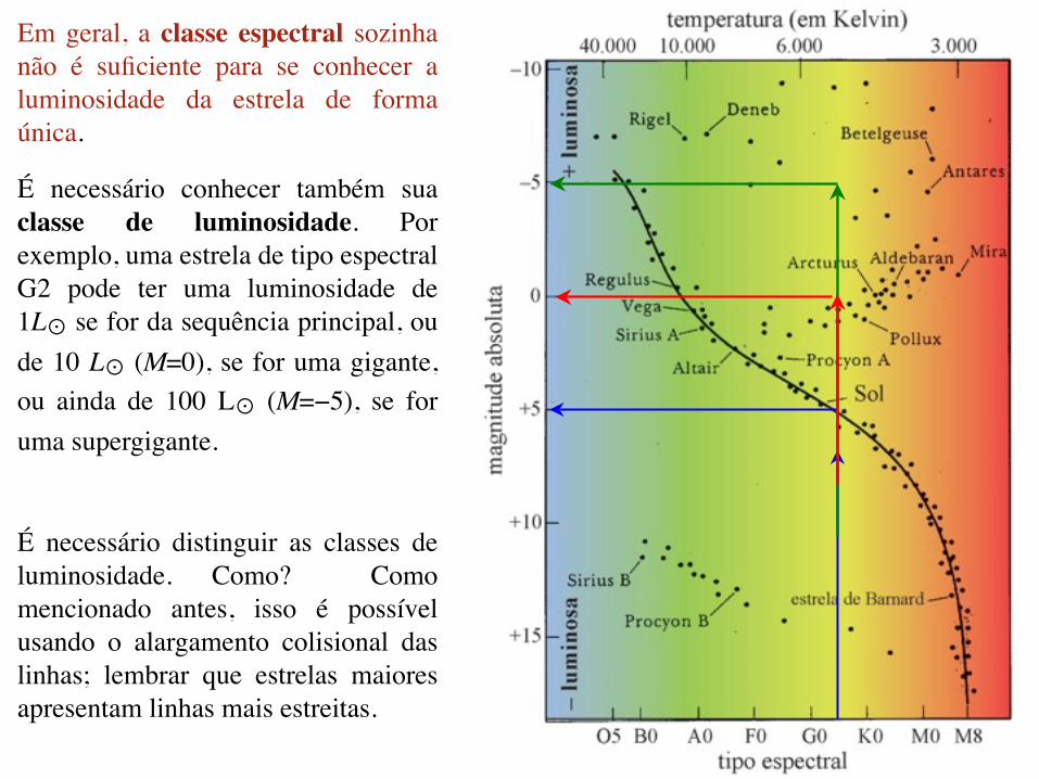
Em geral, a classe espectral sozinha não é suficiente para se conhecer a luminosidade da estrela de forma única.

É necessário conhecer também sua classe de luminosidade. Por exemplo, uma estrela de tipo espectral G2 pode ter uma luminosidade de 1L⊙ se for da sequência principal, ou de 10 L⊙ (M=0), se for uma gigante, ou ainda de 100 L⊙ (M=−5), se for uma supergigante.

É necessário distinguir as classes de luminosidade. Como? Como mencionado antes, isso é possível usando o alargamento colisional das linhas; lembrar que estrelas maiores apresentam linhas mais estreitas.

~ 100.000

Escala de distância

Radar

Paralaxe estelar

Paralaxe espectroscópica

Terra

Dis

tânc

ia

capítulo 5 astrofísica estelar: o diagrama hr · a classificação se estendia até a letra p. na...

Documents