yannick soares de soluÇÕes partilhadas para redes de
TRANSCRIPT

Universidade de Aveiro
2017
Departamento de Eletrónica, Telecomunicações e
Informática
YANNICK SOARES DE BARROS DE CEITA
SOLUÇÕES PARTILHADAS PARA REDES DE
TELECOMUNICAÇÕES
SHARED SOLUTIONS FOR TELECOMMUNICATIONS NETWORKS

Universidade de Aveiro
2017
Departamento de Eletrónica, Telecomunicações e
Informática
YANNICK SOARES DE BARROS DE CEITA
SOLUÇÕES PARTILHADAS PARA REDES DE
TELECOMUNICAÇÕES
SHARED SOLUTION FOR TELECOMMUNICATIONS NETWORKS
Dissertação apresentada à Universidade de Aveiro para cumprimento dos requisitos necessários à obtenção do grau de Mestre em Engenharia Eletrónica e de Telecomunicações, realizada sob a orientação científica do Doutor Manuel de Oliveira Duarte, Professor Catedrático do Departamento de Eletrónica, Telecomunicações e Informática da Universidade de Aveiro.


Aos meus pais, Alcino Ceita e Lígia Barros…

O júri
Presidente Prof. Doutor José Rodrigues Ferreira da Rocha Professor Catedrático da Universidade de Aveiro
Vogal - Arguente Principal Prof. Doutor Rui António Dos Santos Cruz Professor Auxiliar do Instituto Superior Técnico
Vogal – Orientador Professor Doutor Aníbal Manuel de Oliveira Duarte Professor Catedrático da Universidade de Aveiro

Agradecimentos
Queria primeiramente agradecer ao Professor Doutor Manuel de Oliveira Duarte pela superior orientação, disponibilidade e por me ter facultado todas as condições necessárias para o desenvolvimento deste trabalho. Quero agradecer aos meus familiares, principalmente aos meus pais, pelo inesgotável esforço, carinho, paciência e por estarem sempre ao meu lado, sem nunca terem desistido. Sem eles essa jornada não seria possível. Também tenho que deixar os meus agradecimentos à minha namorada Mariwlda pelo constante apoio e motivação dedicados. Por último um agradecimento aos diversos amigos e colegas de curso que partilharam comigo muitas horas de estudo durante essa jornada, em especial aos meus amigos Akssana Neto, Alfrendinho Barros, David Santos.

Palavras-chave
Métodos de partilha de Infraestruturas, Redes Celulares, Rede Móveis, Redes de Acesso, Redes Core, Operador Neutro, Mercados Emergentes, GSM, UMTS, LTE, Dimensionamento de Redes, Planeamento de Redes.
Resumo
Apesar do crescente aumento da superfície terrestre coberta pelas comunicações móveis, há questões que têm dificultado à implementação e desenvolvimento das redes celulares nas regiões onde o mercado e o poder económico ainda estão em desenvolvimento. Muitas dessas questões são de carácter económico e financeiro. O que se torna, curiosamente, um facto contraditório, uma vez que as comunicações móveis em diversas ocasiõesprovaram ser um grande aliado para o crescimento e desenvolvimento económico deste tipo de regiões. Portanto para situações como estas, onde o desenvolvimento ou instalação de redes celulares é travado ou condicionado por fatores de caracter económico e financeiro, a adoção de métodos de partilha de infraestruturas ou serviços consegue facilitar a implementação e expansão de redes celulares nestas regiões. O trabalho desenvolvido nesta dissertação procura identificar e estudar os métodos mais comum de partilha. Através do uso de uma ferramenta de cálculo, analisam-se também os efeitos e benefícios económicos que cada método de partilha trará para os operadores interessados em entrar em mercados com caraterísticas aqui consideradas.

Keywords
Infrastructure Sharing Methods, Mobile Networks, Access Networks, Core Networks, Neutral Operators, Emerging Markets, GSM, UMTS, LTE, Network Dimensioning, Network Planning.
Abstract
Despite the substantial increase in the percentage of the globe surfacecovered by mobile communications, there are issues that have hampered the implementation and development of cellular networks in regions where the market and economic power are still under development. Many of these issues are of economic and financial nature. It is curiously a contradictory fact, since mobile communications on several occasions proved to be a great ally for the growth and economic development of this type of regions. Therefore, in situations such as these, where the development or installation of cellular networks is blocked or conditioned by economic and financial factors, the adoption of infrastructure or service sharing methods can facilitate the implementation and expansion of cellular networks in these regions. The work developed in this dissertation seeks to identify and study the most common methods of cellular network sharing. Through the use of anumerical tool, the effects and techno-economic benefits that each sharing method will bring to the operators interested in entering markets with these characteristics will be analyzed.


INDEX
xv
INDEX
LIST OF ABBREVIATIONS .............................................................................................................. xix
LIST OF SYMBOLS ....................................................................................................................... xxiii
LIST OF FIGURES ........................................................................................................................ xxvii
LIST OF TABLES ........................................................................................................................... xxxi
LIST OF EQUATIONS .................................................................................................................. xxxiii
INTRODUCTION ......................................................................................................................... 1
MOTIVATION ....................................................................................................................... 1
OBJECTIVES AND METHODOLOGY ................................................................................ 1
DISSERTATION STRUTURE .............................................................................................. 2
STATE OF THE ART .................................................................................................................. 5
CELLULAR NETWORKS ..................................................................................................... 5
Cells ................................................................................................................................ 5
Propagation Losses and Interferences........................................................................... 8
Cell Coverage Improvements ......................................................................................... 8
Antennas ...................................................................................................................... 10
Handover ...................................................................................................................... 11
RADIO ACCESS NETWORK ............................................................................................ 12
Topologies .................................................................................................................... 12
Frequency and Transmission modes ........................................................................... 13
Multiple Access Techniques ......................................................................................... 15
TELECOMMUNICATION TECHNOLOGY ........................................................................ 17
GSM – The Second Generation ................................................................................... 20
UMTS – Third Generation ............................................................................................ 24
LTE - The fourth generation ......................................................................................... 29
INFRASTRUCTURE SHARING MODELS ............................................................................... 35
PASSIVE SHARING .......................................................................................................... 36
Site Sharing .................................................................................................................. 36
SHARED SOLUTION FOR TELECOMMUNICATIONS NETWORKS
xvi
Mast Sharing ................................................................................................................ 37
ACTIVE SHARING ............................................................................................................. 38
RAN Sharing ................................................................................................................. 38
Core Sharing ................................................................................................................ 39
Roaming ....................................................................................................................... 41
MVNO ........................................................................................................................... 42
NEUTRAL OPERATOR ..................................................................................................... 44
ASPECTS OF NETWORK PLANNING .................................................................................... 45
OPERATORS UPTAKE BEHAVIOR ................................................................................. 45
NETWORK DIMENSIONING ............................................................................................. 47
RAN Dimensioning ....................................................................................................... 47
Core Dimensioning ....................................................................................................... 57
TECHNO-ECONOMIC PARAMETERS ............................................................................. 58
Capital Expenditures .................................................................................................... 58
Operational Expenditures ............................................................................................. 59
Cash Flow ..................................................................................................................... 59
Revenues ..................................................................................................................... 59
Methods of Evaluating a Project ................................................................................... 60
TECHNO-ECONOMIC TOOL FOR NETWORK DIMENSIONING ........................................... 63
INPUT PARAMETERS ...................................................................................................... 64
FORECAST OF OPERATORS UPTAKE .......................................................................... 66
MARKET ............................................................................................................................ 69
NETWORK TRAFFIC DEMAND ........................................................................................ 70
NodeBs ......................................................................................................................... 70
RNCs ............................................................................................................................ 74
Core .............................................................................................................................. 74
COSTS ............................................................................................................................... 75
NETWORK ELEMENTS DIMENSIONING ........................................................................ 76
Network Granularity for a Market shared by 3 Competing Operators .......................... 77
CAPEX ............................................................................................................................... 78
INDEX
xvii
Shared Capex ............................................................................................................... 80
OPEX ................................................................................................................................. 84
REVENUE .......................................................................................................................... 85
RESULTS ..................................................................................................................... 86
SCENARIOS ANALISYS .......................................................................................................... 87
SCENARIO A – Single Operator ....................................................................................... 88
NETWORK DIMENSIONING ....................................................................................... 90
TECHNO-ECONOMIC ASSESSMENT ........................................................................ 94
ECONOMIC RESULTS ................................................................................................ 95
SCENARIO B – 3 Operators .............................................................................................. 97
NETWORK DIMENSIONING ....................................................................................... 99
TECHNO-ECONOMIC ASSESSMENT ...................................................................... 104
ECONOMIC RESULTS .............................................................................................. 112
CONCLUSIONS OF THE SCENARIOS .......................................................................... 120
CONCLUSIONS ...................................................................................................................... 123
FUTURE WORK .............................................................................................................. 124
REFERENCES ............................................................................................................................... 125
APPENDIXES.......................................................................................................................................i
Appendix A ........................................................................................................................................i
Appendix B ....................................................................................................................................... ii
Appendix C ..................................................................................................................................... iii
Appendix D ..................................................................................................................................... iv

LIST OF ABBREVIATIONS
xix
LIST OF ABBREVIATIONS
3D Three dimensions
1G First Generation of Mobile Telecommunication Technology
2G Second Generation of Mobile Telecommunication Technology
2.5G 2.5 Generation of Mobile Telecommunication Technology
2.75G 2.75 Generation of Mobile Telecommunication Technology
3G Third Generation of Mobile Telecommunication Technology
3.5G 3.5 Generation of Mobile Telecommunication Technology
3GPP Third Generation Partnership Project
4G Fourth Generation of Mobile Telecommunication Technology
5G Fifth Generation of Mobile Telecommunication Technology
AAA Authentication, Authorization and Accounting
ACK Acknowledge
ADSL Asymmetric Digital Subscriber Line
AMPS Advanced Mobile Phone System
APN Access Point Name
AuC Authentication Center
BH Busy Hour
BHCA Busy Hour Call Attempts
BS Base Station
BSC Base Station Controller
BSS Base Station System
BTS Base Transceiver Station
CAPEX Capital Expenditures
CA Carrier Aggregation
CCPU Cash Cost Per User
CDMA Code Division Multiplexing Access
CDMA IS-96 Code Division Multiplexing Access Interim Standard - 96
CG Charging Gateway
CN Core Network
CP Costumer Premises
CoMP Coordinated Multipoint
CS Circuit Switched domain
DHCP Dynamic Host Configuration Protocol
DL Downlink
DNS Domain Name System
DTE Data Terminal Equipment
DVB Digital Video Broadcasting
E-UTRAN Evolved Universal Terrestrial Radio Access Network
EC Echo Canceller
EDGE Enhanced Data for GSM Evolution
EIR Equipment Identity Register
eNB E-UTRAN Node B
eMBMS Evolved Multimedia Broadcast Multicast Service
EPC Evolved Packet Core
EPS Evolved Packet System
SHARED SOLUTION FOR TELECOMMUNICATIONS NETWORKS
xx
ETSI European Telecommunication Standards Institute
EV-DO Evolution Data Optimized
FDD Frequency Division Duplexing
FDMA Frequency Division Multiple Access
FM Frequency Modulation
GERAN GSM EDGE Radio Access Network
GGSN Gateway GPRS Support Node
GMSC Gateway MSC
GMSK Gaussian Minimum Shift Keying
GPRS General Packet Radio Service
GSM Global System for Mobile Communications
GW Gateway
HDTV High-Definition Television
HLR Home Location Register
HSDPA High Speed Downlink Packet Access
HSPA High Speed Packet Access
HSUPA High Speed Uplink Packet Access
HSS Home Subscriber Server
ID Identification
IEEE Institute of Electrical and Electronics Engineers
IMEI International Mobile Equipment Identity
IMS IP Multimedia Subsystem
IMSI International Mobile Subscriber Identity
IMT-2000 International Mobile Telecommunication at 2.000 MHz
IMT-Advanced International Mobile Telecommunication Advanced
IP Internet Protocol
ISDN Integrated Services Digital Network
ITU International Telecommunication Union
ITU-R International Telecommunication Union Radio Communication Sector
IWF Interworking Function
LAI Location Area Identity
LTE Long Term Evolution
LTE-A Long Term Evolution Advanced
MAC Media Access Control
MAP Mobile Application Part
max. maximum
MC-CDMA Multi-Carrier Code Division Multiple Access
MD Mobile Device
ME Mobile Equipment
MGW Media Gateway
MIMO Multiple-Input Multi-Output
min. minute
MME Mobile Management Entity
MMS Multimedia Messaging Service
MS Mobile Station
MSC Mobile Service Switching Center
MSRN Mobile Station Roaming Number
MVNE Mobile Virtual Network Enabler
MVNO Mobile Virtual Network Operator
NMT Nordic Mobile Telephone

LIST OF ABBREVIATIONS
xxi
NO Neutral Operator
NRT Non-Real Time
NSN Nokia Siemens Network
NSS Network Switching System
NTT Nippon Telegraph and Telephone
OA&M Operation, Administrative and Maintenance
OCS Online Charging System
OFDMA Orthogonal Frequency-Division Multiple Access
OMC Operations and Maintenance Center
OMS Operations and Maintenance System
OPEX Operational Expenditures
PAPR Peak to Average Power Ratio
PDC Personal Digital Cellular
PDN Public Data Network
PDP Packet Data Protocol
PCRF Policy Control and Charging Rules Function
PLMN Public Land Mobile Network
PS Packet Switching
PSK Packet Shift Keying
PSTN Public Switched Telephone Network
QAM Quadrature Amplitude Modulation
QoS Quality of Service
QPSK Quadrature Phase Shift Keying
RAN Radio Access Network
RNC Radio Network Controller
RNS Radio Network Subsystem
RRM Radio Resource Management
RT Real Time
RTT Radio Transmission Technology
SAE System Architecture Evolution
SDMA Space Division Multiple Access
SC Service Center
SCDMA Synchronous Code Division Multiple Access
SC-FDMA Single-carrier Frequency-Division Multiple Access
SGSN Serving GPRS Support Node
SG Service Gateway
SIM Subscriber Identity Module
SME Short Message Entity
SMS Short Message Service
SMS-GMSC Gateway MSC for Short Message Service
SMS-IWMSC Interworking MSC for Short Message Service
SMS-SC SMS Service Center
SNR Signal-to-Noise Ratio
SON Self-Organizing Networks
TACS Total Access Communications System
TDD Time Division Duplex
TD-SCDMA Time Division Synchronous Code Division Multiple Access
TDMA Time Division Multiplexing Access
TMSI Temporary Mobile Subscriber Identity
TRAU Transcoding Rate and Adaptation Unit
SHARED SOLUTION FOR TELECOMMUNICATIONS NETWORKS
xxii
TRX Transceiver
UE User equipment
UICC Universal Integrated Circuit Card
UL Uplink
UM User mobile
UMTS Universal Mobile Telecommunication System
UMTS900 Universal Mobile Telecommunication System at 900 MHz
UMTS2100 Universal Mobile Telecommunication System at 2100 MHz
USIM UMTS Subscriber Identity Module
UTRAN Universal Terrestrial Radio Access Network
US/USA United Sates of America
VAS Value Added System
VLR Visitor Location Register
VMSC Visited Mobile Switching Center
VoIP Voice over Internet Protocol
VoLTE Voice over LTE
W-CDMA Wideband Code Division Multiple Access
WiMAX Worldwide interoperability for Microwave Access
WLAN Wireless Local Area Network

LIST OF SYMBOLS
xxiii
LIST OF SYMBOLS
λ Call arrival
° Degree
€ Euro
/ Per
or or
% Percentage
%SOF Percentage of NodeBs with optical fiber connection
%SRL Percentage of NodeBs with radio link connection
Δ Power margin
μ One hour (3.600s)
τi Initial instant the wave of technology appears on the market (time in years)
A Interface between an BSC and a MSC
or Control parameter for market start moment
Abis Interface between an BTS and a BSC
B Interface between an MSC and a VLR
or Control parameter for speed of market start
C Interface between an MSC and a HRL
or Costs
or codes
C1 CAPEX in year 1
CCN1 Cost to implement the Core Network in year 1
CCN_R_n Cost to implement the Core Network in remaining years
CConst Number of NodeBs x Cost per site construction
CGGSN Cost per GGSN
CHLR Cost per HLR
CMSC Cost per MSC/VLR
CM_R_n Cost of implementation per year of mobile communication technologies
COF Cost per km of Optical Fiber passed and tested
CPCN Cost of Packet Core Network
CPCN_upg Cost of Packet Core Network upgrade
CR_n CAPEX in remaining years
CRNC Cost per RNC
CS Cost per NodeBs
CSGSN Cost per SGSN
CTRX Cost per TRX
Cupg Cost of technologies upgrade
ChBw Channel bandwidth
CF Cash Flow
Cu Interface between USIM and a ME
D Interface between an HLR and a VLR
d Reuse distance
DCN Average NodeBs distance to Core Network
dB Decibel
dBi dB isotropic
dBm dB milliwatt
SHARED SOLUTION FOR TELECOMMUNICATIONS NETWORKS
xxiv
E Interface between an MSC and a MSW
E/Erl Erlang
or Total traffic offered to group in Erlang
Eb/No Energy per bit to noise power spectral density ratio
f Frequency
F Interface between an MSC and a EIR
G Interface between an VLR and a VLR
Ga Interface between a GGSN/SGSN and an OCS
Gb Interface between an SGSN and a Base Station System (BSS)
Gc Interface between a GGSN and an HLR
Gd Interface between an SGSN and an SMS-GMSC/IWMSC
Gf Interface between an SGSN and an EIR
GHz Gigahertz
Gi Reference point between GPRS and an external packet data network
Gn Interface between two GSNs within the same PLMN
Gp Interface between two GSNs in different PLMNs. The Gp interface allows support of
GPRS network services across areas served by the co-operating GPRS PLMNs
Gr Interface between an SGSN and an HLR
Gs Interface between an SGSN and an MSC
GB Gigabyte
Gbps Giga bit per second
GBps Gigabyte per second
Gx Interface between an S-GW and an UTRAN
H Interface between an AuC and an HLR
h Average call length or holding time
hB Base Station (BS) antenna height in meters
hM User Equipment (UE) antenna in meters
Hz Hertz
Iu Interface between the RNC and the Core Network (MSC or SGSN)
Iub Interface between an RNC and a Node B
Iu-CS Interface between an RNC and a MGC
Iu-PS Interface between an RNC and a SGSN
IuPS Interface between an RNC and a SGSN
Iur Interface between RNCs
K Cluster size
kbit/s or kbps kilo bit per second
kBps Kilobytes per second
km Kilometer
m2 or km2 Square kilometer
LTE-Uu Interface Between an eNode B and an MS
m Meter
or milli
or number of identical parallel channel
mi Potential market share that each operator will be able to serve of the total market
Mb Megabit
Mbit/s or Mbps Megabit per second
MB Megabyte
mE mili Erlang
MHz Megahertz
ms Millisecond
LIST OF SYMBOLS
xxv
Nº Number
NGGSN Number of GGSN
NGGSN_upg Number of GGSN upgrade
NHLR Number of HLR
NHLR_upg Number of HLR upgrade
NMSC Number of MSC/VLR
NMSC_upg Number of MSC/VLR upgrade
NRNC Number of RNCs
NRNC_upg Number of RNC upgrade
NN Number of NodeBs
NN_upg Number of NodeB upgrade
NSGSN Number of SGSN
NSGSN_upg Number of SGSN upgrade
OPEXNodeB OPEX per NodeB
P0 Starting Level
p10 Starting Level in p1 equation
p1f Saturation Level in p1 equation
p20 Starting Level in p2 equation
p2f Saturation Level in p2 equation
p30 Starting Level in p3 equation
p3f Saturation Level in p3 equation
Pf Saturation Level
pi(t) Function that characterizes the share of each operator in the Market
��� Threshold level
����� Minimum signal level for reasonable voice quality
R Distance between BS and UE in km (NodeB range)
or Revenues
r Discount rate
RX Receiver
Rx Interface between a PCRF and operators IP services
s second
S Space
Si Function that characterizes the actual market share of each operator wave, affected
by the presence of other operators on the market
S1-MME Interface between an eNode B and an MME
S1-U Interface between an eNode B and an S-GW
S10 Control interface between MMEs
S11 Interface between an S-GW and an MME
S12 Interface between an S-GW and an UTRAN
S3 Interface between an MME and an SGSN
S4 Interface between an S-GW and a GERAN
S5 Interface between an S-GW and a PDN-GW
S6a Interface between an MME and an HSS
SGi Interface between an a PDN-GW and operator IP services
t Time (in years)
T Time period of the project
TCh Total number of channel available
TCh Total bandwidth available
TX Transmitter
Um Interface between a BTS and an MS

SHARED SOLUTION FOR TELECOMMUNICATIONS NETWORKS
xxvi
Uu Air interface between a UE and Node B
W Watt
X2 Interface between neighboring Node B
LIST OF FIGURES
xxvii
LIST OF FIGURES
Figure 1 - Work methodology ............................................................................................................ 2
Figure 2 - Cell ...................................................................................................................................... 5
Figure 3 - Cell Clusters [4] .................................................................................................................. 6
Figure 4 - Cluster K=7 [5] .................................................................................................................... 6
Figure 5 - Cluster K=12 [5] .................................................................................................................. 6
Figure 6 - Reuse Distance ................................................................................................................... 7
Figure 7 - Cell Splitting........................................................................................................................ 9
Figure 8 - Cell Sectoring 120º [10], [11] ........................................................................................... 10
Figure 9 - Example of a Sector Antenna [15] .................................................................................... 11
Figure 10 - Handover scenario at two adjacent cell boundaries (adapted from [6]) ....................... 11
Figure 11 - Basic network topology configuration [16] .................................................................... 12
Figure 12 - RAN network topology example (adapted from [16]) ................................................... 12
Figure 13 - FDD and TDD Scheme [17] ............................................................................................. 13
Figure 14 - Existing resources in the access technique [19], [20] .................................................... 15
Figure 15 - FDMA scheme [20] ......................................................................................................... 16
Figure 16 - TDMA scheme [20] ......................................................................................................... 16
Figure 17 - CDMA scheme [20] ......................................................................................................... 16
Figure 18 - Evolution phases of telecommunication technologies (adapted from [19] and [20]) ... 19
Figure 19 - GSM architecture (adapted from [27]) .......................................................................... 21
Figure 20 - Interfaces in GERAN core network (adapted from [19] and [28]) ................................. 22
Figure 21 - Interfaces in UTRAN core network (adapted from [19] and [28]) ................................. 26
Figure 22 - UMTS architecture (adapted from [27], [24] and [29]) ................................................. 27
Figure 23 - UMTS/GSM network compatibility [29] ......................................................................... 29
Figure 24 - OFDMA time-frequency multiplexing [34] ..................................................................... 30
Figure 25 - SC-FDMA time-frequency multiplexing (Adapted form [34]) ........................................ 30
Figure 26 - LTE E-UTRAN architecture [34], [35] .............................................................................. 32
Figure 27 - LTE full Architecture [35] ................................................................................................ 33
Figure 28 - LTE Evolution [36] .......................................................................................................... 33
Figure 29 - Levels of Sharing (Adapted form [38]) ........................................................................... 35
Figure 30 - Simplified example of a cell site [41] ............................................................................. 36
Figure 31 - Site sharing [40] ............................................................................................................. 36
Figure 32 - Mast sharing [40] ........................................................................................................... 37
Figure 33 - Cell Site Scheme [43] ...................................................................................................... 37
Figure 34 - Full RAN Sharing [40], [43] ............................................................................................. 38
Figure 35 - Core Transmission Ring Sharing [40] .............................................................................. 40
Figure 36 - Shared Core Network Elements and Platforms [40] ...................................................... 40
Figure 37 - Network Roaming [40] ................................................................................................... 41
Figure 38 - Sharing Scenarios versus Landscape [43] ....................................................................... 42
Figure 39 - Sharing models versus Cost savings [38]........................................................................ 43
SHARED SOLUTION FOR TELECOMMUNICATIONS NETWORKS
xxviii
Figure 40 - Key drivers for different types of infrastructure sharing [40] ........................................ 43
Figure 41 - Examples of Consumers Uptake [49] ............................................................................. 45
Figure 42 - UMTS RAN ...................................................................................................................... 47
Figure 43 - NodeB Dimensioning Full Scheme (Adapted from [53]) ................................................ 48
Figure 44 - NodeB Capacity Dimensioning Scheme (Adapted from [53]) ........................................ 49
Figure 45 - NodeB Coverage Dimensioning Scheme (Adapted from [53]) ....................................... 51
Figure 46 - RNC calculation scheme [52] .......................................................................................... 56
Figure 47 - UMTS Core ..................................................................................................................... 57
Figure 48 - Core network dimensioning (Inspired on [53]) .............................................................. 57
Figure 49 - Tool flowchart ................................................................................................................ 63
Figure 50 - Tool Modules.................................................................................................................. 64
Figure 51 - Uptake Behavior curve (hypothetical scenario) ............................................................. 68
Figure 52 - Number of network RAN equipment (hypothetical scenario) ....................................... 76
Figure 53 - Number of network Core equipment (hypothetical scenario) ...................................... 76
Figure 54 - Example of Number of RAN equipment of operator 1 (hypothetical scenario) ............ 77
Figure 55 - Example of Number of core equipment of operator 1 (hypothetical scenario) ............ 77
Figure 56 - Example of Number of RAN equipment of operator 2 (hypothetical scenario) ............ 77
Figure 57 - Example of Number of core equipment of operator 2 (hypothetical scenario) ............ 77
Figure 58 - Example of Number of RAN equipment of operator 3 (hypothetical scenario) ............ 78
Figure 59 - Example of Number of core equipment of operator 3 (hypothetical scenario) ............ 78
Figure 60 - Market uptake forecast of the scenario A ..................................................................... 90
Figure 61 - Number of subscribers Scenario A ................................................................................. 90
Figure 62 - Total Number NodeBs of scenario A .............................................................................. 93
Figure 63 - Total Number of RNCs of scenario A .............................................................................. 93
Figure 64 - Total Number of Core components for the base case of scenario A ............................. 93
Figure 65 - Total Number of Core components for the best case of scenario A .............................. 93
Figure 66 - Total Number of Core components for the worst case of scenario A ........................... 93
Figure 67 - Capex of scenario A ........................................................................................................ 94
Figure 68 - Opex of scenario A ......................................................................................................... 94
Figure 69 - Revenue of scenario A .................................................................................................... 95
Figure 70 - Economic Results of scenario A - Base Case .................................................................. 95
Figure 71 - Economic Results of scenario A - Best Case ................................................................... 96
Figure 72 - Economic Results of scenario A - Worst Case ................................................................ 96
Figure 73 - Market uptake forecast of scenario B .......................................................................... 100
Figure 74 - Number of subscribers of operator 1 ........................................................................... 100
Figure 75 - Number of subscribers of operator 2 ........................................................................... 100
Figure 76 - Number of subscribers of operator 3 ........................................................................... 100
Figure 77 - Number of NodeBs for operator 1 ............................................................................... 101
Figure 78 - Number of RNCs for operator 1 ................................................................................... 101
Figure 79 - Number of Best Case Core components for operator 1 .............................................. 102
Figure 80 - Number of Worst Case Core components for operator 1 ........................................... 102
Figure 81 - Number of Base Case Core components for operator 1 .............................................. 102
Figure 82 - Number of NodeBs for operator 2 ............................................................................... 102
LIST OF FIGURES
xxix
Figure 83 - Number of RNCs for operator 2 ................................................................................... 102
Figure 84 - Number of Best Case Core components for operator 2 .............................................. 103
Figure 85 - Number of Worst Case Core components for operator 2 ........................................... 103
Figure 86 - Number of Base Case Core components for operator 2 .............................................. 103
Figure 87 - Number of NodeBs for operator 3 ............................................................................... 103
Figure 88 - Number of RNCs for operator 3 ................................................................................... 103
Figure 89 - Number of Best Case Core components for operator 3 .............................................. 104
Figure 90 - Number of Worst Case Core components for operator 3 ........................................... 104
Figure 91 - Number of Base Case Core components for operator 3 .............................................. 104
Figure 92 - NodeB Sharing Capex of operator 1 ............................................................................. 105
Figure 93 - NodeB Sharing Capex of operator 2 ............................................................................. 105
Figure 94 - NodeB Sharing Capex of operator 3 ............................................................................. 105
Figure 95 - RAN Sharing Capex of operator 1................................................................................. 105
Figure 96 - RAN Sharing Capex of operator 2................................................................................. 105
Figure 97 - RAN Sharing Capex of operator 3................................................................................. 106
Figure 98 - Core Sharing Capex of operator 1 ................................................................................ 106
Figure 99 - Core Sharing Capex of operator 2 ................................................................................ 106
Figure 100 - Core Sharing Capex of operator 3 .............................................................................. 106
Figure 101 - NodeB Sharing Opex of operator 1 ............................................................................ 107
Figure 102 - NodeB Sharing Opex of operator 2 ............................................................................ 107
Figure 103 - NodeB Sharing Opex of operator 3 ............................................................................ 108
Figure 104 - RAN Sharing Opex of operator 1 ................................................................................ 108
Figure 105 - RAN Sharing Opex of operator 2 ................................................................................ 108
Figure 106 - RAN Sharing Opex of operator 3 ................................................................................ 108
Figure 107 - Core Sharing Opex of operator 1 ............................................................................... 109
Figure 108 - Core Sharing Opex of operator 2 ............................................................................... 109
Figure 109 - Core Sharing Opex of operator 3 ............................................................................... 109
Figure 110 - NodeB Sharing Revenue of operator 1 ...................................................................... 110
Figure 111 - NodeB Sharing Revenue of operator 2 ...................................................................... 110
Figure 112 - NodeB Sharing Revenue of operator 3 ...................................................................... 110
Figure 113 - RAN Sharing Revenue of operator 1 .......................................................................... 110
Figure 114 - RAN Sharing Revenue of operator 2 .......................................................................... 110
Figure 115 - RAN Sharing Revenue of operator 3 .......................................................................... 111
Figure 116 - Core Sharing Revenue of operator 1 .......................................................................... 111
Figure 117 - Core Sharing Revenue of operator 2 .......................................................................... 111
Figure 118 - Core Sharing Revenue of operator 3 .......................................................................... 111
Figure 119 - NodeB Sharing Economic Results of operator 1 - Best Case ...................................... 112
Figure 120 - NodeB Sharing Economic Results of operator 1 - Worst Case ................................... 112
Figure 121 - NodeB Sharing Economic Results of operator 1 - Base Case ..................................... 112
Figure 122 - NodeB Sharing Economic Results of operator 2 - Best Case ...................................... 113
Figure 123 - NodeB Sharing Economic Results of operator 2 - Worst Case ................................... 113
Figure 124 - NodeB Sharing Economic Results of operator 2 - Base Case ..................................... 113
Figure 125 - NodeB Sharing Economic Results of operator 3 - Best Case ...................................... 114
SHARED SOLUTION FOR TELECOMMUNICATIONS NETWORKS
xxx
Figure 126 - NodeB Sharing Economic Results of operator 3 - Worst Case ................................... 114
Figure 127 - NodeB Sharing Economic Results of operator 3 - Base Case ..................................... 114
Figure 128 - RAN Sharing Economic Results of operator 1 - Best Case .......................................... 115
Figure 129 - RAN Sharing Economic Results of operator 1 - Worst Case ....................................... 115
Figure 130 - RAN Sharing Economic Results of operator 1 - Base Case ......................................... 115
Figure 131 - RAN Sharing Economic Results of operator 2 - Best Case .......................................... 116
Figure 132 - RAN Sharing Economic Results of operator 2 - Worst Case ....................................... 116
Figure 133 - RAN Sharing Economic Results of operator 2 - Base Case ......................................... 116
Figure 134 - RAN Sharing Economic Results of operator 3 - Best Case .......................................... 117
Figure 135 - RAN Sharing Economic Results of operator 3 - Worst Case ....................................... 117
Figure 136 - RAN Sharing Economic Results of operator 3 - Base Case ......................................... 117
Figure 137 - Core Sharing Economic Results of operator 1 - Best Case ......................................... 118
Figure 138 - Core Sharing Economic Results of operator 1 - Worst Case ...................................... 118
Figure 139 - Core Sharing Economic Results of operator 1 - Base Case ........................................ 118
Figure 140 - Core Sharing Economic Results of operator 2 - Best Case ......................................... 119
Figure 141 - Core Sharing Economic Results of operator 2 - Worst Case ...................................... 119
Figure 142 - Core Sharing Economic Results of operator 2 - Base Case ........................................ 119
Figure 143 - Core Sharing Economic Results of operator 3 - Best Case ......................................... 119
Figure 144 - Core Sharing Economic Results of operator 3 - Worst Case ...................................... 119
Figure 145 - Core Sharing Economic Results of operator 3 - Base Case ........................................ 120
Figure 146 - GSM interfaces [23] [27] ................................................................................................. i
Figure 147 - UMTS Architecture and Interfaces [29] ..........................................................................ii
Figure 148 - LTE Full Architecture ...................................................................................................... iii
LIST OF TABLES
xxxi
LIST OF TABLES
Table 1 - Main aspects of the different generations of technologies. (Updated from [19]) ........... 19
Table 2 - Bandwidth supported in LTE [33] ...................................................................................... 31
Table 3 - Monthly Data Traffic Demand per user ............................................................................. 49
Table 4 - Summary of Uplink SNR [52] ............................................................................................. 53
Table 5 - Demographic settings (hypothetical scenario) .................................................................. 65
Table 6 - Settings of the status of infrastructures (hypothetical scenario) ...................................... 65
Table 7 - Region settings (hypothetical scenario) ............................................................................ 65
Table 8 - Sharing settings (hypothetical scenario) ........................................................................... 66
Table 9 - Price Charged to subscribers (hypothetical scenario) ....................................................... 66
Table 10 - Annual Interest Rate (hypothetical scenario) ................................................................. 66
Table 11 - Technology Parameters (hypothetical scenario) ............................................................. 67
Table 12 - m1, m2 and m3 Parameters (hypothetical scenario) ...................................................... 68
Table 13 - Op1 Parameters (hypothetical scenario) ........................................................................ 68
Table 14 - Op 2 Parameters (hypothetical scenario)........................................................................ 68
Table 15 - Op3 Parameters (hypothetical scenario) ........................................................................ 68
Table 16 - “p” Parameters (hypothetical scenario) .......................................................................... 68
Table 17 - Number of Sectors per NodeB (hypothetical scenario) .................................................. 70
Table 18 - Link Budget Calculation (hypothetical scenario) ............................................................. 71
Table 19 - NodeB Coverage Area Calculation (hypothetical scenario) ............................................ 72
Table 20 - Area increasing Factor (hypothetical scenario) ............................................................... 72
Table 21 - Data Traffic Demand Calculations (hypothetical scenario) ............................................. 72
Table 22 - RAN Traffic Demand Inputs (hypothetical scenario) ....................................................... 73
Table 23 - Core Capacity Parameters (hypothetical scenario) ......................................................... 74
Table 24 - Cost elements Parameters (hypothetical scenario) ........................................................ 75
Table 25 - Market Share (hypothetical scenario) ............................................................................. 81
Table 26 - Demographic Settings of scenario A ............................................................................... 89
Table 27 - Settings of the status of infrastructures of scenario A .................................................... 89
Table 28 - Geographic Settings – Scenario A .................................................................................... 89
Table 29 - Sharing setting of scenario A ........................................................................................... 89
Table 30 - Price Charged to subscribers and annual interest rate – Scenario A .............................. 89
Table 31 - Market uptake parameters -Scenario A .......................................................................... 90
Table 32 - Monthly traffic demand per user of scenario A .............................................................. 91
Table 33 - Bandwidth demand – Scenario A .................................................................................... 91
Table 34 - Link Budget of scenario A ................................................................................................ 92
Table 35 - Number of the NodeBs need in the first year to deploy the network – Scenario A ....... 92
Table 36 - Core parameters – Scenario A ......................................................................................... 92
Table 37 - Connections parameters – Scenario A ............................................................................ 92
Table 38 - NPV, IRR and Payback period for scenario A (Base case) ................................................ 95
Table 39 - NPV, IRR and Payback period for scenario A (Best case) ................................................ 96
SHARED SOLUTION FOR TELECOMMUNICATIONS NETWORKS
xxxii
Table 40 - NPV, IRR and Payback period for scenario A (Worst case) ............................................. 96
Table 41 - Demographic Settings of scenario B................................................................................ 98
Table 42 - Settings of the status of infrastructures of scenario B .................................................... 98
Table 43 - Geographic Settings of scenario B ................................................................................... 98
Table 44 - Sharing settings of scenario B ......................................................................................... 99
Table 45 - Price Charged to subscribers and annual interest rate – Scenario B .............................. 99
Table 46 - Market uptake parameters - Scenario B ......................................................................... 99
Table 47 - NPV, IRR and Payback period for Operator 1 – NodeB Sharing .................................... 112
Table 48 - NPV, IRR and Payback period for Operator 2 – NodeB Sharing .................................... 113
Table 49 - NPV, IRR and Payback period for Operator 3 – NodeB Sharing .................................... 113
Table 50 - NPV, IRR and Payback period for Operator 1 – RAN Sharing ........................................ 114
Table 51 - NPV, IRR and Payback period for Operator 2 – RAN Sharing ........................................ 115
Table 52 - NPV, IRR and Payback period for Operator 3 – RAN Sharing ........................................ 116
Table 53 - NPV, IRR and Payback period for Operator 1 – Core Sharing ....................................... 118
Table 54 - NPV, IRR and Payback period for Operator 2 – Core Sharing ....................................... 118
Table 55 - NPV, IRR and Payback period for Operator 3 – Core Sharing ....................................... 119

LIST OF EQUATIONS
xxxiii
LIST OF EQUATIONS
(1) ....................................................................................................................................................... 7
(2) ....................................................................................................................................................... 7
(3) ....................................................................................................................................................... 7
(4) ....................................................................................................................................................... 7
(5) ....................................................................................................................................................... 7
(6) ....................................................................................................................................................... 7
(7) ..................................................................................................................................................... 11
(8) ..................................................................................................................................................... 45
(9) ..................................................................................................................................................... 46
(10) ................................................................................................................................................... 46
(11) ................................................................................................................................................... 46
(12) ................................................................................................................................................... 46
(13) ................................................................................................................................................... 47
(14) ................................................................................................................................................... 49
(15) ................................................................................................................................................... 50
(16) ................................................................................................................................................... 50
(17) ................................................................................................................................................... 50
(18) ................................................................................................................................................... 50
(19) ................................................................................................................................................... 50
(20) ................................................................................................................................................... 52
(21) ................................................................................................................................................... 53
(22) ................................................................................................................................................... 53
(23) ................................................................................................................................................... 53
(24) ................................................................................................................................................... 54
(25) ................................................................................................................................................... 54
(26) ................................................................................................................................................... 54
(27) ................................................................................................................................................... 55
(28) ................................................................................................................................................... 55
(29) ................................................................................................................................................... 55
(30) ................................................................................................................................................... 55
(31) ................................................................................................................................................... 55
(32) ................................................................................................................................................... 55
(33) ................................................................................................................................................... 55
(34) ................................................................................................................................................... 55
(35) ................................................................................................................................................... 56
(36) ................................................................................................................................................... 56
(37) ................................................................................................................................................... 58
(38) ................................................................................................................................................... 58
(39) ................................................................................................................................................... 58
(40) ................................................................................................................................................... 58

SHARED SOLUTION FOR TELECOMMUNICATIONS NETWORKS
xxxiv
(41) ................................................................................................................................................... 59
(42) ................................................................................................................................................... 59
(43) ................................................................................................................................................... 60
(44) ................................................................................................................................................... 60
(45) ................................................................................................................................................... 66
(46) ................................................................................................................................................... 67
(47) ................................................................................................................................................... 67
(48) ................................................................................................................................................... 67
(49) ................................................................................................................................................... 67
(50) ................................................................................................................................................... 67
(51) ................................................................................................................................................... 67
(52) ................................................................................................................................................... 69
(53) ................................................................................................................................................... 71
(54) ................................................................................................................................................... 71
(55) ................................................................................................................................................... 72
(56) ................................................................................................................................................... 73
(57) ................................................................................................................................................... 73
(58) ................................................................................................................................................... 73
(59) ................................................................................................................................................... 73
(60) ................................................................................................................................................... 73
(61) ................................................................................................................................................... 73
(62) ................................................................................................................................................... 74
(63) ................................................................................................................................................... 74
(64) ................................................................................................................................................... 74
(65) ................................................................................................................................................... 75
(66) ................................................................................................................................................... 75
(67) ................................................................................................................................................... 75
(68) ................................................................................................................................................... 75
(69) ................................................................................................................................................... 79
(70) ................................................................................................................................................... 79
(71) ................................................................................................................................................... 79
(72) ................................................................................................................................................... 80
(73) ................................................................................................................................................... 80
(74) ................................................................................................................................................... 80
(75) ................................................................................................................................................... 81
(76) ................................................................................................................................................... 81
(77) ................................................................................................................................................... 81
(78) ................................................................................................................................................... 82
(79) ................................................................................................................................................... 82
(80) ................................................................................................................................................... 82
(81) ................................................................................................................................................... 82
(82) ................................................................................................................................................... 82
(83) ................................................................................................................................................... 82
LIST OF EQUATIONS
xxxv
(84) ................................................................................................................................................... 83
(85) ................................................................................................................................................... 83
(86) ................................................................................................................................................... 83
(87) ................................................................................................................................................... 83
(88) ................................................................................................................................................... 84
(89) ................................................................................................................................................... 84
(90) ................................................................................................................................................... 84
(91) ................................................................................................................................................... 84
(92) ................................................................................................................................................... 85
(93) ................................................................................................................................................... 85
(94) ................................................................................................................................................... 85
(95) ................................................................................................................................................... 85
(96) ................................................................................................................................................... 85
(97) ................................................................................................................................................... 85
(98) ................................................................................................................................................... 85
(99) ................................................................................................................................................... 86
(100) ................................................................................................................................................. 86
(101) ................................................................................................................................................. 86
(102) ................................................................................................................................................. 86


INTRODUCTION
1
INTRODUCTION
MOTIVATION
The communications sector, especially mobile communications, has been evolving rapidly in
recent decades. This has consequently contributed to the growing incorporation of communication
and information technologies into society's daily lives. Because of this, people's lifestyles have
improved all over the globe.
However, there are many regions where such progress is yet to be achieved. Developing
regions or countries are the ones with the most difficulties. This turns out to be a major disadvantage,
since telecommunications is a strong economic enabler and both private and public organizations
increasingly resort to such technologies to function fluently in modern societies.
OBJECTIVES AND METHODOLOGY
In recent decades, methods of sharing infrastructure and services between operators have been
widely used to try to overcome these kinds of difficulties.
In general, this dissertation aims to contribute to a better understanding of the effects and the
techno-economic advantage of infrastructure sharing in mobile networks.
In specific terms, the objectives of this work can be summarized as follows:
Identification and analysis of telecommunications infrastructure sharing solutions in
both technical and economic terms;
Integration, adaptation and development of numerical tools for planning and designing
mobile networks with infrastructure sharing;
Analysis of the economic viability of the operators involved in the sharing.
All of this will be done in order to verify that, in fact, these methods of sharing are a real facilitator
for the entry of operators into challenging markets.
Due to the objectives intended for this dissertation, it was necessary to make a considerable
amount of assumptions regarding some parameters (e.g.: market uptake, traffic loads, etc.). It was
out of the scope of this dissertation to find good quality estimates for those parameters. Instead,
those parameters were used just for the purpose of constructing possible scenarios based on
plausibility.
SHARED SOLUTION FOR TELECOMMUNICATIONS NETWORKS
2
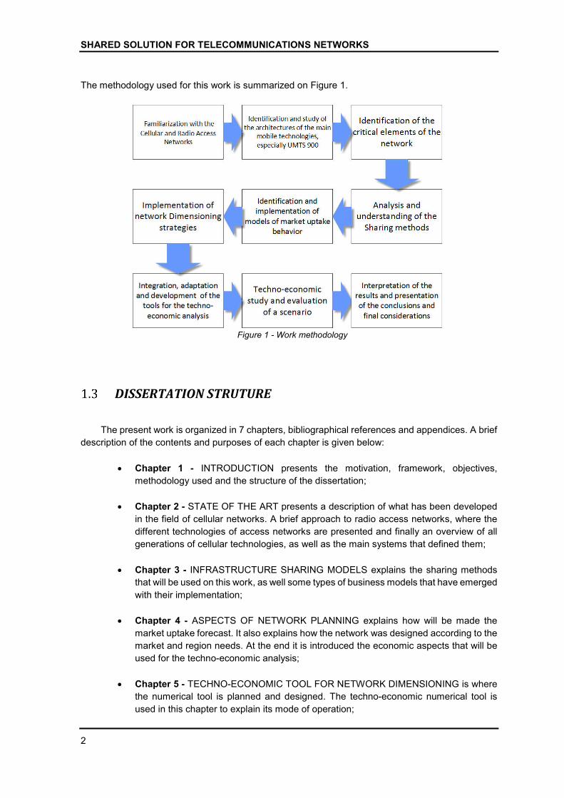
The methodology used for this work is summarized on Figure 1.
Figure 1 - Work methodology
DISSERTATION STRUTURE
The present work is organized in 7 chapters, bibliographical references and appendices. A brief
description of the contents and purposes of each chapter is given below:
Chapter 1 - INTRODUCTION presents the motivation, framework, objectives,
methodology used and the structure of the dissertation;
Chapter 2 - STATE OF THE ART presents a description of what has been developed
in the field of cellular networks. A brief approach to radio access networks, where the
different technologies of access networks are presented and finally an overview of all
generations of cellular technologies, as well as the main systems that defined them;
Chapter 3 - INFRASTRUCTURE SHARING MODELS explains the sharing methods
that will be used on this work, as well some types of business models that have emerged
with their implementation;
Chapter 4 - ASPECTS OF NETWORK PLANNING explains how will be made the
market uptake forecast. It also explains how the network was designed according to the
market and region needs. At the end it is introduced the economic aspects that will be
used for the techno-economic analysis;
Chapter 5 - TECHNO-ECONOMIC TOOL FOR NETWORK DIMENSIONING is where
the numerical tool is planned and designed. The techno-economic numerical tool is
used in this chapter to explain its mode of operation;

INTRODUCTION
3
Chapter 6 - SCENARIOS ANALISYS explores two hypothetical scenarios. One where
there is no sharing, and another where the sharing methodologies will be applied in
order to prove that by applying those methods it can be possible or not to overcome
some of the difficulties encountered by operators in emerging markets;
Chapter 7 - CONCLUSIONS presents the conclusions about the work developed in this
dissertation and some considerations about the results achieved in the scenario
studied. And at the end some suggestions for future work are be presented.

STATE OF THE ART
5
STATE OF THE ART
This chapter presents an overview of the current state of development of cellular network
technologies. It has been written also with the intention of providing a good information source for
future students intended in developing further the topics under consideration.
CELLULAR NETWORKS
Long distance communications evolved from the telegraph to what is known today. Multiple
areas depend nowadays on mobile technologies, and what today goes unnoticed to the new
generation of users, was the reason for the creation, implementation and expansion of the
telecommunications world.
The need to be connected propelled mankind to search for more and more. The new generation
of users have born already knowing a highly-connected world, where stay 6 hours without a
connection to the Internet or to a mobile network was unthinkable and unbearable. Thus, the planning
and implementation of new distribution networks and mobile access services must consider the
increasing number of demand for services, including the growing data demands and the growing
number of users.
To achieve a proper service quality and good covering is necessary to ensure a proper
equilibrium between power, bandwidth and frequency carriers.
Good power balance, to guarantee that the signal can overcome distance to ensure a
good downlink and uplink between the base stations and the mobile terminal;
Suitable bandwidth to allow a constant and clean flow of information without inter-
channel interference, thus improving the signal quality;
Frequency carriers to transport the signal modulated according the convenient
technique.
Cells
Theoretically, on cellular communications systems, the geographic area covered is divided into
hexagonal section called cells. Each cell can be served by a few sets of antenna towers, or by just
one antenna tower, depending on the traffic or coverage profile need.
Each antenna towers have a set of antenna arrays to improve the QoS.
Figure 2 - Cell
Thus, the cell is the basic unit of the cellular system and jointly with others cells they can provide
coverage of large areas without any gaps and overlaps. This association of cells is called clusters.
SHARED SOLUTION FOR TELECOMMUNICATIONS NETWORKS
6
In reality, once deployed, cells usually have an irregular shape, determined by factors such as
propagation of radio waves on the ground, obstacles, and other geographical constraints.
A cluster, as mentioned above, is a group of cells. But in order to be possible to group a bunch
of cells together it is necessary to perform a good planning of the cellular system to avoid
interferences.
Each cell can be assigned with multiple frequencies, but the same group of frequencies cannot
be reused in a neighbor cell, with the consequence of causing co-channel interference.
The shortest distance to which a channel, or set of frequency, can be reused is called the reuse
distance. To optimize the use of those channels the systems must reuse them in cells sufficiently
distant of each other to avoid interferences.
This concept was used in the first systems that made use of the cellular system such as AMPS
(Advanced Mobile Phone System) and GSM (Global System for Mobile Communications) [1], [2], [3].
Today, with the improvement of the techniques of signal processing, this kind of distribution and
care in the reuse of frequencies is dispensable in the access networks.
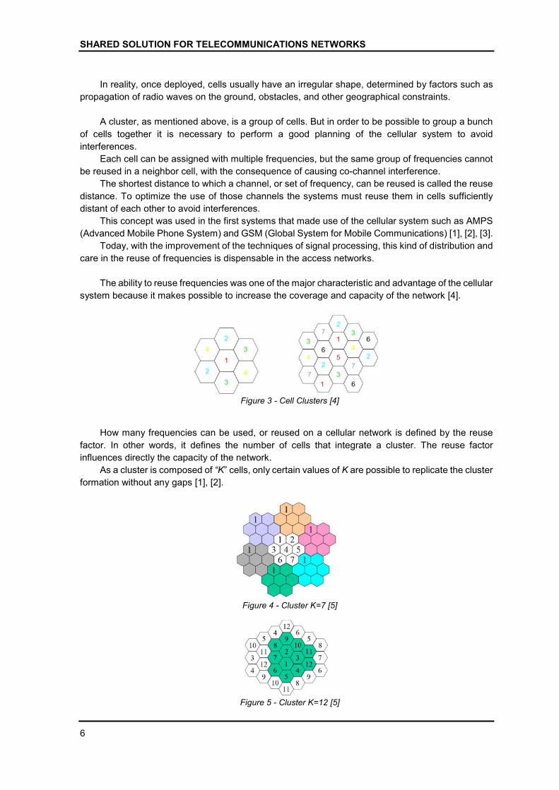
The ability to reuse frequencies was one of the major characteristic and advantage of the cellular
system because it makes possible to increase the coverage and capacity of the network [4].
Figure 3 - Cell Clusters [4]
How many frequencies can be used, or reused on a cellular network is defined by the reuse
factor. In other words, it defines the number of cells that integrate a cluster. The reuse factor
influences directly the capacity of the network.
As a cluster is composed of “K” cells, only certain values of K are possible to replicate the cluster
formation without any gaps [1], [2].
Figure 4 - Cluster K=7 [5]
Figure 5 - Cluster K=12 [5]
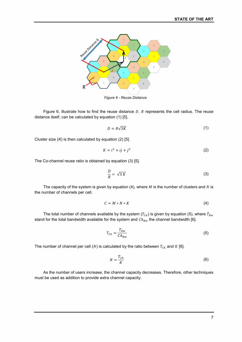
STATE OF THE ART
7
Figure 6 - Reuse Distance
Figure 6, illustrate how to find the reuse distance �. � represents the cell radius. The reuse
distance itself, can be calculated by equation (1) [5].
� = �√3� (1)
Cluster size (K) is then calculated by equation (2) [5].
� = �� + ��+ �� (2)
The Co-channel reuse ratio is obtained by equation (3) [5].
�
�= √3� (3)
The capacity of the system is given by equation (4), where � is the number of clusters and � is
the number of channels per cell.
� = � ∗� ∗ � (4)
The total number of channels available by the system (���) is given by equation (5), where ���
stand for the total bandwidth available for the system and �ℎ�� the channel bandwidth [6].
��� =���
�ℎ��
(5)
The number of channel per cell (�) is calculated by the ratio between ��� and � [6].
� =���
� (6)
As the number of users increase, the channel capacity decreases. Therefore, other techniques
must be used as addition to provide extra channel capacity.

SHARED SOLUTION FOR TELECOMMUNICATIONS NETWORKS
8
Propagation Losses and Interferences
Path loss can be described by the decline of the power density of an electromagnetic wave
during its propagation. The main causes of loss are related to the displacement and propagation of
the radio wave through the medium:
Absorption losses happens when the signal goes through certain media that are not
transparent to the electromagnetic waves, causing the signal to lose part of its energy;
Diffraction losses happens when the signal hits obstacles that change its trajectory.
In summary, most of the causes for path loss are due to the land topography. Propagation losses
are one of the most important elements to take into consideration in the analysis and planning of link
budget on a telecommunications system. But this will be addressed later on the dissertation [7].
As addressed before, the frequency reuse will cause interference in existing cells in a system
of cell clusters if the base stations are faced with neighboring base stations that uses the same
frequency or adjacent frequencies. The degree of aggravation of the interference is proportional to
the distance between those conflicting bases stations.
In fact, it is practically impossible to eliminate the interference, the cells are always subject to
that, but it can be reduced by using some methods, such as the use of filters in the receiver with high
quality factor, dynamic control of power in the base stations, among others.
However, the realization of a strong planning of frequency allocation to base stations and
channels, preventing cells and channels with adjacent frequencies from being allocated at a reduced
distance from one another, is the best alternative [8].
Multipath interference is also a major issue on radio access systems. Multipath interference,
occurs when the transmitted signal reaches the receiver by one or more different paths, which causes
a single emitted signal to reach the destination at different times. It happens in all communications
systems that are near the surface.
Cell Coverage Improvements
Due to the increasing population density that has access to wireless technology and the growing
demand for data services, the number of channels assigned to a cell becomes insufficient to support
the required number of users.
Therefore, the use of techniques such as cell splitting and cell sectoring are solutions that can
expand the capacity of cellular systems.
Although the cell splitting allows the cellular system to grow in an orderly and calculated way, it
causes an increase in the numbers of the base stations.
As cell sectoring uses directional antennas to further control channel frequency interference and
reuse, its implementation simply depends on the installation of additional antennas.
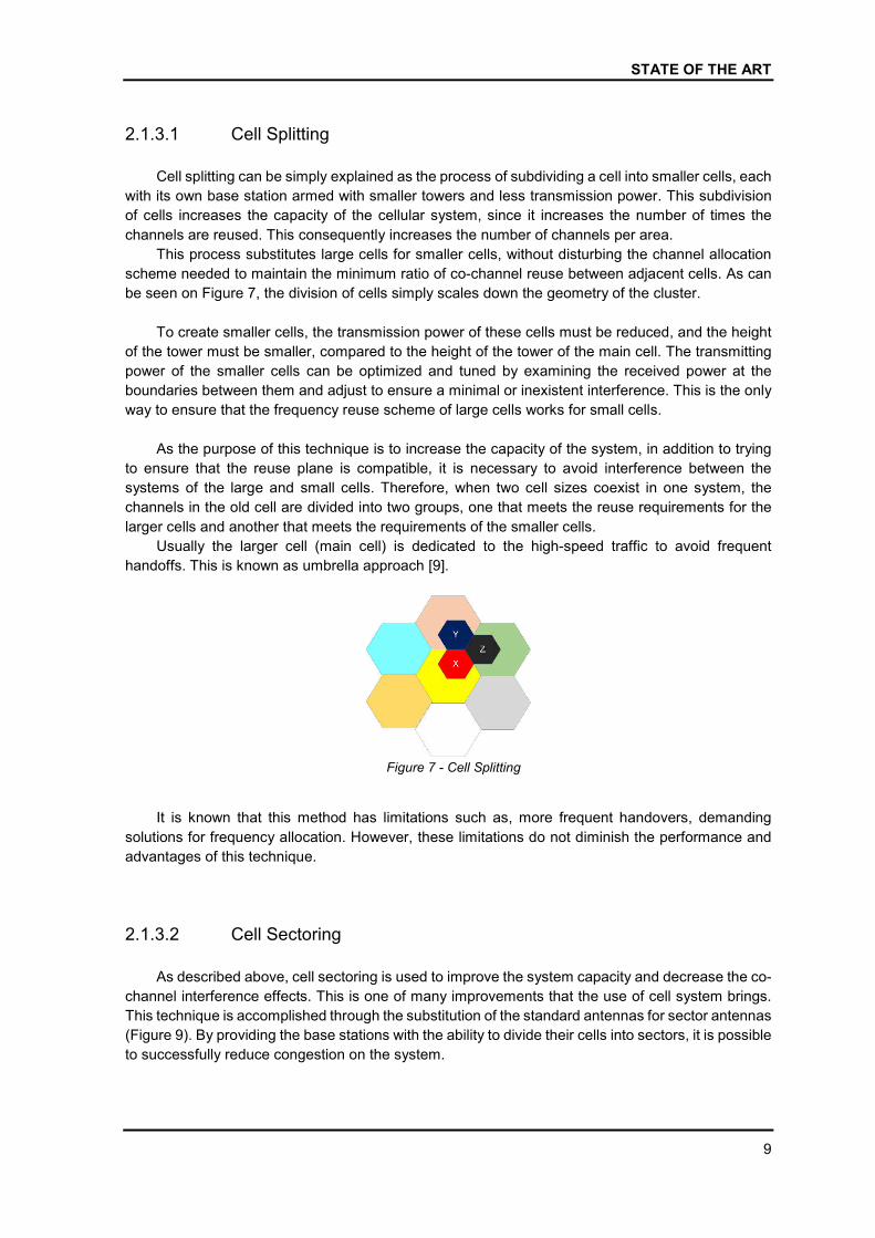
STATE OF THE ART
9
2.1.3.1 Cell Splitting
Cell splitting can be simply explained as the process of subdividing a cell into smaller cells, each
with its own base station armed with smaller towers and less transmission power. This subdivision
of cells increases the capacity of the cellular system, since it increases the number of times the
channels are reused. This consequently increases the number of channels per area.
This process substitutes large cells for smaller cells, without disturbing the channel allocation
scheme needed to maintain the minimum ratio of co-channel reuse between adjacent cells. As can
be seen on Figure 7, the division of cells simply scales down the geometry of the cluster.
To create smaller cells, the transmission power of these cells must be reduced, and the height
of the tower must be smaller, compared to the height of the tower of the main cell. The transmitting
power of the smaller cells can be optimized and tuned by examining the received power at the
boundaries between them and adjust to ensure a minimal or inexistent interference. This is the only
way to ensure that the frequency reuse scheme of large cells works for small cells.
As the purpose of this technique is to increase the capacity of the system, in addition to trying
to ensure that the reuse plane is compatible, it is necessary to avoid interference between the
systems of the large and small cells. Therefore, when two cell sizes coexist in one system, the
channels in the old cell are divided into two groups, one that meets the reuse requirements for the
larger cells and another that meets the requirements of the smaller cells.
Usually the larger cell (main cell) is dedicated to the high-speed traffic to avoid frequent
handoffs. This is known as umbrella approach [9].
Figure 7 - Cell Splitting
It is known that this method has limitations such as, more frequent handovers, demanding
solutions for frequency allocation. However, these limitations do not diminish the performance and
advantages of this technique.
2.1.3.2 Cell Sectoring
As described above, cell sectoring is used to improve the system capacity and decrease the co-
channel interference effects. This is one of many improvements that the use of cell system brings.
This technique is accomplished through the substitution of the standard antennas for sector antennas
(Figure 9). By providing the base stations with the ability to divide their cells into sectors, it is possible
to successfully reduce congestion on the system.
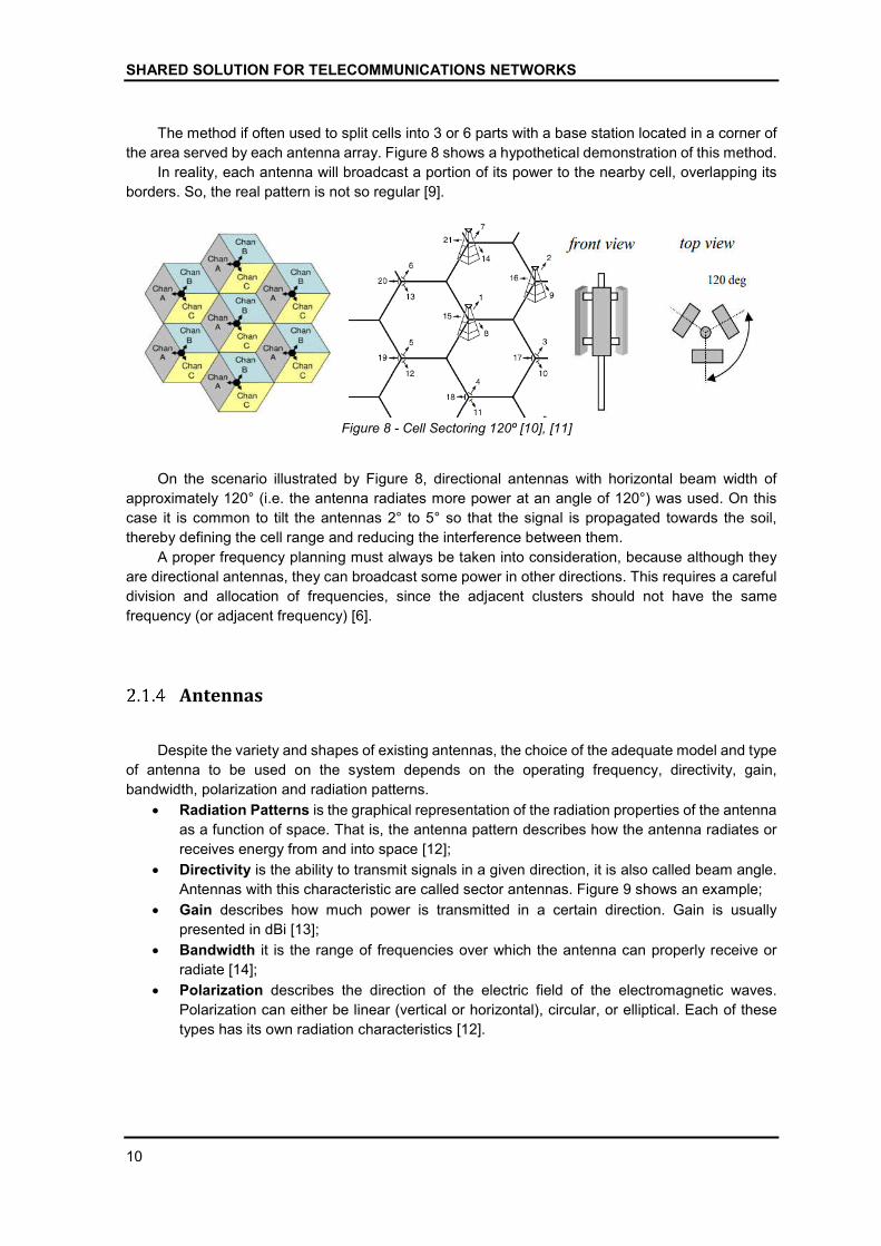
SHARED SOLUTION FOR TELECOMMUNICATIONS NETWORKS
10
The method if often used to split cells into 3 or 6 parts with a base station located in a corner of
the area served by each antenna array. Figure 8 shows a hypothetical demonstration of this method.
In reality, each antenna will broadcast a portion of its power to the nearby cell, overlapping its
borders. So, the real pattern is not so regular [9].
Figure 8 - Cell Sectoring 120º [10], [11]
On the scenario illustrated by Figure 8, directional antennas with horizontal beam width of
approximately 120° (i.e. the antenna radiates more power at an angle of 120°) was used. On this
case it is common to tilt the antennas 2° to 5° so that the signal is propagated towards the soil,
thereby defining the cell range and reducing the interference between them.
A proper frequency planning must always be taken into consideration, because although they
are directional antennas, they can broadcast some power in other directions. This requires a careful
division and allocation of frequencies, since the adjacent clusters should not have the same
frequency (or adjacent frequency) [6].
Antennas
Despite the variety and shapes of existing antennas, the choice of the adequate model and type
of antenna to be used on the system depends on the operating frequency, directivity, gain,
bandwidth, polarization and radiation patterns.
Radiation Patterns is the graphical representation of the radiation properties of the antenna
as a function of space. That is, the antenna pattern describes how the antenna radiates or
receives energy from and into space [12];
Directivity is the ability to transmit signals in a given direction, it is also called beam angle.
Antennas with this characteristic are called sector antennas. Figure 9 shows an example;
Gain describes how much power is transmitted in a certain direction. Gain is usually
presented in dBi [13];
Bandwidth it is the range of frequencies over which the antenna can properly receive or
radiate [14];
Polarization describes the direction of the electric field of the electromagnetic waves.
Polarization can either be linear (vertical or horizontal), circular, or elliptical. Each of these
types has its own radiation characteristics [12].
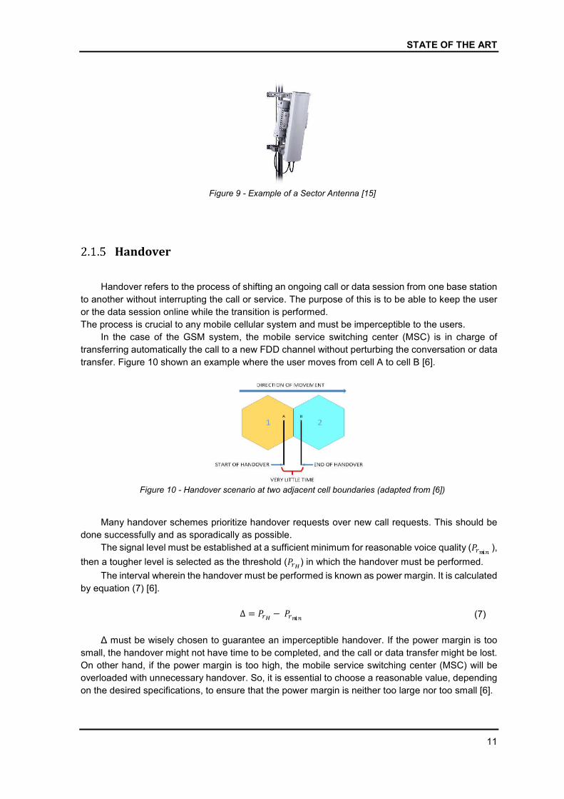
STATE OF THE ART
11
Figure 9 - Example of a Sector Antenna [15]
Handover
Handover refers to the process of shifting an ongoing call or data session from one base station
to another without interrupting the call or service. The purpose of this is to be able to keep the user
or the data session online while the transition is performed.
The process is crucial to any mobile cellular system and must be imperceptible to the users.
In the case of the GSM system, the mobile service switching center (MSC) is in charge of
transferring automatically the call to a new FDD channel without perturbing the conversation or data
transfer. Figure 10 shown an example where the user moves from cell A to cell B [6].
Figure 10 - Handover scenario at two adjacent cell boundaries (adapted from [6])
Many handover schemes prioritize handover requests over new call requests. This should be
done successfully and as sporadically as possible.
The signal level must be established at a sufficient minimum for reasonable voice quality (�����),
then a tougher level is selected as the threshold (���) in which the handover must be performed.
The interval wherein the handover must be performed is known as power margin. It is calculated
by equation (7) [6].
Δ = ���− �����
(7)
Δ must be wisely chosen to guarantee an imperceptible handover. If the power margin is too
small, the handover might not have time to be completed, and the call or data transfer might be lost.
On other hand, if the power margin is too high, the mobile service switching center (MSC) will be
overloaded with unnecessary handover. So, it is essential to choose a reasonable value, depending
on the desired specifications, to ensure that the power margin is neither too large nor too small [6].

SHARED SOLUTION FOR TELECOMMUNICATIONS NETWORKS
12
RADIO ACCESS NETWORK
Radio access network, or RAN, includes all the technologies and equipment that connects the
individual devices to other parts of the network through radio connections. Conceptually, the RAN
resides between the user equipment and the operator’s core network.
It is a crucial part of telecommunications since it is what enables a wireless connection between
the operator and the customer.
Regardless of the system used, the access networks are constituted by sites where the
antennas and radio transmission equipment are installed and aggregation points what interconnects
those sites. The antennas are usually mounted in a tower, or in high places, in location called sites.
These sites are equipped with equipment that packs and process the signals received and sent by
the antennas. The sites are the ones that delimit or form the cells.
Aggregation points are devices that are connected to a set of sites, and handle and aggregate
the signal before distributing to the core network or to another site.
In systems like GSM and UMTS these sites are known as base stations and NodeBs. The
aggregation points are called base stations controllers (BSC) for GSM and radio network controllers
(RNCs) for UMTS. In the case of LTE (Long Term Evolution), due to the characteristics of this system,
it does not have dedicated aggregation points such as GSM and UMTS. Sites in LTE are known as
eNodeB.
Topologies
In telecommunications, the radio access network topology refers to the physical layout of the
equipment and aggregation points. It defines how different aggregation points are placed and
interconnected. Figure 11 illustrates the four basic network topologies of a radio access network;
Chain;
Star;
Ring;
Tree Structure.
On telecommunications systems, where a large amount of ground territory must be covered by
a radio access network, the most basic logical network configuration is the tree-structured access
network because that configuration has several aggregation stages. But a real deployed network
normally has a mixture of topologies, as shown on Figure 12 [16].
Figure 11 - Basic network topology configuration
[16]
Figure 12 - RAN network topology example
(adapted from [16])
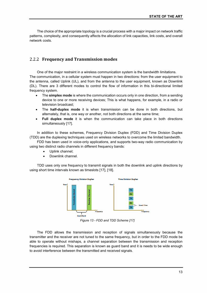
STATE OF THE ART
13
The choice of the appropriate topology is a crucial process with a major impact on network traffic
patterns, complexity, and consequently affects the allocation of link capacities, link costs, and overall
network costs.
Frequency and Transmission modes
One of the major restraint in a wireless communication system is the bandwidth limitations.
The communication, in a cellular system must happen in two directions: from the user equipment to
the antenna, called Uplink (UL), and from the antenna to the user equipment, known as Downlink
(DL). There are 3 different modes to control the flow of information in this bi-directional limited
frequency system.
The simplex mode is where the communication occurs only in one direction, from a sending
device to one or more receiving devices; This is what happens, for example, in a radio or
television broadcast;
The half-duplex mode it is when transmission can be done in both directions, but
alternately, that is, one way or another, not both directions at the same time;
Full duplex mode it is when the communication can take place in both directions
simultaneously [17].
In addition to these schemes, Frequency Division Duplex (FDD) and Time Division Duplex
(TDD) are the duplexing techniques used on wireless networks to overcome the limited bandwidth.
FDD has been used in voice-only applications, and supports two-way radio communication by
using two distinct radio channels in different frequency bands:
Uplink channel;
Downlink channel.
TDD uses only one frequency to transmit signals in both the downlink and uplink directions by
using short time intervals known as timeslots [17], [18].
Figure 13 - FDD and TDD Scheme [17]
The FDD allows the transmission and reception of signals simultaneously because the
transmitter and the receiver are not tuned to the same frequency, but in order to the FDD mode be
able to operate without mishaps, a channel separation between the transmission and reception
frequencies is required. This separation is known as guard band and it is needs to be wide enough
to avoid interference between the transmitted and received signals.

SHARED SOLUTION FOR TELECOMMUNICATIONS NETWORKS
14
As FDD systems utilize frequencies with equal and fixed bandwidth, the channel capacity of
each frequency is, consequently, fixed and equal to all channels on the frequency band. Therefore,
this makes FDD suitable for symmetrical communication in which similar information flows in both
directions, such as voice communications.
Like FDD, TDD also requires a separation between transmit and receive transmissions. But
instead of a guard band, TDD has a guard time.
The guard time give the signals time to pass from a transmitter to a receiver before another
transmission is initiated and the receiver is inhibited. At the same time, it gives time for the base
station to switch from receiver mode to transmitter mode and mobile system to switch from transmitter
mode to receiver mode.
For communications over short distances, TDD is able to guarantee good QoS. But for
communicating over long distances, TDD might not be suitable as the guard interval increases as
the signal propagation time rises.
TDD is able to support voice and other symmetrical communication services as well as
asymmetric data services because it operates by alternating transmission directions over a time
interval. This happens very rapidly and is imperceptible to the user.
The relative capacity of the downlink and uplink can be altered in favor of one direction over the
other. This asymmetry is useful for communication processes characterized by unbalanced
information flow.
Both FDD and TDD transmission modes have their own advantages and disadvantages,
depending on the intended use. It is hence necessary to compare the advantages and disadvantages
of each to determine the best option for the required.
Those advantages can be summarized as follows [18], [17]:
FDD is suited to voice applications, in other words, suited to symmetric traffic, while TDD is
best suited for asymmetric traffic, such as Internet;
Both the transmitter and receiver operate on the same frequency in TDD, but at different
times, eliminating the complexity and costs associated with isolating the transmitter antenna
and the receiver antenna. FDD requires frequency separation and, therefore, cannot reuse
the resources;
TDD has a disadvantage over FDD, because the guard period increases proportionally with
the distance between the receiver and transmitter, reducing its efficiency;
TDD is more flexible than FDD in meeting the need to dynamically reconfigure the allocated
upstream and downstream bandwidth in response to customer needs;
TDD utilizes the spectrum more efficiently than FDD. It requires only one interference free
channel compared with FDD, which requires two interference-free channels plus a guard
band between transmit and receive channels;
TDD also has a more MAC layer complexity, because it is more difficult to achieve an
accurate time synchronization.
As frequencies are a scarce resource and each system requires its own frequency, it is up to
national regulators to manage the allocation of the frequencies.
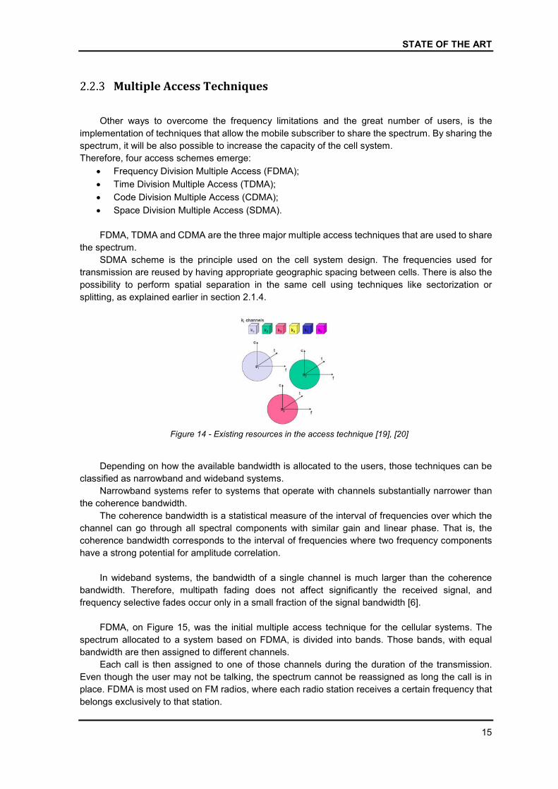
STATE OF THE ART
15
Multiple Access Techniques
Other ways to overcome the frequency limitations and the great number of users, is the
implementation of techniques that allow the mobile subscriber to share the spectrum. By sharing the
spectrum, it will be also possible to increase the capacity of the cell system.
Therefore, four access schemes emerge:
Frequency Division Multiple Access (FDMA);
Time Division Multiple Access (TDMA);
Code Division Multiple Access (CDMA);
Space Division Multiple Access (SDMA).
FDMA, TDMA and CDMA are the three major multiple access techniques that are used to share
the spectrum.
SDMA scheme is the principle used on the cell system design. The frequencies used for
transmission are reused by having appropriate geographic spacing between cells. There is also the
possibility to perform spatial separation in the same cell using techniques like sectorization or
splitting, as explained earlier in section 2.1.4.
Figure 14 - Existing resources in the access technique [19], [20]
Depending on how the available bandwidth is allocated to the users, those techniques can be
classified as narrowband and wideband systems.
Narrowband systems refer to systems that operate with channels substantially narrower than
the coherence bandwidth.
The coherence bandwidth is a statistical measure of the interval of frequencies over which the
channel can go through all spectral components with similar gain and linear phase. That is, the
coherence bandwidth corresponds to the interval of frequencies where two frequency components
have a strong potential for amplitude correlation.
In wideband systems, the bandwidth of a single channel is much larger than the coherence
bandwidth. Therefore, multipath fading does not affect significantly the received signal, and
frequency selective fades occur only in a small fraction of the signal bandwidth [6].
FDMA, on Figure 15, was the initial multiple access technique for the cellular systems. The
spectrum allocated to a system based on FDMA, is divided into bands. Those bands, with equal
bandwidth are then assigned to different channels.
Each call is then assigned to one of those channels during the duration of the transmission.
Even though the user may not be talking, the spectrum cannot be reassigned as long the call is in
place. FDMA is most used on FM radios, where each radio station receives a certain frequency that
belongs exclusively to that station.

SHARED SOLUTION FOR TELECOMMUNICATIONS NETWORKS
16
In a more direct approach, the characteristics of FDMA can be summarized as follows:
The FDMA channel carries only one phone circuit at a given time;
The base station and the user equipment, transmit and receive simultaneously and
continuously;
FDMA is implemented in Narrowband systems and it is less complex than TDMA.
Adapted to operate with analog signals and the symbol time is larger compared to the
average delay spread;
FDMA requires tight filtering and guard bands to minimize the adjacent channel interference;
Handover reveals to be more complex because of the continuous transmission [6], [19].
TDMA, in Figure 16, is another medium access system that works by allowing the access to the
channel at different time intervals. The entire bandwidth is made available to the user or channel, but
only for a finite time period. Thus, as each user only use the channel for a specific amount of time
during transmission, problems such as interference are unlikely to occur [6], [19].
Figure 15 - FDMA scheme [20]
Figure 16 - TDMA scheme [20]
TDMA main features are:
The number of time slots available depends on several factors such as the amount of
available bandwidth, modulation technique used etc.;
As TDMA uses different time slots for transmission and reception there is no need for
duplexes. The signal is transmitted through one time slot and then received by another time
slot. This requires a good time synchronization;
Data transmission is not continuous, it occurs in bursts. Thus, the system will have a low
power consumption;
Because of this discontinuous transmission in TDMA the handoff process is much simpler
for a subscriber since it is able to listen to other base stations during idle time slots;
TDMA has the advantage that is possible to allocate different numbers of time slots to
different users or channel, thus bandwidth can be supplied on demand to different users by
concatenating or reassigning time slot based on priority requests [6], [19].
Figure 17 - CDMA scheme [20]
CDMA, different from FDMA and TDMA, is a technique that allows users to use and share the
frequency band and the same timeslots. That is, the same bandwidth is occupied by all the users, at
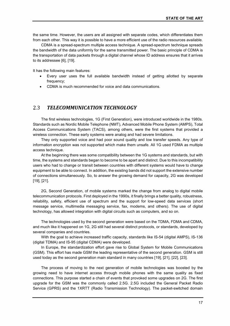
STATE OF THE ART
17
the same time. However, the users are all assigned with separate codes, which differentiates them
from each other. This way it is possible to have a more efficient use of the radio resources available.
CDMA is a spread-spectrum multiple access technique. A spread-spectrum technique spreads
the bandwidth of the data uniformly for the same transmitted power. The basic principle of CDMA is
the transportation of data packets through a digital channel whose ID address ensures that it arrives
to its addressee [6], [19].
It has the following main features:
Every user uses the full available bandwidth instead of getting allotted by separate
frequency;
CDMA is much recommended for voice and data communications.
TELECOMMUNICATION TECHNOLOGY
The first wireless technologies, 1G (First Generation), were introduced worldwide in the 1980s.
Standards such as Nordic Mobile Telephone (NMT), Advanced Mobile Phone System (AMPS), Total
Access Communications System (TACS), among others, were the first systems that provided a
wireless connection. These early systems were analog and had severe limitations.
They only supported voice and had poor sound quality and low transfer speeds. Any type of
information encryption was not supported which make them unsafe. All 1G used FDMA as multiple
access technique.
At the beginning there was some compatibility between the 1G systems and standards, but with
time, the systems and standards began to become to be apart and distinct. Due to this incompatibility
users who had to change or transit between countries with different systems would have to change
equipment to be able to connect. In addition, the existing bands did not support the extensive number
of connections simultaneously. So, to answer the growing demand for capacity, 2G was developed
[19], [21].
2G, Second Generation, of mobile systems marked the change from analog to digital mobile
telecommunication protocols. First deployed in the 1990s, it finally brings a better quality, robustness,
reliability, safety, efficient use of spectrum and the support for low-speed data services (short
message service, multimedia messaging service, fax, modems, and others). The use of digital
technology, has allowed integration with digital circuits such as computers, and so on.
The technologies used by the second generation were based on the TDMA, FDMA and CDMA,
and much like it happened on 1G, 2G still had several distinct protocols, or standards, developed by
several companies and countries.
With the goal to achieve increased traffic capacity, standards like IS-54 (digital AMPS), IS-136
(digital TDMA) and IS-95 (digital CDMA) were developed.
In Europe, the standardization effort gave rise to Global System for Mobile Communications
(GSM). This effort has made GSM the leading representative of the second generation. GSM is still
used today as the second generation main standard in many countries [19], [21], [22], [23].
The process of moving to the next generation of mobile technologies was boosted by the
growing need to have internet access through mobile phones with the same quality as fixed
connections. This purpose started a chain of events that provoked some upgrades on 2G. The first
upgrade for the GSM was the commonly called 2.5G. 2.5G included the General Packet Radio
Service (GPRS) and the 1XRTT (Radio Transmission Technology). The packet-switched domain

SHARED SOLUTION FOR TELECOMMUNICATIONS NETWORKS
18
was implemented in addition to the circuit-switched domain. It does not necessarily provide faster
service because of the timeslots, in addition of being used for circuit-switched, they are also used o
for packet-switched data services.
The next evolution was the 2.75G. GPRS has evolved into the Enhanced Data. Although the
acronyms 2G and 2,5G have not been officially approved by the International Telecommunication
Union (ITU), the fact was that these transition standards, namely the introduction of GPRS, were the
first major step in the evolution from GSM to 3G networks [19], [21], [23].
3G was officially deployed in the 2000s. The main standards of this generation was the Universal
Mobile Telecommunications System (UMTS) standardized by 3rd Generation Partnership Project
(3GPP), CDMA2000 standardized by 3GPP2 and High Speed Packet Access (HSPA).
UMTS was based on GSM, but uses the Wideband Code Division Multiple Access (W-CDMA),
a variant of CDMA. The introduction of HSPA and HSPA+ is defined in some literatures as 3.5G and
3.75G respectively.
UMTS is still used until now, with the respective updates, in some countries, and it became a
representative of the third generation [19], [21], [24].
The next big step in the chain of evolution, was the 4G, the fourth generation of mobile
telecommunication. With higher speeds, higher bandwidth, coverage and network quality, the 4G
comes with the goal of becoming a fully Internet Protocol (IP) system. 4G offer services based on
mobile broadband such as video calls, mobile TV, high definition TV, Digital Video Broadcasting, and
basic services such as voice and data.
Technologies such as Worldwide Interoperability for Microwave Access (WiMax) or Long Term
Evolution (LTE) were introduced in the mid-2000s as potential 4G technologies, but only after the
upgrades to IEEE 802.16m (or WirelessMAN-Advanced) and LTE Advanced they met the technical
requirements needed to be considered 4G technologies.
LTE (and LTE Advanced), also developed by 3GPP, was based on GSM/EDGE and
UMTS/HSPA technologies, and manages to increase capacity and speed using a different radio
interface along with core network enhancements. Instead of W-CDMA used by its predecessors, LTE
uses Orthogonal Frequency Division Multiple Access (OFDMA) for downlink, and Single Carrier
FDMA (SC-FDMA) for uplink [19], [25].
The following generation of mobile systems is the 5G. It is in the final stages of improvement
and testing in some countries, and promises higher speeds than is currently offered by 4G.
Table 1 summarizes the main aspects of the different generations of cellular mobile
technologies, while Figure 18 illustrates the evolution of the main telecommunication technologies.
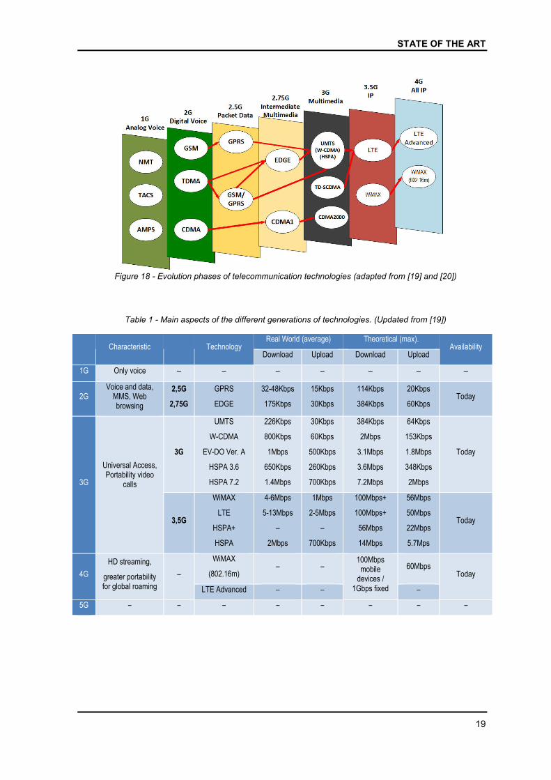
STATE OF THE ART
19
Figure 18 - Evolution phases of telecommunication technologies (adapted from [19] and [20])
Table 1 - Main aspects of the different generations of technologies. (Updated from [19])
Characteristic Technology Real World (average) Theoretical (max).
Availability Download Upload Download Upload
1G Only voice – – – – – – –
2G Voice and data,
MMS, Web browsing
2,5G
2,75G
GPRS
EDGE
32-48Kbps
175Kbps
15Kbps
30Kbps
114Kbps
384Kbps
20Kbps
60Kbps Today
3G
Universal Access, Portability video
calls
3G
UMTS
W-CDMA
EV-DO Ver. A
HSPA 3.6
HSPA 7.2
226Kbps
800Kbps
1Mbps
650Kbps
1.4Mbps
30Kbps
60Kbps
500Kbps
260Kbps
700Kbps
384Kbps
2Mbps
3.1Mbps
3.6Mbps
7.2Mbps
64Kbps
153Kbps
1.8Mbps
348Kbps
2Mbps
Today
3,5G
WiMAX
LTE
HSPA+
HSPA
4-6Mbps
5-13Mbps
–
2Mbps
1Mbps
2-5Mbps
–
700Kbps
100Mbps+
100Mbps+
56Mbps
14Mbps
56Mbps
50Mbps
22Mbps
5.7Mps
Today
4G
HD streaming,
greater portability for global roaming
–
WiMAX
(802.16m) – –
100Mbps mobile
devices / 1Gbps fixed
60Mbps Today
LTE Advanced – – –
5G – – – – – – – –

SHARED SOLUTION FOR TELECOMMUNICATIONS NETWORKS
20
GSM – The Second Generation
As addressed before, GSM was the first to be a digital telecommunication system. GSM was a
standard set proposed by European Telecommunications Standard Institute (ETSI) for 2G digital
cellular networks and eventually became the representative of this generation.
Although originally designed to operate in the 900 MHz range, it was soon adapted to also
operate on 800 MHz, 1800 MHz, and 1900 MHz, supporting FDD for uplink and downlink.
GSM uses a combination of TDMA and FDMA as a medium access technique.
GSM900 system, for example, uses two sets of frequencies in the 900 MHz band, the first in
the 890-915 MHz used for terminal transmissions, and the second in the 935-960 MHZ for network
transmissions.
Therefore, the available 25 MHz of each frequency set are then subdivided into 124 bidirectional
channels, each with a bandwidth of 200 KHz and a transmission capacity around 270 Kbps.
Using TDMA, each 200 KHz channel can be shared between 8 users through 8 time slots, with
one user using the channel over a period of time. In this way, each user has an available bandwidth
of 25 KHz. The modulation scheme used for this is the Gaussian Minimum Shift Keying (GMSK) [21],
[23], [26].
General Packet Radio Service (GPRS) has later developed and added to GSM as an
enhancement to enable packet data transport (packet switching), offering data transfer rates much
higher than previously available in circuit-switched.
In GPRS, timeslots are allocated to a user only when data is being transmitted, unlike GSM,
where slots are allocated statically throughout the connection, even during periods of inactivity. Up
to 8 time slots per TDMA frame can be assigned to a single active user if it is necessary.
Through this dynamic channel allocation, it is possible to optimize the use of network and radio
resources, and allow users to be permanently connected without being taxed only by the traffic used.
With GPRS, GSM networks were able to reach transmission speeds of up to 115 Kbit/s in the
situation where the 8 slots are available. GPRS was designed to support both burst and intermittent
data transmissions [21], [26].
The next enhancements on GSM/GPRS systems were the introduction of Enhanced Data Rates
for Global Evolution (EDGE), a new radio interface technology capable of boost even more the
network capacity and user data rates. It uses the same GSM TDMA/FDMA frame structure, the same
GPRS logical channels and the same 200 KHz channel bandwidth, but a new adaptive modulation
and coding system is applied to increase system efficiency.
The new modulation scheme, 8-PSK (Phase Shift Keying) allows a theoretical data rates of 473
Kbps, although it hardly exceeds 384 Kbps per carrier using the 8 time slots of a TDMA frame.
The advantages of EDGE design are the link quality control, adaptive modulation schemes and
incremental redundancy. The adaptive modulation technique consists of the periodic evaluation of
the quality of the channel in use, and using the values obtained, to select the appropriate modulation
and coding scheme that maximize the bit rate delivered to the user. In the incremental redundancy
scheme, the information is first sent with very little encoding, producing a high bit rate if the decoding
is successful. If it fails, more encoding bits are sent and, consequentially, it generates a transmission
with a low bit rate [21], [26].
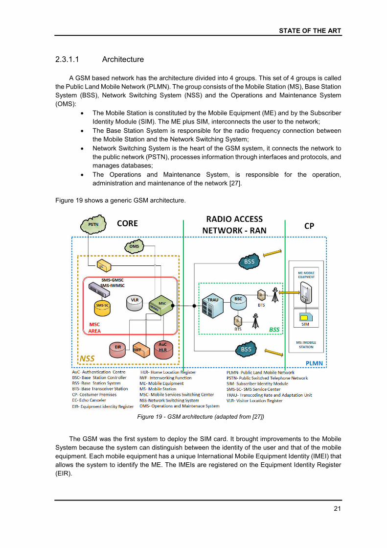
STATE OF THE ART
21
2.3.1.1 Architecture
A GSM based network has the architecture divided into 4 groups. This set of 4 groups is called
the Public Land Mobile Network (PLMN). The group consists of the Mobile Station (MS), Base Station
System (BSS), Network Switching System (NSS) and the Operations and Maintenance System
(OMS):
The Mobile Station is constituted by the Mobile Equipment (ME) and by the Subscriber
Identity Module (SIM). The ME plus SIM, interconnects the user to the network;
The Base Station System is responsible for the radio frequency connection between
the Mobile Station and the Network Switching System;
Network Switching System is the heart of the GSM system, it connects the network to
the public network (PSTN), processes information through interfaces and protocols, and
manages databases;
The Operations and Maintenance System, is responsible for the operation,
administration and maintenance of the network [27].
Figure 19 shows a generic GSM architecture.
Figure 19 - GSM architecture (adapted from [27])
The GSM was the first system to deploy the SIM card. It brought improvements to the Mobile
System because the system can distinguish between the identity of the user and that of the mobile
equipment. Each mobile equipment has a unique International Mobile Equipment Identity (IMEI) that
allows the system to identify the ME. The IMEIs are registered on the Equipment Identity Register
(EIR).

SHARED SOLUTION FOR TELECOMMUNICATIONS NETWORKS
22
The SIM is associated with a globally unique Integrated Circuit Card ID (ICCID) ID number, and
it is intended to store the international mobile subscriber identity (IMSI) number and its related key
that are used to identify and authenticate subscribers on the network. On the SIM it is also possible
to store some contact information.
The integration of the SIM card has added more security to the service processing and billing.
If the mobile phone is lost, the subscriber can go to his provider and request a duplicate, thus regain
access to his account, telephone number, data stored on the card and billing data.
The SIM communicates directly with the Visitor Location Register (VLR) and indirectly with the
Home Location Register (HLR).
The mobile equipment can only successfully connect to a PLMN if the subscriber has a valid
SIM card, being the only exception for emergency calls.
The GSM radio access network includes a set of base station systems (BSS), transcoding rate
and adaption units (TRAU) and base station controllers, as shown on Figure 19. On GSM, the radio
access network is also referred as GERAN (GSM EDGE Radio Access Network).
The main elements found in an GERAN are:
Transcoding Rate and Adaptation Unit (TRAU) that converts the voice signals that are
received from the network switching system to the GSM specifications, and allow an optimal
use of the frequency resources. This maximize the use of the available bandwidth and
consequently maximize the number of calls that can be established with that same
bandwidth;
Base Transceiver Station (BTS) is formed namely by radiofrequency hardware and
antennas that establish the radio link with the Mobile System. These stations are always
linked to the BSC and both control and manage the traffic channels [27];
Base Station Controller (BSC) controls a group of BTS.
GERAN without EDGE is a GRAN, but it still identical in concept [28].
Figure 20 - Interfaces in GERAN core network (adapted from [19] and [28])
The Core Network (CN) is connected to several BSSs and is the central peace of the entire
network. It consists of a Network Switching Systems and a OMS.
The main core components are:
Mobile services Switching Centre (MSC) is the principal component of the Network
Switching System. Its fundamental tasks are:
o Call processing, Link establishment and termination;
o Handover between BSSs and between MSCs;
o Maintenance and supervision;
o Management of interfaces between GSM and other networks and charging.
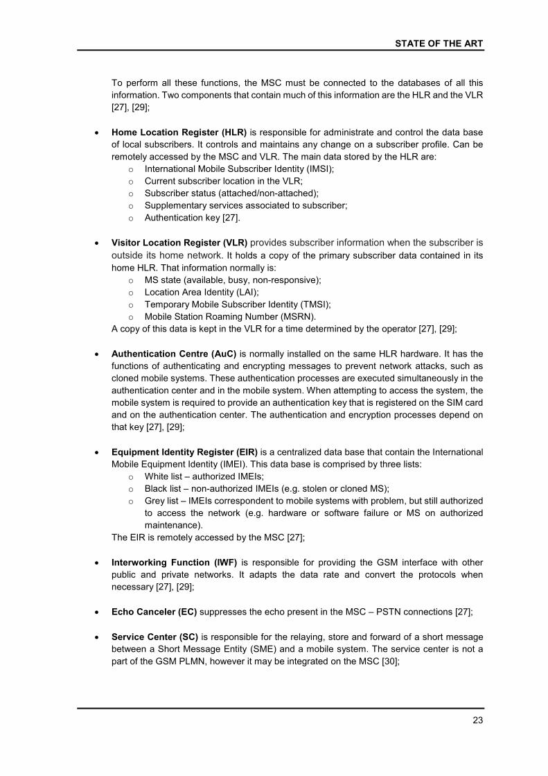
STATE OF THE ART
23
To perform all these functions, the MSC must be connected to the databases of all this
information. Two components that contain much of this information are the HLR and the VLR
[27], [29];
Home Location Register (HLR) is responsible for administrate and control the data base
of local subscribers. It controls and maintains any change on a subscriber profile. Can be
remotely accessed by the MSC and VLR. The main data stored by the HLR are:
o International Mobile Subscriber Identity (IMSI);
o Current subscriber location in the VLR;
o Subscriber status (attached/non-attached);
o Supplementary services associated to subscriber;
o Authentication key [27].
Visitor Location Register (VLR) provides subscriber information when the subscriber is
outside its home network. It holds a copy of the primary subscriber data contained in its
home HLR. That information normally is:
o MS state (available, busy, non-responsive);
o Location Area Identity (LAI);
o Temporary Mobile Subscriber Identity (TMSI);
o Mobile Station Roaming Number (MSRN).
A copy of this data is kept in the VLR for a time determined by the operator [27], [29];
Authentication Centre (AuC) is normally installed on the same HLR hardware. It has the
functions of authenticating and encrypting messages to prevent network attacks, such as
cloned mobile systems. These authentication processes are executed simultaneously in the
authentication center and in the mobile system. When attempting to access the system, the
mobile system is required to provide an authentication key that is registered on the SIM card
and on the authentication center. The authentication and encryption processes depend on
that key [27], [29];
Equipment Identity Register (EIR) is a centralized data base that contain the International
Mobile Equipment Identity (IMEI). This data base is comprised by three lists:
o White list – authorized IMEIs;
o Black list – non-authorized IMEIs (e.g. stolen or cloned MS);
o Grey list – IMEIs correspondent to mobile systems with problem, but still authorized
to access the network (e.g. hardware or software failure or MS on authorized
maintenance).
The EIR is remotely accessed by the MSC [27];
Interworking Function (IWF) is responsible for providing the GSM interface with other
public and private networks. It adapts the data rate and convert the protocols when
necessary [27], [29];
Echo Canceler (EC) suppresses the echo present in the MSC – PSTN connections [27];
Service Center (SC) is responsible for the relaying, store and forward of a short message
between a Short Message Entity (SME) and a mobile system. The service center is not a
part of the GSM PLMN, however it may be integrated on the MSC [30];
SHARED SOLUTION FOR TELECOMMUNICATIONS NETWORKS
24
Gateway MSC for Short Message Service (SMS-GMSC) is a function of an MSC capable
of receiving a short message from the service center, interrogating an HLR for routing
information and SMS info, and delivering the short message to the Visited Mobile Switching
Centre (VMSC) of the recipient mobile system [30], [29];
Interworking MSC for Short Message Service (SMS-IWMSC) is a function of the MSC
capable of receiving a short message from within the PLMN and submitting it to the recipient
service center [30], [29];
Operations and Maintenance System (OMS) is responsible for the administration,
operation, maintenance and centralized remote supervision of the elements of the GSM
network [27].
Figure 19 shows how all those elements come together to form the entire grid of a GSM network.
MSC is the main component of the core network and several of this exist on the network. Figure 19
only show one NSS and one MSC for simplification purposes, but on reality the full network has
several MSCs, each one with all the associated databases and components described above. The
recipe for successful connection is the inter-connection of all the MSCs.
The interfaces that GSM uses to provide interconnection of the different network elements, as
well as the implementation of mobile services and applications between those same elements are
presented on Appendix A.
In a very brief way, those were the main elements that make up a GSM network, it is understood
that there is much more to be addressed about the GSM, its interfaces and protocols, but they are
not objects of study of this dissertation.
UMTS – Third Generation
UMTS it still widely used all over the planet and was the technology that boosted the widely use
and popularization of internet on mobile phones. Seen as the successor to the 2G mobile
telecommunication system (GSM, GPRS and EDGE), UMTS brings an evolution in terms of greatly
enhanced capacity, new data rates and service capabilities, improvement on global mobility and
high-speed transmissions in a wide range of services, thus improving the quality of service. The 3G
systems employs a bandwidth channel greater on the air interface when compared to the GSM
system. It uses a bandwidth of 5 MHz for each channel, while the GSM uses only 200 KHz per
channel [19].
The architecture for a UMTS network is designed to allow packet data to be transmitted over
the network, but still support voice circuit switching.
When the UMTS system is used for voice calls, exist the possibility of having the user connected
to a maximum of three towers (set of antennas), which enables a better QoS.
If the user is on the move, in the event of poor conditions on the radio interface, or the
occurrence of an error during the handover process between base stations and the connection to
one of the towers is lost, the connection is ensured by the other towers (antennas), avoiding a loss
of connection. This means that whenever UMTS coverage exists, the user is always connected to
the network.
STATE OF THE ART
25
If there is no UMTS network coverage available, it is possible to use the GSM/GPRS/EDGE
network. When UMTS coverage is re-established, the call is seamlessly transferred from GSM to
UMTS without the need to be disconnected [22].
UMTS use W-CDMA as medium access technique and FDD and TDD as duplex schemes. W-
CDMA allows a greater share of voice and data traffic, the voice capacity and quality is higher due
to interference control mechanisms, fast power control and soft handover.
The use of TDD and FDD makes the transmission more efficient, since each mode is suitable
for different situations. TDD, for example, is most advantageous in "asymmetric" applications, such
as Web services, where the number of data sent is usually different from the amount received.
Despite the distinct duplex schemes used, the modulation schemes for uplink and downlink is slightly
different, but both based on phase shift keying formats.
The 3G network were upgraded to 3.5G with minor modifications, with the aim of further
increasing data rates through a more efficient use of frequency, increasing capacity and coverage
as well as reducing costs.
High Speed Packet Access (HSPA) is considered an evolution of the W-CDMA, and is based
on two protocols that use 5 MHz carriers:
High Speed Downlink Packet Access (HSDPA) used for uploading;
High Speed Uplink Packet Access (HSUPA) used for download.
HSPA can be deployed over the WCDMA network on the same carrier or, for high capacity and
speed solutions, using another carrier. Nevertheless, WCDMA and HSPA are able to share all
network elements, whether in the core network or the radio network, including sites, base station
antennas or antenna cables [16], [18], [19].
Switching from WCDMA to HSPA only requires new software and potentially new equipment on
the base station and RNC to support the increased rate and data capacity. Due to the high
compatibility between WCDMA and HSPA, the cost of the upgrade is very low compared to building
a new data network.
One of the changes due to the enhancement is reflected on the antennas, in 3G the antenna
sends the signal to all users within a certain area, without any distinction between them while in the
3.5G the antennas can have a signal that searches for users with a low bit rate, and another signal
to users with high bitrate. In this way, by removing users with high bit-rate from the common signal,
it is possible to have more coverage and capacity for other users [16], [18], [19].
2.3.2.1 Architecture
Much like GSM, the UMTS network can be divided into 3 main elements: User Equipment (EU),
UMTS Radio Access Network (UTRAN) and the Core Network.
The user equipment is comprised by two components:
Mobile Equipment (ME), which is the radio terminal that the user uses to connect to the
network;
UMTS Subscriber Identity Module (USIM), that as basically the same function that the
SIM card used on GSM.

SHARED SOLUTION FOR TELECOMMUNICATIONS NETWORKS
26
UTRAN is the section of the network that interfaces with the UE and the Core network. It is the
concept of RAN but applied on a UMTS network.
On UMTS it consists of one or more RNS (Radio Network Subsystems) each containing a Radio
Network Controller (RNC) and a group of NodeBs [16], [18], [29].
NodeB is the denomination used on UMTS for the base station. And just as it happened in
GSM, it manages the flow of data between user equipment and the Core Network [16], [18],
[21], [29];
RNC controls the NodeBs that are connected to it and manages the radio resources on its
domain. RNCs also process the radio signals that come from either the UE or the Core
Network, execute call setup and termination, carry out soft intersystem, hard handover and
has OA&M (Operation, Administrative and Maintenance) competences [16], [18], [21], [29].
As Figure 21 shows, UTRAN has two different interfaces to the Core Network: Iu-CS and Iu-PS.
The air interface is called UMTS User (Uu).
Voice and video calls are traffic in Real-Time (RT) and are handled by CS CN while all other
traffic is called the traffic in Non Real Time (NRT) which is handled by PS CN [16], [19], [21].
Figure 21 - Interfaces in UTRAN core network (adapted from [19] and [28])
Figure 22 illustrates a generic view of a UMTS network. The core network is the highest level of
the hierarchy, which is the backbone of the UMTS network, providing the gateways and connections
to the external networks. The mobile users (UEs) are the lowest level of this hierarchy. A large UMTS
radio access network consists of many RNCs each controlling hundreds of NodeBs [16], [28], [29].
The UMTS main network architecture is identical to the GSM network, but with some more
equipment added to enable the additional functionality required by UMTS.
Considering the different forms of data transmission, the Core Network of UMTS can be divided
into two different areas:
Circuit Switched (CS) is constituted by equipment mainly used in the GSM network, which
carries the data in a circuit switching mode, i.e., a permanent channel during the duration of
the call;
Packet Switched (PS) has network equipment designed to carry packet data, allowing much
greater network usage, due to the ability to share the capacity. When the data are
transported as packets that are able to be routed according to their destination.

STATE OF THE ART
27
Figure 22 - UMTS architecture (adapted from [27], [24] and [29])
The circuit switched equipment’s are the following:
Mobile Services Switching Centre (MSC) is the central element of the circuit switching
System and is responsible for switching and signaling functions.
Has the responsibility to perform:
o Call management and handover between UTRANs and MSCs;
o CS data services operations;
o Maintenance and supervision (data base management and traffic data
measurement);
o Charging [16], [18], [27], [29].
Gateway MSC (GMSC) manage and provide interconnection between the UMTS core
network and the external PSTN / ISDN networks [16], [18], [27], [29];
Media Gateway (MGW) is a translation device or service responsible for converting digital
media streams between disparate telecommunications networks [16], [18], [27], [29].
The circuit switched equipment’s are:
Serving GPRS Support Node (SGSN) was first deployed when the GRPS was introduced.
Provides several functions such as:
o Delivering the data packet from and to UE within its serving area;
o Packet switching/routing and transfer;
o Mobility management (attach/detach and location management);
o Session management, logical link management authentication;
o Subscriber database management;
o Billing functions [16], [18], [27], [29].
Gateway GPRS Support Node (GGSN) like SGSNs, this was also deployed on the
introduction of the GPRS. It is a gateway between UMTS PS/GPRS network and external
data networks like Internet. It can be considered as sophisticated router that handles several
functions such as:
SHARED SOLUTION FOR TELECOMMUNICATIONS NETWORKS
28
o Routing and data encapsulation between a UE and external data networks;
o Security control;
o Network access control and network management.
It also perform Authentication, Authorization, Accounting and Traffic management [16], [18],
[27], [29].
The following equipment are shared by the two switching systems, many of them have the same
responsibility and tasks as in GSM:
Authentication Centre (AuC) is a database that is responsible for authentication and
encryption operations. It stores data needed to authenticate the IMSI (International Mobile
Subscriber Identity) associated to each mobile equipment. These operations are executed
in the AuC and in the UE simultaneously. The AuC communicates only with its associated
HLR, and is usually installed in the HLR hardware [16], [18], [27], [29];
Home Location Register (HLR) is in charge of administrating and controlling the data base
of local users. It manages and keeps all changes made on a subscriber profile, holds the
information about each subscriber along with their last location. The essentials data profiles
information held are:
o Authentication key;
o International Mobile Subscriber Identity (IMSI);
o Supplementary services associated to subscriber (and related information);
o Current subscriber location in the VLR;
o Subscriber status (attached/non-attached) [16], [18], [27], [29].
Equipment Identity Register (EIR) is a local data base that store the International Mobile
Equipment Identities (IMEI). Each mobile equipment has a unique registered number. EIR
decides if a given UE may be allowed in to the network. The EIR holds the black, gray and
white lists with equipment numbers [16], [18], [27], [29];
Visitor Location Register (VLR) is a secondary data base that held responsible for keeping
a copy of the user’s main profile data that are stored on the HLR to minimize the load on the
HLR. Examples of main profile data stored on the VLR are:
o The UE state (e.g. available, busy, non-responsive);
o The LAI (Location Area Identity);
o The TMSI (Temporary Mobile Subscriber Identity);
o The MSRN (Mobile Station Roaming Number) [16], [18], [27], [29].
The Echo Canceler (EC) attenuates the echo present in the MSC – PSTN connections [16],
[18], [27], [29];
The Interworking Function (IWF) is associated with the MSC, and provides the interface
with other public and private networks [16], [18], [27], [29];
Service Center (SC) is responsible for the relaying and store-and-forwarding of a short
message between a Short Message Entity (SME) and a mobile system. The service center
is not a part of the GSM PLMN, however it may be integrated on the MSC [18], [27], [29];
The Interworking MSC for Short Message Service (SMS-IWMSC) is a function of the MSC
that is capable of receiving a short message from within the PLMN and sending it to the
recipient SC [16], [18], [27], [29];
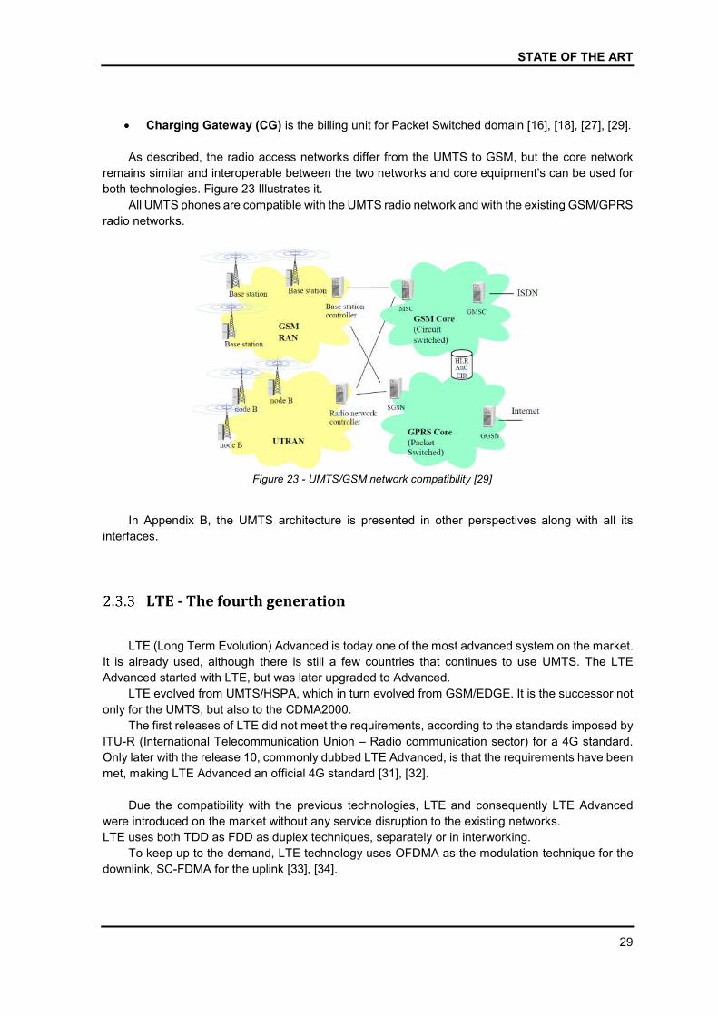
STATE OF THE ART
29
Charging Gateway (CG) is the billing unit for Packet Switched domain [16], [18], [27], [29].
As described, the radio access networks differ from the UMTS to GSM, but the core network
remains similar and interoperable between the two networks and core equipment’s can be used for
both technologies. Figure 23 Illustrates it.
All UMTS phones are compatible with the UMTS radio network and with the existing GSM/GPRS
radio networks.
Figure 23 - UMTS/GSM network compatibility [29]
In Appendix B, the UMTS architecture is presented in other perspectives along with all its
interfaces.
LTE - The fourth generation
LTE (Long Term Evolution) Advanced is today one of the most advanced system on the market.
It is already used, although there is still a few countries that continues to use UMTS. The LTE
Advanced started with LTE, but was later upgraded to Advanced.
LTE evolved from UMTS/HSPA, which in turn evolved from GSM/EDGE. It is the successor not
only for the UMTS, but also to the CDMA2000.
The first releases of LTE did not meet the requirements, according to the standards imposed by
ITU-R (International Telecommunication Union – Radio communication sector) for a 4G standard.
Only later with the release 10, commonly dubbed LTE Advanced, is that the requirements have been
met, making LTE Advanced an official 4G standard [31], [32].
Due the compatibility with the previous technologies, LTE and consequently LTE Advanced
were introduced on the market without any service disruption to the existing networks.
LTE uses both TDD as FDD as duplex techniques, separately or in interworking.
To keep up to the demand, LTE technology uses OFDMA as the modulation technique for the
downlink, SC-FDMA for the uplink [33], [34].
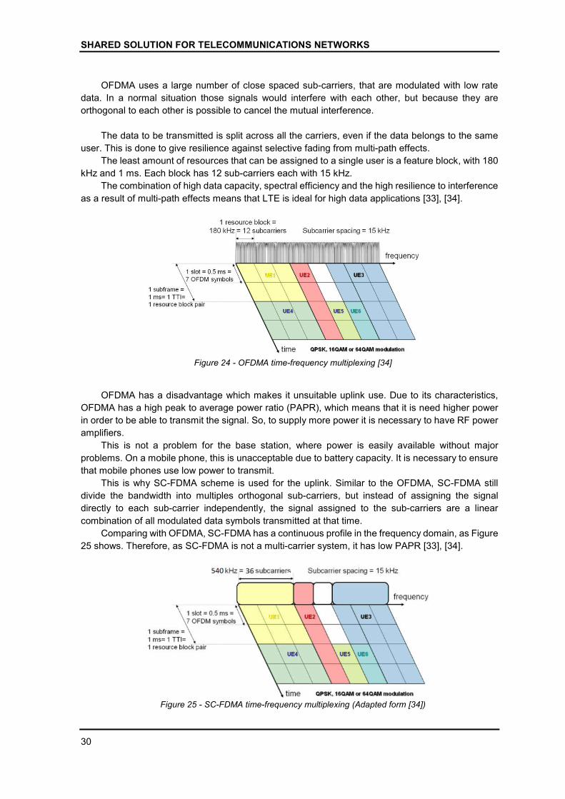
SHARED SOLUTION FOR TELECOMMUNICATIONS NETWORKS
30
OFDMA uses a large number of close spaced sub-carriers, that are modulated with low rate
data. In a normal situation those signals would interfere with each other, but because they are
orthogonal to each other is possible to cancel the mutual interference.
The data to be transmitted is split across all the carriers, even if the data belongs to the same
user. This is done to give resilience against selective fading from multi-path effects.
The least amount of resources that can be assigned to a single user is a feature block, with 180
kHz and 1 ms. Each block has 12 sub-carriers each with 15 kHz.
The combination of high data capacity, spectral efficiency and the high resilience to interference
as a result of multi-path effects means that LTE is ideal for high data applications [33], [34].
Figure 24 - OFDMA time-frequency multiplexing [34]
OFDMA has a disadvantage which makes it unsuitable uplink use. Due to its characteristics,
OFDMA has a high peak to average power ratio (PAPR), which means that it is need higher power
in order to be able to transmit the signal. So, to supply more power it is necessary to have RF power
amplifiers.
This is not a problem for the base station, where power is easily available without major
problems. On a mobile phone, this is unacceptable due to battery capacity. It is necessary to ensure
that mobile phones use low power to transmit.
This is why SC-FDMA scheme is used for the uplink. Similar to the OFDMA, SC-FDMA still
divide the bandwidth into multiples orthogonal sub-carriers, but instead of assigning the signal
directly to each sub-carrier independently, the signal assigned to the sub-carriers are a linear
combination of all modulated data symbols transmitted at that time.
Comparing with OFDMA, SC-FDMA has a continuous profile in the frequency domain, as Figure
25 shows. Therefore, as SC-FDMA is not a multi-carrier system, it has low PAPR [33], [34].
Figure 25 - SC-FDMA time-frequency multiplexing (Adapted form [34])
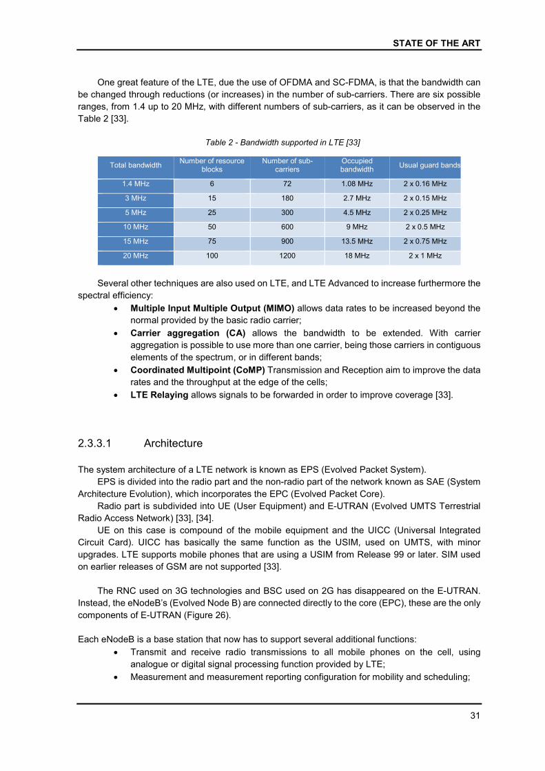
STATE OF THE ART
31
One great feature of the LTE, due the use of OFDMA and SC-FDMA, is that the bandwidth can
be changed through reductions (or increases) in the number of sub-carriers. There are six possible
ranges, from 1.4 up to 20 MHz, with different numbers of sub-carriers, as it can be observed in the
Table 2 [33].
Table 2 - Bandwidth supported in LTE [33]
Total bandwidth Number of resource
blocks Number of sub-
carriers Occupied bandwidth
Usual guard bands
1.4 MHz 6 72 1.08 MHz 2 x 0.16 MHz
3 MHz 15 180 2.7 MHz 2 x 0.15 MHz
5 MHz 25 300 4.5 MHz 2 x 0.25 MHz
10 MHz 50 600 9 MHz 2 x 0.5 MHz
15 MHz 75 900 13.5 MHz 2 x 0.75 MHz
20 MHz 100 1200 18 MHz 2 x 1 MHz
Several other techniques are also used on LTE, and LTE Advanced to increase furthermore the
spectral efficiency:
Multiple Input Multiple Output (MIMO) allows data rates to be increased beyond the
normal provided by the basic radio carrier;
Carrier aggregation (CA) allows the bandwidth to be extended. With carrier
aggregation is possible to use more than one carrier, being those carriers in contiguous
elements of the spectrum, or in different bands;
Coordinated Multipoint (CoMP) Transmission and Reception aim to improve the data
rates and the throughput at the edge of the cells;
LTE Relaying allows signals to be forwarded in order to improve coverage [33].
2.3.3.1 Architecture
The system architecture of a LTE network is known as EPS (Evolved Packet System).
EPS is divided into the radio part and the non-radio part of the network known as SAE (System
Architecture Evolution), which incorporates the EPC (Evolved Packet Core).
Radio part is subdivided into UE (User Equipment) and E-UTRAN (Evolved UMTS Terrestrial
Radio Access Network) [33], [34].
UE on this case is compound of the mobile equipment and the UICC (Universal Integrated
Circuit Card). UICC has basically the same function as the USIM, used on UMTS, with minor
upgrades. LTE supports mobile phones that are using a USIM from Release 99 or later. SIM used
on earlier releases of GSM are not supported [33].
The RNC used on 3G technologies and BSC used on 2G has disappeared on the E-UTRAN.
Instead, the eNodeB’s (Evolved Node B) are connected directly to the core (EPC), these are the only
components of E-UTRAN (Figure 26).
Each eNodeB is a base station that now has to support several additional functions:
Transmit and receive radio transmissions to all mobile phones on the cell, using
analogue or digital signal processing function provided by LTE;
Measurement and measurement reporting configuration for mobility and scheduling;

SHARED SOLUTION FOR TELECOMMUNICATIONS NETWORKS
32
IP header compression and encryption of user data stream;
Routing of user plane data towards serving Gateway;
Control the low-level operation of all mobile phones on the cell, by sending signaling
messages such as handover commands. The X2 interface allows that two eNodeB
decide when a client switches between them, without the need to negotiate this
handover with another network equipment [33].
Figure 26 - LTE E-UTRAN architecture [34], [35]
As seen on Figure 26, the eNodeB’s are connected to each other through X2 interface and to
EPC through S1 interface. Both interfaces are based on IP protocol.
X2 interface supports enhanced mobility, inter-cell interference management, and SON (Self-
Organizing Networks) functionalities. X2 interface is optional, since S1 interface can also handle the
tasks of X2, although with less speed.
The major purpose of eliminating RNCs and BCSs is to reduce the latency on the network [33].
The major difference between EPC and other core networks is that it only works with IP
transmission. EPC is mainly compound are:
Mobility Management Entity (MME) is the main element on the EPC, it is a server in charge
of all control functions related to subscriber and session management. Each mobile phone
is assigned to a single MME, known as serving MME, but if the user moves away, the serving
MME can be changed. MMEs are connected to each other through S10 interfaces and its
main tasks are:
o Authentication and Security;
o Mobility Management;
o Managing Subscription Profile;
o PDN Gateway and Serving Gateway selection [33].
Home Subscriber Server (HSS) is a database with all permanent user data. It stores a
master copy of the subscriber profile and the location of the subscriber. HSS also hold the
function of the AuC used in past architectures. HSSs needs to be able to connect to each
MME on the network [33];
Serving Gateway (SG) forwards data between the eNodeB and the PDN Gateway, and like
MMEs, each mobile phone is assigned to a single SG that can be changed if the user moves
away. SG can also be seen as the point of contact between the E-UTRAN and other
networks such as GSM as UMTS [33];
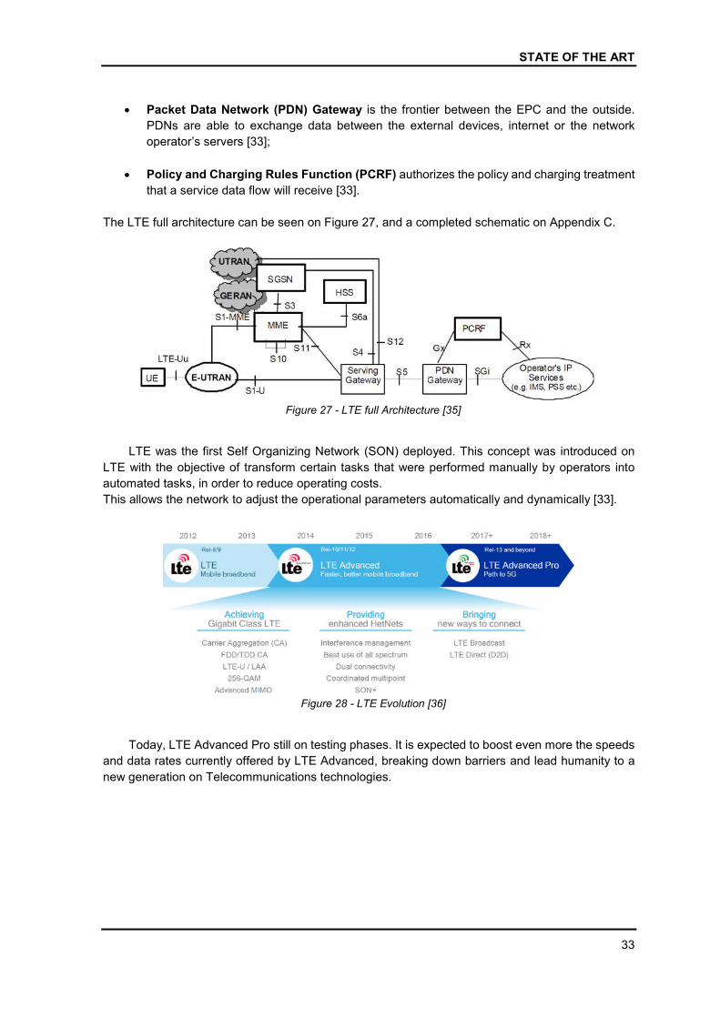
STATE OF THE ART
33
Packet Data Network (PDN) Gateway is the frontier between the EPC and the outside.
PDNs are able to exchange data between the external devices, internet or the network
operator’s servers [33];
Policy and Charging Rules Function (PCRF) authorizes the policy and charging treatment
that a service data flow will receive [33].
The LTE full architecture can be seen on Figure 27, and a completed schematic on Appendix C.
Figure 27 - LTE full Architecture [35]
LTE was the first Self Organizing Network (SON) deployed. This concept was introduced on
LTE with the objective of transform certain tasks that were performed manually by operators into
automated tasks, in order to reduce operating costs.
This allows the network to adjust the operational parameters automatically and dynamically [33].
Figure 28 - LTE Evolution [36]
Today, LTE Advanced Pro still on testing phases. It is expected to boost even more the speeds
and data rates currently offered by LTE Advanced, breaking down barriers and lead humanity to a
new generation on Telecommunications technologies.


INFRASTRUCTURE SHARING MODELS
35
INFRASTRUCTURE SHARING MODELS
Infrastructure sharing in recent years has become a common economic solution for many
countries to cope with new and frequent updates and growing traffic demands. With the rapid
evolution of the market and to be able to stay on board the intense technological development in
telecommunications area, operators have often resort to partnerships.
This allows them to lower the costs of build and operate a network, which enables operators to
expand and improve their performance by providing users with new services, better QoS, and lower
prices.
However, the reasons why an operator chooses to share its own infrastructure or rent the
infrastructures of others differs from operator to operator. But it is important to know and understand
that infrastructure sharing has a crucial role in the development and organization of the
telecommunications industry.
Examples of mobile infrastructure and network sharing can be found in both mature and
developing markets [37].
Sharing can be done at different levels or modes and depending on the operator's business
strategy. The advantages go beyond the economic factor, in fact, many regulators in some regions
impose, or insist that operators adopt techniques of sharing, to reduce the environmental impact,
and impact on the population.
To illustrate the different sharing models, and for the sake of clarity, the use of UMTS technology
will be assumed in the remaining of this chapter.
In a simplified way, there are two main forms of sharing:
Passive sharing, can be summarily described as the sharing of non-electronic
infrastructures;
Active sharing is the exact opposite. Where is sharing the electronic infrastructures. RAN
sharing and core sharing (Deeper sharing or integration) are the main form of this type of
sharing. Figure 29 illustrates the different levels.
Figure 29 - Levels of Sharing (Adapted form [38])
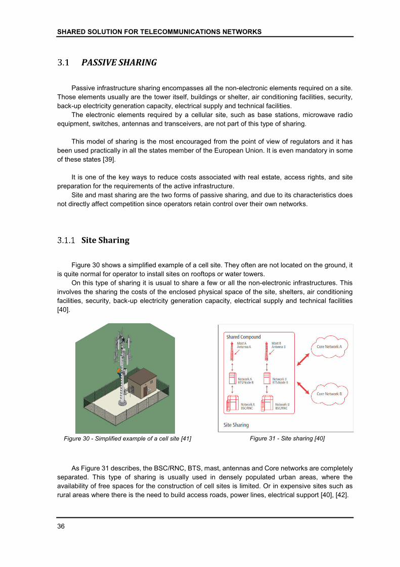
SHARED SOLUTION FOR TELECOMMUNICATIONS NETWORKS
36
PASSIVE SHARING
Passive infrastructure sharing encompasses all the non-electronic elements required on a site.
Those elements usually are the tower itself, buildings or shelter, air conditioning facilities, security,
back-up electricity generation capacity, electrical supply and technical facilities.
The electronic elements required by a cellular site, such as base stations, microwave radio
equipment, switches, antennas and transceivers, are not part of this type of sharing.
This model of sharing is the most encouraged from the point of view of regulators and it has
been used practically in all the states member of the European Union. It is even mandatory in some
of these states [39].
It is one of the key ways to reduce costs associated with real estate, access rights, and site
preparation for the requirements of the active infrastructure.
Site and mast sharing are the two forms of passive sharing, and due to its characteristics does
not directly affect competition since operators retain control over their own networks.
Site Sharing
Figure 30 shows a simplified example of a cell site. They often are not located on the ground, it
is quite normal for operator to install sites on rooftops or water towers.
On this type of sharing it is usual to share a few or all the non-electronic infrastructures. This
involves the sharing the costs of the enclosed physical space of the site, shelters, air conditioning
facilities, security, back-up electricity generation capacity, electrical supply and technical facilities
[40].
Figure 30 - Simplified example of a cell site [41]
Figure 31 - Site sharing [40]
As Figure 31 describes, the BSC/RNC, BTS, mast, antennas and Core networks are completely
separated. This type of sharing is usually used in densely populated urban areas, where the
availability of free spaces for the construction of cell sites is limited. Or in expensive sites such as
rural areas where there is the need to build access roads, power lines, electrical support [40], [42].
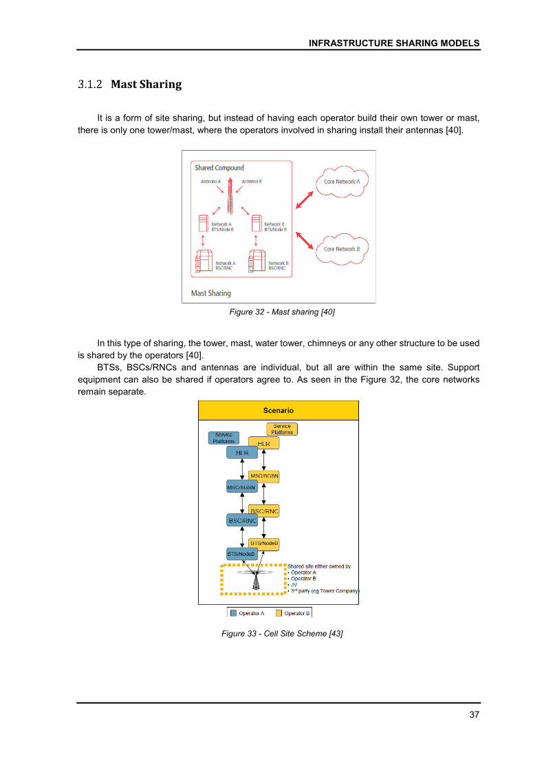
INFRASTRUCTURE SHARING MODELS
37
Mast Sharing
It is a form of site sharing, but instead of having each operator build their own tower or mast,
there is only one tower/mast, where the operators involved in sharing install their antennas [40].
Figure 32 - Mast sharing [40]
In this type of sharing, the tower, mast, water tower, chimneys or any other structure to be used
is shared by the operators [40].
BTSs, BSCs/RNCs and antennas are individual, but all are within the same site. Support
equipment can also be shared if operators agree to. As seen in the Figure 32, the core networks
remain separate.
Figure 33 - Cell Site Scheme [43]

SHARED SOLUTION FOR TELECOMMUNICATIONS NETWORKS
38
These types of sharing have become such a constant phenomenon that in some countries
companies were created that specialize only in the provision of passive infrastructure to multiple
operators. Those companies are commonly known as Tower companies [44].
ACTIVE SHARING
In active sharing, operators usually agree to share BSCs, RNCs, mobile services switching
center/Visiting location register (MSC/VLR), and serving GPRS support node (SGSN). However, is
crucial to realize that each operator has its own individual network that contains the independent
subscriber databases services (such as HLR, AUC, etc.), subscriber billing and connections to
external networks [42].
The depth of sharing depends on the type of active sharing adopted. Active sharing can be done
in two modes:
RAN sharing;
Core network sharing.
Each of these forms has its pros and cons, and the operators need to be aware of the existing
risks and benefits they will have before engaging in this sharing model.
RAN Sharing
In the RAN sharing, all radio access network equipment’s are shared up to the point where the
private core networks belonging to each operator are connected. Sharing the radio access network
is a more economical solution than passive sharing types, since the costs of the entire shared access
network is divided by the operators involved.
The traffic is split through the different operators at the point where the core networks are
connected. Therefore, each operator keeps its on individual logical networks and spectrum.
It is necessary to emphasize that RAN sharing includes the sharing of mast, Site, radio
equipment (antennas), operating and maintenance costs, as shown on the Figure 34.
Figure 34 - Full RAN Sharing [40], [43]
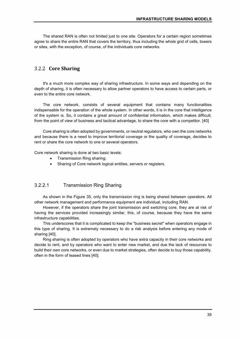
INFRASTRUCTURE SHARING MODELS
39
The shared RAN is often not limited just to one site. Operators for a certain region sometimes
agree to share the entire RAN that covers the territory, thus including the whole grid of cells, towers
or sites, with the exception, of course, of the individuals core networks.
Core Sharing
It's a much more complex way of sharing infrastructure. In some ways and depending on the
depth of sharing, it is often necessary to allow partner operators to have access to certain parts, or
even to the entire core network.
The core network, consists of several equipment that contains many functionalities
indispensable for the operation of the whole system. In other words, it is in the core that intelligence
of the system is. So, it contains a great amount of confidential information, which makes difficult,
from the point of view of business and tactical advantage, to share the core with a competitor. [40]
Core sharing is often adopted by governments, or neutral regulators, who own the core networks
and because there is a need to improve territorial coverage or the quality of coverage, decides to
rent or share the core network to one or several operators.
Core network sharing is done at two basic levels:
Transmission Ring sharing;
Sharing of Core network logical entities, servers or registers.
3.2.2.1 Transmission Ring Sharing
As shown in the Figure 35, only the transmission ring is being shared between operators. All
other network management and performance equipment are individual, including RAN.
However, if the operators share the joint transmission and switching core, they are at risk of
having the services provided increasingly similar, this, of course, because they have the same
infrastructure capabilities.
This underscores that it is complicated to keep the "business secret" when operators engage in
this type of sharing. It is extremely necessary to do a risk analysis before entering any mode of
sharing [40].
Ring sharing is often adopted by operators who have extra capacity in their core networks and
decide to rent, and by operators who want to enter new market, and due the lack of resources to
build their own core networks, or even due to market strategies, often decide to buy those capability,
often in the form of leased lines [40].
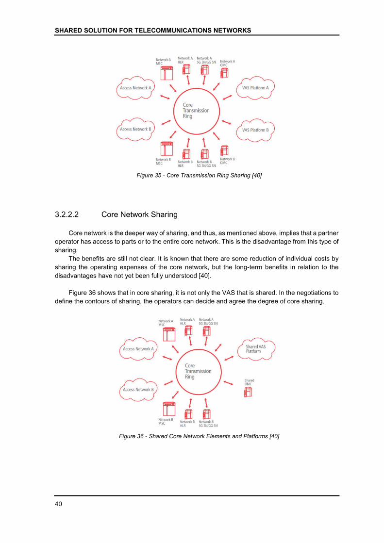
SHARED SOLUTION FOR TELECOMMUNICATIONS NETWORKS
40
Figure 35 - Core Transmission Ring Sharing [40]
3.2.2.2 Core Network Sharing
Core network is the deeper way of sharing, and thus, as mentioned above, implies that a partner
operator has access to parts or to the entire core network. This is the disadvantage from this type of
sharing.
The benefits are still not clear. It is known that there are some reduction of individual costs by
sharing the operating expenses of the core network, but the long-term benefits in relation to the
disadvantages have not yet been fully understood [40].
Figure 36 shows that in core sharing, it is not only the VAS that is shared. In the negotiations to
define the contours of sharing, the operators can decide and agree the degree of core sharing.
Figure 36 - Shared Core Network Elements and Platforms [40]
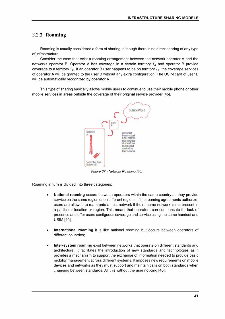
INFRASTRUCTURE SHARING MODELS
41
Roaming
Roaming is usually considered a form of sharing, although there is no direct sharing of any type
of infrastructure.
Consider the case that exist a roaming arrangement between the network operator A and the
networks operator B. Operator A has coverage in a certain territory �� and operator B provide
coverage to a territory ��. If an operator B user happens to be on territory ��, the coverage services
of operator A will be granted to the user B without any extra configuration. The USIM card of user B
will be automatically recognized by operator A.
This type of sharing basically allows mobile users to continue to use their mobile phone or other
mobile services in areas outside the coverage of their original service provider [45].
Figure 37 - Network Roaming [40]
Roaming in turn is divided into three categories:
National roaming occurs between operators within the same country as they provide
service on the same region or on different regions. If the roaming agreements authorize,
users are allowed to roam onto a host network if theirs home network is not present in
a particular location or region. This meant that operators can compensate for lack of
presence and offer users contiguous coverage and service using the same handset and
USIM [40];
International roaming it is like national roaming but occurs between operators of
different countries;
Inter-system roaming exist between networks that operate on different standards and
architecture. It facilitates the introduction of new standards and technologies as it
provides a mechanism to support the exchange of information needed to provide basic
mobility management across different systems. It imposes new requirements on mobile
devices and networks as they must support and maintain calls on both standards when
changing between standards. All this without the user noticing [40].
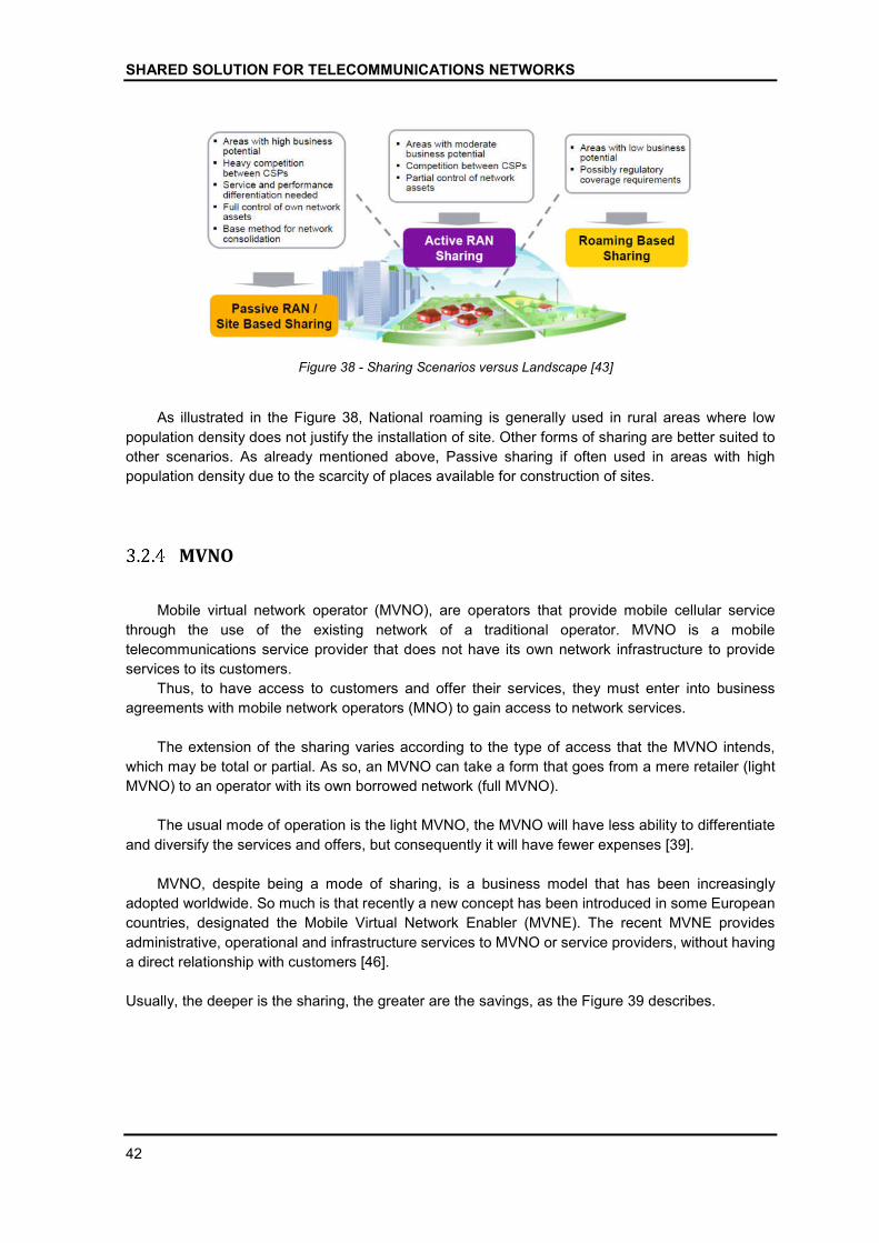
SHARED SOLUTION FOR TELECOMMUNICATIONS NETWORKS
42
Figure 38 - Sharing Scenarios versus Landscape [43]
As illustrated in the Figure 38, National roaming is generally used in rural areas where low
population density does not justify the installation of site. Other forms of sharing are better suited to
other scenarios. As already mentioned above, Passive sharing if often used in areas with high
population density due to the scarcity of places available for construction of sites.
MVNO
Mobile virtual network operator (MVNO), are operators that provide mobile cellular service
through the use of the existing network of a traditional operator. MVNO is a mobile
telecommunications service provider that does not have its own network infrastructure to provide
services to its customers.
Thus, to have access to customers and offer their services, they must enter into business
agreements with mobile network operators (MNO) to gain access to network services.
The extension of the sharing varies according to the type of access that the MVNO intends,
which may be total or partial. As so, an MVNO can take a form that goes from a mere retailer (light
MVNO) to an operator with its own borrowed network (full MVNO).
The usual mode of operation is the light MVNO, the MVNO will have less ability to differentiate
and diversify the services and offers, but consequently it will have fewer expenses [39].
MVNO, despite being a mode of sharing, is a business model that has been increasingly
adopted worldwide. So much is that recently a new concept has been introduced in some European
countries, designated the Mobile Virtual Network Enabler (MVNE). The recent MVNE provides
administrative, operational and infrastructure services to MVNO or service providers, without having
a direct relationship with customers [46].
Usually, the deeper is the sharing, the greater are the savings, as the Figure 39 describes.
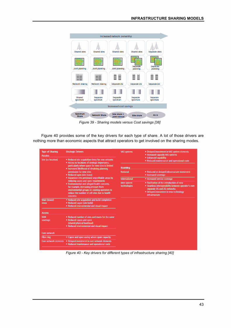
INFRASTRUCTURE SHARING MODELS
43
Figure 39 - Sharing models versus Cost savings [38]
Figure 40 provides some of the key drivers for each type of share. A lot of those drivers are
nothing more than economic aspects that attract operators to get involved on the sharing modes.
Figure 40 - Key drivers for different types of infrastructure sharing [40]
SHARED SOLUTION FOR TELECOMMUNICATIONS NETWORKS
44
NEUTRAL OPERATOR
Despite the efforts to increase the area covered by mobile communications, some progress is
still needed to further increase the penetration of mobile services through all regions, particularly in
rural areas in developing countries.
The deployment of mobile networks requires high investments. This type of investment often
makes mobile services less accessible and may discourage operators from innovating and migrating
to new technologies. It can result in the exclusion of part of the population or even of certain regions
from access to mobile telecommunications services [37].
NO or Neutral Operator, like MVNO, is a concept that has begun to gain ground in recent years.
It is based on the separation of the network infrastructure and the provision of services. The neutral
operator usually invests in infrastructure on remote areas where infrastructure is not yet available.
This is done to stimulate and take the first step in investing in a region that other operators are not
willing to invest. The role of NO is often assumed by government entities that want or need to develop
certain regions.
Becoming more than a technological solution to telecommunication problems, NO is actively
involved in developing a sustainable and profitable way of overcoming mobile telecommunication
restrictions, improving mobile demographic and demographic telecommunication coverage in remote
areas and rural areas [47].
The business model commonly used by neutral operations generally begins with the
construction of its infrastructures, strengthening the region for potential technological growth, and
later negotiates with the licensed operators the models of sharing that interest each one.
In an extreme form, NO can finance the entire access network, and only connects the core
network of operators interested in renting bandwidth.
Due to these types of integration, the neutral operator may also need to follow some set of
requirements defined by the Regulatory Agents. Because it has a mediating role, the concept of a
neutral operator gains a more complex dimension and its implementation and operation need to take
a non-discriminatory approach to the development of protocols and sharing services, while complying
with legal requirements and regulations required [47].
However, there are some counterparts to improve in sharing models, such as concern about
the practical and logistical aspects of dealing with a common infrastructure for different purposes and
operators. But despite these concerns, the pressure currently put on operators to provide more at a
lower price encourages the parties to negotiate a series of solutions that will enable them to continue
in the telecommunications business.
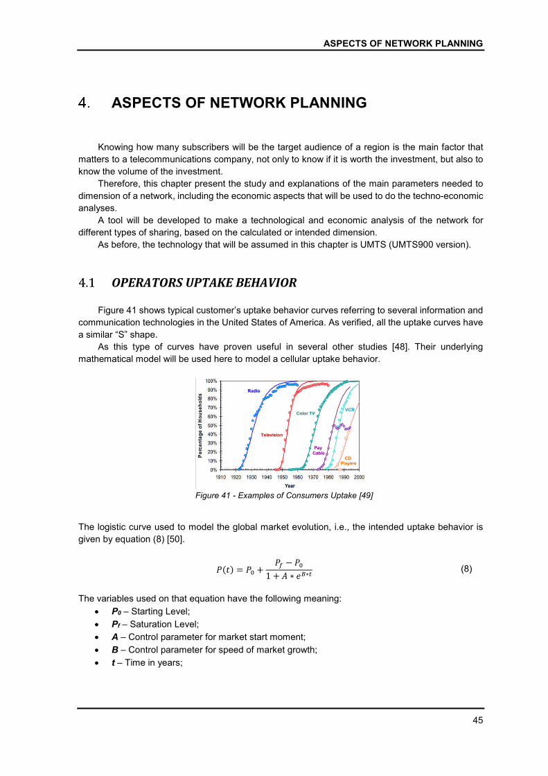
ASPECTS OF NETWORK PLANNING
45
ASPECTS OF NETWORK PLANNING
Knowing how many subscribers will be the target audience of a region is the main factor that
matters to a telecommunications company, not only to know if it is worth the investment, but also to
know the volume of the investment.
Therefore, this chapter present the study and explanations of the main parameters needed to
dimension of a network, including the economic aspects that will be used to do the techno-economic
analyses.
A tool will be developed to make a technological and economic analysis of the network for
different types of sharing, based on the calculated or intended dimension.
As before, the technology that will be assumed in this chapter is UMTS (UMTS900 version).
OPERATORS UPTAKE BEHAVIOR
Figure 41 shows typical customer’s uptake behavior curves referring to several information and
communication technologies in the United States of America. As verified, all the uptake curves have
a similar “S” shape.
As this type of curves have proven useful in several other studies [48]. Their underlying
mathematical model will be used here to model a cellular uptake behavior.
Figure 41 - Examples of Consumers Uptake [49]
The logistic curve used to model the global market evolution, i.e., the intended uptake behavior is
given by equation (8) [50].
�(�) = �� +�� − ��
1 + � ∗ ��∗� (8)
The variables used on that equation have the following meaning:
P0 – Starting Level;
Pf – Saturation Level;
A – Control parameter for market start moment;
B – Control parameter for speed of market growth;
t – Time in years;
SHARED SOLUTION FOR TELECOMMUNICATIONS NETWORKS
46
As equation (8) define the global market evolution, equation (9) will modulate the uptake
behavior of each operator individually [50].
��(�) = ���+
���− ���
1 + �� ∗ ���∗� (9)
When an operator enters the market, it generates a reaction that will affect the evolution, and
uptake of the operators already present on the market, causing them to lose some market share.
This interaction between operators will be modulated by equation (10), (11) and (12).
Despite having a different purpose and interpretation, the model developed for this project had
much of its data inspired by the diffusion model of Bass and Norton [51]. Equation (10) refers to the
evolution of the first operator on the market. Equation (11) to the second operator and finally the
equation (12) model the evolution of the third operator.
The operators do not enter the market at the same time, they enter one after the other in the
ascending order.
��(�) = ��(�)∗ [��− ��(� − ��)∗�� ∗�� − ��(� − ��)∗ (�� − ��)∗��] ∗ �(�) (10)
��(�) = [��(� − ��)∗�� − ��(� − ��)∗�� ∗��] ∗ �(�) (11)
��(�) = ��(� − ��)∗�� ∗�(�) (12)
Where:
Si – Function that characterizes the actual market share of each operator wave, affected by
the presence of other operators on the market;
pi(t) – Function that characterizes the uptake behavior of each operator on the market;
P0 – Starting Level;
Pf – Saturation Level;
A – Control parameter for market start moment;
B – Control parameter for speed of market growth;
t – Time in years;
τi – Initial instant where the operator appears on the market (time in years);
mi – defines the potential market share that each operator will be able to serve of the total
market.
Each coefficient mi, refers to the market share of an operator. That is, m1 refers to the market
share of the operator 1, m2 to the operator 2 and so on. So, if m1 is defined as 100% this means that
operator 1 has the potential to capture 100% of the total market, and if m2 is defined at 40%, that
means that from the moment that operator 2 enters the market it will successively over the years
steal market shares from operator 1 until it can achieve 40% of the total market. This will cause
operator 1 to remain only with 60% of the market, even with m1 set at 100%.
Thus, it is clear that the value of mi+1 influence the value of mi over time. And at each instant t,
the sum of the coefficients mi must be equal to 100% (equation (13)).
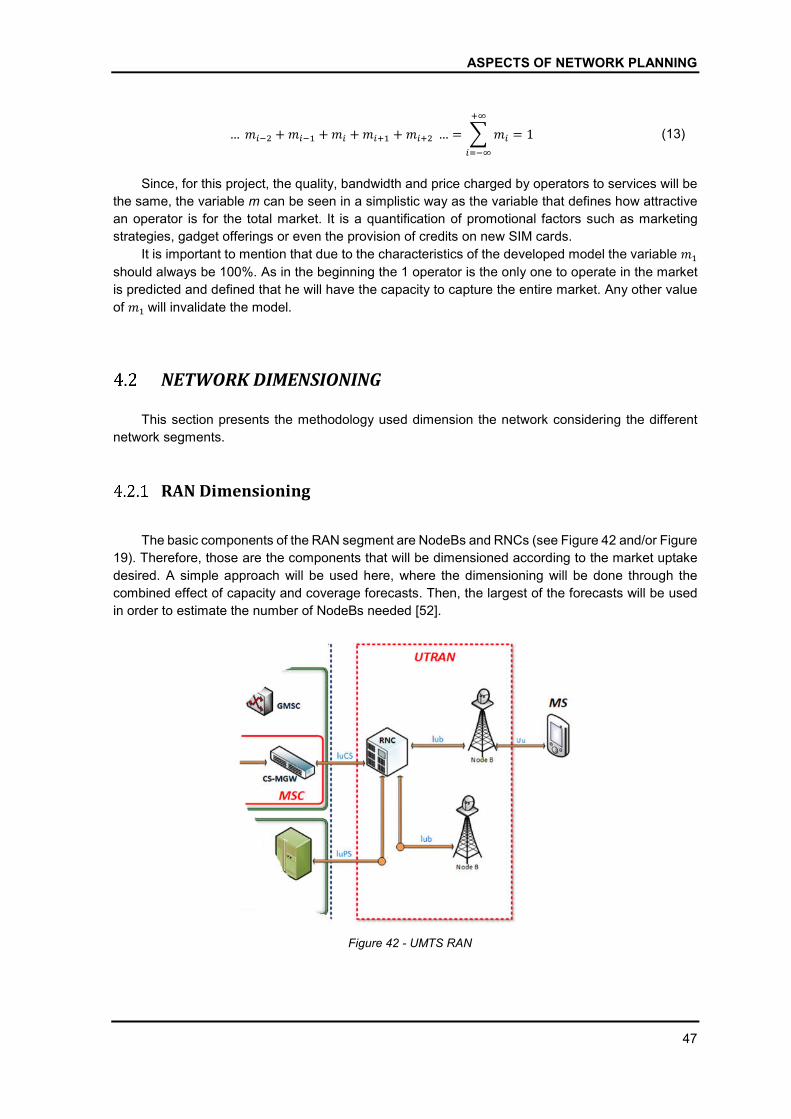
ASPECTS OF NETWORK PLANNING
47
…���� + ���� + �� + ���� + ����… = � ��
��
����
= 1 (13)
Since, for this project, the quality, bandwidth and price charged by operators to services will be
the same, the variable m can be seen in a simplistic way as the variable that defines how attractive
an operator is for the total market. It is a quantification of promotional factors such as marketing
strategies, gadget offerings or even the provision of credits on new SIM cards.
It is important to mention that due to the characteristics of the developed model the variable ��
should always be 100%. As in the beginning the 1 operator is the only one to operate in the market
is predicted and defined that he will have the capacity to capture the entire market. Any other value
of ��will invalidate the model.
NETWORK DIMENSIONING
This section presents the methodology used dimension the network considering the different
network segments.
RAN Dimensioning
The basic components of the RAN segment are NodeBs and RNCs (see Figure 42 and/or Figure
19). Therefore, those are the components that will be dimensioned according to the market uptake
desired. A simple approach will be used here, where the dimensioning will be done through the
combined effect of capacity and coverage forecasts. Then, the largest of the forecasts will be used
in order to estimate the number of NodeBs needed [52].
Figure 42 - UMTS RAN

SHARED SOLUTION FOR TELECOMMUNICATIONS NETWORKS
48
4.2.1.1 NodeB Dimensioning
Figure 43, illustrates the diagram that will be used to estimate the number of needed NodeBs.
As can be seen, the estimate will be made in two parts. On the left side is the diagram for calculating
the number of NodeBs per coverage. On the right side, the diagram for the calculation by capacity.
At the end, the larger of the estimates will be used to define the number of NodeBs.
Figure 43 - NodeB Dimensioning Full Scheme (Adapted from [53])
4.2.1.1.1 Capacity Dimensioning
The data and voice traffic demand needed will be calculated in Busy Hour (BH). That is because
in a communication system, it is not acceptable to provide excellent service most of the time and a
terrible service at the moment when the network has its peak of demands.
Busy Hour is the sliding 60 minutes period which occurs the maximum total traffic load in a given
24-hour period. In other words, is the one hour of the day that a telephone system handles most of
the calls.
To estimate Busy Hour values, the method commonly used is to find the busiest hour of each
day, for 5 or 10 days, during the busiest time of the year and calculate the average traffic load of
those hours. The actual Busy Hour changes over time according the population habits [7], [52].
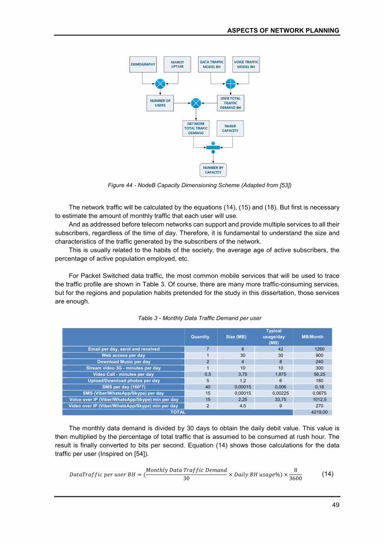
ASPECTS OF NETWORK PLANNING
49
Figure 44 - NodeB Capacity Dimensioning Scheme (Adapted from [53])
The network traffic will be calculated by the equations (14), (15) and (18). But first is necessary
to estimate the amount of monthly traffic that each user will use.
And as addressed before telecom networks can support and provide multiple services to all their
subscribers, regardless of the time of day. Therefore, it is fundamental to understand the size and
characteristics of the traffic generated by the subscribers of the network.
This is usually related to the habits of the society, the average age of active subscribers, the
percentage of active population employed, etc.
For Packet Switched data traffic, the most common mobile services that will be used to trace
the traffic profile are shown in Table 3. Of course, there are many more traffic-consuming services,
but for the regions and population habits pretended for the study in this dissertation, those services
are enough.
Table 3 - Monthly Data Traffic Demand per user
Quantity Size (MB)
Typical
usage/day
(MB)
MB/Month
Email per day, send and received 7 6 42 1260
Web access per day 1 30 30 900
Download Music per day 2 4 8 240
Stream video 3G - minutes per day 1 10 10 300
Video Call - minutes per day 0,5 3,75 1,875 56,25
Upload/Download photos per day 5 1,2 6 180
SMS per day (160*7) 40 0,00015 0,006 0,18
SMS (Viber/WhatsApp/Skype) per day 15 0,00015 0,00225 0,0675
Voice over IP (Viber/WhatsApp/Skype) min per day 15 2,25 33,75 1012,5
Video over IP (Viber/WhatsApp/Skype) min per day 2 4,5 9 270
TOTAL 4219,00
The monthly data demand is divided by 30 days to obtain the daily debit value. This value is
then multiplied by the percentage of total traffic that is assumed to be consumed at rush hour. The
result is finally converted to bits per second. Equation (14) shows those calculations for the data
traffic per user (Inspired on [54]).
�������������������� = (����ℎ�������������������
30× ������������%)×
8
3600 (14)
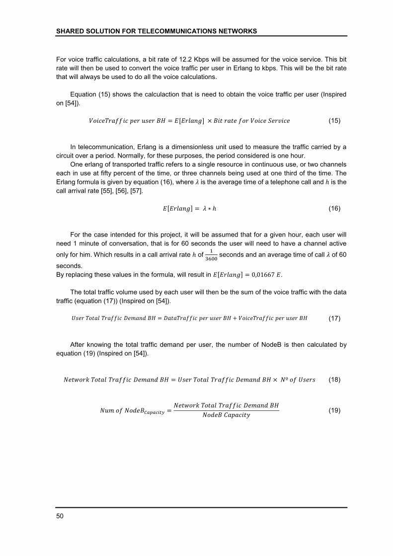
SHARED SOLUTION FOR TELECOMMUNICATIONS NETWORKS
50
For voice traffic calculations, a bit rate of 12.2 Kbps will be assumed for the voice service. This bit
rate will then be used to convert the voice traffic per user in Erlang to kbps. This will be the bit rate
that will always be used to do all the voice calculations.
Equation (15) shows the calculaction that is need to obtain the voice traffic per user (Inspired
on [54]).
��������������������� = �[������]× ���������������������� (15)
In telecommunication, Erlang is a dimensionless unit used to measure the traffic carried by a
circuit over a period. Normally, for these purposes, the period considered is one hour.
One erlang of transported traffic refers to a single resource in continuous use, or two channels
each in use at fifty percent of the time, or three channels being used at one third of the time. The
Erlang formula is given by equation (16), where � is the average time of a telephone call and ℎ is the
call arrival rate [55], [56], [57].
�[������] = � ∗ ℎ (16)
For the case intended for this project, it will be assumed that for a given hour, each user will
need 1 minute of conversation, that is for 60 seconds the user will need to have a channel active
only for him. Which results in a call arrival rate ℎ of �
���� seconds and an average time of call � of 60
seconds.
By replacing these values in the formula, will result in �[������] = 0,01667�.
The total traffic volume used by each user will then be the sum of the voice traffic with the data
traffic (equation (17)) (Inspired on [54]).
������������������������ = �������������������� + ��������������������� (17)
After knowing the total traffic demand per user, the number of NodeB is then calculated by
equation (19) (Inspired on [54]).
��������������������������� = ������������������������ × �º������� (18)
������������������ =���������������������������
������������� (19)
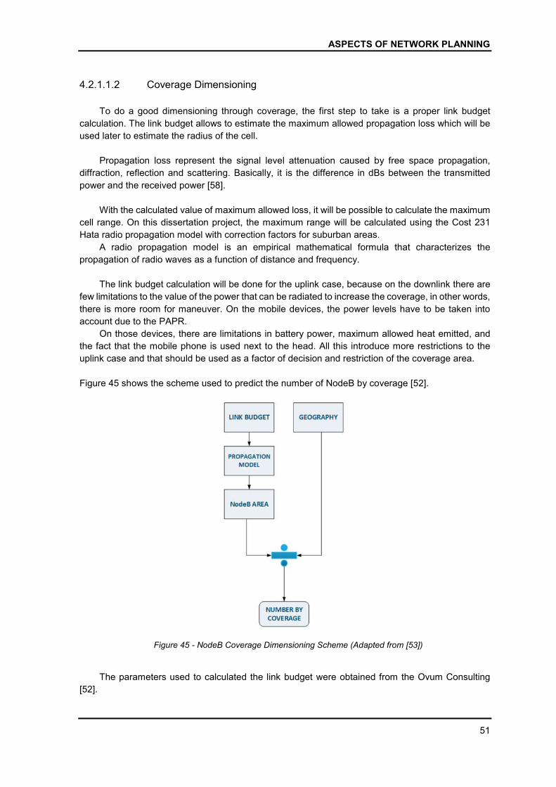
ASPECTS OF NETWORK PLANNING
51
4.2.1.1.2 Coverage Dimensioning
To do a good dimensioning through coverage, the first step to take is a proper link budget
calculation. The link budget allows to estimate the maximum allowed propagation loss which will be
used later to estimate the radius of the cell.
Propagation loss represent the signal level attenuation caused by free space propagation,
diffraction, reflection and scattering. Basically, it is the difference in dBs between the transmitted
power and the received power [58].
With the calculated value of maximum allowed loss, it will be possible to calculate the maximum
cell range. On this dissertation project, the maximum range will be calculated using the Cost 231
Hata radio propagation model with correction factors for suburban areas.
A radio propagation model is an empirical mathematical formula that characterizes the
propagation of radio waves as a function of distance and frequency.
The link budget calculation will be done for the uplink case, because on the downlink there are
few limitations to the value of the power that can be radiated to increase the coverage, in other words,
there is more room for maneuver. On the mobile devices, the power levels have to be taken into
account due to the PAPR.
On those devices, there are limitations in battery power, maximum allowed heat emitted, and
the fact that the mobile phone is used next to the head. All this introduce more restrictions to the
uplink case and that should be used as a factor of decision and restriction of the coverage area.
Figure 45 shows the scheme used to predict the number of NodeB by coverage [52].
Figure 45 - NodeB Coverage Dimensioning Scheme (Adapted from [53])
The parameters used to calculated the link budget were obtained from the Ovum Consulting
[52].
SHARED SOLUTION FOR TELECOMMUNICATIONS NETWORKS
52
First it will be necessary to calculate the power characteristics in the transmitter and the receiver.
Then, through those power characteristics calculate the allowed propagation loss.
Transmitter Power (Mobile Device)
3GPP defines 4 classes with the maximun transmission power and the tolerance values allowed
for mobile devices [52], [59].
o Power Class 1: 33 dBm (2W), +1/-3 dB;
o Power Class 2: 27 dBm (0,5W), +1/-3 dB;
o Power Class 3: 24 dBm (0,25W), +1/-3 dB;
o Power Class 4: 21 dBm (0,125W), +2/-2 dB.
As the antenna of a mobile phone usually radiates in all the diretions, will be treated like an
isotropic antenna. Therefore, its effective radiated power or, for this case, the effective isotropic
radiated power (EIRP) will define the maximum emitted power.
According to the chosen power class, that can be obtained from a mobile phone, the effective
isotropic radiated power (EIRP) can be calculated as following [52]:
����(���)= ��(���)+ ���������(���)− ��(��) (20)
With:
o ��(���) = Power transmitted;
o ���������(���) = Antenna gain;
o ��(��) = Body loss.
The gain of the antenna in a mobile device depends mainly on the size and the intended use of
the device. In a typical telephone, particularly used for voice, the antenna gain is assumed to be 0
dBi. But as nowadays mobile phones are heavily used for applications that consume a significant
amount of data, they may have antennas with gain of 2 dBi [52].
The body loss parameter is introduced due to the use of mobile device close to the user's body.
It represents the additional loss in transmission and reception due to the presence of the body. For
voice applications, the typical values are on average 2 to 3 dB and 0 dB for data [52].
Receiver (Base Station)
o Power rating
Compared to mobile phones, the base station is mainly limited by thermal noise. The
thermal noise density (��) normalized at 1 Hz is -174 dBm / Hz. This noise level is further limited
due to quality of the internal components of the receiver, such as the Low Noise Amplifiers,
filters, etc. All this still generates an amount of additive noise. This extra noise is defined as
receiver noise figure(�) and has typical values of 5 dB [52].
The total noise power at the receiver is limited by its filter bandwidth. For UMTS, the
bandwidth of the chip-compatible filter is equal to the frequency band used by the coding code,
which is approximately 3.84 MHz. Due to the spectral side lobes, results in a 5MHz carrier [52].
The total receiver noise power in dBm is calculated by equation (21):

ASPECTS OF NETWORK PLANNING
53
��(���) = �� ����
��� + �(��)+ 10 ∗ ���(3.84 ∗ 10�) (21)
o Base station Antenna Gain (���������(���)) depend on the antenna beam angle.
o Cable Loss (��(��)) on a base station is typically about 3 dB, it results from the
influence the overall cable system [52].
o Sensitivity
The sensitivity of the receiver can be quantized by considering the following factors:
Margin of interference (�), which is nothing more than a function of the cell
loading. The more load is allowed on a cell, more interference margin will be
required to ensure a good frequency separation. What will therefore result in a
decrease of the covered area. Thus, it is clear that there is a relationship between
the area to be covered and the loading capacity of the cell.
For the case intended for this dissertation, the priority will be given to the
coverage, so, the typical values for the interference margin in the coverage limited
cases are between 1.0 to 3.0 dB, corresponding to 20-50% loading [52].
Processing Gain (��) (equation (22)) is defined as the ratio between the chip
rate, approximately 3.84 MHz, and the user data rate �� [52].
��(��) = 10 ∗ log �3.84 ∗ 10�
��
� (22)
Signal to Noise Ratio (���) typical values for different services with 10-20 ms
interleaving and BLER=10% are presented in Table 4 for uplink. The table was
taken from the Ovum Consulting report [52].
Table 4 - Summary of Uplink SNR [52]
Voice 12.2
kbps
Data 64
Kbps
Data 144
Kbps
Data 384
Kbps
Static 2.9 dB 1.0 dB 0.4 dB 0.6 dB
Multipath 3
km/h 4.2 dB 2.2 dB 1.7 dB 2.0 dB
Multipath 120
km/h 5.5 dB 3.4 dB 2.9 dB 3.4 dB
The sensitivity of the receiver will then be given by equation (23):
��(���)= ���(��)+ ��(���)+ �(��)− ��(��) (23)
SHARED SOLUTION FOR TELECOMMUNICATIONS NETWORKS
54
Maximum Path Loss
After quantifying the above variables, it is possible to estimate the maximum path loss through
the equation below [52]:
���ℎ����(��) = ����(���)− ��(���)+ ���������(���)− ��(��)− ���(��) (24)
Where:
o ����(���) = Mobile device equivalent isotropic radiated power;
o ��(���) = Receiver Sensitivity;
o ���������(���) = Receiver antenna gain, which is the gain of the antennas on the base
station;
o ��(��) = Cable Loss;
o ���(��) = Fast Fading margin, needed to maintain the adequate closed-loop fast
power control in unfavorable propagation conditions such as near the cell edge. The
fast fading margin depends on the mobile speed and its typical value are 4 to 5 dB for
a 3 km/h speed, 1 to 2 dB for 50 km/h speeds and marginal values like 0,1 dB for speed
up to 120 km/h [52].
Allowed Propagation Loss
The final assembly of the above variables plus a few other aspects, presented on equation (25),
will provide the value of the allowed propagation loss [52].
�(��) = ���ℎ����(��)− ���(��)+ ������(��)− ������(��)− ����(��) (25)
The remain variables, presented in the equation above, are:
o Soft handover gain (������(��)), which occurs when a mobile is connected to at least
two cell at a time, situation that happens at the edges of the cells;
o Inference due the co-location with the GSM 900 MHz (����(��)) network;
o Other loss (������(��)), usuallly indoor losses, with typical values of 15 dB, and in-car
losses 8 dB;
o Log-normal fading margin (���(��)), usually 10 to 20 dB for indoor, and 6 to 8 for
outdoor [52].
After obtaining the value of the maximum propagation of path loss, the range can then be
estimated. The following equations correspond to the Cost 231 Hata radio propagation model to the
900 MHz frequency band [60], [61].
For urban environments, the equation for the propagation model is [61]:
�(��)����� = 69,55 + 26,16 log(�)− 13,82 log(ℎ�)+ [44,9 − 6,55 log(ℎ�)] log(�)− �(ℎ�) (26)
ASPECTS OF NETWORK PLANNING
55
Where:
�(ℎ�)= [1,1���(�)− 0,7]ℎ� − [1,56 log(�)− 0,8] (27)
The variables used are:
o ℎ� the base station antenna height in meters;
o ℎ� the user equipment antenna height in meters;
o � the user frequency in MHz;
o R the distance between base station and the user equipment (NodeB range).
For typical values like ℎ� = 30�, ℎ� = 1,5� and � = 920��� the equation (26) can be simplified
to [61]:
�(��)����� = 35,2 log(�)+ 126,6 (28)
For suburban environments [61]:
�(��)�������� = �(�)����� − 2���� ��
28� − 5,4 (29)
For� = 920��� the suburban propagation will be [61]:
�(��)�������� = 35,2 log(�)+ 116,6 (30)
For rural environments [61]:
�(��)����� = �(��)����� − 4,78����(�)+ 18,33 log(�)− 40,94 (31)
Therefore for 920 MHz, the equation (31) can be simplified to [61]:
�(��)����� = 35,2 log(�)+ 98 (32)
Since the intended case for the project are the suburban areas, the equation to be used is the
(30). The resulting NodeB range R (km) is then used to estimate the site area. For a three sector
NodeB the equation for the area is the following [52]:
��������� = 9√3
8�� (33)
Finally, the number of NodeBs by coverage is calculated by the equation (34):
������������������ = ������������
��������� (34)
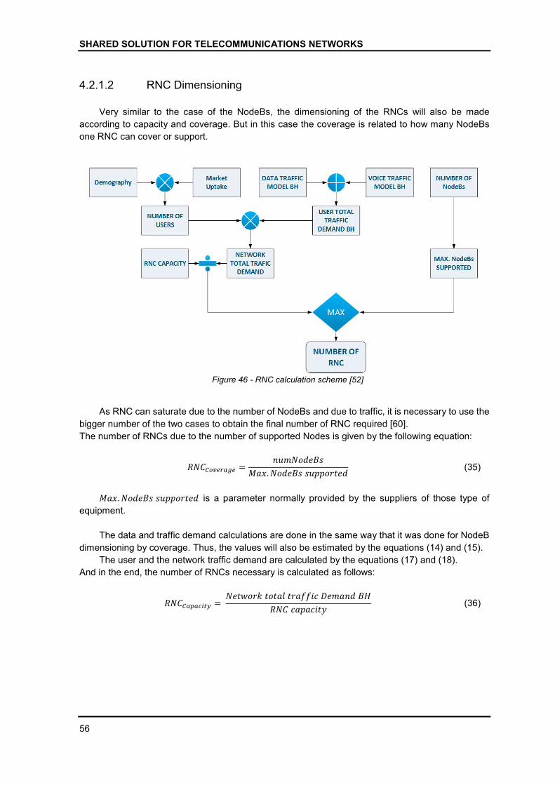
SHARED SOLUTION FOR TELECOMMUNICATIONS NETWORKS
56
4.2.1.2 RNC Dimensioning
Very similar to the case of the NodeBs, the dimensioning of the RNCs will also be made
according to capacity and coverage. But in this case the coverage is related to how many NodeBs
one RNC can cover or support.
Figure 46 - RNC calculation scheme [52]
As RNC can saturate due to the number of NodeBs and due to traffic, it is necessary to use the
bigger number of the two cases to obtain the final number of RNC required [60].
The number of RNCs due to the number of supported Nodes is given by the following equation:
����������� =���������
���. ��������������� (35)
���.��������������� is a parameter normally provided by the suppliers of those type of
equipment.
The data and traffic demand calculations are done in the same way that it was done for NodeB
dimensioning by coverage. Thus, the values will also be estimated by the equations (14) and (15).
The user and the network traffic demand are calculated by the equations (17) and (18).
And in the end, the number of RNCs necessary is calculated as follows:
����������� = ���������������������������
����������� (36)
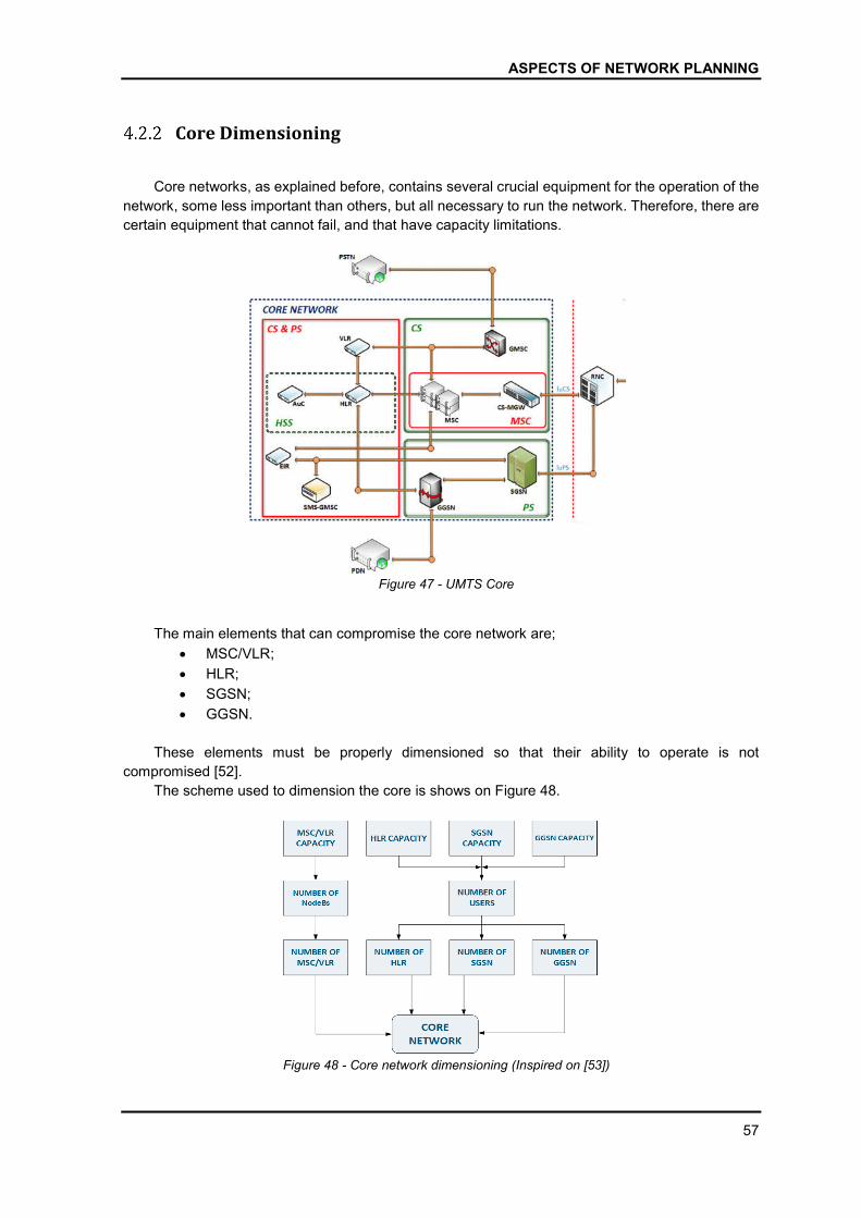
ASPECTS OF NETWORK PLANNING
57
Core Dimensioning
Core networks, as explained before, contains several crucial equipment for the operation of the
network, some less important than others, but all necessary to run the network. Therefore, there are
certain equipment that cannot fail, and that have capacity limitations.
Figure 47 - UMTS Core
The main elements that can compromise the core network are;
MSC/VLR;
HLR;
SGSN;
GGSN.
These elements must be properly dimensioned so that their ability to operate is not
compromised [52].
The scheme used to dimension the core is shows on Figure 48.
Figure 48 - Core network dimensioning (Inspired on [53])
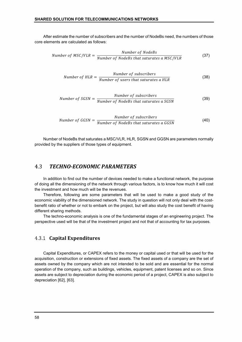
SHARED SOLUTION FOR TELECOMMUNICATIONS NETWORKS
58
After estimate the number of subscribers and the number of NodeBs need, the numbers of those
core elements are calculated as follows:
�����������/��� = ��������������
���������������ℎ���������������/��� (37)
����������� = �������������������
��������������ℎ��������������� (38)
������������ = �������������������
���������������ℎ���������������� (39)
������������ = �������������������
���������������ℎ���������������� (40)
Number of NodeBs that saturates a MSC/VLR, HLR, SGSN and GGSN are parameters normally
provided by the suppliers of those types of equipment.
TECHNO-ECONOMIC PARAMETERS
In addition to find out the number of devices needed to make a functional network, the purpose
of doing all the dimensioning of the network through various factors, is to know how much it will cost
the investment and how much will be the revenues.
Therefore, following are some parameters that will be used to make a good study of the
economic viability of the dimensioned network. The study in question will not only deal with the cost-
benefit ratio of whether or not to embark on the project, but will also study the cost benefit of having
different sharing methods.
The techno-economic analysis is one of the fundamental stages of an engineering project. The
perspective used will be that of the investment project and not that of accounting for tax purposes.
Capital Expenditures
Capital Expenditures, or CAPEX refers to the money or capital used or that will be used for the
acquisition, construction or extensions of fixed assets. The fixed assets of a company are the set of
assets owned by the company which are not intended to be sold and are essential for the normal
operation of the company, such as buildings, vehicles, equipment, patent licenses and so on. Since
assets are subject to depreciation during the economic period of a project, CAPEX is also subject to
depreciation [62], [63].
ASPECTS OF NETWORK PLANNING
59
Operational Expenditures
Operating Expenses or OPEX refers to all expenses necessary for the normal operation of a
company or business. OPEX costs may include maintenance of equipment, communication, energy,
marketing, service management, financial operations, etc. OPEX are not depreciated over time [62],
[64].
Cash Flow
Cash Flow (equation (41)) refers to the amount of money that goes in and out of a business.
This includes profits, i.e. capital inflow, and expenses, capital outflow. Generally, the cash flow of an
investment project is calculated annually.
In addition to cash flow, there is also the cash balance (equation (42)), which in the end is simply
the sum of cash flows up to a specific time [65], [66].
���ℎ����� = ��� = ��� − ��� (41)
Cash flow in year t is defined as the sum of all revenues in year t, ��, subtracted by the sum of
all expenses in year t, ��.
���ℎ�������� = ����
�
���
(42)
T corresponds to the total period of the project. When the cash inflow exceeds the cash outflow,
this is usually an indicator of good financial health
Revenues
Revenue is the amount of money a company receives for their business activities for a specific
period. The activities are usually sales or rental of products or services.
Revenue is basically calculated by multiplying the price at which goods or services are sold or
rented, by the number of units sold or rented.
Revenue alone does not provide a complete picture of a company's finances, it needs to take
into account the expenses. The revenue must be analyzed in relation to the expenses to provide a
significant look at the progress and profit of a company or business [67].
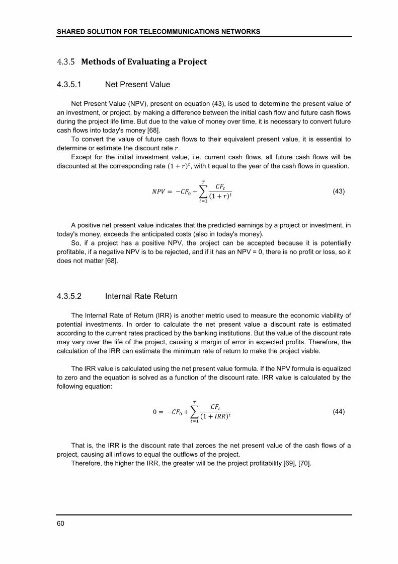
SHARED SOLUTION FOR TELECOMMUNICATIONS NETWORKS
60
Methods of Evaluating a Project
4.3.5.1 Net Present Value
Net Present Value (NPV), present on equation (43), is used to determine the present value of
an investment, or project, by making a difference between the initial cash flow and future cash flows
during the project life time. But due to the value of money over time, it is necessary to convert future
cash flows into today's money [68].
To convert the value of future cash flows to their equivalent present value, it is essential to
determine or estimate the discount rate �.
Except for the initial investment value, i.e. current cash flows, all future cash flows will be
discounted at the corresponding rate (1 + �)�, with t equal to the year of the cash flows in question.
��� = − ��� + ����
(1 + �)�
�
���
(43)
A positive net present value indicates that the predicted earnings by a project or investment, in
today's money, exceeds the anticipated costs (also in today's money).
So, if a project has a positive NPV, the project can be accepted because it is potentially
profitable, if a negative NPV is to be rejected, and if it has an NPV = 0, there is no profit or loss, so it
does not matter [68].
4.3.5.2 Internal Rate Return
The Internal Rate of Return (IRR) is another metric used to measure the economic viability of
potential investments. In order to calculate the net present value a discount rate is estimated
according to the current rates practiced by the banking institutions. But the value of the discount rate
may vary over the life of the project, causing a margin of error in expected profits. Therefore, the
calculation of the IRR can estimate the minimum rate of return to make the project viable.
The IRR value is calculated using the net present value formula. If the NPV formula is equalized
to zero and the equation is solved as a function of the discount rate. IRR value is calculated by the
following equation:
0 = − ��� + ����
(1 + ���)�
�
���
(44)
That is, the IRR is the discount rate that zeroes the net present value of the cash flows of a
project, causing all inflows to equal the outflows of the project.
Therefore, the higher the IRR, the greater will be the project profitability [69], [70].

ASPECTS OF NETWORK PLANNING
61
4.3.5.3 Payback Period
Payback period is the period of time that the invested project takes to recover the investment.
That is, the period of time it will take until the cash flows go from negative to positive (including
the initial cash flow).
Payback period is an important determinant before assuming the project, since longer payback
periods are usually not desirable for investment positions. But it is not advisable to use the payback
period alone as a decision factor when taking an investment, since this metric ignores the time value
of money, unlike the other methods [71].

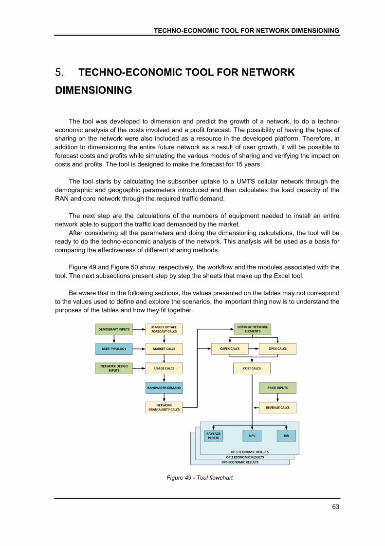
TECHNO-ECONOMIC TOOL FOR NETWORK DIMENSIONING
63
TECHNO-ECONOMIC TOOL FOR NETWORK
DIMENSIONING
The tool was developed to dimension and predict the growth of a network, to do a techno-
economic analysis of the costs involved and a profit forecast. The possibility of having the types of
sharing on the network were also included as a resource in the developed platform. Therefore, in
addition to dimensioning the entire future network as a result of user growth, it will be possible to
forecast costs and profits while simulating the various modes of sharing and verifying the impact on
costs and profits. The tool is designed to make the forecast for 15 years.
The tool starts by calculating the subscriber uptake to a UMTS cellular network through the
demographic and geographic parameters introduced and then calculates the load capacity of the
RAN and core network through the required traffic demand.
The next step are the calculations of the numbers of equipment needed to install an entire
network able to support the traffic load demanded by the market.
After considering all the parameters and doing the dimensioning calculations, the tool will be
ready to do the techno-economic analysis of the network. This analysis will be used as a basis for
comparing the effectiveness of different sharing methods.
Figure 49 and Figure 50 show, respectively, the workflow and the modules associated with the
tool. The next subsections present step by step the sheets that make up the Excel tool.
Be aware that in the following sections, the values presented on the tables may not correspond
to the values used to define and explore the scenarios, the important thing now is to understand the
purposes of the tables and how they fit together.
Figure 49 - Tool flowchart

SHARED SOLUTION FOR TELECOMMUNICATIONS NETWORKS
64
Figure 50 - Tool Modules
INPUT PARAMETERS
In order for the tool to fulfill its purpose some parameters will have to be defined and introduced.
Parameters such as the number of subscribers, typology of subscribers, region area, expected price
paid by subscribers, type of terrain, technological factors and so on, influence the outcome of the
project. So, it is important that they are as faithful as possible to the scenario intended to simulate.
The subscribers are subdivided in 3 main categories:
Institutional;
Business;
Private.
Business subscribers are defined as public and private companies. Institutional subscribers as
the various health centers, courts, hospitals, libraries, schools, universities, among others. And
finally, private subscribers include individuals.
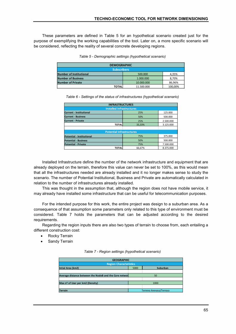
TECHNO-ECONOMIC TOOL FOR NETWORK DIMENSIONING
65
These parameters are defined in Table 5 for an hypothetical scenario created just for the
purpose of exemplifying the working capabilities of the tool. Later on, a more specific scenario will
be considered, reflecting the reality of several concrete developing regions.
Table 5 - Demographic settings (hypothetical scenario)
Table 6 - Settings of the status of infrastructures (hypothetical scenario)
Installed Infrastructure define the number of the network infrastructure and equipment that are
already deployed on the terrain, therefore this value can never be set to 100%, as this would mean
that all the infrastructures needed are already installed and it no longer makes sense to study the
scenario. The number of Potential Institutional, Business and Private are automatically calculated in
relation to the number of infrastructures already installed.
This was thought in the assumption that, although the region does not have mobile service, it
may already have installed some infrastructure that can be useful for telecommunication purposes.
For the intended purpose for this work, the entire project was design to a suburban area. As a
consequence of that assumption some parameters only related to this type of environment must be
considered. Table 7 holds the parameters that can be adjusted according to the desired
requirements.
Regarding the region inputs there are also two types of terrain to choose from, each entailing a
different construction cost:
Rocky Terrain
Sandy Terrain
Table 7 - Region settings (hypothetical scenario)
Number of Institutional 500.000 4,35%
Number of Business 1.000.000 8,70%
Number of Private 10.000.000 86,96%
TOTAL 11.500.000 100,00%
DEMOGRAPHIC
Subscribers
Current - Institutional 25% 125.000
Current - Business 50% 500.000
Current - Private 25% 2.500.000
TOTAL 33,33% 3.125.000
Potential - Institutional 75% 375.000
Potential - Business 50% 500.000
Potential - Private 75% 7.500.000
TOTAL 66,67% 8.375.000
INFRASTRUCTURES
Potential Infrastructures
Installed Infrastructures
Intial Area (km2) 5000 Suburban
Average distance between the NodeB and the Core network
Max nº of User per km2 (Density)
Terrain Terreno Arenoso/Terroso
1000
GEOGRAPHIC
Region Characteristics
50
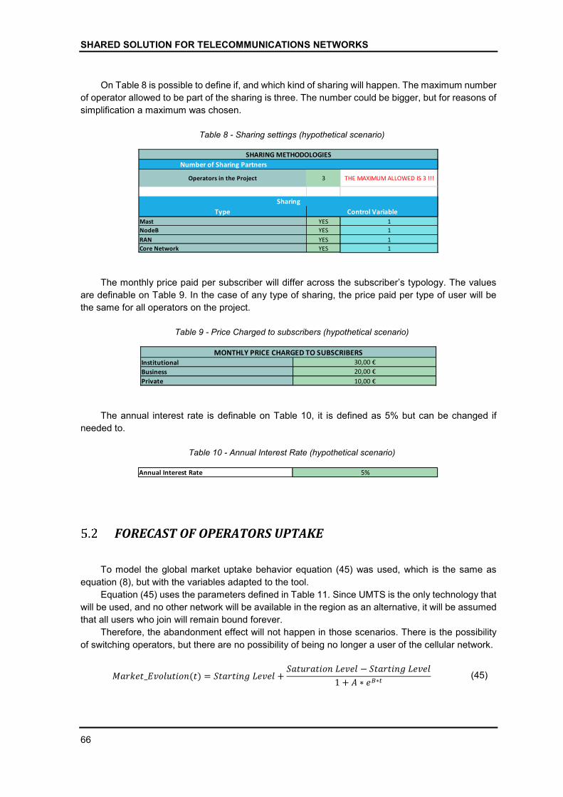
SHARED SOLUTION FOR TELECOMMUNICATIONS NETWORKS
66
On Table 8 is possible to define if, and which kind of sharing will happen. The maximum number
of operator allowed to be part of the sharing is three. The number could be bigger, but for reasons of
simplification a maximum was chosen.
Table 8 - Sharing settings (hypothetical scenario)
The monthly price paid per subscriber will differ across the subscriber’s typology. The values
are definable on Table 9. In the case of any type of sharing, the price paid per type of user will be
the same for all operators on the project.
Table 9 - Price Charged to subscribers (hypothetical scenario)
The annual interest rate is definable on Table 10, it is defined as 5% but can be changed if
needed to.
Table 10 - Annual Interest Rate (hypothetical scenario)
FORECAST OF OPERATORS UPTAKE
To model the global market uptake behavior equation (45) was used, which is the same as
equation (8), but with the variables adapted to the tool.
Equation (45) uses the parameters defined in Table 11. Since UMTS is the only technology that
will be used, and no other network will be available in the region as an alternative, it will be assumed
that all users who join will remain bound forever.
Therefore, the abandonment effect will not happen in those scenarios. There is the possibility
of switching operators, but there are no possibility of being no longer a user of the cellular network.
������_���������(�) = ������������� +��������������� − �������������
1 + � ∗ ��∗� (45)
Number of Sharing Partners
Type
Mast YES 1
NodeB YES 1
RAN YES 1
Core Network YES 1
Control Variable
Operators in the Project 3 THE MAXIMUM ALLOWED IS 3 !!!
Sharing
SHARING METHODOLOGIES
Institutional
Business
Private
20,00 €
10,00 €
MONTHLY PRICE CHARGED TO SUBSCRIBERS30,00 €
Annual Interest Rate 5%
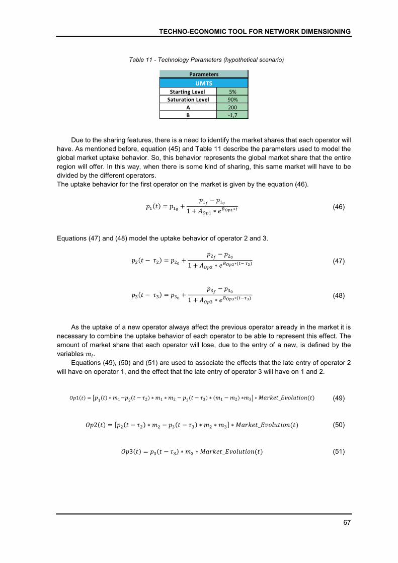
TECHNO-ECONOMIC TOOL FOR NETWORK DIMENSIONING
67
Table 11 - Technology Parameters (hypothetical scenario)
Due to the sharing features, there is a need to identify the market shares that each operator will
have. As mentioned before, equation (45) and Table 11 describe the parameters used to model the
global market uptake behavior. So, this behavior represents the global market share that the entire
region will offer. In this way, when there is some kind of sharing, this same market will have to be
divided by the different operators.
The uptake behavior for the first operator on the market is given by the equation (46).
��(�) = ���+
���− ���
1 + ���� ∗ �����∗� (46)
Equations (47) and (48) model the uptake behavior of operator 2 and 3.
��(� − ��) = ���+
���− ���
1 + ���� ∗ �����∗(����) (47)
��(� − ��) = ���+
���− ���
1 + ���� ∗ �����∗(����) (48)
As the uptake of a new operator always affect the previous operator already in the market it is
necessary to combine the uptake behavior of each operator to be able to represent this effect. The
amount of market share that each operator will lose, due to the entry of a new, is defined by the
variables ��.
Equations (49), (50) and (51) are used to associate the effects that the late entry of operator 2
will have on operator 1, and the effect that the late entry of operator 3 will have on 1 and 2.
��1(�) = ��1
(�)∗�1− �2(� − �2)∗�1 ∗�2 − �3
(� − �3)∗ (�1 − �2)∗�3� ∗������_���������(�) (49)
��2(�) = [��(� − ��)∗�� − ��(� − ��)∗�� ∗��] ∗������_���������(�) (50)
��3(�) = ��(� − ��)∗�� ∗������_���������(�) (51)
5%
90%
200
-1,7
Saturation Level
A
B
Parameters
UMTSStarting Level
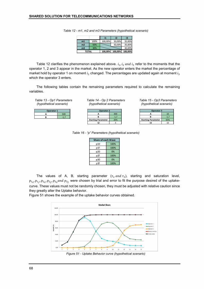
SHARED SOLUTION FOR TELECOMMUNICATIONS NETWORKS
68
Table 12 - m1, m2 and m3 Parameters (hypothetical scenario)
Table 12 clarifies the phenomenon explained above. ��, ������� refer to the moments that the
operator 1, 2 and 3 appear in the market. As the new operator enters the market the percentage of
market hold by operator 1 on moment �� changed. The percentages are updated again at moment ��
which the operator 3 enters.
The following tables contain the remaining parameters required to calculate the remaining
variables.
Table 13 - Op1 Parameters
(hypothetical scenario)
Table 14 - Op 2 Parameters (hypothetical scenario)
Table 15 - Op3 Parameters (hypothetical scenario)
Table 16 - “p” Parameters (hypothetical scenario)
The values of A, B, starting parameter (�������), starting and saturation level,
���, ���
, ���, ���
, ���������
were chosen by trial and error to fit the purpose desired of the uptake-
curve. These values must not be randomly chosen, they must be adjusted with relative caution since
they greatly alter the Uptake behavior.
Figure 51 shows the example of the uptake behavior curves obtained.
Figure 51 - Uptake Behavior curve (hypothetical scenario)
i1 i2 i3
m1 100% 100,00% 50,00% 35,00%
m2 50% 50,00% 35,00%
m3 30% 30,00%
100,00% 100,00% 100,00%TOTAL
500
-1,7
Operator 1
A
B
300
-1,7
20%
3
A
Operator 2
B
Starting Parameter
τ2
10
-1,7
65%
10
B
Starting Parameter
τ3
Operator 3
A
p10 100%
p1f 100%
p20 0%
p2f 100%
p30 0%
p3f 100%
Share of each Wave
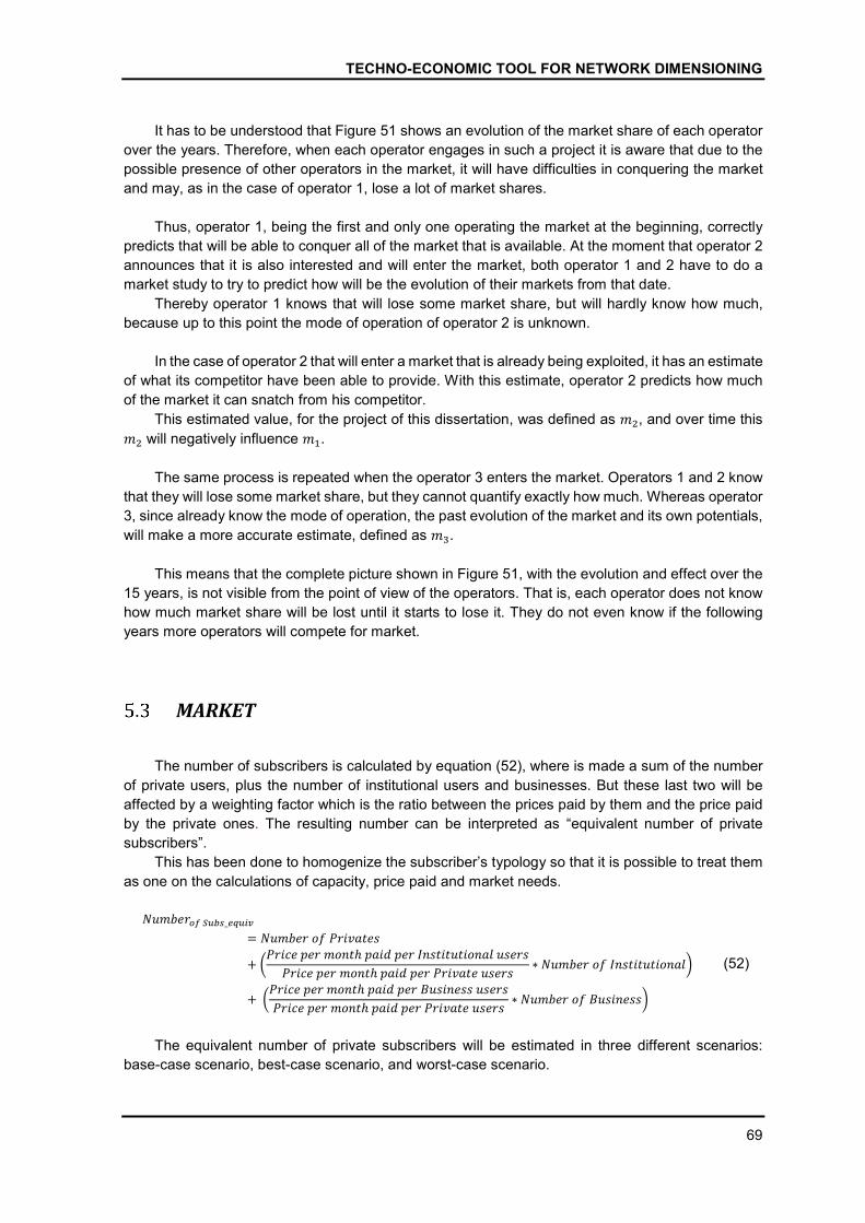
TECHNO-ECONOMIC TOOL FOR NETWORK DIMENSIONING
69
It has to be understood that Figure 51 shows an evolution of the market share of each operator
over the years. Therefore, when each operator engages in such a project it is aware that due to the
possible presence of other operators in the market, it will have difficulties in conquering the market
and may, as in the case of operator 1, lose a lot of market shares.
Thus, operator 1, being the first and only one operating the market at the beginning, correctly
predicts that will be able to conquer all of the market that is available. At the moment that operator 2
announces that it is also interested and will enter the market, both operator 1 and 2 have to do a
market study to try to predict how will be the evolution of their markets from that date.
Thereby operator 1 knows that will lose some market share, but will hardly know how much,
because up to this point the mode of operation of operator 2 is unknown.
In the case of operator 2 that will enter a market that is already being exploited, it has an estimate
of what its competitor have been able to provide. With this estimate, operator 2 predicts how much
of the market it can snatch from his competitor.
This estimated value, for the project of this dissertation, was defined as ��, and over time this
�� will negatively influence ��.
The same process is repeated when the operator 3 enters the market. Operators 1 and 2 know
that they will lose some market share, but they cannot quantify exactly how much. Whereas operator
3, since already know the mode of operation, the past evolution of the market and its own potentials,
will make a more accurate estimate, defined as ��.
This means that the complete picture shown in Figure 51, with the evolution and effect over the
15 years, is not visible from the point of view of the operators. That is, each operator does not know
how much market share will be lost until it starts to lose it. They do not even know if the following
years more operators will compete for market.
MARKET
The number of subscribers is calculated by equation (52), where is made a sum of the number
of private users, plus the number of institutional users and businesses. But these last two will be
affected by a weighting factor which is the ratio between the prices paid by them and the price paid
by the private ones. The resulting number can be interpreted as “equivalent number of private
subscribers”.
This has been done to homogenize the subscriber’s typology so that it is possible to treat them
as one on the calculations of capacity, price paid and market needs.
������������_�����
= ����������������
+ �������������ℎ�������������������������
������������ℎ�������������������∗����������������������
+ �������������ℎ��������������������
������������ℎ�������������������∗�����������������
(52)
The equivalent number of private subscribers will be estimated in three different scenarios:
base-case scenario, best-case scenario, and worst-case scenario.

SHARED SOLUTION FOR TELECOMMUNICATIONS NETWORKS
70
The base case acts as the basis for conducting a sensitivity analysis. For this project, the
sensitivity analysis investigates the impact of variations of +/- 20% relative to the base case.
Beside this, if a sharing mode is selected it will be possible to see that due to the late uptake of
operators 2 and 3 to the network and the effect of ��,�������, the number of subscribers of
operator 1 will decreases as operator 2 enters the market. The same effect happens to operators 1
and 2 when operator 3 enter the market.
NETWORK TRAFFIC DEMAND
Based on the prediction of the number of subscribers, it will be done a forecast as reliable as
possible of the network to be implemented. The RAN and the core network will be planned according
to the traffic load, and the coverage capacity.
Table 17 - Number of Sectors per NodeB (hypothetical scenario)
It is usual in a cellular network the existence of sites/NodeBs with different number of sectors
per cell. This happens normally on dense urban areas, where there is high demand of capacity. But,
for this project all NodeBs are projected to have three sectors. It will be also assumed that the
distribution of customers in each scenario is homogeneous.
NodeBs
The number of sites or NodeBs used, is, as previously referred, dimensioned in two strands,
capacity and coverage.
5.4.1.1 NodeB coverage dimensioning
The coverage area of the NodeB is calculated according to the characteristics of the region, as
explained in section 4.2.1.1.2, for the calculation of the coverage area it is necessary to calculate the
link budget.
Although the link budget for the mobile wireless is normally calculated based only on the voice
service since it is the most critical service. But on this case, it is also intended to ensure the minimum
conditions for data services. Table 18 contains all the calculations and parameters used to calculate
the budget link.
3Number of sectors per NodeB 1 NodeB per Cell
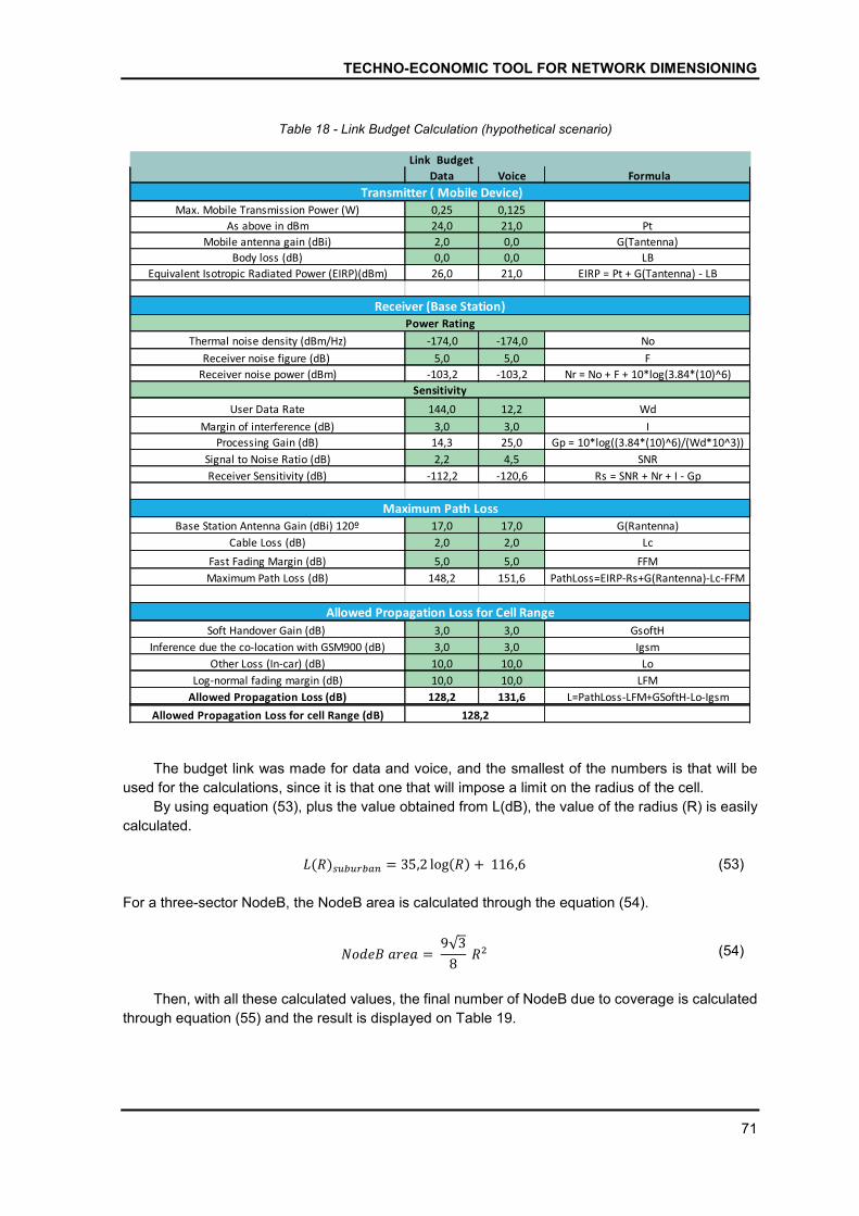
TECHNO-ECONOMIC TOOL FOR NETWORK DIMENSIONING
71
Table 18 - Link Budget Calculation (hypothetical scenario)
The budget link was made for data and voice, and the smallest of the numbers is that will be
used for the calculations, since it is that one that will impose a limit on the radius of the cell.
By using equation (53), plus the value obtained from L(dB), the value of the radius (R) is easily
calculated.
�(�)�������� = 35,2 log(�)+ 116,6 (53)
For a three-sector NodeB, the NodeB area is calculated through the equation (54).
��������� = 9√3
8�� (54)
Then, with all these calculated values, the final number of NodeB due to coverage is calculated
through equation (55) and the result is displayed on Table 19.
Data Voice
0,25 0,125
24,0 21,0
2,0 0,0
0,0 0,0
26,0 21,0
-174,0 -174,0
5,0 5,0
-103,2 -103,2
144,0 12,2
3,0 3,0
14,3 25,0
2,2 4,5
-112,2 -120,6
17,0 17,0
2,0 2,0
5,0 5,0
148,2 151,6
3,0 3,0
3,0 3,0
10,0 10,0
10,0 10,0
128,2 131,6
Power Rating
Sensitivity
Pt
G(Tantenna)
LB
EIRP = Pt + G(Tantenna) - LB
No
F
Nr = No + F + 10*log(3.84*(10)^6)
Other Loss (In-car) (dB)
Log-normal fading margin (dB)
Allowed Propagation Loss (dB)
Maximum Path Loss (dB)
Inference due the co-location with GSM900 (dB)
Allowed Propagation Loss for Cell Range
Soft Handover Gain (dB)
PathLoss=EIRP-Rs+G(Rantenna)-Lc-FFM
GsoftH
Igsm
Lo
LFM
L=PathLoss-LFM+GSoftH-Lo-Igsm
Base Station Antenna Gain (dBi) 120º
Cable Loss (dB)
Fast Fading Margin (dB)
Maximum Path LossG(Rantenna)
Lc
FFM
Transmitter ( Mobile Device)
Receiver (Base Station)
I
Gp = 10*log((3.84*(10)^6)/(Wd*10^3))
SNR
Rs = SNR + Nr + I - Gp
User Data Rate Wd
Thermal noise density (dBm/Hz)
Receiver noise figure (dB)
Receiver noise power (dBm)
Mobile antenna gain (dBi)
Body loss (dB)
Equivalent Isotropic Radiated Power (EIRP)(dBm)
Signal to Noise Ratio (dB)
Receiver Sensitivity (dB)
Link Budget
Allowed Propagation Loss for cell Range (dB)
Max. Mobile Transmission Power (W)
128,2
Margin of interference (dB)
Processing Gain (dB)
Formula
As above in dBm
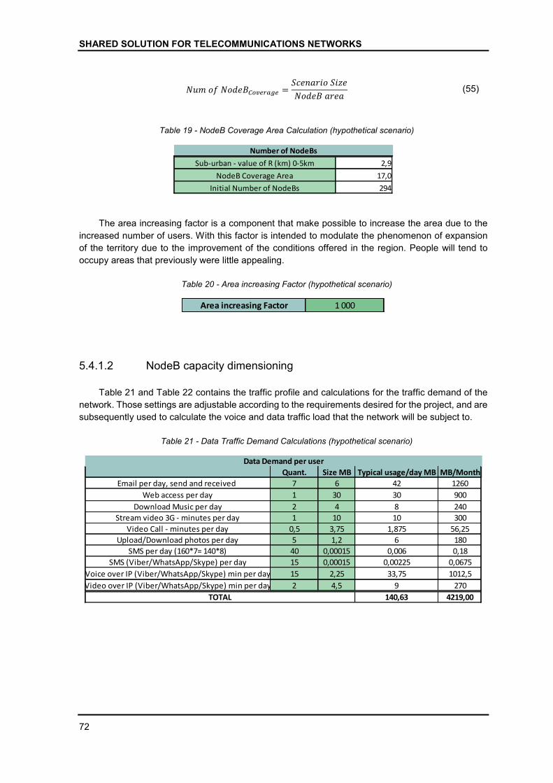
SHARED SOLUTION FOR TELECOMMUNICATIONS NETWORKS
72
������������������ =������������
��������� (55)
Table 19 - NodeB Coverage Area Calculation (hypothetical scenario)
The area increasing factor is a component that make possible to increase the area due to the
increased number of users. With this factor is intended to modulate the phenomenon of expansion
of the territory due to the improvement of the conditions offered in the region. People will tend to
occupy areas that previously were little appealing.
Table 20 - Area increasing Factor (hypothetical scenario)
5.4.1.2 NodeB capacity dimensioning
Table 21 and Table 22 contains the traffic profile and calculations for the traffic demand of the
network. Those settings are adjustable according to the requirements desired for the project, and are
subsequently used to calculate the voice and data traffic load that the network will be subject to.
Table 21 - Data Traffic Demand Calculations (hypothetical scenario)
2,9
17,0
294Initial Number of NodeBs
Sub-urban - value of R (km) 0-5km
NodeB Coverage Area
Number of NodeBs
1 000Area increasing Factor
Quant. Size MB Typical usage/day MB MB/Month
7 6 42 1260
1 30 30 900
2 4 8 240
1 10 10 300
0,5 3,75 1,875 56,25
5 1,2 6 180
40 0,00015 0,006 0,18
15 0,00015 0,00225 0,0675
15 2,25 33,75 1012,5
2 4,5 9 270
140,63 4219,00TOTAL
Upload/Download photos per day
Data Demand per user
Email per day, send and received
Web access per day
Download Music per day
Stream video 3G - minutes per day
Video Call - minutes per day
Voice over IP (Viber/WhatsApp/Skype) min per day
Video over IP (Viber/WhatsApp/Skype) min per day
SMS (Viber/WhatsApp/Skype) per day
SMS per day (160*7= 140*8)
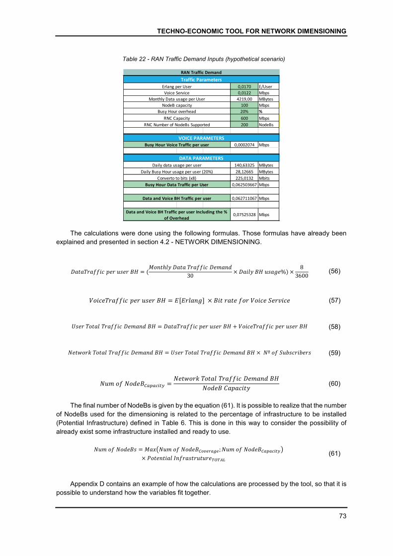
TECHNO-ECONOMIC TOOL FOR NETWORK DIMENSIONING
73
Table 22 - RAN Traffic Demand Inputs (hypothetical scenario)
The calculations were done using the following formulas. Those formulas have already been
explained and presented in section 4.2 - NETWORK DIMENSIONING.
�������������������� = (����ℎ�������������������
30× ������������%)×
8
3600 (56)
��������������������� = �[������]× ���������������������� (57)
������������������������ = �������������������� + ��������������������� (58)
��������������������������� = ������������������������ × �º������������� (59)
������������������ =���������������������������
������������� (60)
The final number of NodeBs is given by the equation (61). It is possible to realize that the number
of NodeBs used for the dimensioning is related to the percentage of infrastructure to be installed
(Potential Infrastructure) defined in Table 6. This is done in this way to consider the possibility of
already exist some infrastructure installed and ready to use.
����������� = ����������������������;�������������������
× ��������������������������� (61)
Appendix D contains an example of how the calculations are processed by the tool, so that it is
possible to understand how the variables fit together.
0,0170 E/User
0,0122 Mbps
4219,00 MBytes
100 Mbps
20% %
600 Mbps
200 NodeBs
0,0002074 Mbps
140,63325 MBytes
28,12665 MBytes
225,0132 Mbits
0,062503667 Mbps
0,062711067 Mbps
VOICE PARAMETERS
RNC Capacity
RNC Number of NodeBs Supported
Busy Hour Voice Traffic per user
Daily Busy Hour usage per user (20%)
Traffic Parameters
RAN Traffic Demand
0,07525328 MbpsData and Voice BH Traffic per user Including the %
of Overhead
Erlang per User
Voice Service
Data and Voice BH Traffic per user
DATA PARAMETERS
Converto to bits (x8)
Busy Hour Data Traffic per User
Daily data usage per user
Monthly Data usage per User
NodeB capacity
Busy Hour overhead
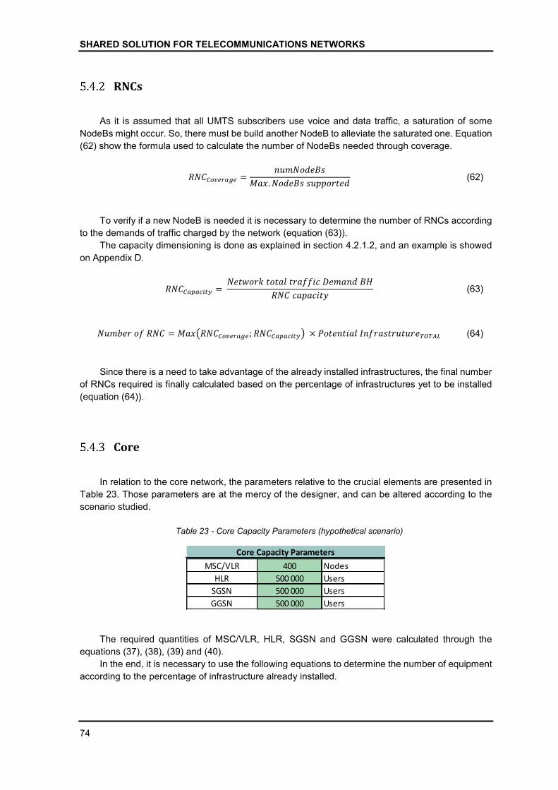
SHARED SOLUTION FOR TELECOMMUNICATIONS NETWORKS
74
RNCs
As it is assumed that all UMTS subscribers use voice and data traffic, a saturation of some
NodeBs might occur. So, there must be build another NodeB to alleviate the saturated one. Equation
(62) show the formula used to calculate the number of NodeBs needed through coverage.
����������� =���������
���. ��������������� (62)
To verify if a new NodeB is needed it is necessary to determine the number of RNCs according
to the demands of traffic charged by the network (equation (63)).
The capacity dimensioning is done as explained in section 4.2.1.2, and an example is showed
on Appendix D.
����������� = ���������������������������
����������� (63)
����������� = ���������������; ������������× ��������������������������� (64)
Since there is a need to take advantage of the already installed infrastructures, the final number
of RNCs required is finally calculated based on the percentage of infrastructures yet to be installed
(equation (64)).
Core
In relation to the core network, the parameters relative to the crucial elements are presented in
Table 23. Those parameters are at the mercy of the designer, and can be altered according to the
scenario studied.
Table 23 - Core Capacity Parameters (hypothetical scenario)
The required quantities of MSC/VLR, HLR, SGSN and GGSN were calculated through the
equations (37), (38), (39) and (40).
In the end, it is necessary to use the following equations to determine the number of equipment
according to the percentage of infrastructure already installed.
MSC/VLR 400 Nodes
HLR 500 000 Users
SGSN 500 000 Users
GGSN 500 000 Users
Core Capacity Parameters
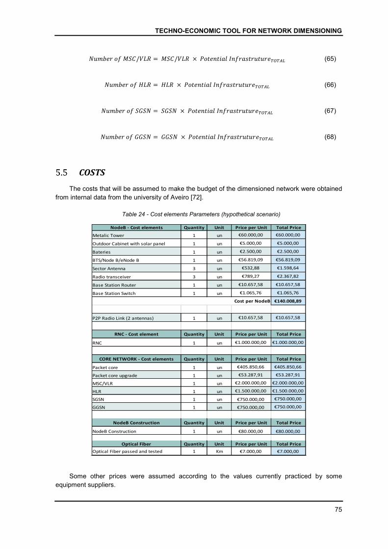
TECHNO-ECONOMIC TOOL FOR NETWORK DIMENSIONING
75
�����������/��� = ���/���× ��������������������������� (65)
����������� = ���× ��������������������������� (66)
������������ = ����× ��������������������������� (67)
������������ = ����× ��������������������������� (68)
COSTS
The costs that will be assumed to make the budget of the dimensioned network were obtained
from internal data from the university of Aveiro [72].
Table 24 - Cost elements Parameters (hypothetical scenario)
Some other prices were assumed according to the values currently practiced by some
equipment suppliers.
NodeB - Cost elements Quantity Unit Price per Unit Total Price
Metalic Tower 1 un €60.000,00 €60.000,00
Outdoor Cabinet with solar panel 1 un €5.000,00 €5.000,00
Bateries 1 un €2.500,00 €2.500,00
BTS/Node B/eNode B 1 un €56.819,09 €56.819,09
Sector Antenna 3 un €532,88 €1.598,64
Radio transceiver 3 un €789,27 €2.367,82
Base Station Router 1 un €10.657,58 €10.657,58
Base Station Switch 1 un €1.065,76 €1.065,76
€140.008,89
P2P Radio Link (2 antennas) 1 un €10.657,58 €10.657,58
RNC - Cost element Quantity Unit Price per Unit Total Price
RNC 1 un €1.000.000,00 €1.000.000,00
CORE NETWORK - Cost elements Quantity Unit Price per Unit Total Price
Packet core 1 un €405.850,66 €405.850,66
Packet core upgrade 1 un €53.287,91 €53.287,91
MSC/VLR 1 un €2.000.000,00 €2.000.000,00
HLR 1 un €1.500.000,00 €1.500.000,00
SGSN 1 un €750.000,00 €750.000,00
GGSN 1 un €750.000,00 €750.000,00
NodeB Construction Quantity Unit Price per Unit Total Price
NodeB Construction 1 un €80.000,00 €80.000,00
Optical Fiber Quantity Unit Price per Unit Total Price
Optical Fiber passed and tested 1 Km €7.000,00 €7.000,00
Cost per NodeB
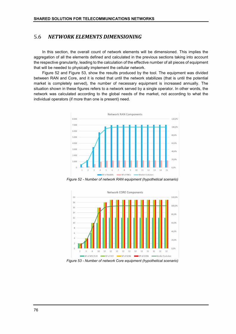
SHARED SOLUTION FOR TELECOMMUNICATIONS NETWORKS
76
NETWORK ELEMENTS DIMENSIONING
In this section, the overall count of network elements will be dimensioned. This implies the
aggregation of all the elements defined and calculated in the previous sections taking into account
the respective granularity, leading to the calculation of the effective number of all pieces of equipment
that will be needed to physically implement the cellular network.
Figure 52 and Figure 53, show the results produced by the tool. The equipment was divided
between RAN and Core, and it is noted that until the network stabilizes (that is until the potential
market is completely served), the number of necessary equipment is increased annually. The
situation shown in these figures refers to a network served by a single operator. In other words, the
network was calculated according to the global needs of the market, not according to what the
individual operators (if more than one is present) need.
Figure 52 - Number of network RAN equipment (hypothetical scenario)
Figure 53 - Number of network Core equipment (hypothetical scenario)
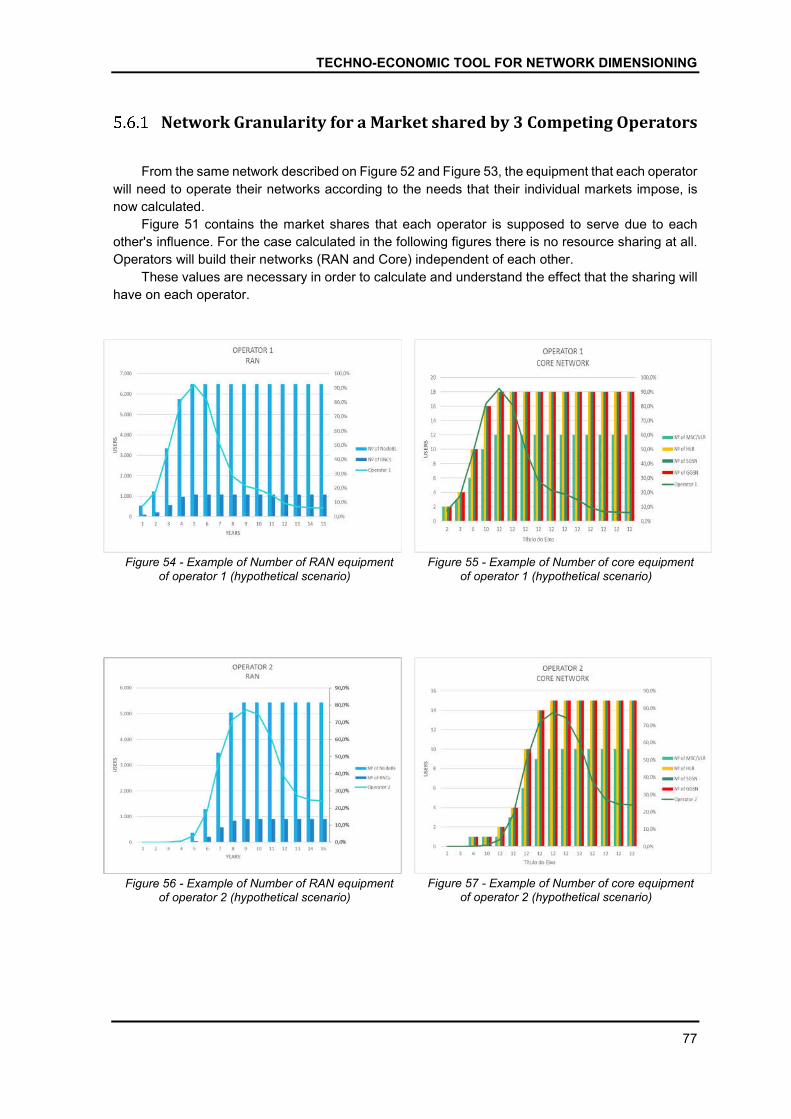
TECHNO-ECONOMIC TOOL FOR NETWORK DIMENSIONING
77
Network Granularity for a Market shared by 3 Competing Operators
From the same network described on Figure 52 and Figure 53, the equipment that each operator
will need to operate their networks according to the needs that their individual markets impose, is
now calculated.
Figure 51 contains the market shares that each operator is supposed to serve due to each
other's influence. For the case calculated in the following figures there is no resource sharing at all.
Operators will build their networks (RAN and Core) independent of each other.
These values are necessary in order to calculate and understand the effect that the sharing will
have on each operator.
Figure 54 - Example of Number of RAN equipment
of operator 1 (hypothetical scenario)
Figure 55 - Example of Number of core equipment
of operator 1 (hypothetical scenario)
Figure 56 - Example of Number of RAN equipment
of operator 2 (hypothetical scenario)
Figure 57 - Example of Number of core equipment
of operator 2 (hypothetical scenario)
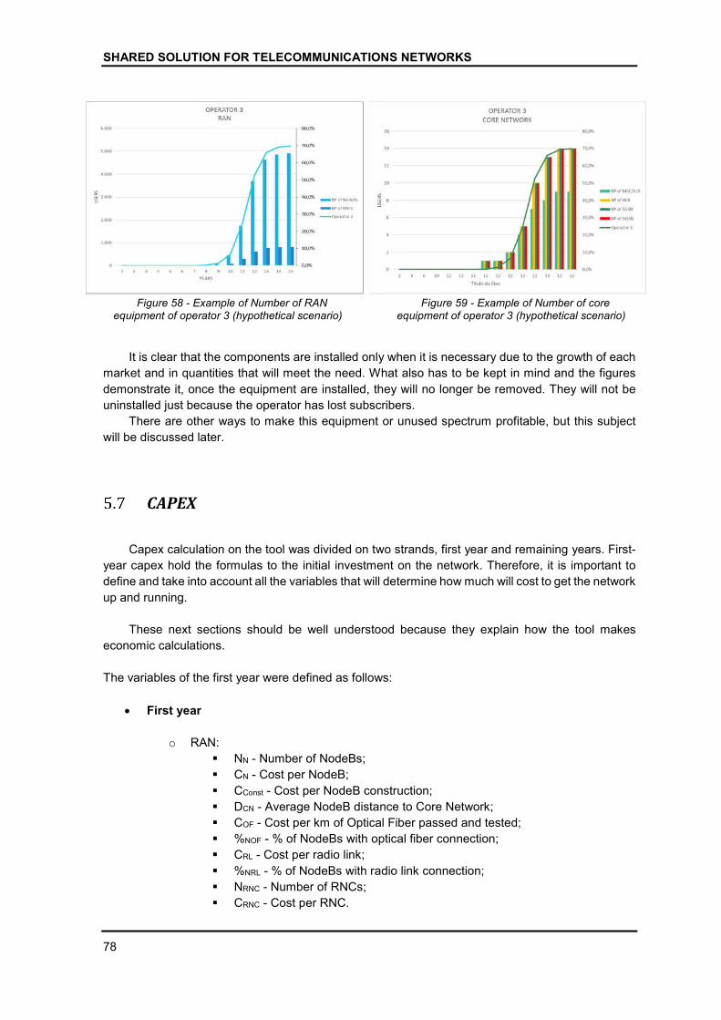
SHARED SOLUTION FOR TELECOMMUNICATIONS NETWORKS
78
Figure 58 - Example of Number of RAN
equipment of operator 3 (hypothetical scenario)
Figure 59 - Example of Number of core
equipment of operator 3 (hypothetical scenario)
It is clear that the components are installed only when it is necessary due to the growth of each
market and in quantities that will meet the need. What also has to be kept in mind and the figures
demonstrate it, once the equipment are installed, they will no longer be removed. They will not be
uninstalled just because the operator has lost subscribers.
There are other ways to make this equipment or unused spectrum profitable, but this subject
will be discussed later.
CAPEX
Capex calculation on the tool was divided on two strands, first year and remaining years. First-
year capex hold the formulas to the initial investment on the network. Therefore, it is important to
define and take into account all the variables that will determine how much will cost to get the network
up and running.
These next sections should be well understood because they explain how the tool makes
economic calculations.
The variables of the first year were defined as follows:
First year
o RAN:
NN - Number of NodeBs;
CN - Cost per NodeB;
CConst - Cost per NodeB construction;
DCN - Average NodeB distance to Core Network;
COF - Cost per km of Optical Fiber passed and tested;
%NOF - % of NodeBs with optical fiber connection;
CRL - Cost per radio link;
%NRL - % of NodeBs with radio link connection;
NRNC - Number of RNCs;
CRNC - Cost per RNC.
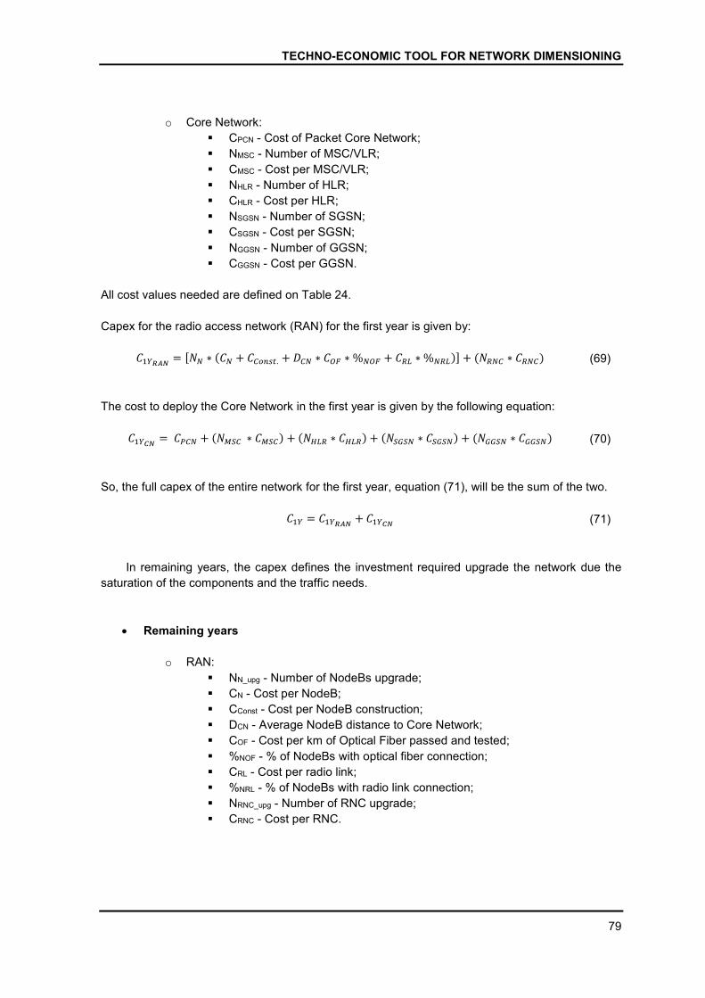
TECHNO-ECONOMIC TOOL FOR NETWORK DIMENSIONING
79
o Core Network:
CPCN - Cost of Packet Core Network;
NMSC - Number of MSC/VLR;
CMSC - Cost per MSC/VLR;
NHLR - Number of HLR;
CHLR - Cost per HLR;
NSGSN - Number of SGSN;
CSGSN - Cost per SGSN;
NGGSN - Number of GGSN;
CGGSN - Cost per GGSN.
All cost values needed are defined on Table 24.
Capex for the radio access network (RAN) for the first year is given by:
������= [�� ∗ (�� + ������. + ��� ∗ ��� ∗%��� + ��� ∗%���)] + (���� ∗ ����) (69)
The cost to deploy the Core Network in the first year is given by the following equation:
�����= ���� + (����∗ ����)+ (���� ∗ ����)+ (����� ∗ �����)+ (����� ∗ �����) (70)
So, the full capex of the entire network for the first year, equation (71), will be the sum of the two.
��� = ������+ �����
(71)
In remaining years, the capex defines the investment required upgrade the network due the
saturation of the components and the traffic needs.
Remaining years
o RAN:
NN_upg - Number of NodeBs upgrade;
CN - Cost per NodeB;
CConst - Cost per NodeB construction;
DCN - Average NodeB distance to Core Network;
COF - Cost per km of Optical Fiber passed and tested;
%NOF - % of NodeBs with optical fiber connection;
CRL - Cost per radio link;
%NRL - % of NodeBs with radio link connection;
NRNC_upg - Number of RNC upgrade;
CRNC - Cost per RNC.

SHARED SOLUTION FOR TELECOMMUNICATIONS NETWORKS
80
o Core Network:
CPCN - Cost of Packet Core Network;
NMSC_upg - Number of MSC/VLR upgrade;
CMSC - Cost per MSC/VLR;
NHLR_upg - Number of HLR upgrade;
CHLR - Cost per HLR;
NSGSN_upg - Number of SGSN upgrade;
CSGSN - Cost per SGSN;
NGGSN_upg - Number of GGSN upgrade;
CGGSN - Cost per GGSN.
For those remaining years the RAN capex calculated by the equation (72) and the core capex
by equation (73).
The t goes between [2; T] and T corresponds to the years of the project.
�����(�) = ������
(�)∗ (�� + ������. + ��� ∗ ��� ∗%��� + ��� ∗%���)� + (�������(�)∗ ����) (72)
����(�) = ��������
(�)∗ ����� + ��������(�)∗ ����� + ���������
(�)∗ ������ + (��������(�)∗ �����) (73)
The final capex is then calculated by equation (74):
��(�) = �����(�)+ ����
(�) (74)
Shared Capex
To be able to impose the effects of the sharing, the formulas for the capex have been projected
so that the operators that enter later can participate in the expenses.
It will be assumed that operator 1, for being the first to enter the market and install the first
infrastructures of the network, is always willing to share those infrastructures. And the remaining
operators will rent the network resources they need and contribute to the construction and upgrade
costs of the new ones.
Table 25 contains the market shares that each operator will have. These values vary according
to the parameters set in section 5.1 - INPUT PARAMETERS and 5.2 - FORECAST OF OPERATORS
UPTAKE.
It is clear that operator 1 starts alone in the market and only then do other operators become
interested.
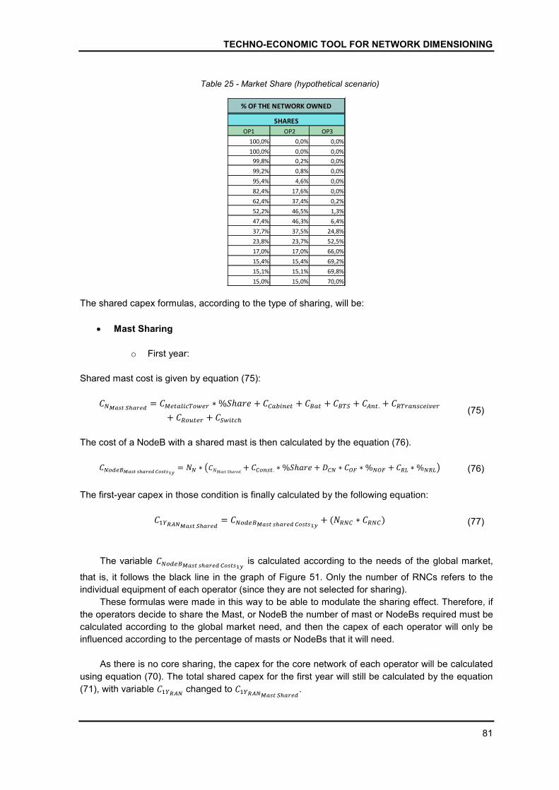
TECHNO-ECONOMIC TOOL FOR NETWORK DIMENSIONING
81
Table 25 - Market Share (hypothetical scenario)
The shared capex formulas, according to the type of sharing, will be:
Mast Sharing
o First year:
Shared mast cost is given by equation (75):
������������= ������������� ∗%�ℎ��� + �������� + ���� + ���� + ����. + �������������
+ ������� + ������� (75)
The cost of a NodeB with a shared mast is then calculated by the equation (76).
�����������������������= �� ∗ ��������ℎ����
+ ������. ∗%�ℎ��� + ��� ∗ ��� ∗%��� + ��� ∗%���� (76)
The first-year capex in those condition is finally calculated by the following equation:
����������������= �����������������������
+ (���� ∗ ����) (77)
The variable ����������������������� is calculated according to the needs of the global market,
that is, it follows the black line in the graph of Figure 51. Only the number of RNCs refers to the
individual equipment of each operator (since they are not selected for sharing).
These formulas were made in this way to be able to modulate the sharing effect. Therefore, if
the operators decide to share the Mast, or NodeB the number of mast or NodeBs required must be
calculated according to the global market need, and then the capex of each operator will only be
influenced according to the percentage of masts or NodeBs that it will need.
As there is no core sharing, the capex for the core network of each operator will be calculated
using equation (70). The total shared capex for the first year will still be calculated by the equation
(71), with variable ������ changed to ����������������
.
OP1 OP2 OP3
100,0% 0,0% 0,0%
100,0% 0,0% 0,0%
99,8% 0,2% 0,0%
99,2% 0,8% 0,0%
95,4% 4,6% 0,0%
82,4% 17,6% 0,0%
62,4% 37,4% 0,2%
52,2% 46,5% 1,3%
47,4% 46,3% 6,4%
37,7% 37,5% 24,8%
23,8% 23,7% 52,5%
17,0% 17,0% 66,0%
15,4% 15,4% 69,2%
15,1% 15,1% 69,8%
15,0% 15,0% 70,0%
SHARES
% OF THE NETWORK OWNED
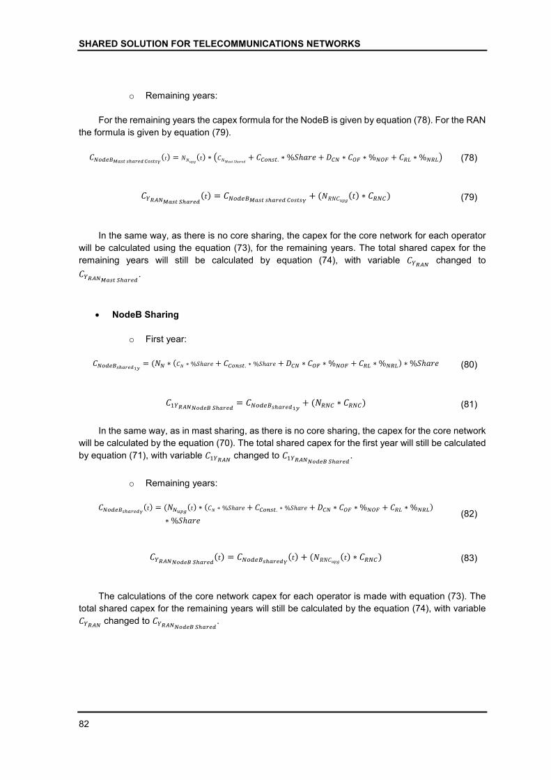
SHARED SOLUTION FOR TELECOMMUNICATIONS NETWORKS
82
o Remaining years:
For the remaining years the capex formula for the NodeB is given by equation (78). For the RAN
the formula is given by equation (79).
����������������������(�) = �����
(�)∗ ��������ℎ����+ ������. ∗%�ℎ��� + ��� ∗ ��� ∗%��� + ��� ∗%���� (78)
���������������(�) = ����������������������
+ (�������(�)∗ ����) (79)
In the same way, as there is no core sharing, the capex for the core network for each operator
will be calculated using the equation (73), for the remaining years. The total shared capex for the
remaining years will still be calculated by equation (74), with variable ����� changed to
���������������.
NodeB Sharing
o First year:
��������������= (�� ∗ (�� ∗ %�ℎ��� + ������. ∗ %�ℎ��� + ��� ∗ ��� ∗%��� + ��� ∗%���)∗%�ℎ��� (80)
�����������������= ��������������
+ (���� ∗ ����) (81)
In the same way, as in mast sharing, as there is no core sharing, the capex for the core network
will be calculated by the equation (70). The total shared capex for the first year will still be calculated
by equation (71), with variable ������ changed to �����������������
.
o Remaining years:
�������������(�) = (�����
(�)∗ (�� ∗ %�ℎ��� + ������. ∗ %�ℎ��� + ��� ∗ ��� ∗%��� + ��� ∗%���)
∗%�ℎ��� (82)
����������������(�) = �������������
(�)+ (�������(�)∗ ����) (83)
The calculations of the core network capex for each operator is made with equation (73). The
total shared capex for the remaining years will still be calculated by the equation (74), with variable
����� changed to ����������������
.
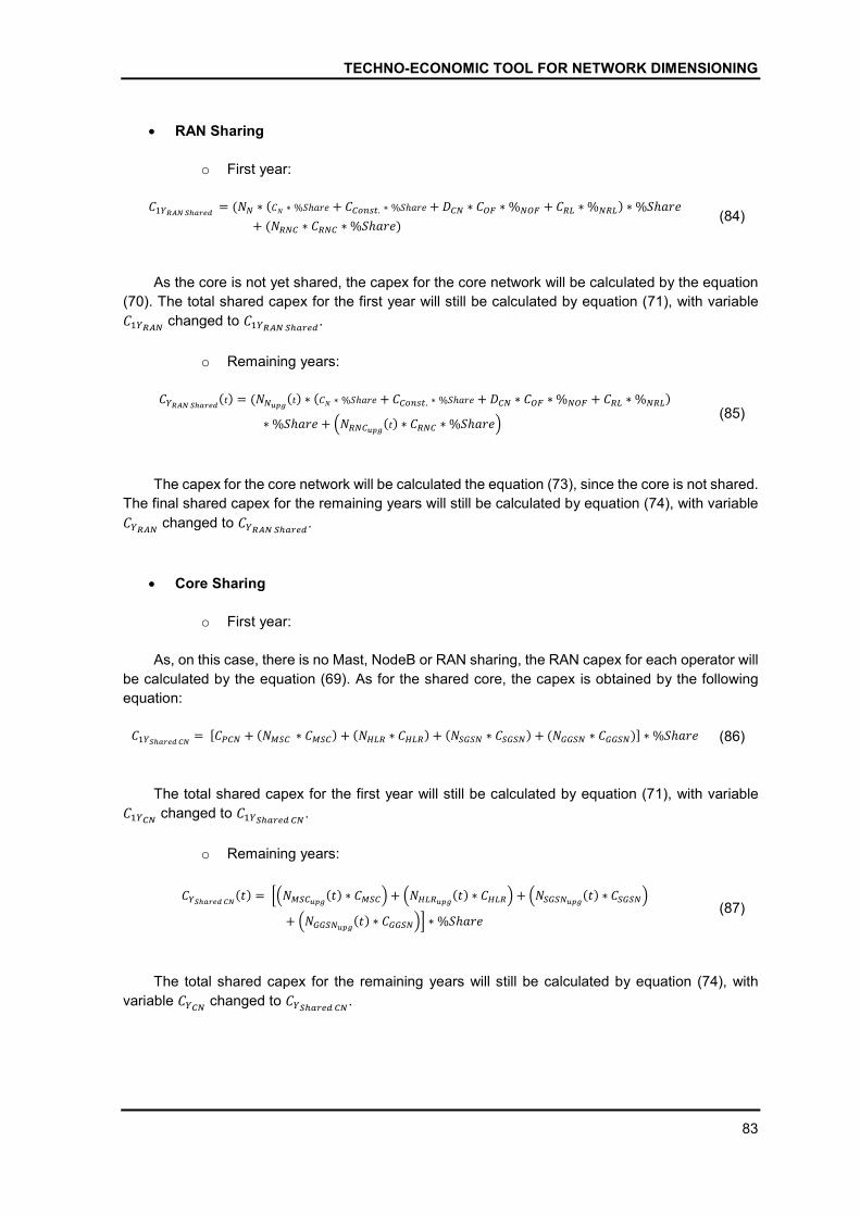
TECHNO-ECONOMIC TOOL FOR NETWORK DIMENSIONING
83
RAN Sharing
o First year:
������������= (�� ∗ (�� ∗ %�ℎ��� + ������. ∗ %�ℎ��� + ��� ∗ ��� ∗%��� + ��� ∗%���)∗%�ℎ���
+ (���� ∗ ���� ∗%�ℎ���) (84)
As the core is not yet shared, the capex for the core network will be calculated by the equation
(70). The total shared capex for the first year will still be calculated by equation (71), with variable
������ changed to ������������
.
o Remaining years:
�����������(�) = (�����
(�)∗ (�� ∗ %�ℎ��� + ������. ∗ %�ℎ��� + ��� ∗ ��� ∗%��� + ��� ∗%���)
∗%�ℎ��� + ��������(�)∗ ���� ∗%�ℎ����
(85)
The capex for the core network will be calculated the equation (73), since the core is not shared.
The final shared capex for the remaining years will still be calculated by equation (74), with variable
����� changed to �����������
.
Core Sharing
o First year:
As, on this case, there is no Mast, NodeB or RAN sharing, the RAN capex for each operator will
be calculated by the equation (69). As for the shared core, the capex is obtained by the following
equation:
�����������
= [���� + (����∗ ����)+ (���� ∗����)+ (����� ∗ �����)+ (����� ∗ �����)] ∗%�ℎ��� (86)
The total shared capex for the first year will still be calculated by equation (71), with variable
����� changed to �����������
.
o Remaining years:
����������(�)= ���������
(�)∗ ����� + ��������(�)∗ ����� + ���������
(�)∗������
+ ���������(�)∗ ������� ∗%�ℎ���
(87)
The total shared capex for the remaining years will still be calculated by equation (74), with
variable ���� changed to ����������
.
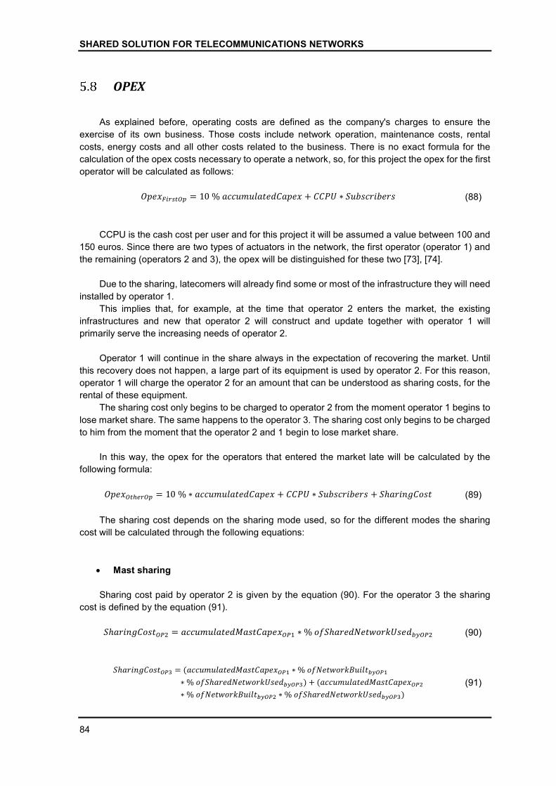
SHARED SOLUTION FOR TELECOMMUNICATIONS NETWORKS
84
OPEX
As explained before, operating costs are defined as the company's charges to ensure the
exercise of its own business. Those costs include network operation, maintenance costs, rental
costs, energy costs and all other costs related to the business. There is no exact formula for the
calculation of the opex costs necessary to operate a network, so, for this project the opex for the first
operator will be calculated as follows:
����������� = 10%���������������� + ���� ∗ ����������� (88)
CCPU is the cash cost per user and for this project it will be assumed a value between 100 and
150 euros. Since there are two types of actuators in the network, the first operator (operator 1) and
the remaining (operators 2 and 3), the opex will be distinguished for these two [73], [74].
Due to the sharing, latecomers will already find some or most of the infrastructure they will need
installed by operator 1.
This implies that, for example, at the time that operator 2 enters the market, the existing
infrastructures and new that operator 2 will construct and update together with operator 1 will
primarily serve the increasing needs of operator 2.
Operator 1 will continue in the share always in the expectation of recovering the market. Until
this recovery does not happen, a large part of its equipment is used by operator 2. For this reason,
operator 1 will charge the operator 2 for an amount that can be understood as sharing costs, for the
rental of these equipment.
The sharing cost only begins to be charged to operator 2 from the moment operator 1 begins to
lose market share. The same happens to the operator 3. The sharing cost only begins to be charged
to him from the moment that the operator 2 and 1 begin to lose market share.
In this way, the opex for the operators that entered the market late will be calculated by the
following formula:
����������� = 10% ∗ ���������������� + ���� ∗ ����������� + �ℎ��������� (89)
The sharing cost depends on the sharing mode used, so for the different modes the sharing
cost will be calculated through the following equations:
Mast sharing
Sharing cost paid by operator 2 is given by the equation (90). For the operator 3 the sharing
cost is defined by the equation (91).
�ℎ������������ = ����������������������� ∗%���ℎ�������������������� (90)
�ℎ������������ = (����������������������� ∗%�������������������
∗%���ℎ��������������������)+ (�����������������������
∗%������������������� ∗%���ℎ��������������������) (91)

TECHNO-ECONOMIC TOOL FOR NETWORK DIMENSIONING
85
NodeB sharing
�ℎ������������ = ������������������������ ∗%���ℎ�������������������� (92)
�ℎ������������ = (������������������������ ∗%�������������������
∗%���ℎ��������������������)+ (������������������������
∗%������������������� ∗%���ℎ��������������������) (93)
RAN sharing
�ℎ������������ = ���������������������� ∗%���ℎ�������������������� (94)
�ℎ������������ = (���������������������� ∗%�������������������
∗%���ℎ��������������������)+ (����������������������
∗%������������������� ∗%���ℎ��������������������) (95)
Core sharing
�ℎ������������ = ����������������������� ∗%���ℎ�������������������� (96)
�ℎ������������ = (����������������������� ∗%�������������������
∗%���ℎ��������������������)+ (�������������������
∗%������������������� ∗%���ℎ��������������������) (97)
REVENUE
The revenue will be calculated as the result of the sum of two parts (equation (98)). The first
one will be treated as the revenue coming from the subscribers (equation (99)), and the second from
the revenue from the sharing (equations (100) and (101)).
������� = ������������������ + ���������������� (98)
Subscribers revenues is calculated by multiplying the number of subscribers with the annual
price paid by each subscriber.
Since the three different categories of subscribers were previously homogenized, in order to do
the network granularity, the price paid by subscribers is calculated based on the price paid by private
subscribers.
Once this project does not differentiate the needs of more powerful and consequently more
expensive, equipment that business and institutional have compared to private, the use of this
method will not harm or invalidate the model.
SHARED SOLUTION FOR TELECOMMUNICATIONS NETWORKS
86
������������������ = ������ ∗ ������������(���) (99)
������������������� = �ℎ������������ +�ℎ������������
2 (100)
������������������� =�ℎ������������
2 (101)
������������(���) = ����ℎ��������ℎ������������������������� ∗ 12 (102)
Although operator 2 only built a small part of the network, operator 2 is viewed by operator 3 as
a co-owner of the network with equal rights to operator 1.
This is idealized in this way because, despite not having built much of the network, operator 2
until the moment that operator 3 enters the market will already have paid operator 1 a significant
amount of �ℎ���������. This �ℎ��������� is seen by operator 2 as opex expenditures that
contributed to operator 1 and 2 being able to keep the network functional.
It cannot be forgotten that operator 1 had substantial losses of subscribers, so part of the
network was leased to operator 2. This portion leased to operator 2, is managed and maintained by
operator 2 itself.
Thus, when operator 3 enters the market the percentage of network managed and operated by
operator 2 is seen as being owned by operator 2.
Operator 3 has no contribution from this part, this is because it is the only one on the sharing
that finds the equipment all installed and the network completed. Therefore, it can be seen as
consumer and not a supplier.
RESULTS
As previously explained the decision criteria methods to determine the return on investment are
the NPV, the IRR and the return period. The tool uses those parameters plus the amount of the
Annual Net Cash Flow and cash balance to determine the profitability of each operator in the different
methods of sharing. These values plus the corresponding graphs will be used to see if there is an
advantage in being involved in a share, and which sharing method has better results.

SCENARIOS ANALISYS
87
SCENARIOS ANALISYS
The scenarios that will be studied in this dissertation are hypothetical, but with characteristics
similar to those found in some developing countries (namely in Africa). These types of regions have
patterns of consumption and traffic usage different from regions that have more developed markets
and greater economic power.
Europeans have a way of life, customs and habits that differs from North Americans, Asians,
Africans and South Americans. This is directly related to the quantity and quality of the existing and
offered technologies. As consequence, this dictates the way people interact with technology.
The countries, so-called world powers, have a much greater daily traffic flow than the developing
and underdeveloped countries. By having most or all of their territories with mobile and fixed
coverage, the industrialization and modernization of their markets is supported and strongly
dependent on these services.
Therefore, private and public companies and institutions rely heavily in those services and
technologies of information and communication. All this is reflected to the user, who has been
accustomed to check his e-mail address, use the social networks and have instant access to the
latest news from the early hours of the day.
As a consequence of these habits, the load on the cellular network in these regions is higher
compared to developing or underdeveloped regions.
The habits in developing regions or countries are related to a reality where, if
telecommunications services are already available, the access to them is often expensive and
unaffordable by the majority of the population. What makes many businesses, services or institutions
to operate their services in a non-digital form.
This reduces the quality of service, quality of life and the interest on the region.
A common challenge for operators operating in these regions is the difficulty of being able to
expand, improve or cover new areas with telecommunications services. The entry into areas that are
not covered by any operator, on a country where the economic power is not abundant, often result
in the abandonment or postponement of the projects.
On nowadays it is clear that the provision of those services has a beneficial and stimulating
effect on the economy, quality of life and development of those regions. So, it must be fund a way to
deploy these technologies in these regions and especially at an affordable cost to the population.
Many methods and forms have been studied and implemented, but work developed in this
dissertation will try to use the sharing of infrastructures as a way to overcome these difficulties.
The idealized scenarios will be identical to a region of a developing country, where the
definitions of the tool will be set to try the best as possible to simulate the real conditions.
It will study 2 types of scenarios:
o Scenario A - only one operator explores the market;
o Scenario B - 3 operators explore the market, under an infrastructure sharing scheme.
SHARED SOLUTION FOR TELECOMMUNICATIONS NETWORKS
88
SCENARIO A – Single Operator
The scenario A will be defined as follows:
Region Characteristic:
o Emerging market;
o Suburban area;
o Region area = 10000 square kilometers
o Expected coverage area = 70% of the region area;
o Type of terrain: sandy / earthy;
o Demography: Approximately 12 million of active population, with approximately 3%
in the service of institutions, 20% make a business use of telecommunications
services, and the remainder makes a private use;
o The distribution of the users will be homogeneous;
o Density = 1685,7.
Technological Aspects:
o UMTS 900 will be the system used;
o All NodeBs have three sectors;
o It will be based on 12,2 Kbps voice service and 144 Kbps data service;
o Telecommunications infrastructure is practically non-existent, with approximately
5% infrastructure installed, with only minimal services installed to serve government
institutions;
o Average distance between a NodeB and the core network is 80 kilometers;
o NodeB do RNC connections will be 80% per optical fiber and 20% per radio link;
o The network equipment has capacity limitation, so at a certain point they will
saturate, and it will be necessary to increase their numbers;
o Sharing methods:
Mast = NO;
NodeB = NO;
RAN = NO;
Core = NO.
Pricing and economic settings:
o The monthly price paid by each user will be defined as follows:
Institutional: 40 €
Business: 25 €
Private: 12 €
o The Annual Interest Rate is 5%.
Operators settings:
o 1 operator;
o �� = 0%;
o �� = 0%
In such regions, the population is generally situated along rivers, main roads and on the coast,
making vast areas of the territory uninhabited. This usually happens due to the search for more fertile
regions and where the transit of goods is facilitated. To modulate this effect, it is assumed that only
a percentage of the territory will be covered by the network to be designed.
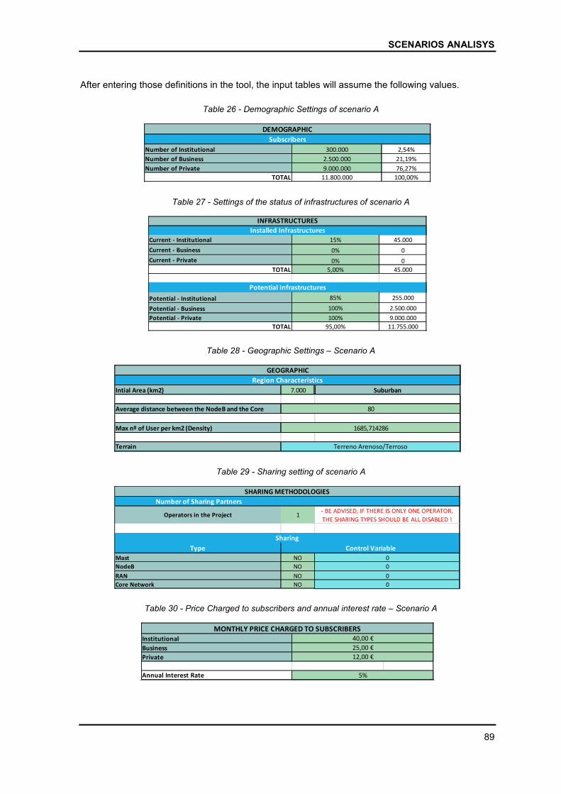
SCENARIOS ANALISYS
89
After entering those definitions in the tool, the input tables will assume the following values.
Table 26 - Demographic Settings of scenario A
Table 27 - Settings of the status of infrastructures of scenario A
Table 28 - Geographic Settings – Scenario A
Table 29 - Sharing setting of scenario A
Table 30 - Price Charged to subscribers and annual interest rate – Scenario A
Number of Institutional 300.000 2,54%
Number of Business 2.500.000 21,19%
Number of Private 9.000.000 76,27%
TOTAL 11.800.000 100,00%
Subscribers
DEMOGRAPHIC
Current - Institutional 15% 45.000
Current - Business 0% 0
Current - Private 0% 0
TOTAL 5,00% 45.000
Potential - Institutional 85% 255.000
Potential - Business 100% 2.500.000
Potential - Private 100% 9.000.000
TOTAL 95,00% 11.755.000
Potential Infrastructures
Installed Infrastructures
INFRASTRUCTURES
Intial Area (km2) 7.000 Suburban
Average distance between the NodeB and the Core
Max nº of User per km2 (Density)
Terrain
Region Characteristics
80
Terreno Arenoso/Terroso
1685,714286
GEOGRAPHIC
Number of Sharing Partners
Type
Mast NO 0
NodeB NO 0
RAN NO 0
Core Network NO 0
Sharing
SHARING METHODOLOGIES
Control Variable
Operators in the Project- BE ADVISED, IF THERE IS ONLY ONE OPERATOR,
THE SHARING TYPES SHOULD BE ALL DISABLED !1
Institutional
Business
Private
Annual Interest Rate 5%
MONTHLY PRICE CHARGED TO SUBSCRIBERS
25,00 €
12,00 €
40,00 €
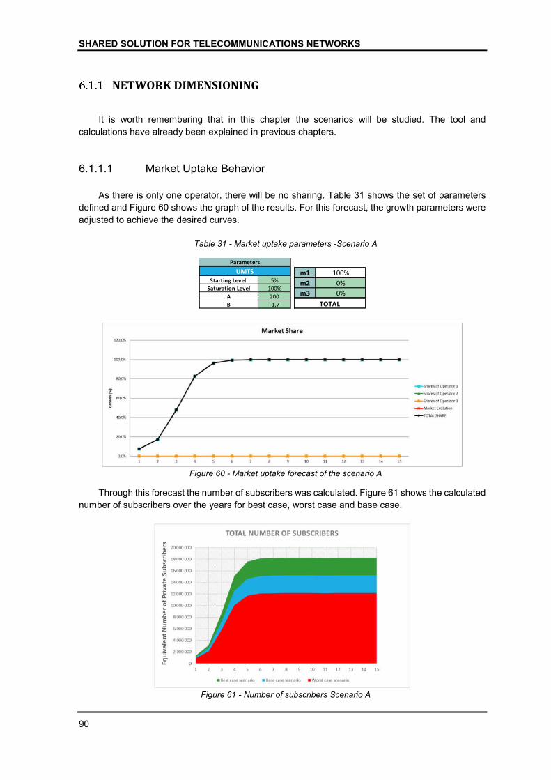
SHARED SOLUTION FOR TELECOMMUNICATIONS NETWORKS
90
NETWORK DIMENSIONING
It is worth remembering that in this chapter the scenarios will be studied. The tool and
calculations have already been explained in previous chapters.
6.1.1.1 Market Uptake Behavior
As there is only one operator, there will be no sharing. Table 31 shows the set of parameters
defined and Figure 60 shows the graph of the results. For this forecast, the growth parameters were
adjusted to achieve the desired curves.
Table 31 - Market uptake parameters -Scenario A
Figure 60 - Market uptake forecast of the scenario A
Through this forecast the number of subscribers was calculated. Figure 61 shows the calculated
number of subscribers over the years for best case, worst case and base case.
Figure 61 - Number of subscribers Scenario A
5%
100%
200
-1,7
Saturation Level
A
B
Parameters
UMTS
Starting Level m1 100%
m2 0%
m3 0%
TOTAL
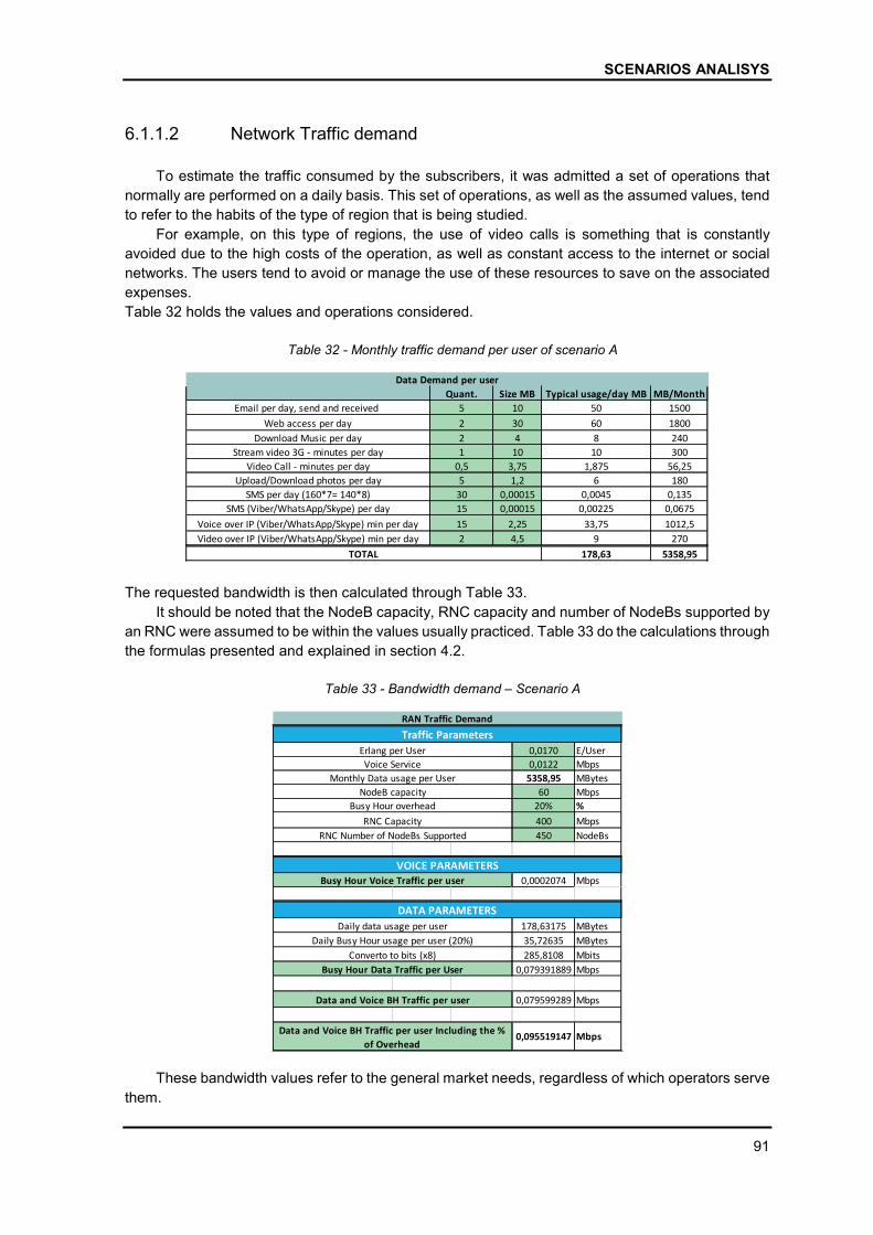
SCENARIOS ANALISYS
91
6.1.1.2 Network Traffic demand
To estimate the traffic consumed by the subscribers, it was admitted a set of operations that
normally are performed on a daily basis. This set of operations, as well as the assumed values, tend
to refer to the habits of the type of region that is being studied.
For example, on this type of regions, the use of video calls is something that is constantly
avoided due to the high costs of the operation, as well as constant access to the internet or social
networks. The users tend to avoid or manage the use of these resources to save on the associated
expenses.
Table 32 holds the values and operations considered.
Table 32 - Monthly traffic demand per user of scenario A
The requested bandwidth is then calculated through Table 33.
It should be noted that the NodeB capacity, RNC capacity and number of NodeBs supported by
an RNC were assumed to be within the values usually practiced. Table 33 do the calculations through
the formulas presented and explained in section 4.2.
Table 33 - Bandwidth demand – Scenario A
These bandwidth values refer to the general market needs, regardless of which operators serve
them.
Quant. Size MB Typical usage/day MB MB/Month
5 10 50 1500
2 30 60 1800
2 4 8 240
1 10 10 300
0,5 3,75 1,875 56,25
5 1,2 6 180
30 0,00015 0,0045 0,135
15 0,00015 0,00225 0,0675
15 2,25 33,75 1012,5
2 4,5 9 270
178,63 5358,95TOTAL
Upload/Download photos per day
Data Demand per user
Email per day, send and received
Web access per day
Download Music per day
Stream video 3G - minutes per day
Video Call - minutes per day
Voice over IP (Viber/WhatsApp/Skype) min per day
Video over IP (Viber/WhatsApp/Skype) min per day
SMS (Viber/WhatsApp/Skype) per day
SMS per day (160*7= 140*8)
0,0170 E/User
0,0122 Mbps
5358,95 MBytes
60 Mbps
20% %
400 Mbps
450 NodeBs
0,0002074 Mbps
178,63175 MBytes
35,72635 MBytes
285,8108 Mbits
0,079391889 Mbps
0,079599289 Mbps
Traffic Parameters
RAN Traffic Demand
0,095519147 MbpsData and Voice BH Traffic per user Including the %
of Overhead
Erlang per User
Voice Service
Data and Voice BH Traffic per user
DATA PARAMETERS
Converto to bits (x8)
Busy Hour Data Traffic per User
Daily data usage per user
Monthly Data usage per User
NodeB capacity
Busy Hour overhead
VOICE PARAMETERS
RNC Capacity
RNC Number of NodeBs Supported
Busy Hour Voice Traffic per user
Daily Busy Hour usage per user (20%)
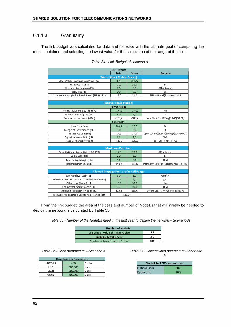
SHARED SOLUTION FOR TELECOMMUNICATIONS NETWORKS
92
6.1.1.3 Granularity
The link budget was calculated for data and for voice with the ultimate goal of comparing the
results obtained and selecting the lowest value for the calculation of the range of the cell.
Table 34 - Link Budget of scenario A
From the link budget, the area of the cells and number of NodeBs that will initially be needed to
deploy the network is calculated by Table 35.
Table 35 - Number of the NodeBs need in the first year to deploy the network – Scenario A
Table 36 - Core parameters – Scenario A
Table 37 - Connections parameters – Scenario A
Data Voice
0,25 0,125
24,0 21,0
2,0 0,0
0,0 0,0
26,0 21,0
-174,0 -174,0
5,0 5,0
-103,2 -103,2
144,0 12,2
3,0 3,0
14,3 25,0
2,2 4,5
-112,2 -120,6
17,0 17,0
2,0 2,0
5,0 5,0
148,2 151,6
3,0 3,0
3,0 3,0
10,0 10,0
10,0 10,0
128,2 131,6
Power Rating
Sensitivity
Pt
G(Tantenna)
LB
EIRP = Pt + G(Tantenna) - LB
No
F
Nr = No + F + 10*log(3.84*(10)^6)
Other Loss (In-car) (dB)
Log-normal fading margin (dB)
Allowed Propagation Loss (dB)
Maximum Path Loss (dB)
Inference due the co-location with GSM900 (dB)
Allowed Propagation Loss for Cell Range
Soft Handover Gain (dB)
PathLoss=EIRP-Rs+G(Rantenna)-Lc-FFM
GsoftH
Igsm
Lo
LFM
L=PathLoss-LFM+GSoftH-Lo-Igsm
Base Station Antenna Gain (dBi) 120º
Cable Loss (dB)
Fast Fading Margin (dB)
Maximum Path LossG(Rantenna)
Lc
FFM
Transmitter ( Mobile Device)
Receiver (Base Station)
I
Gp = 10*log((3.84*(10)^6)/(Wd*10^3))
SNR
Rs = SNR + Nr + I - Gp
User Data Rate Wd
Thermal noise density (dBm/Hz)
Receiver noise figure (dB)
Receiver noise power (dBm)
Mobile antenna gain (dBi)
Body loss (dB)
Equivalent Isotropic Radiated Power (EIRP)(dBm)
Signal to Noise Ratio (dB)
Receiver Sensitivity (dB)
Link Budget
Allowed Propagation Loss for cell Range (dB)
Max. Mobile Transmission Power (W)
128,2
Margin of interference (dB)
Processing Gain (dB)
Formula
As above in dBm
2,1
8,9
898
NodeB Coverage Area
Number of NodeBs
Number of NodeBs of the 1 year
Sub-urban - value of R (km) 0-5km
MSC/VLR 400 Nodes
HLR 500.000 Users
SGSN 500.000 Users
GGSN 500.000 Users
Core Capacity Parameters
Optical Fiber 80%
Radio Link 20%
NodeB to RNC connections
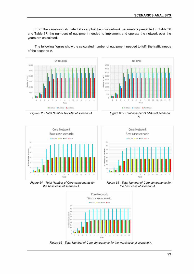
SCENARIOS ANALISYS
93
From the variables calculated above, plus the core network parameters presented in Table 36
and Table 37, the numbers of equipment needed to implement and operate the network over the
years are calculated.
The following figures show the calculated number of equipment needed to fulfil the traffic needs
of the scenario A.
Figure 62 - Total Number NodeBs of scenario A
Figure 63 - Total Number of RNCs of scenario
A
Figure 64 - Total Number of Core components for
the base case of scenario A
Figure 65 - Total Number of Core components for
the best case of scenario A
Figure 66 - Total Number of Core components for the worst case of scenario A
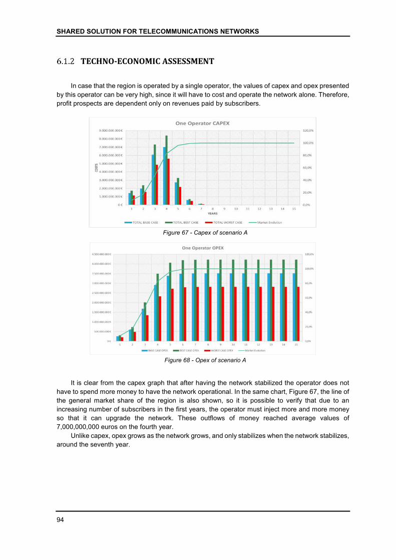
SHARED SOLUTION FOR TELECOMMUNICATIONS NETWORKS
94
TECHNO-ECONOMIC ASSESSMENT
In case that the region is operated by a single operator, the values of capex and opex presented
by this operator can be very high, since it will have to cost and operate the network alone. Therefore,
profit prospects are dependent only on revenues paid by subscribers.
Figure 67 - Capex of scenario A
Figure 68 - Opex of scenario A
It is clear from the capex graph that after having the network stabilized the operator does not
have to spend more money to have the network operational. In the same chart, Figure 67, the line of
the general market share of the region is also shown, so it is possible to verify that due to an
increasing number of subscribers in the first years, the operator must inject more and more money
so that it can upgrade the network. These outflows of money reached average values of
7,000,000,000 euros on the fourth year.
Unlike capex, opex grows as the network grows, and only stabilizes when the network stabilizes,
around the seventh year.

SCENARIOS ANALISYS
95
Figure 69 - Revenue of scenario A
Since, for a single operator, revenue only depends on the number of subscriptions, and
consequently on the price paid by them, the amount collected by the operator as revenue increases
proportionally with the number of subscribers.
ECONOMIC RESULTS
The economic analysis undertaken in this section aims to recognize opportunities and threats.
The methods chosen for this evaluation take into account the time value of the money.
The following tables and graphs present the economic results of scenario A.
Table 38 - NPV, IRR and Payback period for scenario A (Base case)
1,2
Figure 70 - Economic Results of scenario A - Base Case
1 #NUM = Value impossible to be calculated. 2 Payback Period = 16 → Payback period > 15 years.
5%
-27.689.909.490,48 €
#NÚM!
16
Base case scenarioAnnual Interest Rate
NPV
IRR
Payback period (years)
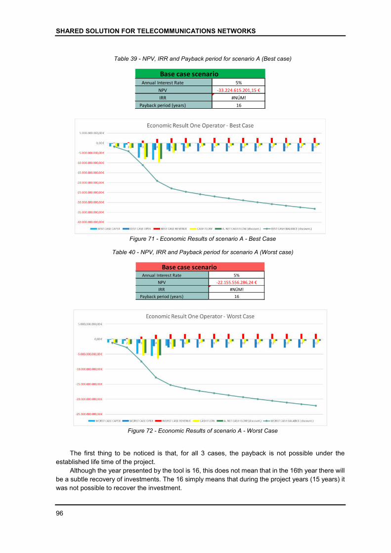
SHARED SOLUTION FOR TELECOMMUNICATIONS NETWORKS
96
Table 39 - NPV, IRR and Payback period for scenario A (Best case)
Figure 71 - Economic Results of scenario A - Best Case
Table 40 - NPV, IRR and Payback period for scenario A (Worst case)
Figure 72 - Economic Results of scenario A - Worst Case
The first thing to be noticed is that, for all 3 cases, the payback is not possible under the
established life time of the project.
Although the year presented by the tool is 16, this does not mean that in the 16th year there will
be a subtle recovery of investments. The 16 simply means that during the project years (15 years) it
was not possible to recover the investment.
5%
-33.224.615.201,15 €
#NÚM!
16
Base case scenarioAnnual Interest Rate
NPV
IRR
Payback period (years)
5%
-22.155.556.286,24 €
#NÚM!
16
Base case scenarioAnnual Interest Rate
NPV
IRR
Payback period (years)
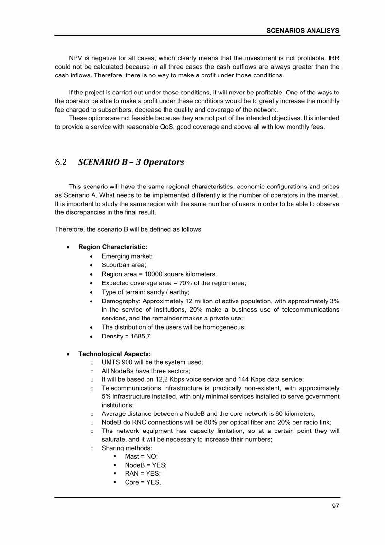
SCENARIOS ANALISYS
97
NPV is negative for all cases, which clearly means that the investment is not profitable. IRR
could not be calculated because in all three cases the cash outflows are always greater than the
cash inflows. Therefore, there is no way to make a profit under those conditions.
If the project is carried out under those conditions, it will never be profitable. One of the ways to
the operator be able to make a profit under these conditions would be to greatly increase the monthly
fee charged to subscribers, decrease the quality and coverage of the network.
These options are not feasible because they are not part of the intended objectives. It is intended
to provide a service with reasonable QoS, good coverage and above all with low monthly fees.
SCENARIO B – 3 Operators
This scenario will have the same regional characteristics, economic configurations and prices
as Scenario A. What needs to be implemented differently is the number of operators in the market.
It is important to study the same region with the same number of users in order to be able to observe
the discrepancies in the final result.
Therefore, the scenario B will be defined as follows:
Region Characteristic:
Emerging market;
Suburban area;
Region area = 10000 square kilometers
Expected coverage area = 70% of the region area;
Type of terrain: sandy / earthy;
Demography: Approximately 12 million of active population, with approximately 3%
in the service of institutions, 20% make a business use of telecommunications
services, and the remainder makes a private use;
The distribution of the users will be homogeneous;
Density = 1685,7.
Technological Aspects:
o UMTS 900 will be the system used;
o All NodeBs have three sectors;
o It will be based on 12,2 Kbps voice service and 144 Kbps data service;
o Telecommunications infrastructure is practically non-existent, with approximately
5% infrastructure installed, with only minimal services installed to serve government
institutions;
o Average distance between a NodeB and the core network is 80 kilometers;
o NodeB do RNC connections will be 80% per optical fiber and 20% per radio link;
o The network equipment has capacity limitation, so at a certain point they will
saturate, and it will be necessary to increase their numbers;
o Sharing methods:
Mast = NO;
NodeB = YES;
RAN = YES;
Core = YES.
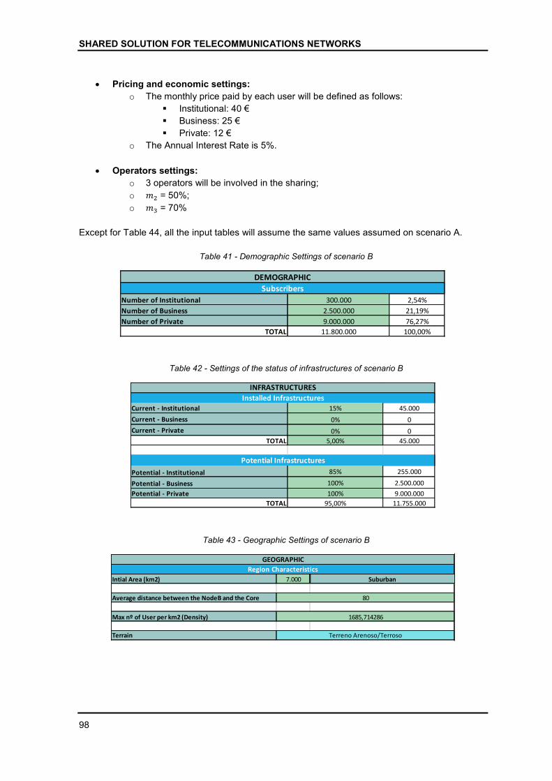
SHARED SOLUTION FOR TELECOMMUNICATIONS NETWORKS
98
Pricing and economic settings:
o The monthly price paid by each user will be defined as follows:
Institutional: 40 €
Business: 25 €
Private: 12 €
o The Annual Interest Rate is 5%.
Operators settings:
o 3 operators will be involved in the sharing;
o �� = 50%;
o �� = 70%
Except for Table 44, all the input tables will assume the same values assumed on scenario A.
Table 41 - Demographic Settings of scenario B
Table 42 - Settings of the status of infrastructures of scenario B
Table 43 - Geographic Settings of scenario B
Number of Institutional 300.000 2,54%
Number of Business 2.500.000 21,19%
Number of Private 9.000.000 76,27%
TOTAL 11.800.000 100,00%
Subscribers
DEMOGRAPHIC
Current - Institutional 15% 45.000
Current - Business 0% 0
Current - Private 0% 0
TOTAL 5,00% 45.000
Potential - Institutional 85% 255.000
Potential - Business 100% 2.500.000
Potential - Private 100% 9.000.000
TOTAL 95,00% 11.755.000
Potential Infrastructures
Installed Infrastructures
INFRASTRUCTURES
Intial Area (km2) 7.000 Suburban
Average distance between the NodeB and the Core
Max nº of User per km2 (Density)
Terrain
Region Characteristics
80
Terreno Arenoso/Terroso
1685,714286
GEOGRAPHIC

SCENARIOS ANALISYS
99
Table 44 - Sharing settings of scenario B
Table 45 - Price Charged to subscribers and annual interest rate – Scenario B
NETWORK DIMENSIONING
6.2.1.1 Market Uptake Behavior
The market sharing model used in this section has been previously presented in Section 4. With
the number of operators defined for sharing equal to 3, the market share values that each expects
to achieve is given by ��,�������, and market uptake behavior can be calculated.
Table 46 shows the set of parameters defined and Figure 73 shows the market uptake behavior
graph. For this scenario, the growth parameters were adjusted to achieve the desired curves.
Table 46 - Market uptake parameters - Scenario B
Number of Sharing Partners
Type
Mast NO 0
NodeB YES 1
RAN YES 1
Core Network YES 1
Sharing
SHARING METHODOLOGIES
Control Variable
Operators in the Project THE MAXIMUM ALLOWED IS 3 !!!3
Institutional
Business
Private
Annual Interest Rate 5%
MONTHLY PRICE CHARGED TO SUBSCRIBERS
25,00 €
12,00 €
40,00 €
5%
100%
200
-1,7
300
-1
100
-1,9
25%
4
300
-1,7
55%
8
Saturation Level
A
B
Parameters
UMTSStarting Level
A
Operator 1
A
B
Operator 2
B
B
Starting Parameter
τ3
Starting Parameter
τ2
Operator 3
A
m1 100%
m2 50%
m3 70%
TOTAL
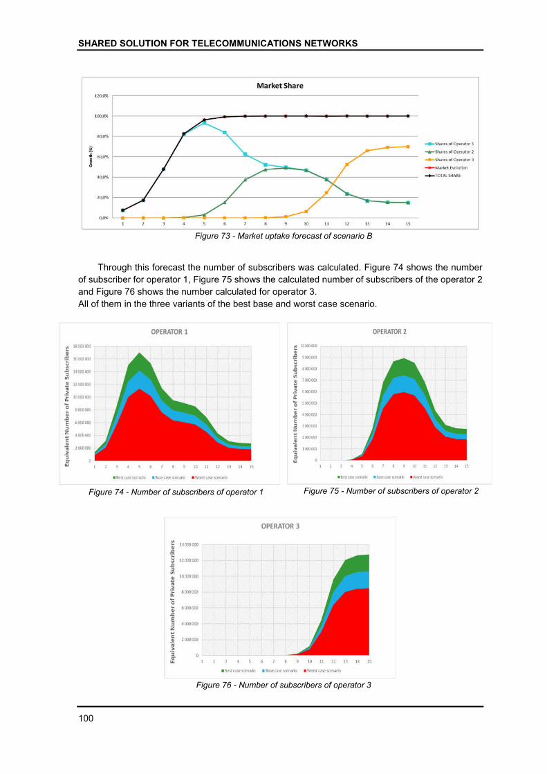
SHARED SOLUTION FOR TELECOMMUNICATIONS NETWORKS
100
Figure 73 - Market uptake forecast of scenario B
Through this forecast the number of subscribers was calculated. Figure 74 shows the number
of subscriber for operator 1, Figure 75 shows the calculated number of subscribers of the operator 2
and Figure 76 shows the number calculated for operator 3.
All of them in the three variants of the best base and worst case scenario.
Figure 74 - Number of subscribers of operator 1
Figure 75 - Number of subscribers of operator 2
Figure 76 - Number of subscribers of operator 3
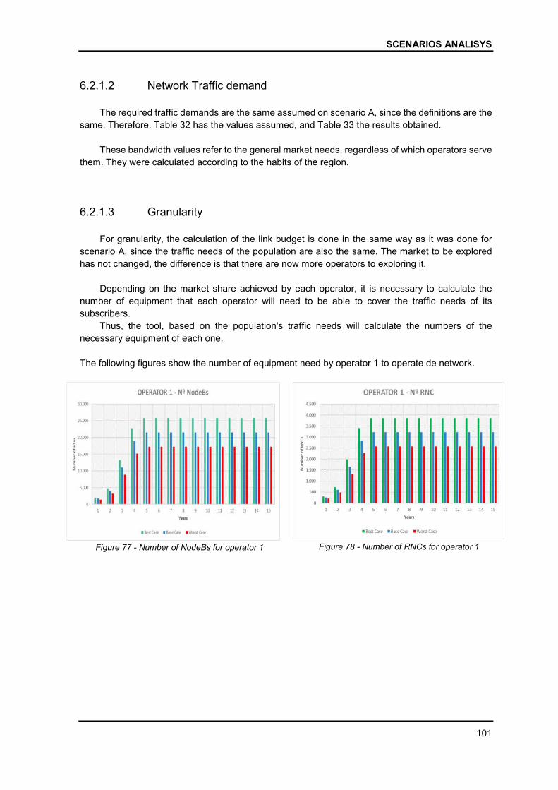
SCENARIOS ANALISYS
101
6.2.1.2 Network Traffic demand
The required traffic demands are the same assumed on scenario A, since the definitions are the
same. Therefore, Table 32 has the values assumed, and Table 33 the results obtained.
These bandwidth values refer to the general market needs, regardless of which operators serve
them. They were calculated according to the habits of the region.
6.2.1.3 Granularity
For granularity, the calculation of the link budget is done in the same way as it was done for
scenario A, since the traffic needs of the population are also the same. The market to be explored
has not changed, the difference is that there are now more operators to exploring it.
Depending on the market share achieved by each operator, it is necessary to calculate the
number of equipment that each operator will need to be able to cover the traffic needs of its
subscribers.
Thus, the tool, based on the population's traffic needs will calculate the numbers of the
necessary equipment of each one.
The following figures show the number of equipment need by operator 1 to operate de network.
Figure 77 - Number of NodeBs for operator 1
Figure 78 - Number of RNCs for operator 1
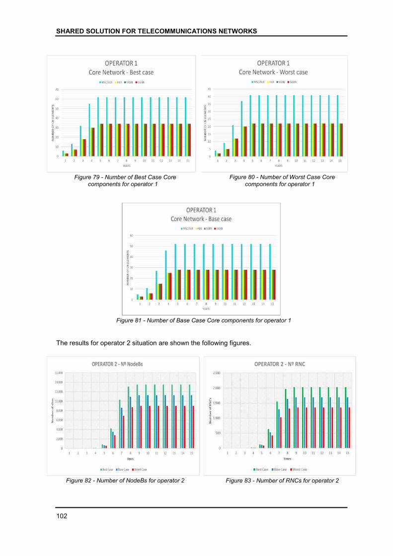
SHARED SOLUTION FOR TELECOMMUNICATIONS NETWORKS
102
Figure 79 - Number of Best Case Core
components for operator 1
Figure 80 - Number of Worst Case Core
components for operator 1
Figure 81 - Number of Base Case Core components for operator 1
The results for operator 2 situation are shown the following figures.
Figure 82 - Number of NodeBs for operator 2
Figure 83 - Number of RNCs for operator 2
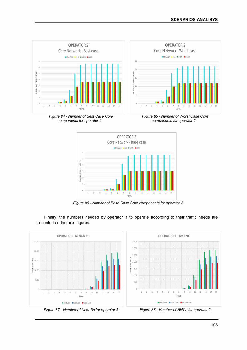
SCENARIOS ANALISYS
103
Figure 84 - Number of Best Case Core
components for operator 2
Figure 85 - Number of Worst Case Core
components for operator 2
Figure 86 - Number of Base Case Core components for operator 2
Finally, the numbers needed by operator 3 to operate according to their traffic needs are
presented on the next figures.
Figure 87 - Number of NodeBs for operator 3
Figure 88 - Number of RNCs for operator 3
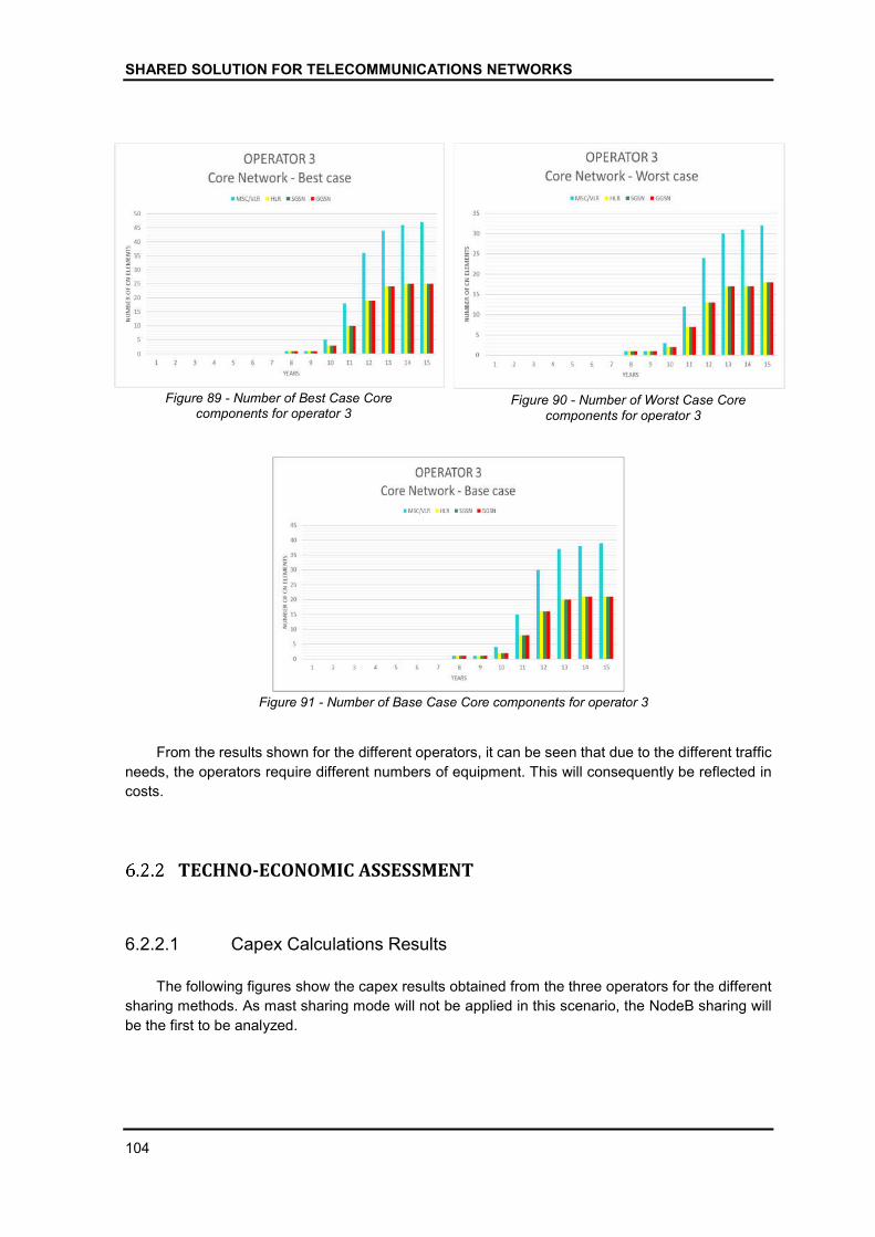
SHARED SOLUTION FOR TELECOMMUNICATIONS NETWORKS
104
Figure 89 - Number of Best Case Core
components for operator 3
Figure 90 - Number of Worst Case Core
components for operator 3
Figure 91 - Number of Base Case Core components for operator 3
From the results shown for the different operators, it can be seen that due to the different traffic
needs, the operators require different numbers of equipment. This will consequently be reflected in
costs.
TECHNO-ECONOMIC ASSESSMENT
6.2.2.1 Capex Calculations Results
The following figures show the capex results obtained from the three operators for the different
sharing methods. As mast sharing mode will not be applied in this scenario, the NodeB sharing will
be the first to be analyzed.
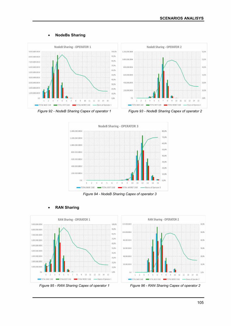
SCENARIOS ANALISYS
105
NodeBs Sharing
Figure 92 - NodeB Sharing Capex of operator 1
Figure 93 - NodeB Sharing Capex of operator 2
Figure 94 - NodeB Sharing Capex of operator 3
RAN Sharing
Figure 95 - RAN Sharing Capex of operator 1
Figure 96 - RAN Sharing Capex of operator 2
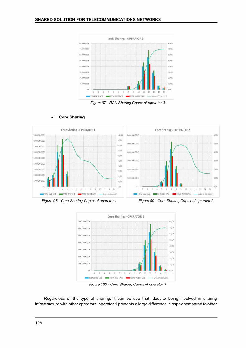
SHARED SOLUTION FOR TELECOMMUNICATIONS NETWORKS
106
Figure 97 - RAN Sharing Capex of operator 3
Core Sharing
Figure 98 - Core Sharing Capex of operator 1
Figure 99 - Core Sharing Capex of operator 2
Figure 100 - Core Sharing Capex of operator 3
Regardless of the type of sharing, it can be see that, despite being involved in sharing
infrastructure with other operators, operator 1 presents a large difference in capex compared to other
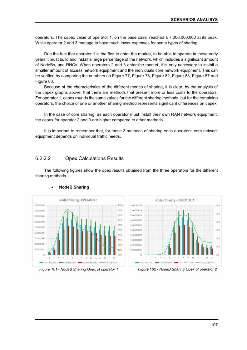
SCENARIOS ANALISYS
107
operators. The capex value of operator 1, on the base case, reached € 7,000,000,000 at its peak.
While operator 2 and 3 manage to have much lower expenses for some types of sharing.
Due the fact that operator 1 is the first to enter the market, to be able to operate in those early
years it must build and install a large percentage of the network, which includes a significant amount
of NodeBs, and RNCs. When operators 2 and 3 enter the market, it is only necessary to install a
smaller amount of access network equipment and the individuals core network equipment. This can
be verified by comparing the numbers on Figure 77, Figure 78, Figure 82, Figure 83, Figure 87 and
Figure 88.
Because of the characteristics of the different modes of sharing, it is clear, by the analysis of
the capex graphs above, that there are methods that present more or less costs to the operators.
For operator 1, capex rounds the same values for the different sharing methods, but for the remaining
operators, the choice of one or another sharing method represents significant differences on capex.
In the case of core sharing, as each operator must install their own RAN network equipment,
the capex for operator 2 and 3 are higher compared to other methods.
It is important to remember that, for these 3 methods of sharing each operator's core network
equipment depends on individual traffic needs.
6.2.2.2 Opex Calculations Results
The following figures show the opex results obtained from the three operators for the different
sharing methods.
NodeB Sharing
Figure 101 - NodeB Sharing Opex of operator 1
Figure 102 - NodeB Sharing Opex of operator 2
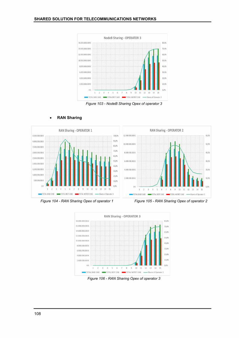
SHARED SOLUTION FOR TELECOMMUNICATIONS NETWORKS
108
Figure 103 - NodeB Sharing Opex of operator 3
RAN Sharing
Figure 104 - RAN Sharing Opex of operator 1
Figure 105 - RAN Sharing Opex of operator 2
Figure 106 - RAN Sharing Opex of operator 3
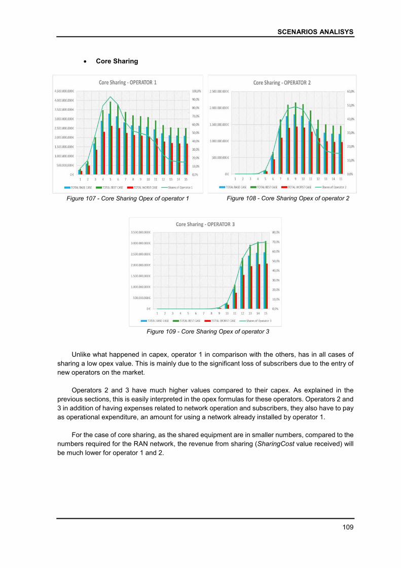
SCENARIOS ANALISYS
109
Core Sharing
Figure 107 - Core Sharing Opex of operator 1
Figure 108 - Core Sharing Opex of operator 2
Figure 109 - Core Sharing Opex of operator 3
Unlike what happened in capex, operator 1 in comparison with the others, has in all cases of
sharing a low opex value. This is mainly due to the significant loss of subscribers due to the entry of
new operators on the market.
Operators 2 and 3 have much higher values compared to their capex. As explained in the
previous sections, this is easily interpreted in the opex formulas for these operators. Operators 2 and
3 in addition of having expenses related to network operation and subscribers, they also have to pay
as operational expenditure, an amount for using a network already installed by operator 1.
For the case of core sharing, as the shared equipment are in smaller numbers, compared to the
numbers required for the RAN network, the revenue from sharing (SharingCost value received) will
be much lower for operator 1 and 2.
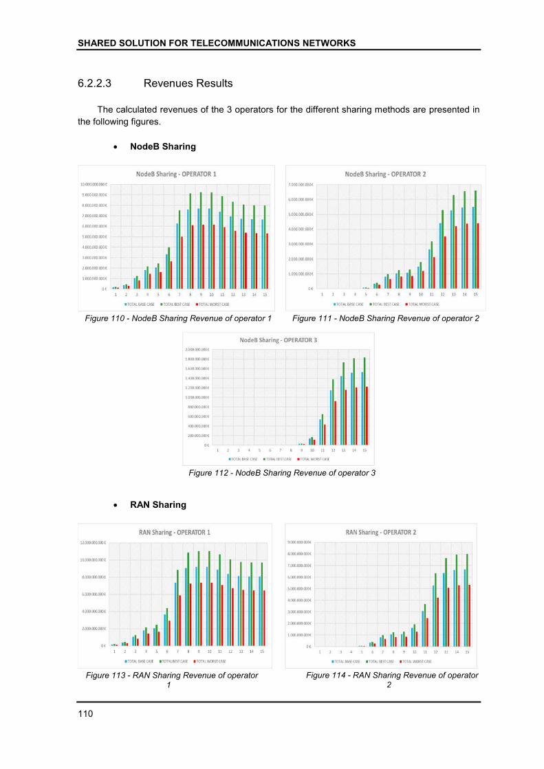
SHARED SOLUTION FOR TELECOMMUNICATIONS NETWORKS
110
6.2.2.3 Revenues Results
The calculated revenues of the 3 operators for the different sharing methods are presented in
the following figures.
NodeB Sharing
Figure 110 - NodeB Sharing Revenue of operator 1
Figure 111 - NodeB Sharing Revenue of operator 2
Figure 112 - NodeB Sharing Revenue of operator 3
RAN Sharing
Figure 113 - RAN Sharing Revenue of operator
1
Figure 114 - RAN Sharing Revenue of operator
2
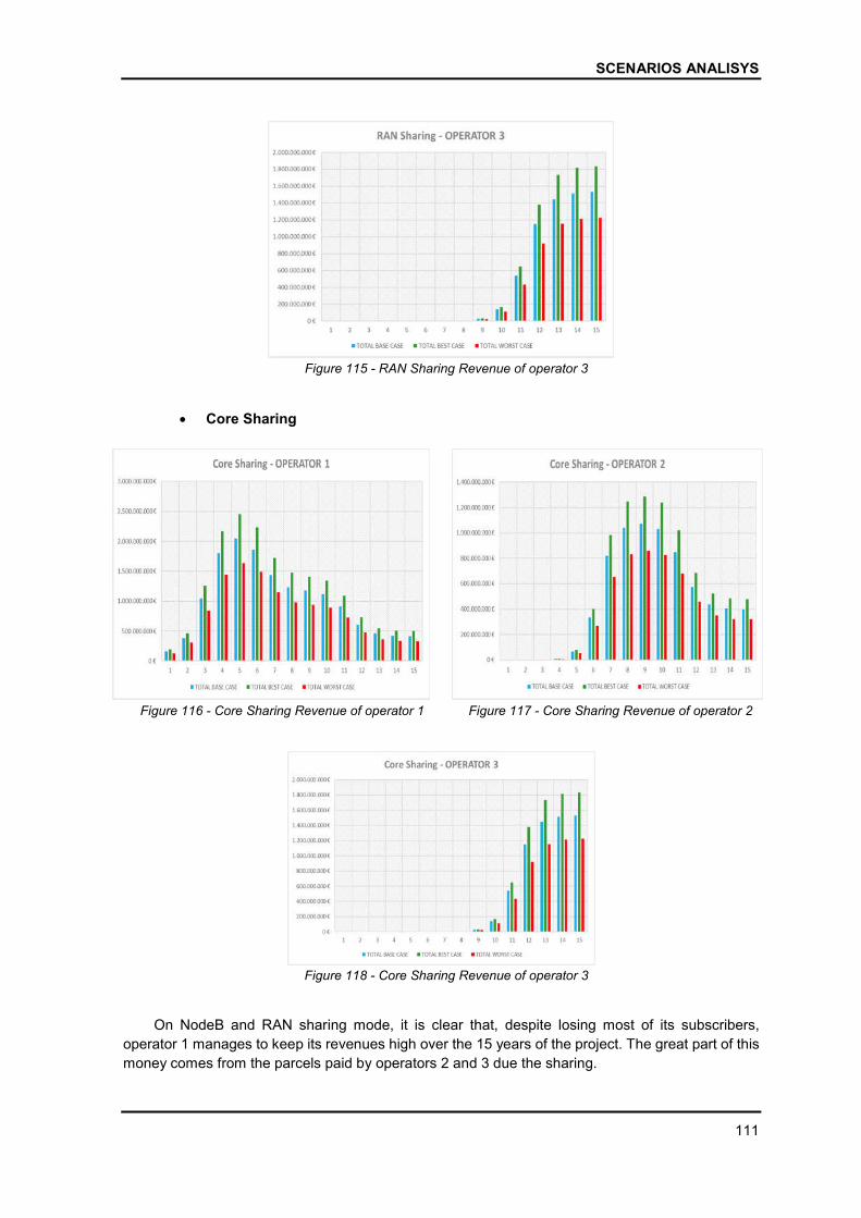
SCENARIOS ANALISYS
111
Figure 115 - RAN Sharing Revenue of operator 3
Core Sharing
Figure 116 - Core Sharing Revenue of operator 1
Figure 117 - Core Sharing Revenue of operator 2
Figure 118 - Core Sharing Revenue of operator 3
On NodeB and RAN sharing mode, it is clear that, despite losing most of its subscribers,
operator 1 manages to keep its revenues high over the 15 years of the project. The great part of this
money comes from the parcels paid by operators 2 and 3 due the sharing.

SHARED SOLUTION FOR TELECOMMUNICATIONS NETWORKS
112
On the core sharing, as the SharingCost paid to operator 1 and 2 due the share of core
equipment is much lower, the revenues of operator 1 and 2 are greatly reduced over the years.
ECONOMIC RESULTS
NodeB Sharing
Results of operator 1:
Table 47 - NPV, IRR and Payback period for Operator 1 – NodeB Sharing
Figure 119 - NodeB Sharing Economic Results of
operator 1 - Best Case
Figure 120 - NodeB Sharing Economic Results of
operator 1 - Worst Case
Figure 121 - NodeB Sharing Economic Results of operator 1 - Base Case
5%
5.110.717.994,34 €
3%
13Payback period (years)
Annual Interest Rate
NPV
IRR
Base case scenario5%
6.137.170.473,48 €
3%
13
Best case scenarioAnnual Interest Rate
NPV
IRR
Payback period (years)
5%
4.089.837.046,81 €
3%
13
Annual Interest Rate
NPV
IRR
Payback period (years)
Worst case scenario
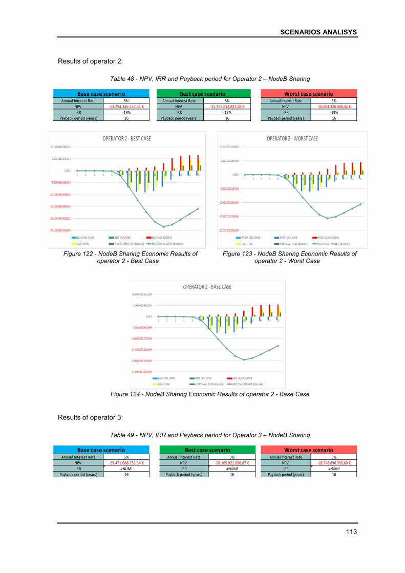
SCENARIOS ANALISYS
113
Results of operator 2:
Table 48 - NPV, IRR and Payback period for Operator 2 – NodeB Sharing
Figure 122 - NodeB Sharing Economic Results of
operator 2 - Best Case
Figure 123 - NodeB Sharing Economic Results of
operator 2 - Worst Case
Figure 124 - NodeB Sharing Economic Results of operator 2 - Base Case
Results of operator 3:
Table 49 - NPV, IRR and Payback period for Operator 3 – NodeB Sharing
5%
-13.254.346.137,31 €
-19%
16
Base case scenarioAnnual Interest Rate
NPV
IRR
Payback period (years)
5%
-15.905.612.827,40 €
-19%
16
Best case scenarioAnnual Interest Rate
NPV
IRR
Payback period (years)
5%
-10.604.326.800,34 €
-19%
16
NPV
IRR
Worst case scenarioAnnual Interest Rate
Payback period (years)
5%
-23.471.688.752,34 €
#NÚM!
16
Annual Interest Rate
NPV
IRR
Payback period (years)
Base case scenario5%
-28.165.921.098,87 €
#NÚM!
16
Best case scenario
IRR
Payback period (years)
Annual Interest Rate
NPV
5%
-18.778.896.995,69 €
#NÚM!
16
NPV
Annual Interest Rate
Worst case scenario
IRR
Payback period (years)

SHARED SOLUTION FOR TELECOMMUNICATIONS NETWORKS
114
Figure 125 - NodeB Sharing Economic Results of
operator 3 - Best Case
Figure 126 - NodeB Sharing Economic Results of
operator 3 - Worst Case
Figure 127 - NodeB Sharing Economic Results of operator 3 - Base Case
The recovery period for operator 1 is 13 years for all three cases. NPV is positive with an
average of 5.112.575.171,54 € and the IRR is 3%. Despite the low IRR the predictions for operator
1 are positive and the investment is profitable.
Although operator 2 has a negative NPV for all three cases and an IRR of -19%, it is possible
to observe in Figure 122, Figure 123 and Figure 124 that in year 12 operator 2 shows a change of
course on the cash balance but it is not enough to guarantee profits in the 15 years analyzed.
Operator 3 presents these results because he simply enters the end of the project and does not
have time to have profit.
RAN Sharing
Results of operator 1:
Table 50 - NPV, IRR and Payback period for Operator 1 – RAN Sharing
5%
12.551.744.577,52 €
7%
11
Base case scenarioAnnual Interest Rate
NPV
IRR
Payback period (years)
5%
15.097.919.278,91 €
7%
11
IRR
Payback period (years)
Best case scenarioAnnual Interest Rate
NPV
5%
10.042.830.961,95 €
7%
11
Annual Interest Rate
IRR
Worst case scenario
Payback period (years)
NPV
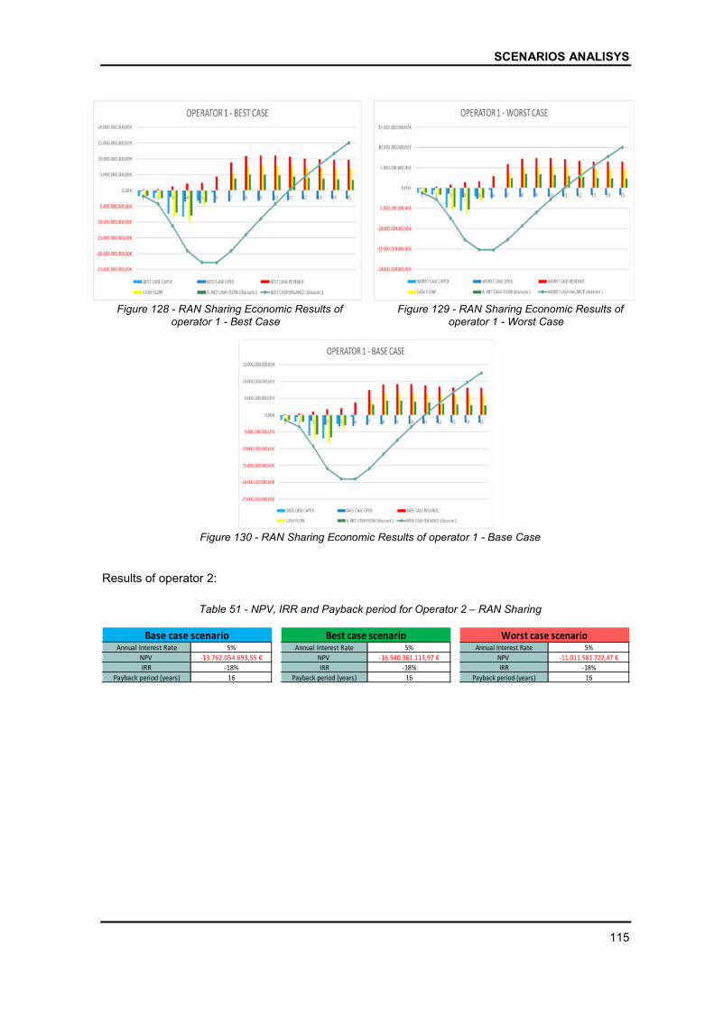
SCENARIOS ANALISYS
115
Figure 128 - RAN Sharing Economic Results of
operator 1 - Best Case
Figure 129 - RAN Sharing Economic Results of
operator 1 - Worst Case
Figure 130 - RAN Sharing Economic Results of operator 1 - Base Case
Results of operator 2:
Table 51 - NPV, IRR and Payback period for Operator 2 – RAN Sharing
5%
-13.762.054.693,55 €
-18%
16
IRR
Payback period (years)
Base case scenarioAnnual Interest Rate
NPV
5%
-16.540.361.113,97 €
-18%
16
Best case scenarioAnnual Interest Rate
NPV
IRR
Payback period (years)
5%
-11.011.581.722,47 €
-18%
16
Worst case scenarioAnnual Interest Rate
NPV
IRR
Payback period (years)
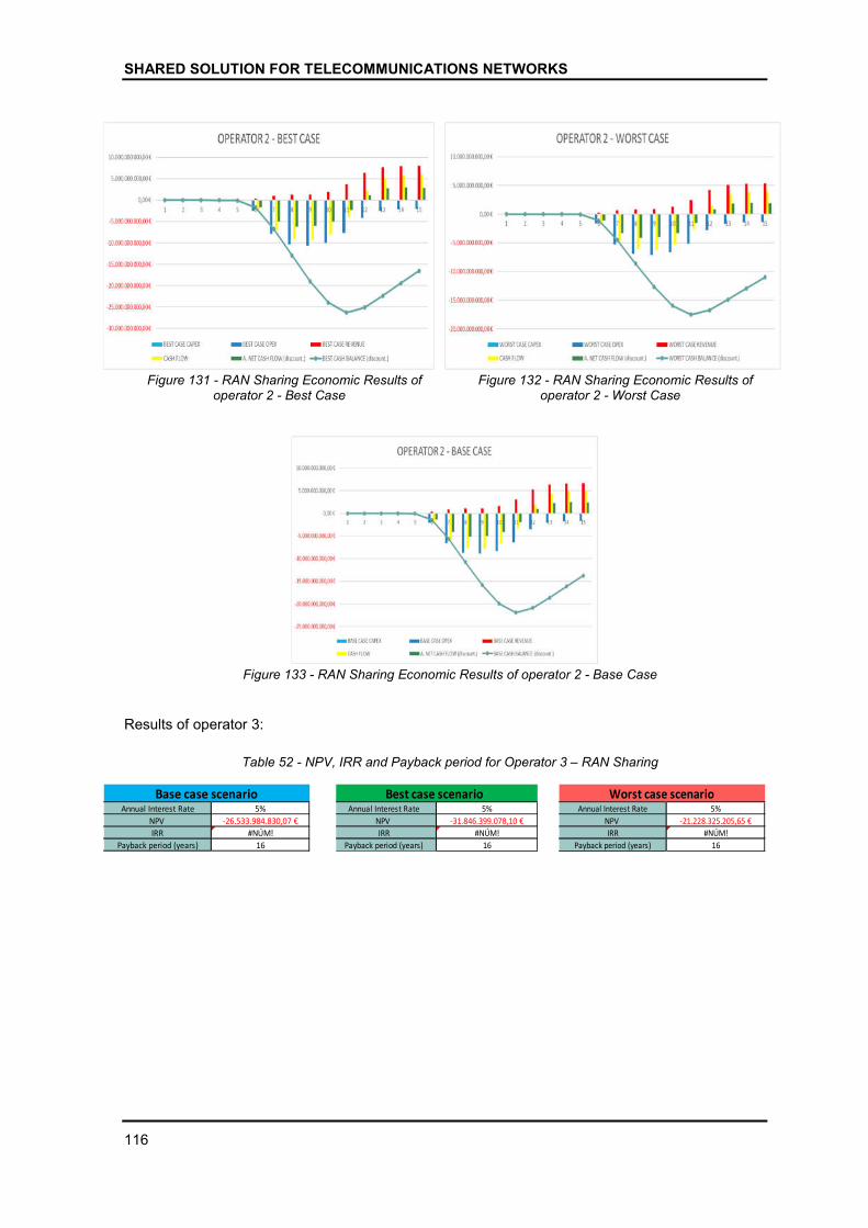
SHARED SOLUTION FOR TELECOMMUNICATIONS NETWORKS
116
Figure 131 - RAN Sharing Economic Results of
operator 2 - Best Case
Figure 132 - RAN Sharing Economic Results of
operator 2 - Worst Case
Figure 133 - RAN Sharing Economic Results of operator 2 - Base Case
Results of operator 3:
Table 52 - NPV, IRR and Payback period for Operator 3 – RAN Sharing
5%
-26.533.984.830,07 €
#NÚM!
16
Base case scenario
Payback period (years)
IRR
Annual Interest Rate
NPV
5%
-31.846.399.078,10 €
#NÚM!
16
Annual Interest Rate
NPV
IRR
Payback period (years)
Best case scenario5%
-21.228.325.205,65 €
#NÚM!
16
Worst case scenarioAnnual Interest Rate
NPV
IRR
Payback period (years)
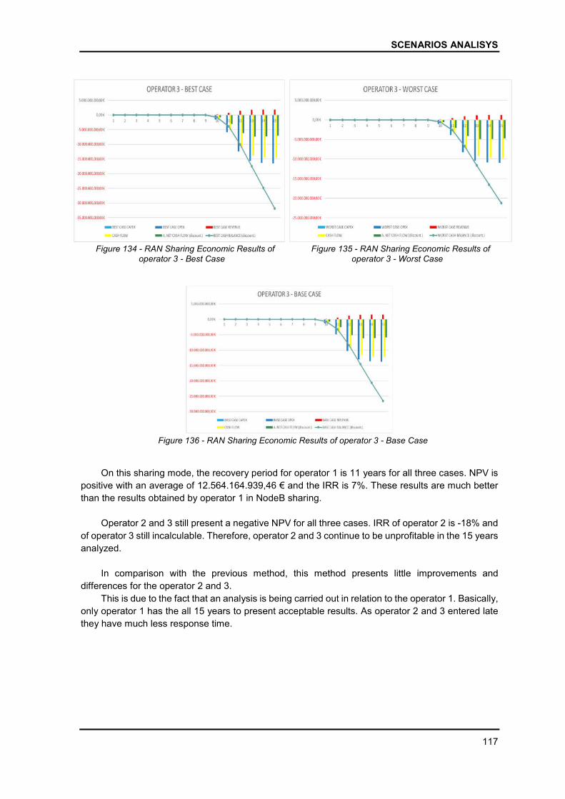
SCENARIOS ANALISYS
117
Figure 134 - RAN Sharing Economic Results of
operator 3 - Best Case
Figure 135 - RAN Sharing Economic Results of
operator 3 - Worst Case
Figure 136 - RAN Sharing Economic Results of operator 3 - Base Case
On this sharing mode, the recovery period for operator 1 is 11 years for all three cases. NPV is
positive with an average of 12.564.164.939,46 € and the IRR is 7%. These results are much better
than the results obtained by operator 1 in NodeB sharing.
Operator 2 and 3 still present a negative NPV for all three cases. IRR of operator 2 is -18% and
of operator 3 still incalculable. Therefore, operator 2 and 3 continue to be unprofitable in the 15 years
analyzed.
In comparison with the previous method, this method presents little improvements and
differences for the operator 2 and 3.
This is due to the fact that an analysis is being carried out in relation to the operator 1. Basically,
only operator 1 has the all 15 years to present acceptable results. As operator 2 and 3 entered late
they have much less response time.
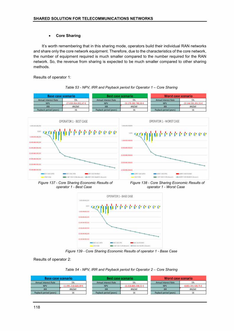
SHARED SOLUTION FOR TELECOMMUNICATIONS NETWORKS
118
Core Sharing
It’s worth remembering that in this sharing mode, operators build their individual RAN networks
and share only the core network equipment. Therefore, due to the characteristics of the core network,
the number of equipment required is much smaller compared to the number required for the RAN
network. So, the revenue from sharing is expected to be much smaller compared to other sharing
methods.
Results of operator 1:
Table 53 - NPV, IRR and Payback period for Operator 1 – Core Sharing
Figure 137 - Core Sharing Economic Results of
operator 1 - Best Case
Figure 138 - Core Sharing Economic Results of
operator 1 - Worst Case
Figure 139 - Core Sharing Economic Results of operator 1 - Base Case
Results of operator 2:
Table 54 - NPV, IRR and Payback period for Operator 2 – Core Sharing
5%
-27.658.064.892,47 €
#NÚM!
16
Annual Interest Rate
NPV
IRR
Payback period (years)
Base case scenario5%
-33.179.392.780,30 €
#NÚM!
16
NPV
IRR
Payback period (years)
Best case scenarioAnnual Interest Rate 5%
-22.144.581.201,53 €
#NÚM!
16
NPV
IRR
Payback period (years)
Worst case scenarioAnnual Interest Rate
5%
-11.095.218.669,39 €
#NÚM!
16
IRR
Payback period (years)
Base case scenarioAnnual Interest Rate
NPV
5%
-13.318.805.598,55 €
#NÚM!
16
IRR
Payback period (years)
Best case scenarioAnnual Interest Rate
NPV
5%
-8.855.593.559,75 €
#NÚM!
16
IRR
Payback period (years)
Worst case scenarioAnnual Interest Rate
NPV
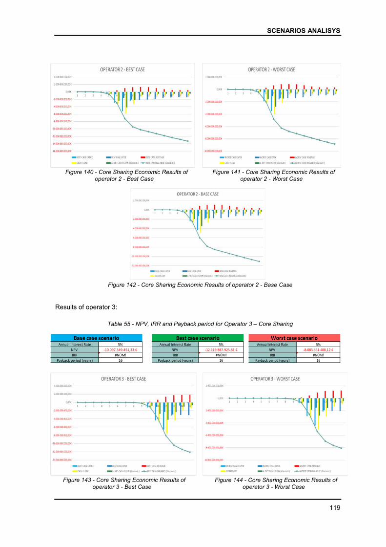
SCENARIOS ANALISYS
119
Figure 140 - Core Sharing Economic Results of
operator 2 - Best Case
Figure 141 - Core Sharing Economic Results of
operator 2 - Worst Case
Figure 142 - Core Sharing Economic Results of operator 2 - Base Case
Results of operator 3:
Table 55 - NPV, IRR and Payback period for Operator 3 – Core Sharing
Figure 143 - Core Sharing Economic Results of
operator 3 - Best Case
Figure 144 - Core Sharing Economic Results of
operator 3 - Worst Case
5%
-10.097.349.451,33 €
#NÚM!
16Payback period (years)
Base case scenarioAnnual Interest Rate
NPV
IRR
5%
-12.119.887.925,81 €
#NÚM!
16
Best case scenario
IRR
Payback period (years)
Annual Interest Rate
NPV
5%
-8.083.361.488,12 €
#NÚM!
16Payback period (years)
Worst case scenarioAnnual Interest Rate
NPV
IRR
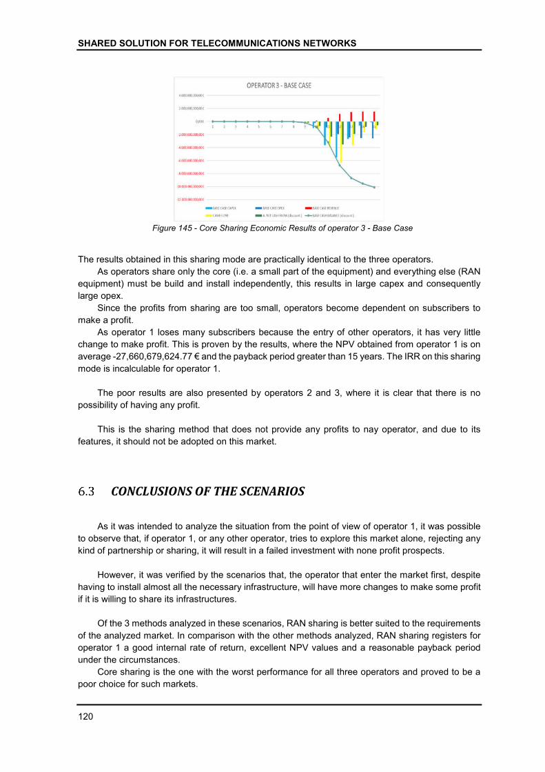
SHARED SOLUTION FOR TELECOMMUNICATIONS NETWORKS
120
Figure 145 - Core Sharing Economic Results of operator 3 - Base Case
The results obtained in this sharing mode are practically identical to the three operators.
As operators share only the core (i.e. a small part of the equipment) and everything else (RAN
equipment) must be build and install independently, this results in large capex and consequently
large opex.
Since the profits from sharing are too small, operators become dependent on subscribers to
make a profit.
As operator 1 loses many subscribers because the entry of other operators, it has very little
change to make profit. This is proven by the results, where the NPV obtained from operator 1 is on
average -27,660,679,624.77 € and the payback period greater than 15 years. The IRR on this sharing
mode is incalculable for operator 1.
The poor results are also presented by operators 2 and 3, where it is clear that there is no
possibility of having any profit.
This is the sharing method that does not provide any profits to nay operator, and due to its
features, it should not be adopted on this market.
CONCLUSIONS OF THE SCENARIOS
As it was intended to analyze the situation from the point of view of operator 1, it was possible
to observe that, if operator 1, or any other operator, tries to explore this market alone, rejecting any
kind of partnership or sharing, it will result in a failed investment with none profit prospects.
However, it was verified by the scenarios that, the operator that enter the market first, despite
having to install almost all the necessary infrastructure, will have more changes to make some profit
if it is willing to share its infrastructures.
Of the 3 methods analyzed in these scenarios, RAN sharing is better suited to the requirements
of the analyzed market. In comparison with the other methods analyzed, RAN sharing registers for
operator 1 a good internal rate of return, excellent NPV values and a reasonable payback period
under the circumstances.
Core sharing is the one with the worst performance for all three operators and proved to be a
poor choice for such markets.

SCENARIOS ANALISYS
121
Although operator 2 failed to provide positive results within 15 years analyzed for any mode of
sharing, it is possible to conclude from the analysis of the results presented in the graphs, that the
cash balance begins to rise around year 12, in the RAN and NodeB sharing modes. This proves to
be a good indicator, because if the conditions do not change operator 2 could have a positive NPV
around year 19.
There is not enough data to conclude whether operator 3 will be able to have profits after a few years.
Nevertheless, it can be concluded that the RAN sharing mode is the solution that best fits all
operators.
It should also be noted that despite the positive results of operator 1, the remaining operators
are unable to have a profitable business in this market. This is something that, in a real situation,
would cause the operator 2 and 3, especially the operator 3, to give up the market and consequently
the sharing. This would have negative consequences for the money balance of operators 1 and 2.
Therefore, it is also important to conclude that only these sharing methods are not enough to
successfully install and develop a sustainable network for all three operators. Additional strategies
should be adopted to further reduce the risk of failed investments.
There is a huge risk for operator 3 to give up sharing, since there are no potential profit
projections for operator 3 in any of the sharing methods studied. In fact, there is little time to obtain
sufficient data to draw an accurate conclusion on the projections of the operator 3, but as in year 15
the whole network is already built and the whole market is already served, there is no leeway for the
operator 3.
The strategies can be several, they can go through further diversifying the subscriber base, thus
creating more price ranges for private, institutional or business. Or even limit the traffic at certain
times of the day to the institutions and businesses, since they do not need so much traffic outside of
business hours.


CONCLUSIONS
123
CONCLUSIONS
The project of this dissertation started from the need to try to prove that existing technologies
and methodologies can get telecommunications to regions and places that do not yet have, but are
in urgent need of have those service available. Nowadays, in the way the world is managed and
operated, it is regrettable that many regions and countries still have a weak or nonexistent
telecommunications service. It is a fact that many of these regions are found in developing countries.
These emerging markets are often in difficulties and have various economic and financial problems.
This results in a population with weak purchasing power.
Regardless of the place, telecommunications is an expensive business. Therefore, this
dissertation analyzes the problem of the implementation of cellular networks in emerging markets
and the implications and benefits that the sharing of infrastructures may have on the economic
viability of the operators involved in the sharing.
It was implemented and adapted a mathematical model for dimensioning a network. Later, a
numerical tool was adapted and developed to model, dimension and calculate the costs of
implementing a cellular network. At the end, a technical-economic study of the projected network
was carried out. The tool calculates the network by the introduction of parameters that define the
type and size of the target market, the market's trafficking needs and the characteristics of the region.
It was conceived 2 scenarios that served as input parameters that allowed to perceive the
problematic introduction of cellular networks in emerging markets with and without shared
infrastructures.
As a consequence of this study it was observed that in fact a shared network brings more
benefits to the operators. If the operator tries to embark on this market alone the profit forecasts are
negligible. One hypothesis would be to greatly increase the fees charged to subscribers to make a
profit. But that would not be possible because the market does not have enough purchasing power.
The most viable solution is to share the infrastructures built with other operators. It has been
observed that the NodeB and RAN sharing methods are those that produce profitable results. The
core sharing mode is not suitable for this market.
With this, it is possible to prove that if there is a need to develop a given region or country with
a market with these characteristics, the network can be implemented by the government and then
shared with other operators through the RAN sharing method. Done this way the government will
have its investment recovered in 11 years and will manage to develop and open the market to other
operators and businesses.
But it is crucial to reaffirm that, in order to avoid having resignations from the operators who
entered the shared market late, additional strategies should be used to keep the interest of all
satisfied. Because it has also been verified that the profit projections of the third operator are reduced,
which can correctly lead to a withdrawal by the third operator.
To apply the models and tools developed in this project, it was necessary to have a large number
of assumptions regarding multiple parameters. It is known that the accuracy of these models and the
SHARED SOLUTION FOR TELECOMMUNICATIONS NETWORKS
124
corresponding tool depend on these parameters, so these assumptions must be as correct as
possible.
It should be stated that the work developed in this document, although designed for the
UMTS900, is applicable to different technologies and different types of traffic.
FUTURE WORK
Due to the vastness of the area of study of this dissertation, it was not possible to cover all the
topics of interest. Therefore, following are presented several topics, parameters and issues which
may be considered for improve the development and performance of this tool:
Take into considerations the abandonment effect on the market uptake and consider the fact that a user can subscribe to more than 1 operator;
Do not assume a static market, but a market in which the number of subscribers and their intensity of use vary over time;
Improve capacity dimensioning techniques taking into account the heterogeneous nature of the traffic and the equipment involved;
Consider the equipment life time;
Include in the tool the possibility of technological evolution (migration UMTS, LTE, 5G, etc.).
REFERENCES
125
REFERENCES
[1] J. E. Flood, "Mobile Communication," in Telecommunication Networks, 2nd ed., London, Institution of Eletrical Engineers, 1997.
[2] V. Pauli, J. D. Naranjo and E. Seidel , "Heterogeneous LTE Networks and Inter-Cell Interference Coordination," Nomor Research, Munich, 2010.
[3] T. Farley and M. Van Der Hoek, "Privateline," [Online]. Available: http://www.ccs.neu.edu/home/futrelle/teaching/com1204sp2001/Farley/Cellbasics.html. [Accessed 16 06 2016].
[4] D. C. Carrilho, "Redes Híbridas de Acesso Fixo sem Fios: Análise TecnoEconómica," Department of Electronics, Telecommunications and Informatics, Aveiro, 2010.
[5] D. Tipper, "Fundamentals of Cellular Networks," University of Pittsburgh, Pittsburgh.
[6] T. S. Rappaport, Wireless Communications: Principles and Practice, 2nd ed., New Jersey: Prentice Hall PTR Upper Saddle River, 2001.
[7] Federal Standard 1037C, "Telecomunications: Glossary of Telecomunication Terms," 7 August 1996. [Online]. Available: http://www.its.bldrdoc.gov/fs-1037/fs-1037c.htm. [Accessed 18 Jul. 2016].
[8] C. Vieira, in Interferência no Sistema WCDMA, Brasil, Escola de Engenharia, Universidade Federal Fluminense, 2010, p. 92.
[9] V. Arokiamary, "Cellular Concept and System Design Fundamentals," in Mobile Comunications, India, Technical Publications Pune, 2009.
[10] B. Lopes, "Technoeconomic study for a Mobile WiMAX Solution in Luanda," 2008.
[11] Wikipedia, "Wikipedia," [Online]. Available: https://en.wikipedia.org/wiki/Cellular_network. [Accessed 10 11 2017].
[12] R. Wallace, "Antenna Selection Guide, Application Notes AN058," Texas Instruments, Texas.
[13] "Antenna Efficiency and Antenna Gain, Antenna Theory," [Online]. Available: http://www.antenna-theory.com/basics/gain.php. [Accessed 19 Jul. 2016].
[14] "Bandwidth, Antenna Theory," [Online]. Available: http://www.antenna-theory.com/basics/bandwidth.php. [Accessed 19 Jul. 2016].
[15] Direct Industry, "Wireless Instruments," [Online]. Available: http://www.directindustry.com/prod/wireless-instruments/product-163454-1705898.html. [Accessed 10 11 2017].
[16] X. Li, "Radio Access Network Dimensioning for 3G UMTS, Communication Networks," University of Bremen, 2009.
[17] I. Poole, "Radio-Electronics.com," [Online]. Available: http://www.radio-electronics.com/info/cellulartelecomms/cellular_concepts/tdd-fdd-time-frequency-division-duplex.php. [Accessed 27 July 2016].
[18] D. Soldani, "QoS Management In UMTS Terrestrial Radio Access FDD Networks," Department of Electrical and Communications Engineering, Helsinki University of Technology, Espoo, 2005.
[19] A. M. d. O. Duarte, "Redes Cellulares - Notas de Estudo," Departament of Electronics, Telecomunication and Information, University of Aveiro, Aveiro, 2014.
[20] A. M. O. Duarte, "Cellular Networks Wireless LANs," Department of Electronics, Telecomunications and Informatics, University of Aveiro, Aveiro, 2012-2013.
[21] M. C. Chuah and Z. Q, Design and performance of 3G wireless networks and wireless lands, Springer, 2006.
SHARED SOLUTION FOR TELECOMMUNICATIONS NETWORKS
126
[22] GSMA, "GSMA," [Online]. Available: https://www.gsma.com/aboutus/gsm-technology. [Accessed 2017].
[23] G. Heine, GSM Network: Protocol, Terminology and Implementation, Norwood: Artech House, 1998.
[24] I. N. Kriaras, W. A. Jarvis, E. V. Phillips and J. D. Richards, "Third-Generation Mobile Network Architecture for the Universal Mobile Telecommunication System (UMTS)," Bell Labs Technical Journal, 1997.
[25] T. N. UMTS, "3G UMTS Network Solution," 2013.
[26] ETSI, "Technologies," [Online]. Available: http://www.etsi.org/technologies-clusters/technologies.
[27] J. U. Sverzut, in Redes GSM, GPRS, EDGE e UMTS, 1º ed., São Paulo, SP: Editora Érica, 2005, pp. 70-394.
[28] T. N. U. "3G UMTS Network Solution," 2013.
[29] A. Mitschele-Thiel and J. Muckenheim, "UMTS System Architecture and Protocol Architecture," 2010.
[30] ETSI, "GSM 03.40," [Online]. Available: http://www.etsi.org/deliver/etsi_gts/03/0340/05.03.00_60/gsmts_0340v050300p.pdf. [Accessed 24 10 2016].
[31] 3GPP, "LTE Network Architecture Technical Specification Release 10," 2011.
[32] 3GPP, "ITU-R Confers IMT-Advanced (4G) Status to 3GPP LTE," 20 10 2010. [Online]. Available: http://www.3gpp.org/news-events/3gpp-news/1319-ITU-R-Confers-IMT-Advanced-4G-Status-to-3GPP-LTE. [Accessed 14 05 2017].
[33] C. Cox, An Introduction to LTE, Wiley, 2012.
[34] C. Gessner, A. Roessler and M. Kottkamp, "UMTS Long Term Evolution (LTE) - Technology Introduction," Rohde & Schwarz, 2012.
[35] D. Flore, "LTE RAN Architecture Aspects," Beijing, 2009.
[36] Qualcomm Technologies, Inc., "Delivereing on the LTE Advanced Promise," 2016.
[37] D.-E. Meddour, T. Rasheed and Y. Gourhant, "On the Role of Infrastructure Sharing for Mobile Network Operators in Emerging Markets".
[38] J. Krzywicki, "Trends in mobile infrastructure sharing," Analysys Mason, 2010.
[39] Autoridade da Concorrência, "Partilha de Redes de Comunicações Eletrónicas," Autoridade da Concorrência, 2012.
[40] GSMA, "Mobile Infrastructure Sharing," United Kingdom, 2012.
[41] Steel in the Air, Inc, "Cell Site Types," Steel in the Air, Inc, [Online]. Available: http://www.steelintheair.com/cell-site-types. [Accessed 14 07 2017].
[42] E. Onuzuruike, "Telecom Infrastructure Sharing as a Strategy for Cost Optimization and Revenue Generation : A Case Study of MTN Nigeria/Zain Nigeria Collocation," Blekinge Institute of Technology, Karlskrona, 2008.
[43] P. Vornpuan, "Infrastruture Sharing in Pratice: Sharing Mobile Networks," Nokia Siemens Networks, 2010.
[44] KPMG, "Passive Infrastructure Sharing in Telecomunications".
[45] GSMA, "www.gsma.com," August 2012. [Online]. Available: http://www.gsma.com/publicpolicy/wp-content/uploads/2012/09/Africa-International-roaming-explained-English.pdf. [Accessed 19 Jul. 2016].
[46] C. B. Lefèvre, "Mobile Sharing," ITU, 2008.
[47] J. P. Guedes Simões Ramos, "Telecommunications Infrastructure Sharing in Mozambique," Universidade de Aveiro, Aveiro, 2014.
[48] ITU - International Telecommunications Union, "Telecom Network Planning for evolving Network Architectures Reference Manual," ITU, Geneva, 2008.
[49] L. K. Vanston, "Residential Broadband Forecasts," Technology Futures, Inc., Austin Texas, 2002.
REFERENCES
127
[50] A. M. d. O. Duarte, "Modeos de Previsão: Adoção e Abandono de Tecnologias e Produtos; Evolução do Preço de um Produto em Função do seu Grau de Maturidade," 2014.
[51] J. A. Norton and F. M. Bass, "A Diffusion Theory Model of Adoption and Substitution for Successive Generations of High-Technology Products," 1987.
[52] Ovum Consulting, "Market Study for UMTS900 - A Report to GSMA," London, 2007.
[53] Nokia Siemens Networks, "LTE RPESS Radio Planning Capacity".
[54] Nokia Siemens Networks, "Mobile Broadband with HSPA and LTE - Capacity and Cost Aspects," Nokia Siemens Networks Corporation, 2010.
[55] Westbay Engineers, "Erlang," 14 07 2014. [Online]. Available: http://www.erlang.com/whatis.html. [Accessed 20 09 2017].
[56] I. Angus, "An Introduction to Erlang B and Erlang C," Telemanagement, Canada, 2001.
[57] R. Parkinson, "Traffic Engineering Techniques in Telecommunications," Infotel Systems Inc. Retrieved, 2005.
[58] H. Holma and A. Toskala, "WCDMA for UMTS: Radio Access for Third Generation Mobile Communications," John Wiley & Sons, 2004.
[59] 3GPP TR 25.101, "User Equipment (UE) radio transmission and reception (FDD)".
[60] F. Simba, L. Trojer, B. Mwinyiwiwa, N. Mvungi and E. Mjema, "Techno-economic Analysis of UMTS900 and UMTS2100 for Rural Connectivity in Tanzania," in 14th IEEE International Conference on Communication Technology (ICCT), Chengdu, 2012.
[61] COST Action 231, Digital Mobile Radio Towards Future Generation Systems : Final Report, European Commission, 1999.
[62] S. Verbrugge and e. a. , "White Paper: Pratical Steps in Techno-Economic Evaluation of Network Deployment Planning," Gent University, 2009.
[63] Investopedia, "Capital Expenditure (CAPEX)," Investopedia, [Online]. Available: http://www.investopedia.com/terms/c/capitalexpenditure.asp. [Accessed 13 09 2017].
[64] Investopedia, "Operating Expense," Investopedia, [Online]. Available: http://www.investopedia.com/terms/o/operating_expense.asp. [Accessed 13 09 2017].
[65] Investopedia, "Cash Flow," Investopedia, [Online]. Available: http://www.investopedia.com/terms/c/cashflow.asp?ad=dirN&qo=investopediaSiteSearch&qsrc=0&o=40186. [Accessed 13 09 2017].
[66] A. M. d. O. Duarte, "Techno-Economic Analysis of Engineering Projects," DETI, Universidade de Aveiro, Aveiro, 2013.
[67] Investopedia, "Revenue," Investopedia, [Online]. Available: http://www.investopedia.com/terms/r/revenue.asp. [Accessed 13 09 2017].
[68] Investopedia, "Net Present Value - NPV," [Online]. Available: http://www.investopedia.com/terms/n/npv.asp. [Accessed 25 9 2017].
[69] Investopedia, "Internal Rate Of Return - IRR," [Online]. Available: http://www.investopedia.com/terms/i/irr.asp. [Accessed 27 09 2017].
[70] N. Nogueira, "Portal Gestão," [Online]. Available: https://www.portal-gestao.com/artigos/6513-o-que-%C3%A9-a-taxa-interna-de-rentabilidade-tir.html. [Accessed 27 09 2017].
[71] Investopedia, "Payback Period," [Online]. Available: http://www.investopedia.com/terms/p/paybackperiod.asp. [Accessed 27 09 2017].
[72] A. M. d. O. Duarte, Comunicação pessoal, Aveiro.
[73] The William and Anita Newman Library, "Telecommunications Industry," The William and Anita Newman Library, 13 07 2017. [Online]. Available: http://guides.newman.baruch.cuny.edu/c.php?g=188304&p=1243472. [Accessed 22 10 2017].
[74] US Business Reporter, "Telecommunication," [Online]. Available: http://www.activemedia-guide.com/datadict.asp?txtSrchWord=Telecommunication. [Accessed 22 10 2017].
SHARED SOLUTION FOR TELECOMMUNICATIONS NETWORKS
128
[75] "Cisco," [Online]. Available: http://www.cisco.com/en/US/prod/collateral/wireless/ps7183/ps469/images/0900aecd806a1a3e_null_null_null_08_07_07-12.jpg. [Accessed 19 Jul. 2016].
[76] "Antenna Theory," [Online]. Available: http://www.antenna-theory.com/. [Accessed 19 Jul. 2016].
[77] K. T. Wong and A. K.-Y. Lai, "Inexpensive Upgrade of BaseStation Dumb Antennas by Two Magnetic Loops for “Blind” Adaptive Downlink," Department of Electrical & Computer Engineering, University of Waterloo, Canada and Department of Electronic Engineering, Chinese University of Hong Kong, Hong Kong, 2005.
[78] I. Poole, "Radio-electronics.com," [Online]. Available: http://www.radio-electronics.com/info/cellulartelecomms/lte-long-term-evolution/lte-mimo.php. [Accessed 19 Jul. 2016].
[79] W. Wang and I. F. Akyildiz, "A New Signaling Protocol for Intersystem Roaming in Next-Generation Wireless Systems," IEEE, 2001.
[80] WordTimeZone, "GSM World Coverage Map and GSM Country List," 02 03 2017. [Online]. Available: http://www.worldtimezone.com/gsm.html. [Accessed 22 06 2017].
[81] D. J. M. Texeira, "Telecommunications Infrastructure Sharing," Universidade de Aveiro, Aveiro, 2015.
[82] J. P. Ramos, "Telecommunication Infrastructure Sharing in Mozambique," Universidade de Aveiro, Aveiro, 2014.
[83] M. Stasiak and e. a. , Modeling and Dimensioning of Mobile Networks – From GSM, Wiley, 2010.
[84] Y. Ouyang and F. H. M, "An Analysis of Traffic and Throughput for UMTS Packet Core Networks," Howe School of Technology Management, Stevens Institute of Technology, Hoboken.
[85] 3GPP TR 25.104, "Base Station (BS) radio transmission and reception (FDD)".
[86] M. J. Nawrocki, M. Dohler and A. H. Aghvami, "Understanding UMTS Radio Network Modeling Planning and Automated Optimization," Wiley, 2006.
[87] ECC within CEPT, "Compatibility study for UMTS operating within the GSM 900 and GSM 1800 frequency bands," ECC REPORT 82, Roskilde, 2006.
[88] A. Drobot, "The Future of Wireless," in IEEE Wireless Communications Networks Conference - WCNC 2010, Sydney, 2010.
[89] Telenor R&D, "Telektronikk," Telecommunications Forecasting, p. 34, 2004.
[90] Huawei, "Huawei RNC Capacity Dimension," Huawei.
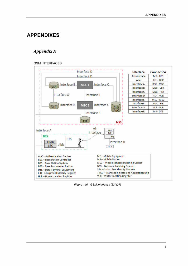
APPENDIXES
i
APPENDIXES
Appendix A
GSM INTERFACES
Figure 146 - GSM interfaces [23] [27]
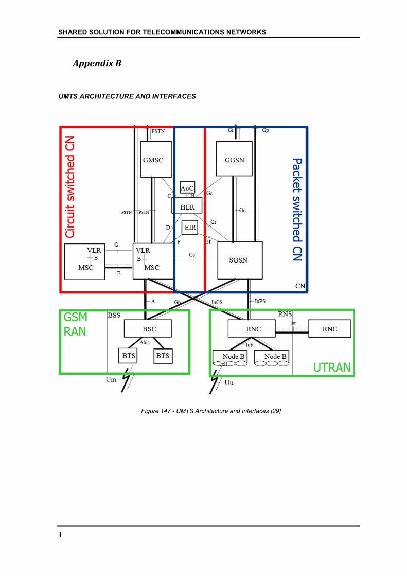
SHARED SOLUTION FOR TELECOMMUNICATIONS NETWORKS
ii
Appendix B
UMTS ARCHITECTURE AND INTERFACES
Figure 147 - UMTS Architecture and Interfaces [29]

APPENDIXES
iii
Appendix C
LTE FULL ARCHITECTURE
Figure 148 - LTE Full Architecture
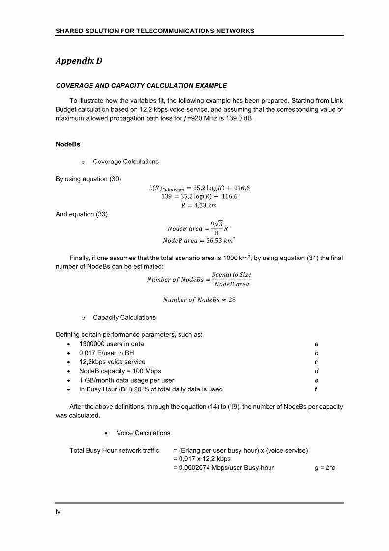
SHARED SOLUTION FOR TELECOMMUNICATIONS NETWORKS
iv
Appendix D
COVERAGE AND CAPACITY CALCULATION EXAMPLE
To illustrate how the variables fit, the following example has been prepared. Starting from Link
Budget calculation based on 12,2 kbps voice service, and assuming that the corresponding value of
maximum allowed propagation path loss for �=920 MHz is 139.0 dB.
NodeBs
o Coverage Calculations
By using equation (30)
�(�)�������� = 35,2 log(�)+ 116,6
139 = 35,2 log(�)+ 116,6
� = 4,33��
And equation (33)
��������� =9√3
8��
��������� = 36,53���
Finally, if one assumes that the total scenario area is 1000 km2, by using equation (34) the final
number of NodeBs can be estimated:
�������������� =������������
���������
�������������� ≈ 28
o Capacity Calculations
Defining certain performance parameters, such as:
1300000 users in data a
0,017 E/user in BH b
12,2kbps voice service c
NodeB capacity = 100 Mbps d
1 GB/month data usage per user e
In Busy Hour (BH) 20 % of total daily data is used f
After the above definitions, through the equation (14) to (19), the number of NodeBs per capacity
was calculated.
Voice Calculations
Total Busy Hour network traffic = (Erlang per user busy-hour) x (voice service)
= 0,017 x 12,2 kbps
= 0,0002074 Mbps/user Busy-hour g = b*c
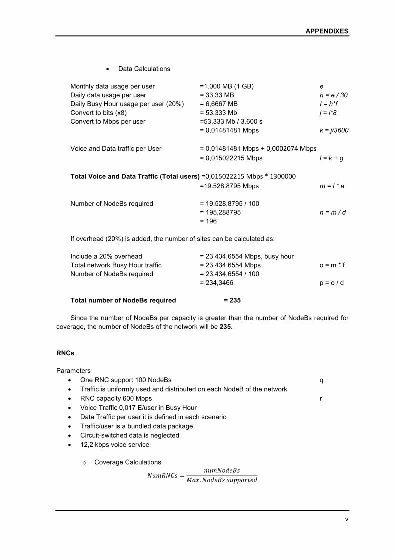
APPENDIXES
v
Data Calculations
Monthly data usage per user =1.000 MB (1 GB) e
Daily data usage per user = 33,33 MB h = e / 30
Daily Busy Hour usage per user (20%) = 6,6667 MB I = h*f
Convert to bits (x8) = 53,333 Mb j = i*8
Convert to Mbps per user =53,333 Mb / 3.600 s
= 0,01481481 Mbps k = j/3600
Voice and Data traffic per User = 0,01481481 Mbps + 0,0002074 Mbps
= 0,015022215 Mbps l = k + g
Total Voice and Data Traffic (Total users) =0,015022215 Mbps * 1300000
=19.528,8795 Mbps m = l * a
Number of NodeBs required = 19.528,8795 / 100
= 195,288795 n = m / d
= 196
If overhead (20%) is added, the number of sites can be calculated as:
Include a 20% overhead = 23.434,6554 Mbps, busy hour
Total network Busy Hour traffic = 23.434,6554 Mbps o = m * f
Number of NodeBs required = 23.434,6554 / 100
= 234,3466 p = o / d
Total number of NodeBs required = 235
Since the number of NodeBs per capacity is greater than the number of NodeBs required for
coverage, the number of NodeBs of the network will be 235.
RNCs
Parameters
One RNC support 100 NodeBs q
Traffic is uniformly used and distributed on each NodeB of the network
RNC capacity 600 Mbps r
Voice Traffic 0,017 E/user in Busy Hour
Data Traffic per user it is defined in each scenario
Traffic/user is a bundled data package
Circuit-switched data is neglected
12,2 kbps voice service
o Coverage Calculations
������� =���������
���. ���������������
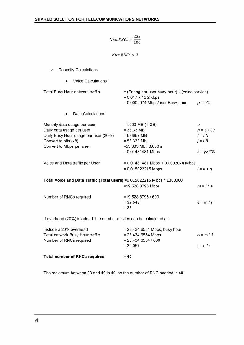
SHARED SOLUTION FOR TELECOMMUNICATIONS NETWORKS
vi
������� =235
100
������� ≈ 3
o Capacity Calculations
Voice Calculations
Total Busy Hour network traffic = (Erlang per user busy-hour) x (voice service)
= 0,017 x 12,2 kbps
= 0,0002074 Mbps/user Busy-hour g = b*c
Data Calculations
Monthly data usage per user =1.000 MB (1 GB) e
Daily data usage per user = 33,33 MB h = e / 30
Daily Busy Hour usage per user (20%) = 6,6667 MB I = h*f
Convert to bits (x8) = 53,333 Mb j = i*8
Convert to Mbps per user =53,333 Mb / 3.600 s
= 0,01481481 Mbps k = j/3600
Voice and Data traffic per User = 0,01481481 Mbps + 0,0002074 Mbps
= 0,015022215 Mbps l = k + g
Total Voice and Data Traffic (Total users) =0,015022215 Mbps * 1300000
=19.528,8795 Mbps m = l * a
Number of RNCs required =19.528,8795 / 600
= 32,548 s = m / r
= 33
If overhead (20%) is added, the number of sites can be calculated as:
Include a 20% overhead = 23.434,6554 Mbps, busy hour
Total network Busy Hour traffic = 23.434,6554 Mbps o = m * f
Number of RNCs required = 23.434,6554 / 600
= 39,057 t = o / r
Total number of RNCs required = 40
The maximum between 33 and 40 is 40, so the number of RNC needed is 40.