DEPARTAMENTO DE FÍSICA

The influence of geometric factors on the wall shear

stress distribution in realistic human coronary

arteries

Jorge André Piedade Pinhal dos Santos

Dissertação apresentada na Faculdade de Ciências e Tecnologia da Universidade Nova de Lisboa para a obtenção do grau de Mestre em Engenharia Biomédica. A presente dissertação foi desenvolvida no Erasmus Medical Center em Roterdão, Holanda.

Orientadora:

Dr. Ir. Jolanda J. Wentzel

Lisboa 2009

Jorge Santos ii

Acknowledgments

In the first place I would like to thanks Dr. Ir. Jolanda Wentzel for her

supportive supervision and for her patience for reading and correcting all the drafts I

have written during this period.

My special thanks to Diana and Sandro, my cousins, and to “our Portuguese

group” in Rotterdam, who helped and supported me during these six months abroad.

I would also like to thank all the researchers and colleagues in the

Biomechanics Laboratory in the Erasmus MC, who welcomed me and treated me as

one of them.

Thanks also to all of my friends, especially to Samuel, Eduardo, Daniel, Barros,

Filipa, Sara, Osório and Hugo, without whom, the last five years wouldn’t have been so

much fun and unforgettable.

To Inês, my special thanks for all the care and courage given. You are my ally.

Finally, my most special thanks to my brother Pedro, and my parents Luís and

Carminda, who are always there for me and are the most important persons in my life.

Jorge Santos iii

Abstract

Background:

Atherosclerosis is the main cause of death in the Western society. It is a geometrically focal

disease, affecting preferentially vessel areas of low wall shear stress (SS), which induces the

expression of atherogenic genes. To predict wall SS several options are available. Among them

Computational Fluid Dynamics (CFD) simulations on 3D reconstructed coronaries using Finite

Element Modeling (FEM). However, to perform CFD a 3D representation is needed. To obtain a

3D representation of the coronary under study different methods can be applied.

Methods:

CFD calculations were performed using FEM on ten 3D reconstructed coronary arteries by the

state-of-the-art ANGUS method (biplane angiography + Intravascular Ultrasound (IVUS)). The

SS outcomes of the CFD calculations were compared with SS calculated by the Poiseuille

equation, and with the SS outcomes of CFD simulations of the same 3D reconstructed arteries

by QCA-3D (biplane angiography – no cross-sectional information) and Straight (IVUS images

stacked on a straight centerline – no curvature information) methods.

Results:

The Poiseuille equation did not have any sensitivity in predicting any low SS (<0.5 Pa) per cross-

section. However, the average correlation coefficient between the average SS per cross section

from the Angus geometries and SS based on the Poiseuille equation was r2 = 0.65 0.09. A

strong correlation was obtained for the SS from the ANGUS and the Straight method, while

only an average correlation was obtained between ANGUS and QCA-3D average SS. Bland-

Altman analysis was performed to confirm the results agreement. The sensitivity and

specificity of the QCA-3D and Straight method in predicting low and high SS was measured.

Geometric factors, such as local curvature, area gradient and torsion were found to be related

to the presence of SS peaks or to regions prone to plaque development. These geometric risk

factors were utilized to give some guidelines on meshing optimization.

Conclusions:

The use of a simpler 3D reconstruction approach, such as the QCA-3D or the Straight method,

in combination with the optimization of meshing based on the geometric features of the

coronaries, has the potential to, in the future, bring CFD calculations of wall SS from bench to

bedside.

Jorge Santos iv

Resumo

Introdução:

A aterosclerose é a principal causa de morte na sociedade ocidental. É uma doença

geometricamente focal que afecta preferencialmente áreas da parede de vasos com baixa

tensão de cisalhamento, induzindo a expressão de genes aterogénicos. Hoje em dia para

prever a tensão de cisalhamento (SS) da parede arterial várias opções são viáveis. Entre elas,

simulações de Dinâmica de Fluidos Computacional (CFD) em coronárias reconstruídas em 3D

em conjugação com Modelação em Elementos Finitos (FEM). Assim sendo, para realizar

cálculos CFD, a representação 3D das coronárias é necessária. Para obter estas representações

3D vários métodos podem ser usados.

Métodos:

Os cálculos CFD são realizados usando FEM em dez artérias coronárias reconstruídas em 3D

pelo método padrão ANGUS (angiografia biplanar + Ultrassom Intravascular (IVUS)). Os valores

de SS obtidos nos cálculos CFD são comparados com os valores de SS calculados pela equação

de Poiseuille, e com o SS obtido pelos cálculos CFD para as mesmas artérias coronárias, mas

reconstruídas em 3D pelo método QCA-3D (angiografia biplanar – sem informação sobre a

forma de cada secção de corte) e pelo método Straight (imagens IVUS empilhadas ao longo de

um eixo recto – sem informação da curvatura).

Resultados:

A equação de Poiseuille não tem sensibilidade para prever um valor de SS baixo (SS<0.5) em

cada secção de corte. Contudo, o coeficiente de correlação média, entre o valor médio de SS

em cada secção de corte por geometrias Angus e SS baseado na equação de Poiseuille são r2 =

0.65 0.09. Uma forte correlação foi obtida a partir dos valores de SS obtido com ANGUS e o

pelo método Straight, enquanto apenas foi obtida uma correlação média entre o SS médio por

corte entre o método ANGUS e o método QCA-3D. Uma análise Bland-Altman foi realizada

para confirmar a concordância dos resultados. A sensibilidade e a especificidade do método

QCA-3D e do método Straight para prever baixos e altos valores de SS foram medidas. Factores

geométricos, como a curvatura local, o gradiente em área e a torção foram relacionados com a

presença de picos de SS ou com regiões propensas ao desenvolvimento de placas. Estes

factores de risco geométricos foram usados para dar algumas orientações para optimização

das malhas de elementos finitos.

Conclusões:

A utilização de reconstruções 3D mais simples, como o método QCA-3D ou o método Straight,

em combinação com a optimização das malhas baseada nos parâmetros geométricos das

artérias coronárias, tem potencial para, no futuro, trazerem os cálculos CFD do SS da parede

arterial da teoria para a prática.

Jorge Santos v

Abbreviations list ANGUS – Angiography + Intravascular ultrasound

CAAS – Cardiovascular Angiography Analysis System

QCA-3D –Quantitative Coronary Analysis 3D

CFD – Computational Fluid Dynamics

De – Dean Number

eNOS – Endothelial nitric oxide synthase

ESS – Endothelial Shear Stress

FDA – Food and Drug Administration

FEM – Finite Element Method

IVUS – Intravascular ultrasound

LAD – Left anterior descending artery

LCA – Left coronary artery

LCX – Left circumflex artery

LDL – Low density lipoprotein

LMCA – Left main coronary artery

RCA – Right coronary artery

Re – Reynolds number

SS – Shear stress

VCAM-1 – Vascular cell adhesion molecule-1

Jorge Santos vi

Table of contents

LIST OF FIGURES VIII

LIST OF TABLES XI

INTRODUCTION 13

CHAPTER 1. BACKGROUND 13

1.1. CORONARY ARTERIES 13

1.2. ARTERIAL WALL ANATOMY 15

1.3. ATHEROSCLEROSIS 15

1.4. THE ROLE OF SHEAR STRESS IN ATHEROSCLEROSIS 17

1.5. NAVIER-STOKES EQUATIONS – CFD AND FEM 20

1.6. POISEUILLE FLOW 21

1.7. 3D RECONSTRUCTION METHODS 22

1.7.1. ANGUS 23

1.7.2. QCA-3D 24

1.7.3. STRAIGHT 24

CHAPTER 2. AIM 25

CHAPTER 3. METHODS 27

3.1. COMPUTATIONAL FLUID DYNAMICS 27

3.1.1. ASSUMPTIONS AND BOUNDARY CONDITIONS 28

3.2. ANALYSIS 29

3.2.1. ANGUS VS. POISEUILLE 29

3.2.2. ANGUS VS. STRAIGHT & ANGUS VS. QCA-3D 30

3.2.3. GEOMETRIC PARAMETERS INFLUENCE 32

CHAPTER 4. ANGUS VS. POISEUILLE 33

4.1. RESULTS 34

4.1.1. AVERAGE SHEAR STRESS VS. LUMEN AREA 34

4.1.2. INFLUENCE OF BLOOD FLOW 36

4.1.3. BLAND-ALTMAN ANALYSIS 38

4.1.4. LOCAL WALL SHEAR STRESS HISTOGRAM 40

4.1.5. VELOCITY PROFILES 41

CHAPTER 5. ANGUS VS. QCA-3D 44

5.1. RESULTS 45

Jorge Santos vii

5.1.1. AVERAGE SHEAR STRESS AND LUMEN AREA 45

5.1.2. BLAND-ALTMAN ANALYSIS 47

5.1.3. MAXIMUM SHEAR STRESS 48

5.1.4. LOCAL WALL SHEAR STRESS HISTOGRAM 49

5.1.5. LOW SS ANALYSIS 50

5.1.6. HIGH SS ANALYSIS 52

CHAPTER 6. ANGUS VS. STRAIGHT 54

6.1. RESULTS 55

6.1.1. AVERAGE SHEAR STRESS AND LUMEN AREA 55

6.1.2. BLAND-ALTMAN ANALYSIS 57

6.1.3. MAXIMUM SHEAR STRESS 59

6.1.5. LOCAL WALL SHEAR STRESS HISTOGRAM 61

6.1.6. LOW SS ANALYSIS 62

6.1.7. HIGH SS ANALYSIS 65

6.1.8. LONGITUDINAL SHEAR STRESS 68

CHAPTER 7. GEOMETRIC FACTORS 71

7.1. RESULTS 71

7.1.1. LUMEN AREA GRADIENT 71

7.1.2. LOCAL CURVATURE 75

7.1.3. OTHER GEOMETRICAL ABNORMALITIES 76

7.1.4. GUIDELINES TO MESH OPTIMIZATION 79

CHAPTER 8. DISCUSSION 80

8.1. LIMITATIONS 80

8.2. ANGUS VS. POISEUILLE 80

8.3. ANGUS VS. QCA-3D 82

8.4. ANGUS VS. STRAIGHT 83

8.5. GEOMETRIC FACTORS 85

CHAPTER 9. CONCLUSION 87

10. REFERENCES 88

11. APPENDIX 91

Jorge Santos viii

List of figures

Figure 1.1 - Main coronary arteries.......................................................................... 14

Figure 1.2 - Arterial wall layers ................................................................................ 15

Figure 1.3 - Healthy human artery vs. artery narrowed by atherosclerotic plaque ... 16

Figure 1.4 - Clot formation on a coronary artery ...................................................... 17

Figure 1.5 - Definition of endothelial shear stress [7] ............................................... 17

Figure 1.6 - Atheroprotective vs. atherogenic phenotype [5] ................................... 19

Figure 1.7 - Eccentric plaque regions [10] ................................................................ 19

Figure 1.8 - Poiseuille flow (velocity) profile ............................................................ 22

Figure 1.9 - Different flow profiles (adapted from Christian Poelma’s Biological Fluid

Mechanics lecture on Blood tissue interaction; the role of wall shear stress. Delft

University of Technology)[16] .................................................................................. 22

Figure 1.10 - A) IVUS images of a RCA; B) Angiographic image from the same artery;

C) 3D reconstruction [18] ........................................................................................ 24

Figure 2.1 - ANGUS, QCA-3D, Straight and Poiseuille – 3D Reconstructions example

and a corresponding cross-section from each method. ........................................... 26

Figure 3.1 - Example of the finite element mesh of a coronary artery ...................... 28

Figure 4.1 - 3D reconstruction of a left anterior descending artery by the ANGUS

method (in the left) and a Poiseuille cylinder with the same cross sectional area .... 33

Figure 4.2 - Average SS vs. Lumen Area plots ........................................................... 34

Figure 4.3 - Average SS vs. Lumen Area, based on the CFD calculations (o) and the

Poiseuille formula (-) ............................................................................................... 35

Figure 4.4 - Poiseuille shear stress versus Average shear stress – Influence of blood

flow ......................................................................................................................... 36

Figure 4.5 - Poiseuille and Average SS scatter plots for 100%, 50%, 10% and 1% of

physiological blood flow .......................................................................................... 37

Figure 4.6 - Average r2 – Average SS vs. Poiseuille SS ............................................... 38

Figure 4.7 - Bland-Altman plot (ANGUS vs Poiseuille) .............................................. 39

Figure 4.8 - Local Wall SS Histogram ........................................................................ 40

Figure 4.9 - Velocity profiles for different blood flows (100%, 50%, 10% and 1%) for a

cross section located in a curved region .................................................................. 41

Jorge Santos ix

Figure 4.10 - Velocity profiles for different blood flows (100%, 50%, 10% and 1%) for

a stenotic cross section ........................................................................................... 43

Figure 4.11 - Velocity profiles for different blood flows (100%, 50%, 10% and 1%) for

a “normal” cross section.......................................................................................... 43

Figure 5.1 - 3D reconstructions of a left anterior descending artery by the ANGUS (in

the left) and the QCA-3D techniques ....................................................................... 44

Figure 5.2 - Average SS vs Lumen Area plots from ANGUS (o) and QCA-3D (o) ......... 45

Figure 5.3 - Lumen area and average SS per cross section from ANGUS and QCA-3D46

Figure 5.4 - Correlation between Average SS from ANGUS and QCA-3D .................. 46

Figure 5.5 - Bland-Altman plot of the average SS per cross section .......................... 47

Figure 5.6 - Lumen Area, Maximum, Average and Minimum SS per cross section –

ANGUS vs QCA-3D (example) .................................................................................. 48

Figure 5.7 - Bland-Altman plot – Maximum SS per cross section .............................. 49

Figure 5.8 - Local wall SS histogram (ANGUS vs QCA-3D) ......................................... 50

Figure 5.9 - Example of a vessel with low SS elements (<0.5 Pa) for the ANGUS, the

QCA-3D method and the overlapping cross-sections. .............................................. 51

Figure 5.10 - Example of a vessel with high SS elements (in this case <5.01 Pa) for the

ANGUS, the QCA-3D method and the overlapping cross-sections. ........................... 53

Figure 6.1 - 3D reconstruction of the curved ANGUS vessel (left) and from the

corresponding straight vessel (right) ....................................................................... 54

Figure 6.2 - 3D view of the local wall SS distribution in both ANGUS original vessel

and in the straight vessel ......................................................................................... 55

Figure 6.3 - Lumen Area and Average SS comparison between ANGUS and Straight

vessels ..................................................................................................................... 56

Figure 6.4 - Lumen Area and Average SS comparison between ANGUS and Straight

vessels ..................................................................................................................... 56

Figure 6.5 - Bland-Altman plot of the average SS per cross section for all patients .. 58

Figure 6.6 - Lumen Area, Average SS and Maximum SS per cross section comparisons,

between ANGUS and Straight vessels ...................................................................... 59

Figure 6.7 - Wall SS distribution of an ANGUS and a Straight geometry ................... 60

Figure 6.8 - 3D view of the SS distribution in the reconstructed ANGUS and Straight

vessels ..................................................................................................................... 60

Jorge Santos x

Figure 6.9 - Wall shear stress histogram (Angus vs Straight) .................................... 61

Figure 6.10 - Example of a vessel with elements with low SS (<0.5 Pa) for the ANGUS,

the Straight method and the overlap of both .......................................................... 63

Figure 6.11 - Example of a vessel with low SS elements (<0.5 Pa) for the ANGUS, the

Straight method and the overlapping cross-sections ............................................... 64

Figure 6.12 - Example of a vessel with elements with high SS (>9.32 Pa) for the

ANGUS and the Straight method, and the overlap of both ...................................... 66

Figure 6.13 - Example of a vessel with elements with high SS (>9.32 Pa) for the

ANGUS and the Straight method, and the overlapping cross-sections. .................... 67

Figure 6.14 - Wall SS distribution an ANGUS and a Straight geometry ..................... 68

Figure 6.15 - Mean Longitudinal SS for ANGUS and the Straight vessel (p060362) ... 68

Figure 6.16 - Longitudinal Shear Stress .................................................................... 69

Figure 7.1 - Average SS Gradient vs Lumen Area Gradient ....................................... 72

Figure 7.2 - Example of the relation between the lumen area gradient and the

gradient in SS .......................................................................................................... 73

Figure 7.3 - Lumen area gradient and average SS per cross section along a coronary

length ...................................................................................................................... 74

Figure 7.4 - Example of the relation between the lumen area gradient and the local

SS ............................................................................................................................ 74

Figure 7.5 - Curvature parameters ........................................................................... 75

Figure 7.6 - Curvature radius vs. maximum SS per cross-section .............................. 76

Figure 7.7 – Dean Number vs. maximum SS per cross-section ................................. 76

Figure 7.8 - Highlight of the dots deviated from the line based on the Poiseuille

equation .................................................................................................................. 77

Figure 11.1 – Average Shear Stress vs. Lumen Area, based on the CFD calculations (o)

and the Poiseuille formula (-), of all ten coronaries ................................................. 92

Jorge Santos xi

List of tables

Table 1.1 - Mean diameters of the main coronaries according to Mosseri et al. [2] . 14

Table 3.1 - Patients, corresponding coronaries and some geometric and flow features

of the ANGUS reconstructed vessels........................................................................ 27

Table 3.2 - Inflow rate and pressure (in and out) values for the CFD calculations ..... 29

Table 3.3 – Measure of sensitivity and Specificity .................................................... 32

Table 4.1 - Correlation coefficients (r2) .................................................................... 38

Table 4.2 - Bland-Altman statistic results ................................................................. 39

Table 4.3 - Average SS from CFD calculations and Poiseuille SS for the 57th cross

section of patient p060233. Re is an abbreviation for Reynolds number ................. 42

Table 5.1 - Average Shear Stress correlation parameters ......................................... 47

Table 5.2 - Correlation coefficients (r2) for the Maximum SS per cross section ........ 49

Table 5.3 – Cross-sections with low SS (<0.5 Pa) by ANGUS and QCA-3D method .... 50

Table 5.4 – High SS threshold for all patients. .......................................................... 52

Table 5.5 - Percentage of cross sections with high SS (> x Pa) in the ANGUS and

QCA-3D method ...................................................................................................... 53

Table 6.1 - Correlation coefficients (r2) for the Average and Maximum SS per cross

section .................................................................................................................... 57

Table 6.2 - Bland-Altman analysis results for all patients individually ...................... 58

Table 6.3 - Percentage of elements with low SS (<0.5 Pa) in the ANGUS and Straight

method ................................................................................................................... 62

Table 6.4 - Percentage of cross sections with low SS (<0.5 Pa) in the ANGUS and

Straight method ...................................................................................................... 63

Table 6.5 - Elements with high SS (> x Pa) in the ANGUS and Straight method .. 65

Table 6.6 - Percentage of cross sections with high SS (> x Pa) in the ANGUS and

Straight method ...................................................................................................... 67

Table 6.7 - Average longitudinal SS .......................................................................... 69

Table 7.1 - Average SS Gradient vs Lumen Area Gradient – correlation coefficient and

linear regression line slope and y-intercept ............................................................. 72

Table 11.1 - Regression line coefficients from the scattering of ANGUS based Average

SS versus Poiseuille based SS ................................................................................... 91

Jorge Santos xii

Table 11.2 - Some geometric and flow parameters of the QCA-3D reconstructed

vessels ..................................................................................................................... 91

Table 11.3 - Some geometric and flow parameters of the Straight reconstructed

vessels ..................................................................................................................... 92

Jorge Santos 13

Introduction

The research to this Master Dissertation in Biomedical Engineering was

performed at the Biomechanics Laboratory of the Biomedical Engineering

Department, which is part of the Thoraxcenter of the Erasmus Medical Center in

Rotterdam, The Netherlands. The supervisor of this project and head of the

Biomechanics Lab. is Dr. ir. Jolanda J. Wentzel. The Biomedical Engineering is a

research group focused on the cardiovascular diseases, namely on its origin,

diagnosis and treatment. The Biomedical Engineering is, then, divided in the

Experimental Echocardiography group and the Biomechanics Lab. At the latest,

researchers study the effects of the mechanical stresses on the development and

progression of vascular disease, namely atherosclerosis. The research includes cell

studies, animal experiments and patient studies. In order to study the relationship

between biomechanical parameters and vascular disease is used the combination of

imaging modalities and computer modeling, resulting in applications such as ANGUS.

Chapter 1. Background

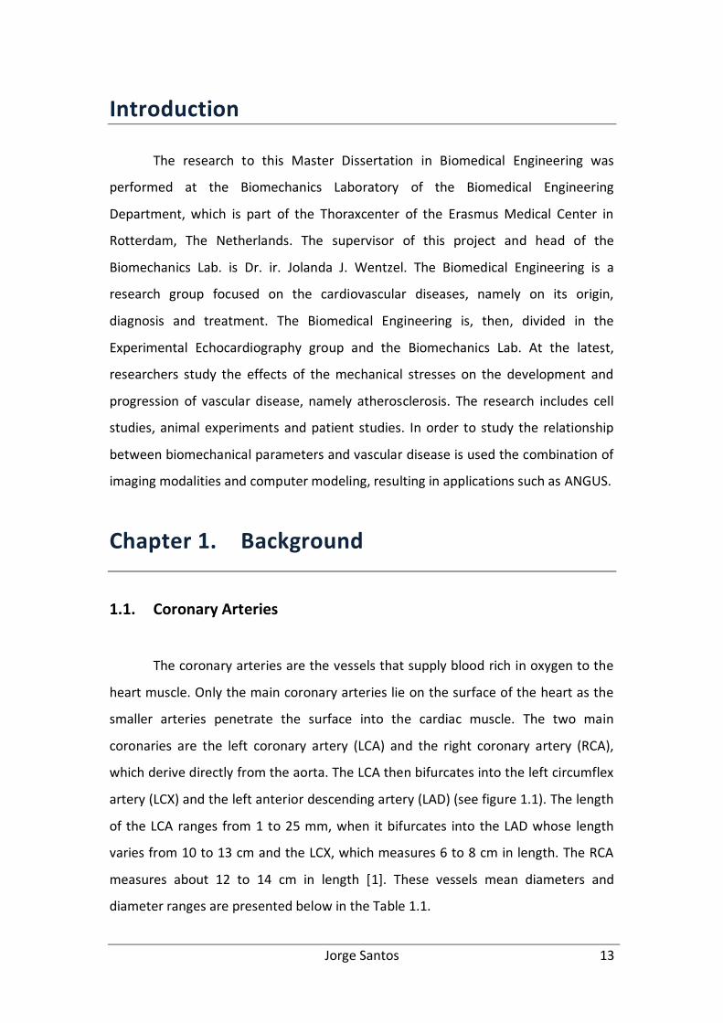
1.1. Coronary Arteries

The coronary arteries are the vessels that supply blood rich in oxygen to the

heart muscle. Only the main coronary arteries lie on the surface of the heart as the

smaller arteries penetrate the surface into the cardiac muscle. The two main

coronaries are the left coronary artery (LCA) and the right coronary artery (RCA),

which derive directly from the aorta. The LCA then bifurcates into the left circumflex

artery (LCX) and the left anterior descending artery (LAD) (see figure 1.1). The length

of the LCA ranges from 1 to 25 mm, when it bifurcates into the LAD whose length

varies from 10 to 13 cm and the LCX, which measures 6 to 8 cm in length. The RCA

measures about 12 to 14 cm in length [1]. These vessels mean diameters and

diameter ranges are presented below in the Table 1.1.

Jorge Santos 14

Figure 1.1 - Main coronary arteries (http://cognitorex.blogspot.com/2007/06/i-got-new-

stent-today.html)

Coronary Artery Mean Diameter (mm) SD Range (mm)

LMCA 4.7 1.0 3.6 – 7.2

Proximal LAD 3.9 0.8 2.4 – 5.6

Distal LAD 1.7 0.4 1.2 – 2.7

LCX 3.4 0.8 1.5 – 5.2

Proximal RCA 3.6 0.8 2.0 – 4.8

Distal RCA 2.7 0.9 1.1 – 4.5

Table 1.1 - Mean diameters of the main coronaries according to Mosseri et al. [2]

The LCA supplies mainly the anterior and lateral portions of the left ventricle

while the RCA supplies most of the right ventricle and the posterior part of the left

ventricle in 80 to 90 percent of people [3].

The blood flow in coronary arteries is laminar, which means that it flows at a

steady rate through the vessels, with each layer of blood remaining at the same

distance from the wall. The central portion of the blood stays in the center of the

vessel [3]. Since the flow in coronary arteries is laminar, the Reynolds number is also

low. The non-dimensional Reynolds number is the measure of tendency for

turbulence to occur and it is represented by the following equation:

vdRe (1)

In equation (1), v is the velocity of blood flow, d is diameter of the vessel, η is

the viscosity and ρ is the density. The transition between laminar and turbulent flow

Jorge Santos 15

does not occur at a specific Reynolds number, even though, if the Reynolds number

is below 2000 the fluid flow is laminar. Between 2000 and 4000 the flow is in

transition between laminar and turbulent flow, and if the Reynolds number is over

4000 the flow is considered to be completely turbulent. The typical Reynolds number

in coronary arteries is around 250[3].

1.2. Arterial Wall Anatomy

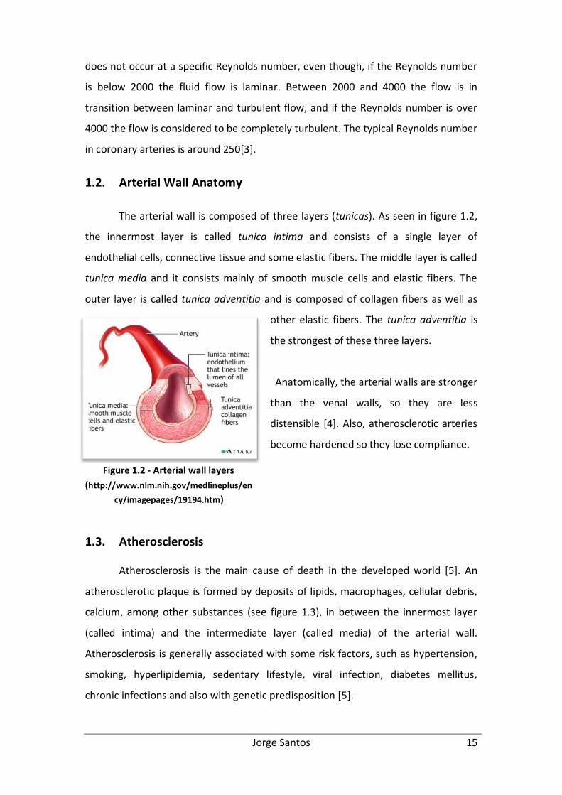
The arterial wall is composed of three layers (tunicas). As seen in figure 1.2,

the innermost layer is called tunica intima and consists of a single layer of

endothelial cells, connective tissue and some elastic fibers. The middle layer is called

tunica media and it consists mainly of smooth muscle cells and elastic fibers. The

outer layer is called tunica adventitia and is composed of collagen fibers as well as

other elastic fibers. The tunica adventitia is

the strongest of these three layers.

Anatomically, the arterial walls are stronger

than the venal walls, so they are less

distensible [4]. Also, atherosclerotic arteries

become hardened so they lose compliance.

1.3. Atherosclerosis

Atherosclerosis is the main cause of death in the developed world [5]. An

atherosclerotic plaque is formed by deposits of lipids, macrophages, cellular debris,

calcium, among other substances (see figure 1.3), in between the innermost layer

(called intima) and the intermediate layer (called media) of the arterial wall.

Atherosclerosis is generally associated with some risk factors, such as hypertension,

smoking, hyperlipidemia, sedentary lifestyle, viral infection, diabetes mellitus,

chronic infections and also with genetic predisposition [5].

Figure 1.2 - Arterial wall layers

(http://www.nlm.nih.gov/medlineplus/en

cy/imagepages/19194.htm)

Jorge Santos 16

The origin of an atherosclerotic

plaque is due to the excessive

accumulation of LDL (low-density

lipoprotein, also known as bad

cholesterol, and composed of

lipids and a protein) particles in

the arterial wall. Those LDL

particles undergo some chemical

alterations such as oxidation. The

cells in the vessel interpret these modified LDLs as a danger sign, so the endothelial

cells of the artery start to display adhesion molecules on their blood-facing surface.

These adhesion molecules attract monocytes and T cells in the blood into the intima,

where the monocytes mature into macrophages that will ingest the modified LDLs

and produce inflammatory mediators. The macrophages become filled with fatty

substances (they transform into foam cells) and along with the T cells they constitute

the early form of a plaque. A fibrous cap is formed over the lipid core and smooth

muscle cells migrate from the media to the top of the intima, multiply and produce a

fibrous matrix that glues the cells together [6]. These plaques can grow into the

artery lumen, restricting it, causing lumen narrowing, which can hamper the blood

delivery to the tissues. Vessel stenosis can provoke, among others, angina pectoris.

Plaques that are at high risk to rupture (called vulnerable plaques) are characterized

by a certain composition: necrotic core, inflammatory cells infiltration (macrophage

and T cells), large lipid pool and a thin fibrous cap. If a vulnerable plaque ruptures it

can cause a thrombus or a clot. If a clot is big enough it can block a blood vessel

causing a heart attack or a stroke, if it is a coronary or a brain artery respectively

(figure 1.4).

Figure 1.3 - Healthy human artery vs. artery

narrowed by atherosclerotic plaque

Jorge Santos 17

Figure 1.4 - Clot formation on a coronary artery

(http://64.143.176.100/library/healthguide/en-us/support/topic.asp?hwid=zm2431)

1.4. The role of shear stress in Atherosclerosis

Forces are inflicted on vascular tissues in different directions. There are

circumferential and radial forces (tensile or compressive), and there are tangential

forces such as shear. The endothelial shear stress (ESS) is the tangential force

derived by the friction of the flowing blood on the endothelial surface. It is the

product of the shear rate (difference of velocity between two different layers divided

by the distance between them, or dV/dr) at the wall and the blood viscosity (µ) [7].

dr

dVs

Figure 1.5 - Definition of endothelial shear stress [7]

Due to the pulsatile nature of the blood flow and the geometric configuration

of the arteries, there are different patterns of endothelial shear stress. In the straight

Jorge Santos 18

parts of the arteries the shear stress varies from 1.5 to 7 Pa [7]. Though, in irregular

regions, like outer walls of vessel bifurcations, the shear stress is usually low and

oscillatory, with values ranging from <1 to 1.2 Pa.

The endothelial cells of the arteries respond to the different range of shear

stress values in different ways. Even though the shear stress has magnitudes of only

5 Pa, the endothelial cells are specially equipped with a dedicated sensing

mechanism, the mechanoreceptors, which are capable to detect those shear stress

stimuli on the endothelial cells surface [8]. After detecting the shear stress stimulus,

a complex pathway known as mechanotransduction is activated.

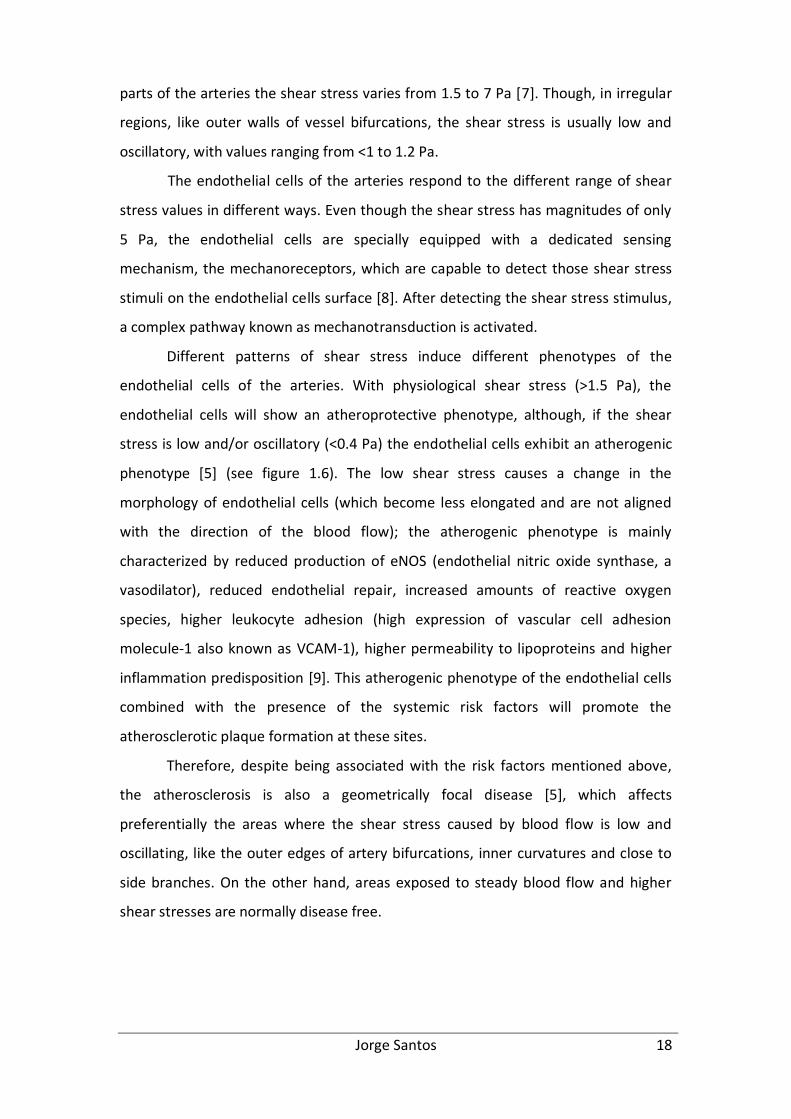
Different patterns of shear stress induce different phenotypes of the

endothelial cells of the arteries. With physiological shear stress (>1.5 Pa), the

endothelial cells will show an atheroprotective phenotype, although, if the shear

stress is low and/or oscillatory (<0.4 Pa) the endothelial cells exhibit an atherogenic

phenotype [5] (see figure 1.6). The low shear stress causes a change in the

morphology of endothelial cells (which become less elongated and are not aligned

with the direction of the blood flow); the atherogenic phenotype is mainly

characterized by reduced production of eNOS (endothelial nitric oxide synthase, a

vasodilator), reduced endothelial repair, increased amounts of reactive oxygen

species, higher leukocyte adhesion (high expression of vascular cell adhesion

molecule-1 also known as VCAM-1), higher permeability to lipoproteins and higher

inflammation predisposition [9]. This atherogenic phenotype of the endothelial cells

combined with the presence of the systemic risk factors will promote the

atherosclerotic plaque formation at these sites.

Therefore, despite being associated with the risk factors mentioned above,

the atherosclerosis is also a geometrically focal disease [5], which affects

preferentially the areas where the shear stress caused by blood flow is low and

oscillating, like the outer edges of artery bifurcations, inner curvatures and close to

side branches. On the other hand, areas exposed to steady blood flow and higher

shear stresses are normally disease free.

Jorge Santos 19

Figure 1.6 - Atheroprotective vs. atherogenic phenotype [5]

In addition to the role shear stress has in the atherosclerotic plaque

formation, it is thought that it also plays an important role in the development of

those plaques, into a quiescent or high-risk (vulnerable) atherosclerotic plaque [7,

10, 11].

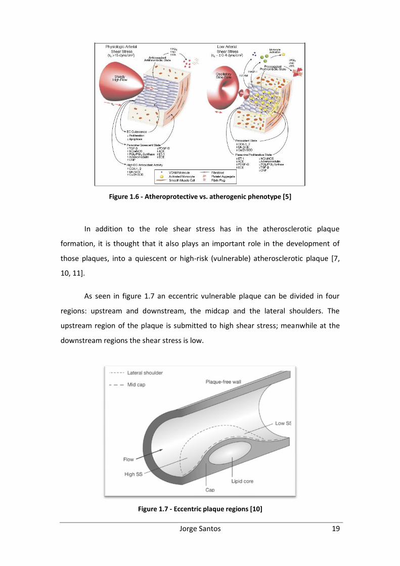
As seen in figure 1.7 an eccentric vulnerable plaque can be divided in four

regions: upstream and downstream, the midcap and the lateral shoulders. The

upstream region of the plaque is submitted to high shear stress; meanwhile at the

downstream regions the shear stress is low.

Figure 1.7 - Eccentric plaque regions [10]

Jorge Santos 20

When a plaque begins to grow, the lumen narrowing is prevented by outward

vessel remodeling [10], in order to maintain normal values of shear stress. However,

this vessel remodeling has some consequences. It can promote the plaque growth or

even the plaque rupture. The plaque growth can occur in the downstream region of

the plaque, due to low shear stress, which favors the atherosclerotic progression.

The plaque fissuring occurs mainly at the upstream lateral plaque shoulders, and it is

suggested that the high shear stress can be a reason for it, as it stimulates the

endothelium to thin the fibrous cap [10]. Subsequently the tensile stress causes the

plaque disruption at the lateral shoulders, because at those regions the fibrous cap is

thinner and has, consequently, less resistance to tensile strength [12]. As the tensile

stress is cyclic (due to oscillations in blood pressure), it can also lead to cap fatigue

and rupture [12].

Thus it is important to continue studying new approaches on estimating wall

shear stress in coronary arteries in order to predict atherosclerotic plaque

development and progression.

1.5. Navier-Stokes equations – CFD and FEM

The Navier-Stokes equations are a set of differential equations that describe

the motion of a viscous fluid. G.G. Stokes and C.L. Navier first derived them

independently in the early 1800’s. This set of equations consists of an equation for

conservation of mass, conservation of momentum equations and a conservation of

energy. Unlike algebraic equations, the Navier-Stokes’s do not establish a relation

among the variables of interest (like velocity or pressure). Instead, they establish

relations among the rates of change of these variables [13, 14].

For an incompressible, Newtonian, temperature independent and uniform

fluid, with a laminar flow, the continuity equation (a) and the Navier-Stokes

equations (b), can be written as:

03

3

2

2

1

1

x

u

x

u

x

uudiv (a)

Jorge Santos 21

,. fdivuut

u

(b)

In which Tuuuu 321 ,, stands for the velocity vector, the density of the

fluid, 321 ,, ffff the body force per unit of mass, and the stress tensor. [15]

In theory, the Navier-Stokes equations, for a given flow problem can be

solved analytically by using methods from calculus. Though, in practice, these

equations are too difficult to solve analytically for real life geometries. So, nowadays,

computers are used to solve approximations to the equations using techniques such

as finite volume or finite element methods. This field of study is called

Computational Fluid Dynamics (CFD).

In order to calculate SS through CFD, in any geometry, the 3D representation

of that geometry in the computer software is needed.

The FEM is a general discretization tool for partial differential equations,

alternative to the finite difference methods or finite volume methods. With FEM it is

fairly easy to solve problems in complex geometries. On the other hand, the

programming of FEM is more complicated than the previously mentioned methods.

In FEM, the region where the differential equation is defined is subdivided

into simple elements. In ℝ the elements are intervals, in ℝ2 are triangles or

quadrilaterals and in ℝ3 are usually tetrahedra or hexahedra. This subdivision of a

region in elements, called mesh, is performed by a mesh generator. In each element

are then chosen a number of nodal points [15] and the unknown function is

approximated by a polynomial (it is common practice to restrict to lower degree

polynomials – linear or quadratic).

1.6. Poiseuille flow model

As written above, the flow in the coronary arteries is considered to be

laminar. So if we consider the blood as an incompressible fluid and the vessels as a

stiff cylindrical tube with a constant diameter, the blood flow can be expressed by

the Hagen-Poiseuille formula: 4

8

r

LQP

. Where P is the pressure drop between

the ends of the cylinder, is the dynamic viscosity of the fluid, L is the length of the

Jorge Santos 22

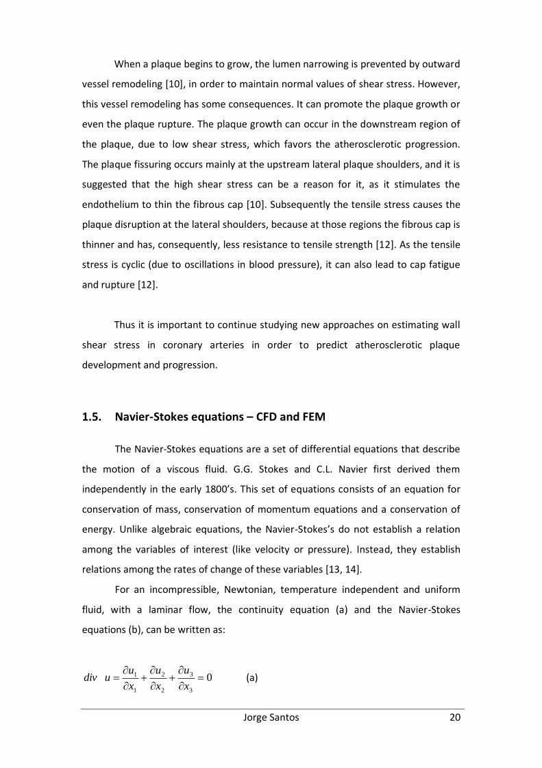
tube, Q is the flow rate and r is the radius of the cylinder. According to Poiseuille’s

theory of flow the velocity has a parabolic profile, where the velocity is highest at the

center of the tube and zero at the tube walls (figure 1.8).

The wall shear stress can be mathematically derived from the Hagen-

Poiseuille equation: 3

4

r

Qs

Figure 1.8 - Poiseuille flow (velocity) profile (adapted from

http://www.columbia.edu/~kj3/Dslide4.jpg)

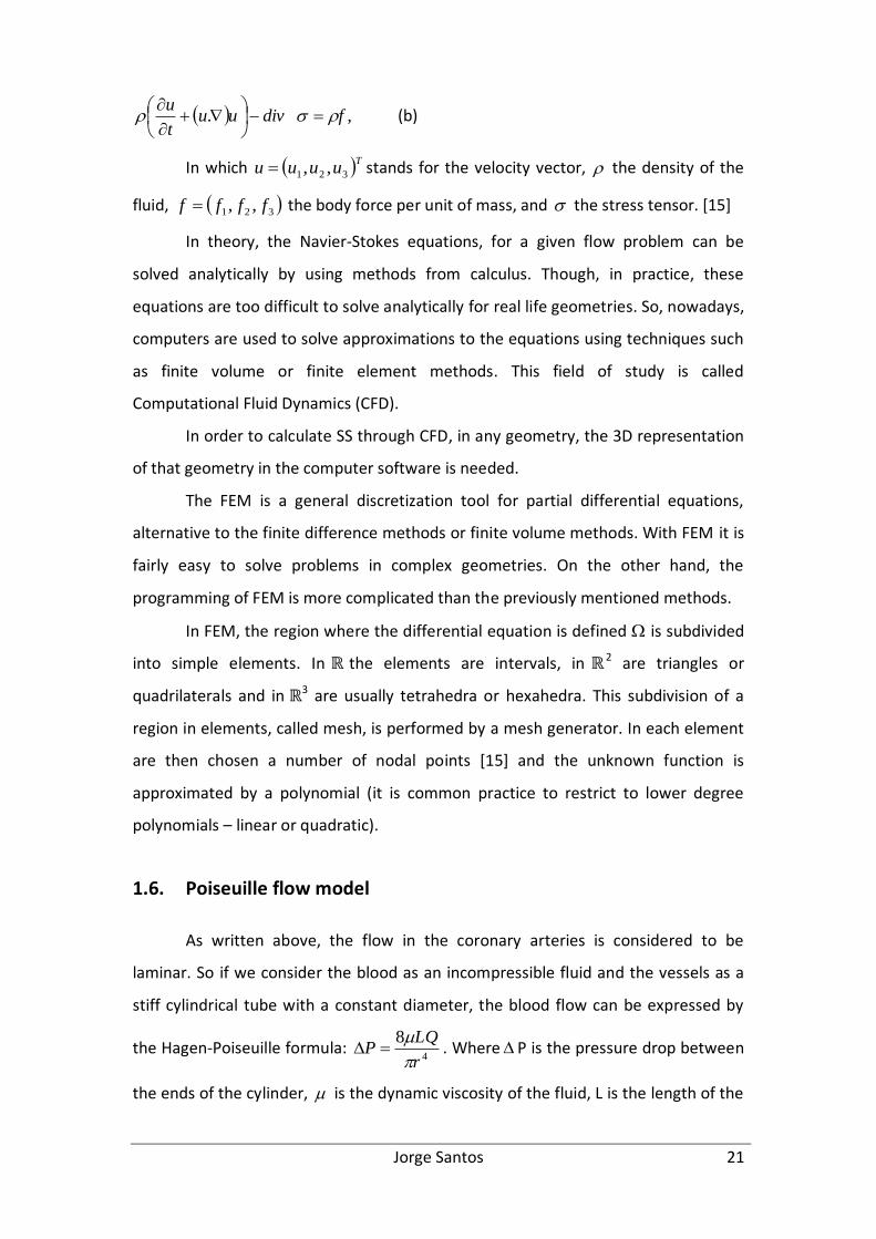
However, the flow in a realistic human coronary artery is not Poiseuille like.

Depending on some geometric factors, the flow profile can exhibit different patterns.

Figure 1.9 shows the different patterns of flow in a cylindrical tube. At location

number 1 a Poiseuille (parabolic) flow is presented; number 2 corresponds to an

asymmetric flow; number 3, which has a flattened profile, represents a turbulent

flow (it can also represent a non-newtonian fluid velocity profile); and number 4

indicates a backflow or a retrograde flow.

Figure 1.9 - Different flow profiles (adapted from Christian Poelma’s Biological Fluid

Mechanics lecture on Blood tissue interaction; the role of wall shear stress. Delft

University of Technology)[16]

1.7. 3D Reconstruction Methods

The first step to perform CFD calculations on realistic human coronary

arteries is to obtain the 3D geometry of those arteries. Therefore, 3D reconstruction

methods are needed. The techniques used to obtain the geometries used in this

study are described next in this section.

Jorge Santos 23

1.7.1. ANGUS

ANGUS is an application that allows the generation of 3D reconstructions of

human coronary arteries in vivo, which involves the fusion of intravascular

ultrasound (IVUS) and angiography. IVUS provides images with high spatial and

temporal resolution. However, since it is a tomographic technique, it makes it

difficult to confer a full 3D reconstruction of the vessel segment in investigation.

Multiple IVUS images can be stacked up along a straight pullback centerline, which is

a simple approach; however more realistic 3D reconstructions are needed. For that

reason fusion of IVUS with biplane angiography was developed [17].

The ANGUS method uses a calibration cube to mathematically describe the

3D space. When a marker is imaged in this geometry, its 3D position can be

determined. The IVUS images are acquired at the top of the R-wave of the ECG, to

reduce the effect of the cardiac motion. Between each image, the IVUS catheter is

pulled back 0.5mm. The X-ray biplane angiographic images are recorded; end-

diastolic frames are selected, stored and used to define the centerline of the

catheter, as such a 3D reconstruction of the catheter path can be obtained [17].

The lumen borders in the IVUS images are detected by a semi-automatic

contour detection program. The contours are described with polar coordinates. By

using the Fourier transform, a 2D Fourier description of the vessel segment is

obtained.

Finally IVUS cross sections are distributed in equidistant intervals on the

reconstructed centerline, with the imaging planes perpendicular to the

reconstructed centerline and rotating it around the trajectory until it is in the right

position [17].

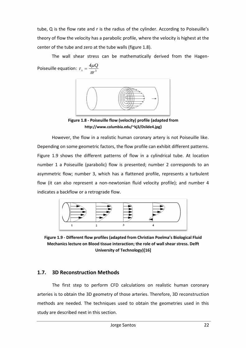
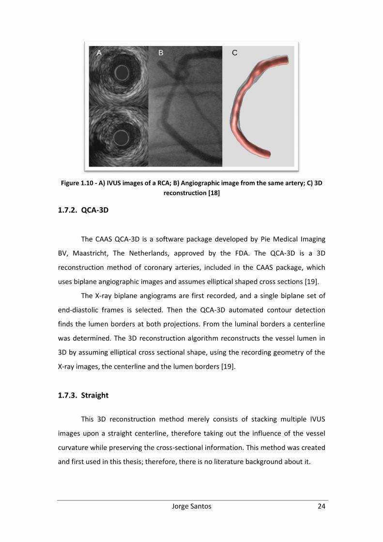
In figure 1.10.A, is shown an example of two IVUS images of an RCA. In figure

1.10.B is shown an angiographic image of that same artery. Figure 1.10.C shows the

3D reconstruction of the artery shown in the previous two images.

Jorge Santos 24

Figure 1.10 - A) IVUS images of a RCA; B) Angiographic image from the same artery; C) 3D

reconstruction [18]

1.7.2. QCA-3D

The CAAS QCA-3D is a software package developed by Pie Medical Imaging

BV, Maastricht, The Netherlands, approved by the FDA. The QCA-3D is a 3D

reconstruction method of coronary arteries, included in the CAAS package, which

uses biplane angiographic images and assumes elliptical shaped cross sections [19].

The X-ray biplane angiograms are first recorded, and a single biplane set of

end-diastolic frames is selected. Then the QCA-3D automated contour detection

finds the lumen borders at both projections. From the luminal borders a centerline

was determined. The 3D reconstruction algorithm reconstructs the vessel lumen in

3D by assuming elliptical cross sectional shape, using the recording geometry of the

X-ray images, the centerline and the lumen borders [19].

1.7.3. Straight

This 3D reconstruction method merely consists of stacking multiple IVUS

images upon a straight centerline, therefore taking out the influence of the vessel

curvature while preserving the cross-sectional information. This method was created

and first used in this thesis; therefore, there is no literature background about it.

A B C

Chapter 2. Aim

The main aim of this project was to investigate the influence of the 3D

geometry of realistic human coronary arteries on the wall shear stress distribution

and to develop methods to estimate the shear stress based on flow and geometrical

parameters.

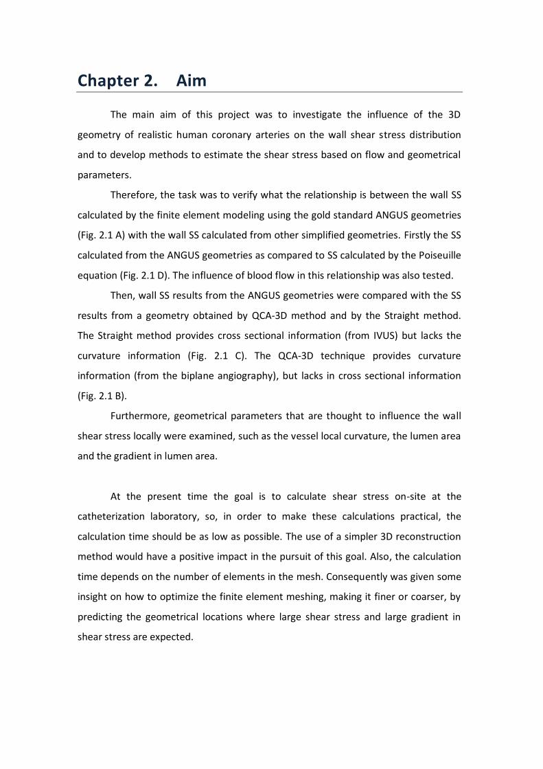
Therefore, the task was to verify what the relationship is between the wall SS

calculated by the finite element modeling using the gold standard ANGUS geometries

(Fig. 2.1 A) with the wall SS calculated from other simplified geometries. Firstly the SS

calculated from the ANGUS geometries as compared to SS calculated by the Poiseuille

equation (Fig. 2.1 D). The influence of blood flow in this relationship was also tested.

Then, wall SS results from the ANGUS geometries were compared with the SS

results from a geometry obtained by QCA-3D method and by the Straight method.

The Straight method provides cross sectional information (from IVUS) but lacks the

curvature information (Fig. 2.1 C). The QCA-3D technique provides curvature

information (from the biplane angiography), but lacks in cross sectional information

(Fig. 2.1 B).

Furthermore, geometrical parameters that are thought to influence the wall

shear stress locally were examined, such as the vessel local curvature, the lumen area

and the gradient in lumen area.

At the present time the goal is to calculate shear stress on-site at the

catheterization laboratory, so, in order to make these calculations practical, the

calculation time should be as low as possible. The use of a simpler 3D reconstruction

method would have a positive impact in the pursuit of this goal. Also, the calculation

time depends on the number of elements in the mesh. Consequently was given some

insight on how to optimize the finite element meshing, making it finer or coarser, by

predicting the geometrical locations where large shear stress and large gradient in

shear stress are expected.

Jorge Santos 26

3D Reconstructions

A

B

ANGUS - IVUS + Angiography:

Cross sectional information

Curvature information

QCA-3D - Biplane Angiography:

Cross sectional information

Curvature information

C

D

Straight - IVUS:

Cross sectional information

Curvature information

Poiseuille - Cylindrical tube:

Cross sectional information

Curvature information

Figure 2.1 - ANGUS, QCA-3D, Straight and Poiseuille – 3D Reconstructions example and a

corresponding cross-section from each method.

Jorge Santos 27

Chapter 3. Methods

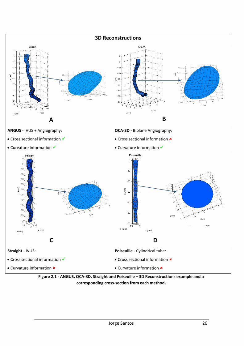
Ten coronary arteries of ten different patients were analyzed. Three of those

arteries were left circumflex arteries (LCX), two were left anterior descending arteries

(LAD) and five of them were right coronary arteries (RCA).

The data for each artery was obtained by a 3D reconstruction technique,

based on IVUS plus biplane angiography (ANGUS). This technique was described

before in the Background chapter. Table 3.1 shows some geometrical information

about the analyzed coronaries (such as the average lumen diameter, the range of

diameters and the length of the segment) and some information about the blood flow

(mean Reynolds number and the inlet flow rate).

Patient Coronary

Artery

Mean Reynolds

Number

Inlet flow

rate (ml/min)

Average lumen

diameter (mm)

Range of

diameter (mm)

Artery Length

(mm)

p060028 LCX 269.8 34.7 105.27 3.0 0.4 2.5 - 3.7 68.8

p060065 RCA 172.7 16.6 73.57 3.2 0.3 2.5 - 3.8 79.6

p060125 RCA 200.6 21.3 93.45 3.5 0.4 2.8 - 4.3 66.7

p060204 LAD 350.1 62.3 165.30 3.3 0.6 2.5 - 4.6 59.8

p060233 LCX 332.9 34.6 156.59 3.5 0.4 2.9 - 4.3 47.7

p060362 RCA 210.0 38.6 97.96 3.6 0.6 2.4 - 4.5 71.3

p061104 LCX 279.7 42.7 113.01 3.1 0.4 2.3 - 3.8 49.4

p061150 LAD 331.8 76.3 102.37 2.4 0.6 1.4 - 3.7 80.8

p062128 RCA 294.4 41.1 140.50 3.3 0.4 2.3 - 4.0 56.9

p062143 RCA 297.7 64.1 130.10 3.3 0.5 1.7 - 3.9 58.3

Table 3.1 - Patients, corresponding coronaries and some geometric and flow features of the

ANGUS reconstructed vessels

3.1. Computational Fluid Dynamics

Computational fluid dynamics (CFD) simulations were executed thereafter, to

solve the Navier-Stokes equations (described in the Background chapter), which

govern fluid motion.

Jorge Santos 28

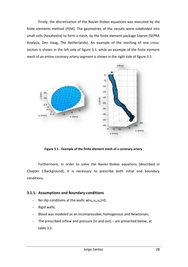
Firstly, the discretization of the Navier-Stokes equations was executed by the

finite elements method (FEM). The geometries of the vessels were subdivided into

small cells (hexahedra) to form a mesh, by the finite element package Sepran (SEPRA

Analysis, Den Haag, The Netherlands). An example of the meshing of one cross-

section is shown in the left side of figure 3.1, while an example of the finite element

mesh of an entire coronary artery segment is shown in the right side of figure 3.1.

Figure 3.1 - Example of the finite element mesh of a coronary artery

Furthermore, in order to solve the Navier-Stokes equations (described in

Chapter 1.Background), it is necessary to prescribe both initial and boundary

conditions.

3.1.1. Assumptions and Boundary conditions

- No slip conditions at the walls: u(ux,uy,uz)=0;

- Rigid walls;

- Blood was modeled as an incompressible, homogenous and Newtonian;

- The prescribed inflow and pressure (in and out) – are presented below, at

table 3.2.

-5-4

-3

-5.5-5

-4.5-4

-3.5

24

25

x (mm)

y (mm)

z (

mm

)

-10-50

-40-20

0-45

-40

-35

-30

-25

-20

-15

-10

-5

0

x (mm)

y (mm)

z (

mm

)

inflow

Jorge Santos 29

Patients Pressure (Pa) Inflow rate (ml/min)

In Out Physiologic 50% 10% 1%

p060028 464.02 -0.89 105.27 52.64 10.53 1.05 p060065 251.82 -0.13 73.57 36.79 7.36 0.74 p060125 178.99 -0.35 93.45 46.73 9.35 0.93 p060204 747.62 -0.66 165.30 82.65 16.53 1.65 p060233 288.74 -1.42 156.59 78.30 15.66 1.57 p060362 287.97 -0.85 97.96 48.98 9.80 0.98 p061104 407.31 -1.67 113.01 56.51 11.30 1.13 p061150 2518.70 -7.83 102.37 51.19 10.24 1.02 p062128 322.42 -0.31 140.50 70.25 14.05 1.41 p062143 828.96 -0.26 130.10 65.05 13.01 1.30

Average 629.66 697.00

-1.44 2.30

117.81 29.42

58.91 14.71

11.78 2.94

1.18 0.29

Table 3.2 - Inflow rate and pressure (in and out) values for the CFD calculations

3.2. Analysis

CFD calculations were performed for the three different geometries, according

to the ANGUS, QCA-3D and Straight 3D reconstruction method, of all ten vessels. The

output files from the CFD calculations, which contained information of the local SS,

flow velocity, pressure and geometry, were processed in MATLAB (Mathworks,

Natick, USA). The analysis of the calculations outcomes is hereby described.

3.2.1. ANGUS vs. Poiseuille

Primarily, the relationship between the average SS per cross-section based on

the CFD calculations and the lumen area were analyzed, and thereafter, the same

relationship was investigated using the SS based on the Poiseuille equation. The

average SS per cross section from the CFD calculations and the one based on

Poiseuille were then compared.

The next step was to analyze the influence of blood flow in the relationships

aforementioned. The input blood flow values in the CFD calculations were changed to

50%, 10% and 1% of the original (physiological) values, and new CFD calculations

were executed. Average SS and Poiseuille based SS, of the four different blood flow

values, were compared using regression analysis. In the Appendix is presented a table

with the input blood flow values used in all the CFD calculation mentioned.

Jorge Santos 30

Furthermore, Bland-Altman statistics were performed. Bland-Altman is a

statistical method that compares two measurement techniques [20]. In a Bland-

Altman plot, the x-axis stands for the average of the two techniques and the y-axis

stands for the difference between the two techniques. Horizontal lines were drawn at

the mean difference and at the limits of agreement, which were defined as the mean

difference plus or minus two times the standard deviation of the differences [21]. In

this case, the mean difference in average SS per cross section represents the

systematic error in average SS, and the regression line represents the proportional

error between techniques, meaning the error dependant on the mean magnitude of

the average SS.

In addition, a local wall SS histogram was built to visualize the local

distribution of both SS from the ANGUS method and Poiseuille based SS1.

Finally, the blood velocity profiles, from the four different blood flow values,

were analyzed. These cross-sections were located in specific regions of interest. Two

of them were located in a curved region and a highly stenotic region, respectively. For

the sake of comparison, the third cross-section, which was located in a “normal”

region (straight, and with low lumen area gradient), was analyzed.

All the results from these analyses are presented and described in Chapter 4.

3.2.2. ANGUS vs. Straight & ANGUS vs. QCA-3D

Since the analysis in these two chapters was similar, the methods used are

here described together.

In the first place, average SS per cross section and Lumen area plots for both

techniques were made, and compared. Then, the average SS from both methods

were compared using regression analysis. The correlation coefficients and the slope

and y-intercept values of the regression lines were registered.

Bland-Altman statistics and a local SS histogram, analogous to the ones

previously described, were also performed for both chapters.

1 Since the Poiseuille equation only provides one SS value per cross section, all the elements

in the same cross section were given the same SS value.

Jorge Santos 31

The maximum SS value per cross section was also analysed, as well as the

longitudinal SS (exclusively in Chapter4. ANGUS vs. Straight).

Furthermore, high and low SS analyses were performed. These analyses were

performed per cross-section and per element (exclusively in Chapter 6 - ANGUS vs.

Straight). The low SS analyses, per element, consisted of locating the low SS elements

(<0.5 Pa) in both methods and calculate the percentage of elements that were

coincident (i.e. at the same location). The high SS analyses, per element, consisted of

locating the high SS elements in both methods and calculate the percentage of

coincident/overlapping elements. A high SS element was considered when the SS was

higher than the average SS per cross section plus the respective standard deviation (>

x Pa). A table with the threshold high SS values is presented in Chapter 5.

The high and low SS analyses per cross section were identical to the ones per

element. However, in this case, a high/low SS cross-section was counted when it

contained at least one element with high/low SS.

The sensitivity and specificity of the QCA-3D and Straight method when

predicting high or low SS elements (or cross-sections), comparing to ANGUS were

calculated. The sensitivity is a statistical measurement of the proportion of actual

positives which are correctly identified as such (e.g. the percentage of low SS cross-

sections determined by the QCA-3D or Straight method that are coincident with low

SS cross-sections determined by the gold standard ANGUS method). The specificity

measures the proportion of negatives which are correctly identified (e.g. the

percentage of non-low SS cross-sections determined by the QCA-3D or Straight

method that were also considered as non-low SS by the gold standard ANGUS

method.

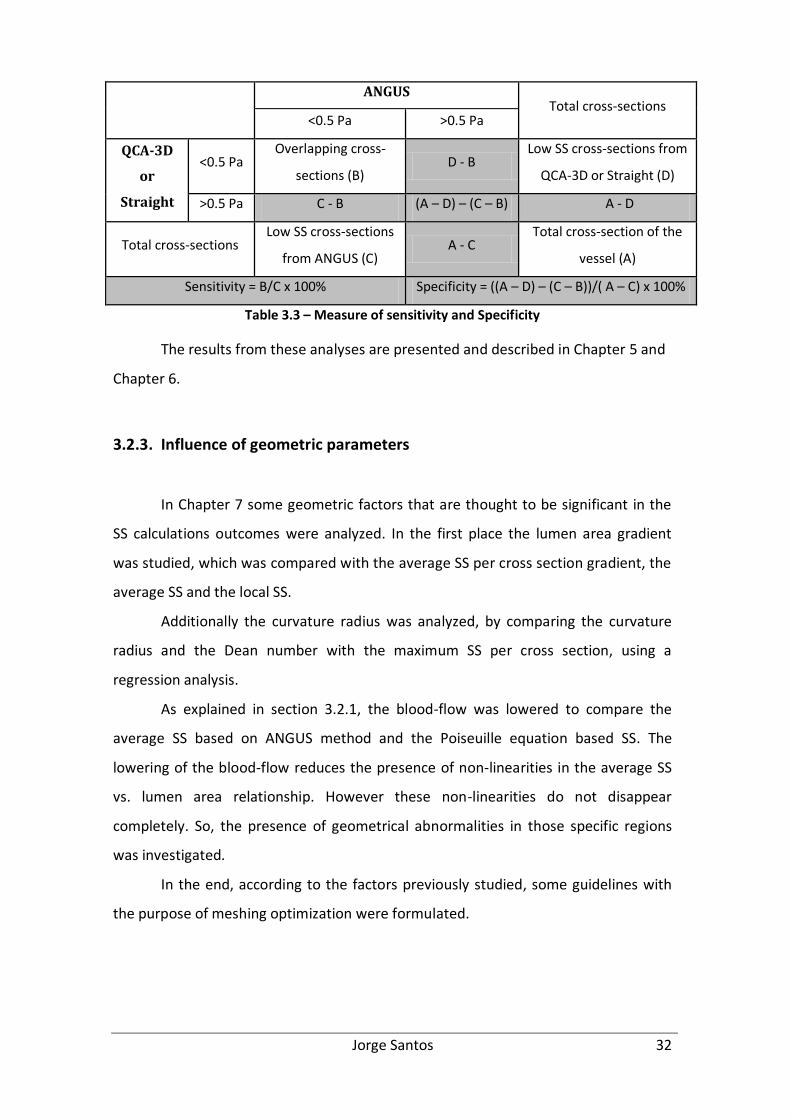
The following table exemplifies how sensitivity and specificity were measured

for the calculation of low SS cross-sections. This procedure was analogous for the

other cases.

Jorge Santos 32

ANGUS

Total cross-sections <0.5 Pa >0.5 Pa

QCA-3D

or

Straight

<0.5 Pa Overlapping cross-

sections (B) D - B

Low SS cross-sections from

QCA-3D or Straight (D)

>0.5 Pa C - B (A – D) – (C – B) A - D

Total cross-sections Low SS cross-sections

from ANGUS (C) A - C

Total cross-section of the

vessel (A)

Sensitivity = B/C x 100% Specificity = ((A – D) – (C – B))/( A – C) x 100%

Table 3.3 – Measure of sensitivity and Specificity

The results from these analyses are presented and described in Chapter 5 and

Chapter 6.

3.2.3. Influence of geometric parameters

In Chapter 7 some geometric factors that are thought to be significant in the

SS calculations outcomes were analyzed. In the first place the lumen area gradient

was studied, which was compared with the average SS per cross section gradient, the

average SS and the local SS.

Additionally the curvature radius was analyzed, by comparing the curvature

radius and the Dean number with the maximum SS per cross section, using a

regression analysis.

As explained in section 3.2.1, the blood-flow was lowered to compare the

average SS based on ANGUS method and the Poiseuille equation based SS. The

lowering of the blood-flow reduces the presence of non-linearities in the average SS

vs. lumen area relationship. However these non-linearities do not disappear

completely. So, the presence of geometrical abnormalities in those specific regions

was investigated.

In the end, according to the factors previously studied, some guidelines with

the purpose of meshing optimization were formulated.

Jorge Santos 33

Chapter 4. ANGUS vs. Poiseuille

One of the aims of this chapter was to prove the inverse relation between

average SS per cross section and the lumen area, by performing CFD calculations on

3D reconstructed geometries (from ANGUS) of real coronary arteries.

The main aim was to verify the relationship between the average wall SS

calculated by the finite element modeling and SS calculated by the Poiseuille

equation. Furthermore, the influences of blood flow in that relationship was tested.

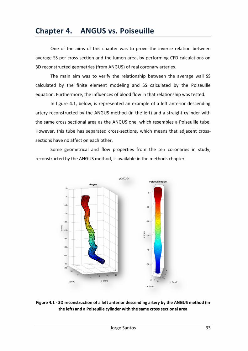
In figure 4.1, below, is represented an example of a left anterior descending

artery reconstructed by the ANGUS method (in the left) and a straight cylinder with

the same cross sectional area as the ANGUS one, which resembles a Poiseuille tube.

However, this tube has separated cross-sections, which means that adjacent cross-

sections have no affect on each other.

Some geometrical and flow properties from the ten coronaries in study,

reconstructed by the ANGUS method, is available in the methods chapter.

Figure 4.1 - 3D reconstruction of a left anterior descending artery by the ANGUS method (in

the left) and a Poiseuille cylinder with the same cross sectional area

0

10

20

-15-10-50

-45

-40

-35

-30

-25

-20

-15

-10

-5

0

y (mm)

Angus

x (mm)

z (

mm

)

-2 0 2-4-2024

-50

-40

-30

-20

-10

0

y (mm)

Poiseuille tube

x (mm)

z (

mm

)

p060204

Jorge Santos 34

4.1. Results

4.1.1. Average shear stress vs. Lumen area

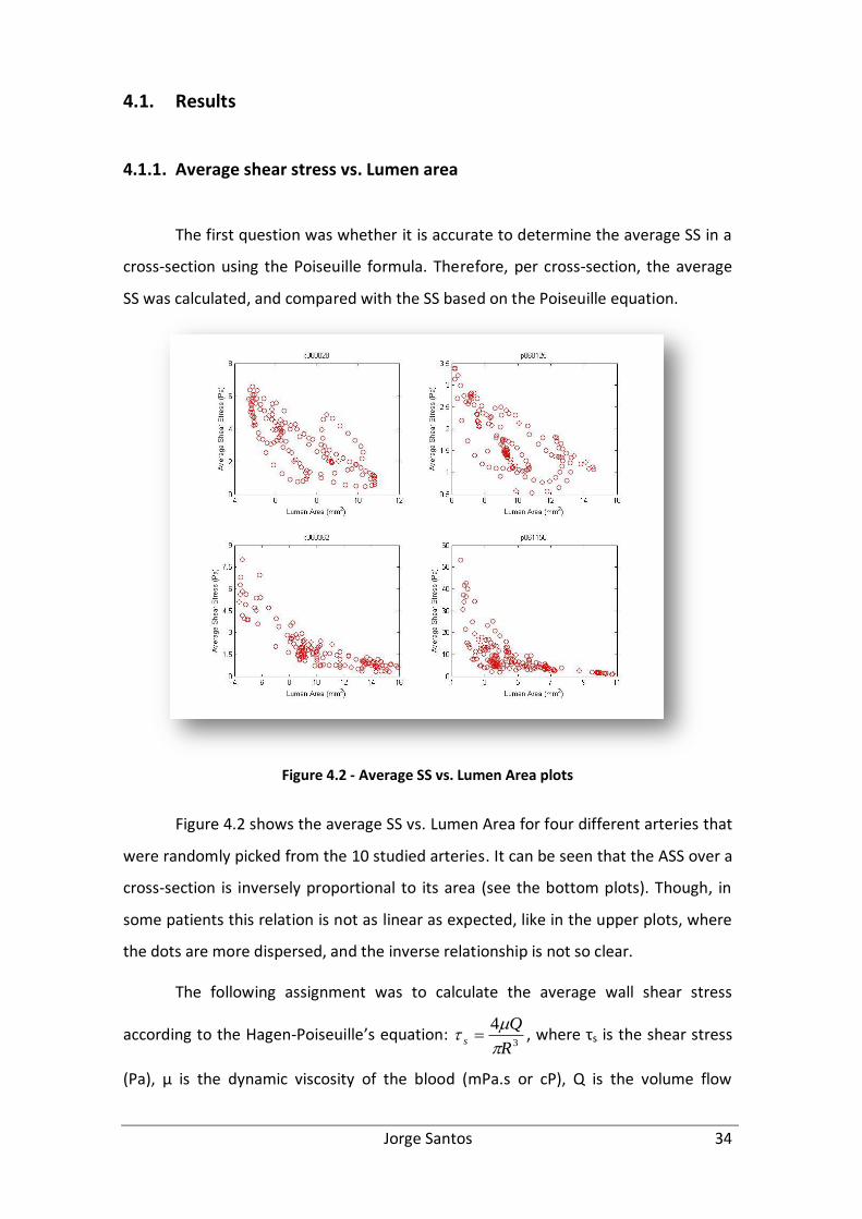
The first question was whether it is accurate to determine the average SS in a

cross-section using the Poiseuille formula. Therefore, per cross-section, the average

SS was calculated, and compared with the SS based on the Poiseuille equation.

Figure 4.2 - Average SS vs. Lumen Area plots

Figure 4.2 shows the average SS vs. Lumen Area for four different arteries that

were randomly picked from the 10 studied arteries. It can be seen that the ASS over a

cross-section is inversely proportional to its area (see the bottom plots). Though, in

some patients this relation is not as linear as expected, like in the upper plots, where

the dots are more dispersed, and the inverse relationship is not so clear.

The following assignment was to calculate the average wall shear stress

according to the Hagen-Poiseuille’s equation: 3

4

R

Qs

, where τs is the shear stress

(Pa), μ is the dynamic viscosity of the blood (mPa.s or cP), Q is the volume flow

Jorge Santos 35

(ml/min) and R is the cylindrical tube radius (m). The lumen radius was derived from

the lumen area. In order to put all the variables in S.I. units, the following equation

was used in MATLAB to calculate the shear stress: 3

610)6000

(4

R

Q

s

. The

viscosity value used in this equation was 3.5 cP, which is an approximate value,

because the blood viscosity can differ a lot, depending on the hematocrit,

temperature and shear rate [22].

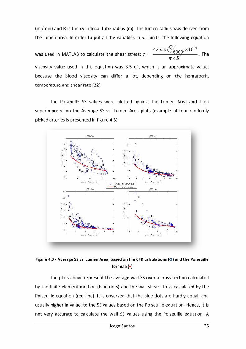
The Poiseuille SS values were plotted against the Lumen Area and then

superimposed on the Average SS vs. Lumen Area plots (example of four randomly

picked arteries is presented in figure 4.3).

Figure 4.3 - Average SS vs. Lumen Area, based on the CFD calculations (o) and the Poiseuille

formula (-)

The plots above represent the average wall SS over a cross section calculated

by the finite element method (blue dots) and the wall shear stress calculated by the

Poiseuille equation (red line). It is observed that the blue dots are hardly equal, and

usually higher in value, to the SS values based on the Poiseuille equation. Hence, it is

not very accurate to calculate the wall SS values using the Poiseuille equation. A

Jorge Santos 36

probable cause for this is the geometric variability of the coronary vessels, since the

Poiseuille’s law only describes the flow in straight cylindrical tubes. In the appendix,

figure 11.1 displays analogous plots for all of the ten coronaries studied.

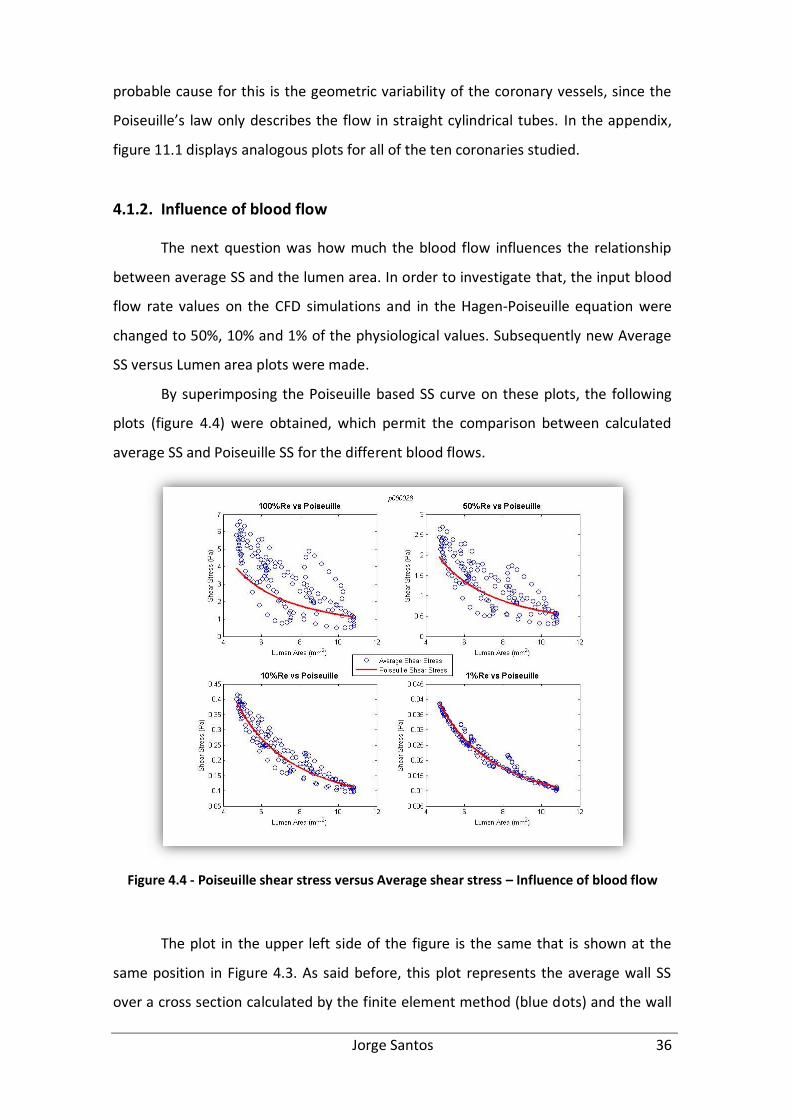
4.1.2. Influence of blood flow

The next question was how much the blood flow influences the relationship

between average SS and the lumen area. In order to investigate that, the input blood

flow rate values on the CFD simulations and in the Hagen-Poiseuille equation were

changed to 50%, 10% and 1% of the physiological values. Subsequently new Average

SS versus Lumen area plots were made.

By superimposing the Poiseuille based SS curve on these plots, the following

plots (figure 4.4) were obtained, which permit the comparison between calculated

average SS and Poiseuille SS for the different blood flows.

Figure 4.4 - Poiseuille shear stress versus Average shear stress – Influence of blood flow

The plot in the upper left side of the figure is the same that is shown at the

same position in Figure 4.3. As said before, this plot represents the average wall SS

over a cross section calculated by the finite element method (blue dots) and the wall

Jorge Santos 37

SS calculated by the Poiseuille equation (red line). By examining this plot it is seen

that the Poiseuille equation cannot accurately predict the wall SS of realistic coronary

arteries. However, when the blood flow rate is lowered (see the other three plots),

the average SS resemble the ones based on Poiseuille formula. This may happen

because when the flow rate is too low, geometric factors that can cause non-

linearities, such as curvature, torsion, sinuosity, among others, have much less

influence on the flow profile in the coronary arteries. However, even when the blood

flow rate is lowered to 1% of its physiological value there are some dots that don’t

follow the Poiseuille based line. The reason for this deviation from the Poiseuille

values will be discussed further in Chapter 7.

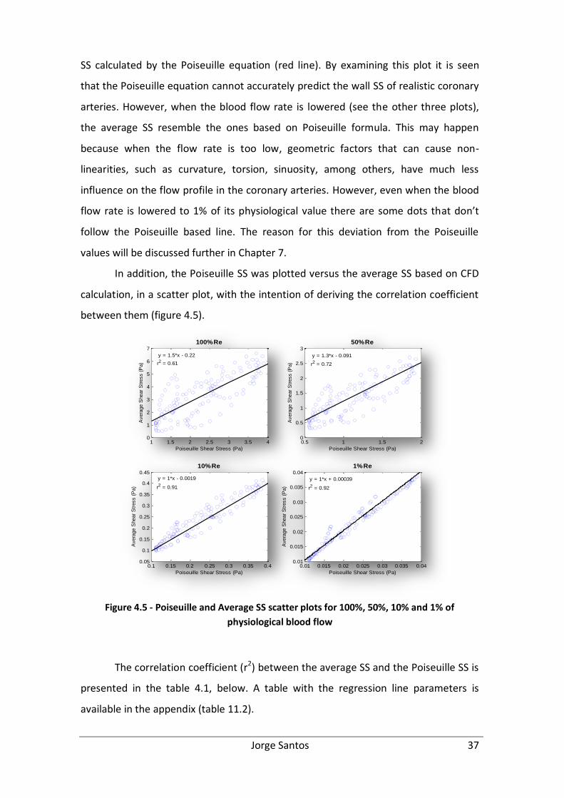
In addition, the Poiseuille SS was plotted versus the average SS based on CFD

calculation, in a scatter plot, with the intention of deriving the correlation coefficient

between them (figure 4.5).

Figure 4.5 - Poiseuille and Average SS scatter plots for 100%, 50%, 10% and 1% of

physiological blood flow

The correlation coefficient (r2) between the average SS and the Poiseuille SS is

presented in the table 4.1, below. A table with the regression line parameters is

available in the appendix (table 11.2).

0.01 0.015 0.02 0.025 0.03 0.035 0.040.01

0.015

0.02

0.025

0.03

0.035

0.04

Poiseuille Shear Stress (Pa)

Avera

ge S

hear

Str

ess (

Pa)

1%Re

y = 1*x + 0.00039

1 1.5 2 2.5 3 3.5 40

1

2

3

4

5

6

7

Poiseuille Shear Stress (Pa)

Avera

ge S

hear

Str

ess (

Pa)

100%Re

0.5 1 1.5 20

0.5

1

1.5

2

2.5

3

Poiseuille Shear Stress (Pa)

Avera

ge S

hear

Str

ess (

Pa)

50%Re

0.1 0.15 0.2 0.25 0.3 0.35 0.40.05

0.1

0.15

0.2

0.25

0.3

0.35

0.4

0.45

Poiseuille Shear Stress (Pa)

Avera

ge S

hear

Str

ess (

Pa)

10%Re

r2 = 0.92

y = 1.5*x - 0.22

r2 = 0.61 r2 = 0.72

y = 1*x - 0.0019

r2 = 0.91

y = 1.3*x - 0.091

Jorge Santos 38

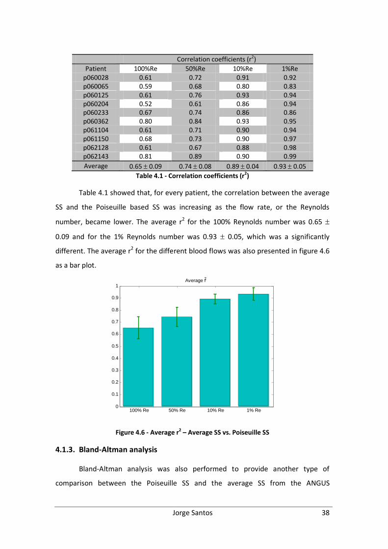
Correlation coefficients (r2)

Patient 100%Re 50%Re 10%Re 1%Re p060028 0.61 0.72 0.91 0.92 p060065 0.59 0.68 0.80 0.83 p060125 0.61 0.76 0.93 0.94 p060204 0.52 0.61 0.86 0.94 p060233 0.67 0.74 0.86 0.86 p060362 0.80 0.84 0.93 0.95 p061104 0.61 0.71 0.90 0.94 p061150 0.68 0.73 0.90 0.97 p062128 0.61 0.67 0.88 0.98 p062143 0.81 0.89 0.90 0.99

Average 0.65 0.09 0.74 0.08 0.89 0.04 0.93 0.05

Table 4.1 - Correlation coefficients (r2)

Table 4.1 showed that, for every patient, the correlation between the average

SS and the Poiseuille based SS was increasing as the flow rate, or the Reynolds

number, became lower. The average r2 for the 100% Reynolds number was 0.65

0.09 and for the 1% Reynolds number was 0.93 0.05, which was a significantly

different. The average r2 for the different blood flows was also presented in figure 4.6

as a bar plot.

100% Re 50% Re 10% Re 1% Re 0 0.1 0.2 0.3 0.4 0.5 0.6 0.7 0.8 0.9

1 Average r 2

100% Re 50% Re 10% Re 1% Re 0 0.1 0.2 0.3 0.4 0.5 0.6 0.7 0.8 0.9

1 Average r 2

Figure 4.6 - Average r2 – Average SS vs. Poiseuille SS

4.1.3. Bland-Altman analysis

Bland-Altman analysis was also performed to provide another type of

comparison between the Poiseuille SS and the average SS from the ANGUS

Jorge Santos 39

geometries, for the four different blood-flow percentages (100, 50, 10 and 1% of

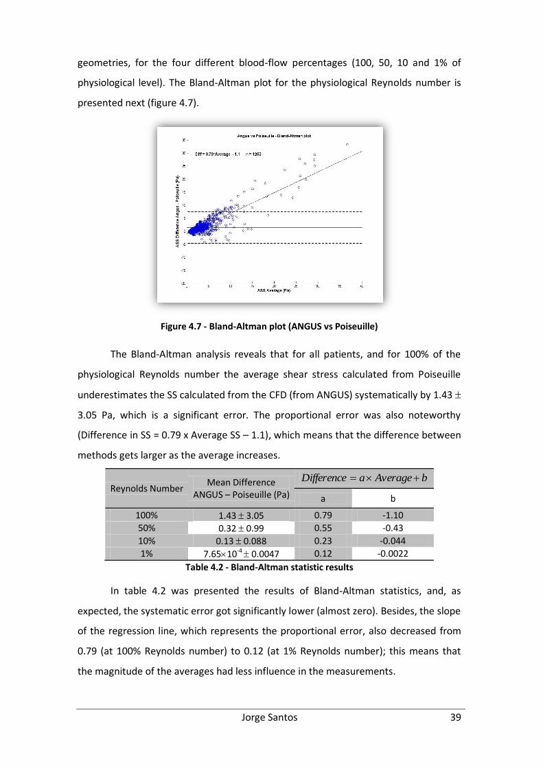
physiological level). The Bland-Altman plot for the physiological Reynolds number is

presented next (figure 4.7).

Figure 4.7 - Bland-Altman plot (ANGUS vs Poiseuille)

The Bland-Altman analysis reveals that for all patients, and for 100% of the

physiological Reynolds number the average shear stress calculated from Poiseuille

underestimates the SS calculated from the CFD (from ANGUS) systematically by 1.43

3.05 Pa, which is a significant error. The proportional error was also noteworthy

(Difference in SS = 0.79 x Average SS – 1.1), which means that the difference between

methods gets larger as the average increases.

Reynolds Number Mean Difference

ANGUS – Poiseuille (Pa)

bAverageaDifference

a b

100% 1.43 3.05 0.79 -1.10

50% 0.32 0.99 0.55 -0.43

10% 0.13 0.088 0.23 -0.044

1% 7.6510-4 0.0047 0.12 -0.0022

Table 4.2 - Bland-Altman statistic results

In table 4.2 was presented the results of Bland-Altman statistics, and, as

expected, the systematic error got significantly lower (almost zero). Besides, the slope

of the regression line, which represents the proportional error, also decreased from

0.79 (at 100% Reynolds number) to 0.12 (at 1% Reynolds number); this means that

the magnitude of the averages had less influence in the measurements.

Jorge Santos 40

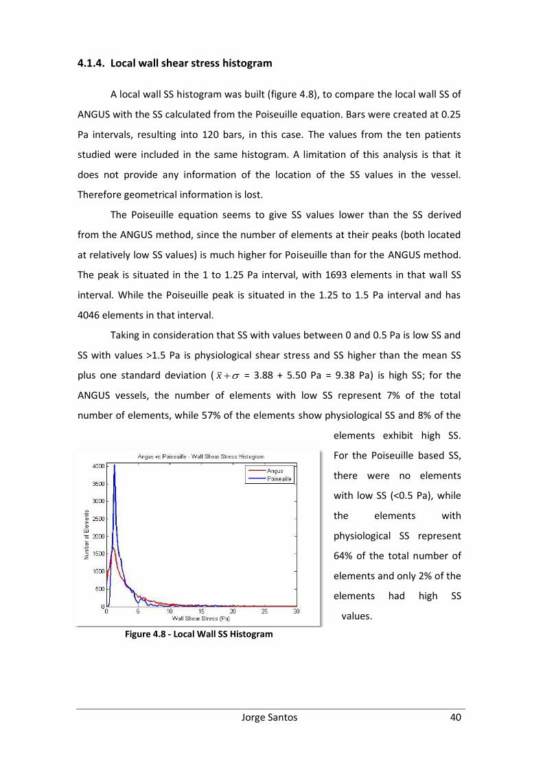
4.1.4. Local wall shear stress histogram

A local wall SS histogram was built (figure 4.8), to compare the local wall SS of

ANGUS with the SS calculated from the Poiseuille equation. Bars were created at 0.25

Pa intervals, resulting into 120 bars, in this case. The values from the ten patients

studied were included in the same histogram. A limitation of this analysis is that it

does not provide any information of the location of the SS values in the vessel.

Therefore geometrical information is lost.

The Poiseuille equation seems to give SS values lower than the SS derived

from the ANGUS method, since the number of elements at their peaks (both located

at relatively low SS values) is much higher for Poiseuille than for the ANGUS method.

The peak is situated in the 1 to 1.25 Pa interval, with 1693 elements in that wall SS

interval. While the Poiseuille peak is situated in the 1.25 to 1.5 Pa interval and has

4046 elements in that interval.

Taking in consideration that SS with values between 0 and 0.5 Pa is low SS and

SS with values >1.5 Pa is physiological shear stress and SS higher than the mean SS

plus one standard deviation ( x = 3.88 + 5.50 Pa = 9.38 Pa) is high SS; for the

ANGUS vessels, the number of elements with low SS represent 7% of the total

number of elements, while 57% of the elements show physiological SS and 8% of the

elements exhibit high SS.

For the Poiseuille based SS,

there were no elements

with low SS (<0.5 Pa), while

the elements with

physiological SS represent

64% of the total number of

elements and only 2% of the

elements had high SS

values.

Figure 4.8 - Local Wall SS Histogram

Jorge Santos 41

4.1.5. Velocity profiles

At some regions, with physiologic blood flow rate, the velocity profile per

cross-section exhibits an asymmetric distribution, which provokes asymmetric wall

shear stress. The patterns also demonstrate that the blood flow at physiological levels

is not Poiseuille like (parabolic distribution). However at low blood flow levels (10 and

1% of physiological) the velocity profile is parabolic. This, in combination to what is

seen at the lower two plots in figure 4.4, demonstrates that by lowering blood flow,

the calculated wall shear stresses are almost equal to the SS values based on the

Poiseuille formula.

Figure 4.9 represents a cross section that has a relatively large lumen area and

is located at a curved region of the artery. Consequently, the velocity profile (at

physiological and 50% Reynolds number) is asymmetric. The blood velocity is higher

near the outer side of the curvature and is lower at the inner side. However, at 10%

and 1% of the physiological Reynolds number, the velocity profile is reasonably close

to parabolic.

110th cross section

Figure 4.9 - Velocity profiles for different blood flows (100%, 50%, 10% and 1%) for a cross section

located in a curved region

Jorge Santos 42

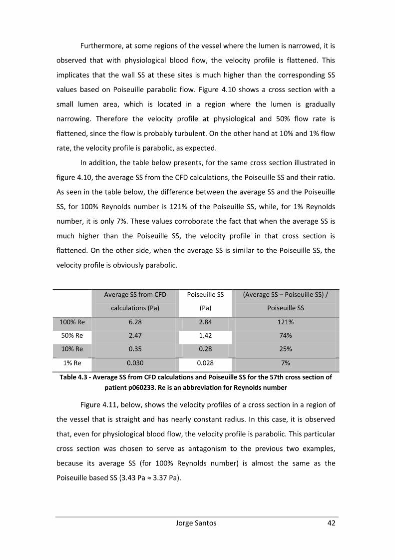
Furthermore, at some regions of the vessel where the lumen is narrowed, it is

observed that with physiological blood flow, the velocity profile is flattened. This

implicates that the wall SS at these sites is much higher than the corresponding SS

values based on Poiseuille parabolic flow. Figure 4.10 shows a cross section with a

small lumen area, which is located in a region where the lumen is gradually

narrowing. Therefore the velocity profile at physiological and 50% flow rate is

flattened, since the flow is probably turbulent. On the other hand at 10% and 1% flow

rate, the velocity profile is parabolic, as expected.

In addition, the table below presents, for the same cross section illustrated in

figure 4.10, the average SS from the CFD calculations, the Poiseuille SS and their ratio.

As seen in the table below, the difference between the average SS and the Poiseuille

SS, for 100% Reynolds number is 121% of the Poiseuille SS, while, for 1% Reynolds

number, it is only 7%. These values corroborate the fact that when the average SS is

much higher than the Poiseuille SS, the velocity profile in that cross section is

flattened. On the other side, when the average SS is similar to the Poiseuille SS, the

velocity profile is obviously parabolic.

Average SS from CFD

calculations (Pa)

Poiseuille SS

(Pa)

(Average SS – Poiseuille SS) /

Poiseuille SS

100% Re 6.28 2.84 121%

50% Re 2.47 1.42 74%

10% Re 0.35 0.28 25%

1% Re 0.030 0.028 7%

Table 4.3 - Average SS from CFD calculations and Poiseuille SS for the 57th cross section of

patient p060233. Re is an abbreviation for Reynolds number

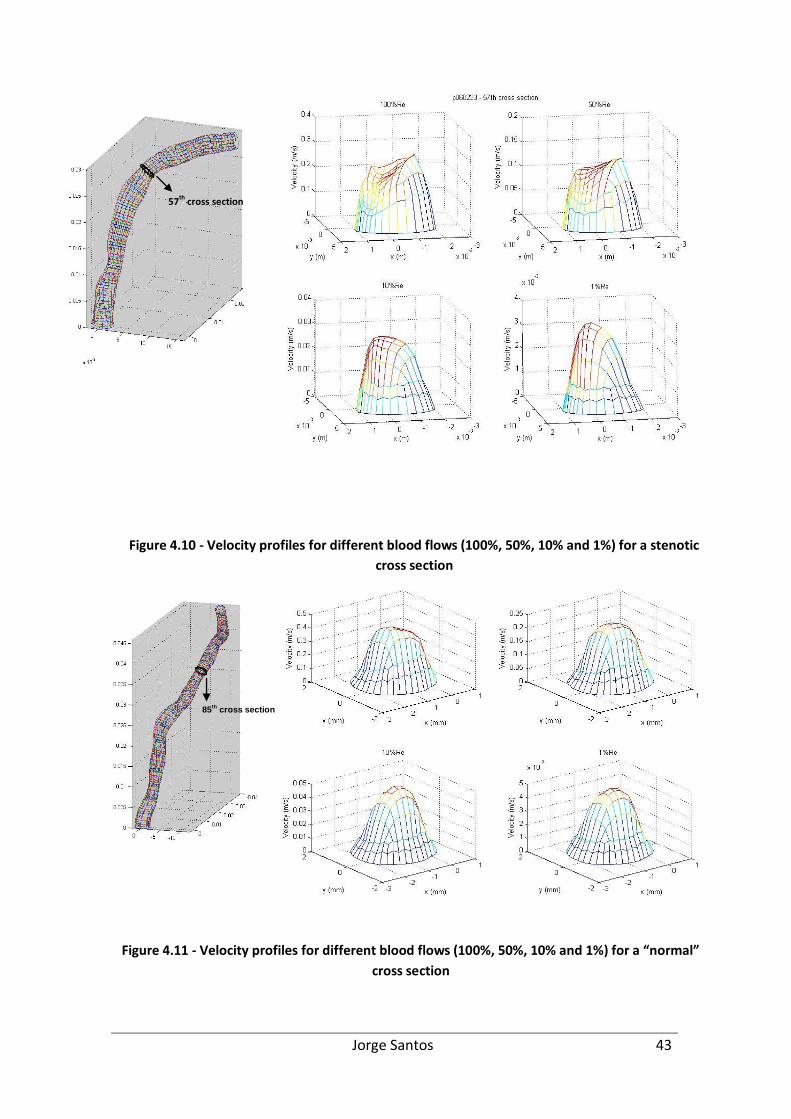
Figure 4.11, below, shows the velocity profiles of a cross section in a region of

the vessel that is straight and has nearly constant radius. In this case, it is observed

that, even for physiological blood flow, the velocity profile is parabolic. This particular

cross section was chosen to serve as antagonism to the previous two examples,

because its average SS (for 100% Reynolds number) is almost the same as the

Poiseuille based SS (3.43 Pa ≈ 3.37 Pa).

Jorge Santos 43

57th

cross section

85th

cross section

Figure 4.10 - Velocity profiles for different blood flows (100%, 50%, 10% and 1%) for a stenotic

cross section

Figure 4.11 - Velocity profiles for different blood flows (100%, 50%, 10% and 1%) for a “normal”

cross section

Jorge Santos 44

Chapter 5. ANGUS vs. QCA-3D

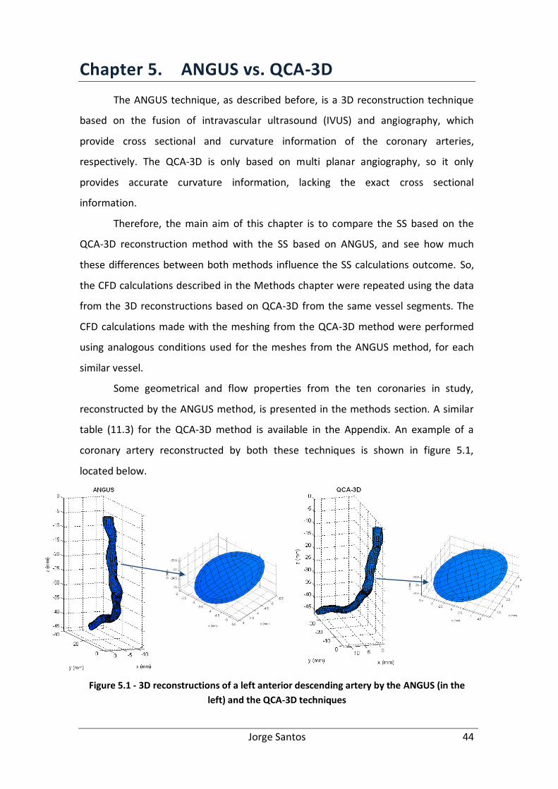
The ANGUS technique, as described before, is a 3D reconstruction technique

based on the fusion of intravascular ultrasound (IVUS) and angiography, which

provide cross sectional and curvature information of the coronary arteries,

respectively. The QCA-3D is only based on multi planar angiography, so it only

provides accurate curvature information, lacking the exact cross sectional

information.

Therefore, the main aim of this chapter is to compare the SS based on the

QCA-3D reconstruction method with the SS based on ANGUS, and see how much

these differences between both methods influence the SS calculations outcome. So,

the CFD calculations described in the Methods chapter were repeated using the data

from the 3D reconstructions based on QCA-3D from the same vessel segments. The

CFD calculations made with the meshing from the QCA-3D method were performed

using analogous conditions used for the meshes from the ANGUS method, for each

similar vessel.

Some geometrical and flow properties from the ten coronaries in study,

reconstructed by the ANGUS method, is presented in the methods section. A similar

table (11.3) for the QCA-3D method is available in the Appendix. An example of a

coronary artery reconstructed by both these techniques is shown in figure 5.1,

located below.

Figure 5.1 - 3D reconstructions of a left anterior descending artery by the ANGUS (in the

left) and the QCA-3D techniques

Jorge Santos 45

5.1. Results

5.1.1. Average shear stress and lumen area

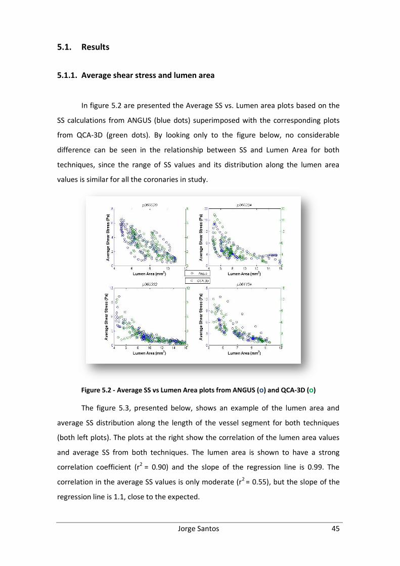
In figure 5.2 are presented the Average SS vs. Lumen area plots based on the

SS calculations from ANGUS (blue dots) superimposed with the corresponding plots

from QCA-3D (green dots). By looking only to the figure below, no considerable

difference can be seen in the relationship between SS and Lumen Area for both

techniques, since the range of SS values and its distribution along the lumen area

values is similar for all the coronaries in study.

Figure 5.2 - Average SS vs Lumen Area plots from ANGUS (o) and QCA-3D (o)

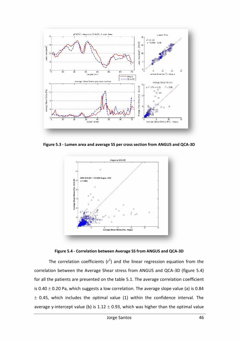
The figure 5.3, presented below, shows an example of the lumen area and

average SS distribution along the length of the vessel segment for both techniques

(both left plots). The plots at the right show the correlation of the lumen area values

and average SS from both techniques. The lumen area is shown to have a strong

correlation coefficient (r2 = 0.90) and the slope of the regression line is 0.99. The

correlation in the average SS values is only moderate (r2 = 0.55), but the slope of the

regression line is 1.1, close to the expected.

Jorge Santos 46

Figure 5.3 - Lumen area and average SS per cross section from ANGUS and QCA-3D

Figure 5.4 - Correlation between Average SS from ANGUS and QCA-3D

The correlation coefficients (r2) and the linear regression equation from the

correlation between the Average Shear stress from ANGUS and QCA-3D (figure 5.4)

for all the patients are presented on the table 5.1. The average correlation coefficient

is 0.40 0.20 Pa, which suggests a low correlation. The average slope value (a) is 0.84

0.45, which includes the optimal value (1) within the confidence interval. The

average y-intercept value (b) is 1.12 0.93, which was higher than the optimal value

Jorge Santos 47

(0), revealing that the QCA-3D shear stress values overestimated the ANGUS ones. In

the last row of the table are also presented the correlation values if using the data

from all the vessels together, instead of averaging them. This type of information will

be present in further tables of this report.

Patient r2 Values Linear Regression equation QCA-3D = a ANGUS + b

a – slope b – y-intercept

p060028 0.26 0.68 0.91

p060065 0.091 0.19 1.40

p060125 0.44 0.81 0.54 p060204 0.54 0.79 1.50 p060233 0.50 1.30 0.059 p060362 0.55 1.10 0.22 p061104 0.50 0.94 0.73 p061150 0.047 1.70 3.30 p062128 0.36 0.46 1.60 p062143 0.66 0.39 0.95 Average 0.40 0.20 0.84 0.45 1.12 0.93

All 0.073 1.50 -0.54

Table 5.1 - Average Shear Stress correlation parameters

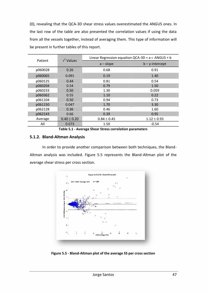
5.1.2. Bland-Altman Analysis

In order to provide another comparison between both techniques, the Bland-

Altman analysis was included. Figure 5.5 represents the Bland-Altman plot of the

average shear stress per cross section.

Figure 5.5 - Bland-Altman plot of the average SS per cross section

Jorge Santos 48

The Bland-Altman analysis reveals that the average shear stress from the QCA-

3D is overestimated systematically by 0.077 3.96 Pa. This value shows that the

average of all differences is almost zero; however it is of less value due to its high

standard deviation. The proportional error was also very small (Difference in SS =

0.061 x Average SS – 0.31). However it can be seen in the plot that the differences got

larger as the averages increased.

5.1.3. Maximum Shear Stress

In figure 5.6 is presented an example of the comparison between ANGUS and

QCA-3D of the lumen area, average SS and Maximum SS per cross-section along the

length of a vessel. Furthermore, in table 5.2 are presented the correlation coefficient

(r2), and the linear regression parameters of the scattering between the maximum SS

per cross-section calculated from the ANGUS and QCA-3D geometries.

Figure 5.6 - Lumen Area, Maximum and Average SS per cross section – ANGUS vs QCA-3D

(example)

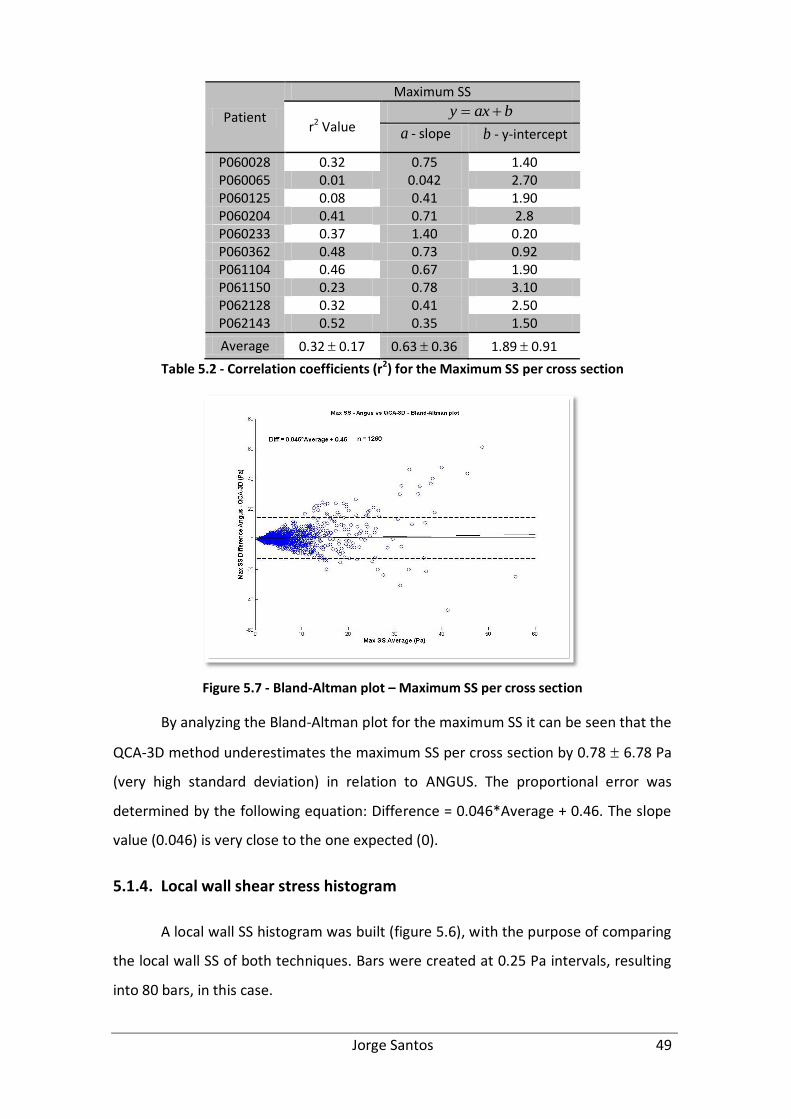
Jorge Santos 49

Patient

Maximum SS

r2 Value baxy

a - slope b - y-intercept

P060028 0.32 0.75 1.40 P060065 0.01 0.042 2.70 P060125 0.08 0.41 1.90 P060204 0.41 0.71 2.8 P060233 0.37 1.40 0.20 P060362 0.48 0.73 0.92 P061104 0.46 0.67 1.90 P061150 0.23 0.78 3.10 P062128 0.32 0.41 2.50 P062143 0.52 0.35 1.50

Average 0.32 0.17 0.63 0.36 1.89 0.91

Table 5.2 - Correlation coefficients (r2) for the Maximum SS per cross section

Figure 5.7 - Bland-Altman plot – Maximum SS per cross section

By analyzing the Bland-Altman plot for the maximum SS it can be seen that the

QCA-3D method underestimates the maximum SS per cross section by 0.78 6.78 Pa

(very high standard deviation) in relation to ANGUS. The proportional error was

determined by the following equation: Difference = 0.046*Average + 0.46. The slope

value (0.046) is very close to the one expected (0).

5.1.4. Local wall shear stress histogram

A local wall SS histogram was built (figure 5.6), with the purpose of comparing

the local wall SS of both techniques. Bars were created at 0.25 Pa intervals, resulting

into 80 bars, in this case.

Jorge Santos 50

The ANGUS and the QCA-3D histograms were very similar. Both of the peaks

are situated in the 1.25 to 1.5 Pa interval. The ANGUS vessels have 1657 elements in

that wall shear stress interval, while the QCA-3D ones have 1612 elements in that

same interval.

Assuming that SS with values between 0 and 0.5 Pa is considered low SS, SS

with values >1.5 Pa is considered physiological SS and SS > x = 3.88 + 5.50 Pa =

9.38 Pa is high SS; for the ANGUS vessels, the number of elements with low SS

represent 7% of the total number of elements, while 57% of the elements show

physiological SS and 8% of the elements exhibit high SS. For the QCA-3D vessels, the

elements with low SS represent 6% of the total number of elements; while the

elements with

physiological SS

represent 58.5% of

the total number

of elements and

9.5% of the

elements have

high SS values.

5.1.5. Low SS Analysis

Patients Number of cross sections with low SS (<0.5 Pa) Sensitivity Specificity ANGUS QCA-3D Overlapping

P060028 18 26 10 56% 86% P060065 65 29 21 32% 91% P060125 40 41 35 88% 94% P060204 21 9 6 29% 97% P060233 32 22 21 66% 98% P060362 79 68 62 78% 90% P061104 13 12 7 54% 94% P061150 44 26 17 39% 92% P062128 36 23 17 47% 93% P062143 39 39 29 74% 87%

All 387 295 225 58% 92% Average 39 21 30 17 23 17 56 20% 92 4 %

Table 5.3 – Cross-sections with low SS (<0.5 Pa) by ANGUS and QCA-3D method

Figure 5.8 - Local wall SS histogram (ANGUS vs QCA-3D)

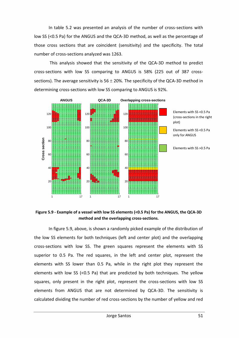
Jorge Santos 51

In table 5.2 was presented an analysis of the number of cross-sections with

low SS (<0.5 Pa) for the ANGUS and the QCA-3D method, as well as the percentage of

those cross sections that are coincident (sensitivity) and the specificity. The total

number of cross-sections analyzed was 1263.

This analysis showed that the sensitivity of the QCA-3D method to predict

cross-sections with low SS comparing to ANGUS is 58% (225 out of 387 cross-

sections). The average sensitivity is 56 20%. The specificity of the QCA-3D method in

determining cross-sections with low SS comparing to ANGUS is 92%.

Figure 5.9 - Example of a vessel with low SS elements (<0.5 Pa) for the ANGUS, the QCA-3D

method and the overlapping cross-sections.

In figure 5.9, above, is shown a randomly picked example of the distribution of

the low SS elements for both techniques (left and center plot) and the overlapping

cross-sections with low SS. The green squares represent the elements with SS

superior to 0.5 Pa. The red squares, in the left and center plot, represent the

elements with SS lower than 0.5 Pa, while in the right plot they represent the

elements with low SS (<0.5 Pa) that are predicted by both techniques. The yellow

squares, only present in the right plot, represent the cross-sections with low SS

elements from ANGUS that are not determined by QCA-3D. The sensitivity is

calculated dividing the number of red cross-sections by the number of yellow and red

1 17

20

40

60

80

100

120

Cro

ss

se

cti

on

ANGUS

1 17

20

40

60

80

100

120

QCA-3D

1 17

20

40

60

80

100

120

Overlapping cross-sections

Elements with SS <0.5 Pa

(cross-sections in the right

plot)

Elements with SS >0.5 Pa

Elements with SS <0.5 Pa

only for ANGUS

Jorge Santos 52

cross-sections. In this case, the sensitivity of the QCA-3D in determining low SS cross-

sections is of 88%.

5.1.6. High SS Analysis

In this analysis, high SS was defined as all values above the mean SS for each

vessel plus one standard deviation (from the ANGUS calculations outcome). So high

SS is > x Pa. The total number of cross-sections analyzed was 1263. In table 5.3,

below, is presented the mean SS, standard deviation and the sum of both, for the ten

coronaries studied.

Patients Mean SS (Pa) Standard deviation (Pa) x (Pa)

P060028 3.20

2.00

5.20

P060065 1.78

1.49 3.27

P060125 1.69

0.89 2.59 P060204 5.40

3.93 9.32 P060233 3.16 1.85 5.01 P060362 2.04

2.22 4.26 P061104 3.46 2.85 6.31 P061150 9.16

10.57 19.73 P062128 3.05

2.91 5.95 P062143 4.99

7.36 12.35

Table 5.4 – High SS threshold for each patient.

The number of cross-sections with high SS, for the ANGUS, the QCA-3D

method and the percentage of coincident cross-sections with high SS, were presented

below in table 5.5. It shows that 58% of the QCA-3D cross-sections with high SS were

coincident with the ANGUS cross-sections with high SS (155 out of 261 cross-

sections). The average percentage of overlapping high SS cross-sections per patient

was 58 20%. The specificity of the QCA-3D method in predicting cross-sections with

high SS relatively to ANGUS is 78%.

In figure 5.10, below, is shown a randomly picked example (patient p060233)

of the distribution of the high SS elements for both techniques (left and center plot)

and the overlapping cross-sections with high SS. The green squares represent the

elements with SS inferior to 5.01 Pa (see table 5.4 for the value). The red squares, in

the left and center plot, represent the elements with SS higher than 5.01 Pa, while in

the right plot they represent the elements with high SS (>5.01 Pa) that are predicted

by both techniques. The yellow squares, only present in the right plot, represent the

cross-sections with high SS elements from ANGUS that are not determined by QCA-

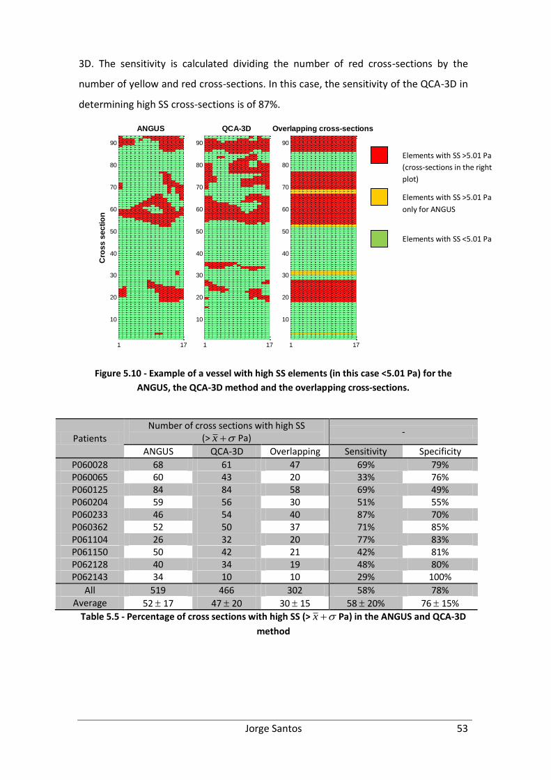
Jorge Santos 53

3D. The sensitivity is calculated dividing the number of red cross-sections by the

number of yellow and red cross-sections. In this case, the sensitivity of the QCA-3D in

determining high SS cross-sections is of 87%.

Figure 5.10 - Example of a vessel with high SS elements (in this case <5.01 Pa) for the

ANGUS, the QCA-3D method and the overlapping cross-sections.

Patients

Number of cross sections with high SS (> x Pa)

-

ANGUS QCA-3D Overlapping Sensitivity Specificity

P060028 68 61 47 69% 79% P060065 60 43 20 33% 76% P060125 84 84 58 69% 49% P060204 59 56 30 51% 55% P060233 46 54 40 87% 70% P060362 52 50 37 71% 85% P061104 26 32 20 77% 83% P061150 50 42 21 42% 81% P062128 40 34 19 48% 80% P062143 34 10 10 29% 100%

All 519 466 302 58% 78% Average 52 17 47 20 30 15 58 20% 76 15%

Table 5.5 - Percentage of cross sections with high SS (> x Pa) in the ANGUS and QCA-3D

method

1 17

10

20

30

40

50

60

70

80

90

Cro

ss

se

cti

on

ANGUS

1 17

10

20

30

40

50

60

70

80

90

QCA-3D

1 17

10

20

30

40

50

60

70

80

90

Overlapping cross-sections

Elements with SS >5.01 Pa

(cross-sections in the right

plot)

Elements with SS <5.01 Pa

Elements with SS >5.01 Pa

only for ANGUS

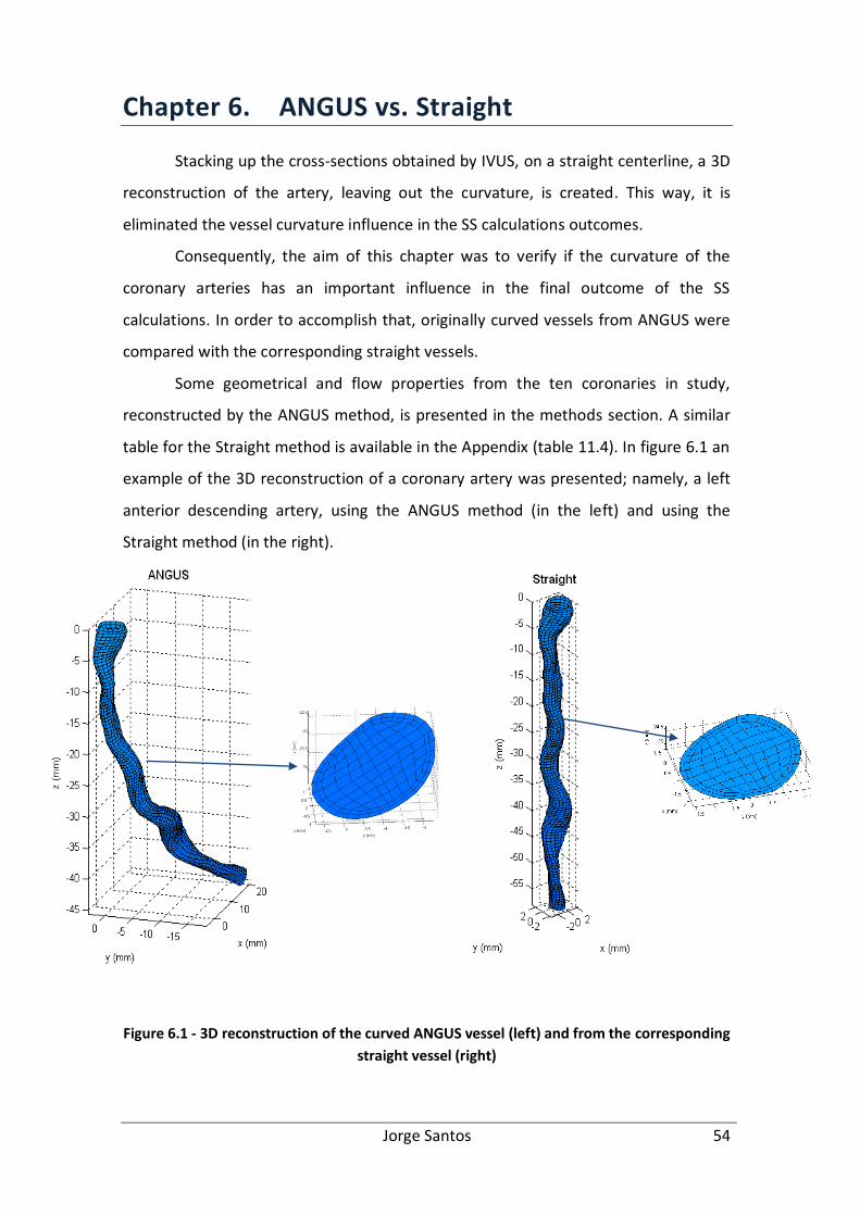
Jorge Santos 54

Chapter 6. ANGUS vs. Straight

Stacking up the cross-sections obtained by IVUS, on a straight centerline, a 3D

reconstruction of the artery, leaving out the curvature, is created. This way, it is

eliminated the vessel curvature influence in the SS calculations outcomes.

Consequently, the aim of this chapter was to verify if the curvature of the

coronary arteries has an important influence in the final outcome of the SS

calculations. In order to accomplish that, originally curved vessels from ANGUS were

compared with the corresponding straight vessels.

Some geometrical and flow properties from the ten coronaries in study,

reconstructed by the ANGUS method, is presented in the methods section. A similar

table for the Straight method is available in the Appendix (table 11.4). In figure 6.1 an

example of the 3D reconstruction of a coronary artery was presented; namely, a left

anterior descending artery, using the ANGUS method (in the left) and using the

Straight method (in the right).

Figure 6.1 - 3D reconstruction of the curved ANGUS vessel (left) and from the corresponding

straight vessel (right)

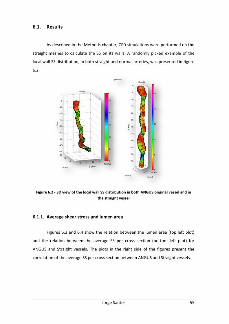
Jorge Santos 55

6.1. Results

As described in the Methods chapter, CFD simulations were performed on the

straight meshes to calculate the SS on its walls. A randomly picked example of the

local wall SS distribution, in both straight and normal arteries, was presented in figure

6.2.

Figure 6.2 - 3D view of the local wall SS distribution in both ANGUS original vessel and in

the straight vessel

6.1.1. Average shear stress and lumen area

Figures 6.3 and 6.4 show the relation between the lumen area (top left plot)

and the relation between the average SS per cross section (bottom left plot) for

ANGUS and Straight vessels. The plots in the right side of the figures present the

correlation of the average SS per cross section between ANGUS and Straight vessels.

-20

-10

00 5 10 15

-45

-40

-35

-30

-25

-20

-15

-10

-5

0

y (mm)

Angus

x (mm)

z (

mm

)

-2 02

-20

2

-55

-50

-45

-40

-35

-30

-25

-20

-15

-10

-5

0

x (mm)

Straight

y (mm)

z (

mm

)

0

5

10

15

20

25

0

5

10

15

20

25

p060204

SS (Pa)

SS (Pa)

Jorge Santos 56

Figure 6.3 - Lumen Area and Average SS comparison between ANGUS and Straight vessels

Figure 6.4 - Lumen Area and Average SS comparison between ANGUS and Straight vessels

In both figure 6.3 and 6.4 it is observed that the average SS per cross section

at ANGUS and the Straight vessel are very much alike. This is confirmed by the strong

correlation seen in the scatter plots (r2 = 0.92 and 0.87). If we perform this analysis for

all patients, we found an average r2 value of 0.79 0.11, and although it is smaller

than the ones presented, it is still a high correlation coefficient (see table 6.1).

Jorge Santos 57

Consequently, only considering the average SS per cross section, it can be said

that the results from the SS based on the ANGUS method and from the Straight vessel

are fairly similar.

However, by analyzing the maximum SS per cross section and the average

longitudinal shear stress from both techniques, some significant differences were

found, which are presented further in this chapter.

Patient

Average SS Maximum SS

r2 Value baxy

r2 Value baxy

a - slope b - y-intercept a - slope b - y-intercept

P060028 0.58 0.62 1.30 0.55 0.65 1.70 P060065 0.66 1.20 0.12 0.56 1.80 -0.61 P060125 0.79 0.81 0.59 0.45 0.64 1.60 P060204 0.92 0.83 0.51 0.69 0.65 2.30 P060233 0.86 1.00 0.59 0.74 0.92 1.50 P060362 0.81 1.00 0.43 0.66 1.40 1.00 P061104 0.83 1.20 0.12 0.67 1.60 -0.23 P061150 0.76 1.20 1.40 0.66 1.50 4.20 P062128 0.90 1.10 0.24 0.74 1.00 1.30 P062143 0.83 1.30 1.00 0.42 1.20 4.60

Average 0.79 0.11 1.03 0.22 0.63 0.46 0.61 0.11 1.14 0.43 1.74 1.66

Table 6.1 - Correlation coefficients (r2) for the Average and Maximum SS per cross section

6.1.2. Bland-Altman Analysis

As in the two previous chapters, a Bland-Altman analysis was performed on

the average SS per cross section. The Bland-Altman plot is shown in figure 6.5.

The Bland-Altman analysis reveals that the average SS from the Straight

vessels underestimated systematically the one from ANGUS by 0.76 2.24 Pa. The

proportional error was defined by the following equation: Difference in SS = 0.29 x

Average SS – 0.25. A slope of 0.29 means that the differences between techniques got

slightly larger as the averages increased.

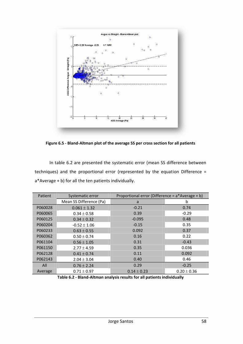
Jorge Santos 58

Figure 6.5 - Bland-Altman plot of the average SS per cross section for all patients

In table 6.2 are presented the systematic error (mean SS difference between

techniques) and the proportional error (represented by the equation Difference =

a*Average + b) for all the ten patients individually.

Patient Systematic error Proportional error (Difference = a*Average + b)

Mean SS Difference (Pa) a b

P060028 0.061 1.32 -0.21 0.74

P060065 0.34 0.58 0.39 -0.29

P060125 0.34 0.32 -0.095 0.48

P060204 -0.52 1.06 -0.15 0.35

P060233 0.63 0.55 0.092 0.37

P060362 0.50 0.74 0.16 0.22

P061104 0.56 1.05 0.31 -0.43

P061150 2.77 4.59 0.35 0.036

P062128 0.41 0.74 0.11 0.092

P062143 2.04 3.04 0.40 0.46

All 0.76 2.24 0.29 -0.25

Average 0.71 0.97 0.14 0.23 0.20 0.36

Table 6.2 - Bland-Altman analysis results for all patients individually

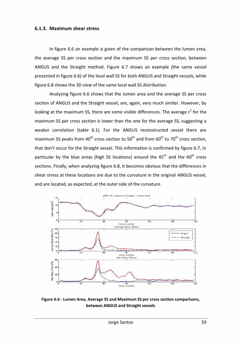
Jorge Santos 59

6.1.3. Maximum shear stress

In figure 6.6 an example is given of the comparison between the lumen area,

the average SS per cross section and the maximum SS per cross section, between

ANGUS and the Straight method. Figure 6.7 shows an example (the same vessel

presented in figure 6.6) of the local wall SS for both ANGUS and Straight vessels, while

figure 6.8 shows the 3D view of the same local wall SS distribution.

Analyzing figure 6.6 shows that the lumen area and the average SS per cross

section of ANGUS and the Straight vessel, are, again, very much similar. However, by

looking at the maximum SS, there are some visible differences. The average r2 for the

maximum SS per cross section is lower than the one for the average SS, suggesting a

weaker correlation (table 6.1). For the ANGUS reconstructed vessel there are

maximum SS peaks from 40th cross section to 50th and from 60th to 70th cross section,

that don’t occur for the Straight vessel. This information is confirmed by figure 6.7, in

particular by the blue areas (high SS locations) around the 45th and the 60th cross

sections. Finally, when analyzing figure 6.8, it becomes obvious that the differences in

shear stress at these locations are due to the curvature in the original ANGUS vessel,

and are located, as expected, at the outer side of the curvature.

Figure 6.6 - Lumen Area, Average SS and Maximum SS per cross section comparisons,

between ANGUS and Straight vessels

Jorge Santos 60

Figure 6.7 - Wall SS distribution of an ANGUS and a Straight geometry

Figure 6.8 - 3D view of the SS distribution in the reconstructed ANGUS and Straight vessels

5 10 15

10

20

30

40

50

60

70

80

90

100

110

Cro

ss s

ections

Angus

5 10 15

10

20

30

40

50

60

70

80

90

100

110

Cro

ss s

ections

Straight

5

10

15

20

25

30

35

40

45

5

10

15

20

25

30

35

40

45

p062143 - Angus vs Straight

WSS (Pa) WSS (Pa)

0

10

20

30

40

-2024

0

5

10

15

20

25

y (mm)

Angus

x (mm)

z (m

m)

-10123 -20

2

0

10

20

30

40

50

y (mm)

Straight

x (mm)

z (m

m)

5

10

15

20

25

30

35

40

45

5

10

15

20

25

30

35

40

45

WSS (Pa)

WSS (Pa)

p062143 - Angus vs Straight

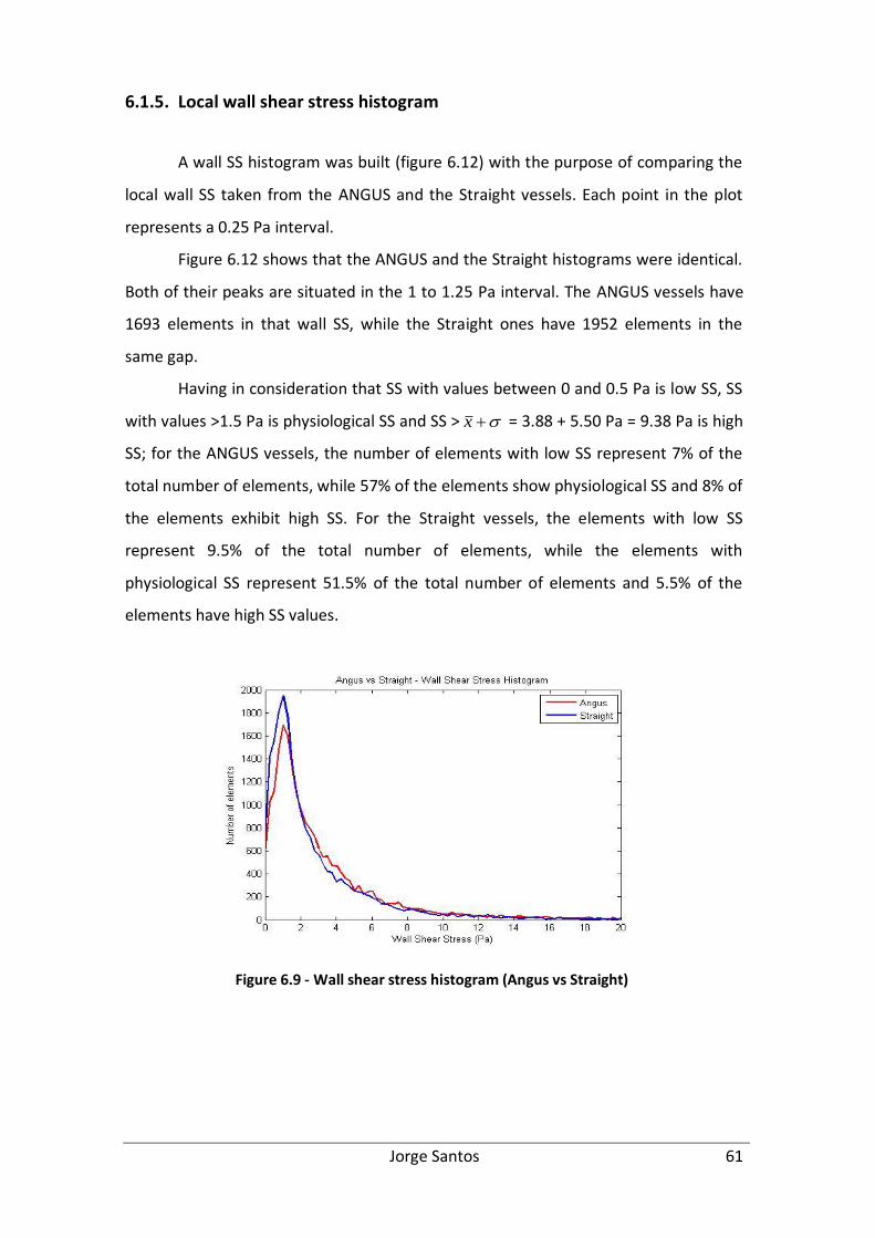
Jorge Santos 61

6.1.5. Local wall shear stress histogram

A wall SS histogram was built (figure 6.12) with the purpose of comparing the

local wall SS taken from the ANGUS and the Straight vessels. Each point in the plot

represents a 0.25 Pa interval.

Figure 6.12 shows that the ANGUS and the Straight histograms were identical.

Both of their peaks are situated in the 1 to 1.25 Pa interval. The ANGUS vessels have

1693 elements in that wall SS, while the Straight ones have 1952 elements in the

same gap.

Having in consideration that SS with values between 0 and 0.5 Pa is low SS, SS

with values >1.5 Pa is physiological SS and SS > x = 3.88 + 5.50 Pa = 9.38 Pa is high

SS; for the ANGUS vessels, the number of elements with low SS represent 7% of the

total number of elements, while 57% of the elements show physiological SS and 8% of

the elements exhibit high SS. For the Straight vessels, the elements with low SS

represent 9.5% of the total number of elements, while the elements with

physiological SS represent 51.5% of the total number of elements and 5.5% of the

elements have high SS values.

Figure 6.9 - Wall shear stress histogram (Angus vs Straight)

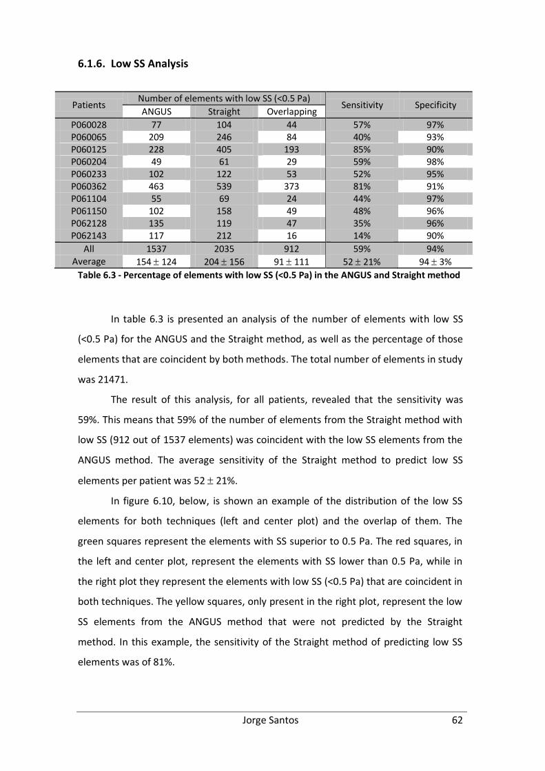
Jorge Santos 62

6.1.6. Low SS Analysis

Patients Number of elements with low SS (<0.5 Pa)

Sensitivity Specificity ANGUS Straight Overlapping

P060028 77 104 44 57% 97% P060065 209 246 84 40% 93% P060125 228 405 193 85% 90% P060204 49 61 29 59% 98% P060233 102 122 53 52% 95% P060362 463 539 373 81% 91% P061104 55 69 24 44% 97% P061150 102 158 49 48% 96% P062128 135 119 47 35% 96% P062143 117 212 16 14% 90%

All 1537 2035 912 59% 94% Average 154 124 204 156 91 111 52 21% 94 3%

Table 6.3 - Percentage of elements with low SS (<0.5 Pa) in the ANGUS and Straight method

In table 6.3 is presented an analysis of the number of elements with low SS

(<0.5 Pa) for the ANGUS and the Straight method, as well as the percentage of those

elements that are coincident by both methods. The total number of elements in study

was 21471.

The result of this analysis, for all patients, revealed that the sensitivity was

59%. This means that 59% of the number of elements from the Straight method with

low SS (912 out of 1537 elements) was coincident with the low SS elements from the

ANGUS method. The average sensitivity of the Straight method to predict low SS

elements per patient was 52 21%.

In figure 6.10, below, is shown an example of the distribution of the low SS

elements for both techniques (left and center plot) and the overlap of them. The

green squares represent the elements with SS superior to 0.5 Pa. The red squares, in

the left and center plot, represent the elements with SS lower than 0.5 Pa, while in

the right plot they represent the elements with low SS (<0.5 Pa) that are coincident in

both techniques. The yellow squares, only present in the right plot, represent the low

SS elements from the ANGUS method that were not predicted by the Straight

method. In this example, the sensitivity of the Straight method of predicting low SS

elements was of 81%.

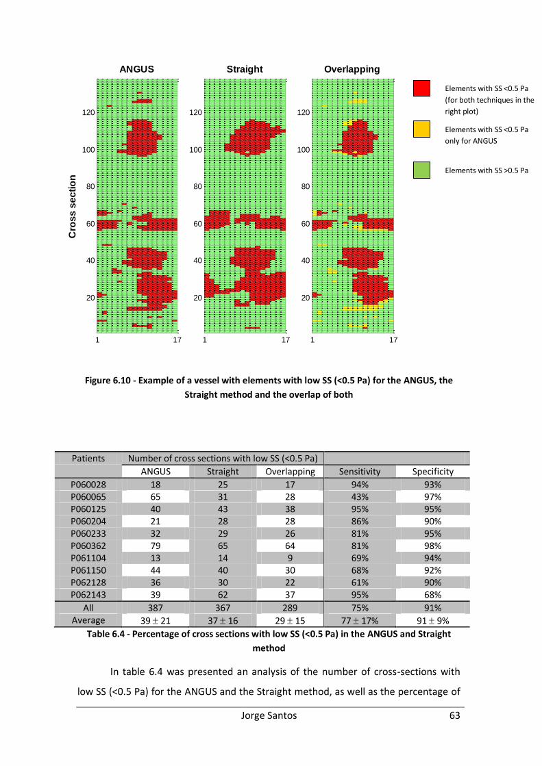
Jorge Santos 63

Figure 6.10 - Example of a vessel with elements with low SS (<0.5 Pa) for the ANGUS, the

Straight method and the overlap of both

Patients Number of cross sections with low SS (<0.5 Pa)

ANGUS Straight Overlapping Sensitivity Specificity

P060028 18 25 17 94% 93% P060065 65 31 28 43% 97% P060125 40 43 38 95% 95% P060204 21 28 28 86% 90% P060233 32 29 26 81% 95% P060362 79 65 64 81% 98% P061104 13 14 9 69% 94% P061150 44 40 30 68% 92% P062128 36 30 22 61% 90% P062143 39 62 37 95% 68%

All 387 367 289 75% 91% Average 39 21 37 16 29 15 77 17% 91 9%

Table 6.4 - Percentage of cross sections with low SS (<0.5 Pa) in the ANGUS and Straight

method

In table 6.4 was presented an analysis of the number of cross-sections with

low SS (<0.5 Pa) for the ANGUS and the Straight method, as well as the percentage of

1 17

20

40

60

80

100

120

Cro

ss

se

cti

on

ANGUS

1 17

20

40

60

80

100

120

Straight

1 17

20

40

60

80

100

120

Overlapping

Elements with SS <0.5 Pa

(for both techniques in the

right plot)

Elements with SS >0.5 Pa

Elements with SS <0.5 Pa

only for ANGUS

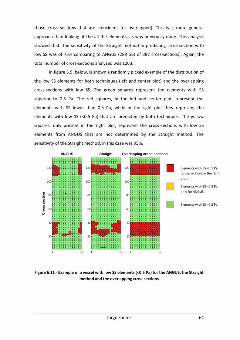
Jorge Santos 64

those cross sections that are coincident (or overlapped). This is a more general

approach than looking at the all the elements, as was previously done. This analysis

showed that the sensitivity of the Straight method in predicting cross-section with

low SS was of 75% comparing to ANGUS (289 out of 387 cross-sections). Again, the

total number of cross-sections analyzed was 1263.

In figure 5.9, below, is shown a randomly picked example of the distribution of

the low SS elements for both techniques (left and center plot) and the overlapping

cross-sections with low SS. The green squares represent the elements with SS

superior to 0.5 Pa. The red squares, in the left and center plot, represent the

elements with SS lower than 0.5 Pa, while in the right plot they represent the

elements with low SS (<0.5 Pa) that are predicted by both techniques. The yellow

squares, only present in the right plot, represent the cross-sections with low SS

elements from ANGUS that are not determined by the Straight method. The

sensitivity of the Straight method, in this case was 95%.

Figure 6.11 - Example of a vessel with low SS elements (<0.5 Pa) for the ANGUS, the Straight

method and the overlapping cross-sections

1 17

20

40

60

80

100

120

Cro

ss

se

cti

on

ANGUS

1 17

20

40

60

80

100

120

Straight

1 17

20

40

60

80

100

120

Overlapping cross-sections

Elements with SS <0.5 Pa

(cross-sections in the right

plot)

Elements with SS >0.5 Pa

Elements with SS <0.5 Pa

only for ANGUS

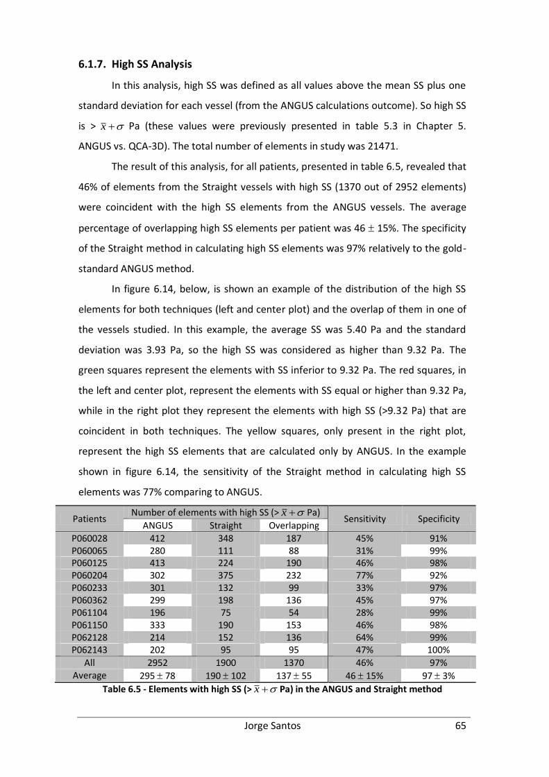
Jorge Santos 65

6.1.7. High SS Analysis

In this analysis, high SS was defined as all values above the mean SS plus one

standard deviation for each vessel (from the ANGUS calculations outcome). So high SS

is > x Pa (these values were previously presented in table 5.3 in Chapter 5.

ANGUS vs. QCA-3D). The total number of elements in study was 21471.

The result of this analysis, for all patients, presented in table 6.5, revealed that

46% of elements from the Straight vessels with high SS (1370 out of 2952 elements)

were coincident with the high SS elements from the ANGUS vessels. The average

percentage of overlapping high SS elements per patient was 46 15%. The specificity

of the Straight method in calculating high SS elements was 97% relatively to the gold-

standard ANGUS method.

In figure 6.14, below, is shown an example of the distribution of the high SS

elements for both techniques (left and center plot) and the overlap of them in one of

the vessels studied. In this example, the average SS was 5.40 Pa and the standard

deviation was 3.93 Pa, so the high SS was considered as higher than 9.32 Pa. The

green squares represent the elements with SS inferior to 9.32 Pa. The red squares, in

the left and center plot, represent the elements with SS equal or higher than 9.32 Pa,

while in the right plot they represent the elements with high SS (>9.32 Pa) that are

coincident in both techniques. The yellow squares, only present in the right plot,

represent the high SS elements that are calculated only by ANGUS. In the example

shown in figure 6.14, the sensitivity of the Straight method in calculating high SS

elements was 77% comparing to ANGUS.

Patients Number of elements with high SS (> x Pa)

Sensitivity Specificity ANGUS Straight Overlapping

P060028 412 348 187 45% 91% P060065 280 111 88 31% 99% P060125 413 224 190 46% 98% P060204 302 375 232 77% 92% P060233 301 132 99 33% 97% P060362 299 198 136 45% 97% P061104 196 75 54 28% 99% P061150 333 190 153 46% 98% P062128 214 152 136 64% 99% P062143 202 95 95 47% 100%

All 2952 1900 1370 46% 97% Average 295 78 190 102 137 55 46 15% 97 3%

Table 6.5 - Elements with high SS (> x Pa) in the ANGUS and Straight method

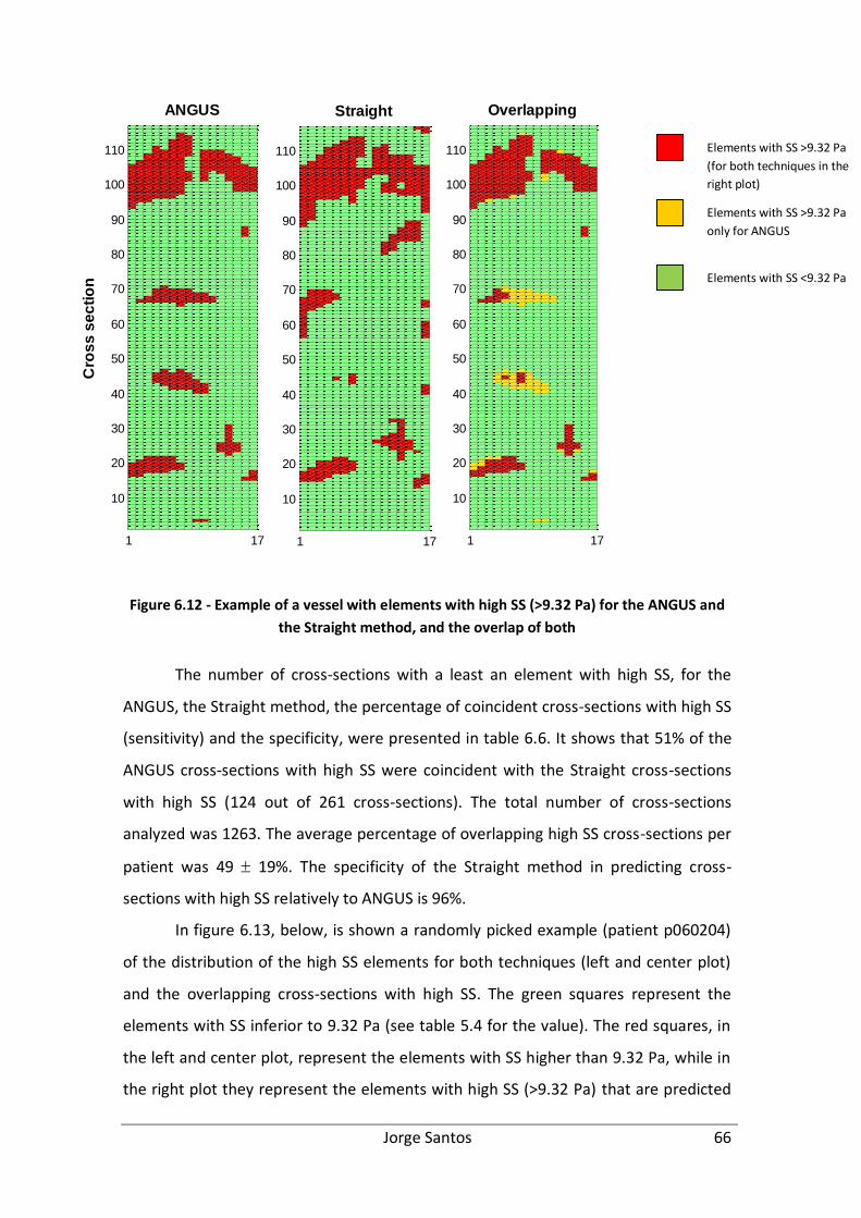
Jorge Santos 66

Figure 6.12 - Example of a vessel with elements with high SS (>9.32 Pa) for the ANGUS and

the Straight method, and the overlap of both

The number of cross-sections with a least an element with high SS, for the

ANGUS, the Straight method, the percentage of coincident cross-sections with high SS

(sensitivity) and the specificity, were presented in table 6.6. It shows that 51% of the

ANGUS cross-sections with high SS were coincident with the Straight cross-sections

with high SS (124 out of 261 cross-sections). The total number of cross-sections

analyzed was 1263. The average percentage of overlapping high SS cross-sections per

patient was 49 19%. The specificity of the Straight method in predicting cross-

sections with high SS relatively to ANGUS is 96%.

In figure 6.13, below, is shown a randomly picked example (patient p060204)

of the distribution of the high SS elements for both techniques (left and center plot)

and the overlapping cross-sections with high SS. The green squares represent the

elements with SS inferior to 9.32 Pa (see table 5.4 for the value). The red squares, in

the left and center plot, represent the elements with SS higher than 9.32 Pa, while in

the right plot they represent the elements with high SS (>9.32 Pa) that are predicted

1 17

10

20

30

40

50

60

70

80

90

100

110

Cro

ss

se

cti

on

ANGUS

1 17

10

20

30

40

50

60

70

80

90

100

110

Straight

1 17

10

20

30

40

50

60

70

80

90

100

110

Overlapping

Elements with SS >9.32 Pa

(for both techniques in the

right plot)

Elements with SS <9.32 Pa

Elements with SS >9.32 Pa

only for ANGUS

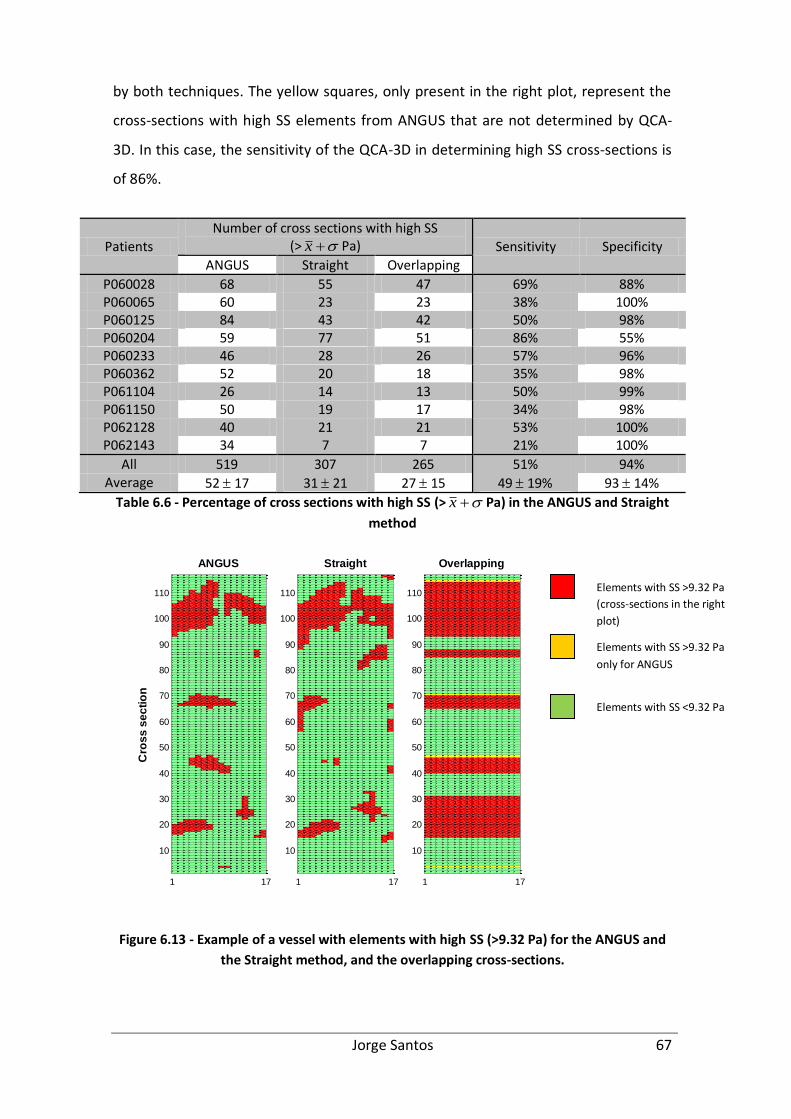
Jorge Santos 67

by both techniques. The yellow squares, only present in the right plot, represent the

cross-sections with high SS elements from ANGUS that are not determined by QCA-

3D. In this case, the sensitivity of the QCA-3D in determining high SS cross-sections is

of 86%.

Patients

Number of cross sections with high SS (> x Pa) Sensitivity Specificity

ANGUS Straight Overlapping

P060028 68 55 47 69% 88% P060065 60 23 23 38% 100% P060125 84 43 42 50% 98% P060204 59 77 51 86% 55% P060233 46 28 26 57% 96% P060362 52 20 18 35% 98% P061104 26 14 13 50% 99% P061150 50 19 17 34% 98% P062128 40 21 21 53% 100% P062143 34 7 7 21% 100%

All 519 307 265 51% 94% Average 52 17 31 21 27 15 49 19% 93 14%

Table 6.6 - Percentage of cross sections with high SS (> x Pa) in the ANGUS and Straight

method

Figure 6.13 - Example of a vessel with elements with high SS (>9.32 Pa) for the ANGUS and

the Straight method, and the overlapping cross-sections.

1 17

10

20

30

40

50

60

70

80

90

100

110

Cro

ss

se

cti

on

ANGUS

1 17

10

20

30

40

50

60

70

80

90

100

110

Straight

1 17

10

20

30

40

50

60

70

80

90

100

110

Overlapping

Elements with SS >9.32 Pa

(cross-sections in the right

plot)

Elements with SS <9.32 Pa

Elements with SS >9.32 Pa

only for ANGUS

Jorge Santos 68

6.1.8. Longitudinal shear stress

Figure 6.14 - Wall SS distribution an ANGUS and a Straight geometry

Figure 6.15 - Mean Longitudinal SS for ANGUS and the Straight vessel (p060362)

The left side of Figure 6.9 and the ANGUS (red) curve of Figure 6.10 suggest

that the average longitudinal SS is not constant for the whole vessel. The columns

from 6 to 13 have lower SS than the columns 1 to 5 and 14 to 17. The 3D image in

Figure 6.10 reveals that the columns that have the lowest SS correspond to the inner

side of the curvature in the ANGUS vessel, while the columns that have the highest SS

correspond to the outer side of curvature.

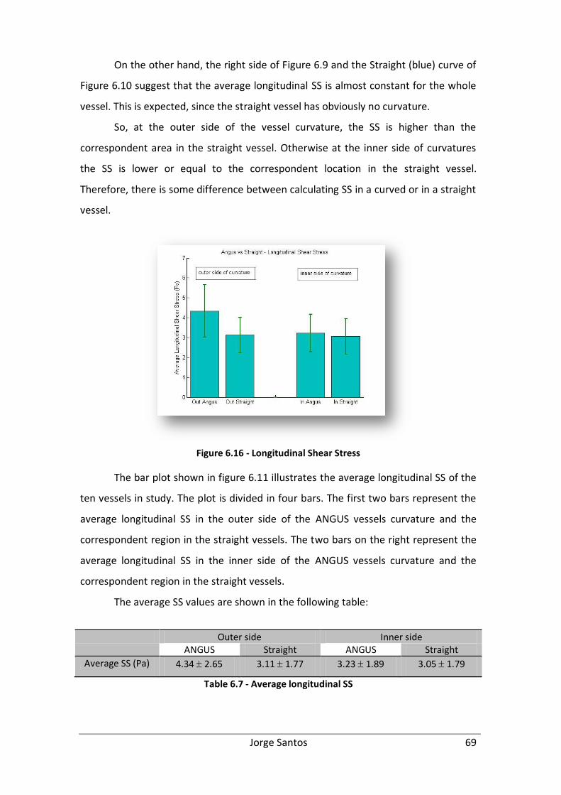
Jorge Santos 69

On the other hand, the right side of Figure 6.9 and the Straight (blue) curve of

Figure 6.10 suggest that the average longitudinal SS is almost constant for the whole

vessel. This is expected, since the straight vessel has obviously no curvature.

So, at the outer side of the vessel curvature, the SS is higher than the

correspondent area in the straight vessel. Otherwise at the inner side of curvatures

the SS is lower or equal to the correspondent location in the straight vessel.

Therefore, there is some difference between calculating SS in a curved or in a straight

vessel.

Figure 6.16 - Longitudinal Shear Stress

The bar plot shown in figure 6.11 illustrates the average longitudinal SS of the

ten vessels in study. The plot is divided in four bars. The first two bars represent the

average longitudinal SS in the outer side of the ANGUS vessels curvature and the

correspondent region in the straight vessels. The two bars on the right represent the

average longitudinal SS in the inner side of the ANGUS vessels curvature and the

correspondent region in the straight vessels.

The average SS values are shown in the following table:

Outer side Inner side

ANGUS Straight ANGUS Straight

Average SS (Pa) 4.34 2.65 3.11 1.77 3.23 1.89 3.05 1.79

Table 6.7 - Average longitudinal SS

Jorge Santos 70

This data confirms the previous assumption that the vessel curvature provokes

higher SS on the outer side and lower SS on the inner side. The average SS on the

outer side of curvature in the ANGUS vessels is 39% higher than in the Straight

vessels, while on the inner side is only 6% higher. When comparing the inner and

outer side of the same method, the outer side of ANGUS is 34% higher than the inner

side and the outer side of the Straight vessels is only 2% higher than the inner side.

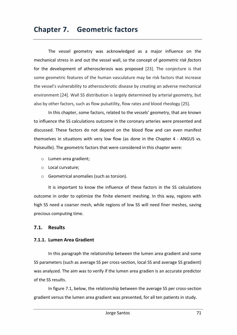
Jorge Santos 71

Chapter 7. Geometric factors

The vessel geometry was acknowledged as a major influence on the

mechanical stress in and out the vessel wall, so the concept of geometric risk factors

for the development of atherosclerosis was proposed [23]. The conjecture is that

some geometric features of the human vasculature may be risk factors that increase

the vessel’s vulnerability to atherosclerotic disease by creating an adverse mechanical

environment [24]. Wall SS distribution is largely determined by arterial geometry, but

also by other factors, such as flow pulsatility, flow rates and blood rheology [25].

In this chapter, some factors, related to the vessels’ geometry, that are known

to influence the SS calculations outcome in the coronary arteries were presented and

discussed. These factors do not depend on the blood flow and can even manifest

themselves in situations with very low flow (as done in the Chapter 4 - ANGUS vs.

Poiseuille). The geometric factors that were considered in this chapter were:

o Lumen area gradient;

o Local curvature;

o Geometrical anomalies (such as torsion).

It is important to know the influence of these factors in the SS calculations

outcome in order to optimize the finite element meshing. In this way, regions with

high SS need a coarser mesh, while regions of low SS will need finer meshes, saving

precious computing time.

7.1. Results

7.1.1. Lumen Area Gradient

In this paragraph the relationship between the lumen area gradient and some

SS parameters (such as average SS per cross-section, local SS and average SS gradient)

was analyzed. The aim was to verify if the lumen area gradien is an accurate predictor

of the SS results.

In figure 7.1, below, the relationship between the average SS per cross-section

gradient versus the lumen area gradient was presented, for all ten patients in study.

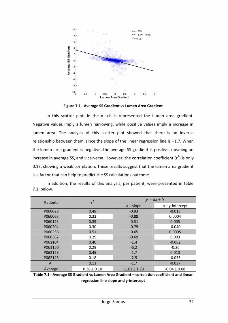
Jorge Santos 72

Figure 7.1 - Average SS Gradient vs Lumen Area Gradient

In this scatter plot, in the x-axis is represented the lumen area gradient.

Negative values imply a lumen narrowing, while positive values imply a increase in

lumen area. The analysis of this scatter plot showed that there is an inverse

relationship between them, since the slope of the linear regression line is –1.7. When

the lumen area gradient is negative, the average SS gradient is positive, meaning an

increase in average SS, and vice-versa. However, the correlation coefficient (r2) is only

0.13, showing a weak correlation. These results suggest that the lumen area gradient

is a factor that can help to predict the SS calculations outcome.

In addition, the results of this analysis, per patient, were presented in table 7.1, below.

Patients r2 baxy

a – slope b – y-intercept

P060028 0.48 -0.93 -0.013 P060065 0.33 -0.88 0.0004 P060125 0.39 -0.31 0.005 P060204 0.30 -0.79 -0.040 P060233 0.51 -0.65 0.0005 P060362 0.29 -0.69 0.003 P061104 0.40 -1.4 -0.052 P061150 0.29 -6.2 -0.26 P062128 0.45 -1.7 0.010 P062143 0.18 -2.5 -0.033

All 0.13 -1.7 -0.037

Average 0.36 0.10 -1.61 1.73 -0.04 0.08

Table 7.1 - Average SS Gradient vs Lumen Area Gradient – correlation coefficient and linear

regression line slope and y-intercept

-2 -1.5 -1 -0.5 0 0.5 1 1.5 2-10

-8

-6

-4

-2

0

2

4

6

8

10

Lumen Area Gradient

Av

era

ge

SS

Gra

die

nt

y = - 1.7*x - 0.037

r2 = 0.13

n = 1263

Jorge Santos 73

Figure 7.2 - Example of the relation between the lumen area gradient and the gradient in SS

In figure 7.2 an example is presented, showing both a positive and negative SS

gradient because of a negative and positive lumen area gradient.

Additionally, the relationship between the gradient in lumen area and the

average SS per cross-section was analyzed. In figure 7.3 was shown the lumen area

gradient (top plot) and the average SS (bottom plot) along the length of one of the

coronaries in study. Cross-sections with negative area gradient (o) and with positive

area gradient (o) were highlighted, as well as the corresponding cross-sections in the

average SS plot. As expected, when the gradient in lumen area is positive, or when

the lumen area is increasing, the average SS over a cross section is decreasing. On the

other hand, when the gradient in lumen area is negative (lumen area decreasing), the

average SS over a cross section increases.

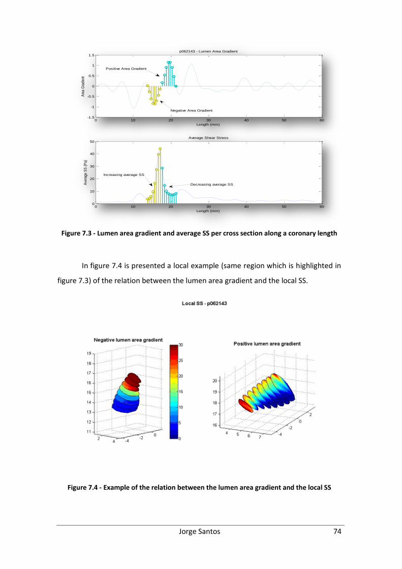
Jorge Santos 74

Figure 7.3 - Lumen area gradient and average SS per cross section along a coronary length

In figure 7.4 is presented a local example (same region which is highlighted in

figure 7.3) of the relation between the lumen area gradient and the local SS.

Figure 7.4 - Example of the relation between the lumen area gradient and the local SS

0 10 20 30 40 50 60-1.5

-1

-0.5

0

0.5

1

1.5

Length (mm)

Are

a G

radi

ent

p062143 - Lumen Area Gradient

0 10 20 30 40 50 600

10

20

30

40

50

Length (mm)

Ave

rage

SS

(P

a)

Average Shear Stress

Negative Area Gradient

Positive Area Gradient

Increasing average SS

Decreasing average SS

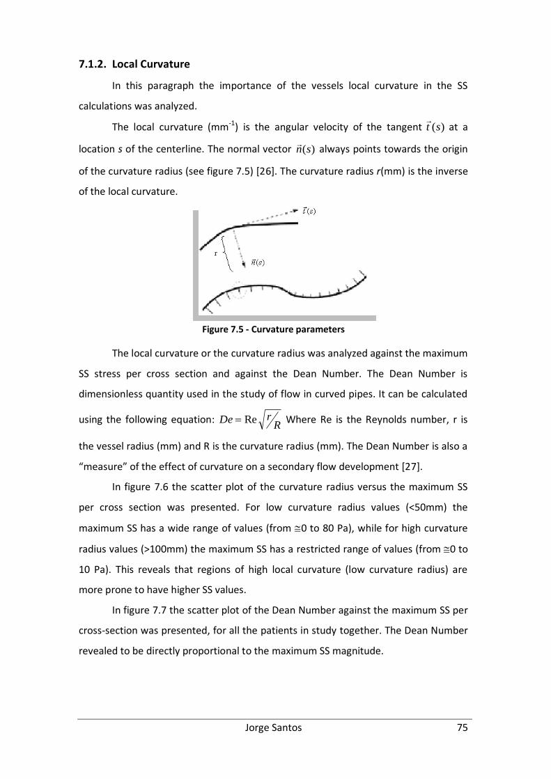
Jorge Santos 75

7.1.2. Local Curvature

In this paragraph the importance of the vessels local curvature in the SS

calculations was analyzed.

The local curvature (mm-1) is the angular velocity of the tangent )(st

at a

location s of the centerline. The normal vector )(sn

always points towards the origin

of the curvature radius (see figure 7.5) [26]. The curvature radius r(mm) is the inverse

of the local curvature.

Figure 7.5 - Curvature parameters

The local curvature or the curvature radius was analyzed against the maximum

SS stress per cross section and against the Dean Number. The Dean Number is

dimensionless quantity used in the study of flow in curved pipes. It can be calculated

using the following equation: R

rDe Re Where Re is the Reynolds number, r is

the vessel radius (mm) and R is the curvature radius (mm). The Dean Number is also a

“measure” of the effect of curvature on a secondary flow development *27].

In figure 7.6 the scatter plot of the curvature radius versus the maximum SS

per cross section was presented. For low curvature radius values (<50mm) the

maximum SS has a wide range of values (from 0 to 80 Pa), while for high curvature

radius values (>100mm) the maximum SS has a restricted range of values (from 0 to

10 Pa). This reveals that regions of high local curvature (low curvature radius) are

more prone to have higher SS values.

In figure 7.7 the scatter plot of the Dean Number against the maximum SS per

cross-section was presented, for all the patients in study together. The Dean Number

revealed to be directly proportional to the maximum SS magnitude.

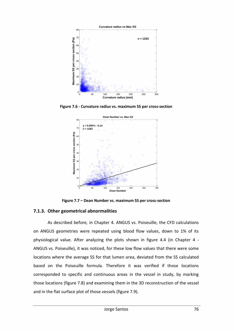
Jorge Santos 76

Figure 7.6 - Curvature radius vs. maximum SS per cross-section

Figure 7.7 – Dean Number vs. maximum SS per cross-section

7.1.3. Other geometrical abnormalities

As described before, in Chapter 4. ANGUS vs. Poiseuille, the CFD calculations

on ANGUS geometries were repeated using blood flow values, down to 1% of its

physiological value. After analyzing the plots shown in figure 4.4 (in Chapter 4 -

ANGUS vs. Poiseuille), it was noticed, for these low flow values that there were some

locations where the average SS for that lumen area, deviated from the SS calculated

based on the Poiseuille formula. Therefore it was verified if those locations

corresponded to specific and continuous areas in the vessel in study, by marking

those locations (figure 7.8) and examining them in the 3D reconstruction of the vessel

and in the flat surface plot of those vessels (figure 7.9).

0 50 100 150 200 250 3000

10

20

30

40

50

60

70

80

Curvature radius (mm)

Ma

xim

um

SS

pe

r c

ros

s s

ec

tio

n (

Pa

)

Curvature radius vs Max SS

n = 1263

0 50 100 150 200 250 3000

10

20

30

40

50

60

70

80

Dean Number

Ma

xim

um

SS

pe

r c

ros

s s

ec

tio

n (

Pa

)

Dean Number vs. Max SS

y = 0.093*x - 0.14

n = 1263

Jorge Santos 77

Figure 7.8 - Highlight of the dots deviated from the line based on the Poiseuille equation

Figure 7.9 - Local SS distribution of a coronary artery – two views of the 3D reconstruction

and a flat surface plot

The green dots () showed in Figure 7.8 represent the SS in the region

between the 58th cross section and the 70th, for 1% of the physiological Reynolds

number. These dots are clearly far from the ones based on Poiseuille formula. Thus,

by analyzing figure 7.9, it can be seen that in this location the vessel has some torsion,

which can be the cause of this difference between the Average SS and the Poiseuille

SS. The Average SS dots illustrated in light blue () and dark yellow () are also non-

coincident with the Poiseuille based SS, probably because of some torsion in the

corresponding regions of the vessel

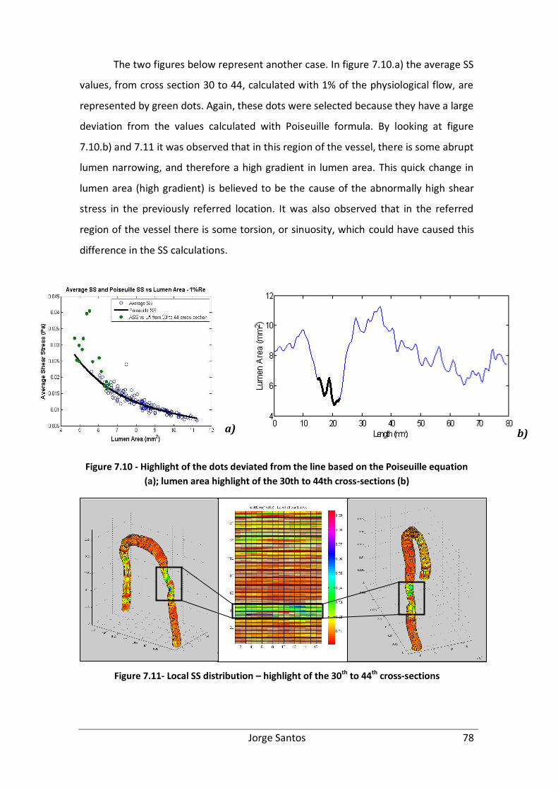
Jorge Santos 78

The two figures below represent another case. In figure 7.10.a) the average SS

values, from cross section 30 to 44, calculated with 1% of the physiological flow, are

represented by green dots. Again, these dots were selected because they have a large

deviation from the values calculated with Poiseuille formula. By looking at figure

7.10.b) and 7.11 it was observed that in this region of the vessel, there is some abrupt

lumen narrowing, and therefore a high gradient in lumen area. This quick change in

lumen area (high gradient) is believed to be the cause of the abnormally high shear

stress in the previously referred location. It was also observed that in the referred

region of the vessel there is some torsion, or sinuosity, which could have caused this

difference in the SS calculations.

Figure 7.10 - Highlight of the dots deviated from the line based on the Poiseuille equation

(a); lumen area highlight of the 30th to 44th cross-sections (b)

Figure 7.11- Local SS distribution – highlight of the 30th to 44th cross-sections

a) b)

Jorge Santos 79

7.1.4. Guidelines to mesh optimization

The results previously presented in this manuscript show that geometric

factors are of most importance in the SS outcome of CFD calculations. These

calculations are difficult and time-consuming. So, if regions of low SS were found,

meshing could be made finer in those regions, whereas areas of higher SS could have

coarser meshes. Therefore some guidelines to improve the finite element meshing

locally in coronary arteries reconstructions were given and compiled in this

paragraph.

- Regions with positive lumen area gradient should have finer meshing, as they

help create low SS locations. On the other hand, regions with negative lumen

area gradient should have coarser meshing, since they are a predictor of high

SS locations.

- Regions with high local curvature values and, therefore, high Dean number

values, should also have finer meshing; since the Dean number is a predictor

of secondary flow development. Therefore, those are regions of predilection

for atherosclerotic plaque formation.

- The inner side of curvatures should also have a finer mesh, since those are

regions commonly with low SS and where plaques are known to develop. In

contrast, the outer side of curvatures should have coarser meshing as SS is

known to have higher magnitudes at those regions.

- Regions with detectable torsion or sinuosity should also have finer meshing

than the overall, since they cause non-linearities, even at extremely slow flow

conditions, where they should be absent.

- On the other side, regions that don’t exhibit any of the factors above

mentioned could have coarser meshing. Computing time depends, among

other factors, on the number of elements. Therefore if meshing is made

coarser in these areas, precious time is saved.

Jorge Santos 80

Chapter 8. Discussion

8.1. Limitations

Some of the limitations in this study concern the CFD calculations, since it is

difficult to account for all exact physiological conditions. The fluid was assumed as

incompressible, homogenous Newtonian, while blood has a non-Newtonian behavior.

However these previous assumptions are common and found reasonable for medium

and large arteries by Friedman et al. in 1992 [28]. The flow was prescribed as steady,

instead of pulsatile. The coronary vessel walls were also assumed as rigid, however at

physiological conditions, the coronary walls are complaint; and due to the cardiac

contraction, the coronaries contract and deform.

Furthermore, sometimes SS artifacts might have occurred due to the different

smoothing in the 3D reconstructions. This fact had some residual effect on the data

obtained from the Straight geometries. One presumption of the Straight method was

that the geometries obtained from it had cross-sections with the exact shape and size

as the ones from the ANGUS method. However, due to the different smoothing in the

reconstructions, sometimes, the area of corresponding cross-sections was not exactly

equal. Nevertheless, these differences in lumen area between methods had residual

effects on the SS calculations outcomes.

The fact that these 3D reconstructions do not include bifurcations and side

branches are a limitation in this study, since ignoring the side branches might have an

impact in the SS distribution.

8.2. ANGUS vs. Poiseuille

In this chapter, one of the goals was to confirm the inverse relationship

between the average SS per cross section and the lumen area of the corresponding

cross-section. However, the main goal was to verify if the SS calculated based on the

Jorge Santos 81

Poiseuille equation2 was accurate enough to predict the average SS per cross section

in a 3D reconstructed coronary artery (by the gold-standard ANGUS method)3, which

is not a straight cylinder with perfectly circular cross-sections.

According to the results obtained, that was not a correct assumption. Though

the average SS and the Poiseuille SS have similar distribution per lumen area (inverse

relation), a large number of cross-sections diverged significantly in terms of value.

Their correlation was only average, with average r2 = 0.65 0.09.

Other goal of this chapter was to quantify the influence of the blood flow,

whether in the average SS versus lumen area relationship, as in the relationship

between the average SS and the Poiseuille SS. Given the results, it was evident that by

lowering the blood flow, the average SS versus lumen area relation became more

linear. The average SS versus Poiseuille SS correlation grew up to an r2 = 0.93 0.05.

This reveals that at 1% of the physiological blood flow, it is so low that the coronaries

exhibit parabolic, Poiseuille-like flow. This means that most of the factors, related to

flow, that caused non-linearities in the results, were suppressed.

The Bland-Altman statistics results showed that the Poiseuille SS

systematically underestimated the average SS and that when the magnitude of the

averages increased, the difference between the methods got larger. A probable cause

for this occurrence may be the presence of the results of a specific vessel (p061150),

which had really high average SS peaks comparing to the estimated Poiseuille SS.

The results from the local wall SS histogram revealed that the Poiseuille

equation did not calculate any low SS (<0.5 Pa) cross-section. While according to the

ANGUS method 7% of the elements had low SS. This fact may indicate that the

Poiseuille equation has difficulties in predicting the low SS regions, which are of great

importance, since the low SS is a cause of the development of an atherogenic

phenotype in the inner surface cells of the arteries. The Poiseuille equation was also

found to have difficulties in predicting the higher magnitudes of SS per cross-section,

comparing to ANGUS. Furthermore, the SS histogram revealed that the SS magnitudes

2, 3 From hereby will be referred only as Poiseuille SS and average SS, respectively.

Jorge Santos 82

obtained from the ANGUS geometries were in agreement with the SS range of

magnitudes presented by Malek et al. in 1999 [5].

The results from the analysis of velocity profiles in some specific cross-sections

were important to confirm and visualize the blood flow/SS behavior inside the

coronaries. The cross section in a curved region of the vessel revealed an asymmetric

profile, with high velocity near the outer side of curvature and low velocity near the

inner side of curvature. The cross section with small lumen area, revealed a flattened

velocity profile. This implies that the SS in this cross section is much higher than what

is predicted by the Poiseuille equation, probably due to abrupt lumen narrowing. Still,

for low blood flow values, these effects were eliminated and the velocity profiles

became parabolic.

In the end, the Poiseuille equation revealed to be a fairly poor method of

calculating SS in coronaries arteries. The main reason is that the SS distribution is

strongly dependent of on the geometry of the vessel, which is not accounted in the

Poiseuille equation. A similar result was found by Berthier et al., who compared the

SS distribution in a model of a realistic RCA and a model with the physiological

trajectory but with circular and constant cross-sections [29].

8.3. ANGUS vs. QCA-3D

In this chapter the primary objective was to compare the SS calculated from

3D geometries created by two different techniques: ANGUS and QCA-3D. The QCA-3D

is based only on biplane angiography, lacking cross-sectional information.

Consequently, the importance of the cross-sectional information was studied

The average SS versus lumen area relationship of both techniques was

analyzed. Both demonstrated an inverse relationship and no relevant differences

were found. On the other side, when comparing the average SS from both methods a

low correlation coefficient was found, r2 = 0.40 0.20. This lack of correlation in the

average SS was mainly due to the different shape of corresponding cross-sections

between each technique, since the difference in lumen area between corresponding

cross-sections are highly correlated, as stated by Schuurbiers et al[19]. Those shape

differences occur because QCA-3D is only based on biplane Angiography, therefore

Jorge Santos 83

has a limited cross sectional information, contrarily to ANGUS which has the cross

sectional information given by IVUS.

It was also studied the sensitivity and the specificity of the QCA-3D method

comparing to the gold-standard ANGUS method, in predicting cross-section with low

or high SS. This analysis revealed that the average sensitivity of the QCA-3D method

to predict low SS cross-sections was 56 ± 20%, while the specificity was 92 ± 4%. As

for high SS, the average sensitivity was 58 ± 20% while the specificity was 76 ± 15%.

These results state that the QCA-3D method has a similar sensitivity in predicting low

SS cross-sections and high SS cross-sections.

In the end, the cross-sectional information (namely the shape of each cross-

section), which lacks in the QCA-3D method, revealed to have some relevance in the

SS outcomes. However, the SS results of the QCA-3D were fairly similar to the ones

from ANGUS. Since the QCA-3D is a simpler approach and less time consuming, it can

be affirmed that QCA-3D has the potential to become a useful tool in the

catheterization laboratory, as it was stated by Schuurbiers et al [19]. Goubergrits et al.

also studied the wall SS profiling of a biplane angiography-based reconstruction

technique (QCA-3D) on a LCA phantom [30], and concluded that it is a practical

approach.

8.4. ANGUS vs. Straight

The purpose of this chapter was to compare the SS results of the CFD

calculations from ANGUS geometries and Straight geometries, therefore studying the

influence of curvature on the SS distribution.

Like in Chapters 4 and 5, the first parameter analyzed was the average SS per

cross section from both techniques. The average correlation coefficient, r2 = 0.79

0.11, was significantly higher than the one obtained for the ANGUS vs. QCA-3D

results. The Straight geometries had similar cross-sectional shape as the ANGUS

geometries, contrasting to the QCA-3D ones. Therefore these results show that when

it comes to predict the average SS per cross-section the shape of the cross-section is a

much more important factor than the curvature of the vessel.

Jorge Santos 84

The analysis of the maximum SS per cross-section or even locally, revealed

that a weaker correlation (r2 = 0.61 0.11) comparing to the average SS. When

observing the maximum SS locally in the ANGUS vessels, the locations at the outer

side of the vessel curvature had much higher values than the corresponding locations

in the Straight vessels. These results are consistent with the prevalence of

atherosclerosis in the inner side of curvatures, since low SS is promotes

atherosclerosis.

The local SS histogram disclosed that the peak for both techniques was

situated at the same interval, 1 to 1.25 Pa. However, there were a higher percentage

of elements with low SS from the Straight geometries than from the ANGUS ones. On

the other hand, a lower percentage of physiological and high SS elements were found

in the Straight geometries comparing to the ANGUS ones.

Like in Chapter 5 - ANGUS vs. QCA-3D, an analysis of the sensitivity and

specificity of the Straight method was performed. However, in this chapter the

sensitivity and the specificity were analyzed per element, as well as on a cross-

sectional basis. The analysis per cross-section revealed that the average sensitivity of

the Straight method in predicting cross-section with low SS was 77 ± 17% comparing

to ANGUS, while the average specificity was 91 ± 9%. As for high SS, the average

sensitivity was only 49 ± 19% and the average specificity was 93 ± 14%. Therefore, the

Straight method seems to have more sensitivity in predicting the cross-sections with

low SS than the cross-sections with high SS. Comparing with the analogous analysis

for the QCA-3D method, it is observed that the Straight method has better sensitivity

than QCA-3D in the prediction of low SS cross-sections. However, the QCA-3D method

has better sensitivity to predict high SS cross-sections.

The sensitivity and specificity analysis per element showed that, for low SS

elements, the Straight method has an average sensitivity of 52 ± 21% and an average

specificity of 94 ± 3%, comparing to the ANGUS method. Concerning the high SS

elements, the average sensitivity of the Straight method was 46 ± 15%, while the

specificity was 97 ± 3%. From these results can be concluded that, comparing to the

cross-sectional analysis, the sensitivity results are slightly worse. However this is

expected, since it is a more specific analysis. Furthermore, the analysis per element

showed that the Straight method has a similar average sensitivity in predicting low SS

Jorge Santos 85

elements and high SS elements, contrarily to the results of the analysis per cross-

section.

As a conclusion, the curvature influence in the SS results revealed to have a

limited importance, in contrast to the cross-sectional shape, since the SS results from

the Straight method were fairly similar to the ones from ANGUS. The Straight method

also revealed to be more accurate in mimicking the ANGUS results than the QCA-3D

method.

8.5. Geometric Factors

The first factor analyzed in this chapter was the lumen area gradient. The

scattering of the lumen area gradient and the average SS gradient from all patients

together, revealed an inverse relationship between them, with a regression line slope

of –1.7. So, as expected, it was observed that when the area gradient was negative

the average SS was increasing in proportion, and vice-versa. These results confirm

that analyzing the lumen area gradient (complemented by the lumen area values), it

can be given an accurate prediction of where SS peaks may occur, and consequently

optimize the meshing in those areas, by making it finer or coarser.

Another parameter analyzed was the local curvature/curvature radius. The

curvature radius showed an inverse relationship with the maximum SS per cross

section, which implies that low curved regions have a predominance of low SS, while

highly curved regions exhibit both high and low SS. Analyzing the maximum SS per

cross-section against the Dean number, a direct relationship was found. This implied

that regions with high local curvature might develop secondary flow. According to

Honda et al [31], the vessel bending together with the pulsatile flow causes areas of

flow reversal; therefore those areas are of predilection for atherosclerosis

development.

The results of the analysis of the Average SS per cross section and the

Poiseuille SS for the lowest blood flow magnitude (1% of the physiological level),

suggested that, even for such a slow flow, the Average SS was not similar to the

Poiseuille SS. A further analysis on the local SS and the geometry in those specific

Jorge Santos 86

locations contributed to the assumption that this occurs due to the torsion or

sinuosity exhibited in that location. The presence of these sinuous regions in the

coronaries impedes the blood flow to behave in a parabolic way even at such low

magnitudes. So, when transported to physiological conditions, these effects might

have a much higher impact on the SS distribution.

Regarding these geometric factors, some guidelines to mesh optimization

were given. In the future, these simplifications in the finite element meshing might

save some precious computing time while allowing the CFD approach in SS calculation

to be transported from bench to bedside.

Jorge Santos 87

Chapter 9. Conclusion

In the course of this project, the distribution of wall SS in coronary arteries

was studied. These studies are important due to the relevance of the SS in the

modulation of endothelial biology and consequent predisposal to atherogenesis.

The methods used revealed to be appropriate, since convergence was reached

in all the CFD calculations executed.

Blood flow was confirmed to have a strong effect on the relationship between

average SS and the lumen area, since it was found out that by lowering blood flow,

non-linearities in that inverse relationship almost vanished and the average SS per

cross section assumed a distribution identical to the SS based on the Poiseuille

equation.

The QCA-3D method, based on biplane angiography, with elliptical cross

sections, revealed to have more accuracy than the Poiseuille in mimicking the SS

results based on the ANGUS geometries.It is essential to know that the results from

QCA-3D geometries are comparable to the state-of-the-art ANGUS, since it is a more

practical approach that can be performed on-site at the catheterization laboratory.

The Straight geometries also revealed to provide results similar to the ones

from the ANGUS geometries. However, originally extremely curved vessels exhibited

significantly higher SS magnitudes on the outer side of the curvature, comparing to

the corresponding sites in the Straight geometries.

Geometric factors, such as lumen area gradient, local curvature or torsion,

were revealed to be important in predicting SS peaks, low SS areas and sites

predisposed to secondary flow development, which contribute to atherosclerotic

plaque formation.

In the future, based on the knowledge of these geometric features, meshes

can be optimized and CFD calculations on 3D reconstructed arteries may become a

faster and bedside approach.

Jorge Santos 88

10. References

[1] http://www.rjmatthewsmd.com/Definitions/coronary_arteries.htm - adapted

from Waller, B.F., MD, Schlant, R.C., MD, Anatomy of the Heart, Hurst's The Heart,

8th edition, p 84-86 (accessed 13 April,2009).

[2] Mosseri M, Zolti E, Rozenman Y, Lotan C, Ershov T, Izak T, Admon D, Gotsman MS.

The diameter of the epicardial coronary arteries in patients with dilated

cardiomyopathy. Internacional Journal of Cardiology. 62 (1997) 133–141.

[3] Guyton&Hall. Textbook of Medical Phisiology - ninth edition, Unit 4, Chapter 21,

page 257.

[4] Guyton&Hall. Textbook of Medical Phisiology - ninth edition, Unit 4, Chapter 15,

page 171.

[5] Malek AM, Alper SL, Izumo S. Hemodynamic Shear Stress and Its Role in

Atherosclerosis. JAMA, December 1, 1999 – Vol 282, No.21

[6] Atherosclerosis: The new view. Peter Libby. Scientific American 2002 –

www.ahs.uwaterloo.ca/~kh346/pdf/libby.pdf

[7] Chatzizisis YS, Coskun AU, Jonas M, Edelman ER, Feldman CL, Stone PH. Role of

endothelial shear stress in the natural history of coronary atherosclerosis and

vascular remodeling – molecular, cellular and vascular behavior. JACC Vol. 49, No.

25, June 26, 2007:2379–93

[8] Helderman F, Segers D, de Crom R, Hierck BP, Poelmann RE, Evans PC, Krams R.

Effect of shear stress on vascular inflammation and plaque development. Curr Opin

Lipidol. 2007. 18:527-533.

[9] Cunningham KS, Gotlieb AI. The role of shear stress in the pathogenesis of

atherosclerosis. Laboratory Investigation (2005) 85, 9–23.

[10] Slager CJ, Wentzel JJ, Gijsen FJH, Schuurbiers JCH, van der Wal AC, van der Steen

AFW, Serruys PW. The role of shear stress in the destabilization of vulnerable

plaques and related therapeutic implications. Nature Clinical Practice Cardiovascular

Medicine. 2005 Vol.2 No.9:456-464.

[11] Slager CJ, Wentzel JJ, Gijsen FJH, Schuurbiers JCH, van der Wal AC, van der Steen

AFW, Serruys PW. The role of shear stress in the generation of rupture-prone

vulnerable plaques. Nature Clinical Practice Cardiovascular Medicine. 2005 Vol.2

No.8:401-407

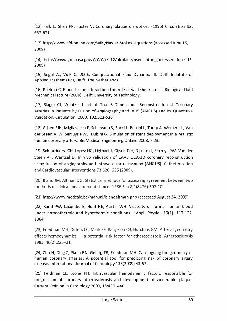
Jorge Santos 89

[12] Falk E, Shah PK, Fuster V. Coronary plaque disruption. (1995) Circulation 92:

657-671.

[13] http://www.cfd-online.com/Wiki/Navier-Stokes_equations (accessed June 15,

2009)

[14] http://www.grc.nasa.gov/WWW/K-12/airplane/nseqs.html (accessed June 15, 2009)

[15] Segal A., Vuik C. 2006. Computational Fluid Dynamics II. Delft Institute of Applied Mathematics, Delft, The Netherlands.

[16] Poelma C. Blood-tissue interaction; the role of wall shear stress. Biological Fluid Mechanics lecture (2008). Delft University of Technology.

[17] Slager CJ, Wentzel JJ, et al. True 3-Dimensional Reconstruction of Coronary

Arteries in Patients by Fusion of Angiography and IVUS (ANGUS) and Its Quantitive

Validation. Circulation. 2000; 102:511-516.

[18] Gijsen FJH, Migliavacca F, Schievano S, Socci L, Petrini L, Thury A, Wentzel JJ, Van

der Steen AFW, Serruys PWS, Dubini G. Simulation of stent deployment in a realistic

human coronary artery. BioMedical Engineering OnLine 2008, 7:23.

[19] Schuurbiers JCH, Lopez NG, Ligthart J, Gijsen FJH, Dijkstra J, Serruys PW, Van der

Steen AF, Wentzel JJ. In vivo validation of CAAS QCA-3D coronary reconstruction

using fusion of angiography and intravascular ultrasound (ANGUS). Catheterization

and Cardiovascular Interventions 73:620–626 (2009).

[20] Bland JM, Altman DG. Statistical methods for assessing agreement between two

methods of clinical measurement. Lancet 1986 Feb 8;1(8476):307-10.

[21] http://www.medcalc.be/manual/blandaltman.php (accessed August 24, 2009)

[22] Rand PW, Lacombe E, Hunt HE, Austin WH. Viscosity of normal human blood

under normothermic and hypothermic conditions. J.Appl. Physiol. 19(1): 117-122.

1964.

[23] Friedman MH, Deters OJ, Mark FF, Bargeron CB, Hutchins GM. Arterial geometry

affects hemodynamics — a potential risk factor for atherosclerosis. Atherosclerosis

1983; 46(2):225–31.

[24] Zhu H, Ding Z, Piana RN, Gehrig TR, Friedman MH. Catologuing the geometry of human coronary arteries: A potential tool for predicting risk of coronary artery disease. International Journal of Cardiology 135(2009) 43-52.

[25] Feldman CL, Stone PH. Intravascular hemodynamic factors responsible for

progression of coronary atherosclerosis and development of vulnerable plaque.

Current Opinion in Cardiology 2000, 15:430–440.

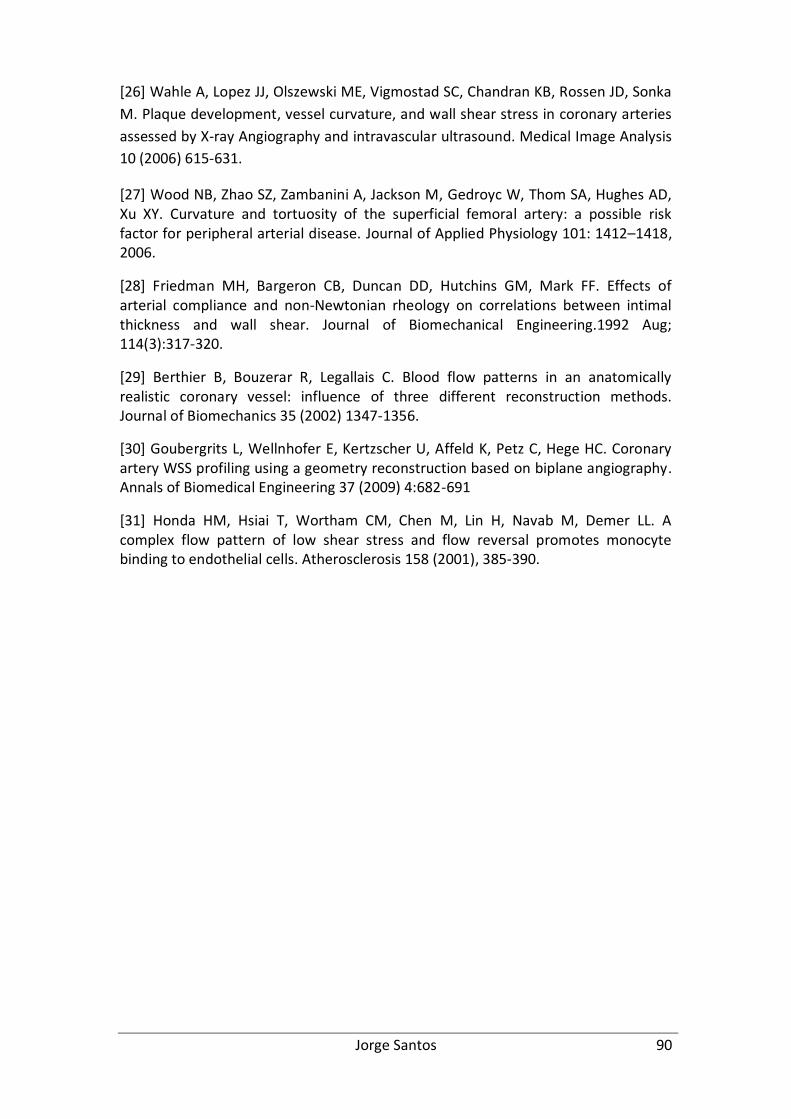
Jorge Santos 90

[26] Wahle A, Lopez JJ, Olszewski ME, Vigmostad SC, Chandran KB, Rossen JD, Sonka

M. Plaque development, vessel curvature, and wall shear stress in coronary arteries

assessed by X-ray Angiography and intravascular ultrasound. Medical Image Analysis

10 (2006) 615-631.

[27] Wood NB, Zhao SZ, Zambanini A, Jackson M, Gedroyc W, Thom SA, Hughes AD, Xu XY. Curvature and tortuosity of the superficial femoral artery: a possible risk factor for peripheral arterial disease. Journal of Applied Physiology 101: 1412–1418, 2006.

[28] Friedman MH, Bargeron CB, Duncan DD, Hutchins GM, Mark FF. Effects of arterial compliance and non-Newtonian rheology on correlations between intimal thickness and wall shear. Journal of Biomechanical Engineering.1992 Aug; 114(3):317-320.

[29] Berthier B, Bouzerar R, Legallais C. Blood flow patterns in an anatomically realistic coronary vessel: influence of three different reconstruction methods. Journal of Biomechanics 35 (2002) 1347-1356.

[30] Goubergrits L, Wellnhofer E, Kertzscher U, Affeld K, Petz C, Hege HC. Coronary artery WSS profiling using a geometry reconstruction based on biplane angiography. Annals of Biomedical Engineering 37 (2009) 4:682-691

[31] Honda HM, Hsiai T, Wortham CM, Chen M, Lin H, Navab M, Demer LL. A complex flow pattern of low shear stress and flow reversal promotes monocyte binding to endothelial cells. Atherosclerosis 158 (2001), 385-390.

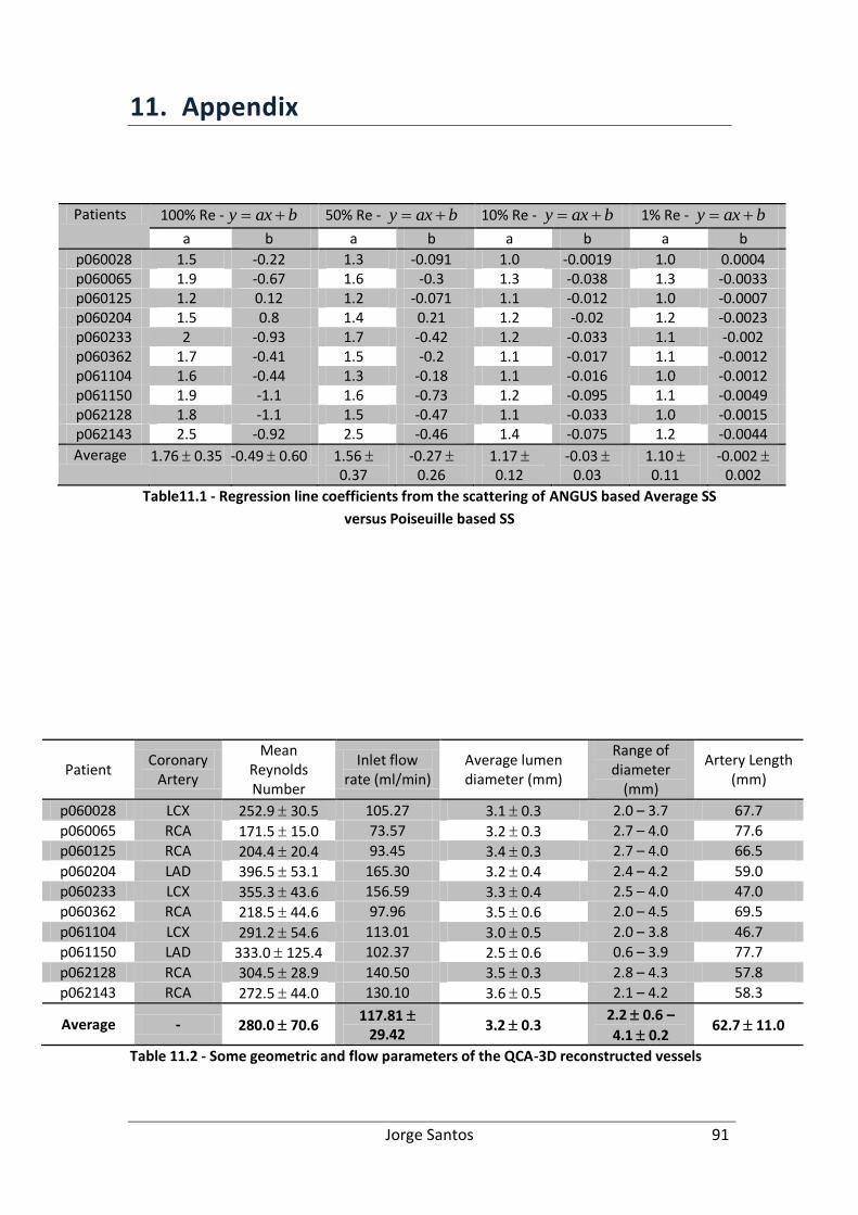
Jorge Santos 91

11. Appendix

Patients 100% Re - baxy 50% Re - baxy 10% Re - baxy 1% Re - baxy

a b a b a b a b

p060028 1.5 -0.22 1.3 -0.091 1.0 -0.0019 1.0 0.0004 p060065 1.9 -0.67 1.6 -0.3 1.3 -0.038 1.3 -0.0033 p060125 1.2 0.12 1.2 -0.071 1.1 -0.012 1.0 -0.0007 p060204 1.5 0.8 1.4 0.21 1.2 -0.02 1.2 -0.0023 p060233 2 -0.93 1.7 -0.42 1.2 -0.033 1.1 -0.002 p060362 1.7 -0.41 1.5 -0.2 1.1 -0.017 1.1 -0.0012 p061104 1.6 -0.44 1.3 -0.18 1.1 -0.016 1.0 -0.0012 p061150 1.9 -1.1 1.6 -0.73 1.2 -0.095 1.1 -0.0049 p062128 1.8 -1.1 1.5 -0.47 1.1 -0.033 1.0 -0.0015 p062143 2.5 -0.92 2.5 -0.46 1.4 -0.075 1.2 -0.0044

Average 1.76 0.35 -0.49 0.60 1.56 0.37

-0.27 0.26

1.17 0.12

-0.03 0.03

1.10 0.11

-0.002 0.002

Table11.1 - Regression line coefficients from the scattering of ANGUS based Average SS

versus Poiseuille based SS

Patient Coronary

Artery

Mean Reynolds Number

Inlet flow rate (ml/min)

Average lumen diameter (mm)

Range of diameter

(mm)

Artery Length (mm)

p060028 LCX 252.9 30.5 105.27 3.1 0.3 2.0 – 3.7 67.7

p060065 RCA 171.5 15.0 73.57 3.2 0.3 2.7 – 4.0 77.6

p060125 RCA 204.4 20.4 93.45 3.4 0.3 2.7 – 4.0 66.5

p060204 LAD 396.5 53.1 165.30 3.2 0.4 2.4 – 4.2 59.0

p060233 LCX 355.3 43.6 156.59 3.3 0.4 2.5 – 4.0 47.0

p060362 RCA 218.5 44.6 97.96 3.5 0.6 2.0 – 4.5 69.5

p061104 LCX 291.2 54.6 113.01 3.0 0.5 2.0 – 3.8 46.7

p061150 LAD 333.0 125.4 102.37 2.5 0.6 0.6 – 3.9 77.7

p062128 RCA 304.5 28.9 140.50 3.5 0.3 2.8 – 4.3 57.8

p062143 RCA 272.5 44.0 130.10 3.6 0.5 2.1 – 4.2 58.3

Average - 280.0 70.6 117.81

29.42 3.2 0.3

2.2 0.6 –

4.1 0.2 62.7 11.0

Table 11.2 - Some geometric and flow parameters of the QCA-3D reconstructed vessels

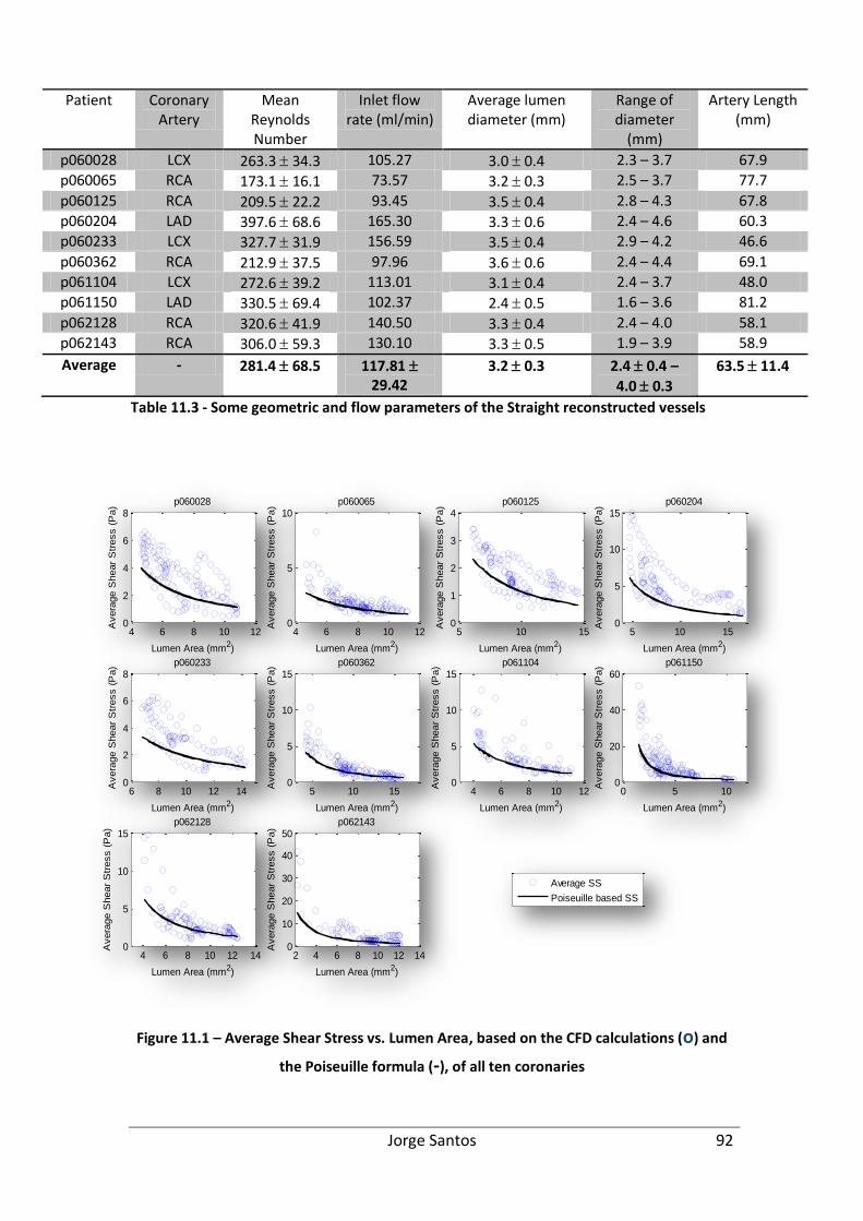
Jorge Santos 92

Patient Coronary Artery

Mean Reynolds Number

Inlet flow rate (ml/min)

Average lumen diameter (mm)

Range of diameter

(mm)

Artery Length (mm)

p060028 LCX 263.3 34.3 105.27 3.0 0.4 2.3 – 3.7 67.9

p060065 RCA 173.1 16.1 73.57 3.2 0.3 2.5 – 3.7 77.7

p060125 RCA 209.5 22.2 93.45 3.5 0.4 2.8 – 4.3 67.8

p060204 LAD 397.6 68.6 165.30 3.3 0.6 2.4 – 4.6 60.3

p060233 LCX 327.7 31.9 156.59 3.5 0.4 2.9 – 4.2 46.6

p060362 RCA 212.9 37.5 97.96 3.6 0.6 2.4 – 4.4 69.1

p061104 LCX 272.6 39.2 113.01 3.1 0.4 2.4 – 3.7 48.0

p061150 LAD 330.5 69.4 102.37 2.4 0.5 1.6 – 3.6 81.2

p062128 RCA 320.6 41.9 140.50 3.3 0.4 2.4 – 4.0 58.1

p062143 RCA 306.0 59.3 130.10 3.3 0.5 1.9 – 3.9 58.9

Average - 281.4 68.5 117.81 29.42

3.2 0.3 2.4 0.4 –

4.0 0.3

63.5 11.4

Table 11.3 - Some geometric and flow parameters of the Straight reconstructed vessels

Figure 11.1 – Average Shear Stress vs. Lumen Area, based on the CFD calculations (o) and

the Poiseuille formula (-), of all ten coronaries

4 6 8 10 120

2

4

6

8

Lumen Area (mm2)

Avera

ge S

hear

Str

ess (

Pa)

p060028

4 6 8 10 120

5

10

Lumen Area (mm2)

Avera

ge S

hear

Str

ess (

Pa)

p060065

5 10 150

1

2

3

4p060125

Lumen Area (mm2)

Avera

ge S

hear

Str

ess (

Pa)

5 10 150

5

10

15p060204

Lumen Area (mm2)

Avera

ge S

hear

Str

ess (

Pa)

6 8 10 12 140

2

4

6

8p060233

Lumen Area (mm2)

Avera

ge S

hear

Str

ess (

Pa)

5 10 150

5

10

15p060362

Lumen Area (mm2)

Avera

ge S

hear

Str

ess (

Pa)

4 6 8 10 120

5

10

15p061104

Lumen Area (mm2)

Avera

ge S

hear

Str

ess (

Pa)

0 5 100

20

40

60p061150

Lumen Area (mm2)

Avera

ge S

hear

Str

ess (

Pa)

4 6 8 10 12 140

5

10

15p062128

Lumen Area (mm2)

Avera

ge S

hear

Str

ess (

Pa)

2 4 6 8 10 12 140

10

20

30

40

50p062143

Lumen Area (mm2)

Avera

ge S

hear

Str

ess (

Pa)

Average SS

Poiseuille based SS

Jorge Santos 93

11.1. CFD script – example

problem

types

elgrp1=900

essbouncond

surfaces(s1)

surfaces(s3)

end

matrix

method=2

end

essential boundary conditions, sequence_number = 1

surfaces(s1 ), degfd3=(func=1)

end

# two steps:

# step 1: creat a good initial solution

# step 2: get final solution thru Re stepping

# coefficients step 1: initial solution

coefficients, sequence_number = 1

elgrp1 (nparm=20)

icoef2 = 1 # Newtonian fluid

icoef5 = 0 # Stokes, linearization

coef6 = 1d-6 # eps

coef7 = 1000 # density

coef12 = 0.030 # viscosity

end

# coefficients step 2: Re stepping

coefficients, sequence_number = 2

elgrp1 (nparm=20)

icoef2 = 1 # Newtonian fluid

icoef5 = 2 # Newtonian linearization

coef6 = 1d-6 # eps

coef7 = 1000 # density

Jorge Santos 94

coef12 = 0.010 # viscosity

end

# change coeffients for the initial solution: 1 and 2

change coefficients, sequence_number = 1

elgrp1

icoef5 = 1 # Picard lin

end

change coefficients, sequence_number = 2

elgrp1

icoef5 = 2 # Newtonian lin

end

# change coeffients for final solution: 3 till 5

change coefficients, sequence_number = 3

elgrp1

coef12 = 0.0075 # viscosity

end

change coefficients, sequence_number = 4

elgrp1

coef12 = 0.005 # viscosity

end

change coefficients, sequence_number = 5

elgrp1

* icoef2=101

coef12 = 0.0035 # viscosity

end

# for deriva we need the same coefficients as in the last iteration

# of the non_linear problem

# it has to be the same as the last change coefficients

coefficients, sequence_number = 3

elgrp1 (nparm=20)

icoef2 = 1 # Newtonian fluid

icoef5 = 2 # Newtonian linearization

coef6 = 1d-6 # eps

Jorge Santos 95

coef7 = 1000 # density

coef12 = 0.0035

end

#step1

nonlinear_equations, sequence_number = 1

global_options, maxiter=100,accuracy=5d-3,print_level=2, lin_solver =1

equation 1

fill_coefficients 1

change_coefficients

at_iteration 2, sequence_number 1

at_iteration 3, sequence_number 2

end

#step2

nonlinear_equations, sequence_number = 2

global_options, maxiter=100,accuracy=1d-4,print_level=2, lin_solver =1

equation 1

fill_coefficients 2

change_coefficients

at_iteration 2, sequence_number 3

at_iteration 3, sequence_number 4

at_iteration 4, sequence_number 5

end

end_of_sepran_input

0.001829 105.384185

0.003600 0.012300 -0.400000

output

to_avs

end