universidade de lisboa - ulisboarepositorio.ul.pt/bitstream/10451/8648/1/ulsd65765_td_rafayel... ·...
TRANSCRIPT

Universidade de LisboaFaculdade de Ciencias
Departamento de Matematica
Obstacle Type Problemsin Orlicz-Sobolev Spaces
Rafayel Teymurazyan
Doutoramento em Matematica
(Fısica Matematica e Mecanica dos Meios Contınuos)
2013


Universidade de LisboaFaculdade de Ciencias
Departamento de Matematica
Obstacle Type Problemsin Orlicz-Sobolev Spaces
Rafayel Teymurazyan
Tese orientada pelo Prof. Jose Francisco Rodrigues
especialmente elaborada para a obtencao do grau de
doutor em Matematica (Fısica Matematica e Mecanica
dos Meios Contınuos)2013


To my mother Karine
to my father Ruben
to my sister Rada
to my brother Samvel


Acknowledgements
I would like to express special thanks to my supervisor, Professor Jose Francisco
Rodrigues, for his guidance and support. This work could not have been done
without his extremely useful suggestions and advices during our meetings and
informal discussions.
I am grateful to Professor Luis Caffarelli for his guidance and support during
part of my PhD studies at the University of Texas at Austin.
I also want to thank Abdeslem Lyaghfouri, Samia Challal and Diego Marcon
Farias for collaboration and for their great investment on some parts of the thesis.
Many thanks to Professor Luıs Sanchez and all the staff at Centro de
Matematica e Aplicacoes Fundamentais (CMAF) for providing excellent work-
ing conditions.
I am grateful to all my professors at University of Lisbon and University of
Texas at Austin. I also want to express my thanks to my professors at Yerevan
State University, where I got my masters degree and my first PhD.
A big thank to my family and friends for all their support and encourage-
ment over the years.
I thank Portugal and Portuguese people for great hospitality.
This work has been supported by Fundacao para a Ciencia e a Tecnologia
(FCT) in the framework of UT Austin-Portugal CoLab program through the
grant SFRH/BD/40819/2007, which I gratefully acknowledge.


Abstract
This thesis consists of four chapters.
In the first chapter we study the regularity of solutions for a class of elliptic
problems in Orlicz-Sobolev spaces. In particular, we see that bounded weak
solutions of
Au := −div(a(x, |∇u|)∇u
)= f(x), x ∈ Ω,
where Ω ⊂ Rn is a bounded domain, for an appropriate a and f are C1,α reg-
ular. Using Lewy-Stampacchia inequalities for one obstacle problem we derive
C1,α regularity results (both locally and up to the boundary) for the solution of
a quasilinear obstacle problem.
In the second chapter we prove Lewy-Stampacchia inequalities in abstract
form for two obstacles problem and for N -membranes problem. Applying those
inequalities we derive C1,α regularity results (both locally and up to the boundary)
for A(x)-obstacle problem with two obstacles and for N -membranes problem.
As another application of Lewy-Stampacchia inequalities, we study a quasi-
variational problem related to a stochastic switching game. We prove, that the
problem admits at least a maximal and a minimal solution.
In the third chapter we extend the regularity of the free boundary of the obsta-
cle problem to a class of heterogeneous quasilinear degenerate elliptic operators
(including p(x)-Laplacian). We prove that the free boundary is a porous set and
hence has Lebesgue measure zero. We also show that the (n − 1)-dimensional
Hausdorff measure of the free boundary is finite (for p(x) > 2), which yields, in
particular, that up to a negligible singular set, the free boundary is the union of

at most a countable family of C1 hypersurfaces.
Finally, in the chapter four of the thesis, after homogenizing the Dirichlet
problem for A(x)-Laplacian in Orlicz-Sobolev spaces, we study the homogeniza-
tion of the A(x)-obstacle problem, then prove convergence of the coincidence sets.
Keywords
Free boundary problems, obstacle problems, quasi-variational inequalities, Orlicz-
Sobolev spaces, p(x)-Laplacian, C1,α regularity, porosity, Hausdorff measure, ho-
mogenization.
vii
Resumo
Esta tese consiste de quatro capıtulos. Estudamos a regularidade da solucao e da
fronteira livre de problemas de obstaculo para uma classe de operadores elıpticos
quasilineares degenerados heterogeneos, principalmente, para o A(x)-Laplaciano,
em espacos de Orlicz-Sobolev. Denominamos tal problema A(x)-problema de
obstaculo.
O problema de obstaculo (com um obstaculo) para o operador
∆Au := div(a(x, |∇u|)∇u) (0.0.1)
consiste em encontrar u ∈ Kψ tal que∫Ω
a(x, |∇u|)∇u · ∇(v − u) dx ≥∫
Ω
f(x)(v − u) dx, ∀v ∈ Kψ,
onde
Kψ := v ∈ W 1,A0 (Ω) : ψ ≤ v q.s. em Ω,
Ω ⊂ Rn e um domınio limitado, u : Ω → R, a : Ω × R+ → R e uma funcao de
Young, f e uma funcao limitada, ψ ∈ W 1,A(Ω), e A esta relacionado com a por
A(x, t) :=∫ t
0a(x, s)s ds, x ∈ Ω, t ≥ 0. Supomos que Kψ 6= ∅.
Para o operador (0.0.6), consideramos tambem o problema de dois obstaculos.
Neste caso, ao inves de Kψ, temos
Kϕψ := v ∈ W 1,A
0 (Ω) : ψ ≤ v ≤ ϕ q.s. em Ω,
e, assim como ψ, ϕ ∈ W 1,A(Ω) com Kϕψ 6= 0.

Para o operador ∆A, o problema de N -membranas consiste em encontrar
u = (u1, u2, ..., uN) ∈ KN tal que
N∑i=1
∫Ω
a(x, |∇ui|)∇ui · ∇(vi − ui) dx
≥N∑i=1
∫Ω
fi(vi − ui) dx, ∀(v1, ...vN) ∈ KN ,
onde KN e um subconjunto convexo do espaco de Orlicz-Sobolev [W 1,A0 (Ω)]N ,
definido por
KN = (v1, ..., vN) ∈ [W 1,A0 (Ω)]N : v1 ≥ ... ≥ vN q.s. em Ω,
e f1,...,fN ∈ LA∗(Ω).
O operador ∆Au e chamado A-Laplaciano (normalmente quando nao ha de-
pendencia em x, isto e, quando a(x, t) = a(t)) ou A(x)-Laplaciano (para salientar
a dependencia em x).
O problema de obstaculo admite uma solucao que e unica (de fato, estamos
minimizando um “bom” funcional no conjunto convexo fechado Kψ, Kϕψ ou KN
respectivamente).
No primeiro capıtulo, provamos que as solucoes fracas limitadas de uma classe
de equacoes elıpticas com expoente variavel em forma divergente (que inclui o
p(x)-Laplaciano) com condicao de fronteira de Dirichlet estao em C1,αloc , para al-
gum α ∈ (0, 1). Provamos tambem regularidade C1,α ate a fronteira, no caso em
que a fronteira e suficientemente regular (ver Teoremas 1.5.1 e 1.5.2).
Para o estudo da regularidade de solucoes generalizadas de equacoes elıpticas
quasilineares e de problemas variacionais, Ladyzhenskaya e Ural’tseva desen-
volveram um metodo inspirado por De Giorgi. Elas introduziram a classe Bm
e provaram continuidade de Holder para funcoes em Bm (ver Definicao 1.2.1).
Utilizado esta ideia, simplificamos uma versao modificada por Fan para provar
ix

continuidade de Holder de solucoes de uma classe de equacoes elıpticas em forma
divergente. Mais precisamente, consideramos o problema de regularidade de
solucoes fracas da equacao
− div(a(x, |∇u|)∇u)
)= f(x), x ∈ Ω, (0.0.2)
onde Ω e um domınio limitado de Rn (n ≥ 2), u : Ω → R, a : Ω × R+ → R, e
f : Ω→ R e uma funcao limitada dada.
O estudo de tais problemas e motivado por questoes em elasticidade, dinamica
de fluidos, modelos de processamento de imagens e problemas do calculo das
variacoes com condicoes no crescimento de p(x) e outras classes mais gerais de
operadores diferenciaveis.
Depois dos resultados de regularidade Holderiana (Corolarios 1.4.1 e 1.4.2),
obtemos a regularidade C1,α de solucoes fracas limitadas de (0.0.7). No caso em
que a fronteira do domınio e de classe C1,γ, para algum γ ∈ (0, 1), temos regular-
idade das solucoes fracas limitadas ate a fronteira. Como aplicacao, deduzimos
regularidade da solucao do problema com um obstaculo, usando a desigualdade
de Lewy-Stampacchia. Caso Ω tenha fronteira suave, deduzimos regularidade
C1,α ate a fronteira da solucao do problema de obstaculo. (Teorema 1.6.1).
No segundo capıtulo, provamos desigualdades de Lewy-Stampacchia em forma
abstrata para problemas com dois obstaculos em espacos de Orlicz-Sobolev (Teo-
rema 2.3.2). Em particular, para o problema com dois obstaculos em espacos de
Orlicz-Sobolev, temos
−∆Aϕ ∧ f ≤ −∆Au ≤ −∆Aψ ∨ f
onde d∧ b = inf(d, b) e d∨d = sup(d, b). Aplicando estas desigualdades, obtemos
resultados de regularidade C1,α (tanto localmente quanto ate a fronteira) para
o A(x)-problema de obstaculo com dois obstaculos (Teorema 2.3.3). Tambem
estendemos as desigualdades de Lewy-Stampacchia para o problema com N -
x
membranas (Teorema 2.4.1), o que nos permite estender os resultados de reg-
ularidade C1,α para a solucao do problema com N -membranas (Teorema 2.4.2).
E entao aproximamos a desigualdade variacional usando penalizacao limitada
(Teorema 2.4.3)
Tambem obtemos as inequacoes de Lewy-Stampacchia para o problema com
um obstaculo (superior ou inferior) a partir das desigualdades de Lewy-Stampacchia
para o problema com dois obstaculos (Proposicao 2.3.1).
Outra aplicacao interessante das inequacoes de Lewy-Stampacchia e no estudo
de desigualdades quasi-variacionais.
Usando a notacao
〈Aw,v〉 :=N∑i=1
〈Awi, vi〉 e 〈L,v〉 :=N∑i=1
∫Ω
fivi dx,
com A = −∆Au, consideramos o seguinte problema quasi-variacional:
encontre u ∈ K(u), tal que,
〈Au− L,v− u〉 ≥ 0, ∀v ∈ K(u),
onde
K(u) = v ∈ [W 1,A0 (Ω)]N : Ψi(u) ≤ vi ≤ Φi(u), i = 1, 2, . . . , N,
f = (f1, . . . , fN) ∈ [LA∗(Ω)]N , e para v = (v1, . . . , vN) escrevemos
Φi(v) :=∧i 6=j
(vj + ϕij) (ϕij constantes positivas),
Ψi(v) :=∨i 6=j
(vj − ψij) (ψij constantes positivas),
para i, j = 1, . . . , N , isto e, consideramos um problema com N -membranas e com
KN = K(u) (obstaculos dependem da solucao).
Usando desigualdades de Lewy-Stampacchia para o problema com N -membranas,
xi

provamos que este problema admite pelo menos uma solucao maximal e uma min-
imal (Teorema 2.4.4).
No terceiro capıtulo, estudamos regularidade da fronteira livre no A(x)-proble-
ma de obstaculo. Estendemos a regularidade da fronteira livre para uma classe de
operadores elıpticos quasilineares degenerados heterogeneos (A(x)-Laplaciano),
que, em particular, inclui o p(x)-Laplaciano.
Foi provado por Caffarelli que o crescimento quadratico da solucao do prob-
lema de obstaculo para o Laplaciano implica uma estimativa da medida de Haus-
dorff (n − 1)-dimensional da fronteira livre, e uma propriedade de estabilidade.
Este resultado tem uma generalizacao simples para operadores elıpticos lineares
de segunda ordem com coeficientes de Lipschitz, que permite a estensao dessas
propriedades para solucoes C1,1 do problema de obstaculo para certos operadores
do tipo superfıcies mınimais.
Estimativas da medida de Hausdorff foram obtidas para operadores nao-
lineares homogeneos do p-problema de obstaculo (2 < p <∞) por Lee e Shahgho-
lian, e para operadores de potencial geral por Monneau num caso especial cor-
respondente a um problema de obstaculo que surge em modelos de supercondu-
tores com energia convexa, e por Challal, A. Lyaghfouri e J. F. Rodrigues para
o chamado problema do A-obstaculo em espacos de Orlicz-Sobolev, que inclui
uma grande classe de operadores elıpticos singulares e degenerados. Como e bem
conhecido da teoria geometrica da medida, uma estimativa para a medida de
Hausdorff (n − 1)-dimensional da fronteira livre e importante porque, por um
resultado de Federer, implica que o conjunto de nao-coincidencia u > 0 e entao
um conjunto de perımetro localmente finito. Como uma consequencia importante,
por um notavel teorema de De Giorgi, a fronteira livre ∂u > 0 pode ser escrita,
a menos possivelmente de um conjunto singular de medida ‖∇χu>0‖-zero, como
uma uniao enumeravel de hipersuperfıcies C1. O resultado principal do capıtulo
3 e a estensao dessas propriedades (o facto da fronteira livre ser porosa (Teorema
3.3.1), da medida de Hausdorff (n − 1)-dimensional da fronteira livre ser finita
(Teorema 3.8.1) e Observacao 3.8.1) para uma classe mais geral de operadores
xii

elıpticos quasi-lineares degenerados heterogeneos, que inclui o p(x)-Laplaciano,
p(x) > 2.
Por outro lado, foi mostrado por Karp, Kilpelainen, Petrosyan e Shahgholian,
para o problema de p-obstaculo (1 < p <∞), que a fronteira livre e porosa com
uma certa constante δ > 0, isto e, existe r0 > 0 tal que, para cada x ∈ ∂u > 0e 0 < r < r0, existe um ponto y tal que Bδr(y) ⊂ Br(x) \ ∂u > 0. Ja que um
conjunto poroso em Rn tem dimensao de Hausdorff estritamente menor do que
n, segue que a fronteira livre tem medida de Lebesgue nula, o que nos permite
escrever a solucao do problema de obstaculo como uma solucao em q.t.p. de
uma equacao elıptica quasilinear em todo o domınio involvendo a funcao carac-
terıstica χu>0 do conjunto de nao-coincidencia. Esta propriedade e importante
para mostrar, supondo que as condicoes iniciais sesao nao degeneradas, a estabil-
idade do conjunto de nao-coincidencia em medida de Lebesgue.
Finalmente, no capıtulo quatro desta tese, usando um lema de compacidade
compensada, homogeinizacao o problema de Dirichlet para o A(x)-Laplaciano
em espacos de Orlicz-Sobolev (Teorema 4.2.1) e descrevemos o operador limite.
Estudamos ainda a homogeinizacao do problema de A(x)-obstaculo (Teorema
4.3.1). Tambem neste caso descrevemos o problema limite. Concluimos o capıtulo
provando a convergencia dos conjuntos de coincidencia no problema de obstaculo
(Teorema 4.4.1).
Concluimos a tese com um apendice sobre os espacos de Orlicz-Sobolev.
Palavras-Chave
Problemas de fronteira livre, problemas de obstaculo, inequacoes quasi-variacionais,
espacos de Orlicz-Sobolev, p(x)-Laplaciano, regularidade C1,α, porosidade, me-
dida de Hausdorff, homogeneizacao.
xiii
Contents
Acknowledgements iv
Abstract vi
Resumo viii
Contents xiv
Introduction 1
1 Regularity of Solutions for a Class of Elliptic Equations 13
1.1 Preliminaries . . . . . . . . . . . . . . . . . . . . . . . . . . . . . 13
1.2 Notations and background information . . . . . . . . . . . . . . . 17
1.3 Boundness of weak solutions . . . . . . . . . . . . . . . . . . . . . 19
1.4 Holder continuity of bounded weak solutions . . . . . . . . . . . . 22
1.5 C1,α regularity of bounded weak solutions . . . . . . . . . . . . . 24
1.5.1 Interior regularity . . . . . . . . . . . . . . . . . . . . . . . 24
1.5.2 Regularity up to the boundary . . . . . . . . . . . . . . . . 30
1.6 The obstacle problem . . . . . . . . . . . . . . . . . . . . . . . . . 34
2 Two Obstacles Problem in Orlicz-Sobolev Spaces 37
2.1 Introduction . . . . . . . . . . . . . . . . . . . . . . . . . . . . . . 37
2.2 Variational solutions . . . . . . . . . . . . . . . . . . . . . . . . . 39
2.3 Lewy-Stampacchia inequalities and their consequences . . . . . . 43
2.4 Applications to Systems . . . . . . . . . . . . . . . . . . . . . . . 51
2.4.1 N-membranes problem . . . . . . . . . . . . . . . . . . . . 51
xiv

CONTENTS
2.4.2 A Quasi-Variational Problem . . . . . . . . . . . . . . . . 54
3 On the Regularity of the Free Boundary 59
3.1 Introduction . . . . . . . . . . . . . . . . . . . . . . . . . . . . . . 59
3.2 A class of functions on the unit ball . . . . . . . . . . . . . . . . . 64
3.3 Porosity of the free boundary . . . . . . . . . . . . . . . . . . . . 72
3.4 Growth rate of the gradient of the solution . . . . . . . . . . . . . 78
3.5 The homogeneous case of p-Laplacian type . . . . . . . . . . . . . 85
3.6 Second order regularity . . . . . . . . . . . . . . . . . . . . . . . . 99
3.7 An auxiliary result . . . . . . . . . . . . . . . . . . . . . . . . . . 107
3.8 Hausdorff measure of the free boundary . . . . . . . . . . . . . . . 117
4 Homogenization Problems for A(x)-Laplacian 125
4.1 Introduction . . . . . . . . . . . . . . . . . . . . . . . . . . . . . . 125
4.2 Homogenization of the Dirichlet problem . . . . . . . . . . . . . . 126
4.3 Homogenization of the obstacle problem . . . . . . . . . . . . . . 132
4.4 Convergence of the coincidence sets . . . . . . . . . . . . . . . . . 140
A Orlicz-Sobolev Spaces 143
A.1 Preliminaries . . . . . . . . . . . . . . . . . . . . . . . . . . . . . 143
A.2 Young functions . . . . . . . . . . . . . . . . . . . . . . . . . . . . 145
A.3 Orlicz and Orlicz-Sobolev spaces . . . . . . . . . . . . . . . . . . . 147
References 155
xv

Introduction
The study of the obstacle problem originated in the context of elasticity as
the equations that models the shape of an elastic membrane which is pushed
by an obstacle from one side affecting its shape. The resulting equation for
the function whose graph represents the shape of the membrane involves two
distinctive regions: in the part of the domain where the membrane does not
touch the obstacle, the function will satisfy an elliptic PDE. In the part of the
domain where the function touches the obstacle (contact set), the function will
be a supersolution of the elliptic PDE. Everywhere, the function is constrained
to stay above the obstacle. Obstacle problem is is deeply related to the study of
minimal surfaces and the capacity of a set in potential theory as well. Applications
include the study of fluid filtration in porous media, constrained heating, elasto-
plasticity, optimal control, and financial mathematics...
More precisely, if we are given a domain Ω ⊂ Rn, for a given (elliptic) operator Aand a function f and for a given (obstacle) function ψ the (one) obstacle problem
consists of finding a function u (with prescribed boundary data, say u = g on
∂Ω) such that
u ≥ ψ, everywhere in Ω,
Au ≥ f, everywhere in Ω,
Au = f, wherever u > ψ.
There are different approaches to study the existence, uniqueness and regularity
of solution.

0. Introduction
Variational and nonvariational techniques
For operators in divergence form obstacle problem can be characterized as a varia-
tional inequality. When operator A is the Euler-Lagrange equation if a functional
I : X → R (where X is an appropriate space of functions) then one can iden-
tify the solution to the obstacle problem as the minimizer of the functional I(u)
among all functions u in the set Kψ := u ∈ X : ψ ≤ u. This is a minimization
problem constrained to a convex set and thus it has a minimum provided I is a
weakly lower semi-continuous functional. If I is a strictly convex functional, then
this minimizer is unique (see, for example, [48]).
For any elliptic equation A that satisfies a comparison principle, the solution
u to the obstacle problem can be identified as the minimum supersolution of the
equation which is above the obstacle the obstacle ϕ.
Obstacle problem in probability
The obstacle problem arises also in probability, when modeling optimal stopping
times. The idea is that one follows a stochastic process and can choose to stop at
any time. Whenever we stop, we receive the value of a given payoff function at
the point the stochastic process ended. It turns out that the expectation of this
payoff function in the best stopping strategy solves an obstacle problem with the
payoff function as the obstacle and an elliptic equation related to the properties of
the stochastic process that we follow. In financial mathematics, American options
are priced using a model that follows this idea. If we consider an optimal stopping
problem with a discontinuous Levy process, one obtains an obstacle problem for
an integro-differential equation. In particular, if we consider an α-stable process,
we will end up with the obstacle problem for the fractional Laplacian. Given a
smooth function ψ : Rn → R, which decays at infinity appropriately, the obstacle
2
0. Introduction
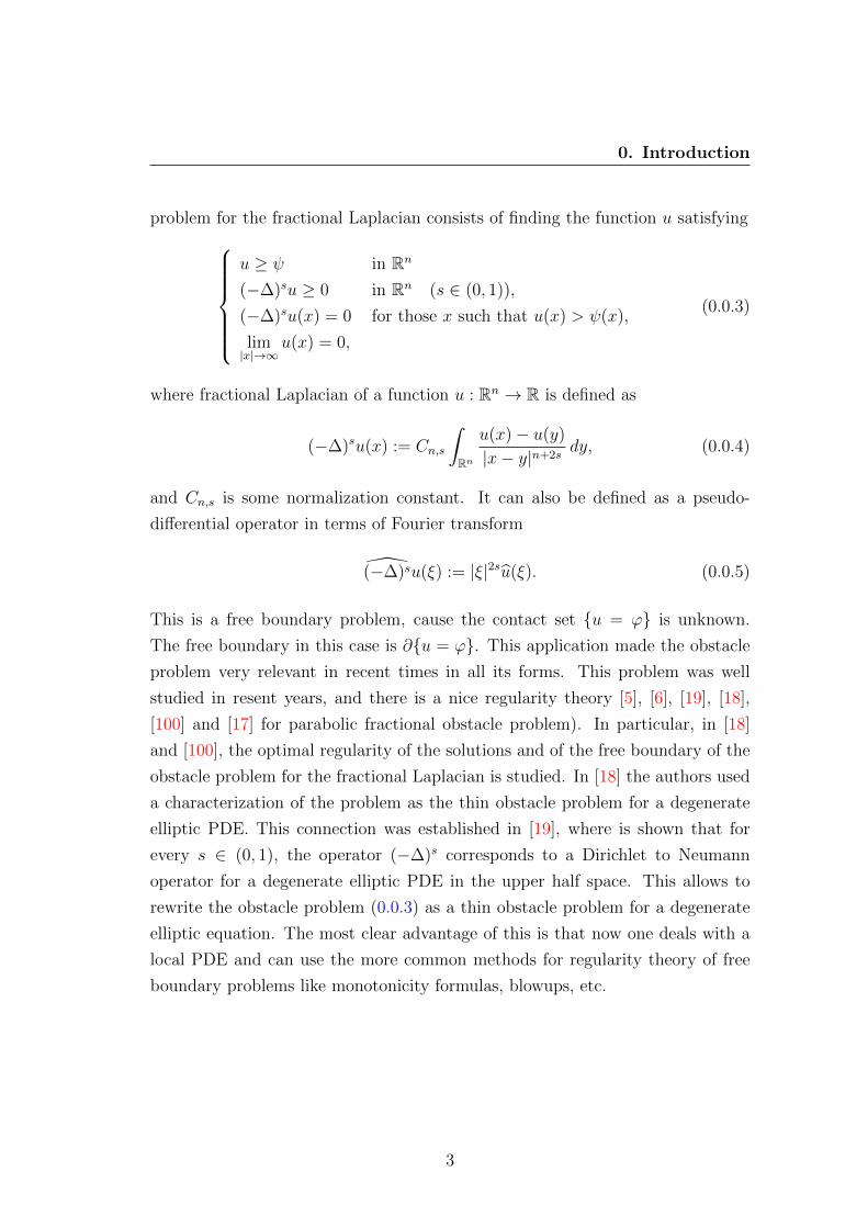
problem for the fractional Laplacian consists of finding the function u satisfyingu ≥ ψ in Rn
(−∆)su ≥ 0 in Rn (s ∈ (0, 1)),
(−∆)su(x) = 0 for those x such that u(x) > ψ(x),
lim|x|→∞
u(x) = 0,
(0.0.3)
where fractional Laplacian of a function u : Rn → R is defined as
(−∆)su(x) := Cn,s
∫Rn
u(x)− u(y)
|x− y|n+2sdy, (0.0.4)
and Cn,s is some normalization constant. It can also be defined as a pseudo-
differential operator in terms of Fourier transform
(−∆)su(ξ) := |ξ|2su(ξ). (0.0.5)
This is a free boundary problem, cause the contact set u = ϕ is unknown.
The free boundary in this case is ∂u = ϕ. This application made the obstacle
problem very relevant in recent times in all its forms. This problem was well
studied in resent years, and there is a nice regularity theory [5], [6], [19], [18],
[100] and [17] for parabolic fractional obstacle problem). In particular, in [18]
and [100], the optimal regularity of the solutions and of the free boundary of the
obstacle problem for the fractional Laplacian is studied. In [18] the authors used
a characterization of the problem as the thin obstacle problem for a degenerate
elliptic PDE. This connection was established in [19], where is shown that for
every s ∈ (0, 1), the operator (−∆)s corresponds to a Dirichlet to Neumann
operator for a degenerate elliptic PDE in the upper half space. This allows to
rewrite the obstacle problem (0.0.3) as a thin obstacle problem for a degenerate
elliptic equation. The most clear advantage of this is that now one deals with a
local PDE and can use the more common methods for regularity theory of free
boundary problems like monotonicity formulas, blowups, etc.
3

0. Introduction
Some words on regularity
For a classical obstacle problem, where A is just the Laplacian the variational
formulation of the obstacle problem would be seeking minimizers of the Dirichlet
energy functional
I(u) :=
∫Ω
|∇u|2 dx− 2
∫Ω
fu dx,
where the functions u represent the vertical displacement of the membrane. In
addition to satisfying Dirichlet boundary conditions corresponding to the fixed
boundary of the membrane, the functions u are constrained to be greater than
some given obstacle function ϕ. The solution breaks down into a region where
the solution is equal to the obstacle function (contact set), and a region where the
solution is above the obstacle. The interface between the two regions is the free
boundary. In general, the solution is continuous and possesses Lipschitz continu-
ous first derivatives. The free boundary is characterized as a Holder continuous
surface except at certain singular points, which reside on a smooth manifold. The
following simple example shows that no matter how regular the obstacle is, the
solution to the obstacle problem, in general, does not have continuous second
derivatives.
Consider the spacial case, when n = 1 and f = 0. Then the obstacle problem for
Laplacian is to minimize the functional∫ b
a
|u′(x)|2 dx
subject to u(a) = ua, u(b) = ub, and u(x) ≥ ψ(x). We suppose that ua > ψ(a)
and ub > ψ(b). Let ψ(x) be strictly concave. Then the minimizing curve y = u(x)
(solution of the obstacle problem) consists of three arcs:
(i) A line segment l1 connecting the point (a, ua) to a point (a′, ψ(a′)), tangent
to y = ψ(x) at x = a′,
(ii) An arc γ : y = ψ(x), a′ < x < b′,
(iii) A line segment l2 connecting the point (b′, ψ(b′)) to (b, ub), tangent to y =
ψ(x) at x = b′.
4

0. Introduction
The free boundary consists of the two points (a′, ψ(a′)) and (b′, ϕ(b′)). So if
ψ′′ < 0, then
u′′(a′−) = 0 6= ψ′′(a′) = u′′(a′+),
hence u′′(x) has a jump discontinuity at x = a′.
The optimal regularity of the solution of classical obstacle problem is known to
be C1,1. This was originally proved by Frehse in [47]. It is known, that up to
C1,1, the solution to the obstacle problem is as regular as the obstacle is. More
precisely, the modulus of continuity of the solution and the modulus of continuity
for its derivative are related to those of the obstacle (see [16]) for classical case
and [75] for more general case of operators):
1. If the obstacle ψ has the modulus of continuity σ(r), that is, |ψ(x)− ψ(y)| ≤σ(|x − y|), the the solution u(x) has modulus of continuity Cσ(2r), where the
constant C depends only on the domain and not the obstacle.
2. If the first derivative of the obstacle has modulus of continuity σ(r), then
the first derivative of the solution has modulus of continuity Crσ(2r), where the
constant C again depends only on the domain (see [16]).
In general one can prove that the free boundary is smooth (analytic in the
case of the Laplacian) in a generic point. However, there can be some exceptional
points where the free boundary forms a cusp singularity, [16].
The theory of the obstacle problem is extended to other divergence form
uniformly elliptic operators (see [66], [92]) and their associated energy functionals.
It can be generalized to degenerate elliptic operators as well, [75].
The double obstacle problem, where the function is constrained to lie above one
obstacle function and below another, is also of interest.
The Signorini problem is a variant of the obstacle problem, where the energy
functional is minimized subject to a constraint which only lives on a surface of
one lesser dimension, which includes the boundary obstacle problem, where the
constraint operates on the boundary of the domain.
The parabolic, time-dependent cases of the obstacle problem and its variants are
also objects of study.
5

0. Introduction
The thesis
This thesis consists of four chapters. We study the regularity of the solution and
of the free boundary of obstacle problem for a class of heterogeneous quasilin-
ear degenerate elliptic operators, mainly, for A(x)-Laplacian, in Orlicz-Sobolev
spaces. We call it the A(x)-obstacle problem.
The obstacle problem (with one obstacle) for the operator
∆Au := div(a(x, |∇u|)∇u) (0.0.6)
consists of finding u ∈ Kψ such that∫Ω
a(x, |∇u|)∇u · ∇(v − u) dx ≥∫
Ω
f(x)(v − u) dx, ∀v ∈ Kψ,
where
Kψ := v ∈ W 1,A0 (Ω) : ψ ≤ v a.e. in Ω,
Ω ⊂ Rn is a bounded domain, u : Ω→ R, a : Ω×R+ → R is a Young function, f
is a bounded function, ψ ∈ W 1,A(Ω), A is related to a by A(x, t) :=∫ t
0a(x, s)s ds,
x ∈ Ω, t ≥ 0. We will assume that Kψ 6= ∅.For this operator (0.0.6) we consider also two obstacles problem. In this case
instead of Kψ we have
Kϕψ := v ∈ W 1,A
0 (Ω) : ψ ≤ v ≤ ϕ a.e. in Ω,
and as ψ, ϕ ∈ W 1,A(Ω).
For the operator ∆A the N -membranes problem consists of finding u =
(u1, u2, ..., uN) ∈ KN such that
N∑i=1
∫Ω
a(x, |∇ui|)∇ui · ∇(vi − ui) dx
≥N∑i=1
∫Ω
fi(vi − ui) dx, ∀(v1, ...vN) ∈ KN ,
6
0. Introduction
where KN is a convex subset of the Orlicz-Sobolev space [W 1,A0 (Ω)]N , defined by
KN = (v1, ..., vN) ∈ [W 1,A0 (Ω)]N : v1 ≥ ... ≥ vN a.e. in Ω,
and f1,...,fN ∈ LA∗(Ω).
The operator ∆Au is called A-Laplacian (usually when there is no x de-
pendence, that is when a(x, t) = a(t)) or A(x)-Laplacian (to emphasize the x-
dependence).
There exists a unique solution to the obstacle problem (in fact, we are dealing
with a minimization of a ”nice” functional over a closed convex set Kψ, Kϕψ or
KN respectively).
In the first chapter we prove that bounded weak solutions for a class of variable
exponent elliptic equations in divergence form (which includes the p(x)-Laplacian)
with Dirichlet boundary condition are in C1,αloc for some α ∈ (0, 1). We also prove
C1,α regularity up to the boundary in case the boundary is smooth enough (see
Theorems 1.5.1 and 1.5.2).
For the study of the regularity of generalized solutions of quasi-linear elliptic
equations and variational problems Ladyzhenskaya and Ural’tseva have devel-
oped a method inspired by De Giorgi. They introduced class Bm and proved
Holder continuity of functions in Bm (see Definition 1.2.1). We follow this idea
simplifying its modified version by Fan to prove Holder continuity of solutions for
a class of elliptic equations in divergence form. More precisely, we consider the
problem of the regularity of weak solutions of equation
− div(a(x, |∇u|)∇u)
)= f(x), x ∈ Ω, (0.0.7)
where Ω is a bounded domain in Rn (n ≥ 2), u : Ω → R, a : Ω × R+ → R, and
f : Ω→ R is a given bounded function.
The study of such problems has been stimulated by problems in elasticity, in
fluid dynamics, image processing models and problems in the calculus of vari-
ations with p(x)-growth conditions and some more general class of differential
7

0. Introduction
operators.
After the Holder regularity results (Corollaries 1.4.1 and 1.4.2) we proceed
to C1,α regularity results of the bounded weak solutions of (0.0.7). In the case
when the boundary of the domain is a class of C1,γ, for some γ ∈ (0, 1), we
have regularity of bounded weak solutions up to the boundary. Applying this we
infer the regularity of the solution of the one obstacle problem from the Lewy-
Stampacchia inequalities. In case of Ω with smooth boundary we deduce up to
the boundary C1,α regularity of the solution of obstacle problem (Theorem 1.6.1).
In the second chapter we prove Lewy-Stampacchia inequalities in abstract
form for two obstacles problem in Orlicz-Sobolev spaces (Theorem 2.3.2). In
particular for the two obstacles problem in Orlicz-Sobolev spaces we have
−∆Aϕ ∧ f ≤ −∆Au ≤ −∆Aψ ∨ f,
where d ∧ b = inf(d, b) and d ∨ d = sup(d, b) Applying those inequalities we
derive C1,α regularity results (both locally and up to the boundary) for A(x)-
obstacle problem with two obstacles (Theorem 2.3.3). We also extend the Lewy-
Stampacchia inequalities for the N -membranes problem (Theorem 2.4.1), which
allows us to extend the C1,α regularity results for the solution of N -membrane
problem (Theorem 2.4.2). Then we approximate the variational inequality using
bounded penalization (Theorem 2.4.3)
We also give a way to get the Lewy-Stampacchia inequalities for one (upper or
lower) obstacle problem from the Lewy-Stampacchia inequalities for two obstacles
problem (Proposition 2.3.1).
Another interesting application of the Lewy-Stampacchia inequalities is its
application in studying quasi-variational inequalities. Some of these problems
are related to a stochastic switching game.
Using the notations
〈Aw,v〉 :=N∑i=1
〈Awi, vi〉 and 〈L,v〉 :=N∑i=1
∫Ω
fivi dx,
8

0. Introduction
with A = −∆Au, we consider the following quasi-variational problem:
find u ∈ K(u), such that,
〈Au− L,v− u〉 ≥ 0, ∀v ∈ K(u),
where
K(u) = v ∈ [W 1,A0 (Ω)]N : Ψi(u) ≤ vi ≤ Φi(u), i = 1, 2, . . . , N,
f = (f1, . . . , fN) ∈ [LA∗(Ω)]N , and for v = (v1, . . . , vN) we set
Φi(v) :=∧i 6=j
(vj + ϕij) (ϕij are positive constants),
Ψi(v) :=∨i 6=j
(vj − ψij) (ψij are positive constants),
for i, j = 1, . . . , N , i.e. we consider an N -membrane problem with KN = K(u)
(the obstacles themselves depend on the solution).
Using Lewy-Stampacchia inequalities for N -membranes problem, we prove that
this problem admits at least a maximal and a minimal solution (Theorem 2.4.4).
In the third chapter we study the regularity of the free boundary in A(x)-
obstacle problem. We extend the regularity of the free boundary of the obsta-
cle problem to a class of heterogeneous quasilinear degenerate elliptic operators
(A(x)-Laplacian), which includes the p(x)-Laplacian, in particular.
It was proved by Caffarelli that the quadratic growth of the solution of the
free boundary of the obstacle problem for the Laplacian implies an estimate of
the (n − 1)-dimensional Hausdorff measure of the free boundary and a stability
property. This result has a simple generalization to second order linear elliptic
operators with Lipschitz continuous coefficients, which allows the extension of
those properties to C1,1 solutions of the obstacle problem for certain quasilinear
operators of minimal surfaces type.
9

0. Introduction
Hausdorff measure estimates were obtained for homogeneous nonlinear oper-
ators of the p-obstacle problem (2 < p < ∞) by Lee and Shahgholian, and for
general potential operators by Monneau in a special case corresponding to an
obstacle problem arising in superconductor modeling with convex energy, and
by S. Challal, A. Lyaghfouri and J. F. Rodrigues to the so called A-obstacle
in Orlicz-Sobolev spaces, that includes a large class of degenerate and singular
elliptic operators. As it is well-known from geometric measure theory, the impor-
tance of the estimate on the (n − 1)-dimensional Hausdorff measure of the free
boundary, by a result of Federer, implies that the non-coincidence set u > 0 is
then a set of locally finite perimeter. As an important consequence, by a well-
known result of De Giorgi, the free boundary ∂u > 0 may be written, up to
a possible singular set of ‖∇χu>0‖-measure zero, as a countable union of C1
hyper-surfaces. The main result of Chapter 3 is the extension of these properties
to a more general class of heterogeneous quasilinear degenerate elliptic operators
which includes the p(x)-Laplacian. In particular, porosity of the free boundary
(Theorem 3.3.1), is proved for a class of operators extending to p(x)-Laplacian
for 1 < p(x) < ∞. The finiteness of (n − 1)-dimensional Hausdorff measure of
the free boundary (Theorem 3.8.1 and Remark 3.8.1) was shown for a class of
heterogeneous quasilinear degenerate elliptic operators, including p(x)-Laplacian,
for p(x) > 2. There is a technical difficulty in the proof for the last result in case
of 1 < p(x) ≤ 2, which we hope overcome in the future.
On the other hand, it was shown by Karp, Kilpelainen, Petrosyan and Shahgho-
lian for the p-obstacle problem (1 < p < ∞), that the free boundary is porous
with a certain constant δ > 0, that is, there exists r0 > 0 such that for each
x ∈ ∂u > 0 and 0 < r < r0, there exists a point y such that Bδr(y) ⊂Br(x) \ ∂u > 0. Since a porous set in Rn has Hausdorff dimension strictly
smaller than n, it follows that the free boundary has Lebesgue measure zero,
which allows us to write the solution of the obstacle problem as an a.e. solution
of a quasilinear elliptic equation in the whole domain involving the characteristic
function χu>0 of the non-coincidence set. This property is important to show,
under general non-degenerate assumptions on the data, a stability of the non-
coincidence set in Lebesgue measure.
10

0. Introduction
One of the main difficulties in extending this results from the constant expo-
nent Sobolev spaces to more general spaces is absence of the analogue of clas-
sical Harnack inequality. Harnack inequality was used to prove the porosity of
the free boundary in [65] (for constant exponent spaces), as well as in [21], for
A(x, t) = A(t)-obstacle problem (the classical Harnack inequality is still valid in
this case and was shown by G. Lieberman in [76]). However, when we pass to the
x variable spaces, the classical Harnack inequality fails (even just for p(·) case).
There is an analogue of the Harnack inequality for this case too (see [33]), but
this is very weak, since the constant c in Harnack inequality is not universal and
depends on function.
Finally, in the chapter four of the thesis using a compensated compactness
lemma we homogenize the Dirichlet problem for A(x)-Laplacian in Orlicz-Sobolev
spaces (Theorem 4.2.1). We describe the limiting operator. In this chapter we also
study the homogenization of the A(x)-obstacle problem (Theorem 4.3.1). Using
Lewy-Stampacchia inequalities, we get a compactness argument (from Rellich-
Kondrachov theorem) to homogenize the problem. We close this chapter by
proving the convergence of the coincidence sets for obstacle problem (Theorem
4.4.1).
Novelties in chapter 1 is C1,α-regularity of the solutions for a class of variable
exponent elliptic equations. This is an adaption of Fan’s result (see [43]) into our
framework.
In chapter 2 the extension of Lewy-Stampacchia inequalities in general frame-
work for the two obstacles problem as well as for the N -membranes problem is
new. This gives a new (and much shorter) prove of the regularity result of the
solution of two obstacles and N -membranes problem.
In chapter 3 the porosity of the free boundary of the obstacle problem as well
as the finitness of its (n−1)-dimensional Hausdorff measure is new. This gives an
information about the regularity of the free boundary. This framework extends
similar results for the fixed exponent Sobolev spaces.
In chapter 4 both homogenization results for the Dirichlet problem and for
11

0. Introduction
the obstacle problem are new in this framework. While the homogenization result
for the Dirichlet problem extends the one done in W 1,p(·) framework, the homog-
enization result of the obstacle problem in certain sense extends the one for done
just for fixed exponent Sobolev spaces. The convergence of the coincidence sets
also is new in this framework.
We close the thesis by an appendix on Orlicz-Sobolev spaces.
12

Chapter 1
Regularity of Solutions for a
Class of Elliptic Equations
1.1 Preliminaries
We prove that bounded weak solutions for a class of variable exponent elliptic
equations in divergence form (which includes the p(x)-Laplacian) with Dirichlet
boundary condition are in C1,αloc . We also prove C1,α regularity up to the boundary
in case the boundary is smooth enough.
For the study of the regularity of generalized solutions of quasi-linear elliptic
equations and variational problems Ladyzhenskaya and Ural’tseva have developed
a method, [70], inspired by De Giorgi (see [54]). They introduced class Bm and
proved Holder continuity of functions in Bm. Here we are going to follow this
idea with its modified version in [44] to prove Holder continuity of solutions for
a class of elliptic equations in divergence form. More precisely, we consider the
problem of the regularity of weak solutions of equation
− div(a(x, |∇u|)∇u)
)= f(x), x ∈ Ω, (1.1.1)
where Ω is a bounded domain in Rn (n ≥ 2), u : Ω → R, a : Ω × R+ → R, and
f : Ω→ R is a given bounded function.
1. Preliminaries
Definition 1.1.1. We will say that u ∈ W 1,A(Ω) is a weak solution of equation
(1.1.1), if∫Ω
a(x, |∇u|)∇u · ∇η dx−∫
Ω
f(x)η dx = 0, ∀η ∈ W 1,A0 (Ω), (1.1.2)
where A is related to a by
A(x, t) =
∫ t
0
a(x, s)s ds, x ∈ Ω, t ≥ 0. (1.1.3)
For the definitions and basic properties of Orlicz-Sobolev spaces we refer to
Appendix.
The study of regularity in case of a(x, t) = a(t) in (1.1.1) is covered by the
work of Lieberman in [76].
When in (1.1.1) we have a(x, t) = tp(x)−2, with p(x) > 1 a given bounded
function in Ω, we deal with problems involving variable growth conditions, the
so called p(x)-Laplacians. The study of such problems has been stimulated by
problems in elasticity (see [105]), in fluid dynamics (see [3], [30], [96], [107]),
image processing models [26] and problems in the calculus of variations with
p(x)-growth conditions (see [1], [89], [83], [105], [109]) and some more general
class of differential operators (see [4], [9], [38], [107]).
We will assume that a(x, t) is given by a function measurable and bounded
in x for all t > 0 and Lipschitz continuous in t, a.e. x ∈ Ω, and, such that, there
are positive constants a− < a+
0 < a− ≤tat(x, t)
a(x, t)+ 1 ≤ a+ for t > 0, (1.1.4)
where at = ∂a/∂t, and also limt→0+
ta(x, t) = 0.
The assumption (1.1.4), in fact, implies
(a(x, |ξ|)ξ − a(x, |ζ|)ζ
)· (ξ − ζ) > 0, ∀ξ, ζ ∈ Rn, ξ 6= ζ
14

1. Preliminaries
and limt→∞
ta(x, t) =∞ for a.e. x ∈ Ω (see [20], for instance).
Let p(x) > 1 be a log-Lipschitz continuous bounded function, i.e.
1 < p− := minx∈Ω
p(x) ≤ maxx∈Ω
p(x) := p+ <∞,
and there exists a constant L > 0, such that
|p(x)− p(y)| log |x− y|−1 ≤ L, for all x, y ∈ Ω, |x− y| ≤ 1
2. (1.1.5)
We assume that a(x, t) is such that a(x, 0) = 0 for a.e. x ∈ Ω, and satisfies the
following structural conditions for some positive constants c0, c1, c2, namely, [25],
[43], [44]
1
|η|
n∑i,j=1
∂a
∂ηj(x, |η|)ξiξjηiηj + a(x, |η|)|ξ|2 ≥ c0|η|p(x)−2|ξ|2, (1.1.6)
1
|η|
n∑i,j=1
(∣∣∣∣ ∂a∂ηj (x, |η|)ηiηj∣∣∣∣+ δija(x, |η|)
)≤ c1|η|p(x)−2 (1.1.7)
for a.e. x ∈ Ω, η = (η1, η2, . . . , ηn) ∈ Rn \0 and for all ξ = (ξ1, ξ2, . . . , ξn) ∈ Rn,
and
|a(x1, |η|)η − a(x2, |η|)η| ≤ c3|x1 − x2|β1(|η|p(x1)−1 + |η|p(x2)−1|
)∣∣ log |η|∣∣ (1.1.8)
for all x1, x2 ∈ Ω, η ∈ Rn \ 0 and for some β1 ∈ (0, 1).
Remark 1.1.1. Assumptions (1.1.6), (1.1.7) imply ([29], [101]) that for some
positive constant c3
a(x, |η|)|η| ≥ c3|η|p(x)−1
Proposition 1.1.1. Under the assumptions (1.1.6), (1.1.7) the Orlicz-Sobolev
space W 1,A(Ω) is continuously embedded in W 1,p(·)(Ω).
Proof. Remark 1.1.1 implies
c3
p+
tp(x) ≤ A(x, t), ∀x ∈ Ω, t ≥ 0,
15

1. Preliminaries
which, by the Theorem 8.5 in [90], in turn, applies the continuous embedding
W 1,A(Ω) → W 1,p(·)(Ω) (see also [89]).
Hereafter we will always assume that assumptions of the Proposition 1.1.1
hold, so we have the continuous embedding of W 1,A(Ω) in W 1,p(·)(Ω). We also
recall the following proposition from [101]:
Proposition 1.1.2. If (1.1.6)-(1.1.8) hold then
|a(x, |η|)η| ≤ c′3|η|p(x)−1,
(a(x, |η|)η − a(x, |ξ|)ξ
)· (η − ξ)
≥
c′1|η − ξ|p(x), if p(x) ≥ 2,
c′1(|η|2 + |ξ|2)(p(x)−2)/2|η − ξ|2, if p(x) < 2,(1.1.9)
where c′1, c′3 are positive constants depending only on c1, c3, p−, p+ and n.
First we see that under the assupmptions (1.1.4)-(1.1.8) bounded weak so-
lutions of (1.1.1) are Holder continuous. Then we go to the C1,α regularity of
solutions of (1.1.1) and then we apply those results in the study of the regularity
of the solution of obstacle problems in Orlicz-Sobolev spaces. When the bound-
ary of Ω is regular enough, then we have the same regularity results up to the
boundary.
Compared with the known local C1,α regularity results for the variable expo-
nent problems, this result is more general than those in [81], [82], where W 1,∞loc (Ω)
regularity has been obtained. Because in general (1.1.2) may not be the Euler
equation of the integral functional, the C1,α regularity result in this chapter in
that sense is more general than those in [1] and [28], where C1,α regularity for
the local minimizers of the integral functionals with p(x) growth is proved.
The C1,α regularity results for quasilinear elliptic equations with constant ex-
ponent p-growth conditions are well known (see [29], [40], [52], [51], [70], [73],
[74], [76], [77], [101]). The proof of C1,α regularity result here is basically done
by Fan in [43], which itself is based on the idea of Acerbi and Mingione in [1] and
16

1. Notations and background information
on Lieberman results in [74], [76] for the constant exponent case. We represent a
simplified version of the proof of [43].
In this chapter, after some background information in section 1.2, in section
1.3 we study boundness of weak solutions. In section 1.4 we see that bounded
weak solutions of (1.1.1) are Holder continuous. Section 1.5 of current chapter
studies C1,α-regularity (both interior and up to the boundary) of bounded weak
solutions. We close this chapter by some applications of the regularity result to
obstacle problem in Orlicz-Sobolev spaces.
1.2 Notations and background information
Throughout this chapter we will use the following notations: for a measurable
set E in R we denote by |E| the n-dimensional Lebesgue measure of E. For a
measurable function u defined in Ω and a measurable set E ⊂ Ω we denote
maxE
u(x) := ess supx∈E
u(x), minEu(x) := ess inf
x∈Eu(x),
oscEu(x) := max
Eu(x)−min
Eu(x).
For r > 0 Br(x0) is the ball of radius r centered at x0. Sometimes it will be
written just Br.
Lemma 1.2.1. If for any Br ⊂ Ω with r < r0 and for any σ ∈ (0, 1) and any
k ≥ k0 > 0∫Bk,r−σr
|∇u|p dx ≤ c
[ ∫Bk,r
∣∣∣∣u− kσr
∣∣∣∣p∗ dx+ (kq + 1)|Bk,r|], (1.2.1)
where u ∈ W 1,p(Ω) (p > 1 is a constant), c > 0 is a constant, 0 < q ≤ p∗, with
p∗ as the Sobolev embedding exponent of p, i.e.
p∗ :=
npn−p , if p < n,
any s > p, if p ≥ n,
then u is locally bounded above on Ω.
17

1. Notations and background information
For the proof we refer to Lemma 2.4 of [50].
Let now (1.1.6), (1.1.7) hold. Then, by Proposition 1.1.1, W 1,A(Ω) is contin-
uously embedded in W 1,p(·)(Ω).
Definition 1.2.1. For positive constants M,γ, γ1, δ with δ ≤ 2 we define the
class BA := BA(Ω,M, γ, γ1, δ) as the set of all functions u ∈ W 1,A(Ω) such that
maxΩ|u(x)| ≤M , and the functions w(x) = ±u(x) satisfy
∫Bk,ρ−σρ
|∇u|p(x) dx ≤ γ
∫Bk,ρ
∣∣∣∣w(x)− kσρ
∣∣∣∣p(x)
dx+ γ1|Bk,ρ| (1.2.2)
for arbitrary Bρ ⊂ Ω, σ ∈ (0, 1) and k such that
maxBρ
w(x)− δM ≤ k, (1.2.3)
where Bk,ρ = x ∈ Bρ : w(x) > k.
Remark 1.2.1. It is not difficult to see that if p(x) satisfies (1.1.5), then there
is a positive constant L′ such that
r−β ≤ L′, ∀Br ⊂ Ω,
where β = oscBrp(x). The conclusion is true also when p ∈ C0,α(Ω) for some
α ∈ (0, 1].
By Proposition 1.1.1 the following theorems are direct consequences of the
Theorem 2.1 and Theorem 2.2 of [44].
Theorem 1.2.1. If p(x) satisfies (1.1.5), (1.1.6)-(1.1.7) hold, then
BA(Ω,M, γ, γ1, δ) ⊂ C0,α(Ω), where α ∈ (0, 1], α = α(n, p−, p+, L′, γ, δ).
Definition 1.2.2. A function u is said to be in class BA(Ω,M, γ, γ1, δ), if u ∈B(Ω,M, γ, γ1, σ) and (1.2.2) holds for any ball Bρ with Bρ ∩ ∂Ω 6= ∅, σ ∈ (0, 1)
and
k ≥ maxmaxΩρ
w(x)− δM, max∂Ωρ
w(x),
where Ωρ := Bρ ∩ Ω, ∂Ωρ := ∂Ω ∩Bρ, Bk,ρ := x ∈ Ωρ : w(x) > k.
18

1. Boundness of weak solutions
Theorem 1.2.2. If p(x) satisfies (1.1.5), u ∈ BA(Ω,M, γ, γ1, δ) and there are
positive constants c0 and θ0 such that for any ball Bρ centered on ∂Ω with radius
ρ ≤ c0 and for any connected branch Ωiρ of Bρ ∩Ω, the following inequality holds:
|Ωiρ| ≤ (1− θ0)|Bρ|
and also u ∈ C0,α1(∂Ω) on ∂Ω, then u ∈ C0,α(Ω), where α depends only on n,
p−, p+, L′, γ, δ and α1.
1.3 Boundness of weak solutions
We prove that under certain assumptions weak solutions of (1.1.1) are locally
bounded. More precisely, we assume that for x ∈ Ω the following conditions hold:
a(x, |∇u|)|∇u|2 ≥ a0|∇u|p(x) − c, (1.3.1)
|a(x, |∇u|)∇u| ≤ a1|∇u|p(x)−1 + c, (1.3.2)
|f(x)| ≤ c (1.3.3)
for some positive constants a0, a1, c and p(x) ∈ C(Ω).
Theorem 1.3.1. If (1.3.1)-(1.3.3) hold and u ∈ W 1,A(Ω) is a weak solution of
(1.1.1), then u ∈ L∞loc(Ω). If in addition u is bounded on the boundary of Ω, then
u ∈ L∞(Ω).
Proof. Let u be a weak solution of (1.1.1) and x0 ∈ Ω. We will prove that u is
locally bounded at x0. Let us take a ball Br0(x0) ⊂ Ω. We will use p− and p+
as the minimum and maximum values of p(x) in the ball Br0 . Without loss of
generality one can assume p− ≤ n. We also will set
p∗− :=
np−n−p− , if p− < n,
p+ + 1, if p− = n.
By the continuity of p(x) we can chose r0 ∈ (0, 1) sufficiently small such that
p+ < p∗−.
19
1. Boundness of weak solutions
For arbitrary balls Bt(x′) ⊂ Bs(x
′) ⊂ Br0(x0), let ϕ ba a C∞ function such that
0 ≤ ϕ ≤ 1, suppϕ ⊂ Bs, ϕ ≡ 1 on Bt, |∇ϕ| ≤2
s− t.
For k ≥ 1 set η := ϕp+
maxu− k, 0. Then η ∈ W 1,A0 (Ω). From (1.1.2) one gets∫
Bk,s
a(x, |∇u|)|∇u|2ϕp+
dx
+ p+
∫Bk,s
[a(x, |∇u|)∇u · ∇ϕ
]ϕp
+−1(u− k) dx
−∫Bk,s
f(x)ϕp+
(u− k) dx = 0, (1.3.4)
where Bk,s = x ∈ Bs : u(x) > k. Hereafter in the proof we are going to write
I1 :=
∫Bk,s
|∇u|p(x)ϕp+
dx, I2 :=
∫Bk,s
∣∣∣∣u− ks− t
∣∣∣∣p∗− dx, ∫ · := ∫Bk,s
·.
From (1.3.1)-(1.3.4) it follows that
a0I1 ≤ c
∫ϕp
+
dx + a1p+
∫|∇u|p(x)−1ϕp
+−1|∇ϕ|(u− k) dx
+ cp+
∫ϕp
+−1|∇ϕ|(u− k) dx
+ c
∫ϕp
+
(u− k) dx. (1.3.5)
It is clear that ∫ϕp
+
dx ≤ |Bk,s|. (1.3.6)
Using Young’s inequality and taking ε1 ∈ (0, 1) such that
a1(p+ − 1)εp+/(p+−1)1 =
a0
4
20

1. Boundness of weak solutions
we get
a1p+
∫|∇u|p(x)−1ϕp
+−1|∇ϕ|(u− k) dx
≤ a1p+
[ ∫p(x)− 1
p(x)εp(x)/(p(x)−1)1 |∇u|p(x)ϕ(p+−1)p(x)/(p(x)−1) dx
+
∫1
p(x)ε−p(x)1 |∇ϕ|p(x)(u− k)p(x) dx
]≤ a1p
+p+ − 1
p+εp
+/(p+−1)
∫|∇u|p(x)ϕp
+
dx
+ a1p+
p−εp
+
1 2p+
∫ ∣∣∣∣u− ks− t
∣∣∣∣p(x)
dx
≤ a0
4I1 + c1I2 + c1|Bk,s|. (1.3.7)
We also have ∫ϕp
+−1|∇ϕ|(u− k) dx ≤ 2
∫u− ks− t
dx+ 2|Bk,s|. (1.3.8)
and ∫ϕp
+
(u− k) dx ≤∫
(u− k) dx ≤ I2 + |Bk,s|. (1.3.9)
From (1.3.5)-(1.3.9) we conclude
I1 ≤ c2
(I2 + (kp
+
+ 1)|Bk,s|)
and therefore∫Bk,t
|∇u|p− dx ≤ c3
[ ∫Bk,s
∣∣∣∣u− ks− t
∣∣∣∣p∗− dx+ (kp+
+ 1)|Bk,s|]. (1.3.10)
By Lemma 1.2.1 the inequality (1.3.10) implies that u is bounded above on
Br0(x0) and so u is locally bounded above on Ω.
Similarly one can show that−u is also locally bounded above on Ω, so u ∈ L∞loc(Ω).
If in addition
maxx∈∂Ω|u(x)| = M ≤ ∞,
21

1. Holder continuity of bounded weak solutions
then for every x0 ∈ ∂Ω, by similar argument as above, we can prove that (1.3.10)
is true for k > M and therefore u ∈ L∞(Ω).
1.4 Holder continuity of bounded weak solutions
We are ready now to do the next step towards Holder continuity of weak solutions
of (1.1.1).
Theorem 1.4.1. If (1.3.1)-(1.3.3) hold and u ∈ W 1,A(Ω) is a weak solution of
(1.1.1) with maxx∈Ω|u(x)| ≤ M , then u ∈ B(Ω,M, γ, γ1, σ), where δ = min
a0
4c, 2
and the constants γ and γ1 depend only on a0, a1, p−, p+.
Proof. Let Bt ⊂ Bs ⊂ Ω and let ϕ be a C∞ function such that
0 ≤ ϕ ≤ 1, suppϕ ⊂ Bs, ϕ ≡ 1 on Bt, |∇ϕ| ≤2
s− t.
For k ≥ maxBs
u(x)− δM set η := ϕp+
maxu− k, 0 with p+ as the maximum of
u in Ω (we also will use p− as the minimum value of u in Ω). Then η ∈ W 1,A0 (Ω)
and from (1.1.2) one gets (1.3.5). We want to estimate the right hand side of
(1.3.5). For convenience we again will use∫· instead of
∫Bk,s·. Using Young’s
inequality and taking ε1 ∈ (0, 1) such that
a1(p+ − 1)εp+/(p+−1)1 ≤ a0
4,
one gets
a1p+
∫|∇u|p(x)−1ϕp
+−1|∇ϕ|(u− k) dx
≤ a1p+
∫p(x)− 1
p(x)εp(x)/(p(x)−1)1 ϕ(p+−1)p(x)/(p(x)−1)|∇u|p(x) dx
+ a1p+
∫1
p(x)ε−p(x)1 |∇ϕ|p(x)(u− k)p(x) dx
≤ a0
4
∫|∇u|p(x)ϕp
+
dx+ d
∫ ∣∣∣∣u− ks− t
∣∣∣∣p(x)
dx, (1.4.1)
where d = d(a0, a1, p−, p+) is a positive constant.
22

1. Holder continuity of bounded weak solutions
Using Young’s inequality and taking ε2 ∈ (0, 1) such that
cp+
p−2p
+
εp−2 = 1,
we get
cp+
∫|∇ϕ|(u− k)ϕp
+−1 dx ≤ cp+
∫|∇ϕ|(u− k) dx
≤ cp+
∫1
p(x)εp(x)2 |∇ϕ|p(x)(u− k)p(x) dx
+ cp+
∫p(x)− 1
p(x)ε−p(x)/(p(x)−1)2 dx
≤∫ ∣∣∣∣u− ks− t
∣∣∣∣p(x)
dx+ c1|Bk,s|, (1.4.2)
where c1 = c1(c, p−, p+) is positive constant. It is clear that
c
∫ϕp
+
dx ≤ c|Bk,s| (1.4.3)
and
c
∫ϕp
+
(u− k) dx ≤ c
∫(u− k) dx
≤ c(maxBs
u− k)|Bk,s|
≤ cδM |Bk,s| ≤a0
4|Bk,s|. (1.4.4)
From (1.3.5) and (1.4.1)-(1.4.4) we conclude
∫Bk,s
|∇u|p(x)ϕp+
dx ≤ γ
∫Bk,s
∣∣∣∣u− ks− t
∣∣∣∣p(x)
dx+ γ1|Bk,s|.
Therefore ∫Bk,t
|∇u|p(x) dx ≤ γ
∫Bk,s
∣∣∣∣u− ks− t
∣∣∣∣p(x)
dx+ γ1|Bk,s| (1.4.5)
for Bt ⊂ Bs ⊂ Ω and k ≥ maxB−s
u − δM , where γ and γ1 are positive constants
depending only on c, a0, a1, p−, p+. (1.4.5) shows that u ∈ BA(Ω,M, γ, γ1, δ).
23

1. Interior regularity
The same way as above one can prove that u ∈ BA(Ω,M, γ, γ1, δ).
As a consequence we get from Theorems 1.2.1 and 1.4.1 we get:
Corollary 1.4.1. Let (1.1.5)-(1.1.7) hold. If u is a weak solution of (1.1.1) with
maxΩ|u| ≤ M , then u ∈ C0,α(Ω), where α ∈ (0, 1] and depends only on a0, a1, c,
M , p−, p+, n.
Theorems 1.2.1, 1.2.2, 1.4.1 and the above corollary give:
Corollary 1.4.2. Let (1.1.5)-(1.1.7) hold. If u is a weak solution of (1.1.1), then
u is locally Holder continuous in Ω. If in addition ∂Ω is such that there are
positive constants c0 and θ0 such that for any ball Bρ centered on ∂Ω with radius
ρ ≤ c0 and for any connected branch Ωiρ of Bρ ∩Ω, the following inequality holds:
|Ωiρ| ≤ (1− θ0)|Bρ|
and u is Holder continuous on the boundary of Ω, then u is Holder continuous
on Ω.
1.5 C1,α regularity of bounded weak solutions
1.5.1 Interior regularity
We will assume that p ∈ C0,β1(Ω), that is, there exists a positive constant C such
that
|p(x1)− p(x2)| ≤ C|x1 − x2|, x1, x2 ∈ Ω. (1.5.1)
Theorem 1.5.1. Let (1.1.6)-(1.1.8), (1.5.1) hold. If u ∈ W 1,A(Ω) is a bounded
weak solution of (1.1.1) with supΩ|u| := ess sup
Ω|u| ≤ M , then u ∈ C1,α
loc (Ω), where
α ∈ (0, 1) and depends only on p−, p+, n, a0, a1, c, M , C, β1.
Remark 1.5.1. Note, that if the assumptions of Theorem 1.5.1 are satisfied,
then all assumptions of Corollary 1.4.1 are satisfied, so we already know that
u C0,α1
loc (Ω) for some α1 ∈ (0, 1].
24
1. Interior regularity
The method of the proof of this theorem is simplified version of the one from
[43], which is similar to the one of [1], however there are some differences in the
proofs of [43] compared to [1]: a higher integrability result for the bounded weak
solutions of (1.1.1) is needed.
Lemma 1.5.1. If (1.1.5)-(1.1.7) hold and u ∈ W 1,A(Ω) is a bounded weak solution
of (1.1.1) with supΩ|u| := ess sup
Ω|u| ≤ M , then for a given open subset Ω0 ⊂ Ω,
there exist positive constants r0, c0, δ0 depending only on p−, p+, n, a0, a1, c,
M , L and dist(Ω0, ∂Ω) such that for every ball B2r ⊂ Ω0 with r ∈ (0, r0] and for
δ ∈ (0, δ0]
(−∫Br
|∇u|p(x)(1+δ) dx
) 11+δ
≤ c0
(1 +−
∫B2r
|∇u|p(x) dx
), (1.5.2)
where −∫E
v dx :=1
|E|
∫E
v dx.
Proof. Let Ω0 ⊂ Ω and let Br ⊂ B2r ⊂ Ω0 be concentric balls. Take ξ ∈ C∞0 (B2r)
such that 0 ≤ ξ ≤ 1, ξ = 1 on Br and ∇ξ ≤ 4r. Let ω := −
∫B2r
u dx. Since
η := ξp+
(u − ω) belongs to W 1,A0 (Ω) we can take it as a test function in (1.1.2).
From (1.3.1)-(1.3.3) and using Young’s inequality one gets
I := a0
∫B2r
|∇u|p(x)ξp+
dx
≤ 2c|B2r|+I
4+ c
∫B2r
∣∣∣∣u− ωr∣∣∣∣p(x)
dx. (1.5.3)
Since ∫Br
|∇u|p(x) dx ≤∫B2r
|∇u|p(x)ξp+
dx,
from (1.5.3) we get a Caccioppoli type inequality
∫Br
|∇u|p(x) dx ≤ c|B2r|+ c
∫B2r
∣∣∣∣u− ωr∣∣∣∣p(x)
dx. (1.5.4)
From (1.1.5) and the classical Pincare inequality we get (see [46], [108]) that there
exist r0 small enough and ε ∈ (0, 1) such that when r ∈ (0, r0] a variable exponent
25

1. Interior regularity
Poincare type inequality holds
−∫B2r
∣∣∣∣u− ωr∣∣∣∣p(x)
dx ≤ c1 + c1
(−∫B2r
|∇u|p(x)1+ε dx
)1+ε
, (1.5.5)
so (1.5.4) and (1.5.5) lead to Gehring type inequality
−∫B2r
|∇u|p(x) dx ≤ c+ c
(−∫B2r
|∇u|p(x)1+ε dx
)1+ε
,
which implies (1.5.2) (see Proposition 1.1 in Chapter 5 of [52]).
Let conditions of Theorem 1.5.1 hold. Let Ω0 ⊂ Ω and x0 ∈ Ω. Since by
Remark 1.5.1 u ∈ C0,α1
loc (Ω), there exists a constant L1 > 0 such that
|u(x1)− u(x2)| ≤ L1|x1 − x2|α1 , ∀x1, x2 ∈ Ω0.
Define β := minα1, β1. Let r0, δ0 be as in Lemma 1.5.1. It is clear that we may
assume r0 ≤ 1. Let B2r1(x0) ⊂ Ω0 with r1 sufficiently small such that r1 ≤ r0,∫B2r1 (x0)
|∇u|p(x) dx ≤ 1,
and
p+(B2r1(x0))(1 +
δ0
2
)≤ p−(B2r1(x0))(1 + δ0), (1.5.6)
where p+(E) = maxE
p(x), p−(E) = minEp(x). So we have that
|∇u| ∈ Lp+(B2r1 (x0))
(1+
δ02
)(B2r1(x0)).
Let Br ⊂ B2r be concentric balls in B2r1(x0). Define p∗(r) = p+(B2r) and let
x∗ ∈ B2r be such that p(x∗) = p∗(r). Define also A(η) := a(x∗, |η|)η and consider
the boundary value problemdivA(∇v) = 0, in Br,
v = u, on ∂Br.(1.5.7)
26

1. Interior regularity
For the proof of the following lemma we refer to [76].
Lemma 1.5.2. Problem (1.5.7) has a unique solution v such that v ∈ C1,γ1
loc (Br)
and
supBr/2
|∇v|p+ ≤ cr−n∫Br
|∇v|p+
dx, (1.5.8)
−∫Bρ
|∇v − (v)ρ|p∗ dx ≤ c
(ρ
r
)γ1
−∫Br
|∇v − (∇v)r|p∗ dx, ∀ρ ∈ (0, r),∫Br
|∇v|p∗ dx ≤ c
∫Br
(1 + |∇u|p∗) dx, (1.5.9)
supBr
|u− v| ≤ oscBru, (1.5.10)
where p∗ = p∗(r), (∇v)ρ = −∫Bρ
∇v dx, γ1 ∈ (0, 1) and c is a positive constant
depending only on p∗, n, a0, a1.
Lemma 1.5.3. If v is the unique solution of (1.5.7), then∫Br
|∇u−∇v|p∗ dx ≤ c′rβ/2∫B2r
(1 + |∇u|p(x)) dx, (1.5.11)
where c′ > 0 is a constant depending only on p−, p+, n, a0, a1, M and dist(Ω0, ∂Ω).
Proof. For a given δ > 0, from
limt→+∞
log t
tδ= 0 and lim
t→0+
log t
t−δ= 0
follows that there exists a positive constant c(δ) depending on δ such that
| log |η|| ≤ c(δ) + |η|δ + |η|−δ
which together with (1.1.8) leads to
|a(x1, |η|)η − a(x2, |η|)η| ≤ c1(δ)|x1 − x2|β1(1 + |η|p∗−1+δ), (1.5.12)
where p∗ := maxp(x1), p(x2) and c1(δ) > 0 is a constant depending only on c3,
p−, p+ and δ.
27

1. Interior regularity
Define
I :=
∫Br
(A(∇u)− A(∇v)) · (∇u−∇u) dx.
Since v is a solution of (1.5.7), we have
I =
∫Br
A(∇u) · (∇u−∇v) dx
=
∫Br
(A(∇u)− a(x, |∇u|)∇u) · (∇u−∇v) dx
+
∫Br
a(x, |∇u|)∇u · (∇u−∇v) dx
:= I1 + I2.
Take δ1 ∈ (0, 1) such that δ1p−−1
< δ02
. By (1.5.6)
p∗
(1 +
δ1
p∗ − 1
)≤ p−(1 + δ0) ≤ p(x)(1 + δ0).
We recall that by the choice of r1∫B2r1 (x0)
|∇u|p(x) dx ≤ 1.
Recalling (1.1.8), (1.5.12) from (1.5.2) we get
I1 ≤ crβ1
∫Br
(1 + |∇u|p∗−1+δ1)(|∇u|+ |∇v|) dx
≤ crβ∫
Br
(1 + |∇u|p∗+δ1) dx
+
∫Br
(1 + |∇u|(p∗−1+δ1) p∗p∗−1 dx+
∫Br
|∇v|p∗ dx
≤ crβ∫Br
(1 + |∇u|p(x)(1+δ0)) dx ≤ crβrn + crn(∫
B2r
|∇u|p(x) dx
)1+δ
≤ crβrn + crβ∫B2r
|∇u|p(x) dx ≤ crβ∫B2r
(1 + |∇u|p(x)) dx.
28

1. Interior regularity
From (1.3.3) and (1.5.10) one gets
I2 ≤ c
∫Br
|u− v| dx ≤ c oscBru ≤ crα1 ≤ crβ,
and so
I ≤ crβ∫B2r
(1 + |∇u|p(x)) dx.
Recalling (1.1.9), when p∗ ≤ 2 we immediately get (1.5.11). In case of p∗ < 2 we
write∫Br
|∇u−∇v|p∗ dx ≤(∫
Br
(|∇u|2 + |∇v|2
)(p∗−2)/2|∇u−∇v|2 dx)1/2
×(∫
Br
(|∇u|2 + |∇v|2
)(2−p∗)/2|∇u−∇v|2p∗−2 dx
)1/2
≤ c
(I
c′1
)1/2(∫B2r
(1 + |∇u|p(x)
)dx
)1/2
,
and again we get (1.5.11).
Having in mind Lemma 1.5.3, (1.5.8) and (1.5.9) we recall the following lemma
from [43]:
Lemma 1.5.4. If Bx0(2r1) is a ball as above, then for given τ ∈ (0, n), there
exist positive constants rτ <r116
and cτ depending only on p−, p+, n, a0, a1, M ,
dist(Ω0, ∂Ω) and τ such that∫Bρ(xc)
|∇u|p∗(ρ) dx ≤ cτρn−τ , ∀xc ∈ Br1/2 , ∀ρ ∈ (0, ρτ ),
where p∗(ρ) := p+(B2ρ(xc)) = supB2ρ
p(x).
Remark 1.5.2. Since τ ∈ (0, n) is arbitrary, Lemma 1.5.4 implies that u ∈C0,αloc (Ω) for all α ∈ (0, 1).
See Remark 3.3 of [1].
Proof of Theorem 1.5.1. Although the proof of Theorem 1.5.1 now is the same
as the one in [43], we give it here to complete the section.
29
1. Regularity up to the boundary
Let B2r1(x0), β, γ1 be as above, xc ∈ Br1/4(x0). Define τ := βγ1
4(n+γ1), θ :=
β2(n+γ1)
. Let ρ <(rτ/4
)1+θ, where rτ is as in Lemma 1.5.4. Set r = (2ρ)1/(1+θ),
then 2ρ < r < 2r < rτ and Bρ(xc) = Bρ ⊂ Br/2 ⊂ B32r ⊂ B2r1(x0). If v is the
unique solution of (1.5.7) then by Lemmas 1.5.2, 1.5.3, 1.5.4 we get∫Bρ
|∇u− (∇u)ρ|p∗(r) dx
≤ c
∫Bρ
|∇v − (∇v)ρ|p∗(r) dx+ c
∫Br
|∇u−∇v|p∗(r) dx
≤ cρn(ρ
r
)γ1
r−n∫Br
(1 + |∇u|p∗(r)
)dx+ c
∫Br
|∇u−∇v|p∗(r) dx
≤ cρn(ρ
r
)γ1
r−nrn−τ + crβ/2∫B2r
(1 + |∇u|p∗(r)
)dx
≤ cρn(ρ
r
)γ1
r−τ + crβ/2+n−τ
= crβ/2+n−τ = cρβ/2+n−τ
1+θ = cρn+ε,
with ε := βγ1
4(n+γ1)(1+θ), which leads to∫
Bρ
|∇u− (∇u)ρ|p− dx ≤ cρn+εp−/p+
.
This implies that u ∈ C1,α(Br1/8(x0)), where α = εp+ .
1.5.2 Regularity up to the boundary
If the boundary of Ω is smooth enough, then up to the boundary we have C1,α
regularity of bounded weak solutions of (1.1.1). More precisely,
Theorem 1.5.2. Let (1.1.6)-(1.1.8), (1.5.1) hold and ∂Ω is a class of C1,γ for
some γ ∈ (0, 1). If u ∈ W 1,A(Ω) is a bounded weak solution of (1.1.1) with
supΩ|u| := ess sup
Ω|u| ≤ M , then u ∈ C1,α(Ω), where α ∈ (0, 1) and depends only
on p−, p+, n, a0, a1, c, M , C, β1 and γ.
The proof of this theorem is based on some auxiliary lemmas and is a simpli-
fication of the corresponding theorem in [43] for our case.
30
1. Regularity up to the boundary
Lemma 1.5.5. Let (1.1.5), (1.3.1)-(1.3.3) hold, and ∂Ω be of class of Lipschitz.
If u ∈ W 1,A0 (Ω) is a bounded weak solution of (1.1.1) with sup
Ω|u| ≤M , then there
exist positive constants r0, c0, δ0 depending only on p−, p+, n, a0, a1, c, M , and
L, such that |∇u| ∈ Lp(·)(1+δ0)(Ω) and for every x ∈ Ω, r ∈ (0, r0), δ ∈ (0, δ0]
(−∫
Ωr(x)
|∇u|p(x)(1+δ) dx
) 11+δ
≤ c0
(1 +−
∫Ω2r(x)
|∇u|p(x) dx
), (1.5.13)
where Ωr(x) := Br(x) ∩ Ω.
Proof. Let x0 ∈ ∂Ω. Define u on Rn \Ω by u = 0. Since from Corollary 1.4.2 we
know that u ∈ C(Ω), we can chose r1 to be small enough to guarantee
|u(x)| ≤ c, ∀x ∈ B2r1(x0) (1.5.14)
and ∫B2r1 (x0)
|∇u|p(x) dx ≤ 1.
We claim that there exist r0 ≤ r1, ε ∈ (0, 1) and c0 constants such that
−∫Br
|∇u|p(x) dx ≤ c0 + c0
(−∫B2r
|∇u|p(x)1+ε dx
)1+ε
, (1.5.15)
for Br ⊂ B2r ⊂ B2r1(x0) with r ≤ r0.
Case 1. If B 32r ⊂ B2r1(x0)∩Ω, using Lemma 1.5.1 (see the Gehring type inequal-
ity after (1.5.5)) we get (1.5.15).
Case 2. In case of B 32r ⊂ B2r1(x0) \ Ω, (1.5.15) is obvious, since the left hand
side is 0.
Case 3. Suppose now that B 32r ∩ ∂Ω 6= ∅. If ξ ∈ C∞0 (B2r) is as in the proof
of Lemma 1.5.1, taking η := ξp+u as a test function in (1.1.2) and using similar
arguments as in the proof of Lemma 1.5.1, (1.5.14), the Poincare type inequality
for u and the Lipschitz regularity of ∂Ω, we can get (1.5.15).
Recalling Gehring lemma (see Proposition 1.1 in Chapter 5 of [52]), (1.5.15) im-
plies that there is δ0 > 0 such that
|∇u| ∈ Lp(·)(1+δ0)loc (B2r1(x0))
31

1. Regularity up to the boundary
and (−∫Br
|∇u|p(x)(1+δ) dx
) 11+δ
≤ c
(1 +−
∫B2r
|∇u|p(x) dx
)(1.5.16)
for Br ⊂ B2r ⊂ B2r1(x0) with r ≤ r0, δ ∈ (0, δ0).
Let x ∈ Br1(x0) ∩ Ω, r ≤ r0, B2r(x) ⊂ B2r1(x0), δ ∈ (0, δ0). Note that for a
constant σ ∈ (0, 1) we have
σ|Br(x)| ≤ |Ωr(x)| ≤ |Br(x)|.
From (1.5.16) one can get (1.5.13).
Hereafter in this chapter we suppose that all the assumptions of the Theorem
1.5.2 hold. If u ∈ W 1,A0 (Ω) is a bounded weak solution of (1.1.1), then by Corollary
1.4.2 we have u ∈ C0,α1(Ω). By Theorem 1.5.1, u ∈ C1,αloc (Ω) and by Lemma 1.5.5
|∇u| ∈ Lp(·)(1+δ0)(Ω).
Below we study the boundary C1,α regularity of u.
Let x0, and chose r1 ∈ (0, r0] small enough to guarantee∫Ω2r1 (x0)
|∇u|p(x) dx ≤ 1
and
p+(Ω2r1(x0))
(1 +
δ0
2
)≤ (1 + δ0)p−(Ω2r1(x0)), (1.5.17)
with r0, δ0 as in Lemma 1.5.5.
Define Ω2r1(x0) := B2r1(x0) ∩ Ω. Let xc ∈ Ω2r1(x0) and Ωr(xc) = Ωr ⊂ Ω2r ⊂Ω2r1(x0). Denote p∗(r) = p+(Ω2r) and let x∗ ∈ Ω2r be such that p(x∗) = p∗(r) :=
p∗. Define A(η) = a(x∗|η|)η and consider the boundary value problemdivA(∇v) = 0, in Ωr,
v = u, on ∂Ωr.(1.5.18)
For the proof of the following lemma we refer to [74].
32
1. Regularity up to the boundary
Lemma 1.5.6. There is a unique solution v to (1.5.18) such that v ∈ C1,γ1(Ωr/2)
and
supBr/2
|∇v|p∗ ≤ c1
rn
∫Br
|∇v|p∗ dx,
oscΩρ|∇v| ≤ c2
(ρ
r
)γ1
supΩr/2
|∇v|, 0 < ρ <r
2, (1.5.19)
∫Ωr
|∇v|p∗ dx ≤ c3
∫Ωr
(1 + |∇u|p∗) dx, (1.5.20)
supΩr
|u− v| ≤ oscΩru,
where γ1 ∈ (0, 1), c1, c2, c3 are positive constants depending only on p∗, n, a0,
a1, M and γ.
With the proofs similar to the ones of Lemmas 1.5.3 and 1.5.4 we have the
following two lemmas:
Lemma 1.5.7. If v is the unique solution of (1.5.18), then there exist a positive
constant c depending only on p∗, n, a0, a1 and M such that∫Ωr
|∇u−∇v|p∗ dx ≤ crβ/2∫
Ω2r
(1 + |∇u|p(x)) dx.
Lemma 1.5.8. For a given τ ∈ (0, n) there exist positive constants rτ <r116
and
cτ depending only on p∗, n, a0, a1, M and τ , such that∫Ωρ(xc)
|∇u|p∗(ρ) dx ≤ cτρn−τ , ∀xc ∈ Ωr1/2(x0), ∀ρ ∈ (x, rτ ),
with p∗(ρ) := p+(Ω2ρ(xc)).
Proof of Theorem 1.5.2. The proof of the Theorem 1.5.2 now is as the corre-
sponding theorem in [43]. Let x0, Ω2r1(x0), β, γ1 and v be as above. Set τ :=βγ1
4(n+γ1), θ := β
2(n+γ1). Let xc ∈ Ωr1/4(x0) and ρ <
(rτ4
)1+θ. If r = (2ρ)1/(1+θ), then
2ρ < r < 2r < rτ with rτ as above, and Ωρ(xc) = Ωρ ⊂ Ωr/2 ⊂ Ω32r ⊂ Ω2r1(x0).
From (1.5.19), (1.5.20) follows that
−∫
Ωρ
|∇v − (∇v)ρ|p∗(ρ) dx ≤ c
(ρ
r
)γ1
−∫
Ωr
(1 + |∇u|p∗(r)) dx,
33

1. The obstacle problem
which, using the same arguments as in the proof of Theorem 1.5.1 leads to∫Ωρ
|∇u− (∇u)ρ|p− dx ≤ cρn+εp−/p+
,
with ε = βγ1
4(n+γ1)(1+θ). This implies that u ∈ C1,α(Ωr1/8(x0)), with α = ε
p+ .
1.6 The obstacle problem
We close this chapter by an application of the C1,α regularity above to one obstacle
problem in Orlicz-Sobolev spaces.
Let Ω ⊂ Rn (n ≥ 2) be a bounded domain. Suppose that a(x, t) satisfies (1.1.4),
and (1.1.5) holds. The obstacle problem (with one obstacle) for the operator
∆Au := div(a(x, |∇u|)∇u
)(1.6.1)
consists of finding u ∈ Kψ such that∫Ω
a(x, |∇u|)∇u · ∇(v − u) dx ≥∫
Ω
f(x)(v − u) dx, ∀v ∈ Kψ, (1.6.2)
where
Kψ := v ∈ W 1,A0 (Ω) : ψ ≤ v a.e. in Ω,
f is a bounded function, ψ ∈ W 1,A(Ω), A is defined by (1.1.3). We will assume
that Kψ 6= ∅.
The operator ∆Au is called A-Laplacian (usually when there is no x de-
pendence, that is when a(x, t) = a(t)) or A(x)-Laplacian (to emphasize the x-
dependence).
It is known that there exists a unique solution to the obstacle problem (in fact,
we are dealing with a minimization of a ”nice” functional over a closed convex
set Kψ). More detailed about the obstacle problems in Orlicz-Sobolev spaces can
be found in Chapter 2 of this thesis.
For the A-Laplacian operator (i.e. when a(x, t) = a(t)) it is shown by Lieber-
man in [75] for two obstacles problem (the same is true also for one obstacle
34
1. The obstacle problem
problem) that up to C1,α the solution of the obstacle is as regular as the obsta-
cles are. The regularity properties of the solutions to the one and two obstacle
problems with non-standard growth was studied in [37], where the Holder con-
tinuity up to the boundary, and stability of solutions with respect to continuous
perturbations in the variable growth exponent is proved.
In this section we infer the regularity of the solution of the obstacle problem
from the Lewy-Stampacchia inequalities for one obstacle problem (see [87]). Let
the operators A and L be defined as in (2.2.2) and (2.2.3). Then the obstacle
problem (1.6.2) can be rewritten in the following form:
〈Au− L, v − u〉 ≥ 0, ∀v ∈ Kψ. (1.6.3)
As we know from Proposition 2.2.1, under the condition (1.1.4) the operator Ais strictly T -monotone, and so, if with (1.3.3) also
−∆Aψ ≤ c (1.6.4)
then, as it is stated in [87], by the Lewy-Stampacchia inequalities together with
(1.6.4) we see that the solution of the obstacle problem (1.6.3) satisfies
−c ≤ f(x) ≤ (−∆Au)(x) ≤ (−∆Aψ ∨ f)(x) ≤ c,
where a ∨ b := sup(a, b), which brings us to the conclusion that ∆Au ∈ L∞(Ω),
and the regularity of the solution of the obstacle problem is the same as the one
of bounded solutions of the respective equation without obstacle. To summarize,
from Theorems 1.3.1, 1.5.1 and 1.5.2 we conclude:
Theorem 1.6.1. If (1.1.6)-(1.1.8), (1.5.1) and (1.6.4) hold, then the solution of
the obstacle problem (1.6.2) with ψ ∈ L∞(Ω) is C1,α(Ω) for some α ∈ (0, 1). If
also ∂Ω ∈ C1,γ for some γ ∈ (0, 1), then u ∈ C1,α(Ω).
We refer to [95] and Chapter 2 for more detailed discussion of this approach
for two obstacles problem and for the N -membranes problem as well.
35


Chapter 2
Two Obstacles Problem in
Orlicz-Sobolev Spaces
2.1 Introduction
We prove the Lewy-Stampacchia inequalities for the two obstacles problem in
abstract form for T -monotone operators. As a consequence for a general class of
quasi-linear elliptic operators of Ladyzhenskaya-Uraltseva type, including p(x)-
Laplacian type operators, we derive new results of C1,α regularity for the solution.
We also apply those inequalities to obtain new results to the N -membranes prob-
lem and the regularity and monotonicity properties to obtain the existence of a
solution to a quasi-variational problem in (generalized) Orlicz-Sobolev spaces.
We consider the two obstacles problem for monotone operators (possibly de-
generate or singular) of the type (1.6.1) with a Dirichlet boundary condition in a
bounded domain Ω ⊂ Rn.
The two obstacles problem for the operator (1.6.1) consists of finding u ∈ Kϕψ
such that∫Ω
a(x, |∇u|)∇u · ∇(v − u) dx ≥∫
Ω
f(v − u) dx, ∀v ∈ Kϕψ, (2.1.1)

2. Introduction
where
Kϕψ = v ∈ W 1,A
0 (Ω) : ψ ≤ v ≤ ϕ a.e. in Ω, (2.1.2)
ψ, ϕ ∈ W 1,A(Ω) (for the definition of the Orlicz-Sobolev spaces see Appendix),
where A is related to a by (1.1.3). Among the large literature already exist-
ing on the p(x)-Laplacian type operators, concerning regularity properties of the
solution to the one obstacle problem we may refer to [61] for the continuity or
to [36], [37] for C0,α and C1,β regularity of minimizers of functionals over obstacles.
Here we are specially interested in the more general class of quasi-linear op-
erators of Ladyzhenskaya-Uraltseva type (see [75], [76]), where a(x, t) satisfies
(1.1.4). We know from [20] that the assumption (1.1.4) implies
(a(x, |ξ|)ξ − a(x, |ζ|)ζ
)· (ξ − ζ) > 0, ∀ξ, ζ ∈ Rn, ξ 6= ζ (2.1.3)
and limt→∞
ta(x, t) = ∞ for a.e. x ∈ Ω. As a consequence, we have the uniqueness
of the solution of the Dirichlet problem and also the weak maximum principle for
Au := − div(a(x, |∇u|)∇u).
Note, that (1.1.4) implies, with the same constants a− < a+,
0 < 1 + a− ≤t2a(x, t)
A(x, t)≤ a+ + 1, a.e. x ∈ Ω t ≥ 0, (2.1.4)
and A satisfies the so called ∆2-condition (see Appendix), so LA(Ω) is a linear
separable space.
This framework includes examples like
a(x, t) = α(x)tp(x)−2 log(β(x)t+ γ(x)),
with bounded functions γ(x), p(x) > 1, and α(x), β(x) > 0 a.e. in x ∈ Ω.
In the next section of this chapter we use the continuity property of the trun-
cation operator v 7→ v+ = v ∨ 0 = sup(v, 0) for the strong topology of W 1,A(Ω)
to extend some continuous dependence results in W 1,A0 (Ω) of the variational so-
lutions to (2.1.1)-(2.1.2) with respect to the data.
In section 2.3, we prove the Lewy-Stampacchia inequalities (here a ∧ b =
38

2. Variational solutions
inf(a, b) and a ∨ b = sup(a, b)) in an abstract form, extending the approach
of Mosco [87] to the two obstacles problem, that includes the above class of
operators. Although Lewy-Stampacchia inequalities are known, in particular, for
linear and some nonlinear operators (see, for instance, [92] for their importance
for the regularity of the solution in the one obstacle problem or [102] for the two
obstacles case), our proof is new and more general. As a consequence, under
additional hypothesis on a(x, ·), we obtain the same regularity for the solution u
of the two obstacles problem as in the equation without constraints (see [76]). For
instance, for bounded obstacles ϕ, ψ we conclude that u ∈ C1,α(Ω), if we impose
f , ∆Aϕ, ∆Aψ ∈ L∞(Ω), a regularity obtained in [75] with different assumptions.
Finally, in section 2.4, we give two new applications to systems of obstacle
type. In the case of the N -membranes problem, when u = (u1, . . . , uN) has the
constraint
u1 ≥ u2 ≥ . . . ≥ uN a.e. in Ω,
we extend some of the results of [8], in particular, the C1,α regularity and the
strong approximation in (W 1,A0 (Ω))N by solutions of a penalized system. For the
case of a special class of implicit double obstacle problems, when the obstacles
depend on the solution in the form∨i 6=j
(uj − ψij) ≤ ui ≤∧i 6=j
(uj + ϕij), i = 1, . . . , N,
where ϕij, ψij are certain given positive constants, we are able to show the exis-
tence of a minimal and maximal solution for the corresponding system of quasi-
variational inequalities, which is of the type arising in problems of stochastic
impulse control (see [64], [87], [102] and [103]).
2.2 Variational solutions
We introduce the energy functional J : W 1,A0 (Ω)→ R by
J(u) =
∫Ω
A(x, |∇u|) dx, ∀u ∈ W 1,A0 (Ω) (2.2.1)
39
2. Variational solutions
which is strictly convex, weakly lower semi-continuous and coercive in W 1,A0 (Ω)
(see [71]). Moreover, J is Gateaux differentiable, and J ′(u) = Au at u ∈ W 1,A0 (Ω)
is given by (see [89], for instance)
〈Au, v〉 =
∫Ω
a(x, |∇u|)∇u · ∇v dx, v ∈ W 1,A0 (Ω). (2.2.2)
Hence Au ∈ W−1,A(Ω) =(W 1,A
0 (Ω))′
, the topological dual of W 1,A0 (Ω) and if we
assume f ∈ LA∗(Ω) ⊂ W−1,A(Ω), A
∗being the conjugate Young function of the
Sobolev conjugate of A, we can rewrite the problem (2.1.1)-(2.1.2) in the form:
find u ∈ Kϕψ, such that,
〈Au− L, v − u〉 ≥ 0, ∀v ∈ Kϕψ, (2.2.3)
where we set
〈L, v〉 =
∫Ω
fv dx, ∀v ∈ W 1,A0 (Ω).
Proposition 2.2.1. Under the condition (2.1.3) the operator A is strictly T -
monotone, i.e., for any u, v ∈ W 1,A(Ω)
〈Au− Av, (u− v)+〉 > 0, if 0 6= (u− v)+ ∈ W 1,A0 (Ω).
Proof. In fact, using Lemma A.3.1, by (2.1.3) we have∫Ω
[a(x, |∇u|)∇u− a(x, |∇v|)∇v
]· ∇(u− v)+
dx
=
∫u>v
[a(x, |∇u|)∇u− a(x, |∇v|)∇v
]· (∇u−∇v)
dx > 0,
if (u− v)+ 6= 0, i.e. if m|u > v| > 0.
In this section we assume (1.1.4) and
ϕ, ψ ∈ W 1,A(Ω) such that Kϕψ 6= ∅, (2.2.4)
for which it is sufficient to assume ϕ ≥ ψ a.e. in Ω and both ϕ−, ψ+ ∈ W 1,A0 (Ω).
40

2. Variational solutions
Theorem 2.2.1. The problem (2.2.3) has a unique solution u = u(f, ϕ, ψ) ∈ Kϕψ
and is equivalent to minimize in Kϕψ the functional F , defined by
F (v) =
∫Ω
A(x, |∇v|) dx−∫
Ω
fv dx, v ∈ W 1,A0 (Ω). (2.2.5)
Moreover, if u denotes the solution corresponding to f , ϕ, ψ, then
f ≥ f , ϕ ≥ ϕ, ψ ≥ ψ implies u ≥ u a.e. in Ω.
Proof. The existence and uniqueness are standard results for strictly monotone,
coercive and potential operators, as observed in more general Orlicz-Sobolev
spaces already in [59] (in fact we are minimizing a ”nice” functional on a closed
convex subset of W 1,A0 (Ω)). The comparison property follows easily by the T -
monotonicity (see, for instance, [87] or [92]): take v = u ∨ u ∈ Kϕψ in (2.2.3) and
v = u ∧ u ∈ Kϕ
ψin ˆ(2.2.3)) for u. By addition, one finds
〈Au− Au, (u− u)+〉+ 〈L− L, (u− u)+〉 ≤ 0.
Since L − L ≥ 0, and A is strictly T -monotone, one immediately deduces (u −u)+ = 0, which means that u ≥ u.
Remark 2.2.1. This argument also shows a weak maximum principle in the
form: if Au ≥ Au in Ω and u ≥ u on ∂Ω in the sense (u− u)+ ∈ W 1,A0 (Ω), then
u ≥ u in Ω.
Similarly we have a “L∞-continuous dependence” property, even without the
L∞ regularity on the solutions:
Proposition 2.2.2.
‖u− u‖L∞(Ω) ≤ ‖ϕ− ϕ‖L∞(Ω) ∨ ‖ψ − ψ‖L∞(Ω),
where u and u are the corresponding solutions of the problem (2.2.3) and ˆ(2.2.3)
with the same f .
Proof. Let l = ‖ϕ− ϕ‖L∞(Ω) ∨‖ψ− ψ‖L∞(Ω) <∞. Set v = u+ (u−u− l)+ ∈ Kϕψ
41

2. Variational solutions
in (2.2.3) and v = u− (u− u− l)+ ∈ Kϕ
ψin ˆ(2.2.3). By addition one gets
I1 :=
∫Ω
(a(x, |∇u|)∇u− a(x, |∇u|)∇u
)· ∇(u− u− l
)+ ≤ 0.
On the other hand, recalling (2.1.3) we know, that if |u > u + l| > 0 (where
|E| is the Lebesgue measure of the set E), then
I2 :=
∫u>u+l
(a(x, |∇u|)∇u− a(x, |∇u|)∇u
)· (∇u−∇u)+ > 0.
Since I1 = I2, we conclude u − u − l ≤ 0. Reversing the role of u with u we get
u− u− l ≤ 0.
Exactly as in Proposition 4.5 of [89], we have the following interesting result.
Lemma 2.2.1. Let (1.1.4) holds and um u weakly in W 1,A0 (Ω). If
lim supm→∞
〈Aum, um − u〉 ≤ 0 (2.2.6)
then um → u in W 1,A0 (Ω) strongly, and Aum → Au in W−1,A(Ω) strongly.
This lemma can be used to prove continuous dependence results as the next
theorem, which is useful in our last section and has also an intrinsic interest by
itself.
Theorem 2.2.2. Under the assumption (1.1.4) let um be the solution to (2.2.3)
with compatible data (fm, ϕm, ψm), such that
fm → f ∈ LA∗, ϕm → ϕ and ψm → ψ in W 1,A(Ω) strongly.
Then um → u strongly in W 1,A0 (Ω), where u is the solution of the limit problem
(2.2.3) with (f, ϕ, ψ).
Proof. For arbitrary v ∈ Kϕψ we obtain that vm = (v ∧ ϕm) ∨ ψm ∈ Kϕm
ψmand,
by Proposition A.3.2, vm → v in W 1,A0 (Ω). Since, by coerciveness, ‖um‖1,A ≤ C,
there is u ∈ W 1,A0 (Ω), such that, for a subsequence um u in W 1,A
0 (Ω) weakly
42

2. Lewy-Stampacchia inequalities and their consequences
and in L1(Ω). So u ∈ Kϕψ and by lower semi-continuity we have
F (u) ≤ lim infm→∞
F (um) ≤ limm→∞
F (vm) = F (v), ∀v ∈ Kϕψ.
Hence u solves (2.2.3) and then, since wm = (u ∧ ϕm) ∨ ψm → u in W 1,A0 (Ω),
lim supm→∞
〈Aum, um − u〉 ≤ limm→∞
〈Aum, um − wm〉+ limm→∞
〈Aum, wm − u〉
≤ limm→∞
∫Ω
fm(wm − um) = 0.
By Lemma 2.2.1, this implies the strong convergence of the whole sequence um
to u.
Remark 2.2.2. In the case of only one obstacle problem, lower (ψ) or upper
(ϕ) obstacle (corresponding to take formally ϕ = +∞ or ψ = −∞ respectively)
all previous results of this section hold in similar way. For instance, Proposition
2.2.2 takes the form
‖u− u‖L∞(Ω) ≤ ‖ψ − ψ‖L∞(Ω) or ‖u− u‖L∞(Ω) ≤ ‖ϕ− ϕ‖L∞(Ω)
respectively.
2.3 Lewy-Stampacchia inequalities and their con-
sequences
Let X be a real reflexive Banach space, which is a lattice with respect to a
partial order ” ≤ ”, and V is a sublattice of X (i.e. V contains the sup and inf of
its elements). Then for every v ∈ X one can write v = v+−v−, where v+ = v∨0,
v− = −v ∧ 0 are the positive and negative parts of v respectively. Thus, X is
generated by the cone P , P − P = X,
P = v ∈ X : v ≥ 0.
43
2. Lewy-Stampacchia inequalities and their consequences
The subspace of V ′ (the dual space of V ) generated by the cone
P ′ = v′ ∈ V ′ : 〈v′, v〉 ≥ 0, ∀v ∈ P,
is called the dual order of V and denoted by V ∗, i.e. V ∗ = P ′ − P ′.
Example. In application to variational and quasi-variational inequalities for
linear second order (elliptic) PDE in divergence form, the space X usually is the
Sobolev space H1(Ω) (or an appropriate Orlicz-Sobolev space, see below), where
Ω is a smooth bounded domain of Rn, and V is either the Sobolev space H10 (Ω),
or any closed subspace of H1(Ω) such that
H10 (Ω) ⊂ V ⊂ H1(Ω).
Under the following order
u ≤ v ⇐⇒ u(x) ≤ v(x) a.e. x ∈ Ω,
the space X = H1(Ω) is a vector lattice and the positive cone P is closed (see
[78]). Note that H1(Ω) can be identified with a sub-lattice of L2(Ω), which is
usually lattice with respect to the order mentioned above (see [98]). The subspace
V is usually defined in terms of the boundary conditions for the problem at
hand. Moreover, one should not forget that V is a sub-lattice of X = H1(Ω).
Particulary, the subspace H10 (Ω) satisfies to the Dirichlet boundary conditions.
If V = H10 (Ω), then V ′ = H−1(Ω), and v′ ∈ V ′ is a positive element for the
dual ordering if and only of v′ is a positive distribution. Hence v′ is a positive
(Radon) measure in Ω, belonging to H−1(Ω). The order dual of H10 (Ω) is thus
the closed subspace of all distributions in H−1(Ω), which can be represented as
the difference of two positive measures in Ω.
We shall consider an operator A : X → V ′ with the properties:
a) hemi-continuous, i.e. the mapping t→ 〈A(u+ tv), w〉 is continuous on [0, 1],
u, v ∈ X, w ∈ V ;
44

2. Lewy-Stampacchia inequalities and their consequences
b) coercive, i.e. ∃w0 ∈ X such that
if u− w0 ∈ V, lim‖u‖→∞
〈Au, u− w0〉‖u‖
=∞, u ∈ X,
c) strictly T-monotone, i.e.
〈Au− Av, (u− v)+〉 > 0
for all u, v ∈ X such that 0 6= (u− v)+ ∈ V .
We recall that L ≥M for L, M ∈ V ′, if L−M ∈ P ′, i.e. L−M is positive on
the positive elements of V . Then, if A is strictly T-monotone, it satisfies a weak
comparison principle: if Au ≤ Av, then u ≤ v.
In this framework we recall the following interesting fact (see [87]).
Theorem 2.3.1. Let A : X → V ′ be a strictly T-monotone, coercive and hemi-
continuous operator. Let also u, v ∈ V be such that Au,Av ∈ V ∗. Then A(u∧ v),
A(u ∨ v) ∈ V ∗ and A(u ∧ v) ≥ Au ∧ Av, A(u ∨ v) ≤ Au ∨ Av for the dual order
in V ′.
Consequently, if Aui ∈ V ∗, then for ∀i ∈ I ⊂ 1, 2, . . . , N
A(∧i∈I
ui
)≥∧i∈I
Aui and A(∨i∈I
ui
)≤∨i∈I
Aui.
In fact, we can take X = W 1,A(Ω), V = W 1,A0 (Ω) and the operator A defined
by (2.2.2) under our assumptions.
Now we prove the Lewy-Stampacchia inequalities in abstract form.
Theorem 2.3.2. Let X be a real reflexive ordered Banach space, V be a closed
subspace of X, which is a sublattice of X, A : X → V ′ be a strictly T-monotone,
coercive and hemi-continuous operator. Let also there are given two elements
ϕ , ψ ∈ X, ψ ≤ ϕ, and L ∈ V ′. If
45

2. Lewy-Stampacchia inequalities and their consequences
(a)
∃ Λ ∈ V ′ such that Λ ≥ L and Λ ≥ Aψ in V ′
∃ λ ∈ V ′ such that λ ≤ L and λ ≤ Aϕ in V ′,
(b)
(ψ − v)+ ∈ V and (v − ϕ)+ ∈ V, ∀v ∈ V,
and let u be the solution of
u ∈ Kϕψ : 〈Au− L, v − u〉 ≥ 0, ∀v ∈ Kϕ
ψ, (2.3.1)
where
Kϕψ = u ∈ V : ψ ≤ u ≤ ϕ. (2.3.2)
Then the following dual estimates hold
λ ≤ Au ≤ Λ in V ′. (2.3.3)
In particular, if L,Aϕ,Aψ ∈ V ∗, then also Au ∈ V ∗, and (2.3.3) gives
L ∧ Aϕ ≤ Au ≤ L ∨ Aψ in V ∗. (2.3.4)
Proof. The assertion (2.3.4) holds, since, if L,Aϕ,Aψ ∈ V ∗, one can take λ =
L ∧ Aϕ = L− (L− Aϕ)+ and Λ = L ∨ Aψ = L+ (Aψ − L)+ in (2.3.3)(4.3).
To prove the upper bound of (2.3.3), consider the unique solution z ∈ V of
auxiliary variational inequality
z ≤ u : 〈Az − Λ, w − z〉 ≥ 0, ∀w ∈ V, w ≤ u. (2.3.5)
It is enough to show, that z = u, since then taking w = u − v in (2.3.5) for an
arbitrary v ≥ 0, it readily follows
Au− Λ = Az − Λ ≤ 0 in V ′.
To prove that z = u, let us first prove that z ≥ ψ. Recalling the first condition
46

2. Lewy-Stampacchia inequalities and their consequences
of (b) and taking w = z + (ψ − z)+ = ψ ∨ z ≤ u in (2.3.5), we get
〈Λ− Az, (ψ − z)+〉 ≤ 0.
Hence, since Λ ≥ Aψ, one obtains
〈Aψ − Λ, (ψ − z)+〉+ 〈Λ− Az, (ψ − z)+〉 ≤ 0
which, by the strict T-monotonicity of A, implies, that (ψ−z)+ = 0. This means
that z ≥ ψ.
Let us now prove that z ≥ u. Since u solves (2.3.1) and in (2.3.5) z ≤ u, one
has that z ≤ ϕ. In other words, z ∈ Kϕψ. Take w = z ∨ u = z + (u − z)+ ≤ u
in (2.3.5) and v = u ∧ z = u − (u − z)+ ≥ ψ in (2.3.1). Then, by addition and
recalling the fact Λ ≥ L from the conditions (a), we conclude
〈Au− Az, (u− z)+〉 ≤ 〈L− Λ, (u− z)+〉 ≤ 0,
and, since A is strictly T-monotone, it follows that (u− z)+ = 0 and so z ≥ u.
So, the unique solution u of (2.3.1) is also the unique solution of (2.3.5). We
already know, that this implies the upper bound in (2.3.3).
To prove the lower bound in (2.3.3), consider the unique solution z ∈ V of
auxiliary variational inequality
z ≥ u : 〈Az − λ,w − z〉 ≥ 0, ∀w ∈ V, w ≥ u. (2.3.6)
The steps are similar as above. It is enough to show, that z = u, since then
taking w = u+ v in (2.3.6) for an arbitrary v ≥ 0, it readily follows
λ− Au = λ− Az ≤ 0 in V ′.
To prove that z = u, let us first prove that z ≤ ϕ. Recalling the second condition
47

2. Lewy-Stampacchia inequalities and their consequences
in (b) and taking w = z − (z − ϕ)+ = z ∧ ϕ ≥ u in (2.3.6), we get
〈Az − λ, (z − ϕ)+〉 ≤ 0.
Hence, since λ ≤ Aϕ, one obtains
〈λ− Aϕ, (z − ϕ)+〉+ 〈Az − λ, (z − ϕ)+〉 ≤ 0,
which, by the strict T-monotonicity of A, implies, that (z − ϕ)+=0, i.e. z ≤ ϕ.
Let us now prove that z ≤ u. Since u solves (2.3.1) and in (2.3.6) z ≥ u, one
has that z ≥ ψ. In other words, z ∈ Kϕψ. Take w = z ∧ u = z − (z − u)+ ≥ u in
(2.3.6) and v = u ∨ z = u + (z − u)+ ≤ ϕ in (2.3.1). Then, by subtracting and
recalling that λ ≤ L from (a), we conclude
〈Az − Au, (z − u)+〉 ≤ 〈λ− L, (z − u)+〉 ≤ 0,
and, since A is strictly T-monotone, it follows, that (z − u)+ = 0 and so z ≤ u.
So, the unique solution u of (2.3.1) is also the unique solution of (2.3.5) (we
already know, that this implies the upper bound in (2.3.3) and the unique solution
of (2.3.6), which, as we see, implies the lower bound in (2.3.3).
Remark 2.3.1. Theorem 2.3.2 is still true when X is just an ordered Banach
space and the operator A is strictly T -monotone, provided the problem (2.3.1),
(2.3.2) has solution. This result extends Theorem 4.1 of [87] that was restricted
to the abstract one obstacle problem, and Theorem 4.35 of [102] was stated only
for linear second order operators in Sobolev spaces, which was recently extended
to the p-Laplacian in [93] and to general Leray-Lions operators in [85]. We refer
to [11] for a Lewy-Stampacchia inequality in quasilinear unilateral problems.
Remark 2.3.2. Since fractional Laplacian operator is strictly T -monotone, then
Lewy-Stampacchia inequalities hold true. In fact, a treatment of the Lewy-Stampac-
chia inequalities for fractional Laplacian (for the definition see (0.0.4) or (0.0.5))
has been proved in [99] as a particular case of Lewy-Stampacchia type inequali-
ties for some more general class of integro-differential operators, which itself is a
48
2. Lewy-Stampacchia inequalities and their consequences
consequence of the general framework.
Another interesting work on this is [91], where Lewy-Stampacchia inequalities
were proved for an obstacle problem in the Heisenberg group.
Let u be the unique solution of (2.3.1), u be the unique solution of (2.3.1) in
Kψ = v ∈ V : ψ ≤ v (i.e. u is the solution of one (lower) obstacle problem)
and let u be the unique solution of (2.3.1) in Kϕ = v ∈ V : v ≤ ϕ (i.e. u is the
solution of one (upper) obstacle problem). We can recover the Lewy-Stampacchia
inequalities for the one obstacle problem easily in the following way.
Proposition 2.3.1. i) If Aϕ ≥ L, then u = u, and one can rewrite (2.3.4) as
L ≤ Au ≤ L ∨ Aψ in V ∗.
ii) If Aψ ≤ L, then u = u, and one can rewrite (2.3.4) as
L ∧ Aϕ ≤ Au ≤ L in V ∗.
Proof. i) By taking v = u− (u−ϕ)+ = u∧ϕ ∈ Kψ in the lower-obstacle problem
u ∈ Kψ : 〈Au− L, v − u〉 ≥ 0, ∀v ∈ Kψ,
we get
〈Au− L, (u− ϕ)+〉 ≤ 0.
On the other hand, by assumption,
〈L− Aϕ, (u− ϕ)+〉 ≤ 0.
Recalling the strictly T -monotonicity of A, by addition, we conclude (u−ϕ)+ = 0
and so u ≤ ϕ, which means, that u ∈ Kϕψ. The uniqueness of the solution gives
u = u.
ii) Similarly, by taking v = u + (ψ − u) = u ∨ ψ ∈ Kϕ in the upper-obstacle
problem
u ∈ Kϕ : 〈Au− L, v − u〉 ≥ 0, ∀v ∈ Kϕ,
49
2. Lewy-Stampacchia inequalities and their consequences
we get, using
〈Aψ − Au, (ψ − u)+〉 = 〈Aψ − L, (ψ − u)+〉+ 〈L− Au, (ψ − u)+〉 ≤ 0.
So (ψ − u)+ = 0, which means that u ∈ Kϕψ, and we conclude by the uniqueness
of the solution that u = u.
We have already observed that the nonlinear operator −∆A given by (1.6.1)
under the generalized condition (1.1.4) of Ladyzhenskaya and Uraltseva type
satisfies the hypothesis of Theorem 2.3.2 in W 1,A0 (Ω). In particular, if we also
assume the existence of c > 0, such that
|f(x)| ≤ c, −∆Aψ ≤ c and −∆Aϕ ≥ −c a.e. x ∈ Ω, (2.3.7)
the solution of (2.2.3) satisfies
−c ≤ (−∆Aϕ ∧ f)(x) ≤ −∆Au(x) ≤ (−∆Aψ ∨ f)(x) ≤ c a.e. x ∈ Ω,
and we conclude that
∆Au ∈ L∞(Ω).
Hence, the regularity of the solution of the two obstacles problem (and, similarly,
for each one obstacle problem as well) is the same as bounded solutions of the
respective equation without obstacles. Summarizing the above facts we get a
theorem similar to Theorem 1.6.1 in Chapter 1. From Theorems 1.5.1 and 1.5.2
we conclude:
Theorem 2.3.3. If (1.1.6)-(1.1.8), (1.5.1) and (1.6.4) hold, then the solution of
the obstacle problem (2.2.3) with ψ, ϕ ∈ L∞(Ω) is C1,α(Ω) for some α ∈ (0, 1). If
also ∂Ω ∈ C1,γ for some γ ∈ (0, 1), then u ∈ C1,α(Ω).
50

2. Applications to Systems
2.4 Applications to Systems
2.4.1 N-membranes problem
For the operator A = −∆A the N -membranes problem consists of finding
u = (u1, u2, ..., uN) ∈ KN such that
N∑i=1
∫Ω
a(x, |∇ui|)∇ui · ∇(vi − ui) dx
≥N∑i=1
∫Ω
fi(vi − ui) dx, ∀(v1, ...vN) ∈ KN , (2.4.1)
where KN is a convex subset of the Orlicz-Sobolev space [W 1,A0 (Ω)]N , defined by
KN = (v1, ..., vN) ∈ [W 1,A0 (Ω)]N : v1 ≥ ... ≥ vN a.e. in Ω,
and f1,...,fN ∈ LA∗(Ω). As observed in Theorem 2.3.1 the existence and unique-
ness of the solution to (2.4.1) follows easily.
Theorem 2.4.1. If a(x, t) satisfies (2.1.3), then the solution (u1, ..., uN) of the
N-membranes problem for ∆A satisfies the following Lewy-Stampacchia type es-
timates:
f1 ∧ Au1 ≤ f1 ∨ ... ∨ fN
f1 ∧ f2 ≤ Au2 ≤ f2 ∨ ... ∨ fN...
f1 ∧ ... ∧ fN−1 ≤ AuN−1 ≤ fN−1 ∨ fN
f1 ∧ ... ∧ fN ≤ AuN ≤ fN
a.e. in Ω.
Proof. Observe that choosing (v, u2, ...uN) ∈ KN , with v ∈ Ku2 , we see that u1 ∈Ku2 solves the “lower-obstacle problem” with f = f1, and so (recall Proposition
2.3.1)
f1 ≤ Au1 ≤ f1 ∨ Au2 a.e. in Ω.
51

2. Applications to Systems
Analogously, we see that uj ∈ Kuj−1uj+1 solves the two-obstacles problem with f = fj,
j = 2, 3, ...N − 1, and satisfies, by (2.3.4),
fj ∧ Auj−1 ≤ Auj ≤ fj ∨ Auj+1 a.e. in Ω.
Since uN ∈ KuN−1 , then (recall Proposition 2.3.1)
fN ∧ AuN−1 ≤ AuN ≤ fN a.e. in Ω.
The proof concludes by simple iteration.
Since for each i = 1, 2, . . . , N , the respective Aui maybe controlled in L∞(Ω)
by ∧1≤j≤i
fj ≤ Aui ≤∨
i≤j≤N
fj,
from the Theorem 1.5.1, 1.5.2 we have
Theorem 2.4.2. If (1.1.4), (1.1.6)-(1.1.7), (1.5.1), (1.6.4) and for each (i =
1, 2, . . . N) fi satisfies (1.1.8), then the solution u of the N-membranes problem
has C1,α(Ω) regularity for some α ∈ (0, 1). If also ∂Ω ∈ C1,γ for some γ ∈ (0, 1),
then the solution u to N-membranes problem belongs to [C1,α(Ω)]N .
As in [8] we may also approximate the variational inequality using bounded
penalization. Defining
ξ0 = max
f1 + · · ·+ fi
i: i = 1, . . . , N
,
ξi = iξ0 − (f1 + · · ·+ fi) for i = 1, . . . , N,
we observe thatξi ≥ 0, if i ≥ 1,
(ξi−1 − ξi−2)− (ξi − ξi−1) = fi − fi−1, if i ≥ 2.
52

2. Applications to Systems
For ε > 0, let θε be define as follows:
θε : R→ R, s 7→
0, if s ≥ 0,
s/ε, if − ε < s < 0,
−1, if s ≤ −ε.
The approximate problem is given by the system for uεi ∈ W1,A0 (Ω)
∆Auεi + ξiθε(u
εi − uεi+1)− ξi−1θε(u
εi−1 − uεi ) = fi, in Ω, i = 1, . . . , N, (2.4.2)
with the convention uε0 = +∞, uεN+1 = −∞. Since the operator ∆A is strictly
T -monotone, then arguing as in [8], we get the following theorem:
Theorem 2.4.3. If (1.1.4) holds, then
(i) the problem (2.4.2) has a unique solution (uε1, . . . , uεN) ∈ [W 1,A
0 (Ω)]N . This
solution satisfies
uεi ≤ uεi−1 + ε for i = 2, . . . , N.
(ii) (uε1, . . . , uεN)→ (u1, . . . , uN) in [W 1,A
0 (Ω)]N strongly as ε→ 0, where
(u1, . . . , uN) is the solution of the N-membranes problem. Under assumptions of
Theorem 2.4.2 the convergence holds in [C1(Ω)]N .
Proof. . As observed in [8], the bounded penalization Bε
〈Bεv,w〉 :=N∑i=1
∫Ω
[ξiθε(vi − vi+1)− ξi−1θε(vi−1 − vi)
]wi dx
is monotone in [L1(Ω)]N . Therefore (i) follows exactly in the same way as in
Proposition 2.1 of [8].
Since 〈Bεv,v−uε〉 = 0 for any v ∈ KN , the weak convergence of (ii) follows also
exactly as in [8] by monotonicity arguments, since we have
〈Auε,v− uε〉 ≥ 〈L,v− uε〉, ∀v ∈ KN . (2.4.3)
53

2. Applications to Systems
Here we have used the notations
〈Aw,v〉 =N∑i=1
〈Awi, vi〉 and 〈L,v〉 =N∑i=1
∫Ω
fivi dx. (2.4.4)
Since uε u ∈ KN weakly in [W 1,A0 (Ω)]N , setting (2.4.2) in variational form,
using (2.4.3) with v = u and taking the lim sup we obtain the strong convergence
(using Lemma 2.2.1). Finally, if also f ∈ [L∞(Ω)]N then the penalization term in
(2.4.2) is also bounded in L∞ and the uεi are uniformly bounded in C1,α.
2.4.2 A Quasi-Variational Problem
Another interesting application of the Lewy-Stampacchia inequalities is its ap-
plication in studying quasi-variational inequalities. Some of these problems are
related to a stochastic switching game.
In this section we assume that ∂Ω ∈ C1,α for some 0 < α < 1, and the
operator A has the C1,α regularity property.
We consider the following quasi-variational problem (with the notations (2.4.4)):
find u ∈ K(u), such that,
〈Au− L,v− u〉 ≥ 0, ∀v ∈ K(u), (2.4.5)
where
K(u) = v ∈ [W 1,A0 (Ω)]N : Ψi(u) ≤ vi ≤ Φi(u), i = 1, 2, . . . , N,
f = (f1, . . . , fN) ∈ [LA∗(Ω)]N , and for v = (v1, . . . , vN) we set
Φi(v) :=∧i 6=j
(vj + ϕij) (ϕij are positive constants),
Ψi(v) :=∨i 6=j
(vj − ψij) (ψij are positive constants),
for i, j = 1, . . . , N , i.e. we consider the problem (2.4.1) with KN = K(u) (the ob-
stacles themselves depend on the solution). A similar problem for linear operators
54

2. Applications to Systems
(and for the one obstacle) was considered in [64] and [102].
We set
µ :=N∧i=1
fi, and ν :=N∨i=1
fi (2.4.6)
and we consider the unique solution u0 and u0 in W 1,A0 (Ω) solving, respectively,
Au0 = µ and Au0 = ν in Ω. (2.4.7)
Assuming fi ∈ [L∞(Ω)]N , we have u0, u0 ∈ C1,α(Ω) and we may define the
constant λ0 by
λ0 = maxΩ
u0 −minΩu0 > 0.
Theorem 2.4.4. Let fi ∈ [L∞(Ω)]N and suppose
ϕij + ψik ≥ λ0 > 0, ∀i, j, k = 1, . . . , N.
Then (2.4.5) admits at least a maximal solution u and a minimal solution u.
Proof. Let µ, ν ∈ L∞(Ω) be given by (2.4.6). By regularity, the set
D := v = (v1, . . . , vN) ∈ [W 1,A0 (Ω)]N µ ≤ Avi ≤ ν in Ω, i = 1, . . . , N
is bounded in [C1,α(Ω)]N for some α > 0. By comparison we have u0 ≤ vi ≤ u0
in Ω, i = 1, . . . , N , for every v ∈ D and, of course, u0 = (u0, . . . , u0) and u0 =
(u0, . . . , u0 also belong to D. Therefore, if v ∈ D we have
maxΩ
vj −minΩvk ≤ λ0, ∀j, k
and
K(v) = z = (z1, . . . , zN) ∈ [W 1,A0 (Ω)]N : Ψi(v) ≤ zi ≤ Φi(v), i = 1, . . . , N 6= ∅.
If we denote by w = σ(v) the unique solution of
w ∈ K(v) : 〈Aw− L, z−w〉 ≥ 0, ∀z ∈ K(v), (2.4.8)
55

2. Applications to Systems
by Lewy-Stampacchia inequalities and Theorem (2.3.1), it satisfies(∧i 6=j
Avj)∧ fi ≤ Awi ≤
(∨i 6=j
Avj)∨ fi in Ω.
Consequently, w ∈ D and σ(D) ⊂ D.
Using (2.4.8) we define u1 = σ(u0) and by the weak maximum principle, we
observe that u1i ≤ u0 in Ω, for all i = 1, . . . , N . By iteration, let um+1 = σ(um)
for m = 1, 2, . . . and observe that, if componentwise umi ≤ um−1i then
Φi(um) ≤ Φi(u
m−1) and Ψi(um) ≤ Ψi(u
m−1).
By monotonicity with respect to the obstacles, we conclude then
um+1i ≤ umi , i = 1, . . . , N for all m = 0, 1, 2, . . .
Therefore we have constructed a decreasing (and bounded in [C1,α(Ω)]N) sequence
um in D, which converges as m → ∞ to u ∈ D in [C1(Ω)]N . In particular, this
implies, u ∈ K(u) and
Φ(um)→ Φ(u) and Ψ(um)→ Ψ(u) in [W 1,A(Ω)]N .
Since um+1 ∈ K(um) also
〈Aum+1 − L,v− um+1〉 ≥ 0, ∀v ∈ K(um).
By Theorem 2.2.2, u solves (2.4.5).
Analogously, for m = 0, 1, 2, . . . we construct an increasing sequence
um ≤ um+1 = σ(um)→ u in [C1(Ω)]N ∩ D
and easily conclude that u ∈ K(u) also solves (2.4.5).
If u = (u1, . . . , uN) is any other solution to (2.4.5), by the Lewy-Stampacchia
56

2. Applications to Systems
inequalities we have for all i = 1, . . . , N
µ ≤(∧i 6=j
Auj)∧ fi ≤ Aui ≤
(∨i 6=j
Auj)∨ fi ≤ ν
and so, by comparison, u0 ≤ ui ≤ u0. Hence u1i ≤ ui ≤ u1
i , by monotonicity of Ψ
and Φ, and so also umi ≤ ui ≤ umi for all m by recurrence.
We then conclude ui ≤ ui ≤ ui, i = 1, . . . , N that yields the minimality of u
and maximality of u.
Remark 2.4.1. The uniqueness of the solution to (2.4.5) is an open problem, as
well as in the linear case with one obstacle of [64] or [102].
57


Chapter 3
On the Regularity of the Free
Boundary
3.1 Introduction
In this chapter we study the regularity of the free boundary for quasilinear
obstacle problems (see [25]). We extend the regularity of the free boundary of
the obstacle problem to a class of heterogeneous quasilinear degenerate elliptic
operators which includes the p(x)-Laplacian, in particular. Under the assumption
of Lipschitz continuity of the order of the power growth p(x), we use the growth
rate of the solution near the free boundary to obtain its porosity, which implies it
is of Lebesgue measure zero. Establishing the growth rate of the gradient of the
solution, we show the finiteness of the (n− 1)-dimensional Hausdorff measure of
the free boundary, which yields, in particular, that up to a negligible singular set
the free boundary is the union of at most a countable family of C1 hypersurfaces.
In [15] Caffarelli remarks that the quadratic growth of the solution of the
free boundary of the obstacle problem for the Laplacian implies an estimate of
the (n − 1)-dimensional Hausdorff measure of the free boundary and a stability
property. This result has a simple generalization to second order linear elliptic
operators with Lipschitz continuous coefficients, as observed by one of the authors
in [92], page 221, which allows the extension of those properties to C1,1 solutions

3. Introduction
of the obstacle problem for certain quasilinear operators of minimal surfaces type
(see Theorem 7:5.1 of [92], page 246).
Hausdorff measure estimates were obtained for homogeneous nonlinear oper-
ators of the p-obstacle problem (2 < p < ∞) by Lee and Shahgholian [72], and
for general potential operators by Monneau [86], in a special case corresponding
to an obstacle problem arising in superconductor modeling with convex energy,
and by three of the authors in [24] to the so called A-obstacle in Orlicz-Sobolev
spaces, that includes a large class of degenerate and singular elliptic operators.
As it is well-known from geometric measure theory, the importance of the esti-
mate on the (n − 1)-dimensional Hausdorff measure of the free boundary, by a
result of Federer, implies that the non-coincidence set u > 0 is then a set of
locally finite perimeter. As an important consequence, by a well-known result of
De Giorgi (see [55], page 54), the free boundary ∂u > 0 may be written, up
to a possible singular set of ‖∇χu>0‖-measure zero, as a countable union of C1
hypersurfaces. The main result of our work is the extension of these properties
to a more general class of heterogeneous quasilinear degenerate elliptic operators
which includes the p(x)-Laplacian. In particular, porosity of the free boundary
(Theorem 3.3.1), is proved for a class of operators extending to p(x)-Laplacian
for 1 < p(x) < ∞. The finiteness of (n − 1)-dimensional Hausdorff measure of
the free boundary (Theorem 3.8.1 and Remark 3.8.1) was shown for a class of
heterogeneous quasilinear degenerate elliptic operators, including p(x)-Laplacian,
for p(x) > 2. There is a technical difficulty in the proof for the last result in case
of 1 < p(x) ≤ 2, which we hope overcome in the future.
On the other hand, it was shown by Karp, Kilpelainen, Petrosyan and Shahgho-
lian [65], for the p-obstacle problem (1 < p < ∞), that the free boundary is
porous with a certain constant δ > 0, that is, there exists r0 > 0 such that
for each x ∈ ∂u > 0 and 0 < r < r0, there exists a point y such that
Bδr(y) ⊂ Br(x) \ ∂u > 0. Since a porous set in Rn has Hausdorff dimen-
sion strictly smaller that n (see [84] or [104]), it follows that the free boundary
has Lebesgue measure zero, which allows us to write the solution of the obstacle
problem as an a.e. solution of a quasilinear elliptic equation in the whole do-
main involving the characteristic function χu>0 of the non-coincidence set (see
Theorem 3.3.1 below, that extends earlier results [21] and [22], respectively, for
60
3. Introduction
the A-obstacle and p(x)-obstacle problems). This property is important to show,
under general non-degenerate assumptions on the data, a stability of the non-
coincidence set in Lebesgue measure, as observed, for instance, in [24], [93] and
[94].
One of the main difficulties in extending this results from the constant expo-
nent Sobolev spaces to more general spaces is absence of the analogue of clas-
sical Harnack inequality. Harnack inequality was used to prove the porosity of
the free boundary in [65] (for constant exponent spaces), as well as in [21], for
A(x, t) = A(t)-obstacle problem (the classical Harnack inequality is still valid in
this case and was shown by G. Lieberman in [76]). However, when we pass to the
x variable spaces, the classical Harnack inequality fails (even just for p(·) case).
There is an analogue of the Harnack inequality for this case too (see [33]), but
this is very weak, since the constant c in Harnack inequality is not universal and
depends on function.
Let Ω be a bounded open connected subset of Rn, n > 2, f ∈ L∞(Ω) and
g ∈ W 1,p(·)(Ω) ∩ L∞(Ω), g > 0. We consider the quasilinear obstacle problem
(A(x)-obstacle problem) with a zero obstacle:Au := div(a(x,∇u)) = f(x) in u > 0,
u > 0 in Ω,
u = g on ∂Ω,
where we denote by u > 0 := x ∈ Ω : u(x) > 0 the non-coincidence set.
The weak formulation of this problem is given by the following variational in-
equality
(P )
Find u ∈ Kg such that :∫
Ω
(a(x,∇u) · ∇(v − u) + f(x)(v − u)
)dx > 0 ∀v ∈ Kg,
where Kg = v ∈ W 1,p(·)(Ω) : v − g ∈ W 1,p(·)0 (Ω), v > 0 a.e. in Ω, p is
a measurable real valued function defined in Ω and satisfying for some positive
61

3. Introduction
numbers p− and p+
1 < p− 6 p(x) 6 p+ <∞ a.e. x ∈ Ω. (3.1.1)
By Br(x) we shall denote the open ball in Rn with center x and radius r. The
conjugate of p(x), defined by p(x)p(x)−1
, will be denoted by q(x). If the center of a
ball is not mentioned, then it is the origin.
We first give some classical properties of the solution below. Then, in the next
section of current chapter, we establish the growth rate of a class of functions.
In section 3.3, we obtain the exact growth rate of the solution of the problem
(P ) near the free boundary, from which we deduce its porosity. In section 3.4,
we give the growth rate of the gradient of the solution. In section 3.5, we prove
the finiteness of the (n− 1)-Hausdorff measure of the free boundary for the par-
ticular homogeneous case of p-Laplacian type operators. Finally, in section 3.6,
we establish the finiteness of (n − 1)-Hausdorff measure of the free boundary.
These results extend those for the Laplacian [15], for the p-Laplacian [65], [72]
(p > 2), for the p(x)-Laplacian [22] (porosity of the free boundary) and for the
A-Laplacian [21], [24].
We assume that the function a : Ω × Rn → Rn is such that a(x, 0) = 0 for
a.e. x ∈ Ω, and satisfies the structural assumptions for some positive constants
c0, c1, c2, namely [43]
n∑i,j=1
∂ai∂ηj
(x, η)ξiξj ≥ c0|η|p(x)−2|ξ|2, (3.1.2)
n∑i,j=1
∣∣∣∣∂ai∂ηj(x, η)
∣∣∣∣ ≤ c1|η|p(x)−2 (3.1.3)
for a.e. x ∈ Ω, a.e. η = (η1, η2, . . . , ηn) ∈ Rn \0 and for all ξ = (ξ1, ξ2, . . . , ξn) ∈Rn, and
|a(x1, η)− a(x2, η)| 6 c2|x1 − x2|(|η|p(x1)−1 + |η|p(x2)−1)∣∣ ln |η|∣∣ (3.1.4)
62
3. Introduction
for all x1, x2 ∈ Ω, η ∈ Rn \ 0. We shall call such an operator of p(x)-Laplacian
type.
Remark 3.1.1. Assumptions (3.1.2), (3.1.3) imply [29], [101], for some positive
constants c3, c4
a(x, ξ) · ξ > c3|ξ|p(x) and |a(x, ξ)| 6 c4|ξ|p(x)−1.
First, we recall the following existence and uniqueness result [49], [94].
Proposition 3.1.1. Assume that f ∈ Lq(·)(Ω) and g ∈ W 1,p(·)(Ω)∩L∞(Ω). Then
there exists a unique solution u to the problem (P ).
In the following proposition, we generalize some classical properties of the
obstacle problem.
Proposition 3.1.2. If u is the solution of (P ) then
i) f > 0 in Ω =⇒ 0 6 u 6 ‖g‖L∞ in Ω.
ii) Au = f in D′(u > 0).
iii) fχu>0 6 Au 6 f a.e. in Ω.
Proof. i) Note that 0 ≤ u since u ∈ Kg. To get the upper bound of u, we take
minu, ‖g‖L∞ = u− (u− ‖g‖L∞)+ as a test function in (P ). We obtain∫Ω
a(x, |∇(u− ‖g‖L∞)+|)|∇(u− ‖g‖L∞)+| ≤ −∫
Ω
f(u− ‖g‖L∞)+ ≤ 0.
Then ∇(u− ‖g‖L∞)+ = 0 a.e. in Ω and so (u− ‖g‖L∞)+ = 0 a.e. in Ω since
u = g on ∂Ω.
ii) Let ζ ∈ D([u > 0]), ζ ≥ 0. Set δ = minsupp ζ
u and take u ± δ ζ‖ζ‖L∞
as a test
function for (P ). Then we get∫[u>0]
a(x,∇u)∇ζ + fζ = 0 and then − Au+ f = 0 in D′([u > 0]).
63
3. A class of functions on the unit ball
iii) Let ζ ∈ D(Ω), ζ ≥ 0. Since u+ ζ ∈ Kg, we have∫Ω
a(x,∇u)∇ζ + fζ ≥ 0 and so − Au+ f ≥ 0 in D′(Ω).
Now for ε > 0, u−Hε(u− ε)ζ ∈ Kg with Hε(s) = min1, s+ε. Then one has∫
Ω
Hε(u− ε)a(x,∇u)∇ζ + fHε(u− ε)ζ ≤ 0.
Letting ε→ 0, we obtain∫Ω
a(x,∇u)∇ζ + fχ[u>0]ζ ≤ 0 and so − Au+ fχ[u>0] ≤ 0 in D′(Ω)
Remark 3.1.2. Equation ii) and inequalities iii) of Proposition 3.1.2 were es-
tablished in [94], in the framework of entropy solutions, under the condition:
ess infx∈Ω
(q1(x)− (p(x)− 1)) > 0, where q1(x) = q0(x)p(x)q0(x)+1
and q0(x) = np(x)n−p(x)
p−−1p−
.
Remark 3.1.3. If f > 0 in Ω and f ∈ L∞loc(Ω), we know from Proposition 3.1.2
that u is bounded and Au is locally bounded in Ω. Moreover, if p(x) is Lipschitz
continuous, and a(x, ξ) satisfies (3.1.2)-(3.1.4), then we have [43], u ∈ C1,αloc (Ω),
for some α ∈ (0, 1).
3.2 A class of functions on the unit ball
In all what follows, we assume that p is Lipschitz continuous, that is, there exists
a positive constant L such that
|p(x)− p(y)| 6 L|x− y| ∀x, y ∈ Ω. (3.2.1)
In this section, we study a family FA = FA(n, c0, c1, c2, p−, p+, L) of solutions of
64
3. A class of functions on the unit ball
problems defined on the unit ball B1. More precisely, u ∈ FA if it satisfies :u ∈ W 1,p(·)(B1), u(0) = 0,
0 6 u 6 1 in B1, ‖Au‖L∞(B1) 6 1.
Condition u(0) = 0 makes sense, since from [43] we know that u ∈ C1,αloc (B1),
for some α ∈ (0, 1). In particular, there exist two positive constants α =
α(n, c0, c1, c2, p−, p+, L) and C = C(n, c0, c1, c2, p−, p+, L) such that
‖u‖C1,α(B3/4) 6 C, ∀u ∈ FA. (3.2.2)
The following theorem gives a growth rate of the elements in the class FA.
Theorem 3.2.1. There exists a positive constant C0 = C0(n, c0, c1, c2, p−, p+, L)
such that, for every u ∈ FA, we have
0 6 u(x) 6 C0|x|q0 , ∀x ∈ B1,
where q0 =p0
p0 − 1is the conjugate of p0 = p(0).
Let us first introduce some notations. For a nonnegative bounded function u,
we define the quantity S(r, u) = supx∈Br
u(x). We also define, for each u ∈ FA, the
set
M(u) = j ∈ N : 2q0S(2−j−1, u) > S(2−j, u).
Then we have
Lemma 3.2.1. If M(u) 6= ∅, then there exists a constant c0 depending only on
n, c0, c1, c2, p−, p+ and L such that
S(2−j−1, u) 6 c0(2−j)q0 , ∀u ∈ FA, ∀j ∈M(u).
Proof. Arguing by contradiction, we assume that ∀k ∈ N there exists uk ∈ FA
65

3. A class of functions on the unit ball
and jk ∈M(uk) such that
S(2−jk−1, uk) > k(2−jk)q0 . (3.2.3)
Consider the function
vk(x) =uk(2
−jkx)
S(2−jk−1, uk)
defined in B1. By definition of vk and M(uk), we have0 6 vk 6
S(2−jk , uk)
S(2−jk−1, uk)6 2q0 in B1,
supx∈B1/2
vk(x) = 1, vk(0) = 0.
Now, let pk(x) = p(2−jkx), sk =2−jk
S(2−jk−1, uk), and define for (x, ξ) ∈ B1 × Rn
ak(x, ξ) := spk(x)−1k a(2−jkx,
1
skξ). (3.2.4)
We claim that
|Akvk(x)| := |div(ak(x,∇vk(x)))| → 0 as k →∞. (3.2.5)
Then one can easily verify that
Akvk(x) = 2−jkspk(x)−1k (Auk)(2
−jkx)
+ 2−jk(ln(sk))spk(x)−1k a(2−jkx,∇uk(2−jkx))∇p(2−jkx).
Using the structural assumptions (second inequality in Remark 3.1.1) and the
fact that uk ∈ FA, and |∇p|L∞(Ω) 6 L (by (3.2.1)), this leads to
|Akvk(x)| 6 2−jkspk(x)−1k + c4L2−jk | ln(sk)|spk(x)−1
k |∇uk(2−jkx)|pk(x)−1.
Since uk > 0 in B1, uk(0) = 0, and uk ∈ C1(B3/4), we have ∇uk(0) = 0.
Combining this result and (3.2.2), we get
66

3. A class of functions on the unit ball
∀k ∈ N, ∀x ∈ B1 |∇uk(2−jkx)| 6 C(2−jk)α.
It follows that
|Akvk(x)| 6 2−jkspk(x)−1k (1 + c4L(C)pk(x)−1| ln(sk)|(2−jk)α(pk(x)−1)). (3.2.6)
Note that S(2−jk−1, uk) = uk(zk), for some zk ∈ B2−jk−1 . Since uk(0) = 0 and
uk ∈ C1(B3/4), we deduce that
S(2−jk−1, uk) 6 C|zk| 6 C2−jk−1.
Consequently, we obtain
sk =2−jk
S(2−jk−1, uk)>
2−jk
C2−jk−1=
2
C= µ.
Now to estimate the righthand side of (3.2.6), we proceed as follows :
Estimate of | ln(sk)|(2−jk)α(pk(x)−1) : Since ln is a continuous function in [µ,∞)
and satisfies limt→∞
t−α(p0−1)2
ln(t) = 0, we deduce that there exists a positive con-
stant c1 = c1(α, p0, µ) such that
| ln(t)| 6 c1tα(p0−1)2 ∀t > µ.
In particular we have
| ln(sk)| 6 c1sα(p0−1)2
k ∀k ∈ N.
We infer from (3.2.3) that
sp0−1k 2−jk 6
1
kp0−1∀k ∈ N. (3.2.7)
67

3. A class of functions on the unit ball
It follows that
| ln(sk)|(2−jk)α(p0−1) 6 c1sα(p0−1)2
k (2−jk)α(p0−1) = c1(sp0−1k 2−jk)α(p0−1)
6c1
kα(p0−1)2 ∀k ∈ N.
Now we write
| ln(sk)|(2−jk)α(pk(x)−1) = | ln(sk)|(2−jk)α(p0−1)(2−jk)α(pk(x)−p0).
Using the Lipschitz continuity of p, we get
(2−jk)α(pk(x)−p0) = eα(p(0)−p(2−jkx)) ln(2jk ) 6 eαL2−jk | ln(2jk )| 6 c2 = c2(α,L).
We deduce that we have for c3 = c1c2
| ln(sk)|(2−jk)α(pk(x)−1) 6c3
kα(p0−1)2 ∀k ∈ N. (3.2.8)
Estimate of 2−jkspk(x)−1k : We first write
2−jkspk(x)−1k = 2−jksp0−1
k spk(x)−p0
k . (3.2.9)
As we did above, we can find a positive constant c4 = c4(p0, µ) such that
| ln(t)| 6 c4tp0−1 ∀t > µ.
In particular, we have
| ln(sk)| 6 c4sp0−1k ∀k ∈ N.
Then we have by using (3.2.7)
spk(x)−p0
k = eα(p(2−jkx)−p(0)) ln(sk) 6 eαLc42−jksp0−1k
6 eαLc4kp0−1 6 eαLc4 = c5(α,L, p0, µ).
We deduce then from (3.2.7) and (3.2.9) that we have
68

3. A class of functions on the unit ball
2−jkspk(x)−1k 6
c5
kp0−1∀k ∈ N. (3.2.10)
We conclude from (3.2.6), (3.2.8) and (3.2.10) that (3.2.5) is true.
Lemma 3.2.2. With the notation above, ak(x, ξ) defined in (3.2.4) satisfies all
structural conditions (with the same constants as a(x, ξ)). Moreover, we have
uniformly in (x, ξ) ∈ B1 ×BM , for any M > 0∣∣∣∣∂aki∂xj
∣∣∣∣ 6 Lk → 0 as k →∞. (3.2.11)
Proof. It is easy to see that
n∑i,j=1
∂aki∂ηj
(x, η)ξjξj =n∑
i,j=1
spk(x)−1k
1
sk
∂ai∂ηj
(2−jkx,1
skη)ξiξj
> c0spk(x)−2k
∣∣∣∣ ηsk∣∣∣∣pk(x)−2
|ξ|2
= c0|η|pk(x)−2|ξ|2.
n∑i,j=1
∣∣∣∣∂akj∂ηj(x, η)
∣∣∣∣ =n∑
i,j=1
spk(x)−1k
1
sk
∣∣∣∣∂ai∂ηj(2−jkx,
1
skη)
∣∣∣∣6 c1s
pk(x)−2k
∣∣∣∣ ηsk∣∣∣∣pk(x)−2
= c1|η|pk(x)−2.
69
3. A class of functions on the unit ball
Now, to prove (3.2.11), we use the second inequality in Remark 3.1.1 and (3.1.4)∣∣∣∣∂aki∂xj
∣∣∣∣ =
∣∣∣∣ ∂∂xj(spk(x)−1k ai
(2−jkx,
1
skξ))∣∣∣∣
6∣∣∇(spk(x)−1
k
)∣∣∣∣ai(2−jkx, 1
skξ)∣∣
+ 2−jkspk(x)−1k
∣∣∣∣ ∂ai∂xj
(2−jkx,
1
skξ)∣∣∣∣
6 c4L2−jkspk(x)−1k | ln(sk)|
∣∣∣∣ ξsk∣∣∣∣pk(x)−1
+ 2c22−jkspk(x)−1k
∣∣∣∣ ξsk∣∣∣∣pk(x)−1∣∣∣∣ ln ∣∣ ξsk ∣∣
∣∣∣∣=
(c4L2−jk | ln(sk)|+ 2c22−jk
∣∣ ln | ξsk|∣∣)|ξ|pk(x)−1 =: Lk
On the other hand,
2−jk |ξ|pk(x)−1∣∣ ln | ξ
sk|∣∣ = 2−jk |ξ|pk(x)−1| ln(|ξ|)− ln(sk)|
6 2−jk |ξ|pk(x)−1| ln(|ξ|)|
+ 2−jk | ln(sk)||ξ|pk(x)−1
The first term uniformly goes to zero (for (x, ξ) ∈ B1×BM , for any M > 0) when
k → ∞. Since 2−jk | ln(sk)| → 0 as k → 0 (we just proved it above), so does the
second term.
Therefore, the pointwise limit of ak(x, ξ) does not depend on x:
ak(x, ξ)→ a(ξ),
where a is a vector field satisfying the same structural assumptions (3.1.2), (3.1.3),
with p(x) replaced by p0 = p(0).
Conclusion of proof of Lemma 3.2.1. Now, by taking into account the uniform
bound of vk, (3.2.5), and the fact that pk satisfies (3.1.1) and (3.2.1) with the
same constants, we deduce [43] that there exist two positive constants δ and
70

3. A class of functions on the unit ball
C, independent of k, such that vk ∈ C1,δ(B3/4) and ‖vk‖C1,δ(B3/4) 6 C, for all
k > k0. It follows then from the Ascoli-Arzella’s theorem that there exists a
subsequence, still denoted by vk, and a function v ∈ C1,δ′(B3/4) such that vk −→ v
in C1,δ′(B3/4), for any δ′ ∈ (0, δ). Moreover, it is clear that v satisfies (in the weak
sense) div(a(∇v)
)= 0 in B3/4, v > 0 in B3/4,
supx∈B1/2
v(x) = 1, v(0) = 0.
By the strong maximum principle (see [63], for instance) we have necessarily
v ≡ 0 in B3/4, which is in contradiction with supx∈B1/2
v(x) = 1.
Proof of Theorem 3.2.1 The theorem is proved by induction. (see also the proof
of Theorem 3.4.1 below).
Let x ∈ B1 \0. There exists j ∈ N∪0 such that 2−j−1 6 |x| 6 2−j. Then
we have
u(x) 6 S(2−j, u). (3.2.12)
We shall prove by induction that we have for some constant c′0 = max(c02q0 , 1)
S(2−j, u) 6 c′0(2−j)q0 ∀j ∈ N ∪ 0. (3.2.13)
For j = 0, we have S(2−0, u) = S(1, u) 6 1 = (2−0)q0 6 c′0(2−0)q0 .
Let j > 1. Assume that S(2−j, u) 6 c′0(2−j)q0 . We distinguish two cases :
– If j ∈M(u), we have by Lemma 3.2.1,
S(2−(j+1), u) = S(2−j−1, u) 6 c0(2−j)q0 = c02q0(2−(j+1))q0 6 c′0(2−(j+1))q0 .
– If j /∈M(u), we have S(2−(j+1), u) = S(2−j−1, u) < 2−q0S(2−j, u). Using the
71

3. Porosity of the free boundary
induction assumption , we get
S(2−(j+1), u) 6 2−q0c′0(2−j)q0 = c′0(2−(j+1))q0 .
We conclude from (3.2.12)-(3.2.13) that
u(x) 6 S(2−j, u) 6 c′0(2−j)q0 6 c′0(2|x|)q0 = C0|x|q0 .
3.3 Porosity of the free boundary
In all what follows, we assume that there exist positive constants λ, Λ such
that
0 < λ 6 f 6 Λ <∞, a.e. in Ω. (3.3.1)
The following lemma and Theorem 3.2.1 give the exact growth rate of the solution
of the problem (P ) near the free boundary. This extends a result established in
[15] for the Laplacian, and generalized in [65] for the p-Laplacian (see also [21]
and [22] for the A-Laplacian and p(x)-Laplacian respectively).
Lemma 3.3.1. Suppose that u ∈ W 1,p(·)(Ω) is a nonnegative continuous function
satisfying
Au = f in D′(u > 0).
Then there exists r∗ > 0 such that for each y ∈ u > 0 and r ∈ (0, r∗) satisfying
Br(y) ⊂ Ω, we have for an appropriate constant C(y) > 0
sup∂Br(y)
u > C(y)rp(y)p(y)−1 + u(y).
Proof. It is enough to prove the result for y ∈ u > 0. For each y we consider
72

3. Porosity of the free boundary
the function defined by
v(x) := v(x, y) := C(y)|x− y|p(y)p(y)−1 ,
where C(y) is to be chosen later.
We claim that there exists r∗ > 0 such that
∀r ∈ (0, r∗), ∀y ∈ Ω, ∀x ∈ Br(y) ⊂ Ω Av 6 λ. (3.3.2)
To prove (3.3.2), we compute ∇xv and divergence of a(x,∇xv):
div(a(x,∇v)
)= div
(a(x,C(y)q(y)|x− y|q(y)−2(x− y)
)=
n∑i=1
∂ai∂xi
(x,w) +n∑
i,j=1
∂ai∂ηj
(x,w) · ∂wj∂xi
(x)
=n∑i=1
∂ai∂xi
+ C(y)q(y)|x− y|q(y)−2
n∑i,j=1
(δij
+ (q(y)− 2)(xi − yi)(xj − yj)
|x− y|2
)∂ai∂ηj
,
where w(x) := C(y)q(y)|x− y|q(y)−2(x− y).
Therefore, using the structural assumptions (3.1.3), (3.1.4), we get
|div(a(x,∇v)
)| 6 2c2|w|p(x)−1
∣∣ ln |w|∣∣+c1 max(1, q(y)− 1)
(C(y)q(y)
)p(x)−1|x− y|(q(y)−1)(p(x)−2)+q(y)−2
=: S1 + S2.
To estimate S1, we write
S1 = 2c2|w|p(x)−1| ln(|w|)|
= 2c2
(C(y)q(y)
)p(x)−1|x− y|(p(x)−1)(q(y)−1)∣∣ ln (C(y)q(y)
)+ (q(y)− 1) ln |x− y|
∣∣6 2c2
(q(y)
)p(x)−1(C(y)
)p(x)−1|x− y|(p(x)−1)(q(y)−1)∣∣ ln (C(y)q(y)
)∣∣+2c2(q(y)− 1)
(C(y)q(y)
)p(x)−1|x− y|(p(x)−1)(q(y)−1)∣∣ ln(|x− y|)
∣∣Since r ln r → 0, when r → 0, then S1 can be made as small as we wish, if x is
73

3. Porosity of the free boundary
close to y, and C(y) is small enough. To estimate S2, we first observe that
|x− y|(q(y)−1)(p(x)−2)+q(y)−2 = |x− y|p(x)−p(y)p(y)−1
and for |x− y| < r < 1e, we have
|x− y|p(x)−p(y)p(y)−1 = e
p(x)−p(y)p(y)−1
ln(|x−y|) 6 eL
p−−1|x−y|| ln(|x−y|)|
6 eL
p−−1r| ln(r)|
,
and since
S2 = c1 max(1, q(y)− 1)(C(y)q(y)
)p(x)−1|x− y|p(x)−p(y)p(y)−1
6 c1 max(1, q(y)− 1)(C(y)q(y)
)p(x)−1e
Lp−−1
r| ln(r)|,
S2 also can be made small, if r and C(y) are small enough.
It is clear now that (3.3.2) holds.
Now let ε > 0 and consider the following function uε(x) = u(x)− (1− ε)u(y).
We have from (3.3.1)-(3.3.2)
Auε = Au = f > λ > Av in Br(y) ∩ u > 0.
Moreover,
uε = −(1− ε)u(y) 6 0 6 v on (∂u > 0) ∩Br(y).
If we also have
uε 6 v on (∂Br(y)) ∩ u > 0,
then we get by the weak maximum principle
uε 6 v in Br(y) ∩ u > 0.
But uε(y) = εu(y) > 0 = v(y), which constitutes a contradiction.
So there exists z ∈ (∂Br(y)) ∩ u > 0 such that uε(z) > v(z). Since v is radial,
74
3. Porosity of the free boundary
we get
sup∂Br(y)
(u− (1− ε)u(y)) = sup∂Br(y)
uε > sup∂Br(y)∩u>0
uε > uε(z)
> v(z) = C(y)rp(y)p(y)−1 .
Letting ε→ 0, we get
supBr(y)
u > sup∂Br(y)
u > C(y)rp(y)p(y)−1 + u(y).
We shall denote by u the solution of the problem (P ). The main result of this
section is the porosity of the free boundary (∂u > 0) ∩ Ω.
We recall that a set E ⊂ Rn is called porous with porosity δ, if there is an r0 > 0
such that
∀x ∈ E, ∀r ∈ (0, r0), ∃y ∈ Rn such that Bδr(y) ⊂ Br(x) \ E.
A porous set of porosity δ has Hausdorff dimension not exceeding n− cδn, where
c = c(n) > 0 is a constant depending only on n. In particular, a porous set has
Lebesgue measure zero (see [84] or [104] for instance).
Theorem 3.3.1. Let r∗ be as in Lemma 3.3.1, R ∈ (0, r∗) and x0 ∈ Ω such
that B4R(x0) ⊂ Ω. Then (∂u > 0) ∩ BR(x0) is porous with porosity constant
depending only on n, p−, p+, L, c0, c1, c2, λ, Λ, R, and ‖g‖L∞. As an immediate
consequence, we have
Au = fχu>0 a.e. in Ω.
We need a lemma.
Lemma 3.3.2. Let R > 0 and x0 ∈ Ω such that B4R(x0) ⊂ Ω. We consider, for
y0 ∈ B2R(x0) ∩ u = 0 and M > 0, the functions defined in B1 by
a(z, ξ) = a(y0 +Rz,Mξ), u(z) =u(y0 +Rz)
MR. (3.3.3)
75

3. Porosity of the free boundary
Then we have u ∈ FA, for all R 6 R0 = 1Λ
and M >M0 = ‖g‖L∞R
, where A is the
operator corresponding to a.
Proof. First, note that a and u are well defined, since we haveBR(y0) ⊂ B3R(x0) ⊂
Ω. Moreover, we have u(0) =u(y0)
MR= 0, and for M >
‖g‖L∞R
, we have 0 6 u 6 1
in B1.
Note that a(z, ξ) satisfies to all structural conditions (not necessarily with the
same constants as for a) with p(z) := p(y0 +Rz) instead of p.
Next, one can easily verify that u satisfies
Au := div(a(z,∇u(z))
)= div
(a(y0 +Rz,∇u(y0 +Rz))
)= R(Au)(y0 +Rz) 6 RΛ 6 1
if R 6 R0 = 1Λ
, and we conclude that u ∈ FA for all M >M0 and R 6 R0.
Proof of Theorem 3.3.1. Now, to prove the theorem, we argue as in [22]. Let
r∗ be as in Lemma 3.3.1 and R∗ = min(r∗, R0). Let then R ∈ (0, R∗) be such
that B4R(x0) ⊂ Ω, and let x ∈ E = ∂u > 0 ∩ BR(x0). For each 0 < r < R, we
have Br(x) ⊂ B2R(x0) ⊂ Ω. Let y ∈ ∂Br(x) such that u(y) = sup∂Br(x)
u. Then we
have by Lemma 3.3.1
u(y) > C ′0rp(x)p(x)−1 + u(x) = C ′0r
p(x)p(x)−1 . (3.3.4)
Hence y ∈ B2R(x0) ∩ u > 0. We denote by d(y) = dist(y,B2R(x0) ∩ u = 0)the distance from y to the set B2R(x0) ∩ u = 0.
From Lemma 3.2.1 and Lemma 3.3.2, there exists a constant C0 such that
u(y) 6 C0(d(y))p(y0)p(y0)−1 . (3.3.5)
We deduce from (3.3.4)-(3.3.5) that
C ′0rp(x)p(x)−1 6 u(y) 6 C0(d(y))
p(y0)p(y0)−1 , (3.3.6)
76

3. Porosity of the free boundary
Using (3.1.1) and (3.2.1), we get
rp(x)p(x)−1 = r
p(y)−p(x)(p(x)−1)(p(y)−1) r
p(y)p(y)−1
= ep(y)−p(x)
(p(x)−1)(p(y)−1)ln(r)r
p(y)p(y)−1
> e−Lr| ln(r)|(p−−1)2 r
p(y)p(y)−1
> m0rp(y)p(y)−1 , (3.3.7)
where
m0 = mint∈[0,D(Ω)/2]
e−Lt| ln(t)|(p−−1)2 , D(Ω) = sup
x,y∈Ω
|x− y|.
Similarly, we have
(d(y))p(y0)p(y0)−1 = (d(y))
p(y)−p(y0)(p(y0)−1)(p(y)−1) (d(y))
p(y)p(y)−1
= ep(y)−p(y0)
(p(y0)−1)(p(y)−1)ln(d(y))
(d(y))p(y)p(y)−1
6 eLd(y)| ln(d(y))|
(p−−1)2 (d(y))p(y)p(y)−1
6 m1(d(y))p(y)p(y)−1 , (3.3.8)
where
m1 = maxt∈[0,D(Ω)]
eLt| ln(t)|(p−−1)2 .
Hence we obtain from (3.3.6)-(3.3.8)
C ′0m0rp(y)p(y)−1 6 u(y) 6 C1m1(d(y))
p(y)p(y)−1 ,
which leads to
d(y) >(m0C0
m1C1
) 1q(y)r > δr,
where
δ = min(1
2,(m0C0
m1C1
)1− 1p− ,(m0C0
m1C1
)1− 1p+
)< 1.
Let now y∗ ∈ [x, y] such that |y − y∗| = δr/2. Then we have ([22])
B δ2r(y∗) ⊂ Bδr(y) ∩Br(x).
77

3. Growth rate of the gradient of the solution
Moreover, we have
Bδr(y) ∩Br(x) ⊂ u > 0,
since Bδr(y) ⊂ Bd(y)(y) ⊂ u > 0 and d(y) > δr.
Hence we have
B δ2r(y∗) ⊂ Bδr(y) ∩Br(x) ⊂ Br(x) \ ∂u > 0 ⊂ Br(x) \ E.
Note that as a consequence of Theorem 3.2.1 and Lemma 3.3.2, we obtain the
growth rate of the solution u of (P ) near the free boundary.
Proposition 3.3.1. Let R0 > 0 be as in Lemma 3.3.2, R ∈ (0, R0) and x0 ∈ Ω
such that u(x0) = 0 and B4R(x0) ⊂ Ω. Then there exists a positive constant C0
depending only on n, p−, p+, L, Λ, c0, c1, c2, and ‖g‖L∞ such that we have
u(x) 6 C0|x− x0|p(x0)p(x0)−1 ∀x ∈ BR(x0).
Proof. Let R and x0 be as in the proposition. Consider the functions a(y, ξ) and
u(y) defined in Lemma 3.3.2, for M > 0. By Lemma 3.3.2, there exists M0 such
that for all M > M0 we have u ∈ FA. Applying Theorem 3.2.1 for M = M0 and
R = R0, we obtain for a positive constant C0 > 0 depending only on n, p−, p+, L,
c0, c1, c2
u(y) 6 C0|y|p(0)p(0)−1 ∀y ∈ B1.
Taking y = |x−x0|R0
for x ∈ BR(x0), we get
u(x) 6C0M0R0
Rp(x0)p(x0)−1
0
|x− x0|p(x0)p(x0)−1 =
C0‖g‖L∞
Rp(x0)p(x0)−1
0
|x− x0|p(x0)p(x0)−1 = C0|x− x0|
p(x0)p(x0)−1 .
3.4 Growth rate of the gradient of the solution
The main result in this section is a growth rate near a free boundary of the
gradient of the solution of the problem (P ), which generalizes results in [15] and
78

3. Growth rate of the gradient of the solution
[72] (see also [24] for the A-Laplace obstacle problem). This result will be used in
section 3.6 to establish that the (n− 1)−Hausdorff measure of the free boundary
is finite.
Theorem 3.4.1. Let R0 > 0 be as in Lemma 3.3.2, R ∈ (0, R0) and x0 ∈ Ω
such that u(x0) = 0 and B4R(x0) ⊂ Ω. Then there exists a positive constant C1
depending only on n, p−, p+, L, Λ, c0, c1, c2, and ‖g‖L∞ such that we have
|∇u(x)| 6 C1|x− x0|1
p(x0)−1 ∀x ∈ BR(x0).
To prove Theorem 3.4.1, we shall need the following theorem which gives a growth
rate of the gradient of the elements of the class FA.
Theorem 3.4.2. There exists a positive constant C1 = C1(n, p−, p+, L, c0, c1, c2)
such that for every u ∈ FA, we have
|∇u(x)| 6 C1|x|1
p(0)−1 ∀x ∈ B1.
For u ∈ FA, we consider the set
P(u) = j ∈ N/ 21
p(0)−1S(2−j−1, |∇u|) > S(2−j, |∇u|).
To prove Theorem 3.4.2, we need the following lemma:
Lemma 3.4.1. If P(u) 6= ∅, then there exists a constant c1 depending only on n,
p−, p+, L, c0, c1, c2 such that
S(2−j−1, |∇u|) 6 c1(2−j)1
p0−1 ∀u ∈ FA, ∀j ∈ P(u).
Proof. Arguing by contradiction, we assume that ∀k ∈ N there exists uk ∈ FA
and jk ∈ P(uk) such that
S(2−jk−1, |∇uk|) > k(2−jk)1
p0−1 . (3.4.1)
79

3. Growth rate of the gradient of the solution
Consider
vk(x) =uk(2
−jkx)
2−jkS(2−jk−1, |∇uk|)
defined in B1. We have by definition of vk and P(uk), and Theorem 3.2.1
0 6 vk 6C0|2−jkx|
p0p0−1
k2−jk(2−jk)1
p0−1
6C0
kin B1 (3.4.2)
supx∈B1/2
|∇vk(x)| = 1, vk(0) = 0 (3.4.3)
supx∈B1
|∇vk(x)| =supx∈B1
|∇uk(2−jkx)|
S(2−jk−1, |∇uk|)=
S(2−jk , |∇uk|)S(2−jk−1, |∇uk|)
6 21
p0−1 . (3.4.4)
Now let pk(x) = p(2−jkx), tk = 1S(2−jk−1,|∇uk|)
and
ak(x, ξ) = tpk(x)−1k a(2−jkx,
1
tkξ).
There exists k0 ∈ N and a positive constant C = C(n, p−, p+, c0, c1, c2, L) inde-
pendent of k such that
|(Akvk)(x)| := |div(ak(x,∇vk(x))
)| 6 C
kp0−16 1 for all k > k0. (3.4.5)
Indeed,
(Akvk)(x) = div(ak(x,∇vk(x))
)= div
(tpk(x)−1k a(2−jkx,∇uk(2−jkx))
)= ∇
(tpk(x)−1k
)a(2−jkx,∇uk(2−jkx))
+ 2−jktpk(x)−1k
(div(a(·,∇uk(·))
))(2−jkx)
Using the fact that uk ∈ FA and |∇p|L∞ 6 L (by (3.2.1)) and structural assump-
tions (second inequality in Remark 3.1.1), we get
80
3. Growth rate of the gradient of the solution
|(Akvk)(x)| 6 2−jktpk(x)−1k + c4L2−jk | ln(tk)|tpk(x)−1
k |∇uk(2−jkx)|pk(x)−1.
Moreover, we have
|∇uk(2−jkx)| 6 S(2−jk , |∇uk|) 6 21
p0−1S(2−jk−1, |∇uk|) =2
1p0−1
tk.
It follows that
|Akvk(x)| 6 2−jktpk(x)−1k + c4L2−jk | ln(tk)|
(2
1p0−1
)pk(x)−1. (3.4.6)
Note that we have by (3.2.2), S(2−jk−1, |∇uk|) 6 S(2−1, |∇uk|) 6 C. Conse-
quently, we obtain
tk =1
S(2−jk−1, uk)> C−1 for all k > 1. (3.4.7)
Estimate of 2−jk | ln(tk)|(2
1p0−1
)pk(x)−1:
First we have (2
1p0−1
)pk(x)−16 2
p+−1
p−−1 . (3.4.8)
Next, using the fact that ln is a continuous function in [C−1,∞) and satisfies
limt→∞
ln t
tp0−1= 0,
we deduce that there exists a positive constant c1 = c1(p0, C) such that
| ln(t)| 6 c1tp0−1 ∀t > C−1.
In particular, we obtain
| ln(tk)| 6 c1tp0−1k ∀k ∈ N. (3.4.9)
81

3. Growth rate of the gradient of the solution
Moreover, we have from (3.4.1)
2−jktp0−1k 6
1
kp0−1. (3.4.10)
We deduce from (3.4.8)-(3.4.10) that
2−jk | ln(tk)|(2
1p0−1
)pk(x)−16 c12
p+−1
p−−1 2−jktp0−1k 6
c12p+−1
p−−1
kp0−1. (3.4.11)
Estimate of 2−jktpk(x)−1k : We first write
2−jktpk(x)−1k = 2−jktp0−1
k tpk(x)−p0
k .
From (3.2.1), (3.4.9) and (3.4.10), we deduce that
tpk(x)−p0
k = e(p(2−jkx)−p(0)) ln(tk) 6 eL2−jk | ln(tk)| 6 ec1L2−jk tp0−1k
6 ec1L
kp0−1 6 ec1L = c2(n, p−, p+, L, c0, c1, c2). (3.4.12)
We deduce then from (3.4.10) and (3.4.12) that we have
2−jktpk(x)−1k 6
c2
kp0−1∀k ∈ N. (3.4.13)
Hence, we conclude from (3.4.6), (3.4.11) and (3.4.13) that (3.4.5) holds.
Conclusion: Now, having in mind Lemma 3.2.2, taking into account the uni-
form bounds (3.4.2) of vk, and the fact that pk satisfies (3.1.1) and (3.2.1)
with the same constants, we deduce [43] that there exist two positive constants
δ = δ(n, p−, p+, L, c0, c1, c2) and C = C(n, p−, p+, L, c0, c1, c2) such that for all
k > k0, vk ∈ C1,δ(B3/4) and ‖vk‖C1,δB3/46 C. It follows then from Ascoli-
Arzella’s theorem that there exists a subsequence, still denoted by vk, and a
function v ∈ C1,δ′(B3/4) such that vk −→ v in C1,δ′(B3/4), for any δ′ ∈ (0, δ).
82

3. Growth rate of the gradient of the solution
Moreover, it is clear from (3.4.2)-(3.4.4) that v satisfies
A0v := div(a(∇v)) = 0 in B3/4, v > 0 in B3/4,
supx∈B1/2
|∇v(x)| = 1, v(0) = 0.
By the strong maximum principle [63], we should have v ≡ 0 in B3/4, which is in
contradiction with supx∈B1/2
|∇v(x)| = 1.
Proof of Theorem 3.4.2. Note that it is enough to prove the estimate for
|x| < 1/2. Let u ∈ FA and x ∈ B1/2 \ 0. Then there exists j ∈ N such that
2−j−1 6 |x| 6 2−j and we have
|∇u(x)| 6 supy∈B
2−j
|∇u(y)| = S(2−j, |∇u|). (3.4.14)
We know that S(1/2, |∇u|) 6 C = C(n, p−, p+, L, c0, c1, c2). We shall prove by
induction that we have for c′1 = max(c1, C21
p0−1 )
S(2−j, |∇u|) 6 c′1(2−j)1
p0−1 ∀j ∈ N. (3.4.15)
For j = 1, we have
S(2−1, |∇u|) = S(1/2, |∇u|) 6 C = C21
p0−1 (2−1)1
p0−1 6 c′1(2−1)1
p0−1 .
Let j > 2. Assume that S(2−j, |∇u|) 6 c′1(2−j)1
p0−1 . We distinguish two cases:
– If j ∈ P(u), we have by Lemma 3.4.1,
S(2−(j+1), |∇u|) = S(2−j−1, |∇u|)
6 c1(2−j)1
p0−1
= c121
p0−1 (2−(j+1))1
p0−1
6 c′1(2−(j+1))1
p0−1 .
– If j /∈ P(u), we have S(2−(j+1), |∇u|) = S(2−j−1, |∇u|) < 2−1p0−1S(2−j, |∇u|).
83

3. Growth rate of the gradient of the solution
By the induction assumption, we get
S(2−(j+1), |∇u|) 6 2−1p0−1 c′1(2−j)
1p0−1 = c′1(2−(j+1))
1p0−1 .
We conclude from (3.4.14)-(3.4.15) that
|∇u(x)| 6 S(2−j, |∇u|) 6 c′1(2−j)1/(p0−1) 6 c′1(2|x|)1
p0−1 = C1|x|1
p0−1 .
Proof of Theorem 3.4.1. Let R and x0 be as in the statement of Theorem
3.4.1. For M > 0, consider the functions a(y, ξ) and u(y) introduced in Lemma
3.3.2. Note that a(y, ξ) satisfies to all structural conditions (not necessarily with
the same constants as for a) with p(y) := p(x0 +Ry) instead of p, and p satisfies
(3.1.1) (with the same constants) and (3.2.1) (with the constant LR). By Lemma
3.3.2, for all M >M0 we have u ∈ FA. Applying Theorem 3.4.2 for M = M0 and
R = R0, we obtain for a positive constant C1, depending only on n, p−, p+, c0,
c1, c2 and LR0, that
|∇u(y)| 6 C1|y|1
p0−1 , ∀y ∈ B1. (3.4.16)
Taking y = |x−x0|R0
for x ∈ BR(x0), we get by (3.4.16)
|∇u(x)| 6 M0C1
R1
p0−1
0
|x− x0|1
p(x0)−1 =C1‖g‖L∞
Rp(x0)p(x0)−1
0
|x− x0|1
p0−1 = C1|x− x0|1
p(x0)−1 .
84

3. The homogeneous case of p-Laplacian type
3.5 The homogeneous case of p-Laplacian type
We consider a vector valued function a : Ω → Rn, satisfying a(0) = 0, and
the structural assumptions for all ξ ∈ Rn and η ∈ Ω:
n∑i,j=1
∂ai∂ηj
(η)ξiξj > c0|η|p−2|ξ|2, (3.5.1)
n∑i,j=1
∣∣∣∣∂ai∂ηj(η)
∣∣∣∣ 6 c1|η|p−2, (3.5.2)
for some positive constants c0 and c1.
For simplicity assume that the right hand side is constant (f = γ) and we con-
sider for a positive constant γ, the following obstacle problem for a homogeneous
operator: div(a(∇u)) = γ in u > 0,
u > 0 in Ω,
u = g on ∂Ω.
(3.5.3)
Then Proposition 3.3.1 and Theorem 3.4.1 apply, and we have:
Theorem 3.5.1. Under the assumptions (3.5.1)-(3.5.2), the solution u to the
obstacle problem (3.5.3), and its gradient have the following growth rates near a
free boundary point x0 ∈ (∂u > 0) ∩ Ω
0 6 u(x) 6 C0|x− x0|pp−1 , ∀x ∈ BR(x0), (3.5.4)
|∇u(x)| 6 C1|x− x0|1p−1 , ∀x ∈ BR(x0), (3.5.5)
for all R ∈ (0, 1/Λ) such that B4R(x0) ⊂ Ω and for positive constants C0, C1
depending on n, p, c0, c1, γ, and ‖g‖L∞.
The main result of this section is the finiteness of the (n−1)-Hausdorff measure
of the free boundary corresponding to the solution of (3.5.3). We follow the idea
of the corresponding facts in [24].
Theorem 3.5.2. Under the assumptions (3.5.1)-(3.5.2), the free boundary of the
solution of the obstacle problem (3.5.3) is locally of finite Hausdorff measure.
85

3. The homogeneous case of p-Laplacian type
Due to the local character of the result of Theorem 3.5.2, we will restrict ourselves
to the unit ball and consider the solutions of the following class of problems
FA :
u ∈ W 1,p(B1) ∩ C1,αloc (B1)
div(a(∇u)) = γ in u > 0 ∩B1,
0 6 u 6M0 in B1,
0 ∈ ∂u > 0,
where M0 is a positive number. We may also assume that there exists a positive
constant M1 = M1(n, p, c0, c1, γ,M0) such that
‖u‖C1,α(B3/4) 6M1 ∀u ∈ FA. (3.5.6)
We shall start by establishing local L2−estimate for the second derivatives of u.
In order to do that, we define for each r > 0 and each function u ∈ FA, the
quantity
E(r, u) =1
|Br|
∫Br∩∇u(x)6=0
[|∇u|p−2|D2u|
]2dx
=1
|B1|
∫B1∩∇u(rx) 6=0
[|∇u(rx)|p−2|D2u(rx)|
]2dx.
For each ε ∈ (0, 1), we introduce the approximation aε of the vector function a
defined by aε(η) = a(η) + εc0n
(ε+ |η|2)p−2
2 η. Then it is easy to verify that we have
for the positive constants c′0 = c0(1+εmin(1, p−1)) and c′1 = c1(1+εmax(1, p−1))
for all ξ, η ∈ Rn:n∑
i,j=1
∂aεi∂ηj
(η)ξiξj > c′0(ε+ |η|2)p−2
2 |ξ|2, (3.5.7)
n∑i,j=1
∣∣∣∣∂aεi∂ηj(η)
∣∣∣∣ 6 c′1(ε+ |η|2)p−2
2 . (3.5.8)
86

3. The homogeneous case of p-Laplacian type
Then we consider, for ε > 0, the unique solution of the problem
(Pε)
uε − u ∈ W 1,p0 (B1)
div(aε(∇uε)) = γHε(uε) in B1,
where Hε(v) := min(1, v+
ε).
First, we have:
Lemma 3.5.1. There exists a positive constant C2 = C2(n, p, c0, c1, γ,M0) such
that we have for every u ∈ FA
E(1/2, u) 6 C2‖∇u‖2(p−1)L∞(B3/4). (3.5.9)
To prove Lemma 3.5.1, we need the following lemma.
Lemma 3.5.2. Let G be a smooth monotone function with G(0) = 0, and ζ
a nonnegative smooth function with compact support in B1. Then we have for
C ′1 =2c′1c′0 ∫
B1
ζ2G′(uεxi)(ε+ |∇uε|2)p−2
2 |∇uεxi |2 dx
6 C ′1
∫B1
ζ|G(uεxi)|(ε+ |∇uε|2)p−2
2 |∇uεxi ||∇ζ| dx. (3.5.10)
Proof. Let G and ζ be as in the lemma. Note that uε ∈ W 2,2loc (B1) [101]. Moreover,
from (3.5.7), we have
Daε(∇uε) · ∇uεxi · ∇uεxi =∑k,j
∂aεk∂ηj
(∇uε)uεxixkuεxixj
> c′0(ε+ |∇uε|2)p−2
2 |∇uεxi|2. (3.5.11)
87

3. The homogeneous case of p-Laplacian type
Similarly, we get by using Cauchy-Schwarz inequality and (3.5.8)
|Daε(∇uε) · ∇uεxi · ∇ζ| =∣∣∣∑k,j
∂aεk∂ηj
(∇uε)uεxixkζxj∣∣∣
6∑k,j
∣∣∣∂aεk∂ηj
(∇uε)∣∣∣|uεxixk ||ζxj |
6∑j
(∑k
∣∣∣∂aεk∂ηj
(∇uε)∣∣∣2)1/2(∑
k
|uεxixk |2)1/2
|∇ζ|
6 |∇ζ|(∑
k,j
∣∣∣∂aεk∂ηj
(∇uε)∣∣∣)|∇uεxi |
6 c′1|∇ζ|(ε+ |∇uε|2)p−2
2 |∇uεxi |. (3.5.12)
Let ϕ = G(uεxi)ζ2. By taking ϕxi as a test function for (Pε) and integrating by
parts and using the monotonicity of Hε and G, we get∫B1
(aε(∇uε))xi · ∇(G(uεxi)ζ2) dx = −
∫B1
γH ′ε(uε)uεxiG(uεxi)ζ2 6 0,
which leads to
I i1 =
∫B1
ζ2G′(uεxi)Daε(∇uε) · ∇uεxi · ∇uεxi dx
6 −∫B1
2ζG(uεxi)Daε(∇uε) · ∇uεxi · ∇ζ dx = I i2. (3.5.13)
From (3.5.11) we have
I i1 > c′0
∫B1
ζ2G′(uεxi)(ε+ |∇uε|2)p−2
2 |∇uεxi |2. (3.5.14)
Similarly, we get from (3.5.12)
|I i2| 6∫B1
2ζG(uεxi)|Daε(∇uε) · ∇uεxi · ∇ζ| dx
6 2c′1
∫B1
ζ|G(uεxi)|(ε+ |∇uε|2)p−2
2 |∇uεxi ||∇ζ| dx. (3.5.15)
Combining (3.5.13), (3.5.14) and (3.5.15), we get (3.5.10).
88

3. The homogeneous case of p-Laplacian type
Proof of Lemma 3.5.1. We consider ζ ∈ D(B3/4) such that0 6 ζ 6 1 in B3/4
ζ = 1 in B1/2
|∇ζ| 6 4 in B3/4.
We shall consider the two possible cases.
1st Case: p > 2.
Let G(t) = (ε+ t2)p−2
2 t. Then we have:
G′(t) = (ε+ t2)p−2
2
[1 +
(p− 2)t2
ε+ t2
]> (p− 1)(ε+ t2)
p−22 .
Setting tε = (ε+ |∇uε|2)1/2 and sε = (ε+ |uεxi |2)1/2 and using Young’s inequality
and the fact that |∇ζ| 6 4, we get from (3.5.10) and the monotonicity of tp−2
∫B1
ζ2sp−2ε tp−2
ε |∇uεxi |2 dx
64C ′1p− 1
∫B1
ζsp−2ε tp−2
ε |uεxi||∇uεxi| dx
61
2
∫B1
ζ2sp−2ε tp−2
ε |∇uεxi|2 dx
+8C ′21
(p− 1)2
∫B3/4
sp−2ε tp−2
ε |uεxi |2 dx
61
2
∫B1
ζ2sp−2ε tp−2
ε |∇uεxi|2 dx
+8C ′21
(p− 1)2
∫B3/4
t2(p−1)ε dx.
Using again the monotonicity of tp−2, the fact that ζ = 1 in B1/2, and summing
up from i = 1 to i = n, we obtain∫B1/2
[tp−2ε |D2uε|
]2
dx 616nC ′21(p− 1)2
∫B3/4
t2(p−1)ε dx. (3.5.16)
89

3. The homogeneous case of p-Laplacian type
It follows from (3.5.16) (because ∇uε is uniformly bounded in B3/4) that tp−2ε D2uε
is bounded in L2(B1/2). So there exists a subsequence and a function W ∈L2(B1/2) such that
tp−2ε D2uε W weakly in L2(B1/2).
Passing to the lim inf in (3.5.16), we obtain by taking into account the fact that
∇uε converges uniformly, up to a subsequence, to ∇u in B3/4∫B1/2
|W |2 dx 6 lim infε→0
∫B1/2
[tp−2ε |D2uε|
]2
dx
616nC ′21(p− 1)2
∫B3/4
|∇u|2(p−1) dx.
Since ∇uε converges uniformly to ∇u in B3/4, we deduce that D2u ∈ L2loc(B1/2 ∩
∇u 6= 0). Consequently we obtain W = |∇u|p−2D2u a.e. in B1/2 ∩ ∇u 6= 0,and therefore we get
E(1/2, u) 616nC ′21(p− 1)2
|B3/4|‖∇u‖2(p−1)L∞(B3/4).
2nd Case: p ≤ 2.
Let G(t) = t. Using Young’s inequality and the fact that |∇ζ| 6 4, we get
from (3.5.10)∫B1
ζ2tp−2ε |∇uεxi |2 dx 6 4C ′1
∫B1
ζtp−2ε |uεxi ||∇uεxi | dx
61
2
∫B1
ζ2tp−2ε |∇uεxi |2 dx
+ 8C ′21
∫B3/4
tp−2ε |uεxi |2 dx
61
2
∫B1
ζ2tp−2ε |∇uεxi |2 dx
+ 8C ′21
∫B3/4
t2(p−1)ε dx.
90

3. The homogeneous case of p-Laplacian type
Using the the fact that ζ = 1 in B1/2 and summing up from i = 1 to i = n, we
obtain ∫B1/2
tp−2ε |D2uε|2 dx 6 16nC ′21
∫B3/4
t2(p−1)ε dx. (3.5.17)
Using the monotonicity of tp−2 and (3.5.17), we get∫B1/2
[tp−2ε |D2uε|
]2
dx =
∫B1/2
tp−2ε tp−2
ε |D2uε|2 dx
6 ‖tε‖p−2L∞(B3/4)
∫B1/2
tp−2ε |D2uε|2 dx
6 16nC ′21 ‖tε‖p−2L∞(B3/4)
∫B3/4
t2(p−1)ε dx
6 16nC ′21 |B3/4|.‖tε‖p−2L∞(B3/4).‖tε‖
2(p−1)L∞(B3/4).(3.5.18)
Passing to the limit, as in the first case, we obtain from (3.5.18)
E(1/2, u) 6 16nC ′21 |B3/4|.‖∇u‖p−2L∞(B3/4).‖∇u‖
2(p−1)L∞(B3/4)
6 16nC ′21 |B3/4|Mp−21 .‖∇u‖2(p−1)
L∞(B3/4).
Hence the lemma holds for C2 =16nC′21 max(1,Mp−2
1 )
min(1,(p−1)2).
Now we prove that E(r, u) is uniformly bounded.
Lemma 3.5.3. There exists a positive constant C3 = C3(n, p, c0, c1, γ,M0) such
that we have
E(r, u) 6 C3, ∀u ∈ FA, ∀r ∈ (0,1
2).
Proof. Note that it is enough to prove the lemma for r ∈ (0, 14). Indeed, for
91
3. The homogeneous case of p-Laplacian type
r ∈ [14, 1
2), we have by Lemma 3.5.1
E(r, u) =1
|Br|
∫Br∩∇u6=0
[|∇u|p−2|D2u|
]2dx
61
|B1/4|
∫B1/2∩∇u6=0
[|∇u|p−2|D2u|
]2dx
=|B1/2||B1/4|
E(1/2, u)
6 C2
|B1/2||B1/4|
‖∇u‖2(p−1)L∞(B3/4)
6 C3 = C3(n, p, c0, c1, γ,M0).
For r ∈ (0, 14), we consider the function vr(x) =
u(2rx)
2rdefined in B1. We
have by definition of vr, and Theorem 3.5.1
0 6 vr 6 C0(2r)
pp−1
2r6 C02
1p−1 r
1p−1 in B1, (3.5.19)
|∇vr(x)| = |∇u(2rx)| 6 C1(2r)1p−1 6 C12
1p−1 r
1p−1 in B1, (3.5.20)
D2vr(x) = 2r(D2u)(2rx). (3.5.21)
Using (3.5.20)-(3.5.21), we compute
E(1/2, vr) =1
|B1|
∫B1∩∇vr( 1
2x)6=0
[|∇vr(
1
2x)|p−2|D2vr(
1
2x)|]2dx
=1
|B1|
∫B1∩∇u(rx)6=0
[|∇u(rx)|p−22r|D2u(rx)|
]2dx
= 4r2E(r, u). (3.5.22)
Moreover, we have
div(a(∇vr(x))) = div(a(∇u(2rx)))
= 2rdiv(a(∇u(·)))(2rx)
= 2rγ in vr > 0.
92

3. The homogeneous case of p-Laplacian type
Using (3.5.5) and Lemma 3.5.1, we obtain
E(1/2, vr) 6 C2‖∇vr‖2(p−1)L∞(B3/4)
6 C2(C121p−1 r
1p−1 )2(p−1)
6 4C2C2(p−1)
1 r2. (3.5.23)
Taking into account (3.5.22) and (3.5.23), we get
E(r, u) 6 C2C2(p−1)1 = C3(n, p, c0, c1, γ,M0).
Lemma 3.5.4. We have
γ2 (Hε(uε))2
4c21
6[(ε+ |∇uε|2)
p−22 |D2uε|
]2
a.e. in B1. (3.5.24)
Proof. Since uε ∈ W 2,2loc (B1), we obtain from (Pε) by using (3.5.8) and Schwarz
inequality
(γHε(uε))2 = (div(aε(∇uε)))2
=(∑
i
∂
∂xiaεi(∇uε)
)2
=(∑
i,j
∂aεi∂ηj
(∇uε)uεxixj)2
6(∑
i,j
∣∣∣∂aεi∂ηj
(∇uε)∣∣∣2)(∑
i,j
|uεxixj |2)
6(∑
i,j
∣∣∣∂aεi∂ηj
(∇uε)∣∣∣)2
|D2uε|2
6 c′21 (ε+ |∇uε|2)p−2
2 |D2uε|2.
Hence (3.5.24) holds.
93
3. The homogeneous case of p-Laplacian type
Lemma 3.5.5. There exists a positive constant C4 = C4(n, p, c0, c1, γ,M0) such
that for any δ > 0 and r < 1/4 with B2r(x0) ⊂ B1 and x0 ∈ ∂u > 0 ∩B1/2, we
have
Ln(Oδ ∩Br(x0) ∩ u > 0) 6 C4δrn−1, (3.5.25)
where Oδ = |∇u| < δ1p−1 ∩B1/2.
Proof. Let r ∈ (0, 1/4), δ > 0 and x0 ∈ ∂u > 0 ∩B1/2 such that B2r(x0) ⊂ B1.
Let G be a smooth monotone function with G(0) = 0, and ζ ∈ D(B1) such that0 6 ζ 6 1 in B2r(x0)
ζ = 1 in Br(x0)
|∇ζ| 6 2
rin B2r(x0).
We denote by uε the unique solution of the problem (Pε). First, we have from
(3.5.10) ∫B1
ζ2G′(uεxi)(ε+ |∇uε|2)p−2
2 |∇uεxi |2 dx
6 C ′1
∫B1
ζG(uεxi)(ε+ |∇uε|2)p−2
2 |∇uεxi ||∇ζ| dx
62C ′1r
∫B2r(x0)
|G(uεxi)|(ε+ |∇uε|2)p−2
2 |∇uεxi | dx
62C ′1r
∫B2r(x0)
|G(uεxi)−G(uxi)|(ε+ |∇uε|2)p−2
2 |∇uεxi | dx
+2C ′1r
∫B2r(x0)
|G(uxi)|(ε+ |∇uε|2)p−2
2 |∇uεxi | dx. (3.5.26)
We shall discuss two cases:
1st Case: p ≤ 2.
94

3. The homogeneous case of p-Laplacian type
For each ε > 0 and η = 2p−1δ, we consider the function
G(t) =
(ε+ η
2p−1 )
p−22 η
1p−1 if t > η
1p−1
(ε+ t2)p−2
2 t if |t| 6 η1p−1
−(ε+ η2p−1 )
p−22 η
1p−1 if t < −η
1p−1 .
G is Lipschitz continuous with G′(t) = (ε+ t2)p−2
2
[1 +
(p− 2)t2
ε+ t2
]χ|t|<η
1p−1
and
(p− 1)(ε+ t2)p−2
2 χ|t|<η
1p−1 6 G′(t) 6 (ε+ t2)
p−22 χ
|t|<η1p−1
.
Let tε = (ε + |∇uε|2)1/2. Since ζ = 1 in Br(x0), and |∇uε| < η1p−1 ⊂ |uεxi | <
η1p−1, we obtain from (3.5.26) and the monotonicity of (ε+ t2)
p−22∫
Br∩|∇uε|<η1p−1
t2(p−2)ε |∇uεxi |2 dx
6∫Br∩|uεxi |<η
1p−1
t2(p−2)ε |∇uεxi |2 dx
62C ′1
(p− 1)r
∫Br∩|uεxi |<η
1p−1 |G(uεxi)|tp−2
ε |∇uεxi | dx
=2C ′1
(p− 1)r
∫Br∩|uεxi |<η
1p−1 |G(uεxi)−G(uxi)|tp−2
ε |∇uεxi | dx
+2C ′1
(p− 1)r
∫Br∩|uεxi |<η
1p−1 |G(uxi)|tp−2
ε |∇uεxi | dx
=2C ′1
(p− 1)r(J i1 + J i2). (3.5.27)
Since |G(uεxi)−G(uxi)| → 0 in L2(B2r(x0)), as ε→ 0 (see [24], proof of Lemma
6.4) and tp−2ε |∇uεxi | is bounded in L2(B2r(x0)) independently of ε (see proof of
Lemma 3.5.1), we obtain
J i1 =
∫B2r(x0)
|G(uεxi)−G(uxi)|tp−2ε |∇uεxi | dx→ 0, as ε→ 0. (3.5.28)
For J i2, we have since |G(t)| 6 (ε+ η2p−1 )
p−12
95

3. The homogeneous case of p-Laplacian type
J i2 =
∫B2r∩∇u6=0
|G(uxi)|tp−2ε |∇uεxi |
6 (ε+ η2p−1 )
p−12
∫B2r(x0)∩∇u6=0
tp−2ε |∇uεxi |
6 (ε+ η2p−1 )
p−12 |B2r(x0)|1/2.
(∫B2r(x0)∩∇u6=0
[tp−2ε |D2uε|
]2)1/2
.(3.5.29)
We claim that Oδ ⊂ |∇uε| < η1p−1. Indeed since ∇uε converges uniformly to
∇u in B1/2, there exists ε0 > 0 such that
∀ε ∈ (0, ε0), ‖∇uε −∇u‖L∞(B1/2) < δ1p−1 .
We deduce that for x ∈ Br(x0) ∩Oδ,
∀ε ∈ (0, ε0), |∇uε(x)| 6 |∇uε(x)−∇u(x)|+ |∇u(x)|
< δ1p−1 + δ
1p−1
< 2δ1p−1 = η
1p−1 .
We obtain from (3.5.27)∫Br(x0)∩Oδ
[tp−2ε |∇uεxi |
]2dx 6
2C ′1(p− 1)r
(J i1 + J i2). (3.5.30)
Summing up from i = 1 to n in (3.5.30) and using (3.5.24) and (3.5.29), we get
1
4c21
∫Br(x0)∩Oδ
(γHε(uε))2 dx 6
2C ′1(p− 1)r
n∑i=1
J i1
+n(ε+ η2p−1 )
p−12 )|B2r(x0)|1/2
(∫B2r(x0)∩∇u6=0
[tp−2ε |D2uε|
]2
dx)1/2
.
(3.5.31)
96

3. The homogeneous case of p-Laplacian type
Letting ε→ 0 in (3.5.31) and using (3.5.28) and Lemma 3.5.3, we obtain∫Br(x0)∩Oδ∩u>0
dx
68nc2
1C′1
γ2(p− 1)rη|B2r(x0)|1/2
(∫B2r(x0)∩∇u6=0
[|∇u|p−2|D2u|
]2
dx)1/2
6η
r|B2r(x0)|1/2(C(n, p, c0, c1, γ,M0)|B2r(x0)|)1/2,
which can be written
Ln(Oδ ∩Br(x0) ∩ u > 0) 6 C(n, p, c0, c1, γ,M0)δrn−1.
2nd Case: p > 2.
For each ε > 0 and η = 2p−1δ, we consider the function
G(t) =
(ε+ η
2p−1 )
p−22 η
1p−1 if t > η
1p−1
(ε+ η2p−1 )
p−22 t if |t| 6 η
1p−1
−(ε+ η2p−1 )
p−22 η
1p−1 if t < −η
1p−1 .
G is Lipschitz continuous and we have
0 6 G′(t) = (ε+ η2p−1 )
p−22 χ
|t|<η1p−1
.
Using the fact that ζ = 1 in Br, and since |G(t)| 6 (ε+ η2p−1 )
p−12 , we obtain from
(3.5.26) ∫Br∩|uεxi |<η
1p−1
(ε+ η2p−1 )
p−22 tp−2
ε |∇uεxi |2 dx
62C ′1r
∫B2r(x0)
|G(uεxi)|tp−2ε |∇uεxi | dx.
Since |∇uε| < η1p−1 ⊂ |uεxi | < η
1p−1, by using the monotonicity of tp−2, we
obtain
97

3. The homogeneous case of p-Laplacian type
∫Br∩|∇uε|<η
1p−1
[tp−2ε |∇uεxi |
]2dx
6∫Br∩|uεxi |<η
1p−1
(ε+ η2p−1 )
p−22 tp−2
ε |∇uεxi |2 dx
62C ′1r
∫Br∩|uεxi |<η
1p−1 |G(uεxi)−G(uxi)|tp−2
ε |∇uεxi | dx
+2C ′1r
∫Br∩|uεxi |<η
1p−1 |G(uxi)|tp−2
ε |∇uεxi | dx
=2C ′1r
(J i1 + J i2). (3.5.32)
Since
|G(uεxi)−G(uxi)| 6 (ε+ η2p−1 )
p−22 |uεxi − uxi |, ∀x ∈ B2r(x0),
we deduce that |G(uεxi)−G(uxi)| −→ 0 in L2(B2r(x0)), as ε→ 0.
As in the first case, tp−2ε ∇uεxi is bounded in L2(B2r(x0)) independently of ε.
Therefore
J i1 =
∫B2r(x0)
|G(uεxi)−G(uxi)|tp−2ε |∇uεxi | dx −→ 0, as ε→ 0. (3.5.33)
For J i2, we have since |G(t)| 6 (ε+ η2p−1 )
p−12
J i2 =
∫B2r(x0)∩∇u6=0
|G(uxi)|tp−2ε |∇uεxi |
6 (ε+ η2p−1 )
p−12
∫B2r(x0)∩∇u6=0
tp−2ε |∇uεxi|
6 (ε+ η2p−1 )
p−12 |B2r(x0)|1/2
(∫B2r(x0)∩∇u6=0
[tp−2ε |D2u|
]2)1/2
. (3.5.34)
As in the first case, we have Oδ ⊂ B1/2 ∩ |∇uε| < η1p−1. Since we have also
|∇uε| < η1p−1 ⊂ |uεxi | < η
1p−1, we obtain from (3.5.32)
98
3. Second order regularity
∫Br(x0)∩Oδ∩u>0
[tp−2ε |∇uεxi |
]2dx 6
2C ′1r
(J i1 + J i2). (3.5.35)
Using (3.5.24), (3.5.34) and (3.5.35), we get by summing up from i = 1 to i = n
1
4c21
∫Br(x0)∩Oδ
(γHε(uε)2 dx 6
2C ′1r
n∑i=1
J i1
+2nC ′1r
(ε+ η2p−1 )
p−12 |B2r(x0)|1/2.
(∫B2r(x0)∩∇u6=0
[tp−2ε |D2uε|
]2dx)1/2
dx.
(3.5.36)
Letting ε→ 0 in (3.5.36) and using (3.5.33) together with Lemma 3.5.3, we obtain∫Br(x0)∩Oδ∩u>0
dx
68nc2
1C′1
γ2rη|B2r(x0)|1/2
(∫B2r(x0)∩∇u6=0
[|∇u|p−2|D2u|
]2dx)1/2
6η
r|B2r(x0)|1/2C3(n, p, c0, c1, γ,M0)|B2r(x0)|)1/2,
which can be written
Ln(Oδ ∩Br(x0) ∩ u > 0) 6 C4 = C4(n, p, c0, c1, γ,M0)δrn−1.
Proof of Theorem 3.5.2. Using Lemma 3.5.5, the proof follows step by step the
one of Theorem 1.5 of [24] (see the proof of Theorem 3.8.1 below).
3.6 Second order regularity
Now we want to pass to an x-dependent case, mainly, we want to prove the
analogue of the Theorem 3.5.2 for the case, when instead of a(η) we have a(x, η)
and p is not constant anymore: p = p(x). In order to do so, as in the case above,
one needs a second order regularity result for approximating functions uε.
99
3. Second order regularity
We assume Ω is a bounded domain of Rn, n ≥ 2. For ε ∈ [0, 1] we define
aε(x, η) := a(x, η) +εc0
n
(ε+ |η|2
) p(x)−22 η, x ∈ Ω, η ∈ Rn,
and consider the family of problems:
(Pε)
div(aε(x,∇u)
)= f in Ω,
u = ϕ on ∂Ω,
where f ∈ L∞(Ω) and ϕ ∈ W1,p(·)0 (Ω), p is a measurable real valued function
defined in Ω and satisfying for some constants p−, p+
2 < p− ≤ p(x) ≤ p+ <∞ a.e. x ∈ Ω. (3.6.1)
We will assume that p satisfies is Lipschitz continuous with Lipschitz constant L:
|p(x1)− p(x2)| ≤ L|x1 − x2| for x1, x2 ∈ Ω. (3.6.2)
We also will assume, that a(x, η) satisfies (3.1.2)-(3.1.4). By a solution of (Pε)
we mean a function u ∈ W 1,p(·)(Ω) satisfying∫
Ω
aε(x,∇u) · ∇ξ dx = −∫
Ω
fξ dx, ∀ξ ∈ W 1,p(·)0 (Ω),
u− ϕ ∈ W 1,p(·)0 (Ω).
We remark that since a(x, η) satisfies (3.1.2)-(3.1.4), then aε(x, η) satisfies to
the similar structural conditions (like aε(η) defined in section 3.5 does). Mainly,
there exist positive constants c′0 = c′0(c0, p+) > c0 and c′1 = c′1(c1, p+) < c1(p+−1),
c′2 = c′2(c2, p+) such that
n∑i,j=1
∂aεi∂ηj
(x, η)ξiξj ≥ c′0(ε+ |η|2
) p(x)−22 |ξ|2, (3.6.3)
n∑i,j=1
∣∣∣∣∂aεi∂ηj(x, η)
∣∣∣∣ ≤ c′1(ε+ |η|2
) p(x)−22 , (3.6.4)
100
3. Second order regularity
|aε(x1, η)− aε(x2, η)| (3.6.5)
≤ c′2|x1 − x2|[(ε+ |η|2
)p(x1)−1+(ε+ |η|2
)p(x2)−1]∣∣ ln(ε+ |η|2)1/2∣∣,
for x ∈ Ω, ξ, η ∈ Rn. Using the classical theory of monotone operators, it is not
difficult to show that this problem has a unique solution.
First, we are concerned about the second order regularity of the solution of
(Pε). We apply the technic based on the difference quotients ∆h and make use
of C1,αloc to prove W 2,2
loc regularity, when ε > 0.
Note, that for x ∈ Ω, ξ ∈ Rn we have from Remark 3.1.1 for some positive
constants c3, c4 and c5
aε(x, ξ) · ξ ≥ c3|ξ|p(x) and |aε(x, ξ)| ≤ c4|ξ|p(x)−1 + c5, (3.6.6)
which yields (Theorem 4.1 in [44]) that in case of f ∈ L∞(Ω) the solution of (Pε)
is locally bounded: u ∈ L∞loc(Ω). If, in addition, ϕ is bounded, then u ∈ L∞(Ω).
More precisely, there exists a positive constant M = M(c0, . . . , c5, p−, p+, L),
independent of ε, such that ‖u‖∞ < M . Since p is Lipschitz continuous, then for
each Ω′ ⊂ Ω we have from [43] that
‖u‖C1,α(Ω′) ≤ C,
where C = C(n, p−, p+, L,M, ‖f‖∞, d(Ω′,Ω)) is a positive number independent
of ε.
At first we assume that ε > 0 and prove that the solution of (Pε) has weak
second derivatives in L2loc(Ω).
We denote by ‖v‖∞ the usual norm of a function v in L∞(Ω).
Theorem 3.6.1. If p(·) satisfies (3.6.1), (3.6.2), and u is the solution of (Pε),
then u ∈ W 2,2loc (Ω).
Proof. We will use the method of difference quotients as in [23], [56], [70] and
[101]. This method was also used for the p(x)-Laplace operator in [39] to establish
higher integrability of the gradient.
Let us define for each h 6= 0 and each vector es (s = 1, . . . , n) of the canonical
101

3. Second order regularity
basis of Rn the difference quotient of a function g by
∆s,hg(x) :=g(x+ hes)− g(x)
h.
The functions ∆s,hg is well defined on the set ∆s,hΩ := x ∈ Ω / x + hes ∈ Ω,which contains the set Ω|h| := x ∈ Ω / d(x, ∂Ω) > |h|.
Since W 1,p(·)(Ω) → W 1,p−(Ω) → W 1,1(Ω), some properties in [56] (p. 263) of
difference quotients are still valid. In particular we have
• If g ∈ W 1,1(Ω), then ∆s,hg ∈ W 1,1(Ω), and we have ∇(∆s,hg) = ∆s,h(∇g).
• ∆s,h(g1g2)(x) = g1(x + hes)∆s,hg2(x) + g2(x)∆s,hg1(x) for functions g1 and
g2 defined in Ω.
• If at least one of the functions g1 or g2 has support contained in Ω|h|, then
we have ∫Ω
g1∆s,hg2 = −∫
Ω
g2∆s,hg1.
• If w ∈ W 1,m(B4R) (m ≥ 1) and ζ2∆s,hw ∈ W 1,1(B3R) for ζ ∈ D(B3R), we
have (see Lemma 8.1 of [56]) for |h| < R and some constant c(n),
‖∆s,hw‖Lm(B2R) ≤ c(n)‖Dsw‖Lm(B3R)
‖∆s,−h(ζ2∆s,hw)‖L1(B2R) ≤ c(n)‖Ds(ζ
2∆s,hw)‖L1(B3R).
For simplicity we will drop the dependence on s and write ∆h for ∆s,h, etc.
Let R > 0 be such that the open ball B2R satisfies B2R ⊂ Ω. We consider a
function ξ ∈ D(B2R) such that0 ≤ ξ ≤ 1, in B2R, ξ = 1 in BR,
|∇ξ|2 + |D2ξ| ≤ cR2 in B2R.
Then ∆s,−h(ξ2∆s,hu) is a test function for (Pε), and we have∫
Ω
aε(x,∇u) · ∇(∆−h(ξ
2∆hu))dx = −
∫Ω
f∆−h(ξ2∆hu) dx, ,
102

3. Second order regularity
which leads to∫Ω
∆haε(x,∇u) ·(ξ2∇(∆hu) + 2ξ∆hu∇ξ
)dx = −
∫Ω
f∆−h(ξ2∆hu) dx. (3.6.7)
Let xh := x+ hes and we write
∆haε(x,∇u(x)
)=
1
h
[aε(xh,∇u(xh)
)− aε
(x,∇u(x)
)]:= U + V, (3.6.8)
where
U :=1
h
[aε(xh,∇u(xh)
)− aε
(x,∇u(xh)
)],
V :=1
h
[aε(x,∇u(xh)
)− aε
(x,∇u(x)
)].
It follows then from (3.6.7) and (3.6.8) that∫Ω
ξ2V · ∇(∆hu) = −∫
Ω
ξ2U · ∇(∆hu)−∫
Ω
2ξ(∆hu)U · ∇ξ dx
−∫
Ω
2ξ(∆hu)V · ∇ξ dx−∫
Ω
f∆−h(ξ2∆hu) dx. (3.6.9)
Writing ∇u(xh) =(∇u + h∆h(∇u)
)(x) and setting θt =
(∇u + th∆h(∇u)
)(x),
we obtain
V =1
h
∫ 1
0
d
dt
[aε(x, (∇u+ th∆h(∇u))(x)
)]dt
=1
h
∫ 1
0
d
dt
[a(x, (∇u+ th∆h(∇u))(x)
)]dt
+εc0
nh
∫ 1
0
d
dt
[(ε+
∣∣(∇u+ th∆h(∇u))(x)∣∣2) p(x)−2
2(∇u+ th∆h(∇u)
)(x)
]dt
=
∫ 1
0
∇ηa(x, (∇u+ th∆h(∇u))(x)
)·∆h(∇u) dt
+εc0
n
[ ∫ 1
0
(ε+ |θt|2
) p(x)−22 ∆h(∇u) dt
+ (p(x)− 2)
∫ 1
0
(ε+ |θt|2
) p(x)−24 〈θt,∆h(∇u)〉θt dt
].
103

3. Second order regularity
It follows then
V · ∇(∆hu) =
∫ 1
0
∇ηa(x, (∇u+ th∆h(∇u))(x)
)·∆h(∇u)∇(∆hu) dt
+εc0
n
∫ 1
0
(ε+ |θt|2
) p(x)−22 |∇(∆hu)|2 dt
+εc0
n(p(x)− 2)
∫ 1
0
(ε+ |θt|2
) p(x)−24 〈θt,∆h(∇u)〉2 dt.
Multiplying the last equality by ξ2 and integrating by x over Ω, we obtain∫Ω
ξ2V · ∇(∆hu) dx
=
∫Ω
[ξ2
∫ 1
0
∇ηa(x, (∇u+ th∆h(∇u))(x)
)·∆h(∇u)∇(∆hu) dt
]dx
+
∫Ω
(ξ2 εc0
n
∫ 1
0
(ε+ |θt|2
) p(x)−22 |∇(∆hu)|2 dt
)dx (3.6.10)
+
∫Ω
ξ2
(εc0
n(p(x)− 2)
∫ 1
0
(ε+ |θt|2
) p(x)−24 〈θt,∆h(∇u)〉2 dt
)dx
:= I1 + I2 + I3.
Remark that
I2 ≥ 0, I3 ≥ 0. (3.6.11)
Using (3.1.3) we deduce that
I1 ≥ −c1
∫Ω
[ξ2|∇(∆hu)|2
∫ 1
0
|θt|p(x)−2 dt
]dx (3.6.12)
≥ −c1
∫Ω
ξ2|∇(∆hu)|2W (x) dx,
where
W (x) :=
∫ 1
0
(ε+ |θt|2
) p(x)−22 dt.
104

3. Second order regularity
We write
U =1
h
a(x,∇u(xh))− a(x,∇u(xh))
+
εc0
nh
[(ε+ |∇u(xh)|2
) p(xh)−2
2 ∇u(xh)−(ε+ |∇u(xh)|2
) p(x)−22 ∇u(xh)
]=
1
h
∫ 1
0
d
dta(x+ thes,∇u(xh)
)dt
+εc0
nh
∫ 1
0
d
dt
[(ε+ |∇u(xh)|2
)p(x+ hes)− 2
2∇u(xh)
]dt
=
∫ 1
0
∇xa(x+ thes,∇u(xh)
)dt
+εc0
2n
[ ∫ 1
0
pxs(x+ thes) ln(ε+ |∇u(xh)|2
)(ε+ |∇u(xh)|2
) p(x+thes)−22 ∇u(xh)
]dt.
Recalling the fact that u ∈ C1,αloc (Ω) and that p(·) is Lipschitz continuous in Ω,
we easily deduce from the above equality, that for some positive constant Cε, one
has
|U | ≤ Cε.
Hence, by Young’s inequality we get for any ν > 0∣∣∣∣ ∫Ω
ξ2U · ∇(∆hu) dx
∣∣∣∣ ≤ ∫Ω
ξ2|U ||∇(∆hu)| dx
≤ ν
∫Ω
ξ2|∇(∆hu)|2 dx+C2ε
4ν
∫Ω
ξ4 dx
≤ ν
∫Ω
ξ2|∇(∆hu)|2 dx+C2ε
4ν|B2R|. (3.6.13)
We estimate the second term in the right hand side of (3.6.9) as follows∣∣∣∣ ∫Ω
ξ(∆hu)U · ∇ξ∣∣∣∣ ≤ 2Cεc
1/2
R
∫B2R
|∆hu| ≤2Cεc
1/2c(n)
R
∫B3R
|∇u| dx. (3.6.14)
In order to estimate the third term in the right hand side of (3.6.9), we need to
105
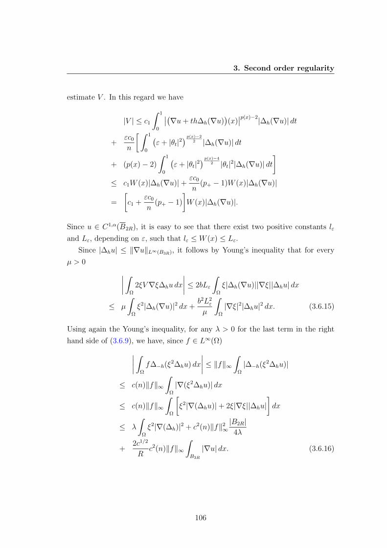
3. Second order regularity
estimate V . In this regard we have
|V | ≤ c1
∫ 1
0
∣∣(∇u+ th∆h(∇u))(x)∣∣p(x)−2|∆h(∇u)| dt
+εc0
n
[ ∫ 1
0
(ε+ |θt|2
) p(x)−22 |∆h(∇u)| dt
+ (p(x)− 2)
∫ 1
0
(ε+ |θt|2
) p(x)−42 |θt|2|∆h(∇u)| dt
]≤ c1W (x)|∆h(∇u)|+ εc0
n(p+ − 1)W (x)|∆h(∇u)|
=
[c1 +
εc0
n(p+ − 1)
]W (x)|∆h(∇u)|.
Since u ∈ C1,α(B2R), it is easy to see that there exist two positive constants lε
and Lε, depending on ε, such that lε ≤ W (x) ≤ Lε.
Since |∆hu| ≤ ‖∇u‖L∞(B3R), it follows by Young’s inequality that for every
µ > 0 ∣∣∣∣ ∫Ω
2ξV∇ξ∆hu dx
∣∣∣∣ ≤ 2bLε
∫Ω
ξ|∆h(∇u)||∇ξ||∆hu| dx
≤ µ
∫Ω
ξ2|∆h(∇u)|2 dx+b2L2
ε
µ
∫Ω
|∇ξ|2|∆hu|2 dx. (3.6.15)
Using again the Young’s inequality, for any λ > 0 for the last term in the right
hand side of (3.6.9), we have, since f ∈ L∞(Ω)∣∣∣∣ ∫Ω
f∆−h(ξ2∆hu) dx
∣∣∣∣ ≤ ‖f‖∞ ∫Ω
|∆−h(ξ2∆hu)|
≤ c(n)‖f‖∞∫
Ω
|∇(ξ2∆hu)| dx
≤ c(n)‖f‖∞∫
Ω
[ξ2|∇(∆hu)|+ 2ξ|∇ξ||∆hu|
]dx
≤ λ
∫Ω
ξ2|∇(∆h)|2 + c2(n)‖f‖2∞|B2R|
4λ
+2c1/2
Rc2(n)‖f‖∞
∫B3R
|∇u| dx. (3.6.16)
106

3. An auxiliary result
Hence, choosing ν = µ = λ = lε/3, from (3.6.9), (3.6.11)-(3.6.16) we obtain
(c1 −
εc0
n(p+ − 1)− 1
) ∫Ω
ξ2|∇(∆hu)|2 dx ≤ C,
where C = C(ε, p−, p+, L,R, ‖f‖∞) is a positive constant. Since ε ∈ (0, 1),
without loss of generality, choosing c1 large enough, we always can assume, that
c1 − εc0n
(p+ − 1) > 1, so ∫BR
|∇(∆hu)|2 dx ≤ C
Letting h→ 0, we obtain the desired result (see Lemma 8.9 of [56]).
3.7 An auxiliary result
For simplicity, from now on we will restrict ourselves to a class of functions
(Fp(·) defined below, p(·) > 2). In remarks we will give the idea of the proofs of
corresponding facts to a more general class of functions.
We consider the solutions of the class of problems
Fp(·)
u ∈ W 1,p(·)(B1) ∩ C1,α(B1),
div(|∇u(x)|p(x)−2∇u(x)
)= f(x) in u > 0 ∩B1,
0 ≤ u ≤M0 in B1,
0 ∈ ∂u > 0,
where M0 > 0 is a constant. We may assume that there exists a positive constant
M1 = M1(n, p−, p+,M0) such that
‖u‖C1,α(B3/4) ≤M1, ∀u ∈ Fp(·). (3.7.1)
We shall start by establishing local L2-estimate for the second derivatives of u.
In order to do that, we define for each r > 0 and each function u ∈ Fp(·), the
107

3. An auxiliary result
quantity
E(r, u) :=1
|Br|
∫Br∩∇u(x)6=0
[|∇u|p(x)−2|D2u|
]2dx
=1
|B1|
∫B1∩∇u(rx)6=0
[|∇u|p(rx)−2(rx)|D2u|(rx)
]2dx,
analogue of the one defined in section 3.5 (page 85). We will assume additionally,
that ∇f ∈ Mnloc(B1) (Morrey space, see [80]), which means that there exists
C0 > 0 constant such that∫B2r
|∇f | dx ≤ C0rn−1, ∀r ∈ (0, 1). (3.7.2)
In particular (3.7.2) is satisfied, if f ∈ C0,1(B1).
For ε ∈ (0, 1) we consider the unique solution of the problemuε − u ∈ W 1,p(·)
0 (B1),
div
((ε+ |∇uε|2
) p(x)−22 ∇uε
)= fHε(uε) in B1,
(3.7.3)
where Hε(v) := min(1, v+/ε).
Next we prove an analogue of the Lemma 3.5.1 for this case.
Lemma 3.7.1. Let p(·) satisfy (3.6.1) and (3.6.2). If 0 < λ ≤ f satisfies (3.7.2),
then there exists a constant C = C(p+, L, n,M1) > 0, independent of ε, such that
E(1/2, u) ≤ C
∫B3/4
|∇u|2(p(x)−1)[(1 + |∇u|)
∣∣ ln |∇u|∣∣+ |∇f |+ 1]dx.
Proof. Let ξ ∈ D(B3/4) be such that0 ≤ ξ ≤ 1, in B3/4, ξ = 1 in B1/2,
|∇ξ| ≤ 4 in B3/4.
and let ϕ := ξ2tp(x)−2ε uεxi , with tε :=
(ε+ |∇uε|2
) 12 . We take ϕxi as a test function
108
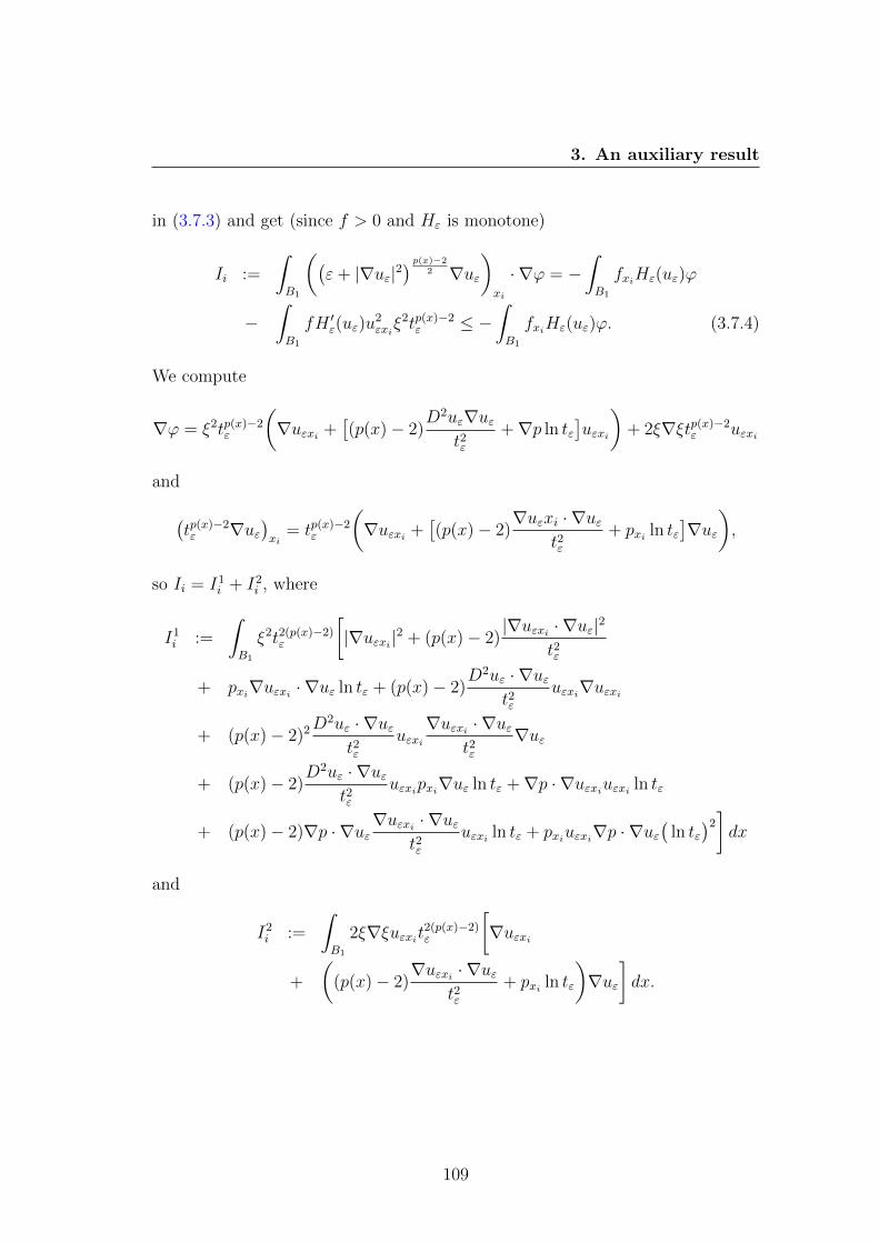
3. An auxiliary result
in (3.7.3) and get (since f > 0 and Hε is monotone)
Ii :=
∫B1
((ε+ |∇uε|2
) p(x)−22 ∇uε
)xi
· ∇ϕ = −∫B1
fxiHε(uε)ϕ
−∫B1
fH ′ε(uε)u2εxiξ2tp(x)−2
ε ≤ −∫B1
fxiHε(uε)ϕ. (3.7.4)
We compute
∇ϕ = ξ2tp(x)−2ε
(∇uεxi +
[(p(x)− 2)
D2uε∇uεt2ε
+∇p ln tε]uεxi
)+ 2ξ∇ξtp(x)−2
ε uεxi
and
(tp(x)−2ε ∇uε
)xi
= tp(x)−2ε
(∇uεxi +
[(p(x)− 2)
∇uεxi · ∇uεt2ε
+ pxi ln tε]∇uε
),
so Ii = I1i + I2
i , where
I1i :=
∫B1
ξ2t2(p(x)−2)ε
[|∇uεxi |2 + (p(x)− 2)
|∇uεxi · ∇uε|2
t2ε
+ pxi∇uεxi · ∇uε ln tε + (p(x)− 2)D2uε · ∇uε
t2εuεxi∇uεxi
+ (p(x)− 2)2D2uε · ∇uεt2ε
uεxi∇uεxi · ∇uε
t2ε∇uε
+ (p(x)− 2)D2uε · ∇uε
t2εuεxipxi∇uε ln tε +∇p · ∇uεxiuεxi ln tε
+ (p(x)− 2)∇p · ∇uε∇uεxi · ∇uε
t2εuεxi ln tε + pxiuεxi∇p · ∇uε
(ln tε
)2]dx
and
I2i :=
∫B1
2ξ∇ξuεxit2(p(x)−2)ε
[∇uεxi
+
((p(x)− 2)
∇uεxi · ∇uεt2ε
+ pxi ln tε
)∇uε
]dx.
109

3. An auxiliary result
Since
(D2v · ∇v)j =∑k
vxjxkvxk = ∇vxj · ∇v
|D2v · ∇v|2 =∑j
|∇vxj · ∇v|2(vxi∇vxi
)·D2v · ∇v =
∑j
(∑i
vxivxixj)(∇vxj · ∇v
)=
∑j
(∇v · ∇vxj)(∇vxj · ∇v) =∑j
|∇v · ∇vxj |2 = |D2v · ∇v|2∑i
vxi∇vxi · ∇v =∑i
vxi(D2v · ∇v)i = (D2v · ∇v) · ∇v∑
i
∇p∇vxivxi =∑j
(∑i
vxixjvxi)pxj =
∑j
(∇vxj · ∇v)pxj
= (D2v · ∇v) · ∇p,
then
n∑i=1
I1i =
∫B1
ξ2t2(p(x)−2)ε
[|D2uε|2 + 2(p(x)− 2)
|D2uε · ∇uε|2
t2ε
+ (p(x)− 2)2
(D2uε · ∇uε · ∇uε
)2
t4ε
]dx+
∫B1
ξ2t2(p(x)−2)ε
[2(D2uε · ∇uε) · ∇p ln tε
+ 2(p(x)− 2)(D2uε · ∇uε) · ∇uε
t2ε∇p · ∇uε ln tε + |∇p · ∇uε|2
(ln tε
)2]dx
:= J1 + J2.
Note that
J1 ≥∫B1
ξ2t2(p(x)−2)ε |D2uε|2 dx. (3.7.5)
Recalling the Lipschitz continuity of p and using Young’s inequality, we estimate
110

3. An auxiliary result
J2 as follows:
|J2| ≤∫B1
ξ2t2(p(x)−2)ε
[2| ln tε||D2uε||∇uε||∇p|
+ 2(p+ + 2)| ln tε||D2uε||∇uε||∇p||∇uε|2
t2ε
+ |∇p|2|∇uε|2∣∣ ln tε∣∣2] dx
≤∫B1
ξ2tp(x)−2ε |D2uε|2L(p+ + 3)tp(x)−2
ε |∇uε|| ln tε| dx
+
∫B1
ξ2t2(p(x)−2)ε L2t2ε
∣∣ ln tε∣∣2 dx ≤ ν1
∫B1
ξ2[tp(x)−2ε |D2uε|
]2dx
+1
ν1
ξ2(2L(p+ + 3)
)2t2(p(x)−1)ε
∣∣ ln tε∣∣2 dx+
∫B1
ξ2L2t2(p(x)−1)ε
∣∣ ln tε∣∣2 dx= ν1
∫B1
ξ2[tp(x)−2ε |D2uε|
]2dx
+
[(2L(p+ + 3)
)2
ν1
+ L2
] ∫B1
ξ2t2(p(x)−1)ε
∣∣ ln tε∣∣2 dx, (3.7.6)
where ν1 > 0 is a constant. On the other hand∣∣∣∣ n∑i=1
I2i
∣∣∣∣ =
∣∣∣∣ ∫B1
2ξ∇ξt2(p(x)−2)ε
[ n∑i=1
∇uεxiuεxi
+ (p(x)− 2)
(D2uε · ∇uε
)· ∇uε
t2ε∇uε +∇uε · ∇p∇uε ln tε
]dx
∣∣∣∣≤
∫B1
8ξt2(p(x)−2)ε
[|D2uε||∇uε|+ (p+ + 2)|D2uε||∇uε|+ L|∇uε|2| ln tε|
]dx
≤ 8(p+ + 3)
∫B1
ξt2(p(x)−2)ε |D2uε||∇uε| dx+ 8L
∫B1
ξt2(p(x)−1)ε | ln tε| dx
≤ ν2
∫B3/4
t2(p(x)−2)ε |D2uε|2 dx+
(8(p+ + 3)
)2
ν2
∫B3/4
t2(p(x)−1)ε dx
+ 8L
∫B3/4
t2(p(x)−1)ε | ln tε| dx (3.7.7)
for ν2 > 0 constant.
111
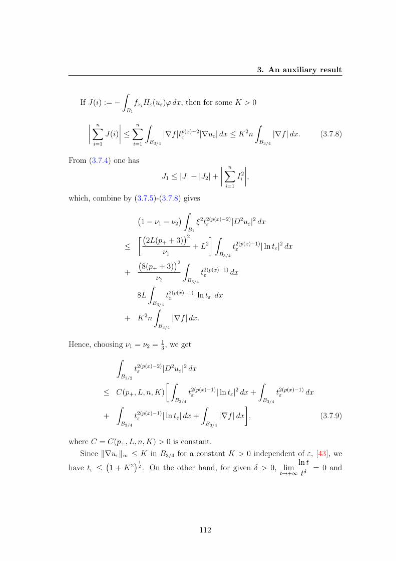
3. An auxiliary result
If J(i) := −∫B1
fxiHε(uε)ϕdx, then for some K > 0
∣∣∣∣ n∑i=1
J(i)
∣∣∣∣ ≤ n∑i=1
∫B3/4
|∇f |tp(x)−2ε |∇uε| dx ≤ K2n
∫B3/4
|∇f | dx. (3.7.8)
From (3.7.4) one has
J1 ≤ |J |+ |J2|+∣∣∣∣ n∑i=1
I2i
∣∣∣∣,which, combine by (3.7.5)-(3.7.8) gives
(1− ν1 − ν2
) ∫B1
ξ2t2(p(x)−2)ε |D2uε|2 dx
≤[(
2L(p+ + 3))2
ν1
+ L2
] ∫B3/4
t2(p(x)−1)ε | ln tε|2 dx
+
(8(p+ + 3)
)2
ν2
∫B3/4
t2(p(x)−1)ε dx
8L
∫B3/4
t2(p(x)−1)ε | ln tε| dx
+ K2n
∫B3/4
|∇f | dx.
Hence, choosing ν1 = ν2 = 13, we get∫
B1/2
t2(p(x)−2)ε |D2uε|2 dx
≤ C(p+, L, n,K)
[ ∫B3/4
t2(p(x)−1)ε | ln tε|2 dx+
∫B3/4
t2(p(x)−1)ε dx
+
∫B3/4
t2(p(x)−1)ε | ln tε| dx+
∫B3/4
|∇f | dx], (3.7.9)
where C = C(p+, L, n,K) > 0 is constant.
Since ‖∇uε‖∞ ≤ K in B3/4 for a constant K > 0 independent of ε, [43], we
have tε ≤(1 + K2
) 12 . On the other hand, for given δ > 0, lim
t→+∞
ln t
tδ= 0 and
112

3. An auxiliary result
limt→0+
tδ ln t = 0, so we deduce that for a constant c∗ = c∗(p−) > 0
| ln t2ε| ≤ c∗ + tp−−1
2ε + t
− p−−1
2ε .
Hence
tp(x)−1ε | ln t2ε| ≤ c∗t
p(x)−1ε + t
p(x)−1+p−−1
2ε + t
p(x)−1− p−−1
2ε
≤ c∗(1 +K2
) p+−1
2 +(1 +K2
) p+−1
2+p−−1
4 +(1 +K2
) p+−1
2− p−−1
4 .
We also have tp(x)−1ε ≤
(1 +K2
) p+−1
2 , so
t2(p(x)−1)ε | ln t2ε| ≤ C(p−, p+, K)
t2(p(x)−1)ε | ln t2ε|2 ≤ C(p−, p+, K)
and we deduce from (3.7.9) that∫B1/2
(ε+ |∇uε|2
)p(x)−2|D2uε|2 dx ≤ C(p−, p+, L,K),
which means, that there exists a subsequence (still denoted by ε) such that
(ε+ |∇uε|2
) p(x)−22 D2uε w weakly in L2(B1/2).
Recalling again (3.7.9), one gets
‖w‖L2(B1/2) ≤ lim infε→0
‖(ε+ |∇uε|2
) p(x)−22 ‖L2(B1/2) (3.7.10)
≤ C
∫B3/4
|∇u|2(p(x)−1)[(1 + |∇u|)
∣∣ ln |∇u|∣∣+ |∇f |+ 1]dx.
Since ‖uε‖C1,α(B3/4) ≤ C for some C > 0 constant independent of ε, we get by
Ascoli-Arzela’s theorem that uε → u uniformly in C1(B3/4). We deduce that
D2u ∈ L2loc
(B1/2 ∩ ∇u 6= 0
). Consequently, we obtain
w = |∇u|p(x)−2D2u on B1/2 ∩ ∇u 6= 0,
113
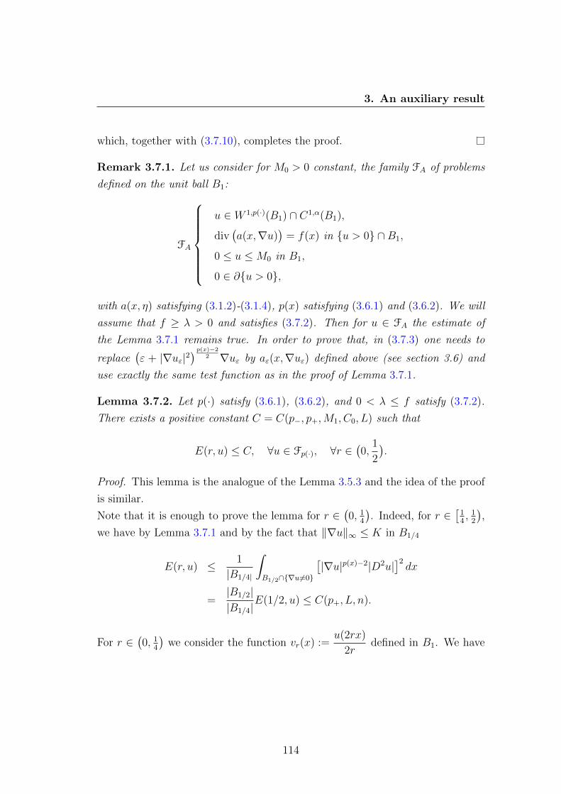
3. An auxiliary result
which, together with (3.7.10), completes the proof.
Remark 3.7.1. Let us consider for M0 > 0 constant, the family FA of problems
defined on the unit ball B1:
FA
u ∈ W 1,p(·)(B1) ∩ C1,α(B1),
div(a(x,∇u)
)= f(x) in u > 0 ∩B1,
0 ≤ u ≤M0 in B1,
0 ∈ ∂u > 0,
with a(x, η) satisfying (3.1.2)-(3.1.4), p(x) satisfying (3.6.1) and (3.6.2). We will
assume that f ≥ λ > 0 and satisfies (3.7.2). Then for u ∈ FA the estimate of
the Lemma 3.7.1 remains true. In order to prove that, in (3.7.3) one needs to
replace(ε + |∇uε|2
) p(x)−22 ∇uε by aε(x,∇uε) defined above (see section 3.6) and
use exactly the same test function as in the proof of Lemma 3.7.1.
Lemma 3.7.2. Let p(·) satisfy (3.6.1), (3.6.2), and 0 < λ ≤ f satisfy (3.7.2).
There exists a positive constant C = C(p−, p+,M1, C0, L) such that
E(r, u) ≤ C, ∀u ∈ Fp(·), ∀r ∈(0,
1
2
).
Proof. This lemma is the analogue of the Lemma 3.5.3 and the idea of the proof
is similar.
Note that it is enough to prove the lemma for r ∈(0, 1
4
). Indeed, for r ∈
[14, 1
2
),
we have by Lemma 3.7.1 and by the fact that ‖∇u‖∞ ≤ K in B1/4
E(r, u) ≤ 1
|B1/4|
∫B1/2∩∇u6=0
[|∇u|p(x)−2|D2u|
]2dx
=|B1/2||B1/4|
E(1/2, u) ≤ C(p+, L, n).
For r ∈(0, 1
4
)we consider the function vr(x) :=
u(2rx)
2rdefined in B1. We have
114

3. An auxiliary result
by definition of vr and by Theorem 2.2.1 and Theorem 3.4.2 that
0 ≤ vr ≤C
2r
(2r|x|
) p0p0−1 ≤ Cr
1p0−1 ≤ C ′
|∇vr(x)| = |∇u(2rx)| ≤ C1
(2r) 1p0−1 < 1 for some r < r0 <
1
4,
D2vr(x) = 2r(D2u)(2rx),
where p0 = p(0). We deduce that there exists r1 ∈ (0, r0) such that |∇vr| ≤C1
(2r) 1p0−1 <
(1e
) 1p−−1 and then
|∇vr|2(pr−1)∣∣ ln |∇vr|∣∣ ≤ (C1
(2r))2(pr−1)∣∣ ln (C1
(2r) 1p0−1
)∣∣where pr(x) := p(2rx). In the same way one can insure, that there exists r2 ∈(0, r1) such that
|∇vr|2pr−1∣∣ ln |∇vr|∣∣ ≤ (C1
(2r))2pr−1∣∣ ln (C1
(2r) 1p0−1
)∣∣.Note that
(∆pr(·)wr
)(x) = 2r
(∆p(·)u
)(2rx) = 2rf(2rx) in u(2rx) > 0.
115

3. An auxiliary result
Therefore, for r ∈ (0, r2) we deduce from Lemma 3.7.1 and (3.7.2)
E(r, u) =1
(2r)2E(1/2, vr)
≤ C
(2r)2
∫B3/4
|∇vr|2(pr(x)−1)[(1 + |∇vr|)
∣∣ ln |∇vr|∣∣+ |∇f |+ 1]dx
≤ C
(2r)2|B3/4|
(C1
(2r)) 2(pr−1)
p0−1[1 +
C0
|B3/4|
+
(C1
(2r))2(pr−1)∣∣ ln (C1
(2r) 1p0−1
)∣∣+
(C1
(2r))2pr−1∣∣ ln (C1
(2r) 1p0−1
)∣∣]≤ C ′(C,C1, p−, p+)
[(1 +
C0
|B3/4|)(2r) 2(pr−1)
p0−1−2
+(2r)2p−−4| ln(2r)|+
(2r)2p−−3| ln(2r)|
]=: d1 + d2 + d3.
Since limt→0+
tδ ln t = 0 for given δ > 0, then d2 and d3 are bounded, when r > 0 is
small enough. Since p is Lipschitz continuous, we remark, that for r > 0 small
enough d1 also is bounded, because
(2r) 2(pr−1)
p0−1−2
=(2r) 2(pr−p0)
p0−1 = e2(pr−p0)p0−1
ln(2r) ≤ e2·L2rp0−1
| ln(2r)| ≤ C,
for some C > 0 constant. Therefore
E(r, u) ≤ C(p−, p+,M1, C0, L), ∀r ∈ (0, r2),
which completes the proof, since for r ∈(r2,
14
)E(r, u) ≤
|B1/2|Br2
E(1/2, u) ≤ C(p−, p+,M1, C0, L).
Next, we proof the analogue of the Lemma 3.5.4.
116
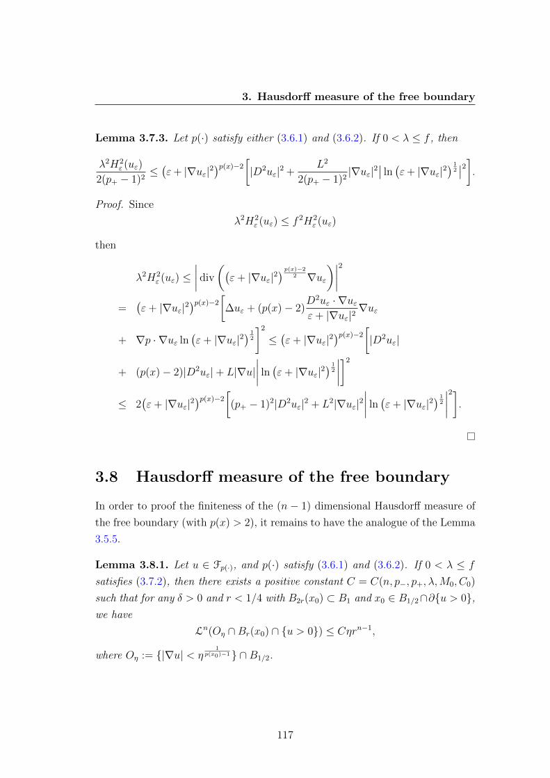
3. Hausdorff measure of the free boundary
Lemma 3.7.3. Let p(·) satisfy either (3.6.1) and (3.6.2). If 0 < λ ≤ f , then
λ2H2ε (uε)
2(p+ − 1)2≤(ε+ |∇uε|2
)p(x)−2[|D2uε|2 +
L2
2(p+ − 1)2|∇uε|2
∣∣ ln (ε+ |∇uε|2) 1
2∣∣2].
Proof. Since
λ2H2ε (uε) ≤ f 2H2
ε (uε)
then
λ2H2ε (uε) ≤
∣∣∣∣ div
((ε+ |∇uε|2
) p(x)−22 ∇uε
)∣∣∣∣2=
(ε+ |∇uε|2
)p(x)−2[∆uε + (p(x)− 2)
D2uε · ∇uεε+ |∇uε|2
∇uε
+ ∇p · ∇uε ln(ε+ |∇uε|2
) 12
]2
≤(ε+ |∇uε|2
)p(x)−2[|D2uε|
+ (p(x)− 2)|D2uε|+ L|∇u|∣∣∣∣ ln (ε+ |∇uε|2
) 12
∣∣∣∣]2
≤ 2(ε+ |∇uε|2
)p(x)−2[(p+ − 1)2|D2uε|2 + L2|∇uε|2
∣∣∣∣ ln (ε+ |∇uε|2) 1
2
∣∣∣∣2].
3.8 Hausdorff measure of the free boundary
In order to proof the finiteness of the (n − 1) dimensional Hausdorff measure of
the free boundary (with p(x) > 2), it remains to have the analogue of the Lemma
3.5.5.
Lemma 3.8.1. Let u ∈ Fp(·), and p(·) satisfy (3.6.1) and (3.6.2). If 0 < λ ≤ f
satisfies (3.7.2), then there exists a positive constant C = C(n, p−, p+, λ,M0, C0)
such that for any δ > 0 and r < 1/4 with B2r(x0) ⊂ B1 and x0 ∈ B1/2∩∂u > 0,we have
Ln(Oη ∩Br(x0) ∩ u > 0) ≤ Cηrn−1,
where Oη := |∇u| < η1
p(x0)−1 ∩B1/2.
117

3. Hausdorff measure of the free boundary
Proof. We will use the following notations: p∗ := minBr(x0)
p(x),
Oεiη := |∇uεxi | < η
1p∗−1 ∩B1/2, Oε
η := |∇uε| < η1
p∗−1 ∩B1/2,
G(t) :=
(ε+ η
2p∗−1
) p∗−22 η
1p∗−1 , if t ≥ η
1p∗−1 ,
(ε+ η2
p∗−1) p∗−2
2 t, if |t| ≤ η1
p∗−1 ,
−(ε+ η
2p∗−1
) p∗−22 η
1p∗−1 , if t ≤ η
1p∗−1 .
Note that G′(t) =(ε+ η
p∗−12
) p∗−22 χ
|t|<η1
p∗−1 and tG(t) ≥ 0, ∀t ∈ R. Let
ξ ∈ D(B2r(x0)), 0 ≤ ξ ≤ 1 in B2r(x0),
ξ = 1 in Br(x0), |∇ξ| ≤ 2
rin B2r(x0).
Taking[ξG(uεxi)
]xi
as a test function in (3.7.3) and using the monotonicity of
Hε, we have∫B2r(x0)
((ε+ |∇uε|2
) p(x)−22 ∇uε
)xi
· ∇(ξG(uεxi)
)dx
−∫B2r(x0)
fxiHε(uε)ξG(uεxi) dx−∫B2r(x0)
fH ′ε(uε)uεxiG(uεxi) dx
≤ −∫B2r(x0)
fxiHε(uε)ξG(uεxi) dx. (3.8.1)
Since ((ε+ |∇uε|2
) p(x)−22 ∇uε
)xi
=(ε+ |∇uε|2
) p(x)−22
[∇uεxi
+ (p(x)− 2)∇uεxi · ∇uεε+ |∇uε|2
∇uε + pxi∇uε ln(ε+ |∇uε|2
) 12
]:= tp(x)−2
ε Aε,
with
tε :=(ε+ |∇uε|2
) 12
and
Aε := ∇uεxi + (p(x)− 2)∇uεxi · ∇uεε+ |∇uε|2
∇uε + pxi∇uε ln(ε+ |∇uε|2
) 12 .
118

3. Hausdorff measure of the free boundary
From (3.8.1) we have that∫B2r(x0)
ξG′(uεxi)∇uεxitp(x)−2ε Aε dx
≤ −∫B2r(x0)
G(uεxi)∇ξtp(x)−2ε Aε dx−
∫B2r(x0)
fxiHε(uε)ξG(uεxi) dx.
So ∫B2r(x0)∩Oεiη
ξ(ε+ η
2p∗−1
) p∗−22 tp(x)−2
ε
[|∇uεxi |2 + (p(x)− 2)
|∇uεxi · ∇uε|2
t2ε
+ pxi∇uεxi · ∇uε ln tε
]dx ≤ −
∫B2r(x0)
(G(uεxi)−G(uxi)
)∇ξtp(x)−2
ε Aε dx
−∫B2r(x0)
G(uxi)∇ξtp(x)−2ε Aε dx−
∫B2r(x0)
fxiHε(uε)ξG(uεxi) dx,
which gives
Ii :=
∫B2r(x0)∩Oεiη
ξ(ε+ η
2p∗−1
) p∗−22 tp(x)−2
ε |∇uεxi |2 dx
≤ −∫B2r(x0)∩Oεiη
ξ(ε+ η
2p∗−1
) p∗−22 tp(x)−2
ε pxi∇uεxi · ∇uε ln tε dx
−∫B2r(x0)
(G(uεxi)−G(uxi)
)∇ξtp(x)−2
ε Aε dx
−∫B2r(x0)
G(uxi)∇ξtp(x)−2ε Aε dx−
∫B2r(x0)
fxiHε(uε)ξG(uεxi) dx
:= J1i + J2
i + J3i + J4
i . (3.8.2)
Using Young’s inequality, we write
|J1i | ≤
∫B2r(x0)∩Oεiη
ξ(ε+ η
2p∗−1
) p∗−22 tp(x)−2
ε L|∇uεxi ||∇uε|∣∣ ln tε∣∣ dx
≤∫B2r(x0)∩Oεiη
ξ(ε+ η
2p∗−1
) p∗−22 tp(x)−2
ε
[ν0|∇uεxi |2 +
L2
ν0
|∇uε|2∣∣ ln tε∣∣2] dx
= ν0Ii + J5i ,
119

3. Hausdorff measure of the free boundary
where ν0 > 0 is constant and
J5i :=
L2
ν0
∫B2r(x0)∩Oεiη
ξ(ε+ η
2p∗−1
) p∗−22 tp(x)−2
ε |∇uε|2∣∣ ln tε∣∣2 dx.
Taking ν0 = 12
we get1
2Ii − J5
i ≤ J2i + J3
i + J4i . (3.8.3)
We remark that as ε→ 0
|G(uεxi)−G(uxi)| ≤(ε+ η
2p∗−1
) p∗−22 |uεxi − uxi| → 0
uniformly, since ‖uε − u‖C1(B3/4) → 0 as ε→ 0.
|J2i | ≤ ‖G(uεxi)−G(uxi)‖L∞(B2r(x0))
2
r
∫B2r(x0)
tp(x)−2ε
[(p+ − 1)|∇uεxi |
+ L|∇uε|∣∣ ln tε∣∣] dx
≤ C
r
(ε+ η
2p∗−1
) p∗−22 ‖uεxi − uxi‖C0(B3/4)
[ ∫B2r(x0)
tp(x)−2ε |∇uεxi |
+
∫B2r(x0)
tp(x)−1ε
∣∣ ln tε∣∣]where C = C(p+, L) > 0 is constant.
On the other hand, we have
∫B2r(x0)
tp(x)−2ε |∇uεxi | ≤
[ ∫B2r(x0)
[tp(x)−2ε |∇uεxi |
]2dx
] 12[ ∫
B2r(x0)
12 dx
] 12
≤ |B2r|12
[ ∫B1/2
t2(p(x)−2)ε |D2uε|2 dx
] 12
.
As we already saw before, the last integral is bounded independent of ε (page
112), and since we also have for a constant C > 0∫B2r(x0)
tp(x)−1ε
∣∣ ln tε∣∣ ≤ C,
120

3. Hausdorff measure of the free boundary
then we deduce that
limε→0
J2i = 0. (3.8.4)
We deduce also that tp(x)−2ε D2uε w in L2(B1/2). Since uε → u in C1(B3/4),
we get that w = |∇u|p(x)−2D2u in B1/2 ∩ ∇u 6= 0. Note that Oη ⊂ Oεη ⊂ Oεi
η
because uε → u in C1(B3/4).
J3i = −
∫B2r(x0)∩∇u6=0
t2(p(x)−2)G(uxi)∇ξ[∇uεi
+ (p(x)− 2)∇uεi · ∇uεε+ |∇uε|2
∇uε
+ pxi∇uε ln(ε+ |∇uε|2
) 12
]dx.
We write
limε→0
J3i = −
∫B2r(x0)∩∇u6=0
G(uxi)∇ξ[wi + (p(x)− 2)
wi · ∇u|∇u|2
∇u
+ pxi∇u ln |∇u|]dx
= −∫B2r(x0)∩∇u6=0
G(uxi)∇ξ|∇u|p(x)−2
[∇uxi + (p(x)− 2)
∇uxi · ∇u|∇u2|
∇u]
+ pxi∇u ln |∇u|dx := J6
i .
From (3.7.1) we have that ‖∇u‖L∞(B3/4) < M1. Note also, that |∇u|∣∣ ln |∇u|∣∣ ≤
C(p−, p+,M1). Using Lemma 3.7.2 we get
|J6i | ≤ η
2
r(p+ − 1)
∫B2r(x0)∩∇u6=0
|∇u|p(x)−2|∇uxi |
+2L
rη
∫B2r(x0)∩∇u6=0
|∇u|p(x)−1∣∣ ln |∇u|∣∣ dx
≤ 2(p+ − 1)
rη
[ ∫B2r(x0)∩∇u6=0
|∇u|2(p(x)−2)|D2u|2 dx] 1
2(∫
2r
12 dx
) 12
+2LC
rη|B2r| ≤ Cηrn−1, (3.8.5)
121
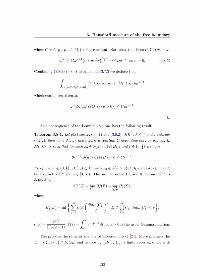
3. Hausdorff measure of the free boundary
where C = C(p−, p+, L,M1) > 0 is constant. Note also, that from (3.7.2) we have
|J4i | ≤ C0r
n−1(ε+ η
2p∗−1
) p∗−12 → C0ηr
n−1 as ε→ 0, (3.8.6)
Combining (3.8.3)-(3.8.6) with Lemma 3.7.3 we deduce that∫Br(x0)∩Oη∩u>0
dx ≤ C(p−, p+, L,M1, λ, C0)ηrn−1
which can be rewritten as
Ln(Br(x0) ∩Oη ∩ u > 0) ≤ Cηrn−1.
As a consequence of the Lemma 3.8.1 one has the following result:
Theorem 3.8.1. Let p(x) satisfy (3.6.1) and (3.6.2). If 0 < λ ≤ f and f satisfies
(3.7.2), then for u ∈ Fp(·) there exists a constant C depending only on p−, p+, L,
M1, C0, λ such that for each x0 ∈ ∂u > 0 ∩B1/2 and r ∈(0, 1
4
)we have
Hn−1(∂u > 0 ∩Br(x0)) ≤ Crn−1.
Proof. Let r ∈(0, 1
4
), Br(x0) ⊂ B1 with x0 ∈ ∂u > 0 ∩ B1/2 and δ > 0. Let E
be a subset of Rn and s ∈ [0,∞). The s-dimensional Hausdorff measure of E is
defined by
Hs(E) = limδ→0
Hsδ (E) = sup
δ>0Hsδ (E),
where
Hsδ (E) = inf
∞∑j=1
α(s)
(diam(Cj)
2
)s ∣∣E ⊂ ∞⋃j=1
Cj, diam(Cj) ≤ δ
,
α(s) =πs/2
Γ(s/2 + 1), Γ(s) =
∫ ∞0
e−tts−1 dt for s > 0 is the usual Gamma function.
The proof is the same as the one of Theorem 1.5 of [24]. More precisely, let
E = ∂u > 0 ∩ Br(x0) and denote by(Bδ(xi)
)i∈I a finite covering of E, with
122
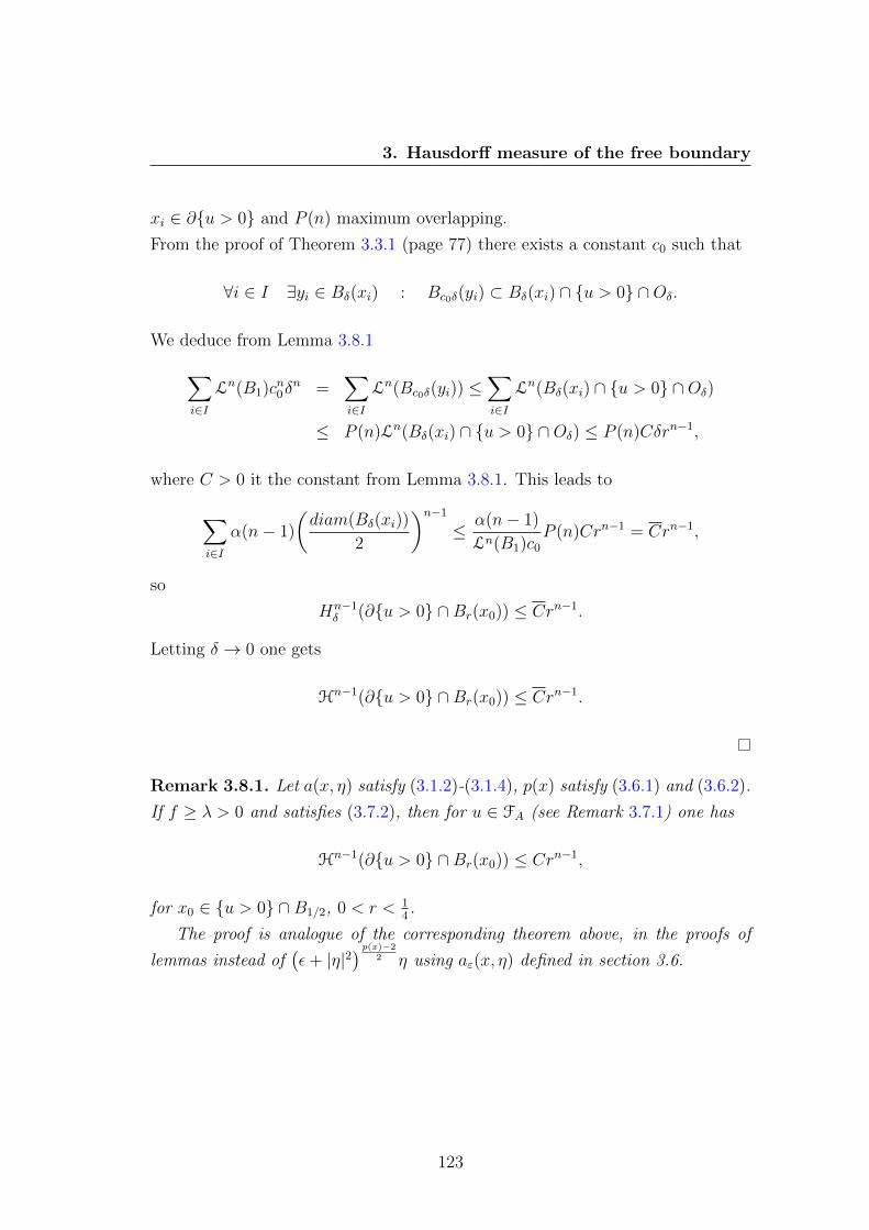
3. Hausdorff measure of the free boundary
xi ∈ ∂u > 0 and P (n) maximum overlapping.
From the proof of Theorem 3.3.1 (page 77) there exists a constant c0 such that
∀i ∈ I ∃yi ∈ Bδ(xi) : Bc0δ(yi) ⊂ Bδ(xi) ∩ u > 0 ∩Oδ.
We deduce from Lemma 3.8.1∑i∈I
Ln(B1)cn0δn =
∑i∈I
Ln(Bc0δ(yi)) ≤∑i∈I
Ln(Bδ(xi) ∩ u > 0 ∩Oδ)
≤ P (n)Ln(Bδ(xi) ∩ u > 0 ∩Oδ) ≤ P (n)Cδrn−1,
where C > 0 it the constant from Lemma 3.8.1. This leads to
∑i∈I
α(n− 1)
(diam(Bδ(xi))
2
)n−1
≤ α(n− 1)
Ln(B1)c0
P (n)Crn−1 = Crn−1,
so
Hn−1δ (∂u > 0 ∩Br(x0)) ≤ Crn−1.
Letting δ → 0 one gets
Hn−1(∂u > 0 ∩Br(x0)) ≤ Crn−1.
Remark 3.8.1. Let a(x, η) satisfy (3.1.2)-(3.1.4), p(x) satisfy (3.6.1) and (3.6.2).
If f ≥ λ > 0 and satisfies (3.7.2), then for u ∈ FA (see Remark 3.7.1) one has
Hn−1(∂u > 0 ∩Br(x0)) ≤ Crn−1,
for x0 ∈ u > 0 ∩B1/2, 0 < r < 14.
The proof is analogue of the corresponding theorem above, in the proofs of
lemmas instead of(ε+ |η|2
) p(x)−22 η using aε(x, η) defined in section 3.6.
123

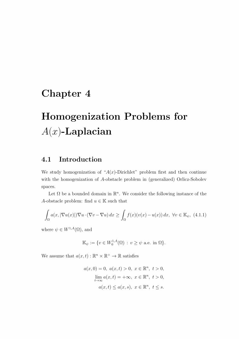
Chapter 4
Homogenization Problems for
A(x)-Laplacian
4.1 Introduction
We study homogenization of “A(x)-Dirichlet” problem first and then continue
with the homogenization of A-obstacle problem in (generalized) Orlicz-Sobolev
spaces.
Let Ω be a bounded domain in Rn. We consider the following instance of the
A-obstacle problem: find u ∈ K such that∫Ω
a(x, |∇u(x)|)∇u · (∇v−∇u) dx ≥∫
Ω
f(x)(v(x)−u(x)) dx, ∀v ∈ Kψ, (4.1.1)
where ψ ∈ W 1,A(Ω), and
Kψ := v ∈ W 1,A0 (Ω) : v ≥ ψ a.e. in Ω.
We assume that a(x, t) : Rn × R+ → R satisfies
a(x, 0) = 0, a(x, t) > 0, x ∈ Rn, t > 0,
limt→∞
a(x, t) = +∞, x ∈ Rn, t > 0,
a(x, t) ≤ a(x, s), x ∈ Rn, t ≤ s.

4. Homogenization of the Dirichlet problem
We suppose that a(x, t) is periodic in x with period 1 in each argument x1, x2,...,
xn, so that Q = (0, 1]n is the periodicity cell. We assume also that for some
positive constants a− and a+ a(x, t) satisfies (1.1.4) or equivalently,
(1 + a−)A(x, t) ≤ a(x, t)t2 ≤ (1 + a+)A(x, t). (4.1.2)
with A defined as
A(x, t) :=
∫ t
0
a(x, s)s ds.
Condition (1.1.4) implies the so called ∆2 condition, and then the corresponding
(generalized) Orlicz-Sobolev spaces are reflexive Banach spaces (see Appendix).
It is not hard to see (Euler-Lagrange) that we can find a solution of (4.1.1) by
minimizing the functional
I(v) =
∫Ω
(A(x, |∇v(x)|) + f(x)v(x)) dx,
in K. In fact, we have uniqueness of the solution since we are dealing with a
minimization of a convex functional on a closed convex set.
4.2 Homogenization of the Dirichlet problem
We will use the following notations afterwards: aε(x, t) = a(xε, t), Aε(x, t) =
A(xε, t).
Theorem 4.2.1. Let f ∈ W−1,1+1/a+(Ω) and
(1 + a+) ≤ (1 + a−)∗, (4.2.1)
where p∗ := n(1 + p)/(n− p) is the Sobolev conjugate. Then the unique solutions
uε ∈ W 1,Aε0 (Ω) of∫
Ω
aε(x, |∇uε|)∇uε · ∇v dx =
∫Ω
fv dx, ∀v ∈ W 1,Aε0 (Ω). (4.2.2)
126

4. Homogenization of the Dirichlet problem
converge when ε→ 0 to the solution of∫Ω
b(∇u0) · ∇v dx =
∫Ω
fv dx, ∀v ∈ C∞0 (Ω),
where
b(ξ) :=
∫Q
a(y, |ξ +∇N |)(ξ +∇N) dy, (4.2.3)
where Q = (0, 1]n is the periodicity cube, and N ∈ W 1,A0 (Q) is the solution of
problem on the periodicity cell:∫Q
a(y, |ξ +∇N |)(ξ +∇N) · ∇ϕdy = 0, ∀ϕ ∈ W 1,A0 (Q),
Proof. The method we use is the classic one in homogenization (see, for example,
[27], [41]). As we know, W 1,1+a+
0 (Ω) → W 1,Aε0 (Ω) → W
1,1+a−0 (Ω) embeddings
are continuous (see Appendix). This allows us to control norms of functions
in W 1,Aε0 (Ω) with the norms of the same functions in fixed exponent Sobolev
spaces. Consequently, this makes easier to adapt the technic used in [111], since
the approach in [111] is based on this kind of embeddings on constants exponent
Sobolev spaces.
Step 1 (existence of weak limits). We define b : Rn → R by (4.2.3),
and let uε ∈ W 1,Aε0 (Ω) be the solution to (4.2.2). Then from Holder and Poincare
inequalities (see Appendix) we conclude∫Ω
aε(x, |∇uε|)|∇uε|2 dx =
∫Ω
fuε dx
≤ ‖f‖LAε‖uε‖LAε≤ C‖f‖L1+1/a+‖∇uε‖LAε ,
(4.2.4)
where F is the Young conjugate function of F :
F (x, t) := sups>0ts− F (x, s), ∀x ∈ Ω, t > 0.
127
4. Homogenization of the Dirichlet problem
On the other hand we know that (see [89] or Appendix below)
‖u‖LA ≥ 1 ⇒ ‖u‖1+a−LA
≤∫
Ω
A(x, |u(x)|) dx ≤ ‖u‖1+a+
LA,
and
‖u‖LA ≤ 1 ⇒ ‖u‖1+a+
LA≤∫
Ω
A(x, |u(x)|) dx ≤ ‖u‖1+a−LA
,
which together with (4.1.2) gives∫Ω
aε(x, |∇uε|)|∇uε|2 dx ≥ (1 + a−)
∫Aε(x, |∇uε|) dx
≥ (1 + a−)‖∇uε‖1+β(ε)
LAε,
(4.2.5)
where β(ε) is either a− or a+, depending on whether ‖∇uε‖LAε ≤ 1 or ‖∇uε‖LAε ≥1. Then, by putting (4.2.4) and (4.2.5) together, we get
‖∇uε‖LAε ≤ C, (4.2.6)
where C is independent of ε (β(ε) takes just two values). Since LAε ⊂ L1+a− (see
Appendix), we get
‖uε‖W 1,1+a−0 (Ω)
≤ C,
hence we conclude the existence of a weakly convergent subsequence:
uε u∗ weakly in W1,1+a−0 (Ω).
In fact, turns out that u∗ coincides with u0 (see step 2 and 3 of the proof).
Now, to check that aε(x, |∇uε(x)|)∇uε(x) is bounded in(LA)n
we use
A(x, a(x, t)t) ≤ (1 + a+)A(x, t),
which is a consequence of (4.1.2). Observe∫Ω
Aε(x, aε(x, |∇uε(x)|)|∇uε(x)|
)dx ≤ C
∫Ω
Aε(x, |∇uε(x)|) dx
≤ C‖∇uε‖1+β(ε)
LAε≤ C,
128
4. Homogenization of the Dirichlet problem
by (4.2.6), and we have
‖aε(·, |∇uε|)∇uε‖γ(LAε (Ω)
)n ≤ ∫Ω
Aε(x, aε(x, |∇uε(x)|)|∇uε(x)|
)dx,
with γ similar to β. Since LAε(Ω) ⊂ L1+1/a+(Ω) (see Theorem A.3.1 in Appendix),
so aε(·, |∇uε|)∇uε is bounded in(L1+1/a+
(Ω))n
, and hence up to a subsequence,
we have
aε(·, |∇uε|)∇uε η weakly in(L1+1/a+
(Ω))n.
Step 2. We now claim that η = b(∇u0).
By the monotonicity of the operator (this is a consequence of (1.1.4)), ∀ϕ ∈C∞0 (Ω), ϕ ≥ 0 the following inequality holds∫
Ω
ϕ[(aε(x, |∇uε|)∇uε − aε(x, |vε|)vε
)]· (∇uε − vε) dx ≥ 0, (4.2.7)
where
vε(x) := ξ +∇N(x/ε),
and N is the solution of the problem on the periodicity cell (see the equality
following (4.2.3)). Define ηε := aε(x, |∇uε|)∇uε. The claim follows from the
following four relations combined with Minty’s trick.
(i) aε(x, |vε|)|vε|2 b(ξ) · ξ in L1(Ω);
(ii) ηε · vε η · ξ in L1(Ω);
(iii) aε(x, |vε|)vε · ∇uε b(ξ) · ∇u0 in L1(Ω);
(iv) ηε · ∇uε dx η · ∇u0 dx in the sense of weak convergence of measures in the
domain Ω.
Suppose for a while that (i)-(iv) are true. Let us show how to obtain the
required claim η = b(∇u0) from these relations.
First, using (i)-(iv), we pass to the limit in each four term on the left hand
side of (4.2.7), which brings us to∫Ω
ϕ(η − b(ξ)) · (∇u0 − ξ) dx ≥ 0,
129

4. Homogenization of the Dirichlet problem
and since ϕ is arbitrary, we have
(η − b(ξ)) · (∇u0 − ξ) ≥ 0
for any ξ ∈ Rn and almost all x ∈ Ω. Using the Minty’s trick, we obtain that
η = b(∇u0). Indeed, assuming x to be a Lebesgue point for ∇u0 and η, we set
ξ = ∇u0(x) + tη, t > 0, η ∈ Rn,
in the last inequality and pass to the limit as t→ 0. Then
(η(x)− b(∇u0(x) + tη)big) · η ≥ 0,
which implies that η(x) = b(∇u0(x)) in view of the fact that η ∈ Rn is arbitrary
and continuity of b(·). The latter is also proved by Minty’s trick. The proof is
exactly the same as the one of corresponding Lemma 5.1 in [111], so we omit it.
Step 3 (on proof of relations (i)-(iv)). It remains to check the va-
lidity of relations (i)-(iv). These relations are exactly the corresponding ones in
[111], and since everything is in the fixed exponent spaces, the proofs are easy to
adapt from p(x)-spaces to A(x) ones. For example, relation (i) is a consequence
of mean value property: if for a periodic function d
d ∈ Lγ(Q), γ ≥ 1 then d
(x
ε
) [d] in Lγ(Ω),
where [·] :=∫Q· is the average over the periodicity cell.
Since (ξ + ∇yN) ∈(LA(Q)
)n, and a(y, |ξ + ∇yN |)(ξ + ∇yN) ∈
(LA)n
, the
product (ξ +∇yN) · a(y, |ξ +∇yN |)(ξ +∇yN) belongs to L1(Q), and by mean
value property
a
(x
ε,
∣∣∣∣ξ +∇yN
(x
ε
)∣∣∣∣)∣∣∣∣ξ +∇yN
(x
ε
)∣∣∣∣2 [a(y, |ξ +∇yN |)|ξ +∇yN |2] = [a(y, |ξ +∇yN |)(ξ +∇yN)] · ξ = b(ξ) · ξ,
weakly in L1(Ω), where the equalities are written in view of the definitions of the
130
4. Homogenization of the Dirichlet problem
homogenized symbol and of the solution of the problem on the cell.
In the tree remaining cases (ii)-(iv), determination of the limits is not obvious.
The proofs of those is based on the following compensated compactness argument:
Lemma 4.2.1. Let uε and wε be such that
a) uε ∈ W 1,Aε0 (Ω) and wε ∈ LAεsol(Ω), where
LAεsol(Ω) := ∇ϕ, ϕ ∈ W 1,A0 (Ω)⊥;
b) ‖uε‖LAε (Ω), ‖wε‖LAε (Ω) ≤ c <∞;
c) ∇uε ∇u weakly in L1+a−, and wε w weakly in L1+1/a+(Ω);
d) the family uε is compact in L1,1+a+.
Then, in the sense of weak convergence of measures in Ω
wε · ∇uε dx w · ∇u dx.
The proof of the lemma is based on some semi-continuity arguments and is
not hard. It is given for the case when we are dealing with variable exponent
Lebesgue spaces (p(·)-spaces) in [111]. The lemma is valid only in the case of
(1 + a+) ≤ (1 + a−)∗ := n(1 + a−)/(n − 1 − a−). This condition seems quite
strong restriction but that is what allows us to use the compensated compactness
lemma. It seems we can not avoid this restriction, which appears also in particular
problems like the one with p(·)-spaces considered in [111]. However, in [110] the
authors give some replacements this condition, which still makes the compensated
compactness lemma work.
In order to find limits in cases (ii)-(iv), one needs to use Lemma 4.2.1. How-
ever, we can not apply this lemma to the vectors appearing in (ii)-(iv), since in
the case under consideration, we can not affirm that assumption d) used in the
lemma is valid. The necessary compactness property allows us to use cut-offs in
potential multipliers. Therefore, one should proceed by the scheme in [111]: first,
one can obtain relations of type (ii)-(iv) with ”cut-off” potential multipliers, then
one can see that cut-offs can be removed everywhere. This part is going to be a
direct repetition of the one in [111], which me omit here.
131
4. Homogenization of the obstacle problem
4.3 Homogenization of the obstacle problem
In this section we consider the unilateral problems Find uε ∈ Kψε such that
〈Aεuε − f, v − uε〉 ≥ 0, ∀v ∈ Kψε ,(4.3.1)
where 〈·, ·〉 is the pairing between W 1,Aε0 (Ω) and W−1,Aε(Ω), f ∈ W−1,1+1/a+
(Ω),
and the Aε are monotone operators acting from W 1,Aε0 (Ω) to W−1,Aε(Ω) defined
by (see also (2.2.3))
Aεv := − div(aε(x, |∇v|)∇v
),
and the sets Kψε are defined by
Kψε := v ∈ W 1,Aε0 (Ω) : v ≥ ψε a.e. in Ω,
ψε ∈ W 1,Aε(Ω) (as usual, Aε(x, t) :=∫ t
0aε(x, s)s ds). We assume that the function
aε(x, t) : Ω× R+ → R together with (1.1.4) satisfies
aε(x, 0) = 0, aε(x, t) > 0, x ∈ Ω, t > 0,
limt→∞
aε(x, t) = +∞, x ∈ Ω, t > 0,
aε(x, t) ≤ aε(x, s), x ∈ Ω, t ≤ s.
Under this conditions Aε is a strictly monotone operator defined from W 1,Aε0 (Ω)
into its dual W−1,Aε(Ω) (see Proposition 2.2.1), and for any f ∈ W−1,1+1/a+(Ω)
there exists a unique solution uε to − div(aε(x, |∇uε|)∇uε
)= f in D′(Ω),
uε ∈ W 1,Aε0 (Ω).
(4.3.2)
Moreover, the solutions uε are bounded in W1,1+a−0 (Ω), independently of ε (see
(4.2.6)).
Definition 4.3.1. Consider aε satisfying the above assumptions and a function
a0 satisfying the same hypotheses. We will say that aε G-converges to a0, if the
132

4. Homogenization of the obstacle problem
unique solution uε of (4.3.2) satisfies uε u weakly in W1,1+a−0 (Ω),
aε(x, |∇uε|)∇uε a0(x, |∇u|)∇u weakly in(L1+1/a−(Ω)
)n,
(4.3.3)
where u is the unique solution of − div(a0(x, |∇u|)∇u
)= f in D′(Ω),
u ∈ W 1,A0
0 (Ω).(4.3.4)
Definition 4.3.2. Consider a sequence of nonempty, closed, convex subsets Kε,
K0 of W1,1+a−0 (Ω). The sequence Kε is said to converge to K0 in the sense of
Mosco, if
(i) for any v0 ∈ K0 there exists a sequence vε ∈ Kε such that
vε → v0 strongly in W1,1+a−0 (Ω); (4.3.5)
(ii) for any v and any subsequence δ of ε such that vδ ∈ Kδ and
vδ v weakly in W1,1+a−0 (Ω) (4.3.6)
one has v ∈ K0.
Since W1,1+a+
0 (Ω) is continuously embedded into W 1,A0
0 (Ω) and all W 1,Aε0 (Ω),
and W 1,A0
0 (Ω), W 1,Aε0 (Ω) are continuously embedded into W
1,1+a−0 (Ω) (see Ap-
pendix), then convex sets Kψε and Kψ0 are subsets of W1,1+a−0 (Ω), the strong
convergence
ψε → ψ0 in W 1,1+a+(Ω)
implies the convergence of Kψε to Kψ0 in the sense of Mosco. The weak conver-
gence
ψ ψ0 weakly in W 1,r(Ω), r > 1 + a+,
also implies the same result (see [7], [13]).
We are concerned with the simultaneous variations of the nonlinear operators
Aε and of the obstacles ψε. If the functions aε G-converge to a0, and if the
133

4. Homogenization of the obstacle problem
unilateral convex sets Kψε converge in the sense of Mosco to Kψ0 , we prove that
the solution uε of (4.3.1) converges to the solution of the same problem relative
to A0v = − div(a0(x, |∇v|)∇v
)and Kψ0 . More precisely, we prove the following
theorem:
Theorem 4.3.1. Let for s > n(1+a−)1+(1+n)a−
, a− < n− 1, f, (−∆Aεψε − f)+ ∈ Ls(Ω),
‖(−∆Aεψε − f)+‖Ls(Ω) ≤ C and are uniformly bounded. If aε G-converge to a
function a0, and Kψε converge to Kψ0 in the sense of Mosco, then the solution
uε ∈ Kψε of the unilateral problem∫Ω
aε(x, |∇uε|)∇uε · ∇(v − uε) ≥ 〈f, v − uε〉, ∀v ∈ Kψε (4.3.7)
converges weakly in W1,1+a−0 (Ω) to the solution u0 ∈ Kψ0 of∫
Ω
a0(x, |∇u0|)∇u0 · ∇(v − u0) ≥ 〈f, v − u0〉, ∀v ∈ Kψ0 . (4.3.8)
This is a generalization of a work [14], which considers on the constant case
of A, and so the work is done in usual Sobolev spaces. This result in [14] itself is
a generalization of the result of [13], where the case of A0 = 2 was studied.
Proof. We will divide the proof into several steps.
Step 1 (apriori estimates). Existence and uniqueness of the solution od
(4.3.7) is a classical result (see Chapter 2 of current thesis, for example). For
a given v0 ∈ Kψ0 consider the sequence vε which strongly converges in W1,1+a−0 to
v0 in view of (4.3.5). Assumption (1.1.4) on aε easily implies that uε is bounded
in W 1,Aε0 (Ω), and hence in W
1,1+a−0 (Ω). Define
σε := aε(x, |∇uε|)∇uε, µε := − div(aε(x, |∇uε|)∇uε
)− f. (4.3.9)
Similarly, as we have seen in the previous section, σε and µε are bounded in corre-
sponding spaces, hence we can extract weakly convergence subsequence (denoted
by δ) from each of them. Thus, there exist u∗, σ∗, µ∗ such that
uδ u∗ in W1,1+a−0 (Ω) and strongly in L1+a−(Ω), (4.3.10)
134

4. Homogenization of the obstacle problem
σδ σ∗ in(L1+1/a−(Ω)
)n, (4.3.11)
µδ µ∗ in W−1,1+1/a−(Ω). (4.3.12)
Note that
µ∗ = − div σ∗ − f, (4.3.13)
and because of (ii) in the Definition 4.3.2
u∗ ∈ Kψ0 . (4.3.14)
Step 2 (compactness argument). Recalling that f , (−∆Aεψε − f)+ ∈ Ls(Ω)
we have the Lewy-Stampacchia inequalities for a single obstacle problem (see
Proposition 2.3.1):
f ≤ f + µε ≤ (−∆Aεψε − f)+ + f,
which implies by Rellich-Kondrachov compactness argument (see, for instance,
[42]), that
µδ → µ∗ strongly in W−1,1+1/a−(Ω). (4.3.15)
Step 3. In this step we prove that σ∗ = a0(x, |∇u∗|)∇u∗. Let w0 ∈ D(Ω) and
wε ∈ W 1,Aε0 (Ω) be the solution of
div(aε(x, |∇wε|)∇wε
)= div
(a0(x, |∇w0|)∇w0
)in D′(Ω). (4.3.16)
We have already seen in the previous section (first inequality following (4.2.6)),
that there exists a constant c independent of ε such that
‖wε‖W 1,1+a− (Ω) ≤ c. (4.3.17)
Fix now ϕ such that
ϕ ∈ D(Ω), 0 ≤ ϕ ≤ 1. (4.3.18)
135

4. Homogenization of the obstacle problem
Recalling the Definition 4.3.1, (4.3.17) implies wε w0 in W 1,1+a−(Ω)
aε(x, |∇wε|)∇wε a0(x, |∇w0|)∇w0 in(L1+1/a−(Ω)
)n.
(4.3.19)
By the monotonicity property of aε (which is a consequence of (1.1.4) as we have
seen before) one has∫Ω
ϕ(aε(x, |∇uε|)∇uε − aε(x, |∇wε|)∇wε
)· (∇uε −∇wε) ≥ 0. (4.3.20)
Since u∗ ∈ Kψ0 , and Kψε → Kψ0 in the sense of Mosco, by (4.3.5) there exists a
sequence uε such that uε → u∗ in W1,1+a−0 (Ω)
uε ∈ Kψε .(4.3.21)
Next, we write (4.3.20) as∫Ω
ϕσε · (∇uε −∇uε) +
∫Ω
ϕσε · ∇uε −∫
Ω
ϕσε · ∇wε
−∫
Ω
ϕaε(x, |∇wε|)∇wε · (∇uε −∇wε)
:= I1 + I2 + I3 + I4. (4.3.22)
Since 0 ≤ ϕ ≤ 1 on Ω, and Kψε is convex, then the function v = ϕuε + (1− ϕ)uε
can be used as a test function in (4.3.7), which gives∫Ω
σε · ∇(ϕ(uε − uε)
)≥ 〈f, ϕ(uε − uε)〉 (4.3.23)
and so
I1 =
∫Ω
σε · ∇(ϕ(uε − uε)
)−∫
Ω
(uε − uε)σε · ∇ϕ
≤ 〈f, ϕ(uε − uε)〉 −∫
Ω
(uε − uε)σε · ∇ϕ.
136

4. Homogenization of the obstacle problem
Since uδ and uε go to u∗ weakly in W1,1+a−0 (Ω) (and strongly in L1+a−(Ω)), we
get
lim supδ→0
I1 ≤ 0. (4.3.24)
As we know from (4.3.21) uε → u∗ strongly in W1,1+a−0 (Ω), which gives
limε→0
I2 =
∫Ω
ϕσ∗ · ∇u∗. (4.3.25)
Note that
I3 = 〈div σ∗, ϕwε〉+
∫Ω
wεσε · ∇ϕ.
Since µδ = − div σδ − f strongly converges in W−1,1+1/a−(Ω) (see (4.3.15) and
(4.3.13)) and ϕwε ϕw0 in W1,1+a−0 (Ω), (from (4.3.19)), it is easy to pass to the
limit in the first term of I3. For the second one it is sufficient to use (4.3.11) and
(4.3.19). This gives
limδ→0
I3 = 〈div σ∗, ϕw0〉+
∫Ω
w0σ∗ · ∇ϕ = −
∫Ω
ϕσ∗∇w0. (4.3.26)
Note also, that
I4 = 〈div(a0(x, |∇w0|)∇w0
), ϕ(uε − wε)〉+
∫Ω
(uε − wε)aε(x, |∇wε|)∇wε · ∇ϕ,
and passing to the limit we get
limδ→0
I4 = −∫
Ω
ϕa0(x, |∇w0|)∇w0 · (∇u∗ −∇w0). (4.3.27)
Recalling (4.3.22), (4.3.24)-(4.3.27), we get∫Ω
ϕ(σ∗ − a0(x, |∇w0|)∇w0) · (∇u∗ −∇w0) ≥ 0 for w0 ∈ D(Ω). (4.3.28)
By density, (4.3.28) is true also for any w0 in W 1,A0
0 (Ω). Consider w0 = u∗ + tϕ,
with t ≥ 0 and ϕ ∈ W 1,A0
0 (Ω). Letting t → 0 by Minty’s trick (see, for example
[48]) one obtains
σ∗ = a0(x, |∇u∗|)∇u∗. (4.3.29)
137

4. Homogenization of the obstacle problem
Step 4 (lower semi-continuity of energy). From (4.3.20) and (4.3.22) one
has ∫Ω
ϕσε · ∇uε ≥∫
Ω
ϕσε · ∇wε +
∫Ω
ϕaε(x, |∇wε|)∇wε · (∇uε −∇wε)
= −I3 − I4.
From (4.3.26), (4.3.27) and (4.3.29) for any w0 ∈ D(Ω) we have
lim infδ→0
∫Ω
ϕσδ · ∇uδ
≥∫
Ω
ϕa0(x, |∇u∗|)∇u∗ · ∇w0
+
∫Ω
ϕa0(x, |∇w0|)∇w0 · (∇u∗ −∇w0). (4.3.30)
Letting w0 tend to u∗ in W 1,A0
0 (Ω), one gets from (4.3.30)
lim infδ→0
∫Ω
ϕσδ · ∇uδ ≥∫ϕa0(x, |∇u∗|)|∇u∗|2, ∀ϕ ∈ D(Ω), 0 ≤ ϕ ≤ 1. (4.3.31)
Step 5. Finally, we show that u∗ is the unique solution u0 of (4.3.8). Let v0 ∈ Kψ0
and let vε ∈ Kψε be the sequence strongly converging to v0 in W1,1+a−0 by (4.3.5).
Using this vε as a test function in (4.3.7) with ϕ ∈ D(Ω), 0 ≤ ϕ ≤ 1, one gets∫Ω
σε · ∇vε − 〈f, vε − uε〉 ≥∫
Ω
σε · ∇uε ≥∫
Ω
σε · ∇uε. (4.3.32)
Now, passing to the limit in δ in each term of (4.3.32) using (4.3.31), (4.3.5),
(4.3.11) and (4.3.29) we obtain∫Ω
a0(x, |∇u∗|)∇u∗ · ∇v0 − 〈f, v0 − u∗〉 ≥∫
Ω
ϕa0(x, |∇u∗|)|∇u∗|2,
∀v0 ∈ Kψ0 , ∀ϕ ∈ D(Ω), 0 ≥ ϕ ≥ 1. Passing to the limit in the last inequality
with ϕ tending to 1 one gets∫Ω
a0(x, |∇u∗|)∇u∗ · (∇v0 −∇u∗)− 〈f, v0 − u∗〉 ≥ 0, ∀v0 ∈ Kψ0 .
138

4. Homogenization of the obstacle problem
Since from (4.3.14) we have that u∗ ∈ Kψ0 , u∗ coincides with the unique solution
u0 of (4.3.8).
Remark 4.3.1. One can also show the convergence of the energies. More pre-
cisely, ∫Ω
aε(x, |∇uε|)|∇uε|2 →∫
Ω
a0(x, |∇u0|)|∇u0|2. (4.3.33)
Proof. For any ϕ ∈ D(Ω), 0 ≤ ϕ ≤ 1 from (4.3.23) we have∫Ω
ϕσε · ∇uε ≤∫
Ω
σε · ∇(ϕuε)−∫
Ω
uεσε · ∇ϕ− 〈f, ϕ(uε − uε)〉,
which gives
lim supε→0
∫Ω
ϕσε · ∇uε ≤∫
Ω
a0(x, |∇u0|)|∇u0|2. (4.3.34)
Recalling (4.3.31), (4.3.34) implies
σε · ∇uε → a0(x, |∇u0|)|∇u0|2 in D′(Ω).
Taking v0 = u0 in (4.3.32), one gets from (4.3.5) that∫Ω
a0(x, |∇u0|)|∇u0|2 ≥ lim supε→0
∫Ω
σε · ∇uε
≥ lim infε→0
∫Ω
σε · ∇uε ≥∫
Ω
ϕa0(x, |∇u0|)|∇u0|2,
for all ϕ ∈ D(Ω), 0 ≤ ϕ ≤ 1, which implies (by letting ϕ→ 1) (4.3.33).
Remark 4.3.2. If in the (4.3.6) one has fε instead of f , and fε → f strongly in
W−1,1+1/a−(Ω), then the conclusion of the Theorem 4.3.1 is still valid.
Remark 4.3.3. Since Lewy-Stampacchia inequalities are true also for two ob-
stacles problem (Theorem 2.3.2), one can extend this result to homogenize two
obstacles problem.
Remark 4.3.4. The G-convergence defined above does not give much information
about the limiting operator A0 (or a0) but if Aε (aε) has a special structure, as in
a few important cases, it is possible to obtain more information about the homog-
enized operator (as we have seen for the homogenization of Dirichlet problem in
139

4. Convergence of the coincidence sets
the previous section). For instance, when aε(x, |∇u(x)|)∇u(x) = a0
(xε, |∇u|
)∇u,
where a0 is a periodic function as a function of variable x, so we are dealing with
a family of operators with rapidly oscillating ”coefficients”, then one can write
the homogenized operator explicitly. Actually, in this case it will have ”constant
coefficients” in the sense that it does not depend on x: a0(x, t) = a0(t) (see [10]).
We also refer to [11] and [12] for more information about G-convergence in
particular cases.
4.4 Convergence of the coincidence sets
In this section we study a stability property of the free boundary (mainly, of
coincidence set) for the obstacle problem (4.3.6). We assume that conditions of
Theorem 4.3.1 are satisfied. The Lewy-Stampacchia inequalities (see section 2.3
and Proposition 2.3.1) allow as to prove a stability result for coincidence sets as
it was done, for example Theorem 6:6.1 in [92]. In order to be able to use the
Lewy-Stampacchia inequalities, we also should assume that ψε ∈ W 1,Aε(Ω), ψε|∂Ω ≤ 0,
f, (Aεψε − f)+ ∈ L1+a−(Ω) and ‖Aεψε − f)+‖L1+a− (Ω) ≤ C, ∀ε > 0(4.4.1)
Theorem 4.4.1. Let A0 satisfy to conditions of Theorem 3.3.1, and (4.4.1) holds.
If the unique solutions of
uε ∈ Kψε ,
∫Ω
aε(x, |∇uε|)∇uε · ∇(v − uε) ≥∫
Ω
f(v − uε), ∀v ∈ Kψε (4.4.2)
satisfy (as ε→ 0)
uε − ψε → u0 − ψ0 in L1(Ω), (4.4.3)
(Aεψε − f)+ → (A0ψ0 − f)+ in L1(Ω), (4.4.4)
Aεuε A0u0 in D′(Ω), (4.4.5)∫S
d(A0ψ0 − f) 6= 0, ∀S ⊂ Ω such that |S| > 0, (4.4.6)
A0u0 − f = (A0ψ0 − f)χ0 a.e. in Ω, (4.4.7)
140

4. Convergence of the coincidence sets
then the coincidence sets Iε := uε = ψε converge in measure, that is, their
characteristic functions are such that
χε → χ0 in Lp(Ω), ∀p ∈ [1,∞), (4.4.8)
where χε is the characteristic function of the set Iε, and χ0 that of I0.
Proof. Once we have Lewy-Stampacchia inequalities and the porosity result of
the free boundary, the proof is actually the same as the one of the corresponding
theorem in [92] (Theorem 6:6.1, page 205), however we bring it here to complete
the chapter.
From Lewy-Stampacchia inequalities we have for every ε ≥ 0 that
f ≤ Aεuε ≤ f + (Aεψε − f)+ a.e. in Ω.
Hence, there exists a function qε ∈ L∞(Ω) such that
Aεuε − f = qε(Aεψε − f)+ a.e. in Ω, (4.4.9)
0 ≤ qε ≤ χε ≤ 1 a.e. in Ω. (4.4.10)
Then for a subsequence, still denoted by ε, we have
qε q and χε χ∗ in L∞(Ω)− weak* (4.4.11)
for functions q, χ∗ ∈ L∞(Ω), which, from (4.4.10) satisfy
0 ≤ q ≤ χ∗ ≤ 1 a.e. in Ω. (4.4.12)
Passing to the limit in (4.4.9), from (4.4.4), (4.4.5) and (4.4.11) we get
A0u0 − f = q(A0ψ0 − f)+ a.e. in Ω,
which with (4.4.7) gives
q(A0ψ0 − f)+ = (A0ψ0 − f)χ0 a.e. in Ω. (4.4.13)
141

4. Convergence of the coincidence sets
Note that (4.4.13) and (4.4.6) imply in the region A0ψ0 > f yields q = χ0,
while in A0ψ0 ≤ f imply χ0 = 0, so q ≥ χ0 a.e. in Ω. Consequently, from
(4.4.12) we get
χ0 ≤ χ∗ a.e. in Ω.
On the other hand, from (4.4.11) and (4.4.3) one has
0 =
∫Ω
χε(uε − ψε)→∫
Ω
χ∗(u0 − ψ0) = 0,
thus χ∗(u0 − ψ0) = 0 a.e. in Ω. Consequently, χ∗ = 0 if u0 > ψ0, and since
0 ≤ χ∗ ≤ 1, one obtains
χ0 ≥ χ∗ a.e. in Ω.
Therefore, χ0 = χ∗, and the whole sequence χε → χ0 converges first weakly,
and since they are characteristic functions, also strongly in any Lp(Ω), for any
p ∈ [1,∞).
Remark 4.4.1. The assumption (4.4.6) is a weaker version of the condition
A0ψ0 − f 6= 0 a.e. in Ω, when A0ψ0 ∈ L1(Ω).
Remark 4.4.2. In case the operator A0 is of p(x)-Laplacian type (i.e. satisfies
to (3.1.2)-(3.1.4)) and satisfies the conditions of Theorem 3.3.1, we know that the
free boundary of the obstacle problem is a porous set (see section 3.3), and hence
has a Lebesgue measure zero, and one has (4.4.7). In case A0 does not depend on
x, the free boundary is porous as it was proved in [24], and hence we have (4.4.7).
In some cases it is possible to show the convergence of the coincidence sets
in Hausdorff metric, as it was done in [92] (Theorem 6:6.5) but for that among
all the conditions above, one needs sufficient conditions to guarantee the uniform
convergence uε(x)⇒ u0(x) for x ∈ Ω.
142

Appendix A
Orlicz-Sobolev Spaces
A.1 Preliminaries
This section mostly introduce the theory of Orlicz-Sobolev spaces, which
turns out often to be the proper setting in which to apply ideas of functional
analysis to glean information concerning partial differential equations.
Let us return for a moment to the Lebesgue spaces Lp(Ω), p ≥ 1 (see, for
example, [2], [33], [42], [53], [69]). A function u defined on a domain Ω ⊂ Rn
belongs to Lp(Ω), if ∫Ω
|u(x)|p dx <∞. (A.1.1)
The space Lp(Ω) is normed by
‖u‖Lp(Ω) :=
(∫Ω
|u(x)|p dx)1/p
. (A.1.2)
If we introduce the function A = A(t) = tp, we can rewrite (A.1.1) and (A.1.2)
in the form ∫Ω
A(|u(x)|) dx <∞,
‖u‖Lp(Ω) = A−1
(∫Ω
A(|u(x)|) dx),
respectively, where A−1 is the inverse function to A, i.e. A−1(t) = t1/p.
Now we can ask of it is possible to replace the function A by a more general

A. Preliminaries
function. Let us start by defining the so-called Orlicz classes.
Definition A.1.1. Let A = A(x, t) be a nonnegative function defined on Ω ×[0,∞) and measurable as a function of x. We denote by LA(Ω) the set of all
(real-valued) Lebesgue measurable functions defined almost everywhere on Ω, such
that ∫Ω
A(x, |u(x)|) dx <∞.
The set LA(Ω) is called (generalized) Orlicz class.
Examples
• The Lebesgue spaces Lp(Ω) are special cases of Orlicz classes LA(Ω): just
take A(x, t) = ctp with c an arbitrary positive constant.
• Take
A(x, t) = A(t) = t log+ t, t ≥ 0,
where log+ t = max(0, log t). The corresponding class LA(Ω) often ”re-
places” the Lebesgue space L1(Ω).
• Take
A(x, t) = tp(x),
with p ∈ C(Ω), p(x) > 1 for all x ∈ Ω, then we are dealing with so-called
variable exponent Lebesgue classes.
• If we put
A(x, t) = A(t) = | sin t|, t ≥ 0,
then every measurable function on Ω belongs to LA(Ω), provided Ω has
finite measure.
• Suppose n = 1, Ω = [0, 1] and A(x, t) = et. Then the function u(x) :=
−12
log x belongs to LA(Ω) while v(x) := − log x = 2u(x) does not.
The last example shows that LA(Ω) is not, in general, a vector space. If it happens
to be a vector space, it is not clear whether one can introduce a norm in LA(Ω).
The analogy with Lebesgue spaces offers the possibility of using the approach
144

A. Young functions
above, but our assumptions on A in the Definition A.1.1 do not imply existence
of the inverse (with respect to the second variable) function A−1. Therefore, we
should restrict the set of functions A in the Definition A.1.1.
A.2 Young functions
Definition A.2.1. Let a = a(x, t) be a real valued function defined on Ω× [0,∞)
and having for every fixed x ∈ Ω the following properties:
• a(x, 0) = 0, a(x, t) > 0 if t > 0, limt→∞
a(t) =∞;
• a(x, t), t > 0 is nondecreasing;
• a(x, t) is right continuous at any point t ≥ 0.
and such that the real valued function A defined on Ω× [0,∞) by
A(x, t) :=
∫ t
0
a(x, s) ds
is measurable as a function of x. Then A is called Young function (or N-
function).
It is not difficult to prove to following lemma (see, for example, [69])
Lemma A.2.1. For every fixed x ∈ Ω any Young function A(x, t) is continuous,
nonnegative, strictly increasing and convex on [0,∞). Moreover,
• A(x, 0) = 0, A(x,∞) = limt→∞
A(x, t) =∞;
• limt→0+
A(x, t)
t= 0, lim
t→∞
A(x, t)
t=∞;
• A(x, αt) ≤ αA(x, t) for α ∈ [0, 1] and t ≥ 0;
• A(x, βt) ≥ βA(x, t) for β > 1 and t ≥ 0.
From the Lemma A.2.1 one can deduce, [69], some properties of Orlicz class
LA(Ω).
145
A. Young functions
Theorem A.2.1. If A is a Young function, then LA(Ω) is convex, and LA(Ω) ⊂L1(Ω), provided Ω has finite measure.
The inclusion, in fact, is strict, because there exists a function u ∈ L1(Ω),
which is not in LA(Ω). On the other hand L1(Ω) can be considered as the union
of all Orlicz classes LA(Ω), where A varies over all Young functions.
Examples
• For a(x, t) = tp−1 with p > 1 we have A(x, t) = tp
p. If p is a continuous
function of x, then we are again dealing with variable exponent Lebesgue
classes, which are related to variational problems including p(x)-Laplacian.
• Another Orlicz class can be constructing by taking
a(x, t) = α(x)tp(x)−1 log(β(x)t+ γ(x)),
with bounded functions γ(x), p(x) > 1 and α(x), β(x) > 0 a.e. in Ω.
• For a(x, t) = et − 1 we have A(x, t) = et − t− 1.
• For a(x, t) = 2tet2
we have A(x, t) = et2 − 1.
• The function A(x, t) = t corresponding to the Lebesgue space L1(Ω) is not
a Young function.
• The functions A(x, t) = t log+ t and A(x, t) = | sin t|, t ∈ [0,∞) are not
Young functions.
Young functions are investigated in detail in [67], where it is shown that if A (as
a function of t) is continuous, increasing and convex in [0,∞) and if
limt→0+
A(x, t)
t= 0, lim
t→∞
A(x, t)
t=∞,
then A is a Young function.
Remark A.2.1. (see [79]) The definition of Young function can be slightly mod-
ified by replacing in Definition A.2.1 (for any fixed x ∈ Ω) condition a(x, t) > 0
146
A. Orlicz and Orlicz-Sobolev spaces
by a(x, t) ≥ 0 for t > 0 and the right continuity condition by the left continuity
condition at any point t > 0.
In general, after this modification all results concerning Orlicz spaces remain
valid.
Remark A.2.2. The function
A(x, t) = A(t) = t log+ t
is a Young function in the sense of Remark A.2.1.
A.3 Orlicz and Orlicz-Sobolev spaces
Finally, we are ready to define Orlicz and Orlicz-Sobolev spaces.
Definition A.3.1. For a Young function A (generalized) Orlicz space LA(Ω)
consists of all measurable functions u : Ω→ R such that
limλ→0+
∫Ω
A(x, λ|u(x)|) dx = 0.
The space LA(Ω) is a Banach space with Luxemburg norm
‖u‖LA(Ω) : ‖u‖A = inf
µ > 0;
∫Ω
A
(x,|u(x)|µ
)dx ≤ 1
or with the equivalent norm (the Orlicz norm)
‖u‖ := sup
∣∣∣∣ ∫Ω
uv dx
∣∣∣∣; v ∈ LA(Ω),
∫Ω
A(x, |v(x)|) dx ≤ 1
,
where A denotes the conjugate Young function of A defined by
A(x, t) := sups>0ts− A(x, s); s ∈ R, ∀x ∈ Ω, t ≥ 0.
147
A. Orlicz and Orlicz-Sobolev spaces
Definition A.3.2. The (generalized) Orlicz-Sobolev space is defined as follows:
W 1,A(Ω) :=
u ∈ LA(Ω);
∂u
∂xi∈ LA(Ω), i = 1, 2, ..., n
,
Orlicz-Sobolev space W 1,A(Ω) is also a Banach space with the norm:
‖u‖W 1,A(Ω) := ‖u‖1,A := ‖|∇u|‖A + ‖u‖A.
On W 1,A(Ω) equivalent norms can be defined (see Proposition 2.4 in [89]):
‖u‖2,A = max‖|∇u|‖A, ‖u‖A
or
‖u‖3,A := inf
µ > 0;
∫Ω
[A
(x,|u(x)|µ
)+ A
(x,|∇u(x)|
µ
)]dx ≤ 1
.
These spaces are more general than the usual Lebesgue or Sobolev spaces, but
many properties of functions in these spaces can be extended. In particular, the
Poincare type inequality∫Ω
A(x, |u|) dx ≤∫
Ω
A(x, c|∇u|) dx,
holds for any u ∈ W 1,A0 (Ω), where c is twice the diameter of Ω and W 1,A
0 (Ω) is
the closure of C∞0 (Ω) in W 1,A(Ω) (see [57]).
The Holder inequality extends to (see [90], Theorem 13.13)∣∣∣∣ ∫Ω
uv dx
∣∣∣∣ ≤ C‖u‖A‖v‖A, ∀u ∈ LA(Ω), v ∈ LA(Ω),
where C is a positive constant, and A is the conjugate Young function of A.
We also denote by A∗ the Sobolev conjugate of A, that is
(A∗)−1(x, t) =
∫ t
0
A−1(x, s)
s(n+1)/nds,
148

A. Orlicz and Orlicz-Sobolev spaces
provided ∫ ∞1
A−1(x, s)
s(n+1)/nds =∞.
It is also well known, that
L∞(Ω) → LA(Ω) → L1(Ω),
with continuous imbeddings, and if Ω is a bounded domain with a smooth bound-
ary, then the imbedding W 1,A0 (Ω) → LA
∗(Ω) is continuous.
In most cases we assume that there exist two positive constants a− < a+ such
that
1 < a− ≤ta(x, t)
A(x, t)≤ a+ <∞, a.e.x ∈ Ω, t ≥ 0. (A.3.1)
The above relation implies the so-called ∆2-condition for A (see the proof of
Proposition A.3.1), that is
A(x, 2t) ≤ αA(x, t), ∀x ∈ Ω, t ≥ 0, (A.3.2)
for some positive constant α. Relation (A.3.2) and Theorem 8.13 in [90] imply
that LA(Ω) = LA(Ω). Furthermore, if we assume that for each x ∈ Ω the function
[0,∞) 3 t → A(x,√t) is convex, then LA(Ω) is an uniformly convex space and
thus, a reflexive space (see Proposition 2.2 in [89]). On the other hand, by
Theorem 8.5 in [90] we have
Theorem A.3.1. If for Young functions A and B
B(x, t) ≤ α1A(x, α2t) + h(x), ∀x ∈ Ω, t ≥ 0, (A.3.3)
where h ∈ L1(Ω), h(x) ≥ 0 a.e. in Ω, and α1, α2 are positive constants, then
there exists continuous embedding LA(Ω) → LB(Ω).
We point out also that assuming that Young functions A and B satisfy (A.3.3)
with
infx∈Ω
A(x, 1) > 0, infx∈Ω
B(x, 1) > 0
we have continuous embedding W 1,A(Ω) → W 1,B(Ω). As a consequence we do
149

A. Orlicz and Orlicz-Sobolev spaces
the following remark:
Remark A.3.1. If for some positive constant M a Young function A satisfies
Mtp(x) ≤ A(x, t), ∀x ∈ Ω, t ≥ 0,
where 1 < p ∈ C(Ω), then W 1,A(Ω) is continuously embedded in W 1,p(·)(Ω) (see
(A.3.3) with B(x, t) = tp(x)). On the other hand, it is known (see [45], [67],
[88]) that W 1,p(·)(Ω) is compactly embedded in Lr(·)(Ω) for any r ∈ C(Ω) with
1 < r− ≤ r+ < np−n−p− , where
s− := infx∈Ω
s(x), s+ := supx∈Ω
s(x).
Thus, we conclude that W 1,A(Ω) is compactly embedded in Lr(·)(Ω) for any r ∈C(Ω) with 1 < r(x) < np−
n−p− , ∀x ∈ Ω.
It is also noteworthy, that an important role in manipulating in these gen-
eralized spaces is played by the modular of LA(Ω), which is the mapping ρA :
LA(Ω)→ R defined by
ρA(u) :=
∫Ω
A(x, |u(x)|) dx.
If um, u ∈ LA(Ω) then (see Proposition A.3.1 below) when ‖u‖A > 1 it holds
‖u‖a−A ≤ ρA(u) ≤ ‖u‖a+
A , and we have
‖um‖A →∞ ⇔ ρA(um)→∞,
and when ‖u‖A < 1 also ‖u‖a+
A ≤ ρA(u) ≤ ‖u‖a−A , which implies
‖um − u‖A → 0 ⇔ ρA(um − u)→ 0.
We recall (with the proof) the Proposition 2.1 from [89]. The proof of this
proposition will also show how (A.3.1) implies (A.3.2).
Proposition A.3.1. Under the assumption (A.3.1) the following relations are
150
A. Orlicz and Orlicz-Sobolev spaces
true
‖u‖a−A ≤ ρA(u) ≤ ‖u‖a+
A , ∀u ∈ LA(Ω) with ‖u‖A > 1, (A.3.4)
‖u‖a+
A ≤ ρA(u) ≤ ‖u‖a−A , ∀u ∈ LA(Ω) with ‖u‖A < 1. (A.3.5)
Proof. Since
a+ ≥ ta(x, t)
A(x, t)
if follows for σ > 1 that
logA(x, σt)− logA(x, t) =
∫ σt
t
a(x, s)
A(x, s)ds ≤
∫ σt
t
a+
sds = log σa
+
,
which implies
A(x, σt) ≤ σa+
A(x, t), ∀x ∈ Ω, t > 0, σ > 1. (A.3.6)
If u ∈ LA(Ω) with ‖u‖A > 1, then using the definition of the Luxemburg norm
and (A.3.6), we conclude∫Ω
A(x, |u(x)|) dx =
∫Ω
A
(x, ‖u‖A
|u(x)|‖u‖A
)dx
≤ ‖u‖a+
A
∫Ω
A
(x,|u(x)|‖u‖A
)dx
≤ ‖u‖a+
A ,
i.e. ρA(u) ≤ ‖u‖a+
A for all u ∈ LA(Ω) with ‖u‖A > 1.
Since
a− ≤ta(x, t)
A(x, t)
arguing in the similar way one can show that
A(x, σt) ≥ σa−A(x, t), ∀x ∈ Ω, t > 0, σ > 1. (A.3.7)
Let u ∈ LA(Ω) with ‖u‖A > 1. Consider β ∈ (1, ‖u‖A). Since β < ‖u‖A it follows
that ∫Ω
A
(x,|u(x)|β
)dx > 1
151

A. Orlicz and Orlicz-Sobolev spaces
otherwise we will obtain a contradiction with the definition of the Luxemburg
norm. So ∫Ω
A(x, |u(x)|) dx =
∫Ω
A
(x, β|u(x)|β
)dx
≥ βa−∫
Ω
A
(x,|u(x)|β
)dx
≥ βa− .
Letting β ‖u‖a−A we conclude (A.3.4).
Next, it is not difficult to show (see the proof of (A.3.6) and (A.3.7)) that
A(x, t) ≤ τa−A(x, t/τ), ∀x ∈ Ω, t > 0, τ ∈ (0, 1).
which will bring us to ρA(u) ≤ ‖u‖a−A for u ∈ LA(Ω) with ‖u‖A < 1.
As in the proof of (A.3.6) we deduce
A(x, t) ≥ τa+
A(x, t/τ), ∀x ∈ Ω, t > 0, τ ∈ (0, 1). (A.3.8)
If u ∈ LA(Ω) with ‖u‖A < 1 and ξ ∈ (0, ‖u‖A) then by (A.3.8)∫Ω
A(x, |u(x)|) dx ≥ ξa+
∫Ω
A
(x,|u(x)|ξ
)dx. (A.3.9)
Define v(x) := u(x)/ξ, x ∈ Ω. We have ‖v‖A = ‖u‖A/ξ > 1. From (A.3.4)∫Ω
A(x, |v(x)|) dx ≥ ‖v‖a−A > 1. (A.3.10)
From (A.3.9) and (A.3.10) we obtain∫Ω
A(x, |u(x)|) dx ≥ ξa+
, ∀ξ ∈ (x, ‖u‖A).
Letting ξ ‖u‖A we conclude (A.3.5).
We refer to [2], [32], [35], [69], [90], [88], [89], [83] and other references cited
above for further properties of (generalized) Orlicz-Sobolev spaces.
152

A. Orlicz and Orlicz-Sobolev spaces
We close this appendix by some simple assertions from [95].
Lemma A.3.1. If u ∈ W 1,A(Ω), then u+, u− ∈ W 1,A(Ω) and
Du+ =
Du, if u > 0,
0, if u ≤ 0,and Du− =
0, if u ≥ 0,
−Du, if u < 0.
Here u+ = u ∨ 0 = sup(u, 0), u− = −u ∧ 0 = inf(u, 0). This lemma holds
in W 1,A0 (Ω) as well, and therefore these Orlicz-Sobolev spaces are closed with
respect to
u ∨ v = u+ (v − u)+ and u ∧ v = u− (u− v)+.
The proof of this lemma is due to Gossez (see [58]) and is basically the same as
for usual Sobolev spaces (see, for instance, Theorem 1.56 in [102]).
Lemma A.3.2. If (A.3.1) holds then the embeddings W 1,a+
0 (Ω) → W 1,A0 (Ω) →
W1,a−0 (Ω) are continuous.
Proof. The second part was observed in [76]. In order to prove the first part,
by Theorem 8.12 in [2] it is enough to check, that ta+
dominates A near infinity,
which is true, since by taking the log in the right inequality of (A.3.1), we conclude
that there exists c > 0 and T > 0 such that A(x, t) ≤ cta+
for t > T .
Proposition A.3.2. If um → u in W 1,A(Ω), then u+m → u+ in W 1,A(Ω).
Proof. This follows by convexity of A and by the inequality (see [83]):
A(x, t+ s) ≤ 2a−(1 + a−)(A(x, t) + A(x, s)
)a.e. a ∈ Ω, ∀t, s > 0.
We have∫Ω
A(x, |∇(u+m − u+)|) dx =
∫Ω
A(x, |χum>0∇um − χu>0∇u|) dx
≤ c
(∫Ω
χum>0A(x, |∇(um − u)|) dx
+
∫Ω
|χum>0 − χu>0|A(x, |∇u|) dx)→ 0,
153

A. Orlicz and Orlicz-Sobolev spaces
where χD is the characteristic function of the set D. So ∇u+m → ∇u+ in LA(Ω).
Arguing in the same way, we get also u+m → u+ in LA(Ω), which completes the
proof.
Remark A.3.2. a) Assuming A(x, t) = A(t), i.e. A is independent of variable
x, we say that LA and W 1,A are Orlicz spaces, respectively Orlicz-Sobolev spaces
(see [2]).
b) Assuming A(x, t) = tp(x) with p(x) ∈ L∞(Ω), p(x) ≥ p− > 1 a.e. in Ω,
we denote LA(Ω) by Lp(·)(Ω) and W 1,A(Ω) by W 1,p(·)(Ω) and we refer them as
variable exponents Lebesgue spaces, respectively variable exponents Sobolev spaces
(see, for instance, [34] or [68]).
c) Our framework enables us to work with spaces which are more general than
those described in a) and b). Besides the following example
a(x, t) = α(x)tp(x)−1 log(β(x)t+ γ(x))
with p(x), γ(x) > 1 and α(x), β(x) > 0 a.e. x ∈ Ω, we could consider any linear
combination with positive coefficients or any composition of functions satisfying
a condition like (A.3.1).
Remark A.3.3. In general smooth functions are not dense in W 1,p(·)(Ω) spaces.
This was observed by Zhikov [106], [108] in the context of the Lavrentiev phe-
nomenon, which means that minimal values of variational integrals may differ
depending on whether one minimizes over smooth functions or Sobolev functions.
Zhikov has also introduced the logarithmic Lipschitz continuity assumption to rec-
tify this. The condition is following: there exists a positive constant L such that
|p(x)− p(y)| log |x− y|−1 ≤ L, ∀x, y ∈ Ω such that |x− y| ≤ 1
2.
If p is bounded and log-Lipschitz continuous, then smooth functions are dense in
variable exponent Sobolev spaces, and we can define W1,p(·)0 (Ω) as the completion
of C∞0 (Ω) in W 1,p(·)(Ω).
We refer to [31], [33], [60], [62], [97] for density results in variable exponent
Sobolev spaces.
154

References
[1] E. Acerbi and G. Mingione, Regularity results for a class of functionals
with non-standard growth, Arch. Ration. Mech. Anal., 156 (2001), pp. 121–
140. 14, 16, 25, 29
[2] R. A. Adams, Sobolev Spaces, Academic Press, Boston, 1975. 143, 152,
153, 154
[3] S. N. Antontsev and J. F. Rodrigues, On stationary thermo-
rheological viscous flows, Ann. Univ. Ferrara, Sez., Sci. Mat., 52 (2006),
pp. 19–36. 14
[4] S. N. Antontsev and S. I. Shmarev, Elliptic equations with anisotropic
nonlinearity and nonstandard growth conditions, Handbook of Differential
Euqations: stationary partial differential equations (M. Chipot and P. Quit-
tner, eds.), 3, Elsevier (2006), pp. 1–100. 14
[5] I. Athanasopoulos and L. A. Caffarelli, Optimal regularity of
lower-dimensional obstacle problems, Journal of Mathematical Sciences, 132
(2006), pp. 274–284. 3
[6] I. Athanasopoulos, L. A. Caffarelli, and S. Salsa, The structure
of the free boundary for lower dimensional obstacle problems, American
Journal of Mathematics, 130 (2008), pp. 485–498. 3
[7] H. Attouch and C. Picard, Variational inequalities with varying ob-
stacles. The general form of the limit problem, J. Funct. Anal., 50 (1983),
pp. 329–386. 133
155
REFERENCES
[8] A. Azevedo, J. F. Rodrigues, and L. Santos, The N-membranes
problem for quasi-linear degenerate systems, Interfaces and Free Boundaries,
7 (2005), pp. 319–337. 39, 52, 53
[9] A. Benkirane and A. Elmahi, An existence theorem for a strong nonlin-
ear elliptic problem in Orlicz spaces, Nonlinear Analysis, 36 (1999), pp. 11–
24. 14
[10] A. Bensoussan, J. L. Lions, and G. Papanicolaou, Asymptotic Anal-
ysis for Peropdic Structures, North Holland, Amsterdam, 1978. 140
[11] L. Boccardo, Lewy-Stampacchia inequalitiy in quasilinear unilateral prob-
lems and application to the G-convergence, Bollettino U.M.I., 9 (2011),
pp. 275–282. 48, 140
[12] L. Boccardo and I. C. Dolcetta, G-convergenza e problema di Dirich-
let unilaterale, Bollettino U.M.I., 4 (1975), pp. 115–123. 140
[13] L. Boccardo and F. Murat, Nouveaux resultas de convergence dans
des problemes unilateraux, Research Notes in Math, 60 (1982), pp. 64–85.
133, 134
[14] , Homogenization of nonlinear unilateral problems, Composite media
and homogenization theory; an International Center for Theoretical Physics
workshop, Trieste, Italy, January 1990, (1991), pp. 81–105. 134
[15] L. A. Caffarelli, A remark on the Hausdorff measure of a free boundary,
and the convergence of the coincidence sets, Bolletino UMI 18, A(5) (1981),
pp. 109–113. 59, 62, 72, 78
[16] , The obstacle problem revisited, Journal of Fourier Analysis and Ap-
plications, 4 (1998), pp. 383–402. 5
[17] L. A. Caffarelli and A. Figalli, Regularity of solu-
tions to the parabolic fractional obstacle problem, to appear,
(http://arxiv.org/abs/1101.5170). 3
156
REFERENCES
[18] L. A. Caffarelli, S. Salsa, and L. Silvestre, Regularity estimates
for the solution and the free boundary of the obstacle problem for the frac-
tional Laplacian, Inventiones mathematicae, 171 (2008), pp. 425–461. 3
[19] L. A. Caffarelli and L. Silvestre, An extension problem related to
the fractional Laplacian, Communication in Partial Differential Equations,
32 (2007), pp. 1245–1260. 3
[20] S. Challal and A. Lyaghfouri, Holder Continuity of Solutions to the
A-Laplace Equation Involving Measures, Commun. on Pure and Applied
Analysis, 8 (2009), pp. 1577–1583. 15, 38
[21] , Porosity of free boundary in A-obstacle problems, Nonlinear Analysis:
Theory, Methods and Applications, 70 (2009), pp. 2772–2778. 11, 60, 61,
62, 72
[22] , On the porosity of the free boundary in the p(x)-obstacle problem,
Portugaliae Matematica, 68 (2011), pp. 109–123. 60, 62, 72, 76, 77
[23] , Second order regularity for p(x)-Laplace operator, Mathematische
Nachrichten, 284 (2011), pp. 1270–1279. 101
[24] S. Challal, A. Lyaghfouri, and J. F. Rodrigues, On the A-obstacle
problem and the Hausdorff measure of its free boundary, Annali di Matem-
atica Pura ed Applicada, 191 (2012), pp. 113–165. 60, 61, 62, 79, 85, 95,
99, 122, 142
[25] S. Challal, A. Lyaghfouri, J. F. Rodrigues, and R. Teymu-
razyan, On the regularity of the free boundary for quasilinear obstacle
problems, to appear, http://arxiv.org/abs/1206.6641. 15, 59
[26] Y. Chen, S. Levine, and M. Rao, Variable exponent, linear growth
functionals in image restoration, SIAM J. Appl. Math., 66 (2006), pp. 1383–
1406. 14
[27] D. Cioranesco and P. Donato, An Introduction to Homogenization,
Oxford lecture series in Mathematics and its application 17, Oxford Uni-
vercity Press Inc., New York, 1999. 127
157

REFERENCES
[28] A. Cosica and G. Mingione, Holder continuity of the gradient of p(x)-
harmonic mappings, C. R. Acad. Sci. Paris, Ser I 328 (1999), pp. 363–368.
16
[29] E. DiBenedetto, C1+α local regularity of weak solutions of degenerate
elliptic equations, Nonlinear Anal., 7 (1983), pp. 827–850. 15, 16, 63
[30] L. Diening, Theorical and Numerical Results for Electrorheological Fluids,
University of Freiburg, PhD Thesis, 2002. 14
[31] , Maximal function on generalized Lebesgue spaces Lp(·), Math. Inequal.
Appl., 7 (2004), pp. 245–253. 154
[32] , Maximal function on Musielak-Orlicz spaces and generalized Lebesgue
spaces, Bull. Sci. Math., 129 (2005), pp. 657–700. 152
[33] L. Diening, P. Harjulehto, P. Hasto, and M. Ruzicka, Lebesgue
and Sobolev Spaces with Variable Exponents, Lecture Notes in Mathematics,
Vol. 2017, 2011. 11, 61, 143, 154
[34] L. Diening, P. Harjulenhto, P. Hasto, and A. Nekvinda, Open
problems in variable exponent Lebesgue and Sobolev spaces, in: P. Drabek, J.
Rakosnik (Eds), FSDONA04 Proceedings, Milovy, Czech Republic, (2004),
pp. 38–58. 154
[35] T. K. Donaldson and N. S. Trudinger, Orlicz-Sobolev spaces and
imbedding theorems, J. Functional Analysis, 8 (1971), pp. 52–75. 152
[36] M. Eleuteri and J. Habermann, Regularity results for a class of ob-
stacle problems under non standard grows conditions, J. Math. Anal. Appl.,
344 (2008), pp. 1120–1142. 38
[37] M. Eleuteri, P. Harjulehto, and T. Lukkari, Global regularity and
stability of solutions to obstacle problems with nonstandard growth, Revista
Matematica Complutense, 26 (2013), pp. 147–181. 35, 38
158
REFERENCES
[38] A. Elmahi and D. Meskine, Elliptic inequalities with lower order terms
and L1 data in Orlicz spaces, J. Math. Anal. Appl., 328 (2007), pp. 1417–
1434. 14
[39] L. Esposito, F. Leonetti, and G. Mingione, Sharp regularity for
functionals with (p, q) growth, J. Differential Equations, 204 (2004), pp. 5–
55. 101
[40] L. C. Evans, A new proof of local C1,α regularity for solutions of certain
degenerate elliptic P.D.E., J. Differential Equations, 45 (1982), pp. 356–373.
16
[41] , Weak Convergence Methods for Nonlinear Partial Differential Equa-
tions, American Mathematical Society, 1990. 127
[42] , Partial Differential Equations, American Math Society, 2nd ed., 2010.
135, 143
[43] X. Fan, Global C1,α regularity for variable exponent elliptic equations in
divergence form, J. Differential Equations, 235 (2007), pp. 397–417. 11, 15,
16, 17, 25, 29, 30, 33, 62, 64, 65, 70, 82, 101, 112
[44] X. Fan and D. Zhao, A class of De Giorgi type and Holder continuity,
Nonlinear Analysis, 36 (1999), pp. 295–318. 13, 15, 18, 101
[45] , On the spaces Lp(x)(Ω) and Wm,p(x)(Ω), J. Math. Anal. Appl., 263
(2001), pp. 424–446. 150
[46] X. L. Fan and D. Zhao, Regularity of minimizers of variational integrals
with continuous p(x)-growth conditions, Chinese J. Contemp. Math., 17
(1996), pp. 327–336. 25
[47] J. Frehse, On the regularity of the solution of a second order variational
inequality, Boll. Un. Mat. Ital., 4 (1972), pp. 312–315. 5
[48] A. Friedman, Variational Principles and Free-Boundary Problems, Dover
Publications, 2010. 2, 137
159

REFERENCES
[49] Y. Fu, Weak solutions for obstacle problem with variable growth, Nonlinear
Analysis: Theory, Methods and Applications, 59 (2004), pp. 371–383. 63
[50] N. Fusco and C. Sbordone, Some remarks on the regularity of minima
of anisotropic integrals, Comm. Partial Differential Equations, 45 (1993),
pp. 153–167. 18
[51] M. Giaguinta and E. Giusti, Global C1+α regularity for second order
quasilinear elliptic equations in divergence form, J. Reine Angew. Math.,
351 (1984), pp. 55–65. 16
[52] M. Giaquinta, Multiple integrals in calculus of variations and nonlinear
elliptic systems, Prinston University Press, Prinston, 1983. 16, 26, 31
[53] D. Gilbarg and N. S. Trudinger, Elliptic Partial Differential Equa-
tions of Second Order, Springer, reprint ed., 2001. 143
[54] E. D. Giorgi, Sulla differenziabilita e l’analiticita delle estremali degli
integrali nultipli regolari, Mem. Accad. Sci. Torino, 3 (1957), pp. 25–43. 13
[55] E. Giusti, Minimal Surfaces and Functions of Bounded Variation,
Birkhauser Boston Inc., Boston, 1984. 60
[56] , Direct Methods in the Calculus of Variations, World Scientific Pub-
lishing Co. Inc., River Edge, NJ, 2003. 101, 102, 107
[57] J. Gossez, Nonlinear elliptic boundary value problems for equations with
rapidly (or slowly) increasing coefficients, Trans. Amer. Math. Soc., 190
(1974), pp. 163–205. 148
[58] , A strongly nonlinear elliptic problems in Orlicz-Sobolev spaces, Proc
Sympos, Pure Math, 45 (1986), pp. 455–461. 153
[59] J. Gossez and V. Mustonen, Variational inequalities in Orlicz-Sobolev
spaces, Nonlinear Anal. Theory Meth. Appl., 11 (1987), pp. 379–392. 41
[60] P. Harjulehto, Variable exponent Sobolev spaces with zero boundary val-
ues, Math. Bohem., 132 (2007), pp. 125–136. 154
160

REFERENCES
[61] P. Harjulehto, P. Hasto, M. Koskenoja, T. Lukkari, and
N. Marola, An obstacle problem and superharmonic functions with non-
standard growth, Nonlinear Anal., 67 (2007), pp. 3424–3440. 38
[62] P. Hasto, On the density of continuous functions in variable exponent
Sobolev space, Rev. Mat. Iberoam., 23 (2007), pp. 215–237. 154
[63] J. Heinonen, T. Kilpelainen, and O. Martio, Nonlinear Potential
Theory of Degenerate Elliptic Equations, Oxford University Press, 1993. 71,
83
[64] J. Joly and U. Mosco, A propos de l’existence ed de la regularite des
solutions de certaines inequations quasi-variationelles, J. Functional Anal.,
34 (1979), pp. 107–137. 39, 55, 57
[65] L. Karp, T. Kilpelainen, A. Petrosyan, and H. Shahgholioan,
On the porosity of free boundaries in degenerate variational inequalities, J.
Differential Equations, 164 (2000), pp. 110–117. 11, 60, 61, 62, 72
[66] D. Kinderlehrer and G. Stampacchia, An Introduction to Varia-
tional Inequalities and Their Applications, Society for Industrial and Ap-
plied Mathematics, 1987. 5
[67] O. Kovacik and J. R. kosnik, On spaces Lp(x) and Wm,p(x), Czechoslo-
vak Math. J., 41 (116) (1991), pp. 592–618. 146, 150
[68] M. A. Krasnosel’skii and Y. B. Rutickii, Convex Functions and Or-
licz Spaces, Noordhoff, Groningen, The Netherlands, 1961. 154
[69] A. Kufner, O. John, and S. Fucik, Function Spaces, Noordhorff, Ley-
den, 1997. 143, 145, 152
[70] O. A. Ladyzhenskaya and N. N. Ural’tseva, Linear and Quasilinear
Elliptic Equations, Nauka, Moscow, 1973. 13, 16, 101
[71] V. K. Le and K. Schmitt, Quasilinear elliptic equations and inequalities
with rapidly growing coefficients, J. London Math. Soc., 62 (2000), pp. 852–
872. 40
161

REFERENCES
[72] K. Lee and H. Shahgholian, Hausdorff measure and stability for the
p-obstacle problem (2 < p < ∞), J. Differential Equations, 195 (2003),
pp. 14–24. 60, 62, 79
[73] G. M. Lieberman, Mixed boundary value problems for elliptic and
parabolic differential equations of second order, J. Math. Anal. Appl., 113
(1986), pp. 422–440. 16
[74] , Boundary regularity for solutions of degenerate elliptic equations,
Nonlinear Anal. TMA, 12 (1988), pp. 1203–1219. 16, 17, 32
[75] , Regularity of solutions to some degenerate double obstacle problems,
Indiana University Mathematics Journal, 40 (1991), pp. 1009–1028. 5, 34,
38, 39
[76] , The natural generalization of the natural conditions of Ladyzhenskaya
and Uraltseva for elliptic equations, Commun. in Partial Differential Equa-
tions, 16 (2&3) (1991), pp. 311–361. 11, 14, 16, 17, 27, 38, 39, 61, 153
[77] F. H. Lin, Boundary C1,α regularity for variational inequalities, Comm.
Pure. Appl. Math., 44 (1991), pp. 715–732. 16
[78] W. Littman, G. Stampacchia, and H. Weinberger, Regular points
for elliptic equations with discontinuous coefficients, Ann. Scuola Norm.
Sup. Pisa, 17 (1963), pp. 43–77. 44
[79] W. Luxemburg, Banach Function Spaces, Thesis, Technische Hogeschool
te Delt, The Netherlands, 1955. 146
[80] J. Maly and W. P. Ziemer, Fine Regularity of Solutions of Elliptic
Partial Differential Equations, Mathematical Surveys and Monographs 51,
American Mathematical Society, Providence, RI, 1997. 108
[81] P. Marcellini, Regularity and existence of solutions of elliptic equations
with (p, q)-growth conditions, J. Differential Equations, 90 (1991), pp. 1–30.
16
162

REFERENCES
[82] , Regularity for elliptic equations with growth conditions, J. Differential
Equations, 105 (1993), pp. 296–333. 16
[83] S. Martinez and N. Wolanski, A minimum problem with free boundary
in Orlicz spaces, Advances in Mathematics, 218 (2008), pp. 1914–1971. 14,
152, 153
[84] O. Martio and M. Vuorinen, Whitney cubes, p-capacity and Minkowski
content, Exposition. Math., 5 (1987), pp. 17–40. 60, 75
[85] A. Mokrane and F. Murat, The Lewy-Stampacchia inequality for bi-
lateral problems, Ricerche Mat., 53 (2004), pp. 139–182. 48
[86] R. Monneau, On the regularity of a free boundary for a nonlinear obsta-
cle problem arising in superconductor modelling, Annales de la Faculte des
Sciences de Toulouse, Ser. 6, 13 (2004), pp. 289–311. 60
[87] U. Mosco, Implicit variational problems and quasi-variational inequalities,
Lecture notes in Mathematics, 543 (1976), pp. 83–156. 35, 39, 41, 45, 48
[88] M. Muhailescu and V. Radulescu, A multiplicity result for a non-
linear degenerate problem arising in the theory of electrorheological fluids,
Proc. R. Soc. Lond. Ser. A. Math Phys. Eng. Sci., 462 (2006), pp. 2625–
2641. 150, 152
[89] , Neumann problems associated to nonhomogeneous differential oper-
ators in Orlicz-Sobolev spaces, Annalies de l’institut Fourier, 58 (2008),
pp. 2087–2111. 14, 16, 40, 42, 128, 148, 149, 150, 152
[90] J. Musielak, Orlicz Spaces and Modular Spaces, Lecture notes in Mathe-
matics, Vol. 1034, Springer-Verlag, Berlin, 1983. 16, 148, 149, 152
[91] A. Pinamonti and E. Valdinoci, A Lewy-Stampacchia esti-
mate for quasilinear variational inequalities in the Heisenberg group,
http://arxiv.org/abs/1105.5075. 49
163
REFERENCES
[92] J. F. Rodrigues, Obstacle Problems in Mathematical Physics, North-
Holland Mathematics Studies 134 (Notas de Matematica 114), Elsevier
Science Publishers B. V., 1987. 5, 39, 41, 59, 60, 140, 141, 142
[93] , Stability remarks to the obstacle problem for p-Laplacian type equa-
tions, Calc. Var., 23 (2005), pp. 51–65. 48, 61
[94] J. F. Rodrigues, M. Sanchon, and J. M. Urbano, The obstacle
problem for nonlinear elliptic equations with variable growth and L1-data,
Monatsh Math., 154 (2008), pp. 303–322. 61, 63, 64
[95] J. F. Rodrigues and R. Teymurazyan, On the two obstacles problem
in Orlicz-Sobolev spaces and applications, Complex Var. Elliptic Equ., 56
(2011), pp. 769–787. 35, 153
[96] M. Ruzicka, Electrorheological Fluids: Modeling and Mathematical The-
ory, Lecture Notes in Mathematics 1748, Springer, Berlin, 2000. 14
[97] S. Samko, Denseness of C∞0 (RN) in the generalized Sobolev spaces
WM,P (X)(RN), Int. Soc. Anal. Appl. Comput., 5 (2000), pp. 333–342. 154
[98] H. Schaeffer, Topological vector spaces, New York, mac-millan ed. 44
[99] R. Servadei and E. Valdinoci, Lewy-Stampacchia type estimates for
variational inequalities driven by (non)local operators, to appear. 48
[100] L. Silvestre, A characterization of optimal two-phase multifunctional
composite designs, Proceedings of the Royal Society of London, A 463
(2007), pp. 2543–2556. 3
[101] P. Tolksdorf, Regularity for a more general class of quasilinear elliptic
equations, J. Differential Equations, 51 (1984), pp. 126–150. 15, 16, 63, 87,
101
[102] G. M. Trioaniello, Elliptic Differential Equations and Obstacle Prob-
lems, Plenum Press, New York, 1987. 39, 48, 55, 57, 153
164

REFERENCES
[103] N. Yamada, Viscosity solutions for a system of inequalities with bilateral
obstacles, Funkcial. Ekvac., 30 (1987), pp. 417–425. 39
[104] L. Zajicek, Porosity and σ-porosity, Real Anal. Exchange, 13 (1987/88),
pp. 314–350. 60, 75
[105] V. V. Zhikov, Averaging of functionals of the calculus of cariations and
elasticity theory, Izv. Akad. Nauk. SSSR, Ser. Mat., 50 (1986), pp. 675–710.
14
[106] , On Lavrentiev’s phenomenon, Russ. J. Math. Phys., 3 (1995), pp. 249–
269. 154
[107] , Meyer-type estimates for solving the nonlinear Stokes system, Diff.
Uravn., 33 (1997), pp. 107–114. 14
[108] , On some variational problems, Russian J. Math. Phys., 5 (1997),
pp. 105–116. 25, 154
[109] , On the technique for passing to the limit in nonlinear elliptic equa-
tions, Functional Analysis and its Applications, 43 (2009), pp. 96–112. 14
[110] V. V. Zhikov and S. E. Pastukhova, On the compensated compactness
principle, Doklady Mathematics, 82 (2010), pp. 590–595. 131
[111] , Homogenization of monotone operators under conditions of coercitiv-
ity and growth of variable order, Mathematical Notes, 90 (2011), pp. 48–63.
127, 130, 131
165