1

UNIVERSIDADE FEDERAL DO PARANÁ

THIAGO CAMARGO VIEIRA

INCORPORATING THE GEMV2 GEOMETRY-BASED VEHICLE-TO-VEHICLE RADIO

PROPAGATION CHANNEL MODEL INTO THE ARTERY SIMULATION FRAMEWORK

FOR VANET APPLICATIONS

CURITIBA

2018

2

THIAGO CAMARGO VIEIRA

INCORPORATING THE GEMV2 GEOMETRY-BASED VEHICLE-TO-VEHICLE RADIO

PROPAGATION CHANNEL MODEL INTO THE ARTERY SIMULATION FRAMEWORK

FOR VANET APPLICATIONS

Dissertação apresentada aos cursos de Pós-Gradua-ção em Engenharia Elétrica, Setor de Ciências Exatas, Universidade Federal do Paraná e em Engenharia Au-tomotiva Internacional, Faculdade de Engenharia Elé-trica e Ciências da Computação, Technische Ho-chschule Ingolstadt como requisito parcial à obtenção dos títulos de Mestre em Engenharia Elétrica e Master em Engenharia Automotiva. Orientador: Prof. Dr. Evelio Martin Garcia Fernández Coorientador: Prof. Dr. Christian Facchi

CURITIBA

2018

3

4

5

To my family, Valdirene, Edilson and Aline.

6

ACKNOWLEDGEMENTS

I would like to express my sincere gratitude to my colleague and co-supervisor

Raphael Riebl for him guidance and friendship providing me fully support whenever

needed.

I would also like to thank Prof. Christian Facchi and Prof. Evelio Fernández for

their orientations, advice and flexible supervision.

I would also like to thank my colleagues from Car2X lab by chats, discusses and

acquaintanceship.

I would also like to thank Fundação Araucária for the scholarship.

Last but not least, would like to thank my entire family by support, unconditional

love, wise advice and faith on my desires. I dedicate this dissertation to them.

7

RESUMO

A comunicação veicular tem como principal objetivo a otimização do tráfego e a diminuição de acidentes nas estradas. Como trata-se de um item de segurança, é necessário que o sistema seja massivamente testado em diversas situações possíveis antes de ser colocado em prática, o que tornaria a aplicação inviável devido ao elevado custo e ao tempo. Através de simuladores computacionais é possível realizar essa operação mais eficientemente assim como confibializar o sistema como um todo. Para isso é necessário que o simulador veicular possua uma precisão mais próxima da realidade possível com uma alta escabilidade, entretanto, com um processo computacional executável. Nesse contexto, essa dissertação tem o objetivo de tornar o ambiente virtual mais realístico através da implantação de um modelo de rádio propagação propício para o ambiente veicular, o qual diferencia dos modelos tradicionais devido à alta mobilidade dos comunicantes (carros) em alta velocidade e o impacto dos mesmos na comunicação. Como simulador, foi utilizado o framework de simulação Artery, o qual é uma extensão melhorada do VEINS uma vez que agrega as funcionalidades de comunicação europeia VANET no mesmo e aumenta sua escabilidade. Além disso o Artery faz uso do Vanetza, o qual é responsável pela implementação da pilha de protocolo do ETSI ITS-G5. Tanto oArtery e Vanetza são desenvolvidos sob a plataforma Omnet++ e possuem licença de código aberto. O GEMV² é um modelo de rádio propagação determinístico e estocástico, o qual considera o impacto dos demais veículos sobre o canal de comunicação veicular. Além disso, apresenta um modelo eficiente para realísticas simulações em larga escala com milhares de veículos comunicantes em vários ambientes veiculares (urbano, rural, rodovia). Além disso apresenta um ótimo tradeoff entre escabilidade e precisão, tendo seu modelo validado através de medições de campo. Após a implementação do modelo GEMV² na estrutura de simulação Artery constatou-se uma alta sensibilidade do mesmo para variações no posicionamento da antena e do carro por si só, e assim como previsto, uma melhora aproximadamente de 82,3 dB na potência recebida se comparado com modelos tradicionais de rádio propagação usados até então no Artery, justificados pelas considerações geométricas que o modelo aplica.

Palavras-chave: VANET, Artery, GEMV², modelo de rádio propagação veicular, framework de simulação. Omnet. MATLAB.

8

ABSTRACT

The main goal of vehicular communication is the traffic optimization and the reduction of accidents on the roads. Since it is a safety item, it is recommended that the system is massively tested in several possible situations before being put into practice, which would become the application infeasible due to the high cost and time. Through computer simulations, it is possible to perform these operations more efficiently as well as getting the whole system more trustworthy. That said, it is necessary that the network and traffic based vehicular simulator has an accuracy as close to reality as possible and with a high scalability, however, with an executable computational process. As for the simulator, the Artery simulation framework was used, which is based on VEINS and enhances this by adding the European VANET communication functionality and by increasing its scalability. In addition, Artery makes use of Vanetza, which is an implementation of the ETSI ITS-G5 protocol stack. Both Artery and Vanetza were developed under the Omnet ++ platform as open source. In this context, this dissertation aims to become the virtual environment more realistic by implementing a radio propagation model that fits the vehicular environment, which differentiates from the traditional models due to the high mobility of the communicators (vehicles) at high speed and their impact over the communication channel. The GEMV² is a deterministic and stochastic radio propagation model, which considers the impact of the other vehicles over the vehicular communication channel. In addition, it presents an efficient model for realistic large-scale simulations with thousands of communicating vehicles in various vehicular environments (urban, rural, highway). Furthermore, it can achieve a good scalability/accuracy tradeoff, having its model validated through extensive field measurements. After the implementation of the GEMV² model into the Artery simulation framework was noticed that the model has a high sensitive in relation to the antenna position and the vehicle’s positioning itself. Moreover, as expected, an improvement of approximately 82.3 dB at received power emerged if compared to the traditional radio propagation models used by Artery till then, justified by the geometric considerations that the model applies.

Keywords: VANET, Artery, GEMV², vehicular radio propagation model, simulation framework. Omnet. MATLAB.

9

LIST OF FIGURES

2.1 – Framework to GEMV²-and-Artery based VANET communication………………..….19

2.2 – SUMO’s Graphic interface………………………………………………………….…...21

2.3 – OMNET++’s Graphic interface……………………………………………………….....23

2.4 – ETSI ITS-G5 reference architecture……………………………………………….…...25

2.5 – European VANET’s communication architecture………………………………….….26

2.6 – Layers supported by Vanetza (grey) in the ITS-G5 architecture………………….....27

2.7 – Structure of a vehicle node in the Artery framework………………………………..…28

2.8 – Spectrum allocation for vehicular communication………………………………….…31

2.9 – GEMV² link types………………………………………………………………………....34

2.10 – GEMV²’s Ellipse-bound area……………………………………………………….….35

2.11 – Two-ray ground reflection model…………………………………………………..…..35

2.12 – Mirror method simplification……………………………………………………….…..36

2.13 – Multiples obstacles……………………………………………………………………..38

3.1 – Flowchart of implementation…………………………………………………………....42

3.2 – GEVM²’s UML diagram on Omnet++………………………………………..………....44

3.3 – First test-scenario for the LOS channel on SUMO………………………………...…..47

3.4 – Speed variation…………………………………………………………………………..48

3.5 – Received power measurements for the first LOS test-scenario………………...……48

3.6 – Second test-scenario for the LOS channel on SUMO…………………………..…….49

3.7 – Received power measurements for the second LOS test-scenario…………..……..50

3.8 – Divergences on the received power measurements for the second LOS test-

scenario………………………………………………………….……………………….51

3.9 – Received power measurements for the third LOS test-scenario……………..……...52

3.10 – First test-scenario for the NLOSv channel on SUMO………………………………..53

3.11 – Received power measurements for the first NLOSv test-scenario…………………54

3.12 – Received power measurements for the second NLOSv test-scenario……..……...55

3.13 – Received power measurements for the third NLOSv test-scenario on Omnet…....56

3.14 – First test-scenario for the NLOSb channel on SUMO………………………………..57

3.15 – Received power measurements for the first NLOSb test-scenario………………...58

10

3.16 – Second test-scenario for the NLOSb channel on SUMO……………………..….….59

3.17 – Received power measurements for the second NLOSb test-scenario……..……...60

4.1 – LuST scenario topology……………………….…………………………………………62

4.2 – Received power measurements over LuST scenario. Number of data points:

4129….…………………………………………………………………………………...63

4.3 – UFPR scenario topology…………………………………………………………….…..64

4.4 – Received power measurements over UFPR scenario. Number of data points:

5221….……………………………………………………………………………………64

11

LIST OF TABLES

2.1 – Minimum and Maximum values of the small-scale signal deviation…………………41

3.1 – Simulation parameters…………………………………………………………………..46

3.2 – Specification for the first LOS test-scenario……………………………………………47

3.3 – Specification for the second LOS test-scenario……………………………………….49

3.4 – Specification for the third LOS test-scenario…………………………………………..51

3.5 – Specification for the first NLOSv test-scenario………………………………………..53

3.6 – Specification for the second NLOSv test-scenario……………………………………54

3.7 – Specification for the third NLOSv test-scenario……………………………………….56

3.8 – Specification for the first NLOSb test-scenario………………………………………..57

3.9 – Specification for the second NLOSb test-scenario……………………………………59

3.10 – Standard deviation of the test-scenarios…………………………………………….. 61

12

LIST OF ABBREVIATIONS

AC Access Categories

ASTM American Society for Testing and Material

DSRC Dedicated Short Range Communication

EDCA Enhanced Distributed Channel Access

FCC Federal Communication Commission

FE Free Space

GEMV² Geometry-based Efficient Propagation Model for V2V

IEEE Institute of Electrical and Electronics Engineers

IP Internet Protocol

ITS Intelligent Transportation Systems

LLC Logic Link Control

LOS Line of Sight

LuST Luxembourg Sumo Traffic

MAC Medium Access Control

MANET Mobile Ad Hoc Networks

MONARCH Mobile Networking Architectures

NHTSA National Highway Traffic Safety Administration

NLOS Non-Line of Sight

NLOSb Non-Line of Sight due to Buildings

NLOSv Non-Line of Sight due to Vehicles

PHY Physical

RSU Roadside Unit

SIMTD Sichere und Intelligente Mobilität- Testfeld Deutschland

STRAW Street Random Waypoint

SUMO Simulation of Urban Mobility

TCP Transmission Control Protocol

TEXAS Traffic Experimental and Analytical Simulation

TRG Two-Rays Ground

UDP User Datagram Protocol

13

UFPR Universidade Federal do Paraná

USDOT United State Department of Transportation

V2M Vehicle to Motorcycle

V2V Vehicle to Vehicle

V2I Vehicle to Infrastructure

V2P Vehicle to Pedestrian

VANET Vehicle Ad Hoc Networks

WAVE Wireless Access in the vehicular Environmental

WSM Wave Short Message

WSMP Wave Short Message Protocol

14

LIST OF SYMBOLS

d Distance

E0 Electric Field Strength in free-space

E(d,t) Electric Field Strength

Eg Electric Field Strength (reflected ray)

ELOS Electric Field Strength (direct ray)

ETOT Total Electric Field Strength

f Carrier Frequency

F(v) Fresnel’s complex integrals

Gb Gain Factor by transmitter antenna height

Gd Diffraction Gain

Gr Gain Factor by receiver antenna height

Gr Receiver Gain

Gt Transmitter Gain

hr Receiver Height

ht Transmitter Height

k Constant related to the E0

Pr Received Power

Pt Transmitter Power

S Shadowing Effect

t Time

v Fresnel-Kirchoff’s Diffraction Parameter

γ Propagation Losses Exponent

Γ Refection Coefficient

λ Wavelength

π Pi Number

ω Angular Frequency

15

CONTENTS 1 INTRODUCTION .................................................................................................. 16 1.1 MOTIVATION AND JUSTIFICATION ............................................................................... 16

1.2 OBJECTIVES ........................................................................................................... 19

1.3 STRUCTURE OF DISSERTATION ................................................................................. 20

2 REVIEW OF THE LITERATURE .......................................................................... 21 2.1 INTRODUCTION ........................................................................................................ 21

2.2 TRAFFIC SIMULATOR - SUMO .................................................................................. 22

2.3 NETWORK SIMULATOR – OMNET++........................................................................... 24

2.4 VEINS ................................................................................................................... 26

2.5 ETSI ITS G5 .......................................................................................................... 27

2.6 VANETZA ................................................................................................................ 28

2.7 ARTERY .................................................................................................................. 30

2.7.1 Message Flow - Receiving a message ................................................................. 32

2.7.2 Message Flow - Sending a message ................................................................... 33

2.7.3 Data Flow ............................................................................................................. 33

2.8 IEEE802.11P STANDARD ........................................................................................ 33

2.8.1 GEMV² .................................................................................................................. 35

3 IMPLEMENTATION AND VALIDATION ............................................................... 44 3.1 METHODOLOGY OF IMPLEMENTATION ....................................................................... 44

3.2 METHODOLOGY OF VALIDATION ............................................................................... 47

3.2.1 LOS LINK TYPE ..................................................................................................... 48

3.2.2 NLOSV LINK TYPE ................................................................................................ 54

3.2.3 NLOSB LINK TYPE ................................................................................................ 58

3.3.4 VALIDATION OF SMALL-SCALE SIGNAL VARIATION ...................................................... 62

3.3.5 FINAL CONSIDERATIONS ......................................................................................... 63

4 IMPACTS OF GEMV² MODEL INTO ARTERY .................................................. 63 5 CONCLUSION AND FURTHER WORK ............................................................ 68 REFERENCES ................................................................................................... 70

16

1 INTRODUCTION

1.1 Motivation and Justification

Nowadays, there is a constant increase of the vehicles on the roads and a high inter-

connectivity among devices. Due to that, it is supposed a scenario where the cars

communicate themselves each other, thereby creating an intelligent vehicles network that

brings comfort to passengers and mainly assistance to drivers. The deployment of a

vehicle network is called Intelligent Transportation Systems (ITS) and it can mainly serve

to improve road safety and in motorways. For this purpose, the vehicles have to act like

sensors and either transmit messages to other vehicles or to an infrastructure. The main

goal is to support the drivers in quick detection of an abnormal situation and to help them

avoid traffic jams and possible accidents. It would also be possible either to notify the

speed limit from different roads or to report obstacles not previously reported or hidden,

as well as accidents and potentially dangerous roads. According to United State

Department of Transportation (USDOT, 2016), the connected vehicles are expected to

reduce unimpaired vehicle crashes by 80%, while also reducing 4.8 billion hours that

Americans spend in traffic annually.

But how to build a vehicular network? For that is suitable to define the Mobile Ad Hoc

Networks (MANET), which is an interconnected group of mobile autonomous devices.

Each device acts like a node that can receive and forward data. The devices can move

themselves freely in any direction. Different from static network that needs an

infrastructure like for example a router that addresses the data, the mobile network works

without an infrastructure. In other words, each node is also a router that forwards the

packets.

The route in a MANET is defined as the temporally establishment of a path since a

source to a destination, without a centralized administration device. The path is defined

by routing Ad hoc protocols by means of some rules that are deployed via algorithms.

That said, the vehicular Ad Hoc network (VANET) is a special type of MANET, in which

the mobiles devices are composed by vehicles that establish connections with a vehicles

(V2V) or with a roadside unit (RSU) well-called as Vehicle to Infrastructure (V2I).

17

Furthermore, some different types of VANET connections can be seen in academic works

such as: Vehicle to Pedestrian (V2P) and Vehicle to Motorcycle (V2M).

The V2X and V2V communication have been considered as an important component

inside the 5th Generation of mobile networks (5G), and at the same time, one of the most

challenging applications of it, due to the specific features that the vehicular environmental

demands. Furthermore, it demands ultra-reliable and low-latency communications for

safety-critical use cases and has to supply high data rates in several scenarios.

Once these challenges are overcome, the vision of advanced driver assistance

system, and, in an even longer perspective, complete autonomous driving cars promise

not only less congested cities, less fatal accidents, but also a wide range of new business

opportunities for a broad range of industries and benefits for the environmental.

All services and applications mentioned above based on VANETs must be tested

properly in order to guarantee their availability and make it feasible in practice, otherwise

instead of getting the traffic safer, it might cause fatalities. Due to the high costs and

complexity to implement field tests that consider as many scenarios as possible, VANET’s

research relies heavily on computational simulations.

A framework, composed by a traffic simulator and a network simulator which

establishes Wi-Fi connections between the traffic participants according to communication

standards for vehicular network, is necessary to create this simulation environment. In

order to simulate the movement of the vehicles was used the traffic simulator tool SUMO

which works over a predefined map. The network simulation is provided by the Discrete

Event Simulation Omnet++. Veins framework makes the connection between both so that

information is swapped bi-directionally between SUMO and Omnet++. In addition, Veins

contains the lower IEEE802.11p layers (PHY and MAC layers) that are an amendment to

the IEEE 802.11 Wi-Fi reference in which some modification are introduced to enhance

the behavior of the communicating nodes under such dynamic scenarios, thereby allowing

exchange of data among vehicles.

However, some VANET’s features are not supported on VEINS, such as Vehicle to X

(V2X) communication, analysis of different sets of VANET applications and the European

ETSI ITS-G5 stack itself over the lower layers (RIEBL, 2016). Artery framework is an ex-

18

tension of VEINS, and offers the possibility to register different implementations of vehic-

ular applications like, for example, the Cooperative Awareness Message (CAM) or the

Decentralized Environmental Notification Message (DENM) service. The last component

is Vanetza, which performs the routing specific tasks inside the network simulation ac-

cording to ETSI ITS-G5 stack.

This entire framework brings a problem when referred to the physical layer, once it is

based on traditional radio propagation models. The signal propagation in vehicular

environmental has some particularities that differentiate from traditional ones and make it

a challenge for being modeled. The main feature that distinguishes vehicular

communications from others types of wireless communications are: The dynamic

environment where the communications happen, since the radio propagation is strongly

affected by the type of environment (most often qualitatively classified as rural, suburban

areas and highways); Low antenna heights, resulting in frequent radio signal blockage;

And at last, the vehicles’ high mobility, which are in motion most part of the time, are

affected by Doppler Shift Effect.

In the last few decades, dedicated wireless channels were specifically allocated to

enable the development and implementation of vehicular communication systems. In

order to guarantee that vehicular communications do not suffer from any type of

interference from unlicensed devices, the Federal Communication Commission (FCC) in

the United States and the European Conference of Postal and Telecommunications

Administrations (CEPT) in Europe allocated a spectrum band at 5.9 GHz so-called

Dedicated Short-Range Communication (DSRC) channel (KAKKASAGERI, 2014). This

propagation is affected by some factors like absorption, refraction, reflection or diffraction

of signal. In urban environment, many of these factors can be found due to the large

amount of buildings and objects.

Wang et al. (2009) analyzed the state of the art in V2V channel measurement and

modeling. Considering the approach that the environment can be modeled in a

geometrically or non-geometrically manner and the distribution of objects in the

environment in a stochastic or deterministic way, three main types of models were

identified: non-geometrical stochastic models, geometry-based deterministic models, and

geometry-based stochastic models;

19

The non-geometric stochastic models (e.g., free space, log-distance path loss

(RAPPAPORT, 1996), etc.) are computationally efficient and easy to implement, however

it does not take into account the surrounding vehicles. Cheng et al. (6) performed

measurements of the V2V channel at 5.9 GHz frequency band and pointed out that

vehicles as obstacles are the most probable cause for the difference in received signal

power between the obtained experimental measurements and the dual slope piecewise

linear channel model used in that study. On the order hand, the geometry-based models

are highly realistic models, based on optical ray tracing (MAURER et. al., 2004). However,

the realism of the model is reached at the expense of high computational complexity and

location-specific modeling. Even with the recent advances in optimizing the execution of

ray tracing models (MAURER et. al., 2004), the method remains computationally too

expensive to be implemented in VANETs simulators.

In this context, the GEMV² radio propagation channel model was introduced, in order

to fill the gap among accuracy, computational cost and scalability. GEMV² uses outlines

of vehicles, building and foliage to assess their impact on the communication link. It can

be considered as a mix between deterministic and stochastic models. The modeled was

validated through an extensive field measurement at 5.9 GHz (BOBAN, 2014).

1.2 Objectives

This work targets the implementation of GEMV² (BOBAN,2014) geometry-based

vehicle-to-vehicle radio propagation channel model into the Artery simulation framework

for VANET applications, in order to simulate V2V communication in terms of received

power and, at the same time, become the simulation framework more realistic.

The specific objectives of this dissertation are:

Making a review of literature in relation to the followings subjects:

o Geometry-based Radio Propagation Models;

o Traffic and Network Simulators;

o VANET simulation framework – Artery;

20

Customize and implement an urban map from UFPR campus and its traffic model

to be used in traffic simulator.

o Identify the research question and/or the research gap;

Integrate the proposed channel model with the SUMO and Artery, in order to

represent the vehicle performance metrics in the network simulator.

Compare the obtained findings with traditional propagation models.

1.3 Structure of Dissertation

The dissertation’s further sections are organized as follows: in Chapter 2 a theorical

foundation of the main items of the GEMV² and Artery based VANET communication in a

top-down view are presented in more details. In Chapter 3 is characterized a methodology

to implement the GEMV² into Artery framework and explained details about the

implementation itself. In the Chapter 4 is introduced a simple methodology to validate the

implementation. In Chapter 05 is made a comparison of the numerical results between

GEMV² and traditional models over Luxembourg large scenario and over UFPR campus

scenario. Finally, in Chapter 6, the conclusion and future work proposals are presented.

21

2 REVIEW OF THE LITERATURE 2.1 Introduction

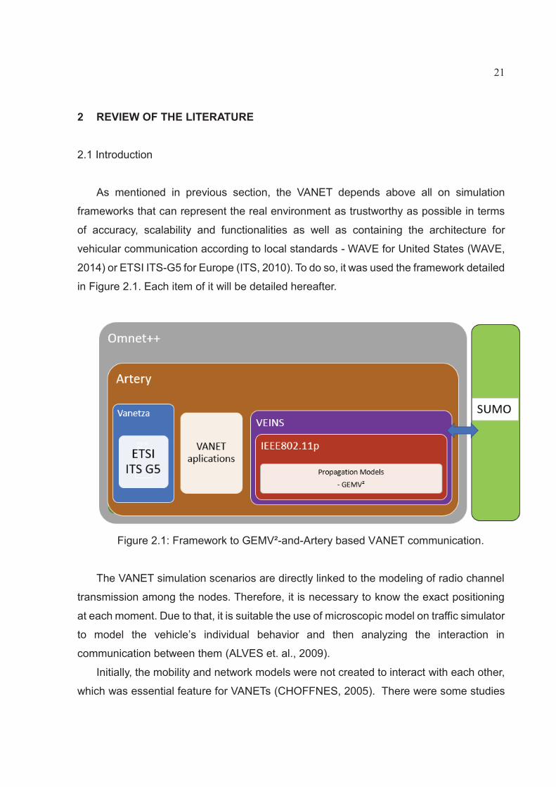
As mentioned in previous section, the VANET depends above all on simulation

frameworks that can represent the real environment as trustworthy as possible in terms

of accuracy, scalability and functionalities as well as containing the architecture for

vehicular communication according to local standards - WAVE for United States (WAVE,

2014) or ETSI ITS-G5 for Europe (ITS, 2010). To do so, it was used the framework detailed

in Figure 2.1. Each item of it will be detailed hereafter.

Figure 2.1: Framework to GEMV²-and-Artery based VANET communication.

The VANET simulation scenarios are directly linked to the modeling of radio channel

transmission among the nodes. Therefore, it is necessary to know the exact positioning

at each moment. Due to that, it is suitable the use of microscopic model on traffic simulator

to model the vehicle’s individual behavior and then analyzing the interaction in

communication between them (ALVES et. al., 2009).

Initially, the mobility and network models were not created to interact with each other,

which was essential feature for VANETs (CHOFFNES, 2005). There were some studies

22

in scientific community to develop specific mobility models for vehicular network

considering aspects like simulation time, and complexity (KOLLER et al., 2012)

(VIRIYASITAVAT et al., 2015).

2.2 Traffic Simulator - SUMO

The development of traffic simulator started for traffic engineering through the

modeling of the highways’ critics points and the urban intersections. The models were

initially created to be analyzed by construction engineers and therefore, they were not

meant for networks simulators. A significant characteristic to develop traffic simulators,

and might even be a limitation, is the complexity of calibration. The realism level on

transport planning is high and demands a large number of parameters, which have a

determined influence on the answer. On the other hand, the vehicular communications

networks developers do not demand high complexity, they only need the mobility path

adapted to their needs.

Many simulators also have commercial license, which may result in a high financial

investment in project. That is why, a large part of scientific community has started to work

in open source simulators development.

The Simulation of Urban Mobility (SUMO) tool (KRAJZEWICK et al., 2012), allows a

traffic simulation for large roads networks, and it is especially attractive for the vehicular

study, since it is a highly portable and open-source software. SUMO includes both a

console to insert the corresponding commands for the simulations executions as well as

a graphic interface to visualize or interact with the traffic simulation output as shown in

Figure 2.2.

The programming platform has been developed on C++ and the code finds itself in

continuous development by German Aerospace Center Transport System (SUMO, 2015).

23

Figure 2.2: SUMO’s Graphic interface.

The generation of the constants like routes, roads and the intersection distribution,

can be elaborated manually to the users’ needs, or it can be used real data. To import the

geographic data several sources can be used like the VISSIM, the GIS ArcView or the

OpenStreetMap (OSM) that are respectively a tool for traffic jam model, a geographic

information system and free editable maps; Each one generates a file with different

extension that can be imported to SUMO. These tools can be used in definition of topology,

thereby configuring the scenario for performance evaluation.

The software can also generate output paths that might be inserted directly to some

networks simulators like Omnet++, detailed in following section. On the other hand, there

are different methods allowed in order to create traffic in SUMO: either it can create itself

a completely random or manual origin-destiny route or it creates an optimal path through

of some available algorithms like the Bellman-Ford (CORMEN et al., 2007).

The SUMO also allows to configure the models of macro and micro mobility. The

macroscopic model describes large amounts of interest like a vehicular density and

average speed. In this type of model, the important issue is the behavior of a sector or

area and not of each individual vehicle. That is why, the simulation space is divided in

sections, thereby decreasing the necessary computational resources in a more detailed

24

simulation. The microscopic model simulates the movement of each existing vehicle on

scenario of the simulation, thus the simulator considers the motor features of each

vehicles as well as the behavior of each driver. Due to high level of detailing for this model,

the computational resources amount is high as well.

To detail the human micro-behavior in the vehicle is necessary to specify the car-

following model (NAGEL et. al., 1992). This model allows describing driver’s different

behavior, for instance, it can determine the decreasing of velocity at the moment in which

the driver is near of a change in vehicle direction. Another situation would be the driver

decides to change lanes or not during his path, what would be subject the interactions

with other vehicles or with its surroundings like the traffic lights or traffic jam. All this would

produce different reactions, like passivity and aggressiveness, that are also implemented

in model. The operation of this mechanism is intuitive and mainly consists in adapting the

vehicle mobility as a series of rules to maximize the vehicle speed, but always trying to

avoid a traffic accident.

Furthermore, some parameters allow approximating the SUMO’s simulation to the

reality, like for example, when the driver will decide to change of lane and overtake another

vehicle. Due to which, the flexibility of configuration and a good interconnection with the

network simulators, that the SUMO is rather requested for vehicular networks.

2.3 Network Simulator – Omnet++

Omnet++ is a modular, object oriented and discrete event simulator based on C++

(VARGA et al., 38). The operational model consists in hierarchical modules that

communicate themselves each other through messages. Highlighting its free-source code,

there is an effort from user community to develop both the simulation interface as well as

the libraries and the simulations modules (like the IpV6, TCP, MANET, etc.). The program

has two execution interfaces, one of them is a graphic environmental and another one is

via console. The visual interface, shown in Figure 2.3, is a mainly didactic tool where can

be visualized the packets interactions at each layer and that also enables the code

debugging. The simulator can be executed in Windows, but it was developed in Linux-

Unix.

25

The simulator uses the NED programming language as tool to model the topology of

the network and the nodes. Thus, a router or an access point will be deployed by different

modules, ensuring a liberty to modify each module with almost total independence.

Therefore, a model is built by hierarchic modules. Each module can contain complex

framework of data with its own personalized parameters.

Figure 2.3: OMNET++’s graphic interface.

Basically, the NED language can define simple, complex and network modules. The

last one contains the components and specifications of a communication network as well

as the number of nodes or the physical distribution of base station. To facilitate the creation

of the code, especially for network module, it can work itself with the graphical editor

(GNED). This editor allows creating, programming and configuring the network elements

without using the language directly, it is only necessary to perform a drawing with elements’

representative icons and it is the GNED that will generate the code lines automatically

which will be available for the users.

The events occur inside of simple modules, which are implemented in C++ using the

Omnet-classes library. Inside these modules, the algorithms and properties of complex

modules start or finalize in each state change. Once all modules have been elaborated

26

and configured, it will be necessary the file creation ‘’.ini’’ that will allow the start of

simulation. In this file is described both the own parameters of the simulation as well as

the number of interactions, the duration time or the values of the attributes of the simple

modules or the entire topology of the network model.

2.4 VEINS

The Vehicles in Networks Simulations (VEINS) tool (SOMMER, 2016) is a framework

for vehicular network simulation. It facilitates the bidirectional interaction among the

SUMO and Omnet++ simulators, that are based on events, what it means that the

elements movements on the simulation will be restricted in periodic-time intervals. When

an execution-time synchronization point is reached between both simulators, the

interconnection is completed and thus, both can be connected bidirectionally. A

communication interface called TraCi, which is implemented over a socket (TCP), allows

that the simulation is sequential and fed back in both simulators.

The TraCi’s role is to provide a communication medium between the Omnet++ and

SUMO. The architecture for that is the client-server, where the client (Omnet++) will send

commands to server (SUMO) to control the simulations state. The basic operation mode

consists of storing in a row all commands that get among the simulation periods to after

being forwarded and executed, thereby ensuring the synchronous execution. At a unit of

determined time, the Omnet++ will send the stored commands to the SUMO, so that it

completes the simulation with the information that it is being executed. Once this state is

over, SUMO will send as answer a series of commands and the location of all vehicles.

When the network simulator receives these information, it will be able to establish the

nodes movement. After that, it will execute the next step of simulation, where the nodes

will react it depending on the new mobility condition, what it will generate new commands

that will once again be sent to SUMO, thus the process is repeated until completing the

simulation.

Finally, Veins makes use of INET framework, that is a model packet for communication

networks to be used on Omnet++. INET is considered the standard protocols models

libraries, containing models for the internet stack (TCP, UDP, IPv4, etc.), wireless and

27

wired link layer and physical protocols (PPP, IEEE 802.11p, etc.) as well as MANET

mobility protocols. However, some VANET applications and features contained in ETSI

ITS-G5 are not supported on VEINS.

2.5 ETSI ITS G5

An intelligent transportation system (ITS) is an advanced application which, without

incorporating intelligence as such, targets to proportion innovative services regarding

different modes of transport and traffic management and enable users to be better

informed and make safer, smarter and more coordinated use of transport networks.

ETSI ITS-G5 is a European protocol stack to enable ITS applications. It was defined

in 2004, and has undergone a thorough standardization process. This included extensive

field testing (starting in 2008 with the German simTD field tests with 400 vehicles

(KOLLER et al., 2012)) and multi-vendor interoperability testing (ETSI plugtests, 2011).

The ETSI ITS-G5 protocol set is detailed in Figure 2.4, which also serves as base for

Artery’s architecture that will be introduced on following section.

The network and transport protocols are based on GeoNetworking protocol (ITS,

2013), which is responsible for routing VANET packets, and Basic Transport Protocol

(BTP) (ITS, 2013). Both are used to find a path in the network. The Facilities layer provides

application support and connects the protocol stack to the vehicle-internal bus systems.

The cross-functional Management and Security layers are intended to maintain system-

wide parameters and protect V2X communication from external attacks respectively.

28

Figure 2.4: ETSI ITS-G5 reference architecture (ITS,2010).

The IEEE 802.11p standard, which specifies the physical and MAC layers (access

layer) for vehicular applications, has been used both for the WAVE and ETSI-ITS G5

architecture. For upper layers, the ETSI-ITS G5 has developed their own protocols

(MAURER et. al., 2004). Those vehicular standards and their respective layers are

highlighted in Figure 2.5.

Figure 2.5: European VANET’s communication architecture.

2.6 Vanetza

Vanetza (RIEBL, 2015) is an open source standalone implementation of some major

ITS-G5 components (ITS, 2013). The main idea behind of Vanetza was the simulation of

hundreds to thousand vehicles interconnected by using the ETSI ITS-G5 implementation,

first operating together with VEINS and then with Artery, detailed in the next section

(RIEBL, 2015). The ITS-G5’s main components implemented by Vanetza are congestion

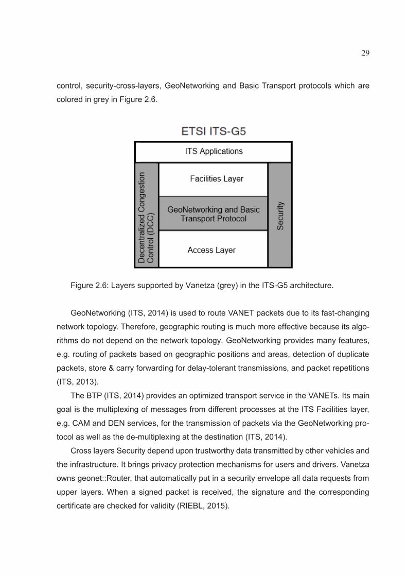
29

control, security-cross-layers, GeoNetworking and Basic Transport protocols which are

colored in grey in Figure 2.6.

Figure 2.6: Layers supported by Vanetza (grey) in the ITS-G5 architecture.

GeoNetworking (ITS, 2014) is used to route VANET packets due to its fast-changing

network topology. Therefore, geographic routing is much more effective because its algo-

rithms do not depend on the network topology. GeoNetworking provides many features,

e.g. routing of packets based on geographic positions and areas, detection of duplicate

packets, store & carry forwarding for delay-tolerant transmissions, and packet repetitions

(ITS, 2013).

The BTP (ITS, 2014) provides an optimized transport service in the VANETs. Its main

goal is the multiplexing of messages from different processes at the ITS Facilities layer,

e.g. CAM and DEN services, for the transmission of packets via the GeoNetworking pro-

tocol as well as the de-multiplexing at the destination (ITS, 2014).

Cross layers Security depend upon trustworthy data transmitted by other vehicles and

the infrastructure. It brings privacy protection mechanisms for users and drivers. Vanetza

owns geonet::Router, that automatically put in a security envelope all data requests from

upper layers. When a signed packet is received, the signature and the corresponding

certificate are checked for validity (RIEBL, 2015).

30

Cross layer Decentralized Congestion Control (DCC) provides stability in the ad-hoc

network by providing resource management when there are a high number of C-ITS mes-

sages in order to avoid interference and degradation of C-ITS applications (ITS, 2013). DCC_acc acts as gatekeeper above the access layer, i.e. it enforces minimum time intervals between outgoing packets of each priority class. DCC_fac adapts the message generation rate, so no packets are delayed or dropped by DCC_acc. DCC_net – whose implementation is currently work in progress – is supposed to share Channel Busy Ratio (CBR) measurements among neighboring nodes (RIEBL, page 3, 2015).

2.7 Artery

Artery is a simulation framework that allows an interface to application layer for VANET

applications. If referred to ETSI ITS-G5 reference architecture depicted in Figure 2.4, it

would represent the facilities and application layers. Artery allows that application layer

registers various applications by creating Omnet++ modules (RIEBL, 2015).

Artery is an extension of Veins framework since it adds to this one the European

VANET communication features. Furthermore, it also comprehends INET framework as

an option to wireless link and PHY layers protocols and supports LTE cellular

communication (ITS, 2013) as well as sensors attached to vehicles for environmental

perception [ITS, 2014], (XU and SAADAWI, 2001).

31

Figure 2.7: Structure of a vehicle node in the Artery framework. Adapted from

(OBERMAIER, 2017).

A vehicular node based on Artery framework is basically composed of three modules

as detailed in Figure 2.7. The Network Interface Card (NIC) which is composed of access

module (PHY and MAC layers) and a part of Vanetza (DCC_acc) module, the application

module and the mobility module.

The access module simulates the physical transmission media among vehicles nodes.

Therefore, it checks whether a frame can be physically delivered at the addressed receiver

or not by applying radio propagation models. If a frame is not thrown away, it is forwarded

to the MAC layer, which performs actions according to the IEEE80211.p protocol. This

includes activities related to channel management such as messages queueing according

to their priority. In addition, the NIC module contains the DCC_acc, which is responsible

for controlling time intervals between outgoing packets.

32

The application module contains the services and facilities/middleware which are the

main Artery’s modules and the routing layers of the ETSI ITS G5 specification (GeoNet-

working, BTP and DCC) implemented by Vanetza. The ITS-G5 middleware is the Artery’s

major element, which acts like an information hub and routing provider to all services. The

services are the applications themselves like standardized messages (ITS, 2014) such as

the DENM and CAM as well as ADAS functionality. Those services can either send or

request messages through Artery’s middleware. Every service registered to the applica-

tion layer is updated on each simulation step performed by Omnet++ (RIEBL, 2015). The

routing layers are responsible for handling packets from or to middleware regarding traffic

class, transport type, destination port, etc, as specified by BTP and GeoNetworking pro-

tocols. Each vehicle provides its own router, which is responsible for addressing other

vehicles and geographic areas (RIEBL, 2015).

Still part of the application module, Artery provides a facility member so that the ser-

vices can interact with the VEINS’ mobility module to retrieve data related to the move-

ment of a vehicle, for example the speed and the position of a vehicle.

2.7.1 Message Flow - Receiving a message

The incoming message flow inside a vehicle node is marked by red arrows in Figure

2.7. If a message is received by the physical layer, a defined, so-called decider calculates

whether a frame can be received without error. If no error is detected, and therefore the

frame is not thrown away, it will be handled up to the MAC layer. After passing the MAC

layer the message will be processed by the router located in the application module of the

vehicle node. The router is responsible of deciding if a packet should be processed by its

own vehicles application layer, or if the packet must be forwarded to another node. If the

router is a valid receiver of the packet, the packet is passed to an application according

to its port number (OBERMAIER, page 23-24, 2017).

33

2.7.2 Message Flow - Sending a message

If a service triggers the sending of a message, the data Packet Data Unit (PDU) gen-

erated by this service is passed into the router. Like in a usual wired network, the router

is responsible for determining the next hop of a packet. According to the used routing

mode a specific next hop or various receivers are addressed. After adding of the routing

information to the packet, it is passed down to the MAC layer. As soon as the sending

request is received by the MAC layer, it will be queued into the output queue according to

the priority of the packet. In case of a higher number of message, the Distributed Conges-

tion Control (DCC) algorithms can drop the packets in order to provide stability (OBER-

MAIER, page 23-24, 2017).

2.7.3 Data Flow

The data flow is specified by green arrows in Figure 2.7. The information according to

the last simulation step is received over the TraCI connection (SOMMER, 2016). This

information is stored and processed inside the facilities submodule. This allows to calcu-

late data, requiring more than one simulation step to obtain. For example, this can be the

curvature or the yaw rate. All applications and services registered in the application mod-

ule can access information from the facilities module when needed. For example, a CA

service needs to know, among others, the position and the speed of its vehicle to generate

CA messages with appropriate data (ITS, 2014) (OBERMAIER, page 23-24, 2017).

2.8 IEEE802.11p Standard

The physical and medium access control layers of the two main protocol stacks for

vehicular communications systems rely on the IEEE802.11p standard.

In comparison with the typical Wi-Fi operation (802.11 Part 11, 2012), the American

Society for Testing and Material (ASTM) has done a number of modifications in order to

enhance the behavior of the communicating nodes under such dynamic scenarios. For

instance, the channel bandwidth is reduced from 20 MHz to 10 MHz, in order to mitigate

34

the effects of multi-path propagation and Doppler shift. As a consequence, the data rate

is half of what can be obtained with standard Wi-Fi, i.e., from 3 Mbit/s to 27 Mbit/s instead

of 6–54 Mbit/s (ITS, 2011).

In order to guarantee that vehicular communications do not suffer from any type of

interference from unlicensed devices, the Federal Communications Commission (FCC) in

the United States and the European Conference of Postal and Telecommunications

Administrations (CEPT) in Europe, allocated a dedicated spectrum band at 5.9 GHz so-

called Dedicated Short-Range Communication (DSRC). The frequency range, located in

DSRC band, covers from 5.86 GHz till 5.92 GHz. So, 7 channels of 10 MHz are used,

where one of them is for control, two of them are for future use and the other ones are

used for different services as shown in Figure 2.8. Moreover, it is mandatory in Europe to

have two radios in each vehicular communication platform, in order to guarantee at least

one radio always tuned in the dedicated safety channel (ITS, 2011).

Figure 2.8: Spectrum allocation for vehicular communication (CAMPOLO and

MOLINARO, 2013).

The radio-propagation model provides information about limitations on the wireless

communications systems performance.

The radio-propagation channels have one of the most complex mathematical models

in a wireless communication system, according to the state-of-the-art study presented in

(VIRIYASITAVAT et. al., 2015), which compares the main radio propagation models

regarding the: spatial and temporal dependency; extensibility to different environments;

applicability; scalability; temporal variance and non-stationary; antenna configuration; The

35

GEMV² model fulfilled all properties presented above, except the antenna configuration.

It is presented as an efficient model for realistic large-scale simulation with thousands of

communicating vehicles in various vehicular environments (urban, rural, highway). In

addition, it allows the analysis of networking related metrics, such as packet delivery rates,

effective transmission range, and neighborhood size (VIRIYASITAVAT et. al., 2015).

One guideline for choosing a suitable radio propagation model is presented in (VIRI-

YASITAVAT et. al., 2015). The type of application (network topology statistics, safety-crit-

ical applications, system-wide performance analysis) and availability of the required data

(either geographical or measurements, system-wide performance analysis).

2.8.1 GEMV²

The Geometry-based Efficient Propagation Model for V2V communication (GEMV²)

(BOBAN, 2014) is a wireless propagation channel model specifically for vehicular envi-

ronment with the goal of predicting the propagation losses in vehicle-to-vehicle communi-

cation. It incorporates the following propagation: 1) diffraction, 2) reflection, and 3) scat-

tering.

Diffraction is the phenomenon liable for explaining the existence of electromagnetic

fields at non-visibility regions caused by obstacles, known as shadowing regions. Such

obstacles encountered by the electromagnetic waves can be natural or artificial in the

urban, suburban or rural environment. Mathematically, the calculation for evaluating the

attenuation by diffraction is complex, making itself necessary the use of the mathematical

formulation based on geometric, it called Geometric Theory of Diffraction (GTD) and its

extension for the Uniform Theory of Diffraction (UTD) (SILVA, 2004).

Reflection is the phenomenon that occurs when the electromagnetic wave hit on a

surface that separates two environments, with dimensions much larger than the

wavelength that it propagates. Part of the energy from this wave is reflected, and the other

part is transmitted, penetrating the other medium. The corresponding parcels to the

transmitted and reflected energies are calculated by the transmission and reflection

coefficients respectively. The transmission and reflection coefficients depend on electrical

and magnetic permeability and medium conductivity in which the electromagnetic wave

36

propagates itself. Moreover, the frequency and the incidence angle on the medium in

question also bias the respectively coefficient. For the analysis of this phenomenon is

used the theory of geometric-optics rays.

The scattering occurs when the propagation medium is constituted with small dimen-

sions objects (rough surfaces, small objects), in relation to the wavelength (PEREIRA,

2007).

Besides that, GEMV² uses outlines of vehicles, buildings, and foliage to distinguish

into three different types of links: line of sight (LOS), non-LOS (NLOS) due to vehicles,

and NLOS due to static objects as seen in Figure 2.9. Such distinctions are made through

of an analyze of first Fresnel ellipsoid. Whether one or more object between the commu-

nication pair intersect the ellipsoid corresponding to 40% of the radius of the first Fresnel

zone, the channel is considered NLOS.

For each link, GEMV² calculates the large-scale signal variations deterministically,

whereas the small-scale signal variations are calculated stochastically based on the num-

ber and size of surrounding objects.

Figure 2.9: GEMV² link types.

37

In order to check which objects influence both large-scale and small-scale signal var-

iation, an analyze is done through ellipse-bound area. The transmitter and receiver cars

are placed on ellipse’s focus whose major axis is equal to the link communication range

(obtained by field measurements – 500, 400 and 300 meters for LOS, NLOSv and NLOSb

respectively), thereby generating the search area as shown in Figure 2.10. The vehicles

are colored of black and the buildings of light-brown.

Figure 2.10: GEMV²’s Ellipse-bound area. Adapted from (BOBAN, 2014).

The modeling of the large-scale signal variations is made according to the link types:

Upon LOS link type, two-ray reflection model.

The two-ray ground reflection model, shown in Figure 2.11, is based on geometric

optics. It considers a direct and reflected path on ground between the transmitter and the

receiver. This model was reasonably considered accurate to predict the signal strength in

large scale (RAPPAPORT, 2000).

Figure 2.11: Two ray ground reflection model

38

The concept of calculation of signal electric field strength, by applying two-ray method,

is given by (SIZENANDO, 2006):

E(d,t)= Eodod

cos(wc(t- dc)) (1)

where E0 is the electric field strength in free-space (V/m) (RAPPAPORT, 2000), d0 is the

arbitrary referential distance from transmitter (m), often 1m, (E0d0)d

represents the electric

field module (E(d, t)) at a distance d (m) from transmitter, t represents the time (s), ωc is

the carrier frequency (rad/s) and c is the light speed (m/s).

The expressions of electric field strength from the direct and reflected ray are

respectively:

ELOS(dLOS,t)= Eodod'

cos(wc(t- dLOSc

)) (2)

Er(di+r,t)=Γ Eodod''

cos(wc(t- (di+dr)c

)) (3)

Where Γ is the reflection coefficient for the soil, which was taken empirically (Γ=-1 for the

case where there is perfect reflection). The total electric field strength ETOT, at receiver,

will be the vector sum of the direct and reflected component.

|ETOT|=|ELOS|+|Er| (4)

Using the geometric optics from the image method illustrated in Figure 2.12, and

evolving the expression of total field strength as well as the simplifications from the angular

considerations, it is obtained:

39

Figure 2.12: Mirror method simplification.

ETOT(d)= 2EoDod

2πhthrλd

≈ kd2 (5)

where, k is a constant related to: E0; transmitter and receiver’s antennas height; wave

length λ (m).

Upon NLOS link type caused by vehicle (NLOSv) (BOBAN, 2011), a multiple knife-

edge model is used to calculate the losses due to the diffraction over both vehicles and

buildings. The multiple knife-edge is an extension of the single knife-edge whenever there

is more than one hurdle.

In order to estimate the losses caused by an obstacle, the single knife-edge model

idealizes that the obstacle have either a knife-edge form of negligible thickness or a thick

smooth form with a well-defined radius of curvature at the top. To do so, all the geometrical

parameters are combined together in a single dimensionless parameter denoted by v and

the wavelength must be fairly small in relation to the size of the obstacles (f > 30 MHz)

(ITU-R, 2007).

v=h 2λ( 1

d1+ 1

d2)= h 2

λd1d2d

(6)

Where h is the height of the top of the obstacle above the straight line joining the two

ends of the path. If the height is below this line, h is negative. d1 and d2 are distances of

40

the two ends of the path from the top of the obstacle respectively and d is the length of

the path.

Through approximation of Fresnel-Kirchhoff loss given by ITU-R P.526, equation 31,

for v greater than -0,78 the losses are in dB (ITU-R, 2007):

J(v)=6.9+20log√((v-0.1)^2+1)+v-0.1 (7)

However, if there are more than one hurdle, some strategies are used in order to

classify the hurdles into primary and secondary according to their impact over the line of

sight and afterwards, applying the single knife-edge model among the primary iteratively

and then among secondary. In addition, a correction term is needed to consider for

spreading loss due to diffraction over successive obstacles. Exemplifying the idea above,

in Figure 2.13 is shown some obstacles’ profiles between the transmitter (T) and receiver

(R), on which are identified the primary (P) and secondary (S) obstacles. These

procedures are contained in ITU-R P.526.

Figure 2.13: Multiple obstacles (ITU-R, 2007).

According to ITU-R P.526, the total diffraction loss, in dB, may be written:

Ld= LPNp=1 + LS

Ms=1 -20 log CN (8)

P1 P2

41

where: N and M is the number of primary and secondary respectively, LP is the diffraction

loss for the section of the path between primary hurdles, LS is the diffraction loss for the

section of the path between secondary hurdles. For instance, the calculus for considering

the first primary (LP=1) would be to apply equation 6 and 7 over T-P1-P2 (Tx-Obstacle-Rx).

CN = (Pa / Pb)0.5 (9)

is the correction factor, which in turn, depends on the distances between the hurdle

and the transmitter (s1) and receive (s2) according to the equations 10 and 11 (ITU-R,

2007).

j

M

si

N

pa ssssP )()( 2

112

11 (10)

ii

N

iNb ssssP )()()()( 21

1211 (11)

Upon NLOSv, it is considered the diffraction loss from both sides of the vehicles and

from vehicle’s roof.

Last but not least, upon NLOS link type caused by buildings (NLOSb), there are two

ways for modeling: The simplest way is to apply the log-distance path loss model (RAP-

PAPORT, 2000) which considers that the received mean power decreases logarithmically

in relation to distance from the transmitter. This model is featured by equation 12:

PL(d)=PL(do)+10nlog( ddo

) (12)

Where n represents the path loss exponent which was obtained empirically, PL(do) is the

pathloss considering the free-space model (RAPPAPORT, 2000) at a reference distance

do, and d is the separation between transmitter and receiver. This model does not depend

on neither frequency nor gains from transmitter and receiver antennas.

42

The hardest and second method considers the diffraction and reflection effects but

only to single-interaction (single-bounce) rays. One exception would be the multiple dif-

fraction due to vehicles, however if there is a NLOS link type due to both vehicle and

building, the GEMV² only considers the NLOSb, since the attenuation is much bigger in

NLOSb than in NLOSv.

The diffraction loss is similar to diffraction over the vehicles in case of NLOSb link type,

the multiple knife-edge is used, however, over buildings are only considered for the hori-

zontal plane, since the buildings are too tall for diffraction over the rooftops.

As for reflection effect, over vehicles’ roof for this sort of link is not regarded due to an

effort to keep the GEMV²’s low computational complexity. Besides that, it is worth remind-

ing that the vehicles’ sides will only be a reflector potential, if the vehicle has height taller

than both communicating vehicles’ antennas. Regarding the reflection off buildings always

is possible, once they are significantly taller than any vehicles.

The small-scale fading is caused by multipath and shadowing. The multipath effect is

characterized as being the composition of the transmitted signal’s original versions that

travels in different ways. The shadowing manifests itself by signal level fluctuation with the

distance caused by surrounding obstacles (SIZENANDO, 2006). It is usually modeled by

a random variable with a certain probability distribution. On GEMV² was adjusted the

collected data in field tests with the zero-mean normal distribution N (0, σ) (GRINSTEAD

and SNELL, 1998). The variation due to the different link types is reached by simple

modeling of the standard deviation, which is proportional to the number of vehicles (NVi)

and the area of buildings and foliage (ASi) around the communicating pair by ellipse-

bound area. The equation for the standard deviation according to (BOBAN, 2014)

σ=σmin+ σmax-σmin2

( NViNVmax

+ ASiASmax

) (13)

where NVmax and ASmax are the maximum number of vehicles and building and foliage

from historical data and geographical database respectively. The minimum and maximum

values of the small-scale signal deviation obtained empirically for each link type by

(BOBAN, 2014) are shown in Table 2.1.

43

Table 2.1: Minimum and Maximum values of the small-scale signal deviation

(BOBAN, 2014)

Link Type

LOS 3.3 dB 5.2 dB

NLOSb 3.8 dB 5.3 dB

NLOSv 0 dB (refl&diffr) /4.1 dB

(MANGEL et al., 2011)

6.8 dB

44

3 IMPLEMENTATION AND VALIDATION

3.1 Methodology of Implementation

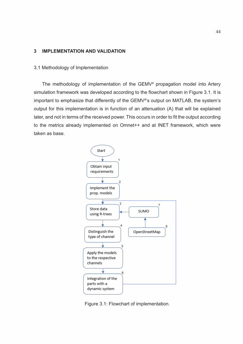
The methodology of implementation of the GEMV² propagation model into Artery

simulation framework was developed according to the flowchart shown in Figure 3.1. It is

important to emphasize that differently of the GEMV²’s output on MATLAB, the system’s

output for this implementation is in function of an attenuation (A) that will be explained

later, and not in terms of the received power. This occurs in order to fit the output according

to the metrics already implemented on Omnet++ and at INET framework, which were

taken as base.

Figure 3.1: Flowchart of implementation.

45

In order to implement the flowchart above, an UML diagram with flowchart’s all

requirements has been created as seen in Figure 3.2. The input parameters (transmission

power, frequency, antenna gains and communicating pair) and the map based traffic

model are not part of the module. The input parameters are adjusted at INET module,

except the communicating pair, that is set according to the application layer demand

(Artery’s service). The traffic model comes from SUMO and will be mentioned later.

The PathLoss is the central class. It mainly depends on the Link Classifier class once

it will say which type of channel is the current communication. It makes use of the Small

Scale Variation, NLOSb, NLOSv and LOS classes to get information about the small and

large-scale values. Finally, it combines properly the values and return the final value. The

returned value refers to the attenuation (A) as already was mentioned above. The

correlation between the pathloss (PL) and this attenuation is demonstrated in equation 15.

Pr =PtGtGrA (14)

The equation 14 shows the way that the INET module computes the received power.

The transmitter power (Pt) and the antenna gains (G) are known in advance and therefore,

our system’s output must be A.

When compared the equation 14 to the traditional received power equation

(RAPPAPORT, 1996), we get the relationship between the attenuation (A) and the path

loss (PL) as seen in equation 14.

A= 1PL

(15)

The Vehicle Index and Obstacle Index are classes responsible for collecting, storing

and handling vehicle and obstacle`s data. Basically, they obtain the vehicle and obstacle´s

data like outline´s position, area value and centroid position from SUMO in real time

through Traci interface. After that, the data are stored in R-tree structures in order to

accelerate searching for objects in space. It was used the rstar as node splitting algorithm,

once it has demonstrated a good querying and building performance. Last but not least,

there are member functions that are responsible for mounting the communication ellipse

46

as already was explained its functionality above and for verifying whether there is anything

intercepting the line of sight between two points.

Figure 3.2: GEMV²’s UML diagram on Omnet++.

The Link Classifier is a class designed for classifying which channel is present in the

given time frame. Basically, it just uses the member function created in the Obstacle Index

47

and Vehicle Obstacle classes that checks intercepting objects between two points, so that

it is able to classify the communication channel in: LOS, NLOSv and NLOSb.

The remaining classes (LOS, NLOSv, NLOSb, Small Scale Variation) implement the

radio propagation model itself. To do so, it uses some objects from Obstacle Index and

Vehicle Obstacle classes in order to get information about the variables demanded on the

models.

Doing a comparison between the GEMV² source code on MATLAB and on Omnet++,

which has been implemented on this dissertation, observes an optimization on the source

code of more than 50 functions on MATLAB to only 8 classes on omnet++, without

mentioning the lines of code. Part of it, it is related to the use of object oriented

programming c++ itself and also the use of some boost libraries.

3.2 Methodology of Validation

In order to validate the implementation, some simple tests have been created some

simple tests scenarios on SUMO manually for each link type, so that it was able to analyze

the key variables of the applied models for each link type. Afterwards, it has been done a

comparison between the values obtained from Sumo and MATLAB over those created

scenarios. An extern manipulation in the result from omnet++ was necessary to become

the values comparable, since omnet++ returns the generic pathloss and the MATLAB

returns received power at receiver, which was standardized as standard comparison unit,

in dB. Furthermore, these comparisons were done only in the obtained values referring to

large-scale signal, once the small-scale signal values varying according to a normal

distribution. The validation of the small-scale signal will be dealt later in this same section.

The common simulation parameters for all test scenario is depicted in Table 3.1.

Table 3.1: Simulation parameters.

Operating Frequency 5.89 GHz

Transmit Power 23.0103 dBm

Antenna Gain 0 dBi

Antenna Polarization Vertical

48

3.2.1 LOS Link Type

Scenario 1

The first test scenario for LOS channel (Figure 3.3) simulates two vehicles leaving

from same point with six seconds delay each other and moving in same way at almost

constant speed. Despite of the fact that the acceleration had set to zero, there was a small

speed variation throughout the path. The antenna position of both cars is placed in the

middle of the car and there is no static object and any other car on this scenario, featuring

a LOS channel. Other specifications are found in Table 3.2.

Figure 3.3: First test-scenario setup for the LOS channel on SUMO.

Table 3.2: Specifications for the first LOS test-scenario.

Specification Value (I.S.) Number of vehicles 2

Vehicle’s way Same

Width 2

Length 4

Total height (vehicle+antenna) 1.5

Antenna position Middle

Tx Rx

49

Acceleration ~0

Depart speed 10

Lanes per way 1

The goal is to maintain a constant scenario without external interference, where

results almost constant are expected. The “almost constant” refers to the speed variation

(positive and negative) that was not possible to keep it constant on Sumo. In Figure 3.4 is

shown the speed (m/s²) in relation to the timestep (s) over the transmitter (orange line)

and receiver (blue one). For both vehicles has obtained a mean speed value at 10,35 m/s²

with a variation of +/- 0,6 m/s².

Figure 3.4: Speed variation.

50

Figure 3.5: Received power measurement for the first LOS test-scenario.

The Figure 3.5 shows the received power over the timestep in seconds. It was

obtained a mean value at -58.9 dBm with a variation of roughly +/- 0,3 dB that comes from

small acceleration variation. In addition, it is observed a good match between data from

MATLAB and omnet++ using GEMV² model, thereby validating the model over this first

scenario.

Scenario 2

The second test scenario for LOS channel differs from the first one in the following

items: the vehicles are moving in opposite direction (Figure 3.6) with an initial distance of

1000 meters each other; They have a positive acceleration of an initial speed at 1m/s.

Moreover, it was varied the size of antenna. The entire scenario specification is found in

Table 3.3.

Figure 3.6: Second test-scenario setup for the LOS channel on SUMO.

51

Table 3.3: Specifications for the second LOS test-scenario.

Specification Value (I.S.) Scenario 1 Scenario 2 Scenario 3

Number of vehicles 2

Vehicle’s way Opposite

Width 2

Length 4

Total height (vehicle+antenna) 1,5 4 1

Antenna position Middle of vehicle

Acceleration 2,6

Depart speed 1

Lanes per way 1

These changes aim to change the main two variables of the Two Ray Ground Model

– distance between antennas and set size composed by antenna and vehicle height.

In Figure 3.7 is demonstrated the variation of received power in relation to the

timestep in each setup created, where the orange line represents the vehicle and antenna

height based setup with 1,5 meters, the grey one with 1,0 meter and the blue one with 4,0

meters. Correctly, when the cars get closer each other, the received power increases

proportionally and as the cars move away from each other, the received power returns

back to lower levels with the same proportionally. Another interesting point is in relation to

the system’s performance to each setup. The setup with antenna and vehicle’s height

equal 1,5 meters had the best performance than other ones. At timestep 41, the cars are

nearest each other, the difference is about -20 dB to the third setup.

52

Figure 3.7: Received power measurement for the second LOS test-scenario.

The match of data from Omnet++ and MATLAB were fulfilled for this scenario too, as

it can be seen in Figure 3.8, which represents the percentage value of difference between

the Omnet++ and MATLAB’s data in relation to the timestep over the 03 setups. At

timestep 41s had the largest difference to both setups, however, it is extremely derisory

and might be linked a small position variation.

Figure 3.7: Divergences on the received power measurements for the second LOS test-

scenario.

Scenario 3

The third scenario keeps the same configuration of the second scenario, except for

the fact that the antenna and vehicle’s height were fixed at 1,5 meters. The idea behind

this scenario is to change the antenna position over the car in order to check the impact

53

thereof. It was possible, because was created an external module on omnet++ to

reallocate the antenna position over the vehicle which prior was at front of the car (come

from SUMO´s setting).

On MATLAB´s setting the antenna position has been placed at middle of the car and

would demand too much effort to change it all. Because of that, it was not possible to

compare the results of both implementations for this scenario. The entire scenario

specification is found in Table 3.4.

Table 3.4: Specifications for the third LOS test-scenario.

Specification Value (I.S.) Scenario 1 Scenario 2 Scenario 3

Number of vehicles 2

Vehicle’s way opposite

Width 2

Length 4

Total height (vehicle+antenna) 1,5

Antenna position Rear Middle Front

Acceleration 2.6

Depart speed 1

Lanes per way 1

In Figure 3.9 is represented the received power values according to each

configuration of the antenna position. The blue, orange and grey lines represents the

antenna position at middle, rear and front on the vehicle respectively. According to the

measurements shown in Figure 3.9, there is no expressive variation regarding the

antenna position over the car.

54

Figure 3.9: Received power measurement for the third LOS test-scenario.

3.2.2 NLOSv Link Type

Scenario 1

The first test scenario for NLOSv channel considers the same aspect of first LOS test

scenario, with one more vehicle though (Figure 3.10). The third car is added in order to

obtain a car for intercepting the communicating pair, featuring a NLOSv channel. The

antenna position of both cars is located in the middle of the car and there is no static

object. The full scenario specification is found in Table 3.5.

Figure 3.10: First test-scenario for the NLOSv channel on SUMO.

Rx Tx

55

Table 3.5: Specifications for the first NLOSv test-scenario.

Specification Value (I.S.) Number of vehicles 3

Vehicle’s way Same

Width 2

Length 4

Total height (vehicle+antenna) 1.5

Antenna position Middle

Acceleration ~0

Depart speed 10

Lanes per way 1

The received power measurements in relation to the timestep and Tx and Rx’s indexes

for this scenario are presented in Figure 3.11. It was obtained a mean value at -60,81 dBm

with a variation about +/- 0,4 dB that comes from acceleration small variation (same from

Figure 3.4). Moreover, it also observes a good match between data from MATLAB and

omnet++, thereby validating the model over this first scenario.

Figure 3.11: Received power measurement for the first NLOSv test-scenario.

56

Scenario 2

In order to configure a more realist scenario and consider other important

variables for the knife-edge obstacle model like the number of vehicles that obstructs

the line of sight and hurdle’s penetration rate (obstructing vehicle’s height and width),

it has been taken the first NLOSv test-scenario and added more vehicles in both ways.

Besides that, the impact of the vehicles’ height variation was evaluated by varying

only the height of the communicating vehicles (Tx and Rx). The entire scenario

specification is found in Table 3.6.

Table 3.6: Specifications for the second NLOSv test-scenario.

Specification Value (I.S.) Scenario 1 Scenario 2 Scenario 3

Number of vehicles 8

Vehicle’s way both

Width 2

Length 4

Total height (vehicle+antenna) 1,5 4 1

Antenna position Middle

Acceleration 2.6

Depart speed 1

Lanes per way 2

The receiver power measurements according to the height variation are shown in

Figure 3.12. At higher level, the dark blue and green lines represent values referring to

vehicles with height at 1,5 and 4,0 meters respectively from Omnet. Similarly for the yellow

and green ones respectively, although the values are from MATLAB. At lower level, the

orange and light blue ones represent the setting with height at 1.0 meter from Omnet and

MATLAB respectively. It is noticed from those results a good match between data from

MATLAB and Omnet and also observed a worst performance when the height is set at

57

1,0m of about -5 dB. It might have happened by the fact that taller vehicles are more likely

to block reflection coming from building walls or other vehicles.

Figure 3.12: Received power measurements for the second NLOSv test-scenario.

Scenario 3

The third test-scenario for the NLOSv channel differs from the second one by

changing vehicles’ width instead of changing their height – another variable of the

penetration rate of the knife-edge model as mentioned above. The entire scenario

specification is found in Table 3.7.

Table 3.7: Specifications for the third NLOSv test-scenario.

Specification Value (I.S.) Scenario 1 Scenario 2 Scenario 3

Number of vehicles 8

Vehicle’s way both

Width 2 3 4

Length 4

Total height (vehicle+antenna) 1,5

Antenna position Middle

Acceleration 2.6

58

Depart speed 1

Lanes per way 2

Despite of these changes, in Figure 3.13 observes that did not occur any variation at

the received power by varying the cars’ width. Both scenarios have the same received

power and therefore, the GEMV² model is little influenced by the variation of the vehicle

width.

Figure 3.13: Received power measurements for the third NLOSv test-scenario on

Omnet.

3.2.3 NLOSb Link Type

Scenario 1

A scenario with an crossing was created on SUMO in order to feature a test scenario

for NLOSb channel. On that scenario was inserted two vehicles moving into this crossing

and then moving out from it but keeping straight. In addition, four types of outlines were

added as the static objects in attempt of creating different diffraction and reflection points

as shown in Figure 3.14. These different geometries interfere in reflection and diffraction

model’s parameters. The length of the roadways are 300 meters, so that the vehicles can

communicate themselves since their departures. The entire scenario specification is found

in Table 3.8.

59

Figure 3.14: First test-scenario for the NLOSb channel on SUMO.

Table 3.8: Specifications for the first NLOSb test-scenario.

Specification Value (I.S.) Number of vehicles 2

Vehicle’s way Mix

Width 2

Length 4

Total height (vehicle+antenna) 1.5

Antenna position Middle of vehicle

Acceleration 2,6

Depart speed 1

Lanes per way 1

Length of roadways 300

This scenario operates under two models: log-distance and reflection-and-diffraction

(geometric) models. The receiver power measurements obtained from these models are

shown in Figure 3.15. The blue and grey lines represent the log-distance and geometric

models respectively on MATLAB. The blue one is not visible on graph because is

completely under of the yellow one. On the other hand, the yellow and orange ones are

60

respectively on Omnet. There is noticeable a good fit between the data from MATLAB and

Omnet when operated over the log-distance model. However, the measurements

regarding the reflection and diffraction model came out with a constant offset roughly -30

dB between MATLAB and Omnet over whole path. These variations might have occurred

due to the different simplifications referring to the static objects’ outlines.

Figure 3.15: Received power measurements for the first NLOSb test-scenario.

Scenario 2

The second test scenario for NLOSb channel is also a crossing, however, the static-

objects and roadway’s outlines were modified if compared to the first scenario, so that the

scenario become more realist and explore different conditions through different

geometries, especially for reflection and diffraction model. In addition, three more cars

were added which depart according to blue arrows in Figure 3.16. The full scenario

specification is found in Table 3.9.

61

Figure 3.16: Second test scenario for the NLOSb channel on SUMO.

Table 3.9: Specifications for the second NLOSb test-scenario.

Specification Value (I.S.) Number of vehicles 4

Vehicle’s way mix

Width 2

Length 4

Total height (vehicle+antenna) 1.5

Antenna position Middle of vehicle

Acceleration 2,6

Depart speed 1

Lanes per way 1

In Figure 3.17 is detailed the received power values according to the correspondent

timestep and communication pair’s indexes. The blue and yellow lines represent the log-

distance and geometric models respectively on MATLAB. The blue one is not visible on

graph because is completely under of the grey one. On the other hand, the grey and

orange ones are respectively on Omnet.

Likewise that the first scenario, there were a good match between the data between

MATLAB and Omnet when used the log-distance model and, an offset roughly -30 dB

arose over whole path when used the geometric model.

62

Figure 3.17: Received power measurements for the second NLOSb test-scenario.

3.3.4 Validation of small-scale signal variation

The small-scale signal was obtained through a normal distribution with mean value 0

and standard deviation σ (BOBAN, 2014). So, basically, if it ensures that the standard

deviation is equal for both MATLAB and Omnet++ on scenarios tested above, ensures the

validation of small-scale signal. In order to simulate the small-scale signal for all scenarios

above was used 10 as standard value for both NVmax and ASmax.

The standard deviations obtained in each scenario from both MATLAB and Omnet are

shown in Table 3.10. All LOS scenarios had the same standard deviation, since both has

the same number of vehicles and the same area of static objects (LOS scenarios do not

have any static object over test scenarios) inside the communication ellipse. Likewise that

the scenarios 1 and 2 of the NLOSv channel.

Table 3.10: Standard deviation of the test-scenarios

Scenarios Standard Deviation on Omnet++

Standard Deviation on MATLAB

Difference

LOS – Scenario 1 3,300849706 3,29428006 0,006601699 LOS – Scenario 2 3,300849706 3,29428006 0,006601699 LOS – Scenario 3 3,300849706 3,29428006 0,006601699

NLOSv – Scenario 1 3,80102698 3,808629034 -0,007602054

63

NLOSv – Scenario 2 3,301300841 3,307903443 -0,006602602 NLOSv – Scenario 3 3,301300841 3,307903443 -0,006602602 NLOSb – Scenario 1 4,18016463 4,171804301 0,008360329 NLOSb – Scenario 2 4,179426844 4,17106799 0,008358854

3.3.5 Final considerations

After performing all the test simulations mentioned above and obtaining from those

coherent values, some aspects deserve to be highlighted:

The most models have had a reasonable match between the values from

MATLAB and Omnet, thereby ensuring a correct implementation.

Despite of having an offset roughly -30 dB over geometric model, even

changing some key parameters, the offset value has kept constant over the

whole path and over scenarios with different features, thereby characterizing a

reliable system. These variations might have occurred due to the different

simplifications referring to the static objects’ outlines.

The small-scale signal has shown a negligible small variation.

4 IMPACTS OF GEMV² MODEL INTO ARTERY

After ensuring that the GEMV² model has been implemented into the Artery simulation

framework correctly, the real impact of the model was demonstrated through a comparison

between values came from the traditional radio propagation models used by Artery till then

and the GEMV² model implemented. Furthermore, in order to obtain a more robust and

realistic comparison, the simulation was carried out over a map and traffic model well

known in the literature – so-called Luxembourg SUMO Traffic (LuST) Scenario (Figure

4.1), which is composted by more than 4k cars, 14.174 polygons and 155.95 km² of area

(CODECA et. al., 2017). However, due to the large simulation time that would take to

simulate the whole scenario, the comparison was carried out at a specific time interval

(t=30’’ till t=5’14), which demonstrated a steady and common daily traffic scenario.

64

Figure 4.1: LuST Scenario Topology (CODECA et. al., 2017).

According to Rappaport (2000), in order to model the small-scale signal over LOS and

NLOS environments is recommended using the Rice or Nakagami Distribution and the

Rayleigh Distribution respectively. The two-ray model was picked for large scale instead

of the free-space model, once it is more realistic and because there were only the two in

the framework. In addition, the simulation parameters were used the same as those used

in the previous section.

The received power measurements during the specific time interval for the LuST

scenario are presented in Figure 4.2. More than 4.000 points were simulated, which the

grey ones are referring to the GEMV² model and the yellow ones are referring to the

traditional models. The light-brown line indicates the threshold power at receiver (-85

dBm).

65

Figure 4.2: Received power measurements over LuST scenario. Number of data points:

4129.

The GEMV² model has a better estimation for vehicular environments regarding the

received power, in such a way that the receiver change from “not decodable’’ to

“decodable”, once the reception threshold is set at -85 dBm at Artery. Furthermore, it is

observed so many point from timestep=106,5s that not even appear over GEMV² model.

It happens because of the Artery’s previous condition that had a communication range of

1.000 meters for all link types while GEMV² model limits the communication range to 500,

400 and 300 meters for the LOS, NLOSv and NLOSb link types respectively, and on the

LuST scenario, from timestep=70s, the vehicles reach a distance larger than 500 meters

each other.

A second comparison was made based on an UFPR’s campus customized map and

traffic model. Once this new scenario is predominately filled by buildings and has a length

much smaller if compared to the LuST scenario, added the heavy traffic, this scenario is

featured as NLOS environment mostly. Therefore, the Rayleigh distribution was used for

small scale instead of Rice distribution.

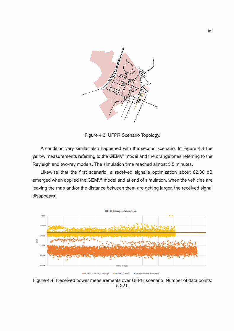
66

Figure 4.3: UFPR Scenario Topology.

A condition very similar also happened with the second scenario. In Figure 4.4 the

yellow measurements referring to the GEMV² model and the orange ones referring to the

Rayleigh and two-ray models. The simulation time reached almost 5,5 minutes.

Likewise that the first scenario, a received signal’s optimization about 82,30 dB

emerged when applied the GEMV² model and at end of simulation, when the vehicles are

leaving the map and/or the distance between them are getting larger, the received signal

disappears.

Figure 4.4: Received power measurements over UFPR scenario. Number of data points:

5.221.

67

The optimization upon both comparisons might have relation to the GEMV² model’s

geometric considerations (reflections and diffraction methods), that increment the large-

scale received power and the fact of normal distribution be much less severe than Rice

and Rayleigh models for small-scale signal.

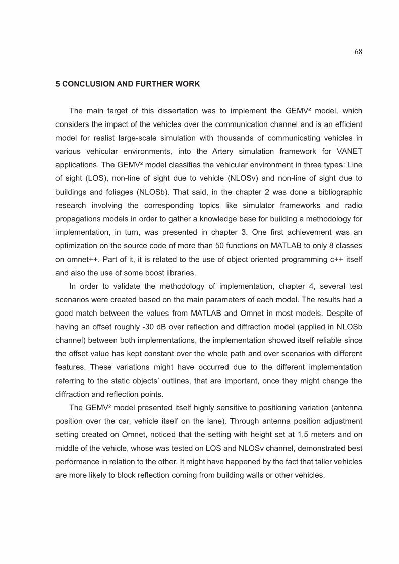
68

5 CONCLUSION AND FURTHER WORK

The main target of this dissertation was to implement the GEMV² model, which

considers the impact of the vehicles over the communication channel and is an efficient

model for realist large-scale simulation with thousands of communicating vehicles in

various vehicular environments, into the Artery simulation framework for VANET

applications. The GEMV² model classifies the vehicular environment in three types: Line

of sight (LOS), non-line of sight due to vehicle (NLOSv) and non-line of sight due to

buildings and foliages (NLOSb). That said, in the chapter 2 was done a bibliographic

research involving the corresponding topics like simulator frameworks and radio

propagations models in order to gather a knowledge base for building a methodology for

implementation, in turn, was presented in chapter 3. One first achievement was an

optimization on the source code of more than 50 functions on MATLAB to only 8 classes

on omnet++. Part of it, it is related to the use of object oriented programming c++ itself

and also the use of some boost libraries.

In order to validate the methodology of implementation, chapter 4, several test

scenarios were created based on the main parameters of each model. The results had a

good match between the values from MATLAB and Omnet in most models. Despite of

having an offset roughly -30 dB over reflection and diffraction model (applied in NLOSb

channel) between both implementations, the implementation showed itself reliable since

the offset value has kept constant over the whole path and over scenarios with different

features. These variations might have occurred due to the different implementation

referring to the static objects’ outlines, that are important, once they might change the

diffraction and reflection points.

The GEMV² model presented itself highly sensitive to positioning variation (antenna

position over the car, vehicle itself on the lane). Through antenna position adjustment

setting created on Omnet, noticed that the setting with height set at 1,5 meters and on

middle of the vehicle, whose was tested on LOS and NLOSv channel, demonstrated best

performance in relation to the other. It might have happened by the fact that taller vehicles

are more likely to block reflection coming from building walls or other vehicles.

69

Last but not least, the Artery simulation framework operating with the GEMV² model

proved to become the simulation more realistic and with a good accuracy/scalability

tradeoff through comparisons between the traditional radio propagation models used by

Artery till then and the GEMV² over large scenarios. The received power measurements

have been optimized about 82,3 dB. Similar gains were also obtained in (VIRIYASITAVAT

et. al., 2015).

As a suggestion for further works, it would be interesting to redesign the INET

framework in order to insert more performance parameters referring to the physical layer

that are well known and used in the research environment, however it is missing out on

Omnet. The current simulation framework uses only noise and received power as

performance indicative.

70

REFERENCES

802.11 Part 11: Wireless LAN Medium Access Control (MAC) and Physical Layer (PHY) Specifications; Institute of Electrical and Electronics Engineers, Mar. 2012. ALVES, R. S. et al.; “Redes veiculares: Princípios, aplicações e desafios”. In: SBRC. 27 Simpósio Brasileiro de Redes de Computadores e Sistemas Distribuídos - SBRC.2009. BOBAN, M.; BARROS, J.; TONGUZ, O. K.; “Geometry-Based Vehicle-to-Vehicle Chan-nel Modeling for Large-Scale Simulation”. IEEE Transaction on vehicular technology, vol. 63, nº. 9, Nov. 2014. BOBAN, M.; VINHOZA, T. T. V.; FERREIRA, M.; BARROS, J.; TONGUZ, O. K.; “Impact of Vehicles as Obstacles in Vehicular Ad Hoc Networks”. IEEE Journal on selected ar-eas in communications, vol. 29, nº. 1, Jan. 2011. CAMPOLO, C.; MOLINARO, A.; Multichannel communications in vehicular ad hoc networks: a survey. IEEE Commun. Mag., 51 (5) (2013), pp. 158 169, 10.1109/MCOM.2013.6515061 CrossRefView Record in Scopus. CHENG, L.; HENTY, B. E.; STANCIL, D. D.; BAI, F.; MUDALIGE, P.; “Mobile vehicle-to-vehicle narrow-band channel measurement and characterization of the 5.9 GHz dedicated short range communication (DSRC) frequency band” IEEE J. Sel. Areas Commun., vol. 25, no. 8, pp. 1501–1516, Oct. 2007. CHOFFNES, D. R. et al.; An integrated mobility and traffic model for vehicular wireless networks. In: ACM International Workshop on Vehicular Ad Hoc Networks. 2005. CODECA, L.; FRANK, R.; FAYE, S.; ENGEL, T.; "Luxembourg SUMO Traffic (LuST) Sce-nario: Traffic Demand Evaluation" in IEEE Intelligent Transportation Systems Maga-zine, vol. 9, no. 2, pp. 52-63, Summer 2017. CORMEN, T. H.; LEISERSON, C.; RIVEST, R. L.; STEIN, C.; “ Algorithmen – Eine Einfüh-rung” in 2. ed. München: Oldenbourg Wissenschaftsverlag. pp. 585–586. 2007. ETSI, EN 302 665 - Intelligent Transport Systems (ITS); Communications Architecture, V1.1.1, European Telecommunications Standards Institute, Sep. 2010. ETSI, Final draft ETSI ES 202 663 V1.1.0 (2009–11), ETSI standard, intelligent transport systems (ITS); European profile standard for the physical and medium access control layer of intelligent transport systems operating in the 5 GHz frequency band, November 2011. GRINSTEAD, C. M.; SNELL, J. L.; Introduction to Probability. American Mathematical Society. 2nd edition, 1998.

71

IEEE Guide for Wireless Access in Vehicular Environments (WAVE) - Architecture. IEEE Std1609.0-2013, p. 1–78, March 2014. Intelligent Transport Systems (ITS); Users and applications requirements; Part1: Facility layer structure, functional requirements and specifications, European Telecommunica-tions Standards Institute, Aug. 2013. Intelligent Transport Systems (ITS); Vehicular Communications; Basic Set of Applica-tions; Part 2: Specification of Cooperative Awareness Basic Service, ETSI EM 302 637-2, European Telecommunications Standards Institute, Nov. 2014. Intelligent Transport Systems (ITS); Vehicular Communications; GeoNetworking; Part 4: Geographical addressing and forwarding for point-to-point and point-to-multipoint commu-nications; Sub-part 1: Media-Independent Functionality, ETSI EN 302 636-4-1, European Telecommunications Standards Institute, Jul. 2014. Intelligent Transport Systems (ITS); Vehicular Communications; GeoNetworking; Part 5: Transport Protocols; Sub-part 1: Basic Transport Protocol, European Telecommunica-tions Standards Institute, Aug. 2014. ITU-R, “Propagation by diffraction,” International Telecommunication Union Radio-communication Sector, Geneva, Recommendation P.526, Feb. 2007. KAKKASAGERI, M. et al. Information management in vehicular ad hoc networks: A review. Journal of Network and Computer Applications, v. 39, n. 0, p. 334 – 350, 2014. ISSN 1084-8045. KOLLER, M.; ELSTER, A.; REHBORN, H.; KERNER, B. S.; “A system for vehicle data processing to detect spatiotemporal congested patterns: The SIMTD-approach” 19th ITS World Congress, Vienna, Austria, 22/26 Oct. 2012. MANGEL, T.; MICHL, M.; KLEMP, O.; HARTENSTEIN, H.; “Real-world measurements of non-line-of-sight reception quality for 5.9 GHz IEEE802.11p at intersections,” in Proc. 3rd Int. Conf. Commun. Technol. Vehicles, ser. Nets4Cars/Nets4Trains, Berlin, Germany, 2011, pp. 189–202, Springer-Verlag. MAURER, J.; FUGEN, T.; SCHAFER, T.; WIESBECK, W.; “A new inter-vehicle communi-cations (ivc) channel model,” in Proc. IEEE 60th Vehicular Technology Conference (VTC 2004-Fall), vol. 1, Sept. 2004, pp. 9–13. NAGEL, K. et al.; A cellular automaton model for freeway traffic. Journal de Physique, v.2, n. 12, December 1992.

72

OBERMAIER, C.; ‘’Real-Time Testing of Car2X Hardware with OMNeT++’’, Report of Master Degree. Technische Hochschule Ingolstadt. Computer Science Faculty. 2017. PEREIRA, M. A.; “Análise de modelos de propagação na área urbana da região de Curitiba/PR na faixa de frequência de 1800 MHz”, Dissertation of Master Degree. Federal University of Parana. DELT. 2007. RAPPAPORT, T. S.; Wireless Communications: Principles and Practice. Englewood Cliffs, NJ, USA: Prentice-Hall, 1996. RAPPAPORT, T. S.; Wireless Communications: Principles and Practice. Prentice-Hall PTR. 2000. RIEBL, R.; OBERMAIER, C.; FACCHI, C.; NEUMEIER, S.; “Vanetza: Boosting Research on Inter-Vehicle Communication”. [Online]. Available: https://github.com/riebl/vanetza. RIEBL, R.; GUNTHER, H. J.; FACCHI, C.; WOLF, L.; “Artery: Extending Veins for VANET applications”, in Models and Technologies for Intelligent Transportation Systems (MT-ITS), 2015 International Conference on, Jun. 2015, pp. 450–456. [Online]. Available on: https://github.com/riebl/artery. SILVA, R.; “Características da Propagação ponto-área na faixa de 2 a 15 GHz com aplicações em Comunicações Móveis”. Dissertation of Master Degree. Military Institute of Engineering. Rio de Janeiro, 2004. SIZENANDO, F.; “Avaliação dos Modelos de Predição de Propagação para Telefonia Móvel Celular na Cidade de Natal”. Dissertation of Master Degree. Federal University of Rio Grande do Norte. Natal, 2006. SOMMER, C.; Veins Documentation. [Online]. Available on: http://veins.car2x.org/docu-mentation/. SUMO. Simulation of Urban Mobility. December 2015. Road Traffic Simulator. Availa-ble on: http://www.dlr.de/ts/en/desktopdefault.aspx/tabid-9883. United States Department of transportation (USDOT). Planning Future Transportation: Connected Vehicles and ITS. 2016. Available on: <http://www.its.dot.gov/factsheets/pdf/PlanningFutureTransportation_FactSheet.pdf> VARGA, A. et al. Omnet++ Simulation Framework. Available on: < https://om-netpp.org/>. VIRIYASITAVAT, W.; BOBAN, M.; TSAI, H.; VASILAKOS, A. V.; “Survey and Challenges of Channel and Propagation Models”. IEEE vehicular technology magazine. June, 2015.

73

XU, S.; SAADAWI, T.; “Does the IEEE 802.11 MAC Protocol Work Well in Multihop Wire-less Ad Hoc Networks”, in IEEE Communications Magazine, European Telecommuni-cations Standards Institute, jun. 2001, pp. 130–137. WANG, C.-X.; CHENG, LAURENSON, X. D. I.; “Vehicle-to-vehicle channel modeling and measurements: Recent advances and future challenges,” IEEE Commun. Mag., vol. 47, no. 11, pp. 96–103, November 2009.