PONTIFÍCIA UNIVERSIDADE CATÓLICA DE SÃO PAULO FEA ‐ Faculdade de Economia e Administração 

Programa de Estudos Pós‐Graduados em Administração  

 

 

 

 

REGRESSÃO LOGÍSTICA  

E  INDICADORES DE GOVERNANÇA GLOBAL  

 

 

Disciplina: Métodos Quantitativos 

Prof. Dr. Arnoldo Jose de Hoyos 

Carlos Barbosa Correa Junior 

 

1. INTRODUÇÃO 

O objetivo deste trabalho é pesquisar A Regressão Logistica.. Serão utilizados dimensionadores 

do WGI  (Worldwide Governance  Indicators)  que  envolve  207  países.  Será  considerada  uma 

amostra de 30 países e analisados os dois primeiros componentes principais, para cada uma 

das  variáveis  apresentadas  pelo  índice  e  a  seguir  a  análise  dos  conglomerados. O  software 

estatístico utilizado é o MINITAB. 

  Os dimensionadores são: 

– Transparência e representatividade 

 – Estabilidade política e ausência de violência 

 – Efetividade governamental 

 – Qualidade regulatória 

 – Regras da Lei 

 – Controle da corrupção 

 

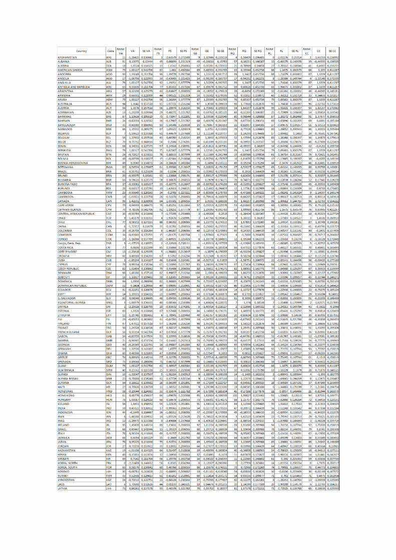
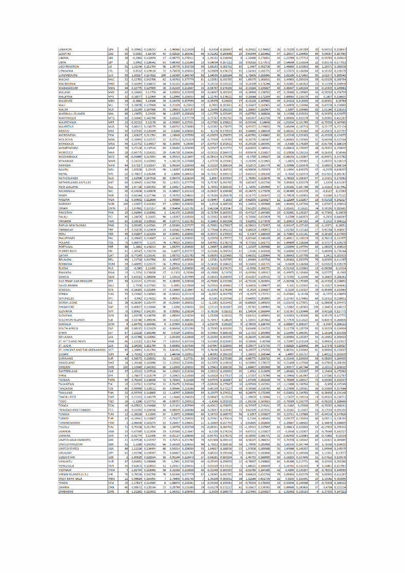
Os dados iniciais do universo são os listados a seguir: 

 

 

 

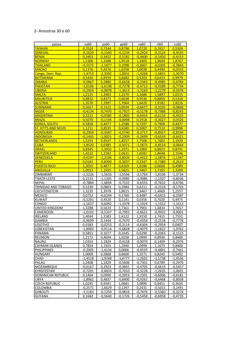
2‐ Amostras 30 e 60 

paises va60 ps60 ge60 rq60 rl60 cc60TAIWAN 0,7024 0,7244 0,8798 1,0720 0,7657 0,5504SENEGAL ‐0,1620 ‐0,1560 ‐0,1234 ‐0,2924 ‐0,3124 ‐0,4535BENIN 0,3403 0,3452 ‐0,5181 ‐0,4600 ‐0,5450 ‐0,4153NORWAY 1,5306 1,3288 1,9518 1,3405 1,9649 1,8767THAILAND ‐0,5575 ‐1,1877 0,1098 0,2607 ‐0,0305 ‐0,3844MACAO 0,1376 0,4576 1,0258 1,0038 0,4490 ‐0,0333Congo, Dem. Rep. ‐1,4753 ‐2,3392 ‐1,8931 ‐1,4268 ‐1,6831 ‐1,3070BOTSWANA 0,5450 0,9559 0,6682 0,5203 0,6433 0,9979ZAMBIA ‐0,0867 0,2880 ‐0,6628 ‐0,3343 ‐0,4985 ‐0,4784PAKISTAN ‐1,0106 ‐2,6138 ‐0,7278 ‐0,4713 ‐0,9189 ‐0,7734LIBERIA ‐0,2904 ‐0,9878 ‐1,3613 ‐1,3169 ‐1,2279 ‐0,5978MALTA 1,2125 1,2963 1,2570 1,1686 1,5897 1,0115MAURITIUS 0,8832 0,8373 0,6038 0,9536 0,8850 0,5318AUSTRIA 1,3576 1,2997 1,7064 1,6420 1,9182 1,8216SURINAME 0,5657 0,1522 0,0034 ‐0,6677 ‐0,3335 ‐0,0866NIGER ‐0,4134 ‐0,7470 ‐0,7927 ‐0,5178 ‐0,7988 ‐0,8243ARGENTINA 0,3211 ‐0,0385 ‐0,1805 ‐0,6454 ‐0,6116 ‐0,4425BRAZIL 0,5070 ‐0,1194 ‐0,0098 0,1918 ‐0,3027 ‐0,0326KOREA, SOUTH 0,5858 0,4077 1,2588 0,7297 0,7908 0,4477ST. KITTS AND NEVIS 1,1211 0,8535 0,6580 0,5007 0,7510 0,9996HONDURAS ‐0,2904 ‐0,3587 ‐0,5740 ‐0,2717 ‐0,8937 ‐0,8194INDONESIA ‐0,1445 ‐1,0021 ‐0,2909 ‐0,2699 ‐0,6559 ‐0,6421NETHERLANDS 1,5291 0,9547 1,8557 1,7506 1,7602 2,1929CUBA ‐1,8520 0,0385 ‐0,5071 ‐1,5875 ‐0,8514 ‐0,0644ISRAEL 0,6945 ‐1,3932 1,2971 1,1969 0,8823 0,8741SWITZERLAND 1,4532 1,2282 2,0631 1,6581 1,8648 2,1546VENEZUELA ‐0,6247 ‐1,2336 ‐0,8503 ‐1,4412 ‐1,5876 ‐1,1347PERU 0,0181 ‐0,8390 ‐0,3037 0,3347 ‐0,7380 ‐0,2619PUERTO RICO 1,3055 0,4877 0,6569 1,0186 0,6600 0,4989ANGUILLA 1,0013 1,1925 1,5621 1,3467 1,7165 1,3209ZIMBABWE ‐1,5226 ‐1,5633 ‐1,5556 ‐2,1764 ‐1,8106 ‐1,3734TIMOR‐LESTE 0,1533 ‐1,1305 ‐0,9985 ‐1,3986 ‐1,1507 ‐0,8936NEPAL ‐0,7884 ‐1,6894 ‐0,7532 ‐0,6555 ‐0,7632 ‐0,6766TRINIDAD AND TOBAGO 0,5339 0,0803 0,2984 0,6211 ‐0,2516 ‐0,1703LIECHTENSTEIN 1,3235 1,3978 1,8615 1,3467 1,4669 1,2557MEXICO 0,0752 ‐0,6244 0,1760 0,4487 ‐0,6415 ‐0,2587KUWAIT ‐0,5291 0,4520 0,1141 0,0356 0,7020 0,4975CONGO ‐1,1637 ‐0,6092 ‐1,3378 ‐1,1924 ‐1,1552 ‐1,1613UNITED KINGDOM 1,3288 0,5633 1,7361 1,7901 1,6834 1,7657CAMEROON ‐1,0192 ‐0,5337 ‐0,7992 ‐0,6621 ‐0,9932 ‐0,9001IRELAND 1,4044 1,1583 1,6122 1,9150 1,7415 1,7551GAMBIA ‐0,9699 0,1444 ‐0,7670 ‐0,4358 ‐0,2518 ‐0,7778LESOTHO 0,0383 ‐0,0253 ‐0,3114 ‐0,6304 ‐0,2954 0,0407UZBEKISTAN ‐1,8983 ‐0,9114 ‐0,6828 ‐1,4079 ‐1,1822 ‐1,0762PANAMA 0,5851 0,1077 0,1645 0,6290 ‐0,2043 ‐0,1515REUNION 1,2172 0,4694 1,0258 1,0999 0,8930 0,8400NAURU 1,0353 1,1829 ‐0,4158 ‐0,9070 0,1409 ‐0,2976CAYMAN ISLANDS 0,7854 1,1925 1,2940 1,0999 1,1675 0,8400PHILIPPINES ‐0,2005 ‐1,4134 0,0006 ‐0,0535 ‐0,4891 ‐0,7461HUNGARY 1,0009 0,5868 0,6600 1,2571 0,8245 0,5492CHAD ‐1,4518 ‐1,9248 ‐1,4777 ‐1,2632 ‐1,5738 ‐1,4536PALAU 1,2408 1,1829 ‐0,5606 ‐0,7301 0,6789 ‐0,2976MOZAMBIQUE ‐0,0167 0,2923 ‐0,3841 ‐0,4705 ‐0,6619 ‐0,5457KYRGYZSTAN ‐0,7201 ‐0,6833 ‐0,7010 ‐0,3228 ‐1,2635 ‐1,0601DOMINICAN REPUBLIC 0,1404 0,0990 ‐0,3953 ‐0,2391 ‐0,6006 ‐0,6181LIBYA ‐1,8962 0,4837 ‐0,8400 ‐0,9262 ‐0,6468 ‐0,8058CZECH REPUBLIC 1,0245 0,9341 1,0681 1,0890 0,8451 0,3650COLOMBIA ‐0,2571 ‐1,6629 0,1297 0,2431 ‐0,5015 ‐0,2491DJIBOUTI ‐1,1183 ‐0,1259 ‐0,9816 ‐0,7476 ‐0,5360 ‐0,3274GUYANA 0,1682 ‐0,5640 ‐0,1726 ‐0,5458 ‐0,6958 ‐0,4735  

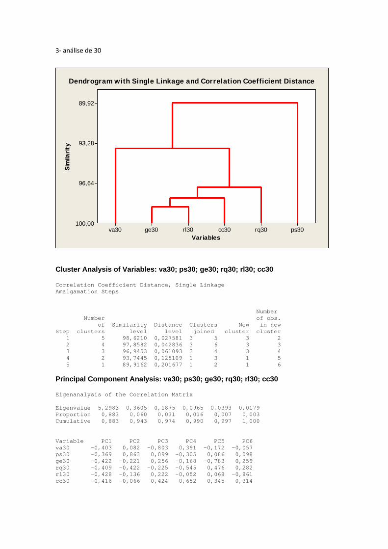
3‐ análise de 30 

Variables

Sim

ilari

ty

ps30rq30cc30rl30ge30va30

89,92

93,28

96,64

100,00

Dendrogram with Single Linkage and Correlation Coefficient Distance

Cluster Analysis of Variables: va30; ps30; ge30; rq30; rl30; cc30 Correlation Coefficient Distance, Single Linkage Amalgamation Steps Number Number of obs. of Similarity Distance Clusters New in new Step clusters level level joined cluster cluster 1 5 98,6210 0,027581 3 5 3 2 2 4 97,8582 0,042836 3 6 3 3 3 3 96,9453 0,061093 3 4 3 4 4 2 93,7445 0,125109 1 3 1 5 5 1 89,9162 0,201677 1 2 1 6

Principal Component Analysis: va30; ps30; ge30; rq30; rl30; cc30 Eigenanalysis of the Correlation Matrix Eigenvalue 5,2983 0,3605 0,1875 0,0965 0,0393 0,0179 Proportion 0,883 0,060 0,031 0,016 0,007 0,003 Cumulative 0,883 0,943 0,974 0,990 0,997 1,000 Variable PC1 PC2 PC3 PC4 PC5 PC6 va30 -0,403 0,082 -0,803 0,391 -0,172 -0,057 ps30 -0,369 0,863 0,099 -0,305 0,086 0,098 ge30 -0,422 -0,221 0,256 -0,168 -0,783 0,259 rq30 -0,409 -0,422 -0,225 -0,545 0,476 0,282 rl30 -0,428 -0,136 0,222 -0,052 0,068 -0,861 cc30 -0,416 -0,066 0,424 0,652 0,345 0,314

 

Component Number

Eige

nval

ue

654321

6

5

4

3

2

1

0

Scree Plot of va30; ...; cc30

  First Component

Seco

nd C

ompo

nent

543210-1-2-3-4

1,0

0,5

0,0

-0,5

-1,0

-1,5

-2,0

Score Plot of va30; ...; cc30

 

 

First Component

Seco

nd C

ompo

nent

0,0-0,1-0,2-0,3-0,4

1,00

0,75

0,50

0,25

0,00

-0,25

-0,50

cc30rl30

rq30

ge30

ps30

va30

Loading Plot of va30; ...; cc30

 

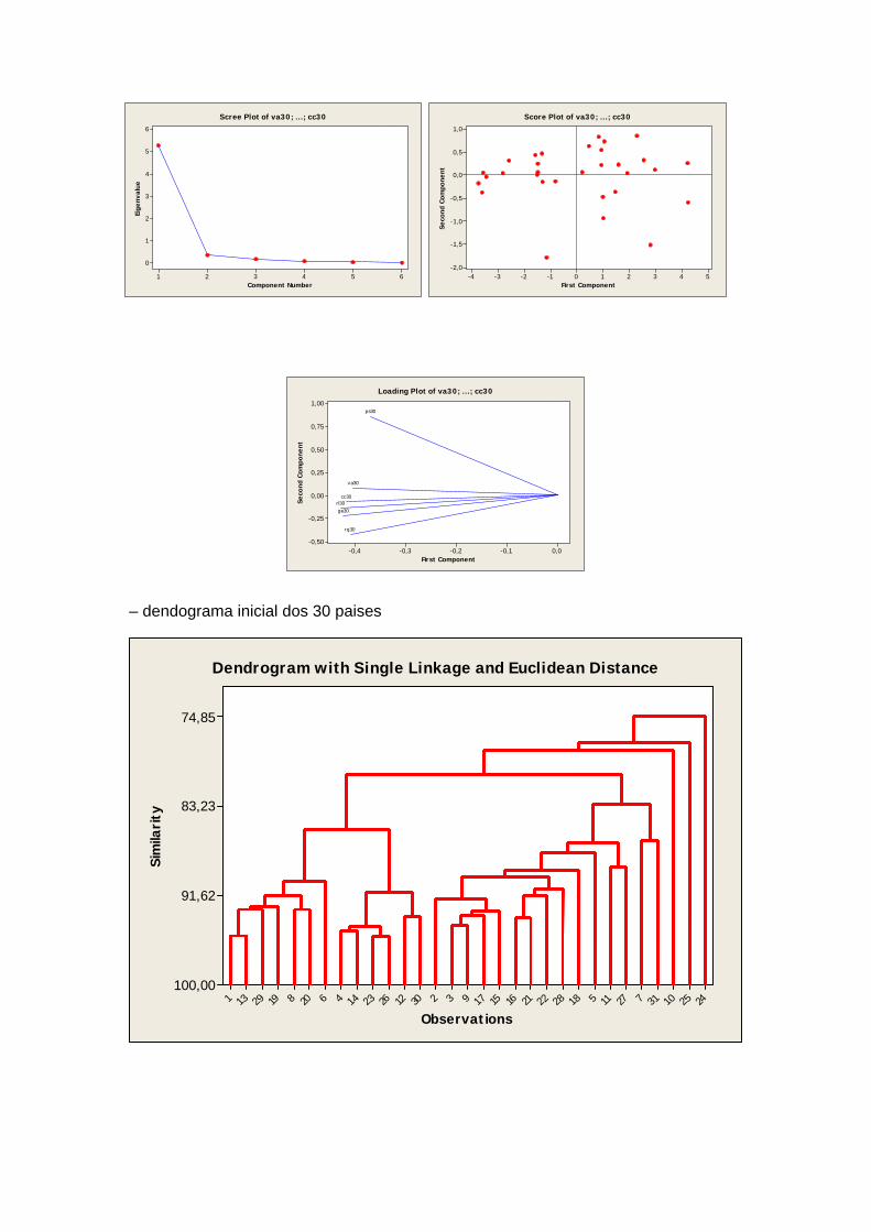
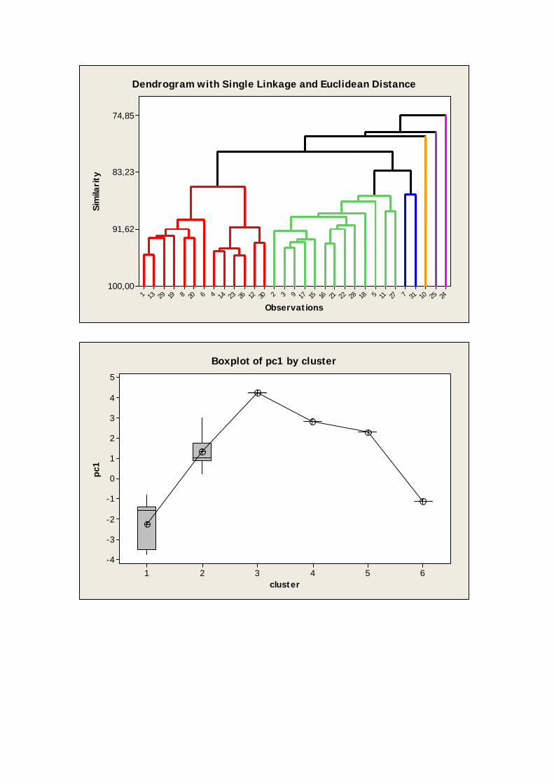
– dendograma inicial dos 30 paises

Observations

Sim

ilari

ty

24251031727115182822211615179323012262314462081929131

74,85

83,23

91,62

100,00

Dendrogram with Single Linkage and Euclidean Distance

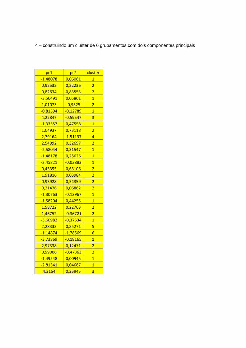
4 – construindo um cluster de 6 grupamentos com dois componentes principais

pc1  pc2  cluster 

‐1,48078  0,06081  1 

0,92532  0,22236  2 

0,82634  0,83553  2 

‐3,56491  0,05861  1 

1,01073  ‐0,9325  2 

‐0,81594  ‐0,12789  1 

4,22847  ‐0,59547  3 

‐1,33557  0,47558  1 

1,04937  0,73118  2 

2,79164  ‐1,51137  4 

2,54092  0,32697  2 

‐2,58044  0,31547  1 

‐1,48178  0,25626  1 

‐3,45821  ‐0,03883  1 

0,45355  0,63106  2 

1,91816  0,03984  2 

0,93928  0,54359  2 

0,21476  0,06862  2 

‐1,30763  ‐0,13967  1 

‐1,58204  0,44255  1 

1,58722  0,22763  2 

1,46752  ‐0,36721  2 

‐3,60982  ‐0,37534  1 

2,28333  0,85271  5 

‐1,14874  ‐1,78569  6 

‐3,73869  ‐0,18165  1 

2,97338  0,12471  2 

0,99006  ‐0,47363  2 

‐1,49548  0,00945  1 

‐2,81541  0,04687  1 

4,2154  0,25945  3 

Observations

Sim

ilari

ty

24251031727115182822211615179323012262314462081929131

74,85

83,23

91,62

100,00

Dendrogram with Single Linkage and Euclidean Distance

 

cluster

pc1

654321

5

4

3

2

1

0

-1

-2

-3

-4

Boxplot of pc1 by cluster

 

 

cluster

pc1

654321

5

4

3

2

1

0

-1

-2

-3

-4

Individual Value Plot of pc1 vs cluster

 

Cluster Analysis of Observations: va30; ps30; ge30; rq30; rl30; cc30 Euclidean Distance, Single Linkage Amalgamation Steps Number Number of obs. of Similarity Distance Clusters New in new Step clusters level level joined cluster cluster 1 30 95,4895 0,38017 23 26 23 2 2 29 95,4024 0,38751 1 13 1 2 3 28 94,8688 0,43249 4 14 4 2 4 27 94,4780 0,46543 4 23 4 4 5 26 94,3286 0,47802 3 9 3 2 6 25 93,6851 0,53226 16 21 16 2 7 24 93,5886 0,54040 12 30 12 2 8 23 93,4899 0,54871 3 17 3 3 9 22 93,1373 0,57843 3 15 3 4 10 21 92,9370 0,59532 8 20 8 2 11 20 92,8887 0,59939 1 29 1 3 12 19 92,6293 0,62125 1 19 1 4 13 18 91,9121 0,68170 2 3 2 5 14 17 91,5964 0,70831 1 8 1 6 15 16 91,5754 0,71008 16 22 16 3 16 15 91,2988 0,73339 4 12 4 6 17 14 91,0421 0,75503 16 28 16 4 18 13 90,2099 0,82517 1 6 1 7 19 12 89,8432 0,85608 2 16 2 9 20 11 89,2561 0,90556 2 18 2 10 21 10 88,9567 0,93080 11 27 11 2 22 9 87,5302 1,05104 2 5 2 11 23 8 86,6271 1,12716 2 11 2 13 24 7 86,4691 1,14047 7 31 7 2 25 6 85,3790 1,23235 1 4 1 13 26 5 82,9727 1,43517 2 7 2 15 27 4 80,2670 1,66322 1 2 1 28 28 3 78,0239 1,85228 1 10 1 29 29 2 77,2872 1,91438 1 25 1 30 30 1 74,8522 2,11962 1 24 1 31

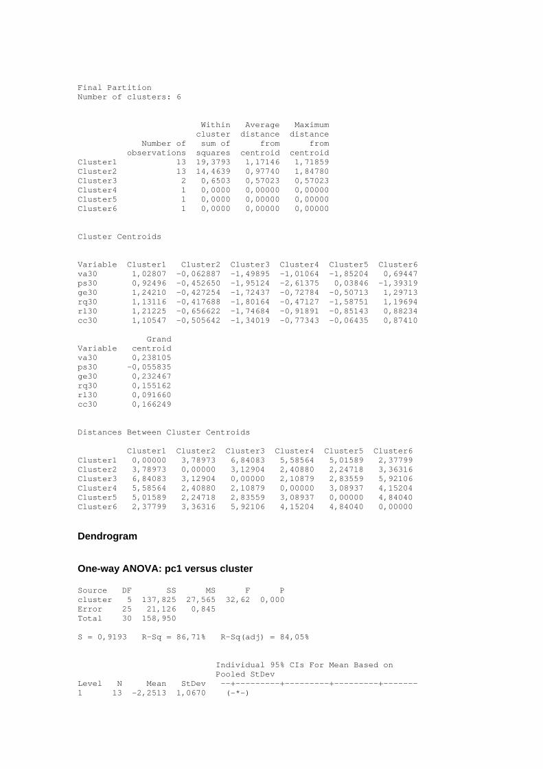
Final Partition Number of clusters: 6 Within Average Maximum cluster distance distance Number of sum of from from observations squares centroid centroid Cluster1 13 19,3793 1,17146 1,71859 Cluster2 13 14,4639 0,97740 1,84780 Cluster3 2 0,6503 0,57023 0,57023 Cluster4 1 0,0000 0,00000 0,00000 Cluster5 1 0,0000 0,00000 0,00000 Cluster6 1 0,0000 0,00000 0,00000 Cluster Centroids Variable Cluster1 Cluster2 Cluster3 Cluster4 Cluster5 Cluster6 va30 1,02807 -0,062887 -1,49895 -1,01064 -1,85204 0,69447 ps30 0,92496 -0,452650 -1,95124 -2,61375 0,03846 -1,39319 ge30 1,24210 -0,427254 -1,72437 -0,72784 -0,50713 1,29713 rq30 1,13116 -0,417688 -1,80164 -0,47127 -1,58751 1,19694 rl30 1,21225 -0,656622 -1,74684 -0,91891 -0,85143 0,88234 cc30 1,10547 -0,505642 -1,34019 -0,77343 -0,06435 0,87410 Grand Variable centroid va30 0,238105 ps30 -0,055835 ge30 0,232467 rq30 0,155162 rl30 0,091660 cc30 0,166249 Distances Between Cluster Centroids Cluster1 Cluster2 Cluster3 Cluster4 Cluster5 Cluster6 Cluster1 0,00000 3,78973 6,84083 5,58564 5,01589 2,37799 Cluster2 3,78973 0,00000 3,12904 2,40880 2,24718 3,36316 Cluster3 6,84083 3,12904 0,00000 2,10879 2,83559 5,92106 Cluster4 5,58564 2,40880 2,10879 0,00000 3,08937 4,15204 Cluster5 5,01589 2,24718 2,83559 3,08937 0,00000 4,84040 Cluster6 2,37799 3,36316 5,92106 4,15204 4,84040 0,00000

Dendrogram One-way ANOVA: pc1 versus cluster Source DF SS MS F P cluster 5 137,825 27,565 32,62 0,000 Error 25 21,126 0,845 Total 30 158,950 S = 0,9193 R-Sq = 86,71% R-Sq(adj) = 84,05% Individual 95% CIs For Mean Based on Pooled StDev Level N Mean StDev --+---------+---------+---------+------- 1 13 -2,2513 1,0670 (-*-)

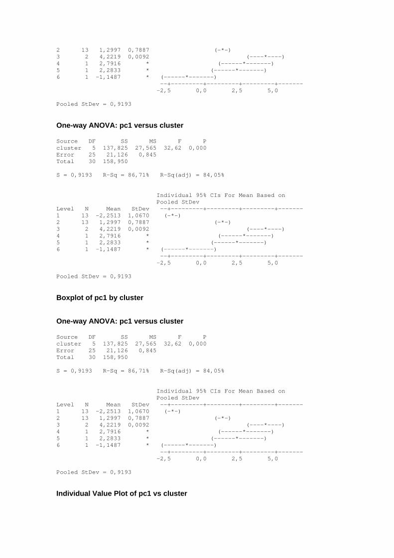
2 13 1,2997 0,7887 (-*-) 3 2 4,2219 0,0092 (----*----) 4 1 2,7916 * (------*-------) 5 1 2,2833 * (------*-------) 6 1 -1,1487 * (------*-------) --+---------+---------+---------+------- -2,5 0,0 2,5 5,0 Pooled StDev = 0,9193

One-way ANOVA: pc1 versus cluster Source DF SS MS F P cluster 5 137,825 27,565 32,62 0,000 Error 25 21,126 0,845 Total 30 158,950 S = 0,9193 R-Sq = 86,71% R-Sq(adj) = 84,05% Individual 95% CIs For Mean Based on Pooled StDev Level N Mean StDev --+---------+---------+---------+------- 1 13 -2,2513 1,0670 (-*-) 2 13 1,2997 0,7887 (-*-) 3 2 4,2219 0,0092 (----*----) 4 1 2,7916 * (------*-------) 5 1 2,2833 * (------*-------) 6 1 -1,1487 * (------*-------) --+---------+---------+---------+------- -2,5 0,0 2,5 5,0 Pooled StDev = 0,9193

Boxplot of pc1 by cluster

One-way ANOVA: pc1 versus cluster Source DF SS MS F P cluster 5 137,825 27,565 32,62 0,000 Error 25 21,126 0,845 Total 30 158,950 S = 0,9193 R-Sq = 86,71% R-Sq(adj) = 84,05% Individual 95% CIs For Mean Based on Pooled StDev Level N Mean StDev --+---------+---------+---------+------- 1 13 -2,2513 1,0670 (-*-) 2 13 1,2997 0,7887 (-*-) 3 2 4,2219 0,0092 (----*----) 4 1 2,7916 * (------*-------) 5 1 2,2833 * (------*-------) 6 1 -1,1487 * (------*-------) --+---------+---------+---------+------- -2,5 0,0 2,5 5,0 Pooled StDev = 0,9193

Individual Value Plot of pc1 vs cluster

Boxplot of pc1 by cluster

One-way ANOVA: pc1 versus cluster Source DF SS MS F P cluster 5 137,825 27,565 32,62 0,000 Error 25 21,126 0,845 Total 30 158,950 S = 0,9193 R-Sq = 86,71% R-Sq(adj) = 84,05% Individual 95% CIs For Mean Based on Pooled StDev Level N Mean StDev --+---------+---------+---------+------- 1 13 -2,2513 1,0670 (-*-) 2 13 1,2997 0,7887 (-*-) 3 2 4,2219 0,0092 (----*----) 4 1 2,7916 * (------*-------) 5 1 2,2833 * (------*-------) 6 1 -1,1487 * (------*-------) --+---------+---------+---------+------- -2,5 0,0 2,5 5,0

 

 

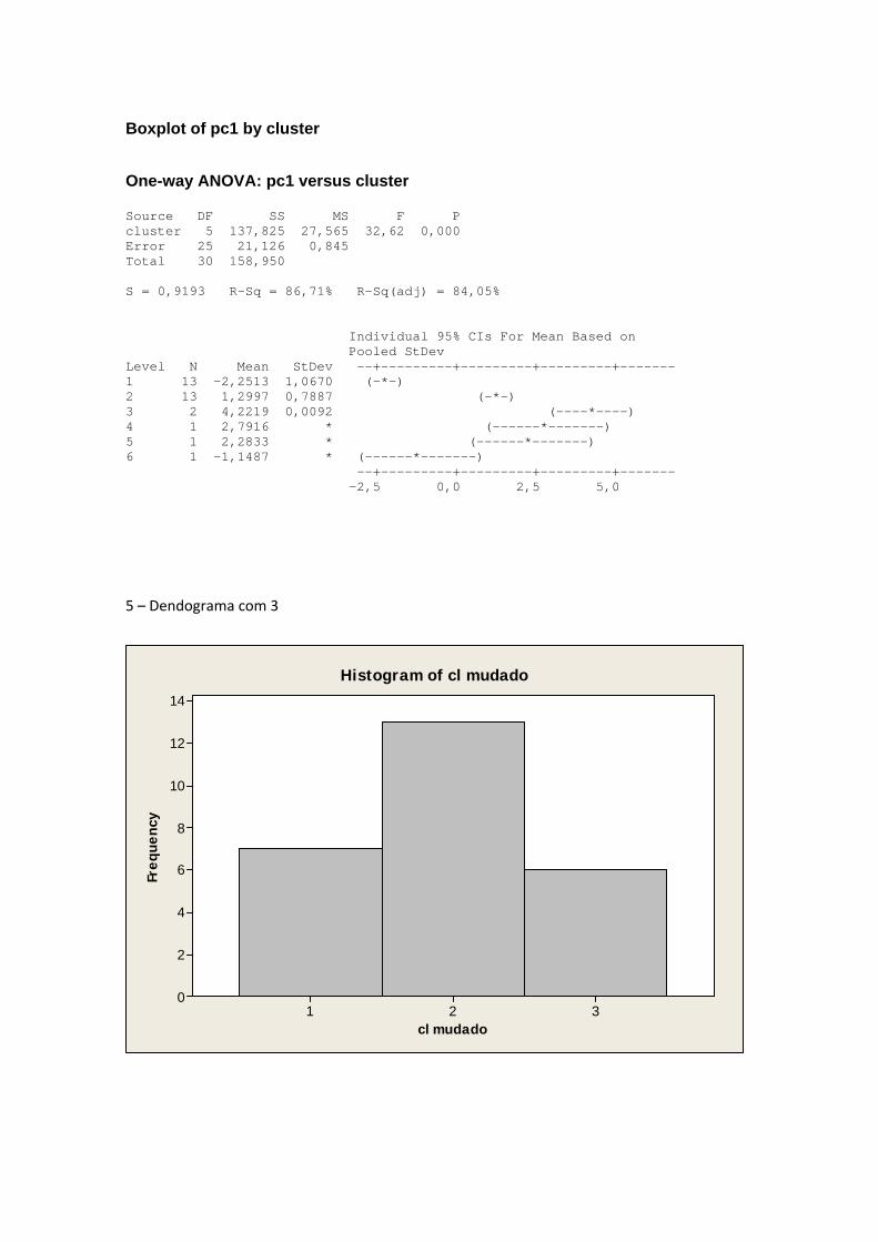
5 – Dendograma com 3 

cl mudado

Freq

uenc

y

321

14

12

10

8

6

4

2

0

Histogram of cl mudado

 

 

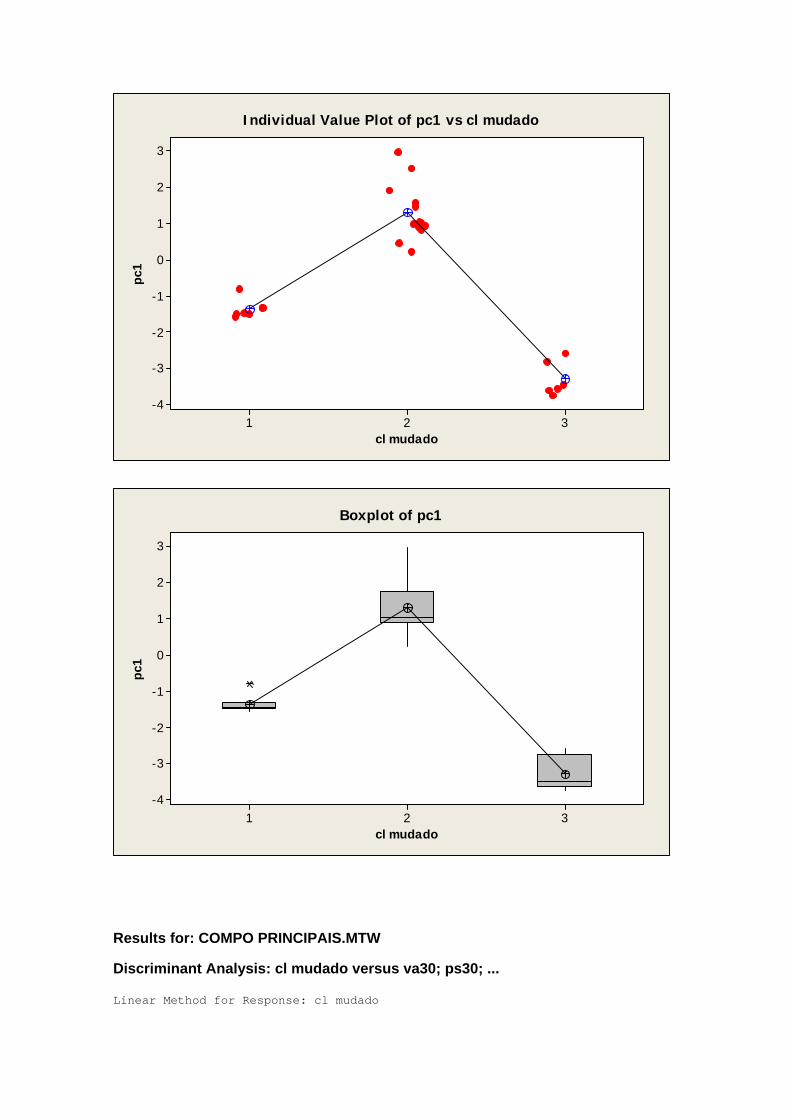
cl mudado

pc1

321

3

2

1

0

-1

-2

-3

-4

Individual Value Plot of pc1 vs cl mudado

 

cl mudado

pc1

321

3

2

1

0

-1

-2

-3

-4

Boxplot of pc1

 

 

Results for: COMPO PRINCIPAIS.MTW

Discriminant Analysis: cl mudado versus va30; ps30; ... Linear Method for Response: cl mudado

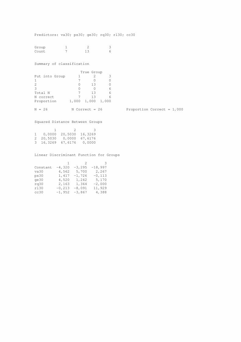
Predictors: va30; ps30; ge30; rq30; rl30; cc30 Group 1 2 3 Count 7 13 6 Summary of classification True Group Put into Group 1 2 3 1 7 0 0 2 0 13 0 3 0 0 6 Total N 7 13 6 N correct 7 13 6 Proportion 1,000 1,000 1,000 N = 26 N Correct = 26 Proportion Correct = 1,000 Squared Distance Between Groups 1 2 3 1 0,0000 20,5030 16,3269 2 20,5030 0,0000 67,6176 3 16,3269 67,6176 0,0000 Linear Discriminant Function for Groups 1 2 3 Constant -4,320 -3,295 -18,997 va30 4,562 5,700 2,267 ps30 1,417 -1,726 -0,113 ge30 4,520 1,242 5,170 rq30 2,163 1,364 -2,000 rl30 -0,213 -8,091 11,929 cc30 -1,952 -3,867 4,388

 

 

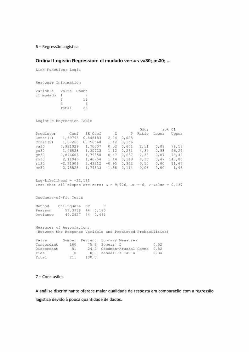
6 – Regressão Logística 

Ordinal Logistic Regression: cl mudado versus va30; ps30; ... Link Function: Logit Response Information Variable Value Count cl mudado 1 7 2 13 3 6 Total 26 Logistic Regression Table Odds 95% CI Predictor Coef SE Coef Z P Ratio Lower Upper Const(1) -1,89793 0,848183 -2,24 0,025 Const(2) 1,07268 0,756560 1,42 0,156 va30 0,921029 1,76307 0,52 0,601 2,51 0,08 79,57 ps30 1,46828 1,30723 1,12 0,261 4,34 0,33 56,29 ge30 0,846606 1,79358 0,47 0,637 2,33 0,07 78,42 rq30 2,11946 1,46754 1,44 0,149 8,33 0,47 147,80 rl30 -2,31006 2,43212 -0,95 0,342 0,10 0,00 11,67 cc30 -2,75825 1,74333 -1,58 0,114 0,06 0,00 1,93 Log-Likelihood = -22,131 Test that all slopes are zero: G = 9,726, DF = 6, P-Value = 0,137 Goodness-of-Fit Tests Method Chi-Square DF P Pearson 52,3938 44 0,180 Deviance 44,2627 44 0,461 Measures of Association: (Between the Response Variable and Predicted Probabilities) Pairs Number Percent Summary Measures Concordant 160 75,8 Somers' D 0,52 Discordant 51 24,2 Goodman-Kruskal Gamma 0,52 Ties 0 0,0 Kendall's Tau-a 0,34 Total 211 100,0

   

7 – Conclusões 

A análise discriminante oferece maior qualidade de resposta em comparação com a regressão 

logística devido à pouca quantidade de dados.