modeling and optimization of desalination...
TRANSCRIPT
Universidade Federal do Rio de Janeiro
Escola de Química
Programa de Pós-graduação em Engenharia de
Processos Químicos e Bioquímicos
MODELING AND OPTIMIZATION OF DESALINATION
SYSTEMS
TESE DE DOUTORADO
Abdón Parra López
Rio de Janeiro, março de 2019
ABDON PARRA LOPEZ
MODELING AND OPTIMIZATION OF DESALINATION SYSTEMS
Tese de Doutorado submetida ao Corpo Docente do
Curso de Pós-Graduação em Engenharia de Processos
Químicos e Bioquímicos da Escola de Química da
Universidade Federal do Rio de Janeiro, como parte dos
requisitos necessários para a obtenção do grau de Doutor
em Ciências (D.Sc.).
Orientadores: Lidia Yokoyama
Miguel Jorge Bagajewicz
Rio de Janeiro
Março de 2019
CIP - Catalogação na Publicação
Elaborado pelo Sistema de Geração Automática da UFRJ com os dados fornecidospelo(a) autor(a), sob a responsabilidade de Miguel Romeu Amorim Neto - CRB-7/6283.
P258mParra Lopez, Abdon Modeling and Optimization of DesalinationSystems / Abdon Parra Lopez. -- Rio de Janeiro,2019. 121 f.
Orientadora: Lidia Yokoyama. Coorientador: Miguel Bagajewicz. Tese (doutorado) - Universidade Federal do Riode Janeiro, Escola de Química, Programa de PósGraduação em Engenharia de Processos Químicos eBioquímicos, 2019.
1. Dessalinização. 2. Osmose Inversa. 3.Optimização. 4. Meta-modelos. 5. MINLP. I. Yokoyama,Lidia, orient. II. Bagajewicz, Miguel, coorient.III. Título.
MODELING AND OPTIMIZATION OF DESALINATION SYSTEMS
Abdon Parra Lopez
TESE DE DOUTORADO SUBMETIDA AO CORPO DOCENTE DO CURSO DE PÓS-GRADUAÇÃO EM ENGENHARIA DE PROCESSOS QUÍMICOS E BIOQUÍMICOS DA ESCOLA DE QUÍMICA DA UNIVERSIDADE FEDERAL DO RIO DE JANEIRO, COMO PARTE DOS REQUISITOS NECESSÁRIOS PARA A OBTENÇÃO DO GRAU DE DOUTOR EM CIÊNCIAS (D.SC.).
Examinada por:
___________________________________________________
Prof. Lidia Yokoyama, D.Sc. - Orientadora, (UFRJ)
___________________________________________________
Prof. Miguel Jorge Bagajewicz, Ph.D. - Orientador, (OU)
___________________________________________________
Prof. André Luiz Hemerly Costa , D.Sc., (UERJ)
___________________________________________________
Prof. Fernando Luiz Pellegrini Pessoa, D.Sc., (UFRJ)
___________________________________________________
Prof. Heloisa Lajas Sanches , D.Sc., (UFRJ)
___________________________________________________
Prof. Reinaldo Coelho Mirre, D.Sc., (UFBA)
Rio de Janeiro
Março de 2019
RESUMO
Tendo em conta a crescente demanda por água tanto urbana quanto industrial, e
considerando a atual escassez de água doce, geralmente extraída de reservatórios superficiais e
subterrâneos, é necessário considerar a água salgada, devidamente tratada, como um recurso
viável para consumo humano e industrial.
As tecnologias de dessalinização disponíveis no mercado podem ser classificadas como
em térmicas e de membranas. A osmose inversa (RO), o flash multi-estágio (MSF) e a
destilação multi-efeito (MED) são as principais tecnologias comerciais de dessalinização, sendo
a osmose inversa a de maior crescimento.
As plantas de osmose inversa têm sido tradicionalmente projetadas pelos fabricantes
usando abordagens empíricas e heurísticas. No entanto, o desempenho de custo da
dessalinização por osmose inversa, é sensível aos parâmetros de projeto e às condições de
operação e, portanto, é necessário dar atenção à obtenção de projetos com ótimo custo-
benefício.
O problema da síntese de uma rede de osmose inversa (RON) consiste em obter uma
solução econômica baseada em valores ótimos das seguintes variáveis: número de estágios,
número de vasos de pressão por estágio, número de módulos de membrana por vaso de pressão,
número e tipo de equipamentos auxiliares, bem como as variáveis operacionais para todos os
dispositivos da rede, este problema poderia ser formulado como uma programação não linear
inteira mista (MINLP).
Neste trabalho, propõe-se uma metodologia para resolver um modelo matemático não-
linear para o projeto ótimo de redes de osmose inversa, que melhore as deficiências do
desempenho computacional e, às vezes, falhas de convergência de software comercias para
resolver os modelos rigorosos MINLP. A estratégia consiste no uso de um algoritmo genético
para obter valores iniciais para um modelo completo não linear MINLP. Além disso, como o
algoritmo genético baseado nas equações do modelo rigoroso é muito lento, o uso de meta-
modelos para reduzir a complexidade matemática e acelerar consideravelmente a corrida é
proposto. O efeito da vazão de alimentação, a concentração de água do mar, o número de
estágios de osmose inversa e o número máximo de módulos de membrana em cada vaso de
pressão no custo total anualizado da planta é explorado.
Palavras-chave: Osmose Inversa, optimização, meta-modelos, MINLP.
ABSTRACT
The increasing demand for freshwater both urban and industrial, and considering the
current scarcity of freshwater, usually extracted from superficial and underground reservoirs, it
is necessary to consider salt water, properly treated, as a viable resource for human and
industrial consumption.
The available desalination technologies in the market can be classified as thermal-based
and membrane-based processes. Reverse osmosis (RO), multi-stage flash (MSF), and multi-
effect distillation (MED) are the main commercial desalination technologies, with RO being
the fastest growing (GHAFFOUR et al., 2015).
Desalination plants using RO have been traditionally designed by manufacturers using
empirical approaches and heuristics (GHOBEITY; MITSOS, 2014). However, the cost
performance of RO desalination is sensitive to the design parameters and operating conditions
(CHOI; KIM, 2015) and therefore, attention needs to be placed in obtaining cost-optimal
designs.
The problem of synthesizing a reverse osmosis network (RON) consists of obtaining a
cost-effective solution based on optimum values of the following: number of stages, number
of pressure vessels per stage, number of modules per pressure vessel, number and type of
auxiliary equipment, as well as the operational variables for all the devices of the network, this
problem could be formulated as a mixed integer nonlinear programming (MINLP).
In this work, a methodology to solve a nonlinear mathematical model for the optimal
design of RO networks, which ameliorates the shortcomings of the computational performance
and sometimes convergence failures of commercial software to solve the rigorous MINLP
models is proposed. The strategy consists of the use of a genetic algorithm to obtain initial
values for a full nonlinear MINLP model. In addition, because the genetic algorithm based on
the rigorous model equations is insurmountably slow, the use of metamodels to reduce the
mathematical complexity and considerably speed up the run is proposed. The effect of the feed
flow, seawater concentration, number of reverse osmosis stages, and the maximum number of
membrane modules in each pressure vessel on the total annualized cost of the plant is explored.
Keywords: Reverse osmosis network, optimization, metamodels, MINLP.
LIST OF FIGURES
Figure 1. Global optimum vs, local optimum ........................................................................... 23
Figure 2. Convex function ........................................................................................................ 24
Figure 3. Desalination market growth forecasts ....................................................................... 26
Figure 4. Multi-effect distillation ............................................................................................. 27
Figure 5. Multiple Stage Flash ................................................................................................. 27
Figure 6. Spiral wound membrane module .............................................................................. 29
Figure 7. Concentration polarization – salt concentration gradients adjacent to the membrane
.................................................................................................................................................. 31
Figure 8. Osmotic driving force profiles for PRO. Internal and external polarization............. 33
Figure 9. Superstructure of two stages Reverse Osmosis configuration .................................. 43
Figure 10. Structure of reverse osmosis (RO) stage and pressure vessel. ................................ 45
Figure 11. By-pass representation of a single pressure vessel. ................................................ 47
Figure 12. Permeate and brine transport through the membrane ............................................. 48
Figure 13. Superstructure of RO+PRO (Configuration 1). ...................................................... 54
Figure 14. Superstructure of a RO+PRO (Configuration 2). .................................................... 54
Figure 15. PRO unit arrangement. ............................................................................................ 54
Figure 16. Bound contraction – interval elimination strategy. ................................................. 62
Figure 17. Genetic algorithm set up ......................................................................................... 65
Figure 18. Stochastic – deterministic flowchart methodology ................................................. 66
Figure 19. Extended interval elimination – RO inlet Pressure ................................................. 71
Figure 20. Influence of feed pressure and concentration on the permeate concentration.. ...... 76
Figure 21. Influence of feed pressure and concentration on permeate flow rate, brine
concentration and brine flow rate. ............................................................................................ 78
Figure 22. Linear metamodel correlation and rigorous solutions.. ........................................... 79
Figure 23. Non-Linear metamodel correlation and validation. ................................................ 81
Figure 24. TAC for different inlet flows and seawater concentrations (two stages) ................ 85
Figure 25. Effect of the number of stages. ............................................................................... 87
Figure 26. TAC for different inlet flows and seawater concentrations max number of membrane
modules (Nmaxe) equal to 16 ...................................................................................................... 88
Figure 27. Optimal TAC per unit permeate flow. .................................................................... 89
Figure 28. Permeate flow (2 stages, 500 ppm permeate). ........................................................ 89
Figure 29. Water flux rigorous and metamodel meshes.. ......................................................... 93
Figure 30. Solute flux rigorous and metamodel meshes.. ........................................................ 94
Figure 31. TAC RO+PRO configuration 2 for different inlet flows and seawater concentrations.
.................................................................................................................................................. 97
Figure 32. Comparison between TAC for RO and RO+PRO (configuration 2) for different feed
concentration and flow. ............................................................................................................ 98
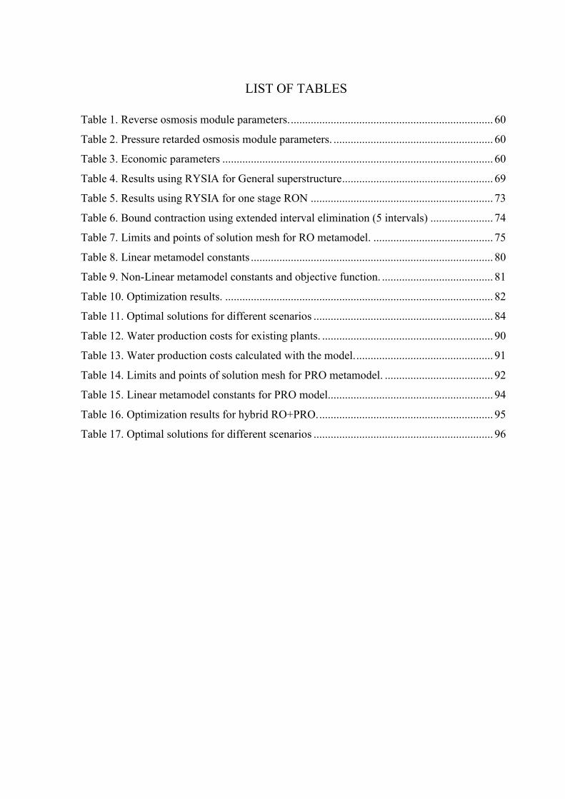
LIST OF TABLES
Table 1. Reverse osmosis module parameters. ....................................................................... 60
Table 2. Pressure retarded osmosis module parameters. ........................................................ 60
Table 3. Economic parameters ............................................................................................... 60
Table 4. Results using RYSIA for General superstructure ..................................................... 69
Table 5. Results using RYSIA for one stage RON ................................................................ 73
Table 6. Bound contraction using extended interval elimination (5 intervals) ...................... 74
Table 7. Limits and points of solution mesh for RO metamodel. .......................................... 75
Table 8. Linear metamodel constants ..................................................................................... 80
Table 9. Non-Linear metamodel constants and objective function. ....................................... 81
Table 10. Optimization results. .............................................................................................. 82
Table 11. Optimal solutions for different scenarios ............................................................... 84
Table 12. Water production costs for existing plants. ............................................................ 90
Table 13. Water production costs calculated with the model. ................................................ 91
Table 14. Limits and points of solution mesh for PRO metamodel. ...................................... 92
Table 15. Linear metamodel constants for PRO model.......................................................... 94
Table 16. Optimization results for hybrid RO+PRO. ............................................................. 95
Table 17. Optimal solutions for different scenarios ............................................................... 96

ACRONYMS
ACM – Aspen Custom Modeler
AOC – Annual Operational Cost
BARON – Computational system for solving nonconvex optimization problems to global
optimality
CONOPT – Generalized reduced-gradient (GRG) algorithm for solving large-scale nonlinear
programs involving sparse nonlinear constraints
CPLEX – Simplex method as implemented in the C programming language
DAOPs – Differential Algebraic Optimization Problems
DICOPT – Discrete and Continuous Optimizer
FO – Forward Osmosis
GAMS – General Algebraic Modeling System
gPROMS – general Process Modeling System
IP – Integer Programming
IPOPT – Interior Point Optimizer
LINDO – Software for Integer Programming, Linear Programming, Nonlinear Programming,
Stochastic Programming, Global Optimization
LINGO – Optimization Modeling Software for Linear, Nonlinear, and Integer Programming
MED – Multi-effect Distillation
MEE – Multiple Effect Evaporation
MILP – Mixed Integer Linear Programming
MINLP – Mixed Integer Nonlinear Programming
MINOS – Modular In-core Nonlinear Optimization System
MIP – Mixed Integer Programming
MSF – Multi-stage Flash
MSF-BR – Multi-effect Distillation with Brine Recirculation
MVMD – Multi-stage vacuum membrane distillation
NLP – Non-Linear Programming
PRO – Pressure Retarded Osmosis
RO – Reverse Osmosis
RON – Reverse Osmosis Network
ROSA – Reverse Osmosis System Analyzer
SBB – Spatial Branch and Bound
SPSPRO – Split Partial Second Pass Reverse Osmosis
TAC – Total Annualized Cost
TCC – Total Capital Cost
TVC – Thermal Vapor Compression
NOMENCLATURE
AOC Annual operational cost [$] C salt concentration [ppm]
,B wallC membrane wall concentration [ppm] Max
PC maximum permeate concentration [ppm] ,D inC high salinity current inlet concentration [ppm] ,F inC low salinity current inlet concentration [ppm] ,D outC high salinity current out concentration [ppm] ,F outC low salinity current inlet concentration [ppm] ,D bC high salinity current bulk concentration [ppm] ,F bC low salinity current bulk concentration [ppm]
equipCC total equipment cost [$]
ccf capital charge factor
HPPCC high pressure pump cost [$]
memCC membrane module cost [$]
memproCC PRO membrane module cost [$]
labc labor cost factor [$]
enC electricity cost [$/(kWh)]
memc membrane module unitary cost [$]
memproc PRO membrane module unitary cost [$]
pvCC total pressure vessel cost [$]
pvproCC PRO total pressure vessel cost [$]
pvc unitary pressure vessel cost [$]
pvproc PRO unitary pressure vessel cost [$]
swipCC Seawater intake and pretreatment system cost [$]
TCC turbine cost [$]
TproCC PRO turbine cost [$]
F flow rate [kg/s]
DF high salinity flow rate [kg/s]
T
DF high salinity turbine flow rate [kg/s] ,D inF high salinity inlet flow rate to a single PRO module [kg/s] ,D outF high salinity out flow rate from a single PRO module [kg/s] ,F inF low salinity inlet flow rate to a single PRO module [kg/s] ,F outF low salinity out flow rate from a single PRO module [kg/s]
FF low salinity flow rate [kg/s]
RO
SF seawater flow rate to RO [kg/s] PRO
SF seawater flow rate to PRO [kg/s] avF average flow rate [kg/s]
RF recycle flow rate [kg/s] SJ solute flux [kg/(s.m2)] WJ water flux [kg/(s.m2)] PRO
SJ solute reverse flux for PRO [kg/(s.m2)] PRO
WJ water flux for PRO [kg/(s.m2)]
ir annual interest rate ks mass transfer coefficient [m/s] Ne number of membrane modules per pressure vessel
pvN number of pressure vessels of the stage m
pvproN number of pressure vessels for the PRO unit
RON number of reverse osmosis stages
PRON number of membrane modules for the PRO unit
chemOC cost of chemicals [$]
insOC Insurance costs [$]
labOC labors cost [$]
powOC Electric energy costs [$]
OCm cost for replacement and maintenance [$]
memrOC Membrane replacement cost [$]
memproOC PRO membrane replacement cost [$]
P pressure [bar]
SWIPPP Energy consumed for intake and pre-treatment system [kWh]
ROPP Electric energy consumed by the reverse osmosis plant [kWh]
Q flow rate [m3/h] RQ recycle flow rate [m3/h]
SW INQ feed flow rate to the system [m3/h]
TproQ PRO turbine flow rate [m3/h]
Re Reynold’s number
Sc Schmidt number, TAC total annualized cost [$] TCC total capital cost [$]
sU superficial velocity [m/s] wV permeation velocity [m/s]
y binary variable
at annual operation time [hours]
1t lifetime of the plant [years] BP brine side pressure difference [bar] ndP net driving pressure difference [bar] TproP PRO turbine pressure difference [bar] HPPRP Recycle pump pressure difference [bar]
P pressure difference [bar] Parameters
A Pure water permeability [kg/(s.m2.bar)]
a Van’t Hoff ´s constant [bar/(K.ppm)]
B Salt permeability [kg/(s.m2)]
d membrane module feed space thickness [m]
D salt diffusivity [m2/s] ˆ
hd hydraulic diameter [m]
K solute resistivity for diffusion ˆ
sph
membrane module channel height [m]
ˆLl effective length of the module [m]
ˆL
n number of leaves
ˆ PeP permeate outlet pressure [bar] ˆ
fcS feed cross-section open area [m2]
ˆmemS RO active membrane area [m2]
ˆ PRO
memS PRO active membrane area [m2]
ˆspS
specific surface area of the spacer for the membrane module [m2]
T inlet temperature [K]
t support layer thickness [m]
support layer tortuosity [m]
ˆL
w width of the module [m]
SWIPP seawater intake pressure difference [bar]
Superscripts
av average
B brine Be brine current of module e from the stage m
BOB F interconnection between brine and brine final discharge
HPP high pressure pump HPPR recycle high pressure pump IN inlet
inem inlet of firsts modules of the stage m
O outlet P permeate Pe permeate current of module e from the stage m
PRO reverse osmosis RO reverse osmosis T turbine
BOT F interconnection between turbine and brine final discharge
W membrane wall Subscripts
BO brine final discharge
e membrane module e
d discretized interval d
m RO stage m
p pump p
pv pressure vessel
PO permeate final current S feed current SWIP seawater intake and pretreatment t turbine t Symbols
density [kg/m3]
membrane module void fraction Γ maximum value for the corresponding variable dynamic viscosity [kg/m.s]
efficiency
osmotic pressure [bar]
SUMMARY
1 INTRODUCTION ............................................................................................................. 17
1.1 Document description: ............................................................................................... 19
1.2 Literature contributions: ............................................................................................ 20
2 LITERATURE REVIEW .................................................................................................. 21
2.1 Mathematical models: ................................................................................................ 21
2.2 Optimization problems and definitions: .................................................................... 21
2.3 Mixed Integer Optimization: ..................................................................................... 22
2.4 Process synthesis: ...................................................................................................... 23
2.5 Global Optimization: ................................................................................................. 23
2.6 Desalination: .............................................................................................................. 25
2.7 Desalination Technologies: ........................................................................................ 25
2.8 Challenges and advances in desalination: .................................................................. 34
2.9 Reverse osmosis networks design and some hybrid systems: ................................... 35
3 OBJECTIVES ................................................................................................................... 41
3.1 General Objective: ..................................................................................................... 41
3.2 Specific objectives: .................................................................................................... 41
4 METHODOLOGY ............................................................................................................ 42
4.1 Reverse osmosis network – superstructure representation: ....................................... 42
4.2 Reverse osmosis network – MINLP model: .............................................................. 43
4.2.1 Mass Balances: ................................................................................................... 43
4.2.2 Reverse osmosis stages model: .......................................................................... 44
4.2.3 Membrane modules model: ................................................................................ 47
4.2.4 Costs and objective function: ............................................................................. 52
4.3 Hybrid reverse osmosis - pressure retarded osmosis superstructure ......................... 53
4.3.1 RO+PRO mathematical model ........................................................................... 55
4.4 MINLP problem statement ........................................................................................ 59
4.5 Bound contraction methodology ................................................................................ 61
4.6 Stochastic – deterministic methodology .................................................................... 62
4.6.1 Reverse osmosis metamodel construction: ......................................................... 63
4.6.2 Pressure retarded osmosis metamodel construction: .......................................... 64
5 BOUND CONTRACTION METHODOLOGY RESULTS FOR REVERSE OSMOSIS NETWORKS ............................................................................................................................ 67
6 STOCHASTIC-DETERMINISTIC METHODOLOGY RESULTS FOR REVERSE OSMOSIS NETWORKS. ......................................................................................................... 75
6.1 Reverse osmosis metamodel adjustment ................................................................... 75
6.2 Reverse osmosis network results ............................................................................... 82
6.3 Water production costs comparison with existing facilities: ..................................... 90
7 STOCHASTIC-DETERMINISTIC METHODOLOGY RESULTS FOR RO+PRO HYBRID SUPERSTRUCTURES. ........................................................................................... 92
7.1 Pressure retarded osmosis metamodel adjustment ..................................................... 92
7.2 Reverse osmosis – pressure retarded osmosis (RO+PRO) results: ............................ 95
8 CONCLUSIONS AND RECOMMENDATIONS ........................................................... 99
8.1 Conclusions ................................................................................................................ 99
8.2 Recommendations to future works .......................................................................... 101
9 REFERENCES ................................................................................................................ 102
APPENDIX ............................................................................................................................ 110
17
1 INTRODUCTION
Industrialization and urbanization has caused a per capita increase by fresh water
making the desalination a competitive technology for the generation of pure water from the sea
water, as well as other low-quality water containing salts and other dissolved solids (KUCERA,
2014).
The available desalination technologies in the market can be classified as thermal-based
and membrane-based processes. Reverse osmosis (RO), multi-stage flash (MSF), and multi-
effect distillation (MED) are the main commercial desalination technologies, with RO being
the fastest growing (GHAFFOUR et al., 2015). This last technology (RO) is, in most cases, the
technology of choice for seawater desalination in places where inexpensive waste heat is not
available.
Desalination plants using RO have been traditionally designed by manufacturers using
empirical approaches and heuristics (GHOBEITY; MITSOS, 2014). However, the cost
performance of RO desalination is sensitive to the design parameters and operating conditions
(CHOI; KIM, 2015) and therefore, attention needs to be placed in obtaining cost-optimal
designs.
The problem of synthesizing a reverse osmosis network (RON) consists of obtaining a
cost-effective solution based on optimum values of the following: number of stages, number
of pressure vessels per stage, number of modules per pressure vessel, number and type of
auxiliary equipment, as well as the operational variables for all the devices of the network.
After the early works of Evangelista (1985), El-Halwagi (1997) and Voros et al. (1996;
1997) many papers have followed (MASKAN et al., 2000; MARCOVECCHIO; AGUIRRE;
SCENNA, 2005; GERALDES; PEREIRA; NORBERTA DE PINHO, 2005; LU, Y. Y. et al.,
2007; VINCE et al., 2008; KIM, Y. S. Y. M. et al., 2009; OH; HWANG; LEE, 2009;), mainly
using the solution-diffusion model proposed by Al-Bastaki et al. (2000), a model that includes
the effect of concentration polarization, which eliminates the problem of significant
overestimation of the total recovery (WANG. et al., 2014) and the economic model from Malek
et al. (1996).
Many authors proposed solving the problem of the design of a RON using Mixed
Integer Nonlinear Programming (MINLP) or Nonlinear Programming (NLP) (GHOBEITY;
MITSOS, 2014). For example, Du et al. (2012) used a two-stage superstructure representation
and solved the resulting MINLP using the solvers CPLEX/MINOS using several starting points
18
to obtain the best solution. However, it was not clarified how to generate these starting points.
Sassi and Mujtaba (2012) proposed a MINLP model and solved the problem using an outer
approximation algorithm within gPROMS to evaluate the effects of temperature and salt
concentration in the feed current. The work was based on generating “various structures and
design alternatives that are all candidates for a feasible and optimal solution”, without
specifying how their initial values are obtained. Alnouri and Linke (2012) explored different
specific RON structures and they optimized each using the ‘‘what’sBest’’ Mixed-Integer
Global Solver for Microsoft Excel by LINDO Systems Inc. The solver is global and does not
require initial points. The authors used “reduced super-structures resembling fundamentally
distinct design classes”. Lu et al. (2013) obtained an optimal RON using a two stages RON
structure and used an MINLP technique with several starting points obtained from an ad-hoc
preliminary simulation. Finally, Skyborowsky et al. (2012) proposed an optimization strategy
with a special initialization scheme where a feasible initial solution is obtained in two steps:
first, all variables are initialized with reasonable values (some obtained by heuristics) and then
a solution is obtained using SBB and SNOPT solvers. These local minima are reportedly
obtained within a few minutes of computation. It was also reported an attempt to solve a RON
using the global solver Baron indicating that the solver finished after 240 hours with a relative
gap of 15.66%.
All the aforementioned works have a few things in common: it is observed the
complexity of the problem modeling and the difficulty of the solution procedure that stem from
the nonlinearities associated with the concentration polarization model. In some cases, it is not
shown in detail what pre-processing was done and how the initial data and/or the computing
time were obtained. Regarding computing time, it varies: one to few minutes (SKIBOROWSKI
et al., 2012), 3 to 16 minutes (MARCOVECCHIO; AGUIRRE; SCENNA, 2005) or 5 to 28
hours (DU et al., 2012). The experience indicates that without the initial values, there is no
convergence in several solvers. In addition, although computational time is not critical in design
procedures, it is believed it ought to be reasonable. In some cases, the computational time is
unacceptable (DU et al., 2012), as it is in the order of days. In this work, an intend to ameliorate
these shortcomings providing these initial data systematically and reducing the computing time
to the order of minutes is done.
To aid in this work, surrogate models often called Metamodels are also used, which
have been proposed to address the issue of model complexity and the associated difficulties of
convergence when poor or no initial points are given. Such metamodels are sets of equations of
19
simple structure (low-order polynomial regression, and Kriging or Gaussian process
(KLEIJNEN, 2017)) that facilitate an increased computational performance (mostly time
(MAHMOUDI; TRIVAUDEY; BOUHADDI, 2016)). It can be built with the information of
the rigorous method and their functions approximate well the image of the more complicated
models (PRACTICE, 2015). Metamodels were implemented in the optimization for heat
exchanger network (PSALTIS; SINOQUET; PAGOT, 2016; WEN et al., 2016), also, the
optimization of water infrastructure planning (BEH et al., 2017; BROAD; DANDY; MAIER,
2015), in stochastic structural optimization (BUCHER, 2017) and building energy performance
(JAFFAL; INARD, 2017).
In this work, the RON optimization problem is formulated as an MINLP problem that
minimizes the total annualized cost (TAC). First, the model is solved using a genetic algorithm,
which provides good initial values for the rigorous MINLP model. As it shall be observed, a
genetic algorithm, using the full non-linear and rigorous equations is computationally very
expensive, while the MINLP is rather fast when good initial values are provided. This work
will show that replacing the use of rigorous equations of the model by the use of a metamodel
in genetic algorithm speeds up the solution time orders of magnitude and provides a similar
solution.
The previously described solution methodology was also used to optimize a reverse
osmosis (RO) – pressure retarded osmosis (PRO) hybrid superstructure.
1.1 Document description:
This work is organized in eight (8) chapters. In chapter 2 is presented a literature review,
where the most relevant desalination technologies are presented, the main transport phenomena
for reverse osmosis and pressure retarded osmosis are discussed, and finally, previous related
optimization works are cited.
In chapter 3 are presented the general and specific objectives of this thesis.
Chapter 4 denominated methodology presents the detailed mathematical model for the
RON optimization, and the two optimization methodologies used: bound contraction and the
new stochastic-deterministic technique proposed.
Chapter 5 presents the bound contraction methodology for the RON optimization results,
with the intention to emphasize the difficulties of the mathematical problem.
Chapter 6 presents the new stochastic-deterministic methodology for the RON
optimization, successfully implemented to explore the influence of the feed flow, seawater
20
concentration, number of reverse osmosis stages, and the maximum number of membrane
modules in each pressure vessel on the total annualized cost of the plant.
Chapter 7 shows the optimization results of the proposed solution methodology for a
hybrid RO+PRO superstructure.
And finally, chapter 8 presents general conclusions and some recommendations for future
continuity of this work.
1.2 Literature contributions:
After implementing both proposed methodologies, bound contraction and the stochastic-
deterministic methodology for the optimal design of a reverse osmosis network, an international
paper was published and a second one using the proposed methodology for a hybrid RO+PRO
superstructure will be submitted.
Published paper:
1. PARRA, A.; NORIEGA, M.; YOKOYAMA, L.; BAGAJEWICZ, M. J. “Reverse
Osmosis Network Rigorous Design Optimization”, Industrial & Engineering
Chemistry Research, v. 58, p. 3060–3071, 2019. ISSN: 0888-5885, DOI:
10.1021/acs.iecr.8b02639.
Paper to be submitted:
1. “Reverse Osmosis Network integrated with Pressure Retarded Osmosis: Rigorous
Design Optimization”, Industrial & Engineering Chemistry Research.
21
2 LITERATURE REVIEW
2.1 Mathematical models:
The mathematical model of a system is a set of mathematical relations, which represent
an abstraction of a real system that is being studied. Mathematical models can be developed
using (1) fundamental approaches (theories accepted by science used to obtain equations), (2)
empirical methods (input and output data are used in conjunction with the principles of
statistical analysis to generate empirical models also called “black box models” (3) methods
based on analogy (the analogy is used to determine the essential characteristics of the system
of interest from a well understood similar system) (FLOUDAS, C. a, 1995).
A mathematical model of a system usually has three fundamental elements:
(1) Variables: the variables can take different values and their values define different states of
the system, they can be continuous, integer, or a mix of both.
(2) Parameters: are fixed values, that are data provided externally. Different case studies have
different parameters values.
(3) Mathematical relations and constraints: these can be classified as equalities, inequalities and
logical conditions.
Equalities are usually related to mass balances, energy balances, equilibrium relationships,
physical property calculations, and engineering design relationships that describe the
physical phenomena of the system.
Inequalities usually consist of operational regimes, quality specifications, the feasibility of
mass and heat transfer, equipment performance, and limits of availability and demand.
Logical conditions provide the link between continuous and integer variables.
2.2 Optimization problems and definitions:
An optimization problem is a mathematical model, which contains, in addition to the
previously described elements, one or multiple performance criteria. The performance criterion
is called the objective function, which can be cost minimization, profit maximization, process
efficiency, etc. If the problem has multiple selection criteria, the problem is classified as a multi-
objective optimization (FLOUDAS, C. a, 1995).

22
Generally, an optimization problem can be associated with three essential categories:
(1) One or multiple objective functions to be optimized.
(2) Equality constraints (equations).
(3) Inequality constraints.
Categories (2) and (3) constitute the model of the process or equipment and category (1) is
commonly called the economic model.
A feasible solution to an optimization problem is defined as a set of variables that meet the
categories (2) and (3) with a desired degree of accuracy. An optimal solution is a set of variables
satisfying the components of categories (2) and (3), as well as providing an optimal value for
the function of category (1). In most cases, the optimal solution is one, in others, there are
multiple solutions (EDGAR; HIMMELBLAU; LASDON, 2001).
2.3 Mixed Integer Optimization:
There are many problems regarding the design, operation, location, and established
programming for the operation of process units, involve continuous and integer variables.
Decision variables for which levels are a dichotomy (whether to install equipment, for
example), are termed "0-1" or binary variables. In some cases, that integer variables are treated
as continuous variables, without affecting significantly the value of the objective function
(EDGAR; HIMMELBLAU; LASDON, 2001). In other words, are solve with the continuous
variable and after the solution is obtained the objective function is recalculated.
The structure of a Mixed Integer Programming (MIP) problem, is presented as follows:
,min ( , )
subject to: ( , ) 0
( , ) 0
integer
x y
n
f x y
h x y
g x y
x X
y Y
Where x, is a vector of n continue variables, y is an integer variables vector, h(x,y) = 0,
represents m equality constraints, g(x,y) ≤ 0, p inequality constraints and f(x,y) the objective
function.
A problem involving only integer variables is classified as an integer programming (IP)
problem. The case of an optimization problem where the objective function and all constraints
are linear, containing continuous and integer variables is classified as mixed integer linear
23
programming (MILP) and finally, problems involving discrete variables in which some of the
functions are nonlinear are classified as mixed integer nonlinear programming (MINLP).
2.4 Process synthesis:
The main objective of process synthesis is to obtain systematically process diagrams for
the transformation of available raw materials into desired products, that satisfy the following
performance criteria: maximum profit and minimum cost, energy efficiency and good
operability (FLOUDAS, C. a, 1995).
To determine optimal process diagrams according to the previous performance criteria
imposed, the following questions need to be answered (FLOUDAS, C. a, 1995):
Which process units should be included in the process diagram.
How the involved process units should be interconnected.
What are the optimum operating conditions and size of the selected process
units.
2.5 Global Optimization:
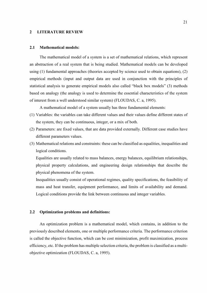
A local optimum, of an optimization problem, is an optimal solution of a set of nearby
set of solutions, while a global optimum is an optimal solution among all possible solutions. In
Figure 1 point (X2, Y2), is a local optimum, and point (X1, Y1) is a local and a global optimum.
Figure 1. Global optimum vs, local optimum
Global optimization deals with computation and characterization of global solutions for
continuous non-convex, mixed integer, algebraic differential, two-level, and non-factorizable
problems. Given an objective function f that must be minimized and a set of equality and
inequality constraints S, the main function of global deterministic optimization is to determine
24
(with theoretical guarantees) a global minimum for the objective function f subject to the set of
constraints S (FLOUDAS, C. A.; GOUNARIS, 2009).
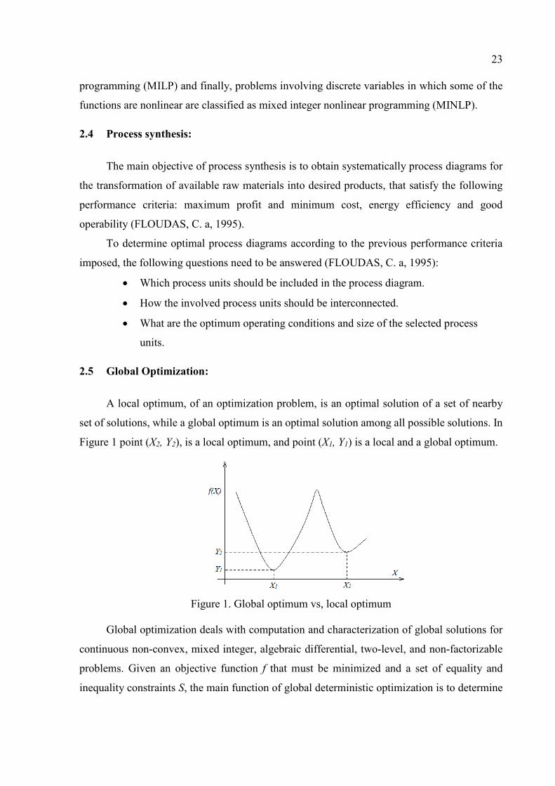
A function is convex (Figure 2), if the midpoint B of each chord A1A2 lies above the
corresponding point A0 of the graph of the function or coincides with this point. When solving
minimization problems of continuous variables with convex viable regions and convex
objective functions, any local minimum is a global minimum (EDGAR; HIMMELBLAU;
LASDON, 2001).
Figure 2. Convex function
The models that include non-linear equality constraints, such as those of mass balances
(bilinear terms - concentration flow product), non-linear physical property relations, nonlinear
blending equations, non-linear process models, and so, non-convexity that does not guaranty
that any local minimum is a global minimum. Any problem containing discretely valued
variables is a nonconvex problem (EDGAR; HIMMELBLAU; LASDON, 2001).
For global optimization, there are two categories of methods, deterministic methods and
heuristic methods. Deterministic methods, when executed until they reach their termination
criteria, allows to find a solution close to a global optimum and theoretically demonstrate that
this optimal value corresponds to a global solution. Heuristic methods can find globally optimal
solutions, but it is not theoretically possible to prove that the solution is a global solution
(EDGAR; HIMMELBLAU; LASDON, 2001).
25
2.6 Desalination:
Desalination process is a relatively consolidated technology for removing dissolved ions
in brackish water, seawater, or industrial effluents. This technique has allowed seawater to be
used for industrial purposes as well as for human consumption or even for water reuse
(KUCERA, 2014).
Desalination is seen as a relatively sustainable and viable technology to attain the need
of water increasing demand. However, the high energy demand of the processes currently used
combined to environmental concerns, water scarcity, high energy costs and the potential use of
renewable energy sources for desalination it has revived research and development in water
desalination.
Desalination has a great potential for development on a global scale. This is attributed
to the fact that of the 71 largest cities in the world that do not have local access to new freshwater
sources, 42 are located along the coasts, in addition, 2,400 million of the entire world
population, representing 39% of the total, live at a distance of less than 100 km from the sea
(GHAFFOUR; MISSIMER; AMY, 2013).
This shows the use of desalination technology in large proportions, to attain urban and industrial
freshwater demand.
2.7 Desalination Technologies:
Commercially available desalination technologies can be classified into thermals and
membranes, reverse osmosis (RO), multi-effect distillation (MED) and multi-stage flash (MSF)
are the dominant technologies in the market, of which, reverse osmosis being the fastest
growing application (SHATAT; RIFFAT, 2014).
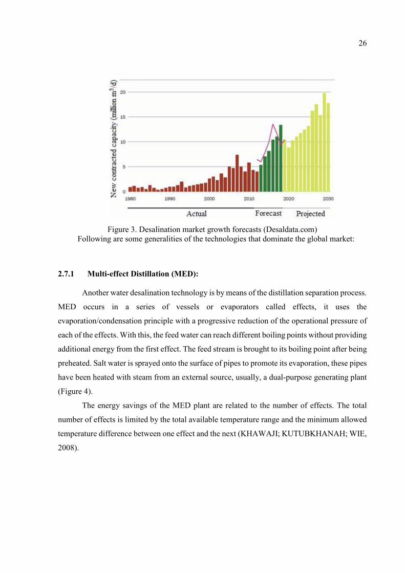
The global desalination capacity in 2015 was 100 million m3/day. On a global scale, 68%
of desalinated water is produced by membrane technologies, 30% by thermal technologies and
the remaining 2% is produced with other technologies. Desalination water supplies are divided
into 59% seawater, 22% ground brackish water, and the remainder, surface water, and effluents
with some degree of salinity (GHAFFOUR et al., 2015).
The forecast for market growth for the following years is shown in Figure 3 and it is
expected that by the year 2024 the desalination capacity will be close to 180 million m3/day and
by the year 2030 will be 280 million m3/day.
26
Figure 3. Desalination market growth forecasts (Desaldata.com) Following are some generalities of the technologies that dominate the global market:
2.7.1 Multi-effect Distillation (MED):
Another water desalination technology is by means of the distillation separation process.
MED occurs in a series of vessels or evaporators called effects, it uses the
evaporation/condensation principle with a progressive reduction of the operational pressure of
each of the effects. With this, the feed water can reach different boiling points without providing
additional energy from the first effect. The feed stream is brought to its boiling point after being
preheated. Salt water is sprayed onto the surface of pipes to promote its evaporation, these pipes
have been heated with steam from an external source, usually, a dual-purpose generating plant
(Figure 4).
The energy savings of the MED plant are related to the number of effects. The total
number of effects is limited by the total available temperature range and the minimum allowed
temperature difference between one effect and the next (KHAWAJI; KUTUBKHANAH; WIE,
2008).

27
Figure 4. Multi-effect distillation (SHATAT; RIFFAT, 2014)
2.7.2 Multiple Stage Flash (MSF):
In this case, the multistage flash distillation process is based on the flash evaporation
principle.
In the MSF process, the saline water is evaporated by reducing the pressure rather than
raising the temperature. The economy of the MSF technology is achieved by regenerative
heating where the saline water that is suffering the flash at each stage or camera flash is giving
some of its heat to the brine stream being fed at this stage.
The heat of condensation released by water vapor condensing on each step increases
gradually the temperature of the incoming stream. An MSF plant consists of heat input, heat
recovery system, waste heat sections (KHAWAJI; KUTUBKHANAH; WIE, 2008). Figure 5
presents an MSF representation.
Figure 5. Multiple Stage Flash (SHATAT; RIFFAT, 2014) Project and design of desalination plants are usually based on a series of environmental
studies and engineering decisions such as: water source assessment (chemical composition,
salinity, distance from the source to the plant), concentrate management options, pretreatment
options, desalination technology selection (MSF, MED, RO, or others), plant capacity,
28
estimation of energy requirements, post-treatment requirements (if necessary), among others
(VOUTCHKOV, 2012).
2.7.3 Reverse Osmosis (RO):
Water desalination by RO occurs when the feed solution is subjected to pressure larger
than the value its osmotic pressure, causing the water ions diffusion through a semipermeable
membrane, obtaining two streams: permeate (water desalted) and concentrated (a concentrated
aqueous solution containing salts). The amount of desalinated water obtained will depend on
the quantity and quality of the feed water, the quantity, and quality of the desired product, as
well as the technology and types of membranes involved and the operating pressure.
A reverse osmosis desalination system usually has five components: a water supply
system, a pre-treatment system, high-pressure pumping, arrangement of membrane modules
and post-treatment. These components are referenced as reverse osmosis network (RON).
Prior to the reverse osmosis process, there are the pretreatment steps. Pre-treatment aims
to remove suspended and colloidal solids to prevent fouling and biofilm growth on the surface
of the membranes, which decrease the permeate flux. The high-pressure pump needs to provide
sufficient pressure required to ensure the permeation of water through the membrane. Operating
pressures depend on the concentration of salts in the water but typically range from 15-25 bar
to brackish water and from 54-80 bar to seawater (SHATAT; RIFFAT, 2014).
Membrane modules arrangement consists of a number of pressure vessels in parallel,
each of which containing a number of membrane modules in series, where the number of
modules usually are 1 to 8 modules (Figure 10).
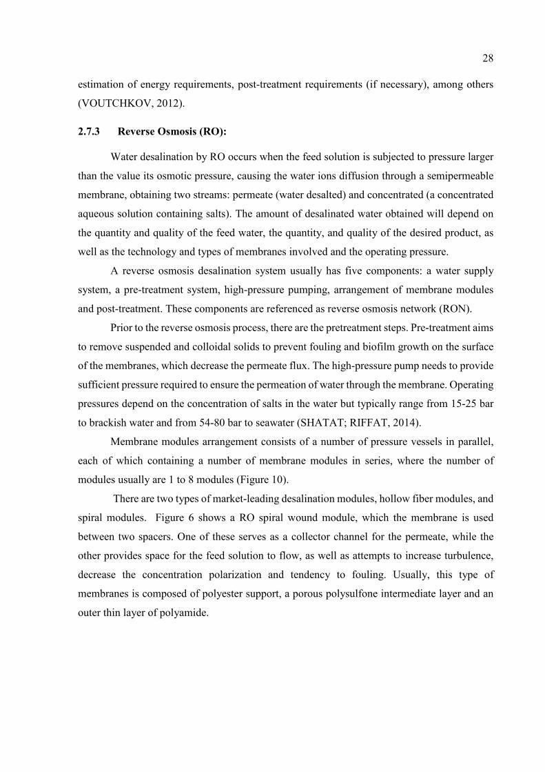
There are two types of market-leading desalination modules, hollow fiber modules, and
spiral modules. Figure 6 shows a RO spiral wound module, which the membrane is used
between two spacers. One of these serves as a collector channel for the permeate, while the
other provides space for the feed solution to flow, as well as attempts to increase turbulence,
decrease the concentration polarization and tendency to fouling. Usually, this type of
membranes is composed of polyester support, a porous polysulfone intermediate layer and an
outer thin layer of polyamide.
29
Figure 6. Spiral wound membrane module (DOW WATER & PROCESS SOLUTIONS, 2011)
Since this work focuses on the use and modeling of this technology, more detail on the
salt and water transport in reverse osmosis membranes is following:
The main transport properties of the processes that use pressure gradient as driving force
are: permeate flux, rejection of a certain component present in the feed solution and recovery
(HABERT; BORGES; NOBREGA, 2006).
The permeate flux (J) represents the volumetric water flowing through the membrane
per unit of time and unit of permeation area. The permeate flux is a function of the membrane
thickness, chemical composition of the feed, porosity, operating time and pressure across the
membrane (SINCERO & SINCERO, 2003). For water desalination, there are two main fluxes,
water, and salt (solute).
The model to describe the permeation mechanism used in this work is the solution-
diffusion model. According to this mechanism, the water flux Jw, is linked to the pressure and
concentration gradient across the membrane by the following equation:
( )WJ A p (1)
Where P is the pressure difference across the membrane, is the osmotic pressure
differential across the membrane and (A) is a constant (pure water permeability).
From this equation could see that when low pressure is applied ( P ) water flows
from the dilute to the concentrated salt-solution side of the membrane by normal osmosis; when
P there is no flow, and when P , water flows from the concentrate site to the
diluted side (desalination occurs).
The salt flux Js, is described by the equation:
( )S F PJ B C C (2)
30
where (B) is the salt permeability constant and FC and PC , respectively, are the salt
concentrations on the feed and permeate sides of the membrane.
From equations 1 and 2 could be observed that the water flux depends on the pressure,
but the salt flux is independent of the operating pressure since it is diffusive.
Recovery is a measure of the membrane selectivity and usually it's calculated as a
percentual relation between the produced permeate and the feed stream.
Temperature also affects both water and salt fluxes, since it affects the osmotic pressures
calculations and the values of the parameters (A) and (B) usually given by the membrane
fabricant and obtained in the laboratory.
So, the main operating parameters on membrane water and salt rejection are feed
pressure, salt concentration of feed solution and temperature. In this work, the effect of the
temperature is not considered (all problems solved at 25°C - standard conditions for the
parameters (A) and (B) given by the membrane fabricant), the feed salt concentration becomes
in an input parameter for a given problem living the pressure as the optimization variable.
In case of the RON arrangement where multiple membrane modules are used, the total
number of modules and its configuration is also an optimization variable since it is related to
the total membrane used and so to the total amount of fresh water produced.
In this work, for the transport phenomena model of the RO modules, the effect of the
polarization of the concentration is also considered, a phenomenon that occurs when a solution
permeates through a membrane selective to the solute, occurring an increase of solute
concentration in the membrane/solution interface, causing an increase in the osmotic pressure
of the solution near the membrane (CF of the equation 2), and decrease in driving force for the
separation and thus reducing the permeate flow (HABERT; BORGES; NOBREGA, 2006).
31
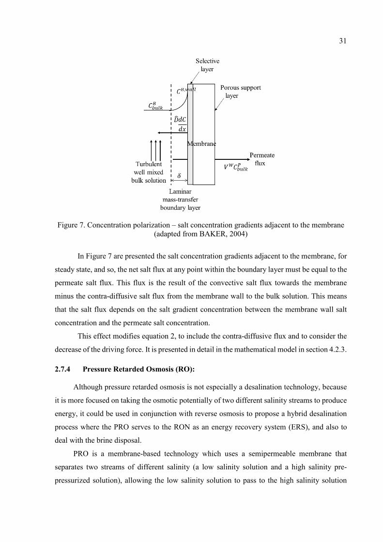
Figure 7. Concentration polarization – salt concentration gradients adjacent to the membrane (adapted from BAKER, 2004)
In Figure 7 are presented the salt concentration gradients adjacent to the membrane, for
steady state, and so, the net salt flux at any point within the boundary layer must be equal to the
permeate salt flux. This flux is the result of the convective salt flux towards the membrane
minus the contra-diffusive salt flux from the membrane wall to the bulk solution. This means
that the salt flux depends on the salt gradient concentration between the membrane wall salt
concentration and the permeate salt concentration.
This effect modifies equation 2, to include the contra-diffusive flux and to consider the
decrease of the driving force. It is presented in detail in the mathematical model in section 4.2.3.
2.7.4 Pressure Retarded Osmosis (RO):
Although pressure retarded osmosis is not especially a desalination technology, because
it is more focused on taking the osmotic potentially of two different salinity streams to produce
energy, it could be used in conjunction with reverse osmosis to propose a hybrid desalination
process where the PRO serves to the RON as an energy recovery system (ERS), and also to
deal with the brine disposal.
PRO is a membrane-based technology which uses a semipermeable membrane that
separates two streams of different salinity (a low salinity solution and a high salinity pre-
pressurized solution), allowing the low salinity solution to pass to the high salinity solution
32
side. The additional volume increases the pressure on this side, which can be depressurized by
a hydro-turbine to produce power (HELFER; LEMCKERT; ANISSIMOV, 2014). Since PRO
uses two streams with different osmotic potential to produce electrical power it can be aid to a
RO network by using the brine reject of the RO as the high salinity stream, in case of the low
salinity stream different authors has proposed the use of river water (NAGHILOO et al., 2015),
wastewater retentate (WAN; CHUNG, 2015), treated sewage (SAITO et al., 2012) and so. With
the aim of fully integrate RO and PRO technologies in this work pre-treated seawater as the
low salinity stream was used.
As for RO and other membrane-based technology, the phenomena are described by
determination of both salt and water fluxes, being the main operating variables the operating
feed pressure, the feed solution (low salinity stream) flow and salt concentration, the draw
solution (high salinity stream) flow and salt concentration, and temperature. In this work, as for
RO optimization, the effect of temperature is not considered.
Membrane parameters used for modeling are also pure water permeability (A) and solute
permeability (B), and an additional parameter usually referred as solute resistivity for diffusion
within the porous support layer (K) that group all the structural membrane parameters as
thickness, tortuosity, and porosity of the support layer.
As for RO, another phenomenon which reduces the effective osmotic pressure difference
across the membrane is the concentration polarization. As a result of water crossing the
membrane, the solute is concentrated on the feed side of the membrane surface and diluted on
the permeate side of the membrane surface (PRANTE et al., 2014).
33
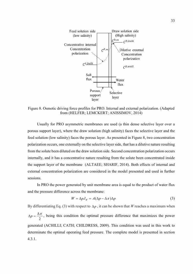
Figure 8. Osmotic driving force profiles for PRO. Internal and external polarization. (Adapted from (HELFER; LEMCKERT; ANISSIMOV, 2014)
Usually for PRO asymmetric membranes are used (a thin dense selective layer over a
porous support layer), where the draw solution (high salinity) faces the selective layer and the
feed solution (low salinity) faces the porous layer. As presented in Figure 8, two concentration
polarization occurs, one externally on the selective layer side, that has a dilutive nature resulting
from the solute been diluted on the draw solution side. Second concentration polarization occurs
internally, and it has a concentrative nature resulting from the solute been concentrated inside
the support layer of the membrane (ALTAEE; SHARIF, 2014). Both effects of internal and
external concentration polarization are considered in the model presented and used in further
sessions.
In PRO the power generated by unit membrane area is equal to the product of water flux
and the pressure difference across the membrane:
( )WW pJ A p p (3)
By differentiating Eq. (3) with respect to p , it can be shown that W reaches a maximum when
2p
, being this condition the optimal pressure difference that maximizes the power
generated (ACHILLI; CATH; CHILDRESS, 2009). This condition was used in this work to
determinate the optimal operating feed pressure. The complete model is presented in section
4.3.1.
34
2.8 Challenges and advances in desalination:
The main challenges and recent advances in desalination are directly or indirectly related
to the high energy cost of desalination. To meet desalination energy needs, researchers focused
on cogeneration, the use of renewable energy sources, and optimization of design and operation.
For desalination, power consumption is a key concern since energy costs constitute a major
portion of the operating costs. (GHOBEITY; MITSOS, 2014).
Desalination plants have traditionally been designed by manufacturers using empirical
and heuristic approaches (KUCERA, 2014). Membrane Manufacturers, for example, provide
engineering simulation tools, like Osmose Reverse System Analyzer (ROSA) by Dow
Chemicals, Rodesing and Rodata by Hydranautics, Ropro and Costpro by Koch Fluid systems,
Winflows by osmonics and Wincarol and 2pflows by Toray, all for the evaluation of various
types of membrane under several potential RO networks (RON). However, these tools have
limited capabilities, and allow only typical designs and limited operating conditions, for
example, constant operation.
The focus of advances has historically been the reduction of the specific capital cost of
desalination through technological advances, for example, improvements in membranes and the
development of low-cost heat exchangers for thermal desalination. However, advances in
computer simulation and mathematical programming have opened new avenues for improving
desalination technologies. Specifically, the development of new projects for desalination
systems through experimentation is not practical because of the high costs of the technologies
involved. The simulation of the design and, more specifically, the synthesis processes through
systematic optimization are, however, relatively cheap, considering the advances in
computational tools and numerical techniques.
In addition, optimization allows to explore various design configurations, for example,
process conditions and connectivity of equipment that may initially appear as unpromising, but
have not been evaluated or tested either experimentally or by simulation (GHOBEITY;
MITSOS, 2014).
Computational advances and optimization-based models for solving complex problems,
has provided opportunities to assess the performance of new systems, considering large
numbers of design variables and minimum parameters for optimization problems. Specifically,
nonlinear programming (NLP) has provided the opportunity to evaluate and develop new and
innovative projects as well as operational strategies (DAHDAH; MITSOS, 2014).
35
2.9 Reverse osmosis networks design and some hybrid systems:
Following is a review of the state of the art and the main work developed, involving
representation of desalination systems through superstructures, as well as the works involving
hybrid systems of thermal technologies, membranes or mixture of both.
Evangelista (1985) presented a graphical method for the design of reverse osmosis
plants, analogous to the stage calculations for unit operations, a turbulent regime, the
polarization of concentration neglected, and constant mass transfer coefficient were considered.
El-Halwagi et al. (1992) were the first to employ the superstructure representation for a
reverse osmosis network and developed a systematic procedure to solve the problem by
minimizing the discharge stream.
Voros et al. (1996) employed the methodology presented by Halwagi (1992), modified
for seawater desalination applications, the problem was formulated as an NLP, different
structures were analyzed, and some optimum configurations were identified.
El - Halwagi et al. (1997) presented an iterative procedure to solve the problem of design
and operation of a reverse osmosis network under different feeding conditions and maintenance
routines. The problem was formulated as a MINLP, using the superstructure representation and
using the Total Annualized Cost (TAC) as an objective function, the MINLP was solved using
the LINGO software.
Maskan et al. (2000) formulated a multivariable nonlinear optimization problem for
different configurations of the reverse osmosis network and different operating conditions. The
objective function was the annual profit, and different two stages RO configurations were
optimized.
Marcovecchio et al. (2005) presented a global optimization algorithm to find the
optimum design and operating conditions of reverse osmosis networks for seawater desalination
using hollow fiber modules and considering the polarization of the concentration. The proposed
algorithm is deterministic and reaches finite convergence to the global optimum. The procedure
is iterative and uses a bound contraction technique to accelerate convergence. The problem was
solved using the CONOPT solver of the General Algebraic Modeling System (GAMS). They
continued this work with a resolution of an MSF/RO hybrid system, proposed as an NLP
problem and solved again with CONOPT/GAMS. However, due to the high non-convexity of
the problem the global optimum could not be guaranteed (MARCOVECCHIO et al., 2005).
36
Vince et al. (2008) resolved a proposed RON as a MINLP problem, with multiple
objective functions (economic, technological and environmental performance indicators) using
an evolutionary algorithm as a solution method. In some cases, the authors found multiple
solutions.
An extensive review of engineering approaches to the design of reverse osmosis plants
for seawater desalination has been presented by KIM et al. (2009). The authors identified the
factors that influence the total cost of the RO plant, considering feed, pre-treatment, process
configuration, and post-treatment, specifically to the process configuration highlighted the
following: type of modules used, the number and capacity of stages, the number of pressure
vessels for each stage, mixture of different qualities of permeate and possibility of concentrate
recycling.
Optimization tools have also been applied for thermal desalination systems. Kamali e
Mohebinia (2008) used parametric optimization methods to increase the energy efficiency of
MED-TVC (multi-effect distillation with vapor compression), Shakib et al. (2012) e Ansari et
al.(2010) used genetic algorithms to improve the performance of a system MED-TVC coupled
with a generation turbine and a nuclear power plant respectively.
Abdulrahim e Alasfour (2010) performed a multi-objective optimization study for a
Multi-Stage Flash with concentrate recirculation (MSF-BR) and for a hybrid MSF/RO system,
using a genetic algorithm as a solution strategy. The results showed that the optimization with
multiple objectives tends to improve the performance of both systems.
Du et al. (2012) used a superstructure representation and formulated the optimization of
a RON as a MINLP problem. It was solved using the GAMS software and the outer
approximation algorithm, which consists of a series of iterations between NLP type
subproblems and a MILP type master problem. The GAMS/CPLEX and GAMS/MINOS
solvers were used to solve the MILP and NLP problems respectively. The global optimum
condition could not be guaranteed according to the methods used, since changes in the initial
values provided, produce different objective function results.
Park et al. (2012) used a Monte Carlo method to optimize forward osmosis and reverse
osmosis (FO/RO) hybrid systems, to identify the parameters that affect the energy efficiency of
the system. The authors found that the concentration polarization effect was the main
influencing factor and decreasing it was essential to maximize energy efficiency.
Sassi e Mujtaba (2012) formulated a MINLP optimization problem for a RON to
investigate the effects of temperature and concentration variations for the feed stream on the
37
optimum final structure. The objective of the optimization was to obtain the minimum total cost
of the plant, and the solution method was the outer approximation method using the gPROMS
software. The results revealed that the temperature and feed concentration have a significant
impact on the resulting structure and operating conditions.
Skiborowski et al. (2012) used a superstructure representation for a multi-effect
distillation/reverse osmose hybrid system (MED-RO). The problem is formulated as a MINLP,
a generalized superstructure for the hybrid desalination plant is constructed and conceptual
design considerations are used to reduce its complexity. The solvers GAMS/SBB and GAMS
/SNOPT were used. They found that the hybrid system was not the best option than the
individual MED or RO. The authors also solved a two-stage RON with commercial tool
BARON to compute the global optimal. After a predefined user maximum time of 250 hours,
it could not attain convergence, identifying the high structural complexity and non-linearity of
the problem.
Alnouri e Linke (2012) used Microsoft Excel (LINDO) to get the optimal configuration
of a RON considering generalized types of superstructures, in search of global optimal. The
authors applied the approximation proposed to examples developed by other authors, the results
were numerically close, but the computation times decreased considerably, however, the used
structures end up being restricted.
Lu et al. (2013) used a simplified superstructure of RON, and formulated the problem
as a MINLP, using as an objective function the Total Annual Cost (TAC).
The MINLP was solved using the GAMS software, and a previous simulation based on
heuristics considerations were made to obtain initial conditions of the variables for the MINLP
resolution. The type of membrane model used was an optimized variable.
Sassi e Mujtaba (2013) developed a MINLP model to evaluate boron rejection in an RO
process, with the objective of analyzing and optimizing the design and operation of a RON,
maintaining the desired levels of Boron in the desalinated water. The effects of seasonal
variation of temperature and pH for seawater feed stream on boron removal were considered.
The solution method was the outer approximation algorithm within software gPROMS. Results
suggest that pH and temperature are determining factors for achieving the desired boron
rejection.
Druetta et al. (2013) used structural optimization for thermal Multiple Effect
Evaporation (MEE). The authors used flow patterns as optimization variables and using
CONOPT / GAMS as a solution tool were able to reduce the specific area of heat exchange.

38
Saif et al. (2014) proposed a different operation of RON pressure vessels, considering
the partial removal of permeate at different stages of membrane modules along the pressure
vessel. Split partial second pass reverse osmoses (SPSPRO) is the concept and was formulated
as a MINLP. The solver DICOPT/GAMS was used. Since the answer is a local optimum, it
depends on the initial values provided. Although several starting points were used to solve the
case studies the global solution could not be guaranteed.
Zak e Mitsos (2014) have used large-scale numerical simulation to evaluate several
concepts of nontraditional hybrid thermal systems that mix the merits of MSF, MED, and MED-
TVC, finding for certain operating conditions, thermal hybrids that present higher energy
performance and required less area for heat exchange, compared to individual thermal systems,
in addition to these results, the authors emphasize the need for more detailed models and more
rigorous optimizations for future works that seek to propose new technological configurations.
Dahdah e Mitsos (2014) have used structural optimization to optimize the design of
hybrid thermal systems, specifically to combine desalination systems with vapor compression
systems, thus being able to propose new desalination technologies involving MSF, MED with
TVC. The hybrid configurations reported higher performance (relation between the amount of
distilled water obtained and energy supplied) and a smaller area of heat exchange compared to
conventional configurations.
Jiang et al. (2014) proposed a process model for a RON based on solution-diffusion
theory and mass transfer. The model is expressed in differential and algebraic equations with
some equality and inequality constraints. The model was transformed by orthogonal collocation
in an NLP model that was solved using the solver IPOPT/GAMS, the authors obtained profiles
of the pressure and feed concentration, in these profiles an optimum value was identified in the
energy consumption/desalinated water production curve, showing the potential of the
optimization in the design of RON systems.
Wang et al. (2014) optimized the operation of a large reverse osmosis desalination plant
(100.000 m3/day), using an evolutionary differential algorithm. The scheduling operation
problem was formulated as a MINLP, with the purpose to decrease the total cost of operation
when the conditions for which the plant was designed changes over the years. For this case,
when comparing the typical manual operation of the plant with the new operating routines
suggested by the optimization method, the operating cost decreased by 5%.
Alamansoori e Saif (2014) formulated a MINLP problem for the optimization of a
hybrid superstructure of Reverse Osmosis and Pressure Retarded Osmosis (RO/PRO) for the
39
simultaneous production of desalted water and electric energy. The MINLP problem was solved
with the solver SBB/GAMS, being initialized with random starting points, the optimal values
found are local optimum. The results show that the RO operation can be a viable source of the
salinity gradient required by PRO for the generation of electric energy,
Malik et al. (2015) have used Aspen Custom Modeler (ACM) software for the modeling
and simulation of an MSF/RO hybrid superstructure, to study and optimize various process
configurations. The process conditions such as temperatures and pressures and the design
variables such as MSF number of stages and the number of RON membrane modules were the
optimization variables to minimize the objective function (energy cost per kilogram fed). The
results suggest that the hybrid system is recommended for areas where high product quality is
required.
Jiang et al. (2015) formulated a nonlinear optimization problem as a differential
algebraic optimization problems (DAOPs), to reduce the operating costs of a full-scale RO plant
for variations in operating conditions. The DAOPs problem was discretized to be transformed
into an NLP problem that was resolved with the IPOPT/GAMS solver. The variables considered
were feed temperature, seawater salinity, electricity cost, and desalinated water demand. The
results showed that up to 26% cost savings can be achieved, compared to the conventional
process.
Lee et al. (2015) proposed a Multi-stage vacuum membrane distillation (MVMD) and
PRO hybrid system for the continuous production of desalinated water and electricity. The
system is proposed and the equations that define the system are established by means of a
numerical study, however, no optimization method was applied, resulting in a possibility of
future study subject to optimization.
Du et al. (2015) present an optimization study of an SPSPRO structure, with the purpose
of obtaining better qualities and permeate flows in the pressure vessel. The problem is proposed
as a MINLP and solved with the DICOPT/GAMS solver. It was observed that the strategy does
not guarantee the global optimum and the results depend strongly on the initial values provided.
However, the authors report that the SPSPRO configuration could provide a lower cost, lower
power consumption, and a smaller system size than the conventional process.
Wan e Chung (2016) have modeled a PRO / RO hybrid system with the option of closed-
cycle operation, trying to reduce seawater pretreatment costs. The authors report that the
specific energy consumption of a RO plant can be reduced by including PRO in the energy
recovery system. In addition, they identified the need to determine the optimum operating
40
pressure of the PRO that maximizes the energy utilization and minimizes the power
consumption of the PRO / RO hybrid system.
As previously mentioned this work aims to provide initial data systematically to reduce
the computing time of a RON MINLP, since most of the aforementioned works, in some cases
not give detail of how the preprocessing was done and how the initial data are obtained. The
proposed methodology in this work is based in the use of surrogated models that replace the
rigorous equations in a genetic algorithm that is used to provide the initial data used to solve
the rigorous MINLP.
41
3 OBJECTIVES
3.1 General Objective:
The general objective of this work is to develop a mathematical model and optimization
for the rigorous design of reverse osmosis networks and develop technological criteria, with no
introduction of initial values by the user. This procedure is based on the hypothesis considering
the possibility to achieve the optimal rigorous solution for the design of reverse osmosis
networks with no initial values previously known.
3.2 Specific objectives:
Construct a mathematical model for the design of reverse osmosis networks and
formulate an optimization problem using the total annualized cost as the
objective function and including the most relevant operational variables.
Using a new deterministic optimization methodology to solve the optimization
problem and obtain global solutions.
Propose a new combined stochastic – deterministic optimization methodology
to solve the optimization problem.
Using the stochastic – deterministic methodology to explore the effect of the
feed flow, seawater concentration, number of reverse osmosis stages, and the
maximum number of membrane modules in each pressure vessel on the total
annualized cost of the plant.
Propose a reverse osmosis – pressure retarded osmosis hybrid superstructure
where the PRO acts as an energy recovery unit and optimize it using the
stochastic – deterministic methodology proposed.
42
4 METHODOLOGY
The problem of synthesizing a reverse osmosis network (RON) consist in propose a cost-
effective network, including the optimum values for the number of reverse osmosis stages to
be used, the number of pressure vessels per stage, the number of modules per pressure vessel,
the number and type of auxiliary equipment, as well as the operational variables for all the
devices of the network, so the RON structure is formulated as a MINLP with the total
annualized cost TAC is used as an objective function.
To solve the problem of get optimal rigorous solutions for the design of RON, two
methodologies are used, the first is based on a new deterministic bound contraction strategy not
previously used for this kind of problems, and the second is a mixed stochastic – deterministic
strategy that also use surrogated models to reduce the mathematical complexity and aims to
reduce the computational effort.
Following are presented: the complete mathematical model, the metamodel construction,
and both strategies solutions proposed.
4.1 Reverse osmosis network – superstructure representation:
Figure 9 presents a superstructure of two stages reverse osmosis network involving a set
of parallel pressure vessels per reverse osmosis stage, high-pressure pumps and turbines. These
are the units that are going to be considered in the superstructure representation. The feed flow
enters a high-pressure pump and is sent to the first RO stage where it is separated into two
streams: permeate and brine. The brine leaving the first RO stage feeds the second RO stage,
but a fraction could be recycled. Recycling increases the velocity through the membrane module
and thus reduces the concentration polarization. The final brine from the second stage goes to
a turbine to recover the residual energy. The permeates from stages 1 and 2 are mixed to get the
final permeate.
All the possible connections between the existing units are obtained by taking into
account the following considerations:
• The feed stream (Fs) enters at atmospheric pressure, so it can’t be connected directly to
the RO stages.
• Blending the brine final stream (FB) is not necessary because there is no restriction of
concentration discharge of the concentrated stream.
• The pressurization of product streams (FP and FB) is unnecessary.
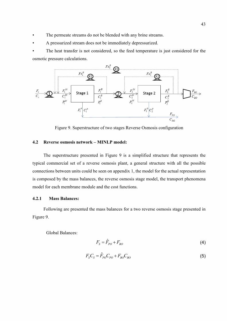
43
• The permeate streams do not be blended with any brine streams.
• A pressurized stream does not be immediately depressurized.
• The heat transfer is not considered, so the feed temperature is just considered for the
osmotic pressure calculations.
Figure 9. Superstructure of two stages Reverse Osmosis configuration
4.2 Reverse osmosis network – MINLP model:
The superstructure presented in Figure 9 is a simplified structure that represents the
typical commercial set of a reverse osmosis plant, a general structure with all the possible
connections between units could be seen on appendix 1, the model for the actual representation
is composed by the mass balances, the reverse osmosis stage model, the transport phenomena
model for each membrane module and the cost functions.
4.2.1 Mass Balances:
Following are presented the mass balances for a two reverse osmosis stage presented in
Figure 9.
Global Balances:
ˆS PO BOF F F (4)
ˆS S PO PO BO BOF C F C F C (5)
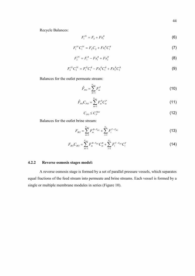
44
Recycle Balances:
1 1IN B
S RF F F (6)
1 1 1 1IN IN B B
S S RF C F C F C (7)
2 1 1 2IN B B B
R RF F F F (8)
2 2 1 1 1 1 2 2IN IN B B B B B B
R RF C F C F C F C (9)
Balances for the outlet permeate stream:
1
ˆRON
P
PO m
m
F F
(10)
1
ˆRON
P P
PO PO m m
m
F C F C
(11)
Max
PO PC C (12)
Balances for the outlet brine stream:
1 1
RO T
BO BO
N NB F T F
BO m t
m t
F F F
(13)
1 1
RO T
BO BO
N NB F T FB T
BO BO m m t t
m t
F C F C F C
(14)
4.2.2 Reverse osmosis stages model:
A reverse osmosis stage is formed by a set of parallel pressure vessels, which separates
equal fractions of the feed stream into permeate and brine streams. Each vessel is formed by a
single or multiple membrane modules in series (Figure 10).
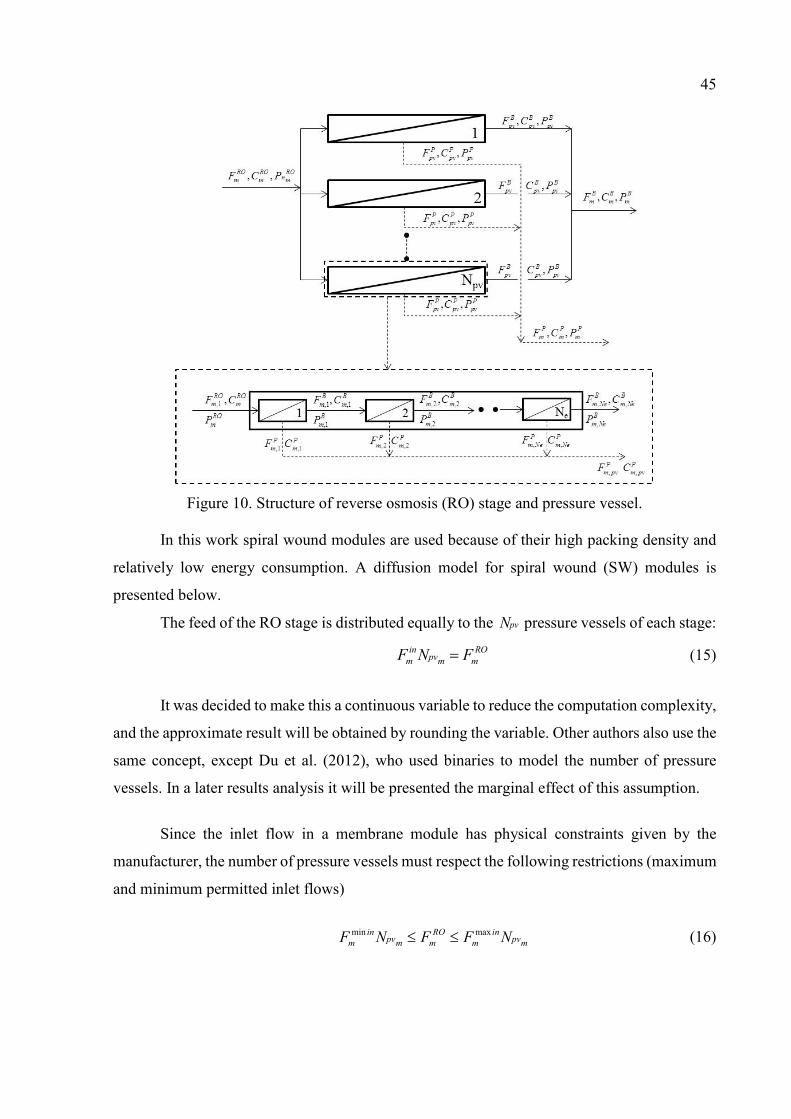
45
Figure 10. Structure of reverse osmosis (RO) stage and pressure vessel.
In this work spiral wound modules are used because of their high packing density and
relatively low energy consumption. A diffusion model for spiral wound (SW) modules is
presented below.
The feed of the RO stage is distributed equally to the pvN pressure vessels of each stage:
in RO
m m mpvF N F (15)
It was decided to make this a continuous variable to reduce the computation complexity,
and the approximate result will be obtained by rounding the variable. Other authors also use the
same concept, except Du et al. (2012), who used binaries to model the number of pressure
vessels. In a later results analysis it will be presented the marginal effect of this assumption.
Since the inlet flow in a membrane module has physical constraints given by the
manufacturer, the number of pressure vessels must respect the following restrictions (maximum
and minimum permitted inlet flows)
min maxin RO in
m m m m mpv pvF N F F N (16)
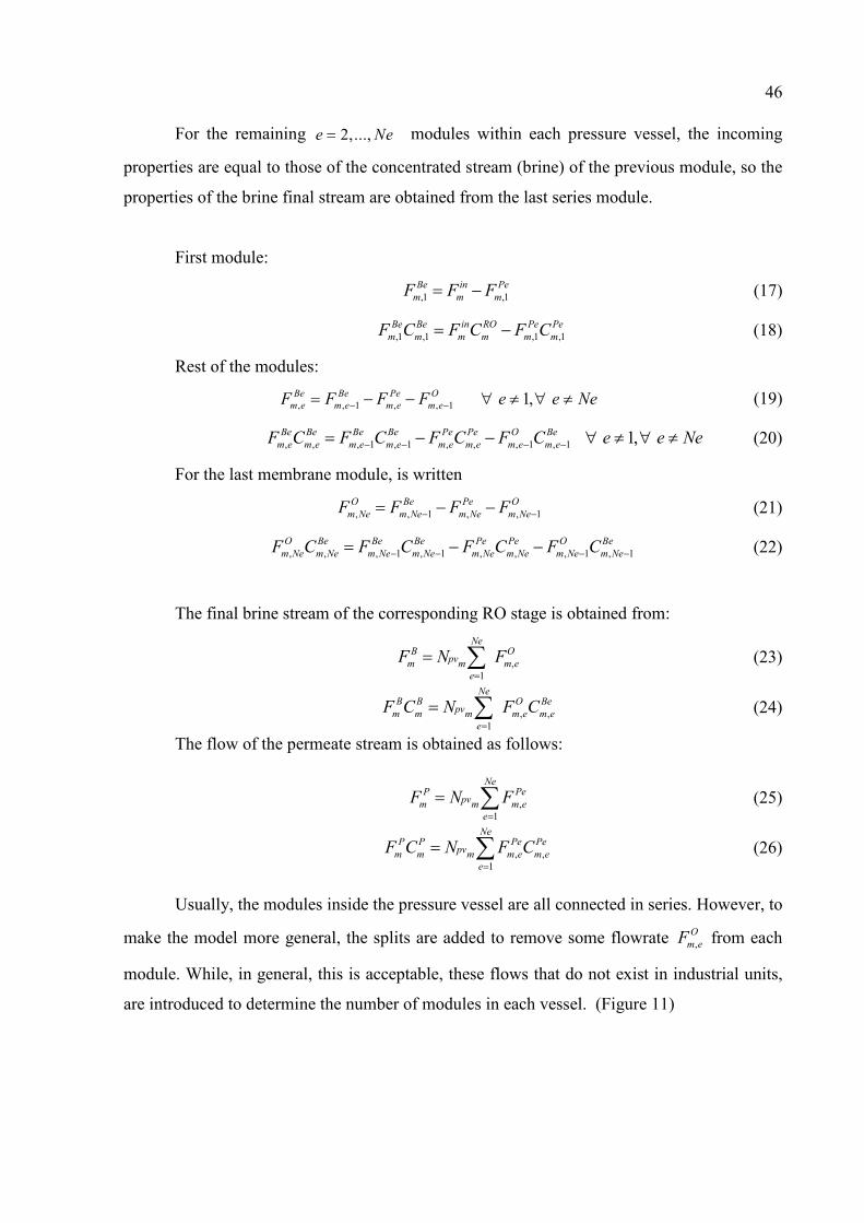
46
For the remaining 2,...,e Ne modules within each pressure vessel, the incoming
properties are equal to those of the concentrated stream (brine) of the previous module, so the
properties of the brine final stream are obtained from the last series module.
First module:
,1 ,1 Be in Pe
m m mF F F (17)
,1 ,1 ,1 ,1 Be Be in RO Pe Pe
m m m m m mF C F C F C (18)
Rest of the modules:
, , 1 , , 1 1, Be Be Pe O
m e m e m e m eF F F F e e Ne (19)
, , , 1 , 1 , , , 1 , 1 1, Be Be Be Be Pe Pe O Be
m e m e m e m e m e m e m e m eF C F C F C F C e e Ne (20)
For the last membrane module, is written
, , 1 , , 1O Be Pe O
m Ne m Ne m Ne m NeF F F F (21)
, , , 1 , 1 , , , 1 , 1O Be Be Be Pe Pe O Be
m Ne m Ne m Ne m Ne m Ne m Ne m Ne m NeF C F C F C F C (22)
The final brine stream of the corresponding RO stage is obtained from:
,1
NeB O
m m m e
e
pvF N F
(23)
, ,1
NeB B O Be
m m m m e m e
e
pvF C N F C
(24)
The flow of the permeate stream is obtained as follows:
,1
NeP Pe
m m m e
e
pvF N F
(25)
, ,1
NeP P Pe Pe
m m m m e m e
e
pvF C N F C
(26)
Usually, the modules inside the pressure vessel are all connected in series. However, to
make the model more general, the splits are added to remove some flowrate ,O
m eF from each
module. While, in general, this is acceptable, these flows that do not exist in industrial units,
are introduced to determine the number of modules in each vessel. (Figure 11)
47
Figure 11. By-pass representation of a single pressure vessel.
For these, binary variables ,O
m ey are further introduced which are one if a flow ,O
m eF
>0, and zero otherwise. Thus, the following equations are introduced:
, , 0O O
m e m eF y (27)
By adding the following equation, only one of the flows to be different from zero is
forced:
,1
1Ne
O
m e
e
y
(28)
In addition, to make sure that , ,Be O
m e m eF F when ,O
m ey =1, is written:
, , ,( ) (1 ) 0Be O O
m e m e m eF F y (29)
To obtain the number of modules Ne in a pressure vessel the next expression is used:
,1 ,2 ,3 ,4 ,5 ,6 ,7 ,81* 2* 3* 4* 5* 6* 7* 8*O O O O O O O O
m m m m m m m mNe y y y y y y y y (30)
4.2.3 Membrane modules model:
To obtain the permeate flow and concentration of each membrane module a widely used
and accepted solution-diffusion model is used (ALBASTAKI; ABBAS, 1999) which describes
the transport phenomena of salt and water through the membrane (Figure 12). It depends on the
pure water and salt permeabilities, which are parameters provided by the membrane modules
manufactures (HABERT; BORGES; NOBREGA, 2006).
Another phenomenon that must be considered in the model is the polarization of the
concentration since it decreases the permeate flux (BAKER, 2004). To describe this
phenomenon is widely used the liquid film theory, being necessary to determine the mass
transfer coefficient calculated as the relationship between the numbers of Sherwood, Reynolds,
and Schmidt (SCHOCK; MIQUEL, 1987).
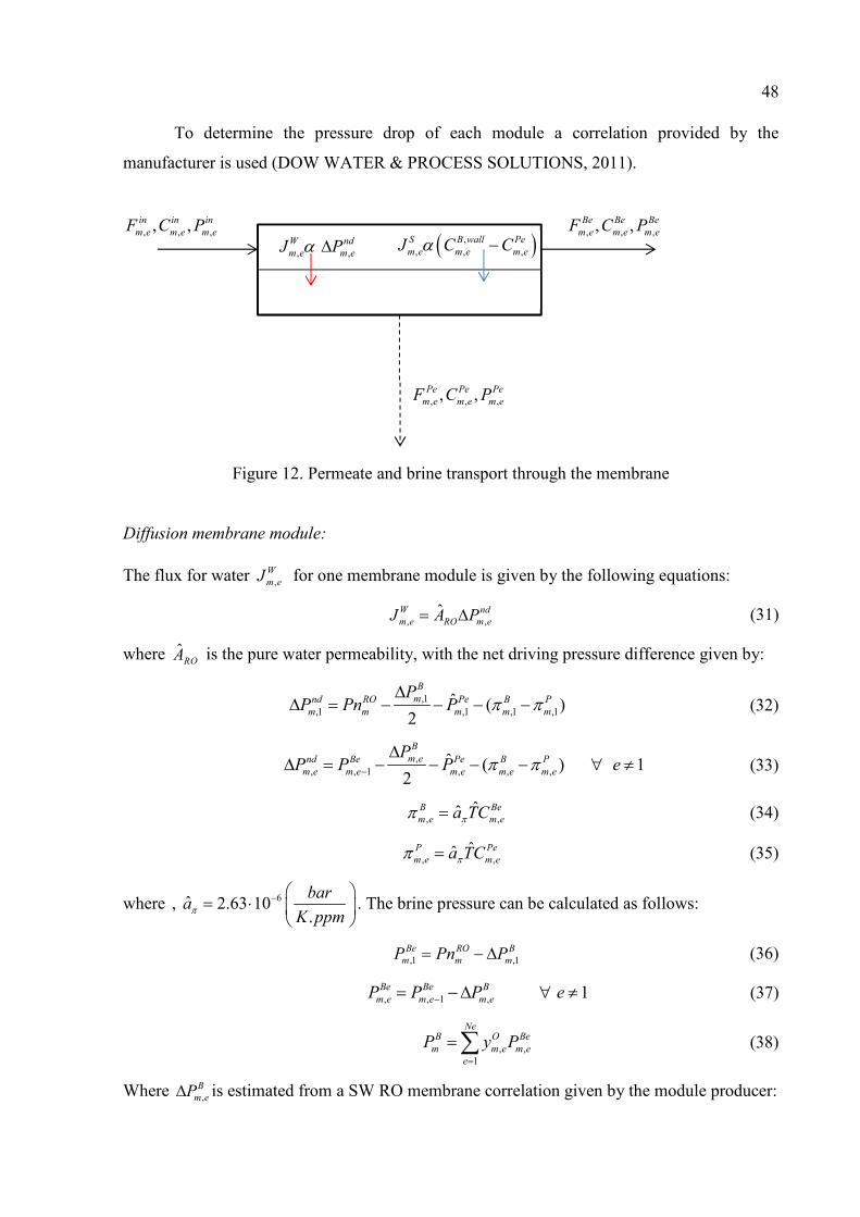
48
To determine the pressure drop of each module a correlation provided by the
manufacturer is used (DOW WATER & PROCESS SOLUTIONS, 2011).
Figure 12. Permeate and brine transport through the membrane Diffusion membrane module:
The flux for water ,
W
m eJ for one membrane module is given by the following equations:
, ,ˆW nd
m e RO m eJ A P (31)
where ˆROA is the pure water permeability, with the net driving pressure difference given by:
,1,1 ,1 ,1 ,1
ˆ ( )2
B
mnd RO Pe B P
m m m m m
PP Pn P
(32)
,, , 1 , , ,
ˆ ( ) 12
B
m end Be Pe B P
m e m e m e m e m e
PP P P e
(33)
, ,ˆˆB Be
m e m ea TC (34)
, ,ˆˆP Pe
m e m ea TC (35)
where 6ˆ, 2.63 10.
bara
K ppm
. The brine pressure can be calculated as follows:
,1 ,1 Be RO B
m m mP Pn P (36)
, , 1 , 1Be Be B
m e m e m eP P P e (37)
, ,1
Ne
B O Be
m m e m e
e
P y P
(38)
Where ,B
m eP is estimated from a SW RO membrane correlation given by the module producer:
, , ,, ,in in in
m e m e m eF C P
, , ,, ,Be Be Be
m e m e m eF C P
, , ,, ,Pe Pe Pe
m e m e m eF C P
, , W nd
m e m eJ P ,, , ,
S B wall Pe
m e m e m eJ C C
49
1.7
,, 9532.4
ˆ
av
m eB
m e
av
FP
(39)
,1,1
2
in Be
m mav
m
F FF
(40)
, 1 , 1 ,, 1,
2
Be O Be
m e m e m eav
m e
F F FF e e Ne
(41)
, 1 , 1 ,, 2
Be O O
m Ne m Ne m Neav
m Ne
F F FF
(42)
In turn, the flux solute ,S
m eJ is given by:
,, , ,
ˆS B wall Pe
m e RO m e m eJ B C C (43)
where ˆROB is the salt permeability. The membrane wall concentration is:
,
,,, , , ,( )
wm e
m e
V
ksB wall Pe Be Pe
m e m e m e m eC C C C e (44)
Where ,m e
mks
s
is the mass transfer coefficient, and ,w
m e
mV
s
the permeation velocity, which
are estimated using the following expressions:
0.75 0.33, ,
ˆˆ0.04 Re
ˆm e m e
Dks Sc
d (45)
, ,, ˆ
W S
m e m ew
m e
P
J JV
(46)
,ˆRe , , m e Sc D and d are the Reynolds, Schmidt, salt diffusivity, and feed space
thickness, respectively. They are given by:
,,
ˆ ˆRe
ˆ
s
h m e
m e
d U
(47)
ˆˆˆˆ
ScD
(48)
The hydraulic diameter ˆhd of a spiral wound module used to calculate the Reynolds
number depends on the channel height ˆsph , the specific surface area of the spacer ˆ
spS and the
void fraction (Figure 6):
50
ˆ4ˆ2 ˆˆ(1 )ˆ
h
sp
sp
d
Sh
(49)
The superficial velocity ,s
m eU depends on the average flow rate ,av
m eF , the density, and the
feed cross-section open area ˆfcS .
,, ˆˆ
av
m es
m e
fc
FU
S (50)
ˆˆ ˆ ˆfc L L spS w n h (51)
The feed cross-section open area is the product of the membrane leaf width ˆLw , the
number of leaves ˆLn and the spacer height ˆ
sph .
Finally, the permeate concentration and flow rate are:
,,
,
*1000S
m ePe
m e W
m e
JC
V (52)
, ,ˆ ˆPe W
m e m e mem PF V S (53)
ˆˆ ˆ ˆmem L L LS n l w (54)
Where ˆL
n is the number of leaves, ˆLl is the effective length and ˆ
Lw the width of the
module.
To avoid numerical problems, caused by zero values for non-existing membrane
modules in a pressure vessel the flux, a binary variable ,nd
m ey is introduced in the water flux ,W
m eJ
expression as follows:
, , ,ˆW nd nd
m e RO m e m eJ A P y (55)
The next constraint, guarantees that the binary variable ,nd
m ey takes a value of zero if a
flow ,av
m eF = 0, and one otherwise.
1
, ' ,' 1
(1 )e
O nd
m e m e
e
y y
(56)
51
Indeed, when the flux has been diverted in the previous vessel, the summation will
become one and ,nd
m ey will become zero. Before the flow is diverted, the summation is zero and
,nd
m ey will be forced to one.
Now the following change of variable is introduced:
, , ,nd nd nd
m e m e m ew P y (57)
So, the water flux expression ,W
m eJ turns into:
, ,ˆW nd
m e RO m eJ A w (58)
With the corresponding set of equations, to deal with the product of a binary and a
continuous variable, as follows:
, , 0nd nd nd
m e m ew y (59)
, 0nd
m ew (60)
, , ,( ) (1 ) 0nd nd nd
m e m e m eP w y (61)
, , 0nd nd
m e m eP w (62)
Now for the membrane wall concentration, because of the mass transfer coefficient
,m e
mks
s
, could take zero values when there is no flux through the membrane module, the
expression is re-written with the following change of variable:
,,, , , ,( ) m eB wall Pe Be Pe
m e m e m e m eC C C C e (63)
Where:
, , ,w
m e m e m eks V (64)
52
4.2.4 Costs and objective function:
The following economic model is based in the one proposed by Malek et al. (1996).
Objective function
Minimize the Total Annualized Cost (TAC), given by:
TAC AOC ccf TCC (65)
where 1
1
( 1)
( 1) 1
t
t
ir iccf
ir
. In turn,
1.25 (1.15 )equipTCC CC (66)
The equipment cost is given by:
equip swip HPP T mem pvCC CC CC CC CC CC (67)
The salted water intake and pretreatment system cost:
0.8996(24( ))swip SW INCC Q (68)
where SW INQ is the feed flow rate to the system in m3/h.
Cost of pump and turbines:
52 ( )HPP HPP
HPP p p
p
CC P Q (69)
52 ( )HPPR
HPPR m m
m
RCC P Q (70)
52 ( )T T
T t t
t
CC P Q (71)
where HPP
pP , HPP
pQ , HPPR
mP , m
RQ and T
tP , T
tQ are the pressure drop in bar and flow rate in
m3/h for the high-pressure pump, recycle pump and turbine respectively. It should be noted that
this cost of capital is linear with power, a known shortcoming of previous models because it
cannot capture the nonlinear behaviors of costs (GUTHRIE, 1969). It will be discussed the
impact of this assumption in the results section.
Membrane module cost:
1
RON
mem m m mem
m
pvCC N Ne c
(72)
Pressure vessels cost:
1
RON
pv m
m
pv pvCC N c
(73)
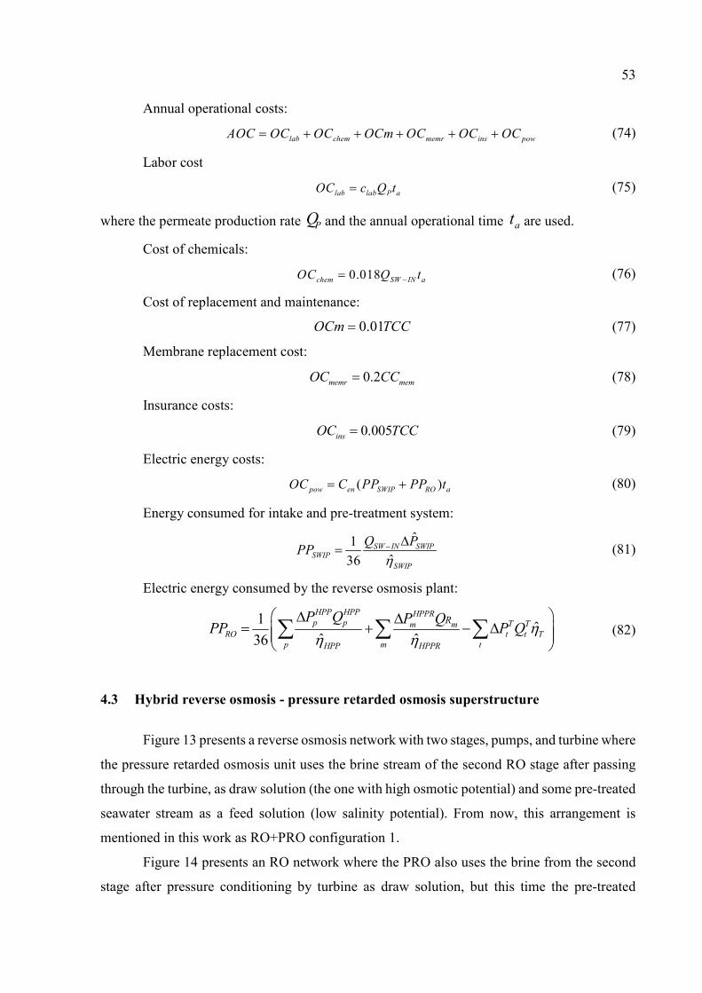
53
Annual operational costs:
lab chem memr ins powAOC OC OC OCm OC OC OC (74)
Labor cost
lab lab P aOC c Q t (75)
where the permeate production rate PQ and the annual operational time at are used.
Cost of chemicals:
0.018chem SW IN aOC Q t (76)
Cost of replacement and maintenance:
0.01OCm TCC (77)
Membrane replacement cost:
0.2memr mem
OC CC (78)
Insurance costs:
0.005ins
OC TCC (79)
Electric energy costs:
( )pow en SWIP RO aOC C PP PP t (80)
Energy consumed for intake and pre-treatment system:
ˆ1ˆ36
SW IN SWIPSWIP
SWIP
Q PPP
(81)
Electric energy consumed by the reverse osmosis plant:
1ˆ
ˆ ˆ36
HPP HPP HPPRp p T Tm m
RO t t T
p m tHPP HPPR
RP Q P QPP P Q
(82)
4.3 Hybrid reverse osmosis - pressure retarded osmosis superstructure
Figure 13 presents a reverse osmosis network with two stages, pumps, and turbine where
the pressure retarded osmosis unit uses the brine stream of the second RO stage after passing
through the turbine, as draw solution (the one with high osmotic potential) and some pre-treated
seawater stream as a feed solution (low salinity potential). From now, this arrangement is
mentioned in this work as RO+PRO configuration 1.
Figure 14 presents an RO network where the PRO also uses the brine from the second
stage after pressure conditioning by turbine as draw solution, but this time the pre-treated
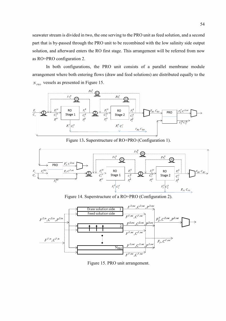
54
seawater stream is divided in two, the one serving to the PRO unit as feed solution, and a second
part that is by-passed through the PRO unit to be recombined with the low salinity side output
solution, and afterward enters the RO first stage. This arrangement will be referred from now
as RO+PRO configuration 2.
In both configurations, the PRO unit consists of a parallel membrane module
arrangement where both entering flows (draw and feed solutions) are distributed equally to the
PRON vessels as presented in Figure 15.
Figure 13. Superstructure of RO+PRO (Configuration 1).
Figure 14. Superstructure of a RO+PRO (Configuration 2).
Figure 15. PRO unit arrangement.
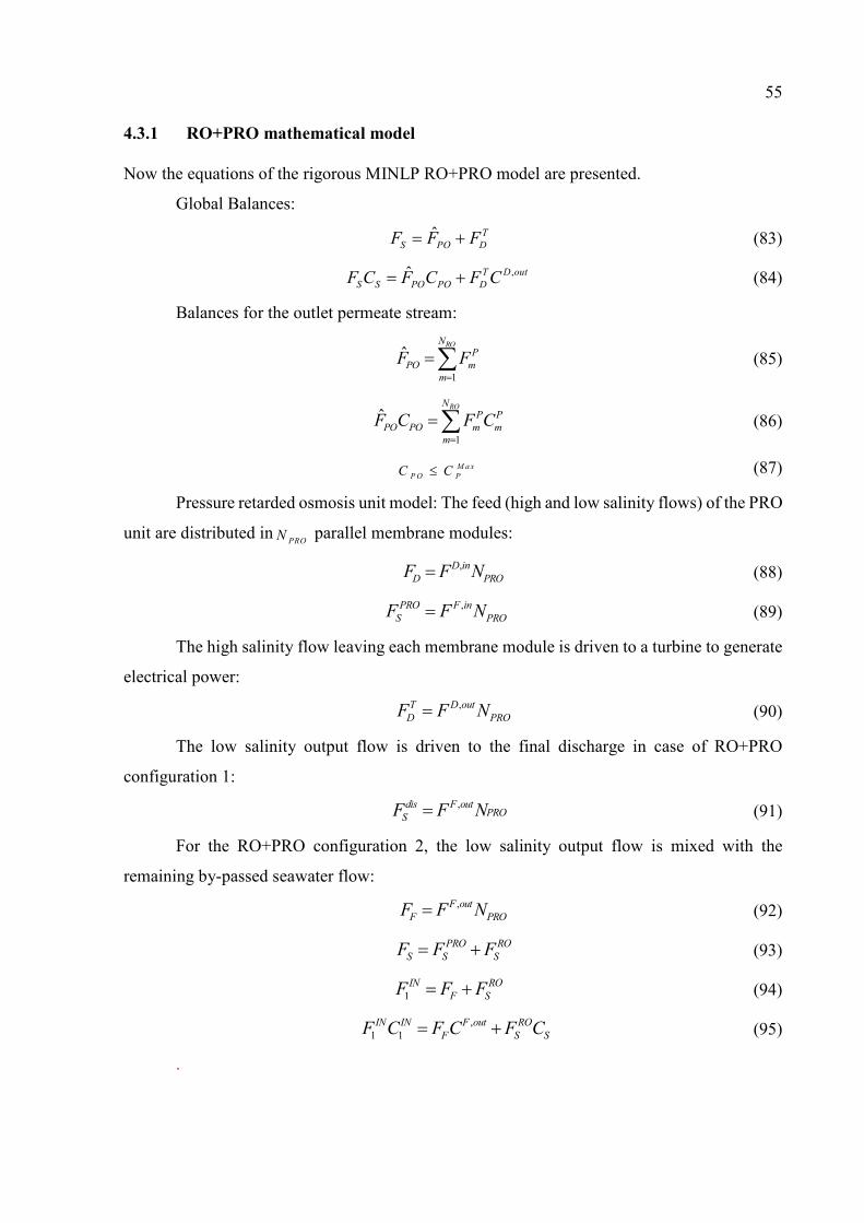
55
4.3.1 RO+PRO mathematical model
Now the equations of the rigorous MINLP RO+PRO model are presented.
Global Balances:
ˆ T
S PO DF F F (83)
,ˆ T D out
S S PO PO DF C F C F C (84)
Balances for the outlet permeate stream:
1
ˆRON
P
PO m
m
F F
(85)
1
ˆRON
P P
PO PO m m
m
F C F C
(86)
M a x
P O PC C (87)
Pressure retarded osmosis unit model: The feed (high and low salinity flows) of the PRO
unit are distributed inPRO
N parallel membrane modules:
,D in
D PROF F N (88)
,PRO F in
S PROF F N (89)
The high salinity flow leaving each membrane module is driven to a turbine to generate
electrical power:
,T D out
D PROF F N (90)
The low salinity output flow is driven to the final discharge in case of RO+PRO
configuration 1:
,dis F out
S PROF F N (91)
For the RO+PRO configuration 2, the low salinity output flow is mixed with the
remaining by-passed seawater flow:
,F out
F PROF F N (92)
PRO RO
S S SF F F (93)
1IN RO
F SF F F (94)
,1 1IN IN F out RO
F S SF C F C F C (95)
.
56
The inlet flows of a PRO membrane module are restricted to a specific range by the
commercial provider:
, m in , m axD in D D in
P RO P R OF N F F N (96)
, min , maxF in PRO F in
PRO S PROF N F F N (97)
The output conditions for the high salinity (draw solution) side:
, , ˆD out D in PRO PRO
W memF F J S (98)
, ,,
,
ˆD in D in PRO PROD out S mem
D out
F C J SC
F
(99)
Output conditions for the low salinity (feed solution) side:
, , ˆF out F in PRO PRO
W memF F J S (100)
, ,,
,
ˆF in F in PRO PROF out S mem
F out
F C J SC
F
(101)
Where ˆ PRO
memS , is the PRO membrane area, and the PRO water flux PRO
WJ , considering
internal and external polarization and the solute reverse flux could be obtained from:
ˆexp exp
1ˆˆ ˆ2
1 exp exp
PRO PROD FW W
PRO
PRO D
W PROPRO PRO
PRO W W
PRO PRO
W
J J K
kJ A P
B J K J
J k
(102)
where ˆP R OA is the pure water permeability, ˆ
P R OB is the salt permeability and
PRO mk
s
is the mass transfer coefficient that could be estimated as:
0.57 0.40ˆ
ˆ0.2 Reˆ
PRO
h
Dk Sc
d (103)
where ,ˆRe , , m e Sc D and ˆ
hd are the Reynolds, Schmidt, salt diffusivity, and hydraulic
diameter, respectively. They are given by:
ˆ ˆRe
ˆ
s
hd U
(104)
ˆˆˆˆ
ScD
(105)
57
The superficial velocity ,s
m eU depends on the average flow rate ,av
m eF , the density, and the feed
cross-section open area ˆfcS .
ˆˆ
avs
fc
FU
S (106)
, ,
2
D in D outav F F
F
(107)
The parameter K is the solute resistivity for diffusion within the porous support layer
and is defined by:
ˆˆ ˆˆˆ ˆˆ
t SK
D D
(108)
Where t , , and , are the thickness, tortuosity, and porosity of the support layer,
respectively and S is known as the structural parameter.
According to Schock (SCHOCK; MIQUEL, 1987), for low Reynolds numbers
(100<Re<1000) the local solution pressure losses in spiral wound modules can be calculated as
(where DP is in pascals):
0.3 26.23Re ( )ˆ2
sD
h
U LP
d
(109)
With the osmotic pressure of the draw and feed solution:
,ˆˆD D ba TC (110)
,ˆˆF F ba TC (111)
Calculated at bulk concentration conditions:
, ,,
2
D out D inD b C C
C
(112)
, ,,
2
F out F inF b C C
C
(113)
The reverse salt flux is given by:
, ,ˆ
exp expˆ
ˆ ˆ1 exp exp
PRO PROD b F bW W
PRO
PRO
S PROPRO PRO
PRO W W
PRO PRO
W
J J KC C
kJ B
B J K J
J k
(114)
58
The reverse osmosis stages model is the same as presented in sections 4.2.2 and 4.2.3.
The objective function and the cost equations for the RO+PRO superstructure are
essentially the same as presented in section 4.2.4 with the following modifications (all related
with the additional costs associated with the PRO unit):
The equipment cost is given by:
equip sw ip H P P H PPR T m em pv Tpro m em pro pvproC C C C C C CC CC C C CC C C CC CC
(115) Additional required turbine:
52( )Tpro Tpro
TproCC P Q (116)
Membrane module cost for PRO:
PRON
mempro mempropvproCC N c (117)
Pressure vessels cost for PRO:
pvpro pvpro pvproC C N c (118)
Annual operational costs:
la b ch em m em r ins p o w m em proA O C O C O C O C m O C O C O C O C
(119)
Membrane replacement cost for PRO:
0.2mempro memproOC CC (120)
Electric energy consumed by the RO+PRO plant:
1ˆ ˆ
ˆ ˆ36
HPP HPP HPPRp p T T Tpro Tprom m
RO t t T T
p m tHPP HPPR
RP Q P QPP P Q P Q
(121)
59
4.4 MINLP problem statement
The mass balances of mixing and division nodes for the distribution box, the reverse
osmosis stages model, the transport model for each module, the cost functions, the objective
function, as well as all possible physical constraints (flow and concentration of permeate,
maximum pressures and brine concentration allowed) form the proposed MINLP model for the
optimization of a reverse osmosis network.
Thus, the optimization problem is state as the following considerations:
Given:
Feed water concentration, membrane module parameters to be used, permeate flow
required, maximum salt concentration allowed for discharge stream, and energy costs.
Optimize:
Number of membrane modules in each pressure vessel, recycles, and operational
variables (seawater flowrate, feed pressure for each RO stage, and inlet flow to the first
membrane module).
To minimize:
Total annualized cost for the RO network, subject to process constraints: equality
constraints such as model equations, and inequality constraints such as the limits of the
optimization variables.
In case of the hybrid RO+PRO superstructure, the optimization problem statement is
basically the same, it just includes the additional PRO membrane model equations and its
respective operational parameters.
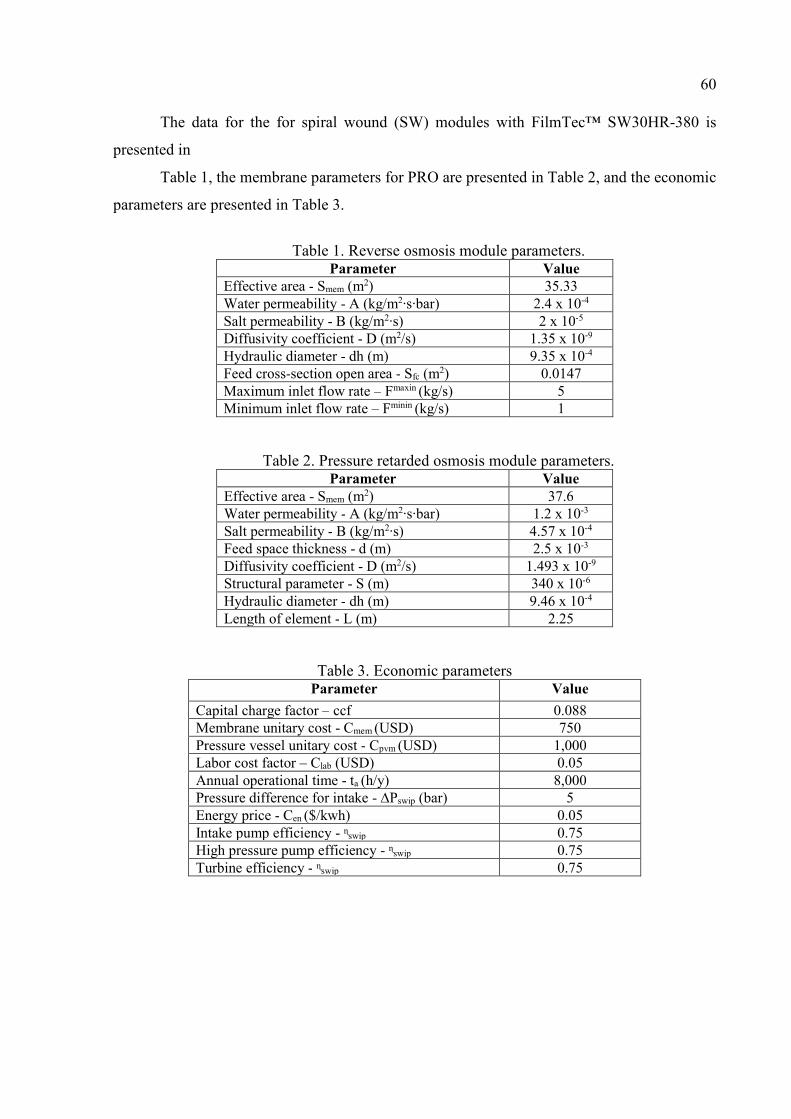
60
The data for the for spiral wound (SW) modules with FilmTec™ SW30HR-380 is
presented in
Table 1, the membrane parameters for PRO are presented in Table 2, and the economic
parameters are presented in Table 3.
Table 1. Reverse osmosis module parameters.
Parameter Value
Effective area - Smem (m2) 35.33 Water permeability - A (kg/m2∙s∙bar) 2.4 x 10⁻⁴ Salt permeability - B (kg/m2∙s) 2 x 10⁻⁵ Diffusivity coefficient - D (m2/s) 1.35 x 10⁻⁹ Hydraulic diameter - dh (m) 9.35 x 10⁻⁴ Feed cross-section open area - Sfc (m2) 0.0147 Maximum inlet flow rate – Fmaxin (kg/s) 5 Minimum inlet flow rate – Fminin (kg/s) 1
Table 2. Pressure retarded osmosis module parameters. Parameter Value
Effective area - Smem (m2) 37.6 Water permeability - A (kg/m2∙s∙bar) 1.2 x 10⁻³ Salt permeability - B (kg/m2∙s) 4.57 x 10⁻⁴ Feed space thickness - d (m) 2.5 x 10⁻³ Diffusivity coefficient - D (m2/s) 1.493 x 10⁻⁹ Structural parameter - S (m) 340 x 10-6 Hydraulic diameter - dh (m) 9.46 x 10⁻⁴ Length of element - L (m) 2.25
Table 3. Economic parameters Parameter Value
Capital charge factor – ccf 0.088 Membrane unitary cost - Cmem (USD) 750 Pressure vessel unitary cost - Cpvm (USD) 1,000 Labor cost factor – Clab (USD) 0.05 Annual operational time - ta (h/y) 8,000 Pressure difference for intake - ∆Pswip (bar) 5 Energy price - Cen ($/kwh) 0.05 Intake pump efficiency - ᶯswip 0.75 High pressure pump efficiency - ᶯswip 0.75 Turbine efficiency - ᶯswip 0.75
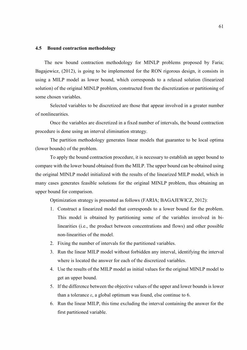
61
4.5 Bound contraction methodology
The new bound contraction methodology for MINLP problems proposed by Faria;
Bagajewicz, (2012), is going to be implemented for the RON rigorous design, it consists in
using a MILP model as lower bound, which corresponds to a relaxed solution (linearized
solution) of the original MINLP problem, constructed from the discretization or partitioning of
some chosen variables.
Selected variables to be discretized are those that appear involved in a greater number
of nonlinearities.
Once the variables are discretized in a fixed number of intervals, the bound contraction
procedure is done using an interval elimination strategy.
The partition methodology generates linear models that guarantee to be local optima
(lower bounds) of the problem.
To apply the bound contraction procedure, it is necessary to establish an upper bound to
compare with the lower bound obtained from the MILP. The upper bound can be obtained using
the original MINLP model initialized with the results of the linearized MILP model, which in
many cases generates feasible solutions for the original MINLP problem, thus obtaining an
upper bound for comparison.
Optimization strategy is presented as follows (FARIA; BAGAJEWICZ, 2012):
1. Construct a linearized model that corresponds to a lower bound for the problem.
This model is obtained by partitioning some of the variables involved in bi-
linearities (i.e., the product between concentrations and flows) and other possible
non-linearities of the model.
2. Fixing the number of intervals for the partitioned variables.
3. Run the linear MILP model without forbidden any interval, identifying the interval
where is located the answer for each of the discretized variables.
4. Use the results of the MILP model as initial values for the original MINLP model to
get an upper bound.
5. If the difference between the objective values of the upper and lower bounds is lower
than a tolerance ε, a global optimum was found, else continue to 6.
6. Run the linear MILP, this time excluding the interval containing the answer for the
first partitioned variable.
62
7. If an infeasible solution, or feasible with an objective value greater than the actual
upper bound are obtained, all the intervals that were not excluded are eliminated,
and the surviving feasible interval is partitioned again.
8. Repeat steps 6 and 7 for the rest of the partitioned variables, one at the time.
9. Return to step number 3, a new iteration starts with the new contracted bounds.
Iterations are made until attaining convergence or until the bounds cannot be contracted
anymore, in that case, there are two possibilities:
Increase the number of intervals to a level at which the size of the intervals is small
enough to generate a lower bound with an acceptable tolerance to the upper bound.
Divide the problem into two or more subproblems using a strategy similar to the branch
and bound procedures.
Figure 16 presents the bound contraction methodology summarized.
Figure 16. Bound contraction – interval elimination strategy.
4.6 Stochastic – deterministic methodology
A genetic algorithm is used to provide good initial values for the rigorous MINLP model,
to compute optimal solutions. Two different solutions are tested, first the genetic algorithm
using the rigorous equations is solved followed by the rigorous MINLP, and second, the use of
rigorous equations of the model in the genetic algorithm is replaced by a metamodel and the
solution is again used as initial values for the rigorous MINLP.
63
4.6.1 Reverse osmosis metamodel construction:
Simple quadratic polynomials are used as metamodels: The equations of the membrane
diffusion model were solved numerically for different inlet conditions (values selected
according to the bounds of the problem) to obtain a mesh of input-output data pairs. Two
different regions were identified for the permeate concentration: A Linear Region and a Non-
Linear Region, the expressions are presented next.
Linear Region: The concentration was adjusted to first order polynomial as follows:
1 2 3 4Pe IN IN INC K K P K C K F (122)
Non-Linear Region: Permeate concentration was adjusted according to the mathematical
expression presented below:
2 2 2
1 2 3 4 5 6
2 2 2 2 2 2
7 , 8 9 10
2 2 2
11 12 13 14
15
Pe IN IN IN IN IN
in IN IN IN IN IN IN
m e
IN IN IN IN IN IN IN IN IN
IN IN IN
C K K P K C K F K P K C
K F K P C K P F K C F
K P C F K P C K P F K C F
K P C F
(123)
The permeate flow was adjusted to a first-order polynomial for all the operation region:
1 2 3 4 5
6 7 8
Pe IN IN IN IN IN
IN IN IN IN IN IN IN
F K K P K C K F K P C
K P F K C F K P C F
(124)
To obtain the coefficients of the metamodel a Diploid Genetic Algorithm (DGA)
programmed in MATLAB® (THE MATHWORKS INC., 2016) was used. The Simulations
were developed in a laptop with processor Intel(R) Core (TM) i7 – 3610QM CPU @ 2.3GHz
(8 CPUs) with 8192MB of RAM. Each variable ( PeC , PeF ), was evaluated using the equations
(122-124) for different inlet conditions ( INP , INC and INF ) using
estimated coefficients, to generate the metamodel solutions mesh. The same inlet conditions
were used with equations (31-54) to generate the rigorous solutions mesh. The fitness function
that was minimized to obtain the coefficients is the following:
2NRig Met
i
Fobj V V (125)
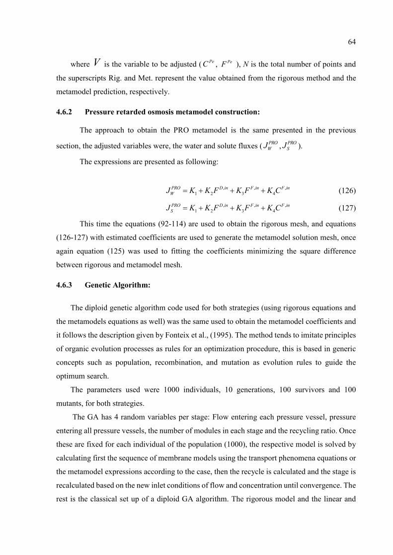
64
where V is the variable to be adjusted ( PeC , PeF ), N is the total number of points and
the superscripts Rig. and Met. represent the value obtained from the rigorous method and the
metamodel prediction, respectively.
4.6.2 Pressure retarded osmosis metamodel construction:
The approach to obtain the PRO metamodel is the same presented in the previous
section, the adjusted variables were, the water and solute fluxes ( PRO
WJ , PRO
SJ ).
The expressions are presented as following:
, , ,1 2 3 4
PRO D in F in F in
WJ K K F K F K C (126)
, , ,1 2 3 4
PRO D in F in F in
SJ K K F K F K C (127)
This time the equations (92-114) are used to obtain the rigorous mesh, and equations
(126-127) with estimated coefficients are used to generate the metamodel solution mesh, once
again equation (125) was used to fitting the coefficients minimizing the square difference
between rigorous and metamodel mesh.
4.6.3 Genetic Algorithm:
The diploid genetic algorithm code used for both strategies (using rigorous equations and
the metamodels equations as well) was the same used to obtain the metamodel coefficients and
it follows the description given by Fonteix et al., (1995). The method tends to imitate principles
of organic evolution processes as rules for an optimization procedure, this is based in generic
concepts such as population, recombination, and mutation as evolution rules to guide the
optimum search.
The parameters used were 1000 individuals, 10 generations, 100 survivors and 100
mutants, for both strategies.
The GA has 4 random variables per stage: Flow entering each pressure vessel, pressure
entering all pressure vessels, the number of modules in each stage and the recycling ratio. Once
these are fixed for each individual of the population (1000), the respective model is solved by
calculating first the sequence of membrane models using the transport phenomena equations or
the metamodel expressions according to the case, then the recycle is calculated and the stage is
recalculated based on the new inlet conditions of flow and concentration until convergence. The
rest is the classical set up of a diploid GA algorithm. The rigorous model and the linear and
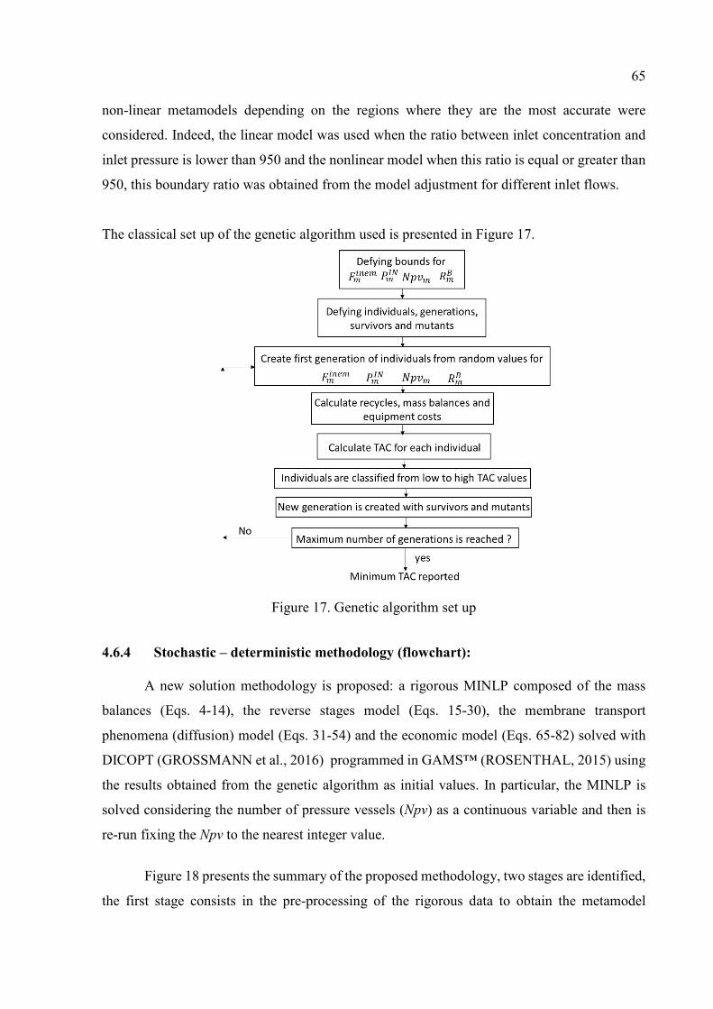
65
non-linear metamodels depending on the regions where they are the most accurate were
considered. Indeed, the linear model was used when the ratio between inlet concentration and
inlet pressure is lower than 950 and the nonlinear model when this ratio is equal or greater than
950, this boundary ratio was obtained from the model adjustment for different inlet flows.
The classical set up of the genetic algorithm used is presented in Figure 17.
Figure 17. Genetic algorithm set up
4.6.4 Stochastic – deterministic methodology (flowchart):
A new solution methodology is proposed: a rigorous MINLP composed of the mass
balances (Eqs. 4-14), the reverse stages model (Eqs. 15-30), the membrane transport
phenomena (diffusion) model (Eqs. 31-54) and the economic model (Eqs. 65-82) solved with
DICOPT (GROSSMANN et al., 2016) programmed in GAMS™ (ROSENTHAL, 2015) using
the results obtained from the genetic algorithm as initial values. In particular, the MINLP is
solved considering the number of pressure vessels (Npv) as a continuous variable and then is
re-run fixing the Npv to the nearest integer value.
Figure 18 presents the summary of the proposed methodology, two stages are identified,
the first stage consists in the pre-processing of the rigorous data to obtain the metamodel
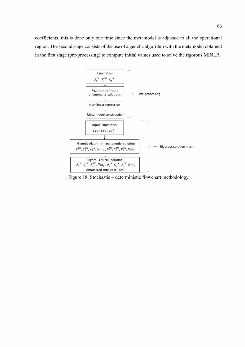
66
coefficients, this is done only one time since the metamodel is adjusted to all the operational
region. The second stage consists of the use of a genetic algorithm with the metamodel obtained
in the first stage (pre-processing) to compute initial values used to solve the rigorous MINLP.
Figure 18. Stochastic – deterministic flowchart methodology
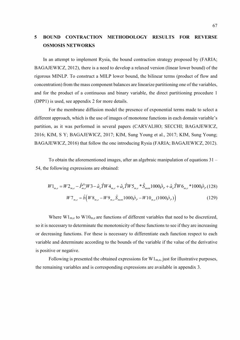
67
5 BOUND CONTRACTION METHODOLOGY RESULTS FOR REVERSE
OSMOSIS NETWORKS
In an attempt to implement Rysia, the bound contraction strategy proposed by (FARIA;
BAGAJEWICZ, 2012), there is a need to develop a relaxed version (linear lower bound) of the
rigorous MINLP. To construct a MILP lower bound, the bilinear terms (product of flow and
concentration) from the mass component balances are linearize partitioning one of the variables,
and for the product of a continuous and binary variable, the direct partitioning procedure 1
(DPP1) is used, see appendix 2 for more details.
For the membrane diffusion model the presence of exponential terms made to select a
different approach, which is the use of images of monotone functions in each domain variable’s
partition, as it was performed in several papers (CARVALHO; SECCHI; BAGAJEWICZ,
2016; KIM, S Y; BAGAJEWICZ, 2017; KIM, Sung Young et al., 2017; KIM, Sung Young;
BAGAJEWICZ, 2016) that follow the one introducing Rysia (FARIA; BAGAJEWICZ, 2012).
To obtain the aforementioned images, after an algebraic manipulation of equations 31 –
54, the following expressions are obtained:
, , , , , ,ˆˆ ˆ ˆ ˆˆ ˆˆ ˆ ˆ1 2 3 4 5 * 1000 6 *1000Pe
m e m e m e m e m e mem P m e PW W P W a TW a TW S a TW (128)
, , , ,ˆ ˆ ˆ ˆ7 8 9 1000 10 (1000 )m e m e m e mem P m e PW b W W S W (129)
Where W1m,e to W10m,e are functions of different variables that need to be discretized,
so it is necessary to determinate the monotonicity of these functions to see if they are increasing
or decreasing functions. For these is necessary to differentiate each function respect to each
variable and determinate according to the bounds of the variable if the value of the derivative
is positive or negative.
Following is presented the obtained expressions for W1m,e, just for illustrative purposes,
the remaining variables and is corresponding expressions are available in appendix 3.
68
ˆ
ˆ
ˆˆ
ˆ
, , , , , , , , ˆ ˆ ˆ, ,, , , , ,2
, , , , , ,
, ,( 1) , ,( 1)
,
ˆ ˆ ˆ ˆˆ( )1
ˆˆ ˆ ˆˆ( )
ˆ ˆ ˆˆ(1
P F P J
P F J
P F JP P J
P F
P F J
nd in nd S
m e d m e d m e d m e dP Fin Js
m e d d d m end nd S
d d dm e d m e d m e d mem
nd in
m e d m e d
m e
d d d
P F a P JW W
P a P J S
P F a PW
ˆ
ˆ
ˆ
, ,( 1) , ,( 1) ˆ ˆ ˆ, ,, , , ,2
, ,( 1) , ,( 1) , ,( 1)
ˆ )
ˆˆ ˆ ˆˆ( )
P J
P F J
P P J
nd S
m e d m e dP Fin Js
m e d d dnd nd S
m e d m e d m e d mem
JW
P a P J S
(130)
Where the product of binary variables is substituted by the following continuous
variable and its corresponding set of equations:
ˆ
ˆ ˆ ˆ ˆ, ,, , , , , ,P F PJ
P Fin Js P
m e d d d m e dW y
(131)
ˆ
ˆ ˆ ˆ ˆ, ,, , , , , ,P F FJ
P Fin Js Fin
m e d d d m e dW y
(132)
ˆ ˆ
ˆ ˆ ˆ ˆ, ,, , , , , ,P F J J
P Fin Js Js
m e d d d m e dW y
(133)
ˆ ˆ
ˆ ˆ ˆ ˆ ˆ ˆ, ,, , , , , , , , , , 2
P F P FJ J
P Fin Js P Fin Js
m e d d d m e d m e d m e dW y y y
(134)
To use the expressions presented in appendix 3, the partitioned variables appearing in
equations needs are discretized according to:
ˆ ˆ
, , , , , , ,( 1) , ,ˆ ˆ
P P P P
P P
nd P nd nd P
m e d m e d m e m e d m e d
d d
P y P P y
(135)
ˆ ˆ ˆ ˆ
ˆ ˆ
ˆ ˆ
, , , , , , ,( 1) , ,ˆ ˆ
J J J J
J J
S Js S S Js
m e d m e d m e m e d m e d
d d
J y J J y (136)
ˆ ˆ
, , , , , , ,( 1) , ,ˆ ˆ
F F F F
F F
in Fin in in Fin
m e d m e d m e m e d m e d
d d
F y F F y (137)
ˆ ˆ
, , , , , , ,( 1) , ,ˆ ˆ
C C C C
C C
in Cin in in Cin
m e d m e d m e m e d m e d
d d
C y C C y (138)
ˆ ˆ
, , , , , , ,( 1) , ,ˆ ˆ
P P P P
P P
in Pin in in Pin
m e d m e d m e m e d m e d
d d
P y P P y (139)
When running Rysia, the upper bound is the rigorous MINLP and is run using the results
from the lower bound as initial values, although some results for the general superstructure can
be obtained with the lower bound model, the system was evaluated rigorously by fixing as many
variables as possible with the values of the LB to obtain a feasible solution.
Before trying bound contraction, an attempted to increase the number of partitions in
the lower bound to see if the gap at the root node can be reduced, was done. Results for a two
stages RON, with seawater concentration of 35,000 ppm and a target permeate production of
100 kg/s (maximum permeate concentration 500 ppm, and maximum brine concentration
87,000 ppm) are presented in Table 4. Results show that a region where there is no improvement
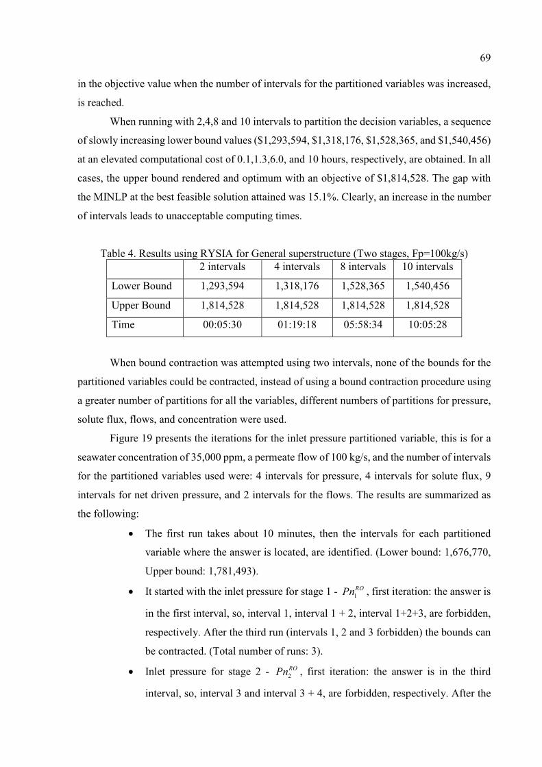
69
in the objective value when the number of intervals for the partitioned variables was increased,
is reached.
When running with 2,4,8 and 10 intervals to partition the decision variables, a sequence
of slowly increasing lower bound values ($1,293,594, $1,318,176, $1,528,365, and $1,540,456)
at an elevated computational cost of 0.1,1.3,6.0, and 10 hours, respectively, are obtained. In all
cases, the upper bound rendered and optimum with an objective of $1,814,528. The gap with
the MINLP at the best feasible solution attained was 15.1%. Clearly, an increase in the number
of intervals leads to unacceptable computing times.
Table 4. Results using RYSIA for General superstructure (Two stages, Fp=100kg/s) 2 intervals 4 intervals 8 intervals 10 intervals
Lower Bound 1,293,594 1,318,176 1,528,365 1,540,456
Upper Bound 1,814,528 1,814,528 1,814,528 1,814,528
Time 00:05:30 01:19:18 05:58:34 10:05:28
When bound contraction was attempted using two intervals, none of the bounds for the
partitioned variables could be contracted, instead of using a bound contraction procedure using
a greater number of partitions for all the variables, different numbers of partitions for pressure,
solute flux, flows, and concentration were used.
Figure 19 presents the iterations for the inlet pressure partitioned variable, this is for a
seawater concentration of 35,000 ppm, a permeate flow of 100 kg/s, and the number of intervals
for the partitioned variables used were: 4 intervals for pressure, 4 intervals for solute flux, 9
intervals for net driven pressure, and 2 intervals for the flows. The results are summarized as
the following:
The first run takes about 10 minutes, then the intervals for each partitioned
variable where the answer is located, are identified. (Lower bound: 1,676,770,
Upper bound: 1,781,493).
It started with the inlet pressure for stage 1 - 1ROPn , first iteration: the answer is
in the first interval, so, interval 1, interval 1 + 2, interval 1+2+3, are forbidden,
respectively. After the third run (intervals 1, 2 and 3 forbidden) the bounds can
be contracted. (Total number of runs: 3).
Inlet pressure for stage 2 - 2ROPn , first iteration: the answer is in the third
interval, so, interval 3 and interval 3 + 4, are forbidden, respectively. After the
70
second run (intervals 3 and 4, forbidden) the bounds can be contracted. (Total
number of runs: 2).
Variables: first stage concentration ( 1ROC ) and turbine pressure difference ( T
tP
), also allows to contract their bounds in the first iteration. (Total number of
runs: 3).
Second iteration: 1ROPn - the answer is located in interval 1, forbidding intervals
1, 2, and 3 bounds can be contracted. (Total number of runs: 3)
Second iteration: 2ROPn - the answer is located in interval 2, forbidding intervals
1 + 2, 2, 1+2+3, 2+3, 2+3+4 bounds cannot be contracted (Total number of runs:
5).
This time variables 1ROC , T
tP cannot be contracted.
Third iteration: for each variable 1ROPn , 2
ROPn , 5 runs are made, but no bound
contraction is possible. The procedure finishes. Lower and upper bounds by the
end of the extended interval elimination strategy: 1,713,724 (LB) vs 1,781,493
(UB), gap = 3.78%.
After a total number of 21 runs of the MILP lower bound, the extended interval
elimination took about 3.5 hours to reach a gap of 3.78% between the lower and the
corresponding MINLP. Getting a better result than those presented in Table 4.
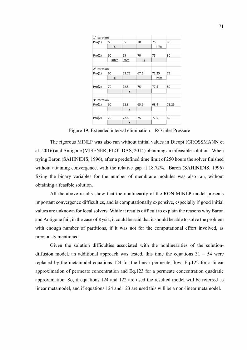
71
Figure 19. Extended interval elimination – RO inlet Pressure
The rigorous MINLP was also run without initial values in Dicopt (GROSSMANN et
al., 2016) and Antigone (MISENER; FLOUDAS, 2014) obtaining an infeasible solution. When
trying Baron (SAHINIDIS, 1996), after a predefined time limit of 250 hours the solver finished
without attaining convergence, with the relative gap at 18.72%. Baron (SAHINIDIS, 1996)
fixing the binary variables for the number of membrane modules was also ran, without
obtaining a feasible solution.
All the above results show that the nonlinearity of the RON-MINLP model presents
important convergence difficulties, and is computationally expensive, especially if good initial
values are unknown for local solvers. While it results difficult to explain the reasons why Baron
and Antigone fail, in the case of Rysia, it could be said that it should be able to solve the problem
with enough number of partitions, if it was not for the computational effort involved, as
previously mentioned.
Given the solution difficulties associated with the nonlinearities of the solution-
diffusion model, an additional approach was tested, this time the equations 31 – 54 were
replaced by the metamodel equations 124 for the linear permeate flow, Eq.122 for a linear
approximation of permeate concentration and Eq.123 for a permeate concentration quadratic
approximation. So, if equations 124 and 122 are used the resulted model will be referred as
linear metamodel, and if equations 124 and 123 are used this will be a non-linear metamodel.
1° Iteration
Pro(1) 60 65 70 75 80
x infes
Pro(2) 60 65 70 75 80
infes infes x
2° Iteration
Pro(1) 60 63.75 67.5 71.25 75
x infes
Pro(2) 70 72.5 75 77.5 80
x
3° Iteration
Pro(1) 60 62.8 65.6 68.4 71.25
x
Pro(2) 70 72.5 75 77.5 80
x
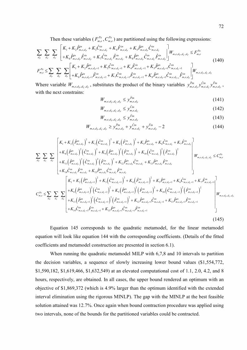
72
Then these variables ( ,Pe
m eF , ,Pe
m eC ) are partitioned using the following expressions:
1 2 , , 3 , , 4 , , 5 , , , ,
, , , , ,
6 , , , , 7 , , , , 8 , , , , , ,
1 2
,
ˆ ˆˆ ˆ ˆ
ˆ ˆˆ ˆ ˆ ˆ ˆ
ˆ
P C F P C
P C F
P C FP F C F P C F
P C
in in in in in
m e d m e d m e d m e d m e d Pe
m e d d d m ein in in in in in in
d d dm e d m e d m e d m e d m e d m e d m e d
Pe
m e
d d
K K P K C K F K P CW F
K P F K C F K P C F
K K PF
1
, , 1 3 , , 1 4 , , 1 5 , , 1 , , 1
, , , ,
6 , , 1 , , 1 7 , , 1 , , 1 8 , , 1 , , , ,
ˆ ˆˆ ˆ
ˆ ˆˆ ˆ ˆ ˆ ˆP C F P C
P C F
FP F C F P C F
in in in in in
m e d m e d m e d m e d m e d
m e d d din in in in in in in
dm e d m e d m e d m e d m e d m e d m e d
K C K F K P CW
K P F K C F K P C F
(140)
Where variable , , , ,P C Fm e d d dW , substitutes the product of the binary variables ˆˆ ˆ
, , , , , ,P C F
Pin Cin Fin
m e d m e d m e dy y y ,
with the next constrains: ˆ
, , , , , ,P C F P
Pin
m e d d d m e dW y (141) ˆ
, , , , , ,P C F C
Cin
m e d d d m e dW y (142) ˆ
, , , , , ,P C F F
Fin
m e d d d m e dW y (143) ˆˆ ˆ
, , , , , , , , , , 2P C F P C F
Pin Cin Fin
m e d d d m e d m e d m e dW y y y (144)
22 2
1 2 , , 3 , , 4 , , 5 , , 6 , , 7 , ,
2 22 2 2 2
8 , , , , 9 , , , , 10 , , , ,
22
11 , , , , , ,
ˆ ˆˆ ˆ ˆ ˆ
ˆ ˆˆ ˆ ˆ ˆ
ˆˆ ˆ
P C F P C F
P C P F C F
P C F
P C
in in in in in in
m e d m e d m e d m e d m e d m e d
in in in in in in
m e d m e d m e d m e d m e d m e d
d d d in in
m e d m e d m e
K K P K C K F K P K C K F
K P C K P F K C F
K P C F
, , , , ,2
12 , , , , 13 , , , ,
14 , , , , 15 , , , , , ,
22
1 2 , , 1 3 , , 1 4
,
ˆˆ ˆ ˆ
ˆ ˆˆ ˆ ˆ
ˆˆ ˆ
P C F
F P C P F
C F P C F
P C
P C
Pe
m e d d d m e
in in in in in
d m e d m e d m e d m e d
in in in in in
m e d m e d m e d m e d m e d
in in
m e d m e d
Pe
m e
d d
W C
K P C K P F
K C F K P C F
K K P K C K
C
2
, , 1 5 , , 1 6 , , 1 7 , , 1
2 22 2 2 2
8 , , 1 , , 1 9 , , 1 , , 1 10 , , 1 , , 1
22 2
11 , , 1 , , 1 , , 1 12 , ,
ˆˆ ˆ
ˆ ˆˆ ˆ ˆ ˆ
ˆˆ ˆ ˆ
F P C F
P C P F C F
P C F P
in in in in
m e d m e d m e d m e d
in in in in in in
m e d m e d m e d m e d m e d m e d
in in in
m e d m e d m e d m e d
F K P K C K F
K P C K P F K C F
K P C F K P
, , , ,
1 , , 1 13 , , 1 , , 1
14 , , 1 , , 1 15 , , 1 , , 1 , , 1
ˆ ˆ ˆ
ˆ ˆˆ ˆ ˆ
P C F
F
C P F
C F P C F
m e d d d
d in in in in
m e d m e d m e d
in in in in in
m e d m e d m e d m e d m e d
W
C K P F
K C F K P C F
(145)
Equation 145 corresponds to the quadratic metamodel, for the linear metamodel
equation will look like equation 144 with the corresponding coefficients. (Details of the fitted
coefficients and metamodel construction are presented in section 6.1).
When running the quadratic metamodel MILP with 6,7,8 and 10 intervals to partition
the decision variables, a sequence of slowly increasing lower bound values ($1,554,772,
$1,590,182, $1,619,466, $1,632,549) at an elevated computational cost of 1.1, 2.0, 4.2, and 8
hours, respectively, are obtained. In all cases, the upper bound rendered an optimum with an
objective of $1,869,372 (which is 4.9% larger than the optimum identified with the extended
interval elimination using the rigorous MINLP). The gap with the MINLP at the best feasible
solution attained was 12.7%. Once again when bound contraction procedure was applied using
two intervals, none of the bounds for the partitioned variables could be contracted.
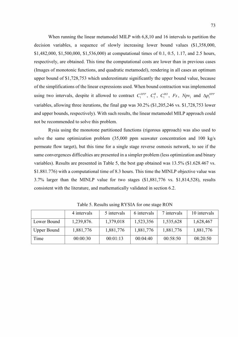
73
When running the linear metamodel MILP with 6,8,10 and 16 intervals to partition the
decision variables, a sequence of slowly increasing lower bound values ($1,358,000,
$1,482,000, $1,500,000, $1,536,000) at computational times of 0.1, 0.5, 1.17, and 2.5 hours,
respectively, are obtained. This time the computational costs are lower than in previous cases
(Images of monotonic functions, and quadratic metamodel), rendering in all cases an optimum
upper bound of $1,728,753 which underestimate significantly the upper bound value, because
of the simplifications of the linear expressions used. When bound contraction was implemented
using two intervals, despite it allowed to contract 1HPPC , 2
BC , 1ROC , Fs , 1Npv and 1
HPPp
variables, allowing three iterations, the final gap was 30.2% ($1,205,246 vs. $1,728,753 lower
and upper bounds, respectively). With such results, the linear metamodel MILP approach could
not be recommended to solve this problem.
Rysia using the monotone partitioned functions (rigorous approach) was also used to
solve the same optimization problem (35,000 ppm seawater concentration and 100 kg/s
permeate flow target), but this time for a single stage reverse osmosis network, to see if the
same convergences difficulties are presented in a simpler problem (less optimization and binary
variables). Results are presented in Table 5, the best gap obtained was 13.5% ($1.628.467 vs.
$1.881.776) with a computational time of 8.3 hours. This time the MINLP objective value was
3.7% larger than the MINLP value for two stages ($1,881,776 vs. $1,814,528), results
consistent with the literature, and mathematically validated in section 6.2.
Table 5. Results using RYSIA for one stage RON
4 intervals 5 intervals 6 intervals 7 intervals 10 intervals
Lower Bound 1,239,876. 1,379,018 1,523,356 1,535,628 1,628,467
Upper Bound 1,881,776 1,881,776 1,881,776 1,881,776 1,881,776
Time 00:00:30 00:01:13 00:04:40 00:58:50 08:20:50
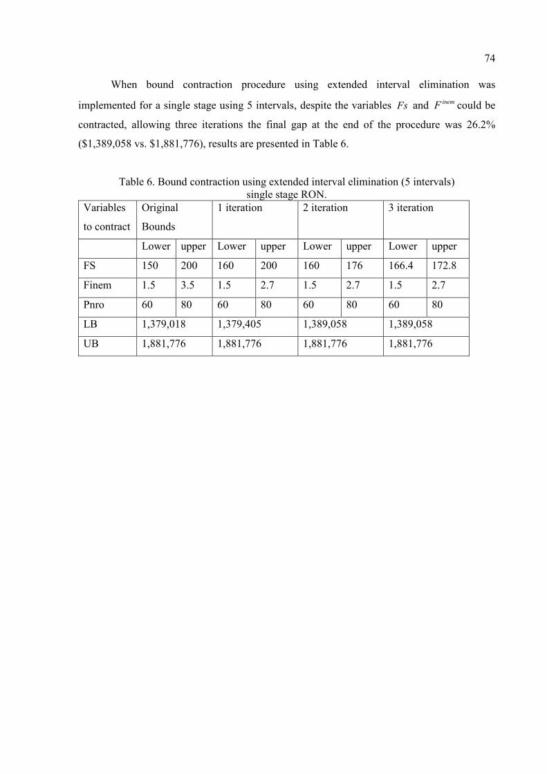
74
When bound contraction procedure using extended interval elimination was
implemented for a single stage using 5 intervals, despite the variables Fs and inemF could be
contracted, allowing three iterations the final gap at the end of the procedure was 26.2%
($1,389,058 vs. $1,881,776), results are presented in Table 6.
Table 6. Bound contraction using extended interval elimination (5 intervals) single stage RON.
Variables
to contract
Original
Bounds
1 iteration 2 iteration 3 iteration
Lower upper Lower upper Lower upper Lower upper
FS 150 200 160 200 160 176 166.4 172.8
Finem 1.5 3.5 1.5 2.7 1.5 2.7 1.5 2.7
Pnro 60 80 60 80 60 80 60 80
LB 1,379,018 1,379,405 1,389,058 1,389,058
UB 1,881,776 1,881,776 1,881,776 1,881,776
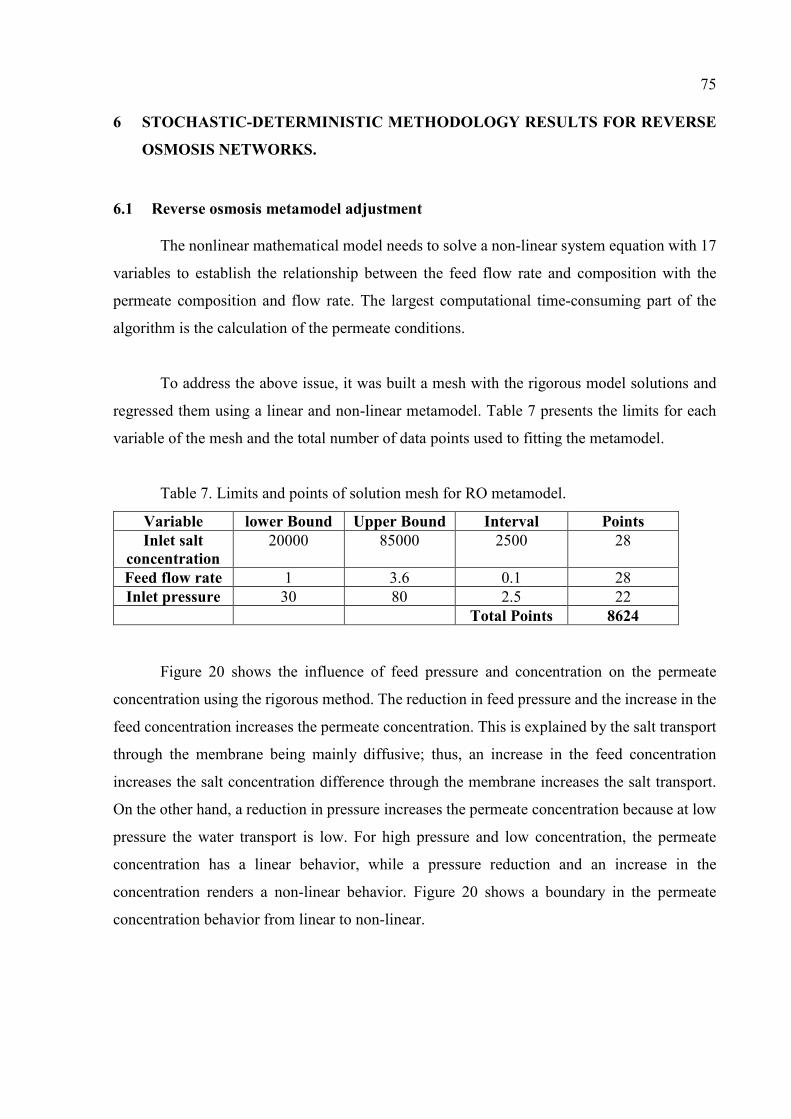
75
6 STOCHASTIC-DETERMINISTIC METHODOLOGY RESULTS FOR REVERSE
OSMOSIS NETWORKS.
6.1 Reverse osmosis metamodel adjustment
The nonlinear mathematical model needs to solve a non-linear system equation with 17
variables to establish the relationship between the feed flow rate and composition with the
permeate composition and flow rate. The largest computational time-consuming part of the
algorithm is the calculation of the permeate conditions.
To address the above issue, it was built a mesh with the rigorous model solutions and
regressed them using a linear and non-linear metamodel. Table 7 presents the limits for each
variable of the mesh and the total number of data points used to fitting the metamodel.
Table 7. Limits and points of solution mesh for RO metamodel.
Variable lower Bound Upper Bound Interval Points
Inlet salt
concentration
20000 85000 2500 28
Feed flow rate 1 3.6 0.1 28 Inlet pressure 30 80 2.5 22
Total Points 8624
Figure 20 shows the influence of feed pressure and concentration on the permeate
concentration using the rigorous method. The reduction in feed pressure and the increase in the
feed concentration increases the permeate concentration. This is explained by the salt transport
through the membrane being mainly diffusive; thus, an increase in the feed concentration
increases the salt concentration difference through the membrane increases the salt transport.
On the other hand, a reduction in pressure increases the permeate concentration because at low
pressure the water transport is low. For high pressure and low concentration, the permeate
concentration has a linear behavior, while a pressure reduction and an increase in the
concentration renders a non-linear behavior. Figure 20 shows a boundary in the permeate
concentration behavior from linear to non-linear.
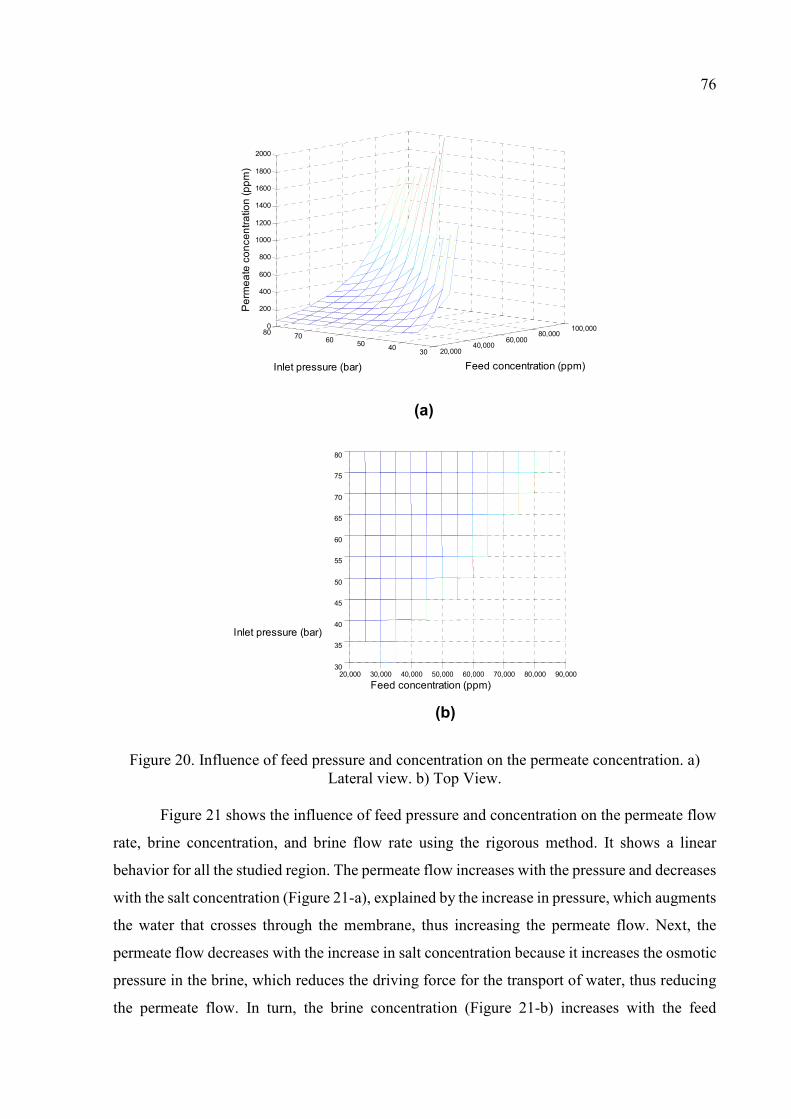
76
Figure 20. Influence of feed pressure and concentration on the permeate concentration. a) Lateral view. b) Top View.
Figure 21 shows the influence of feed pressure and concentration on the permeate flow
rate, brine concentration, and brine flow rate using the rigorous method. It shows a linear
behavior for all the studied region. The permeate flow increases with the pressure and decreases
with the salt concentration (Figure 21-a), explained by the increase in pressure, which augments
the water that crosses through the membrane, thus increasing the permeate flow. Next, the
permeate flow decreases with the increase in salt concentration because it increases the osmotic
pressure in the brine, which reduces the driving force for the transport of water, thus reducing
the permeate flow. In turn, the brine concentration (Figure 21-b) increases with the feed
20,00040,000
60,00080,000
100,000
3040
5060
7080
0
200
400
600
800
1000
1200
1400
1600
1800
2000
Feed concentration (ppm)Inlet pressure (bar)
Pe
rme
ate
co
nce
ntr
atio
n (
pp
m)
20,000 30,000 40,000 50,000 60,000 70,000 80,000 90,00030
35
40
45
50
55
60
65
70
75
80
Feed concentration (ppm)
Inlet pressure (bar)
(a)
(b)
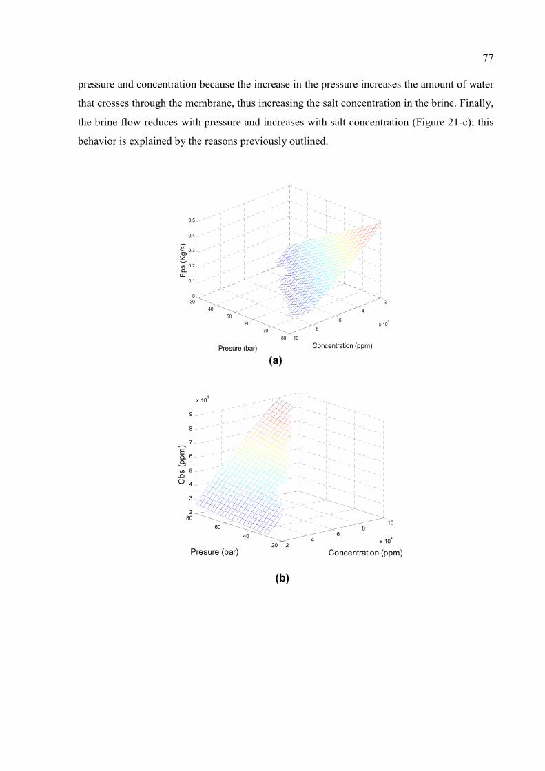
77
pressure and concentration because the increase in the pressure increases the amount of water
that crosses through the membrane, thus increasing the salt concentration in the brine. Finally,
the brine flow reduces with pressure and increases with salt concentration (Figure 21-c); this
behavior is explained by the reasons previously outlined.
2
4
6
8
10
x 104
30
40
50
60
70
80
0
0.1
0.2
0.3
0.4
0.5
Concentration (ppm)Presure (bar)
Fp
s (
Kg
/s)
24
68
10
x 104
20
40
60
802
3
4
5
6
7
8
9
x 104
Concentration (ppm)Presure (bar)
Cb
s (
pp
m)
(a)
(b)
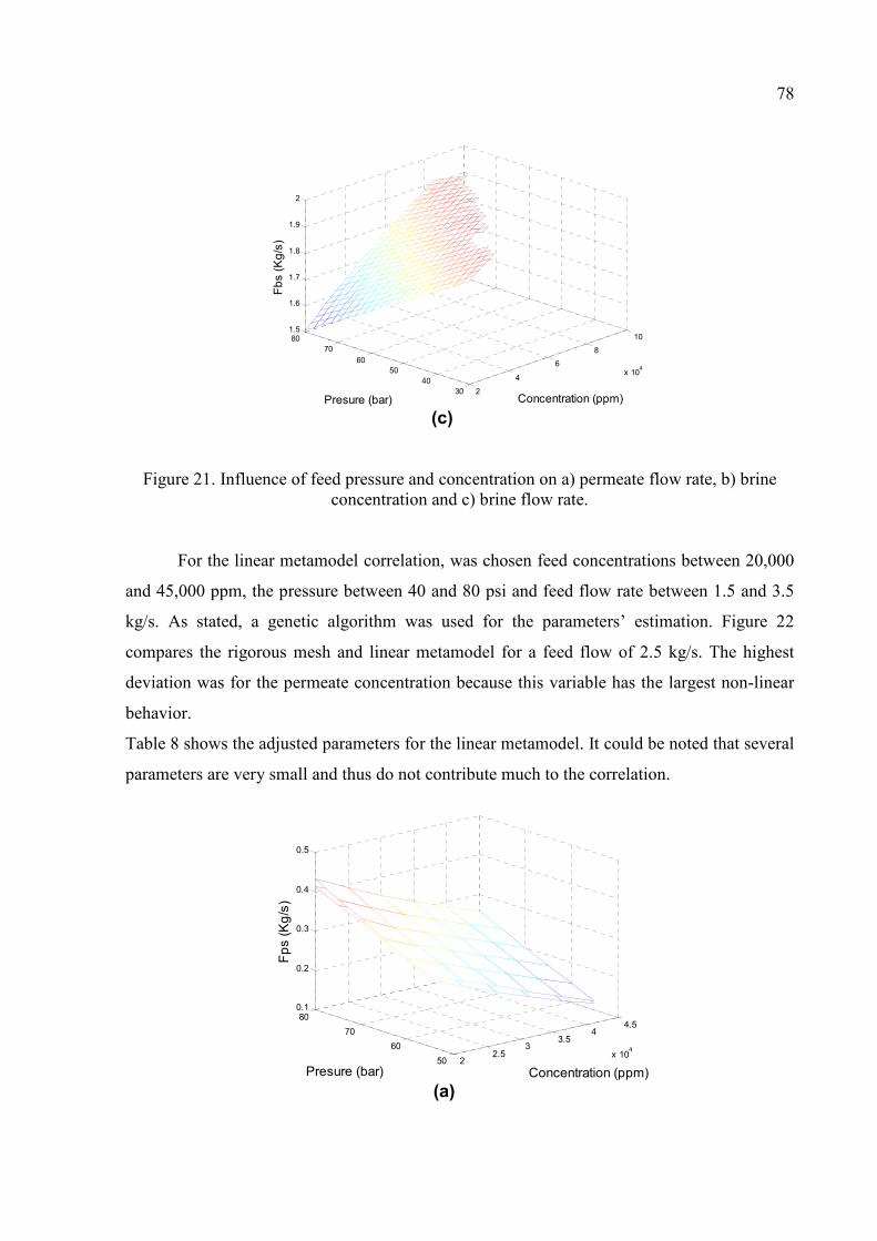
78
Figure 21. Influence of feed pressure and concentration on a) permeate flow rate, b) brine concentration and c) brine flow rate.
For the linear metamodel correlation, was chosen feed concentrations between 20,000
and 45,000 ppm, the pressure between 40 and 80 psi and feed flow rate between 1.5 and 3.5
kg/s. As stated, a genetic algorithm was used for the parameters’ estimation. Figure 22
compares the rigorous mesh and linear metamodel for a feed flow of 2.5 kg/s. The highest
deviation was for the permeate concentration because this variable has the largest non-linear
behavior.
Table 8 shows the adjusted parameters for the linear metamodel. It could be noted that several
parameters are very small and thus do not contribute much to the correlation.
2
4
6
8
10
x 104
30
40
50
60
70
801.5
1.6
1.7
1.8
1.9
2
Concentration (ppm)Presure (bar)
Fb
s (
Kg
/s)
22.5
33.5
44.5
x 104
50
60
70
800.1
0.2
0.3
0.4
0.5
Concentration (ppm)Presure (bar)
Fp
s (
Kg
/s)
(c)
(a)
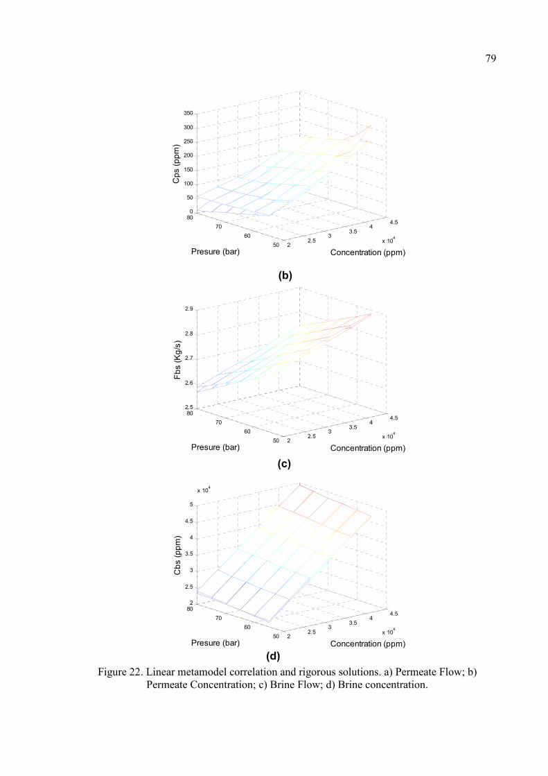
79
Figure 22. Linear metamodel correlation and rigorous solutions. a) Permeate Flow; b) Permeate Concentration; c) Brine Flow; d) Brine concentration.
22.5
33.5
44.5
x 104
50
60
70
800
50
100
150
200
250
300
350
Concentration (ppm)Presure (bar)
Cp
s (
pp
m)
22.5
33.5
44.5
x 104
50
60
70
802.5
2.6
2.7
2.8
2.9
Concentration (ppm)Presure (bar)
Fb
s (
Kg
/s)
22.5
33.5
44.5
x 104
50
60
70
802
2.5
3
3.5
4
4.5
5
x 104
Concentration (ppm)Presure (bar)
Cb
s (
pp
m)
(c)
(d)
(b)
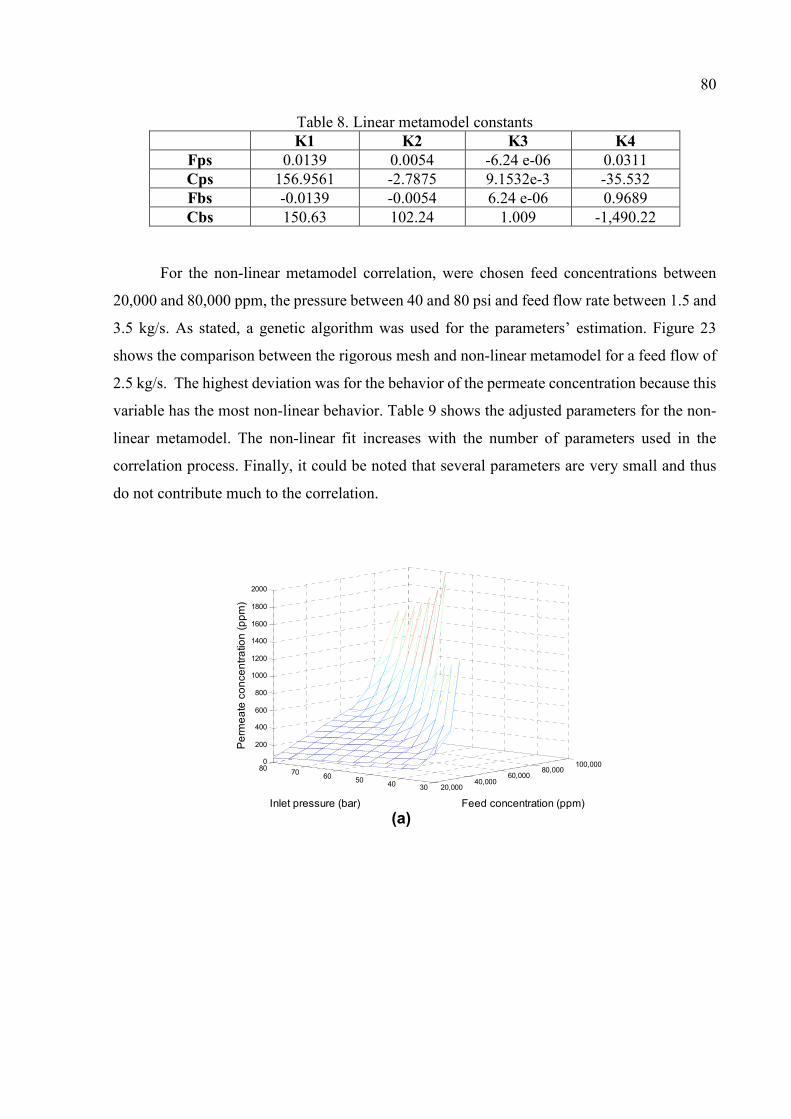
80
Table 8. Linear metamodel constants K1 K2 K3 K4
Fps 0.0139 0.0054 -6.24 e-06 0.0311 Cps 156.9561 -2.7875 9.1532e-3 -35.532 Fbs -0.0139 -0.0054 6.24 e-06 0.9689 Cbs 150.63 102.24 1.009 -1,490.22
For the non-linear metamodel correlation, were chosen feed concentrations between
20,000 and 80,000 ppm, the pressure between 40 and 80 psi and feed flow rate between 1.5 and
3.5 kg/s. As stated, a genetic algorithm was used for the parameters’ estimation. Figure 23
shows the comparison between the rigorous mesh and non-linear metamodel for a feed flow of
2.5 kg/s. The highest deviation was for the behavior of the permeate concentration because this
variable has the most non-linear behavior. Table 9 shows the adjusted parameters for the non-
linear metamodel. The non-linear fit increases with the number of parameters used in the
correlation process. Finally, it could be noted that several parameters are very small and thus
do not contribute much to the correlation.
20,00040,000
60,00080,000
100,000
304050
6070
800
200
400
600
800
1000
1200
1400
1600
1800
2000
Feed concentration (ppm)Inlet pressure (bar)
Pe
rme
ate
co
nce
ntr
atio
n (
pp
m)
(a)
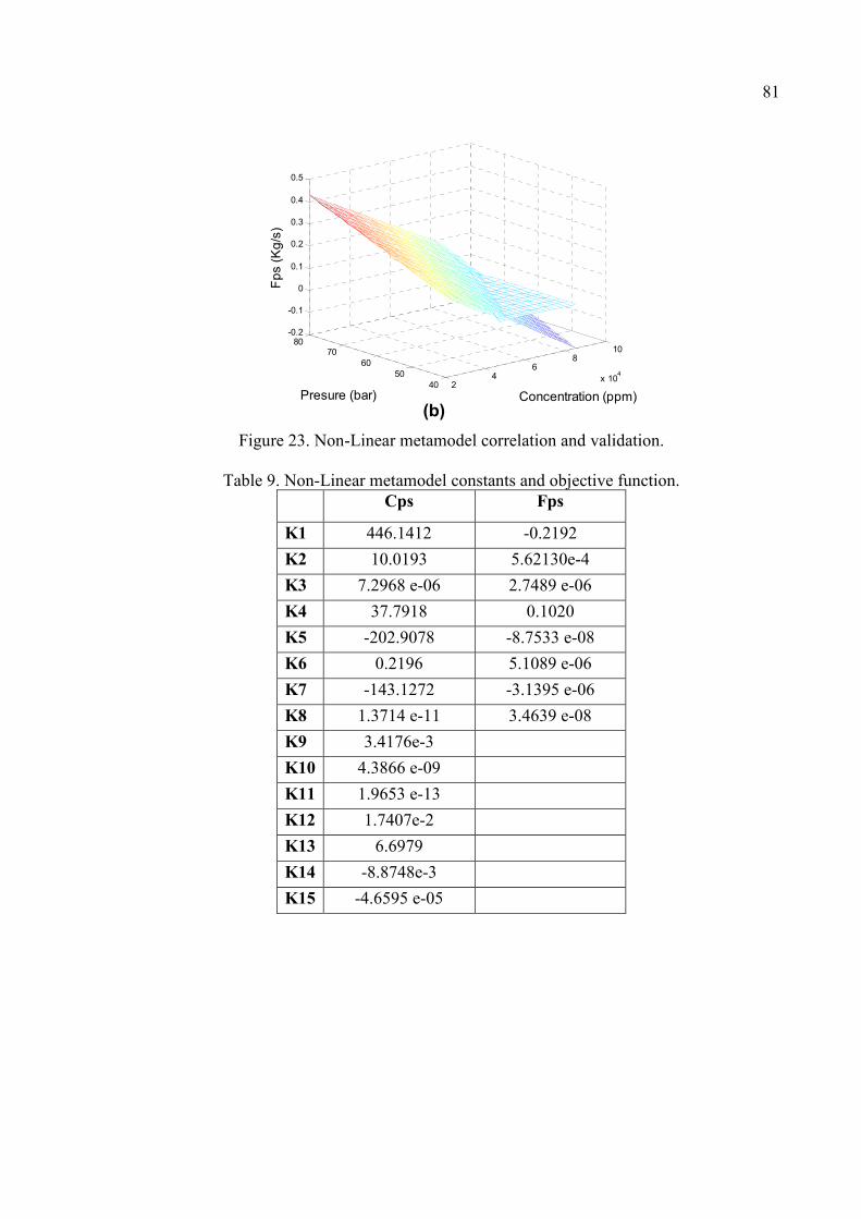
81
Figure 23. Non-Linear metamodel correlation and validation.
Table 9. Non-Linear metamodel constants and objective function. Cps Fps
K1 446.1412 -0.2192
K2 10.0193 5.62130e-4
K3 7.2968 e-06 2.7489 e-06
K4 37.7918 0.1020
K5 -202.9078 -8.7533 e-08
K6 0.2196 5.1089 e-06
K7 -143.1272 -3.1395 e-06
K8 1.3714 e-11 3.4639 e-08
K9 3.4176e-3
K10 4.3866 e-09
K11 1.9653 e-13
K12 1.7407e-2
K13 6.6979
K14 -8.8748e-3
K15 -4.6595 e-05
24
68
10
x 104
4050
6070
80-0.2
-0.1
0
0.1
0.2
0.3
0.4
0.5
Concentration (ppm)Presure (bar)
Fp
s (
Kg
/s)
(b)
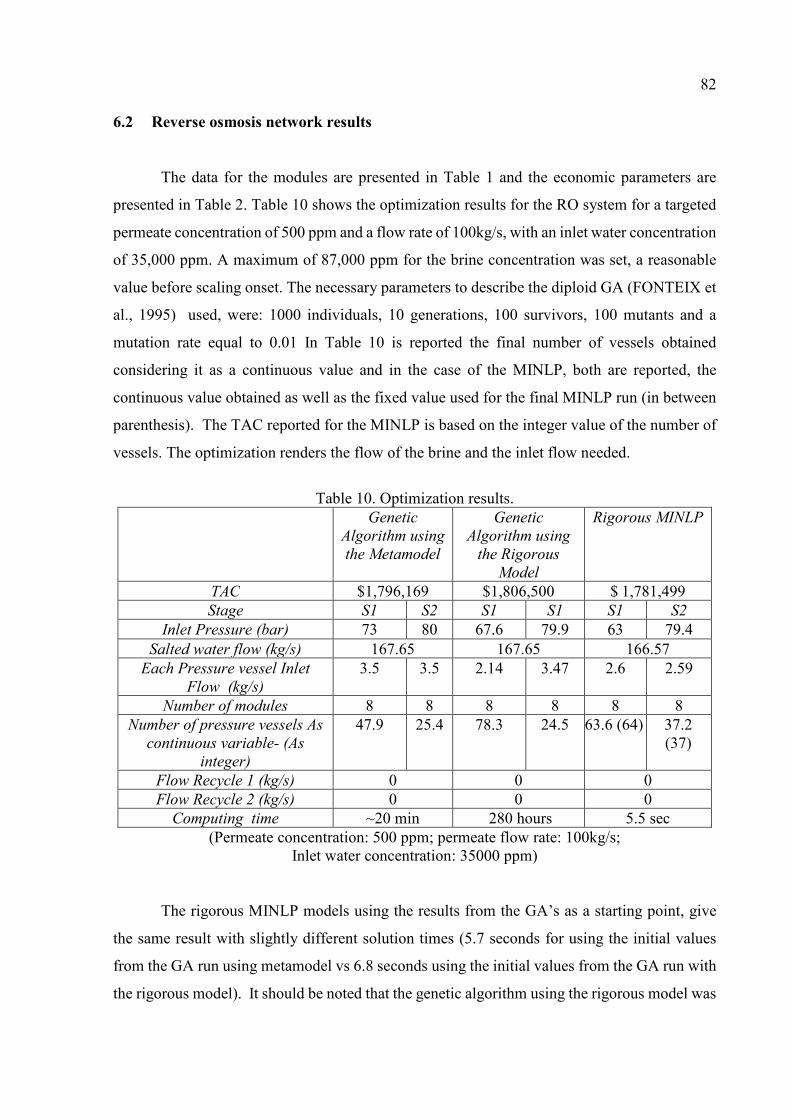
82
6.2 Reverse osmosis network results
The data for the modules are presented in Table 1 and the economic parameters are
presented in Table 2. Table 10 shows the optimization results for the RO system for a targeted
permeate concentration of 500 ppm and a flow rate of 100kg/s, with an inlet water concentration
of 35,000 ppm. A maximum of 87,000 ppm for the brine concentration was set, a reasonable
value before scaling onset. The necessary parameters to describe the diploid GA (FONTEIX et
al., 1995) used, were: 1000 individuals, 10 generations, 100 survivors, 100 mutants and a
mutation rate equal to 0.01 In Table 10 is reported the final number of vessels obtained
considering it as a continuous value and in the case of the MINLP, both are reported, the
continuous value obtained as well as the fixed value used for the final MINLP run (in between
parenthesis). The TAC reported for the MINLP is based on the integer value of the number of
vessels. The optimization renders the flow of the brine and the inlet flow needed.
Table 10. Optimization results.
Genetic
Algorithm using
the Metamodel
Genetic
Algorithm using
the Rigorous
Model
Rigorous MINLP
TAC $1,796,169 $1,806,500 $ 1,781,499 Stage S1 S2 S1 S1 S1 S2
Inlet Pressure (bar) 73 80 67.6 79.9 63 79.4 Salted water flow (kg/s) 167.65 167.65 166.57
Each Pressure vessel Inlet
Flow (kg/s)
3.5 3.5 2.14 3.47 2.6 2.59
Number of modules 8 8 8 8 8 8 Number of pressure vessels As
continuous variable- (As
integer)
47.9 25.4 78.3 24.5 63.6 (64) 37.2 (37)
Flow Recycle 1 (kg/s) 0 0 0 Flow Recycle 2 (kg/s) 0 0 0
Computing time ~20 min 280 hours 5.5 sec (Permeate concentration: 500 ppm; permeate flow rate: 100kg/s;
Inlet water concentration: 35000 ppm)
The rigorous MINLP models using the results from the GA’s as a starting point, give
the same result with slightly different solution times (5.7 seconds for using the initial values
from the GA run using metamodel vs 6.8 seconds using the initial values from the GA run with
the rigorous model). It should be noted that the genetic algorithm using the rigorous model was
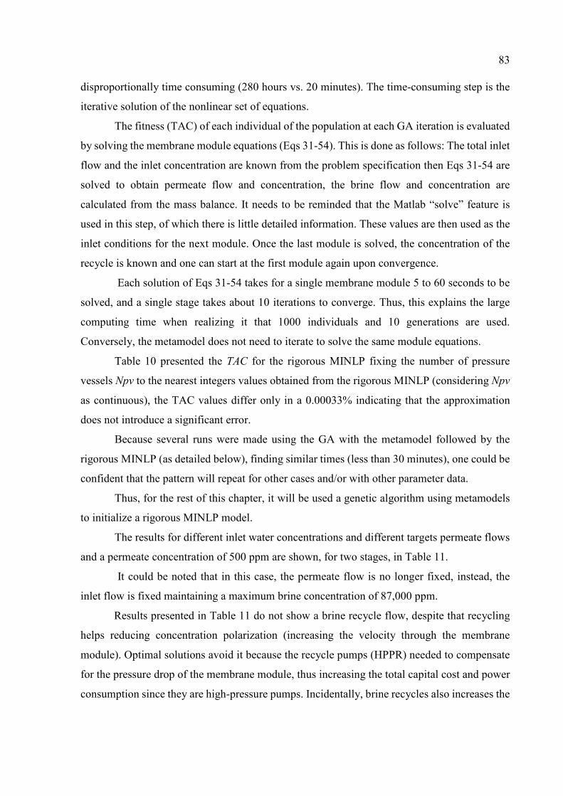
83
disproportionally time consuming (280 hours vs. 20 minutes). The time-consuming step is the
iterative solution of the nonlinear set of equations.
The fitness (TAC) of each individual of the population at each GA iteration is evaluated
by solving the membrane module equations (Eqs 31-54). This is done as follows: The total inlet
flow and the inlet concentration are known from the problem specification then Eqs 31-54 are
solved to obtain permeate flow and concentration, the brine flow and concentration are
calculated from the mass balance. It needs to be reminded that the Matlab “solve” feature is
used in this step, of which there is little detailed information. These values are then used as the
inlet conditions for the next module. Once the last module is solved, the concentration of the
recycle is known and one can start at the first module again upon convergence.
Each solution of Eqs 31-54 takes for a single membrane module 5 to 60 seconds to be
solved, and a single stage takes about 10 iterations to converge. Thus, this explains the large
computing time when realizing it that 1000 individuals and 10 generations are used.
Conversely, the metamodel does not need to iterate to solve the same module equations.
Table 10 presented the TAC for the rigorous MINLP fixing the number of pressure
vessels Npv to the nearest integers values obtained from the rigorous MINLP (considering Npv
as continuous), the TAC values differ only in a 0.00033% indicating that the approximation
does not introduce a significant error.
Because several runs were made using the GA with the metamodel followed by the
rigorous MINLP (as detailed below), finding similar times (less than 30 minutes), one could be
confident that the pattern will repeat for other cases and/or with other parameter data.
Thus, for the rest of this chapter, it will be used a genetic algorithm using metamodels
to initialize a rigorous MINLP model.
The results for different inlet water concentrations and different targets permeate flows
and a permeate concentration of 500 ppm are shown, for two stages, in Table 11.
It could be noted that in this case, the permeate flow is no longer fixed, instead, the
inlet flow is fixed maintaining a maximum brine concentration of 87,000 ppm.
Results presented in Table 11 do not show a brine recycle flow, despite that recycling
helps reducing concentration polarization (increasing the velocity through the membrane
module). Optimal solutions avoid it because the recycle pumps (HPPR) needed to compensate
for the pressure drop of the membrane module, thus increasing the total capital cost and power
consumption since they are high-pressure pumps. Incidentally, brine recycles also increases the
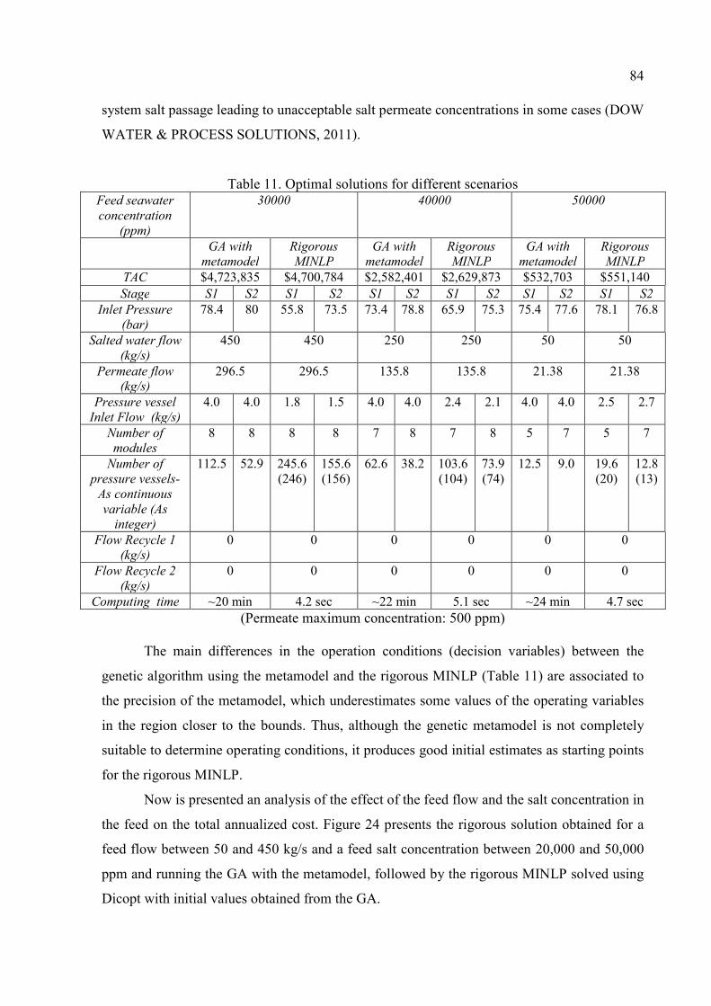
84
system salt passage leading to unacceptable salt permeate concentrations in some cases (DOW
WATER & PROCESS SOLUTIONS, 2011).
Table 11. Optimal solutions for different scenarios Feed seawater
concentration
(ppm)
30000 40000 50000
GA with
metamodel
Rigorous
MINLP
GA with
metamodel
Rigorous
MINLP
GA with
metamodel
Rigorous
MINLP
TAC $4,723,835 $4,700,784 $2,582,401 $2,629,873 $532,703 $551,140 Stage S1 S2 S1 S2 S1 S2 S1 S2 S1 S2 S1 S2
Inlet Pressure
(bar)
78.4 80 55.8 73.5 73.4 78.8 65.9 75.3 75.4 77.6 78.1 76.8
Salted water flow
(kg/s)
450 450 250 250 50 50
Permeate flow
(kg/s)
296.5 296.5 135.8 135.8 21.38 21.38
Pressure vessel
Inlet Flow (kg/s)
4.0 4.0 1.8 1.5 4.0 4.0 2.4 2.1 4.0 4.0 2.5 2.7
Number of
modules
8 8 8 8 7 8 7 8 5 7 5 7
Number of
pressure vessels-
As continuous
variable (As
integer)
112.5 52.9 245.6 (246)
155.6 (156)
62.6 38.2 103.6 (104)
73.9 (74)
12.5 9.0 19.6 (20)
12.8 (13)
Flow Recycle 1
(kg/s)
0 0 0 0 0 0
Flow Recycle 2
(kg/s)
0 0 0 0 0 0
Computing time ~20 min 4.2 sec ~22 min 5.1 sec ~24 min 4.7 sec (Permeate maximum concentration: 500 ppm)
The main differences in the operation conditions (decision variables) between the
genetic algorithm using the metamodel and the rigorous MINLP (Table 11) are associated to
the precision of the metamodel, which underestimates some values of the operating variables
in the region closer to the bounds. Thus, although the genetic metamodel is not completely
suitable to determine operating conditions, it produces good initial estimates as starting points
for the rigorous MINLP.
Now is presented an analysis of the effect of the feed flow and the salt concentration in
the feed on the total annualized cost. Figure 24 presents the rigorous solution obtained for a
feed flow between 50 and 450 kg/s and a feed salt concentration between 20,000 and 50,000
ppm and running the GA with the metamodel, followed by the rigorous MINLP solved using
Dicopt with initial values obtained from the GA.
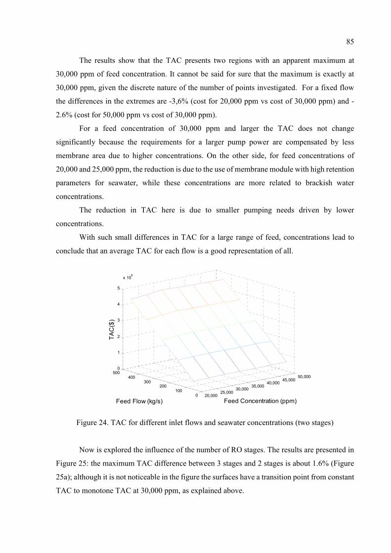
85
The results show that the TAC presents two regions with an apparent maximum at
30,000 ppm of feed concentration. It cannot be said for sure that the maximum is exactly at
30,000 ppm, given the discrete nature of the number of points investigated. For a fixed flow
the differences in the extremes are -3,6% (cost for 20,000 ppm vs cost of 30,000 ppm) and -
2.6% (cost for 50,000 ppm vs cost of 30,000 ppm).
For a feed concentration of 30,000 ppm and larger the TAC does not change
significantly because the requirements for a larger pump power are compensated by less
membrane area due to higher concentrations. On the other side, for feed concentrations of
20,000 and 25,000 ppm, the reduction is due to the use of membrane module with high retention
parameters for seawater, while these concentrations are more related to brackish water
concentrations.
The reduction in TAC here is due to smaller pumping needs driven by lower
concentrations.
With such small differences in TAC for a large range of feed, concentrations lead to
conclude that an average TAC for each flow is a good representation of all.
Figure 24. TAC for different inlet flows and seawater concentrations (two stages)
Now is explored the influence of the number of RO stages. The results are presented in
Figure 25: the maximum TAC difference between 3 stages and 2 stages is about 1.6% (Figure
25a); although it is not noticeable in the figure the surfaces have a transition point from constant
TAC to monotone TAC at 30,000 ppm, as explained above.
20,00025,000
30,00035,000
40,00045,000
50,000
0100
200300
400500
0
1
2
3
4
5
x 106
Feed Concentration (ppm)Feed Flow (kg/s)
TA
C($
)
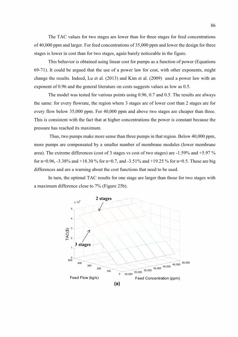
86
The TAC values for two stages are lower than for three stages for feed concentrations
of 40,000 ppm and larger. For feed concentrations of 35,000 ppm and lower the design for three
stages is lower in cost than for two stages, again barely noticeable in the figure.
This behavior is obtained using linear cost for pumps as a function of power (Equations
69-71). It could be argued that the use of a power law for cost, with other exponents, might
change the results. Indeed, Lu et al. (2013) and Kim et al. (2009) used a power law with an
exponent of 0.96 and the general literature on costs suggests values as low as 0.5.
The model was tested for various points using 0.96, 0.7 and 0.5. The results are always
the same: for every flowrate, the region where 3 stages are of lower cost than 2 stages are for
every flow below 35,000 ppm. For 40,000 ppm and above two stages are cheaper than three.
This is consistent with the fact that at higher concentrations the power is constant because the
pressure has reached its maximum.
Thus, two pumps make more sense than three pumps in that region. Below 40,000 ppm,
more pumps are compensated by a smaller number of membrane modules (lower membrane
area). The extreme differences (cost of 3 stages vs cost of two stages) are -1.59% and +5.97 %
for n=0.96, -3.38% and +18.30 % for n=0.7, and -3.51% and +19.25 % for n=0.5. These are big
differences and are a warning about the cost functions that need to be used.
In turn, the optimal TAC results for one stage are larger than those for two stages with
a maximum difference close to 7% (Figure 25b).
20,00025,000
30,00035,000
40,00045,000
50,000
0100
200300
400500
0
1
2
3
4
5
x 106
Feed Concentration (ppm)Feed Flow (kg/s)
TA
C($
)
2 stages
3 stages
(a)
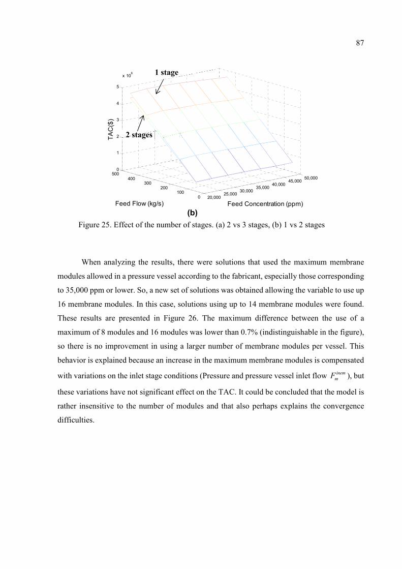
87
Figure 25. Effect of the number of stages. (a) 2 vs 3 stages, (b) 1 vs 2 stages
When analyzing the results, there were solutions that used the maximum membrane
modules allowed in a pressure vessel according to the fabricant, especially those corresponding
to 35,000 ppm or lower. So, a new set of solutions was obtained allowing the variable to use up
16 membrane modules. In this case, solutions using up to 14 membrane modules were found.
These results are presented in Figure 26. The maximum difference between the use of a
maximum of 8 modules and 16 modules was lower than 0.7% (indistinguishable in the figure),
so there is no improvement in using a larger number of membrane modules per vessel. This
behavior is explained because an increase in the maximum membrane modules is compensated
with variations on the inlet stage conditions (Pressure and pressure vessel inlet flow inem
mF ), but
these variations have not significant effect on the TAC. It could be concluded that the model is
rather insensitive to the number of modules and that also perhaps explains the convergence
difficulties.
20,00025,000
30,00035,000
40,00045,000
50,000
0100
200300
400500
0
1
2
3
4
5
x 106
Feed Concentration (ppm)Feed Flow (kg/s)
TA
C($
)
1 stage
2 stages
(b)
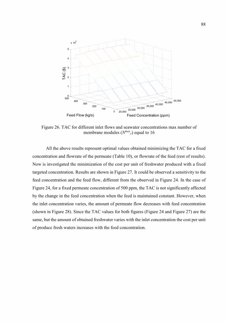
88
Figure 26. TAC for different inlet flows and seawater concentrations max number of membrane modules (Nmax
e) equal to 16
All the above results represent optimal values obtained minimizing the TAC for a fixed
concentration and flowrate of the permeate (Table 10), or flowrate of the feed (rest of results).
Now is investigated the minimization of the cost per unit of freshwater produced with a fixed
targeted concentration. Results are shown in Figure 27. It could be observed a sensitivity to the
feed concentration and the feed flow, different from the observed in Figure 24. In the case of
Figure 24, for a fixed permeate concentration of 500 ppm, the TAC is not significantly affected
by the change in the feed concentration when the feed is maintained constant. However, when
the inlet concentration varies, the amount of permeate flow decreases with feed concentration
(shown in Figure 28). Since the TAC values for both figures (Figure 24 and Figure 27) are the
same, but the amount of obtained freshwater varies with the inlet concentration the cost per unit
of produce fresh waters increases with the feed concentration.
20,00025,000
30,00035,000
40,00045,000
50,000
0100
200300
400500
0
1
2
3
4
5
x 106
Feed Concentration (ppm)Feed Flow (kg/s)
TA
C (
$)
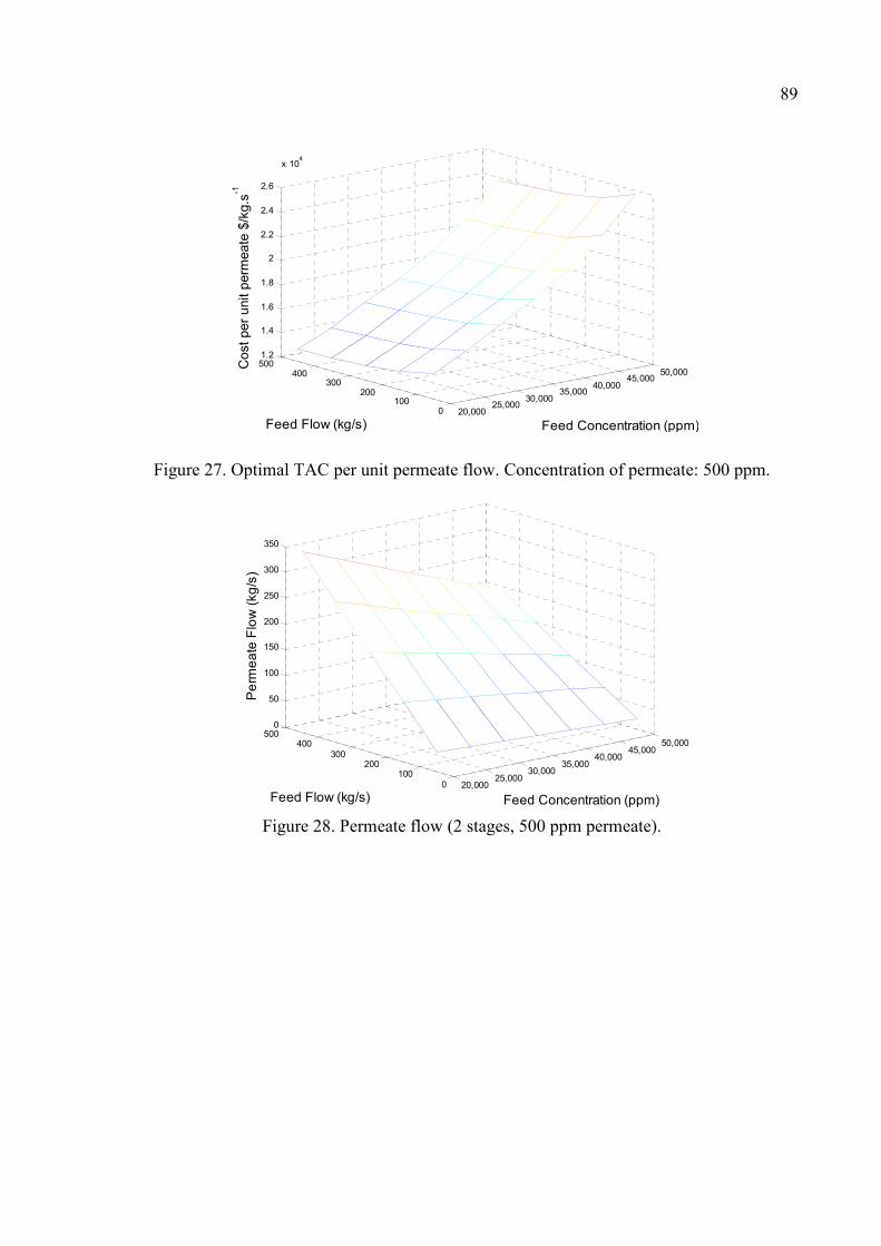
89
Figure 27. Optimal TAC per unit permeate flow. Concentration of permeate: 500 ppm.
Figure 28. Permeate flow (2 stages, 500 ppm permeate).
20,00025,000
30,00035,000
40,00045,000
50,000
0100
200300
400500
0
50
100
150
200
250
300
350
Feed Concentration (ppm)Feed Flow (kg/s)
Pe
rme
ate
Flo
w (
kg
/s)
20,00025,000
30,00035,000
40,00045,000
50,000
0100
200300
4005001.2
1.4
1.6
1.8
2
2.2
2.4
2.6
x 104
Feed Concentration (ppm)Feed Flow (kg/s)
Co
st
pe
r u
nit p
erm
ea
te $
/kg.s
-1
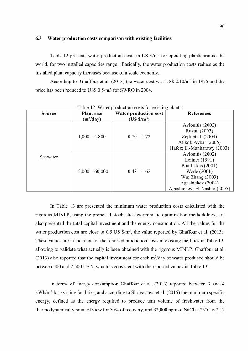
90
6.3 Water production costs comparison with existing facilities:
Table 12 presents water production costs in US $/m3 for operating plants around the
world, for two installed capacities range. Basically, the water production costs reduce as the
installed plant capacity increases because of a scale economy.
According to Ghaffour et al. (2013) the water cost was US$ 2.10/m3 in 1975 and the
price has been reduced to US$ 0.5/m3 for SWRO in 2004.
Table 12. Water production costs for existing plants. Source Plant size
(m3/day)
Water production cost
(US $/m3)
References
Seawater
1,000 – 4,800 0.70 – 1.72
Avlonitis (2002) Rayan (2003)
Zejli et al. (2004) Atikol; Aybar (2005)
Hafez; El-Manharawy (2003)
15,000 – 60,000 0.48 – 1.62
Avlonitis (2002) Leitner (1991)
Poullikkas (2001) Wade (2001)
Wu; Zhang (2003) Agashichev (2004)
Agashichev; El-Nashar (2005)
In Table 13 are presented the minimum water production costs calculated with the
rigorous MINLP, using the proposed stochastic-deterministic optimization methodology, are
also presented the total capital investment and the energy consumption. All the values for the
water production cost are close to 0.5 US $/m3, the value reported by Ghaffour et al. (2013).
These values are in the range of the reported production costs of existing facilities in Table 13,
allowing to validate what actually is been obtained with the rigorous MINLP. Ghaffour et al.
(2013) also reported that the capital investment for each m3/day of water produced should be
between 900 and 2,500 US $, which is consistent with the reported values in Table 13.
In terms of energy consumption Ghaffour et al. (2013) reported between 3 and 4
kWh/m3 for existing facilities, and according to Shrivastava et al. (2015) the minimum specific
energy, defined as the energy required to produce unit volume of freshwater from the
thermodynamically point of view for 50% of recovery, and 32,000 ppm of NaCl at 25°C is 2.12
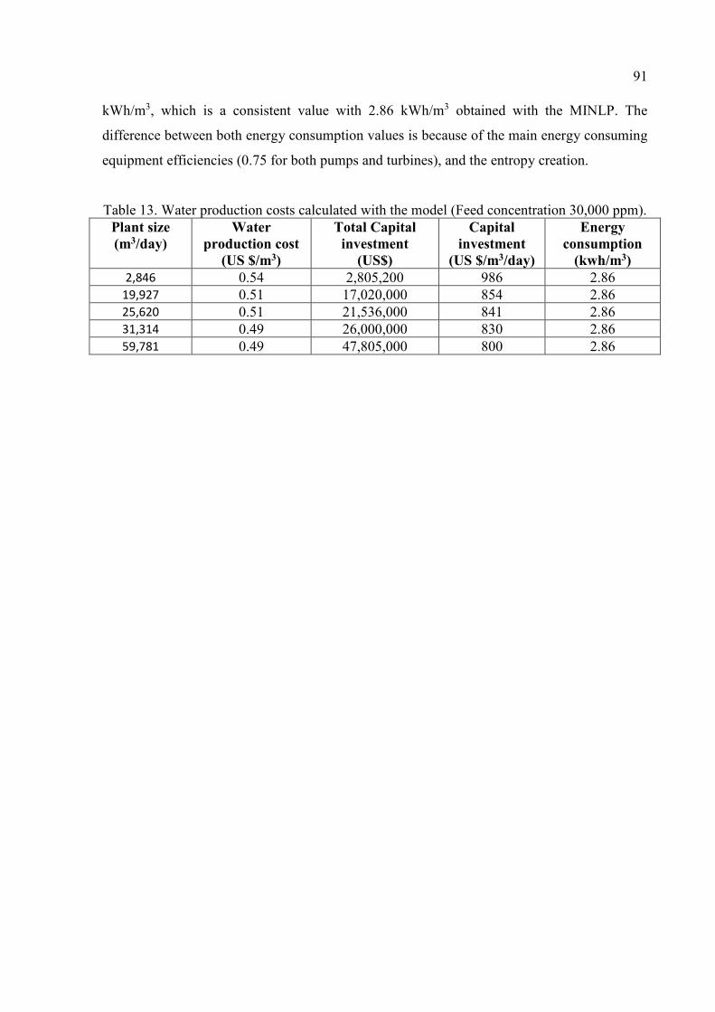
91
kWh/m3, which is a consistent value with 2.86 kWh/m3 obtained with the MINLP. The
difference between both energy consumption values is because of the main energy consuming
equipment efficiencies (0.75 for both pumps and turbines), and the entropy creation.
Table 13. Water production costs calculated with the model (Feed concentration 30,000 ppm). Plant size
(m3/day)
Water
production cost
(US $/m3)
Total Capital
investment
(US$)
Capital
investment
(US $/m3/day)
Energy
consumption
(kwh/m3)
2,846 0.54 2,805,200 986 2.86 19,927 0.51 17,020,000 854 2.86 25,620 0.51 21,536,000 841 2.86 31,314 0.49 26,000,000 830 2.86 59,781 0.49 47,805,000 800 2.86
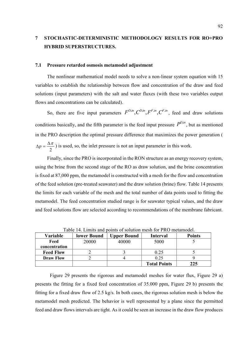
92
7 STOCHASTIC-DETERMINISTIC METHODOLOGY RESULTS FOR RO+PRO
HYBRID SUPERSTRUCTURES.
7.1 Pressure retarded osmosis metamodel adjustment
The nonlinear mathematical model needs to solve a non-linear system equation with 15
variables to establish the relationship between flow and concentration of the draw and feed
solutions (input parameters) with the salt and water fluxes (with these two variables output
flows and concentrations can be calculated).
So, there are five input parameters , , , ,, , ,D in D in F in F inF C F C , feed and draw solutions
conditions basically, and the fifth parameter is the feed input pressure ,D inP , but as mentioned
in the PRO description the optimal pressure difference that maximizes the power generation (
2p
) is used, so, the inlet pressure is not an input parameter in this work.
Finally, since the PRO is incorporated in the RON structure as an energy recovery system,
using the brine from the second stage of the RO as draw solution, and the brine concentration
is fixed at 87,000 ppm, the metamodel is constructed with a mesh for the flow and concentration
of the feed solution (pre-treated seawater) and the draw solution (brine) flow. Table 14 presents
the limits for each variable of the mesh and the total number of data points used to fitting the
metamodel. The feed concentration studied range is for seawater typical values, and the draw
and feed solutions flow are selected according to recommendations of the membrane fabricant.
Table 14. Limits and points of solution mesh for PRO metamodel. Variable lower Bound Upper Bound Interval Points
Feed
concentration 20000 40000 5000 5
Feed Flow 2 3 0.25 5 Draw Flow 2 4 0.25 9
Total Points 225
Figure 29 presents the rigorous and metamodel meshes for water flux, Figure 29 a)
presents the fitting for a fixed feed concentration of 35.000 ppm, Figure 29 b) presents the
fitting for a fixed draw flow of 2.5 kg/s. In both cases, the rigorous solution mesh is below the
metamodel mesh predicted. The behavior is well represented by a plane since the permitted
feed and draw flows intervals are tight. As it could be seen an increase in the draw flow produces
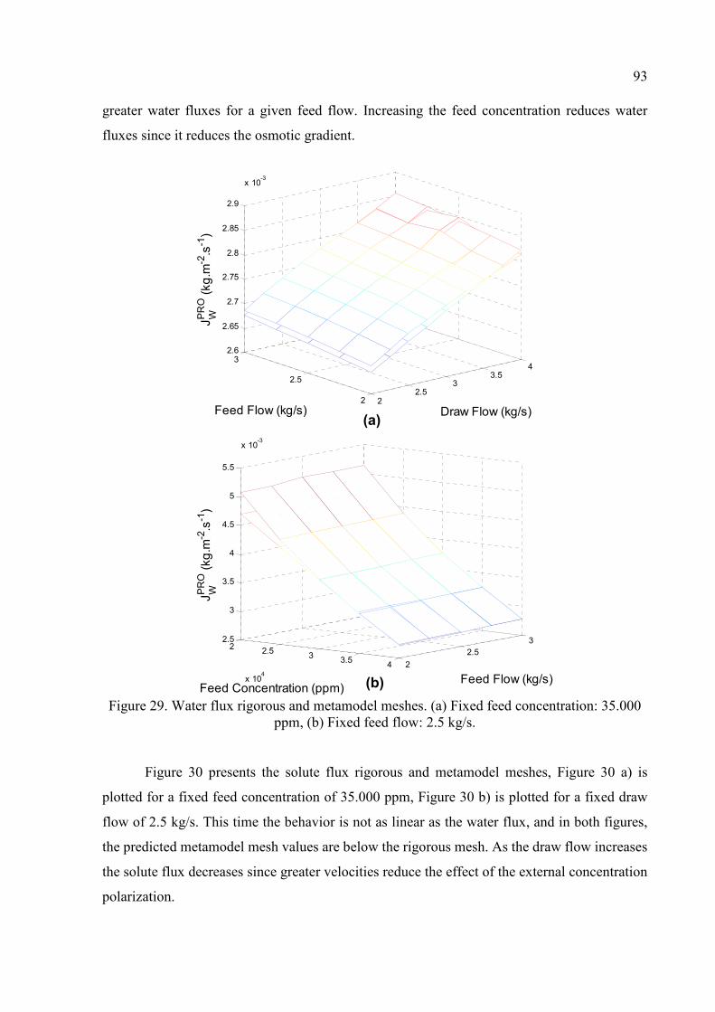
93
greater water fluxes for a given feed flow. Increasing the feed concentration reduces water
fluxes since it reduces the osmotic gradient.
Figure 29. Water flux rigorous and metamodel meshes. (a) Fixed feed concentration: 35.000
ppm, (b) Fixed feed flow: 2.5 kg/s. Figure 30 presents the solute flux rigorous and metamodel meshes, Figure 30 a) is
plotted for a fixed feed concentration of 35.000 ppm, Figure 30 b) is plotted for a fixed draw
flow of 2.5 kg/s. This time the behavior is not as linear as the water flux, and in both figures,
the predicted metamodel mesh values are below the rigorous mesh. As the draw flow increases
the solute flux decreases since greater velocities reduce the effect of the external concentration
polarization.
22.5
33.5
4
2
2.5
32.6
2.65
2.7
2.75
2.8
2.85
2.9
x 10-3
Draw Flow (kg/s)Feed Flow (kg/s)
JWP
RO
(kg
.m-2
.s-1
)
22.5
33.5
4
x 104
2
2.5
32.5
3
3.5
4
4.5
5
5.5
x 10-3
Feed Flow (kg/s)Feed Concentration (ppm)
JWP
RO
(kg
.m-2
.s-1
)
(a)
(b)
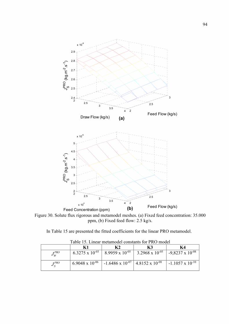
94
Figure 30. Solute flux rigorous and metamodel meshes. (a) Fixed feed concentration: 35.000
ppm, (b) Fixed feed flow: 2.5 kg/s.
In Table 15 are presented the fitted coefficients for the linear PRO metamodel.
Table 15. Linear metamodel constants for PRO model K1 K2 K3 K4
PRO
WJ 6.3275 x 10-03 8.9959 x 10-05 3.2968 x 10-05 -9,8237 x 10-08
PRO
SJ 6.9048 x 10-06
-1.6486 x 10-07 4.8152 x 10-08
-1.1057 x 10⁻¹⁰
22.5
33.5
4 2
2.5
32.4
2.5
2.6
2.7
2.8
2.9
x 10-6
Feed Flow (kg/s)Draw Flow (kg/s)
JSP
RO
(kg
.m-2
.s-1
)
22.5
33.5
4x 10
4 2
2.5
32
2.5
3
3.5
4
4.5
5
x 10-6
Feed Flow (kg/s)Feed Concentration (ppm)
JSP
RO
(kg
.m-2
.s-1
)
(a)
(b)
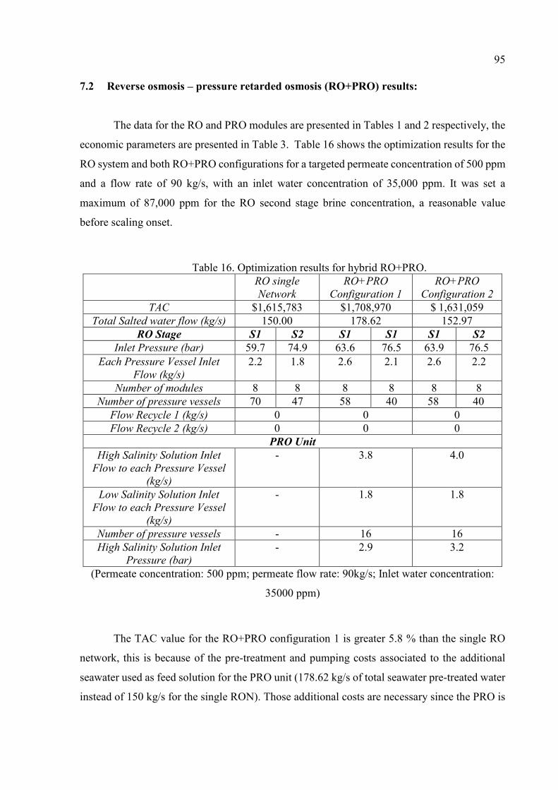
95
7.2 Reverse osmosis – pressure retarded osmosis (RO+PRO) results:
The data for the RO and PRO modules are presented in Tables 1 and 2 respectively, the
economic parameters are presented in Table 3. Table 16 shows the optimization results for the
RO system and both RO+PRO configurations for a targeted permeate concentration of 500 ppm
and a flow rate of 90 kg/s, with an inlet water concentration of 35,000 ppm. It was set a
maximum of 87,000 ppm for the RO second stage brine concentration, a reasonable value
before scaling onset.
Table 16. Optimization results for hybrid RO+PRO. RO single
Network
RO+PRO
Configuration 1
RO+PRO
Configuration 2
TAC $1,615,783 $1,708,970 $ 1,631,059 Total Salted water flow (kg/s) 150.00 178.62 152.97
RO Stage S1 S2 S1 S1 S1 S2
Inlet Pressure (bar) 59.7 74.9 63.6 76.5 63.9 76.5 Each Pressure Vessel Inlet
Flow (kg/s)
2.2 1.8 2.6 2.1 2.6 2.2
Number of modules 8 8 8 8 8 8 Number of pressure vessels 70 47 58 40 58 40
Flow Recycle 1 (kg/s) 0 0 0 Flow Recycle 2 (kg/s) 0 0 0
PRO Unit
High Salinity Solution Inlet
Flow to each Pressure Vessel
(kg/s)
- 3.8 4.0
Low Salinity Solution Inlet
Flow to each Pressure Vessel
(kg/s)
- 1.8 1.8
Number of pressure vessels - 16 16 High Salinity Solution Inlet
Pressure (bar)
- 2.9 3.2
(Permeate concentration: 500 ppm; permeate flow rate: 90kg/s; Inlet water concentration:
35000 ppm)
The TAC value for the RO+PRO configuration 1 is greater 5.8 % than the single RO
network, this is because of the pre-treatment and pumping costs associated to the additional
seawater used as feed solution for the PRO unit (178.62 kg/s of total seawater pre-treated water
instead of 150 kg/s for the single RON). Those additional costs are necessary since the PRO is
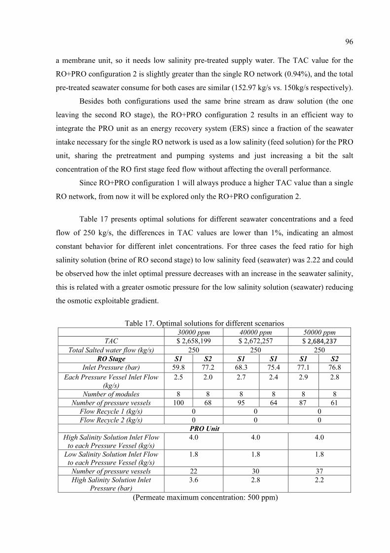
96
a membrane unit, so it needs low salinity pre-treated supply water. The TAC value for the
RO+PRO configuration 2 is slightly greater than the single RO network (0.94%), and the total
pre-treated seawater consume for both cases are similar (152.97 kg/s vs. 150kg/s respectively).
Besides both configurations used the same brine stream as draw solution (the one
leaving the second RO stage), the RO+PRO configuration 2 results in an efficient way to
integrate the PRO unit as an energy recovery system (ERS) since a fraction of the seawater
intake necessary for the single RO network is used as a low salinity (feed solution) for the PRO
unit, sharing the pretreatment and pumping systems and just increasing a bit the salt
concentration of the RO first stage feed flow without affecting the overall performance.
Since RO+PRO configuration 1 will always produce a higher TAC value than a single
RO network, from now it will be explored only the RO+PRO configuration 2.
Table 17 presents optimal solutions for different seawater concentrations and a feed
flow of 250 kg/s, the differences in TAC values are lower than 1%, indicating an almost
constant behavior for different inlet concentrations. For three cases the feed ratio for high
salinity solution (brine of RO second stage) to low salinity feed (seawater) was 2.22 and could
be observed how the inlet optimal pressure decreases with an increase in the seawater salinity,
this is related with a greater osmotic pressure for the low salinity solution (seawater) reducing
the osmotic exploitable gradient.
Table 17. Optimal solutions for different scenarios
30000 ppm 40000 ppm 50000 ppm
TAC $ 2,658,199 $ 2,672,257 $ 2,684,237 Total Salted water flow (kg/s) 250 250 250
RO Stage S1 S2 S1 S1 S1 S2
Inlet Pressure (bar) 59.8 77.2 68.3 75.4 77.1 76.8 Each Pressure Vessel Inlet Flow
(kg/s)
2.5 2.0 2.7 2.4 2.9 2.8
Number of modules 8 8 8 8 8 8 Number of pressure vessels 100 68 95 64 87 61
Flow Recycle 1 (kg/s) 0 0 0 Flow Recycle 2 (kg/s) 0 0 0
PRO Unit
High Salinity Solution Inlet Flow
to each Pressure Vessel (kg/s)
4.0 4.0 4.0
Low Salinity Solution Inlet Flow
to each Pressure Vessel (kg/s)
1.8 1.8 1.8
Number of pressure vessels 22 30 37 High Salinity Solution Inlet
Pressure (bar)
3.6 2.8 2.2
(Permeate maximum concentration: 500 ppm)
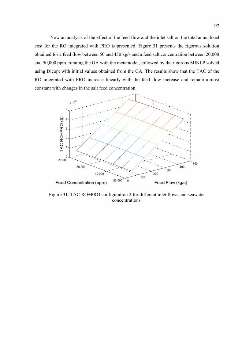
97
Now an analysis of the effect of the feed flow and the inlet salt on the total annualized
cost for the RO integrated with PRO is presented. Figure 31 presents the rigorous solution
obtained for a feed flow between 50 and 450 kg/s and a feed salt concentration between 20,000
and 50,000 ppm, running the GA with the metamodel, followed by the rigorous MINLP solved
using Dicopt with initial values obtained from the GA. The results show that the TAC of the
RO integrated with PRO increase linearly with the feed flow increase and remain almost
constant with changes in the salt feed concentration.
Figure 31. TAC RO+PRO configuration 2 for different inlet flows and seawater concentrations.
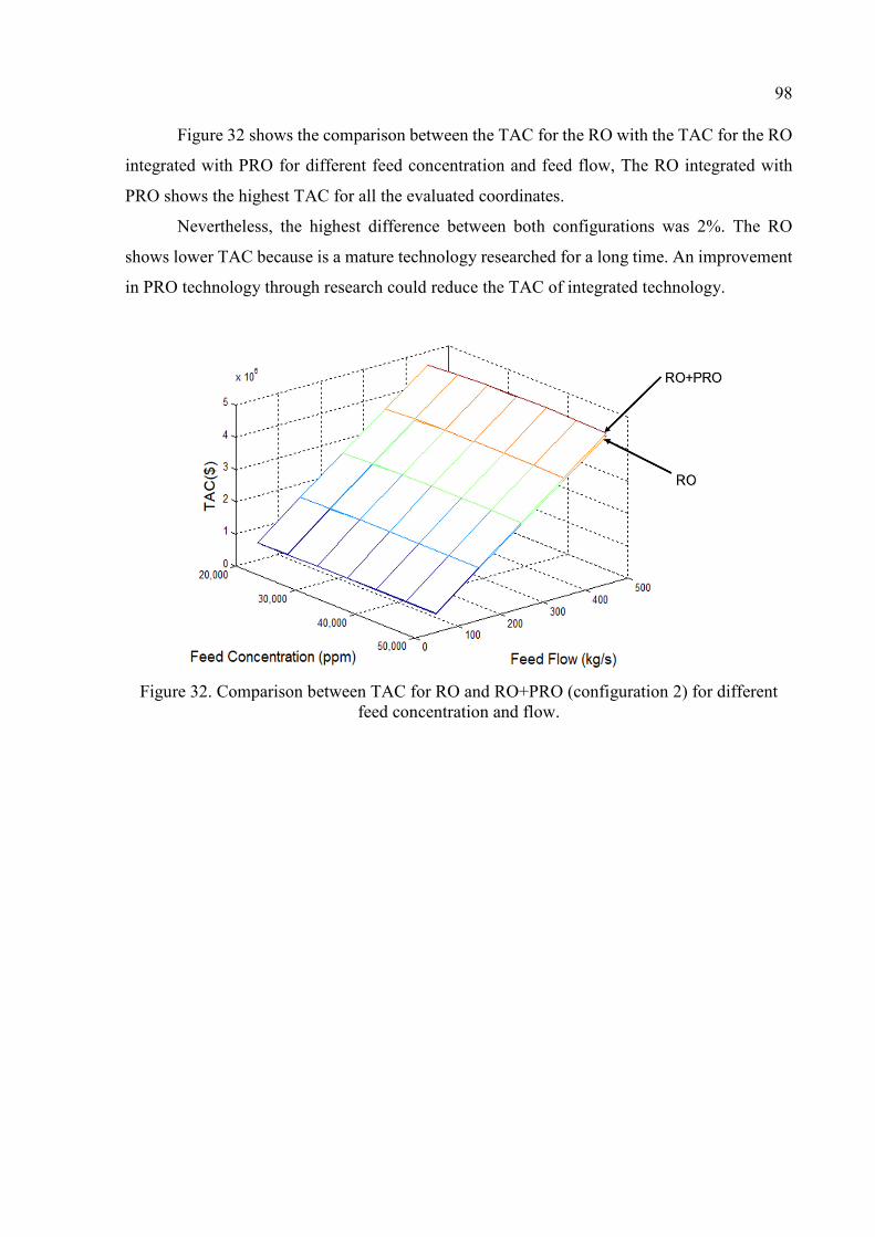
98
Figure 32 shows the comparison between the TAC for the RO with the TAC for the RO
integrated with PRO for different feed concentration and feed flow, The RO integrated with
PRO shows the highest TAC for all the evaluated coordinates.
Nevertheless, the highest difference between both configurations was 2%. The RO
shows lower TAC because is a mature technology researched for a long time. An improvement
in PRO technology through research could reduce the TAC of integrated technology.
Figure 32. Comparison between TAC for RO and RO+PRO (configuration 2) for different feed concentration and flow.
99
8 CONCLUSIONS AND RECOMMENDATIONS
8.1 Conclusions
A new methodology to solve a nonlinear mathematical model for the optimal design of
RO is proposed. Metamodels were used to reduce the mathematical complexity and get accurate
solutions using a genetic algorithm. Then, the results were used as initial values to solve the
full nonlinear model using GAMS/DICOPT. This allows getting optimal solutions for a
complex MINLP problem with less computational effort. One of the major advances of this
approach is that initial values are not needed (always a problem for practitioners using MINLP
codes), as the GA provides them.
When the new bound contraction methodology was used, the upper bound is the
rigorous MINLP and is run using the results from the lower bound (constructed by images of
monotone functions in each domain variable’s partition) as initial values. Before trying bound
contraction, it was attempted to increase the number of partitions in the lower bound to see if
the gap at the root node can be reduced. The result is that a region where there is no
improvement in the objective value when the number of intervals for the partitioned variables
was increased, was reached. When bound contraction was attempted using two intervals, none
of the bounds for the partitioned variables could be contracted.
The new stochastic – deterministic proposed methodology allows exploring the effect
of the feed flow, seawater concentration, number of reverse osmosis stages, and the maximum
number of membrane modules in each pressure vessel on the total annualized cost of the plant.
The total annualized cost increases with an increase in the feed flow and presents little
variations for different feed salt concentrations at a fixed inlet flow, indicating that a reverse
osmosis plant could have adaptation capability for variations in the inlet concentration without
major effects on the TAC.
The effect of the number of stages was studied for different feed flows and seawater
concentrations, finding that one stage has the largest TAC and the differences between two and
three stages are small, but dependent on the costing of pumps used.
100
The effect of the number of membrane modules in a pressure vessel was also investigated,
finding that increasing the maximum number of membranes allowed in a commercial pressure
vessel does not have any advantage over the TAC values obtained.
Two-hybrid RO+PRO superstructures were the PRO unit uses the chemical potential of
the brine stream of the RO to generate electrical power, acting as an energy recovery unit, were
proposed, and optimized with the new stochastic-deterministic methodology.
The second proposed configuration for the system RO+PRO showed a lower TAC than
the first one. Besides both configurations used the same brine stream as draw solution, the
second one results in an efficient way to integrate the PRO unit as an energy recovery system,
since a fraction of the seawater intake necessary for the single RO network is used as a low
salinity (feed solution) for the PRO unit, sharing the pretreatment and pumping systems and
just increasing a bit the salt concentration of the RO first stage feed flow without affecting the
overall performance. So, the second configuration is recommended for the industrial
implementation of the integrated technology.
The hybrid RO+PRO configuration presents the same behavior to variations in feed flow
and concentration as the single RON, this is an increase in TAC values with an increase in the
feed flow and little variations for different feed salt concentrations at a fixed inlet flow.
The comparison between the TAC for the RO with the TAC for the RO integrated with
PRO for different feed concentration and feed flow was developed. The RO integrated with
PRO shows the highest TAC for all the evaluated coordinates. Nevertheless, the highest
difference between both configurations was 2%. The RO shows lower TAC because is a mature
technology researched for a long time. An improvement in the PRO energy recovery efficiency
could reduce the TAC of the integrated technology since the energy cost of the RO network
represents its major operational costs.
101
8.2 Recommendations to future works
As identified in this work, it will be helpful to obtain actualized cost functions for high-
pressure pumps and turbines that capture the nonlinear behavior of costs, for example, a power
law for cost, with other exponents might change the results.
A sensitivity analysis using different energy cost values will be interesting, the effect of
the feed temperature also could be included in this analysis.
Construction of metamodels for different commercial membrane modules, and the use of
binary variables for the choice of one or another might help to obtain efficient reverse osmosis
networks with lower TAC values.
For the RO+PRO hybrid system, it will be interesting to validate the use of a fraction of
permeate as low salinity feed solution since it will increase the osmotic potential.
The use of the proposed optimization methodology could allow constructing
technological roadmap of other hybrid technologies as forward osmosis, membrane distillation,
or thermal technologies coupled with reverse osmosis.
The proposed stochastic-deterministic methodology with the use of metamodels will be
an interesting optimization tool to apply to other engineering problems.
102
9 REFERENCES
ABDULRAHIM, H. K.; ALASFOUR, F. N. Multi-Objective Optimisation of hybrid MSF
RO desalination system using Genetic Algorithm. International Journal of Exergy, [s.l.], v. 7, no 3, p. 387, 2010. ISSN: 1742-8297, DOI: 10.1504/IJEX.2010.031991. ABOU RAYAN, M.; KHALED, I. Seawater desalination by reverse osmosis (case study). Desalination, [s.l.], v. 153, no 1–3, p. 245–251, 2003. ISSN: 0011-9164, DOI: 10.1016/S0011-9164(02)01143-8. ACHILLI, A.; CATH, T. Y.; CHILDRESS, A. E. Power generation with pressure retarded
osmosis : An experimental and theoretical investigation. [s.l.], v. 343, p. 42–52, 2009. DOI: 10.1016/j.memsci.2009.07.006. AGASHICHEV, S. P. Analysis of integrated co-generative schemes including MSF, RO
and power generating systems (present value of expenses and “levelised” cost of water). Desalination, [s.l.], v. 164, no 3, p. 281–302, 2004. ISSN: 0011-9164, DOI: 10.1016/S0011-9164(04)00196-1. AGASHICHEV, S. P.; EL-NASHAR, A. M. Systemic approach for techno-economic
evaluation of triple hybrid (RO, MSF and power generation) scheme including accounting
of CO2 emission. Energy, [s.l.], v. 30, no 8, p. 1283–1303, 2005. ISSN: 0360-5442, DOI: 10.1016/J.ENERGY.2004.02.002. AL-BASTAKI, N. M.; ABBAS, A. Predicting the performance of RO membranes. Desalination, [s.l.], v. 132, no 1–3, p. 181–187, 2000. ISSN: 00119164, DOI: 10.1016/S0011-9164(00)00147-8. ALBASTAKI, N.; ABBAS, A. Modeling an industrial reverse osmosis unit1. Desalination, [s.l.], v. 126, no 1–3, p. 33–39, 1999. ISSN: 00119164, DOI: 10.1016/S0011-9164(99)00152-6. ALMANSOORI, A.; SAIF, Y. Structural optimization of osmosis processes for water and
power production in desalination applications. Desalination, [s.l.], v. 344, p. 12–27, 2014. ISSN: 00119164, DOI: 10.1016/j.desal.2014.03.002. ALNOURI, S. Y.; LINKE, P. A systematic approach to optimal membrane network
synthesis for seawater desalination. Journal of Membrane Science, [s.l.], v. 417–418, p. 96–112, 2012. ISSN: 03767388, DOI: 10.1016/j.memsci.2012.06.017. ALTAEE, A.; SHARIF, A. Pressure retarded osmosis: advancement in the process
applications for power generation and desalination. Desalination, [s.l.], 2014. ISBN: 4479865179, ISSN: 00119164, DOI: 10.1016/j.desal.2014.09.028. ANSARI, K.; SAYYAADI, H.; AMIDPOUR, M. Thermoeconomic optimization of a hybrid
pressurized water reactor (PWR) power plant coupled to a multi effect distillation
desalination system with thermo-vapor compressor (MED-TVC). Energy, [s.l.], v. 35, no 5, p. 1981–1996, 2010. ISSN: 03605442, DOI: 10.1016/j.energy.2010.01.013.
103
ATIKOL, U.; AYBAR, H. S. Estimation of water production cost in the feasibility analysis
of RO systems. Desalination, [s.l.], v. 184, no 1–3, p. 253–258, 2005. ISSN: 0011-9164, DOI: 10.1016/J.DESAL.2005.02.065. AVLONITIS, S. A. Operational water cost and productivity improvements for small-size
RO desalination plants. Desalination, [s.l.], v. 142, no 3, p. 295–304, 2002. ISSN: 0011-9164, DOI: 10.1016/S0011-9164(02)00210-2. BAKER, R. W. Membrane Technology and Applications. 2 ed. [s.l.]: John Wiley & Sons, Inc., 2004. ISBN: 0470854456. BEH, E. H. Y. et al. Environmental Modelling & Software Robust optimization of water
infrastructure planning under deep uncertainty using metamodels. Environmental
Modelling and Software, [s.l.], v. 93, p. 92–105, 2017. ISSN: 1364-8152, DOI: 10.1016/j.envsoft.2017.03.013. BROAD, D. R.; DANDY, G. C.; MAIER, H. R. Environmental Modelling & Software A
systematic approach to determining metamodel scope for risk- based optimization and its
application to water distribution system. Environmental Modelling and Software, [s.l.], v. 69, p. 382–395, 2015. ISSN: 1364-8152, DOI: 10.1016/j.envsoft.2014.11.015. BUCHER, C. Metamodels of optimal quality for stochastic structural optimization. Probabilistic Engineering Mechanics, [s.l.], 2017. ISSN: 0266-8920, DOI: 10.1016/j.probengmech.2017.09.003. CARVALHO, M.; SECCHI, A. R.; BAGAJEWICZ, M. Model Reformulation and Global
Optimization of Oil Production Using Gas Lift. Industrial and Engineering Chemistry
Research, [s.l.], v. 55, no 38, 2016. ISSN: 15205045, DOI: 10.1021/acs.iecr.6b00223. CHOI, J. S.; KIM, J. T. Modeling of full-scale reverse osmosis desalination system:
Influence of operational parameters. Journal of Industrial and Engineering Chemistry, [s.l.], v. 21, p. 261–268, 2015. ISSN: 22345957, DOI: 10.1016/j.jiec.2014.02.033. DAHDAH, H.; MITSOS, A. Structural optimization of seawater desalination : I . A flexible
superstructure and novel MED – MSF configurations. Desalination, [s.l.], v. 344, no 2014, p. 252–265, 2014. DOI: 10.1016/j.desal.2014.03.030. DOW WATER & PROCESS SOLUTIONS. FILMTEC TM Reverse Osmosis Membranes
Technical Manual, Formno.609-00071-1009. [s.l.]: [s.n.], 2011. 181 p. ISBN: 6090007110. DRUETTA, P.; AGUIRRE, P.; MUSSATI, S. Optimization of Multi-Effect Evaporation
desalination plants. Desalination, [s.l.], v. 311, p. 1–15, 2013. ISSN: 00119164, DOI: 10.1016/j.desal.2012.10.033. DU, Y. et al. Optimization of Reverse Osmosis Networks with Spiral-Wound Modules. Industrial & Engineering Chemistry Research, [s.l.], v. 51, p. 11764–11777, 2012. DU, Y. et al.Optimization of reverse osmosis networks with split partial second pass
design. Desalination, [s.l.], v. 365, p. 365–380, 2015. ISSN: 00119164, DOI: 10.1016/j.desal.2015.03.019.
104
EDGAR, T. F.; HIMMELBLAU, D. M.; LASDON, L. S. Optimization of Chemical
Processes. 2 ed. [s.l.]: McGraw-Hill, 2001. 651 p. ISBN: 9780070393592, ISSN: 00092509, DOI: 10.1016/0009-2509(89)85111-5. EL-HALWAGI, M. M. Synthesis of Reverse-Osmosis Networks for Waste Reduction. AIChE Journal, [s.l.], v. 38, no 8, p. 1185–1198, 1992. EL-HALWAGI, M.; AL-AHMAD, M.; ZHU, M. Optimal design and scheduling of flexible
reverse osmosis networks. Journal of Membrane Science, [s.l.], v. 129, p. 161–174, 1997. EVANGELISTA, F. A Short Cut Method for the Design of Reverse Osmosis Desalination
Plants. Industrial & Engineering Chemistry Process Design and Development, [s.l.], v. 24, p. 211–223, 1985. FARIA, C.; BAGAJEWICZ, M. J. A New Approach for Global Optimization of a Class of
MINLP Problems with Applications to Water Management and Pooling Problems. AICHE
Journal, [s.l.], v. 58, no 8, 2012. DOI: 10.1002/aic. FLOUDAS, C. A.; GOUNARIS, C. E. A review of recent advances in global optimization. Journal of Global Optimization, [s.l.], v. 45, no 1, p. 3–38, 2009. ISBN: 0925-5001, ISSN: 09255001, DOI: 10.1007/s10898-008-9332-8. FLOUDAS, C. a. Nonlinear and Mixed-Integer Optimization: Fundamentals and
Applications. Handbook of Applied Optimization. [s.l.]: Oxford University Press, 1995. 462 p. ISBN: 0-19-510056-5, ISSN: 09255001, DOI: 10.1023/A:1008256302713. FONTEIX, C. et al. Haploid and diploid algorithms, a new approach for global
optimization: Compared performances. International Journal of Systems Science, [s.l.], v. 26, no 10, p. 1919–1933, 1995. ISBN: 0020-7721, ISSN: 14645319, DOI: 10.1080/00207729508929145. GERALDES, V.; PEREIRA, N. E.; NORBERTA DE PINHO, M. Simulation and
Optimization of Medium-Sized Seawater Reverse Osmosis Processes with Spiral-Wound
Modules. Industrial & Engineering Chemistry Research, [s.l.], v. 44, p. 1897–1905, 2005. ISBN: 0035121841751, ISSN: 0888-5885, DOI: 10.1021/ie049357s. GHAFFOUR, N. et al. Renewable energy-driven desalination technologies: A
comprehensive review on challenges and potential applications of integrated systems. Desalination, [s.l.], v. 356, p. 94–114, 2015. ISBN: 00119164, ISSN: 00119164, DOI: 10.1016/j.desal.2014.10.024. GHAFFOUR, N.; MISSIMER, T. M.; AMY, G. L. Technical review and evaluation of the
economics of water desalination: Current and future challenges for better water supply
sustainability. Desalination, [s.l.], v. 309, no 2013, p. 197–207, 2013. ISBN: 0011-9164, ISSN: 00119164, DOI: 10.1016/j.desal.2012.10.015.
105
GHOBEITY, A.; MITSOS, A. Optimal design and operation of desalination systems : new
challenges and recent advances. Current Opinion in Chemical Engineering, [s.l.], v. 6, p. 61–68, 2014. ISSN: 2211-3398, DOI: 10.1016/j.coche.2014.09.008. GROSSMANN, I. et al. DICOPT. GAMS Development Corporation. 2016. Disponível em: <https://www.gams.com/>. GUTHRIE, K. M. Data and Techniques for Preilinary Capital Cost Estimation. Chemical
Engineering, [s.l.], no March 24, p. 114–142, 1969. HABERT, A. C.; BORGES, C. P.; NOBREGA, R. Processos de Separação por Membranas. [s.l.]: e-papers, 2006. 180 p. ISBN: 857650085X. HAFEZ, A.; EL-MANHARAWY, S. Economics of seawater RO desalination in the Red
Sea region, Egypt. Part 1. A case study. Desalination, [s.l.], v. 153, no 1–3, p. 335–347, 2003. ISSN: 0011-9164, DOI: 10.1016/S0011-9164(02)01122-0. HELFER, F.; LEMCKERT, C.; ANISSIMOV, Y. G. Osmotic power with Pressure Retarded
Osmosis: Theory, performance and trends - A review. Journal of Membrane Science, [s.l.], v. 453, p. 337–358, 2014. ISBN: 0376-7388, ISSN: 03767388, DOI: 10.1016/j.memsci.2013.10.053. JAFFAL, I.; INARD, C. A metamodel for building energy performance. Energy &
Buildings, [s.l.], v. 151, p. 501–510, 2017. ISSN: 0378-7788, DOI: 10.1016/j.enbuild.2017.06.072. JIANG, A. et al. Mathematical Modeling and Simulation of SWRO Process Based on
Simultaneous Method. Journal of Applied Mathematics, [s.l.], v. 2014, 2014. JIANG, A. et al. Operational cost optimization of a full-scale SWRO system under multi-
parameter variable conditions. Desalination, [s.l.], v. 355, p. 124–140, 2015. ISSN: 0011-9164, DOI: 10.1016/j.desal.2014.10.016. KAMALI, R. K.; MOHEBINIA, S. Experience of design and optimization of multi-effects
desalination systems in Iran. Desalination, [s.l.], v. 222, no 1–3, p. 639–645, 2008. ISSN: 00119164, DOI: 10.1016/j.desal.2007.01.182. KHAWAJI, A. D.; KUTUBKHANAH, I. K.; WIE, J. M. Advances in seawater desalination
technologies. Desalination, [s.l.], v. 221, no 1–3, p. 47–69, 2008. ISBN: 0011-9164, ISSN: 00119164, DOI: 10.1016/j.desal.2007.01.067. KIM, S Y; BAGAJEWICZ, M. Global Optimization of Heat Exchanger Networks. Part 2:
Stages/Substages Superstructure with Variable Cp. Industrial and Engineering Chemistry
Research, [s.l.], v. 56, no 20, p. 5958–5969, 2017. DOI: 10.1021/acs.iecr.6b04687. KIM, Sung Young et al. Global Optimization of Heat Exchanger Networks. Part 1:
Stages/Substages Superstructure. Industrial & Engineering Chemistry Research, [s.l.], v. 56, no 20, p. 5944–5957, 2017. ISSN: 0888-5885, DOI: 10.1021/acs.iecr.6b04686.
106
KIM, Sung Young; BAGAJEWICZ, M. Global optimization of heat exchanger networks
using a new generalized superstructure. Chemical Engineering Science, [s.l.], v. 147, p. 30–46, 2016. ISSN: 00092509, DOI: 10.1016/j.ces.2016.02.002. KIM, Y. S. Y. M. et al. Overview of systems engineering approaches for a large-scale
seawater desalination plant with a reverse osmosis network. Desalination, [s.l.], v. 238, no 1–3, p. 312–332, 2009. ISBN: 0011-9164, ISSN: 00119164, DOI: 10.1016/j.desal.2008.10.004. KLEIJNEN, J. P. C. Regression and Kriging metamodels with their experimental designs
in simulation : A review. [s.l.], v. 256, p. 1–16, 2017. KUCERA, J. Desalination: Water from Water. 1 ed. [s.l.]: John Wiley and Sons, 2014. 664 p. ISBN: 9781118208526. LEE, J. G. et al. Numerical study of a hybrid multi-stage vacuum membrane distillation
and pressure-retarded osmosis system. Desalination, [s.l.], v. 363, p. 82–91, 2015. ISSN: 00119164, DOI: 10.1016/j.desal.2015.01.043. LEITNER, G. F. Total water costs on a standard basis for three large, operating , S.W.R.O.
plants. Desalination, [s.l.], v. 81, no 1–3, p. 39–48, 1991. ISSN: 0011-9164, DOI: 10.1016/0011-9164(91)85043-T. LU, Y.; LIAO, A.; HU, Y. Design of reverse osmosis networks for multiple freshwater
production. Korean Journal of Chemical Engineering, [s.l.], v. 30, no 5, p. 988–996, 2013. ISBN: 0256-1115, ISSN: 02561115, DOI: 10.1007/s11814-013-0009-8. LU, Y. Y. et al. Optimum design of reverse osmosis system under different feed
concentration and product specification. Journal of Membrane Science, [s.l.], v. 287, no 2, p. 219–229, 2007. ISBN: 5326678187, ISSN: 03767388, DOI: 10.1016/j.memsci.2006.10.037. MAHMOUDI, S.; TRIVAUDEY, F.; BOUHADDI, N. Bene fi ts of metamodel-reduction for
nonlinear dynamic response analysis of damaged composite structures. Finite Elements in
Analysis and Design, [s.l.], v. 119, p. 1–14, 2016. ISSN: 0168-874X, DOI: 10.1016/j.finel.2016.05.001. MALEK, A.; HAWLADER, M. N. A.; HO, J. C. Design and economics of RO seawater
desalination. Desalination, [s.l.], v. 105, no 3, p. 245–261, 1996. ISBN: 0011-9164, ISSN: 00119164, DOI: 10.1016/0011-9164(96)00081-1. MALIK, S. N.; BAHRI, P. A.; VU, L. T. T. Superstructure Development, Simulation and
Optimization of Desalination Systems using Aspen Custom Modeler. In: 12th International
Symposium on Process Systems Engineering and 25th European Symposium on Computer
Aided Process Engineering. [s.l.]: Elsevier, 2015. Disponível em: <http://linkinghub.elsevier.com/retrieve/pii/B9780444635785500591>. ISSN: 1570-7946, DOI: 10.1016/B978-0-444-63578-5.50059-1. MARCOVECCHIO, M. G. et al. Optimization of hybrid desalination processes including
multi stage flash and reverse osmosis systems. Desalination, [s.l.], v. 182, no 1–3, p. 111–122, 2005. ISSN: 00119164, DOI: 10.1016/j.desal.2005.03.011.
107
MARCOVECCHIO, M. G.; AGUIRRE, P. a.; SCENNA, N. J. Global optimal design of
reverse osmosis networks for seawater desalination: modeling and algorithm. Desalination, [s.l.], v. 184, no 1–3, p. 259–271, 2005. ISSN: 00119164, DOI: 10.1016/j.desal.2005.03.056. MASKAN, F. et al. Optimal Design of Reverse Osmosis Module Networks. AICHE Journal, [s.l.], v. 46, no 5, 2000. MISENER, R.; FLOUDAS, C. A. ANTIGONE: Algorithms for continuous / Integer Global
Optimization of Nonlinear Equations. Journal of Global Optimization, [s.l.], v. 59, no 2–3, p. 503–526, 2014. ISBN: 1573-2916, ISSN: 15732916, DOI: 10.1007/s10898-014-0166-2. NAGHILOO, A. et al. Modeling and design of a 25MW osmotic power plant (PRO) on
Bahmanshir River of Iran. Renewable Energy, [s.l.], v. 78, no November 2009, p. 51–59, 2015. ISSN: 18790682, DOI: 10.1016/j.renene.2014.12.067. OH, H. J.; HWANG, T. M.; LEE, S. A simplified simulation model of RO systems for
seawater desalination. Desalination, [s.l.], v. 238, no 1–3, p. 128–139, 2009. ISBN: 0011-9164, ISSN: 00119164, DOI: 10.1016/j.desal.2008.01.043. PARK, S.-M. et al. Optimization of hybrid system consisting of forward osmosis and
reverse osmosis: a Monte Carlo simulation approach. Desalination and Water Treatment, [s.l.], v. 43, no 1–3, p. 274–280, 2012. ISSN: 1944-3994, DOI: 10.1080/19443994.2012.672196. POULLIKKAS, A. Optimization algorithm for reverse osmosis desalination economics. Desalination, [s.l.], v. 133, no 1, p. 75–81, 2001. ISSN: 0011-9164, DOI: 10.1016/S0011-9164(01)00084-4. PRACTICE, S. M. Simulation Modelling Practice and Theory Interval metamodels for the
analysis of simulation Input – Output relations. [s.l.], v. 54, p. 86–100, 2015. DOI: 10.1016/j.simpat.2015.03.008. PRANTE, J. L. et al. RO-PRO desalination: An integrated low-energy approach to
seawater desalination. Applied Energy, [s.l.], v. 120, p. 104–114, 2014. ISBN: 0306-2619, ISSN: 03062619, DOI: 10.1016/j.apenergy.2014.01.013. PSALTIS, A.; SINOQUET, D.; PAGOT, A. Systematic optimization methodology for heat
exchanger network and simultaneous process design. Computers and Chemical
Engineering, [s.l.], v. 95, p. 146–160, 2016. ISSN: 0098-1354, DOI: 10.1016/j.compchemeng.2016.09.013. ROSENTHAL, R. E. GAMS — A User ’ s Guide. [s.l.], no October, 2015. SAHINIDIS, N. V. BARON: A general purpose global optimization software package. Journal of Global Optimization, [s.l.], v. 8, no 2, p. 201–205, 1996. ISBN: 0925-5001, ISSN: 0925-5001, DOI: 10.1007/BF00138693.
108
SAIF, Y.; ALMANSOORI, A.; ELKAMEL, A. Optimal Design of Split Partial Second Pass
Reverse Osmosis Network for Desalination Applications. [s.l.], v. 60, no 2, 2014. DOI: 10.1002/aic. SAITO, K. et al. Power generation with salinity gradient by pressure retarded osmosis
using concentrated brine from SWRO system and treated sewage as pure water. Desalination and Water Treatment, [s.l.], v. 41, no 1–3, p. 114–121, 2012. ISBN: 1944-3994, ISSN: 19443986, DOI: 10.1080/19443994.2012.664696. SASSI, K. M.; MUJTABA, I. M. Effective design of reverse osmosis based desalination
process considering wide range of salinity and seawater temperature. Desalination, [s.l.], v. 306, p. 8–16, 2012. ISBN: 0011-9164, ISSN: 00119164, DOI: 10.1016/j.desal.2012.08.007. SASSI, K. M.; MUJTABA, I. M. MINLP based superstructure optimization for boron
removal during desalination by reverse osmosis. Journal of Membrane Science, [s.l.], v. 440, p. 29–39, 2013. ISSN: 03767388, DOI: 10.1016/j.memsci.2013.03.012. SCHOCK, G.; MIQUEL, A. Mass transfer and pressure loss in spiral wound modules. Desalination, [s.l.], v. 64, no C, p. 339–352, 1987. ISBN: 0011-9164, ISSN: 00119164, DOI: 10.1016/0011-9164(87)90107-X. SHAKIB, S. E.; AMIDPOUR, M.; AGHANAJAFI, C. Simulation and optimization of multi
effect desalination coupled to a gas turbine plant with HRSG consideration. Desalination, [s.l.], v. 285, p. 366–376, 2012. ISSN: 00119164, DOI: 10.1016/j.desal.2011.10.028. SHATAT, M.; RIFFAT, S. B. Water desalination technologies utilizing conventional and
renewable energy sources. International Journal of Low-Carbon Technologies, [s.l.], v. 9, no 1, p. 1–19, 2014. ISBN: 1748-1317, ISSN: 17481317, DOI: 10.1093/ijlct/cts025. SHRIVASTAVA, A.; ROSENBERG, S.; PEERY, M. Energy efficiency breakdown of
reverse osmosis and its implications on future innovation roadmap for desalination. Desalination, [s.l.], v. 368, p. 181–192, 2015. ISSN: 0011-9164, DOI: 10.1016/J.DESAL.2015.01.005. SKIBOROWSKI, M. et al. Model-based structural optimization of seawater desalination
plants. Desalination, [s.l.], v. 292, p. 30–44, 2012. ISSN: 0011-9164, DOI: 10.1016/j.desal.2012.02.007. THE MATHWORKS INC. MATLAB - MathWorks. www.mathworks.com/products/matlab. 2016. Disponível em: <http://www.mathworks.com/products/matlab/>. DOI: 2016-11-26. VINCE, F. et al. Multi-objective optimization of RO desalination plants. Desalination, [s.l.], v. 222, no 1–3, p. 96–118, 2008. ISBN: 0011-9164, ISSN: 00119164, DOI: 10.1016/j.desal.2007.02.064. VOROS, N. G.; MAROULIS, Z. B. Short-cut structural design of reverse osmosis
desalination plants. [s.l.], v. 127, p. 47–68, 1997.
109
VOROS, N.; MAROULIS, Z. B. Pergamon FOR SEAWATER DESALINATION. Science, [s.l.], v. 20, no 96, 1996. VOROS, N.; MAROULIS, Z. B.; MARINOS-KOURIS, D. Optimization of reverse osmosis
networks for seawater desalination. Computers & Chemical Engineering, [s.l.], v. 20, p. S345–S350, 1996. ISSN: 00981354, DOI: 10.1016/0098-1354(96)00068-3. VOUTCHKOV, N. Desalination Engineering: Planning and Design. 1 ed. [s.l.]: McGraw-Hill, 2012. 688 p. ISBN: 0071777156 / 9780071777155, ISSN: 1098-6596, DOI: 10.1007/s13398-014-0173-7.2. WADE, N. M. Distillation plant development and cost update. Desalination, [s.l.], v. 136, no 1–3, p. 3–12, 2001. ISSN: 0011-9164, DOI: 10.1016/S0011-9164(01)00159-X. WAN, C. F.; CHUNG, T. S. Osmotic power generation by pressure retarded osmosis using
seawater brine as the draw solution and wastewater retentate as the feed. Journal of
Membrane Science, [s.l.], v. 479, p. 148–158, 2015. ISBN: 0014-4827, ISSN: 18733123, DOI: 10.1016/j.memsci.2014.12.036. FENG, C.; CHUNG, T. Energy recovery by pressure retarded osmosis (PRO) in SWRO-
PRO integrated processes. Applied Energy, [s.l.], v. 162, p. 687–698, 2016. ISSN: 03062619, DOI: 10.1016/j.apenergy.2015.10.067. WANG, Jian et al. Operational Optimization of Large-Scale Parallel-Unit SWRO
Desalination Plant Using Differential Evolution Algorithm. Scientific World Journal, [s.l.], v. 2014, 2014. ISSN: 1537-744X, DOI: 10.1155/2014/584068. WANG, Jinwen et al. A critical review of transport through osmotic membranes. Journal
of Membrane Science, [s.l.], v. 454, p. 516–537, 2014. ISSN: 0376-7388, DOI: 10.1016/j.memsci.2013.12.034. WEN, J. et al. International Journal of Heat and Mass Transfer Energy and cost
optimization of shell and tube heat exchanger with helical baffles using Kriging
metamodel based on MOGA. [s.l.], v. 98, p. 29–39, 2016. DOI: 10.1016/j.ijheatmasstransfer.2016.02.084. WU, S.; ZHANG, Z. An approach to improve the economy of desalination plants with a
nuclear heating reactor by coupling with hybrid technologies. Desalination, [s.l.], v. 155, no 2, p. 179–185, 2003. ISSN: 0011-9164, DOI: 10.1016/S0011-9164(03)00295-9. ZAK, G.; MITSOS, A. Hybrid thermal-thermal desalination structures. Desalination and
Water Treatment, [s.l.], v. 52, p. 2905–2919, 2014. ZEJLI, D. et al. Economic analysis of wind-powered desalination in the south of Morocco. Desalination, [s.l.], v. 165, p. 219–230, 2004. ISSN: 0011-9164, DOI: 10.1016/J.DESAL.2004.06.025.
110
APPENDIX
Appendix 1.
Reverse osmosis network general mathematical model
The State Space version of a generalized superstructure with all the possible connections
between units is shown in Figure A1. In this representation, the inputs of the distribution box
are considered splitting nodes and all the outputs are considered mixing nodes.
Distribution box:
The distribution box is a network, describing the connection between the units and the
feed and product streams, and consists of a series of splitting nodes (inputs) and mixing nodes
(outputs), all the streams are characterized by a flow rate (F), a salt concentration (C) and a
pressure (P), the superscripts HPP, T, RO, P, and B represents high-pressure pump, turbine,
reverse osmosis stage, permeate and brine respectively, therefore B-HPP indicates the
distribution from B to HPP, and so. The subscripts p, t and m are indexes that indicate the
number of pumps, turbines and reverse osmosis stages respectively. The subscripts S, P and B
means seawater, permeate and brine.
In addition, each stream that is distributed from a unit to another has a binary decision
variable associated with it, that will take the value of one (1) if the stream exists or zero (0) if
not. For example, if a distribution from a (p) pump to a reverse osmosis stage (m) , 0HPP RO
p mF
, the corresponding binary variable ,HPP RO
p my takes a value of one.
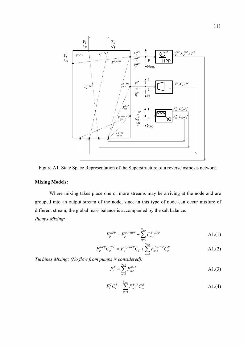
111
Figure A1. State Space Representation of the Superstructure of a reverse osmosis network.
Mixing Models:
Where mixing takes place one or more streams may be arriving at the node and are
grouped into an output stream of the node, since in this type of node can occur mixture of
different stream, the global mass balance is accompanied by the salt balance.
Pumps Mixing:
,1
RO
s
NF HPPHPP B HPP
p p m p
m
F F F
A1.(1)
,1
ˆRO
s
NF HPPHPP HPP B HPP B
p p p S m p m
m
F C F C F C
A1.(2)
Turbines Mixing: (No flow from pumps is considered):
,1
RONT B T
t m t
m
F F
A1.(3)
,1
RONT T B T B
t t m t m
m
F C F C
A1.(4)
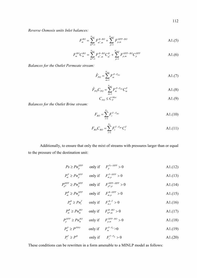
112
Reverse Osmosis units Inlet balances:
* ,,* 1 1
RO HPPN NRO B RO HPP RO
m p mm mm p
F F F
A1.(5)
* * ,,* 1 1
RO HPPN NRO RO B RO B HPP RO HPP
m m p m pm m mm p
F C F C F C
A1.(6)
Balances for the Outlet Permeate stream:
1
ˆRO
PO
NP F
PO m
m
F F
A1.(7)
1
ˆRO
PO
NP F P
PO PO m m
m
F C F C
A1.(8)
Max
PO PC C A1.(9)
Balances for the Outlet Brine stream:
1
T
BO
NT F
BO t
t
F F
A1.(10)
1
T
BO
NT F T
BO BO t t
t
F C F C
A1.(11)
Additionally, to ensure that only the mixt of streams with pressures larger than or equal
to the pressure of the destination unit:
only if 0HPP Fs HPP
p pPs Pn F A1.(12)
, only if 0P HPP P HPP
m p m pP Pn F A1.(13)
* *, only if 0HPP HPP HPP HPP
p p p pP Pn F A1.(14)
, only if 0B HPP B HPP
m p m pP Pn F A1.(15)
, only if 0B T B T
m t m tP Pn F A1.(16)
*, only if 0B RO B RO
m m m mP Pn F A1.(17)
, only if 0HPP RO HPP RO
p m p mP Pn F A1.(18)
only if >0 PP FP PPO
m mP P F A1.(19)
only if 0BT FT B
t tP P F A1.(20)
These conditions can be rewritten in a form amenable to a MINLP model as follows:
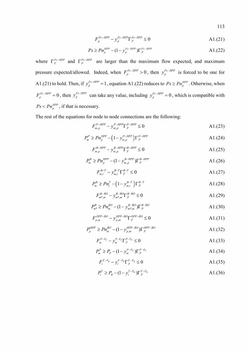
113
0 Fs HPP Fs HPP Fs HPP
p p FF y A1.(21)
(1 ) HPP Fs HPP Fs HPP
p p PPs Pn y A1.(22)
where Fs HPP
F
and Fs HPP
P
are larger than the maximum flow expected, and maximum
pressure expected/allowed. Indeed, when 0Fs HPP
pF , then Fs HPP
py is forced to be one for
A1.(21) to hold. Then, if 1Fs HPP
py , equation A1.(22) reduces to HPP
pPs Pn . Otherwise, when
0Fs HPP
pF , then can take any value, including 0Fs HPP
py , which is compatible with
HPP
pPs Pn , if that is necessary.
The rest of the equations for node to node connections are the following:
, , 0P HPP P HPP P HPP
m p m p FF y A1.(23)
,1P HPP P HPP P HPP
m p m p PP Pn y A1.(24)
, , 0B HPP B HPP B HPP
m p m p FF y A1.(25)
,(1 )B HPP B HPP B HPP
m p m p PP Pn y A1.(26)
, , 0B T B T B T
m t m t FF y A1.(27)
,1B T B T B T
m t m t PP Pn y A1.(28)
*, *, 0B RO B RO B RO
m m m m FF y A1.(29)
* *,(1 )B RO B RO B RO
m m m m PP Pn y A1.(30)
, , 0HPP RO HPP RO HPP RO
p m p m FF y A1.(31)
,(1 )HPP RO HPP RO HPP RO
p m p m PP Pn y A1.(32)
0P P PP F P F P F
m m FF y A1.(33)
(1 )P PP F P FP
m P m PP P y A1.(34)
0B B BT F T F T F
t t FF y A1.(35)
(1 )B BT F T FT
t B t PP P y A1.(36)
Fs HPP
py
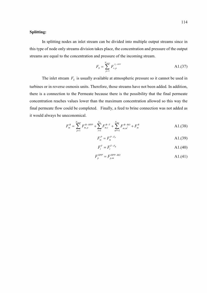
114
Splitting:
In splitting nodes an inlet stream can be divided into multiple output streams since in
this type of node only streams division takes place, the concentration and pressure of the output
streams are equal to the concentration and pressure of the incoming stream.
,1
HPPF HPPs
N
S s p
p
F F
A1.(37)
The inlet stream SF is usually available at atmospheric pressure so it cannot be used in
turbines or in reverse osmosis units. Therefore, those streams have not been added. In addition,
there is a connection to the Permeate because there is the possibility that the final permeate
concentration reaches values lower than the maximum concentration allowed so this way the
final permeate flow could be completed. Finally, a feed to brine connection was not added as
it would always be uneconomical.
*, , ,1 1 * 1
ROHPP T NN NB B HPP B T B RO R
m m p m t mm mp t m
F F F F F
A1.(38)
PP FP
m mF F A1.(39)
BT FT
t tF F A1.(40)
,HPP HPP RO
p p mF F A1.(41)
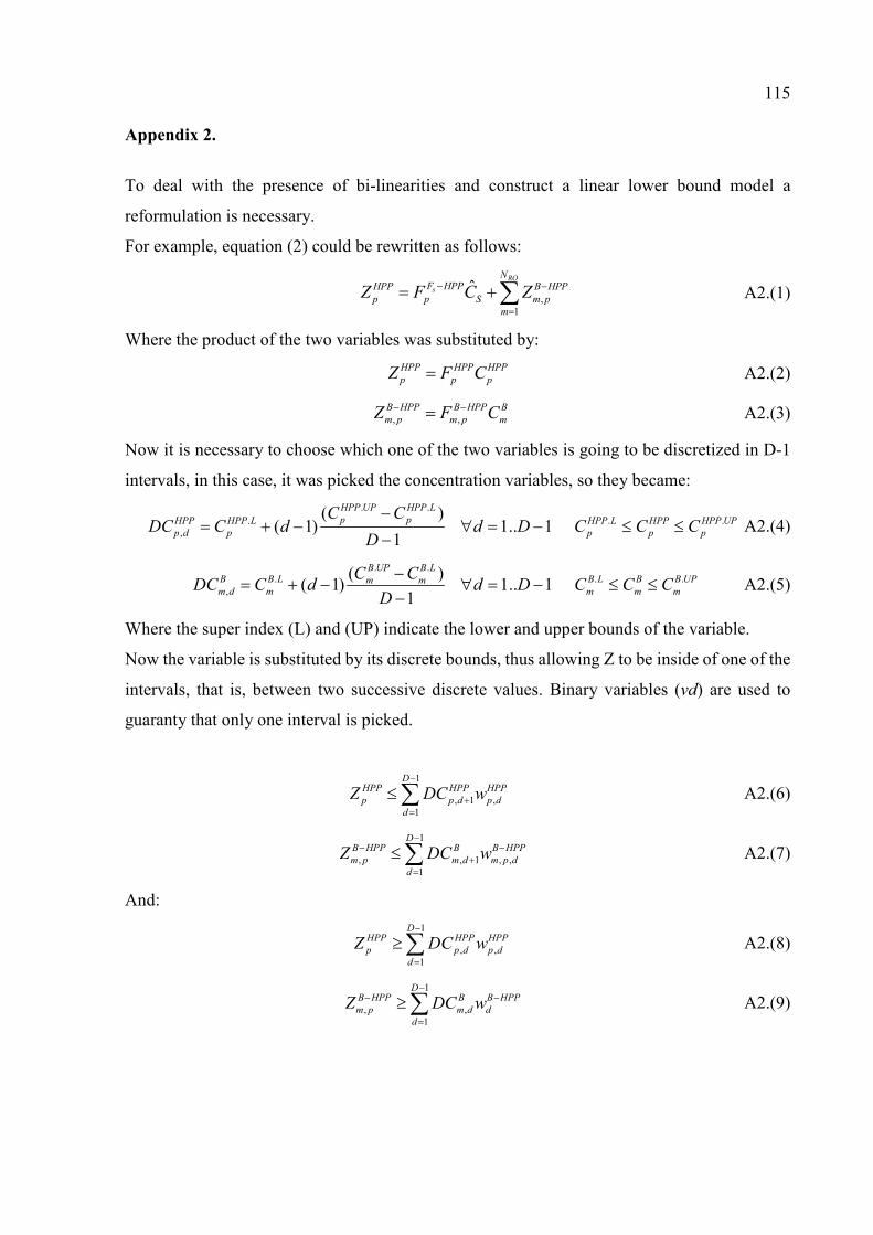
115
Appendix 2.
To deal with the presence of bi-linearities and construct a linear lower bound model a
reformulation is necessary.
For example, equation (2) could be rewritten as follows:
,1
ˆRO
s
NF HPPHPP B HPP
p p S m p
m
Z F C Z
A2.(1)
Where the product of the two variables was substituted by:
HPP HPP HPP
p p pZ F C A2.(2)
, ,B HPP B HPP B
m p m p mZ F C A2.(3)
Now it is necessary to choose which one of the two variables is going to be discretized in D-1
intervals, in this case, it was picked the concentration variables, so they became:
. .. . .
,
( )( 1) 1.. 1
1
HPP UP HPP L
p pHPP HPP L HPP L HPP HPP UP
p d p p p p
C CDC C d d D C C C
D
A2.(4)
. .. . .
,
( )( 1) 1.. 1
1
B UP B LB B L B L B B UPm mm d m m m m
C CDC C d d D C C C
D
A2.(5)
Where the super index (L) and (UP) indicate the lower and upper bounds of the variable.
Now the variable is substituted by its discrete bounds, thus allowing Z to be inside of one of the
intervals, that is, between two successive discrete values. Binary variables (vd) are used to
guaranty that only one interval is picked.
1
, 1 ,1
DHPP HPP HPP
p p d p d
d
Z DC w
A2.(6)
1
, , 1 , ,1
DB HPP B B HPP
m p m d m p d
d
Z DC w
A2.(7)
And:
1
, ,1
DHPP HPP HPP
p p d p d
d
Z DC w
A2.(8)
1
, ,1
DB HPP B B HPP
m p m d d
d
Z DC w
A2.(9)
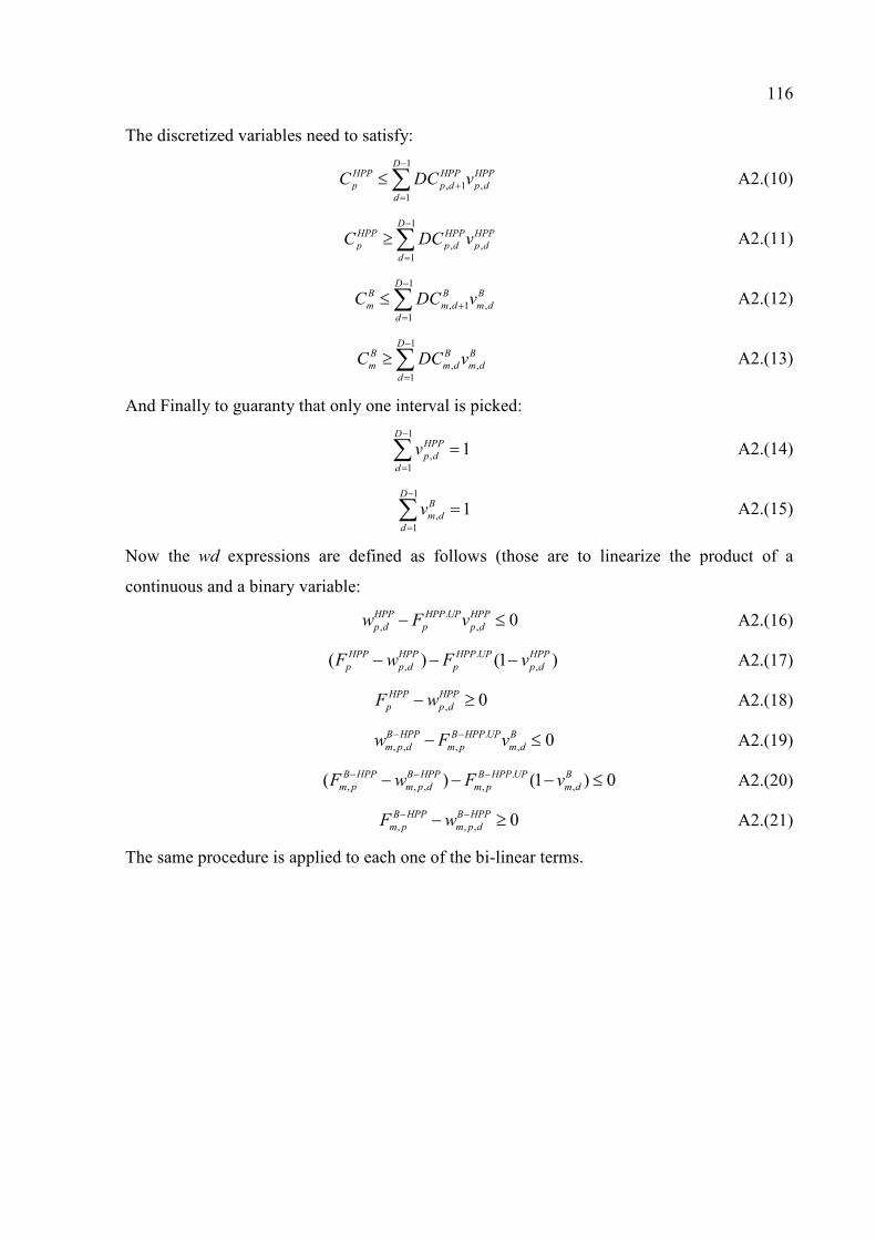
116
The discretized variables need to satisfy:
1
, 1 ,1
DHPP HPP HPP
p p d p d
d
C DC v
A2.(10)
1
, ,1
DHPP HPP HPP
p p d p d
d
C DC v
A2.(11)
1
, 1 ,1
DB B B
m m d m d
d
C DC v
A2.(12)
1
, ,1
DB B B
m m d m d
d
C DC v
A2.(13)
And Finally to guaranty that only one interval is picked:
1
,1
1D
HPP
p d
d
v
A2.(14)
1
,1
1D
B
m d
d
v
A2.(15)
Now the wd expressions are defined as follows (those are to linearize the product of a
continuous and a binary variable:
., , 0HPP HPP UP HPP
p d p p dw F v A2.(16)
., ,( ) (1 )HPP HPP HPP UP HPP
p p d p p dF w F v A2.(17)
, 0HPP HPP
p p dF w A2.(18)
., , , , 0B HPP B HPP UP B
m p d m p m dw F v A2.(19)
., , , , ,( ) (1 ) 0B HPP B HPP B HPP UP B
m p m p d m p m dF w F v A2.(20)
, , , 0B HPP B HPP
m p m p dF w A2.(21)
The same procedure is applied to each one of the bi-linear terms.
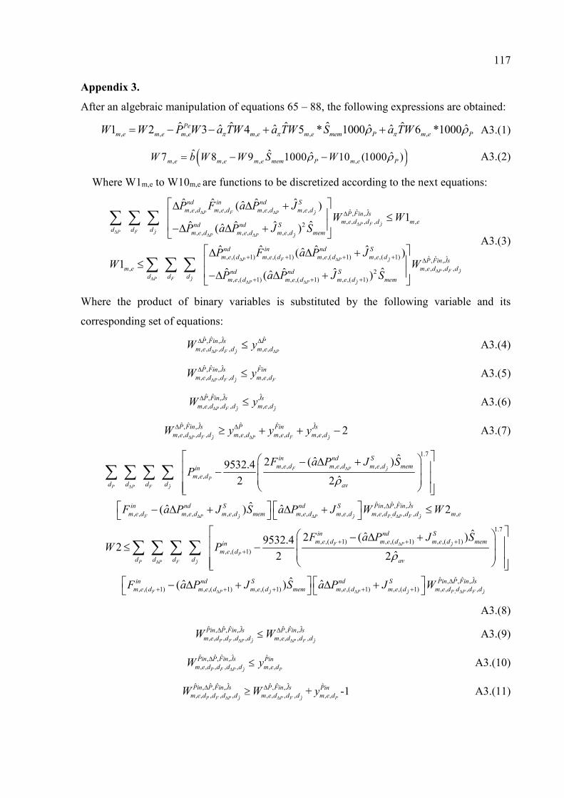
117
Appendix 3.
After an algebraic manipulation of equations 65 – 88, the following expressions are obtained:
, , , , , ,ˆˆ ˆ ˆ ˆˆ ˆˆ ˆ ˆ1 2 3 4 5 * 1000 6 *1000Pe
m e m e m e m e m e mem P m e PW W P W a TW a TW S a TW A3.(1)
, , , ,ˆ ˆ ˆ ˆ7 8 9 1000 10 (1000 )m e m e m e mem P m e PW b W W S W A3.(2)
Where W1m,e to W10m,e are functions to be discretized according to the next equations:
ˆ
ˆ
ˆˆ
ˆ
, , , , , , , , ˆ ˆ ˆ, ,, , , , ,2
, , , , , ,
, ,( 1) , ,( 1)
,
ˆ ˆ ˆ ˆˆ( )1
ˆˆ ˆ ˆˆ( )
ˆ ˆ ˆˆ(1
P F P J
P F J
P F JP P J
P F
P F J
nd in nd S
m e d m e d m e d m e dP Fin Js
m e d d d m end nd S
d d dm e d m e d m e d mem
nd in
m e d m e d
m e
d d d
P F a P JW W
P a P J S
P F a PW
ˆ
ˆ
ˆ
, ,( 1) , ,( 1) ˆ ˆ ˆ, ,, , , ,2
, ,( 1) , ,( 1) , ,( 1)
ˆ )
ˆˆ ˆ ˆˆ( )
P J
P F J
P P J
nd S
m e d m e dP Fin Js
m e d d dnd nd S
m e d m e d m e d mem
JW
P a P J S
A3.(3)
Where the product of binary variables is substituted by the following variable and its
corresponding set of equations:
ˆ
ˆ ˆ ˆ ˆ, ,, , , , , ,P F PJ
P Fin Js P
m e d d d m e dW y
A3.(4)
ˆ
ˆ ˆ ˆ ˆ, ,, , , , , ,P F FJ
P Fin Js Fin
m e d d d m e dW y
A3.(5)
ˆ ˆ
ˆ ˆ ˆ ˆ, ,, , , , , ,P F J J
P Fin Js Js
m e d d d m e dW y
A3.(6)
ˆ ˆ
ˆ ˆ ˆ ˆ ˆ ˆ, ,, , , , , , , , , , 2
P F P FJ J
P Fin Js P Fin Js
m e d d d m e d m e d m e dW y y y
A3.(7)
ˆ
ˆ
ˆ ˆ ˆ,
1.7
, , , , , ,
, ,
ˆ ˆ ˆ, ,, , , , , , , , , , , , , ,
ˆˆ2 ( )9532.4ˆ2 2
ˆˆ ˆ( )
F P J
P
P P F J
F P P P P FJ J J
in nd S
m e d m e d m e d memin
m e d
d d d d av
in nd S nd S Pin P Fin
m e d m e d m e d mem m e d m e d m e d d d d
F a P J SP
F a P J S a P J W
ˆ
ˆ
ˆ
ˆ,,
1.7
, ,( 1) , ,( 1) , ,( 1)
, ,( 1)
, ,( 1) , ,( 1) , ,( 1) , ,(
2
ˆˆ2 ( )9532.42
ˆ2 2
ˆˆ ˆ ( )
F P J
P
P P F J
F P PJ
Js
m e
in nd S
m e d m e d m e d memin
m e d
d d d d av
in nd S
m e d m e d m e d mem m e d
W
F a P J SW P
F a P J S a P
ˆ ˆ,
ˆ ˆ ˆ ˆ, , ,1) , ,( 1) , , , ,P P FJ J
nd S Pin P Fin Js
m e d m e d d d dJ W
A3.(8)
ˆ
ˆ ˆ ˆ ˆ, , ,, , , , ,P F P J
Pin P Fin Js
m e d d d dW
ˆ
ˆ ˆ ˆ, ,, , , ,P F J
P Fin Js
m e d d dW
A3.(9)
ˆ
ˆ ˆ ˆ ˆ, , ,, , , , ,P F P J
Pin P Fin Js
m e d d d dW
ˆ
, , P
Pin
m e dy A3.(10)
ˆ
ˆ ˆ ˆ ˆ, , ,, , , , ,P F P J
Pin P Fin Js
m e d d d dW
ˆ
ˆ ˆ ˆ, ,, , , ,P F J
P Fin Js
m e d d dW
+ˆ
, , P
Pin
m e dy -1 A3.(11)
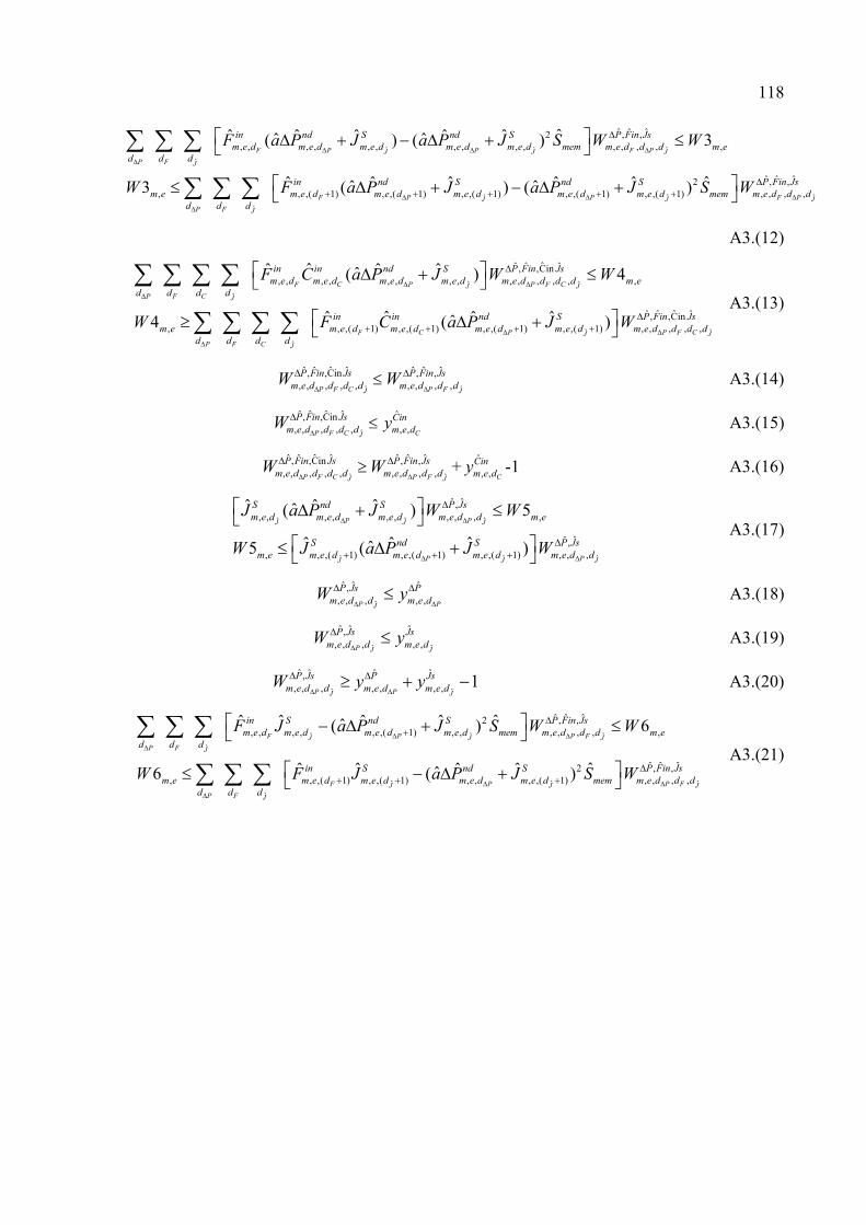
118
ˆ ˆ ˆ
ˆ
ˆ
ˆ
ˆ ˆ ˆ2 , ,, , , , , , , , , , , , , , ,
, , ,( 1) , ,( 1) , ,( 1) , ,(
ˆˆ ˆ ˆ ˆ ˆˆ ˆ( ) ( ) 3
ˆ ˆ ˆ ˆˆ ˆ3 ( ) (
F P P F PJ J J
P F J
F P PJ
P F J
in nd S nd S P Fin Js
m e d m e d m e d m e d m e d mem m e d d d m e
d d d
in nd S
m e m e d m e d m e d m e d
d d d
F a P J a P J S W W
W F a P J a P
ˆ ˆ
ˆ ˆ ˆ2 , ,1) , ,( 1) , , , ,
ˆˆ )F PJ J
nd S P Fin Js
m e d mem m e d d dJ S W
A3.(12)
ˆ ˆ
ˆ
ˆ
ˆ
ˆˆ ˆ ˆ, ,Cin, , , , , , , , , , , , , ,
, , ,( 1) , ,( 1) , ,( 1) , ,( 1) , ,
ˆˆ ˆ ˆˆ( ) 4
ˆˆ ˆ ˆˆ4 ( )
F C P P F CJ J
P F C J
F C P PJ
P F C J
in in nd S P Fin Js
m e d m e d m e d m e d m e d d d d m e
d d d d
in in nd S
m e m e d m e d m e d m e d m e d
d d d d
F C a P J W W
W F C a P J W
ˆ
ˆˆ ˆ ˆ, ,Cin, , ,F C J
P Fin Js
d d d
A3.(13)
ˆ
ˆˆ ˆ ˆ, ,Cin, , , , ,P F C J
P Fin Js
m e d d d dW
ˆ
ˆ ˆ ˆ, ,, , , ,P F J
P Fin Js
m e d d dW
A3.(14)
ˆ
ˆˆ ˆ ˆ, ,Cin, , , , ,P F C J
P Fin Js
m e d d d dW
ˆ
, , C
Cin
m e dy A3.(15)
ˆ
ˆˆ ˆ ˆ, ,Cin, , , , ,P F C J
P Fin Js
m e d d d dW
ˆ
ˆ ˆ ˆ, ,, , , ,P F J
P Fin Js
m e d d dW
+ˆ
, , C
Cin
m e dy -1 A3.(16)
ˆ ˆ ˆ
ˆ ˆ ˆ
ˆ ˆ,, , , , , , , , , ,
ˆ ˆ,, , ,( 1) , ,( 1) , ,( 1) , , ,
ˆ ˆ ˆˆ( ) 5
ˆ ˆ ˆˆ5 ( )
P PJ J J
P PJ J J
S nd S P Js
m e d m e d m e d m e d d m e
S nd S P Js
m e m e d m e d m e d m e d d
J a P J W W
W J a P J W
A3.(17)
ˆ
ˆ ˆ ˆ,, , , , ,P PJ
P Js P
m e d d m e dW y
A3.(18)
ˆ ˆ
ˆ ˆ ˆ,, , , , ,P J J
P Js Js
m e d d m e dW y
A3.(19)
ˆ ˆ
ˆ ˆ ˆ ˆ,, , , , , , , 1
P PJ J
P Js P Js
m e d d m e d m e dW y y
A3.(20)
ˆ ˆ ˆ
ˆ
ˆ ˆ
ˆ
ˆ ˆ ˆ2 , ,, , , , , ,( 1) , , , , , , ,
2, , ,( 1) , ,( 1) , , , ,( 1) , ,
ˆˆ ˆ ˆ ˆˆ( ) 6
ˆˆ ˆ ˆ ˆˆ6 ( )
F P P FJ J J
P F J
F PJ J
P F J
in S nd S P Fin Js
m e d m e d m e d m e d mem m e d d d m e
d d d
in S nd S
m e m e d m e d m e d m e d mem m e d
d d d
F J a P J S W W
W F J a P J S W
ˆ
ˆ ˆ ˆ, ,, ,P F J
P Fin Js
d d
A3.(21)
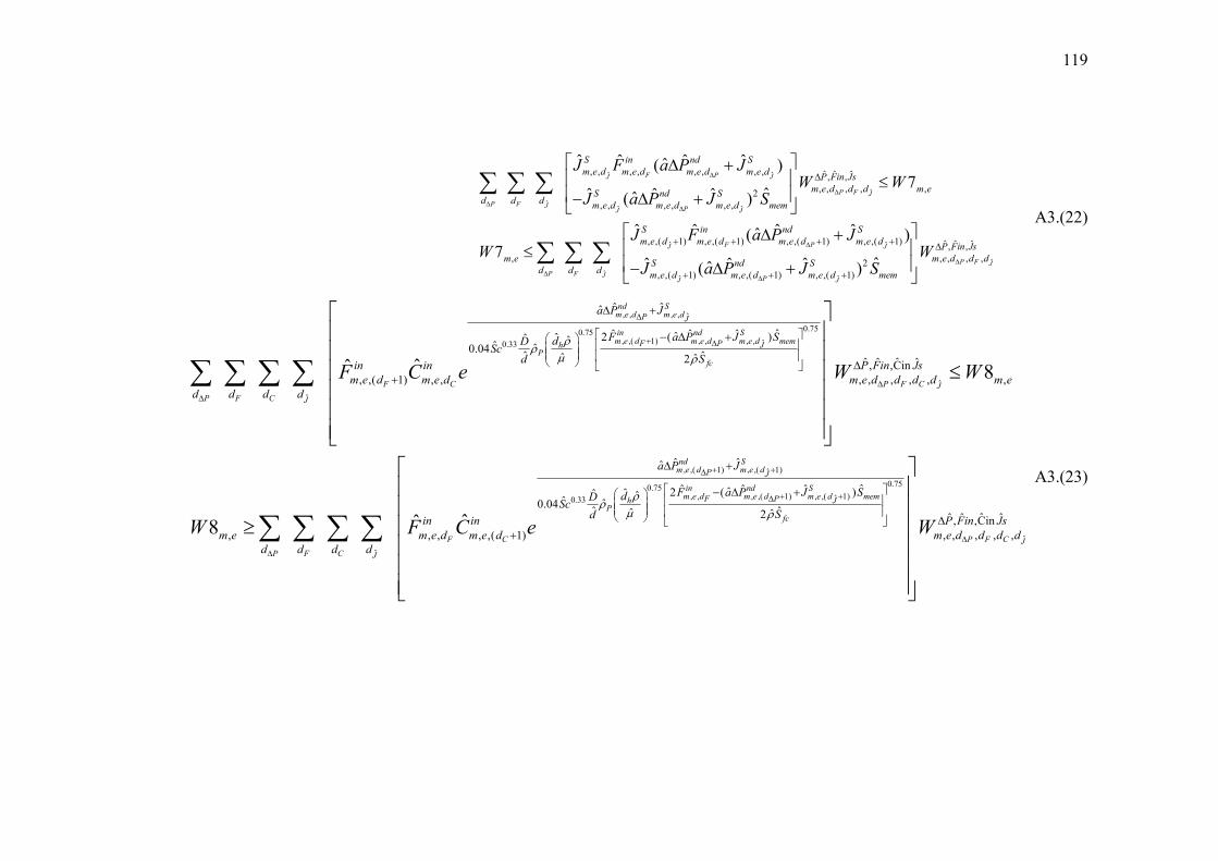
119
ˆ ˆ
ˆ
ˆˆ ˆ
ˆ
ˆ
, , , , , , , , ˆ ˆ ˆ, ,, , , , ,2
, , , , , ,
, ,( 1) , ,( 1) , ,(
,
ˆ ˆ ˆ ˆˆ( )7
ˆˆ ˆ ˆˆ( )
ˆ ˆ ˆˆ(7
F PJ J
P F J
P F JPJ J
FJ
P F J
S in nd S
m e d m e d m e d m e dP Fin Js
m e d d d m eS nd S
d d dm e d m e d m e d mem
S in
m e d m e d m e d
m e
d d d
J F a P JW W
J a P J S
J F a PW
ˆ
ˆ
ˆ ˆ
1) , ,( 1) ˆ ˆ ˆ, ,, , , ,2
, ,( 1) , ,( 1) , ,( 1)
ˆ )
ˆˆ ˆ ˆˆ( )
P J
P F J
PJ J
nd S
m e dP Fin Js
m e d d dS nd S
m e d m e d m e d mem
JW
J a P J S
A3.(22)
, , , , ˆ
0.750.75, ,( 1) , , , , ˆ0.33
ˆ
ˆ ˆˆ
ˆˆ ˆ ˆˆ2 ( )ˆˆ ˆˆ ˆ0.04ˆ ˆˆ ˆ2
, ,( 1) , , , , , , ,ˆˆ
nd Sm e d m e dP J
in nd Sm e d m e d m e d memF Ph J
P
fc
F C P F C
P F C J
a P J
F a P J SdDSc
Sdin in
m e d m e d m e d d d d
d d d d
F C e W
ˆ
, ,( 1) , ,( 1)ˆ
0.75, , , ,( 1) , ,( 1)ˆ0.33
ˆ
ˆˆ ˆ ˆ, ,Cin,
ˆ ˆˆ
ˆˆ ˆ ˆˆ2 ( )ˆˆ ˆˆ ˆ0.04ˆ ˆˆ ˆ2
, , , , ,( 1)
8
ˆˆ8
J
nd Sm e d m e dP J
in nd Sm e d m e d m e d memF Ph J
P
fc
F C
P F C J
P Fin Js
m e
a P J
F a P J SdDSc
Sdin in
m e m e d m e d
d d d d
W
W F C e
0.75
ˆ
ˆˆ ˆ ˆ, ,Cin, , , , ,P F C J
P Fin Js
m e d d d dW
A3.(23)
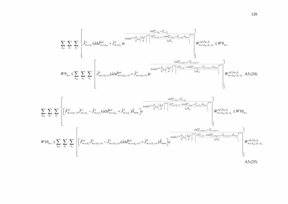
120
, , , , ˆ
0.750.75, ,( 1) , , , , ˆ0.33
ˆ ˆ
ˆ
ˆ ˆˆ
ˆˆ ˆ ˆˆ2 ( )ˆˆ ˆˆ ˆ0.04ˆ ˆˆ ˆ2
, , , , , , , ,ˆ ˆ ˆˆ( )
nd Sm e d m e dP J
in nd Sm e d m e d m e d memF Ph J
P
fc
PJ J
P F J
a P J
F a P J SdDSc
SdS nd S
m e d m e d m e d m e d
d d d
J a P J e W
ˆ
, ,( 1) , ,( 1)ˆ
0.75, , , ,( 1) ,0.33
ˆ ˆ
ˆ
ˆ ˆ ˆ, ,, , ,
ˆ ˆˆ
ˆ ˆ ˆˆ2 (ˆˆ ˆˆ ˆ0.04ˆ ˆ
, , ,( 1) , ,( 1) , ,( 1)
9
ˆ ˆ ˆˆ9 ( )
P F J
nd Sm e d m e dP J
in ndm e d m e d mF Ph
P
PJ J
P F J
P Fin Js
d d m e
a P J
F a P JdDSc
dS nd S
m e m e d m e d m e d
d d d
W
W J a P J e
0.75
,( 1)ˆ
ˆ
ˆ)
ˆˆ2 ˆ ˆ ˆ, ,, , , ,
Se d mem
J
fc
P F J
S
SP Fin Js
m e d d dW
A3.(24)
, , , , ˆ
0.75, ,( 1) , , , , ˆ0.33
ˆ ˆ ˆ
ˆ
ˆ ˆˆ
ˆˆ ˆ ˆˆ2 ( )ˆˆ ˆˆ ˆ0.04ˆ ˆˆ ˆ2
, ,( 1) , , , , , , , ,ˆˆ ˆ ˆ ˆ ˆˆ( )
nd Sm e d m e dP J
in nd Sm e d m e d m e d memF Ph J
P
fc
F PJ J J
P F J
a P J
F a P J SdDSc
Sdin S S nd S
m e d m e d m e d m e d m e d mem
d d d
F J J a P J S e
0.75
ˆ
, ,( 1) , ,( 1)ˆ
ˆ ˆ ˆ
ˆ
ˆ ˆ ˆ, ,, , , , ,
ˆ ˆˆ
0.0
, , , , ,( 1) , ,( 1) , ,( 1) , ,( 1)
10
ˆˆ ˆ ˆ ˆ ˆˆ10 ( )
P F J
nd Sm e d m e dP J
F PJ J J
P F J
P Fin Js
m e d d d m e
a P J
in S S nd S
m e m e d m e d m e d m e d m e d mem
d d d
W W
W F J J a P J S e
0.750.75, , , ,( 1) , ,( 1)ˆ0.33
ˆ
ˆˆ ˆ ˆˆ2 ( )ˆˆ ˆˆ ˆ4ˆ ˆˆ ˆ2 ˆ ˆ ˆ, ,
, , , ,
in nd Sm e d m e d m e d memF Ph J
P
fc
P F J
F a P J SdDSc
SdP Fin Js
m e d d dW
A3.(25)
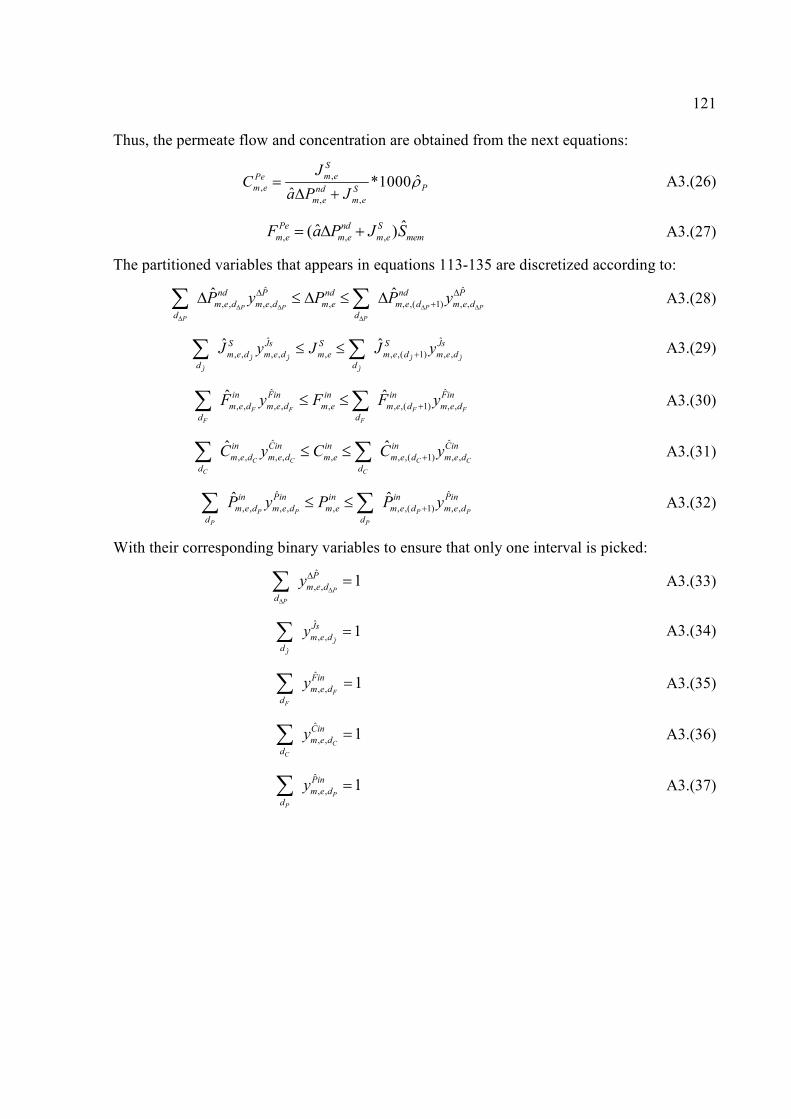
121
Thus, the permeate flow and concentration are obtained from the next equations:
,,
, ,
ˆ*1000ˆ
S
m ePe
m e Pnd S
m e m e
JC
a P J
A3.(26)
, , ,ˆˆ( )Pe nd S
m e m e m e memF a P J S A3.(27)
The partitioned variables that appears in equations 113-135 are discretized according to:
ˆ ˆ
, , , , , , ,( 1) , ,ˆ ˆ
P P P P
P P
nd P nd nd P
m e d m e d m e m e d m e d
d d
P y P P y
A3.(28)
ˆ ˆ ˆ ˆ
ˆ ˆ
ˆ ˆ
, , , , , , ,( 1) , ,ˆ ˆ
J J J J
J J
S Js S S Js
m e d m e d m e m e d m e d
d d
J y J J y A3.(29)
ˆ ˆ
, , , , , , ,( 1) , ,ˆ ˆ
F F F F
F F
in Fin in in Fin
m e d m e d m e m e d m e d
d d
F y F F y A3.(30)
ˆ ˆ
, , , , , , ,( 1) , ,ˆ ˆ
C C C C
C C
in Cin in in Cin
m e d m e d m e m e d m e d
d d
C y C C y A3.(31)
ˆ ˆ
, , , , , , ,( 1) , ,ˆ ˆ
P P P P
P P
in Pin in in Pin
m e d m e d m e m e d m e d
d d
P y P P y A3.(32)
With their corresponding binary variables to ensure that only one interval is picked:
ˆ
, , 1P
P
P
m e d
d
y
A3.(33)
ˆ
ˆ
ˆ
, , 1J
J
Js
m e d
d
y A3.(34)
ˆ
, , 1F
F
Fin
m e d
d
y A3.(35)
ˆ
, , 1C
C
Cin
m e d
d
y A3.(36)
ˆ
, , 1P
P
Pin
m e d
d
y A3.(37)