maria gracia bustamante rosell · 2016-09-28 · espeleotema 3. nordeste dos andes peruanos 4....
TRANSCRIPT

UNIVERSIDADE DE SÃO PAULO
INSTITUTO DE GEOCIÊNCIAS
MARIA GRACIA BUSTAMANTE ROSELL
“Reconstituição da Monção Sul-Americana durante os últimos 38 mil anos
e seus efeitos na precipitação no Nordeste dos Andes nas escalas de tempo
orbital a multidecenal”
TESE DE DOUTORAMENTO
Programa de Pós-Graduação em Geoquímica e Geotectônica
Orientador: Prof. Dr. Francisco William da Cruz Júnior
SÃO PAULO
2015
2
MARIA GRACIA BUSTAMANTE ROSELL
“Reconstituição da Monção Sul-Americana durante os últimos 38 mil anos e seus
efeitos na precipitação no Nordeste dos Andes nas escalas de tempo orbital a
multidecenal”
SÃO PAULO
2015
Tese apresentada ao Instituto de
Geociências da Universidade de São
Paulo para obtenção de título de
Doutor em Geologia.
Área de concentração: Geoquímica
Orientador: Prof. Dr. Francisco
William da Cruz Júnior

3
Autorizo a reprodução e divulgação total ou parcial deste trabalho, por qualquer meio
convencional ou eletrônico, para fins de estudo e pesquisa, desde que citada a fonte.
Ficha catalográfica preparada pelo Serviço de Biblioteca e
Documentação do Instituto de Geociências da Universidade de São Paulo
Rosell, Maria Gracia Bustamante
Reconstituição da Monção Sul-Americana durante
os últimos 38 mil anos e seus efeitos na
precipitação no Nordeste dos Andes nas escalas de
tempo orbital a multidecenal/Maria Gracia Bustamante
Rosell. – São Paulo, 2015.
171 p. : il.
Tese(Doutorado):IGc/USP
Orient.: da Cruz Jr., Francisco W.
1. Monção Sul-Americana 2. Espeleotema 3. Nordeste
dos Andes Peruanos 4. Isótopos estáveis 5.
Paleoclima 6. Holoceno 7. Último Período Glacial
Superior

4
Tese apresentada ao Instituto de
Geociências da Universidade de São
Paulo para obtenção de título de
Doutor em Geologia
Área de concentração: Geoquímica
[Cite sua fonte aqui.]
Nome: Maria Gracia Bustamante Rosell
Título: Reconstituição da Monção Sul-Americana durante os últimos 38 mil anos e seus efeitos
na precipitação no Nordeste dos Andes nas escalas de tempo orbital a multidecenal.
Aprovado em: __/__ /__
Prof. Dr.:______________________________Instituição:_______________________
Julgamento:____________________________Assinatura:_______________________
Prof. Dr.:______________________________Instituição:_______________________
Julgamento:____________________________Assinatura:_______________________
Prof. Dr.:______________________________Instituição:_______________________
Julgamento:____________________________Assinatura:_______________________
Prof. Dr.:______________________________Instituição:_______________________
Julgamento:____________________________Assinatura:_______________________
Prof. Dr.:______________________________Instituição:_______________________
Julgamento: ___________________________Assinatura: _______________________

5
À Meus pais,
Julio Bustamante P. e Cecilia Rosell

6
AGRADECIMENTOS
Sou grata pela confiança, o apoio e a alegria dos momentos compartilhados, aos doutores Abdel
Sifeddine, Bruno Turcq, Claire Lazareth, Guy Cabioch, Jean Loup Guyot, Luc Ortlieb, assim
como aos professores Ivo Karmann e Renato Paes de Almeida.
Sou grata à banca de qualificação, os professores Cristiano Chiessi e Ilana Wainer pela
contribuição no texto, as ideias e a discussão frutífera que houve na avaliação.
Àqueles que coletaram as amostras e com os que compartilhamos boas experiências nas
cavernas de Brasil e Perú, entre eles, Augusto Auler, James Apaèstegui, Jean Loup Guyot, Jean
Sebastian Moquet, Jean Yves Bigot, Patricia Turcq e William Santini.
Aos técnicos de Laboratorio, Alyne Barros e Osmar Antunes, pois sem eles o trabalho teria sido
mais difícil e muito maior.
A meus colegas de laboratório, Christian Millo, Eline Alves, James Apaèstegui, Jean Sebastian
Moquet, Narubia Gonçalves, Nicolas Strikis, Valdir Novello e Verônica Ramirez pelo espírito
de equipe, a amizade, as conversas e as discussões de artigos. Assim como pelas revisões de
texto deste trabalho.
A meus companheiros e amigos do IGc, Bruno Boita, Eva Kaiser, Ezequiel Ferreira, Guillaume
Bertrand, Marcelo Barbara, Suellyn Garcia, Tabatha Hoeger, Thaize Hipólito, Vinicius Ribau e
Vinicius Tieppo e a todos aqueles que estiveram presentes sempre me apoiando.
A Francisco William da Cruz Junior, orientador, pela oportunidade de realizar este estudo, pelo
apoio, a paciência, e a confiança. Entre muitas outras coisas boas que aprendi ao trabalhar junto.
Ao Andre Stern, pela grande pessoa que vc é. Pelos momentos compartilhados e ter-me apoiado
quando precisei. Obrigada por estes quatro anos, assim como pela ajuda no tratamento de
imagens, e correções de texto deste trabalho.
Não tenho palavras para agradecer a meus pais, Cecilia Rosell e Julio Bustamante, sem os quais,
nada disto teria sido possível. Agradeço-lhes por estarem sempre presentes, pela sua força, pelos
seus conselhos, pela sua amizade, a sua grande paciência, o inacavábel apoio e o carinho
enorme. Obrigada por me ensinar a insistir e acreditar naquilo que me proponho a pesar das
dificuldades.
Finalmente, também gostaria de agradecer ao Instituto de Geociências da Universidade de São
Paulo (IGc-USP), ao Programa de Pós-Graduação em Geoquímica e Geotectônica e ao apoio
financeiro da Fundação de Amparo à Pesquisa do Estado de São Paulo (FAPESP) e do
Conselho Nacional de Desenvolvimento Científico e Tecnológico (CNPq).

7
SUMÁRIO
RESUMO .................................................................................................................................... 10
ABSTRACT ................................................................................................................................ 12
LISTA DE FIGURAS ................................................................................................................. 14
1. Introdução ............................................................................................................................... 18
2. Objetivos da Pesquisa.............................................................................................................. 19
3. Materiais e Métodos ................................................................................................................ 20
3.1. Área de estudo ...................................................................................................................... 20
3.2. Coleta de estalagmites .......................................................................................................... 25
3.3. Preparação das amostras para datação radiométrica e análises isotópicas ........................... 26
3.4. Datação geocronológica pelo método U/Th ......................................................................... 27
3.5. Amostragem de calcita para isótopos estáveis e análises isotópicas .................................... 28
3.6. Obtenção da série temporal paleoclimática .......................................................................... 30
4. Climatologia Moderna............................................................................................................. 32
5. Hidrogeoquímica isotópica ..................................................................................................... 37
5.1. Definições, padrões e notações ............................................................................................ 38
5.1.1. Fracionamento isotópico no Ciclo Hidrológico ................................................................ 39
5.2. Linha de água meteórica local e global ................................................................................ 40
5.3. A variabilidade da precipitação do regime de monções e sua assinatura isotópica ............. 44
6. Paleoclimatologia do Nordeste dos Andes desde o último período Glacial até o Holoceno ... 46
6.1. Mudanças paleoclimáticas na escala orbital ......................................................................... 47
6.2. Mudanças paleoclimáticas abruptas ..................................................................................... 51
6.2.1 – Eventos climáticos durante os últimos períodos Glacial e Deglacial ............................. 51
6.2.1 – Eventos climáticos durante o Holoceno .......................................................................... 55
7. Considerações Finais ............................................................................................................... 58
REFERÊNCIAS BIBLIOGRÁFICAS ........................................................................................ 60
ANEXOS..................................................................................................................................... 78

8
LISTA DE ABREVIATURAS
δ13
C Razão isotópica de Carbono
δD Razão isotópica de Deutério
δ18
O Razão isotópica do Oxigênio
A.D. Anno Domini
AP Antes do Presente (antes de A.D. 2000)
AIEA Agência Internacional de Energia Atômica
AIM Antarctic Isotope Maxima
AMO Atlantic Multidecadal Oscillation
AMOC Atlantic Meridional Overturning Circulation
AS América do Sul
ASM Asian Summer Monsoon
ASI Austral Summer Insolation
B/A Bølling-Allerød
BP Before Present (antes de A.D. 2000)
ca. Circa
D-O Dansgaard-Oeschger
ECHAM European Centre Hamburg Model
ENSO El Niño Southern Oscillation
EPICA European Ice Core Project in Antarctica
EDML EPICA Dronning Maud Land
ET Evapotranspiração
GI Greenland Interstadial
GMWL Global Meteoric Water Line
GNIP Global Network for Isotopes in Precipitation
GS Greenland Stadial
H Heinrich Event
HSG Hematite Stained Grains

9
ICP-MS Inductively coupled plasma mass spectrometry
IRD Ice Rafted Debris
ITCZ Intertropical Convergence Zone
ka Kilo ano (Mil anos)
ky Kilo year
LGM Last Glacial Maximum
LIA Little Ice Age
LLJ Low Level Jet
LMWL Local Meteoric Water Line
MCA Medieval Climate Anomaly
MSA Monção Sul-Americana
MIS Marine Isotope Stage
NAO North Atlantic Oscillation
NEB Nordeste brasileiro
NGRIP North Greenland Ice Core Project
PDB Pee Dee Belemnite
PDO Pacific Decadal Oscillation
SACZ South Atlantic Convergence Zone
SASM South American Summer Monsoon
SMOW Standard Mean Ocean Water
SST Sea Surface Temperature
TC Taxa de Crescimento
TSM Temperatura da Superfície do Mar
TRMM Tropical Rainfall Measuring Mission
V-PDB Vienna-Pee Dee Belemnite
V-SMOW Vienna-Standard Mean Ocean Water
YD Younger Dryas

10
RESUMO
Neste estudo investigou-se a variabilidade da Monção Sul-Americana (MSA) ao longo dos
últimos 38ka, por meio de um registro em alta resolução de δ18
O baseado em três espeleotemas
da caverna Shatuca, localizada no norte do Peru ( ̴ 5ºS). O registro da caverna Shatuca é um dos
primeiros registros paleoclimáticos da zona de altitude intermediária no flanco oriental dos
Andes setentrionais (1960m).
O registro isotópico da Shatuca compreende espeleotemas bem datados e de alta resolução que
são usados para investigar a atividade da MSA no passado, em resposta tanto ao ciclo de
precessão da insolação, como às mudanças na circulação oceânica, ocorridas durante o último
período Glacial – Deglacial, as quais são definidas nos testemunhos marinhos e de gelo do
Hemisfério Norte.
Os registros de espeleotemas da caverna Shatuca, não mostram nenhum controle claro da
insolação sobre a MSA nos Andes entre 38-11 ka AP, o que pode ser explicado por um controle
predominante das condições de contorno glaciais sobre a MSA.
Mudanças abruptas, entre períodos mais úmidos e mais secos da MSA, em escalas de tempo
milenar, são observadas no registro de espeleotemas de Shatuca através de valores de δ18
O
anormalmente baixos e altos, respectivamente. Estes eventos são interpretados como uma
resposta aos eventos Heinrich (H) e Dansgaard-Oeschger (D-O) através de deslocamentos
latitudinais da Zona de Convergência Intertropical (Intertropical Convergence Zone-ITCZ). No
entanto, a intensidade da resposta a esses ciclos foi variável. Em particular, os episódios
climáticos mais extremos foram aqueles relacionados aos eventos Heinrich 1 e 2.
O período de ocorrência e a estrutura do evento Heinrich 1 (H1) são mais precisamente
descritos nos espeleotemas da caverna Shatuca do que em registros anteriores dos Andes e da
Bacia de Cariaco. O evento H1 é caracterizado por valores isotópicos baixos entre 18.0 e 14.7
ka AP, o que indica condições predominantemente úmidas; mas um pico, nunca antes
registrado, de valores de δ18
O altos foi registrado em 16.2 ka AP. Este resultado é
particularmente importante dado que a ITCZ poderia ter estado deslocada mais ao sul do que
5ºS. Além disso, a estrutura dos períodos do Bølling-Allerød (B/A) e Younger Dryas (YD)
assemelha-se à dos testemunhos de gelo da Groenlândia.
Durante o Holoceno, o clima da região da caverna Shatuca foi controlado pela insolação,
consistente com outros registros de isótopos de diferentes altitudes nos Andes peruanos. O
Holoceno Inferior é marcado pelo severo enfraquecimento da MSA na região da Shatuca, sendo
seguido por uma tendência de aumento gradual das condições de umidade em direção ao
Holoceno Superior, esta tendência climática, em longo prazo, ocorreu em união à tendência de

11
aumento da insolação modulada pelo ciclo de precessão. Condições particularmente úmidas
foram sentidas na região da caverna Shatuca após 5.0 ka AP.
Várias mudanças abruptas ocorridas, em escalas de tempo centenárias e multidecenais, durante
o Holoceno, são descritas pela primeira vez nos Andes. Durante o Holoceno Inferior, o caso
mais extremo, é o registrado em 9.5 ka AP, mas outros eventos úmidos ocorreram também, tais
como o registrado em 8.1 ka AP. Por outro lado, durante o Holoceno Médio, a comparação com
outros registros andinos, na região afetada pela MSA, aponta para uma série de eventos abruptos
que ocorreram entre 5.1 e 5.0 ka AP. Finalmente, um resultado importante do presente estudo é
a semelhança observada, durante o Holoceno Superior, entre o registro da caverna Shatuca com
o do lago Pallcacocha, situado no sul dos Andes equatorianos e amplamente utilizado como um
proxy da frequência do fenômeno El Niño Oscilação Sul (El Niño Southern Oscillation -
ENSO). O registro Shatuca não apresenta nenhuma evidência clara de ter sofrido algum controle
climático influenciado por ENSO. Pelo contrário, propõe-se que ambos registros, o lago
Pallcacocha e a caverna Shatuca, indicam um aumento da umidade entre 3.5 e 2.5 ka AP,
resultado do controle da alta insolação de verão austral sobre a MSA, e de uma profunda
reorganização do sistema climático ocorrido na borda oeste da MSA, entre terras altas e
intermediárias dos Andes.
Palavras chave: Monção Sul-Americana, Espeleotema, Nordeste dos Andes Peruanos, Isótopos
Estáveis, Paleoclima, Holoceno, Último Período Glacial

12
ABSTRACT
In this study, we investigated the South American Summer Monsoon (SASM) variability
through the last 38 ky with a high-resolution δ18
O record based on three speleothems from
Shatuca cave, located in northern Peru ( ̴ 5ºS). The Shatuca cave record is one of the first
paleoclimate records from mid-altitude (1960m) sites in the northeastern Andean slopes.
The Shatuca isotope record comprises well-dated and high-resolution speleothems that were
used to investigate the past activity of SASM, in response to both insolation precession cycle
and changes in oceanic circulation during the last Glacial-Deglacial period, defined in ice cores
and marine core records from the northern Hemisphere.
The speleothem records from Shatuca cave show no clear insolation control over the SASM
between 38-11 ky BP, which could be explained by a prevailing control of the glacial boundary
conditions over SASM.
Abrupt millennial shifts between wetter and drier monsoon phases are observed in Shatuca
speleothem record based on abnormally low and high values of δ18
O, respectively. These events
are interpreted as a response to Heinrich (H) and Dansgaard-Oeschger (D-O) events through
latitudinal displacements in the Intertropical Convergence Zone (ITCZ). However, the response
intensity to these events was variable. In particular, the most extreme climate episodes were
those related to the Heinrich events 1 and 2.
The structure and timing of the Heinrich event 1 (H1) event are more precisely described in
Shatuca speleothems than in previous records from Andes and Cariaco Basin. The H1 event is
characterized by low δ18
O values from 18.0 to 14.7 ky BP, indicative of predominantly wet
conditions; but a peak, never reported before, of high δ18
O values is recorded at 16.2 ky BP.
This result is of particular importance given that the ITCZ was probably displaced even more to
the south than 5ºS. In addition, the structure of the Bølling–Allerød (B/A) and Younger Dryas
(YD) periods resembles that of the Greenland ice cores.
Insolation control on climate at Shatuca site is evident during the Holocene, which is consistent
with other Andean isotope records from different altitudes in the Peruvian Andes. The early
Holocene is marked by a extremely weak SASM activity over Shatuca area, that is followed by
a gradual increasing trend toward wetter conditions at the late Holocene period, this long term
climate trend occurred in union with increasing insolation trend modulated by the precession
cycle. Particularly wet conditions were felt in Shatuca site after 5.0 ky BP.
During the Holocene, several abrupt multidecadal to centennial events are for the first time
described in Andes. During the early Holocene, the most extreme event is the one logged at 9.5
ky BP, however other wet events occurred, such as the one logged at 8.1 ky BP. On the other

13
side, during the mid Holocene, the comparison with other Andean records affected by the
SASM, points out to a striking series of events that occurred between 5.1 and 5.0 ky BP.
Finally, one important result from the present study is the similarity observed during the late
Holocene between Shatuca cave and the Pallcacocha lake record in southern Equadorian Andes,
a record that has been widely used as a proxy for El Niño Southern Oscillation (ENSO)
frequency during Holocene. Shatuca record presents no clear evidence for climate control by
ENSO. On the contrary, it is proposed that the increase in moisture logged between 3.5 and 2.5
ky BP, in both Pallcacocha lake and Shatuca cave records, resulted from high austral insolation
control over the SASM and a major reorganization of the climatic system in the western border
of the SASM at mid- to high altitudes of the Andes.
Keywords: South American Summer Monsoon, Speleothem, Northeastern Peruvian Andes,
Stable Isotopes, Paleoclimate, Holocene, Last Glacial Period

14
LISTA DE FIGURAS
Capítulo 3: Materiais e Métodos
Figura 3.1. Localização da caverna Shatuca (5.70°S, 77.90°W) em altitudes intermediárias
(1960m). No mapa pode-se também observar a localização de outros registros paleoclimáticos
andinos em alta e baixa altitude. À direita: Mapa de acesso e localização da caverna Shatuca e
das cavernas de terras baixas Tigre Perdido-1000m anm (van Breukelen et al., 2008), El
Diamante-960m anm (Cheng et al., 2013a) e Palestina - 870m anm (Apaèstegui et al., 2014).
Figura 3.2. Localização das regiões andinas referidas neste estudo e o seu posicionamento com
respeito ao Jato de Baixos Níveis e à umidade transportada pela Monção Sul-Americana
(MSA). Mapa modificado de Marengo et al. (2004).
Figura 3.3. a) Variações sazonais de chuva registradas pelas estações pluviométricas situadas na
região nordeste dos Andes peruanos, entre 1300 e 2500m anm e entre 800-900m anm, para o
periodo entre 1964 e 2014. b) Mapa de precipitação média anual a partir dos dados do satélite
TRMM 2B31 (média para 1998-2009, em mm/ano) (Bookhagen and Strecker, 2008) c) Perfil
altitudinal que mostra a localização da caverna Shatuca e das caverna Tigre Perdido e Palestina,
com respeito ao vento vindo do leste.
Figura 3.4. Mapa topográfico da caverna Shatuca. Fonte: Grupo Espeleológico de Bagnols-
Marcoule (GSBM) e Club Espeleo-Andino de Lima (ECA).
Figura 3.5. Foto do microamostrador Sherline 5400, equipamento utilizado para coleta de
carbonato de cálcio (CaCO3) em espeleotemas, e dos tubos de amostragem utilizados nas
análises isotópicas.
Capítulo 4. Climatología Moderna
Figura 4.1. a) Circulação oceano- atmosfera no Oceano Pacífico Tropical durante condições
normais e El Niño. b) Série temporal de um índice de El Niño (índice de anomalia El Niño 3,
indica anomalias de temperatura da superfície do mar (TSM) entre 5°N-5°S e 150-90°W).
Fonte: Chiang (2009).
Figura 4.2. Esquema simplificado da circulação oceânica, associado à circulação de
revolvimento meridional com foco especial na parte Atlântica do fluxo (Atlantic Meridional
Overturning Circulation, AMOC). Fonte: Kuhlbrodt et al. (2007).
Capítulo 5. Hidrogeoquímica Isotópica

15
Figura 5.1. Valores de 18
O e D de estações de monitoramento do GNIP (Global Network for
Isotopes in Precipitation) em conjunto com a Linha de Água Meteórica Global (Global
Meteoric Water Line-GMWL). Fonte: Lachniet (2009).
Figura 5.2. Valores de 18
O e D na caverna Palestina, localidade próxima a área de estudo no
nordeste dos Andes peruanos (cortesía de J. Apaèstegui).
Figura 5.3. Resultados de δ18
O de água de chuva, gotejamento e rio subterrâneo na caverna
Palestina, localizada no nordeste dos Andes peruanos (cortesía de J. Apaèstegui).
Capítulo 6: Paleoclimatologia do Nordeste dos Andes desde o último periodo Glacial até o
Holoceno
Figura 6.1. Registros de paleopluviosidade na região andina em terras altas, intermediárias e
baixas, comparados com a curva da insolação para o mês de fevereiro em 10ºS (Berger e Loutre,
1991).
Figura 6.2. Comparação entre os registros paleoclimáticos da América do Sul, durante os
últimos 40 ka AP, com a curva de insolação do mês de fevereiro para 10ºS.
Figura 6.3. Comparação entre o registro de gelo NGRIP (Rasmussen et al., 2014) com os
registros paleoclimáticos da América do Sul para o período entre 40-10 ka AP.
Figura 6.4. Variabilidade milenar em registros isotópicos da América do Sul durante o período
do Holoceno, e a curva de concentração de Hematite Stained Grains (%HSG) em sedimentos
marinhos do Atlântico Norte de Bond et al. (2001).
ANEXOS
ANEXO 1. Cortes longitudinais das estalagmites analisadas com a locação das amostras
datadas: a) Amostra Sha-1, b) Amostra Sha-2, c) Amostra Sha-3.
ANEXO 2. Tabela com as Idades U/Th para as amostras Sha-1, Sha-2 e Sha-3.
ANEXO 3. Procedimentos analíticos para abertura de amostra e concentração de íons de U e
Th.
ANEXO 4. Intervalos de deposição das estalagmites Sha-1, Sha-2 e Sha-3, com o nome dos
espeleotemas no eixo vertical. Os pontos destacados são referentes à posição das idades U/Th.
ANEXO 5. Taxas de Crescimento para cada amostra.
ANEXO 6. Holocene changes in monsoon precipitation in the NE Peruvian Andes based on
δ18
O speleothem records.

16
A6. Figure 1. Location of Shatuca cave record (5.70°S, 77.90°W) and other Andean
paleoclimate records used for comparison.
A6. Figure 2. a) Histogram indicating mean monthly precipitation (1964-2014) in
meteorological stations located at mid-altitudes and lowlands. b) Altitude profile and location of
Shatuca, Tigre Perdido and Palestina caves in relation to the moisture transport direction. c)
Mean annual precipitation from TRMM 2B31satellite data.
A6. Figure 3. Rainwater isotopic results obtained during the Palestina cave monitoring program.
A6. Figure 4. Comparison between isotope records from the central and northeastern Peruvian
Andes and the insolation trend for the month of February at 10ºS (Berger and Loutre, 1991).
A6. Figure 5. Comparison between Holocene South American paleoprecipitation records and
the Hematite stained grains record from the North Atlantic Ocean.
A6. Figure 6. Early Holocene comparison of high-resolution records from South America and
the Hematite stained grains from the North Atlantic Ocean.
A6. Figure 7. Early Holocene spectral analysis (REDFIT) (Schulz and Mudelsee, 2002)
performed by software PAST (Hammer et al., 2001) using Sha-2 sample (with Sha-3 covering
the hiatus of Sha-2).
A6. Figure 8. Early Holocene wavelet analyses (Torrence and Compo, 1998) performedby
software PAST (Hammer et al., 2001) using Sha-2 sample (with Sha-3 covering the hiatus of
Sha-2).
A6. Figure 9. Detailed comparison between South American high-resolution paleorecords from
7.2 to 4.5 ky BP.
A6. Figure 10. Spectral analysis (REDFIT) (Schulz and Mudelsee, 2002) for the period between
5132-4780 yrs BP (with evidence in Bond 4), performed by software PAST (Hammer et al.,
2001).
A6. Figure 11. Wavelet analyses (Torrence and Compo, 1998) for the period between 5132-
4780 yrs BP (with evidence in Bond 4), performed by software PAST (Hammer et al., 2001).
A6. Figure 12. Comparison between South American paleorecords during the late Holocene.
A6. Figure 13. Increasing monsoon precipitation in Shatuca record through the Holocene,
shown as a step process.
A6. Figure S1. Topographic map: Shatuca cave profile. Located in Yambrasbamba, Bongará
province, Amazonas –Peru. Source: Bigot (2008).

17
A6. Table S1. U/Th ages for samples Sha-2 and Sha-3.
A6. Figure S2. Growth rate of samples Sha-2 and Sha-3.
A6. Figure S3. Isotopic record for Shatuca cave samples: Sha-2 in black and sample Sha-3 in
red. The U/Th ages, are located in the bottom part of the graphic, black for Sha-2 and red for
Sha-3.
ANEXO 7. Orbital to millennial changes in monsoon precipitation in western Amazon from the
last Glacial to the Holocene from speleothem isotope records.
A7. Figure 1. Location of Shatuca cave record (5.70°S, 77.90°W) and other paleoclimate
records used for comparison. To the right: Access and location map for Shatuca, Diamante and
Condor cave sites.
A7. Figure 2. a) Histogram indicating mean monthly precipitation (1964-2014) in
meteorological stations located at mid-altitudes and lowlands. b) Altitude profile and location of
Shatuca, Tigre Perdido and Palestina caves in relation to the moisture transport direction. c)
Mean annual precipitation from TRMM 2B31 satellite data.
A7. Figure 3. Rainwater isotopic results obtained during the Palestina cave monitoring program.
A7. Figure 4. Comparison between the Shatuca record with lower altitude (900m asl) montane
forest records (3-6ºS) and the Salar de Uyuni record (Baker et al., 2001a) in the Atliplano region
(20ºS) from 40 ky BP to present.
A7. Figure 5. Paleoclimate records comparison for the period 40-0 ky BP.
A7. Figure 6. Millennial variability among Andean records from 40 to 10 ky BP and its relation
to the Greenland ice core records.
A7. Figure S1. Topographic map: Shatuca cave profile. Located in Yambrasbamba, Bongará
province, Amazonas –Peru. Source: Bigot (2008).
A7. Table S1. U/Th ages for the speleothem samples Sha-1, Sha-2 and Sha-3.
A7. Figure S2. Growth rate of samples Sha-1, Sha-2 and Sha-3.
A7. Figure S3. Isotopic record of samples Sha-1, Sha-2 and Sha-3, compared to the insolation
precession cycle.
A7. Figure S4. Comparison between northeastern Andean records located between 3-6ºS.
A7. Figure S5. Comparison between Andean records at lowlands, midlands and highlands with
the EDML and NGRIP ice core records.

18
1. Introdução
A região dos Andes apresenta grande diversidade de climas devido à extensa área que abrange,
assim como por sua elevada altitude (Guyot, 1993; Ronchail e Gallaire, 2006; Laraque et al.,
2007; Espinoza, 2009). Dessa forma, é razoável observar variabilidade na escala espaço-tempo
nos registros paleoclimáticos da região andina (Fritz et al., 2007, 2010). Devido a esta
variabilidade, é fundamental que haja nos Andes novas reconstituições paleoclimáticas, em
escala latitudinal e altitudinal, pois a falta desses registros leva à construção de modelos
simplistas e com maior probabilidade de erros em suas predições. No entanto, até hoje, os
estudos paleoclimáticos na região andina cobrem só regiões de terras baixas (~<1000 m anm) e
de terras altas (~>3000 m anm).
No flanco oriental andino, encontra-se a floresta montana, que consiste no limite ocidental da
floresta Amazônica e é considerada um “hot spot” da biodiversidade e cuja resposta a mudança
climática atual, é ainda desconhecida (Gentry, 1988; León et al., 1992; Young, 1991). Nesta
região, também nascem os principais rios tributários do rio Amazonas, do qual depende em
grande parte a biodiversidade da Bacia Amazônica (Moquet et al., 2011). Ambos, os rios
tributários andinos do Amazonas e o bosque montano, dependem da Monção de Verão Sul-
Americana (MSA) para a sua subsistência, por isso entender a variabilidade da mesma neste
flanco oriental, é de suma importância.
Até o momento poucos estudos têm se concentrado no flanco oriental dos Andes Setentrionais,
área que se encontra diretamente influenciada pela MSA. Pode-se ressaltar os estudos de
Hansen e Rodbell (1995), Bush et al. (2005), Reuter et al. (2009), van Breukelen et al. (2008),
Mosblech et al. (2012) e Apaèstegui et al. (2014), com base em espeleotemas e testemunhos
lacustres.
A presente pesquisa investigou a variabilidade paleoclimática durante os últimos 38 mil anos,
com ênfase nas mudanças ocorridas no nordeste dos Andes peruanos, no período que envolve
parte do último período Glacial (entre 38 e 19 ka AP, Seltzer et al., 2002), a transição do Glacial
para o Holoceno (período Deglacial) e o Holoceno (após 11 mil anos). O estudo baseia-se na
análise dos perfis isotópicos do oxigênio (δ18
O), em alta resolução, de três espeleotemas
provenientes na caverna Shatuca (5°S), localizada numa altitude intermediária (1960m).
A importância desse estudo é em parte devido à ausência de dados paleoclimáticos em altitudes
equivalentes à da caverna Shatuca. Desse modo, o registro de Shatuca pode revelar o porquê das
diferenças climáticas existentes, entre as terras altas e baixas, nos registros paleoclimáticos do
flanco oriental andino.

19
A tese está organizada na forma de capítulos, onde os primeiros dois capítulos são introdutórios
(Introdução e Objetivos da Pesquisa). Após o detalhamento da área de estudo, no capítulo 3
descreve-se a metodologia aplicada no desenvolvimento desta pesquisa (Materiais e Métodos).
No capítulo 4, descrevem-se brevemente os sistemas climatológicos que afetam o regime de
chuvas na área de estudo. Posteriormente, no capítulo 5, são explicados detalhes da
hidrogeoquímica isotópica, base do estudo paleoclimático com espeleotemas. No capítulo 6, se
faz uma breve revisão dos estudos paleoclimátologicos existentes na região da Monção Sul-
Americana, e se introduzem os resultados da pesquisa, que serão apresentados em forma de dois
artigos (ANEXO 6 e 7). O primeiro artigo “Holocene changes in monsoon precipitation in the
NE Peruvian Andes based on δ18
O speleothem records” descreve e discute o sinal isotópico
dos espeleotemas durante o período Holocênico, e o segundo artigo “Orbital to millennial
changes in monsoon precipitation in western Amazon from the last Glacial to the Holocene
from speleothem isotope records”, aborda a variabilidade paleoclimática da região andina
durante o Pleistoceno Superior, numa escala espaço-temporal que se baseia na comparação do
registro isotópico da caverna Shatuca com registros prévios da região.
2. Objetivos da Pesquisa
- Realizar um estudo paleoclimático, com base em perfis isotópicos de δ18
O em estalagmites
depositadas nos últimos 38 ka AP durante o último período Glacial e o Holoceno, na caverna
Shatuca, localizada no nordeste dos Andes peruanos.
- Identificar e descrever os padrões de variação na paleopluviosidade da região nordeste dos
Andes peruanos, em diferentes escalas de tempo. Primeiramente de acordo com o ciclo de
precessão (periodicidade de aproximadamente 23 mil anos), e em segundo lugar, de acordo com
a ocorrência de eventos milenares tipo Dansgaard-Oeschger (D-O), Heinrich (H), Bølling-
Allerød (B/A), Younger Dryas (YD), e dos eventos Bond (que se repetem a cada 1.5 - 3.0 mil
anos).
- Discutir os possíveis mecanismos responsáveis pelas mudanças climáticas no nordeste dos
Andes peruanos. Região que na atualidade é diretamente afetada pela Monção Sul-Americana
(MSA) e indiretamente afetada pelas variações de temperatura da superfície do mar (TSM) do
Pacífico tropical.

20
3. Materiais e Métodos
3.1. Área de estudo
A caverna Shatuca está situada no distrito de Yambrasbamba- Província de Bongorá, no
Departamento de Amazonas no Perú. Sua localização geográfica é 5.70°S; 77.90°W, no
nordeste dos Andes peruanos (Fig. 3.1). Trata-se de uma área onde as formações carbonáticas
de idade Triássica-Jurássica estão expostas (Cobbing et al., 1981).
A região nordeste dos Andes peruanos encontra-se diretamente influenciada pelos ventos alísios
de nordeste, os quais transportam umidade desde o Atlântico tropical norte até a Amazônia. Ao
chegar aos Andes, estes ventos viram em direção sudeste, devido ao efeito de bloqueio da
Cordilheira Andina e formam o Jato de Baixos Níveis (Low Level Jet- LLJ) que transporta
umidade desde a Amazônia até a Bacia da Plata (Nogués-Paegle et al., 1998). Na estação
chuvosa austral, este LLJ se desloca em direção oeste (Poveda et al., 2014). Sendo o LLJ a
feição oeste da MSA, pode-se dizer que a caverna Shatuca, encontra-se na da borda da região de
influência da MSA, sendo diretamente afetada pela mesma (Fig. 3.2).
Em escalas de tempo interanuais, durante os últimos eventos El Niño-extremos (1982-83, 1991-
92 e 1997-98), extremas secas ocorreram nesta região nordeste dos Andes junto com um
fortalecimento do LLJ, enquanto inundações ocorreram durante os últimos eventos La Niña-
extremos (1970-71, 1973-74, 1975-76, 1988-89), devido a um enfraquecimento do LLJ
(Marengo e Nobre, 2001; Nogués-Paegle e Mo, 2002; Vuille et al., 2003; Bradley et al., 2003;
Marengo, 2009; Garreaud et al., 2003, 2009; Grimm, 2011; Lavado e Espinoza, 2014). No
entanto, as extremas secas da Amazônia de 2005 e 2010 foram relacionadas a temperaturas
anômalamente quentes da superfície do mar (TSM) no Atlântico tropical norte (Marengo et al.,
2008, 2011; Espinoza et al., 2011; Lavado et al., 2012; Lavado e Espinoza, 2014). Ademais, em
escalas de tempo decenais, Marengo et al. (2004) mostraram que a Oscilação Decenal do
Pacífico (Pacific Decadal Oscillation- PDO) e a Oscilação do Atlântico Norte (North Atlantic
Oscillation- NAO) podem afetar a atividade do LLJ.
Portanto, o sinal paleoclimático obtido com os registros isotópicos de espeleotemas da caverna
Shatuca, reflete variações da MSA, assim como tráz informações sobre os mecanismos que
atuam nos Andes em diferentes altitudes a diferentes escalas de tempo.
Na figura 3.3a são apresentados os valores de precipitação média anual durante o período
(1964-2014) para as estações pluviométricas (SENAMHI PERU, Serviço Nacional de
Meteorologia e Hidrologia do Peru) situadas nas proximidades do local de estudo. É possível
observar que todas as estações usadas, mostram um regime de precipitação bimodal, o qual se

21
encontra relacionado à passagem sazonal da Zona de Convergência Intertropical (Intertropical
Convergence Zone- ITCZ) sobre a região. Aproximadamente 85% da chuva anual ocorre entre
setembro e maio, como parte da MSA, e outro 15% da precipitação é relativo à chuva equatorial
residual. Além disso, observa-se que o volume de chuva diminui conforme a altitude aumenta.
Áreas localizadas entre 800-900m anm são mais úmidas (1600mm/ano) do que as regiões
localizadas entre 1300- 2500m anm, onde a média anual é de 855mm/ano.
A grande variabilidade climática em diferentes altitudes deve-se a topografia dos Andes
orientais, que gera uma complexa distribuição das chuvas com flancos úmidos e secos
ocorrendo face à face nos mesmos vales. Isso pode ser observado na figura 3.3b, obtida a partir
do satélite TRMM2B31 (Bookhagen and Strecker, 2008) que mostra o local da caverna Shatuca
como sendo mais seco em relação aos arredores, provavelmente devido a um efeito de
“rainshadow”, o qual ocorre nas áreas situadas a sotavento das cadeias de montanha, nas áreas
influenciadas pelos ventos alísios (Fig. 3.3c).
Figura 3.1. Localização da caverna Shatuca (5.70°S, 77.90°W) (estrela branca) em altitudes
intermediárias (1960m). No mapa pode-se também observar a localização de outros registros
paleoclimáticos andinos em alta e baixa altitude. Estes registros são: o testemunho lacustre do
lago Pallcacocha, no Equador ( ̴ 3ºS, 4200m anm) (Rodbell et al., 1999; Moy et al., 2002); o
testemunho de gelo da geleira Huascarán ( ̴ 9ºS, 6048m anm) (Thompson et al., 1995); o

22
testemunho lacustre do lago Pumacocha ( ̴ 11ºS, 4300m anm) (Bird et al., 2011a,b); o
testemunho de gelo da geleira Quelccaya ( ̴ 13ºS, 5670m anm) (Ramirez et al., 2003) e os
testemunhos lacustres do lago Titicaca ( ̴ 16ºS, 3812m anm) (Baker et al., 2001b; Baker et al.,
2005; Fornace et al., 2014), nos Andes peruanos. Na Bolívia, o testemunho de gelo do vulcão
Sajama ( ̴ 18ºS, 6542m anm) (Thompson et al., 1998) e o testemunho sedimentar do Salar de
Uyuni ( ̴ 20ºS, 3653m anm) (Baker et al., 2001a). Também é indicada a localização de outros
registros da América do Sul, como o registro baseado em espeleotemas da caverna de Botuverá
no sudeste brasileiro ( ̴ 27ºS) (Cruz et al., 2005a,b), o registro da caverna Lapa Grande no
centro-leste brasileiro ( ̴ 14ºS) (Strikis et al., 2011), a área do nordeste brasileiro (NEB) onde
existem vários registros baseados em espeleotemas ( ̴ 12ºS) (Wang et al., 2004; Novello et al.,
2012) e finalmente os testemunhos marinhos da Bacia de Cariaco na Venezuela (10ºN) (Haug
et al. 2001; Deplazes et al., 2013). A figura indica a posição destes registros no âmbito da
região da América do Sul afetada pela atividade da Monção Sul-Americana (MSA), também é
indicada a localização das feições da MSA, como a Zona de Convergência Intertropical
(Intertropical Convergence Zone-ITCZ) e da Zona de Convergência do Atlântico Sul (South
Atlantic Convergence Zone-SACZ). À direita: Mapa de acesso e localização da caverna
Shatuca e das cavernas de terras baixas Tigre Perdido - 1000m anm (van Breukelen et al.,
2008), El Diamante - 960m anm (Cheng et al., 2013a) e Palestina - 870m anm (Apaèstegui et
al., 2014).

23
Figura 3.2. Localização das regiões andinas referidas neste estudo e o seu posicionamento com
respeito ao Jato de Baixos Níveis (Low Level Jet, LLJ) e à umidade transportada pela Monção
Sul-Americana. Localização do nordeste dos Andes (nº1), ao redor dos 5ºS, onde se encontram
os registros da caverna Shatuca (este estudo) em terras de altitude intermediária (1960m), e em
terras de baixa altitude (entre 800-1000m) as cavernas de Tigre Perdido (van Breukelen et al.,
2008), Cascayunga (Reuter et al., 2009), El Condor, El Diamante (Cheng et al., 2013a) e
Palestina (Apaèstegui et al., 2014). Também é indicada a localização dos registros de alta
altitude, como a do lago Pumacocha (Bird et al., 2011a,b) e a das cavernas Papahuacain e
Huagapo (Kanner et al., 2012, 2013), localizadas nos Andes centrais peruanos ao redor de
10ºS (nº2). Também se indica a localização da região do Altiplano, onde se encontram os
registros do lago Titicaca (Fornace et al., 2014) (nº3), e do Salar de Uyuni (Baker et al.,
2001a) (nº4). No mapa pode-se observar a localização dos ventos alísios de nordeste que
transportam umidade desde o oceano Atlântico tropical norte, a evapotranspiração (ET) da
Bacia Amazônica que alimenta a MSA com vapor de água enriquecido em 18
O, e a localização
do Jato de Baixos Níveis (Low Level Jet, LLJ), que transporta a umidade ao longo dos Andes
até a região do El Chaco. Mapa modificado de Marengo et al. (2004).

24
c)
Figura 3.3. a) Variações sazonais de chuva registradas pelas estações pluviométricas situadas
entre 1300 e 2500m anm (Chachapoyas, Pomacochas, Jazan e Jumbilla) e aquelas entre 800-
900m anm (Soritor, Rioja e Naranjilllo) na região nordeste dos Andes peruanos, para o período
entre 1964 e 2014. b) Mapa de precipitação média anual a partir dos dados do satélite TRMM
2B31 (média para 1998-2009, em mm/ano) (Bookhagen and Strecker, 2008). A localização da
a)
b)

25
caverna Shatuca (triângulo vermelho), das cavernas Tigre Perdido e Palestina (triângulo
amarelo), e das estações pluviométricas situadas entre 1300 e 2500m anm (círculos amarelos
numerados de 1-4) e entre 800-900m anm (círculos verdes numerados de 5-7). c) Perfil
altitudinal que mostra a localização da caverna Shatuca (“S”) em sotavento com respeito ao
vento vindo do leste. Enquanto as cavernas Tigre Perdido “T” e Palestina “P”, se encontram
em barlavento.
3.2. Coleta de estalagmites
A qualidade da amostra depende de vários fatores. Em primeiro lugar, é importante que a
estalagmite não apresente alterações secundárias mineralógicas que afetem a composição
isotópica da amostra, para isso se preferiu coletar estalagmites formadas por carbonato de cálcio
(CaCO3) de coloração clara e com ausência de camadas ricas em argilominerais (camadas mais
escuras). Também se descartaram aquelas que apresentaram feições indicativas de dissolução.
Em segundo lugar, foram evitadas amostras com variações na posição do eixo de crescimento,
já que a presença dessas variações aumenta a possibilidade de hiatos, e portanto necessita de
maior número de datações geocronológicas, o que ocasiona maior tempo de trabalho e de
recursos laboratoriais. Por isso, foram coletadas preferencialmente estalagmites com formato
cilíndrico cujo eixo de crescimento é melhor definido e portanto, têm uma ordenação
estratigráfica mais simples.
Em terceiro lugar, para que as variações das razões isotópicas dos espeleotemas possam refletir
mudanças do ciclo hidrológico é necessário que durante a precipitação da calcita (CaCO3), o
fracionamento do oxigênio ocorra em condições de equilíbrio isotópico entre a água e a calcita.
Deste modo, para obter amostras cuja deposição tivesse ocorrido em condições de equilíbrio
isotópico, a coleta das estalagmites se deu em galerias e salões isolados com mínima circulação
de ar, alta umidade relativa e mínima variação de temperatura (Lachniet, 2009). Desse modo, o
rigor no procedimento de coleta é condição básica para que valores de δ18
O do CaCO3 dos
espeleotemas possam ser associados à composição da água meteórica e dessa forma às variações
paleoclimáticas.
Finalmente, as amostras foram coletadas a 120 m, no ponto mais distante da entrada da caverna,
a alguns metros acima do rio subterrâneo, longe da atuação de correntes de ar, da exposição às
variações climáticas externas e da baixa umidade relativa da atmosfera. Condições que
poderiam induzir a uma precipitação de CaCO3 sob processos de fracionamento cinético devido
a condições evaporativas ou de rápida degaseificação.
Na figura 3.4 mostra-se o levantamento topográfico da caverna, realizado pelos Grupos Speleo
Bagnols Marcoule (GSBM - França) e Espeleo Club Andino (ECA-Perú) em 2007 (Bigot,

26
2008); só um ano depois as estalagmites foram coletadas. A caverna Shatuca com um
comprimento de 670m no eixo sul-norte e com galerias fósseis e ativas que têm uma extensão
vertical total de 30m, é um sistema ativo que apresenta um rio subterrâneo com ampla variação
de vazão.
Figura 3.4. Mapa topográfico da caverna Shatuca. A seta vermelha indica onde as amostras
foram coletadas. Fonte: Bigot (2008).
3.3. Preparação das amostras para datação radiométrica e análises isotópicas
A preparação das amostras foi realizada em quatro etapas. Na primeira, as estalagmites foram
cortadas longitudinalmente ao longo do eixo de crescimento com uma serra Diamond Wire
Saws (Modelo 7230-480). Na segunda etapa, ambas faces das amostras foram polidas com uma
politriz Bosch Modelo GPO 12, com prato de velcro e lixas de grano 220, 320 e por último, de
grano 600 e 1200 para o acabamento final. O polimento das faces permite realizar uma melhor
observação das camadas de crescimento (estratigrafia) e coloração das mesmas, assim como
facilita a visualização das feições texturais e estruturais do espeleotema e a identificação de
possíveis zonas de dissolução. Em seguida, foi realizada uma triagem das amostras
potencialmente mais propícias para o estudo isotópico de acordo com as feições internas dos
espeleotemas. Durante a triagem das amostras, são levados em consideração os aspectos
mineralógicos, texturais e estruturais do espeleotema. Foram selecionadas amostras
preferencialmente monominerálicas, sem feições de alterações secundárias e que apresentassem
a maior continuidade deposicional possível. Em outras palavras, aquelas com menor número de
hiatos e/ou variações da posição do eixo de crescimento.

27
A terceira etapa consistiu na digitalização das faces com um scanner convencional.
Posteriormente, as imagens das faces foram trabalhadas com o software Corel Draw e nelas se
realizou a pré- seleção das camadas onde seriam feitas as datações 234
U/230
Th, bem como a pré-
definição do eixo de crescimento de cada uma, onde se realizaria o perfil isotópico.
A quarta etapa consiste na amostragem geocronológica das estalagmites. A extração de CaCO3
do espeleotema para datação radiométrica foi realizada com o uso de uma microrretífica de eixo
flexível do fabricante Dremel, modelo 225. Para cada camada amostrada foram extraídas entre
0.2 e 0.4 g de CaCO3 do espeleotema, dependendo da concentração média de urânio de cada
amostra. Com o objetivo de tornar a amostragem geocronológica das estalagmites mais
confiável e conferir melhor a exatidão e precisão das idades, se realizou o detalhamento dos
trechos localizados entre possíveis hiatos deposicionais ou com mudança do eixo de
crescimento.
Evitaram-se trechos com indicações de processos de dissolução e recristalização, assim como
camadas amarronzadas a avermelhadas, por estas últimas serem indicativas de maior
concentração de material terrígeno, fonte de 230
Th detrítico e portanto de erro nas datações
baseadas no método U/Th. A figura do ANEXO 1 apresenta a imagem dos cortes longitudinais
das estalagmites analisadas com a locação das amostras datadas.
3.4. Datação geocronológica pelo método U/Th
As datações pelo método 230
U/234
Th foram realizadas, pelo aluno de mestrado Nicolas Strikis,
nos Estados Unidos no Laboratório de Geocronologia do Departamento de Geologia e Geofísica
da Universidade de Minnesota, com a utilização do espectrômetro de massa do tipo ICP-MS
(Inductively Coupled Plasma Mass Spectrometry), modelos Finnigan Elements e Finnigan
Neptune, de acordo com os procedimentos estabelecidos por Shen et al. (2002).
De modo geral, o cálculo das idades foi realizado com base nas medidas das razões isotópicas e
dos fatores de correção para eliminar efeitos de contaminação de Th detrítico (Edwards et al.,
1986; Richard e Dorale, 2003). A precisão obtida, na maior parte das datações, foi de
aproximadamente 1% ou inferior, segundo estimativa 2σ.
Uma vez obtidas as datações (ANEXO 2), observou-se a presença de alguns hiatos no
crescimento dos espeleotemas, que não tinham sido identificados previamente na análise visual.
Por isso, mais datações foram feitas ao longo da pesquisa. Esses refinos geocronológicos foram
também realizados no laboratório da Universidade de Minnesota, de acordo com os
procedimentos estabelecidos por Cheng et al. (2013b). O detalhamento dos procedimentos
laboratoriais para as medidas de concentração de U e Th no material amostrado das estalagmites
se encontra no ANEXO 3 (Strikis, 2011).

28
3.5. Amostragem de calcita para isótopos estáveis e análises isotópicas
Após obtenção dos dados geocronológicos foi realizada a seleção das estalagmites que seriam
submetidas a análises isotópicas. Na seleção considerou-se que o intervalo temporal preenchido
por cada amostra, permitisse a obtenção de um registro paleoclimático que fosse o mais
contínuo possível.
Foram eleitas três estalagmites (Sha-1, Sha-2 e Sha-3) que cobriam os últimos 38 mil anos AP
(Antes do Presente, onde o “Presente” refere-se ao ano 2000 A.D.), cujo comprimento variou
entre 20cm e 1.60m. O ANEXO 4, apresenta o modelo de idade para as amostras selecionadas.
Estabeleceu-se um perfil de amostragem para cada estalagmite, seguindo aproximadamente o
eixo de crescimento das mesmas. Posteriormente, com a utilização do software Corel Draw, se
mediram digitalmente as distâncias entre as camadas datadas. A razão entre as distâncias e as
datações previamente obtidas, foi utilizada nos cálculos das taxas de crescimento (TC) das
estalagmites (ANEXO 5). A representatividade dos valores de TC em termos de variação
paleoclimática depende intrinsecamente do detalhamento geocronológico realizado em cada
estalagmite.
A escolha da resolução temporal de amostragem, para análise dos isótopos estáveis de O e C,
levou em conta a duração dos principais eventos paleoclimáticos conhecidos. Para as
estalagmites depositadas durante o Holoceno, período em que se avaliaram os impactos de
variações climáticas abruptas em escalas de tempo seculares até decenais, se realizaram
amostragens com resolução de 0.3 a 20 anos. Para as estalagmites depositadas durante o último
período Glacial e Deglacial foram realizadas amostragens de menor detalhe, com resolução
entre 5 e 33 anos, para avaliar as variações climáticas em escala de tempo milenar. Esses valores
correspondem a intervalos de amostragem entre 0,1 mm e 4 mm.
A amostragem de CaCO3 das estalagmites para análises isotópicas foi realizada usando dois
equipamentos dependendo da resolução requerida para o perfil isotópico: 1) microamostrador
modelo 5400 da Sherline acoplado a um medidor digital da distância entre os pontos
amostrados, que permite uma resolução máxima de 0.4mm entre amostras (Fig. 3.5); e 2) o
Micromill - Micromachining System, microamostrador de alta precisão e velocidade, acoplado
em um stereomicroscópio com montagem para controle de movimento nos eixos X, Y e Z que
permite uma resolução máxima de 0.1mm. Para cada amostra, foram extraídos
aproximadamente 0.2 mg de amostra de CaCO3, em pó, por meio de uma broca de aço carbono.
A amostra foi depositada com o auxílio de finas espátulas no fundo de um tubo de ensaio com
tampa rosqueada. Os tubos de ensaio contendo as amostras foram então levados para o
laboratório de isótopos estáveis do Centro de Pesquisas Geocronológicas (LIE-CPGeo) do

29
IGc/USP, onde se realizaram as análises isotópicas de oxigênio e carbono, com a utilização de
espectrômetros de massa de fonte gasosa, modelo Thermo - Finnigan Delta Plus Advantage.
Figura 3.5. Foto do microamostrador Sherline 5400, equipamento utilizado para coleta de
carbonato de cálcio (CaCO3) em espeleotemas, e dos tubos de amostragem utilizados nas
análises isotópicas.
Ao todo foram analisadas sequêncialmente entre 60 e 64 amostras de CaCO3 por vez,
dependendo da quantidade de padrões utilizados. Em geral, a razão entre o número de amostras
e padrões foi de um para seis respectivamente. No caso, foram utilizados dois padrões
internacionais NBS19, NBS18, e um padrão produzido pelo LIE-CPGeo, chamado de REI, cuja
composição foi calibrada em relação ao padrão internacional V-PDB (Vienna- Pee Dee
Belemnite), utilizado para rochas carbonáticas.
O princípio básico dos procedimentos analíticos para a obtenção das razões dos isótopos de O e
C consiste na extração do dióxido de carbono (CO2) da calcita do espeleotema, por meio da
reação (hidrólise ácida) entre o CaCO3 da amostra e H3PO4 a 100%, num reator sob temperatura
controlada a 72°C. O CO2 é arrastado dos tubos de ensaio através de um fluxo de Hélio para o
acessório tipo Finnigan Gas Bench, de onde é separado do vapor de água dentre outros gases
por um sistema de cromatografia de gases. Esse sistema opera de forma automatizada. Dentro
do espectrômetro, um sistema composto por triplo coletor de O/C realiza a determinação das
razões isotópicas do CO2, através de uma fonte iônica.
A proporção entre os isótopos estáveis do oxigênio (18
O e 16
O) e do carbono (13
C e 12
C) são
estimadas em relação a um padrão e expressas através da notação delta (δ), de acordo com as
equações 3.1 e 3.2. Os valores obtidos são reportados em ‰ (partes por mil), o que torna mais

30
fácil a leitura e a interpretação das razões entre isótopos estáveis. Assim a expressão da notação
δ para os isótopos de O e C fica:
δ18
O (‰) = [(18
O/16
Oamostra / 18
O/16
Opadrão) -1]*1000
Eq. 3.1
δ13
C (‰) = [(13
C/12
Camostra / 13
C/12
Cpadrão) -1]*1000
Eq. 3.2
Os resultados analíticos foram baseados na análise de dez alíquotas sequênciais de cada
amostra. A precisão analítica é aproximadamente ± 0.08‰ para o carbono e de ± 0.15‰ para o
oxigênio, nas amostras contendo no mínimo 100 µg de carbonato de cálcio em pó.
3.6. Obtenção da série temporal paleoclimática
A idade de cada amostra analisada para isótopos estáveis foi obtida por meio de uma
interpolação linear entre as datações U/Th, considerando o número de amostras de isótopos
estáveis existentes entre datação e datação. Só uma vez obtida a idade de cada valor de δ18
O, foi
possível fazer o gráfico da série temporal paleoclimática dos espeleotemas. O objetivo da
interpretação das séries temporais é a previsão de valores futuros e a análise da estrutura interna
da série.
Segundo Spiegel (1993), uma série temporal é representada pela construção de um gráfico de Y
em função de t, onde a variável Y (temperatura, precipitação, etc.) varia no tempo t, assim
Y=F(t).
Nas séries temporais, ocorrem geralmente três tipos de movimentos característicos,
denominados componentes da série temporal (Morettin e Toloi, 2006):
1) Tendência da série: movimento regular e contínuo de longo prazo que pode ser crescente,
decrescente ou constante.
2) Variações cíclicas: padrões idênticos, ou quase, em torno da curva de tendência,
denominados geralmente de ciclos como, por exemplo, as variações sazonais ciclos do
comportamento de manchas solares que ocorrem a cada onze anos.
3) Variações irregulares ou aleatórias: deslocamentos esporádicos das séries temporais,
provocados por eventos casuais, naturais ou mesmo antrópicos, como enchentes, secas,
erupções vulcânicas, guerras, entre outros.

31
As séries podem ser discretas ou continuas. A série é chamada discreta quando as observações
são feitas em tempos específicos, geralmente equiespacados, enquanto as séries contínuas são
obtidas quando as observações são feitas continuamente no tempo. Note-se que estes termos não
se referem à variável observada, pois esta pode assumir valores discretos ou contínuos. Por
outro lado, séries contínuas podem ser discretizadas (Ehlers, 2009).
Uma série paleoclimática apresenta um comportamento discreto onde os intervalos Δt entre um
ponto e outro, são marcados pela resolução do registro. Os dados de registros (paleo) ambientais
são geralmente interpolados de forma linear entre as datações geocronológicas, de forma que o
registro passa a ser composto por uma composição de séries temporais entre uma datação
geocronológica e outra. Sendo o Δt a resolução amostral do segmento.
A análise da série temporal construída a partir do registro paleoclimático (ou
instrumental/histórico), visa principalmente determinar:
(1) Se a série apresenta comportamento periódico ou aleatório;
(2) Se constatado o comportamento periódico, em qual frequência esse comportamento é mais
expressivo e qual é a relação entre as frequências de oscilação mais baixas em relação as mais
altas, e vice-versa;
(3) Em que período do tempo os eventos ou ciclos foram mais intensos;
(4) A relação quantificada de quanto um registro é semelhante a outro registro ou proxy (índice),
tanto no que diz respeito ao aspecto das frequências, como no âmbito comportamental ao longo
da série temporal.
Para isso, foram realizadas as análises estatísticas de REDFIT (Schulz e Mudelsee, 2002) e de
Ondeletas (Wavelet Analysis) (Torrence e Compo, 1998).
A análise por REDFIT consiste numa série de procedimentos implementados por Schulz e
Mudelsee (2002), baseados no peridiograma de Lomb, cuja função é obter um espectro de
densidade espectral. Nessa análise são consideradas sobreposições de “janelas” formadas pela
divisão dos dados com base em um ajuste para altas frequências ou ruído vermelho (red noise) e
testes para oscilações aleatórias, que não tenham significado no que diz respeito ao
comportamento do sinal, conhecidas como ruído branco (white noise). Os testes de significância
dessa análise são baseados nos métodos de Monte Carlo e χ2 (Ghil et al., 2002).
A análise de Ondeletas (Torrence e Compo, 1998) tem como principal objetivo mostrar onde
ocorreram eventos periódicos ao longo do registro e a sua intensidade em relação a outros
eventos periódicos, tanto no âmbito temporal como no das periodicidades. Nessa análise, o sinal
é decomposto em diferentes níveis de resolução conhecidos como multiresolução e é ajustado à

32
função de onda, determinada através de uma transformada entre a série e a função de onda. O
termo ondeleta refere-se a um conjunto de funções de ondas "Ψ(t)" geradas por dilatação,
Ψ(t)→Ψ(at), e translação Ψ(t)→Ψ(t+b). Essa função tem que apresentar energia finita com
média zero, de forma que suas funções filhas, geradas a partir dos coeficientes de dilatação "a" e
translação "b", tomem a forma:
Eq. 3.3
Sendo a transformada de ondeletas de uma função temporal f (t), definida por:
Eq. 3.4
A função de onda é definida de acordo com o objetivo da análise, sendo a ondeleta Morlet a
mais utilizada na análise de registros paleoclimáticos. O resultado da análise de ondeletas pode
ser visualizado a partir de diversos softwares e rotinas de programação disponíveis na internet,
esse resultado consiste num diagrama tridimensional onde a intensidade dos eventos periódicos
é mostrada através de um índice de cor, o eixo vertical mostra os períodos em uma escala
exponencial (geralmente de base 2) e o eixo horizontal apresenta o tempo (o mesmo da série
paleoclimática). Maiores detalhes sobre os algoritmos, aplicações e limitações dessa análise
podem ser vistos em Torrence e Compo (1998), Grinsted et al. (2004) e Bolzan (2004, 2006).
4. Climatologia Moderna
A compreensão prévia da atuação de certos sistemas climatológicos do presente é importante
para melhor entendimento dos prováveis mecanismos que explicam a variabilidade
paleoclimática em escala milenar e orbital nas regiões tropicais. Por esse motivo, uma breve
descrição da Monção Sul-Americana (MSA) será abordada neste capítulo.
Em 1998, Zhou e Lau demonstraram que a circulação atmosférica da América do Sul (AS)
podia ser considerada como um regime de monção. No geral, em outras regiões tropicais o
termo monção consiste numa reversão sazonal da circulação de grande escala, devido a um
aquecimento diferencial entre continente e oceano. Na AS, o padrão sazonal da circulação
atmosférica é diferente, já que durante todo o ano prevalece um fluxo de circulação atmosférica
proveniente do leste, tanto no Atlântico tropical como no norte de AS. No entanto, quando a
média anual da circulação de ventos do leste é removida, torna-se evidente a ocorrência de

33
anomalías sazonais na circulação de baixos níveis, os quais são semelhantes as anomalias de um
regime de monção (Bombardi e Carvalho, 2008).
O inicio da MSA ocorre entre o fim de setembro e inicios de outubro com a formação de
convecção sobre o noroeste da região Amazônica, a qual se estende na direção sudeste da AS,
intensificando-se progressivamente. No geral, o período de estabelecimento da MSA dura um
mês, após do qual abundante chuva cai. Em outubro, a zona de umidade chega ao sul da
Amazônia e ao Planalto brasileiro e em novembro, a mesma se estende desde o equador até
20°S, tendo como núcleo o centro da AS (Vera et al., 2006). Entretanto, nem a Bacia
Amazônica oriental nem o nordeste brasileiro (NEB) recebem chuvas. Este início da MSA é
simultâneo ao início do deslocamento da Zona de Convergência Intertropical (Intertropical
Convergence Zone- ITCZ) para o sul, devido à intensificação dos ventos alísios de nordeste, que
transportam maior quantidade de umidade desde o Atlântico tropical norte, aumentando assim, a
umidade transportada pela MSA (Vuille et al., 2012). Somente no final do mês de novembro, a
chuva chega ao sudeste de América do Sul (Kousky, 1988; Marengo et al., 2001; Gan et al.,
2004; Vera et al., 2006).
Durante a fase madura da MSA (fim de novembro até fim de fevereiro), forma-se, em baixos
níveis da tropósfera, uma banda de convecção noroeste-sudeste, que se estende desde o sul da
Amazônia e Altiplano, até o sudeste de América do Sul, conhecida como a Zona de
Convergência do Atlântico Sul (South Atlantic Convergence Zone - SACZ). A SACZ é uma
feição predominante da MSA (Kodama, 1992), que pode afetar parte da região mais próxima ao
Atlântico Sul (Vera et al., 2006).
Em resposta ao aquecimento convectivo da Amazônia e Brasil central, a Baixa do Chaco
(localizada em 850 hPa) se intensifica e impulsiona o Jato de Baixos Níveis (Low Level Jet-
LLJ) em direção sudeste (Gandu e Silva Dias, 1998). Este LLJ se origina na parte norte de
América do Sul, no sopé da Cordilheira dos Andes e traz condições de umidade para a Bacia
Amazônica e à vertente leste dos Andes, tanto setentrionais como centrais (Nogués–Paegle e
Mo, 1997; Labraga et al., 2000). Simulações indicam que o LLJ transporta cerca de 40% de
umidade na região influenciada pela MSA e que aproximadamente 80% das chuvas anuais do
Altiplano correspondem à MSA (Vuille et al., 2003).
Por outro lado, em altos níveis da troposfera (200hPa), a circulação atmosférica inclui uma
circulação anticiclônica (a Alta da Bolívia) localizada próximo a 15°S, 65°W e o Cavado de
Nordeste, na região litorânea do nordeste brasileiro. Juntas, estas condições de altos e baixos
níveis permitem o estabelecimento da MSA (Fig. 3.1 e 3.2). Assim, forma-se um giro em escala
continental, que transporta umidade em direção oeste desde o oceano Atlântico até a Bacia
Amazônica e depois em direção sul às regiões extratropicais da AS (Fig. 3.1 e 3.2), e que se
intensifica devido a presencia dos Andes e do LLJ. Ademais, a liberação de calor latente na

34
região da MSA parece promover a alta subtropical do Atlântico Sul durante o verão austral
(Silva Dias et al., 1983; Rodwell e Hoskins, 2001), o que contribui ainda mais com a entrada de
umidade na AS.
A fase de decaimento da MSA inicia-se entre os meses de março e maio, com a diminuição da
precipitação sobre as regiões do sul da Amazônia e do Brasil central, e a migração gradual da
convecção para o noroeste em direção ao equador, conforme a estação úmida ao longo da costa
leste do nordeste brasileiro e leste da Amazônia se estabelecem (Rao e Hada, 1990).
Durante o inverno austral ocorre enfraquecimento da Baixa do Chaco, bem como da intensidade
dos ventos alísios de nordeste, de maneira que a ITCZ se desloca ao norte e a convecção sobre a
Bacia Amazônica diminui. O LLJ e as chuvas associadas à MSA também se enfraquecem. Outra
característica importante climática é a incursão não periódica de polar outbreaks (ondas de frio)
ao leste dos Andes, que atingem latitudes tropicais, e que geram importantes baixas de
temperatura , altas pressões e nuvens que ocasionam importantes chuvas (Garreaud, 2000).
Desse modo, a ITCZ é um fator muito importante na intensidade da MSA, no entanto, existem
outros fatores também relacionados ás TSMs do Atlântico e Pacífico tropical, que afetam a
variabilidade da MSA (Vera et al., 2006). Por exemplo, durante episódios El Niño (Fig. 4.1) o
LLJ se intensifica devido a ocorrência de anomalias anticiclônicas sobre o centro da América do
Sul e anomalias ciclônicas no sudoeste da AS (Marengo et al., 2012), enquanto que os episódios
La Niña, têm sido associados a um enfraquecimento do LLJ. Associados a esta variabilidade do
LLJ, em escalas de tempo interanuais, nos últimos eventos El Niño-extremos ocorreram
extremas secas na região noroeste da Bacia Amazônica (que inclui os Andes nordeste peruanos),
enquanto que inundações ocorreram durante os últimos eventos La Niña-extremos (Marengo e
Nobre, 2001; Nogués-Paegle e Mo, 2002; Vuille et al., 2003; Bradley et al., 2003; Marengo,
2009; Garreaud et al., 2003, 2009; Grimm, 2011; Lavado e Espinoza, 2014).
Ademais, em escalas de tempo decenais, Marengo et al. (2004) mostrou que a Oscilação
Decenal do Pacífico (Pacific Decadal Oscillation, PDO) pode afetar a atividade do LLJ,
afetando assim a nossa região de estudo. A PDO tem sido descrita como um padrão tipo - El
Niño ou “El Niño-like” de longa duração porque na escala espacial as duas oscilações climáticas
têm efeitos climáticos semelhantes no oceano Pacífico, mas comportamentos temporais muito
diferentes. Fases quentes da PDO estão correlacionadas com anomalias de temperatura e
precipitação El Niño-like, enquanto as fases frias da PDO estão correlacionadas com os padrões
climáticos La Niña-like. Minobe (1999) mostrou que para o século 20, as flutuações da PDO
ocorreram com mais força em duas periodicidades: uma entre 15-25 anos e outra entre 50-70
anos.

35
Duas características principais distinguem a PDO do ENSO: 1) “eventos” PDO do século 20
persistiram por 20 a 30 anos, enquanto os eventos El Niño típicos persistiram por 6 a 18 meses;
2) os efeitos climáticos da PDO são mais visíveis no Pacífico Norte e na América do Norte,
enquanto efeitos secundários existem nos trópicos - o oposto sucede com ENSO.
Figura 4.1. a) Circulação oceano- atmosfera no oceano Pacífico tropical durante condições
normais (esquerda), e El Niño (direita), mostrando a relativa profundidade da termoclina,
temperatura da superfície do mar (cores), a anomalia das direções dos ventos alísios (setas
brancas), a posição da convecção de umidade e a circulação atmosférica (setas pretas). b)
Série temporal de um índice de El Niño (índice de anomalia El Niño 3, indica anomalias de
temperatura da superfície do mar (TSM) entre 5°N-5°S e 150-90°W). Os maiores eventos El
Niño de 72-72, 82-83, 86-87 e 97-98 são aparentes nas séries temporais. Fonte: Chiang (2009).
Além das associadas ao oceano Pacífico, outras conexões entre precipitação e anomalias de
TSM têm sido descritas, mas as suas causas e efeitos são difíceis de identificar (Marengo et al.,
2012). Por exemplo, uma intensificação do LLJ tem sido associada com anomalias positivas de
TSM sobre o oceano Atlântico tropical sudoeste por Doyle e Barros (2002). E o reforço

36
(supressão) da precipitação na SACZ tem sido relacionado com TSMs mais frias (mais quentes)
no sudoeste subtropical do Atlântico próximo á SACZ (Robertson e Mechoso, 2000; Doyle e
Barros, 2002), indicando controle atmosférico sobre o oceano nesta região.
Outro fator, importante de ser levado em consideração, é a intensidade da Circulação de
Revolvimento Meridional do Atlântico (Atlantic Meridional Overturning Circulation, AMOC,
Fig. 4.2), devido a sua importante influência nas TSMs superficiais do Atlântico tropical e pelo
tanto, no posicionamento da ITCZ e intensidade da MSA.
A AMOC é um componente importante do sistema climático da Terra caracterizada por um
fluxo em direção norte, de água quente e salgada nas camadas superiores do Atlântico, e um
fluxo em direção sul de água fria nas profundezas do Atlântico (Fig. 4.2). Delworth et al. (2008)
a definem como o total de circulação (na bacia inteira) num plano de latitude e profundidade,
quantificado por uma corrente de transporte meridional.
Este sistema de circulação oceânica transporta quantidades substanciais de calor desde os
trópicos do Hemisfério Sul em direção ao Atlântico Norte, onde o calor é transferido para a
atmosfera. Há evidências claras que as flutuações na TSM do Atlântico estão relacionadas às
flutuações da AMOC, desempenhando um papel proeminente nas flutuações climáticas da
Terra, em várias escalas de tempo (Delworth et al., 2008).
A AMOC está possivelmente associada com a variabilidade da Oscilação Multidecadal do
Atlântico (Atlantic Multidecadal Oscillation - AMO), um padrão de flutuação de grande escala
na TSM do Atlântico com uma periodicidade de ~65 anos. O índice AMO é baseado nas
anomalias da TSM promedio do Atlântico Norte, entre 0°N e 60°N (Knight et al., 2005; Sutton
e Hodson, 2005). A fase positiva da AMO é caracterizada por anomalias quentes de TSM no
Atlântico Norte e anomalias frias no Atlântico Sul, quando a intensidade da AMOC supõe-se ser
máxima. Durante a sua fase negativa, este padrão é no sentido oposto, e acredita-se que a
AMOC atinge intensidade mínima (McManus et al., 2004; Knight et al, 2005; Chiessi et al.,
2009).
Desta forma, o gradiente térmico estabelecido pela fase negativa da AMO gera o deslocamento
da ITCZ para o sul, o que aumenta a convergência de umidade do oceano para a Bacia
Amazônica, e intensifica a MSA (Strikis, 2011).
Chiessi et al. (2009) investigou o impacto da Oscilação Multidecadal do Atlântico (AMO) sobre
a MSA entre 18.6 e 14.05 ka AP, usando registros de foraminíferos plactônicos que permitem
estudar a variabilidade de descarga na bacia de drenagem do rio La Prata. Os resultados
sugerem uma oscilação periódica de ~64 anos, tanto na extensão da pluma do rio como na fonte
dos sedimentos terrígenos. Posteriormente, esse cenário também foi validado para o nordeste

37
brasileiro (NEB) através de registros paleoclimáticos da MSA que abrangem os últimos ~2800
anos por Novello et al. (2012) e para os Andes peruanos por Apaèstegui et al. (2014) com
registros abrangendo os últimos ~2000 anos.
Figura 4.2. Esquema simplificado da circulação oceânica (Rahmstorf, 2002), associado à
circulação de revolvimento meridional com foco especial na parte Atlântica do fluxo (Atlantic
Meridional Overturning Circulation, AMOC). As curvas vermelhas (azuis) no Atlântico indicam
o fluxo de água para o norte (sul) nas camadas superiores (inferiores). Os círculos alaranjados
no mar do Norte e Labrador indicam regiões onde a água perto da superfície esfria e se torna
mais densa, fazendo com que a água afunde até as camadas mais profundas do Atlântico.
Fonte: Kuhlbrodt et al. (2007).
5. Hidrogeoquímica isotópica
Durante a última década, a pesquisa paleoclimática baseada em espeleotemas cresceu devido ao
potencial destes materiais, ricos em informação paleoclimática continental, e tem contribuído
com alguns dos melhores registros paleoclimáticos. Em parte, graças à utilização das mais
recentes técnicas de espectrometria de massa, como o ICP-MS multi-collector e a ablação laser,
os espeleotemas estão hoje na vanguarda das reconstruções paleoclimáticas (Fairchild et al.,
2006). Entre os proxies mais comumente analisados nas reconstruções com espeleotemas estão:
1) as taxas de crescimento que ajudam a diferençar os períodos úmidos daqueles secos (Ayliffe
et al., 1998; Spötl et al., 2002), 2) as razões isotópicas de oxigênio (δ18
O) que são interpretadas
como variações de temperatura e/ou composição isotópica da chuva devido à quantidade ou
origem da umidade precipitação (McDermott et al., 2004), 3) as razões isotópicas de carbono,
interpretados como mudanças da vegetação (plantas C3 versus C4) e da densidade de vegetação
sobrejacente (Dorale et al., 1998; Baldini et al., 2008) ou dissolução da rocha encaixante

38
(Fairchild et al., 2006), 4) a espessura das bandas anuais, usada como proxy para volume de
chuva ou da temperatura média anual (Polyak et al., 2001; Frisia et al., 2003; Tan et al., 2003;
Fleitmann et al., 2004), e por último 5) os elementos traços que auxiliam na interpretação de
variações de chuva, vegetação, taxa de crescimento e que pela ablação laser podem render
informação climática sazonal (Treble et al., 2003; Johnson et al., 2006).
No presente trabalho estão sendo realizadas reconstituições climáticas com base nos registros
isotópicos de δ18
O. As interpretações paleoclimáticas realizadas neste estudo têm como base os
dados de monitoramento de chuva realizados anteriormente na região andina (Vimeux et al.,
2005) e também os estudos da composição isotópica da chuva em função do clima na região
tropical da América do Sul realizadas a partir da simulação da composição isotópica da chuva
(Vuille et al., 2003; Vuille e Werner, 2005). A fim de complementar esses estudos e apoiar as
interpretações paleoclimáticas, estão sendo utilizados os dados de monitoramento de água de
chuva e de cavernas em área próxima a caverna Shatuca, realizado por Apaèstegui et al. (2014).
Nos itens a seguir será apresentada uma fundamentação para a interpretação isotópica das
variações nas razões isotópicas do oxigênio na água da chuva e por conseguinte nas formações
carbonáticas da caverna Shatuca.
5.1. Definições, padrões e notações
A proporção entre os isótopos de oxigênio (16
O e 18
O) da calcita dos espeleotemas é estimada
em relação a um padrão e expressa-se na notação . Esta notação representa a abundância
relativa com base nas razões isotópicas do oxigênio das amostras estudadas em relação a um
padrão, assim como expresso na Eq 3.1. Por conta da diferença entre os isótopos nos matériais
terrestres serem muito pequenas, os valores de são expressos em partes por mil (Sharp, 2007;
Lachniet, 2009).
Para os estudos de geoquímica isotópica em carbonatos, tanto continentais como oceânicos, é
utilizado o padrão PDB (Pee Dee Belemnite); referente à formação carbonática que contém o
fóssil Belemnitella americana, pertencente às unidades carbonáticas cretáceas da Formação Pee
Dee, localizadas na Carolina do Sul, Estados Unidos. Já, para as medições isotópicas em água,
foi convencionada a utilização do padrão SMOW (Standard Mean Ocean Water).
Por conta da exaustão no uso dos padrões PDB e SMOW novos padrões foram confeccionados
pela Agência Internacional de Energia Atômica (AIEA), baseada em Viena, para os quais são
acrescentados a letra V. Assim temos atualmente os padrões V-PDB (Vienna-Pee Dee
Belemnite) e V-SMOW (Vienna-Standard Mean Ocean Water) (Lachniet, 2009).

39
Os valores de 18
O dos padrões internos e internacionais usados neste estudo (calibrados em
relação ao V-PDB) são medidos juntamente com as amostras de interesse e, portanto, as suas
variações na razão 18
O/16
O são expressas como diferenças relativas ao padrão de composição
isotópica conhecida. As medidas das razões isotópicas são realizadas por meio de
espectrômetros de massa.
Se o valor do 18
O de uma amostra é maior que o de uma segunda amostra é dito que a primeira
está enriquecida (empobrecida), por apresentar maior (menor) proporção do isótopo pesado
(18
O) que a outra.
5.1.1. Fracionamento isotópico no Ciclo Hidrológico
O fracionamento isotópico ocorre devido a diferenças no fluxo de isótopos entre um
reservatório e outro, gerando uma redistribuição de isótopos durante mudanças de estado físico
(Clark e Fritz, 1997; Lachniet, 2009). O resultado disso é uma concentração desproporcional de
isótopos leves e pesados entre diferentes fases. O fracionamento isotópico é geralmente
exprimido mediante o Fator de Fracionamento (definido na seguinte forma:
= RA/ RB
onde R é a razão isotópica (e.g. 18
O/16
O) entre duas sustâncias A e B.
Eq. 5.1
ex. 18
O água-vapor = Rágua /Rvapor= (18
O/16
O) água/ (18
O/16
O) vapor
Eq.5.2
O fracionamento isotópico pode ser cinético, quando as condições em que ocorre são de
desequilíbrio termodinâmico, ou em equilíbrio quando ocorre em condições de equilíbrio
termodinâmico. Nos casos de fracionamento cinético, o sinal climático pode ser obliterado
como resultado de uma variação isotópica mais pronunciada gerada pelas condições de
desequilíbrio.
Condições de umidade relativa igual a 100%, normalmente observadas no interior das cavernas
(Fairchild et al., 2006), contribuem para as condições de equilíbrio termodinâmico, fazendo que
o intercâmbio isotópico ocorra na mesma taxa na mudança de fase líquida para vapor e vice-
versa (Clark e Fritz, 1997).

40
5.2. Linha de água meteórica local e global
De acordo com Clark e Fritz (1997), em condições de equilíbrio, a correlação linear entre D
(razão isotópica de Deutério) e 18
O na precipitação global, define a “Linha de Água Meteórica
Global”, referida pela sigla em inglês GMWL (Global Meteoric Water Line) (Fig. 5.1). Em
condições de equilíbrio isotópico, a composição isotópica do hidrogênio da chuva é
proporcional á composição isotópica do oxigênio, o que determina a seguinte equação da
Linha de Água Meteórica:
D = 8*18O + 10
Eq. 5.3
Figura 5.1. Valores de 18O e D de estações de monitoramento do GNIP (Global Network for
Isotopes in Precipitation) em conjunto com a Linha de Água Meteórica Global (Global
Meteoric Water Line-GMWL). Fonte: Lachniet (2009).
Quando a evaporação ocorre em ambientes onde a umidade relativa é inferior a 100%, o
fracionamento cinético ganha maior participação e conseqüentemente ambos, 18
O e D, são
lançados abaixo da GMWL, descrevendo uma reta com coeficiente angular <8 (Fig. 5.1). No
caso onde as fontes de umidade são caracterizadas por pequenos reservatórios, a exemplo de
lagos, rios ou mesmo solos encharcados, mesmo que não haja fracionamento cinético, o
progressivo empobrecimento da fonte em isótopos leves faz com que a composição isotópica do
vapor acompanhe à do reservatório.

41
Medições isotópicas locais da precipitação permitem estabelecer a “linha de água meteórica
local” comumente referida pela sigla em inglês LMWL (Local Meteoric Water Line). A
determinação da LMWL é importante para os estudos de geoquímica isotópica em
espeleotemas, já que permite avaliar o efeito da evaporação da água do solo/gotejamento em
relação à precipitação (Lachniet, 2009). A LMWL pode ser obtida para diversas localidades do
planeta a partir do banco de dados fornecido pela Agência Internacional de Energia Atômica
(AIEA) que disponibiliza os dados coletados nas estações meteorológicas da Global Network
for Isotopes in Precipitation (GNIP).
A fim de discutir esta questão utilizaram-se dados de composição isotópica da chuva coletados
no monitoramento realizado, entre 2011 e 2013, na caverna Palestina, situada a 870 m de
altitude no departamento de San Martín (Peru) (Apaèstegui et al., 2014). A área monitorada está
localizada a cerca de 66 km do local de estudo, a caverna Shatuca. Em ambas áreas, a
climatologia da precipitação é muito similar permitindo utilizar os dados isotópicos da área da
caverna Palestina (ver Fig. 3.3).
Os dados de 18
O e D demonstram que a linha de água meteórica local na área da caverna
Palestina não difere significativamente da linha de água meteórica global (Fig. 5.2). Quando
plotados no mesmo gráfico, os dados de 18
O e D das amostras da água de gotejamento e
também do rio dentro da caverna se dispõem sobre ou bem próximo a GMWL. Ambos fatores
indicam que existe predominância de processos de fracionamento em equilíbrio nas razões
isotópicas de H e O tanto na água da chuva na região quanto nas águas de cavernas onde foram
coletados espeleotemas.
-140
-120
-100
-80
-60
-40
-20
0
-16 -14 -12 -10 -8 -6 -4 -2 0
δD
‰
δ18O ‰
Rainfall
River
Drip waters
GMWL
LMWL
Figura 5.2. Valores de 18O e D na caverna Palestina, localizada próxima a área de estudo
(cortesía de J. Apaèstegui). A linha de água meteórica global (Global Meteoric Water Line-
GMWL, em azul) e a linha de água meteórica local (Local Meteoric Water Line-LMWL, em

42
verde claro) apresentam forte correlação, o que indica o controle de processos de
fracionamento em equilíbrio nas razões isotópicas de H e O da água da chuva na região
(Apaèstegui et al., 2014). Note-se que os pontos relativos às amostras de água dos rios e dos
gotejamentos em galerias da caverna estão dispostos sobre a linha de água meteórica.
A composição isotópica das precipitações é afetada por uma combinação de fatores, incluindo
quantidade de chuva, temperatura de condensação, transporte de umidade e fonte de umidade
(Dansgaard, 1964; Rozanski e Araguás-Araguás, 1995; Rozanski et al., 1993; Vuille et al.,
2003). Esses fatores geram o que é chamado de efeito isotópico. Assim, temos o efeito
quantidade de chuva, efeito temperatura, etc. A influência desses efeitos isotópicos sobre a
precipitação pode variar enormemente de acordo com a região. Determinar quais desses fatores
são determinantes em áreas específicas é crucial para a interpretação da natureza e da causa da
variabilidade climática observada nas séries isotópicas de 18
O, quer sejam de espeleotemas,
quer sejam de testemunhos de gelo ou lacustres (Kanner, 2011). A seguir são detalhados os
principais efeitos isotópicos observados nas precipitações de água:
a. Efeito quantidade: traduzido do inglês “amount effect”, refere-se à forte correlação negativa
entre o volume de chuva que se abate sobre uma região e ao valor de 18
O da mesma (Clark e
Fritz, 1997). O efeito quantidade é um efeito isotópico dominante nas zonas tropicais onde as
precipitações estão comumente relacionadas ao desenvolvimento de grandes células de
convecção (chuvas relacionadas à ITCZ, ciclones tropicais). A magnitude deste efeito não é
constante, pois depende de diversos fatores tais como: massa inicial de umidade, temperatura da
superfície do mar, dinâmica microclimática das nuvens e taxa de resfriamento das grandes
células de convecção. Na área da Amazônia peruana e nos Andes, o “amount effect” é
claramente evidenciado em simulações com a aplicação do modelo geral de circulação
atmosférica ECHAM-4 realizado por Vuille et al. (2003).
Em regiões da América do Sul cuja pluviosidade é claramente sazonal e ocorre predominância
de uma mesma fonte de umidade, o “amount effect” é evidente nos dados de chuva. Este fator
tem sido considerado na interpretação de dados de espeleotemas no Brasil em áreas localizadas
nos estados de Minas Gerais (Strikis et al., 2011), Bahia (Novello et al., 2012) e São Paulo
(Cruz et al., 2006; Vuille et al., 2012).
b. Efeito altitude: o efeito da altitude na isotopía promove o progressivo empobrecimento
isotópico do oxigênio conforme aumenta a altitude. O decréscimo dos valores de 18
O é causado
não apenas pela consequente redução de temperatura de condensação, da ordem de -5 a -6
C/km, mas também pelo efeito da destilação Rayleight que atua sobre as massas de ar

43
conforme ascendem na topografia, gerando chuvas orográficas. Em geral, o efeito altitude varia
tipicamente entre -2 a -3 ‰ de 18
O/km (Gonfiantini et al., 2001).
No artigo do ANEXO 6, “Holocene changes in monsoon precipitation in the NE Peruvian
Andes based on δ18
O speleothem records” se discute que o fator altitude é responsável por
valores absolutos relativamente mais negativos nos registros isotópicos do Peru provenientes de
lagos e cavernas situados a mais de 3000m de altitude, comparativamente aos registros de
cavernas situadas em altitudes inferiores a 2000m. No entanto, o efeito altitude não explica
valores em média 1.5‰ mais altos de δ18
O na caverna Shatuca (1960m anm) do que os
observados na caverna Tigre Perdido (van Breukelen et al., 2008), visto que esta última está
situada a 1000m de altitude. Nesse caso são sugeridas duas possibilidades para explicar os
valores mais negativos de δ18
O na área de caverna Tigre Perdido, primeiro porque a
pluviosidade em terras mais baixas é pelo menos o dobro, e a segunda, é devido a caverna
Shatuca sofrer maior influência da cobertura de nuvens, cujas chuvas podem ter maior
influência de umidade localmente reciclada, em que as razões isotópicas são mais baixas. O
processo de evapotranspiração que ocorre com a vegetação também promove reciclagem de
umidade, entretanto esse processo não promove fracionamento isotópico significativo (Gat et
al., 1994). Na Bacia Amazônica a evapotranspiração é responsável pelo tamponamento da
destilação Rayleigh sobre a precipitação, reduzindo o efeito de fracionamento sobre as razões
isotópicas da chuva (Gat e Matsui, 1991).
c. Efeito continentalidade: descreve a redução dos valores de 18
O das massas de ar com o seu
progressivo distanciamento do oceano, sendo observado tanto em áreas de baixas como de altas
latitudes (Clark e Fritz, 1997). O efeito continentalidade é a manifestação da progressiva
extração de umidade (em forma de chuva) que as massas de ar experimentam enquanto
adentram nas zonas continentais. Em algumas regiões, a perda de umidade pode ser
contrabalançada pela reciclagem de umidade continental gerado pela evaporação de água do
solo, rios e lagos e que apresenta alto 18
O (Koster et al., 1993).
O efeito de continentalidade é importante na variabilidade das razões isotópicas de oxigênio e
hidrogênio da chuva nos Andes orientais. A razão disso é que a maior parte da umidade que
alimenta as chuvas de verão nessa região é proveniente do oceano Atlântico após longo
transporte até os Andes (Vimeux et al., 2005, Vuille e Werner, 2005; Kanner et al., 2013). Por
conseguinte, as chuvas de verão no flanco oriental dos Andes peruanos tendem a integrar o
fracionamento isotópico ocorrido ao longo do transporte de umidade desde o oceano Atlântico
até o local de estudo, não refletindo propriamente o volume de chuvas locais. Portanto, os
registros paleoclimáticos dos Andes peruanos com base em 18
O são interpretados como

44
indicadores da intensidade das chuvas de monções de verão na Bacia Amazônica (Bird et al.,
2011a,b; Kanner et al., 2013; Apaèstegui et al., 2014).
d. Efeito fonte: é a diferença observada entre os valores de 18
O das precipitações provenientes
de massas de ar derivadas de fontes diferentes. Um exemplo é a região sul e parte da região
sudeste do Brasil, onde durante o verão são observadas precipitações geradas pela atuação das
monções Sul-Americanas, com fonte de umidade continental caracterizada por valores de 18
O
mais empobrecidos, e durante o inverno ocorrem chuvas relacionadas a ciclones extratropicais,
cuja fonte de umidade é predominantemente oceânica e com valores de 18
O mais enriquecidos
(Cruz et al., 2005a).
e. Efeito volume de gelo: afeta os valores de 18
O na escala de tempo que envolve ciclos
glaciais/interglaciais. Durante períodos glaciais a formação de calotas de gelo nos continentes
gera um aumento significativo nos valores de 18
O dos oceanos, assim durante o período de
máxima expansão de gelo no Quaternário o 18
O dos oceanos registrou um aumento de ~1.2‰
(Sharp, 2007). De acordo com Sharp (2007) esse valor deve ser corrigido ao se interpretarem os
valores isotópicos em espeleotemas. No entanto, a variação na extensão do fracionamento
cinético e em equilíbrio em virtude das mudanças de temperatura durante períodos glaciais,
também deve ter afetado a composição isotópica da água no ciclo hidrológico como um todo.
Deste modo, a cadeia de efeitos isotópicos imposta pelo período Glacial poderia não ter de fato
aumentado os valores de 18
O das precipitações (Lachniet, 2009).
No caso dos registros isotópicos de espeleotemas dos Andes, a amplitude dos valores de 18
O
observados é superior a 4‰ entre o último período Glacial e Holoceno, de forma que esse efeito
seria secundário (Cheng et al., 2013a). De fato, esse efeito não parece ser significativo, pois os
valores de 18
O durante o Último Máximo Glacial são bem mais negativos do que em boa parte
do Holoceno (Cheng et al., 2013a; Fornace et al., 2014).
5.3. A variabilidade da precipitação do regime de monções e sua assinatura
isotópica
Os fatores que podem influenciar na composição isotópica de O e C da calcita vão além da
variabilidade climática regional. Há basicamente três outros fatores, de importância local, que
podem influenciar o sinal isotópico da água de gotejamento e consequentemente da geoquímica
dos espeleotemas: a cobertura de vegetação/solo, o aquífero cárstico (efeito reservatório) e as
taxas de precipitação da calcita. Todos esses fatores são independentemente importantes e são
atuantes desde o princípio da infiltração da água até a formação do espeleotema (Fairchild et al.,
2006). No presente trabalho, as interpretações paleoclimáticas levam em consideração,
principalmente, os estudos prévios de monitoramento e modelamento da composição isotópica

45
da água da chuva em relação a parâmetros climáticos. Os trabalhos de Vuille e Werner (2005) e
Vimeux et al. (2005) mostram que, na região da Monção Sul-Americana, o δ18
O da chuva está
relacionado diretamente com a intensidade da MSA, apresentando valores isotópicos menores
(maiores) durante intensas (fracas) estações de monção. Isto significa que em registros como os
espeleotemas, os valores isotópicos refletem a intensidade da precipitação ao longo da trajetória
de umidade, ao invés da quantidade de chuva local (Schmidt et al., 2007). E que registros
isotópicos locais de chuva podem ser usados para inferir mudanças de grande-alcance na
intensidade de precipitação sobre América do Sul tropical (Vuille e Werner, 2005).
Assim, as variações isotópicas de δ18
O dos espeleotemas de Shatuca e outros registros andinos
que dependem da variabilidade da umidade, como as geleiras, lagos e anéis de arvores, são
interpretadas como indicadores da intensidade de precipitação da MSA sobre os Andes (Bird et
al., 2011a,b; Mosblech et al., 2012; Kanner et al., 2013; Cheng et al, 2013a). Por consequência,
os dados do monitoramento isotópico da caverna Palestina (Apaèstegui et al., 2014), que se
encontra nas proximidades da caverna Shatuca, serão utilizados para um melhor entendimento
do sinal isotópico de nosso registro.
Os resultados do programa de monitoramento realizado, entre 2011 e 2013, na caverna Palestina
mostram que os valores de δ18
O de acúmulos semanais de chuva decresceram rapidamente em
mais de 10‰ a partir de janeiro de 2012, até o final da estação de monção em abril de 2012.
Após o final da estação, durante os meses mais secos (de julho a setembro de 2012), os valores
de δ18
O aumentaram abruptamente até 15‰ alcançando os valores máximos (Fig. 5.3).
Diferentemente do primeiro ano, os valores de δ18
O oscilaram bastante ao longo da estação de
monção, mas novamente alcançaram os valores mínimos no final da estação em abril de 2013.
Em resumo, o sinal isotópico das chuvas associadas com o regime de monções é claramente
caracterizado por valores mais empobrecidos de δ18
O. Por outro lado, os valores isotópicos mais
enriquecidos são observados durante eventos de chuvas equatoriais residuais ou fora da estação
de monção. Entretanto, a relação entre δ18
O e o volume de chuva não é tão evidente na escala
mensal, visto o pequeno coeficiente de correlação estatístico obtido (r2 = 0.3, p < 0.01).
Além disso, os dados de δ18
O das amostras de gotejamentos de cavernas e do rio subterrâneo no
seu interior diminuem em mais de 2‰ ao final da estação de monções do primeiro ano de
monitoramento (Fig. 5.3). Isso demonstra que os dados de espeleotemas da caverna Shatuca,
podem ser interpretados como bons indicadores da intensificação das monções.
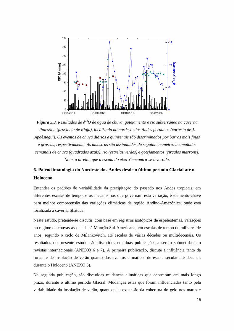
46
0
-5
-10
-15
01/04/2011 01/01/2012 01/10/2012 01/07/2013
0
50
100
150
200
250
300
350
400
1
8O
(V
-SM
OW
)
RIO
JA
(m
m)
A
Figura 5.3. Resultados de δ18
O de água de chuva, gotejamento e rio subterrâneo na caverna
Palestina (provincia de Rioja), localizada no nordeste dos Andes peruanos (cortesía de J.
Apaèstegui). Os eventos de chuva diários e quinzenais são discriminados por barras mais finas
e grossas, respectivamente. As amostras são assinaladas da seguinte maneira: acumulados
semanais de chuva (quadrados azuis), rio (estrelas verdes) e gotejamentos (círculos marrons).
Note, a direita, que a escala do eixo Y encontra-se invertida.
6. Paleoclimatologia do Nordeste dos Andes desde o último período Glacial até o
Holoceno
Entender os padrões de variabilidade da precipitação do passado nos Andes tropicais, em
diferentes escalas de tempo, e os mecanismos que governam esta variação, é elemento-chave
para melhor compreensão das variações climáticas da região Andino-Amazônica, onde está
localizada a caverna Shatuca.
Neste estudo, pretende-se discutir, com base em registros isotópicos de espeleotemas, variações
no regime de chuvas associadas à Monção Sul-Americana, em escalas de tempo de milhares de
anos, segundo o ciclo de Milankovitch, até escalas de várias décadas ou multidecenais. Os
resultados do presente estudo são discutidos em duas publicações a serem submetidas em
revistas internacionais (ANEXO 6 e 7). A primeira publicação, discute a influência tanto da
forçante de insolação de verão quanto dos eventos climáticos de escala secular até decenal,
durante o Holoceno (ANEXO 6).
Na segunda publicação, são discutidas mudanças climáticas que ocorreram em mais longo
prazo, durante o último período Glacial. Mudanças estas que foram influenciadas tanto pela
variabilidade da insolação de verão, quanto pela expansão da cobertura do gelo nos mares e

47
continentes do Hemisfério Norte (ANEXO 7). A estas mudanças de longo-prazo se sobrepõem
vários eventos abruptos de enfraquecimento ou fortalecimento da MSA, os quais estão
associados aos eventos Heinrich (H) e Daansgard-Oeschger (D-O), definidos em testemunhos
marinhos e de gelo, respectivamente.
A seguir, será feita uma breve revisão dos estudos prévios a respeito do paleoclima da América
do Sul, com ênfase nos registros isotópicos, assim como uma introdução aos artigos em anexo.
6.1. Mudanças paleoclimáticas na escala orbital
A variação da insolação, segundo o ciclo de precessão, tem sido considerada a principal forçante
do ciclo hidrológico (em escalas de tempo orbitais) na região sob o domínio da MSA (Cruz et
al., 2005a; Cheng et al., 2012; Cheng et al., 2013a).
Estas variações na insolação de verão, segundo o ciclo de precessão (19 a 23 ka), são inversas
entre os Hemisférios Sul e Norte, produzindo mudanças antífásicas no clima nas regiões
tropicais (Kutzbach et al., 2008). O aumento da insolação de verão austral produz um maior
gradiente térmico entre o continente e o oceano, o qual favorece a convergência de umidade na
Bacia Amazônica, intensificando desta forma o regime de monções na América do Sul (Cheng
et al., 2012). Coerente com isto, estudos do Hemisfério Norte (Wang et al., 2001; Yuan et al.,
2004) e do Hemisfério Sul (Cruz et al., 2005a, 2006; Wang et al., 2006, 2007a,b) registram um
regime de precipitação antifásico entre a MSA e a monção asiática na China.
Em concordancia com essa relação, os registros de espeleotemas de regiões situadas nos Andes
tropicais mostram que a intensidade da MSA aumentou desde o Holoceno Inferior até o
Holoceno Superior (van Breukelen et al., 2008; Bird et al., 2011a; Kanner et al., 2013) (Fig.
6.1). Por outro lado, registros paleoclimáticos de regiões diretamente afetadas pela ITCZ, na
Bacia de Cariaco (Haug et al., 2001; Deplazes et al., 2013) e nas regiões sob o domínio da
monção asiática, mostram uma tendência à diminuição da intensidade da precipitação.
Mais ao sul, em altas altitudes (> 6000m anm), o registro da geleira Huascarán (9ºS) (Thompson
et al., 1995) mostra uma forte correlação entre a insolação e o sinal isotópico entre 11 ka AP e o
presente, o que é semelhante ao ocorrido nas terras intermediárias e baixas do nordeste andino
peruano (Fig. 6.2). Originalmente, este registro teve seu δ18
O interpretado como sendo um
indicador de paleotemperatura, mas posteriormente foi verificado que as suas variações
isotópicas estavam correlacionadas primariamente à intensificação dos regimes de chuvas de
monção (Hoffmann et al., 2003).

48
-16
-14
-12
-10
Insolaçao Fev. 10oS
Pumacocha
Huagapo
960
940
920
900
880
0 2 4 6 8 10
-8
-6
-4
1
8O
1
8O
Idade (ka AP)
Shatuca
Tigre Perdido
960
940
920
900
880
Figura 6.1. Registros de paleopluviosidade na região andina comparados com a curva da
insolação, em preto, para o mês de fevereiro em 10ºS (Berger e Loutre, 1991). Em terras altas:
o registro da caverna de Huagapo em preto (Kanner et al., 2013), e o registro do lago
Pumacocha em azul (Bird et al., 2011a); em terras intermediárias o registro da caverna
Shatuca (este estudo) em vermelho; em terras baixas o registro da caverna Tigre Perdido (van
Breukelen et al., 2008) em verde. As datações são indicadas para cada registro, com a cor
correspondente.
Esta relação, entre insolação de verão e a MSA, será pela primeira vez estudada em registros
isotópicos de altitudes intermediárias na cordilheira dos Andes, com o registro da caverna
Shatuca. O artigo 1 (ANEXO 6) discute o forte controle da insolação de verão durante o
Holoceno, com enfoque na progressão das monções desde regiões de baixa altitude até terras
altas nos Andes (Fig. 6.1). Para isso, foi feita uma comparação com o registro lacustre de
Pallcacocha (>4000m anm), área afetada diretamente pela MSA (Rodbell et al., 1999; Moy et
al., 2002). Nesse sentido, um dos resultados mais interessantes deste trabalho foi a constatação
de que, na fase de máxima insolação de verão durante o Holoceno Superior, as chuvas
relacionadas ao regime de monção foram bastante acentuadas desde regiões de terras baixas até
as terras altas da Cordilheira dos Andes.
Similarmente, o registro sedimentar de Ti/Ca e Fe/Ca de testemunhos marinhos na costa do
Pacífico, no Golfo de Guaiaquil, mostra uma correlação positiva entre a insolação de verão

49
austral e a deposição fluvial de sedimentos dos rios na costa do Pacífico a 4ºS (Fig. 6.2). Isso
indica que a insolação de verão austral controlou também a precipitação na região onde nascem
os rios do flanco ocidental dos Andes setentrionais peruanos (Mollier-Vogel et al., 2013).
0 4 8 12 16 20 24 28 32 36 40
60
40
20
0
940
920
900
880
-0.4
-0.6
-0.8
log
(T
i/C
a)
W/m
2
Botuvera
Ga
mm
a (
cp
s)
Idade (ka AP)
Salar Uyuni
-5
-4
-3
-2
-11
8O
1
8O
1
8O
-24
-20
-16
Insolaçao Fev. 10oS
Golfo de Guaiaquil
Sajama
Huascaran
Sajama-27
-24
-21
-18
-15
-8
-6
-4
1
8O
87
987
6
5.1
5.2
6
5.1
5.2
2.1
2.2
2.2
4
4
3 32.1c2.1b2.1a11
Figura 6.2. Comparação entre os registros paleoclimáticos da América do Sul, durante os
últimos 40 ka AP, com a curva de insolação do mês de fevereiro para 10ºS. De cima para
baixo: em vermelho o registro da caverna Shatuca, presente estudo; em preto o registro do
Golfo de Guaiaquil (Mollier-Vogel et al., 2013); em azul o registro dos testemunhos de gelo da
geleira Huascarán (Thompson et al., 1995); em preto o registro de gelo do vulcão Sajama
(Thompson et al., 1998); em verde o registro da caverna Botuverá (Cruz et al., 2005a); em
preto o registro do testemunho sedimentar do Salar de Uyuni (Baker et al., 2001a), junto com a
curva de insolação em azul (Berger e Loutre, 1991). As barras azul claro e laranja indicam a
ocorrência dos estadiais (Greenland Stadials –GS) e interestadiais da Groenlândia (Greenland
Interstadials-GI), numerados segundo Rasmussen et al. (2014). As datações são indicadas para
cada registro, com a cor correspondente.

50
No entanto, no Holoceno Superior, a intensificação do regime de monções na região subtropical
do Brasil, nos Andes equatorianos e peruanos até o lago Titicaca (Baker et al., 2001b), não
afetou as áreas situadas no limite sul do sistema da MSA, como o Salar de Uyuni (Baker et al.,
2001a) e o Nevado de Sajama (Thompson et al., 1998), situadas mais para o sul da Bolívia (Fig.
6.2).
Já durante os últimos períodos Glacial (38 a 20 ka AP) e Deglacial (20 a 11 ka AP), não foi
observada uma relação evidente entre as curvas de insolação de verão e a curva de δ18
O do
registro da Shatuca (Fig. 6.2). Isso sugere que outras forçantes climáticas podem estar
envolvidas na modulação do clima em escalas de tempo mais longas, assim como discutido
previamente por Cruz et al. (2007) para o sul do Brasil.
De fato, os dados isotópicos da caverna Shatuca revelam um padrão semelhante à outros
registros isotópicos da região andina e sul do Brasil que são afetadas pela MSA (Cruz et al.,
2007; Mosblech et al., 2012; Cheng et al., 2013a; Fornace et al., 2014). Na figura 6.2 nota-se
que os valores de δ18
O, durante o último período Glacial, são significativamente mais baixos do
que aqueles observados durante o Holoceno Inferior (11 a 7.5 ka AP). A partir de 5 ka AP os
dados de δ18
O tornam-se mais negativos, o que é condizente com as mudanças de insolação de
verão no Hemisfério Sul.
No sul do Brasil (27ºS), o registro isotópico da caverna de Botuverá mostra que a insolação
controlou a intensidade da Monção Sul-Americana entre 120-0 ka AP (ver Fig. 6.2) (Cruz et al.,
2005a). No entanto, Cruz et al. (2006) notou que as anomalias de δ18
O tanto dos espeleotemas
em Botuverá, Santa Catarina, quanto na caverna Santana, São Paulo, não mostram um
acoplamento tão evidente com a insolação durante o Último Máximo Glacial. Na verdade, foi
constatada uma intensificação no regime de chuvas de monções durante 70-17 ka AP, período
caracterizado por anomalias negativas de δ18
O e por valores muito baixos das razões Sr/Ca e
Mg/Ca dos espeleotemas (Cruz et al., 2007). Posteriormente, a mesma feição é descrita em
registros isotópicos dos Andes (Kanner et al., 2012; Mosblech et al., 2012; Cheng et al., 2013a;
Fornace et al., 2014). Por exemplo, em 16ºS, o registro de isótopos estáveis de compostos
orgânicos do lago Titicaca (Fornace et al., 2014) indica que a paleopluviosidade começou a ser
mais claramente controlada pela insolação de verão austral em 11 ka AP, enquanto que entre 60-
20 ka AP prevaleceram condições substancialmente mais úmidas que as do Holoceno. Todavia,
uma pluviosidade mais alta, durante a fase tardia do último período Glacial, não poderia ser
explicada apenas pela influência da insolação de verão devido à falta de relação entre a curva da
insolação do mês de fevereiro a 10ºS e os dados isotópicos, tanto de espeleotemas, como de
testemunhos de gelo e lagos.

51
As condições de contorno durante o período Glacial foram responsáveis pela redução da
intensidade da AMOC, a qual induziu a expansão do gelo preferencialmente no Hemisfério
Norte e resultou no deslocamento da ITCZ para o sul, intensificando o transporte de umidade do
oceano Atlântico para a Bacia Amazônica (Chiang et al., 2003; Chiang e Bitz, 2005). Esse
mecanismo pode explicar as condições mais úmidas inferidas a partir dos registros
paleoclimáticos situados ao sul do equador (Cruz et al., 2007; Cheng et al., 2013a; Fornace et
al., 2014) e mais secos na região norte da América do Sul (Peterson et al., 2000; Deplazes et al.,
2013). De fato, a variabilidade da MSA depende fortemente da posição da ITCZ, a qual foi
impactada pela expansão da cobertura de gelo, nos mares e nos continentes (condições de
contorno glacial), particularmente no Hemisfério Norte (Chiang et al., 2003; Chiang e Bitz,
2005). Assim, as condições mais úmidas entre 70 e 17 ka AP, período correspondente aos
Estágios Isotópicos Marinhos 2- 4 (Marine Isotope Stages 2-4, MIS 2-4), foram provavelmente
influenciadas por condições mais frias no oceano Atlântico ao norte da linha do equador (Cruz
et al., 2007; Fornace et al., 2014). Este tópico é discutido no artigo apresentado no ANEXO 7.
6.2. Mudanças paleoclimáticas abruptas
6.2.1 – Eventos climáticos durante os últimos períodos Glacial e Deglacial
Os registros isotópicos de testemunhas de gelo da Groenlândia (e.g. NGRIP) revelaram que o
último período Glacial se caracterizou por mudanças climáticas abruptas e eventos recorrentes
em escala de tempo milenar (Dansgaard et al., 1984, 1993). Essas mudanças abruptas,
ocorreram em alguns anos ou em até algumas décadas (Alley et al., 1993; Taylor et al., 1993) e
se repetiram aproximadamente a cada 1470 anos (Bond et al., 1999; Schulz, 2002), mostrando
aquecimentos bruscos de até 10°C na atmosfera nas fases quentes. Essas oscilações hoje
chamadas Dansgaard-Oeschger (D-O) (Dansgaard et al., 1984, 1993), foram seguidas por um
retorno gradual a condições glaciais mais frias (Fig. 6.3).
Por outro lado, Heinrich (1988) observou em testemunhos sedimentares do Atlântico Norte,
grande concentração de sedimentos continentais transportados por icebergs (IRD, Ice Rafted
Debris), em latitudes mais baixas que o habitual, entre 40-53°N (IRD-Belt) (Bond et al., 1992).
A presença destes IRD no sedimento representa a ocorrência de eventos frios abruptos durante o
período Glacial, durante os quais icebergs se deslocaram para o sul a uma maior distância em
relação ao polo norte. Estes eventos, hoje conhecidos como “Eventos Heinrich” (Broecker,
1994; Rahmstorf, 2002), ocorreram em algumas das fases frias (ou estadiais da Groenlândia)
dos ciclos D-O. Seis eventos Heinrich (H) foram definidos no final de alguns ciclos D-O,
enquanto os eventos D-O, conhecidos também como interestadiais da Groenlândia, são pelo
menos vinte (Rahmstorf, 2003).

52
Desde a descoberta dos eventos Heinrich, grandes esforços têm se realizado para revelar os
mecanismos responsáveis pela sua origem. Até o momento, o melhor mecanismo físico para
explicar a origem dessas mudanças abruptas, que afetam diferentes regiões do mundo, é a
entrada de água doce de degelo nas altas latitudes do Atlântico Norte e o seu efeito sobre o
transporte de calor para a região nórdica através da desaceleração da AMOC (Rooth, 1982;
Broecker et al., 1985; Bond et al., 1993; Rahmstorf, 1995; Alley et al., 1999; Ganopolski e
Rahmstorf, 2001; Knutti et al., 2004). No entanto, ainda não está claro se as mudanças da
AMOC explicam por si só as mudanças climáticas registradas tanto no Atlântico Norte como
em outras regiões do mundo (Wunsch, 2006).
12 16 20 24 28 32 36 40
940
920
900
880
5060708090100
-45
-42
-39
-36
-18
-16
-14
-12-9.0
-7.5
-6.0
-4.5
-8
-6
-4
1
8O
87
9876
5.15.2
65.1
5.2
2.1
2.2
2.2 4
433
2.1c2.1b2.1a11
Idade (ka AP)
Ti/C
a
1
8O
1
8O
1
8O
W/m
2
Papahuacain (Kanner et al., 2012)
Cariaco
(Deplazes et al., 2013)
Shatuca
NGRIP
(Ramussen et al., 2014)
Condor
(Cheng et al., 2013)
Insolaçao 10oS
Fevereiro
Figura 6.3. Comparação entre o registro de gelo NGRIP (Rasmussen et al., 2014) com os
registros paleoclimáticos da América do Sul para o período entre 40-10 ka AP. De cima para
baixo: NGRIP em preto; a Bacia de Cariaco em azul (Deplazes et al., 2013); a caverna Shatuca
em vermelho (presente estudo); a caverna El Condor em preto (Cheng et al., 2013a); a caverna
Papahuacain em verde (Kanner et al., 2012); a insolação para 10ºS no mês de fevereiro em
turquesa (Berger e Loutre, 1991). As barras azul claro e laranja indicam a ocorrência dos

53
estadiais (Greenland Stadials –GS) e interstadiais da Groenlândia (Greenland Interstadials-
GI), numeradas segundo a terminologia de Rasmussen et al. (2014). As datações são indicadas
para cada registro, com a cor correspondente.
Modelos sugerem que uma desaceleração da AMOC gera anomalias positivas de TSM no
Atlântico Sul, bem como uma intensificação anômala de ventos alísios de nordeste. Desse modo
os modelos também sugerem uma assimetria da circulação Hadley, entre ambos os hemisférios,
junto com a correspondente assimetria do posicionamento da ITCZ (Lindzen e Hou, 1988;
Peterson et al., 2000; Chiang, 2002; Vellinga e Wood, 2002; Wang et al., 2004, 2007a,b; Zhang
e Delworth, 2005; Clement e Peterson, 2008).
Durante os eventos de resfriamento das águas superficiais, em altas latitudes do Atlântico Norte,
associados aos eventos Heinrich, ocorre uma intensificação da alta dos Açores (Wang et al.,
2005; Ruddiman, 2008; Naughton et al., 2009) e uma intensificação dos ventos alísios de
nordeste (Arz et al., 1998; Peterson et al., 2000; Fleitmann et al., 2003; Cruz et al., 2009). Por
sua vez, isso conduz a anomalias positivas (negativas) de precipitação nos trópicos do
Hemisfério Sul (Norte), isto é, uma ITCZ localizada mais ao sul (Arz et al., 1998; Wang et al.,
2004; Jaeschke et al., 2007) e uma MSA mais ativa (Cruz et al., 2006; Wang et al., 2006). Da
mesma maneira, os registros andinos a diferentes altitudes mostram a MSA intensificada (Fritz
et al., 2010; Kanner et al., 2012; Mosblech et al., 2012; Cheng et al., 2013a). Em contraste, os
eventos Heinrich são marcados no registro de Cariaco como eventos mais áridos (Hughen et al.,
1996; Peterson et al., 2000; Haug et al., 2001; Lea et al., 2003; Peterson e Haug, 2006; Deplazes
et al., 2013).
A situação climática se inverte na América do Sul durante os eventos quentes D-O, registrados
nos testemunhos de gelo do pólo norte durante o período Glacial (Rasmussen et al., 2014). Estes
eventos, estão associados ao aquecimento do Atlântico tropical norte (Lea et al., 2003),
causando anomalias positivas de precipitação ao norte da América do Sul (Hughen et al., 1996;
Peterson et al., 2000; Peterson e Haug, 2006; Deplazes et al., 2013).
O registro da Bacia de Cariaco na Venezuela (Deplazes et al., 2013) mostra que durante os
ciclos D-O, no período de transição do interestadial (fase quente) ao estadial (fase fria), ainda é
possível observar a influência sazonal da ITCZ nas latitudes da Bacia de Cariaco a 10°N.
Porém, durante os eventos Heinrich e nas fases finais dos D-O o deslocamento da ITCZ foi
tanto ao sul que não houve um retorno sazonal da ITCZ para estas latitudes. Ademais, é
interessante ressaltar que o evento Heinrich 1 (H1) teve uma intensidade muito maior nos
testemunhos marinhos de Cariaco do que a observada nas altas latitudes, por exemplo no
testemunho de NGRIP (Fig. 6.3).

54
Os impactos dos eventos D-O no clima dos trópicos, ao sul do continente, ainda não são bem
conhecidos. Até agora, o registro de Kanner et al. (2012) da caverna de Papahuacain, localizada
em terras altas (3850m anm), e os registros de Cheng et al. (2013a) das cavernas El Condor e El
Diamante, localizados em terras baixas (800m anm) do Peru, são os que melhor registraram a
variação abrupta dos eventos D-O nos Andes.
O presente trabalho consiste numa nova reconstituição dos eventos milenares, que afetaram a
precipitação na região da MSA durante os últimos 38 ka AP (em resolução subdecenal). Esta
reconstituição é baseada em registros de δ18
O da calcita de três estalagmites (Sha-1, Sha-2 e
Sha-3), com objetivo de contribuir na pesquisa sobre o entendimento da MSA na porção andina
da Bacia Amazônica. Trata-se do registro isotópico de melhor resolução dentre os que já foram
produzidos até o momento. Nele se destacam tanto os eventos Heinrich, quanto os eventos
Daansgard-Oeschger, bem como os eventos ocorridos durante o período Deglacial. O modo de
ocorrência de tais eventos é descrito em um dos artigos a ser submetido (ANEXO 7).
Recentemente, foi sugerido que algumas características dos eventos Heinrich, foram em parte
influenciadas por mudanças climáticas ocorridas na Antártica, durante o último período Glacial
(Weaver et al., 2003; Kanner et al., 2012). Por exemplo, o aquecimento da Antártica tem sido
proposto como forçante para a ocorrência do evento H1 por Weaver et al. (2003).
Já durante o período Deglacial nos Andes, existe um debate a respeito se o padrão ocorrido
durante este período é parecido ao Deglacial da Antártica como observado nos registros das
geleiras de Huascarán e Illimani (Thompson et al., 1995; Ramirez et al., 2003), ou se é mais
semelhante ao Deglacial da Groenlândia como sugerido pelo registro da geleira Sajama, na
Bolívia. Pois, este último, mostra os eventos Bølling-Allerød (B/A) e o Younger Dryas (YD),
com uma estrutura similar ao do registro NGRIP, na Groenlândia. Ademais, uma maior
influência do oceano Pacífico foi sugerida para os registros de gelo andinos por Vimeux (2009).
Assim, questões fundamentais permanecem em aberto sobre as mudanças na paleopluviosidade
sobre os Andes tropicais em diferentes escalas de tempo e espaço, considerando as diferentes
altitudes, latitudes e condições topográficas que determinaram os diferentes climas sobre a
região, em escalas de tempo interanuais até orbitais.
O registro isotópico da caverna Shatuca pode ser considerado o melhor registro paleoclimático
do período Deglacial já produzido ate o momento, em termos de resolução e controle
cronológico, pelo método U/Th. Com este arquivo paleoclimático será detalhada a estrutura dos
eventos isotópicos, correlatos aos períodos estadiais e interstadiais da Groenlândia. Entre eles o
mais estudado tem sido o Younger Dryas (YD), que corresponde à fase fria do primeiro ciclo D-
O e que junto com o evento H1 é caracterizado por um retorno abrupto à temperaturas quase
glaciais. Este evento teve uma duração de aproximadamente um milênio e é um evento frio,
55
equivalente aos eventos Heinrich, enquanto o evento Bølling-Allerød (B/A), ocorrido entre o
H1e o YD, é um evento quente do período Deglacial e é equivalente aos eventos D-O (fases
quentes dos ciclos D-O). O registro da caverna Shatuca apresenta uma excelente sincronia com
estes eventos típicos do Hemisfério Norte e, portanto, torna-se uma importante evidência a ser
utilizada na discussão sobre a ocorrência de eventos, com duração de vários séculos até alguns
milênios, que impactam abruptamente o clima da América do Sul.
6.2.1 – Eventos climáticos durante o Holoceno
Após a publicação dos primeiros registros isotópicos de δ18
O dos testemunhos de gelo da
Groenlândia, o período do Holoceno foi caracterizado como sendo de grande estabilidade
climática (Dansgaard et al., 1993). No entanto, Bond et al. (1997, 2001) postularam que durante
o Holoceno ocorreram variações na temperatura da superfície do Atlântico Norte
aproximadamente a cada 1500 anos. Sugerindo que esse ciclo representa a continuação dos
eventos Heinrich no Holoceno, só que com menor amplitude e duração. Os autores se basearam
em vários indicadores paleoclimáticos e paleoecológicos dos quais o que se mostrou mais
robusto, na determinação e na delimitação dos eventos, foi o índice de clastos transportados por
icebergs (Ice Rafted Debris- IRD). Assim, a partir dos picos de aumento de concentração de
IRD se determinou a ocorrência de períodos de resfriamento abrupto no Atlântico Norte, mais
tarde chamados na literatura como Eventos Bond.
Vários estudos têm tentado entender os mecanismos por trás da variabilidade do Holoceno.
Entre eles, se destacam Mayewski et al. (2004, 2005, 2009), Wanner e Bütikofer (2008) e
Wanner et al. (2008, 2011, 2014). Na América do Sul tropical, cada vez mais registros
paleoclimáticos apresentam um Holoceno marcado por fortes oscilações abruptas no ciclo
hidrológico, que comparados ao registro de IRD do Atlântico Norte (Bond et al., 2001) (Fig.
6.4), confirmam a resposta da MSA aos eventos frios do Hemisfério Norte também para o
Holoceno (Baker et al., 2005; Cheng et al., 2009; Strikis et al., 2011; Moreira-Turcq et
al.,2014). Assim sendo, se confirma a hipótese do deslocamento da ITCZ para o sul, durante
eventos de resfriamento abrupto das águas superficiais de altas latitudes do Atlântico Norte
(Peterson et al., 2000; Haug et al., 2001). A ITCZ deslocada mais para o sul, durante estes
eventos, tem como consequência o aumento da umidade transportada pela Monção Sul
Americana ao longo do continente, sendo refletido como um aumento da umidade nos registros
paleoclimáticos (Vuille et al., 2012).
Nas últimas duas décadas houve um aumento do número de registros andinos que cobrem a
maior parte do período Holoceno (Moy et al., 2002; Bush et al., 2005; van Breukelen et al.,
2008; Bird et al., 2011a; Kanner et al., 2013). Entre os eventos mais estudados do Holoceno
para a América do Sul, se destacam o evento 8.2 ka AP (Cheng et al., 2009, Strikis et al, 2011),

56
a Pequena Idade de Gelo (Little Ice Age -LIA) e a Anomalia Climática Medieval (Medieval
Climate Anomaly -MCA) (Reuter et al., 2009; Bird et al., 2011b; Vuille et al., 2012; Novello et
al., 2012; Apaèstegui et al., 2014).
Os estudos com base em registros de pólen, realizados no flanco oriental andino, mostram o
Holoceno como um período de grande variabilidade na vegetação e a ocorrência de incêndios
florestais, tanto de causa humana como de causa natural (Bush et al., 2005; Urrego et al., 2009;
Hillyer et al., 2009; Urrego et al., 2010). No entanto, estes registros têm baixo controle
cronológico e pouca resolução temporal, o que os torna difíceis de serem utilizados para estudos
de eventos abruptos com duração de décadas.
Nesse contexto, destaca-se um estudo baseado em espeleotemas do centro-leste brasileiro
(Strikis et al., 2011) que apresentou mudanças abruptas no ciclo hidrológico em sincronia com
os eventos Bond do Atlântico Norte. Recentemente, o estudo de Moreira-Turcq et al. (2014)
ressaltou o evento ocorrido em 2.7 ka AP, como um evento úmido nas planícies de inundação
do rio Amazonas e outras regiões da AS, e o associou ao possível deslocamento da ITCZ para o
sul causado pela provável desaceleração da Circulação de Revolvimento Meridional do Oceano
Atlântico (AMOC) (Fig. 6.4). Por outro lado, pouco se sabe sobre a ocorrência de eventos do
tipo Bond na região andina.
Mais ao norte, a 3ºS, o registro do lago Pallcacocha, localizado acima dos 4000m anm nos
Andes do Equador, mostra um aumento das precipitações ao longo do Holoceno, que os autores
interpretaram como sendo associado ao aumento da frequência de eventos El Niño (Rodbell et
al., 1999; Moy et al., 2002). Entretanto, estes eventos de maior erosão nas cabeceiras do lago,
em períodos mais chuvosos, não são consistentes com os registros do lago El Junco (Conroy et
al., 2008; Zhang et al., 2014), localizado mais ao oeste nas Ilhas Galápagos. O registro de
Shatuca foi comparado a estes arquivos paleoclimáticos, com o intuito de contribuir na
discussão da influência do fenômeno ENSO nas chuvas no domínio da MSA. Essa discussão é
feita no artigo que se encontra disponível no ANEXO 6.
Dado que o nordeste dos Andes peruanos se encontra na borda do sistema de monção, lugar
onde na atualidade o Jato de Baixos Níveis se desloca em direção oeste durante o verão (Poveda
et al., 2014), é possível que alguns eventos que ocorrem em terras baixas não sejam observados
em terras altas. Por isso, nosso registro pode contribuir para o entendimento da intensidade e
extensão do sistema de monções ao refletir mudanças desse sistema em diferentes altitudes. Para
isso comparamos o registro isotópico da caverna Shatuca com outros registros em alta resolução
provenientes dos Andes.

57
-1,4
-0,7
0,0
0,7
1,4
Tigre
Perdido_destendenciado
0 2 4 6 8 10
2015105
Shatuca
Composite_destendenciado
-8
-7
-6
-5
-4
Lapa
Grande
-1
0
1
-1
0
1
2
18O
Pumacocha_destendenciado
Huagapo_destendenciado
-2
0
2
18O
18O
18O
18O
Idade (ka AP)
Figura 6.4. Variabilidade milenar em registros isotópicos da América do Sul durante o período
do Holoceno, e a curva de concentração de Hematite Stained Grains (%HSG) em sedimentos
marinhos do Atlântico Norte de Bond et al. (2001). Os registros andinos apresentados foram
destendenciados retirando a componente da forçante da insolação das séries isotópicas com a
finalidade de poder observar melhor a variabilidade milenar. Os registros apresentados são (de
cima para baixo): o do lago Pumacocha (Bird et al., 2011a) e o da caverna Huagapo (Kanner
et al., 2013), ambos em terras altas dos Andes centrais peruanos; o registro da caverna Lapa
Grande (Strikis et al., 2011) localizada no centro-leste brasileiro; o registro da caverna do
Tigre Perdido (van Breukelen et al., 2008) e o registro da caverna Shatuca (este estudo), ambos
no nordeste dos Andes peruanos, em terras baixas e intermediárias respectivamente; e a curva
de %HSG de Bond et al. (2001). As barras laranjas (azuis) indicam períodos de menor (maior)
umidade.

58
7. Considerações Finais
Neste estudo, investigou-se pela primeira vez a variabilidade da Monção de verão Sul-
Americana (MSA), com base em espeleotemas provenientes de uma altitude intermediária
(1960 m), na região nordeste dos Andes peruanos durante os últimos 38 ka AP.
Durante o último período Glacial e o Holoceno, a caverna Shatuca registrou condições de aridez
maiores às registradas por estudos paleoclimáticos anteriores, em regiões andinas de alta (acima
dos 4000m anm) e baixa altitude (abaixo dos 1000m anm).
Observou-se que nas terras localizadas em altitudes intermediárias e baixas, entre 3-6ºS nos
Andes, as condições de umidade durante o Último Máximo Glacial (Last Glacial Maximum -
LGM) parecem ter sido semelhantes às ocorridas no Holoceno Superior. Ademais, notou-se
ausência de controle de insolação sobre a MSA entre 38-11 ka AP, o que pode ser explicado
pela influência de condições de contorno glaciais sobre a MSA durante este período, como
sugerido por estudos paleoclimáticos prévios realizados na AS.
O período Deglacial, na região nordeste dos Andes, aparece como uma mudança gradual em
direção às condições mais áridas do Holoceno Inferior. Após este período seco, com
aproximadamente 2000 anos de duração, houve um aumento gradual da umidade que
caracterizou o período Holoceno. Este aumento foi síncrono com a tendência de aumento da
insolação, modulada pelo ciclo da precessão, e ocorreu ao longo dos Andes desde 3ºS até 16ºS.
No entanto, notou-se que os registros da região central dos Andes, especificamente no Altiplano
(18-20ºS), não indicam um aumento da umidade durante o Holoceno.
A caverna Shatuca é o primeiro registro em terras intermediárias que apresenta várias mudanças
climáticas abruptas, ocorridas em escalas de tempo milenar até decenal, sobrepostas às
tendências de mais longo prazo dos últimos 38ka. Assim mesmo, a amplitude das mudanças
climáticas ocorridas em terras intermediárias, parece ter sido maior à observada em terras altas e
baixas, provavelmente porque o local da caverna Shatuca encontra-se na borda de influência da
MSA.
Durante os últimos períodos Glacial e Deglacial, reconheceram-se no registro da Shatuca
mudanças relacionadas aos estadiais da Groenlândia (Greenland Stadials-GS), porém com
intensidades variáveis. A estrutura do evento H1 no registro da Shatuca é de particular interesse,
pois uma inversão extrema para condições secas ocorreu dentro do evento, em 16.2 ka AP, que
parece ter ocorrido também em terras baixas, no entanto menos severa. A correlação notável
deste evento com o registro de Cariaco, no norte da América do Sul (em 10ºN), parece indicar
que a ITCZ está deslocada mais ao sul do que 5°S.

59
A caverna Shatuca, registrou um YD úmido, de condições menos extremas que as atingidas no
período úmido relativo ao H1. Entre o H1 e o YD, o período árido Bølling–Allerød (B/A)
mostrou uma reversão para condições úmidas dentro de sua estrutura.
No fim do YD, uma mudança abrupta ocorreu em 11 ka AP, que levou às condições áridas do
Holoceno Inferior. No entanto, durante o Holoceno Inferior, o registro de Shatuca registrou pelo
menos duas mudanças climáticas abruptas para condições de maior. Sendo este, o primeiro
registro isotópico da região andina que mostra a ocorrência de vários eventos úmidos abruptos
durante o Holoceno Inferior.
Durante o Holoceno Médio, constatou-se que diversas mudanças climáticas bruscas ocorreram
em altitudes intermediárias andinas (5°S), no período entre 5.1 e 5.0 ka AP. A comparação com
outros registros da AS revela que esta série de eventos foi contemporânea a um periodo de
mudanças climáticas abruptas ocorridas na região da América do Sul afetada pela MSA. O fato
de este evento ter sido abrupto ou gradual vem sendo debatido para outras regiões do mundo,
em especial na região da Monção Africana, mas até agora, não existiam registros isotópicos de
alta resolução que permitissem discutir a sua estrutura para a América do Sul. Assim mesmo,
durante o evento 5 ka AP, parece ter ocorrido uma reorganização do sistema climático, que
interrompeu a gradual tendência de incremento de umidade, após a qual houve aumento de
intensidade da monção e maior frequência de eventos úmidos a diferentes altitudes dos Andes.
Isto pode estar relacionado em grande parte ao aumento da insolação no verão austral.
Durante o Holoceno Superior foram registrados os períodos de maior umidade do Holoceno. No
entanto, a tendência de aumento de umidade diminui e há um aumento da variabilidade em
escala decenal e centenária. O registro isotópico de Shatuca possui um baixo controle
cronológico para este período, complicando a comparação com outros registros andinos. No
entanto, entre 4-1 ka AP, houve sincronicidade durante alguns dos períodos úmidos registrados
em registros andinos de diferentes altitudes.
Uma das comparações mais importantes obtidas neste trabalho se dá entre o registro da Shatuca
e o registro do lago Pallcacocha, localizado ao sul dos Andes equatorianos. O registro de
Pallcacocha tem sido amplamente utilizado como indicador de frequência de ocorrência do
fenômeno El Niño. Dado o efeito oposto causado pelo El Niño nestas duas regiões, e o aumento
de umidade registrado em ambas localidades, entre 3.5 e 2.5 ka AP, propomos que esta
variabilidade pode ter sido causada por um aumento da umidade transportada pela MSA e uma
maior extensão da mesma, devido talvez a ocorrência do evento Bond 2 unido a um aumento da
insolação de verão austral.

60
REFERÊNCIAS BIBLIOGRÁFICAS
Alley, R.; Clark, P.U.; Keigwin, L.D.; Webb R.S. Making sense of millennial-scale climate
change. In: Mechanisms of Global Climate Change at Millennial Time Scales. Clark,
P.U.; Webb, R.S.; Keigwin, L.D. (Eds.), Geophysical Monograph Series, v.112, p.385–
394, AGU, Washington, D.C, 1999.
Alley, R.B.; Meese, D.A.; Schuman, C.A.; Gow, A.J.; Taylor, K.C.; Grootes, P.M.; White,
J.W.; Ram, M.; Waddington, E.D.; Mayewski, P.A.; Zielinski, G.A. Abrupt increase in
Greenland snow accumulation at the end of the Younger Dryas event. Nature, v.362,
p.527-529, doi: 10.1038/362527a0., 1993.
Apaèstegui, J.; Cruz, F.W.; Sifeddine, A.; Vuille, M.; Espinoza, J.C.; Guyot, J.L.; Khodri, M.;
Strikis, N.; Santos, R.V.; Cheng, H.; Edwards, L.; Carvalho, E.; Santini, W. Hydroclimate
variability of the northwestern Amazon Basin near the Andean foothills of Peru related to
the South American Monsoon System during the last 1600 years. Climate of the Past,
v.10, p.1967–1981, doi: 10.5194/cp-10-1967-2014, 2014.
Arz, H.W.; Patzold, J.; Wefer, G. Correlated millennial-scale changes in surface hydrography
and terrigenous sediment yield inferred from Last-Glacial marine deposits off
Northeastern Brazil. Quaternary Research, v.50, p.157–166, 1998.
Ayliffe, L.K.; Marianelli, P.C.; McCulloch, M.T.; Mortimeter, G.E.; Hellstrom, J.C.; Moriarty,
K.C.; Wells, R.T. 500 ka precipitation record from southeastern Australia: Evidence for
interglacial relative activity. Geology, v.26, p.147-150, 1998.
Baker, P.A.; Rigsby, C.A.; Seltzer, G.O.; Fritz, S.C.; Lowensteink, T.K.; Bacher, N.P.; Veliz, C.
Tropical climate changes at millennial and orbital timescales on the Bolivian Altiplano.
Nature, v.409, p.698-701, 2001a.
Baker, P.A.; Seltzer, G.O.; Fritz, S.C.; Dunbar, R.B.; Grove, M.J.; Tapia, P.M.; Cross, S.L.;
Rowe, H.D.; Broda, J.P. The history of South American tropical precipitation for the past
25,000 years. Science, v.291, p.640-643, 2001b.
Baker, P.A.; Fritz, S.C.; Garland, J.; Ekdahl, E. Holocene hydrologic variation at Lake Titicaca,
Bolivia/Peru, and its relationship to North Atlantic climate variation. Journal of
Quaternary Science, v.20, p.655–662, doi:10.1002/jqs.987, 2005.
Baldini, J.U.L.; McDermott, F.; Hoffmann, D.L.; Richards, D.A.; Clipson, N. Very high-
frequency and seasonal cave atmosphere P(CO2) variability: Implications for stalagmite

61
growth and oxygen isotope-based paleoclimate records. Earth and Planetary Science
Letters, v.272, p.118-129, 2008.
Berger, A.; Loutre, M.F. Insolation values for the climate of the last 10 million years.
Quaternary Science Reviews, v.10, p.297–317, 1991.
Bigot J.Y. La riviere souterraine de Shatuca = El rio subterraneo de Shatuca. Bulletin du Groupe
Speleologique Bagnols Marcoule, Hors serie special Chaquil 2006 & Santiago 2007, p.
52-56, 2008.
Bird, B.W.; Abbott, M.B.; Rodbell, D.T.; Vuille, M. Holocene tropical South American
hydroclimate revealed from a decadally resolved lake sediment δ18O record. Earth and
Planetary Science Letters, v.310, p.192-202, 2011a.
Bird, B.W.; Abbott, M.B.; Vuille, M.; Rodbell, D.T.; Stansell, N.D.; Rosenmeier, M.F. A 2,300-
year-long annually resolved record of the South American summer monsoon from the
Peruvian Andes. Proceedings of the National Academy of Sciences of the United States
of America, v.108, p.8583-8588, 2011b.
Bolzan, M.J.A. Análise da transformada em ondeletas aplicada em sinal geofísico. Revista
Brasileira de Ensino de Física, v.26, p.37-41, 2004.
Bolzan, M.J.A. Transformada em ondeleta: Uma necessidade. Revista Brasileira de Ensino de
Física, v.28, p.563-567, 2006.
Bombardi, R.J.; Carvalho, L.M.V. Variabilidade do regime de monções sobre o Brasil: o clima
presente e projeções para um cenário com 2xCO2 usando o modelo MIROC. Revista
Brasileira de Meteorologia, v.23, p.58-72, 2008.
Bond, G.; Broecker, W.; Jehnsen, S.; McManus, J.; Labeyrie, L.; Jouzel, J.; Bonani, G.
Correlations between climate records from north Atlantic sediments and Greenland ice.
Nature, v.365, p.143-147, 1993.
Bond G.; Heinrich, H.; Broecker, W.; Labeyrie, L.; McManus, J.; Andrews, J.; Huon, S;
Jantschik, R.; Clasen, S.; Simet, C.; Tedesco, K; Klas, M.; Bonani, G.; Ivy, S. Evidence
of Massive Discharges of Icebergs into the North Atlantic during the Last Glacial Period.
Nature, v 360, p. 245-249, 1992.
Bond, G.; Kromer, B.; Beer, J.; Muscheler, R.; Evans, M.N.; Showers, W.; Hoffmann, S.; Lotti-
Bond, R.; Hajdas, I.; Bonani, G. Persistent solar influence on North Atlantic climate
during the Holocene. Science, v.294, p.2130-2136, 2001.

62
Bond, G.; Showers, W.; Cheseby, M.; Lotti, R.; Almasi, P.; de Menocal, P.; Priore, P.; Cullen,
H.; Hajdas, I.; Bonani, G. A Pervasive Millennial-Scale Cycle in North Atlantic Holocene
and Glacial Climates. Science, v.278, p.1257–1266, 1997.
Bond, G; Showers, W.; Elliot, M.; Evans, M.; Lotti, R.; Hajdas, I.; Bonani, G.; Johnson, S. The
North Atlantic’s 1 – 2 kyr climate rhythm: Relation to Heinrich events,
Dansgaard/Oeschger cycles, and the Little Ice Age, in Mechanisms of Global Climate
Change at Millennial Time Scales. Clark, P.U.; Webb, R.S.; Keigwin L.D. (Eds.),
Geophysical Monography Series, v.112, p.35 – 58, AGU, Washington, D.C., 1999.
Bookhagen, B.; Strecker, M.R Orographic barriers, high resolution TRMM rainfall, and relief
variations along the eastern Andes. Geophysical Research Letters v.35, L06403, 2008.
Bradley, R.S.; Vuille, M.; Hardy, D.; Thompson, L.G. Low latitude ice cores record Pacific sea
surface temperatures. Geophysical Research Letters, v.30, 1174,
doi:10.1029/2002GL016546, 2003.
Broecker, W.S.; Peteet, D.M.; Rind D. Does the ocean-atmosphere system have more than one
stable mode of operation? Nature, v.315, p.21–25, doi: 10.1038/315021a0, 1985.
Broecker, W.S. Massive iceberg discharges as triggers for global climate changes. Nature,
v.372, p.421-424, 1994.
Bush, M.B.; Hansen, B.C.S.; Rodbell, D.T.; Seltzer, G.O.; Young, K.R.; Leon, B.; Abbott,
M.B.; Silman, M.R.; Gosling, W.D. A 17 000-year history of Andean climate and
vegetation change from Laguna de Chochos, Peru. Journal of Quaternary Science, v.20,
p.703–714, 2005.
Cheng H.; Edwards, R.L.; Shen, C.C.; Polyak, V.J.; Asmerom, Y.; Woodhead, J.; Hellstrom, J.;
Wang, Y.; Kong, X.; Spötl, C.; Wang, X.; Alexander Jr, E.C. Improvements in 230Th
dating, 230Th and 234U half-lifevalues, and U–Th isotopic measurements by multi-
collector inductively coupled plasma mass spectrometry. Earth and Planetary Science
Letters, v.371-372, p.82-91, 2013b.
Cheng, H.; Fleitmann, D.; Edwards, L.R.; Wang, X.; Cruz, F.W.; Auler, A.S.; Mangini, A;
Wang, Y.; Kong, X.; Burns, S. J.; Matter, A. Timing and structure of the 8.2 kyr BP event
inferred from d18O records of stalagmites from China, Oman, and Brazil. Geology, v. 37,
p.1007-1010, 2009.
Cheng, H.; Sinha, A.; Cruz, F.W.; Wang, X.; Edwards, R.L.; d’Horta, F.M.; Ribas, C.C.;
Vuille, M.; Stott, L.D.; Auler, A.S. Climate change patterns in Amazonia and
biodiversity. Nature communications, doi: 10.1038/ncomms2415, 2013a.

63
Cheng, H.; Sinha, A.; Wang, X.; Cruz, F.; Edwards, L. The Global Paleomonsoon as seen
through speleothem records from Asia and the Americas. Climate Dynamics, v.39,
p.1045-1062, doi: 10.1007/s00382-012-1363-7, 2012.
Chiang, J.C.; Bitz, C.M. Influence of high latitude ice cover on the marine Intertropical
Convergence Zone. Climate Dynamics, v.25, p.477-496, 2005.
Chiang, J.C.H. Deconstructing Atlantic Intertropical Convergence Zone variability: influence of
the local cross-equatorial sea surface temperature gradient and remote forcing from the
eastern equatorial Pacific. Journal of Geophysical Research, v.107, D1404, 2002.
Chiang, J.C.H. The Tropics in Paleoclimate. Annual Review of Earth and Planetary Sciences,
v.37, p.263;297, 2009.
Chiang, J.C.H.; Biasutti, M.; Battisti, D.S. Sensitivity of the Atlantic Intertropical Convergence
Zone to the last glacial maximum boundary conditions. Paleoceanography, v.18, p.1094-
1112, 2003.
Chiessi, C.M.; Mulitza, S.; PÄtzold, J.; Wefer, G.; Marengo, J.A. Possible impact of the
Atlantic Multidecadal Oscillation on the South American summer monsoon. Geophysical
Research Letters, v.36, L21707, 2009.
Clark, I.; Fritz, P. Environmental Isotopes in Hydrology. CRC Press, Boca Raton, p.328, 1997.
Clement, A.C.; Peterson, L.C. Mechanism of abrupt climate change of the last glacial period.
Reviews of Geophysics, v.46, p.1-39, 2008.
Cobbing, E.J.; Pitcher, W.S.; Wilson, J.J.; Baldock, J.W.; Taylor, W.P.; McCourt, W.; Snelling,
N.J. The geology of the Western Cordillera of northern Peru. Overseas Memoires,
Institute of Geological Sciences, v.5, p.143, 1981.
Conroy, J.L.; Overpeck, J.T.; Cole, J.E.; Shanahan, T.M.; Steinitz-Kannan, M. Holocene
changes in eastern tropical Pacific climate inferred from a Galápagos lake sediment
record. Quaternary Science Reviews, v.27, p.1166–1180, 2008.
Cruz, F.W.; Burns, S.J.; Jercinovic, M.; Karmann, I.; Sharp, S.J.; Vuille, M. Evidence of rainfall
variations in Southern Brazil from trace element ratios (Mg/Ca and Sr/Ca) in a Late
Pleistocene stalagmite. Geochimica et Cosmochimica Acta, v.71, p.2250–2263, 2007.
Cruz, F.W.; Burns, S.J.; Karmannn, I.; Sharp, W.D.; Vuille, M. Reconstruction of regional
atmospheric circulation features during the late Pleistocene in subtropical Brazil from
oxygen isotope composition of speleothems. Earth and Planetary Sciences Letters, v.248,
p.494-506, 2006.

64
Cruz Jr., F.W.; Burns, S.J.; Karmann, I.; Sharp, W.D.; Vuille, M.; Cardoso, A.O.; Ferrari, J.A.;
Silva Dias, P.L.; Viana Jr., O. Insolation-driven changes in atmospheric circulation over
the past 116 ky in subtropical Brazil. Nature, v.434, p.63-66, 2005a.
Cruz Jr., F.W.; Karmann, I.; Viana Jr., O.; Burns, S.J.; Ferrari, J.A.; Vuille, M.; Moreira, M.Z.;
Sial, A.N. Stable isotope study of cave percolation waters in subtropical Brazil:
implications for paleoclimate inferences from speleothems. Chemical Geology, v.220,
p.245-262, 2005b.
Cruz, F.W.; Wang, X.; Auler, A.; Vuille, M.; Burns, S.B.; Edwards, L.R.; Karmann, I.; Cheng,
H. Orbital and millenial-scale precipitation change in Brazil from speleothem records. In:
Past Climate Variability in South America and Surrounding Regions, From the Last
Glacial Maximum to the Holocene. Vimeux, F.; Sylvestre, F.; Khodri, M. (Eds.), v.14,
ch.2, p.29-60, doi: 10.1007/978-90-481-2672-9, 2009.
Dansgaard, W.; Johnsen, S.J.; Clausen H.B.; Dahl-Jensen, D.; Gundestrup, N.S.; Hammer,
C.U.; Hvidberg, C.S.; Steffensen J.P.; Sveinbjornsdottir, A.E.; Jouzel. J.; Bond, G.C.
Evidence for general instability of past climate from a 250-kyr ice core record. Nature,
v.364, p.218-220, 1993.
Dansgaard, W.; Johnsen, S.J.; Clausen, H.B.; Dahl-Jensen, D.; Gundestrup, N.; Hammer, C. U.;
Oeschger, H. North Atlantic climatic oscillations revealed by deep Greenland ice cores.
In: Climate Processes and Climate Sensitivity. Hansen, E.; Takahashi, T. (Eds.),
Geophysical Monograph Series, v.29, p.288–298, AGU, Washington, D.C., 1984.
Dansgaard, W. Stable isotopes in precipitation. Tellus, v.16, p.436–468, 1964.
Delworth, T.L.; Clark, P.; Holland, M.; Johns, W.M.; Kuhlbrodt, T.; Lynch-Stieglitz, J.; Morrill,
C.; Seager, R.; Weaver, A.J.; Zhang, R. The potential for abrupt change in the Atlantic
Meridional Overturning Circulation. In: Abrupt Climate Change. U.S. Geological Survey,
ch.4, p.258-359, 2008.
Deplazes, G.; Lückge, A.; Peterson, L.C.; Timmermann, A.; Hamann, Y.; Hughen, K.A.; Röhl,
U.; Lak, C.; Cana, M.A.; Sigman, D.M.; Haug, G.H. Links between tropical rainfall and
North Atlantic climate during the last glacial period. Nature Geoscience, v.6, p.213-217,
doi: 10.1038/NGEO1712, 2013.
Dorale, A.J; Edwards, R.L.; Ito, E; Gonzalez, L.A. Climate and vegetation history of the
midcontinent from 75 to 25 ka: A speleothem record from Crevice Cave, Missouri, USA.
Science, v.282, p.1871-1874, 1998.

65
Doyle, M.E.; Barros, V.R. Midsummer low-level circulation and precipitation in subtropical
South America and related sea surface temperature anomalies in the South Atlantic.
Journal of Climate, v.15, p.3394–3410, 2002.
Edwards, R.L.; Chen, J.H.; Wasserburh, G.J. 238U - 234U - 230Th - 232Th systematics and the
precise measurement of time over the past 500.000 years. Earth Planetary Science Letters,
v.81, p.175-192, 1986.
Ehlers, R.S. Análise de séries temporais. Departamento de Estatística da Universidade Federal
do Paraná, p.53, 2009.
Espinoza Villar, J.C. Impact de la variabilité climatique sur l’hydrologie du bassin amazonien.
Université Paris 6 - Pierre et Marie Curie, Paris - France, Thèse de Doctorat, p.207,
2009.
Espinoza, J.C.; Ronchail, J.; Guyot, J.L.; Junquas, C.; Vauchel, P.; Lavado, W.S.; Drapeau, G.;
Pombosa, R. Climate variability and extreme drought in the upper Solimões River
(Western Amazon Basin): Understanding the exceptional 2010 drought. Geophysical
Research Letters, v.38, L13406, doi: 10.1029/2011GL047862, 2011.
Fairchild, I.J.; Smith, C.L.,; Baker, A.; Fuller, L.; Spötl, C.; Mattey, D.; McDermott, F.;
E.I.M.F. Modification and preservation of environmental signals in speleothems. Earth-
Science Reviews, v.75, p.105-153, 2006.
Fleitmann, D.; Burns, S.J.; Mudelsee, M.; Neff, U.; Kramers, J.; Mangini, A.; Matter, A.
Holocene Forcing of the Indian Monsoon Recorded in a Stalagmite from Southern Oman.
Science, v.300, p.1737-1739, doi 10.1126/science.1083130, 2003.
Fleitmann, D.; Burns, S.J.; Neff, U.; Mudelsee, M.; Mangini, A.; Mattera, A. Palaeoclimatic
interpretation of high-resolution oxygen isotope profiles derived from annually laminated
speleothems from Southern Oman. Quaternary Science Reviews, v.23, p.935-945, 2004.
Fornace, K.L.; Hughen, K.A.; Shanahanc, T.M.; Fritz, S.C.; Baker, P.A.; Sylva, S.P. A 60,000-
year record of hydrologic variability in the Central Andes from the hydrogen isotopic
composition of leaf waxes in Lake Titicaca sediments. Earth and Planetary Science
Letters, v.408, p.263–271, 2014.
Frisia, S.; Borsato, A.; Preto, N.; McDermott, F. Late Holocene annual growth in three Alpine
stalagmites records the influence of solar activity and the North Atlantic Oscillation on
winter climate. Earth and Planetary Science Letters, v.216, p.411-424, 2003.
Fritz, S.C.; Baker, P.A.; Seltzer, G.O.; Ballantyne, A.; Tapia, P.; Cheng, H.; Edwards, R.L.
Quaternary glaciation and hydrologic variation in the South American tropics as

66
reconstructed from the Lake Titicaca drilling project. Quaternary Research, v.68, p.410–
420, 2007.
Fritz; S.C.; Baker, P.A.; Ekdahl, E.; Seltzer, G.O.; Stevens, L.R. Millennial-scale climate
variability during the Last Glacial period in the tropical Andes. Quaternary Science
Reviews, v.29, p.1017–1024, 2010.
Gan, M.A.; Kousky, V.E.; Ropelewski, C.F. The South American monsoon circulation and its
relationship to rainfall over West-Central Brazil. Journal of Climate, v.17, p.47–66, 2004.
Gandu, A.W.; Silva Dias, P.L. Impact of tropical heat sources on the South American
tropospheric upper circulation and subsidence. Journal of Geophysical Research, v.103,
p.6001–6015, 1998.
Ganopolski, A.; Rahmstorf , S. Rapid changes of glacial climate simulated in a coupled climate
model. Nature, v.409, p.153–158, doi:10.1038/35051500, 2001.
Garreaud, R. Cold air incursions over Subtropical South America: Mean structure and
dynamics. Monthly Weather Review, v.128, p.2544–2559, 2000.
Garreaud, R.; Vuille, M.; Clement, A.C. The climate of the Altiplano: observed current
conditions and mechanisms of past changes. Palaeogeography Palaeoclimatology
Palaeoecology, v.194, p.5–22, 2003.
Garreaud, R.; Vuille; M.; Compagnucci; R.; Marengo, J. Present-day South American climate.
Palaeogeography Palaeoclimatology Palaeoecology, v.281, p.180–195, 2009.
Gat, J.R.; Bowser, C.J.; Kendall, C. The Contribution of evaporation from the Great-Lakes to
the continental atmosphere – estimate based on stable-isotope data. Geophysical Research
Letters, v. 21, p. 557–560, 1994.
Gat, J.R.; Matsui, E. Atmospheric water balance in the Amazon basin: an isotopic
evapotranspiration model. Journal of Geophysical Research, v.96, p.13179–13188, 1991.
Gentry, A.H. Changes in plant community diversity and floristic composition on environmental
and geographical gradients. Annals of the Missouri Botanical Garden, v.75, p.1-34, 1988.
Ghil, M.; Allen, M.R.; Dettinger, M.D.; Ide, K.; Kondrashov, D.; Mann, M.E.; Robertson,
A.W.; Saunders, A.; Tian, Y.; Varadi, F.; Yiou, P. Advanced Spectral Methods for
Climatic Time Series. American Geophysical Union, v.40, p.1-41, doi:
10.1029/2001RG000092, 2002.
Gonfiantini, R.; Roche, M.A., Olivry, J.C.; Fontes, J.C.; Zuppi, G.M. The altitude effect on the
isotopic composition of tropical rains. Chemical Geology, v.181, p.147–167, 2001.

67
Grimm, A.M. Interannual climate variability in South America: impacts on seasonal
precipitation, extreme events and possible effects of climate change. Stochastic
Environmental Research and Risk Assessment, v.25, p.537-564, doi: 10.1007/s00477-
010-0420-1, 2011.
Grinsted, A.; Jevrejeva, S.; Moore, J. Application of the cross wavelet transform and wavelet
coherence to geophysical time series. Nonlinear Processes in Geophysics, v.11, p.561-
566, 2004.
Guyot, J.L. Hydrogéochimie des fleuves de l’Amazonie bolivienne. Editions de l’ORSTOM,
Paris, p.261, 1993.
Hansen, B.C.S.; Rodbell, D.T. A late-glacial/Holocene pollen record from the eastern Andes of
northern Peru. Quaternary Research, v.44, p.216–227, 1995.
Haug, G.H.; Hughen, K.A.; Sigman, D.M.; Peterson, L.C.; Röhl, U. Southward migration of the
intertropical convergence zone through the Holocene. Science, v.293, p.1304-1308, 2001.
Heinrich, H. Origin and consequences of cyclic ice rafting in the northeast Atlantic Ocean
during the past 130,000 years. Quaternary Research, v.29, p.142-152, 1988.
Hillyer, R.; Valencia, B.G.; Bush, M.; Siman, M.R.; Steinitz-Kannan, M. A 24,000-year
paleolimnological history from the Peruvian Andes. Quaternary Research, v.71, p. 71–82,
2009.
Hoffmann, G.; Ramirez, E.; Taupin, J.D.; Francou, B.; Ribstein, P.; Delmas, R.; Dürr, H.;
Gallaire, R.; Simões, J.; Schotterer, U.; Stievenard, M.; Werner, M. Coherent isotope
history of Andean ice cores over the last century. Geophysical Research Letters, v.30,
p.1179, doi: 10.1029/2002GL014870, 2003.
Hughen, K.A.; Overpeck, J.T.; Peterson, L.C.; Trumbore, S. Rapid climate changes in the
tropical Atlantic region during deglaciation. Nature, v.380, p.51–54, 1996.
Jaeschke, A.; Rühlemann, C.; Arz, H.; Heil, G.; Lohmann, G. Coupling of millennial-scale
changes in sea surface temperature and precipitation off northeastern Brazil with high-
latitude climate shifts during the last glacial period. Paleoceanography, v.22, PA4206,
2007.
Johnson, K.R.; Hu, C.Y.; Belshaw, N.S.; Henderson, G.M. Seasonal trace-element and stable-
isotope variations in a Chinese speleothem: The potential for high-resolution
paleomonsoon reconstruction. Earth and Planetary Science Letters, v.244, p.394-407,
2006.

68
Kanner, L.C.; Burns, S.J.; Cheng, H.; Edwards, R.L. High-latitude forcing of the South
American summer monsoon during the last glacial. Science, v.335, p.570-573, doi:
10.1126/science.1213397, 2012.
Kanner, L.C.; Burns, S. J.; Cheng, H.; Edwards, R.L.; Vuille, M. High-resolution variability of
the South American summer monsoon over the last seven millennia: insights from a
speleothem record from the central Peruvian Andes. Quaternary Science Reviews, v.75,
p.1–10, doi:10.1016/j.quascirev.2013.05.008, 2013.
Kanner, L.C. An Isotopic Perspective on Climatic change in Tropical South America from the
mordern through the last Glacial Period. Tese de Doutoramento, p.166, 2011.
Knight, J.R; Allan, R.J.; Folland, C.K.; Vellinga, M.; Mann, M.E. A signature of persistent
natural thermohaline circulation cycles in observed climate. Geophysical Research
Letters, v.32, L20708, 2005.
Knutti, R.; Flückiger, J.; Stocker, T.F.; Timmermann, A. Strong hemispheric coupling of glacial
climate through freshwater discharge and ocean circulation. Nature, v.430, p.851-856,
doi: 10.1038/nature02786, 2004.
Kodama, Y. Large–scale common features of subtropical precipitation zones (the Baiu Frontal
Zone, the SPCZ and the SACZ. Part I: Characteristic of subtropical frontal zones. Journal
of the Meteorological Society of Japan, v.70, p.813–836, 1992.
Koster, R.D.; de Valpine, P.; Jouzel J. Continental water recycling and H218O concentrations.
Geophysical Research Letters, v.20, p.2215–2218, doi: 10.1029/93GL01781, 1993.
Kousky, V.E. Pentad outgoing longwave radiation climatology for the South American sector.
Revista Brasileira de Meteorologia, v.3, p.217–231, 1988.
Kuhlbrodt, T.; Griesel, A.; Montoya, M.; Levermann, A.; Hofmann, M.; Rahmstorf, S. On the
driving processes of the Atlantic meridional overturning circulation. Reviews of
Geophysics, v.45, RG2001, doi:10.1029/2004RG000166, 2007.
Kutzbach, J.E., Liu, X.; Liu, Z.; Chen, G. Simulation of the evolutionary response of global
summer monsoons to orbital forcing over the past 280,000 years, Climate Dynamics,
v.30, p.567–579, 2008.
Labraga, J.C.; Frumento, O.; López, M. The atmospheric water vapor cycle in South America
and the tropospheric circulation. Jounal of Climate, v.13, p.1899–1915, 2000.
Lachniet, M. Climatic and environmental controls on speleothem oxygen-isotope values.
Quaternary Science Reviews, v.28, p.412-432, 2009.

69
Laraque, A.; Ronchail, J.; Cochonneau, G.; Pombosa, R.; Guyot, J.L. Heterogeneous
distribution of rainfall and discharge regimes in the Ecuadorian Amazon basin. Journal of
Hydrometeorology, v.8, p.1364–1381, 2007.
Lavado, W.; Labat, D.; Ronchail, J.; Espinoza, J.C.; Guyot, J.L. Trends in rainfall and
temperature in the Peruvian Amazon – Andes basin over the last 40 years (1965–2007).
Hydrological Processes, v.41, p.2944–2957, doi:10.1002/hyp.9418, 2012.
Lavado, W.; Espinoza, J.C. Impactos de El Niño y La Niña en las lluvias del Perú (1965-2007).
Revista Brasileira de Meteorologia, v.29, p.171-182, 2014.
Lea, D.W.; Pak, D.K.; Peterson, L.C.; Hughen, K.A. Synchroneity of tropical and high-latitude
Atlantic temperatures over the last glacial termination. Science, v.301, p.1361 – 1364,
2003.
León, B.; Young, K.R.; Brako, L. Análisis de la composición florística del bosque montano
oriental del Perú. In Biogeografía, Ecología y Conservación del Bosque Montano en el
Perú. Young, K.R.; Valencia, N. (Eds.), Memorias del Museo de Historia Natural
U.N.M.S.M. (Lima), v.21, p.141-154, 1992.
Lindzen, R.S.; Hou A.Y. Hadley circulations for zonally averaged heating centered off the
equator. Journal of the Atmospheric Sciences, v.45, p.2416–2427, 1988.
Marengo, J.A.; Liebmann, B.; Grimm, A. M.; Misra, V.; Silva Dias, P.L.; Cavalcanti, I.F.A.;
Carvalho, L.M.V.; Berbery, E.H.; Ambrizzi, T.; Vera, C.S.; Saulo, A.C.; Nogués-Paegle,
J.; Zipser, E.; Sethk, A.; Alvese. L.M. Review: Recent developments on the South
American monsoon system. International Journal of Climatology, v.32, p.1–21, doi:
10.1002/joc.2254, 2012.
Marengo, J.A.; Liebmann, B.; Kousky, V.E.; Filizola, N.P.;Wainer, I.C. Onset and end of the
rainy season in the Brazilian Amazon Basin. Journal of Climate, v.14, p.833-852, 2001.
Marengo, J.A. Long‐term trends and cycles in the hydrometeorology of the Amazon basin since
the late 1920s. Hydrology Processes, v.23, p.3236–3244, doi:10.1002/hyp.7396, 2009.
Marengo, J.A.; Nobre, C. General characteristics and variability of climate in the Amazon basin
and its links to the global climate system. In: The Biochemistry of the Amazon basin.
Clain, M.E.; Victoria, R.L.; Richey, J.E. (Eds.), Oxford University Press, p.17-41, 2001.
Marengo, J.A.; Nobre, C.; Tomasella, J.; Oyama, M.; Sampaio, G.; Camargo, H.; Alves, L.;
Oliveira, R. The drought of Amazonia in 2005. Journal of Climate, v.21, p.495–516,
2008.

70
Marengo, J.A.; Soares, W.; Saulo, W.; Nicolini, M. Climatology of the LLJ east of the Andes as
derived from the NCEP reanalyses. Journal of Climate, v.17, p.2261–2280, 2004.
Marengo, J.A.; Tomasella, J.; Alves, L.M.; Soares, W.R.; Rodriguez, D.A. The drought of 2010
in the context of historical droughts in the Amazon region. Geophysical Research Letters,
v.38, L12703, doi: 10.1029/2011GL047436, 2011.
Mayewski, P.A., Maasch, P.K.A.; Yan, Y.; Kang, S.; Meyerson, E.A.; Sneed, S.B.; Kaspari,
S.D.; Dixon, D.A.; Osterberg, E.C.; Morgan, V.I.; van Ommen, T.; Curran, M.A.J. Solar
forcing of the polar atmosphere. Annals of Glaciology, v.41, p.147–154, doi:
10.3189/172756405781813375, 2005.
Mayewsky, P.A.; Meredith, M.P.; Summerhayes, C.P.; Turner, J.; Worby, A.; Barrett, P.J.;
Casassa, G.; Bertler, N.A.N.; Bracegirdle, T.; Naveira Garabato, A.C.; Bromwich, D.;
Campbell, H.; Hamilton, G.S.; Lyons, W.B.; Maasch, K.A.; Aoki, S.; Xiao, C.; van
Ommen, T. State of the Antarctic and Southern Ocean Climate System. Reviews of
Geophysics, v.47, RG1003, 2009.
Mayewski, P.A.; Rohling, E.E.; Stager, J.C.; Karlén W.; Maasch, K.A.; Meeker, L.D.;
Meyerson, E.A.; Gasse, F.; van Kreveld, S.; Holmgren, K.; Lee-Thorp, J.; Rosqvist, G.;
Rack, F.; Staubwasser, M.; Schneider, R.R.; Steig, E.J. Holocene climate variability.
Quaternary Research, v.62, p.243–255, doi:10.1016/j.yqres.2004.07.001, 2004.
McDermott, F. Palaeo-climate reconstruction from stable isotope variations in speleothems: a
review. Quaternary Science Reviews, v.23, p.901-918, 2004.
McManus, J.F.; Francois, R.; Gherardi, J.M.; Keigwin, L.D.; Brown-Leger, S. Collapse and
rapid resumption of Atlantic meridional circulation linked to deglacial climate changes.
Nature, v.428, p.834–837, 2004.
Minobe, S. Resonance in bidecadal and pentadecadal climate oscillations over the North Pacific:
Role in climatic regime shifts. Geophysical Research Letters, v.26, p.855-858, 1999.
Mollier-Vogel, E.; Leduc, G.; Böschen, T.; Martinez, P.; Schneider, R.R. Rainfall response to
orbital and millennial forcing in northern Peru over the last 18 ka. Quaternary Science
Reviews, v.76, p.29-38, 2013.
Moquet, J.S.; Crave, A.; Viers, J.; Seyler, P.; Armijos, E.; Bourrel, L.; Chavarri, E.; Lagane, C.;
Laraque, A.; Lavado Casimiro, W.S.; Pombosa, R.; Noriega, L.; Vera, A.; Guyot, J.L.
Chemical weathering and atmospheric/soil CO2 uptake in the Andean and Foreland
Amazon basins. Chemical Geology, v.287, p.1–26, 2011.

71
Moreira-Turcq, P.; Turcq, B.; Moreira, L.S.; Amorim, M.; Cordeiro, R.C.; Guyot, J.L. A 2700
cal yr BP extreme flood event revealed by sediment accumulation in Amazon floodplains.
Palaeogeography Palaeoclimatology Palaeoecology, v.415, p.175-182. doi:
10.1016/j.palaeo.2014.07.037, 2014.
Morettin P.A.; Toloi, C.M.C. Análise de séries temporais. Blücher, E. (Eds.), Instituto de
Matemática e Estadística, Universidade de São Paulo, SP-Brasil, 2a edição, p.564, 2006.
Mosblech, N.A.S.; Bush, M.B.; Gosling, W.D.; Hodell, D.; Thomas, L.; van Calsteren, P.;
Correa-Metrio, A.; Valencia, B.G.; Curtis, J.; vanWoesik, R. North Atlantic forcing of
Amazonian precipitation during the last ice age. Nature Geoscience, v.5, p.817-820, doi:
10.1038/NGEO1588, 2012.
Moy, C.M.; Seltzer, G.O.; Rodbell, D.T.; Anderson, D.M. Variability of El Niño/ Southern
Oscillation activity at millennial timescales during the Holocene epoch. Nature, v.420,
p.162–165, 2002.
Nogués-Paegle, J. A comparative review of South American low-level jets. Meteorologica, v.3,
p.73-82, 1998.
Nogués-Paegle, J.; Mo, K.C. Alternating wet and dry conditions over South America during
summer. Monthly Weather Review, v.125, p.279–291, 1997.
Nogués-Paegle, J.; Mo, K.C. Linkages between summer rainfall variability over South America
and sea surface temperature anomalies. Journal of Climate, v.15, p.1389–1407, 2002.
Novello, V.F.; Cruz, F.W.; Karmann, I.; Burns, S.J.; Stríkis, N.M.; Vuille, M.; Cheng, H.;
Edwards, R.L.; Barreto, E.A.S.; Frigo, E. Multidecadal climate variability in Brazil
Nordeste during the last 3000 years based on speleothem isotope records. Geophysical
Research Letters, v.39, L23706, doi: 10.1029/2012GL053936, 2012.
Peterson, L.C.; Haug, G.H.; Hughen, K.A.; Röhl, U. Rapid changes in the hydrologic cycle of
the tropical Atlantic during the last glacial. Science, v.290, p.1947-1951, 2000.
Peterson, L.C., Haug, G.H. Variability in the mean latitude of the Atlantic Intertropical
Convergence Zone as recorded by riverine input of sediments to the Cariaco Basin
(Venezuela). Palaeogeography Palaeoclimatology Palaeoecology, v.234, p.97–113, 2006.
Polyak, V.J.; Asmerom, Y. Late Holocene climate and cultural changes in the southwestern
United States. Science, v.294, p.148-151, 2001.

72
Poveda, G.; Jaramillo, L.; Vallejo, L.F. Seasonal precipitation patterns along pathways of South
Americanlow-level jets and aerial rivers. Water Resources Research, v.50, p.1–21,
doi:10.1002/2013WR014087, 2014.
Rahmstorf, S. Bifurcations of the Atlantic thermohaline circulation in response to changes in the
hydrological cycle. Nature, v.378, p.145–149, doi: 10.1038/378145a0, 1995.
Rahmstorf, S. Ocean circulation and climate during the past 120,000 years. Nature, v.419,
p.207–214, 2002.
Rahmstorf, S. Timing of abrupt climate change: A precise clock. Geophysical Research Letters,
v. 30, 1510, doi:10.1029/2003GL017115, 2003.
Ramirez, E.; Hoffmann, G.; Taupin, J.D.; Francou, B.; Ribstein, P.; Caillon, N.; Ferron, F.A.;
Landais, A.; Petit, J.R.; Pouyaud B.; Schotterer, U.; Simoes, JC.; Stievenard, M. A new
Andean deep ice core from Nevado Illimani, (6350 m), Bolivia. Earth and Planetary
Science Letters, v.212, p.337–350, 2003.
Rao, V.B.; Hada, K. Characteristics of rainfall over Brazil: Annual variations and connections
with the Southern Oscillation. Theoretical and App1ied Climatology, v.42, p.81-91, 1990.
Rasmussen, S.O.; Bigler, M.; Blockley, S.P.; Blunier, T.; Buchardt, S.L.; Clausen, H.B.;
Cvijanovic, I.; Dahl-Jensen, D.; Johnsen, S.J.; Fischer, H.; Gkinis, V.; Guillevic, M.;
Hoek, W.Z.; Lowe, J.J.; Pedro, J.B.; Popp, T.; Seierstad, I.K.; Steffensen, J.P.; Svensson,
A.M.; Vallelonga, P.; Vinther, B.M.; Walker, M.J.C.; Wheatley, J.J.; Winstrup, M. A
stratigraphic framework for abrupt climatic changes during the Last Glacial period based
on three synchronized Greenland ice core records: refining and extending the INTIMATE
event stratigraphy. Quaternary Science Reviews, v.106, p.14-28, 2014.
Reuter, J.; Stott, L.; Khider, D.; Sinha, A.; Cheng, H.; Edwards, R.L. A new perspective on the
hydroclimate variability in northern South America during the Little Ice Age.
Geophysical Research Letters, v.36, L21706, doi:10.1029/2009GL041051, 2009.
Richard, D.A.; Dorale, J.A. Uranium-series chronology and environmental applications of
speleothem. Reviews in Mineralogy and Geochemistry, v.52, p.407-460, doi:
10.2113/0520407, 2003.
Robertson, A.; Mechoso, C. Interannual and interdecadal variability of the South Atlantic
Convergence Zone. Journal of Climate, v.11, p.2947–2957, 2000.
Rodbell, D.T.; Seltzer, G.O.; Anderson, D.M.; Abbott, M.B.; Enfield, D.B., Newman, J.H. An
15,000-year record of El-Niño alluviation in southwestern Ecuador. Science, v.283,
p.516–520, 1999.

73
Rodwell, M. J., Hoskins, B. J. Subtropical anticyclones and summer monsoons. Journal of
Climate, v.14, p.3192–3211, 2001.
Ronchail, J.; Gallaire, R. ENSO and rainfall along the Zongo valley (Bolivia) from the
Altiplano to the Amazon basin. International Journal of Climatology, v.26, p.1223–1236,
2006.
Rooth, C.G.H. Hydrology and ocean circulation, Progress in Oceanography, v.11, p.131–149,
doi: 10.1016/0079-6611(82)90006-4, 1982.
Rozanski, K.; Araguás-Araguás, L. Spatial and temporal variability of stable isotope
composition of precipitation over the South American continent. Bulletin de l’Institut
Français d’Études Andines, v.24, p.379-390, 1995.
Rozanski, K.; Araguas-Araguas, L.; Gonfiantini, R. Isotopic patterns in modern global
precipitation. American Geophysical Union, Geophysical Monograph, v.78, p.1-36, 1993.
Ruddiman, W.F. Earth's climate: past and future. Freeman, W.H. (Eds.), 2ª edição, Nova Iorque,
p.465, 2008.
Schmidt, G.; Le Grande, A.; Hoffmann, G. Water isotope expressions of intrinsic and forced
variability in a coupled ocean-atmosphere model. Journal of Geophysical Research,
v.112, D10103, 2007.
Schulz, M. On the 1470-year .pacing of Dansgaard-Oeschger warm events. Paleoceanography,
v. 17, doi: 10.1029/2000PA000571, 2002.
Schulz, M.; Mudelsee, M. REDFIT: estimating red-noise spectra directly from unevenly spaced
paleoclimatic time series. Computers and Geosciences, v.28, p.421-426, 2002.
Seltzer, G.O.; Rodbell, D.T.; Baker, P.A.; Fritz, S.C.; Tapia, P.M.; Rowe, H.D.; Dunbar, R.D.
Early warming of tropical South America at the last glacial-interglacial transition.
Science, v.296, p.1685–1686, 2002.
Sharp, Z. Principles of Stable Isotope Geochemistry. Pearson Prentice Hall, Upper Saddle
River, New Jersey, 2007.
Shen, C.C.; Edwards, R.L.; Cheng, H.; Dorale, J.A.; Thomas, R.B.; Moran, S.B.; Weinstein,
S.E.; Edmonds, H.N. Uranium and thorium isotopic and concentration measurements by
magnetic sector inductively coupled plasma mass spectrometry. Chemical Geology,
v.185, p.165-178, 2002.
Silva Dias, P.L.; Schubert, W.H.; Demaria, M. Large-scale response of the tropical atmosphere
to transient convection. Journal of the Atmospheric Sciences, v.40, p.2689–2707, 1983.

74
Spiegel, M.R. Estatística. Makron Books, São Paulo, 3a Edição, 1993.
Spötl, C.; Mangini, A.; Frank, N.; Eichstädter, R.; Burns, S.J. Start of the last interglacial period
at 135 ka: evidence from a high Alpine speleothem. Geology, v.30, p.815-818, 2002.
Stríkis, N.M. Paleopluviosidade no Norte de Minas Gerais Durante o Glacial Tardio e Holoceno
com Base em Registros de Espeleotemas. Dissertação (Mestrado) - Instituto de
Geociências, Universidade de São Paulo, São Paulo, 2011.
Strikis, N.M.; Cruz Jr., F.W.; Cheng, H.; Karmann, I.; Edwards, R.L.; Vuille, M.; Wang, X.; de
Paula, M.S.; Novello, V.F.; Auler, A.S. Abrupt variations in South American monsoon
rainfall during the Holocene based on a speleothem record from central-eastern Brazil.
Geology, v.39, p.1075–1078, 2011.
Sutton, R.T.; Hodson, D.L.R. Atlantic Ocean Forcing of North American and European
Summer Climate. Science, v. 309, p. 115-117, doi: 10.1126/science.1109496, 2005.
Tan, M.; Liu, T.; Hou, J.; Qin, X.; Zhang, H.; Li, T. Cyclic rapid warming on centennial-scale
revealed by a 2650-year stalagmite record of warm season temperature. Geophysical
Research Letters, v.30, 1617, doi: 10.1029/2003GL017352, 2003.
Taylor, K.C.; Lamorey, G.W.; Doyle, G.A.; Alley, R.B.; Grootes, P.M.; Mayewski, P.A.;
White, W.C.; Barlow, L.K. The ‘flickering switch’ of late Pleistocene climate change.
Nature, v.361, p.432-436, doi:10.1038/361432a0, 1993.
Thompson, L.G.; Davis, M.E.; Mosley-Thompson, E.; Sowers, T.A.; Henderson, K.A.;
Zagorodnov, V.S.; Lin, P.N. ; Mikhalenko, V.N. ; Campen, R.K. ; Bolzan, J.F. ; Cole-
Dai, J. ; Francou, B. A 25,000-year tropical climate history from Bolivian ice cores.
Science, v.282, p.1858–1864, 1998.
Thompson, L.G.; Mosley-Thompson, E.; Davis, M.E.; Lin, P.N.; Henderson, K.A.; Cole-Dai, J.;
Bolzan, J.F.; Kiu, K.B. Late Glacial stage and Holocene tropical ice core records from
Huascaran, Peru. Science, v.269, p.46–50, 1995.
Torrence, C.; Compo, G. P. A practical guideto wavelet analysis. Bulletin of the American
Meteorological Society, v.79, p. 61–78, 1998.
Treble, P.; Shelley, J.M.G.; Chappell, J. Comparison of high resolution sub-annual records of
trace elements in a modern (1911-1992) speleothem with instrumental climate data from
southwest Australia. Earth and Planetary Science Letters, v.216, p.141-153, 2003.
Urrego, D.H.; Bush, M.B.; Silman, M.R. A long history of cloud and forest migration from
Lake Consuelo, Peru. Quaternary Research, v.73, p. 364–373, 2010.

75
Urrego, D.H.; Bush, M.B.; Silman, M.R.; Correa-Metrio, A.; Ledru, M-P.; Mayle, F.E.;
Paduano, G.; Valencia, B.G. Millennial-Scale Ecological Changes in Tropical South
America Since the Last Glacial Maximum. In: Past Climate Variability in South America
and Surrounding Regions, From the Last Glacial Maximum to the Holocene. Vimeux, F.;
Sylvestre, F.; Khodri, M. (Eds.), v.14, ch.12, p.281-300, doi: 10.1007/978-90-481-2672-
9, 2009.
van Breukelen, M.R.; Vonhof, H.B.; Hellstrom, J.C.; Wester, W.C.G.; Kroon, D. Fossil
dripwater in stalagmites reveals Holocene temperature and rainfall variation in Amazonia.
Earth and Planetary Science Letters, v.275, p.54-60, 2008.
Vellinga, M.; Wood, R. Global climate impacts of collapse of the Atlantic Thermohaline
Circulation. Climate Change, v.54, p.251-267, 2002.
Vera, C.; Higgins, W.; Amador, J.; Ambrizzi, T.; Garreaud, R.; Gochis, D.; Gutzler, D.;
Lettenmaier, D.; Marengo, J.; Mechoso, C.R.; Nogués-Paegle, J.; Silva Dias, P.L.; Zhang,
C. Toward a unified view of the American Monsoon Systems. American Meteorological
Society, v.19, p.4977-5000, 2006.
Vimeux, F.; Gallaire, R.; Bony, S.; Hoffmann, G.; Chiang, J.C.H. What are the climate controls
on δD in precipitation in the Zongo Valley (Bolivia)? Implications for the Illimani ice
core interpretation. Earth and Planetary Science Letters, v.240, p.205-220, 2005.
Vimeux. F. Similarities and Discrepancies between Andean Ice Cores over the Last
Deglaciation: Climate Implications. In: Past Climate Variability in South America and
Surrounding Regions, From the Last Glacial Maximum to the Holocene. Vimeux, F.;
Sylvestre, F.; Khodri, M. (Eds.), v.14, ch.10, p.239-258, doi: 10.1007/978-90-481-2672-
9, 2009.
Vuille, M.; Bradley, R.S.; Werner, M.; Healy, R.; Keimig, F. Modeling δ18
O in precipitation
over the tropical Americas: 1. Interannual variability and climatic controls. Journal of
Geophysical Research, v.108, p.4174-4175, doi: 10.1029/2001JD002039, 2003.
Vuille, M.; Burns, S.J.; Taylor, B.L.; Cruz, F.W.; Bird, B.W.; Abbott, M.B.; Kanner, L.C.;
Cheng, H.; Novello, V.F. A review of the South American monsoon history as recorded
in stable isotopic proxies over the past two millennia. Climate of the Past, v.8, p.1309–
1321, doi:10.5194/cp-8-1309-2012, 2012.
Vuille, M.; Werner, M. Stable isotopes in precipitation recording South American summer
monsoon and ENSO variability observations and model results. Climate Dynamics, v.25,
p.401-413, 2005.

76
Wang, X.F.; Auler, A.S.; Edwards, R.L.; Cheng, H.; Cristalli, P.S.; Smart, P.L.; Richards, D.A.;
Shen, C.C. Wet periods in northeastern Brazil over the past 210 kyr linked to distant
climate anomalies. Nature, v.432, p.740-743, 2004.
Wang, X.; Auler, A.S.; Edwards, R.L.; Cheng, H.; Ito, E.; Solheid, M. Interhemispheric anti-
phasing of rainfall during the last glacial period. Quaternary Science Reviews, v.25,
p.3391–3403, 2006.
Wang, X.; Auler, A.S.; Edwards, R.L.; Cheng, H.; Ito E.; Solheid, M.; Wang, Y.J.; Kong, X.G.
Millennial-scale precipitation changes in southern Brazil over the past 90,000 years.
Geophysical Research Letters, v.34, L 23701, doi: 10.1029/2007GL031149, 2007a.
Wang, X.; Edwards, R.L.; Auler, A.S.; Cheng, H.; Ito, E. Millennial-scale interhemispheric
asymmetry of low-latitude precipitation: Speleothem evidence and possible high-latitude
forcing. In: Ocean Circulation: Mechanisms and Impacts. AGU Geophysical Monograph,
v.173, p.279-294. doi:10.1029/173GM18, 2007b.
Wang, Y.; Cheng, H.; Edwards, R.L.; He, Y.; Kong, X.; An, Z.; Wu, J.; Kelly, M.J.; Dykoski,
C.A.; Li, X.. The Holocene Asian Monsoon: Links to Solar Changes and North Atlantic
Climate. Science, v.308, p.854-857, doi: 10.1126/science.1106296, 2005.
Wang, Y.J.; Cheng, H.; Edwards, R.L.; An, Z.S.; Wu, J.Y.; Shen, C.C.; Dorale, J.A. A high-
resolution absolute-dated Late Pleistocene monsoon record from Hulu Cave, China.
Science, v.294, p.2345-2348, 2001.
Wanner, H.; Beer, J.; Bütikofer, J.; Crowley, T.J.; Cubasch, U.; Flückiger, J.; Goosse, H.;
Grosjean, M.; Joos, F.; Kaplan, J.O.; Küttel, M.; Müller, S.; Prentice, I.C.; Solomina, O.;
Stocker, T.F.; Tarasov, P.; Wagner, M.; Widmann, M. Mid- to late Holocene climate
change: an overview. Quaternary Science Reviews, v.27, p.1791-1828, 2008.
Wanner, H.; Bütikofer, J. Holocene Bond Cycles e real or imaginary? Geografie, v.4, p.338-
349, 2008.
Wanner, H.; Mercolli, L.; Grosjean, M.; Ritz, S.P. Holocene climate variability and change; a
data-based review. Journal of the Geological Society, doi:10.1144/jgs2013-101, 2014.
Wanner, H.; Solomina, O.; Grosjean, M.; Ritz, S.P.; Jetel, M. Structure and origin of Holocene
cold events. Quaternary Science Reviews, v.30, p.3109-3123, 2011.
Weaver, A.J.; Saenko, O.A.; Clark, P.U.; Mitrovica, J.X. Meltwater pulse 1A from Antarctica as
a trigger of the Bolling Allerod warm interval. Science, v.299, p.1709-1713, 2003.

77
Wunsch, C. Abrupt climate change: An alternative view. Quaternary Research, v.65, p.191–203,
2006.
Young, K.R. Floristic diversity on the eastern slopes of the Peruvian Andes. Candollea, v.46, p.
125-143, 1991.
Yuan, D.; Cheng, H.; Edwards, R.L.; Dykoski, C.A.; Kelly, M.J.; Zhang, M.; Qing, J.; Lin, Y.;
Wang, Y.; Wu, J.; Dorale, J.A.; An, Z.; Cai, Y. Timing, Duration and Transitions of the
Last Interglacial Asian Monsoon. Science, v.302, p.575-578, 2004.
Zhang, R.; Delworth, T.L. Simulated tropical response to a substantial weakening of the
Atlantic thermohaline circulation. Journal of Climate, v.18, p.1853-1860, 2005.
Zhang, Z.; Leduc, G.; Sachs, J. El Niño evolution during the Holocene revealed by a biomarker
rain gauge in the Galápagos Islands. Earth and Planetary Science Letters, v.404, p.420–
434, 2014.
Zhou, J.; Lau, K. Does a monsoon climate exist over South America? Journal of Climate, v.11,
p.1020–1040, 1998.

78
ANEXOS
ANEXO 1.
Cortes longitudinais das estalagmites analisadas com a locação das amostras datadas: a)
Amostra Sha-1, b) Amostra Sha-2, c) Amostra Sha-3.

79


82
ANEXO 2.
Tabela com as Idades U/Th para as amostras Sha-1, Sha-2 e Sha-3. As linhas em cor vermelho
indicam aquelas datações que não foram usadas por causa de terem um erro maior.

83
230Th dating results. The error is 2s error.Sample
Number
Espeleotema SHA 1
SHA1-1 43.2 ±0.0 1069 ±21 217 ±4 985.8 ±1.8 0.3256 ±0.0010 19248 ±67 18894 ±259 1040 ±2 18836 ±259
SHA1a-A 48.1 ±0.1 793 ±16 332 ±7 872.3 ±2.5 0.3325 ±0.0016 21002 ±111 20753 ±208 925 ±3 20695 ±208
SHA1a-B 53.2 ±0.1 627 ±13 525 ±11 883.8 ±2.7 0.3756 ±0.0016 23831 ±121 23654 ±173 945 ±3 23596 ±173
SHA 1a-C 51.5 ±0.1 362 ±7 995 ±20 948.4 ±2.9 0.4233 ±0.0017 26186 ±124 26085 ±143 1021 ±3 26027 ±143
SHA1a-D 50.0 ±0.1 371 ±8 968 ±20 928.2 ±2.9 0.4356 ±0.0018 27354 ±133 27247 ±153 1002 ±3 27189 ±153
SHA1a-E 61.5 ±0.1 798 ±16 559 ±11 858.1 ±2.8 0.4396 ±0.0017 28824 ±133 28628 ±192 930 ±3 28570 ±192
SHA1-2 50.1 ±0.1 506 ±10 683 ±14 760.3 ±2.4 0.4191 ±0.0010 29067 ±92 28906 ±146 825 ±3 28848 ±146
SHA1a-F 56.5 ±0.1 139 ±3 2863 ±61 727.3 ±2.7 0.4257 ±0.0017 30243 ±148 30203 ±151 792 ±3 30145 ±151
SHA1-3 64.4 ±0.1 564 ±11 914 ±18 711.3 ±3.0 0.4852 ±0.0010 35501 ±114 35358 ±152 786 ±3 35300 ±152
SHA1-4 80.2 ±0.1 1491 ±30 466 ±9 738.6 ±2.1 0.5250 ±0.0009 38176 ±96 37879 ±231 822 ±2 37821 ±231
SHA1-5 91.7 ±0.1 64972 ±1302 14 ±0 689.3 ±2.1 0.6127 ±0.0013 47532 ±142 35242 ±8810 761 ±19 35184 ±8810
SHA1-6 101.1 ±0.2 70230 ±1409 15 ±0 673.7 ±2.9 0.6215 ±0.0016 48944 ±191 36808 ±8698 747 ±19 36750 ±8698
Espeleotema SHA 2
SHA2-1 68.6 ±0.1 1749 ±35 16 ±1 1062.9 ±2.5 0.0247 ±0.0007 1311 ±35 951 ±257 1066 ±3 893 ±257
SHA2-2 66.6 ±0.1 605 ±12 19 ±1 1061.9 ±3.1 0.0106 ±0.0005 560 ±29 431 ±95 1063 ±3 373 ±95
SHA2-3 73.5 ±0.1 186 ±4 44 ±3 1066.1 ±3.1 0.0067 ±0.0005 356 ±25 321 ±36 1067 ±3 263 ±36
SHA2-4 68.6 ±0.1 121 ±3 85 ±5 1065.3 ±2.6 0.0091 ±0.0005 481 ±29 457 ±34 1067 ±3 399 ±34
SHA2-5 68.7 ±0.1 2544 ±51 21 ±1 1056.7 ±3.4 0.0465 ±0.0006 2491 ±35 1967 ±372 1063 ±4 1909 ±372
SHA2-6 59.1 ±0.1 4296 ±86 25 ±1 1039.1 ±2.9 0.1085 ±0.0007 5936 ±43 4902 ±733 1054 ±4 4844 ±733
SHA2-7 69.4 ±0.1 1557 ±31 38 ±1 1056.7 ±3.1 0.0523 ±0.0006 2802 ±32 2485 ±226 1064 ±3 2427 ±226
SHA2-8 96.3 ±0.1 1506 ±30 54 ±1 1048.3 ±2.8 0.0516 ±0.0004 2779 ±24 2557 ±159 1056 ±3 2499 ±159
sha-2a-9mm 117.8 ±0.2 2246 ±45 55 ±1 1042.4 ±3.2 0.0639 ±0.0005 3458 ±28 3187 ±194 1052 ±3 3124 ±194
SHA2-9 98.9 ±0.1 1161 ±23 93 ±2 1039.3 ±2.7 0.0662 ±0.0005 3589 ±26 3422 ±121 1049 ±3 3364 ±121
SHA2-10 110.1 ±0.1 508 ±10 317 ±7 1009.7 ±2.6 0.0887 ±0.0005 4905 ±26 4838 ±54 1024 ±3 4780 ±54
SHA2-11 133.7 ±0.2 183 ±4 1130 ±23 1004.1 ±3.3 0.0938 ±0.0004 5209 ±26 5190 ±29 1019 ±3 5132 ±29
sha-2a-4mm 91.7 ±0.1 242 ±5 685 ±15 996.1 ±2.2 0.1095 ±0.0006 6124 ±36 6086 ±45 1013 ±2 6023 ±45
SHA2-12 104.3 ±0.1 241 ±5 835 ±17 992.6 ±2.7 0.1172 ±0.0004 6578 ±26 6545 ±35 1011 ±3 6487 ±35
SHA2-14 110.1 ±0.2 154 ±3 1526 ±32 987.2 ±3.0 0.1292 ±0.0006 7291 ±37 7271 ±40 1008 ±3 7213 ±40
SHA2-16 117.5 ±0.1 146 ±3 1828 ±38 985.1 ±1.9 0.1377 ±0.0005 7793 ±32 7775 ±34 1007 ±2 7717 ±34
sha-2c-14mm 119.8 ±0.1 139 ±3 1976 ±43 984.0 ±2.4 0.1392 ±0.0006 7890 ±34 7873 ±36 1006 ±2 7810 ±36
SHA2-17 75.0 ±0.1 173 ±4 1109 ±23 987.1 ±2.4 0.1548 ±0.0007 8786 ±45 8752 ±51 1012 ±3 8694 ±51
SHA2-18 109.8 ±0.2 253 ±5 1147 ±23 984.7 ±2.8 0.1604 ±0.0006 9128 ±38 9094 ±44 1010 ±3 9036 ±44
SHA2-20 106.0 ±0.2 181 ±4 1631 ±34 985.6 ±2.7 0.1688 ±0.0007 9621 ±42 9597 ±45 1013 ±3 9539 ±45
sha-2c-48mm 113.6 ±0.1 183 ±4 1827 ±39 992.2 ±2.4 0.1789 ±0.0007 10186 ±44 10162 ±47 1021 ±2 10099 ±47
SHA2-22 41.8 ±0.0 317 ±6 411 ±9 993.0 ±2.1 0.1888 ±0.0009 10769 ±57 10660 ±96 1023 ±2 10602 ±96
SHA2-23 76.2 ±0.1 893 ±18 299 ±6 994.9 ±2.8 0.2124 ±0.0007 12167 ±47 11999 ±128 1029 ±3 11941 ±128
sha-2d-97mm 80.3 ±0.1 207 ±4 1331 ±28 987.4 ±2.6 0.2084 ±0.0008 11975 ±53 11938 ±59 1021 ±3 11875 ±59
sha-2d-105mm 76.2 ±0.1 134 ±3 1972 ±43 985.3 ±3.1 0.2110 ±0.0008 12143 ±53 12117 ±55 1020 ±3 12054 ±55
sha-2d-118mm 91.2 ±0.1 894 ±18 374 ±8 973.9 ±3.2 0.2222 ±0.0007 12899 ±48 12757 ±111 1010 ±3 12694 ±111
sha-2d-128mm* 84.3 ±0.1 415 ±9 759 ±16 995.6 ±2.6 0.2270 ±0.0007 13041 ±46 12970 ±68 1033 ±3 12907 ±68
sha-2d-160mm* 75.2 ±0.1 286 ±6 990 ±23 997.0 ±2.5 0.2287 ±0.0017 13134 ±102 13079 ±109 1035 ±3 13016 ±109
SHA2-25 65.3 ±0.1 182 ±4 1390 ±28 996.7 ±2.5 0.2353 ±0.0007 13535 ±48 13495 ±56 1035 ±3 13437 ±56
sha-2d-183mm 69.0 ±0.1 83 ±2 3258 ±73 992.8 ±2.8 0.2379 ±0.0008 13722 ±54 13704 ±55 1032 ±3 13641 ±55
sha-2d-187mm 74.9 ±0.1 248 ±5 1199 ±25 992.6 ±2.4 0.2403 ±0.0008 13871 ±53 13824 ±62 1032 ±3 13761 ±62
sha-2d-218mm 65.7 ±0.1 166 ±4 1660 ±37 997.8 ±2.9 0.2547 ±0.0009 14711 ±57 14675 ±63 1040 ±3 14612 ±63
sha-2d-252mm 71.6 ±0.1 262 ±6 1184 ±26 979.4 ±2.4 0.2631 ±0.0009 15374 ±60 15322 ±71 1023 ±3 15259 ±71
SHA2-26 53.1 ±0.0 272 ±5 849 ±17 973.3 ±2.5 0.2640 ±0.0009 15484 ±59 15410 ±79 1017 ±3 15352 ±79
SHA2-27 44.1 ±0.1 64 ±1 3092 ±68 943.8 ±2.6 0.2740 ±0.0012 16373 ±79 16351 ±81 988 ±3 16293 ±81
SHA2-28 58.6 ±0.1 448 ±9 635 ±13 936.3 ±2.3 0.2940 ±0.0010 17726 ±71 17614 ±106 984 ±2 17556 ±106
SHA2-29 60.6 ±0.1 282 ±6 1049 ±21 929.0 ±3.1 0.2967 ±0.0009 17973 ±69 17905 ±84 977 ±3 17847 ±84
sha-2e-27mm 62.3 ±0.1 586 ±12 553 ±11 906.9 ±2.5 0.3157 ±0.0012 19460 ±85 19320 ±130 958 ±3 19257 ±130
SHA2-31 38.8 ±0.1 89 ±2 2439 ±53 922.3 ±3.1 0.3396 ±0.0014 20873 ±98 20839 ±101 978 ±3 20781 ±101
SHA 2 34 69.3 ±0.1 206 ±4 2237 ±46 962.5 ±2.1 0.4040 ±0.0013 24669 ±94 24627 ±99 1032 ±2 24569 ±99
SHA 2 36 76.5 ±0.1 723 ±15 730 ±15 940.7 ±2.5 0.4187 ±0.0013 25989 ±97 25853 ±137 1012 ±3 25795 ±137
sha-2f-98mm 166.6 ±0.2 930 ±19 1258 ±26 827.6 ±2.0 0.4261 ±0.0011 28368 ±90 28282 ±108 896 ±2 28219 ±108
SHA2-38 36.8 ±0.0 80 ±2 3187 ±69 784.8 ±2.1 0.4179 ±0.0015 28522 ±118 28488 ±120 851 ±2 28430 ±120
Espeleotema SHA 3
SHA3-1 188.9 ±1.2 324 ±7 248 ±5 1095.7 ±16.5 0.0258 ±0.0003 1350 ±18 1327 ±25 1100 ±17 1269 ±25
SHA3-2 181.0 ±0.3 148 ±3 596 ±14 1090.8 ±3.1 0.0297 ±0.0003 1556 ±15 1545 ±17 1096 ±3 1487 ±17
SHA3-3 199.6 ±0.3 89 ±2 1209 ±27 1084.8 ±2.6 0.0326 ±0.0002 1715 ±13 1709 ±14 1090 ±3 1651 ±14
SHA3-4 202.3 ±0.3 216 ±4 598 ±13 1101.8 ±2.8 0.0387 ±0.0002 2025 ±12 2010 ±16 1108 ±3 1952 ±16
SHA3-5 113.5 ±0.1 269 ±5 803 ±17 1026.9 ±2.9 0.1157 ±0.0005 6380 ±30 6346 ±39 1045 ±3 6288 ±39
SHA3-6 155 ±0 2110 ±42 159.4 ±3.3 1059.4 ±2.7 0.1315 ±0.0006 7156 ±35 6965 ±139 1080 ±3 6903 ±139
SHA3-7 135 ±0 163 ±3 1847.1 ±40.3 1056.2 ±2.1 0.1356 ±0.0006 7395 ±37 7379 ±39 1078 ±2 7317 ±39
SHA3-8 142.8 ±0.2 51 ±1 6371 ±142 1061.7 ±2.8 0.1391 ±0.0004 7574 ±25 7569 ±25 1085 ±3 7511 ±25
SHA3-9 80.9 ±0.1 40 ±1 1785 ±44 2940.9 ±5.0 0.0531 ±0.0004 1477 ±12 1474 ±13 2953 ±5 1416 ±13
SHA3-10 142.7 ±0.1 159 ±3 2239 ±46 1076.8 ±2.1 0.1517 ±0.0004 8218 ±26 8202 ±29 1102 ±2 8144 ±29
SHA3-11 138.0 ±0.1 419 ±8 851 ±17 1080.7 ±2.0 0.1568 ±0.0006 8491 ±33 8449 ±44 1107 ±2 8391 ±44
SHA3-12 126.3 ±0.1 545 ±11 636 ±13 1072.0 ±2.4 0.1662 ±0.0005 9058 ±30 8998 ±52 1100 ±2 8940 ±52
SHA3-13 211.5 ±0.3 704 ±14 921 ±19 1058.9 ±3.0 0.1861 ±0.0005 10248 ±34 10202 ±47 1090 ±3 10144 ±47
*234
U = ([234
U/238
U]activity – 1)x1000. ** 234
Uinitial was calculated based on 230
Th age (T), i.e., 234
Uinitial = 234
Umeasured x el234xT
.
Corrected 230
Th ages assume the initial 230
Th/232
Th atomic ratio of 4.4 ±2.2 x10⁻⁶
. Those are the values for a material at secular
equilibrium, with the bulk earth 232
Th/238
U value of 3.8. The errors are arbitrarily assumed to be 50%.
Lines in red, indicate those Ages that were nor used due to higher error
* THE RESULTS OF THESE TWO SAMPLES (128mm and 160mm) ARE QUESTIONABLE FOR THEY WERE MIXED DURING WEIGHING
(corrected) (corrected )
230Th Age (yr)
234UInitial**
230Th Age (yr BP)
(corrected)(ppb) (ppt) (atomic x10- (measured) (activity) (uncorrected
)
238U
232Th
230Th /
232Th
234U*
230Th /
238U
230Th Age (yr)

84
ANEXO 3.
Procedimentos analíticos para abertura de amostra e concentração de íons de U e Th.

85
Procedimentos analíticos para abertura de amostra e concentração de íons de U e Th.
Texto extraído da Tese de Mestrado de Nicolas Strikis sustentada em 2011
“A massa de CaCO3 analisada, varia de acordo com a concentração de U estimada para cada
estalagmite. Normalmente utiliza-se 0.2 g de amostra, mas em casos de amostras contendo altas
concentrações de U (> 1ppm), utiliza-se por volta de 0.1 g. A amostra é posta em um béquer de teflon e
em seguida dissolvida com adição de HNO3 7N. Constatada a completa dissolução da amostra, é
adicionado à solução o spike contendo 236U
-233
U-229
Th, e depois 4 gotas de HClO4. O número de gotas de
HClO4, varia de acordo com a relativa quantidade de matéria orgânica, presente na amostra. Em
algumas amostras, as impurezas associadas à matéria orgânica são muito visíveis logo após a
dissolução; nesses casos, deve ser adicionado por volta de 7 gotas de HClO4. A fim de garantir a
completa homogeneização entre a amostra e o spike, o béquer de teflon contendo a amostra, é tampado e
então posto para aquecer por 20 minutos em uma chapa quente. Em seguida a tampa do béquer é
removida e a amostra é posta para secar completo. Ao final, um precipitado de cor branca é formado no
fundo do béquer.
Tendo finalizado o processo de abertura e adição de spike, é feita a precipitação de Fe para
concentração dos íons pesados e eliminação do Ca da amostra. O precipitado formado é dissolvido com
HCl 2N e então a solução é transferida para um tubo de ensaio, onde é previamente adicionado cerca de
2 a 3 gotas de solução rica em ferro. Em seguida é feito o procedimento para precipitação de óxidos de
Fe pela adição gradativa de gotas NH4OH, até que a solução atinja o ponto de saturação. Na sequência,
os tubos são cobertos com parafilme e postos para centrifugar. Após a centrifugação todo o
sobrenadante é dispensado, e ao tubo de ensaio se lhe adiciona água deionizada; então a amostra é
posta novamente para centrifugar. Esse procedimento é realizado 3 vezes. Ao término da última
centrifugação o precipitado é redissolvido com HNO3 7N e então é retornado ao béquer de teflon.
Finalizada essa etapa, a amostra é posta para secar por completo em uma chapa quente, e ao final do
processo um pequeno precipitado, com dimensões milimétricas a submilimétricas, é depositado no fundo
do béquer.O precipitado é então dissolvido com aproximadamente 3 gotas de HCl4 e em seguida posto
para secar por completo. A mesma amostra é dissolvida com aproximadamente 2 gotas de HNO3 14N,
retorna à chapa quente até a solução evaporar por completo. Após repetir procedimento com a utilização
de algumas gotas de HNO3 7N, a amostra estará pronta para ser introduzida às colunas de troca
aniônica.
Para a separação de U e Th são utilizadas colunas pequenas, com aproximadamente 7cm de
comprimento. As colunas são montadas com a resina SPECTRA/GEL® ION EXCHANGE Ix8. Antes de
receber as amostras, as colunas são condicionadas de acordo com os seguintes procedimento:
- Adiciona-se água deionizada, de modo a preencher todo o volume do reservatório superior, por duas
vezes. Na segunda vez é adicionada uma gota de HNO3 14N;
- Em seguida adiciona-se HNO3 7N em duas etapas. Cada uma delas com a adição de cerca de 2/3 do
volume do reservatório da coluna.

86
Finalizada essa etapa, a coluna está pronta para receber a amostra. A amostra é então despejada com
cuidado dentro da coluna e a diluição dos reagentes é realizada de acordo com os seguintes passos:
- Após toda a amostra ser adsorvida pela coluna, é adicionado 2/3 do volume do reservatório com HNO3
7N.
-Em seguida, adiciona-se 1/3 do volume do reservatório com HNO3 7N.
- Após a última adição de HNO3 7N atravessar toda a coluna, troca-se o béquer usado para a coleta das
soluções despejadas por um béquer de teflon devidamente limpo para dar início à coleta de Th.
-Para a coleta de Th, adiciona-se 2/3 do volume do reservatório com HCL 6N, e em seguida repete-se o
procedimento.
- Após todo o HCL 6N ter atravessado a coluna, inicia-se a coleta de U.
- Trocam-se os béqueres de teflon usados na coleta de Th por aqueles utilizados anteriormente na
manipulação da amostra.
- Para a coleta de U, adiciona-se água deionizada por quase todo o reservatório da coluna. Em seguida
repete-se o procedimento mais uma vez, e a coleta de U é finalizada.
Finalizada a coleta de U e Th, são adicionadas 2 gotas de HCLO4 ao concentrado que segue para chapa
quente para evaporar por completo. Após isso, nota-se a formação de um pequeno precipitado escuro
submilimétrico que é dissolvido com 1 a 2 gotas de HCLO4 14N para nova evaporação por completo. Em
duas etapas semelhantes, adiciona-se mais 1 a 2 gotas de solução padrão para análise em ICP-MS
(solução preparada em uma garrafa de 1L, formada para uma mistura de água deionizada com 1%
HNO3 14N e algumas gotas de HF). A partir desse ponto os concentrados de U e Th estão prontos para
as análises espectrométricas em ICP-MS.
Os cálculos das idades foram, de modo geral, realizados com base nas razões isotópicas medidas e
fatores de correção para eliminar efeitos de contaminação de Th detrítico (Edwards et al., 1986;
Richards e Dorale, 2003). A precisão obtida, na maior parte das datações, foi de aproximadamente 1%
ou inferior, segundo estimativa 2s”.

87
ANEXO 4.
Intervalos de deposição das estalagmites Sha-1, Sha-2 e Sha-3, com o nome dos
espeleotemas no eixo vertical. Os pontos destacados são referentes à posição das idades
U/Th.

88
0 5 10 15 20 25 30 35 40
Sha-1
Sha-3
Idade (ka AP)
Sha-2

89
ANEXO 5.
Taxas de Crescimento para cada amostra.

90
15 20 25 30 35 40
0,005
0,010
0,015
0,020
0,025
0,030
0,035
(mm
/an
o)
Idade (ka AP)
Sha-1
0 5 10 15 20 25 30
0,0
0,1
0,2
0,3
0,4
0,5
Sha-2
(mm
/an
o)
Idade (ka AP)
0 2 4 6 8 10
0,02
0,03
0,04
0,05
0,06
0,07
0,08
0,09
0,10
0,11
Sha-3
(mm
/an
o)
Idade (ka AP)

91
ANEXO 6.
“Holocene changes in monsoon precipitation in the NE Peruvian Andes based on δ18
O
speleothem records”

92
Holocene changes in monsoon precipitation in the NE Peruvian Andes based on δ18
O
speleothem records
M.G. Bustamante Rosell1,2
, F.W. Cruz1,2
, A. Sifeddine2,4
, H. Cheng5,6
, J. Apaèstegui2,3
, M.
Vuille7, N. Strikis
1, J.S. Moquet
1, J.L. Guyot
4, R.L. Edwards
6.
1- Universidade de São Paulo, Instituto de Geociências, Rua do Lago 562, São Paulo-SP,
Brasil 05508-080.
2- LMI PALEOTRACES (IRD, UPMC, UFF, Uantof, UPCH), Departamento de
Geoquímica- Univ. Federal Fluminense, Niteroi-RJ, Brasil.
3- Instituto Geofísico del Perú, IGP, Lima-Peru.
4- GET, HYBAM (IRD-CNRS-UPS Toulouse), IRD, Lima-Peru.
5- Institute of Global Environmental Change, Xi’an Jiaotong University, Xi’an 710049,
China.
6- Department of Earth Sciences, University of Minnesota, Minneapolis, MN 55455, USA.
7- Department of Atmospheric and Environmental Sciences, University at Albany
(SUNY), Albany, NY 12222, USA.
Abstract
Two well-dated δ18
O-speleothem records from Shatuca cave, situated in the northeastern flank
of the Peruvian Andes (1960m asl) were used to reconstruct high-resolution changes in
precipitation during the Holocene. The records show that precipitation increased gradually
through the Holocene in union with the insolation trend modulated by the precession cycle, in
agreement with several paleoclimatic records from the Andes and South American lowlands.
Additionally the Shatuca speleothem record shows profound hydroclimatic changes not
described in previous isotopic studies from the Andean region on both longer- and shorter-term
timescales. For instance, significant changes to negative values in the Shatuca δ18
O record are
possibly related to abrupt multi-decadal events in South American Summer Monsoon (SASM),
likely associated with changes in sea surface temperatures (SST) during Bond events in the
North Atlantic.
Other climate episodes, not reported so far in previous Andean records, were clearly marked by
higher δ18
O values in Shatuca record and reflect a decrease in monsoon intensity at 6.4, 5.1, 4.9
and 2.2 ky BP, that disrupted the relation between δ18
O-speleothem and insolation. This feature

93
is particularly clear in mid-altitude areas such as Shatuca cave, probably because of its position
at the edge of the area of influence of the SASM.
Notably low δ18
O values in Shatuca record are contemporaneous to periods of increased
sediment influx into high altitude Pallcacocha lake record suggesting that the intensification of
the monsoon in Shatuca is connected to wet periods across the northern Andes from east to
west, responding to a progressive increase in austral insolation.
Keywords: South American Summer Monsoon, Speleothem, Northeastern Peruvian Andes,
Stable Isotopes, Paleoclimate, Holocene
1. Introduction
The South American Summer Monsoon (SASM) variability in Peru during the Holocene has
been the focus of many studies (Hansen and Rodbell, 1995; Abbott et al., 1997a; Abbott et al.,
1997b; Seltzer et al., 2000; Baker et al., 2001; Abbott et al., 2003; Bush et al., 2005; van
Breukelen et al., 2008; Bird et al., 2011a,b; Kanner et al., 2013, Cheng et al., 2013a; Apaèstegui
et al., 2014). However, paleohydrological variations in western Amazonia and the northeastern
Peruvian Andes are still poorly documented.
Understanding how SASM precipitation changed in this region during the past and the
mechanisms controlling this variability is of major interest because the main tributaries of the
Amazon River are originating along the eastern flank of the Andean cordillera. Hence changes
in the SASM behavior over higher terrain in the Andes may serve as a significant contributor to
floods or droughts in the lowlands of the western Amazon Basin (Moquet et al., 2011).
However, it remains poorly understood and documented how sensitively the SASM has
responded along the Andean foothills to extreme climate events, known to have affected other
areas of the continent during the Holocene as seen in central-eastern Brazil (Strikis et al., 2011).
The impact of summer insolation changes on SASM activity in the South American tropics and
subtropics has been widely documented in several paleoclimatic records from the lowlands
(Cruz et al., 2005, 2006; Wang et al., 2006; van Breukelen et al., 2008; Mosblech et al., 2012;
Cheng et al., 2013a; Apaèstegui et al., 2014) and the high Andes (Thompson et al., 1995;
Seltzer et al., 2000; Baker et al., 2001; Bird et al., 2011a,b; Kanner et al., 2013). These records
from the northern to central Andes are characterized by a gradual intensification of the SASM
throughout the Holocene and show an overall opposite trend to those of the northern
Hemisphere monsoons (Cheng et al., 2012), in response to increasing (decreasing) southern
(northern) Hemisphere summer insolation related to the precessional cycle of insolation. During
the early Holocene proxy records suggest that the SASM was very weak, in particular over

94
Peru, where speleothems indicate that the SASM during the early to mid Holocene was the
weakest ever recorded during the last 250 ky in the Amazon region (Cheng et al., 2013a).
Abrupt variability in monsoon precipitation during the last millennium has been documented in
Andean paleoclimate records, in periods corresponding to the Medieval Climate Anomaly
(MCA) and the Little Ice Age (LIA), which are respectively marked by weaker and stronger
SASM activity (Reuter et al., 2009; Bird et al., 2011b; Vuille et al., 2012; Novello et al., 2012;
Kanner et al., 2013; Apaèstegui et al., 2014). Other paleorecords from South America have
revealed abrupt changes in monsoon precipitation linked to cooler North Atlantic SST during
the Holocene Bond events (Baker et al., 2005; Strikis et al., 2011; Novello et al., 2012; Moreira-
Turcq et al., 2014). For the Andean region, one of the reasons for the scarcity of paleorecords
showing abrupt moisture changes across the whole Holocene period may be the lack of well-
dated and high-resolution records of sufficient length from the Andes region, most of which are
limited to the last two millennia (Vuille et al., 2012). Another possible reason is that the abrupt
climatic events that originated over the North Atlantic Ocean had a weaker impact on monsoon
precipitation over the Andes during the early and middle Holocene, which may have obscured
the identification of most Bond events in isotopic records from this region (Thompson et al.,
1995; Seltzer et al., 2000; Bird et al., 2011a; Kanner et al., 2013).
The Peruvian Andes Cordillera is a barrier between the humid Amazon rainforest to the east and
a desert on the Pacific coast (Garreaud et al., 2009). These two sides are affected by distinctly
different climatic systems. The humid Amazon Basin is sensitive to changes in the sea surface
temperature (SST) of the Atlantic Ocean and in particular to the meridional SST gradients in the
tropical Atlantic Basin. This Atlantic SST gradient affects the latitudinal displacement of the
Intertropical Convergence Zone (ITCZ), which is associated with the SASM activity (Vuille et
al., 2012).
The Pacific coast on the other hand is dry due to the cold Humboldt Current and the upwelling
of cold waters, which lead to a highly stratified atmospheric column with a stable low-level
inversion that prevents convection and moisture influx toward the Andes. This situation is
broken up when coastal Pacific SST warms up, as occurs during the warm phase of the El Niño
- Southern Oscillation (ENSO) (Garreaud et al., 2009). ENSO influence during the Holocene
has been described by studies such as those based on high-altitude lake records from the
Ecuadorian Andes, which suggests that El Niño events became progressively more frequent
since the mid Holocene (Rodbell et al., 1999; Moy et al., 2002). In addition, it has been
suggested that El Niño-like conditions may have contributed to abrupt climate events at
millennial timescales over the high Andes of Peru (Kanner et al., 2013). However these summit
areas are in the transitional zone between the eastern and western Andean flanks and hence, it

95
remains a challenge to separate the Atlantic from the Pacific SST impact on moisture transport
and precipitation over the tropical Andes (Vuille et al., 2000).
To date, most of the isotopic studies performed in Andean regions of Peru are in the relatively
dry (puna) central and southern regions (Thompson et al., 1995; Seltzer et al., 2000; Bird et al.,
2011a,b; Kanner et al., 2013) at altitudes at or above 4000 m asl. In the last decade results of
some studies from the wetter (rainforests) lowlands (<1000 m asl) near the northeastern
Peruvian Andes have been published (van Breukelen et al., 2008; Reuter et al., 2009; Cheng et
al., 2013a; Apaèstegui et al., 2014). But so far there are no high-resolution paleoprecipitation
studies at mid-altitude Andean locations in-between the high puna regions and the lowland
rainforests. Importantly, this narrow transition zone is home to the humid montane forest belt,
an extremely relevant biome for biodiversity and biogeography studies, as well as for
conservation issues.
In the Andes, this forest zone often spans laterally 10-30 km over the eastern slopes and is
located within a narrow temperature range, usually from 1500 m asl (at the elevation where the
average minimum temperature drops below 18°C) to the tree line, often located at around 3500
m asl (Grubb, 1974, 1977; Young, 1991, 1992; Leon et al., 1992; Webster, 1995; Young and
León, 1999). Within this altitude range, there is a level (typically between 2000 and 3000 m asl)
where cloud condensation turns to be more persistent and the cloud forest starts (Grubb and
Whitmore, 1966; Grubb, 1977; Bruijinzeel, 2001; Jarvis and Mulligan, 2011). This altitude
ranges change depending on the latitude and altitude of the Andean region, and have varied over
the last millennia due to climatic and anthropogenic causes, as shown by palynological records
from Peruvian montane forests (Hansen and Rodbell, 1995; Bush et al., 2005; Hillyer et al.,
2009; Urrego et al., 2010; Valencia et al., 2010). Eventhough, montane forests are diverse and
may respond to a climate event in different ways (Gentry, 1988; Bush et al., 2004), little is
known about their response to precipitation variability during periods when the SASM changed
dramatically.
The complex orographic conditions of the eastern Andes, characterized by high summits,
mountain ridges and deep valleys impose sharp boundaries on climate conditions (Guyot, 1993;
Ronchail and Gallaire, 2006; Laraque et al., 2007; Espinoza, 2009). The steep environmental
gradients and the short spatial distances over which communities change, make this Andean
region particularly sensitive to climatic change (Weng et al., 2006). Hence, it is important to
have paleoclimate records from the different areas and various ecosystems of the Andean
region.
In this study, we investigate for the first time a paleohydrologic record from a mid-altitude site
(1960m) in the northeastern Peruvian Andes, located in the transition zone between the humid

96
Amazon lowland and the drier highlands. This study is based on two well-dated δ18
O-
speleothem records from Shatuca cave that record the last 10.5ky.
2. Study Site and Modern Climatic Conditions
Speleothems were collected from Shatuca cave (5.70°S; 77.90°W), located at 1960m asl in the
northeastern Peruvian Andes (Fig. 1), in a Triassic–Jurassic limestone–dolomitic formation
(Cobbing et al., 1981). The cave was mapped by the GSBM–ECA team (Bigot, 2008), it is
670m long -on a south-north axis- and its active and fossil galleries have a total vertical extent
of 30m (Fig. S1. in Supp. Mat.). Samples used in this study were collected a few meters above
the underground river in the most distant point from the entrance.
Rainfall measurements of the last 5 decades (Peruvian Meteorological Service, SENAMHI,
1964-2014) from different rain gauge stations located near the Shatuca site show a bimodal
precipitation regime that is related to the seasonal march of convective precipitation across the
region. The vast majority of the rainfall (~ 85% of the annual total) occurs between October and
April, mostly as part of the SASM, while the other 15% is related to residual equatorial rainfall
during winter season.
Along the eastern slopes of the Andes the rainfall amount diminishes with increasing altitude,
and areas between ~800-900m asl are wetter (~1600mm/yr) than regions located between
~1300-2500m asl (~855mm/yr) (Fig. 2a). However, the Andean topography generates a
complex rainfall distribution, and depending on the exposure to the moisture being transported
from the Amazon, drier and wetter slopes may occur in close proximity (Fig. 2b,c). TRMM
2B31 (Bookhagen and Strecker, 2008) satellite data shows that Shatuca cave is in a relatively
drier location (Fig. 2b), when compared to its surroundings, most likely due to rain-shadow
effects from mountain ridges further upstream (Fig. 2b,c).
The northeastern Peruvian Andes are directly affected by the northeast trade winds that
transport moisture from the tropical North Atlantic to the Amazon. It is at this point that the
trade winds veer southeast due to the blocking effect of the Andes and generate a Low Level Jet
(LLJ) that transports moisture from the Amazon to the La Plata Basin (Nogués-Paegle, 1998).
During the austral wet season this transport is enhanced and the preferential pathway of the LLJ
is located more to the west (Poveda et al., 2014). At interannual timescales, the last extreme El
Niño events (1982-83, 1991-92 and 1997-98) were related to an enhancement of the LLJ and
extreme droughts in the northeastern Peruvian Andes (Lavado and Espinoza, 2014), while the
strongest floods occurred during the last extreme La Niña events (1970-71, 1973-74, 1975-76,
1988-89) due to a weakening of the LLJ (Marengo and Nobre, 2001; Nogués-Paegle and Mo,
2002; Garreaud et al., 2003, 2009; Grimm, 2011; Lavado and Espinoza, 2014). However, the
97
extreme Amazon droughts of 2005 and 2010 were related to anomalously warm SSTs in the
tropical North Atlantic (Marengo et al., 2008, 2012; Espinoza et al., 2011; Lavado et al., 2012).
Furthermore at decadal timescales, Marengo et al. (2004) showed that the Pacific Decadal
Oscillation (PDO) and the North Atlantic Oscillation (NAO) may affect the activity of the LLJ.
3. Samples and Methods
The U/Th geochronology of the stalagmites was determined at the University of Minnesota
using an inductively coupled plasma-mass spectrometry (ICP-MS) technique following the
procedures described by Cheng et al. (2013b).
Two speleothems, Sha-2 and Sha-3, collected by the GSBM-ECA team from Shatuca cave were
used in this study. The Sha-3 sample is a 23.8 cm long stalagmite that formed from 10.5 to 1.3
ky BP (Fig. S2) with a hiatus from 6.3 to 2 ky BP and a mean growth rate of 0.05 mm/yr. Its
chronology is based on 11 U/Th dates, yielding an uncertainty (2s) <1% (Table S1). The
isotopic profile of stalagmite Sha-3, consists of 632 δ18
O samples, with a mean resolution of
7.25 yrs. In order to cover the depositional gap in sample Sha-3, we use the Holocene portion of
Sha-2 sample, a 1.60 cm long stalagmite (Fig. S2) that covers the last 29 ky BP, with a hiatus
from 1.9 to 0.4 ky BP. This portion of the stalagmite (82 cm long), has a mean growth rate of
0.11 mm/yr and a robust chronology based on 19 U/Th dates, yielding an uncertainty (2s) < 1%
(Table S1). Its isotopic profile of Sha-2 is based on 1564 δ18
O samples for the Holocene, which
provides a mean resolution of 5 yrs.
Together both stalagmites (Sha-2 and Sha-3) cover the entire Holocene, with the exception of
the period 1.3-0.4 ky BP (Fig. S3.). Oxygen isotope ratios are reported as δ18
O relative to the
Vienna-Peedee Belemnite standard (V-PDB). Thus, δ18
O = [((18
O/16
O) sample/ (18
O/16
O) V-
PDB) - 1] × 1000. For each measurement, approximately 200 μg of powder were drilled from
the sample and analyzed with an on-line, automated, carbonate preparation system linked to a
Thermo - Finnigan Delta Plus Advantage mass spectrometer at the Stable Isotope Laboratory of
São Paulo University, Brazil (LIESP-CPGeo). The speleothem reproducibility of standard
materials is 0.15‰ for δ18
O.
Water samples for isotope analyses (15 mL bottles) were collected twice a month between May
2011 and September 2013 in order to evaluate the isotopic signature of precipitation in the
isotope rainfall collector installed close to Palestina cave, located at 870m asl and 66km apart
from Shatuca cave. Water analyses were performed in the Laboratório de Estudos
Geodinâmicos e Ambientais at the University of Brasilia (UnB) using a Picarro L2120-i water
isotope analyzer, which allows measurements at an analytical precision of 0.1‰ and reports
18O‰ relative to Vienna Standard Mean Ocean Water (SMOW) standard.

98
The Shatuca composite record is composed by 1763 δ18
O values. It was constructed by
averaging the δ18
O records obtained from the independent δ18
O time series of Sha-2 and Sha-3
speleothems. The average resolution for the composite record is ~5.23 years.
To better compare records at millennial timescales, some of the figures show the detrended time
series, which were obtained by calculating the quadratic polynomial function for the δ18
O-curve.
This effectively removes the orbital-component of the records, allowing a comparison of the
residual time series with the Shatuca δ18
O record.
4. Basis for Interpretation of δ18
O Values
The oxygen isotopic composition of precipitation over tropical South America is principally
controlled by Raleigh-type fractionation during rainout, and is not simply a measure of
precipitation amount at the site (Vuille et al., 2003; Vuille and Werner, 2005; Vimeux et al.,
2005; Schmidt et al., 2007). Other factors such as moisture source area, condensation
temperature and degree of rainout upstream might also exert a significant influence on isotopic
signature of rainwater and therefore in the δ18
O variation of speleothems. In order to address this
question we are presenting the results of a monitoring program for isotopic composition of
rainwater in Palestina area (Apaèstegui et al., 2014) that is located approximately 66km apart
from Shatuca and at altitudes of 870m asl. Precipitation seasonality is similar at these sites with
most of the annual rainfall related to SASM activity (Fig. 2a). Our data show that the δ18
O
values of rainfall decrease rapidly by more than 10‰ from the middle (January 2012) to the end
of monsoon season (April 2012). After the demise of the monsoon season, the δ18
O values start
increasing abruptly by 15‰, reaching the highest δ18
O values during the driest months from
July to September 2012 (Fig. 3). Unlike the first year of monitoring, the δ18
O values oscillate
between lower and higher values during the 2nd monsoon season, but again reach the lowest
δ18
O values at end of the monsoon season in April 2013. The values increase from May to
September associated with non-monsoonal rainfall events. In summary, the monsoon rainfall is
characterized by more negative δ18
O values while higher values are clearly observed during
residual equatorial rainfall events outside of the monsoon season. However, the relationship
between δ18
O and rainfall amount is not evident on monthly timescales and is statistically weak
(r2 = 0.3, p < 0.01).
Although the most depleted δ18
O values are observed during the rainiest months of the monsoon
season, it is apparent that the rainfall isotopic signature is significantly influenced by distal
processes associated with the long transport of the moisture from the tropical Atlantic across the
Amazon Basin towards the tropical Andes (Salati et al., 1979; Garcia et al., 1998; Vuille et al.,
2003; Vimeux et al., 2005). Because of rainout upstream along the moisture trajectory, the
residual water vapor becomes progressively lower in 18
O of precipitation over the course of the

99
monsoon season. Our data is consistent with results from ECHAM4 model simulation of δ18
O in
monsoon rainfall in South America where a stronger SASM is associated with more depleted
values in 18
O of summer precipitation (Vuille and Werner, 2005).
The removal of moisture from an air mass is temperature-dependent. Vapor condensation
requires cooling of the air mass and because of Rayleigh distillation implies a process of
equilibrium fractionation (Dansgaard, 1964; Lachniet, 2009). In this case the δ18
O of the
moisture condensed from a saturated air mass becomes more negative with lower temperature
(Dansgaard, 1964). A typical range for the altitude effect is -2 to -3‰ δ18
O km-1
related to the
decrease in mean annual temperature with elevation along the local environmental lapse rate
that is typically of -5 to -6 ºC km-1
(Gonfiantini et al., 2001). On the other hand, the cooling of
an air parcel because of orographic lifting in the Andes is unlikely to be a major factor
explaining δ18
O variations in rainwater feeding cave speleothems. This is supported by the fact
that the absolute δ18
O values from the Shatuca isotope record are systematically 1 to 2‰ higher
than the ones in speleothems from Tigre Perdido, a cave located at about 1000 m meter
downslope (van Breukelen et al., 2008).
Similarly, the high amplitude δ18
O changes observed in Shatuca isotopic time series cannot be
accounted for the temperature dependence of isotope fractionation between calcite and drip
water in the cave. For instance, a decrease of more than 3‰ observed during the Holocene in
the speleothems would require an increase in cave temperature of about 12°C. These
temperatures ranges are entirely inconsistent with mean annual temperature outside the cave,
which was not subject to changes of more than few degrees at the same period (Bush et al.,
2004; van Breukelen et al., 2008).
Although the Atlantic Ocean is the only source of moisture to regional precipitation in the
Amazon Basin and the adjacent eastern Andes, rainfall in different seasons shows distinct δ18
O
values based on our monitoring program (Fig. 3). For example, the eastern Andes receive more
enriched residual equatorial rainfall outside the monsoon season from May to September than
during the monsoon demise in March/April (Apaèstegui et al., 2014). This is because the
rainfall during monsoon months originates from moisture transported from the more distal
tropical Atlantic Ocean, while rainfall in other months derives preferentially from recycled
moisture over the Amazon Basin that is relatively 18
O-enriched (Salati et al., 1979). Studies in
the Amazon Basin estimate that 48–80% of rainfall originates from water vapor recycled
through evapotranspiration (Salati et al., 1979; Gat and Matsui, 1991; Martinelli et al., 1996),
and d-excess indicates that up to 40% of that source might be attributed to evaporation (Gat and
Matsui, 1991).

100
While discussing the Shatuca isotopic signature, we will consider that more negative δ18
O
values in the studied speleothems most likely reflect an intensification of the South American
Summer Monsoon, associated with enhanced rainout upstream across the Amazon Basin.
Higher δ18
O values in speleothems, on the other hand, are likely related to periods of a weaker
SASM, when rainfall is more influenced by recycled moisture within the basin. It is of course
possible that periods of SASM intensification also lead to increased precipitation in-situ over
the Andes and that periods of weaker SASM might have seen decreased rainfall as is observed
today. But since the region is also influenced by isotopically heavier residual equatorial rainfall
changes in absolute local precipitation amounts cannot be precisely constrained from our
speleothem oxygen isotope records.
In addition, two important factors need to be considered when trying to explain the higher
absolute δ18
O values at mid-altitude sites in comparison with lowland caves: the higher total
annual precipitation in the lowland Tigre Perdido cave area, which doubles the amount of
Shatuca cave (Fig. 2a,b) and the stronger influence of less fractionated (hence isotopically
heavier) rainfall associated with low-level clouds during the dry season and the stronger
influence of recycled moisture at Shatuca cave site given its mid-altitude location.
5. Results and Discussion
5.1. Long-term changes driven by summer insolation
Through the Holocene, a decreasing trend is observed in the Shatuca δ18
O record (Fig. 4). In
sample Sha-3, the δ18
O-signal decreases from -3.7‰ to -7.3‰ in the transition from the early
Holocene (10.5-7.0 ky BP) to the late Holocene (4-0 ky BP) (Fig. S3). Similarly, sample Sha-2
records heavier isotopic values (-3.3‰) for the early Holocene while the lightest isotopic values
(-7.2‰) appear in the late Holocene (Fig. S3). From 10.5 to 6.3 ky BP, both samples show the
same trend and the same amplitude of changes. Moreover the mean isotopic δ18
O value is
similar in both speleothems, -4.7‰ for Sha-2 (σ = 0.4‰) and -5.1‰ for Sha-3 (σ = 0.4‰),
these results confirm that the δ18
O values were strongly influenced by the same climatic forcing.
We therefore combine them to yield a composite paleohydrologic record for the Holocene.
Previous isotopic paleorecords from the tropical Peruvian Andes (Seltzer et al., 2000; van
Breukelen et al., 2008; Bird et al., 2011a; Kanner et al., 2013) show similar trends for the
Holocene and have been interpreted as showing an enhancement of the SASM precipitation in
response to increasing austral summer insolation during the Holocene. This trend seen in the
tropical Andes is also reported at cave sites influenced by SASM in subtropical Brazil (Cruz et
al., 2005, 2006; Wang et al., 2006). In Figure 4 we show how this long-term decreasing trend in
the Shatuca isotopic record resembles the trend of the austral summer insolation for 10ºS, where

101
lower (higher) values of insolation (W/m2) are contemporaneous with less (more) depleted δ
18O
values in the Shatuca record during the early (late) Holocene. This similarity suggests that the
gradual summer insolation increase in the southern Hemisphere and its previously documented
influence on the SASM, also affected the Shatuca site.
In Figure 4, we compare Shatuca to other Andean records and it is possible to observe that, from
10.5 to 3.5 ky BP, a gradual decrease of the isotopic signal occurs related to the increasing
austral summer insolation, but that at 3.5 ky BP the decreasing trend stops and turns into a
flatter trend. In the northeastern Andes (Shatuca and Tigre Perdido records) this change in trend
seems to occur at 4 ky BP whereas in the central Andes this occurs one millennium later at
around 3 ky BP. This climate system reorganization, matches with the inflection in the
insolation curve at around 3.5 ky BP that is modulated by the precession cycle.
However, it is interesting to note that during the early and middle Holocene, in both the
northeastern and central Peruvian Andes, all the isotope records are more 18
O-enriched, likely
because of lower amounts of rainfall, higher contribution of recycled moisture to the rainfall and
diminished influence of depleted moisture transported to the Andes across the Amazon Basin.
During the late Holocene, it is possible to observe that the records in the northeastern Andes
(Shatuca and Tigre Perdido caves) show a sinusoidal behavior with strong amplitude; the same
characteristics can be observed in the central Andes with the high elevation records (Lake
Pumacocha and Huagapo cave) (Fig. 4). Unlike the other isotope records from the Andes, the
long-term negative trend in δ18
O at Shatuca is not as gradual, but marked by abrupt δ18
O
increases followed by periods of gradual δ18
O decrease, with approximately similar negative
slopes (Fig. 4). These negative slopes occurred successively from 10 to ~5.0 ky BP, 4.9 to 3.0
ky BP and during a third period in which a negative trend might exist from 2.2 to 1.0 ky BP but
it is not as clearly defined because both speleothems, Sha-2 and Sha-3, show no deposition
between 1.3-0.3 ky BP. Each period with negative trend represents a progressive depletion of
δ18
O values associated with an intensification of the SASM, followed by a strong decrease of
the monsoon regime or the monsoonal influence in the region, suggesting a reorganization of
the climate system in the region.
5.2. Abrupt climate events in SASM rainfall over Andes
Except for the last millennium (Reuter et al., 2009; Bird et al., 2011b; Apaèstegui et al., 2014),
no abrupt events or rapid state changes in monsoon intensity have been discussed in detail in
Holocene Andean records (Bird et al., 2011b; Kanner et al., 2013). Hence, the abrupt δ18
O
changes characterize Shatuca isotopic record as the Andean record with highest variability
during the early and mid Holocene (Fig. 5). The next sections will describe in detail the

102
centennial to decadal timescale variability recorded in Shatuca cave during the Holocene, and
how it compares, within the constraints of age control, to the variability observed in the other
isotope records from this region.
5.2.1 – Early Holocene
Some of the abrupt isotopic changes seen in Shatuca time series have no counterpart in other
Andean records but only in lowland records that also show very high variability during the early
Holocene (Strikis et al., 2011). For instance, two abrupt events toward lighter δ18
O isotopic
values, logged at 9.5 and 8.1 ky BP, in Shatuca record, were also present in the Lapa Grande
speleothem record (Strikis et al., 2011) (Fig. 6). Previous lake, pollen, ice cores and cave studies
usually point to the dryness of the early Holocene in the Andes, but the presence of a wetter 8.2
ky BP event is not always evident. On the other side, in high-altitude records, such as
Pumacocha record, the larger chronologic uncertainty combined with its lower isotopic
resolution between 10.5-5 ky BP, hampers the identification of climatic changes at multidecadal
to centennial timescales. However, it is possible that some events influenced the climate at low
to mid-altitudes, but were not significant at highland sites such as Lake Pumacocha.
The longest wet period in Shatuca time series occurred between 9.7-9.5 ky BP and was marked
by a decrease of ~1.5‰, but it is not clearly recorded in the Tigre Perdido or Pumacocha
records, although it is very evident in Lapa Grande cave record and seems to be related to Bond
event 6 (Fig. 6). However, the negative shift in Lapa Grande isotopic time series is offset by 300
years. On the other side, the wet period logged at 8.1 ky BP in Shatuca record was characterized
by a decrease of about 1.5‰, which coincides with the timing of the 8.2 ky event, which is also
seen in other speleothem records from Brazil (Cheng et al., 2009). The structure of this event is
marked by a double-plunge and a peak in the isotopic values at about 8.1 and 8.2 ky BP (Cheng
et al., 2009). The same event may also have occurred in Tigre Perdido but its chronology is not
very robust at this time period (Fig. 6).
Furthermore, the spectral analysis for Shatuca record during the early Holocene (Fig. 7) shows
periodicities of 150, 100, 50 and 37 yr. Eventhough the periodicities of 150 and 100 yr are
multiple of the 50 yr periodicity, being a possible reflection of this; the 150 yr cycle appears to
be stronger in the wavelet analysis (Fig. 8) during almost all the early Holocene. This is
probably due to a solar modulation of the higher frequencies by the solar cycle of 120 yr. In
periods when the cycle of 150 yr is weakened, the periodicity of 100 yr becomes stronger, this
occurs principally in points centered in 9.5, 8.9, 8.4 and 8.1 ky BP, which were periods of
increased monsoon intensity (Fig. 6).

103
5.2.2 - Mid Holocene
Different from the early Holocene, multi-decadal events that impact monsoon rainfall on a
regional scale are more evident during the mid to late Holocene, with changes that are
synchronous between Shatuca, Huagapo and Pumacocha isotopic records. The Huagapo cave
record (Kanner et al., 2013) is relatively well-dated during the mid Holocene and with similar
resolution as Shatuca δ18
O time series. Lake Pumacocha record (Bird et al., 2011a) may also be
used to discuss some short-term events during this period, as its chronology is better constrained
with additional ages relative to the early Holocene.
In Figure 9 the Shatuca δ18
O time series shows periods of relative weak monsoon and intense
monsoon. The changes toward drier monsoon periods, logged at 6.4, 5.1 and 4.9 ky BP, were
not necessarily abrupt (Fig. 9), but they are anomalous periods characterized by decreased
humidity, interrupting the long-term trend toward more humid conditions driven by changes in
summer insolation (Fig. 4).
It seems that the eastern Andean slopes experienced wetter conditions during the mid Holocene
than in the early Holocene, but dry periods still occurred in between (Hansen and Rodbell,
1995; Bush et al., 2005). Some paleorecords match better with Shatuca δ18
O time series than
others, such as Lake Pacucha (13°S), which was deeper but marked by frequent dry events
between 8.3-5 ky BP. Similarily, in Surucucho (3°S at 3180m asl) and Chochos lakes (7°S at
3285m asl) the higher occurrence of charcoal peaks (6000–4000 yrs BP) (Colinvaux et al.,
1997; Bush et al., 2005; Mayle and Power, 2008) was probably linked to the occurrence of these
drier periods in Shatuca record. However, dry events are not clearly defined in such records due
to insufficient temporal resolution and lack of robust geochronological control.
It is important to note that some dry monsoon events are clearly recorded in Shatuca δ18
O time
series, for instance the event that marks the mid Holocene at 6.4 ky BP. Although this event was
never reported in other oxygen isotope records from the Andes it is also evident in the
Pumacocha and Huagapo records indicating that it affected both high and mid-altitude locations
at about the same time within age errors (Fig. 9). In addition, it can be also recognized in the
Lapa Grande monsoon record in eastern Brazil (Strikis et al., 2011). After the 6.4 ky BP event,
an isotopic decrease of ~1-1.5‰ occurred in high and mid-altitude Andean records, at
approximately 6.1 ky BP (Fig. 9), suggesting that the monsoon intensified significantly at that
time. However, it is possible that this monsoon increase was not recorded by lowland isotopic
time series given the lower resolution of Tigre Perdido record and the hiatus present in Lapa
Grande record at this time period.

104
From 5.2 to 5.1 ky BP, an increase of δ18
O values in Shatuca record (also recorded in Huagapo
cave record as an extreme dry event) was followed by an abrupt shift to lower δ18
O values
marking the start of a series of wet events with periodicity centered in 35 yr, statistically
significant at 90% confidence (Fig. 10) that prevailed between 5.1 and 5.0 ky BP, as shown by
the wavelet analysis (Fig. 11). These series of events were synchronous with Bond event 4,
henceforth we will refer to this event as the 5 ky BP event (Fig. 11). To verify the structure of
this event, we sampled the portion between the U/Th dates 5132 ±29 and 4780 ± 54 yr BP at a
higher resolution, of approximately 2 years, and we found four abrupt changes of similar
amplitude. Even more important than the correspondence with the Bond event 4 in the Atlantic
Ocean is the confirmation that this event was also registered at other monsoon sites in South
America. Indeed, it is evident from the comparison between Shatuca, Pumacocha, Huagapo and
Lapa Grande isotope records (Fig. 9) that such series of events of monsoon intensification
occurred not only at lowland sites in Brazil (Strikis et al., 2011) but also in Andean sites, even
though this has not previously been reported in the related studies (Bird et al, 2011a; Kanner et
al., 2013). However, the duration of this event is not the same in all records, likely because of
uncertainties in the chronology of the various archives. For example, the event lasted ~100 years
in Shatuca and Huagapo cave records but only 52 years in Pumacocha lake record, while it is
significantly longer in Lapa Grande. Moreover, an approximately 100 yr long dry period
followed this 5 ky BP event at Shatuca, which was also present in the Huagapo and Pumacocha
records, although not as an extreme dry event (Fig. 9). Nonetheless this suggests that the 5 ky
BP event took place in-between two relatively long dry periods that were felt in the northern
and central Peruvian Andes, at both mid- and high altitudes. However, the low resolution of
Tigre Perdido record at this time period may explain why these series of abrupt changes were
not recorded in lowland records from the Andes.
The 5 ky BP event has been documented in several records around the world (Duplessy et al.,
1992; Gasse and Van Campo, 1994; Gasse, 2000; Cullen et al., 2000; Morrill et al., 2003) and is
described as a not well-understood hydrologic event, from wet to dry conditions in the northern
tropics, occurring around 5 ky ago. In fact, it is considered as the moment when the Sahara
desert stopped being green and started turning into a hyper arid desert at around 5.5 ky BP
(deMenocal et al., 2000). On the other side, Petit-Maire and Guo (1996) reported large climatic
fluctuations in the Sahara, with a wet period occurring around 5 ky BP, while Cremaschi et al.
(2006) described major drought spells at 5.9-5.7 ky BP and at 5.1 ky BP. Moreover, this period
was a period with global widespread glacier advances as observed by Mayewski et al. (2004).
The abruptness of the 5 ky BP event remains a topic of active discussion (Claussen, 2008).
Some studies have suggested that the event at ~5.2 ky BP was part of an abrupt widespread

105
global cooling (Magny and Haas, 2004) while others suggest a more gradual change (Fleitmann
et al., 2003). Although the 5 ky BP event structure has not been discussed in previous studies
from the Andean region, some paleorecords already indicated the occurrence of an abrupt
change toward cooler (Thompson et al., 2006) and /or wetter conditions in north-western
(Stansell et al., 2013) and southeastern Peruvian Cordillera where an abrupt ice advance
occurred at Quelccaya at ~5 ky BP (Buffen et al., 2009).
5.2.3 – Late Holocene
Recognizing relatively abrupt climate events during the last 4 ky BP is more difficult in the
Shatuca isotope record because the U/Th chronology of the Sha-2 speleothem is not that precise
due to high content of detrital Th. Even though the comparison of isotope records from different
regions in South America suggests the occurrence of contemporaneous changes in SASM
intensity, such events have not been discussed by previous studies performed in the Andes (Fig.
10).
For instance, the significant decrease in δ18
O values at about 4 ky BP in Shatuca record seems to
be linked to a wet monsoon period in Tigre Perdido and in Lapa Grande δ18
O time series, while
this climate anomaly is not evident at highland sites such as Huagapo cave and Lake Pumacocha
(Fig. 10). Indeed the resemblance between the Shatuca and Tigre Perdido oxygen isotope curves
is enhanced during the late Holocene, in particular from 4 to 1 ky BP, a time period when the
latter record is more accurately dated and more highly resolved. Multidecadal δ18
O wet
excursions, varying from 1.0 to ~2.0‰ in amplitude, at Shatuca speleothem record have similar
counterparts in the Tigre Perdido δ18
O time series (Fig. 10). Moreover, the wet monsoon event
at 2.7 ky BP that was reported as one of the most extreme events during the Holocene in the
Amazon floodplains (Moreira-Turcq et al., 2014) and also in other areas under dominant
influence of the SASM regime (Novello et al., 2012; Strikis et al., 2011), could be related to the
wet incursions between 3.5 – 2.5 ky BP in Shatuca record.
On the other side, a long dry period that lasted more than 200 years and reached the most
enriched δ18
O values of the late Holocene in Shatuca record is logged at about 2.2 ky BP. This
event was the driest period of the late Holocene, and apparently marked the end of a long-term
insolation trend influence but it is difficult to correlate with other records because age
uncertainties of more than 200 years at this period.
5.3 –Summer Insolation versus oceanic forcing of changes in monsoon rainfall
The increasingly negative δ18
O values during last five millennia in our new speleothem record,
from Shatuca cave in Peru, confirms that the monsoon regime intensified during this period in a
mid-altitude Andean area, close to the border of the region affected by the SASM. Since

106
nowadays El Niño events lead to drought in the northwestern Amazon (Espinoza et al., 2011;
Lavado and Espinoza, 2014), the strong trend toward an enhanced monsoon observed in
Shatuca record cannot be attributed to changes in the mean state of ENSO, which was
characterized by a reinforcement of El Niño events in South America during the same period.
Moreover, during the Holocene, there is no close resemblance between Shatuca time series and
proxy records of ENSO precipitation from the eastern equatorial Pacific (Fig.13) (Rein et al.,
2005; Conroy et al., 2008; Zhang et al., 2014). On the other hand, if we compare Shatuca and
Pallcacocha records, during the entire Holocene period, there is a remarkable synchronicity
between periods of higher ENSO frequency (5.0- 4.7 ky BP, 3.5-2.5 ky BP and 1.7-0.3 ky BP)
in the Pallacacocha record (Rodbell et al., 1999; Moy et al., 2002) and increased monsoon
intensity in the Shatuca record.
One question still far from fully answered is whether higher ENSO variability during the late
Holocene is responsible or not, for long wet periods observed in some areas over the Andes.
Continental records such as Pallcacocha lake in the high Andes are not only influenced by
ENSO and the increase in frequency of El Niño events does not necessarily imply long-term
changes in rainfall. For instance, one of the periods of maximum El Niño frequency reported in
the Lake Pallcacocha record from ~3.5 to 2.5 ky BP (Rodbell et al.,1999; Moy et al., 2002)
corresponds to the minimum values of δ18
O in the Shatuca record, marking the maximum
monsoon intensity of the entire Holocene in northern Peru (Fig. 13).
Although precipitation in Pallcacocha and Shatuca sites is largely influenced by the SASM, the
response to El Niño events is very different between these two regions. While a strong positive
correlation with rainfall is observed in Pallcacocha lake (Ambrizzi et al., 2004; Garreaud et al.,
2009), a negative correlation is detected in the Shatuca cave region (Espinoza et al., 2011;
Lavado and Espinoza, 2014). Furthermore, when comparing Shatuca and Pallcacocha records
with the lower frequency proxy record of El Niño events from El Junco lake in the Galápagos
Islands (Conroy et al., 2008; Zhang et al., 2014), we find no correspondence between the SASM
rainfall indicated by the Andean records and the changes in precipitation at El Junco lake (Fig.
13). In addition, Shatuca and Pallacacocha time series show a decrease in the precipitation
intensity that starts abruptly at about 2.4 ky BP and persists until 2.1 ky BP in Shatuca site and
until 1.8 ky BP in Pallcacocha lake, while the El Junco lake record suggests that precipitation
related to ENSO remains at its maximum frequency from 2.3 to 1.5 ky BP. Hence, it is unlikely
to consider that the increase in ENSO frequency, as pointed out in previous studies (Rodbell et
al., 1999; Moy at al., 2002), is in any way responsible for the period of strong SASM from ~3.5
to 2.5 ky BP.
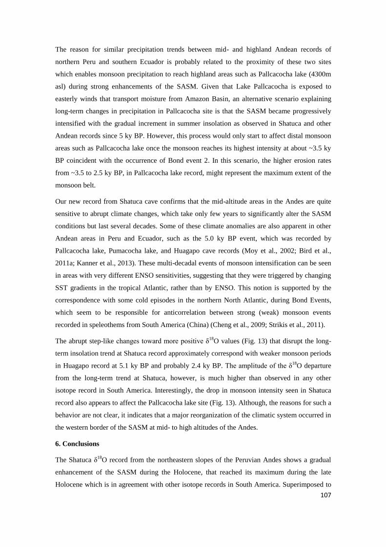
107
The reason for similar precipitation trends between mid- and highland Andean records of
northern Peru and southern Ecuador is probably related to the proximity of these two sites
which enables monsoon precipitation to reach highland areas such as Pallcacocha lake (4300m
asl) during strong enhancements of the SASM. Given that Lake Pallcacocha is exposed to
easterly winds that transport moisture from Amazon Basin, an alternative scenario explaining
long-term changes in precipitation in Pallcacocha site is that the SASM became progressively
intensified with the gradual increment in summer insolation as observed in Shatuca and other
Andean records since 5 ky BP. However, this process would only start to affect distal monsoon
areas such as Pallcacocha lake once the monsoon reaches its highest intensity at about ~3.5 ky
BP coincident with the occurrence of Bond event 2. In this scenario, the higher erosion rates
from ~3.5 to 2.5 ky BP, in Pallcacocha lake record, might represent the maximum extent of the
monsoon belt.
Our new record from Shatuca cave confirms that the mid-altitude areas in the Andes are quite
sensitive to abrupt climate changes, which take only few years to significantly alter the SASM
conditions but last several decades. Some of these climate anomalies are also apparent in other
Andean areas in Peru and Ecuador, such as the 5.0 ky BP event, which was recorded by
Pallcacocha lake, Pumacocha lake, and Huagapo cave records (Moy et al., 2002; Bird et al.,
2011a; Kanner et al., 2013). These multi-decadal events of monsoon intensification can be seen
in areas with very different ENSO sensitivities, suggesting that they were triggered by changing
SST gradients in the tropical Atlantic, rather than by ENSO. This notion is supported by the
correspondence with some cold episodes in the northern North Atlantic, during Bond Events,
which seem to be responsible for anticorrelation between strong (weak) monsoon events
recorded in speleothems from South America (China) (Cheng et al., 2009; Strikis et al., 2011).
The abrupt step-like changes toward more positive δ18
O values (Fig. 13) that disrupt the long-
term insolation trend at Shatuca record approximately correspond with weaker monsoon periods
in Huagapo record at 5.1 ky BP and probably 2.4 ky BP. The amplitude of the δ18
O departure
from the long-term trend at Shatuca, however, is much higher than observed in any other
isotope record in South America. Interestingly, the drop in monsoon intensity seen in Shatuca
record also appears to affect the Pallcacocha lake site (Fig. 13). Although, the reasons for such a
behavior are not clear, it indicates that a major reorganization of the climatic system occurred in
the western border of the SASM at mid- to high altitudes of the Andes.
6. Conclusions
The Shatuca δ18
O record from the northeastern slopes of the Peruvian Andes shows a gradual
enhancement of the SASM during the Holocene, that reached its maximum during the late
Holocene which is in agreement with other isotope records in South America. Superimposed to

108
this long-term trend, several abrupt changes occurred toward wetter and drier conditions in the
Andes that appear to be widespread in South America, occurring from lowland to high elevation
sites. While some of these events were observed in other Andean paleorecords, they were not as
abrupt as in Shatuca record, and sometimes occurred with a temporal mismatch, probably due to
geochronological problems or differences in temporal resolution. These results highlight the
need for additional high-resolution and well-dated precipitation proxy records to allow
identification of such events in different areas under the influence of the SASM.
The temporal correspondence between many cold episodes in the North Atlantic during Bond
events, drying at many sites in the northern Hemisphere and periods of enhanced SASM,
reinforce the notion that most of these abrupt events in the Andes are related to SST changes in
the Atlantic Ocean. The Pacific may have played a role as well; modulating the SASM activity,
but its exact influence remains unclear during the Holocene. The comparison between Shatuca
and Pallcacocha records suggests that long-term increases in SASM precipitation, previously
attributed to increased frequency of ENSO, such as the one described between 3.5 and 2.5 ky
BP, may rather reflect the coupling between the Bond event 2 and the higher austral summer
insolation forcing, even at distal sites, once the monsoon belt reached its maximum extent over
the high Andes.
7. References
Abbott, M.B.; Binford, M.W.; Brenner, M.; Kelts, K.R. A 3500 C-14 yr high-resolution record
of water-level changes in Lake Titicaca, Bolivia/Peru. Quaternary Research, v. 47, p.169-
180, 1997a.
Abbott, M.B.; Seltzer, G.O.; Kelts, K.R.; Southon, J. Holocene paleohydrology of the tropical
Andes from lake records. Quaternary Research, v.47, p.70-80. 1997b.
Abbott M.B; Wolfe, B.B.; Wolfe, A.; Seltzer, G.; Aravena, R.; Mark, B.G.; Polissar, P.J.;
Rodbell, D.T.; Rowe, H.D.; Vuille, M. Holocene paleohydrology and glacial history of
the central Andes using multiproxy lake sediment studies. Palaeogeography,
Palaeoclimatology, Palaeoecology, v.194, p.123-138, 2003.
Ambrizzi, T.; de Souza, E.B.; Pulwarty, R.S. The Hadley and Walker regional circulations and
associated ENSO impacts on the South American Seasonal Rainfall. In: The Hadley
Circulation: Present, Past and Future. Diaz, H.F.; Bradley, R.S. (Eds.), Springer
Netherlands, Kluwer Academic Publishers, v.21, p.203-235, 2004.
Apaèstegui, J.; Cruz, F.W.; Sifeddine, A.; Vuille, M.; Espinoza, J.C.; Guyot, J.L.; Khodri, M.;
Strikis, N.; Santos, R.V.; Cheng, H.; Edwards, L.; Carvalho, E.; Santini, W. Hydroclimate
variability of the northwestern Amazon Basin near the Andean foothills of Peru related to

109
the South American Monsoon System during the last 1600 years. Climate of the Past,
v.10, p.1967–1981, doi:10.5194/cp-10-1967-2014, 2014.
Baker, P.A.; Seltzer, G.O.; Fritz, S.C.; Dunbar, R.B.; Grove, M.J.; Tapia, P.M.; Cross, S.L.;
Rowe, H.D.; Broda, J.P. The history of South American tropical precipitation for the past
25,000 years. Science, v.291, p.640-643, 2001.
Baker, P.A.; Fritz, S.C.; Garland, J.; Ekdahl, E. Holocene hydrologic variation at Lake Titicaca,
Bolivia/Peru, and its relationship to North Atlantic climate variation. Journal of
Quaternary Science, v.20, p.655–662, doi:10.1002/jqs.987, 2005.
Berger, A.; Loutre, M.F. Insolation values for the climate of the last 10 million years.
Quaternary Science Reviews, v.10, p.297–317, 1991.
Bigot J.Y. La riviere souterraine de Shatuca = El rio subterraneo de Shatuca. Bulletin du Groupe
Speleologique Bagnols Marcoule, Hors serie special Chaquil 2006 & Santiago 2007, p.
52-56, 2008.
Bird, B.W.; Abbott, M.B.; Rodbell, D.T.; Vuille, M. Holocene tropical South American
hydroclimate revealed from a decadally resolved lake sediment δ18O record. Earth and
Planetary Science Letters, v.310, p.192-202, 2011a.
Bird, B.W.; Abbott, M.B.; Vuille, M.; Rodbell, D.T.; Stansell, N.D.; Rosenmeier, M.F. A 2,300-
year-long annually resolved record of the South American summer monsoon from the
Peruvian Andes. Proceedings of the National Academy of Sciences of the United States
of America, v.108, p.8583-8588, 2011b.
Bond, G.; Kromer, B.; Beer, J.; Muscheler, R.; Evans, M.N.; Showers, W.; Hoffmann, S.; Lotti-
Bond, R.; Hajdas, I.; Bonani, G. Persistent solar influence on North Atlantic climate
during the Holocene. Science, v.294, p.2130–2136, 2001.
Bruijnzeel, L.A. Hydrology of tropical montane cloud forests: A reassessment. Land Use and
Water Resources Research, v.1, 1.1-1.18, 2001.
Buffen, A.M.; Thompson, L.G.; Mosley-Thompson, E.; Huh, K.I. Recently exposed vegetation
reveals Holocene changes in the extent of the Quelccaya Ice Cap, Peru. Quaternary
Research, v.72, p.157, 2009.
Bookhagen, B.; Strecker, M.R Orographic barriers, high resolution TRMM rainfall, and relief
variations along the eastern Andes. Geophysical Research Letters v.35, L06403, 2008.
Bush, M.B.; Hansen, B.C.S.; Rodbell, D.T.; Seltzer, G.O.; Young, K.R.; Leon, B.; Abbott,
M.B.; Silman, M.R.; Gosling, W.D. A 17 000-year history of Andean climate and

110
vegetation change from Laguna de Chochos, Peru. Journal of Quaternary Science., v.20,
p.703–714, 2005.
Bush, M.B.; Silman, M.R.; Urrego, D.H. 48,000 Years of climate and forest change in a
biodiversity hot spot. Science, v.303, p.827-829, 2004.
Cheng, H., Edwards, R.L.; Shen, C.C.; Polyak, V.J.; Asmerom, Y.; Woodhead, J.; Hellstrom,
J.; Wang, Y.; Kong, X.; Spötl, C.; Wang, X.; Alexander Jr, E.C. Improvements in 230Th
dating, 230Th and 234U half-lifevalues,and U–Th isotopic measurements by multi-
collector inductively coupled plasma mass spectrometry. Earth and Planetary Science
Letters, v.371-372, p.82-91, 2013b.
Cheng, H.; Fleitmann, D.; Edwards, L.R.; Wang, X.; Cruz, F.W.; Auler, A.S.; Mangini, A;
Wang, Y.; Kong, X.; Burns, S. J.; Matter, A. Timing and structure of the 8.2 kyr BP event
inferred from δ18
O records of stalagmites from China, Oman, and Brazil. Geology, v. 37,
p.1007-1010, 2009.
Cheng, H.; Sinha, A.; Cruz, F.W.; Wang, X.; Edwards, R.L.; d’Horta, F.M.; Ribas, C.C.; Vuille,
M.; Stott, L.D.; Auler, A.S. Climate change patterns in Amazonia and biodiversity.
Nature Communications, v.4, p.1-6, doi: 10.1038/ncomms2415, 2013a.
Cheng, H.; Sinha, A.; Wang, X.; Cruz, F.; Edwards, L. The Global Paleomonsoon as seen
through speleothem records from Asia and the Americas. Climate Dynamics, v.39,
p.1045-1062, doi: 10.1007/s00382-012-1363-7, 2012.
Claussen, M. Holocene rapid land cover change – evidence and theory. In: Natural Climate
Variability and Global Warming. Battarbee, R.; Binney, H. (Eds.), Wiley-Blackwell,
ch.9. p.232-253, 2008.
Cobbing, E.J.; Pitcher, W.S.; Wilson, J.J.; Baldock, J.W.; Taylor, W.P.; McCourt, W.; Snelling,
N.J. The geology of the Western Cordillera of northern Peru (Overseas Geology and
Mineral Resources). British Geological Survey, v.5, p.143, 1981.
Colinvaux, P.A.; Bush, M.B.; Steinitz-Kannan, M.; Miller, M. Glacial and Postglacial Pollen
Records from the Ecuadorian Andes and Amazon. Quaternary Research, v.48, p.69-78,
1997.
Conroy, J.L.; Overpeck, J.T.; Cole, J.E.; Shanahan, T.M.; Steinitz-Kannan, M. Holocene
changes in eastern tropical Pacific climate inferred from a Galápagos lake sediment
record. Quaternary Science Reviews, v.27, p.1166–1180, 2008.

111
Cremaschi, M.; Pelfini, M.; Santilli, M. Cupressus dupreziana: a dendroclimatic record for the
middle–late Holocene in the central Sahara. The Holocene, v.16, p.293–303, doi:
10.1191/0959683606hl926rr, 2006.
Cruz, F.W.; Burns, S.J.; Karmann, I.; Sharp, W.D.; Vuille, M.; Cardoso, A.O.; Ferrari, J.A.;
Dias, P.L.S.; Viana, O. Insolation-driven changes in atmospheric circulation over the past
116,000 years in subtropical Brazil. Nature, v.434, p.63-66,
http://dx.doi.org/10.1038/Nature03365, 2005.
Cruz, F.W.; Burns, S.J.; Karmannn, I.; Sharp, W.D.; Vuille, M. Reconstruction of regional
atmospheric circulation features during the late Pleistocene in subtropical Brazil from
oxygen isotope composition of speleothems. Earth and Planetary Sciences Letters, v. 248,
p.494-506, 2006.
Cullen, H.M.; de Menocal, P.B.; Hemming, S.; Hemming, G.; Brown, F.H.; Guilderson, T.;
Sirocko, F. Climate change and the collapse of the Akkadian empire: Evidence from the
deep sea. Geology, v.28, p.379-383, 2000.
Dansgaard, W. Stable isotopes in precipitation. Tellus, v.16, p.436–468, doi:10.1111/j.2153-
3490.1964.tb00181.x, 1964.
deMenocal P.B.; Ortiz J.; Guilderson T.; Adkins, J.; Sarnthein, M.; Baker, L.; Yarusinsky, M.
Abrupt onset and termination of the African Humid Period: rapid climate response to
gradual insolation forcing. Quaternary Science Review, v.19, p.347–361, 2000.
Duplessy, J.C.; Labeyrie, L.D.; Juillet-Leclerc, A.; Maitre, F.; Duprat, J.; Sarnthein, M. Changes
in surface salinity of the North Atlantic Ocean during the last deglaciation. Nature, v.358,
p.485-488, 1992.
Espinoza, J.C.; Ronchail, J.; Guyot, J.L.; Junquas, C.; Vauchel, P.; Lavado, W.S.; Drapeau, G.;
Pombosa, R. Climate variability and extreme drought in the upper Solimões River
(Western Amazon Basin): Understanding the exceptional 2010 drought. Geophysical
Research Letters, v.38, L13406, doi:10.1029/2011GL047862, 2011.
Espinoza Villar, J.C. Impact de la variabilité climatique sur l’hydrologie du bassin amazonien.
Thèse de Doctorat, Université Paris 6 - Pierre et Marie Curie, Paris - France, p.207, 2009.
Fleitmann, D.; Burns, S.J.; Mudelsee, M.; Neff, U.; Kramers, J.; Mangini, A.; Matter, A.
Holocene forcing of the indian monsoon recorded in a stalagmite from southern Oman.
Science 300, 1737–1739. http://dx.doi.org/10.1126/science.1083130, 2003.
Garcia, M.; Villalba, F.; Araguas-Araguas, L.; Rozanski, K. The role of atmospheric circulation
patterns in controlling the regional distribution of stable isotope contents in precipitation:

112
preliminary results from two transects in the Ecuadorian Andes. In: Proceedings series of
International Atomic Energy Agency: isotope techniques in the study of environmental
change, Vienna, IAEA-SM 349/7, p.127–140, 1998.
Garreaud, R.; Vuille, M.; Clement, A.C. The climate of the Altiplano: observed current
conditions and mechanisms of past changes. Palaeogeography Palaeoclimatology
Palaeoecology, v.194, p.5–22, 2003.
Garreaud, R.; Vuille, M.; Compagnucci, R.; Marengo, J. Present-day South American climate.
Palaeogeography Palaeoclimatology Palaeoecology, v.281, p.180–195, 2009.
Gasse, F.; Van Campo, E. Abrupt post-glacial events in West Asia and North Africa monsoon
domains. Earth and Planetary Science Letters, v.126, p.435-456, 1994.
Gasse, F. Hydrological changes in the African tropics since the Last Glacial Maximum.
Quaternary Science Reviews, v.19, p.189–211, 2000.
Gat, J.R.; Matsui, E. Atmospheric water balance in the Amazon basin: an isotopic
evapotranspiration model. Journal of Geophysical Research, v.96, p.13179–13188, 1991.
Gentry, A.H. Changes in plant community diversity and floristic composition on environmental
and geographical gradients. Annals of the Missouri Botanical Garden, v.75, p.1-34, 1988.
Gonfiantini, R.; Roche, M.A.; Olivry, J.C.; Fontes, J.C.; Zuppi, G.M. The altitude effect on the
isotopic composition of tropical rains. Chemical Geology, v.181, p.147–167, 2001.
Grimm, A.M. Interannual climate variability in South America: impacts on seasonal
precipitation, extreme events and possible effects of climate change. Stochastic
Environmental Research and Risk Assessment, v.25, p.537-564, doi: 10.1007/s00477-
010-0420-1, 2011.
Grubb, P.J. Factors controlling the distribution of forests on tropical mountains: new facts and a
new perspective. In: Flenley, J.R. (Ed.), Altitudinal Zonation in Malesia. Geography
Department Miscellaneous, Series 16, University of Hull, p. 1–25, 1974
Grubb, P.J. Control of forest growth and distribution on wet tropical mountains, with special
reference to mineral nutrition. Annual Review of Ecology and Systematics, v.8, p.83–
107, 1977.
Grubb, P.J.; Whitmore, T.C. A comparison of montane and lowland rain forest in Ecuador. II.
The climate and its effects on the distribution and physiognomy of the forests. Journal of
Ecology, v.54, p.303-333, 1966.

113
Guyot, J.L. Hydrogéochimie des fleuves de l’Amazonie bolivienne. Editions de l’ORSTOM,
Paris, p.261, 1993.
Hammer, Ø.; Harper, D.A.T.; Ryan, P.D. PAST: Paleontological Statistics software package for
education and data analysis. Paleontologia Electronica, v.4, p.1-9, 2001.
Hansen, B.C.S.; Rodbell, D.T. A late-glacial/Holocene pollen record from the eastern Andes of
northern Peru. Quaternary Research, v.44, p.216–227, 1995.
Hillyer, R.; Valencia, B.G.; Bush, M.B.; Silman, M.R.; Steinitz- Kannan, M. A 24,700-year
paleolimnological history from the Peruvian Andes. Quaternary Research, v.71, p.71-82,
2009.
Jarvis, A.; Mulligan, M. The climate of cloud forests. Hydrological Processes, v.25, p.327-343.
http://dx.doi.org/10.1002/hyp.7847, 2011.
Kanner, L.C.; Burns, S.J.; Cheng, H.; Edwards, R.L.; Vuille, M. High-resolution variability of
the South American summer monsoon over the last seven millennia: insights from a
speleothem record from the central Peruvian Andes. Quaternary Science Reviews, v.75,
p.1–10, doi: 10.1016/j.quascirev.2013.05.008, 2013.
Lachniet, M. Climatic and environmental controls on speleothem oxygen-isotope values.
Quaternary Sciences Reviews, v. 28, p.412–432, 2009.
Laraque, A.; Ronchail, J.; Cochonneau, G.; Pombosa, R.; Guyot, J.L. Heterogeneous
distribution of rainfall and discharge regimes in the Ecuadorian Amazon basin. Journal of
Hydrometeorology, v.8, p.1364–1381, 2007.
Lavado, W.L.; Espinoza, J.C. Impactos de El Niño y La Niña en las lluvias del Perú (1965-
2007). Revista Brasileira de Meteorologia, v.29, p.171-182, 2014.
Lavado, W.; Labat, D.; Ronchail, J.; Espinoza, J.C.; Guyot, J.L. Trends in rainfall and
temperature in the Peruvian Amazon – Andes basin over the last 40 years (1965–2007).
Hydrological Processes, v.41, p.2944–2957, doi:10.1002/hyp.9418, 2012.
León, B.; Young, K.R.; Brako, L. Análisis de la composición florística del bosque montano
oriental del Perú. In: Biogeografía, Ecología y Conservación del Bosque Montano en el
Perú. Young K.R.; Valencia N. (Eds.), Memorias del Museo de Historia Natural
UNMSM, v. 21, p.141-154, 1992.
Magny, M.; Haas, J.N. A major widespread climatic change around 5300 cal. yr BP at the time
of the Alpine Iceman. Journal of Quaternary Science, v.19, p. 423–430, 2004.

114
Marengo, J.A.; Liebmann, B.; Grimm, A.M.; Misra, V.; Silva Dias, P.L.; Cavalcanti, I.F.A.;
Carvalho, L.M.V.; Berbery, E.H.; Ambrizzi, T.; Vera, C.S.; Saulo, A.C.; Nogués-Paegle,
J.; Zipser, E.; Sethk, A.; Alvese, L.M. Review: Recent developments on the South
American monsoon system. International Journal of Climatology, v.32, p.1–21,
10.1002/joc.2254, 2012.
Marengo, J.A.; Nobre, C. General characteristics and variability of climate in the Amazon basin
and its links to the global climate system. In: The Biogeochemistry of the Amazon Basin.
Clain, M.E.; Victoria, R.L.; Richey, J.E. (Eds.), Oxford University Press, p.17–41, 2001.
Marengo, J.A.; Nobre, C.; Tomasella, J.; Oyama, M.; Sampaio, G.; Camargo, H.; Alves, L.;
Oliveira, R. The drought of Amazonia in 2005. Journal of Climate, v.21, p.495–516,
2008.
Marengo, J.A.; Soares, W.; Saulo, W.; Nicolini, M. Climatology of the LLJ east of the Andes as
derived from the NCEP reanalyses. Journal of Climate, v.17, p.2261–2280, 2004.
Martinelli, L.M.; Victoria, R.L.; Sternberg, L.S.L.; Ribeiro, A.; Moreira, M.Z. Using stable
isotopes to determine sources of evaporated water to the atmosphere in the Amazon
basin. Journal of Hydrology, v.183, p.191-204, 1996.
Mayewski, P.A.; Rohling, E.E.; Stager, J.C.; Karlén W.; Maasch, K.A.; Meeker, L.D.;
Meyerson, E.A.; Gasse, F.; van Kreveld, S.; Holmgren, K.; Lee-Thorp, J.; Rosqvist, G.;
Rack, F.; Staubwasser, M.; Schneider, R.R.; Steig, E.J. Holocene climate variability.
Quaternary Research, v.62, p.243–255, doi:10.1016/j.yqres.2004.07.001, 2004.
Mayle, F.E.; Power, M.J. Impact of a drier early-mid Holocene climate upon Amazonian
forests. Philosophical Transactions of the Royal Society B: Biological Sciences, v.363,
p.1829–1838, doi: 10.1098/rstb.2007.0019, 2008.
Moquet, J.S., Crave, A., Viers, J., Seyler, P., Armijos, E., Bourrel, L., Chavarri, E., Lagane, C.,
Laraque, A., Lavado Casimiro, W.S., Pombosa, R., Noriega, L., Vera, A., Guyot, J.L.,
Chemical weathering and atmospheric/soil CO2 uptake in the Andean and Foreland
Amazon basins. Chemical Geology, v.287, p.1–26, 2011.
Moreira-Turcq, P.; Turcq, B.; Moreira, L.S.; Amorim, M.; Cordeiro, R.C.; Guyot, J.L. A 2700
cal yr BP extreme flood event revealed by sediment accumulation in Amazon floodplains.
Palaeogeography Palaeoclimatology Palaeoecology, v.415, p.175-182. doi:
10.1016/j.palaeo.2014.07.037, 2014.
Morrill, C.; Overpeck, J.T.; Cole, J.E. A synthesis of abrupt changes in the Asian summer
monsoon since the last deglaciation. The Holocene, v.13, p.465–476, 2003.

115
Mosblech, N.A.S.; Bush, M.B.; Gosling, W.D.; Hodell, D.; Thomas, L.; van Calsteren, P.;
Correa-Metrio, A.; Valencia, B.G.; Curtis, J.; vanWoesik, R. North Atlantic forcing of
Amazonian precipitation during the last ice age. Nature Geoscience, v.5, p. 817-820, doi:
10.1038/NGEO1588, 2012.
Moy, C.M.; Seltzer, G.O.; Rodbell, D.T.; Anderson, D.M. Variability of El Niño / Southern
Oscillation activity at millennial timescales during the Holocene epoch. Nature, v.420,
p.162–165, 2002.
Nogués-Paegle, J.; Mo, K.C. Linkages between summer rainfall variability over South America
and sea surface temperature anomalies. Journal of Climate, v.15, p.1389–1407, 2002.
Nogués-Paegle J. A comparative review of South American low-level jets. Meteorologica, v.3,
p.73-82, 1998.
Novello, V.F.; Cruz, F.W.; Karmann, I.; Burns, S.J.; Stríkis, N.M.; Vuille, M.; Cheng, H.;
Edwards, R.L.; Barreto, E.A.S.; Frigo, E. Multidecadal climate variability in Brazil
Nordeste during the last 3000 years based on speleothem isotope records. Geophysical
Research Letters, v.39, L23706, doi: 10.1029/2012GL053936, 2012.
Petit-Maire N.; Guo Z. Mise en évidence de variations climatiques holocènes rapides, en phase
dans les déserts actuels de Chine et du Nord de l’Afrique. Sciences de la Terre et des
Planètes, v.322, p.847–851, 1996.
Poveda, G.; Jaramillo, L.; Vallejo, L.F. Seasonal precipitation patterns along pathways of South
Americanlow-level jets and aerial rivers. Water Resources Research, v.50, p.1–21,
doi:10.1002/2013WR014087, 2014.
Rein, B.; Lückge, A.; Reinhardt, L.; Sirocko, F.; Wolf, A.; Dullo, W.C. El Niño variability off
Peru during the last 20,000 years. Paleoceanography, v.20, PA4003, 2005.
Reuter, J.; Stott, L.; Khider, D.; Sinha, A.; Cheng, H.; Edwards, R.L. A new perspective on the
hydroclimate variability in northern South America during the Little Ice Age.
Geophysical Research Letters, v.36, L21706, doi:10.1029/2009GL041051, 2009.
Rodbell, D.T.; Seltzer, G.O.; Anderson, D.M.; Abbott, M.B.; Enfield, D.B., Newman, J.H. An
15,000-year record of El-Niño alluviation in southwestern Ecuador. Science, v.283,
p.516–520, 1999.
Ronchail, J.; Gallaire, R. ENSO and rainfall along the Zongo valley (Bolivia) from the
Altiplano to the Amazon basin. International Journal of Climatology, v. 26, p.1223–1236,
2006.

116
Salati, E.; Dallolio, A.; Matsui, E.; Gat, J.R. Recycling of water in the Amazon basin - Isotopic
study. Water Resources Research, v.15, p.1250-1258, 1979.
Schmidt, G.; Le Grande, A.; Hoffmann, G. Water isotope expressions of intrinsic and forced
variability in a coupled ocean-atmosphere model. Journal of Geophysical Research,
v.112, D10103, 2007.
Schulz, M.; Mudelsee, M. REDFIT: estimating red-noise spectra directly from unevenly spaced
paleoclimatic time series. Computers & Geoscience. V.28, p.421–426, 2002.
Seltzer, G.; Rodbell, D.; Burns, S. Isotopic evidence for late Quaternary climatic change in
tropical South America. Geology, v.28, p.35-38, 2000.
Stansell, N.D.; Rodbell, D.T.; Abbott, M.B.; Mark, B.G. Proglacial lake sediment records of
Holocene climate change in the western Cordillera of Peru. Quaternary Science Reviews,
v.70, p.1-14, 2013.
Strikis, N.M.; Cruz Jr., F.W.; Cheng, H.; Karmann, I.; Edwards, R.L.; Vuille, M.; Wang, X.; de
Paula, M.S.; Novello, V.F.; Auler, A.S. Abrupt variations in South American monsoon
rainfall during the Holocene based on a speleothem record from central-eastern Brazil.
Geology, v.39, p.1075–1078, 2011.
Thompson, L.G.; Mosley-Thompson, E.; Davis, M.E.; Lin, P.N.; Henderson, K.A.; Cole-Dai, J.;
Bolzan, J.F.; Kiu, K.B. Late Glacial stage and Holocene tropical ice core records from
Huascaran, Peru. Science, v.269, p.46–50, 1995.
Torrence, C.; Compo, G.P. A practical guide to wavelet analysis. Bulletin of the American
Meteorological Society, v.79, p.61–78, 1998.
Urrego, D.H.; Bush, M.B.; Silman, M.R. A long history of cloud and forest migration from
Lake Consuelo, Peru. Quaternary Research, v. 73, p. 364–373, 2010.
Valencia, B.G.; Urrego, D.H.; Silman, M.R.; Bush, M.B. From ice age to modern: a record of
landscape change in an Andean cloud forest. Journal of Biogeography, v.37, p.1637–
1647, 2010.
van Breukelen, M.R.; Vonhof, H.B.; Hellstrom, J.C.; Wester, W.C.G.; Kroon, D. Fossil
dripwater in stalagmites reveals Holocene temperature and rainfall variation in Amazonia.
Earth and Planetary Science Letters, v.275, p.54-60, 2008.
Vimeux, F.; Gallaire, R.; Bony, S.; Hoffmann, G.; Chiang, J.C.H. What are the climate controls
on dD in precipitation in the Zongo Valley (Bolivia)? Implications for the Illimani ice
core interpretation. Earth and Planetary Science Letters, v.240, p.205-220, 2005.

117
Vuille, M.; Bradley, R.S.; Keimig, F. Climatic variability in the Andes of Ecuador and its
relation to tropical Pacific and Atlantic sea surface temperature anomalies. Journal of
Climate, v.13, p.2520-2535, 2000.
Vuille, M.; Burns, S.J.; Taylor, B.L.; Cruz, F.W.; Bird, B.W.; Abbott, M.B.; Kanner, L.C.;
Cheng, H.; Novello, V.F. A review of the South American monsoon history as recorded
in stable isotopic proxies over the past two millennia. Climate of the Past, v.8, p.1309–
1321, doi:10.5194/cp-8-1309-2012, 2012.
Vuille, M.; Bradley, R.S.; Werner, M.; Healy, R.; Keimig, F. Modeling δ18O in precipitation
over the tropical Americas: 1. Interannual variability and climatic controls. Journal of
Geophysical Research, v.108, p.4174-4175, doi:10.1029/2001JD002039, 2003.
Vuille, M.; Werner, M. Stable isotopes in precipitation recording South American summer
monsoon and ENSO variability - observations and model results. Climate Dynamics,
v.25, p.401-413, 2005.
Wang, X.; Auler, A.S.; Edwards, R.L.; Cheng, H.; Ito, E.; Solheid, M. Interhemispheric anti-
phasing of rainfall during the last glacial period. Quaternary Science Reviews, v.25,
p.3391–3403, 2006.
Webster, G. L. The panorama of Neotropical cloud forests. In: Biodiversity and Conservation of
Neotropical Montane Forests. Churchill, S.P.; Balslev, H.; Forero, E.; Luteyn, J.L.
(Eds.), New York Botanical Garden, Bronx, p. 53-77, 1995.
Weng, C.; Bush, M.B.; Curtis, J.H.; Kolata, A.L.; Dillehay, T.D.; Binford, M.W. Deglaciation
and Holocene climate change in the western Peruvian Andes. Quaternary Research, v.66,
p.87–96, 2006.
Young, K.R. Biogeography of the montane forest zone of the eastern slopes of Peru. In
Biogeografía, Ecología y Conservación del Bosque Montano en el Perú. Young, K.R.;
Valencia, N. (Eds.), Memorias del Museo de Historia Natural, U.N.M.S.M. (Lima), v.21,
p.119-140, 1992.
Young, K.R. Floristic diversity on the eastern slopes of the Peruvian Andes. Candollea, v.46,
p.125-143, 1991.
Young K.R.; León B. Peru’s humid eastern montane forests: an overview of their physical
settings, biological diversity, human use and settlement, and conservation needs. DIVA,
Technical Report n°5, p. 97, 1999.

118
Zhang, Z.; Leduc, G.; Sachs, J. El Niño evolution during the Holocene revealed by a biomarker
rain gauge in the Galápagos Islands. Earth and Planetary Science Letters, v.404, p.420–
434, 2014.

119
FIGURES
A6. Figure 1. Location of Shatuca cave record (5.70°S, 77.90°W, red triangle) and other
Andean paleoclimate records (black triangles) used for comparison. These paleoclimate
records are Lake Pallcacocha (Rodbell et al., 1999; Moy et al., 2002) in southwestern Ecuador;
Tigre Perdido cave (van Breukelen et al., 2008) and Palestina cave (Apaèstegui et al., 2014), in
the northeastern Peruvian Andes; Lake Pumacocha (Bird et al., 2011a,b) and Huagapo cave
(Kanner et al., 2013), in central Peruvian Andes. On the top: location of Lapa Grande cave
record (“LG”, black triangle, Strikis et al., 2011) and of the Intertropical Convergence Zone
(ITCZ).

120
A6. Figure 2. a) Histogram indicating mean monthly precipitation (1964-2014) in
meteorological stations located at mid-altitudes (1300-2500m asl) and lowlands (900-800m
asl). b) Altitude profile and location of Shatuca “S”, Tigre Perdido “T” and Palestina
“P”caves, in relation to the moisture transport direction. c) Mean annual precipitation from
TRMM 2B31 satellite data (average from 1998-2009, in mm/yr). Shatuca (Tigre Perdido and
Palestina) cave location is indicated with a red (yellow) triangle and meteorological stations
are indicated with circles. Meteorological stations located at the drier mid-altitudes, as Shatuca
cave, are represented by yellow circles (1 to 4) and at the wetter lowlands, as Tigre Perdido
and Palestina caves, by green circles (5 to 7).
a)
c)
b)

121
0
-5
-10
-15
01/04/2011 01/01/2012 01/10/2012 01/07/2013
0
50
100
150
200
250
300
350
400
1
8O
(V
-SM
OW
)
RIO
JA
(m
m)
A6. Figure 3. Rainwater isotopic results obtained during the Palestina cave monitoring
program. Daily rain (black filled bars), 15 days accumulated rain (black open bars) and
rainwater isotopes (blue squares) in Palestina cave region (located in Rioja province). Note
that scale for δ18
O is reversed.

122
-16
-14
-12
-10
Insolation Feb. 10oS
Pumacocha
Huagapo
960
940
920
900
880
0 2 4 6 8 10
-8
-6
-4
1
8O
1
8O
Age (ky BP)
Shatuca
Tigre Perdido
960
940
920
900
880
A6. Figure 4. Comparison between isotope records from the central and northeastern Peruvian
Andes and the insolation trend (black line) for the month of February at 10ºS (Berger and
Loutre, 1991). Pumacocha lake (4300m asl) record in blue (Bird et al., 2011a) and Huagapo
cave (3850m asl) record in black (Kanner et al., 2013) are situated in high altitude areas of
central Peruvian Andes, while Shatuca cave (1960m asl) record in red (this study) and Tigre
Perdido cave (1000m asl) record in green (van Breukelen et al., 2008) are located at lower
altitude sites in northeastern Peruvian Andes. Ages and error bar for each record are also
shown.

123
-1,4
-0,7
0,0
0,7
1,4
Tigre
Perdido_detrended
0 2 4 6 8 10
2015105
Shatuca
Composite_detrended
-8
-7
-6
-5
-4
Lapa
Grande
-1
0
1
-1
0
1
2
Pumacocha_detrended
Huagapo_detrended
-2
0
2
18O
18O
18O
18O
18O
Age (ky BP)
A6. Figure 5. Comparison between Holocene South American paleoprecipitation records and
the Hematite stained grains record (HSG%) from the North Atlantic Ocean. Pumacocha lake
detrended record in blue (Bird et al., 2011a), Huagapo cave detrended record in black (Kanner
et al., 2013), Lapa Grande cave in orange (Strikis et al., 2011), Tigre Perdido cave detrended
record in green (van Breukelen et al., 2008), Shatuca cave detrended record in red (this study)
and the HSG% record in purple (Bond et al., 2001). Blue bars indicate wet events in Shatuca
record, which are contemporaneous with wet considitions in other Andean records and with
some Bond events in the Noth Atlantic. Orange bars indicate abrupt changes toward dry
conditions in Shatuca record contemporaneous with dry events in other Andean records. Ages
and error bars are shown for each record.

124
7.0 7.5 8.0 8.5 9.0 9.5 10.0 10.5-2
-1
0
1
20
15
10
5
-7
-6
-5
-4
-2
-1
0
1
2
18O
HS
G%
Shatuca Composite
Lapa Grande
IRD
Age (ky BP)
18O
Tigre Perdido
18O
A6. Figure 6. Early Holocene comparison of high-resolution records from South America and
the Hematite stained grains record (HSG%) from the North Atlantic Ocean. HSG% record of
the Bond et al. (2001) shown in black, Shatuca composite_detrended record shown in red (this
study), Tigre Perdido_detrended record in green (van Breukelen et al., 2008) and Lapa
Grande_detrended record shown in orange (Strikis et al., 2011). Blue bars indicate wet events
which are synchronous with Bond events, and yellow bars indicate reversals to drier conditions
within the wet events. Gray bars indicate periods of increased moisture with 100-yr cyclicity.
Ages and error bars for each record are also shown.

125
A6. Figure 7. Early Holocene spectral analysis (REDFIT) (Schulz and Mudelsee, 2002)
performed by software PAST (Hammer et al., 2001) using Sha-2 sample (with Sha-3 covering
the hiatus of Sha-2).
A6. Figure 8. Early Holocene wavelet analyses (Torrence and Compo, 1998) performed by
software PAST (Hammer et al., 2001) using Sha-2 sample (with Sha-3 covering the hiatus of
Sha-2).

126
4.8 5.2 5.6 6.0 6.4 6.8 7.2
-1.0
-0.5
0.0
0.5
1.0
1.5
-1
0
1
-1
0
1
Shatuca
Composite
Lapa
Grande
Huagapo
Pumacocha
-8
-7
-6
-5
Age (ky BP)
1
8O
1
8O
1
8O
1
8O
A6. Figure 9. Detailed comparison between South American high-resolution paleorecords from
7.2 to 4.5 ky BP: Lapa Grande cave in green (Strikis et al., 2011), Lake Pumacocha_detrended
in blue (Bird et al., 2011a), Huagapo cave_detrended in black (Kanner et al., 2013), Shatuca
cave_detrended in red (this study). Blue bars indicate wet events, and orange bars indicate
reversals to drier conditions within the wet events. Ages and its error bars for each record.

127
A6. Figure 10. Spectral analysis (REDFIT) (Schulz and Mudelsee, 2002) for the period between
5132-4780 years BP (with evidence in Bond 4), performed by software PAST (Hammer et al.,
2001).
A6. Figure 11. Wavelet analyses (Torrence and Compo, 1998) for the period between 5132-
4780 years BP (with evidence in Bond 4), performed by software PAST (Hammer et al., 2001).

128
0 1 2 3 4-2
-1
0
1
-1,0
-0,5
0,0
0,5
1,0
-1
0
1
1
8O
-2
0
2
1
8O
Shatuca
Tigre Perdido
Age (ky BP)
Lapa Grande
Huagapo
Pumacocha
-8
-7
-6
-5
1
8O
1
8O
1
8O
A6. Figure 12. Comparison between South American paleorecords during the late Holocene:
Lapa Grande cave in orange (Strikis et al., 2011), Lake Pumacocha in blue (Bird et al., 201a),
Huagapo cave in black (Kanner et al., 2013), Tigre Perdido cave record in green (van
Breukelen et al., 2008) and Shatuca cave composite record in red (this study). Ages and its
error bars for each record. Blue bars indicate wet events, and orange bars indicate reversals to
drier conditions.

129
200
160
120
80
-7
-6
-5
-4
-3
0 2000 4000 6000 8000 10000
30
25
20
15
10
5
0
More
El Nino
Wet
strong SASM
Pallcacocha
red
co
lor
inte
nsity
(eve
nts
pe
r 3
0yrs
)
1
8O
% S
an
d
weak SASM
Shatuca
El Junco
Age (ky BP)
A6. Figure 13. Increasing monsoon precipitation in Shatuca record (green) through the
Holocene, shown as a step process. In red, Pallcacocha lake record (Moy et al., 2002) and in
blue El Junco lake record (Conroy et al., 2008).

130
SUPPLEMENTARY MATERIAL
A6. Figure S1. Topographic map: Shatuca cave profile. Located in Yambrasbamba, Bongará
province, Amazonas –Peru. Source: Bigot (2008)

131
230Th dating results. The error is 2s error.Sample
Number
Espeleotema SHA 2
SHA2-1 68.6 ±0.1 1749 ±35 16 ±1 1062.9 ±2.5 0.0247 ±0.0007 1311 ±35 951 ±257 1066 ±3 893 ±257
SHA2-2 66.6 ±0.1 605 ±12 19 ±1 1061.9 ±3.1 0.0106 ±0.0005 560 ±29 431 ±95 1063 ±3 373 ±95
SHA2-3 73.5 ±0.1 186 ±4 44 ±3 1066.1 ±3.1 0.0067 ±0.0005 356 ±25 321 ±36 1067 ±3 263 ±36
SHA2-4 68.6 ±0.1 121 ±3 85 ±5 1065.3 ±2.6 0.0091 ±0.0005 481 ±29 457 ±34 1067 ±3 399 ±34
SHA2-5 68.7 ±0.1 2544 ±51 21 ±1 1056.7 ±3.4 0.0465 ±0.0006 2491 ±35 1967 ±372 1063 ±4 1909 ±372
SHA2-6 59.1 ±0.1 4296 ±86 25 ±1 1039.1 ±2.9 0.1085 ±0.0007 5936 ±43 4902 ±733 1054 ±4 4844 ±733
SHA2-7 69.4 ±0.1 1557 ±31 38 ±1 1056.7 ±3.1 0.0523 ±0.0006 2802 ±32 2485 ±226 1064 ±3 2427 ±226
SHA2-8 96.3 ±0.1 1506 ±30 54 ±1 1048.3 ±2.8 0.0516 ±0.0004 2779 ±24 2557 ±159 1056 ±3 2499 ±159
sha-2a-9mm 117.8 ±0.2 2246 ±45 55 ±1 1042.4 ±3.2 0.0639 ±0.0005 3458 ±28 3187 ±194 1052 ±3 3124 ±194
SHA2-9 98.9 ±0.1 1161 ±23 93 ±2 1039.3 ±2.7 0.0662 ±0.0005 3589 ±26 3422 ±121 1049 ±3 3364 ±121
SHA2-10 110.1 ±0.1 508 ±10 317 ±7 1009.7 ±2.6 0.0887 ±0.0005 4905 ±26 4838 ±54 1024 ±3 4780 ±54
SHA2-11 133.7 ±0.2 183 ±4 1130 ±23 1004.1 ±3.3 0.0938 ±0.0004 5209 ±26 5190 ±29 1019 ±3 5132 ±29
sha-2a-4mm 91.7 ±0.1 242 ±5 685 ±15 996.1 ±2.2 0.1095 ±0.0006 6124 ±36 6086 ±45 1013 ±2 6023 ±45
SHA2-12 104.3 ±0.1 241 ±5 835 ±17 992.6 ±2.7 0.1172 ±0.0004 6578 ±26 6545 ±35 1011 ±3 6487 ±35
SHA2-14 110.1 ±0.2 154 ±3 1526 ±32 987.2 ±3.0 0.1292 ±0.0006 7291 ±37 7271 ±40 1008 ±3 7213 ±40
SHA2-16 117.5 ±0.1 146 ±3 1828 ±38 985.1 ±1.9 0.1377 ±0.0005 7793 ±32 7775 ±34 1007 ±2 7717 ±34
sha-2c-14mm 119.8 ±0.1 139 ±3 1976 ±43 984.0 ±2.4 0.1392 ±0.0006 7890 ±34 7873 ±36 1006 ±2 7810 ±36
SHA2-17 75.0 ±0.1 173 ±4 1109 ±23 987.1 ±2.4 0.1548 ±0.0007 8786 ±45 8752 ±51 1012 ±3 8694 ±51
SHA2-18 109.8 ±0.2 253 ±5 1147 ±23 984.7 ±2.8 0.1604 ±0.0006 9128 ±38 9094 ±44 1010 ±3 9036 ±44
SHA2-20 106.0 ±0.2 181 ±4 1631 ±34 985.6 ±2.7 0.1688 ±0.0007 9621 ±42 9597 ±45 1013 ±3 9539 ±45
sha-2c-48mm 113.6 ±0.1 183 ±4 1827 ±39 992.2 ±2.4 0.1789 ±0.0007 10186 ±44 10162 ±47 1021 ±2 10099 ±47
SHA2-22 41.8 ±0.0 317 ±6 411 ±9 993.0 ±2.1 0.1888 ±0.0009 10769 ±57 10660 ±96 1023 ±2 10602 ±96
Espeleotema SHA 3
SHA3-1 188.9 ±1.2 324 ±7 248 ±5 1095.7 ±16.5 0.0258 ±0.0003 1350 ±18 1327 ±25 1100 ±17 1269 ±25
SHA3-2 181.0 ±0.3 148 ±3 596 ±14 1090.8 ±3.1 0.0297 ±0.0003 1556 ±15 1545 ±17 1096 ±3 1487 ±17
SHA3-3 199.6 ±0.3 89 ±2 1209 ±27 1084.8 ±2.6 0.0326 ±0.0002 1715 ±13 1709 ±14 1090 ±3 1651 ±14
SHA3-4 202.3 ±0.3 216 ±4 598 ±13 1101.8 ±2.8 0.0387 ±0.0002 2025 ±12 2010 ±16 1108 ±3 1952 ±16
SHA3-5 113.5 ±0.1 269 ±5 803 ±17 1026.9 ±2.9 0.1157 ±0.0005 6380 ±30 6346 ±39 1045 ±3 6288 ±39
SHA3-6 155 ±0 2110 ±42 159.4 ±3.3 1059.4 ±2.7 0.1315 ±0.0006 7156 ±35 6965 ±139 1080 ±3 6903 ±139
SHA3-7 135 ±0 163 ±3 1847.1 ±40.3 1056.2 ±2.1 0.1356 ±0.0006 7395 ±37 7379 ±39 1078 ±2 7317 ±39
SHA3-8 142.8 ±0.2 51 ±1 6371 ±142 1061.7 ±2.8 0.1391 ±0.0004 7574 ±25 7569 ±25 1085 ±3 7511 ±25
SHA3-9 80.9 ±0.1 40 ±1 1785 ±44 2940.9 ±5.0 0.0531 ±0.0004 1477 ±12 1474 ±13 2953 ±5 1416 ±13
SHA3-10 142.7 ±0.1 159 ±3 2239 ±46 1076.8 ±2.1 0.1517 ±0.0004 8218 ±26 8202 ±29 1102 ±2 8144 ±29
SHA3-11 138.0 ±0.1 419 ±8 851 ±17 1080.7 ±2.0 0.1568 ±0.0006 8491 ±33 8449 ±44 1107 ±2 8391 ±44
SHA3-12 126.3 ±0.1 545 ±11 636 ±13 1072.0 ±2.4 0.1662 ±0.0005 9058 ±30 8998 ±52 1100 ±2 8940 ±52
SHA3-13 211.5 ±0.3 704 ±14 921 ±19 1058.9 ±3.0 0.1861 ±0.0005 10248 ±34 10202 ±47 1090 ±3 10144 ±47
*234
U = ([234
U/238
U]activity – 1)x1000. ** 234
Uinitial was calculated based on 230
Th age (T), i.e., 234
Uinitial = 234
Umeasured x el234xT
.
Corrected 230
Th ages assume the initial 230
Th/232
Th atomic ratio of 4.4 ±2.2 x10⁻⁶
. Those are the values for a material at secular
equilibrium, with the bulk earth 232
Th/238
U value of 3.8. The errors are arbitrarily assumed to be 50%.
Lines in red, indicate those Ages that were nor used due to higher error
* THE RESULTS OF THESE TWO SAMPLES (128mm and 160mm) ARE QUESTIONABLE FOR THEY WERE MIXED DURING WEIGHING
(correct
ed)
(corrected )
230Th Age (yr)
234UInitial
230Th Age (yr
(ppb) (ppt) (atomic x10-6
) (measured) (activity) (uncorrected
)
(corrected)
238U
232Th
230Th /
232Th
234U*
230Th /
238U
230Th Age (yr)
A6. Table S1. U/Th ages for samples Sha-2 and Sha-3.

132
0 2 4 6 8 10
0,0
0,1
0,2
0,3
0,4
0,5
Sha-2
(mm
/yr)
Age (ky BP)
0 2 4 6 8 10
0,02
0,03
0,04
0,05
0,06
0,07
0,08
0,09
0,10
0,11
Sha-3
(mm
/yr)
Age (ky BP)
A6. Figure S2. Growth rate of samples Sha-2 and Sha-3.

133
-7
-6
-5
-4
-3
1
8O
Late
Holocene Mid
Holocene
HIA
TU
S
1
8O
Age (yr BP)
Early
Holocene
0 2000 4000 6000 8000 10000
-7
-6
-5
-4
-3
Sha-2
Sample
broke
Sha-3
A6. Figure S3. Isotopic record for Shatuca cave samples: Sha-2 in black and sample Sha-3 in
red. The U/Th ages, are located in the bottom part of the graphic, black for Sha-2 and red for
Sha-3.

134
ANEXO 7.
“Orbital to millennial changes in monsoon precipitation in western Amazon from the last
Glacial to the Holocene from speleothem isotope records”

135
Orbital to millennial changes in monsoon precipitation in western Amazon from the last
Glacial to the Holocene from speleothem isotope records
M.G. Bustamante Rosell1,2
, F.W. Cruz1,2
, A. Sifeddine2,4
, H. Cheng5,6
, J. Apaèstegui2,3
, M.
Vuille7, N. Strikis
1,
J.S. Moquet
1, L. XiangLei
4, J.L. Guyot
4, R.L. Edwards
6.
1- Universidade de São Paulo, Instituto de Geociências-Rua do Lago 562, CEP: 05508-080,
São Paulo- Brazil.
2- LMI PALEOTRACES (IRD, UPMC, UFF, Uantof, UPCH), Departamento de
Geoquímica- Univ. Federal Fluminense, Niteroi-RJ, Brasil.
3- Instituto Geofísico del Perú, IGP, Lima- Perú.
4- GET, HYBAM (IRD-CNRS-UPS Toulouse), IRD, Lima-Peru.
5- Institute of Global Environmental Change, Xi’an Jiaotong University, Xi’an 710049,
China.
6- Department of Earth Sciences, University of Minnesota, Minneapolis, MN 55455, USA.
7- Department of Atmospheric and Environmental Sciences, University at Albany
(SUNY), Albany, NY 12222, USA.
Abstract
Three well-dated δ18
O-speleothem records were collected from Shatuca cave, situated on the
northeastern flank of the Peruvian Andes (1960m asl) to reconstruct high-resolution changes in
precipitation, during the last 38 ky BP. The record suggests that moisture conditions remained
under similar ranges during the last Glacial and Holocene periods, and that a similar amplitude
change ( ̴3.5‰) occurred through the Deglacial and Holocene periods, toward drier and wetter
conditions, respectively.
Moreover, precipitation seems to be modulated by the precession cycle only since 11 ky BP but
not before, and moisture conditions during the Last Glacial Maximum (LGM) were similar to
the ones of the late Holocene. Some of the lowest isotopic values, at Shatuca site, occurred
during the late Holocene, when the Austral Summer Insolation (ASI) was at its maximum;
whereas the most enriched values occurred during the early Holocene, when the ASI was at its
minimum. The Shatuca speleothem record shows a higher number of dry episodes than at
highlands, some of them never reported before in Andean regions, such as the one logged at
16.2 ky BP. For instance, some of these episodes were also present in previous lowland records

136
from northeastern Peruvian Andes, although these were fewer and not as intense as in midlands.
Moreover, these dry episodes were not necessarily related to Greenland interstadials (GI),
instead we found that some of them were related to dry events in the Cariaco basin, particularly
clear for the 16.2 ky BP event.
Keywords: South American Summer Monsoon, Northeastern Peruvian Andes, Stable Isotopes,
Last Glacial Period, Dansgaard Oeschger cycle, Heinrich event
1. Introduction
Estimating how the Amazon forest and its biodiversity could be threatened on the next decades
due to the current climate change, have generated a great deal of debate among scientists that is
far from solved. To this aim it is important to improve our knowledge of previous climate
changes on the tropics and understand how vegetation was affected through these changes.
A general consensus exists about a much colder tropical South America during the Last Glacial
Maximum (LGM, globally defined between 24-18 ky BP), however, the moisture conditions
which are extremely important for the maintenance of the Amazon forest remain a matter of
debate in part due to the paucity of the paleoclimatic reconstructions (Sylvestre, 2009).
Several paleorecords show that the LGM occurred earlier in the tropical Andes, between 30-26
ky BP (Zech et al., 2009), and that conditions were wetter than today’s (Wirmann et al., 1992;
Ybert, 1992; Thompson et al., 1998; Sylvestre et al., 1998; Baker et al., 2001a, b; Sylvestre,
2002; Ramirez et al., 2003; Placzek et al., 2006; Sylvestre, 2009; Kanner et al., 2012; Mosblech
et al., 2012; Cheng et al., 2013a; Fornace et al., 2014). In contrast, models (Cook and Vizy,
2006; Vizy and Cook, 2005, 2007) suggest a substantial reduction of the rainforest coverage,
while palynological records from the Amazon basin, reveal a more complex pattern (Sylvestre,
2009), in part due to conflicting discussions concerning the interpretation of the pollen spectra
(Mayle et al., 2009).
Nowadays, precipitation over the Amazon and eastern Andean flanks depends on the moisture
transported by the trade winds from the Atlantic Ocean (Vuille and Werner, 2005; Garreaud et
al., 2009). During austral summer, an intensification of the northeasterly trade winds occurs and
higher amounts of moisture are transported from the Atlantic Ocean through the Amazon forest
until the Andes where it veers to southeast, flowing along the eastern Andean slopes until the
region of El Chaco and southeast Brazil. This intensification of moisture transport into the
Amazon basin is known as the South American Summer Monsoon (SASM).

137
Given that the SASM is the source of moisture for both the Amazon and the tropical Andes,
understanding how wet conditions prevailed in the Andes while drier conditions coexisted in the
Amazon forest, as suggested by previous paleorecords, is considered to be a paradox (Sylvestre,
2009). Some studies have attempted to solve this paradox, for example, Cheng et al. (2013a)
suggested that western Amazon was wet due to the transport of evaporated water vapor from a
drier eastern Amazon (Absy et al., 1991; Sifeddine et al., 1994; 2004; Behling, 2002). However,
the eastern dryness is still under debate (Auler and Smart, 2001; Wang et al., 2004; Sylvestre,
2009).
Montane forests are located at the foothills of the Andes, in the supposedly transition zone
between the dry (wet) LGM conditions of the Amazon Basin (Andes), and hence precipitation
proxies at this region could provide insights on the mechanisms that generated a drier Amazon
and wetter Andes, or at least could tell us where was the division line, in terms of altitude, for
these wet and dry conditions. Previous pallynological studies from montane forests have studied
the downslope or upslope advance/retraction of this western edge of the Amazon forest (Hansen
and Rodbell, 1995; Bush et al., 2004; Bush et al., 2005; Urrego et al., 2005; Hillyer et al., 2009;
Urrego et al., 2009), and usually consider temperature as the principal cause for vegetation
change (Mayle et al., 2009). On the other side, the studies that have discussed past moisture
changes tend to suggest that during the LGM conditions were sufficiently wet to maintain
montane forests, although with different taxa due to the cooler conditions.
The SASM variability depends strongly on the position of the Atlantic Intertropical
Convergence Zone (ITCZ) which is impacted by different climate forcing mechanisms, such as
insolation precession cycle (Clement et al., 2004; Cruz et al., 2005; Wang et al., 2006) and
land/sea-ice coverage in the northern Hemisphere (Chiang et al., 2003; Chiang and Bitz, 2005).
On orbital timescales, the global paleomonsoon notion was proposed, given that several
paleorecords from tropical areas affected by monsoons show an antiphased precipitation pattern
between northern and southern Hemispheres, similar to what occurs nowadays on seasonal
timescales (Wang et al., 2008). For this, robust evidence has been presented by speleothems
from the SASM and Asian Summer Monsoon (ASM) areas (Cheng et al., 2012). However,
recent studies suggest that this antiphased correlation between northern and southern tropics had
a more complex pattern in South America; and that there is not such an antiphased correlation
between the ASM and the SASM, from 45 to 17 ky BP, at the southern Equadorian Andes
(Mosblech et al., 2012), during MIS 2-4 in northern Peruvian Andes (Cheng et al., 2013a), and
from 60 to 17 ky BP, in the southern Peruvian Andes (Fornace et al., 2014).
For the last Glacial period, it has been discussed that the buildup of large ice sheets in the
northern Hemisphere generates glacial boundary conditions that seem to have exerted a stronger

138
control over the SASM dynamics, than the insolation forcing during MIS 2-4 (Cruz et al., 2007;
Fornace et al., 2014). Melting icebergs at periods of more pronounced ice buildup during the
last glaciations, would have caused a strengthening of the Azores high in the subtropical North
Atlantic (Naughton et al., 2009), generating increased northeast trade winds and hence, a
southward displacement of the ITCZ (Chiang et al., 2003; Clement et al., 2004; Chiang and
Bitz, 2005). This has been corroborated by paleoproxy records from tropical monsoon regions
that show that tropical precipitation had an inter-hemispheric anti-phased relationship on a wide
range of timescales (Peterson et al. 2000; Wang et al. 2004; Cruz et al., 2007; Cheng et al.,
2012). Associated to a more southern position of the Atlantic ITCZ there is an increase in
SASM moisture transport to the Amazon and Andean regions (Vuille et al., 2012; Fornace et al.,
2014).
On the other side, Cheng et al. (2013a) demonstrated that while precipitation over eastern
Amazon was always antiphased with the Northern Hemisphere monsoons, this was not the case
for the western Amazon. Moreover, they noted that during (MIS 2-4 and 6) the western Amazon
precipitation did not seem to be controlled by the austral summer insolation (ASI), but instead
by orbital ENSO mean state variability (Zebiak and Cane model, Clement et al. (1999)). Given
that nowadays El Niño strengthens the wet/dry conditions in eastern Amazonia and buffers the
wet/dry conditions in western Amazonia, the authors suggested that strong El Niño-like
conditions during these low sea-level conditions (MIS 2-4 and 6) could have buffered
(strengthened) the moisture conditions on the western (eastern) Amazon. Thus, generating to
some extent an antiphased (in-phase) precipitation pattern between eastern and western Amazon
during the MIS 2-4 and 6 (MIS 1, 5 and 7) periods. However, they left open the possibility of
more complex glacial boundary conditions on South America (Clement et al., 2004).
At millennial timescales, Greenland ice cores (Dansgaard et al., 1984; Johnsen et al., 1992;
Alley et al., 1993; Stuiver and Grootes, 2000) and North Atlantic sediments (Bard et al., 2000;
Shackleton et al., 2000) suggest that during the last Glacial and Deglacial periods, abrupt
temperature fluctuations occurred at these northern high latitudes, known as Dansgaard-
Oeschger cycles (D-O). During these cycles the transition to warmer (colder) temperatures was
more abrupt (gradual), over a few years or decades. The cold periods of these cycles are known
as Greenland stadials (GS) and warmer intervals are known as Greenland interstadials (GI)
(Rasmussen et al., 2014). These cycles also seem to have caused latitudinal shifts of the ITCZ
(Clement et al., 2004), affecting SASM intensity (Cheng et al., 2012).
In contrast, the Antarctic counterparts (Jouzel et al., 2007) of these temperature abrupt shifts
occurred over hundreds to thousands of years and hence were more gradual than those in
Greenland (Blunier and Brook, 2001), probably due to the heat capacity of the Southern Ocean

139
(Barker et al., 2009). Moreover, ice core records from the Antarctic Atlantic sector reveal an
antiphased behavior during stadials and interstadials between Greenland and Antartica, which
has led to the notion of a bipolar seesaw (EPICA, 2006). It has been suggested that a
desintensification of the Atlantic Meridional Overturning Circulation (AMOC) could lead to
this seesaw (Crowley, 1992; Broecker, 1998) by decreasing the heat transport from the tropics
to the northern high latitudes, this would generate cooler (warmer) North Atlantic (South
Atlantic) SSTs and hence cooler (warmer) surface air temperatures at the North Atlantic (South
Atlantic). This teleconnection between the North and South Atlantic sectors could take only a
few decades (Vellinga and Wood, 2002).
Models suggest that these cold stadial conditions in the northern high latitudes, would lead to a
southward displacement of the ITCZ, generating a change in the meridional moisture transport
with intense ascending air masses in southern low latitudes and increased subsidence in the
northern subtropics (Clement et al., 2004; Chiang and Bitz, 2005). This hypothesis would
explain why drying is observed in the northern tropics (such as in Cariaco Basin record), while
southeastern Brazil (Cruz et al., 2005) and previous Andean records reveal enhanced SASM
during the Greenland stadials (GS) and Heinrich events (H) at a range of altitudes (Fritz et al.,
2010; Kanner et al., 2012; Mosblech et al., 2012; Cheng et al., 2013a).
A remarkable correlation between the Andes moisture conditions and the D-O cycles of the
North Greenland Ice Core Project (NGRIP) record was found in the high-resolution record of
Papahuacain cave located at 3800m asl in central Peruvian Andes (Kanner et al., 2012) and in
the records of Condor and Diamante caves (Cheng et al., 2013a) located at lowlands in
northeastern Peruvian Andes. However, recent studies suggest that some features of the D-O
cycles were to some extent influenced by Antarctic climate changes during the last Glacial
(Kanner et al., 2012) and Deglacial periods (Baker et al., 2001b; Ramirez et al., 2003; Vimeux
et al., 2005). Recently, Deplazes et al. (2013) found that the tropics (directly influenced by the
ITCZ position) show a more variable response to the North Atlantic cooling than to the
Greenland temperature records. The authors suggest that the NGRIP record is not a good
template to identify D-O cycles in the tropical climate, given that hydroclimatic variability in
the tropics seem to be more correlated with northern Hemisphere mid-latitude temperature
variations, while the Greenland temperature variations seem to be primarily driven by the North
Atlantic system- in particular sea ice extent.
In South America, there is a debate on whether the Deglacial pattern in the Andes resembles the
Antarctic Deglacial progression, as shown by the Illimani and Huascaran ice core records
(Ramirez et al., 2003; Thompson et al., 1995), or to a Greenland Deglacial progression, as
suggested by the Sajama ice core, that has an structure that is more similar to the cold YD of

140
Greenland. Moreover, a higher influence of the Pacific Ocean on Illimani has also been
suggested (Vimeux, 2009). More high-resolution records could help to understand which pole
was the driver of deglaciation in the Andes and in which degree the Pacific Ocean influenced
the Deglacial pattern over the Andes region (Vimeux et al., 2005; Vimeux, 2009).
Fundamental questions remain about the paleoprecipitation changes over tropical Andes, on a
spatio-temporal scale, considering the different altitudes, latitudes and topographic conditions
that determine different climates over the Andes today and the paleoclimate from interannual to
orbital timescales. We present a 38 ky-δ18
O record from three speleothems collected at the
eastern flanks of the Andes from a mid-altitude cave (“Shatuca cave”) that covers the last
Glacial, Deglacial and Holocene periods with a 7-yr -resolution, the highest resolution existent
to date for the Deglacial period over the Andean region.
Shatuca cave is located in a montane forest region, a region that is considered as a biodiversity
hot spot (Myers et al., 2000). This special location of Shatuca cave, make it an ideal isotopic
record for the study of the paleoprecipitation variability driven by the SASM intensification and
ITCZ displacements at the western edges of the Amazon forest.
2. Study site and Local Climate conditions
Speleothems were collected from Shatuca cave (5.70°S; 77.90°W), located at 1960m asl in the
northeastern Peruvian Andes (Fig. 1), in a Triassic–Jurassic limestone–dolomitic formation
(Cobbing et al., 1981). The cave was mapped by the GSBM–ECA team (Bigot, 2008), it is
670m long -on a south-north axis- and its active and fossil galleries have a total vertical extent
of 30m (Fig. S1. in Supp. Mat.).
Rainfall measurements of the last 5 decades (Peruvian Meteorological Service, SENAMHI,
1964-2014) from different rain gauge stations, located near Shatuca site, show a bimodal
precipitation regime that is related to the passage of the ITCZ across the equator that occurs in
this region. About 85% of the annual rainfall occurs between September and May mostly as part
of the SASM and the other 15% is related to residual equatorial rainfall.
As altitude increases in the Andes, the rainfall amount diminishes, and lands between ~800-
900m asl are wetter (~1600mm/yr) than those lands between ~1300-2500m asl (~855mm/yr)
(Fig. 2a.). However, the Andes topography generates a complex rainfall distribution, and
depending on the exposure to the moisture coming from the Amazon, drier and wetter slopes
may occur face to face in the same valley (Fig 2b,c). Images from the TRMM2B31 satellite
(Bookhagen and Strecker, 2008), show that Shatuca cave is in a drier location than its
surroundings (Fig. 2b), probably due to mountain protection from the transported moisture (Fig.
2c).

141
The northeastern Andes are directly affected by the northeast trade winds that transport moisture
from the tropical North Atlantic to the Amazon basin. It is at this point that the trade winds veer
southeast due to the blocking effect of the Andes and generate a Low Level Jet (LLJ) that
transports moisture from the Amazon to the La Plata Basin (Nogués-Paegle, 1998). During the
austral wet season this transport is enhanced, and the preferential pathway of the LLJ is located
more to the west (Poveda et al., 2014). At interannual timescales the last extreme-El Niño
events (1982-83, 1991-92 and 1997-98) were related to an enhancement of the LLJ and to
extreme droughts in the northwestern Amazon (including northeastern Andes), while the
strongest floods occurred during the last extreme-La Niña events (1970-71, 1973-74, 1975-76,
1988-89) due to a weakening of the LLJ (Marengo and Nobre, 2001; Nogués-Paegle and Mo,
2002; Vuille et al., 2003; Bradley et al., 2003; Garreaud et al., 2003, 2009; Marengo, 2009;
Grimm, 2011; Lavado and Espinoza, 2014). However, the extreme Amazon droughts of 2005
and 2010 were related to anomalously warm SSTs in the tropical North Atlantic (Marengo et al.,
2008, 2012; Espinoza et al., 2011; Lavado et al., 2012; Lavado and Espinoza, 2014).
Furthermore, at decadal timescales, Marengo et al. (2004) showed that the PDO and the North
Atlantic Oscillation (NAO) may affect the activity of the LLJ.
3. Controls on the δ18
O p
The primary climatic control on rainfall δ18
O for tropical South America is precipitation amount
(Vuille et al., 2003), consistent with the ‘amount effect’ (Dansgaard, 1964) and Rayleigh-type
fractionation during rainout, a stronger SASM leads to lower δ18
O values in tropical South
American rainfall (Vuille and Werner, 2005). Several studies (Vuille et al., 2000; Seltzer et al.,
2000; Cruz et al., 2005) demonstrate that rainfall δ18
O in the central Andean records is
influenced by the intensity of large-scale continental atmospheric convection, showing more
negative rainfall δ18
O values when there is enhanced SASM activity and increased rainout.
However, the Huascarán δ18
O ice core record was interpreted as proxy for paleotemperatures
(Thompson et al., 1995), but other explanations of the tropical Andean ice core records suggest
that precipitation amount and degree of δ18
O rainout upstream is the primary influence
(Hoffmann et al., 2003; Hastenrath et al., 2004). In other words, as it rains the air masses lose
the heavier oxygen isotopes (18
O), becoming more depleted in 18
O, and therefore the next rains
will be more depleted in 18
O. Hence factors, such as altitude effect and continental effect,
contribute to the depletion of the δ18
O signal. The opposite occurs during evaporation, because
during this process the lighter isotopes (16
O) are the first to be evaporated, enriching the air
masses above and buffering the effect of amount, altitude and continental effect.
In order to support the climate interpretation based on the δ18
O of our speleothem record, we are
presenting the results of a monitoring program for isotopic composition of rainwater in Palestina

142
area (Apaèstegui et al., 2014) that is located approximately 66 km apart from Shatuca cave, at
870 m asl. Precipitation seasonality is similar at these sites with most of the annual rainfall
related to SASM activity (Fig. 3). Our data show that the δ18
O values of rainfall decrease rapidly
by more than 10‰ from the middle (January 2012) to the end of monsoon season (April 2012).
After the demise of the monsoon season, the δ18
O values start increasing abruptly by 15‰,
reaching the highest δ18
O values during the driest months from July to September 2012 (Fig. 3).
Unlike the first year of monitoring, the δ18
O values oscillate between lower and higher values
during the 2nd
monsoon season, but again reach the lowest δ18
O values at end of the monsoon
season in April 2013. The values increase from May to September associated with non-
monsoonal rainfall events. In summary, the monsoon rainfall is characterized by more negative
δ18
O values while higher values are clearly observed during residual equatorial rainfall events
outside of the monsoon season. However, the relationship between δ18
O and rainfall amount is
not evident on monthly timescales and is statistically weak (r2 = 0.3, p < 0.01).
Although the Atlantic Ocean is the only source of moisture to regional precipitation in the
Amazon Basin and the adjacent eastern Andes, rainfall in different seasons shows distinct δ18
O
values based on our monitoring program (Fig. 3). For example, the eastern Andes receive more
enriched residual equatorial rainfall outside the monsoon season from May to September than
during the monsoon demise in March/April (Apaèstegui et al., 2014). This is because the
rainfall during monsoon months originates from moisture transported from the more distal
tropical Atlantic Ocean, while rainfall in other months derives preferentially from recycled
moisture over the Amazon Basin that is relatively 18
O-enriched (Salati et al., 1979). Studies in
the Amazon Basin estimate that 48–80% of rainfall originates from water vapor recycled
through evapotranspiration (Salati et al., 1979; Gat and Matsui, 1991; Martinelli et al., 1996),
and d-excess indicates that up to 40% of that source might be attributed to evaporation (Gat and
Matsui, 1991).
While discussing the Shatuca isotopic signature, we will consider that more negative δ18
O
values in the studied speleothems most likely reflect an intensification of the SASM, associated
with enhanced rainout upstream across the Amazon Basin. Higher δ18
O values in speleothems,
on the other hand, are likely related to periods of a weaker SASM, when rainfall is more
influenced by recycled moisture within the basin. It is of course possible that periods of SASM
intensification also lead to increased precipitation in-situ over the Andes and that periods of
weaker SASM might have seen decreased rainfall as is observed today. But since the region is
also influenced by isotopically heavier residual equatorial rainfall changes in absolute local
precipitation amounts cannot be precisely constrained from our speleothem oxygen isotope
records.

143
4. Methods
Three speleothems collected from Shatuca cave by the GSBM-ECA team (Bigot, 2008) were
used at this study to reconstruct the paleoprecipitation last 38000 yrs. Sample Sha-1 is 50 cm-
long (growth rate of 0.01 mm/yr, Fig. S2) and covers the oldest part of the record (from 38 to
18.4 ky BP) (Fig. S3). Its isotopic profile consists of 1992 δ18
O data, linearly interpolated
between 10 U/Th dates (Table S1).
Stalagmite Sha-2 (1.60 m-long) covers the last 28 ky BP, with a hiatus from 1.9 to 0.4 ky BP.
Sha-2 record consists in 3221 δ18
O data (Fig. S3), its chronology is based on 39 U/Th dates
(Table S1) and has a growth rate of 0.09 mm/yr (Fig. S2).
The Sha-3 sample is a 23.8 cm-long stalagmite which grew from 10.5 to 1.3 ky BP (Fig. S3),
with a hiatus from 6.3 to 2 ky BP. Its chronology is based on 11 U/Th dates, yielding errors (2s)
<1% (Table S1). Its growth rate is of 0.05 mm/yr (Fig. S2) and its isotopic profile consists of
632 δ18
O samples (Fig. S3).
The stalagmites were dated based on U/Th geochronology at the University of Minnesota, using
an inductively coupled plasma-mass spectrometry (ICP-MS) technique, following the
procedures described by Cheng et al. (2013b). Oxygen isotope ratios are reported as δ18
O,
relative to the Vienna-Peedee Belemnite standard (V-PDB). Thus, δ18
O = [((18
O/16
O) sample/
(18
O/16
O) V-PDB) - 1] ×1000. For each measurement, approximately 200 µg of powder were
drilled from the sample and analyzed with an on-line, automated, carbonate preparation system
linked to a Thermo - Finnigan Delta Plus Advantage mass spectrometer at the Stable Isotope
Laboratory of Geosciences Institute of Sao Paulo University, Brazil (LIESP-CPGeo). The
speleothem reproducibility of standard materials is 0.15‰for 18
O.
Water samples for isotope analyses (15 mL bottles) were collected twice a month between May
2011 and September 2013 in order to evaluate the isotopic signature of precipitation in the
isotope rainfall collector installed close to the Palestina cave, located at 870m asl and 66km
apart from Shatuca cave. Water analyses were performed in the Laboratório de Estudos
Geodinâmicos e Ambientais at the University of Brasilia (UnB) using a Picarro L2120-i water
isotope analyzer, which allows measurements at an analytical precision of 0.1‰ and reports
18O‰ relative to Vienna Standard Mean Ocean Water (SMOW) standard.
The Shatuca composite record is composed by 5552 δ18
O values. The Shatuca record was
constructed by averaging the δ18
O records obtained from the independent δ18
O time series of
Sha-1, Sha-2 and Sha-3 speleothems. The average resolution for the record is ~6.65 years.

144
5. Results and Discussion
5.1. Climatic changes at orbital scale
The Shatuca δ18
O record presents similar isotopic values during the last Glacial (between -8.2
and -3.9‰) and Holocene periods (-7.3 and -3.3‰). Moreover, a similar amplitude change
(~3.5‰) occurred through the Deglacial and Holocene periods, toward more enriched and more
depleted isotopic values, respectively (Fig. 4).
Previous studies from eastern South America suggest that the SASM intensity was controlled by
the austral summer insolation (ASI) (Cruz et al., 2005) and that an antiphased correlation
existed on orbital timescales between the SASM and the Monsoon regions from the northern
tropics (Cheng et al., 2012). However, recent studies from the Andes suggest that this ASI
control occurred only at certain periods (Mosblech et al., 2012; Cheng et al., 2013a; Fornace et
al., 2014). In agreement, with these studies, the Shatuca record shows no correlation with the
ASI between 40-11 ky BP (Fig.4).
The Shatuca δ18
O record shows a long-term trend similar to previous speleothem records from
northeastern (3-6ºS) Andean slopes, located at lowlands ̴ 900m asl (Mosblech et al., 2012;
Cheng et al., 2013a) (Fig. 4). These records are in phase with each other and show also a slight
decreasing isotopic trend from 40 to 30 ky BP toward the most depleted isotopic values of the
records (indicating SASM intensification). Note that this trend was antiphased to the expected
by an ASI control. After 17 ky BP, all the records start an increasing isotopic trend toward the
dry early Holocene, toward an interval that lasted approximately 2000yr and that appears as the
driest period of the last 40 ky BP at these northern montane forests, at least between 800 to 2000
m asl. After this dry early Holocene, a gradual decrease in the δ18
O values is observed until the
late Holocene, in union with the insolation trend modulated by the precession cycle of
insolation. Hence, precipitation seems to be modulated by the precession cycle only during the
Holocene but not before, and moisture conditions between 40-17 ky BP remained similarly wet
than those attained in the late Holocene at these northern montane regions.
Similarly, at the Pacific coast (Gulf of Guayaquil), the recent record of Mollier-Vogel et al.
(2013), shows a correlation between the ASI and sediment input of rivers on the Peruvian
Pacific coast at 4ºS, indicating that the ASI was controlling the precipitation also at the summits
of the western Andean flanks. This could be explained due to the lower Andean altitude at these
latitudes, allowing SASM moisture to cross the Andes summits (Fig. 5).
Further south, from 11.0 ky BP to present, the same correlation between insolation precession
cycle and isotopic signal, is observed in the Huascaran ice core record (9ºS) (Thompson et al.,
1995) and the Titicaca lake record (16ºS) (Fornace et al., 2014) (Fig. 5). These high altitude

145
records show much enriched isotopic values between 11-4 ky BP than during 60-20 ky BP,
when substantial depleted values prevailed. On the other side, in the Bolivian Altiplano, at 20ºS,
a match between the insolation and the gamma signal of the high altitude Salar de Uyuni record
(Baker et al., 2001a) occurs earlier, from 40 to 9 ky BP, while during the Holocene this match is
lost (Fig.4). Similarly, the highland Sajama ice core record (18ºS) (Thompson et al., 1998)
shows no ASI control over the isotopic signal during the Holocene (Fig. 5).
Apparently, between 3-16ºS at the Andes, another forcing was buffering the insolation control
over SASM precipitation from 40 to 20 ky BP. This could be explained by a more southern
position of the ITCZ between 40 and 17 ky BP due to glacial boundary conditions as suggested
by models (Chiang and Bitz, 2005).
To explain why the western Amazon records and Andean records do not follow ASI as the
eastern Amazon records do, Cheng et al. (2013a) suggested that at the western (eastern)
Amazon EL Niño-like conditions during the MIS 2-4 could have buffered (enhanced) the
increased moisture conditions imposed by the strong ASI at 21 ky BP. This is in agreement with
the observations above; none of the Andean records except for the Salar de Uyuni record seem
to be controlled by ASI during MIS 2-4 (Fig. 4). Moreover, nowadays during extreme El Niño
events, northwestern Amazon and the Altiplano regions experience dryness, which matches
with the drier conditions recorded by northeastern Andean speleothems during the LGM, but
not with the wetter conditions experienced at the southern Andes, for this, a probable
explanation are the polar outbreaks reaching the altitude of the Bolivian Altiplano during the
winter, as suggested by Sylvestre (2002).
Note that across the last 38 ky, dry episodes in Shatuca site were more frequent and drier than in
lowlands, whereas the wet periods were equally depleted at midlands and lowlands (Fig. S4).
This causes an isotopic range at intermediate altitudes (4-5‰) that was larger than at lowlands
(2.5-3.5‰). Apparently, the source of evaporated water together with the drier conditions that
affected Shatuca site during the Holocene period (Bustamante et al., in prep.), were also
important factors during the last Glacial and Deglacial periods. This is an important aspect
given that the lack of habitat availability could make montane systems from intermediate
altitudes more sensitive to climate change than lowlands (Urrego et al., 2009).
In agreement with our isotopic results, Peruvian pollen records from Chochos (Bush et al.,
2005) and Laguna Baja (Hansen and Rodbell, 1995), located at 7ºS above 3500m asl, also
indicate that wet conditions prevailed between 15-11.5 ky BP and that in Laguna Baja drier (or
cooler) conditions occurred between 11.6-10 ky BP and at 9 ky BP (Hansen and Rodbell, 1995),
and between 10-7.3 ky BP in Chochos record (Bush et al., 2005). Further south, at ̴ 13ºS,
Consuelo lake (Bush et al., 2004; Urrego, 2006) and Siberia lake at ̴ 17ºS (Mourguiart and

146
Ledru, 2003), respectively located in the lower and upper limit of the cloud forest, show that
during the LGM, montane Andean taxa descended into the lowlands to form novel non-
analogue forest communities with lowland Amazonian species, and that although the main
cause of changes in montane Andean forests was due to temperature cooling, lowlands must
have been wet enough to support forests (Bush et al., 2004; Urrego et al., 2005; Mayle et al.,
2009).
5.1. Climate changes at millennial scales
During the late Pleistocene (38-10.5 ky BP), Shatuca δ18
O record ranged from –8.2‰ to –4.3‰
and was characterized by high amplitude (2-3‰) millennial timescale events with rapid δ18
O
increases/decreases occurring over a few decades/centuries (Fig. 6). These δ18
O oscillations
were synchronous with the Greenland D-O cycles (Bond et al., 1993), when depleted (enriched)
δ18
O values- indicative of wetter (drier) SASM conditions- were recorded, cooler (warmer)
conditions occurred in the Greenland ice cores (NGRIP) (Steffensen et al., 2008; Wolff et al.,
2010; Rasmussen et al., 2014).
However, while in the NGRIP record, the D-O cycles show a sawtooth structure, characterized
by abrupt (gradual) transitions toward warmer (cooler) conditions, the transition toward dry and
wet conditions in the Shatuca record, was more variable in amplitude and abruptness. Moreover,
while generally constant amplitude changes toward cooler temperatures occurred during
Greenland stadials (GS) in the NGRIP record, the Shatuca record shows that some of the wet
episodes (related to the GS) were clearly wetter than others, this is the case of Heinrich events 3,
2, 1 (H3, H2, H1). Similarly, in a recent sediment record from Cariaco Basin (Deplazes et al.,
2013), amplitude differences among the regular GS and those related to Heinrich layers were
observed (Fig. 5).
From 38 to 30 ky BP, six (five) stadials (interstadials) were recorded in the NGRIP record, the
temperature of each stadial (interstadials) decreased slightly (clearly) from GS-8 to GS-5.1 (GI-
8 to GI-5.1) (Fig. 6). The Shatuca cave record and previous records from the eastern Andean
lowlands show a similar trend, although toward lower δ18
O values, indicating that both the dry
and wet episodes in this region were getting wetter from 38 to 30 ky BP. However, in the
Shatuca record, the first of the wet episodes (that seems to be related to the GS-8) started earlier
(GI-8c) and had substantially wetter conditions (note that two datations mark the onset and end
of this event). In highlands at 11ºS, the Papahuacain cave record shows a similar although
steeper decreasing δ18
O trend (Fig. 6).
The lower age control obtained in Shatuca record, for the period between 38-30 ky BP, does not
allow to compare in detail the (inter)stadials that occurred within this period. However, a rapid

147
spatio-temporal comparison, shows that the GS-7 and GS-6 were well constrained in this region
as suggested by Shatuca, Condor, Diamante and Papahuacain cave records (Fig. 6). The GS-5.2
in the Shatuca record, is seen as a relatively higher (similar) amplitude change than in lowlands
(highlands), but it seems to have started earlier in Shatuca time series, probably due to the low
chronological control of Shatuca record at this time period (Fig. 6).
Note that GS-5.1 is related to the H3 stadial, and accordingly with a more southerly position of
the ITCZ, the Shatuca record and all the speleothem records located between 5-11ºS show that
this stadial was stronger than the previous ones, but this is not observed in Santiago cave
probably because of its lower δ18
O resolution (Fig. 6). In fact it seems that conditions were
getting wetter toward the occurrence of this H3, when the trend changes toward drier conditions,
until the occurrence of H2, logged at 25 ky BP. On the other side, the Papahuacain record shows
a steeper increase in moisture conditions toward the H3 event and there is no trend toward drier
conditions between H3 and H2 events, a gradual southward displacement of the ITCZ may be
behind this effect, that remained at a more southern position between H3 and H2, explaining
why conditions after H2 were markedly wetter in the Papahuacain record and other records
located further south, while those records located more near to the equator, experienced drier
conditions (Fig. 6).
An abrupt moisture increase occurs in Shatuca site at 25 ky BP, which seems to be related to the
H2, this event was present also in lowlands from 3-6ºS, and in highlands at 11ºS. After the H2,
conditions returned to be dry (for the last Glacial mean) in the Shatuca record and in the
northern lowlands from 24 to 18.5 ky BP. These drier conditions remained until the occurrence
of the H1 that was logged at the end of the GS-2.1b. In contrast, the Papahuacain cave record,
shows wet Glacial conditions until mid-GS-2.1a (17 ky BP).
The onset of H1 (18.3 ky BP), is synchronous in Santiago and Shatuca caves, and appears as a
two phased event in both records, however, a lower chronological control in the Santiago
record, seems to prolong this event into the next interstadial. For the Shatuca record, a peculiar
high resolution was obtained for this event (Fig. 6).The H1 in Shatuca time series lasted until
14.7 ky BP, it was composed by three dry reversals (ca. 17.5, 16.2, 15.2 ky BP) and two wet
phases, each composed two wet peaks (ca. 17.8, 16.6, 15.5 and 15 ky BP). Those wet peaks
logged at 17.8 ky BP (ca. 400yr-long) and 16.6 ky BP (ca. 800yr-long) reached similar depleted
isotopic values (ca. -7.2‰). The peak logged at 16.6 ky BP, was also composed by two shorter
peaks ca. 200yr-long each.
The most abrupt reversal of the H1 was logged at 16.2 ky BP and it is the one that separates the
first and second phase of the H1. This reversal was also recorded by the lowland records of

148
Santiago and Diamante caves (Mosblech et al., 2012; Cheng et al., 2013a), and matches with an
abrupt δ18
O increase in the highland record of Papahuacain cave (Kanner et al., 2012) (Fig.6).
We note that this dry reversal has a structure that remembers the sawtooth pattern of the
Greenland interstadials, although less abrupt (Fig. 6). In the Shatuca record, the dry conditions
that seem to be attained during this reversal were only surpassed by the dry conditions of the
early Holocene, the same happened in Santiago and Diamante cave records (Fig. 6). Kanner et
al. (2012) observed the occurrence of isotopic reversals during the H4 and H5 in the Papahucain
cave record; the authors related these reversals to the occurrence of Antarctic Isotope Maxima
(AIM) events in the Southern Ocean. We do not find a correlation with the EPICA (European
Project for Ice Coring in Antarctica) Dronning Maud Land (EDML) ice core record for the
Shatuca reversal at 16.2 ky BP (Fig. S5), but what we do find is an extreme dry event with a
similar structure in the Cariaco and Arabian sea records (Deplazes et al., 2013) (Fig. 5).
Based on a comparison between a Bermuda Rise Sea surface temperature record (Sachs and
Lehman, 1999) and Papahuacain cave, Kanner et al. (2012) suggested that the reversals during
the H4 and H5 were due to northward displacements of the ITCZ. However, given the dry
conditions felt at this interval in Cariaco Basin and Arabian Sea records (Deplazes et al., 2013),
and the absence of this dry event in southern Andes, we suggest as Deplazes et al. (2013) that a
southward displacement of the ITCZ ocurred during this period.
After this dry reversal, the second phase of the H1 starts with a more gradual return to depleted
isotopic values that prevailed between 15.7-14.7 ky BP. The isotopic values attained in this
second phase (-6.6‰) were less depleted than those of the first phase. This phase comprises the
third and fourth peak (ca. 300yr-long each) of the H1. This is the first time that this structure is
clearly identified in an Andean proxy record.
At 14.7 ky BP, synchronous with the Bølling–Allerød (B/A) of the NGRIP, an abrupt change
toward drier conditions occurred in the eastern Andean flanks, around 4-5ºS, as recorded by the
speleothem records of Shatuca and Condor caves. At 3ºS the transition toward drier conditions
appears to be more gradual (Fig. 5). This B/A in the Shatuca record presented high internal
variability, with a wet reversal located at GI-1c (Fig. 5). At the end of the B/A a dry peak occurs
in Shatuca record that contrasts with two wet peaks occurring in the Diamante (Cheng et al.,
2013a) and Santiago cave records (Mosblech et al., 2012) (Fig. 6).
After this dry peak at the end of the B/A interstadial in Shatuca site, a return to wet conditions
(almost as wet as those recorded in the second phase of the H1) occurs, that seems to be related
to the Younger Dryas event (YD). Wet events also occurred in the lowlands, although the
synchronicity between these events is low, probably due to a lower age control on the lowland

149
records (Fig. 6). In contrast, a remarkable synchronicity is found between Shatuca record and
high-resolution records, such as the NGRIP and the Cariaco Basin record (Fig. 5). It seems that
at this northern Andean region (3-6ºS), in low/midlands from east to west (look Guayaquil Gulf
record), the YD event was not as wet as the H1.
After the YD a similar abrupt onset of dry conditions (early Holocene onset) occurs in Shatuca
record and in highland sites of central Andes, such as the Sajama ice core record (Thompson et
al., 1998) and the Salar de Uyuni record (Baker et al., 2001a). On the other side, the NGRIP ice
core record (Rasmussen et al., 2014) shows a change to warmer conditions as abrupt as a change
to wet conditions recorded by the Cariaco Basin time series (Deplazes et al., 2013). Moreover,
this abrupt transition toward dry conditions in Shatuca record, coincides with a warm episode of
a peculiar structure that is also observed in the NGRIP ice core record (Rasmussen et al., 2014).
6. Conclusions
For the first time a high-resolution record is presented for a mid-altitude Andean region. This
new record of Shatuca cave together with previous paleoprecipitation records from the northern
Andean region, shows that the northern Andes between 3-6ºS, at a different range of altitudes
and from the eastern to the western slopes, were similarly affected by the SASM.
Moreover, Shatuca record and other northeastern Andean records show that from 40 to 11 ky
BP, the δ18
O does not seem to be under the dominant control of insolation precession cycle.
Glacial boundary conditions have been proposed as the principal control over the SASM during
the LGM, this hypothesis is in agreement with our results. However, LGM conditions do not
seem to be wetter than those of the late Holocene, while records from highlands at central
Andes show that LGM moisture conditions were much wetter than those of the late Holocene.
Moreover, along the last 38ky, the Shatuca record shows the most enriched isotopic values,
indicative of drier conditions at this site and the probable influence of a proximate moisture
source of evaporated water.
On millennial timescales, changes in the AMOC seem to be behind the occurrence of extreme
moisture shifts toward wetter conditions in the tropical Andes. Heinrich events seem to be the
result of a southward ITCZ displacement even more to the south than during the regular GS,
specially during H2 and H1. This displacement may have been of such abruptness (Deplazes et
al., 2013) that it caused a reversal inside the H1 at least in those records located between 3-6ºS.

150
References
Absy, M.L.; Cleef, A.; Fournier, M.; Martin, L.; Servant, M.; Sifeddine, A.; Ferreira da Silva,
M.; Soubies, F.; Suguio, K.; Turq, B.; Van Der Hammen, T. Mise en évidence de quatre
phases d’ouverture de la forêt dense dans le sud-est de l’Amazonie au cours des 60.000
dernières années. Première comparaison avec d’autres régions tropicales. Comptes
Rendus d'Academie des Sciences, Paléoclimatologie/PaIeoclimatoIogy, t. 312, Serie II,
p.673-678, 1991.
Alley, R.B.; Meese, D.A.; Shuman, C.A.; Gow, A.J.; Taylor, K.C.; Grootes, P.M.; White,
J.W.C.; Ram, M.; Waddington, E.D.; Mayewski, P.A.; Zielinski, G.A. Abrupt increase in
Greenland snow accumulation at the end of the Younger Dryas event. Nature, v.362,
p.527-529, 1993.
Apaèstegui, J.; Cruz, F.W.; Sifeddine, A.; Vuille, M.; Espinoza, J.C.; Guyot, J.L.; Khodri, M.;
Strikis, N.; Santos, R.V.; Cheng, H.; Edwards, L.; Carvalho, E.; Santini, W. Hydroclimate
variability of the northwestern Amazon Basin near the Andean foothills of Peru related to
the South American Monsoon System during the last 1600 years. Climate of the Past,
v.10, p.1967–1981, doi: 10.5194/cp-10-1967-2014, 2014.
Auler, A.S.; Smart, P.L. Late Quaternary paleoclimate in semiarid Northeastern Brazil from U-
series dating of travertine and water-table speleothems. Quaternary Research, v.55,
p.159–167, 2001.
Baker, P.A.; Rigsby, C.A.; Seltzer, G.O.; Fritz, S.C.; Lowensteink, T.K.; Bacher, N.P.; Veliz, C.
Tropical climate changes at millennial and orbital timescales on the Bolivian Altiplano.
Nature, v.409, p.698-701, 2001a.
Baker, P.A.; Seltzer, G.O.; Fritz, S.C.; Dunbar, R.B.; Grove, M.J.; Tapia, P.M.; Cross, S.L.;
Rowe, H.D.; Broda, J.P. The history of South American tropical precipitation for the past
25,000 years. Science, v.291, p.640-643, 2001b.
Bard, E.; Rostek, F.; Turon, J.L.; Gendreau, S. Hydrological impact of Heinrich events in the
subtropical northeast Atlantic. Science, v.289, p.1321–1324, 2000.
Barker, S.; Diz, P.; Vautravers, M.J.; Pike, J.; Knorr, G.; Hal, I.R.; Broecker, W.S.
Interhemispheric Atlantic seesaw response during the last deglaciation. Nature, v.457, p.
1097-1103, doi:10.1038/nature07770, 2009.
Behling, H. South and southeast Brazilian grasslands during Late Quaternary times: a synthesis.
Palaeogeography Palaeoclimatology Palaeoecology, v.177, p.19–27, 2002.

151
Berger, A.; Loutre, M.F. Insolation values for the climate of the last 10 million years.
Quaternary Science Reviews, v.10, p.297–317, 1991.
Bigot J.Y. La riviere souterraine de Shatuca = El rio subterraneo de Shatuca. Bulletin du Groupe
Speleologique Bagnols Marcoule, Hors serie special Chaquil 2006 & Santiago 2007, p.
52-56, 2008.
Blunier, T.; Brook, E.J. Timing of millennial-scale climate change in Antarctica and Greenland
during the last glacial period. Science, v.291, p.109–112, 2001.
Bond, G.; Broecker, W.; Jehnsen, S.; McManus, J.; Labeyrie, L.; Jouzel, J.; Bonani, G.
Correlations between climate records from north Atlantic sediments and Greenland ice.
Nature, v.365, p.143-147, 1993.
Bookhagen, B.; Strecker, M.R Orographic barriers, high resolution TRMM rainfall, and relief
variations along the eastern Andes. Geophysical Research Letters v.35, L06403, 2008.
Bradley, R.S.; Vuille, M.; Hardy, D.; Thompson, L. G. Low latitude ice cores record Pacific sea
surface temperatures. Geophysical Research Letters, v.30, 1174,
doi:10.1029/2002GL016546, 2003.
Broecker, W.S. Paleocean circulation during the last deglaciation: A bipolar seesaw?
Paleoceanography, v.13, p.119–121, 1998.
Bush, M.B.; Hansen, B.C.S.; Rodbell, D.T.; Seltzer, G.O.; Young, K.R.; Leon, B.; Abbott,
M.B.; Silman, M.R.; Gosling, W.D. A 17 000-year history of Andean climate and
vegetation change from Laguna de Chochos, Peru. Journal of Quaternary Science., v.20,
p.703–714. 2005.
Bush, M.B.; Silman, M.R.; Urrego, D.H. 48,000 years of climate and forest change in a
biodiversity hot spot. Science, v.303, p.827–829, 2004.
Cheng H.; Edwards, R.L.; Shen, C.C.; Polyak, V.J.; Asmerom, Y.; Woodhead, J.; Hellstrom, J.;
Wang, Y.; Kong, X.; Spötl, C.; Wang, X.; Alexander Jr, E.C. Improvements in 230Th
dating, 230Th and 234U half-life values, and U–Th isotopic measurements by multi-
collector inductively coupled plasma mass spectrometry. Earth and Planetary Science
Letters, v.371-372, p.82-91, 2013b.
Cheng, H.; Sinha, A.; Cruz, F.W.; Wang, X.; Edwards, R.L.; d’Horta, F.M.; Ribas, C.C.;
Vuille, M.; Stott, L.D.; Auler, A.S. Climate change patterns in Amazonia and
biodiversity. Nature communications, doi: 10.1038/ncomms2415, 2013a.

152
Cheng, H.; Sinha, A.; Wang, X.; Cruz, F.; Edwards, L. The Global Paleomonsoon as seen
through speleothem records from Asia and the Americas. Climate Dynamics, v.39,
p.1045-1062, doi: 10.1007/s00382-012-1363-7, 2012.
Chiang, J.C.H.; Biasutti, M.; Battisti, D.S. Sensitivity of the Atlantic Intertropical Convergence
Zone to the last glacial maximum boundary conditions. Paleoceanography, v.18, p.1094-
1112, 2003.
Chiang, J.C.; Bitz, C.M. Influence of high latitude ice cover on the marine Intertropical
Convergence Zone. Climate Dynamics, v.25, p.477-496, 2005.
Clement, A.C.; Hall, A.; Broccoli, A.J. The importance of precessional signals in the tropical
climate. Climate Dynamics, v.22, p.327–341, 2004.
Clement, A.C.; Seager, R.; Cane, M.A. Orbital controls on the El Niño/ Southern Oscillation
and the tropical climate. Paleoceanography, v.14, p.441–456, 1999.
Cobbing, E.J.; Pitcher, W.S.; Wilson, J.J.; Baldock, J.W.; Taylor, W.P.; McCourt, W.; Snelling,
N.J. The geology of the Western Cordillera of northern Peru. Overseas Memoires,
Institute of Geological Sciences, v.5, p.143, 1981.
Cook, K. H.; Vizy E.K. South American climate during the Last Glacial Maximum: Delayed
onset of the South American monsoon. Journal of Geophysical. Research, v.111, D02110,
doi: 10.1029/ 2005JD005980, 2006.
Crowley, T. J. North Atlantic deep water cools the Southern Hemisphere. Paleoceanography,
v.7, p.489–497, doi: 10.1029/92PA01058,1992.
Cruz, F.W.; Burns, S.J.; Jercinovic, M.; Karmann, I.; Sharp, S.J.; Vuille, M. Evidence of rainfall
variations in Southern Brazil from trace element ratios (Mg/Ca and Sr/Ca) in a Late
Pleistocene stalagmite. Geochimica et Cosmochimica Acta, v.71, p.2250–2263, 2007.
Cruz Jr., F.W.; Burns, S.J.; Karmann, I.; Sharp, W.D.; Vuille, M.; Cardoso, A.O.; Ferrari, J.A.;
Silva Dias, P.L.; Viana Jr., O. Insolation-driven changes in atmospheric circulation over
the past 116 ky in subtropical Brazil. Nature, v.434, p.63-66, 2005.
Dansgaard, W. Stable isotopes in precipitation. Tellus, v.16, p.436–468, 1964.
Dansgaard, W.; Johnsen, S.J.; Clausen, H.B.; Dahl-Jensen, D.; Gundestrup, N.; Hammer, C. U.;
Oeschger, H. North Atlantic Climatic Oscillations Revealed by Deep Greenland Ice
Cores. In: Climate Processes and Climate Sensitivity. Hansen, J.E..; Takahashi, T. (Eds.),
Geophysical Monograph Series, v.29, p.288–298, AGU, Washington, D.C., doi:
10.1029/GM029p0288, 1984.

153
Deplazes, G.; Lückge, A.; Peterson, L.C.; Timmermann, A.; Hamann, Y.; Hughen, K.A.; Röhl,
U.; Lak, C.; Cana, M.A.; Sigman, D.M.; Haug, G.H. Links between tropical rainfall and
North Atlantic climate during the last glacial period. Nature Goescience, v. 6, p. 213-217,
doi: 10.1038/NGEO1712, 2013.
EPICA Community Members. One-to-one coupling of glacial climate variability in Greenland
and Antarctica. Nature, v.444, p.195–198, 2006.
Espinoza, J.C.; Ronchail, J.; Guyot, J.L.; Junquas, C.; Vauchel, P.; Lavado, W.S.; Drapeau, G.;
Pombosa, R. Climate variability and extreme drought in the upper Solimões River
(Western Amazon Basin): Understanding the exceptional 2010 drought. Geophysical
Research Letters, v.38, L13406, doi: 10.1029/2011GL047862, 2011.
Fornace, K.L.; Hughen, K.A.; Shanahanc, T.M.; Fritz, S.C.; Baker, P.A.; Sylva, S.P. A 60,000-
year record of hydrologic variability in the Central Andes from the hydrogen isotopic
composition of leaf waxes in Lake Titicaca sediments. Earth and Planetary Science
Letters, v.408, p.263–271, 2014.
Fritz; S.C.; Baker, P.A.; Ekdahl, E.; Seltzer, G.O.; Stevens, L.R. Millennial-scale climate
variability during the Last Glacial period in the tropical Andes. Quaternary Science
Reviews, v.29, p.1017–1024, 2010.
Garreaud, R.; Vuille, M.; Clement, A.C. The climate of the Altiplano: observed current
conditions and mechanisms of past changes. Palaeogeography Palaeoclimatology
Palaeoecology, v.194, p.5–22, 2003.
Garreaud, R.; Vuille; M.; Compagnucci; R.; Marengo, J. Present-day South American climate.
Palaeogeography Palaeoclimatology Palaeoecology, v.281, p.180–195, 2009.
Gat, J.R.; Matsui, E. Atmospheric water balance in the Amazon basin: an isotopic
evapotranspiration model. Journal of Geophysical Research, v.96, p.13179–13188, 1991.
Grimm, A.M. Interannual climate variability in South America: impacts on seasonal
precipitation, extreme events and possible effects of climate change. Stochastic
Environmental Research and Risk Assessment, v.25, p.537-564, doi: 10.1007/s00477-
010-0420-1, 2011.
Hansen, B.C.S.; Rodbell, D.T. A late-glacial/Holocene pollen record from the eastern Andes of
Northern Peru. Quaternary Research, v.44, p.216–227, 1995.
Hastenrath, S.; Polzin, D.; Francou, B. Circulation variablity reflected in ice core and lake
records of the southern tropical Andes. Climatic Change, v.64, p.361–75, 2004.

154
Hillyer, R.; Valencia, B.G.; Bush, M.; Siman, M.R.; Steinitz-Kannan, M. A 24,000-year
paleolimnological history from the Peruvian Andes. Quaternary Research, v.71, p.71–82,
2009.
Hoffmann, G.; Ramirez, E.; Taupin, J.D.; Francou, B.; Ribstein, P.; Delmas, R.; Dürr, H.;
Gallaire, R.; Simões, J.; Schotterer, U.; Stievenard, M.; Werner, M. Coherent isotope
history of Andean ice cores over the last century. Geophysical Research Letters, v.30,
1179, doi: 10.1029/2002GL014870, 2003.
Johnsen, S.J.; Clausen, H.B.; Dansgaard, W.; Fuhrer, K.; Gundestrup, N.; Hammer, C.U.;
Iversen, P.; Steffensen, J.P.; Jouzel, J.; Stauffer, B. Irregular glacial interstadials recorded
in a new Greenland ice core. Nature, v.359, p.311-313, 1992.
Jouzel, J.; Masson-Delmotte, V.; Cattani, O.; Dreyfus, G.; Falourd, S.; Hoffmann, G.; Minster,
B.; Nouet, J.; Barnola, J.M.; Chappellaz, J.; Fischer, H.; Gallet, J.C.; Johnsen, S.;
Leuenberger, M.; Loulergue, L.; Luethi, D.; Oerter, H.; Parrenin, F.; Raisbeck, G.;
Raynaud, D.; Schwander, J.; Spahni, R.; Souchez, R.; Selmo, E.; Schilt, A.; Steffensen, J.
P.; Stenni, B.; Stauffer, B.; Stocker, T.F.; Tison, J.L.; Werner, M.; Wolff, E.W. Orbital
and millennial Antarctic climate variability over the past 800 000 years. Science, v.317,
p.793-796, doi: 10.1126/science.1141038, 2007.
Kanner, L.C.; Burns, S.J.; Cheng, H.; Edwards, R.L. High-latitude forcing of the South
American summer monsoon during the last glacial. Science, v.335, p.570-573, doi:
10.1126/science.1213397, 2012.
Lavado, W.; Espinoza, J.C. Impactos de El Niño y La Niña en las lluvias del Perú (1965-2007).
Revista Brasileira de Meteorologia, v.29, p.171-182, 2014.
Lavado, W.; Labat, D.; Ronchail, J., Espinoza, J.C.; Guyot, J.L. Trends in rainfall and
temperature in the Peruvian Amazon – Andes basin over the last 40 years (1965–2007).
Hydrological Processes, v.41, p.2944–2957, doi:10.1002/hyp.9418, 2012.
Marengo, J.A.; Liebmann, B.; Grimm, A. M.; Misra, V.; Silva Dias, P.L.; Cavalcanti, I.F.A.;
Carvalho, L.M.V.; Berbery, E.H.; Ambrizzi, T.; Vera, C.S.; Saulo, A.C.; Nogués-Paegle,
J.; Zipser, E.; Sethk, A.; Alvese. L.M. Review: Recent developments on the South
American monsoon system. International Journal of Climatology, v.32, p.1–21, doi:
10.1002/joc.2254, 2012.
Marengo, J.A. Long‐term trends and cycles in the hydrometeorology of the Amazon basin since
the late 1920s. Hydrology Processes, v.23, p.3236–3244, doi:10.1002/hyp.7396, 2009.

155
Marengo, J.A.; Nobre, C. General characteristics and variability of climate in the Amazon basin
and its links to the global climate system. In: The Biochemistry of the Amazon Basin.
Clain, M.E.; Victoria R.L.; Richey, J.E. (Eds.), Oxford University Press, p.17-41, 2001.
Marengo, J.A.; Nobre, C.; Tomasella, J.; Oyama, M.; Sampaio, G.; Camargo, H.; Alves, L.;
Oliveira, R. The drought of Amazonia in 2005. Journal of Climate, v.21, p.495–516,
2008.
Marengo, J.A.; Soares, W.; Saulo, W.; Nicolini, M. Climatology of the LLJ east of the Andes as
derived from the NCEP reanalyses. Journal of Climate, v.17, p.2261–2280, 2004.
Martinelli, L.M.; Victoria, R.L.; Sternberg, L.S.L.; Ribeiro, A.; Moreira, M.Z. Using stable
isotopes to determine sources of evaporated water to the atmosphere in the Amazon
basin. Journal of Hydrology, v.183, p.191-204, 1996.
Mayle, F.E.; Burn, M.J.; Power, M.; Urrego, D. Vegetation and fire at the last Glacial
Maximum in tropical South America. In: Past Climate Variability in South America and
Surrounding Regions, From the Last Glacial Maximum to the Holocene. Vimeux, F.;
Sylvestre, F.; Khodri, M. (Eds.), v.14, ch.4, p.89-112, doi: 10.1007/978-90-481-2672-
9_4, 2009.
Mollier-Vogel, E.; Leduc, G.; Böschen, T.; Martinez, P.; Schneider, R.R. Rainfall response to
orbital and millennial forcing in northern Peru over the last 18 ka. Quaternary Science
Reviews, v.76, p.29-38, 2013.
Mosblech, N.A.S.; Bush, M.B.; Gosling, W.D.; Hodell, D.; Thomas, L.; van Calsteren, P.;
Correa-Metrio, A.; Valencia, B.G.; Curtis, J.; vanWoesik, R. North Atlantic forcing of
Amazonian precipitation during the last ice age. Nature Geoscience, v.5, p.817-820, doi:
10.1038/NGEO1588, 2012.
Mourguiart, P.; Ledru, M.P. Last Glacial Maximum in an Andean cloud forest environment
(Eastern Cordillera, Bolivia). Geology, v.31, p.195-198, 2003.
Myers, N.; Mittermeier, R.A.; Mittermeier, C.G.; da Fonseca G.A.B.; Kent, J. Biodiversity
hotspots for conservation priorities. Nature, v.403. p.853-858, 2000.
Naughton, F.; Sánchez Goñi, M.F.; Kageyama, M.; Bard, E.; Duprat, J.; Cortijo, E.; Desprat, S.;
Malaizé, B.; Joly, C.; Rostek, F.; Turon, J.L. Wet to dry climatic trend in north-western
Iberia within Heinrich events. Earth and Planetary Science Letters, v.284, p.329-342,
2009.
Nogués-Paegle J. A comparative review of South American low-level jets. Meteorologica, v.3,
p.73-82, 1998.

156
Nogués-Paegle, J.; Mo, K.C. Linkages between summer rainfall variability over South America
and sea surface temperature anomalies. Journal of Climate, v.15, p.1389–1407, 2002.
Peterson, L.C.; Haug, G.H.; Hughen, K.A.; Röhl, U. Rapid changes in the hydrologic cycle of
the tropical Atlantic during the last glacial. Science, v.290, p.1947-1951, 2000.
Placzek, C.; Quade, J.; Patchett, P.J. Geochronology and stratigraphy of late Pleistocene lake
cycles on the southern Bolivian Altiplano: implications for causes of tropical climate
change. The Geological Society of America Bulletin, v.118, p.515–532,
doi: 10.1130/B25770.1, 2006.
Poveda, G.; Jaramillo, L.; Vallejo, L.F. Seasonal precipitation patterns along pathways of South
Americanlow-level jets and aerial rivers. Water Resources Research, v.50, p.1–21, doi:
10.1002/2013WR014087, 2014.
Ramirez, E.; Hoffmann, G.; Taupin, J.D.; Francou, B.; Ribstein, P.; Caillon, N.; Ferron, F.A.;
Landais, A.; Petit, J.R.; Pouyaud B.; Schotterer, U.; Simoes, JC.; Stievenard, M. A new
Andean deep ice core from Nevado Illimani, (6350 m), Bolivia. Earth and Planetary
Science Letters, v.212, p.337–350, 2003.
Rasmussen, S.O.; Bigler, M.; Blockley, S.P.; Blunier, T.; Buchardt, S.L.; Clausen, H.B.;
Cvijanovic, I.; Dahl-Jensen, D.; Johnsen, S.J.; Fischer, H.; Gkinis, V.; Guillevic, M.;
Hoek, W.Z.; Lowe, J.J.; Pedro, J.B.; Popp, T.; Seierstad, I.K.; Steffensen, J.P.; Svensson,
A.M.; Vallelonga, P.; Vinther, B.M.; Walker, M.J.C.; Wheatley, J.J.; Winstrup, M. A
stratigraphic framework for abrupt climatic changes during the Last Glacial period based
on three synchronized Greenland ice-core records: refining and extending the INTIMATE
event stratigraphy. Quaternary Science Reviews, v.106, p.14-28, 2014.
Sachs, J.P.; Lehman, S.J. Subtropical North Atlantic temperatures 60,000 to 30,000 years ago.
Science, v.286, p.756-759, 1999.
Salati, E.; Dallolio, A.; Matsui, E.; Gat, J.R. Recycling of water in the Amazon basin - Isotopic
study. Water Resources Research, v.15, p.1250-1258, 1979.
Seltzer, G.; Rodbell, D.; Burns, S. Isotopic evidence for late Quaternary climatic change in
tropical South America. Geology, v.28, p.35-38, 2000.
Shackleton, N.J.; Hall, M.A.; Vincent, E. Phase relationships between millennialscale events
64,000-24,000 years ago. Paleoceanography, v.15, p.565–569, 2000.
Sifeddine, A.; Albuquerque, A.L.S.; Ledru, M.P.; Martin, L.; Dominguez, J.M.L.; Bittencourt,
A.C.S.P. A 21 000 cal years paleoclimatic record from Caçó Lake, northern Brazil:
evidence from sedimentary and pollen analyses. Palaeogeogr from Caçó Lake, northern

157
Brazil: evidence from sedimentary and pollen analyses. Palaeogeography Palaeoclimatoly
Palaeoecology, v.189, p.25–34, 2004.
Sifeddine, A.; Fröhlich, F.; Fournier, M.; Martin, L.; Servant, M.; Soubiès, F.; Turcq, B.;
Suguio, K.; Volkmer-Ribeiro, C. La sédimentation lacustre indicateur de changements
des paléoenvironnements au cours des 30 000 dernières années (Carajas, Amazonie,
Brésil). Comptes Rendus Académie des Sciences Paris: Géosciences de Surface, t.318,
p.1645–1652, 1994.
Steffensen, J.P.; Andersen, K.K.; Bigler, M.; Clausen, H.B.; Dahl-Jensen, D.; Fischer, H.; Goto-
Azuma, K.; Hansson, M.; Johnsen, S.J.; Jouzel, J.; Masson-Delmotte, V.; Popp, T.;
Rasmussen, S.O.; Röthlisberger, R.; Ruth, U.; Stauffer, B.; Siggaard- Andersen, M.L.;
Sveinbjörnsdóttir, Á.E.; Svensson, A.; White, J.W.C. High resolution Greenland ice core
data show abrupt climate change happens in few years. Science, v.321, p.680-684, 2008.
Stuiver, M.; Grootes, P.M. GISP2 oxygen isotope ratios. Quaternary Research, v.53, p.277–283,
2000.
Sylvestre, F. A high resolution diatom-reconstruction between 21 and 17 kyr B.P. from the
southern Bolivian Altiplano. Journal of Paleolimnology, v.27, p.45–57, 2002.
Sylvestre, F. Moisture pattern during the last glacial maximum in South America. In: Past
Climate Variability in South America and Surrounding Regions, From the Last Glacial
Maximum to the Holocene. Vimeux, F.; Sylvestre, F.; Khodri, M. (Eds.), v.14, ch.1, p.3-
28, doi: 10.1007/978-90-481-2672-9_1, 2009.
Sylvestre, F.; Servant-Vildary, S.; Servant, M. Le Dernier Maximum glaciaire (21 000–17 000
14C ans B.P.) dans les Andes tropicales de Bolivie d’après l’étude des diatomées.
Comptes Rendus de l’Académie des Sciences Paris: Géosciences de Surface
(Paléoclimatologie), v.327, p.611–618, 1998.
Thompson, L.G.; Davis, M.E.; Mosley-Thompson, E.; Sowers, T.A.; Henderson, K.A.;
Zagorodnov, V.S.; Lin, P.N. ; Mikhalenko, V.N. ; Campen, R.K. ; Bolzan, J.F. ; Cole-
Dai, J. ; Francou, B. A 25,000-year tropical climate history from Bolivian ice cores.
Science, v.282, p.1858–1864, 1998.
Thompson, L.G.; Mosley-Thompson, E.; Davis, M.E.; Lin, P.N.; Henderson, K.A.; Cole-Dai, J.;
Bolzan, J.F.; Liu, K.B. Late Glacial Stage and Holocene tropical ice core records from
Huascarán, Peru. Science, v.269, p.46-50, 1995.
Urrego, D.H.; Bush, M.B.; Silman, M.R.; Correa-Metrio, A.; Ledru, M-P.; Mayle, F.E.;
Paduano, G.; Valencia, B.G. Millennial-Scale Ecological Changes in Tropical South

158
America Since the Last Glacial Maximum. In: Past Climate Variability in South America
and Surrounding Regions, From the Last Glacial Maximum to the Holocene. Vimeux, F.;
Sylvestre, F.; Khodri, M. (Eds.), v.14, ch.12, p.281-300, doi: 10.1007/978-90-481-2672-
9_12, 2009.
Urrego, D.H. Long-term vegetation and climate change in Western Amazonia. Biological
Sciences. Melbourne, FL, Florida Institute of Technology. Doctor of Philosophy: 278.,
2006.
Urrego, D.H.; Silman, M.R.; Bush, M.B. The Last Glacial Maximum: stability and change in a
western Amazonian cloud forest. Journal of Quaternary Science, v.20, p.693–701, 2005.
Vellinga, M.; Wood, R.A. Global climatic impacts of a collapse of the Atlantic thermohaline
circulation. Climatic Change, v.54, p.251–267, 2002.
Vimeux, F.; Gallaire, R.; Bony, S.; Hoffmann, G.; Chiang, J.C.H. What are the climate controls
on δD in precipitation in the Zongo Valley (Bolivia)? Implications for the Illimani ice
core interpretation. Earth and Planetary Science Letters, v.240, p.205-220, 2005.
Vimeux. F. Similarities and Discrepancies between Andean Ice Cores over the Last
Deglaciation: Climate Implications. In: Past Climate Variability in South America and
Surrounding Regions, From the Last Glacial Maximum to the Holocene. Vimeux, F.;
Sylvestre, F.; Khodri, M. (Eds.), v.14, ch.10, p.239-258, doi: 10.1007/978-90-481-2672-
9_10, 2009.
Vizy, E.K.; Cook, K.H. Evaluation of Last Glacial Maximum sea surface temperature
reconstructions through their influence on South American climate. Journal of
Geophysical Research, v.110, D11105, doi:10.1029/2004JD005415, 2005.
Vizy, E.K.; Cook, K.H. Relationship between Amazon and high Andes precipitation. Journal of
Geophysical Research-Atmospheres, v.112, D07107, 2007.
Vuille, M.; Burns, S.J.; Taylor, B.L.; Cruz, F.W.; Bird, B.W.; Abbott, M.B.; Kanner, L.C.;
Cheng, H.; Novello, V.F. A review of the South American monsoon history as recorded
in stable isotopic proxies over the past two millennia. Climate of the Past, v.8, p.1309–
1321, doi:10.5194/cp-8-1309-2012, 2012.
Vuille, M.; Bradley, R.; Keiming, F. Interannual climate variability in the central Andes and its
relation to tropical Pacific and Atlantic forcing. Journal of Geophysical Research, v.105,
p.12447–12460, 2000.

159
Vuille, M.; Bradley, R.S.; Werner, M.; Healy, R.; Keimig, F. Modeling δ18
O in precipitation
over the tropical Americas: 1. Interannual variability and climatic controls. Journal of
Geophysical Research, v.108, p.4174-4175, doi: 10.1029/2001JD002039, 2003.
Vuille, M.; Werner, M. Stable isotopes in precipitation recording South American summer
monsoon and ENSO variability observations and model results. Climate Dynamics, v.25,
p.401-413, 2005.
Wang, P.X.; Wang, B.; Kiefer, T. Global monsoon in observations, simulations and geological
records. PAGES News, v.17, p.82–83, 2008.
Wang, X.F.; Auler, A.S.; Edwards, R.L.; Cheng, H.; Cristalli, P.S.; Smart, P.L.; Richards, D.A.;
Shen, C.C. Wet periods in northeastern Brazil over the past 210 kyr linked to distant
climate anomalies. Nature, v.432, p.740-743, 2004.
Wang, X.; Auler, A.S.; Edwards, R.L.; Cheng, H.; Ito, E.; Solheid, M. Interhemispheric anti-
phasing of rainfall during the last glacial period. Quaternary Science Reviews, v.25,
p.3391-3403, 2006.
Wirmann, D.; Ybert, J.P; Mouguiart, P. A 20,000 years paleohydrological record from Lake
Titicaca. In: Lake Titicaca, a synthesis of limnological knowledge. Dejoux, C.; Iltis, A.
(Eds.), Kluwer Academic Publishers, Dordrecht, p: 40-48, 1992.
Wolff, E.W.; Chappellaz, J.; Blunier, T.; Rasmussen, S.O.; Svensson, A. Millennial-scale
variability during the last glacial: the ice core record. Quaternary Science Reviews, v.29,
p.2828-2838, 2010.
Ybert, J.P. Ancient lake environments as deduced from pollen analysis. In: Lake Titicaca, a
synthesis of limnological knowledge. Dejoux, C.; Iltis, A. (Eds.), Kluwer Academic
Publishers, Dordrecht, p.49–62, 1992.
Zech, R.; Smith, J.A; Kaplan, M.R. Chronologies of the Last Glacial Maximum and its
Termination in the Andes (∼10–55°S) Based on Surface Exposure Dating. In: Past
Climate Variability in South America and Surrounding Regions, From the Last Glacial
Maximum to the Holocene. Vimeux, F.; Sylvestre, F.; Khodri, M. (Eds.), v.14, ch.3, p.61-
87, doi: 10.1007/978-90-481-2672-9_3, 2009.
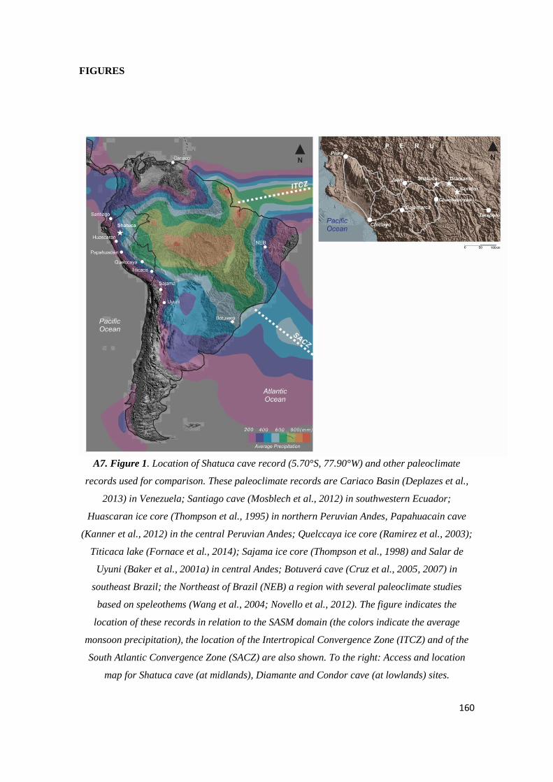
160
FIGURES
A7. Figure 1. Location of Shatuca cave record (5.70°S, 77.90°W) and other paleoclimate
records used for comparison. These paleoclimate records are Cariaco Basin (Deplazes et al.,
2013) in Venezuela; Santiago cave (Mosblech et al., 2012) in southwestern Ecuador;
Huascaran ice core (Thompson et al., 1995) in northern Peruvian Andes, Papahuacain cave
(Kanner et al., 2012) in the central Peruvian Andes; Quelccaya ice core (Ramirez et al., 2003);
Titicaca lake (Fornace et al., 2014); Sajama ice core (Thompson et al., 1998) and Salar de
Uyuni (Baker et al., 2001a) in central Andes; Botuverá cave (Cruz et al., 2005, 2007) in
southeast Brazil; the Northeast of Brazil (NEB) a region with several paleoclimate studies
based on speleothems (Wang et al., 2004; Novello et al., 2012). The figure indicates the
location of these records in relation to the SASM domain (the colors indicate the average
monsoon precipitation), the location of the Intertropical Convergence Zone (ITCZ) and of the
South Atlantic Convergence Zone (SACZ) are also shown. To the right: Access and location
map for Shatuca cave (at midlands), Diamante and Condor cave (at lowlands) sites.
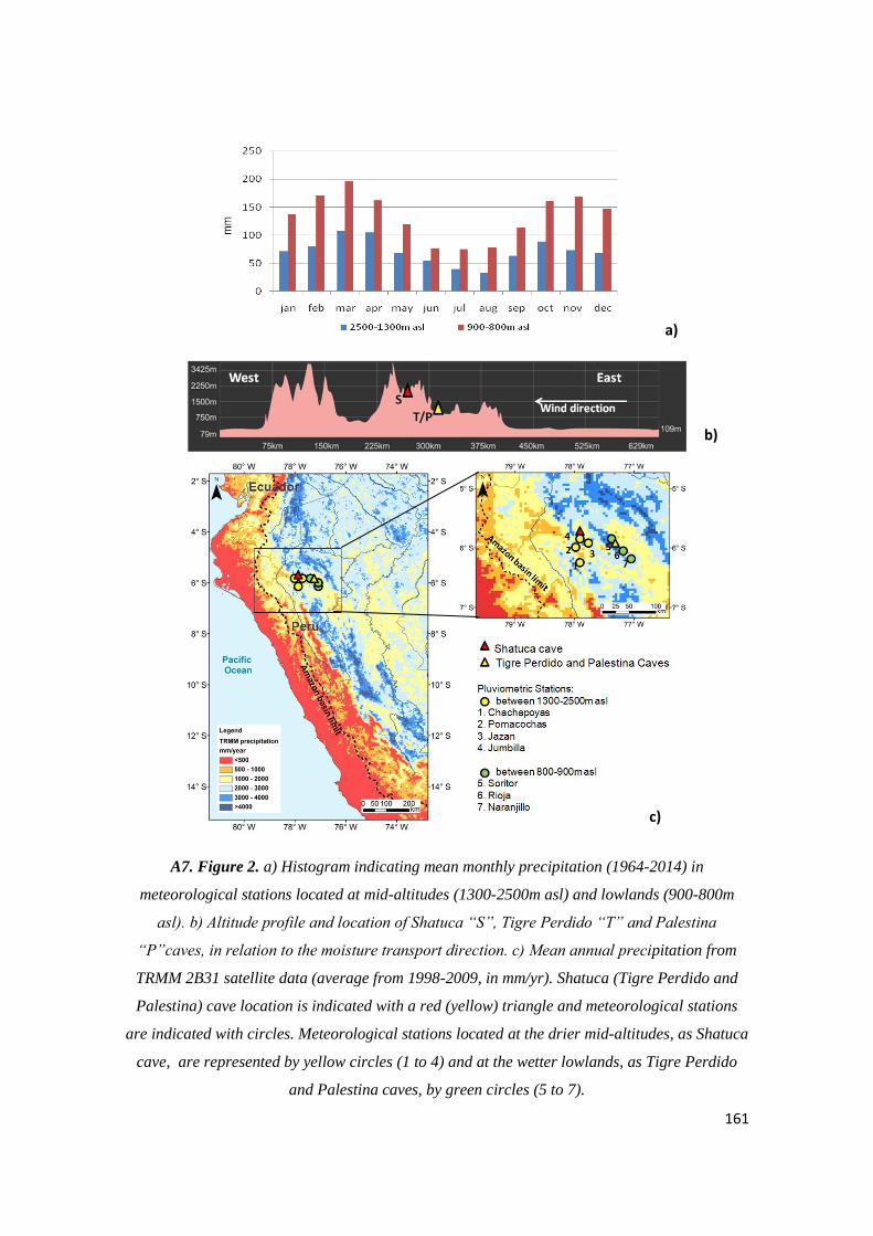
161
A7. Figure 2. a) Histogram indicating mean monthly precipitation (1964-2014) in
meteorological stations located at mid-altitudes (1300-2500m asl) and lowlands (900-800m
asl). b) Altitude profile and location of Shatuca “S”, Tigre Perdido “T” and Palestina
“P”caves, in relation to the moisture transport direction. c) Mean annual precipitation from
TRMM 2B31 satellite data (average from 1998-2009, in mm/yr). Shatuca (Tigre Perdido and
Palestina) cave location is indicated with a red (yellow) triangle and meteorological stations
are indicated with circles. Meteorological stations located at the drier mid-altitudes, as Shatuca
cave, are represented by yellow circles (1 to 4) and at the wetter lowlands, as Tigre Perdido
and Palestina caves, by green circles (5 to 7).
a)
c)
b)

162
0
-5
-10
-15
01/04/2011 01/01/2012 01/10/2012 01/07/2013
0
50
100
150
200
250
300
350
400
1
8O
(V
-SM
OW
)
RIO
JA
(m
m)
A7. Figure 3. Rainwater isotopic results obtained during the Palestina cave monitoring
program. Daily rain (black filled bars), 15 days accumulated rain (black open bars), rainwater
isotopes (blue squares) in Palestina cave (located in Rioja province). Note that scale for δ18
O is
reversed.

163
-9,0
-7,5
-6,0
-4,5
-9,0
-7,5
-6,0
-4,5
0 5 10 15 20 25 30 35 40960
940
920
900
880
860
-8
-7
-6
-5
-8
-6
-4
60
40
20
0
W/m
2
Gamma
18O
1
8O
18
O18
O
Salar de Uyuni
Shatuca
Diamante
Condor
Insolation
10oS Feb
Santiago
Age (ky BP)
1 1
98765.25.14
3 875.2 65.1432.1c2.1a 2.1b
A7. Figure 4. Comparison between the Shatuca record with lower altitude (900m asl) montane
forest records (3-6ºS) and the Salar de Uyuni record (Baker et al., 2001a) in the Atliplano
region (20ºS) from 40 ky BP to present. Note that the Altiplano region correlates better to the
insolation curve than the montane forest records. From top to base: Shatuca record (this study);
Diamante cave (860m asl) and Condor cave records (960m asl) (Cheng et al., 2013a); Santiago
cave record-980m asl (Mosblech et al., 2012); Salar de Uyuni record-3653m asl (Baker et al.,
2001a); Insolation 10ºS February (Berger and Loutre, 1991). Blue and orange bars indicate
Greenland stadials (GS) and Greenland interstadials (GI), respectively; as suggested by
Rasmussen et al. (2014). Ages and error bars are shown for each record.

164
0 5 10 15 20 25 30 35 40
60
40
20
0
930
900
870
-0,4
-0,6
-0,8
50
60
70
80
90
100-45
-42
-39
-36
-33
Insolation 10oS
W/m
2
log
(T
i /
Ca
)
Salar de Uyuni
Shatuca
Re
fle
cta
nce
Ga
mm
a (
cp
s)
Age (ky BP)
Cariaco Basin
-24
-20
-16-27
-24
-21
-18
-15
-8
-6
-4
1
8O
87
987
6
5.1
5.2
6
5.1
5.2
2.1
2.22.2
4
4
3 32.1c2.1b2.1a11
Guayaquil Gulf
1
8O
1
8O
1
8O
Sajama
Huascaran
NGRIP
A7. Figure 5. Paleoclimate records comparison for the period 40-0 ky BP. From top to base:
NGRIP record (Rasmussen et al., 2014), Cariaco Basin record (Deplazes et al., 2013), Shatuca
cave record (this study), Guayaquil Gulf record (Mollier-Vogel et al., 2013), Huascaran and
Sajama ice cores record (Thompson et al., 1995, 1998) and Salar de Uyuni record (Baker et al.,
2001a) with insolation precession cycle for Feb. 10°S in red (Berger and Loutre, 1991). Note
that the peak at 16.2 ky BP is only seen in Shatuca and Cariaco records. Moreover, neither the
Salar de Uyuni record nor the Sajama ice core record follow the insolation trend during the
Holocene. Blue and orange bars indicate Greenland stadials (GS) and Greenland interstadials
(GI), respectively; as suggested by Rasmussen et al. (2014). Ages and error bars are shown for
each record.

165
-9,0
-7,5
-6,0
-4,5-9,0
-7,5
-6,0
-4,5
10 15 20 25 30 35 40
-18
-16
-14
-8
-7
-6
-5
-8
-6
-4 -48
-44
-40
-36
Diamante
Condor
Shatuca
Papahuacain
Age (ky BP)
Santiago
H4H3H2
1
8O
1
8O
H1
2.1c2.1b3
2.1a3 4 5.2 6 7
1
8O
1
8O
1
8O
9
887
5.1
65.25.1411
1
8O
A7. Figure 6. Millennial variability among Andean records from 40 to 10 ky BP and its relation
to the Greenland ice core records. From top to base: NGRIP record (Rasmussen et al., 2014);
Shatuca cave record (this study); Santiago cave record (Mosblech et al., 2012); El Condor and
Diamante cave records (Cheng et al., 2013a) and Papahuacain cave record (Kanner et al.,
2012). Note that the occurrence of the Heinrich events, is indicated for the Shatuca record. Blue
and orange bars indicate Greenland stadials (GS) and Greenland interstadials (GI),
respectively; as suggested by Rasmussen et al. (2014). Ages and error bars are shown for each
record.

166
SUPPLEMENTARY MATERIAL
A7. Figure S1. Topographic map: Shatuca cave profile. Located in Yambrasbamba, Bongará
province, Amazonas –Peru. Source: Bigot (2008).

167
230Th dating results. The error is 2s error.Sample
Number
Espeleotema SHA 1
SHA1-1 43.2 ±0.0 1069 ±21 217 ±4 985.8 ±1.8 0.3256 ±0.0010 19248 ±67 18894 ±259 1040 ±2 18836 ±259
SHA1a-A 48.1 ±0.1 793 ±16 332 ±7 872.3 ±2.5 0.3325 ±0.0016 21002 ±111 20753 ±208 925 ±3 20695 ±208
SHA1a-B 53.2 ±0.1 627 ±13 525 ±11 883.8 ±2.7 0.3756 ±0.0016 23831 ±121 23654 ±173 945 ±3 23596 ±173
SHA 1a-C 51.5 ±0.1 362 ±7 995 ±20 948.4 ±2.9 0.4233 ±0.0017 26186 ±124 26085 ±143 1021 ±3 26027 ±143
SHA1a-D 50.0 ±0.1 371 ±8 968 ±20 928.2 ±2.9 0.4356 ±0.0018 27354 ±133 27247 ±153 1002 ±3 27189 ±153
SHA1a-E 61.5 ±0.1 798 ±16 559 ±11 858.1 ±2.8 0.4396 ±0.0017 28824 ±133 28628 ±192 930 ±3 28570 ±192
SHA1-2 50.1 ±0.1 506 ±10 683 ±14 760.3 ±2.4 0.4191 ±0.0010 29067 ±92 28906 ±146 825 ±3 28848 ±146
SHA1a-F 56.5 ±0.1 139 ±3 2863 ±61 727.3 ±2.7 0.4257 ±0.0017 30243 ±148 30203 ±151 792 ±3 30145 ±151
SHA1-3 64.4 ±0.1 564 ±11 914 ±18 711.3 ±3.0 0.4852 ±0.0010 35501 ±114 35358 ±152 786 ±3 35300 ±152
SHA1-4 80.2 ±0.1 1491 ±30 466 ±9 738.6 ±2.1 0.5250 ±0.0009 38176 ±96 37879 ±231 822 ±2 37821 ±231
SHA1-5 91.7 ±0.1 64972 ±1302 14 ±0 689.3 ±2.1 0.6127 ±0.0013 47532 ±142 35242 ±8810 761 ±19 35184 ±8810
SHA1-6 101.1 ±0.2 70230 ±1409 15 ±0 673.7 ±2.9 0.6215 ±0.0016 48944 ±191 36808 ±8698 747 ±19 36750 ±8698
Espeleotema SHA 2
SHA2-1 68.6 ±0.1 1749 ±35 16 ±1 1062.9 ±2.5 0.0247 ±0.0007 1311 ±35 951 ±257 1066 ±3 893 ±257
SHA2-2 66.6 ±0.1 605 ±12 19 ±1 1061.9 ±3.1 0.0106 ±0.0005 560 ±29 431 ±95 1063 ±3 373 ±95
SHA2-3 73.5 ±0.1 186 ±4 44 ±3 1066.1 ±3.1 0.0067 ±0.0005 356 ±25 321 ±36 1067 ±3 263 ±36
SHA2-4 68.6 ±0.1 121 ±3 85 ±5 1065.3 ±2.6 0.0091 ±0.0005 481 ±29 457 ±34 1067 ±3 399 ±34
SHA2-5 68.7 ±0.1 2544 ±51 21 ±1 1056.7 ±3.4 0.0465 ±0.0006 2491 ±35 1967 ±372 1063 ±4 1909 ±372
SHA2-6 59.1 ±0.1 4296 ±86 25 ±1 1039.1 ±2.9 0.1085 ±0.0007 5936 ±43 4902 ±733 1054 ±4 4844 ±733
SHA2-7 69.4 ±0.1 1557 ±31 38 ±1 1056.7 ±3.1 0.0523 ±0.0006 2802 ±32 2485 ±226 1064 ±3 2427 ±226
SHA2-8 96.3 ±0.1 1506 ±30 54 ±1 1048.3 ±2.8 0.0516 ±0.0004 2779 ±24 2557 ±159 1056 ±3 2499 ±159
sha-2a-9mm 117.8 ±0.2 2246 ±45 55 ±1 1042.4 ±3.2 0.0639 ±0.0005 3458 ±28 3187 ±194 1052 ±3 3124 ±194
SHA2-9 98.9 ±0.1 1161 ±23 93 ±2 1039.3 ±2.7 0.0662 ±0.0005 3589 ±26 3422 ±121 1049 ±3 3364 ±121
SHA2-10 110.1 ±0.1 508 ±10 317 ±7 1009.7 ±2.6 0.0887 ±0.0005 4905 ±26 4838 ±54 1024 ±3 4780 ±54
SHA2-11 133.7 ±0.2 183 ±4 1130 ±23 1004.1 ±3.3 0.0938 ±0.0004 5209 ±26 5190 ±29 1019 ±3 5132 ±29
sha-2a-4mm 91.7 ±0.1 242 ±5 685 ±15 996.1 ±2.2 0.1095 ±0.0006 6124 ±36 6086 ±45 1013 ±2 6023 ±45
SHA2-12 104.3 ±0.1 241 ±5 835 ±17 992.6 ±2.7 0.1172 ±0.0004 6578 ±26 6545 ±35 1011 ±3 6487 ±35
SHA2-14 110.1 ±0.2 154 ±3 1526 ±32 987.2 ±3.0 0.1292 ±0.0006 7291 ±37 7271 ±40 1008 ±3 7213 ±40
SHA2-16 117.5 ±0.1 146 ±3 1828 ±38 985.1 ±1.9 0.1377 ±0.0005 7793 ±32 7775 ±34 1007 ±2 7717 ±34
sha-2c-14mm 119.8 ±0.1 139 ±3 1976 ±43 984.0 ±2.4 0.1392 ±0.0006 7890 ±34 7873 ±36 1006 ±2 7810 ±36
SHA2-17 75.0 ±0.1 173 ±4 1109 ±23 987.1 ±2.4 0.1548 ±0.0007 8786 ±45 8752 ±51 1012 ±3 8694 ±51
SHA2-18 109.8 ±0.2 253 ±5 1147 ±23 984.7 ±2.8 0.1604 ±0.0006 9128 ±38 9094 ±44 1010 ±3 9036 ±44
SHA2-20 106.0 ±0.2 181 ±4 1631 ±34 985.6 ±2.7 0.1688 ±0.0007 9621 ±42 9597 ±45 1013 ±3 9539 ±45
sha-2c-48mm 113.6 ±0.1 183 ±4 1827 ±39 992.2 ±2.4 0.1789 ±0.0007 10186 ±44 10162 ±47 1021 ±2 10099 ±47
SHA2-22 41.8 ±0.0 317 ±6 411 ±9 993.0 ±2.1 0.1888 ±0.0009 10769 ±57 10660 ±96 1023 ±2 10602 ±96
SHA2-23 76.2 ±0.1 893 ±18 299 ±6 994.9 ±2.8 0.2124 ±0.0007 12167 ±47 11999 ±128 1029 ±3 11941 ±128
sha-2d-97mm 80.3 ±0.1 207 ±4 1331 ±28 987.4 ±2.6 0.2084 ±0.0008 11975 ±53 11938 ±59 1021 ±3 11875 ±59
sha-2d-105mm 76.2 ±0.1 134 ±3 1972 ±43 985.3 ±3.1 0.2110 ±0.0008 12143 ±53 12117 ±55 1020 ±3 12054 ±55
sha-2d-118mm 91.2 ±0.1 894 ±18 374 ±8 973.9 ±3.2 0.2222 ±0.0007 12899 ±48 12757 ±111 1010 ±3 12694 ±111
sha-2d-128mm* 84.3 ±0.1 415 ±9 759 ±16 995.6 ±2.6 0.2270 ±0.0007 13041 ±46 12970 ±68 1033 ±3 12907 ±68
sha-2d-160mm* 75.2 ±0.1 286 ±6 990 ±23 997.0 ±2.5 0.2287 ±0.0017 13134 ±102 13079 ±109 1035 ±3 13016 ±109
SHA2-25 65.3 ±0.1 182 ±4 1390 ±28 996.7 ±2.5 0.2353 ±0.0007 13535 ±48 13495 ±56 1035 ±3 13437 ±56
sha-2d-183mm 69.0 ±0.1 83 ±2 3258 ±73 992.8 ±2.8 0.2379 ±0.0008 13722 ±54 13704 ±55 1032 ±3 13641 ±55
sha-2d-187mm 74.9 ±0.1 248 ±5 1199 ±25 992.6 ±2.4 0.2403 ±0.0008 13871 ±53 13824 ±62 1032 ±3 13761 ±62
sha-2d-218mm 65.7 ±0.1 166 ±4 1660 ±37 997.8 ±2.9 0.2547 ±0.0009 14711 ±57 14675 ±63 1040 ±3 14612 ±63
sha-2d-252mm 71.6 ±0.1 262 ±6 1184 ±26 979.4 ±2.4 0.2631 ±0.0009 15374 ±60 15322 ±71 1023 ±3 15259 ±71
SHA2-26 53.1 ±0.0 272 ±5 849 ±17 973.3 ±2.5 0.2640 ±0.0009 15484 ±59 15410 ±79 1017 ±3 15352 ±79
SHA2-27 44.1 ±0.1 64 ±1 3092 ±68 943.8 ±2.6 0.2740 ±0.0012 16373 ±79 16351 ±81 988 ±3 16293 ±81
SHA2-28 58.6 ±0.1 448 ±9 635 ±13 936.3 ±2.3 0.2940 ±0.0010 17726 ±71 17614 ±106 984 ±2 17556 ±106
SHA2-29 60.6 ±0.1 282 ±6 1049 ±21 929.0 ±3.1 0.2967 ±0.0009 17973 ±69 17905 ±84 977 ±3 17847 ±84
sha-2e-27mm 62.3 ±0.1 586 ±12 553 ±11 906.9 ±2.5 0.3157 ±0.0012 19460 ±85 19320 ±130 958 ±3 19257 ±130
SHA2-31 38.8 ±0.1 89 ±2 2439 ±53 922.3 ±3.1 0.3396 ±0.0014 20873 ±98 20839 ±101 978 ±3 20781 ±101
SHA 2 34 69.3 ±0.1 206 ±4 2237 ±46 962.5 ±2.1 0.4040 ±0.0013 24669 ±94 24627 ±99 1032 ±2 24569 ±99
SHA 2 36 76.5 ±0.1 723 ±15 730 ±15 940.7 ±2.5 0.4187 ±0.0013 25989 ±97 25853 ±137 1012 ±3 25795 ±137
sha-2f-98mm 166.6 ±0.2 930 ±19 1258 ±26 827.6 ±2.0 0.4261 ±0.0011 28368 ±90 28282 ±108 896 ±2 28219 ±108
SHA2-38 36.8 ±0.0 80 ±2 3187 ±69 784.8 ±2.1 0.4179 ±0.0015 28522 ±118 28488 ±120 851 ±2 28430 ±120
Espeleotema SHA 3
SHA3-1 188.9 ±1.2 324 ±7 248 ±5 1095.7 ±16.5 0.0258 ±0.0003 1350 ±18 1327 ±25 1100 ±17 1269 ±25
SHA3-2 181.0 ±0.3 148 ±3 596 ±14 1090.8 ±3.1 0.0297 ±0.0003 1556 ±15 1545 ±17 1096 ±3 1487 ±17
SHA3-3 199.6 ±0.3 89 ±2 1209 ±27 1084.8 ±2.6 0.0326 ±0.0002 1715 ±13 1709 ±14 1090 ±3 1651 ±14
SHA3-4 202.3 ±0.3 216 ±4 598 ±13 1101.8 ±2.8 0.0387 ±0.0002 2025 ±12 2010 ±16 1108 ±3 1952 ±16
SHA3-5 113.5 ±0.1 269 ±5 803 ±17 1026.9 ±2.9 0.1157 ±0.0005 6380 ±30 6346 ±39 1045 ±3 6288 ±39
SHA3-6 155 ±0 2110 ±42 159.4 ±3.3 1059.4 ±2.7 0.1315 ±0.0006 7156 ±35 6965 ±139 1080 ±3 6903 ±139
SHA3-7 135 ±0 163 ±3 1847.1 ±40.3 1056.2 ±2.1 0.1356 ±0.0006 7395 ±37 7379 ±39 1078 ±2 7317 ±39
SHA3-8 142.8 ±0.2 51 ±1 6371 ±142 1061.7 ±2.8 0.1391 ±0.0004 7574 ±25 7569 ±25 1085 ±3 7511 ±25
SHA3-9 80.9 ±0.1 40 ±1 1785 ±44 2940.9 ±5.0 0.0531 ±0.0004 1477 ±12 1474 ±13 2953 ±5 1416 ±13
SHA3-10 142.7 ±0.1 159 ±3 2239 ±46 1076.8 ±2.1 0.1517 ±0.0004 8218 ±26 8202 ±29 1102 ±2 8144 ±29
SHA3-11 138.0 ±0.1 419 ±8 851 ±17 1080.7 ±2.0 0.1568 ±0.0006 8491 ±33 8449 ±44 1107 ±2 8391 ±44
SHA3-12 126.3 ±0.1 545 ±11 636 ±13 1072.0 ±2.4 0.1662 ±0.0005 9058 ±30 8998 ±52 1100 ±2 8940 ±52
SHA3-13 211.5 ±0.3 704 ±14 921 ±19 1058.9 ±3.0 0.1861 ±0.0005 10248 ±34 10202 ±47 1090 ±3 10144 ±47
*234
U = ([234
U/238
U]activity – 1)x1000. ** 234
Uinitial was calculated based on 230
Th age (T), i.e., 234
Uinitial = 234
Umeasured x el234xT
.
Corrected 230
Th ages assume the initial 230
Th/232
Th atomic ratio of 4.4 ±2.2 x10⁻⁶
. Those are the values for a material at secular
equilibrium, with the bulk earth 232
Th/238
U value of 3.8. The errors are arbitrarily assumed to be 50%.
Lines in red, indicate those Ages that were nor used due to higher error
* THE RESULTS OF THESE TWO SAMPLES (128mm and 160mm) ARE QUESTIONABLE FOR THEY WERE MIXED DURING WEIGHING
(corrected) (corrected )
230Th Age (yr)
234UInitial**
230Th Age (yr BP)
(corrected)(ppb) (ppt) (atomic x10- (measured) (activity) (uncorrected
)
238U
232Th
230Th /
232Th
234U*
230Th /
238U
230Th Age (yr)
A7. Table S1. U/Th ages for the speleothem samples Sha-1, Sha-2 and Sha-3.

168
15 20 25 30 35 40
0,005
0,010
0,015
0,020
0,025
0,030
0,035 Sha-1
(mm
/yr)
Age (ky BP)
0 5 10 15 20 25 30
0,0
0,1
0,2
0,3
0,4
0,5
Sha-2
(mm
/yr)
Age (ky BP)
0 2 4 6 8 10
0,02
0,03
0,04
0,05
0,06
0,07
0,08
0,09
0,10
0,11
Sha-3
(mm
/yr)
Age (ky BP)
A7. Figure S2. Growth rate of samples Sha-1, Sha-2 and Sha-3.

169
0 3 6 9 12 15 18 21 24 27 30 33 36 39
940
920
900
880
-7,5
-7,0
-6,5
-6,0
-5,5
-5,0
-4,5
-4,0
-3,5
-8
-7
-6
-5
-4
-3
-9
-8
-7
-6
-5
-4
1
8O
Insolation
10o Feb
Sha-3
Sha-1
87
987
6
5.1
5.2
6
5.1
5.2
2.1
2.22.2
4
4
3 32.1c2.1b2.1a1
Sha-2
1
1
8O
1
8O
W
/m2
Age (ky BP)
A7. Figure S3. Isotopic record of samples Sha-1 (black), Sha-2 (red) and Sha-3 (green),
compared to the insolation precession cycle for Feb. 10°S (black). Blue and orange bars
indicate Greenland stadials (GS) and Greenland interstadials (GI), respectively; as suggested
by Rasmussen et al. (2014). Ages and error bars are shown for each sample.

170
0 5 10 15 20 25 30 35 40-9,0
-7,5
-6,0
-4,5
-3,0
1
8O
Age (ky BP)
Shatuca
Condor
Diamante
Santiago
A7. Figure S4. Comparison between northeastern Andean records located between 3-6ºS:
Shatuca record shown in red (this study), Condor and Diamante cave records shown in black
and blue, respectively (Cheng et al., 2013a) and Santiago record shown in green (Mosblech et
al., 2012). Note that Shatuca cave record presents more enriched δ18
O values along the last
38ky.

171
-8
-7
-6
-5
-4
-3
10 12 14 16 18 20 22 24 26 28 30 32 34 36 38 40-54
-52
-50
-48
-46
-9
-8
-7
-6
-5-8
-7
-6
-5
-18
-17
-16
-15
-14
-48
-46
-44
-42
-40
-38
-36
Shatuca
EDML
Log (
Ti/C
a)
4 85.22.1c2.1b
Diamante
11 2.1a 3 4 5.1 6 7 8 9
18O
18O
Condor
Papahuacain
18O
18O
18O
NGRIP
Age (ky BP)
A7. Figure S5. Comparison between Andean records at lowlands (Condor and Diamante
caves), midlands (Shatuca cave) and highlands (Papahuacain cave) with the EDML and NGRIP
ice core records. Blue and orange bars indicate Greenland stadials (GS) and Greenland
interstadials (GI), respectively; as suggested by Rasmussen et al. (2014). Ages and error bars
are shown for Shatuca record.