groupoid c*-algebras, conformal measures and rodrigo souza ... · rausino,f rodrigo souza groupoid...

Groupoid C*-algebras, Conformal Measures andPhase Transitions

Rodrigo Souza Frausino

Dissertação apresentadaao

Instituto de Matemática e Estatísticada

Universidade de São Paulopara

obtenção do títulode

Mestre em Ciências

Programa: Mestrado em Matemática Aplicada

Orientador: Prof. Dr. Rodrigo Bissacot

Durante o desenvolvimento deste trabalho o autor recebeu auxílio nanceiro da CAPES

São Paulo, Maio de 2018

Groupoid C*-algebras, Conformal Measures and Phase Transitions

Esta é a versão original da dissertação elaborada pelo candidato Rodrigo Souza Frausino, tal como

submetida à Comissão Julgadora.

Comissão Julgadora:

Prof. Dr. Rodrigo Bissacot - IME-USP

Prof. Dr. Ruy Exel - UFSC

Profa. Dra. Cristina Cerri - IME-USP

Resumo

Frausino, Rodrigo Souza C*-álgebras de Grupóides, Medidas Conformes e Transições de

Fase.

O objetivo deste trabalho é o estudo do fenômeno de transição de fase no contexto de Grupóides

e suas C*-álgebras. O resultado principal é devido a Klaus Thomsen em [Tho17], que explora a

conexão entre medidas conformes no formalismo clássico e estados KMS do contexto quântico. A

transição de fase no caso quântico é consequência desta ligação entre os dois formalismos e do

fato de que no setting clássico eram conhecidos exemplos de potenciais contínuos que apresentam

o fenômeno de transição de fase. O potencial utilizado é aquele introduzido por Hofbauer [Hof77],

um exemplo que mostra que, diferentemente de potenciais de variação somável, potenciais apenas

contínuos podem apresentar transição de fase.

Palavras-chave: Grupóide, C*-álgebra, Medidas Conformes, Transição de Fase, Estados KMS.

i

Abstract

Frausino, Rodrigo Souza Groupoid C*-algebras, Conformal Measures and Phase Transi-

tions.

The objective of this work is the study of phase transitions on the context of Groupoids and their

C*-Algebras. The main result of this dissertation is due to Klaus Thomsen in [Tho17], which in-

vestigates the connection between conformal measures in the classical formalism and KMS-states

in the quantum formalism. The phase transition in the quantum setting is a consequence of this

connection between both formalisms and the fact that on the classical setting it was known exam-

ples of continuous potentials that show the phenomena of phase transition. The potential used was

introduced by Hofbauer [Hof77], an example that shows, dierently from potential of summable

variations, potentials only continuous can exhibit phase transition.

Keywords: Groupoid, C*-algebras, Conformal Measures, Phase Transition, KMS States.

iii

Contents

1 Preliminaries 5

1.1 Thermodynamic Formalism and Hofbauer Potential . . . . . . . . . . . . . . . . . . 5

1.1.1 Shift Space and the Ruelle-Perron Frobenius Operator . . . . . . . . . . . . . 5

1.1.2 Partitions, Entropy and Pressure: introducing equilibrium states . . . . . . . 6

1.2 C*-algebras and KMS states . . . . . . . . . . . . . . . . . . . . . . . . . . . . . . . . 10

1.3 Universal C*-algebras: Generators and Relations . . . . . . . . . . . . . . . . . . . . 17

2 Algebraic Structure 21

2.1 Basic Denitions and results . . . . . . . . . . . . . . . . . . . . . . . . . . . . . . . . 21

2.2 The ∗-algebra Cc(G) . . . . . . . . . . . . . . . . . . . . . . . . . . . . . . . . . . . . 25

2.3 The Full Groupoid C*-algebra . . . . . . . . . . . . . . . . . . . . . . . . . . . . . . . 27

2.4 The Reduced Groupoid C*-algebra . . . . . . . . . . . . . . . . . . . . . . . . . . . . 30

3 Conformal Measures 37

3.1 Conformal Measures . . . . . . . . . . . . . . . . . . . . . . . . . . . . . . . . . . . . 37

3.2 The Renault-Deaconu Groupoid . . . . . . . . . . . . . . . . . . . . . . . . . . . . . . 40

3.3 The Dinamics and KMS states . . . . . . . . . . . . . . . . . . . . . . . . . . . . . . 46

3.4 Cuntz-Krieger Algebras and Groupoids . . . . . . . . . . . . . . . . . . . . . . . . . . 48

4 Phase Transition and Main Result 53

Bibliography 61

i

Introduction

The phenomenon of phase transition is perhaps the most important topic in equilibrium sta-tistical mechanics and, the mathematics involved studying models, the presence or not of phasetransitions, critical temperatures, and other properties requires a high sophistication which culmi-nated to the Fields Medal to Stanislav Smirnov in 2010.

Perhaps the most straightforward examples are the magnets, which lose their magnetic prop-erties (attraction and repulsion of other materials) when you put them in a high temperatures.For ferromagnetic systems there exists precisely one temperature where the system changes thebehavior and in this case, we call this value of critical temperature. The model proposed by thephysicists to study magnets is called Ising model and is perhaps the most successfully understoodof the entire statistical mechanics [FV17, Bov06, Geo11]. This model belongs to a class of modelscalled spin systems, where the position of the particles are the vertices of a graph (for instance,Z,Zd) and each particle has a spin associated to it. This spin usually is represented by an integernumber and in many cases can assume an only nite number of values. To explore the connectionwith symbolic dynamics, we denote by A the set of spin values and we call this set of alphabet. Forour propose, it will be a nite subset of N. A unidimensional spin system is basically dened byhis conguration space Σ = AZ and an interaction Φ = (ΦΛ)Λ: a collection of continuous functionsΦΛ which are functions depending on a nite region Λ of the lattice Z. The interaction denes howthese spins will interact with each other and with them we can construct the measures (equilibrium,DLR, conformal etc) which describe the system.

This approach to constructing the objects with local functions is very common in the literaturewritten by physicists, on another hand, the mathematical physics community has a big inuencefrom ergodic theory and convex analysis, perhaps the main responsible are Y. Sinai and D. Ruellewhich had a big inuence on both communities. From the ergodic perspective much of this iswritten in terms of a function which we call potential given by fΦ : Σ → R dened as fΦ(x) =∑

Λ30 ΦΛ(x)/|Λ|. We can study the pressure P (fΦ) and the measures which describe these systems.Naturally, the abstract generalization to study pressure, equilibrium and DLR measures for a generalcontinuous function f (which we will continue calling potential) was immediately considered. Thestudy, from this more general point of view, is today known as thermodynamic formalism and isa big branch of ergodic theory with intense and recent activity, some classical references whichconsider this approach are [PP90, Bow08, Rue04, Sim14, Isr15]. For a recent review which dealswith this question of the connection between potentials and interactions see [CL17].

Thanks to the famous Sinai's trick [Bow08], for suitable potentials f : AZ → R, we can denea cohomologous potential f ′ : AN → R such that the thermodynamics of both potentials are closeand they have the same equilibrium states. After this observation, since we will stay in the unidi-mensional setting, we can focus our attention on potentials f : AN → R and their thermodynamicformalisms. The equilibrium measures for f are shift-invariant probabilities µ which satisfy the vari-ational problem for the pressure, that is, P (f) = hµ +

∫fdµ. They are one of the main objects

in the classical setting. The phase transition, which physically means some change on the system,can be codied by regarding the number of equilibrium states (more generally, the DLR measures)for the potential f . One of the advantages of work on AN instead of AZ is the fact that we canuse the machinery of the transfer (Ruelle) operator as we will see. In fact, in the case of enoughregular potentials, any equilibrium measure µ comes from the Ruelle's operator. The Ruelle-Perron-Frobenius theorem says that the equilibrium measures are hdν where h is an eigenfunction (ν is an

1

2 CONTENTS 0.0

eigenmeasure of the dual) of the Ruelle operator from the potential f .Now, remember that our concrete example were magnets who lose their magnetic properties at

low temperatures, so the models should include a parameter associated with the temperature. Wedenote by β > 0 the inverse of the temperature T > 0 and the potential will be the function βfand, it is usual to consider the pressure at the inverse of temperature β. In this case, we denote thepressure at temperature β−1 by P (β) := P (βf) and the equilibrium measures at this temperatureby µβ . Sometimes we have more than one measure satisfying P (βf) = hµβ +

∫βfdµβ , this is

the mathematical manifestation of the phenomenon of phase transition, for the Ising model whichmodelizes the magnets, this is the situation for β large enough (low temperatures) in dimensiontwo.

In dimension one (our setting) is more dicult to see phase transitions, if the potential isLipschitz (or more generally, has summable variations) we have unicity of the equilibrium measureµβ for all β > 0 and the pressure function P (β) is analytic with respect to the parameter β, see[Bow08, Rue04]. So, is natural try to nd a less regular potential f , only continuos for example, whichadmits more than one equilibrium state. This was done by F. Hofbauer in [Hof77], we rememberthis potential at Chapter 1.

The DLR measures (in honor of the mathematical physicists R.L. Dobrushin, O. E. Lanfordand D. Ruelle) are the measures considered by the statistical mechanics community to describethe spin systems at the equilibrium; they usually call these measure by Gibbs measures. We avoidthis nomenclature because there exist several measures which today are called Gibbs measuresby both communities of statistical mechanics and ergodic theory. The notion of DLR measure(which we will not explain here, see the Chapter 1) was introduced in the papers [Dob68, LR69].Roughly speaking, a DLR measure is a probability measure which is compatible with a collection ofconditional probabilities with respect to sigma-algebras generated by the variables outside of niteregions Λ of the lattice which are dened according to the interaction Φ. Perhaps, at this point, themost important thing is to mention that the translation-invariant DLR measures are precisely theequilibrium measures which we just dened, see [Kel98, Rue04, Mey13].

Now, it is natural to ask what kind of condition characterizes the equilibrium states in quantumstatistical mechanics, the answer is the KMS condition [HHW67], in honor of R. Kubo, P. C. Martinand J. Schwinger. The quantum analogous of the DLR states are the KMS states.

From now, we start to explore connections and analogies between the classical and quantumsettings and, at this point, C*-algebras get involved. The quantum counterpart of the shift spacesAN with nite symbols are the Cuntz algebras [Cun77], denoted as On (n is the number of symbols),which we introduce throughout the text. We describe the KMS states in detail in Chapter 1. Themotivation of K. Thomsen, and by consequence, our motivation, is to try to push the phenomenonof phase transition of the Hofbauer potential and equilibrium measures in the classical setting toC*-algebras, in this case, the Cuntz algebra O2 and the KMS states.

Connections between conformal measures (eigenmeasures from the dual of the Ruelle operator)and KMS states are already known, see, for instance, [KSS07, Ren80], so it is natural to try topush the phase transition from the classical to the quantum formalism. In fact, as we will see, theidea can be implemented and the main motivation of this thesis is to describe this path done by K.Thomsen [Tho17].

The thesis is structured in the following way:

Chapter 1: Here we set the stage. First we give a short introduction to the classical thermody-namic formalism, in particular introducing the notions of equilibrium states and phase transition;we dene as well the Hofbauer potential, which is a generalization of the potential in Chapter 4.Here we give as well an introduction to KMS states and an important way to generate C*-algebras.

Chapter 2: We dene a algebraic structure known as groupoid and endow it with a compatibletopology in order to study the continuous and compactly supported functions on it. We give such aspace with operations such as it becomes a ∗-algebra. Finally, in this context, we are able to denetwo kinds of C*-algebras, the Full C*-algebra and the Reduced and we provide some properties for

0.0 CONTENTS 3

them.Chapter 3: We dene the notion of conformal measure, which plays a central role in the classical

thermodynamic formalism. These measures are eigenmeasures of the Ruelle operator and, whenthe potential is regular enough, it is possible to show that any equilibrium measure comes froma conformal measure. To make the connection with the quantum setting, we prove that everyconformal measure has a KMS state associated with it, in a proper context. We dene as well theCuntz Algebra, relating it to the algebraic structure of groupoids dened in Chapter 2.

Chapter 4: As the last chapter of this thesis, we present a result from K. Thomsen, which useda theorem from S. Neshveyev and the connection of the quantum setting with the classical one,to generate a cocycle given by a potential which is substantially the same provided by Hofbauer.The result essentially says that the phase transition in the classical sense, looking for the numberof equilibrium measures, generates a phase transition concerning the number of KMS states.

Chapter 1

Preliminaries

1.1 Thermodynamic Formalism and Hofbauer Potential

In this section, we present a crash course about classical thermodynamic formalism. There area myriad of good references when we are talking about thermodynamic formalism, in particular werefer to Bowen's lecture notes [Bow08].

1.1.1 Shift Space and the Ruelle-Perron Frobenius Operator

Consider a nite set A and the countable cartesian product AN. A is called the alphabet. Oneelement x ∈ AN is a sequence, indexed by N, of elements in A. For all i ∈ N we denote xi ≡ πi(x),πi is the canonical projection in the i coordinate of AN.

We wish to endow the set AN with a topology, for that, consider the metric d : AN ×AN → R,dened as

d(x, y) = 2− infn:xn 6=yn. (1.1)

(AN, d) is a compact metric space. More than that, the topology induced by the metric dcoincides with the topology generated by cylinder sets, i.e, the sets dened for a nite word ω =(ω1, ..., ωn) as [ω] := (xi)i∈N ∈ AN|x1 = ω1, ..., xn = ωn. As a nal topological coincidence, if weendow A with the discrete topology, then the product topology is equal with the previous ones.Now we can dene the Shift Space with alphabet A.

Denition 1. Given a nite set A, the function σ : AN → AN dened by

σ(x)i = xi+1, ∀x ∈ AN, ∀i ∈ N; (1.2)

is called the shift map. The pair (AN, σ) is denominated as the one-sided full shift, or simply by thefull shift.

From now on, let us restrain ourselves in the case A = 1, ..., n, n ∈ N. In this case the fullshift is denoted as Σn, i.e,

Σn := 1, ..., nN.

Now, let A ∈ Mn(R) be a matrix with entries with only zeros or ones. We impose that A istransitive, i.e, for every i, j ∈ 1, 2, ..., n there exists an m ∈ N such that (Am)ij 6= 0. We candene the following subset of Σn, associated with A,

ΣA := (xi)i∈N ∈ 1, ..., nN|A(xi, xi+1) = 1.

An important observation is that ΣA is invariant under the shift map, i.e, σ(ΣA) = ΣA and itis a closed set of Σn. Now some notation for the rest of this section. Let X, a non empty set, and

5

6 Preliminaries 1.1

consider a topology on X such that it is metrizable and compact. Let T : X → X a continuousfunction.

1. M(X) is the set of probability measure over the borel σ-algebra of X, denoted as BX ;

2. MT (X) ⊂M(X) is the set of measures inM(X) that are T -invariant, i.e, µ(T−1(B)) = µ(B),∀B ∈ BX ;

3. Given a σ-algebra F on X and a measure µ on F , we use a rather common notation: µ(f) :=∫X fdµ, for all f F-measurable;

4. C(X) is the Banach space of functions of X into R, endowed with the supremum norm || · ||∞.

In this context, we can take X = ΣA and T = σ, the shift map. We present now the Ruelle operator,which is very important in rigorous statistical mechanics.

Denition 2. Given ϕ ∈ C(ΣA), the Ruelle operator in respect with ϕ is the linear operatorLϕ : C(ΣA)→ C(ΣA), dened as

Lϕf(x) :=∑

y∈σ−1(x)

eϕ(y)f(y), ∀x ∈ ΣA (1.3)

Let ϕ ∈ C(ΣA) and dene Sm(ϕ(x)) :=∑m−1

i=0 ϕ(σi(x)) for all m ∈ N and for all x ∈ ΣA.

1.1.2 Partitions, Entropy and Pressure: introducing equilibrium states

Before we dene equilibrium states, we present the notions of partitions and relative entropy.These denitions can be found in many places, but we refer to [VO16].

Let (X,Σ, µ) be a probability space. Here, partition is a countable family P of measurablesubsets of X, two by two disjoint and that µ(

⋃P∈P P ) = 1. Given two partitions P and Q, we

dene P ∨ Q to be the partition whose elements are the intersections P ∩ Q, where P ∈ P andQ ∈ Q. More Generally, if Pn is a countable family of partitions, we dene∨

n

Pn :=⋂

n

Pn|Pn ∈ Pn for all n.

The entropy of a partition P is the number

Hµ(P) =∑P∈P−µ(P ) logµ(P ).

Now, if f : X → X is measurable function such that µ(f−1(A)) = µ(A) for all A ∈ Σ, then theentropy of f with respect to µ and a partition P is the limit

hµ(f,P) := limn

1

nHµ(

n−1∨i=0

P)

The limit exists because one can show that the sequence Hµ(∨n−1i=0 P) is subadditive and by Fekete's

Subadditive Lemma we conclude the limit indeed exists. Finally the entropy of the system (f, µ) isdened as

hµ(f) = supPhµ(f,P).

Observe that we could choose X to be the shift space ΣA and Σ to be its borel σ-algebra. Next wedene the pressure.

1.1 Thermodynamic Formalism and Hofbauer Potential 7

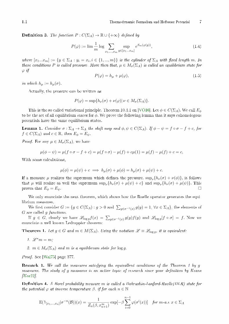
Denition 3. The function P : C(ΣA)→ R ∪ +∞ dened by

P (ϕ) := lim1

mlog

∑x1,...,xm

supy∈[x1...xm]

eSm(ϕ(y)), (1.4)

where [x1...xm] := y ∈ ΣA : yi = xi, i ∈ 1, ...,m is the cylinder of ΣA with xed length m. Inthese conditions P is called pressure. More then that, µ ∈Mσ(ΣA) is called an equilibrium state forϕ if

P (ϕ) = hµ + µ(ϕ), (1.5)

in which hµ := hµ(σ).

Actually, the pressure can be written as

P (ϕ) = suphν(σ) + ν(ϕ)| ν ∈Mσ(ΣA).

This is the so called variational principle, Theorem 10.4.1 on [VO16]. Let φ ∈ C(ΣA). We call Eφto be the set of all equilibrium states for φ. We prove the following lemma that it says cohomologouspotentials have the same equilibrium states.

Lemma 1. Consider σ : ΣA → ΣA the shift map and φ, ψ ∈ C(ΣA). If φ− ψ = f σ − f + c, forf ∈ C(ΣA) and c ∈ R, then Eφ = Eψ.

Proof. For any µ ∈Mσ(ΣA), we have

µ(φ− ψ) = µ(f σ − f + c) = µ(f σ)− µ(f) + cµ(1) = µ(f)− µ(f) + c = c,

With some calculations,

µ(φ) = µ(ψ) + c =⇒ hµ(σ) + µ(φ) = hµ(σ) + µ(ψ) + c.

If a measure µ realizes the supremum which denes the pressure, supνhν(σ) + ν(φ), it followsthat µ will realize as well the supremum supνhν(σ) + µ(ψ) + c and supνhν(σ) + µ(ψ). Thisproves that Eφ = Eψ.

We only enunciate the next theorem, which shows how the Ruelle operator generates the equi-librium measures.

We rst consider G := g ∈ C(ΣA) : g > 0 and∑

y∈σ−1(x) g(y) = 1, ∀x ∈ ΣA, the elements ofG are called g-functions.

If g ∈ G, clearly we have Llog gf(x) =∑

y∈σ−1(x) g(y)f(y) and Llog g[f σ] = f . Now weenunciate a well known Ledrappier theorem:

Theorem 1. Let g ∈ G and m ∈M(ΣA). Using the notation L ≡ Llog g, it is equivalent:

1. L ∗m = m;

2. m ∈Mσ(ΣA) and m is a equilibrium state for log g.

Proof. See [Wal75] page 377.

Remark 1. We call the measures satisfying the equivallent conditions of the Theorem 1 by g-measures. The study of g-measures is an active topic of research since your denition by Keane[Kea72].

Denition 4. A Borel probability measure m is called a Dobrushin-Lanford-Ruelle(DLR) state forthe potential ϕ at inverse temperature β, if for each n ∈ N

E(1[x1,...,xn]|σ−n(B))(x) =1

Zn(β, x∞n+1)exp[−β

n−1∑i=0

ϕ(σi(x))] for m-a.e x ∈ ΣA

8 Preliminaries 1.1

where Zn(β, x∞n+1) :=∑

y∈σ−n(σn(x)) exp[−β∑n−1

i=0 ϕi(y)] and B is the borel σ-algebra for ΣA.

When considering a function ϕ ∈ C(ΣA) and the set of equilibrium measures Eϕ, we might askhow many elements there are in Eϕ. The next condition on the function ϕ forces the set Eϕ to haveonly one element.

Denition 5. We say that ϕ ∈ C(ΣA) satisfy the Ruelle-Perron-Frobenius condition, or RPFcondition, if there are λ > 0, h ∈ C(ΣA), h > 0 and ν ∈M(ΣA) such that

1. Lϕh = λh;

2. L ∗ϕν = λν, L ∗ is the dual of the operator L ;

3. ν(h) = 1;

4. ||λ−mLmϕ f − ν(f)h||∞ → 0 when m→∞, ∀f ∈ C(ΣA).

The measure µ dened byµ(f) = ν(hf), ∀f measurable. (1.6)

is called RPF measure.

We enunciate the next theorem, which arms the uniqueness of the equilibrium state for afunction φ ∈ C(ΣA) that satises the RPF condition, as we said before.

Theorem 2. Let ϕ ∈ C(ΣA) that satises the RPF condition. It follows that µ(·) := ν(h·) is theunique equilibrium state for ϕ. The measure ν ∈M(ΣA) and h > 0 are as in the denition 5.

Proof. See [Hof77] page 225.

Remark 2. Let ΣA a topologically mixing subshift and ϕ : ΣA → R a potential with summablevariations. Then, ϕ has the RPF property. For the proof, see [Bow08], page 9.

If we have a function g : Σn → R we say it admits a Gibbs-Bowen measure µ ∈ Mσ(Σn) if theare two constants c1, c2 > 0 and λ > 0 such that

c1 ≤µ([x1 · · ·xm])

λ−m exp[Sm(g(x))]≤ c2 (1.7)

For all x ∈ [x1 · · ·xm] and m ∈ N.

Remark 3. Let ΣA a topologically mixing subshift and ϕ : ΣA → R a potential with summablevariations. By the remark 2, ϕ has the RPF property and then there exists a RPF measure associatedto ϕ. This measure is Gibbs-Bowen. For the proof see [Bow08], page 15.

Remark 4. Under the same hypotheses of the remark 3, for which we know that there existsan eigenmeasure for ϕ, we know that the set of eigenprobabilities coincides with the set of DLRprobabilities measures, see [CL17].

Next, we dene the potential due to Hofbauer, which will appear again in the last chapter of thisdissertation, although in a dierent context. This potential and its properties were the motivationbehind the paper [Tho17], since the potential considered in aforementioned article is a special casewhen we consider the full shift with two symbols. For that dene

M1 := Σn \ [1],

Mk := x ∈ Σn : xi = 1 for 1 ≤ i ≤ k − 1 and xk 6= 1, k ∈ 2, 3, ....

Observe that those sets are disjoint and the sequence with only ones is not in any of those sets. Wesee as well that

⋃∞k=1Mk ∪ (1, 1, 1, ...) = Σn. Let (ak)N be a sequence of real numbers such that

1.1 Thermodynamic Formalism and Hofbauer Potential 9

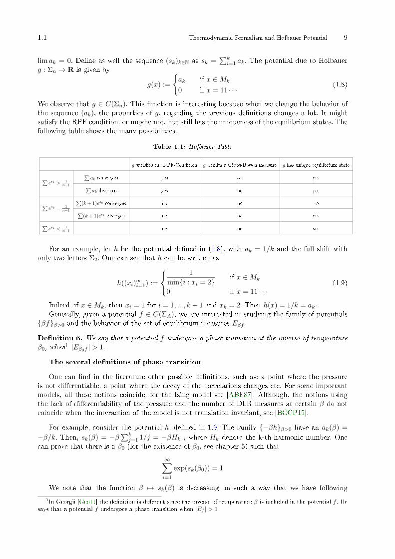
lim ak = 0. Dene as well the sequence (sk)k∈N as sk =∑k

i=1 ak. The potential due to Hofbauerg : Σn → R is given by

g(x) :=

ak if x ∈Mk

0 if x = 11 · · ·(1.8)

We observe that g ∈ C(Σn). This function is interesting because when we change the behavior ofthe sequence (ak), the properties of g, regarding the previous denitions changes a lot. It mightsatisfy the RPF condition, or maybe not, but still has the uniqueness of the equilibrium states. Thefollowing table shows the many possibilities.

Table 1.1: Hofbauer Table

g satises the RPF-Condition g admits a Gibbs-Bowen measure g has unique equilibrium state

∑esk > 1

n−1

∑ak converges yes yes yes∑ak diverges yes no yes

∑esk = 1

n−1

∑(k + 1)esk converges no no no∑(k + 1)esk diverges no no yes∑

esk < 1n−1 no no yes

For an example, let h be the potential dened in (1.8), with ak = 1/k and the full shift withonly two letters Σ2. One can see that h can be written as

h((xi)∞i=1) :=

1

mini : xi = 2if x ∈Mk

0 if x = 11 · · ·(1.9)

Indeed, if x ∈Mk, then xi = 1 for i = 1, ..., k − 1 and xk = 2. Then h(x) = 1/k = ak.Generally, given a potential f ∈ C(ΣA), we are interested in studying the family of potentials

βfβ>0 and the behavior of the set of equilibrium measures Eβf .

Denition 6. We say that a potential f undergoes a phase transition at the inverse of temperatureβ0, when

1 |Eβ0f | > 1.

The several denitions of phase transition

One can nd in the literature other possible denitions, such as: a point where the pressureis not dierentiable, a point where the decay of the correlations changes etc. For some importantmodels, all these notions coincide, for the Ising model see [ABF87]. Although, the notions usingthe lack of dierentiability of the pressure and the number of DLR measures at certain β do notcoincide when the interaction of the model is not translation invariant, see [BCCP15].

For example, consider the potential h, dened in 1.9. The family −βhβ>0 have an ak(β) =

−β/k. Then, sk(β) = −β∑k

j=1 1/j = −βHk , where Hk denote the k-th harmonic number. Onecan prove that there is a β0 (for the existence of β0, see chapter 5) such that

∞∑i=1

exp(sk(β0)) = 1

We note that the function β 7→ sk(β) is decreasing, in such a way that we have following

1In Georgii [Geo11] the denition is dierent since the inverse of temperature β is included in the potential f . Hesays that a potential f undergoes a phase transition when |Ef | > 1

10 Preliminaries 1.2

expressions∞∑i=1

exp(sk(β)) > 1 if β < β0 (1.10)

∞∑i=1

exp(sk(β)) < 1 if β > β0 (1.11)

By the table 1.1, in both cases we have unique equilibrium measures. In the case for β0, on theother hand, we have non uniqueness. This provides us with an example of phase transition that isrelevant for our purposes, for the reason that the potential we use in the quantum setting is exactlythe potential h. In addition, in [Hof77] it is shown that the measure δ1∞ is an equilibrium measurewhen

∑esk(β) < 1 and it is interesting to see that we have a certain correspondence in the quantum

seeting, since for β > β0 we have a certain measure m1∞ which creates KMS states.

1.2 C*-algebras and KMS states

Since the subject of C*-algebras is really vast, in this section I have no intention of provingmost of the results of C*-Algebras that is to be used in this work. A prior knowledge of operatoralgebras is required from the reader, standard references for this subject are [Dav96, Mur14]. Thissection is mostly to dene the notion of KMS state and everything described here can be found inBratteli's books [BR79, BR81]

Denition 7. Let (A,+, ·) be an algebra over C, we say that the operation ∗ : A → A, a 7→ a∗, isan involution of the algebra A if:

(a∗)∗ = a

(ab)∗ = b∗a∗

(αa+ βb)∗ = αa∗ + βb∗

for all α, β ∈ C and for all a, b ∈ A. An algebra with such a operation is called a ∗−algebra.

The element 1 ∈ A is called the identity of the algebra if for all a ∈ A, we have 1 · a = a · 1, Inthis case we call A an algebra with identity.

Denition 8. Let A,B two ∗−algebras with identity. The function φ : A→ B, with properties:

φ(a+ αb) = φ(a) + αφ(b)

φ(ab) = φ(a)φ(b)

φ(a∗) = φ(a)∗

φ(1A) = 1B

for all a, b ∈ A and all α ∈ C is called a ∗−homomorphism. If φ is bijective then it is called a∗−isomorphism. If A = B and φ is a ∗−isomorphism we say that φ is a ∗−automorphism.

Let A be an algebra and ‖ · ‖ a norm in A such that

‖a · b‖ ≤ ‖a‖‖b‖ ∀a, b ∈ A,

This property is called sub-multiplicativity. We say that (A, ‖ · ‖) is a normed algebra. A com-plete(every Cauchy sequence converges) normed algebra is called a Banach algebra.

Denition 9. A is a C∗−algebra if A is a Banach ∗−algebra such that the following property issatised:

‖a∗a‖ = ‖a‖2 ∀ a ∈ U.

1.2 C*-algebras and KMS states 11

This property is usually called the C∗−property.

Denition 10. Let A be a C∗−algebra. A linear functional ω is called a state if it is positive, i.eω(a∗a) ≥ 0 for all a ∈ A and it is normalized, i.e ω(1) = 1. Of course this only makes sense if Ahas an identity, if it does not, we put the property that the operator norm ||ω|| = 1.

We say that τ = τtt∈R is a 1−parameter group of ∗−automorphisms of a C*-algebra A ifτt : A→ A is a ∗−automorphism in A and:

i) τt+s = τt τs, for all t, s ∈ R;

ii) τ0 = id.

Denition 11 (C∗−Dynamical System). A C∗−dynamical system is a pair (A, τ) where A is aC*-algebra and τ = τtt∈R is a 1−parameter group of ∗−automorphisms strongly continuous, i.et 7→ τt(A) is continuous in the norm for all A ∈ A.

Let X be a complex Banach space and X∗ its dual. Let σ(X,X∗) denote the topology in Xinduced by the functionals in F , i.e the weak topology on X.

Denition 12. A 1−parameter t 7→ τt family of linear and bounded applications from X into itselfis called a one-parameter σ(X,X∗)-continuous group of isometries if:

1) τt+s = τt τs for all t, s ∈ R and τ0 = id;

2) ‖τt‖ = 1, for all t ∈ R;

3) t 7→ τt(A) is σ(X,X∗)-continuous for all A ∈ X;

Denition 13 (Analytic Elements). Let τ be a one-parameter σ(X,X∗)-continuous group of isome-tries. An element A ∈ X is analytic for τ if there exists λ > 0 and a function f : Iλ → X, whereIλ = z ∈ C|Im z < λ, such that

(i) f(t) = τt(A) ∀t ∈ R;

(ii) z 7→ η(f(z)) is analytic in the strip Iλ for all η ∈ X∗.

In those conditions we write

τz(A) := f(z), z ∈ Iλ.

If λ =∞ we say that A is entire analytic for τ .

Proposition 1. If t 7→ τt is a one-parameter group σ(X,X∗)-continuous of isometries, and A ∈ X,dene

An =

√n

π

∫τt(A)e−nt

2dt, n = 1, 2, · · · .

Then each An is an entire analytic element for τ, ‖An‖ ≤ ‖A‖ for all n, and An → A on theσ(X,X∗) topology when n→∞. In particular, the set of entire analytic elements , denoted by Xτ ,are σ(X,X∗)−dense in X.

Proof. First, dene

fn(z) :=

√n

π

∫τt(A)e−n(t−z)2

dt

for z ∈ C. It is well dened since e−n(t−z)2is an integrable function. Note, that for z = s ∈ R,


fn(s) =

√n

π

∫τt(A)e−n(t−s)2

dt

=

√n

π

∫τt+s(A)e−nt

2dt

= τs

(√n

π

∫τt(A)e−nt

2dt

)= τs(An).

Suppose that η ∈ X∗. We can use the inequality |η (τt(A))| ≤ ‖η‖‖A‖ and conclude that∣∣∣∣η(fn(z))− η(fn(z0))

z − z0−√n

π

∫2n(t− z)e−n(t−z)2

η(τt(A))dt

∣∣∣∣=

√n

π

∣∣∣∣∣∫ (

e−n(t−z)2 − e−n(t−z0)2

z − z0− 2n(t− z)e−n(t−z)2

)η(τt(A))dt

∣∣∣∣∣≤ ‖η‖‖A‖

√n

π

∫ ∣∣∣∣∣e−n(t−z)2 − e−n(t−z0)2

z − z0− 2n(t− z)e−n(t−z)2

∣∣∣∣∣ dt.The integral on the right-hand side goes to zero when z → z0 and the entire analyticity follows.

In addition, we have the inequality

‖An‖ ≤ supt‖τt(A)‖

√n

π

∫e−nt

2dt = ‖A‖.

Observe that

η(An −A) = η(An)− η(A) =

√n

π

∫e−nt

2(η(τt(A))− η(A))dt

for all η ∈ X∗. On the other hand, for all ε > 0 there is a δ > 0 such that |t| < δ implies that|η(τt(A))− η(A)| < ε

2 . More than that, we can choose a N such that for all n > N√n

π

∫|t|≥δ

e−nt2dt <

ε

4 ‖ η ‖ ‖ A ‖. (1.12)

It follows that for n > N

|η(An −A)| =∣∣∣∣η(√n

π

∫e−nt

2τt(A)dt−

√n

π

∫e−nt

2A dt

)∣∣∣∣=

∣∣∣∣∣√n

π

∫|t|≥δ

e−nt2η (τt(A)−A) dt

∣∣∣∣∣+

∣∣∣∣∣√n

π

∫|t|<δ

e−nt2η (τt(A)−A) dt

∣∣∣∣∣≤√n

π

∫|t|≥δ

e−nt2‖ϕ‖ (‖αt(A)‖+ ‖α0(A)‖) dt

+

√n

π

∫|t|<δ

e−nt2‖ϕ (αt(A)−A) ‖dt

< ε.

(1.13)

Which proves that An → A in the topology σ(X,X∗).


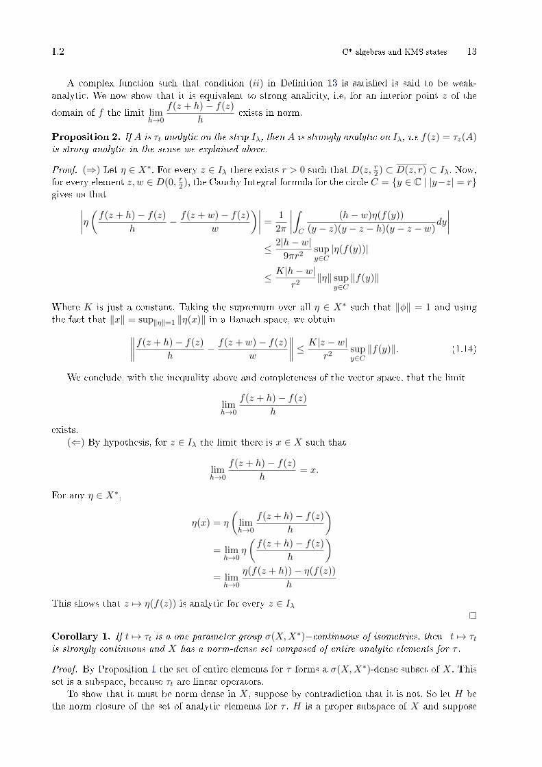
A complex function such that condition (ii) in Denition 13 is satised is said to be weak-analytic. We now show that it is equivalent to strong analicity, i.e, for an interior point z of the

domain of f the limit limh→0

f(z + h)− f(z)

hexists in norm.

Proposition 2. If A is τt analytic on the strip Iλ, then A is strongly analytic on Iλ, i.e f(z) = τz(A)is strong analytic in the sense we explained above.

Proof. (⇒) Let η ∈ X∗. For every z ∈ Iλ there exists r > 0 such that D(z, r2) ⊂ D(z, r) ⊂ Iλ. Now,for every element z, w ∈ D(0, r2), the Cauchy Integral formula for the circle C = y ∈ C | |y−z| = rgives us that∣∣∣∣η(f(z + h)− f(z)

h− f(z + w)− f(z)

w

)∣∣∣∣ =1

2π

∣∣∣∣∫C

(h− w)η(f(y))

(y − z)(y − z − h)(y − z − w)dy

∣∣∣∣≤ 2|h− w|

9πr2supy∈C|η(f(y))|

≤ K|h− w|r2

‖η‖ supy∈C‖f(y)‖

Where K is just a constant. Taking the supremum over all η ∈ X∗ such that ‖φ‖ = 1 and usingthe fact that ‖x‖ = sup‖η‖=1 ‖η(x)‖ in a Banach space, we obtain∥∥∥∥f(z + h)− f(z)

h− f(z + w)− f(z)

w

∥∥∥∥ ≤ K|z − w|r2

supy∈C‖f(y)‖. (1.14)

We conclude, with the inequality above and completeness of the vector space, that the limit

limh→0

f(z + h)− f(z)

h

exists.(⇐) By hypothesis, for z ∈ Iλ the limit there is x ∈ X such that

limh→0

f(z + h)− f(z)

h= x.

For any η ∈ X∗,

η(x) = η

(limh→0

f(z + h)− f(z)

h

)= lim

h→0η

(f(z + h)− f(z)

h

)= lim

h→0

η(f(z + h))− η(f(z))

h

This shows that z 7→ η(f(z)) is analytic for every z ∈ Iλ

Corollary 1. If t 7→ τt is a one parameter group σ(X,X∗)−continuous of isometries, then t 7→ τtis strongly continuous and X has a norm-dense set composed of entire analytic elements for τ .

Proof. By Proposition 1 the set of entire elements for τ forms a σ(X,X∗)-dense subset of X. Thisset is a subspace, because τt are linear operators.

To show that it must be norm dense in X, suppose by contradiction that it is not. So let H bethe norm closure of the set of analytic elements for τ . H is a proper subspace of X and suppose


that y ∈ X is such that y ∈ X \H. By the geometric form of Hahn-Banach for the sets H and ythere exists a ϕ ∈ X∗ such that

Reϕ(y) < Reϕ(w), w ∈ H. (1.15)

Since H is a proper subspace of X and Reϕ is a real linear functional , Reϕ(H) must be 0 orR. By equation (1.15), Reϕ(H) = 0. Next, it is not dicult to prove that Imϕ(x) = −Reϕ(ix),so Imϕ(H) = 0 as well. We conclude that ϕ vanishes on H and ϕ(y) 6= 0. This contradicts thefact that for y ∈ X there exists a sequence (xn)n∈N in H that ϕ(xn)→ ϕ(x). Now for A an analyticelement, t 7→ τt(A) is norm dierentiable by Proposition 2 and hence t 7→ τt(A) is norm continuous.For a general A ∈ X, we can nd a sequence of analytic elements An converging to A and estimate

‖τt(A)−A‖ ≤ ‖τt(A−An)‖+ ‖τt(An)−An‖+ ‖An −A‖= 2‖An −A‖+ ‖τt(An)−An‖

We conclude that τ is strongly continuous.

The previous Corollary is relevant, because we can apply it for a C*-Dynamical system (A, τ),since automatically ∗ − automorphisms of C*-algebras are isometries. We can nally dene whatis a KMS state.

Denition 14. Let (A, τ) be a C∗−Dynamical System, ω a state in A and β ∈ R. We say ω is a(τ, β)−KMS state if

ω(Aτiβ(B)) = ω(BA) (1.16)

for all A, B in a ∗−subalgebra A0 composed of entire analytic elements such that A0 is norm-denseand τ−invariant (this means τt(A) ∈ A0 for all A ∈ A0 and t ∈ R).

Some simple results are summarized in the following proposition.

Proposition 3. Let (A, τ) be a C*-Dynamical System, and A is unital. Then we have the following

i) ω is a (τ, 0)−KMS state ⇔ ω is a tracial2 state.

ii) ω is a (1, β)−KMS state ⇔ ω is a tracial state.

iii) ω is a (τt, β)−KMS state ⇔ ω is (τt/λ, λβ)−KMS.

Proof. Itens i) and ii) are trivial. Let a, b ∈ A0, where A0 is the dense ∗−sub-algebra of A indenition 14. We dene a new 1-parameter group, τ , as τ t = τt/λ. By equation (14) we have,

ω(aτ iλβ(b)) = ω(ba).

Therefore saying that ω is a (τ t, λβ)−KMS state is the same as saying that ω is a (τt/λ, λβ)−KMSstate.

Remark 5. Note thatτa+ib(A) = τa τib(A), para todo A ∈ U (1.17)

where a, b ∈ R. To prove that, let A ∈ A, by the Corollary 1 there is a sequence Ann≥1 of analyticelements such that An → A. To show (1.17) it is enough to prove τ−a τa+ib(An) = τib(An) and usethe fact that An → A. Using Proposition 1 we deduce

τ−a τa+ib(An) = τ−a

(√n

π

∫τt(An)e−n(t−a−ib)2

dt

)2A state ω is tracial if ω(AB) = ω(BA).


=

√n

π

∫τt−a(An)e−n(t−a−ib)2

dt

=

√n

π

∫τt(An)e−n(t−ib)2

dt

= τib(An).

We will use the following lemma from complex analysis in the proof of Theorem 3.

Lemma 2. Let O ⊆ C be a open and connected set such that V := O ∩ R 6= ∅. Dene

D = z ∈ C | Im z > 0 ∩ O.

Let F be a complex function which is holomorphic on D and continuous in D ∪ V. Suppose thatF (x) = 0 for all x ∈ V. Then F (z) = 0 for all z ∈ D.

Theorem 3. Let (A, τ) be a C∗-dynamical system, β ∈ R, and ω a state over A. Dene a strip as,

Dβ = z ∈ C | 0 < Imz < β if β > 0

Dβ = z ∈ C, | β < Imz < 0 if β < 0

In case β = 0, Dβ = R. The following statements are equivalent

1. ω is a (τ, β)−KMS state.

2. For any A,B ∈ A there exists a complex function FA,B which is analytic in the strip Dβ andcontinuous and bounded on Dβ satisfying

FA,B(t) = ω(Aτt(B)) ∀t ∈ R,FA,B(t+ iβ) = ω(τt(B)A) ∀t ∈ R;

(1.18)

3. For any A,B ∈ A there exists a complex function FA,B which is analytic in Dβ and continuouson Dβ satisfying

FA,B(t) = ω(Aτt(B)) ∀t ∈ R,FA,B(t+ iβ) = ω(τt(B)A) ∀t ∈ R;

(1.19)

Proof. (1) ⇒ (2) Let A0 be the ∗−sub-algebra in the denition of KMS state. For A,B entireanalytic elements. Since B is analytic, the function t 7→ ω(Aτt(B)) has an analytic extension andwe dene FA,B as

FA,B(z) = ω(Aτz(B)),

for all z ∈ C. Then FA,B is entire analytic. Since z 7→ τz(A) is analytic, we know it must be boundedin the compact set z ∈ C| Re z = 0, 0 ≤ Im ≤ β and FA,B must be continuous in Dβ as well,since

|FA,B(t+ iy)| = |ω (Bτt (τiy(A)))| ≤ ‖B‖‖τiy(A)‖ ≤ ‖B‖ sup0≤y≤β

‖τiy(A)‖.

for t+ iy ∈ Dβ . Observe as well that

FA,B(t+ iβ) = ω(Aτt+iβ(B)) = ω(Aτiβ(τt(B))) = ω(τt(B)A).

Then item (2) is satised when A,B ∈ A0.For A,B ∈ A there exists sequences An, Bn, both in A0 such that An → A, Bn → B. We dene

FAn,Bn(z) asFAn,Bn(z) = ω(Anτz(Bn)), z ∈ C


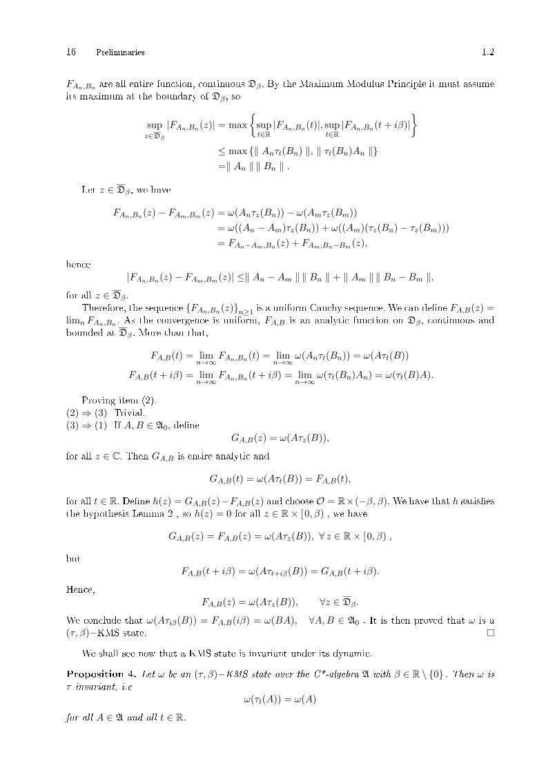
FAn,Bn are all entire function, continuous Dβ . By the Maximum Modulus Principle it must assumeits maximum at the boundary of Dβ , so

supz∈Dβ

|FAn,Bn(z)| = max

supt∈R|FAn,Bn(t)|, sup

t∈R|FAn,Bn(t+ iβ)|

≤ max ‖ Anτt(Bn) ‖, ‖ τt(Bn)An ‖=‖ An ‖ ‖ Bn ‖ .

Let z ∈ Dβ , we have

FAn,Bn(z)− FAm,Bm(z) = ω(Anτz(Bn))− ω(Amτz(Bm))

= ω((An −Am)τz(Bn)) + ω((Am)(τz(Bn)− τz(Bm)))

= FAn−Am,Bn(z) + FAm,Bn−Bm(z),

hence|FAn,Bn(z)− FAm,Bm(z)| ≤‖ An −Am ‖ ‖ Bn ‖ + ‖ Am ‖ ‖ Bn −Bm ‖,

for all z ∈ Dβ.Therefore, the sequence FAn,Bn(z)n≥1 is a uniform Cauchy sequence. We can dene FA,B(z) =

limn FAn,Bn . As the convergence is uniform, FA,B is an analytic function on Dβ , continuous andbounded at Dβ . More than that,

FA,B(t) = limn→∞

FAn,Bn(t) = limn→∞

ω(Anτt(Bn)) = ω(Aτt(B))

FA,B(t+ iβ) = limn→∞

FAn,Bn(t+ iβ) = limn→∞

ω(τt(Bn)An) = ω(τt(B)A).

Proving item (2).(2)⇒ (3) Trivial.(3)⇒ (1) If A,B ∈ A0, dene

GA,B(z) = ω(Aτz(B)),

for all z ∈ C. Then GA,B is entire analytic and

GA,B(t) = ω(Aτt(B)) = FA,B(t),

for all t ∈ R. Dene h(z) = GA,B(z)−FA,B(z) and choose O = R×(−β, β).We have that h satisesthe hypothesis Lemma 2 , so h(z) = 0 for all z ∈ R× [0, β) , we have

GA,B(z) = FA,B(z) = ω(Aτz(B)), ∀ z ∈ R× [0, β) ,

butFA,B(t+ iβ) = ω(Aτt+iβ(B)) = GA,B(t+ iβ).

Hence,FA,B(z) = ω(Aτz(B)), ∀z ∈ Dβ.

We conclude that ω(Aτiβ(B)) = FA,B(iβ) = ω(BA), ∀A,B ∈ A0 . It is then proved that ω is a(τ, β)−KMS state.

We shall see now that a KMS state is invariant under its dynamic.

Proposition 4. Let ω be an (τ, β)−KMS state over the C*-algebra A with β ∈ R \ 0 . Then ω isτ invariant, i.e

ω(τt(A)) = ω(A)

for all A ∈ A and all t ∈ R.

1.3 Universal C*-algebras: Generators and Relations 17

Proof. We assume β > 0. For A ∈ A0, the ∗−sub-algebra from the denition of KMS state, we setthe function f : C→ C as

f(z) = ω(τz(A))

Then f is analytic on C (or entire), since A is an entire analytic element for τ .

Let z ∈ R× [0, β], then:

|f(z)| = |ω(τz(A))| ≤ ‖τz(A)‖ = ‖τRe z τiIm z(A)‖ ≤ ‖τiIm z(A)‖ ≤M <∞

where M = sup‖τit(A)‖ | t ∈ [0, β]. It is nite because γ ∈ [0, β] →‖ τiγ(B) ‖ is continuous.Then we have that f(z) is bounded on the strip R× [0, β].

We show that f(z) is periodic with period iβ:

f(z + iβ) = ω(τz+iβ(A)) = ω(1τiβ(τz(A))) = ω(τz(A)1) = ω(τz(A)) = f(z).

Above we used the KMS condition and that τz(A) is a entire analytic element for τ . Then we havethat f(z) is bounded and analytic on C. By Liouville's Theorem we have that f(z) is constant and

ω(A) = f(0) = f(t) = ω(τt(A)), for all t ∈ R.

Since A0 is dense on A is follows that ω is τ−invariant

Now the following proposition will show us that the set of β such that there is a (τ, β)−KMSstate, is closed.

Proposition 5. Let (A, τ) a C∗−dynamical system and ωβn (τ, βn)−KMS for (A, τ) and βn → β.Then any accumulation point ω of ωβn is a (τ, β)−KMS state for (A, τ).

Proof. Let ω be an accumulation point of ωβn. Without loss of generality, we assume that ωβn →ω. Let A,B be entire analytic elements for τ , then τiβn → τiβ(B), we have

|ω(Aτiβ(B))− ω(BA)| ≤ |ω(Aτiβ(B))− ωβn(Aτiβn(B))| (1.20)

+ |ωβn(Aτiβn(B))− ωβn(BA)| (1.21)

+ |ωβn(BA)− ω(BA)| (1.22)

We just need to estimate the three terms on the right side. (1.22) goes to zero because ωβn → ω.(1.21) is zero because of the KMS condition. The rst we do a new estimation,

|ω(Aτiβ(B))− ωβn(Aτiβn(B))| ≤ |ω(Aτiβ(B))− ωβn(Aτiβ(B))| (1.23)

+ |ωβn(Aτiβ(B))− ωβn(Aτiβn(B))| (1.24)

Now, equation (1.23) goes to zero because ωβn → ω. Equation 1.24 goes to zero, since ωβn → ωand τiβn → τiβ . We conclude that ω(Aτiβ(B)) = ω(BA), so ω is (τ, β)-KMS.

1.3 Universal C*-algebras: Generators and Relations

This section is based on [Bla85, Phi89]. Here we shall be observing an important way to createC*-algebras.

In this section we consider a set G which we call its elements by generators. We dene a setG∗ := g∗ : g ∈ G. Then we denote by F(G) the free associative complex (or real) ∗-algebra(without identity) on G, i.e., the set of all polynomials in the noncommuting variables G t G∗


(disjoint union), with complex coecients and no constant term. By construction, any functionf : G→ A, where A is a C*-algebra, extends to a unique ∗-homomorphism from F(G) to A, whichwe also call f .

We also will consider a set R of relations on G, consisting in a collection of statements aboutthe elements of G which can be formulated for elements of a C*-algebra. These are some examples:

‖x‖ ≤ 1, where x can an element of S ⊆ F(G);

x is positive, x ∈ S ⊆ F(G);

x = x∗ for a specic x ∈ G

Since we want to see the generators as elements of a C*-algebra, we need to consider functions fromG to A, where A is any C*-algebra. However we need to keep the relations in R valid on A. Thatmotivates the following denition.

Denition 15. Let (G,R) be a pair of a set of generators and a set of relations. A representationof (G,R) in a C*-algebra A is a function π : G → A such that the elements the relations in R aresatised in A when we replace g by π(g) for all g ∈ G. A representation on a Hilbert space H is arepresentation in B(H).

Now we will establish some conditions which will assure the well denition of a universal C*-algebra.

Denition 16 (Admissibility). A pair (G,R) of generators and relations is said to be admissibleif the following conditions hold:

(1) the function from G to the zero C*-algebra is a representation of (G,R);

(2) if π is a representation of (G,R) in a C*-algebra A and B is a C*-subalgebra of A whichcontains π(G), then π is a representation of (G,R) in B;

(3) if π is a representation of (G,R) in a C*-algebra A and ϕ : A → B is a surjective ∗-homomorphism between C*-algebras, then ϕ π is a representation of (G,R) in B;

(4) for every g ∈ G there is a constant M(g) such that ‖π(g)‖ ≤ M(g) for every representationof (G,R) on any C*-algebra;

(5) if παα∈I is a family of representations of (G,R) on Hilbert spaces Hα, then g 7→ π(g) :=⊕α∈I πα(g) is a representation of (G,R) on H =

⊕α∈I Hα.

Remark 6. In presence of (3), the condition (1) is equivalent to there exists a representation of(G,R).

Some pairs (G,R) which are not admissible:

(a) G = x and R = ‖x‖ = 1 does not satisfy (1);

(b) G = 1, u andR = 1 is an identity , uu∗ = u∗u = 1, there exists a continuous path t 7→ut with u0 = 1, u1 = u, utu

∗t = u∗tut = 1 satisfy (1) but not (2);

(c) G = x and R = ‖x‖ ∈ 0, 1 satisfy (1) and (2), but not (3);

(d) G = x and R = x∗ = x satisfy (1), (2) and (3), but not (4);

(e) G = x and R = x∗ = x, ‖x‖ < 1 satisfy (1), (2), (3) and (4), but not (5).

1.3 Universal C*-algebras: Generators and Relations 19

Denition 17 (Universal C*-algebra on the Generators and Relations). Given a pair of generatorsand relations (G,R), the universal C*-algebra on (G,R) is a C*-algebra C∗(G,R) with a represen-tation π : G→ C∗(G,R), such that, given any representation ζ : G→ B, with B being a C*-algebra,there exists an unique ∗-homomorphism ϕ : C∗(G,R)→ B such that ζ = ϕ π.

Notice that, by construction, any two universal C*-algebras on the same pair (G,R) are isomor-phic with an unique isomorphism. This property is called universal property. And now, the mostimportant result on this construction.

Theorem 4. If (G,R) is admissible, then C∗(G,R) exists. Moreover, C∗(G,R) is the Hausdorcompletion3 of F(G) in the C∗-seminorm

‖x‖ := sup‖π(x)‖ : π is a representation of (G,R). (1.25)

Proof. By construction, any function fromG to any C*-algebra A extends to an unique ∗-homomorphismfrom F(G) to A, and in particular this result is valid for representations of (G,R) in A and on Hilbertspaces. Such representations do exist because the validity of the condition (1) of the denition 16.

The condition (4) in the same denition grants that ‖x‖ <∞ for any x ∈ F(G), then (1.25) iswell dened as a C∗-seminorm and the Hausdor completion of F(G) is granted, leading to a C*-algebra. The condition (5) guarantees that the obvious map G→ C∗(G,R) is also a representation.The conditions (2) and (3) ensure the universal property.

3Quotient by the usual equivalence relation of the C∗-seminorm.

Chapter 2

Algebraic Structure

In this Chapter we will dene what is a Groupoid, giving some examples for a better intuitionand some propositions about this structure. We have as a objective the study of the C*-algebrasassociated with those Groupoids. We used manly [Sim, Put].

2.1 Basic Denitions and results

Before we give the denition of a Groupoid, be aware that such denition varies throughoutthe literature and in particular the next denition is not how it is in [Put], but they are in factequivalent.

Denition 18. (Groupoid)A groupoid consists of a set G, a subset G(0) ⊂ G called units or the objects, two surjective maps

s, r : G→ G(0)(called source and range maps) and a law of composition (y1, y2) ∈ G(2) → y1y2 ∈ G,where

G(2) = (y1, y2) ∈ G×G : s(y1) = r(y2)

G(2) is called the set of composable parts. A groupoid must have the properties:

1. s(y1y2) = s(y2), r(y1y2) = r(y1) ∀(y1, y2) ∈ G(2) ;

2. s(x) = r(x) = x ∀x ∈ G(0) ;

3. ys(y) = y, r(y)y = y ∀y ∈ G;

4. (y1y2)y3 = y1(y2y3) when (y1, y2) ∈ G(2) and (y2, y3) ∈ G(2)

5. each y has a two-sided inverse y−1, so that yy−1 = r(y), y−1y = s(y)

The denition above does not seem natural as it is, however there is a really good picture ofhow a groupoid operates.

The elements of a groupoid G can be thought as an arrow between two nodes, much like this

The composition/product of a groupoid can be thought as a concatenation of arrow,

21

22 Algebraic Structure 2.1

And for the inverse.

The reader is invited to see how these pictures are related with all the axioms of a groupoid.For example, axiom 1 is simply saying that the source of the concatenation of two arrows is thesame as the source of the rst one. We think similarly about the range of the concatenation.

Example 1. As a simple example (probably the most simple) let H be a group and e its identity.Let G = H and G(0) = e. The range and source maps, both of them are constant maps s(x) =r(y) = e ∀x, y ∈ G. The law of composition is the same as the Group. We see that G(2) = G×Gand all the itens on the denition of a groupoid is easily veried.

A picture of a group H, as a groupoid, is of a loop.

Example 2. Let X be a set. We can think the cartesian product G := X × X as groupoid suchthat the unit space G(0) can be identied with X. Given an element g = (x, y) ∈ X ×X we denethe functions range and source as r(g) = (x, x) and s(g) = (y, y). G(0) := (x, x) : x ∈ X. Notethat we can identify G(0) with X with the canonical map (x, x) 7→ x Let h = (w, z), then the(g, h) ∈ G(2) if and only if s(g) = r(h), i.e (y, y) = (w,w) or simply y = w. We dene the productas (x, y)(y, z) = (x, z) and the inverse as (x, y)−1 = (y, x). It is not dicult to verify the axioms.Now, the nice picture here is that a pair (x, y) ∈ G can be thought as an arrow from y into x andthe mental image is the same as what we described before.

Denition 19. We say that a groupoid G is a topological groupoid if it is endowed with a topologysuch that all structure maps are continuous, i.e the source, range, composition and inverse mapsare continuous.

We note that the topology on G(2) is the one induced by the product topology. We don't needto check all of those maps as the next proposition tells.

Proposition 6. In a topological Groupoid G, continuity of the inverse map and the compositionimplies continuity of the source and range maps.

Proof. We show only that the range map is continuous, the proof is analogous for the source map.Denote the composition map by c and the inverse map by f . Dene ρ : G→ G(2) by ρ(y) = (y, y−1).Then the range map r can be written as

r = c ρ.

This implies that the continuity of the range map depends on the continuity of ρ. Let W ⊂ G(2)

be an open set. Without loss of generality, W has the form π−11 (U) ∩ π−1

2 (V ) ∩ G(2), where thoseπi denote the projection of G × G on the i-coordinate and U, V are open sets of G. This is truesince these kind of sets form a basis for the topology of G(2). Let y ∈ ρ−1(W ). The inverse map iscontinuous so f−1(V )∩U is an open set that contains y and it is contained in ρ−1(W ). This provesthat every y ∈ ρ−1(W ) is an interior point, making ρ−1(W ) an open set. ρ is therefore continuousand we conclude the proposition.

2.1 Basic Denitions and results 23

Denition 20. (Local Homeomorphism) A map f : X → Y between two topological spaces is alocal homeomorphism if, for every x in X, there is an open set U containing x such that f(U) isopen in Y and f |U : U → f(U) is a homeomorphism.

Proposition 7. Let X,Y be topological spaces and f : X → Y a local homeomorphism. Then f isa continuous open map.

Proof. First we prove continuity. Let x ∈ X. We want to show that, for every open neighborhood Vof f(x), there exists a neighborhood U of x such that f(U) ⊆ V . Let Ux be an open neighborhoodof x and Vx an open set in Y such that f induces a homeomorphism f |Ux : Ux → Vx and chooseany open neighborhood V of f(x). Then V ∩Vx is an open set in Y containing f(x), so there existsan open neighborhood U of x in Ux such that f(U) ⊆ V ∩ Vx; since U is open in Ux it is open inX as well and f(U) ⊆ V as requested.

Now we want to prove that f is open. Let A be open in X and, for each x ∈ A, choose opensets Ux ⊆ X and Vx ⊆ Y so that x ∈ Ux and f induces a homeomorphism between Ux and Vx. Foreach x ∈ A, f(Ux ∩A) is open in Vx, so it is open in Y as well. Therefore⋃

x∈Af(Ux ∩A) = f(A)

and f(A), as a union of open sets, must be open itself.

Denition 21. (Étale Groupoid)A topological groupoid G is said to be étale if s and r are local homeomorphisms. Any open set

U as in denition (20) is called an open bisection.

Remark 7. When G is an étale groupoid, a sucient condition to prove that an open set W ⊂ Gis also an open bisection is to prove that r and s are injective maps on W . Indeed since r and s areopen maps r(W ) and s(W ) are open. r|W is again an open map and it is continuous, the inverseis continuous as well, so r|W is a homeomorphism, similarly for s.

In this work, we deal with groupoids whose topology is locally compact Hausdor and étale. Wewon't be dealing with other types of topological groupoids.

Proposition 8. If G is an étale groupoid, then the subspace topology on Gx := y ∈ G : s(y) = xand Gx := y ∈ G : r(y) = x is equivalent to the discrete topology for all x ∈ G(0).

Proof. The subspace topology is trivially contained in the discrete topology. Now assume for acontradiction that there exists some z ∈ Gx such that z is not open in the subspace topology.Then any open set, U , of G, which z ∈ U must contain another element y in Gx. Since s is alocal homeomorphism, there exists a open set W of G, which z ∈W and s is injective on W . Thiscontradicts the previous statement, because there is no y ∈ Gx such that y ∈W . Hence we provedthat z is open in the subspace topology of Gx, hence this topology is the discrete one. The sameargument can be done for Gx.

Proposition 9. If G is a LCH étale groupoid, then G(0) is a clopen subset of G. The topology onG(0) is the one induced by G.

Proof. We divide the proof in two parts.G(0) is Closed:: Let ui be a net in G(0) that converges to u ∈ G. The functions r and s are

continuous, so r(ui) → r(u) and s(ui) → s(u). As ui ∈ G(0), we have r(ui) = s(ui) = ui. Henceu = s(u) = r(u) ∈ G(0), i.e, G(0) is closed in G.

G(0) is Open: Let x ∈ G(0). Since G is étale, there is an open U containing x such that s is ahomeomorphism on U . By the continuity of s, s−1(U) is open in G. Consider V := U ∩ s−1(U), an


open set containing x. We observe that V ⊆ G(0), since s(γ) = s(s(γ)) for all γ ∈ V . This showsthat x is an interior point and G(0) is open.

We need some properties for the set of bisections.

Proposition 10. Let G be an étale groupoid, then the set of bisections of G form an open basis forthe topology of G.

Proof. Given two open bisection V and W , it is clear that V ∩W is an open bisection as well. Now,let U be an arbitrary open set of G, then for every x ∈ U , there exists open sets V x

1 , Vx

2 such thatx ∈ V x

1 ∩ V x2 and r|V x1 is injective and s|V x2 as well. If Hx := V x

1 ∩ V x2 ∩ U , Hx is an open bisection

and⋃x∈U Hx = U . We conclude that the set of all bisections form an open basis for G.

Proposition 11. Let G be an étale groupoid, then if U, V are open bisections,

1. U−1 := γ−1 : γ ∈ U is an open bisection.

2. If p is the composition/product map of G, then UV := γη : γ ∈ U, η ∈ V and (γ, η) ∈G(2) = p((U × V ) ∩G(2)) is an open bisection.

Proof. Let us prove the rst assertion. The inversion map i is a homeomorphism, because it isbijective, continuous and the inverse is itself, i.e i−1 = i. Hence U−1 is an open set. Now forx, y ∈ U−1 such that r(x) = r(y), we have that x−1, y−1 ∈ U and r(x) = s(x−1) = r(y) = s(y−1).Since U is an open bisection, y−1 = x−1 which implies x = y. A similar argument shows that s isinjective in U−1 and we conclude that U−1 is an open bisection.

Now we prove the second assertion. We start by dening W = s(U) ∩ r(V ), an open subset ofG(0). Let U ′ = s|−1

U (W ) ⊂ U and V ′ = r|−1V (W ) ⊂ V . U ′ and V ′ are open bisections, because they

are open subsets of an open bisection. We have s(U ′) = r(V ′) = W . In addition, U×V ∩G(2) = U ′×V ′∩G(2), because if (g, h) ∈ U ×V ∩G(2), then s(g) = r(h) ∈W , so there are g′ ∈ U ′, h′ ∈ V ′ suchthat s(g) = s(g′) and r(h) = r(h′). Nevertheless as U ′ and V ′ are subsets of U and V respectively,by the injective property of r and s, g = g′ and h = h′. This justies U ×V ∩G(2) = U ′×V ′∩G(2).We can now, without loss of generality, suppose that our open bisections satisfy s(U) = r(V ).

U×V ∩G(2) is an open set of G(2). The map φ := r|−1V s|U : U → V is a homeomorphism, since it

is a composition of homeomorphisms. The map f from U to U×V dened by f(g′) = (g′, φ(g′)) hasimage in G(2), since r(φ(g′)) = s(g′). We claim that its image is precisely U ×V ∩G(2). We alreadyknow that its image is contained in U × V ∩G(2). For the reverse inclusion, suppose (g, h) ∈ G(2).Then g ∈ U , h ∈ V and s(g) = r(h). It follows that h = φ(g) and we proved the claim. f is injective.Since φ is continuous, and f is basically the identity on the rst coordinate, f is continuous as well.Denote by π1 the projection of U × V ∩ G(2) in U . Clearly π1 f is the identity on U and usingthe fact that f is onto U × V ∩ G(2), we conclude that π1 is injective. In addition, for all u ∈ U ,we have s(u) ∈ s(U) = r(V ), so s(u) = r(v) for some v ∈ V , then (u, v) ∈ U × V ∩ G(2) andπ1((u, v)) = u, which proves that π1 is onto. Since π1 and f are continuous, what we showed is thatboth are homeomorphisms.

Now we can consider the product p : U × V ∩ G(2) → UV and observe that for all (g, h) ∈U × V ∩G(2), the property that r(gh) = r(g) implies that

r|UV p = r|U π1. (2.1)

This proves that r|UV p is a homeomorphism and, since p is surjective, r|UV is injective,therefore a bijection onto UV . In addition, p is injective because, if p(x) = p(y), by equation (2.1)r|U π1(x) = r|U π1(y), hence x = y. Then p and r|W are continuous bijections such that theircomposition is an homeomorphism, which implies that both of them are homeomorphisms. SinceU×V ∩G(2) is an open set , so is UV . r is injective on UV . The proof ends with a similar argumentfor s|UV and we have that UV is an open bisection.

2.2 The ∗-algebra Cc(G) 25

2.2 The ∗-algebra Cc(G)

From now we will suppose that our groupoid is LCH étale and second countable, since that isour interest in rst place. The second countability is a hypothesis that [Sim] uses and so will us. Onthe other hand, this hypothesis is not fundamentally important for the construction that follows.Nevertheless a topological space which is LCH and secound countable is metrizable and this is aresult we use plenty in Chapter 4. The metrizability comes from Urysohn's metrization theorem.The construction of the C*-algebra can be generalized even more for groupoids that are not evenétale or Hausdor. We refer to [Ren80].

Let G be an étale, LCH and second countable groupoid. By the proposition 8, Gx and Gx arediscrete in G for every x ∈ G(0), which makes them have a countable number of elements as thespace is second countable. Let Cc(G) denote the the space of all continuous compactly supportedfunctions and we dene a convolution operation · and a involution ∗ : Cc(G)→ Cc(G) given by

f · g(γ) =∑αβ=γ

f(α)g(β) =∑

β∈Gs(γ)

f(γβ−1)g(β) =∑

α∈Gr(γ)

f(α)g(α−1γ) (2.2)

f∗(γ) = f(γ−1) (2.3)

Remark 8. We justify the second equality in (2.2), which is a change of variables. Let αβ = γ, sos(γ) = s(β), which implies that β ∈ Gs(γ). Since αβ = γ, α = γβ−1 we conclude that∑

αβ=γ f(α)g(β) =∑

β∈Gs(γ)f(γβ−1)g(β) For the third equality in (2.2), the argument is

analogous.

Remark 9. The sum in (2.2) is in fact nite. Denote K = supp(g) which is compact on G. Wehave

f · g(γ) =∑

β∈Gs(γ)

f(γβ−1)g(β) =∑

β∈Gs(γ)∩Kf(γβ−1)g(β)

Now, since K is compact and Gs(γ) is discrete, Gs(γ) ∩K is nite.

We still need to show that those operations are well dened. This is the content of the nexttheorem. First we prove the following lemma which is really useful for calculations. We denote thefunctions in Cc(G) which are supported on an open bisection by C(G)

Lemma 3. Let G be an étale groupoid which is locally compact and Hausdor. Every element ofCc(G) is a sum of functions in C(G).

Proof. Let f be in Cc(G). Using the fact that the support of f is compact and that the openbisections form a neighborhood base for the topology, we may nd a nite cover, Uini=1, of thesupport of f by open bisections. Dene Un+1 := G \ supp(f). Since G is locally compact andHausdor there exists a partition of unity αin+1

i=1 of G which is subordinate to the cover Uin+1i=1 .

Then we have

f =

n+1∑i=1

fαi =n∑i=1

fαi

. Now just observe that fαi ∈ C(G) i = 1, ..., n, concluding the proof.

Now we can prove that the operations of convolution and involution are well dened. This willbe fundamental for the denition of the groupoid C*-algebra.

Theorem 5. Let G be a LCH étale groupoid that is second countable. For any f, g ∈ Cc(G), theset Cc(G) with the operations

f · g(γ) =∑αβ=γ

f(α)g(β) =∑

β∈Gs(γ)

f(γβ−1)g(β) =∑

α∈Gr(γ)

f(α)g(α−1γ)


f∗(γ) = f(γ−1)

is a ∗-algebra

Proof. If f ∈ Cc(G) has support on a open bisection U , we will be using the notation that f ∈(Cc(G), U). We divide the proof in the following steps

Good denition of the involution:

Given f ∈ Cc(G) we prove that f∗ ∈ Cc(G). First, suppose that f ∈ (Cc(G), U), U anopen bisection. That f∗ is continuous comes with ease because the complex conjugation andinversion in G are both continuous. Since f∗(x) = f(x−1), we have that

supp(f∗) = x ∈ G|f(x−1) 6= 0 =: H,

Given x ∈ supp(f∗), there is a sequence (xi)i on H such that xi → x and since xi ∈ H wehave f(x−1

i ) 6= 0. As f(x−1i ) 6= 0, we have x−1

i ∈ supp(f). By continuity x−1i → x−1, therefore

x−1 ∈ supp(f) ⊂ U and we conclude that x ∈ U−1. This shows that supp(f∗) ⊂ U−1.

Now we show that supp(f∗) is compact. Since supp(f) is compact, supp(f)−1 is compact. Wehave that H ⊂ x−1|f(x) 6= 0 ⊂ supp(f)−1 and so supp(f∗) = H is a closed set inside acompact set, then supp(f∗) is compact.

We have shown that for f ∈ C(G), f∗ ∈ C(G). For f ∈ Cc(G), f =∑

i fi and fi ∈ C(G),which implies that f∗ =

∑i f∗i , f

∗i ∈ C(G). We conclude that f∗ ∈ Cc(G) because Cc(G) is a

linear space.

Now we take a look at the convolution. We need that f · g has compact support and iscontinuous if both f and g are.

f · g has compact support:

Let supp(f) · supp(g) denote the set γ ∈ G : γ = αβ, α ∈ supp(f), β ∈ supp(g). Note thatthis set is compact as p(supp(f)× supp(g)) = supp(f) · supp(g), where p is the compositionmap on G. We claim that supp(f · g) ⊆ supp(f) · supp(g). Let γ ∈ supp(f · g). Then,∑

αβ=γ

f(α)g(β) 6= 0 =⇒ ∃α, β αβ = γ and f(α)g(β) 6= 0

=⇒ f(α) 6= 0 and g(β) 6= 0 =⇒ α ∈ supp(f), β ∈ supp(g).

So γ ∈ supp(f) · supp(g). It means that supp(f · g) is a closed subset of a compact set and,since the topology is Hausdor, we conclude that supp(f · g) is compact.

Given f ∈ (Cc(G), U) and g ∈ (Cc(G), V ), then f · g ∈ (Cc(G), UV ): Let γ ∈ G andf · g(γ) 6= 0. There are x, y ∈ G such that xy = γ and f(x), g(y) 6= 0, which by hypothesis onthe support guarantees x ∈ U and y ∈ V and that implies γ ∈ UV . Since r(γ) = r(x) andx ∈ U , an open bisection, we can write x = r|−1

U (r(γ)). By the same argument we also havey = s|−1

V (s(γ)).

In fact for γ ∈ UV there are unique x ∈ U and y ∈ V such that xy = γ, which are given bythe above formula. We conclude that

f · g(γ) = f(r|−1U (r(γ)))g(s|−1

V (s(γ))), γ ∈ UV ,

and the expression is zero for γ /∈ UV . Since the functions f, g, r, s are continuous (and theinverse of r, s are continuous on the appropriate domain) we observe that f ·g|UV is continuous.Our job is done when proving continuity on all domain. On the proof that f · g has compactsupport, we have shown that supp(f · g) ⊂ supp(f) · supp(g) ⊂ UV . From now on we dene

2.3 The Full Groupoid C*-algebra 27

A := supp(f) and B := supp(g). Given x ∈ G and a sequence xi → x, x /∈ UV impliesx ∈ G \ AB and the latter is an open set, meaning that xi ∈ G \ AB for large enough i. Weconclude for x /∈ UV that f · g(x) = 0 = limi f · g(xi). Now, if x ∈ UV , xi ∈ UV for largeenough i since it is open, by continuity on UV we conclude f · g(xi)→ f · g(x). This is truenow for every x ∈ G, so f · g is continuous with support on UV .

f · g ∈ Cc(G):

Now consider any f, g ∈ Cc(G) = span C(G), so f =∑

i fi and g =∑

j gj , fi ∈ (Cc(G), Ui)and gj ∈ (Cc(G), Vj). By linearity f · g =

∑i,j fi · gj and by the item we proved above this

one, we have fi · gj ∈ (Cc(G), UiVj). As Cc(G) is a vector space, f · g ∈ Cc(G).

∗−algebra structure:

Let f, g, h ∈ Cc(G). That (f∗)∗ = f is pretty evident, knowing that (γ−1)−1 = γ for γ ∈ G.To prove that (f · g)∗ = g∗ · f∗, let γ ∈ G,

(f · g)∗(γ) = f · g(γ−1) =∑

αβ=γ−1

f(α)g(β) =∑

β−1α−1=γ

g∗(β−1)f∗(α−1) =∑xy=γ

g∗(x)f∗(y)

= (g∗ · f∗)(γ).

Now let us prove the associativity of the convolution. Let γ ∈ G:

(f · g) · h(γ) =∑ab=γ

f · g(a)h(b) =∑ab=γ

(∑cd=a

f(c)g(d)

)h(b) =

∑cdb=γ

f(c)g(d)h(b)

On the other hand:

f · (g · h)(γ) =∑ab=γ

f(a)(g · h)(b) =∑ab=γ

f(a)

(∑cd=b

g(c)h(d)

)=∑acd=γ

f(a)g(c)h(d)

We conclude that (f · g) · h = f · (g · h).

Using the *-algebra Cc(G), we present rst the Full Groupoid C*-Algebra.

2.3 The Full Groupoid C*-algebra

Here in this section, one of our main concerns will be studying the representations of Cc(G) ona Hilbert space, i.e the *-homeomorphisms from Cc(G) as a ∗-algebra to the C*-Algebra B(H), thebounded linear operators on a Hilbert space H.

Proposition 12. Let G be a LCH étale and second countable groupoid with G(0) its unit space.Cc(G

(0)), as a set, is a union of C*-algebras.

Proof. Let K be a compact set in G(0). We dene

CK := f : G→ C | supp(f) ⊂ K and f is continuous.

Next, we equip this set with point-wise multiplication and the involution given by the complexconjugation. Endowing it with the natural norm ||f ||∞ = supx∈K |f(x)|, CK is a C*-algebra. Indeedthe completeness comes from the fact that all of its elements have support on the same compactK. Here, we remember that the unit space G(0) is open and closed on G, in such a way that every


function f on Cc(G(0)) has a simple extension on Cc(G), which is f1(x) = 0 for x ∈ G \ G(0) and

f1(x) = f(x) for x ∈ G(0). We identify f and f1. Hence, we shall think Cc(G(0)) as a subset of

Cc(G). Now we claim that

Cc(G(0)) =

⋃f∈Cc(G(0))

Csupp(f).

This proves our proposition since CK is a C*-algebra as we said above. Let f ∈ Cc(G(0)),

then f ∈ Csupp(f) and it proves one inclusion. If h ∈⋃f∈Cc(G(0))Csupp(f) then h ∈ Csupp(f) for a

f ∈ Cc(G(0)), which implies that supp(h) ⊂ supp(f). As the later is compact, supp(h) is compact.As supp(f) is a subset of G(0) we conclude so it is supp(h).

Proposition 12 is important since it will permit us to prove the inequality ||π(f)|| ≤ ||f ||∞for every f ∈ C(G) and π a representation of Cc(G). This is not trivial because Cc(G) is not aC*-algebra. Now let f ∈ C(G) and U the bisection it is supported. We have already seen that f∗

has support on U−1, hence f · f∗ ∈ Cc(UU−1) ⊂ Cc(G(0)). By proposition 12, we have that f · f∗ isin one C*-algebra B. If π is a representation of Cc(G), π|B : B → B(H) is a representation of theB. We have that

||π(f · f∗)|| ≤ ||f · f∗||∞ =⇒ ||π(f)||2 = ||π(f · f∗)|| ≤ ||f · f∗||∞.

Now we need to see what is ||f · f∗||∞ in terms of ||f ||∞ if f ∈ C(G). We basically need to verifywhat is the value of f ·f∗(x) for x ∈ G. Consider U to be the open bisection such that supp(f) ⊂ U .By the convolution formula we have f · f∗(x) =

∑yz=x f(y)f(z−1). Considering x ∈ G such that

f · f∗(x) 6= 0, this sum trivialize to only one pair (y, z) such that yz = x and f(y), f(z−1) 6= 0,because U is an open bisection. We see that y, z−1 ∈ U . If there was another pair (y1, z1) in the sameconditions, clearly r(y) = r(x) = r(y1) and since y, y1 ∈ U and r is injective there, we concludey = y1. A similar argument can be used for z and z1.

We can see that in fact y = r|−1U (r(x)) and s(y) = r(z) = s(z−1) which implies that y = z−1.

Finally, we conclude that for every x ∈ G such that f · f∗(x) 6= 0 there exists a unique y ∈ G suchthat f · f∗(x) = f(y)f(y) = |f(y)|2 and so

||f · f∗||∞ = supx∈G|f · f∗(x)| = sup

x∈U|f(x)|2 = ||f ||2∞.

The last equality is a consequence of supp(f) ⊂ U . We conclude that for f ∈ C(G) and π arepresentation of Cc(G) that ||π(f)|| ≤ ||f ||∞.

Proposition 13. Let G be a LCH étale and second countable groupoid. For each f ∈ Cc(G), thereis a constant Kf ≥ 0 such that ||π(f)|| ≤ Kf for every *-representation π : Cc(G) → B(H) ofCc(G) on a Hilbert space. If f is supported on a bisection, we can take Kf = ||f ||∞.

Proof. Take f ∈ Cc(G). By the lemma 3 we have f =∑n

i=1 fi, where fi is supported on a bisection.We dene then Kf :=

∑ni=1 ||fi||∞. Now take π a *-representation of Cc(G) and it is true that

||π(fi)|| ≤ ||fi||∞.It is clear then that ||π(f)|| = ||

∑i π(fi)|| ≤

∑i ||fi||∞ = Kf , which proves the statement.

Denition 22. Let G be an LCH étale and second countable groupoid and f ∈ Cc(G). We dene

||f ||u := supπ rep.

||π(f)||

We dene the full C∗-algebra of G, denoted by C∗(G) by being the completion of Cc(G) by the"norm" || · ||u, i.e:

C∗(G) := Cc(G)||·||u

2.3 The Full Groupoid C*-algebra 29

Remark 10. Observe that we put in quotes the word norm on the previous denition. The reasonfor that is that at this point of the work, we only know that || · ||u is a C∗-seminorm. In the nextsection, we prove the existence of a representation of Cc(G) that is faithful, therefore showing that|| · ||u is indeed a norm.

Before we proceed to the next section, there is an important remark to be made about thedenition the above C*-algebra. At rst, it does not agrees with Renault's denition. This is because,in his book [Ren80], he deals with a more general framework, the non-étale case. In the non-étalecase, Renault denes the full norm, not as the supremum over all ∗-representations of Cc(G), but asthe supremum only over ∗-representations of Cc(G) that are bounded with respect to the I-normon Cc(G). If G is étale, the I-norm is given by

‖f‖I = supx∈G(0)

max ∑γ∈Gx

|f(γ)|,∑γ∈Gx

|f(γ)|.

Renault shows that it is equivalent to say that a *-representation is bounded in the I-normand that it is continuous in the inductive-limit topology on Cc(G), i.e, the topology obtained byregarding Cc(G) as the inductive limit of the subspaces XK :=

(f ∈ C(G) | supp(f) ⊆ K, ‖ · ‖∞

)indexed by compact subsets K of G, we refer to [Con90] if one is not familiar with this topologyand its properties. It is in Chapter IV, section 5.

So to be sure we are talking about the same C∗-algebra as Renault, we must verify that every∗-representation of Cc(G) is continuous in the inductive-limit topology when G is étale; and forcompleteness we should also prove that continuity in this topology implies boundedness with respectto the I-norm, which shows that both denitions agree on our setting.

Lemma 4. Suppose that G is LCH étale groupoid. Then every ∗-representation π of Cc(G) is bothcontinuous in the inductive-limit topology, and bounded in the I-norm.

Proof. Fix a ∗-representation of Cc(G). By Proposition 5.7 on [Con90], to see that π is continuous inthe inductive-limit topology, we just have to check that π|XK is continuous for each compactK ⊆ G.Now, let K ⊆ G be compact. Since the range and source functions are local homeomorphisms wecan cover K by open bisections, and then use compactness to obtain a nite subcover K ⊆

⋃ni=1 Ui,

each Ui an open bisection. Fix a partition of unity hi for K subordinate to the Ui. Then forf ∈ XK , Proposition 13 gives

‖π(f)‖ =∥∥∥∑

i

π(hif)∥∥∥ ≤ n∑

i=1

‖π(hif)‖ ≤n∑i=1

‖hif‖∞ ≤( n∑i=1

‖hi‖)‖f‖∞ ≤ n‖f‖∞.

So π is Lipschitz on XK with Lipschitz constant at most n, which shows continuity on XK for everyK and by what we discussed above, π is continuous in the inductive-limit topology.

To see that it is I-norm bounded, observe that if f ∈ Cc(G), then for any γ ∈ G, γ ∈ Gs(γ)∩Gr(γ)

and clearly,

|f(γ)| ≤ max ∑γ∈Gs(γ)

|f(γ)|,∑

γ∈Gr(γ)

|f(γ)|.

With that in mind, we have ‖f‖∞ ≤ ‖f‖I . So the inductive-limit topology is weaker than theI-norm topology, and we deduce that π is continuous for the I-norm. Since continuity is equivalentto boundedness for linear maps on normed spaces, we deduce that π is I-norm bounded. Forcompleteness , we now show that such bound is less or equal to 1, i.e, that ‖π(f)‖ ≤ ‖f‖I . Forthat, we rst observe that ‖ · ‖I is a ∗-algebra norm, so π extends to a ∗-homomorphism from the

Banach ∗-algebra completion Cc(G)Iof Cc(G) in the I-norm into B(H). Write ρA : A→ [0,∞) for

the spectral-radius function on a Banach algebra A. Now, since π is a *-homeomorphism, it is clear

that it does not enlarge spectra of self-adjoint elements, i.e, If y ∈ Cc(G)Iis a self adjoint element,

then sp(π(y)) \ 0 ⊆ sp(y) \ 0.


With that in mind, for each f ∈ Cc(G), we have, observing that f∗ · f is self adjoint,

‖π(f)‖2 = ‖π(f∗ · f)‖ = ρB(H)(π(f∗ · f)) ≤ ρCc(G)

I (f∗ · f) ≤ ‖f∗ · f‖I ≤ ‖f‖2I .

This concludes the proof.

2.4 The Reduced Groupoid C*-algebra

Here we proceed to show a faithful representation of Cc(G), called the regular representation.Eventually we are going to use the following fact.

Proposition 14. For any locally compact Hausdor space X, let

C0(X) := f ∈ C(X) : ∀ε > 0 the set x : |f(x)| ≥ ε is compact

With pointwise addition, multiplication, complex conjugation and supremum norm C0(X) is a C*-algebra.

We start by taking u ∈ G(0). With that consider the Hilbert space `2(s−1(u)) of functions froms−1(u) to C that are square summable. As a reminder we write its denition, namely

`2(s−1(u)) =

ζ : s−1(u)→ C :∑

x∈s−1(u)

|ζ(x)|2 <∞

The inner product is clearly given by 〈ζ, η〉 =

∑x∈s−1(u) ζ(x)η(x). We remember as well the

notation s−1(u) = Gu and note that, since G is second countable, Gu is countable by proposition8. We now dene πuλ : Cc(G)→ B(`2(Gu)) by

πuλ(f)ζ(x) :=∑

y:r(y)=r(x)

f(y)ζ(y−1x), f ∈ Cc(G) ζ ∈ B(`2(Gu)) x ∈ `2(Gu)

There is some work to do here. First we need to prove that this function is well dened and is arepresentation of Cc(G) to B(`2(Gu)). In order to prove these claims, dene for each γ ∈ G(0) theelement

δγ(η) =

1, γ = η

0, γ 6= η

which belongs to `2(Gu). Moreover, the set δγ : γ ∈ G(0) is an orthonormal basis for `2(Gu),therefore the function πuλ could have been dened only on those elements.

Proposition 15. πuλ is a representation of Cc(G).

Proof. Good Denition of πuλ

First, the sum∑

y:r(y)=r(x) f(y)ζ(y−1x) is nite on a similar argument we made for the def-inition of the convolution product on Cc(G). Let f ∈ C(G). It is not dicult to verify thatπuλ(f) is a linear operator. We prove that ||πuλ(f)ζ|| ≤ ||f ||∞||ζ||. For that, consider U to bethe open bisection which f is supported. We shall see how the formula for πuλ reduces for suchfunctions,

πuλ(f)ζ(x) =∑

y:r(y)=r(x)

f(y)ζ(y−1x).

The sum is on y ∈ r−1(r(x)) ∩ supp(f), x ∈ Gu, since the points where f is zero does notconcern us. This set, in fact, contains at most one element. Let y1, y2 ∈ r−1(r(x)) ∩ supp(f).Then r(y1) = r(y2) = r(x) and both are in U , since r is a homeomorphism in such set y1 = y2.We write y = yx for the unique element in r−1(r(x)) ∩ supp(f) with x ∈ Gu. We have

2.4 The Reduced Groupoid C*-algebra 31

πuλ(f)ζ(x) =

f(yx)ζ(y−1

x x), If r−1(r(x)) ∩ supp(f) 6= ∅0, otherwise

.

||πuλ(f)ζ||2 =∑x∈Gu

|f(yx)ζ(y−1x x)|2 ≤ ||f ||2∞

∑x∈Gu

|ζ(y−1x x)|2 ≤ ||f ||2∞||ζ||2

This proves that ||πuλ(f)|| ≤ ||f ||∞ < ∞ for f ∈ C(G), but by linearity on f(which is easyto verify) we have as well ||πuλ(f)|| < ∞ for all f ∈ Cc(G), proving that πuλ(f) ∈ B(`2(Gu))which proves that πuλ is well dened.

Compatibility with involution, i.e πuλ(f∗) = πuλ(f)∗

For this calculation and the next item we shall be using the basis of `2(Gu) given by δx. Letus calculate πuλ in this basis.

πuλ(f)δx(h) =∑

y:r(y)=r(x)

f(y)δx(y−1h) = f(hx−1)

And that implies,

πuλ(f)δx =∑

h:s(h)=u

f(hx−1)δh

.

We, then, can calculate

〈πuλ(f∗)δx1 , δx2〉 = 〈∑

h:s(h)=u

f∗(hx−11 )δh, δx2〉 =

∑h:s(h)=u

f(x1h−1)〈δh, δx2〉

= f(x1x−12 ) =

∑h:s(h)=u

f(hx−12 )〈δx1 , δh〉

= 〈δx1 ,∑

h:s(h)=u

f(hx−12 )δh〉 = 〈δx1 , π

uλ(f)δx2〉.

As x1 and x2 are arbitrary elements of Gu, we conclude that πuλ(f∗) = πuλ(f)∗.

Multiplicative property, i.e πuλ(f · g) = πuλ(f)πuλ(g)

Consider again δx. We already proved that

πuλ(f)δx =∑

y:s(y)=u

f(yx−1)δy. (2.4)

Now, using the above equality, changing f → f · g and using the convolution product thirdequality in (2.2), we have the expression

πuλ(f · g)δx =∑

y:s(y)=u

∑k:r(k)=r(yx−1)=r(y)

f(k)g(k−1yx−1)

δy

Using (2.4) and linearity of πuλ(f) we have

πuλ(f)πuλ(g)δx =∑

y:s(y)=u

w :∑

s(w)=u

f(yw−1)g(wx−1)

δy


What it is needed to do here is to show that in fact πuλ(f)πuλ(g)δx = πuλ(f · g)δx with thosetwo expressions at hand.

Let y ∈ G such that s(y) = u. We dene the function Uy : s−1(u)→ r−1(r(y)) by x 7→ yx−1.One can verify that it is a bijection and the inverse U−1

y : r−1(r(y))→ s−1(u) is given by themap k 7→ k−1y.

With all of this in hand, we have:∑w:s(w)=u

f(yw−1)g(wx−1) =∑

w:s(w)=u

f(Uy(w))g(U−1y Uy(w)x−1) =

∑k:r(k)=r(y)

f(k)g(U−1y (k)x−1)

=∑

k:r(k)=r(y)

f(k)g(k−1yx−1)

And this nally proves that πuλ(f)πuλ(g)δx = πuλ(f · g)δx, since the two expressions coincide.We conclude then that πuλ is a *-homomorphism.

For f ∈ Cc(G), we showed in the prove above that, for x ∈ Gu,

πuλ(f)δx =∑

y:s(y)=u

f(yx−1)δy

We, in fact, can write it in another form. Consider the functions

φ : s−1(u)→ s−1(r(x)), y 7→ yx−1

ψ : s−1(r(x)) 7→ s−1(u), h 7→ hx

They are bijections and inverse one of the other. Indeed, if φ(y1) = φ(y2) we have yx−1 = y2x−1

which implies y1 = y2. Similarly for ψ. They are inverses, since φ(ψ(z)) = φ(hx) = hxx−1 = z. Theother relation is analogous. We conclude that∑

y:s(y)=u

f(yx−1)δy =∑

y:s(y)=u

f(φ(y))δy

=∑

h:s(z)=r(x)

f(φ(ψ(h)))δψ(h)

=∑

h:s(z)=r(x)

f(h)δhx

Then, for f ∈ Cc(G) and x ∈ G such that x ∈ Gu we can derive the identity

πuλ(f)δx =∑

h:s(h)=r(x)

f(h)δhx

This is going to be useful for the next proposition.

Proposition 16. Let f ∈ Cc(G). Then it is true:

f(y) = 〈πs(y)λ (f)δs(y), δy〉

for all y ∈ G.

Proof. Consider an element y ∈ G, by the considerations we've done:


πuλ(f)δx =∑

h:s(h)=r(x)

f(h)δhx =⇒ πs(y)λ (f)δs(y) =

∑h:s(h)=r(s(y))=s(y)

f(h)δhs(y) =∑

h:s(h)=s(y)

f(h)δh

Then:

〈πs(y)λ (f)δs(y), δy〉 =

∑h:s(h)=s(y)

f(h)〈δh, δy〉 = f(y)

We now have the resources to show the regular representation of Cc(G). Each πuλ, for u ∈ G(0)

is a representation of Cc(G) on the Hilbert space `2(Gu). Now consider the direct sum

S :=⊕u∈G(0)

`2(Gu)

Which are the vectors (xu) indexed onG(0) such that xu ∈ `2(Gu) and the sum∑

u∈G(0)〈xu, xu〉`2(Gu)

is nite. The inner product on S is

〈(xu), (yu)〉 =∑

u∈G(0)

〈xu, yu〉`2(Gu)

Naturally such inner product induces a norm on S and we can consider the completion of suchspace, a Hilbert space denoted by `2(G) := S.

We can consider in S , for f ∈ Cc(G), the function πλ(f) : S → S which is dened as

(xu) 7→ (πuλ(f)(xu))

It is routine to verify that it is a linear operator and that it is continuous. Since S is dense in`2(G), πλ(f) has a unique continuous extension and to not use too much notation, such extensionwill still be denoted by πλ(f).

We can nally dene the regular representation of Cc(G) by being the *-homomorphism

πλ : Cc(G)→ B(`2(G))

f 7→ πλ(f)

By construction, we observe that is satises πλ(f)(x) = (πuλ(f)(xu)) for x ∈ S. Now we wish toshow that such a representation is faithful.

Theorem 6. The regular representation πλ is faithful

Proof. Here where comes the importance of the formula on Proposition 16. Let f ∈ Cc(G) suchthat πλ(f) = 0. Then πλ(f)x = (πuλ(f)(xu)) = 0 for all x ∈ S. Let y ∈ G and consider the vectorx ∈ S such that xs(y) = δs(y) and zero otherwise. This makes sense because δs(y) ∈ `2(Gs(y)). By the

above πs(y)λ (f)δs(y) = 0 and by the formula on proposition 16 we have that f(y) = 0. Since y ∈ G

was arbitrary, we conclude that f = 0.

We can now dene the reduced C*-algebra:

Denition 23. The reduced C∗-algebra of an LCH étale second countable groupoid G, denoted byC∗r (G), is the completion of Cc(G) by the norm

||f ||r := ||πλ(f)||.

We are now interested in showing that the above norm can be rewritten as the supremum overthe representations we used to dene πλ.


Proposition 17. For f ∈ Cc(G):

||f ||r = supu∈G(0)

||πuλ(f)||

Proof. We prove the two inequalities, namely supu∈G(0) ||πuλ(f)|| ≤ ||f ||r and ||f ||r ≤ supu∈G(0) ||πuλ(f)||.For the rst, let xu ∈ `2(Gu) and dene x = (0, ..., xu, ...), i.e the element of `2(Gu) such that

in the u component is equal to xu. Clearly ||xu|| = ||x|| and by the denition of πλ, we haveπλ(f)(x) = πuλ(f)(xu). With that

||πuλ(f)(xu)|| = ||πλ(f)(x)|| ≤ ||πλ(f)||||x|| = ||πλ(f)||||xu||

Since ||πuλ(f)|| = sup||xu||≤1 ||πuλ(f)(xu)|| we have that supu∈G(0) ||πuλ(f)|| ≤ ||f ||r.Now, for the other side, consider

||f ||r = supx∈`2(G),||x||≤1

||πλ(f)x||

The supremum on the right hand side could have been done on the elements x ∈ S because Sis dense in `2(G). Then

||πλ(f)x||2 = ||(πuλ(f)(xu))||2 =∑

u∈G(0)

||πuλ(f)xu||2 ≤ supu∈G(0)

||πuλ(f)||2||x||2

The above proves that ||f ||r ≤ supu∈G(0) ||πuλ(f)|| and we conclude that they must be equal.

Now, since we have nally dened both C*-Algebras, we should see how they relate with eachother; that is the content of the next proposition.

Proposition 18. Let G be a LCH étale and second countable groupoid. There exists an closed idealI of C∗(G) such that

C∗(G)/I ' C∗r (G)

.

Proof. First, consider the identity function i : (Cc(G), || · ||u)→ C∗r (G), which means that i(f) = ffor f ∈ Cc(G). Clearly, it is a *-homomorphism and

||i(f)||r = ||f ||r ≤ ||f ||u,

i.e, it is bounded. Since (Cc(G), || · ||u) is dense in C∗(G), there is a extension q of i to all C∗(G)and this extension is a *-homomorphism. We have that Cc(G) ⊂ Im q and, because Im q is anC*-algebra, we conclude that

C∗r (G) = Cc(G)||·||r ⊂ Im q.

By the above q is surjective. Dene I := Ker q, which is an closed ideal of C∗(G) and consider thequotient C∗(G)/I. Now, q induces an injective *-homomorphism of C∗(G)/I onto C∗r (G). Indeed,for h+ I ∈ C∗(G)/I dene

q′ : C∗(G)/I → C∗r (G), h+ I 7→ q(h).

It is well dened, since given h+ I ∈ C∗(G)/I and g ∈ h+ I, i.e g = h+ f for f ∈ I we have,since f ∈ Ker q,

q′(h+ I) = q(h) = q(h+ f) = q(g) = q′(g + I).

It is routine to verify the axioms for *-homomorphism, we prove that it is injective. Indeed, letq′(h + I) = q′(g + I), which implies q(h) = q(g) and q(h − g) = 0, which means that h − g ∈ I.


This proves that h ∈ g + I and h + I = g + I, concluding that q′ is an injective *-homomorphismbeetween the two C*-Algebras C∗(G)/I and C∗r (G) , i.e, C∗(G)/I ' C∗r (G).

This is, in particular, a relevant proposition, because if we know that C∗(G) is simple, i.e, thereare no non-trivial closed ideals, then by proposition 18 we have C∗(G) ' C∗r (G). This will be thecase for the groupoid we study on the next chapter.

Now we wish to see hoe the C*-Algebra C0(G(0)) is related with those. In fact, it is a sub-C*-algebra of C∗r (G) and C∗(G). Next we introduce a conditional expectation of C∗r (G) (C∗(G))onto C0(G(0)). By Conditional expectation of a C*-Algebra A onto a sub-C*-algebra B, we meana positive and continuous linear map P , such that its restriction to B is the identity in B and fora ∈ A, b1, b2 ∈ B, we have P (b1ab2) = b1P (a)b2.

Proposition 19. Let G be a LCH, étale and second countable groupoid. For any B ⊂ G, an openbisection, there exists j : C0(B)→ C∗r (G) and h : C0(B)→ C∗(G), both linear and isometric maps.

Proof. We already have, for f ∈ C(G), that ‖π(f)‖ ≤ ‖f‖∞ , where π is a representation of Cc(G).Clearly, taking the supreme over all representations or only the regular representations we havethat ‖f‖u ≤ ‖f‖∞ and ‖f‖r ≤ ‖f‖∞. First, we prove the proposition for C∗r (G). Fix B an openbisection and consider the inclusion map i : Cc(B) → C∗r (G), f 7→ f . It is linear and continuous,indeed the continuity comes from the fact that i is bounded,

‖i(f)‖r = ‖f‖r ≤ ‖f‖∞.

By proposition 16, for any f ∈ Cc(G) and x ∈ G,

|f(x)| = |〈πs(x)λ (f)δs(x), δx〉| ≤ ‖π

s(x)λ (f)‖.

Where we used the Cauchy-Schwartz inequality. Taking the supreme over all x ∈ G,

‖f‖∞ ≤ supx∈G‖πs(x)

λ (f)‖ ≤ ‖f‖r

This shows that for f ∈ C(G), the reduced norm and the uniform norm coincides. Since ‖f‖r ≤‖f‖u, we see that all those norms coincide when f ∈ C(G). In particular, this shows that theinclusion map i is an isometry and, since (Cc(B), ‖ · ‖∞) is dense in C0(B), i extends to a linearisometry from C0(B) to C∗r (G).

Now, for the full C∗-Algebra is similar, just consider h : Cc(B) → C∗(G) to be the inclusionmap. The above considerations show that h is a linear isometry and it extends to a linear isometryfrom C0(B) to C∗(G).

Proposition 20. C0(G(0)) with pointwise product, the usual vector space structure, with the uniformnorm || · ||∞ and the involution f∗(x) = f(x) for f ∈ C0(G(0)) and x ∈ G(0) is a sub-C*algebra ofC∗r (G) and C∗(G).

Proof. Clearly G(0) is an open bisection, since the maps r,s are the identity(therefore injective) andG(0) is open in G. By proposition 19 with B = G(0), C0(G(0)) is a closed subspace of C∗(G) orC∗r (G). It is left to prove that C0(G(0)) is a sub-algebra, i.e for any h, u ∈ C0(G(0)), hu = h · u.In other words, the pointwise product coincides with the convolution product that we dened forCc(G). With that in mind, let f1, f2 ∈ Cc(G(0)), which we can identify with elements of Cc(G) withsupport on G(0). For x ∈ G,

f1 · f2(x) =∑ab=x

f1(a)f2(b).

Since both functions are supported on G(0), the above a, b can be taken as elements of G(0). Inthis case the equation x = ab has a unique solution, i.e, x = a = b. Indeed, a = b because otherwisewe would have r(b) = b 6= a = s(a), and so x = a = b. With this f1 ·f2(x) = f1(x)f2(x) for x ∈ G(0),zero otherwise. We should show, as well, that the involutions are the same, indeed, this is a simple


conclusion of the fact that for x ∈ G(0), x = x−1. Proved for the dense set Cc(G(0)) of C0(G(0)), we

have nally that C0(G(0)) is a sub-C*-algebra of C∗(G) and C∗r (G).

Now, we talk about the conditional expectation mentioned previously. Consider for f ∈ Cc(G)the restriction map f 7→ f |G(0) of Cc(G) to Cc(G

(0)) which is continuous and linear. It then extendsby continuity to a bounded linear map P : C∗r (G)→ C0(G(0)) (it could've been C∗(G) in the placeof C∗r (G) as well). First we need to prove that it is a positive map. Indeed take a positive elementof Cc(G),i.e, take h = g∗ · g, for g ∈ Cc(G); since a positive element of C0(G(0)) with the usualC*-algebra structure is just the positive functions, we just need to show that h|G(0) is a positivefunction. We compute, for x ∈ G(0)

h(x) = g∗ · g(x) =∑β∈Gx

g∗(xβ−1)g(β) =∑β∈Gx

g∗(β−1)g(β) =∑β∈Gx

g(β)g(β) =∑β∈Gx

|g(β)|2 ≥ 0.

We have, then, proved that for h ∈ Cc(G), positive in C∗r (G) (or C∗(G)), P (h) = h|G(0) is apositive element of C0(G(0)). Since Cc(G) is dense in C∗r (G) (or C∗(G)), for a positive elementp = w∗ · w ∈ C∗r (G) there exist a sequence (wn)n in Cc(G) such that wn → w, so p = limnw

∗n · wn

and by continuity of P we have P (p) = limn P (w∗n · wn). As we've done before P (w∗n · wn) is apositive element and since the positive elements form a closed set we nally conclude that P (p) ispositive for every positive element of C∗r (G), i.e, P is a positive map.

Observe that P restricted to C0(G0) is the identity map, since for f ∈ C0(G0) take fn → f ,fn ∈ Cc(G(0)), then

P (f) = limnP (fn) = lim

nfn|G(0) = lim

nfn = f.

Now, let f ∈ Cc(G) and g1, g2 ∈ Cc(G(0)). P (g1 · f · g2) = (g1 · f · g2)|G(0) .We observe that, for x ∈ G

(g1 · f · g2)(x) = (g1 · (f · g2))(x) = g1(r(x))(f · g2)(x) = g1(r(x))f(x)g2(s(x)).

If x ∈ G(0) then, (g1 · f · g2)(x) = g1(x)f(x)g2(x) = (g1P (f)g2)(x). This proves that P (g1 · f · g2) =g1 · P (f) · g2 for f ∈ Cc(G) and gi ∈ Cc(G(0)). The conclusion for a ∈ C∗r (G) and bi ∈ C0(G(0))i = 1, 2 comes from density and continuity of P . All this shows that P : C∗r (G) → C0(G(0)) is aconditional expectation.

Chapter 3

Conformal Measures

3.1 Conformal Measures

Here we introduce the notion of conformal measure as in [DU91]. We will be showing, in acertain context, how these measures relate to C*-algebras and KMS states.

Consider a measurable endomorphism T : X → X on a measurable space (X,F) and a measur-able nonnegative function f on X.

Denition 24. A measure m on (X,F) is called f − conformal, if

m(T (A)) =

∫Af(z)m(dz) (3.1)

whenever A ∈ F is a measurable set, for which T (A) is measurable and T : A → T (A) isinvertible. Such kinds of set are called special sets.

First we present results that relates these kind of measures with the Perron Frobenius operator,that we introduced in a particular seeting in Chapter 1.

Proposition 21. Let m be a f -conformal measure, then mT is absolutely continuous with respectto m on the σ- algebra F ∩ A for every special set A such that T : A → T (A) is a measurableisomorphism.

Proof. We rst prove that m T is indeed a measure. f is nonnegative, so m T (C) ≥ 0. LetBnn∈N a sequence of sets of F ∩A, that are disjoint, then, obviously m T (∅) = 0 and

m T (∪Bn) = m(T (∪Bn)) = m(∪T (Bn)) =∑

m T (Bn)

Where in the equality it was used that T is injective. Let B ∈ F ∩ A so that m(B) = 0. To provethat m T m let f =

∑nj=1 ajχEj a simple function, then

m T (B)3.1=∑

ajm(Ej ∩B) = 0

For f measurable non negative just use the monotone convergence theorem.

The last proposition show us that (3.1) is equivalent to the fact that the Radon-Nikodymderivative dmT

dm = f|A. Let m be an f -conformal measure and dene f (1) = f and f (n) = (f (n−1) T )f . From (3.1), m is also f (n)-conformal with respect to the transformation Tn and∫

TAgdm =

∫A

(g T )fdm (3.2)

for any measurable function g, which is nonnegative and integrable on T (A). To prove it just prove itfor g a characteristic function and the rest goes by usual means(linearity and monotone convergencetheorem).

37

38 Conformal Measures 3.1

Let T be a measurable endomorphism (X,F), which is nite-to-one, i.e ∃n ∈ N such that ∀x ∈ Xn ≥ |T−1(x)|. For a measurable function f : X → R+ the Perron-Frobenius operator:

Lfϕ(x) = Lϕ(x) =∑

T (y)=x

ϕ(y)

f(y)

is well dened for measurable functions ϕ and all x ∈ X such that f(y) > 0 for all preimages yof x.

Theorem 7. Assume that there exists a nite partition of X into special sets Xi (1 ≤ i ≤ s), suchthat T : Xi → T (Xi) is a measurable isomorphism. Let f : X → R+ be a measurable function andm be a probability measure on (X,F). Then m is f -conformal if and only if Lf acts on L1(m) andL∗m = m.

Proof. Suppose m is f -conformal. If ϕ is an integrable function, (3.2) implies that:∫T (Xi)

ϕ

f (T|Xi)

−1dm =

∫Xi

ϕdm

summing over i we have ∫XLϕdm =

∫Xϕdm

We conclude that L∗m = m.Conversely, assume that L acts on L1(m) and that L∗m = m. Let A be a special set. Then by

the denition of the Perron-Frobenius operator we have

m(χAf) = L∗m(χAf) = m(L(χAf)) =

∫X

∑T (y)=x

χA(y)m(dx) = m(T (A))

Then m is f - conformal, proving the theorem.

Remark 11. Note that if we say that f(y) = e−g(y), for a measurable function g then the Perron-Froebenius operator becomes

Lϕ(x) =∑

T (y)=x

ϕ(y)eg(y)

Which is the usual form this operator in Statistical Mechanics.

Remark 12. Note as well that the theorem applies to X = ΣA and T = σ, the shift map. In thiscase, since the alphabet is nite and the fact that the cylinders are special sets for σ we have acharacterization for f -conformal measures.

Now, we dene a new kind of conformal measure, which the structure of a groupoid is moreevident, see [Tho14].

Denition 25. (G, c)-conformal with exponent βLet β ∈ R\0, G a étale locally compact Groupoid and c : G 7→ R a continuous homomorphism.

A nite Borel measure m on G(0) is (G, c)-conformal with exponent β when

m(s(W )) =

∫r(W )

eβc(r−1W (x))dm(x) (3.3)

for every open bisection W of G.

3.1 Conformal Measures 39

We shall see throughout this work, that these denitions are actually equivalent, for a certainGroupoid G and a particular continuous homomorphism. For this purpose, we dene the notion ofquasi-invariant measure, which appears in Renault's Lecture Notes [Ren80].

Denition 26. Let G be a LCH étale groupoid with G(0) the unit space. A Radon measure µ onG(0) is quasi-invariant if the measures r∗µ and s∗µ on G are equivalent(Have the same null-sets),where r∗µ is the measure on G dened for f ∈ Cc(G) by∫

Gfd(r∗µ) =

∫G(0)

∑γ∈r−1(x)

f(γ)dµ(x)

a similar expression for s∗µ, changing r to s.

Denition 27. The Radon-Nikodym derivative D of a quasi-invariant measure µ is the function

D =dr∗µ

ds∗µ, which makes sense since they are equivalent.

Next lemma shows how these measures are related.

Lemma 5. Let G be an locally compact Hausdor étale Groupoid. A regular measure µ ∈ G(0)

is (G, c) − conformal with exponent β if and only if it is quasi invariant with Radon-Nikodymderivative e−βc

Proof. Thoughout this proof we are going to abuse of the following fact from measure-theory. If

two nite measures µ1 and µ2 are such that µ1 µ2, f =dµ1

dµ2and f > 0 , then µ2 µ1 and

dµ2

dµ1= f−1.

First, we prove that (G, c)−conformal with exponent β is equivalent to the following expression,for every open bisection W ,

dH∗µ

dµ(x) = eβc(r|

−1W (x)) x ∈ r(W ) (3.4)

Where H : s(W ) → r(W ) is dened by H(s(x)) = r(x), which is well dened, since W is an openbisection, indeed it can be written as s|−1

W r. For the forward direction consider any open setA ⊆ r(W ), since A is a subset of G(0), r and s act as the identity on A, so A is an open bisection.Applying the denition of (G, c)− conformal we have

µ(s(A)) =

∫r(A)

eβc(r|−1W (x))dµ(x) =⇒ H∗µ(A) =

∫Aeβc(r|

−1W (x))dµ(x)

Since this is true for every open set A ⊆ r(W ), we conclude it is true for every measurable setE ⊆ r(W ) by outer regularity of µ and we have the result. The converse is trivial using thedenition of Radon-Nikodym derivative.

Now consider T : r(W )→ s(W ) the inverse map of H. We show that (3.4) is equivalent to thesimilar expression

dT∗µ

dµ(x) = e−βc(s|

−1W (x)) x ∈ s(W ) (3.5)

First the forward direction. Let B ⊆ s(W ), H(B) ⊆ r(W ), so

µ(B) = H∗µ(H(B))3.4=

∫B

dH∗µ

dµ(H(y))dµ(H(y)) =

∫B

dH∗µ

dµH(y)dT∗µ(y)

This equation then shows that, by the denition of Radon-Nikodym derivative,

dµ

dT∗µ(y) =

dH∗µ

dµH(y) =⇒ dT∗µ

dµ(y) =

(dH∗µ

dµH(y)

)−1

y ∈ s(W )


And this proves that

dT∗µ

dµ(x) = e−βc(s|

−1W (x)) x ∈ s(W ).

The other direction is a similar calculation. Finally we prove that (3.5) is equivalent to µ beingquasi invariant with Radon-Nikodym derivative e−βc. First suppose that (3.5) is true. Let W be anopen bisection and let f ∈ Cc(G) be such that supp(f) ⊆W . Note that for such functions∫

fdr∗µ =

∫r(W )

f(r|−1W (x))dµ(x)

∫fds∗µ =

∫s(W )

f(s|−1W (x))dµ(x)

Then,

∫fdr∗µ =

∫r(W )

f(r|−1W (x))dµ(x) =

∫s(W )

f(r|−1W (T−1x))dµ(T−1(x)) =

∫s(W )

f(s|−1W (x))dT∗µ(x)

3.5=

∫s(W )

f(s|−1W (x))e−βc(s|

−1W (x))dµ =

∫fe−βcds∗µ.

We conclude that ∫fdr∗µ =

∫fe−βcds∗µ

for every f ∈ Cc(G) with support on an open bisection. By Lemma 3 every f ∈ Cc(G) is in thelinear span of functions of the previous type. By the linearity of the integral we conclude that the

identity works for every such f and sodr∗µ

ds∗µ= e−βc.

On the other hand if we havedr∗µ

ds∗µ= e−βc, in a similar calculation as above we have for any

W ⊂ G open bisection,∫s(W )

f(s|−1W (x))e−βc(s|

−1W (x))dµ =

∫s(W )

f(s|−1W (x))dT∗µ(x),

for every f ∈ Cc(G) such that supp(f) ⊂ W . We conclude using that 1D for D ⊂ s(W ) canbe approximated by functions of the form f s|−1

W , for f ∈ Cc(G) and supp(f) ⊂ W , then by the

Dominated Convergence Theorem we have T∗µ(D) =∫D e−βc(s|−1

W (x)), concluding the lemma.

3.2 The Renault-Deaconu Groupoid

We will now dene one of the most important objects for this work, the Renault-DeaconuGroupoid. Let X be a locally compact second countable Hausdor space and σ a local homeomor-phism on X 1. We dene the set

G = (x, k, y) ∈ X × Z×X : ∃n,m ∈ N, k = n−m,σn(x) = σm(y).

The set of composable parts is

G(2) = ((x, k, y), (x′, k′, y′)

)∈ G × G : y = x′.

We dene the multiplication and inversion by

1An important observation is that X, with those hypothesis is a metric space.

3.2 The Renault-Deaconu Groupoid 41

(x, k, y)(y, k′, y′) = (x, k + k′, y′) and (x, k, y)−1 = (y,−k, x).

For the unit space we have

G(0) = (x, 0, x) : x ∈ X.

It is clear that G(0) ⊆ G and from now on we identify G(0) and X by the identication map x 7→(x, 0, x). The range and source maps are dened as r((x, k, y)) = (x, 0, x) = x and s((x, k, y)) = y.That all this constitutes a groupoid structure is rather trivial. Now we will put a certain topology onG with the intention that it becomes a locally compact Hausdor étale groupoid and our previousresults will apply to it. Consider the sets:

Un,mA,B = (x, k, y) ∈ G : k = n−m,σn(x) = σm(y), x ∈ A, y ∈ B

Where A and B are open sets of X and n,m ∈ N

Theorem 8. The groupoid of Renault-Deaconu G, with the topology dened by Un,mA,B is an topologicalgroupoid, LCH étale and second countable.

Proof. The sets of the form Un,mA,B constitutes a basis for the topology of G. Indeed, let:

(x, k, y) ∈ Un1,m1

A1,B1∩ Un2,m2

A2,B2

Clearly, k = ni − mi and σni(x) = σmi(y), for i = 1, 2. Dene p1 = n2 and p2 = n1. Since σpi

is a local homeomorphism, there exists an open neighborhood Ui ⊆ X of σni(x) such that σpi isinjective. Now dene Un,mA,B by:

n = n1 + p1,m = m1 + p1

A = A1 ∩A2 ∩ σ−n1(U1) ∩ σ−n2(U2)

B = B1 ∩B2 ∩ σ−m1(U1) ∩ σ−m2(U2).

Clearly n−m = k and by construction we have x ∈ A and y ∈ B. Both are open sets. Finally

σn(x) = σn1+p1(x) = σp1(σn1(x)) = σp1(σm1(y)) = σm(y)

Concluding that (x, k, y) ∈ Un,mA,B . Now we just need to verify that Un,mA,B ⊆ Un1,m1

A1,B1∩Un2,m2

A2,B2. Now let

(x′, k, y′) ∈ Un,mA,B . For i=1,2, we have:

σpi(σni(x′)) = σn(x′) = σm(y′) = σmi+pi(y′) = σpi(σmi(y′))

Now by injectivity of σpi in Ui and the fact that x′ ∈ A ⊆ σ−ni(Ui), y′ ∈ B ⊆ σ−mi(Ui), we

have σni(x′) = σmi(y′), concluding that (x′, k, y′) ∈ Un1,m1

A1,B1∩ Un2,m2

A2,B2.

Now let us prove that it is a topological groupoid, i.e, the inverse and composition maps arecontinuous. Consider the inverse I : G → G, (x, k, y) 7→ (y, k−1, x). Let λ = (x, k, y) ∈ G and aconvergent net λi = (xi, ki, yi)→ λ. There exists λ ∈ Un,mA,B for certain n,m,A,B, since it constitutes

a basis. There exists a index i0 such that λi ∈ Un,mA,B for all i > i0. It is then clear that I(λi), I(λ) ∈Um,nB,A which proves the continuity of the map I. Now, let c : G(2) → G, ((x, k, y), (y, h, z)) 7→(x, kh, z), the composition map. Let η = ((x, k, y), (y, h, z)) ∈ G(2) and a convergent net ηi =((xi, ki, yi), (yi, hi, zi))→ η. We remember that G(2) is given the product topology, so (xi, ki, yi)→(x, k, y) and (yi, hi, zi)→ (y, h, z). Now, there exists n,m, j, l ∈ N and open sets A,B,C of X such

that (x, k, y) ∈ Un,mA,B and (y, h, z) ∈ U j,lB,C . It follows that (xi, ki, yi) ∈ Un,mA,B and (yi, hi, zi) ∈ U j,lB,C ,for all i > i0. Observe that k + h = (n+ j)− (m+ l), then:

c((xi, ki, yi), (yi, hi, zi)) = (xi, ki + hi, zi) ∈ Un+j,m+lA,C


c((x, k, y), (y, h, z)) = (x, k + h, z) ∈ Un+j,m+lA,C

Which guarantees the continuity of c. Now it is needed to prove that such topology is Hausdor andlocally compact. For Hausdor, consider ξ = (x, k, y), η = (x′, h, y′) ∈ G. As always, ξ ∈ Un,mA,B := Vξ

and η ∈ U j,lA′,B′ := Vη. If x 6= x′, there exists two disjoint open neighborhoods of x and x′. Whentaking A and A′ above we could have made them subsets of the neighborhoods and then we wouldconclude that Vξ ∩Vη = ∅. If we have y 6= y′, we could have done a similar thing. Finally let, x = x′,y = y′ and k 6= h, clearly Vξ and Vη are disjoint. G is then Hausdor.

For the proof of locally compact, consider for n,m ∈ N:

R(n,m) := (x, y) ∈ X ×X|σn(x) = σm(y)

and the function i : R(n,m) → G, (x, y) 7→ (x, n −m, y). Let us show that i is continuous andR(n,m) is a locally compact subspace on the product topology of X ×X. For the second, considera net ξi = (xi, yi) in R(n,m) which converges to ξ = (x, y) ∈ X × X =⇒ xi → x, yi → y, andby continuity σn(xi) → σn(x) and σm(yi) → σm(y). We have σn(xi) = σm(yi), and so we haveσn(x) = σm(y). We have then proved that ξ ∈ R(n,m), i.e, R(n,m) is a closed set of X × X,therefore a locally compact in the subspace topology.

We now need to prove that i is a continuous map.Given (x0, y0) ∈ R(n,m) and V ′ an open neighborhood of (x0, n−m, y0), which is the image of

(x0, y0) by i. There are k, l, A,B such that:

(x0, n−m, y0) ∈ Uk,lA,B ⊆ V′

Clearly we have n−m = k− l =⇒ (n−k) = (m− l) and σk(x0) = σl(y0). There exists an openneighborhood V of σk(x0) such that σm is injective (As always it was used local homeomorphism).Dene:

W := B ∩ σ−l(V )

U := A ∩ σ−k(V )

Z := (U × V ) ∩R(n,m)

We have that (x0, y0) ∈ Z, and Z is an open set. We should now be able to prove that i(Z) ⊆ V ′and conclude that i is continuous. Let (x, y) ∈ Z ,therefore i((x, y)) = (x, n−m, y), we rememberthat n−m = k − l. Clearly x ∈ A and y ∈ B. Now:

σm(σk(x)) = σm+k = σn+l(x) = σm(σl(y))

By the denition of U, V , we have that σk(x), σl(y) ∈ V . Therefore, since σm is injective in suchset we conclude that:

σk(x) = σl(y) =⇒ i((x, y)) ∈ Uk,lA,B ⊆ V′ =⇒ i(Z) ⊆ V ′

This proves the continuity of i. We restrict i onto its image, i.e, i : R(n,m)→ Un,mX,X , the continuityof the inverse has a similar proof as the continuity of i, then i is not only continuous but a openmap. Given ξ ∈ G, there exists n,m,A,B s.t ξ ∈ Un,mA,B ⊆ U

n,mX,X . Which means there is λ ∈ R(n,m)

such that i(λ) = ξ. By local compactness of R(n,m) there is a open set V and a compact set Ksuch that λ ∈ V ⊂ K. By continuity i(K) is compact, by it being a open map and Un,mX,X being openon G, i(V ) is open on G. Then ξ ∈ i(V ) ⊂ i(K), concluding that G is locally compact.

Finally we prove that G is an étale groupoid. Since r and s have analogous proofs, we just provethat r is a local homeomorphism. We remember that given ξ = (x, k, y) =⇒ r(ξ) = x. Now thereexists n,m,A,B such that ξ ∈ Un,mA,B , k = n −m and σn(x) = σm(y). Now, since σn and σm arelocal homeomorphisms, there are open neighborhoods U ⊆ A and V ⊆ B of x and y such that σn|U


and σm|V are homeomorphisms.Let Y := Un,mU,V . It is clear that ξ is in Y . We show that r|Y is injective. Given two point

(x1, k, y1), (x2, k, y2) ∈ Y such that their range are the same (it means x1 = y1), then σn(x1) =σn(x2) =⇒ σm(y1) = σm(y2). The map is one to one in V , then y1 = y2 and r|Y is injective andY is an open set. Since it is a topological groupoid r is continuous, therefore we just need to provethat the inverse is continuous and r(Y ) is an open set. For the inverse, it is the map:

u : r(Y ) = z ∈ U | (z, k, h) ∈ Y → Y

z 7→ (z, k, h)

Here h is the unique element of V such that σm(h) = σn(z). Consider zi → z on r(Y ). We needthat u(zi) → u(z), i.e, (zi, k, hi) → (z, k, h). As u(zi) and u(z) are in Y , we have that σn(zi) =σm(hi) and σn(z) = σm(h). Then we have σn(zi) → σn(z) =⇒ σm(hi) → σm(h). Now sincehi, h ∈ V and σm is an homeomorphism on V , σ−m is the inverse and it is continuous =⇒ hi → h.The later implies that u(zi)→ u(z).

Finally we show that r(Y ) is open, which concludes the proposition. Let z ∈ r(Y ) and aconvergent net zi → z. We need to show that zi ∈ r(Y ) for large i, (it is an interior point). Weremember that σn|U and σm|V are homeomorphisms, dening H := σn(U)∩σm(V ), it is non emptybecause ξ is there. As z ∈ r(Y ), z ∈ U , and it being an open set zi ∈ U for large enough i andσn(zi)→ σn(z) = σm(h).

Now, (σm|H)−1(σn(zi)) → (σm|H)−1(σm(h)) = h and (zi, k, (σm|H)−1(σn(zi))) ∈ Y =⇒ zi ∈

r(Y ), which concludes that r(Y ) is open, therefore r is a local homeomorphism and it is done.

Although not explicit in the computations above, the second countability of G comes from thefact that we could have used basic open sets of X on the denition of Un,mA,B , which does not changethe previous proof and it is clear that this basis is countable.

Now we want to dene a continuous homomorphism that will be interesting for our groupoid G.Let F : X → R be a continuous function and dene cF : G→ R, the continuous cocycle associatedto F , as

cF (x, k, y) = limn→∞

(n+k∑i=0

F (σi(x))−n∑i=0

F (σi(y))

)We don't need to worry about the limit, because for all (x, k, y) ∈ G there are n,m ∈ N s.t k = n−m

and σn(x) = σm(y), and with that we can verify that,

cF (x, k, y) =

n−1∑i=0

F (σi(x))−m−1∑i=0

F (σi(y)).

This means that the limit in the denition is, in fact, always a nite sum.

Proposition 22. cF is a continuous homomorphism.

Proof. Consider (x, k, y), (y, l, z) ∈ G. Let k = n−m and l = o− p, such that σn(x) = σm(y) andσo(y) = σp(z).

cF [(x, k, y)(y, l, z)] = cF [(x, k + l, z)] =n+o−1∑i=0

F (σi(x))−m+p−1∑i=0

F (σi(z))

= cF (x, k, y) +m−1∑i=0

F (σi(y))−o−1∑i=0

F (σi(y)) +n+o−1∑i=n

F (σi(x))−m+p−1∑i=p

F (σi(z)) + cF (y, l, z)

= cF (x, k, y) + cF (y, l, z)


For the continuity let (xl, kl, yl)→ (x, k, y) and (x, k, y) ∈ Un,mW,V . For large enough l, (xl, kl, yl) ∈Un,mW,V .

cF (x, k, y) =n−1∑i=0

F (σi(x))−m−1∑i=0

F (σi(y)) =n−1∑i=0

F (limlσi(xl))−

m−1∑i=0

F (limlσi(yl))

= liml

n−1∑i=0

F (σi(xl))−m−1∑i=0

F (σi(yl)) = limlcF (xl, kl, yl)

The following sets are going to be useful in the next lemma. Fix k ∈ Z, for each n ∈ N suchthat n+ k ≥ 0 , take

G(k, n) = (x, l, y) ∈ X × Z×X : l = k, σk+n(x) = σn(y)

We observe that G(k, n) ⊆ G(k, n+ 1).Dene as well:

G(k) =⋃

n≥−k,n∈NG(k, n)

Note that G =⊔k∈Z G(k).

This next lemma show us that our denition in the beginning of Chapter 3, is equivalent todenition 25, what we mentioned before.

Lemma 6. Let m be a regular Borel measure on X and G the Renault-Deaconu Groupoid. Then mis (G, cF )− conformal with exponent β if and only if m is eβF − conformal.

Proof. Assume that m is (G, cF )− conformal with exponent β and consider a Borel subset A ⊆ Xsuch that σ is injective on A. Since σ is a local homeomorphism and X is second countable we canwrite A as a countable disjoint union

A =⊔i∈I

Ai

of Borel sets with the property that for each i there is an open set Ui such that Ai ⊆ Ui andσ : Ui → σ(Ui) is a homeomorphism. To prove that, see that for every x ∈ A there is a basic set Bixsuch that σ|Bix is a homeomorphism. Bix : x ∈ A = Bqn : n ∈ N since the rst is countable.

Let Ci = Bqi ∩A, so A =⋃i∈NCi. Dening Ai = Ci \

⋃i−1n=1Cn we conclude what was stated.

For each i and each open subset V ⊆ Ui the set W = (x, 1, σ(x)) : x ∈ V is open, r|W isinjective since if r(x, 1, σ(x)) = r(z, 1, σ(z)) =⇒ x = z, but then σ(x) = σ(z), the same canbe done for s, noting that σ is injective on V . The set W is then a open bisection in G withs(W ) = σ(V ), r(W ) = V , and therefore we have:

m(σ(V )) =

∫VeβcF (x,1,σ(x))dm(x) =

∫VeβF (x)dm(x)

.By additivity and regularity of m,

m(σ(A)) =∑i∈I

m(σ(Ai)) =∑i

∫Ai

eβF (x)dm(x) =

∫AeβF (x)dm(x)

Assume next that m is eβF − conformal. If A ⊆ X is such that σn|A is injective then clearly


σp|A is injective for all 1 ≤ p ≤ n. We shall prove the expression:

m(σn(A)

)=

∫Aeβ

∑n−1i=0 F (σi(x))dm(x) (3.6)

For that consider B(X), the Borel sigma algebra of X and let A be the set we said above. Thenfor each 1 ≤ i ≤ n we can dene the measures m σi(E) := m

(σi(E)

)for E ∈ B(X) ∩ A. One

needs to ask if σi(E) ∈ B(X), for that we use two non-trivial results. First we use that every locallycompact second contable Hausdor space is a Polish space. Second we use Lusin-Souslin theorem(it can be found in [Kec95] page 89), the fact that σi is continuous and σi|E is injective. To verifythe axioms of measure is not dicult. Observe that m σi+1 m σi for i = 0, ..., n− 1 . We cansee as well that:

m σi+1(E) = m(σ(σi(E))) =

∫σi(E)

eβF (x)dm(x) =

∫EeβF (σi(x))dm σi(x)

We can then have the Radon-Nikodym derivative:

dm σi+1

dm σi= eβF (σi|A)

With this it is not dicult to arrive at equation (3.6). Now let B be a Borel subset of X suchthat σm is injective on B and σn(A) = σm(B). Consider σj : σm−j(B)→ σm(B) = σn(A), for j =1, ...,m. These functions are injective in such domains, since if σj(x) = σj(y) =⇒ σj(σm−j(z1)) =σj(σm−j(z2)) =⇒ z1 = z2 =⇒ x = y.

Now consider the measures mσ−j(E) := m(σ−j(E)), for E ∈ B(X)∩σn(A), j = 1, ...,m, then

m σ−l+1(E) =

∫σ−l(E)

eβF (x)dm(x)

So m σ−l+1 m σ−l, l = 1, ...,m. We have as well that

dm σ−l

dm σ−l+1(x) = e−βF (σ−l(x))

With that we have

m(B) = m(σ−m(σn(A))) = m σ−m(σn(A)) =

∫σn(A)

dm σ−m(x) =

∫σn(A)

dm σ−m

dm σ−m+1(x)dm σ−m+1(x) = ... =

∫σn(A)

e−β(∑mj=1 F (σ−j(x)))dm(x)

Finally we have get to the identity:

m(B) =

∫Aeβ(

∑n−1i=0 F (σi(x))−

∑mj=1 F (σ−j(σn(x))))dm(x) (3.7)

Now consider a open bisection W of G. For k ∈ Z we set Wk = G(k) ∩W . By the σ-additivityof the measure m, we just need to look at those set to establish (25), we can reduce it once moreif we consider sets W (k, n) = W ∩ G(k, n). σn+k is injective on r(W (k, n)) and σn is injective ons(W (k, n)). We have as well that σn+k(r(W (k, n))) = σn(s(W (k, n))). We can then use the identity(3.7) and get:

m(s(W (k, n))) =

∫r(W (k,n))

eβ(∑n+k−1i=0 F (σi(x))−

∑mj=1 F (σ−j(σn+k(x))))


on the other hand:

cF (r−1W (k,n)(x)) =

n+k−1∑i=0

F (σi(x))−n−1∑i=0

F (σi(y))

=n+k−1∑i=0

F (σi(x))−n∑i=1

F (σ−j(σn+k(x)))

and we conclude that m is (G, cF )− conformal with exponent β.

Now let us prove a result about a certain decomposition of a measure.

Denition 28. Non-atomic and purely atomic measureLet G be a LCH étale groupoid. A nite Borel measure m on G(0) is non-atomic when m(x) =

0 ∀x ∈ G(0)

It is called Purely atomic when there is a borel set A ⊆ G(0) such that m(A) = m(G(0)) andm(a) > 0 ∀a ∈ A

Let m be a nite Borel measure on G(0), by corollary 2.6 of [Joh70] we have a decompositionm = mc +ma where mc is non-atomic measure and ma is a purely atomic measure.

Lemma 7. m is (G, c)− conformal with exponent β if and only if mc and ma both are.

Proof. Let's assume rst that m is (G, c) − conformal with exponent β. Take W ⊆ G a openbi-section. When V is a open subset of r(W ), r−1

W (V ) is a open bisection since r−1W (V ) ⊆ W . It

follows that m(s(r−1

W (V )))

=∫V e

βc(r−1W (x))dm(x) for every open subset V ⊆ r(W ).

The measures on r(W ) given by B 7→ m(s(r−1W (B)

))and B 7→

∫B e

βc(r−1W (x))dm(x) are outer

regular on r(W ) so it follows that

m(s(r−1

W (B)))

=

∫Beβc(r

−1W (x))dm(x) (3.8)

for every borel B ⊆ r(W ). Let E be the set of atoms for m, i.e the points that have positivemeasure. Since G is covered by bi-sections, we have by (3.8) that s

(r−1(E)

)= E = r

(s−1(E)

);

puting back into (3.8) we have

mc(s(W )) = m(s(W ) \ E) = m(s(r−1

W (r(W ) \ E)))

=

∫r(W )\E

eβc(r−1W (x))dm(x) =

∫r(W )

eβc(r−1W (x))dmc(x)

Similarly ma(s(W )) =∫r(W ) e

βc(r−1W (x))dma(x) and we conclude that mc and ma are (G, c) −

conformal with exponent β. The converse is simple.

3.3 The Dinamics and KMS states

We now wish to dene a one-parameter group of automorphisms on the C∗r (G), which, in thecase of the Renault-Deaconu groupoid, is isomorphic to C∗(G). Again, in this section G is theRenault-Deaconu Groupoid. This section has as reference [Ren09].

For each t ∈ R we dene the map τt : Cc(G)→ Cc(G) by τt(f)(γ) = eitcF (γ)f(γ), for f ∈ Cc(G)and γ ∈ G. One needs to verify that τt ∈ Aut(Cc(G)) and that τ is a one-parameter group of the∗-algebra Cc(G).

3.3 The Dinamics and KMS states 47

Proposition 23. The one-parameter group τ above extends to a strongly continuous one-parameterautomorphism group of C∗r (G).

Proof. Let x ∈ G(0) and let πxλ be the regular representation of Cc(G) on `2(Gx), which we introducedin chapter 2. For all f ∈ Cc(G), we can deduce the equality πxλ τt(f) = V πxλ(f)V ∗ where V isthe unitary operator on `2(Gx) given by V ζ(γ) = eitcF (γ)ζ(γ). With that in mind, we have that‖τt(f)‖r = ‖f‖r, which shows that τ extends to a one-parameter automorphism group of C∗r (G).For f ∈ Cc(G), it is clear that t 7→ τt(f) is continuous, since it is basically a multiplication. Bydensity of Cc(G) in C∗(G) we have that τ is strongly continuous.

Our objective now is to prove that a eβF -conformal measure m has a state φm associated withit which is KMSβ under the the dynamics τ

Proposition 24. The elements of the ∗-algebra Cc(G) are entire analytic for τ .

Proof. The linear operator δ on the domain D(δ) = Cc(G) given by δf(x) = icF (x)f(x) is therestriction of the generator of τ on Cc(G). To prove that, we must rst remember that representationson Cc(G) are bounded by the I-norm, dened in Chapter 3. Then, for any continuous function φ onG and f ∈ Cc(G),

‖φf‖r ≤ ‖φf‖I ≤ supx∈K|φ(x)| ‖f‖I .

Where K is the support of f . Using the above inequality Then we compute,

‖τtf − ft

− δf‖r ≤ supK|eitcF (x) − 1

t− icF (x) |‖f‖I

Letting t → 0+, the right hand side goes to zero and, indeed δ is the restriction of the generatorof τ . Now, δn exists for every n and we observe that δnf(x) = (icF (x))nf(x) and using again theinequality above

‖δnf‖r ≤ (supK|cF (x)|)n‖f‖I

Therefore∑∞

n=0tn

n!‖δnf‖r < ∞ for all t ∈ R. This proves that f ∈ Cc(G) is entire analytic for

τ .

Theorem 9. With the Renault-Deaconu Groupoid G, the continuous homomorphism cF and theassociated automorphism group τ . Let β ∈ R.

A eβF − conformal Borel probability measure m on X ∼ G(0) gives rise to a KMSβ state φmfor τ such that

φm(f) =

∫Xf(x, 0, x)dm(x)

when f ∈ Cc(G). In fact, using the conditional expectation we dened in chapter 2, we can writeφm(f) =

∫X P (f)dm(x) for f ∈ Cc(G).

Proof. First, we observe that φm is a state. It is clear that it is positive linear functional. Now,

||φm(f)|| ≤ ||f ||∞m(X) ≤ ||f ||rSo φm is continuous, bounded by 1 on a dense subset of C∗r (G), it extends continuously by

density.

1 = m(X) = sup∫Xf(x)dm(x)|0 ≤ f ≤ 1, f ∈ Cc(G(0))

= supφm(f)|0 ≤ f ≤ 1, f ∈ Cc(G(0)) ≤ ||φm||

By the above, φm is a state.


For f, g ∈ Cc(G) the KMS condition says that∫He−βcd(s∗m) =

∫Hd(r∗m)

where H(γ) = f(γ−1)g(γ). Indeed,

φm(gf) =

∫Xgf(x)dm(x) =

∫ ∑h∈r−1(x)

g(h)f(h−1x) =

∫ ∑h∈r−1(x)

g(h)f(h−1)

=

∫ ∑h∈r−1(x)

H(h)dm(x) =

∫Hd(r∗m)

φm(fτiβ(g)) =

∫ ∑h∈s−1(x)

f(xh−1)τiβ(g)(h) =

∫ ∑h∈s−1(x)

f(h−1)e−βcF (h)g(h)

=

∫ ∑h∈s−1(x)

H(h)e−βcF (h) =

∫He−βcF d(s∗m)

It is clear on the other hand that if m is quasi-invariant with Radon-Nikodym derivative e−βcF

the above equality is satised for every H ∈ Cc(G), by denition. We conclude that φm is a KMSβstate of C∗r (G) if m is quasi-invariant with Radon-Nikodym derivative e−βcF , but by lemma 5 and6 m is eβF − conformal Borel probability measure.

3.4 Cuntz-Krieger Algebras and Groupoids

First, x a n×nmatrixA and consider the Shift space ΣA as in the chapter Preliminaries. Now let`2(ΣA) be the Hilbert space whose elements are functions f : ΣA → C such that

∑x∈ΣA

|f(x)| <∞.

There is a canonical orthonormal basis `2(ΣA), given by the functions δxx∈ΣA such that δx(y) = 0if y = x and δx(y) = 1 if x = y, x, y ∈ ΣA. We can consider B(`2(ΣA)), the space of bounded linearoperators on `2(ΣA). Now we dene the following operators, for i = 1, ..., n,

Viδx =

δix if A(i, x1) = 1

0 otherwise

The adjoint operator can be shown to be

V ∗i δx =

δσ(x) if x1 = i

0 otherwise

The Cuntz-Krieger relations are given by

S∗i Si = (S∗i Si)2 ∀i ∈ 1, ..., n

n∑i=1

SiS∗i = 1

S∗i Si =

n∑j=1

A(i, j)SjS∗j

(3.9)

It is not dicult to prove that the Vi we dened above satises the those relations. For example,the second relation comes from the fact that ViV

∗i δx = δx if x1 = i and zero otherwise, then given

any x ∈ ΣA, suppose x1 = j, then VjV∗j δx = δx, but ViV

∗i δx = 0 for all i 6= j. Hence

∑i ViV

∗i = 1.

The C∗-Algebra generated by those Vi, which is a sub-C∗-algebra of B(`2(ΣA)) is called the

3.4 Cuntz-Krieger Algebras and Groupoids 49

Cuntz-Krieger algebra OA. In fact, if we had a set of generators Yini=1 that satises the aboverelations, the universal C∗-algebra generated by them is isomorphic to OA, a result provided byCuntz and Krieger in [CK80]. Let us see now how is the set C(ΣA) of complex valued continuousfunctions relates to OA.

Proposition 25. The C∗-Algebra C(ΣA) is isomorphic to a C∗-subalgebra of OA

Proof. For every f ∈ C(ΣA) consider the map f 7→Mf , where Mf : `2(ΣA)→ `2(ΣA) is dened asMfδx = f(x)δx. Since Mf is an element of B(`2(ΣA)) we dene the set B := Mf : f ∈ C(ΣA) ⊂B(`2(ΣA)). The map f 7→Mf is a injective ∗-homomorphism from C(ΣA) into B(`2(ΣA)), so it is,in particular, an isometry and the image of such map is B. Next, for a nite word α of length min the alphabet 1, ..., n, we dene Sα := Sα1Sα2 ...Sαm . If 1[α] is the characteristic function of thecylinder set [α], then, since [α] is clopen 1[α] ∈ C(ΣA). Using the denitions above, we can verifythat M1[α]

= SαS∗α ∈ OA. We conclude that B ⊂ OA using the Stone-Weierstrass Theorem.

Consider now X = ΣA and the Renault-Deaconu Groupoid for this particular X by

Γσ = (x, k, y) ∈ X × Z×X : ∃n,m ∈ N, k = n−m,σn(x) = σm(y)

where σ is the shift map on X. Denote L to be the set of all admissible and nite words of Xand let | · | : L → N to be the length map. In fact every element of Γσ is of the form (ax, |a|− |b|, bx)a, b ∈ L and A(a|a|, x1) = A(b|b|, x1) = 1. Consider now the sets:

Z(a, b) = (ax, l(a)− l(b), bx) : x ∈ σ|a|[a] ∩ σ|b|[b]

Those sets form a base for the topology on Γσ and they are compact. Dene as wellYk := (kx, 1, x) : x ∈ σ[k]), for k = 1, 2..., n. Yk is compact because considering hk : σ[k] → Γσby h(x) = (kx, 1, x). It is a bijection onto Yk and it is continuous. Continuity is because the onlyelements of the topology basis that has non empty intersection with Yk are of the form Z(ka, a), itis not dicult to see that h−1

k (Z(ka, a)) = [a] which is open. Yk is compact is clear by the fact that[k] is compact.

We remember as well some facts about the convolution formula on Cc(G) that we saw throughoutthis text.

Lemma 8. Suppose that G is a locally compact Hausdor étale groupoid. If U, V ⊆ G are openbisections and f, g ∈ Cc(G) satisfy supp(f) ⊆ U and supp(g) ⊆ V , then supp(f · g) ⊆ UV and forγ = αβ ∈ UV , we have

(f · g)(γ) = f(α)g(β).

For f ∈ Cc(G) and h ∈ Cc(G(0)), we have

(h · f)(γ) = h(r(γ))f(γ) and (f · h)(γ) = f(γ)h(s(γ))

Theorem 10. Let Sk := 1Yk for k = 1, ..., n. Then Sk satises the Cuntz-Krieger relations (3.9)and Sk generates the C*-algebra C∗(Γσ).

Proof. It is clear that Sk ∈ Cc(Γσ). Observe that:

1∗Yk

(γ) = 1Yk(γ−1) = 1Y −1k

(γ)

Yk are open bisections, so by the lemma supp(S∗kSk) = Y −1k Yk = σ[k]. If γ ∈ σ[k] again by the

lemma there are α ∈ Y −1k and β ∈ Yk such that

1Y −1k· 1Yk(γ) = 1Y −1

k(α)1Yk(β) = 1

In other words


1Y −1k· 1Yk = 1σ[k]

Observe now that YkY−1k = Z(k, k). We have 1Yk · 1Y −1

k= 1Z(k,k).

n∑j=1

A(i, j)1Σj · 1Σ−1j

=

n∑j=1

A(i, j)1σ[j] = 1σ[k]

n∑k=1

1Yk · 1Y −1k

=

n∑k=1

1Z(k,k) = 1Γ

(0)σ

And so the Sk indeed satises the Cuntz-Krieger relations.Now consider P to be the set of all polynomials on the variables 1Yk and 1Y −1

k. P forms a

*-algebra and we remember that the norm of C∗(Γσ) on Cc(Γ(0)σ ) is just the sup norm. We claim

the following thing:

Σa0 ...ΣamΣ−1bj...Σ−1

b0= Σ(a0...am, b0...bj)

When this makes sense(a0...am and b0...bj are admissible words). I will only show the key steps.Let's see what is Σa0Σa1 , its elements are of the form (a0x, 1, x)(a1y, 1, y), we need then that x startswith a1 and xi = yi+1, so (a0a1y, 1, a1y)(a1y, 1, y) = (a0a1y, 2, y) y ∈ σ[a1]. It is clear then thatelements of Σa0 ...Σam are of the form (a0...amx,m+1, x) for x ∈ σ[am]. Now, consider Σa0 ...Σamσ

−1bj

,

its elements are of the form (a0...amx,m + 1, x)(y,−1, bjy), so x = y , x ∈ σ[am] ∩ σ[bj ] and itbecomes (a0...amx,m + 1 − 1, bjx), for the last step, for us, we consider now Σa0 ...ΣamΣ−1

bjΣ−1bj−1

,

which has elements of the form (a0...amx,m + 1 − 1, bjx)(y,−1, bj−1y), so y = bjx and we have(a0...am,m+ 1− 2, bj−1bjx) x ∈ σ[am] ∩ σ[bj ]. It is now easy to conclude what we claimed.

In the particular case that j = m and each ai = bi, one can show that with the previous identitythat

1Σa0· ... · 1Σam · 1

−1Σam· ... · 1−1

Σa0= 1Σ(a0...am,a0...am)

The later can be identied with 1[a0...am], where [·] denote the cylinder set onX. This means thatin P there is a sub *-algebra B which is the polynomials on the variables 1[k], k = 1, ..., n. One canverify that 1[w] is in B for every admissible word w and so we can conclude that B separates points

of X. By Stone-Weierstrass theorem B||·||∞

= C(X), and so C(X) ⊂ P ||·||C∗(Γσ) ⊆ C∗(Γσ). We

nally show that Cc(Γσ) ⊂ P ||·||C∗(Γσ) and we conclude that P ||·||C∗(Γσ) = C∗(Γσ). Let f ∈ Cc(Γσ).Z(a, b) are open bisections, they are compact and they cover Γσ. Then as f has compact support,nitely many sets of the form Z(a, b) cover the support of f , call them by Uimi=1. Now we shallbe disjointing those Ui like this:

Let W1 = U1 and Wi = Ui \ ∪i−1j=1Uj . Clearly Wimi=1 still cover the support of f and observe,

since each Uj is compact thatWi is an open subset of Ui and therefore eachWi is an open bisection,but pair-wise disjoint. Clearly f can be written as a nite sum f =

∑mi=1 f1Wi . Take one such Wi,

now consider g = f r|−1Wi

. g ∈ C(X) and for γ ∈ Wi we have g(r(γ)) = f(γ). Now by the lemma(8) g ∗ 1Wi = f1Wi .

Now observe that 1Wi ∈ P. Indeed

1Wi = 1Ui\∪i−1j=1Uj

= 1Ui

i−1∏j=1

(1− 1Ui)

so 1Wi is a polynomial on 1Uj and the later is a polynomial on Sk, in other words 1Wi ∈ P ⊂P ||·||C∗(Γσ) .

Since g ∈ C(X) ⊂ P ||·||C∗(Γσ) we have f =∑m

i=1 f1Wi =∑m

i=1 g ∗ 1Wi ∈ P||·||C∗(Γσ) . The proof

3.4 Cuntz-Krieger Algebras and Groupoids 51

is complete since we conclude that:

C∗(Γσ) = Cc(Γσ)||·||C∗(Γσ) ⊆ P ||·||C∗(Γσ) ⊆ C∗(Γσ)

The Cuntz-Krieger algebras are closely related to the Renault-Deaconu Groupoid. The full orreduced C∗-Algebra of the Renault-Deaconu Groupoid(they can be shown to be isomorphic), whenX is the shift space X we dened above, with nite alphabet and A its transition matrix, thenC∗(Γσ) is isomorphic to the Cuntz-Krieger Algebra OA and the isomorphism is given by a mapρ : OA → C∗(Γσ) such that ρ(Vi) = 1Yk . The proof is non trivial and can be found, in a even moregeneral setting in [KPR98].What we did above is just one step of such proof.

Chapter 4

Phase Transition and Main Result

This chapter follows close the section 3 of our main reference [Tho17]. The arguments are donein detail, except the proofs of the theorems due S. Neshveyev in [Nes13], which are important butwe don't touch here. We use the objects described on the previous sections.

For a Locally compact Hausdor second-countable space X we can consider the Renault-Deaconu Groupoid G, as already dened. Let F : X → R be a continuous function and thecontinuous homomorphism cF : G → R given by

cF (x, k, y) =

n−1∑i=0

F (σi(x))−m−1∑i=0

F (σi(y))

when (x, k, y) ∈ Un,mW,V . Also, the one-parameter group τF on C∗(G) such that

τFt (f)(x, k, y) = eitcF (x,k,y)f(x, k, y)

for f ∈ Cc(G). We already know one kind of KMS state, indeed, a main concern in chapter 4 wasto prove that given a eβF -conformal measure m there is associated to it a KMSβ state φm givenby

φm(f) =

∫Xf(x, 0, x)dm(x)

for all f ∈ Cc(G).One question that arises is that if there are others KMSβ states. The answer is armative as

we will see below.Let x ∈ X be a σ-periodic point, i.e there is p ∈ N such that σp(x) = x. We take p as the

minimal period of x. Let this x be such that

p−1∑j=0

F (σj(x)) = 0 (4.1)

Assume that β ∈ R satises the following condition

M =∞∑n=1

∑y∈Yn

exp

−β n−1∑j=0

F (σj(y))

<∞ (4.2)

Where

Yn = σ−n(x) \n−1⋃j=0

σ−j(x).

In those conditions we dene a measure mx as

53

54 Phase Transition and Main Result 4.0

mx = (1 +M)−1

δx +∞∑n=1

∑y∈Yn

exp

−β n−1∑j=0

F (σj(y))

δy

is a Borel probability measure and it is eβF -conformal.

Lemma 9. Let λ ∈ T, the complex circle, and y ∈ ∪∞n=0σ−n(x), the map (y, kp, y) 7→ λk is a

character of the group Gyy .

Proof. we remember that Gyy is the set r−1(y) ∩ s−1(y) and his elements then are of the form(y, l, y) ∈ G. This means that there is n,m ∈ N such that σn(y) = σm(y), n−m = l and more thanthat y = σk(x) for some k ∈ N. Without loss of generality, suppose n ≥ m, then σn+k(x) = σm+k(x)implies σl(x) = x, hence l is a multiple of the period p, if m ≥ n we would have l to be a negativemultiple of p. The function is then well dened and it is easy to verify that it is a homomorphismof the Group Gyy into T.

Now, theorems 1.1 and 1.3 of [Nes13], tell us that there exists a KMSβ state φλx such that

φλx(f) =

∫X

∑k∈Z

λkf(y, kp, y)dmx(y)

for all f ∈ Cc(G). We remember that x is a periodic point in which condition (4.1) applies.

Denition 29. For z ∈ X, we denote by O(z) the full orbit of z, i.e, the set of points y ∈ X suchthat

σn(z) = σm(y) (4.3)

for some n,m ∈ N

A point z ∈ X is called aperiodic when O(z) does not contain a periodic orbit, i.e, there is noy ∈ O(z) and p ∈ N such that σp(y) = y.

Remark 13. If there were such a periodic orbit, then σn(z) = σm(y) = σm(σkp(y)) = σm+kp(y) forevery k ∈ N. We could make k big enough so that m+ kp > n and we would have σm+kp−n(z) = z,which shows that z is periodic.

For such a point z aperiodic, we can dene F : O(z)→ R such that

F(y) =

m−1∑j=0

F (σj(y))−n−1∑j=0

F (σj(z))

where n,m are the numbers associated with y in equation (4.3).

Denition 30. Let β ∈ R. We say that z is β−summable when

M =∑

y∈O(z)

e−βF(y) <∞.

Proposition 26. Let z ∈ X be aperiodic. The Borel probability measure

mz := M−1∑

y∈O(z)

e−βF(y)δy

is eβF -conformal.

Proof. The fact that mz is a probability measure is trivial. Now given A measurable such that σ|Ais injective we compute,

mz(σ(A)) = M−1∑

y∈O(z)∩σ(A)

e−βF(y) (4.4)

4.0 55

Next we observe that O(z) ∩ σ(A) = σ(O(z) ∩ A) and σ is a bijection from σ(O(z) ∩ A) ontoO(z) ∩ σ(A). Indeed if y ∈ σ(O(z) ∩ A), then there is x ∈ A s.t y = σ(x), and this x is unique.Clearly y ∈ σ(A) and since σm(y) = σn(z) implies σm+1(x) = σn(z) and we have x ∈ O(z). Thisproves that σ(O(z)∩A) ⊂ O(z)∩ σ(A). The other side is analogous and because of the uniquenessof the x above, σ is a bijection on those sets. Now, using the change of variables y → σ(y) onequation (4.4), we have,

mz(σ(A)) = M−1∑

y∈O(z)∩A

e−βF(σ(y)) = M−1∑

y∈O(z)∩A

e−β(∑m

j=1 F (σj(y))−∑n−1j=0 F (σj(z))

)

Wherem and n are such that σm+1(y) = σn(z). On the other hand, a the expression for∫A e

βF (y)dmz(y)is∫

AeβF (y)dmz(y) = M−1

∑y∈O(z)∩A

eβF (y)e−βF(y) = M−1∑

y∈O(z)∩A

e−β(∑m−1

j=1 F (σj(y))−∑n−1j=0 F (σj(z))

)where m and n are such that σm(y) = σn(z). With that in mind, these expressions concide and

we have that mz is eβF conformal.

Remember that we want to explore the connection between conformal measures and KMSβstates. In fact, under suitable hypotheses, we have a complete characterization of the extremalKMSβ states as follows:

Theorem 11. Let β ∈ R \ 0. Assume that the periodic point of σ are countable. The extremalKMSβ states for τF are

1. States φm,where m is an extremal and continuous(non-atomic) eβF -conformal borel probabilitymeasure on X

2. The states φλx, where λ ∈ T and x is a p-periodic point for σ for which (4.1) and (4.2) bothhold, and

3. The states φmz , where z is aperiodic and β-summable

Proof. It is as combination of arguments which can be found in [Nes13] and [Tho12].

We will apply what we discussed above in the particular case that X = 0, 1N, the full shift,but this time, to make it consistent with the source, we are using the alphabet 0, 1, the discussionswe had in previous chapters when considering the alphabet 1, 2 and Σ2 are entirely analogous,just changing 2→ 0. Let us now dene our potential function F : 0, 1N → R

F ((xi)∞i=1) =

1

mini : xi = 0, (xi)

∞i=1 6= 1∞

0 (xi)∞i=1 = 1∞

(4.5)

This is clearly inuenced by the potential due to Hofbauer, that we dened in the preliminaries.

In this case, the sequence of ak is given by ak =1

k. Now, we remember that we can see F as an

element ofO2, due to the function F 7→MF . Since F is a real value function, F is self adjoint and so ifMf in O2. Then we can dene the one parameter group of automorphism of O2 as η

Ft (Vi) = eitMF Vi,

where Vi are the operators we previously dened. Now due to the ∗-isomorphism ρ : O2 → C∗(Γσ),we can observe that ηFt becomes τFt under this isomorphism. Indeed ηFt : O2 → O2, then using ρ,we need to show that ηFt = ρ−1 τFt ρ. In fact

ρ−1 τFt ρ(Vi) = ρ−1τFt (1x,1,σ(x):x1=i) = ρ−1(eitF (·)1x,1,σ(x):x1=i) = eitMF Vi = ηFt (Vi).


This basically means that if we know the KMSβ states for τF , automatically we know for ηF .Another observation here is that there is only one periodic point x ∈ 0, 1N such that the condition4.1 is satised, the point 1∞.

Let us dene the critical for this potential. The main result of this chapter is to show that thispoint is precisely the value of β where the cardinality of the set of KMSβ changes. Let β0 ≥ 0 besuch that

∞∑k=1

exp

−β0

k∑j=1

1

j

= 1 (4.6)

Remark 14. Let us prove that such β0 exists. Dene Hk :=∑k

j=1 1/k, the harmonic numbers. Weuse a common lower and upper bound for Hn, usually deduced in calculus courses. We have

log(k + 1) < Hk ≤ 1 + log(k)

Then, for β > 0−β log(k + 1) > −βHk ≥ −β

(1 + log(k)

)(4.7)

Dene g(β) :=∑∞

k=1 exp (−βHk). Using the inequality (4.7), we deduce

∞∑k=1

exp (−β − β log(k)) ≤∞∑k=1

exp (−βHk) <∞∑k=1

exp (−β log(k + 1))

exp(−β)

∞∑k=1

k−β ≤ g(β) <

∞∑k=1

(k + 1)−β

Note that g(β) converges only if β > 1. Now, one can verify that for β = 8 we get g(β) < 1 andfor β = 1.2 g(β) > 1. The function g is continuous on (1,+∞), since, for βn → β, we can exchangethe order of the innite sum with the limit by monotonous convergence theorem. Then, we concludethere exists a β0 ∈ R such that g(β0) = 1.

Now, we need two technical lemmas and a standard proposition about the set of KMS states beclosed to get the main result about the phase transition to this potential:

Lemma 10. For each β ∈ R there is at most one eβF -conformal probability measure for σ, andnone if β < β0

Proof. Let u be a word, i.e u ∈ 0, 1n and let [u] correspond to its cylinder set. A eβF −conformalborel probability measure µ must satisfy, using A = [0]

µ(σ([0])) =

∫[0]eβF (x)dµ(x) =

∫[0]eβdµ(x) = eβµ([0])

Remark 15. The above choice for A makes sense to the denition because the shift σ is one-to-onewhen we restrict its domain on the cylinder set [0], in fact this is true for every cylinder set in theform [0w] or [1w] where w is a word .

Note that µ(σ([0])) = µ(0, 1N) = 1, due to be a probability measure. We have

eβµ([0]) = 1

So we have µ([0]) = e−β and 1 − e−β = 1 − µ([0]) = µ(Ω \ [0]) = µ([1]). It means that everyeβF − conformal borel probability measure must satisfy these values at those cylinders, in fact weshow that this happens to every cylinder. Assume that we have determined µ([w]) for every wordw ∈ 0, 1n, we will be showing the uniqueness by induction. Use in the denition of eβF -conformalmeasure A = [0w], so that

4.0 57

µ(σ([0w])) = µ([w]) =

∫[0w]

eβF (x)dµ(x) = eβµ([0w])

Just to make it clear, F (x) = 1 in the above integral because we are integrating in the set [0w] andfor all x ∈ [0w] we have F (x) = 1, by the denition. We conclude that µ([0w]) = e−βµ([w]). Letsassume that w is a word that is not composes only by 1's, say j is the position of the rst 0. Wehave, choosing A = [1w]

µ(σ([1w])) = µ([w]) =

∫[1w]

eβF (x)dµ(x) = eβj+1µ([1w])

the third equality is because the rst zero in [1w] is on j+1. We conclude µ([1w]) = e− βj+1µ([w]).

We have, then, determined the value of µ([u]) for every word u ∈ 0, 1n+1, except the wordcomposed only on 1's. Lets say the word composing only on 1's is h ∈ 0, 1n+1, we can't determinehis measure with the process above, but it's measure depends on the measures of the others wordsu ∈ 0, 1n+1, because its true that ⋃

u∈0,1n+1\h

[u] ∪ [h] = 0, 1N

This union is disjoint, so

µ([h]) = 1−∑

u∈0,1n+1\h

µ([u])

This proves that every eβF -conformal probability measure must have a certain value at thecylinder. It so happens that the cylinders generate the borel σ-algebra, so we by the Carathéodoryextension theorem for a measure, we have at most one eβF -conformal probability measure for σ.Now we need to prove that there are none if β < β0. Consider the sets [0], [10], [110], [1110], they aremutually disjoint. We have that for every Borel measure µ satisfying the denition of eβF -conformalmeasure that

µ([1k−10]) = exp

−β k∑j=1

1

j

We prove this by induction in k. If k = 1 it is obviously satised. Let it be true for k then we

have

µ([1k0]) = µ([11k−10)]) = e−βk+1µ([1k−10]) = e

−βk+1 exp

−β k∑j=1

1

j

= exp

−β k+1∑j=1

1

j

so it is proven the identity, now since they are mutually disjoint when we sum for all k ∈ N we musthave that

∑k µ([1k−10]) ≤ 1, so ∑

k

exp

−β k∑j=1

1

j

≤ 1

i.e β ≥ β0 . The lemma is proved.

Lemma 11. Let β ∈ R. Then

∞∑n=1

∑x∈σ−n(1∞)\σ−n+1(1∞)

exp

−β n−1∑j=0

F (σj(x))

<∞

i β > β0


Proof. We set Y0 = 1∞ and Yn = σ−n(1∞) \ σ−n+1(1∞), n ≥ 1.Then

Yn = 0Yn−1 ∪ 10Yn−2 ∪ 110Yn−3 ∪ 1110Yn−4 ∪ · · · ∪ 1n−10Y0 (4.8)

This is seen by the following: Yn must be of the form (x1, . . . , xn−1, 0, 1, . . . ), where those xi maybe 0 or 1. We see that

(x1, . . . , xn−1, 0, 1, . . . ) = (0, x2, . . . , xn−1, 0, 1, . . . ) ∪ (1, x2, . . . , xn−1, 0, 1, . . . )

But the rst term is precisely the form of 0Yn−1. Now is matter of induction, since we can dothe same for (1, x2, . . . , xn−1, 0, 1, . . . ). As a illustration we shall do one more step.

(1, x2, . . . , xn−1, 0, 1, . . . ) = (1, 0, x3, . . . , xn−1, 0, 1, . . . ) ∪ (1, 1, x3, . . . , xn−1, 0, 1, . . . )

The rst term is precisely of the form of 10Yn−2, the process goes on analysing (1, 1, x3, . . . , xn−1, 0, 1, . . . ).Now, let

Zn =∑x∈Yn

exp

−β n∑j=0

F (σj(x))

for n ≥ 0, and sk = 1 + 1/2 + · · ·+ 1/k. It follows from the equation for Yn that

Zn = e−βs1Zn−1 + e−βs2Zn−2 + · · ·+ e−βsnZ0 (4.9)

for all n ≥ 1. For that let us analyse some particular elements. The union in (4.8) are disjoint, sothe summation on Yn is the same as the summation over 0Yn, 10Yn−2, so on. Let us see how we

compute∑

x∈0Yn−1exp

(−β∑n

j=0 F (σj(x))),the others will be somewhat analogous. Observe that

∑x∈0Yn−1

exp

−β n∑j=0

F (σj(x))

=∑

x∈0Yn−1

exp

−β n∑j=1

F (σj(x)− β)

=

∑x∈0Yn−1

exp

−β n−1∑j′=0

F (σj′+1(x)− βs1)

=

∑x∈Yn−1

exp

−β n−1∑j′=0

F (σj′(x))

e−βs1

= Zn−1e−βs1

(4.10)

Now we use (4.9) to conclude that

N∑n=1

Zn ≤

(N∑n=0

Zn

)(N∑k=1

e−βsk

)≤

2N∑n=1

Zn

for N ≥ 1. We deduce from the above that∑∞

k=1 e−βsk < 1 i

∑∞n=1 Zn < ∞. We conclude the

lemma since the condition∑∞

k=1 e−βsk < 1 is the same as saying β > β0

Proposition 27. Let A be a C*-algebra with identity 1, and τnn≥1 a sequence of strongly contin-uous one-parameter groups of ∗-automorphisms of A converging strongly to a one-parameter groupτ , i.e,

limn→∞

‖τnt (A)− τt(A)‖ = 0

for each t ∈ R and A ∈ A. Assume that there exists a (τnt , βn) −KMS state ωn on A for each n,

59

where βnn≥1 ⊂ R ∪ ±∞ converges to a β ∈ R ∪ ±∞, i.e,

limn→∞

βn = β.

It follows that each weak*-limit point ω of the sequence ωn is a (τ, β)-KMS state on A. Inparticular there exists a (τ, β)−KMS state on A

Proof. See [BR81]

Corollary 2. Let A be a C*-algebra with identity 1, and τ a strongly continuous one-parametergroup of ∗-automorphisms of A. Then the set C := β ∈ R| ∃ a (τ, β)-KMS state is closed.

Proof. Let βn be a sequence in C converging to β. Then there exists a sequence ωn of (τ, βn)−KMSstates. By Proposition 27 there exists a (τ, β)-KMS state ω, which means that β ∈ C.

We can now prove the main theorem from this chapter which says that there is a phase transitionfor the Hofbauer potential also in the quantum case. The result below is a simplied version of theoriginal one from [Tho17], where the author also obtained a description for the set of KMSβ stateswhen β > β0 .

Theorem 12. Let ηF be the one-parameter group of automorphism on O2 dened in this section.Then let β0 ≥ 0 be such that

∞∑k=1

exp

−β0

k∑j=1

1

j

= 1 (4.11)

There is no KMSβ states for ηF when β < β0 , a unique KMSβ0 state and for β > β0 uncountablemany extremal KMSβ states.

Proof. The Theorem comes from the last two Lemmas and Theorem (11).For β < β0 Lemma10 implies that there are no eβF -conformal probability measure and by the Theorem 11, none ofpossibilities are available, so there are no KMSβ for β < β0. For β > β0, x = 1∞ satises (4.1) andby Lemma 11, β satisifes condition(4.2). By Theorem 11 item 2 we have innitely many extremalKMSβ states, one for each λ ∈ T. This means, for now, that the set of β s.t there are KMSβ statesis (β0,+∞), but by Corollary 2, this set must be closed, then there is a KMSβ0 state. It is uniquebecause by Lemma 11, the KMS states on item 2 in Theorem 11 do not occur and by Lemma 10there is only one eβ0F − conformal measure.

Bibliography

[ABF87] M. Aizenman, D. J Barsky, and R. Fernández. The phase transition in a general classof ising-type models is sharp. Journal of Statistical Physics, 47(3-4):343374, 1987. 9

[BCCP15] R. Bissacot, M. Cassandro, L. Cioletti, and E. Presutti. Phase transitions in ferro-magnetic ising models with spatially dependent magnetic elds. Communications inMathematical Physics, 337(1):4153, 2015. 9

[Bla85] B. Blackadar. Shape theory for c*-algebras. Mathematica Scandinavica, pages 249275,1985. 17

[Bov06] A. Bovier. Statistical mechanics of disordered systems: a mathematical perspective, vol-ume 18. Cambridge University Press, 2006. 1

[Bow08] R. Bowen. Equilibrium States and the Ergodic Theory of Anosov Dieomorphisms (Lec-ture Notes in Mathematics). Springer, 2008. 1, 2, 5, 8

[BR79] O. Bratteli and DW. Robinson. Operator Algebras and Quantum Statistical Mechanics1. Springer Verlag, Berlin, 1979. 10

[BR81] O. Bratteli and DW. Robinson. Operator Algebras and Quantum Statistical Mechanics2. Springer Verlag, Berlin, 1981. 10, 59

[CK80] J. Cuntz and W. Krieger. A class of c*-algebras and topological markov chains. Inven-tiones mathematicae, 56(3):251268, 1980. 49

[CL17] L. Cioletti and A. O. Lopes. Interactions, specications, dlr probabilities and the ruelleoperator in the one-dimensional lattice. Discrete and Continuous Dynamical Systems -A, 37(3):6139, 2017. 1, 8

[Con90] J. B. Conway. A course in functional analysis, volume 96 of graduate texts in mathe-matics, 1990. 29

[Cun77] J. Cuntz. Simple c*-algebra generated by isometries. Communications in mathematicalphysics, 57(2):173185, 1977. 2

[Dav96] Kenneth R Davidson. C*-algebras by example, volume 6. American Mathematical Soc.,1996. 10

[Dob68] R. L. Dobrushin. Gibbsian random elds for lattice systems with pairwise interactions.Functional Analysis and its applications, 2(4):292301, 1968. 2

[DU91] M. Denker and M. Urba«ski. On the existence of conformal measures. Transactions ofthe American Mathematical Society, 328(2):563587, 1991. 37

[FV17] S. Friedli and Y. Velenik. Statistical mechanics of lattice systems: a concrete mathemat-ical introduction. Cambridge University Press, 2017. 1

[Geo11] H.O Georgii. Gibbs measures and phase transitions, volume 9. Walter de Gruyter, 2011.1, 9

61

62 BIBLIOGRAPHY

[HHW67] Rudolf Haag, Nicolaas Marinus Hugenholtz, and Marinus Winnink. On the equilibriumstates in quantum statistical mechanics. Communications in Mathematical Physics,5(3):215236, 1967. 2

[Hof77] F. Hofbauer. Examples for the nonuniqueness of the equilibrium state. Transactions ofthe American Mathematical Society, 228:223223, 1977. i, iii, 2, 8, 10

[Isr15] R. B. Israel. Convexity in the theory of lattice gases. Princeton University Press, 2015.1

[Joh70] R. A. Johnson. Atomic and nonatomic measures. Proceedings of the American Mathe-matical Society, 25(3):650655, 1970. 46

[Kea72] M. Keane. Strongly mixingg-measures. Inventiones mathematicae, 16(4):309324, 1972.7

[Kec95] A. Kechris. Classical descriptive set theory. Springer Science & Business Media, 1995.45

[Kel98] G. Keller. Equilibrium states in ergodic theory, volume 42. Cambridge university press,1998. 2

[KPR98] A. Kumjian, D. Pask, and I. Raeburn. Cuntzkrieger algebras of directed graphs. PacicJournal of Mathematics, 184(1):161174, 1998. 51

[KSS07] M. Kesseböhmer, M. Stadlbauer, and B. Stratmann. Lyapunov spectra for kms stateson cuntz-krieger algebras. Mathematische Zeitschrift, 256(4):871893, 2007. 2

[LR69] OE Lanford and D. Ruelle. Observables at innity and states with short range correla-tions in statistical mechanics. Communications in Mathematical Physics, 13(3):194215,1969. 2

[Mey13] T. Meyerovitch. Gibbs and equilibrium measures for some families of subshifts. ErgodicTheory and Dynamical Systems, 33(3):934953, 2013. 2

[Mur14] G. J. Murphy. C*-algebras and operator theory. Academic press, 2014. 10

[Nes13] S. Neshveyev. Kms states on the c*-algebras of non-principal groupoids. Journal ofOperator Theory, 70(2):513530, 2013. 53, 54, 55

[Phi89] N. C. Phillips. Inverse limits of c*-algebras and applications. In David E. Evans andMasamichi Takesaki, editors, Operator Algebras and Applications: Volume 1, StructureTheory; K-theory, Geometry and Topology (London Mathematical Society Lecture NoteSeries), pages 127185. Cambridge University Press, 1989. 17

[PP90] W. Parry and M. Pollicott. Zeta functions and the periodic orbit structure of hyperbolicdynamics. Société mathématique de France, 1990. 1

[Put] I. F. Putnam. Lecture Notes on C*-algebras. 21

[Ren80] J. Renault. A groupoid approach to C*-algebras, volume 793. Springer, 1980. 2, 25, 29,39

[Ren09] J. Renault. C*-algebras and Dynamical Systems. IMPA, 2009. 46

[Rue04] D. Ruelle. Thermodynamic formalism: the mathematical structure of equilibrium statis-tical mechanics. Cambridge University Press, 2004. 1, 2

[Sim] A. Sims. Hausdor étale groupoids and their c*-algebra. 21, 25

BIBLIOGRAPHY 63

[Sim14] B. Simon. The statistical mechanics of lattice gases, volume 1. Princeton UniversityPress, 2014. 1

[Tho12] K. Thomsen. Kms states and conformal measures. Communications in MathematicalPhysics, pages 126, 2012. 55

[Tho14] K. Thomsen. Kms weights on groupoid and graph c*-algebras. Journal of FunctionalAnalysis, 266(5):29592988, 2014. 38

[Tho17] K. Thomsen. Phase transition in O2. Communications in Mathematical Physics,349(2):481492, 2017. i, iii, 2, 8, 53, 59

[VO16] M. Viana and K. Oliveira. Foundations of ergodic theory, volume 151. CambridgeUniversity Press, 2016. 6, 7

[Wal75] P. Walters. Ruelle's operator theorem and g-measures. Transactions of the AmericanMathematical Society, 214:375387, 1975. 7

groupoid c*-algebras, conformal measures and rodrigo souza ... · rausino,f rodrigo souza groupoid...

Documents