faculdade de ciÊncias · o processo tem início com a execução de cortes transversais nos...
TRANSCRIPT

UNIVERSIDADE DE LISBOA
FACULDADE DE CIÊNCIAS
DEPARTAMENTO DE BIOLOGIA VEGETAL
Differential proteomics: a study in
Medicago truncatula somatic
embryogenesis
Miguel André Lourenço da Luz Ventosa
Master in Biologia Celular e Biotecnologia
2010

UNIVERSIDADE DE LISBOA
FACULDADE DE CIÊNCIAS
DEPARTAMENTO DE BIOLOGIA VEGETAL
Differential proteomics: a study in
Medicago truncatula somatic
embryogenesis
Thesis oriented by Professor Pedro Fevereiro and André Almeida PhD
Miguel André Lourenço da Luz Ventosa
Biologia Celular e Biotecnologia
2010

Resumo
As leguminosas são um importante grupo de cultivares, utilizadas como alimento humano e
animal, principalmente devido ao seu alto conteúdo proteico. A informação disponível sobre
leguminosas modelo como Medicago truncatula e Lotus japonicus nos últimos anos tem
melhorado consideravelmente a nossa compreensão sobre a estrutura do genoma, função de
gene e de proteínas, das leguminosas em geral. A sequenciação de genomas em grande escala,
bem como a anotação de genes tem evoluído, permitindo uma alta resolução em abordagens
de comparações genómicas ou proteómicas.
M. truncatula tem um pequeno genoma diplóide (2n = 16), um ciclo de vida rápido, é
autogâmica produzindo um número razoável de sementes. Esta planta tem também um
tamanho reduzido e é passível de transformar geneticamente. O laboratório de biotecnologia
de células vegetais do ITQB/UNL utiliza a linha M9-10a da cultivar Jemalong para diversos
estudos. Um desses estudos é a indução de embriogénese somática nos folíolos dessa mesma
linha, na presença de dois fitorreguladores, 0.4 μM ácido 2,4-diclorofenoxiacético (auxina) e
0.9 μM zatina (cinetina).
Ao contrário da embriogénese zigótica, a embriogénese somática ocorre sem a necessidade
de fecundação gamética. Este potencial constitui a demonstração mais clara da totipotência
das células vegetais que pode ter importantes aplicações práticas, como por exemplo, a
propagação de plantas em larga escala e a regeneração a partir de células geneticamente
transformadas.
O processo pelo qual células somáticas se tornam células embriogénicas implica três etapas
principais: indução, proliferação e diferenciação. O processo tem início com a execução de
cortes transversais nos folíolos e com a colocação desses mesmos folíolos em meio indutor.
Após os primeiros dois a cinco dias, as células proliferam até que apenas se observe uma
imensa massa calosa de modo a que seja pouco perceptível que aquele material derivou de
folíolos. Nesse momento, o material é composto por um grupo de células vegetais
indiferenciadas com uma cor ligeiramente esverdeada. Após catorze dias de cultura,
começamos a notar o aparecimento de massas pré-embriogénicas. Esta etapa corresponde ao
início do processo de diferenciação, onde com o decorrer do tempo observamos as massas
pré-embriogénicas dando origem a embriões em desenvolvimento. Ao final de mais cinco

dias de cultura, observa-se na periferia do material caloso, vários embriões numa fase globular
ou em forma de coração, originando cada um, uma nova planta.
A capacidade de gerar vários embriões está presente na linha M9-10a, que foi isolada a
partir de uma linha não embriogénica, M9, estando também ao nosso dispôr.
O objectivo deste trabalho é identificar as proteínas que estão relacionadas com a regulação
da indução de embriogénese somática em M. truncatula. Para isso o tecido da amostra foi
colectado de folíolos em meio de indução, em diferentes tempos (0, 2, 5, 14, 21 dias). O
material vegetal foi cuidadosamente recolhido, tendo havido uma selecção das novas células
que se desenvolveram. As proteínas foram extraídas por um protocolo de precipitação com
ácido triclorocético e acetona melhorámos o processo de extracção face desafios do novo
processo de recolha. As proteínas, foram marcadas com vários corantes fluorescentes (que
têm excitação e espectros de emissão distintos) e resolvidas quer pelo seu pI (ponto
isoelétrico) que pela sua MM (massa molecular) numa abordagem 2D-DIGE. A técnica de
DIGE implica que em cada gel electroforético são corridas ao mesmo tempo três grupos de
proteínas (duas amostras únicas e uma mistura de todas as amostras em análise), marcadas
com três fluoróforos diferentes (Cy2, Cy3 e Cy5). Esta técnica é muito sensível e permite
reduzir o erro técnico em trabalhos de expressão diferencial de proteínas. Torna-se então, uma
abordagem poderosa para a selecção de proteínas realmente envolvidas no nosso processo
biológico.
A análise dos géis foi feita com recurso ao software Progenesis SameSpots (Nonlinear
Dynamics), revelando aproximadamente 1300 “spots” individualizados. Desse total de
proteínas, diferentes grupos foram considerados a fim de se proceder ao tratamento estatístico
através de ANOVA. Para identificar as proteínas em questão gerámos uma lista de
coordenadas que continha todas as proteínas diferencialmente expressas em qualquer planta,
em qualquer ponto de amostragem, dando um total de 545. Essa lista de coordenadas foi
introduzida num “spot picker” que isolou os pedaços de gel contendo as proteínas de
interesse. Como a digestão e análise de todas essas proteínas em tempo útil seria bastante
difícil, procedeu-se a escolha de 174 proteínas para a continuação do nosso trabalho,
envolvendo: digestão tríptica, análise num espectrómetro de massa (MALDI TOF-TOF) e
identificação de proteínas nas bases de dados. No total, tivemos uma taxa de identificação de
43%.
Comparámos tanto a linha M9-10a versus M9 em cada tempo de amostragem, como cada
uma destas linhas no decorrer do tempo de cultura. Observámos que, mesmo antes de ambas
as linhas serem submetidas ao processo de embriogénese, ambas apresentam diferenças ao

nível de proteínas. O número de proteínas diferencialmente expressas é gradualmente
reduzido ao longo dos três primeiros tempos. Esta fase corresponde à etapa de proliferação e
no dia cinco apenas apresenta três proteínas diferencialmente expressas. Já na presença de
massas embriogénicas, a linha M9-10a apresenta um padrão de expressão bastante distinto da
linha M9. Existe um elevado número de proteínas que apresentam um pico de expressão por
volta deste tempo (catorze dias), tendo provavelmente uma influência directa no aparecimento
das massas pre-embriogénicas, que originarão embriões. Por outro lado a linha M9 tem várias
proteínas a aumentar gradualmente de expressão entre os dias cinco e vinte e um, o que
provavelmente corresponde a proteínas de senescência celular, visto os tecidos do callus desta
linha apresentarem na fase final do tempo de recolha, tecidos amarelados, acabando
eventualmente por morrerem. Com um maior detalhe foram discutidos os padrões de
expressão das proteínas nucloside diphosphate kinases, PAP fibrillins e transposases.
Com a continuação deste trabalho, identificando a maioria do restante número de proteínas,
esperamos estar na condição de descrever com maior detalhe a regulação de proteínas e vias
metabólicas relacionadas com a resposta embriogénica contribuindo assim para o
aperfeiçoamento de várias espécies de plantas leguminosas e simultaneamente para um
melhoramento da nutrição humana e animal.
Palavras-chave: A embriogénese somática, Medicago truncatula, proteómica, 2D-DIGE,
MALDI TOF-TOF

Abstract
Legumes are a major crop plants group used as both human food and animal feed, mainly
because of the high protein content in pasture and fodder species. The use of model legumes
like Medicago truncatula or Lotus japonicus over the last years has dramatically improved
our understanding of the genomic structure, gene function and protein content of legumes in
general. Large-scale genomic sequencing and gene annotation is well advanced for both
model legumes, thus allowing high resolution comparative genomics and proteomics
approaches.
M. truncatula has a small diploid genome (2n = 16), a rapid life cycle; is autogamous and
produces a fair number of seeds. Additionally, plants have a reduced size and are amenable
for genetic transformation. The Plant Cell Biotechnology Lab at the ITQB/UNL uses the M9-
10a line of the cultivar Jemalong for several studies. One of these studies is the embryogenic
response of leaves in the presence of some phytoregulators. The ability of generating several
embryos is present in the line M9-10a, which was isolated from a non-embryogenic line - M9
- also available at the ITQB.
The goal of this work is to identify which proteins are related with the regulation of the
induction of somatic embryogenesis in M. truncatula. Sample tissue was collected from
leaflets induction medium at several time points (0, 2, 5, 14, 21 days). The plant material was
meticulously collected and proteins extracted by TCA precipitation protocol. The proteins,
labelled with fluorescent cyanine dyes (which have distinct excitation and emission spectra)
were separated according to the pI (Isoelectric point) and Mm (molecular mass) in a 2D-
DIGE approach (DIGE stands for “differential gel electrophoresis“). This technique is very
sensitive and reduces non-biological variation in differential protein expression experiments.
Therefore it is a powerful approach to select, with high confidence, proteins truly involved in
a given biological process.
The end point of this work was the identification of 74 differentially expressed proteins by
Mass Spectrometry analysis using a MALDI-TOF-TOF 4800 apparatus and database
inference in a “bottom-up” strategy. We have seen that the at the beginning the two lines have
differences at the protein level. Those differences are reduced by the number of differentially
expressed proteins in the proliferation stage and then increase again. We have looked at

protein expression patterns and discuss a possible role of nucloside diphosphate kinases, PAP
fibrillins and transposases in the somatic embryogenic process.
Keywords: somatic embryogenesis, Medicago truncatula, proteomics, 2D-DIGE, MALDI
TOF-TOF

Index 1. Introduction ......................................................................................................................................... 1
1.1 Medicago truncatula ........................................................................................................ 1
1.2 Somatic Embryogenesis ................................................................................................... 2
1.3 Plant Proteomics ............................................................................................................... 4
1.4 Mass spectrometry ............................................................................................................ 7
1.5 Aim of this project ............................................................................................................ 9
2. Results ............................................................................................................................................... 10
2.1 Trial with coomassie staining ......................................................................................... 10
2.2 Differentially expressed proteins ................................................................................... 11
3. Discussion .......................................................................................................................................... 18
3.1 Trial with coomassie staining ......................................................................................... 18
3.2 Differentially expressed proteins ................................................................................... 19
4. Conclusions and future prospects ..................................................................................................... 25
5. Material and Methods ....................................................................................................................... 26
5.1. Plants ............................................................................................................................. 26
5.2. Protein extraction .......................................................................................................... 26
5.3. Two-dimensional gel electrophoresis ............................................................................ 27
5.3.1. Preparative gels .......................................................................................................... 27
5.3.2. Differential gel electrophoresis (DIGE) ..................................................................... 27
5.4. Image acquisition and Software Analysis ..................................................................... 29
5.5. Mass spectrometry analysis ........................................................................................... 30
5.6. Protein identification ..................................................................................................... 31
6. Acknowledgement ............................................................................................................................. 32
7. References ......................................................................................................................................... 33
8. Annex ................................................................................................................................................. 37

1
1. Introduction
There are approximately 18,000 species of the legumes family (Fabaceae). Almost all
species have the ability to undertake symbioses with fungi (arbuscular mycoorhiza) and
rhizobia, two organisms present in the soil. Fungi and rhizobia make available phosphate and
amonia, respectively, to the plant as well as some antibiotic protection against pathogens. In
return, the legume plant is able to supply a confined and stable environment with less abiotic
variation.1 With these interactions, legumes fixate nitrogen from the air and soil and are able
to incorporate transformed inorganic phosphorus, the two major soil fractions of which are
not assessable for the direct root assimilation.2,3
Those particular abilities were probably a
major determinant in such an evolutionary, ecological, and economical success.4 Legumes
play also a major role in agriculture worldwide, accounting for a significant proportion of the
world's crop production. In a mature seed the protein content may be up to 50 % of its weight.
This makes legumes an important source of nitrogen, carbon and sulphur for both humans and
animals.5 In fact, several bean species, soybean, chickpea, and lentil are staple foods in many
parts of the world particularly in the tropics where are frequently the most important source of
protein in local diets. Additionally, forage legumes such as alfalfa and clover are important
sources of nutrition for ruminant feed, while soybeans transformation residues are essential to
pork, dairy and poultry production.6 Legumes are also an important tool in the ability to
maintain the sustainability of agricultural system facing the challenges of increasing food and,
more recently, biofuel demands. Medicago truncatula was one of the first legumes adopted as
a model legume and with the genomic sequence published. It will be the species used in this
study and will be discussed in the next section.
1.1 Medicago truncatula
First studies on M. truncatula (Figure 1) as a model legume were related with its symbiotic
relationship, Sinorhizobium meliloti in the early 1990s. Since that time, the spectrum of
research in this model plant has evolved significantly as studies on root development,
secondary metabolism, disease resistance, and ultimately to genomics, transcriptomics,
proteomics, and metabolomics are being conducted.7,8

2
Medicago truncatula is an annual relative of
alfalfa (annual medic) with a genome size of
about 500 Mbp, half of alfalfas. It has a
diploid genome with 2n = 16 chromosomes, a
short seed-to-seed generation time,
susceptible of transformation, diverse mutant
populations, large collections of diverse
ecotypes and a good system for recombinant
protein production.9
M. truncatula genomic sequence began at
the University of Oklahoma in 200110
and is
now in the version 3.0 (10/10/2009 -
www.medicago.org). Lotus japonicus was the
second legume species being sequenced. Both species have advanced rapidly over the past
few years11-13
and since both are closely related, their genomic sequence along with predicted
genes offer a great chance for plant comparative genomics. L. japonicus shares many of the
same properties of M. truncatula. Therefore, also a lot of studies are made in this species. It
could be a disadvantage to investigate two legume model plants as significant funds for each
model plant would be needed. Instead, the parallel sequencing has shown to be an advantage
because aspects of plant genome organization and evolution can be shown, among others.
Moreover, a detailed comparison of these two model plants will improve the knowledge in a
systematic and integrated way.14
In our study two lines of Medicago truncatula Gaertn cv. Jemalong were used: M9 and M9-
10a. The latter is susceptible of being regenerated though somatic embryogenesis, according
to methodologies developed in the Laboratory of Plant Cell Biotechnology at the ITQB/UNL,
Oeiras, Portugal, and was obtained from the M9 genotype through somaclonal variation.15,16
Subsequently, an efficient protocol for transformation and regeneration by indirect SE was
also successfully established. 17,18
1.2 Somatic Embryogenesis
Embryogenesis is a crucial process in the life cycle of plants spanning the transition from
the fertilized egg to the generation of a mature embryo. In this process, the embryo acquires a
Figure 1 – Medicago truncatula Plant

3
defined apical–basal pattern along the
main body axis with shoot and root
poles, a hypocotyl and cotyledons.
Alternatively to the zygotic
embryogenesis, somatic embryogenesis
(SE) can also take place without need of
gamete fusion (Figure 2). This process
is possible due to the plants capability
of cellular totipotency, where individual somatic cells can regenerate whole plants.19,20
SE is
the developmental restructuring of somatic cells toward the embryogenic pathway. This way,
somatic cells, in culture, are able to form complete embryos. The process throughout the
somatic cells become embryogenic cells implies three major steps: induction, proliferation
and differentiation. The first days are characterized by the induction of many stress-related
genes leading some authors to think that SE could be an extreme stress response of cultured
plant cells21
. Many authors also conclude that the stress-response of cultured tissue could play
a major role in somatic embryo induction.22-24
This step is usually acquired by direct stress
stimulus or by the use of phytoregulators. Most embryogenesis cultures described in the
literature require phytoregulators such as auxins and cytokinins but there are also
phytoregulators free mediums to achieve the same response.22,25
After the first two to five days, the cells proliferate until we barely notice that at the
beginning, we start with a leaflet. At this point we are in a presence of callus mass, a group of
undifferentiated plant cells with
a less greenish colour. Starting
around day fourteen we could
notice pre embryogenic masses
appearing. This is the beginning
of the differentiation process,
where we observe the pre-
embryogenic masses turning into
embryo in development. After
five more days of culture, we
will start seeing several embryos
in a late globular/heart stage, that
Figure 2 – M9-10a leaflet callus with a somatic
embryogenesis embryo (arrow).
Figure 3 – Example of BCV laboratory in vitro culture system.
Several glass flask where both lines are grown. Each flask contains
three plants.

4
each will lead to a new plant.
For in vitro culture (including SE), only a small amount of space is required (Figure 3),
propagation is carried out under sterile conditions, and the rate of propagation is much greater
than in macropropagation. Those characteristics make SE an important tool for the
productivity of some commercial crops and a potential model system for the study of
regulation of the earliest developmental events in the life of higher plants, namely the
developmental mechanism of embryogenesis.26
These methodologies are also very commonly
used as basis for cellular and genetic engineering, playing an important role in genetic
transformation, commercial important metabolite production, somatic hybridization,
somaclonal variation and more recently, plant stress studies.27-31
There are several works in the SE research. The majority of them on legumes are from M.
truncatula, probably due to the fact that it is a model plant as said in last section. In the
literature we could also found SE papers in Medicago sativa, Cajanus cajan, Lotus japonicus,
Glycine max, Vigna unguiculata, Arachis hypogaea and Astragalus melilotoides. Most of
them describe micropropagation methodologies to obtain somatic embryos and regenerate
new plants but there are also papers reporting plant transformation32,33
, characterization of
genes34
or the identification of quantitative trait loci (QTL)35
.
In M. truncatula, Imin N. et al. have conducted a genome-wide transcriptional analysis in
another highly embryogenic Jemalong line 2HA, reporting differences in transcriptomes
between that line and its non-embryogenic progenitor Jemalong at an early time point. The
main differences were in carbon and flavonoid metabolism, phytohormone biosynthesis and
signalling, cell to cell communication and gene regulation.36
Still, almost half a century of research in the SE area has passed by and knowledge on the
acquisition of somatic embryogenesis is still in its infancy.37
1.3 Plant Proteomics
Over the past twenty five years, particularly in the last decade we have witnessed an
increased effort to develop technologies that can identify and quantify large amounts of
proteins in biological systems (cells or tissues, organs and ultimately whole organisms) in the
hope of detecting disease and stress biomarkers, and mapping protein metabolic pathways,
identify novel sites of phosphorylation among others. The complexity of a proteome led to the
development of methods that aimed to a more efficient separation and increasing sensitivity in

5
detecting proteins.38
The latest advances in mass spectrometry (MS) provided significant
improvements, such as sensitivity as well as speed and ease of detection.39,40
Still, MS
techniques are frequently not able to characterize all the components in the complexity of a
proteome. The analysis strategy, most of the time, involves temporarily limiting the number
of proteins. With protein separation from a sample as a goal, science has used electrophoretic
and chromatographic techniques, either separately or in combination. Although all these
efforts lead to the separation and identification of thousands of proteins, no method can
resolve all the proteins of a proteome, mainly due to the large number of different proteins
and their different concentrations.41
Although used in particular circumstance, one dimensional separation is clearly inadequate
to deal with complex protein mixtures such as those occurring in a variety of proteomic
analysis. This was first recognized by Smithies and Poulik,42
which combined two
electrophoretic processes in the same gel. This was the basis of many existing methodologies
such as gel and capillary electrophoresis, and chromatographic.43
The technology of two dimensional polyacrylamide gel electrophoresis (2-D PAGE) was
really accepted as described by O 'Farrell in 1975,44
separating proteins in two steps. It
involved denaturing conditions and allowed the resolution of hundreds of proteins spots. The
principle applied was as follows: The proteins were first resolved according to their
isoelectric point (Figure 4), in a process called isoelectric focusing (IEF), and subsequently
separated by electrophoresis in the presence of an anionic detergent, sodium dodecyl sulfate
(SDS), which separates proteins according to the molecular mass (MM). This method leads to
the resolution of about 300 different protein spots at that date.45
The technique of 2-D gels can
now separate roughly from
5,000 to 10,000 proteins
through optimized protocols.
The protein spots may be
visualized and quantified in
amounts of about 1 ng of
protein per spot. A map of a
2-D gel can provide
information about changes in
protein expression level,
isoforms and post-
A N O D
E
+ + + + + + + +
+
_ _ _ _ _ _ _ _
_
C A T HO D
E
Increasing pH
pI = 8.6 pI = 6.4 pI = 5.1
Figure 4 – Illustration of the effect of the electrical field on the proteins.
The proteins tend to migrate to where the pH region that corresponds to its
pI, having no net charge. In blue the proteins are positively charged,
travelling to the cathode. In red is the opposite, the proteins, negatively
charged, travel to the anode.

6
translational modifications.46
In the field of
plants, a large-scale study on the proteome of the
A. thaliana identified 2943 spots that were
derived from only 663 different genes.47
This is
only a small number of genes, considering that
more than 27,000 coding genes are provided in
the genome sequence of A. thaliana.
The latest method of protein visualization uses
fluorescent markers and cyanine dyes (Figure 5).
This method allowed a great advance in the
technique of 2-D gels, especially in terms of
comparing different samples as it is highly
reproducible. In fact, if proteins from different
experimental conditions were tagged with
different cyanine dyes, it is then possible to run
both samples in one gel, avoiding the gel to gel variation. Fluorescent dye provide a great
sensitivity, detecting about 125 pg of protein and providing a linear response to protein
concentration of up to four orders of magnitude. However these dyes are more expensive than
other techniques and require the use of expensive and sophisticated fluorescence scanner not
frequently available in most plant research institutions.
After software analysis, gels are ready to be cut, choosing to be excised, spots of greatest
interest to the matter under study. These will be submitted to an in gel digestion, typically
with trypsin, so that the peptides generated can then be analyzed by MS and the protein
identification inferred.
Proteomic studies, are also conducted in organisms with genomes not fully annotated,48
but
have disadvantages in the treatment of data and the establishment of results with greater
confidence. At present there are about ten fully sequenced genomes of plants (Arabidopsis
thaliana, Medicago truncatula, Glycine max, Oryza sativa, Vitis vinifera, Populus
trichocarpa, citing some examples), others almost completed eg Lotus japonicus or Solanum
lycopersicum. However, there are about 300,000 known species of terrestrial plants and the
plant model only represents a very small percentage of these. Even with the arrival of new
model plants it will be difficult to reflect all the diversity of the plant kingdom.
Figure 5 – Example of a workflow scheme of the
labelling of one sample with Cyanine dye in the
DIGE technique. The protein samples and the IS
run in the same gel throughout all electrophoretic
process. Depending on each filter and excitation
wavelength of the scanner, three different images
are acquired and image analysis is ready to be
performed.

7
1.4 Mass spectrometry
Mass spectrometry (MS) has become the analytical technology of choice for many aspects
of proteomics analysis. MS provide direct information of the mass and the different structural
modifications of a particular peptide, such as patterns of glycosylation, phosphorylation or
other post-translational modifications by measuring mass changes. More detailed information
could also be acquired by peptide fragmentation generating information of the peptide de
novo sequence. Mass spectrometry coupled to proteomics is extremely fast and can analyze
hundreds of samples sequentially from extremely small quantities of protein.
The proteins are huge cellular units. They need to be cleaved in small peptides in order to fit
in the apparatus analysis range. As described before, trypsin is the most commonly used
peptidase. Trypsin is an endopeptidase which cleaves the proteins in the region of the
carboxylic residues of lysine or arginine. The distribution of these residues in the protein is in
such a frequency that guarantees that the molecular weight of generated peptides is possible to
be analyzed by the mass spectrometer.49
In the MS analysis, the sample requires a specific preparation. The Matrix-Assisted Laser
Desorption Ionization (MALDI) method involves the formation of a gaseous phase by the use
of excess matrix. Typically the matrix is composed by small organic molecules such as α-
cyano-4-hydroxycinnamic acid or dihydrobenzoic acid, which co-crystallize with the
molecules. After this step, samples are ready to go to MALDI apparatus and be submitted to
subsequent ionization by nano-second laser pulses (Figure 6).50
In conjunction with the
matrix, the peptides absorb light at a wavelength of the laser, ionizing and evaporating the
molecules of the sample. This technique is common in studies to estimate the mass of the
samples because it is versatile enough to analyze a large number of samples.51
The principle
of Time-Of-Flight (TOF) analysers involves a separation based on time that the molecules
take to travel a known distance. The ionized molecules are accelerated with the same kinetic
energy and the velocity of the ions at the end is recorded in a detector, producing a spectrum.
The mass of the protein peaks increases from left to right. The height of each peak is
proportional to the number of ions that were on that particular ratio of mass / charge.
The spectrometers were improved when the tandem TOF apparatus appeared. The results of
protein inference were improved and more trustable. Now we are able to generate much more
information per peptide than before. The difference between MS and MS/MS is that after
peptides generated with trypsin (see methods) were target and fragmented in ions like in MS,
a precursor is selected in a mass analyzer and fragmented by collision with a gas (collision-
induced dissociation). Afterwards its fragments are reaccelerated and travel until they reach

8
the detector. This will provide a set of new peaks specific for that precursor, that should be
very similar to the one predicted by the in silico cuts, because the fragmentation occurs
mainly in peptide bonds.40
It becomes easy to identify the major spot on a gel when matching
to a specific database (our case), although it is directly dependent on the quality of the
sequences. When using an organism protein database such as M. truncatula or A. thaliana this
type of approach should be used. If the study organism doesn’t have a database with a high
number of protein entries, still the MS technique could be used for several different analyses
(despite less specific) or the MS/MS results could be submitted to a larger protein database or
even sequenced de novo and submitted to a blast search. MALDI TOF-TOF is the apparatus
used in this work. This type of technique is being routinely used in biological mass
spectrometry. Although not directly related to electrophoresis or 2-D gels, mass spectrometry
is indeed a fundamental tool in any work of proteomics analysis.
Figure 6 – View from outside (left) of the MALDI TOF-TOF 4800 apparatus and a scheme of the major
components (right).

9
1.5 Aim of this project
About ten years ago, a highly embryogenic line of Medicago truncatula (M9-10a) was
derived from a non-embryogenic line (M9) of the Jemalong cultivar. This work was
conducted in the Plant Cell Biotechnology Laboratory (ITQB/UNL, Portugal), as described in
Neves et al. (1999) and in Santos and Fevereiro (2002).15,16
These two lines could be
considered an ideal to be used in the study of SE process as they share an extremely similar
genetic background, differing essentially at the level of the SE ability. The aim of this project
is to analyze differentially expressed proteins in two lines of M. truncatula, the non-
embryogenic (M9) and the embryogenic one (M9-10a) in order to further understand the
process of embryogenesis. Since we already knew the time course of the shift in embryogenic
development, we choose the time points thought to be the most critical. Using a combination
of two-dimensional electrophoresis and protein identification by mass spectrometry we
analyze the proteome of the lines according to those time points, 0, 2, 5, 14 and 21 days.
The long term goals for this project is to be able to identify regulatory and metabolic
pathways (such as hormone activation, wounding, cell division or differentiation) and place
them in the somatic embryogenesis overall view. Pathway identification can for example lead
to a suggestion on how to improve the somatic embryogenenis accomplishment in plants that
does not have those characteristics and are hard to genetic engineer. Results obtained are
likely to be extrapolated to other legume species of economic importance, therefore of
relevance to the genetic improvement of these crops and consequently, to world agriculture.

10
2. Results
2.1 Trial with coomassie staining
Since we were aiming to obtain the new cells that were growing after the
wounding of leaflets and this was carefully conducted using macroscopic
lenses, we had to avoid tissue oxidation and protein cleavage (Figure 7).
We had used a simple sucrose-tris-DTT solution at 4ºC and extract the
tissue directly. In the statistical analysis we didn’t have the majority of high
molecular mass proteins down regulated and the small MM proteins up
regulated, showing that we avoided protein cleavage and also the tissue
didn’t show signs of oxidation. With this new buffer we wanted to assure
that the protein precipitation using cold acetone would still be a good
extraction method. For that we collected the tissue to the medium and
macerated the plant material in liquid nitrogen and try to precipitate the
material in microcentrifuge tubes with cold acetone. Samples were run in a
1-D gel and show interfering compounds in the low molecular mass part of
the gel. With that we have try to minimize the sucrose interference. After
tissue collection was done, the excess of buffer was removed and were samples frozen. We
also had the opportunity to use an homogenizer to grind reproducibly the tissues and we
incorporated an intermediate washing step with ammonium acetate in methanol. With those
modifications the resolution did improve significantly and we could start testing for IEF.
For the IEF we first tried to run the samples at 7 cm strips with protein loading being done
passively. The first part of an IEF run usually corresponds to low voltage steps. The time
spent on this low voltage periods is important because it is in this step that some interfering
compounds such as salts or other molecules are removed. Salts, as example, would give a
high conductivity and therefore interfering in protein focussing, until they reach the edge of
the strip.
From a few protocols we have chosen the protocol with one cleaning hour and two and a
half focusing hour. From this point we have tried to adapt it to a similar one able to run 24 cm
strips with 400 µg of proteins and now with six hours for the cleaning part and fourteen for
the protein focusing. The gel performance was considered reasonable to continue (Annex
figure I), so we have progressed our work with the protein labelling with cyanine dyes, the
DIGE technique as described below.
Figure 7 – Example
of the sample
isolated parts in the
buffer.

11
2.2 Differentially expressed proteins
After the optimization of the extracting methods and good focusing in 24 cm strips we went
further on with proteomic analysis. Before we ran our batch of fifteen gels, we wanted to see
if the samples were ready to be labelled. The pH of each sample is one important aspect of
labelling, being pH 8.5 the optimal and pH below 8.0 or above 9.0 not suitable for it. Even
though the measurements of the pH were done by pH strips, and this could lead to miss
interpretation, the trial gel with two samples and one internal standard showed that the
samples were correctly labelled and well focussed.
The same procedures of the trial were used in the analysis gel. Differently from the
optimization runs’ the proteins were now loaded by the cup loading method. In the IEF of all
the analysis gels, the current never reach the limit of 50 µA and then, never limiting the
voltage. This is a parameter that would help to evaluate the consistence of the protein
focussing.
The beginning of analysis with the Progenesis SameSpots (Nonlinear Dynamics) software
revealed about 1300 individual spots. From this total of proteins, several groups were made in
order to do the Anova statistic analysis. For spot picking we have chose the sum of proteins
differentially expressed in each time point for both plant lines and for each line along the
time, giving a total of 545 protein spots. Since it would have been almost impossible to
identify all of them in such a short time, a total of 174 proteins were selected to the tryptic
digestion and consequent identification. About 43% of the spots had a significant hit. In here
we present the tables of the differentially expressed proteins for each time point with the
identification, if we had a match (see methods).
In Table 1 we could see the SameSpots attributed number for each spot, the correspondent p
value (significance) and protein fold change. In the last column (Average Normalized
Volumes) both values, M9 and M9-10a gave the value to the correspondent chart (Figure 8).
From this data we were able to understand that the plant lines had some proteome
differences even before the leaflets being induced to somatic embryogenesis medium. There
were thirty proteins differentially expressed and we were able to identify about half of them.
The most different identified spots were 917, 921, 1093, 1078, being more expressed in the
embryogenic line (M9-10a) and 1419, 1422 being more expressed on the non-embryogenic
one (M9).
At day two we had identified two differentially expressed proteins from a total of six (Table
2). Only one was more expressed in M9-10a (358) and all the other were more abundant in

12
Table 1 – Spots showing statistical significance
differences between the two lines, M9 and M9-10a
at Day 0. Identified spots are marked in red.
Spot Anova (p) Fold
Average Normalised
Volumes
M9 M9-10a
413 0,01 3 0,383 1,136
431 0,017 2,2 0,495 1,088
659 0,012 1,6 0,645 1,024
671 0,014 1,7 0,441 0,755
680 0,015 1,5 0,74 1,117
696 0,013 1,8 0,776 1,377
697 0,014 2,1 0,315 0,672
782 0,01 1,6 0,661 1,082
825 0,006 1,8 0,805 1,487
831 0,002 1,7 0,406 0,671
874 0,002 1,8 0,848 1,548
917 0,016 2,4 1,807 4,316
921 0,019 1,9 1,647 3,139
951 0,013 1,7 0,571 0,947
1055 0,011 1,8 1,709 3,099
1066 0,009 1,7 3,755 6,359
1067 0,005 1,8 3,058 5,571
1069 0,012 1,9 2,645 4,928
1078 0,017 1,7 2,025 3,461
1093 0,012 1,9 2,476 4,825
1094 0,012 2,3 2,316 5,245
1111 0,019 1,6 1,593 2,476
1121 0,006 2 0,724 1,418
1404 0,019 1,5 0,476 0,699
1412 0,004 2,1 2,201 1,051
1419 0,003 2,2 3,138 1,406
1422 0,019 2,3 4,28 1,871
1715 0,011 1,5 0,396 0,599
1745 0,012 1,6 0,382 0,608
1746 0,002 1,7 0,489 0,835
Table 2 – Spots showing statistical significance
differences between the two lines, M9 and M9-10a at
Day 2. Identified spots are marked in red.
Spot Anova (p) Fold
Average Normalised
Volumes
M9 M9-10a
358 0,015 2,1 0,671 1,441
709 0,003 2,7 0,984 0,369
1120 0,013 1,5 2,531 1,716
1228 0,017 2 2,789 1,375
1356 0,011 1,8 1,883 1,034
1701 0,007 1,6 0,55 0,334
Table 3 – Spots showing statistical significance
differences between the two lines, M9 and M9-10a at
Day 5.
Spot Anova (p) Fold
Average Normalised
Volumes
M9 M9-10a
384 0,013 1,8 1,034 1,813
1088 0,002 1,6 1,034 1,632
1716 0,000381 1,7 0,881 1,481

13
0
1
2
3
4
5
6
7
41
3
43
1
65
9
67
1
68
0
69
6
69
7
78
2
82
5
83
1
87
4
91
7
92
1
95
1
10
55
10
66
10
67
10
69
10
78
10
93
10
94
11
11
11
21
14
04
14
12
14
19
14
22
17
15
17
45
17
46
Day 0
M9 M9-10a
0
0,5
1
1,5
2
2,5
3
358 709 1120 1228 1356 1701
Day 2
M9 M9-10a
0
0,5
1
1,5
2
384 1088 1716
Day 5
M9 M9-10a
Figure 8 – Graphical representation of the averaged Normalised Volumes for Day 0.
Figure 9 - Graphical representation of the averaged
Normalised Volumes for Day 2.
Figure 10 - Graphical representation of the averaged
Normalised Volumes for Day 5.

14
Table 4 – Spots showing statistical significance
differences between the two lines, M9 and M9-
10a at Day 14. Identified spots are marked in red.
Spot Anova (p) Fold
Average Normalised
Volumes
M9 M9-10a
222 0,018 1,6 1,082 0,696
261 0,015 1,8 1,24 0,684
387 0,008 2,3 1,313 0,561
913 0,018 1,8 0,917 0,5
916 0,014 1,8 1,344 0,736
927 0,012 2,5 0,77 1,912
972 0,007 4,1 2,582 0,637
990 0,018 3,8 2,48 0,661
1000 0,006 1,8 0,973 1,73
1106 0,007 1,9 0,688 1,309
1111 0,003 2,1 1,665 0,78
1140 0,005 1,9 1,535 0,813
1281 0,002 1,9 0,866 1,644
1290 0,018 2,7 1,59 4,306
1312 0,002 1,7 0,978 1,666
1322 0,000867 1,7 0,857 1,472
1348 0,000225 2,8 1,094 3,064
1359 0,005 1,6 1,429 2,226
1363 0,014 2,9 0,868 2,525
1366 0,000201 3,1 1,067 3,346
1371 0,002 1,7 0,881 1,537
1397 0,00100 2,5 1,13 2,775
1399 0,000496 2,8 0,976 2,732
1409 0,009 2,1 0,532 1,101
1411 0,009 2,6 0,84 2,159
1450 0,013 2,4 0,477 1,129
1469 0,011 3 0,617 1,836
1502 0,007 1,7 0,942 1,622
1527 0,012 2,7 0,643 1,705
1702 0,019 1,9 1,261 2,391
Table 5 – Spots showing statistical significance
differences between the two lines, M9 and M9-10a
at Day 21. Identified spots are marked in red.
Spot Anova (p) Fold
Average Normalised
Volumes
M9 M9-10a
353 0,018 2,5 1,043 2,583
410 0,003 1,9 1,41 0,754
459 0,007 2,8 0,782 2,179
474 0,016 2,5 0,727 1,82
487 0,002 1,8 0,606 1,101
703 0,004 2,5 1,086 2,667
803 0,009 3,4 0,502 1,684
812 0,012 2 0,798 1,612
927 0,000422 3,6 0,615 2,224
938 0,000229 1,8 1,569 0,858
940 0,009 2,4 2,401 0,993
947 0,003 2 0,983 0,493
955 0,014 2,1 1,553 0,733
971 0,017 1,6 1,158 1,875
982 0,0130 2,2 1,006 2,191
992 0,017 2 1,897 0,926
1010 0,000247 2,7 1,907 0,706
1013 0,003 2,9 1,987 0,677
1016 0,017 3,3 2,433 0,747
1018 0,019 3,4 2,606 0,759
1027 0,014 1,8 1,635 0,929
1030 0,002 2,1 1,454 0,693
1042 0,000101 2 1,543 0,756
1049 0,012 1,9 1,987 1,038
1065 0,0180 1,7 0,78 1,312
1102 0,0150 2 2,135 1,094
1107 0,018 2,1 2,276 1,078
1111 0,0160 2,2 2,021 0,935
1121 0,002 3,4 3,695 1,101
1128 0,013 2,6 3,094 1,204
1209 0,012 1,6 0,823 1,321
1221 0,006 2,8 1,089 0,388
1259 0,009 2,2 2,056 0,937
1264 0,002 2,3 2,27 0,986
1300 0,014 1,7 2,003 1,159
1345 0,000741 3 2,043 0,679
1352 0,006 1,8 1,523 0,841
1359 0,006 1,9 2,109 1,107
1396 0,011 1,7 0,72 1,26
1411 0,01 1,6 0,758 1,23
1417 0,000419 1,6 1,191 0,732
1488 0,007 3,5 1,504 0,427
1527 0,017 2,4 0,553 1,32
1698 0,004 2,5 2,708 1,09
1699 0,001 2,6 2,822 1,073
1702 0,011 2,2 1,685 0,764
1788 0,004 1,7 1,099 0,649

15
0
0,5
1
1,5
2
2,5
3
3,5
4
353
410
459
474
487
703
803
812
927
938
940
947
955
971
982
992
101
0
101
3
101
6
101
8
102
7
103
0
104
2
104
9
106
5
110
2
110
7
111
1
112
1
112
8
120
9
122
1
125
9
126
4
130
0
134
5
135
2
135
9
139
6
141
1
141
7
148
8
152
7
169
8
169
9
170
2
178
8
Day 21
M9 M9-10a
0
0,5
1
1,5
2
2,5
3
3,5
4
4,5
52
22
26
1
38
7
91
3
91
6
92
7
97
2
99
0
10
00
11
06
11
11
11
40
12
81
12
90
13
12
13
22
13
48
13
59
13
63
13
66
13
71
13
97
13
99
14
09
14
11
14
50
14
69
15
02
15
27
17
02
Day 14
M9 M9-10a
Figure 11 - Graphical representation of the averaged Normalised Volumes for Day 14
Figure 12 - Graphical representation of the averaged Normalised Volumes for Day 21.

16
the non-embryogenic lines (Figure 9). In the next time point, samples in induction medium for
five days, we weren’t able to identify differentially expressed proteins, although there were
three differentially expressed proteins all of them more abundant in M9-10a (Table 3 and
Figure 10). At the fourteen days stage we expect the beginning of cellular reorganization. In
this time point the majority of proteins identified were again more expressed in the
embryogenic line (Table 4). The biggest differences in protein accumulation were in spot 927,
1290, 1348, 1363, 1366, 1397, 1399, 1411, 1469 and 1527 (Figure 11). These spots were
more had more protein accumulation in M9-10a with fold changes from 2.5 to 3.1. All of
them were identified except 1397 and 1399. The spots 387, 972, 990 and 1111 were more
present in M9, with fold changes from 2.1 to 4.1, unfortunately none of these were identified.
At last, after twenty one days of the leaflets placed on induction medium, we identified
twelve differentially expressed proteins (Table 5) from a total of forty seven. Five of them
being more present in M9-10a line, 803, 927, 1065, 1411 and 1527, with fold changes of 3.4
and 3.6 for the first two, (respectively) and 2.4 for the last one. The others were more
abundant in M9 with a maximum of 3 fold change for spot 1345 (Figure 12).
We also tried to look at our data with a different point of view, in the embryogenic
development point of view. In order to do that we have also compared the different time
points in each plant along with the time and try to relate those proteins with the
embryogenesis stage. If we look at the Annex figure III, from a total of sixty four
differentially expressed proteins in M9 and two hundred and twenty two in M9-10a, we
barely could notice what expression patterns are occurring. Consequently, to compare our
proteins, we have chosen just the identified proteins and split them in two groups, the ones
that seem to be present in the initial stages and absent at the end or vice versa. From what we
observe, a lot of proteins have similar pattern, both in M9 and M9-10.
With less frequency we could see that, from our identified proteins, just two of them have
different patterns in the different lines according to our grouping (992 and 1411). Also there
are some proteins that are present just in one of the plant lines, two in the M9 line, being up
regulated and several in M9-10a both up and down regulated (Annex figure IV). What we
have notice is that there are at least one specific pattern of protein expression that seem to be
characteristic of the embryogenic line. After drawing the proteins common in both lines being
up regulated to each other, we could see that at fourteen days of culture, there are several
proteins that seem to have an expression peak at that time point. This is the time point where
the pro-embryogenic masses are visible in our tissues, point to the probable importance of
those proteins in the development of the embryo (Figure 13).

17
In the principal component analysis (PCA), where the spots of each gel are combined in one
single spot, we can see that each set of biological replica group together. This is consistent
with the significance of the analysis, where the differences that we observe in each spot are
not random but driven by experimental conditions (Annex figure V).
The ratio of the identification of proteins was not as high as we expected. In sequenced
organism usually the identification rates are above 65%. Even thought we had used a
combined search in multiple databases our identification ratio was lower than expected. A
major factor for this was probably an excessive amount of spots sent to be cut, being the
usage of the spot picker compromised. The table of identification is reported on the annex
section, in the Annex table I as well as the image of our picking gel after the extraction with
the spot picker (Annex figure VI).
Figure 13 – Comparison of the expression of the same differentially expressed proteins in both lines. In
the red square we highlight the peak of expression that is characteristic of the embryogenic line.

18
3. Discussion
3.1 Trial with coomassie staining
Sample extraction on proteomic works is an important subject. One of the many reasons of
the poor
reproducibility of
2D-gels is sample
handling, mainly
between experiments
in different labs.52,53
In order to avoid
protease degradation,
the majority of protein extraction protocols demand a rapid sample disruption and protein
denaturation using TCA or SDS or urea. However, depending on the extraction method used,
a different fraction of the proteome could be obtained.54
In order to avoid fading the
differences in the differentially expressed protein, we tried to recover as much as possible the
new cells in division after wounding (Figure 14). By doing so,
we hoped to get rid of most of the leaf ordinary metabolic
proteins.
Our extraction methodology was a regular precipitation
protocol with TCA and acetone with some adaptation in the
washing steps from Wang et al. protocol.55
The combination of
the homogenizer and the washing solution (see methods) had
proved to be a good add-on to our extraction methodology. The
homogenizer brought considerable advantage in terms of speed,
protein extraction yield and reproducibility, and the washing
steps helped us to get rid of interfering compounds (Figure 15).
After confirming that the IEF protocol was resolving efficiently the proteins, we continued
throughout the next step, the protein labelling with cydyes. In the annex we present an image
of the DIGE gel used as reference for the alignment (Annex figure II). This image is clearly
better than the one of the last coomassie gel (Annex figure I). The coomassie image doesn´t
look as good as our DIGE gels but it should be taken in consideration the sensibility of the
staining and the quality of the image acquisition. Even though the image of coomassie gel
Figure 14 – Examples of the section isolated from M9-10a after 5days in induction
medium. The cuts were performed with a scaffold in a macroscopic lens.
Figure 15 – In A we have a
1D-gel from samples ready to
use in DIGE and B is a 1D-gel
before using homogenizer and
washing steps.
A B

19
shows that we were successful in the application of the IEF program and extraction buffer,
having a good focusing in low contaminants.
3.2 Differentially expressed proteins
Somatic embryogenesis in the
M9-10a genotype of M. truncatula
was first described in Santos et al.
and a global scheme of the all
process, in comparison with M9,
is shown in Figure 16.16
During
the initial phases of
embryogenesis, somatic cells
progress through a series of events
referred usually induction,
competence acquisition and
differentiation.
In the first days we could
observe some new cells,
proliferating in the wounding
zones. These cells keep
continuously multiplying leading
to a formation of a callus,
normally at fourteen days. The
callus stage is where we could
barely notice that cell masses
originate from leaflets. From that
time point, the embryonic masses
begin a differentiation process
where we could see rounded green
masses coming out from the callus. Those masses will give origin to the embryos (globular
and heart shaped) in about twenty one days after the beginning of the culture. On the other
hand, even though the initial phases of M9 explants are quite similar to the embryogenic line,
Figure 16 – Figure comparing each line to each other when the
samples were collected. Arrows point to the pro-embryogenic
masses at 14 days and developing embryos in 21 days (M9-10a).
M9-10a M9

20
as days pass by, will maintain a callus stage. Also we can notice that the size of the callus are
smaller and the leaflets cells become yellow and eventually die. Despite the M9-10a is
derived from the M9 line in this and in previous experiments it has never proceeded to the
next embryonic step.
The difference in the proteome before explants placed in induction medium revealed that a
priori we weren’t starting with exactly the same plants. From the proteins referred on the
results we highlight 917, an RNA-binding region RNP-1 (RNA recognition motif) and a low
molecular mass spot, 1419, identified as ubiquitin extension protein.
RNA-binding proteins are cellular proteins that regulate gene expression principally at the
post-transcriptional level, which involves pre-mRNA splicing, nucleocytoplasmic mRNA
transport, mRNA stability and decay, and translation.39, 40
They could be characterized by the
presence of several conserved motifs and domains, including the RNA-recognition motif
(RRM), glycine-rich domain, K homology domain, RGG-box, and zinc-finger motif 58,59
.
Despite being a bit vague this could point a major factor in the difference between both lines.
The somaclonal variation that could have happened when the M9-10a was generated could
lead to different gene regulation as mentioned above. Also the presence of a high level of
ubiquitin in the M9 line could be an indicator that some proteins important to the induction of
the embryogenic process aren´t being accumulated in the cell. The covalent attachment of
ubiquitin to a substrate protein changes its fate. Proteins typically tagged polyubiquitin chain
(several ubiquitin residues) become substrates for degradation by proteosome units.60
At days 2 and 5 we could observe that the differences in proteins between lines become
shorter. At day 2, we just have six different proteins and this count drops to three different
proteins expressed at day 5. This can point to two different situations: either we could have
the tissues become equal at the protein level, and the differences for the embryogenic process
are happening in other time points; or the differences in protein expression in this time point
are crucial for the embryogenesis process. With the identification of the remaining proteins,
we hope to achieve the answer to our question. In the latest time points we begin seeing more
proteins being at M9-10a, consistent with the fact that the tissue is on a differentiation process
but later, at twenty one days, is the M9 line that has larger expression of the majority of
proteins. Since the M9 callus in the last time points is turning yellow and it will eventually
die, upon a wider overview, we believe that the majority of the proteins with greater amount
is justified by cellular senescence.

21
Regarding a continuing time overview with the identified proteins (Annex figure IV) we
could see that we have several proteins following the same pattern along the time (Figure 13 –
Comparison of the expression of the same differentially expressed proteins in both lines.black
spot numbers), some exclusive differentially expressed proteins in each line for (red spots
numbers) and another one following different patterns in each line (blue spots numbers). In
Figure 17 we could see that the majority of the proteins that had similar patterns were proteins
related to stress response. This major number appears probably due the fact that in vitro
culture is not a natural condition in the M. truncatula. Also we have noticed two big groups
related with the cells in continuous proliferation and also with the differentiation step (cellular
component organization and developmental process).
For another example of how interesting this approach could be, we will focus on the blue
spot 1411 (Figure 18),
identified as nucleoside
diphosphate kinase
(NDPKs). These are thought
to be involved in processes
such as control of cell
proliferation56
and oxidative
stress tolerance44,45
or
hormone response.63,64
The
chart of protein expression
Figure 17 - Pie chart generate by blast2go software. The represented biological process groups contain the
proteins that on the time evaluation comparison have showed the similar expression pattern (black spots)
Figure 18 - Chart comparing the expression profiling of the nucleoside
diphosphate kinase (1411), in both lines, M9 and M9-10a.
Response to
abiotic stimulus
9% Translation
13%
Catabolic process
9%
Signal transduction
9%
Cellular component
organization
13%
Developmental
process
13%
Response to biotic
stimulus
9%
Response to stress
25%
Biological Process
0
1
2
3
0 5 10 15 20M9-10a M9

22
on both lines shows that usually the M9
line has a bigger amount of this protein
but as days pass by in the induction
medium, the accumulation keeps a
residual level. On the other hand, M9-10a
has a lower accumulation on its leaflets
but after a few days in culture, protein
accumulation increases. The peak of
accumulation coincides with the
formation of embryogenic masses and
then it returns to its basal level. This could
be one major factor of what is illustrated in Figure 19. The phenomena looks like an
accumulation of anthocyanines also know to be related with oxidative stress tolerance.65
NDPK protein could be up regulating this pathway or being regulated along with this
pathway. Citing two more proteins with similar pattern in M9-10a, we have 1290 and 1699,
identified as PAP fibrillin and transposase, respectively. PAP fibrillins (Figure 20), also
named as plastoglobulins, have a predominantly structural role, possibly regulating size and
shape of lipoprotein structures in plastids.66
They had been described as being up regulated in
pathways linked to the cellular redox state, participating in structural stabilization of
thylakoids upon environmental constraints and preventing damage resulting from osmotic or
oxidative stress.67
If so, it could also be involved in the above mentioned phenomena.
Regarding the transposases (Figure 21), their function is to move double-stranded DNA
directly by excision and insertion and they are sometimes associated with insertion sequences,
but often just catalyze their own mobilization. They were described as possibly essential for
plant growth and development as when a transposase sequence in Arabidopsis was
Figure 19 - Image of the concentration of the pigment
molecules at day 14.
0
1
2
3
4
5
0 5 10 15 20
M9-10a M9
0
1
2
3
4
5
0 5 10 15 20
M9-10a M9
Figure 20 - Chart comparing the expression profiling of
the PAP fibrillin (1290), in both lines, M9 and M9-10a.
Figure 21 - Chart comparing the expression profiling of
the Transposase (1699), in both lines, M9 and M9-10a.

23
interrupted, seedlings grew very slowly, and showed no expansion of the cotyledons or
development of normal leaves.68
The increasing expression in the M9 line of this protein
could also be related with the probable cause of the M9-10a throughout somaclonal variation.
Some authors have described the relation between this protein and the somaclonal variation
process, which is boosted by the use of in vitro culture system.69,70
Plant transposons appears
to be regulated by DNA methylation. A correlation between increased DNA methylation and
plant transposon inactivity has been described for several transposon families in maize and
other plants.71,72
A deeper evaluation would then need to be done. In fact, there are several proteins that have
the peak of expression at day fourteen. In the software analysis we have used a dendrogram to
sort them out (Figure 22). From the total of two hundred and twenty two proteins, eighty are
marked in red.
Closing this section with a method evaluation, we could say that the electrophoresis
technique using the cyanine dye labelling has proved to be an excellent tool to compare our
different plant lines. The protein identification in further works should be optimized. The use
of spot picker in proteomics works is commonly known for being high throughput, since in
one hour we could have up to five hundred spots; less exposed to contaminants, mainly due to
the fact that the cutting is done in a closed environment; more precise, because it is the
analysis software that generates a coordinate list that the spot picker interpret itself. Our major
problems in the use of this apparatus were the difficulty in the loading of the coordinate list
and “excess throughput” for one single gel. Since the ExQuest (Bio-Rad) spot cutter isn’t
fully compatible with our analysis software, we had to generate a generic coordinate list that
later on needed to be fitted in the right spots. This generates some loss of precision due to
human manipulation. In the future some precise reference coordinates should be used in this
Figure 22 – Dendrogram generated by SameSpots in the M9-10a analysis along the 21 days of culture. Each
blue mark at distance 0 corresponds to a differential expressed protein. The red clade is marking the group of
proteins that have an expression peak at day 14.

24
system. Also a less number of spots to be taken per gel should be taken in account. In some
spots, the surrounding excision area, have been damaged. If two spots were really close to
each other, the second one would probably not be taken. With those improvements we are
expecting to have better results than when performing manual picking.

25
4. Conclusions and future prospects
We were able to mount an efficient system in order to collect meticulously our sample
material. We have shown that the DIGE technique is a very sensible approach, leading to a
huge amount of information. In order to reach its potential, extraction and focusing of the
samples must have a careful attention. In this work we were able to optimize both steps and
successfully label our samples detecting a total of 1300 individual spots. From these, 540
spots were chosen for gel picking as they were differentially expressed in any time point.
Some of the more interesting spots were chosen to be firstly identified, summing 174 spots. A
total of 73 differential protein spots were identified by the mass spectrometer apparatus
MALDI TOF-TOF and with the continuation of our work, we expect to identify several more.
The protein profile of M9-10a has shown interesting patterns, with several proteins having an
expression peak around day fourteen. This coincides with the formation of the pro-
embryogenic masses that will lead to embryo formation. Some proteins have been highlighted
and their probable role in the somatic embryogenesis discussed. With the identification of the
majority of the others, we hope to find ourselves in position to describe more extensively
some pathways related with the embryogenic response, and in that way, enlighten the process
of somatic embryogenesis in plants and contribute to the improvement of legume plant
species and simultaneously of human and animal nutrition.

26
5. Material and Methods
5.1. Plants
Embryogenic (M9-10a) and non-embryogenic (M9) lines of Medicago truncatula Gaertn cv.
Jemalong were used.15
Both lines were maintained under in vitro culture in MS (Murashige
and Skoog) medium, including minerals and vitamins (Duchefa Biochemie) with 30 g L-1
sucrose. pH was adjusted to 5.85 and the medium solidified with 7 g L-1
micro agar. Plant
cultures were transferred to fresh medium monthly and maintained in a growth chamber
(Phytotron EDPA 700, Aralab) under 16h photoperiod of 100 μmol m−2
s−1
applied as cool
white fluorescent light and halogen light. The day/night temperature was 24ºC/22ºC.
Calli was induced from well-expanded leaflets. Leaflets were placed onto a wet sterile filter
paper in a Petri dish to prevent excessive desiccation and wounded perpendicularly to the
central vein using a scalpel blade. The wounded explants were transferred to EIM
(embryogenic induction medium), MS basal medium with 30 g L-1
sucrose, pH 5.85, 0.4 μM
2,4-dichlorophenoxyacetic acid (2,4-D), 0.9 μM zeatin, solidified with 2 g L-1
gelrite.
Embryogenic calli cultures were maintained in the same growth chamber as plant lines.
Samples were collected from leaflets at five time points after placing the folioles in EIM: 0, 2,
5, 14 and 21 days.
5.2. Protein extraction
Plant material was collected to a solution of 100mM Tris-HCl pH 8.0, 10mM DTT, 30%
Sucrose, and kept at -80ºC until the extraction was performed. The plant material was
emerged in N2 and grinded with a Mikro-Dismembrator S (Sartorius) at 3.000 rpm for 90
seconds. Proteins were precipitated with a solution of 60 mM DTT, 10 % TCA in Acetone
(w/v) cooled at -20ºC and incubated for 1 hour at -20ºC for later 15 seconds vortex and a
16,000g, 10 minutes, at 4ºC centrifugation. The pellet was first washed in 100 mM
ammonium acetate in methanol cooled at -20ºC and then in 80 % acetone cooled at -20ºC.
Between each washes, pellet was incubated at -20ºC for 30 min, afterwards 15 seconds vortex
and 16,000g, 10 minutes at 4ºC centrifugation. The pellets dried for 1 hour in a Thermomixer
(Eppendorf) at 800 rpm, at room temperature (RT) and then were dissolved in IEF DIGE lysis

27
(buffer 30 mM Tris, 7 M Urea, 2 M Thiourea, 4% (w/v) CHAPS, pH 8.5) for 2D gel
electrophoresis.
5.3. Two-dimensional gel electrophoresis
5.3.1. Preparative gels
Samples were completely dried from the acetone and then thoroughly dissolved in 200 µL
of DIGE lysis buffer at RT in a Thermomixer (Eppendorf) at 1,000 rpm for 4 hours. Samples
were then centrifuged at 20,000g for 30 min at RT and supernatant collected to new tubes.
The protein concentration was determined with 2-D Quant Kit following manufacturer’s
instructions (GE Healthcare) and results were subsequently confirmed with 1D gel.
Rehydration loading was performed with 450 μl solution, consisting of 400 μg proteins,
DeStreak Rehydration Solution (GE Healthcare) to a final volume of 450 μl, and 0.5% IPG
buffer (pH 3-11, GE Healthcare).
The staining method used was Colloidal Coomassie Brilliant Blue, where firstly the proteins
were fixed (50 % Ethanol (v/v) and 2.55 % phosphoric acid (v/v)) for 18 h. Afterwards the
gels were pre-incubated (34 % methanol (v/v), 2.55 % phosphoric acid (v/v) and 17 %
ammonium sulphate (w/v)) for 1 h and then incubated with Coomassie Brilliant Blue (350 mg
Coomassie Brilliant Blue (G-250) per litre), staining for 100 h. Subsequently, gel was washed
three times in 500 mL double distilled water to remove background stain and was left in water
for 20 h. For testing the sample extraction and the IEF methods both 7cm and 24cm IEF strips
were used.
5.3.2. Differential gel electrophoresis (DIGE)
The pH of each sample was adjusted to 8.5 with 100 mM and 250 mM NaOH solution in the
day when labelling would be performed. An internal standard was made by mixing 15 μg of
each of the samples used in the study. The samples (30 μg) and the internal standard were
labelled with CyDye DIGE Fluor minimal dyes (240 pmol per 30 μg protein, GE Healthcare)
and incubated on ice for 30 min in the dark. One microlitter of 10 mM Lysine was then added
to stop the reaction, and the samples were left on ice for 10 min in the dark. Replicates were

28
multiplexed randomly and CyDye swop was performed according to the experimental
defined, as present in Table 6, in order to prevent bias results in gel image analysis.
The two samples (30 μg) for each batch (see Table 6 for further details) and the internal
standard (30 μg) were mixed before adding 2x lysis buffer (7 M urea, 2 M thiourea, 4%
CHAPS (w/v), 12 μl ml-1 DeStreak Reagent (GE Healthcare)) to a final volume of 130 μl,
and 2% v/v ampholytes immobilized pH gradient (IPG) buffer (pH 3-11, GE Healthcare). The
batch was left on ice for 10 min in the dark before loading onto IPG strips (Immobiline Dry
Strips, 24 cm, pH 3-11 NL, GE Healthcare) for isoelectric focusing. The current experiment
thus contained three biological replicates.
Protein batches were then loaded on each strip via sample cups at the anodic end of the gel
and covered with Dry Strip Cover Fluid (GE Healthcare). Isoelectric focusing (IEF) was
carried out on an IPGphor II system (GE Healthcare) using the following program: 100 V
(step and hold) for 300 Vh, 300 V (step and hold) for 900 Vh, 3,500 V (gradient) for 2 h,
3500 V (step and hold) for 7,000 Vh, 8,000V (gradient) for 2 h and 8,000 V (step and hold)
for 64000 Vh.
After IEF the proteins were reduced and alkylated by equilibration of the strips for 15 min
in equilibration buffer (50mM Tris-HCl pH8.8, 6 M urea, 30 % glycerol (v/v), 2 % SDS
(w/v), 0.002 % bromophenol blue (w/v)) containing 6.5 mM DTT followed by 15 min in
Table 6 - Experimental design for the 2-D DIGE analysis of the
embryogenic (M9-10a) and non-embryogenic (M9) lines at
respective times (in days). The internal standard (IS) was labelled
with Cy2 and the samples were labelled with Cy3 and Cy5,
according to the table. Numbers 1-3, in braces, indicate biological
replicates. A short scheme is shown at the right.
Gel Cy3 Cy5 Cy2 1 M9 0d (1) M9-10a 0d (1) IS
2 M9 0d (2) M9-10a 14d (1) IS
3 M9-10a 2d (1) M9 0d (3) IS
4 M9-10a 0d (2) M9 21d (2) IS
5 M9 14d (1) M9-10a 0d (3) IS
6 M9 2d (1) M9 5d (1) IS
7 M9-10a 21d (2) M9 2d (2) IS
8 M9-10a 5d (1) M9 2d (3) IS
9 M9 21d (1) M9-10a 2d (2) IS
10 M9-10a 2d (3) M9-10a 14d (3) IS
11 M9 5d (2) M9 14d (2) IS
12 M9 5d (3) M910a 21d (1) IS
13 M9 14d (3) M9-10a 5d (2) IS
14 M9 21d (3) M9-10a 5d (3) IS
15 M9-10a 14d (2) M9-10a 21d (3) IS

29
equilibration buffer containing 10 mM iodacetamide. Separation of the second dimension was
performed on 1.0 mm thick gels under low fluorescence glass plates (GE Healthcare). For
spot picking, gels plates were treated with Bind-Silane solution (80% ethanol (v/v), 2% acetic
acid (v/v) and 0.1% Bind-Silane (v/v) (GE Healthcare)) before casting, so that the gel would
adhere firmly to the glass plate. IPG strips were loaded on SDS-PAGE 12.5 % acrylamide
gels and sealed with a 0.5% (w/v) agarose solution. For the second dimension an Ettan
DALTtwelve electrophoresis unit (Amersham Biosciences) was used with electrophoresis
buffer (Tris 25 mM, glycine 192 mM, 0.2 % SDS (w/v)). Gels were run at 20 ºC, 1 W/gel for
17H and 17 W/gel until dye front reaches bottom.
5.4. Image acquisition and Software Analysis
Stained gels were scanned at 300-dpi resolution using a calibrated densitometer,
ImageScanner (Amersham Biosciences), under LabScan version 5.0.
The DIGE images were created with a laser-based scanner FLA-5100 (FujiFilm) using 532
and 635 nm excitation lasers (DGR1double filter) for Cy3 and Cy5, respectively, and a 473
nm excitation laser (LPB filter) for Cy2 under Image Reader FLA 5000 version 1.0
(FujiFilm). 2D gels were scanned between low-fluorescence glassplates at a resolution of 100
μm. The gel images were then analyzed using Progenesis SameSpots analysis software
version 3.3.1 from NonLinear Dynamics. All analytical gels were aligned to its IS and the IS
of each gel was aligned to a IS reference gel (chosen by the user). Following detection and
filtering of spots, images were separated into groups (M9 versus M9-10a at each time and at
all time) and analyzed to determine significant changes in 2-D spot abundance. A hit list was
generated of protein species that changed in abundance. An Anova score was included for
each spot and any proteins with an Anova p-value > 0.05 or an absolute abundance variation
of less than 1.5 fold were excluded from further consideration. Similarly, PCA analysis was
also carried out and any spots with a power value below 0.8 were also excluded.
A picking list was generated and spots of interest were excised from a picking gel with
ExQuest (Bio-Rad) automated spot cutter under PDQuest 2-D analysis software version 8.0
(Bio-Rad) following manufacturer’s instructions.

30
5.5. Mass spectrometry analysis
Previously excised gel spots and bands were washed with 50 % (v/v) acetonitrile (ACN) to
remove stain traces and dehydrated with ACN and vacuum-drying. In-gel digestions were
performed by adding 20 μL 6.7 ng/μL modified porcine trypsin (Promega) in 50 mM
NH4CO3. The gel pieces absorbed the trypsin solution for 30 min on ice and remaining liquid
was removed. Finally 30 μL 50 mM NH4CO3 was added and the samples incubated at 37 °C
for 16 h. The obtained supernatant was recovered and gel plugs were further incubated with
sufficient volume of 5 % (v/v) formic acid and ACN in order to extract higher molecular mass
peptides. Peptides were desalted and concentrated according to the method of Gobom et al.73
using homemade zip-tip columns (GELoader tip, Eppendorf) with POROS 20R2
resin (Applied Biosystems). The column was washed with 20 μL 1 % Formic Acid (FA). The
tryptic peptides was loaded on the column and afterwards bound peptides were eluted with
0.8 μL of matrix solution (α-cyano-4-hydrocynnamic acid 5 gL-1
in 50 % acetronitrile, 0.1 %
FA) directly on the MALDI target. Peptide mass spectra were acquired by
Applied Biosystems 4800 Plus MALDI TOF-TOF Analyzer apparatus. Data were acquired in
positive MS reflector using a CalMix5 (Applied Biosystems) standard to calibrate the
instrument. Each reflector MS spectrum was collected in a result-independent acquisition
mode, typically using one thousand laser shots per spectra in an 800−3,500 m/z range and a
fixed laser intensity of 3,500V. Fifteen of the strongest precursors were selected for MS/MS,
the strongest precursors being fragmented first. MS/MS analyses were performed using CID
(Collision Induced Dissociation) assisted with air, with a collision energy of 1 kV and a gas
pressure of 1 x 10⁶ torr. An exclusion list was used in order to ignore MS peaks from trypsin
and human keratin. Two thousand laser shots were collected for each MS/MS spectrum using
a fixed laser intensity of 4,500V. Processing and interpretation of the MS spectra was
performed with 4000 Series Explorer™ Software (Applied Biosystems). For the non
identified spot at the first time, laser intensity and number of laser shots were varied to obtain
optimal spectra.
Both the MS and MS/MS spectra were converted into peak lists using the Data Explorer
software (v4.4, Applied Biosystems) with default parameters. All spectra from a single
sample were merged into one MASCOT generic file using a PERL script (courtesy of Jakob
Bunkenborg, University of Southern Denmark) and utilized to search for matches in several
databases using the Mascot Daemon 2.1.0 software

31
5.6. Protein identification
The resulting peak lists were used to search for matches in an in-house compiled database of
IMGAG annotated M. truncatula genome sequence (Mt3.0_proteins_20090702 –
53,423 sequences, 12,992,982 residues and Mt3.0_cds_20090702 – 53,423 sequences,
3,9137,494 residues) using Mascot search program.74
For each spot, PMF data and the
respective MS/MS spectra were combined into a single search performed with a
peptide tolerance of 50 ppm and a MS/MS tolerance value of 0.3 Da. Peptides produced by
trypsin with the tolerance of one missed cleavage were considered. Searches were performed
with carbamidomethyl as a fixed modification on cysteines and oxidation on methionines as a
variable modification.
If no hit was found the data search was continued in an inhouse compiled database of M.
truncatula TC and EST sequences (68,848 sequences, 53,266,630 residues) obtained from
Gene Index (release 10.0 April 15, 2010) and finally in Swiss-Prot (2010-08- 51,8415
sequences, 18,282,9264 residues) and NCBInr (2010-08 – 11,592,253 sequences,
3,961,371,819 residues) databases. The significance (p < 0.05) of the results was calculated
by the MASCOT program for each database. If the MOWSE score in the protein/peptide
summary was 20 values near the threshold, spectrums were manually validated. Manually
inspected spectra were only considered significant if they contained a peptide sequence tag of
at least three consecutive b and/or y ions. For each identification, GO annotation and the
proteins EC numbers were retrieved with the help of blast2go software75
in order to see the
groups of proteins in our analysis.

32
6. Acknowledgement
First of all I would like to thank Professor Pedro Fevereiro for the opportunity to work in
this exciting project, for always providing the best working environment and for allowing me
to present this work at the Proteolux 2010 and EUPA 2010 congresses. I also thank André
Almeida for supporting my decisions as well as for offering me the best advices, lab tips and
company. It has been a gratifying experience to work with you.
A special thank to Ricardo Gomes and Catarina Franco that helped me out in the DIGE
protocol assembly as well as in other proteomics “fast lab doubts”.
This work would have less impact if it was not possible to combine a mass spectrometer
approach. For that I thank Professor Ana Coelho and also for the discussions and the
contribution for the improvement of our work.
I could not forget the friends from both labs: From the MS, Ângela, Beta, Kamila, Sofia,
Renata and Romana thanks for the lab happiness, for the help in the beginning of my work
and for all times that I ask for the location of something; From BCV, I thank Carlota, Jorge,
both Susanas, Helena and Nuno for giving the best advices, for the lab joy and for the support,
not forgetting Leonor for always having an extra medium or extra plant leaflets. It has been a
pleasure to work with all of you, contributing a lot for the achievement of our results.
A special thank to Mara Alves, Inês Trindade and Susana Leitão, for the funny moments,
the laughs, the coffee breaks as well as the discussions, the late and weekend company and for
your friendship.
At last, I would like to thank to my friends and family. Pepe Félix, Pedro Pissarra, and
Nelson Cruz, I thank you for sometimes bringing me a less scientific world with happy,
relaxing and funny moments. Strong friendships last forever. João, Tiago and António my
little devil brothers, I thank you for every time you call me for playing and for not letting me
grow up too fast. António and Lurdes, my parents, I thank you for supporting me, providing
me the best education and for giving me the opportunity to be here, at this moment, writing
this manuscript. To finish I thank a lot to Tatiana for the support and patience and for turning
each day, working or not, happier than the day before.

33
7. References
1. Tikhonovich, I. & Provorov, N. Cooperation of plants and microorganisms: getting closer to the genetic construction
of sustainable agro-systems. Biotechnology journal 2, 833-48(2007).
2. Vance, C.P. Symbiotic nitrogen fixation and phosphorus acquisition. Plant nutrition in a world of declining renewable resources. Plant Physiology 127, 390(2001).
3. Jones, K.M. et al. How rhizobial symbionts invade plants: the Sinorhizobium-Medicago model. Nature reviews. Microbiology 5, 619-33(2007).
4. De Faria, S. et al. Occurrence of nodulation in the Leguminosae. New Phytologist 111, 607–619(1989).
5. Tabe, L. Plasticity of seed protein composition in response to nitrogen and sulfur availability. Current Opinion in Plant Biology 5, 212-217(2002).
6. Ané, J.M., Zhu, H. & Frugoli, J. Recent advances in Medicago truncatula genomics. International journal of plant genomics 2008, 256597-11
7. Rose, R.J. Medicago truncatula as a model for understanding plant interactions with other organisms, plant development and stress biology: past, present and future. Functional Plant Biology 35, 253(2008).
8. Benedito, V.A. et al. A gene expression atlas of the model legume Medicago truncatula. The Plant journal : for cell
and molecular biology 55, 504-13(2008).
9. Abranches, R. et al. Plants as bioreactors: a comparative study suggests that Medicago truncatula is a promising
production system. Journal of biotechnology 120, 121–134(2005).
10. Hopkins, A. et al. Molecular Breeding of Forage and Turf. 11, 333-344(Kluwer Academic Publishers: Dordrecht, 2004).
11. Young, N. Legume genomes: more than peas in a pod. Current Opinion in Plant Biology 6, 199-204(2003).
12. Singh, R.J., Chung, G.H. & Nelson, R.L. Landmark research in legumes. Genome / National Research Council Canada = Génome / Conseil national de recherches Canada 50, 525-37(2007).
13. Zhu, H. et al. Bridging model and crop legumes through comparative genomics. Plant physiology 137, 1189-1196(2005).
14. Young, N.D. et al. Sequencing the genespaces of Medicago truncatula and Lotus japonicus. Plant physiology 137, 1174-81(2005).
15. Neves, L.O. das et al. Repetitive somatic embryogenesis in Medicago truncatula ssp. Narbonensis and M. truncatula Gaertn cv. Jemalong. Plant Cell Reports 18, 398-405(1999).
16. Santos, D. & Fevereiro, P. Loss of DNA methylation affects somatic embryogenesis in Medicago truncatula. Plant
Cell, Tissue and Organ Culture 70, 155–161(2002).
17. Araújo, S. de S. et al. An Efficient Transformation Method to Regenerate a High Number of Transgenic Plants
Using a New Embryogenic Line of Medicago truncatula cv. Jemalong. Plant Cell, Tissue and Organ Culture 78, 123-131(2004).
18. Duque, A.S.R.L.A. et al. Optimisation of a Selection Scheme using Kanamycin to Improve Transformation of Medicago truncatula cv. Jemalong. Plant Cell, Tissue and Organ Culture 78, 277-280(2004).
19. Dodeman, V.L., Ducreux, G. & Kreis, M. Zygotic embryogenesis versus somatic embryogenesis. Journal of Experimental Botany 48, 1493-1509(1997).

34
20. Karami, O., Aghavaisi, B. & Mahmoudi Pour, A. Molecular aspects of somatic-to-embryogenic transition in plants. Journal of chemical biology 177-190(2009).doi:10.1007/s12154-009-0028-4
21. Dudits, D. et al. Molecular biology of somatic embryogenesis. In Vitro Embryogenesis in Plants 267–308(1995).
22. Smith, D.L. & Krikorian, A.D. Growth and maintenance of an embryogenic cell culture of daylily (Hemerocallis) on hormone-free medium. Annals of botany 67, 443-9(1991).
23. Lee, E.-K., Cho, D.-Y. & Soh, W.-Y. Enhanced production and germination of somatic embryos by temporary starvation in tissue cultures of Daucus carota. Plant Cell Reports 20, 408–415(2001).
24. Nolan, K.E., Saeed, N.A. & Rose, R.J. The stress kinase gene MtSK1 in Medicago truncatula with particular reference to somatic embryogenesis. Plant cell reports 25, 711-22(2006).
25. Dudits, D., Bogre, L. & Gyorgyey, J. Molecular and cellular approaches to the analysis of plant embryo
development from somatic cells in vitro. Journal of Cell Science 99, 475-484(1991).
26. Konan, E.E. et al. A modeling approach of the in vitro conversion of oil palm (Elaeis guineensis) somatic embryos. Plant Cell, Tissue and Organ Culture 84, 100-113(2005).
27. Raemakers, C.J.J.M., Jacobsen, E. & Visser, R.G.F. Secondary somatic embryogenesis and applications in plant breeding. Euphytica 81, 93-107(1995).
28. Raemakers, K., Jacobsen, E. & Visser, R. The Use of Somatic Embryogenesis for Plant Propagation in Cassava. Molecular Biotechnology 14, 215-221(2000).
29. Lyngved, R. et al. Embryo-specific Proteins in Cyclamen persicum Analyzed with 2-D DIGE. Journal of Plant Growth Regulation 27, 353-369(2008).
30. Nhut, D.T. et al. Liquid culture as a positive condition to induce and enhance quality and quantity of somatic embryogenesis of Lilium longiflorum. Scientia Horticulturae 110, 93-97(2006).
31. Zavattieri, M.A. et al. Induction of somatic embryogenesis as an example of stress-related plant reactions. Electronic
Journal of Biotechnology 13, 1-9(2010).
32. Tanaka, H. et al. Transgenic superroots of Lotus corniculatus can be regenerated from superroot-derived leaves
following Agrobacterium-mediated transformation. Journal of plant physiology 165, 1313-6(2008).
33. Athmaram, T.N., Bali, G. & Devaiah, K.M. Integration and expression of Bluetongue VP2 gene in somatic embryos of peanut through particle bombardment method. Vaccine 24, 2994-3000(2006).
34. Szucs, A. et al. Characterization of three Rop GTPase genes of alfalfa (Medicago sativa L.). Biochimica et biophysica acta 1759, 108-15(2006).
35. Song, X. et al. Identification of QTL underlying somatic embryogenesis capacity of immature embryos in soybean (Glycine max (L.) Merr.). Plant cell reports 29, 125-31(2010).
36. Imin, N. et al. Genome-wide transcriptional analysis of super-embryogenic Medicago truncatula explant cultures. BMC plant biology 8, 110(2008).
37. Namasivayam, P. Acquisition of embryogenic competence during somatic embryogenesis. Plant Cell, Tissue and Organ Culture 90, 1-8(2007).
38. Katano, T. et al. Proteomic identification of a novel isoform of collapsin response mediator protein-2 in spinal
nerves peripheral to dorsal root ganglia. Proteomics 6, 6085-94(2006).
39. Yin, Q.Y. et al. Mass spectrometry-based proteomics of fungal wall glycoproteins. Trends in microbiology 16, 20-
6(2008).

35
40. Elias, J.E. et al. Comparative evaluation of mass spectrometry platforms used in large-scale proteomics investigations. Nature methods 2, 667-75(2005).
41. Kalia, A. & Gupta, R.P. Proteomics: a paradigm shift. Critical reviews in biotechnology 25, 173-98(2008).
42. Smithies, O. & Poulik, M. Two-dimensional electrophoresis of serum proteins. Nature 177, 1033(1956).
43. Issaq, H. & Veenstra, T. Two-dimensional polyacrylamide gel electrophoresis (2D-PAGE): advances and perspectives. BioTechniques 44, 697-8, 700(2008).
44. O’Farrell, P.H. High resolution two-dimensional electrophoresis of proteins. The Journal of biological chemistry 250, 4007-21(1975).
45. Manabe, T. et al. Two-dimensional electrophoresis of plasma proteins without denaturing agents. Journal of biochemistry 85, 649-59(1979).
46. Weiss, W. & Görg, A. Two-dimensional electrophoresis for plant proteomics. Methods in molecular biology
(Clifton, N.J.) 355, 121-43(2007).
47. Giavalisco, P. et al. Proteome analysis of Arabidopsis thaliana by two-dimensional gel electrophoresis and matrix-
assisted laser desorption/ionisation-time of flight mass spectrometry. Proteomics 5, 1902-13(2005).
48. Carpentier, S.C. et al. Proteome analysis of non-model plants: a challenging but powerful approach. Mass spectrometry reviews 27, 354-77(2008).
49. Mann, M., Hendrickson, R.C. & Pandey, A. Analysis of proteins and proteomes by mass spectrometry. Annual review of biochemistry 70, 437-73(2001).
50. Karas, M. & Hillenkamp, F. Laser desorption ionization of proteins with molecular masses exceeding 10,000 daltons. Analytical chemistry 60, 2299-301(1988).
51. Önnerfjord, P. et al. Homogeneous sample preparation for automated high throughput analysis with matrix-assisted
laser desorption/ionisation time-of-flight mass spectrometry. Rapid Communications in Mass Spectrometry 13, 315-
322(1999).
52. Marengo, E., Robotti, E. & Bobba, M. 2D-PAGE maps analysis. Methods In Molecular Biology 428, 291-
325(2008).
53. López, J.L. Two-dimensional electrophoresis in proteome expression analysis. Journal of chromatography. B, Analytical technologies in the biomedical and life sciences 849, 190-202(2007).
54. Saravanan, R.S. & Rose, J.K.C. A critical evaluation of sample extraction techniques for enhanced proteomic analysis of recalcitrant plant tissues. Proteomics 4, 2522-32(2004).
55. Wang, W. et al. A universal and rapid protocol for protein extraction from recalcitrant plant tissues for proteomic analysis. Electrophoresis 27, 2782-6(2006).
56. Dreyfuss, G. et al. hnRNP proteins and the biogenesis of mRNA. Annual review of biochemistry 62, 289-321(1993).
57. Simpson, G.G. & Filipowicz, W. Splicing of precursors to mRNA in higher plants: mechanism, regulation and sub-nuclear organisation of the spliceosomal machinery. Plant Molecular Biology 32, 1-41(1996).
58. Lorković, Z.J. & Barta, A. Genome analysis: RNA recognition motif (RRM) and K homology (KH) domain RNA-binding proteins from the flowering plant Arabidopsis thaliana. Nucleic acids research 30, 623-35(2002).
59. Burd, C. & Dreyfuss, G. Conserved structures and diversity of functions of RNA-binding proteins. Science 265, 615-621(1994).
60. Dreher, K. & Callis, J. Ubiquitin, hormones and biotic stress in plants. Annals of botany 99, 787-822(2007).

36
61. Kim, Y.-H. et al. Transgenic poplar expressing Arabidopsis NDPK2 enhances growth as well as oxidative stress tolerance. Plant biotechnology journal (2010).doi:10.1111/j.1467-7652.2010.00551.x
62. Haque, M.E., Yoshida, Y. & Hasunuma, K. ROS resistance in Pisum sativum cv. Alaska: the involvement of
nucleoside diphosphate kinase in oxidative stress responses via the regulation of antioxidants. Planta 232, 367-82(2010).
63. Nato, A. et al. Immunological detection of potential signal-transduction proteins expressed during wheat somatic
tissue culture. Plant physiology 113, 801-7(1997).
64. Novikova, G.V. et al. The effect of ethylene and cytokinin on guanosine 5′-triphosphate binding and protein phosphorylation in leaves of Arabidopsis thaliana. Planta 208, 239-246(1999).
65. Butelli, E. et al. Enrichment of tomato fruit with health-promoting anthocyanins by expression of select transcription factors. Nature biotechnology 26, 1301-8(2008).
66. Bréhélin, C., Kessler, F. & Wijk, K.J. van Plastoglobules: versatile lipoprotein particles in plastids. Trends in plant science 12, 260-6(2007).
67. Gillet, B. et al. Molecular characterization of CDSP 34, a chloroplastic protein induced by water deficit in Solanum
tuberosum L. plants, and regulation of CDSP 34 expression by ABA and high illumination. The Plant Journal 16, 257-262(1998).
68. Bundock, P. & Hooykaas, P. An Arabidopsis hAT-like transposase is essential for plant development. Nature 436,
282-4(2005).
69. Barret, P., Brinkman, M. & Beckert, M. A sequence related to rice Pong transposable element displays
transcriptional activation by in vitro culture and reveals somaclonal variations in maize. Genome 1407, 1399-1407(2006).
70. Kaeppler, S.M., Kaeppler, H.F. & Rhee, Y. Epigenetic aspects of somaclonal variation in plants. Plant Molecular Biology 43, 179-188-188(Springer Netherlands: 2000).
71. Grappin, P. et al. Molecular and functional characterization of Slide, an Ac-like autonomous transposable element from tobacco. Molecular & general genetics : MGG 252, 386-97(1996).
72. Martin, C. et al. Activity of the transposon Tam3 in Antirrhinum and tobacco: possible role of DNA methylation. The EMBO journal 8, 997-1004(1989).
73. Gobom, J. et al. Sample purification and preparation technique based on nano-scale reversed-phase columns for the
sensitive analysis of complex peptide mixtures by matrix-assisted laser desorption/ionization mass spectrometry. Journal of Mass Spectrometry 34, 105-116(1999).
74. Perkins, D.N. et al. Probability-based protein identification by searching sequence databases using mass spectrometry data. Electrophoresis 20, 3551-3567(1999).
75. Conesa, A. et al. Blast2GO: a universal tool for annotation, visualization and analysis in functional genomics research. Bioinformatics (Oxford, England) 21, 3674-6(2005).

37
8. Annex
3 10
Annex figure I - 24 cm 2D-gel, loaded with 350 µg of protein and stained with Coomassie Colloidal Blue
method. The IPG range of the strip is 3-10 NL.

38
Annex table I – Table with all the identified spots. Predicted mass and Hit score were given by the MASCOT
search algorithm. The predictions were retrieved from the database blast annotation and from blas2go blast
annotation. #
SameSpot Accession Predicted mass Hit score Predicted function (Ec # when possible) Database
261 Medtr7g097030.1 93185 40 Glycoside hydrolase (EC:3.2.1.24) MT 3.0
cds
396 Medtr7g103050.1 84530 111 5-methyltetrahydropteroyltriglutamate-homocysteine
S-methyltransferase (EC:2.1.1.13; EC:2.1.1.14)
MT 3.0
AA
397 Medtr7g103050.1 84530 253 5-methyltetrahydropteroyltriglutamate-homocysteine
S-methyltransferase (EC:2.1.1.13; EC:2.1.1.14) MT 3.0
AA
433 Medtr4g157910.1 69738 343 Phosphoglucomutase/phosphomannomutase
(EC:5.4.2.2)
MT 3.0
AA
559 Medtr4g157910.1 69738 55 Phosphoglucomutase/phosphomannomutase
(EC:5.4.2.2) MT 3.0
AA
680 TC143176 56036 128 homologue to Glycolate oxidase MT GI
EST TC
691 Medtr1g076700.1 38082 265 Carbohydrate kinase (EC:2.7.1.20) MT 3.0
AA
702 gi|22266001 16582 86 Pprg2 protein [Medicago sativa] NCBInr
709 AC234842_12.1 38503 150 Haem peroxidase (EC:1.11.1.7) MT 3.0
AA
782 Q9N0V4 25789 153 Glutathione S-transferase Mu 1 (EC 2.5.1.18) Uniprot
KB
803 Medtr3g127910.1 50207 327 Cell division protein FtsZ (EC:3.6.5.1; EC:3.6.5.2;
EC:3.6.5.3; EC:3.6.5.4)
MT 3.0
AA
822 Medtr2g021910.1 58027 174 Glycine hydroxymethyltransferase (EC:2.1.2.1) MT 3.0
AA
825 Medtr7g133710.1 43708 169 S-adenosylmethionine synthetase (EC:2.5.1.6) MT 3.0
AA
831 Medtr2g006000.1 54847 197 dag-like protein MT 3.0
AA
836 TC144728 54521 41 similar to UniRef100_A7P372, now D7T959 MT GI
EST TC
852 TC164193 50284 41 Glucosyltransferase-13 MT GI
EST TC
855,854 Medtr1g107740.1 53596 51 Fumarate lyase; Fumarate hydratase (EC:4.2.1.2) MT 3.0
AA
874 gi|283831548 16627 198 harvest-induced protein [Medicago sativa] NCBInr
917 Medtr4g095700.1 18493 209 RNA-binding region RNP-1 (RNA recognition motif)
(EC:1.2.1.44) MT 3.0
AA
921 TC156165 46424 56 similar to UniRef100_A7PCN3 MT GI
EST TC
927 gi|22266001 16582 61 Pprg2 protein [Medicago sativa] NCBInr
960 Medtr1g086600.1 33297 51 Phenazine biosynthesis PhzC/PhzF MT 3.0
AA
991 Medtr4g109110.1 72306 52
Carbohydrate kinase, PfkB; Acyl-CoA
dehydrogenase C-terminal-like (EC:1.3.99.3;
EC:1.3.3.6; EC:1.9.3.1)
MT 3.0 cds
992 Medtr7g081000.1 60728 85 Alkaline phosphatase; Phosphoglycerate mutase, 2,3-
bisphosphoglycerate-independent
(EC:3.1.3.1;EC:5.4.2.1;EC:5.4.2.1)
MT 3.0
AA
1037 TC156642 47556 429 Isoflavone reductase-like NAD(P)H-dependent
oxidoreductase MT GI
EST TC
1042 Medtr2g038570.1 40045 129 Glycoside hydrolase (EC:3.2.1.39) MT 3.0
AA
1065 Medtr2g117790.1 41358 94 Leucine-rich repeat, N-terminal (EC:1.3.1.74) MT 3.0
AA
1078 Medtr2g038570.1 40045 83 Glycoside hydrolase (EC:3.2.1.39) MT 3.0
AA
1093 AC146630_2.1 29246 85 Alkyl hydroperoxide reductase/ Thiol specific
antioxidant/ Mal allergen (EC:1.11.1.7;
EC:1.11.1.15)
MT 3.0
AA
1106 Medtr2g096040.1 22159 137 Flavodoxin/nitric oxide synthase (EC:1.6.5.7) MT 3.0
AA
1120 Medtr3g132980.1 24942 236 Peptidase T1A, proteasome beta-subunit
(EC:3.4.25.0)
MT 3.0
AA
1164 Medtr5g090670.1 27927 169 Rubrerythrin (EC:1.16.3.1) MT 3.0
AA
1195 AC146630_2.1 29246 28 Alkyl hydroperoxide reductase/ Thiol specific
antioxidant/ Mal allergen (EC:1.11.1.7;
MT 3.0
AA

39
EC:1.11.1.15)
1202 TC147677 48913 109 similar to UniRef100_A7NWE4 MT GI
EST TC
1259 Medtr5g006900.1 41534 392 NADH:flavin oxidoreductase/NADH oxidase MT 3.0
AA
1281 Medtr6g005720.1 23950 71 Ribossomal protein (EC:3.6.5.3) MT 3.0
AA
1290 Medtr1g090230.1 29791 343 PAP fibrillin MT 3.0
AA
1295 Medtr6g099220.1 17593 441 Thioredoxin fold (EC:1.11.1.7; EC:1.11.1.15) MT 3.0
AA
1297 Medtr5g035580.1 32499 45 Carbonic anhydrase (EC:4.2.1.1) MT 3.0
AA
1312 TC148138 28083 316 similar to UniRef100_Q8L6K8 Cluster: Pprg2
protein
MT GI
EST TC
1321 Medtr6g099220.1 17593 154 Thioredoxin fold (EC:1.11.1.7; EC:1.11.1.15) MT 3.0
AA
1333 Medtr4g100810.1 18409 157 Peptidyl-prolyl cis-trans isomerase, cyclophilin type
(EC:5.2.1.8)
MT 3.0
AA
1339 Q43560 16634 111 Class-10 pathogenesis-related protein 1 (MSPR10-1)
- Medicago sativa (Alfalfa)
Uniprot
KB
1345 TC153191 23392 276 weakly similar to UniRef100_A7QLD3 MT GI
EST TC
1348 TC144318 33556 102 Ubiquitin conjugating enzyme (EC:6.3.2.19) MT GI
EST TC
1350 Q43560 16634 111 Class-10 pathogenesis-related protein 1 (MSPR10-1)
- Medicago sativa (Alfalfa)
Uniprot
KB
1352 TC144318 33556 66 Ubiquitin conjugating enzyme (EC:6.3.2.19) MT GI
EST TC
1363 Medtr4g142880.1 15588 571 Ribosomal protein L7Ae/L30e/S12e/Gadd45
(EC:3.6.5.3) MT 3.0
AA
1366 Medtr4g095640.1 15767 589 RNA-binding region RNP-1 (RNA recognition motif)
(EC:4.1.1.39)
MT 3.0
AA
1371 Medtr5g095410.1 16908 86 Calcium-binding (Calmodulin) (EC:1.3.1.74) MT 3.0
AA
1376 TC154679 25439 49 Pathogenesis-related protein 4A (EC:3.2.1.14) MT GI
EST TC
1386 TC150297 27108 453 Oxygen-evolving enhancer protein 3 MT GI
EST TC
1388 TC150297 27108 147 Oxygen-evolving enhancer protein 3 MT GI
EST TC
1404 Medtr6g017890.1 16898 148 Histidine triad (HIT) protein (EC:3.6.2.1) MT 3.0
AA
1411 TC149263 24717 76 Nucleoside diphosphate kinase 1 (EC:2.7.4.6) MT GI
EST TC
1419 Medtr6g086740.1 5886 116 Ubiquitin extension protein (EC:1.15.1.1; EC:3.6.5.3) MT 3.0
AA
1420 Medtr6g020280.1 19938 373 Ribulose bisphosphate carboxylase, small chain
(EC:4.1.1.39)
MT 3.0
AA
1422 Medtr2g076840.2 13552 639 Photosystem II protein MT 3.0
AA
1426 BQ149957 27076 114 Photosystem I reaction center subunit psaK,
chloroplast precursor
MT GI
EST TC
1469 Medtr6g020280.1 19938 360 Ribulose bisphosphate carboxylase, small chain
(EC:4.1.1.39) MT 3.0
AA
1475 TC146498 25195 272 similar to UniRef100_Q41050 Cluster: Core protein
amino acid channel
MT GI
EST TC
1527 Medtr1g028610.1 13444 100 Thioredoxin-related; Thioredoxin domain 2
(EC:1.8.4.0)
MT 3.0
AA
1661 TC151445 28993 39 Nuclear transport factor 2 MT GI
EST TC
1698 Medtr7g084190.1 12234 63 Ribosomal protein S21e (EC:3.6.5.3) MT 3.0
AA
1699 TC142416 76997 615 Transposase MT GI
EST TC
1700 Medtr3g125230.1 41823 214 Alcohol dehydrogenase superfamily, zinc-containing
(EC:1.1.1.1) MT 3.0
AA
1715 AC233109_18.1 20368 447 Ribulose bisphosphate carboxylase, small chain
(EC:4.1.1.39)
MT 3.0
AA
1725 TC156642 47556 100 Isoflavone reductase-like NAD(P)H-dependent
oxidoreductase MT GI
EST TC
1742 Medtr5g077730.1 38392 931 Fructose-bisphosphate aldolase (EC:4.1.2.13) MT 3.0
AA

40
1743 Medtr5g087780.1 52536 502 AAA ATPase, central region (RuBisCO activase) MT 3.0
AA
1746 Medtr8g109660.1 36751 677 Glyceraldehyde-3-phosphate dehydrogenase
(EC:1.2.1.12)
MT 3.0
AA
1753 Medtr4g109110.1 72306 35 Carbohydrate kinase, PfkB; Acyl-CoA
dehydrogenase C-terminal-like (EC:1.3.99.3;
EC:1.3.3.6; EC:1.9.3.1)
MT 3.0
cds
1784 Medtr3g122450.1 23806 105 Ubiquitin-associated; Nascent polypeptide-associated
complex NAC (EC:3.6.3.8)
MT 3.0
AA

41
3 10
Annex figure II – Image of the DIGE reference gel used for alignment of all other gels. The pH range of the IEF
strip is 3-10 NL and the amount of protein loaded was 30 µg. the marked spots correspond to the proteins
differentially expressed at 14 days.

42
0
1
2
3
4
5
6
0 5 10 15 20
Ave
rage
No
rmal
ized
Vo
lum
es
time (days)
M9
0
1
2
3
4
5
6
0 5 10 15 20
Ave
rage
No
rmal
ised
Vo
lum
es
Days
M9-10a
Annex figure III – Chart of total M9 (up) and M9-10a (down) differentially expressed proteins in the time frame of our
samples.

43
Annex figure IV – Representation of the differentially expressed spots in both lines during somatic embryogenesis.
The black colour in the legend corresponds to proteins present in both lines, similar pattern. The spots in blue are
proteins present in both lines but have opposite pattern. The red spots are proteins just present in one of the plant lines.
0
1
2
3
4
5
0 2 5 14 21
M9 up 7098319921259129013121345135213631404169816991715
0
1
2
3
4
5
0 2 5 14 21
M9 down80310421065109311061120141114191422
0
1
2
3
4
5
0 2 5 14 21
M9-10a up7099271281129013121345134813521363136613711404141114691527169816991715
0
1
2
3
4
5
0 2 5 14 21
M9-10a down 26180391792199210421065107810931106112014191422
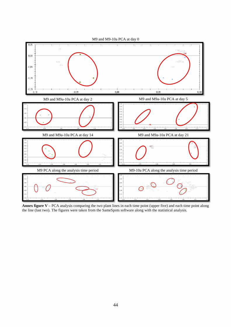
44
M9 and M9-10a PCA at day 0
M9 and M9a-10a PCA at day 2
M9 and M9a-10a PCA at day 5
M9 and M9a-10a PCA at day 14
M9 and M9a-10a PCA at day 21
M9 PCA along the analysis time period
M9-10a PCA along the analysis time period
Annex figure V – PCA analysis comparing the two plant lines in each time point (upper five) and each time point along
the line (last two). The figures were taken from the SameSpots software along with the statistical analysis.

45
Annex figure VI - 24 cm 2D-gel, loaded with 300 µg of protein and stained with Sypro Ruby methodology. The
IPG range of the strip is 3-10 NL. The holes that we could see in white on the gel image were done by the spot
picker.
3 10