efeito da heterogeneidade estrutural na …
TRANSCRIPT

ALVARO AUGUSTO VIEIRA SOARES
EFEITO DA HETEROGENEIDADE ESTRUTURAL NA PRODUTIVIDADE E
NA DINÂMICA DO CRESCIMENTO DE POVOAMENTOS MONOCLONAIS
DE EUCALIPTO
Tese apresentada à Universidade Federal
de Viçosa, como parte das exigências do
Programa de Pós-Graduação em Ciência
Florestal, para obtenção do título de
Doctor Scientiae.
VIÇOSA
MINAS GERAIS – BRASIL
2017

Ficha catalográfica preparada pela Biblioteca Central da UniversidadeFederal de Viçosa - Câmpus Viçosa
T Soares, Alvaro Augusto Vieira, 1986-S676e2017
Efeito da heterogeneidade estrutural na produtividade e nadinâmica do crescimento de povoamentos monoclonais deeucalipto / Alvaro Augusto Vieira Soares. – Viçosa, MG, 2017.
x, 52f. : il. ; 29 cm. Inclui apêndices. Orientador: Hélio Garcia Leite. Tese (doutorado) - Universidade Federal de Viçosa. Inclui bibliografia. 1. Eucalipto - Crescimento (Plantas). 2. Árvores -
Crescimento (Plantas) - Produtividade. 3. Tamanho.I. Universidade Federal de Viçosa. Departamento de EngenhariaFlorestal. Programa de Pós-graduação em Ciência Florestal.II. Título.
CDO adapt. CDD 22 ed. 634.9228


ii
“Prefiro ter questões que não podem ser respondidas
a respostas que não podem ser questionadas.”
Richard Feynam
“A frase mais empolgante de ouvir em ciência,
a que prenuncia novas descobertas, não é “Eureka”,
mas sim “Isto é estranho...”
Isaac Asimov
“Se um homem, por mais sábio que seja,
se tem na conta de bastante sábio para poder desprezar os outros,
assemelha-se a um cego que leva uma lâmpada:
ilumina os outros, mas continua cego.”
Buda
“Sei o que devo ser e ainda não sou,
mas rendo graças a Deus por estar trabalhando,
embora que lentamente, por dentro de mim próprio,
para chegar, um dia, a ser o que devo ser.”
Chico Xavier

iii
À HETEROGENEIDADE do mundo,
como força motriz de aprendizado e tolerância
entre as ciências e os povos...
DEDICO

iv
AGRADECIMENTOS
Agradeço primeiramente a DEUS, por todas as oportunidades e aprendizados da
vida.
Agradeço à minha família, o alicerce da minha formação pessoal, porto seguro e
fonte de amparo incondicional.
Agradeço à minha noiva e parceira de vida, Daniele Arriel, pelo companheirismo,
cumplicidade, amor e pela força em todos os momentos bons e ruins.
Agradeço aos amigos dos lugares por onde passei e principalmente, nesta
caminhada de doutorado, os amigos de Viçosa e de Freiburg pelo companheirismo, pelos
momentos de descontração e pelos auxílios imprescindíveis.
Agradeço à Universidade Federal de Viçosa (UFV), em especial ao Departamento
de Engenharia Florestal (DEF), pelos recursos humanos e materiais investidos na minha
formação, os quais garanto que serão retribuídos por mim com muita dedicação e trabalho
no empenho de contribuir com o avanço das ciências florestais e com a formação de
outrem.
Agradeço à Albert-Ludwigs Universität Freiburg (Uni-Freiburg) por me ter
aceitado por um ano no doutorado sanduíche e pelos colegas, pesquisadores e professores
de lá pela hospitalidade e pela colaboração.
Agradeço ao Conselho Nacional de Desenvolvimento Científico e
Tecnológico (CNPq) e à Coordenação de Aperfeiçoamento de Pessoal de Nível Superior
(CAPES), pela bolsa de doutorado e doutorado sanduíche, respectivamente.
Agradeço às empresas parceiras VERACEL e COPENER pelo apoio e pela cessão
das bases de dados.
Agradeço aos funcionários do DEF, obviamente incluídos nos amigos acima
citados, que sempre tornaram a rotina do doutorado mais amena, compartilhando prosas
e momentos amistosos.
Agradeço aos Professores pela contribuição na minha formação profissional.
Agradeço aos meus orientadores Helio Garcia, David Forrester e Agostinho
Lopes, que contribuíram incomensuravelmente para minha formação profissional e
também pessoal. Agradeço pelos conselhos, paciência, pelo direcionamento e por me
deixarem sempre à vontade para desenvolver minhas ideias. São exemplos nos quais me
espelharei para ser um bom orientador.
MUITO OBRIGADO A TODOS!

v
BIOGRAFIA
Alvaro Augusto Vieira Soares, filho de Elaís Aparecida Vieira Soares e Paulo
César Costa Soares, nasceu no dia 21 de Julho de 1986 na cidade de Carmópolis de Minas,
Minas Gerais. Viveu na cidade de Oliveira, Minas Gerais, até completar o ensino médio.
Em 2005, mudou-se para Lavras para cursar Engenharia Florestal na Universidade
Federal de Lavras-UFLA.
Durante seu curso de graduação, participou de diversos projetos acadêmicos como
estagiário voluntário e bolsista de iniciação científica nas áreas de ecologia de florestas
tropicais, inventário e manejo florestal, viveiros florestais e melhoramento florestal. Foi
integrante do Núcleo de estudos em Silvicultura no qual ocupou os cargos de vice-
presidente e presidente.
Nesta mesma instituição, cursou o mestrado em Engenharia Florestal na área de
Silvicultura, desenvolvendo trabalhos na área de recuperação de áreas degradadas como
recuperação de nascentes, recuperação de áreas mineradas na Amazônia, e recomposição
de vegetação nas margens de reservatórios artificiais de hidrelétricas, sendo este o foco
de sua dissertação. Concluiu o mestrado em 2012.
Concluído seu mestrado, trabalhou no Laboratório de Estudos e Projetos em
Manejo Florestal-LEMAF da UFLA com quantificação de carbono no solo e
compartimentos da biomassa de ecossistemas florestais de Minas Gerais e auxiliando em
campanhas de campo para medição de experimentos de manejo sustentável de candeia.
Em agosto de 2012 mudou-se para Corvallis, Oregon, Estados Unidos, para cursar
o doutorado em Forest Ecosystems and Society na Oregon State Univerity, sendo este
interrompido em 2013.
Em agosto de 2013 começou o doutorado em Ciência Florestal na Universidade
Federal de Viçosa-UFV na área de Manejo Florestal. Durante seu doutorado, desenvolveu
trabalhos envolvendo modelagem de florestas plantadas de eucalipto, teca e araucária,
estudos do crescimento e da produção, uso de redes neurais artificiais na modelagem
florestal, entre outros, e auxiliou na ministração das disciplinas de Manejo Florestal e
Métodos Estatísticos Aplicado à Ciência Florestal.
Passou o ano de 2015 desenvolvendo sua tese na Albert-Ludwigs Universität
Freiburg (Uni-Freiburg), Freiburg, Alemanha, pelo programa de doutorado sanduíche da
Coordenação de Aperfeiçoamento de Pessoal de Nível Superior- CAPES.
Concluiu seu doutorado em fevereiro de 2017.

vi
SUMÁRIO
RESUMO ........................................................................................................................ vii
ABSTRACT ..................................................................................................................... ix
1 INTRODUÇÃO GERAL ............................................................................................... 1
1.1 REFERÊNCIAS DA INTRODUÇÃO GERAL .................................................. 5
2 CAPÍTULO 1 ................................................................................................................. 9
2.1 INTRODUCTION ............................................................................................... 9
2.2 MATERIAL AND METHODS ......................................................................... 11
2.3 RESULTS .......................................................................................................... 15
2.4 DISCUSSION .................................................................................................... 18
2.5 REFERENCES .................................................................................................. 23
3 CAPÍTULO 2 ............................................................................................................... 28
3.2 INTRODUCTION ............................................................................................. 29
3.2 MATERIAL AND METHODS ......................................................................... 31
3.2.1 Site and data description ........................................................................... 31
3.2.2 Measurements and analysis ...................................................................... 32
3.3 RESULTS .......................................................................................................... 35
3.3 DISCUSSION .................................................................................................... 40
3.4 REFERENCES .................................................................................................. 44
5 CONSIDERAÇÕES FINAIS ....................................................................................... 52

vii
RESUMO
SOARES, Alvaro Augusto Vieira Soares, D.Sc., Universidade Federal de Viçosa, fevereiro de 2017. Efeito da heterogeneidade estrutural na produtividade e na dinâmica do crescimento de povoamentos monoclonais de eucalipto. Orientador: Helio Garcia Leite. Coorientador: Agostinho Lopes de Souza.
A heterogeneidade estrutural, representada pela desigualdade do tamanho das árvores, é
um atributo-chave nos povoamentos florestais. Por exemplo, algumas investigações em
povoamentos mistos inequiâneos mostraram que a heterogeneidade estrutural pode ser
positivamente correlacionada com a produtividade, enquanto em povoamentos puros
equiâneos e especialmente em plantios monoclonais, o contrário tem sido freqüentemente
encontrado. O objetivo desta tese, dividida em dois capítulos, foi contribuir para a
compreensão de como a desigualdade do tamanho da árvore afeta a produtividade e a
dinâmica de crescimento de povoamentos monoclonais de eucalipto. No primeiro
capítulo, foram estudados o efeito da heterogeneidade estrutural na produção e o efeito
do genótipo e espaçamento sobre a heterogeneidade. Utilizou-se um conjunto de ensaios
de espaçamento × genótipo de Eucalyptus ao longo de um gradiente de produtividade.
Foi verificada associação inversa entre a heterogeneidade estrutural e a produtividade dos
povoamentos. A relação entre produtividade e heterogeneidade diferiu entre os genótipos,
sendo mais produtivos aqueles que resultaram em povoamentos mais homogêneos.
Dentro da faixa de densidades estudadas, o aumento da densidade resultou no aumento
da produtividade e da heterogeneidade. Em geral, o efeito positivo do aumento da
densidade sobre a produtividade foi maior do que o efeito negativo da heterogeneidade,
embora tenha sido mostrado que o contrário pode ocorrer. No segundo capítulo, foram
utilizados dados de experimentos de peso de desbaste para avaliar como a
heterogeneidade estrutural e a dominância do crescimento se desenvolvem ao longo do
tempo e como são afetados por diferentes pesos de desbaste. Os experimentos foram
estabelecidos em três localidades com um gradiente de produtividade. Desbastes por
baixo foram aplicados nas idades de 58 e 146 meses. Os pesos de desbaste testados foram
de 20%, 35% e 50% de remoção da área basal, além de um tratamento adicional com 35%
de remoção da área basal e desrama artificial feita aos 27 meses. A heterogeneidade
estrutural e a dominância de crescimento foram imediatamente reduzidas pelo desbaste,
resultando em povoamentos mais uniformes para maiores pesos de desbaste. A
dominância do crescimento foi muito próxima de zero após cada desbaste. A
heterogeneidade estrutural e a dominância do crescimento cresceram ao longo do tempo,

viii
antes e após o primeiro desbaste, mas as taxas de aumento após o primeiro desbaste foram
geralmente mais baixas do que antes do mesmo. Além disso, as taxas de aumento na
heterogeneidade e dominância do crescimento foram inversamente relacionadas com o
peso do desbaste. Após o segundo desbaste, a heterogeneidade estrutural tendeu a
permanecer constante, enquanto a dominância do crescimento tendeu a diminuir,
atingindo valores negativos. Por fim, os resultados e discussões apresentados reforçam
que a compreensão dos mecanismos por trás do efeito da heterogeneidade estrutural dos
povoamentos florestais contribui para o melhor entendimento dos processos que regem a
dinâmica do crescimento florestal. No caso de plantios monoclonais, tanto a
heterogeneidade estrutural como o efeito de dominância do crescimento constituem
variáveis altamente influentes na dinâmica e partição do crescimento, com reflexo na
eficiência e, consequentemente, na produtividade dos povoamentos. Logo, o uso de
métricas dessas variáveis pode auxiliar no manejo para a obteção de povoamentos mais
produtivos e que usem os recursos de forma mais eficiente.

ix
ABSTRACT
SOARES, Alvaro Augusto Vieira Soares, D.Sc., Universidade Federal de Viçosa, February, 2017. Effect of stand structural heterogeneity on the productivity and on growth dynamics of Eucalyptus monoclonal stands. Advisor: Helio Garcia Leite. Co-advisor: Agostinho Lopes de Souza.
Structural heterogeneity, as represented by tree size inequality, is a key attribute in forests
stands. For example, some investigations in mixed stands have shown that the structural
heterogeneity may be positively correlated with productivity, while in monospecific and
especially in monoclonal stands, the opposite has often been found. The aim of this
dissertation, divided in two chapters, was to contribute to the comprehension of how tree
size inequality affects stand productivity and stand growth dynamics. In the first study,
the effect of stand structural heterogeneity on production and the effect of genotype and
spacing on heterogeneity were examined using a set of spacing × genotype trials along a
large gradient in site productivity. As a result, stand heterogeneity was negatively
associated with productivity. Within the range of densities hereby tested, the relationship
between yield and heterogeneity differed between genotypes and the most productive
genotypes were generally the most homogeneous. While stand density increased
productivity, it also increased structural heterogeneity. The positive effect of increasing
density on productivity was generally greater than the negative effect of heterogeneity,
but it was shown that the contrary can also occur. In the second study, thinning-intensity
experiments were used to assess how stand heterogeneity and growth dominance develop
through time and across different thinning intensities in Eucalyptus stands. The
experiments were established along a three-site gradient in productivity. The plots were
thinned at ages 58 and 146 months. The thinning intensities tested were 20%, 35% and
50% of basal area removal and an additional treatment of 35% removal plus pruning at
27 months. Stand structural heterogeneity and growth dominance were immediately
reduced by thinning from below. The more intense the thinning, the less heterogeneous
the resulting stands. Growth dominance was very close to zero following each thinning
event. Stand structural heterogeneity and growth dominance both increased before and
after the first thinning but the rates of increase after the first thinning were generally lower
than they were before the first thinning. Also, the rates of increase in heterogeneity and
growth dominance were inversely related to thinning intensity. After the second thinning,
structural heterogeneity tended to remain constant whereas growth dominance tended to
decrease, reaching negative values. The results of the first study show that structural

x
heterogeneity per se, in the absence of genetic diversity and species diversity, can have a
strong negative effect on productivity, and an understanding of the mechanisms causing
these contrasting patterns (with versus without genetic diversity) will be important when
engineering forest reforestation projects and plantations for wood production, carbon
sequestration and many ecosystem functions correlated with productivity. Lastly, the
results and discussions here presented reinforce the comprehension of the mechanisms
behind the effect of the structural heterogeneity in forest stands contribute to a better
understanding of the processes that governs the dynamics of forest growth. In the case of
monoclonal stands, structural heterogeneity and growth dominance highly influence
growth dynamics and partitioning, which reflects on growth efficiency and, consequently,
on productivity. Therefore, taking these variables into account can furnish valuable
information for managing forest towards more productive and resource-efficient stands.

1
1. INTRODUÇÃO GERAL
Ao longo das últimas décadas, avanços no manejo florestal intensivo permitiram
um considerável aumento na produtividade de povoamentos de eucalipto no Brasil. Na
década de 1970, quando se difundiam os plantios pelo Brasil, principalmente com os
incentivos fiscais para reflorestamento, a média de crescimento dos povoamentos era de
15 m³ ha-1 ano-1, em idade em torno do oito anos (QUEIROZ; BARRICHELO, 2007).
Atualmente tem-se a média de 36 m³ ha- 1 ano-1 próximo aos seis anos de idade
(IBÁ, 2016), podendo chegar a valores bem mais elevados em situações experimentais e
específicas de sítio, solo, e manejo. Por exemplo, Stape et al. (2006) obtiveram o
incremento médio anual aos seis anos de 62 m³ ha-1 ano-1 com tratamento suplementar
intensivo de adubação e controle de formiga e matocompetição no estado de São Paulo.
Estimativas de 48 m³ ha-1 ano-1 a 80 m³ ha-1 ano-1 foram obtidas em plantios comerciais
no sul da Bahia (OLIVEIRA, 2007) e de 57 m³ ha-1 ano-1 a 103 m³ ha-1 ano-1 em
experimentos de fertirrigação em Minas Gerais (LOURENÇO, 2009).
Este considerável salto de produtividade é fruto de esforços em pesquisa que
embasaram importantes aprimoramentos silviculturais como a geração de clones mais
produtivos e adaptados a determinadas características ambientais, produção de mudas de
alta qualidade e a melhoria do sítio (STAPE et al., 2001; GONÇALVES et al., 2008;
GONÇALVES et al., 2013). Neste último, destacam-se os aprimoramentos na
fertilização, preparo do solo, otimização da densidade de plantas, combate a formigas,
cupins e outras pragas, controle da matocompetição, entre outros. (STAPE et al., 2001,
WILCKEN; RAETANO; FORTI, 2002; DU TOIT et al., 2010; SOUZA; ZANETTI;
CALEGARIO, 2011, GONÇALVES et al., 2013).
Estas operações visam principalmente aumentar a disponibilidade de recursos
como água, nutrientes e luz e diminuir fatores que podem restringir a disponibilidade e,
ou, o uso dos mesmos. Ultimamente, investimentos em silvicultura de precisão, na qual
o planejamento e a prescrição de tais tratamentos silviculturais são feitos específicos para
escalas menores de área, auxiliados pelo uso de sistemas de informação geográfica, tem
colaborado para a qualidade e adequabilidade dos tratamentos silviculturais e,
consequentemente, para o aumento da produtividade dos povoamentos (XAVIER;
SILVA, 2010, MACHADO, 2014; VALE et al., 2014; MAEDA et al., 2014).
Concomitante ao aumento da produtividade, os povoamentos, antes heterogêneos,
com grandes diferenças na altura e diâmetro das árvores e mortalidade elevada, tornaram-
se mais uniformes e com altas taxas de sobrevivência. Do ponto de vista operacional, a

2
uniformidade no tamanho das plantas já há tempo vem sendo apontada como uma
caraterística vantajosa, que aumenta a eficiência da colheita e processamento da madeira
(DAVIS, 1969 apud CARLISLE; TEICH, 1971), além de diminuir a taxa de mortalidade
e o número de árvores suprimidas.
A heterogeneidade estrutural, como também pode ser chamada a heterogeneidade
no tamanho das árvores, origina-se das diferentes taxas de crescimento em nível de árvore
individual. Estas diferentes taxas estão relacionadas a três componentes: quantidade de
recursos (água, nutrientes e luz) disponíveis, proporção destes recursos que as árvores são
capazes de absorver e eficiência com a qual as árvores usam estes recursos para o
crescimento (MONTEITH, 1977; BINKLEY, 2004). Qualquer fator que afete um destes
três componentes será um promotor da heterogeneidade estrutural.
Na fase inicial de uma monocultura florestal, a heterogeneidade estrutural é
afetada pelo tipo de propagação e a qualidade das mudas, pela heterogeneidade ambiental
e pela qualidade das operações silviculturais. O tipo de propagação já determina se haverá
diferença no uso de recursos. Se as plantas provêm de propagação seminal, a diversidade
genética implica em uma potencial diferença, mesmo que pequena, no crescimento das
plantas. Com a propagação vegetativa, as plantas são geneticamente idênticas e possuem,
a princípio, o mesmo potencial de crescimento. No entanto, mesmo que propagadas
vegetativamente, pode haver diferença na capacidade de crescimento inicial devido a
qualidade das mudas, tal qual vigor e sanidade (XAVIER; SILVA, 2010), resultantes do
processo de produção no viveiro e mesmo no transporte até a área do plantio.
A heterogeneidade ambiental é dada pela desuniformidade das características
físico-químicas do solo, relevo e face de exposição. Manchas de solo mais ou menos
férteis ou com camadas compactadas, pequenas áreas com má drenagem ou que
acumulam muita água, terrenos ondulados, entre outros, podem favorecer o crescimento
de algumas plantas, em detrimentos de plantas próximas, por aumentar ou restringir a
quantidade de recursos disponível (SCHUME; JOST; HAGER, 2004; BOYDEN;
BINKLEY, 2016; BOYDEN et al., 2012).
As operações silviculturais como plantio, preparo do solo, adubação, combate a
formigas e cupins, controle da matocompetição, são prescritas com o intuito de aumentar
a quantidade e a disponibilidade de recursos e reduzir os fatores que limitam do uso dos
mesmos. Entretanto, quando efetuadas de forma inadequada, com implementos
descalibrados e não obedecendo às prescrições, estas operações podem intensificar a
heterogeneidade ambiental, promovendo uma maior desuniformidade no crescimento das
plantas (RADTKE; WESTFALL; BURKHART, 2003).

3
À medida que as árvores crescem e suas copas e raízes se aproximam, dá-se início
à competição por recursos. Após o fechamento do dossel, as plantas que, por
consequência dos fatores supracitados, foram favorecidas e puderam crescer mais,
desenvolvem, portanto, maior copa e maior volume de raízes, que farão com que elas
sejam capazes de absorver mais radiação solar, nutrientes e água, e usá-los de forma mais
eficiente (BINKLEY et al., 2002; BINKLEY et al., 2010b; CAMPOE et al., 2013;
FORRESTER et al., 2013). Isto, por sua vez, permite que elas cresçam ainda mais em
relação às plantas menores.
A competição passa a ser um fator de restrição ao crescimento das plantas
menores, uma vez que as plantas maiores diminuem a disponibilidade de recursos para as
plantas menores. Assim o povoamento se diferencia em várias classes de dominância
(BINKLEY, 2004) cujo efeito dura por toda a rotação (DOI; BINKLEY; STAPE, 2010).
Mesmo com o manejo intensivo, em plantios monoclonais com genótipos altamente
produtivos e com prescrições silviculturais sítio-específicas, os povoamentos ainda
podem portar considerável heterogeneidade no tamanho das plantas (LUU; BINKLEY;
STAPE, 2013).
Só recentemente, com a intensificação das pesquisas em ecologia da produção e
ecofisiologia de plantações florestais, a uniformidade estrutural dos povoamentos
florestais (se e como ela afeta a produtividade) tem sido mais profundamente investigado.
Em uma pesquisa direcionada a várias empresas florestais no Brasil, promovida pelo
projeto Brazil Eucalyptus Potential Productivity (BEPP), o efeito da uniformidade do
tamanho das árvores na produção foi considerado um dos tópicos de maior relevância
(BINKLEY; LACLAU; et al., 2010)
Alguns trabalhos já mostraram que existe uma tendência de que povoamentos
mais heterogêneos sejam menos produtivos que povoamentos mais uniformes.
Stape et al. (2010) compararam talhões monoclonais heterogêneos, cujo plantio foi feito
de forma escalonada (um terço das mudas plantadas inicialmente, outro terço plantado 40
dias depois e o terço final 80 dias após o plantio), com talhões mais uniformes, nos quais
o plantio ocorreu em somente uma ocasião. Estes autores encontraram que as árvores dos
tratamentos uniformes cresceram em média 13% mais que as árvores do tratamento
heterogêneo.
Binkley et al. (2002) compararam o crescimento de talhões estabelecidos com
mudas de origem seminal e clonal e evidenciaram que grande parte do maior crescimento
dos plantios clonais pode ter resultado mais devido à maior uniformidade no tamanho das
árvores do que da capacidade de crescimento dada pelo genótipo. Luu, Binkley e

4
Stape (2013), estudando o efeito da competição com árvores vizinhas, uniformidade e do
tamanho das árvores no crescimento das árvores em nível individual concluíram que
tratamentos que promovam a uniformidade no tamanho das árvores podem resultar em
um aumento de 5% a 15% na produção em nível de talhão.
Apesar de algumas evidências, há ainda muito a ser investigado não somente sobre
o efeito da heterogeneidade estrutural na produtividade do talhão em si, mas também
sobre como a heterogeneidade afeta a dinâmica do crescimento das árvores. O
crescimento em nível de talhão emerge do crescimento das árvores individualmente. Este
processo é fortemente afetado pelas complexas interações de competição, dominância e
supressão que afetam a capacidade das plantas de usar os recursos do sítio. Desta forma,
entender como a heterogeneidade se desenvolve, bem como sua relação com a dinâmica
do crescimento das plantas é essencial para delinear e prescrever tratamentos que
otimizem o crescimento.
Além disso, é necessário investigar os fatores promotores da heterogeneidade em
plantios monoclonais, como eles interagem entre si, o quanto é possível manipulá-los para
se obter maior produtividade e se é economicamente viável manipulá-los para tal. Estas
investigações contribuirão não somente para o aprofundamento do entendimento sobre o
crescimento de povoamentos florestais, como também abrem uma nova oportunidade
para o aumento da produtividade.
O objetivo desta tese foi, portanto, contribuir com o melhor entendimento do
efeito da heterogeneidade na produtividade e na dinâmica de povoamentos monoclonais
de eucalipto. Dois capítulos são apresentados:
No primeiro capítulo, entitulado “Increasing stand structural heterogeneity
reduces productivity in brazilian Eucalyptus monoclonal stands”, estudou-se o efeito da
heterogeneidade estrutural na produtividade. Para isso, foram utilizados dados de uma
rede de experimentos de espaçamentos e clones conduzidos no sul da Bahia. Investigou-
se também se duas importantes prescrições silviculturais, o espaçamento de plantio e o
genótipo, têm efeito na heterogeneidade estrutural dos povoamentos.
No segundo capítulo, “Development of stand structural heterogeneity and growth
dominance in thinned Eucalyptus stands in Brazil”, objetivou-se estudar o
desenvolvimento da heterogeneidade estrutural e do efeito de dominância do crescimento
em povoamentos monoclonais de eucalipto com diferentes níveis de redução da
competição via desbastes. Para este estudo, foram utilizados experimentos de pesos de
desbastes no nordeste da Bahia.

5
1.1. REFERÊNCIAS DA INTRODUÇÃO GERAL
BINKLEY, D. A hypothesis about the interaction of tree dominance and stand
production through stand development. Forest Ecology and Management, v. 190, n.
2–3, p. 265–271, mar. 2004.
BINKLEY, D.; LACLAU, J.-P.; STAPE, J. L.; RYAN, M. G. Applying ecological
insights to increase productivity in tropical plantations. Forest Ecology and
Management, v. 259, p. 1681–1683, 2010a.
BINKLEY, D.; STAPE, J. L.; BAUERLE, W. L.; RYAN, M. G. Explaining growth of
individual trees: Light interception and efficiency of light use by Eucalyptus at four
sites in Brazil. Forest Ecology and Management, v. 259, n. 9, p. 1704–1713, abr.
2010b.
BINKLEY, D.; STAPE, J. L.; RYAN, M. G.; BARNARD, H. R.; FOWNES, J. Age-
related decline in forest ecosystem growth: an individual-tree, stand-structure
hypothesis. Ecosystems, v. 5, n. 1, p. 58–67, 1 jan. 2002.
BOYDEN, S.; BINKLEY, D. The effects of soil fertility and scale on competition in
ponderosa pine. European Journal of Forest Research, v. 135, n. 1, p. 1–8, 2016.
BOYDEN, S.; MONTGOMERY, R.; REICH, P. B.; PALIK, B. Seeing the forest for
the heterogeneous trees: stand-scale resource distributions emerge from tree-scale
structure. Ecological applications : a publication of the Ecological Society of
America, v. 22, n. 5, p. 1578–88, jul. 2012.
CAMPOE, O. C.; STAPE, J. L.; NOUVELLON, Y.; LACLAU, J.-P.; BAUERLE, W.
L.; BINKLEY, D.; LE MAIRE, G. Stem production, light absorption and light use
efficiency between dominant and non-dominant trees of Eucalyptus grandis across a
productivity gradient in Brazil. Forest Ecology and Management, v. 288, p. 14–20,
jan. 2013.
CARLISLE, A.; TEICH, A. H. The costs and benefits of tree improvement
programs. Ottawa: Canadian Forest Service, 1971. 34 pp.
DAVIS, L. S. Economic models for program evaluation. In: 2nd World Consult. Forest
tree breeding. FAO-FO-FTB-6913/4, Washington, D.C. Anais... Washington, D.C.:
1969.

6
DOI, B. T.; BINKLEY, D.; STAPE, J. L. Does reverse growth dominance develop in
old plantations of Eucalyptus saligna? Forest Ecology and Management, v. 259, n. 9,
p. 1815–1818, abr. 2010.
DU TOIT, B.; SMITH, C. W.; LITTLE, K. M.; BOREHAM, G.; PALLETT, R. N.
Intensive, site-specific silviculture: Manipulating resource availability at establishment
for improved stand productivity. A review of South African research. Forest Ecology
and Management, v. 259, n. 9, p. 1836–1845, abr. 2010.
FORRESTER, D. I.; COLLOPY, J. J.; BEADLE, C. L.; BAKER, T. G. Effect of
thinning, pruning and nitrogen fertiliser application on light interception and light-use
efficiency in a young Eucalyptus nitens plantation. Forest Ecology and Management,
v. 288, p. 21–30, 2013.
GONÇALVES, J. L. D. M.; ALVARES, C. A.; HIGA, A. R.; SILVA, L. D.;
ALFENAS, A. C.; STAHL, J.; FERRAZ, S. F. D. B.; LIMA, W. D. P.;
BRANCALION, P. H. S.; HUBNER, A.; BOUILLET, J.-P. D.; LACLAU, J.-P.;
NOUVELLON, Y.; EPRON, D. Integrating genetic and silvicultural strategies to
minimize abiotic and biotic constraints in Brazilian eucalypt plantations. Forest
Ecology and Management, v. 301, p. 6–27, ago. 2013.
GONÇALVES, J.; STAPE, J.; LACLAU, J.-P.; BOUILLET, J.-P.; RANGER, J.
Assessing the effects of early silvicultural management on long-term site productivity of
fast-growing eucalypt plantations: the Brazilian experience. Southern Forests: a
Journal of Forest Science, v. 70, n. 2, p. 105–118, ago. 2008.
IBA. Industria Brasileira de Árvores - Anuário 2016 . Brasília: IBÁ. 2016. 96 pp.
LOURENÇO, H. M. Crescimento e eficiência do uso de água e nutrientes em
eucalipto fertirrigado. 2009. Tese (Doutorado). Universidade federeal de Viçosa,
2009.
LUU, T. C.; BINKLEY, D.; STAPE, J. L. Neighborhood uniformity increases growth
of individual Eucalyptus trees. Forest Ecology and Management, v. 289, p. 90–97,
2013.

7
MACHADO, C. C. Colheita florestal. 3a. ed. Viçosa, Brazil: Editora UFV, 2014.
MAEDA, S.; AHRENS, S.; CHIARELLO, R.; OLIVEIRA, E. B. De; STOLLE, L.;
ANTONIO, J.; FOWLER, P.; BOGNOLA, I. A. Silvicultura de precisão. In:
Agricultura De Precisão: resultados de um novo olhar. Brasilia: Embrapa, 2014. p.
467–477.
MONTEITH, J. L. Climate and the efficiency of crop production in Britain.
Philosophical Transactions of the Royal Society B: Biological Sciences, v. 281, p.
277–294, 1977.
OLIVEIRA, M. L. R. de. Mensuração e modelagem do crescimento e da prdução de
povoamentos não-desbastados de eucalipto. 2007. 103f. Tese (Doutorado)
Universidade Federal de Viçosa, 2007.
QUEIROZ, L. R. de S.; BARRICHELO, L. E. G. O Eucalipto - um século no Brasil.
São Paulo: Dutarex S.A., 2007. 127 pp.
RADTKE, P. J.; WESTFALL, J. A; BURKHART, H. E. Conditioning a distance-
dependent competition index to indicate the onset of inter-tree competition. Forest
Ecology and Management, v. 175, n. 1–3, p. 17–30, mar. 2003.
SOUZA, A.; ZANETTI, R.; CALEGARIO, N. Nível de dano econômico para formigas-
cortadeiras em função do índice de produtividade florestal de eucaliptais em uma região
de mata Atlântica. Neotropical Entomology, v. 40, n. 4, p. 483–488, 2011.
STAPE, J. L.; BINKLEY, D.; JACOB, W. S.; TAKAHASHI, E. N. A twin-plot
approach to determine nutrient limitation and potential productivity in Eucalyptus
plantations at landscape scales in Brazil. Forest Ecology and Management, v. 223, n.
1–3, p. 358–362, mar. 2006.
STAPE, J. L.; BINKLEY, D.; RYAN, M. G.; FONSECA, S.; LOOS, R. A.;
TAKAHASHI, E. N.; SILVA, C. R.; SILVA, S. R.; HAKAMADA, R. E.; FERREIRA,
J. M. D. a.; LIMA, A. M. N.; GAVA, J. L.; LEITE, F. P.; ANDRADE, H. B.; ALVES,
J. M.; SILVA, G. G. C.; AZEVEDO, M. R. The Brazil Eucalyptus Potential
Productivity Project: Influence of water, nutrients and stand uniformity on wood
production. Forest Ecology and Management, v. 259, n. 9, p. 1684–1694, abr. 2010.

8
STAPE, J. L.; LEONARDO, J.; GONÇALVES, M.; GONÇALVES, A. N.
Relationships between nursery practices and field performance for Eucalyptus
plantations in Brazil A historical overview and its increasing importance. New Forests,
v. 22, p. 19–41, 2001.
VALE, A. B. do; MACHADO, C. C.; PIRES, J. M. M.; VILAR, M. B.; COSTA, C. B.;
NACIF, A. de P. Eucaliptocultura no brasil: silvicultura, manejo e ambiência.
Viçosa, Brazil: Sociedade de Investigações Florestais, 2014.
WILCKEN, C. F.; RAETANO, C. G.; FORTI, L. C. Termite pests in Eucalyptus forests
in Brazil. Sociobioloy, v. 40, n. 1, p. 179–190, 2002.
XAVIER, A.; SILVA, R. L. Evolução da silvicultura clonal de Eucalyptus no Brasil.
Agronomia Costarricense, v. 34, n. 1, p. 93–98, 2010.

9
2. CAPÍTULO 1
INCREASING STAND STRUCTURAL HETEROGENEITY REDUCES
PRODUCTIVITY IN BRAZILIAN Eucalyptus MONOCLONAL STANDS*
*Artigo publicado: Soares, A.A.V., Leite, H.G., Souza, A.L. de, Silva, S.R., Lourenço, H.M., Forrester, D.I., 2016. Increasing stand structural heterogeneity reduces productivity in Brazilian Eucalyptus
monoclonal stands. Forest Ecology and Management. 373, 26–32.
Abstract
The effect of stand structural heterogeneity on production was examined in the
northeastern region of Brazil using a set of spacing × genotype trials of Eucalyptus along
a large gradient in site productivity. This experimental platform enabled an analysis of
relationships between productivity and structural heterogeneity for entire rotations while
controlling the confounding effects of species and genetic diversity. Stand heterogeneity
was negatively correlated with productivity. A 10-unit increase in heterogeneity,
quantified using Gini´s coefficient, was associated with a loss of approximately 17 m³ ha-1
to 23 m³ ha-1 for the lowest planting density (667 trees ha-1) and highest planting density
(1667 trees ha-1), respectively, by the end of a 7-year rotation. The most productive
genotypes were generally the most homogeneous. While stand density increased
productivity, it also increased structural heterogeneity. In general, the positive effect on
productivity of increasing density was greater than the negative effect of heterogeneity,
but we found that the contrary can also occur. The relationship between planting density
and heterogeneity differed between genotypes, with some much less plastic than others.
The results show that structural heterogeneity per se, in the absence of genetic diversity
and species diversity, can have a strong negative effect on productivity, and an
understanding of the mechanisms causing these contrasting patterns (with versus without
genetic diversity) will be important when engineering forest reforestation projects and
plantations for wood production, carbon sequestration and many ecosystem functions
correlated with productivity.
Key words: Tree plantation; Stand structure; Stand uniformity; Gini’s coefficient;
Genotype; Planting spacing
2.1. INTRODUCTION
The global area of forests has declined by 36% or 16.5 million km2 over the last
200 years (Meiyappan and Jain, 2012), resulting in large carbon (C) emissions, a lower
capacity for C storage (van der Werf et al., 2009), and declines in biodiversity (Butchart

10
et al., 2010). This problem is being partially addressed by increasing reforestation efforts
and using plantations (FAO 2010). For instance, even though the plantations’ share of
land comprised only 7% of the world’s forested land, their share in the supply of
roundwood, for example, was 30% in 2005 and is estimated to reach up to 80% by 2030
(Seppäla, 2007; Carle and Holmgren, 2008).
There has also been increasing interest in the establishment and use of mixed-
species stands as opposed to monocultures due to their potential to provide higher levels
of ecosystem services (Thompson et al., 2014). The potential of mixed-species stands is
attributed, in part, to their greater structural heterogeneity compared with monocultures,
such as the development of canopy or root stratification (Kelty, 1992; Forrester et al.,
2006). Conversely, however, recent studies show that structural heterogeneity, in the
absence of species and genetic diversity, can reduce productivity by up to 20% (Binkley
et al., 2010; Stape et al., 2010; Ryan et al., 2010; Aspinwall et al., 2011; Luu et al., 2013).
The reduction in stand-level productivity with increasing variability in tree sizes
in monocultures is thought to result from contrasting responses by suppressed versus
dominant trees (Binkley et al., 2010). That is, in more structurally heterogeneous stands,
dominant trees are likely to have smaller neighbors than they would in less heterogeneous
stands and they therefore grow faster because they capture more resources and use them
more efficiently (Binkley et al., 2002, 2010, 2013; Campoe et al., 2013; Forrester et al.,
2013). However, at the stand level, this increase in growth of dominant trees is
outweighed by the reduction in growth and resource-use efficiency of the smaller trees
(Binkley et al., 2013; Campoe et al., 2013; Luu et al., 2013).
Clearly, the structural heterogeneity of monocultures, as well as mixtures, is a
major factor influencing forest productivity and, therefore, probably also other ecosystem
functions and services that are linked to productivity, including water use, carbon
sequestration, nutrient cycles and the response and susceptibility of stands to droughts
and other variations in climate.
The contrasting effect of structural heterogeneity, depending on the presence of
genetic (or species) diversity, highlights the value of experiments using clonal
monocultures. These allow species and genetic diversity to be reduced to zero in order to
focus on the structural heterogeneity effects. Moreover, the importance of understanding
the effect of structural heterogeneity on the productivity of monocultures is highlighted
by the increasing contribution that monospecific plantations make to the global wood
supply, and the related effects that these plantations have on other ecosystem functions.

11
Some plantations, such as Eucalyptus in Brazil, are the most productive
ecosystems in the world, capable of achieving current annual increments in excess of 70
m³ ha-1 year-1 or 35 Mg ha-1 year-1 (Almeida et al., 2007; Stape et al., 2010). Due to their
high productivity, plantations play an important role as carbon sinks in the face of climate
change (Böttcher and Lindner. 2010). They have also reduced logging pressure on native
forests in some regions (Gladstone and Thomas Ledig, 1990; Brockerhoff et al., 2008).
Therefore, understanding the relationship between structural heterogeneity and
productivity has both ecological and economic implications.
Three factors that have a major influence on productivity, and potentially also on
structural heterogeneity, are site quality, planting density and genotype. In this study, a
regional assessment of the relationships between structural heterogeneity and
productivity was done in tropical Eucalyptus plantations across northeastern Brazil.
The objective was to test the hypothesis that the heterogeneity reduces plot growth
across genotypes, spacing, and site productivity. More specifically, this was divided into
four main components: (1) Stand structural heterogeneity increases with age and with
increasing planting density (because both increase the expression of dominance within a
stand); (2) Increases in stand structural heterogeneity reduce productivity for a given site,
planting spacing and age, and this is a general pattern across all the plantations examined;
(3) Stand heterogeneity as well as the above mentioned relationships are influenced by
genotype; (4) Increasing planting density increases productivity but also increases
heterogeneity (which reduces productivity). This trade-off can be managed using
genotypes that are less inclined to develop high structural heterogeneity.
2.2. MATERIAL AND METHODS
We used six genotype × spacing experiments of Eucalyptus located in the state of
Bahia in the northeast of Brazil, which were established with the main purpose of
determining the best combination of genotype and spacing for each given region. These
experiments were chosen because of the control of genotype and spacing. They were also
selected because they maximize the variability in productivity and heterogeneity because
they were established across sites with a wide range of site quality such that mean annual
volume increment differed by more than 50 m3 ha-1 year-1 (20 - 71 m3 ha-1 year-1). A brief
summary of the experiments’ characterization is presented in Table 1.

12
Table 2.1. Characterization of six genotype × spacing experiments of Eucapytus in Bahia,
northeastern Brazil. The experiments (Exp) were coded E1 to E6. Genotypes G2 and G6
are clones of E. grandis, and G1, G3, G4 and G5 are hybrids of E. grandis × E. urophylla.
Age refers to the age of the last measurement (years). Precip, Tmed, Tmax and Tmin are,
respectively, mean annual precipitation (mm) and monthly mean, maximum and
minimum temperatures (oC) corresponding to the periods of 2005-2013 for E1 and E3;
2008-2013 for E5, E4 and E6; and 2007-2013 for E2. MAI is the mean annual increment
(m³ ha-1 year-1) estimated at the age of 7 years for genotype G1, the only genotype present
in all experiments.
Exp Age Genotypes MAI Soil order Precip Tmed Tmax Tmin
E1 8 G1; G2; G3; G4 71.7 Ultisol 1498 23 28 20
E2 4 G1; G2 G3; G4; G5 52.2 Ultisol 1459 23 28 20
E3 8 G1; G2; G3 G4; G5 50.3 Oxisol 1312 23 24 21
E4 7 G1; G2; G3; G4; G5 42.8 Oxisol 1075 22 27 20
E5 8 G1; G2 G3; G4; G5 41.1 Ultisol 1392 24 28 21
E6 6 G1;;G6 20.6 Oxisol 650 24 29 21
Genotype G1 was used to compare site quality because it was the only genotype
present in all experiments. Productivity values (MAI) in Table 1 were estimated by
Equation 1 fitted for each experiment, relating total plot volume (V; m³ ha-1) of genotype
G1 to age in years.
� = ��� − ���� �� + � Equation 2.1
All experiments were implemented in a factorial (spacings × genotypes) scheme
and a randomized block design with four blocks. Five spacings were compared in each
experiment, corresponding to planting densities from 667 to 1667 trees ha-1, namely:
4 × 3.75 m, 5 × 2.4 m, 4 × 3 m, 3 × 3 m and 3 × 2 m. The first number is the distance
between tree rows and the second is the distance between trees within a row. The number
of genotypes tested varied between experiments as shown in Table 1. The plots were
composed of 50 trees in E6 and 72 trees in the other experiments, but only the innermost
25 and 36 trees, respectively, were analyzed.
To examine the relationship between production and stand structural
heterogeneity, production was quantified as the over bark stem volume per hectare,

13
hereafter named yield (m³ ha-1). Stand structural heterogeneity of each plot was quantified
using the Gini coefficient (non-dimensional) calculated using the over bark stem volume
of individual trees. Gini’s coefficient was derived from the Lorenz curve in which the
cumulative percentage of trees was plotted against the cumulative percentage of tree
volume. Gini’s coefficient was then calculated as one minus the ratio between the area
under the Lorenz curve and the area under the perfect equality line (1:1 line). This
coefficient is originally a proportion, ranging from 0 to 1, but we transformed it into
percentage, by multiplying it by 100, which considerably reduced issues with non-
convergence during the mixed effect fitting process (described below). The greater the
value of Gini’s coefficient, the more heterogeneous the plot. This index was calculated
using the package “ineq” in R (Zeileis, 2014).
Total tree height (ht) was measured with a Suunto clinometer with a precision of
0.5 m. Bole circumference at 1.3 m above soil surface was measured with a tape-measure
with the precision of 0.5 cm, and converted to diameter (dbh). Both variables were
measured approximately annually, starting at about the age of one year, but only data
from the second year was used in this analysis. Individual tree over-bark stem volume
(V) was estimated using Schumacher and Hall’s model (equation 2), summed to compute
total plot volume and converted to volume per hectare (Yield).
ln ��� = β� + β�ln ���ℎ� + β�ln �ℎ�� + � Equation 2.2
The relationships between yield, Gini’s coefficient, age, spacing and genotype
were analyzed using generalized linear mixed effect models, following the 3-step model
selection approach suggested by Zuur et al. (2009) and Pinheiro and Bates (2000). First,
we decided the random structure in the presence of the full set of fixed effects (main
effects and second-order interactions). When testing the random component, model fitting
was performed via restricted maximum likelihood (REML). After selecting the random
structure, we analyzed the fixed component. In this step, model parameterization was
performed by maximum likelihood (ML). Spacing was entered as a categorical variable
in the random component and as a continuous variable, “planting density” (trees ha-1),
when in the fixed component of the models. Two spacings had the same area per plant
but different arrangements, 4 × 3 m and 5 × 2.4 m, therefore the latter, more rectangular
spacing, was excluded to avoid potential confounding effects of rectangularity (DeBell
and Harrington, 2002; Stape and Gonçalves, 2002). When necessary, the variance
structure or autocorrelation were also modeled in this step. Inference was made after
refitting the best models via REML.

14
To test for an effect of spacing on stand structural heterogeneity, Gini’s coefficient
was modeled as a function of planting density, age and their interaction in the fixed
component (Gini 1). We tried adding either only random intercepts or both random
intercepts and slopes. When only random intercepts were used, experiment, block and
genotype were initially added following the nested structure of genotype nested within
block, nested within experiment. Random slopes were always related to age and whenever
tested, spacing (always as categorical variable when in the random component) was also
included in the random component as part of the nested structure
(experiment/block/spacing/genotype). This allowed for each genotype inside the nested
structure to have a different trajectory of heterogeneity development through time. This
model was also used to check whether heterogeneity increases with time and whether
different planting densities present different development of heterogeneity.
We rearranged the previous model to test for differences in stand uniformity due
to genotypes and whether heterogeneity develops at different rates for each genotype.
Genotype and age were included in the fixed structure while spacing was added to the
random component that included either random intercepts or both random intercepts and
slopes (Gini 2).
The effect of planting density, age and Gini on stem volume yield were examined
by fitting yield as a function of these variables and their interactions (Yield 1) in the fixed
component. The same random structure was used as in the Gini 1 model. The interaction
with Gini’s coefficient was used to test whether there was an increasing effect of
heterogeneity as stands age (“Gini × Age” interaction) and whether the effect of
heterogeneity increased with density (“Gini × planting density” interaction). To test
whether heterogeneity impacts yield differently depending on the genotype, we shifted
genotype to the fixed component and tree density was added in the random component,
but as spacing (categorical variable) (Yield 2).
The assumptions of normality of residuals and homoscedasticity were graphically
checked using scatterplots of the normalized residuals against the estimated values and
for the continuous explanatory variables, using box plots of the normalized residuals
against the categorical explanatory variables and normal probability plots (qq-plots) at all
levels of nesting. The assumption of independence of the residuals regarding the time
series was assessed by plotting variograms because the time span between measurements
was not constant. The normal distribution of the coefficients of the random components
were checked with qq-plots at all levels of nesting.

15
All analyzes were carried out using R (R Core Team, 2013). The partial F test
and the log-likelihood test, both at 5% significance, were used, respectively, on the fixed
and on the random components of the models. In the case of any non-nested models,
comparisons were made with their Akaike’s Information Criteria (AIC). Model fitting
and tests were performed with the package “nlme” (Pinheiro et al., 2015).
2.3. RESULTS
For all experiments, disregarding treatments, Gini’s coefficient had a mean of
20 and ranged from 4 to 51. In terms of the coefficient of variation of individual tree
volume, this had a mean of 32% and a range from 8% to 84% with values concentrated
between 10% and 45%. Figure 2.1 shows the frequency distributions of Gini’s coefficient.
Figure 2.1. Frequency distribution of Gini’s coefficient in six genotype × spacing
experiments of Eucalyptus in Northeastern Brazil throughout the rotation.
Block did not improve the fit of the models and was therefore removed from all
of them. Assumptions were met for all of the models except by Yield 1. After the
procedure of model selection, model Gini 1 contained age, planting density and their

16
interaction as fixed terms and random intercepts and slopes (in relation to age) for
genotype nested within experiment. Significance of terms and goodness-of-fit statistics
are presented in Table 2 (see Appendix A1 for the terms’ estimated coefficients).
Table 2.2. Explanatory variables of the models for Gini’s coefficient and stem volume
yield and their p-values in the partial F-test at a 5% significance level. Main effects were
tested as in sequential ANOVA and interactions as in marginal ANOVA. Gini = plot-
wise Gini’s coefficient for the over-bark stem volume of individual trees; age = age from
planting in years; density = number of trees per hectare; R²adj = adjusted coefficient of
determination; RMSE = root mean squared error in percentage; ��� = Pearson’s
coefficient of correlation between estimates and observed values (all significant at a 5%
level). * = statistics calculated at the lowest level of nesting.
Fixed component Models
Gini 1 Gini 2 Yield 1 Yield 2
Age <0.0001 <0.0001 <0.0001 <0.0001
Density <0.0001 - <0.0001 -
Genotype - 0.0218 - <0.0001
Gini <0.0001 <0.0001 <0.0001 <0.0001
Age² - - <0.0001 <0.0001
Density × Age <0.0001 - 0.0098 -
Density × Gini <0.0001 - 0.0428 -
Genotype × Age - <0.0001 - <0.0001
Genotype × Gini - <0.0001 - <0.0001
Age × Gini <0.0001 <0.0001 <0.0001 <0.0001
R²adj* 0.82 0.81 0.93 0.98
RMSE (%)* 22.22 19.69 9.04 10.10 ��� * 0.86 0.89 0.99 0.99
Greater Gini’s coefficient was associated with denser treatments and Gini also
increased with age (coefficient = 0.13, p-value < 0.001, for “Age”). In addition, this
increase in heterogeneity with age was even higher for denser treatments (coefficient =
0.002, p-value < 0.001, for the “Density × Age” interaction).
The final model relating Gini’s coefficient to genotypes and age (Gini 2) consisted
of genotype, age and their interaction in the fixed component allowing for random
intercepts and slopes for genotype nested within spacing (as categorical variable) nested
within experiment. According to this model, genotype had a significant effect on stand
structural heterogeneity with a different rhythm of heterogeneity development with age

17
(p-value < 0.001 for the “Genotype × Gini” interaction, coefficients for each Genotype in
Appendix A1).
The model Yield 1 contained a fixed component with age, age squared (to
correct for curvature), planting density and Gini’s coefficient and the interactions “density
× age”, “density × Gini” and “age × Gini”. The random structure comprised of random
intercepts and slopes for genotype nested within spacing nested within experiment.
Several variance structures were tested to correct for heteroskedasticity across
experiments.The best one was selected by comparing models using the log-likelihood test
(at 5% significance level) or AIC for nested and non-nested models, respectively, aided
by comparisons of plots of normalized residuals against estimates and against each of the
explanatory variables.
The selected variance structure was implemented using the varIdent() function
from the “nlme” package with “Experiment” as the grouping categorical variable, within
which variance was allowed to vary (refer to Pinheiro and Bates, 2000 and Zuur et al.,
2009) for computational methods and details). The model with the variance structure was
statistically better than the one without it (AIC =14638.36 vs. 15021.36; log-likelihood
ratio = 392.99 with p-value < 0.0001). After the addition of this variance structure, the
diagnostic plots were rechecked.
An increase in stand heterogeneity was associated with a decrease in stem
volume yield (Figure 2.2). The significant interaction between density and Gini resulted
in a greater heterogeneity effects with increasing density (coefficient = -0.0006,
p-value = 0.043).
The effect of heterogeneity on growth also increased with age (coefficient for
“Gini × Age” interaction = -0.39, p-value < 0.0001), as shown by the steeper curves for
lower levels of Gini in Figure 2.2. Notice that as density increases, so do the distances
between the lines. This indicates that the negative effect of heterogeneity is stronger for
denser stands and that this effect increases as the stands age (non-parallel curves).

18
Figure 2.2. The effect of stand density and structural heterogeneity (represented by Gini’s
coefficient) on stem volume yield for an entire rotation in Eucalyptus plantations in
northeastern Brazil.
The model Yield 2 showed a significant effect of genotype on yield with some
genotypes presenting distinct growth rates (p-value for “Age × Genotype”
interaction < 0.0001; coefficients shown in Appendix A1), increasing effect of
heterogeneity on yield with age (coefficient for “Gini × Age” interaction = -0.44, p-value
< 0.0001) and different effect of heterogeneity on yield depending on genotype (p-value
for “Gini × Genotype” interaction < 0.0001; coefficients shown in Appendix A1).
2.4. DISCUSSION
By isolating the effect of structural heterogeneity from genetic diversity, this study
showed that stand heterogeneity, represented by Gini’s coefficient, was negatively related
to stand production, in accordance our hypothesis (2) and with other studies (Stape et al.,
2010; Luu et al., 2013; Binkley et al., 2010; Ryan et al., 2010; Aspinwall et al., 2011). In
general (fixed component of Gini 1 model), a 10-unit increase in heterogeneity was
associated with a productivity loss of approximately 17 m³ ha-1 for the widest spacing of
667 trees ha-1 and 23 m³ ha-1 for the closest spacing of 1667 trees ha-1 by the end of the
7-year rotation.
19
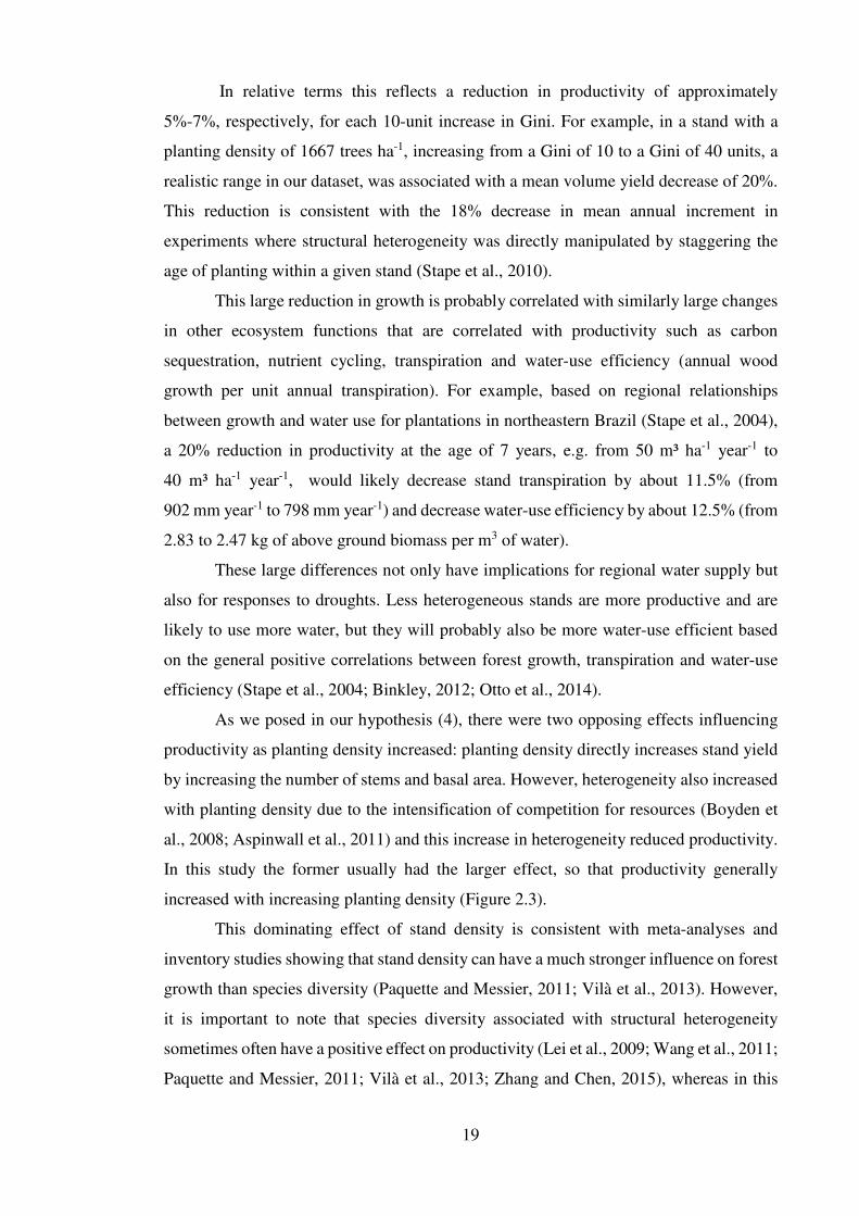
In relative terms this reflects a reduction in productivity of approximately
5%-7%, respectively, for each 10-unit increase in Gini. For example, in a stand with a
planting density of 1667 trees ha-1, increasing from a Gini of 10 to a Gini of 40 units, a
realistic range in our dataset, was associated with a mean volume yield decrease of 20%.
This reduction is consistent with the 18% decrease in mean annual increment in
experiments where structural heterogeneity was directly manipulated by staggering the
age of planting within a given stand (Stape et al., 2010).
This large reduction in growth is probably correlated with similarly large changes
in other ecosystem functions that are correlated with productivity such as carbon
sequestration, nutrient cycling, transpiration and water-use efficiency (annual wood
growth per unit annual transpiration). For example, based on regional relationships
between growth and water use for plantations in northeastern Brazil (Stape et al., 2004),
a 20% reduction in productivity at the age of 7 years, e.g. from 50 m³ ha-1 year-1 to
40 m³ ha-1 year-1, would likely decrease stand transpiration by about 11.5% (from
902 mm year-1 to 798 mm year-1) and decrease water-use efficiency by about 12.5% (from
2.83 to 2.47 kg of above ground biomass per m3 of water).
These large differences not only have implications for regional water supply but
also for responses to droughts. Less heterogeneous stands are more productive and are
likely to use more water, but they will probably also be more water-use efficient based
on the general positive correlations between forest growth, transpiration and water-use
efficiency (Stape et al., 2004; Binkley, 2012; Otto et al., 2014).
As we posed in our hypothesis (4), there were two opposing effects influencing
productivity as planting density increased: planting density directly increases stand yield
by increasing the number of stems and basal area. However, heterogeneity also increased
with planting density due to the intensification of competition for resources (Boyden et
al., 2008; Aspinwall et al., 2011) and this increase in heterogeneity reduced productivity.
In this study the former usually had the larger effect, so that productivity generally
increased with increasing planting density (Figure 2.3).
This dominating effect of stand density is consistent with meta-analyses and
inventory studies showing that stand density can have a much stronger influence on forest
growth than species diversity (Paquette and Messier, 2011; Vilà et al., 2013). However,
it is important to note that species diversity associated with structural heterogeneity
sometimes often have a positive effect on productivity (Lei et al., 2009; Wang et al., 2011;
Paquette and Messier, 2011; Vilà et al., 2013; Zhang and Chen, 2015), whereas in this

20
study, where genetic diversity was reduced to zero, structural heterogeneity had a
negative effect on growth.
There were also exceptions where the negative heterogeneity effect was actually
greater than the positive spacing effect on growth. For example, assuming no mortality,
the smallest difference in planting density, between the 667 trees ha-1 and 833 trees ha-1
treatments, is 166 trees ha-1. Close to the rotation length (seven years), the maximum Gini
for the density 833 trees ha-1 was 33, found in Experiment E1, and the minimum Gini
found in the 667 trees ha-1 treatment, in this same experiment, was 21. Based on the
estimated coefficients of the model Yield 1, this 12-unit difference in the Gini’s
coefficient has an effect of 21.4 m³ ha-1 while the difference in density (a difference of
166 trees ha-1) has an effect of 8.4 m³ ha-1. That is, in this case, increasing the number of
trees did not offset the negative effect of heterogeneity.
Figure 2.3. Yield (a) and Gini’s coefficient (b) throughout time for four planting densities
in a genotype × spacing trial of Eucalyptus in northeastern Brazil
Even though this is not the rule, it illustrates the fact that the effect of stand
heterogeneity on productivity is not necessarily always smaller than the effect of planting
density. When choosing closer spacings, opting for genotypes that are less likely to form
heterogeneous stands could minimize any loss in production due to tree competition and
suppression.
Despite the clones deployed in these experiments may be considered very
genetically related, they differed in production, in tree size variability. The relationship
between structural heterogeneity and productivity was also influenced by genotype.

21
These findings corroborate our hypothesis (3). As expected, the most uniform genotypes
were generally the most productive (Figure 2.4). Similarly, Aspinwall et al. (2011)
examined genotype and uniformity in Pinus taeda stands and also observed that the most
uniform genotypes were generally the most productive.
These results have important management implications. Given that forest
plantation companies typically use a greater collection of genotypes (but not in the same
stand), the effect of genotype on stand uniformity and production may be even greater.
This suggests the potential for future selection of genotypes that are able to form more
uniform and productive stands.
Figure 2.4. Yield (a) and Gini’s coefficient (b) throughout time for six genotypes in a
genotype × spacing trial of Eucalyptus in northeastern Brazil
The within-genotype variability also has ecological implications. Our results
contrast with the often expected increase in productivity associated with increases in
structural diversity of mixed-species stands compared with monocultures. That is, greater
productivity of mixtures is often attributed, in part, to the structural heterogeneity that
results from inter-specific differences in growth and allometry (Kelty, 1992; Forrester et
al., 2006), or with the plasticity of a given species that allows it to modify its allometry
(or physiology, phenology) when growing in a mixture that is complementary to other
species (Bauhus et al., 2004; Pretzsch, 2014).
This study shows that in the absence of genetic diversity, structural heterogeneity
by itself is not necessarily as useful as indicated by some studies that confound genetic
and structural diversity.Tree-level studies in monospecific stands have shown that the

22
reduction in stand-level productivity with increasing heterogeneity occurs because there
is a decrease in growth, resource use and use efficiency of suppressed trees that outweighs
any increase in the growth and resource-use efficiency of the dominant trees (Stape et al.
2010; Campoe et al. 2013; Luu et al. 2013).
The contrasting effects of structural heterogeneity on growth with, versus
without, the presence of genetic diversity, and also inter-genotype differences in this
study, are likely to reflect shifts in this balance between the positive response of dominant
trees and the negative response of suppressed trees. The balance will also likely be
influenced by the fact that within a stand there can be large variability in soil nutrients,
soil moisture and light availability (Schume et al., 2004; Boyden et al., 2012).
The faster growing and less heterogeneous genotypes may have traits, such as
rapid root development, that make them less responsive to micro-site heterogeneity. In
stands where there is genetic diversity, such as mixed-species stands, the greater genetic
diversity may increase the probability that trees in lower resource supply micro-sites have
traits that enable them to make more efficient use of their environment than trees of a
similar dominance class in stands with less genetic diversity. We suggest that greater
insight into the driving mechanisms of structural heterogeneity-productivity relationships
could be obtained by combining tree- and stand-level analyses with process-based
analyses (e.g. Binkley et al., 2010). In addition, Eucalyptus species are generally very
shade intolerant, so it would be of great interest to repeat these experiments with shade
tolerant species.
In conclusion, we found a negative association between the heterogeneity in tree
sizes and volume yield for monoclonal Eucalyptus plantations in northeastern Brazil.
Increases in structural heterogeneity reduced productivity by as much as 20% over a
seven-year rotation period and is likely to have a similar impact on other ecosystem
services that are correlated with productivity. The most uniform genotypes tended to have
greater productivity than the most heterogeneous ones. Closer spacings were associated
with greater heterogeneity, however, productivity generally increased with closer
spacings because the greater number of stems generally had a greater positive effect on
productivity than the negative effect of greater heterogeneity. The negative relationship
between heterogeneity and productivity contrasts with the positive relationship observed
in some studies in forests with genetic diversity. An understanding of the mechanisms
behind these contrasting effects would improve our knowledge about how forest structure
and genetic diversity influence forest growth and other ecosystem functions and services.

23
2.5. REFERENCES
Almeida, A.C., Soares, J. V., Landsberg, J.J., Rezende, G.D., 2007. Growth and water
balance of Eucalyptus grandis hybrid plantations in Brazil during a rotation for
pulp production. For. Ecol. Manage. 251, 10–21.
Aspinwall, M.J., King, J.S., McKeand, S.E., Bullock, B.P., 2011. Genetic effects on
stand-level uniformity and above- and belowground dry mass production in
juvenile loblolly pine. For. Ecol. Manage. 262, 609–619.
Bauhus, J., van Winden, A.P., Nicotra, A.B., 2004. Aboveground interactions and
productivity in mixed-species plantations of Acacia mearnsii and Eucalyptus
globulus. Can. J. For. Res. 694, 686–694.
Binkley, D., 2012. Understanding the role resource use efficiency in determining the
growth of trees and forests, in: Schlichter, T., Montes, L. (Eds.), Forests in
Development: A Vital Balance. Springer, Netherlands, pp. 13–26.
Binkley, D., Campoe, O.C., Gspaltl, M., Forrester, D.I., 2013. Light absorption and use
efficiency in forests: Why patterns differ for trees and stands. For. Ecol. Manage.
288, 5–13.
Binkley, D., Stape, J.L., Bauerle, W.L., Ryan, M.G., 2010. Explaining growth of
individual trees: Light interception and efficiency of light use by Eucalyptus at
four sites in Brazil. For. Ecol. Manage. 259, 1704–1713.
Binkley, D., Stape, J.L., Ryan, M.G., Barnard, H.R., Fownes, J., 2002. Age-related
decline in forest ecosystem growth: an individual-tree, stand-structure hypothesis.
Ecosystems 5, 58–67.
Böttcher, H., Lindner, M., 2010. Managing forest plantations for carbon sequestration
today and in the future, in: Ecosystems Goods and Services from Plantattion
Forests. Earthscan, London, pp. 43–76.
Boyden, S., Binkley, D., Stape, J.L., 2008. Competition among Eucalyptus trees
depends on genetic variation and resource supply. Ecology 89, 2850–2859.
Boyden, S., Montgomery, R., Reich, P.B., Palik, B., 2012. Seeing the forest for the
heterogeneous trees: stand-scale resource distributions emerge from tree-scale
structure. Ecol. Appl. 22, 1578–88.

24
Brockerhoff, E.G., Jactel, H., Parrotta, J.A., Quine, C.P., Sayer, J., 2008. Plantation
forests and biodiversity: Oxymoron or opportunity? Biodivers. Conserv. 17, 925–
951.
Butchart, S.H.M., Walpole, M., Collen, B., et al., 2010. Global Biodiversity : Indicators
of recent declines. Science (80-. ). 328, 1164–1168.
Campoe, O.C., Stape, J.L., Nouvellon, et al., 2013. Stem production, light absorption
and light use efficiency between dominant and non-dominant trees of Eucalyptus
grandis across a productivity gradient in Brazil. For. Ecol. Manage. 288, 14–20.
Carle, J., Holmgren, P., 2008. Wood from Planted Forests, A Global Outlook 2005-
2030. For. Prod. J. 58, 6–18.
DeBell, D.S., Harrington, C.A., 2002. Density and rectangularity of planting influence
20-year growth and development of red alder. Can. J. For. Res. 32, 1244–1253.
Food and Agriculture Organization of the United Nations (FAO), 2010. Global forest
resource assessment. Rome, Italy.
Forrester, D.I., Bauhus, J., Cowie, A.L., Vanclay, J.K., 2006. Mixed-species plantations
of Eucalyptus with nitrogen-fixing trees: A review. For. Ecol. Manage. 233, 211–
230.
Forrester, D.I., Collopy, J.J., Beadle, C.L., Baker, T.G., 2013. Effect of thinning,
pruning and nitrogen fertiliser application on light interception and light-use
efficiency in a young Eucalyptus nitens plantation. For. Ecol. Manage. 288, 21–30.
Gladstone, W.T., Thomas Ledig, F., 1990. Reducing pressure on natural forests through
high-yield forestry. For. Ecol. Manage. 35, 69–78.
Kelty, M.J., 1992. Comparative productivity of monocultures and mixed-species stands,
in: Kelty, M.J., Larson, B.C., Oliver, C.D. (Eds.), The Ecology and Silviculture of
Mixed-Species Forests. Kluwer Academic Publishers, Dordrecht, pp. 125–141.
Lei, X., Wang, W., Peng, C., 2009. Relationships between stand growth and structural
diversity in spruce-dominated forests in New Brunswick, Canada. Can. J. For. Res.
39, 1835–1847.
Luu, T.C., Binkley, D., Stape, J.L., 2013. Neighborhood uniformity increases growth of
individual Eucalyptus trees. For. Ecol. Manage. 289, 90–97.

25
Meiyappan, P., Jain, A.K., 2012. Three distinct global estimates of historical land-cover
change and land-use conversions for over 200 years. Front. Earth Sci. 6, 122–139.
Otto, M.S.G., Hubbard, R.M., Binkley, D., Stape, J.L., 2014. Dominant clonal
Eucalyptus grandis x urophylla trees use water more efficiently. For. Ecol.
Manage. 328, 117–121.
Paquette, A., Messier, C., 2011. The effect of biodiversity on tree productivity: From
temperate to boreal forests. Glob. Ecol. Biogeogr. 20, 170–180.
Pinheiro, J., D, B., DebRoy, S., Sarkar, D., Team, and R.C., 2015. nlme: Linear and
Nonlinear Mixed Effects Models.R package version 3.1-121.
Pinheiro, J.C., Bates, G.M., 2000. Mixed Effcects Models in S and S-Plus. Springer,
Berlag New York Berlin Heidelberg.
Pretzsch, H., 2014. Canopy space filling and tree crown morphology in mixed-species
stands compared with monocultures. For. Ecol. Manage. 327, 251–264.
R Core Team, 2015. R: A language and environment for statistical computing. R
Foundation for Statistical Computing.
Ryan, M.G., Stape, J.L., Binkley, et al., 2010. Factors controlling Eucalyptus
productivity: How water availability and stand structure alter production and
carbon allocation. For. Ecol. Manage. 259, 1695–1703.
Schume, H., Jost, G., Hager, H., 2004. Soil water depletion and recharge patterns in
mixed and pure forest stands of European beech and Norway spruce. J. Hydrol.
289, 258–274.
Seppäla, R., 2007. Global forest sector: trends, threats and opportunities, in: Freer-
Smith, P. H., Broadmeadow, M. S. J. and Lynch, J. M. (Eds) Forestry and Climate
Change. CAB International, pp. 25–30.
Stape, J.., Binkley, D., Ryan, M.G., 2004. Eucalyptus production and the supply, use
and efficiency of use of water, light and nitrogen across a geographic gradient in
Brazil. For. Ecol. Manage. 193, 17–31.
Stape, J.L., Binkley, D., Ryan, M.G., et al., 2010. The Brazil Eucalyptus Potential
Productivity Project: Influence of water, nutrients and stand uniformity on wood
production. For. Ecol. Manage. 259, 1684–1694.

26
Stape, J.L., Gonçalves, J.L.M., 2002. Meeting of the silvicultural and management
cooperative program PTSM, 18. Entre-Rios.
Thompson, I.D., Okabe, K., Parrotta, J. a., Brockerhoff, E., Jactel, H., Forrester, D.I.,
Taki, H., 2014. Biodiversity and ecosystem services: Lessons from nature to
improve management of planted forests for REDD-plus. Biodivers. Conserv. 23,
2613–2635.
van der Werf, G.R., Morton, D.C., DeFries, R.S., Olivier, J.G.J., Kasibhatla, P.S.,
Jackson, R.B., Collatz, G.J., Randerson, J.T., 2009. CO2 emissions from forest
loss. Nat. Geosci. 2, 9–11.
Vilà, M., Carrillo-Gavilán, A., Vayreda, J., Bugmann, H., Fridman, J., Grodzki, W.,
Haase, J., Kunstler, G., Schelhaas, M.J., Trasobares, A., 2013. Disentangling
Biodiversity and Climatic Determinants of Wood Production. PLoS One 8, 1–9.
Wang, W., Lei, X., Ma, Z., Kneeshaw, D.D., Peng, C., 2011. Structural Diversity in
Spruce-Dominated Forest Stands in New Brunswick, Canada. For. Sci. 57, 506–
515.
Zeileis, A., 2014. ineq: Measuring Inequality, Concentration, and Poverty. R package
version 0.2-13.
Zhang, Y., Chen, H.Y.H., 2015. Individual size inequality links forest diversity and
above-ground biomass. J. Ecol. 103, 1245–1252. d
Zuur, A.F., Ieno, E.N., Walker, N.J., Saveliev, A. a, Smith, G.M., Ebooks Corporation.,
2009. Mixed Effects Models and Extensions in Ecology with R, Statistics for
Biology and Health. Springer, New York.

27
APPENDIX A1
Fixed components of the models for Gini’s coefficient and stem volume yield and their effect
sizes. Gini = plot-wise Gini’s coefficient for the over-bark stem volume of individual trees;
age = age from planting in years; density = number of trees per hectare; ()= standard error; * =
Genotype G1 set as the baseline level; the number in the models’ names represent whether the
variable density (1) or genotype (2) was used as fixed effect.
Fixed component Models
Gini 1 Gini 2 Yield 1 Yield 2
Intercept* 8.56311
(2.76397) 9.03589
(2.57434) -102.93380 (11.44290)
-55.20333 (7.91105)
Age 0.13086
(0.66498) 2.53161
(0.65961) 72.41484 (9.31299)
74.90272 (8.58877)
Density 0.00019
(0.00075) -
0.02825 (0.00687)
-
Gen
otyp
e
G2 - -1.80971 (0.74823)
- -34.08279 (3.79506)
G3 - 0.73820
(0.88306) -
-30.76564 (5.22834)
G4 - 2.33223
(1.08651) -
-53.42374 (5.90317)
G5 - -1.02270 (1.44250)
- -22.96544 (6.09971)
G6 - 0.21859
(2.66980) - -8.57528
Gini - - 1.2666
(0.43198) 0.31006
(0.29770)
Age² - - -1.67396 (0.22622)
-1.41932 (0.22712)
Density × Age 0.00216
(0.00015) -
0.00474 (0.00187)
-
Density × Gini - - -0.00059 (0.00029)
-
Gen
otyp
e ×
Age
G2 - 0.01063
(0.15808) -
4.40599 (0.91504)
G3 - -0.48707 (0.17696)
- 0.59657
(1.08417)
G4 - -0.66732 (0.21609)
- 8.96963
(1.22880)
G5 - 0.41799
(0.30280) -
-0.74620 (1.37127)
G6 - 0.12739
(0.86029) -
-0.40480 (2.24392)
Gen
otyp
e ×
Gin
i
G2 - - - 0.39879
(0.19378)
G3 - - - 2.32586
(0.24958)
G4 - - - 1.47993
(0.31774)
G5 - - - 0.57467
(0.26721)
G6 - - - -0.01531 (0.32103)
Age × Gini - - -0.36879
(0.060280) -0.44562 (0.05183)

28
3. CAPÍTULO 2
DEVELOPMENT OF STAND STRUCTURAL HETEROGENEITY AND
GROWTH DOMINANCE IN THINNED Eucalyptus STANDS IN BRAZIL*
*Artigo publicado: Soares, A.A.V., Leite, H.G., Cruz, J.P., Forrester, D.I., 2017. Development of stand structural heterogeneity and growth dominance in thinned Eucalyptus stands in Brazil. Forest Ecology and Management. 384, 339–346.
Abstract
Higher tree size heterogeneity in forests has been linked to lower productivity, especially
in monocultures. Thinning the stand can directly manipulate tree size variability, thereby
changing growth partitioning across tree dominance classes and consequently changing
the development of stand structural heterogeneity compared to its course in unthinned
stands. We used three thinning-intensity experiments to assess how stand heterogeneity
and growth dominance develop through time and across different thinning intensities in
Eucalyptus stands in one of the most productive regions of Brazil. The experiments were
established along a three-site gradient in productivity. The plots were thinned from below
at ages 58 and 146 months. The thinning intensities tested were 20%, 35% and 50% of
basal area removal and an additional treatment of 35% removal plus pruning at 27 months.
Thinning reduced stand heterogeneity and growth dominance as well as their
development through time and this reduction was greater the more intense the thinnings
were. Stand structural heterogeneity and growth dominance both increased before and
after the first thinning, but the rates of increase after the first thinning were lower than
they were before the first thinning. After the second thinning, heterogeneity tended to
remain constant, whereas growth dominance tended to decrease, reaching negative
values. This was contrary to our expectations of observing the same trends in both
variables. Our results show that thinning from below not only reduces heterogeneity and
growth dominance by removing the smaller trees, but can also slow the development of
stand heterogeneity and growth dominance in Eucalyptus stands and potentially other
monocultures.
Keywords: Tree size inequality; Gini’s coefficient; Growth dominance; Growth
partition; Asymmetric competition.

29
3.1. INTRODUCTION
Stand structure is a key feature of forests because of its relationship with forest
functioning. An assessment of stand structure, and how it develops through time, can
indicate which processes are likely to be driving stand dynamics. It can reveal, for
instance, which individuals or cohorts are contributing the most to stand growth and how
resources are being partitioned between individuals or cohorts. Many studies have shown
a correlation between variability in stand structure and forest productivity (e.g. Binkley
et al., 2002; Lei et al., 2009; Forrester and Bauhus, 2016; Bourdier et al., 2016; Soares et
al., 2016) and some have even suggested how different tree cohorts might therefore
respond to climate change (Trouvé et al., 2014; Fernández-de-Uña et al., 2015).
Stand structure, in terms of size heterogeneity, arises from differences in
individual tree growth, which are driven by three components: the amount of resources
available, the proportion of these resources that the trees are able to acquire and the
efficiency with which trees use them to grow (Monteith, 1977; Binkley et al., 2004).
Among the myriad of factors that may affect those components (e.g. Zenner and Hibbs,
2000; Little et al., 2003; Boyden et al., 2012; Skovsgaard and Vanclay, 2013),
competition plays a crucial role as it affects the trees access to resources.
For example, faster growing trees are able to increase resource acquisition by
growing bigger crowns and root systems, and increasing resource use-efficiency, while
decreasing the availability of resources for the suppressed trees, e.g. by partially or totally
shading other crowns (Binkley et al., 2002, 2010, 2013; Campoe et al., 2013; Forrester et
al., 2013a). These trees become dominant in the stand as the trees differentiate into size
classes according to the level of suppression and their ability to cope with competition
(Schwinning and Weiner, 1998).
The contributions of individual tree growth can be assessed at the stand level by
the proportional contribution of the trees’ growth relative to their size, known as the
growth dominance coefficient (Binkley et al., 2003; Binkley et al., 2006; West, 2012). In
addition to the ecological contribution of understanding changes in growth dominance
patterns through time and between species and forest types (Binkley et al., 2006; Doi et
al., 2010; Fernández et al., 2011; Tschieder et al., 2012; Binkley and Kashian, 2015), this
coefficient may also work as a tool for understanding the response to silvicultural
treatments, such as thinning (Doi et al., 2010; Bradford et al., 2010; Trouvé et al., 2014).
The link between growth dominance and stand structural heterogeneity is that the
development of tree size inequality is determined by the different growth rhythms of the
trees, especially in relation to their size. That is, in the absence of structural changes

30
resulting from natural disturbances or silvicultural treatments, growth dominance
determines tree size inequality. When the biggest trees grow disproportionately faster
than smaller trees, heterogeneity increases. When growth is proportional to tree size,
heterogeneity remains the same. When smaller trees grow disproportionately faster than
bigger trees, structural heterogeneity decreases and the stand becomes more uniform in
terms of tree size.
Elucidating the dynamics of forest stands as affected by stand structural
heterogeneity has relevant implications for silvicultural decisions, such as thinning
regimes. For example, in plantations of Eucalyptus globulus, E. grandis and E. nitens in
Australia, the effect of stand structure was as strong, or even stronger, than site quality in
determining the thinning response (Forrester et al., 2013b). In these areas, the relative and
the absolute thinning responses, of the 200 largest-diameter trees per hectare, were higher
in stands with smaller coefficients of variation in diameter and with diameter distributions
containing higher proportions of trees in the larger size classes than in the smaller size
classes.
Therefore, thinning responses may not only result from the response to greater
resource availability, but also to the change in stand structure and the partitioning of
resources between the retained individual trees (Forrester et al., 2013b). However, the
effect of thinning on structural heterogeneity and growth dominance has received little
attention.
Thinning from below can be expected to reduce structural heterogeneity and
growth dominance because it systematically reduces the variability in individual tree sizes
and growth rates by removing the smaller trees within the stand. Thinning might also be
expected to slow the rates at which structural heterogeneity and growth dominance
increase through time because it reduces competition; the greater the thinning intensity,
the slower the increase in structural heterogeneity and growth dominance. Therefore, we
posed the following predictions: (i) stand structural heterogeneity and growth dominance
are immediately reduced by thinning; (ii) the more intense the thinning, the greater the
decrease in the level of heterogeneity and growth dominance, as well as in their
development through time; (iii) stand structural heterogeneity and growth dominance
increase rapidly until the first thinning, after which the rate of increase declines, and after
a second thinning, the heterogeneity and growth dominance remain constant through
time; (iv) stand structural heterogeneity and growth dominance are directly related and
therefore should display the same pattern of development through time and across
thinning treatments.

31
3.2. MATERIAL AND METHODS
3.2.1. Site and data description
We used data from a thinning experiment in Eucalyptus stands established in 1995
in the state of Bahia, northeastern Brazil. The stands comprised monoclonal plantations
of hybrids of E. grandis x E. urophylla. The experiment was installed at three sites (A, B
and C), with altitudes of 285 m, 290 m and 150 m and an annual rainfall of 900 mm year-1 ,
1100 mm year-1 and 1200 mm year-1, respectively.
There was a gradient of productivity, which increased from site A to site C
(Figure 3.1), such that the mean annual increment at the age of about 58 months (before
the first thinning) was 27 m3 ha-1 year-1, 31m3 ha-1 year-1 and 35 m3 ha-1 year-1,
respectively for site A, B and C.
Figure 3.1. Total height of dominant trees (Dh) as a function of age in the three
Eucalyptus thinning experiments. The dominant trees are the tallest 100 trees per ha.
R² = coefficient of determination, Syx = residual standard error. The three curves are
statistically different from each other (P-values < 0.0001 for all pairwise contrasts of
intercepts and slopes for the log-transformed equations, analysis not shown).
The experiment was implemented in a randomized block design with two blocks
per site. Within block, each treatment was replicated twice, so that each treatment had 12
plots in total (3 sites × 2 blocks per site × 2 replicate within each block). The plots had an
area of approximately 2600 m² (~ 46 m × ~ 56 m) with initial tree spacing of 3 m × 3 m.

32
The treatments corresponded to different percentages of basal area removed in
each thinning event, namely: 20%, 35%, 50%. There was also an additional 35%
treatment where the remaining trees were pruned to a height of 6.0 m at the age of 27
months. Thinning was performed at 58 and 146 months, with each plot receiving the same
thinning intensity at 146 months as it did at age 58 months. At Site C, the experiment was
felled before reaching the age of the second thinning. No control treatment (i.e. non-
thinned plots) was present. The trees that were removed by thinning were those with the
smallest heights and or diameters, or crooked, forked or broken trees. The thinning
schedule was determined by the percent entries method as in Nogueira et al. (2001). In a
previous study using these experiments, Nogueira et al. (2015) found that thinning
improved tree and stand growth, but pruning had no effect.
3.2.2. Measurements and analysis
Each plot was measured approximately at the ages of 26, 40, 50, 58, 60, 75, 87,
100, 111, 114, 136, 146, 158, 164 months, except in Site C where the last measurement
was performed at the age of 87 months. The total height (Ht) of the first15 trees in each
plot, the total height of the five largest-diameter trees (Dh) and the diameter at 1.3 m
height (dbh) of all trees in the plot were recorded. The heights of the unmeasured trees
were estimated using the equation:
ln�Ht� = β� + β� × ln�Age� + β' × Age + β( × ln�SI� + β+ × SI + β, × ln�dbh� + β0 × dbh + ε Equation 3.1
Site index is a predictor in Equation 1 and was estimated using the dominant
height measurements. This was done by firstly estimating the dominant height as a
function of the stand age with Equation 2. Then, Equation 2 was rearranged into Equation
3, according to the guide-curve method (Clutter et al., 1983) to estimate site index.
ln�Dh� = α4 + α� × 5 �6789 + ln�ε� Equation 3.2
ln�SI� = ln �Dh� + α� × 5 �,� − �
6789 + ln�ε� Equation 3.3
In the equations above: Ht is the tree height, SI is the site index,
�: , ��, ��, ��, �', �(, �+, �,, �0 are coefficients estimated by ordinary least squares and �

33
is the random error assumed to be �~=�0, ?��. Equations 1 and 2 were fitted to data
separately for each of the three sites. Tree volume was estimated using Equation 4,
previously fitted for each site by Nogueira et al. (2015) (Appendix A2.1 ):
ln��� = @� + @� × ln���ℎ� + @� × ln�A�� + � Equation 3.4
The individual tree volumes were used to calculate Gini’s coefficient, a commonly
used proxy for stand structural heterogeneity (Weiner and Thomas 1986; Lexerød and
Eid 2006; Wang et al. 2011; Pretzsch and Schütze 2014; McGown et al. 2016). This
coefficient is a measure of inequality derived from the Lorenz curve. It can range,
theoretically, from zero to one, but we multiplied it by 100 for better visualization. The
closer Gini’s coefficient is to zero, the more homogeneous the individual tree volumes.
To model the development of heterogeneity, we used mixed-effect models with
Gini’s coefficient as the response variable. We started with the full model in which the
predictors in the fixed components were: time, thinning treatment, growth period and all
their interactions. Growth period is a dummy variable and indicates whether the
measurements are from the period before the first thinning, after the first thinning or after
the second thinning. Thinning treatment refers to the aforementioned thinning intensities
and was entered as a categorical variable. Time refers to the period in months elapsed
from the start of each given growth period. To conform with the nested structure of the
experiments, the initial random component of the model consisted of Plot, nested within
Block nested within Site.
Model selection was performed by firstly selecting the best random structure in
the presence of the full set of fixed effects (main effects and interactions). This selection
was based on log-likelihood tests on the removal of the levels of the nested structure.
Once the best random structure was obtained, a series of partial (sequential) F-tests were
performed comparing the nested models, removing terms one by one, starting from the
highest order interaction. When testing the random component, the model was fitted by
restricted maximum likelihood procedure (REML), whereas when testing the fixed
structure, the model fit was made through maximum likelihood (ML). These steps were
according to Pinheiro and Bates (2000) and Zuur et al. (2009). The analyses were
performed using the package “nlme” (Pinheiro et al., 2015) in R 3.2.2 (R Core Team,
2015). Final goodness-of-fit was assessed using the following statistics: the proportion of
the total variance explained by only the fixed component of the models (marginal R²) and
by the full structure (conditional R²) calculated with the piecewiseSEM package

34
(Lefcheck, 2016), the root mean squared error (RMSE), and the Pearson’s correlation
coefficient between estimates and observed values (��� ).
To test the hypothesis regarding growth dominance, we used mixed-effect models
with the plot-wise growth dominance coefficient (GDC) as the response variable. The
GDC is an index inspired by Gini’s coefficient. It is calculated by ordering the trees in
ascending order of a size variable (volume in this study) and plotting the cumulative
percent initial values on the x axis against the cumulative percent increments on the y
axis. In this experiment, there was no record of tree identity between measurements.
Therefore, after ordering the trees we grouped them in groups of five, assuming that there
was a greater likelihood of a change in the tree order within a group than trees changing
between the groups. The GDC was then calculated as the relative difference between the
area under the conceptual perfect equality curve (1:1) and the area under the actual
inequality curve. This statistic was calculated according to West (2012) using the function
“trapz” from the package “caTools” (Tuszynski, 2014) to perform the integration of the
Lorenz curves by trapezoidal approximation, so that the GDC was calculated as:
BCD = 1 − ∑ �GH − GH��IHJ� �KH + KH�� Equation 3.5
where x is the cumulative percent volume and y is the cumulative percent increment in
volume. Therefore, the GDC ranges from -1 to 1, but we also multiplied it by 100, as for
Gini’s coefficient. If all groups of trees grow in proportion to their size, the GDC equals
0; positive values indicate that the biggest trees contribute disproportionally more to stand
total volume growth than smaller trees; and negative values indicates the opposite, such
that smaller trees grow disproportionally more than bigger trees in relation to tree size.
Figure 3.2 illustrates three examples of plots and their respective GDC’s (negative, close
to zero and positive). All of the initial fixed and random effects, as well as the steps for
model selection were performed as for the Gini model.

35
Figure 3.2. Examples of growth dominance curves (actual data from the studied
experiments) and their respective growth dominance coefficients (GDC). The values of
GDC -7.78 and 19.10 refer, respectively to a plot 164 months old which was thinned twice
with an intensity of 35% of basal area removal; and a plot 136 months old which was
thinned once at an intensity of 20% of basal area removal.
In both Gini and GDC models, the intercepts are interpreted as the estimated level
of stand structural heterogeneity or growth dominance immediately after thinning. The
slopes are the rates of change (i.e. rate of increase, rate of decrease or no change) of those
variables through time within the given growth period. Therefore, to infer whether the
thinning treatments had an effect on Gini or GDC, the treatments’ intercepts, as well as
the slopes, were compared to each other within a given growth period. To assess whether
there was a change in the levels of Gini and GDC, as well as in their development, across
the growth periods, the intercepts across the growth periods were compared to each other,
per treatment, and the same was performed with the slopes. For such comparison, we used
pairwise t-tests at 5% significance level.
3.3. RESULTS
The thinning clearly affected the yield such that the yield declined with increasing
thinning intensity (Figure 3.3a). Mortality was very low, so thinning was almost
exclusively responsible for any changes in stand density (Figure 3.3b).
The final model for Gini’s coefficient included the fixed main effects Thinning
treatment, Time, Growth period and all the two- and three-way interactions. The three-

36
way interaction was kept, though not statistically significant, as it allows the slope of each
thinning treatment through time to vary between growth periods. In the absence of the
threeway interaction, all of the other interactions were significant (i.e. p-values less than
0.0001 for the interactions ‘‘Thinning intensity × Time” and ‘‘Time × Growth period”
and equal to 0.0011 for ‘‘Thinning intensity × Growth period”). The random component
comprised random intercepts and slopes (in relation to Time) with the full nested structure
(Plot within Block within Site). A summary of the model fits is shown in Table 1.
Figure 3.3. Observed values of yield (a; m³ ha-1) and density (b; trees ha-1) against age
for the thinning intensities of 20%, 35%, 35% plus pruning up to 6 m and 50% of basal
area removal in Eucalyptus plantations in northeastern Brazil. Vertical dotted lines mark
the two thinnings.
As expected, given that thinning was applied from below, thinning reduced stand
heterogeneity. After the drop in heterogeneity that resulted from thinning, the
development of heterogeneity through time differed between the growth periods (P-value
for the interaction Growth period × Time < 0.0001). All of the treatment’s slopes before
the first thinning were greater than their respective slopes in the other growth periods

37
(results not shown), i.e., the rate of increase in heterogeneity was the greatest before
thinning was applied (Figure 3.4).
After the first thinning, heterogeneity continued to increase but at a much slower
rate (Figure 3.4). The only statistically different treatment within this period was the 20%
basal area removal, which presented a faster increase in heterogeneity (greater slope) than
the others (refer Appendix A2.2 for the pair-wise slope coefficient comparisons between
treatments). In terms of the intercept, that is, the estimated level of heterogeneity
immediately after the first thinning, the levels of heterogeneity were inversely related to
the thinning intensity.
Table 3.1. P-values of the partial F-tests for Gini and GDC models. Treatment refers to
the thinning weights of 20%, 35%, 35% + pruning and 50% basal area removal; Growth
Period refers to the periods before first thinning, after first thinning and after second
thinning; Time is the time in months elapsed from planting or from any of the thinnings.
Refer to Appendix A2.1 for the terms’ estimated coefficients.
Terms Model
Gini GDC
Thinning weight <0.0001 <.0001
Time <0.0001 0.0382
Growth period <0.0001 0.0020
Thinning weight × Time 0.3807 0.6656
Thinning weight × Growth period <0.0001 <0.0001
Time × Growth period <0.0001 <.0001
Thinning weight × Time × Growth period 0.3765 0.5665
L�(marginal/conditional ) 0.93 / 0.97 0.14 / 0.69
RMSE (m / %) 0.95 / 6.59 2.91 / 89.48
��� 0.98 0.73
R² is the proportion of the total variance explained by only the fixed (marginal)
component of the model (marginal) and by the full structure (conditional); RMSE is the
root mean squared error given in meters and as a percentage of the mean response, and
��� is the Pearson’s correlation coefficient between estimates and observed values.
The intercepts significantly differed between the thinning intensities, but pruning
in the 35% treatment had no effect. Pruning in this experiment was also reported to have
no effect on tree growth (Nogueira et al., 2015). The comparison between the 35% plus

38
pruning treatment against the 50% treatment, though not significant, was close to the
significance level (0.08).
After the second thinning, heterogeneity either remained the same or decreased
slightly, especially in the 50% basal area removal treatment. However, this decreasing
trend was not significant for any of the treatments. When After second thinning was set
as the baseline level, none of the coefficients for Time, either as a main effect or
interactions with it, were different from zero (Appendix A2.2; Figure 3.4).
The intercepts, on the other hand, followed the same patterns as before. The 20%
treatment presented the highest Gini coefficient immediately after the second thinning.
The other treatments where not different from each other (Appendix A2.2) but the
significances between the 35% treatments (with and without pruning) against the 50%
treatment showed the trend of differentiation between these two thinning intensities.
Figure 3.4. Development of heterogeneity (Gini coefficient) in Eucalyptus plantations in
Brazil. The grey vertical dotted lines correspond to the thinnings.
The final model for GDC had the same structure as the Gini model. It included
the fixed main effects Thinning treatment, Time, Growth period and all the two- and
three-way interactions (see Table 1 for the partial F-tests summary). Like in the Gini
model, the non-significance of the third-order interaction in the GDC model might have

39
occurred because only one statistically different slope within growth periods was found,
i.e. the slope for the 20% basal area removal after the first thinning.
The random component was also comprised of random intercepts and slopes with
the full nested structure. The boxplots of the normalized residuals against the sites
revealed a very heterogeneous distribution and, hence, we added the variance structure
model so that each site can have a different variance (i.e. �HM~=�0, ?M��, where j = sites
A, B or C). This model fixes one category as the baseline level and estimates the variance
of the other levels as rates of the baseline level. In our model the variance of site B and C
were estimated, respectively as 0.87 and 0.59 of site A’s variance. This improved the
residual dispersion and yielded a better model. The Akaike’s information criterion (AIC)
was reduced to 2131.70 from 2149.46 when using the models with the variance structure
modeling, and the P-value was smaller than 0.001 in the log-likelihood test.
The development of GDC differed between growth periods (P-value for the
interaction Growth period × Time < 0.0001). Growth dominance increased faster before
the first thinning than in the following growth periods. The only exception was the 20%
thinning intensity after the first thinning whose slope was not statistically different from
before thinning (P-value = 0.48). Even though the curves in Figure 3.5 show a pattern of
smaller intercepts and slopes with increasing intensity of the first thinning, only the slope
of the 20% treatment was significantly different from zero (Appendix A2.3).
After the second thinning, the curves also revealed a trend of declining intercepts
and slopes with increasing thinning intensity, but unlike the other growth periods, all
curves had a declining trend. Only the intercept of the 20% treatment was significantly
different from zero, but it did not differ from the other intercepts, which did not differ
from each other either (Appendix A2.3). There was no statistical difference between the
slopes of any treatment (Appendix A2.3). No slope in this period was significantly
different from zero, despite of the descending curves shown in Figure 3.5, nor did they
differ from each other (Appendix A2.3).

40
Figure 3.5. Development of the growth dominance coefficient (GDC) in Eucalyptus
plantations in Brazil. The grey vertical dotted lines correspond to the thinnings.
3.3. DISCUSSION
We used three thinning-intensity experiments in northeastern Brazil to assess how
stand heterogeneity and growth dominance develop with time in response to thinning
interventions in Eucalyptus stands in one of the most productive regions of Brazil. As
posed in our hypothesis, stand structural heterogeneity and growth dominance were
reduced by thinning from below and this decrease was related to thinning intensity.
Congruent with prediction (i), there was a decrease in stand heterogeneity and
growth dominance immediately after thinning. The more intense the thinning, the less
heterogeneous the resulting stands, because more small trees were removed. Growth
dominance was very close to zero at the beginning of every growth period. This is
consistent with the open environment created by thinning and with trees experiencing
little competition, thereby enabling them to grow fairly proportionally to their sizes
(Binkley et al., 2006; Fernández and Gyenge, 2009).
The decrease in the level of heterogeneity as well as in their development through
time was greater the more intense the thinning was (Figures 3.4 and 3.5), consistent with

41
our prediction (ii). Higher density, as related to more intense competition, has been shown
to intensify asymmetric competition in the direction of a greater disproportional growth
of the largest trees (Fernández and Gyenge, 2009; Bradford et al., 2010; Keyser, 2012;
Trouvé et al., 2014).
Regarding the trends of stand heterogeneity and growth dominance through time,
both of these variables tended to increase before and after the first thinning, consistent
with our prediction (iii). The rate of increase in heterogeneity decreased after the first
thinning, which was also evident for the growth dominance trend, except for the lightest
thinning intensity (20% of basal area removal) in which the rate of increase was not
different from before the first thinning was applied.
Increasing variability in tree size with age is commonly shown in monospecific
even-aged stands (Binkley et al., 2002; Hakamada et al., 2015; Soares et al., 2016) as a
result of different individual tree competitive abilities leading to different growth rates
(Luu et al., 2013). Thus, the hereby evidenced differences in heterogeneity and growth
dominance development across growth periods, and across thinning intensities within a
growth period, can be explained by two interacting characteristics, both of which are
directly related to individual tree growth rhythms: the variability in tree size at the
beginning of the growth period and the level of competition.
Reducing the range in tree size also reduces the variability in the size-inherent
ability of a tree to acquire resources and/or to use them more efficiently. For example, for
Pinus ponderosa in Argentina, a difference in water use efficiency between the largest
and the smallest trees was found at a site with a wide range in tree size, while no statistical
difference was detected at a site with a narrower range in tree size (Fernández and
Gyenge, 2009). The level of competition amplifies the effect of initial tree-size variability
because competition can be very size-asymmetric and distance dependent in Eucalyptus
monoclonal stands (Little et al., 2003; Boyden et al., 2008; Luu et al., 2013)
After the second thinning some trends deviated from what was expected in
prediction (iii). Heterogeneity remained constant through time for most treatments, but
showed a trend of decrease for the most intense thinning (50% basal area removal for the
second time resulting in a stand density of around 220 trees ha-1; Figure 3.4). Growth
dominance decreased reaching negative values for all of the thinning intensities, which
indicates that non-dominant trees grew slightly disproportionately faster than the
dominant trees (e.g. the -7.78 GDC line in Figure 3.1). Therefore, contrary to prediction
(iv), stand structural heterogeneity and growth dominance were not perfectly related,
though this was revealed only after the second thinning.

42
This pattern after the second thinning, when heterogeneity and growth dominance
generally remained the same or slightly decreased, can be explained by the level of
competition in the remaining density. Tree density was reduced to around 620, 380 and
220 trees ha-1, respectively, in the 20%, 35% and 50% basal area removal treatments. At
this level of canopy openness, tree competition is likely to be relatively low, and
consequently, competition-induced differences in tree growth rate would be minimal.
Furthermore, Eucalyptus in Brazil are normally intensively cultivated (Gonçalves et al.,
2004), which involves the removal of all understory competition. Therefore, in relatively
open stands with very small initial variation in tree size, trees were able to grow fairly
proportionally to their size (Binkley et al. 2006; Fernández and Gyenge 2009), thereby
maintaining or even slightly reducing the level of heterogeneity.
This slight decrease in stand heterogeneity and the trends of decreasing growth
dominance, reaching negative values, might have happened because retained trees
belonging to intermediate dominance classes may present a greater relative response to
thinning than the dominant ones (Forrester et al., 2013b). This can happen because both
dominant and non-dominant trees benefit from the increased water and nutrient
availability, whereas dominant trees already have the most access to light so increases in
light availability should be more relevant to non-dominant trees (Forrester, 2013).
The same reasoning applies to growth dominance patterns. Besides the alleviated
competition after thinning, an increase in the relative response of intermediate trees
decreases the difference in growth between dominant and intermediate trees, which may
reach a level in which the intermediate trees present greater relative growth rates than the
dominant trees. For example, in the plot illustrated in Figure 3.2 with a GDC of 7.78, the
biggest 25 trees, the second biggest 25 trees and the following 25 trees had a relative
growth of 1.83%, 2.26% and 2.65%, respectively.
The reason for differing patterns for Gini’s coefficient and the growth dominance
coefficient after the second thinning is likely due to the absolute values of the increments.
Growth dominance summarizes the distribution of the relative increment among the trees.
Intuitively, its trend through time is directly related to Gini’s coefficient, but this is not
necessarily the case, for example, when there are very small increments. Very small
increments that are heterogeneously distributed may reveal a high growth dominance, but
they may not correspond to enough absolute increment to actually be reflected in a change
in stand structural heterogeneity. This can be seen in our data. Even though all of the
treatments presented a decreasing trend in growth dominance (Figure 3.5), only the
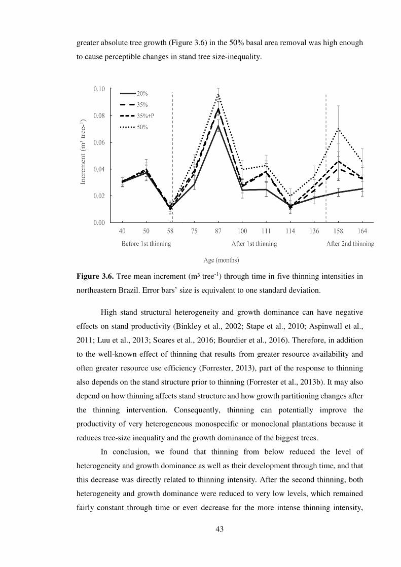
43
greater absolute tree growth (Figure 3.6) in the 50% basal area removal was high enough
to cause perceptible changes in stand tree size-inequality.
Figure 3.6. Tree mean increment (m³ tree-1) through time in five thinning intensities in
northeastern Brazil. Error bars’ size is equivalent to one standard deviation.
High stand structural heterogeneity and growth dominance can have negative
effects on stand productivity (Binkley et al., 2002; Stape et al., 2010; Aspinwall et al.,
2011; Luu et al., 2013; Soares et al., 2016; Bourdier et al., 2016). Therefore, in addition
to the well-known effect of thinning that results from greater resource availability and
often greater resource use efficiency (Forrester, 2013), part of the response to thinning
also depends on the stand structure prior to thinning (Forrester et al., 2013b). It may also
depend on how thinning affects stand structure and how growth partitioning changes after
the thinning intervention. Consequently, thinning can potentially improve the
productivity of very heterogeneous monospecific or monoclonal plantations because it
reduces tree-size inequality and the growth dominance of the biggest trees.
In conclusion, we found that thinning from below reduced the level of
heterogeneity and growth dominance as well as their development through time, and that
this decrease was directly related to thinning intensity. After the second thinning, both
heterogeneity and growth dominance were reduced to very low levels, which remained
fairly constant through time or even decrease for the more intense thinning intensity,

44
indicating stand homogenization due to a greater relative thinning response of the
intermediate trees.
3.4. REFERENCES
Aspinwall, M.J., King, J.S., McKeand, S.E., Bullock, B.P., 2011. Genetic effects on
stand-level uniformity and above- and belowground dry mass production in
juvenile loblolly pine. For. Ecol. Manage. 262, 609–619.
Binkley, D., Campoe, O.C., Gspaltl, M., Forrester, D.I., 2013. Light absorption and use
efficiency in forests: Why patterns differ for trees and stands. For. Ecol. Manage.
288, 5–13.
Binkley, D., Kashian, D.M., 2015. Tree-level patterns of lodgepole pine growth and leaf
area in Yellowstone National Park: Explaining anomalous patterns of growth
dominance within stands. Ecosystems 18, 251–259.
Binkley, D., Kashian, D.M., Boyden, S., Kaye, M.W., Bradford, J.B., Arthur, M.A.,
Fornwalt, P.J., Ryan, M.G., 2006. Patterns of growth dominance in forests of the
Rocky Mountains, USA. For. Ecol. Manage. 236, 193–201.
Binkley, D., Olsson, U., Rochelle, R., Stohlgren, T., Nikolov, N., 2003. Structure,
production and resource use in some old-growth spruce/fir forests in the Front
Range of the Rocky Mountains, USA. For. Ecol. Manage. 172, 271–279.
Binkley, D., Stape, J.L., Bauerle, W.L., Ryan, M.G., 2010. Explaining growth of
individual trees: Light interception and efficiency of light use by Eucalyptus at
four sites in Brazil. For. Ecol. Manage. 259, 1704–1713.
Binkley, D., Stape, J.L., Ryan, M.G., 2004. Thinking about efficiency of resource use in
forests. For. Ecol. Manage. 193, 5–16.
Binkley, D., Stape, J.L., Ryan, M.G., Barnard, H.R., Fownes, J., 2002. Age-related
decline in forest ecosystem growth: an individual-tree, stand-structure hypothesis.
Ecosystems 5, 58–67.
Bourdier, T., Cordonnier, T., Kunstler, G., Piedallu, C., Lagarrigues, G., Courbaud, B.,
2016. Tree size inequality reduces forest productivity: An analysis combining
inventory data for ten European species and a light competition model. PLoS One.
Boyden, S., Binkley, D., Stape, J.L., 2008. Competition among Eucalyptus trees
depends on genetic variation and resource supply. Ecology 89, 2850–2859.

45
Boyden, S., Montgomery, R., Reich, P.B., Palik, B., 2012. Seeing the forest for the
heterogeneous trees: stand-scale resource distributions emerge from tree-scale
structure. Ecol. Appl. 22, 1578–88.
Bradford, J.B., D’Amato, A.W., Palik, B.J., Fraver, S., 2010. A new method for
evaluating forest thinning: growth dominance in managed Pinus resinosa stands.
Can. J. For. Res. 40, 843–849.
Campoe, O.C., Stape, J.L., Nouvellon, Y., Laclau, J.-P., Bauerle, W.L., Binkley, D., Le
Maire, G., 2013. Stem production, light absorption and light use efficiency
between dominant and non-dominant trees of Eucalyptus grandis across a
productivity gradient in Brazil. For. Ecol. Manage. 288, 14–20.
Clutter, J.L., Forston, J.C., Pienaar, L. V., Brister, G.H., Bailey, R.L., 1983. Timber
management: a quantitative approach. Wiley, New York.
Doi, B.T., Binkley, D., Stape, J.L., 2010. Does reverse growth dominance develop in
old plantations of Eucalyptus saligna? For. Ecol. Manage. 259, 1815–1818.
Fernández-de-Uña, L., Cañellas, I., Gea-Izquierdo, G., 2015. Stand competition
determines how different tree species will cope with a warming climate. PLoS One
10, 1–18.
Fernández, M.E., Gyenge, J., 2009. Testing Binkley’s hypothesis about the interaction
of individual tree water use efficiency and growth efficiency with dominance
patterns in open and close canopy stands. For. Ecol. Manage. 257, 1859–1865.
Fernández, M.E., Tschieder, E.F., Letourneau, F., Gyenge, J.E., 2011. Why do Pinus
species have different growth dominance patterns than Eucalyptus species? A
hypothesis based on differential physiological plasticity. For. Ecol. Manage. 261,
1061–1068.
Forrester, D.I., 2013. Growth responses to thinning, pruning and fertiliser application in
Eucalyptus plantations: A review of their production ecology and interactions. For.
Ecol. Manage. 310, 336–347.
Forrester, D.I., Bauhus, J., 2016. A Review of processes behind diversity-productivity
relationships in forests. Curr. For. Reports 45–61.
Forrester, D.I., Collopy, J.J., Beadle, C.L., Baker, T.G., 2013a. Effect of thinning,
pruning and nitrogen fertiliser application on light interception and light-use
efficiency in a young Eucalyptus nitens plantation. For. Ecol. Manage. 288, 21–30.

46
Forrester, D.I., Elms, S.R., Baker, T.G., 2013b. Tree growth-competition relationships
in thinned Eucalyptus plantations vary with stand structure and site quality. Eur. J.
For. Res. 132, 241–252.
Gonçalves, J.L.D.M., Stape, J.L., Laclau, J.-P., Smethurst, P., Gava, J.L., 2004.
Silvicultural effects on the productivity and wood quality of eucalypt plantations.
For. Ecol. Manage. 193, 45–61.
Hakamada, R.E., Stape, J.L., Lemos, C.C.Z. de, Almeida, A.E.A., Silva, L.F., 2015.
Uniformidade entre árvores durante uma rotação e sua relação com a produtividade
em Eucalyptus clonais. Cerne 21, 465–472.
Keyser, T.L., 2012. Patterns of growth dominance in thinned yellow-poplar stands in
the southern Appalachian Mountains, USA. Can. J. For. Res. 42, 406–412.
Lefcheck, J.S., 2016. piecewiseSEM: Piecewise structural equation modelling in r for
ecology, evolution, and systematics. Methods Ecol. Evol. 7, 573–579.
Lei, X., Wang, W., Peng, C., 2009. Relationships between stand growth and structural
diversity in spruce-dominated forests in New Brunswick, Canada. Can. J. For. Res.
39, 1835–1847.
Lexerød, N.L., Eid, T., 2006. An evaluation of different diameter diversity indices
based on criteria related to forest management planning. For. Ecol. Manage. 222,
17–28.
Little, K.M., Staden, J.V.A.N., Clarke, G.P.Y., 2003. Eucalyptus grandis x E .
camaldulensis variability and intra-genotypic competition as a function of different
vegetation management treatments 1. New For. 25, 227–242.
Luu, T.C., Binkley, D., Stape, J.L., 2013. Neighborhood uniformity increases growth of
individual Eucalyptus trees. For. Ecol. Manage. 289, 90–97.
McGown, K.I., O’Hara, K.L., Youngblood, A., 2016. Patterns of size variation over
time in ponderosa pine stands established at different initial densities. Can. J. For.
Res. 46, 101–113.
Monteith, J.L., 1977. Climate and the Efficiency of Crop Production in Britain. Philos.
Trans. R. Soc. B Biol. Sci. 281, 277–294.
Nogueira, G.S., Leite, H.G., Campos, J.C.C., De Souza, A.L., Couto, L., 2001.
Determinação da idade técnica de desbaste em plantações de eucalipto utilizando o
método dos ingressos percentuais. Sci. For. Sci. 51–59.

47
Nogueira, G.S., Marshall, P.L., Leite, H.G., Carlos, J., Campos, C., 2015. Thinning
intensity and pruning impacts on Eucalyptus plantations in Brazil. Intenational J.
For. Res. 2015, 1–11.
Pinheiro, J., D, B., DebRoy, S., Sarkar, D., Team, and R.C., 2015. nlme: Linear and
Nonlinear Mixed Effects Models.R package version 3.1-121.
Pinheiro, J.C., Bates, G.M., 2000. Mixed Effcects Models in S and S-Plus. Springer,
Berlag New York Berlin Heidelberg.
Pretzsch, H., Schütze, G., 2014. Size-structure dynamics of mixed versus pure forest
stands. For. Syst. 23, 560–572.
R Core Team, 2015. R: A language and environment for statistical computing. R
Foundation for Statistical Computing.
Schwinning, S., Weiner, J., 1998. Mechanisms determining the degree of size
asymmetry in competition among plants. Oecologia 113, 447–455.
Skovsgaard, J.P., Vanclay, J.K., 2013. Forest site productivity: A review of spatial and
temporal variability in natural site conditions. Forestry 86, 305–315.
Soares, A.A.V., Leite, H.G., Souza, A.L. de, Silva, S.R., Lourenço, H.M., Forrester,
D.I., 2016. Increasing stand structural heterogeneity reduces productivity in
Brazilian Eucalyptus monoclonal stands. For. Ecol. Manage. 373, 26–32.
Stape, J.L., Binkley, D., Ryan, M.G., Fonseca, S., Loos, R. a., Takahashi, E.N., Silva,
C.R., Silva, S.R., Hakamada, R.E., Ferreira, J.M.D. a., Lima, A.M.N., Gava, J.L.,
Leite, F.P., Andrade, H.B., Alves, J.M., Silva, G.G.C., Azevedo, M.R., 2010. The
Brazil Eucalyptus Potential Productivity Project: Influence of water, nutrients and
stand uniformity on wood production. For. Ecol. Manage. 259, 1684–1694.
Trouvé, R., Bontemps, J.D., Collet, C., Seynave, I., Lebourgeois, F., 2014. Growth
partitioning in forest stands is affected by stand density and summer drought in
sessile oak and Douglas-fir. For. Ecol. Manage. 334, 358–368.
Tschieder, E.F., Fernández, M.E., Schlichter, T.M., Pinazo, M.A., Crechi, E.H., 2012.
Influence of growth dominance and individual tree growth efficiency on Pinus
taeda stand growth. A contribution to the debate about why stands productivity
declines. For. Ecol. Manage. 277, 116–123.
Tuszynski, J., 2014. caTools: Tools: moving window statistics, GIF, Base64, ROC
AUC, etc.. R package version 1.17.1.

48
Wang, W., Lei, X., Ma, Z., Kneeshaw, D.D., Peng, C., 2011. Structural Diversity in
Spruce-Dominated Forest Stands in New Brunswick, Canada. For. Sci. 57, 506–
515.
Weiner, J., Thomas, S.C., 1986. Size variability and competition in plant monocultures.
Oikos 47, 211–222.
West, P.W., 2012. Calculation of a Growth dominance statistic for forest stands. For.
Ecol. 60, 1021–1023.
Zenner, E.K., Hibbs, D.E., 2000. A new method for modeling the heterogeneity of
forest structure. For. Ecol. Manag. 129, 75–87.
Zuur, A.F., Ieno, E.N., Walker, N.J., Saveliev, A. a, Smith, G.M., Ebooks Corporation.,
2009. Mixed Effects Models and Extensions in Ecology with R, Statistics for
Biology and Health. Springer, New York.

49
APPENDIX 2
A2.1. Parameters estimates and goodness-of-fit statistics for the dominant height, total
tree height and tree overbark stem volume equations. L�NNNN = adjusted coefficient of
determination; Syx = residual standard error (m); * = single equation for the three sites
whose parameters’ estimates were taken from Nogueira et al (2015); nr = not reported.
Model Site Parameter Estimate L�NNNN Syx
Dominant height
A
3.5095 0.96 0.04
-24.3844
B
3.5690 0.95 0.05
-26.1667
C
3.6655 0.96 0.04
-29.0767
Total tree height
A
5.3029
0.97 0.04
0.4838
-0.0033
-3.1357
0.1712
0.8671
-0.0309
B
-2.8436
0.97 0.04
0.6057
-0.0045
0.6475
0.0084
0.6604
-0.0194
C
-1.5748
0.97 0.05
0.9562
-0.0099
-0.6249
0.0548
0.9837
-0.0402
Tree volume*
−10.2886
0.98 nr - 1.7512
1.2352
��
����
����
���������'�(�+�,�� �����'�(�+�,
�� ���� �' �(�+ �,
@�@�@�

50
A2.2. Gini coefficient model’s estimates of the intercepts and slopes for the thinning
intensities (20%, 30%, 35%+pruning + 50% of basal area removal) across the growth
periods (before 1st thinning, after 1st thinning and after 2nd thinning) and their pair-wise
difference within growth period.
Period Coeff. Baseline Contrasting treatments
20% 35% 35%+P 50%
Bef
ore
1st th
inni
ng
Intercept
20% 16.875(0.000) -0.432 0.144 0.036
35% 0.606 17.294(0.000) 0.576 0.468
35%+P 0.863 0.492 16.725(0.000) -0.108
50% 0.966 0.576 0.897 16.834(0.000)
Slope
20% 0.101(0.000) 0.004 -0.009 -0.005
35% 0.810 0.097(0.000) -0.014 -0.009
35%+P 0.617 0.459 0.111(0.000) 0.004
50% 0.789 0.611 0.816 0.106(0.000)
Aft
er 1
st th
inni
ng
Intercept
20% 12.228(0.000) 1.772 1.317 2.398
35% 0.000 10.459(0.000) -0.455 0.626
35%+P 0.001 0.200 10.912(0.000) 1.081
50% 0.000 0.080 0.004 9.830(0.000)
Slope
20% 0.067(0.000) 0.025 0.029 0.038
35% 0.001 0.042(0.000) 0.003 0.012
35%+P 0.000 0.684 0.038(0.000) 0.009
50% 0.000 0.113 0.239 0.029(0.000)
Aft
er 2
nd th
inni
ng
Intercept
20% 9.935(0.000) 2.768 2.759 3.376
35% 0.000 7.170(0.000) -0.009 0.609
35%+P 0.000 0.987 7.175(0.000) 0.617
50% 0.000 0.252 0.246 6.556(0.000)
Slope
20% 0.002(0.951) 0.003 0.003 0.040
35% 0.737 -0.012(0.678) -0.011 0.027
35%+P 0.936 0.799 -0.001(0.958) 0.037
50% 0.310 0.350 0.340 -0.038(0.174)
Intercepts and slopes (obtained by resetting each combination of “Thinning intenisy ×
Growth period” as the baseline level in the model) and their respective P-values (in italic
in parenthesis) for the t-test (H0: coefficient = 0; H1: coefficient ≠ 0) are given in the bold
diagonals. The estimated difference in intercepts or in slopes (Time × Thinning treatment
i) between the baseline level and treatment i within growth periods and their P-values are
given, respectively, above and below the bold diagonal.

51
A2.3. Growth dominance coefficient model’s estimates of the intercepts and slopes for
the thinning intensities (20%, 30%, 35%+pruning + 50% of basal area removal) across
the growth periods (before 1st thinning, after 1st thinning and after 2nd thinning) and their
pair-wise difference within growth period.
Period Coefficient Baseline Contrasting treatments
20% 35% 35%+P 50%
Bef
ore
1st t
hinn
ing Intercept
20% -5.882(0.072) 2.480 1.963 3.681
35% 0.561 -8.361(0.012) -0.517 1.201
35%+P 0.645 0.904 -7.844(0.019) 1.718
50% 0.386 0.779 0.688 -9.562(0.004)
Slope
20% 0.183(0.017) -0.049 -0.043 -0.079
35% 0.565 0.232(0.003) 0.006 -0.029
35%+P 0.611 0.947 0.226(0.004) -0.035
50% 0.354 0.732 0.682 0.261(0.001)
Aft
er 1
st t
hinn
ing Intercept
20% 0.392(0.811) 0.409 -0.134 0.103
35% 0.750 -0.017(0.992) -0.543 0.037
35%+P 0.917 0.670 0.526(0.746) 0.029
50% 0.731 0.978 0.652 -0.051(0.975)
Slope
20% 0.138(0.009) 0.066 0.074 0.103
35% 0.027 0.072(0.169) 0.008 0.037
35%+P 0.014 0.789 0.064(0.222) 0.029
50% 0.001 0.207 0.324 0.034(0.512)
Aft
er 2
nd t
hinn
ing Intercept
20% 9.874(0.047) 2.086 4.159 3.902
35% 0.755 7.788(0.107) 2.073 1.816
35%+P 0.523 0.745 5.714(0.210) -0.257
50% 0.563 0.784 0.968 5.971(0.223)
Slope
20% -0.499(0.109) 0.047 -0.131 -0.169
35% 0.912 -0.545(0.066) -0.177 -0.216
35%+P 0.748 0.654 -0.368(0.175) -0.039
50% 0.687 0.598 0.921 -0.329(0.260)
Intercepts and slopes (obtained by resetting each combination of “Thinning intenisy ×
Growth period” as the baseline level in the model) and their respective P-values (in italic
in parenthesis) for the t-test (H0: coefficient = 0; H1: coefficient ≠ 0) are given in the bold
diagonals. The estimated difference in intercepts or in slopes (Time × Thinning treatment
i) between the baseline level and treatment i within growth periods and their P-values are
given, respectively, above and below the bold diagonal.

52
5. CONCLUSÃO GERAL
A heterogeneidade estrutural por si própria, na ausência de diversidade genética e
diversidade de espécies, teve um forte efeito negativo sobre a produtividade de madeira.
Ambos os fatores espaçamento e genótipo tiveram efeito tanto na heterogeneidade quanto
na produtividade.
O desbaste por baixo diminuiu a heterogeneidade estrutural e o efeito de
dominância do crescimento, além de retardar o desenvolvimento de ambos. Quanto mais
pesado o desbaste, mais pronunciadas foram estas diminuições.
Os resultados e discussões apresentados reforçam que a estrutura do povoamento
tem grande influência na dinâmica do crescimento. No caso de povoamentos
monoclonais, a menor produção de povoamentos mais desuniformes, mostrada no
Capítulo 1, e o crescimento desproporcionalmente menor das árvores menores, mostrado
no Capítulo 2, corroboram com as evidências de que o efeito negativo da heterogeneidade
estrutural está relacionada à menor produção das árvores suprimidas.
Como discutido, estas árvores têm seu acesso a recursos restringido pelas árvores
maiores, além de serem menos eficientes no uso dos mesmos. Assim, práticas que
favoreçam o crescimento mais homogêneo das árvores e que evitem o desenvolvimento
de forte dominância tem o potencial de permitir que os recursos do sítio sejam utilizados
de forma mais eficiente pelas árvores, resultando em povoamentos mais produtivos. Por
fim, métricas que descrevam a estrutura bem como a partição do crescimento ao longo do
tempo constituem ferramentas úteis na caracterização dos povoamentos, auxiliando o
manejo em direção não somente a maior produtividade, mas também a maior eficiência
no uso de recursos.