A Brief History of Excitable Map-Based Neurons andNeural Networks
M. Girardi-Schappoa, M. H. R. Tragtenberga, O. Kinouchib
aDepartamento de Física, Universidade Federal de Santa Catarina, 88040-900,Florianópolis, Santa Catarina, Brazil
bDepartamento de Física, FFCLRP, Universidade de São Paulo, 14040-900, RibeirãoPreto, São Paulo, Brazil
Abstract
This review gives a short historical account of the excitable maps approach for
modeling neurons and neuronal networks. Some early models, due to Pase-
mann (1993), Chialvo (1995) and Kinouchi and Tragtenberg (1996), are com-
pared with more recent proposals by Rulkov (2002) and Izhikevich (2003).
We also review map-based schemes for electrical and chemical synapses and
some recent findings as critical avalanches in map-based neural networks.
We conclude with suggestions for further work in this area like more effi-
cient maps, compartmental modeling and close dynamical comparison with
conductance-based models.Keywords: Difference equations, Neuron Models, Coupled Map Lattices,
Neural Networks, Excitable Dynamics, Excitable Media, Bursting,
Map-based Neuron, Map-based Synapses
1. Introduction
The number of neurons in the human brain (86 billions (Azevedo et al.,
2009)) is near six times the number of trees in Amazonia. So, brain mod-
Preprint submitted to Journal of Neuroscience Methods November 6, 2018
arX
iv:1
303.
0256
v1 [
q-bi
o.N
C]
1 M
ar 2
013
elers must not forget that their job is comparable to modeling patches of
Amazonia, a staggering task. Since well developed models for single neurons
already exist (Bower and Beeman, 2003; Carnevale and Hines, 2006), with
complex dendritic geometry and tens of equations and parameters (Dayan
and Abbott, 2001), it is not obvious what modeling level we should use in
general.
As the proverbial forest not seen because of the trees, the detailed study
of singular neurons is an interesting subject per se but perhaps not necessary
to understand the macroscopic dynamics and function of neuronal networks.
Indeed, neuronal networks present collective phenomena, like synchroniza-
tion, waves and avalanches, with regimes separated by global bifurcations or
phase transitions, that cannot be studied in small neuronal populations. The
history of neuronal networks modeling is marked by this trade-off between
analytical/computational tractability and biological realism.
Since the connection between neurons is only sensitive to the action po-
tentials that arrive at (electrical or chemical) synapses, the important thing
is to model the dynamics of these action potentials (their frequency or inter-
spike intervals, if they come in bursts or single events etc.). The empha-
sis in modeling the transmembrane voltage dynamical behavior is called a
phenomenological approach (in contrast to a mechanistic or biophysical ap-
proach), leads to a class of neuron models where map-based neurons are a
new and promising tool. This paper gives a brief account of the pionnering
proposals of neuronal maps due to Chialvo (1995), Pasemann (1993, 1997),
Kinouchi and Tragtenberg (1996) and Kuva et al. (2001) and compare them
with more recent proposals due to Rulkov (2001, 2002) and Izhikevich (2003);
2

Izhikevich and Hoppensteadt (2004).
There is two main routes to achieve map-based neuron models with realis-
tic dynamical properties. The first one is to start from Hodgkin-Huxley (HH)
type models, composed by coupled nonlinear ordinary differential equations
(ODE) which are already a simplification (due to spatial discretization) of full
partial differential equations that describes the neuron membrane. Computa-
tional neuroscience models based on the HH formalism, called conductance-
based neurons, is a well developed subject (Dayan and Abbott, 2001), but
suffers from some limitations (de Schutter, 2010):
• The HH-type models consist in several nonlinear coupled EDOs: the
simulation of a single neuron is orders of magnitude more costly than
simplified neuron models;
• The biophysical data for constraining the parameter values (like capac-
itances, axial resistances, density of ion channels, etc.) is scarce and
often obtained from diverse preparations (different animals, in vitro
experiments etc.). Most of the parameter ranges used in simulations
are simply informed guesses.
• The remaining parameter space of these models is huge and suffer from
the so called curse of dimensionality (Bellman, 2003). It is very costly
to trace full phase diagrams, since with P parameters, for example, we
can have P (P − 1) parameter planes. The minimal model of Hodgkin-
Huxley, with only two active ion channels, has at least P = 40 param-
eters (Dayan and Abbott, 2001).
• The set of parameters to be used for reproducing a given firing pattern
3
is subdetermined. This means that the same dynamical behavior can
be achieved by different sets of parameters. Adjusting these parameters
to the known neuron behavior is susceptible of overfitting: the model
reproduces the given data but do not generalizes well, for example, for
different input situations.
In order to deal with these drawbacks, we may opt to reproduce the dy-
namical behavior of neurons instead of reproducing the involved biophysical
mechanisms (mechanistic modeling). Starting from a complicated HH-model,
perhaps even a multicompartimental model, we can perform a sequence of
simplifications more or less justified in order to obtain simpler models with
fewer equations and lumped parameters (de Schutter, 2010). Examples of
these reduced ODE’s based models are the FitzHugh-Nagumo excitable neu-
ron (FitzHugh, 1955; Nagumo et al., 1962), the Hindmarsh-Rose bursting
neuron (Hindmarsh and Rose, 1984) and the Izhikevitch model (Izhikevich,
2003). If we numerically integrate these ODEs with the Euler method with
a large time step, we can arrive to maps with similar dynamical properties
as the original systems (Rulkov, 2002; Izhikevich, 2004).
Phenomenological modeling can start the other way around. This occurs
because the phenomena to be studied sets the level of modeling. Continuing
with our forest modeling analogy, if our interest is to study a single tree
(or neuron), a biophysical HH-like modeling is desirable. But if we want
to understand, say, the propagation of a forest fire, the modeling of the
tree biophysics is mostly immaterial, and trees could be represented by sites
with two states (0 = normal, 1 = burnt) (Christensen et al., 1993). In the
same vein, McCulloch and Pitts (1943) proposed a binary threshold neuron,
4
whose state is given by 0 = rest and 1 = firing. With this method, one
starts with discrete time systems and searches for increasing complexity until
achieve dynamical models that reproduce the full phenomenology of neuronal
dynamics.
Both approachs tend to converge at a middle ground formalism: dynam-
ical systems with discrete space and discrete time, but with continuous state
variables, that is, dynamical maps (Ibarz et al., 2011). Neuronal networks
composed by these maps will be an instance of coupled maps lattices (CMLs)
(Kaneko, 1993, 1994). In this paper, we review the early proposals of map-
based neuron models and the coupling schemes used to create such coupled
maps networks. We also suggest some unexplored research topics that could
be examined both with conductance-based neurons and map-based neurons,
in order to stimulate computational neuroscientists to use both approachs in
a synergetic way.
This review is intended to organize the map-based neuron models in se-
quential time (Sec. 2), highlighting two families of map-based modeling:
(I) back from McCulloch and Pitts (1943) approach to the Kinouchi and
Tragtenberg (1996) and its extension (Kuva et al., 2001) and (II) back from
Chialvo (1995) to Rulkov (2002) and Izhikevich (2003). Then, we perform a
short computational comparison of the main neuronal models (Sec. 3). The
main purpose of Sec. 4 is to neatly list the most relevant couplings which
may be used to link maps into networks, only pointing to the most promi-
nent results obtained with them. We finally terminate the review with some
important remarks in Sec. 5.
5
2. History of Map-based Neurons
This section is devoted to draw a line which connects the early modeling
of neurons, as state machines, to the most recent and powerful models, which
are dynamical systems on their own, presenting their most relevant features
and reviewing some models that are still not well known, although they have
been used recently to model neural networks.
The generalized mathematical form of any map is:
~x(t+ 1) = ~F [~x(t)] , (1)
where ~F : Rn → Rn is any vector function and we are assuming that the
curve given by the set of values {~x(t)} defines the temporal evolution of
some quantity. In the case of neurons, each component of the vector ~x(t)
accounts for a relevant neuronal quantity.
Generally, the first component, x1(t), is the membrane potential (the
fast variable) and the second component, x2(t), may be the slow inward
and outward currents or an auxiliary variable. When present, the third
component, x3(t), accounts for the slow currents. For the sake of simplicity,
we define x(t) ≡ x1(t), y(t) ≡ x2(t) and z(t) ≡ x3(t) throughout this paper.
The subscript index is intended to identify elements of a network.
2.1. Early History
McCulloch and Pitts (1943) formal neuron can be viewed, if coupled to
N presynaptic neurons with parallel update, as a discrete time dynamical
system (Little, 1974):
xi(t+ 1) = H
(N∑j 6=i
Jijxj(t)− θ + Ii(t)
)(2)
6
where the Heaviside (step) function gives H(y) = 1 if y ≥ 0 (zero otherwise),
Ii(t) is the external input and θ is a firing threshold.
In the statistical physics community, due to symmetry motivations, it is
common to scale the neuron output as a sign function with values ±1, that
is, S(y) = 2H(y)− 1.
The isolated McCulloch-Pitts neuron has no intrinsic dynamics (notice
that the input sum is over j 6= i). However we can introduce a dependence
on the past values of its variable, as in the Caianello (1961) equations:
xi(t+ 1) = H
[τ∑
n=0
(W
(n)i xi(t− n) +
N∑j 6=i
J(n)ij xj(t)
)− θ + Ii(t)
], (3)
where now theW (n)i parameters weight the contributions of the delayed xi(t−
n) values within a memory window τ . So, the isolated neuron (Jij = 0) can
present interesting dynamical behavior.
Indeed, Nagumo and Sato (1972) studied an isolated formal neuron with
an exponential decay of refractory influence, that is,
x(t+ 1) = H
(τ∑
n=0
W (n)x(t− n)− θ + I(t)
), (4)
whereW (n) = −αwn, with a decay constant w. It has been shown that almost
all solutions of the Nagumo-Sato model are periodic and form a complete
devil staircase – chaotic solutions lie at the complementary zero measure
cantor set (Aihara and Suzuki, 2010).
Since the x(t) variable has a discrete set of values, this kind of formal
neurons corresponds to cellular automata, not to continuous maps. But
starting from the decade of 1980, modelers substituted the discontinuous
7
step or sign functions by continuous ones:
x(t+ 1) = F
(τ∑
n=0
W (n)x(t− n)− θ + I(t)
), (5)
where, for example, the transfer function is a logistic function F (y) = [1 +
exp(−γy)]−1 or a hyperbolic tangent F (y) = tanh(y/T ) (Hopfield, 1984;
Aihara et al., 1990), where γ and 1/T are gain parameters. Now, the
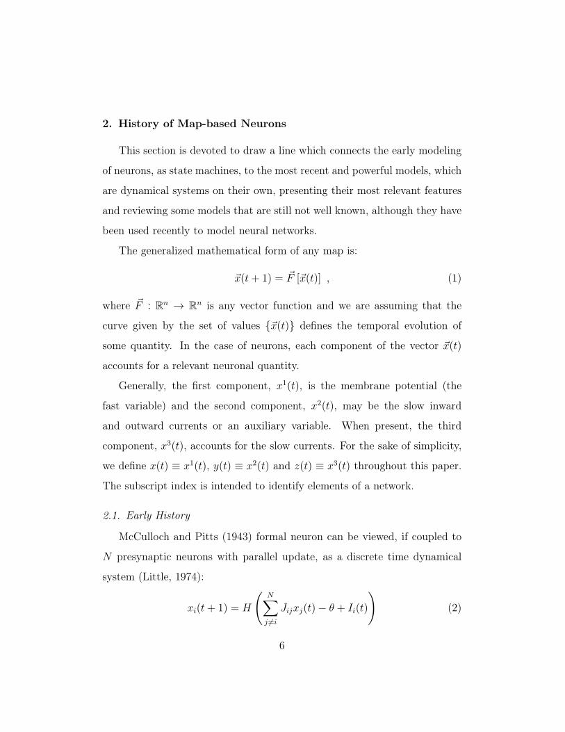
x(t + 1) = F (x(t), x(t− 1), ..., x(t− τ)) is a τ + 1 dimensional map. Fig.
1 illustrates the differences between Eqs. 2 and 5 for τ = 1.
The case τ = 0 with a logistic function F (y), that is, x(t+1) = F (γ(x(t) + I(t)− θ))
was examined by Pasemann (1993). In the plane (γ, H = I − θ) it presents
only three behaviors: a fixed point phase, a period two phase and a bistability
(two fixed points) phase (Pasemann, 1993; Kinouchi and Tragtenberg, 1996).
A chaotic version of this neuron map has also been studied by Pasemann
(1997).
Due to a lucky accident, the case τ = 1 implements a powerful excitable
element with a very rich behavior. We call this system a second order dy-
Figure 1: (a) Scheme of a single-layer perceptron (Eq. 2) and (b) the so-called dynamical
perceptron (Eq. 5 with τ = 1). In both cases, the output xi(t+ 1) may be calculated by
a continuous function or by a discret step function.
8
namical perceptron or the Kinouchi and Tragtenberg (1996) map (also known
in the statistical mechanics literature as the YOS map (Yokoi et al., 1985;
Tragtenberg and Yokoi, 1995)). This excitable neuron model is reviewed in
the next section.
So far all the models follow the same principle: they are built directly
from discrete time dynamics. However, neuronal models can be built the
other way around: starting from continuous time differential equations, like
the HH model, and then simplify them to keep only their wanted features.
A result of this kind of simplification is proposed by Chialvo (1995) to study
excitable systems (and, in particular, neural excitability):
x(t+ 1) = [x(t)]2 exp[y(t)− x(t)] + I(t)
y(t+ 1) = ay(t)− bx(t) + c, (6)
where a, b and c are parameters and I(t) may account for a bias membrane
potential or external input. Chialvo inspired more recent works, like the
Rulkov (2002) and the Izhikevich (2003) models, both studied in Sec. 2.3.
2.2. KT and KTz Maps
The case τ = 1 with F(y) = tanh(y) was extensively studied in the context
of Statistical Mechanics and resulted in many phase diagrams (Tragtenberg
and Yokoi, 1995). In order to build on these results, Kinouchi and Tragten-
berg (1996) imposed, in Eq. 5, the change of parameters K ≡ −W (1)/W (0),
T ≡ 1/W (0) and H ≡ (θ + W (0) + W (1))/W (0). Rewriting Eq. 5 leads us to
the KT model:
x(t+ 1) = tanh
(x(t)−Ky(t) +H + I(t)
T
),
y(t+ 1) = x(t) ,(7)
9
where −1 < x(t) < +1 represents the actual membrane potential of the
neuron at time t – measured in timesteps (ts). The term I(t) corresponds
to an external input. In section 4, the coupling is done via I(t) as well.
Both x(t), I(t) and t may be conveniently rescaled to any unit system, like
mili-Volts or mili-seconds (ms). The authors assumed 1 ts = 0.1 ms whilst
the membrane potential may be rescaled to fit a Hodgkin-Huxley model, for
instance, by relating the value of the membrane potential at the fixed point
and at the peak of the spike in both models.
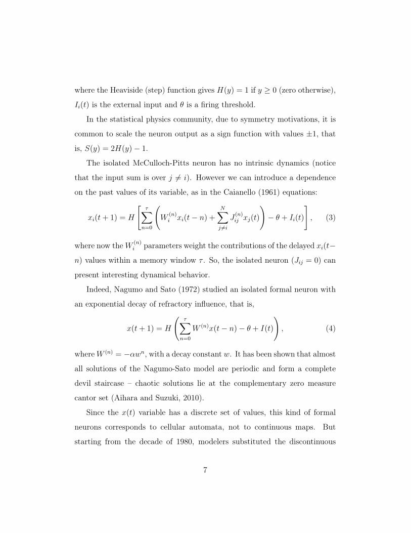
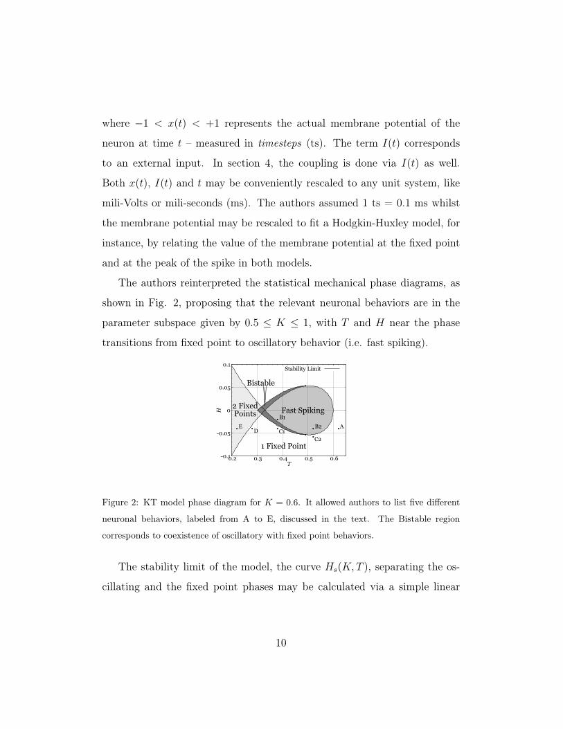
The authors reinterpreted the statistical mechanical phase diagrams, as
shown in Fig. 2, proposing that the relevant neuronal behaviors are in the
parameter subspace given by 0.5 ≤ K ≤ 1, with T and H near the phase
transitions from fixed point to oscillatory behavior (i.e. fast spiking).
H
T
Stability Limit
-0.1
-0.05
0
0.05
0.1
0.2 0.3 0.4 0.5 0.6
1 Fixed Point
ED C1
C2
B2 A
Fast Spiking2 Fixed Points
Bistable
B1
Figure 2: KT model phase diagram for K = 0.6. It allowed authors to list five different
neuronal behaviors, labeled from A to E, discussed in the text. The Bistable region
corresponds to coexistence of oscillatory with fixed point behaviors.
The stability limit of the model, the curve Hs(K,T ), separating the os-
cillating and the fixed point phases may be calculated via a simple linear
10
stability analysis, which yields:
H±s (K,T ) = Tatanh(x∗s)− (1−K)x∗s , (8)
where x∗s is the fixed point over the line Hs(K,T ), given by:
x∗s =
±√
1− T
1−K, if 0 < K ≤ 0.5
±√
1− T
K, if 0.5 < K ≤ 1
. (9)
Differently from the statistical mechanical model, the KT model may be
extended for T < 0 and K < 0. It would result in a slightly different x∗s,
although the analysis would keep the same (Kinouchi and Tragtenberg, 1996).
Thus, we will focus on positive parameters.
Notice that the parameter H may be redefined as H̃ = H + I(t), so the
effect of an external input is to drag the solution x(t) for Eq. 7 along any
vertical line (with fixed T ) on Fig. 2. This is the basic mechanism of the KT
model excitability, in which I(t) is such that H+I(t) > Hs(K,T ) – assuming
the neuron is adjusted below de bubble of Fig. 2. This allows the authors to
list five distinct neuronal behaviors (labeled from A to E in Fig. 2). These
behaviors are present in Hodgkin-Huxley-like neurons and in experimental
setups (Kinouchi and Tragtenberg, 1996):
• Neuron A: Silent neuron – it will not fire any action potential, regardless
the external stimulus intensity – no bifurcation occurs;
• Neuron B (1 and 2): Pacemaker neuron – it is an autonomous oscil-
lator, although external stimulation may bring the neuron to outside
of the bulb in Fig. 2 temporarily via a Subcritical Neimarck-Sacker
bifurcation (B1) or a Supercritical Neimarck-Sacker bifurcation (B2);
11
• Neuron C (1 and 2): Excitable neuron – it will fire only for a stimulus
greater than some threshold; the stimulus takes the neuron inside the
bulb in Fig. 2 through a Subcritical Neimarck-Sacker Bifurcation (C1)
or a Supercritical Neimarck-Sacker Bifurcation (C2). If a neuron C1
is adjusted over the Bistable region, then external stimuli may switch
between fast spiking and fixed point response (phenomenon known as
pacemaker activity annihilation);
• Neuron D: presents a single fixed point; however, a strong enough ex-
ternal current, I(t), may transform it into a bistable neuron with two
stable fixed points;
• Neuron E: presents two stable fixed points even without external input;
the neuron may switch between states through some stimulation I(t).
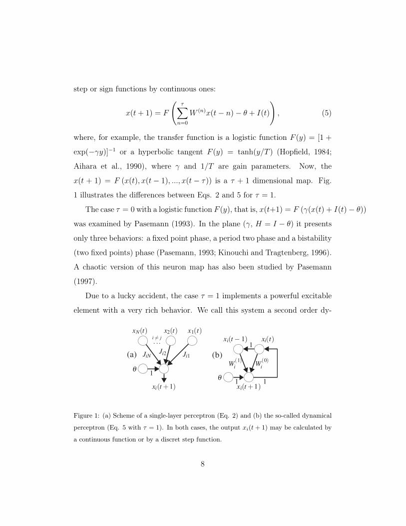
Type C1 neuron, specially, presents a rich repertoire of excitable responses
(see Fig. 3). It also gave the authors insights about the mathematical na-
ture of transient oscillations – not explained, but experimentally observed by
Morris and Lecar (1981): all behaviors of type C1 are achieved because the
neuron lies near a bifurcation point.
KT model also presents a well defined excitability, as shown in the last
panel of Fig. 3 – in which the neuron receives a delta current input I(t) =
I0δt,t0 in t0 = 0 with increasing intensity I0. The circle-dash line shows
the approximate threshold Is: any stronger stimulus causes a spike. The
nullclines of the model are of the same shape as those of the FitzHugh-
Nagumo model (see Fig. 4).
Besides excitability, KT model also presents regular and chaotic au-
12

fixed point
transient osc. tonic spiking
nerve blocking bistability
I (t)x(t)20 ts
excitability
threshold
Figure 3: Excitable response of KT type C1 model. The solution x(t) (–◦–) corresponds
only to the circle points (the lines are just guides so one can follow the sequence in which
the map evolves through time). Solid line is external input and the bolder line segment
corresponds to 20 ts.
y
H = 0
-0.8
-0.4
0
0.4
0.8
-1 -0.5 0 0.5 1 x
H = 0.03
-1 -0.5 0 0.5 1
H = 0.08K = 0.6T = 0.32
x(t+1) = x(t)y(t+1) = y(t)
-1 -0.5 0 0.5 1
Figure 4: Effect of varying parameter H on the nullclines of the KT model. Notice the
similarity with the nullclines of the FitzHugh-Nagumo model.
tonomous behavior (Fig. 5). The authors also proposed a mechanism to
generate bursts based on the Hindmarsh-Rose model (Kinouchi and Tragten-
berg, 1996): by letting the parameter H ≡ z(t), in Eq. 7, oscillate slowly in
time, with
z(t+ 1) = (1− δ)z(t)− λ(x(t)− y(t))2 , (10)
where δ and λ are paremeters that control the inward and the outward ionic
13
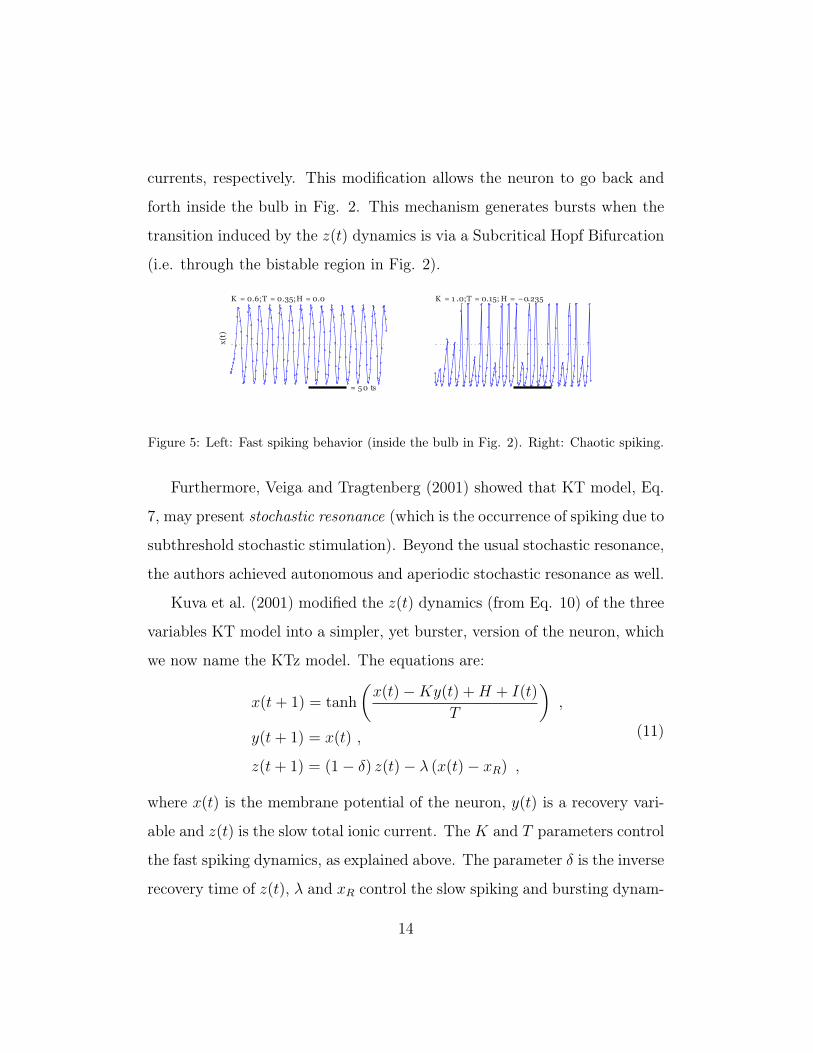
currents, respectively. This modification allows the neuron to go back and
forth inside the bulb in Fig. 2. This mechanism generates bursts when the
transition induced by the z(t) dynamics is via a Subcritical Hopf Bifurcation
(i.e. through the bistable region in Fig. 2).
= 5 0 ts
K = 0.6;T = 0.35;H = 0.0
x(t)
K = 1 .0;T = 0.15; H = −0.235
Figure 5: Left: Fast spiking behavior (inside the bulb in Fig. 2). Right: Chaotic spiking.
Furthermore, Veiga and Tragtenberg (2001) showed that KT model, Eq.
7, may present stochastic resonance (which is the occurrence of spiking due to
subthreshold stochastic stimulation). Beyond the usual stochastic resonance,
the authors achieved autonomous and aperiodic stochastic resonance as well.
Kuva et al. (2001) modified the z(t) dynamics (from Eq. 10) of the three
variables KT model into a simpler, yet burster, version of the neuron, which
we now name the KTz model. The equations are:
x(t+ 1) = tanh
(x(t)−Ky(t) +H + I(t)
T
),
y(t+ 1) = x(t) ,
z(t+ 1) = (1− δ) z(t)− λ (x(t)− xR) ,
(11)
where x(t) is the membrane potential of the neuron, y(t) is a recovery vari-
able and z(t) is the slow total ionic current. The K and T parameters control
the fast spiking dynamics, as explained above. The parameter δ is the inverse
recovery time of z(t), λ and xR control the slow spiking and bursting dynam-
14

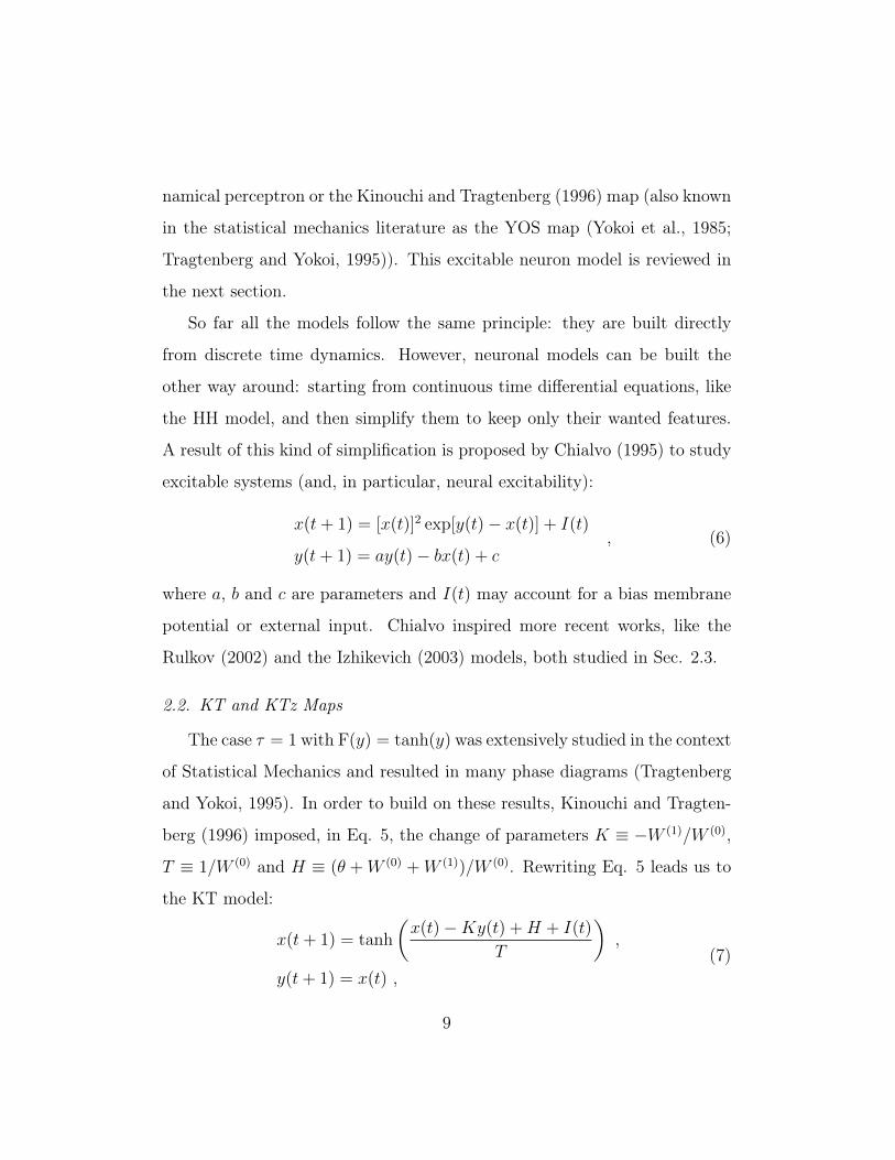
ics Kuva et al. (2001). In practice, though, δ, λ and xR roles are illustrated
in Fig. 6.
-1
-0.5
0
0.5
1
x(t)
Fixed point
δ = 0.01 I = 0.3δt,0
(a) δ = 0.1 I = 0.3(δt,0+δt,30)
(b)
-1
-0.5
0
0.5
1
0 20 40 60 80
x(t)
t
δ = 0.01 I = 0.3(δt,0+δt,30)
(c)
K=0.6; T=0.35; λ=0.1; xR=-0.9
0 20 40 60 80t
δ = 0.001 I = 0.3(δt,0+δt,30)
(d)
-1
-0.5
0
0.5
1
x(t)
λ = 0 I = 0.3δt,0
(e) λ = 0.006 I = 0.3δt,0
(f)
-1
-0.5
0
0.5
1
0 20 40 60 80
x(t)
t
λ = 0.01 I = 0.3δt,0
(g)
0 20 40 60 80t
λ = 0.1 I = 0.3δt,0
(h)
K=0.6; T=0.35; δ=0.1; xR=-0.9
-1
-0.5
0
0.5
1
x(t)
xR = -0.9(i)K=0.6; T=0.35; δ=0.1; λ=0.1;
xR = -0.6(j)
-1
-0.5
0
0.5
1
0 500 1000 1500 2000
x(t)
t
xR = -0.5(k)
0 500 1000 1500 2000t
xR = -0.2(l)
Figure 6: (a) to (d): δ control the length of the refractory period; (e) to (h): λ control the
damping of oscillations; (i) to (l): xR control the bursting dynamics. Parameters’ values
are listed in the panels.
KTz autonomous behaviors are listed in Fig. 8 whilst the excitable be-
haviors are in Fig. 9. A phase diagram for λ = δ = 0.001 and K = 0.6 is
given by Kuva et al. (2001) (see Fig. 7). The fixed point stability of this
model has been studied by Copelli et al. (2004).
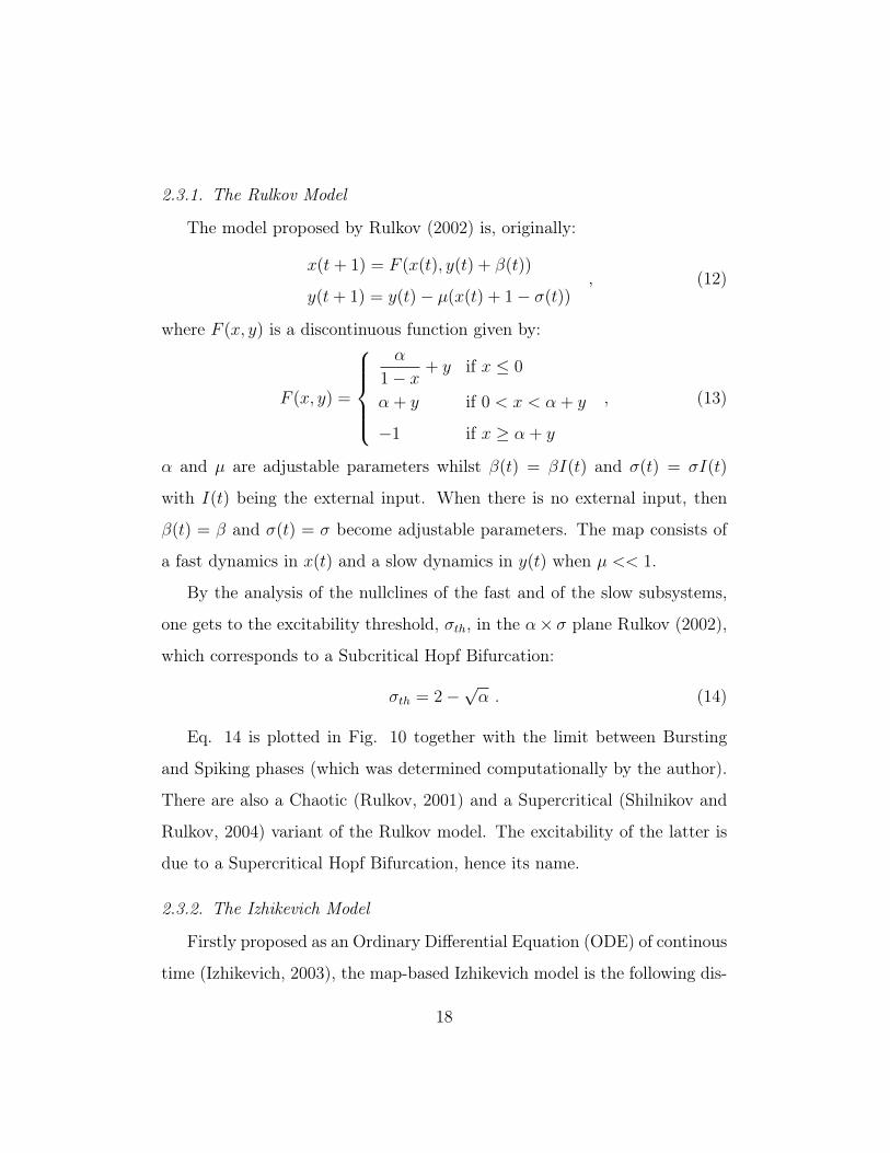
We classified the KTz excitable behaviors according to Izhikevich and
Hoppensteadt (2004), searching for qualitative similarities between their model
and the KTz model. The latter presented 15 out of the 20 excitable behaviors
described by Izhikevich and Hoppensteadt (2004).
Although it does not present every excitable behavior, it is a minimal
model, based on only five parameters (K, T , δ, λ and xR). Besides, the KTz
15
xR
T
0.0
-0.2
-0.4
-0.6
-0.80.0 0.1 0.2 0.3 0.4 0.5 0.6 0.7
Fast andSlowSpikingCardiac
Spikes
Bur
stin
g
FixedPoint
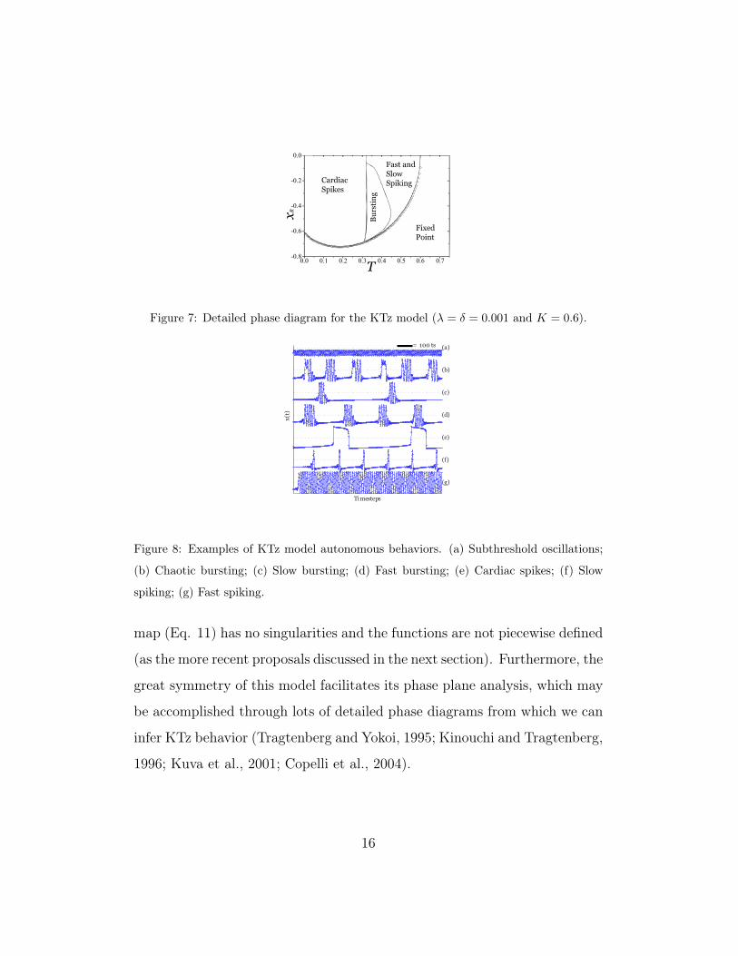
Figure 7: Detailed phase diagram for the KTz model (λ = δ = 0.001 and K = 0.6).
(g)
(f)
(e)
(d)
(c)
(b)
(a)= 100 ts
Timesteps
x(t)
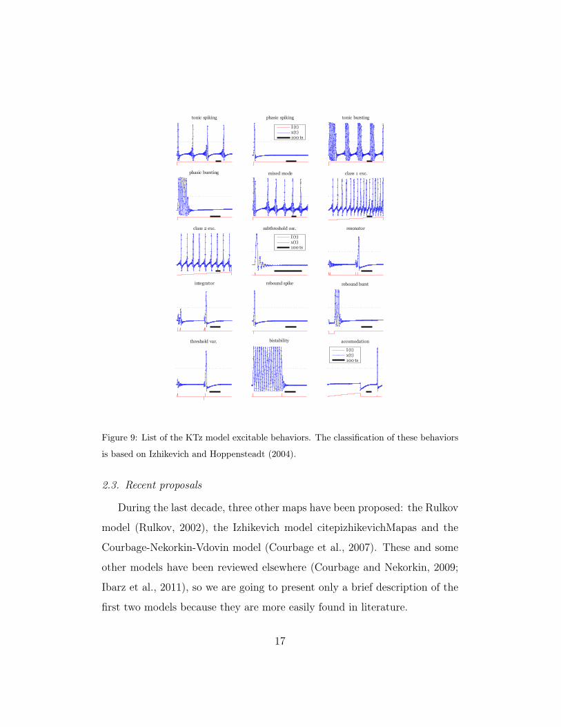
Figure 8: Examples of KTz model autonomous behaviors. (a) Subthreshold oscillations;
(b) Chaotic bursting; (c) Slow bursting; (d) Fast bursting; (e) Cardiac spikes; (f) Slow
spiking; (g) Fast spiking.
map (Eq. 11) has no singularities and the functions are not piecewise defined
(as the more recent proposals discussed in the next section). Furthermore, the
great symmetry of this model facilitates its phase plane analysis, which may
be accomplished through lots of detailed phase diagrams from which we can
infer KTz behavior (Tragtenberg and Yokoi, 1995; Kinouchi and Tragtenberg,
1996; Kuva et al., 2001; Copelli et al., 2004).
16
tonic spiking phasic spiking
tonic bursting
phasic bursting mixed mode class 1 exc.
I (t)x(t)100 ts
class 2 exc. subthreshold osc.
resonator
integrator rebound spike rebound burst
I (t)x(t)100 ts
threshold var. bistability accomodation
I (t)x(t)100 ts
Figure 9: List of the KTz model excitable behaviors. The classification of these behaviors
is based on Izhikevich and Hoppensteadt (2004).
2.3. Recent proposals
During the last decade, three other maps have been proposed: the Rulkov
model (Rulkov, 2002), the Izhikevich model citepizhikevichMapas and the
Courbage-Nekorkin-Vdovin model (Courbage et al., 2007). These and some
other models have been reviewed elsewhere (Courbage and Nekorkin, 2009;
Ibarz et al., 2011), so we are going to present only a brief description of the
first two models because they are more easily found in literature.
17
2.3.1. The Rulkov Model
The model proposed by Rulkov (2002) is, originally:
x(t+ 1) = F (x(t), y(t) + β(t))
y(t+ 1) = y(t)− µ(x(t) + 1− σ(t)), (12)
where F (x, y) is a discontinuous function given by:
F (x, y) =
α
1− x+ y if x ≤ 0
α + y if 0 < x < α + y
−1 if x ≥ α + y
, (13)
α and µ are adjustable parameters whilst β(t) = βI(t) and σ(t) = σI(t)
with I(t) being the external input. When there is no external input, then
β(t) = β and σ(t) = σ become adjustable parameters. The map consists of
a fast dynamics in x(t) and a slow dynamics in y(t) when µ << 1.
By the analysis of the nullclines of the fast and of the slow subsystems,
one gets to the excitability threshold, σth, in the α× σ plane Rulkov (2002),
which corresponds to a Subcritical Hopf Bifurcation:
σth = 2−√α . (14)
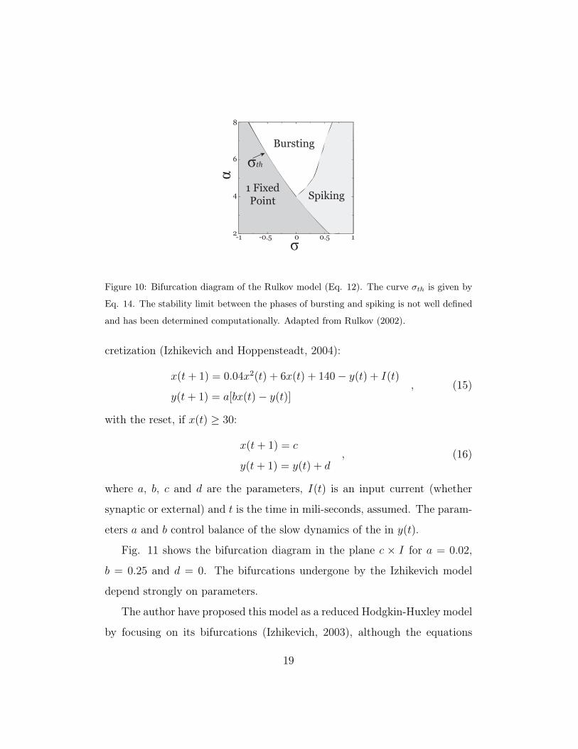
Eq. 14 is plotted in Fig. 10 together with the limit between Bursting
and Spiking phases (which was determined computationally by the author).
There are also a Chaotic (Rulkov, 2001) and a Supercritical (Shilnikov and
Rulkov, 2004) variant of the Rulkov model. The excitability of the latter is
due to a Supercritical Hopf Bifurcation, hence its name.
2.3.2. The Izhikevich Model
Firstly proposed as an Ordinary Differential Equation (ODE) of continous
time (Izhikevich, 2003), the map-based Izhikevich model is the following dis-
18
Bursting
1 FixedPoint Spiking
ασ
σth
2
4
6
8
-1 -0.5 0 0.5 1
Figure 10: Bifurcation diagram of the Rulkov model (Eq. 12). The curve σth is given by
Eq. 14. The stability limit between the phases of bursting and spiking is not well defined
and has been determined computationally. Adapted from Rulkov (2002).
cretization (Izhikevich and Hoppensteadt, 2004):
x(t+ 1) = 0.04x2(t) + 6x(t) + 140− y(t) + I(t)
y(t+ 1) = a[bx(t)− y(t)], (15)
with the reset, if x(t) ≥ 30:
x(t+ 1) = c
y(t+ 1) = y(t) + d, (16)
where a, b, c and d are the parameters, I(t) is an input current (whether
synaptic or external) and t is the time in mili-seconds, assumed. The param-
eters a and b control balance of the slow dynamics of the in y(t).
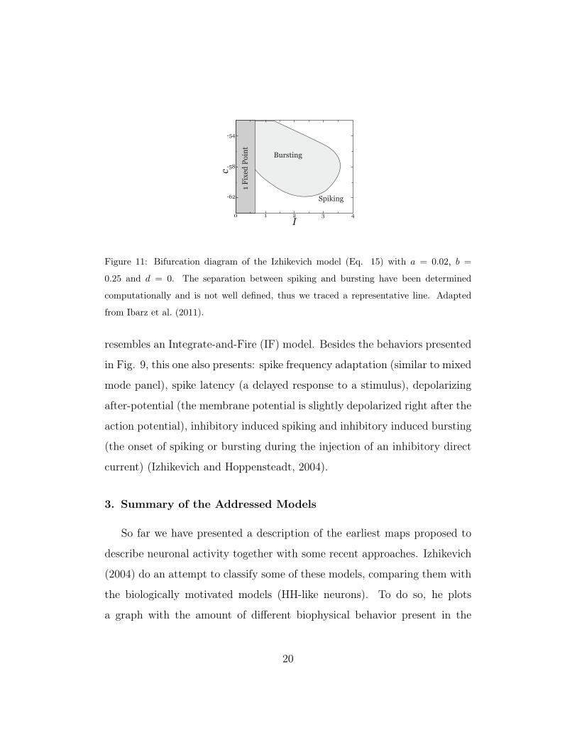
Fig. 11 shows the bifurcation diagram in the plane c × I for a = 0.02,
b = 0.25 and d = 0. The bifurcations undergone by the Izhikevich model
depend strongly on parameters.
The author have proposed this model as a reduced Hodgkin-Huxley model
by focusing on its bifurcations (Izhikevich, 2003), although the equations
19
cI
-62
-58
-54
0 1 2 3 4
Bursting
Spiking
1 Fi
xed
Poin
t
Figure 11: Bifurcation diagram of the Izhikevich model (Eq. 15) with a = 0.02, b =
0.25 and d = 0. The separation between spiking and bursting have been determined
computationally and is not well defined, thus we traced a representative line. Adapted
from Ibarz et al. (2011).
resembles an Integrate-and-Fire (IF) model. Besides the behaviors presented
in Fig. 9, this one also presents: spike frequency adaptation (similar to mixed
mode panel), spike latency (a delayed response to a stimulus), depolarizing
after-potential (the membrane potential is slightly depolarized right after the
action potential), inhibitory induced spiking and inhibitory induced bursting
(the onset of spiking or bursting during the injection of an inhibitory direct
current) (Izhikevich and Hoppensteadt, 2004).
3. Summary of the Addressed Models
So far we have presented a description of the earliest maps proposed to
describe neuronal activity together with some recent approaches. Izhikevich
(2004) do an attempt to classify some of these models, comparing them with
the biologically motivated models (HH-like neurons). To do so, he plots
a graph with the amount of different biophysical behavior present in the
20
model versus the amount of floating-point operations (FLOP – i.e. sums and
multiplications) it would take for the computer to compute 1 ts of the model.
The Hodgkin-Huxley model may produce any biophysically plausible be-
havior, although it takes almost 100 times more FLOP. The Izhikevich model,
with only 13 FLOP, may describe 20 different behaviors. Since the amount
of FLOP is not a precise measure of the performance of any equation (as it
discard anything else than sums and multiplications, like divisions, memory
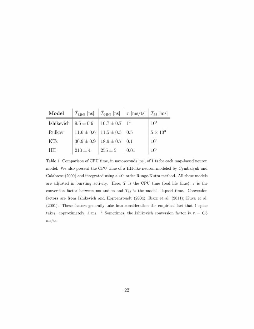
assignments, function calls, etc), we decided to do a benchmark test with the
last three presented models by averaging the CPU time, T in nanoseconds
(ns), each model takes to perform a total of Tts = 10000 ts. We do that
a number S = 10000× to reduce the variation of the measures. Thus, 1
ts takes, in average, T̄ = T/Tts/S real life nanoseconds to complete. The
results are in Table 1 for codes running in 32 bits and 64 bits assemblies
(both in a 64 bits CPU). In this table, the ellapsed time for each model, TM ,
is calculated by TM = τTts, where τ is the amount of miliseconds for each
timestep of the considered model [ms/ts].
Changing from 32 bits to 64 bits makes the KTz neuron reduce by half its
CPU time, reaching the other models’ performance, whilst the others keep
with their same CPU time. Nevertheless, one must remind that the choosing
of the model depends strongly on the problem one is trying to study. For
example, map-based neurons are more suitable for large-scale simulations or
for generic studies (e.g. the cause of bifurcations, the rise of chaotic orbits,
synchronization dynamics, avalanche dynamics, pattern recognition, memory
21
Model T̄32bit [ns] T̄64bit [ns] τ [ms/ts] TM [ms]
Izhikevich 9.6± 0.6 10.7± 0.7 1∗ 104
Rulkov 11.6± 0.6 11.5± 0.5 0.5 5× 10³
KTz 30.9± 0.9 18.9± 0.7 0.1 103
HH 210± 4 255± 5 0.01 102
Table 1: Comparison of CPU time, in nanoseconds [ns], of 1 ts for each map-based neuron
model. We also present the CPU time of a HH-like neuron modeled by Cymbalyuk and
Calabrese (2000) and integrated using a 4th order Runge-Kutta method. All these models
are adjusted in bursting activity. Here, T̄ is the CPU time (real life time), τ is the
conversion factor between ms and ts and TM is the model ellapsed time. Conversion
factors are from Izhikevich and Hoppensteadt (2004); Ibarz et al. (2011); Kuva et al.
(2001). These factors generally take into consideration the empirical fact that 1 spike
takes, approximately, 1 ms. ∗ Sometimes, the Izhikevich conversion factor is τ = 0.5
ms/ts.
22
modeling, etc); and biologically inspired models are more suitable for single
cell studies (e.g. synaptic integration, dendritic cable filtering, effects of
dendritic morphology, the dynamics of ionic currents, etc) or even small-
scale network simulations – at least when there is worry with the simulation
time.
Regardless of the chosen model and besides computational time and being
a generic framework, maps bring many other advantages:
• There is no need for integration nor integration timestep adjustment;
In fact, adjusting an integration timestep turns the ODE we are trying
to solve into a discretized map. The bad thing in this approach is that
the stability of the ODE may not correspond to the map stability.
• The solution is exact; When solving an ODE, the adjustment of an
integration timestep turns the obtained solution in an approximation.
• They are more plausible than pure cellular automaton; The latter is also
used to model neuronal activity (Copelli et al., 2002, 2005; Kinouchi
and Copelli, 2006; Ribeiro et al., 2010), however it is a very abstract
entity in which not only the time, but even the neuronal states are
discretized.
• They keep the main biophysical properties of the Hodgkin-Huxley-like
neurons, as we have seen in the previous section.
Thus, one is encouraged to choose the model which fits better to his purpose:
choosing the best performance may make the phase plane analysis more
difficult, as any of the Rulkov or Izhikevich model depends on a piecewise
23

defined function. Or choosing simplicity over performance with the KTz
model.
4. Coupling Maps
The modeling of neurons as maps is an important and active field of re-
search in the past two decades, as we have seen in the previous sections of this
paper. However, building up a network requires connecting the discrete time
elements through synapses distributed along a particular network topology.
This section is devoted to the synapse models. We summarize some types
of connections, then we list some map models for them and eventually dis-
cuss the main behaviors of these models. We are aware of the risk of being
repetitive, but we go through this for the sake of clarity and neatness.
In short, modeling synapses may or may not take into account the types
of connections biologically observed. We can classify the simpler map-based
synapse models in three cathegories: nonbiologically motivated, biologically
motivated with diffusive (electrical) character and biologically motivated
with impulsive (chemical) character.
The nonbiologically motivated models are usually rooted in the paradigm
of coupled map lattices (Kaneko, 1993; Kaneko and Tsuda, 2001), which are
not necessarily neuronal networks.
Diffusive (electrical) couplings are fast connections, also called gap junc-
tions, that couple neighbouring neurons electrically in a direct form through
channels. They are usually modelled by Ohm’s law, where electric poten-
tial difference generates synaptic current through a time dependent (or not)
conductance.
24

Impulsive (chemical) synapses are connections with exchange of neuro-
transmitters and form the basis for neuronal communication (Keener and
Sneyd, 1998). Phenomenological models or biological models describe the
time dependence of the conductances, due to the release of the neurotrans-
mitters.
In the next subsections, these three kind of models and their applications
will be briefly reviewed. The neurons can also connect or disconnect as a
function of time.This is called synapse plasticity and is an issue that will not
be addressed in this paper.
4.1. Types of Coupling
4.1.1. Nonbiologically Motivated Coupling
A simplification of a neuronal network can be made if the neuron model
is disconnected from biological background and the couplings between them
are based in the paradigm of Coupled Map Lattices, i.e., the functions are
not necessarily rooted on biological foundations.
The typical Coupled Map Lattices (CML) coupling of maps (given by
Eq. 1) can be written in the following generalized mathematical form (Ibarz
et al., 2011):
~xi(t+ 1) = (1− α)~F [~xi(t)] +α
Ni
Ni∑j 6=i
~F [~xj(t)] , (17)
where ~xi(t) is the vector state of the ith neuron (node) at time t, with
1 ≤ i ≤ N , N being the total number of neurons, and Ni is the total number
of nodes connected to the ith node. α ∈ [0; 1) is the coupling parameter:
α = 0 means no coupling and α→ 1 means that the node i’s neighbors play
a more important role to this element state than the node i itself.
25
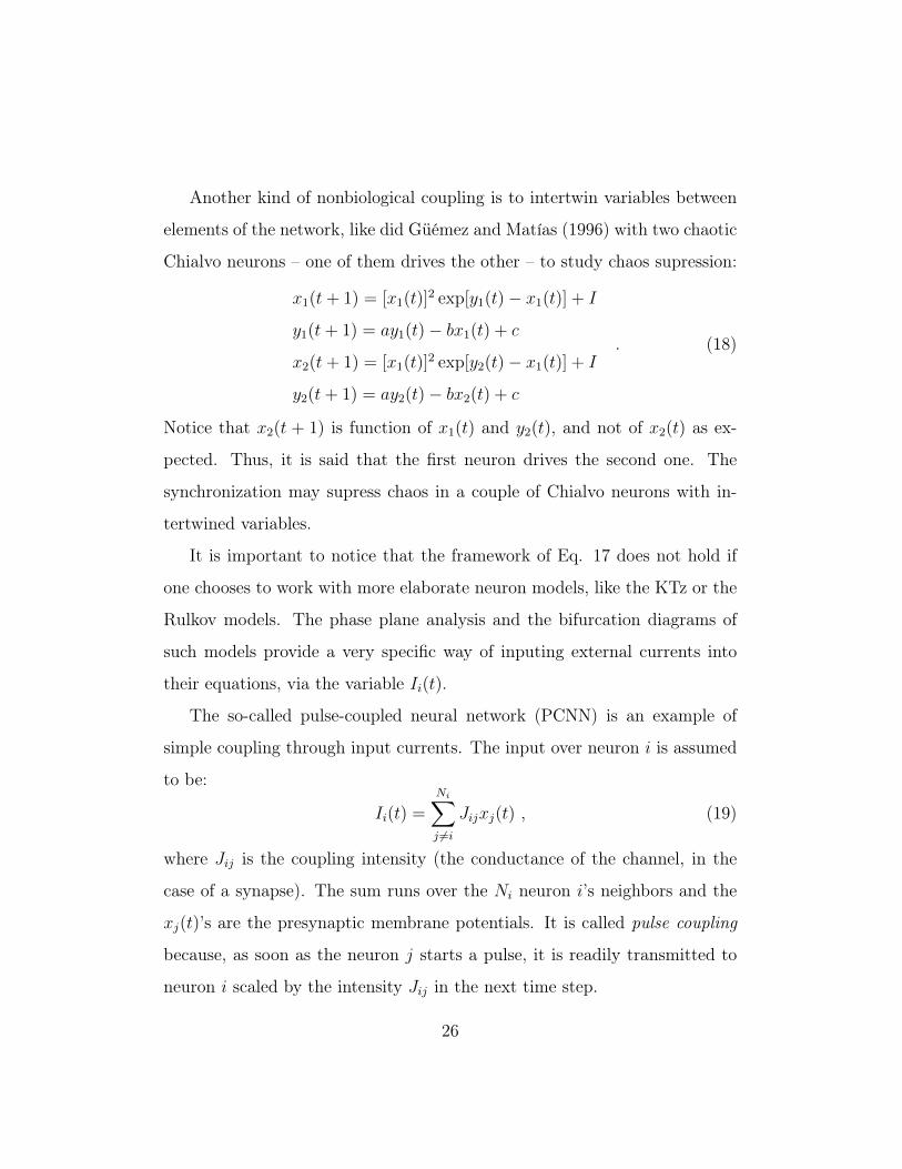
Another kind of nonbiological coupling is to intertwin variables between
elements of the network, like did Güémez and Matías (1996) with two chaotic
Chialvo neurons – one of them drives the other – to study chaos supression:
x1(t+ 1) = [x1(t)]2 exp[y1(t)− x1(t)] + I
y1(t+ 1) = ay1(t)− bx1(t) + c
x2(t+ 1) = [x1(t)]2 exp[y2(t)− x1(t)] + I
y2(t+ 1) = ay2(t)− bx2(t) + c
. (18)
Notice that x2(t + 1) is function of x1(t) and y2(t), and not of x2(t) as ex-
pected. Thus, it is said that the first neuron drives the second one. The
synchronization may supress chaos in a couple of Chialvo neurons with in-
tertwined variables.
It is important to notice that the framework of Eq. 17 does not hold if
one chooses to work with more elaborate neuron models, like the KTz or the
Rulkov models. The phase plane analysis and the bifurcation diagrams of
such models provide a very specific way of inputing external currents into
their equations, via the variable Ii(t).
The so-called pulse-coupled neural network (PCNN) is an example of
simple coupling through input currents. The input over neuron i is assumed
to be:
Ii(t) =
Ni∑j 6=i
Jijxj(t) , (19)
where Jij is the coupling intensity (the conductance of the channel, in the
case of a synapse). The sum runs over the Ni neuron i’s neighbors and the
xj(t)’s are the presynaptic membrane potentials. It is called pulse coupling
because, as soon as the neuron j starts a pulse, it is readily transmitted to
neuron i scaled by the intensity Jij in the next time step.
26

As examples of PCNN, take the Kinouchi and Tragtenberg (1996) ap-
proach to study emergence of collective oscillatory state: a fully connected
network of KT neurons (Sec. 2.2) coupled via Eq. 19 homogeneously (Jij =
Jji = J) and heterogeneously. The coupled model reads:
xi(t+ 1) = tanh
[xi(t)−Kyi(t) +H +
∑Ni
j 6=i Jijxj(t)
T
]yi(t+ 1) = xi(t)
. (20)
Another example is the chaotic Rulkov (2001) model in a mean field
pulse-coupled network, implemented by the equation:
xi(t+ 1) =αi
1 + [xi(t)]2+ yi(t) +
ε
N
N∑j 6=i
xj(t)
yi(t+ 1) = yi(t)− µ[xi(t)− σi], (21)
used to study the synchronization of bursts when the network is not homoge-
neous (notice the indices in σi and in αi). In this case, pulse coupling allows
chaotic bursts to synchronize.
The next two kinds of coupling are biologically inspired and, hence, they
are modeled by input currents just like the one used by PCNN.
4.1.2. Diffusive Coupling
Generally speaking, diffusive (electrical) couplings, also called gap junc-
tions, are fast couplings, where channels between neighboring cells are formed
and allow ions or small molecules to pass through them. Their exchange
speed allow faster synchronization than chemical synapses. They are usual
in the heart, other muscles and during development where synchronization
play a major role (Keener and Sneyd, 1998), but in vertebrates they are a
minority.
27
Typically, they have the form (Connors and Long, 2004):
Ii(t) =
Ni∑j 6=i
Jij[xj(t)− xi(t)] , (22)
where xi,j are membrane potentials and Jij is the conductance of the gap
junction channel.
4.1.3. Impulsive Coupling
The couplings via neurotransmitter exchanges are slower than the elec-
trical ones, but more frequent in vertebrates. They are also called chemical
of impulsive couplings and are responsible by the signal processing.
Generally, the synaptic current Isyn(t) is given by
Isyn(t) = gsyn(t)[xpost(t)− Esyn] (23)
where gsyn(t) is the synaptic current, xpost(t) the postsynaptic membrane
potential, Esyn is the reversal postsynaptic potential. The synaptic conduc-
tance may be modeled by a instantaneous rise with single exponential decay,
an alpha function (with a continuous rise and fall) and a difference of expo-
nentials (Roth and van Rossum, 2010).
Another punch line is the fast threshold modulation (FTM) approxima-
tion (Somers and Kopell, 1993), where there is a very sharp activation thresh-
old and a constant conductance for each coupling such that
Ii(t) =∑k
Ii,k(t) (24)
where
Ii,k(t) = gk[xi(t)− xr,k]∑k
H[xj(t)− θk] (25)
28

where H(x) is the step function, and the index k labels the different types
of chemical synapses. The synaptic reversal potential is xr,k and θk are the
presynaptic threshold of activation.
However, there is indeed a time scale (or more) for the synaptic coupling.
Rulkov et al. (2004) and Bazhenov et al. (2005) propose an equation for the
synaptic current:
Isyn(t+ 1) = γIsyn(t)− g[xpost − xr]δ(t− tpre,k) (26)
where g is a conductance and tpre,k is the time steps the presynaptic neuron
has fired.
Kuva et al. (2001) proposed a map-based equation to model the chem-
ical synaptic coupling between neurons. Their objective is to allow further
research on Computational Neuroscience via biologically motivated Coupled
Map Lattices. The input over neuron i due to coupling current is the simple
sum of the synaptic currents:
Ii(t) =
Ni∑j
Yij(t) , (27)
where Ni is the amount of neighbors of neuron i and Yij(t) is the synaptic
current given by:
Yij(t+ 1) =
(1− 1
τ1
)Yij(t) + hij(t)
hij(t+ 1) =
(1− 1
τ2
)hij(t) + JijΘ[xj(t)]
, (28)
where τ1 and τ2 are exponential time constants, Jij is the coupling intensity
(with dimension of conductance) and Θ(x) = 1 if x > 0 and 0 otherwise is
the Heaviside function. This synaptic current may be excitatory (J > 0) or
inhibitory (J < 0).
29
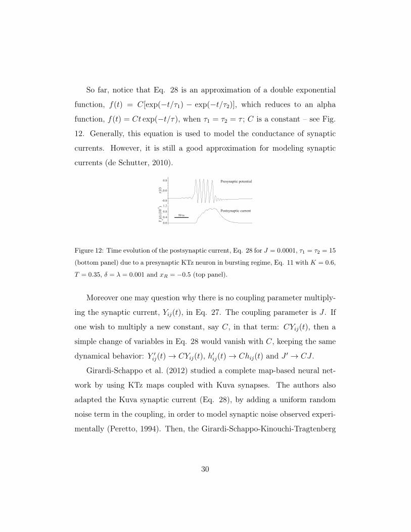
So far, notice that Eq. 28 is an approximation of a double exponential
function, f(t) = C[exp(−t/τ1) − exp(−t/τ2)], which reduces to an alpha
function, f(t) = Ct exp(−t/τ), when τ1 = τ2 = τ ; C is a constant – see Fig.
12. Generally, this equation is used to model the conductance of synaptic
currents. However, it is still a good approximation for modeling synaptic
currents (de Schutter, 2010).
Figure 12: Time evolution of the postsynaptic current, Eq. 28 for J = 0.0001, τ1 = τ2 = 15
(bottom panel) due to a presynaptic KTz neuron in bursting regime, Eq. 11 with K = 0.6,
T = 0.35, δ = λ = 0.001 and xR = −0.5 (top panel).
Moreover one may question why there is no coupling parameter multiply-
ing the synaptic current, Yij(t), in Eq. 27. The coupling parameter is J . If
one wish to multiply a new constant, say C, in that term: CYij(t), then a
simple change of variables in Eq. 28 would vanish with C, keeping the same
dynamical behavior: Y ′ij(t)→ CYij(t), h′ij(t)→ Chij(t) and J ′ → CJ .
Girardi-Schappo et al. (2012) studied a complete map-based neural net-
work by using KTz maps coupled with Kuva synapses. The authors also
adapted the Kuva synaptic current (Eq. 28), by adding a uniform random
noise term in the coupling, in order to model synaptic noise observed experi-
mentally (Peretto, 1994). Then, the Girardi-Schappo-Kinouchi-Tragtenberg
30
(GKT) model is composed of Eq. 28 with Jij ≡ Jij(t) given by:
Jij(t) = J + εij(t) , (29)
where J is the coupling parameter and εij(t) is the uniform random time
signal of amplitude |R|. The noise is different for every synapse j → i. To
keep the synaptic coherence (i.e. in order to the keep inhibitory synapses
always inhibitting and excitatory synapses always exciting), the sign of R is
the same sign of J , then if J > 0, we have εij(t) ∈ [0;R], otherwise we have
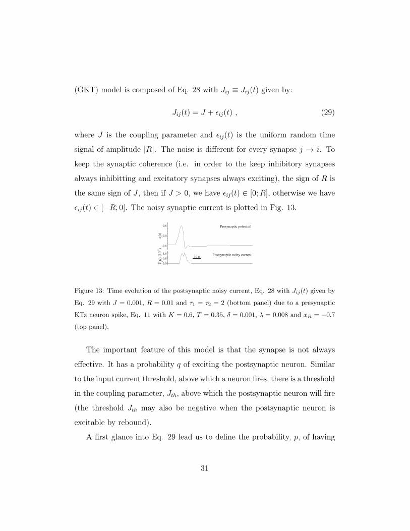
εij(t) ∈ [−R; 0]. The noisy synaptic current is plotted in Fig. 13.
Figure 13: Time evolution of the postsynaptic noisy current, Eq. 28 with Jij(t) given by
Eq. 29 with J = 0.001, R = 0.01 and τ1 = τ2 = 2 (bottom panel) due to a presynaptic
KTz neuron spike, Eq. 11 with K = 0.6, T = 0.35, δ = 0.001, λ = 0.008 and xR = −0.7
(top panel).
The important feature of this model is that the synapse is not always
effective. It has a probability q of exciting the postsynaptic neuron. Similar
to the input current threshold, above which a neuron fires, there is a threshold
in the coupling parameter, Jth, above which the postsynaptic neuron will fire
(the threshold Jth may also be negative when the postsynaptic neuron is
excitable by rebound).
A first glance into Eq. 29 lead us to define the probability, p, of having
31
|Jij(t)| > |Jth|:
p =J +R− Jth
R. (30)
Note that |J + R| > |Jth| always, because J , R and Jth have always the
same sign. One could expect that q = p. That is not true because there
is an internal dynamics in the synaptic current equations: as long as the
spike takes place (xj(t) > 0), the current keeps summing different quantities
J + εij(t). Thus, the same set (J,R) may not always lead to a postsynaptic
spike. Anyway, the quantity p may be regarded as a first approximation to
q.
4.2. Applications of the synapse models
A summary of the results obtained by each of the classes of synapse mod-
els (nonbiologically motivated, electric, chemical) in recognizing image pat-
terns, modeling cat visual cortex, synchronization (connected with topology
network, noise, spike-burst behavior, delay, rewiring, ...), bistable states of
the brain, effects of external signals, information transmission and criticality
in neuronal avalanches is given in this subsection.
4.2.1. Nonbiologically motivated
As one example of CML application is the study of synchonization made
by Jampa et al. (2007). They connected Chialvo neurons through a short
version of Eq. 17, in which the coupling term is written only as (ε/2)[xj(t)(t)+
xk(t)(t)], where the indices j(t) and k(t) are picked at each timestep, with
probability p, by randomly assigning to each node an index, l ∈ [1;N ], and
then calculating j(t) = l−1 and k(t) = l+1 (modulo N). The rewiring prob-
ability p and the coupling strength ε determine the kind of synchronization:
32
chaotic, spatio-temporal chaos or fixed point.
On the other hand, the PCNN approach is used for many purposes: mod-
eling cat visual cortex(Eckhorn et al., 1990), recognizing image patterns
(Wang et al., 2010), synchronization and related problems (Kinouchi and
Tragtenberg, 1996; Goel and Ermentrout, 2002; Zou et al., 2009).
Eckhorn et al. (1990) modeled the cat visual cortex via PCNN, particu-
larly the stimulus-induced oscillations, used for pattern recognition and fea-
ture associations. Wang et al. (2010) reviewed the successful use of PCNN in
many dimensions of image processing: segmentation, denoising, object and
edge detection, feature extraction and pattern recognition (enhancement, fu-
sion, etc). Goel and Ermentrout (2002) discretized an ODE, and found waves
in a ring and synchonization stability dependent of the number of neurons.
Stable chaos was found in a PCNN of discontinuous maps by Zou et al.
(2009).
Pontes et al. (2008) found that the coupling strength needed to synchro-
nized Rulkov bursters is smaller when the range of couplings is bigger.
de Vries (2001a,b) showed that mean field-coupling of the same system
can turn isolated spiking into coupled bursting neurons. Then, in this case
bursting can be seen as an emergent behavior.
de Vries (2012a) used coupled logistic maps, as well as Stuart-Landau
oscillators and leaky IF neurons, to study dynamical properties of coupled
oscillator sparse lattices in many scales of length. They show a transition
from micro to macroscopic scale in network syncronization driven by a critical
conectivity.
López-Ruiz and Fournier-Prunaret (2012) mimicked a bistable (sleep-
33
awaken) brain by a logistic map lattice, with usual CML interactions.
The pulse-coupled KT model with homogeneous couplings, Jij = J , may
lead a network of silent neurons (adjusted with (K,T,H < Hs) – Eq. 8,
outside of the bubble in Fig. 2 into a collective oscillating phase if the sum
Ii(t) = J∑〈j〉 xj(t) is sufficiently big – such that H̃ = H + Ii(t) > Hs(K,T )
(for neurons with H < 0).
More clearly, if H < 0, the fixed point is also x∗ < 0. Thus, if J < 0
(inhibitory coupling), the sum Ii(t) = J∑〈j〉 xj(t) will be a positive number
and the achieved state will have a new H̃ given by H̃ = H + Ii(t). Then,
there is a threshold – exactly equal to the excitability threshold discussed in
Sec. 2.2 – above which the network will spontaneously oscillate, even though
any uncoupled neuron is silent (in the fixed point). This is a counter-intuitive
result, although it also happens with realistic neurons (Golomb and Rinzel,
1993; Ernst et al., 1995).
If the term |J | is big enough, the network will cross through the bubble
in Fig. 2 and will reach the upper fixed point, x∗ > 0. This picture may
be generalized to the heterogeneous case, however the value of Ii(t), in such
case, is not guaranteed to be positive.
The heterogeneous case may be used both for modeling practical problems
and for investigation purposes. As examples, one could assemble a neural
network for pattern recognition by mixing linear neurons (in the output) and
KT units and adjusting weights according to a training algorithm (Kinouchi
and Tragtenberg, 1996) (see Albano et al. (1992) for an application with
neurons given by Eq. 2, but with a nonlinear activation function). On the
other hand, Izhikevich (2003) studies brain rythms via a PCNN made of his
34
neuron model (discretized with a 0.1 ms timestep).
The Izhikevich heterogeneous network consists in mixed excitatory (Jij >
0) and inhibitory (Jij < 0) coupling. From the network’s time evolution,
emerge groups of synchronized neurons in different phases – the so called
polychronous state. Izhikevich (2006) discuss that these polychronous groups
represent the memory of the network, as different external stimuli produce
different polychronization patterns. Yet, the number of produced patterns is
far greater than the number of neurons in the network, yielding a very big
memory capacity.
4.2.2. Diffusive coupling
Diffusive coupling has been extensively used in the study of synchroniza-
tion, spatio-temporal chaos, effects of external inputs on a neuronal network,
spiking-bursting transition, among other subjects.
Rulkov (2002) studied the existence of synchronization regimes for spiking
and bursting activities of rulkov-map a function of neuron coupling strength.
de Vries (2012b) connected Rulkov neurons in a small-world network
through typical electrical connections to study synchronization and spatio-
temporal chaos.
Subthreshold stimulus were found to induce synchronization in a noisy
square lattice Rulkov network by Wang et al. (2007). The study of Rulkov
neurons with information transmission delay in a small-world geometry with
additive noise and delay, as done by Wang et al. (2008), show the existence
of transitions in synchronization as a function of the delay. The delay may
also induce stochastic resonance in a scale-free network of Rulkov neurons,
have shown Wang et al. (2009).
35
The increasing of diversity of Rulkov neuron connections may induce syn-
chronization in a Rulkov map neural network, as analyzed by Chen and Liu
(2009). The influence of a mix of electrical and chemical synapses connecting
Rulkov neurons on burst synchonization and transmission (seen as chaotic
itinerancy Kaneko and Tsuda (2003)) were studied by Tanaka et al. (2006).
Ivanchenko et al. (2007) and Ivanchenko et al. (2004) studied transitions be-
tween bursting and spiking Rulkov neurons connected by electrical synapses
in many time scales and the chaotic phase synchronization by an external pe-
riodic input to a single neuron. Batista et al. (2007) and Batista et al. (2009)
also showed that external periodic signals can generate burst synchronization
in networks of Rulkov neurons electrically coupled.
4.2.3. Impulsive coupling
Connecting map neurons by chemical synapses is not as popular as us-
ing electrical synapses, despite the chemical are more widespread than the
electrical. One of the most popular approaches is the FTM, which shows
no synaptic dynamics. However, there are some proposals of describing the
chemical synapse dynamics applied to network behavior.
In the FTM front, Ivanchenko et al. (2007) showed that electrical and
impulsive (chemical) synapses behave like electrical, since networks of Rulkov
maps exhibit transition syncronized-desynchronized transition as a function
of the coupling strength.
Ibarz et al. (2008) used FTM to show a bunch of effects of impulsive
synapses: excitatory synapses may generate antiphase synchronization, synapse
may change from excitatory to inhibitory as a change in conductance and
with the same reversal potential, small variations in the synaptic threshold
36
may cause big changes in synchronization of spikes within bursts.
Shi and Lu (2009) also applied FTM coupling in the studiyg of in-phase
burst synchronization of Rulkov neurons.
Inhibitory bursting Rulkov maps chemically coupled may exhibit power-
law behavior at the onset of a synchronization transition, driven by the cou-
pling strength or stimulation current(Franovic and Miljkovic, 2010).
The effect of delay in in-phase and anti-phase synchronization was the
object of Franovic and Miljkovic (2011) in Rulkov map neural network con-
nected by reciprocal sigmoid chemical synapses.
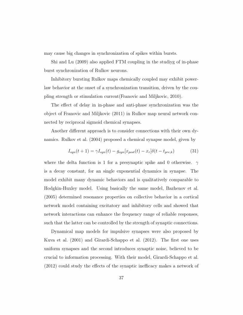
Another different approach is to consider connections with their own dy-
namics. Rulkov et al. (2004) proposed a chemical synapse model, given by
Isyn(t+ 1) = γIsyn(t)− gsyn[xpost(t)− xr]δ(t− tpre,k) (31)
where the delta function is 1 for a presynaptic spike and 0 otherwise. γ
is a decay constant, for an single exponential dynamics in synapse. The
model exhibit many dynamic behaviors and is qualitatively comparable to
Hodgkin-Huxley model. Using basically the same model, Bazhenov et al.
(2005) determined resonance properties on collective behavior in a cortical
network model containing excitatory and inhibitory cells and showed that
network interactions can enhance the frequency range of reliable responses,
such that the latter can be controlled by the strength of synaptic connections.
Dynamical map models for impulsive synapses were also proposed by
Kuva et al. (2001) and Girardi-Schappo et al. (2012). The first one uses
uniform synapses and the second introduces synaptic noise, believed to be
crucial to information processing. With their model, Girardi-Schappo et al.
(2012) could study the effects of the synaptic inefficacy makes a network of
37
neurons coupled with GKT synapses a matter of stochastic dynamics, since
the amount of neurons, s, that will fire in the network due to an initial
stimulation is not obvious. The network activity due to one stimulus is
called an avalanche. The authors investigated regular square lattices with free
boundary conditions of KTz neurons coupled with GKT synapses and found
that s follows a powerlaw P (s) ∼ s−µ with µ = 1.35. Besides, the duration
of avalanches, w, also follows a powerlaw P (w) ∼ w−ν , with ν = 1.50.
Moreover, the authors measured the activity of a subsampled network – a
network in which the measurement can be made in only a very small fraction
of the elements. Generally, experimental setups are subsampled, since the
number of neurons which are recorded is far less than the number of neurons
in the sample (Priesemann et al., 2009; Ribeiro et al., 2010). The subsampling
results matched the experiments of Ribeiro et al. (2010) and, together with
the powerlaw behavior in the network activity, both in temporal and spatial
dimensions, show that the system is critical and suggests that there may be
a Self-Organized Critical (SOC) state in brain activity and neural network
models (Girardi-Schappo et al., 2012).
The SOC state is, generally, present when there is a balance between ten-
sioning and relaxing the system (Bak et al., 1987, 1988; Christensen et al.,
1993; Jensen, 1998; Dhar, 2006; Bonachela and Muñoz, 2009, and many
others). Due to theoretical considerations about criticality in neural net-
works (Usher et al., 1995; Stassinopoulos and Bak, 1995; Herz and Hopfield,
1995), Beggs and Plenz (2003) proposed SOC to explain the brain activ-
ity. Avalanches are experimentally observed (Beggs and Plenz, 2003, 2004;
Priesemann et al., 2009; Ribeiro et al., 2010; Chialvo, 2010; Werner, 2010;
38
Beggs and Timme, 2012; Shew and Plenz, 2013, and references there in),
although there is a great debate on the criticality of the brain.
The basic idea is that the brain works with the precisely needed amount
of activity and that there may be a homeostatic mechanism which led the
brain to such a state. Within this framework, mental diseases and disorders
would be associated with deviations from the critical amount of activity
(Chialvo, 2004, 2010; Vertes et al., 2011). The critical state has been shown
to enhance the dynamical range of sensitivity to external stimuly (Kinouchi
and Copelli, 2006; Shew et al., 2009), to optimize the memory and learning
processes (de Arcangelis et al., 2006) and the computational power of the
brain (Werner, 2010; Shew and Plenz, 2013; Beggs and Timme, 2012).
A necessary condition for SOC is that the system may not be imposed into
the critical state, rather it should find its own path towards criticality with no
fine tuning. As no computer model could work on its own, without external
tuning of parameters, Kinouchi (1998) proposed to call these systems Self-
Organized quasi-Critical (SOqC). SOqC systems have a balance dynamical
equation that makes the system oscillate in the neighborhood of the critical
point. In this sense, the GKT model is not SOC, nor SOqC, because the
authors had to adjust the parameters J and R. However, a variation of the
GKT model could contain a homeostatic mechanism over the parameter R
or J , for instance, that would take the system towards the critical point,
turning the system into a SOqC system.
39
5. Concluding Remarks
Although generally studied in the context of dynamical systems, some of
the models outlined in this work may be used in computational applications,
such as pattern recognition, data analysis, data classification, data associa-
tion and so on, like the McCulloch-Pitts model utilized in the perceptron.
We directed our studies mainly through the historical development of the
map-based models, by theoretically constructing over the McCulloch-Pitts
model, adding delayed self-couplings (which creates dynamical behaviors),
changing to a continuous activation function and adding coupling currents
to the model.
This approach allowed us to close the gap between the first discrete time
models and the most recent maps. In general, we tried to keep the original
design concepts of the models, except for the Izhikevich’s, which was orig-
inally designed as an ODE. Nevertheless we assume that the discretization
of an ODE results in a map, with behavior of its own. Thus, we linked two
entire family of models with very rich excitable and dynamical behaviors,
namely the perceptron family (from McCulloch-Pitts until KTz) and the HH
family (from Chialvo to Izhikevich). We also showed that there is a close
dynamical correspondence between KTz and the behaviors of HH.
The models of the HH family are, generally, piecewise defined functions.
However, all of these models present bursting activity with only two dynam-
ical variables, differently from the KTz map (whose bursting behavior was
based in Hindmarsh-Rose model). On the other hand, the symmetry and
simplicity of the KTz map may be of great help during the phase plane and
bifurcation analysis. KT and KTz also may be suitable when there is a need
40
to explore the effects of the whole action potential, as all the other models
assume that the spike occurs instantly. Therefore, if one wants to model a
more rigorous synaptic transmission with the map framework, KT or KTz
are should be chosen.
Every map model presents a similar computational performance, as dis-
cussed in Sec. 3, which is approximately 20× faster than the HH perfor-
mance. Thus, the most prominent features of all the studied models are their
simiplicity, reliability, numerical stability and computational performance.
Moreover, we categorized the many types of coupling used to connect
the covered models. Many times, the coupling and the network topology
are indissociable, forcing one to study the coupling of neurons under a given
topology. From pulse-coupled networks to map-based modeling of chemical
synapses, we presented their most common usability, relating with the re-
sults achieved in each case. Since synapses is, alone, a broad research area,
we highlight the importance of modeling synapses specifically for working
with map-based neural networks, as did Kuva et al. (2001), otherwise the
differential equations would have to be discretized for each case, bringing ad-
ditional modeling problems, namely how to synchronize the time evolution of
the map-based neuron with the time evolution of the synapses, as the latter
should be precisely solved to avoid numerical inaccuracy?
Finally, recent results have shown that map-based neural networks is a
promising developing field, for example, Girardi-Schappo et al. (2012) mod-
eled both synapses and neurons with maps and showed that a critical state
may develop in regular lattices when the coupling is subjected to uniform
noise. Just as examples, on the list of some still unexplored paths in map-
41
based neuronal modeling is the compartimental modeling and the seek for
a canonical purely map-based model (in the ODE framework, the neuron
model differs from the whole class of HH-type neurons by just a change o
variables (Hoppensteadt and Izhikevich, 2002); on the other hand, a canoni-
cal map-based model would be the most simple model capable of describing
all the HH-type neurons behaviors).
With this work, we hope we have brought more attention to this kind of
modeling, which may play an important role in the forthcoming years, both
in technologic applications and in neuroscientific research.
6. Acknowledgement
We would like to thank the invitation to make this neuron map modeling
overview from Antonio Carlos Roque da Silva.
References
Aihara, K., Suzuki, H., 2010. Theory of hybrid dynamical systems and its
applications to biological and medical systems. Phil. Trans. R. Soc. A 368,
4893–4914.
Aihara, K., Takabe, T., Toyoda, M., 1990. Chaotic neural networks. Phys.
Lett. A 144(6,7), 333–340.
Albano, A. M., Passamante, A., Hediger, T., Farrell, M. E., 1992. Using
neural nets to look for chaos. Physica D 58, 1–9.
Azevedo, F. A. C., Carvalho, L. R. B., Grinberg, L. T., Farfel, J. M., Ferretti,
R. E. L., Leite, R. E. P., Filho, W. J., Lent, R., Herculano-Houzel, S., 2009.
42
Equal numbers of neuronal and nonneuronal cells make the human brain
an isometrically scaled-up primate brain. J. Comp. Neurol. 513, 532–541.
Bak, P., Tang, C., Wiesenfeld, K., 1987. Self-organized criticality: An expla-
nation of 1/f noise. Phys. Rev. Lett. 59(4), 381–384.
Bak, P., Tang, C., Wiesenfeld, K., 1988. Self-organized criticality. Phys. Rev.
A 38(1), 364–374.
Batista, C. A. S., Batista, A. M., de Pontes, J. A. C., Lopes, S. R., Viana,
R. L., 2009. Bursting synchronization in scale-free networks. Chaos, Soli-
tons and Fractals 41, 2220–2225.
Batista, C. A. S., Batista, A. M., de Pontes, J. A. C., Viana, R. L., Lopes,
S. R., 2007. Bursting synchronization in scale-free networks. Phys. Rev. E
76, 016218.
Bazhenov, M., Rulkov, N. F., Fellous, J., Timofeev, I., 2005. Role of network
dynamics in shaping spike timing reliability. Phys. Rev. E 72, 041903.
Beggs, J. M., Plenz, D., 2003. Neuronal avalanches in neocortical circuits. J.
Neurosci. 23(35), 11167–11177.
Beggs, J. M., Plenz, D., 2004. Neuronal avalanches are diverse and precise
activity patterns that are stable for many hours in cortical slice cultures.
J. Neurosci. 24(22), 5216–5229.
Beggs, J. M., Timme, N., 2012. Being critical of criticality in the brain. Front.
Physiol. 3, 163.
43
Bellman, R. E., 2003. Dynamic Programming. Dover.
Bonachela, J. A., Muñoz, M. A., 2009. Self-organization without conserva-
tion: true or just apparent scale-invariance? J. Stat. Mech., P09009.
Bower, J. M., Beeman, D., 2003. The Book of GENESIS: Exploring Realis-
tic Neural Models with the GEneral NEural SImulation System. Internet
Edition.
Caianello, E. R., 1961. Outline of a theory of thought process and thinking
machines. J. Theor. Biol. 1, 204–235.
Carnevale, N. T., Hines, M. L., 2006. The NEURON Book. Cambridge Uni-
versity Press.
Chen, H., Liu, J. Z. J., 2009. Enhancement of neuronal coherence by diversity
in couple rulkov-map models. Physica A 19, 023112.
Chialvo, D. R., 1995. Generic excitable dynamics on a two-dimensional map.
Chaos Solitons Fractals 5, 461–479.
Chialvo, D. R., 2004. Critical brain networks. Physica A 340, 756–765.
Chialvo, D. R., 2010. Emergent complex neural dynamics. Nat. Phys. 6, 744–
750.
Christensen, K., Flyvbjerg, H., Olami, Z., 1993. Self-organized critical forest-
fire model: Mean-field theory and simulation results in 1 to 6 dimensions.
Phys. Rev. Lett. 71(17), 2737–2740.
44
Connors, B. W., Long, M. A., 2004. Electrical synapses in the mammalian
brain. Annual Review of Neuroscience 27, 393–418.
Copelli, M., Oliveira, R. F., Roque, A. C., Kinouchi, O., 2005. Signal com-
pression in the sensory periphery. Neurocomputing 65–66, 691–696.
Copelli, M., Roque, A. C., Oliveira, R. F., Kinouchi, O., 2002. Physics of
psychophysics: Stevens and weber-fechner laws are transfer functions of
excitable media. Phys. Rev. E 65, 060901.
Copelli, M., Tragtenberg, M. H. R., Kinouchi, O., 2004. Stability diagrams
for bursting neurons modeled by three-variable maps. Physica A 342, 263–
269.
Courbage, M., Nekorkin, V. I., 2009. Map based models in neurodynamics.
Int. J. Bifurcat. Chaos 20(6), 1631–1651.
Courbage, M., Nekorkin, V. I., Vdovin, L. V., 2007. Chaotic oscillations in a
map-based model of neural activity. Chaos 17(4), 043109.
Cymbalyuk, G., Calabrese, R. L., 2000. Oscillatory behaviors in pharmaco-
logically isolated heart interneurons from the medicinal leech. Neurocom-
puting 32–33, 97–104.
Dayan, P., Abbott, L. F., 2001. Theoretical Neuroscience: Computational
and Mathematical Modeling of Neural Systems. The MIT Press.
de Arcangelis, L., Perrone-Capano, C., Herrmann, H. J., 2006. Self-organized
criticality model for brain plasticity. Phys. Rev. Lett. 96, 028107.
45

de Schutter, E. (Ed.), 2010. Computational Modeling Methods for Neuroci-
entists. The MIT Press.
de Vries, G., 2001a. Bursting as an emergent phenomenon in coupled chaotic
maps. Phys. Rev. E 64, 051914.
de Vries, G., 2001b. From spikers to bursters via coupling: help from hetero-
geneity. Bull. Math. Biol 63, 371–391.
de Vries, G., 2012a. Collective dynamics in sparse networks. Phys. Rev. Lett.
109, 138103.
de Vries, G., 2012b. Collective dynamics in sparse networks. Phys. Rev. Lett.
109, 138103.
Dhar, D., 2006. Theoretical studies of self-organized criticality. Physica A
369, 29–70.
Eckhorn, R., Reitboeck, H. J., Arndt, M., Dicke, P. W., 1990. Feature linking
via synchronization among distributed assemblies: simulations of results
on cat visual cortex. Neural Computation 2, 293–307.
Ernst, U., Pawelzik, K., Geisel, T., 1995. Synchronization induced by tem-
poral delays in pulse-coupled oscillators. Phys. Rev. Lett. 74, 1570–1573.
FitzHugh, R., 1955. Mathematical models of threshold phenomena in the
nerve membrane. Bulletin of Mathematical Biophysics 17, 257–278.
Franovic, I., Miljkovic, V., 2010. Power law behavior related to mutual syn-
chronization of chemically coupled map neurons. Euro. Phys. J. B 76,
613–624.
46
Franovic, I., Miljkovic, V., 2011. The effects of synaptic time delay on mo-
tifs of chemically coupled rulkov model neurons. Commun. Nonlinear Sci.
Numer. Simul. 16, 623–633.
Girardi-Schappo, M., Kinouchi, O., Tragtenberg, M. H. R., 2012.
Critical avalanches and subsampling in map-based neural networks.
arXiv:1209.3271 [cond-mat.dis-nn].
Goel, P., Ermentrout, B., 2002. Synchrony, stability, and firing patterns in
pulse-coupled oscillators. Physica D 163, 191–216.
Golomb, D., Rinzel, J., 1993. Dynamics of globally coupled inhibitory neu-
rons with heterogeneity. Phys. Rev. E 48, 4810–4814.
Güémez, J., Matías, M. A., 1996. Synchronous oscillatory activity in assem-
blies of chaotic model neuron. Physica D 96, 334–343.
Herz, A. V. M., Hopfield, J. J., 1995. Earthquake cycles and neural rever-
berations: Collective oscillations in systems with pulse-coupled threshold
elements. Phys. Rev. Lett. 75, 1222–1225.
Hindmarsh, J. L., Rose, R. M., 1984. A model of neuronal bursting using
three coupled first order differential equations. Proc. R. Soc. Lond., B,
Biol. Sci. 221, 87–102.
Hopfield, J. J., 1984. Neurons with graded response have collective compu-
tational properties like those of two-sate neurons. Proc. Nat. Acad. Sci.
(USA) 81, 3088–3092.
47
Hoppensteadt, F. C., Izhikevich, E. M., 2002. Canonical Neural Models. The
MIT Press.
Ibarz, B., Cao, H., Sanjuan, M. A. F., 2008. Bursting regimes in map-based
neuron models coupled through fast threshold modulation. Phys. Rev. E
77, 051918.
Ibarz, B., Casado, J. M., Sanjuán, M. A. F., 2011. Map-based models in
neuronal dynamics. Phys. Rep. 501, 1–74.
Ivanchenko, M. V., Osipov, G. V., Shalfeev, V. D., Kurths, J., 2004. Phase
synchronization in ensembles of bursting oscillators. Phys. Rev. Lett. 93,
134101.
Ivanchenko, M. V., Osipov, G. V., Shalfeev, V. D., Kurths, J., 2007. Network
mechanism for burst generation. Phys. Rev. Lett. 98, 108101.
Izhikevich, E. M., 2003. Simple model of spiking neurons. IEEE Trans. Neural
Netw. 14(6), 1569–1572.
Izhikevich, E. M., 2004. Which model to use for cortical spiking neurons?
IEEE Trans. Neural Netw. 15, 1063–1070.
Izhikevich, E. M., 2006. Polychronization: Computation with spikes. Neural
Comput. 18(2), 245–282.
Izhikevich, E. M., Hoppensteadt, F., 2004. Classification of bursting map-
pings. Int. J. Bifurcat. Chaos 14(11), 3847–3854.
Jampa, M. P. K., Sonawane, A. R., Gade, P. M., Sinha, S., 2007. Sincroniza-
tion in a network of model neurons. Physical Review E 75, 026215.
48

Jensen, H. J., 1998. Self-Organized Criticality: Emergent Complex Behavior
in Phyical and Biological Systems. Cambridge University Press.
Kaneko, K., 1993. Theory and Applications of Coupled Map Lattices. Wiley.
Kaneko, K., 1994. Relevance of dynamic clustering to biological networks.
Physica D 75, 55–73.
Kaneko, K., Tsuda, I., 2001. Complex Systems: Chaos and Beyond. A Con-
structive Approach with Applications in Life Sciences. Springer.
Kaneko, K., Tsuda, I., 2003. Chaotic itinerancy. Chaos 13, 926–936.
Keener, J., Sneyd, J., 1998. Mathematical Physiology. Springer.
Kinouchi, O., Fevereiro 1998. Self-organized (quasi-)criticality: the extremal
feder and feder model. arXiv:cond-mat/9802311v1.
Kinouchi, O., Copelli, M., 2006. Optimal dynamical range of excitable net-
works at criticality. Nat. Phys. 2, 348–351.
Kinouchi, O., Tragtenberg, M. H. R., 1996. Modeling neurons by simple
maps. Int. J. Bifurcat. Chaos 6, 2343–2360.
Kuva, S. M., Lima, G. F., Kinouchi, O., Tragtenberg, M. H. R., Roque,
A. C., 2001. A minimal model for excitable and bursting elements. Neuro-
computing 38–40, 255–261.
Little, W. A., 1974. The existence of persistent states in the brain. Math.
Biosci. 19, 101–120.
49
López-Ruiz, R., Fournier-Prunaret, D., August 2012. The bistable brain: a
neuronal model with symbiotic interactions. arXiv:nlin.CD/1208.0223v1.
McCulloch, W. S., Pitts, W. H., 1943. A logical calculus of the ideas imma-
nent in nervous activity. Bull. Math. Biophys. 5, 115–133.
Morris, C., Lecar, H., 1981. Voltage oscillations in the barnacle giant muscle
fiber. Biophysics Journal 35, 193–213.
Nagumo, J., Arimoto, S., Yoshizawa, S., 1962. An active pulse transmission
line simulating nerve axon. Proceedings of the IRE 50, 2061–2070.
Nagumo, J., Sato, S., 1972. On a response characteristic of a mathematical
neuron model. Kybernetik 10, 155–164.
Pasemann, F., 1993. Dynamics of a single model neuron. Int. J. Bifurcat.
Chaos 2, 271–278.
Pasemann, F., 1997. A simple chaotic neuron. Physica D 104, 205–2011.
Peretto, P., 1994. An Introduction to the Modeling of Neural Networks. Cam-
bridge University Press.
Pontes, J. C. A., Viana, R. L., Lopes, S. R., Batista, C. A. S., Batista, A. M.,
2008. Bursting synchronization in non-locally coupled maps. Physica A
387, 4417–4428.
Priesemann, V., Munk, M. H. J., Wibral, M., 2009. Subsampling effects in
neuronal avalanche distributions recorded in vivo. BMC Neurosci. 10, 40.
50
Ribeiro, T. L., Copelli, M., Caixeta, F., Belchior, H., Chialvo, D. R.,
Nicolelis, M. A. L., Ribeiro, S., 2010. Spike avalanches exhibit universal
dynamics across the sleep-wake cycle. PLoS ONE 5(11), e14129.
Roth, A., van Rossum, M. C. W., 2010. Modeling Synapses. The MIT Press.
Rulkov, N. F., 2001. Regularization of synchronized chaotic bursts. Phys.
Rev. Lett. 86, 183–186.
Rulkov, N. F., 2002. Modeling of spiking-bursting neural behavior using two-
dimensional map. Phys. Rev. E 65, 041922.
Rulkov, N. F., Timofeev, I., Bazhenov, M., 2004. Oscillations in large-scale
cortical networks: map-based model. J. Comput. Neurosci. 17, 203–223.
Shew, W. L., Plenz, D., 2013. The functional benefits of criticality in the
cortex. Neuroscientist 19(1), 88–100.
Shew, W. L., Yang, H., Petermann, T., Roy, R., Plenz, D., 2009. Neuronal
avalanches imply maximum dynamic range in cortical networks at critical-
ity. J. Neurosci. 29(49), 15595–15600.
Shi, X., Lu, Q., 2009. Burst synchronization of electrically and chemically
coupled map neurons. Physica A 388, 2410–2419.
Shilnikov, A. L., Rulkov, N. F., 2004. Subthreshold oscillations in a map-
based neuron model. Phys. Lett. A 328, 177–184.
Somers, D., Kopell, N., 1993. Rapid synchronization through fast threshold
modulation. Biol. Cybern. 68, 393–407.
51

Stassinopoulos, D., Bak, P., 1995. Democratic reinforcement: A principle for
brain function. Phys. Rev. E 51(5), 5033–5039.
Tanaka, G., Ibarz, B., Sanjuán, M. A. F., Aihara, K., 2006. Synchronization
and propagation of bursts in networks of coupled map neurons. Chaos 16,
013113.
Tragtenberg, M. H. R., Yokoi, C. S. O., 1995. Field behavior of an ising model
with competing interactions on the bethe lattice. Phys. Rev. E 52(3), 2187–
2197.
Usher, M., Stemmler, M., Olami, Z., 1995. Dynamic pattern formation leads
to 1/f noise in neural populations. Phys. Rev. Lett. 74, 326–329.
Veiga, F. L. S., Tragtenberg, M. H. R., 2001. A very stochastic resonant
neuron model. Neurocomputing 38–40, 423–431.
Vertes, P. E., Bassett, D. S., Duke, T., 2011. Scale-free statistics of neuronal
assemblies predict learning performance. BMC Neurosci. 12(Suppl 1), O4.
Wang, Q. Y., Duan, Z., Perc, M., Chen, G. R., 2008. Synchonization transi-
tions on small-world neuronal networks: effects of information transmission
delay and rewiring probability. Europhys. Lett. 83, 50008.
Wang, Q. Y., Lu, Q. S., Chen, G. R., 2007. Subthreshold stimulus-aided tem-
poral order and synchronization in a square lattice noisy neuronal network.
Europhys. Lett. 77, 10004.
Wang, Q. Y., Perc, M., Duan, Z., Chen, G. R., 2009. Delay-induced multiple
stochastic resonances on scale-free neuronal networks. Chaos 19, 023112.
52
Wang, Z., Ma, Y., Cheng, F., Yang, L., 2010. Review of pulse-coupled neural
networks. Image Vis. Comput. 28, 5–13.
Werner, G., 2010. Fractals in the nervous system: conceptual implications
for theoretical neuroscience. Front. Physiol. 1, 15.
Yokoi, C. S. O., de Oliveira, M. J., Salinas, S. R., 1985. Strange attractor in
the ising model with competing interactions on the cayley tree. Phys. Rev.
Lett. 54(3), 163–166.
Zou, H., Guan, S., Lai, C.-H., 2009. Dynamical formation of stable irregular
transients in discontinuous map systems. Phys. Rev. E 80, 046214.
53


