En vue de l'obtention du

DOCTORAT DE L'UNIVERSITÉ DE TOULOUSEDélivré par :

Institut National Polytechnique de Toulouse (INP Toulouse)Discipline ou spécialité :

COMPOSANTS ET SYSTEMES DE GESTION DE L'ENERGIE

Présentée et soutenue par :M. JOAO LUCAS DA SILVA

le vendredi 14 juillet 2017

Titre :

Unité de recherche :

Ecole doctorale :

Design and Control of a Multicell Interleaved Converter for a HybridPhotovoltaic-Wind Generation System

Génie Electrique, Electronique, Télécommunications (GEET)

Laboratoire Plasma et Conversion d'Energie (LAPLACE)Directeur(s) de Thèse :M. THIERRY MEYNARDMME ANA MARIA LLOR

Rapporteurs :M. MARCELO LOBO HELDWEIN, UNIV.FED.DE SANTA CATARINA FLORIANOPOLIS

M. PORFIRIO CABALEIRO CORTIZO, UNIV.FED.DE MINAS GERAIS BELO HORIZONTE

Membre(s) du jury :M. SELEME ISAAC SELEME, UNIV.FED.DE MINAS GERAIS BELO HORIZONTE, Président

Mme ANA MARIA LLOR, INP TOULOUSE, MembreM. THIERRY MEYNARD, INP TOULOUSE, Membre

III

Abstract

The solution for the generating energy derived from non-polluting sources configures a worldwide problem, which is undetermined, complex, and gradual; and certainly, passes through the diversification of the energetic matrix. Diversification means not only having different sources converted into useful energy, like the electricity, but also decentralizing the energy generation in order to fit with higher adequacy the demand, which is decentralized too. Distributed Generation proposes this sort of development but in order to increase its penetration several technical barriers must be overpassed. One of them is related to the conversion systems, which must be more flexible, modular, efficient and compatible with the different energy sources, since they are very specific for a certain area. The present study drives its efforts towards this direction, i.e. having a system with several inputs for combining different renewable energy sources into a single and efficient power converter for the grid connection. It focuses on the design and control of an 11.7 kW hybrid renewable generation system, which contains two parallel circuits of photovoltaic panels and a wind turbine. A multicell converter divided in two stages accomplishes the convertion: Generation Side Converter (GSC) and Mains Side Converter (MSC). Two boost converters responsible for the photovoltaic generation and a rectifier and a third boost, for the wind constitue the GSC. It allows the conversion to the fixed output DC voltage, controlling individually and performing the maximum power point tracking in each input. On the other side, the single-phase 4-cell MSC accomplishes the connection to the grid through an LCL filter. This filter uses an Intercell Transformer (ICT) in the first inductor for reducing the individual ripple generated by the swicthicng. The MSC controls the DC-link voltage and, by doing that, it allows the power flow from the generation elements to the network.

Key words:

Hybrid renewable generation

Photovoltaic cells

Wind generation

Distributed Generation

Interleaved converter

Intercell transformer (ICT)

IV

Résumé

La solution pour l'énergie génératrice issue de sources non polluantes configure un problème mondial, indéterminé, complexe et progressif; Et certainement, passe par la diversification de la matrice énergétique. La diversification signifie non seulement que des sources différentes sont converties en énergie utile, comme l'électricité, mais aussi décentraliser la production d'énergie afin de s'adapter à une plus grande adéquation de la demande, qui est décentralisée aussi. La Génération Distribuée propose ce type de développement, mais pour accroître sa pénétration, plusieurs obstacles techniques doivent être surpassés. L'un d'entre eux est lié aux systèmes de conversion, qui doivent être plus flexibles, modulaires, efficaces et compatibles avec les différentes sources d'énergie, car ils sont très spécifiques pour une certaine zone. La présente étude pousse ses efforts vers cette direction, c'est-à-dire comportant un système avec plusieurs entrées pour combiner différentes sources d'énergie renouvelables en un seul et efficace convertisseur de puissance pour la connexion au réseau. Elle porte sur la conception et le contrôle d'un système de production hybride de 11,7 kW utilisant des panneaux solaires photovoltaïques et une éolienne. Un convertisseur multicellulaire divisé en deux parties réalise la conversion: Convertisseur Côté Génération (GSC) et Convertisseur Côté Réseau (MSC).Les deux convertisseurs élévateurs (boost) responsables de la conversion photovoltaïque et du redresseur et de boost du générateur éolien, ainsi que les inductances d'entrée et les condensateurs, effectuent le GSC. La GSC permet la conversion en une tension de liaison CC fixe, mais garantit également la commande indépendante pour chaque entrée permettant le suivi du point de puissance maximum des panneaux et de l'éolienne.De l'autre côté, le MSC monophasé a quatre cellules effectue la connexion au réseau à travers un filtre LCL. Ce filtre utilise un Intercell Transformers (ICT) ou inducteurs couplés magnétiquement dans la première inductance pour réduire l'ondulation individuelle actuelle générée par la commutation. Le MSC contrôle la tension de la liaison CC et, ce faisant, il permet le flux de puissance des éléments de génération vers le réseau.

Mots clés :

Génération Hybride Renouvelable

Cellule photovoltaïque

Éolienne

Génération Distribuée

Convertisseurentrelacées

Inducteurs couplés magnétiquement(ICT)

V

Acknowledgements

What a long and intense journey! Naturally, it would not have been taken without the help of a great network of professionals, instituions, friends and family to whom I address my acknowledgements in their respective languages.

Agradeço às brasileiras e aos brasileiros, “povo marcado, povo feliz” que através do seu trabalho financiou este doutorado por meio do programa Ciências sem Fronteiras. Expresso minha gratidão também aos profissionais do Laplace e da Unifei, instituições nas quais este doutorado foi realizado, que deram suporte e permitiram sua realização.

J'adresse ma reconnaissance à mon directeur de thèse, Thierry Meynard:nos réunions courtes m'a toujours inspiré et clarifié les étapes que je devais prendre pour aller de l'avant.

Muchas gracias, Ana Llor por todo el aporte técnico y por las constantes palabras de incentivo, por el cariño y atención. Tenerte como co-directora de tesisfue dejar a un lado la fría impersonalidad de la academia.

Agradeço ao mestre e amigo Seleme, professor que me acompanha desde a graduação e quem considero um grande exemplo profissional e de pessoa. Estendo o meu agradecimento à sua querida família por quem tenho um grande carinho.

Obrigado aos parceiros do Grupo de Pesquisa CCEE, brilhantemente coordenado pelo Clodu, que por sinal, foi um dos principais incentivadores à continuidade deste trabalho. Ao Geovani, companheiro de caminhada, obrigado pela dedicação, parceria e bom astral. Aos demais colegas professores, Waner, Fred, Tiago, Coxa, valeu pelo apoio e presença. Ameus alunos (destacando os que estiveram diretamente envolvidos neste projeto Renata, Samuel, Kelton, Moisés e Rafael) que me motivam a ser um profissional e uma pessoa cada vez melhor, direciono o meu agradecimento.

Seb, Ethienne, Sam, Nico, Didier, Bene: merci pour les discussion (techniques ou non), les cafés, les happy hours et les bons moments passés aulabo.

Ao passo em que muitos profissionais estavam ao meu lado para garantir suporte técnico no decorrer deste trabalho, várias pessoas fizeram parte dessa trajetória no âmbito pessoal. Começo agradecendo à Sílvia, irmãzinha do coração, sempre presente e quem me encaminhou o e-mail que plantou a sementinha desse grande desafio. À querida Aninha, envio minha gratidão por ter estado comigo no começo dessa jornada e em momentos não tão felizes, me ajudando a ser uma pessoa melhor. Ao querido amigo, Vinícius Guimarães: valeu pelo resgate.

¡A mis hermanos latinos de Toulouse, muchísimas gracias! Dudu, Bea y hermanos, Juliancho, Lis, a la Casa Gloria: que momentos felizes tuvimos juntos. Siempre me sentía en casa cuando llegaba a Toulouse y eso es por los grandes amigos que esa ciudad me regaló.

A todos os amigos que com uma palavra, um conselho, um sorriso, cervejas e emoções, angústias e alegrias compartilhadas, me impulsionam a buscar caminhos para uma vida e um mundo melhor. Destaco aqui alguns que tiveram e têm uma presença mais constante, tais como Fabim, Nadja e Carol, Jana e Zequinha, Ointiq, Carol, goiabinhas, amigos de escalada, de travessias, de música... Aos avós não-biológicos da Nina, Tio Beras e Luzia, Tia Sônia e

VI

Domício obrigado pelo amor e acolhimento de sempre. Agradeço às famílias Ferreira e Silva, as quais eu me orgulho muito em fazer parte e carregá-lasem meu sangue, em especial às queridas matriarcas e avós Irene e Guiomar. Ao núcleo familiar, Nini, Cata, Bebela, Lulu, Viva, Samuca, Flavitcha, Pai e Mãe: obrigado por sempre estarem ao meu lado, me resgatando em momentos difíceis, me elevando, celebrando momentos juntos, reafirmando a beleza do nosso lindo convívio e por sempre respeitarem e apoiarem as minhas decisões.

Paralelamente ao trabalho, o destino me sorriu com três seres que hoje são o principal combustível para eu seguir adiante. Chicão, Vanessa e Nina chegaram para me tornar uma pessoa mais completa e feliz e me mostrarem outro nível de amor e entrega, que antes eu não havia experimentado. Obrigado por transformarem minha vida.

Por todos os lugares por onde andei e carrego em mim, em especial a Itabira, Ouro Preto, Toulouse e Serra dos Alves. Finalmente, agradeço à Mãe Natureza e às forças espirituais que me guiam, confortam, ensinam e me permitem trilhar meu caminho.

A vida é um grande livro de aventuras e que não têm sentido se não compartilhadas e vividas em intensidade! Obrigado a todos e que venham outros capítulos tão felizes quanto este que se encerra...

VII

Aos meus pais.

VIII

Contents

Abstract .......................................................................................................................... III

Résumé ........................................................................................................................... IV

Acknowledgements .......................................................................................................... V

Contents ...................................................................................................................... VIII

List of Figures ............................................................................................................... XII

List of Tables .............................................................................................................. XVII

Glossary of terms ..................................................................................................... XVIII

Résumé en Français (Étendu) .................................................................................... XIX

General Introduction ....................................................................................... 1The Research and Text Organization ..................................................................................1

List of Publications ...........................................................................................................3

Chapter I Energy Generation: Historical Perspective, Environmental Issues and Renewable Small Scale Systems .................................................... 5

I.1 Introduction .......................................................................................................6

I.2 Energy Use by Mankind: A Historical Perspective ..........................................6

I.3 Electric Power Systems and Energy Generation .............................................9

I.3.1 The Brazilian an French Examples .................................................................... 10

I.3.2 Distributed Generation ...................................................................................... 13

I.4 Environmental Issues ...................................................................................... 14

I.5 Hybrid Systems ............................................................................................... 16

I.6 Conclusion ....................................................................................................... 17

Chapter II Parallel Interleaved Converters: Filter Design, Control and Bandwidth Analysis ....................................................................................... 18

II.1 Introduction ..................................................................................................... 19

II.2 Parallel Interleaved Boost Converters ........................................................... 20

II.3 Parallel Multicell Voltage Source Inverter ..................................................... 22

II.4 Converter output filters .................................................................................. 24

II.4.1 L filter ............................................................................................................... 25

IX

II.4.2 LC filter ............................................................................................................ 25

II.4.3 LCL filter .......................................................................................................... 25

II.4.4 Intercell Transformer (ICT) ............................................................................... 27

II.4.5 LCL Filter Design ............................................................................................. 29

II.5 Controller Design Methodology ...................................................................... 31

II.5.1 Introduction ....................................................................................................... 31

II.5.2 Calculation of the system's closed loop settling time with no controller (Tsnc) .... 32

II.5.3 Pole Placement and Root locus in the Z-Plane ................................................... 33

II.5.4 Controller design examples for LCL filters ........................................................ 35

II.6 Experimental results ....................................................................................... 38

II.7 Frequency Analysis for an N-Cell Converter ................................................. 40

II.8 Conclusion ....................................................................................................... 41

Chapter III Design, Modeling and Identification of the Wind/Photovoltaic Hybrid Renewable Generation System (HRGS) .......................................... 43

III.1 Introduction ..................................................................................................... 44

III.2 Wind/Photovoltaic Hybrid Renewable Generation System (HRGS) ............ 45

III.3 Photovoltaic generation ................................................................................... 47

III.3.1 Photovoltaic Panels Modeling ........................................................................... 48

III.3.2 Photovoltaic Panels Identification ..................................................................... 51

III.4 Wind Power Generation ................................................................................. 52

III.4.1 Vertical Axis Turbine ........................................................................................ 52

III.4.1.1 Mechanical Dynamics Identification .......................................................... 54

III.4.2 Permanent Synchronous Generator .................................................................... 55

III.4.2.1 PMSG Model ............................................................................................ 56

III.4.2.2 PMSG Identification .................................................................................. 57

III.5 Conversion System .......................................................................................... 59

III.5.1 Mains Side Conversion (MSC) .......................................................................... 59

III.5.1.1 Intercell Transformer Design and Modeling ............................................... 60

III.5.1.2 ICT Identification ...................................................................................... 61

III.5.1.3 LCL Filter Design ..................................................................................... 62

X

III.5.1.4 LCL Filter Identification ............................................................................ 63

III.5.2 Generation Side Converter (GSC) ..................................................................... 63

III.5.2.1 Boosts’ Filter Identification ....................................................................... 65

III.5.3 DC-link ............................................................................................................. 65

III.6 Conclusion ....................................................................................................... 66

Chapter IV Definition of the Control Strategy on the HRGS .................. 67

IV.1 Introduction ..................................................................................................... 68

IV.2 GSC Control Strategy ..................................................................................... 68

IV.2.1 WT Control ....................................................................................................... 70

IV.2.1.1 WT Current Control .................................................................................. 70

IV.2.1.2 PLL for the Encoderless Operation ............................................................ 71

IV.2.1.3 WT Maximum Power Point Tracking (WT-MPPT) ................................... 73

IV.2.2 Photovoltaic Panels Control .............................................................................. 74

IV.2.3 Photovoltaic Maximum Power Point Tracking (PV-MPPT) ............................... 76

IV.3 MSC Control Strategy .................................................................................... 78

IV.3.1 Single-Phase Fictitious Power Based PLL ......................................................... 79

IV.3.2 Single-Phase Vector Control and Fictitious Axis Emulation .............................. 81

IV.3.3 Current Control ................................................................................................. 83

IV.3.3.1 Common Mode Current Control ................................................................ 86

IV.3.3.2 Control of the Differential Mode Current ................................................... 88

IV.3.4 DC-Link Voltage Control .................................................................................. 89

IV.4 Conclusion ....................................................................................................... 91

Chapter V Simulation and Experimental Results ................................... 93

V.1 Introduction ..................................................................................................... 94

V.2 Complete Control Strategy and Hardware Description ................................ 94

V.3 Generation Side Converter (GSC) .................................................................. 97

V.3.1 Wind Turbine .................................................................................................... 97

V.3.2 PV Panels ........................................................................................................ 101

V.4 Mains Side Converter (MSC) ....................................................................... 103

XI

V.5 Conclusion ..................................................................................................... 109

General Conclusion and Perspectives ......................................................... 111

Future Work ................................................................................................................. 113

References ..................................................................................................... 115

XII

List of Figures

Figure 1: L'évolution de la production énergétique au XXe siècle: une grande dépendance à l'égard des combustibles fossiles......................................................................................... XX

Figure 2: Filtre LCL utilisé souvent dans VSIs. .............................................................. XXIII

Figure 3: Fréquence de résonance du filtre LCL (fres) en haut et fréquence de crossover du circuit en boucle fermé (fco) en bas. ................................................................................ XXVI

Figure 4: Schémas du système de conversion 11,7 Wind/Photovoltaic. ........................ XXVIII

Figure 5: Contrôle de cellules WT et PV. ......................................................................... XXX

Figure 6: PLL Monophasé Park-inverse. ....................................................................... XXXI

Figure 7: Schéma-bloc de l’algorithme P&O................................................................. XXXII

Figure 8: Schéma de la stratégie de contrôle du MSC. ................................................ XXXIII

Figure 9: Emulation d'axe fictif (FAE) dans le contrôle vectoriel des systèmes monophasés. .................................................................................................................................... XXXIII

Figure 10: Échelon dans la référence de tension en tenant compte de la valeur RMS de Vdc. ..................................................................................................................................... XXXV

Figure 11: Les variables électriques du Boost WT simulé (gauche) et mesuré (droite) pendant son fonctionnement nominal. ....................................................................................... XXXVI

Figure 12: Variables PV pendant le fonctionnement. ................................................... XXXVI

Figure 13: Tensions du PV (VPV1, VPV2), courants du boost (IB1, IB2) et courants PV (IPV1) pendant l’opération. ................................................................................................... XXXVII

Figure 14: Démarrage du convertisseur: tension du bus DC courant continu (VDC) et courant (réseau IM) des condensateurs (I) de la dérivation de la résistance de précharge (II) et commutation initiale (III)............................................................................................ XXXVII

Figure 15: Réponse de Iq à un échelon. ..................................................................... XXXVIII

Figure 16: Simulated (left) and measured (right) converter (I), common mode (Icm) and mains currents (Im). ............................................................................................................... XXXIX

Figure I.1: Annual energy consumption per head (megajoules) in England and Wales from the 16th to 19th century [18]. ....................................................................................................7

Figure I.2: The evolution of the energetic production during the 20th century: a great dependency on fossil fuel [16] .................................................................................................8

Figure I.3: Energy generation in world. ............................................................................... 10

Figure I.4: Electric energy matrix in Brazil in 2015 [24]. ..................................................... 11

XIII

Figure I.5: Electric production by source in France since 1973 [28]. ................................... 12

Figure I.6: Electric energy matrix in Brazil in 2015 [24]. ..................................................... 12

Figure I.7:Carbon cycle change by the anthropogenic action in the last 10 years [35]. ........ 15

Figure I.8:Carbon emissions over the last century[24]. ........................................................ 15

Figure II.1:Three-cell step-up converter ................................................................................ 20

Figure II.2: Three-cell iBC currents. .................................................................................... 22

Figure II.3: Four-cell parallel iVSI with an LCL output filter. ............................................... 23

Figure II.4:Current ripple variation as the number of cells and duty-cycle change. .............. 24

Figure II.5: Three main topologies used as filters in voltage source converters: L, LC and LCL. ..................................................................................................................................... 24

Figure II.6: LCL filter often used in VSIs. ............................................................................. 26

Figure II.7: Current ripple relation as C3 and L2 varies. ....................................................... 26

Figure II.8: Two-cell ICT. .................................................................................................... 28

Figure II.9: Comparison between current ripples in regular inductors and ICTs used in a 2-cell iVSI. ............................................................................................................................... 29

Figure II.10: Frequency responses of the LCL filter in N-cell parallel inverters. .................. 31

Figure II.11: Comparison between the system natural dynamic and the simplified reference dynamic obtained from the MDI analysis. ............................................................................. 33

Figure II.12: Block diagram of a control loop. ..................................................................... 33

Figure II.13: Pole-zero location of the LCL filter in the S-Domain (a) and Z-Domain (b). The narrows show the poles and zeros path as the damping resistance is divided from 1 to 3. ..... 36

Figure II.14: Pole-zero maps in the Z-plane of the open loop system (left) and root locus with the controller (right). ............................................................................................................ 36

Figure II.15: Root locus differences when the system z0 not saturated (first line of graphs) and when it is saturated (second line). ......................................................................................... 37

Figure II.16: Step response comparison of the systems with and without saturation in z0. ..... 38

Figure II.17: Hybrid photovoltaic/wind conversion system ................................................... 39

Figure II.18: Step response of the closed loop current control. ............................................. 39

Figure II.19: Individual ICT currents (top) and total i1 current (bottom). ............................. 40

Figure II.20: LCL filter resonance frequency (fres) in the top and closed loop crossover frequency (fco) in the bottom graphic. ................................................................................... 41

Figure III.1: Schematics of the 11.7 Wind/Photovoltaic conversion system. .......................... 45

XIV

Figure III.2:Photovoltaic panels and vertical axis turbine in the HRGS installed at Unifei (Itabira, Brazil). ................................................................................................................... 46

FigureIII.3:Converter cabinet of the HRGS. ......................................................................... 47

III.4:Panels’azimuth orientation. .......................................................................................... 48

III.5: Equivalent model of a photovoltaic panel. ................................................................... 49

Figure III.6: Electrical characteristics of the panels YL255P-29b. ....................................... 51

Figure III.7: Electrical characteristics of a 10 cells array measured in a sunny day (1317W/m2). ......................................................................................................................... 51

Figure III.8:PV Model validation with the measured data. ................................................... 52

Figure III.9:Darrieus-type straight-bladed vertical axis turbine of the HRGS. ...................... 53

Figure III.10: Power curve of the Darrieus turbine used in the HRGS. ................................. 54

Figure III.11: Slow-down induced stator voltage. ................................................................. 55

Figure III.12: Permanent magnet synchronous generator of the wind turbine in the HRSG. . 56

Figure III.13: Configuration for the dq alignment. Right: For measuring the d-axis impedance Left: For measuring q-axis impedance. ............................................................... 58

Figure III.14: Step tests for defining dq-axis inductance: the stator voltages and currents are presented in orange and blue, respectively. In the left, the d-axis is shown and in the right, the q-axis. ............................................................................................................................. 58

Figure III.15: Three 4-cells iVSIs circuits. ............................................................................ 59

Figure III.16: Voltage Output (V0) versus modulation index (α) in the three 4-cell iVSIs circuits. ................................................................................................................................ 59

Figure III.17: Physical ICT parameters to be defined in the optimization algorithm. ............ 61

Figure III.18:Set-up for the ICT identification tests (left) and measurements (right). ............ 62

Figure III.19:Measured (red dots) and theoretical (blue curve) filter frequency response (using the measurement resistor which changes the system curve). ....................................... 63

Figure III.20: Boost step response. ....................................................................................... 65

Figure III.21: DC-link discharge in the chopper resistance. ................................................. 66

Figure IV.1: WT and PV cell’s control. ................................................................................. 69

Figure IV.2: Simulation result: step response of the boost current control loop. ................... 70

Figure IV.3: Single-phase inverse-park PLL. ........................................................................ 71

Figure IV.4: PLL start-up dynamical (left) and steady-state behavior (right). ....................... 72

Figure IV.5: Simulation result: step response of the generator’s speed control loop. ........... 73

XV

Figure IV.6: Turbine Razec 266 power curve characteristics. ............................................... 73

Figure IV.7: Increase in the solar radiation and P&O tracking. ........................................... 75

Figure IV.8: Flowchart of the P&O algorithm. ..................................................................... 76

Figure IV.9: MPPT response during the system initialization with different current steps (I) ............................................................................................................................................. 77

Figure IV.10: MPPT responses during the radiation change from 1000W/m2 to 1200W/m2 .. 77

Figure IV.11: P&O efficiency (left) and power standard deviation (right) as the current step changes. ............................................................................................................................... 78

Figure IV.12: Schematics of the MSC control strategy. ......................................................... 79

Figure IV.13: Single-phase fictitious power-based PLL. ....................................................... 79

Figure IV.14: Fictitious power PLL start-up performance and frequency oscillation highlighting the estimation settling time (ST) and frequency oscillation (Δω). ...................... 81

Figure IV.15: Fictitious power PLL start-up performance and frequency oscillation. ........... 82

Figure IV.16: Fictive axis emulation (FAE) in the vector control of single-phase systems. .... 82

Figure IV.17: ICT common mode and differential mode currents. ......................................... 83

Figure IV.18: ICT symmetry. ................................................................................................ 84

Figure IV.19: PWM pulses of the iVSI in two distinguish conditions: in C1/C2 and C3/C4 are phase-shifted by π (Situation A - left) and C1/C2 and C3/C4 are phase-shifted by π/2 (Situation B - right). ............................................................................................................. 85

Figure IV.20: Step response of icm. ....................................................................................... 87

Figure IV.21: ICT currents (top), common mode and mains current during a step test in the Iq*. ....................................................................................................................................... 87

Figure IV.22: Step response in the iq loop and impact in the Vdc and iq loops. ....................... 87

Figure IV.23: Differential mode current control. .................................................................. 89

Figure IV.24: Variation in differential mode current (idm) when the PR controller is enabled at t=0s when a variation in the ICT resistance is forced. ...................................................... 89

Figure IV.25: Step in Vdc reference. ...................................................................................... 90

Figure IV.26: Step in the voltage reference taking into consideration the RMS value of Vdc. . 91

Figure IV.27: Step in the voltage reference taking into consideration the Vdc RMS value (top) and not considering it (bottom). ............................................................................................ 91

Figure V.1: Complete diagram of the control strategy adopted in the HRGS. ....................... 95

Figure V.2: Control and interface boards in the HRGS. ........................................................ 96

Figure V.3: Differential current measurement. ..................................................................... 96

XVI

Figure V.4: Machines used for emulating the WT and PMSG. .............................................. 97

Figure V.5: Labview control panel for the WT emulation. ..................................................... 98

Figure V.6: WT boost current step response. ........................................................................ 99

Figure V.7: Speed controller negative and positive step response. ........................................ 99

Figure V.8: Boost simulated (left) and measured (right) electrical variables during nominal operation. ........................................................................................................................... 100

Figure V.9: Generator currents in nominal operation. ........................................................ 100

Figure V.10: Generator currents in nominal operation. ...................................................... 101

Figure V.11: Generator currents in nominal operation. ...................................................... 102

Figure V.12: PV voltages (VPV1, VPV2), boost currents (IB1, IB2) on the left and PV current, voltage (IPV1, VPV1) and boost current (IB1) during operation on the right. ........................... 102

Figure V.13: Converter start-up: DC-link voltage (VDC) and mains current (IM) capacitors charge (I), pre-charge resistor bypass (II) and initial switching (III). ................................. 103

Figure V.14: Step response of the Iq loop averaged by several iterations for a better visualization of the loop dynamical behavior. ..................................................................... 103

Figure V.15: Iq step response. ............................................................................................. 104

Figure V.16: DC-link voltage loop step response. ............................................................... 105

Figure V.17: DC-link voltage (VDC) oscillation and mains voltage and current (VM, IM) during operation in 8.6 KW. .......................................................................................................... 105

Figure V.18: Converter current waveforms during different modulation indexes. ............... 106

Figure V.19: Converter currents using ICT and non-coupled inductors. ............................. 107

Figure V.20: Simulated (left) and measured (right) converter (I1), common mode (Icm) and mains currents (Im). ............................................................................................................ 107

Figure V.21: Simulated (left) and measured (right) converter (I), common mode (Icm) and mains currents (Im). ............................................................................................................ 108

Figure V.22: Power harmonic analyzer screen during a 7.5 KW operation. ....................... 108

Figure V.23: Thermographic image of the filter components. ............................................. 109

XVII

List of Tables

Table 1: Parameters of the 11.7 KW HRGS. ................................................................... XXIX

Table II-1: Fixed parameters for different LCL filters designed. ........................................... 30

Table II-2: Parameters for different LCL filters. ................................................................... 30

Table III-1: Parameters of the 11.7 KW HRGS. .................................................................... 46

Table III-2: Ideality factor (A) per technology.[90] ............................................................... 49

Table III-3: Electric parameters of the YL255P-29b,Yngli Solar Panel informed by the manufacture. ........................................................................................................................ 50

Table III-4: Panel’s electric parameters derived from the PV analyzer data. ........................ 52

Table III-5: Parameters of the 11.7Kw HRGS. ...................................................................... 53

Table III-6: Mechanical dynamical parameters of the turbine............................................... 55

Table III-7: Electrical dynamic parameters of the turbine. ................................................... 58

Table III-8: ICT mechanical parameters. .............................................................................. 60

Table III-9: Identification of the LCL filter parameters. ........................................................ 63

Table III-10: Boosts input filters’ parameters. ...................................................................... 64

Table III-11: DC-link parameters. ........................................................................................ 65

Table III-12: DC-link parameters. ........................................................................................ 66

Table V-1: Measured variables for the control routine. ........................................................ 94

XVIII

Glossary of terms

DG Distributed Generation PMSG Permanent Magnet Synchronous Generator ICE Internal Combustion Engines EPS Electric Power Systems HRGS Hybrid Renewable Generation System HVDC High Voltage, Direct Current PWM Pulse Width Modulation ICT Inter Cell Transformer Unifei Federal University of Itajubá MPPT Maximum Power Point Tracking MPP Maximum Power Point PID Proportional Integral Derivative PI Proportional Integral PR Proportional Resonant PIR Proportional Integral Resonant iVSI Interleaved Voltage Source Inverter iBC Interleaved Boost Converter VSI Voltage Source Inverter BC Boost Converter MSC Mains Side Converter GSC Generation Side Converter PV Photovoltaic WT Wind Turbine PLL Phase Locked Loop dq-axis Direct and Quadracture Axis P&O Perturb and Observe ASD adjustable speed drives STATCOM static synchronous compensator UPS uninterruptible power supply FACTS flexible AC transmission system RMS Root mean square HPS Hybrid Power Systems PO Percentual Overshoot DSP Digital Signal Processor DTC Direct Torque Control PC Personal Computer PPPE Photovoltaic Power Profile Emulation MPC Model Predictive Control

XIX

Résumé en Français (Étendu)

Chapitre I - Génération Renouvelable Distribuée dans les Systèmes à Petite Puissance.

L'évolution de la société, depuis les premiers êtres humains jusqu'à l'actualité, est liée à la façon dont l'humanité a converti l'énergie disponible en une production utile. De la manipulation du feu, en passant par la vapeur, les moteurs à combustion, l'électricité et la manutention de l'énergie nucléaire, la société a changé sa façon d'interagir avec l'environnement extérieur et la planète elle-même. Si, d'une part, l'utilisation de l'énergie a permis des améliorations de la qualité de vie et de la longévité, d'autre part, elle a causé d'importants impacts et une importante « empreinte écologique » qui modifie le bilan énergétique de la planète, réduisant la biodiversité et créant des changements irréversibles dans notre biosphère.

Les principaux jalons des systèmes d'énergie anthropogéniques dans la société moderne découlent de trois innovations principales. La première d'entre elles est la manipulation de la vapeur pendant la Révolution Industrielle. L'utilisation des machines à vapeur a permis la mécanisation du processus productif, qui a évolué du travail manuel. Les machines à vapeur ont remplacé le travail de plusieurs ouvriers, fabriquant des produits manufacturés plus rapidement et moins chers.

Plus tard, au XIXe siècle, l'invention des premiers moteurs à combustion interne apparaît comme une alternative aux machines à vapeur pour une efficacité croissante, en réduisant la taille et l'intensité du travail. La grande percée pour atteindre un niveau plus élevé d'efficacité dans des machines plus petites était d'utiliser en interne l'énergie de combustion qui était auparavant utilisée uniquement à l'extérieur, pour créer de la vapeur, ce qui entraînerait alors les machines. En conséquence, les machines plus petites utilisées pour un seul homme ont commencé à remplacer les autres, volumineuses, qui exigeaient plusieurs personnes pour les exploiter.

Dans la même période, de nouvelles découvertes dans la physique des champs électromagnétiques dérivées de plusieurs études de scientifiques et de mathématiciens ont été résumées par James Clark Maxwell, dans ses célèbres équations différentielles. Cette formulation a servi de base à l'électromagnétisme classique, à l'optique et aux circuits électriques, et a clarifié et unifié plusieurs phénomènes étudiés pendant des siècles en établissant également les bases théoriques demandées pour la naissance et la vulgarisation des systèmes d'énergie électrique.

Ensemble, l'énergie électrique et les moteurs à combustion alimentent l'humanité depuis le XXe siècle. Les moteurs à combustion interne ont progressivement remplacé les moteurs à vapeur, transformant le pétrole en un élément essentiel pour les inventions humaines, évoquant les guerres et la création des plus grandes sociétés dans les jours modernes. D'autre part, l'électricité a apporté une nouvelle dimension à la consommation d'énergie. L'énergie électrique peut être convertie à partir de combustibles fossiles comme le charbon et le gaz naturel, les matériaux nucléaires, mais aussi des flux d'énergie naturelle comme le soleil, le vent, l'eau, les vagues océaniques. L'utilisation de l'énergie des systèmes d'énergie électrique (Electrical Power Systems, EPS) et des moteurs à combustion interne a augmenté notre qualité de vie et notre longévité, a changé notre société, les villes et contribué à la croissance démographique. Cependant, la forte dépendance vis-à-vis des combustibles

XX

fossiles n'a pas changé depuis la révolution industrielle et les conséquences néfastes pour notre biosphère sont un consensus. En 2015, 81,2% de la consommation mondiale d'énergie provient des ressources en combustibles fossiles. Apparemment, les combustibles fossiles continueront d'être le pilier principal de la consommation mondiale d'énergie pour les prochaines décennies. Néanmoins, l'utilisation de sources d'énergie renouvelables a le potentiel de remplacer les combustibles fossiles à long terme, avec plein de défis techniques, politiques, sociaux et économiques, qui commencent justement dans les EPS.

The answer for his world-wide problem is undetermined and extremely complex since it demands severe changes on the ruling social and economic model. Although, many answers are unclear, it is a consensus that a gradual and positive change, necessary passes through two central issues:

La réponse à ce problème mondial est indéterminée et extrêmement complexe, car elle exige de graves changements sur le modèle social et économique dominant. Bien que de nombreuses réponses ne sont pas claires, il est un consensus qu'un changement progressif et positif, nécessaire passe par deux questions centrales:

1) La diversification de la matrice énergétique et utilisation des sources primaires renouvelables.

2) La génération d’énergie décentralisée.

Figure 1: L'évolution de la production énergétique au XXe siècle: une grande dépendance à l'égard des

combustibles fossiles.

Ces deux sujets de base doivent être considérés comme intrinsèquement liés et dépendants l’un de l’autres. Les systèmes électriques à travers le monde ont été conçus pour convertir l'énergie primaire en électricité de manière centralisée. Elle privilégie seulement les sources d'énergie les plus abondantes, exploitées de façon centralisée qui, dans plusieurs cas, ne sont pas renouvelables. Néanmoins, de grandes quantités d'énergie primaire utile sont étalées et pourraient facilement être converties dans des systèmes de production plus petits et

XXI

décentralisés, appelés Génération distribuée (DG). De cette façon, la DG accroît la flexibilité et la possibilité d'utiliser différentes sources et, en outre, elle permet une meilleure adéquation entre la production et la consommation.

Le chapitre I propose une discussion sur comment l'humanité a manipulé l'énergie et comment réduire son impact. On présente une perspective historique de la consommation d'énergie des premiers établissements humains jusqu'à nos jours. Cette analyse donne l'idée du fait que la capacité de gérer une grande quantité d'énergie est très récente. Ensuite l’étude du modèle actuel de génération d'énergie dans le monde entier est présenté, en se concentrant sur le cas français et brésilien, puisque l'étude a été réalisée dans ces deux pays. Le concept et les conséquences de la DG seront discutés suivis d'un aperçu des sources renouvelables mettant l'accent sur la production photovoltaïque et éolienne. Ces deux sources d'énergie primaire sont discutées car elles présentent un rôle important en termes de production d'énergie. Conformément à tout ce contexte, cette thèse proposera la conception d'un système hybride de génération renouvelable (HRGS) pour la micro-génération, dans les prochains chapitres.

Génération Distribuée

La génération distribuée (DG) est définie par des sources d'énergie électrique connectées directement au réseau de distribution ou du côté client du compteur. Les défis techniques liés à la pénétration croissante des DG sont énormes puisqu'ils modifient le paradigme du système de génération traditionnel et centralisé, caractérisé par un modèle de flux de puissance radiale et unidirectionnelle des grandes entreprises de production, passant par le Réseau de Transmission aux charges et clients finales dans le réseau de distribution. Bien qu'il existe de nombreuses questions techniques non encore résolues, la DG est une tendance mondiale. De nombreuses raisons expliquent pourquoi la DG joue un rôle important dans les systèmes d'énergie électrique et certains d'entre elles sont énumérés comme suit.

Les systèmes DG garantissent un contrôle plus efficace de différentes sources et flux d'énergie dans la nature, qui sont dispersés et disponibles dans une large gamme et quantité. De cette façon, la DG augmente la diversification de la matrice énergétique, ce qui est important pour la fiabilité et pour la production d'énergie de décarbonisation que de nombreux pays sont forcés de faire.

Il pourrait également accroître la robustesse des EPS, car dans les systèmes traditionnels, la déconnexion ou la connexion des grandes centrales de production peuvent créer de forts transitoires, entraînant un effet de chaîne, créant des effondrements.

La DG démocratise la génération et crée un nouveau marché dans lequel les clients pourraient économiser de l'argent ou même vendre de l'énergie. Elle crée des personnes ou des sociétés énergétiquement indépendantes qui ne seront pas victimes des fluctuations des prix. Cette question est particulièrement importante dans les économies moins stables, comme les pays en développement.

Elle offre une alternative à la construction de nouvelles grandes centrales électriques et de leurs lignes de transmission et évite les impacts environnementaux massifs que ces investissements entraînent.

La DG peut garantir l'approvisionnement énergétique lorsque le réseau principal est soumis à tout type de problème qui peut interrompre la distribution. Dans ce cas, la DG peut opérer l'alimentation des charges à partir d'un réseau isolé plus petit et temporaire. Dans les hôpitaux, par exemple, cette possibilité est extrêmement importante.

XXII

En résumé, un système DG est une alternative au système énergétique traditionnel potentiellement efficace, fiable et respectueuse de l'environnement. Pour cette raison, de nombreuses agences nationales chargées de la réglementation de l'électricité ont promulgué des politiques pour promouvoir l'exploitation et l'utilisation des ressources d'énergie renouvelable pour les petits et moyens producteurs indépendants de livrer leur puissance générée aux réseaux nationaux.

Génération Hybride

Au cours des dernières années, les systèmes de génération hybrides sont devenus un important champ de recherche dans le monde entier pour exploiter les différentes sources disponibles dans une certaine région, en particulier les énergies renouvelables. Un système d'alimentation hybride (HPS) utilise au moins deux sources d'énergie, des convertisseurs de puissance et certains d'entre eux, des composants de stockage. L'objectif de la HPS est de combiner plusieurs dispositifs de stockage de sources d'énergie qui se complètent. Ainsi, un rendement plus élevé est obtenu par la conversion de chaque source d'énergie individuelle. Cela peut réduire les émissions de carbone, en augmentant la pénétration des énergies renouvelables dans la production de combustibles fossiles. Dans le cas de la génération hybride renouvelable, le caractère stochastique de sa disponibilité est le grand inconvénient de ces types d'énergie. Bien que, dans les systèmes hybrides, ce problème soit réduit et le facteur de capacité de production augmente. En outre, en intégrant les différentes sources dans un système de conversion, un HPS plus simple et moins coûteux est accompli.

Une application importante de la HPS est la production locale de l’énergie qui, pendant de nombreuses années, était généralement basée sur des générateurs diesel. Cela a été le moyen standard de délivrer de l'électricité aux îles, aux communautés éloignées, aux sites industriels ou au chargement de sites importants pendant les pannes des services publics - comme dans les hôpitaux et les lieux publics, par exemple. Dans les systèmes isolés, la génération hybride constitue une alternative importante pour les systèmes diesel. Les microréseaux peuvent être définis comme un ensemble d'éléments électriques interconnectés à partir desquels de l'énergie est générée, consommée et stockée dans des réseaux basse tension. Ces réseaux pourraient être connectés ou complètement isolés du réseau électrique. Ils ont la possibilité d'utiliser les sources régionales et de réduire le fardeau des lignes de transmission. Les microentreprises augmentent rapidement et les auteurs prévoient que la capacité annuelle mondiale passera de son niveau de 685 MW en 2013 à plus de 4000 MW d'ici 2020.

Il y a beaucoup d'études autourdes systèmes hybrides Éolien / Diesel dans lesquels le moteur à combustion est réduit ou éteint dans les périodes de vents forts, réduisant ainsi la consommation de carburant et les émissions. D'autres études ajoutent la génération des piles à combustible pour garantir une efficacité et une prévisibilité supérieures sans émissions. Bien que plusieurs combinaisons soient possibles dans la production d'énergie renouvelable, le vent et le photovoltaïque ont été largement étudiés. La facilité de la mise à l'échelle, le coût relativement faible, la grande présence de ces sources dans le monde et la complémentarité entre leur disponibilité sont les principales raisons qui justifient cette importance et pourquoi une telle combinaison a été abordée dans cette étude.

Chapitre II – Convertisseurs Parallèles Entrelacés : Design des Filtres et Analyse de Contrôle et Bande Passante

XXIII

L'association en série ou parallèle de cellules de commutation dans l'électronique de puissance est largement adoptée dans plusieurs applications sur une large gamme de fréquences de commutation et d'alimentation. Ces topologies ont pour objectif d'obtenir des valeurs de tension et / ou de courant plus élevées avec des composants à capacité réduite. Une deuxième caractéristique remarquable est l'augmentation de la fréquence de commutation apparente et la réduction conséquente des composantes passives de filtrage lorsque les impulsions envoyées aux commutateurs sont déphasées - appelées entrelacées. Une autre caractéristique importante dans les systèmes de conversion entrelacés est d'avoir une largeur de bande élevée puisqu'elle est un point clé pour un fonctionnement sûr et stable, principalement lorsque le système subit des perturbations, ce qui compromet des caractéristiques de qualité d'alimentation. Malgré l'amélioration de la dynamique, l'augmentation du nombre de cellules présente quelques inconvénients: dans le cas de cellules de commutation connectées en parallèle, l'une d'entre elles est l'augmentation possible de l'ondulation dans les cellules individuelles si l'ondulation de sortie est maintenue fixe. Cela signifie qu'un système à N cellules avec une ondulation de sortie fixe présentera une ondulation N fois plus grande dans chaque cellule individuelle, ce qui augmentera les pertes dans les inductances et demandera des composants plus élevés. Une façon de réduire ce problème est de coupler magnétiquement les cellules avec l'utilisation d'Intercell Transformers (ICT) ou d'inducteurs couplés magnétiquement. Ils assurent l'annulation de l'ondulation effectuée dans le chemin magnétique, réduisant les ondulations de courant individuelles comme détaillé dans d’autres sections. Dans le premier chapitre, une analyse d'un inverseur en source de tension entrelacée à N cellules (iVSI), opérant avec un filtre de sortie LCL utilisant des ICTs est accomplie. Pour ce faire, il sont développés la conception du filtre et des méthodes de conception du contrôleurs.

Filtre LCL

Le schéma d'un filtre LCL est présenté dans la Figure 1. Dans le contexte des convertisseurs multicellulaires parallèles, L1 représente l'impédance des N inducteurs de sortie parallèles.

Figure 2: Filtre LCL utilisé souvent dans VSIs.

Par rapport aux filtres L simples, en ajoutant un condensateur supplémentaire et une inductance (C3 et L2), une atténuation importante est obtenue et une ondulation inférieure dans le courant de sortie est possible. Comme la complexité du filtre est augmentée en ajoutant des composants supplémentaires, le comportement de la résonance doit être analysé et amorti lors de l'augmentation de l'ordre du système. La manière la plus simple de faire ceci, est en ajoutant une résistance en série avec C3. Naturellement, l'association de résistances et d'inductances impose également cette atténuation, mais néanmoins leurs valeurs doivent être minimisées pour réduire les pertes de filtres, puisqu'elles font partie du chemin de courant principal. Ces petites résistances ne modifient pas de manière significative les fonctions de

XXIV

transfert du système et, pour cette raison, elles seront négligées dans les expressions analytiques du filtre.

Le comportement d'intérêt peut être exprimé par l'auto-admittance directe et la trans-admittance vers l'avant, qui sont les fonctions de transfert, qui relient respectivement I1 et I2 à la tension de sortie du convertisseur. La principale différence entre leurs caractéristiques est que l'auto-admittance vers l'avant (1) a une paire de zéros dont l'emplacement est défini par Rd, L2 et C3.

I (s)V (s) = 1L s + s +s s + 2ζ ω s + ω (1)

La fréquence de résonance des fonctions de transfert (ωp) et l’amortissement (ζp) sont définies par

ω = 1L C ζ = 2 CL = + (2)

Ces fonctions de transfert sont utilisées pour l'identification, le contrôle et l'analyse de fréquence dans cette étude.

Comme déjà présenté, une configuration LCL fournit une solution intéressante pour atténuer la fréquence de commutation réduisant la taille, les pertes et le coût du filtre de sortie. Sa conception commence par la spécification de l'ondulation de sortie admissible et les étapes suivantes dépendent d'autres exigences et limitations du système. Suivant les considérations pour obtenir des performances plus élevées, les contraintes suivantes doivent être prises en considération:

1. Capacité limitée par la puissance réactive dans le système, recommandé de ne pas dépasser 5% de la puissance nominale. Si cette valeur est dépassée, le système de conversion présentera un facteur de puissance plus faible et le convertisseur serait appelé à conduire un courant plus élevé pour atteindre le facteur de puissance unitaire.

2. Les valeurs d'inductance doivent être réduites pour éviter les chutes de tension élevées dans ces éléments. Une chute de tension plus élevée dans l'inductance du filtre exige une tension également plus élevée dans la liaison continue pour maintenir la commande. De plus, une tension plus élevée dans le circuit continu peut augmenter les pertes de commutation et entraîner le système à travailler plus près des limites des semi-conducteurs.

3. La fréquence de résonance doit être dans une plage de fréquence sûre (entre dix fois la fréquence fondamentale et la moitié de la fréquence de commutation) pour éliminer les harmoniques présentes dans le système.

4. La résistance d'amortissement doit être calculée en tenant compte de la fréquence de résonance et des pertes dans les basses fréquences.

Les quatre éléments listés ajoutent des restrictions mais ne suffisent pas à définir les quatre paramètres du filtre (L1, L2, C3 et Rd). Afin d'avoir toutes les valeurs spécifiées, le concepteur peut choisir d'autres restrictions ou définitions en fonction des caractéristiques du

XXV

système. Si le filtre utilise un ICT, par exemple, la complexité liée à la conception de ce composant rend L1 qui est l’inductance de fuite dans ce cas, pas facilement modulable pour différentes conditions. Dans ce cas, la conception de l’ICT peut être gérée en fixant d'abord la valeur de L1 et ensuite les autres paramètres du filtre spécifiés pour l'ondulation de sortie souhaitée, en respectant les quatre restrictions énumérées ci-dessus.

Méthodologie de Conception du Contrôleur

Bien que les contrôleurs PI et PID soient largement adoptés dans une vaste gamme de processus, la définition de leurs gains est loin d'être un consensus. Plusieurs différences dans les modèles des processus et des exigences en boucle fermée rendent cette tâche pas évidente. Le Chapitre II propose un processus de réglage du régulateur qui peut être résumé dans les neuf étapes ci-dessous.

Étape 1: Calculer la fonction de transfert en boucle fermée sans contrôleur.

Étape 2: Utiliser le Modal Dominance Index (MDI) pour définir le temps de référence du réglage en boucle fermée (Tsnc).

Étape 3: Définir le temps de stabilisation pour le système en boucle fermée avec le contrôleur comme une fraction de la référence (par exemple, 0.9Tsnc).

Étape 4: Calculer l'amortissement par le dépassement maximal admissible - à ce stade, un facteur de sécurité devrait être ajouté, car il y a d'autres pôles non-dominantes.

Étape 5: Trouver le pôle de boucle fermée souhaité dans le plan z (z0).

Étape 6: Discrétiser la fonction de transfert du système.

Étape 7: Calculer les gains du contrôleur en utilisant les formules obtenues à partir des critères d'angle et d'amplitude (méthode de placement de pôles / lieu des racines).

Étape 8: Vérifier si le système présente le comportement souhaité. Sinon, augmenter le facteur de sécurité en 4 et répéter les étapes suivantes.

Étape 9: Si même en augmentant les facteurs de sécurité, la dynamique souhaitée n'est pas atteinte, le temps de stabilisation doit être augmenté. Cela sera nécessaire, surtout si d'autres pôles sont assez proches des dominants souhaités.

Pour tester la méthodologie de conception de contrôle proposée, un système de conversion de 10 kW pour la production d'énergie renouvelable a été utilisé. Dans ce système de conversion, le filtre LCL a été calculé comme décrit ci-dessus, un ICT a été modélisé comme L1. L'analyse MDI a été effectuée en vue d'une référence dynamique, puis les paramètres du contrôleur ont été calculés. D'autres détails sur l'installation expérimentale sont présentés au Chapitre III. Afin d'éviter la propagation du bruit dans le système, un comportement en boucle fermée sur-amortissé a été défini pour l'opération, c'est-à-dire sans dépassement et un temps de stabilisation de 35 ms. Un échelon de 20A (0,3 pu) a été effectué dans la boucle de courant LCL et les courbes réelles et simulées attestent la bonne qualité du modèle.

Analyse de Fréquence pour un convertisseur à N-Cellules

XXVI

L'augmentation de la bande passante du filtre LCL est utile pour augmenter la robustesse du système de conversion en ce qui concerne le rejet de perturbations. Pour calculer le filtre tout en maintenant d'autres paramètres constants, comme la tension du circuit intermédiaire (450 V), l'inductance L1 (40 μH) et la fréquence de commutation (10 kHz), on a défini une ondulation de courant de sortie fixe de 2%. Les autres paramètres du filtre ont été calculés sur la base des éléments précisés dans la Section II. Dans le premier graphique, on observe une évolution linéaire de la fréquence de résonance (fres) à mesure que le nombre de cellules augmente. Cela représente des composants plus petits et moins chers ainsi qu'une dynamique plus rapide. C'est un avantage consensuel d'une telle topologie qui a été souligné par de nombreux auteurs. Cependant, la Figure 3-bas montre qu'un comportement quelque peu différent se produit dans la dynamique en boucle fermée.

Il convient de noter que, pour chaque filtre de la Figure 3, un contrôleur a été calculé sur la base de la méthodologie présentée dans la Section IV.

Figure 3: Fréquence de résonance du filtre LCL (fres) en haut et fréquence de crossover du circuit en boucle fermé (fco) en bas.

Naturellement, à mesure que la constante de temps du système décroît, les pôles de la fonction de transfert deviennent plus rapides. Dans l'analyse MDI, cela implique des pôles plus grands, qui sont utilisés comme entrée dans la conception du contrôleur. Enfin, la dynamique en boucle fermée aura également une vitesse croissante. Néanmoins, cette condition est limitée par la période d'échantillonnage du système. Comme la constante de temps du filtre se rapproche de la période d'échantillonnage / commutation, le système en boucle fermée perd la capacité de suivre la vitesse croissante. La Figure 3 montre que, à mesure que le nombre de cellules augmente et que la fréquence de crossover en boucle fermée (fco) atteint 1kHz (environ un dixième de la fréquence de commutation), le contrôleur est limité et la dynamique globale du système ne sera pas plus rapide en augmentant d’avantage le nombre des cellules. Cette saturation apparaît après N = 4 et c'est une question importante surtout dans les systèmes à haute puissance, où une grande quantité de cellules peut être utilisée avec une faible fréquence de commutation. Dans ces cas, le VSC entrelacé aura de petits filtres mais souffrira de limitations dans la dynamique en boucle fermée.

XXVII

Les convertisseurs entrelacés sont largement adoptés et présentent plusieurs avantages en raison de l'augmentation de la fréquence de commutation apparente d'un facteur N. Ces avantages donnent lieu à des composants passifs plus petits du filtre et, par conséquent, à des pertes de filtres plus faibles et à une plus grande bande passante du système. Néanmoins, comme il a été discuté dans ce chapitre, la dynamique du filtre peut être limitée par la performance du contrôle lorsque la bande passante du système atteint des valeurs proches de la fréquence d'échantillonnage, et cette caractéristique n'est pas habituellement mentionnée dans la littérature. Les aspects qualitatifs et quantitatifs de cette conclusion ne s'appliquent qu'aux paramètres de contrôle adoptés, c'est-à-dire à une approche classique: régulateurs PI linéaires, PWM fixe et égal et fréquence d'échantillonnage.

Chapitre III - Conception, Modélisation et Identification du Système de Génération Hybride Renouvelable Éolienne/Photovoltaïque (HRGS)

La présente étude porte sur la conception et le contrôle d'un système de production hybride de 11,7 kW utilisant des panneaux solaires photovoltaïques et une éolienne. Un convertisseur multicellulaire divisé en deux parties réalise la conversion: Convertisseur côté génération (GSC) et Convertisseur côté réseau (MSC). Le Chapitre III présente en détail la conception d'un tel système mettant en évidence les éléments clés (éolienne, cellules photovoltaïques, éléments de commutation, filtre passif, etc.), leurs modèles et leurs paramètres d'identification.

Afin de s'assurer que le système fonctionne correctement avec des normes élevées de sécurité et de performance, il est obligatoire que la stratégie de contrôle soit bien définie et que le système soit bien paramétré. Pour ce faire, une identification systématique du système pourrait être effectuée. Les principales dynamiques à contrôler dans ce système sont énumérées comme suit:

les paramètres mécaniques et électriques du générateur éolien tels que le moment d'inertie, le facteur de frottement et les inductances, les résistances et le flux magnétique,

tension des panneaux solaires par rapport au comportement actuel, la dynamique des filtres et des liaisons CC en GSC et MSC.

Les modèles de ces éléments sont décrits et l'identification des paramètres correspondants est présentée avec des tests et des expériences spécifiques pour chaque dynamique.

Système de Génération Hybride Renouvelable Éolienne/Photovoltaïque (HRGS)

Le HRGS éolien / photovoltaïque focalisé sur la présente étude est présenté sur la Figure 3. Il contient deux circuits parallèles de panneaux photovoltaïques connectés au système de conversion. Chaque circuit est constitué de deux réseaux de 10 panneaux en parallèle. Il y a 40 panneaux de 255W réalisant, au total, 10,2 kW de génération photovoltaïque. Les deux circuits sont reliés aux convertisseurs boost, qui sont responsables de la commande de courant indépendante de chacun. Il est important de contrôler séparément les circuits puisque les panneaux sont exposés à différentes irradiations solaires et le contrôle indépendant permet une meilleure performance pendant la génération, en maintenant des valeurs optimales de fonctionnement dans chaque réseau. Les convertisseurs boost présentent

XXVIII

non seulement une inductance d'entrée mais également un condensateur, réalisant un filtre LC, afin de réduire l'ondulation de la tension de sortie des panneaux. Une ondulation réduite dans les tensions des panneaux est importante pour une opération avec un rendement plus élevé et pour garantir un meilleur suivi au point de puissance maximale (MPPT).

Figure 4: Schémas du système de conversion 11,7 Wind/Photovoltaic.

La partie éolienne est constituée d'une turbine à axe vertical reliée à un générateur synchrone à aimant permanent triphasé de 1,5 kW (PMSG). Un redresseur non commandé est connecté au PMSG et un troisième convertisseur élévateur contrôle le flux de courant du générateur vers le circuit intermédiaire. Le courant d'entrée du convertisseur élévateur est proportionnel au couple électromagnétique et il contrôle la vitesse de la turbine.

Les deux convertisseurs élévateurs (boost) responsables de la conversion photovoltaïque (B1 et B2) et le redresseur et le boost du générateur éolien (R1 et B3), ainsi que les inductances d'entrée et les condensateurs, constituent le convertisseur côté génération (GSC). Le GSC permet la conversion en une tension de liaison CC fixe, mais garantit également la commande indépendante pour chaque entrée, permettant le suivi du point de puissance maximum des panneaux solaires et de l'éolienne.

De l'autre côté, le convertisseur côté réseau (MSC) effectue la connexion au réseau à travers un filtre LCL. Le MSC monophasé a quatre cellules (C1-C4), chacune connectée à un bras de l’ICT. L'ICT à quatre cellules est la première inductance (L1) du filtre LCL. Le MSC contrôle la tension de la liaison CC et, ce faisant, il permet le flux de puissance des éléments de génération vers le réseau. Si la puissance est augmentée dans les panneaux solaires ou l'éolienne, le courant d'entrée augmente dans le GSC. La tension du circuit intermédiaire tend à atteindre des valeurs plus élevées, mais en fonctionnement normal, la commande du MSC augmente la référence de courant et lorsque la puissance d'entrée et de sortie est la même, le système atteint l'état stable. De cette façon, la liaison CC est la connexion entre le GSC et le MSC: elle est connectée à une capacité relativement élevée pour absorber les oscillations de puissance pendant la commutation. Pour des raisons de sécurité, le système a été conçu avec un hacheur de freinage capable d'absorber un éventuel déséquilibre de puissance entre l'entrée et la sortie. Si la puissance d'entrée du convertisseur est supérieure à la sortie, la charge des condensateurs de liaison continue augmente la tension du circuit intermédiaire. Le hacheur de freinage est activé si la tension atteint des valeurs excessives, dissipant l'énergie

XXIX

supplémentaire dans une résistance. Les paramètres les plus importants de la HRGS sont résumés dans le Tableau 1.

Table 1: Parameters of the 11.7 KW HRGS. System overall power 11.7 kW

Photovoltaic generation

Photovoltaic nominal power 10.2 kW Number of cells 40 Type of cells Multi-crystalline silicon Individual Power 255 W Number of arrays 4 Nominal voltage per array 298 V Nominal current per array 8.49 A

Wind generation

Wind generation nominal power 1.5 kW Number of generators 1 Type of turbine Vertical axis type Darrieus Type of machine Permanent magnet synchronous Number of phases 3 Nominal voltage 220 V Nominal current 2,3 A

GSC

Nominal B1 and B2 input currents 8.49 ADC

Nominal B1 and B2 input voltages 300 V

Nominal B3 input voltage 311 V Nominal B3 input current 4.82 A B1, B2 and B3 switching frequency 10 kHz

MSC

Nominal current (AC) 53.18 A Mains nominal voltage 220 V Mains nominal frequency 60 Hz Switching frequency 10 kHz

DC-link

DC-link operating voltage 400 V DC-link nominal current 29.25A DC-link capacitance 9400 µF Chopper resistance 100Ω

Chapitre IV - Définition de la Stratégie de Contrôle pour le HRGS

Un système hybride de production renouvelable (HRGS) a l'avantage d'utiliser différentes sources d'énergie pour produire de l'électricité. Si ces sources sont complémentaires, cette caractéristique augmente de manière significative la production d'énergie augmentant le facteur de capacité du système. Le HRGS conçu dans l'étude actuelle permet la connexion de quatre sources d'énergie différentes au système de conversion, car il a quatre convertisseurs boost dans le convertisseur côté génération (GSC). Cela signifie qu'un groupe photovoltaïque, un générateur hydroélectrique, une pile à combustible et une éolienne, par exemple, peuvent être connectés au convertisseur en même temps. Bien que, seuls deux types de production d'énergie soient utilisés: deux réseaux photovoltaïques et une éolienne à axe horizontal. Dans les deux, la production éolienne et photovoltaïque, un suivi de puissance maximum doit être utilisé pour garantir la génération maximale. Dans le cas de l'énergie éolienne, il existe une relation optimale entre la puissance générée et la vitesse de rotation. Dans le cas de la production photovoltaïque, une relation spécifique entre la tension et le courant définira le point de puissance maximale de fonctionnement.

XXX

GSC Stratégie de Contrôle

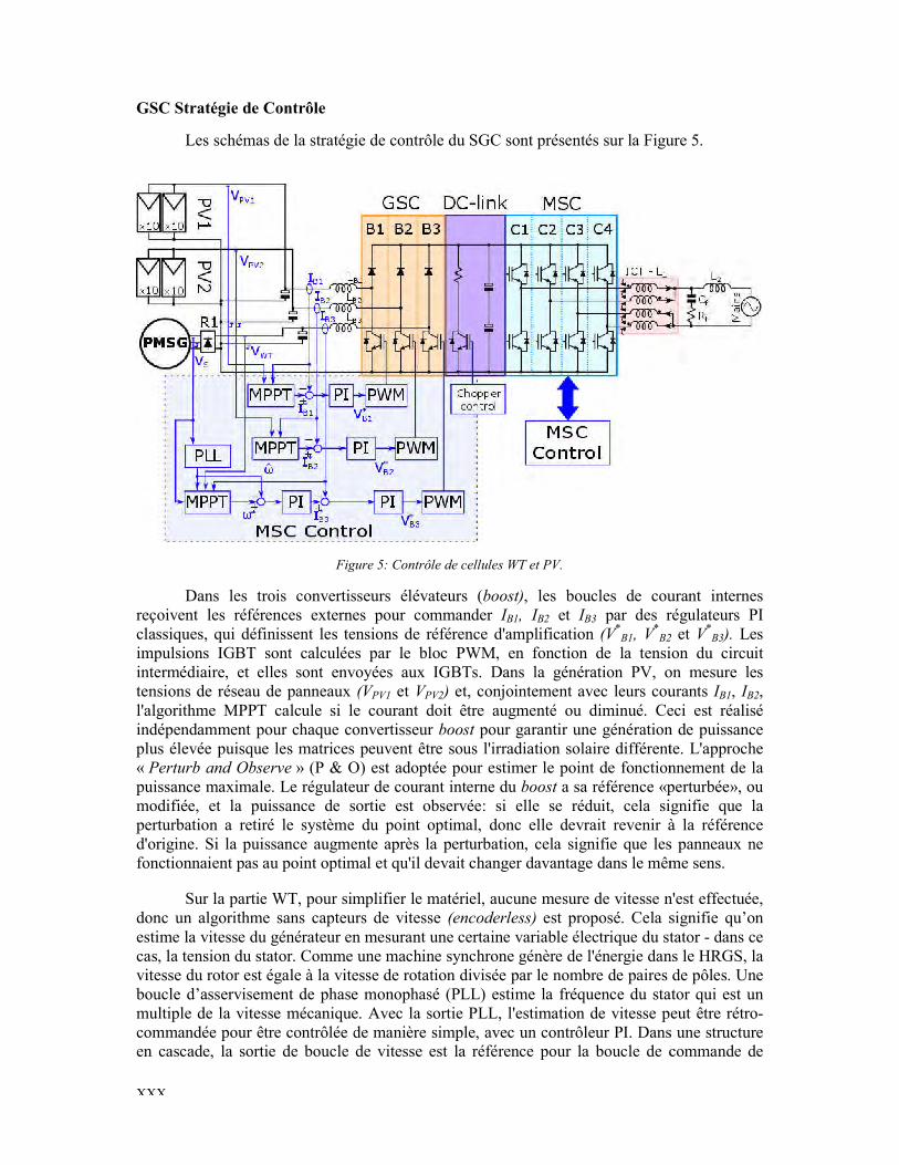
Les schémas de la stratégie de contrôle du SGC

Figure

Dans les trois convertisseurs élévateurs (reçoivent les références externes pour commander classiques, qui définissent les tensions de référence d'amplification impulsions IGBT sont calculées paintermédiaire, et elles sont envoyées aux IGBTs. Dans la génération PV, on mesure les tensions de réseau de panneaux l'algorithme MPPT calcule si le courant doit être augmenté ou diminué. Ceci est réalisé indépendamment pour chaque convertisseur plus élevée puisque les matrices peuvent être sous l'irradiation solaire différente. L'approche « Perturb and Observe » (P & O) est adoptée pour estimer le point de fonctionnement de la puissance maximale. Le régulateur de courant interne du modifiée, et la puissance de sortie est observée: si elle se réduit, cela signifperturbation a retiré le système du point optimal, donc elle devrait revenir à la référence d'origine. Si la puissance augmente après la perturbation, cela signifie que les panneaux ne fonctionnaient pas au point optimal et qu'il devait changer d

Sur la partie WT, pour simplifier le matériel, aucune mesure de vitesse n'est effectuée, donc un algorithme sans capteurs de vitesse estime la vitesse du générateur en mesurant une cas, la tension du stator. Comme une machine synchrone génère de l'énergie dans le HRGS, la vitesse du rotor est égale à la vitesse de rotation divisée par le nombre de paires de pôles. Une boucle d’asservisement de phase monophasé (PLL) estime la fréquence du stator qui est un multiple de la vitesse mécanique. Avec la sortie PLL, l'estimation de vitesse peut être rétrocommandée pour être contrôlée de manière simple, avec un contrôleur PI. Dans une structureen cascade, la sortie de boucle de vitesse est la référence pour la boucle de commande de

Les schémas de la stratégie de contrôle du SGC sont présentés sur la Figure 5

Figure 5: Contrôle de cellules WT et PV.

Dans les trois convertisseurs élévateurs (boost), les boucles de courant internes reçoivent les références externes pour commander IB1, IB2 et IB3 par des régulateurs PI classiques, qui définissent les tensions de référence d'amplification (V*

B1, V*B2

impulsions IGBT sont calculées par le bloc PWM, en fonction de la tension du circuit intermédiaire, et elles sont envoyées aux IGBTs. Dans la génération PV, on mesure les tensions de réseau de panneaux (VPV1 et VPV2) et, conjointement avec leurs courants

e si le courant doit être augmenté ou diminué. Ceci est réalisé indépendamment pour chaque convertisseur boost pour garantir une génération de puissance plus élevée puisque les matrices peuvent être sous l'irradiation solaire différente. L'approche

» (P & O) est adoptée pour estimer le point de fonctionnement de la puissance maximale. Le régulateur de courant interne du boost a sa référence «perturbée», ou modifiée, et la puissance de sortie est observée: si elle se réduit, cela signifperturbation a retiré le système du point optimal, donc elle devrait revenir à la référence d'origine. Si la puissance augmente après la perturbation, cela signifie que les panneaux ne fonctionnaient pas au point optimal et qu'il devait changer davantage dans le même sens.

Sur la partie WT, pour simplifier le matériel, aucune mesure de vitesse n'est effectuée, donc un algorithme sans capteurs de vitesse (encoderless) est proposé. Cela signifie qu’on estime la vitesse du générateur en mesurant une certaine variable électrique du stator cas, la tension du stator. Comme une machine synchrone génère de l'énergie dans le HRGS, la vitesse du rotor est égale à la vitesse de rotation divisée par le nombre de paires de pôles. Une

ement de phase monophasé (PLL) estime la fréquence du stator qui est un multiple de la vitesse mécanique. Avec la sortie PLL, l'estimation de vitesse peut être rétrocommandée pour être contrôlée de manière simple, avec un contrôleur PI. Dans une structureen cascade, la sortie de boucle de vitesse est la référence pour la boucle de commande de

sont présentés sur la Figure 5.

, les boucles de courant internes par des régulateurs PI

B2 et V*B3). Les

r le bloc PWM, en fonction de la tension du circuit intermédiaire, et elles sont envoyées aux IGBTs. Dans la génération PV, on mesure les

et, conjointement avec leurs courants IB1, IB2, e si le courant doit être augmenté ou diminué. Ceci est réalisé

pour garantir une génération de puissance plus élevée puisque les matrices peuvent être sous l'irradiation solaire différente. L'approche

» (P & O) est adoptée pour estimer le point de fonctionnement de la a sa référence «perturbée», ou

modifiée, et la puissance de sortie est observée: si elle se réduit, cela signifie que la perturbation a retiré le système du point optimal, donc elle devrait revenir à la référence d'origine. Si la puissance augmente après la perturbation, cela signifie que les panneaux ne

avantage dans le même sens.

Sur la partie WT, pour simplifier le matériel, aucune mesure de vitesse n'est effectuée, est proposé. Cela signifie qu’on

certaine variable électrique du stator - dans ce cas, la tension du stator. Comme une machine synchrone génère de l'énergie dans le HRGS, la vitesse du rotor est égale à la vitesse de rotation divisée par le nombre de paires de pôles. Une

ement de phase monophasé (PLL) estime la fréquence du stator qui est un multiple de la vitesse mécanique. Avec la sortie PLL, l'estimation de vitesse peut être rétro-commandée pour être contrôlée de manière simple, avec un contrôleur PI. Dans une structure en cascade, la sortie de boucle de vitesse est la référence pour la boucle de commande de

courant interne. Pour garantir la MPPT, la référence de vitesse est calculée en tenant compte la puissance maximale attendue pour chaque vitesse, étant donné que lesturbine sont connues. La puissance générée est comparée à la puissance maximale de référence pour chaque vitesse estimée et la référence de vitesse est augmentée ou diminuée si la puissance est inférieure ou supérieure à ce qui étai

Les algorithmes PLL monophasés peuvent garantir le fonctionnement sans codeur dans les machines synchrones puisque la fréquence électrique du stator est proportionnelle à la vitesse. L'algorithme utilisé dans cette étude pour estimer la vitesse esmonophasé représenté sur la Figure 6.

Figure

Etant donné que dans ce cas, il n'est pas nécessaire de définir l'angle du stator, seulement la vitesse, peu importe si laquelle des trois mesures de la tension statorique (du PLL. Une fois que la fréquence nominale du stator est de 54Hz, les paramètres de détection de phase sont choisis pour répondre aux exigences en fonctionnement nominal.

Une fois l'estimation de la vitesse établie, toutes les conditions de régulation de la vitesse sont remplies. Le point de puissance maximum (MPP) est obtenu dans une éolienne lorsque l'efficacité optimale de la turbine est atteinte et maintenue pour un certain vent. Ici, le MPPT est réalisé par une expression polynomiale de troisième ordre qui relie la vitesse de référence (ω*) en fonction de la puissance mesur

Dans les panneaux photovoltaïques, lpour augmenter l'efficacité du système de génération et ici une routine responsable de celle-ci. Le problème inhérent à l'algorithme P & O est cette oscillation autour du MPP, qui réduit l'efficacité du système. Néanmoins, en comparaison avec d'autres algorithmes, il peut présenter un comportement supérieur combiné à une petite complexité. L'algorithme MPPT proposé utilise une boucle de courant interne et un algorithme de P&O externe et l'organigramme détaillé de la routine est présenté à la l'algorithme a été initialisé, la puissance réelle (P [k]) est calculée en fonction de la tension et du courant du réseau (V [k], I [k]). Si la variation de puissance (DP [k]) est possignifie que la modification de la référence de courant (I* [k]) doit garder la même direction

courant interne. Pour garantir la MPPT, la référence de vitesse est calculée en tenant compte la puissance maximale attendue pour chaque vitesse, étant donné que les caractéristiques de la turbine sont connues. La puissance générée est comparée à la puissance maximale de référence pour chaque vitesse estimée et la référence de vitesse est augmentée ou diminuée si la puissance est inférieure ou supérieure à ce qui était prévu.

Les algorithmes PLL monophasés peuvent garantir le fonctionnement sans codeur dans les machines synchrones puisque la fréquence électrique du stator est proportionnelle à la vitesse. L'algorithme utilisé dans cette étude pour estimer la vitesse est le PLL inverse monophasé représenté sur la Figure 6.

Figure 6: PLL Monophasé Park-inverse.

Etant donné que dans ce cas, il n'est pas nécessaire de définir l'angle du stator, seulement la vitesse, peu importe si VGd ou VGq seront mis à zéro, et même pas de savoir laquelle des trois mesures de la tension statorique (Vab, Vbc ou Vac) sera utilisée comme entrée du PLL. Une fois que la fréquence nominale du stator est de 54Hz, les paramètres de

our répondre aux exigences en fonctionnement nominal.

Une fois l'estimation de la vitesse établie, toutes les conditions de régulation de la vitesse sont remplies. Le point de puissance maximum (MPP) est obtenu dans une éolienne

le de la turbine est atteinte et maintenue pour un certain vent. Ici, le MPPT est réalisé par une expression polynomiale de troisième ordre qui relie la vitesse de

ω*) en fonction de la puissance mesurée (P).

Dans les panneaux photovoltaïques, la présence d'algorithmes MPPT est obligatoire pour augmenter l'efficacité du système de génération et ici une routine Perturb & Observe

ci. Le problème inhérent à l'algorithme P & O est cette oscillation autour 'efficacité du système. Néanmoins, en comparaison avec d'autres

algorithmes, il peut présenter un comportement supérieur combiné à une petite complexité. L'algorithme MPPT proposé utilise une boucle de courant interne et un algorithme de P&O

rganigramme détaillé de la routine est présenté à la Figure 7.l'algorithme a été initialisé, la puissance réelle (P [k]) est calculée en fonction de la tension et du courant du réseau (V [k], I [k]). Si la variation de puissance (DP [k]) est possignifie que la modification de la référence de courant (I* [k]) doit garder la même direction

XXXI

courant interne. Pour garantir la MPPT, la référence de vitesse est calculée en tenant compte caractéristiques de la

turbine sont connues. La puissance générée est comparée à la puissance maximale de référence pour chaque vitesse estimée et la référence de vitesse est augmentée ou diminuée si

Les algorithmes PLL monophasés peuvent garantir le fonctionnement sans codeur dans les machines synchrones puisque la fréquence électrique du stator est proportionnelle à

t le PLL inverse

Etant donné que dans ce cas, il n'est pas nécessaire de définir l'angle du stator, seront mis à zéro, et même pas de savoir

) sera utilisée comme entrée du PLL. Une fois que la fréquence nominale du stator est de 54Hz, les paramètres de

our répondre aux exigences en fonctionnement nominal.

Une fois l'estimation de la vitesse établie, toutes les conditions de régulation de la vitesse sont remplies. Le point de puissance maximum (MPP) est obtenu dans une éolienne

le de la turbine est atteinte et maintenue pour un certain vent. Ici, le MPPT est réalisé par une expression polynomiale de troisième ordre qui relie la vitesse de

a présence d'algorithmes MPPT est obligatoire Perturb & Observe est

ci. Le problème inhérent à l'algorithme P & O est cette oscillation autour 'efficacité du système. Néanmoins, en comparaison avec d'autres

algorithmes, il peut présenter un comportement supérieur combiné à une petite complexité. L'algorithme MPPT proposé utilise une boucle de courant interne et un algorithme de P&O

Figure 7. Après que l'algorithme a été initialisé, la puissance réelle (P [k]) est calculée en fonction de la tension et du courant du réseau (V [k], I [k]). Si la variation de puissance (DP [k]) est positive, cela signifie que la modification de la référence de courant (I* [k]) doit garder la même direction

XXXII

que dans l'itération précédente; Sinon, l'algorithme doit changer de direction. Enfin, les variables sont mises à jour et la routine est prête pour l

Figure

Le P&O classique met à jour le cycle d'asservissement et a le courant comme référence. Dans le présent travail, un contrôleur de courant a été utilisé à la plla possibilité d'avoir un courant contrôlé pour garantir une limitation plus facile de la puissance générée, si nécessaire. Cela peut être considéré comme une variante simple de l'approche classique, en conservant prendre en compte dans cette routine est la définition de la variation de référence de courant (DI). Si cette valeur est élevée, le système converge rapidement vers la stabilité après un changement de rayonnement ou de tempérune oscillation plus élevée autour du MPP, réduisant ainsi l'efficacité à l'état stationnaire. Cependant, si un petit DI est choisi, le système prendra trop de temps pour se stabiliser après un transitoire. Quelques résultats de simulation montrent comment l'efficacité de a augmenté.

Stratégie de Contrôle du MSC

Le convertisseur côté secteur (MSC) est responsable du flux de puissance actif depuis le DC-Link vers le réseau. Pour ce faire, le HRGScellules entrelacées pour la connexion au réseau. La stratégie de commande du MSC est représentée sur la Figure 8.

que dans l'itération précédente; Sinon, l'algorithme doit changer de direction. Enfin, les variables sont mises à jour et la routine est prête pour la prochaine itération.

Figure 7: Schéma-bloc de l’algorithme P&O.

Le P&O classique met à jour le cycle d'asservissement et a le courant comme référence. Dans le présent travail, un contrôleur de courant a été utilisé à la place pour garantir la possibilité d'avoir un courant contrôlé pour garantir une limitation plus facile de la puissance générée, si nécessaire. Cela peut être considéré comme une variante simple de

, en conservant sa simplicité originale. Le seul compromis important à prendre en compte dans cette routine est la définition de la variation de référence de courant (DI). Si cette valeur est élevée, le système converge rapidement vers la stabilité après un changement de rayonnement ou de température. Comme inconvénient, le système présentera une oscillation plus élevée autour du MPP, réduisant ainsi l'efficacité à l'état stationnaire. Cependant, si un petit DI est choisi, le système prendra trop de temps pour se stabiliser après

Quelques résultats de simulation montrent comment l'efficacité de

Le convertisseur côté secteur (MSC) est responsable du flux de puissance actif depuis le . Pour ce faire, le HRGS contient un VSI à une seule phase et quatre

cellules entrelacées pour la connexion au réseau. La stratégie de commande du MSC est

que dans l'itération précédente; Sinon, l'algorithme doit changer de direction. Enfin, les

Le P&O classique met à jour le cycle d'asservissement et a le courant comme ace pour garantir

la possibilité d'avoir un courant contrôlé pour garantir une limitation plus facile de la puissance générée, si nécessaire. Cela peut être considéré comme une variante simple de

Le seul compromis important à prendre en compte dans cette routine est la définition de la variation de référence de courant (DI). Si cette valeur est élevée, le système converge rapidement vers la stabilité après un

ature. Comme inconvénient, le système présentera une oscillation plus élevée autour du MPP, réduisant ainsi l'efficacité à l'état stationnaire. Cependant, si un petit DI est choisi, le système prendra trop de temps pour se stabiliser après

Quelques résultats de simulation montrent comment l'efficacité de la génération

Le convertisseur côté secteur (MSC) est responsable du flux de puissance actif depuis le contient un VSI à une seule phase et quatre

cellules entrelacées pour la connexion au réseau. La stratégie de commande du MSC est

Figure 8: Schéma de l

Pour obtenir une synchronisation avec le réseau, on utilise une structure PLL dérivée d’une PLL fictive à trois phases. Compte tenu de l'adoption du contrôle vectoriel, c’est un moyen d'émuler l'axe bêta, assurant un meilleuapproche est également utilisée dans le présente étude et est présentée dans la Figure cette stratégie, au lieu d’écarter la composante beta comme à la manière traditionnelle, il est utilisé pour l'Emulation d'Axe Fictif (FAE) avec la tension beta du réseau. La différence entre la tension du réseau et la tension beta du contrôleur génère un courant bêta émulé prenant en compte le comportement dynamique du filtre de sortie du convertisseur, c'estfonction de transfert. Le FAE garantit la stabilité et un comportement dynamique supérieur (réponse plus rapide et oscillations plus faibles) par rapport à l'approche conventionnelle.

Figure 9: Emulation d'axe fictif (FAE) da

Les régulateurs de courant sont les boucles intérieures dans le MSC et ils ont pour objectif de laisser transiter le flux de puissance du bus DC au réseau. Ils sont également importants pour maintenir le coprincipalement pour éviter la saturation du noyau magnetique. Des variations temporaires des signaux de commande ou des paramètres du réseau, ainsi que des asymétries dans les bras du convertisseur peuvent entraîner un déséquilibre de courant dans les différentes cellules du

: Schéma de la stratégie de contrôle du MSC.

Pour obtenir une synchronisation avec le réseau, on utilise une structure PLL dérivée d’une PLL fictive à trois phases. Compte tenu de l'adoption du contrôle vectoriel, c’est un moyen d'émuler l'axe bêta, assurant un meilleur comportement dynamique au système. Cette approche est également utilisée dans le présente étude et est présentée dans la Figure cette stratégie, au lieu d’écarter la composante beta comme à la manière traditionnelle, il est

on d'Axe Fictif (FAE) avec la tension beta du réseau. La différence entre la tension du réseau et la tension beta du contrôleur génère un courant bêta émulé prenant en compte le comportement dynamique du filtre de sortie du convertisseur, c'estonction de transfert. Le FAE garantit la stabilité et un comportement dynamique supérieur

(réponse plus rapide et oscillations plus faibles) par rapport à l'approche conventionnelle.

: Emulation d'axe fictif (FAE) dans le contrôle vectoriel des systèmes monophasés.

Les régulateurs de courant sont les boucles intérieures dans le MSC et ils ont pour objectif de laisser transiter le flux de puissance du bus DC au réseau. Ils sont également importants pour maintenir le courant égal dans le convertisseur et les brasde l'ICT, principalement pour éviter la saturation du noyau magnetique. Des variations temporaires des signaux de commande ou des paramètres du réseau, ainsi que des asymétries dans les bras du

ent entraîner un déséquilibre de courant dans les différentes cellules du

XXXIII

Pour obtenir une synchronisation avec le réseau, on utilise une structure PLL dérivée d’une PLL fictive à trois phases. Compte tenu de l'adoption du contrôle vectoriel, c’est un

r comportement dynamique au système. Cette approche est également utilisée dans le présente étude et est présentée dans la Figure 9. Dans cette stratégie, au lieu d’écarter la composante beta comme à la manière traditionnelle, il est

on d'Axe Fictif (FAE) avec la tension beta du réseau. La différence entre la tension du réseau et la tension beta du contrôleur génère un courant bêta émulé prenant en compte le comportement dynamique du filtre de sortie du convertisseur, c'est-à-dire sa onction de transfert. Le FAE garantit la stabilité et un comportement dynamique supérieur

(réponse plus rapide et oscillations plus faibles) par rapport à l'approche conventionnelle.

ns le contrôle vectoriel des systèmes monophasés.

Les régulateurs de courant sont les boucles intérieures dans le MSC et ils ont pour objectif de laisser transiter le flux de puissance du bus DC au réseau. Ils sont également

urant égal dans le convertisseur et les brasde l'ICT, principalement pour éviter la saturation du noyau magnetique. Des variations temporaires des signaux de commande ou des paramètres du réseau, ainsi que des asymétries dans les bras du

ent entraîner un déséquilibre de courant dans les différentes cellules du

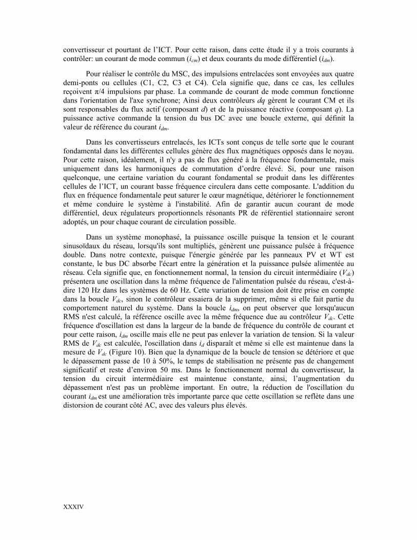
XXXIV

convertisseur et pourtant de l’ICT. Pour cette raison, dans cette étude il y a trois courants à contrôler: un courant de mode commun (icm) et deux courants du mode différentiel (idm).

Pour réaliser le contrôle du MSC, des impulsions entrelacées sont envoyées aux quatre demi-ponts ou cellules (C1, C2, C3 et C4). Cela signifie que, dans ce cas, les cellules reçoivent π/4 impulsions par phase. La commande de courant de mode commun fonctionne dans l'orientation de l'axe synchrone; Ainsi deux contrôleurs dq gèrent le courant CM et ils sont responsables du flux actif (composant d) et de la puissance réactive (composant q). La puissance active commande la tension du bus DC avec une boucle externe, qui définit la valeur de référence du courant idm.

Dans les convertisseurs entrelacés, les ICTs sont conçus de telle sorte que le courant fondamental dans les différentes cellules génère des flux magnétiques opposés dans le noyau. Pour cette raison, idéalement, il n'y a pas de flux généré à la fréquence fondamentale, mais uniquement dans les harmoniques de commutation d’ordre élevé. Si, pour une raison quelconque, une certaine variation du courant fondamental se produit dans les différentes cellules de l’ICT, un courant basse fréquence circulera dans cette composante. L'addition du flux en fréquence fondamentale peut saturer le cœur magnétique, détériorer le fonctionnement et même conduire le système à l'instabilité. Afin de garantir aucun courant de mode différentiel, deux régulateurs proportionnels résonants PR de référentiel stationnaire seront adoptés, un pour chaque courant de circulation possible.

Dans un système monophasé, la puissance oscille puisque la tension et le courant sinusoïdaux du réseau, lorsqu'ils sont multipliés, génèrent une puissance pulsée à fréquence double. Dans notre contexte, puisque l'énergie générée par les panneaux PV et WT est constante, le bus DC absorbe l'écart entre la génération et la puissance pulsée alimentée au réseau. Cela signifie que, en fonctionnement normal, la tension du circuit intermédiaire (Vdc) présentera une oscillation dans la même fréquence de l'alimentation pulsée du réseau, c'est-à-dire 120 Hz dans les systèmes de 60 Hz. Cette variation de tension doit être prise en compte dans la boucle Vdc, sinon le contrôleur essaiera de la supprimer, même si elle fait partie du comportement naturel du système. Dans la boucle idm, on peut observer que lorsqu'aucun RMS n'est calculé, la référence oscille avec la même fréquence due au contrôleur Vdc. Cette fréquence d'oscillation est dans la largeur de la bande de fréquence du contrôle de courant et pour cette raison, idm oscille mais elle ne peut pas enlever la variation de tension. Si la valeur RMS de Vdc est calculée, l'oscillation dans id disparaît et même si elle est maintenue dans la mesure de Vdc (Figure 10). Bien que la dynamique de la boucle de tension se détériore et que le dépassement passe de 10 à 50%, le temps de stabilisation ne présente pas de changement significatif et reste d’environ 50 ms. Dans le fonctionnement normal du convertisseur, la tension du circuit intermédiaire est maintenue constante, ainsi, l’augmentation du dépassement n'est pas un problème important. En outre, la réduction de l'oscillation du courant idm est une amélioration très importante parce que cette oscillation se reflète dans une distorsion de courant côté AC, avec des valeurs plus élevés.

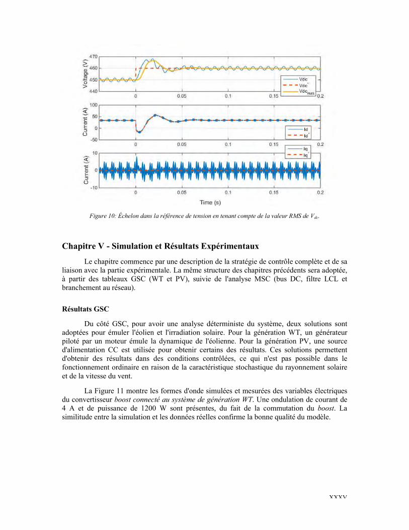
Figure 10: Échelon dans la référence de tension en tenant compte de la valeur RMS de V

Chapitre V - Simulation et Résultats Expérimentaux

Le chapitre commence par une description de la stratégie de contrôle complète et de sa liaison avec la partie expérimentale. La même structure des chapitres précédents sera adoptée, à partir des tableaux GSC (WT et PV), suivie de l'analyse MSC (bus DC, filtre LCL et branchement au réseau).

Résultats GSC

Du côté GSC, pour avoir une analyse déterministe du système, deux solutions sont adoptées pour émuler l'éolien et l'irradiation solaire. Pour la génération WT,piloté par un moteur émule la dynamique de l'éolienne. Pour la génération PV, une source d'alimentation CC est utilisée pour obtenir certains des résultats. Ces solutions permettent d'obtenir des résultats dans des conditions contrôlées, ce fonctionnement ordinaire en raison de la caractéristique stochastique du rayonnement solaire et de la vitesse du vent.

La Figure 11 montre les formes d'onde simulées et mesurées des variables électriques du convertisseur boost connecté au système de génération WT4 A et de puissance de 1200 W sont présentes, du fait de la commutation du similitude entre la simulation et les données réelles confirme la bonne qualité du modèle.

: Échelon dans la référence de tension en tenant compte de la valeur RMS de V

Simulation et Résultats Expérimentaux

Le chapitre commence par une description de la stratégie de contrôle complète et de sa liaison avec la partie expérimentale. La même structure des chapitres précédents sera adoptée,

(WT et PV), suivie de l'analyse MSC (bus DC, filtre LCL et

Du côté GSC, pour avoir une analyse déterministe du système, deux solutions sont adoptées pour émuler l'éolien et l'irradiation solaire. Pour la génération WT, un générateur piloté par un moteur émule la dynamique de l'éolienne. Pour la génération PV, une source d'alimentation CC est utilisée pour obtenir certains des résultats. Ces solutions permettent d'obtenir des résultats dans des conditions contrôlées, ce qui n'est pas possible dans le fonctionnement ordinaire en raison de la caractéristique stochastique du rayonnement solaire

La Figure 11 montre les formes d'onde simulées et mesurées des variables électriques t connecté au système de génération WT. Une ondulation de courant de

4 A et de puissance de 1200 W sont présentes, du fait de la commutation du similitude entre la simulation et les données réelles confirme la bonne qualité du modèle.

XXXV

: Échelon dans la référence de tension en tenant compte de la valeur RMS de Vdc.

Le chapitre commence par une description de la stratégie de contrôle complète et de sa liaison avec la partie expérimentale. La même structure des chapitres précédents sera adoptée,

(WT et PV), suivie de l'analyse MSC (bus DC, filtre LCL et

Du côté GSC, pour avoir une analyse déterministe du système, deux solutions sont un générateur

piloté par un moteur émule la dynamique de l'éolienne. Pour la génération PV, une source d'alimentation CC est utilisée pour obtenir certains des résultats. Ces solutions permettent

qui n'est pas possible dans le fonctionnement ordinaire en raison de la caractéristique stochastique du rayonnement solaire

La Figure 11 montre les formes d'onde simulées et mesurées des variables électriques . Une ondulation de courant de

4 A et de puissance de 1200 W sont présentes, du fait de la commutation du boost. La similitude entre la simulation et les données réelles confirme la bonne qualité du modèle.

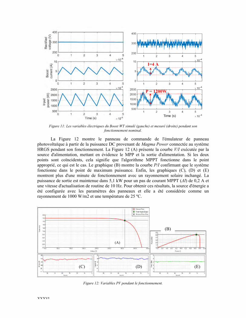
XXXVI

Figure 11: Les variables électriques du Boost WT simulé (gauche) et mesuré (droite) pendant son

fonctionnement nominal.

La Figure 12 montre le panneau de commande de l'émulateur de panneau photovoltaïque à partir de la puissance DC provenant de Magma Power connectée au système HRGS pendant son fonctionnement. La Figure 12 (A) présente la courbe V/I exécutée par la source d'alimentation, mettant en évidence le MPP et la sortie d'alimentation. Si les deux points sont coïncidents, cela signifie que l'algorithme MPPT fonctionne dans le point approprié, ce qui est le cas. Le graphique (B) montre la courbe P/I confirmant que le système fonctionne dans le point de maximum puissance. Enfin, les graphiques (C), (D) et (E) montrent plus d'une minute de fonctionnement avec un rayonnement solaire inchangé. La puissance de sortie est maintenue dans 5,1 kW pour un pas de courant MPPT (ΔI) de 0,2 A et une vitesse d'actualisation de routine de 10 Hz. Pour obtenir ces résultats, la source d'énergie a été configurée avec les paramètres des panneaux et elle a été considérée comme un rayonnement de 1000 W/m2 et une température de 25 ºC.

Figure 12: Variables PV pendant le fonctionnement.

P = 1200W

I=4 A

(A)

(C) A

(D) (E) A

(B) A

XXXVII

Les tests effectués avec la source d'alimentation sont importants pour confirmer le contrôle et l'efficacité du MPPT. Après la réalisation des tests, le convertisseur a été connecté à des panneaux solaires réels et les résultats en régime permanent du courant du boost, dans deux conditions différentes, sont présentés sur la Figure 13. Les formes d'onde dans le graphique de droite représentent les courants et les tensions d'entrée à 10 AM, d'un jour clair. La puissance générée dans le panneaux 1 et le panneaux 2 a atteint la valeur de 4,77 kW, chacun. L'ondulation du courant du boost présentait une valeur d'environ 4,8 A, soit environ 30% du courant nominal comme prévu dans le boost. L'ondulation dans le réseau PV (courbe verte) est inférieure à 0,8 A (5%) même si dans les résultats présentés (Figure 13- droite) le bruit de mesure ne permet pas la mesure exacte.

Figure 13: Tensions du PV (VPV1, VPV2), courants du boost (IB1, IB2) et courants PV (IPV1) pendant l’opération.

Résultats MSC

L'opération MSC commence par la charge des condensateurs du bus DC. Ils peuvent être chargés à partir du MSC ou GSC. Dans le second cas, seulement s'il y a des conditions de vent pour accélérer la turbine ou le rayonnement solaire suffisant pour augmenter la tension des cellules. Une fois que le bus DC atteint une valeur qui permet la commande, la commutation peut démarrer.

Figure 14: Démarrage du convertisseur: tension du bus DC courant continu (VDC) et courant (réseau IM) des

condensateurs (I) de la dérivation de la résistance de précharge (II) et commutation initiale (III).

IB2

VPV2 IB1

VPV1 VPV1 IB1

IPV1

I

III II

IM

VDC

XXXVIII

La charge du bus DC se produit par l'intermédiaire d'une résistance de précharge pour réduire le transitoire de courant pendant la connexion du réseau et elle est présentée à la Figure 14. La courbe en bleu est la tension du bus DC (VDC) et celle en orange est le courant du réseau (IM). Dans l'instant I, le convertisseur est connecté au réseau et les condensateurs sont chargés à travers la résistance de précharge. Dès que la tension se stabilise, la résistance est contournée en terminant le processus de charge (instant II). Enfin, le MSC commence la commutation et la tension du circuit intermédiaire est contrôlée et réglée sur sa valeur de fonctionnement (instant III).

Les résultats expérimentaux du contrôle de courant dans le MSC sont présentés sur la Figure 15. La spécification de boucle fermée a été définie comme étant: le temps de stabilisation égal au temps de stabilisation en boucle fermée du système sans contrôleur (Tsnc) et un dépassement de courant de 25% maximum. Le résultat obtenu a un dépassement de pourcentage (PO) et un temps de stabilisation respectivement de 16% et de 0,94 ms. Dans ce résultat, une variation d'échelon de 10 A est réalisée dans la référence de courant q (Iq*). Une comparaison entre les données simulées et réelles confirme la bonne qualité de la modélisation et de l'identification du système. Dans le deuxième graphique, la sortie du contrôleur indique que pour un échelon de 10 A, la sortie du contrôleur varie d'environ 20 V, ce qui correspond à environ 5% de la capacité de synthèse de tension du convertisseur pour une tension de bus DC 450 V. Cela montre que le contrôleur fonctionne dans une zone confortable, loin des limites de linéarité en ce qui concerne la capacité de la tension. Par conséquent, les non-linéarités momentanées causées par la saturation du contrôleur sont minimisées.

Figure 15: Réponse de Iq à un échelon.

Sur la Figure 16, on présente des mesures de simulation et expérimentales du convertisseur, du mode commun et des courants de réseau (I1, ICM, IM). L'ondulation de courant dans le bras du convertisseur est de 17 A, l'ondulation dans le courant de mode commun est 10 A et dans le courant du réseau est de 0,6 A, dans le pire des cas. Cela représente une distorsion provoquée par les harmoniques de commutation de 23%, 13% et 0,8%, respectivement, en fonctionnement nominal.

Ts = 0.94 ms

PO= 16%

ΔV=20 V

XXXIX

Figure 16: Simulated (left) and measured (right) converter (I), common mode (Icm) and mains currents (Im).

Afin de mesurer la performance du système en ce qui concerne la distorsion harmonique faible dans le courant du réseau, certaines mesures ont été réalisées avec l'analyseur d'harmonique de puissance Fluke 437. Les résultats montrent une distorsion de courant de 8,1%, principalement générés par les harmoniques bas d'ordre impair jusqu'au 13ème harmonique, pour une génération de 7,7 KW. La valeur de distorsion du courant en Ampères présente un pourcentage de 5% en fonctionnement nominal. Ces harmoniques sont causés par l'interaction entre la distorsion de tension du réseau et le fonctionnement du convertisseur, et ils sont intrinsèquement liés à la performance de la commande.

Enfin, une analyse thermodynamique du convertisseur a été réalisée pour s'assurer que les composants fonctionnent dans les limites de température appropriées. Les composants qui fonctionnent à des températures plus élevées sont ceux du filtre: les inducteurs et la résistance d'amortissement. L'analyse a été réalisée après 3 heures de fonctionnement avec une puissance moyenne de 8,5 kW et l'image thermographique des composants du filtre est montrée à la Figure V.20. Les inductances présentaient une température moyenne de 64 ºC et une température maximale de 69 ºC. Les ICTs ont présenté une température de 59 ºC dans son noyau et une température maximale de 108 ºC dans les enroulements. L'inductance L2 du filtre LCL présentait une température de 80 ºC. Toutes ces températures sont dans la plage de sécurité puisque ces composants sont de classe H, conçus pour fonctionner à une température maximale de 180 ºC selon la norme CEI 60085.

CONCLUSION

La solution pour l'énergie générée des sources non polluantes constitue un problème mondial, indéterminé, complexe et progressif; Et certainement, passe par la diversification de la matrice énergétique. La diversification signifie non seulement que des sources différentes sont converties en énergie utile, comme l'électricité, mais aussi décentraliser la production d'énergie afin de s'adapter à une plus grande adéquation de la demande, qui est décentralisée aussi. La Génération Distribuée propose ce type de développement, mais pour accroître sa pénétration, plusieurs obstacles techniques doivent être surpassés. L'un d'entre eux est lié aux systèmes de conversion, qui doivent être plus flexibles, modulaires, efficaces et compatibles avec les différentes sources d'énergie, car ils sont très spécifiques pour une certaine zone. La

I= 0.6 A

I= 10 A

I= 17 A

XL

présente étude pousse ses efforts vers cette direction, c'est-à-dire, comportant un système avec plusieurs entrées pour combiner différentes sources d'énergie renouvelables en un seul et efficace convertisseur de puissance pour la connexion au réseau. Conformément à ces idées, la présente étude propose les contributions décrites dans la liste qui suit :

Contribution 1: conception de HRGS Contribution 2: Une nouvelle méthodologie de conception de contrôleurs Contribution 3: Analyse globale de la bande passante pour un iVSI Contribution 4: Modélisation et identification du système de génération Contribution 5: La conception de la stratégie de contrôle dans le SGC et le MSC

Plusieurs solutions dans la conception de systèmes hybrides à petite échelle ont été proposées, mais, également, d'autres chemins à suivre comme travaux futurs ont été tracés. Certains de ces points sont énumérés comme suit.

Définir des stratégies de contrôle plus sophistiquées pour les convertisseurs multicellulaires

Conception et implémentation du filtre actif pour le MSC Testez l'algorithme MPPT dans la turbine réelle déjà installée et connectée au

HRGS Calculer l'efficacité du système Mettre en œuvre un fonctionnement modulaire du convertisseur parallèle

Tous les éléments mentionnés représentent des zones très difficiles de la recherche et délimitent les futures étapes à accomplir par l'auteur.

General Introduction

1

General Introduction

This PhD research has a peculiar characteristic in what concerns the way it was defined, accomplished and financed. Several institutions and people combined efforts for intellectual and financial contributions to this study.

The thesis was developed at the “Laboratoire Plasma et Conversion d’Energie” (LAPLACE), at Toulouse, France, supervised by the professors Thierry Meynard and Ana Llor. The expertise of this laboratory and professors in what concerns multilevel conversion, control and the use of InterCell Transformers (ICT) guided the investigations and made the results possible.

The experimental set-up was constructed at the Laboratory on Conversion and Control of the Electric Energy, in the Federal University of Itajubá (Unifei), at Itabira, Brazil, where the author of this thesis is an assistant professor. The test-bench was financed by a Public-Private-Partnership (PPP) between this university and Vale SA, a Multinational Brazilian corporation in metals and mining. This PPP had the goal of equipping the laboratories of Unifei in the new campus of Itabira. The equipment and components purchase was operationalized with the technical support of Professor Clodualdo Sousa.

The financial support of the PhD student was covered by the Brazilian national program “Ciências sem Fronteiras” (Science Without Borders), operated by CNPq (National Council for Scientific and Technological Development), a Brazilian public organization of which objective, among others, is to fund Brazilians to acquire scientific and technological skills around the world.

This research also received the technical support from Professor Seleme Isaac Seleme Jr., from the Federal University of Minas Gerais (UFMG), at Belo Horizonte, Brazil. This study, unified directly and informally the three institutions mentioned previously: Unifei, UFMG and Laplace. This was an important benchmark for the formalization of the international cooperation between these three institutions financed by the Brazilian agency Capes (Coordination for the Improvement of Higher Education Personnel) and the French Cofecub (Committee for the Evaluation of Academic and Scientific Cooperation).

The Research and Text Organization

Looking for alternatives that guarantees more efficient and environmental-friendly solutions for energy supply is a one of the most discussed issues of our quotidian and it generates massive concerns. Several researchers, governments, politicians, environmentalists etc drive their efforts into this direction but carbon emissions were never as high as in actual days and 81% of our energetic matrix derived from fossil fuel. The solution for this global problem is uncertain, as well as its real consequences. This study is placed in the international trend of increasing the decentralization and the usage of renewable sources for generating electricity, causing low impact in nature. This is just one part of a whole set of innovations being proposed around the world, but the participation of this type of generation is still neglectable.

General Introduction

2

Its popularization depends on finding solutions for several economic, social, political and technical issues.

In what concerns the technical challenges, one of them is having systems each time more efficient, cheap and versatile for converting the electric energy from the different sources. This question guided the study reported in this text and configures as the main motivation for this work. In order to propose solutions for that, a test Hybrid Renewable Generation System in real scale was designed and constructed using photovoltaic and wind generation. A control strategy for this system was also proposed, simulated and implemented. This manuscript contains the whole steps of this work: the bibliographical research, the most important analysis accomplished, the design process and finally the results.

The content of this study was divided in five chapters. In Chapter I, a contextualization of anthropogenic energy systems and how they evolve during the history of mankind is given. It is also described our current energetic matrix in what concerns resources and the most important environmental effects were discussed. The cases of Brazil and France were approached due to their representativeness, importance and for being the countries where this study was accomplished. The chapter ends with an overview of Distributed Generation and the Photovoltaic and Wind Generation.

In Chapter II, a discussion about the control of interleaved converters having LCL filters in the output with Intercell Transformers is done. It presents an embracing methodology for the design of discrete PI controllers for generic systems. This methodology is applied in the current control of a four-cell interleaved Voltage Source Inverter (iVSI) and a frequency domain analysis is performed and extended for an N-cell iVSIs. This topology of converter is used in the test bench for the grid connection.

Chapter III brings the design and identification of the 11.7kW hybrid generation system using solar photovoltaic panels and a wind turbine. A multicell converter divided in two parts accomplishes the conversion: Generation Side Converter (GSC) and Mains Side Converter (MSC). The chapter presents in detail the design of such a system highlighting the key components (wind turbine, photovoltaic cells, switching elements, passive filter etc), their models and parameters’ identification.

In both, wind and photovoltaic generation, a maximum power point tracking must be employed for guarantying maximum generation. The grid connection guarantees the power flow from the generation elements to the network. Chapter IV presents the definition of the control strategy of the HRGS whose design and modeling processes were presented in Chapter III. Simulation results are presented confirming the effectiveness of the proposed strategy. The controller design method for all the control loops (speed, current and voltage loops) are the same introduced in Chapter II.

Chapter V is dedicated to show the experimental results of the constructed test bench and a comparison with the simulation results is presented. Like the previous chapters, each subsystem is presented separately starting from the photovoltaic and wind generation. Posteriorly, the grid connection is focused and the most important transients and steady-state waveforms are shown.

General Introduction

3

List of Publications

Some parts of the results presented in this manuscript and related studies were published during the period of accomplishment of this thesis by the author. The list of these publications is presented as follows.

[1] J. L. da Silva, R. Reis, G., Silva, R. M., S. I. Seleme, T. A. Meynard, e Llor, A. M., “Design, Modeling and Identification of the Mains Side Converter in an 11.7 kW Wind/Photovoltaic Hybrid Renewable Generation System”, in 8th IEEE International Symposium on Power Electronics for Distributed Generation Systems, 2017.

[2] J. L. da Silva, R. Reis, G., Silva, R. M., S. I. Seleme, T. A. Meynard, e Llor, A. M., “Design, Modeling and Identification of the Generation Side Converter in an 11.7 kW Wind/Photovoltaic Hybrid Renewable Generation System”, in 8th IEEE International Symposium on Power Electronics for Distributed Generation Systems, 2017.

[3] da Silva, R. C, Souza, S. M., Ricardi, V., R. Reis, G., e J. L. da Silva, “Control Design of a Synchronous Generator of a Horizontal Axis Wind Turbine”, in 8th IEEE International Symposium on Power Electronics for Distributed Generation Systems, 2017.

[4] J. L. da Silva, Reis, G., S. I. Seleme, e T. Meynard, “Control Design and Frequency Analysis of an Output Filter in Parallel Interleaved Converters”, IEEE 6th Conference on Power and Energy (PECON), Melaka, Malaysia, 2016.

[5] N. Videau, G. Fontes, D. Flumian, G. Gateau, T. Meynard, J. L. da Silva, O. Verdu, “High Ratio Non-Isolated DC-DC Converter for Hydrogen Battery Using a 50 kW PEM Fuel Cell”, Fuel Cells, set. 2016.

[6] N. Videau, G. Fontes, D. Flumian, G. Gateau, T. Meynard, J. L. da Silva, O. Verdu, “Non-isolated High Efficiency High Voltage Ratio DC-DC Converter for Hydrogen Battery using a 50kW PEM Fuel Cell”, presentedin 6th International Conference on Fundamentals and Development of Fuel Cells, Toulouse, France., 2015.

[7] G. Resende, C. V. Sousa, F. F. Matos, J. L. Silva, T. V. M. Flores, e J. L. S. R. Silva, “Sistema Regenerativo para Testes de Transformadores de Potência sob Condições Especiais de Carregamento”, apresentado em V Simpósio Brasileiro de Sistemas Elétricos, Foz do Iguaçu, Brasil, 2014.

The author also participated as supervisor, co-supervisor or by technical support in three other studies developed in the platform designed in this thesis. These studies are detailed as follows.

Master’s degree dissertation

[8] G. Reis, “Projeto e Construção de um Conversor Monofásico Híbrido em Ponte H Multicelular Entrelaçado para Geração Fotovoltaica e Eólica de Pequeno Porte”, Universidade Federal de Minas Gerais, Belo Horizonte, MG, 2017.

Final graduation projects

General Introduction

4

[9] R. C. da Silva e S. M. de Souza, “Control Design of a Synchronous Generator in a Hybrid Renewable Generation System”, Universidade Federal de Itajubá, Itabira, MG, 2016.

[10] K. A. Pereira, “Controle de um Conversor Multicelular Entrelaçado com Indutores Acoplados Magneticamente em um Sistema Híbrido de Micro-Geração On-Grid”, Universidade Federal de Itajubá, Itabira, MG, 2017.

[11] M. Gonçalves, “Implementação de um Algoritmo MPPT Perturba & Observa em Conversor Híbrido”, Universidade Federal de Itajubá, Itabira, MG, 2017.

Energy Generation: Historical Perspective, Environmental Issues and Renewable Small Scale Systems

5

Chapter I

Energy Generation: Historical Perspective, Environmental Issues and

Renewable Small Scale Systems

Chapter I

6

I.1 Introduction The evolution of society, from the first human beings until actuality, is related to the way mankind has converted the available energy into a useful output. From the fire manipulation, passing through steam, combustion engines, electricity and nuclear energy handling, the society has changed the way it interacts with the external environment and the planet itself. If, in one hand, the energy use made possible improvements in life quality and longevity, on the other hand, it caused big impacts and an important “ecological footprint” that alters the planet’s energy balance, reducing the biodiversity and creating irreversible changes in our biosphere.

In the context of energy manipulation, electricity plays an important role from the 19th century due to its ease of conversion from most of the primary sources of energy. After generated, the electric energy is easily handled and transformed into useful energy if compared to the other secondary sources. The big challenge we face nowadays is how to reduce the impact of the way we convert energy in order to achieve a sustainable future. The answer for his world-wide problem is undetermined and extremely complex since it demands severe changes on the ruling social and economic model. Although, many answers are unclear, it is a consensus that a gradual and positive change, necessary passes through two central issues:

1) Diversification of the energetic matrix and use of renewable primary sources. 2) Decentralizing energy generation.

These two core subjects must be considered intrinsically connected and dependent from each other. Electrical systems across the globe have been designed to convert primary energy into electricity in a centralized way. It prioritizes only the most abundant and centralized energy sources which in several cases are not renewable. Nevertheless, great portions of useful primary energy are spread-out and could easily be converted in smaller and decentralized generation systems, known as Distributed Generation (DG). This way, DG increases flexibility and possibility of using different sources and furthermore, it allows a better matching between generation and consumption.

This chapter proposes a discussion about how mankind has manipulated the energy and how to reduce its impact. It starts with a historical perspective of the energy use from the first human settlements until nowadays. This analysis gives the idea of how recent is our capacity of handling a big amount of energy. It will be followed by the current model of energy generation world-wide focusing on the French and Brazilian case, since the study was accomplished in these two countries. Afterwards, the concept and consequences of DG will be discussed, followed by an overview of the renewable sources focusing the photovoltaic and wind generation. These two primary energy sources are discussed since they present an important role in terms of energy generation. In accordance with all this background, this thesis will propose the design of a Hybrid Renewable Generation System (HRGS) for micro-generation in the next chapters.

I.2 Energy Use by Mankind: A Historical Perspective The human beings have always manipulated the resources of energy available in nature for improving their chance of survival and life quality, creating anthropogenic energy systems. In these systems, the energy is converted into useful outcome and three points are required: the energy source, the conversion process and the use of the transformed energy [12]. The use of

Energy Generation: Historical Perspective, Environmental Issues and Renewable Small Scale Systems

7

an anthropogenic energy system, likely appeared with the hominids who lived in highly flammable savannas [13] in Africa. A fossil from 1,900,000 years suggests that hominids cooked their food and more reliable evidences appear in the archaeological record until after 400,000 years [14], [15]. Although the date is undefined, the mastery of fire is configured as one of the most important milestones in the mankind use of energy and it improved consistently the capacity of adaptation and survival. It made possible the creation of ovens for pottery and refine metals from ore. A second remarkable transition is related to the Agricultural Revolution, which made possible for men to have access to a greater amount of food, allowing the first permanent settlements and gradually proposed an alternative to nomadism [16]. A key point for permitting this revolution was the domestication and use of animal force and fire during pre-history. In a closer past, the use of water and windmills offered a new source of energy and it was used for crushing grains, sawing wood etc. The pre-industrialized society basically used biomass, muscle force, water and wind for its basic energy needs like heating, lighting, transportation, construction and farming and this period is called is the Organic Energy Economy [17].

In the 18th century, a profound change in the society started in England and spread throughout the world with the Industrial Revolution. This process is considered the birth of our actual economical model, which was only possible due to the creation of several inventions and innovations that made possible to harness greater nature’s energies. The Scottish scientist and engineer James Watt (1736-1819) and the British engineer Thomas Newcomen are considered the fathers of the main innovations, which guaranteed the design of steam machines.

Figure I.1: Annual energy consumption per head (megajoules) in England and Wales from the 16th to 19th

century [18].

The use of steam machines made possible the mechanization of the productive process, which evolved from manual work. Steam engines substituted the work of several workers, making faster and cheaper manufactured products. Locomotive and steamships allowed the transportation of the goods to several parts of the world and a more dynamical market emerged. This growing energy consumption was only possible due to the substitution of the primary source from muscles and biomass (wood) into a coal based economy. The growing

Chapter I

8

industries caused a new organization in the society, modernizing cities, transportation, agriculture and all the structure necessary for the productive process from the extraction of raw material till the delivery to the markets. This change characterized the transition from the Organic Energy Economy to the Fossil Fuels Economy. Figure I.1 shows the exponential growth of the coal consumption in England and Wales from the 16th to 19th century.

The French-German inventor Rudolf Christian Karl Diesel (1858-1913) was responsible for a new page in the History of Anthropogenic Energy Systems by creating Internal Combustion Engines (ICE). In these type or motors, a fuel is pulverized into a chamber where it is mixture with oxygen. When this fluid is compressed, there is a great increase in its temperature and starts the combustion liberating mechanical, thermal and acoustic energy moving a piston which drives a shaft. ICE appeared as an alternative to steam engines for increasing efficiency, reducing size and labor intensity. The great break-through for achieving higher level of efficiency in smaller machines was to internally use the combustion energy which was previously used only externally for creating steam, which would then drive the machines. As a consequence, smaller machines operated for a single man started to replace bulky ones, which demanded several people for being operated.

Figure I.2: The evolution of the energetic production during the 20th century: a great dependency on

fossil fuel [16]

In the same period, new discoveries in the field physics derived from several studies of scientists and mathematicians since the end of the 19th century were summarized by James Clark Maxwell, in his famous differential equations. This formulation offered the basis of Classical Electromagnetism, Optics and Electric Circuits and clarified and unified several phenomena studied for centuries, also establishing the theoretical background demanded for the birth and popularization of Electrical Power Systems (EPS).

Together, electric energy and combustion engines power the humanity since 20th century. ICE gradually substituted steam engines converting petrol into a valuable material in nature for the human inventions evoking wars and creating the biggest corporations in modern days. On the

Energy Generation: Historical Perspective, Environmental Issues and Renewable Small Scale Systems

9

other hand, electricity brought a new dimension on the energy use. Electric energy can be converted from fossil fuels like coal and natural gas, but also from nature energy flows like solar, wind, water, ocean waves, nuclear. The use of energy from EPS and ICE increased our life quality and longevity, changed our society, cities, contributed to the population growth. However, the strong dependency from fossil fuels has not changed since the Industrial Revolution (Figure I.1 and Figure I.2) and the harmful consequences to our biosphere are a consensus. In 2015, 81.2% of the world energy consumption derived from fossil fuels resources [19]. Apparently, the fossil fuels will still be the main pillar of global energy consumption for the next decades. Nevertheless, the use of renewable energy sources has the potential to replace fossil fuels in long journey, full of technical, political, social and economic challenges, which is just starting in EPS.

I.3 Electric Power Systems and Energy Generation Electric Power Systems are the set of interconnected elements and processes responsible for generating, transmitting and distributing electric energy to the final costumers (residential, institutional, commercial and industrial). The first commercial EPS system date from 1882 and it was constructed in New York by the Thomas Edson’s company. It was constituted of a steam powered generator powering 300 lamps. A couple of years later, George Westinghouse’s company invested in AC grid after buying the patents for AC distribution solution’s and Nichola Tesla’s multi-phase induction machine. The competition between AC and DC systems technologies was about to boost the commercial use of electricity in the United States, which would spread worldwide. The use of multi-phase AC power in transmission with transformers for stepping-up and down the voltage levels for a proper adequacy appeared as the most adequate and efficient mode for EPS systems. Gradually, greater systems using higher and higher voltages started to emerge as the market increased. In 1890, the 3300V transmission lines were used in the United States and the voltage levels gradually increased to 100 kV, in 1907, 150 kV in 1913, 220 kV in 1923, 224 kV in 1926, 287 kV in 1936, 345 kV in 1953 and so on. [20]. As the distances and voltage levels were increasing, the isolated EPS systems started to be interconnected, in order to guarantee a more economically viable and stable way for generating and transmitting energy.

Later on, with the scientific developments in power electronic components, it became technically and economically viable to use direct current in transmission lines creating High Voltage Direct Current (HVDC) transmission lines. HVDC presents the advantage of interconnecting two unsynchronized systems, which improves the robustness of the whole EPS in the sense that strong disturbances from one side are not as impacting in the other side as it would be in synchronized interconnected AC systems. It also allows the connection of 50 and 60 Hz system, important for the international energy trade. It is the case for the energy produced in the bi-national Hydropower Plant Itaipu. This hydropower has the record of energy generation and it is located in the frontier between Brazil and Paraguay. It produces energy in 50 Hz (mostly for Paraguay) and 60 Hz for the Brazilian network and an HVDC connects the Brazilian grid to the Itaipu’s 50 Hz generation system.

As transmitting electric energy became viable in longer distances as the time passes, big power stations were constructed in strategic places in what concerns primary sources availability, reducing the price and popularizing electricity. Energy generation from coal, water flows, natural gas and nuclear represent the most important share in the EPS around the world. The global total electricity generation was over 22000 TWh in 2014, from which 66%

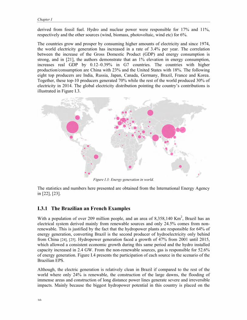
Chapter I

10

derived from fossil fuel. Hydro and nuclear power were responsible for 17% and 11%, respectively and the other sources (wind, biomass, photovoltaic, wind etc) for 6%.

The countries grow and prosper by consuming higher amounts of electricity andthe world electricity generation has increased in a rate of 3.4% per year. The correlation between the increase of the Gross Domestic Product (GDP) and energy consumption is strong, and in [21], the authors demonstrate that an 1% elevation in energy consumption, increases real GDP by 0.12production/consumption are China wieight top producers are India, Russia, Japan, Canada, Germany, Brazil, France and Korea. Together, these top-10 producers generated 70% while the rest of the world produced 30% of electricity in 2014. The global electricity distribution pointing the country’s contributions is illustrated in Figure I.3.

Figure

The statistics and numbers here presented are obtained from the International Energy Agency in [22], [23].

I.3.1 The Brazilian an French Examples

With a population of over 209 million people, and an area of 8,358,140 Kmelectrical system derived mainly from renewable sources and only 24.5% comes from nonrenewable. This is justified by the fact that the hydropower plants are responsible for 64% of energy generation, converting Brazil is the second producer of hydroelectricity only behind from China [24], [25]. Hydropower generation faced a growth of 47% from 2001 until 2015, which allowed a consistent economic growth during thcapacity increased in 2.4 GW. From the nonof energy generation. Figure I.4 presentsBrazilian EPS.

Although, the electric generation is relatively clean in Brazil if compared to the rest of the world where only 24% is renewable, the construction of the large dawns, the flooding of immense areas and construction of long distaimpacts. Mainly because the biggest hydropower potential in this country is placed on the

derived from fossil fuel. Hydro and nuclear power were responsible for 17% and 11%, respectively and the other sources (wind, biomass, photovoltaic, wind etc) for 6%.

The countries grow and prosper by consuming higher amounts of electricity andthe world electricity generation has increased in a rate of 3.4% per year. The correlation between the increase of the Gross Domestic Product (GDP) and energy consumption is

, the authors demonstrate that an 1% elevation in energy consumption, increases real GDP by 0.12–0.39% in G7 countries. The countries with higher production/consumption are China with 23% and the United States with 18%. The following eight top producers are India, Russia, Japan, Canada, Germany, Brazil, France and Korea.

10 producers generated 70% while the rest of the world produced 30% of e global electricity distribution pointing the country’s contributions is

Figure I.3: Energy generation in world.

ers here presented are obtained from the International Energy Agency

The Brazilian an French Examples

With a population of over 209 million people, and an area of 8,358,140 Km2, Brazil has an electrical system derived mainly from renewable sources and only 24.5% comes from non

ewable. This is justified by the fact that the hydropower plants are responsible for 64% of energy generation, converting Brazil is the second producer of hydroelectricity only behind

. Hydropower generation faced a growth of 47% from 2001 until 2015, which allowed a consistent economic growth during this same period and the hydro installed capacity increased in 2.4 GW. From the non-renewable sources, gas is responsible for 52.6%

presents the participation of each source in the sc

Although, the electric generation is relatively clean in Brazil if compared to the rest of the world where only 24% is renewable, the construction of the large dawns, the flooding of immense areas and construction of long distance power lines generate severe and irreversible impacts. Mainly because the biggest hydropower potential in this country is placed on the

derived from fossil fuel. Hydro and nuclear power were responsible for 17% and 11%, respectively and the other sources (wind, biomass, photovoltaic, wind etc) for 6%.

The countries grow and prosper by consuming higher amounts of electricity and since 1974, the world electricity generation has increased in a rate of 3.4% per year. The correlation between the increase of the Gross Domestic Product (GDP) and energy consumption is

, the authors demonstrate that an 1% elevation in energy consumption, 0.39% in G7 countries. The countries with higher

th 23% and the United States with 18%. The following eight top producers are India, Russia, Japan, Canada, Germany, Brazil, France and Korea.

10 producers generated 70% while the rest of the world produced 30% of e global electricity distribution pointing the country’s contributions is

ers here presented are obtained from the International Energy Agency

, Brazil has an electrical system derived mainly from renewable sources and only 24.5% comes from non-

ewable. This is justified by the fact that the hydropower plants are responsible for 64% of energy generation, converting Brazil is the second producer of hydroelectricity only behind

. Hydropower generation faced a growth of 47% from 2001 until 2015, is same period and the hydro installed

renewable sources, gas is responsible for 52.6% the participation of each source in the scenario of the

Although, the electric generation is relatively clean in Brazil if compared to the rest of the world where only 24% is renewable, the construction of the large dawns, the flooding of

nce power lines generate severe and irreversible impacts. Mainly because the biggest hydropower potential in this country is placed on the

Energy Generation: Historical Perspective, Environmental Issues and Renewable Small Scale Systems

11

Amazon area (north), while the biggest consumption is centralized in the south-east. As a consequence, a high number of projects are on the way in the Amazon area in Brazil and neighbor countries on the basin’s rivers, with 191 dams finished and a further 243 planned or under construction [26]. The fast and increasing demand to use the basin’s vast renewable energy capacity comes without proper consideration of the negative environmental consequences on the world’s most speciose freshwater and terrestrial biotas. The most emblematic expression of this rush is the Belo Monte project, whose cost reached the value of over $13 billion and a quantity of soil and rock being excavated worth to the Panama Canal. The original project of 14.6 GW and 7000 Km2 of flood area was reduced to 11.2 GW and 516 Km2, due to the pressure of environmentalists [27]. The problem of having a system strongly dependent on one renewable source is the vulnerability to natural of anthropogenic-caused variations in the climate characteristics. In the last years, strong droughts demanded an increase in the thermoelectrical power generation, increasing energy cost and carbon emissions.

Figure I.4: Electric energy matrix in Brazil in 2015 [24].

Metropolitan France is a country with biggest population in European Union (64.7 million people) and a land of 549.000 Km2. The electricity generation in this country derives mainly from nuclear plants: from the 563.2 TWh produced in 2015, 77.7% was nuclear, followed by hydro and wind generation with 9.7% and 3.8%, respectively. France has the second highest level of nuclear energy generation (after the United States) and the world’s highest share of this type of energy. The French EPS has a level of interconnection over 10% with the neighbor countries, which has an economical importance for exportation. It also guarantees stability in the EPS during the strong winter day in which energy is imported from these countries [28].

The French nuclear program gain force in the 80’s as Figure I.5 shows and it was a response to the 70’s oil crises. With most part of these power plants about 30 years old, a big concern about safety issues arise due to the long-term operation. The cost of remodeling and modernization of these plants are still under investigation and this might impact directly the country’s economy in the near future. Another event impacted directly the nuclear generation worldwide, mainly in the countries with higher production. After the accident in the Fukushima Power Plant in Japan in 2011, caused by an earthquake followed by the tsunami, several countries revisited their plans related to nuclear energy. Germany, for example, decided to shut-off their plants until 2025. China and India slowed down the schedule of

Chapter I

12

constructions and Switzerland revisited new projects. France, with its strong dependency on this type of energy, has stablished the goal of reducing nuclear penetration to 50% by 2025.

Figure I.5: Electric production by source in France since 1973 [28].

Brazil and France present a substantial divergence in their electric energy matrix, although their energy productions are in similar levels. Figure I.6 presents some comparison between these two countries.

Figure I.6: Electric energy matrix in Brazil in 2015 [24].

Brazil occupies the eightieth position in energy production, generating 2.5% of the world’s energy, while France is right after, producing 2.3% and occupies the ninth position. Just in 2014 these two countries changed positions due to the stabilization of French consumption in the last 10 years in contrast with the Brazilian continuous growth in the last 40 years. If the electricity consumption of these two countries are compared, France has its value close to 7.5 MWh/capita, while Brazil is about 2.2 MWh/capita. Despite on this big difference, in the French per capita consumption has a decreasing trend in opposition to the Brazilian positive rates. In what concerns emissions and fossil fuels share in electricity, both countries also

Energy Generation: Historical Perspective, Environmental Issues and Renewable Small Scale Systems

13

present relatively low rates. France decreased dramatically the emission during the 1980’s due to the nuclear program and until 2011. In the last 5 years, Brazil has increased consistently its emissions mainly due to the increase of the thermal generation caused by the drought more pronounced after 2013. Finally, the share of renewables is also very discrepant in the two countries as already mentioned.

I.3.2 Distributed Generation

Distributed Generation (DG) is a topic that researches have been focused their efforts more intensely since the beginning of the 21st century, since by that time there were assumptions and prognostics of its continuous crescent penetration in the electric power systems, which is now a reality.

Several authors and legislations have slightly different definitions for DG and in this study, it will be used the same defined in [29], which defines DG as “electric power sources connected directly to the distribution network or on the customer site of the meter”. The technical challenges related to the increasing penetration of DG are enormous since it changes the paradigm of traditional and centralized generation system, characterized by a radial and unidirectional power flow pattern from the big generation utilities, passing through the Transition Network to the final loads and costumers in the Distribution Network. Although there are many technical issues not yet solved concerning DG, it is a world-wide trend. Many reasons explain why DG is achieving an important role in the Electric Power Systems and some of them are listed as follows.

DG systems guarantee a more effective harness of different sources and fluxes of energy in nature, which are dispersed and available in a wide range of quantities. This way, it increases the diversification of the energetic matrix, which is important for reliability and for the decarbonizing energy generation as many countries are being forced to.

It might also increase the EPS robustness since in the traditional systems, the disconnection or connection of big generation plants could create strong transients, leading to a chain effect, creating collapses.

It democratizes the generation and creates a new market in which the costumers could save money or even sell energy. It creates energetically independent people or corporations that will not be a victim of prices fluctuations. This question is especially important in less stables economies, like development countries.

It gives an alternative to the construction of new large-scale power plants and their transmission lines and avoids the massive environmental impacts that these investments cause.

It can guaranty energy supply when the main grid is submitted to any sort of problem which interrupts the distribution. In this case, DG can operate supplying the loads from a smaller and temporary isolated grid. In hospitals, for example, this possibility is extremely important.

Summarizing, a DG system is a potential efficient, reliable and environmentally friendly alternative to the traditional energy system. For this reason, many national agencies responsible for the electrical power regulations have promulgated policies for promoting the exploitation and use of renewable energy resources for small and medium independent producer to deliver their generate power to the national grids [30].

Chapter I

14

The German network is an expressive example of importance of DG is already a reality in some EPS. During a sunny day in August 2015 in that country, photovoltaic panels generated 25 GW (plus 18 GW of wind generation) for a total demand of 55 GW. In a country where over 98% of the PV generation is connected to low and medium voltage grids and the PV plants with installed capacity over 1 MW are only 15% of the installed capacity; over 50% percent of the energy was fed to the system by DG during that period [31].

It is important to mention, that the reversal power flux in the utilities of the EPS, which were designed in the conventional, radial and unidirectional flow generate problems related to disturbances, power quality and security when the penetration of DG is increased. From the perspective of power quality, the voltage characteristics are altered and instability in amplitude and frequency might occur, as well as variation the harmonic contributions. From the operational security aspect, the variation in the short-circuit currents and the inverse power flux itself, demands variations in the physical protection elements and in the whole distribution parametrization.

I.4 Environmental Issues The combustion of fossil fuels generates several gases which are harmful to the environment in several ways. In locations placed close to concentrated emissions zones (big cities, industrial areas and their surroundings), that is, in a regional perspective, acid rains and air pollution are the most common consequences. The acid rains are generated by the interaction of the humidity in the atmosphere and the gases with sulfur dioxide (SO2) and nitrogen oxides (NOx), derived from fossil fuels burning. These rains can cause damage to vegetation, soil, fresh-water sources, in aquatic life and infra-structure. The air pollution can trigger off a series of problems in animals and vegetal life, in general. In humans, the particles and gases in suspension can provoke from simple allergies to lung, cardiovascular, neurological and cognitive harmful consequences, even driving people to death by diseases like cancer [32]–[34].

Likely, the most important global effect caused by the combustion of carbon-base fuels, such as natural gas, petrol distillates (gasoline, diesel, kerosene, propane), coal, wood and any organic matter is the increase of carbon dioxide (CO2) concentration in the planet’s atmosphere, which cause the global warming.

Although CO2 is an abundant gas in our atmosphere, the rise of its concentration increases the absorption of infrared thermal radiation from the earth’s surface, increasing the planet’s temperature. This action changes the cycle of carbon and water in the planet and the long-term consequences are hard to precise, but several studies indicate catastrophic effects (like rising sea levels, altered rainfall patterns, increased intensity of storms, etc). The diagram in Figure I.7 shows the anthropogenic carbon emissions and the natural response in our biosphere. Mankind possesses three major sources of carbon emissions: the industry, the combustion of fossil fuels from our energetic matrix and by land-use change. Land-use change refers to the process of deforestation and conversion of land for agriculture or any other man-use goal. In contrast, nature absorbs part of these emissions by the land and ocean sinks. The difference between the emissions and absorption stays in the atmosphere, increasing the CO2 concentration. The carbon balance in the last 10 years (from 2006 to 2015) are 34.1 Gton of emission by industry/fossil fuels, 3.5 Gton by land-use change and an absorption of 11.5 and 9.7 Gton, by land and ocean sink, respectively. As a consequence, the atmosphere has 16.4 more carbon dioxide than it had 10 years ago.

Energy Generation: Historical Perspective, Environmental Issues and Renewable Small Scale Systems

15

Figure I.7:Carbon cycle change by the anthropogenic action in the last 10 years [35].

Figure I.8 presents the evolution of the carbon cycle since the end of the 19th century.

Figure I.8:Carbon emissions over the last century[24].

Chapter I

16

The continuous and linear growth from in the first decade of the 20th century, turned into an exponential rate after the 50’s and the concentration in the atmosphere presents the same waveform (Figure I.8-right). What makes the problem worse is the fact that the higher temperatures compromises land and ocean sinks, generating a positive feedback in the global warming problem.

A United Nations organism for studying and defining polices related to climate changes was created in 1988. It is the Intergovernmental Panel on Climate Change (IPCC) constituted of hundreds of officials and experts from ministries, agencies and research institutions from many countries. The creation of such an international organism shows the importance and magnitude of the climate change issue and IPCC assessment has guided national governments worldwide and the general public to adopt policies for reducing the carbon emissions.

I.5 Hybrid Systems In the last few years, hybrid generation systems have become an important research field all over the world as a way of harnessing different available sources in a certain area, specially the renewable ones. A Hybrid Power System (HPS) uses at least two energy sources, power converters and some of them, storage components. The purpose of the HPS is to combine several energy sources and storage devices which complement each other. As a consequence, higher generation is obtained by the conversion of each individual energy source. It can reduce the carbon emissions, increasing the penetration of renewable energy in fossil-fuel based generation. In the case of renewable hybrid generation, the stochastic pattern of the availability is the great drawback of these types of energy. Although in hybrid systems, this problem is reduced and the generation capacity factor increases. Furthermore, by integrating the different sources in one conversion system, a simpler and cheaper HPS is accomplished.

An important application of HPS is in local generation that, for many years, was typically based on diesel generators. It has been the standard way to deliver power to islands, remote communities, and industrial sites or for delivering energy in critical sites during the utilities failures – like in hospitals and public places, for example. In isolated systems, hybrid generation gives an important alternative for diesel powered systems. Microgrids can be defined as a set of interconnected electric elements from which energy is generated, consumed and storage in low voltage networks. These networks could be connected or completely isolated from the utility grid. They have the possibility of using the regional sources and reduce the burden of the transmission lines. Microgrids are rapidly increasing and in [36], it forecasts the global annual capacity will increase from its 2013 level of 685 MW to more than 4000 MW by 2020.

Many studies have studied Wind/Diesel Hybrid systems in which the combustion engine is reduced or switched off in strong wind periods reducing, this way, fuel consumption and emissions [37]–[40]. Other studies add generation from fuel cells for guarantying a higher efficiency and predictability with no emissions. In such topology, since fast currents could cause irreversible damage to the membranes, a fast dynamic response can be achieved by using supercapacitors. In [41], an interesting solution is added to a fuel-cell-based applications, which is the addition of an electrolizer utility for generating the hydrogen for the system. Performing electrolysis, the system’s fuel is water and a second renewable source of energy, although the cost of such a solution makes it economically not viable in commercial applications.

Energy Generation: Historical Perspective, Environmental Issues and Renewable Small Scale Systems

17

Biogas is an important energy source and fits adequately in hybrid systems mainly in rural areas where there is abundant organic matter from animals raise (especially cattle). The gas is generated by an anaerobycal process generating clean energy and fertilizing the soil with the system waiste offering an environmentally friendly manure management [42]. Other renewable energy sources like geothermal, wave and tidal might also present an interesting solution for the generation diversification, although they can only be employed in specific places where these resources are available.

Although several combinations are possible in renewable generation, the wind and photovoltaic match have been extensively investigated. The ease of scaling down, the relatively low cost, the vast presence of these sources worldwide and the complementarity between their availability are the main reasons that justify that importance. These sources of energy face an important rise in the last years. In 2014, the increase in the world installed capacity was 28.3 % and 16% for photovoltaic and wind generation, respectively [43]. Despite of this fact, the non-permanent generation caused by their stochastic and intermittent behavior configures the most relevant drawback of these generation types. Hybrid systems configure a possibility to reduce this disadvantage, mainly in places with good sun and wind characteristics.

Another remarkable characteristic of hybrid photovoltaic systems is the complementarity between these two sources: since strong winds are mostly to occur during the nighttime and cloudy days, whereas sunny days are often calm with weak wind [44]. The applications of this type of generation are several and some examples are telecommunication stations, public illumination, irrigation, micro-generation in isolated grids (for rural electrification, for example), industrial, domestic, for desalination process, mobile houses etc. In this study, a hybrid system using these two generation types will be approached.

I.6 Conclusion The capacity of mankind to manipulate energy creating anthropogenic energetic systems increased our ability to adapt and live an any location, increased our life quality and health conditions. Nevertheless, since the manipulation of fire until nowadays, energy conversion was accomplished by combustion processes, initially from the biomass (mainly wood) and more recently from fossil fuels. Since the Industrial Revolution our consumption of coal and petrol derivatives increases continually and in an exponential pattern after the 50’s. As a consequence, the human activities generate carbon emissions in a rate much higher than the planet’s capacity to absorb it, increasing the concentration of CO2 and provoking the climate change. The diversification of the energy using renewable in the large and small scale are one of the way outs for reducing the emissions. Based on this principle, this study will approach a small-scale renewable generation system.

Chapter II

18

Chapter II

Parallel Interleaved Converters: Filter Design, Control and Bandwidth Analysis

Parallel Interleaved Converters: Filter Design, Control and Bandwidth Analysis

19

II.1 Introduction The series or parallel association of commutation cells in power electronics is widely adopted in several applications in a broad range of power and switching frequencies. These topologies have the objective of achieving higher voltage and/or current operational values with reduced capacity components. A second remarkable characteristic is the increase of the apparent switching frequency and consequent reduction in filtering passive components when the pulses sent to the switches are phase shifted – known as interleaving. In any ordinary conversion system, assuming a fixed current ripple, the increase in the switching frequency allows reducing the value of filter components, increasing the power density and reducing losses in the filtering stage. On the other hand, increasing the switching frequency increases the switching losses in the semiconductors, which can reduce the system overall efficiency. This trade-off between bigger filter and higher switching frequency finds an interesting way-out in interleaved converters.

Interleaved power conversion is the interconnection between multiple commutation cells with the exact frequency and duty-cycle, but different switching instants [45]. The objective is to reduce or cancel the ripple by phase shifting the pulses by 360°/N, where N is the number of switching cells. In this case, the apparent switching frequency in the output is increased N times compared to each cell’s frequency. As a consequence, the energy stored in the filter impedance can be reduced by a factor of N2 for the same output ripple, due to the higher output frequency [46]. With smaller filter’s passive components, the system overall dynamics is also enhanced and a better performance is achieved.

Another important characteristic in conversion systems is having a high bandwidth since it is a key point for secure and stable operation, mainly when the system suffers disturbances, which compromise power quality characteristics. In grid-connected converters for example, grid harmonics can be damped or amplified depending on the interaction with the power electronic systems and its dynamical characteristics. In renewable generation systems, fault ride-through is demanded from the regulatory agencies requiring the capability of equipment to stay connected when strong voltages transients occur. In High Voltage Direct Current (HVDC) transitions, in active filters, machine connected converters, i.e. basically in any power electronic application; a high disturbance rejection is suitable. This characteristic is improved when a multicell interleaved converter is used. In this case, the filter components (responsible for the system dominant dynamics) are reduced and velocity enhanced.

Despite the improvement in the dynamics, the rise in the number of cells has some drawbacks: in the case of parallel commutation cells, the possible increase in the ripple of the individual cells, if the output ripple is kept fixed, is one of them. This means that an N-cell system with a fixed output ripple will present an N times greater ripple in each individual cell, which will increase the losses in the inductors and will demand higher components. A way of reducing this problem is by coupling them magnetically with the use of Intercell Transformers (ICTs) or Magnetically Coupled Inductors. They assure that the ripple cancelation will be performed in the magnetic path reducing individual current ripples as detailed in the further sections.

The current chapter will address the design and current control in parallel interleaved converters focusing on two different topologies:

Topology 1: single phase interleaved Voltage-Source-Inverters (iVSI);

Chapter II

20

Topology 2: interleaved Boost Converters (iBC).

The four main groups of converters (AC-to-DC, DC-to-AC, DC-to-DC and AC-to-AC) in single or multi-phase systems are represented in the two chosen topologies since it can be accomplished with combinations of these two, i.e. they are very representative in the power electronics world. They were also chosen since both converters are presented in the generation system addressed in this study and detailed in next chapters.

This chapter presents an embracing methodology for the design of discrete PI controllers for generic systems. This methodology will be applied in the current control of a four-cell iVSI and a frequency domain analysis will be performed and extended for an N-cell iVSIs.

II.2 Parallel Interleaved Boost Converters DC-DC converters are the most basic power converters presented in electrical systems since the 20’s. In almost one hundred years of use, more than 500 DC-DC topologies for industrial, medical, residential and many other segments have been introduced and studied. All the DC-DC converters generations were developed from the three fundamental circuits which are the buck, boost and buck-boost [47]. Although simple, these topologies have been widely used since the early years of power electronics until today. This chapter will focus on the step-up topology (boost); a similar analysis can be easily achieved for the other two fundamental topologies (buck and buck-boost).

Figure II.1:Three-cell step-up converter

Figure II.1 presents a three-cell boost converter. The principle of operation of each cell is quite easy to understand: when the switch (in this case, an IGBT) conducts, the input inductor is directly connected to the DC-source increasing the energy stored in its magnetic circuit. As soon as the IGBT is switched off, the current keeps flowing in the same direction through the diode, charging the DC-link capacitor increasing the output voltage, which will present a higher value compared to the input voltage. This current will flow until the current reaches zero discharging completely the energy stored in the magnetic circuit (discontinuous conduction mode, DCM) or until the switch is turned on again, increasing the inductor current (continuous conduction mode, CCM). When more cells are connected in parallel, the input current can be increased since it will be shared in the different phases enhancing reliability and efficiency as will be presented later on. Further advantages of paralleling cells might be

Parallel Interleaved Converters: Filter Design, Control and Bandwidth Analysis

21

listed as lower maintenance and repair costs, higher fault tolerance, low heat dissipation and modularity [48].

The modes of operation in boost converters (CCM, DCM) present a distinct behavior in what concerns current ripple, switching losses and harmonic distortions. In the CCM, a better use of the power components happens with lower conduction losses and lower input ripple. For this reason, a boost working in CCM is addressed in this study. Nevertheless, in DCM, the losses during switching-on and rectifier reverse-recovery are reduced[49]. The input current ripple ( I) in a boost converter in CCM is a function of the output and input voltages (Vo and Vi), the modulation index (), switching frequency (fs) and input inductance (L) as described in Equation (II.3).

= ( )(1 ) (II.3) In this converter, the output and input voltages are related and they depend on the modulation index as follows: = (1 ) (II.4) thus, the ripple can be rewritten as:

= ( )(1 ) (II.5) In a single cell boost converter, the ripple can only be reduced when the inductance or the switching frequency is increased. When more cells are added in parallel and the pulses are interleaved, a consistent ripple reduction is obtained if the phase shift is defined in a way to cancel partially or totally the ripple. Figure II.2 shows the effect where the individual currents present complementary ripple and their sum presents the effect of multiplication by N the input current frequency. Thus, a reduced ripple and an apparent switching frequency and conduction time differ from the real values. The input current ripple is thus presented with this following equation:

= ( )(1 ) (II.6) where ′ is the apparent duty cycle. Although the real duty-cycle is the relation between the switch-on (Ton) and the switching period (Ts), the apparent duty cycle is related to the apparent switching frequency noticed in the input and output current (iin and io). In this context, the apparent duty-cycle can be expressed as the relation between the apparent switch-on (τon) and the apparent switching period (τ), = (II.7) The apparent duty-cycle is also a function of the number of cells (N) and the real duty cycle (α):

Chapter II

22

= ( ) (II.8) where trunc denotes the integer part of Nα.

Figure II.2: Three-cell iBC currents.

An important issue when paralleling cells or any other electric component is the current sharing between both. The current sharing might vary for inductors variation, for example. The tolerance in boost inductance are typically 5% according to [49]. In the same study, the authors say that 5% of induction mismatch can generate a variation in the current sharing of up to 20%. The current unbalance can reach 58% when the inductance variation is 10% in a 2-cell boost converter. This is a problem not only in what concerns the conduction limitation of each leg but the current unbalance also increases the input current ripple [49].

Although it is common to find BCs with only the input inductor, if a current with low harmonic distortion is demanded by the application, extra passive components can be associated with the input inductor increasing the order of the circuit performing LC or LCL filters (Section II.4).

II.3 Parallel Multicell Voltage Source Inverter Static power converters present their most relevant application in systems where it is demanded a conversion from a DC-source to an AC-load or vice-versa [50]. They are used in adjustable speed drives (ASD), static synchronous compensators (STATCOMs), uninterruptible power supplies (UPSs), active filters, flexible AC transmission systems (FACTSs), voltage compensators etc. In order to guarantee the synthesis of an AC voltage from a continuous source, a modulation technique must be adopted as the pulse-width modulation. As a consequence, the output voltage waveform in a VSI is composed by high frequency pulses, which depends on the voltage value being synthesized. Naturally, these

Parallel Interleaved Converters: Filter Design, Control and Bandwidth Analysis

23

high frequencies must be damped for a good operational behavior where only the fundamental frequency is necessary.

A four-cell iVSI is presented in Figure II.3 as an illustration. In such a case, a 90° phase delayed pulse should be applied to the parallel half bridges for guaranteeing the interleaving and a reduced ripple in the output current. The basic principle is that the currents in converter output inductors will present complementary ripples and will have their values subtracted, minimizing or even canceling the ripple in the output current.

Figure II.3: Four-cell parallel iVSI with an LCL output filter.

Regardless of the focus on parallel converters in the present study, a duality between this and multicell series converter can guarantee similar analysis: multilevel output voltage of series multicell converters is transposed to multilevel input current in the parallel configuration [46].

The equation which calculates the current ripple in an iVSI is very similar to for iBCs,

= ( )(1 ) (II.9) where is the DC-link voltage.

The ripple characteristic in converter output current is presented in Figure II.4: it decreases inversely as the number of cells increases but the duty-cycle also interferes in its value. In a single cell converter, for example, maximum ripple occurs in a duty cycle of 50%. In both iBC and iVSI, the ripple is cancelled when the duty-cycle is a multiple of 1/N.

Another important attribute of parallel multicell converters is the possibility to operate in reduced power if a cell presents a fault. In such a case, the problematic cell can be opened and operational availability lengthened. In practice, this is not a simple feature to implement, but the converter modularity allows it. In what concerns drawbacks, the most significant in these systems is the increase of complexity since more control signals are required for the interleaving and for the output current equalization (addition of extra control loops can be required for guaranteeing this). Nevertheless, conduction losses and positive temperature coefficient naturally help in limiting the unbalance in parallel switches reducing the severity of this issue [51].

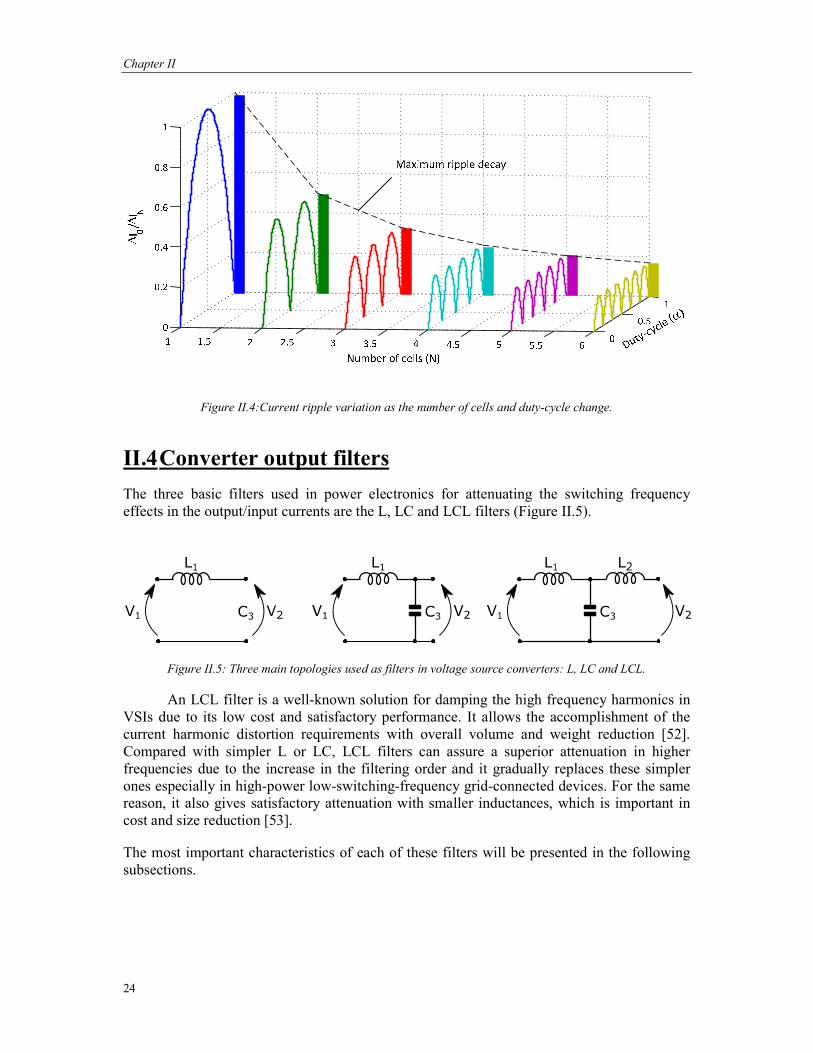
Chapter II

24

Figure II.4:Current ripple variation as the number of cells and duty-cycle change.

II.4 Converter output filters The three basic filters used in power electronics for attenuating the switching frequency effects in the output/input currents are the L, LC and LCL filters (Figure II.5).

Figure II.5: Three main topologies used as filters in voltage source converters: L, LC and LCL.

An LCL filter is a well-known solution for damping the high frequency harmonics in VSIs due to its low cost and satisfactory performance. It allows the accomplishment of the current harmonic distortion requirements with overall volume and weight reduction [52]. Compared with simpler L or LC, LCL filters can assure a superior attenuation in higher frequencies due to the increase in the filtering order and it gradually replaces these simpler ones especially in high-power low-switching-frequency grid-connected devices. For the same reason, it also gives satisfactory attenuation with smaller inductances, which is important in cost and size reduction [53].

The most important characteristics of each of these filters will be presented in the following subsections.

Parallel Interleaved Converters: Filter Design, Control and Bandwidth Analysis

25

II.4.1 L filter

The simplest filter for VSIs, BCs etc, is an inductance, or an L-filter. Its simplicity lays on the fact that a unique component is used forming a Type-1 system (neglecting its resistance) with the correspondent transfer function,

I (s)V (s) = 1Ls (II.10)

This filter presents an attenuation of 20dB/decade which means that, for systems which requires very low harmonic distortion; a high valued inductor is demanded and, as a consequence, size, cost and losses rise. Controllability can also be compromised in grid connected systems since the high voltage drop in the inductor increases the necessary output voltage to keep controllability. These drawbacks indicate that increasing the system order is necessary in several cases.

II.4.2 LC filter

Second-order LC filters can achieve higher filtering performance since the second passive component, the capacitor, increase the filter order and the attenuation becomes 40 dB/decade in the stop-band. However, a new matter appears: resonance. The filter design should place the resonance (fres),

= 12π√LC (II.11)

in a specific frequency or range which is far enough from common system harmonics. Beyond that, it should be damped passively or actively in order for the system to present a good and safe performance. Basically, all the studies about higher order filters (LC or LCL) present solutions for this possible problem by adding a simple resistor in series with the capacitor to more complex ones by adding further passive shunt circuits or by handling the damping in the control level (active damping) [52]–[62].

The LC filter also presents a second restriction in grid-connected devices, which is the dependency on the grid impedance. This occurs because when the grid impedance is negligible, that is, in a stiff grid system, the shunt capacitor in the LC filter will present higher impedance to the switching harmonics than the grid itself. This means that the current harmonics will flow to the network and the total harmonic distortion will not be changed with the shunt capacitor addition. In other words, the filter will have the same behavior of a single L filter. This is not a realistic condition and in most of the cases, the grid impedance is not negligible, and it will also attenuate the current harmonic components, thus, the filter will actually present a second inductor, i.e. an LCL filter [61]. For this reason, a more detailed analysis will be presented for this topology in the next section.

II.4.3 LCL filter

The scheme of an LCL-filter is presented inFigure II.6. In the context of parallel multicell converters, L1 represent the impedance of the N parallel output inductors.

Chapter II

26

Figure II.6: LCL filter often used in VSIs.

Compared to simple L-filters, by adding extra capacitor and inductor (C3 and L2), a relevant attenuation is obtained and a lower ripple in the output current is possible. Figure II.7shows the relation in converter output ripple ( i1) and grid current ripple ( i2) when L1 is kept constant and C3 and L2 varies.

0.10.2

0.30.4

0.5

0.02

0.03

0.04

0.05

0

0.05

0.1

0.15

0.2

L2 / L1C3 (pu)

i 2 /

i 1

Figure II.7: Current ripple relation as C3 and L2 varies.

As the filter complexity is increased by adding extra components, the resonance behavior should be analyzed and damped when increasing the order of the system. The simplest way of doing this, is by adding a resistor in series with C3. Naturally, the association of inductances resistances also enforces this attenuation, but their values must be minimized for reducing the filter losses, since they are part of the main current path. These small resistances do not change significantly the system’s transfer functions and for this reason, they will be neglected in the analytical expressions of the filter [59].

The behavior of interest can be expressed by the forward self-admittance and forward trans-admittance, which are the transfer functions, which relate I1 and I2, respectively, to the converter output voltage. The main difference between their characteristics is that the forward self-admittance (1) has a pair of zeros whose location is defined by Rd, L2 and C3.

Parallel Interleaved Converters: Filter Design, Control and Bandwidth Analysis

27

I (s)V (s) = 1L s + s +s s + 2ζ ω s + ω (II.12)

The forward trans-admittance (II.13), in the other hand, has just one zero whose time constant is RdC3.

I (s)V (s) = RL L s +s s + 2ζ ω s + ω (II.13)

The transfer functions resonance frequency (ωp) and damping (ζp) are defined by:

ω = 1L C (II.14)

ζ = 2 CL (II.15)

where

= + (II.16)

These transfer functions will be used for the identification, control and frequency analysis in this study.

II.4.4 Intercell Transformer (ICT)

The previous section has demonstrated that an LCL configuration presents a good compromise in what concerns size, cost and losses in the output filter. It allows the reduction of the converter output inductance (L1) by increasing the order and the number of components. In this section, a special attention will be driven to L1. Whereas this study focuses on the parallel multicell implementation of conversion systems, L1 is actually a parallel association of N inductors, where N is the number of switching cells. It is important to point some aspects concerning this inductance:

1. The role of this component is to filter the switching harmonics and for this specific function, the higher the inductance, the higher the attenuation at these frequencies.

2. Although L1 is required for reducing the switching harmonics, it has an important

effect in the fundamental frequency since the whole converter current flows thought it. As a consequence, if L is increased for a better filtering, a big inductor should be designed, since the energy stored (E) in the magnetic components follows the equation:

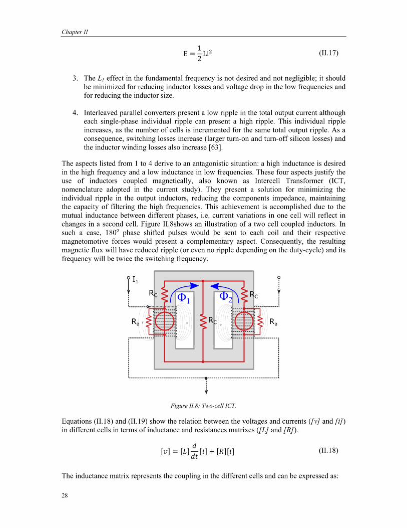
Chapter II

28

E = 12 Li (II.17)

3. The L1 effect in the fundamental frequency is not desired and not negligible; it should be minimized for reducing inductor losses and voltage drop in the low frequencies and for reducing the inductor size.

4. Interleaved parallel converters present a low ripple in the total output current although

each single-phase individual ripple can present a high ripple. This individual ripple increases, as the number of cells is incremented for the same total output ripple. As a consequence, switching losses increase (larger turn-on and turn-off silicon losses) and the inductor winding losses also increase [63].

The aspects listed from 1 to 4 derive to an antagonistic situation: a high inductance is desired in the high frequency and a low inductance in low frequencies. These four aspects justify the use of inductors coupled magnetically, also known as Intercell Transformer (ICT, nomenclature adopted in the current study). They present a solution for minimizing the individual ripple in the output inductors, reducing the components impedance, maintaining the capacity of filtering the high frequencies. This achievement is accomplished due to the mutual inductance between different phases, i.e. current variations in one cell will reflect in changes in a second cell. Figure II.8shows an illustration of a two cell coupled inductors. In such a case, 180o phase shifted pulses would be sent to each coil and their respective magnetomotive forces would present a complementary aspect. Consequently, the resulting magnetic flux will have reduced ripple (or even no ripple depending on the duty-cycle) and its frequency will be twice the switching frequency.

Figure II.8: Two-cell ICT.

Equations (II.18) and (II.19) show the relation between the voltages and currents ([v] and [i]) in different cells in terms of inductance and resistances matrixes ([L] and [R]).

[ ] = [ ] [ ] + [ ][ ] (II.18)

The inductance matrix represents the coupling in the different cells and can be expressed as:

Parallel Interleaved Converters: Filter Design, Control and Bandwidth Analysis

29

[ ] = …… …… (II.19)

where the parameters in the diagonal are the self-inductances (Lii) and the others are the mutual inductances between cell i and j (Lij). In the case of non-coupled inductors, the [L] is a diagonal matrix and the mutual inductances are zero. It is important to notice that a correct coupling orientation acts summing or canceling the individual ripple. As long as the mutual inductances are negative between each pair of ICT legs, the coupling will reduce both currents and increase their frequency. In other words, the minimization of the ripple and the increase in the apparent switching frequency will occur in the magnetic circuit. The ICT represents a clever solution in interleaved converters since the three desired characteristics listed in the beginning of this section where respected:

I. since the ripple cancelation occurs in the magnetic circuit, each cell will present a ripple of N times the switching frequency and consequently the impedance will be bigger presenting a good attenuation at this frequency,

II. at the fundamental frequency, only the leakage inductance will act and lower energy will be stored in the magnetic field demanding a smaller component and reducing the losses,

III. the individual current ripple will also be reduced, for a given fixed output ripple which represents an opposite behavior compared to non-coupled inductors.

These aspects can be observed inFigure II.9.

Figure II.9: Comparison between current ripples in regular inductors and ICTs used in a 2-cell iVSI.

II.4.5 LCL Filter Design

As already presented, an LCL configuration provides an attractive solution for attenuating the switching frequency reducing size, losses and cost of the output filter. Its design starts with the specification of the admissible output ripple and the following steps depend on other

Chapter II

30

system requirements and limitations. Following the considerations proposed in [1][2], for obtaining higher performance the following constraints should be considered:

5. Capacitance limited by the reactive power in the system, recommended not to exceed 5% of rated power. If this value is exceeded, the conversion system will present a lower power factor and the converter would be demanded to drive a higher current to achieve unity factor.

6. Inductance values should be reduced for avoiding high voltage drops in these elements. Higher voltage drop in the filter inductor demands an also higher voltage in the DC-link for maintaining controllability. Also, higher voltage in the DC –link can increase the switching losses and drive the system to work closer to the semiconductors limits.

7. Resonance frequency should be in a safe frequency range (in between ten times the fundamental frequency and half the switching frequency) to put away harmonics present in the system.

8. Damping resistor should be calculated taking into consideration the resonance frequency and the losses in low frequencies. In [56], the authors recommend to use two times the capacitor impedance in the resonance frequency.

The four items listed add restrictions but they are not enough for defining the four filter parameters (L1, L2, C3 and Rd). In order to have all the values specified, the designer can choose further restrictions or definitions depending on the system characteristics. If the filter uses an ICT, for example, the complexity related to the design of this component makes L1 which is inductor leakage inductance in this case, not easily scalable for different conditions. In this case, the ICT design could be handled first fixing the value of L1 and afterwards the other filters parameters specified for the desired output ripple, following the four restrictions listed above. In a second example, both converter and output ripple can have their values limited, also making possible the definition of the parameters.

Considering these observations, several filters were designed for the same output ripple of 2% for N-cell iVSIs, considering the system parameters defined in Table II-1.

Table II-1: Fixed parameters for different LCL filters designed. Mains current ripple 2% DC-link voltage (VDC) 400V Mains voltage (Vm) 220V (60Hz) iVSC nominal power 11.7kW

Taking into consideration the inputs defined in Table II-1, the designed filters for the number of cells varying from N=1 to 4 are presented in Table II-2.

Table II-2: Parameters for different LCL filters. Parameter N=1 N=2 N=3 N=4

L1 40µH (3.6%) 20µH (1.8%) 13µH (1.2%) 10µH (0.9%) L2 39µH (3.5%) 19µH (1.78%) 13µH (1.19%) 9.7µH (0.89%) C3 22.8µF (3.5%) 1.14µF (1.78%) 7.6µF (1.19%) 5.7µF (0.089%) Rd 5.88Ω (140%) 5.88Ω (140%) 5.88Ω (140%) 5.88Ω (140%)

The frequency responses of the forward self-admittance of three different filters (N=3, N=4 and N=5) are presented in Figure II.10.The filter bandwidth increases linearly as the number of cells increases.

Parallel Interleaved Converters: Filter Design, Control and Bandwidth Analysis

31

Figure II.10: Frequency responses of the LCL filter in N-cell parallel inverters.

II.5 Controller Design Methodology

II.5.1 Introduction

Although PI and PID controllers are widely adopted in a vast variety of processes, the definition of their gains is far from being a consensus. Several differences in the models of the processes and closed loop requirements make this task not obvious at all. The control specialist should answer two important questions during the design process:

1. What is the desired closed loop behavior I want the system to achieve?

2. How can I calculate the controller parameters in order to achieve that goal?

The second question tends to be easily answered. There are several empirical and analytical methods for calculating the controller gains depending on the plant’s model.

Answering the first question, in the other hand, might be difficult as long as no clear requirements are available. It depends on the process characteristics, actuator constraints and a tradeoff between robustness and velocity. In the present study, a simple, generic and embracing method is proposed for finding a solution for both questions. It takes into consideration the behavior of the closed loop system without controller as reference in what concerns the bandwidth. A unitary proportional controller is used as reference for the closed loop specification since the controller usually does not vary significantly the plant time constant (unless an oversized actuator is used). Afterwards, the controller gains are calculated so that the system has dominant poles satisfying the desired performance. The steps of the proposed methodology are detailed and described in the next section.

Chapter II

32

II.5.2 Calculation of the system's closed loop settling time with no controller (Tsnc)

The calculation of the system without controller is performed by taking into consideration the time constant of the pole with higher dominance. In order to determine which one is this pole, the modal dominance index (MDI) is calculated [64].

If the transfer function of a system is written in partial fractions,

G(s) = ( ) + + ( ) + ( ) +

+ ( ) + + + (II.20)

where Ji, i = 1,…,k+q is the residue corresponding to pole λi and the asterisks represents the complex conjugates; k is the number of real poles and q is the number of complex conjugate poles. The MDI of such a system is:

γ = (II.21)

for i=1,2,…k in respect to the real poles. For the complex conjugate ones, the expression bellow represents the MDI:

= +2 (II.22)

for l = 1,2,…k and i=k+2l-1, k+2l. It important to mention that the complex conjugate poles present the same index in Equation (II.22), that is, = .

The pole with the highest MDI absolute value presents the most relevant dynamics in the system and its time constant is used as a reference to calculate the specified closed loop settling time. If pole λh presents the highest MDI, the reference closed loop 2% settling time (Tsnc) will be

= 4( ) (II.23)

Figure II.11 presents a comparison between the step response of a no-controlled closed loop LCL filter and the reference system obtained from the MDI analysis. Knowing the MDI, the closed loop constraints - damping and the settling time - are defined as a fraction of Tsnc and are the only two inputs in the proposed control design methodology.

Parallel Interleaved Converters: Filter Design, Control and Bandwidth Analysis

33

Figure II.11: Comparison between the system natural dynamic and the simplified reference dynamic obtained from the MDI analysis.

II.5.3 Pole Placement and Root locus in the Z-Plane

In power electronics and in several other applications, Classical Control Theory is commonly applied for achieving satisfactory dynamical performance. Single closed loop controllers are adopted in engineering since the development of steam engines in the 18th century, propelling the industrial revolution [65]. Since the first books in Control Theory from the 1940’s until nowadays a very special attention has been given to Proportional, Integral and Derivative Controllers (PID controllers) [66]. For example, PID controllers are continuously applied and statistics show that over 95% of the industrial loops use this type of controller due to its robustness and wide applicability [67]. In the control of electric systems, classical control allied to vector manipulations is used in the great majority of AC/DC systems. Although the PID controllers present only three parameters to be determined, systematic and analytical methods for defining them are not trivial. A visit to process plants will often present poorly tuned controllers; one of the reasons is the high amount and diverse methods for tuning controllers [68], [69].

Pole placement methods based in the root locus design was first proposed by Evans in the 1950 [70] and it has an important place in the Control Theory since it gives a better understanding of the system dynamics from the path the poles will make when a parameter is changed. The block diagram in Figure II.12 represents a control loop, where K is the proportional gain, Gc is the controller and Gp is the plant transfer function.

.

Figure II.12: Block diagram of a control loop.

Chapter II

34

In power electronics, when pulse width modulation is applied, PI controllers are preferred (with no derivative term) since the high frequency current ripple allied with the derivation can raise the variability and deteriorate performance. The PI controller transfer function can be written as:

= 1 + (II.24)

where Ki is the integral gain. Equation (II.25) presents the characteristic equation of such a system.

1 + = 0 (II.25)

From the characteristic equation, the root locus diagram can be drawn showing the possible roots of such a system when a parameter varies. A certain complex number s0 will be a pole of the transfer function if it respects the angle criteria in (II.26).

∠ ( ) ( ) = 180 (II.26)

The proportional gain (K) can assume any value, but it can be calculated for any given pole when Equation (II.27) is used.

= 1 (II.27)

Both angle and gain criteria, (II.26) and (II.27), derive from the characteristic equation (II.25).

These simple equations are the basis for the Root Locus Design and for the Pole Placement used here for tuning the controller (defining its gains). For this, the design equations proposed in [71] were used. The method is based on poles placement after the desired closed-loop dominant poles (z0) in Z-domain are determined as a function of settling time and overshoot. From the angle criteria, we have:

∠ ( ) = 180 ∠ ( ) (II.28)

Thus, the goal is to calculate the parameter β in the discrete PI controller transfer function:

( ) = 1 (II.29)

which respects (II.28).

This design method is not that direct since it only guarantees that certain pair of poles will be part of the root locus, i.e. it will influence the system dynamics but not define it. This way, after the controller is tuned, some iteration for refining its values by adding safety factors (in the damping factor, for example) might be necessary depending on the plant. If non-dominant poles are not far enough from the z0, the transient response restrictions will not be respected

Parallel Interleaved Converters: Filter Design, Control and Bandwidth Analysis

35

[72]. Some methods were proposed in order to guaranty that the non-dominant poles are placed far enough from the dominant one as variations of the classical methods [69], [72], [73] but for simplicity, they were not used.

The controller tuning process can be summarized in the nine steps bellow.

Step 1: Calculate the closed loop transfer function with no controller. Step 2: Use the MDI for defining the reference closed loop settling time ( ). Step 3: Define the settling time for the closed loop system with controller as a

fraction of the reference (for example, 0.9 ). Step 4: Calculate the damping by the maximum admissible overshoot – at this

point, a security factor should be added since there are other non-dominant poles.

Step 5: Find the desired closed loop pole in the z-plane (z0). Step 6: Discretize the system’s transfer function. Step 7: Calculate the controller gains by using the formulas obtained from the

angle and magnitude criteria (Pole Placement/Root locus method). Step 8: Check if the system presents the desired behavior. If not, increase the

security factor in 4 and repeat the subsequent steps. Step 9: If even by increasing the safety factors, the desired dynamic is not

achieved, the settling time must be increased. This will be necessary, especially if other poles are close enough from the desired dominant ones.

II.5.4 Controller design examples for LCL filters

For demonstrating the proposed method for tuning the control loop, an LCL filter for a 4-cell iVSI will be used. The idea is to control the converter output current and the transfer function of such a system was already showed in Equation (II.12). In Section II.4.5 the methodology for designing filters for an N-cell iVSI was presented, i.e. as the number of cells changes, the filter is calculated to maintain the same output ripple.

In order to make the analysis of the discretized system, the bilinear approximation (Tustin) is used. In this approximation, the Laplace operator s is substituted by:

= 2 1+ 1 (II.30)

where Ts is the sampling period.

Figure II.13 shows the mapping from the continuous to the discrete domain (s to z-plane) by using the bilinear approximation of a filter designed for a 4-cell iVSI. As an illustration, the damping resistor varies from 1 to 1/3 of its initial value in the graphs. By the poles movement in the plans, a qualitative comprehension of how the system becomes under damped is straight forward and it denotes the importance of actively or passively attenuating the resonance frequency in order to avoid problems in operation. It is also possible to observe that the discretized system has two more elements: one zero and one pole. The zero is added by the bilinear approximation and it is located in z=-1 (Equation(II.30)). The pole presented in z=0 is derived from the time delay of one sampling period due to the analog-to-digital and

Chapter II

36

digital-to-analog conversion processes. This delay is especially important in systems where the sampling frequency is relatively low and this phenomenon will be presented further.

Figure II.13: Pole-zero location of the LCL filter in the S-Domain (a) and Z-Domain (b). The narrows show the poles and zeros path as the damping resistance is divided from 1 to 3.

Following the proposed steps for the controller design (Section II.5), the MDI analysis is performed and the desired dominant pole (z0) is determined by closed loop requirements (maximum overshoot of 20% and settling time of 2Tsnc). In Figure II.14-left, the open-loop complete system zeros and poles are presented in blue. The desired dominant poles are highlighted in red. The controller adds one zero and one pole in open loop system and its parameters are calculated in a way that z0is part of the root locus, as presented in Figure II.14-right.

Real Axis

Imag

inar

y Ax

is

-1 -0.5 0 0.5 1-1

-0.8

-0.6

-0.4

-0.2

0

0.2

0.4

0.6

0.8

1

-1.5 -1 -0.5 0 0.5 1 1.5-1

-0.8

-0.6

-0.4

-0.2

0

0.2

0.4

0.6

0.8

1

Real Axis

Figure II.14: Pole-zero maps in the Z-plane of the open loop system (left) and root locus with the

controller (right).

This method has the advantage of being very simple, but it does not guarantee that the closed loop constraints will be respected; it only assures that the z0 will be part of the root locus. It does not even assure that the system will be stable. If z0 is not well defined, for example, if too fast behavior is demanded, the closed loop system can be unstable. For this reason, the

Parallel Interleaved Converters: Filter Design, Control and Bandwidth Analysis

37

definition of the desired settling time and damping should be reasonable since the sampling frequency limits the controller speed as explained further.

Figure II.15: Root locus differences when the system z0 not saturated (first line of graphs) and when it is saturated (second line).

As the number of cells increase in an iVSI, it was already presented that the filter becomes faster: less filtering efforts are demanded, thus smaller components (capacitors and inductors can be used). Therefore, the system open loop dynamics is improved and a faster controller is possible without increasing its burden until limit. The continuous cell’s increment leads to a continuous increase in the filter passband, but a digital controller is not capable of continuously increase its speed. The diagrams in Figure II.15 and the graphs in

Figure II.16 clarify it. They present three different filters designed for 8, 10 and 12-cells iVSIs. Accomplishing the MDI analysis for the three filters and using the criteria of 2Tsnc for the settling time specification, their values will be respectively: 0.83, 0.65 and 0.54 ms. These values are relatively close to the sampling period of 0.1ms. The desired dominant poles (z0) becomes faster and gradually closer to the origin as highlighted. The question is that, the controller’s zero is shifted to the right in order to guarantee that the root locus will pass in z0. This is explained by the angle criteria: a zero attracts and a pole repels the root locus since a zero contributes positively to the angle sum and a pole negatively. The control books which discuss this topic and explain the steps for drawing the Root Locus Diagram explain in details this characteristic in the diagram [74]–[77]. Since the zeros move to the right, there are two natural consequences:

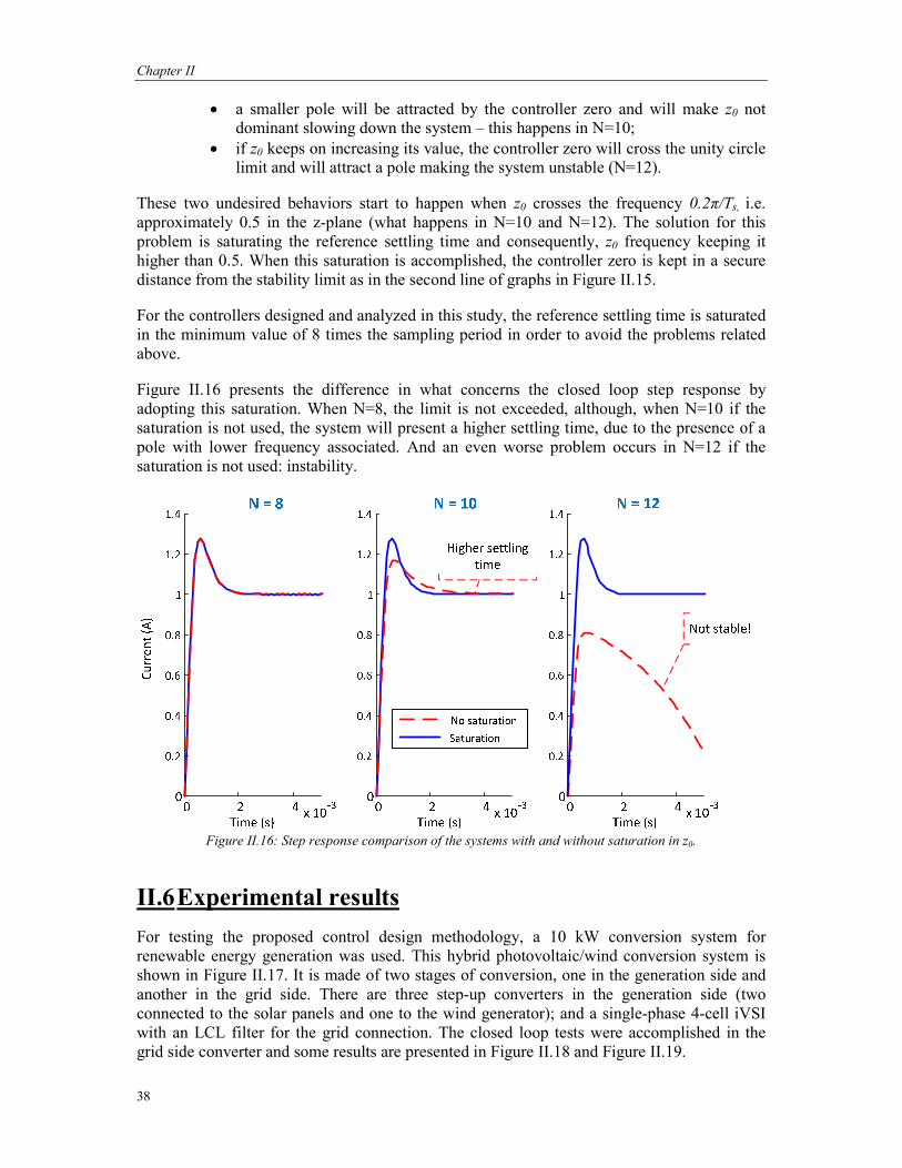
Chapter II

38

a smaller pole will be attracted by the controller zero and will make z0 not dominant slowing down the system – this happens in N=10;

if z0 keeps on increasing its value, the controller zero will cross the unity circle limit and will attract a pole making the system unstable (N=12).

These two undesired behaviors start to happen when z0 crosses the frequency 0.2π/Ts, i.e. approximately 0.5 in the z-plane (what happens in N=10 and N=12). The solution for this problem is saturating the reference settling time and consequently, z0 frequency keeping it higher than 0.5. When this saturation is accomplished, the controller zero is kept in a secure distance from the stability limit as in the second line of graphs in Figure II.15.

For the controllers designed and analyzed in this study, the reference settling time is saturated in the minimum value of 8 times the sampling period in order to avoid the problems related above.

Figure II.16 presents the difference in what concerns the closed loop step response by adopting this saturation. When N=8, the limit is not exceeded, although, when N=10 if the saturation is not used, the system will present a higher settling time, due to the presence of a pole with lower frequency associated. And an even worse problem occurs in N=12 if the saturation is not used: instability.

Figure II.16: Step response comparison of the systems with and without saturation in z0.

II.6 Experimental results For testing the proposed control design methodology, a 10 kW conversion system for renewable energy generation was used. This hybrid photovoltaic/wind conversion system is shown in Figure II.17. It is made of two stages of conversion, one in the generation side and another in the grid side. There are three step-up converters in the generation side (two connected to the solar panels and one to the wind generator); and a single-phase 4-cell iVSI with an LCL filter for the grid connection. The closed loop tests were accomplished in the grid side converter and some results are presented in Figure II.18 and Figure II.19.

Parallel Interleaved Converters: Filter Design, Control and Bandwidth Analysis

39

Figure II.17: Hybrid photovoltaic/wind conversion system

In this conversion system, the LCL filter was calculated as described in II.4.5 and an ICT was modeled as L1. The MDI analysis was performed aiming at a dynamical reference, then the controller parameters were calculated. Further details of the experimental set-up will be presented in Chapter III. In order to avoid noise propagation in the system, an overdamped closed loop behavior was defined for the operation, that is, no overshoot and a settling time of 35 ms. A 20A step (0.3 pu) was performed in the LCL current loop as presented in Figure II.18. The real and simulated curves enhance the good quality of the model.

0 0.005 0.01 0.015 0.02 0.025 0.03-5

0

5

10

15

20

25

Time (s)

Curr

ent (

A)

real datamodelsetpoint

Figure II.18: Step response of the closed loop current control.

The ICT currents are presented in Figure II.19 (top) and the total current i1 in Figure II.19 (bottom). Differently from the regular parallel inductors in interleaved converters, the

Mains Side Converter

(MSC)

L1 (ICT) LCL filter

L2 Rd

Generation Side

Converter (GSC)

Chapter II

40

apparent switching frequency of four times the real switching frequency appears in the individual currents smoothing and reducing their ripples.

Figure II.19: Individual ICT currents (top) and total i1 current (bottom).

The continuous current component was removed from this result since the goal was to emphasize the current ripple. Although the same 20A was applied in for these results (Figure II.18): a 1A (5%) ripple was observed in the total current i1. These tests were accomplished with a 6 KHz switching frequency and a 50V DC-link voltage. Since these results were performed with no grid connection or extra load, this voltage level is enough for controlling the system in nominal current.

II.7 Frequency Analysis for an N-Cell Converter The increase in the LCL filter bandwidth is useful in order to increase the robustness of the conversion system in what concerns perturbation rejection. Figure II.20shows some characteristics of interleaved parallel VSI with LCL filters. For the analysis, a fixed 2% output current ripple was defined in order to calculate the filter while keeping other parameters constant, like DC-link voltage (450V), L1 inductance (40 µH) and switching frequency (10 kHz). The other filter parameters were calculated based on the items clarified in section II. In the first graph, a linear evolution of the resonance frequency (fres) is observed as the number of cells increases. This represents smaller and cheap components as well as faster dynamics. This is a consensual benefit of such a topology and has been pointed out by many authors. However, Figure II.20-bottom shows that a somewhat different behavior occurs in the closed loop dynamics.

It should be noticed that, for each filter in Figure II.20, a controller was calculated based on the methodology presented in section IV.

0.0408 0.0409 0.041 0.041 0.041 0.0411 0.0411-2

-1

0

1

2In

divi

dual

I (A

)

0.0408 0.0409 0.041 0.041 0.041 0.0411 0.0411-2

-1

0

1

2

Time (s)

Tota

l I (A

)

Parallel Interleaved Converters: Filter Design, Control and Bandwidth Analysis

41

Figure II.20: LCL filter resonance frequency (fres) in the top and closed loop crossover frequency (fco) in the bottom graphic.

Naturally, as the system’s time constant decays, the poles of the transfer function become faster. In the MDI analysis, this will imply larger poles, which are used as input in the controller design. Finally, the closed loop dynamics will also have an increasing speed. Nevertheless, this condition is limited by the system sampling period. As the filter’s time constant gets closer to the sampling/switching period, the closed loop system loses the capability to keep following the increasing speed. Figure II.20-bottom shows that, as the number of cells increases and the closed loop crossover (fco) reaches 1kHz (approximately one tenth of the switching frequency), the controller is limited and the system overall dynamics will not get any faster as the number of cells is augmented. This saturation appears after N=4 and it is an important issue especially in high power systems, where a large number of cells can be used with low switching frequency. In these cases, the interleaved VSC will have small filters but will suffer from limitations in the closed loop dynamics.

II.8 Conclusion Interleaved converters are widely adopted and present several advantages due to the increase of the apparent switching frequency by a factor of N. These advantages result in smaller passive components of filter and, consequently, smaller filter losses and higher system bandwidth. Nevertheless, as shown in this chapter, filter dynamics can be limited by the control performance when the system bandpass reaches values close to the sampling frequency and this characteristic is not usually mentioned in the researched literature. For duality issues, this conclusion can also be extended to series multicell VSI. This limitation depends on the defined control strategy and controller design criteria. In our case, the classical perspective was approached: fixed sampling frequency equal to the switching frequency; PI controllers and the design based on the MDI analysis. Different approaches (like using MPC or higher sampling frequency for the fixed switching one) can push the dynamical enhancement further.

Chapter II

42

In order to accomplish this analysis, a known LCL filter design criterion was used and a control design methodology was proposed for calculating the parameters of the discrete compensator. It results in an embracing method that can be applied to any plant (not only in power conversion systems). The results were validated experimentally in a four-cell parallel interleaved converter.

Design, Modeling and Identification of the Wind/Photovoltaic Hybrid Renewable Generation System (HRGS)

43

Chapter III

Design, Modeling and Identification of the Wind/Photovoltaic Hybrid Renewable

Generation System (HRGS)

Chapter III

44

III.1 Introduction Distributed and micro-energy generation systems represent an important solution for the energetic matrix diversification in opposition to the classical centralized way of production. The first positive aspect is that the natural resource should not be abundant since the generation is in small scale. For the same reason, the implantation costs are reduced and affordable for regular citizens and not only for big companies. When a person generates his/her own energy, he/she becomes independent from the volatile prices of electricity, which depends on market circumstances. Among the technologies for small scale production, photovoltaic and wind energy generation have become the most promising sources due to their worldwide availability, null cost and sustainability [78]. Both types of generation, when allied, can increase significantly the electricity produced once the resources’ availability can present simultaneity or complementarily due to their stochastic pattern. For example, a windy night can guarantee high-energy production in a hybrid system; there would be no generation if just a photovoltaic system was implanted. When both resources are available, high or nominal generation is achieved guarantying a higher capacity factor. The possibility of increasing the capacity factor is very important since no high investments in the resource availability are usually accomplished in small-scale systems, because it would deeply increase the costs of implantation. This is already a difficult task in large-scale plants due to the stochastic behavior of the renewable resources. For this reason some specialists believe that an electrical network depending strongly on small scale renewable generation is unpredictable or even unreliable compared to the traditional one [79].

This study focuses on the design and control of an 11.7kW hybrid generation system using solar photovoltaic panels and a wind turbine. A multicell converter divided in two parts accomplishes the conversion: Generation Side Converter (GSC) and Mains Side Converter (MSC). The actual chapter presents in detail the design of such a system highlighting the key components (wind turbine, photovoltaic cells, switching elements, passive filter etc), their models and parameters’ identification.

The description of the control strategy and the simulation and experimental results of this system will be the aim of Chapters IV and V. Nevertheless, to make sure the system works properly with high standards of security and performance, it is mandatory that the control strategy is well defined and the system well parameterized. For doing so, consistent system identification might be carried out. The main dynamics to be controlled in this system are listed as follows:

wind generator mechanical and electrical parameters such as moment of inertia, friction factor and inductances, resistances and magnetic flux,

solar panels voltage versus current behavior, filter and DC-link’s dynamics in GSC and MSC.

The models of these elements will be described in this chapter, and the identification of corresponding parameters will be presented. Initially, an overview of the HRGS will be given with the detailed description of each element. Following, the wind generator and solar panels will be presented and their models and parameters, obtained from measurements and tests, will be showed. Finally, the filters of the conversion system will be analyzed: the input LC filter from the GSC and the output LCL filter from the MSC.

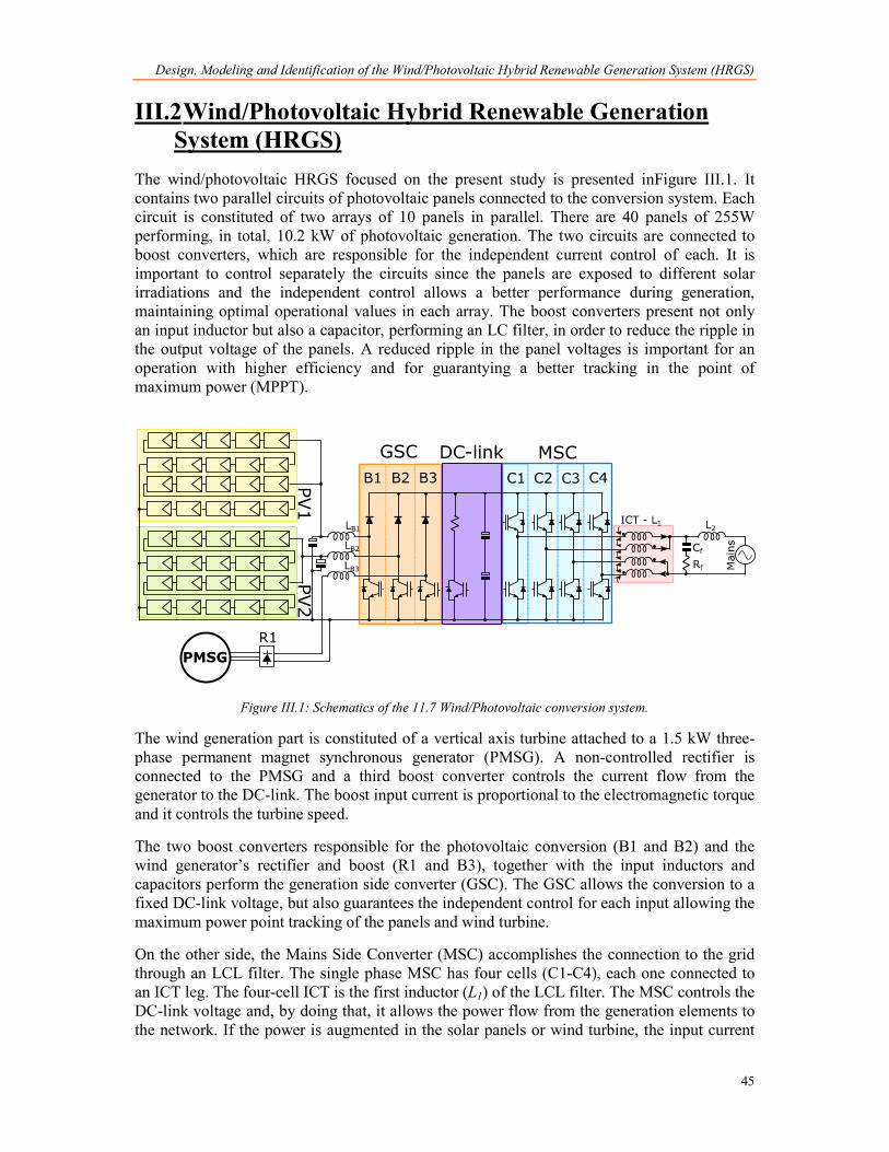
Design, Modeling and Identification of the Wind/Photovoltaic Hybrid Renewable Generation System (HRGS)

45

III.2 Wind/Photovoltaic Hybrid Renewable Generation System (HRGS)

The wind/photovoltaic HRGS focused on the present study is presented inFigure III.1. It contains two parallel circuits of photovoltaic panels connected to the conversion system. Each circuit is constituted of two arrays of 10 panels in parallel. There are 40 panels of 255W performing, in total, 10.2 kW of photovoltaic generation. The two circuits are connected to boost converters, which are responsible for the independent current control of each. It is important to control separately the circuits since the panels are exposed to different solar irradiations and the independent control allows a better performance during generation, maintaining optimal operational values in each array. The boost converters present not only an input inductor but also a capacitor, performing an LC filter, in order to reduce the ripple in the output voltage of the panels. A reduced ripple in the panel voltages is important for an operation with higher efficiency and for guarantying a better tracking in the point of maximum power (MPPT).

Figure III.1: Schematics of the 11.7 Wind/Photovoltaic conversion system.

The wind generation part is constituted of a vertical axis turbine attached to a 1.5 kW three-phase permanent magnet synchronous generator (PMSG). A non-controlled rectifier is connected to the PMSG and a third boost converter controls the current flow from the generator to the DC-link. The boost input current is proportional to the electromagnetic torque and it controls the turbine speed.

The two boost converters responsible for the photovoltaic conversion (B1 and B2) and the wind generator’s rectifier and boost (R1 and B3), together with the input inductors and capacitors perform the generation side converter (GSC). The GSC allows the conversion to a fixed DC-link voltage, but also guarantees the independent control for each input allowing the maximum power point tracking of the panels and wind turbine.

On the other side, the Mains Side Converter (MSC) accomplishes the connection to the grid through an LCL filter. The single phase MSC has four cells (C1-C4), each one connected to an ICT leg. The four-cell ICT is the first inductor (L1) of the LCL filter. The MSC controls the DC-link voltage and, by doing that, it allows the power flow from the generation elements to the network. If the power is augmented in the solar panels or wind turbine, the input current

Chapter III

46

increases in the GSC. The DC-link voltage tends to reach higher values, but in normal operation, the MSC’s control increases the current reference and when the input and output power are the same, the systems reaches steady state. This way, the DC-link is the connection between the GSC and MSC: it is connected to a relatively high capacitance to absorb power oscillations during switching. For security reasons, the system was designed with a braking chopper able to absorb an eventual power unbalance between the input and output. If the converter input power is higher than the output, the DC-link capacitors charge increasing the DC-link voltage. The braking chopper is activated if the voltage reaches excessive values, dissipating the extra energy in a resistance. The most important parameters of the HRGS are summarized in Table III-1.

Table III-1: Parameters of the 11.7 KW HRGS. System overall power 11.7 kW

Photovoltaic generation

Photovoltaic nominal power 10.2 kW Number of cells 40 Type of cells Multi-crystalline silicon Individual Power 255 W Number of arrays 4 Nominal voltage per array 298 V Nominal current per array 8.49 A

Wind generation

Wind generation nominal power 1.5 kW Number of generators 1 Type of turbine Vertical axis type Darrieus [80] Type of machine Permanent magnet synchronous Number of phases 3 Nominal voltage 220 V Nominal current 2,3 A

GSC

Nominal B1 and B2 input currents 8.49 ADC Nominal B1 and B2 input voltages 300 V Nominal B3 input voltage 311 V Nominal B3 input current 4.82 A B1, B2 and B3 switching frequency 10 kHz

MSC

Nominal current (AC) 53.18 A Mains nominal voltage 220 V Mains nominal frequency 60 Hz Switching frequency 10 kHz

DC-link

DC-link operating voltage 400 V DC-link nominal current 29.25A DC-link capacitance 9400 µF Chopper resistance 100Ω

Figure III.2:Photovoltaic panels and vertical axis turbine in the HRGS installed at Unifei (Itabira, Brazil).

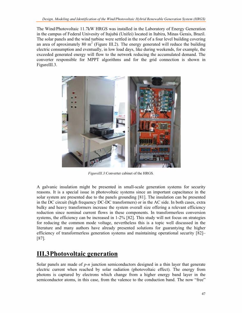
Design, Modeling and Identification of the Wind/Photovoltaic Hybrid Renewable Generation System (HRGS)

47

The Wind/Photovoltaic 11.7kW HRGS was installed in the Laboratory of Energy Generation in the campus of Federal Univesity of Itajubá (Unifei) located in Itabira, Minas Gerais, Brazil. The solar panels and the wind turbine were settled in the roof of a four level building covering an area of aproximately 80 m2 (Figure III.2). The energy generated will reduce the building electric consumption and eventually, in low load days, like during weekends, for example, the exceeded generated energy will flow to the network reducing the accumulated demand. The converter responsible for MPPT algorithms and for the grid connection is shown in FigureIII.3.

FigureIII.3:Converter cabinet of the HRGS.

A galvanic insulation might be presented in small-scale generation systems for security reasons. It is a special issue in photovoltaic systems since an important capacitance in the solar system are presented due to the panels grounding [81]. The insulation can be presented in the DC circuit (high frequency DC-DC transformers) or in the AC side. In both cases, extra bulky and heavy transformers increase the system overall size offering a relevant efficiency reduction since nominal current flows in these components. In transformerless conversion systems, the efficiency can be increased in 1-2% [82]. This study will not focus on strategies for reducing the common mode voltage, nevertheless this is a topic well discussed in the literature and many authors have already presented solutions for guarantying the higher efficiency of transformerless generation systems and maintaining operational security [82]–[87].

III.3 Photovoltaic generation Solar panels are made of p-n junction semiconductors designed in a thin layer that generate electric current when reached by solar radiation (photovoltaic effect). The energy from photons is captured by electrons which change from a higher energy band layer in the semiconductor atoms, in this case, from the valence to the conduction band. The now “free”

Chapter III

48

electrons move following the electric field created by the p-n junction, creating a current flow and generating energy. This phenomenon has an intrinsic non-linear nature demanding specific operational conditions for an enhanced performance, since it provides a current-voltage and power-voltage non-linear relations (I-V and P-V) which depend on the solar radiation and cell’s temperature. For this reason, maximum power point tracking (MPPT) algorithms are used for increasing the generated power in solar cells. For the definition, simulation, tests and implementation of these algorithms a consistent model of the solar cells and the photovoltaic phenomenon is mandatory and the panel modeling will be described in next section.

FigureIII.4:Panels’azimuth orientation.

In a solar installation, the panel orientation and inclination (azimuth and tilt angle) interferes in the generation capacity factor. For optimum generation, the panels should face the geographic north (in installations made in the southern hemisphere) and the inclination should be the value of the latitude for higher performance. Naturally, this cannot always be followed due to site physical restrictions, like following the roof orientation, for example. This was the case in the installation of the HRGS and it presented a real azimuth of 290º and an average tilt inclination of 12º. This will reduce the system’s capacity factor in 4% according to SWERA solarimetric database obtained in Radiasol21[88].

III.3.1 Photovoltaic Panels Modeling

1Radiasol2 is a program developed in the Federal University of Rio Grande do Sul which calculates solarimetric parameters from raw irradiance data.

Design, Modeling and Identification of the Wind/Photovoltaic Hybrid Renewable Generation System (HRGS)

49

An equivalent model of a photovoltaic panel is presented in FigureIII.5. It consists on a current source, an anti-parallel diode and two series and parallel resistances. This model is also known as five-parameter model and it adequately fits most of the modern PV panels in environmental situations close to the standard rating conditions (irradiation of 1000 W/m2 and cell temperature of 25ºC) [89].

FigureIII.5: Equivalent model of a photovoltaic panel.

The current source generates the photovoltaic current (Iph), i.e. a current generated by the photovoltaic effect which is a function of the solar radiation and temperature. The cell output current (I) is defined by:

= (III.1)

where Id is the diode current, Ish is the current drained by the shunt resistor (Rsh) given by:

= + (III.2)

Rs is the series resistance and V is the output voltage.

The diode current Id is written as:

= ( + ) 1 (III.3)

where Is is the diode reverse saturation current, also known as leakage current; q is the charge of an electron (q=1.6e-19C); k is the Boltzmann’s constant (k=1.38x10-23 J/K); Tc is the cell’s temperature in Kelvin and A is the ideality factor and depends on the panel technology (as shown in Table III-2).

Table III-2: Ideality factor (A) per technology.[90]

Technology A Si-mono 1.2 Si-poly 1.3 a-Si-H 1.8 a-Si-H tandem 3.3 a-Si-H triple 5 cdTe 1.5 CTs 1.5 AsGa 1.3

Chapter III

50

The saturation current (Is) is expressed as:

= (III.4)

where IRS is the reference reverse saturation current at a given temperature and solar radiation; Eg is the band-gap of the semiconductor. Finally, with some simplifications we can express IRS as:

= 1 (III.5)

where ISC is the short circuit current and VOC is the open circuit voltage. Both parameters are often used for informing the electrical characteristics of the panel and most of the manufactures give these values in the component datasheet. The simplifications for arriving in III.5 are ignoring Id and Ish during the short circuit test. That is to say,

= (III.6)

Finally, all these equations permit an analysis of the panel characteristics as function of easily obtained parameters or constants. In the HRGS, 255 W panels perform the photovoltaic generation; model YL255P-29b from the manufacture Yngli Solar. Some electric characteristics are presented in Table III.3.

Table III-3: Electric parameters of the YL255P-29b,Yngli Solar Panel informed by the manufacture.

Module efficiency Η 15.7% Voltage at Pmax Vmpp 30.0 Current at Pmax Impp 8.49 Open-circuit voltage VOC 37.7 Short-circuit current ISC 9.01

By the equations and parameters presented in this section, the I-V curves of the YL255P-29b panels are shown in Figure III.6 for different solar radiations.

Design, Modeling and Identification of the Wind/Photovoltaic Hybrid Renewable Generation System (HRGS)

51

0 50 100 150 200 250 300 3500

2

4

6

8

10

12

Vout (V)

I out (A

)

Figure III.6: Electrical characteristics of the panels YL255P-29b.

III.3.2 Photovoltaic Panels Identification

In order to confirm and refine the solar panels’ characteristics, some measurements were accomplished by the PV analyzer model PVA-600 from the manufacturer Solmetric. This instrument measures and traces the panel’s “I versus V” and “P versus V” as presented in Figure III.7. In order to obtain these curves, the instrument measures not only the electrical variables (panel’s voltage and current), but also the irradiance and the cells’ backside temperature. As an example, the figure shows a measurement accomplished in a 10 panels series array with good irradiation condition: no cloud obstruction and close to midday.

Figure III.7: Electrical characteristics of a 10 cells array measured in a sunny day (1317W/m2).

The irradiance reached the value of 1317 W/m2 and the panel’s temperature was 63.9ºC. The power curve (in gray) shows that the maximum power obtained in this condition was 2642 W for the 10 panels of 255 W each; the array voltage for maintaining the maximum power was

Chapter III

52

close to 250 V. Due to an antagonistic characteristic of photovoltaic generation, the generation was limited by the high panel temperature.

The measurements of panels’ variables are important for refining the parameters given by the manufacturer and also for finding the values that are not available, like the series and parallel resistances. Figure III.8 presents the comparison between measured and simulated data after the identification, in order to validate the model. The results show an important similarity corroborating to the good quality of the model.

Figure III.8:PV Model validation with the measured data.

The parameters obtained from the system identification are presented in Table III-4.

Table III-4: Panel’s electric parameters derived from the PV analyzer data.

Series resistance Rs 0.35 Ω Parallel resistance Rp 286.9 Ω Temperature coefficient (in Volts per Kelvin) αPV 0.06 %/ºC Open-circuit voltage VOC 39.58 V Short-circuit current ISC 9.01 A

III.4 Wind Power Generation The description of the wind turbine and the electric generator and their main characteristics will be presented in the following topics.

III.4.1 Vertical Axis Turbine

A Darrieus-type straight-bladed vertical axis turbine performs the wind generation of the HRGS. As already mentioned in Chapter I, vertical axis turbines are usually employed due to its simplicity since no yaw mechanism is required for orientation with the wind direction. The straight-bladed turbines increase even more the mechanical simplicity of the system once the

Design, Modeling and Identification of the Wind/Photovoltaic Hybrid Renewable Generation System (HRGS)

53

uniform section configuration is much easier to build, unlike the twisted and tampered blades often used in horizontal-axis or other vertical-axis turbines [91]. A French aeronautical engineer patented the design and baptized this type of turbine in 1931 [80]. The major drawbacks of the Darrieus turbine are the operation in extreme conditions. During low speed, it presents inadequate or even negative torque which demands a relatively high wind conditions for the start-up. This reduces the operational range or even removes the possibility of self-starting and consequently reduces the system efficiency. Beyond that, in high speeds, the turbine protection is compromised reducing the safety in this condition. These problems can be overpassed by changing the blades pitch angle, but this would make the turbine design and control more complex. For this reason, variable pitch blades turbines are unpractical for small scale and a fixed one is prioritized in this study.

Figure III.9:Darrieus-type straight-bladed vertical axis turbine of the HRGS.

The turbine model used in the generation system is called Razec 266, from the Brazilian manufacturer Enersud, presented in Figure III.9. Some characteristics given by the manufacturer are presented in Table III-5.

Table III-5: Parameters of the 11.7Kw HRGS. Nominal power 1.5 kW Rotor diameter 2 m Blades height 2.66 m Rotation starts at (wind speed) 2,2 m/s Generation starts at (wind speed) 3,9 m/s Nominal power at (wind speed) 12 m/s Weight 110 kg

The operational rotational speed is from 60 to 180 RPM.

Chapter III

54

The turbine’s mechanical power, either vertical or horizontal, absorbed from the wind is given by the equation,

= 12 (λ) (III.7)

where v and ρ are the wind speed and density, respectively, A is the sweep area covered and Cp is the turbine power coefficient. The power coefficient is a turbine aerodynamic characteristic which depends on the tip speed ratio (λ), expressed as:

= (III.8)

where ω is the angular velocity and R is the turbine radius.

The turbine’s power coefficient informed by the manufacturer is presented in Figure III.10 in which optimal λ of 1.6 can be noticed.

Figure III.10: Power curve of the Darrieus turbine used in the HRGS.

The mechanical dynamics are expressed as a first order transfer function (Gm) and can be written as:

= 1+ (III.9)

where J is turbine’s moment of inertia and B is the friction coefficient. It is important to identify this dynamic in order to allow good speed control as detailed in next section.

III.4.1.1 Mechanical Dynamics Identification

In order to define the turbine’s moment of inertia and friction coefficient, a simple test should be performed. The test consists on imposing a torque, which drives the system to a certain speed, removing the input torque and getting the slowdown curve. If there is no speed

Design, Modeling and Identification of the Wind/Photovoltaic Hybrid Renewable Generation System (HRGS)

55

measurement, this curve can be obtained from the induced voltage (proportional to the speed, number of poles and the fixed flux from magnets). This test is shown in Figure III.11.

Figure III.11: Slow-down induced stator voltage.

Although the electrical frequency decays linearly with the mechanical speed, the voltages presented in Figure III.11 does not present this characteristic. The reason for that is the aliasing effect derived from the high sampling period (200 ms) required for recording a long period in a standard oscilloscope (TPS2000 from Tektronix). Despite the aliasing effect, the peak voltage decay could be registered allowing the system identification. Table III-6 presents the parameters obtained from the slow-down curve.

Table III-6: Mechanical dynamical parameters of the turbine.

Moment of inertia J 45 kg.m2

Friction coefficient B 0.34 Nms Mechanical time constant τm 132 s

III.4.2 Permanent Synchronous Generator

Asynchronous machines dominated the market of small-scale wind turbines until the years 2010s. After this period, the utilization of Permanent Magnet Synchronous Generators (PMSG) increased significantly [92] and the advantages of this topology justifies this fact. The high torque density and higher efficiency are responsible for the expansion of this technology in renewable generation and many other segments such as automotive applications, electrical mobility, compressors, aircrafts and home appliances [93]. The fixed magnetic field provided by the magnets, which eliminates the necessity of electrical excitation, reduces significantly the driver complexity since no external electronic circuit and control is demanded for the flux control. Once magnets substitute the excitation windings, the number of poles can be increased to allow the machine operations at lower speeds. As a consequence, the turbine can be directly attached to the generator with no gearbox between them, also reducing the mechanical complexity and increasing the efficiency [94].

The mechanical details of the PMSG used in the test bench are presented in Figure III.12.

Chapter III

56

Figure III.12: Permanent magnet synchronous generator of the wind turbine in the HRSG.

III.4.2.1 PMSG Model

The direct and quadrature voltage equations of a PMSG can be expressed as:

= += (III.10)

where Rs is the stator resistance; ωe is the rotor electrical speed, vs, is and λs are the stator voltage, current and flux, respectively. According to the adopted orientation, the d-axis reference frame is aligned with the flux of the magnets ( ). The stator linkage fluxes decomposed in dq-axes are expressed as

= += (III.11)

where Lsd is the stator inductance in the direct axis and Lsq in the quadrature. The electrical torque (Te) is calculated as a function of the fluxes and currents interaction and the number of poles (np) in the machine.

= 32 (III.12)

For simplicity, it is better to represent the torque as a function of inductances, currents and .

Design, Modeling and Identification of the Wind/Photovoltaic Hybrid Renewable Generation System (HRGS)

57

= 32 + ( ) (III.13)

III.4.2.2 PMSG Identification

From equations presented in the previous section, it is possible to notice that in order to define the PMSG’s dynamics; the following parameters must be identified or measured: stator resistance, magnets’ flux, and dq-inductances.

The magnets’ flux can be derived from the same measurements for the mechanical parameters identification. From Equations (III.10) and (III.11), it is possible to notice that the induced voltage only depends on the magnets’ flux and stator electrical frequency. During open circuit tests, the induced voltage is presented in the stator terminals since there is no voltage drop in the stator impedance at zero current. This way, the same test presented in Figure III.11 is used, and the flux was calculated based on the equation bellow,

= (III.14)

During the machine’s open circuit test, only the q component of the stator voltage is presented.

For the mechanical characteristics of the rotor, some saliency is expected due to its characteristics designed to settle the magnets. The rotor non-cylindrical aspect imposes different machine permeance depending on the rotor position. In fact, when the rotor flux is aligned with the stator polarity (d-axis), the inductance is lower since the position of the magnets increases the flux reluctance. The inverse effect happens when the rotor position is shifted by 90º with respect to the stator. In order to measure this difference, the rotor position should be known and fixed. This way, the measurement of the dq-inductance was accomplished following the steps below:

1) connect phases B and C and apply a DC voltage between phases A and BC (Figure III.13-left);

2) align the rotor with the stator resultant flux (d axis) and lock the rotor; 3) apply a voltage step and measure the current response dynamics (defined by Ld and

Rs), 4) remove the connection and apply a DC voltage between phases C and B leaving

phase A opened (Figure III.13 right), 5) align the rotor with the stator resultant flux and lock the rotor; the new position

will be 90º electrical degrees from the first position (q axis), 6) apply a voltage step and measure the current response dynamics defined by Lq and

Rs as in step 3 with phases B and C re-connected.

Chapter III

58

Figure III.13: Configuration for the dq alignment. Right: For measuring the d-axis impedance Left: For

measuring q-axis impedance.

A current sensor A622 and an oscilloscope TPS2000 and passive voltage probes, all from Tektronix, accomplished the measurements. Figure III.14 presents the step applied to the stator winding (orange) and the current response (blue) for the dq inductances measurements.

Figure III.14: Step tests for defining dq-axis inductance: the stator voltages and currents are presented in

orange and blue, respectively. In the left, the d-axis is shown and in the right, the q-axis.

Finally, the identified PMSG electrical parameters are presented in Table III-7.

Table III-7: Electrical dynamic parameters of the turbine.

Direct axis inductance Ld 11.5mH Quadrature axis inductance Lq 11.7mH Stator resistance Rs 16.7 Ω Pair of poles np 18 Magnets flux ψm 0.79V.s

Design, Modeling and Identification of the Wind/Photovoltaic Hybrid Renewable Generation System (HRGS)

59

III.5 Conversion System The conversion system is composed of two Semikron Stacks (converters) model B6CI+B1CI+B6U. Each stack contains four half-bridges (IGBT model SKM100GB12T4), a non-controlled rectifier, drivers and snubber circuits, DC-link capacitors and balance resistors. One stack is the Mains Side Converter (MSC) and the second is the Generation Side Converter (GSC). They are interconnected through their DC-link in a back-to-back configuration as Figure III.1shows in detail. A DSP model TMS320F28335 from Texas Instruments performs the control. The following sections will discuss in detail the design, model and identification of the whole conversion system.

III.5.1 Mains Side Conversion (MSC)

The MSC is constituted of a series-parallel association of four commutation cells and it represents a modified but analogous 4-cell VSI, compared to the topology presented in Chapter II.3. In order to present differences in analogous 4-cells VSIs, Figure III.15 illustrates three different circuits with output inductors.

Figure III.15: Three 4-cells iVSIs circuits.

All of the circuits are analogous in the sense that they can synthesize five output voltage levels.

0 0.5 1

-1*Vdc

-0.75

-0.5

-0.25

0

0.25

0.5

0.75

+1*Vdc

V o

0 0.5 1

-1

-0.75

-0.5

-0.25

0

0.25

0.5

0.75

1

0 0.5 1

-1

-0.75

-0.5

-0.25

0

0.25

0.5

0.75

1

4cell iVSI – Circuit A 4cell iVSI – Circuit B 4cell iVSI – Circuit C

Figure III.16: Voltage Output (V0) versus modulation index (α) in the three 4-cell iVSIs circuits.

Chapter III

60

The parallel configuration in circuit A (buck converter), analyzed in Chapter II, cannot synthesize negative output voltages and for this reason, it is only used in DC applications. The output voltage range goes from 0 to +Vdc. In the half bridge configuration of circuit B, both positive and negative output voltages are accomplished, and the range goes from –0.5Vdc to +0.5Vdc. Topology C is adopted in the HRGS: this full bridge configuration allows a wider use of the DC-link voltage since the five-output voltage levels go from -Vdc to +Vdc.

III.5.1.1 Intercell Transformer Design and Modeling

The ICT design is a complex task to be accomplished due to the several mechanical, electrical and magnetic constraints. Depending on the application, different characteristics are expected from the ICT in what concerns cost, volume, weight and efficiency. The several constraints and considerations for defining the LCL parameters have been already commented in Chapter II: output ripple, converter ripple, series fundamental voltage drop, reactive power, resonance frequency, attenuation, losses etc. The filter losses are a special issue to consider in a VSI connected to the grid since it contributes to the major losses in the conversion system [95]. The first inductor (L1) has its input subjected to a high dV/dt and it is usually the component responsible for attenuating the greater portion of the current ripple. Moreover, the nominal current flows through it and consequently, high losses in the electrical and magnetic paths are present and for these reasons, this component has an extreme importance. Losses are reduced by using an ICT in multicell systems, but extra parameters must be taken into consideration in the design process and the control complexity also increases during operation. This leads to the necessity of optimization algorithms in the ICT design in which variables, parameters, constraints and objectives are taken into consideration. The physical parameters to be defined are presented in Figure III.17.

The optimization routine used for the ICT design was developed in the Laplace Laboratory (Toulouse) and accomplishes geometrical calculations to find volume, mass, resistance, thermal exchange, DC and AC flux density, current ripple defined by the AC leakage inductance, copper and core losses, etc. The details of this routine can be found in [46] and will not be presented due to its complexity and deviation from the main issues discussed in the present study. The ICT parameters given by the optimization algorithm are presented in Table III-8.

Table III-8: ICT mechanical parameters. Conductor width ec 0.6 mm Conductor height hc 40 mm Interwinding distance eww 4.38 mm Vertical core leg width eli 20.44 mm Horizontal core leg height elih 10 mm Core width ei 100.13 mm Core depth hi 135.9 mm Core height ei 76.83 mm Number of Turns Nt 30

Design, Modeling and Identification of the Wind/Photovoltaic Hybrid Renewable Generation System (HRGS)

61

Figure III.17: Physical ICT parameters to be defined in the optimization algorithm.

III.5.1.2 ICT Identification

The parameters that represent the electrical behavior of an ICT are the mutual and proper inductances, which compose the inductance matrix of this component. In order to identify the ICT’s mutual inductances, voltage inductance tests were performed, that is, a fixed current is imposed in a certain coil (Ij) and the induced voltage (Vi) is measured in each coil. The mutual inductance between these coils (Lij) is calculated as in Equation(III.15).

= 1 (III.15)

where ω is the frequency of the applied current.

For that, a 20A current was applied to each coil and the induced voltages measured. This was made with the universal calibrator CMC256 from the manufacture Omicron, a current sensor A622 and an oscilloscope TPS2000 from Tektronix. Figure III.18 presents the set-up for the tests and one example of measurement: a 20 ARMS current was applied in phase 1 (I1) and all the coil voltages where measured (V1 to V4). The inverse aspect of V2, V3 and V4 in respect to V1 shows that there is a negative coupling between the coil 1 and the rest with the polarity adopted in the measurement. This characteristic is important for the ripple cancelation during the iVSI operation. It can also be observed in Figure III.18-right that the induced voltages have different peak values showing different mutual impedances L12, L13 and L14, fruit of non-symmetric physical characteristic of the ICT. Although the described procedure accomplishes a good mutual inductance measurement, the leakage inductance is measured with higher precision when all the ICT cells are connected in series and the whole inductance of circuit is measured since only the total leakage inductance is measured in this case.

Chapter III

62

Figure III.18:Set-up for the ICT identification tests (left) and measurements (right).

Equations (III.16) and (III.17) present the ICT inductance matrix for 60 Hz and 1 kHz.

= +0.1340 0.03080.0308 +0.1340 0.0211 0.00960.0098 0.01980.0210 0.00950.0099 0.0202 +0.1340 0.03200.0319 +0.1340 (III.16)

= +0.1340 0.03410.0338 +0.1340 0.0228 0.01080.0110 0.02230.0228 0.01060.0111 0.0219 +0.1340 0.03470.0348 +0.1340 (III.17)

The small variations in the inductance (in hundredths of mili-Henrys) show that the impedance is not dependent on the frequency. This is justified by the non-conducting characteristic of the ferrite that eliminates the core induced currents, not affecting the magnetic flux and keeping the permeability constant [96].

III.5.1.3 LCL Filter Design

The LCL filter design was explained in Chapter II for iVSI and for the HRGS it followed the steps presented as follows.

1) ICT design: this means, the definition of L1. The designed ICT will guarantee a common mode current ripple in L1 of 20% approximately.

2) Selection of the capacitance value: this parameter was chosen in order to guarantee the maximum reactive power of 3%.

3) Selection of the L2 inductance: the second inductor was chosen for achieving a mains’ ripple below 1%.

4) Selection of the filter damping: the resistor was chosen in order to present the same capacitor impedance in the resonance frequency.

Design, Modeling and Identification of the Wind/Photovoltaic Hybrid Renewable Generation System (HRGS)

63

III.5.1.4 LCL Filter Identification

In order to identify the LCL filter parameters, the frequency response method was adopted. A sinusoidal voltage was applied in the LCL filter input and the L1 current was measured. A measurement resistor was used for limiting the current and for permitting a higher current measurement precision. In order to perform the test a signal generator model AFG3021B, an oscilloscope model TPS2000 and voltage probes from Tektronix were employed. Figure III.19 presents the frequency filter response. The addition of a measurement resistor changes the systems response but the objective was to identify the model and this objective was fulfilled.

Figure III.19:Measured (red dots) and theoretical (blue curve) filter frequency response

(using the measurement resistor which changes the system curve).

Table III-9 presents the parameters obtained from the measurements.

Table III-9: Identification of the LCL filter parameters.

Converter’s side filter equivalent inductor L1 153 µH Mains side filter inductance L2 367 µH Filter capacitance Cf 20 µF Damping resistor Rf 2.7 Ω

III.5.2 Generation Side Converter (GSC)

Three interleaved boost converters (iBC1, iBC2 and iBC3) independently controlled constitutes the Generation Side Converter. Two of these converters are connected to the two solar panels arrays and the third one is connected to the rectifier of the wind generator. The photovoltaic boost converters are connected to LC filters and the wind boost converter to a single inductor.

The steps for the boost parameters design are described as follows.

Chapter III

64

1) Defining the desired boost ripple (ΔIBC) and consequently the component’s inductance (L) as a function of the input and DC-link voltages (Vi, VDC) and the switching frequency (fs), as presented below:

= ( )2 (III.18)

2) Defining the input capacitance for reducing the ripple in the solar panels in order

to keep high efficiency. For the wind generator, this step is not required. The capacitance required depends on the cell’s desired output voltage ripple (ΔVPV)., the array total power and voltage (PPV, VPV) and switching frequency as follows:

= 2 (III.19)

A current ripple value of 7% was adopted for calculating the boost inductance in the PV boosts. For simplification, the same inductance was used in the wind generator boost and a similar absolute ripple will be presented in the circuit. In order to accomplish that, an inductor of 1.5 mH was used. Since the nominal photovoltaic and wind generator’s voltage are similar (300V and 311V, respectively), similar current ripples will be present in DC-DC converters: 1.25 A in the PV circuit and 1.27 A in the wind circuit. It is important to notice that the ripple percentages are very different due to the sources’ power variation: 7% current ripple in the photovoltaic circuits (of 5 kW each) and 30% in the wind generator circuit (of 1.5 kW).

For defining the input capacitance of the boost converter, the panel’s voltage/current desired ripple is the parameters to be analyzed. As already mentioned, in order to operate in maximum power, a specific voltage might be applied to the solar array for each irradiation. Once a boost converter is used for stepping-up the panel output voltage, a high frequency component will be presented in this variable. The voltage ripple reduces the generated power since the oscillations vary the maximum power voltage (Vmpp) allowing the panel to operate with lower efficiency. In [97], it is shown that in order to keep the utilization ratio above 98%, the voltage ripple should be below 8.5% of the Vmpp. The efficiency is lower, 95% for the same ripple in the study presented in [98]. According to a third reference [98] even lower ripples may be required: in this case 2.7% and 6.83% power reduction are obtained with ripples equal to respectively 5% and 8%. This last study emphasizes that under variations in the irradiance, the power loss can be significantly even higher than the number presented. These differences obtained in the different studies are justified by the dependence on the cells’ characteristics and on the MPPT algorithm adopted. In the generation system design, a conservative voltage ripple of 2% is adopted in the system design. In order to limit the size of magnetics, a capacitor of 450 µF is adopted in the panel output to obtain a low current ripple. However using such a capacitor has a negative impact on the system lifetime; it has been shown in [97] that capacitors are the most limiting factor of the system lifetime. Finally, the LC parameters are presented in Table III-10.

Table III-10: Boosts input filters’ parameters. PV boosts inductance LBC 1.5 mH WT boost inductance CCB 1.5 mH PV boosts capacitance CCB 450 µF WT boost capacitance CCB 450 µF

Design, Modeling and Identification of the Wind/Photovoltaic Hybrid Renewable Generation System (HRGS)

65

III.5.2.1 Boosts’ Filter Identification

The boost LC model (Gb) can be represented by the transfer function presented below:

= + + 1 (III.20)

where Lb, Cb and Rb are the boost inductance, capacitance and resistance, respectively. For the system identification, a step response test was used as can be observed in Figure III.20. The same idea adopted for the tests in the LCL filter was adopted: a resistor was added in series to the circuit for allowing a better current measurement and for limiting its value. It changes the system dynamics but allows a better identification.

Figure III.20: Boost step response.

After performing the tests, the parameters’ measurement was refined and the values are presented in Table III-11.

Table III-11: DC-link parameters. PV boosts inductance LB1 1.49 mH WT boost inductance LB2 1.48 µF PV boosts capacitance CB 474 µF WT boost capacitance CB 473 µF

III.5.3 DC-link

The DC-link decouples the mains and the generation side. This is fundamental for not allowing grid fluctuations to be seen by the panels and generator, guarantying high efficiency and operational security. Up to a point, capacitors can absorb these transients changing their voltage (VDC) that can be expressed as:

-5 0 5 10 15 20

x 10-3

-5

0

5

10

VB

1 (V)

-5 0 5 10 15 20

x 10-3

-0.5

0

0.5

1

1.5

Time(s)

I B1 (A

)

MeasuredModel

Chapter III

66

= 1 ( ) (III.21)

where CDC is the DC-link capacitance, ib and ivsi are the DC currents fed by the boosts and drained by the VSIs, respectively. For security reasons, since voltage in the DC-link is limited and overvoltage can damage the capacitors, a chopper circuit is connected to the bus. The chopper IGBT switches on when an excessive voltage appears and part of the DC-link power is dissipated in a resistance, helping the system to survive the transient. The DC-link chopper discharge is presented in Figure III.21.

Figure III.21: DC-link discharge in the chopper resistance.

The discharge curve was used for identifying the DC-link parameters and they are presented in Table III-12.

Table III-12: DC-link parameters. DC-link capacitance CDC 9400 µF Chopper resistance RCH 99.7 Ω

III.6 Conclusion The present chapter presented the design of the 11.7kW photovoltaic/wind HRGS. The generation elements are the solar panels, wind turbine and PMSG. After these elements are chosen for the HRGS, the conversion topology must be selected and the design accomplished. The power sources are connected to boost converters (GSC) which are linked to a 4-cell iVSI (MSC) through a DC-link. The design of GSC and MSC were presented as well as their modeling. For the proper simulation and operation, all the dynamics to be controlled must be identified through measurements for guarantying similarity to the real system. Design, modeling and identifying are fundamental steps for a proper operation and all these steps were presented in Chapter III.

Definition of the Control Strategy on the HRGS

67

Chapter IV

Definition of the Control Strategy on the HRGS

Chapter IV

68

IV.1 Introduction A Hybrid Renewable Generation System (HRGS) has the advantage of using different energy sources for generating electricity. If these sources are complementary, this characteristic increase significantly the energy production enhancing the system capacity factor. The HRGS designed in the current study allows the connection of four different energy sources to the conversion system since it has four boost converters in the Generation Side Converter (GSC). This means that a photovoltaic array, a hydropower generator, a fuel cell and a wind turbine, for example, can be connected to the converter at the same time. In our case, only two types of energy generation are used: two photovoltaic arrays and a horizontal axis wind turbine. It has been seen in Chapter I, that these two generation types are the easiest to scale down and use in small scale generation systems, that is why they have been chosen. Combining them within a single system has a second advantage; although they have a stochastic characteristic, some studies have measured and proved their complementary aspect since it is more windy at night, when there is no photovoltaic generation [99], [100].

In both wind and photovoltaic generation, a maximum power point tracking must be employed for guarantying maximum generation. In the case of wind power, there is an optimum relation between the generated power and the speed of rotation. In the case of photovoltaic generation, a specific relation between voltage and current will define the maximum power point of operation. Both relations were already mentioned in Chapter III and the goal of the current chapter is, firstly to define the MPPT algorithms for both generations in the HRGS. The generation elements are connected to boost converters which control the current in the input inductors and indirectly on the PV arrays and in the generator. Second, we will present the control of the Mains Side Converter (MSC) which guarantees the power flow from the generation elements to the network. It is accomplished by controlling and keeping the DC-link voltage constant. As the DC-link is the connection between the GSC and MSC, when the capacitors present a fixed voltage, it means that the power generated is equal to the power delivered to the mains. The MSC control must guarantee that this power balance happens.

The current chapter presents the definition of the control strategy of the HRGS whose design and modeling processes were presented in Chapter III. Simulation results will be presented confirming the effectiveness of the proposed strategy. The controller design method for all the control loops (speed, current and voltage loops) are the same introduced in chapter II. All the simulations were accomplished in the simulation software PLECS standalone. The experimental results for both GSC and MSC control loops will be presented in Chapter V.

IV.2 GSC Control Strategy The GSC Control Strategy is divided into two parts: Wind Turbine (WT) and Photovoltaic Panels (PV Panels) control. The schematic of the GSC control strategy is depicted inFigure IV.1.

Figure

In the three boost converters, inner current loops receive the external referecontrolling IB1, IB2 and IB3by classical PI controllers which define the boost reference voltages ( , and ). The IGBT pulses are calculated by the PWM block, depending on the DClink voltage, and they are sent to the measured (VPV1 and VPV2) and together with their currents calculates if the current must be increased or decreased. This is accomplished independently for each boost for guarantying a higher power generation since the arrays can be under different solar irradiation. The Perturb and Observe (P&O) approach is adopted for estimating the maximum power operational point. The inner current boost current controller has its reference “perturbed”, or changed, and the output power is observed: if it reduces, it means that the perturbation removed the system from the optimal point, thus it should return to the original reference. If power increases after the perturbation, it means thatoperating at the optimal point, and it should change further.

On the WT part, for simplifying the hardware, no speed measurement is accomplished, thus an encoderless algorithm is proposed: the generator speed is estimated by measuringstator electrical variable – in this case, the stator voltage. Since a synchronous machine generates energy in the HRGS, the rotor speed is equal to the rotating speed divided by the number of pair of poles. A singleis a multiple of the mechanical speed. With the PLL output, the speed estimation can be feedbacked for being controlled in a simple way, with a PI controller. In a cascaded structure, the speed loop output is the reference for thMPPT, the speed reference is calculated taking into consideration the expected maximum power for each speed, since the turbine characteristics are known. The generated power is compared with the reference mreference is increased or decreased if the power is lower or higher than expected.

Definition of the Control Strategy on the HRGS

Figure IV.1: WT and PV cell’s control.

In the three boost converters, inner current loops receive the external refereby classical PI controllers which define the boost reference voltages

). The IGBT pulses are calculated by the PWM block, depending on the DClink voltage, and they are sent to the gates. In the PV generation, the panel array voltages are

) and together with their currents IB1, IB2the MPPT algorithm calculates if the current must be increased or decreased. This is accomplished independently

uarantying a higher power generation since the arrays can be under different solar irradiation. The Perturb and Observe (P&O) approach is adopted for estimating the maximum power operational point. The inner current boost current controller has its

ce “perturbed”, or changed, and the output power is observed: if it reduces, it means that the perturbation removed the system from the optimal point, thus it should return to the original reference. If power increases after the perturbation, it means that the panels were not operating at the optimal point, and it should change further.

On the WT part, for simplifying the hardware, no speed measurement is accomplished, thus an encoderless algorithm is proposed: the generator speed is estimated by measuring

in this case, the stator voltage. Since a synchronous machine generates energy in the HRGS, the rotor speed is equal to the rotating speed divided by the number of pair of poles. A single-phase-locked-loop (PLL) estimates the stator frequency that is a multiple of the mechanical speed. With the PLL output, the speed estimation can be feedbacked for being controlled in a simple way, with a PI controller. In a cascaded structure, the speed loop output is the reference for the inner current control loop. For guarantying the MPPT, the speed reference is calculated taking into consideration the expected maximum power for each speed, since the turbine characteristics are known. The generated power is compared with the reference maximum power for each estimated speed and the speed reference is increased or decreased if the power is lower or higher than expected.

Definition of the Control Strategy on the HRGS

69

In the three boost converters, inner current loops receive the external references for by classical PI controllers which define the boost reference voltages

). The IGBT pulses are calculated by the PWM block, depending on the DC-gates. In the PV generation, the panel array voltages are

the MPPT algorithm calculates if the current must be increased or decreased. This is accomplished independently

uarantying a higher power generation since the arrays can be under different solar irradiation. The Perturb and Observe (P&O) approach is adopted for estimating the maximum power operational point. The inner current boost current controller has its

ce “perturbed”, or changed, and the output power is observed: if it reduces, it means that the perturbation removed the system from the optimal point, thus it should return to the

the panels were not

On the WT part, for simplifying the hardware, no speed measurement is accomplished, thus an encoderless algorithm is proposed: the generator speed is estimated by measuring some

in this case, the stator voltage. Since a synchronous machine generates energy in the HRGS, the rotor speed is equal to the rotating speed divided by the

the stator frequency that is a multiple of the mechanical speed. With the PLL output, the speed estimation can be feedbacked for being controlled in a simple way, with a PI controller. In a cascaded structure,

e inner current control loop. For guarantying the MPPT, the speed reference is calculated taking into consideration the expected maximum power for each speed, since the turbine characteristics are known. The generated power is

aximum power for each estimated speed and the speed reference is increased or decreased if the power is lower or higher than expected.

Chapter IV

70

IV.2.1 WT Control

In order to work at the maximum power point (MPP), the proposed control strategy defined for the wind turbine presents the cascaded form detailed in the diagram in Figure IV.1. The speed is estimated by a single-phase PLL algorithm, which receives the voltage measurement in the stator terminals of the wind turbine. The PLL is used just for the speed estimation since no vector control is applied to the machine. In the classic vector control strategy applied to synchronous motors or generators, the stator frequency and angle must be estimated for guarantying the control in the synchronous oriented axis. Consequently, it allows independent changes in the stator active and reactive power. The topology approached in our study is simpler in the hardware and software aspects. In what concerns the hardware, instead of having three half-bridges (six switching cells), there is just one switching cell; a non-controlled rectifier and a diode to rectify and boost the voltage in the circuit. By controlling the boost current, the electromagnetic torque can also be changed, guarantying the machine’s speed controllability. Although simple, this topology presents the disadvantage of not being able to control generator reactive power and strategies like field weakening cannot be used. For this reason, the generator voltage cannot overpass the DC-link operational value because there is no possibility to reduce the generator voltage for a certain speed in a PMSG for its fixed excitation.

Once the control system has the speed estimation, the MPPT curve can be defined according to the measured power and estimated speed: it changes the speed reference in order to adjust its value to the respective optimal value according to the turbine model, the MPPT sends the reference to the speed controller whose output is connected to the inner boost current controller.

IV.2.1.1 WT Current Control

The inner loop is the boost current loop: an increase in the boost current (DC side), refers to an increase in the generator active current (AC side) which changes the electromagnetic torque imposed in the turbine. In other words, increasing the boost current is braking the generator, thus reducing its speed. If the speed must be increased, the modulation index must be changed in order to reduce both current and electromagnetic torque, speeding up the machine.

Figure IV.2: Simulation result: step response of the boost current control loop.

The boost current model and parameter identification was presented in Section controller’s parameters were calculated according to the methodoII.5and the settling time factor was chosen to be 4 times the reference time constant (closedloop system with no control).

Figure IV.2 presents the simulationto the current reference. The current ripple of approximately 0.5 A can be observed in the current pattern and it is caused by the switched voltage across the boost inductor.

IV.2.1.2 PLL for the Encoderles

Single-phase PLL algorithms can guarantee the encoderless operation in synchronous machines since the stator electrical frequency is proportional to the speed. The algorithm used in this study for estimating the speed is the singleIV.3. It is proposed in [101] derived from the three

Figure

In order to apply the vector control in threereference frame (αβ-frame) is obtained from the threetransformation. Then, a second operation, known as Park transformation, converts the twophase orthogonal stationary system into orthogonal rotating reference frame (example, three phase voltages Vastationary axis Vαand Vβand finally to variables in the rotating reference frame PLL is the element responsible for estimating the angle of a given voltasystem orientation. In the single-(the generator stator voltage - VGVGβ is obtained from the inverse-beta axis voltage is emulated allowing the adaptation from a threeVGd and VGq voltages are filtered by two firstquadrature time constants τd and to be handled by the PI controller. The goal of the controller is to assure that one of the oriented voltages will be zero: this means that the estimated will be the same as the reference voltage. Since, in this case, there is no need to define the stator angle, only the speed, it does not matter if VGd or VGq will be set to zero and not even which of the three stator voltage

Definition of the Control Strategy on the HRGS

The boost current model and parameter identification was presented in Section controller’s parameters were calculated according to the methodology proposed in Section

and the settling time factor was chosen to be 4 times the reference time constant (closed

presents the simulation of the current step response when a 2 A change is applied to the current reference. The current ripple of approximately 0.5 A can be observed in the current pattern and it is caused by the switched voltage across the boost inductor.

PLL for the Encoderless Operation

phase PLL algorithms can guarantee the encoderless operation in synchronous machines since the stator electrical frequency is proportional to the speed. The algorithm used in this study for estimating the speed is the single-phase inverse Park PLL depicted in

derived from the three-phase PLL described in [102]

Figure IV.3: Single-phase inverse-park PLL.

In order to apply the vector control in three-phase systems, a two-axis orthogonal stationary frame) is obtained from the three-phase variables using the Clarke

transformation. Then, a second operation, known as Park transformation, converts the twophase orthogonal stationary system into orthogonal rotating reference frame (dq

Va, Vb and Vc are converted to two orthogonal variables in the and finally to variables in the rotating reference frame V

PLL is the element responsible for estimating the angle of a given voltage or current for the -phase PLL adopted, since there is a single reference voltage

VG), this variable is considered the alpha voltage (-Park transformation of the oriented dq voltages. This way, a

axis voltage is emulated allowing the adaptation from a three-phase system. The oriented voltages are filtered by two first-order transfer functions defined by the direct and

and τq. These constants will define the phase detection dynamics to be handled by the PI controller. The goal of the controller is to assure that one of the oriented voltages will be zero: this means that the estimated will be the same as the reference voltage. Since, in this case, there is no need to define the stator angle, only the speed, it does

will be set to zero and not even which of the three stator voltage

Definition of the Control Strategy on the HRGS

71

The boost current model and parameter identification was presented in Section III.5.2.1. The logy proposed in Section

and the settling time factor was chosen to be 4 times the reference time constant (closed-

of the current step response when a 2 A change is applied to the current reference. The current ripple of approximately 0.5 A can be observed in the current pattern and it is caused by the switched voltage across the boost inductor.

phase PLL algorithms can guarantee the encoderless operation in synchronous machines since the stator electrical frequency is proportional to the speed. The algorithm used

e Park PLL depicted inFigure [102].

axis orthogonal stationary phase variables using the Clarke

transformation. Then, a second operation, known as Park transformation, converts the two-dq-frame). For

are converted to two orthogonal variables in the Vd and Vq. The

ge or current for the phase PLL adopted, since there is a single reference voltage

voltage (Vα) and the voltages. This way, a

phase system. The oriented order transfer functions defined by the direct and

. These constants will define the phase detection dynamics to be handled by the PI controller. The goal of the controller is to assure that one of the oriented voltages will be zero: this means that the estimated will be the same as the reference voltage. Since, in this case, there is no need to define the stator angle, only the speed, it does

will be set to zero and not even which of the three stator voltage

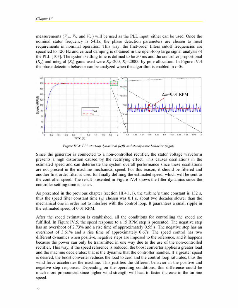
Chapter IV

72

measurements (Vab, Vbc and Vac) will be used as the PLL input, either can be used. Once the nominal stator frequency is 54Hz, the phase detection parameters are chosen to meet requirements in nominal operation. This way, the first-order filters cutoff frequencies are specified to 120 Hz and critical damping is obtained in the open-loop large signal analysis of the PLL [103]. The system settling time is defined to be 50 ms and the controller proportional (Kp) and integral (Ki) gains used were Kp=200, Ki=20000 by pole allocation. In Figure IV.4 the phase detection behavior can be analyzed when the algorithm is enabled in t=0s.

Figure IV.4: PLL start-up dynamical (left) and steady-state behavior (right).

Since the generator is connected to a non-controlled rectifier, the stator voltage waveform presents a high distortion caused by the rectifying effect. This causes oscillations in the estimated speed and can deteriorate the system overall performance since these oscillations are not present in the machine mechanical speed. For this reason, it should be filtered and another first order filter is used for finally defining the estimated speed, which will be sent to the controller speed. The result presented in Figure IV.4 shows the filter dynamics since the controller settling time is faster.

As presented in the previous chapter (section III.4.1.1), the turbine’s time constant is 132 s, thus the speed filter constant time (τf) chosen was 0.1 s, about two decades slower than the mechanical one in order not to interfere with the control loop. It guarantees a small ripple in the estimated speed of 0.01 RPM.

After the speed estimation is established, all the conditions for controlling the speed are fulfilled. In Figure IV.5, the speed response to a 15 RPM step is presented. The negative step has an overshoot of 2.73% and a rise time of approximately 0.55 s. The negative step has an overshoot of 3.61% and a rise time of approximately 0.67s. The speed control has two different dynamics when positive, negative steps are imposed to the reference, and it happens because the power can only be transmitted in one way due to the use of the non-controlled rectifier. This way, if the speed reference is reduced, the boost converter applies a greater load and the machine decelerates: that is the dynamic that the controller handles. If a greater speed is desired, the boost converter reduces the load to zero and the control loop saturates, thus the wind force accelerates the machine. This justifies the different behavior in the positive and negative step responses. Depending on the operating conditions, this difference could be much more pronounced since higher wind strength will lead to faster increase in the turbine speed.

Δω=0.01 RPM

Definition of the Control Strategy on the HRGS

73

Figure IV.5: Simulation result: step response of the generator’s speed control loop.

IV.2.1.3 WT Maximum Power Point Tracking (WT-MPPT)

The maximum power point (MPP) is obtained in a wind turbine when the optimum turbine efficiency is achieved and maintained for a certain wind speed as presented in section III.4.1. In Figure IV.6, this characteristic can be observed when the mechanical power is calculated for each wind speed as a function of the turbine speed.

Figure IV.6: Turbine Razec 266 power curve characteristics.

There are many methods to implement the maximum power point track and they can be divided in two main groups: based on interactive search or based on the power turbine mechanical characteristics [104]. In the first group, based on interactive search, the idea is that during the maximum power generation, the generator power variation ( Pg) should not change with speed variation ( ωg), i.e. the condition presented in Equation (IV.1) might be preserved.

Pω = 0 (IV.1)

This type of algorithm might reduce the number of required sensors and is easily implemented. The main idea is to define a hysteresis band from which the duty-cycle should

Chapter IV

74

be reduced or increased if the power overpasses the limits. Although simple to implement, the definition of the parameters in this type of MPPT algorithms can present some difficulties. Variations in the measured power caused by noise should be ignored and this can be achieved by filtering or by increasing the hysteresis band. In both cases, the overall behavior might change and unwanted variations or slow response could be observed. A second option is using Perturb and Observe (P&O) algorithms which continuously drive the system away from a certain point of operation in order to verify if the operation point is a local maximum of power. This variation presents an intrinsic characteristic of reducing the system efficiency for the constant variation imposed in the operational point. It will be explained further that it is not a very important issue in the photovoltaic generation due to the static characteristics of the solar panels. In the wind turbine, however, the relatively big mechanical time constant can impose severe limitations in the perturbation frequency reducing its frequency and consequently the MPPT speed.

The second group of MPPT algorithms in wind generations is based on the knowledge of the aerodynamic characteristics of the turbine. These algorithms are simpler and faster since they represent a curve to be followed by the machine which can receive either a current, torque or speed reference depending on the chosen controlled variable. The principle in this second group is to determine the operational point for the actual wind speed. In order to accomplish that, some authors propose the measurement of the wind speed [105]–[107]. This variable might not be necessary on the other hand, because at the MPP there is a relation between the rotational speed and generated power depending on the turbine characteristics. This relation can be expressed as a polynomial equation. For this reason, many algorithms do not need to measure the wind speed for guarantying the MPPT [108]. Operating in a wind-speed sensorless mode is recommended in small systems for allowing lower complexity equipment, reducing costs and maintenance. Although simpler, the MPPT obtained from the turbine’s aerodynamic characteristics are dependent on the quality of this model. Having a good quality might not be a simple task to validate since it depends on measurements made in wind tunnels, which is a very complex and expensive equipment, economically unviable to build as the turbines’ sizes increase.

In the present study, the MPPT is accomplished by third order polynomial expression that relates the reference speed (ω*) to the measured power (P) as defined in the Equation (IV.2):

ω = + + + (IV.2)

where a3 to a0 are the curve coefficients obtained by a polynomial approximation and the curve is plotted in Figure IV.6 (purple dashed graph).

IV.2.2 Photovoltaic Panels Control

In the actual state of the art of PV generation, one great limitation is related to the low efficiency in the light-to-energy conversion that does not reach values higher than 20% in economically viable panels. This characteristic makes the use of MPPT algorithms mandatory for increasing the generation system efficiency. Several techniques have been already proposed in the literature from simpler Perturb and Observe and Incremental Conductance methods (P&O and IC) [109], [110], to more complex ones using Neural Network [111],

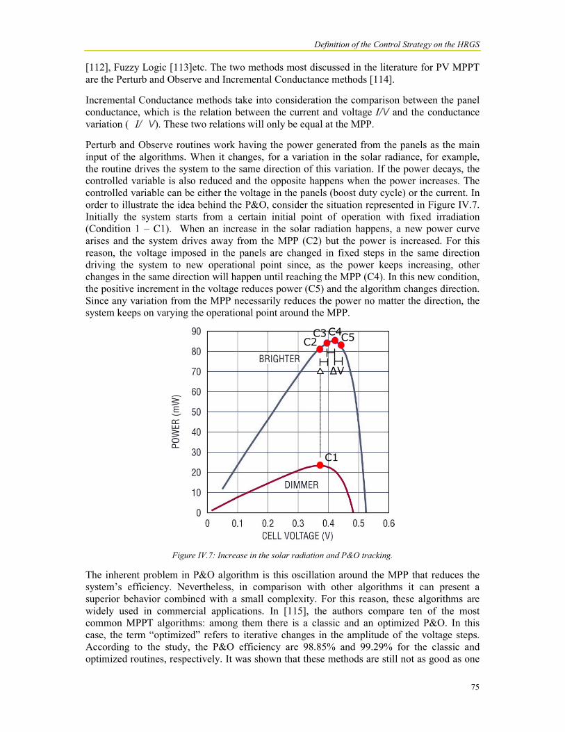
Definition of the Control Strategy on the HRGS

75

[112], Fuzzy Logic [113]etc. The two methods most discussed in the literature for PV MPPT are the Perturb and Observe and Incremental Conductance methods [114].

Incremental Conductance methods take into consideration the comparison between the panel conductance, which is the relation between the current and voltage I/V and the conductance variation ( I/ V). These two relations will only be equal at the MPP.

Perturb and Observe routines work having the power generated from the panels as the main input of the algorithms. When it changes, for a variation in the solar radiance, for example, the routine drives the system to the same direction of this variation. If the power decays, the controlled variable is also reduced and the opposite happens when the power increases. The controlled variable can be either the voltage in the panels (boost duty cycle) or the current. In order to illustrate the idea behind the P&O, consider the situation represented in Figure IV.7. Initially the system starts from a certain initial point of operation with fixed irradiation (Condition 1 – C1). When an increase in the solar radiation happens, a new power curve arises and the system drives away from the MPP (C2) but the power is increased. For this reason, the voltage imposed in the panels are changed in fixed steps in the same direction driving the system to new operational point since, as the power keeps increasing, other changes in the same direction will happen until reaching the MPP (C4). In this new condition, the positive increment in the voltage reduces power (C5) and the algorithm changes direction. Since any variation from the MPP necessarily reduces the power no matter the direction, the system keeps on varying the operational point around the MPP.

Figure IV.7: Increase in the solar radiation and P&O tracking.

The inherent problem in P&O algorithm is this oscillation around the MPP that reduces the system’s efficiency. Nevertheless, in comparison with other algorithms it can present a superior behavior combined with a small complexity. For this reason, these algorithms are widely used in commercial applications. In [115], the authors compare ten of the most common MPPT algorithms: among them there is a classic and an optimized P&O. In this case, the term “optimized” refers to iterative changes in the amplitude of the voltage steps. According to the study, the P&O efficiency are 98.85% and 99.29% for the classic and optimized routines, respectively. It was shown that these methods are still not as good as one

Chapter IV

76

Incremental Inductance algorithm, which demands the radiation measurement. Thimethod reached 99.48% but the need of a radiation sensor and all the issues related to this measurement (higher system complexity, cost, maintenance, calibration, noise, measuring deviations) might not justify the small improvement of the efficiency

IV.2.3 Photovoltaic Maximum Power Point Tracking (PV

The proposed MPPT algorithm uses an inner current loop and an external P&O algorithm as Figure IV.1shows and the detailed flowchart of the routine is presented the algorithm is initialized, the actual power (P[k]) is calculated as a function of the array voltage and current (V [k], I[k]). If the power variation (DP[k]) is positive, it means that the change in the current reference (I*[k]) should keep the same direction as in previous iteration; otherwise, the algorithm should change direction. Finally, the variables are updated and the routine is ready for the next iteration.

Figure

The classic P&O updates the boost dutypresent work, a current controller was used instead for guarantying the possibility of having a controlled current, and so an easier limitation in the generated power if necessary. It can be considered as a simple variant of the classic approach once its original simplicity is kept. The only important compromise to be taken into consideration in this rothe current reference variation (stability after a change happens in radiation or temperature. As a drawback, the system will present higher oscillation around the MPP, thus reducing the efficiency in steady state. However, if a small I is chosen, the system will take too long to stabilize after a transient. In cloudy days, for example, where the radiation’s variability is high, the HRGS would present a low performance. Figure IV.9 an

Incremental Inductance algorithm, which demands the radiation measurement. Thimethod reached 99.48% but the need of a radiation sensor and all the issues related to this measurement (higher system complexity, cost, maintenance, calibration, noise, measuring deviations) might not justify the small improvement of the efficiency.

Photovoltaic Maximum Power Point Tracking (PV-MPPT)

The proposed MPPT algorithm uses an inner current loop and an external P&O algorithm as shows and the detailed flowchart of the routine is presented inFigure

the algorithm is initialized, the actual power (P[k]) is calculated as a function of the array voltage and current (V [k], I[k]). If the power variation (DP[k]) is positive, it means that the hange in the current reference (I*[k]) should keep the same direction as in previous iteration;

otherwise, the algorithm should change direction. Finally, the variables are updated and the routine is ready for the next iteration.

Figure IV.8: Flowchart of the P&O algorithm.

The classic P&O updates the boost duty-cycle and has the current as a reference. In the present work, a current controller was used instead for guarantying the possibility of having a

trolled current, and so an easier limitation in the generated power if necessary. It can be considered as a simple variant of the classic approach once its original simplicity is kept. The only important compromise to be taken into consideration in this routine is the definition of

I). If this value is high, the system will converge rapidly to stability after a change happens in radiation or temperature. As a drawback, the system will present higher oscillation around the MPP, thus reducing the efficiency in steady state.

is chosen, the system will take too long to stabilize after a transient. In cloudy days, for example, where the radiation’s variability is high, the HRGS would present a

and Figure IV.10 illustrates well the drawback of increasing the

Incremental Inductance algorithm, which demands the radiation measurement. This last method reached 99.48% but the need of a radiation sensor and all the issues related to this measurement (higher system complexity, cost, maintenance, calibration, noise, measuring

MPPT)

The proposed MPPT algorithm uses an inner current loop and an external P&O algorithm as Figure IV.8. After

the algorithm is initialized, the actual power (P[k]) is calculated as a function of the array voltage and current (V [k], I[k]). If the power variation (DP[k]) is positive, it means that the hange in the current reference (I*[k]) should keep the same direction as in previous iteration;

otherwise, the algorithm should change direction. Finally, the variables are updated and the

cycle and has the current as a reference. In the present work, a current controller was used instead for guarantying the possibility of having a

trolled current, and so an easier limitation in the generated power if necessary. It can be considered as a simple variant of the classic approach once its original simplicity is kept. The

utine is the definition of ). If this value is high, the system will converge rapidly to

stability after a change happens in radiation or temperature. As a drawback, the system will present higher oscillation around the MPP, thus reducing the efficiency in steady state.

is chosen, the system will take too long to stabilize after a transient. In cloudy days, for example, where the radiation’s variability is high, the HRGS would present a

illustrates well the drawback of increasing the

Definition of the Control Strategy on the HRGS

77

I. Figure IV.9 shows the initialization of the converter when the ambient conditions are 1000 W/m2 of radiation and 30oC of temperature. In this condition, since the capacitors are charged with the open voltage of the PV array, the power does not start from zero. While the MPPTs with I of 1 A and 0.5 A reach the steady state after less than 20ms, the algorithms parameterized with 0.1 A and 0.05 A take 40 ms and 80 ms, respectively.

Time(s)0 0.02 0.04 0.06 0.08 0.1 0.12

Out

put P

ower

(W)

0

1000

2000

3000

4000

5000

6000

I=1AI=0.5AI=0.1AI=0.05AMPP

Figure IV.9: MPPT response during the system initialization with different current steps (I)

In Figure IV.10, another situation is simulated: a variation in the radiance from 1000 W/m2 to 1200 W/m2, keeping the same temperature of 30oC. Although in this situation, all the algorithms converge faster than the results presented in the previous figure; the same behavior occurs, that is, the MPPTs with higher I take longer to achieve the MPP. However, their oscillation in steady state condition is lower and this reflects in higher efficiency.

Sdfgdsfg

Time(s)0.25 0.26 0.27 0.28 0.29 0.3 0.31 0.32 0.33 0.34 0.35

4800

5000

5200

5400

5600

5800

6000

6200

I=1AI=0.5AI=0.1AI=0.05AMPPO

utpu

t Pow

er (W

)

G = 1000 W/m2

G = 1200 W/m2

Figure IV.10: MPPT responses during the radiation change from 1000W/m2 to 1200W/m2

The graphs presented in Figure IV.11 show how the generation efficiency increases as the current reference variation (I) is reduced in steady state conditions. The left graph presents the MPPT efficiency, which is over 99.9% in fixed condition of 1000 W/m2 of radiation and 30oC of temperature. This high efficiency is achieved due to the low power standard deviation (STD) compared to higher current steps. These simulation results were obtained for a 5 kW array of the Yngli Solar PV panels of the HRGS.

Chapter IV

78

I (A)1 0.1 0.05

%

99.6

99.7

99.8

99.9

100MPPT Effiency

I (A)

%

0

0.05

0.1

0.15

0.2

0.25

Power STD

0.5 1 0.1 0.050.5

Figure IV.11: P&O efficiency (left) and power standard deviation (right) as the current step changes.

The real efficiency must be computed taking into account the radiation and temperature variation that would reduce the efficiency gap between the MPPT with lower and higher I, since the more efficient in steady state the algorithm is, as well slower during transients. As future work, statistical analysis can be performed in order to optimize the I or even for adjusting and comparing the proposed algorithm to other ones.

IV.3 MSC Control Strategy The Mains Side Converter (MSC) is responsible for allowing the active power flow from the DC-link to the mains. In order to accomplish that, the HRGS contains a single-phase four-cell interleaved VSI for the grid connection. The control strategy of the MSC is depicted inFigure IV.12.

The control is accomplished by a cascaded structure having the DC-link voltage controller as the outer loop sending the reference to the inner current controller. Any variation in the DC-link represents a power unbalance between the GSC (generated power from the WT/PV panels) and the MSC (power delivered to the network). In steady state, a PI controller guarantees that the DC-link voltage is kept constant; it also ensures that the input power is equal to the output (converter losses neglected).

The converter current is controlled by three control loops: one common mode and two differential mode controllers. The common mode current is the AC-current which flows from the converter to grid and vice-versa. A vector control is used in the application; thus, the common mode is derived in dq-axis components where the direct axis handles active power and quadrature axis, reactive power. Therefore, the DC-link controller sends a reference to the d-axis common mode current control loop. Working with vector control (rotational grid-oriented axis) requires knowing the grid voltage angle and this is accomplished by a single-phase PLL. Beyond that, the vector control also needs a phasor to be decomposed in stationary and rotational axis. In three phase systems, this is done by the Clarke and Park transformations which allow the electrical variables to be represented in alpha-beta and dq axis. In single-phase systems, some manipulation must be carried out in order to perform

these transformations and a fictitious mains voltage (VM) and the beta component of the controller output voltage (

Figure IV.

The output LCL filter contains a 4saturate the inductor core leading to damage or operatiodifferential currents, that is, the current difference between two cells must be minimized and, in order to achieve that, two PIR controllers are added in the control structures. It will be explained further that the use of these controllers in the stationary reference eliminates the necessity of having more controllers, reducing the micro

IV.3.1 Single-Phase Fictitious Power Based PLL

In order to obtain grid synchronization,is derived from the three-phase Fictitious Power Based PLL proposed in structure used in speed estimation in the control of the synchronous generator as presented in Section IV.2.1.2. Both PLLs (for the speed estimation in the GSC and for the grid angle estimation in the MSC) are compared in

Figure IV.13

The phase detection is based on a fictitious electrical power (current (is) and real grid normalized voltage measurement (

Definition of the Control Strategy on the HRGS

these transformations and a fictitious beta current is calculated by the measurement of the component of the controller output voltage (Vβ).

.12: Schematics of the MSC control strategy.

The output LCL filter contains a 4-cell ICT and a current unbalance between these cells can saturate the inductor core leading to damage or operational problems. For this reason, the differential currents, that is, the current difference between two cells must be minimized and, in order to achieve that, two PIR controllers are added in the control structures. It will be

of these controllers in the stationary reference eliminates the necessity of having more controllers, reducing the micro-controller burden.

Phase Fictitious Power Based PLL

synchronization, the PLL structure presented in Figure IVphase Fictitious Power Based PLL proposed in [102]. It is a similar

structure used in speed estimation in the control of the synchronous generator as presented in . Both PLLs (for the speed estimation in the GSC and for the grid angle

re compared in [103].

13: Single-phase fictitious power-based PLL.

The phase detection is based on a fictitious electrical power (p) calculated from a fictitious ) and real grid normalized voltage measurement (ei) as follows:

ei

Definition of the Control Strategy on the HRGS

79

current is calculated by the measurement of the ).

cell ICT and a current unbalance between these cells can nal problems. For this reason, the

differential currents, that is, the current difference between two cells must be minimized and, in order to achieve that, two PIR controllers are added in the control structures. It will be

of these controllers in the stationary reference eliminates the

IV.13 is used. It . It is a similar

structure used in speed estimation in the control of the synchronous generator as presented in . Both PLLs (for the speed estimation in the GSC and for the grid angle

) calculated from a fictitious

Chapter IV

80

= (IV.3)

where ei=cos(θM).

The current isis defined to be 90o lagging.

= sin ( ) (IV.4)

Fictitious power can be then rewritten as:

= cos ( )sin ( ) (IV.5)

= sin + sin ( + ) (IV.6)

When the estimated grid angle is equal to the real one, p will present a frequency of twice the grid frequency, that is, 120 Hz for 60 Hz systems. For this reason, a low pass filter is used for removing the second term of Equation (IV.6) and the PI controller is responsible for guarantying that the filtered fictitious power is equal to zero. This structure presents a drawback related to the existence of the second order harmonic that demands the filter to present high attenuation at this frequency, that is, a low cutoff frequency. As a result, the PLL dynamics defined by the PI controller must be slowed down in order to guarantee stability. This problem can be reduced by increasing the filter order, thus allowing a higher bandpass while maintaining the demanded attenuation at the second harmonics for systems in which a fast phase detection is demanded. In [103], the authors propose a trial and error approach for defining the parameters which will be summarized in the four following steps:

1. Define the open loop cross over frequency, which should be smaller than the fundamental frequency.

2. Define the filter attenuation at the second harmonic having as a reference the maximum allowed angle oscillation. Define the filter type and order which respect the defined attenuation and does not present a great phase delay in the cross over frequency.

3. Define the controller gains for a desired phase margin taking into consideration that the system to be controlled is composed of the integrator and the designed filter. So, if M is the system’s gain and is the phase in the cross over frequency. A phase margin of can be obtained with controller gains (proportional and integral, Kpand Ki) calculated as:

= cos (IV.7)

= (IV.8)

where = 180 .

4. Observe the system performance and change the crossover filter andfilter parameters for guarantying the desired behavior.

The controller parameters obtained from the four steps above are and a fourth order Butterworth filter was used with 80 Hz cutparameters were phase margin of 30º and a crossover frequency of 20 Hz. The PLLsettling time (ST) of 0.15 s in the beginning of the operation considering the worst case, when the estimated angle is shifted by 180º from the real at oscillation of 22 rad/s (approximately 5.8%).

Figure IV.14: Fictitious power PLL startsettling time (ST) and frequency oscillation (

IV.3.2 Single-Phase Vector Control and Fictitious Axis Emula

The control orientation scheme usually adopted in singlemain groups: stationary and synchronous axis. In first group, simple PI/PID controllers can be used for controlling the current in stationary axis. However, in ACwill not guarantee zero error in steady state due to the alternate characteristics of the electrical variables and for this reason, a change in the traditional PID structure is used for guarantying infinite gain in the fundamental frequency allowing the steady state error to be eliminated. These controllers are known as resonant PI controllers, or PIR and they add a resonant term tuned on the grid fundamental frequency. PIR controllers present important drawbacks mainly related to stability issues and nonchanges are applied to the loop, a high sensitivity to variations in the fundamental frequency, driving the system to instability and low phase margins. Although syststationary axis present the disadvantages listed above, their simplicity compared to vector control justify their use in some cases.

The vector control uses a synchronous rotating reference for the current and voltages orientation transforming the AC system in constant variables. Therefore, standard PI/PID can be utilized to the oriented variables guarantying system’s simplicity and robustness. In threephase systems, the orientation of the system is straightforward and is accomplished b

ST= 0.15 s

Definition of the Control Strategy on the HRGS

Observe the system performance and change the crossover filter andfilter parameters for guarantying the desired behavior.

e controller parameters obtained from the four steps above are Kp=116.48 and and a fourth order Butterworth filter was used with 80 Hz cut-off frequency. The further parameters were phase margin of 30º and a crossover frequency of 20 Hz. The PLLsettling time (ST) of 0.15 s in the beginning of the operation considering the worst case, when the estimated angle is shifted by 180º from the real at t=0s. It also has a steady state oscillation of 22 rad/s (approximately 5.8%).

Fictitious power PLL start-up performance and frequency oscillation highlighting the estimation settling time (ST) and frequency oscillation (Δω).

Phase Vector Control and Fictitious Axis Emula

The control orientation scheme usually adopted in single-phase VSI can be divided in two main groups: stationary and synchronous axis. In first group, simple PI/PID controllers can be used for controlling the current in stationary axis. However, in AC systems, these controllers will not guarantee zero error in steady state due to the alternate characteristics of the electrical variables and for this reason, a change in the traditional PID structure is used for guarantying

al frequency allowing the steady state error to be eliminated. These controllers are known as resonant PI controllers, or PIR and they add a resonant term tuned on the grid fundamental frequency. PIR controllers present important drawbacks mainly

o stability issues and non-linearity listed as: exponentially decaying transients if step changes are applied to the loop, a high sensitivity to variations in the fundamental frequency, driving the system to instability and low phase margins. Although systems controlled with stationary axis present the disadvantages listed above, their simplicity compared to vector control justify their use in some cases.

The vector control uses a synchronous rotating reference for the current and voltages forming the AC system in constant variables. Therefore, standard PI/PID can

be utilized to the oriented variables guarantying system’s simplicity and robustness. In threephase systems, the orientation of the system is straightforward and is accomplished b

ST= 0.15 s

Δω= 22 rad

Definition of the Control Strategy on the HRGS

81

Observe the system performance and change the crossover filter and/or the

=116.48 and Ki=5.92e+3 off frequency. The further

parameters were phase margin of 30º and a crossover frequency of 20 Hz. The PLL presents a settling time (ST) of 0.15 s in the beginning of the operation considering the worst case, when

=0s. It also has a steady state

up performance and frequency oscillation highlighting the estimation

Phase Vector Control and Fictitious Axis Emulation

phase VSI can be divided in two main groups: stationary and synchronous axis. In first group, simple PI/PID controllers can be

systems, these controllers will not guarantee zero error in steady state due to the alternate characteristics of the electrical variables and for this reason, a change in the traditional PID structure is used for guarantying

al frequency allowing the steady state error to be eliminated. These controllers are known as resonant PI controllers, or PIR and they add a resonant term tuned on the grid fundamental frequency. PIR controllers present important drawbacks mainly

linearity listed as: exponentially decaying transients if step changes are applied to the loop, a high sensitivity to variations in the fundamental frequency,

ems controlled with stationary axis present the disadvantages listed above, their simplicity compared to vector

The vector control uses a synchronous rotating reference for the current and voltages forming the AC system in constant variables. Therefore, standard PI/PID can

be utilized to the oriented variables guarantying system’s simplicity and robustness. In three-phase systems, the orientation of the system is straightforward and is accomplished by the

Chapter IV

82

Park and Clarke transforms (from phasors. This way, the alpha-betafixed or oriented axis, respectively. In a singlepossible if one of the alpha-beta orthogonal, simply delaying the measurement by ninety degrees and taking the measured value as alpha and the delayed one as the two components for the Park transformation are available for the vector control. The conventional time-delaying scheme for applying the vector control is presented in IV.15. The current measurement (real axis) is considered the one quarter of the fundamental period is applied to this measurement for emulating the axis. After that, normal vector transformation and control is are transformed back from dq to the beta component is discarded. Although simple to implement, adding the delay deteriorates the system dynamical behavior, slows down[116].

Figure IV.15: Fictitious power PLL start

Another approach for emulating the system was proposed in [116]; it is also used in the present study and is presented inIV.16.

Figure IV.16: Fictive axis emulation (FAE) in

In this strategy, instead of discarding the Emulation (FAE) together with the network controller beta voltages generatebehavior of the converter output filter, i.e. its transfer function guarantees stability and a superior dynamical behavior (faster response and if compared to the conventional approach

Park and Clarke transforms (from abc to dq) due to the existence of voltages and currents beta and dq components represent the projection of phasor in the

fixed or oriented axis, respectively. In a single-phase system, applying vector control is only components is emulated. Since these components are always

orthogonal, simply delaying the measurement by ninety degrees and taking the measured and the delayed one as beta, is the most conventional approach. By doing that,

the two components for the Park transformation are available for the vector control. The delaying scheme for applying the vector control is presented in

. The current measurement (real axis) is considered the alpha component and a delay of one quarter of the fundamental period is applied to this measurement for emulating the axis. After that, normal vector transformation and control is done and the controller’s output

to alpha/beta; only the alpha component is used in the PWM, component is discarded. Although simple to implement, adding the delay deteriorates

the system dynamical behavior, slows down the system response and generates oscillations

power PLL start-up performance and frequency oscillation.

Another approach for emulating the beta axis, ensuring a better dynamical behavior to the ; it is also used in the present study and is presented in

Fictive axis emulation (FAE) in the vector control of single-phase systems.

In this strategy, instead of discarding the beta component, it is used for Fictive Axis Emulation (FAE) together with the network beta voltage. The difference of the grid and the

voltages generate an emulated beta current taking into account the dynamical behavior of the converter output filter, i.e. its transfer function –Equation(II.12guarantees stability and a superior dynamical behavior (faster response and lower oscillations) if compared to the conventional approach [116].

) due to the existence of voltages and currents components represent the projection of phasor in the

plying vector control is only components is emulated. Since these components are always

orthogonal, simply delaying the measurement by ninety degrees and taking the measured he most conventional approach. By doing that,

the two components for the Park transformation are available for the vector control. The delaying scheme for applying the vector control is presented in Figure

component and a delay of one quarter of the fundamental period is applied to this measurement for emulating the beta

done and the controller’s output component is used in the PWM,

component is discarded. Although simple to implement, adding the delay deteriorates the system response and generates oscillations

up performance and frequency oscillation.

axis, ensuring a better dynamical behavior to the ; it is also used in the present study and is presented inFigure

phase systems.

component, it is used for Fictive Axis voltage. The difference of the grid and the

current taking into account the dynamical 12). The FAE

lower oscillations)

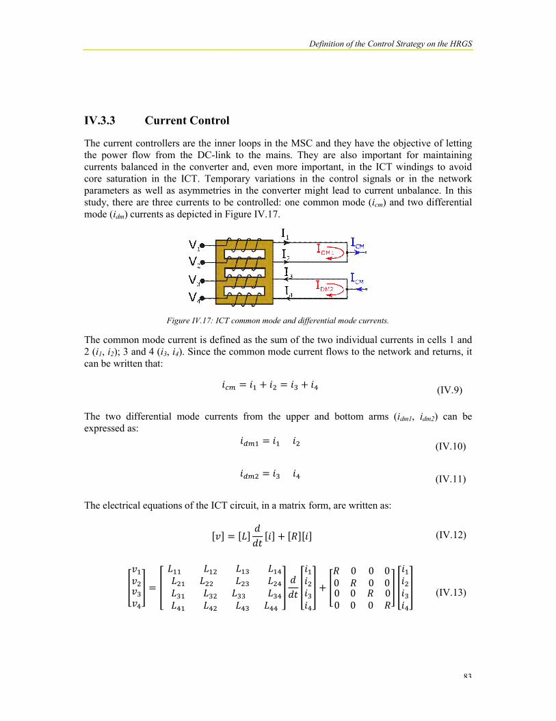
IV.3.3 Current Control

The current controllers are the inner loops in the power flow from the DC-link to the mains. They are also important for currents balanced in the converter and, even more important, in the ICT windings to avoid core saturation in the ICT. Tempoparameters as well as asymmetries in the converter might lead to current unbalance. In this study, there are three currents to be controlled: one common mode (mode (idm) currents as depicted in

Figure IV.17: ICT common mode and differential mode currents.

The common mode current is defined as the sum of the two individu2 (i1, i2); 3 and 4 (i3, i4). Since the common mode current flows to the network and returns, it can be written that:

The two differential mode currents from the upper and bottom arms (expressed as:

The electrical equations of the ICT circuit, in a matrix form, are

[=

Definition of the Control Strategy on the HRGS

Current Control

The current controllers are the inner loops in the MSC and they have the objective of letting link to the mains. They are also important for

balanced in the converter and, even more important, in the ICT windings to avoid core saturation in the ICT. Temporary variations in the control signals or in the network parameters as well as asymmetries in the converter might lead to current unbalance. In this study, there are three currents to be controlled: one common mode (icm) and two differential

rents as depicted in Figure IV.17.

ICT common mode and differential mode currents.

The common mode current is defined as the sum of the two individual currents in cells 1 and ). Since the common mode current flows to the network and returns, it

= + = +

The two differential mode currents from the upper and bottom arms (idm1, =

=

The electrical equations of the ICT circuit, in a matrix form, are written as:

[ ] = [ ] [ ] + [ ][ ] + 00 0 00 00 00 0 00

Definition of the Control Strategy on the HRGS

83

the MSC and they have the objective of letting link to the mains. They are also important for maintaining

balanced in the converter and, even more important, in the ICT windings to avoid rary variations in the control signals or in the network

parameters as well as asymmetries in the converter might lead to current unbalance. In this ) and two differential

al currents in cells 1 and ). Since the common mode current flows to the network and returns, it

(IV.9)

, idm2) can be

(IV.10)

(IV.11)

(IV.12)

(IV.13)

Chapter IV

84

The ICT used in the present study has the symmetry detailed in Figure IV.18. Due to its dimensions, many mutual inductances are equal and there are only three distinct values of mutual inductance (M1, M2 and M3) according to the equations that follow.

= = = = (IV.14)

= = = = (IV.15)

= = = = (IV.16)

Figure IV.18: ICT symmetry.

All the self-inductances L11, L22, L33 and L44 also present the same value (L). For this reason, we could rearrange the terms of expression (IV.13) according to the Equations (IV.14)-(IV.16) and (IV.9)-(IV.11) in order to obtain the following common and differential mode relations:

= 0 000 + 0 00 00 0 (IV.17)

where Lcm, Ldm1 and Ldm2 are the equivalent inductances of the common mode and differential mode circuits. These values are given by the equations that follow. = 2[ ( + + )] (IV.18)

= + (IV.19)

C1

C2 C3

C4 ei=100.13 mm

hi=135.9 mm

Magnetically coupled inductor

ICT

Definition of the Control Strategy on the HRGS

85

= (IV.20) The inductance Ldm2 (difference between mutual inductances) is zero in symmetrical ICTs. It is not the case in our ICT, although it has a small value if compared to the other inductances: Lcm =145 μH, Ldm1 = 164 μH and Ldm2 =12 μH. For this reason, the cross-coupling between idm1 and idm2 is neglectable.

It is clear that there are two different behaviors in current dynamics: the common mode (icm) and the two differential mode ones (idm1 and idm2). The differences are not only in the value of the inductance but also in the order of the system:

on the one hand, the DM current is defined by a first order system that depends exclusively on the ICT parameters (mutual and leakage inductances and resistance),

on the other hand, the common mode current that depends on the dynamic imposed by the ICT summed the other filter elements (capacitance and L2 inductance) as detailed in Chapter III.

For this reason, the controllers are designed in different manners and structures as the following subsections detail.

In order to accomplish the control of the MSC, interleaved pulses are sent to the four half-bridges or cells (C1, C2, C3 and C4). This means, in this case, the cells receive π/4 out-of-phase pulses. As in our structure, a single-phase voltage must be generated between C1/C2 and C3/C4, so the pulses of these cells are complementary. In other words, if C1/C2 pulses have the duty-cycle of 80%, C3/C4 pulses will be 20%. It changes the phase between the four cells to two possibilities (in respect to C1): C2 pulses are diphase-shifted by π (Situation A) or +/- π/2 (Situation B). If Situation A is chosen, C3 and C4 must be phase-shifted by π; if Situation B is chosen, C3 and C4 must be phase-shifted by +/- π/2 (Figure IV.19).

Figure IV.19: PWM pulses of the iVSI in two distinguish conditions: in C1/C2 and C3/C4 are phase-shifted by π (Situation A - left) and C1/C2 and C3/C4 are phase-shifted by π/2 (Situation B - right).

As the comparison between the two conditions suggests, Situation B is preferable since the individual currents will present lower ripple. This can be explained by the fact that, in this condition, all cells can be in the same state (ON or OFF) simultaneously, driving the converter output voltage to present the instantaneous value of 0 V, minimizing the current variation. This condition is highlighted on the right graph of Figure IV.19. In Situation A, the same is

Situation A Situation B

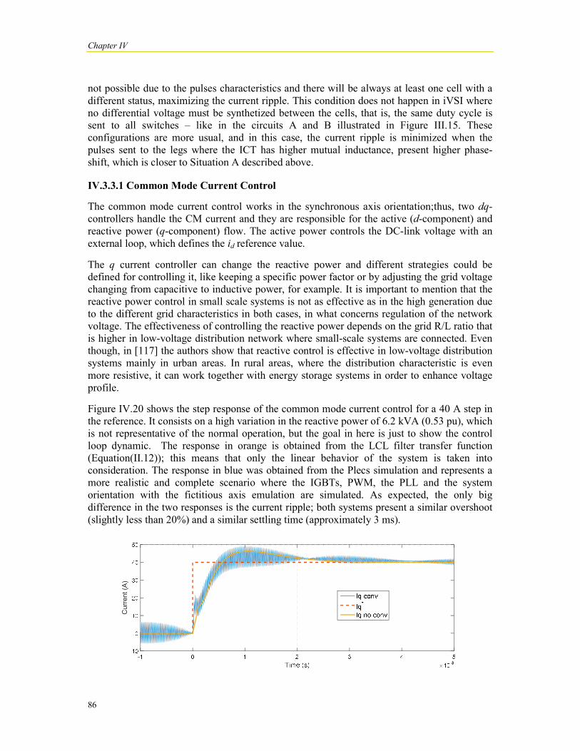
Chapter IV

86

not possible due to the pulses characteristics and there will be always at least one cell with a different status, maximizing the current ripple. This condition does not happen in iVSI where no differential voltage must be synthetized between the cells, that is, the same duty cycle is sent to all switches – like in the circuits A and B illustrated in Figure III.15. These configurations are more usual, and in this case, the current ripple is minimized when the pulses sent to the legs where the ICT has higher mutual inductance, present higher phase-shift, which is closer to Situation A described above.

IV.3.3.1 Common Mode Current Control

The common mode current control works in the synchronous axis orientation;thus, two dq-controllers handle the CM current and they are responsible for the active (d-component) and reactive power (q-component) flow. The active power controls the DC-link voltage with an external loop, which defines the id reference value.

The q current controller can change the reactive power and different strategies could be defined for controlling it, like keeping a specific power factor or by adjusting the grid voltage changing from capacitive to inductive power, for example. It is important to mention that the reactive power control in small scale systems is not as effective as in the high generation due to the different grid characteristics in both cases, in what concerns regulation of the network voltage. The effectiveness of controlling the reactive power depends on the grid R/L ratio that is higher in low-voltage distribution network where small-scale systems are connected. Even though, in [117] the authors show that reactive control is effective in low-voltage distribution systems mainly in urban areas. In rural areas, where the distribution characteristic is even more resistive, it can work together with energy storage systems in order to enhance voltage profile.

Figure IV.20 shows the step response of the common mode current control for a 40 A step in the reference. It consists on a high variation in the reactive power of 6.2 kVA (0.53 pu), which is not representative of the normal operation, but the goal in here is just to show the control loop dynamic. The response in orange is obtained from the LCL filter transfer function (Equation(II.12)); this means that only the linear behavior of the system is taken into consideration. The response in blue was obtained from the Plecs simulation and represents a more realistic and complete scenario where the IGBTs, PWM, the PLL and the system orientation with the fictitious axis emulation are simulated. As expected, the only big difference in the two responses is the current ripple; both systems present a similar overshoot (slightly less than 20%) and a similar settling time (approximately 3 ms).

Cur

rent

(A)

Definition of the Control Strategy on the HRGS

87

Figure IV.20: Step response of icm.

The same transient is represented in Figure IV.21 but the AC currents waveforms are plotted instead. In t=0s, the 40 A step is applied and in the first graph, the four converter/ICT currents (i1, i2, i3 and i4) are represented; these currents are characterized by the high ripple of approximately 25A. On the second graph, the common mode current (icm) in blue and the mains current (iM) transients are observed. The icm and im ripple are 7 A and 0.3 A, respectively.

Figure IV.21: ICT currents (top), common mode and mains current during a step test in the Iq*.

Finally, Figure IV.22 shows how the DC-link voltage (Vdc) and the d-axis common mode current id reacts to the iq transient. Since this simulation result was accomplished with no active power flow (no generation), no oscillation is observed in Vdc before the reference step at t=0s. As soon as the reference varies, the converter apparent power starts oscillating since it is a single-phase system. This oscillation is reflected in the capacitors voltage in the DC-link as a 120 Hz ripple which will be constantly presented during normal operation. The third graph shows how the Vdc controller changes the id reference and how the d-current control follows the reference in order to surpass the voltage transient after 40 ms.

Figure IV.22: Step response in the iq loop and impact in the Vdc and iq loops.

0 0.005 0.01 0.015 0.02 0.025 0.03

ICT

curr

ents

(A)

-50

0

50

Time (s)0 0.005 0.01 0.015 0.02 0.025 0.03

Cur

rent

(A)

-50

0

50IcmIg

Cur

rent

(A)

Cur

rent

(A)

Vol

tage

(V)

IM IM ICM

Chapter IV

88

IV.3.3.2 Control of the Differential Mode Current

In interleaved converters, the ICT is designed so the fundamental current in the different cells generate inverse magnetic fluxes in the core. For this reason, ideally, there is no flux generated at the fundamental frequency, only high order switching harmonics are present. If, for any reason, some variation in the fundamental current occurs in the different ICT cells, a low frequency current will circulate in this component. This extra flux at the fundamental frequency can saturate the core, deteriorating the operation and even driving the system to instability [118]. According to [119] and [120], the circulating currents (here referenced as differential mode currents) can occur due to the following reasons:

variation in the on-state voltage drop in the switching devices, ICT parameters mismatch due to the manufacturing process, different contact resistances, variations in the turn on and turn off times of the pulses sent to the

semiconductors’ gates, variation in the cables impedance which are used for connecting the different

ICT cells, deviation of the closed loop control itself due to an error of the measurement of

the difference of currents (calibration, tolerance, offset etc). In order to guarantee no differential mode current, two stationary frame Proportional Resonant PR controllers will be adopted, one for each possible circulating current. This solution was proposed in [119] and [120] and despite their already mentioned drawbacks, the PR structure was chosen due to its simplicity. In our case, if the vector control were also used for controlling the idm1 and idm2,two extra controllers would be required for each differential current plus the FAE for these loops. In total, the whole control scheme would demand six current controllers and three FAE for controlling icm, idm1 and idm2. By using PR controllers, only two controllers are required for the differential mode currents and no FAE is needed since it operates in the stationary frame axis.

The transfer function of the PR controller is presented as:

= + +

(IV.21)

where ω0 is the grid frequency.

A PI controller in vector control is analogous to the PR controller in the sense that both of them impose an infinite gain in the fundamental frequency; the tuning process proposed in Chapter II can thus be used for calculating the Kp and Ki as if the system was controlled by a standard PI in synchronous reference. This controller is intended to maintain zero differential mode currents; in order to show its effectiveness,Figure IV.23 presents the control dynamic when a variation of 30 Apeak in the reference of the differential mode current occurs at t=0 s.

Definition of the Control Strategy on the HRGS

89

Figure IV.23: Differential mode current control.

In a second situation, a variation of 30 times in the ICT resistance between two cells is assumed. This exaggerated variation is used in order to show how the current is controlled after the PR controller is enabled at t=0s (Figure IV.24).

Figure IV.24: Variation in differential mode current (idm) when the PR controller is enabled at t=0s when a

variation in the ICT resistance is forced.

IV.3.4 DC-Link Voltage Control

In a single-phase system, imposing a sinusoidal current in phase with the line voltage induces a pulsating power at twice the line frequency. In our context, since the energy generated by the PV panels and WT are constant, the DC-link must absorb the deviation between the generation and the pulsating power driven to the mains. This means that, in normal operation, the DC-link voltage (Vdc) will present an oscillation at 120 Hz in 60 Hz systems. This voltage variation must be taken into consideration in Vdc loop, otherwise the controller will try to remove it, even though it is part of the system natural behavior. This can be seen in the simulation results of Figure IV.25 starting with a step response in the Vdc loop.

PR enabled

Chapter IV

90

Figure

The same 10 V step in the both figures, the first graph shows the DC(id); and the third the quadrature current loop (voltage measurement is used directly as the feedback value, i.e. in the error calculation for the controller. In the other hand, in Figure (RMS) value and this value is used for calculating the error. Naturally, this calculation imposes a non-linear behavior and another dynamic added that can border system with time settling time equal to half the RMS period. Since, the oscillation in is at 120 Hz, the RMS calculation reaches steady state after half(0.5/120 s).

Figure IV.25: Step in Vdc reference.

The same 10 V step in the Vdc reference is applied in the simulation ofFigure both figures, the first graph shows the DC-link dynamic; the second the direct current loop

ird the quadrature current loop (iq). In the example of Figure IVvoltage measurement is used directly as the feedback value, i.e. in the error calculation for the

Figure IV.26, the control calculates the Vdc root mean square (RMS) value and this value is used for calculating the error. Naturally, this calculation

linear behavior and another dynamic added that can be approximated to a first order system with time settling time equal to half the RMS period. Since, the oscillation in is at 120 Hz, the RMS calculation reaches steady state after half-cycle, that is 4.167 ms

Figure IV.26. In link dynamic; the second the direct current loop

IV.25, the Vdc voltage measurement is used directly as the feedback value, i.e. in the error calculation for the

root mean square (RMS) value and this value is used for calculating the error. Naturally, this calculation

e approximated to a first order system with time settling time equal to half the RMS period. Since, the oscillation in Vdc

cycle, that is 4.167 ms

Figure IV.26: Step in the voltage reference taking into consideration the RMS value of V

In the id loop, it can be seen that when no RMS is calculated, the reference oscillates at the same frequency due to the Vdc control bandwidth and for this reason, When the RMS value is calculated, the oscillation in present in Vdc measurement. For this reason, the voltage loop dynamic deteriorates and the overshoot goes from 10 to 50%. The settling time does not present a relevant change and it is equal to roughly 50 ms. In the normal operation of the converter, the DCconstant so that the increased overshoot is not a problem. Furthermore, the reduction in the oscillation is a very important improvement because this oscillating results in a higher current distortion on the AC side.

Figure IV.27 shows how the grid current is affected by using the RMS value for controlling Vdc instead of the direct measurement. The grid current presents a high distortion since the voltage control imposes current oscillations, which are reflectedAC currents. For this reason, the control taking into consideration the accomplished in the DC-link voltage control.

Figure IV.27: Step in the voltage reference

IV.4 Conclusion Chapter IV presented the control strategy of the GSC and MSC in the HRGS. The control in the GSC consists of two distinct parts, which are the wind turbine MPPT panels MPPT.

For the WT, a single-phase PLL estimates the generator speed that allows encoderless operation, thus reducing the system complexity. Having the estimated speed, the curve relating the optimum power and the rotational speeMPPT. The whole algorithm is accomplished by cascaded blocks as follows:

1. the PLL estimates2. the MPPT measures3. the speed controller receives the optimum speed reference and estimation, and

controls the speed with a PI algorithm

Definition of the Control Strategy on the HRGS

: Step in the voltage reference taking into consideration the RMS value of V

loop, it can be seen that when no RMS is calculated, the reference oscillates at the controller. This oscillation frequency is within the current

control bandwidth and for this reason, id oscillates but it cannot remove the voltage variation. When the RMS value is calculated, the oscillation in id disappears and even though it is still

ment. For this reason, the voltage loop dynamic deteriorates and the overshoot goes from 10 to 50%. The settling time does not present a relevant change and it is equal to roughly 50 ms. In the normal operation of the converter, the DC-link voltage is keptconstant so that the increased overshoot is not a problem. Furthermore, the reduction in the oscillation is a very important improvement because this oscillating results in a higher current

shows how the grid current is affected by using the RMS value for controlling instead of the direct measurement. The grid current presents a high distortion since the

voltage control imposes current oscillations, which are reflected in high odd harmonics in the AC currents. For this reason, the control taking into consideration the VdcRMS value is

link voltage control.

: Step in the voltage reference taking into consideration the Vdc RMS value (top) and not considering it (bottom).

Chapter IV presented the control strategy of the GSC and MSC in the HRGS. The control in the GSC consists of two distinct parts, which are the wind turbine MPPT and the photovoltaic

phase PLL estimates the generator speed that allows encoderless operation, thus reducing the system complexity. Having the estimated speed, the curve relating the optimum power and the rotational speed is implemented for guarantying the MPPT. The whole algorithm is accomplished by cascaded blocks as follows:

s the speed by measuring the generator voltage, measures power, estimates speed, and defines the optimum speedontroller receives the optimum speed reference and estimation, and

controls the speed with a PI algorithm,

Definition of the Control Strategy on the HRGS

91

: Step in the voltage reference taking into consideration the RMS value of Vdc.

loop, it can be seen that when no RMS is calculated, the reference oscillates at the cillation frequency is within the current

oscillates but it cannot remove the voltage variation. disappears and even though it is still

ment. For this reason, the voltage loop dynamic deteriorates and the overshoot goes from 10 to 50%. The settling time does not present a relevant change and it is

link voltage is kept constant so that the increased overshoot is not a problem. Furthermore, the reduction in the id oscillation is a very important improvement because this oscillating results in a higher current

shows how the grid current is affected by using the RMS value for controlling instead of the direct measurement. The grid current presents a high distortion since the

in high odd harmonics in the RMS value is

RMS value (top) and not

Chapter IV presented the control strategy of the GSC and MSC in the HRGS. The control in and the photovoltaic

phase PLL estimates the generator speed that allows encoderless operation, thus reducing the system complexity. Having the estimated speed, the curve

d is implemented for guarantying the

the optimum speed,

ontroller receives the optimum speed reference and estimation, and

Chapter IV

92

4. the current controller defines the boost duty cycle by a current PI controller having as reference the speed controller output.

For PV tracking, a P&O method is proposed with an internal current loop. Fixed current steps are imposed for finding the maximum power point. The adopted strategy differs from the classic one in which the duty-cycle is directly changed. Simulation results showed that the system converged in 0.1 ms which is fast enough since the radiation varies in a much slower way (in the rage of several seconds). The amplitude of the perturbation should be defined in order to minimize the distance from the maximum power point, i. e. system efficiency. Beyond that, dynamical characteristic of the perturbation should be defined according to the current control speed in order to guarantee stability. This P&O algorithm continuously takes the system slightly away from the optimal point of operation, but this works very well in PV generation because changes in the current, voltage, radiance or temperature of the panels lead to a quasi-instantaneous variation in the output power. It should be noted that such an algorithm cannot be used for wind generation. A variation in the generator current would reduce the electromagnetic torque speeding up or slowing down the turbine speed. The mechanical dynamics is very slow compared to the electrical one and this comparison would happen after the system reached the new stationary point. Only after this speed transient passes, it would be possible to compare the output before and after the current change. Another issue that makes this strategy more complicated is the fact that the wind might have changed during this transient, thus the conditions would not be the same anymore for power comparison purposes. As a conclusion, such P&O algorithm are suitable and easy to use in systems with short electrical response time and should not be used in systems with a significant dynamical behavior.

In what concerns the MSC control strategy, a more complex scheme is defined from controlling the currents and DC-link voltage. A second PLL is demanded for tracking the grid voltage and a Fictitious Axis Emulation (FAE) is used for guarantying the vector control that presents an improved performance in the common mode current control. The dq-controllers handles the active and reactive power respectively, so that the DC-link voltage controller imposes the reference to the id controller. In order to allow the 120 Hz oscillation in the DC-link voltage and not propagate this oscillation in the control scheme, it is important to calculate and control Vdcby its RMS value. Finally, the differential mode current control is proposed by PR controllers reducing circulating currents in the ICT for avoiding current circulation and core saturation.

The last chapter will present the experimental results in the HRGS and a comparison with the simulation results will be accomplished.

Simulation and Experimental Results

93

Chapter V

Simulation and Experimental Results

Chapter V

94

V.1 Introduction So far, in the present document, it has been presented all the design, modeling, identification and simulation of the 11.7 KW HRGS. This chapter is dedicated to showing the experimental results of the constructed test bench and a comparison with the simulation results is presented. Chapter III gave a description of the whole generation system and components. Chapter V will present further details; instruments and structure used for the tests.

The chapter starts with a description of the whole control strategy and its link to the hardware. The same structure of the previous chapters will be adopted, starting from the GSC (WT and PV panels), followed by the MSC analysis (DC-link, LCL filter and mains connection).

In the GSC side, for having a deterministic analysis of the system, two solutions are adopted for emulating the wind and solar irradiation. For the WT generation, a generator driven by a motor emulates the wind turbine dynamics. For the PV generation, a DC power source is used for obtaining some of the results. These solutions permit to get results under controlled conditions, which is not possible in the ordinary operation due to the stochastic characteristic of the solar radiation and wind speed.

The results here presented consist on the simulation and experimental records of the dynamical behavior of the control loops and steady state waveforms of the most important electrical variables. A harmonic distortion analysis is presented in the grid current and finally, a thermograph of the system is performed. This chapter finishes with all the analysis performed and the conclusions of this study are presented in the last section of this document.

V.2 Complete Control Strategy and Hardware Description The control strategy is explained in the previous chapter and the individual schematics for the GSC and MSC are presented. In total, twelve variables are measured for the control and monitoring algorithm to work; these variables are listed in Table V-1.

Table V-1: Measured variables for the control routine.

GSC

PV array voltages VPV1, VPV2

PMSG stator voltage Vs WT rectifier output voltage VWT Boosts currents IB1, IB2, IB3

MSC

DC-link voltage VDC ICT differential mode currents IDM1, IDM2 ICT common mode current ICM Mains voltage VM

The mains and DC-link currents are also measured for monitoring purposes and they are not used in the control algorithm. The routine is constituted of two MPPTs, two single-phase PLLs, six PIs, a FAE, two blocks of Clark and inverse-Clark transformations, a hysteresis control (for the DC-link monitoring), eleven PWM pulses for the IGBTs from which 7 are independent (and the other four are complementary, for the bottom switches in the MSC). Finally, several RMS calculations are accomplished for monitoring, like active, reactive power from PV panels, WT, grid etc. Figure V.1shows the system’s complete control diagram, which was discussed in details in the previous chapter.

Figure V.1: Complete diagram of the control strategy adopted in the HRGS.

Once the DC-link detaches the two converter sides, the completely independent and could even work in different processors with no communication between them. It is not the case in our system, where the main controller board accomplishes the whole algorithm. It is a kit boardpresents the following main characteristics:

Digital Signal Processor (DSP) model from Texas Instruments

Clock frequency of 150 MHz; A/D model with 16 inputs of 12 bits; An external 256 K

Flash memory; A JTAG connector for real time emulation.

The processor accomplishes all the calculations of the routine in 40 frequency of 20.16 KHz, two times the switchiGSC cells. Working in a sampling frequency two times greater than the switching one guarantees the update before the PWM positive and negative transition and enhances the system dynamical behavior if compared to systare the same.

The Processor Board is connected to the signal interface boards for accomplishing the control scheme. The names and description of each interface board are presented as follows.

Analog boards - There are two different analog boards for the signal conditioning of the measured variables. One of them is for the AC measurements, where an offset is added for using the whole A/D converter scale, from 0 to 3.3 V. The second receives the DC

Simulation and Experimental Results

: Complete diagram of the control strategy adopted in the HRGS.

link detaches the two converter sides, the algorithms for each one of them are completely independent and could even work in different processors with no communication between them. It is not the case in our system, where the main controller board accomplishes the whole algorithm. It is a kit board from Spectrum Digital, model eZdspTM F28335, which presents the following main characteristics:

Digital Signal Processor (DSP) model TMS320F28335 with floating point from Texas Instruments Clock frequency of 150 MHz; A/D model with 16 inputs of 12 bits;

Kb SRAM memory, an internal 68 Kb RAM and a 512Kb

A JTAG connector for real time emulation.

The processor accomplishes all the calculations of the routine in 40 μs for the sampling frequency of 20.16 KHz, two times the switching frequency of 10.8 KHz of the MSC and GSC cells. Working in a sampling frequency two times greater than the switching one guarantees the update before the PWM positive and negative transition and enhances the system dynamical behavior if compared to systems whose sampling and switching frequency

The Processor Board is connected to the signal interface boards for accomplishing the control scheme. The names and description of each interface board are presented as follows.

e are two different analog boards for the signal conditioning of the measured variables. One of them is for the AC measurements, where an offset is added for using the whole A/D converter scale, from 0 to 3.3 V. The second receives the DC

ulation and Experimental Results

95

algorithms for each one of them are completely independent and could even work in different processors with no communication between them. It is not the case in our system, where the main controller board accomplishes

F28335, which

with floating point

b SRAM memory, an internal 68 Kb RAM and a 512Kb

s for the sampling ng frequency of 10.8 KHz of the MSC and

GSC cells. Working in a sampling frequency two times greater than the switching one guarantees the update before the PWM positive and negative transition and enhances the

ems whose sampling and switching frequency

The Processor Board is connected to the signal interface boards for accomplishing the control scheme. The names and description of each interface board are presented as follows.

e are two different analog boards for the signal conditioning of the measured variables. One of them is for the AC measurements, where an offset is added for using the whole A/D converter scale, from 0 to 3.3 V. The second receives the DC

Chapter V

96

measurements and no offset is demanded. These boards also perform the analog filtering, in which a Bessel filter with a cutoff frequency of 2.5 kHz is used.

PWM Board - It is constituted of 11 channels and it converts the pulses from the Controller Board to the range of the power switches’ drivers (model SKHI 22B, from Semikron).

Digital Input Board (DI Board) feedbacks) for the controller board and it has 11 inputs.

Digital Output Board (DO Board) control eight relays.

Figure V.2 shows the control boards and their interconnection.

Figure V.2

The Hall Effect voltage and current transducers used in the test bench are the LV 25100-P from the manufacturer LEM. The differential mode currents are directly measured with the HO 25-P/SP33 transducer with lower fullshows it in detail.

Figure

DC Analog

AC Analog

no offset is demanded. These boards also perform the analog filtering, in which a Bessel filter with a cutoff frequency of 2.5 kHz is used.

It is constituted of 11 channels and it converts the pulses from the Controller e power switches’ drivers (model SKHI 22B, from Semikron).

Digital Input Board (DI Board) - It converts the digital inputs signals (like the relay feedbacks) for the controller board and it has 11 inputs.

Digital Output Board (DO Board) - It makes the reverse path of the previous board and it can

shows the control boards and their interconnection.

2: Control and interface boards in the HRGS.

The Hall Effect voltage and current transducers used in the test bench are the LV 25P from the manufacturer LEM. The differential mode currents are directly measured with

P/SP33 transducer with lower full-scale value for a higher resolution as

Figure V.3: Differential current measurement.

I1

I2

I3 I4

Controller

DI

no offset is demanded. These boards also perform the analog filtering, in which a Bessel filter with a cutoff frequency of 2.5 kHz is used.

It is constituted of 11 channels and it converts the pulses from the Controller e power switches’ drivers (model SKHI 22B, from Semikron).

It converts the digital inputs signals (like the relay

rse path of the previous board and it can

The Hall Effect voltage and current transducers used in the test bench are the LV 25-P and LA P from the manufacturer LEM. The differential mode currents are directly measured with

e value for a higher resolution as Figure V.3

PWM

DO

V.3 Generation Side Converter (GSC)The power generation is handled by the GSC that is the first stage in the power conversion and it operates the PV arrays and the WT in the MPPT mode. Some experimental results are presented in the following sections, starting the wind generation, followed by the phoone.

V.3.1 Wind Turbine

In the wind generation part, in order to guarantee a deterministic and controlled power conversion, two machines connected by their shaft emulate the Darrieusin section III.4.1) - Figure V.4. Machine II is the turbine emulator and consists of a threephase squirrel-cage induction machine, 11 kW, 220V, 1175 RPM. It is driven by an ABB inverter model ACS800 working in the Direct Torque Contr

Figure V.4: Machines used for emulating the WT and PMSG.

The torque reference follows the turbine power curve of function of the machine speed and a useraccomplish that, the inverter is connected to a signal acquisition board from National Instruments model NI Elvis II+. The algorithm is implemented in the Labwhich the operator can select the wind speed as the main input and the further turbine parameters. Figure V.5 shows the Control and the Labimplementation of the WT torque curve.

Synchronous generator

Simulation and Experimental Results

Generation Side Converter (GSC) generation is handled by the GSC that is the first stage in the power conversion

and it operates the PV arrays and the WT in the MPPT mode. Some experimental results are presented in the following sections, starting the wind generation, followed by the pho

In the wind generation part, in order to guarantee a deterministic and controlled power conversion, two machines connected by their shaft emulate the Darrieus-type WT (described

. Machine II is the turbine emulator and consists of a threecage induction machine, 11 kW, 220V, 1175 RPM. It is driven by an ABB

inverter model ACS800 working in the Direct Torque Control (DTC) mode.

: Machines used for emulating the WT and PMSG.

The torque reference follows the turbine power curve of Figure IV.6 and is calculated as afunction of the machine speed and a user-defined parameter: the wind speed. In order to accomplish that, the inverter is connected to a signal acquisition board from National Instruments model NI Elvis II+. The algorithm is implemented in the Labview Plawhich the operator can select the wind speed as the main input and the further turbine

shows the Control and the Labview Block Diagram of the implementation of the WT torque curve.

Machine I Synchronous generator

Machine IIInduction motor

ulation and Experimental Results

97

generation is handled by the GSC that is the first stage in the power conversion and it operates the PV arrays and the WT in the MPPT mode. Some experimental results are presented in the following sections, starting the wind generation, followed by the photovoltaic

In the wind generation part, in order to guarantee a deterministic and controlled power type WT (described

. Machine II is the turbine emulator and consists of a three-cage induction machine, 11 kW, 220V, 1175 RPM. It is driven by an ABB

and is calculated as a defined parameter: the wind speed. In order to

accomplish that, the inverter is connected to a signal acquisition board from National iew Platform in

which the operator can select the wind speed as the main input and the further turbine iew Block Diagram of the

Machine II Induction motor

Chapter V

98

Figure V.5: Labview control panel for the WT emulation.

While Machine II imposes torque to the shaft, Machine I generates energy by breaking the system, controlling the speed through the conversion system (GSC). Machine II is a synchronous generator of 10 kVA, 220V, 1200 RPM with six poles. In the real WT, there is a 36 poles PMSG and it achieves the nominal power, that is, 1500 W at 180 RPM with the wind speed of 12 m/s. Since the machine used for the emulation presents a lower number of poles, the field excitation and nominal torque imposed were adapted in order to present the same stator frequency, voltage and current values of the real application. This means that the emulation of the WT happens in a higher mechanical speed but the same electrical frequency due to the difference in the number of poles, thus, the converter is under similar operational conditions.

The dynamical response of the current control in the WT boost is presented in Figure V.6 in which a 6 A step is applied to the control loop reference. An overdamped behavior was chosen; thus, the closed loop step response presents a settling time of approximately 28 ms and no overshoot. When defining controller parameters, the trade-off between a faster response and a more stable system is always presented. If in one hand, one might prioritize load rejection and short rise time, it might obtain lower stability margins, increasing the overshoot and increasing the measurement noise propagation. This drawback must be taken into consideration in defining the controller gains and in a multi-loop system, the inner loops

Machine II – Turbine emulator

Signal aquisition board

USB

Torque and speed estimation from the inverter and torque reference from the signal board.

ABB inverter operating in DTC

Torque curve and interface implemented in a PC

Simulation and Experimental Results

99

tend to be pushed to faster dynamics for a better reference tracking. However, in the generator control, the great dynamical difference between the electrical and mechanical dynamics, which are the current (inner) and speed (outer) loops, allows a slower inner loop response without compromising the outer one. Therefore, a more stable operation can be assured and for this reason, an overdamped behavior was defined for the current control specification: no overshoot and a maximum settling time (Tst) of 30 ms.

Figure V.6: WT boost current step response.

The speed loop step response is presented in Figure V.7 in positive and negative variations. As mentioned in Chapter IV, these transitions present different characteristics in what concerns settling time and overshoot values. In this result, the negative transition presents a settling time (Tst) of 6.7 s and a neglegitable percentual overshoot (PO), while the positive the values are 8.0 s and 37.5%, respectevely, with the nominal wind speed value of 12 m/s. In the positive transition, the torque imposed by the wind speeds-up the turbine and the control saturates during the transition and it justifies the difference, which varies depending on the step applied and the torque imposed.

Figure V.7: Speed controller negative and positive step response.

Tst= 28 ms

Tst= 6.7 s

Tst= 8.0 s

PO= 37.5%

Chapter V

100

Figure 11 shows the simulated and measured stedy-state waveforms of the boost electrical variables and the ripple of 4 A and 1200 W are present in the current and power, respectevely, due to the boost switching. The similarity between simulation and real data confimrs the model’s good quality.

Figure V.8: Boost simulated (left) and measured (right) electrical variables during nominal operation.

Figure V.9 shows the generator currents during the same test where the low order harmonics generated by the the rectification can be observed.

Figure V.9: Generator currents in nominal operation.

Due to the poor wind conditions during the weeks the tests were accomplished, there was not possible to get results of the real wind turbine.

I=4 A

P = 1200W

Simulation and Experimental Results

101

V.3.2 PV Panels

The photovoltaic panels in the HRGS are arranged in two arrays independently controlled by two interleaved boost converters. As in the WT control, an internal current loop has its reference changed by the MPPT algorithm for guarantying the maximum energy production. Confirming the MPPT effectiveness is not a straightforward task, once it demands a good and validated PV model and additional and reliable measurements, like the panels average temperature and solar radiation. In order to simplify this process, a DC Power Source XR400-20 from the manufacturer Magma Power was used for emulating the PV generation. The power source contains a dedicated software called Photovoltaic Power Profile Emulation (PPPE), which allows the creation of a certain V versus I curve according to the configured PV characteristics. This way, the software was parameterized for emulating one of the 5.1 kW PV arrays in the HRGS, constituted of the 20 Yngli Solar Panels, model YL255P-29b.

Figure 14 shows the Control Panel of the PPPE connected to the HRGS during operation. The graph (A) presents the V versus I curve being executed by the power source highlighting the MPP and the power supply output. If the two points are coincident, it means that the MPPT algorithm operates in the proper point, which is the case. Graph (B) shows the P versus I curve confirming that the system operates in the maximum point. Finally, the graphs (C), (D) and (E) show these variables over one minute of operation with unaltered radiation. The output power is kept in 5.1 KW for a MPPT current step (ΔI) of 0.2 A and a routine actualization rate of 10 Hz. In order to obtain these results, the power source was configured with the panel’s parameters and it was considered a radiation of 1000 W/m2 and a temperature of 25 ºC.

Figure V.10: Generator currents in nominal operation.

In what concerns the dynamical response, Figure V.11 presents two step responses in the emulated solar radiation. In the graph A, a 100 W/m2 and in graph B, a 300 W/m2 step are accomplished. In example A, and after a transient of approximately 2 s, the boost achieves the new steady state value. In the second example (B), a saturation in the current controller drives the system to operate in the short-circuit mode, that is, zero voltage output and short-circuit current. This condition is undesirable since it varies the output power down to zero and some studies have already analyzed this problem [121], [122]. It appears in systems where the current is used for tracking the MPP, instead of the voltage. Although this can be considered a limitation in choosing the current to be controlled and altered by the MPPT routine, the result

(A)

(C) A

(D) (E) A

(B)

Chapter V

102

in Figure V.11 shows that the change in the radiation must be really severe and fast in order to drive the system to saturation, which is not a realistic condition since the radiation’s change happens in a range of seconds.

Figure V.11: Generator currents in nominal operation.

The tests accomplished with the power source are important for confirming the control and MPPT effectiveness. After these tests were accomplished, the converter was connected to the real arrays and the steady state results of the boost current in two different conditions are presented in Figure 13. The waveforms in the left graph represent the boosts currents and input voltages at 10 AM in a clear day. The generated power in the Array 1 and Array 2 achieved the value of 4.77 KW each. The boost current ripple presented the value of approximately 4.8 A, that is approximately 30% of the nominal current as expected in the boost design (SectionIII.5.2). The right graph shows the ripple in the PV array (green curve) is below 0.8 A (5%) and in the presented results (Figure 13-right) the measurement noise does not allow the exact measurement.

Figure V.12: PV voltages (VPV1, VPV2), boost currents (IB1, IB2) on the left and PV current, voltage (IPV1, VPV1) and

boost current (IB1) during operation on the right.

(A) (B) 800 W/m2

700 W/m2 800 W/m2

500 W/m2

Saturation of the current controller

IB2

VPV2 IB1

VPV1 VPV1 IB1

IPV1

Simulation and Experimental Results

103

V.4 Mains Side Converter (MSC) The MSC operation starts with the charge of the DC-link capacitors. They can be charged from the MSC or GSC, in the second case, only if there are wind conditions for speeding up the turbine or solar radiation for increasing the cells’ voltage. Once the DC-link reaches a value that allows controllability, the switching can start.

Figure V.13: Converter start-up: DC-link voltage (VDC) and mains current (IM) capacitors charge (I), pre-

charge resistor bypass (II) and initial switching (III).

The DC-link charge happens through a pre-charge resistor for reducing the current transient during the grid connection and it is presented inFigure V.13. The curve in blue is the DC-link voltage (VDC) and the one in orange is the mains current (IM). In the instant I, the converter is connected to the grid and the capacitors are charged through the pre-charge resistor. As soon as the voltage stabilizes, the resistor is by-passed ending the charge process (instant II). Finally, the MSC starts switching and the DC-link voltage controlled and set to its operational value (instant III).

Figure V.14: Step response of the Iq loop averaged by several iterations for a better visualization of the loop

dynamical behavior.

I

III II

Two iterations

Fifty iterations Five hundred iterations

Ten iterations

IM

VDC

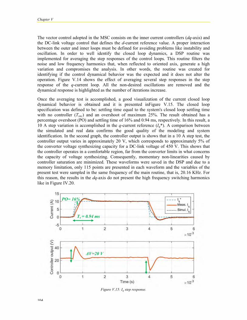
Chapter V

104

The vector control adopted in the MSC consists on the inner current controllers (dq-axis) and the DC-link voltage control that defines the d-current reference value. A proper interaction between the outer and inner loops must be defined for avoiding problems like instability and oscillation. In order to well identify the closed loop dynamics, a DSP routine was implemented for averaging the step responses of the control loops. This routine filters the noise and low frequency harmonics that, when reflected to oriented axis, generate a high variation and compromises the analysis. In other words, the routine was created for identifying if the control dynamical behavior was the expected and it does not alter the operation. Figure V.14 shows the effect of averaging several step responses in the step response of the q-current loop. All the non-desired oscillations are removed and the dynamical response is highlighted as the number of iterations increase.

Once the averaging test is accomplished, a good visualization of the current closed loop dynamical behavior is obtained and it is presented inFigure V.15. The closed loop specification was defined to be: settling time equal to the system's closed loop settling time with no controller (Tsnc) and an overshoot of maximum 25%. The result obtained has a percentage overshoot (PO) and settling time of 16% and 0.94 ms, respectively. In this result, a 10 A step variation is accomplished in the q-current reference (Iq*). A comparison between the simulated and real data confirms the good quality of the modeling and system identification. In the second graph, the controller output is shows that in a 10 A step test, the controller output varies in approximately 20 V, which corresponds to approximately 5% of the converter voltage synthesizing capacity for a DC-link voltage of 450 V. This shows that the controller operates in a comfortable region, far from the converter limits in what concerns the capacity of voltage synthesizing. Consequently, momentary non-linearities caused by controller saturation are minimized. These waveforms were saved in the DSP and due to a memory limitation, only 115 points are presented in each waveform and the variables of the present test were sampled in the same frequency of the main routine, that is, 20.16 KHz. For this reason, the results in the dq-axis do not present the high frequency switching harmonics like in Figure IV.20.

Figure V.15: Iq step response.

Ts = 0.94 ms

PO= 16%

ΔV=20 V

Simulation and Experimental Results

105

Figure V.16 presents the DC-link step response and it presents an overshoot of 45% and a settling time of 0.091 s. The capacitor’s RMS voltage adds a non-linearity to the loop and contributes for increasing the overshoot.

Figure V.16: DC-link voltage loop step response.

The measured VDC oscillation caused by the power pulsation in a single-phase system is presented in Figure V.17. The voltage variation in the DC-link is 11.1 V in 120 Hz (two times the grid fundamental frequency) for an output power of 8.6 kW. The amplitude of this fluctuation varies linearly together with the output power and achieves the nominal value of 15 V.

Figure V.17: DC-link voltage (VDC) oscillation and mains voltage and current (VM, IM) during

operation in 8.6 KW.

The modulation index(α) changes the converter waveform and ripple of the current in each converter leg. Consequently, the current ripple in the converter and ICT varies from 35.2 A to 44 A which is equivalent to 47% and 58% of the system nominal current (75 Apeak) operating with 450 V in the DC-link. Figure V.18 presents the current waveforms for four different conditions.

PO= 45%

Tst= 0.091 s

VDC

IM

VM

Chapter V

106

Figure V.18: Converter current waveforms during different modulation indexes.

The modulation index informed refer to the cell related to current I1, which is the one represented in green. The cells C1/ C2 (related to the currents I1/I2) have similar modulation index and C3/C4 have a complementary value in respect to the 0.5. For example, if C1/C2 receives a pulse modulated in 0.2, C3/C4 will be 0.8, that is +/- 0.3 in respect to the middle point of the modulation index. This pulses pattern is necessary for generation the differential voltage between C1/C2 and C3/C4 controlling the common mode current (ICM).

Although the converter currents present a high ripple, this value would be even higher if non-coupled inductors were used. Figure V.19 shows simulation results which perform a comparison of the converter currents with and without magnetically coupling inductances in our application. The simulation shows that the ripple is reduced in 12.6% by using ICTs in nominal condition, reducing the filter size and the system losses and cost.

α = 0.2 α = 0.5

α = 0.65 α = 0.85

I1 I2

I3 I4

Simulation and Experimental Results

107

Figure V.19: Converter currents using ICT and non-coupled inductors.

The idea of using a third order filter like the LCL circuit used in the present study is to obtain a high attenuation in the switching frequency. This is achieved with relatively small component in an N-cell interleaved converter once the common mode current (Icm) and consequently the mains current (Im) have the ripple in N-times the switching frequency, that is, 40.32 KHz in the HRGS. Figure V.20 shows simulated and measured results from the currents in the MSC during one period of the grid fundamental frequency.

Figure V.20: Simulated (left) and measured (right) converter (I1), common mode (Icm) and mains currents (Im).

InFigure V.21, the same variables are presented but in a time scale closer to the switching period. The current ripple in the converter currents are 17 A, the ripple in the common mode current is 10 A and in grid current is 0.6 A in the worst case, for the measured results. This represents a distortion caused by the switching harmonics of 23%, 13% and 0.8%, respectively, in nominal operation.

Chapter V

108

Figure V.21: Simulated (left) and measured (right) converter (I), common mode (Icm) and mains currents (Im).

In order to measure the system’s performance in what concerns the low harmonic distortion in the grid current, some measurements were accomplished with the power harmonic analyzer Fluke 437 and some results are presented in Figure V.22.

Figure V.22: Power harmonic analyzer screen during a 7.5 KW operation.

The results show a current distortion of 8.1% mainly generated from the odd low order harmonics until the 13th in a generation of 7.7 KW. The current distortion value in amperes presents a percentage of 5% in nominal operation. These harmonics are caused by the interaction between the grid voltage distortion and the converter operation and it is intrinsically related to the control performance. In order to reduce the distortion for achieving a higher quality in operation, active strategies for filtering these low harmonics should be accomplished in future work like several authors have already proposed.

Finally, a thermodynamic analysis of the converter was accomplished in order to assure that the components are operation in the proper limits. The components that operate in higher temperatures are the filter ones: inductors and damping resistor. The analysis was accomplished after 3 hours of operation in an average power of 8.5 kW and the thermographic image of the filter components are shown in Figure V.23. The boost inductors presented the average temperature of 64 ºC and maximum temperature of 69 ºC. The ICT presented the

I = 0.6 A

I = 10 A

I = 17 A

Simulation and Experimental Results

109

temperature of 59 ºC in its core and the maximum temperature of 108 ºC in the windings. The L2 inductor of the LCL filter presented the temperature of 80 ºC. All these temperatures are in the safe range since these components are Class-H, designed to operate in the maximum temperature of 180 ºC according to the IEC 60085 [123]. The damping resistor of the LCL filter was the component, which presented the higher temperature in the converter of 162 ºC. Since the content of the low harmonic current is relatively high as the power quality analysis showed, the current flowing in the RC shunt circuit of the LCL filter also increases creating an overload condition. This condition can be improved by adopting strategies for reducing these harmonics.

Figure V.23: Thermographic image of the filter components.

V.5 Conclusion This chapter presented the experimental and complementary simulation results of the HRGS. Initially, the GSC results were presented first for the wind and photovoltaic generation. For the WT experimental tests, two machines connected by their axis emulated the turbine behavior as well as the generator. The turbine power curve was implemented in a computer, which was connected to a commercial converter by a data acquisition board. The results from the real turbine were not presented due to the poor wind conditions during the weeks in which the tests where accomplished. The results of the photovoltaic generation were accomplished by a power source emulating the panels’ behavior but also from the 40 panels installed in the roof of the laboratory. The boost current ripple presented the value of approximately 4.8 A, that is approximately 30% of the nominal current and the ripple in the PV array is below 0.8 A (5%). The use of the power source emulating the panel’s behavior could guarantee the effectiveness of the proposed MPPT.

In MSC side, the controllers’ dynamics were presented and the comparison with simulation results verified the good quality of the modeling and identification detailed in Chapter III. The converter common mode and mains current were measured and their waveforms and switching ripple were measured, and the adequacy with the system design was confirmed. The measured ripple in the converter currents are 17 A, in the common mode current is 10 A and

Chapter V

110

in grid current is 0.6 A. This represents a distortion caused by the switching harmonics of 23%, 13% and 0.8%, respectively, in nominal operation. Beyond that, simulation results show that the ripple is reduced in 12.6% by using an ICT, instead of separated inductors, reducing the filter size and the system losses and cost. A power quality analysis was performed and the grid current presented a high distortion in the low frequency harmonics (from the third to the 13th) and this demands an active filtering for a more adequate operation. Finally, a thermographic analysis confirmed that the components are operating in the desired thermal range. Several comparisons between real and simulated date were presented and their similarity confirms the good quality of the models and parameters obtained from the identification process.

Conclusion

111

General Conclusion and Perspectives One of the greater challenges the society faces nowadays is how to promote scientific and social development, minimizing the environmental impact of the human actions. Our current model of development bases on a continuous growth of the energy demand, which derives mostly from fossil fuels. Beyond the fact that this source is not renewable, that is, one day it will end, it is a consensus among the specialists that the impact of this model is extremely harmful to the earth environmental balance, which compromises the biodiversity and the life of future generations of plants, animals, including ours. The solution for this worldwide problem is undetermined, complex, and gradual; and certainly passes through the diversification of the energetic matrix. Diversification means not only having different sources converted into useful energy, like the electricity, but also decentralizing the energy generation in order to fit with higher adequacy the demand, which is decentralized too. Distributed Generation proposes this sort of development but in order to increase its penetration several technical barriers must be overpassed. One of them is related to the conversion systems, which must be more flexible, modular, efficient and compatible with the different energy sources, since they are very specific for a certain area. The present study drives its efforts towards this direction, i.e. having a system with several inputs for combining different renewable energy sources into a single and efficient power converter for the grid connection. Since photovoltaic and wind generation present a prominence in the actual scenario due to the energy availability and commercial and technological advancements, they are used in the HRGS designed and constructed. In accordance with these ideas, this study proposes the contributions described in the list that follows.

Contribution 1: HRGS design

The main purpose of this thesis was to propose a system capable of tracking independently the maximum power point for each input and guarantees the connection with the network using the state of art in what concerns the switching harmonics filtering and control. For this reason, a power conversion system with a four independently controlled and interleaved boosts converters were designed where three of them were used for the controlling the power generation of two PV arrays and a WT. In order to guarantee the grid connection, a 4-cell interleaved VSI was used, together with an output LCL filter. For reducing the size, cost and losses in switching harmonics filtering, an ICT was used in the first filtering element. The design of such a system was one of the most important contributions of this study.

Contribution 2: A Novel Controller Design Methodology

In order to define the controller gains for guaranteeing a specific dynamical behavior in closed loop, the classical control approach is to define the system requirements and then, calculate the gains. The question that always arises in this approach is how to define the requirement, that is, how fast can my system be? The proposed methodology uses the closed loop behavior with no controller as a reference of the natural system dynamic. This way, it is calculated the pole which contributes the most for the system closed loop response with no controller with the Modal Dominance Index (MDI). With the MDI, the system's closed loop settling time with no controller (Tsnc) is used as a reference for the system requirements. If a

Conclusion

112

settling time (Tst) is higher than the Tsnc, it means that the calculated parameters make the system slower than it is with no controller, i.e. the controller worsen the system’s behavior. In the other extreme, a Tst much smaller than the Tsnc demands an over dimensioned actuator, which is not economically viable. For this reason, Tst should be close or even equal to Tsnc, for a proper control dynamic.

Contribution 3: A overall bandwidth analysis for an iVSI

Interleaved VSIs reduces by N2 the energy storage capacity in the switching harmonic filtering, where N is the number of cells. Having smaller filters contributes to the reduction of cost, size and losses. Beyond that, it guarantees a better dynamical performance of the system due to the increase of the filter bandwidth. Nevertheless, this improvement must be analyzed taking into consideration not only the hardware but also the influence of the sampling and the control in the system overall behavior. And it was demonstrated that the improvement is limited when these two effects are analyzed. For this, it was simulated the condition in which the sampling and switching frequencies are equal and classical PI controllers handles the converter currents. Beyond that, the novel control design methodology described in Chapter II is used. The analysis shows that the system overall bandpass is limited to 10% of the switching frequency and for a 10 KHz case, no bandwidth enhancement is obtained with increasing the number of cells after N = 5. The controller design influences this result, but it suggests that in order to keep increasing the system’s overall bandwidth, new strategies must be carried out, like increasing the sampling frequency (maintaining the switching) or adopting alternative control methods as Model Predictive Control.

Contribution 4: The modeling and identification of the generation system

An effective operation in any electrical device depends on the proper conciliation of the hardware and firmware design. In a high complexity system like the HRGS, this issue is crucial and the firmware is constituted basically on the control strategy defined and implemented. The control, in the other hand, demands a proper modeling, identification and validation and these steps were proposed and accomplished for the whole system: PV panels, WT, DC-link and LCL output filter.

Contribution 5: The control strategy design in the GSC and MSC

The control of the HRGS was proposed including the PV and WT MPPT algorithms. For the WT, the speed estimation is accomplished by a single-cell PLL for guarantying an encoderless operation, reducing the complexity and cost. In the MSC, a second PLL gives the grid angle reference and Fictive Axis Emulation (FAE) is also demanded for the vector control. Since it is a single-phase system, the beta current must be emulated and the FAE guarantees an improved dynamical behavior if compared with the traditional way, in which beta is emulated by delaying in 90º the measured current. The ICT demands an accurate current equalization once small variations can saturate the core, changing the filtering capacity and even driving the system to instability. A strategy that uses resonant controllers (PR) is adopted and it guarantees the current equalization.

Conclusion

113

Future Work

This study proposed several solutions in the design of small scale hybrid systems, but it also oriented further paths to be followed as future work. Some of these points are listed as follows.

Define more sophisticated control strategies for the multicell converters

The Chapter II analyzed the control performance and a bandwidth analysis was accomplished in parallel multicell converters by adopting classical and digital PI controllers operating in switching frequency. It was concluded that, under these conditions and according to the other assumptions (DC-link of 450 V, 10 kW of switching frequency and the controller design adopted), no expressive improvement in the system overall bandwidth is obtained if the number of cells (N) is increased after N = 5. But this limit might probably be pushed further if some other control strategies are adopted like using MPC, for example. Or even by increasing the sampling frequency to the apparent switching frequency which is Ntimes the real switching frequency.

Design and implementation of the active filter for the MSC

The experimental results showed that the current THD is 5% in nominal operation, mainly caused by the low harmonics presented in the mains voltage. In the simulation results, for example, the current distortion was much smaller since the mains voltage was a pure sine wave. This characteristic can be improved by active filtering these harmonic components keeping the hardware unaltered.

Test the MPPT algorithm in the real turbine already installed and connected to the HRGS

Due to the poor wind conditions, the real WT could not operate during the period the tests were accomplished and it was emulated by two machines connected by their shaft. In order the system to really generate in nominal condition, the WT operation must be tested.

Calculate the system’s efficiency

The system efficiency is one the most important design criterion and many relevant decisions were taken to improve this parameter. One example of this concernment is the choice of using an ICT in the LCL filter. Nevertheless, the system efficiency was not measured or calculated and the comparison with other converters (commercial or described in the literature) was not accomplished. This is an important metric and should be carried out in the future work for confirming the system’s effectiveness.

Implement a modular operation of the parallel converter

Parallel multicell converters enable a modular operation during low power generation moments, that is, just part of the cells operates while the others are switched off. This possibility could increase the system efficiency since a small number of switching cells would work during these periods. It would also increase the system life span, once the cells would reduce their time of operation, that is, some cells would simply not work during low generation moments. Although important, this feature is not easily implemented and it

Conclusion

114

imposes some complex problems to be solved. One of them is how to guarantee a low distortion if some cells are not operating in an interleaved converter? How to deal with the ICT under this condition? How to accomplish the transition of a certain cell on and off operation state?

All the items mentioned represent very challenging areas of research and delimit the future steps to be accomplished by the author.

115

References

[1] J. L. da Silva, R. Reis, G., Silva, R. M., S. I. Seleme, T. A. Meynard, e Llor, A. M., “Design, Modeling and Identification of the Mains Side Converter in an 11.7 kW Wind/Photovoltaic Hybrid Renewable Generation System”, apresentado em 8th IEEE International Symposium on Power Electronics for Distributed Generation Systems, Florianópolis, Brazil., 2017.

[2] J. L. da Silva, R. Reis, G., Silva, R. M., S. I. Seleme, T. A. Meynard, e Llor, A. M., “Design, Modeling and Identification of the Generation Side Converter in an 11.7 kW Wind/Photovoltaic Hybrid Renewable Generation System”, apresentado em 8th IEEE International Symposium on Power Electronics for Distributed Generation Systems, 2017.

[3] da Silva, R. C, Souza, S. M., Ricardi, V., R. Reis, G., e J. L. da Silva, “Control Design of a Synchronous Generator of a Horizontal Axis Wind Turbine”, in 8th IEEE International Symposium on Power Electronics for Distributed Generation Systems, Florianópolis, Brazil., 2017.

[4] J. L. da Silva, Reis, G., S. I. Seleme, e T. Meynard, “Control Design and Frequency Analysis of an Output Filter in Parallel Interleaved Converters”, apresentado em IEEE Conference on Power and Energy (PECON), Melaka, Malaysia, 2016.

[5] N. Videau et al., “High Ratio Non-Isolated DC-DC Converter for Hydrogen Battery Using a 50 kW PEM Fuel Cell”, Fuel Cells, set. 2016.

[6] N. Videau et al., “Non-isolated High Efficiency High Voltage Ratio DC-DC Converter for Hydrogen Battery using a 50kW PEM Fuel Cell”, apresentado em 6th International Conference on Fundamentals and Development of Fuel Cells, Toulouse, France., 2015.

[7] G. Resende, C. V. Sousa, F. F. Matos, J. L. Silva, T. V. M. Flores, e J. L. S. R. Silva, “Sistema Regenerativo para Testes de Transformadores de Potência sob Condições Especiais de Carregamento”, apresentado em V Simpósio Brasileiro de Sistemas Elétricos, Foz do Iguaçu, Brasil, 2014.

[8] R. C. da Silva, “Projeto e Construção de um Conversor Monofásico Híbrido em Ponte H Multicelular Entrelaçado para Geração Fotovoltaica e Eólica de Pequeno Porte”, Universidade Federal de Minas Gerais, Belo Horizonte, MG, 2017.

[9] R. C. da Silva e S. M. de Souza, “Control Design of a Synchronous Generator in a Hybrid Renewable Generation System”, Universidade Federal de Itajubá, Itabira, MG, 2016.

[10] K. A. Pereira, “Controle de um Conversor Multicelular Entrelaçado com Indutores Acoplados Magneticamente em um Sistema Híbrido de Micro-Geração On-Grid”, Universidade Federal de Itajubá, Itabira, MG, 2017.

References

116

[11] M. Gonçalves, “Implementação de um Algoritmo MPPT Perturba & Observa em Conversor Híbrido”, Universidade Federal de Itajubá, Itabira, MG, 2017.

[12] V. Smil, Energy Transitions: History, Requirements, Prospects. ABC-CLIO, 2010.

[13] L. Ségalen, J. A. Lee-Thorp, e T. Cerling, “Timing of C4 grass expansion across sub-Saharan Africa”, J. Hum. Evol., vol. 53, no 5, p. 549–559, nov. 2007.

[14] R. W. Wrangham, J. H. Jones, G. Laden, D. Pilbeam, e N. Conklin‐Brittain, “The Raw and the Stolen: Cooking and the Ecology of Human Origins”, Curr. Anthropol., vol. 40, no 5, p. 567–594, dez. 1999.

[15] P. Karkanas et al., “Evidence for habitual use of fire at the end of the Lower Paleolithic: Site-formation processes at Qesem Cave, Israel”, J. Hum. Evol., vol. 53, no 2, p. 197–212, ago. 2007.

[16] K. Bithas e P. Kalimeris, “A Brief History of Energy Use in Human Societies”, in Revisiting the Energy-Development Link, Cham: Springer International Publishing, 2016, p. 5–10.

[17] G. Barker, The Agricultural Revolution in Prehistory: Why Did Foragers Become Farmers? Oxford University Press, 2009.

[18] E. A. Wrigley, “Energy and the English Industrial Revolution”, Philos. Trans. R. Soc. Math. Phys. Eng. Sci., vol. 371, no 1986, p. 20110568–20110568, jan. 2013.

[19] International Energy Agency, “Key World Energy Trends”, 2016.

[20] W. D. Stevenson, Elements of Power System Analysis. McGraw-Hill, 1982.

[21] P. K. Narayan e R. Smyth, “Energy consumption and real GDP in G7 countries: New evidence from panel cointegration with structural breaks”, Energy Econ., vol. 30, no 5, p. 2331–2341, set. 2008.

[22] Electricity Information 2016. S.l.: s.n., 2016.

[23] International Energy Agency, Org., World energy outlook 2015. Paris: OECD, 2015.

[24] Ministério de Minas e Energia, “Resenha Energética Brasileira”, Maio 2016.

[25] International Hydropower association, “2016 Hydropower Status Report”.

[26] A. C. Lees, C. A. Peres, P. M. Fearnside, M. Schneider, e J. A. S. Zuanon, “Hydropower and the future of Amazonian biodiversity”, Biodivers. Conserv., vol. 25, no 3, p. 451–466, mar. 2016.

[27] F. Almeida Prado, S. Athayde, J. Mossa, S. Bohlman, F. Leite, e A. Oliver-Smith, “How much is enough? An integrated examination of energy security, economic growth and climate change related to hydropower expansion in Brazil”, Renew. Sustain. Energy Rev., vol. 53, p. 1132–1136, jan. 2016.

[28] International Energy Agency, “Energy Policies of IEA Countries - France 2016 Review”.

117

[29] T. Ackermann, G. Andersson, e L. Söder, “Distributed generation: a definition”, Electr. Power Syst. Res., vol. 57, no 3, p. 195–204, 2001.

[30] P. T. Manditereza e R. Bansal, “Renewable distributed generation: The hidden challenges – A review from the protection perspective”, Renew. Sustain. Energy Rev., vol. 58, p. 1457–1465, maio 2016.

[31] I. J. Perez-Arriaga, “The Transmission of the Future: The Impact of Distributed Energy Resources on the Network”, IEEE Power Energy Mag., vol. 14, no 4, p. 41–53, jul. 2016.

[32] I. Bos, P. De Boever, L. Int Panis, e R. Meeusen, “Physical Activity, Air Pollution and the Brain”, Sports Med., vol. 44, no 11, p. 1505–1518, nov. 2014.

[33] J. G. Allen, P. MacNaughton, U. Satish, S. Santanam, J. Vallarino, e J. D. Spengler, “Associations of Cognitive Function Scores with Carbon Dioxide, Ventilation, and Volatile Organic Compound Exposures in Office Workers: A Controlled Exposure Study of Green and Conventional Office Environments”, Environ. Health Perspect., vol. 124, no 6, out. 2015.

[34] M. Goldberg, “A Systematic Review of the Relation Between Long-term Exposure to Ambient Air Pollution and Chronic Diseases”, Rev. Environ. Health, vol. 23, no 4, jan. 2008.

[35] C. Le Quéré et al., “Global Carbon Budget 2016”, Earth Syst. Sci. Data, vol. 8, no 2, p. 605–649, nov. 2016.

[36] C. Mahieux e A. Oudalov, “Microgrids enter the mainstream”, Renew. Energy Focus, vol. 17, no 2, p. 70–72, mar. 2016.

[37] R. Sebastián e R. P. Alzola, “Simulation of an isolated Wind Diesel System with battery energy storage”, Electr. Power Syst. Res., vol. 81, no 2, p. 677–686, fev. 2011.

[38] E. Muljadi e H. E. McKenna, “Power quality issues in a hybrid power system”, IEEE Trans. Ind. Appl., vol. 38, no 3, p. 803–809, Maio 2002.

[39] R. Sebastián e R. P. Alzola, “Effective active power control of a high penetration wind diesel system with a Ni–Cd battery energy storage”, Renew. Energy, vol. 35, no 5, p. 952–965, maio 2010.

[40] M. U. Hassan, M. Humayun, R. Ullah, B. Liu, e Z. Fang, “Control strategy of hybrid energy storage system in diesel generator based isolated AC micro-grids”, J. Electr. Syst. Inf. Technol., jan. 2017.

[41] J. J. More, P. F. Puleston, C. Kunusch, e M. A. Fantova, “Development and Implementation of a Supervisor Strategy and Sliding Mode Control Setup for Fuel-Cell-Based Hybrid Generation Systems”, IEEE Trans. Energy Convers., vol. 30, no 1, p. 218–225, mar. 2015.

[42] K. Saravanan, R. Suganthi, e V. K. Chinnaiyan, “Review on biogas from organic waste”, in 2014 International Conference on Green Computing Communication and Electrical Engineering (ICGCCEE), 2014, p. 1–4.

References

118

[43] Renewable Energy Policy Network for the 21st Century, “Renewables 2016 - Global Status Report”.

[44] Y.-M. Chen, Y.-C. Liu, S.-C. Hung, e C.-S. Cheng, “Multi-Input Inverter for Grid-Connected Hybrid PV/Wind Power System”, IEEE Trans. Power Electron., vol. 22, no 3, p. 1070–1077, maio 2007.

[45] B. A. Miwa, “Interleaved conversion techniques for high density power supplies”, Thesis, Massachusetts Institute of Technology, 1992.

[46] B. Cougo, “Design and optimization of intercell transformers for parallel multicell converters”, Institut National Polytechnique de Toulouse-INPT, 2010.

[47] M. H. Rashid, Org., Power electronics handbook: devices, circuits, and applications handbook, 3rd ed. Burlington, MA: Elsevier, 2011.

[48] H.-B. Shin, J.-G. Park, S.-K. Chung, H.-W. Lee, e T. A. Lipo, “Generalised steady-state analysis of multiphase interleaved boost converter with coupled inductors”, IEE Proc. - Electr. Power Appl., vol. 152, no 3, p. 584, 2005.

[49] L. Huber, B. T. Irving, e M. M. Jovanovic, “Open-Loop Control Methods for Interleaved DCM/CCM Boundary Boost PFC Converters”, IEEE Trans. Power Electron., vol. 23, no 4, p. 1649–1657, jul. 2008.

[50] “Rashid, Power Electronics: Circuits, Devices & Applications, 4th Edition”. [Online]. Disponível em: https://www.pearsonhighered.com/program/Rashid-Power-Electronics-Circuits-Devices-Applications-4th-Edition/PGM320786.html. [Acessado: 24-ago-2016].

[51] T. A. Meynard, H. Foch, P. Thomas, J. Courault, R. Jakob, e M. Nahrstaedt, “Multicell converters: basic concepts and industry applications”, IEEE Trans. Ind. Electron., vol. 49, no 5, p. 955–964, out. 2002.

[52] M. Liserre, F. Blaabjerg, e S. Hansen, “Design and control of an LCL-filter-based three-phase active rectifier”, IEEE Trans. Ind. Appl., vol. 41, no 5, p. 1281–1291, set. 2005.

[53] Q. Liu, L. Peng, Y. Kang, S. Tang, D. Wu, e Y. Qi, “A Novel Design and Optimization Method of an Filter for a Shunt Active Power Filter”, IEEE Trans. Ind. Electron., vol. 61, no 8, p. 4000–4010, août 2014.

[54] R. Peña-Alzola, M. Liserre, F. Blaabjerg, R. Sebastián, J. Dannehl, e F. W. Fuchs, “Analysis of the Passive Damping Losses in LCL-Filter-Based Grid Converters”, IEEE Trans. Power Electron., vol. 28, no 6, p. 2642–2646, jun. 2013.

[55] R. Teodorescu, F. Blaabjerg, M. Liserre, e A. Dell’Aquila, “A stable three-phase LCL-filter based active rectifier without damping”, in Industry Applications Conference, 2003. 38th IAS Annual Meeting. Conference Record of the, 2003, vol. 3, p. 1552–1557.

[56] M. Liserre, F. Blaabjerg, e S. Hansen, “Design and control of an LCL-filter based three-phase active rectifier”, in Industry Applications Conference, 2001. Thirty-Sixth IAS Annual Meeting. Conference Record of the 2001 IEEE, 2001, vol. 1, p. 299–307.

119

[57] Y. Tang, P. C. Loh, P. Wang, F. H. Choo, e F. Gao, “Exploring Inherent Damping Characteristic of LCL-Filters for Three-Phase Grid-Connected Voltage Source Inverters”, IEEE Trans. Power Electron., vol. 27, no 3, p. 1433–1443, mar. 2012.

[58] M. Liserre, A. Dell’Aquila, e F. Blaabjerg, “Genetic Algorithm-Based Design of the Active Damping for an LCL-Filter Three-Phase Active Rectifier”, IEEE Trans. Power Electron., vol. 19, no 1, p. 76–86, jan. 2004.

[59] A. A. Rockhill, M. Liserre, R. Teodorescu, e P. Rodriguez, “Grid-Filter Design for a Multimegawatt Medium-Voltage Voltage-Source Inverter”, IEEE Trans. Ind. Electron., vol. 58, no 4, p. 1205–1217, abr. 2011.

[60] M. Liserre, R. Teodorescu, e F. Blaabjerg, “Multiple harmonics control for three-phase grid converter systems with the use of PI-RES current controller in a rotating frame”, IEEE Trans. Power Electron., vol. 21, no 3, p. 836–841, maio 2006.

[61] K. H. Ahmed, S. J. Finney, e B. W. Williams, “Passive filter design for three-phase inverter interfacing in distributed generation”, in 2007 Compatibility in Power Electronics, 2007, p. 1–9.

[62] M. Liserre, A. Dell’Aquila, e F. Blaabjerg, “Stability improvements of an LCL-filter based three-phase active rectifier”, in Power Electronics Specialists Conference, 2002. pesc 02. 2002 IEEE 33rd Annual, 2002, vol. 3, p. 1195–1201.

[63] E. Laboure, A. Cuniere, T. A. Meynard, F. Forest, e E. Sarraute, “A Theoretical Approach to InterCell Transformers, Application to Interleaved Converters”, IEEE Trans. Power Electron., vol. 23, no 1, p. 464–474, jan. 2008.

[64] L. A. Aguirre, “Quantitative measure of modal dominance for continuous systems”, in Decision and Control, 1993., Proceedings of the 32nd IEEE Conference on, 1993, p. 2405–2410.

[65] Z. Gao, “Active disturbance rejection control: a paradigm shift in feedback control system design”, in 2006 American control conference, 2006, p. 7–pp.

[66] L. A. Aguirre, “The historical development of texts for teaching classical control of linear systems”, Annu. Rev. Control, vol. 39, p. 1–11, 2015.

[67] K. J. Åström, T. Hägglund, e K. J. Åström, PID controllers: Theory, Design and Tuning, 2nd ed. Research Triangle Park, N.C: International Society for Measurement and Control, 1995.

[68] S. Skogestad, “Simple analytic rules for model reduction and PID controller tuning”, J. Process Control, vol. 13, no 4, p. 291–309, 2003.

[69] Q.-G. Wang, Z. Zhang, K. J. Astrom, e L. S. Chek, “Guaranteed dominant pole placement with PID controllers”, J. Process Control, vol. 19, no 2, p. 349–352, fev. 2009.

[70] W. R. Evans, “Control system synthesis by root locus method”, Trans. Am. Inst. Electr. Eng., vol. 69, no 1, p. 66–69, 1950.

References

120

[71] R. T. O’Brien e J. M. Watkins, “A unified procedure for discrete-time root locus and Bode design”, in Proceedings of the 2005, American Control Conference, 2005., 2005, p. 4935–4940.

[72] E. Dincel e M. T. Söylemez, “Estimate of the farthest possible non-dominant pole locations with PID controllers”, in 2015 23th Mediterranean Conference on Control and Automation (MED), 2015, p. 237–241.

[73] E. Dincel e M. Söylemez, “Guaranteed dominant pole placement with discrete-PID controllers: a modified Nyquist plot approach”, Int. Fed. Autom. Control IFAC Cape Town South Afr., p. 3122–3127, 2014.

[74] N. S. Nise, Control Systems Engineering, 6 edition. Hoboken, NJ: Wiley, 2010.

[75] C. L. Phillips e R. D. Harbor, Feedback control systems, 4th ed. Upper Saddle River, N.J: Prentice Hall, 2000.

[76] K. Ogata, Modern control engineering, 5th ed. Boston: Prentice-Hall, 2010.

[77] R. C. Dorf e R. H. Bishop, Modern control systems, 9th ed. Upper Saddle River, NJ: Prentice Hall, 2001.

[78] N. A. Ahmed, M. Miyatake, e A. K. Al-Othman, “Power fluctuations suppression of stand-alone hybrid generation combining solar photovoltaic/wind turbine and fuel cell systems”, Energy Convers. Manag., vol. 49, no 10, p. 2711–2719, out. 2008.

[79] K. Mitchell, M. Nagrial, e J. Rizk, “Simulation and optimisation of renewable energy systems”, Int. J. Electr. Power Energy Syst., vol. 27, no 3, p. 177–188, mar. 2005.

[80] Darrieus Georges Jean Marie, “Turbine having its rotating shaft transverse to the flow of the current”, US 1835018 A, 1931.

[81] J. M. Myrzik e M. Calais, “String and module integrated inverters for single-phase grid connected photovoltaic systems-a review”, in Power Tech Conference Proceedings, 2003 IEEE Bologna, 2003, vol. 2, p. 8–pp.

[82] T. Kerekes, R. Teodorescu, P. Rodriguez, G. Vazquez, e E. Aldabas, “A New High-Efficiency Single-Phase Transformerless PV Inverter Topology”, IEEE Trans. Ind. Electron., vol. 58, no 1, p. 184–191, jan. 2011.

[83] P. E. Ferraz, M. C. Cavalcanti, F. Bradaschia, G. M. Azevedo, e F. A. Neves, “Two-stage converter with reduced leakage currents for transformerless photovoltaic systems”, in 2013 Brazilian Power Electronics Conference, 2013, p. 525–532.

[84] R. Gonzalez, E. Gubia, J. Lopez, e L. Marroyo, “Transformerless Single-Phase Multilevel-Based Photovoltaic Inverter”, IEEE Trans. Ind. Electron., vol. 55, no 7, p. 2694–2702, jul. 2008.

[85] T. Kerekes, R. Teodorescu, e M. Liserre, “Common mode voltage in case of transformerless PV inverters connected to the grid”, in 2008 IEEE International Symposium on Industrial Electronics, 2008, p. 2390–2395.

121

[86] T. Kerekes, R. Teodorescu, M. Liserre, C. Klumpner, e M. Sumner, “Evaluation of Three-Phase Transformerless Photovoltaic Inverter Topologies”, IEEE Trans. Power Electron., vol. 24, no 9, p. 2202–2211, set. 2009.

[87] B. Yang, W. Li, Y. Gu, W. Cui, e X. He, “Improved Transformerless Inverter With Common-Mode Leakage Current Elimination for a Photovoltaic Grid-Connected Power System”, IEEE Trans. Power Electron., vol. 27, no 2, p. 752–762, fev. 2012.

[88] “SWERA”, Swera database. [Online]. Disponível em: https://maps.nrel.gov/swera. [Acessado: 18-out-2016].

[89] V. Lo Brano, A. Orioli, G. Ciulla, e A. Di Gangi, “An improved five-parameter model for photovoltaic modules”, Sol. Energy Mater. Sol. Cells, vol. 94, no 8, p. 1358–1370, ago. 2010.

[90] Huan-Liang Tsai, Ci-Siang Tu, and Yi-Jie Su, “Development of Generalized Photovoltaic Model Using MATLAB/SIMULINK”, Hong Kong, 2008.

[91] M. Islam, D. Ting, e A. Fartaj, “Aerodynamic models for Darrieus-type straight-bladed vertical axis wind turbines”, Renew. Sustain. Energy Rev., vol. 12, no 4, p. 1087–1109, maio 2008.

[92] N. A. Orlando, M. Liserre, R. A. Mastromauro, e A. Dell’Aquila, “A Survey of Control Issues in PMSG-Based Small Wind-Turbine Systems”, IEEE Trans. Ind. Inform., vol. 9, no 3, p. 1211–1221, Agosto 2013.

[93] R. Bojoi, M. Pastorelli, J. Bottomley, P. Giangrande, e C. Gerada, “Sensorless control of PM motor drives—A technology status review”, in Electrical Machines Design Control and Diagnosis (WEMDCD), 2013 IEEE Workshop on, 2013, p. 168–182.

[94] A. Mirecki, X. Roboam, e F. Richardeau, “Architecture Complexity and Energy Efficiency of Small Wind Turbines”, IEEE Trans. Ind. Electron., vol. 54, no 1, p. 660–670, fev. 2007.

[95] P. Channegowda e V. John, “Filter Optimization for Grid Interactive Voltage Source Inverters”, IEEE Trans. Ind. Electron., vol. 57, no 12, p. 4106–4114, dez. 2010.

[96] L. Havez, E. Sarraute, e D. Flumian, “3D Virtual Identification of a Power Inter Cell Transformer”, in Renewable Energy and Energy Management; Proceedings of PCIM Europe 2015; International Exhibition and Conference for Power Electronics, Intelligent Motion, 2015, p. 1–8.

[97] S. B. Kjaer, J. K. Pedersen, e F. Blaabjerg, “A Review of Single-Phase Grid-Connected Inverters for Photovoltaic Modules”, IEEE Trans. Ind. Appl., vol. 41, no 5, p. 1292–1306, set. 2005.

[98] C. R. Sullivan, J. J. Awerbuch, e A. M. Latham, “Decrease in Photovoltaic Power Output from Ripple: Simple General Calculation and the Effect of Partial Shading”, IEEE Trans. Power Electron., vol. 28, no 2, p. 740–747, fev. 2013.

[99] T. Markvart, “Sizing of hybrid photovoltaic-wind energy systems”, Sol. Energy, vol. 57, no 4, p. 277–281, Outubro 1996.

References

122

[100] A. Kaabeche, M. Belhamel, e R. Ibtiouen, “Sizing optimization of grid-independent hybrid photovoltaic/wind power generation system”, Energy, vol. 36, no 2, p. 1214–1222, fev. 2011.

[101] L. N. Arruda, S. M. Silva, e others, “PLL structures for utility connected systems”, in Industry Applications Conference, 2001. Thirty-Sixth IAS Annual Meeting. Conference Record of the 2001 IEEE, 2001, vol. 4, p. 2655–2660.

[102] L. G. Barbosa Rolim, D. Rodrigues da CostaJr., e M. Aredes, “Analysis and Software Implementation of a Robust Synchronizing PLL Circuit Based on the pq Theory”, IEEE Trans. Ind. Electron., vol. 53, no 6, p. 1919–1926, dez. 2006.

[103] R. M. Santos Filho, P. F. Seixas, P. C. Cortizo, L. A. B. Torres, e A. F. Souza, “Comparison of Three Single-Phase PLL Algorithms for UPS Applications”, IEEE Trans. Ind. Electron., vol. 55, no 8, p. 2923–2932, août 2008.

[104] R. Kot, M. Rolak, e M. Malinowski, “Comparison of maximum peak power tracking algorithms for a small wind turbine”, Math. Comput. Simul., vol. 91, p. 29–40, maio 2013.

[105] S.-H. Song, S. Kang, e N.-K. Hahm, “Implementation and control of grid connected AC-DC-AC power converter for variable speed wind energy conversion system”, in Applied Power Electronics Conference and Exposition, 2003. APEC’03. Eighteenth Annual IEEE, 2003, vol. 1, p. 154–158.

[106] K. Amei, Y. Takayasu, T. Ohji, e M. Sakui, “A maximum power control of wind generator system using a permanent magnet synchronous generator and a boost chopper circuit”, in Power Conversion Conference, 2002. PCC-Osaka 2002. Proceedings of the, 2002, vol. 3, p. 1447–1452.

[107] H.-G. Park, S.-H. Jang, D.-C. Lee, e H.-G. Kim, “Low-cost converters for micro wind turbine systems using PMSG”, in 2007 7th Internatonal Conference on Power Electronics, 2007, p. 483–487.

[108] K. Tan e S. Islam, “Optimum Control Strategies in Energy Conversion of PMSG Wind Turbine System Without Mechanical Sensors”, IEEE Trans. Energy Convers., vol. 19, no 2, p. 392–399, jun. 2004.

[109] U. S. Ali, D. V. Veeraraghavulu, M. Niveditha, N. Priyadharshini, e P. Sandhiya, “Stateflow based incremental conductance MPPT of a photovoltaic system using Z - source DC - DC converter”, 2016, p. 1–6.

[110] E. Elgharbaoui, A. Essadki, e T. Nasser, “MPPT commands for a photovoltaic generator using the Incremental Conductance Method and the fuzzy logic command”, 2014, p. 1–6.

[111] H. Afghoul, F. Krim, e D. Chikouche, “Increase the photovoltaic conversion efficiency using Neuro-fuzzy control applied to MPPT”, 2013, p. 348–353.

[112] F. Khosrojerdi, S. Taheri, e A.-M. Cretu, “An adaptive neuro-fuzzy inference system-based MPPT controller for photovoltaic arrays”, 2016, p. 1–6.

123

[113] T. L. Kottas, Y. S. Boutalis, e A. D. Karlis, “New Maximum Power Point Tracker for PV Arrays Using Fuzzy Controller in Close Cooperation With Fuzzy Cognitive Networks”, IEEE Trans. Energy Convers., vol. 21, no 3, p. 793–803, set. 2006.

[114] D. Sera, L. Mathe, T. Kerekes, S. V. Spataru, e R. Teodorescu, “On the Perturb-and-Observe and Incremental Conductance MPPT Methods for PV Systems”, IEEE J. Photovolt., vol. 3, no 3, p. 1070–1078, jul. 2013.

[115] R. Faranda e S. Leva, “Energy comparison of MPPT techniques for PV Systems”, WSEAS Trans. Power Syst., vol. 3, no 6, p. 446–455, 2008.

[116] B. Bahrani, A. Rufer, S. Kenzelmann, e L. A. C. Lopes, “Vector Control of Single-Phase Voltage-Source Converters Based on Fictive-Axis Emulation”, IEEE Trans. Ind. Appl., vol. 47, no 2, p. 831–840, mar. 2011.

[117] M. N. Kabir, Y. Mishra, G. Ledwich, Z. Y. Dong, e K. P. Wong, “Coordinated Control of Grid-Connected Photovoltaic Reactive Power and Battery Energy Storage Systems to Improve the Voltage Profile of a Residential Distribution Feeder”, IEEE Trans. Ind. Inform., vol. 10, no 2, p. 967–977, Maio 2014.

[118] E. H. Solano Saenz, “Étude des convertisseurs multicellulaires série-parallèle et de leurs stratégies de commande, approches linéaire et prédictive”, 2014.

[119] L. Bede, G. Gohil, M. Ciobotaru, T. Kerekes, R. Teodorescu, e V. G. Agelidis, “Circulating current controller for parallel interleaved converters using PR controllers”, in IECON 2015 - 41st Annual Conference of the IEEE Industrial Electronics Society, 2015, p. 003997–004002.

[120] L. Bede, G. Gohil, M. Ciobotaru, T. Kerekes, R. Teodorescu, e V. G. Agelidis, “Circulating current control for parallel interleaved VSCs connected in whiffletree configuration”, in Power Electronics for Distributed Generation Systems (PEDG), 2016 IEEE 7th International Symposium on, 2016, p. 1–6.

[121] W. Xiao, N. Ozog, e W. G. Dunford, “Topology Study of Photovoltaic Interface for Maximum Power Point Tracking”, IEEE Trans. Ind. Electron., vol. 54, no 3, p. 1696–1704, jun. 2007.

[122] W. Xiao, W. Dunford, P. Palmer, e A. Capel, “Regulation of Photovoltaic Voltage”, IEEE Trans. Ind. Electron., vol. 54, no 3, p. 1365–1374, jun. 2007.

[123] International Electrotechnical Comission, “IEC 60085, Electrical insulation - Thermal classification”. 2004.