did negative interest rates improve bank lending?*
TRANSCRIPT
Did Negative Interest Rates Improve Bank Lending?*
Phil Molyneuxa, Alessio Reghezzab, John Thorntonc and Ru Xied
College of Business Administration,
University of Sharjah, UAE ( *corresponding author)
b [email protected], Bangor Business School, Bangor University, UK
c [email protected], US Department of the Treasury, Washington DC, USA
d [email protected], School of Management, University of Bath, UK
*The views expressed in this paper are those of the authors and should not be attributed to the organizations that they represent.
Abstract
Since 2012 several central banks have introduced a negative interest rate policy (NIRP) aimed at
boosting real spending by facilitating an increase in the supply and demand for bank loans. We
employ a bank-level dataset comprising 6558 banks from 33 OECD member countries over 2012-
2016 and a matched difference-in differences estimator to analyze whether NIRP resulted in a
change in bank lending in NIRP-adopter countries compared to those that did not adopt the policy.
Our results suggest that following the introduction of negative interest rates, bank lending was
weaker in NIRP-adopter countries. The result is robust to a wide range of checks. This adverse
NIRP effect appears to have been stronger for banks that were smaller, more dependent on retail
deposit funding, less well capitalized, had business models reliant on interest income, and operated
in more competitive markets.
JEL: E43, E44, E52, G21, F34
Keywords: Negative interest rates, monetary policy transmission, bank lending, difference in
differences estimation, propensity score matching
2
1 Introduction
The global financial crisis of 2008-09 resulted in the worst economic recession in advanced
economies since the 1930s. Central banks initially responded by reducing policy interest rates
sharply. When these rates approached zero without there being the hoped-for recovery in nominal
spending, many central banks experimented with a range of unconventional monetary policies
(UMP) to provide further stimulus, including large-scale asset purchases (LSAPs) to raise asset
prices and increase the supply of bank reserves, targeted asset purchases to alter the relative prices
of different assets, and forward guidance to communicate about future policy rate paths. The
effectiveness of these policies in raising nominal spending has been at the center of a vigorous
policy and academic debate with no clear consensus emerging. Nonetheless, since 2012 six
European economies (Denmark, the Euro area, Hungary, Norway, Sweden and Switzerland) and
Japan have taken unconventional monetary policy a step further by introducing a negative interest
rate policy (NIRP) aimed at additional monetary accommodation.1 The primary objective of NIRP
in adopter countries is to stabilize inflation expectations and support economic growth, and in
Denmark and Switzerland the policy was also aimed at discouraging capital inflows to reduce
exchange rate appreciation pressures (see Jobst and Lin, 2016). Support for the real economy was
expected to come from a greater supply and demand for loans, with loan supply increasing as
banks ran down their (large) excess reserve balances, and loan demand increasing in response to a
further fall in lending rates. As for UMP more generally, NIRP fueled debate on the likelihood that
it would be successful (see, for example, Arteta et al. 2016; Ball et al. 2016; Jobst and Lin, 2016).
The key issues relate to NIRP’s efficacy and limitation in stimulating economic growth and
inflation, as well as how the policy influences bank profitability, financial stability, and exchange
rates. Skeptics of NIRP (for example, McAndrews, 2015) point to several possible complications,
including a limited pass-through to lending rates as banks may hold deposit rates steady to maintain
their deposit funding base. Such behavior has an adverse influence on bank profitability, which
can limit credit growth if banks charge higher lending rates or fees to cover losses, or if a
1 See Bech and Malkhozov (2016) for a discussion of the implementation mechanisms of NIRP in adopting countries. The time of introduction of NIRP is noted in Table A1 in the Appendix.
3
diminished capital base makes banks more reluctant to lend. Other associated distortions in asset
valuations can create asset price bubbles threatening financial stability.
The empirical literature on NIRP and its effects is small and generally comprises overviews of
developments in key banking and other financial aggregates in the immediate pre- and post-NIRP
periods rather than rigorous econometric analysis (see Section 2). Our paper contributes to the
literature by examining how NIRP has performed with respect to a key policy objective--achieving
an increase in bank lending to support economic growth. To examine this issue, we employ a bank-
level dataset comprising 6558 banks from 33 OECD member countries over the period 2012-2016
and a matched difference-in-differences approach. This approach provides a sound basis for
drawing conclusions as to whether NIRP resulted in a change in bank lending in pre-and post-
NIRP periods and whether NIRP-adopter countries improved bank lending compared to countries
that did not adopt the policy. It also allows us to examine factors that might have been influential
in the effectiveness of NIRP compared to other monetary policy approaches. In contrast to the
conclusions of most of the recent research in the area, we find that banks in NIRP-adopter countries
reduce lending significantly compared to those in countries that do not adopt the policy. This
adverse NIRP effect is stronger for banks that were smaller, more dependent on retail deposits,
less well capitalized, had business models reliant on net interest margins, and operated in more
competitive market environments.
The paper proceeds as follows. Section 2 reviews the related academic literature on NIRP. Section
3 introduces our data and methodology. Section 4 presents our results along with several
robustness checks to address threats to validity and a final section concludes.
2. Related literature
Until the global financial crisis, the benchmark monetary theory for many macroeconomists drew
upon Wallace (1981) and Eggertsson and Woodford (2003) who viewed liquidity as having no
further role once nominal policy rates reached their lower bound. After the crisis, various studies
highlight mechanisms through which UMP (policy guidance, LSAPs and NIRP) can have an
impact. Curdia and Woodford (2011) provide a model with heterogeneous agents and
imperfections in private financial intermediation to demonstrate that UMP will affect the economy
4
providing either an increase in banks’ reserves to boost lending to the private sector, or that UMP
changes expectations about future interest-rate policy. Brunnermeier and Sannikov (2016) show
that UMP can work against adverse feedback loops that precipitate crises by affecting the prices
of assets held by constrained agents. Drechsler et al. (2016) point out the role played by LSAPs,
equity injections, and asset guarantees in supporting risky asset prices. Del Negro et al. (2017)
investigate the effects of interventions in which the government provides liquidity in exchange for
illiquid private paper once nominal interest rates reach the zero bound. Similarly, Brunnermeier
and Koby (2016) present a “reversal interest rate” hypothesis according to which there is a rate of
interest at which accommodative monetary policy “reverses” its effect and becomes
contractionary. The reversal interest rate depends on such factors as the composition of banks'
asset holdings, the degree of interest rate pass-through to loan and deposit rates, and banks funding
structures - they argue that quantitative easing increases the reversal rate and should only be
employed after interest rates cuts have been exhausted.2
UMP relates to policies that guide longer-term interest rate expectations and expand and change
the composition of central bank’s balance sheets (Bernanke and Reinhart, 2004). It is aimed at
facilitating credit expansion in order to boost economic growth. However, little is known about
the effectiveness and pass-through of unconventional policy to bank lending. Studying the Term
Auction Facility, Berger et al. (2017) find an increase in both short- and long-term lending for
most loan categories. Focusing on the effect of UMP on bank lending in the U.S, Rodnyansky and
Darmouni (2016) confirm that quantitative easing and mortgage backed securities purchases
facilitated an increase in mortgage lending. However, Chakraborty et al. (2017) show that
increased mortgage lending may crowd-out commercial lending at the same time. Bowman et al.
(2015) examine the effectiveness of the Bank of Japan’s injections of liquidity into the interbank
market in promoting bank lending (using bank-level data from 2000 to 2009). They report a robust,
positive, and statistically significant effect of bank liquidity positions on lending suggesting that
the expansion of reserves associated with UMP likely boosted the flow of credit (although the
overall increase was modest). Butt et al. (2014) report no evidence of a traditional bank lending
2 Our later empirical analysis tests dimensions of the Brunnermeier and Koby (2016) hypothesis.
5
channel associated with LSAPs in the UK and suggest that this was because it gave rise to deposits
that were likely to quickly leave banks.3
The effect of NIRP is expected to be transmitted via lower money market and bank lending rates
to households and corporates (Jobst and Lin, 2016). These lower rates impact both sides of bank’s
balance sheets. When lower policy rates are transmitted to bank loan rates, they reduce the value
of bank assets. Conversely, lower policy rates also reduce the cost of bank liabilities, namely,
lower funding expenses. Heider et al. (2017) find that when policy rates remain positive, deposit
rates closely track policy rates. However, when policy rates turn negative, banks that rely on
deposit funding are reluctant to reduce deposit rates fearing a loss of their funding base. In cases
where sticky deposit rates compress lending margins, banks tend to shift activities toward fee-
based services. Ball et al. (2016) survey recent developments in the monetary policy transmission
mechanism in NIRP-adopter countries. They argue that policy rate cuts below zero are generally
transmitted to bank lending rates, although sluggishly. They also conclude that there is no clear
relationship between NIRP and bank credit expansion. Arteta et al. (2016) suggest that lending
rates generally decline under NIRP, particularly in countries with greater bank competition, but
the pass-through is only partial due to downward rigidities in retail deposit rates (reflecting the
importance of retail deposits as a source of bank funding). In two recent studies that focus on NIRP
in the Euro area Bräuning and Wu (2017) suggest that negative rate policy reduces loan rates and
boosts lending to businesses and households. In a similar study using bank level data, Demiralp et
al. (2017) also find that banks increase lending as a reaction to NIRP. However, the latter studies
may provide misleading inferences as the authors do not compare the differential effects of policy
rates on bank lending behaviour in NIRP adopter and non-adopter countries.
Empirical analysis of the impact of NIRP is also linked to the bank lending channel literature.
Kashyap and Stein (2000) and Altunbas et al. (2014) provide evidence of the bank lending channel
for the transmission of conventional monetary policy. Maddaloni and Peydro (2011) find that low
short-term interest rates for an extended period soften lending standards for household and
3 A related literature focuses on the broader macroeconomic effects of LSAPs (e.g., Lenza et al. 2010; Baumeister and Benati, 2013; Fujiwara, 2004; Berkmen, 2012; Schenkelberg and Watzka, 2013; Kapetanios et al., 2012) and generally finds a positive—albeit often small—impact of LSAPs on output and inflation.
6
corporate loans. Jimenez et al. (2014) show that lower overnight interest rates induce less
capitalized banks to lend to riskier firms and Jimenez et al. (2012) illustrate that tighter monetary
policy and deteriorating economic conditions substantially reduce lending by distressed banks.
Agarwal et al. (2018) estimate banks’ marginal propensity to lend out of a decrease in their cost of
funds to show that banks were reluctant to lend to riskier borrowers in the aftermath of the global
financial crisis. Our paper makes a significant contribution to the empirical literature on the impact
of UMP on bank lending by focusing specifically on the effectiveness of the most recent UMP
innovation: the adoption of negative central bank policy rates.
3. Methodology and data
3.1 Methodology
The empirical strategy aims at identifying the causal effect of NIRP on stimulating bank lending.
For this purpose, we combine propensity score matching (PSM) with difference-in-differences to
investigate the impact of NIRP on bank lending in NIRP affected countries compared with non-
affected countries. Since the decision to undertake NIRP is not random but dictated by monetary
authorities based on inflation target and macroeconomic conditions, it may suffer from
endogeneity and selection bias, as there can be unobservable factors correlated with both the
treatment and with bank lending. We attempt to mitigate this counterfactual issue by constructing
a control sample using propensity score matching, proposed by Rosenbaum and Rubin (1983). The
predicted probability (propensity score) of NIRP to be undertaken by a country is obtained from
the estimation of a Probit model. Monetary authorities typically make policy decisions based on
their forecast of the performance of the economy. Thus, we use forecasted macroeconomic
variables (output gap and inflation rate) to match banks operating in NIRP-adopter and non-
adopter countries. Furthermore, to make sure that the propensity score predicted from the Probit
model is successful in controlling for bank-specific differences between treated and the
comparison group in the pre-NIRP period, we include bank size, bank equity strength, and
profitability in the propensity score estimation. The propensity score matching model can be
represented as follow:
7
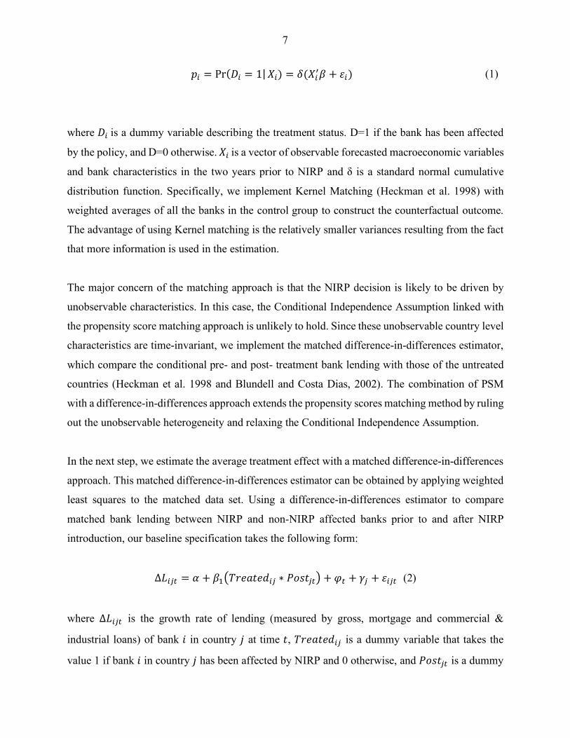
𝑝" = Pr(𝐷" = 1| 𝑋") = 𝛿(𝑋"-𝛽 + 𝜀")
(1)
where 𝐷" is a dummy variable describing the treatment status. D=1 if the bank has been affected
by the policy, and D=0 otherwise. 𝑋" is a vector of observable forecasted macroeconomic variables
and bank characteristics in the two years prior to NIRP and δ is a standard normal cumulative
distribution function. Specifically, we implement Kernel Matching (Heckman et al. 1998) with
weighted averages of all the banks in the control group to construct the counterfactual outcome.
The advantage of using Kernel matching is the relatively smaller variances resulting from the fact
that more information is used in the estimation.
The major concern of the matching approach is that the NIRP decision is likely to be driven by
unobservable characteristics. In this case, the Conditional Independence Assumption linked with
the propensity score matching approach is unlikely to hold. Since these unobservable country level
characteristics are time-invariant, we implement the matched difference-in-differences estimator,
which compare the conditional pre- and post- treatment bank lending with those of the untreated
countries (Heckman et al. 1998 and Blundell and Costa Dias, 2002). The combination of PSM
with a difference-in-differences approach extends the propensity scores matching method by ruling
out the unobservable heterogeneity and relaxing the Conditional Independence Assumption.
In the next step, we estimate the average treatment effect with a matched difference-in-differences
approach. This matched difference-in-differences estimator can be obtained by applying weighted
least squares to the matched data set. Using a difference-in-differences estimator to compare
matched bank lending between NIRP and non-NIRP affected banks prior to and after NIRP
introduction, our baseline specification takes the following form:
Δ𝐿"45 = 𝛼 + 𝛽78𝑇𝑟𝑒𝑎𝑡𝑒𝑑"4 ∗ 𝑃𝑜𝑠𝑡45C + 𝜑5 + 𝛾4 + 𝜀"45 (2)
where Δ𝐿"45 is the growth rate of lending (measured by gross, mortgage and commercial &
industrial loans) of bank 𝑖 in country 𝑗 at time 𝑡, 𝑇𝑟𝑒𝑎𝑡𝑒𝑑"4 is a dummy variable that takes the
value 1 if bank 𝑖 in country 𝑗 has been affected by NIRP and 0 otherwise, and 𝑃𝑜𝑠𝑡45 is a dummy
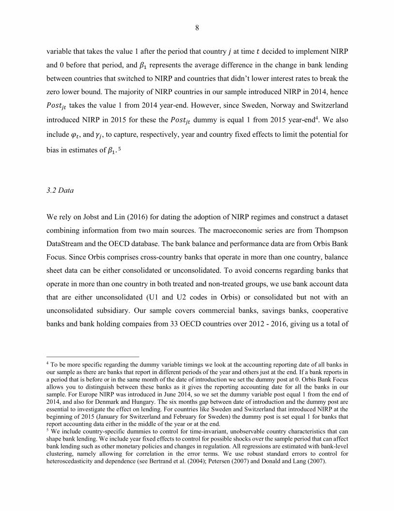
8
variable that takes the value 1 after the period that country 𝑗 at time 𝑡 decided to implement NIRP
and 0 before that period, and 𝛽7 represents the average difference in the change in bank lending
between countries that switched to NIRP and countries that didn’t lower interest rates to break the
zero lower bound. The majority of NIRP countries in our sample introduced NIRP in 2014, hence
𝑃𝑜𝑠𝑡45 takes the value 1 from 2014 year-end. However, since Sweden, Norway and Switzerland
introduced NIRP in 2015 for these the 𝑃𝑜𝑠𝑡45 dummy is equal 1 from 2015 year-end4. We also
include 𝜑5, and 𝛾4, to capture, respectively, year and country fixed effects to limit the potential for
bias in estimates of 𝛽7. 5
3.2 Data
We rely on Jobst and Lin (2016) for dating the adoption of NIRP regimes and construct a dataset
combining information from two main sources. The macroeconomic series are from Thompson
DataStream and the OECD database. The bank balance and performance data are from Orbis Bank
Focus. Since Orbis comprises cross-country banks that operate in more than one country, balance
sheet data can be either consolidated or unconsolidated. To avoid concerns regarding banks that
operate in more than one country in both treated and non-treated groups, we use bank account data
that are either unconsolidated (U1 and U2 codes in Orbis) or consolidated but not with an
unconsolidated subsidiary. Our sample covers commercial banks, savings banks, cooperative
banks and bank holding compaies from 33 OECD countries over 2012 - 2016, giving us a total of
4 To be more specific regarding the dummy variable timings we look at the accounting reporting date of all banks in our sample as there are banks that report in different periods of the year and others just at the end. If a bank reports in a period that is before or in the same month of the date of introduction we set the dummy post at 0. Orbis Bank Focus allows you to distinguish between these banks as it gives the reporting accounting date for all the banks in our sample. For Europe NIRP was introduced in June 2014, so we set the dummy variable post equal 1 from the end of 2014, and also for Denmark and Hungary. The six months gap between date of introduction and the dummy post are essential to investigate the effect on lending. For countries like Sweden and Switzerland that introduced NIRP at the beginning of 2015 (January for Switzerland and February for Sweden) the dummy post is set equal 1 for banks that report accounting data either in the middle of the year or at the end. 5 We include country-specific dummies to control for time-invariant, unobservable country characteristics that can shape bank lending. We include year fixed effects to control for possible shocks over the sample period that can affect bank lending such as other monetary policies and changes in regulation. All regressions are estimated with bank-level clustering, namely allowing for correlation in the error terms. We use robust standard errors to control for heteroscedasticity and dependence (see Bertrand et al. (2004); Petersen (2007) and Donald and Lang (2007).
9
23,247 observations.6 There are 20 countries in the treated group and 13 countries in the control
group.7 Descriptive statistics for the bank lending series, other bank balance sheet variables, and
the macroeconomic series in the treatment and control groups of countries are shown in Table 1.
Panel A of Table 1 presents summary statistics for bank lending. In a recent study on monetary
stimulus and bank lending, Chakraborty et al. (2017) find that in response to the Federal Reserve’s
asset purchases, banks shift resources away from C&I lending into mortgage origination. To take
this potential crowding-out effect between bank lending activities into consideration, we group
bank lending behaviour into three types: gross loans, mortgage loans and C&I loans. We use the
logarithm growth rate of gross loans, mortgage loans and commercial and industrial (C&I) loans
as our measures of interest.
Panel B of Table 1 presents summary statistics on other bank balance sheet data, including bank
size (log(TA)), equity ratio (E/TA), profitability (ROE), liquidity ratio (Liquidity), total capital
ratio (Capital), funding structure (Funding_Structure), and income structure (Income_Structure).
In a recent theoretical study, Brunnermeier and Koby (2016) suggest that monetary policy may
have unintended contractionary effects on lending due to bank capital constraints, bank business
models and market competition. To empirically test the hypothesis of Brunnermeier and Koby
(2016), we also include variables that account for bank funding and income structures and the
Hirshman-Herfindahl market structure index (HHI) to proxy the impact of bank competition.
Earlier literature also highlighted the major transmission channels of other UMP policies including
central banks’ asset purchase programs (Di Maggio et. al, 2016; Rodnyanski and Darmouni, 2017;
Kandrac and Schulsche, 2017; Chakraborty et. al, 2017). In-line with Gambacorta et al. (2014),
we employ the logarithm growth rate of a country’s central bank balance sheet as a further control
to isolate the impact of other UMP’s on bank lending behavior.
6 The sample period is intentionally short. According to Roberts and Whited (2013) and Bertrand et al. (2004) the change in the treatment group should be concentrated around the onset of the treatment. Moving away leads to unobservable and other factors that affect the treatment outcome threatening the validity of the model. 7 We exclude Japan in our sample as the country only adopted NIRP in early 2016, which provides too short of a period to examine the impact of NIRP on bank lending.
10
Another issue is that bank lending may be driven by loan demand from households and corporates.
To address this concern, we construct loan demand indices based on data from the ECB and FED
bank lending surveys. Both of these surveys identify loan demand as the need of enterprises and
households for bank loan financing, irrespective of whether a loan is granted or not.8 Based on
data from these two surveys, we construct loan demand indices for the Euro area and US, focusing
on increases or decreases in loan demand. Panel C of Table 1 presents summary statistics of
macroeconomic conditions, monetary policy and loan demand indices.
(Insert Table 1 here)
Despite the fact that we use PSM to match countries with similar forecasted macroeconomic
variables, it can be argued that a reduction in bank lending is driven by weak economic prospects.
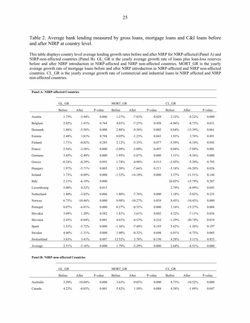
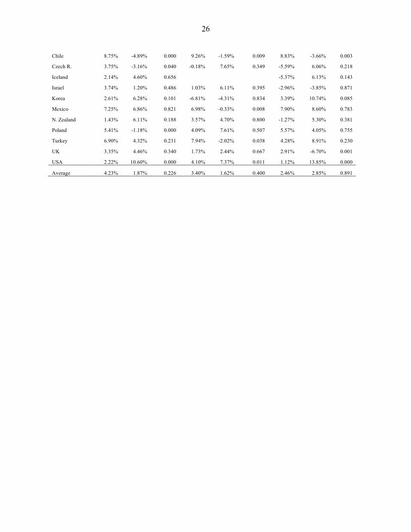
To gain further insight, in Table 2, we provide country level average lending growth rates before
and after NIRP. Panel A shows before and after NIRP average lending growth for NIRP-affected
countries while Panel B is for counties that did not experience NIRP. Although the results suggest
that both NIRP- affected and non-affected countries experienced a reduction in bank lending after
the treatment period, the reduction in lending experienced by NIRP-adopter countries was larger
and the difference between mean lending in the two periods for this group was statistically
significant.
(Insert Table 2 here)
4. Empirical results
4.1 Propensity score matching
8 The bank lending surveys from ECB and FED are available at:
1) https://www.federalreserve.gov/boarddocs/snloansurvey/ 2) https://www.ecb.europa.eu/stats/money/surveys/lend/html/index.en.html
11
Propensity score matching is implemented to mitigate the issue of selection bias. To establish an
adequate control group we match countries according to pre-treatment characteristics. The results
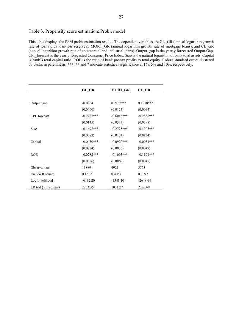
from the Probit model, that are used to generate propensity scores of being affected by NIRP, are
presented in Table 3. As displayed, the majority of the covariates are significant at the 1% level
suggesting that banks operating in countries with weaker economic prospects represented by lower
forecasted inflation (CPI_forecast) and wider forecasted output gap (Output_gap) have a higher
probability of being affected by the negative interest rate policy. Moreover, countries with banks
that are small (Size), with lower profitability (ROE), and that are less capitalised (Capital) tend to
have a higher probability of being the target of NIRP.
(Insert Table 3 here)
4.2 Combined PSM Difference-in-Differences estimator
The PSM approach reduces but does not eliminate the selection bias caused by unobservable time
invariant country-characteristics. Thus, we implement the combined PSM difference-in-
differences estimator to remove the unobserved heterogeneity. The results from the PSM matching
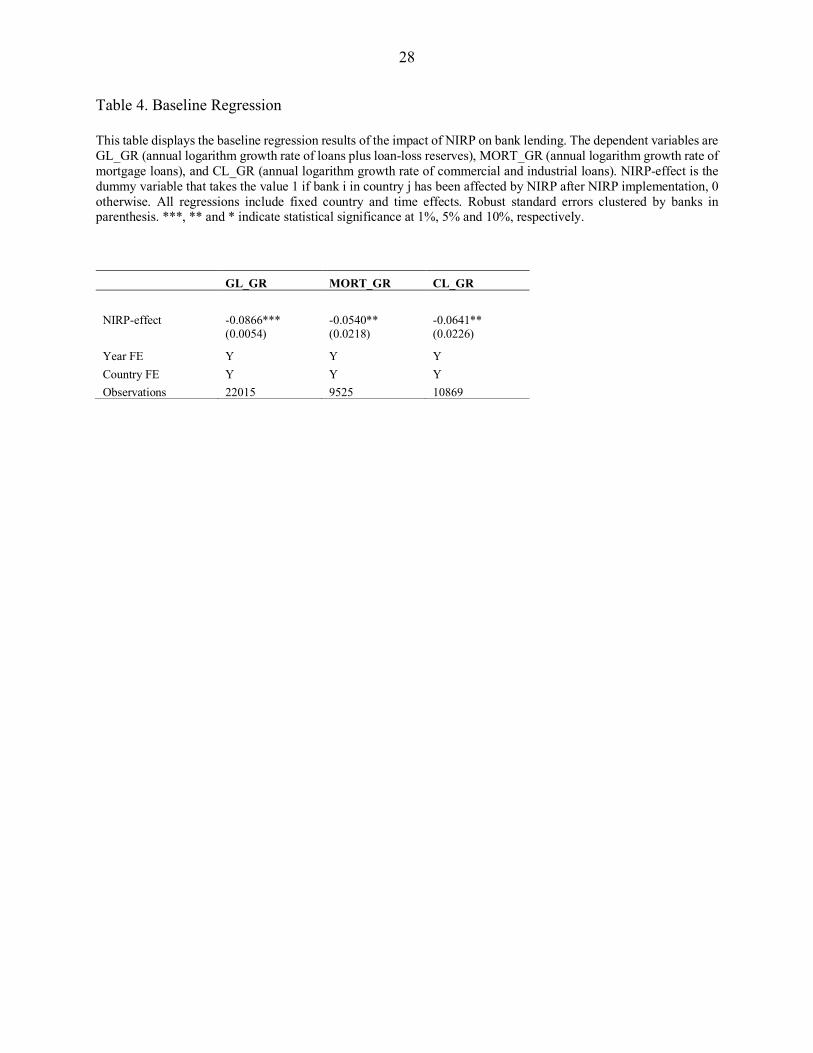
difference-in-differences estimations are presented in Table 4. The dependent variables are the
(natural logarithm) growth rate of gross loans (GL_GR), mortgage loans (MORT_GR) and
commercial and industrial (CL_GR) loans. In column 1 of Table 4 with GL_GR as the dependent
variable, the coefficients on NIRP is sizeable, negative and statistically significant at the 1% level,
indicating that countries, in which central banks implemented NIRP experienced a decline in total
bank lending of around 8.7% relative to those countries in which central banks did not follow this
policy. The remaining columns with MORT_GR and CL_GR as dependent variables demonstrate
similar results with negative and significant coefficients on NIRP. The sizeable, negative and
statistically significant results on NIRP indicates that countries that implemented NIRP
experienced a decline in bank lending relative to those in which central banks did not follow this
policy. Negative rates break the zero lower bound of interest rates. However, banks rely on deposit
funding and are reluctant to pass-on the negative rates to depositors. Due to this imperfect pass-
12
through the narrower margins add pressure on banks to reduce lending. Our results are in-line with
Heider et al. (2017).
(Insert Table 4 here)
4.3 Robustness tests
In this section, we take an in-depth exploration of the transmission of negative rates on bank
lending. The results also serve as robustness checks of our baseline model.
NIRP was brought into the UMP mix by central banks together with the adoption of other
unconventional monetary policies, most particularly extensive outright asset purchases, and it is
important to disentangle the effects of NIRP on lending from the effects of these policies. Outright
asset purchases were aimed at expanding the central bank’s balance sheet to increase the level of
the monetary base in order to boost nominal spending (Bernanke and Reinhart, 2004). We proxy
for the use of other UMPs by including the log of the growth rate of central bank total assets to
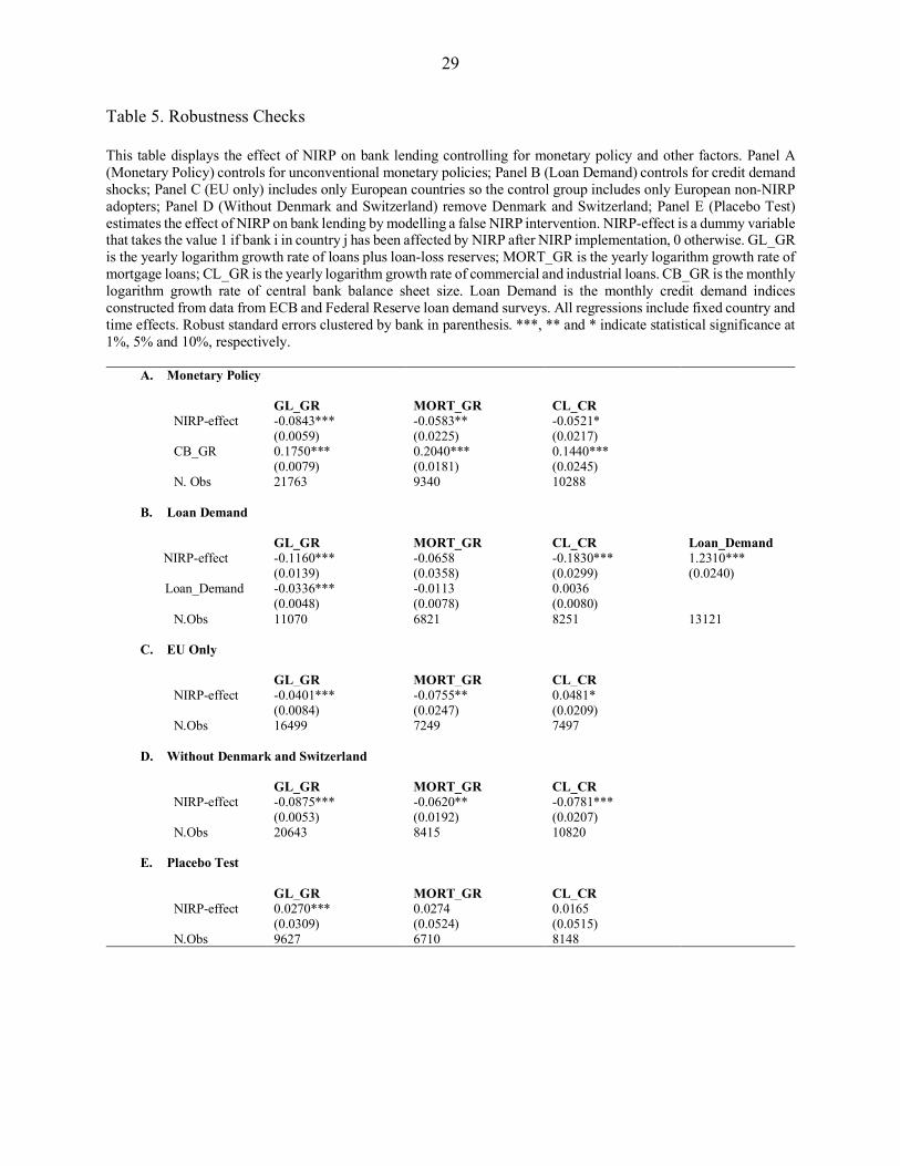
take account of central bank balance sheet size. The results reported in panel A of Table 5 are for
each of the three categories of bank lending and suggest that NIRP and central bank asset purchases
had the opposite impact on bank lending. Other UMPs are positively associated with bank lending
growth but the coefficients on NIRP remain negative and significant. Thus, the estimates suggest
that NIRP did not manage to achieve the intended results of stimulating bank lending and economic
growth. On the other hand, other UMPs appear to have been more effective in boosting bank
lending.
Our second robustness check aims to control for the effect of credit demand on bank lending
behavior. To this end, we make use of indicators of loan demand from the U.S Federal Reserve
Board’s Senior Loan Officer Opinion Survey on Bank Lending Practices and the ECB’s Euro Area
Bank Lending Survey, both of which have elements focused on the need of firms and households
for bank loan financing (irrespective of whether the loan is granted). We construct monthly credit
demand indices from the aforementioned ECB and Federal Reserve surveys. These results are
13
reported in columns 1, 2 and 3 of panel B (Table 5) where the coefficient on NIRP remains negative
and statistically significant for gross and C&I loans. The results demonstrate that the negative
relationship between NIRP and bank lending is not driven by loan demand. In column 4 of panel
B (Table 5) we report the result with Loan demand as the dependent variable. The result reveals a
positive relationship between loan demand and the dummy variable for the NIRP-effect, which
indicates an increase in loan demand in treated countries. The result suggests a gap between loan
supply and loan demand in NIRP adopter countries and confirms that the reduction in bank lending
is not driven by loan demand.
For a third robustness check, we alter our country sample where the treatment group includes only
European countries so the control group includes only European non-NIRP adopters.9 These
results are reported in panel C of Table 5. The coefficients on NIRP-effect in the cases of gross
loans and mortgage loans remain negative and statistically significant. However, in a sample
within the EU, C&I loans and NIRP- effect demonstrates a positive and significant relationship.
The motivations for Denmark and Switzerland to adopt NIRP was focused on discouraging capital
inflows to reduce exchange rate appreciation pressures; a policy fundamentally different from
other treated countries. In the fourth robustness check, we remove Denmark and Switzerland from
our sample. The results are reported in panel D of Table 5 and show the coefficient on the NIRP
dummy remains negative and significant, which confirms our baseline results.
As a final robustness test, we try to eliminate the possibility that bank behavior in the treatment
group may have altered prior to the introduction of NIRP—for example, in anticipation of adverse
effects of NIRP, or for some bank-specific reasons—thereby invalidating our choice of difference-
in-differences estimation. We model false NIRP periods for 2012 and 2013. If the estimated
coefficients on the ‘false’ NIRP are not statistically significant or negative, we can be more
confident that our baseline coefficient is capturing a genuine monetary policy shock. The results
are reported in panel E of Table 5. The coefficients on the NIRP dummy are positive and
9 We follow Bertrand and Mullainathan (2003) and Jayaratne and Strahan (1996) that use different control groups as a further test to control for the omitted variables problem. Multiple control and treatment groups reduce biases and unobservable variables associated with just one comparison.
14
statistically significant in the cases of gross loans, and positive and insignificant in the case of
mortgage loans and C&I loans adding further support to the validity of our baseline results. The
results also reaffirm and strengthen the conclusion of our baseline results that differential bank
lending behavior was driven by NIRP.
(Insert Table 5 here)
4.3 NIRP and the reverse interest rate hypothesis
In this section, we report results from a test of aspects of the Brunnemeier and Koby (2016)
‘reversal rate hypothesis’ within a matched difference-in-differences framework by creating
NIRP-adopter treatment groups and non-adopter control groups according to whether banks meet
representations of bank-specific factors that these authors suggest might reduce bank lending in a
low interest rate setting.10 Specifically, we focus on banks’ capitalization, funding structure,
business model, interest rate exposure, and competitive conditions in the banking market. First,
we examine the impact of bank capital on lending by grouping banks in the treatment and control
groups according to whether they have total capital ratios above or below the median for banks in
our sample, labelling banks with higher than median capital ratios as ‘well-capitalized’ and those
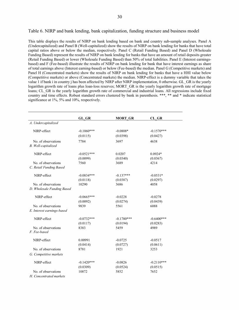
below the median as ‘under-capitalized’. The results for the different categories of loans are
reported in panels A and B of Table 6. In panel A, the coefficients on NIRP-effect for all the
categories of bank lending are negative and statistically significant suggesting a substantially
larger decline in lending by under-capitalized banks after the introduction of NIRP. Panel B
exhibits different results in the group of well-capitalized banks. The coefficient on gross loan is
smaller in magnitude and the coefficients on mortgage and business loans turn positive, indicating
a mixed and unclear effect of NIRP on bank lending in the group of well-capitalized banks. This
is consistent with the Brunnemeier and Koby’s (2016) assertion that suggests that in situations of
economic uncertainty and changing regulation, binding capital requirements can limit the pass-
through of monetary policies to bank lending. These results are also in-line with Carlson et al.
10 As already mentioned in section 4.2, splitting control and treatment groups in different sub-groups allows us also to reduce bias and unobservable variables associated with just one comparison.
15
(2013) and Gambacorta and Mistrulli (2004). Both studies show the importance of capital as a
buffer against monetary policy shocks on lending.
Second, we consider how NIRP interacts with bank funding structure. We distinguish between
retail deposit based and wholesale funding based banks on the assumption that if interest rates on
retail deposits are more downwards sticky then the introduction of NIRP would likely pose greater
limitations on retail deposit based banks to increase lending (Sääskilahti, 2018). We consider as
retail deposit banks those with retail deposits greater that 50% of total liabilities. This is confirmed
by the results reported in panels C and D of Table 6, where the coefficients on NIRP are highly
negative and significant in all the three categories of bank lending for deposit-based banks but
indicate that NIRP resulted in a unclear relationship with bank lending for wholesale funding based
banks. The result is consistent with the argument of Dell’Ariccia et al. (2014) that NIRP enabled
wholesale-funded banks to take greater advantage of the decline in funding costs and provide more
loans.
We assess the impact of banks’ business models on lending in a NIRP context by distinguishing
between traditional interest-dependent banks from those that have a more fee-dependent business
model. For our purposes, a bank is defined as interest-dependent if the interest earnings share of
total earnings is above the median for banks in our sample; banks are deemed to be fee-based if
their interest earnings share is below the median. If interest rates on retail deposits are sticky
downwards then the introduction of NIRP would likely pose more constraints for banks with
interest-dependent than fee-dependent business models. The results from these estimates are
reported in panels E and F of Table 6 and show that banks whose business model is mainly interest-
based reduced their lending by more than banks whose business model was more fees orientated.
Our final test of the Brunnemeier and Koby (2016) hypothesis is to assess the impact of NIRP on
lending in the context of competitive conditions in banking markets. In this case, we proxy market
competition by focusing on market concentration in each country as indicated by the Herfindahl-
Hirschman Index (HHI). Sørensen and Werner (2006), for example, use the concentration ratio as
a proxy for competition and conclude that banks operating in a less competitive environment make
slower adjustments to interest rates (and therefore to net interest margins), which slows the
16
transmission of monetary policy changes to bank lending.11 We define markets as competitive with
a HHI value below 1000 (the median value in our sample) and split the sample for the treatment
and control groups. According to Brunnemeier and Koby (2016) low interest policy is likely to
have a more limiting effect on bank lending in competitive markets because of the associated
pressure on net interest margins. The results reported in panels G and H of Table 6 support this
view: the impact of NIRP on bank lending in competitive markets is highly negative and
statistically significant for the categories of gross loans and C&I loans, suggesting that banks in
these markets have little option but to generate alternative income from other sources to maintain
profitability. In more concentrated markets, the impact of NIRP is weaker suggested by smaller
and less significant coefficients on NIRP-effect.
(Insert Table 6 here)
5. Conclusions
Beginning in 2012, several central banks adopted a negative interest rate policy aimed at boosting
real spending by facilitating an increase in the supply and demand for loans. The policy generated
controversy with skeptics pointing to several factors that might complicate the transmission from
negative policy rates to higher bank lending. Empirical evidence on the impact of the policy is
scant. In this paper, we provide new evidence that bank lending fared worse in NIRP-adopter
countries than it did in countries that did not adopt the policy. Specifically, countries in which
central banks implemented NIRP experienced a decline in total bank lending relative to those
countries in which central banks did not follow this policy. This result holds for gross bank lending
and separately for mortgage and C&I lending, the key categories of bank lending, and is robust to
the inclusion of several bank-specific control variables. It also stands up in the face of a wide array
11The US Department of Justice ‘generally considers markets in which the HHI is between 1,500 and 2,500 points to be moderately concentrated, and consider markets in which the HHI is in excess of 2,500 points to be highly concentrated’. https://www.justice.gov/atr/herfindahl-hirschman-index. We recognize that there are shortcomings with using the HHI as a proxy for competitive conditions. There are different views about competition and concentration in the literature. Claessens and Laeven (2003), for example, point out that there are some countries, such as USA, that show levels of monopolistic competition in banking despite the large number of banks, while countries like Canada are highly competitive, although the number of banks is relatively small. For this reason we also cross-checked using Boone and Lerner indicators. These estimations are available upon request.
17
of robustness checks, including controlling for the effects of other aspects of UMP, developments
in loan demand across countries, for possible bank funding constraints, and to (possible) changes
in bank behavior prior to the introduction of NIRP. Finally, our results are relevant to the validity
of the ‘reverse interest rate hypothesis’ developed recently by Brunnemeier and Koby (2016) in
that bank-specific factors (capitalization, funding structure, business model, interest rate exposure,
competitive conditions) appear to reduce banks’ willingness to lend in a negative interest rate
setting.
References
Agarwal, S., Chomsisengphet, S., Mahoney, N., Stroebel, J., 2018. Do banks pass through credit
expansion to consumers who want to borrow? Quarterly Journal of Economics, 133, 129-190.
Altunbas, Y., Gambacorta, L., Marqués-Ibáñez, D., 2014. Does monetary policy affect bank risk-
taking? The International Journal of Central Banking, (March), 95-136.
Arteta, C., Kose, M.A., Stocker, M., Taskin, T., 2016. Negative interest rate policies: Sources and
implications. World Bank Policy Research Paper 7791, August. Washington DC: World Bank.
Ball, L., Gagnon, J., Honohan, P., Krogstrup, S., 2016. What else can central banks do? Geneva
Reports on the World Economy 18, The International Center for Monetary and Banking Studies
(ICMB) and the Centre for Economic Policy Research (CEPR). ICBM: Zurich and CEPR: London.
Baumeister, C., Benati, L., 2013. Unconventional monetary policy and the Great Recession –
estimating the impact of a compression in the yield spread at the zero lower bound. International
Journal of Central Banking (June), 165-212
Bech, M., Malkhozov, A., 2016. How have central banks implemented negative policy rates? Bank
for International Settlements Quarterly Review (March), 31-44.
18
Berger, A. N., Black, L. K., Bouwman, C. H. S., Dlugosz, J. 2017. Bank loan supply responses to
Federal Reserve emergency liquidity facilities. Journal of Financial Intermediation 32, 1-15.
Berkmen, P., 2012. Bank of Japan’s quantitative and credit easing: are they now more effective?
International Monetary Fund Working Paper 12/2 (January). Washington D.C: IMF.
Bernanke, B., Reinhart, V., 2004. Conducting monetary policy at very low short-term interest
rates. American Economic Review 94(2), 85–90.
Bertrand, M., Mullainathan, S., 2003. Enjoying the quiet life? Corporate governance and
managerial preferences, Journal of Political Economy 111, 1043-1075.
Bertrand, M., Duflo, E., Mullainathan, S., 2004. How much should we trust difference-in-
differences estimates? Quarterly Journal of Economics, 119, 249-275.
Blundell, R., Costa Dias, M., 2002. Alternative approaches to evaluation in empirical microeconomics. Portuguese Economic Journal 1, 91-115.
Bowman, D., Cai, F., Davies, S., Kamin, S., 2015. Quantitative easing and bank lending: evidence
from Japan. Journal of International Money and Finance 57 (October), 15-30.
Bräuning, F., Wu, B., 2017. ECB monetary policy transmission during normal and negative
interest rate periods (March 24 http://dx.doi.org/10.2139/ssrn.2940553
Butt, N.,Churmz, R., McMahon, M., Morotzz, A., Jochen Schanz, J., 2014. QE and the bank
lending channel in the United Kingdom. Bank of England Working Paper 511 (September),
London: Bank of England.
Brunnermeier, M.K., Koby, Y., 2016. The reversal interest rate: the effective lower bound of
monetary policy. Princeton University Department of Economics Working Paper August 27.
https://scholar.princeton.edu/sites/default/files/markus/files/08f_reversalrate.pdf
19
Brunnermeier, M.K., Sannikov, Y., 2016. The I theory of money. Princeton University Department
of Economics Working Paper, August 18.
https://scholar.princeton.edu/sites/default/files/markus/files/10r_theory.pdf
Carlson, M., Shan, H., Warusawitharana, M. 2013. Capital ratios and bank lending: A matched
bank approach. Journal of Financial Intermediation 22 (4), 603-687
Chakraborty, I., Goldstein, I, MacKinlay, A., 2017. Monetary stimulus and bank lending. Finance
Down Under 2017 Building on the Best from the Cellars of Finance.
June.http://dx.doi.org/10.2139/ssrn.2734910
Claessens, S., Laeven, L., 2003. What drives bank competition? Some international evidence.
Journal of Money, Credit and Banking 36(3), 563-583.
Curdia, V., Woodford, M., 2011. The central bank’s balance sheet as an instrument of monetary
policy. Journal of Monetary Economics 58(1), 54–79.
Demiralp, S., Eisenschmidt, J., Vlassopoulos, T., 2017. Negative interest rates, excess liquidity
and bank business models: Banks’ reaction to unconventional monetary policy in the euro area.
Koç University-TUSIAD Economic Research Forum Working Papers 1708, Koc University-
TUSIAD Economic Research Forum.
Dell’Ariccia, G., Laeven, L., Marquez, R., 2014. Real interest rates, leverage and bank risk taking.
Journal of Economic Theory 149 (1), 65-99.
Del Negro, M., Eggertsson, G.B., Ferrero, A., Kiyotaki, N., 2017. The great escape? A quantitative
evaluation of the Fed’s liquidity facilities. American Economic Review 107(3), 824-857.
20
Di Maggio, M., Kermani, A., and Palmer, C., 2016, How quantitative easing works: Evidence on
the refinancing channel. National Bureau of Economic Research Working Paper No. 22638,
September 2016, Washington D.C: NBER.
Donald, S., Lang, K., 2007. Inference with difference-in-differences and other panel data. Review
of Economics and Statistics 89 (2), 221-233
Drechsler, I., Savov, A., Schnabl, P., 2016. The deposits channel of monetary policy. National
Bureau of Economic Research Working Paper No. 22152, April Washington D.C: NBER.
Eggertsson, G., Woodford, M., 2003. The zero bound on interest rates and optimal monetary
policy. Brookings Papers on Economic Activity 34(1), 139–235.
Fujiwara, I., 2004. Evaluating monetary policy when nominal interest rates are almost zero.
Journal of the Japanese and International Economy 20(3), 434-453.
Gambacorta, L., Mistrulli, P. E. 2004. Does bank capital affect lending behavior? Journal of
Financial Intermediation 13 (4), 436-457.
Gambacorta, L., Hofmann, B. and Peersman, G., 2014. The effectiveness of unconventional
monetary policy at the zero lower bound: A cross-country analysis. Journal of Money, Credit and
Banking 46 (4), 615–642.
Heider, F., Saidi, F., Schepens, G., 2017. Life below zero: bank lending under negative policy
rates. Available at SSRN: https://ssrn.com/abstract=2788204
Heckman, J., Ichimura, H., Smith, J.A., Todd, P.,1998. Characterizing selection bias using
experimental data. Econometrica 65, 1017-1098.
Jayaratne, J., Strahan, P. E., 1996. The finance-growth nexus: Evidence from bank branch
deregulation. Quarterly Journal of Economics 101, 639-670.
21
Jimenez, G., Ongena, S., Peydro, J-L., 2012. Credit supply and monetary policy: identifying the
bank balance-sheet channel with loan applications. American Economic Review 102(5), 2301–
2326.
Jimenez, G., Ongena, S., Peydro, J-L., Saurina, J., 2014. Hazardous times for monetary policy:
what do twenty-three million bank loans say about the effects of monetary policy on credit risk-
taking? Econometrica 82(2), 463–505.
Jobst, A., Lin, H., 2016. Negative interest rate policy (NIRP): implications for monetary
transmission and bank profitability in the euro area. International Monetary Fund Working Paper
16/172 (August). Washington D.C: IMF.
Kandrac, J., and Schulsche, B., 2017. Quantitative easing and bank risk taking: evidence from
lending. (September 25). Available from http://dx.doi.org/10.2139/ssrn.2684548
Kapetanios, G., Mumtaz, H., Stevens, I., Theodoridis, K., 2012. Assessing the economy-wide
effects of quantitative easing. The Economic Journal 122 (564), 316-347.
Kashyap, A. K., Stein, J.C., 2000. What do a million observations on banks say about the
transmission of monetary policy? American Economic Review 90(3), 407–428.
Lenza, M., Pill, H., Reichlin, L., 2010. Monetary policy in exceptional times. Economic Policy
25(62), 295–339.
Maddaloni, A., and Peydro, J.L., 2011. Bank risk-taking, securitization, supervision, and low
interest rate: evidence from the Euro-area and the U.S lending standards. Review of Financial
Studies 24(6), 2121-2165.
22
McAndrews, J., 2015. Negative nominal central bank policy rates: where is the lower bound?
Remarks at the University of Wisconsin, May 8, New York Federal Reserve Speeches.
https://www.newyorkfed.org/newsevents/speeches/2015/mca150508.html
Petersen, M., 2009. Estimating standard error in finance panel dataset: comparing approaches.
Review of Financial Studies 22 (1), 435-480
Roberts, M. R., Whited, T. M., 2012. Endogeneity in empirical corporate finance. Handbook of
the Economics of Finance, Editors G.M. Constantinides, M. Harris and R. M. Stulz, Volume 2 Part
A, Chapter 7, 493-572 (NY: Elsevier)
Rodnyansky, A., Darmouni, O., 2017. The effects of quantitative easing on bank lending behavior.
The Review of Financial Studies 30(11), 3858-3887.
Rosenbaum, P. R., Rubin, D. B., 1983. The central role of the propensity score in observational
studies for causal effects. Biometrika 70, 41–55.
Sääskilahti, J., 2018. Retail bank interest margins in low interest rate environments. Journal of
Financial Services Research 53(1) , 37-68
Sørensen, K. C., Werner, T., 2006. Bank interest rate pass-through in the euro area: a cross-country
comparison. European Central Bank Working Paper Series 580 (January). Frankfurt: ECB.
Schenkelberg, H., Watzka, S., 2013. Real effects of quantitative easing at the zero lower bound:
structural VAR-based evidence from Japan. Journal of International Money and Finance 33
(March), 327-357.
Wallace, N., 1981. A Modigliani-Miller theorem for open-market operations. American Economic
Review 71(3), 267–274.

23
Table 1. Descriptive statistics: treatment and control groups This table reports the summary statistics of the key variables used in our analysis for both the treatment and the control groups. Panel A, Panel B and Panel C show descriptive statistics for the dependent variables, bank balance sheet data and macroeconomic condition and monetary policy variables, respectively. GL_GR is the yearly logarithm growth rate of loans plus loan-loss reserves; MORT_GR is the yearly logarithm growth rate of mortgage loans; CL_GR is the yearly logarithm growth rate of commercial and industrial loans. Log(TA) is the natural logarithm of bank total assets. E/TA is the ratio of bank equity to total assets. ROE is the ratio of bank pre-tax profits to total equity. Liquidity is the ratio of bank liquid asset to total assets. Capital is bank’s total capital ratio. Income_Structure is the ratio of bank interest income to total income. Funding_Structure is the ratio of bank deposit funding to total liabilities. HHI is the Herfindahl-Hirschman index. Output_gap is the yearly forecasted Output Gap. CPI_forecast is the yearly forecasted Consumer Price Index. GDP_GR is the yearly growth rate of real GDP. Inflation is the yearly Consumer Price Index in percentage. Unemployment is the rate of yearly unemployment in percentage. CB_GR is the monthly logarithm growth rate of central bank balance sheet size. M0_GR is the logarithm growth rate of the money supply M0. Deposit Rate is the country level aggregate deposit rate in percentage. Loan Demand is the monthly credit demand indices constructed from data from ECB and Federal Reserve loan demand surveys.
I. Treatment group: II. Control group Variable Obs. Mean Std.
Dev. Min Max Obs. Mean Std.
Dev Min Max
Panel A: Bank Lending
GL_GR 7543 -0.04 0.41 -9.73 8.54 15704 0.03 0.45 -10.17 7.31
MORT_GR 3795 -0.03 0.39 -7.00 7.90 5938 0.02 0.50 -9.13 7.71 CL_GR 3259 -0.11 0.54 -6.96 4.83 8018 0.02 0.61 -8.25 6.76 Panel B: Bank Balance Sheet Data Log(TA) 8138 13.77 2.12 3.94 21.72 18700 14.07 2.38 2.95 21.90 E/TA 8136 10.48% 5.71% 3.83% 24.93% 17703 11.74% 6.56% 3.83% 24.93%
ROE 8099 4.56% 4.40% 0.00% 16.83% 18261 6.27% 5.18% 0.00% 16.83%
Liquidity 7895 21.76% 15.12% 0.90% 46.94% 17264 20.67% 15.44% 0.90% 46.94%
Capital 5700 18.38% 4.57% 11.00% 26.30% 11302 17.40% 4.59% 11.00% 26.30%
Income_Structure 7881 6.67% 5.69% 0.00% 16.99% 18261 4.97% 5.05% 0.00% 16.99%
Funding_Structure 7465 64.61% 20.30% 20.40% 85.32% 14752 65.06% 20.98% 20.40% 85.32%
HHI 10092 855 536 453 3777 56608 446 397 249 4237
Panel C: Macroeconomic Conditions and Monetary Policy Output_gap 20456 -2.09% 2.64% -15.09% 0.56% 45588 -2.36% 1.04% -6.03% 2.70%
CPI_forecast 20456 1.00% 1.08% -1.39% 5.65% 46244 1.50% 1.17% -0.87% 8.89%
GDP growth 10092 0.41% 0.66% -0.19% 6.62% 56604 0.44% 0.28% -1.13% 1.89%
Inflation 10092 0.43% 0.77% -1.73% 4.39% 56608 1.51% 1.14% -1.73% 8.93%
Unemployment 4978 7.91% 4.71% 4.50% 26.30% 45047 7.34% 2.51% 3.1% 27.20%

24
CB_GR 5700 -0.02 0.15 -0.41 0.35 46991 0.09 0.16 -0.66 0.45
M0_GR 6588 8.07 10.17 -4.55 20.12 51648 9.51 9.22 -26.63 51.56
Deposit Rate 1962 0.50% 0.57% -0.18% 1.41% 5512 3.38% 4.83% 0.03% 16.77%
Loan Demand 8360 15.74 13.85 -22.92 48.33 46772 10.40 16.00 -68.33 23.10
25
Table 2. Average bank lending measured by gross loans, mortgage loans and C&I loans before and after NIRP at country level. This table displays country level average lending growth rates before and after NIRP for NIRP-affected (Panel A) and NIRP-non-affected countries (Panel B). GL_GR is the yearly average growth rate of loans plus loan-loss reserves before and after NIRP introduction in NIRP-affected and NIRP non-affected countries. MORT_GR is the yearly average growth rate of mortgage loans before and after NIRP introduction in NIRP-affected and NIRP non-affected countries. CL_GR is the yearly average growth rate of commercial and industrial loans in NIRP affected and NIRP non-affected countries.
Panel A: NIRP-affected Countries
GL_GR MORT_GR CL_GR
Before After P-value Before After P-value Before After P-value
Austria 1.73% -3.94% 0.000 1.27% -7.83% 0.029 2.32% -8.22% 0.000
Belgium 2.02% 1.41% 0.764 4.01% -7.23% 0.458 -4.96% -8.73% 0.631
Denmark 1.86% -5.56% 0.000 2.88% -9.36% 0.002 0.84% -13.39% 0.061
Estonia 2.48% 3.81% 0.794 0.05% -1.23% 0.843 1.93% 3.76% 0.891
Finland 1.71% -0.82% 0.285 2.12% -5.33% 0.077 -5.59% -6.10% 0.943
France 2.56% -3.58% 0.000 -2.09% -3.09% 0.497 0.04% -7.88% 0.001
Germany 3.45% -2.49% 0.000 1.95% -3.07% 0.000 1.51% -8.36% 0.000
Greece -0.24% -0.29% 0.993 1.74% -4.98% 0.515 -2.95% -5.39% 0.793
Hungary 1.97% -5.71% 0.003 1.20% -7.66% 0.211 -3.18% -16.20% 0.026
Ireland 1.73% -8.09% 0.000 -1.32% -14.10% 0.000 3.37% -11.51% 0.144
Italy 2.11% -6.19% 0.000 26.02% -15.79% 0.207
Luxembourg 5.00% 0.52% 0.015 2.70% -8.99% 0.043
Netherland 1.80% -3.82% 0.006 1.80% -7.76% 0.000 1.18% -5.02% 0.233
Norway 6.75% -10.46% 0.000 9.98% -10.27% 0.039 8.45% -10.43% 0.000
Portugal 0.07% -6.81% 0.000 0.27% -8.51% 0.000 1.16% -15.27% 0.004
Slovakia 3.09% 1.20% 0.582 1.81% 3.61% 0.802 4.32% -7.11% 0.036
Slovenia 2.43% -8.84% 0.001 4.01% -4.53% 0.216 -1.29% -20.74% 0.019
Spain 1.51% -5.72% 0.000 -1.36% -7.40% 0.193 5.62% -1.26% 0.197
Sweden 4.40% -1.31% 0.000 1.00% -0.32% 0.698 6.91% -6.75% 0.005
Switzerland 3.83% 3.41% 0.497 12.52% 3.78% 0.150 4.28% 3.11% 0.923
Average 2.51% -3.16% 0.000 1.79% -5.29% 0.000 2.64% -8.51% 0.000 Panel B: NIRP-non-affected Countries
GL_GR MORT_GR CL_GR
Before After P-value Before After P-value Before After P-value
Australia 3.20% -10.04% 0.000 3.63% -9.65% 0.000 8.73% -10.52% 0.000
Canada 4.22% -0.85% 0.001 5.42% 1.50% 0.088 4.38% -1.89% 0.047
26
Chile 8.75% -4.89% 0.000 9.26% -1.59% 0.009 8.83% -3.66% 0.003
Czech R. 3.75% -3.16% 0.040 -0.18% 7.65% 0.349 -5.59% 6.06% 0.218
Iceland 2.14% 4.60% 0.656 -5.37% 6.13% 0.143
Israel 3.74% 1.20% 0.486 1.03% 6.11% 0.395 -2.96% -3.85% 0.871
Korea 2.61% 6.28% 0.101 -6.81% -4.31% 0.834 3.39% 10.74% 0.085
Mexico 7.25% 6.86% 0.821 6.98% -0.33% 0.008 7.90% 8.60% 0.783
N. Zealand 1.43% 6.11% 0.188 3.57% 4.70% 0.800 -1.27% 5.30% 0.381
Poland 5.41% -1.18% 0.000 4.09% 7.61% 0.507 5.57% 4.05% 0.755
Turkey 6.90% 4.32% 0.231 7.94% -2.02% 0.038 4.28% 8.91% 0.230
UK 3.35% 4.46% 0.340 1.73% 2.44% 0.667 2.91% -6.70% 0.001
USA 2.22% 10.60% 0.000 4.10% 7.37% 0.011 1.12% 13.85% 0.000
Average 4.23% 1.87% 0.226 3.40% 1.62% 0.400 2.46% 2.85% 0.891
27
Table 3. Propensity score estimation: Probit model This table displays the PSM probit estimation results. The dependent variables are GL_GR (annual logarithm growth rate of loans plus loan-loss reserves), MORT_GR (annual logarithm growth rate of mortgage loans), and CL_GR (annual logarithm growth rate of commercial and industrial loans). Output_gap is the yearly forecasted Output Gap. CPI_forecast is the yearly forecasted Consumer Price Index. Size is the natural logarithm of bank total assets. Capital is bank’s total capital ratio. ROE is the ratio of bank pre-tax profits to total equity. Robust standard errors clustered by banks in parenthesis. ***, ** and * indicate statistical significance at 1%, 5% and 10%, respectively.
GL_GR MORT_GR CL_GR
Output_gap -0.0054 0.2152*** 0.1918***
(0.0060) (0.0123) (0.0094)
CPI_forecast -0.2725*** -0.6013*** -0.2836***
(0.0145) (0.0347) (0.0298)
Size -0.1697*** -0.2725*** -0.1305***
(0.0083) (0.0174) (0.0134)
Capital -0.0430*** -0.0920*** -0.0954***
(0.0024) (0.0076) (0.0049)
ROE -0.0782*** -0.1095*** -0.1191***
(0.0026) (0.0062) (0.0045)
Observations 11889 4921 5753
Pseudo R square 0.1512 0.4057 0.3097
Log Likelihood -6182.20 -1341.10 -2648.64
LR test ( chi square) 2203.35 1831.27 2376.69
28
Table 4. Baseline Regression This table displays the baseline regression results of the impact of NIRP on bank lending. The dependent variables are GL_GR (annual logarithm growth rate of loans plus loan-loss reserves), MORT_GR (annual logarithm growth rate of mortgage loans), and CL_GR (annual logarithm growth rate of commercial and industrial loans). NIRP-effect is the dummy variable that takes the value 1 if bank i in country j has been affected by NIRP after NIRP implementation, 0 otherwise. All regressions include fixed country and time effects. Robust standard errors clustered by banks in parenthesis. ***, ** and * indicate statistical significance at 1%, 5% and 10%, respectively.
GL_GR MORT_GR CL_GR
NIRP-effect -0.0866*** -0.0540** -0.0641**
(0.0054) (0.0218) (0.0226)
Year FE Y Y Y Country FE Y Y Y Observations 22015 9525 10869
29
Table 5. Robustness Checks This table displays the effect of NIRP on bank lending controlling for monetary policy and other factors. Panel A (Monetary Policy) controls for unconventional monetary policies; Panel B (Loan Demand) controls for credit demand shocks; Panel C (EU only) includes only European countries so the control group includes only European non-NIRP adopters; Panel D (Without Denmark and Switzerland) remove Denmark and Switzerland; Panel E (Placebo Test) estimates the effect of NIRP on bank lending by modelling a false NIRP intervention. NIRP-effect is a dummy variable that takes the value 1 if bank i in country j has been affected by NIRP after NIRP implementation, 0 otherwise. GL_GR is the yearly logarithm growth rate of loans plus loan-loss reserves; MORT_GR is the yearly logarithm growth rate of mortgage loans; CL_GR is the yearly logarithm growth rate of commercial and industrial loans. CB_GR is the monthly logarithm growth rate of central bank balance sheet size. Loan Demand is the monthly credit demand indices constructed from data from ECB and Federal Reserve loan demand surveys. All regressions include fixed country and time effects. Robust standard errors clustered by bank in parenthesis. ***, ** and * indicate statistical significance at 1%, 5% and 10%, respectively.
A. Monetary Policy GL_GR MORT_GR CL_CR NIRP-effect -0.0843*** -0.0583** -0.0521* (0.0059) (0.0225) (0.0217) CB_GR 0.1750*** 0.2040*** 0.1440*** (0.0079) (0.0181) (0.0245) N. Obs 21763 9340 10288
B. Loan Demand GL_GR MORT_GR CL_CR Loan_Demand
NIRP-effect -0.1160*** -0.0658 -0.1830*** 1.2310*** (0.0139) (0.0358) (0.0299) (0.0240)
Loan_Demand -0.0336*** -0.0113 0.0036 (0.0048) (0.0078) (0.0080)
N.Obs 11070 6821 8251 13121
C. EU Only GL_GR MORT_GR CL_CR NIRP-effect -0.0401*** -0.0755** 0.0481*
(0.0084) (0.0247) (0.0209) N.Obs 16499 7249 7497
D. Without Denmark and Switzerland GL_GR MORT_GR CL_CR NIRP-effect -0.0875*** -0.0620** -0.0781***
(0.0053) (0.0192) (0.0207) N.Obs 20643 8415 10820
E. Placebo Test
GL_GR MORT_GR CL_CR NIRP-effect 0.0270*** 0.0274 0.0165 (0.0309) (0.0524) (0.0515) N.Obs 9627 6710 8148
30
Table 6. NIRP and bank lending, bank capitalization, funding structure and business model This table displays the results of NIRP on bank lending based on bank and country sub-sample analyses. Panel A (Undercapitalized) and Panel B (Well-capitalized) show the results of NIRP on bank lending for banks that have total capital ratios above or below the median, respectively. Panel C (Retail Funding Based) and Panel D (Wholesale Funding Based) represent the results of NIRP on bank lending for banks that have an amount of retail deposits greater (Retail Funding Based) or lower (Wholesale Funding Based) than 50% of total liabilities. Panel E (Interest earnings-based) and F (Fee-based) illustrate the results of NIRP on bank lending for bank that have interest earnings as share of total earnings above (Interest earning-based) or below (Fee-based) the median. Panel G (Competitive markets) and Panel H (Concentrated markets) show the results of NIRP on bank lending for banks that have a HHI value below (Competitive markets) or above (Concentrated markets) the median. NIRP-effect is a dummy variable that takes the value 1 if bank i in country j has been affected by NIRP after NIRP implementation, 0 otherwise. GL_GR is the yearly logarithm growth rate of loans plus loan-loss reserves; MORT_GR is the yearly logarithm growth rate of mortgage loans; CL_GR is the yearly logarithm growth rate of commercial and industrial loans. All regressions include fixed country and time effects. Robust standard errors clustered by bank in parenthesis. ***, ** and * indicate statistical significance at 1%, 5% and 10%, respectively.
GL_GR MORT_GR CL_GR
A. Undercapitalized NIRP-effect -0.1060*** -0.0808* -0.1570*** (0.0115) (0.0398) (0.0427) No. of observations 7784 3697 4638 B. Well-capitalized NIRP-effect -0.0521*** 0.0207 0.0924* (0.0099) (0.0340) (0.0367) No. of observations 7560 3689 4214 C. Retail Funding Based NIRP-effect -0.0834*** -0.137*** -0.0531* (0.0118) (0.0387) (0.0297) No. of observations 10290 3686 4058 D. Wholesale Funding Based NIRP-effect -0.0665*** -0.0228 -0.0278 (0.0092) (0.0274) (0.0439) No. of observations 9839 5561 6088 E. Interest earnings-based NIRP-effect -0.0732*** -0.1780*** -0.6400*** (0.0117) (0.0194) (0.0283) No. of observations 8383 5459 4989 F. Fee-based NIRP-effect 0.00991 -0.0725 -0.0517 (0.0414) (0.0727) (0.0611) No. of observations 8781 1921 3253 G. Competitive markets NIRP-effect -0.1420*** -0.0826 -0.2110*** (0.0309) (0.0524) (0.0515) No. of observations 10872 5852 7652 H. Concentrated markets

31
NIRP-effect -0.0623* 0.0105 -0.0975** (0.0204) (0.1220) (0.0501) No. of observations 11538 3659 3189

32
APPENDIX Table A1. Time of Adoption of NIRP.
Country NIRP adoption date
Austria June 2014 Belgium June 2014 Denmark July 2012 Estonia June 2014 Finland June 2014 France June 2014 Germany June 2014 Greece June 2014 Hungary March 2014 Ireland June 2014 Italy June 2014 Luxembourg June 2014 Netherlands June 2014 Norway September 2015 Portugal June 2014 Slovakia June 2014 Slovenia June 2014 Spain June 2014 Sweden February 2015 Switzerland January 2015