PHYSICAL REVIEW B 84, 064441 (2011)

Slow magnetic dynamics and hysteresis loops of the bulk ferromagnet Co7(TeO3)4Br6

M. Prester,1,* I. Zivkovic,1 D. Drobac,1 V. Surija,1 D. Pajic,2 and H. Berger3

1Institute of Physics, P.O.B.304, HR-10 000, Zagreb, Croatia2Department of Physics, Faculty of Science, Bijenicka c.32, HR-10 000 Zagreb, Croatia

3Institute of Physics of Complex Matter, EPFL, CH-1015 Lausanne, Switzerland(Received 4 July 2011; published 30 August 2011)

Magnetic dynamics of a bulk ferromagnet, a new single crystalline compound Co7(TeO3)4Br6, was studied byac susceptibility and related techniques. Very large Arrhenius activation energy of 17.2 meV (201 K) and longattempt time (2 × 10−4 s) span the full spectrum of magnetic dynamics inside a convenient frequency window,offering a rare opportunity for general studies of magnetic dynamics. Within the experimental window, the acsusceptibility data build almost ideally semicircular Cole-Cole plots. A comprehensive study of experimentaldynamic hysteresis loops of the compound is presented and interpreted within a simple thermal-activation-assistedspin-lattice relaxation model for spin reversal. Quantitative agreement between the experimental results and themodel’s prediction for dynamic coercive field is achieved by assuming the central physical quantity, the Debyerelaxation rate, to depend on frequency, as well as on the applied field strength and sample temperature. Crossoverbetween minor to major hysteresis loops is carefully analyzed. Low-frequency limitations of the model, relyingon domain-wall pinning effects, are experimentally detected and appropriately discussed.

DOI: 10.1103/PhysRevB.84.064441 PACS number(s): 75.60.Ch, 75.78.Fg

I. INTRODUCTION

Magnetic hysteresis, historically the most intensively inves-tigated nonequilibrium phenomenon, is only recently gettingbetter understood in all necessary details and aspects. Tradi-tionally, the subject has a more than a century-long historyestablished in research and the applications of ferromagneticmaterials in bulk- and thin-film forms. In the latter systems,hysteresis relies on dynamics of pinned domain walls,1 asubject playing a pivotal role in various fundamental aspectsof magnetism2 and its applied outcomes.3 Nowadays, thesubject expands to nanomagnetic systems,4 i.e., to systems ofmagnetic nanoparticles,5 as well as to molecular- and single-chain magnets,6 not necessarily involving magnetic long-rangeorder at all.6 Aside from fundamental reasons, profoundunderstanding of hysteresis and the related magnetic dynamicsis urged by the demands of rapidly growing applicationsvarying from, e.g., the ultrahigh-density magnetic recording5

to magnetic hyperthermia in anticancer medical therapy.7

Let us briefly recapitulate the main physical ingredientsinvolved in the problem of magnetic hysteresis and the un-derlying dynamics.8 A central phenomenon that any magnetichysteresis relies on is a dissipative spin reversal. Althoughan atomic-scale event, spin reversal is subject to hierarchyof interactions rendering the hysteresis problem mesoscopicin its character. In their hierarchy, interactions generate boththe equilibrium and nonequilibrium conditions for rever-sals. Equilibrium follows from the appropriate free-energyfunctional (known as micromagnetic free energy4) listingthe relevant energies: exchange interaction, microcrystallineanisotropy, sample-geometry-dependent magnetostatic, andthe Zeeman energy. Minimization of micromagnetic functionaldefines then, depending on the strength of the applied field,the equilibrium single-domain or multidomain state. Thearchetypal Stone-Wohlfarth hysteresis model,9 e.g., followsfrom such an equilibrium consideration of a single-domainsample.

Nonequilibrium aspects in spin reversal are the conse-quences of energy barriers separating the metastable spin statesin neighboring local minima10: By modeling the free energy ofa hysteretic system as a multivariable function of its magneticdegrees of freedom, one sweeps, in the course of hysteresiscycle, over a complicated energy landscape. The barriersthemselves rely on a number of possible sources, such as adomain-wall pinning on impurities or imperfections, spatialvariations in local anisotropies, etc. Energy barriers are thekey elements of magnetic dynamics; on basis of the Arrheniusthermal activation,4,10 they introduce, e.g., the relaxation timeeffects.

Finally, spin reversal is a cooperative phenomenon: revers-ing spins belong collectively to the mesoscopic or macroscopicobjects, domain walls, involving large number of spins. Thedetails are material specific via the peculiarities of the free-energy landscape.

Out of different features characterizing hysteresis, the mostprominent one is coercive field, a characteristic reverse fieldinducing massive nucleation and propagation of domain walls.The ambition of any hysteresis model is to provide a realisticprediction for the the coercive field. Usually, the models reporttheir results formulated as the corrections to the elementaryStoner-Wohlfarth result by taking into account dynamicalfeatures and effects.4 In this paper, we present experimentalstudy and appropriate modelings approaching the hysteresisproblem the other way around; a central investigated topic isdynamical hysteresis, while the hypothetical dc hysteresis isconsidered as a dynamical one taken in the low-frequencylimit. The opened frequency window is very important inhysteresis studies11,12 for a number of reasons. In coercivitystudies on real samples, the frequency-sensitive methodshelp, for example, to distinguish between the contributionsoriginating from the Arrhenius (or Neel-Brown) thermalactivation or from the static micromagnetism.10 There havebeen a lot of efforts invested in the attempts to reconcilethe predictions of these two approaches and to identify the

064441-11098-0121/2011/84(6)/064441(11) ©2011 American Physical Society

M. PRESTER et al. PHYSICAL REVIEW B 84, 064441 (2011)

conditions (such as temperature, frequency range) favoringone over the other;10 this work keeps on the similar track.

In this paper, we focus on the low-frequency, domain-wall-related magnetic dynamics of a new oxi-halide systemCo7(TeO3)4Br6.13,14 Owing to a rare combination of parame-ters determining its magnetodynamics, conveniently matchingthe experimental window of the dynamical hysteresis, weshow that the experimental hysteresis can be quantitativelyreproduced within a simple Debye-relaxation-based modelfor thermally activated spin reversals. For this model tobe successful in the interpretation of spin dynamics, asrepresented by the corresponding dynamic hysteresis loops,one has to allow the relaxation time to depend on frequencyand field, as well as on temperature.

This paper is organized as follows. The involved experi-mental techniques, sample information, as well as the mainmotivations, are introduced in Sec. II. In Sec. III, we show thatdomain-wall dynamics just below the ferromagnetic transition(of the first-order type) obeys the Debye relaxational dynamicsin a wide frequency range of the presented Cole-Cole plots.We also discuss the reasons for the observed exceptionallylong relaxation times and elaborate why the conditions arefavorable for in-depth studies of magnetic dynamics. Exper-imental insight into various stages of the spin-reversal-baseddomain-wall dynamics is presented in that section. Section IVpresents a simple model of thermal-activation-assisted Debyerelaxations comparing afterward the model predictions withthe detailed experimental study of dynamic hysteresis ofCo7(TeO3)4Br6. In Sec. V, we discuss the low-frequencylimitations of the model, drawing out appropriate conclusions.

II. SAMPLE AND EXPERIMENTAL DATA

The measurements were performed on single crystals of anew, cobalt-based oxi-halide compound Co7(TeO3)4Br6.13,14

Magnetism of this system is characterized by strong magneticanisotropy extending far into the paramagnetic temperaturerange. The measured bulk anisotropy relies on the strongsingle-ion anisotropy energy of variously coordinated Co2+ions. At TN = 34 K, an incommensurate antiferromagneticorder sets in. Its propagation vector is temperature dependentand, at Tc = 27.2 K, an abrupt spin reorientation transitionintroduces a ferromagnetic component along the b axis.Standard phenomenology of ferromagnetism characterizesmeasurements along this axis only;13 along other axes,standard phenomenology of antiferromagnetic order, such asspin-flip (or flop) transition, persists below Tc.

The ferromagnetic component of magnetic order ofCo7(TeO3)4Br6 sets in, accompanied by an extremely sharpand sizable peak13,14 in ac susceptibility. Surprisingly, the peakin imaginary susceptibility (χ ′′) was found, depending on thestrength and frequency of the applied field, significantly biggerthan the peak in real susceptibility (χ ′). The latter result isat variance with the usual finding χ ′′ � χ ′, dominating byfar magnetic transitions studies of various magnetic systemsin general. In an attempt to figure out why Co7(TeO3)4Br6

deviates so much from the standard behavior, we realized thatit represents, in fact, a rather unique system: its intrinsic mag-netic parameters discussed below enable the entire spectrum ofmagnetic dynamics to unfold within the most convenient and

sensitive experimental window, i.e., in the frequency range0.05 Hz–1 kHz. It thus enables a direct experimental access tovarious stages of magnetic dynamics by ac susceptibility andthe related techniques. A surprising observation mentionedabove, χ ′′ � χ ′, a remark of big dissipation exploding in thetransition, can be then very simply interpreted.

The ac susceptibility and dynamic hysteresis studies wereperformed by the use of a non-SQUID CryoBIND ac suscep-tibility system, revealing high (2 nanoemu) sensitivity, withinthe frequency range 50 mHz–1 kHz. The samples used wereoriented single crystals cut into the rodlike geometry (typicalsize 0.1 × 1 × 4 mm3), thus minimizing the value of thedemagnetizing factor. The longest sample axis corresponds tothe ferromagnetic b axis and all measurements were performedwith dc or ac field applied parallel to this axis.

III. RELAXATIONAL DYNAMICS OF DOMAIN WALLS

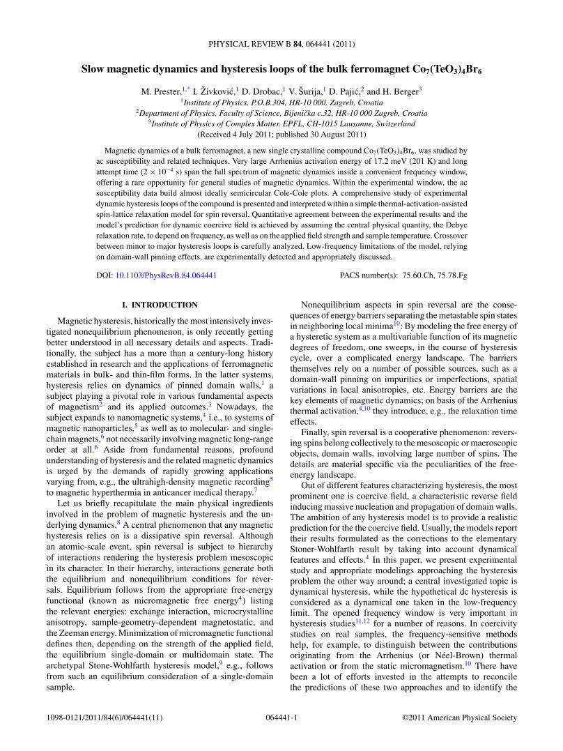
In order to clear out the nature of the ferromagnetictransition at Tc, we first show in Fig. 1 a set of dynamichysteresis loops of Co7(TeO3)4Br6 (discussed at length inthe next sections). In the transition region, these loops weretaken within a narrow, 0.14 K-wide, temperature interval.Ferromagnetic order parameter (saturation magnetization)builds up its low-temperature (4.2-K) value practically within0.1 K, illustrating the first-order character of the ferromag-netic transition.15 This means that the magnetocrystallineanisotropy, which inherits its temperature dependence fromthe temperature-dependent saturation magnetization,16 is fullydeveloped already at 27 K and barely changes by loweringtemperature below 27 K. Simultaneously with anisotropyand bulk magnetization, it is clear from the first principles9

that magnetic domains and the domain walls set in andself-organize just below Tc, in order to keep the magnetic freeenergy minimal.9 The domain pattern then responds to anychanges in the parameter values by dissipative domain-wallrearrangements.

FIG. 1. Dynamic hysteresis loops of Co7(TeO3)4Br6 taken atseveral temperatures within the ferromagnetic transition. Numbersadjacent to the loops designate the temperatures. A small hysteresisasymmetry (a shift to the left) is commented in Sec. IV.

064441-2

SLOW MAGNETIC DYNAMICS AND HYSTERESIS LOOPS . . . PHYSICAL REVIEW B 84, 064441 (2011)

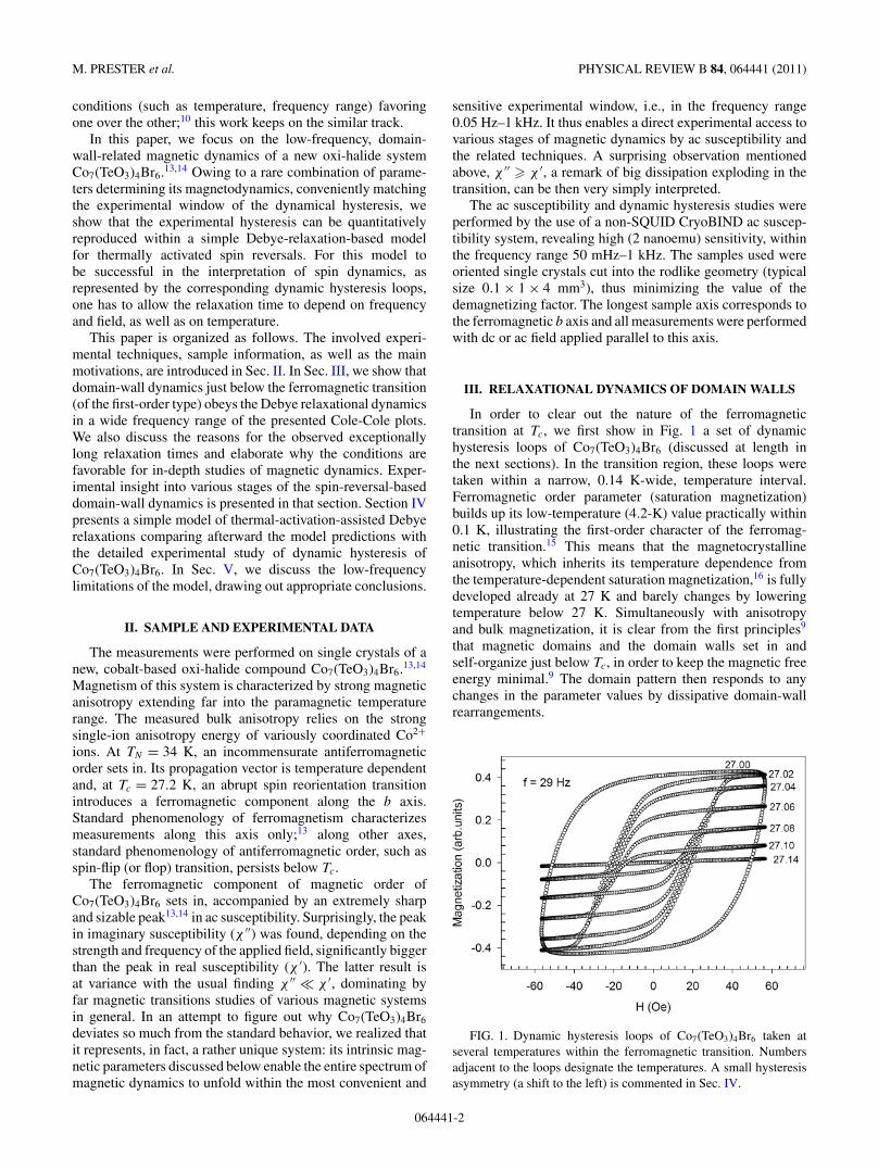
FIG. 2. (Color online) Frequency dependence of χ ′ (open sym-bols) and χ ′′ (solid symbols) of Co7(TeO3)4Br6 just below Tc =27.2 K (main panel). Solid lines are fits to the standard expressions forthe relaxing complex susceptibility (Ref. 9) [Eq. (3)] with the additionof a prefactor in the formula for χ ′′ to account for its asymmetry.Dynamic hysteresis and dissipation scans were measured in the tailarea characterized by χ ′′ > χ ′. The inset shows the same data fromthe main panel but plotted in the χ ′,χ ′′ diagram; the data are nowcollapsed on the single Cole-Cole semicircle.

A. Cole-Cole plots

Frequency dependence of ac susceptibility χ (ω) providesthe most elementary insight into magnetic dynamics of orderedsystems. Figure 2 shows the frequency dependence of thesusceptibility components χ ′(ω),χ ′′(ω) of Co7(TeO3)4Br6

crystal taken at several temperatures below Tc. This plotprovides a detailed insight into magnetic dynamics of thecompound. The type of response shown in Fig. 2 indicatesthat the responsible magnetic subsystem, in its response to theapplied field, interacts strongly with the lattice: the pattern ofχ ′(ω,T ),χ ′′(ω,T ) curves is reminiscent of a simple Debye-type spin-lattice relaxation.9 Indeed, the χ ′(ω,T ),χ ′′(ω,T )data, if presented in the form of the Cole-Cole plot,17 i.e.,as the functional form χ ′′(χ ′) (Fig. 2 inset), all collapseon a somewhat distorted Debye semicircle (common forall temperatures within the range18). The ideal semicircle,a fingerprint17 of single relaxation time τ , intersects thehorizontal χ ′ axis in the values of adiabatic χS (=0, ω → ∞)and isothermal χT (ω → 0) susceptibility.18

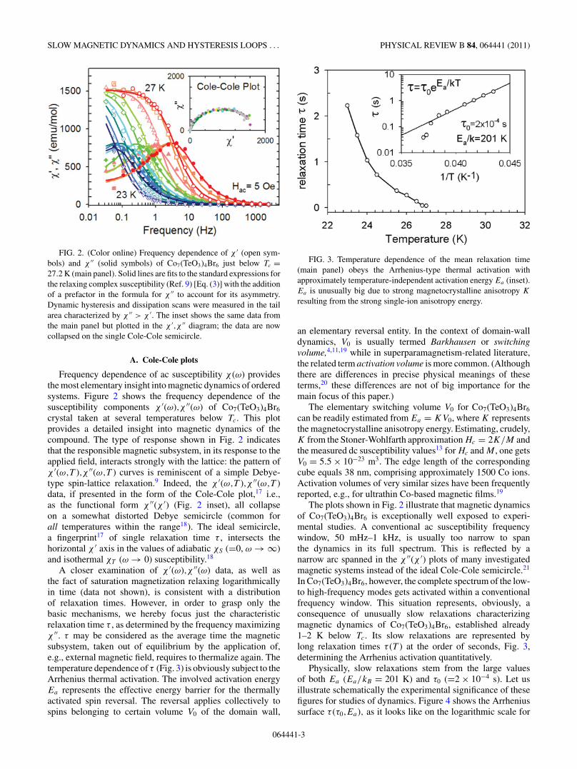
A closer examination of χ ′(ω),χ ′′(ω) data, as well asthe fact of saturation magnetization relaxing logarithmicallyin time (data not shown), is consistent with a distributionof relaxation times. However, in order to grasp only thebasic mechanisms, we hereby focus just the characteristicrelaxation time τ , as determined by the frequency maximizingχ ′′. τ may be considered as the average time the magneticsubsystem, taken out of equilibrium by the application of,e.g., external magnetic field, requires to thermalize again. Thetemperature dependence of τ (Fig. 3) is obviously subject to theArrhenius thermal activation. The involved activation energyEa represents the effective energy barrier for the thermallyactivated spin reversal. The reversal applies collectively tospins belonging to certain volume V0 of the domain wall,

FIG. 3. Temperature dependence of the mean relaxation time(main panel) obeys the Arrhenius-type thermal activation withapproximately temperature-independent activation energy Ea (inset).Ea is unusually big due to strong magnetocrystalline anisotropy K

resulting from the strong single-ion anisotropy energy.

an elementary reversal entity. In the context of domain-walldynamics, V0 is usually termed Barkhausen or switchingvolume,4,11,19 while in superparamagnetism-related literature,the related term activation volume is more common. (Althoughthere are differences in precise physical meanings of theseterms,20 these differences are not of big importance for themain focus of this paper.)

The elementary switching volume V0 for Co7(TeO3)4Br6

can be readily estimated from Ea = KV0, where K representsthe magnetocrystalline anisotropy energy. Estimating, crudely,K from the Stoner-Wohlfarth approximation Hc = 2K/M andthe measured dc susceptibility values13 for Hc and M , one getsV0 = 5.5 × 10−23 m3. The edge length of the correspondingcube equals 38 nm, comprising approximately 1500 Co ions.Activation volumes of very similar sizes have been frequentlyreported, e.g., for ultrathin Co-based magnetic films.19

The plots shown in Fig. 2 illustrate that magnetic dynamicsof Co7(TeO3)4Br6 is exceptionally well exposed to experi-mental studies. A conventional ac susceptibility frequencywindow, 50 mHz–1 kHz, is usually too narrow to spanthe dynamics in its full spectrum. This is reflected by anarrow arc spanned in the χ ′′(χ ′) plots of many investigatedmagnetic systems instead of the ideal Cole-Cole semicircle.21

In Co7(TeO3)4Br6, however, the complete spectrum of the low-to high-frequency modes gets activated within a conventionalfrequency window. This situation represents, obviously, aconsequence of unusually slow relaxations characterizingmagnetic dynamics of Co7(TeO3)4Br6, established already1–2 K below Tc. Its slow relaxations are represented bylong relaxation times τ (T ) at the order of seconds, Fig. 3,determining the Arrhenius activation quantitatively.

Physically, slow relaxations stem from the large valuesof both Ea (Ea/kB = 201 K) and τ0 (=2 × 10−4 s). Let usillustrate schematically the experimental significance of thesefigures for studies of dynamics. Figure 4 shows the Arrheniussurface τ (τ0,Ea), as it looks like on the logarithmic scale for

064441-3

M. PRESTER et al. PHYSICAL REVIEW B 84, 064441 (2011)

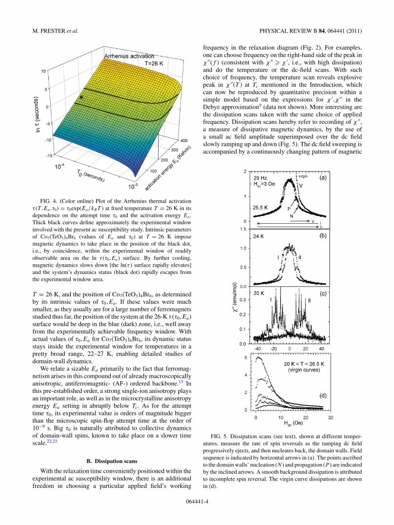
FIG. 4. (Color online) Plot of the Arrhenius thermal activationτ (T ,Ea,τ0) = τ0exp(Ea/kBT ) at fixed temperature T = 26 K in itsdependence on the attempt time τ0 and the activation energy Ea .Thick black curves define approximately the experimental windowinvolved with the present ac susceptibility study. Intrinsic parametersof Co7(TeO3)4Br6 (values of Ea and τ0) at T = 26 K imposemagnetic dynamics to take place in the position of the black dot,i.e., by coincidence, within the experimental window of readilyobservable area on the ln τ (τ0,Ea) surface. By further cooling,magnetic dynamics slows down [the ln(τ ) surface rapidly elevates]and the system’s dynamics status (black dot) rapidly escapes fromthe experimental window area.

T = 26 K, and the position of Co7(TeO3)4Br6, as determinedby its intrinsic values of τ0,Ea . If these values were muchsmaller, as they usually are for a large number of ferromagnetsstudied thus far, the position of the system at the 26-K τ (τ0,Ea)surface would be deep in the blue (dark) zone, i.e., well awayfrom the experimentally achievable frequency window. Withactual values of τ0,Ea for Co7(TeO3)4Br6, its dynamic statusstays inside the experimental window for temperatures in apretty broad range, 22–27 K, enabling detailed studies ofdomain-wall dynamics.

We relate a sizable Ea primarily to the fact that ferromag-netism arises in this compound out of already macroscopicallyanisotropic, antiferromagntic- (AF-) ordered backbone.13 Inthis pre-established order, a strong single-ion anisotropy playsan important role, as well as in the microcrystalline anisotropyenergy Ea setting in abruptly below Tc. As for the attempttime τ0, its experimental value is orders of magnitude biggerthan the microscopic spin-flop attempt time at the order of10−9 s. Big τ0 is naturally attributed to collective dynamicsof domain-wall spins, known to take place on a slower timescale.22,23

B. Dissipation scans

With the relaxation time conveniently positioned within theexperimental ac susceptibility window, there is an additionalfreedom in choosing a particular applied field’s working

frequency in the relaxation diagram (Fig. 2). For examples,one can choose frequency on the right-hand side of the peak inχ ′′(f ) (consistent with χ ′′ � χ ′, i.e., with high dissipation)and do the temperature or the dc-field scans. With suchchoice of frequency, the temperature scan reveals explosivepeak in χ ′′(T ) at Tc mentioned in the Introduction, whichcan now be reproduced by quantitative precision within asimple model based on the expressions for χ ′,χ ′′ in theDebye approximation9 (data not shown). More interesting arethe dissipation scans taken with the same choice of appliedfrequency. Dissipation scans hereby refer to recording of χ ′′,a measure of dissipative magnetic dynamics, by the use ofa small ac field amplitude superimposed over the dc fieldslowly ramping up and down (Fig. 5). The dc field sweeping isaccompanied by a continuously changing pattern of magnetic

FIG. 5. Dissipation scans (see text), shown at different temper-atures, measure the rate of spin reversals as the ramping dc fieldprogressively ejects, and then nucleates back, the domain walls. Fieldsequence is indicated by horizontal arrows in (a). The points ascribedto the domain walls’ nucleation (N ) and propagation (P ) are indicatedby the inclined arrows. A smooth background dissipation is attributedto incomplete spin reversal. The virgin curve dissipations are shownin (d).

064441-4

SLOW MAGNETIC DYNAMICS AND HYSTERESIS LOOPS . . . PHYSICAL REVIEW B 84, 064441 (2011)

domains through processes of domain nucleation and/ordomain-wall propagation. On atomic scale, these processes areunderlined by dissipative spin reversals. Thus, the dissipativescans tell directly about the average rate of spin reversals insuccessive stages of domain-wall dynamics, otherwise takingplace in standard dc hysteresis cycling.

In the scan-starting condition of a zero-field-cooled sampleat Hdc = 0, necessarily composed of equal number of +M

and −M domains, the measured dissipation was already at ahigh initial level [Fig. 5(a)]. To achieve the highest possiblerate of spin reversals, application of a small temperature-dependent dc field is obviously required [Fig. 5(d)]. Wespeculate that a maximum in dissipation is achieved afterthe field supplies enough magnetic energy to overcome aweak domain-wall pinning energy. In the virgin curve, arapid dissipation decay indicates ejection of the domain wallsout of the sample, rendering it single domain and revealingjust residual dissipation afterwards. In the field backswing,reversed domains start nucleating again and further dissipationevolves through propagation of the domain walls as well. Bothprocesses are integrated into the “dissipation dome” structure(Fig. 5). The temperature-dependent positions of the maximacan naturally be identified with the coercive field Hc(T ). TheHc(T ) values, being small immediately below Tc but welldefined, are in good quantitative agreement with the dc-SQUIDHc(T ) data.13

The structure of the dissipation dome indicates not onlyon the activation of the dissipative nucleation and propagationmodes, but also on the importance of thermal activation. Afterbeing expelled from the sample, the domain renucleation relieson overcoming the anisotropy-related energy barriers for spinreversal of the activation volume. This obviously takes placewith the most frequent rate at Hc revealing, naturally, the fieldstrengths being negative in sign (in the field first backswing).But, one also notes, for loops taken at T = 26.5 and 24 K, thatthe very onset of nucleation takes place already for positivefield values. Domain nucleation in positive field can onlyrely on thermally induced reversals of the activation volumes.The latter finding provides an independent argument favoringthe importance of thermal activation in studies of magneticdynamics in Co7(TeO3)4Br6. Figure 5 also shows that, unlikethe domain-wall ejection from the virgin state, the Hc buildupis not a smooth process. Obviously, at lower temperatures, itprogresses via erratic, perhaps avalanche-based, mechanismwhich is not well understood as yet (and is not elaborated inthis work any further).

IV. DYNAMIC HYSTERESIS LOOPS OF Co7(TeO3)4Br6

Now, we present a more detailed study of the evolution ofmagnetic dynamics in Co7(TeO3)4Br6. One way to do it, asshown in the studies on ultrathin films,24,25 would consist ofcollecting a set of the Cole-Cole plots for different Hac. Inour work, however, the magnetic dynamics was studied moredirectly by measuring the induction-type dynamic hysteresisresponding to the sinusoidal applied field Hac = H0 sin ωt .The M-H loops were determined at different temperatures andstudied as functions of the field amplitude H0 and frequency ω.

Magnetization M(t) of the sample was determined by fastdigital acquisition of voltage Vind(t), induced in the highly

FIG. 6. An example of dynamic hysteresis measurement onCo7(TeO3)4Br6 in the time domain. Magnetic field pulse Hac(t)and the induced voltage Vind(t) (circles) are measured and recordeddirectly while magnetization [M(t) (triangles)] is obtained bynumerical integration of Vind(t). The phase shift between Hac(t) andM(t) brings a direct information on the involved magnetic dynamics(see text). All quantities are plotted scaled by their maximal values.

balanced secondary coil of our ac susceptometer by theapplication of sinusoidal current through the primary. By virtueof Faraday law, Vind(t) ∼ dφ/dt ∼ dM/dt . Figure 6 showsthe relevant signals in the time domain.

The period of the applied pulse was varied within therange 1 ms–1 s, enabling studies of magnetic dynamics on the1 Hz–1 kHz frequency scale. In order to improve statistics, theidentical subsequent strings of Vind(t) data were appropriatelyaveraged. Depending on the field frequency, averaging takes1–100 s, enabling continuous measurements of appropriatelyaveraged Vind(t) data in the course of a slow temperature drift.The field signal Hac(t) was taken by recording voltage onthe standard resistor connected in series with the primarycoil. In numerical elaboration of the data, taken afterward,magnetization M[= ∫

Vind(t)dt] was obtained by numericalintegration and subtraction of the background. M(t) is thenplotted versus Hac(t) to get the hysteresis loops in theirtemperature evolution.

In Fig. 7, a set of representative dynamic hysteresis dataon Co7(TeO3)4Br6 is shown. At fixed chosen frequencies andmeasurement temperatures, a sequence of loops were taken inincreasing magnetic field amplitudes, defining a broad rangeof conditions for dissipative spin reversals.

Referring to the loop dependence on H0, there is obviouslya crossover between the two generic loop types, i.e., betweenthe minor loops for small values of H0 and, in increasingH0, the major loops revealing characteristic “whiskers.” Asit is generally well understood,2 minor loops correspond todomain-wall dynamics taking place in the limit of infinitesample size, while the major ones correspond to saturation tothe sample-size-limited total magnetization. In the whiskerlikehysteresis regions, domain walls are entirely ejected out of thesample, thus, any dynamics calms down in the whisker region.During the cycle, dynamics reappears again within the reversedmagnetic field swing. It is then underlined by back nucleationand propagation of domain walls. The activation energies

064441-5

M. PRESTER et al. PHYSICAL REVIEW B 84, 064441 (2011)

FIG. 7. (Color online) Experimental, induction-type dynamichysteresis on a 2.9-mg single crystal taken with sinusoidal magneticfield pulses varying in amplitudes (5–100 Oe RMS). Calibration toabsolute units was performed by the use of dc susceptibility results.The pulse widths were t = 34 ms and t = 0.59 s, shown in panels (a),(c), (d), and (b), respectively. At higher frequencies (29 Hz), the loops(generic ellipses) are characteristically horizontally aligned [panel(c)], reflecting fulfillment of the condition χ ′′ � χ ′ (see text). Atlower temperatures, the domain-wall propagation does not reach thesample boundaries within the available field amplitudes. All aspectsof magnetic dynamics are revealed in the set of 29-Hz hysteresis loopsat different temperatures, shown in (d), including the collapse of orderparameter for T passing through Tc. The loops are also characterizedby small asymmetry, commented in the text.

involved with minor and major loops are not identical; whilethe domain-wall propagation is mostly involved with the minorloops, the major loops rely, aside from propagation, on thedomain-wall nucleation.19,26 Thus, the dynamical features ofminor and major loops are expected to be at least quantitativelydifferent. The details of these differences, showing up ina continuous transformation of minor into major loops inincreasing H0, are presented and analyzed in this paper.

Hereby, we pay particular attention to the phenomenologyof minor loops, attracting recently a pronounced renewedinterest.12,27 As illustrated in Fig. 7(c) and elaborated below,the minor loop is a generic ellipsis, the parameters of whichdepend sensitively on the applied field magnitude H0, itsfrequency f , and the sample temperature T . To the best ofour knowledge, the detailed elaboration of the latter aspectsof magnetic dynamics has not been presented so far for anyferromagnetic system. For this purpose, we first introduce asimple model for minor loops. Then, in the next section, weshow the model to be in sound qualitative and quantitativeagreement with the presented experimental investigations ofmagnetic dynamics of Co7(TeO3)4Br6.

A. Model for minor hysteresis loops

For the sake of interpretation of the experimental loops,we first invoke the simplest phenomenological concept ofhysteretic behavior in general: macroscopic “response” of ahysteretic system (i.e., magnetization in our case) lags behind

FIG. 8. Coercive field factor h(ω,τ ) ≡ ωτ/√

1 + ω2τ 2 for threerepresentative values of τ , effective in thermal activation ofCo7(TeO3)4Br6 at approximately 24, 26.5, and 27 K, have beenselected for the plots. Inset: Magnetization vs applied field fromEq. (1), normalized to respective amplitude values H0,M0, for severalchosen values of the phase-shift parameter φ (numbers adjacent toeach loop).

the “external probe” (i.e., instantaneous value of the appliedmagnetic field) for the phase shift φ. Thus, the magnetizationM(t), lagging behind the field H (t), reads as

H (t) = H0 sin ωt,

M(t) = M0 sin(ωt − φ) = M0 cosφ sin ωt −−M0 sinφ cos ωt. (1)

If one then defines the in-phase and the out-of-phase sus-ceptibility components as χ ′ = (M0/H0) cos φ and χ ′′ =(M0/H0) sin φ, respectively, the magnetization becomes

M(t) = χ ′H0 sin ωt − χ ′′H0 cos ωt. (2)

The phase shift is now determined as the ratio of the twosusceptibility components tanφ = χ ′′/χ ′.

At this stage, it is instructive to visualize several charac-teristic M(H ) plots for several chosen values of φ. In theinset to Fig. 8, we show the corresponding M(t),H (t) values[for t treated as an implicit variable in Eq. (1)], revealingthe hysteretic M-H loops. The loops are represented bygeneric ellipses tilted with respect to the H axis for an angledetermined by the phase factor φ.

The latter simple model for hysteresis loops is very generalas no assumption for the involved type of magnetization(irrespective if it is of paramagnetic, ferromagnetic, super-paramagnetic,..., origin), nor for the involved phase-laggingmechanism, has been introduced. It, however, strictly appliesonly to the case of linear magnetic response, i.e., to M0 beingindependent on H0, a condition ascribed to minor loop regime.We focus our elaboration now on the specific dynamics ofdomain walls in Co7(TeO3)4Br6. As shown in Sec. III, thelatter dynamics fits nicely the model of Arrhenius-Brown-Neelthermal activation. Within the latter model, the dissipative spinreversal is thermally activated, thus, it is natural to assumethat thermal activation plays an important role in hysteresis

064441-6

SLOW MAGNETIC DYNAMICS AND HYSTERESIS LOOPS . . . PHYSICAL REVIEW B 84, 064441 (2011)

formation as well; hereby, we think of dc hysteresis as thedc limits of the frequency-dependent dynamic hysteresis.The general model of dynamic hysteresis becomes specificonce the phase parameter φ gets defined. We thereforeintroduce the phase relationship inherent to the domain-wall-related relaxational dynamics. In its simplest Debye form(single relaxation time τ ) and within the Casimir-du Preapproximation, this dynamics is represented by the well-known nonresonant magnetic susceptibility form9

χ ′ = χS + χT − χS

1 + ω2τ 2,

(3)

χ ′′ = (χT − χS)ωτ

1 + ω2τ 2.

In this simple linear response theory approach, all physicsof the system is condensed in the phenomenological constantτ , which, in turn, can depend on a number of microscopicand macroscopic parameters. Remaining consistently at thephenomenological level, one can put now the phase shift φ, aquantity decisive for the shape of general hysteresis (inset toFig. 8), on physical grounds by relating it to the relaxation timeτ : Taking for adiabatic susceptibility χS = 0 (in accordancewith our experimental data), one gets28 from Eq. (3) that theDebye-Casimir-du Pres relaxation implies tanφ = χ ′′/χ ′ =ωτ , thus, φ = arctan ωτ .

One naturally asks to what extent the experimental detailsof dynamical hysteresis of Co7(TeO3)4Br6 shown in Fig. 7 canbe described by such a model. As a demanding test, one maylook for coercive field and its dependence on the strength andthe frequency of the applied magnetic fields. In this paper,the term “coercive field” is used strictly in the context ofdynamical hysteresis loops; the corresponding values differ alot from the technical coercive fields, usually extracted fromthe dc magnetic hysteresis on samples reaching magneticsaturation. Similarly as for the dc hysteresis, we define the(dynamic) coercive field Hc simply as M(Hc) = 0. As onereads from Eq. (1), magnetization extinguishes wheneverωt = φ, i.e., disregarding the periodicity, at instant tc = φ/ω.The corresponding field value (i.e., coercive field) is

H (tc) = Hc(ω,τ ) = H0 sin ωtc = H0 sinφ

= H0 sin arctan ωτ = H0 sin arcsinωτ√

1 + ω2τ 2

= H0ωτ√

1 + ω2τ 2. (4)

Equation (4) represents the operative result of this simplemodel, which can be tested now on the experimental dynamichysteresis curves.

Depending on the frequency of the applied field, thereare obviously two limits. In the limit of a long measure-ment period with respect to the relaxation time (hysteresisat low frequencies, ωτ � 1), Eq. (4) implies Hc ≈ H0ωτ .Hysteresis axis is then approximately aligned along the lineM(H ) = M0H in the M-H plot (cf. inset to Fig. 8). In theopposite limit of short measurement period (high frequencies,ωτ � 1), Eq. (4) implies Hc ≈ H0 and the phase laggingapproaches its maximum value φ ≈ π/2; the hysteresis axisis then horizontally aligned (cf. inset to Fig. 8). The mainpanel of Fig. 8 shows the frequency dependence of the

factor h(ω,τ ) ≡ ωτ/√

1 + ω2τ 2, which rules, at fixed τ , thefrequency dependence of Hc in this model [Eq. (4)].

Invoking now our experimental dynamic hysteresis (Fig. 7),one easily notes that there is at least qualitative accordance: Achange in hysteresis alignment, from a steep almost verticalone [Fig. 7(b)] to the horizontally aligned one [Fig. 7(c)],can naturally be interpreted as transformation in measuringconditions introducing a crossover between the low- to high-frequency limits in the presented model.

Summarizing the physical ingredients built-in in thisdynamic hysteresis model, we note that these ingredientsare identical to those underlying the standard spin-latticerelaxation model9 for χ ′,χ ′′, usually presented in the form ofthe Cole-Cole plots (see Sec. III A). Thus, dynamic hysteresisstudies, interpreted within this model, could represent amethod alternate and/or complementary to the usual spin-lattice χ ′,χ ′′ route. For example, Eq. (4) offers, in its low-frequency limit, the relaxation rate τ to be extracted from themeasurements of Hc. Especially in measurements looking fortemperature dependence of τ , the dynamic hysteresis routemight turn out to be advantageous.

Referring again to all our experimental dynamical hystere-sis (Figs. 1, 7, and 10), one notes a small but systematic shiftof the hysteresis body (at the amount of a few Oersted) tothe left. Thus, if one defines H−

c and H+c as the coercive

fields for the field-down and the field-up hysteresis branches,respectively, one notes | H−

c |>| H+c |. One reason for the loop

asymmetry could be a b axis component of the Earth’s field,not compensated in the presented experiments. Hysteresisshift of typically 3–5 Oe would, however, be difficult tointerpret on the basis of the interference with the Earth’sfield (approximately 0.3 Oe). Another possible reason for theloop asymmetry might rely on the fact that a subject b-axisferromagnetism in Co7(TeO3)4Br6 represents just a componentof the global antiferromagnetic order. We thus speculate thata scenario similar to the one valid in the exchange-biasedstructures, revealing characteristic hysteresis shifts, might be

FIG. 9. Temperature dependence of Hc as determined from thedynamical hysteresis curves collected during a slow temperature drift[such as those shown in Fig. 7(d)]. Some sample dependence hasbeen observed in the Hc(T ) measured on different samples. The solidline is a guide to the eye.

064441-7

M. PRESTER et al. PHYSICAL REVIEW B 84, 064441 (2011)

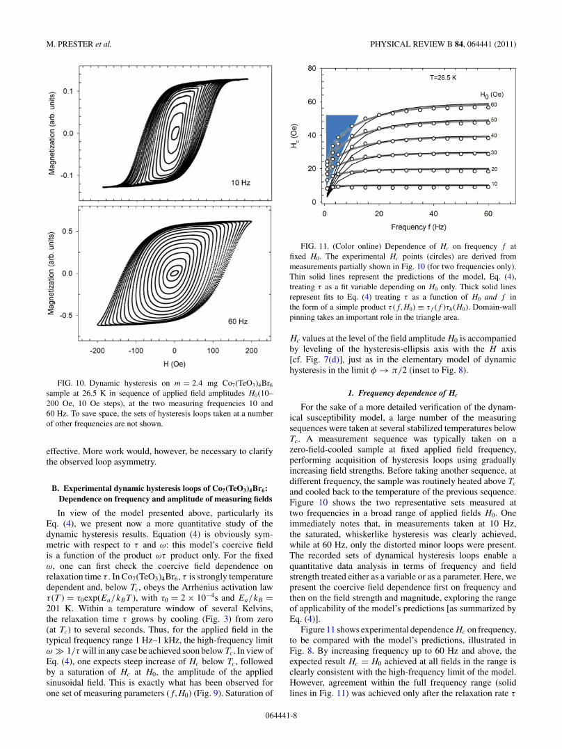
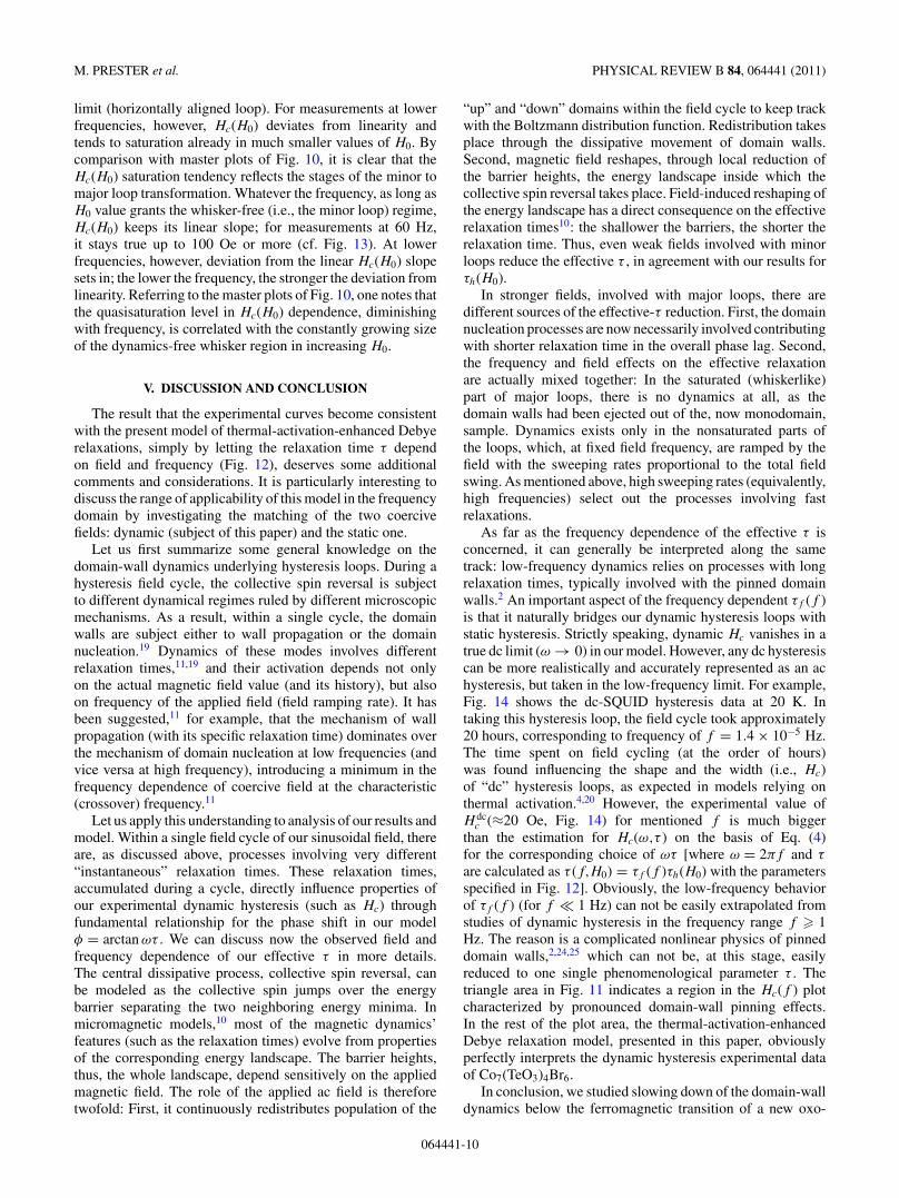
FIG. 10. Dynamic hysteresis on m = 2.4 mg Co7(TeO3)4Br6

sample at 26.5 K in sequence of applied field amplitudes H0(10–200 Oe, 10 Oe steps), at the two measuring frequencies 10 and60 Hz. To save space, the sets of hysteresis loops taken at a numberof other frequencies are not shown.

effective. More work would, however, be necessary to clarifythe observed loop asymmetry.

B. Experimental dynamic hysteresis loops of Co7(TeO3)4Br6:Dependence on frequency and amplitude of measuring fields

In view of the model presented above, particularly itsEq. (4), we present now a more quantitative study of thedynamic hysteresis results. Equation (4) is obviously sym-metric with respect to τ and ω: this model’s coercive fieldis a function of the product ωτ product only. For the fixedω, one can first check the coercive field dependence onrelaxation time τ . In Co7(TeO3)4Br6, τ is strongly temperaturedependent and, below Tc, obeys the Arrhenius activation lawτ (T ) = τ0exp(Ea/kBT ), with τ0 = 2 × 10−4s and Ea/kB =201 K. Within a temperature window of several Kelvins,the relaxation time τ grows by cooling (Fig. 3) from zero(at Tc) to several seconds. Thus, for the applied field in thetypical frequency range 1 Hz–1 kHz, the high-frequency limitω � 1/τ will in any case be achieved soon below Tc. In view ofEq. (4), one expects steep increase of Hc below Tc, followedby a saturation of Hc at H0, the amplitude of the appliedsinusoidal field. This is exactly what has been observed forone set of measuring parameters (f,H0) (Fig. 9). Saturation of

FIG. 11. (Color online) Dependence of Hc on frequency f atfixed H0. The experimental Hc points (circles) are derived frommeasurements partially shown in Fig. 10 (for two frequencies only).Thin solid lines represent the predictions of the model, Eq. (4),treating τ as a fit variable depending on H0 only. Thick solid linesrepresent fits to Eq. (4) treating τ as a function of H0 and f inthe form of a simple product τ (f,H0) ≡ τf (f )τh(H0). Domain-wallpinning takes an important role in the triangle area.

Hc values at the level of the field amplitude H0 is accompaniedby leveling of the hysteresis-ellipsis axis with the H axis[cf. Fig. 7(d)], just as in the elementary model of dynamichysteresis in the limit φ → π/2 (inset to Fig. 8).

1. Frequency dependence of Hc

For the sake of a more detailed verification of the dynam-ical susceptibility model, a large number of the measuringsequences were taken at several stabilized temperatures belowTc. A measurement sequence was typically taken on azero-field-cooled sample at fixed applied field frequency,performing acquisition of hysteresis loops using graduallyincreasing field strengths. Before taking another sequence, atdifferent frequency, the sample was routinely heated above Tc

and cooled back to the temperature of the previous sequence.Figure 10 shows the two representative sets measured attwo frequencies in a broad range of applied fields H0. Oneimmediately notes that, in measurements taken at 10 Hz,the saturated, whiskerlike hysteresis was clearly achieved,while at 60 Hz, only the distorted minor loops were present.The recorded sets of dynamical hysteresis loops enable aquantitative data analysis in terms of frequency and fieldstrength treated either as a variable or as a parameter. Here, wepresent the coercive field dependence first on frequency andthen on the field strength and magnitude, exploring the rangeof applicability of the model’s predictions [as summarized byEq. (4)].

Figure 11 shows experimental dependence Hc on frequency,to be compared with the model’s predictions, illustrated inFig. 8. By increasing frequency up to 60 Hz and above, theexpected result Hc = H0 achieved at all fields in the range isclearly consistent with the high-frequency limit of the model.However, agreement within the full frequency range (solidlines in Fig. 11) was achieved only after the relaxation rate τ

064441-8

SLOW MAGNETIC DYNAMICS AND HYSTERESIS LOOPS . . . PHYSICAL REVIEW B 84, 064441 (2011)

.

FIG. 12. Plots of the single-variable functions τf (f ) and τh(H0)used in heuristic expression for τ , τ (f,H0) = τf (f )τh(H0). Thesefunctions are used to interpret the experimental Hc(f ) and Hc(H0)points (Figs. 11 and 13, respectively).

was assumed to represent not only a function of temperature,but also a function of frequency and magnitude of theapplied field, thus, τ = τ (T ,f,H0). The physical backgroundbehind this assumption is discussed in the next section. The

FIG. 13. Coercive field Hc as a function of applied field am-plitudes H0 for three measuring frequencies. The plots are derivedfrom measurements shown in Fig. 10. Solid lines represent the Hc

values calculated from Eq. (4) using the same τ (f,H0) functionaldependence involved in the thick-line fit specified in Fig. 11, with theparameters listed in Fig. 12.

fitting procedure was performed in two steps. First, the bestpossible agreement between the experimental Hc(f ) pointsand Eq. (4) was found assuming τ to depend only on H0

in the form of a simple second-degree polynomial in H0

(thin solid lines in Fig. 11). While for frequencies above15–20 Hz the thin lines, representing the Hc(f ) valuescalculated from Eq. (4), are in sound agreement with theexperimental Hc(f ) points, there are large deviations inthe low-frequency range. Frequency dependence of τ wastherefore introduced as well by assuming a heuristic expressionfor τ , τ (f,H0) = τh(H0)τf (f ). With τf (f ) and τh(H0) both inthe form of second-degree polynomial, there is obviously a fullagreement between the experimental points and the predictionof the model for the Hc(f ) dependence extending in the wholefrequency range. The analytical forms for τh(H0) and τf (f ),found to give the best fit, are shown in Fig. 12. We note thatthe τh(H0) depends, to a large extent, on the applied H0 range;if a wider range were applied, the fit parameters of τh wouldbe very different.

2. Dependence of Hc on the field magnitude: Minor to majorhysteresis loop crossover

Focusing primarily on the minor loop mechanisms, wewere focusing, up to now, on the low-field regime (far frommagnetic saturation). Now, we want to extend our results tohigher fields. Instead of presenting the frequency dependenceof Hc, it is instructive to plot the dependence of Hc on theapplied field magnitude H0 for fixed frequencies. Figure 13shows the Hc(H0) dependence in the broad range (up to200 Oe) of H0 at the three frequencies, as extracted fromFig. 10 data. Within this field range, transformation of minorinto the major hysteresis loops inevitably takes place (Figs. 7and 10). Deviation of the experimental points in Fig. 13 fromthe present minor loop model (solid lines) can naturally beinterpreted as a consequence of the latter transformation. At thehighest frequency (60 Hz), the functional form Hc = Hc(H0)is not only linear, but the simple equality Hc = H0 holds,up to high values of H0. Such a behavior is fully consistentwith the model’s prediction in the high-frequency (ωτ � 1)

FIG. 14. The dc SQUID hysteresis of Co7(TeO3)4Br6 at 20 K.Field cycle time took approximately 20 hours.

064441-9

M. PRESTER et al. PHYSICAL REVIEW B 84, 064441 (2011)

limit (horizontally aligned loop). For measurements at lowerfrequencies, however, Hc(H0) deviates from linearity andtends to saturation already in much smaller values of H0. Bycomparison with master plots of Fig. 10, it is clear that theHc(H0) saturation tendency reflects the stages of the minor tomajor loop transformation. Whatever the frequency, as long asH0 value grants the whisker-free (i.e., the minor loop) regime,Hc(H0) keeps its linear slope; for measurements at 60 Hz,it stays true up to 100 Oe or more (cf. Fig. 13). At lowerfrequencies, however, deviation from the linear Hc(H0) slopesets in; the lower the frequency, the stronger the deviation fromlinearity. Referring to the master plots of Fig. 10, one notes thatthe quasisaturation level in Hc(H0) dependence, diminishingwith frequency, is correlated with the constantly growing sizeof the dynamics-free whisker region in increasing H0.

V. DISCUSSION AND CONCLUSION

The result that the experimental curves become consistentwith the present model of thermal-activation-enhanced Debyerelaxations, simply by letting the relaxation time τ dependon field and frequency (Fig. 12), deserves some additionalcomments and considerations. It is particularly interesting todiscuss the range of applicability of this model in the frequencydomain by investigating the matching of the two coercivefields: dynamic (subject of this paper) and the static one.

Let us first summarize some general knowledge on thedomain-wall dynamics underlying hysteresis loops. During ahysteresis field cycle, the collective spin reversal is subjectto different dynamical regimes ruled by different microscopicmechanisms. As a result, within a single cycle, the domainwalls are subject either to wall propagation or the domainnucleation.19 Dynamics of these modes involves differentrelaxation times,11,19 and their activation depends not onlyon the actual magnetic field value (and its history), but alsoon frequency of the applied field (field ramping rate). It hasbeen suggested,11 for example, that the mechanism of wallpropagation (with its specific relaxation time) dominates overthe mechanism of domain nucleation at low frequencies (andvice versa at high frequency), introducing a minimum in thefrequency dependence of coercive field at the characteristic(crossover) frequency.11

Let us apply this understanding to analysis of our results andmodel. Within a single field cycle of our sinusoidal field, thereare, as discussed above, processes involving very different“instantaneous” relaxation times. These relaxation times,accumulated during a cycle, directly influence properties ofour experimental dynamic hysteresis (such as Hc) throughfundamental relationship for the phase shift in our modelφ = arctan ωτ . We can discuss now the observed field andfrequency dependence of our effective τ in more details.The central dissipative process, collective spin reversal, canbe modeled as the collective spin jumps over the energybarrier separating the two neighboring energy minima. Inmicromagnetic models,10 most of the magnetic dynamics’features (such as the relaxation times) evolve from propertiesof the corresponding energy landscape. The barrier heights,thus, the whole landscape, depend sensitively on the appliedmagnetic field. The role of the applied ac field is thereforetwofold: First, it continuously redistributes population of the

“up” and “down” domains within the field cycle to keep trackwith the Boltzmann distribution function. Redistribution takesplace through the dissipative movement of domain walls.Second, magnetic field reshapes, through local reduction ofthe barrier heights, the energy landscape inside which thecollective spin reversal takes place. Field-induced reshaping ofthe energy landscape has a direct consequence on the effectiverelaxation times10: the shallower the barriers, the shorter therelaxation time. Thus, even weak fields involved with minorloops reduce the effective τ , in agreement with our results forτh(H0).

In stronger fields, involved with major loops, there aredifferent sources of the effective-τ reduction. First, the domainnucleation processes are now necessarily involved contributingwith shorter relaxation time in the overall phase lag. Second,the frequency and field effects on the effective relaxationare actually mixed together: In the saturated (whiskerlike)part of major loops, there is no dynamics at all, as thedomain walls had been ejected out of the, now monodomain,sample. Dynamics exists only in the nonsaturated parts ofthe loops, which, at fixed field frequency, are ramped by thefield with the sweeping rates proportional to the total fieldswing. As mentioned above, high sweeping rates (equivalently,high frequencies) select out the processes involving fastrelaxations.

As far as the frequency dependence of the effective τ isconcerned, it can generally be interpreted along the sametrack: low-frequency dynamics relies on processes with longrelaxation times, typically involved with the pinned domainwalls.2 An important aspect of the frequency dependent τf (f )is that it naturally bridges our dynamic hysteresis loops withstatic hysteresis. Strictly speaking, dynamic Hc vanishes in atrue dc limit (ω → 0) in our model. However, any dc hysteresiscan be more realistically and accurately represented as an achysteresis, but taken in the low-frequency limit. For example,Fig. 14 shows the dc-SQUID hysteresis data at 20 K. Intaking this hysteresis loop, the field cycle took approximately20 hours, corresponding to frequency of f = 1.4 × 10−5 Hz.The time spent on field cycling (at the order of hours)was found influencing the shape and the width (i.e., Hc)of “dc” hysteresis loops, as expected in models relying onthermal activation.4,20 However, the experimental value ofH dc

c (≈20 Oe, Fig. 14) for mentioned f is much biggerthan the estimation for Hc(ω,τ ) on the basis of Eq. (4)for the corresponding choice of ωτ [where ω = 2πf and τ

are calculated as τ (f,H0) = τf (f )τh(H0) with the parametersspecified in Fig. 12]. Obviously, the low-frequency behaviorof τf (f ) (for f � 1 Hz) can not be easily extrapolated fromstudies of dynamic hysteresis in the frequency range f � 1Hz. The reason is a complicated nonlinear physics of pinneddomain walls,2,24,25 which can not be, at this stage, easilyreduced to one single phenomenological parameter τ . Thetriangle area in Fig. 11 indicates a region in the Hc(f ) plotcharacterized by pronounced domain-wall pinning effects.In the rest of the plot area, the thermal-activation-enhancedDebye relaxation model, presented in this paper, obviouslyperfectly interprets the dynamic hysteresis experimental dataof Co7(TeO3)4Br6.

In conclusion, we studied slowing down of the domain-walldynamics below the ferromagnetic transition of a new oxo-

064441-10

SLOW MAGNETIC DYNAMICS AND HYSTERESIS LOOPS . . . PHYSICAL REVIEW B 84, 064441 (2011)

halide system Co7(TeO3)4Br6 by the induction-type dynamichysteresis loops. Convenient quantitative matching of thedynamics’ time scale with the available frequency windowenabled detailed studies of minor loops in their dependenceson frequency and applied field amplitude. The presented modelfor dynamic hysteresis loops relies just on the traditionalingredients of the spin-lattice relaxation theory and on theNeel-Brown thermal activation. The very-low-frequency devi-ations of experimental results from the model predictions are

ascribed to specific physics of pinned domain walls, whichremains outside scope of this paper.

ACKNOWLEDGMENT

M.P., I. Z., D.D., and D.P. acknowledge financial supportfrom Projects No. 035-0352843-2845 and No. 119-1191458-1017 of the Croatian Ministry of Science, Education andSport.

*prester@ifs.hr1F. H. de Leeuw, R. van den Doel, and U. Enz, Rep. Prog. Phys. 43,689 (1980).

2T. Nattermann, V. Pokrovsky, and V. M. Vinokur, Phys. Rev. Lett.87, 197005 (2001), and references therein.

3L. Krusin-Elbaum, T. Schibauchi, B. Argyle, L. Gignac, andD. Wellers, Nature (London) 410, 444 (2001), and referencestherein.

4See, e.g., R. Skomski, J. Phys. Condens. Matter 15, R841 (2003),and references threin.

5N. A. Frey and S. Sun, in Inorganic Nanoparticles: Synthe-sis, Applications, and Perspectives, edited by C. Altavilla andE. Ciliberto (CRC Press, Boca Raton, FL, 2010).

6R. Sessoli, Inorg. Chim. Acta 361, 3356 (2008), and referencestherein.

7Q. A. Pankhurst, J. Connolly, S. K. Jones, and J. Dobson, J. Phys.D: Appl. Phys. 36, R167 (2003).

8With the focus on ferromagnetically ordered systems, this shortoverview does not directly apply to equilibrium properties ofmolecular or single-chain magnets (Ref. 6) (revealing no long-rangeorder, thus no domain pattern). Dynamical aspects, presentedthroughout the paper, are however equally relevant for the lattersystems as well.

9See, e.g., A. H. Morrish, The Physical Principles of Magnetism(IEEE Press, New York, 2001), p. 344.

10R. Skomski, J. Zhou, R. D. Kirby, and D. J. Sellmyer, J. Appl. Phys.99, 08B906 (2006); R. Skomski, ibid. 101, 09B104 (2007).

11See., e.g., T. A. Moore and J. A. C. Bland, J. Phys. Condens. Matter16, R1369 (2004), and the references therein.

12I. S. Poperechny, Yu. L. Raikher, and V. I. Stepanov, Phys. Rev. B82, 174423 (2010).

13M. Prester, I. Zivkovic, O. Zaharko, D. Pajic, P. Tregenna-PigRefsgott, and H. Berger, Phys. Rev. B 79, 144433 (2009).

14R. Becker, M. Johnsson, H. Berger, M. Prester, I. Zivkovic,D. Drobac, M. Miljak, and M. Herak, Solid State Sci. 8, 836(2006).

15Specific-heat measurements (K. Kiefer et al., unpublished) arefully consistent with the first-order character of the ferromagnetictransition at Tc.

16C. Zener, Phys. Rev. 96, 1335 (1954).17K. S. Cole and R. H. Cole, J. Chem. Phys. 9, 341 (1941).

18Collapse of the different-temperature Cole-Cole plots is actuallynot expected as the isothermal susceptibility χT (see text) shouldmonotonically rise by lowering temperature (Refs. 24 and 25). Weattribute the apparently temperature-independent χT to an artifactof uncertain demagnetizing field corrections. One notes a very highvalue of χT (close to 2000 emu/mol, corresponding to almost 60, inSI units), suggestive of demagnetizing factor corrections. However,the available data for the demagnetizing factor of homogeneouslymagnetized rectangular rods (in saturation) were found inapplicablefor susceptibility corrections of our multidomain sample (in lowapplied field). Thus, the intrinsic Cole-Cole plot might differto some extent from the experimental ones. In particular, thelow-frequency asymmetry might be attributed to lack of thedemagnetizing factor corrections.

19B. Raquet, R. Mamy, and J. C. Ousset, Phys. Rev. B 54, 4128(1996).

20M. P. Sharrock, J. Appl. Phys. 76, 6413 (1994).21See, e.g., N. A. Chernova, Y. Song, P. Y. Zavalij, and M. S.

Whittingham, Phys. Rev. B 70, 144405 (2004).22S. Krause, G. Herzog, T. Stapelfeldt, L. Berbil-Bautista, M. Bode,

E. Y. Vedmedenko, and R. Wiesendanger, Phys. Rev. Lett. 103,127202 (2009).

23R. H. Koch, G. Grinstein, G. A. Keefe, Yu Lu, P. L. Trouilloud,W. J. Gallagher, and S. S. P. Parkin, Phys. Rev. Lett. 84, 5419(2000).

24W. Kleemann, J. Rhensius, O. Petracic, J. Ferre, J. P. Jamet, andH. Bernas, Phys. Rev. Lett. 99, 097203 (2007).

25X. Chen, O. Sichelschmidt, W. Kleemann, O. Petracic, Ch. Binek,J. B. Sousa, S. Cardoso, and P. P. Freitas, Phys. Rev. Lett. 89, 137203(2002).

26M. Labrune, S. Andrieu, F. Rio, and P. Bernstein, J. Magn. Magn.Mater. 80, 211 (1989).

27S. Kobayashi, S. Takahashi, T. Shishido, Y. Kamada, andH. Kikuchi, J. Appl. Phys. 107, 023908 (2010)

28It is interesting to note that the same result for the relationshipbetween the phase and the relaxation rate follows from thetheoretically more rigorous approach (Ref. 29) based on the masterequation for the kinetic Ising model within the scheme of Glauberdynamics (Ref. 30).

29K. Leung and Z. Neda, Phys. Lett. A 246, 505 (1998).30R. J. Glauber, J. Math. Phys. 4, 294 (1963).

064441-11