ÁREA DE INTERESSE Área II: Teoria Econômica e Métodos Quantitativos

MACROECONOMIC INTERDEPENDENCE AND EXCHANGE RATE REGIMES IN LATIN AMERICA

Márcio Holland Professor Adjunto do Instituto de Economia da Universidade Federal de Uberlândia, Doutor em Economia pela Unicamp. Pesquisador CNPq e coordenador do Projeto de Pesquisa “Taxa de Câmbio e Equilíbrio de Longo Prazo na América Latina”. Além disso, ministro cursos nas áreas de Macroeconomia e Econometria no Programa de Pós-graduação em Economia da UFU. É, atualmente, coordenador da Pós-graduação lato sensu em Finanças e Planejamento Empresarial. Endereço: Universidade Federal de Uberlândia – Instituto de Economia. Campus Santa Mônica, Bloco J. Uberlândia, MG. Cep. 38.4108-100. Tel. (34) 3239-4374. Fax.: (34) 3239-4205. E-mail: mholland@ufu.br

Otaviano Canuto Professor da Faculdade de Economia e Administração da USP, e do Instituto de Economia da Unicamp. Pesquisador CNPq. Autor de dois livros em Economia Internacional, sendo o último em co-autoria com o nome “A Nova Economia Internacional”, publicado pela Editora Campus. É, atualmente, colunista do Jornal Valor e membro do Conselho de Economia da FEBRABAN. Foi Secretário Executivo da ANPEC (2000-2001). Endereço: Rua Maria Aparecida Carlos Marques, no. 51 – Bairro Barão Geraldo – Campinas, SP. Cep. 13.085-810. Tel.: (19) 3289-4898. Fax. (19) 3788-5711. E-mail: ocanuto@eco.unicamp.br

MACROECONOMIC INTERDEPENDENCE AND EXCHANGE RATE REGIMES IN LATIN AMERICA

Keys-words: Macroeconomic interdependence; exchange rate regimes; Latin American economies. Palavras-Chaves: Interdependência Macroeconômica; Regimes Cambiais; América Latina

Márcio Holland Professor at Federal Univ. of Uberlândia CNPq Researcher E-mail: mholland@ufu.br

Otaviano Canuto Professor at UNICAMP CNPq Researcher E-mail: ocanuto@eco.unicamp.br

This paper approaches the macroeconomic mechanisms of shock transmission

among Latin American largest economies (Argentina, Brazil, Chile and Mexico) in the 90s. We attempt to show that the heterogeneity of exchange rate regimes among those economies has not implied their national autonomy insofar as monetary policy. As a policy conclusion, we argue that those economies should jointly search for national foreign-liquidity cushions against region-level shocks.

Firstly, the paper outlines the heterogeneity of exchange-rate regimes among Latin American economies, as an outcome of stabilization policies and foreign-exchange crises in the 90s. We then recall some of the arguments regarding the adequacy of exchange-rate regimes that have been raised in the debate on the "international financial archictecture". Afterwards, we present some econometric evidence on macroeconomic transmission of disturbances in Latin America, pointing out that even though different exchange rate regimes have implied different national macroeconomic responses, no one single economy has been able to escape from regionally significant shocks. Our results lead us to suggest that Latin American large economies should jointly attempt to build some regional "liquidity defence" at each national level, given that their financial common fate does not seem to be vanishing, despite efforts of national differentiation.

Este trabalho investiga a intensidade da interdependência macroeconômica na

América Latina, nos anos 90, especialmente em quatro economias chaves (Argentina, Brasil Chile e México). Após um painel geral sobre o problema de escolhas de regimes cambiais e da caracterização do processo de ajustamento externo nas economias da região, passa-se para alguns tratamentos econométricos sobre a interdependência cambial, sobre as relações entre o saldo comercial e a taxa de câmbio, sobre o papel das reservas externas e o contágio de vizinhança e sobre as relações entre as reservas cambiais, a taxa de câmbio e a taxa de juros. São realizados testes de raiz unitária, análises de cointegração segundo procedimento de Johansen e Juselius, análises de causalidade no sentido Granger, e análise de impulso-resposta. Os resultados dos testes apontam para o fato de que há uma forte assimetria, principalmente quanto ao timming, na definição de regimes cambiais nestas economias, que impacta fortemente sobre as respostas em termos de política econômica de modo bastante diferenciado em alguns casos. Mais do que isto, não é possível provar que a maior rigidez cambial tenha efetivamente ampliando o grau de interdependência macroeconômica ou que o regime de câmbio mais flexível tenha tornado a economia mais insular. Summary: Introduction; Latin American Exchange Rate Regimes and the Bipolar View; Shocks and Macroeonomic Interdependence in Latin America: an econometric approach; Final Remarks. JEL: F41, F42, C22, C5

3

INTRODUCTION This paper approaches the macroeconomic mechanisms of shock transmission among

Latin American largest economies (Argentina, Brazil, Chile and Mexico) in the 90s. We attempt to show that the heterogeneity of exchange rate regimes among those economies has not implied their national autonomy insofar as monetary policy. As a policy conclusion, we argue that those economies should jointly search for national foreign-liquidity cushions against region-level shocks.

Firstly, the paper outlines the heterogeneity of exchange-rate regimes among Latin American economies which resulted from stabilization policies and foreign-exchange crises in the 90s. After sucessful stabilization programs based on exchange-rate pegging and on capital inflows, each one of the large LA economies underwent shocks associated to capital flows reversal. Whereas Mexico, Chile and Brazil moved afterwards towards more flexible exchange-rate regimes, Argentina stuck to her hard peg (currency board), making of Latin America a blueprint case for the hypothesis of "bipolarization" of exchange-rate regimes as an inevitable trend among emerging economies (Eichengreen, 1999) (Fischer, 2001).

We then review some of the arguments regarding the adequacy of those bipolar types of exchange-rate regimes - hard pegs and floating - that have appeared in the debate on the "international financial archictecture". The aim is to recall that there will be "no single currency regime right for all countries or at all times" (Frankel, 1999). In fact, any generalization based on recent experience is liable to be dismissed by future developments.

Section 2 presents some econometric evidence on macroeconomic transmission of disturbances in Latin America, pointing out that even though different exchange rate regimes have implied different national macroeconomic responses to shocks, no one single LA economy has been able to escape from regionally significant shocks. Whether or not the region move on towards flexible or bipolar regimes, macroeconomic interpendence is likely to continue to be worth considering.

For our argument, we resorted to some time series econometric exercises regarding error correction models, causality tests and impulse-response analyses from dynamic simulations and forecast analyses. The estimated econometric models presented in Section 2 attempt to answer the following. With respect to exchange rate regimes in those countries, we try to investigate whether nominal and real exchange rates follow some long-term trajectory; whether there is evidence of Granger causality among these variables; and how intensively nominal and real exchange rate shocks of those economies affect the other exchange rates along the region. We develop a similar exercise regarding exchange rates and trade. Finally, we go to how each of the LA large economies reacts to monetary shocks originated from neighbours, focusing mainly on whether external shocks on foreign exchange reserves have preceded changes in exchange rates as well as whether they were transmitted to interest rates, and how intensively. We expect to have been able to illustrate how the absence of a high nominal exchange-rate interdependence, due to the heterogeneity of regimes, may hide a very strong macroeconomic interdependence through other vehicles. This result comes out forcefully whenenever we gather both foreign exchange reserves and local interest rates as indicators of stress, in lieu of solely the former.

We conclude the paper by highlighting some means by which Latin American large economies could join efforts towards building a regional "liquidity blindage". Besides regional monetary cooperation, as well as individual negotiation of stand-by credit lines with foreign private sources, LA large countries might consider a joint movement towards gaining access to IMF´s so far unused Contingency Credit Line.

4

1. LATIN AMERICAN EXCHANGE RATE REGIMES AND THE BIPOLAR VIEW There has been a wide variety of experiences with exchange rate regimes along Latin

America since the 80s. The spectrum goes from adoption of "hard pegs" (currency board, dollarization), to experiences with fixed, but adjustable, exchange rates or sliding bands, with these "soft pegs" ending up being superseded by regimes with more flexible nominal adjustments of the exchange rate.

The most common sequence begun with the adoption, at some moment, of either exchange rate "soft pegs" (fixed-but-adjustable rates, crawling bands) or "hard pegs" as a basis of inflation stabilization programs. Given residual rates of inflation - mostly come from prices of non-traded goods and services - usually there occurred some overvaluation of local currencies. Loss of trade competitiveness and "domestic growth bubbles" (derived from consumption booms) often led to current-account deficits in the balance of payments, easily sustained by abundant capital flows to emerging markets in the first half of the 90s. Simultaneously, there tended to happen an excessive "dollarization of liabilities" (both as unit-of-account and as means of payment), as well as a corresponding currency (and often maturity) mismatch in portfolios, given declining perceived exchange-rate risks.

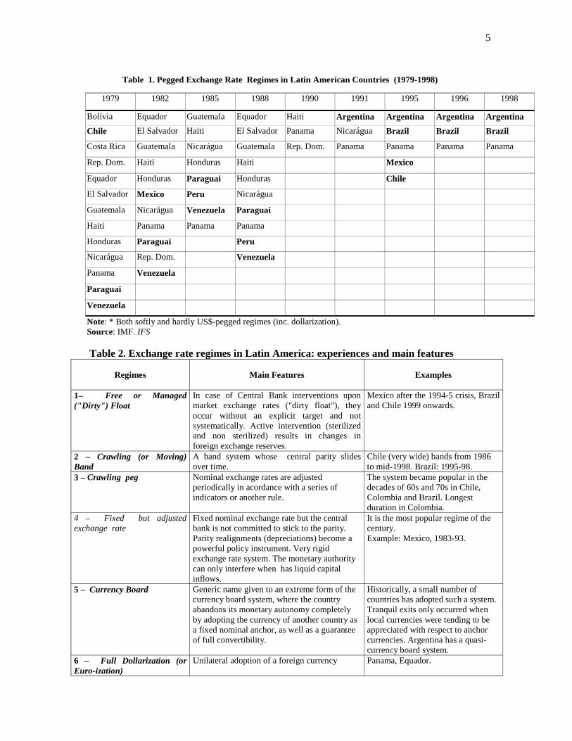
After some "sudden stop" and reversal of capital flows, triggering a "twin" (private or public sector) financial and balance-of-payments crisis, "soft pegs" were replaced by exchange rate fluctuation, usually going through some intermediary period of overshooting of the local currency devaluation. Chile was the smoothest recent experience of change, with a band being replaced by a floating regime. In turn, Argentina´s currency board was maintained during Mexico´s and Brazil´s exchange-rate regime upheavals, as well as (so far, at least) along her current crisis. Tables 1 and 2 illustrate how pegged exchange-rate regimes became widespread in Latin America until recently, as well as how only hardly pegged regimes have survived since then (Brazil´s change came after, as well as Equador´s full dollarization ). Intermediate ranges of Table 2 lost weight as compared to top and down ones. This is the reason why Latin America became a major reference for the so-called "bipolar view" of surviving exchange rate regimes in emerging countries, according to which only extreme regimes are intertemporally sustainable when the emerging country is fully open to capital mobility (Eichengreen, 1999) (Fischer, 2001). Indeed, each of the major "twin crises" in emerging economies involved some local sort of exchange-rate peg at corresponding core countries: Mexico (1994), Thailand, Indonesia and South Korea (1997), Russia and Brazil (1998), Argentina and Turkey (2000). On the other hand, economies with higher exchange-rate flexibility were able to undergo those turbulent moments without a major macroeconomic disruption: Taiwan (1997), South Africa, Israel, Turkey and Mexico (1998). Only "hard pegs" - Hong Kong and Argentina - survived.

Full capital mobility implies that markets avail themselves of arbitrage or speculative opportunities whenever there is some misalignment between active monetary and exchange-rate policies. Therefore, one of these has to be abdicated, i.e. one policy has to follow the other.

5

Table 1. Pegged Exchange Rate Regimes in Latin American Countries (1979-1998)

1979 1982 1985 1988 1990 1991 1995 1996 1998

Bolívia Equador Guatemala Equador Haiti Argentina Argentina Argentina Argentina

Chile El Salvador Haiti El Salvador Panama Nicarágua Brazil Brazil Brazil

Costa Rica Guatemala Nicarágua Guatemala Rep. Dom. Panama Panama Panama Panama

Rep. Dom. Haiti Honduras Haiti Mexico

Equador Honduras Paraguai Honduras Chile

El Salvador Mexico Peru Nicarágua

Guatemala Nicarágua Venezuela Paraguai

Haiti Panama Panama Panama

Honduras Paraguai Peru

Nicarágua Rep. Dom. Venezuela

Panama Venezuela

Paraguai

Venezuela

Note: * Both softly and hardly US$-pegged regimes (inc. dollarization). Source: IMF. IFS Table 2. Exchange rate regimes in Latin America: experiences and main features

Regimes

Main Features

Examples

1– Free or Managed ("Dirty") Float

In case of Central Bank interventions upon market exchange rates ("dirty float"), they occur without an explicit target and not systematically. Active intervention (sterilized and non sterilized) results in changes in foreign exchange reserves.

Mexico after the 1994-5 crisis, Brazil and Chile 1999 onwards.

2 – Crawling (or Moving) Band

A band system whose central parity slides over time.

Chile (very wide) bands from 1986 to mid-1998. Brazil: 1995-98.

3 – Crawling peg Nominal exchange rates are adjusted periodically in acordance with a series of indicators or another rule.

The system became popular in the decades of 60s and 70s in Chile, Colombia and Brazil. Longest duration in Colombia.

4 – Fixed but adjusted exchange rate

Fixed nominal exchange rate but the central bank is not committed to stick to the parity. Parity realignments (depreciations) become a powerful policy instrument. Very rigid exchange rate system. The monetary authority can only interfere when has liquid capital inflows.

It is the most popular regime of the century. Example: Mexico, 1983-93.

5 – Currency Board Generic name given to an extreme form of the currency board system, where the country abandons its monetary autonomy completely by adopting the currency of another country as a fixed nominal anchor, as well as a guarantee of full convertibility.

Historically, a small number of countries has adopted such a system. Tranquil exits only occurred when local currencies were tending to be appreciated with respect to anchor currencies. Argentina has a quasi-currency board system.

6 – Full Dollarization (or Euro-ization)

Unilateral adoption of a foreign currency Panama, Equador.

6

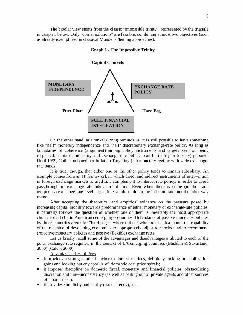
The bipolar view stems from the classic "impossible trinity", represented by the triangle in Graph 1 below. Only "corner solutions" are feasible, combining at most two objectives (such as already exemplified in classical Mundell-Fleming approaches).

Graph 1 - The Impossible Trinity

On the other hand, as Frankel (1999) reminds us, it is still possible to have something like "half" monetary independence and "half" discretionary exchange-rate policy. As long as boundaries of coherence (alignment) among policy instruments and targets keep on being respected, a mix of monetary and exchange-rate policies can be (softly or loosely) pursued. Until 1999, Chile combined her Inflation Targeting (IT) monetary regime wtih wide exchange-rate bands.

It is true, though, that either one or the other policy tends to remain subsidiary. An example comes from an IT framework in which direct and indirect instruments of intervention in foreign exchange markets is used as a complement to interest rate policy, in order to avoid passthrough of exchange-rate hikes on inflation. Even when there is some (implicit and temporary) exchange rate level target, interventions aim at the inflation rate, not the other way round. After accepting the theoretical and empirical evidence on the pressure posed by increasing capital mobility towards predominance of either monetary or exchange-rate policies, it naturally follows the question of whether one of them is inevitably the most appropriate choice for all (Latin American) emerging economies. Defendants of passive monetary policies by those countries argue for "hard pegs", whereas those who are skeptical about the capability of the real side of developing economies to appropriately adjust to shocks tend to recommend (re)active monetary policies and passive (flexible) exchange rates. Let us briefly recall some of the advantages and disadvantages attibuted to each of the polar exchange-rate regimes, in the context of LA emerging countries (Mishkin & Savastano, 2000) (Calvo, 2000). Advantages of Hard Pegs !"it provides a strong nominal anchor to domestic prices, definitely locking in stabilization

gains and locking out any sparkle of domestic cost-price spirals; !"it imposes discipline on domestic fiscal, monetary and financial policies, obstaculizing

discretion and time-inconsistency (as well as bailing out of private agents and other sources of "moral risk");

!"it provides simplicity and clarity (transparency); and

Capital Controls

Pure Float Hard Peg

MONETARY INDEPENDENCE EXCHANGE RATE

POLICY

FULL FINANCIAL INTEGRATION

7

!"it eliminates (or reduces) currency risks of domestic financial transactions, lowering funding costs for both private and public sectors, as well as fostering financial deepening

Disadvantages of Hard Pegs !"monetary policies will not be available against domestically originated shocks (e.g., supply

shocks). Most LA economies feature lack of "fiscal flexibility", as well as a low capacity to swiftly adjust to shocks on the real side of the economy. In this setting, large and protracted fluctuations of investments, output and employment may generate credit risks so high as to more than compensate for reduced currency risks;

!"there will be no Lender of Last Resort, what circumscribes "financial safety nets" to privately constituted deposit insurances and thin interbank markets. Given low degrees of domestic financial development, hard-to-access financial safety nets tend to curb the propensity to assume risks and, therefore, financial leverage and investments; and

!"easy "exit strategies" are very difficult to find. Given that optimality conditions may change over time (see below), an occasional need of regime change will face strong hysteretical effects (liability dollarization and strong "fear of floating").

Advantages of Floating Exchange Rates !"monetary policy becomes free to target inflation or other macroeconomic goal. Thus,

monetary policy can deal with investment and output fluctuations, including certain external shocks. Simultaneously, exchange rate flexibility helps to adjust nominal and relative prices;

!"exchange rates become a thermometer of the economy´s health, something that may remain hidden within a hard peg; and

!"it decreases the likelihood of underestimation of effective exchange-rate risks Disadvantages of Floating Exchange Rates

!"exchange-rate instability may lead to high currency risks and financial instability, whenever there is partial dollarization of (private and/or public sector) liabilities (as unit of account or as an effective means of payment). Vulnerability with respect to currency fluctuations add to the other "financial fragility" features of emerging economies. On the other hand, one must not forget that protracted real adjustments under hard pegs may result in other even more dangerous sources of risks;

!"some degree of financial development is required in order to make available instruments appropriate to manage currency risks. Otherwise, foreign exchange markets will become too subject to herding behavior and manipulation, i.e. it will be too volatile. In any case, one should expect a higher degree of "dirtiness" in emerging economies´ fluctuation, as compared to advanced countries, given their dependence on foreign capital flows and their more frequent "liquidity droughts" and sudden credit squeezes;

!"nominal price volatility of tradable goods may increase inflation volatility, given the critical position assumed by imported inputs and products in emerging countries´ GDP. This pass-through is one of the main reasons underlying the observed "fear of floating" in emerging countries (Calvo & Reinhart, 2000);

!"price volatility of imports and exports may also hurt trade; and !"active monetary policies require a strong national will to build policy credibility, rigorous

prudential supervision of finance, no "fiscal dominance" on monetary policy, and adjustment flexibility in the production system, whereas hard pegs directly impose a discipline towards these attributes. On the other hand, one knows that those are pre-requisites for any monetary system to be stable and efficient. An attempt to establish hard pegs can also be frustrated at its beginning if the country fails to attend those preconditions. The relevant difference may boil down to the higher speed with which monetary credibility tends to be attained in the hard peg case, if successfully established.

8

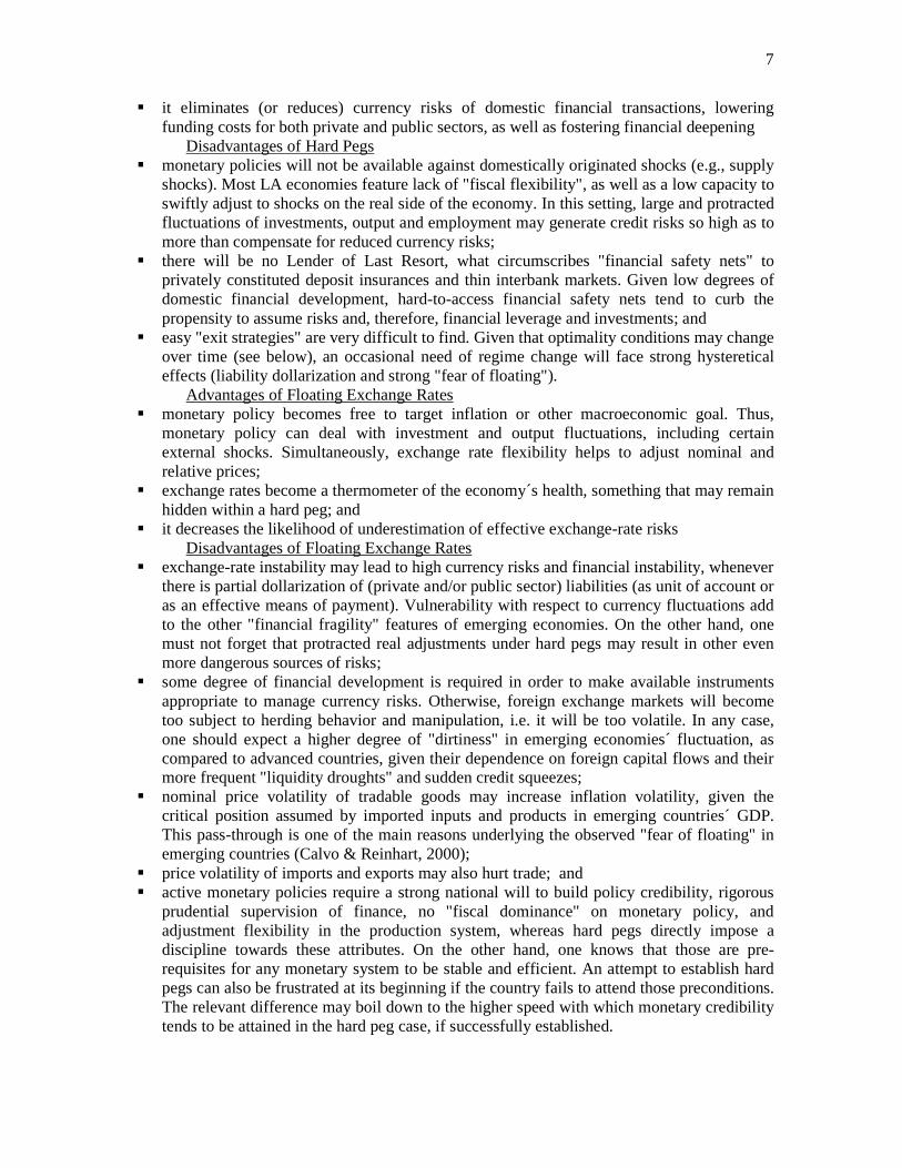
This balance of advantages and disadvantages can be translated into Robert Mundell´s criteria for an Optimum Currency Area (OCA), as adapted by textbook discussions about the convenience of tying local currencies versus letting them float. As the degree of economic integration with the rest of the world increases, advantages of fixed exchange rates increase with it, whereas advantages of flexible exchange rates tend to fall. This happens because of: larger potential gains in terms of lower transaction costs and currency risks; higher inflationary credibility and heavier weight of nominal anchor via hard pegs; and lower losses derived from the loss of monetary policy. Lower losses derived from the loss of monetary policy can be approached through observing the degree of correlation among shocks in the economy and in the rest of the world (or for that matter a regional currency whose pegging to is under consideration). Simmetry between those shocks means that required monetary initiatives can be let to abroad. In turn, labor mobility alliviates inconveniences associated to assimmetry of shocks, whereas an overall redistributive fiscal system is also helpful to compensate for that asimmetry. Graph 2 (adapted from Frankel, 1999) presents the "extent of trade" and the "degree of income-correlation" between the regions as indicators for assessing optimum degrees of exchange-rate pegging (or OCA). The OCA line divides the space into two sets, to the right of which , under prevailing conditions, the advantages of hard pegs predominate. Frankel (1999) calls attention to differing possible hypotheses about what tends to occur through time with respect to income-correlation as cross-border trade rises. Line AA describes a trajectory for a country whose income-correlation with the rest of the world augments as its trade increases. Some authors, however, sustain that increasing specialization, accompanying higher trade, might reduce income-correlation as represented by line BB. The only unambiguous conclusion is that there is "no single regime right for all countries or at all times". In this respect, the difficulties to exit from hard peg strategies should be taken into account. One can also notice that OCA criteria should not be approached exclusively on a static base. Provided that the starting position is not too far from the borderline, OCA favourability can be endogenously built through institutional adaptation. A more recently stressed criteria for choosing exchange rate regimes has been the existing degree of policy credibility, as we outlined above. Lack of monetary credibility makes hard pegs more attractive. One cannot forget, on the other hand, that this credibility will only be sustained, once stabilization gains have been settled, if the latter ends up followed by good performance also in other macroeconomic criteria (such as growth, high employment, low default risks etc.).

Graph 2 - Hardly Pegged and Floating Currency Areas

Extent of Trade

Income Correlation

HARD PEGS DOMINATE

FLEXIBLE RATES DOMINATE

BB

AA

OCA

9

Insofar as current exchange-rate regimes in LA economies, at this point we proppose the following intuitive observations (to be empirically supported in the following section): (i) its (bipolar) heterogeneity stems from their different recent experiences with exchange-

rate-based stabilization and crises. But there is nothing to allow any expectation that their present configuration will remain as such in the future, or converge either towards one or the other extreme of the continuum of regimes;

(ii) current levels of foreign trade among Southern neighbours are hardly relatively large - and sectorally important - enough to underpin currency pegging among themselves. At the same time, those levels are perhaps sufficiently high as to undermine national currency pegs to outside regions; and

(iii) notably in the case of LA emerging countries, OCA trade-based criteria adapted to Optimum Exchange-rate Regimes leave aside some relevant financial dimensions of macroeconomic interdependence. Contagion and other neighborhood financial effects may turn their interdependence more significant than it looks like from a trade perspective. It is to these points that we now turn.

2. SHOCKS AND MACROEONOMIC INTERDEPENDENCE IN LATIN

AMERICA: AN ECONOMETRIC APPROACH This section brings some econometric evidence on macroeconomic transmission of

shocks throughout the largest Latin American economies. We intend to show that, despite national differences in responses to shocks - coming from abroad or within the region -, they all have shown some common macroeconomic sensitivity to them. Heterogeneous exchange rate regimes have implied different national macroeconomic responses, but neither flexible or hardly pegged exchange rates have implied isolation. Whether or not the region move on towards flexible or bipolar regimes, macroeconomic interpendence is likely to continue to be worth considering by their policy makers.

The estimated econometric models here presented deal with the following: With respect to exchange rate regimes in those countries, we try to investigate whether

nominal and real exchange rates follow some long-term trajectory; whether there is evidence of Granger causality among these variables; and how intensively nominal and real exchange rate shocks of those economies affect the other exchange rates along the region. As one can expect from our previous discussion, no significant structural trend towards convergence of regimes or rates was found.

We develop a similar exercise regarding exchange rates and trade. Macroeconomic interdependence through trade flows is shown to be relevant, but significantly asymmetric and dependent upon exchange-rate regimes.

Finally, we go to how each of the LA large economies reacts to monetary shocks originated from neighbours, focusing mainly on whether external shocks on foreign exchange reserves have preceded changes in exchange rates as well as whether the former were transmitted to interest rates, and how intensively. We expect to have been able to illustrate how the absence of a high nominal exchange-rate interdependence, due to the heterogeneity of regimes, may hide a very strong macroeconomic interdependence through other vehicles. This result comes out forcefully when we gather both foreign exchange reserves and local interest rates as indicators of stress, instead of including only those reserves.

Our sample for exchange-rate interdependence goes from the first quarter of 1990 to the first quarter of 2000. A first approach is made through a graphic analysis of the series to be researched. Afterwards, we present some estimates of VAR models for nominal and real exchange rates of those countries, searching for long run movements in terms of causality and dynamic effects, according to impulse-response analysis (see Appendix).

10

A similar procedure was followed to observe relations among foreign exchange reserves, interest rates and exchange rates for each economy, aiming at discovering their reactions to external shocks. In the same way, we estimated a VAR model to relate exchange rate behavior and trade balances. 2.1. Exchange rate interdependence

The table 1 shows the outcomes of the unit root tests for exchange rate in level and in first difference for Brazil, Chile and Mexico. As known, a unit root test is always necessary before the empirical studies. Under null hypothesis of unit root against alternative hypothesis of stationarity, the test is basically a regression of the series in study according to equation:

∆yt = µ + βt + αyt-1 + i

p

=∑

1

δi∆yt-1 + εt (1)

where t is the linear deterministic trend. That equation is estimated in the beginning with very large lags and, afterwards, it is not significant to go through eliminating lags rightway. The significance of the trend and of the constant is evaluated in each lag reduction. The critical values of the ADF test are not obtained from a usual distribution, but they were derived by MacKinnon (1991) for any sample size. However, the ADF test is a weak one when the sample includes extreme events of types such as intense price depression, supply shocks, among others. To control this problem Perron and Vogelsang (1992) introduced dummy variables in

(1): ∆yt = µ + βt + αyt-1 + γDUt(λ) + i

p

=∑

1

δi∆yt-1 + εt (2)

where DUt(λ) = 1 to t > Tλ, e DUt(λ) = 0; λ = TB/T represent the moment where the structural break is observed, T is the sample size and TB is the date in which the structural break occurred.

In the same way that the ADF model fails in the consideration of problems associated with structural breaks, the procedure proposed by Engle and Granger (1987), for the co-integration technique, faces the same difficulty. Gregory and Hansen (1996) review the Engle and Granger (1987) model, considering regime changes through the cointegration technique based on the residual. Gregory and Hansen's model (1996) is estimated in two stages, and the first step consists of estimating the following multiple regression:

y1t = α + βt + γDUt(λ) + θ1y2t + ut (3) where y1t and y2t are first order integrated time series, denoted for I(1), and y2t is a variable or a set of variables; DUt(λ) has the same definition as in (2). The second step is to test the stationarity of ut in (3), through the ADF or Phillips-Perron tests. If ut is stationary, it can be said that there is a cointegration vector among y1t and y2t, or a cointegration vector matrix for the case of y2t to represent a set of variables. Unit root tests, that are shown syntheticly in table 1, indicated that1: !"nominal exchange rates of Mexico and Chile are first order integrated in level, and

stationary in first difference; !"whereas nominal exchange rates in Brazil are second order integrated in level, with no

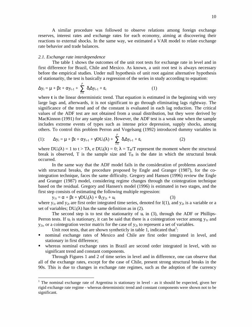
significant trend and constant components. Through Figures 1 and 2 of time series in level and in difference, one can observe that

all of the exchange rates, except for the case of Chile, present strong structural breaks in the 90s. This is due to changes in exchange rate regimes, such as the adoption of the currency

1 The nominal exchange rate of Argentina is stationary in level - as it should be expected, given her rigid exchange rate regime - whereas deterministic trend and constant components were shown not to be significant.

11

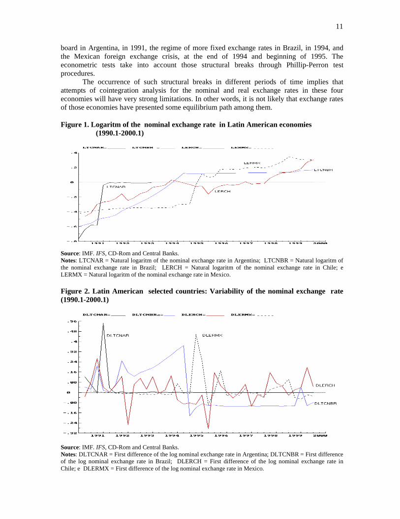
board in Argentina, in 1991, the regime of more fixed exchange rates in Brazil, in 1994, and the Mexican foreign exchange crisis, at the end of 1994 and beginning of 1995. The econometric tests take into account those structural breaks through Phillip-Perron test procedures. The occurrence of such structural breaks in different periods of time implies that attempts of cointegration analysis for the nominal and real exchange rates in these four economies will have very strong limitations. In other words, it is not likely that exchange rates of those economies have presented some equilibrium path among them. Figure 1. Logaritm of the nominal exchange rate in Latin American economies (1990.1-2000.1)

Source: IMF. IFS, CD-Rom and Central Banks. Notes: LTCNAR = Natural logaritm of the nominal exchange rate in Argentina; LTCNBR = Natural logaritm of the nominal exchange rate in Brazil; LERCH = Natural logaritm of the nominal exchange rate in Chile; e LERMX = Natural logaritm of the nominal exchange rate in Mexico. Figure 2. Latin American selected countries: Variability of the nominal exchange rate (1990.1-2000.1)

Source: IMF. IFS, CD-Rom and Central Banks. Notes: DLTCNAR = First difference of the log nominal exchange rate in Argentina; DLTCNBR = First difference of the log nominal exchange rate in Brazil; DLERCH = First difference of the log nominal exchange rate in Chile; e DLERMX = First difference of the log nominal exchange rate in Mexico.

12

Table 1 - Unit Tests for Exchange Rate in level and in first difference – Argentina, Brazil, Chile e México – Sample (1990.1-2000.1) Variables Lags ADF Results LTCNAR 5 3,33a Stationary LTCNBR 1 -2,35a Not Stationary LTCNCH 1 -2,00b Not Stationary LTCNMX 3 -2,36b Not Stationary DLTCNBR 1 -3,06b Not Stationary DLTCNCH 1 -6,04a Stationary DLTCNMX 1 -4,29b Stationary DDTCNBR 1 -7,50b Stationary Critical Values: (a) 5% = -2,953 e 1% = -3,642. (b) 5% = -3,531 e 1% = -4,216.

Due to the differences in integration order of those four time series, we moved to the

cointegration analysis exclusively for the cases of the nominal exchange rates of Chile and Mexico. In this case, it will be investigated whether at least two of the four economies could escape from the constraints imposed by exchange rate disruptions verified in the decade of 1990s. After an analysis of information criteria, a VAR with one lag was considered, as recommended in the Schwarz and Hannan-Quinn criteria.

Since Sims (1980), the VAR (Vector Auto-Regressive) models have become an alternative to traditional estimation procedures. Sims considered, in a first stage, all variables as endogenous, avoiding to capture false or spurious restrictions in the model. Starting from statistical procedures, the appropriate lag is determined, as well as the appropriate treatment to be given to the trend of variables. More recently, estimations of impulse-response functions have been increasingly used for analysis of shock effects on the set of variables of the system. Just as an illustration, we will refer to the finite order bivariate VAR model, specified as:

+

+

=

−

−

t

t

t

t

t

t

t

t

y

y

AA

AA

w

w

CC

CC

y

y

2

1

12

11

2221

1211

2

1

2221

1211

2

1

)()(

)()(

)()(

)()(

εε

!!

!!

!!

!! (4)

where t1y and t2y are vectors of dimension m1 x 1 and m2 x 1, respectively, with m1 + m2 = m.

The matrix C(l) contains the coefficients on [ ] '21

' , ttt www = , which include all deterministic

components in the two blocks of equation: [ ]'21

' , ttt εεε = . The following step becomes to

search for the autorregression lag and what to do in case of no stationarity or explosive roots appearing in matrix )(A ! .

The estimation of the long term equilibrium relation is based on the following vector autorregressive:

∆yt = µ + Πyt-1 + j

k

=

−

∑1

1

Γj∆yt-j + εt (5)

where the matrix ΠΠΠΠ has a reduced rank when there is cointegration, that is to say, when linear combinations of Yt are stationaries. So, the matrix ΠΠΠΠ can be decomposed in two matrix p x r αααα and ββββ such as ΠΠΠΠ = αααα.ββββ’. The matrix ββββ represents the cointegration vectors and the matrix αααα represents the weight, or the importance, of the cointegration relations in each equation. In other words, the Johansen test estimates the equation above under the restriction that ΠΠΠΠ has reduced rank; the non-restrictive model assumes that ΠΠΠΠ has a complete rank. εt is gaussian with covariance matrix Ω.

After estimating the VAR, the hypothesis that there is a cointegration vector between nominal exchange rates of Chile and of Mexico was analyzed, following Johansen (1988) e

13

Johansen & Juselius (1990) procedures. Using the Trace Test (λTrace Test) a test for p (the maximum number of cointegrating relationship) is done, where:

)ˆ1log(1

∑+=

−−=n

piiTrace T λλ

where iλ is the i-th largest eignvalue. λTrace is the of the null of r cointegrating rank against the alternative of a p cointegrating rank. And the test of hypothesis of p cointegrating vectors can be based on the Maximum Eignvalue Statistic :

)ˆ1log( 1+−−= pMax T λλ

In this last test the H0: p cointegrating vectors against H1: p+1 cointegrating vectors. So, the first row test H0: p = 0 against H1: p = 1. If this is significant H0 is rejected. The trace statistics are reported as well. This tests H0: p cointegrating vectors against H1: > p cointegrantig vectors. So the first row tests H0: p = 0 against H1: p > 0. If this is significant H0 is rejected, and the next row tests H0: p = 1 against H1: p > 1.

As expressed in table 2 below, the hypothesis that there is a cointegration vector between exchange rates of Chile and Mexico cannot be rejected. This result can be explained, possibly, by the fact that Chile was under a regime of more flexible exchange rates, whereas Mexico moved from a soft peg to a more flexible regime exactly at the middle of the period covered by the sample. Table 2 - Test Statistics for Cointegration Analysis for Exchange Rates in the Chile and Mexico Sample: 1990.1-2000.1

Ho:rank=p Max Eigenvalue Test 95% Trace Test 95% p=0 18.57* 15,7 21,88* 20,0

p<=1 3,307 9,2 3,307 9,2 Note: * marks significance at 95%.

For a system with all the four exchange rates (Argentina, Mexico, Chile and Brazil) - in

this case a system with stationary variables - we proceeded in the same way. In other words, we chose a system according to information criteria to reduce the model. Thus, from a system of VAR in I(0) space, with one lag, we tested the reduction of the model presented soon above, to accomplish analysis of forecast 1-step dynamics.

How intensively exchange rate shocks of those economies affect the other exchange rates along the region? Impulse-responde functions were estimated to answer this question. Impulse-response functions are useful to sumarize dynamic relations between the variables in a vector autoregressive. As known, a VAR can be written in vector MA(∞) form as the following:

∞−∞−− +++++= ttttty εψεψεψεµ ...2211 (6)

Thus, the matrix Ψs has been interpreted as: s't

styψψψψ====

εεεε∂∂∂∂∂∂∂∂ ++++

That is, the row i, column j element of sψψψψ identifies the consequences of a one-unit

increase in the jth variable’s innovations at date t ( jtεεεε ) for the value of the ith variable at time t

+ s ( st,iy ++++ ), holding all other innovations at all dates constant. If the first element of

tεεεε changed by 1δδδδ at the same time that the second element changed by 2δδδδ and the nth element

of nδ , then the combined effect of these changes on the value of the vector y would be given

by (Hamilton, 1994:318-319):

14

δψy...

yyy sn

nt

st2

t2

st1

t1

stst ====δδδδ

εεεε∂∂∂∂∂∂∂∂++++++++δδδδ

εεεε∂∂∂∂∂∂∂∂++++δδδδ

εεεε∂∂∂∂∂∂∂∂====∆∆∆∆ ++++++++++++

++++ where ),...,δ,δ(δδ 21 νννν==== .(7)

Thus, each element of the matrix sψ in row i and column j, jt

st,iy

εεεε∂∂∂∂∂∂∂∂ ++++

is called the impluse-response function, which describes the response of st,iy ++++ to a one-unit

impulse in jty , with all other variables dated t or earlier held constant.

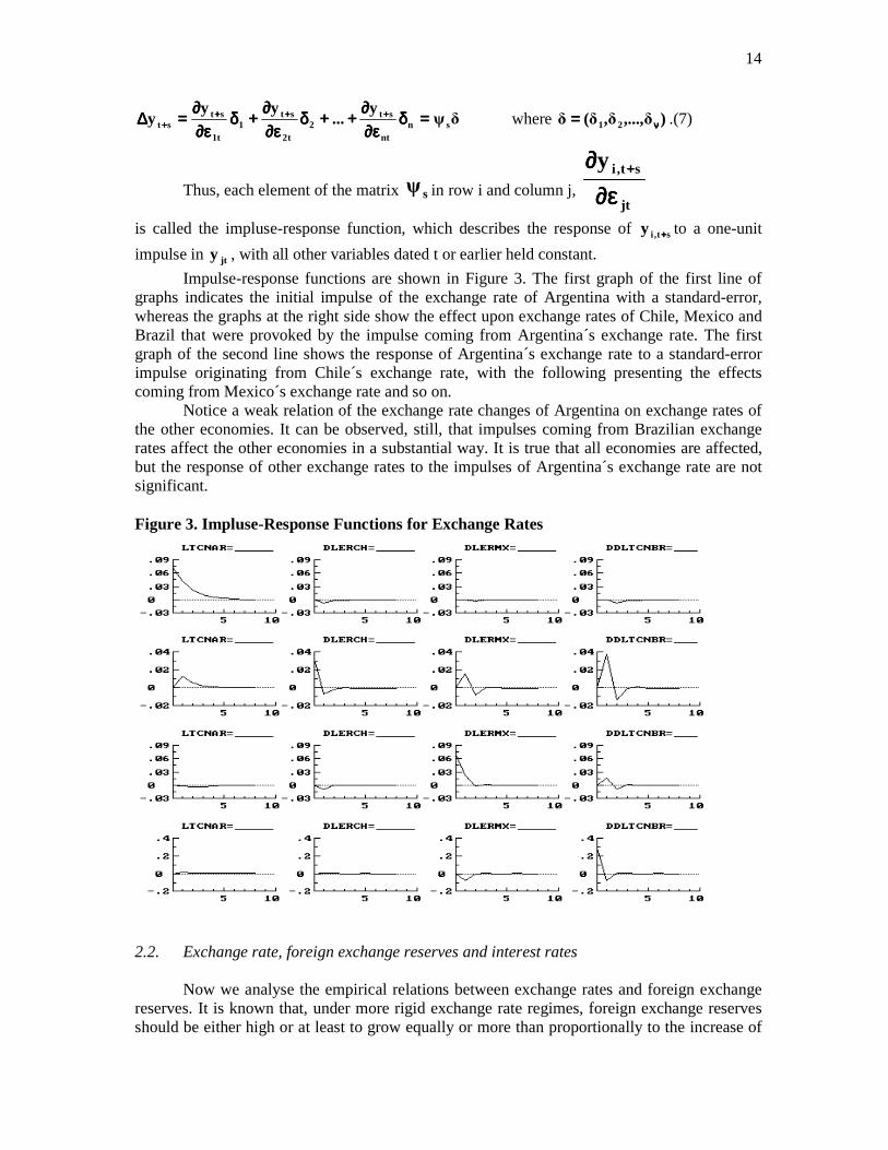
Impulse-response functions are shown in Figure 3. The first graph of the first line of graphs indicates the initial impulse of the exchange rate of Argentina with a standard-error, whereas the graphs at the right side show the effect upon exchange rates of Chile, Mexico and Brazil that were provoked by the impulse coming from Argentina´s exchange rate. The first graph of the second line shows the response of Argentina´s exchange rate to a standard-error impulse originating from Chile´s exchange rate, with the following presenting the effects coming from Mexico´s exchange rate and so on.

Notice a weak relation of the exchange rate changes of Argentina on exchange rates of the other economies. It can be observed, still, that impulses coming from Brazilian exchange rates affect the other economies in a substantial way. It is true that all economies are affected, but the response of other exchange rates to the impulses of Argentina´s exchange rate are not significant. Figure 3. Impluse-Response Functions for Exchange Rates

2.2. Exchange rate, foreign exchange reserves and interest rates

Now we analyse the empirical relations between exchange rates and foreign exchange

reserves. It is known that, under more rigid exchange rate regimes, foreign exchange reserves should be either high or at least to grow equally or more than proportionally to the increase of

15

eventual trade balance and current account deficits. As Chile´s exchange rate was throughout the period more flexible than the ones of the other countries, one could expect that relation to be weaker in this country. On the other hand, insofar as foreign exchange reserves as a leading indicator of foreign exchange crises, it is often expected that, under conditions of abrupt falls of the former, the latter undergoes strong alteration, and even that the exchange rate regime will change to another.

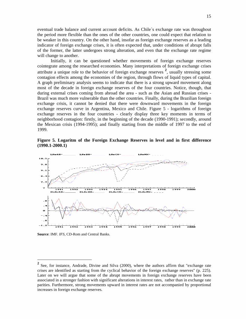
Initially, it can be questioned whether movements of foreign exchange reserves cointegrate among the researched economies. Many interpretations of foreign exchange crises attribute a unique role to the behavior of foreign exchange reserves 2, usually stressing some contagion effects among the economies of the region, through flows of liquid types of capital. A graph preliminary analysis seems to indicate that there is a strong upward movement along most of the decade in foreign exchange reserves of the four countries. Notice, though, that during external crises coming from abroad the area - such as the Asian and Russian crises - Brazil was much more vulnerable than the other countries. Finally, during the Brazilian foreign exchange crisis, it cannot be denied that there were downward movements in the foreign exchange reserves curve in Argentina, Mexico and Chile. Figure 5 - logarithms of foreign exchange reserves in the four countries - clearly display three key moments in terms of neighborhood contagion: firstly, in the beginning of the decade (1990-1991); secondly, around the Mexican crisis (1994-1995); and finally starting from the middle of 1997 to the end of 1999. Figure 5. Logaritm of the Foreign Exchange Reserves in level and in first difference (1990.1-2000.1)

Source: IMF. IFS, CD-Rom and Central Banks.

2 See, for instance, Andrade, Divine and Silva (2000), where the authors affirm that "exchange rate

crises are identified as starting from the cyclical behavior of the foreign exchange reserves" (p. 225). Later on we will argue that some of the abrupt movements in foreign exchange reserves have been associated in a stronger fashion with significant alterations in interest rates, rather than in exchange rate parities. Furthermore, strong movements upward in interest rates are not accompanied by proportional increases in foreign exchange reserves.

16

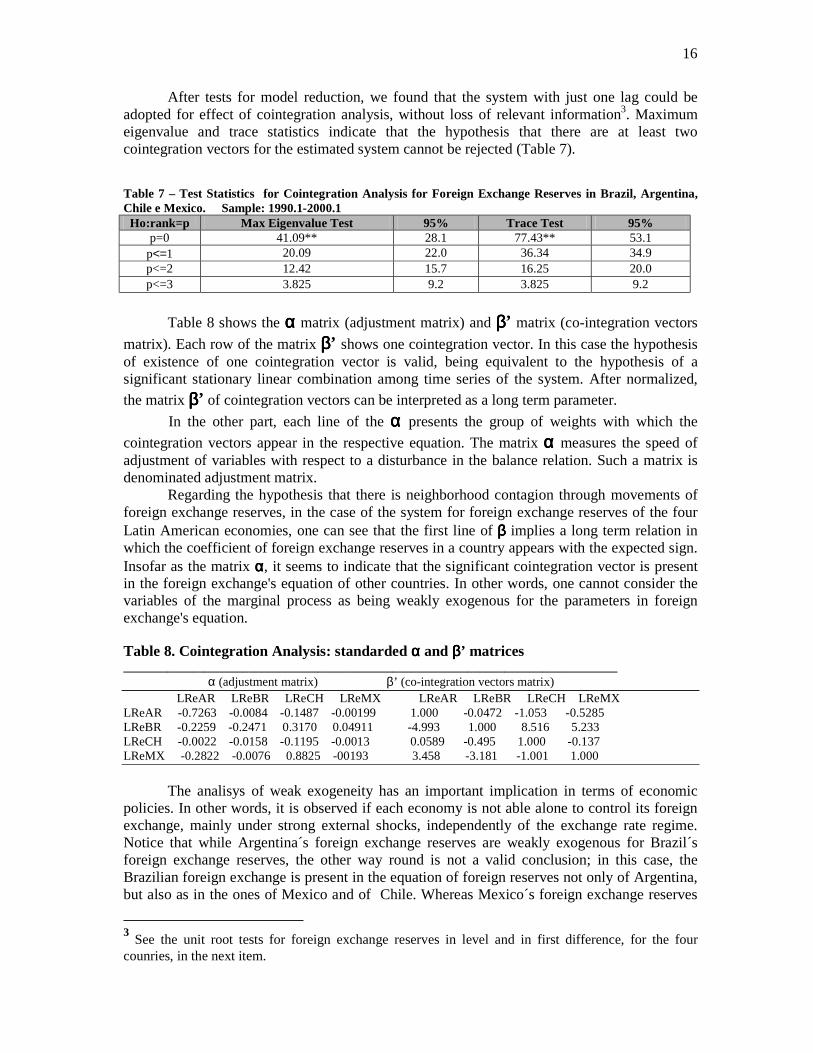
After tests for model reduction, we found that the system with just one lag could be adopted for effect of cointegration analysis, without loss of relevant information3. Maximum eigenvalue and trace statistics indicate that the hypothesis that there are at least two cointegration vectors for the estimated system cannot be rejected (Table 7). Table 7 – Test Statistics for Cointegration Analysis for Foreign Exchange Reserves in Brazil, Argentina, Chile e Mexico. Sample: 1990.1-2000.1

Ho:rank=p Max Eigenvalue Test 95% Trace Test 95% p=0 41.09** 28.1 77.43** 53.1

p<=1 20.09 22.0 36.34 34.9 p<=2 12.42 15.7 16.25 20.0 p<=3 3.825 9.2 3.825 9.2

Table 8 shows the αααα matrix (adjustment matrix) and ββββ’ matrix (co-integration vectors

matrix). Each row of the matrix ββββ’ shows one cointegration vector. In this case the hypothesis of existence of one cointegration vector is valid, being equivalent to the hypothesis of a significant stationary linear combination among time series of the system. After normalized,

the matrix ββββ’ of cointegration vectors can be interpreted as a long term parameter.

In the other part, each line of the αααα presents the group of weights with which the

cointegration vectors appear in the respective equation. The matrix αααα measures the speed of adjustment of variables with respect to a disturbance in the balance relation. Such a matrix is denominated adjustment matrix. Regarding the hypothesis that there is neighborhood contagion through movements of foreign exchange reserves, in the case of the system for foreign exchange reserves of the four Latin American economies, one can see that the first line of ββββ implies a long term relation in which the coefficient of foreign exchange reserves in a country appears with the expected sign. Insofar as the matrix αααα, it seems to indicate that the significant cointegration vector is present in the foreign exchange's equation of other countries. In other words, one cannot consider the variables of the marginal process as being weakly exogenous for the parameters in foreign exchange's equation.

Table 8. Cointegration Analysis: standarded αααα and ββββ’ matrices _______________________________________________________________________________ α (adjustment matrix) β’ (co-integration vectors matrix) LReAR LReBR LReCH LReMX LReAR LReBR LReCH LReMX LReAR -0.7263 -0.0084 -0.1487 -0.00199 1.000 -0.0472 -1.053 -0.5285 LReBR -0.2259 -0.2471 0.3170 0.04911 -4.993 1.000 8.516 5.233 LReCH -0.0022 -0.0158 -0.1195 -0.0013 0.0589 -0.495 1.000 -0.137 LReMX -0.2822 -0.0076 0.8825 -00193 3.458 -3.181 -1.001 1.000

The analisys of weak exogeneity has an important implication in terms of economic

policies. In other words, it is observed if each economy is not able alone to control its foreign exchange, mainly under strong external shocks, independently of the exchange rate regime. Notice that while Argentina´s foreign exchange reserves are weakly exogenous for Brazil´s foreign exchange reserves, the other way round is not a valid conclusion; in this case, the Brazilian foreign exchange is present in the equation of foreign reserves not only of Argentina, but also as in the ones of Mexico and of Chile. Whereas Mexico´s foreign exchange reserves

3 See the unit root tests for foreign exchange reserves in level and in first difference, for the four

counries, in the next item.

17

show up in foreign exchange reserve equations of all the other countries, Argentina´s one is only present in Chile´s foreign exchange equation.

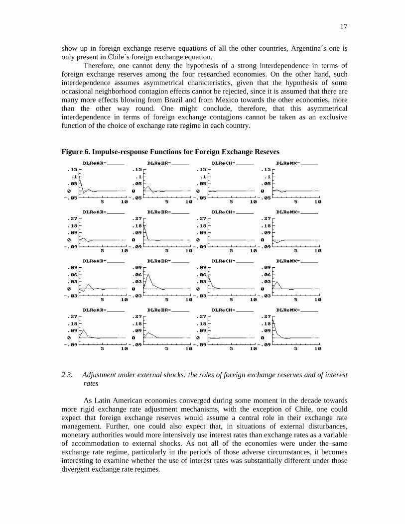
Therefore, one cannot deny the hypothesis of a strong interdependence in terms of foreign exchange reserves among the four researched economies. On the other hand, such interdependence assumes asymmetrical characteristics, given that the hypothesis of some occasional neighborhood contagion effects cannot be rejected, since it is assumed that there are many more effects blowing from Brazil and from Mexico towards the other economies, more than the other way round. One might conclude, therefore, that this asymmetrical interdependence in terms of foreign exchange contagions cannot be taken as an exclusive function of the choice of exchange rate regime in each country. Figure 6. Impulse-response Functions for Foreign Exchange Reseves

2.3. Adjustment under external shocks: the roles of foreign exchange reserves and of interest

rates As Latin American economies converged during some moment in the decade towards

more rigid exchange rate adjustment mechanisms, with the exception of Chile, one could expect that foreign exchange reserves would assume a central role in their exchange rate management. Further, one could also expect that, in situations of external disturbances, monetary authorities would more intensively use interest rates than exchange rates as a variable of accommodation to external shocks. As not all of the economies were under the same exchange rate regime, particularly in the periods of those adverse circumstances, it becomes interesting to examine whether the use of interest rates was substantially different under those divergent exchange rate regimes.

18

A preliminary graphic analysis points to the fact that all of the researched countries used interest rates as an instrument for taming capital flows, independently of the degree of flexibility in nominal exchange-rate adjustments. However, only Brazil and Chile made intensive use of this variable. At first sight, when focusing solely upon the interest rate - in per cent terms -, one is tempted to conclude that neither Argentina nor Mexico did substantially use interest rates after the Mexican crisis, even under the Asian, Russian and Brazilian crises.

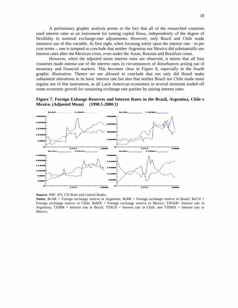
However, when the adjusted mean interest rates are observed, it seems that all four countries made intense use of the interest rates in circumstances of disturbances arising out of monetary and financial markets. This becomes clear in Figure 8, especially in the fourth graphic illustration. Thence we are allowed to conclude that not only did Brazil make substantial alterations in its basic interest rate but also that neither Brazil nor Chile made more regular use of this instrument, as all Latin American economies in several moments traded off some economic growth for sustaining exchange rate parities by raising interest rates. Figure 7. Foreign Exhange Reserves and Interest Rates in the Brazil, Argentina, Chile e Mexico. (Adjusted Mean) (1990.1-2000.1)

Source: IMF. IFS, CD-Rom and Central Banks. Notes: ReAR = Foreign exchange reserve in Argentina; ReBR = Foreign exchange reserve in Brazil; ReCH = Foreign exchange reserve in Chile; ReMX = Foreign exchange reserve in Mexico; TJDAR= Interest rate in Argentina; TJDBR = Interest rate in Brazil; TJDCH = Interest rate in Chile; and TJDMX = Interest rate in Mexico.

19

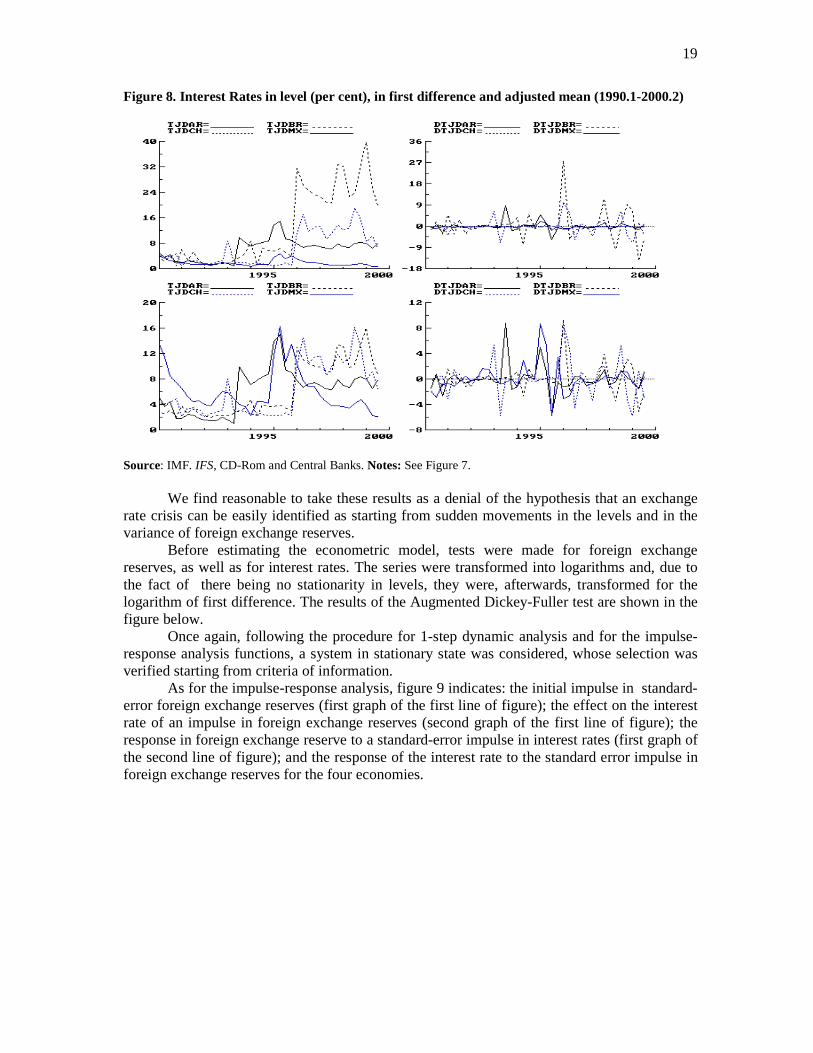
Figure 8. Interest Rates in level (per cent), in first difference and adjusted mean (1990.1-2000.2)

Source: IMF. IFS, CD-Rom and Central Banks. Notes: See Figure 7.

We find reasonable to take these results as a denial of the hypothesis that an exchange rate crisis can be easily identified as starting from sudden movements in the levels and in the variance of foreign exchange reserves.

Before estimating the econometric model, tests were made for foreign exchange reserves, as well as for interest rates. The series were transformed into logarithms and, due to the fact of there being no stationarity in levels, they were, afterwards, transformed for the logarithm of first difference. The results of the Augmented Dickey-Fuller test are shown in the figure below.

Once again, following the procedure for 1-step dynamic analysis and for the impulse-response analysis functions, a system in stationary state was considered, whose selection was verified starting from criteria of information.

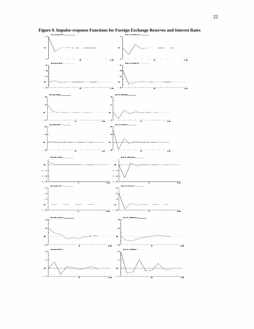
As for the impulse-response analysis, figure 9 indicates: the initial impulse in standard-error foreign exchange reserves (first graph of the first line of figure); the effect on the interest rate of an impulse in foreign exchange reserves (second graph of the first line of figure); the response in foreign exchange reserve to a standard-error impulse in interest rates (first graph of the second line of figure); and the response of the interest rate to the standard error impulse in foreign exchange reserves for the four economies.

20

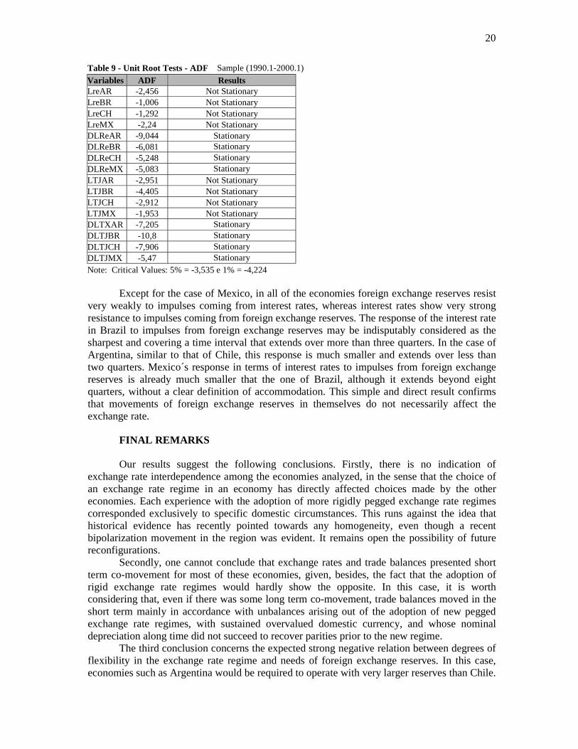
Table 9 - Unit Root Tests - ADF Sample (1990.1-2000.1) Variables ADF Results LreAR -2,456 Not Stationary LreBR -1,006 Not Stationary LreCH -1,292 Not Stationary LreMX -2,24 Not Stationary DLReAR -9,044 Stationary DLReBR -6,081 Stationary DLReCH -5,248 Stationary DLReMX -5,083 Stationary LTJAR -2,951 Not Stationary LTJBR -4,405 Not Stationary LTJCH -2,912 Not Stationary LTJMX -1,953 Not Stationary DLTXAR -7,205 Stationary DLTJBR -10,8 Stationary DLTJCH -7,906 Stationary DLTJMX -5,47 Stationary Note: Critical Values: 5% = -3,535 e 1% = -4,224

Except for the case of Mexico, in all of the economies foreign exchange reserves resist very weakly to impulses coming from interest rates, whereas interest rates show very strong resistance to impulses coming from foreign exchange reserves. The response of the interest rate in Brazil to impulses from foreign exchange reserves may be indisputably considered as the sharpest and covering a time interval that extends over more than three quarters. In the case of Argentina, similar to that of Chile, this response is much smaller and extends over less than two quarters. Mexico´s response in terms of interest rates to impulses from foreign exchange reserves is already much smaller that the one of Brazil, although it extends beyond eight quarters, without a clear definition of accommodation. This simple and direct result confirms that movements of foreign exchange reserves in themselves do not necessarily affect the exchange rate.

FINAL REMARKS Our results suggest the following conclusions. Firstly, there is no indication of exchange rate interdependence among the economies analyzed, in the sense that the choice of an exchange rate regime in an economy has directly affected choices made by the other economies. Each experience with the adoption of more rigidly pegged exchange rate regimes corresponded exclusively to specific domestic circumstances. This runs against the idea that historical evidence has recently pointed towards any homogeneity, even though a recent bipolarization movement in the region was evident. It remains open the possibility of future reconfigurations. Secondly, one cannot conclude that exchange rates and trade balances presented short term co-movement for most of these economies, given, besides, the fact that the adoption of rigid exchange rate regimes would hardly show the opposite. In this case, it is worth considering that, even if there was some long term co-movement, trade balances moved in the short term mainly in accordance with unbalances arising out of the adoption of new pegged exchange rate regimes, with sustained overvalued domestic currency, and whose nominal depreciation along time did not succeed to recover parities prior to the new regime. The third conclusion concerns the expected strong negative relation between degrees of flexibility in the exchange rate regime and needs of foreign exchange reserves. In this case, economies such as Argentina would be required to operate with very larger reserves than Chile.

21

The most interesting case detected by our empirical exercises was that these economies presented signs of neighborhood contagion effects with respect to movements of their foreign exchange reserves, with common moments of intense oscillations in the latter. One can arrive to the conclusion that, given strong contagion effects, the divergence among exchange rate regimes was not sufficient to imply significant differences with respect to autonomy of macroeconomic policies. Independently of their heterogeneous regimes, all four economies showed up jointly vulnerable regarding abrupt changes in capital flows towards the region. Fouth, we raised doubts about some established hypotheses regarding the use of macroeconomic adjustment mechanisms along the divergent exchange rate regimes in the region. According to our empirical results, except for Mexico, foreign exchange reserves resist very weakly to the impulses coming from interest rates, whereas interest rates resist very strongly to the impulses from foreign exchange reserves. This implies that macroeconomic adjustment policies had to resort to very high interest rates as an instrument to control foreign exchange, in situations of impulses, given that increases in interest rates often presented weak response in terms of foreign exchange reserves. This also suggests that one should go beyond simple matching of sudden behavior changes of foreign exchange reserves with situations of exchange rate crises.

Interest rate responses in Brazil to impulses of foreign exchange reserves can be considered as the most accentuated and for a time interval that extends over more than three quarters. In the case of Argentina, similarly to Chile, this response is much smaller and extend over less than two quarters. Mexico´s response in terms of interest rates to impulses from foreign exchange reserves is already much smaller than that of Brazil, yet extends beyond eight quarters, without a clear definition of accommodation. One can conclude that the intensity of use of interest rates as a control instrument over foreign exchange reserves is independent from the degree of rigidity of exchange rate regimes in the economies and, thus, one must look somewhere else in order to explain such a divergence in monetary policies. As a last educated guess, insofar as policy, we suggest that Southern Latin American large economies should jointly attempt to build some regional "liquidity defence", given that their financial common fate does not seem to be vanishing, despite efforts of national differentiation. Besides searching for macroeconomic convergence and for private sources of stand-by credit lines, maybe time is ripe for a joint negotiation towards an entrance into IMF´s Contingency Credit Line. Given current stages of macroeconomic policies and interdependence, joint movements towards national liquidity cushions might help substantially to reduce disruptive propagation of shocks along the region.

22

Figure 9. Impulse-response Functions for Foreign Exchange Reserves and Interest Rates

23

REFERENCES Andrade, J. P., Divino, J. A. e Silva, M. L. (2000). "Revisando a história das crises cambiais

brasileiras recentes". In: R. Fontes e M. Arbex (ed.). Economia Aberta: ensaios sobre fluxos de capitais, câmbio e exportações. Viçosa:Ed UFV.

Calvo, G. (2000). The case for hard pegs in the brave new world of global finance. ABCDE Europe, Paris, June 26, (draft).

Calvo, G. & Reinhart, C. (2000). Fear of floating: theory and evidence, April (www.puaf.umd.edu/papers/reinhart.htm).

Canova, F. (1999). "Vector autoregressive models: specification, estimation, inference and forecasting". In: M Hashem Pesaran & Michael Wickens (eds.), Handbook of applied econometrics. Vol 1. Macroeconomics.

Edwards, S. (1998a). Capital inflows into Latin America: a stop-go story? NBER Working Paper, n. 6441, March 1998.

Edwards, S. (1998b). Capital flows, real exchange rates, and capital controls: some Latin American experience. NBER Working Paper, n. 6800, November 1998.

Edwards, S. (1998c). Interest rate volatility, capital controls and contagions. NBER Working Paper, n.6756, October.

Eichengreen, B. (1999). Toward a new international financial archictecture:a practical post-Asia agenda. Washington: Institute for International Economics.

Engle, R. & C. Granger (1987). "Co-integration and error correlation: representation, estimation and testing". Econometrica, 35, 251-276.

Frankel, J. A. (1999). No single currency regime is right for all countries or at all times. NBER Working Paper , n. 7338, september.

Fischer, S. (2001). Exchange rate regimes: is the bipolar view correct?, IMF speeches, Jan. 06. Granger, C. W. (1969). "Investigating causal relations by econometric models and cross-

spectral methods". Econometrica, july, pp.424-438. Granger, C. W., B. Huang & C. W. Yang (1998). A bivariate causality between stock prices

and exchange rates: evidence from recent Asia Flu. Discussion Paper 98-09, Universidade of California, San Diego, Departament of Economics, april 1998.

Gregory, C. & B. E. Hansen (1996). "Residual-based tests for cointegration in models with regime shift". Journal of Econometrics, 70, p. 99-126.

Hamilton, J. D. (1994). Time Series Analysis. Princeton, UP. IMF. International Financial Statistics. CD-Rom. Johansen, S (1988). "Statistical analusis of cointegrating vectors". Journal of Economic

Dynamics and Control, 12. Johansen, S. & Juselius, K. (1990). "Maximum likelihood estimation and inference on

cointegration". Oxford Bulletin of Economics and Statistics, 52. Mishkin, F. e Savastano (2000). Monetary policy strategies for Latin America.. NBER

Working Paper 7617. March 2000. Perron, P. & T. J. Vogelsang (1992). "Nonstationarity and Level Shift with na aplication to

Purchasing Power Parity". Journal of Business and Economic Statistics, 10(3), 301-320. Sachs, Jeffrey; Tornell, Aaron; Velasco, Andrés. "The colapse of the Mexican peso: what have

we learned?". Economic Policy. Abril,1996. Sims, C. (1980). "Macroeconomics and reality". Econometrica, 48.