apres coloquio eduardo - biênio da matemática no brasilw3.impa.br/~aschulz/cs/lecture2.pdf ·...
TRANSCRIPT

Compressive Sensing
2 - Signal Compression
Adriana SchulzLuiz Velho
([email protected], [email protected])
Instituto de Matemática Pura e Aplicada
Eduardo A. B. da Silva([email protected])
Laboratório de Processamento de Sinais – COPPE/UFRJ
27o CBM - Compressive Sensing — Page: CPR-1 July 2009
1 – Signal Representations
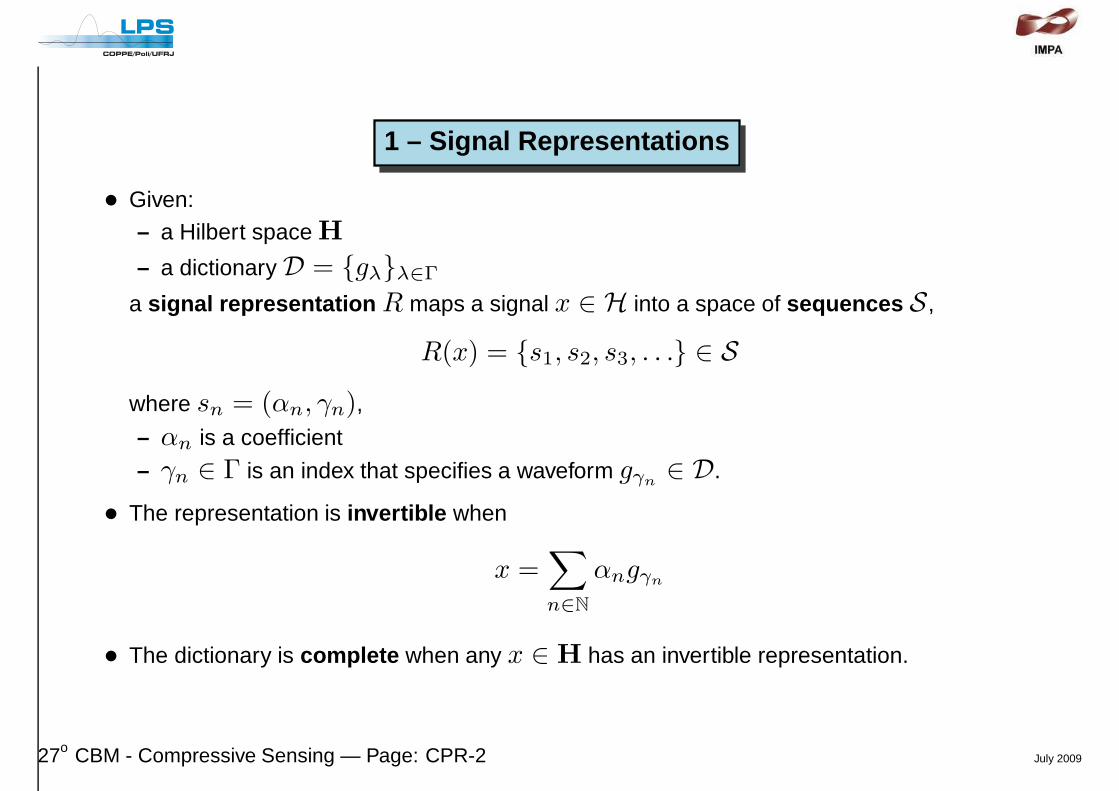
• Given:– a Hilbert space H
– a dictionary D = {gλ}λ∈Γ
a signal representation R maps a signal x ∈ H into a space of sequences S ,
R(x) = {s1, s2, s3, . . .} ∈ S
where sn = (αn, γn),
– αn is a coefficient
– γn ∈ Γ is an index that specifies a waveform gγn∈ D.
• The representation is invertible when
x =∑
n∈N
αngγn
• The dictionary is complete when any x ∈ H has an invertible representation.
27o CBM - Compressive Sensing — Page: CPR-2 July 2009
1.1 – Decomposition on a Basis
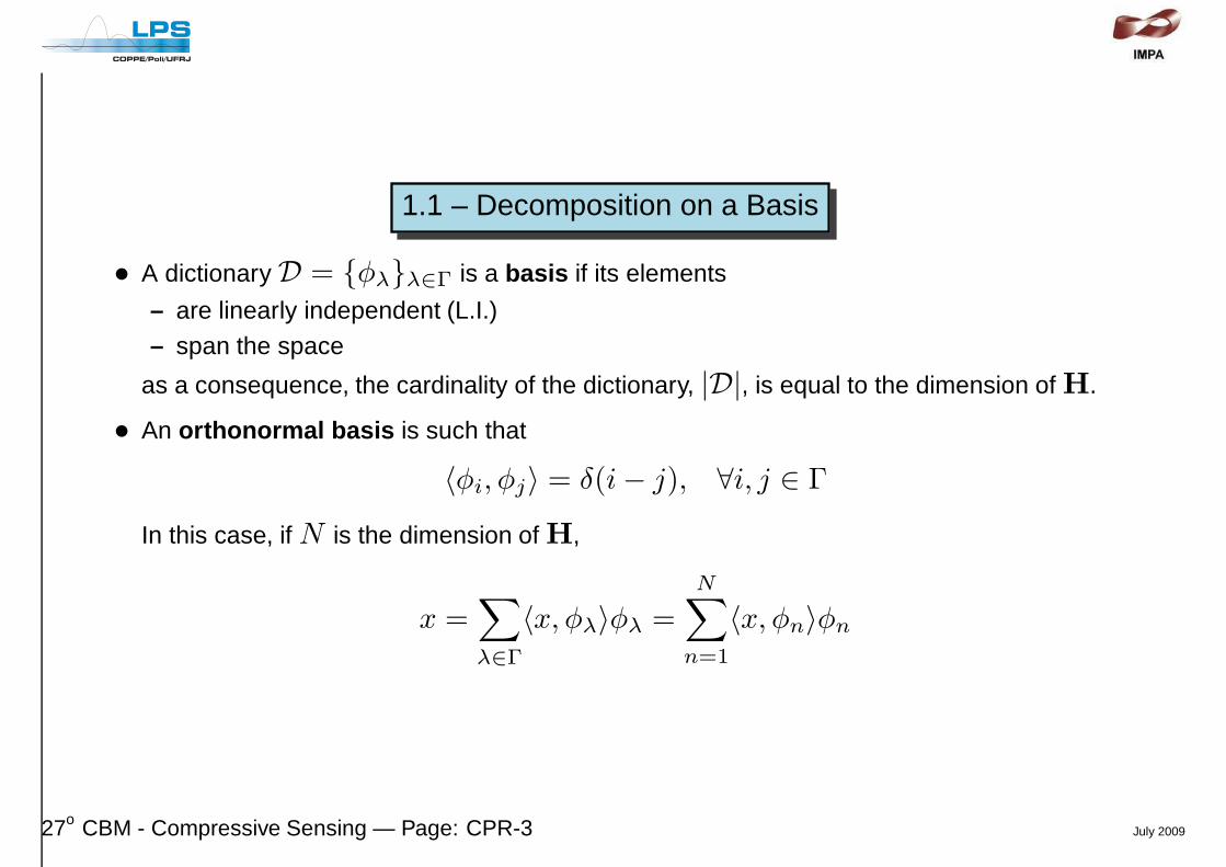
• A dictionary D = {φλ}λ∈Γ is a basis if its elements
– are linearly independent (L.I.)– span the space
as a consequence, the cardinality of the dictionary, |D|, is equal to the dimension of H.
• An orthonormal basis is such that
〈φi, φj〉 = δ(i− j), ∀i, j ∈ Γ
In this case, if N is the dimension of H,
x =∑
λ∈Γ
〈x, φλ〉φλ =
N∑
n=1
〈x, φn〉φn
27o CBM - Compressive Sensing — Page: CPR-3 July 2009

1.2 – Decomposition on a Frame
• A dictionary D = {φλ}λ∈Γ is a frame if its elements span the space
– Note that they do not need to be L.I.
⇒ the cardinality of the dictionary, |D|, may be larger than the dimension of H.
• More formally, ∃A,B > 0 such that
A‖x‖2 ≤∑
λ∈Γ
|〈x, φλ〉|2 ≤ B‖x‖2
– IfA > 0 then there are no elements that are orthogonal to all elements of D (that is, Dis complete ).
– If ∃M such that B < M then there is no direction where D is “excessivelycrowded” .
• For an orthonormal basis,A = B = 1.
27o CBM - Compressive Sensing — Page: CPR-4 July 2009
1.3 – Linear Representations on a Basis
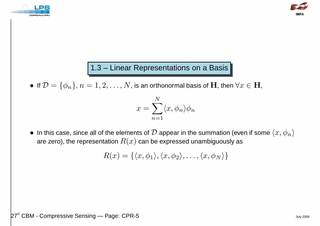
• If D = {φn}, n = 1, 2, . . . , N , is an orthonormal basis of H, then ∀x ∈ H,
x =N
∑
n=1
〈x, φn〉φn
• In this case, since all of the elements of D appear in the summation (even if some 〈x, φn〉are zero), the representationR(x) can be expressed unambiguously as
R(x) = {〈x, φ1〉, 〈x, φ2〉, . . . , 〈x, φN〉}
27o CBM - Compressive Sensing — Page: CPR-5 July 2009

• Now, supposing that
x =N
∑
n=1
anφn and y =N
∑
n=1
bnφn
we have that
R(x) = {a1, a2, . . . , aN} and R(y) = {b1, b2, . . . , bN} .
Since
x+ λy =N
∑
n=1
(an + λbn)φn
then
R(x+ λy) = {a1 + λb1, a2 + λb2, . . . , aN + λbN}
= R(x) + λR(y)
This implies that the representation is linear .
27o CBM - Compressive Sensing — Page: CPR-6 July 2009
1.4 – Non-linear Representations on a Basis
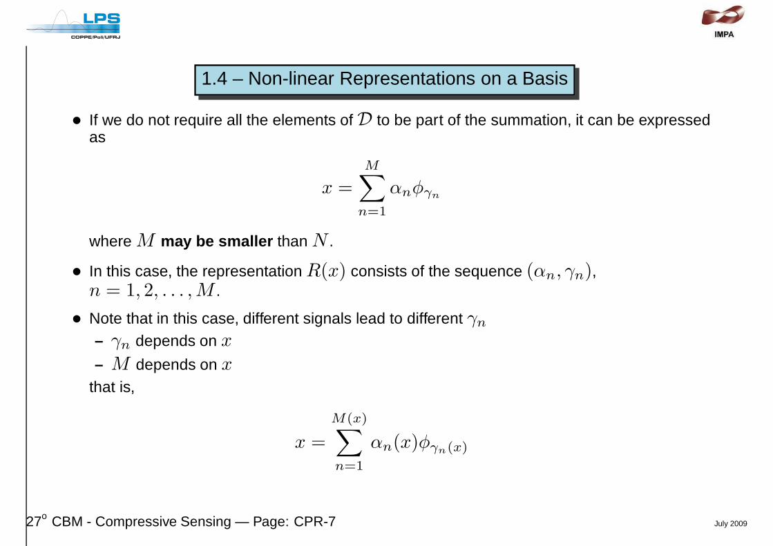
• If we do not require all the elements of D to be part of the summation, it can be expressedas
x =M∑
n=1
αnφγn
where M may be smaller than N .
• In this case, the representationR(x) consists of the sequence (αn, γn),n = 1, 2, . . . ,M .
• Note that in this case, different signals lead to different γn
– γn depends on x
– M depends on xthat is,
x =
M(x)∑
n=1
αn(x)φγn(x)
27o CBM - Compressive Sensing — Page: CPR-7 July 2009
• Now, supposing that
x =
M∑
n=1
αnφγnand y =
L∑
n=1
βnφζn
we have that
R(x) = {(α1, γ1), (α2, γ2), . . . , (αM , γM )}
R(y) = {(β1, ζ1), (β2, ζ2), . . . , (βL, ζL)} .
Even if M = L,
R(x) + λR(y) = {(α1, γ1), (λβ1, ζ1), (α2, γ2), (λβ2, ζ2), . . . , (αM , γM ), (λβM , ζM )}
6= R(x+ λy), in general.
This implies that this type of representation is non-linear .
27o CBM - Compressive Sensing — Page: CPR-8 July 2009

Example :
• Be D the canonical basis of R4,
φ1 =
1000
, φ2 =
0100
, φ3 =
0010
, φ4 =
0001
,
and
x =
53
−12
, y =
3−3
11
.
then
R(x) = {(5, 1), (3, 2), (−1, 3), (2, 4)} and R(y) = {(3, 1), (−3, 2), (1, 3), (1, 4)} .
But
x+ y =
8003
and R(x+ y) = {(8, 1), (3, 4)}
andR(x) +R(y) = {(8, 1), (0, 2), (0, 3), (3, 4)} 6= R(x+ y)
27o CBM - Compressive Sensing — Page: CPR-9 July 2009
1.5 – Examples
• Trivial basis for discrete signals (sequences): D = {δ(n− k)}, k ∈ Z.
– The decomposition represents a signal by its samples
x(n) =∑
k
x(k)δ(n− k)
R(x) = {. . . , x(−1), x(0), x(1), x(2), . . .}
• Discrete cosine transform (DCT) basis for signals in RN :
D = {ck(n)}, k = 0, 1, . . . , N − 1, where
ck(n) =
√
2 − δ(k)
Ncos
[
π(2n+ 1)k
2N
]
– The decomposition represents the signal as a sum of discrete cosines
x(n) =
N−1∑
k=0
a(k)ck(n)
R(x) = {a(0), a(1), . . . , a(N − 1)}
27o CBM - Compressive Sensing — Page: CPR-10 July 2009
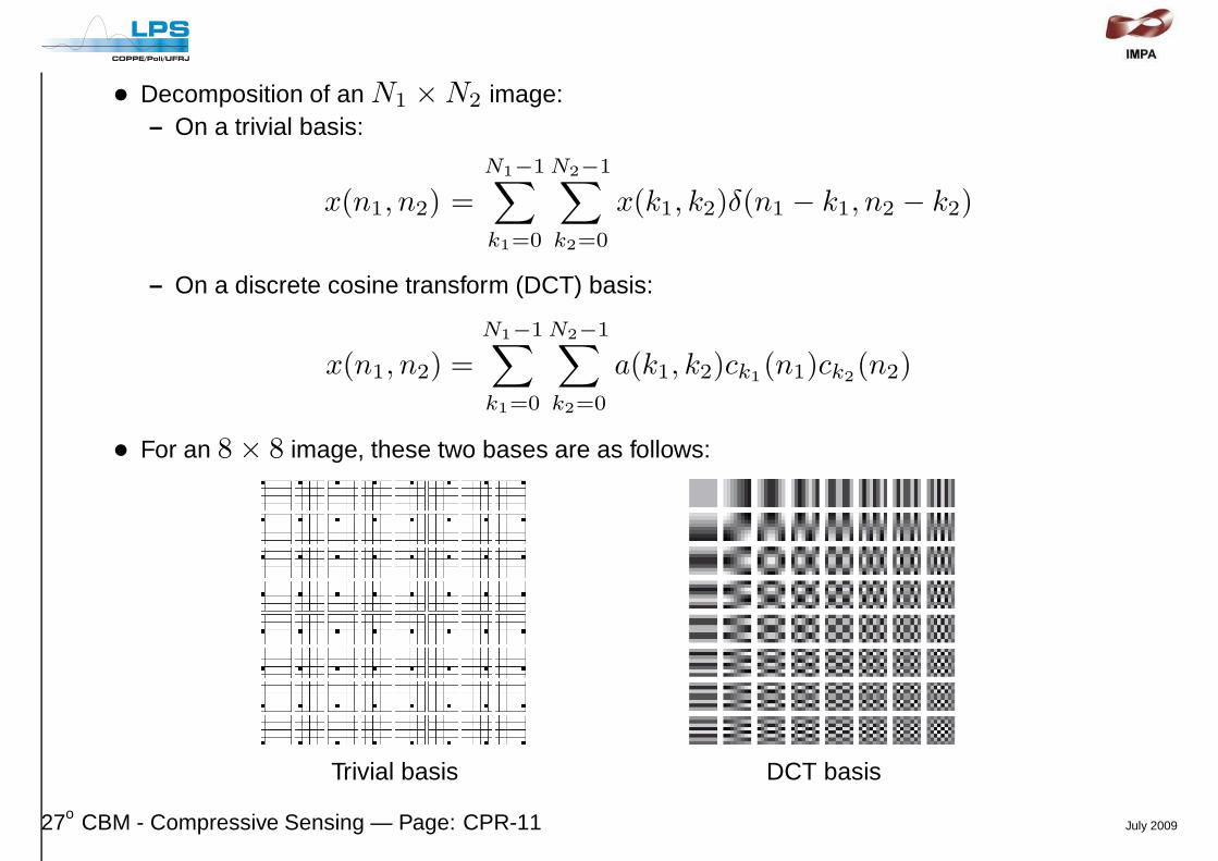
• Decomposition of an N1 ×N2 image:– On a trivial basis:
x(n1, n2) =
N1−1∑
k1=0
N2−1∑
k2=0
x(k1, k2)δ(n1 − k1, n2 − k2)
– On a discrete cosine transform (DCT) basis:
x(n1, n2) =
N1−1∑
k1=0
N2−1∑
k2=0
a(k1, k2)ck1(n1)ck2
(n2)
• For an 8 × 8 image, these two bases are as follows:
Trivial basis DCT basis
27o CBM - Compressive Sensing — Page: CPR-11 July 2009

2 – Signal Representations and Compression
• When compression is concerned, one is interested in the most compact representation. In
x =
M∑
n=1
αnφγn
this implies the smallest possible M , that corresponds to the smallest number of pairs(αn, φγn
), and thus tends to provide the smallest number of bits.
• To achieve this goal, one is even willing to lose some information, that is,
x ≈M∑
n=1
αnφγn
according to a certain fidelity criterion.
• In this context, we analyze in the sequel the answer to the following question:
How should a basis be in order to generate compact representa tions for images?
27o CBM - Compressive Sensing — Page: CPR-12 July 2009
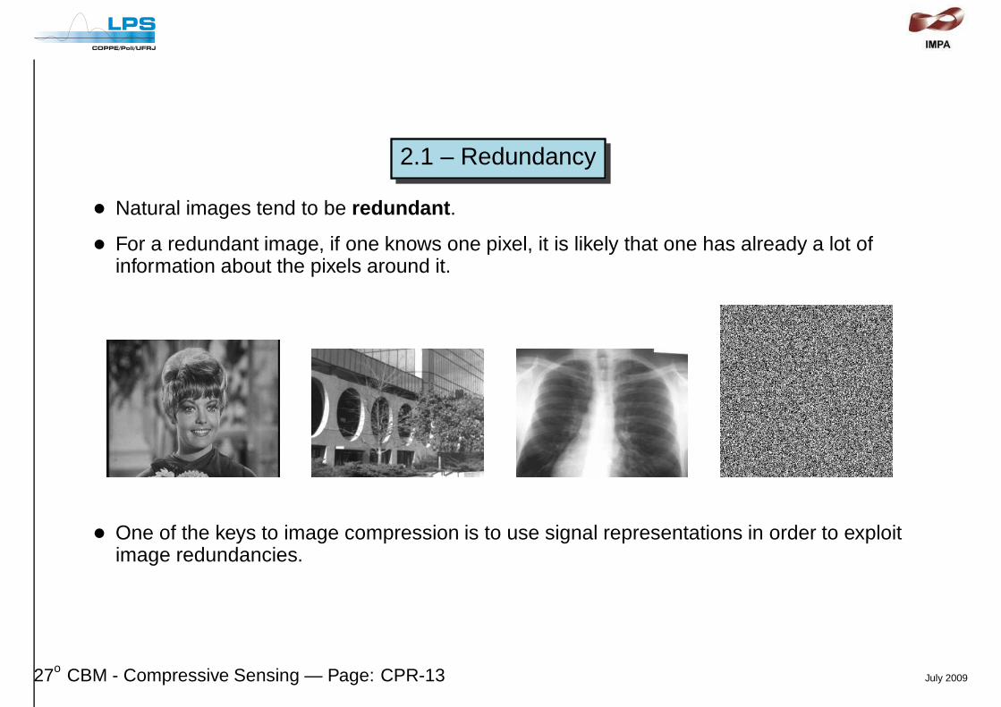
2.1 – Redundancy
• Natural images tend to be redundant .
• For a redundant image, if one knows one pixel, it is likely that one has already a lot ofinformation about the pixels around it.
• One of the keys to image compression is to use signal representations in order to exploitimage redundancies.
27o CBM - Compressive Sensing — Page: CPR-13 July 2009
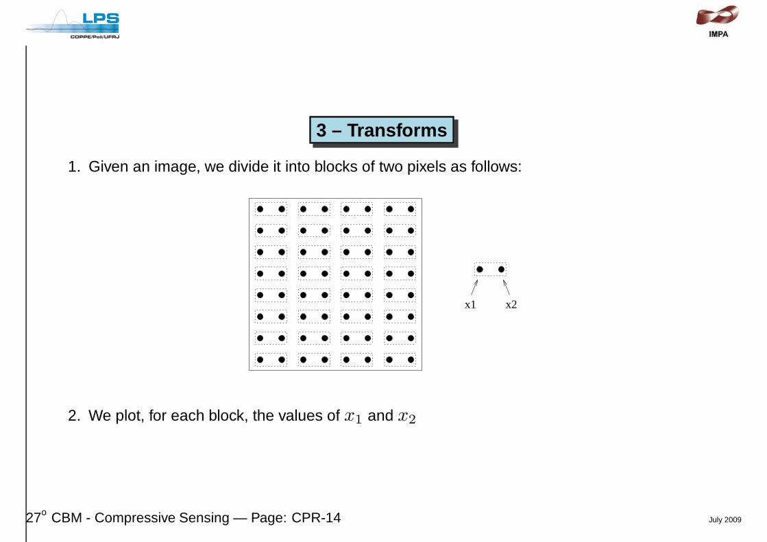
3 – Transforms
1. Given an image, we divide it into blocks of two pixels as follows:
x2x1
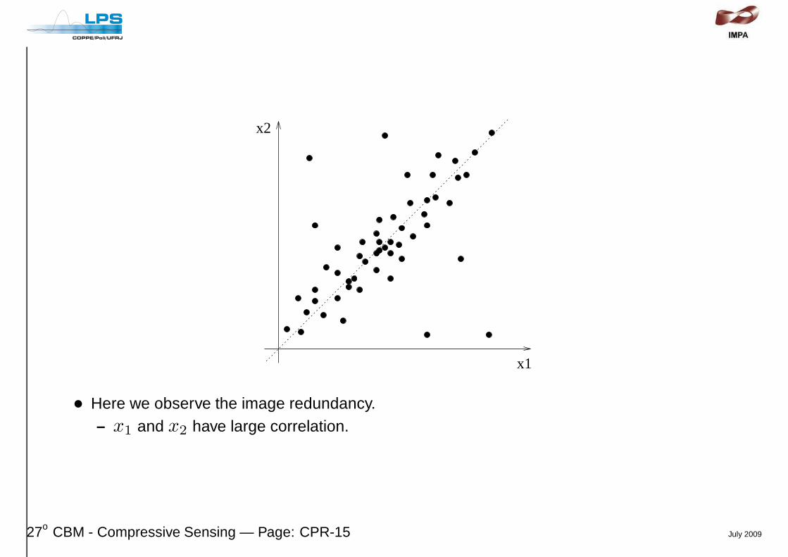
2. We plot, for each block, the values of x1 and x2
27o CBM - Compressive Sensing — Page: CPR-14 July 2009
x1
x2
• Here we observe the image redundancy.– x1 and x2 have large correlation.
27o CBM - Compressive Sensing — Page: CPR-15 July 2009
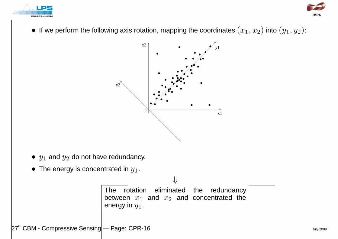
• If we perform the following axis rotation, mapping the coordinates (x1, x2) into (y1, y2):
x1
x2y1
y2
• y1 and y2 do not have redundancy.
• The energy is concentrated in y1.
⇓The rotation eliminated the redundancybetween x1 and x2 and concentrated theenergy in y1.
27o CBM - Compressive Sensing — Page: CPR-16 July 2009

• We usually refer to such a rotation as a transform .
• Given a probability distribution of the pixels, there is a transformation that minimizescorrelation , or in other words, maximizes energy concentration .
• If we take blocks of N pixels,
– There is a rotation in RN that minimizes correlation among them and maximizes
energy concentration (diagonalizes the autocovariance matrix).– Such a rotation is efficient whenever the pixels are concentrated in some directions and
spread in others.∗ This is just the case for images, since they are redundant .
– For a given class of images, such an optimum rotation is referred to as theKarhunen-Loève Transform (KLT) .
– For natural images, the KLT is well approximated by the Discrete Cosine Transform(DCT).
27o CBM - Compressive Sensing — Page: CPR-17 July 2009
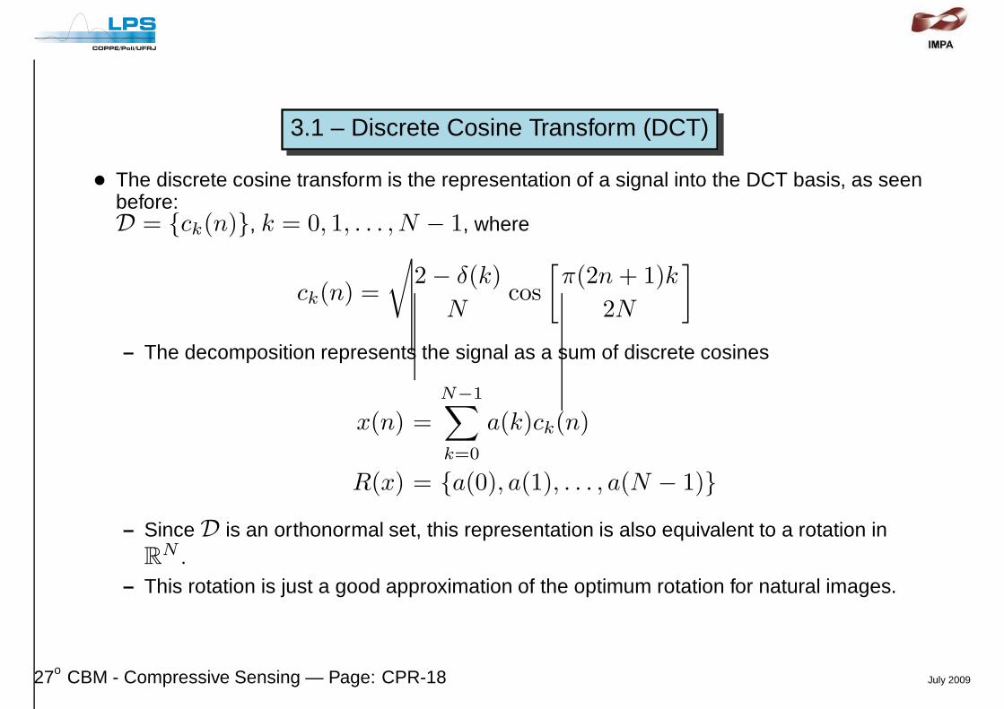
3.1 – Discrete Cosine Transform (DCT)
• The discrete cosine transform is the representation of a signal into the DCT basis, as seenbefore:D = {ck(n)}, k = 0, 1, . . . , N − 1, where
ck(n) =
√
2 − δ(k)
Ncos
[
π(2n+ 1)k
2N
]
– The decomposition represents the signal as a sum of discrete cosines
x(n) =N−1∑
k=0
a(k)ck(n)
R(x) = {a(0), a(1), . . . , a(N − 1)}
– Since D is an orthonormal set, this representation is also equivalent to a rotation inR
N .– This rotation is just a good approximation of the optimum rotation for natural images.
27o CBM - Compressive Sensing — Page: CPR-18 July 2009
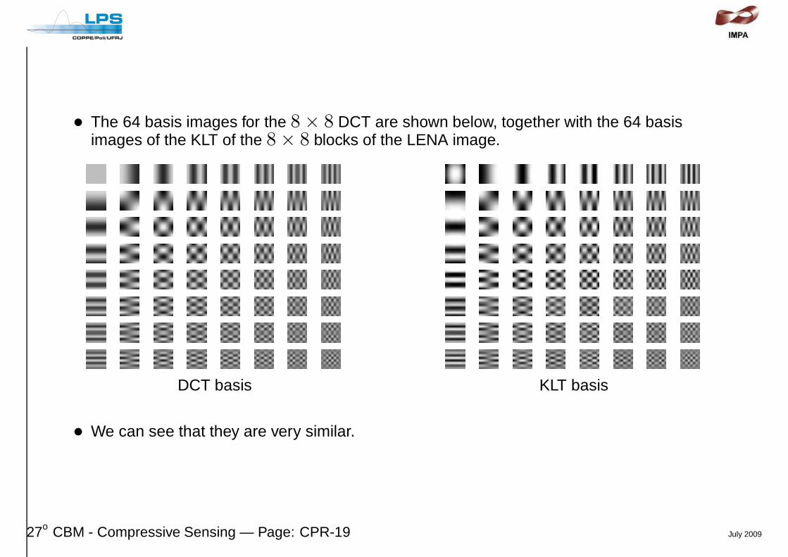
• The 64 basis images for the 8 × 8 DCT are shown below, together with the 64 basisimages of the KLT of the 8 × 8 blocks of the LENA image.
DCT basis KLT basis
• We can see that they are very similar.
27o CBM - Compressive Sensing — Page: CPR-19 July 2009
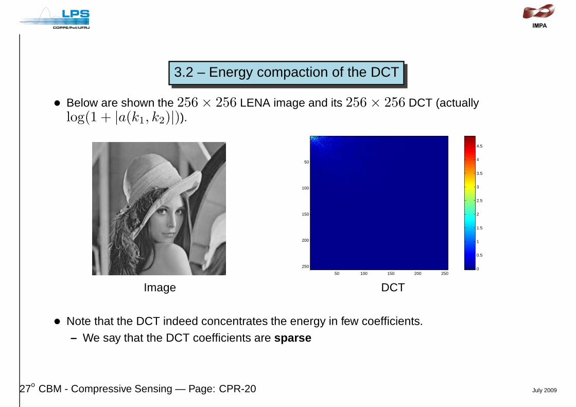
3.2 – Energy compaction of the DCT
• Below are shown the 256 × 256 LENA image and its 256 × 256 DCT (actuallylog(1 + |a(k1, k2)|)).
50 100 150 200 250
50
100
150
200
250 0
0.5
1
1.5
2
2.5
3
3.5
4
4.5
Image DCT
• Note that the DCT indeed concentrates the energy in few coefficients.– We say that the DCT coefficients are sparse
27o CBM - Compressive Sensing — Page: CPR-20 July 2009

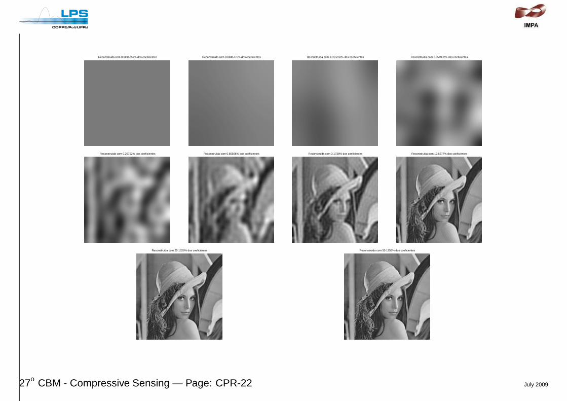
• What would happen to the resconstructed image if we used only the DCT coefficients oflargest energy , discarding the others?
• Observe the reconstructed images that follow, where the DCT coefficients out of the grayregion have been discarded, for j = 1, 2, 4, 8, 16, 32, 64, 128, 181, 256
j
j
• The reconstructed image is almost indistinguishable from the original even for a largenumber of discarded coefficients.
27o CBM - Compressive Sensing — Page: CPR-21 July 2009
Reconstruida com 0.0015259% dos coeficientes Reconstruida com 0.0045776% dos coeficientes Reconstruida com 0.015259% dos coeficientes Reconstruida com 0.054932% dos coeficientes
Reconstruida com 0.20752% dos coeficientes Reconstruida com 0.80566% dos coeficientes Reconstruida com 3.1738% dos coeficientes Reconstruida com 12.5977% dos coeficientes
Reconstruida com 25.1328% dos coeficientes Reconstruida com 50.1953% dos coeficientes
27o CBM - Compressive Sensing — Page: CPR-22 July 2009

• We can conclude that the DCT is powerful for concentrating the information on a naturalimage in few coefficients.
• Indeed, we can discard a large number of coefficients and still recover the image with anacceptable quality.
• However, to effectively compress an image, the remaining coefficients must be efficientlyrepresented.⇒ After the transform, we have to first map the coefficients in a finite number of symbols
(quantization ), and then associate a code for each one (encoding ).
27o CBM - Compressive Sensing — Page: CPR-23 July 2009

3.3 – Quantization
• Process of mapping a set of numbers to a single number.
x ∈ [xk, xk+1) ⇒ Q(x) = rk
• Decreases the number of symbols to be encoded, and, therefore, the number of bits torepresent them.
• In general, the smaller is the number of reconstruction levels, the smaller is the number ofbits needed.
27o CBM - Compressive Sensing — Page: CPR-24 July 2009

3.4 – Compression using the DCT
• Observe the BARBARA image:– Two blocks are marked, one with low level of details and another with high level of
details.
27o CBM - Compressive Sensing — Page: CPR-25 July 2009
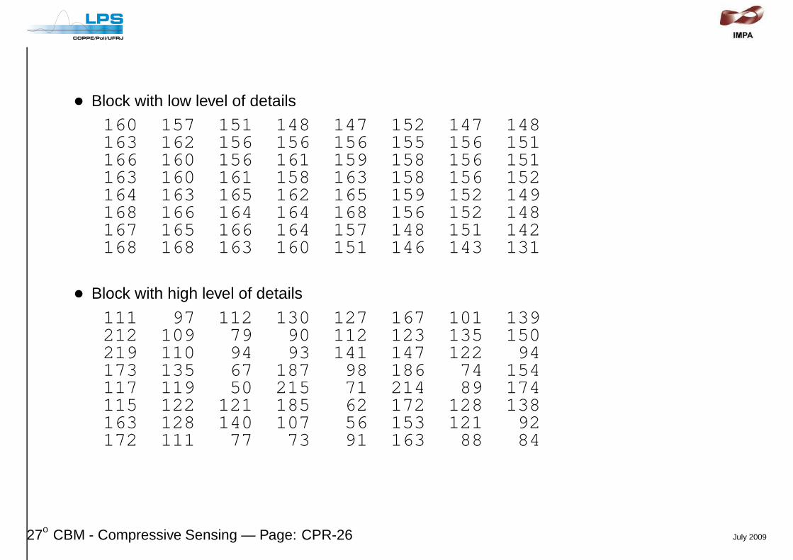
• Block with low level of details
160 157 151 148 147 152 147 148163 162 156 156 156 155 156 151166 160 156 161 159 158 156 151163 160 161 158 163 158 156 152164 163 165 162 165 159 152 149168 166 164 164 168 156 152 148167 165 166 164 157 148 151 142168 168 163 160 151 146 143 131
• Block with high level of details
111 97 112 130 127 167 101 139212 109 79 90 112 123 135 150219 110 94 93 141 147 122 94173 135 67 187 98 186 74 154117 119 50 215 71 214 89 174115 122 121 185 62 172 128 138163 128 140 107 56 153 121 92172 111 77 73 91 163 88 84
27o CBM - Compressive Sensing — Page: CPR-26 July 2009
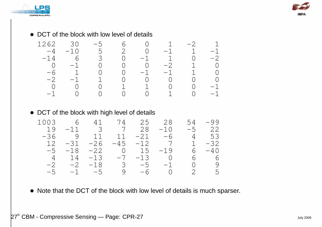
• DCT of the block with low level of details
1262 30 -5 6 0 1 -2 1-4 -10 5 2 0 -1 1 -1
-14 6 3 0 -1 1 0 -20 -1 0 0 0 -2 1 0
-6 1 0 0 -1 -1 1 0-2 -1 1 0 0 0 0 00 0 0 1 1 0 0 -1
-1 0 0 0 0 1 0 -1
• DCT of the block with high level of details
1003 6 41 74 25 28 54 -9919 -11 3 7 28 -10 -5 22
-36 9 11 11 -21 -6 4 5312 -31 -26 -45 -12 7 1 -32-5 -18 -22 0 15 -19 6 -404 14 -13 -7 -13 0 6 6
-2 -2 -18 3 -5 -1 0 9-5 -1 -5 9 -6 0 2 5
• Note that the DCT of the block with low level of details is much sparser.
27o CBM - Compressive Sensing — Page: CPR-27 July 2009
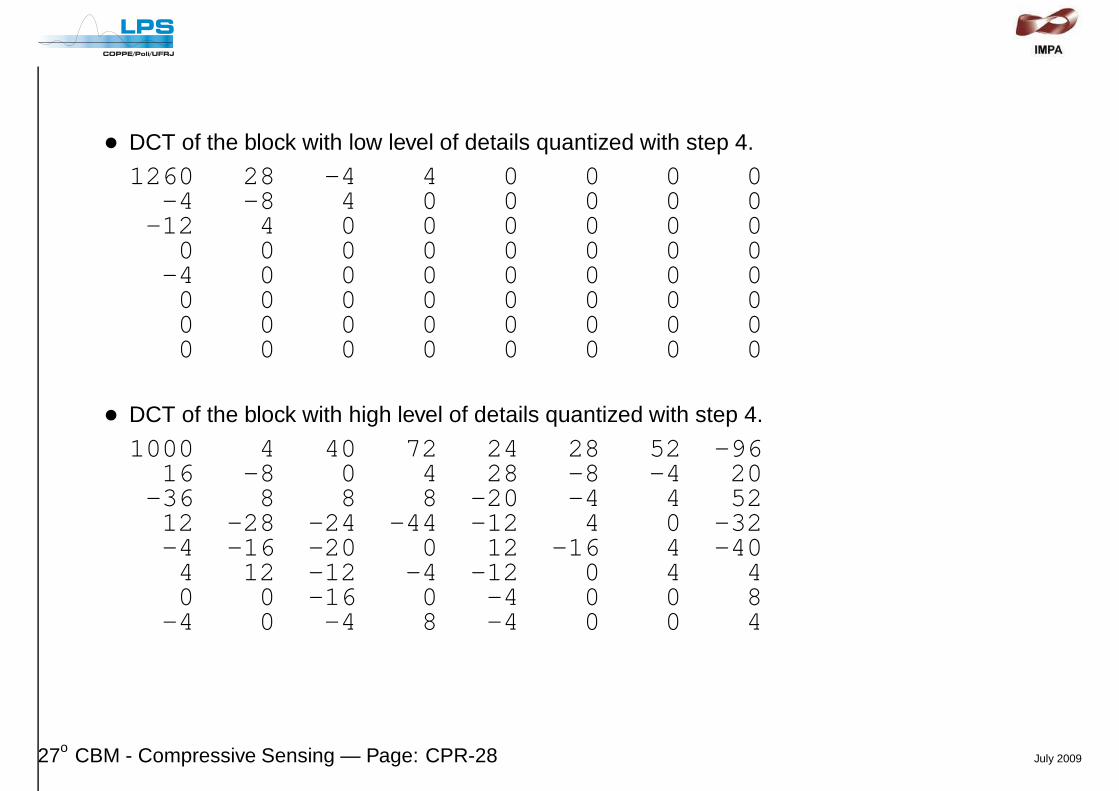
• DCT of the block with low level of details quantized with step 4.
1260 28 -4 4 0 0 0 0-4 -8 4 0 0 0 0 0
-12 4 0 0 0 0 0 00 0 0 0 0 0 0 0
-4 0 0 0 0 0 0 00 0 0 0 0 0 0 00 0 0 0 0 0 0 00 0 0 0 0 0 0 0
• DCT of the block with high level of details quantized with step 4.
1000 4 40 72 24 28 52 -9616 -8 0 4 28 -8 -4 20
-36 8 8 8 -20 -4 4 5212 -28 -24 -44 -12 4 0 -32-4 -16 -20 0 12 -16 4 -404 12 -12 -4 -12 0 4 40 0 -16 0 -4 0 0 8
-4 0 -4 8 -4 0 0 4
27o CBM - Compressive Sensing — Page: CPR-28 July 2009

• DCT of the block with low level of details quantized with step 16.
1248 16 0 0 0 0 0 00 0 0 0 0 0 0 00 0 0 0 0 0 0 00 0 0 0 0 0 0 00 0 0 0 0 0 0 00 0 0 0 0 0 0 00 0 0 0 0 0 0 00 0 0 0 0 0 0 0
• DCT of the block with high level of details quantized with step 16.
992 0 32 64 16 16 48 -9616 0 0 0 16 0 0 16
-32 0 0 0 -16 0 0 480 -16 -16 -32 0 0 0 -320 -16 -16 0 0 -16 0 -320 0 0 0 0 0 0 00 0 -16 0 0 0 0 00 0 0 0 0 0 0 0
• Note that the DCT starts to get quite sparse, specially for low detail blocks.
27o CBM - Compressive Sensing — Page: CPR-29 July 2009
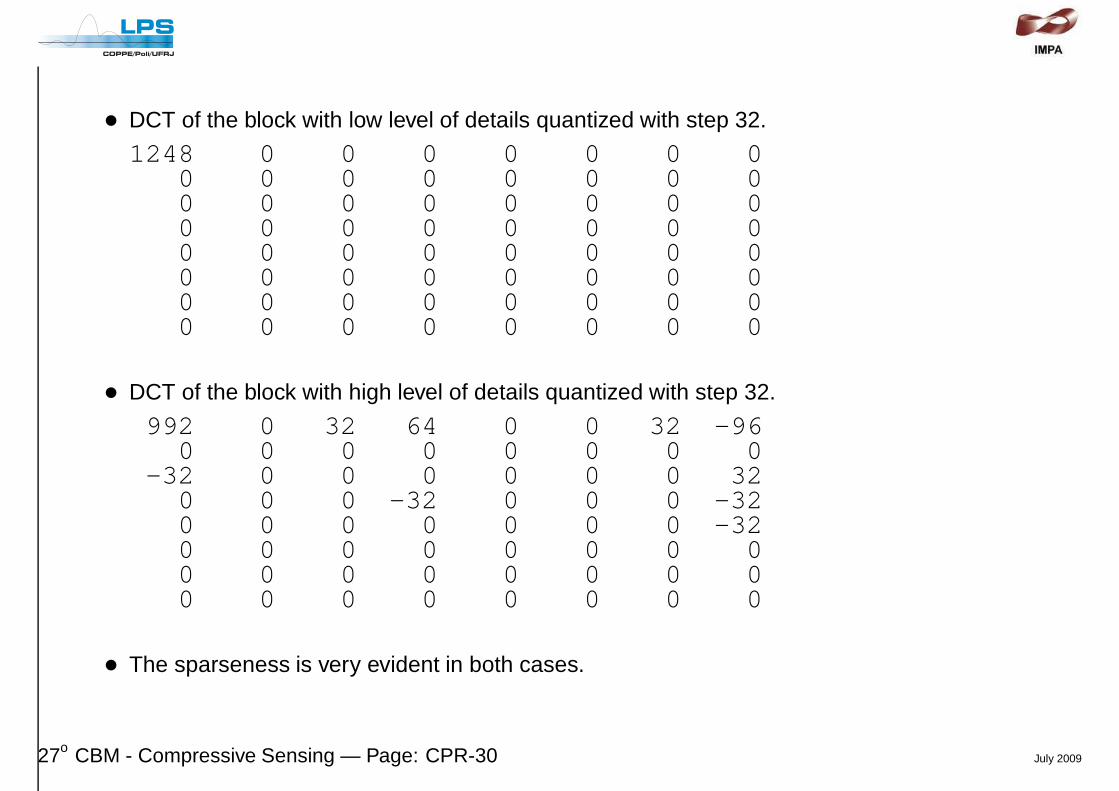
• DCT of the block with low level of details quantized with step 32.
1248 0 0 0 0 0 0 00 0 0 0 0 0 0 00 0 0 0 0 0 0 00 0 0 0 0 0 0 00 0 0 0 0 0 0 00 0 0 0 0 0 0 00 0 0 0 0 0 0 00 0 0 0 0 0 0 0
• DCT of the block with high level of details quantized with step 32.
992 0 32 64 0 0 32 -960 0 0 0 0 0 0 0
-32 0 0 0 0 0 0 320 0 0 -32 0 0 0 -320 0 0 0 0 0 0 -320 0 0 0 0 0 0 00 0 0 0 0 0 0 00 0 0 0 0 0 0 0
• The sparseness is very evident in both cases.
27o CBM - Compressive Sensing — Page: CPR-30 July 2009
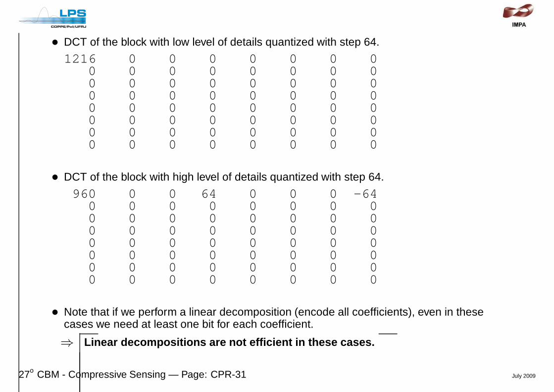
• DCT of the block with low level of details quantized with step 64.
1216 0 0 0 0 0 0 00 0 0 0 0 0 0 00 0 0 0 0 0 0 00 0 0 0 0 0 0 00 0 0 0 0 0 0 00 0 0 0 0 0 0 00 0 0 0 0 0 0 00 0 0 0 0 0 0 0
• DCT of the block with high level of details quantized with step 64.
960 0 0 64 0 0 0 -640 0 0 0 0 0 0 00 0 0 0 0 0 0 00 0 0 0 0 0 0 00 0 0 0 0 0 0 00 0 0 0 0 0 0 00 0 0 0 0 0 0 00 0 0 0 0 0 0 0
• Note that if we perform a linear decomposition (encode all coefficients), even in thesecases we need at least one bit for each coefficient.
⇒ Linear decompositions are not efficient in these cases.
27o CBM - Compressive Sensing — Page: CPR-31 July 2009

Block with low level of details Block with high level of details
Quantization step=4
Quantization step=16
Quantization step=32
Quantization step=64
Blocks with low and high level of details reconstructed using the DCT and several quantizationstep sizes.
27o CBM - Compressive Sensing — Page: CPR-32 July 2009

• We can be very efficient if we skip the zeros.
• In other words, we have to encode the value and position of each non-zero coefficient.
• But the position of a coefficient corresponds to the basis function it corresponds to.
⇒ Skippping the zeros is equivalent to performing a non-linear decomposition , that is,
x ≈
M(x)∑
n=1
αn(x)φγn(x)
– The number and position of the non-zero coefficients also depend on the signal .
• This happens due to the sparseness of the DCT of natural images.
27o CBM - Compressive Sensing — Page: CPR-33 July 2009
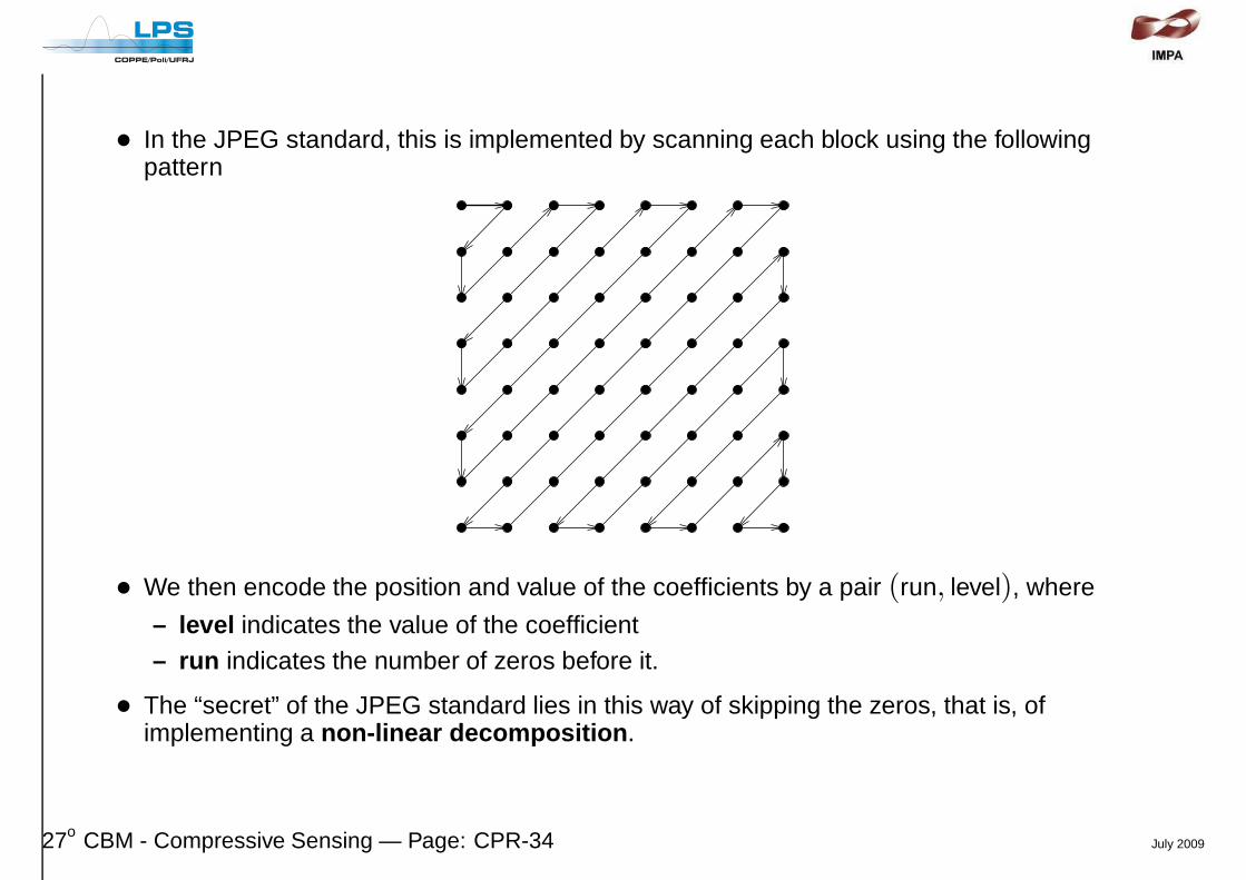
• In the JPEG standard, this is implemented by scanning each block using the followingpattern
• We then encode the position and value of the coefficients by a pair (run, level), where
– level indicates the value of the coefficient– run indicates the number of zeros before it.
• The “secret” of the JPEG standard lies in this way of skipping the zeros, that is, ofimplementing a non-linear decomposition .
27o CBM - Compressive Sensing — Page: CPR-34 July 2009
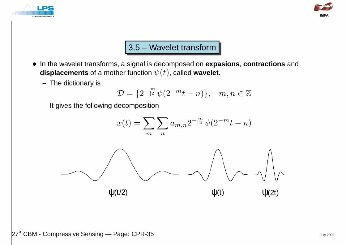
3.5 – Wavelet transform
• In the wavelet transforms, a signal is decomposed on expasions , contractions anddisplacements of a mother function ψ(t), called wavelet .
– The dictionary is
D = {2−m
2 ψ(2−mt− n)}, m, n ∈ Z
It gives the following decomposition
x(t) =∑
m
∑
n
am,n2−m
2 ψ(2−mt− n)
ψ(2t)ψ(t/2) ψ(t)
27o CBM - Compressive Sensing — Page: CPR-35 July 2009
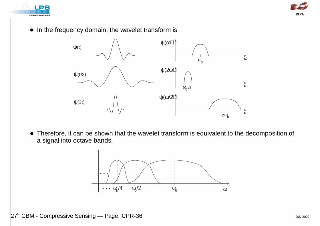
• In the frequency domain, the wavelet transform is
ω 0
ω 0
ω /2
ψ(2ω)
ω 0
ω
ψ(ω)
ω 2
ψ(ω/2) ψ(2t)
ψ(t /2)
ψ(t)
• Therefore, it can be shown that the wavelet transform is equivalent to the decomposition ofa signal into octave bands.
ω ω 0 ω 0 /2 ω 0 /4
…
…
27o CBM - Compressive Sensing — Page: CPR-36 July 2009

3.6 – Examples of Wavelet Transforms of Images
• For images, a wavelet transform is applied first to the rows and then to the columns of animage.
• They look like this
27o CBM - Compressive Sensing — Page: CPR-37 July 2009
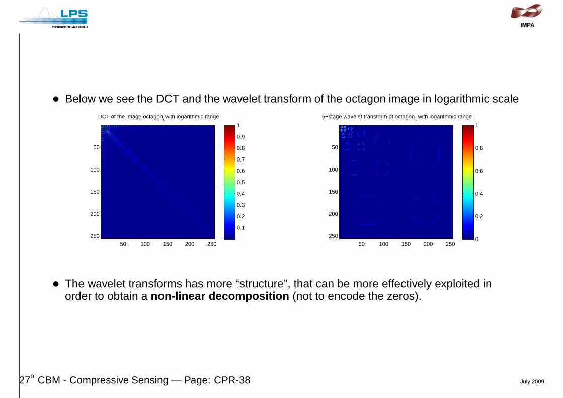
• Below we see the DCT and the wavelet transform of the octagon image in logarithmic scaleDCT of the image octagon
swith logarithmic range
50 100 150 200 250
50
100
150
200
250
0.1
0.2
0.3
0.4
0.5
0.6
0.7
0.8
0.9
1
5−stage wavelet transform of octagons with logarithmic range
50 100 150 200 250
50
100
150
200
250 0
0.2
0.4
0.6
0.8
1
• The wavelet transforms has more “structure”, that can be more effectively exploited inorder to obtain a non-linear decomposition (not to encode the zeros).
27o CBM - Compressive Sensing — Page: CPR-38 July 2009
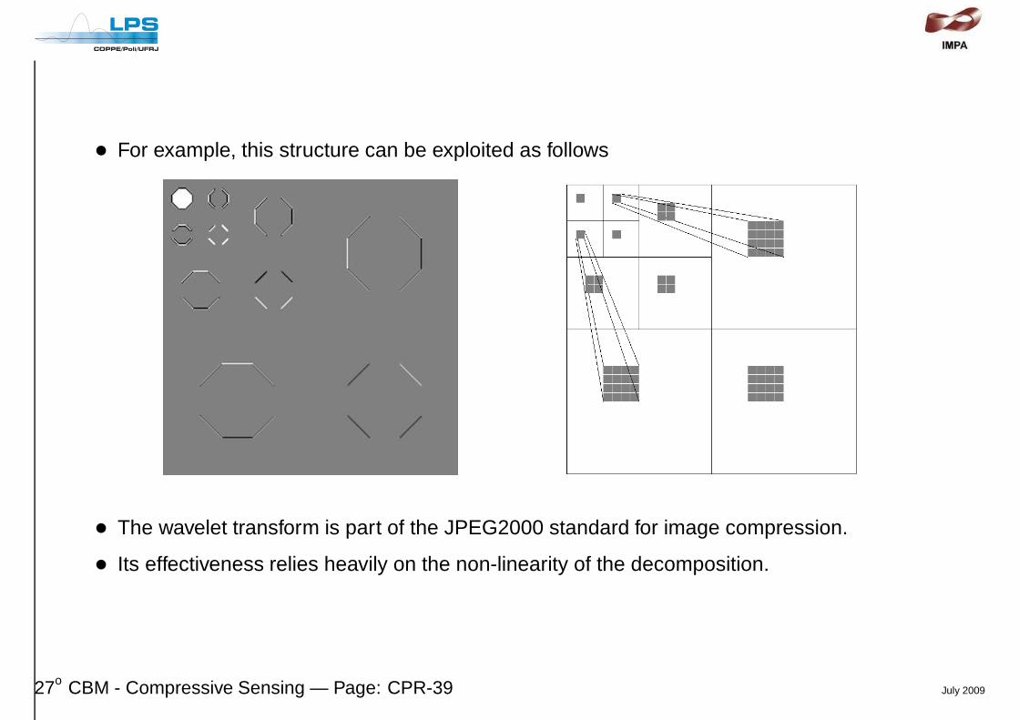
• For example, this structure can be exploited as follows
• The wavelet transform is part of the JPEG2000 standard for image compression.
• Its effectiveness relies heavily on the non-linearity of the decomposition.
27o CBM - Compressive Sensing — Page: CPR-39 July 2009

4.1 – Comparison of DCT and Wavelets in Compression
• LENA image compressed using DCT and Wavelets at 0.5bits/pixel
LENA original JPEG a 0.5 bits/pixel LENA codificada com WAVELETS a 0.5bits/pixel
Original DCT Wavelets
27o CBM - Compressive Sensing — Page: CPR-40 July 2009

5 – Non-linear Decompositions × Compressive Sensing
• In non-linear decompositions, we have to indicate which coefficients are encoded.– Although we spend bits to do this, it is worthy.
• In compressive sensing, similarly to the non-linear case, we do not need to encode all thecoefficients, since the number of measurement functions tend to be much smaller than thesignal dimension (provided that the signal is sparse when decomposed on some basis).– However, contrary to the non-linear case, the measurement functions will not be
signal-dependent (again, provided that the signal is sparse when decomposed in somebasis).
⇒ We do not need to specify which coefficients need to be encoded, since they arealways the same, irrespective of the image.
• In the next lecture we will see why and how this is done in compressive sensing.
27o CBM - Compressive Sensing — Page: CPR-41 July 2009