abordagem bayesiana para estimar a biomassa das anchovas na
TRANSCRIPT

Abordagem Bayesiana para estimar a biomassa dasanchovas na costa do Perú
Zaida Jesús Quiroz Cornejo
Dissertação apresentadaao
Instituto de Ciências Exatas - Departamento de
Estatísticada
Universidade Federal de Minas Gerais
Programa de Pós-Graduação em EstatísticaOrientador: Prof. Dr. Marcos Oliveira Prates
Coorientador: Prof. Dr. Håvard Rue
Belo Horizonte, Janeiro de 2014

Abordagem Bayesiana para estimar a biomassa dasanchovas na costa do Perú
Dissertação apresentada ao Programa dePós-Graduação em Estatística da Universidade
Federal de Minas Gerais como requisitoparcial para a obtenção do grau de
Mestre em Estatística.
Belo Horizonte, Janeiro de 2014

A Bayesian Approach to estimate the biomass ofanchovies in the coast of Perú
Dissertation presented to the GraduateProgram in Statistics of the Universidade Federal
de Minas Gerais in partial fulfillment ofthe requirements for the degree of Master
in Statistics.
Belo Horizonte, January 2014

UNIVERSIDADE FEDERAL DE MINAS GERAIS
FOLHA DE APROVAÇÃO
Abordagem Bayesiana para estimar a biomassa dasanchovas na costa do Perú
Zaida Jesús Quiroz Cornejo
Dissertação defendida e aprovada pela banca examinadora constituída por:
Prof. Dr. Marcos Oliveira PratesUniversidade Federal de Minas Gerais - UFMG
Prof. Dr. Flávio Bambirra GonçcalvesUniversidade Federal de Minas Gerais - UFMG
Profa. Dra. Thais Cristina Oliveira da FonsecaUniversidade Federal do Rio de Janeiro - UFRJ
Belo Horizonte, Janeiro de 2014

Acknowledgments
Agradeço primeiramente a Deus, por me dar forças para superar às dificuldades, pelasaúde e pelas alegrias vividas ao longo desses dois anos.
A minha querida família por todo o carinho e amor, em especial a minha mãe e irmã peloapoio incondicional, ao meu pai por sempre me acompanhar nas idas e voltas ao aeroportoe os gratos cafés de amanhã ou lanches, ao Victor pela compreensão, por estar ao meu ladose fazendo sempre presente mesmo eu estando tão longe, ao meu cunhado Juan Carlos pelasbem-vindas sempre a casa e ao meu sobrinho Luquitas pelas alegrias e beijinhos pelo skype.
Ao meu orientador, o Professor Marcos Oliveira Prates, pela ajuda na realização dessetrabalho, pela paciência em cada uma das nossas reuniões, por me motivar a gostar dapesquisa em todo momento e por me incentivar a continuar meus estudos de pós-graduação.
Gostaria de agradecer também ao meu co-orientador, o Professor Håvard Rue, por aceitarem participar dessa dissertação e pelas valiosas sugestões dadas.
A todos os meus professores do programa de pós graduação em Estatística na UFMG,pelo conhecimento transmitido.
À Professora Glaura, pelas sugestões e grande apoio dado tanto antes como depois daseleção do mestrado.
À Professora Lourdes, pela sua amizade e apoio, e acreditar em mim desde o comencinho.Gostaria de agradecer também ao Professor Renato Assunção, pelos comentários valiosos
para melhoria desse trabalho.Aos Professores Flávio Bambirra Gonçcalves e Thais Cristina Oliveira da Fonseca, por
aceitar em participar da banca dessa dissertação.Às secretárias do programa de pós graduação, Rogéria e Rose, por prestativamente re-
sponder os infinitos e-mails que eu enviei, e pela amizade e ajuda ao longo do mestrado.Á Arnaud Bertrand e Sophie Bertrand, mercie beaucoup pour mon initiation scientifique
et leur motivation et l’intérêt à poursuivre mes études.Aos meus amigos do IMARPE-IRD, que mesmo longe sempre lembraram de mim, à Chio,
à Ross, e em especial ao Danielinho, você me ajudou muito mesmo.Aos amigos na UFMG, em especial a minha querida amiga Márcia, pela grata companhia
no LESTE, pelo bate-papo, carinho e sincera amizade, valeu por todo guria!.A minha avozinha brasileira Carmen, por todo o apoio, carinho e amizade ao longo desses
dois anos, você foi meu anjo, não tenho palavras para lhe-agradecer, e a minha irmãzinhaCecilia pela amizade e brincadeiras, muito obrigada!
i

Resumo
O Sistema da Corrente de Humboldt do norte (NHCS) é um dos mais produtivos ecossis-temas em termos de peixes do mundo. Em particular, a anchova peruana (Engraulis ringens)é a maior presa dos predadores superiores, como mamíferos, aves, peixes e pescadores. Nessecontexto, é importante compreender a dinâmica da distribuição de anchova para preservá-la,bem como para explorar sua capacidade econômica. Usando os dados recolhidos pelo “Insti-tuto del Mar del Perú” (IMARPE), durante uma pesquisa científica em 2005, apresenta-seuma análise estatística que tem como objetivos principais: (i) se adaptar às característi-cas dos dados amostrados como: dependência espacial, altas proporções de zeros e grandestamanhos de amostras, (ii) fornecer informações importantes da dinâmica da população deanchovas e propor um modelo para estimação e previsão da biomassa da anchova no NHCSdo Perú. Os dados são analisados em um contexto Bayesiano usando a metodologia Inte-grated Nested Laplace Approximation (INLA). Finalmente, usa-se critérios de comparaçõesentre modelos para selecionar o modelo proposto de melhor ajuste. Também é feito um es-tudo do poder preditivo de cada modelo. Além disso, é realizado um diagnóstico de influênciaBayesiana para o modelo preferido.
Palavras-chave: Inferência Bayesiana Aproximada ; Geoestatística; Integrated Nested LaplaceApproximation; Modelo Gaussiano Latente; Ecologia Marinha.
ii

Abstract
The Northern Humboldt Current System (NHCS) is the world most productive ecosys-tem in terms of fish. In particular, Peruvian anchovy (Engraulis ringens) is the major preyof the principal top predators, like mammals, seabirds, fish and fishers. In this context, it isimportant to understand the dynamics of the anchovy distribution to preserve it as well asto explore its economical capacities. Using the data collected by the “Instituto del Mar delPerú” (IMARPE), during a scientific survey in 2005, we present a statistical analysis thathas as main goals: (i) adapt to the characteristics of the sampled data, such as spatial de-pendence, high proportions of zeros and big samples size, (ii) provide important insights onthe dynamics of the anchovy population and propose a model for estimation and predictionof anchovy biomass in the NHCS of Perú. These data are analyzed in a Bayesian frameworkusing the Integrated Nested Laplace Approximation (INLA) methodology. Finally, modelcomparison is performed to select the best model and predictive checks to study the predic-tive power of each model. Moreover, a Bayesian spatial influence diagnostic is performed forthe preferred model.
Keywords: Approximate Bayesian inference; Geostatistics; Integrated Nested Laplace Ap-proximation; Latent Gaussian model; Marine Ecology.
iii

Resumo Estendido
O ecossistema pelágico peruano é dominado pela anchova peruana. Atualmente, a an-chova é responsável pela maior pesca de peixes no mundo. Devido a sua importância econômicae ecológica o “Instituto del Mar del Perú” (IMARPE) realiza pesquisas todos os anos sobreo ecossistema para orientar as decisões de gestão do país. Assim, a bordo de um cruzeirode pesquisa científico-acústico obtem-se a massa da anchova por milha náutica que seráchamada de biomassa da anchova ao longo desse trabalho. A distribuição da anchova é car-acterizada por estruturas de agregação, tal padrão é devido ao seu comportamento de defesapara enfrentar a predação. Logo, os dados da biomassa da anchova caracterizam-se por umaelevada proporção de valores zeros e dependência espacial.
A motivação desse trabalho é propor um modelo estatístico capaz de estimar a biomassade anchova, o qual deve considerar os valores zero e não zeros usando uma abordagem in-tegrada como os modelos zero-inflacionados ou os modelos Hurdle. Nesse sentido, nos últimosanos um grande esforço tem se dedicado a lidar com esse tipo de modelos. Porém, muitasvezes esses desenvolvimentos têm sido focados principalmente na modelagem de dados dis-cretos (Mullahy, 1986; Cameron and Trivedi, 1998; Agarwal et al., 2002). A ideia subjacentenesse trabalho é estender a definição desses modelos para dados discretos à modelagem dedados contínuos, e, ao mesmo tempo, acomodar a dependência espacial. Para isso, propomosuma modelagem Hierárquica Bayesiana. Os modelos hierárquicos, diferentemente dos mod-elos tradicionais baseados na modelagem multivariada da variável resposta, através de umaestrutura de covariância permitem modelar de forma simplificada respostas discretas, con-tínuas e/ou misturas, impondo à estrutura de auto-correlação espacial em um nível inferiorna hierarquia.
Geralmente, inferência Bayesiana de modelos complexos pode ser realizada utilizandométodos tais como o Markov Chain Monte Carlo (MCMC). No entanto, sabe-se que paramodelos que incluem vários efeitos fixos e aleatórios com dependência espacial e/ou grandesconjuntos de dados, obter as distribuições posteriores é um desafio, pois estas raramentepossuem solução analítica, tornando assim a inferência através de métodos MCMC com-putacionalmente muito cara. Uma nova abordagem, chamada Intagrated Nested LaplaceApproximation (INLA), foi proposta por Rue et al. (2009) para executar de forma eficienteinferência Bayesiana em modelos hierárquicos Gaussianos latentes. O método baseia-se emaproximações precisas e determinísticas ao invés de simulações aleatórias, e portanto, nãoprecisa de diagnósticos de convergência necessários nos métodos MCMC.
iv

v
Esse trabalho está organizado da seguinte maneira: No Capítulo 1 falamos brevementeda motivação do trabalho e definimos os objetivos e as contribuições do mesmo. No Capí-tulo 2 é feita uma revisão da literatura utilizada nos próximos capítulos. Introduzimos osconceitos de Modelos Gaussianos Latentes e a relação deles com os modelos Bayesianos hi-erárquicos. Em seguida, apresentamos os Campos aleatórios Gaussianos e campos aleatóriosMarkovianos Gaussianos (CAMG), assim como as vantagens em termos computacionais dosCAMG. Logo, apresentamos a aproximação Gaussiana no caso univariado. Finalizamos ocapítulo apresentando o método de aproximação determinística INLA usado para a obtençãodas distribuições marginais a posteriori na inferência Bayesiana. No Capítulo 3 é apresen-tada uma descrição detalhada dos dados que motivam a nossa modelagem. Nesse capítuloé descrita de forma resumida como são obtidos os dados, em particular, a variável de in-teresse, a biomassa da anchova. Além disso, descrevemos outras variáveis disponíveis quepodem contribuir para explicar à variabilidade da variável resposta. O Capítulo 4 descrevea estrutura da modelagem para o ajuste e previsão da biomassa de anchova proposta pelaautora. Além disso, apresentamos como a inferência Bayesiana é realizada usando o INLA. Ocapítulo termina apresentando uma variedade de critérios de seleção dos modelos, critériosde previsão dos modelos, e finalizamos apresentando um possível diagnóstico de influência.O Capítulo 5 apresenta à aplicação da modelagem proposta. Primeiramente, é apresentadauma análise exploratória das covariáveis, e exploramos possíveis distribuições contínuas paracompor o modelo misto. Em seguida, apresentamos diversos modelos e os seus resultadosutilizando a metodologia descrita no capítulo anterior. Os resultados da seleção de modelosmostram que a inclusão de efeitos espaciais estruturados nas duas componentes do modeloHurdle são realmente necessários para um melhor ajuste. Assim o modelo preferido incluindoambos efeitos espaciais é o de melhor ajuste para a biomassa da anchova e, é ainda, capazde explicar melhor a distribuição espacial dos dados. Além disso, o poder de previsão dosmodelos é estudado através de um estudo de simulação. Nesse estudo, separamos o bancoem treino e validação com diferentes porcentagens de corte e rodamos 100 iterações paradeterminar o modelo com melhor previsão. Os resultados mostraram que o modelo commelhor previsão é também o modelo selecionado como o de melhor ajuste. Finalizamos ocapítulo diagnosticando as regiões de influência através da divergência de Kullback-Liberpara o modelo selecionado. No Capítulo 6 apresentamos algumas discussões a respeito dasvantagens do modelo escolhido para estimar a biomassa da anchova. Finalmente, no Capí-tulo 7 apresentamos ainda algumas possíveis extensões que podem ser feitas como trabalhosfuturos.

Contents
List of Figures viii
List of Tables x
1 Introduction 11.1 Motivation . . . . . . . . . . . . . . . . . . . . . . . . . . . . . . . . . . . . . 11.2 Objetives . . . . . . . . . . . . . . . . . . . . . . . . . . . . . . . . . . . . . 11.3 Contributions . . . . . . . . . . . . . . . . . . . . . . . . . . . . . . . . . . . 21.4 Organization of manuscript . . . . . . . . . . . . . . . . . . . . . . . . . . . 2
2 Literature Review 32.1 Latent Models and Hierarchical models . . . . . . . . . . . . . . . . . . . . . 32.2 Gaussian Fields and Gaussian Markov Random Fields . . . . . . . . . . . . . 4
2.2.1 Gaussian Fields . . . . . . . . . . . . . . . . . . . . . . . . . . . . . . 42.2.2 Gaussian Markov Random Fields . . . . . . . . . . . . . . . . . . . . 5
2.3 Gaussian approximation . . . . . . . . . . . . . . . . . . . . . . . . . . . . . 72.4 Integrated Nested Laplace Approach . . . . . . . . . . . . . . . . . . . . . . 8
2.4.1 Approximating π(θ|y) . . . . . . . . . . . . . . . . . . . . . . . . . . 92.4.2 Approximating π(xi|θ, y) . . . . . . . . . . . . . . . . . . . . . . . . 102.4.3 Approximating π(θj|y) . . . . . . . . . . . . . . . . . . . . . . . . . . 10
3 Description of Data 12
4 Model Structure 144.1 Bayesian Inference . . . . . . . . . . . . . . . . . . . . . . . . . . . . . . . . 164.2 Model Assessment . . . . . . . . . . . . . . . . . . . . . . . . . . . . . . . . . 17
4.2.1 Model Comparison . . . . . . . . . . . . . . . . . . . . . . . . . . . . 174.2.2 Model Predictive checks . . . . . . . . . . . . . . . . . . . . . . . . . 184.2.3 Influence Diagnostics . . . . . . . . . . . . . . . . . . . . . . . . . . . 19
5 Application 205.1 Exploratory Analysis . . . . . . . . . . . . . . . . . . . . . . . . . . . . . . . 205.2 Data Analysis . . . . . . . . . . . . . . . . . . . . . . . . . . . . . . . . . . . 22
vi

CONTENTS vii
6 Discussion 28
7 Future works 307.1 Introduction . . . . . . . . . . . . . . . . . . . . . . . . . . . . . . . . . . . . 307.2 The Stochastic Partial Differential equation (SPDE) approach . . . . . . . . 30
A Proof of result 4.7 34
Bibliography 35

List of Figures
2.1 Simulation of a GRMF using sparse Precision matrix. . . . . . . . . . . . . . 62.2 Correlation function for the fitted GMRF (red line) and the Matern CF (blue
line) with range 15 and 5× 5 neighbourhood. . . . . . . . . . . . . . . . . . 72.3 Original posterior density (continuous black line) and Gaussian approximation
of posterior density (dashed grey line) for each x0=0,0.5,1,1.5. The value ofx0 is represented by the small dot point in each plot. . . . . . . . . . . . . . 8
2.4 Location of the integration points in a two dimensional θ-space using the (a)grid and the (b) CCD strategy. . . . . . . . . . . . . . . . . . . . . . . . . . 10
3.1 Left: The observed data, where the trajectory of survey tracks is representedby parallel cross-shore transects (red and gray dots). Furthermore, the size ofred dots correspond to the biomass of anchovy (higher than zero) and graydots correspond to the biomass of anchovy equal to zero. Right: Exploratoryanalysis. Histogram for all anchovy biomass observations and Histogram fornon-zero anchovy biomass observations. . . . . . . . . . . . . . . . . . . . . . 13
5.1 The black grids dots represent the translated regular lattice, here red grid dotsare samples of anchovy biomass traslated too. And green grids dots representthe rotated Regular lattice, here blue grid dots are samples of anchovy biomassrotated too. . . . . . . . . . . . . . . . . . . . . . . . . . . . . . . . . . . . . 21
5.2 Left: Regular lattice for distance to the coast. Right: Regular lattice for oceandepth. . . . . . . . . . . . . . . . . . . . . . . . . . . . . . . . . . . . . . . . 21
5.3 Results. Left: Observed anchovy absence/presence. Right: Mean posteriorprobability of anchovy absence under model I. . . . . . . . . . . . . . . . . . 26
5.4 Results. Left: Observed anchovy biomass (on the logarithmic scale). Right:Mean posterior anchovy biomass under model I (on the logarithmic scale). . 27
5.5 Results. Left: Probability qi of influence regions. Right: Mean posterior ofanchovy biomass influence regions (on the logarithmic scale). . . . . . . . . . 27
7.1 Representation of piewise-linear approximationof a function in two dimensionsover a triangulated mesh. . . . . . . . . . . . . . . . . . . . . . . . . . . . . . 31
viii

LIST OF FIGURES ix
7.2 Meshs constructed using Constrained refined Delaunay triangulation. Redgrid dots are samples of anchovy biomass samples. The region defined bythe sky-blue line is the edge boundary which defines the priority area forestimation. Outside this region the boundary effects are higher. Right: Meshhave less resolution than left plots. Top: Mesh for all data. Down: Mesh fornorthern region of top panel. . . . . . . . . . . . . . . . . . . . . . . . . . . . 33

List of Tables
5.1 Selection criteria for the different positive Distributions . . . . . . . . . . . . 215.2 Linear predictors and hyperparameters for each proposed model . . . . . . . 235.3 The selection criteria for the models proposed with different linear predictors 245.4 Predictive model checks. Mean of RMSPE (MRMSPE) out 100 validation
samples. . . . . . . . . . . . . . . . . . . . . . . . . . . . . . . . . . . . . . . 245.5 Summary statistics (point, standard deviation and 95% credible interval (CI))
for Fixed effects and Hyperparameters estimation. . . . . . . . . . . . . . . 25
7.1 Summary of functions φk and precision matrices Qα for each α . . . . . . . . 32
x

Chapter 1
Introduction
1.1 MotivationThe Peruvian pelagic ecosystem (Northern HCS) is highly dominated by the Peruvian
anchovy. Anchovy is a small pelagic fish characterized by a fast growth, an early maturity(1 year), a short life span (4 years), fast response to environmental variability, plasticity interms of the prey it consumes and foraging behaviour (Bertrand et al., 2008). At the present,anchovy species sustain the largest single-species fishery in the world with average landingsover 6.5 millions tons per year during the last decade (Bertrand et al., 2008). Because ofits economic and ecological importance “Instituto del Mar del Perú” (IMARPE) conductsresearch on the ecosystem and fisheries to guide management decisions. In Perú, annualacoustic surveys of fish population distribution and abundance have been conducted since1983 by IMARPE. In particular, acoustic data are collected onboard the research vessel“José Olaya Balandra” from the IMARPE during a scientific acoustic survey “Pelagic 2005”.Using these data it is obtained the mass of anchovy per nautical mile which will be calledanchovy biomass along the current paper.
Another relevant feature of anchovy involves its distribution which within suitable habitatis characterized by nested aggregation structures (Fréon and Misund, 1999). Such patternresults from its foraging behavior and defense behavior to face predation. For this reason,anchovy biomass data are characterized by a high proportions of zero values and spatialdependence.
Such characteristics have to be considered to develop an appropriate statistical model toestimate anchovy biomass. The excessive zero observations is the main reason to assume thatanchovy distribution can not be modeled by only one distribution. In this context, Woillezet al. (2009) developed an integrated model approach involving non-parametric transforma-tion processes to investigate schooling fish estimates, while Boyd (2012) developed anotherintegrated model to simulate the spatial distribution of anchovy biomass for a small regionusing likelihood-based Geostatistics approach (Diggle et al., 1998). Therefore, an appropriatemodel needs to account for the zero and for the non-zero values as an integrated approach,like zero-inflated models or Hurdle models. In particular, Hurdle models are attractive be-cause they do not assume that zero values represent error measures, may be due to a poorsample design, or are false zeros, in fact, here anchovy biomass is equally collected overall studied area, and most important, anchovy absence is not unusual within unsuitablehabitat. Furthermore, to accommodate spatial dependence, we need to develop a modelingframework that allow for spatial autocorrelation with excessive zeros in the observations.
1.2 ObjetivesThe main objectives of this study are: (i) Adapt to the characteristics of the sampled data
to predict anchovy biomass at unsampled locations, (ii) Provide important spatial insights
1

1.4 CONTRIBUTIONS 2
on the anchovy distribution and biomass. In order to achieve our objectives a Hurdle modelfor continuous data is developed. In particular, we use a Bayesian Hierarchical Model whichis very flexible and powerful allowing for the model to have all characteristics presented.
1.3 ContributionsA fair amount of statistical effort has been devoted to dealing with zero-inflated data sets.
However, often these developments have been focused mainly on the modelling of discretedata (Mullahy (1986), Agarwal et al. (2002)). The idea behind a Hurdle model for discretedata is to separate the zero structure from the non zero structure with a finite mixture of apoint mass at zero with a truncated-at-zero distribution (Cameron and Trivedi, 1998), suchdefinition will be extended for continuous data.
Generally, Bayesian inference for complex models can be performed using simulationmethods such as Markov Chain Monte Carlo Method (MCMC). However, it is known thatfor models which include several fixed and random effects with spatial dependence and/orlarge datasets, like in our framework, obtain posterior distributions is seldom analiticallyavailable, making inference using MCMC methods computationally expensive. A new ap-proach, called integrated nested Laplace approximation (INLA), was proposed by Rue et al.(2009) to perform fast Bayesian inference. The method relies on accurate and determinis-tic approximations instead of sthocastic simulations and thus, it does not require conver-gence diagnostics. Recently, Muñoz et al. (2013) studied the presence/absence of Trachurusmediterraneus in the Western Mediterrian under the context of Bayesian Hierarchical Modelusing the R-INLA software.
1.4 Organization of manuscriptThe dissertation is organized as follows: Chapter 2 presents some literature review needed
for next sections. Chapter 3 presents some description of data. Chapter 4 describes theproposed model structure to fit and to predict anchovy biomass. Also, it is presented asummary of how Bayesian inference is achieved using INLA. The chapter ends presentinga variety of model assesment criteria. Chapter 5 presents the application of the proposedmodel and the results obtained. Chapter 6 discusses meaningful results and finally Chapter 7discusses future works.

Chapter 2
Literature Review
Integrated Nested Laplace Approximation (INLA) is a relatively new approach to imple-ment fast Bayesian inference for Latent Gaussian Models (LGM). Many well known modelslike Geostatistical models, spatial and spatio-temporal models, among many others, areLGM’s. These models are usually complex because they usually include several fixed andrandom effects. As a result their posterior distributions are rarely analitically available andinference becomes very difficult. In these cases model fitting is usually based on simulationmethods like Markov Chain Monte Carlo (MCMC), which are very accurate if the conver-gence is achieved, but on the other hand in term of computational time are very expensive.In that sense, INLA with accurate, deterministic approximations to posterior marginal dis-tributions is an attractive alternative to MCMC simulations.In the next sections LGM’s and their main features are described, then some definitionsabout Gaussian Fields and Gaussian Random Markov Fields are given, then it is discussedthe relationship between those ones and the computational advantages of GRMF over Gaus-sian Fields; and finally Gaussian approximations used to introduce the INLA approach aredefined.
2.1 Latent Models and Hierarchical modelsLatent Models are a subclass of structured additive models which can also be seen as a
representation of a Hierarchical model. First of all, let us assume that for i = 1, ..., n we haven observed (or response) variables yi with a distribution usually but not necessarily from theexponential family. The latent variable ηi defined by Equation (2.1) is a linear predictor whichenters the likelihood through some link function g(.) = ηi. Thus, ηi is modeled additively ondifferent effects of various covariates,
ηi = β0 +
ηf∑j=1
wijf(k)(uij) +
ηβk∑k=1
βkzki + εi. (2.1)
Here, β′ks are coefficients for linear effects on a vector of covariates z, which capture thevariability in data caused by explanatory variables; f (k)’s represent unknown functions ona set of covariates u, useful to incorporate dependence between observations which can beof various kind like spatial, temporal or spatiotemporal; wij are known as weights; and εrepresents unstructured random effects.The latent field x is composed by a vector: x = ηi, β0, βk, f (k). If the distributionof latent field is set as Gaussian such model becomes a Latent Gaussian Model (LGM). If,in addition, this latent field is Gaussian and admits conditional independence properties itis called Gaussian Random Markov Field.
Hierarchical Models are a generalization of Linear and Generalized Linear Models. They are
3

2.2 GAUSSIAN FIELDS AND GAUSSIAN MARKOV RANDOM FIELDS 4
specified by several stages of observations and parameters. A typical Hierarchical model isdefined by: a first stage, where a distributional assumption is formulated for the observationswhich depend on the latent field. Here, we assume observations conditionally independentgiven the latent field. A second stage, is a latent field which might follow a MultivariateGaussian distribution with mean µ and covariance matrix Σ(θ). And a third stage com-posed by all the unknown parameters called hyperparameters, here a prior model is assignedfor these unknown parameters.
Thus, a LGM can be defined like a Hierarchical model with the following structure:(i) A likelihood model for the response variable assumed to be independent given the latentparameters x :
y|x, θ ∼∏i∈I
π(yi|xi, θ)
(ii) A latent Gaussian field:x|θ ∼ N(µ,Σ(θ))
(iii) And hyperparameters θ:θ ∼ π(θ).
In many LGM’s and Hierarchical models the latent Gaussian field is also a Gaussian MarkovRandom Field (GRMF), or can be approximated by GRMF’s, an overview of this topic ispresented in the following section.
2.2 Gaussian Fields and Gaussian Markov Random Fields2.2.1 Gaussian Fields
Informally a random field, also called as spatial process in spatial statistics, is a collectionof random variables that exist exclusively in the d-dimensional space domain D and thesevariables are indexed by some set D ⊂ <d containing spatial coordinates s1, s2, ..., sk ∈ D.Furthermore, if all these random variables follow a jointly Gaussian distribution the randomfield is called ”Gaussian random field”.
In geostatistics, it is usually used a spatial random field which is assumed to be normallydistributed and is known as “Gaussian field” (GF). A large reference about Gaussian fieldscan be found for example in Cressie (1993) or Diggle et al. (1998).
Definition 1. Let z(s), s ∈ D be a stochastic process where D ⊂ <d and s ∈ D representsthe location. The process z(s), s ∈ D is a Gaussian Field (GF) if for any k ≥1 and for anylocation s1, s2, . . . , sk ∈ D, (z(s1), ...z(sk))t follows a multivariate Gaussian distribuion.The mean function and covariance function of z are:
µ(s) = E(z(s)); s = (s1, s2, . . . , sk)t,
C(si, sj) = cov(z(si), z(sj)) = σ2ρ(si, sj); i, j = 1, . . . , k,
which are assumed to exist for all si and sj.The Gaussian field is Weakly stationary if µ(s) = µ for all s ∈ D and if the covariancefunction only depends on si − sj. The Gaussian field is called isotropic if the correlationfunction (ρ(si, sj)), and thus the covariance function, only depends on the Euclidean distanceh between si and sj, i.e., ρ(si, sj) = ρ(h) with h = ‖ si − sj ‖.
Thus, the covariance matrix of the Gaussian field z(s) is defined to be the k × k matrixwith ij element C(si, sj), then the covariance structure reflects the strengths of relationship

2.2 GAUSSIAN FIELDS AND GAUSSIAN MARKOV RANDOM FIELDS 5
between random variables z(si) and z(sj).
One of the most used correlation functions is the Matérn correlation function defined asfollows
ρ(h) =(sνh)νKν(svh)
Γ(ν)2ν−1.
where Kν is the modified Bessel function of order ν > 0, this last one is a shape parameterand determines the smoothness of the process and sv is a scale parameter. Such correlation
function can be re-defined depending on the range (r =
√(8ν)
sν) by
ρ(h) =1
Γ(ν)2ν−1(
√(8ν)h
r)
ν
Kν(
√(8ν)h
r),
This last useful parameter introduced in the correlation function called range (r) is inter-preted as the minimum distance for which two locations are not more correlated. It meansthat if two locations are separated for more than r distance, these locations are nearlyindependent.
2.2.2 Gaussian Markov Random Fields
Previously to define a Gaussian Markov Random Field (GMRF) will be introduced somebasic theory about graphs.
Definition 2. A graph G = (V, E) is defined by a group of V vertices, usually called nodes,joined between them by a group of lines called edges E. If two nodes i, j ∈ V are joined byan edge, they are said to be neighbors (i ∼ j).
If all edges have no direction this graph is called undirected graph. Furthermore, fromthis definition it is implicity that i ∼ j ⇔ j ∼ i. This definition of graph is very general, infact many “things” can be seen like graphs, for example in the spatial context, a regular orirregular lattice can represent a graph.
Theorem. Let a random vector x = (x1, x2, . . . , xn)t be normal distributed with mean µ andprecision matrix Q > 0. Then for i6=j,
xi ⊥ xj|x−ij ⇐⇒ Qij = 0.
In other words, this theorem says that we are able to know if two nodes are conditionallyindependent “reading off” the precision matrix Q, where Q determines the graph G by itsnon-zero values. Now follows a formal definition of GMRF.
Definition 3. A random vector x (∈ Rn) is a Gaussian Markov Random Field (GRMF)with respect to a graph G=(V,E) with mean µ and precision matrix Q >0 (positive definite),if and only if, a joint distribution of x is given by
fX(x) = (2π)(−n/2)|Q1/2|exp(−1
2(x− µ)TQ(x− µ))
whereQij 6= 0⇐⇒ i, j ∈ E,∀i 6= j.
Here the vertex set V corresponds to the nodes (indices) 1, . . . , n and the edge set Especifies the dependencies between the random variables x1, x2, . . . , xn. Furthermore, if Q is

2.2 GAUSSIAN FIELDS AND GAUSSIAN MARKOV RANDOM FIELDS 6
−6
−4
−2
02
4
Figure 2.1: Simulation of a GRMF using sparse Precision matrix.
a symmetric and positive definite matrix n x n, then Qij is equal to zero if and only if, thenodes i and j are not connected by an edge. Then, for i 6=j,
xi ⊥ xj|x−ij ⇐⇒ Qij = 0,
which implies that xi and xj are conditionally independent and it means that the conditionaldistribution of observed variable at some node only depends on its neighbors. In addition,any multivariate normal distribution with symmetric positive definite precision matrix whichadmits conditional independence properties it is also a Gaussian Markov Random Field.Then, any “Gaussian Field” which admits conditional independence properties it is also aGRMF with respect to some neighboor graph.Another important feature about GMRF’s it is that due to their preserved Markov propertiesthe precision matrix Q is sparse i.e., it will have a few non-null elements. Therefore, workingwith a sparse precision matrix instead of a dense covariance matrix allow us to obtain muchquicker inference. Thus, the benefit of using a GMRF it is purely computational and lies inthe sparness of the precision matrix, because there are many numerical methods which usethis feature for fast computing.
In order to understand better the idea behind a GRMF let us simulate the GRMFx ∼ N(0, Q−1), where Q is a sparse precision matrix. Specifically, let the (i,j)-th element ofQ to be 0 if and only if (i, j) 6∈ E, to be equal to −0.25 if (i, j) ∈ E and i 6= j, and to be1 if i = j. A consequence of this construction it is that the conditional distribution of eachrandom variable xi given all other random variables is equal to the conditional distributionof xi given only its neighbors. The algorithm to simulate a GRMF from Q is very simple (seeRue and Held, 2005). Given that Q is sparse, its Cholesky decomposition Q = LLt, where Lis a lower triangular matrix, can be computed very efficiently. Then, it is easy to show thatx = µ + L−tz is a sample from the GMRF x ∼ N(µ,Q−1), where z ∼ N(0, I). Figure 2.1shows the simulation for this GRMF.
It is important to notice that Gaussian fields can be well “approximated” by GMRFs.Figure 2.2 shows the approximated correlation function provided by GMRFs (red line) andcompare it with the true Matérn correlation function (blue line). For further details onhow to perform such approximations see Rue and Tjelmeland (2002); Rue and Held (2005);Lindgren et al. (2011).
Definition 4. Let Λ be a regular lattice of size nr x nc (for a two dimensional lattice) andxij denote the value of x at site ij. Then a Gaussian field on Λ is a GMRF if it satisfies the

2.3 GAUSSIAN APPROXIMATION 7
Figure 2.2: Correlation function for the fitted GMRF (red line) and the Matern CF (blue line)with range 15 and 5× 5 neighbourhood.
Markov propertyπ(xij|xkl ∈ Λ\(i, j)) = π(xij|xkl, (k, l) ∈ ∂ij)
where ∂ij is the neighbourhood of (i,j)
This neigbourhood ∂ij(i, j) ∈ Λ implies the Markov property. Then the precision matrixQ associated to this regular lattice will have many zeros because there is a finite number ofneighbors for each cell and consequently Q will be an sparse matrix. Again the benefit ofusing a GMRF instead of GF it is purely computational.
2.3 Gaussian approximationLet π(x|y) be a posterior density distribution of the form
π(x|y) ∝ π(x)π(y|x) = exp(f(x)),
such function f(x) can be approximated using a quadratic Taylor expansion around the valuex0. That is,
f(x) ≈ f(x0) + f (1)(x0)(x− x0) +1
2f (2)(x0)(x− x0)2
= a+ bx− 1
2cx2,
where b = f (1)(x0) − f (2)(x0)x and c = −f (2)(x0). Thus, the Gaussian approximation ofπ(x|y) is given by
πG(x|y) ∝ exp
(−1
2cx2 + bx
),
then πG(x|y) is normally distributed with mean b/c and variance 1/c. In order to illustratethis approximation suppose that y follows a Poisson distribution with mean λ and the prior ofx follows a normal distribution with mean µ=0 and variance equal to k−1, define x = log(λ).Then,
π(x|y) ∝ π(x)π(y|x) = exp
(−k
2
2(x− µ)2 + yx− exp(x)
), and

2.4 INTEGRATED NESTED LAPLACE APPROACH 8
−2 −1 0 1 2 30
.00
.40
.8
x
trueGA
−2 −1 0 1 2 3
0.0
0.4
0.8
x
trueGA
−2 −1 0 1 2 3
0.0
0.4
0.8
x
trueGA
−2 −1 0 1 2 3
0.0
0.4
0.8
x
trueGA
Figure 2.3: Original posterior density (continuous black line) and Gaussian approximation ofposterior density (dashed grey line) for each x0=0,0.5,1,1.5. The value of x0 is represented by thesmall dot point in each plot.
πG(x|y) ∝ exp
(−1
2cx2 + bx
),
where b = −k2x0 + k2µ+ y− exp(x0) + cx0 and c = −k2− exp(x0). Figure 2.3 shows π(x|y)and πG(x|y) for different values of x0=0,0.5,1,1.5; y=3, µ=0 and k=0.001. Note that thenormal approximation for the density π(x|y) improves when x0 is closer to the mode ofπ(x|y). The Gaussian approximation from this univariate case can easily be generalized tothe multivariate case (Rue and Held, 2005).
2.4 Integrated Nested Laplace ApproachAlthough inference for LGM’s is usually performed through MCMC methods, it is also
known that such methods are computational expensive, specially when we are dealing withcomplex models. The main reasons are that the components of the latent field x are stronglydependent on each other and that θ and x are strongly dependent, specially when n is large.On the other hand INLA (Rue et al., 2009) works out with LGM’s that satisfy two properties:(i) The latent field x admits conditional independence properties, as a result the latent fieldis a GMRF; (ii) The number of hyparameters m is small (m≤15). And these properties makeit possible to obtain fast Bayesian inference.The join posterior of LGM can be calculated using the likelihood distribution, latent Gaus-sian distribution and the distribution of hyperparameters,
π(x, θ|y) ∝ π(θ)π(x|θ)∏i∈I
π(yi|xi, θ).
Letx|θ ∼ N(0,Σ(θ))

2.4 INTEGRATED NESTED LAPLACE APPROACH 9
here Q−1 = Σ(θ) is the precision matrix, then
π(x, θ|y) ∝ π(θ)|Q1/2| exp
(−1
2xTQx+
∑i∈I
logπ(yi|xi, θ)
).
The posterior marginals of the latent variables π(xi|y) and the posterior marginal of hyper-parameters π(θj|y) are defined by:
π(xi|y) =
∫π(xi|θ, y)π(θ|y)dθ
π(θj|y) =
∫π(θ|y)dθ−j.
These posterior marginals are not easy to calculate, and that is the main aim of INLA. Thus,approximations to the posterior marginals of the latent variables and hyperparameters aregiven by Equation (2.2) and Equation (2.3), which are both very accurate and extremelyfast to compute,
π(xi|y) =
∫π(xi|θ, y)π(θ|y)dθ (2.2)
π(θj|y) =
∫π(θ|y)dθ−j, (2.3)
where π denotes an approximation to a probability density function (pdf).
In summary the main idea of INLA is divided into the next tasks:
• First, it provides an approximation of π(θ|y) to the join posterior of hyperparametersgiven the data π(θ|y),
• Second, it provides an approximation of π(xi|θ,y) to the marginals of the conditionaldistribution of the latent field given the data and the hyperparameters π(xi|θ,y),
• And third, it explores π(θ|y) on a grid and use it to integrate out θ in Equation (2.2)and θ−j in Equation (2.3).
2.4.1 Approximating π(θ|y)
In the first case, the denominator π(x|θ, y) is not available in closed form but it can beapproximated using a Gaussian approximation, that is:
π(θ|y) =π(x, θ|y)
π(x|θ, y)∝ π(x, θ, y)
π(x|θ, y)
which is approximated by:
π(θ|y) ∝ π(x, θ, y)
πG(x|θ, y)|x=x∗(θ) (2.4)
where πG denotes a Gaussian approximation to the full conditional density of x. In particular,the Gaussian approximation was contructed by matching the mode and the curvature at themode to ensure a good approximation of the true marginal density (Section 2.3). Herex∗(θ) is the mode of the full conditional for x for a given θ, and it is obtained by using someoptimization method like Newton-Raphson. In additon, Equation (2.4) is also called Laplaceapproximation.

2.4 INTEGRATED NESTED LAPLACE APPROACH 10
Figure 2.4: Location of the integration points in a two dimensional θ-space using the (a) grid andthe (b) CCD strategy.
2.4.2 Approximating π(xi|θ, y)
In order to approximate π(xi|θ, y), three options are available. The first option, is to usethe marginals of the Gaussian approximation πG(x|θ, y). The extra cost to obtain πG(xi|θ, y)is to compute the marginal variances from the sparse precision matrix (matrix with many nullelements) of πG(x|θ, y). The second and third options solve the fact that even if the Gaussianapproximation often gives aceptable results, there still can be errors in the location and/orerrors due to the lack of skewness (see Rue and martino, 2007). Then, the second option isto do again a Laplace approximation, this approximation is more accurate and it is denotedby πLA(xi|θ, y):
πLA(xi|θ, y) ∝ π(x, θ, y)
πGG(x−i|xi, θ, y)|x−i=x∗−i(xi,θ), (2.5)
where πGG is the Gaussian approximation to π(x−i|xi, θ, y) and x∗−i(xi, θ) is the mode.The third option is the simplified Laplace approximation πSLA(xij|θ, y), which is obtainedby doing a Taylor expansion on the numerator and denominator of Equation (2.5). It thuscorrect the Gaussian approximation for location and skewness with a moderate extra costwhen compared to the Laplace approximation.
2.4.3 Approximating π(θj|y)
It can be calculated from π(θ|y), however, this solution has a high computational cost.Then, an easier approach is to select good evaluation points for the numerical solution ofπ(θj|y). To find these points, two approaches are proposed: the GRID and the central com-posit design (CCD) strategies (Rue et al., 2009).(i) The GRID strategy is more accurate but also time consuming, it defines a grid of pointscovering the area where most of the mass of π(θ|y) is located . (ii) On the other hand, theCCD strategy consists in laying out a small amount of points in a m-dimensional space inorder to estimate the curvature of π(θ|y) (Figure 2.4). For this reason this last one requiresmuch less computational power compared to the GRID strategy.
Then using approximations π(xi|θ, y) and π(θj|y) the posterior marginal for latent vari-ables π(xi|y) can be computed via numerical integration:
π(xi|y) =
∫π(xi|θ, y)π(θ|y)dθ

2.4 INTEGRATED NESTED LAPLACE APPROACH 11
π(xi|y) =∑j
π(xi|θj, y)π(θj|y)4θj.
Finally to conclude this section, we have to add that when the model is too complex it isrecommended to use the Simplified Laplace approximation and the Central composit design(CCD) strategy; both options are used by default via the R-INLA-package.

Chapter 3
Description of Data
The data used in this study were collected onboard the research vessel “José Olaya Ba-landra” from the “Instituto del Mar del Perú” (IMARPE) during a scientific acoustic survey“Pelagic 2005”, between February 20 and April 4, 2005. The idea behind acoustic surveysperformed by marine researchers, it is to do sea “travels” at some area of interest onboarda research vessel which has an echosounder. An echosounder has a transducer that emitssound waves which are spreaded at sea and when they find any “target” (fish, zooplank-ton, bottom, etc.) a sound is reflected, so a certain energy is returned to the transducer,this back scattered energy (echo) is detected again by the transducer and converted intoelectrical signal. After a while the transducer emits again a pulse and repeats this process(for more details see Simmonds and MacLennan (2005)). Finally the sounds measured indecibels (dB) are known as back-scattered strength (Sv). This technology allows to studythe composition of the sea, spatial distributions of marine populations and their change overtime, among others. How it is designed the trajectory of survey (survey tracks) depends onareas of study, but commomnly parallel cross-shore transects are performed, as was donein this study. Another feature in acoustic surveys is that the data can be collected in dif-ferent frequencies depending on the echosounders used, this is important because for eachfrequency the Sv of marine organisms are different depending on their size, volume, amongother features. Thus, using the catches from associated fishing trawls and frequencies it ispossible to classify better those organisms. In this study, acoustic data were collected usinga scientific echo-sounder EK500 working at frequencies 38 and 120 kHz. Selection and clas-sification (including anchovy data) of acoustic data were carried out by IMARPE.The variables used in this study are: (i) Biomass of anchovy (NASC in m2/nm2), back-scattered strength (Sv) of anchovy are recorded along survey tracks in each geo-referencedelementary sampling distance unit (ESDU), in this case, equal to one nautical mile. Theneach Sv is trasnformed into the Nautical area scattering coefficient (NASC in m2/nm2,MacLennan et al. (2002) for acoustic units), NASC = 4π(1852)2Sv. This variable is an in-dicator of fish biomass. In particular, the mass of anchovy in each ESDU. (ii) Distance tothe coast (km), is computed as the minimum orthodromic distance to the Peruvian coast(km). The orthodromic distance is the shortest distance between two points on the surfaceof a sphere. Let Φs and Λs be some position (longitude, latitude) at the shoreline and letΦij and Λij be some position (longitude, latitude) in the sea, then the orthodromic distance(od) between them is computed as follows, od(s, ij) = 60 × 1.852 × 180×arccos(A+B)
πwhere,
A = sin(Λsπ180
) sin(Λij180
) and B = cos(Λsπ180
) cos(Λij180
) cos(Φsπ180− Φij
180). (iii) Depth (meters < 0), the
gridded bathymetric data sets for Peruvian’s ocean are provided by the General Bathymet-ric Chart of the Oceans (GEBCO, http://www.gebco.net/). (iv) Latitude (degrees < 0) andLongitude (degrees < 0) are also used to incorporate the spatial effect.
An appropriate model structure to estimate anchovy biomass depends on the under-standing of the processes that structure their distribution. In fact, (Figure 3.1) shows that
12

3.0 13
Anchovy biomass
Fre
qu
ency
0 1000 2500
01
00
030
00
500
0
Non−zero Anchovy biomass
Fre
qu
ency
0 1000 2500
020
06
00
100
0
Figure 3.1: Left: The observed data, where the trajectory of survey tracks is represented by parallelcross-shore transects (red and gray dots). Furthermore, the size of red dots correspond to the biomassof anchovy (higher than zero) and gray dots correspond to the biomass of anchovy equal to zero.Right: Exploratory analysis. Histogram for all anchovy biomass observations and Histogram fornon-zero anchovy biomass observations.
anchovy presence was fairly broadly distributed from near shore to the shelfbreak, with somemedium random aggregations over this area. One of the reasons for this spatial distributionof anchovy may be attributable to the aggregative behaviors of anchovy within suitable habi-tat. Furthermore, the distribution of anchovy biomass was characterized by high proportionsof zero values, in particular offshore, reaching approximately 57% of the 8308 observations.This may suggests that a trend surface term in the model might be appropriate and alsocould be necessary to lead with these zero and non-zero values (absence/presence). In ad-dition, the left-hand histogram in Figure 3.1 shows a high frequency of zero values for allanchovy biomass while the right-hand histogram also shows a strongly right-skewed distri-bution for non-zero anchovy biomass. Those last results confirm that an appropriate modelstructure would model zero and non-zero values as an integrated process.

Chapter 4
Model Structure
Let us first define a regular lattice composed by n grid points, with n = nrow × ncol,i = 1, . . . , nrow; j = 1, . . . , ncol. Then, let Yij be the observational (response) variable andyij be the observed values computed as the mean of anchovy biomass at each sample locationthat belong to the discrete n set of sampling grids. Note that this is a lattice approximation ofthe observed anchovy biomass. This approximation can be as good as the lattice resolution,where there is a trade off between better resolution and computational time.
As presented in Chapter 1 the idea behind a Hurdle model is to separate the zero struc-ture from the non zero structure. Generally such Hurdle model is defined as a finite mixtureof a point mass at zero with a truncated-at-zero distribution. However, in our case yij’sare positive values (≥ 0), then our Hurdle model has to be defined as a finite mixture ofa a degenerate distribution with point mass at zero and a distribution with support on<+. Bayesian approaches of this kind of mixture have been developed mainly for longitudi-nal data in biomedical applications using for instance logarithmic transformations of data(Ghosh and Albert, 2009) or a Log-Normal distribution (Neelon et al., 2011). In the spatialcontext, recently Dreassi et al. (2014) adopted a mixture with a Gamma distribution to getsmall area estimates of grape wine production. Hence, we proposed to use the next con-tinuous distributions with support on <+: Gamma, the Log-Normal and the Log-Logisticdistributions, well-known distributions used quite effectively in analyzing skewed positivedata. The Gamma has more of a tail on the left, and less of a tail on the right; while the farright tail of the Log-Normal is heavier and its left tail lighter. Moreover, the Log-Logistic issimilar in shape to the Log-normal distribution but it has heavier tails.
Let’s suppose that anchovy absence ocurrs with probability pij. Therefore, presenceocurrs with probability 1 − pij. Define h as a probability density function (pdf) for someparametric unknown distribution with support on <+, thus, the associated distribution forYij has the following mixture density
π(yij|pij, µij, ψ) = pijδ0 + (1− pij)h(yij|µij, ψ)I[yij>0]
where δ0 is the Dirac measure at zero, µij and ψ parameters corresponding to the distri-bution with pdf h. That is, Yij might assume a zero value with probability pij while withprobability 1−pij, Yij > 0 follows an unkonwn distribution with pdf h. Such notation can bea bit confusing, to avoid missunderstanding and understand how this model is obtained, weintroduce a “latent” indicator variable Tij, that marginally follows a Bernoulli distributionwith success probability pij, while conditionally on Y is defined by
Tij =
1 if yij = 0,0 if yij > 0.
In particular, π(yij|tij = 1, µij, ψ) = δ0 if yij = 0, while π(yij|tij = 0, µij, ψ) = h(yij|µij, ψ) if
14
4.0 15
yij > 0. Then, we have that
π(yij|tij, µij, ψ) = tijδ0 + (1− tij)h(yij|µij, ψ); tij = 0, 1. (4.1)
Another important result is the relation between the mean posterior probability of successand the posterior predictive probability of success,
P (Tij = 1|Y = y) =
∫P (Tij|pij, Y = y)p(pij|Y = y)dpij,
=
∫pijp(pij|Y = y)dpij,
= E[pij|Y = y].
This result is intuitive and it says that the future probability to have anchovy absence con-ditioned to the observed data is the mean posterior probability of success. A consequent andtrivial result is that P (Tij = 0|Y = y) = 1− E[pij|Y = y].
Using the fact that Tij follows a Bernoulli distribution with succes probability pij,π(yij|tij, µij, ψ) = π(yij|tij, pij, µij, ψ), then the marginal density of Yij can be calculatedas follows
π(yij|pij, µij, ψ) =∑tij
π(yij|tij, pij, µij, ψ)π(tij|pij),
=∑tij
π(yij|tij, pij, µij, ψ)ptijij (1− pij)1−tij .
and using Equation (4.1),
π(yij|pij, µij, ψ) =∑tij
[tijδ0 + (1− tij)h(yij|µij, ψ)] ptijij (1− pij)1−tij , tij = 0, 1.
Finally, the marginal density of Yij is defined by the next Hurdle model,
π(yij|x, θ) = pijδ0 + (1− pij)h(yij|µij, ψ)I[yij>0], (4.2)
where pij and µij are components of the Latent Gaussian process x, and ψ is a componentof the hyperparameters θ.The marginal likelihood function is given by
L(y|x, θ) =n∏ij
pijδ0 + (1− pij)h(yij|µij, ψ)I[yij>0], (4.3)
where Yij’s given a Latent Gaussian process x and the hyperparameters θ are conditionallyindependent.
In order to accommodate the spatial dependence and covariates we can use Equation (4.2)to define our hierarchical model as:
π(yij|x, θ) = pijδ0 + (1− pij)h(yij|µij, ψ)I[yij>0],
logit(pij) = η(1)ij = Z(1)β(1) + fs(sij)
(1),
g(µij) = η(2)ij = Z(2)β(2) + fs(sij)
(2), (4.4)

4.1 BAYESIAN INFERENCE 16
where logit is a cannonical link function connecting the linear predictor η(1)ij with the prob-
ability of zeros pij and g is an appropriate link function which connects the linear predictorη
(2)ij to the parameter µij, and it could be an identity link, a log-link, among others, depend-ing on the unknown distribution pdf h. For each linear predictor we have that Z(k) is thecovariate matrix, β(k) are the fixed effects and fs(sij)
(k) are the structured random effectsfor k = 1, 2. Here, Z(1) and Z(2) may share some common covariates but they do not needto be the same.
On the other hand, to account for the spatial random dependence we represent fs(sij)(k)
with a Gaussian field. More specifically, with a Gaussian field with a Matérn covariance
function defined by 1τsρ(h), where ρ(h) = 1
Γ(ν)2ν−1 (
√(8ν)h
r)ν
Kν(
√(8ν)h
r) is a Matérn correlation
function, Kν the modified Bessel function of fixed order ν > 0, ν is a shape parameter anddetermines the smoothness of the process, h is the Euclidean distance between two locations,and the last parameter introduced called range (r) is interpreted as the minimum distancefor which two locations are nearly independent. Rue and Tjelmeland (2002) showed that fora regular lattice, the Matérn correlation function can be well approximated by a GaussianMarkov random field (GMRF) (Rue and Held, 2005) which joined with analytical results givenin Lindgren et al. (2011) can improved computational perfomance dramatically. Finally, itwould be worth to mention that if pij and µij are not related, it is reasonable to assumethat fs(sij)(1) and fs(sij)(2) are also independent of each other but if they are related one ofthem may depend from the other one.
4.1 Bayesian InferenceThe posterior estimates of parameters and hyperparameters are computed using Inte-
grated Nested Laplace Approximation (INLA) (Rue et al., 2009). INLA works out withLatent Gaussian Models (LGM’s), a subclass of structured additive models which can beseen as a representation of hierarchical models. In order for INLA to work properly it isnecessary that the LGM’s satisfy: (i) The latent field x admits conditional independenceproperties, thus the latent field is a GMRF; (ii) The number of hyparameters is small. Inour model proposed (Equation 4.4), the spatial Gaussian fields can not be exactly GMRF’sbut they can be approximated to GMRF’s (Rue and Held, 2005; Lindgren et al., 2011), andthe number of hyperparameters which we might include is reasonable small (dim(θ) ≤ 5).These properties make it possible to obtain fast Bayesian inference.
The join posterior of LGM can be computed using the likelihood distribution of Y (Equa-tion (4.3)), the latent Gaussian field x and the distribution of hyperparameters θ,
π(x, θ|y) ∝ π(θ)π(x|θ)∏ij∈I
pijδ0 + (1− pij)h(yij|µij, ψ)I[yij>0].
From Equation (4.4), pij and µij are connected to the likelihood through the two linearpredictors defined into the latent field x. Let x|θ ∼ N(U,Q(θ)−1), then
π(x, θ|Y ) ∝ π(θ)|Q1/2| exp
(−1
2(x− U)tQ(x− U) +
∑ij∈I
logπ(yij|xij, θ)
),
where U is a mean vector which dependes on Z(1)β(1) and Z(2)β(2) and Q is a precisionmatrix which depend on hyperparameters (τ
(1)ε , τ
(k)s , r
(k)s , ψ), k = 1, 2 . Furthermore, the
fixed effects β(k) have independent Gaussian priors and the priors for the hyperparametersmodel are chosen accordingly.
The posterior marginals of the latent variables π(xij|y) and the posterior marginal of

4.2 MODEL ASSESSMENT 17
hyperparameters π(θp|Y ) are defined by:
π(xij|y) =
∫π(xij|θ, y)π(θ|y)dθ
π(θp|y) =
∫π(θ|y)dθ−p.
These posterior marginals are not easy to compute, and that is the main aim of INLA, provid-ing approximations to the posterior marginals of the latent variables and hyperparameters,given by Equation (4.5) and Equation (4.6),
π(xij|y) =
∫π(xij|θ, y)π(θ|y)dθ, (4.5)
π(θp|y) =
∫π(θ|y)dθ−p, (4.6)
which are both very accurate and extremely fast to compute. Here π denotes an approxima-tion to a probability density function (pdf). In summary the main idea of INLA is dividedinto the following tasks: First, it provides a Gaussian approximation of π(θ|y) to the joinposterior of hyperparameters given the data π(θ|y). Then, it provides an approximation ofπ(xij|θ, y) to the marginals of the conditional distribution of the latent field given the dataand the hyperparameters π(xij|θ, y). And finally, it explores π(θ|y) on a grid and use it tointegrate out θ and θ−p in Equation (4.5) and Equation (4.6) respectively. For more detailson INLA calculations we refer to Rue et al. (2009).
4.2 Model Assessment4.2.1 Model Comparison
In order to study the goodness of fit of the studied models we use the Deviance Informa-tion Criterion (DIC), the logarithm of the Pseudo Marginal Likelihood (LPML), accuracyrate and the mean squared estimation error (MSEE).
The DIC (Spiegelhalter et al., 2002) is a common Bayesian criterion also computed byINLA as the posterior mean of the deviance Ex,θ(D(θ, x)) plus the effective number ofparameters pD. For the model proposed the deviance is given by,
D(θ, x) = −2N∑k=1
log(π(yk|x, θ)) = −2N∑k=1
log(pkδ0 + (1− pk)h(yk|·)I[yk>0]),
where N is the number of observations (total number of grids with yij ≥ 0). Then usingINLA approximations, the posterior mean of the deviance is computed by
Ex,θ(D(θ, x)) =
∫θ,x
D(θ, x)π(θ|y)π(x|θ, y)∂θ∂x.
And finally the effective number of parameters is approximated by
pD ≈ Nx − traceQ(θme)Q?(θme)−1,
where Nx is the dimension of x, θme denotes the posterior median, Q denotes the prior preci-sion matrix and Q? denotes the posterior covariance matrix of the Gaussian approximation

4.2 MODEL ASSESSMENT 18
π(θ|y) (Rue et al., 2009).
Another alternative Bayesian model choice criterion is the conditional predictive or-dinate (Geisser and Eddy, 1979; Gelfand et al., 1992) defined as CPOk = π(yk|y−k) =
1/∫ π(xk|y)
π(y−k|xk)dxk, where y−k is given by y without the k-th component. Although INLA can
also compute CPOk values, it was not providing the correct values for our Hurdle model.Therefore, we decided to compute them explicitly. The Monte Carlo estimation for the CPOk
(Dey et al., 1997; Held et al., 2010) is defined as the harmonic mean of the conditional densityπ(yk|xw, θ),
CPOk =
1
W
W∑w=1
1
π(yk|xw, θ)
−1
; k = 1, ..., N ;
evaluated at samples x1, ..., xW from π(xk|y). Furthermore, since the CPOk is a goodnessof fit measure for each observation, it can be summarized for all the data via a single valuecalled the Logarithm of the Pseudo Marginal Likelihood (LPML), so comparison betweenmodels can be made using, LPML =
∑Nk=1 log π(yk|y−k) ≈
∑Nk log(CPOk), that is, the
higher value of LPML better the model.
On the other hand, we also calculate the accuracy rate, that is, which observations areestimated as presence when actually they are presence, and which observations are estimatedas absence when actually they are absence.
Finally, to assess the closeness between the mean posterior estimation of anchovy biomassand the observed anchovy biomass it is computed the root of mean squared estimation error(RMSEE). Here, the mean posterior estimation of anchovy biomass is computed using themean posterior estimated parameters which are computed using all observations. The rootof mean squared estimation error (RMSEE) is computed as follows
MSEE =
√√√√ 1
N
N∑k
d2k; dk = yk − E(Yk|x, θ).
4.2.2 Model Predictive checks
In this section, to evaluate the predictive power of the proposed models is performedfurther comparison. In particular, we define three different scenarios in which each one ofthem follows the next four steps:
1. First it is selected a random validation sample y∗V whose size is V ∗% of the totalobserved values (yij ≥ 0), and these values are not considered in the model fitting.
2. Then we fit all proposed models with the training values (data with the validationsample removed).
3. Then using the mean posterior estimated parameters by each fitted model the root ofthe mean squared prediction error (RMSPE) is computed using the validation randomsample y∗V ,
RMSPE =
√√√√ 1
V
V∑vd2v; dv = y∗v − E(Yv|Y−v); v = 1, · · · ,V;V = N× V∗%

4.2 MODEL ASSESSMENT 19
4. Then steps 1-3 are repeated M times, where M is the number of simulations. Finally,the mean RMSPE is computed for each model, MRMSPE=Mean(RMSPEm,(model)),where m = 1, . . . ,M .
The three scenarios are created selecting V ∗ to be 5, 10 and 20, repectively.
4.2.3 Influence Diagnostics
In order to locate any globally influential observations, we use Bayesian influence diag-nostics. A common measure to assess the influence from one observation into the posteriorestimations is the Kullback-Leibler(KL) divergence measure. The KL is defined by
KL(π(x|y(−k)), π(x|y)) = Ex|Y
[− log
(π(x|y(−k))
π(x|y)
)].
A simplified expression of KL for general Bayesian models is derived in Lachos et al. (2013),and after some algebra, as shown in Appendix A the KL for a Latent Gaussian model is
KL(π(x|y(−k)), π(x|y)) = − log(CPOk) + Ex|Y [log(π(yk|x, θ))], (4.7)
where Ex|Y [.] denotes the expectation with respect to the posterior distribution π(x|y).Therefore, a Monte Carlo estimation for KL measure, is given by
KL(π(x|y(−k)), π(x|y)) = − log(CPOk) +1
W
W∑w=1
log[π(yk|xw, θ)]. (4.8)
Note that the KL measure does not directly define when some observation is influentialor not. In order to define an inlfluential observation it is necessary to define a cutoffpoint. McCulloch (1989) proposes a calibration method to determine which observationsare influential. The calibration is done by comparing the density of unbiased coin π1 withthe density of a biased coin π2. The divergence of these densities can be calculated as afunction of the KL measure. The measure is zero only when qk = 0.5 and it is increas-ing when |qk − 0.5| increases. Therefore, this calibration can be done by solving for qksuch that KL(π(x|y(−k)), π(x|y)) = KL(Ber(0.5);Ber(qk)) = − log[4qk(1 − qk)]/2, whereBer(qk) denotes the Bernoulli distribution with success probability qk. This implies that,qk = 0.5[1 +
√1− exp(−2KL(π(x|y(−k)), π(x|y)))] and the ith observation is called influen-
tial if qk 0.5.
Finally, to end this chapter it would be worth to mention the importance of Monte Carlomethods to estimate the conditional predictive ordinate and the KL measure. Because evenwhen INLA is used, such methods are helpful when we are dealing with complex modelswhere these kind of measures have to be computed explicitly.

Chapter 5
Application
The shape of the coast of Perú is a bit northwest diagonal, using this fact we define aregular lattice for the spatial domain of interest as a diagonal regular lattice. This strategyreduces significatly computational time requirements, in particular for Bayesian inference.Although diagonal regular lattices can not be directly treated as matrices into their origi-nal space, applying suitable translations and rotations to the coordinates it is possible towork with the diagonal regular lattice as a matrix into another space. Thus, original gridcoordinates (Lonij, Latij) are translated to the origin (0,0) and rotated α radians, that is,
Lonij = (Lonij + a)cos(α) + (Latij + b)sin(α),
Latij = −(Lonij + a)sin(α) + (Latij + b)cos(α),
where a = max(Lonij) and b = min(Latij).The translated and rotated regular lattice is composed by 6400 (n=6400) grid dots (Fig-ure 5.1).
It should also be noted that although the model structure is implemented using thistranslated and rotated regular lattice, our final results are re-transformed into the originalspatial coordinates, to avoid misleading interpretations.
5.1 Exploratory AnalysisThe relationship between anchovy presence and biomass against covariates may involve
the existence of spatial trends which need to be included in the model. In Figure 3.1 it isshown that the higher region of anchovy presence ranged from latitudes between 6 and 12S,while anchovy biomass is dispersed all over the coast. Furthermore, a higher distance to thecoast seems to involve higher anchovy absence and higher anchovy biomass when it is present(Figure 5.2, left panel) . Also bigger depth seems to involve higher anchovy absence whileanchovy biomass seems to be concentrated within depths less than 500 meters (Figure 5.2,right panel). Until this moment, the model proposed has not been defined completely, it isnecessary to specify the pdf h of the mixture. In order to find out which distribution betteradjust to the positive biomass observations (y?ij = yij ≥ 0) we fit a simple generalized linearregression model of the form
g(µij) = Zijβ,
where g is the appropriate link function for the unknown distribution, and Zij is the covariatematrix defined by an intercept, distance to the coast, latitude, latitude2 and depth.
Finally, the three models are adjusted with different distribution choices: Gamma, Log-Logistic and Log-Normal. Table 5.1 shows that the DIC and LPML statistics agreed thatthe Gamma distribution is the preferred model. From now on the paper we set the unknown
20

5.1 EXPLORATORY ANALYSIS 21
−20 −15 −10 −5 0
−5
05
10
15
Longitude
Latitu
de
Figure 5.1: The black grids dots represent the translated regular lattice, here red grid dots aresamples of anchovy biomass traslated too. And green grids dots represent the rotated Regular lattice,here blue grid dots are samples of anchovy biomass rotated too.
−85 −80 −75 −70
−2
0−
15
−1
0−
5
Longitude
La
titu
de
0
100
200
300
400
500
−85 −80 −75 −70
−2
0−
15
−1
0−
5
Longitude
La
titu
de
−7000
−6000
−5000
−4000
−3000
−2000
−1000
Figure 5.2: Left: Regular lattice for distance to the coast. Right: Regular lattice for ocean depth.
Table 5.1: Selection criteria for the different positive Distributions
DIC LPML
Gamma 8923.844 -4458.199Log-Logistic 8991.108 -4492.816Log-Normal 9020.682 -4507.793

5.2 DATA ANALYSIS 22
distribution to be a Gamma(φ, φ/µ) having the following density
h(y?ij) =1
Γ(φ)
((φ)
µij
)(φ)
(y?ij)φ−1 exp
(−(φ)
y?ijµij
)then E(Y ?
ij) = µij and Var(Y ?ij) = µ2
ij/(φ), where µij is the mean and φ is the precisionparameter. And the linear predictor η(2)
ij is linked to the mean µij using a log-link function,then µij = exp(η
(2)ij ).
Thus, the model proposed in Equation (4.2) is defined by
π(yij|x, θ) = pijδ0 + (1− pij)h(yij|µij, ψ)I[yij>0],
logit(pij) = η(1)ij = Z(1)β(1) + fs(sij)
(1),
log(µij) = η(2)ij = Z(2)β(2) + fs(sij)
(2).
Furthermore, only the distance to the coast and the depth result significant covariates.Then, all explanatory variables will be included in Z(1) but only the distance to the coastand the depth will be included in Z(2).
It would be worth to mention that this criteria to choose the unknown distribution mightnot be the best choice because it does not assure that if we run the proposed models (Ta-ble 5.2) including the structured spatial terms for the three distributions the distributionchosen would not be changed. But it is a reasonable criteria in order to reduce the compu-tational time requirements.
5.2 Data AnalysisAfter selecting the distribution for positive anchovy biomass as Gamma and in order to
verify the necessity of the full model presented in Equation (4.4), we introduce a variety ofsubmodels that will be used for model comparison. All submodels are presented in Table 5.2.The “full model”, model I, is the model with all possible components. Model II have ashared spatial component instead of two separate spatial components, this model incorporateanother hyperparameter called δ, an unknown scale parameter that explain the degree ofrelation from the structured spatial term fs(sij)
(1) to the linear predictor η(2)ij . Models III
and IV have only one spatial component in the linear predictor of the anchovy biomass or inthe linear predictor of the probability of zero, respectively. Finally, Model V has no spatialeffect.
Table 5.3 presents the selection criteria of the fitted models with different choices of thesmooth parameter ν = 1, 2, 3 as presented in Section 4.2.1. Overall model I is the preferedone among all criteria and all scenarios. Specifically, the best accuracy rate of classification(anchovy absence/presence) is for model I and model IV (97.61%) with ν = 1. Althoughmodel IV classifies fairly good anchovy presence, the RMSEE for the anchovy biomass isnot good for this model due to the lack of a spatial effect to specifically predict anchovybiomass. For this reason DIC and LPML values indicate that model I with ν = 1, 2 and3 have a better goodness of fit than the rest of models. On the other hand, RMSEE is byfar in favour of model I for all choices of ν, being better for ν = 1. We can conclude, ifthe model classifies correctly anchovy presence/absence, the global estimation of anchovybiomass would be better too. This means that it is really necessary first to classify anchovypresence and then estimate anchovy biomass, using the knownledge that anchovy is presentwith high probability, like model I does. Furthermore, models with ν = 1 have a betterperfomance than its similar with other choices of ν.
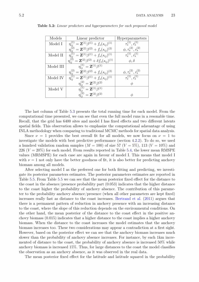
5.2 DATA ANALYSIS 23
Table 5.2: Linear predictors and hyperparameters for each proposed model
Models Linear predictor HyperparametersModel I η
(1)ij = Z(1)β(1) + fs(sij)
(1) τ(1)s , r(1)
s
η(2)ij = Z(2)β(2) + fs(sij)
(2) φ, τ(2)s , r(2)
s
Model II η(1)ij = Z(1)β(1) + fs(sij)
(1) τ(1)s , r(1)
s
η(2)ij = Z(2)β(2) + δfs(sij)
(1) φ, δ
Model III η(1)ij = Z(1)β(1)
η(2)ij = Z(2)β(2) + fs(sij)
(2) φ, τ(2)s , r(2)
s
Model IV η(1)ij = Z(1)β(1) + fs(sij)
(1) τ(1)s , r(1)
s
η(2)ij = Z(2)β(2) φ
Model V η(1)ij = Z(1)β(1)
η(2)ij = Z(2)β(2) φ
The last column of Table 5.3 presents the total running time for each model. From thecomputational time presented, we can see that even the full model runs in a resonable time.Recall, that the grid has 6400 sites and model I has fixed effects and two different latentsspatial fields. This observation allows to emphasize the computational adavantage of usingINLA methodology when comparing to traditional MCMC methods for spatial data analysis.
Since ν = 1 provides the best overall fit for all models, we now focus on ν = 1 toinvestigate the models with best predictive performance (section 4.2.2). To do so, we useda hundred validation random samples (M = 100) of size 57 (V = 5%), 113 (V = 10%) and226 (V = 20%) for each model. From results reported in Table 5.4, the lower mean RMSPEvalues (MRMSPE) for each case are again in favour of model I. This means that model Iwith ν = 1 not only have the better goodness of fit, it is also better for predicting anchovybiomass among all models.
After selecting model I as the preferred one for both fitting and predicting, we investi-gate its posterior parameters estimates. The posterior parameters estimates are reported inTable 5.5. From Table 5.5 we can see that the mean posterior fixed effect for the distance tothe coast in the absence/presence probability part (0.053) indicates that the higher distanceto the coast higher the probability of anchovy absence. The contribution of this parame-ter to the probability anchovy absence/presence (when all other parameters are kept fixed)increases really fast as distance to the coast increases. Bertrand et al. (2011) argues thatthere is a permanent pattern of reduction in anchovy presence with an increasing distanceto the coast, where the slope of this reduction depends on the environmental conditions. Onthe other hand, the mean posterior of the distance to the coast effect in the positive an-chovy biomass (0.015) indicates that a higher distance to the coast implies a higher anchovybiomass. When the distance to the coast increases the model estimates that the anchovybiomass increases too. These two considerations may appear a contradiction at a first sight.However, based on the posterior effect we can see that the anchovy biomass increases muchslower than the probability of anchovy absence increases. For instance, by each 1km incre-mented of distance to the coast, the probability of anchovy absence is increased 50% whileanchovy biomass is increased 15%. Thus, for large distances to the coast the model classifiesthe observation as an anchovy absence, as it was observed in the real data.
The mean posterior fixed effect for the latitude and latitude squared in the probability

5.2 DATA ANALYSIS 24
Table 5.3: The selection criteria for the models proposed with different linear predictors
LPML DIC Accurate rate RMSEE Total run time (min)ν = 1
Model I -3209.41 7114.95 97.61% 165.94 16.05Model II -3390.66 7283.56 89.46% 1069.71 7.94Model III -3384.17 7244.60 86.71% 499.55 3.22Model IV -4632.66 9523.28 97.61% 1507.39 4.41Model V -4843.13 9696.66 86.71% 1539.13 0.13ν = 2
Model I -3236.78 7073.40 96.46% 251.83 22.70Model II -3378.76 7224.86 89.01% 1052.14 12.23Model III -3405.80 7253.58 86.71% 499.42 5.70Model IV -4647.40 9517.15 96.46% 1509.88 5.62Model V -4843.13 9696.66 86.71% 1539.88 0.13ν = 3
Model I -3254.41 7114.28 96.10% 262.04 31.20Model II -4686.77 9526.58 94.06% 1528.39 132.81Model III -3388.50 7273.37 86.71% 499.32 7.73Model IV -4653.28 9515.72 96.10% 1510.47 7.89Model V -4843.13 9696.66 86.71% 1539.88 0.13
Table 5.4: Predictive model checks. Mean of RMSPE (MRMSPE) out 100 validation samples.
MRMSPEν = 1 5% 10% 20%
Model I 1341 1515 1786Model II 1541 1886 2355Model III 1387 1581 1827Model IV 1863 2386 3147Model V 2106 2745 3568

5.2 DATA ANALYSIS 25
Table 5.5: Summary statistics (point, standard deviation and 95% credible interval (CI)) for Fixedeffects and Hyperparameters estimation.
Mean sd 95% CIProbability of anchovy absence/presence
Intercept 16.530 7.215 (4.641,33.138)Distance to the coast 0.053 0.022 (0.019,0.104)
Latitude 4.384 1.608 (1.819,8.127)Latitude2 0.184 0.069 (0.072,0.346)Depth -0.002 0.001 (-0.003,-0.001)τ
(1)s 0.056 0.027 (0.019,0.124)r(1)s 7.089 1.291 (4.853,9.903)
Positive anchovy biomassIntercept 5.056 0.208 (4.650,5.467)
Distance to the coast 0.015 0.007 (0.015,0.015)Depth 0.001 0.000 (0.000,0.001)φ 148.601 111.494 (25.170,438.440)τ
(2)s 0.214 0.015 (0.186,0.245)r(2)s 1.370 0.159 (1.085,1.708)
anchovy absence/presence (4.384 and 0.184, respectively) are evidence that there is a higherprobability of anchovy absence when latitudes are near to the extremes. When looking at themean posterior fixed effect for the depth in the absence/presence probability part (-0.002)there is an indication that for deeper ocean parts there is a higher probability of anchovyabsence. On the other hand, the fixed effect for the depth in the positive anchovy biomass(0.001) suggests that a lower ocean depth size implies a higher anchovy biomass.
The mean posterior range r(1)s for the structured spatial effect of the probability of an-
chovy absence/presence is approximately 7.089 “units”, where units here means number ofcells. Here the lattice have cells of size aproximately 14x14km (width x height). Thus, themodel states that the probability of absence of anchovy for some site are depedent of neigh-bors observations until a distance of 100 km. The mean posterior range r(2)
s for the structuredspatial effect of the positive biomass is approximately 1.37 “units”. Therefore, by model I an-chovy biomass (when anchovy is present) depends on neighbors observations until a distanceof 20 km.
Finally we can see that the spatial dependence is captured by the random spatial effectf(1)s , thus, we can conclude that the spatial model is capable of accomodating the variabilityin the anchovy distribution. On the otherhand, the variability of positive anchovy biomassnot explained by the structured spatial term f(2)
s depends on µij and /φ, that is, if φ µ2ij
then there is very little unexplained variability in the positive anchovy biomass, otherwise,there is high variability of anchovy biomass not explained by the covariates and/or thestructured spatial effect.
The mean posterior probability of anchovy absence/presence (Figure 5.3, right panel) iscomputed using the posterior mean linear predictor η(1)
ij . On the left panel we can see theoriginal anchovy absence/presence values. Comparing both sides we can see that the rightpanel classifies very closely to the observed absence/presence of anchovy in the left side,supporting the good classification performance under model I.

5.2 DATA ANALYSIS 26
−85 −80 −75 −70
−20
−15
−1
0−
5
Longitude
Latitu
de
presenceabsencepresenceabsencepresence(=0)absence(=1)presenceabsence
−85 −80 −75 −70
−20
−15
−1
0−
5
LongitudeL
atitu
de
0.2
0.4
0.6
0.8
1.0
Figure 5.3: Results. Left: Observed anchovy absence/presence. Right: Mean posterior probabilityof anchovy absence under model I.
Then the estimated mean posterior anchovy biomass is computed using the above resultand the model proposed in Equation (5.1). Thus, for each grid point it is defined the followingprediction rule: If the mean posterior of anchovy absence probability is higher than 0.5 thesite is classified like anchovy absence, while if the mean posterior anchovy absence probabilityis lower than 0.5 the site is defined like anchovy presence (anchovy biomass(> 0)) withestimation computed using the mean posterior linear predictor exp(η
(2)ij ).
The posterior mean estimated anchovy biomass map is presented in Figure 5.4. On theleft panel we can see the original observation values, while on the right panel the estimatedpattern is presented (both cases on the logarithmic scale for anchovy biomass). Comparingboth sides we can see that the right panel agrees very closely to the observed values in theleft side. This is an indication of good model fitting, and thus, model I is used for predictionon the unobserved sites.
Furthermore, probabilities qi from section 4.2.3 are computed using Kullback-Leibler(KL)measure presented in Equation( 4.8). Then a threshold of 0.9 is set for qi. After detecting theinfluential observations we define an influential region at those sites i where qi > 0.9 and atleast five neighboor(from eight) have qj > 0.9 for site j neighboor from site i. Thus, if a gridpoint have more than one neighboor with qj > 0.90, we call it an influential region. Figure 5.5shows the probability qi value and mean posterior biomass anchovy for all influential regions.Such regions probably represent shoal clusters with higher anchovy biomass values.

5.2 DATA ANALYSIS 27
−85 −80 −75 −70
−20
−15
−1
0−
5
Longitude
Latitu
de
0
2
4
6
8
10
−85 −80 −75 −70−
20
−15
−1
0−
5
Longitude
Latitu
de
0
2
4
6
8
10
Figure 5.4: Results. Left: Observed anchovy biomass (on the logarithmic scale). Right: Mean pos-terior anchovy biomass under model I (on the logarithmic scale).
−85 −80 −75 −70
−2
0−
15
−1
0−
5
Longitude
La
titu
de
0.880.890.900.910.920.930.940.95
−85 −80 −75 −70
−2
0−
15
−1
0−
5
Longitude
La
titu
de
2345678
Figure 5.5: Results. Left: Probability qi of influence regions. Right: Mean posterior of anchovybiomass influence regions (on the logarithmic scale).

Chapter 6
Discussion
The Peruvian anchovy is a dominant fish at the Peruvian pelagic ecosystem. For thisreason, understanding the anchovy biomass distribution is very important for either aneconomic perspective as well as an ecological perspective. Because of the nature of anchovybiomass there is a need for a spatial model that can accommodate its main characteristics.The anchovy biomass has three main characteristics: (1) high proportions of zero, (2) strongspatial dependence and (3) very right skewed distribution. In this study we proposed aBayesian Hurdle type model which showed its capability of adapting to the characteristicsof the anchovy biomass in the coast of Perú. In fact, including a component to capturethe excess of zeros was necessary and it was an indication that the source of overdispersionpresent in the data might comes essentially from the excess of zeros. The Gamma distributionfor fitting anchovy positive biomass data was very effectively for analyzing our skewed non-negative data.
The main advantage of the Bayesian formulation, in particular using INLA, is com-putational. The complex model chosen including two spatial components runs in slightlyover sixteen minutes. Moreover, Bayesian inference and model comparison suggest that suchmodel provides a plausible description of the anchovy biomass, being capable of successfullyaddress the data challenging characteristics. The effectiveness of such model for identifyingthe absence/presence of anchovy is fairly good. And the mean posterior estimations verifythat this model has potential not only to identify absence/presence of anchovy but also toestimate anchovy biomass given that anchovy is present.
In addition, we verify the prediction performance of the proposed models. The datasetwere separated into two parts: a validation part and a fitting part. This procedure wasrepeated one hundred times and the prediction power of the models were estimated. It isworth noting that again the computational cost to run all this simulations using INLA wasvery low. From the results we conclude that the full model has the best performance inboth fitting and predicting, being the one selected from the majority of the model assesmentmeasures.
From our results we observe that anchovy absence is higher when distance to the coastincreases, that is, in offshore waters (>150km from the coast) where ocean depth is alsodeeper. And anchovy presence is higher in the central region, such area is characterized bylower oxygen, cold and fresh water in coastal surface layers which is an ideal habitat for an-chovy (Bertrand et al., 2011). Furthermore, anchovy biomass slightly increases when distanceto the coast increases within 150 km from the coast, reflecting the existence of dense schoolsnot too near to the coast but where ocean depth is not too deeper. Moreover, we showedthat anchovy absence/presence at some location is not independent of absence/presence atneighboring locations, as well as biomass anchovy at some location is not independent ofbiomass anchovy at nearest neighboring locations, supporting the inclusion of spatial ef-fects. Bayesian influence diagnostic also suggests that classifying absence/presence suffers
28

6.0 29
less influence than correctly estimating the current anchovy positive biomass.Finally, the current model is based on data from only one year, but it can be extended
in several ways. The most inmediate one, is to a spatio-temporal model including data frommore years, seasons, among others.
All code implementing our data analysis are available, please contact to the authors forproviding them.

Chapter 7
Future works
7.1 IntroductionIn this study the GRMF was a discretely indexed Gaussian field, thus our approach was
restricted to graphs like regular lattices (Rue and Held, 2005). The problem of doing this isthe necessity to approximate the position of the locations. Thus a lot of effort going intocollecting locations data with a high degree of precision is lost. Clearly, the finer the lattice,better estimations, in particular, better predictions at unsampled locations. Therefore thequality of our estimations primarily depends on the size of the grid. As a result, we arerequired to compute on a much finer grid than it is necessary for better results, then latticebased approaches might be computationally expensive.
Throughout the next section, it is discussed a recent work of Lindgren et al. (2011) thathas broken down the barrier between GMRFs and spatially continuous Gaussian randomfield models. They suggest a link between Gaussian Random fields and Gaussian MarkovRandom Fields (GRMF) through the stochastic partial differential Equations (SPDE) for aGaussian field with Matérn covariance function. In particular, for irregular grids they usethe finite element method (FEM) to discretize complex geometries, even irregular geometricareas, and at the same time they get an approximation to the solution of the SPDE usingbasis functions. That allows us to hold on to the continuous interpretation of space, whilethe computational algorithms only see discrete structures with Markov properties. A greatvariety of applications using SPDE approach for geostatistical data can be found in Bolin(2012), Simpson et al. (2012), Blangiardo et al. (2013) and Cameletti et al. (2013).
7.2 The Stochastic Partial Differential equation (SPDE) approachA differential equation can be defined informally as any equation which contains deriva-
tives. In particular, a differential which has differential derivatives is called partial differen-tial. Generally, a Stochastic Partial Differential equation (SPDE) is a equation which allowsrandomness in the coefficients of the differential equation, i.e., involves one or more stochasticprocesses. Then any solution of a stochastic differential equation must involve some random-ness, that is, we are only able to say something about the probability distribution of thesolutions.
In this context, a Gaussian field Z(s) with the Matérn Covariance is a solution to thelinear fractional stochastic partial differential equation (SPDE)
(κ2 −4)α/2Z(s) = W (s), s ∈ Rn, α = ν + d/2, (7.1)
where (κ2−4)α/2 is the pseudo - differential operator of Laplace and W is spatial GaussianWhite noise. This explicit formulation is the strong version of the SPDE specification, an
30

7.2 THE STOCHASTIC PARTIAL DIFFERENTIAL EQUATION (SPDE) APPROACH 31
Figure 7.1: Representation of piewise-linear approximationof a function in two dimensions over atriangulated mesh.
alternative is the weak formulation given by
[< φj, (κ2 −4)α/2Z >Ω]
d−→ [< φj,W >Ω]; j = 1, ...,m (7.2)
where φj is an arbitrary well-behaved function, < f, g > is the inner product of functions fand g , and d−→ denotes convergence in distribution. This definition implies that a process issaid to achieve weakly convergence if the first and second moments exist.
If the spatial locations are on some irregular grid Lindgren et al. (2011) proposed to con-struct a representation of the finite element as solution to the SPDE, thus using the finiteelement method (FEM) observations are interpolated to the nearest grid point. In order todo this, suppose that <2 is subdivided into a set of non-intersecting triangles, where any twotriangles meet in at most a common edge. The suggestion is to start with the locations of theobserved points and add some triangles with some restriction to maximize the allowed lengthedge and to minimize the desired angles (Figure 7.1). Therefore, this approach need to con-struct a finite dimensional representation of solutions to the Equation (7.1), for some chosenbasis functions ψk, weights wk normally distributed and n vertices in the triangulation. Thisapproximation is of the form,
Z(s) =n∑k=1
ψk(s)wk. (7.3)
In particular, the basic functions ψk used by Lindgren et al. (2011) are piecewise linear in eachtriangle, where ψk is 1 at vertex k and 0 at all other vertices. Therefore, the weights determinethe field values at the vertices, and the values inside the triangles are calculated by linearinterpolation. Hence , the finite dimensional solution is obtained by finding the distributionof weights wk in Equation (7.3) that fulfils the weak SPDE specification (Equation (7.2))for a specific set of functions φk and for m = n. Then wk ∼ N(0, Q−1
α ) and the finitedimensional representation of solutions to the Equation (7.1) has precision matrix Qα definedas a function of κ2 e α. Functions φk and precision matrices Qα for each α are defined inTable 7.1. Here C, G and K are matrices defined by,
Ci,j = 〈ψi, ψj〉, Gi,j = 〈∇ψi,∇ψj〉, (Kκ2)i,j = κ2Ci,j +Gi,j (7.4)

THE STOCHASTIC PARTIAL DIFFERENTIAL EQUATION (SPDE) APPROACH 32
Table 7.1: Summary of functions φk and precision matrices Qα for each α
α φk Qα
1 (κ2 −4)1/2ψk Kκ2
2 ψk Kκ2C−1Kκ2
3,4,. . . recursive Garleky formulation Kκ2C−1Qα−2,κ2C−1Kκ2
In particular, these matrices are calculated by using triangulation and geometry of any arbi-trary triangle defined by their vertices, edges and angles (Lindgren and Rue, 2007; Lindgrenet al., 2011). Finally, the fact that C−1 is a dense matrix implies that the precision matrixwill also be dense, for this reason C is approximated by a diagonal sparse matrix C, thuswe get the precision matrix of a GRMF.
Then we are able to re-write the linear predictor of interest using such GRMF, for example:
η(s) = β0 +
ηβk∑k=1
βkxk(s) + Z(s) + ε(s),
where Z is a Gaussian field, can be re-written as
η(s) = β0 +
ηβk∑k=1
βkxk(s) + Z(s) + ε(s),
where the Z(s) is a GRMF with precision matrix Qα.
Coming back to our data analysis, as future work is feasible to extend our study usingirregular grids to hold on the natural continuous interpretation of space. Thus, we mightextend the model structure defined in Chapter 4 but instead of using a regular lattice andcompute the observed response as the mean of anchovy biomass we could use a irregulargrid and construct a mesh using Constrained Refined Delaunay Triangulation. Thus, eachsample location of anchovy biomass can be defined at each vertice or if we want to reducecomputational requirements we might interpolate sample locations given some maximumtriangle edge length. Although this step is easy to implement using the R-INLA package,the mesh size influences computational time needed to fit the model. More nodes on themesh need more computational time. Moreover, spatial dependence is also influenced byscales. Thus, when using irregular grids the size of triangles has to be carefully thought out.Figure 7.2 displays examples of meshs constructed for anchovy biomass data. Then makinguse of the link between Gaussian fields and GRMF through SPDE, the proposed modeldefined in Equation (4.4) can be re-defined. Then we are able to focus on estimation andprediction procedures.
Finally, although this work was focus on a particular hierarchical spatial Hurdle-model,the SPDE approach can also be extended to spatio-temporal models. For instance, Camelettiet al. (2013) consider a spatio-temporal model with separable covariance function and usealso INLA for fast Bayesian inference. Furthermore, it is feasible to consider models withmore complex structures like non-separable covariance functions. With this modeling wouldbe plausible to interpret changes on especies behavior due to changes on environmentalconditions, and develop efficient and realistic simulation tools enabling to anticipate betterthe efficacy of different management strategies and conservation of peruvian anchovy.

THE STOCHASTIC PARTIAL DIFFERENTIAL EQUATION (SPDE) APPROACH 33
Figure 7.2: Meshs constructed using Constrained refined Delaunay triangulation. Red grid dots aresamples of anchovy biomass samples. The region defined by the sky-blue line is the edge boundarywhich defines the priority area for estimation. Outside this region the boundary effects are higher.Right: Mesh have less resolution than left plots. Top: Mesh for all data. Down: Mesh for northernregion of top panel.

Appendix A
Proof of result 4.7
Proof of Kullback-Leibler (KL) divergence measure:
KL(π(x|Y−k), π(x|Y )) = Ex|Y
[− log
π(x|Y−k)π(x|Y )
]= Ex|Y
[log
π(x|Y )
π(x|Y−k)
],
by definition of expectation,
KL(π(x|Y−k), π(x|Y )) =
∫π(x|Y ) log
[π(x|Y )
π(x|Y−k)
]dx,
by Bayes Theorem
KL(π(x|Y−k), π(x|Y )) =
∫π(x|Y ) log
[π(Y |x)π(x)
π(Y )
π(Y−k)
π(Y−k|x)π(x)
]dx
=
∫π(x|Y ) log
[π(Y |x)
π(Y−k|x)
π(Y−k)
π(Y )
]dx
=
∫π(x|Y ) log
[π(Y |x)
π(Y−k|x)
]dx+
∫π(x|Y ) log
[π(Y−k)
π(Y )
]dx
=
∫π(x|Y ) log
[π(Y |x)π(x|θ)π(Y−k|x)π(x|θ)
]dx+
∫π(x|Y )dx log
[π(Y−k)
π(Y )
]π(x|Y ) is a density, then
KL(π(x|Y−k), π(x|Y )) =
∫π(x|Y ) log
[π(Y |x)π(x|θ)π(Y−k|x)π(x|θ)
]dx+ 1× log
[π(Y−k)
π(Y )
]by conditional probability
KL(π(x|Y−k), π(x|Y )) =
∫π(x|Y ) log
[π(Y |x, θ)π(Y−k|x, θ)
]dx+ log
[π(Y−k)
π(Y )
]=
∫π(x|Y ) log
[π(Y |x, θ)π(Y−k|x, θ)
]dx− log
[π(Y )
π(Y−k)
]=
∫π(x|Y ) log
[π(Y |x, θ)π(Y−k|x, θ)
]dx− log
[π(Yk, Y−k)
π(Y−k)
]=
∫π(x|Y ) log
[π(Y |x, θ)π(Y−k|x, θ)
]dx− log[π(Yk|Y−k)]
Y ’s are independent given x, θ, then
KL(π(x|Y−k), π(x|Y )) =
∫π(x|Y ) log [π(Yk|x, θ)] dx− log[π(Yk|Y−k)]
KL(π(x|Y−k), π(x|Y )) = Ex|Y [log[π(Yk|x, θ)]− log[CPOk].
34
Bibliography
Agarwal, D. K., Gelfand, A. E., and Citron-Pousty, S. (2002). Zero-inflated models withapplication to spatial count data. Environmental and Ecological Statistics 9, 341–355. iv,2
Bertrand, A., Chaigneau, A., Peraltilla, S., Ledesma, J., Graco, M., Monetti, F., and Chavez,F. (2011). Oxygen: A fundamental property regulating pelagic ecosystem structure in thecoastal southeastern tropical pacific. PLoS One 6, 12. 23, 28
Bertrand, A., Gerlotto, F., Bertrand, S., Gutiérrez, M., Alza, L., and Chipollini, A. (2008).Schooling behaviour and environmental forcing in relation to anchoveta distribution: Ananalysis across multiple spatial scales. Progress in Oceanography 79, 264–277. 1
Bertrand, S., DÃaz, E., and Lengaigne, M. (2008). Patterns in the spatial distribution ofPeruvian anchovy (Engraulis ringens) revealed by spatially explicit fishing data. Progressin Oceanography 79, 379–389. 1
Blangiardo, M., Cameletti, M., Baio, G., and Rue, H. (2013). Spatial and Spatio-Temporalmodels with R-INLA. Spatial and Spatio-Temporal Epidemiology 4, 33–49. 30
Bolin, D. (2012). Models and methods for random fields in spatial statistics with computa-tional efficiency from Markov properties. PhD thesis, Lund University. 30
Boyd, C. (2012). The Predator Dilemma: Investigating the responses of seabirds to changesin the abundance and distribution of small pelagic prey. PhD thesis, University of Wash-ington. 1
Cameletti, M., Lindgren, F., Simpson, D., and Rue, H. (2013). Spatio-temporal modeling ofparticulate matter concentration through the spde approach. AStA Advances in StatisticalAnalysis 97(2), 109–131. 30, 32
Cameron, A. and Trivedi, P. (1998). Regression Analysis of Count Data. University Press,Cambridge. iv, 2
Cressie, N. A. C. (1993). Statistics for Spatial Data. Wiley. 4
Dey, D. K., Chen, M.-H., and Chang, H. (1997). Bayesian Approach for Nonlinear RandomEffects Models. Biometrics 53(4), 1239–1252. 18
Diggle, P., Tawn, J., and Moyeed, R. A. (1998). Model based geostatistics (with discussion).Applied Statistics 47, 299–350. 1, 4
Dreassi, E., Petrucci, A., and Rocco, E. (2014). Small area estimation for semicontinuousskewed spatial data: An application to the grape wine production in Tuscany. BiometricalJournal 1, 141–156. 14
35
BIBLIOGRAPHY 36
Fréon, P. and Misund, O. A. (1999). Dynamics of Pelagic Fish Distribution and Behaviour:Effects on Fisheries and Stock Assessment. Wiley-Blackwell. 1
Geisser, S. and Eddy, W. F. (1979). A Predictive Approach to Model Selection (Corr: V75p765). Journal of the American Statistical Association 74, 153–160. 18
Gelfand, A. E., Dey, D. K., and Chang, H. (1992). Model Determination Using PredictiveDistributions, with Implementation Via Sampling-based Methods (Disc: P160-167). InBernardo, J. M., Berger, J. O., Dawid, A. P., and Smith, A. F. M., editors, BayesianStatistics 4. Proceedings of the Fourth Valencia International Meeting, pages 147–159.Clarendon Press [Oxford University Press]. 18
Ghosh, P. and Albert, P. S. (2009). A Bayesian analysis for longitudinal semicontinuousdata with an application to an acupuncture clinical trial. Computational Statistical DataAnalysis 53, 699–706. 14
Held, L., Schordle, B., and Rue, H. (2010). Posterior and cross-validatory predictive checks:a comparison of MCMC and INLA. Statististical Modelling and Regression Structurespages 91–110. 18
Lachos, V. H., Barbosa, C. R., and Medina, A. W. (2013). Modelos Não Lineares As-simétricos. Instituto de Matemática e Estatística-USP and ABE Associação Brasileira deEstatística. 19
Lindgren, F. and Rue, H. (2007). Explicit construction of GRMF approximations to gener-alised matérn fields on irregular grids. Technical report, Centre for Mathematical Sciences,Lund University. 32
Lindgren, F., Rue, H., and Lindstrom, J. (2011). An explicit link between Gaussian fieldsand Gaussian Markov random fields: The SPDE approach. Journal of the Royal StatisticalSociety. Series B. Statistical Methodology 73(1), 423–498. 6, 16, 30, 31, 32
MacLennan, D. N., Fernandes, P. G., and Dalen, J. (2002). A consistent approach to defi-nitions and symbols in fisheries acoustics. ICES Journal of Marine Science 59, 365–369.12
McCulloch, R. E. (1989). Local model influence. Journal of the American Statistical Asso-ciation 84, 473–478. 19
Mullahy, J. (1986). Specifications and testing of some modified count data model. Journalof Econometrics 33, 341–365. iv, 2
Muñoz, F., Pennino, M., Conesa, D., López-Quélez, A., and Bellido, J. (2013). Estimationand prediction of the spatial ocurrence of fish species using Bayesian Latent Gaussianmodels. Sthocastic Environmental Research and Risk Assessment 27, 1171–1180. 2
Neelon, B., O’Malley, A. J., and Normand, S.-L. T. (2011). A Bayesian two-part latent classmodel for Longitudinal Medical expenditure data: Assesing the impact of mentral healthand substance abuse parity. Biometrics 67, 280–289. 14
Rue, H. and Held, L. (2005). Gaussian Markov Random Fields: Theory and Applications.Chapman and Hall-CRC Press. 6, 8, 16, 30

BIBLIOGRAPHY 37
Rue, H. and martino, S. (2007). Approximate Bayesian Inference for Hierarchical GaussianMarkov Random fields models. Journal of Statistical Planning and Inference 137, 3177–3192. 10
Rue, H., martino, S., and Chopin, N. (2009). Approximate Bayesian inference for latentGaussian models by using integrated nested Laplace approximations. Journal of the RoyalStatistical Society, Series B 71(2), 319–392. iv, 2, 8, 10, 16, 17, 18
Rue, H. and Tjelmeland, H. (2002). Fitting Gaussian Markov Random Fields to GaussianFields. Scandinavian Journal of Statistics 29(1), 31–49. 6, 16
Simmonds, J. and MacLennan, D. (2005). Fisheries Acoustics: Theory and Practice. Wiley-Blackwell. 12
Simpson, D., Lindgren, F., and Rue, H. (2012). Think continuous: Markovian Gaussianmodels in spatial statistics. Spatial Statistics 1, 16–29. 30
Spiegelhalter, D. J., Best, N., Carlin, B. P., and van der Linde, A. (2002). Bayesian measuresof model complexity and fit (with discussion). Journal of the Royal Statistical Society,Series B 64, 583–639. 17
Woillez, M., Rivoirard, J., and Fernandes, P. G. (2009). Evaluating the uncertainty ofabundance estimates from acoustic surveys using geostatistical simulations. ICES Journalof Marine Science 66, 1377–1383. 1