a inversão da forma de onda completa pode compensar a ... · generalização da lei de hooke, e...

Universidade Federal do Rio Grande do NorteCentro de Ciências Exatas e da Terra

Programa de Pós-Graduação em Geodinâmica e Geofísica

DISSERTAÇÃO DE MESTRADO

A inversão da forma de onda completa podecompensar a falta de iluminação na tomografia

poço-a-poço?

Autor:

Alex Tito de Oliveira

Orientador:

Prof. Dr. Walter Eugênio de Medeiros (UFRN)

Dissertação n.o 220/PPGG.

Natal, RN, 17 de Dezembro de 2018

UNIVERSIDADE FEDERAL DO RIO GRANDE DO NORTECENTRO DE CIÊNCIAS EXATAS E DA TERRA

PROGRAMA DE PÓS-GRADUAÇÃO EM GEODINÂMICA E GEOFÍSICA

DISSERTAÇÃO DE MESTRADO

A inversão da forma de onda completa podecompensar a falta de iluminação na tomografia

poço-a-poço?

Autor:Alex Tito de Oliveira

Dissertação apresentada em 17 de De-zembro de dois mil e dezoito, ao Pro-grama de Pós-Graduação em Geodinâ-mica e Geofísica – PPGG, da Universi-dade Federal do Rio Grande do Norte -UFRN como requisito à obtenção do Tí-tulo de Mestre em Geodinâmica e Geofí-sica, com área de concentração em Geofí-sica.

Comissão Examinadora:

Prof. Dr. Walter Eugênio de Medeiros (UFRN) - OrientadorProf. Dr. Amin Bassrei (UFBA) - Examinador externo

Prof. Dr. Aderson Farias do Nascimento (UFRN) - Examinador interno

Natal, RN, 17 de Dezembro de 2018

Oliveira, Alex Tito de. A inversão da forma de onda completa pode compensar a faltade iluminação na tomografia poço-a-poço? / Alex Tito deOliveira. - 2018. 85f.: il.

Dissertação (Mestrado) - Universidade Federal do Rio Grandedo Norte, Centro de Ciências Exatas e da Terra, Programa de Pós-Graduação em Geodinâmica e Geofísica. Natal, 2018. Orientador: Walter Eugênio de Medeiros.

1. Geofísica - Dissertação. 2. Inversão da forma de onda -Dissertação. 3. Arranjo poço-a-poço - Dissertação. 4. Tomografiasísmica - Dissertação. I. Medeiros, Walter Eugênio de. II.Título.

RN/UF/CCET CDU 550.3

Universidade Federal do Rio Grande do Norte - UFRNSistema de Bibliotecas - SISBI

Catalogação de Publicação na Fonte. UFRN - Biblioteca Setorial Prof. Ronaldo Xavier de Arruda - CCET

Elaborado por Joseneide Ferreira Dantas - CRB-15/324

Resumo

A iluminação sísmica em cada ponto da região interpoços pode ser definida como o ângulo

máximo entre os raios que passam por esse ponto. Interfaces completamente contidas nas aberturas

angulares podem ser imageadas com a tomografia de tempo de trânsito da primeira chegada (first

arrival travel time tomography, ou FATTT). Nós investigamos se a inversão de forma de onda (full

waveform inversion, ou FWI) 2D acústica pode compensar a falta de iluminação. Nós usamos

dados sintéticos gerados com fontes de forma Ricker com frequências de pico de 100 ou 500 Hz,

resultando em superposição pequena das bandas de frequência, de tal forma que uma abordagem de

FWI multiescala é aplicada, em que os resultados com o conjunto de dados de 100 Hz são usados

como entrada para o conjunto de 500 Hz. Nós investigamos dois casos: no primeiro (FWI T),

somente as ondas registradas no poço oposto são usadas enquanto, no segundo caso (FWI T+R), as

ondas registradas em ambos os poços são usadas. Para uma única interface separando dois meios,

a forma da onda transmitida varia significantemente apenas quando a interface está contida dentro

das aberturas angulares. Portanto, famílias de tiro comum para modelos de camadas com interfaces

fora das aberturas angulares podem ser aproximadamente reproduzidas com um meio homogêneo

equivalente. Dessa forma, em comparação com FATTT, ambos os casos de FWI resultam em uma

melhoria moderada para modelos com interfaces dentro da cobertura angular, mas não conseguem

compensar a falta de iluminação. Nessa situação, pequenos aumentos de resolução são obtidos

tanto com FWI T como com FWI T+R. Contudo, para modelos na condição mista em que camadas

com interfaces contidas na abertura angular são cortadas por uma falha, a FWI oferece melhorias

substanciais sobre a FATTT, mesmo se o plano de falha está fora da cobertura angular e a FWI T é

aplicada. Nessa situação mista, a resolução também aumenta quando FWI T+R e fontes de maior

conteúdo de frequência são usadas.

Palavras-chave: Inversão da forma de onda, arranjo poço a poço, tomografia sísmica.

i

Abstract

Seismic illumination at each point of the interwell region can be defined as the maximum an-

gle between the rays that pass through the point. Interfaces completely contained in the angular

apertures can be imaged with first arrival travel time tomography (FATTT), but interfaces comple-

tely outside cannot be imaged even under regularized FATTT. We investigate if 2D acoustic full

waveform inversion (FWI) can compensate for the lack of illumination. We use synthetic data

generated with Ricker source wavelets with peak frequencies at 100 or 500 Hz, resulting in a small

overlapping in the frequency bandwidths, so that a multiscale FWI approach is employed where

the results with the 100 Hz dataset are used as input for the 500 Hz dataset. We investigate two

FWI cases: in the first (FWI T), just the waves recorded at the opposite borehole are used whilst,

in the second case (FWI T+R), the waves recorded at the two boreholes are used. For a single

interface separating two media, the shape of the transmitted waveform varies significantly only

when the interface is contained in the angular apertures. Accordingly, shot gathers for layered mo-

dels with interfaces outside the angular apertures can be approximately reproduced with equivalent

homogeneous media. As a result, in comparison with FATTT, both FWI cases give a mild impro-

vement for models with interfaces inside the angular coverage, but cannot compensate for the lack

of illumination. In this situation, minor resolution increases are obtained either with FWI T or

FWI T+R cases. However, for models in the mixed condition where layers with interfaces inside

the angular coverage are cut by a fault, FWI offers substantial improvements over FATTT, even if

the fault plane is outside the angular coverage and FWI T is employed. In this mixed situation,

resolution also increases when FWI T+R and source wavelets with a higher frequency content are

used.

Keywords: Full waveform inversion, crosswell tomography, seismic tomography.

ii

Agradecimentos

Agradeço, primeiramente, a Deus, por todas as coisas em minha vida.

Agradeço ao PRH 229 pela bolsa de mestrado e pelo apoio financeiro para participar do Congresso

Internacional de Geofísica (SBGf 2017).

Agradeço aos meus familiares, Maria Cristina Tito, Maria Lucia de Oliveira Bastos, Severina

Vicente Ferreira e Iracema Leopoldo por todo apoio e dedicação que elas sempre mostraram.

Agradeço a Fabiana Cirino dos Santos por todo apoio, dedicação e conselhos em grande parte

dessa jornada.

Agradeço ao meu orientador, Prof. Dr. Walter Eugênio de Medeiros, por ter me orientado por dois

anos e pelas valiosas contribuições humanas.

Agradeço a Renato Ramos pela participação essencial nessa pesquisa, por toda ajuda e compreen-

são durante toda essa jornada.

Agradeço a Jessé C. Costa pelas contribuições para o desenvolvimento dessa pesquisa.

Agradeço aos alunos do PPGG Elizangela Amaral, Gilsijane Vieira, Rafaela Silva, Marcio Barboza

e Renato Ramos, pelos momentos de descontração e pelas importantes discussões e contribuições.

iii

Sumário

Resumo i

Abstract ii

Agradecimentos iii

Sumário iv

1 Contextualização 1

1.1 Importância da tomografia sísmica . . . . . . . . . . . . . . . . . . . . . . . . . . 1

1.2 Resolução em tomografia sísmica poço-a-poço . . . . . . . . . . . . . . . . . . . 2

1.3 Modelagem sísmica acústica . . . . . . . . . . . . . . . . . . . . . . . . . . . . . 2

1.4 Inversão da forma de onda completa . . . . . . . . . . . . . . . . . . . . . . . . . 3

2 Manuscrito submetido: Can full waveform inversion compensate for the lack of illu-

mination on crosswell tomography?" 4

Referências bibliográficas 63

Apêndice A: Modelagem direta 70

Apêndice B: Modelagem inversa 73

Apêndice C: Bordas de absorção 78

iv

Capítulo 1

Contextualização

1.1 Importância da tomografia sísmica

A tomografia sísmica poço-a-poço é uma das técnicas clássicas da inversão de dados sísmicos,

frequentemente aplicada na exploração de recursos minerais, monitoramento de reservatórios de

hidrocarbonetos e imageamento de estruturas geológicas complexas (e.g.Ajo-Franklin, 2009, Ajo-

Franklin et al., 2007, Byun et al., 2010, Plessix, 2006b). A tomografia é importante para o estudo

de áreas de descarte de lixo radioativo (e.g. Peterson et al., 1985), e também tem grande atuação em

projetos de injeção de CO2 (e.g. Ajo-Franklin, 2009, Byun et al., 2010, Harris et al., 1995). Ainda

na questão exploratória, pode ser utilizada na exploração mineral em minas, mapeando tanto corpos

mineralizados de alta densidade como possíveis zonas de fraqueza, auxiliando na lavra da mina

(e.g. Gustavsson et al., 1986). A tomografia também tem relevância em problemas de geofísca

rasa. De Iaco et al. (2003) e Lanz et al. (1998) mostram a utilidade e as limitações da tomografia

na delimitação das bases de aterros. Liu and Guo (2005) imageiam a distribuição de velocidades

da coluna de concreto de uma ponte, de modo a avaliar a competência do material e localizar

possíveis zonas de fraqueza. Outra aplicação da tomografia em em problemas de geofísca rasa é na

investigação de sítios arqueológicos (Metwaly et al., 2005, Polymenakos and Papamarinopoulos,

2005).

CAPÍTULO 1. CONTEXTUALIZAÇÃO 2

1.2 Resolução em tomografia sísmica poço-a-poço

Os estudos sobre a resolução tomográfica poço-a-poço definiram que o aspecto principal que

limita a resolução é a iluminação. Rector III and Washbourne (1994) mostraram que, para um

modelo homogêneo, a limitação da cobertura angular acarreta em uma variação espacial da reso-

lução do experimento. Essa variação se deve ao fato de que a resolução associada a determinado

ponto do espaço está diretamente relacionada à maior abertura angular dos raios disponíveis para

esse ponto. Menke (1984) e Rector III and Washbourne (1994) concluíram que para uma arranjo

padrão com fontes e receptores igualmente espaçados em cada poço e dentro do mesmo intervalo

de profundidade, a resolução máxima disponível para um modelo homogêneo é obtida no centro

da região coberta pelos raios. Dantas and Medeiros (2016) evidenciaram que não é possível para

a tomografia de tempos de trânsito reconstruir interfaces de alto ângulo devido à ausência de raios

quase verticais, mesmo com a utilização de vínculos mais sofisticados.

1.3 Modelagem sísmica acústica

A modelagem sísmica é uma simulação do campo de ondas sísmicas, na qual são estabelecidas

as amplitudes sísmicas em todo o tempo de registro e para cada par fonte-receptor (Rego, 2014).

A Terra é um meio heterogêneo, anisotrópico, inelástico e dispersivo. Contudo, realizar uma

modelagem considerando todas essas características incorpora um alto nível de complexidade ao

problema e pode demandar um alto custo computacional. Assim, em geral, utilizamos modelos que

fazem uma boa aproximação da realidade e possibilitam resultados satisfatórios, como no caso da

modelagem acústica.

As modelagem sísmicas se baseiam no fato de que grandezas mensuráveis, como esforço e

deformação, estão relacionadas através das leis constitutivas. A maneira como essas grandezas se

relacionam depende do meio e em geral é possível agrupar a modelagem dos materiais em modelos

constitutivos que incluem um ou mais comportamentos como os que são citados nas modelagens

de elasticidade, plasticidade, viscoelasticidade, viscoplasticidade, dentre outras.

Na modelagem acústica, o campo acústico é descrito pelos campos de pressão e velocidade que

CAPÍTULO 1. CONTEXTUALIZAÇÃO 3

estão relacionados através da relação constitutiva para fluidos perfeitamente elásticos, que é uma

generalização da Lei de Hooke, e também se relacionam pela segunda lei de Newton (Di Bartolo,

2010).

1.4 Inversão da forma de onda completa

A inversão de forma de onda completa (Full Waveform Inversion, ou FWI) é um dos méto-

dos utilizados para superar as limitações da teoria do raio e conseguir uma melhor resolução de

imageamento de um meio. Ela se baseia em resolver numericamente a equação da onda durante

a etapa de modelagem. Desse modo, elimina-se a necessidade de filtragem de várias fases que

não seriam utilizadas pelas abordagens padrões (múltiplas, por exemplo), aproveitando-se quase

todo o conteúdo do traço sísmico como sinal e utilizando essa informação adicional para melhorar

substancialmente a resolução da imagem reconstruída (Virieux and Operto, 2009).

Teoricamente, a técnica de FWI é capaz de fornecer modelos de velocidade com maior reso-

lução do que a tomografia de tempos de trânsito. Espera-se esse resultado porque a FWI tenta

ajustar simultaneamente as informações de fase e amplitude obtidas através da equação da onda.

Por outro lado, estudos já mostraram que a FWI necessita de um modelo de velocidade inicial

próximo do modelo real, de modo a garantir sua convergência, sendo a construção de um modelo

inicial adequado um dos grandes desafios para o uso dessa técnica.

Capítulo 2

Manuscrito submetido: Can full waveform

inversion compensate for the lack of

illumination on crosswell tomography?"

Manuscrito submetido à revista Journal of Applied Geophysics.

Can full waveform inversion compensate for the lack ofillumination in crosswell tomography?

Alex T. Oliveiraa,d, Walter E. Medeirosb,d,∗, Renato R. S. Dantasa,d, Jesse C.Costac,d

aPrograma de Pos-graduacao em Geodinamica e Geofısica,Universidade Federal do Rio G. do Norte - UFRN, Natal/RN, Brazil

bDepartamento de Geofısica, Universidade Federal do Rio G. do Norte - UFRN,Natal/RN, Brazil

cFaculdade de Geofısica, Universidade Federal do Para - UFPA, Belem/PA, BrazildINCT-GP/CNPq/CAPES - Instituto Nacional de Ciencias e Tecnologia em Geofısica do

Petroleo - CNPq, Brazil

Abstract

Seismic illumination at each point of the interwell region can be de-

fined as the maximum angle between the rays that pass through the

point. Interfaces completely contained in the angular apertures can

be imaged with first arrival travel time tomography (FATTT), but

interfaces completely outside cannot be imaged even under regular-

ized FATTT. We investigate if 2D acoustic full waveform inversion

(FWI) can compensate for the lack of illumination. We use synthetic

data generated with Ricker source wavelets with peak frequencies

at 100 or 500 Hz, resulting in a small overlapping in the frequency

bandwidths, so that a multiscale FWI approach is employed where

the results with the 100 Hz dataset are used as input for the 500 Hz

dataset. We investigate two FWI cases: in the first (FWI T), just

the waves recorded at the opposite borehole are used whilst, in the

∗Corresponding authorEmail addresses: [email protected] (Alex T. Oliveira),

[email protected] (Walter E. Medeiros), [email protected] (Renato R. S. Dantas),[email protected] (Jesse C. Costa)

Preprint submitted to Journal of Applied Geophysics December 19, 2018

second case (FWI T+R), the waves recorded at the two boreholes

are used. For a single interface separating two media, the shape of

the transmitted waveform varies significantly only when the inter-

face is contained in the angular apertures. Accordingly, shot gathers

for layered models with interfaces outside the angular apertures can

be approximately reproduced with equivalent homogeneous media.

As a result, in comparison with FATTT, both FWI cases give a mild

improvement for models with interfaces inside the angular coverage,

but cannot compensate for the lack of illumination. In this situa-

tion, minor resolution increases are obtained either with FWI T or

FWI T+R cases. However, for models in the mixed condition where

layers with interfaces inside the angular coverage are cut by a fault,

FWI offers substantial improvements over FATTT, even if the fault

plane is outside the angular coverage and FWI T is employed. In

this mixed situation, resolution also increases when FWI T+R and

source wavelets with a higher frequency content are used.

Keywords: Full waveform inversion, crosswell tomography, seismic

tomography

1. Introduction

Crosswell tomography is a classic technique of seismic inversion

which, in its simplest form, is based on the inversion of first ar-

rival travel times of the transmitted waves between two boreholes

(e.g. Lo and Inderwiesen, 1994). Crosswell tomography might also5

be formulated as a full waveform inversion (FWI) (e.g. Pratt and

Goulty, 1991). In fact a substantial part of the effort to develop

2

and understand FWI was done in crosswell problems. Belina et al.

(2009) compare the results of FWI and travel time inversion in

crosswell tomography using synthetic horizontally-layered stochas-10

tic models and highlight the advantages and limitations of each ap-

proach. Pratt et al. (1996) point out that inverting the waveform

offers tomograms with higher resolution than the ones obtained with

first arrival travel time inversion. The better resolution of FWI is

a result of the fact that travel time inversion resolution is limited15

by the width of the first Fresnel zone (Williamson, 1991), while the

resolution of waveform inversion is of the order of half the wave-

length (Pratt et al., 1996). The solution of travel time tomogra-

phy might be suitable as an input to waveform inversion, due to its

low wavenumber content, which is important to avoid cycle-skipping20

(Pratt and Goulty, 1991; Song et al., 1995; Pratt, 1999). Trying to

obtain the better from the two inversion approaches, Zhou et al.

(1995) jointly invert travel time and waveform in crosswell tomog-

raphy. In addition, Zhou and Greenhalgh (2003) normalize the am-

plitude in the FWI misfit functional to attenuate the influence of25

the highest amplitudes.

Either as first arrival inversion or as FWI, crosswell tomography

has been applied in many problems such as oil reservoir charac-

terization and monitoring (e.g. Mathisen et al., 1995; Pratt and

Sams, 1996; Watanabe et al., 2004; Plessix, 2006b; Zhang et al.,30

2007; Asnaashari et al., 2012; Hicks et al., 2016), hydrogeology,

environmental, and engineering geology problems (e.g. Hyndman

et al. 1994; Yamamoto et al. 1994; Daily and Ramirez 1995; Daley

3

et al. 2004; Moret et al. 2006; Almalki et al. 2013; Emery and Parra

2013; Rumpf and Tronicke 2014; Gheymasi et al. 2016), monitoring35

gas carbon sequestration (e.g. Li, 2003; Gasperikova and Hover-

sten, 2006; Saito et al., 2006; Ajo-Franklin et al., 2007; Daley et al.,

2007; Ajo-Franklin, 2009; Onishi et al., 2009; Byun et al., 2010; Ajo-

Franklin et al., 2013), mineral exploration (e.g. Greenhalgh et al.,

2003; Xu and Greenhalgh, 2010; Perozzi et al., 2012), and civil engi-40

neering and archaeology problems (e.g. Soupios et al., 2011; Cheng

et al., 2016; Butchibabu et al., 2017).

Compared with the seismic reflection method based on surface

measurements, crosswell tomography might offer higher resolution

because it uses higher frequency wavelet sources. However, cross-45

well tomography has severe limitations associated with illumination

(Menke, 1984; Rector III and Washbourne, 1994). Seismic illumina-

tion at each point of the interwell region can be defined as the maxi-

mum angle between the rays that pass through the point. Crosswell

tomography based on first arrival travel time inversion cannot im-50

age interfaces dipping in angles which are not contained in the an-

gular coverage. In this situation, Dantas and Medeiros (2016) show

that estimated tomograms are unreliable because they might con-

tain artefacts with no correspondence to actual structures. To make

matters worse, even inversion approaches incorporating constraints55

might not alleviate this problem (Dantas and Medeiros, 2016). We

investigate now if 2D acoustic full waveform inversion (FWI) can

compensate for the lack of illumination, allowing to image interfaces

outside the angular coverage or in mixed condition.

4

2. Methodology summary60

2.1. Validating the acoustic modeling for the crosswell case

In the inversion results to be presented we assume that the inter-

well region might be represented by a 2D isotropic non homogeneous

medium described by its P-wave distribution. After discretizing the

P-wave velocity field in a regular mesh, the resulting acoustic wave65

equation is solved using a finite-difference scheme of second order in

time and 14th order in space (Silva Neto et al., 2005). In order to

reduce numerical dispersion and numerical anisotropy we optimized

the spatial operators according to Holberg (1987).

The finite-difference modeling of the wave equation might present70

undesirable reflections caused by the boundaries that artificially sim-

ulate infinitely distant interfaces (e.g. Cerjan et al., 1985). These

undesirable reflections might be eliminated or at least, highly at-

tenuated by using absorbing boundary conditions (Cerjan et al.,

1985; Sochacki et al., 1987; Gao et al., 2015). Figure 1 shows three75

snapshots of a wave front propagating in a homogeneous isotropic

medium that was generated at position 64 m in the left borehole for

non absorbing and absorbing boundaries associated with the limits

of the interwell region. By comparing the three pairs of snapshots

one can conclude that the undesirable artificial reflections were sat-80

isfactorily attenuated.

2.2. Full waveform inversion

Full waveform inversion (FWI) consists in estimating model pa-

rameter fields based on the reproduction of the complete waveform

5

of the observed seismic dataset (e.g. Virieux and Operto, 2009), ac-

cordingly to a given wave propagation assumption that is compatible

with the observed dataset. For the 2D acoustic case, defining c(r) as

the P-wave velocity at point r, and ugs(rg, c, t; rs) and vgs(rg, t; rs)

as respectively the modeled and measured seismic traces at time t

(t ∈ [0, T ]) and at points rg due to a source located at point rs, the

FWI solution can be described as the minimum in relation to c(r)

of the functional

ψ =1

TNgNs

Ng∑

g

Ns∑

s

∫ T

0

F (ugs, vgs)dt , (1)

where Ns and Ng are the number of source and measurement points,

respectively, and F (ugs, vgs) is the function defining the misfit be-

tween measured and modeled seismic traces.85

We use the classic FWI version where F (ugs, vgs) is given by the

least-squares misfit function

F (ugs, vgs) =1

2σ2[ugs(rg, t; rs; c)− vgs(rg, t; rs)]2 , (2)

being σ2 an estimate of the variance of F (ugs, vgs).

After discretizing the P-wave velocity field in a 2D mesh, min-

imizing ψ (equation 1) is often solved with local methods of opti-

mization. In the synthetic examples to be presented, the mesh used

for inversion and modeling is the same. In addition, because FWI90

(even in this simple acoustic formulation) is computationally very

expensive and time-consuming, the adjoint-state method is the most

common approach to calculate efficiently the gradient of ψ (Chavent,

1974; Tarantola, 1984; Plessix, 2006a; Chavent, 2010).

6

We use the conjugate gradient method (e.g. Press et al., 2007) to95

minimize ψ (equation 1) and, in order to obtain better convergence,

the gradient of ψ is preconditioned using the pseudo-Hessian oper-

ator proposed by Shin et al. (2001). In this approximation to the

Hessian, only the diagonal elements of this matrix are taken into

account, their values being estimated from the autocorrelation of100

the incident wavefield at each mesh point.

As stopping criteria, we impose a maximum number of iterations

(50) or a Cauchy-type convergence criterion (e.g. Bartle, 1964) given

by:‖ck+1 − ck‖‖ck‖

< ε , (3)

where ck and ck+1 are the estimates of c(r) at iterations k and

k+1, respectively, and ε is a small positive number (typically around

10−3).

We will obtain FWI solutions for the two arrays outlined in Figure105

2, where the source is always positioned in the left borehole. In the

first array, named as FWI T, the generated wavefield is recorded

just in the right borehole whilst in the second case, named as FWI

T+R, the wavefield is recorded in both boreholes (except at the

source point). Although we name the first FWI case as FWI T110

(T as a mnemonic for transmission), note that in this array events

caused by internal reflections might also be recorded at the right

borehole. The advantages of the FWI T+R case over the FWI T case

were studied by Bube and Langan (1995), Van Schaack (1997), and

Bube and Langan (2008) for the first arrival travel time tomography115

approximation.

7

Except when it is explicitly stated, the seismic array for the FWI

T case contains 64 sources, spaced of 2 m and located in the left

borehole, and 64 receivers, spaced of 2 m and located in the right

borehole. For the FWI T+R case, 127 receivers are then used for120

each shot. In addition, for the conceptual models we treat, the

first arrival in each receiver located at the left borehole is the wave

propagating along a subvertical trajectory joining the receiver and

the source. This event has a relatively high amplitude and adds

no information to the velocity profile along the borehole, which is125

assumed to be known. Because of the unfavorable influence of the

high amplitude events in the classic FWI functional (equations 1 and

2) (e.g. Zhou and Greenhalgh, 2003), the first arrival is silenced (or

at least strongly attenuated) by applying a mute filter in the form

of a Gaussian window. For each pair source-receiver located in the130

same borehole, the peak time of the Gaussian filter is estimated

from the velocity profile along the borehole and the filter width is

estimated from the source wavelet width.

We employ two seismic datasets generated with Ricker wavelets

in the two frequency bands shown in Figure 3. The source wavelets135

have peak frequencies at 100 and 500 Hz, so that there is little

overlapping in the frequency content and the usual criteria (Sirgue

and Pratt, 2004; Boonyasiriwat et al., 2009) for separating frequency

bandwidths in multiscale FWI approaches (Bunks et al., 1995; Ficht-

ner, 2011) are satisfied. To model the wave propagation in the 100140

and 500 Hz cases, we use square meshes with sizes 25 m and 5 m,

respectively.

8

3. Results

3.1. Dependence of waveform on angular coverage

The concept of seismic illumination in crosswell tomography as145

result of angular coverage (Rector III and Washbourne, 1994; Dan-

tas and Medeiros, 2016) is illustrated in Figures 4a and 4b for an

isotropic homogeneous medium. For each point of the interwell re-

gion, Figure 4a shows the angular aperture defined as the maximum

angle between the rays that pass through the point. Figure 4b is150

a simplified version where the interwell region is divided into just

nine sectors and, for each sector, the angular aperture in its center is

shown. Note that angular aperture varies significantly, being higher

around the center of the interwell region.

Dantas and Medeiros (2016) show that interfaces completely con-155

tained in the angular apertures, as the interfaces shown in Model 1

(Figure 5a), can be imaged with crosswell first arrival travel time to-

mography. On the other hand, interfaces outside the angular aper-

tures, as in Model 2 (Figure 5b), can not be imaged even under

regularized inversion (Dantas and Medeiros, 2016). So the question160

we answer in this work is: can FWI image the interfaces completely

outside the angular apertures, as in Model 2, or at least in mixed

condition?

Certainly the possibility of imaging the interfaces of Model 2

relies on their influence on the shape of the recorded waves. For165

Models 1 and 2, Figure 6 shows the common shot gathers of the

waves recorded in the right borehole due to a source located in the

left borehole at three different depths (the green stars in Figure 5).

9

The source is a Ricker wavelet with peak frequency equal to 100

Hz. Note that the common shot gathers of Model 1 (Figures 6a, 6c,170

and 6e) has comparatively much more geometric details than the one

generated with Model 2 (Figures 6b, 6d, and 6f). To explain the shot

gathers of Model 1 an heterogeneous medium is necessary. However,

taking as example Figure 6d generated with the source located in

the center of the left borehole, except for the presence of a slight175

asymmetry and of delayed events of weak amplitude, this shot gather

can be approximately reproduced with an isotropic homogeneous

medium. In fact Figure 7, which was generated with a uniform

medium with velocity equal to 2300 m/s, reasonably reproduces

Figure 6d. The value 2300 m/s for the equivalent velocity results180

from an approximate visual reproduction by trial-and-error of Figure

6d.

Let us now investigate how the waveform itself changes its shape

in relation to the incidence angle with a single interface separat-

ing two isotropic homogeneous media (Model 3), including the two185

group of cases where the interface is contained or not contained in

the angular aperture. As shown in Figures 8a, 8c, 8e, and 8g, the

locations of source and receiver are kept fixed but the interface is

rotated around the center point of the interwell region, being the

recorded traces shown in Figures 8b, 8d, 8f, and 8h, respectively.190

Note that the first arrival travel time varies significantly (Figure 9).

The waveform variation every 10 degrees is shown in Figure 10. The

cases where the interface is not contained in the angular aperture are

shown in Figures 10a and 10c whilst the cases where the interface

10

is contained in the angular aperture are shown in Figures 10b and195

10d. Comparatively, the variation of waveform shape is small for the

cases where the interface is not contained in the angular aperture.

Both results described above sinalize that imaging interfaces out-

side the angular aperture with crosswell tomography is a hard task

even with FWI. In the following sections, we investigate this ques-200

tion using the FWI T and the FWI T+R cases for the two source

wavelets with peak frequencies equal to 100 and 500 Hz (Figure 3).

For all shown results, the velocity distribution referred as the initial

model is the starting model for the FWI 100 Hz T and FWI 100 Hz

T+R cases. On the other hand, the final results of the FWI 100 Hz205

T and FWI 100 Hz T+R cases are the starting models for the FWI

500 Hz T and FWI 500 Hz T+R cases, respectively.

3.2. Vertical interface

In Figure 11a one of the cases of vertical interfaces of Model 3 is

shown. This is the worst situation for crosswell tomography imag-210

ing (Rector III and Washbourne, 1994; Dantas and Medeiros, 2016).

Figure 11b is the initial model for FWI, which is a linear interpola-

tion between the velocity values at the two boreholes. In addition,

Figures 11c, 11d, 11e, and 11f are the tomograms resulting from the

FWI 100 Hz T, FWI 500 Hz T, FWI 100 Hz T+R, and FWI 500215

Hz T+R cases, respectively. The true and initial models, besides

all FWI results, are shown in Figure 12 as horizontal profiles pass-

ing through the interwell center. None of the FWI results is even a

reasonable reproduction of the true model. In fact, the changes in

relation to the initial model are small and there are almost no im-220

11

provements with the frequency increase of the source wavelet. Also,

employing the waves reaching at the left borehole (T+R cases) did

not add significant improvements and even some spurious oscilla-

tions were introduced (marked by the arrow in Figure 12).

3.3. Layers completely inside or outside the angular coverage225

We now apply FWI to Models 1 and 2 (Figures 5a and 5b, re-

spectively). Figure 13 shows the gradients at the first iteration for

both Model 1 (left column of Figure 13) and Model 2 (right column

of Figure 13) for the cases FWI T (upper row of Figure 13) and FWI

T+R (lower row of Figure 13), in all cases with 500 Hz. For Model230

1, the gradient is sensitive to the velocity contrasts and interfaces

for both FWI T (Figure 13a) and FWI T+R (Figure 13c) cases,

with practically no improvement from the T to the T+R case. On

the other hand, for Model 2 the striking features of the gradient do

not conform with the interfaces for the FWI T case (Figure 13b)235

or show spurious features of the same magnitude of those associ-

ated with the interface for the FWI T+R case (for example, see the

features inside the rectangle in Figure 13d).

The true and initial models, besides the FWI results, are shown

in Figures 14 and 15 for Models 1 and 2, respectively. In addition,240

Figure 16 shows vertical or diagonal (left column) and horizontal

(right column) profiles along the tomograms. From now on, all

shown initial models were obtained from a non linear first arrival

travel time regularized tomography using ray tracing (e.g. Dantas

and Medeiros, 2016). All FWI results reproduce satisfactorily the245

recorded wavefield. As examples, Figures 17 and 18 show for Models

12

1 and 2, respectively, the shot gathers for the source positioned at

depth 64 m of the recorded, fitted, and residual wavefields in the

500 Hz cases.

For Model 1, because all interfaces are inside the angular coverage250

(Figure 5a), the initial model (Figure 14b) is already a good esti-

mate of the true model (Figures 14a and 14b). Nonetheless, quite

good improvements of the velocity contrats were obtained with FWI

(Figures 16a and 16b). In addition, some spurious artefacts were

even reduced when the T+R array is employed or two frequencies255

were used (see features near the right borehole in Figures 14c-14f).

On the other hand, for Model 2 (Figure 5b) no significant improve-

ments on the velocity contrasts were obtained, even for the T+R

cases (Figure 15). Basically FWI introduced oscillations around the

initial solution (Figures 16c and 16d). In some cases, it appear that260

these oscillations are related with the corners of the velocity con-

trasts, as the case marked by a arrow in Figure 16c; however, there

are other oscillations that show no correlation with corners, as the

cases marked by arrows in Figure 16d.

3.4. Horizontal layers cut by a vertical fault265

Each model above treated falls into one of the two extreme cate-

gories: the interfaces are completely inside or completely outside the

angular coverage. Now we treat a mixed case (Model 4) shown in

Figure 19a, where horizontal layers (whose interfaces are completely

inside the angular coverage) are cut by a vertical fault (a plane com-270

pletely outside the angular coverage). The initial model, besides the

FWI results, are shown in Figures 19b to 19f. In addition, Figure

13

20 shows a vertical profile along the tomograms at position 15 m.

The initial model (Figure 19b) allows the interpreter to infer the

presence of vertical velocity contrasts. However it is not possible to275

infer the fault because the tomogram features might be explained

with curved deposition surfaces. As expected, this first arrival travel

time tomogram is a very smoothed version of the true velocity dis-

tribution (Figure 20). On the other hand, the fault presence can be

readily inferred from any of the FWI results (Figures 19c to 19f),280

particularly in the FWI T+R cases (Figures 19e and 19f), in spite

of the presence of some oscillations in the estimated velocity profiles

(see arrows in Figure 20).

The results of this model evidence that discontinuities, such as

faults, cutting interfaces contained in the angular coverage might be285

well imaged with FWI even when the discontinuity plane is outside

the angular coverage.

3.5. A realistic layered sequence cut by a dipping fault

We investigate now in more detail using Model 5 (Figure 21) the

possibility of imaging with FWI a complex layered sequence cut by290

a subvertical fault. In this model, we use 80 sources in the left bore-

hole and 80 receivers in the right borehole, both spaced every 1.0

m. Model 5 was designed to represent a realist sedimentary case,

where a curved erosional surface located around depth 20 m (Figure

21a) separates two major sedimentary sequences. The velocity val-295

ues were attributed to the modeled lithologies according to Schon

(2015). Above the erosional surface, it was deposited a sandstone

package and, below the erosional surface, there are three sedimen-

14

tary packages (Figure 21b) representing a sandstone sequence (the

dark blue one in Figure 21a) intercalated between two shale se-300

quences. Note that each sedimentary package is formed by thin

layers showing velocity variation (Figure 21b), including a high ve-

locity thin layer around depth 45 m. In addition, note that the

layer package above the erosional surface is dipping (≈ 20o) and

that the upper part of the interwell region, where it is located, has305

very poor angular coverage (Figure 4), so that the layer interfaces

are in most cases outside the local angular aperture. Note also that

a subvertical normal fault affects just the sedimentary package be-

low the erosional surface (Figure 21a). This fault might be possibly

inferred from the vertical shift in the velocity profiles of the two310

boreholes (Figure 21b). However, this fault is syndepositional be-

cause its offset varies with depth, a characteristic that is clear in

the true model (Figure 22a) because the offset of the high velocity

thin layer around depth 45 m is smaller than the offset of the thick

sandstone sequence. This characteristic of the fault could hardly be315

inferred from the velocity profiles in the boreholes (Figure 21a).

The true and initial models, besides the FWI results, are shown

in Figure 22 and vertical profiles along the tomograms at position

75 m are shown in Figure 23. As in the previous example, the

initial model (Figure 22b) allows the interpreter to infer the presence320

of the main vertical velocity contrasts, besides the lateral velocity

variation above the erosional surface. However, inferring a fault

from this tomogram is a hard task because their features might

be explained with curved deposition surfaces. Note that this first

15

arrival travel time tomogram, besides being a very smoothed version325

of the true velocity distribution (Figure 23), has spurious artefacts

particularly around the fault region (Figure 22b). In addition, no

velocity variations inside the sedimentary packages can be inferred

(Figure 23) and the geometry of the erosional surface is wrongly

imaged, possibly due to the superposition of the referred spurious330

artefacts around the fault region. On the other hand, the FWI

results, even for the 100 Hz T case, show clearly the fault presence,

the velocity variation inside the sedimentary packages (Figure 23),

and the correct geometry of the erosional surface. In particular, the

FWI T+R 500 Hz result (Figure 22f) shows very good resolution335

and images all relevant features of the model, including the sharp

boundaries associated with the fault, even in the region where the

high velocity thin layer is present (depth 45 m). Because of this good

resolution, the fact that the fault is syndepositional can be inferred

from Figure 22f, due to the clear imaged variation with depth of the340

fault offset.

4. Conclusions

In comparison with the classic first arrival regularized tomo-

grams, for the tested class of models FWI gives a mild improvement

in the case where all interfaces are completely inside the angular cov-345

erage, but FWI can not compensate for the lack of illumination in

crosswell tomography when the interfaces are completely outside the

angular coverage. In this extreme case, minor resolution increases

are obtained with FWI, even when the waves recorded in the two

16

boreholes are taken into account. However, in the mixed and very350

important case where discontinuities, such as faults, cut interfaces

contained in the angular coverage, the FWI results offer substantial

improvements over the first arrival tomograms, even when the dis-

continuity plane is outside the angular coverage and only the waves

regisitered at the opposite borehole are employed. In this case, reso-355

lution also increases in the tomograms after taking into account the

waves recorded in the two boreholes and employing source wavelets

with a higher frequency content.

5. Acknowledgments

The Human Resources Training Program PRH-229 (PETRO-360

BRAS, UFRN, and ANP) is thanked for the MSc scholarship to

ATO. The Brazilian agency CNPq is thanked for the PhD scholar-

ship to RRSD and the research fellowships and associated grants to

WEM and JCC. The financial support to purchase the computa-

tional infrastructure used in this study was given by the INCT-GP365

(CNPq/CAPES).

References

Ajo-Franklin, J., Peterson, J., Doetsch, J., Daley, T., 2013. High-

resolution characterization of a CO2 plume using crosswell seismic

tomography: Cranfield, MS, USA. International Journal of Green-370

house Gas Control 18, 497–509.

Ajo-Franklin, J.B., 2009. Optimal experiment design for time-lapse

traveltime tomography. Geophysics 74(4), Q27–Q40.

17

Ajo-Franklin, J.B., Minsley, B.J., Daley, T.M., 2007. Applying com-

pactness constraints to differential traveltime tomography. Geo-375

physics 72(4), R67–R75.

Almalki, M., Harris, B., Dupuis, J.C., 2013. Field and synthetic ex-

periments for virtual source crosswell tomography in vertical wells:

Perth Basin, Western Australia. Journal of Applied Geophysics

98, 144–159.380

Asnaashari, A., Brossier, R., Garambois, S., Audebert, F., Thore,

P., Virieux, J., 2012. Time-lapse imaging using regularized FWI:

a robustness study, in: SEG Technical Program Expanded Ab-

stracts 2012. Society of Exploration Geophysicists, pp. 1–5.

Bartle, R.G., 1964. The elements of real analysis. Wiley New York.385

Belina, F.A., Ernst, J.R., Holliger, K., 2009. Inversion of crosshole

seismic data in heterogeneous environments: Comparison of wave-

form and ray-based approaches. Journal of Applied Geophysics 68,

85–94.

Boonyasiriwat, C., Valasek, P., Routh, P., Cao, W., Schuster, G.T.,390

Macy, B., 2009. An efficient multiscale method for time-domain

waveform tomography. Geophysics 74(6), WCC59–WCC68.

Bube, K.P., Langan, R.T., 1995. Resolution of crosswell tomogra-

phy with transmission and reflection traveltimes, in: SEG Tech-

nical Program Expanded Abstracts 1995. Society of Exploration395

Geophysicists, pp. 77–80.

18

Bube, K.P., Langan, R.T., 2008. Resolution of slowness and re-

flectors in crosswell tomography with transmission and reflection

traveltimes. Geophysics 73(5), VE321–VE335.

Bunks, C., Saleck, F.M., Zaleski, S., Chavent, G., 1995. Multiscale400

seismic waveform inversion. Geophysics 60, 1457–1473.

Butchibabu, B., Sandeep, N., Sivaram, Y., Jha, P., Khan, P., 2017.

Bridge pier foundation evaluation using cross-hole seismic tomo-

graphic imaging. Journal of Applied Geophysics 144, 104–114.

Byun, J., Yu, J., Seol, S.J., 2010. Crosswell monitoring using virtual405

sources and horizontal wells. Geophysics 75(3), SA37–SA43.

Cerjan, C., Kosloff, D., Kosloff, R., Reshef, M., 1985. A nonre-

flecting boundary condition for discrete acoustic and elastic wave

equations. Geophysics 50, 705–708.

Chavent, G., 1974. Identification of functional parameters in partial410

differential equations, in: Joint Automatic Control Conference,

pp. 155–156.

Chavent, G., 2010. Nonlinear least squares for inverse problems:

theoretical foundations and step-by-step guide for applications.

Scientific Computation, Springer Science & Business Media.415

Cheng, F., Liu, J., Wang, J., Zong, Y., Yu, M., 2016. Multi-hole

seismic modeling in 3-D space and cross-hole seismic tomography

analysis for boulder detection. Journal of Applied Geophysics 134,

246–252.

19

Daily, W., Ramirez, A., 1995. Environmental process tomography420

in the United States. The Chemical Engineering Journal and the

Biochemical Engineering Journal 56, 159–165.

Daley, T.M., Majer, E.L., Peterson, J.E., 2004. Crosswell seismic

imaging in a contaminated basalt aquifer. Geophysics 69, 16–24.

Daley, T.M., Solbau, R.D., Ajo-Franklin, J.B., Benson, S.M., 2007.425

Continuous active-source seismic monitoring of CO2 injection in a

brine aquifer. Geophysics 72(5), A57–A61.

Dantas, R.R., Medeiros, W.E., 2016. Resolution in crosswell trav-

eltime tomography: The dependence on illumination. Geophysics

81(1), W1–W12.430

Emery, X., Parra, J., 2013. Integration of crosswell seismic data for

simulating porosity in a heterogeneous carbonate aquifer. Journal

of Applied Geophysics 98, 254–264.

Fichtner, A., 2011. Full Seismic Waveform Modelling and Inver-

sion. Advances in Geophysical and Environmental Mechanics and435

Mathematics, Springer Berlin Heidelberg.

Gao, Y., Song, H., Zhang, J., Yao, Z., 2015. Comparison of arti-

ficial absorbing boundaries for acoustic wave equation modelling.

Exploration Geophysics 48, 76–93.

Gasperikova, E., Hoversten, G.M., 2006. A feasibility study of non-440

seismic geophysical methods for monitoring geologic CO2 seques-

tration. The Leading Edge 25, 1282–1288.

20

Gheymasi, H.M.h., Gholami, A., Siahkoohi, H., Amini, N., 2016.

Robust total-variation based geophysical inversion using split

Bregman and proximity operators. Journal of Applied Geophysics445

132, 242–254.

Greenhalgh, S., Zhou, B., Cao, S., 2003. A crosswell seismic ex-

periment for nickel sulphide exploration. Journal of Applied Geo-

physics 53, 77–89.

Hicks, E., Hoeber, H., Houbiers, M., Lescoffit, S.P., Ratcliffe, A.,450

Vinje, V., 2016. Time-lapse full-waveform inversion as a reservoir-

monitoring tool - A North Sea case study. The Leading Edge 35,

850–858.

Holberg, O., 1987. Computational aspects of the choice of oper-

ator and sampling interval for numerical differentiation in large-455

scale simulation of wave phenomena. Geophysical Prospecting 35,

629–655.

Hyndman, D.W., Harris, J.M., Gorelick, S.M., 1994. Coupled seis-

mic and tracer test inversion for aquifer property characterization.

Water Resources Research 30, 1965–1977.460

Li, G., 2003. 4D seismic monitoring of CO2 flood in a thin fractured

carbonate reservoir. The Leading Edge 22, 690–695.

Lo, T.w., Inderwiesen, P.L., 1994. Fundamentals of seismic tomog-

raphy. volume 6 of Geophysical Monograph Series. SEG Books.

Mathisen, M.E., Vasiliou, A.A., Cunningham, P., Shaw, J., Justice,465

J., Guinzy, N., 1995. Time-lapse crosswell seismic tomogram in-

21

terpretation: Implications for heavy oil reservoir characterization,

thermal recovery process monitoring, and tomographic imaging

technology. Geophysics 60, 631–650.

Menke, W., 1984. The resolving power of cross-borehole tomogra-470

phy. Geophysical Research Letters 11, 105–108.

Moret, G.J., Knoll, M.D., Barrash, W., Clement, W.P., 2006. In-

vestigating the stratigraphy of an alluvial aquifer using crosswell

seismic traveltime tomography. Geophysics 71(3), B63–B73.

Onishi, K., Ueyama, T., Matsuoka, T., Nobuoka, D., Saito, H.,475

Azuma, H., Xue, Z., 2009. Application of crosswell seismic tomog-

raphy using difference analysis with data normalization to monitor

CO2 flooding in an aquifer. International Journal of Greenhouse

Gas Control 3, 311–321.

Perozzi, L., Gloaguen, E., Rondenay, S., McDowell, G., 2012. Us-480

ing stochastic crosshole seismic velocity tomography and Bayesian

simulation to estimate Ni grades: Case study from Voisey’s Bay,

Canada. Journal of Applied Geophysics 78, 85–93.

Plessix, R.E., 2006a. A review of the adjoint-state method for com-

puting the gradient of a functional with geophysical applications.485

Geophysical Journal International 167, 495–503.

Plessix, R.E., 2006b. Estimation of velocity and attenuation coeffi-

cient maps from crosswell seismic data. Geophysics 71(6), S235–

S240.

22

Pratt, R., Song, Z.M., Williamson, P., Warner, M., 1996. Two-490

dimensional velocity models from wide-angle seismic data by wave-

field inversion. Geophysical Journal International 124, 323–340.

Pratt, R.G., 1999. Seismic waveform inversion in the frequency

domain, Part 1: Theory and verification in a physical scale model.

Geophysics 64, 888–901.495

Pratt, R.G., Goulty, N.R., 1991. Combining wave-equation imaging

with traveltime tomography to form high-resolution images from

crosshole data. Geophysics 56, 208–224.

Pratt, R.G., Sams, M.S., 1996. Reconciliation of crosshole seismic

velocities with well information in a layered sedimentary environ-500

ment. Geophysics 61, 549–560.

Press, W.H., Teukolsky, S.A., Vetterling, W., Flannery, B.P., 2007.

Numerical Recipes: The Art of Scientific Computing. Cambridge

University Press.

Rector III, J.W., Washbourne, J.K., 1994. Characterization of reso-505

lution and uniqueness in crosswell direct-arrival traveltime tomog-

raphy using the Fourier projection slice theorem. Geophysics 59,

1642–1649.

Rumpf, M., Tronicke, J., 2014. Predicting 2D geotechnical param-

eter fields in near-surface sedimentary environments. Journal of510

Applied Geophysics 101, 95–107.

Saito, H., Nobuoka, D., Azuma, H., Xue, Z., Tanase, D., 2006. Time-

lapse crosswell seismic tomography for monitoring injected CO2 in

23

an onshore aquifer, Nagaoka, Japan. Exploration Geophysics 37,

30–36.515

Schon, J.H., 2015. Physical properties of rocks: Fundamentals

and principles of petrophysics. volume 65 of Developments in

Petroleum Sciences. Elsevier.

Shin, C., Jang, S., Min, D.J., 2001. Improved amplitude preser-

vation for prestack depth migration by inverse scattering theory.520

Geophysical Prospecting 49, 592–606.

Silva Neto, F., Costa, J., Novais, A., Barbosa, B., 2005. Finite dif-

ference elastic modeling in 2.5D, in: 9th International Congress of

The Brazilian Geophysical Society, Salvador, Expanded Abstracts.

Brazilian Geophysical Society.525

Sirgue, L., Pratt, R.G., 2004. Efficient waveform inversion and imag-

ing: A strategy for selecting temporal frequencies. Geophysics 69,

231–248.

Sochacki, J., Kubichek, R., George, J., Fletcher, W., Smithson, S.,

1987. Absorbing boundary conditions and surface waves. Geo-530

physics 52, 60–71.

Song, Z.M., Williamson, P.R., Pratt, R.G., 1995. Frequency-domain

acoustic-wave modeling and inversion of crosshole data: Part

II—Inversion method, synthetic experiments and real-data results.

Geophysics 60, 796–809.535

Soupios, P., Akca, I., Mpogiatzis, P., Basokur, A.T., Papazachos,

24

C., 2011. Applications of hybrid genetic algorithms in seismic

tomography. Journal of Applied Geophysics 75, 479–489.

Tarantola, A., 1984. Inversion of seismic reflection data in the acous-

tic approximation. Geophysics 49, 1259–1266.540

Van Schaack, M.A., 1997. Velocity estimation for crosswell reflec-

tion imaging using combined direct and reflected arrival traveltime

tomography. Ph.D. thesis. Stanford University.

Virieux, J., Operto, S., 2009. An overview of full-waveform inversion

in exploration geophysics. Geophysics 74(6), WCC1–WCC26.545

Watanabe, T., Shimizu, S., Asakawa, E., Matsuoka, T., 2004. Differ-

ential waveform tomography for time-lapse crosswell seismic data

with application to gas hydrate production monitoring, in: SEG

Technical Program Expanded Abstracts 2004. Society of Explo-

ration Geophysicists, pp. 2323–2326.550

Williamson, P., 1991. A guide to the limits of resolution imposed

by scattering in ray tomography. Geophysics 56, 202–207.

Xu, K., Greenhalgh, S., 2010. Ore-body imaging by crosswell seis-

mic waveform inversion: A case study from Kambalda, Western

Australia. Journal of Applied Geophysics 70, 38–45.555

Yamamoto, T., Nye, T., Kuru, M., 1994. Porosity, permeability,

shear strength: Crosswell tomography below an iron foundry. Geo-

physics 59, 1530–1541.

Zhang, W., Youn, S., Doan, Q.T., 2007. Understanding reservoir

architectures and steam-chamber growth at Christina Lake, Al-560

25

berta, by using 4D seismic and crosswell seismic imaging. SPE

Reservoir Evaluation & Engineering 10, 446–452.

Zhou, B., Greenhalgh, S.A., 2003. Crosshole seismic inversion with

normalized full-waveform amplitude data. Geophysics 68, 1320–

1330.565

Zhou, C., Cai, W., Luo, Y., Schuster, G.T., Hassanzadeh, S.,

1995. Acoustic wave-equation traveltime and waveform inversion

of crosshole seismic data. Geophysics 60, 765–773.

26

List of Figures

Figure 1. Snapshots in a homogeneous isotropic medium570

with P-wave velocity equal to 3000 m/s at propaga-

tion times equal to 21 ms (upper row), 32 ms (middle

row), and 43 ms (bottom row). A 100 Hz Ricker

wavelet was generated at depth 64 m in the left bore-

hole. Left and right columns show results for non ab-575

sorbing and absorbing boundary conditions, respec-

tively. . . . . . . . . . . . . . . . . . . . . . . . . . . 36

Figure 2. Schematic figure showing the two seismic arrays

used in this study for Full Waveform Inversion (FWI).

A source (the star) positioned in the left borehole B1580

generates the incident wave (I), that propagates to

a point P of an interface and generates transmitted

(T) and reflected (R) waves, which are respectively

recorded in the right (B2) and left (B1) boreholes

(at the triangles). In this simplified figure, internal585

reflections in the interwell region generating events

that might also be recorded at the right borehole are

not included. In the first FWI array, only the waves

recorded at the opposite borehole B2 are used whilst,

in the second array, both the waves recorded at bore-590

holes B1 and B2 are used (except at the point co-

incinding with the source). For the sake of simplicity,

we refer to the first and second FWI cases as FWI T

and FWI T+R, respectively. . . . . . . . . . . . . . . 37

27

Figure 3. Ricker wavelets used as source signatures for595

FWI. The wavelets have peak frequencies at 100 Hz

(in black) and 500 Hz (in red). Note that there is

little overlapping in the frequency content. . . . . . . 38

Figure 4. Seismic illumination in crosswell tomography

as result of angular coverage for an isotropic homoge-600

neous medium. For each point of the interwell region,

the angular aperture defined as the maximum angle

between the rays that pass through the point is shown

in (a). A simplified version is given in (b), where the

interwell region is divided into just nine sectors and,605

for each sector, the angular aperture in its center is

shown. Adapted from Dantas and Medeiros (2016). . 39

Figure 5. Models 1 (a) and 2 (b) which have interfaces

completely inside or completely outside, respectively,

the available angular coverage. That is, in (a) the610

dip of the interface at every point is contained in the

angular aperture at the point whilst, in (b), it is not

contained. The green stars show the source positions

that generate the shot gathers shown in Figure 6.

Adapted from Dantas and Medeiros (2016). . . . . . 40615

28

Figure 6. Shot gathers for Model 1 (left column) and

Model 2 (right column) formed with the wavefield

recorded at the opposite borehole for sources located

at depths 12 m (upper row), 64 m (middle row), and

116 m (bottom row). The source positions are shown620

as green stars in Figure 5. The source wavelet is a

Ricker pulse with peak frequency at 100 Hz (Figure 3). 41

Figure 7. Shot gather formed with the transmitted wave-

field in an isotropic homogeneous medium with veloc-

ity equal to 2300 m/s for a source located at depth625

64 m, which is at the center of the left borehole. The

source wavelet is a Ricker pulse with peak frequency

at 100 Hz. This shot gather reasonably reproduces

Figure 6d, except for the slight asymmetry and de-

layed events of weak amplitude in the latter figure. . 42630

29

Figure 8. Model 3 - Synthetic experiment showing how

time arrival and shape of a Ricker pulse (peak fre-

quency at 100 Hz) change in relation to the incidence

angle with a plane interface separating two isotropic

homogeneous media with velocities equal to 2000 m/s635

(white region) and 3000 m/s (black region). Four

cases of the interface angle are shown in the left col-

umn and, for each case, the resulting trace is shown

at the right in the same row. The source (green star)

and receiver (red triangle) positions are kept fixed but640

the interface is rotated around the center of the inter-

well region. The blue lines show the angular aperture

at the center. The trace amplitudes are normalized

by the maximum value of the four traces. The first

arrival travel time varies significantly as shown in Fig-645

ure 9. . . . . . . . . . . . . . . . . . . . . . . . . . . . 43

Figure 9. Model 3 - First arrival travel times (red curve)

for the synthetic experiment outlined in Figure 8.

The black line shows the travel time for the approxi-

mate straight ray trajectory. . . . . . . . . . . . . . 44650

30

Figure 10. Model 3 - Waveform variation every 10 de-

grees of the synthetic experiment outlined in Figure

8. The two groups of cases where the interface angle

is not contained in the angular aperture at the center

of the interwell region (the rotating point of the in-655

terface) are shown in (a) and (c). On the other hand,

the two groups of cases where the interface angle is

contained in the angular aperture are shown in (b)

and (d). The trace amplitudes are normalized by the

maximum value of all traces. The source wavelet is a660

Ricker pulse with peak frequency at 100 Hz. . . . . . 45

Figure 11. Model 3 - True model (a), initial model (b),

and FWI results for the 100 Hz T (c), 500 Hz T (d),

100 Hz T+R (e), and 500 Hz T+R (f) cases. The

initial model in (b) is a linear interpolation between665

the velocity values at the two boreholes. . . . . . . . 46

Figure 12. Model 3 - Horizontal profiles at depth 64

m along the velocity distributions shown in Figure

11. None of the FWI results is even a reasonable

reproduction of the true model. . . . . . . . . . . . . 47670

31

Figure 13. Models 1 and 2 - Gradients at the first iter-

ation for Model 1 (left column) and Model 2 (right

column) for the cases FWI T (upper row) and FWI

T+R (lower row). In all cases the source wavelet is a

Ricker pulse with peak frequency at 500 Hz. The true675

interfaces are shown in black (left column) or white

(right column) lines. The rectangle in (d) contains

spurious features of the same magnitude of those as-

sociated with the interfaces. . . . . . . . . . . . . . . 48

Figure 14. Model 1 - True model (a), initial model (b),680



initial model in (b) was obtained from a non linear

first arrival travel time regularized tomography using

ray tracing (e.g. Dantas and Medeiros, 2016). The685

true interfaces are shown in black lines. . . . . . . . . 49




initial model in (b) was obtained from a non linear690


ray tracing (e.g. Dantas and Medeiros, 2016). The

true interfaces are shown in white lines. . . . . . . . . 50

32

Figure 16. Models 1 and 2 - Profiles of the FWI results

shown in Figures 14 and 15, respectively. For Model695

1, vertical profiles at position 64 m (a) and horizon-

tal profiles at depth 64 m (b); for Model 2, profiles

along the diagonal direction that is perpendicular to

the interfaces (b) and horizontal profiles at depth 64

m (d). The arrow in (c) marks oscillations in the700

FWI results that are possibly related with a corner

of the velocity contrast whilst the arrows in (d) mark

oscillations that apparently show no correlation with

corners. . . . . . . . . . . . . . . . . . . . . . . . . . 51

Figure 17. Model 1 - Shot gathers for the source po-705

sitioned at depth 64 m of the observed (upper row),

modeled (middle row), and residual (lower row) wave-

fields for the FWI T (left column) and FWI T+R

(right column) cases. In all cases, the source wavelet

is a Ricker pulse with peak frequency at 500 Hz. The710

shot gathers for the T+R cases (right column) are in

fact the superposition of the shot gathers observed in

the two boreholes; in these cases, the channel identi-

fies the two receivers which are at the same depth in

the two boreholes. . . . . . . . . . . . . . . . . . . . 52715

33

Figure 18. Model 2 - Shot gathers for the source po-

sitioned at depth 64 m of the observed (upper row),

modeled (middle row), and residual (lower row) wave-

fields for the FWI T (left column) and FWI T+R

(right column) cases. In all cases, the source wavelet720

is a Ricker pulse with peak frequency at 500 Hz. The

shot gathers for the T+R cases (right column) are in

fact the superposition of the shot gathers observed in

the two boreholes; in these case, the channel identi-

fies the two receivers which are at the same depth in725

the two boreholes. . . . . . . . . . . . . . . . . . . . 53




initial model in (b) was obtained from a non linear730



fault plane is shown in dotted white line. . . . . . . . 54

Figure 20. Model 4 - Vertical profiles at position 15 m

along the velocity distributions shown in Figure 19.735

The black arrows mark oscillations in the FWI re-

sults. . . . . . . . . . . . . . . . . . . . . . . . . . . 55

34

Figure 21. Model 5 - Realistic layered sequence cut by

a syndepositional subvertical fault (a) and velocity

profiles at the two boreholes (b). The black and red740

lines in (b) identify the velocity profiles in the left

and right boreholes, respectively. . . . . . . . . . . . 56



100 Hz T+R (e), and 500 Hz T+R (f) cases. The745

initial model in (b) was obtained from a non linear



fault plane is shown in black line. . . . . . . . . . . 57

Figure 23. Model 5 - Vertical profiles at position 75 m750

along the velocity distributions shown in Figure 22. . 58

35

Figure 1

36

Figure 2

37

Figure 3

38

Figure 4

39

Figure 5

40

Figure 6

41

Figure 7

42

Figure 8

43

Figure 9

44

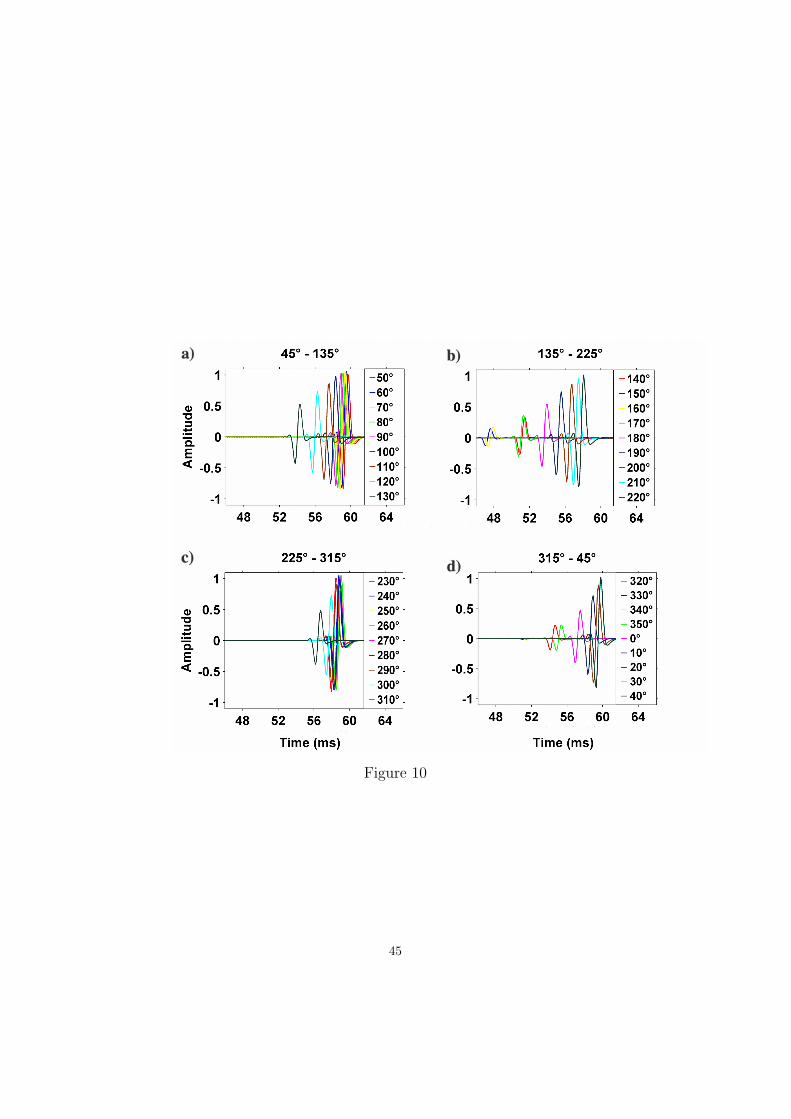
Figure 10

45

Figure 11

46

Figure 12

47

Figure 13

48

Figure 14

49

Figure 15

50

Figure 16

51

Figure 17

52

Figure 18

53

Figure 19

54

Figure 20

55

Figure 21

56

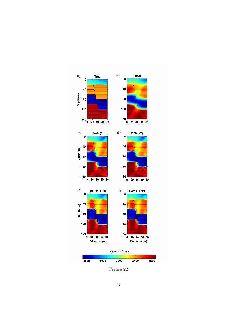
Figure 22

57

Figure 23

58

Referências bibliográficas

Ajo-Franklin, J., Peterson, J., Doetsch, J., Daley, T., 2013. High-resolution characterization of a

CO2 plume using crosswell seismic tomography: Cranfield, MS, USA. International Journal of

Greenhouse Gas Control 18, 497–509.

Ajo-Franklin, J.B., 2009. Optimal experiment design for time-lapse traveltime tomography. Ge-

ophysics 74(4), Q27–Q40.

Ajo-Franklin, J.B., Minsley, B.J., Daley, T.M., 2007. Applying compactness constraints to diffe-

rential traveltime tomography. Geophysics 72(4), R67–R75.

Alford, R., Kelly, K., Boore, D.M., 1974. Accuracy of finite-difference modeling of the acoustic

wave equation. Geophysics 39, 834–842.

Almalki, M., Harris, B., Dupuis, J.C., 2013. Field and synthetic experiments for virtual source

crosswell tomography in vertical wells: Perth Basin, Western Australia. Journal of Applied

Geophysics 98, 144–159.

Asnaashari, A., Brossier, R., Garambois, S., Audebert, F., Thore, P., Virieux, J., 2012. Time-

lapse imaging using regularized FWI: a robustness study, in: SEG Technical Program Expanded

Abstracts 2012. Society of Exploration Geophysicists, pp. 1–5.

Bartle, R.G., 1964. The elements of real analysis. Wiley New York.

Belina, F.A., Ernst, J.R., Holliger, K., 2009. Inversion of crosshole seismic data in heterogene-

ous environments: Comparison of waveform and ray-based approaches. Journal of Applied


Boonyasiriwat, C., Valasek, P., Routh, P., Cao, W., Schuster, G.T., Macy, B., 2009. An effici-

63

REFERÊNCIAS BIBLIOGRÁFICAS 64

ent multiscale method for time-domain waveform tomography. Geophysics 74(6), WCC59–

WCC68.

Bube, K.P., Langan, R.T., 1995. Resolution of crosswell tomography with transmission and reflec-

tion traveltimes, in: SEG Technical Program Expanded Abstracts 1995. Society of Exploration

Geophysicists, pp. 77–80.

Bube, K.P., Langan, R.T., 2008. Resolution of slowness and reflectors in crosswell tomography

with transmission and reflection traveltimes. Geophysics 73(5), VE321–VE335.

Bunks, C., Saleck, F.M., Zaleski, S., Chavent, G., 1995. Multiscale seismic waveform inversion.


Butchibabu, B., Sandeep, N., Sivaram, Y., Jha, P., Khan, P., 2017. Bridge pier foundation eva-

luation using cross-hole seismic tomographic imaging. Journal of Applied Geophysics 144,

104–114.

Byun, J., Yu, J., Seol, S.J., 2010. Crosswell monitoring using virtual sources and horizontal wells.

Geophysics 75(3), SA37–SA43.

Cerjan, C., Kosloff, D., Kosloff, R., Reshef, M., 1985. A nonreflecting boundary condition for

discrete acoustic and elastic wave equations. Geophysics 50, 705–708.

Chavent, G., 1974. Identification of functional parameters in partial differential equations, in: Joint

Automatic Control Conference, pp. 155–156.

Chavent, G., 2010. Nonlinear least squares for inverse problems: theoretical foundations and step-

by-step guide for applications. Scientific Computation, Springer Science & Business Media.

Cheng, F., Liu, J., Wang, J., Zong, Y., Yu, M., 2016. Multi-hole seismic modeling in 3-D space and

cross-hole seismic tomography analysis for boulder detection. Journal of Applied Geophysics

134, 246–252.

Daily, W., Ramirez, A., 1995. Environmental process tomography in the United States. The

Chemical Engineering Journal and the Biochemical Engineering Journal 56, 159–165.


Daley, T.M., Majer, E.L., Peterson, J.E., 2004. Crosswell seismic imaging in a contaminated basalt

aquifer. Geophysics 69, 16–24.

Daley, T.M., Solbau, R.D., Ajo-Franklin, J.B., Benson, S.M., 2007. Continuous active-source

seismic monitoring of CO2 injection in a brine aquifer. Geophysics 72(5), A57–A61.

Dantas, R.R., Medeiros, W.E., 2016. Resolution in crosswell traveltime tomography: The depen-

dence on illumination. Geophysics 81(1), W1–W12.

De Iaco, R., Green, A., Maurer, H.R., Horstmeyer, H., 2003. A combined seismic reflection and

refraction study of a landfill and its host sediments. Journal of Applied Geophysics 52, 139–156.

Di Bartolo, L., 2010. Modelagem sısmica Anisotrópica Através do Método das diferenças fini-

tas utilizando sistemas de equações em segunda ordem. Ph.D. thesis, COPPE/UFRJ, Rio de

Janeiro/RJ, Brasil.

Emery, X., Parra, J., 2013. Integration of crosswell seismic data for simulating porosity in a

heterogeneous carbonate aquifer. Journal of Applied Geophysics 98, 254–264.

Fichtner, A., 2011. Full Seismic Waveform Modelling and Inversion. Advances in Geophysical

and Environmental Mechanics and Mathematics, Springer Berlin Heidelberg.

Gao, Y., Song, H., Zhang, J., Yao, Z., 2015. Comparison of artificial absorbing boundaries for

acoustic wave equation modelling. Exploration Geophysics 48, 76–93.

Gasperikova, E., Hoversten, G.M., 2006. A feasibility study of nonseismic geophysical methods

for monitoring geologic CO2 sequestration. The Leading Edge 25, 1282–1288.

Gheymasi, H.M.h., Gholami, A., Siahkoohi, H., Amini, N., 2016. Robust total-variation based

geophysical inversion using split Bregman and proximity operators. Journal of Applied Ge-

ophysics 132, 242–254.

Greenhalgh, S., Zhou, B., Cao, S., 2003. A crosswell seismic experiment for nickel sulphide

exploration. Journal of Applied Geophysics 53, 77–89.


Gustavsson, M., Ivansson, S., Moren, P., Pihl, J., 1986. Seismic borehole tomo-

graphy—measurement system and field studies. Proceedings of the IEEE 74, 339–346.

Harris, J.M., Nolen-Hoeksema, R.C., Langan, R.T., Van Schaack, M., Lazaratos, S.K., Rector III,

J.W., 1995. High-resolution crosswell imaging of a west texas carbonate reservoir: Part 1-project

summary and interpretation. Geophysics 60, 667–681.

Hicks, E., Hoeber, H., Houbiers, M., Lescoffit, S.P., Ratcliffe, A., Vinje, V., 2016. Time-lapse

full-waveform inversion as a reservoir-monitoring tool - A North Sea case study. The Leading

Edge 35, 850–858.

Holberg, O., 1987. Computational aspects of the choice of operator and sampling interval for nu-

merical differentiation in large-scale simulation of wave phenomena. Geophysical Prospecting

35, 629–655.

Hyndman, D.W., Harris, J.M., Gorelick, S.M., 1994. Coupled seismic and tracer test inversion for

aquifer property characterization. Water Resources Research 30, 1965–1977.

Iserles, A., 2009. A first course in the numerical analysis of differential equations. Number 44 in

Cambridge Texts in Applied Mathematics, Cambridge University Press.

Lanz, E., Maurer, H., Green, A.G., 1998. Refraction tomography over a buried waste disposal site.


Li, G., 2003. 4D seismic monitoring of CO2 flood in a thin fractured carbonate reservoir. The

Leading Edge 22, 690–695.

Liu, L., Guo, T., 2005. Seismic non-destructive testing on a reinforced concrete bridge column

using tomographic imaging techniques. Journal of Geophysics and Engineering 2, 23.

Lo, T.w., Inderwiesen, P.L., 1994. Fundamentals of seismic tomography. volume 6 of Geophysical

Monograph Series. SEG Books.

Mathisen, M.E., Vasiliou, A.A., Cunningham, P., Shaw, J., Justice, J., Guinzy, N., 1995. Time-

lapse crosswell seismic tomogram interpretation: Implications for heavy oil reservoir characteri-


zation, thermal recovery process monitoring, and tomographic imaging technology. Geophysics

60, 631–650.

Menke, W., 1984. The resolving power of cross-borehole tomography. Geophysical Research

Letters 11, 105–108.

Metwaly, M., Green, A.G., Horstmeyer, H., Maurer, H., Abbas, A.M., 2005. Combined seismic

tomographic and ultrashallow seismic reflection study of an early dynastic mastaba, saqqara,

egypt. Archaeological Prospection 12, 245–256.

Moret, G.J., Knoll, M.D., Barrash, W., Clement, W.P., 2006. Investigating the stratigraphy of an

alluvial aquifer using crosswell seismic traveltime tomography. Geophysics 71(3), B63–B73.

Onishi, K., Ueyama, T., Matsuoka, T., Nobuoka, D., Saito, H., Azuma, H., Xue, Z., 2009. Ap-

plication of crosswell seismic tomography using difference analysis with data normalization to

monitor CO2 flooding in an aquifer. International Journal of Greenhouse Gas Control 3, 311–

321.

Perozzi, L., Gloaguen, E., Rondenay, S., McDowell, G., 2012. Using stochastic crosshole seismic

velocity tomography and Bayesian simulation to estimate Ni grades: Case study from Voisey’s

Bay, Canada. Journal of Applied Geophysics 78, 85–93.

Peterson, J.E., Paulsson, B.N., McEvilly, T.V., 1985. Applications of algebraic reconstruction

techniques to crosshole seismic data. Geophysics 50, 1566–1580.

Plessix, R.E., 2006a. A review of the adjoint-state method for computing the gradient of a functi-

onal with geophysical applications. Geophysical Journal International 167, 495–503.

Plessix, R.E., 2006b. Estimation of velocity and attenuation coefficient maps from crosswell seis-

mic data. Geophysics 71(6), S235–S240.

Polymenakos, L., Papamarinopoulos, S., 2005. Exploring a prehistoric site for remains of human

structures by three-dimensional seismic tomography. Archaeological Prospection 12, 221–233.


Pratt, R., Song, Z.M., Williamson, P., Warner, M., 1996. Two-dimensional velocity models from

wide-angle seismic data by wavefield inversion. Geophysical Journal International 124, 323–

340.

Pratt, R.G., 1999. Seismic waveform inversion in the frequency domain, Part 1: Theory and

verification in a physical scale model. Geophysics 64, 888–901.

Pratt, R.G., Goulty, N.R., 1991. Combining wave-equation imaging with traveltime tomography

to form high-resolution images from crosshole data. Geophysics 56, 208–224.

Pratt, R.G., Sams, M.S., 1996. Reconciliation of crosshole seismic velocities with well information

in a layered sedimentary environment. Geophysics 61, 549–560.

Press, W.H., Teukolsky, S.A., Vetterling, W., Flannery, B.P., 2007. Numerical Recipes: The Art of

Scientific Computing. Cambridge University Press.

Rector III, J.W., Washbourne, J.K., 1994. Characterization of resolution and uniqueness in cros-

swell direct-arrival traveltime tomography using the Fourier projection slice theorem. Geophy-

sics 59, 1642–1649.

Rego, E.C.G., 2014. Modelagem e migração sísmica usando método de expansão rápida REM

através dos polinômios de Hermite e Laguerre. Trabalho de Graduação. Universidade Federal

da Bahia.

Rumpf, M., Tronicke, J., 2014. Predicting 2D geotechnical parameter fields in near-surface sedi-

mentary environments. Journal of Applied Geophysics 101, 95–107.

Saito, H., Nobuoka, D., Azuma, H., Xue, Z., Tanase, D., 2006. Time-lapse crosswell seismic

tomography for monitoring injected CO2 in an onshore aquifer, Nagaoka, Japan. Exploration


Santos, R.H.M.d., Figueiró, W.M., 2006. Modelagem acústica bidimensional usando diferentes

parametrizações de campos de velocidades. Revista Brasileira de Geofísica 24, 103–105.


Schön, J.H., 2015. Physical properties of rocks: Fundamentals and principles of petrophysics.

Volume 65 of Developments in Petroleum Sciences. Elsevier.

Shin, C., Jang, S., Min, D.J., 2001. Improved amplitude preservation for prestack depth migration

by inverse scattering theory. Geophysical Prospecting 49, 592–606.

Silva Neto, F.A., 2004. Modelagem acústica por diferenças finitas e elementos finitos em 2-D e

2,5-D. Master’s thesis. Universidade Federal do Pará.

Silva Neto, F., Costa, J., Novais, A., Barbosa, B., 2005. Finite difference elastic modeling in

2.5D, in: 9th International Congress of The Brazilian Geophysical Society, Salvador, Expanded

Abstracts. Brazilian Geophysical Society.

Sirgue, L., Pratt, R.G., 2004. Efficient waveform inversion and imaging: A strategy for selecting

temporal frequencies. Geophysics 69, 231–248.

Sochacki, J., Kubichek, R., George, J., Fletcher, W., Smithson, S., 1987. Absorbing boundary

conditions and surface waves. Geophysics 52, 60–71.

Song, Z.M., Williamson, P.R., Pratt, R.G., 1995. Frequency-domain acoustic-wave modeling and

inversion of crosshole data: Part II—Inversion method, synthetic experiments and real-data re-

sults. Geophysics 60, 796–809.

Soupios, P., Akca, I., Mpogiatzis, P., Basokur, A.T., Papazachos, C., 2011. Applications of hybrid

genetic algorithms in seismic tomography. Journal of Applied Geophysics 75, 479–489.

Tarantola, A., 1984. Inversion of seismic reflection data in the acoustic approximation. Geophysics

49, 1259–1266.

Van Schaack, M.A., 1997. Velocity estimation for crosswell reflection imaging using combined

direct and reflected arrival traveltime tomography. Ph.D. thesis. Stanford University.

Virieux, J., Operto, S., 2009. An overview of full-waveform inversion in exploration geophysics.

Geophysics 74(6), WCC1–WCC26.


Watanabe, T., Shimizu, S., Asakawa, E., Matsuoka, T., 2004. Differential waveform tomography

for time-lapse crosswell seismic data with application to gas hydrate production monitoring, in:

SEG Technical Program Expanded Abstracts 2004. Society of Exploration Geophysicists, pp.

2323–2326.

Williamson, P., 1991. A guide to the limits of resolution imposed by scattering in ray tomography.


Xu, K., Greenhalgh, S., 2010. Ore-body imaging by crosswell seismic waveform inversion: A

case study from Kambalda, Western Australia. Journal of Applied Geophysics 70, 38–45.

Yamamoto, T., Nye, T., Kuru, M., 1994. Porosity, permeability, shear strength: Crosswell tomo-

graphy below an iron foundry. Geophysics 59, 1530–1541.

Zhang, W., Youn, S., Doan, Q.T., 2007. Understanding reservoir architectures and steam-chamber

growth at Christina Lake, Alberta, by using 4D seismic and crosswell seismic imaging. SPE

Reservoir Evaluation & Engineering 10, 446–452.

Zhou, B., Greenhalgh, S.A., 2003. Crosshole seismic inversion with normalized full-waveform

amplitude data. Geophysics 68, 1320–1330.

Zhou, C., Cai, W., Luo, Y., Schuster, G.T., Hassanzadeh, S., 1995. Acoustic wave-equation travel-

time and waveform inversion of crosshole seismic data. Geophysics 60, 765–773.

Apêndice A: Modelagem direta

Seja c(r) um modelo de velocidades da onda P definido na região de interesse V . A modela-

gem sísmica acústica bidimensional consiste em calcular o campo de pressão us(r, t;rs;c) propa-

gado na região de interesse ao longo do tempo t, partindo de uma fonte linear s localizada em rs.

Dada a função temporal da fonte S(t) e considerando a densidade uniforme, o campo de pressão

us(r, t;rs;c) pode ser calculado na posição r ∈V resolvendo a equação da onda escalar:

(∇

2− 1c(r)2

∂2

∂t2

)us(r, t;rs;c) = S(t)δ(r− rs) . (A.1)

Nessa dissertação, a equação A.1 foi resolvida através do método das diferenças finitas (e.g.

Iserles, 2009), que consiste em substituir as derivadas parciais da equação da onda acústica por

aproximações discretas. Essa aproximação é feita através de uma expansão em série de Taylor

truncada no ND-ésimo termo. ND é escolhido pelo usuário e definirá a ordem do operador de

diferenças finitas. Quanto maior a ordem desse operador, melhor será a aproximação numérica

(e.g. Iserles, 2009). Contudo, aumentar a ordem do operador de diferenças finitas requer um

aumento no custo computacional do cálculo das diferenças.

Por outro lado, se a ordem do operador não for grande o suficiente, a discretização do opera-

dor de onda tanto no espaço como no tempo pode incorporar efeitos indesejáveis de dispersão e

instabilidade numéricas à solução do problema de modelagem (Santos and Figueiró, 2006). Nor-

malmente esses erros numéricos se apresentam através de oscilações na forma de onda temporal.

Para que esses erros sejam pequenos e não cresçam arbitrariamente com o tempo, é necessário es-

colher intervalos de amostragem espaciais ∆x e ∆z e temporais ∆t suficientemente pequenos para

uma dada frequência máxima de fonte fmax. Quanto maior for a ordem do operador de diferen-

ças finitas, menos fina poderá ser a amostragem espacial e temporal, acarretando em economia de

memória computacional. Dessa forma, um compromisso entre a ordem do operador de diferenças

72

finitas usado e a taxa de amostragem temporal e espacial é necessário para produzir simulações

adequadas e computacionalmente viáveis.

Para evitar a dispersão numérica na modelagem de um campo de onda em uma malha uniforme

(∆x = ∆z = h), foram calculados os intervalos de amostragem máximos para a modelagem usando

as seguintes relações (Santos and Figueiró, 2006):

h≤ cmin

α fmax, (A.2)

∆t ≤ hβcmax

, (A.3)

em que cmin e cmax são as velocidades mínima e máxima presentes no modelo. α e β são valores

relacionados às ordens dos operadores espaciais e temporais. O valor de α corresponde à norma-

lização do comprimento de onda pelo intervalo de discretização da malha espacial e determina a

menor quantidade de pontos por comprimento de onda que permite manter o erro de fase dentro

de um nível de tolerância. β controla a estabilidade do esquema de diferenças finitas através da

avaliação do erro de fase (Silva Neto, 2004).

Nesta pesquisa, foi utilizado um esquema de diferenças finitas de 12a ordem no espaço e de

segunda ordem no tempo, de modo a garantir uma boa estabilidade numérica e a reduzir substan-

cialmente os efeitos de dispersão numérica (Alford et al., 1974).

Apêndice B: Modelagem inversa

O problema da inversão da forma de onda consiste em estimar o campo de velocidades c(r)

que melhor ajusta os traços modelados ugs = u(rg, t;rs;c) e registrados vgs = v(rg, t;rs) no receptor

localizado no ponto rg, gerado por uma fonte em rs, segundo algum critério de desajuste. Esse

critério, incorporado ao funcional ajustante pela função F(ugs,vgs), definirá a forma do funcional

ajustante e suas características. Assim, podemos estimar c(r) minimizando o funcional:

ψ =1

T NgNs

Ng

∑g

Ns

∑s

∫ T

0F(ugs,vgs)dt , (B.1)

em que Ns e Ng são, respectivamente, o número de fontes e de receptores, T é o tempo de registro

e σ2g é o desvio padrão associado a F(ugs,vgs). Tradicionalmente, o FWI usa o critério de mínimos

quadrados no ajuste do traço sísmico:

F(ugs,vgs) =1

2σ2g[ugs− vgs]

2 . (B.2)

Normalmente, a inversão da forma de onda é resolvida por métodos baseados no gradiente da

função objetivo em relação aos parâmetros do modelo. Contudo, é inviável calcular as derivadas

do gradiente diretamente (via diferenças finitas) devido à quantidade expressiva de parâmetros e ao

alto custo computacional de cada modelagem sísmica. Sendo assim, para calcular o gradiente de

forma econômica, usaremos o método do estado adjunto (Chavent, 1974, 2010, Plessix, 2006a, Ta-

rantola, 1984). Para isso, o campo de onda teórico é definido como variável de estado, e a equação

de modelagem desse campo de onda (equação A.1) define uma equação de estado associada a essa

variável de estado. No desenvolvimento a seguir, usaremos a mesma notação para uma variável de

estado e para uma de suas realizações.

Para maior praticidade no desenvolvimento que vem a seguir, definimos o operador de onda

74

como W :

W = ∇2− 1

c2∂2

∂t2 . (B.3)

Assim, podemos reescrever a equação A.1 de forma mais simplificada para o desenvolvimento

do gradiente do funcional via método do estado adjunto:

W us = S(t)δ(r− rs) . (B.4)

Adicionaremos a aderência do estado de campo de onda modelado em todo o domínio V à

equação de estado correspondente (equação B.4) como um vínculo ao problema de minimização

do funcional ψ definido na equação B.1. Usando o teorema dos multiplicadores de Lagrange, o

problema de minimizar ψ com esse vínculo equivale a minimizar o funcional ampliado

ψ[u,c,λ] =1

T NgNs

Ng

∑g

Ns

∑s

∫ T

0F(ugs,vgs)dt +

Ns

∑s

∫ T

0〈λs, [W us−S(t)δ(r− rs)]〉V dt , (B.5)

em que o multiplicador de Lagrange λs = λs(r,c, t;rs) é a variável de estado adjunto associada a

us, e 〈·, ·〉V denota produto interno entre duas funções definidas no domínio V :

〈p(r),q(r)〉V =∫

Vp(r)q(r)d2r (B.6)

Definamos, agora, a perturbação δψ no funcional ampliado e a perturbação δu nos traços sís-

micos, ambas devidas à perturbação no campo de velocidades δc. Pela regra da cadeia,

δψ =∂ψ

∂uδu+

∂ψ

∂cδc+

∂ψ

∂λδλ (B.7)

Dessa forma, podemos calcular a perturbação no funcional δψ através do cálculo dessas três

derivadas parciais. Para as realizações estacionárias das variáveis de estado e estado adjunto, as

derivadas em relação a u e λ serão zero. Logo, δψ será o gradiente do funcional em relação a c

para essas realizações. Como a derivada parcial em relação a λ, por construção, leva à equação da

onda (equação B.4), calcularemos as derivadas parciais em relação a c e u. A derivada em relação

75

a c é:∂ψ

∂c= 2

Ns

∑s

∫ T

0〈λs,

1c3

∂2us

∂t2 〉V dt . (B.8)

Com exceção em rs, a equação da onda é homogênea:

W us = 0 . (B.9)

Então,

∇2us =

1c2

∂2us

∂t2 , (B.10)

o que torna possível permutar a derivada temporal de us por c2∇2us na equação B.8. Assim:

∂ψ

∂c= 2

Ns

∑s

∫ T

0〈λs,

1c

∇2us〉V dt . (B.11)

A equação B.11 define como calcularemos o gradiente, dadas realizações das variáveis de es-

tado u e λ: ele será proporcional ao lag zero da correlação cruzada entre o campo λs e o laplaciano

do campo us.

Por último, efetuamos a derivada em relação a u:

∂ψ

∂u=

1T NgNs

Ng

∑g

Ns

∑s

∫ T

0

∂F(ugs,vgs)

∂udt +

Ns

∑s

∫ T

0

∂

∂u〈λs(t),W us(t)〉V dt . (B.12)

Pode-se mostrar que, usando o teorema da reciprocidade,

〈λs(t),W us(t)〉V = 〈us(t),W λs(T − t)〉V . (B.13)

Aplicando a equação B.13 na equação B.12 e reorganizando os termos, temos:

∂ψ

∂u=

Ns

∑s

∫ T

0

{1

T NgNs

Ng

∑g

∂F(ugs,vgs)

∂u+ 〈1,W λs(T − t)〉V

}dt (B.14)

Para introduzir o somatório no produto interno, podemos usar o fato de que:

F(ugs,vgs) = 〈1,F(us,vs)δ(r− rg)〉V . (B.15)

76

Substituindo a equação B.15 na equação B.14 e usando o fato de que a derivada do funcional

em relação a u é zero por construção, obtemos a equação da onda adjunta:

W λs(T − t) =− 1T NgNs

Ng

∑g

∂F(us,vs)

∂uδ(r− rg) . (B.16)

Logo, é possível calcular λ(t) através da retropropagação de uma fonte que depende dos traços

sísmicos e da função de ajuste escolhida. Para essa dissertação, usando a função F definida na

equação B.2, temos:

W λs(T − t) =− 1T NgNsσ2

g

Ng

∑g[ugs− vgs]δ(r− rg) , (B.17)

e as fontes adjuntas se caracterizam como os resíduos de cada receptor.

A maneira usual de resolver o problema da forma de onda é através de métodos iterativos que

buscam uma solução c∗ na vizinhança do modelo inicial c0. Sendo assim, o modelo de velocidades

na k-ésima iteração de um algoritmo de otimização local que tente minimizar ψ é:

ck = ck−1 +αk−1hk−1 , (B.18)

em que o subscrito k indica a iteração, ck e ck+1 são as estimativas de c(r) das iterações k e k+1,

respectivamente, o parâmetro αk−1 é o tamanho do passo, calculado usando um algoritmo de busca

linear, e hk−1 é a direção do passo, calculado pelo método dos gradientes conjugados (e.g. Press

et al., 2007). Esse método se baseia em minimizações do funcional ao longo de um conjunto de

direções conjugadas pelo hessiano de ψ.

Nesta pesquisa, uma aproximação do hessiano de ψ é usada para precondicionar o gradiente do

funcional em cada iteração. O hessiano foi aproximado pelo método da pseudohessiana proposta

por Shin et al. (2001), aproximando a hessiana pela autocorrelação de zero lag das fontes virtuais,

definidas como a fonte do campo jacobiano ∂u/∂c.

Aplicamos dois critérios de parada preliminares: número máximo de iterações (50) e tamanho

77

mínimo do passo em relação à norma do modelo anterior:

‖cn+1‖−‖cn‖‖cn‖

< ε , (B.19)

em que o subscrito n indica iteração e ε é um número pequeno.

Apêndice C: Bordas de absorção

As modelagens da equação onda por diferenças finitas apresentam problemas com as bordas

dos modelos, que introduzem reflexões indesejáveis no modelo, prejudicando o campo de onda que

se obtém em seu interior. Para mitigar esse problema, utilizou-se um método baseado em Cerjan

et al. (1985) e em Sochacki et al. (1987), nomeada de fronteira esponjosa (Gao et al., 2015). Esse

método consiste em aumentar a bordas do modelo de velocidade e resolver a equação da onda com

um termo adicional de amortecimento dentro da região das bordas:

(∇

2− 1c(r)2

∂2

∂t2 −γ(r)c(r)2

∂

∂t

)us(r, t;rs;c) = S(t)δ(r− rs) , (C.1)

em que o fator de amortecimento γ é proporcional ao quadrado da distância entre as bordas reais e

as estendidas:

γ(r) = γx(x)+ γz(z) , (C.2)

γx(x) =

0 se x ∈ [0,X ]

µω∆t(

x−XXa

)2se x > X

µω∆t(

xXa

)2se x < 0

, (C.3)

e

γz(z) =

0 se z ∈ [0,Z]

µω∆t(

z−ZZa

)2se z > Z

µω∆t(

zZa

)2se z < 0

, (C.4)

em que µ é uma constante com dimensão de frequência, ω é a frequência angular dominante da

fonte, X e Z são as dimensões da região de interesse, e Xa e Za são as dimensões da região de ab-

sorção, de acordo com o sistema de coordenadas (x,z) definido na Figura C.1. Dessa forma, temos

uma maneira prática, simples e robusta de atenuar as reflexões espúrias. Contudo, essa implemen-

tação acarreta em um aumento no custo computacional, já que, para construir a zona de absorção,

79

expandimos as dimensões do modelo original, aumentando também o tempo de propagação.

Figura C.1: Sistema de coordenadas definido neste trabalho. A região de interesse (na qual γ = 0), emcinza, são todos os pontos em [0,X ]× [0,Z]. A região de absorção (na qual γ > 0) compreende todos ospontos em [−Xa,X +Xa]× [−Zb,Z +Zb]− [0,X ]× [0,Z].

a inversão da forma de onda completa pode compensar a ... · generalização da lei de hooke, e...

Documents