universidade federal do rio grande do sul€¦ · agradeço à lidi, à raquel e ao mindo (que foi...
TRANSCRIPT
UNIVERSIDADE FEDERAL DO RIO GRANDE DO SUL FACULDADE DE AGRONOMIA
PROGRAMA DE PÓS-GRADUAÇÃO EM ZOOTECNIA
Sistemas integrados de produção agropecuária: o papel da pastagem na solução do dilema produção versus conservação
TAISE ROBINSON KUNRATH Engenheira Agrônoma, Mestre em Zootecnia - UFRGS
Tese apresentada como um dos requisitos à obtenção do Grau de Doutor em
Zootecnia. Área de Concentração Plantas Forrageiras
Porto Alegre (RS), Brasil Agosto de 2014

1

2
“A resposta certa, não importa nada: o
essencial é que as perguntas estejam certas.”
Mário Quintana
3
DEDICATÓRIA
À todas as pessoas que tornaram este sonho possível.
4
AGRADECIMENTOS
Agradeço a Deus e a minha Mãe Iemanjá por guiar e iluminar meu caminho. Por dar a saúde, a família e os amigos que tenho.
A minha mãe, Tais, ao meu pai e meu irmão, ambos Carlos, a minha cunhada Odalisca e ao paidrasto, Aquino, por todo apoio. As minhas Dindas, Tânia e Tamara, por serem minhas segundas mães. Obrigada pela existência de vocês.
Gostaria de agradecer especialmente, àquela pessoa que sabe escolher os melhores títulos para teses, artigos, resumos e apresentações: prof. Paulo Carvalho. Que continua me “desorientando”, apoiando todas as minhas loucuras científicas, ou não, incentivando e motivando sempre. Além da amizade, agradeço pela confiança depositada em mim e pelos ensinamentos. Mais que um orientador, um grande amigo que faz parte da minha família.
Agradeço ao professor Carlos Nabinger pelo apoio em todos os momentos, pelas discussões, pelas conversas e pelas orientações, não só científicas, mas também de vida.
Às minhas “guruas” da estatística, Mónica Cadenazzi e Carolina Bremm. Obrigada por toda ajuda, incentivo, doce de leite e whisky compartilhados. Quando eu crescer quero ser como vocês!
Agradeço à Lidi, à Raquel e ao Mindo (que foi o único colega do GPEP que foi a minha festa de aniversário na França!) por toda ajuda, sempre, e pela amizade! Nós somos os “polegares e indicadores” do Bigode!
Agradeço aos colegas Sérgio Ely Valadão Gigante de Andrade Costa, Joice Assmann, Amanda Posselt Martins, Diego Cecagno, Willian de Souza Filho, Pedro André (Augusto Humberto Frederico Tiago) Albuquerque, entre outros tantos, que de alguma forma contribuíram para a realização desse trabalho, e acima de tudo, pela amizade.
A Cabanha Cerro Coroado, em nome do Sr. Armando, e a todos seus funcionários, que tornam esse experimento possível por mais de uma década. Ao Marquinhos e ao Ramiro muito obrigada pela ajuda e disposição. Ao Curso de Pós-graduação em Zootecnia da UFRGS e ao incentivo financeiro do CNPq.
Je remercie le Dr. Jean-Louis Durand, que m’a reçu avec les bras ouverts à Lusignan pendant mon séjour de doctorat sandwiche. A Gilles Lemaire et les autres chercheurs de l’INRA-Lusignan: Didier Combes, Ela Frak, François Gastal, Abad Chabi, Gaetan Louarn, Abraham Escobar pour la coexistence inestimable. Les techniciens de l’INRA pour l’aide: Xavier et Christophe; Annie, Jean-Pierre, Arnaud, Eric’s, Cédric. Particulièrement à Isabelle Boissou et Nathalie Bonnet !
A Serge Zaka (et ses toupoutous) pour m’accueillir dans sa maison. Pour toutes les macdos q’on mangera ensemble! Des autres collégues, Javier Nebot, Lorena Corona, Vincent Migault, André Giostri, Giovana Zanetti, Tiago Baldissera, Edina Cristiane Lopes et Lina Quadir pour la compagnie et les parties. Encore à l’etranger, je remercie toutes les vaches et les chèvres françaises pour le lait produit et destinés à la fabrication des célèbres et délicieux fromages.
A todos mencionados e aos não citados, meu reconhecimento e agradecimento.
5
SISTEMAS INTEGRADOS DE PRODUÇÃO AGROPECUÁRIA: O PAPEL DA PASTAGEM NA SOLUÇÃO DO DILEMA PRODUÇÃO VERSUS CONSERVAÇÃO 1 Autora: Taise Robinson Kunrath Orientador: Paulo César de Faccio Carvalho Co-orientador: Gilles Lemaire Resumo – Além dos fins produtivos, as pastagens desempenham importante papel na preservação ambiental e na dinâmica da atmosfera e hidrosfera. Esta tese apresenta dois trabalhos, que demonstram as duas faces da pastagem nos sistemas produtivos. O primeiro trabalho, se refere a produção aliada à conservação e teve por objetivos (i) verificar se existe padrão no comportamento das variáveis de produção animal de pastos manejados em diferentes alturas e (ii) identificar metas de manejo que aliem produção e conservação. Este trabalho foi desenvolvido em um sistema integrado de produção agropecuária (SIPA) de longo prazo (2001-2011), localizado na região sul do Brasil. Os tratamentos consistiram de quatro alturas de manejo do pasto: 10, 20, 30 e 40 cm, delineados em blocos ao acaso, com três repetições. Foram utilizados novilhos com idade inicial média de 12 meses, sob pastoreio contínuo com taxa de lotação variável. As variáveis de produção animal e de pasto estudadas mostraram-se afetadas pelos anos experimentais. No entanto, existe padrão nas relações entre produção animal e de pasto ao longo dos 10 anos de experimento. A altura de manejo do pasto de 30 cm permite o acúmulo de resíduo sobre o solo, que beneficia o SIPA, e que proporciona ganho animal satisfatório e estável ao longo dos anos. O segundo trabalho, de cunho conservacionista, objetivou avaliar (i) o efeito de diferentes períodos de duração da pastagem em sistemas de rotação de cultura na drenagem e lixiviação de nitrogênio; (ii) o impacto do nível de intensificação, mais precisamente do uso da adubação nitrogenada durante a fase de pastagens; e (iii) analisar se ocorre um pico de lixiviação após a saída da pastagem e retorno das culturas de grãos, como conseqüência de uma maior mineralização N. Foi realizado na Região centro-oeste da França, com uma base de dados de 9 anos, comparando sistemas de rotação de cultura de milho, trigo e cevada com diferentes períodos de participação de pastagem mista de Festuca arundinacea, Lolium perenne e Dactylis glomerata (0, 3, 6 e 20 anos). Concluiu-se que a introdução de pastagem na rotação de culturas reduz a concentração de nitrato na água drenada. Quanto maior o tempo de participação da pastagem, maior é a redução na concentração de nitrato e, consequentemente, menor a lixiviação de nitrogênio, independentemente da adubação nitrogenada durante a fase pastagem. Palavras-chave – Drenagem; Lixiviação; Nitrato; Pastejo; Produção animal. 1 Tese de doutorado em Zootecnia – Plantas Forrageiras, Faculdade de Agronomia, Universidade Federal do Rio Grande do Sul, Porto Alegre, RS, Brasil. 130p. Agosto, 2014.
6
INTEGRATED CROP-LIVESTOCK SYSTEMS: THE ROLE OF GRASSLAND IN SOLVING THE DILEMMA PRODUCTION VERSUS CONSERVATION¹ Author: Taise Robinson Kunrath Advisor: Paulo César de Faccio Carvalho Co-advisor: Gilles Lemaire Abstract – Further to productive targets, grasslands present an important role
in environmental preservation and the atmospheric and hydrospheric dynamics. This thesis presents both issues, demonstrating the two roles of pastures in productive systems. The first work, refers to production with to conservation, and the objective was (i) verifying the pattern in animal and pasture production under different swards heights and (ii) identifying management targets that combine production and conservation. This work was carried out in a long term integrated crop-livestock system (ICLS) (2001-2011) in Southern Brazil. Treatments consisted of four swards heights: 10, 20, 30 and 40 cm, in a randomized block design with three replicates. Steers 12 months old were used, under continuous grazing with variable stocking rates. Animal and sward production were affected by the years effect, however, there are pattern on animal-sward relationship throughout ten years of experiment. 30 cm sward height allows soil residue accumulation that enables satisfactory livestock weight gain along the years on ICLS. The second work, which had more conservation nature, had the objectives: (i) the quantification of the grassland effect on drainage water quality at the level of a whole crop rotation according to the duration of the “grassland” phase and then on the relative importance of grassland area vs arable cropping area in the land use system; (ii) the impact of the level of intensification and more precisely of the N fertilization use during the grassland phase; and (iii) the analysis of the risk for peak of nitrate leaching after grassland re-cultivation as a consequence of a higher N mineralization. This experiment was carried out in France middle-west with a 9 year data base, comparing maize, wheat and barley crop rotation systems with different mixture pastures (Festuca arundinacea, Lolium perenne and Dactylis glomerata) cycle participation (0, 3, 6 and 20 years). We concluded that the introduction of mowed grassland sequences with this arable crop rotation leads to a strong reduction of the nitrate concentration of the ground water, the more proportion of grassland within the rotation the more NO3
- concentration is reduced, whatever the level of N fertilization during the grassland sequence. Keywords – drainage; leaching; nitrate; grazing; animal production.
1 Doctoral thesis in Animal Science, Faculdade de Agronomia, Universidade Federal do Rio Grande do Sul, Universidade Federal do Rio Grande do Sul, Porto Alegre, RS, Brazil. 130p. August, 2014

7
SUMÁRIO
Páginas 1. CAPÍTULO I ......................................................................................... 12 1.1 Introdução geral ................................................................................. 13 1.2 Sistema integrado de produção agropecuária.................................... 14 1.3 Influência das pastagens na drenagem e lixiviação de nitrogênio ..... 15 1.4 Histórico das áreas experimentais ..................................................... 17 1.4.1 Sistema integrado de produção agropecuária na Região sul do Brasil – Tupanciretã/RS ...................................................................... 17 1.4.2 Systeme d'observation et d'experimentation sur le long terme pour la recherche en environnement - Agro-ecosysteme, cycle bio-geochimique et biodiversite (SOERE-ACBB) – Lusignan/FR ................... 19 1.5 Hipóteses do trabalho ........................................................................ 23 1.6 Objetivos ............................................................................................ 24 2. CAPÍTULO II – Sistema integrado de produção agropecuária: buscando padrões de resposta na produção de pasto e do animal em experimento de longo prazo ........................................................... 25 Resumo .................................................................................................... 28 Introdução ................................................................................................ 29 Material e métodos ................................................................................... 30 Resultados ............................................................................................... 34 Discussão................................................................................................. 36 Conclusões .............................................................................................. 39 Referências bibliográficas ........................................................................ 40 3. CAPÍTULO III – How much do sod-based rotations reduce nitrate leaching in a cereal cropping system? ................................................ 51 Abstract .................................................................................................... 53 Introduction .............................................................................................. 54 Material and methods ............................................................................... 55 Results ..................................................................................................... 58 Discussion ................................................................................................ 61 Appendix .................................................................................................. 66 References ............................................................................................... 69 4. CAPÍTULO IV ...................................................................................... 87 4.1 Conclusões gerais .............................................................................. 89 4.2 Referencias bibliográfica.................................................................... 90 5. Apêndices ........................................................................................... 95
8
RELAÇÃO DE TABELAS
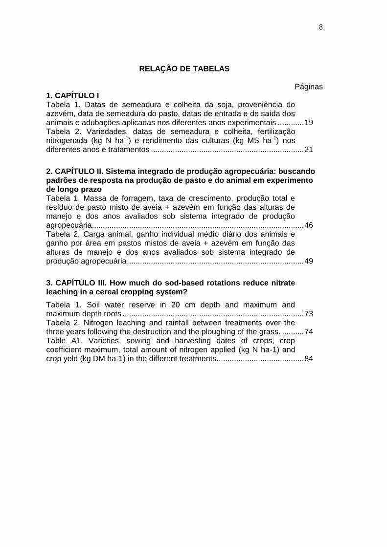
Páginas 1. CAPÍTULO I Tabela 1. Datas de semeadura e colheita da soja, proveniência do azevém, data de semeadura do pasto, datas de entrada e de saída dos animais e adubações aplicadas nos diferentes anos experimentais ............ 19 Tabela 2. Variedades, datas de semeadura e colheita, fertilização nitrogenada (kg N ha-1) e rendimento das culturas (kg MS ha-1) nos diferentes anos e tratamentos ...................................................................... 21
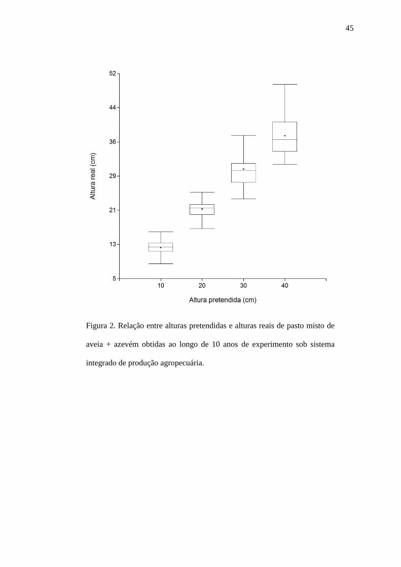
2. CAPÍTULO II. Sistema integrado de produção agropecuária: buscando padrões de resposta na produção de pasto e do animal em experimento de longo prazo Tabela 1. Massa de forragem, taxa de crescimento, produção total e resíduo de pasto misto de aveia + azevém em função das alturas de manejo e dos anos avaliados sob sistema integrado de produção agropecuária ................................................................................................. 46 Tabela 2. Carga animal, ganho individual médio diário dos animais e ganho por área em pastos mistos de aveia + azevém em função das alturas de manejo e dos anos avaliados sob sistema integrado de produção agropecuária ................................................................................. 49
3. CAPÍTULO III. How much do sod-based rotations reduce nitrate leaching in a cereal cropping system?
Tabela 1. Soil water reserve in 20 cm depth and maximum and maximum depth roots ................................................................................... 73 Tabela 2. Nitrogen leaching and rainfall between treatments over the three years following the destruction and the ploughing of the grass. .......... 74 Table A1. Varieties, sowing and harvesting dates of crops, crop coefficient maximum, total amount of nitrogen applied (kg N ha-1) and crop yeld (kg DM ha-1) in the different treatments ........................................ 84
9
RELAÇÃO DE FIGURAS
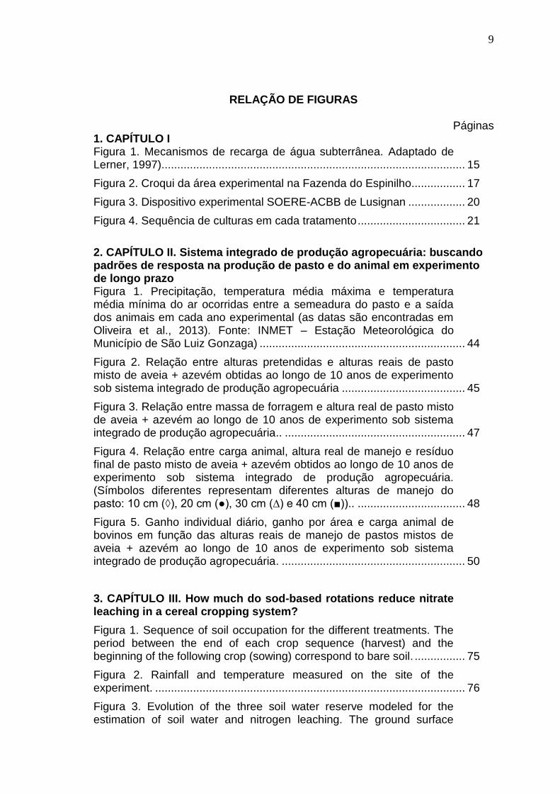
Páginas 1. CAPÍTULO I Figura 1. Mecanismos de recarga de água subterrânea. Adaptado de Lerner, 1997)... ............................................................................................. 15
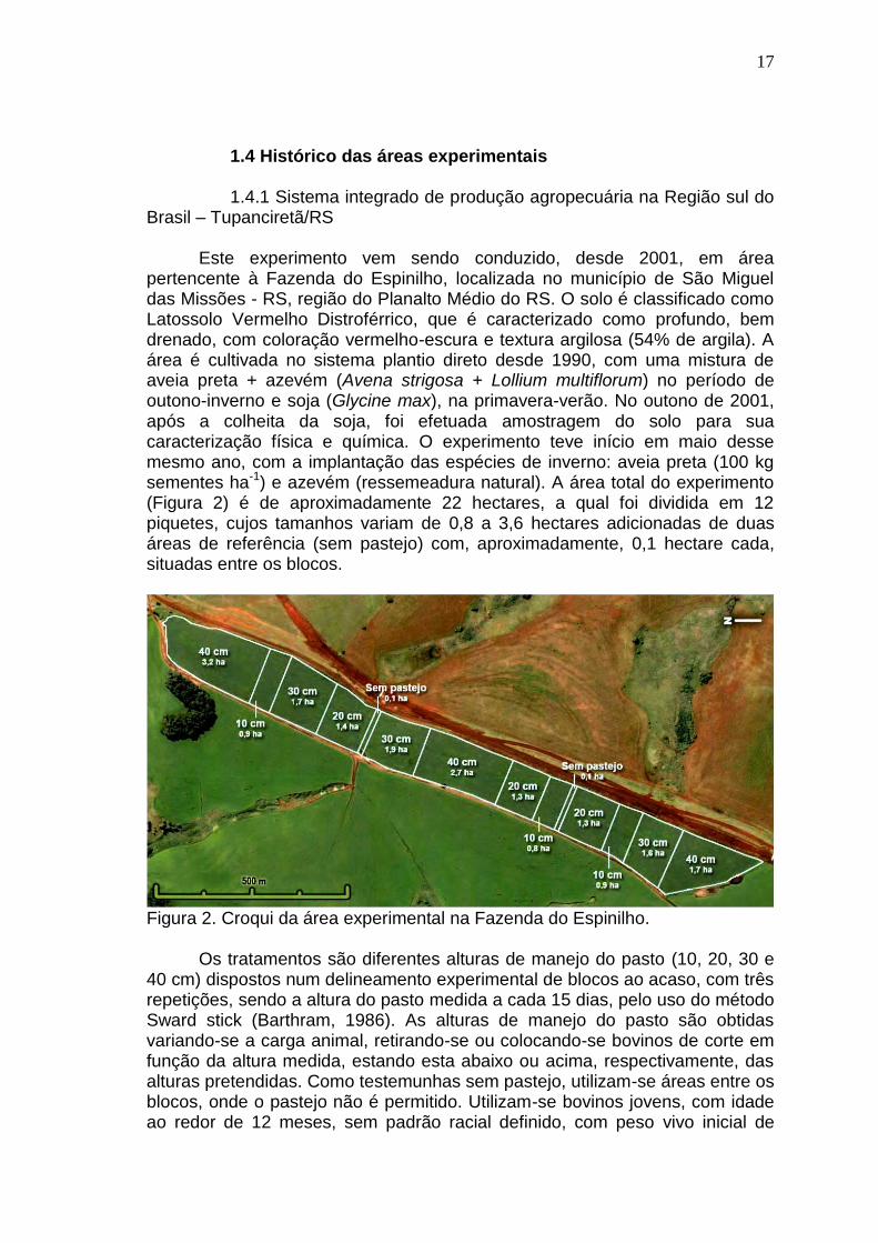
Figura 2. Croqui da área experimental na Fazenda do Espinilho................. 17
Figura 3. Dispositivo experimental SOERE-ACBB de Lusignan .................. 20
Figura 4. Sequência de culturas em cada tratamento .................................. 21
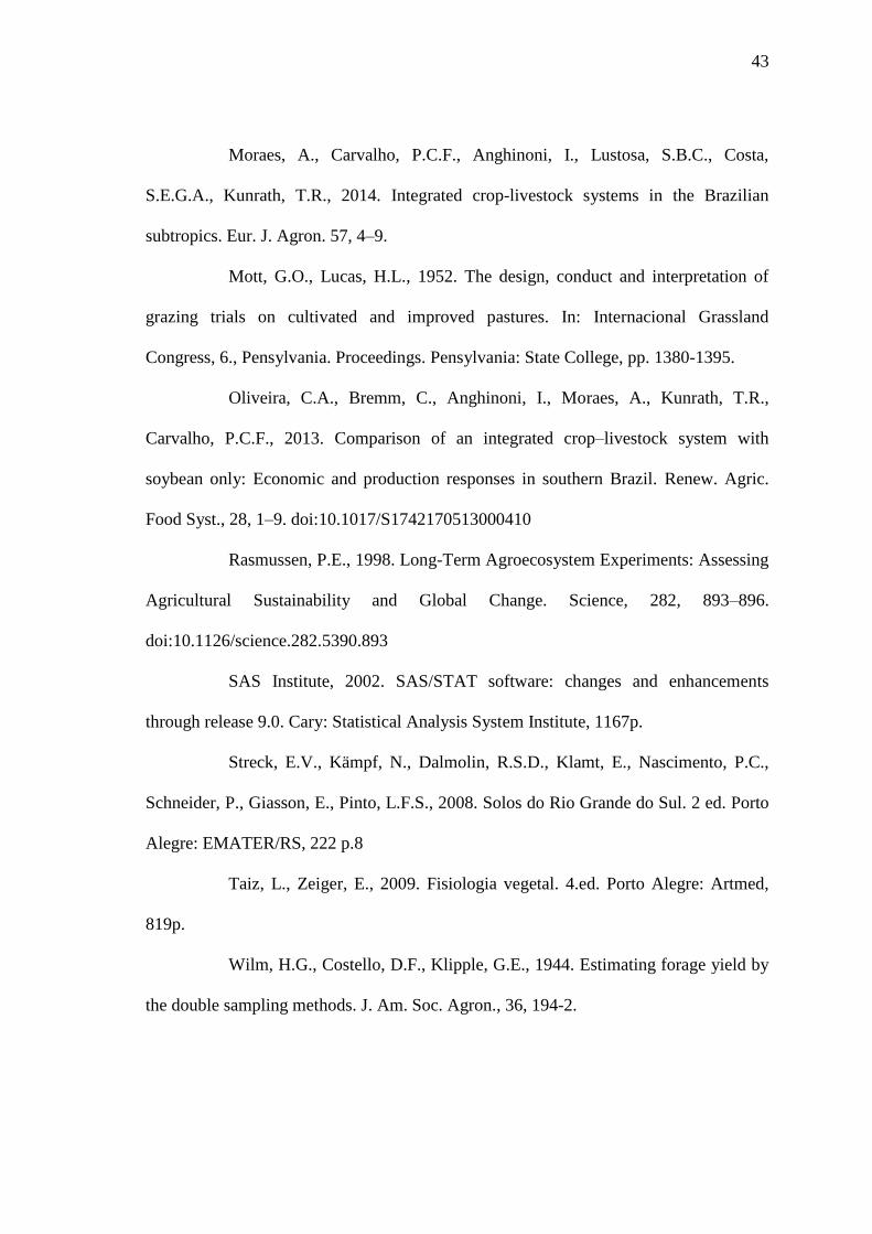
2. CAPÍTULO II. Sistema integrado de produção agropecuária: buscando padrões de resposta na produção de pasto e do animal em experimento de longo prazo Figura 1. Precipitação, temperatura média máxima e temperatura média mínima do ar ocorridas entre a semeadura do pasto e a saída dos animais em cada ano experimental (as datas são encontradas em Oliveira et al., 2013). Fonte: INMET – Estação Meteorológica do Município de São Luiz Gonzaga) ................................................................. 44
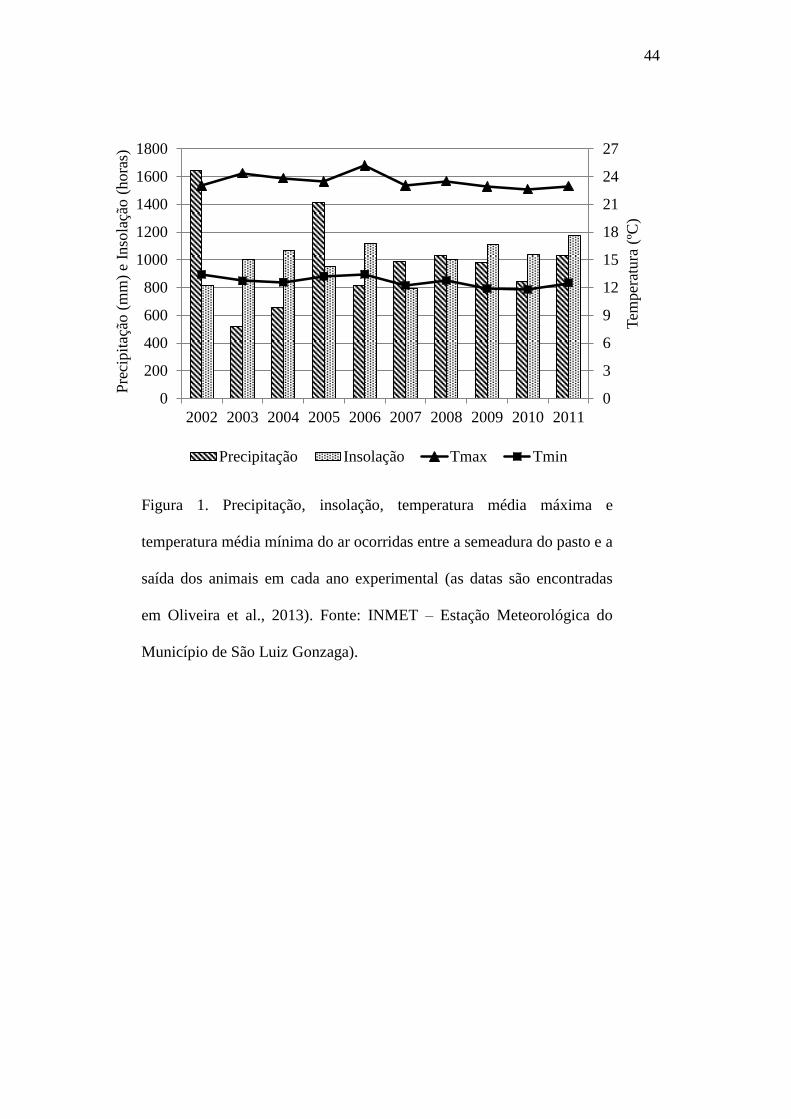
Figura 2. Relação entre alturas pretendidas e alturas reais de pasto misto de aveia + azevém obtidas ao longo de 10 anos de experimento sob sistema integrado de produção agropecuária ....................................... 45
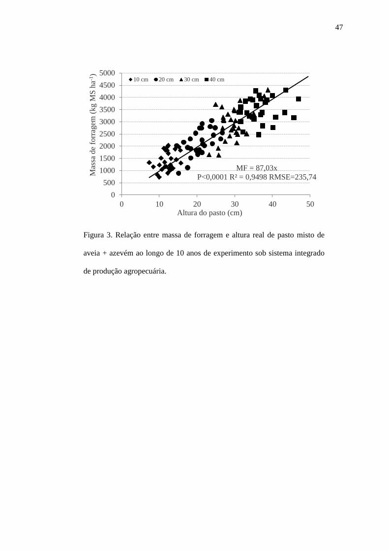
Figura 3. Relação entre massa de forragem e altura real de pasto misto de aveia + azevém ao longo de 10 anos de experimento sob sistema integrado de produção agropecuária.. ......................................................... 47
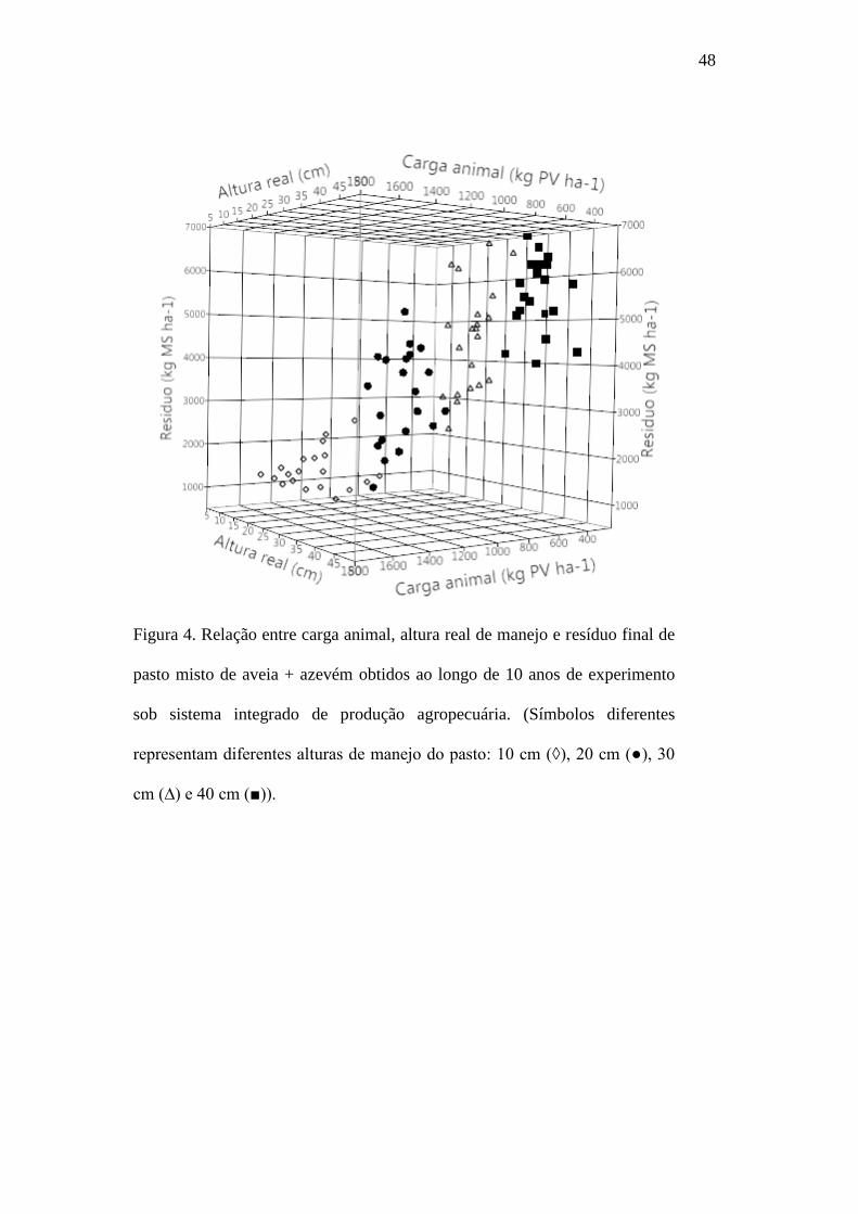
Figura 4. Relação entre carga animal, altura real de manejo e resíduo final de pasto misto de aveia + azevém obtidos ao longo de 10 anos de experimento sob sistema integrado de produção agropecuária. (Símbolos diferentes representam diferentes alturas de manejo do pasto: 10 cm (◊), 20 cm (●), 30 cm (∆) e 40 cm (■)).. .................................. 48
Figura 5. Ganho individual diário, ganho por área e carga animal de bovinos em função das alturas reais de manejo de pastos mistos de aveia + azevém ao longo de 10 anos de experimento sob sistema integrado de produção agropecuária. .......................................................... 50
3. CAPÍTULO III. How much do sod-based rotations reduce nitrate leaching in a cereal cropping system?
Figura 1. Sequence of soil occupation for the different treatments. The period between the end of each crop sequence (harvest) and the beginning of the following crop (sowing) correspond to bare soil. ................ 75
Figura 2. Rainfall and temperature measured on the site of the experiment. .................................................................................................. 76
Figura 3. Evolution of the three soil water reserve modeled for the estimation of soil water and nitrogen leaching. The ground surface

10
(R20) is divided into a tank of at least 20 cm deep, a reservoir between 20 cm and root depth (where they are deeper than 20 cm – Rroot) and a reservoir between the root depth and the maximum depth observed during the 9 years of the trial (Rmax). Root depth zero at the time of implantation, is proportional to the coefficient of the crop (Kc) and hence increases as a function of the sum of temperature. Water flows are expected only vertical and rising damp considered negligible in Lusignan. Drainage is calculated as the difference between the water balance of each tank and its useful reserve when higher ............................. 77
Figura 4. Illustration of the methodology for calculating the soil water reserve (Grassland in Oct/2010). .................................................................. 78
Figura 5. Comparison of soil water reserve evolution for the five treatments over the 9 years.. ........................................................................ 79
Figura 6. Estimated drainage and nitrate concentration of soil solution collected by lysimetric plates for treatment C (a) and G (b). ......................... 80
Figura 7. Comparison of the evolution of the cumulative drainage over the 9 years between the 5 treatments. (*significant difference between treatments in the periods; different letters mean differences between treatments for cumulative drainage; P>0.0001). ........................................... 81
Figure 8. Comparison of the evolution of the cumulative nitrogen leaching between the 5 treatments over the 9 years. (*significant difference between treatments in the periods; different letters mean differences between treatments for cumulative nitrogen leaching; P>0.0001). .................................................................................................... 82
Figure 9. Average nitrate concentration of drained solution as a function of the duration of grassland in a mixed cropping system over 9 years. ........ 83
11
LISTA DE ABREVIATURAS E SÍMBOLOS
ACBB Agroecossistema, ciclos biogeoquímicos e biodiversidade
Al Alumínio C Carbono cm Centímetro cmolc Centimol de carga CNPq Centro Nacional de Pesquisa DM Dry matter dm Decímetro EC Comunidade europeia ET0 Evapotranspiração de referência ETR Evapotranspiração real FAO Food and Agriculture Organization ha Hectare INRA Institut National de Recherche Agronomique kg Quilograma L Litro m Metro mg Miligrama mm Milímetro MOS Matéria orgânica do solo MS Matéria seca N Nitrogênio n Número NO3
- Nitrato ºC Graus celsius P Significância PV Peso vivo r Coeficiente de correlação R² Coeficiente de determinação RMSE Desvio padrão RS Rio Grande do Sul S Sul SIPA Sistema integrado de produção agropecuária SOERE Systeme d'Observation et d'Experimentation
sur le long terme pour la Recherche en Environnement
UE Unidade Experimental UFRGS Universidade Federal do Rio Grande do Sul W Oeste
1. CAPÍTULO I
1.1 Introdução geral
1.2 Sistema integrado de produção agropecuária
1.3 Influência das pastagens na drenagem e lixiviação de nitrogênio
1.4 Histórico das áreas experimentais
1.5 Hipóteses de trabalho
1.6 Objetivos
13
1.1 INTRODUÇÃO GERAL As pastagens desempenham papel fundamental na dinâmica da
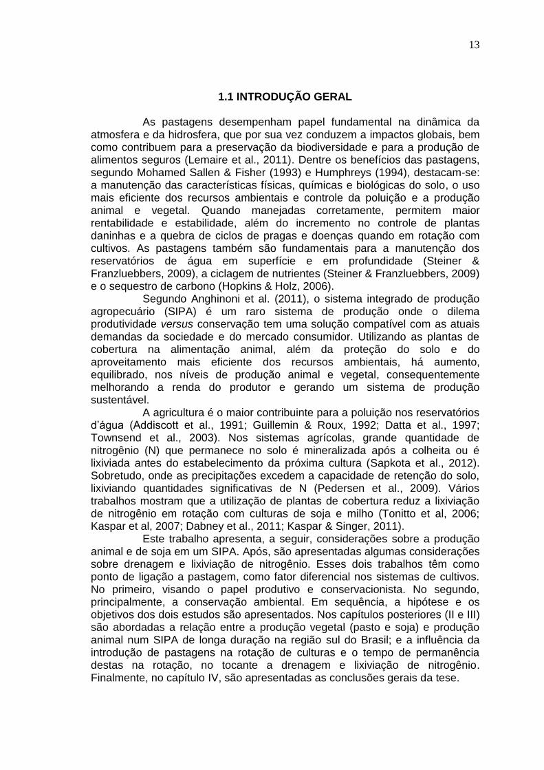
atmosfera e da hidrosfera, que por sua vez conduzem a impactos globais, bem como contribuem para a preservação da biodiversidade e para a produção de alimentos seguros (Lemaire et al., 2011). Dentre os benefícios das pastagens, segundo Mohamed Sallen & Fisher (1993) e Humphreys (1994), destacam-se: a manutenção das características físicas, químicas e biológicas do solo, o uso mais eficiente dos recursos ambientais e controle da poluição e a produção animal e vegetal. Quando manejadas corretamente, permitem maior rentabilidade e estabilidade, além do incremento no controle de plantas daninhas e a quebra de ciclos de pragas e doenças quando em rotação com cultivos. As pastagens também são fundamentais para a manutenção dos reservatórios de água em superfície e em profundidade (Steiner & Franzluebbers, 2009), a ciclagem de nutrientes (Steiner & Franzluebbers, 2009) e o sequestro de carbono (Hopkins & Holz, 2006).
Segundo Anghinoni et al. (2011), o sistema integrado de produção agropecuário (SIPA) é um raro sistema de produção onde o dilema produtividade versus conservação tem uma solução compatível com as atuais demandas da sociedade e do mercado consumidor. Utilizando as plantas de cobertura na alimentação animal, além da proteção do solo e do aproveitamento mais eficiente dos recursos ambientais, há aumento, equilibrado, nos níveis de produção animal e vegetal, consequentemente melhorando a renda do produtor e gerando um sistema de produção sustentável.
A agricultura é o maior contribuinte para a poluição nos reservatórios d’água (Addiscott et al., 1991; Guillemin & Roux, 1992; Datta et al., 1997; Townsend et al., 2003). Nos sistemas agrícolas, grande quantidade de nitrogênio (N) que permanece no solo é mineralizada após a colheita ou é lixiviada antes do estabelecimento da próxima cultura (Sapkota et al., 2012). Sobretudo, onde as precipitações excedem a capacidade de retenção do solo, lixiviando quantidades significativas de N (Pedersen et al., 2009). Vários trabalhos mostram que a utilização de plantas de cobertura reduz a lixiviação de nitrogênio em rotação com culturas de soja e milho (Tonitto et al, 2006; Kaspar et al, 2007; Dabney et al., 2011; Kaspar & Singer, 2011).
Este trabalho apresenta, a seguir, considerações sobre a produção animal e de soja em um SIPA. Após, são apresentadas algumas considerações sobre drenagem e lixiviação de nitrogênio. Esses dois trabalhos têm como ponto de ligação a pastagem, como fator diferencial nos sistemas de cultivos. No primeiro, visando o papel produtivo e conservacionista. No segundo, principalmente, a conservação ambiental. Em sequência, a hipótese e os objetivos dos dois estudos são apresentados. Nos capítulos posteriores (II e III) são abordadas a relação entre a produção vegetal (pasto e soja) e produção animal num SIPA de longa duração na região sul do Brasil; e a influência da introdução de pastagens na rotação de culturas e o tempo de permanência destas na rotação, no tocante a drenagem e lixiviação de nitrogênio. Finalmente, no capítulo IV, são apresentadas as conclusões gerais da tese.
14
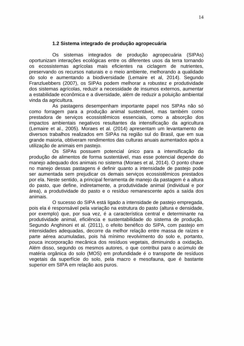
1.2 Sistema integrado de produção agropecuária Os sistemas integrados de produção agropecuária (SIPAs)
oportunizam interações ecológicas entre os diferentes usos da terra tornando os ecossistemas agrícolas mais eficientes na ciclagem de nutrientes, preservando os recursos naturais e o meio ambiente, melhorando a qualidade do solo e aumentando a biodiversidade (Lemaire et al, 2014). Segundo Franzluebbers (2007), os SIPAs podem melhorar a robustez e produtividade dos sistemas agrícolas, reduzir a necessidade de insumos externos, aumentar a estabilidade econômica e a diversidade, além de reduzir a poluição ambiental vinda da agricultura.
As pastagens desempenham importante papel nos SIPAs não só como forragem para a produção animal sustentável, mas também como prestadora de serviços ecossistêmicos essenciais, como a absorção dos impactos ambientais negativos resultantes da intensificação da agricultura (Lemaire et al., 2005). Moraes et al. (2014) apresentam um levantamento de diversos trabalhos realizados em SIPAs na região sul do Brasil, que em sua grande maioria, obtiveram rendimentos das culturas anuais aumentados após a utilização de animais em pastejo.
Os SIPAs possuem potencial único para a intensificação da produção de alimentos de forma sustentável, mas esse potencial depende do manejo adequado dos animais no sistema (Moraes et al, 2014). O ponto chave no manejo dessas pastagens é definir quanto a intensidade de pastejo pode ser aumentada sem prejudicar os demais serviços ecossistêmicos prestados por ela. Neste sentido, a principal ferramenta de manejo da pastagem é a altura do pasto, que define, indiretamente, a produtividade animal (individual e por área), a produtividade do pasto e o resíduo remanescente após a saída dos animais.
O sucesso do SIPA está ligado a intensidade de pastejo empregada, pois ela é responsável pela variação na estrutura do pasto (altura e densidade, por exemplo) que, por sua vez, é a característica central e determinante na produtividade animal, eficiência e sustentabilidade do sistema de produção. Segundo Anghinoni et al. (2011), o efeito benéfico do SIPA, com pastejo em intensidades adequadas, decorre da melhor relação entre massa de raízes e parte aérea acumuladas, pois há mínimo revolvimento do solo e, portanto, pouca incorporação mecânica dos resíduos vegetais, diminuindo a oxidação. Além disso, segundo os mesmos autores, o que contribui para o acúmulo de matéria orgânica do solo (MOS) em profundidade é o transporte de resíduos vegetais da superfície do solo, pela macro e mesofauna, que é bastante superior em SIPA em relação aos puros.
15
1.3 Influencia das pastagens na drenagem e lixiviação de nitrogênio
A água subterrânea é uma das principais fontes de água potável em
muitos países, e é frequentemente utilizada sem tratamento, particularmente em poços particulares (Jégo et al., 2008). Quantificar sua taxa atual de recarga é pré-requisito para a gestão eficiente e sustentável dos recursos hídricos subterrâneos. E segundo Vries et al. (2002), é chave para o desenvolvimento econômico de regiões que delas dependem para seu desenvolvimento.
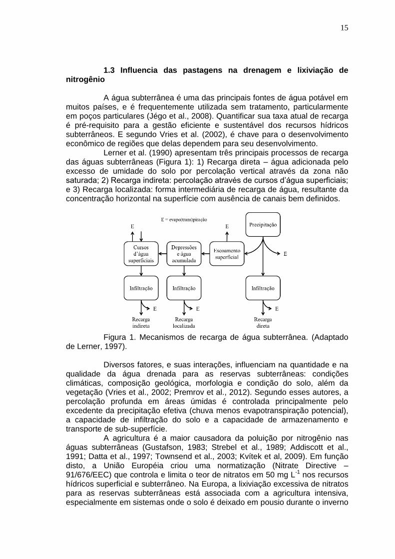
Lerner et al. (1990) apresentam três principais processos de recarga das águas subterrâneas (Figura 1): 1) Recarga direta – água adicionada pelo excesso de umidade do solo por percolação vertical através da zona não saturada; 2) Recarga indireta: percolação através de cursos d’água superficiais; e 3) Recarga localizada: forma intermediária de recarga de água, resultante da concentração horizontal na superfície com ausência de canais bem definidos.
Figura 1. Mecanismos de recarga de água subterrânea. (Adaptado
de Lerner, 1997). Diversos fatores, e suas interações, influenciam na quantidade e na
qualidade da água drenada para as reservas subterrâneas: condições climáticas, composição geológica, morfologia e condição do solo, além da vegetação (Vries et al., 2002; Premrov et al., 2012). Segundo esses autores, a percolação profunda em áreas úmidas é controlada principalmente pelo excedente da precipitação efetiva (chuva menos evapotranspiração potencial), a capacidade de infiltração do solo e a capacidade de armazenamento e transporte de sub-superfície.
A agricultura é a maior causadora da poluição por nitrogênio nas águas subterrâneas (Gustafson, 1983; Strebel et al., 1989; Addiscott et al., 1991; Datta et al., 1997; Townsend et al., 2003; Kvítek et al, 2009). Em função disto, a União Européia criou uma normatização (Nitrate Directive – 91/676/EEC) que controla e limita o teor de nitratos em 50 mg L-1 nos recursos hídricos superficial e subterrâneo. Na Europa, a lixiviação excessiva de nitratos para as reservas subterrâneas está associada com a agricultura intensiva, especialmente em sistemas onde o solo é deixado em pousio durante o inverno
16
(Neill, 1989). As menores precipitações que ocorrem no verão, associadas a elevada evapotranspiração, geralmente, são suficientes para restringir os períodos de drenagem nesta época do ano, permitindo o acúmulo de nitratos no solo, que poderá ser lixiviado com os eventos de drenagem que ocorrem no período de outono/inverno (Cuttle & Scholenfield, 1995).
Além dos fatores que interferem na drenagem da água, a lixiviação de nitrogênio é ligada ao sistema de cultura e às fertilizações utilizadas, ao manejo e características do solo, teor de matéria orgânica e a presença ou não de escoamento superficial (Shepherd et al., 2001; Oenema et al., 2005; Jégo et al., 2008; Kopacek et al., 2013).
As comparações dos níveis de nitrato lixiviado observados em diferentes sistemas de cultivo demonstram a relação entre o uso da terra e as concentrações médias de nitrogênio em fluxo de água (Kvítek et al., 2009). Uma das maneiras de diminuir a lixiviação de nitratos é a utilização de culturas de cobertura durante o período entre-culturas (Dabney et al., 2011; Kaspar & Singer, 2011; Kaspar et al., 2012). O levantamento realizado por Tonitto et al. (2006), com 69 trabalhos realizados nos USA, mostrou que plantas de cobertura (não leguminosas) reduziram em média 70% das perdas por lixiviação de nitratos e essa redução foi diretamente relacionada com o crescimento das culturas. As pastagens são capazes de absorver e utilizar maiores quantidades de nitrogênio que as culturas anuais, diminuindo as perdas por lixiviação (Whitehead, 1995). Estudos demonstram que houve aumento na área cultivada com pastagens em detrimento das culturas anuais com reduções significativas nos teores de nitrogênio lixiviado (Kvítek et al., 2009).
17
1.4 Histórico das áreas experimentais 1.4.1 Sistema integrado de produção agropecuária na Região sul do
Brasil – Tupanciretã/RS
Este experimento vem sendo conduzido, desde 2001, em área pertencente à Fazenda do Espinilho, localizada no município de São Miguel das Missões - RS, região do Planalto Médio do RS. O solo é classificado como Latossolo Vermelho Distroférrico, que é caracterizado como profundo, bem drenado, com coloração vermelho-escura e textura argilosa (54% de argila). A área é cultivada no sistema plantio direto desde 1990, com uma mistura de aveia preta + azevém (Avena strigosa + Lollium multiflorum) no período de outono-inverno e soja (Glycine max), na primavera-verão. No outono de 2001, após a colheita da soja, foi efetuada amostragem do solo para sua caracterização física e química. O experimento teve início em maio desse mesmo ano, com a implantação das espécies de inverno: aveia preta (100 kg sementes ha-1) e azevém (ressemeadura natural). A área total do experimento (Figura 2) é de aproximadamente 22 hectares, a qual foi dividida em 12 piquetes, cujos tamanhos variam de 0,8 a 3,6 hectares adicionadas de duas áreas de referência (sem pastejo) com, aproximadamente, 0,1 hectare cada, situadas entre os blocos.
Figura 2. Croqui da área experimental na Fazenda do Espinilho.
Os tratamentos são diferentes alturas de manejo do pasto (10, 20, 30 e
40 cm) dispostos num delineamento experimental de blocos ao acaso, com três repetições, sendo a altura do pasto medida a cada 15 dias, pelo uso do método Sward stick (Barthram, 1986). As alturas de manejo do pasto são obtidas variando-se a carga animal, retirando-se ou colocando-se bovinos de corte em função da altura medida, estando esta abaixo ou acima, respectivamente, das alturas pretendidas. Como testemunhas sem pastejo, utilizam-se áreas entre os blocos, onde o pastejo não é permitido. Utilizam-se bovinos jovens, com idade ao redor de 12 meses, sem padrão racial definido, com peso vivo inicial de
18
aproximadamente 200 kg. O método de pastoreio adotado é o contínuo, com início de pastejo na área quando o pasto atinge 20 cm de altura (aproximadamente, 2000 kg de MS ha-1). Geralmente, o ciclo de pastejo é iniciado na primeira quinzena de julho, estendendo-se até a primeira quinzena de novembro.
Após o primeiro ciclo de pastejo e antecedendo a implantação do primeiro ciclo da soja (novembro de 2001), foram aplicadas, na superfície do solo de toda a área experimental, 4,5 Mg ha-1 de calcário (PRNT 62%), que corresponde à dose recomendada (CQFS RS/SC, 2004) para elevar o pH do solo até 5,5 na camada de 0 – 10 cm, na condição de plantio direto consolidado. Na área sem pastejo, algumas parcelas receberam calcário na dose equivalente ao restante do experimento (SP-4,5), enquanto outras permaneceram sem calcário (SP-0). A soja foi colhida em maio de 2002.
A partir do outono desse ano e até o presente momento, repetiu-se o mesmo procedimento de implantação da pastagem e pastejo com os animais, seguidos da implantação e condução da cultura da soja (Tabela 1). No outono de 2010, antecedendo ao pastejo, o calcário foi reaplicado na superfície do solo, em parte da área (600 m2 dentro de cada parcela), na dose de 3,6 Mg ha-
1, novamente com o objetivo de elevar o pH do solo a 5,5 na camada de 0 – 10 cm, conforme CQFS RS/SC (2004).
No período experimental têm sido efetuadas avaliações periódicas do crescimento e da qualidade do pasto, do resíduo após pastejo, da carga animal utilizada para manter os tratamentos, do ganho individual e por área dos animais. Na soja, além do rendimento de grãos, tem sido determinada a quantidade dos resíduos remanescentes e determinados os componentes de rendimento de grão. Amostras de solo são retiradas para a avaliação de atributos físicos (densidade, porosidade, umidade e estado de agregação), em três camadas; mecânicos (resistência à penetração e compressibilidade), também em três camadas; e químicos (pH em água, matéria orgânica, fósforo e potássio disponíveis e cálcio, magnésio e alumínio trocáveis e capacidade de troca de cátions), em nove camadas. No terceiro e no nono anos foi também avaliada a qualidade de carcaça dos bovinos ao final do período de pastejo e no quarto ano foi avaliado o comportamento ingestivo dos animais. No quarto ano iniciou-se o trabalho na área de Mecanização Agrícola (Relação Solo-Máquina), para avaliar a eficiência de sulcadores de semeadoras de plantio direto nas diferentes condições de compactação do solo, e no sétimo ano, o estudo da variabilidade espacial de atributos químicos (indicadores de fertilidade do solo), físico (resistência à penetração) e mecânico (esforço de tração em hastes sulcadoras) e seu efeito no rendimento da soja. A partir do quarto ano, passou-se a estudar a ciclagem de nutrientes, especialmente a do carbono e do fósforo em suas respectivas formas, frações e disponibilidades e, ainda, o estado de agregação do solo em função dos diferentes aportes de resíduo da pastagem, da soja e dos animais e da adubação utilizada. Nos anos de 2009 a 2011 foi efetuado um estudo da decomposição dos resíduos (pasto, esterco e soja) e a cinética de liberação de nitrogênio, fósforo, potássio, cálcio e magnésio, visando à sua ciclagem no sistema.
A partir de 2011 começou-se a estudar as emissões de gases de efeito estufa pelo solo e pelos animais. Atualmente (2014), iniciaram-se
19
estudos com bioacústica e com o deslocamento e utilização da pastagem pelos animais.
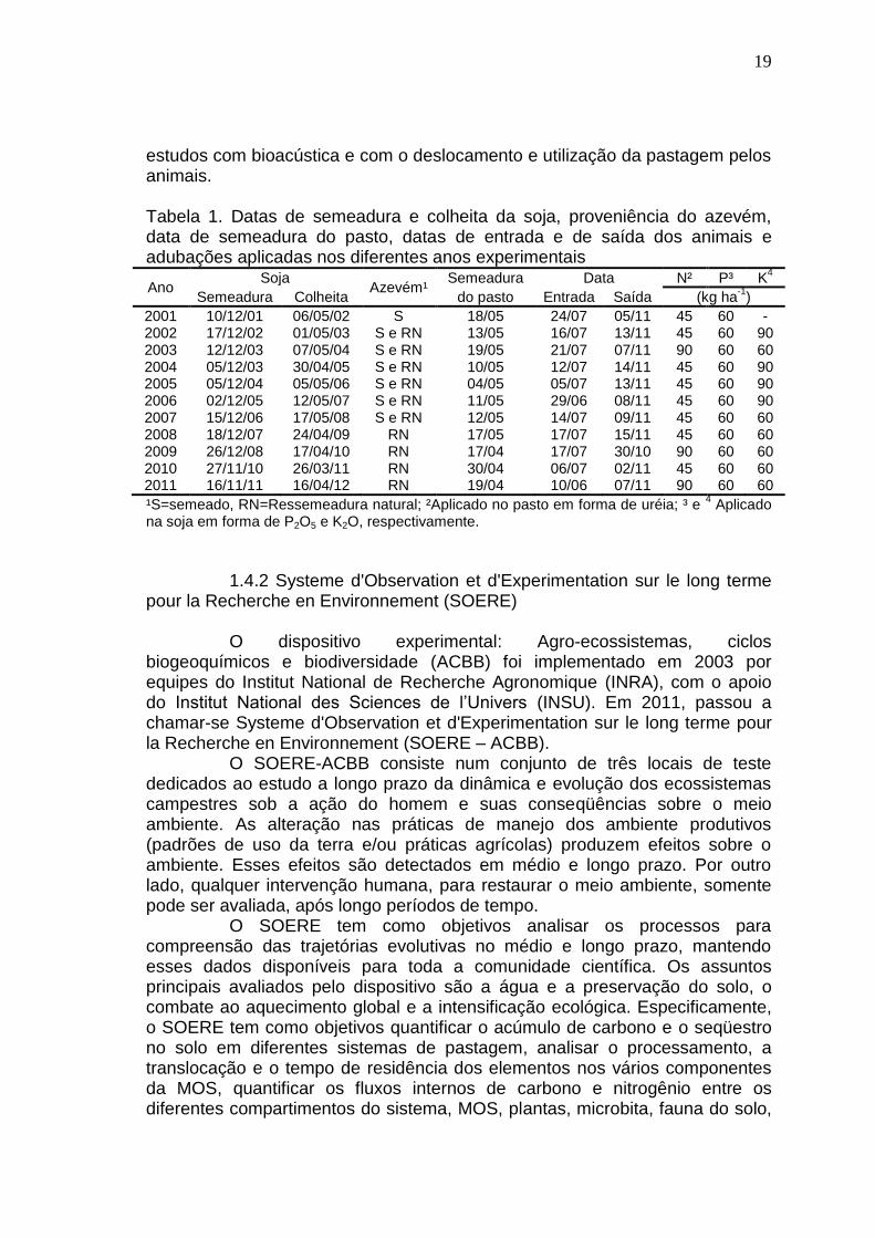
Tabela 1. Datas de semeadura e colheita da soja, proveniência do azevém, data de semeadura do pasto, datas de entrada e de saída dos animais e adubações aplicadas nos diferentes anos experimentais
Ano Soja
Azevém¹ Semeadura Data N² P³ K
4
Semeadura Colheita do pasto Entrada Saída (kg ha-1
)
2001 10/12/01 06/05/02 S 18/05 24/07 05/11 45 60 - 2002 17/12/02 01/05/03 S e RN 13/05 16/07 13/11 45 60 90 2003 12/12/03 07/05/04 S e RN 19/05 21/07 07/11 90 60 60 2004 05/12/03 30/04/05 S e RN 10/05 12/07 14/11 45 60 90 2005 05/12/04 05/05/06 S e RN 04/05 05/07 13/11 45 60 90 2006 02/12/05 12/05/07 S e RN 11/05 29/06 08/11 45 60 90 2007 15/12/06 17/05/08 S e RN 12/05 14/07 09/11 45 60 60 2008 18/12/07 24/04/09 RN 17/05 17/07 15/11 45 60 60 2009 26/12/08 17/04/10 RN 17/04 17/07 30/10 90 60 60 2010 27/11/10 26/03/11 RN 30/04 06/07 02/11 45 60 60 2011 16/11/11 16/04/12 RN 19/04 10/06 07/11 90 60 60
¹S=semeado, RN=Ressemeadura natural; ²Aplicado no pasto em forma de uréia; ³ e 4 Aplicado
na soja em forma de P2O5 e K2O, respectivamente.
1.4.2 Systeme d'Observation et d'Experimentation sur le long terme
pour la Recherche en Environnement (SOERE) O dispositivo experimental: Agro-ecossistemas, ciclos
biogeoquímicos e biodiversidade (ACBB) foi implementado em 2003 por equipes do Institut National de Recherche Agronomique (INRA), com o apoio do Institut National des Sciences de l’Univers (INSU). Em 2011, passou a chamar-se Systeme d'Observation et d'Experimentation sur le long terme pour la Recherche en Environnement (SOERE – ACBB).
O SOERE-ACBB consiste num conjunto de três locais de teste dedicados ao estudo a longo prazo da dinâmica e evolução dos ecossistemas campestres sob a ação do homem e suas conseqüências sobre o meio ambiente. As alteração nas práticas de manejo dos ambiente produtivos (padrões de uso da terra e/ou práticas agrícolas) produzem efeitos sobre o ambiente. Esses efeitos são detectados em médio e longo prazo. Por outro lado, qualquer intervenção humana, para restaurar o meio ambiente, somente pode ser avaliada, após longo períodos de tempo.
O SOERE tem como objetivos analisar os processos para compreensão das trajetórias evolutivas no médio e longo prazo, mantendo esses dados disponíveis para toda a comunidade científica. Os assuntos principais avaliados pelo dispositivo são a água e a preservação do solo, o combate ao aquecimento global e a intensificação ecológica. Especificamente, o SOERE tem como objetivos quantificar o acúmulo de carbono e o seqüestro no solo em diferentes sistemas de pastagem, analisar o processamento, a translocação e o tempo de residência dos elementos nos vários componentes da MOS, quantificar os fluxos internos de carbono e nitrogênio entre os diferentes compartimentos do sistema, MOS, plantas, microbita, fauna do solo,
20
quantificar e modelar os fluxos externos de C e N para a atmosfera e a hidrosfera.
O SOERE-ACBB é composto por três locais de experimentação:
Pastagens temporárias, localizado em Lusignan/Poitou-
Charentes, onde se avalia a dinâmica dos sistemas de
rotação cultura/pastagem;
Pastagens permanentes, em Theix e Laqueuille/Auverne,
onde se aborda a dinâmica em pastagens naturais;
Grandes culturas, situado em Mons/Picardie, onde se estuda
a evolução dos sistemas de grandes culturas em diferentes
níveis de perturbação do solo.
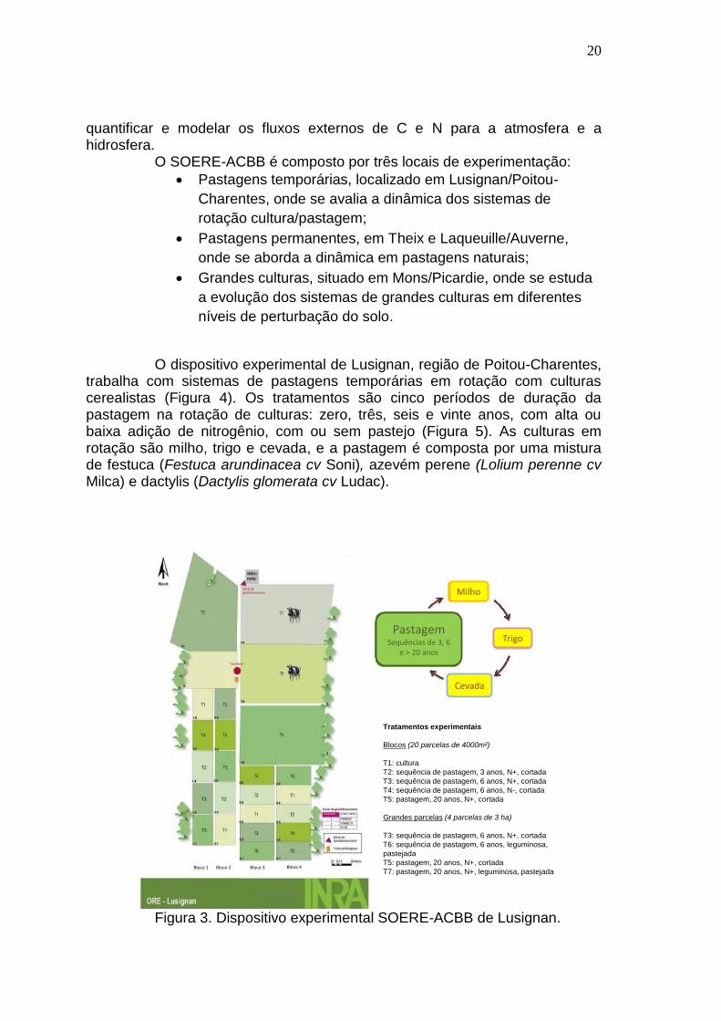
O dispositivo experimental de Lusignan, região de Poitou-Charentes,
trabalha com sistemas de pastagens temporárias em rotação com culturas cerealistas (Figura 4). Os tratamentos são cinco períodos de duração da pastagem na rotação de culturas: zero, três, seis e vinte anos, com alta ou baixa adição de nitrogênio, com ou sem pastejo (Figura 5). As culturas em rotação são milho, trigo e cevada, e a pastagem é composta por uma mistura de festuca (Festuca arundinacea cv Soni), azevém perene (Lolium perenne cv Milca) e dactylis (Dactylis glomerata cv Ludac).
Figura 3. Dispositivo experimental SOERE-ACBB de Lusignan.
Bloco 1 Bloco 2 Bloco 3 Bloco 4
PastagemSequências de 3, 6
e > 20 anos
Milho
Trigo
Cevada
Tratamentos experimentais
Blocos (20 parcelas de 4000m²)
T1: cultura
T2: sequência de pastagem, 3 anos, N+, cortada
T3: sequência de pastagem, 6 anos, N+, cortada
T4: sequência de pastagem, 6 anos, N-, cortada
T5: pastagem, 20 anos, N+, cortada
Grandes parcelas (4 parcelas de 3 ha)
T3: sequência de pastagem, 6 anos, N+, cortada
T6: sequência de pastagem, 6 anos, leguminosa,
pastejada
T5: pastagem, 20 anos, N+, cortada
T7: pastagem, 20 anos, N+, leguminosa, pastejada
21
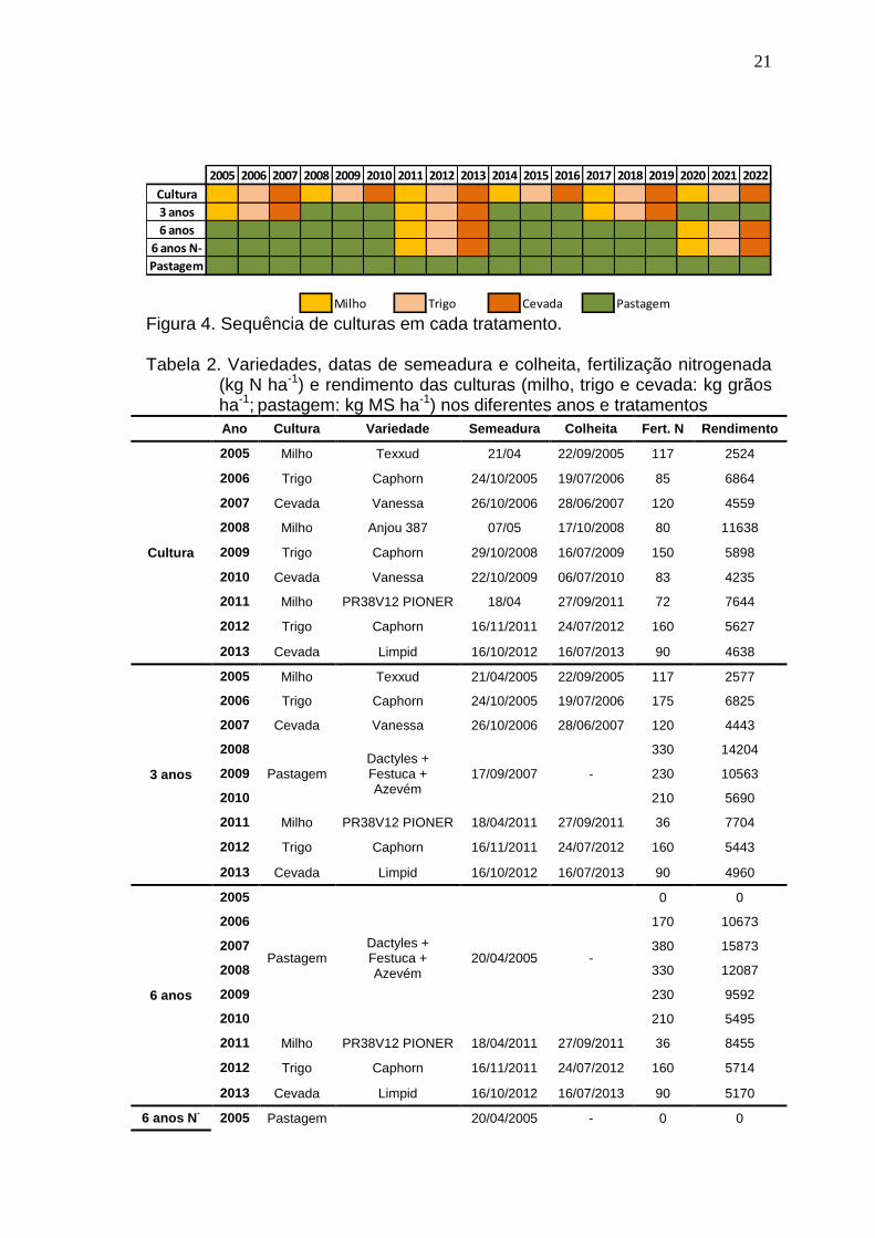
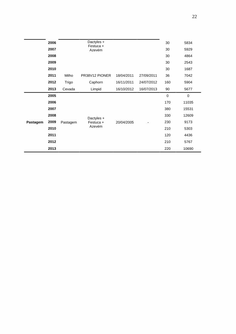
Figura 4. Sequência de culturas em cada tratamento. Tabela 2. Variedades, datas de semeadura e colheita, fertilização nitrogenada
(kg N ha-1) e rendimento das culturas (milho, trigo e cevada: kg grãos ha-1; pastagem: kg MS ha-1) nos diferentes anos e tratamentos
Ano Cultura Variedade Semeadura Colheita Fert. N Rendimento
Cultura
2005 Milho Texxud 21/04 22/09/2005 117 2524
2006 Trigo Caphorn 24/10/2005 19/07/2006 85 6864
2007 Cevada Vanessa 26/10/2006 28/06/2007 120 4559
2008 Milho Anjou 387 07/05 17/10/2008 80 11638
2009 Trigo Caphorn 29/10/2008 16/07/2009 150 5898
2010 Cevada Vanessa 22/10/2009 06/07/2010 83 4235
2011 Milho PR38V12 PIONER 18/04 27/09/2011 72 7644
2012 Trigo Caphorn 16/11/2011 24/07/2012 160 5627
2013 Cevada Limpid 16/10/2012 16/07/2013 90 4638
3 anos
2005 Milho Texxud 21/04/2005 22/09/2005 117 2577
2006 Trigo Caphorn 24/10/2005 19/07/2006 175 6825
2007 Cevada Vanessa 26/10/2006 28/06/2007 120 4443
2008
Pastagem Dactyles + Festuca + Azevém
17/09/2007 -
330 14204
2009 230 10563
2010 210 5690
2011 Milho PR38V12 PIONER 18/04/2011 27/09/2011 36 7704
2012 Trigo Caphorn 16/11/2011 24/07/2012 160 5443
2013 Cevada Limpid 16/10/2012 16/07/2013 90 4960
6 anos
2005
Pastagem Dactyles + Festuca + Azevém
20/04/2005 -
0 0
2006 170 10673
2007 380 15873
2008 330 12087
2009 230 9592
2010 210 5495
2011 Milho PR38V12 PIONER 18/04/2011 27/09/2011 36 8455
2012 Trigo Caphorn 16/11/2011 24/07/2012 160 5714
2013 Cevada Limpid 16/10/2012 16/07/2013 90 5170
6 anos N- 2005 Pastagem 20/04/2005 - 0 0
2005 2006 2007 2008 2009 2010 2011 2012 2013 2014 2015 2016 2017 2018 2019 2020 2021 2022
Cultura M B O M B O M B O M B O M B O M B O
3 anos M B O P P P M B O P P P M B O P P P
6 anos P P P P P P M B o P P P P P P M B o
6 anos N- P P P P P P M B o P P P P P P M B o
Pastagem P P P P P P P P P P P P P P P P P P
M Milho B Trigo O Cevada P Pastagem
22
2006 Dactyles + Festuca + Azevém
30 5834
2007 30 5929
2008 30 4864
2009 30 2543
2010 30 1687
2011 Milho PR38V12 PIONER 18/04/2011 27/09/2011 36 7042
2012 Trigo Caphorn 16/11/2011 24/07/2012 160 5904
2013 Cevada Limpid 16/10/2012 16/07/2013 90 5677
Pastagem
2005
Pastagem Dactyles + Festuca + Azevém
20/04/2005 -
0 0
2006 170 11035
2007 380 15531
2008 330 12609
2009 230 9173
2010 210 5303
2011 120 4436
2012 210 5767
2013 220 10690

23
1.5 HIPÓTESES DO TRABALHO 1. Diferentes alturas de manejo de pastos mistos de aveia e azevém,
independentemente das características de ano, proporcionam um padrão de resposta na produção do pasto e na produção animal em um sistema integrado de produção agropecuária.
2. A presença de pastagem em rotação com culturas cerealistas reduz contaminação da água por nitrato devido à lixiviação de nitrogênio.

24
1.6 OBJETIVOS Este trabalho teve por objetivo avaliar se existe padrão no
comportamento das variáveis de produção animal e de pasto manejado sob
diferentes alturas em SIPA, bem como definir metas de manejo de pastos
mistos de aveia + azevém que beneficiem o desempenho animal e a
conservação do sistema de produção. Um segundo objetivo foi avaliar o efeito
de diferentes períodos de duração da pastagem em sistemas de rotação de
cultura na drenagem e lixiviação de nitrogênio.
2. CAPÍTULO II
Sistema integrado de produção agropecuária: buscando padrões de resposta na produção de pasto e do animal em experimento de longo
prazo1
1 Elaborado de acordo com as normas da Agriculture, Ecosystems and Environment (Apêndice 1).

27
Sistema integrado de produção agropecuária: buscando padrões de resposta na
produção de pasto e do animal em experimento longo prazo
Taise Robinson Kunratha*
, Mónica Cadenazzib, Carolina Bremm
c, Ibanor Anghinoni
d,
Paulo César de Faccio Carvalhoe
(a)Bolsista CNPq – Programa de Pós-graduação em Zootecnia -
Universidade Federal do Rio Grande do Sul (UFRGS), Faculdade de Agronomia -
Avenida Bento Gonçalves, 7712 Bairro Agronomia, Porto Alegre – RS, cep: 91540-
000. [email protected]
(b)Departamento Biometría, Estadística y Computación; EEMAC -
Universidad de La República, Ruta 3 km 363, Paysandú – Uruguay.
(c)Fundação Estadual de Pesquisa Agropecuária (FEPAGRO) – Gonçalves
Dias, 570 Bairro Menino Deus, Porto Alegre – RS, cep: 90130-070.
(d)Departamento de Solos - Universidade Federal do Rio Grande do Sul
(UFRGS), Faculdade de Agronomia - Avenida Bento Gonçalves, 7712 Bairro
Agronomia, Porto Alegre – RS, cep: 91540-000. [email protected]
(e)Departamento de Plantas Forrageiras e Agrometeorologia - Universidade
Federal do Rio Grande do Sul (UFRGS), Faculdade de Agronomia - Avenida Bento
Gonçalves, 7712 Bairro Agronomia, Porto Alegre – RS, cep: 91540-000.
*Autor correspondente: Avenida Bento Gonçalves, 7712 Bairro Agronomia,
Porto Alegre – RS, cep: 91540-000. [email protected] +55 51 33087402
28
Resumo – Sistemas integrados de produção agropecuária (SIPAs)
promovem diversos benefícios ao sistema de cultivo e para o ambiente. No entanto, para
que esses benefícios ocorram, é necessário assegurar práticas de manejo que permitam
rendimento e conservação. Apesar de existirem resultados que indiquem quais são as
intensidades de pastejo (alturas de manejo do pasto) que assegurem desempenho e
conservação, estes resultados são pontuais e variáveis em decorrência dos efeitos de
ano. Em função disto, utilizando uma base de 10 anos de dados (2001-2011), propomos
neste trabalho analisar e investigar a existência de padrões no comportamento das
variáveis de produção animal e de pasto manejado sob diferentes alturas em SIPA.
Também propõe-se definir metas de manejo de pastos mistos de aveia + azevém que
beneficiem o desempenho animal e a conservação do sistema de produção. O SIPA é
composto de pastagem mista de aveia preta x azevém durante o período hibernal com
pastoreio contínuo e soja durante o período estival. Os tratamentos são quatro alturas do
pasto (10, 20, 30 e 40 cm), que definem diferentes intensidades de pastejo. A variação
na altura real do pasto aumentou com o aumento na altura pretendida. As variáveis de
produção animal e de pasto estudadas são afetadas pelas condições climáticas anuais, no
entanto, existe padrão nas relações entre produção animal e de pasto ao longo dos 10
anos de experimento. A altura de manejo do pasto de 30 cm permite o acúmulo de
resíduo sobre o solo, que beneficia o SIPA, e que proporciona crescimento do pasto e
ganho animal satisfatório e estável ao longo dos anos.
Palavras-chave: altura do dossel, conservação, experimento de longo prazo,
plantio direto, sustentabilidade.
29
1. Introdução
Sistemas integrados de produção agropecuária (SIPAs) promovem
interações ecológicas entre os diferentes componentes do ecossistema produtivo,
tornando-os mais eficientes na ciclagem de nutrientes, preservando os recursos naturais
e o meio ambiente, melhorando a qualidade do solo e aumentando a biodiversidade
(Lemaire et al., 2014). Para que isso ocorra, é necessário assegurar práticas de manejo
conservacionistas, como o plantio direto. Os benefícios da presença de resíduos sobre o
solo já foram amplamente discutidos internacionalmente (Franzluebbers, 2007;
Franzluebbers and Stuedemann, 2007, 2008, 2014; Fernandéz et al, 2010).
No caso do sul do Brasil, um dos arranjos de SIPA mais utilizados é o
cultivo de soja durante o verão e produção de bovinos de corte em pastagens de aveia e
azevém no período de inverno (Anghinoni et al., 2013). Este sistema tem apresentado
maior retorno econômico quando comparado ao cultivo exclusivo da soja (Oliveira et
al., 2013). No entanto, para o sucesso do sistema, é necessário adequar a intensidade de
pastejo de forma que concilie bons rendimentos de produção animal e da produção de
soja, e que permita quantidade de resíduo suficiente para o sistema plantio direto.
Alguns trabalhos demonstram que a altura de manejo que maximiza a
produção animal em pastos mistos de aveia e azevém ou azevém solteiro está entre 20 e
30 cm (Aguinaga et al., 2006; Lopes et al., 2008; Amaral et al., 2012; Kunrath et al.,
2014). Apesar de existirem resultados que indiquem que essas alturas promovem
melhor desempenho animal, estes resultados são pontuais e variáveis em decorrência
dos efeitos de ano pelas condições climáticas.
Dessa forma, para este trabalho, utilizamos uma base de dados de dez anos,
uma vez que experimentos de longa duração aumentam a confiabilidade na
30
interpretação dos resultados (Rasmussen et al, 1998), objetivando i) analisar e investigar
se existe padrão no comportamento das variáveis de produção animal e de pasto
manejado sob diferentes alturas em SIPA e ii) definir metas de manejo de pastos mistos
de aveia + azevém que beneficiem o desempenho animal em SIPAs.
2. Material e Métodos
2.1 Localização, caracterização e histórico da área experimental
A área experimental vem sendo conduzida sob sistema integrado de
produção agropecuária (SIPA) desde 2001 em parceria público-privada entre os
departamentos de Solos e de Plantas Forrageiras e Agrometeorologia da Universidade
Federal do Rio Grande do Sul (UFRGS) com a Cabanha Cerro Coroado. A área está
localizada na Fazenda do Espinilho, no município de São Miguel das Missões (28°56' S
54°20' O). O clima caracteriza-se como subtropical úmido e quente (Cfa) segundo a
classificação de Köppen (Kottek et al., 2006), com temperatura média anual de 19°C e
precipitação média anual de 1850 mm (Matzenauer et al., 2011). O relevo é ondulado a
suavemente ondulado com altitude média de 465 m. A temperatura média e a
precipitação ocorrida no período invernal (maio à outubro) foram coletadas da Estação
Meteorológica do Município de São Luiz Gonzaga, mantida pelo Instituto Nacional de
Meteorologia (Figura 1), situada a 70 km da área experimental.
O solo é classificado como Latossolo Vermelho distroférrico (EMBRAPA,
2006) da unidade de mapeamento Santo Ângelo (Streck et al., 2008), profundo, bem
drenado, com coloração vermelho-escura e textura muito argilosa (0,54, 0,17 e 0,29 kg
kg-1
, de argila, silte e areia, respectivamente). A área era cultivada em sistema plantio
direto desde 1993 com aveia preta (Avena strigosa Schreb) no outono-inverno (maio a
31
novembro) e soja (Glycine max) na primavera-verão (novembro a maio). Em novembro
de 2000, foi realizada a caracterização química inicial do solo: 10,5 mg dm-3
de fósforo,
94 mg dm-3
de potássio, 3,2 cmolc dm-3
de Al+3
, 34 g kg-1
de matéria orgânica e pH de
4,3 (Cassol, 2003). Em abril de 2001, a área foi semeada com pasto misto de aveia preta
x azevém (Lolium multiflorum) e utilizada para o pastejo de animais pela primeira vez,
dando início ao sistema integrado de produção agropecuária.
2.2 Tratamentos e delineamento experimental
A área total experimental é de 22 ha, dividida em piquetes que variam de
0,8 a 3,6 ha. O SIPA é composto de pastagem mista de aveia preta x azevém durante o
período hibernal com pastejo contínuo e soja durante o período estival. Os tratamentos
são quatro alturas de manejo do pasto (10, 20, 30 e 40 cm), que definem diferentes
intensidades de pastejo. O delineamento experimental é de blocos casualizados com três
repetições, totalizando 12 piquetes (unidades experimentais – UE).
2.3 Período experimental e manejo do SIPA
Foi utilizada uma base de dados de 10 anos do período hibernal (2001 –
2011) de um SIPA típico da região Sul do Brasil. O manejo experimental foi o mesmo
entre os anos. A data média de semeadura do pasto foi 08 de maio, de entrada dos
animais nas UEs foi 09 de julho e de saída dos animais em 08 de novembro (para
maiores detalhes, vide Oliveira et al., 2013). Foram aplicados no pasto 45 kg N ha-1
, na
forma de ureia, anualmente, em dose única aos 40 dias após a semeadura. Nos anos de
2003, 2009 e 2011, foram aplicados 90 kg N ha-1
em duas doses, sendo a 1ª dose 30 dias
após a semeadura e 2ª dose 15 dias antes do início do pastejo.
32
Em todos os anos a aveia-preta foi semeada em linha e o azevém, além da
ressemeadura natural, foi semeado a lanço, excetuando-se os anos de 2008 à 2010 em
que o azevém foi proveniente exclusivamente de ressemeadura natural. O
monitoramento dos tratamentos foi realizado quinzenalmente, medindo-se 100 pontos
de altura do pasto por unidade experimental com o método do bastão graduado (sward
stick), proposto por Barthram (1985). Para manter as alturas pretendidas foram
realizados ajustes na taxa de lotação animal com intervalos de 15 dias, com entradas ou
saídas de animais conforme a metodologia de pastoreio contínuo com taxa de lotação
variável proposta por Mott and Lucas (1952). Três animais-teste por piquete eram
mantidos, com número variável de animais reguladores. Por ocasião do início do
pastejo, a altura média do pasto e a massa de forragem nos anos avaliados foi 23,2 ± 3,9
cm e 1595,4 ± 709,5 kg MS ha-1
, respectivamente. O peso inicial médio dos animais
para os 10 anos foi 203,0 ± 13,2 kg.
2.4 Avaliações no pasto
Nos pastos foram avaliadas: massa de forragem (kg de matéria seca (MS)
ha-1
), taxa de crescimento diário do pasto (kg de MS ha-1
) e produção total de pasto (kg
de MS ha-1
). A estimativa da massa de forragem foi realizada a cada 28 dias, utilizando-
se a técnica de dupla amostragem (Wilm et al., 1944). Foram realizados cinco cortes
aleatórios de forragem por UE. Nesses mesmos locais foram medidos cinco pontos de
altura do pasto com o “sward stick”, para posterior ajuste da massa de forragem em
função da altura real do pasto, por meio da equação de regressão: yi = b0 +b1xi . A taxa
de crescimento diário foi monitorada a cada 28 dias utilizando-se três gaiolas de
exclusão ao pastejo por piquete, empregando a técnica descrita por Klingman et al.
33
(1943). A massa de forragem dentro e fora da gaiola foi obtida pela média dos cortes
avaliados, em cada piquete. Todos os cortes foram realizados acima do mantilho, em
área de 0,25m2. As amostras foram secas em estufa de circulação forçada de ar a 60ºC,
até peso constante. A produção total de pasto foi estimada pelo somatório da massa de
forragem inicial com as produções dos sub-períodos (taxa de acúmulo x número de dias
do sub-período). No último período de amostragem, após a saída dos animais, realizou-
se avaliação para quantificar o resíduo (kg de MS ha-1
) nos diferentes tratamentos. Foi
recolhido todo o material existente sobre o solo nos mesmos pontos utilizados para os
cortes de massa de forragem. O resíduo foi determinado pelo somatório da massa de
forragem final (saída dos animais) com o material que permaneceu sobre o solo.
2.5 Avaliações animais
Foram avaliados o ganho médio diário individual (kg de peso vivo (PV) dia-
1) e o ganho por área (kg PV ha
-1). O ganho por área foi calculado pela média do ganho
individual dos três animais teste multiplicada pelo número de animais-dia e pela área
total do piquete. A carga animal do período de pastejo, também expressa em kg de PV
ha-1
, foi calculada pela adição do peso médio dos animais-teste com o peso médio de
cada animal regulador, multiplicado pelo número de dias que estes permaneceram na
pastagem, dividido pelo número total de dias de pastejo. Para todas as estimativas, os
animais foram pesados com jejum de sólidos e líquidos de 12 horas.
2.6 Análises estatísticas
Os dados foram analisados mediante analise de variância e de contrastes,
seguindo o modelo que integra os efeitos simples do ano e dos tratamentos e sua
34
interação. Para tanto, os anos foram considerados aleatórios no modelo.
Assim, a normalidade dos dados foi testada pelo teste de Kolmogorov-
Smirnov (P>0,05). Após esta análise, os resultados foram submetidos à análise de
homogeneidade de variâncias (Levene’s Test) em nível de 5% de significância, para que
se pudesse determinar se os diferentes anos deveriam ser avaliados de forma conjunta
ou independentes.
Para as variáveis em que a análise de homogeneidade de variâncias
apresentou interação dos efeitos de ano e tratamento (P<0,05), sinalizando que as
análises deveriam ser realizadas independentemente a cada ano, foram realizadas
análises de comparação entre os tratamentos nos anos avaliados e sua interação
(ano*tratamento), modelando a heterocedasticidade. Para isso foi realizada uma análise
de variância com 5% de significância para comparação das alturas de pastejo
(tratamentos). As variáveis que apresentaram diferenças significativas tiveram suas
médias comparadas pelo Teste de Tukey com o mesmo nível de significância.
Com a intenção de analisar e investigar a existência de padrão no
comportamento das variáveis resposta, foram realizadas análises de correlação de
Pearson e regressão até segunda ordem para as variáveis-resposta segundo valores de
altura real do pasto. Para as análises de regressão, o ano foi considerado como variável
aleatória. Sempre que a função-resposta foi significativa (P<0,05), optou-se por
apresentar os resultados pela equação de regressão de maior coeficiente de
determinação (R2). Os dados foram analisados pelo aplicativo SAS (2002).
3. Resultados
As alturas médias reais (Figura 2) se mantiveram próximas às alturas
35
propostas como tratamentos. A variação na altura real do pasto aumentou com o
aumento na altura proposta. As médias foram de 12,1±1,89 cm; 20,9±3,02 cm;
30,1±3,81 cm e 37,8±4,92 cm, respectivamente para os tratamentos 10, 20, 30 e 40 cm
de altura do pasto.
3.1 Produção do pasto
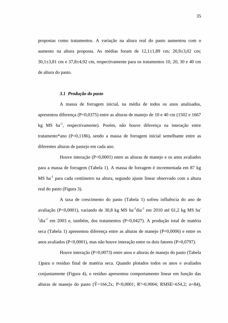
A massa de forragem inicial, na média de todos os anos analisados,
apresentou diferença (P=0,0375) entre as alturas de manejo de 10 e 40 cm (1502 e 1667
kg MS ha-1
, respectivamente). Porém, não houve diferença na interação entre
tratamento*ano (P=0,1186), sendo a massa de forragem inicial semelhante entre as
diferentes alturas de pastejo em cada ano.
Houve interação (P<0,0001) entre as alturas de manejo e os anos avaliados
para a massa de forragem (Tabela 1). A massa de forragem é incrementada em 87 kg
MS ha-1
para cada centímetro na altura, segundo ajuste linear observado com a altura
real do pasto (Figura 3).
A taxa de crescimento do pasto (Tabela 1) sofreu influência do ano de
avaliação (P<0,0001), variando de 30,8 kg MS ha-1
dia-1
em 2010 até 61,2 kg MS ha-
1dia
-1 em 2003 e, também, dos tratamentos (P=0,0427). A produção total de matéria
seca (Tabela 1) apresentou diferença entre as alturas de manejo (P=0,0006) e entre os
anos avaliados (P<0,0001), mas não houve interação entre os dois fatores (P=0,0797).
Houve interação (P=0,0073) entre anos e alturas de manejo do pasto (Tabela
1)para o resíduo final de matéria seca. Quando plotados todos os anos e avaliados
conjuntamente (Figura 4), o resíduo apresentou comportamento linear em função das
alturas de manejo do pasto (Ŷ=166,2x; P<0,0001; R²=0,9004; RMSE=654,2; n=84),
36
aumentando em 166 kg MS ha-1
para cada centímetro aumentado na altura do pasto.
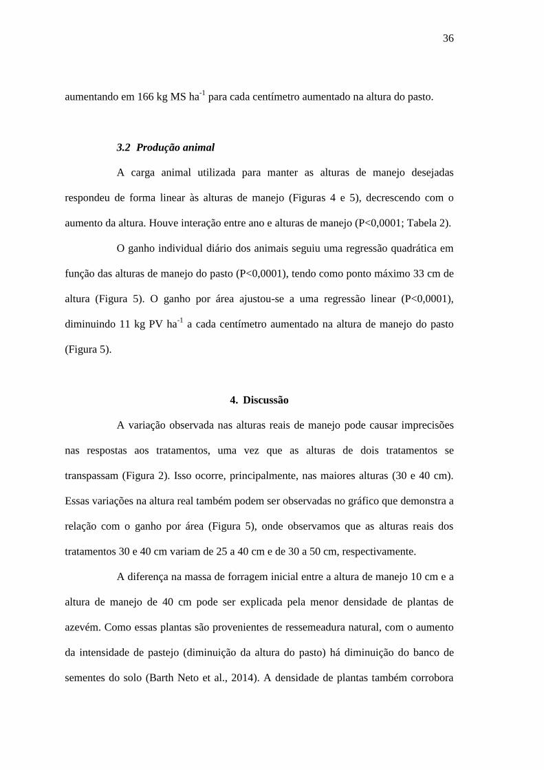
3.2 Produção animal
A carga animal utilizada para manter as alturas de manejo desejadas
respondeu de forma linear às alturas de manejo (Figuras 4 e 5), decrescendo com o
aumento da altura. Houve interação entre ano e alturas de manejo (P<0,0001; Tabela 2).
O ganho individual diário dos animais seguiu uma regressão quadrática em
função das alturas de manejo do pasto (P<0,0001), tendo como ponto máximo 33 cm de
altura (Figura 5). O ganho por área ajustou-se a uma regressão linear (P<0,0001),
diminuindo 11 kg PV ha-1
a cada centímetro aumentado na altura de manejo do pasto
(Figura 5).
4. Discussão
A variação observada nas alturas reais de manejo pode causar imprecisões
nas respostas aos tratamentos, uma vez que as alturas de dois tratamentos se
transpassam (Figura 2). Isso ocorre, principalmente, nas maiores alturas (30 e 40 cm).
Essas variações na altura real também podem ser observadas no gráfico que demonstra a
relação com o ganho por área (Figura 5), onde observamos que as alturas reais dos
tratamentos 30 e 40 cm variam de 25 a 40 cm e de 30 a 50 cm, respectivamente.
A diferença na massa de forragem inicial entre a altura de manejo 10 cm e a
altura de manejo de 40 cm pode ser explicada pela menor densidade de plantas de
azevém. Como essas plantas são provenientes de ressemeadura natural, com o aumento
da intensidade de pastejo (diminuição da altura do pasto) há diminuição do banco de
sementes do solo (Barth Neto et al., 2014). A densidade de plantas também corrobora
37
para as diferenças ocorridas na massa de forragem (Figura 3). A relação apresentada
entre a massa de forragem e a altura de manejo é semelhante a outros trabalhos
(Carvalho et al., 2010, Kunrath et al, 2014). Essas duas variáveis apresentam relação
consistente (P<0,0001 r=0,86). Um modelo confiável pode ser gerado por essa relação
entre altura e massa de forragem. Isso se faz importante na medida que as avaliações de
massa de forragem são destrutivas e ocorrem frequentemente. Esse modelo poderia
auxiliar na predição da massa de forragem diminuindo a quantidade e frequência destas
avaliações. Apesar das diferenças climáticas entre os anos, a massa de forragem
aparenta sofrer menor influência que a produtividade animal.
A taxa de crescimento do pasto variou entre os anos em função das
diferenças climáticas (precipitação, temperatura e radiação) ocorridas. As diferenças
anuais são mais difíceis de serem explicadas, pois além das diferenças climáticas
existem, ainda, as diferenças no comportamento das alturas ao longo do ciclo, as
diferenças na adubação nitrogenada e a interação entre esses fatores. As diferentes
alturas de manejo possibilitam diferentes quantidades de áreas foliares, responsáveis
pela captação da energia solar (Taiz and Zeiger, 2009), influenciando a taxa de
crescimento do pasto. Porém, essas diferenças não são limitantes mesmo para a menor
altura de manejo (10 cm), uma vez que a taxa de crescimento é semelhante às alturas de
20 e 30 cm.
A produção total de pasto obteve o mesmo comportamento da taxa de
crescimento, uma vez que é calculada a partir dessa variável. No entanto, as diferenças
entre os tratamentos são melhor evidenciadas (Tabela 1). A produção de pasto é menor
nas alturas de manejo de 10 e 20 cm em consequência das menores taxas de crescimento
e da menor massa de forragem inicial, enquanto que nos tratamentos 30 e 40 cm as

38
produções são maiores em função dos mesmos fatores serem superiores para essas
alturas de manejo.
O resíduo é uma das variáveis mais importantes de um SIPA. Ele é que faz a
ligação entre o ciclo de inverno e a cultura de verão, pois possui papel fundamental na
proteção do impacto físico do casco do animal minimizando o adensamento e a
compactação do solo (Flores et al., 2007; Franzluebbers and Stuedemann, 2008) e na
diminuição da erosão do solo (Franzluebbers et al., 2012). Os principais fatores que
afetam a quantidade de resíduo são, principalmente, a altura de manejo (r=0,82,
P<0,0001), massa de forragem (r=0,93, P<0,0001) e a carga animal (r=-0,84, P<0,0001)
utilizada para a manutenção dessa altura.
Oliveira et al. (2013), trabalhando com a mesma base de dados deste
trabalho, não observaram diferença no rendimento da cultura de soja entre as áreas
pastejadas e a testemunha sem pastejo. Esse resultado indica que a presença de animais
em pastejo no inverno não prejudica o desenvolvimento da cultura de soja no verão,
como já havia sido demonstrado por trabalhos anteriores (Cassol, 2003; Flores et al.,
2007). Em levantamento realizado por Moraes et al. (2014), analisando diversos
trabalhos em SIPA, demonstrou que a presença do animal em pastejo melhora
significativamente as produções da diversas culturas em sequência ao pastejo. Além
disso, a presença de animais em SIPAs proporciona aumento no retorno financeiro para
os produtores (Franzluebbers and Stuedemann, 2007, Oliveira et al., 2013).
O ganho individual sofre influência da altura de manejo do pasto (P<0,0001
r=0,47) e da carga animal utilizada para a manutenção destas alturas (P<0,0001 r=-
0,61). As alturas de manejo de 30 e 40 cm são semelhantes entre si e entre todos os anos
avaliados. As diferenças são percebidas, geralmente, entre a maior intensidade de
39
pastejo (10 cm) e as demais alturas. O ganho por área sofre as mesmas influências que o
ganho individual pela altura de manejo e pela carga animal (P<0,0001 r=-0,84 e r=0,89,
respectivamente), e também da massa de forragem (P<0,0001 r=-0,78). No entanto, o
ganho por área aumenta com a diminuição na altura de manejo do pasto. Tendo em vista
que o ganho individual apresenta comportamento quadrático e o ganho por área linear
negativo deve-se, portanto, buscar uma altura de manejo que otimize o ganho individual
(em torno de 30 cm, como demonstrado pela Figura 5) sem penalizar o ganho por área.
A altura de manejo é a chave central na produtividade do sistema. Em
função da altura que definimos como meta, seremos responsáveis pela carga animal
utilizada (P<0,0001 r=-0,86) e pela massa de forragem disponível para esses animais,
pela produtividade animal do sistema e, ainda, pela manutenção dos resíduos sobre o
solo e todos os benefícios que isso acarreta ao sistema de produção (físicos, químicos,
biológicos e ambientais).
5. Conclusão
As variáveis de produção animal e de pasto estudadas são afetadas pelos
anos experimentais, no entanto, existe um padrão nas relações entre produção animal e
de pasto ao longo dos 10 anos de experimento sob sistema integrado de produção
agropecuária.
A altura de manejo do pasto de 30 cm permite o acúmulo de resíduo sobre o
solo e proporciona ganho animal satisfatório e estável ao longo dos anos.
40
6. Agradecimentos
Agradecemos à Agropecuária Cerro Coroado pela parceria e confiança
investida por mais de 10 anos na condução deste experimento. Esse trabalho foi
fomentado pelo CNPq, com bolsa de doutoramento, bolsa de produtividade de pesquisa
e pelo projeto Universal (485169/2012-6).
7. Referências Bibliográficas
Anghinoni, I., Carvalho, P.C.F., Costa, S.E.V.G.A., 2013. Abordagem
sistêmica do solo em sistemas integrados de produção agrícola e pecuária no subtrópico
brasileiro. Tópicos Especiais em Ciência do Solo, 8. pp. 221–278.
Aguinaga, A.A.Q., Carvalho, P.C.D.F., Anghinoni, I., Teixeira, D., Freitas,
F.K. De, Lopes, M.T., 2006. Produção de novilhos superprecoces em pastagem de aveia
e azevém submetida a diferentes alturas de manejo. Rev. Bras. Zootec. 35, 1765–1773.
Amaral, M.F., Mezzalira, J.C., Bremm, C., Da Trindade, J.K., Gibb, M.J.,
Suñe, R.W.M., Carvalho, P.C.F., 2012. Sward structure management for a maximun
short-term intake rate in anual ryegrass. Grass Forage Sci., 68, 271-277.
Barth Neto, A., Savian, J.V., Schons, R.M.T., Bonnet, O.J.F., Canto, M.W.,
Moraes, A., Lemaire, G., Carvalho, P.C.D.F., 2014. Italian ryegrass establishment by
self-seeding in integrated crop-livestock systems: Effects of grazing management and
crop rotation strategies. Eur. J. Agron. 53, 67–73. doi:10.1016/j.eja.2013.11.001
Barthram, G.T. 1985. Experimental techniques: the HFRO sward stick. Hill
Farming Research Organization/Biennial Report, p.29-30, 1985.
Carvalho, P.C.F., Rocha, L.M., Baggio, C., Macari, S., Kunrath, T.R.,
Moraes, A., 2010. Característica produtiva e estrutural de pastos mistos de aveia e
41
azevém manejados em quatro alturas sob lotação contínua. R. Bras. Zootec., 39, p.1857-
1865.
Cassol, L.C. Relação solo-planta-animal num sistema de integração lavoura-
pecuária em semeadura direta com calcário na superfície. 157 f. Tese (Doutorado) –
Programa de Pós-Graduação em Ciência do Solo, Faculdade de Agronomia,
Universidade Federal do Rio Grande do Sul, Porto Alegre, 2003.
EMBRAPA – Empresa Brasileira De Pesquisa Agropecuária, 2006. Sistema
Brasileiro de Classificação de Solos. Rio de Janeiro, Centro Nacional de Pesquisa de
Solos, 306p.
Fernández, P.L., Álvarez, C.R., Schindler, V., Taboada, M.A., 2010.
Changes in topsoil bulk density after crop residues under no-till farming. Geoderma,
159, 24-30.
Flores, J.P.C., Anghinoni, I., Cassol, L.C., Carvalho, P.C.F., Leite, J.G.B.,
Fraga, T.I., 2007. R. Bras. Ci. Solo, 31, 771-780.
Franzluebbers, A.J., 2007. Integrated Crop–Livestock Systems in the
Southeastern USA. Agron. J. 99, 361-372. doi:10.2134/agronj2006.0076
Franzluebbers, A.J., Paine, L.K., Winsten, J.R., Krome, M., Sanderson,
M.A., Ogles, K., Thompson, D., 2012. Well-managed grazing systems: A forgotten hero
of conservation. J. Soil Water Conserv. 67, 100A–104A. doi:10.2489/jswc.67.4.100A
Franzluebbers, A.J., Stuedemann, J.A., 2007. Crop and cattle responses to
tillage systems for integrated crop–livestock production in the Southern Piedmont,
USA. Renew. Agric. Food Syst. 22, 168. doi:10.1017/S1742170507001706
Franzluebbers, A.J, Stuedemann, J.A., 2008. Soil physical responses to
cattle grazing cover crops under conventional and no tillage in the Southern Piedmont
42
USA. Soil Tillage Res. 100, 141–153. doi:10.1016/j.still.2008.05.011
Franzluebbers, A.J., Stuedemann, J.A., 2014. Crop and cattle production
responses to tillage and cover crop management in an integrated crop–livestock system
in the southeastern USA. Eur. J. Agron. 57, 62–70. doi:10.1016/j.eja.2013.05.009
Klingman, D.L., Miles, S.R., Mott, G.O., 1943. The cage method for
determining consumption and yield of pasture herbage. J. Am. Soc. Agron., 35, 739-
746.
Kottek, M., Grieser, J., Beck, C., Rudolf, B., Rubel, F., 2006. World map of
the Köppen–Geiger climate classification updated. Meteorol. Z. 15, 259–263.
Kunrath, T.R., Cadenazzi, M., Brambilla, D.M., Anghinoni, I., Moraes, A.,
Barro, R.S., Carvalho, P.C.F., 2014. Management targets for continuously stocked
mixed oat×annual ryegrass pasture in a no-till integrated crop–livestock system. Eur. J.
Agron. 57, 71–76. doi:10.1016/j.eja.2013.09.013
Lemaire, G., Franzluebbers, A.J., Carvalho, P.C.F., Didieu, B., 2014.
Integrated crop-livestock systems: Strategies to archieve synergy between agricultural
production and environmental quality. Agric. Ecosys. Environ., 190, 4-8.
Lopes, M.L.T., Carvalho, P.C.D.F., Anghinoni, I., Santos, D.T. Dos, Kuss,
F., Freitas, F.K. De, Flores, J.P.C., 2008. Sistema de integração lavoura-pecuária:
desempenho e qualidade da carcaça de novilhos superprecoces terminados em pastagem
de aveia e azevém manejada sob diferentes alturas. Ciência Rural 38, 178–184.
doi:10.1590/S0103-84782008000100029
Matzenauer, R., Radin, B., Almeida, I.R., 2011. Atlas Climático: Rio
Grande do Sul. Porto Alegre: Secretaria da Agricultura Pecuária e Agronegócio;
Fundação Estadual de Pesquisa Agropecuária (FEPAGRO).
43
Moraes, A., Carvalho, P.C.F., Anghinoni, I., Lustosa, S.B.C., Costa,
S.E.G.A., Kunrath, T.R., 2014. Integrated crop-livestock systems in the Brazilian
subtropics. Eur. J. Agron. 57, 4–9.
Mott, G.O., Lucas, H.L., 1952. The design, conduct and interpretation of
grazing trials on cultivated and improved pastures. In: Internacional Grassland
Congress, 6., Pensylvania. Proceedings. Pensylvania: State College, pp. 1380-1395.
Oliveira, C.A., Bremm, C., Anghinoni, I., Moraes, A., Kunrath, T.R.,
Carvalho, P.C.F., 2013. Comparison of an integrated crop–livestock system with
soybean only: Economic and production responses in southern Brazil. Renew. Agric.
Food Syst., 28, 1–9. doi:10.1017/S1742170513000410
Rasmussen, P.E., 1998. Long-Term Agroecosystem Experiments: Assessing
Agricultural Sustainability and Global Change. Science, 282, 893–896.
doi:10.1126/science.282.5390.893
SAS Institute, 2002. SAS/STAT software: changes and enhancements
through release 9.0. Cary: Statistical Analysis System Institute, 1167p.
Streck, E.V., Kämpf, N., Dalmolin, R.S.D., Klamt, E., Nascimento, P.C.,
Schneider, P., Giasson, E., Pinto, L.F.S., 2008. Solos do Rio Grande do Sul. 2 ed. Porto
Alegre: EMATER/RS, 222 p.8
Taiz, L., Zeiger, E., 2009. Fisiologia vegetal. 4.ed. Porto Alegre: Artmed,
819p.
Wilm, H.G., Costello, D.F., Klipple, G.E., 1944. Estimating forage yield by
the double sampling methods. J. Am. Soc. Agron., 36, 194-2.
44
Figura 1. Precipitação, insolação, temperatura média máxima e
temperatura média mínima do ar ocorridas entre a semeadura do pasto e a
saída dos animais em cada ano experimental (as datas são encontradas
em Oliveira et al., 2013). Fonte: INMET – Estação Meteorológica do
Município de São Luiz Gonzaga).
0
3
6
9
12
15
18
21
24
27
0
200
400
600
800
1000
1200
1400
1600
1800
2002 2003 2004 2005 2006 2007 2008 2009 2010 2011
Tem
per
atura
(ºC
)
Pre
cipit
ação
(m
m)
e In
sola
ção (
hora
s)
Precipitação Insolação Tmax Tmin
45
Figura 2. Relação entre alturas pretendidas e alturas reais de pasto misto de
aveia + azevém obtidas ao longo de 10 anos de experimento sob sistema
integrado de produção agropecuária.
46
Tabela 1. Massa de forragem, taxa de crescimento, produção total e resíduo de pasto
misto de aveia + azevém em função das alturas de manejo e dos anos avaliados sob
sistema integrado de produção agropecuária
Altura do pasto Média*
10 cm 20 cm 30 cm 40 cm
Massa de forragem (kg MS ha-1
) 2001 1644 C abc 2632 B abc 3729 A ab 4015 A a 3005
2002 1328 C abcd 2159 B abcd 3104 A bc 3551 A abc 2535
2003 1901 C ab 2868 B a 4137 A a 4123 A a 3257
2004 1508 B abcd 1893 B de 2750 A cd 3254 A bc 2352
2005 1940 C a 2740 B ab 3417 AB abc 3974 A ab 3018
2006 1244 C abcd 1912 C cd 2972 B c 3921 A ab 2512
2008 1130 C cd 1931 B cd 2798 A cd 2917 A c 2194
2009 1193 C bcd 1983 B cd 2707 AB cd 3283 A bc 2291
2010 919 C d 1173 C e 2090 B de 3007 A c 1797
2011 949 C cd 1917 B bcd 2132 B e 2975 A c 1993
Média* 1376 2142 2962 3502
Taxa de crescimento do pasto (kg MS ha-1
dia-1
) 2001 46,2 47,5 52,6 49,3 48,9 ab
2002 35,3 43,7 46,7 32,6 39,6 bc
2003 56,0 60,8 62,6 65,4 61,2 a
2004 41,4 51,7 47,8 49,7 47,7 ab
2005 64,1 32,2 44,0 46,2 46,6 b
2006 35,9 36,2 35,2 50,3 39,4 bc
2008 50,7 43,1 41,7 48,9 46,1 b
2009 33,6 43,2 56,5 64,1 49,4 ab
2010 18,3 23,5 33,4 47,6 30,8 c
2011 33,4 42,1 33,4 40,8 37,4 bc
Média* 41,5 B 42,4 B 45,4 AB 49,5 A
Produção total de pasto (kg MS ha-1
) 2001 6616 6644 7330 6711 6825 bcd
2002 6062 6718 7542 6441 6691 cd
2003 9144 10174 10428 10002 9937 a
2004 8877 8144 7869 7756 8161 bc
2005 9213 7269 8601 7758 8210 b
2006 5835 6039 5945 7897 6429 de
2008 2442 3316 3810 4517 3521 f
2009 4762 5949 7511 8505 6681 cd
2010 3376 4170 5558 7514 5155 e
2011 5003 7016 5365 6913 6074 de
Média* 6133 C 6544 BC 6996 AB 7401 A
Resíduo (kg MS ha-1
) 2001 1501 C a 3544 B ab 6320 A a 6565 A a 4486
2002 1727 C a 3820 B ab 4917 AB abc 5527 A ab 3998
2005 2363 B a 4306 A a 5774 A ab 6167 A ab 4652
2008 1239 C a 2410 BC bc 3779 AB cd 4765 A b 3048
2009 1330 C a 3245 B ab 4636 AB bcd 6545 A ab 3864
2010 812 B a 1551 B c 3387 A cd 4951 A ab 2675
2011 980 C a 3115 B abc 3151 B d 4855 A b 3025
Média* 1422 3147 4561 5582
*Letras maiúsculas diferentes demonstram diferença estatística na coluna (alturas de manejo) pelo
teste de Tukey (P<0,05), enquanto que letras minúsculas demonstram diferenças na linha (ano).
47
Figura 3. Relação entre massa de forragem e altura real de pasto misto de
aveia + azevém ao longo de 10 anos de experimento sob sistema integrado
de produção agropecuária.
MF = 87,03x
P<0,0001 R² = 0,9498 RMSE=235,74
0
500
1000
1500
2000
2500
3000
3500
4000
4500
5000
0 10 20 30 40 50
Mas
sa d
e fo
rrag
em (
kg M
S h
a-1)
Altura do pasto (cm)
10 cm 20 cm 30 cm 40 cm
48
Figura 4. Relação entre carga animal, altura real de manejo e resíduo final de
pasto misto de aveia + azevém obtidos ao longo de 10 anos de experimento
sob sistema integrado de produção agropecuária. (Símbolos diferentes
representam diferentes alturas de manejo do pasto: 10 cm (◊), 20 cm (●), 30
cm (∆) e 40 cm (■)).
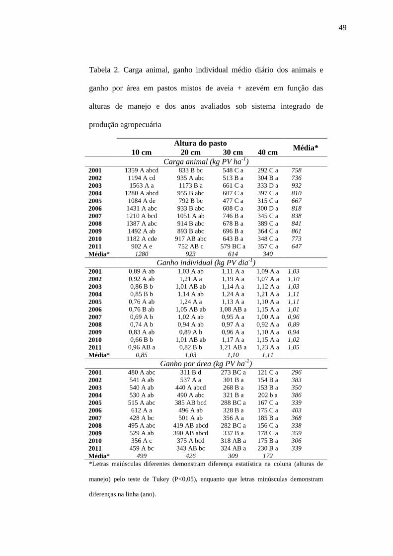
49
Tabela 2. Carga animal, ganho individual médio diário dos animais e
ganho por área em pastos mistos de aveia + azevém em função das
alturas de manejo e dos anos avaliados sob sistema integrado de
produção agropecuária
Altura do pasto Média*
10 cm 20 cm 30 cm 40 cm
Carga animal (kg PV ha-1
) 2001 1359 A abcd 833 B bc 548 C a 292 C a 758
2002 1194 A cd 935 A abc 513 B a 304 B a 736
2003 1563 A a 1173 B a 661 C a 333 D a 932
2004 1280 A abcd 955 B abc 607 C a 397 C a 810
2005 1084 A de 792 B bc 477 C a 315 C a 667
2006 1431 A abc 933 B abc 608 C a 300 D a 818
2007 1210 A bcd 1051 A ab 746 B a 345 C a 838
2008 1387 A abc 914 B abc 678 B a 389 C a 841
2009 1492 A ab 893 B abc 696 B a 364 C a 861
2010 1182 A cde 917 AB abc 643 B a 348 C a 773
2011 902 A e 752 AB c 579 BC a 357 C a 647
Média* 1280 923 614 340
Ganho individual (kg PV dia-1
) 2001 0,89 A ab 1,03 A ab 1,11 A a 1,09 A a 1,03
2002 0,92 A ab 1,21 A a 1,19 A a 1,07 A a 1,10
2003 0,86 B b 1,01 AB ab 1,14 A a 1,12 A a 1,03
2004 0,85 B b 1,14 A ab 1,24 A a 1,21 A a 1,11
2005 0,76 A ab 1,24 A a 1,13 A a 1,10 A a 1,11
2006 0,76 B ab 1,05 AB ab 1,08 AB a 1,15 A a 1,01
2007 0,69 A b 1,02 A ab 0,95 A a 1,00 A a 0,96
2008 0,74 A b 0,94 A ab 0,97 A a 0,92 A a 0,89
2009 0,83 A ab 0,89 A b 0,96 A a 1,10 A a 0,94
2010 0,66 B b 1,01 AB ab 1,17 A a 1,15 A a 1,02
2011 0,96 AB a 0,82 B b 1,21 AB a 1,23 A a 1,05
Média* 0,85 1,03 1,10 1,11
Ganho por área (kg PV ha-1
) 2001 480 A abc 311 B d 273 BC a 121 C a 296
2002 541 A ab 537 A a 301 B a 154 B a 383
2003 540 A ab 440 A abcd 268 B a 153 B a 350
2004 530 A ab 490 A abc 321 B a 202 b a 386
2005 515 A abc 385 AB bcd 288 BC a 167 C a 339
2006 612 A a 496 A ab 328 B a 175 C a 403
2007 428 A bc 501 A ab 356 A a 185 B a 368
2008 495 A abc 419 AB abcd 282 BC a 156 C a 338
2009 529 A ab 390 AB abcd 337 B a 178 C a 359
2010 356 A c 375 A bcd 318 AB a 175 B a 306
2011 459 A bc 343 AB bc 324 AB a 230 B a 339
Média* 499 426 309 172
*Letras maiúsculas diferentes demonstram diferença estatística na coluna (alturas de
manejo) pelo teste de Tukey (P<0,05), enquanto que letras minúsculas demonstram
diferenças na linha (ano).
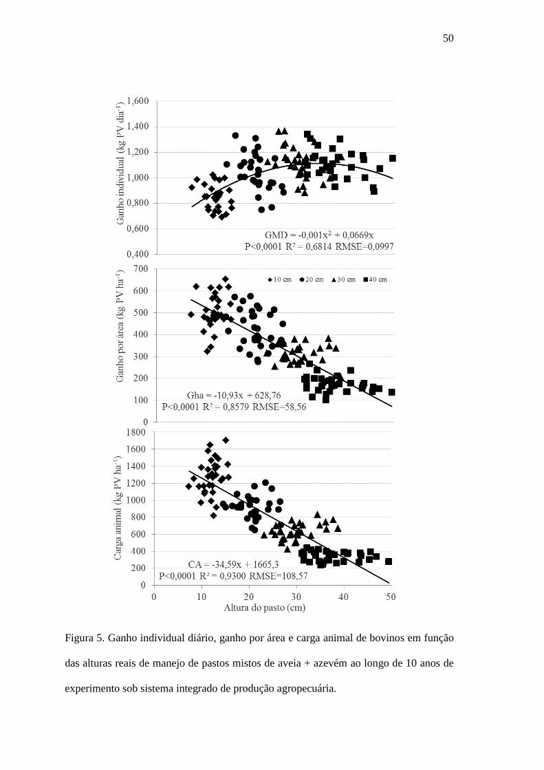
50
Figura 5. Ganho individual diário, ganho por área e carga animal de bovinos em função
das alturas reais de manejo de pastos mistos de aveia + azevém ao longo de 10 anos de
experimento sob sistema integrado de produção agropecuária.


²Artigo redigido sob as normas da Revista Agricultural Water Managenement (Apêndice 2).
³Dados pertencentes à SOERE-ACBB.
3. CAPÍTULO III
How much do sod-based rotations reduce nitrate leaching in a cereal cropping system?²,³
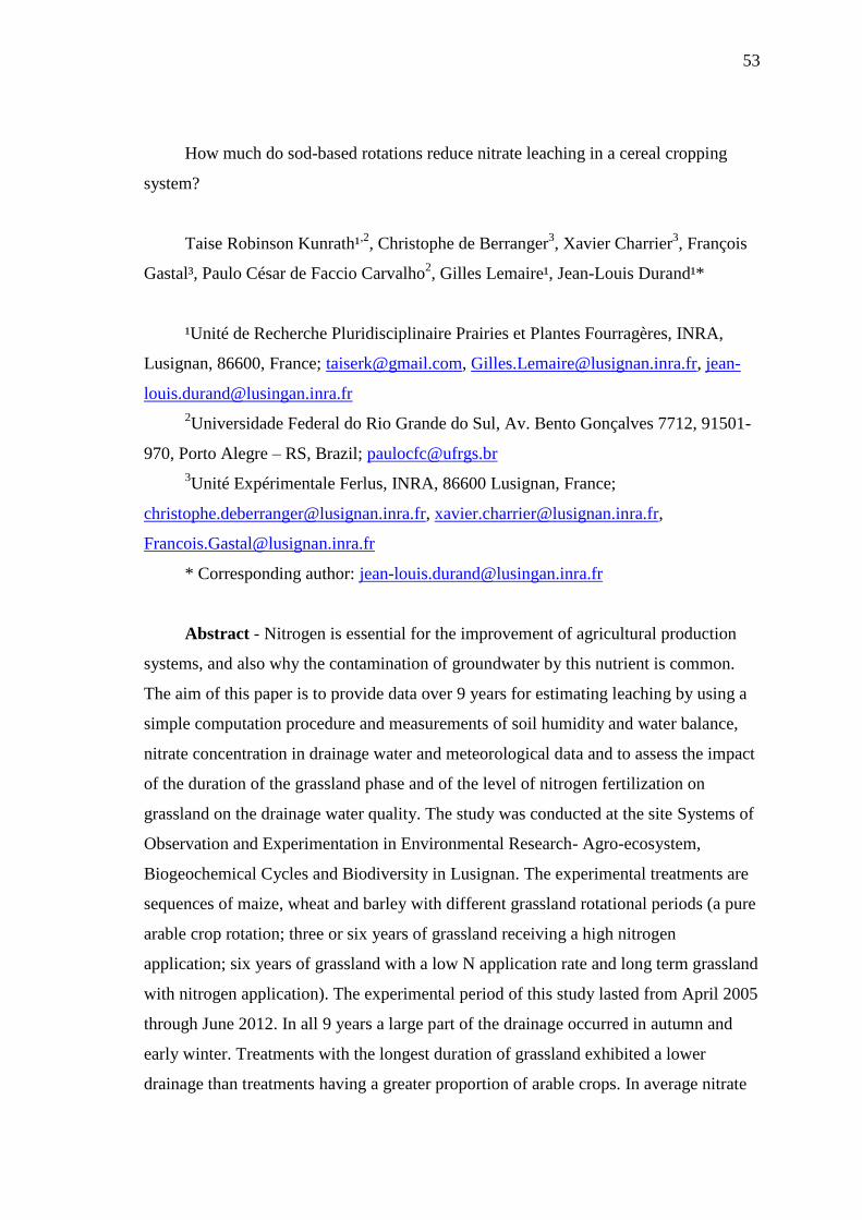
53
How much do sod-based rotations reduce nitrate leaching in a cereal cropping
system?
Taise Robinson Kunrath¹,2
, Christophe de Berranger3, Xavier Charrier
3, François
Gastal³, Paulo César de Faccio Carvalho2, Gilles Lemaire¹, Jean-Louis Durand¹*
¹Unité de Recherche Pluridisciplinaire Prairies et Plantes Fourragères, INRA,
Lusignan, 86600, France; [email protected], [email protected], jean-
2Universidade Federal do Rio Grande do Sul, Av. Bento Gonçalves 7712, 91501-
970, Porto Alegre – RS, Brazil; [email protected]
3Unité Expérimentale Ferlus, INRA, 86600 Lusignan, France;
[email protected], [email protected],
* Corresponding author: [email protected]
Abstract - Nitrogen is essential for the improvement of agricultural production
systems, and also why the contamination of groundwater by this nutrient is common.
The aim of this paper is to provide data over 9 years for estimating leaching by using a
simple computation procedure and measurements of soil humidity and water balance,
nitrate concentration in drainage water and meteorological data and to assess the impact
of the duration of the grassland phase and of the level of nitrogen fertilization on
grassland on the drainage water quality. The study was conducted at the site Systems of
Observation and Experimentation in Environmental Research- Agro-ecosystem,
Biogeochemical Cycles and Biodiversity in Lusignan. The experimental treatments are
sequences of maize, wheat and barley with different grassland rotational periods (a pure
arable crop rotation; three or six years of grassland receiving a high nitrogen
application; six years of grassland with a low N application rate and long term grassland
with nitrogen application). The experimental period of this study lasted from April 2005
through June 2012. In all 9 years a large part of the drainage occurred in autumn and
early winter. Treatments with the longest duration of grassland exhibited a lower
drainage than treatments having a greater proportion of arable crops. In average nitrate
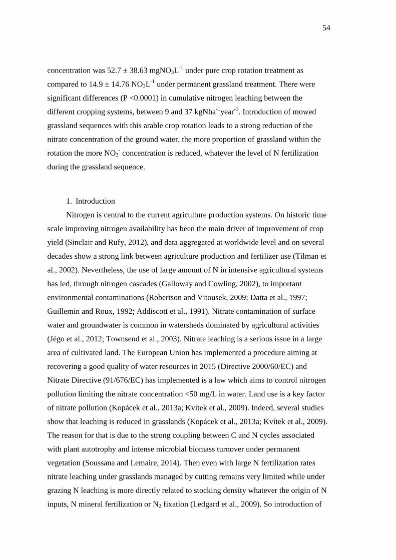
54
concentration was 52.7 ± 38.63 mgNO3L-1
under pure crop rotation treatment as
compared to 14.9 ± 14.76 NO3L-1
under permanent grassland treatment. There were
significant differences (P <0.0001) in cumulative nitrogen leaching between the
different cropping systems, between 9 and 37 kgNha-1
year-1
. Introduction of mowed
grassland sequences with this arable crop rotation leads to a strong reduction of the
nitrate concentration of the ground water, the more proportion of grassland within the
rotation the more NO3- concentration is reduced, whatever the level of N fertilization
during the grassland sequence.
1. Introduction
Nitrogen is central to the current agriculture production systems. On historic time
scale improving nitrogen availability has been the main driver of improvement of crop
yield (Sinclair and Rufy, 2012), and data aggregated at worldwide level and on several
decades show a strong link between agriculture production and fertilizer use (Tilman et
al., 2002). Nevertheless, the use of large amount of N in intensive agricultural systems
has led, through nitrogen cascades (Galloway and Cowling, 2002), to important
environmental contaminations (Robertson and Vitousek, 2009; Datta et al., 1997;
Guillemin and Roux, 1992; Addiscott et al., 1991). Nitrate contamination of surface
water and groundwater is common in watersheds dominated by agricultural activities
(Jégo et al., 2012; Townsend et al., 2003). Nitrate leaching is a serious issue in a large
area of cultivated land. The European Union has implemented a procedure aiming at
recovering a good quality of water resources in 2015 (Directive 2000/60/EC) and
Nitrate Directive (91/676/EC) has implemented is a law which aims to control nitrogen
pollution limiting the nitrate concentration <50 mg/L in water. Land use is a key factor
of nitrate pollution (Kopácek et al., 2013a; Kvítek et al., 2009). Indeed, several studies
show that leaching is reduced in grasslands (Kopácek et al., 2013a; Kvítek et al., 2009).
The reason for that is due to the strong coupling between C and N cycles associated
with plant autotrophy and intense microbial biomass turnover under permanent
vegetation (Soussana and Lemaire, 2014). Then even with large N fertilization rates
nitrate leaching under grasslands managed by cutting remains very limited while under
grazing N leaching is more directly related to stocking density whatever the origin of N
inputs, N mineral fertilization or N2 fixation (Ledgard et al., 2009). So introduction of
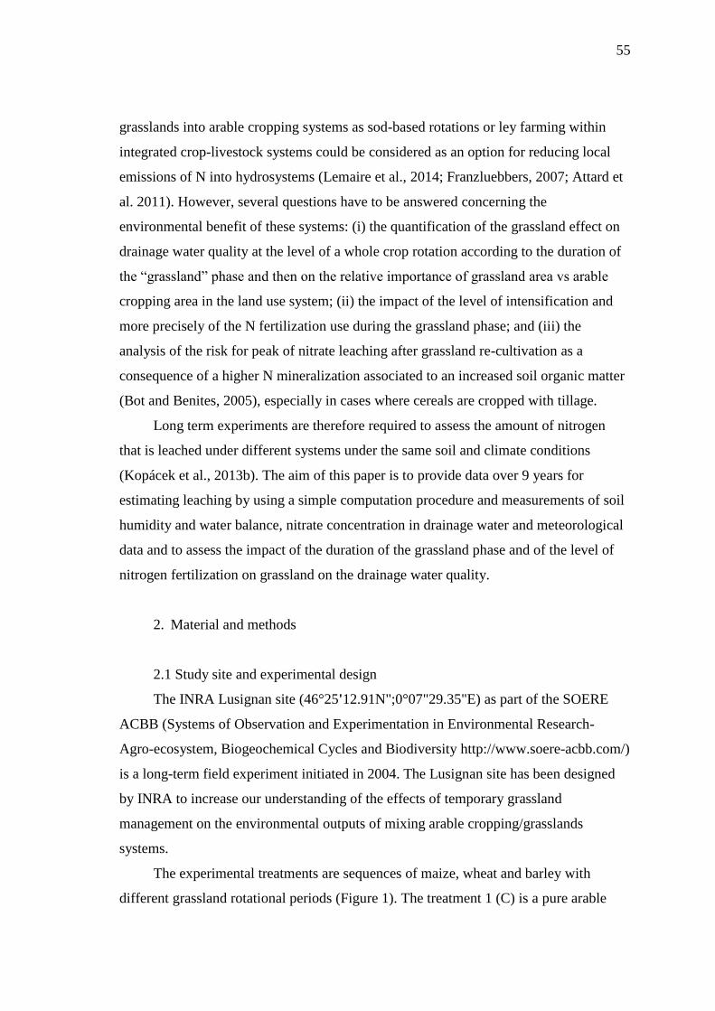
55
grasslands into arable cropping systems as sod-based rotations or ley farming within
integrated crop-livestock systems could be considered as an option for reducing local
emissions of N into hydrosystems (Lemaire et al., 2014; Franzluebbers, 2007; Attard et
al. 2011). However, several questions have to be answered concerning the
environmental benefit of these systems: (i) the quantification of the grassland effect on
drainage water quality at the level of a whole crop rotation according to the duration of
the “grassland” phase and then on the relative importance of grassland area vs arable
cropping area in the land use system; (ii) the impact of the level of intensification and
more precisely of the N fertilization use during the grassland phase; and (iii) the
analysis of the risk for peak of nitrate leaching after grassland re-cultivation as a
consequence of a higher N mineralization associated to an increased soil organic matter
(Bot and Benites, 2005), especially in cases where cereals are cropped with tillage.
Long term experiments are therefore required to assess the amount of nitrogen
that is leached under different systems under the same soil and climate conditions
(Kopácek et al., 2013b). The aim of this paper is to provide data over 9 years for
estimating leaching by using a simple computation procedure and measurements of soil
humidity and water balance, nitrate concentration in drainage water and meteorological
data and to assess the impact of the duration of the grassland phase and of the level of
nitrogen fertilization on grassland on the drainage water quality.
2. Material and methods
2.1 Study site and experimental design
The INRA Lusignan site (46°25'12.91N";0°07"29.35"E) as part of the SOERE
ACBB (Systems of Observation and Experimentation in Environmental Research-
Agro-ecosystem, Biogeochemical Cycles and Biodiversity http://www.soere-acbb.com/)
is a long-term field experiment initiated in 2004. The Lusignan site has been designed
by INRA to increase our understanding of the effects of temporary grassland
management on the environmental outputs of mixing arable cropping/grasslands
systems.
The experimental treatments are sequences of maize, wheat and barley with
different grassland rotational periods (Figure 1). The treatment 1 (C) is a pure arable
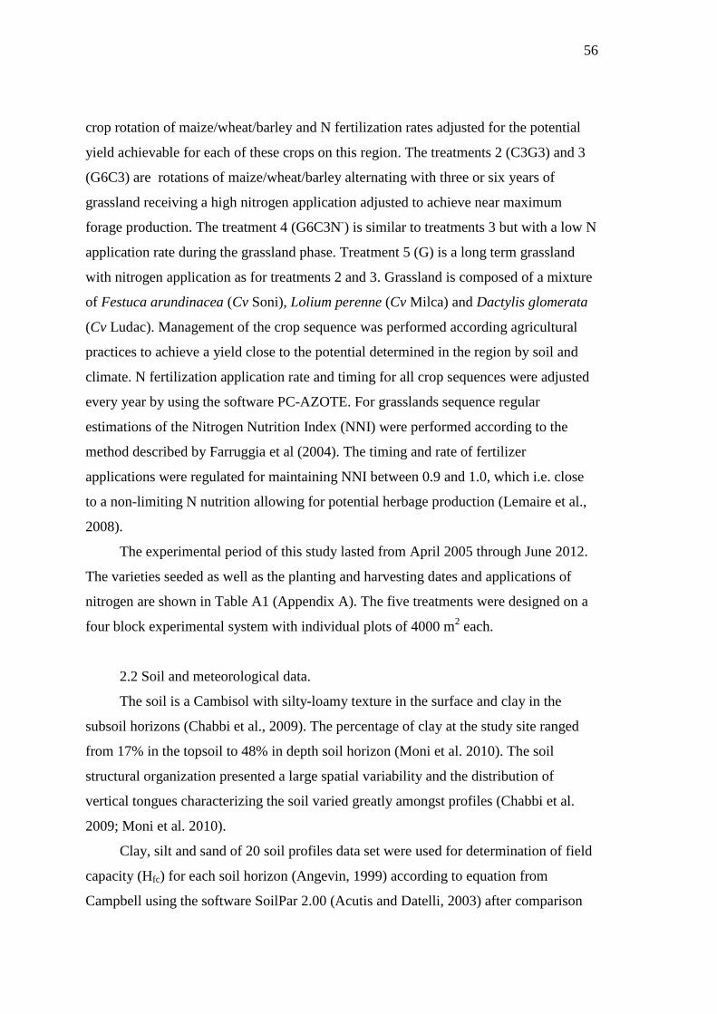
56
crop rotation of maize/wheat/barley and N fertilization rates adjusted for the potential
yield achievable for each of these crops on this region. The treatments 2 (C3G3) and 3
(G6C3) are rotations of maize/wheat/barley alternating with three or six years of
grassland receiving a high nitrogen application adjusted to achieve near maximum
forage production. The treatment 4 (G6C3N-) is similar to treatments 3 but with a low N
application rate during the grassland phase. Treatment 5 (G) is a long term grassland
with nitrogen application as for treatments 2 and 3. Grassland is composed of a mixture
of Festuca arundinacea (Cv Soni), Lolium perenne (Cv Milca) and Dactylis glomerata
(Cv Ludac). Management of the crop sequence was performed according agricultural
practices to achieve a yield close to the potential determined in the region by soil and
climate. N fertilization application rate and timing for all crop sequences were adjusted
every year by using the software PC-AZOTE. For grasslands sequence regular
estimations of the Nitrogen Nutrition Index (NNI) were performed according to the
method described by Farruggia et al (2004). The timing and rate of fertilizer
applications were regulated for maintaining NNI between 0.9 and 1.0, which i.e. close
to a non-limiting N nutrition allowing for potential herbage production (Lemaire et al.,
2008).
The experimental period of this study lasted from April 2005 through June 2012.
The varieties seeded as well as the planting and harvesting dates and applications of
nitrogen are shown in Table A1 (Appendix A). The five treatments were designed on a
four block experimental system with individual plots of 4000 m2 each.
2.2 Soil and meteorological data.
The soil is a Cambisol with silty-loamy texture in the surface and clay in the
subsoil horizons (Chabbi et al., 2009). The percentage of clay at the study site ranged
from 17% in the topsoil to 48% in depth soil horizon (Moni et al. 2010). The soil
structural organization presented a large spatial variability and the distribution of
vertical tongues characterizing the soil varied greatly amongst profiles (Chabbi et al.
2009; Moni et al. 2010).
Clay, silt and sand of 20 soil profiles data set were used for determination of field
capacity (Hfc) for each soil horizon (Angevin, 1999) according to equation from
Campbell using the software SoilPar 2.00 (Acutis and Datelli, 2003) after comparison
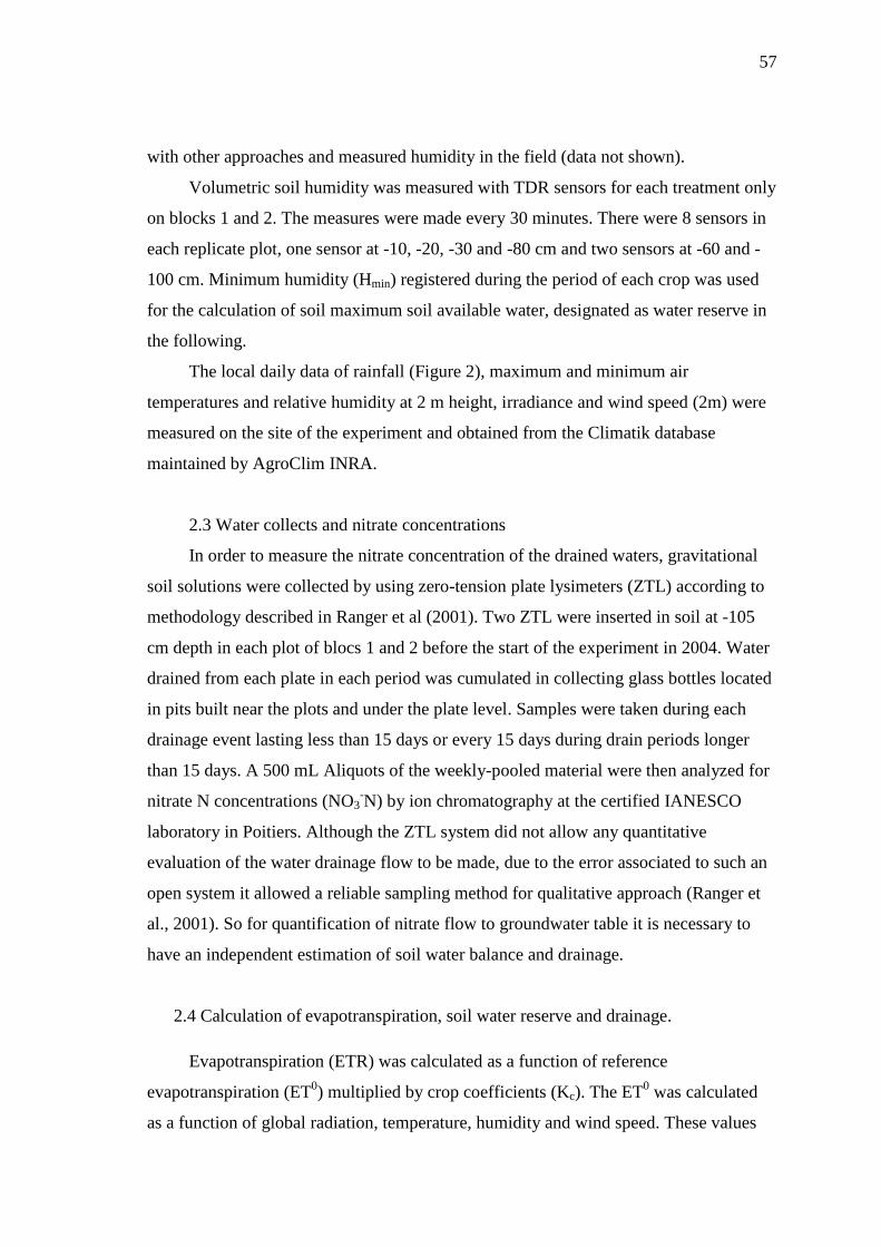
57
with other approaches and measured humidity in the field (data not shown).
Volumetric soil humidity was measured with TDR sensors for each treatment only
on blocks 1 and 2. The measures were made every 30 minutes. There were 8 sensors in
each replicate plot, one sensor at -10, -20, -30 and -80 cm and two sensors at -60 and -
100 cm. Minimum humidity (Hmin) registered during the period of each crop was used
for the calculation of soil maximum soil available water, designated as water reserve in
the following.
The local daily data of rainfall (Figure 2), maximum and minimum air
temperatures and relative humidity at 2 m height, irradiance and wind speed (2m) were
measured on the site of the experiment and obtained from the Climatik database
maintained by AgroClim INRA.
2.3 Water collects and nitrate concentrations
In order to measure the nitrate concentration of the drained waters, gravitational
soil solutions were collected by using zero-tension plate lysimeters (ZTL) according to
methodology described in Ranger et al (2001). Two ZTL were inserted in soil at -105
cm depth in each plot of blocs 1 and 2 before the start of the experiment in 2004. Water
drained from each plate in each period was cumulated in collecting glass bottles located
in pits built near the plots and under the plate level. Samples were taken during each
drainage event lasting less than 15 days or every 15 days during drain periods longer
than 15 days. A 500 mL Aliquots of the weekly-pooled material were then analyzed for
nitrate N concentrations (NO3-N) by ion chromatography at the certified IANESCO
laboratory in Poitiers. Although the ZTL system did not allow any quantitative
evaluation of the water drainage flow to be made, due to the error associated to such an
open system it allowed a reliable sampling method for qualitative approach (Ranger et
al., 2001). So for quantification of nitrate flow to groundwater table it is necessary to
have an independent estimation of soil water balance and drainage.
2.4 Calculation of evapotranspiration, soil water reserve and drainage.
Evapotranspiration (ETR) was calculated as a function of reference
evapotranspiration (ET0) multiplied by crop coefficients (Kc). The ET
0 was calculated
as a function of global radiation, temperature, humidity and wind speed. These values

58
are routinely computed and downloaded from the Climatik data base. Crop coefficients
were found in the FAO document for wheat, maize, barley and grassland for each stage
of crop development (Allen et al., 2006). The actual evapotranspiration was further
reduced depending on the relative soil water content.
To take the impact of the soil water content on ETR into account, the soil was
divided into three layers (Figure 3): one surface layer 0-20 cm; one layer explored by
roots (for each crop) which increased in depth from 0 at sowing to a maximum depth at
flowering; and a deep layer which was the maximum depth reached by roots during the
whole period studied (2006-2013). The maximum depth was estimated using the
humidity profiles measured throughout the experiment.
Kc was actualized every day following the crop development, and assuming it was
0.3 at sowing and maximum at flowering. Flowering date was derived from the value
growing degree days provided for maize, wheat or barley (Table A1 – Appendix A). In
each case, the maximum value of Kc was taken from the FAO (Allen et al., 2006). The
root depth was proportional to Kc, growing from zero at sowing to maximum root depth
on day of flowering. The maximum root depth was computed for each crop and plot
using the profile of minimum soil water content observed over 100 cm, extrapolating
the depth value at which soil humidity would be equal to field capacity (eg, Figure 4).
Further details of the computation of ETR and drainage, depending on development
stage of the crops, are given in appendix B.
2.5 Statistical methods.
Data were subjected to analysis of variance and contrasts with significance level
of 5%. Drainage data were also analyzed for each period (crop). For these analyzes, the
GLM and Mixed of SAS software (SAS, 2002) package was used.
3. Results.
3.1 Estimate of drainage
Maximum soil water reserve (Table 1) was similar between treatments (P=
0.0957), allowing the evaluation of treatment effects on water draining from the soil and
leaching of nitrogen.
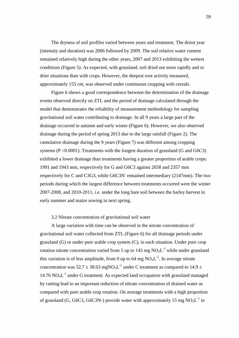
59
The dryness of soil profiles varied between years and treatment. The driest year
(intensity and duration) was 2006 followed by 2009. The soil relative water content
remained relatively high during the other years, 2007 and 2013 exhibiting the wettest
conditions (Figure 5). As expected, with grassland, soil dried out more rapidly and to
drier situations than with crops. However, the deepest root activity measured,
approximately 155 cm, was observed under continuous cropping with cereals.
Figure 6 shows a good correspondence between the determination of the drainage
events observed directly on ZTL and the period of drainage calculated through the
model that demonstrates the reliability of measurement methodology for sampling
gravitational soil water contributing to drainage. In all 9 years a large part of the
drainage occurred in autumn and early winter (Figure 6). However, we also observed
drainage during the period of spring 2013 due to the large rainfall (Figure 2). The
cumulative drainage during the 9 years (Figure 7) was different among cropping
systems (P <0.0001). Treatments with the longest duration of grassland (G and G6C3)
exhibited a lower drainage than treatments having a greater proportion of arable crops:
1991 and 1943 mm, respectively for G and G6C3 against 2658 and 2357 mm
respectively for C and C3G3, while G6C3N- remained intermediary (2147mm). The two
periods during which the largest difference between treatments occurred were the winter
2007-2008, and 2010-2011, i.e. under the long bare soil between the barley harvest in
early summer and maize sowing in next spring.
3.2 Nitrate concentration of gravitational soil water
A large variation with time can be observed in the nitrate concentration of
gravitational soil water collected from ZTL (Figure 6) for all drainage periods under
grassland (G) or under pure arable crop system (C), in each situation. Under pure crop
rotation nitrate concentration varied from 5 up to 145 mg NO3L-1
while under grassland
this variation is of less amplitude, from 0 up to 64 mg NO3L-1
. In average nitrate
concentration was 52.7 ± 38.63 mgNO3L-1
under C treatment as compared to 14.9 ±
14.76 NO3L-1
under G treatment. As expected land occupation with grassland managed
by cutting lead to an important reduction of nitrate concentration of drained water as
compared with pure arable crop rotation. On average treatments with a high proportion
of grassland (G, G6C3, G6C3N-) provide water with approximately 15 mg NO3L-1
in
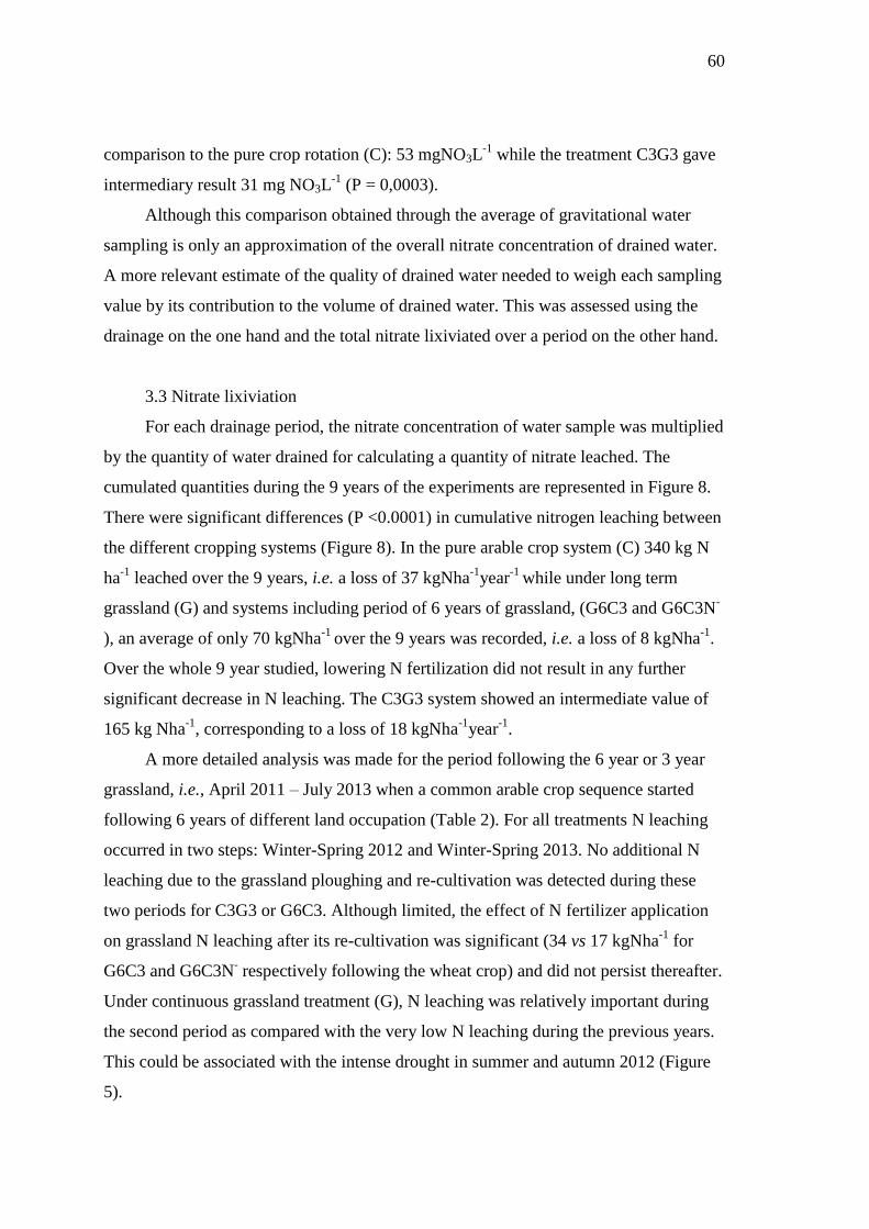
60
comparison to the pure crop rotation (C): 53 mgNO3L-1
while the treatment C3G3 gave
intermediary result 31 mg NO3L-1
(P = 0,0003).
Although this comparison obtained through the average of gravitational water
sampling is only an approximation of the overall nitrate concentration of drained water.
A more relevant estimate of the quality of drained water needed to weigh each sampling
value by its contribution to the volume of drained water. This was assessed using the
drainage on the one hand and the total nitrate lixiviated over a period on the other hand.
3.3 Nitrate lixiviation
For each drainage period, the nitrate concentration of water sample was multiplied
by the quantity of water drained for calculating a quantity of nitrate leached. The
cumulated quantities during the 9 years of the experiments are represented in Figure 8.
There were significant differences (P <0.0001) in cumulative nitrogen leaching between
the different cropping systems (Figure 8). In the pure arable crop system (C) 340 kg N
ha-1
leached over the 9 years, i.e. a loss of 37 kgNha-1
year-1
while under long term
grassland (G) and systems including period of 6 years of grassland, (G6C3 and G6C3N-
), an average of only 70 kgNha-1
over the 9 years was recorded, i.e. a loss of 8 kgNha-1
.
Over the whole 9 year studied, lowering N fertilization did not result in any further
significant decrease in N leaching. The C3G3 system showed an intermediate value of
165 kg Nha-1
, corresponding to a loss of 18 kgNha-1
year-1
.
A more detailed analysis was made for the period following the 6 year or 3 year
grassland, i.e., April 2011 – July 2013 when a common arable crop sequence started
following 6 years of different land occupation (Table 2). For all treatments N leaching
occurred in two steps: Winter-Spring 2012 and Winter-Spring 2013. No additional N
leaching due to the grassland ploughing and re-cultivation was detected during these
two periods for C3G3 or G6C3. Although limited, the effect of N fertilizer application
on grassland N leaching after its re-cultivation was significant (34 vs 17 kgNha-1
for
G6C3 and G6C3N- respectively following the wheat crop) and did not persist thereafter.
Under continuous grassland treatment (G), N leaching was relatively important during
the second period as compared with the very low N leaching during the previous years.
This could be associated with the intense drought in summer and autumn 2012 (Figure
5).
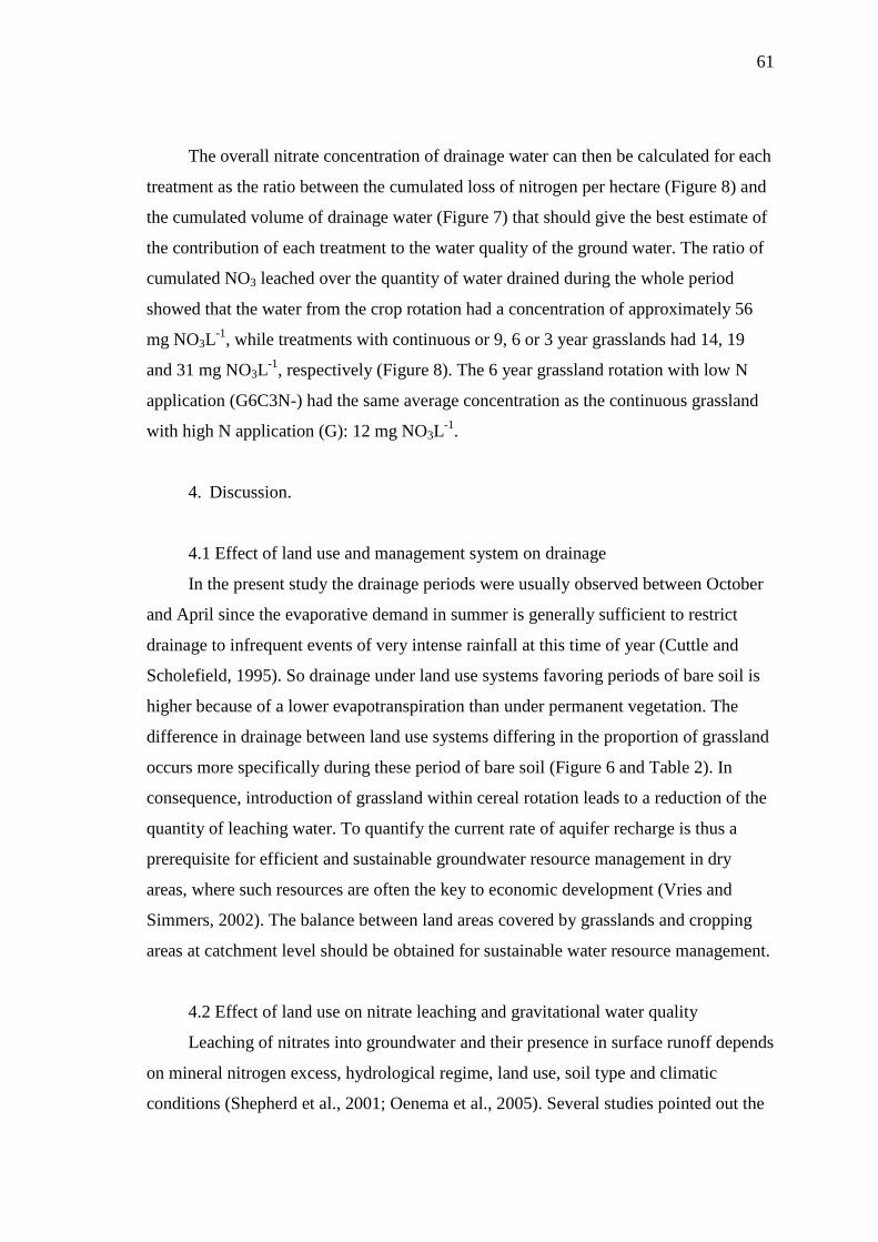
61
The overall nitrate concentration of drainage water can then be calculated for each
treatment as the ratio between the cumulated loss of nitrogen per hectare (Figure 8) and
the cumulated volume of drainage water (Figure 7) that should give the best estimate of
the contribution of each treatment to the water quality of the ground water. The ratio of
cumulated NO3 leached over the quantity of water drained during the whole period
showed that the water from the crop rotation had a concentration of approximately 56
mg NO3L-1
, while treatments with continuous or 9, 6 or 3 year grasslands had 14, 19
and 31 mg NO3L-1
, respectively (Figure 8). The 6 year grassland rotation with low N
application (G6C3N-) had the same average concentration as the continuous grassland
with high N application (G): 12 mg NO3L-1
.
4. Discussion.
4.1 Effect of land use and management system on drainage
In the present study the drainage periods were usually observed between October
and April since the evaporative demand in summer is generally sufficient to restrict
drainage to infrequent events of very intense rainfall at this time of year (Cuttle and
Scholefield, 1995). So drainage under land use systems favoring periods of bare soil is
higher because of a lower evapotranspiration than under permanent vegetation. The
difference in drainage between land use systems differing in the proportion of grassland
occurs more specifically during these period of bare soil (Figure 6 and Table 2). In
consequence, introduction of grassland within cereal rotation leads to a reduction of the
quantity of leaching water. To quantify the current rate of aquifer recharge is thus a
prerequisite for efficient and sustainable groundwater resource management in dry
areas, where such resources are often the key to economic development (Vries and
Simmers, 2002). The balance between land areas covered by grasslands and cropping
areas at catchment level should be obtained for sustainable water resource management.
4.2 Effect of land use on nitrate leaching and gravitational water quality
Leaching of nitrates into groundwater and their presence in surface runoff depends
on mineral nitrogen excess, hydrological regime, land use, soil type and climatic
conditions (Shepherd et al., 2001; Oenema et al., 2005). Several studies pointed out the
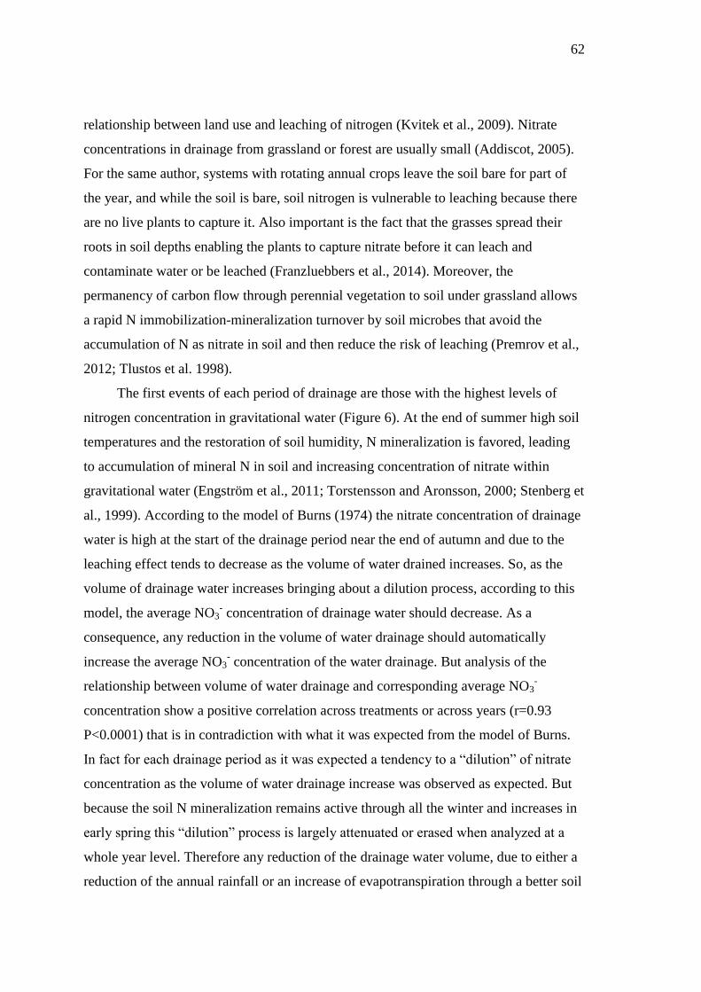
62
relationship between land use and leaching of nitrogen (Kvitek et al., 2009). Nitrate
concentrations in drainage from grassland or forest are usually small (Addiscot, 2005).
For the same author, systems with rotating annual crops leave the soil bare for part of
the year, and while the soil is bare, soil nitrogen is vulnerable to leaching because there
are no live plants to capture it. Also important is the fact that the grasses spread their
roots in soil depths enabling the plants to capture nitrate before it can leach and
contaminate water or be leached (Franzluebbers et al., 2014). Moreover, the
permanency of carbon flow through perennial vegetation to soil under grassland allows
a rapid N immobilization-mineralization turnover by soil microbes that avoid the
accumulation of N as nitrate in soil and then reduce the risk of leaching (Premrov et al.,
2012; Tlustos et al. 1998).
The first events of each period of drainage are those with the highest levels of
nitrogen concentration in gravitational water (Figure 6). At the end of summer high soil
temperatures and the restoration of soil humidity, N mineralization is favored, leading
to accumulation of mineral N in soil and increasing concentration of nitrate within
gravitational water (Engström et al., 2011; Torstensson and Aronsson, 2000; Stenberg et
al., 1999). According to the model of Burns (1974) the nitrate concentration of drainage
water is high at the start of the drainage period near the end of autumn and due to the
leaching effect tends to decrease as the volume of water drained increases. So, as the
volume of drainage water increases bringing about a dilution process, according to this
model, the average NO3- concentration of drainage water should decrease. As a
consequence, any reduction in the volume of water drainage should automatically
increase the average NO3- concentration of the water drainage. But analysis of the
relationship between volume of water drainage and corresponding average NO3-
concentration show a positive correlation across treatments or across years (r=0.93
P<0.0001) that is in contradiction with what it was expected from the model of Burns.
In fact for each drainage period as it was expected a tendency to a “dilution” of nitrate
concentration as the volume of water drainage increase was observed as expected. But
because the soil N mineralization remains active through all the winter and increases in
early spring this “dilution” process is largely attenuated or erased when analyzed at a
whole year level. Therefore any reduction of the drainage water volume, due to either a
reduction of the annual rainfall or an increase of evapotranspiration through a better soil
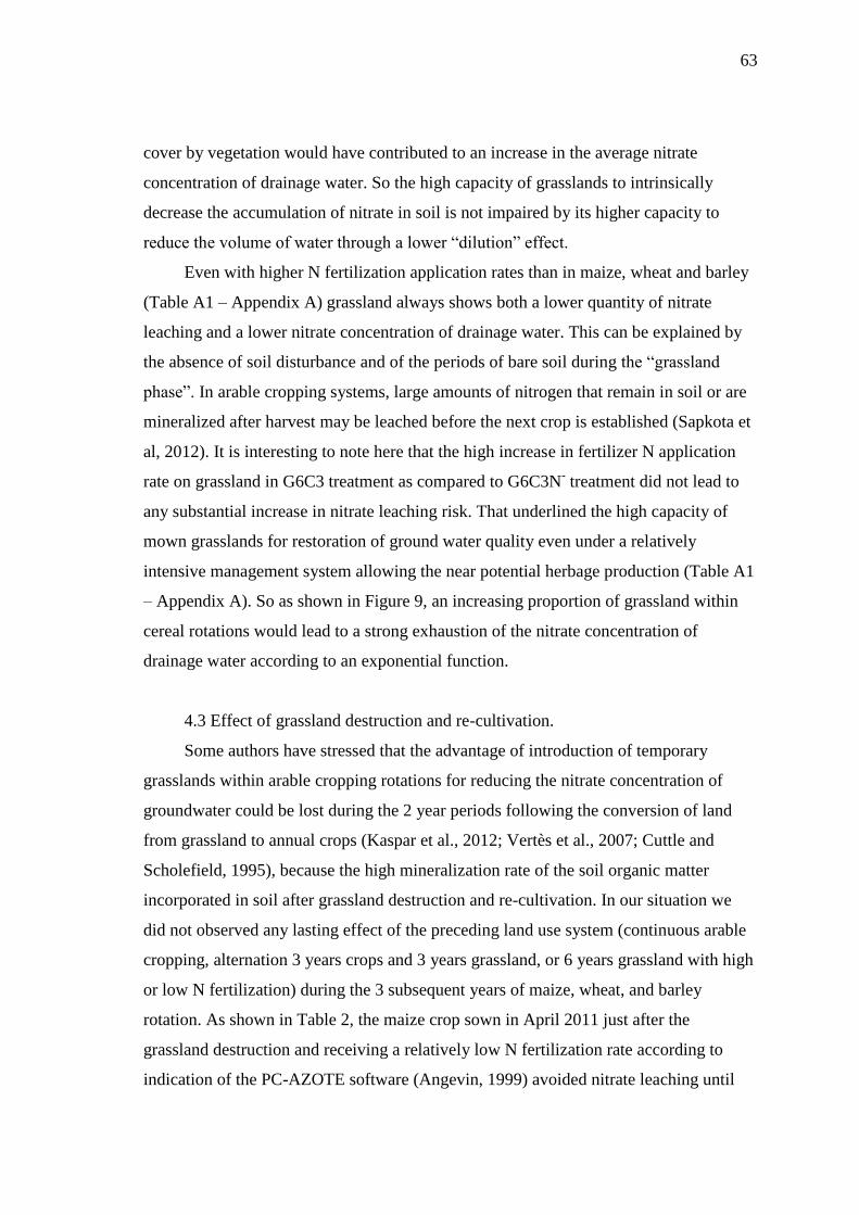
63
cover by vegetation would have contributed to an increase in the average nitrate
concentration of drainage water. So the high capacity of grasslands to intrinsically
decrease the accumulation of nitrate in soil is not impaired by its higher capacity to
reduce the volume of water through a lower “dilution” effect.
Even with higher N fertilization application rates than in maize, wheat and barley
(Table A1 – Appendix A) grassland always shows both a lower quantity of nitrate
leaching and a lower nitrate concentration of drainage water. This can be explained by
the absence of soil disturbance and of the periods of bare soil during the “grassland
phase”. In arable cropping systems, large amounts of nitrogen that remain in soil or are
mineralized after harvest may be leached before the next crop is established (Sapkota et
al, 2012). It is interesting to note here that the high increase in fertilizer N application
rate on grassland in G6C3 treatment as compared to G6C3N- treatment did not lead to
any substantial increase in nitrate leaching risk. That underlined the high capacity of
mown grasslands for restoration of ground water quality even under a relatively
intensive management system allowing the near potential herbage production (Table A1
– Appendix A). So as shown in Figure 9, an increasing proportion of grassland within
cereal rotations would lead to a strong exhaustion of the nitrate concentration of
drainage water according to an exponential function.
4.3 Effect of grassland destruction and re-cultivation.
Some authors have stressed that the advantage of introduction of temporary
grasslands within arable cropping rotations for reducing the nitrate concentration of
groundwater could be lost during the 2 year periods following the conversion of land
from grassland to annual crops (Kaspar et al., 2012; Vertès et al., 2007; Cuttle and
Scholefield, 1995), because the high mineralization rate of the soil organic matter
incorporated in soil after grassland destruction and re-cultivation. In our situation we
did not observed any lasting effect of the preceding land use system (continuous arable
cropping, alternation 3 years crops and 3 years grassland, or 6 years grassland with high
or low N fertilization) during the 3 subsequent years of maize, wheat, and barley
rotation. As shown in Table 2, the maize crop sown in April 2011 just after the
grassland destruction and receiving a relatively low N fertilization rate according to
indication of the PC-AZOTE software (Angevin, 1999) avoided nitrate leaching until
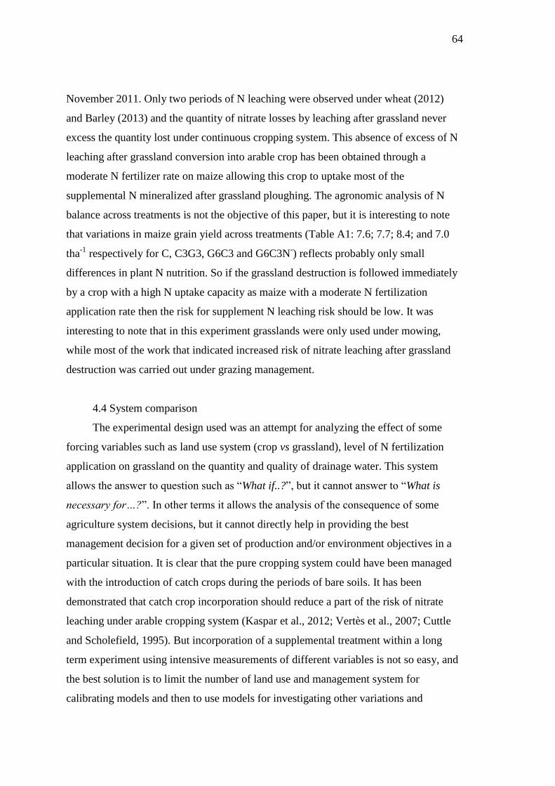
64
November 2011. Only two periods of N leaching were observed under wheat (2012)
and Barley (2013) and the quantity of nitrate losses by leaching after grassland never
excess the quantity lost under continuous cropping system. This absence of excess of N
leaching after grassland conversion into arable crop has been obtained through a
moderate N fertilizer rate on maize allowing this crop to uptake most of the
supplemental N mineralized after grassland ploughing. The agronomic analysis of N
balance across treatments is not the objective of this paper, but it is interesting to note
that variations in maize grain yield across treatments (Table A1: 7.6; 7.7; 8.4; and 7.0
tha-1
respectively for C, C3G3, G6C3 and G6C3N-) reflects probably only small
differences in plant N nutrition. So if the grassland destruction is followed immediately
by a crop with a high N uptake capacity as maize with a moderate N fertilization
application rate then the risk for supplement N leaching risk should be low. It was
interesting to note that in this experiment grasslands were only used under mowing,
while most of the work that indicated increased risk of nitrate leaching after grassland
destruction was carried out under grazing management.
4.4 System comparison
The experimental design used was an attempt for analyzing the effect of some
forcing variables such as land use system (crop vs grassland), level of N fertilization
application on grassland on the quantity and quality of drainage water. This system
allows the answer to question such as “What if..?”, but it cannot answer to “What is
necessary for…?”. In other terms it allows the analysis of the consequence of some
agriculture system decisions, but it cannot directly help in providing the best
management decision for a given set of production and/or environment objectives in a
particular situation. It is clear that the pure cropping system could have been managed
with the introduction of catch crops during the periods of bare soils. It has been
demonstrated that catch crop incorporation should reduce a part of the risk of nitrate
leaching under arable cropping system (Kaspar et al., 2012; Vertès et al., 2007; Cuttle
and Scholefield, 1995). But incorporation of a supplemental treatment within a long
term experiment using intensive measurements of different variables is not so easy, and
the best solution is to limit the number of land use and management system for
calibrating models and then to use models for investigating other variations and
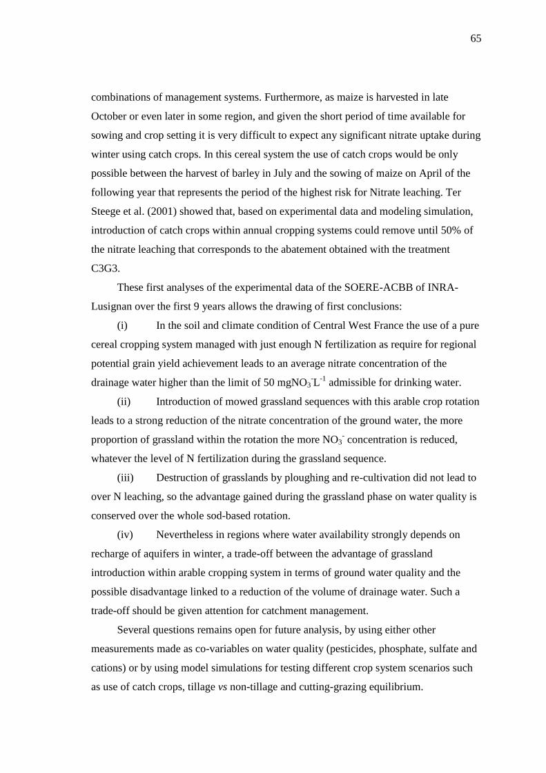
65
combinations of management systems. Furthermore, as maize is harvested in late
October or even later in some region, and given the short period of time available for
sowing and crop setting it is very difficult to expect any significant nitrate uptake during
winter using catch crops. In this cereal system the use of catch crops would be only
possible between the harvest of barley in July and the sowing of maize on April of the
following year that represents the period of the highest risk for Nitrate leaching. Ter
Steege et al. (2001) showed that, based on experimental data and modeling simulation,
introduction of catch crops within annual cropping systems could remove until 50% of
the nitrate leaching that corresponds to the abatement obtained with the treatment
C3G3.
These first analyses of the experimental data of the SOERE-ACBB of INRA-
Lusignan over the first 9 years allows the drawing of first conclusions:
(i) In the soil and climate condition of Central West France the use of a pure
cereal cropping system managed with just enough N fertilization as require for regional
potential grain yield achievement leads to an average nitrate concentration of the
drainage water higher than the limit of 50 mgNO3-L
-1 admissible for drinking water.
(ii) Introduction of mowed grassland sequences with this arable crop rotation
leads to a strong reduction of the nitrate concentration of the ground water, the more
proportion of grassland within the rotation the more NO3- concentration is reduced,
whatever the level of N fertilization during the grassland sequence.
(iii) Destruction of grasslands by ploughing and re-cultivation did not lead to
over N leaching, so the advantage gained during the grassland phase on water quality is
conserved over the whole sod-based rotation.
(iv) Nevertheless in regions where water availability strongly depends on
recharge of aquifers in winter, a trade-off between the advantage of grassland
introduction within arable cropping system in terms of ground water quality and the
possible disadvantage linked to a reduction of the volume of drainage water. Such a
trade-off should be given attention for catchment management.
Several questions remains open for future analysis, by using either other
measurements made as co-variables on water quality (pesticides, phosphate, sulfate and
cations) or by using model simulations for testing different crop system scenarios such
as use of catch crops, tillage vs non-tillage and cutting-grazing equilibrium.
66
5. Acknowledgments.
The authors thank the SOERE-ACBB for providing the necessary infrastructure
and the complete data set to perform the present work. Indeed, we are grateful to INRA,
Allenvi, CNRS-INSU, ANR (Abad Chabbi coordinateur) and the regional council of
Poitou-Charente for financial support of the SOERE-ACBB and the functioning cost of
the Taise Robinson Kunrath. Also, Taise Robinson Kunrath thanks the Brazilian
Ministry of Education ‘Coordenação de Aperfeiçoamento de Pessoal de Nível Superior’
(CAPES) for providing financial assistance via CAPES/COFECUB Project 684/10 and
Dr. Abad Chabbi (the SOERE ACBB scientific coordinator) for the valuables
comments.
6. Appendix
6.1 Appendix A.
6.2 Appendix B.
The soil is split in three layers: the 20 top cm, the layer explored by the current
crop’s roots and the deepest root layer over the whole 8 year period studied. When the
soil was bare the top 20 layer contribution to ETR of the day j ( ) was computed
using equation (B.1):
(B.1)
Where, K20 was set constant equal to 0.3 (Allen et al., 2006), is the daily soil
water reserve of the 20 cm layer of the day j and RU20 is the maximum available water
of the 20 cm layer. and RU20 were determined using equations (B.2) and (B.3):
(B.2)
𝑅𝑈20 = {[(𝐻10𝑓𝑐
− 𝐻10𝑀𝑖𝑛) ∗ 10] + [(𝐻10
𝑓𝑐− 𝐻20
𝑀𝑖𝑛) ∗ 10 + (𝐻20𝑀𝑖𝑛 − 𝐻10
𝑀𝑖𝑛) ∗ 5 +
(𝐻20𝑓𝑐
− 𝐻10𝑓𝑐
) ∗ 5]} (B.3)
Where R20j-1
is the available water of the top layer of the day j-1, Pj is the rainfalls
of the day j, HMin
is the minimum humidity and Hfc
is the field capacity humidity in
jETR20
20
20
20204.0
;1**RU
RMinETKETR
j
j
jR20
jR20
jjjj ETRPRRUMinR 20
1
2020;20
67
each depth. Hfc
was calculated using the software Soilpar 2.00 (Acutis & Donatelli,
2003).
When Root depth was deeper than 20cm, ETR was computed using equation
(B.4).
(B.4)
Where and RUR are the soil available water content of the day j-1 and the
maximum available water content in the root zone below 20 cm, respectively. was
determined using equation. (B.5)
Drainage between top layer and root zone and under the root zone was computed
making the balance on each layer and neglecting the capillary rise because the water
table is 30 m under the ground, approximately (equations B.5, B.7 and B.9).
(B.5)
Where DRj-1
is the drainage under the root zone and was determined using
equation (B.6).
(B.6)
(B.7)
(B.8)
𝑅𝑈𝑅 = {[(𝐻10𝑓𝑐
− 𝐻10𝑀𝑖𝑛) ∗ 10] + [(𝐻10
𝑓𝑐− 𝐻20
𝑀𝑖𝑛) ∗ 10 + (𝐻20𝑀𝑖𝑛 − 𝐻10
𝑀𝑖𝑛) ∗ 5 +
(𝐻20𝑓𝑐
− 𝐻10𝑓𝑐
) ∗ 5] + [(𝐻20𝑓𝑐
− 𝐻30𝑀𝑖𝑛) ∗ 10 + (𝐻30
𝑀𝑖𝑛 − 𝐻20𝑀𝑖𝑛) ∗ 5 + (𝐻30
𝑓𝑐− 𝐻20
𝑓𝑐) ∗ 5] +
[(𝐻30𝑓𝑐
− 𝐻60𝑀𝑖𝑛) ∗ 30 + (𝐻60
𝑀𝑖𝑛 − 𝐻30𝑀𝑖𝑛) ∗ 15 + (𝐻60
𝑓𝑐− 𝐻30
𝑓𝑐) ∗ 15] + [(𝐻60
𝑓𝑐− 𝐻80
𝑀𝑖𝑛) ∗
20 + (𝐻80𝑀𝑖𝑛 − 𝐻60
𝑀𝑖𝑛) ∗ 10 + (𝐻80𝑓𝑐
− 𝐻60𝑓𝑐
) ∗ 10] + [(𝐻80𝑓𝑐
− 𝐻100𝑀𝑖𝑛) ∗ 20 +
(𝐻100𝑀𝑖𝑛 − 𝐻80
𝑀𝑖𝑛) ∗ 10 + (𝐻100𝑓𝑐
− 𝐻80𝑓𝑐
) ∗ 10] +
[(𝐻𝑀𝑎𝑥 𝑑𝑒𝑝𝑡ℎ𝑓𝑐
− 𝐻100𝑀𝑖𝑛) ∗
(𝑀𝑎𝑥 𝑑𝑒𝑝𝑡ℎ−100)
2]} (B.9)
Where max depth is the maximum root depth for each crop in each plot. For each
plot, the values RU20, maximum root depth and maximum RU are given in Table 1.
The drainage under the maximum root depth of the day j (Dj) is determined
according to equation (B.10).
j
R
j
Rc
j ETRRU
RMinETKETR 20
1
4.0;1**
j
RR
j
RR
1
2020
1 )(; jjjj
RR
j
R DETRETRRRUMinR
)( 20
1
2020
1
20
jjjj ETRPRRUD
1
20
1 )(; j
R
jjjj DETRETRRRUMinR
)( 11 jjj
RR
j
R ETRPRRUD

68
(B.10)
Were RU is the maximum available water for 9 years.
For calculating the amount of nitrate leached, the Nitrate concentration
(%Nitratej) of drained water was linearly interpolated between two samples values.
Nitrogen leaching was calculated according to equation (B.11).
(B.11)
)( 1 jjj
R
j ETRPRRUD
226.0*%* jj
leaching NitrateDN

69
7. References.
Acutis, M., Donatelli, M, 2003. SOILPAR 2.00: software to estimate soil
hydrological parameters and functions. Europ. J. Agronomy 18, 373-377.
Addiscott, T.M., Whitmore, A.P., Powlson, D.S., 1991. Farming, Fertilizers and
the Nitrate Problem. CAB Int., Wallingford.Allen, R.G., Pereira, L.S., Raes, D., Smith,
M., 2006. Crop evapotranspiration: Guidelines for computing crop requirements.
Irrigation and Drainage Paper No. 56, FAO, Rome.
Addiscott, T.M. 2005. Nitrate, agriculture and the environment. CAB Int.,
Wallingford.
Angevin, F. (1999). Raisonnement de la fertilisation azotée. Le logiciel PCazote
en Poitou-Charentes. Oléoscope, 54, 32-34.
Attard, E., Recous, S., Chabbi, A., De Berranger, C. Guillaumaud, N., Labreuche,
J. Philippot, L., Schmid, B., Le Roux, X. 2011. Soil environmental conditions rather
than denitrifier abundance and diversity drive potential denitrification after changes in
land uses. Global Change Biology 17, 1975–1989.
Bot, A., Benites, J., 2005. The importance of soil organic matter. Key to drought-
resistant soil and sustained food and production. FAO Soil bulletin 80.
Burns, I.G., 1974. A model for predicting the redistribution of salts applied to
fallow soils after excess rainfall or evaporation. J. Soil Sci., 25: 165-178.
Chabbi, A., Kogel-Knabner, I. and Rumpel C. 2009. Stabilised carbon in subsoil
horizons is located in spatially distinct parts of the soil profile. Soil Biology &
Biochemistry, 41, 256–261.
Cuttle, S.P., Scholefield, D., 1995. Management aptons to limit nitrate leaching
from grassland. J. Contam. Hydrol, 20, 299-312.
Datta, P.S., Deb, D.L., Tyagi, S.K., 1997. Assessment of groundwater
contamination from fertilizers in the Delhi area based on 18O, NO3 and K+
composition. J. Contam. Hydrol. 27, 249–262.
Engström, L., Stenberg, M., Aronsson, H., Lindén, B., 2011. Reducing nitrate
leaching after winter oilseed rape and peas by optimising crop management. Agron.
Sustain. Dev. 31, 337–347.
Farruggia A., Gastal, F., Scholefield, D., 2004. Assessment of the nitrogen status
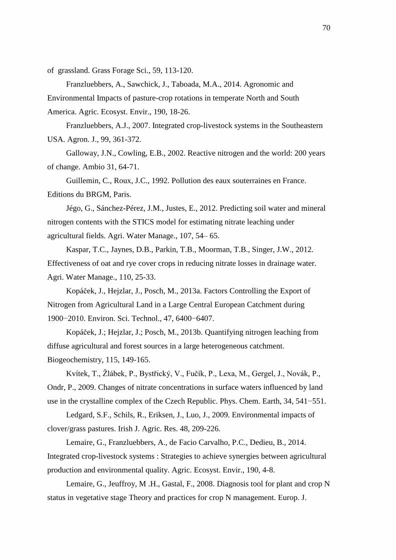
70
of grassland. Grass Forage Sci., 59, 113-120.
Franzluebbers, A., Sawchick, J., Taboada, M.A., 2014. Agronomic and
Environmental Impacts of pasture-crop rotations in temperate North and South
America. Agric. Ecosyst. Envir., 190, 18-26.
Franzluebbers, A.J., 2007. Integrated crop-livestock systems in the Southeastern
USA. Agron. J., 99, 361-372.
Galloway, J.N., Cowling, E.B., 2002. Reactive nitrogen and the world: 200 years
of change. Ambio 31, 64-71.
Guillemin, C., Roux, J.C., 1992. Pollution des eaux souterraines en France.
Editions du BRGM, Paris.
Jégo, G., Sánchez-Pérez, J.M., Justes, E., 2012. Predicting soil water and mineral
nitrogen contents with the STICS model for estimating nitrate leaching under
agricultural fields. Agri. Water Manage., 107, 54– 65.
Kaspar, T.C., Jaynes, D.B., Parkin, T.B., Moorman, T.B., Singer, J.W., 2012.
Effectiveness of oat and rye cover crops in reducing nitrate losses in drainage water.
Agri. Water Manage., 110, 25-33.
Kopácek, J., Hejzlar, J., Posch, M., 2013a. Factors Controlling the Export of
Nitrogen from Agricultural Land in a Large Central European Catchment during
1900−2010. Environ. Sci. Technol., 47, 6400−6407.
Kopácek, J.; Hejzlar, J.; Posch, M., 2013b. Quantifying nitrogen leaching from
diffuse agricultural and forest sources in a large heterogeneous catchment.
Biogeochemistry, 115, 149-165.
Kvítek, T., Zlabek, P., Bystricky, V., Fucík, P., Lexa, M., Gergel, J., Novak, P.,
Ondr, P., 2009. Changes of nitrate concentrations in surface waters influenced by land
use in the crystalline complex of the Czech Republic. Phys. Chem. Earth, 34, 541−551.
Ledgard, S.F., Schils, R., Eriksen, J., Luo, J., 2009. Environmental impacts of
clover/grass pastures. Irish J. Agric. Res. 48, 209-226.
Lemaire, G., Franzluebbers, A., de Facio Carvalho, P.C., Dedieu, B., 2014.
Integrated crop-livestock systems : Strategies to achieve synergies between agricultural
production and environmental quality. Agric. Ecosyst. Envir., 190, 4-8.
Lemaire, G., Jeuffroy, M .H., Gastal, F., 2008. Diagnosis tool for plant and crop N
status in vegetative stage Theory and practices for crop N management. Europ. J.
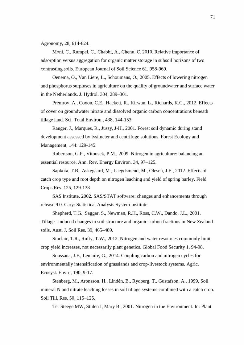
71
Agronomy, 28, 614-624.
Moni, C., Rumpel, C., Chabbi, A., Chenu, C. 2010. Relative importance of
adsorption versus aggregation for organic matter storage in subsoil horizons of two
contrasting soils. European Journal of Soil Science 61, 958-969.
Oenema, O., Van Liere, L., Schoumans, O., 2005. Effects of lowering nitrogen
and phosphorus surpluses in agriculture on the quality of groundwater and surface water
in the Netherlands. J. Hydrol. 304, 289–301.
Premrov, A., Coxon, C.E., Hackett, R., Kirwan, L., Richards, K.G., 2012. Effects
of cover on groundwater nitrate and dissolved organic carbon concentrations beneath
tillage land. Sci. Total Environ., 438, 144-153.
Ranger, J., Marques, R., Jussy, J-H., 2001. Forest soil dynamic during stand
development assessed by lysimeter and centrifuge solutions. Forest Ecology and
Management, 144: 129-145.
Robertson, G.P., Vitousek, P.M., 2009. Nitrogen in agriculture: balancing an
essential resource. Ann. Rev. Energy Environ. 34, 97–125.
Sapkota, T.B., Askegaard, M., Laegdsmend, M., Olesen, J.E., 2012. Effects of
catch crop type and root depth on nitrogen leaching and yield of spring barley. Field
Crops Res. 125, 129-138.
SAS Institute, 2002. SAS/STAT software: changes and enhancements through
release 9.0. Cary: Statistical Analysis System Institute.
Shepherd, T.G., Saggar, S., Newman, R.H., Ross, C.W., Dando, J.L., 2001.
Tillage –induced changes to soil structure and organic carbon fractions in New Zealand
soils. Aust. J. Soil Res. 39, 465–489.
Sinclair, T.R., Rufty, T.W., 2012. Nitrogen and water resources commonly limit
crop yield increases, not necessarily plant genetics. Global Food Security 1, 94-98.
Soussana, J.F., Lemaire, G., 2014. Coupling carbon and nitrogen cycles for
environmentally intensification of grasslands and crop-livestock systems. Agric.
Ecosyst. Envir., 190, 9-17.
Stenberg, M., Aronsson, H., Lindén, B., Rydberg, T., Gustafson, A., 1999. Soil
mineral N and nitrate leaching losses in soil tillage systems combined with a catch crop.
Soil Till. Res. 50, 115–125.
Ter Steege MW, Stulen I, Mary B., 2001. Nitrogen in the Environment. In: Plant
72
Nitrogen, P.J. Lea & J.F. Morot-Gaudry eds, INRA-Springer ISBN3-540-67799-2, 379-
397.
Tilman, D., Cassman, K.G., Pamela, A., Matson, P.A., Naylor, R., Polasky, S.,
2002. Agricultural sustainability and intensive production practices. Nature Biotech.
418, 671-677.
Tlustos, P., Willison, T.W., Baker, J.C., Murphy, D.V., Pavlikova, D., Goulding,
K.W.T., Powlson, D.S., 1998. Short-term effects of nitrogen on methane oxidation in
soils. Biol. Fert. Soils, 28, 64-70.
Torstensson, G., Aronsson, H., 2000. Nitrogen leaching and crop availability in
manured catch crop systems in Sweden. Nutr. Cycl. Agroecosyst. 56, 139–152.
Townsend, A.R., Howarth, R.W., Bazzaz, F.A., Booth, M.S., Cleveland, C.C.,
Collinge, S.K., Dobson, A.P., Epstein, P.R., Holland, E.A., Keeny, D.R., Mallin, M.A.,
Rogers, C.A., Wayne, P., Wolfe, A.H., 2003. Human health effects of a changing global
nitrogen cycle. Frontiers Ecol. Environ. 5, 240–246.
Vertès, F., Simon, J.C., Laurent, F., Besnard, A., 2007. Prairies et qualité de l’eau.
Evaluation des risques de lixivixtion d’azote et optimisation des pratiques. Fourrages,
192, 423-440.
Vries, J.J, Simmers, I., 2002. Groundwater recharge: an overview of processes
and challenges. Hydrogeology, 10, 5-17.
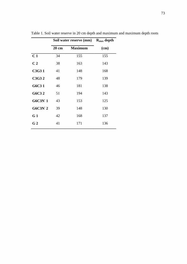
73
Table 1. Soil water reserve in 20 cm depth and maximum and maximum depth roots
Soil water reserve (mm) Rmax depth
20 cm Maximum (cm)
C 1 34 155 155
C 2 38 163 143
C3G3 1 41 148 168
C3G3 2 48 179 139
G6C3 1 46 181 138
G6C3 2 51 194 143
G6C3N- 1 43 153 125
G6C3N- 2 39 148 130
G 1 42 168 137
G 2 41 171 136
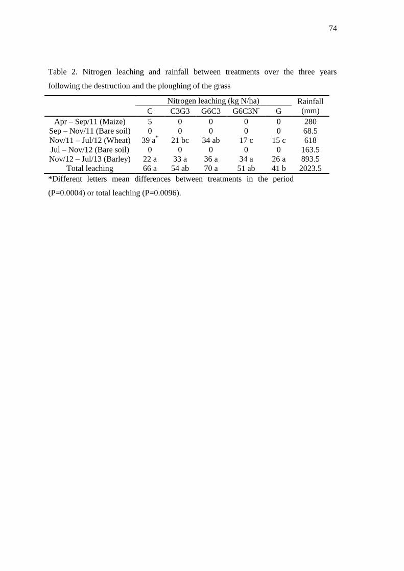
74
Table 2. Nitrogen leaching and rainfall between treatments over the three years
following the destruction and the ploughing of the grass
Nitrogen leaching (kg N/ha) Rainfall
(mm) C C3G3 G6C3 G6C3N- G
Apr – Sep/11 (Maize) 5 0 0 0 0 280
Sep – Nov/11 (Bare soil) 0 0 0 0 0 68.5
Nov/11 – Jul/12 (Wheat) 39 a* 21 bc 34 ab 17 c 15 c 618
Jul – Nov/12 (Bare soil) 0 0 0 0 0 163.5
Nov/12 – Jul/13 (Barley) 22 a 33 a 36 a 34 a 26 a 893.5
Total leaching 66 a 54 ab 70 a 51 ab 41 b 2023.5
*Different letters mean differences between treatments in the period
(P=0.0004) or total leaching (P=0.0096).
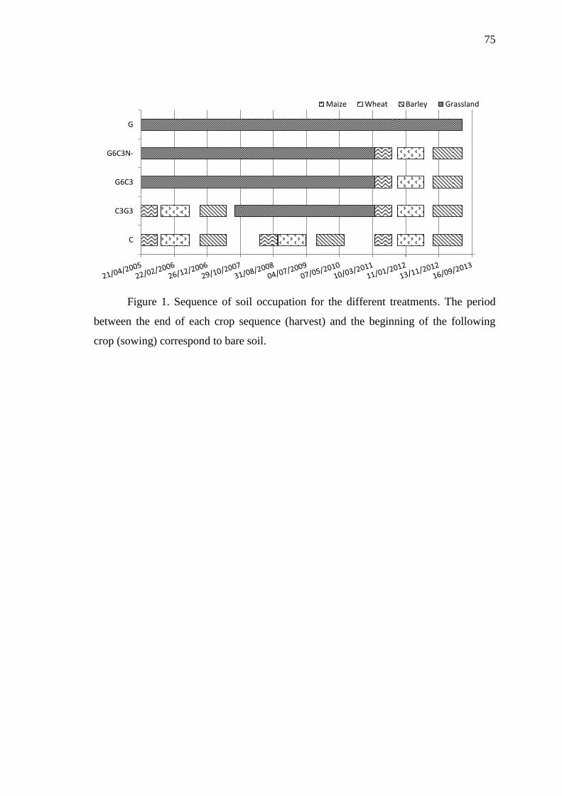
75
Figure 1. Sequence of soil occupation for the different treatments. The period
between the end of each crop sequence (harvest) and the beginning of the following
crop (sowing) correspond to bare soil.
00/01/0005/11/0011/09/0118/07/0224/05/0329/03/0402/02/0509/12/0515/10/0621/08/0726/06/08
C
C3G3
G6C3
G6C3N-
G
Maize Wheat Barley Grassland
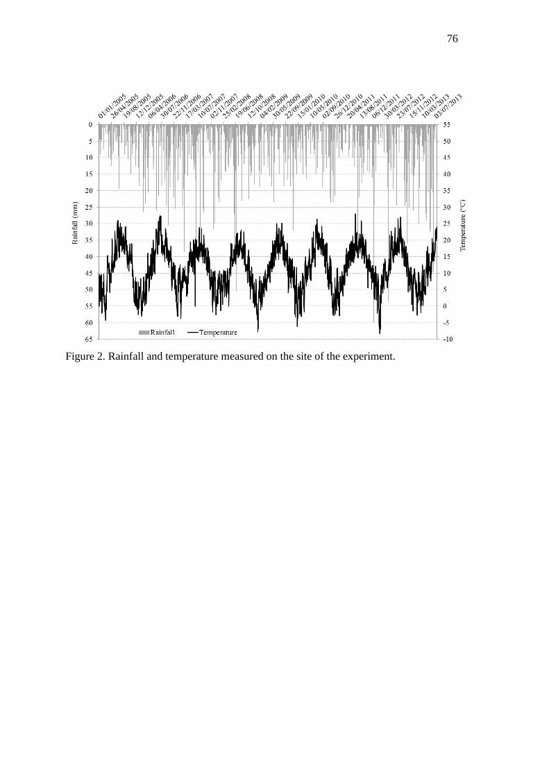
76
Figure 2. Rainfall and temperature measured on the site of the experiment.
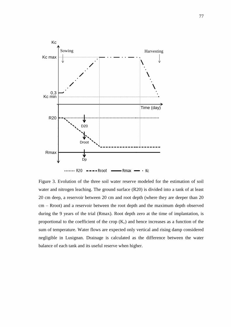
77
Figure 3. Evolution of the three soil water reserve modeled for the estimation of soil
water and nitrogen leaching. The ground surface (R20) is divided into a tank of at least
20 cm deep, a reservoir between 20 cm and root depth (where they are deeper than 20
cm – Rroot) and a reservoir between the root depth and the maximum depth observed
during the 9 years of the trial (Rmax). Root depth zero at the time of implantation, is
proportional to the coefficient of the crop (Kc) and hence increases as a function of the
sum of temperature. Water flows are expected only vertical and rising damp considered
negligible in Lusignan. Drainage is calculated as the difference between the water
balance of each tank and its useful reserve when higher.
-140
-120
-100
-80
-60
-40
-20
0
Time (day)
Kc max
Kc min0.3
R20
Rmax
D20
Kc
Dp
Droot
Sowing Harvesting
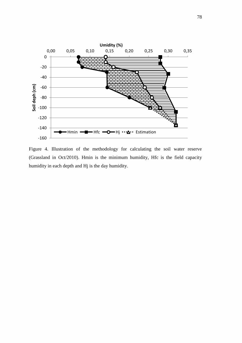
78
Figure 4. Illustration of the methodology for calculating the soil water reserve
(Grassland in Oct/2010). Hmin is the minimum humidity, Hfc is the field capacity
humidity in each depth and Hj is the day humidity.
-160
-140
-120
-100
-80
-60
-40
-20
0
0,00 0,05 0,10 0,15 0,20 0,25 0,30 0,35
Soil
dep
h (
cm)
Umidity (%)
Hmin Hfc Hj Estimation

79
Figure 5. Comparison of soil water reserve evolution for the five treatments over the 9
years.
-180
-160
-140
-120
-100
-80
-60
-40
-20
0
So
il d
essi
cca
tio
n (
mm
)
C C3G3 G6C3 G6C3N- G
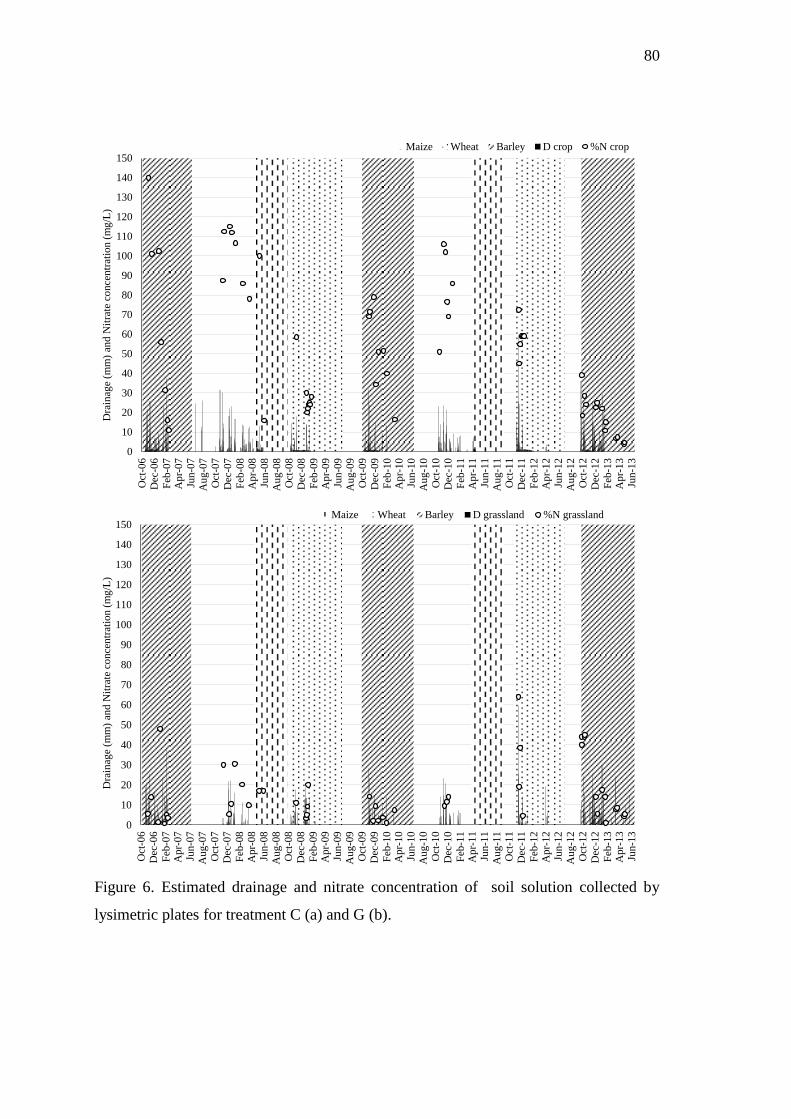
80
Figure 6. Estimated drainage and nitrate concentration of soil solution collected by
lysimetric plates for treatment C (a) and G (b).
0
10
20
30
40
50
60
70
80
90
100
110
120
130
140
150
Oct
-06
Dec
-06
Feb
-07
Ap
r-0
7Ju
n-0
7A
ug-0
7O
ct-0
7D
ec-0
7
Feb
-08
Ap
r-0
8Ju
n-0
8A
ug-0
8O
ct-0
8D
ec-0
8
Feb
-09
Ap
r-0
9Ju
n-0
9A
ug-0
9O
ct-0
9D
ec-0
9
Feb
-10
Ap
r-1
0Ju
n-1
0A
ug-1
0O
ct-1
0D
ec-1
0
Feb
-11
Ap
r-1
1Ju
n-1
1A
ug-1
1O
ct-1
1D
ec-1
1
Feb
-12
Ap
r-1
2Ju
n-1
2A
ug-1
2O
ct-1
2D
ec-1
2
Feb
-13
Ap
r-1
3Ju
n-1
3
Dra
inag
e (m
m)
and
Nit
rate
co
nce
ntr
atio
n (
mg
/L)
Maize Wheat Barley D crop %N crop
0
10
20
30
40
50
60
70
80
90
100
110
120
130
140
150
Oct
-06
Dec
-06
Feb
-07
Ap
r-0
7Ju
n-0
7A
ug-0
7O
ct-0
7D
ec-0
7
Feb
-08
Ap
r-0
8Ju
n-0
8A
ug-0
8O
ct-0
8D
ec-0
8
Feb
-09
Ap
r-0
9Ju
n-0
9A
ug-0
9O
ct-0
9D
ec-0
9
Feb
-10
Ap
r-1
0Ju
n-1
0A
ug-1
0O
ct-1
0D
ec-1
0
Feb
-11
Ap
r-1
1Ju
n-1
1A
ug-1
1O
ct-1
1D
ec-1
1
Feb
-12
Ap
r-1
2Ju
n-1
2A
ug-1
2O
ct-1
2D
ec-1
2
Feb
-13
Ap
r-1
3Ju
n-1
3
Dra
inag
e (m
m)
and
Nit
rate
co
nce
ntr
atio
n (
mg
/L)
Maize Wheat Barley D grassland %N grassland
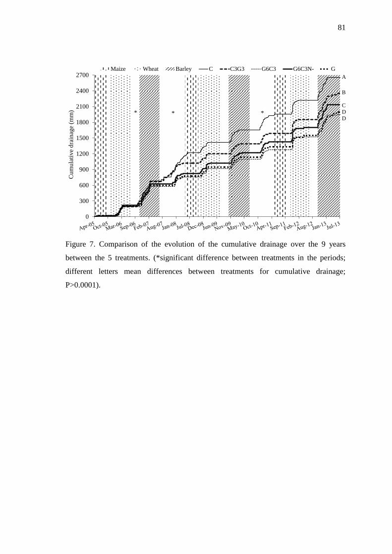
81
Figure 7. Comparison of the evolution of the cumulative drainage over the 9 years
between the 5 treatments. (*significant difference between treatments in the periods;
different letters mean differences between treatments for cumulative drainage;
P>0.0001).
0
300
600
900
1200
1500
1800
2100
2400
2700C
um
ula
tive
dra
inag
e (m
m)
Maize Wheat Barley C C3G3 G6C3 G6C3N- G
* * *
A
B
C
D
D

82
Figure 8. Comparison of the evolution of the cumulative nitrogen leaching between the
5 treatments over the 9 years. (*significant difference between treatments in the periods;
different letters mean differences between treatments for cumulative nitrogen leaching;
P>0.0001).
0
50
100
150
200
250
300
350
Cu
mu
lati
ve
nit
rog
en l
each
ing
(k
g N
/ha
)
Maize Wheat Barley C C3G3 G6C3 G6C3 N- G
A
B
C
C
C
** * * ***
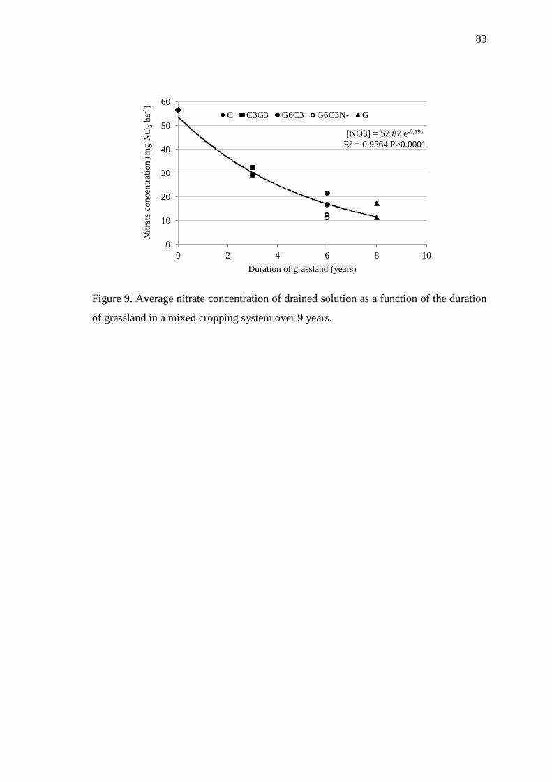
83
Figure 9. Average nitrate concentration of drained solution as a function of the duration
of grassland in a mixed cropping system over 9 years.
[NO3] = 52.87 e-0,19x
R² = 0.9564 P>0.0001
0
10
20
30
40
50
60
0 2 4 6 8 10
Nit
rate
co
nce
ntr
atio
n (
mg N
O3
ha-1
)
Duration of grassland (years)
C C3G3 G6C3 G6C3N- G
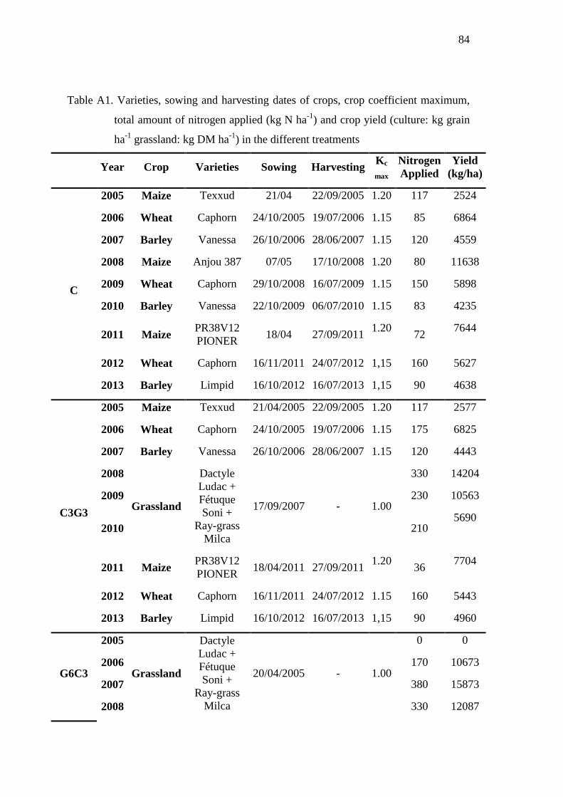
84
Table A1. Varieties, sowing and harvesting dates of crops, crop coefficient maximum,
total amount of nitrogen applied (kg N ha-1
) and crop yield (culture: kg grain
ha-1
grassland: kg DM ha-1
) in the different treatments
Year Crop Varieties Sowing Harvesting Kc
max
Nitrogen
Applied
Yield
(kg/ha)
C
2005 Maize Texxud 21/04 22/09/2005 1.20 117 2524
2006 Wheat Caphorn 24/10/2005 19/07/2006 1.15 85 6864
2007 Barley Vanessa 26/10/2006 28/06/2007 1.15 120 4559
2008 Maize Anjou 387 07/05 17/10/2008 1.20 80 11638
2009 Wheat Caphorn 29/10/2008 16/07/2009 1.15 150 5898
2010 Barley Vanessa 22/10/2009 06/07/2010 1.15 83 4235
2011 Maize PR38V12
PIONER 18/04 27/09/2011
1.20 72
7644
2012 Wheat Caphorn 16/11/2011 24/07/2012 1,15 160 5627
2013 Barley Limpid 16/10/2012 16/07/2013 1,15 90 4638
C3G3
2005 Maize Texxud 21/04/2005 22/09/2005 1.20 117 2577
2006 Wheat Caphorn 24/10/2005 19/07/2006 1.15 175 6825
2007 Barley Vanessa 26/10/2006 28/06/2007 1.15 120 4443
2008
Grassland
Dactyle
Ludac +
Fétuque
Soni +
Ray-grass
Milca
17/09/2007 - 1.00
330 14204
2009 230 10563
2010 210 5690
2011 Maize PR38V12
PIONER 18/04/2011 27/09/2011
1.20 36
7704
2012 Wheat Caphorn 16/11/2011 24/07/2012 1.15 160 5443
2013 Barley Limpid 16/10/2012 16/07/2013 1,15 90 4960
G6C3
2005
Grassland
Dactyle
Ludac +
Fétuque
Soni +
Ray-grass
Milca
20/04/2005 - 1.00
0 0
2006 170 10673
2007 380 15873
2008 330 12087
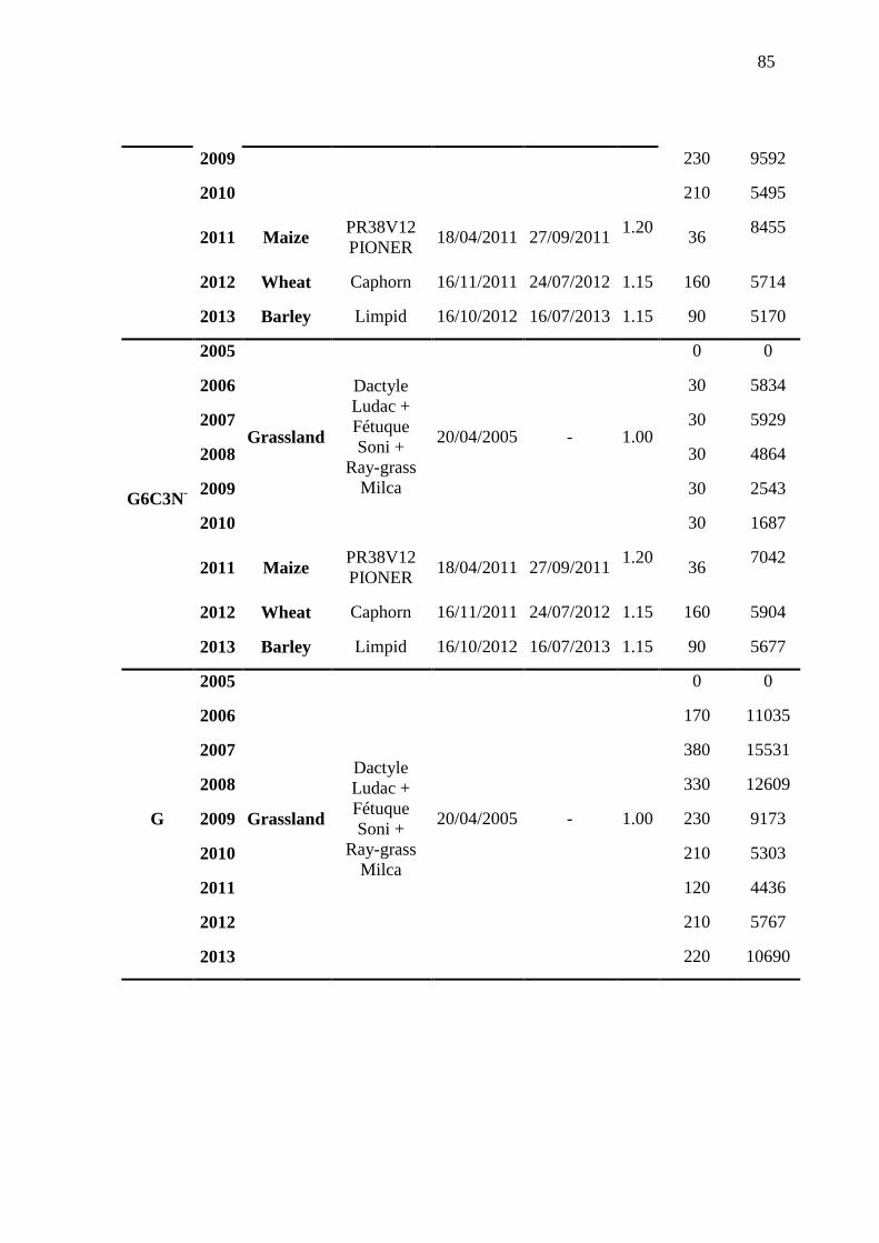
85
2009 230 9592
2010 210 5495
2011 Maize PR38V12
PIONER 18/04/2011 27/09/2011
1.20 36
8455
2012 Wheat Caphorn 16/11/2011 24/07/2012 1.15 160 5714
2013 Barley Limpid 16/10/2012 16/07/2013 1.15 90 5170
G6C3N-
2005
Grassland
Dactyle
Ludac +
Fétuque
Soni +
Ray-grass
Milca
20/04/2005 - 1.00
0 0
2006 30 5834
2007 30 5929
2008 30 4864
2009 30 2543
2010 30 1687
2011 Maize PR38V12
PIONER 18/04/2011 27/09/2011
1.20 36
7042
2012 Wheat Caphorn 16/11/2011 24/07/2012 1.15 160 5904
2013 Barley Limpid 16/10/2012 16/07/2013 1.15 90 5677
G
2005
Grassland
Dactyle
Ludac +
Fétuque
Soni +
Ray-grass
Milca
20/04/2005 - 1.00
0 0
2006 170 11035
2007 380 15531
2008 330 12609
2009 230 9173
2010 210 5303
2011 120 4436
2012 210 5767
2013 220 10690
4. CAPÍTULO IV
4.1 Conclusões gerais
4.2 Referências bibliográficas
89
4.1 CONCLUSÕES GERAIS
Utilizando-se 10 anos de dados de um sistema integrado de
produção agropecuária foi possível detectar padrões de comportamento nas relações entre as variáveis de pasto e animal, mesmo existindo influencia dos anos avaliados. Para se atingir ganhos satisfatórios na produção animal, sem afetar negativamente outros parâmetros do sistema, sugerimos que o manejo seja feito mantendo-se o pasto com 30 cm de altura.
Na condição de solo e clima do Centro-Oeste da França, a introdução de pastagem na rotação de culturas diminui a concentração de nitrato na água drenada. A redução nas perdas de nitrogênio é proporcional ao tempo de permanência da pastagem na rotação. A destruição de pastagens por aração e o cultivo com culturas de grãos não aumentam a lixiviação de nitrogênio. Porém, em regiões onde a disponibilidade de água depende fortemente de recarga de aquíferos no inverno, deve-se fazer um balanço entre a vantagem da introdução de pastagens no sistema de cultivo, que melhora a qualidade da água drenada e da possível desvantagem associada a uma redução no volume da água drenada.
90
4.2 REFERÊNCIAS BIBLIOGRÁFICAS
ADDISCOTT, T. M.; WHITMORE, A. P.; POWLSON, D. S. Farming, Fertilizers and the Nitrate Problem. Wallingford: CAB International, 1991. 170 p.
ANGHINONI, I. et al. Benefícios da integração lavoura-pecuária sobre a fertilidade do solo em sistema plantio-direto. In: FONSECA, A.; CAIRES, E. F.; BARTZ, G. (Eds.). Fertilidade do solo e nutrição de plantas no sistema plantio direto. Ponta Grossa: Fundação ABC, 2011. p.272-309.
BARTHRAM, G. T. Experimental techniques: the HFRO sward stick. In: Hill farming research. Edinburgh: HFRO, 1985. p.29-30. (Organisation Biennial Report 1984–85)
CQFS-RS/SC – COMISSÃO DE QUÍMICA E FERTILIDADE DO SOLO - RS/SC. Manual de adubação e calagem para os Estados do Rio Grande do Sul e Santa Catarina. Porto Alegre: SBCS-NRS/EMBRAPA-CNPT, 2004. 400 p.
CUTTLE, S. P.; SCHOLEFIELD, D. Management options to limit nitrate leaching from grassland. Journal of Contaminant Hydrology, Amsterdam, v. 20, n. 3-4, p. 299–312, 1995.
DABNEY, S. M. et al. Using cover crops and cropping systems for nitrogen management. In: DELGADO, J.A., FOLLETT, R.F. (Ed.). Advances in Nitrogen Management for Water Quality. Ankeny: Soil and Water Conservation Society, 2011. p. 230–281.
DATTA, P. S., DEB, D. L., TYAGI, S. K. Assessment of groundwater contamination from fertilizers in the Delhi area based on 18O, NO3 and K+ composition. Journal of Contaminant Hydrology, Amsterdam, v. 27, n. 3-4, p. 249–262, 1997.
FRANZLUEBBERS, A. J. Integrated crop–livestock systems in the southeastern USA. Agronomy Journal, Madison, v. 99, n. 2, p. 361-372, 2007.
GUILLEMIN, C.; ROUX, J. C. Pollution des eaux souterraines en France. Paris: Editions du BRGM, 1992. 175 p.
GUSTAFSON, A. Leaching of nitrate from arable land into groundwater in Sweden. Environmental Geology, Uppsala, v. 5, n. 2, p.65–71, 1983.
HOPKINS, A.; HOLZ, B. Grassland for agriculture and nature conservation : production, quality and multi-functionality. Agronomy Research, Saku, Estonia, v. 4, n. 1, p. 3–20, 2006.
HUMPHREYS, L. R. Tropical forages: their role in sustainable agriculture. Harlow: Longman Scientific & Technical, 1994. 414p.
91
JÉGO, G.; SÁNCHEZ-PÉREZ, J. M.; JUSTES, E. Predicting soil water and mineral nitrogen contents with the STICS model for estimating nitrate leaching under agricultural fields. Agricultural Water Management, Amsterdam, v. 107, p. 54–65, 2012.
KASPAR, T. C. et al. Rye cover crop and gamagrass strip effects on NO3 concentration and load in tile drainage. Journal of Environmental Quality, Madison, v. 36, n. 5, p. 1503–1511, 2007.
KASPAR, T. C. et al. Effectiveness of oat and rye cover crops in reducing nitrate losses in drainage water. Agricultural Water Management, Amsterdam, v. 110, p. 25–33, 2012.
KASPAR, T. C.; SINGER, J. W. The use of cover crops to manage soil. In: HATFIELD, J.L., SAUER, T.J. (Ed.), Soil Management: building a stable base for agriculture. Madison: Am. Soc. Agron. Soil Sci. Soc. Am., 2011. p. 321–337.
KOPÁČEK, J.; HEJZLAR, J.; POSCH, M. Factors controlling the export of nitrogen from agricultural land in a large central European catchment during 1900-2010. Environmental Science & Technology, Washington DC, v. 47, n. 12, p. 6400–6407, 2013.
KVÍTEK, T. et al. Changes of nitrate concentrations in surface waters influenced by land use in the crystalline complex of the Czech Republic. Physics and Chemistry of the Earth, Oxford, v. 34, n. 8, p. 541–551, 2009.
LEMAIRE, G. et al. Integrated crop–livestock systems: Strategies to achieve synergy between agricultural production and environmental quality. Agriculture, Ecosystems & Environment, Amsterdam, v. 190, p. 4–8, 2014.
LEMAIRE, G.; HODGSON, J.; CHABBI, A. Food security and environmental impacts—challenge for grassland sciences. In: LEMAIRE, G., HODGSON, J., CHABBI, A. (Ed.). Grassland Productivity and Ecosystem Services. Wallingford: CAB International, 2011. p. xii- xvii.
LEMAIRE, G.; WILKINS, R.; HODGSON, J. Challenge for grassland science: Managing research priorities. Agriculture, Ecosystems & Environment, Amsterdam, v. 108, p. 99–108, 2005.
LERNER D. N. Groundwater recharge. In: Saether OM, de Caritat P. (eds) Geochemical processes, weathering and groundwater recharge in catchments. AA Balkema, Rotterdam, 1997. pp 109–150.
LERNER, D. N.; ISSAR, A. S.; SIMMERS, I. Groundwater recharge. A guide to understanding and estimating natural recharge. Hannover: Int. Contrib. Hydrogeol., 1990. 345 p.
MOHAMED SALLEN, M. A.; FISHER, M.J. Role of ley farming in crop rotations in the tropics. In: INTERNATIONAL GRASSLAND CONGRESS, 17., 1993, Rockhampton. Proceedings. Rockhampton, 1993. p. 2179-2187.
92
MORAES, A. et al. Integrated crop – livestock systems in the Brazilian subtropics. European Journal of Agronomy, Amsterdam, v. 57, p. 4–9, 2014.
NEILL, M. Nitrate concentrations in river waters in the south-east of Ireland and their relationship with agricultural practice. Water Research, Oxford, v. 23, n. 11, p. 1339–1355, 1989.
OENEMA, O.; VAN LIERE, L.; SCHOUMANS, O. Effects of lowering nitrogen and phosphorus surpluses in agriculture on the quality of groundwater and surface water in the Netherlands. Journal of Hydrology, Amsterdam, v. 304, n. 3, p. 289–301, 2005.
PEDERSEN, A.; THORUP-KRISTENSEN, K.; JENSEN, L. S. Simulating nitrate retention in soils and the effect of catch crop use and rooting pattern under the climatic conditions of Northern Europe. Soil Use and Management, Oxford, v. 25, p. 243–254, 2009.
PREMROV, A. et al. Effects of cover on groundwater nitrate and dissolved organic carbon concentrations beneath tillage land. Science of the Total Environment, Amsterdam, v. 438, p. 144-153, 2012.
SAPKOTA, T. B. et al. Effects of catch crop type and root depth on nitrogen leaching and yield of spring barley. Field Crops Research., Amsterdam, v. 125, p. 129-138, 2012.
SHEPHERD, T. G. et al. L. Tillage –induced changes to soil structure and organic carbon fractions in New Zealand soils. Australian Journal of the Soil Research, Lismore, v. 39, n. 3, p. 465–489, 2001.
STEINER, J. L.; FRANZLUEBBERS, A. J. Farming with grass—for people, for profit, for production, for protection. Journal of Soil and Water Conservation, Ankeny, v. 64, n. 2, p. 75A–80A, 2009.
STREBEL, O.; DUYNISVELD, W. H. M.; BÖTTCHER, J. Nitrate pollution of ground water in western Europe. Agriculture, Ecosystems & Environment, Amsterdam, v. 26, n. 3-4, p. 189–214, 1989.
TONITTO, C.; DAVID, M. B.; DRINKWATER, L. E. Replacing bare fallows with cover crops in fertilizer-intensive cropping systems: ameta-analysis of crop yield and N dynamics. Agriculture, Ecosystems & Environment, Amsterdam, v. 112, n. 1, p. 58–72, 2006.
TOWNSEND, A. R. et al. Human health effects of a changing global nitrogen cycle. Frontiers in Ecology and the Environment, Washington DC, v. 1, n. 5, p. 240–246, 2003.
VRIES, J. J; SIMMERS, I. Groundwater recharge: an overview of processes and challenges. Hydrogeology, Hannover, v. 10, n. 1, p. 5-17, 2002.
WHITEHEAD, D. C. Grassland Nitrogen. Wallingford: CABI Publishing, 1995.

93
368p.
ZHU, C. J. et al. Runoff, soil, and dissolved nutrient losses from no-till soybean with winter cover crops. Soil Science Society of America Journal, Madison, v. 53, p. 1210-1214, 1989.

5. APÊNDICES

97
Apêndice 1. Normas utilizadas para escrever o Capítulo II.

98
Apêndice 1 (cont.). Normas utilizadas para escrever o Capítulo II.
99
Apêndice 1 (cont.). Normas utilizadas para escrever o Capítulo II.
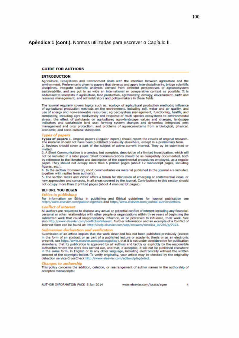
100
Apêndice 1 (cont.). Normas utilizadas para escrever o Capítulo II.
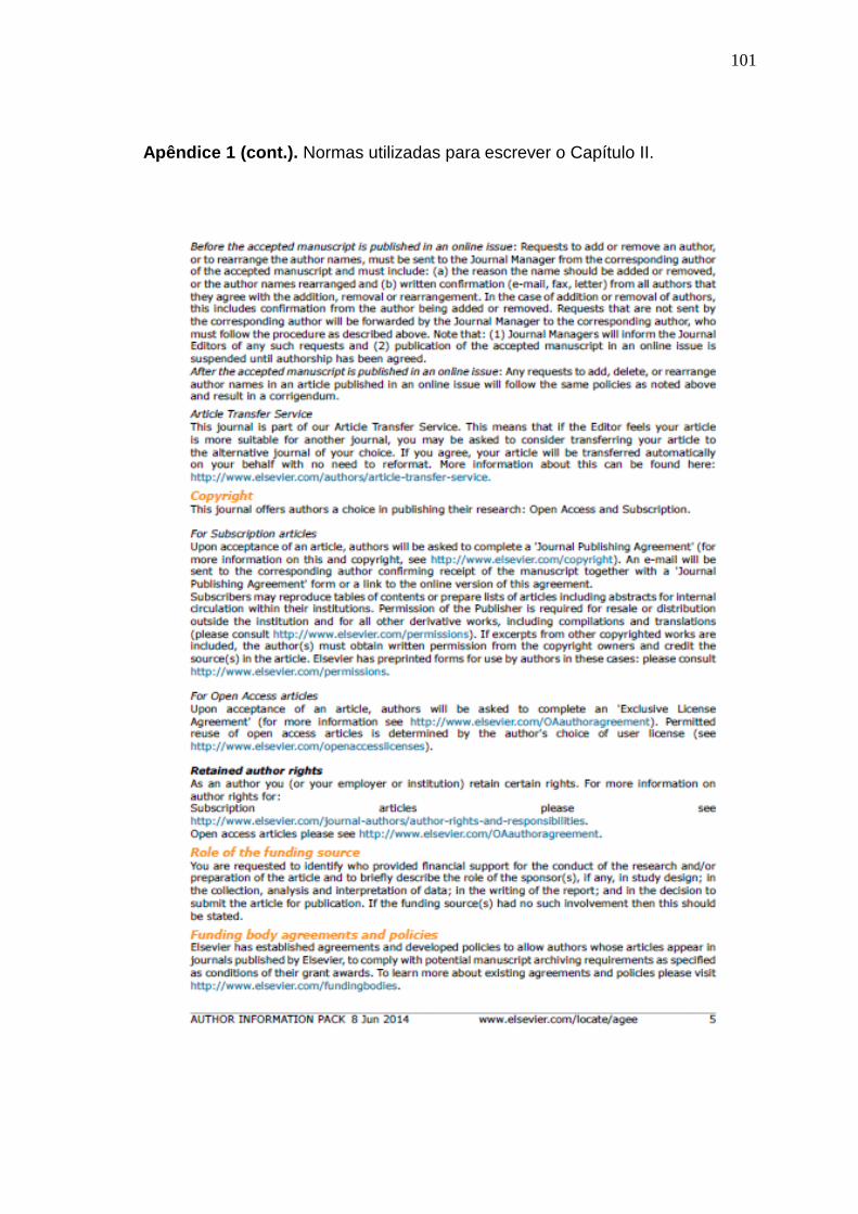
101
Apêndice 1 (cont.). Normas utilizadas para escrever o Capítulo II.
102
Apêndice 1 (cont.). Normas utilizadas para escrever o Capítulo II.
103
Apêndice 1 (cont.). Normas utilizadas para escrever o Capítulo II.
104
Apêndice 1 (cont.). Normas utilizadas para escrever o Capítulo II.
105
Apêndice 1 (cont.). Normas utilizadas para escrever o Capítulo II.
106
Apêndice 1 (cont.). Normas utilizadas para escrever o Capítulo II.
107
Apêndice 1 (cont.). Normas utilizadas para escrever o Capítulo II.
108
Apêndice 1 (cont.). Normas utilizadas para escrever o Capítulo II.
109
Apêndice 2 (cont.). Normas utilizadas para escrever o Capítulo III.

110
Apêndice 2 (cont.). Normas utilizadas para escrever o Capítulo III.
111
Apêndice 2 (cont.). Normas utilizadas para escrever o Capítulo III.

112
Apêndice 2 (cont.). Normas utilizadas para escrever o Capítulo III.
113
Apêndice 2 (cont.). Normas utilizadas para escrever o Capítulo III.
114
Apêndice 2 (cont.). Normas utilizadas para escrever o Capítulo III.
115
Apêndice 2 (cont.). Normas utilizadas para escrever o Capítulo III.
116
Apêndice 2 (cont.). Normas utilizadas para escrever o Capítulo III.

117
Apêndice 2 (cont.). Normas utilizadas para escrever o Capítulo III.
118
Apêndice 2 (cont.). Normas utilizadas para escrever o Capítulo III.
119
Apêndice 2 (cont.). Normas utilizadas para escrever o Capítulo III.
120
Apêndice 2 (cont.). Normas utilizadas para escrever o Capítulo III.

121
Apêndice 2 (cont.). Normas utilizadas para escrever o Capítulo III.
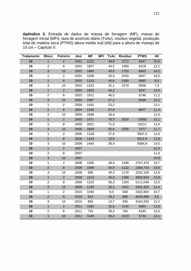
122
Apêndice 3. Entrada de dados de massa de forragem (MF), massa de forragem inicial (MFI), taxa de acúmulo diário (TxAc), resíduo vegetal, produção total de matéria seca (PTMS) altura média real (Alt) para a altura de manejo de 10 cm – Capítulo II. Tratamento Bloco Potreiro Ano MF MFI TxAc Resíduo PTMS Alt
10 1 2 2001 1222 48,8 1272 6947 10,0
10 2 8 2001 1827 44,2 1480 6219 12,1
10 3 10 2001 1883 45,6 1750 6683 14,2
10 1 2 2002 1508 33,9 2030 5847 10,5
10 2 8 2002 1153 40,8 1580 6680 8,4
10 3 10 2002 1322 31,1 1570 5658 7,3
10 1 2 2003 1826 64,2 9247 15,6
10 2 8 2003 1911 46,5 8746 11,2
10 3 10 2003 1967 57,2 9438 15,2
10 1 2 2004 1491 23,2 13,1
10 2 8 2004 1336 57,6 8877 11,4
10 3 10 2004 1698 43,4 12,4
10 1 2 2005 1971 70,3 2520 10050 12,1
10 2 8 2005 2021 71,5 10211 12,4
10 3 10 2005 1828 50,6 2205 7377 11,7
10 1 2 2006 1128 37,6 5907,5 13,3
10 2 8 2006 1162 33,6 5511,8 11,8
10 3 10 2006 1443 36,4 6084,8 14,5
10 1 2 2007 12,4
10 2 8 2007 11,4
10 3 10 2007 10,8
10 1 2 2008 1305 48,4 1406 2707,476 15,7
10 2 8 2008 1086 54,6 1132 2364,743 13,6
10 3 10 2008 999 49,2 1178 2252,169 12,9
10 1 2 2009 1215 34,4 1386 4843,654 12,9
10 2 8 2009 1223 36,3 1264 5111,046 13,0
10 3 10 2009 1140 30,2 1341 4331,845 11,4
10 1 2 2010 1040 9,0 606 2332,804 10,7
10 2 8 2010 823 29,1 896 4629,999 9,5
10 3 10 2010 893 13,7 935 3164,292 12,2
10 1 2 2011 1082 35,6 1134 5083 12,6
10 2 8 2011 725 28,3 783 4193 10,0
10 3 10 2011 1040 36,4 1023 5733 13,1

123
Apêndice 4. Entrada de dados de ganho médio diário individual (GMD), ganho por área (Gha) e carga animal (CA) para a altura de manejo de 10 cm – Capítulo II.
Tratamento Bloco Potreiro Ano GMD Gha CA
10 1 2 2001 0,849 481 1382
10 2 8 2001 0,840 488 1467
10 3 10 2001 0,994 472 1229
10 1 2 2002 0,848 513 1168
10 2 8 2002 0,981 619 1254
10 3 10 2002 0,921 491 1159
10 1 2 2003 0,810 539 1422
10 2 8 2003 463
10 3 10 2003 0,900 618 1703
10 1 2 2004 0,865 554 1296
10 2 8 2004 446 1276
10 3 10 2004 0,835 590 1268
10 1 2 2005 0,996 501 988
10 2 8 2005 0,868 572 1090
10 3 10 2005 1,018 471 1173
10 1 2 2006 0,880 616 1392
10 2 8 2006 0,700 566 1647
10 3 10 2006 0,710 654 1255
10 1 2 2007 0,822 470 1171
10 2 8 2007 344 1361
10 3 10 2007 0,743 471 1099
10 1 2 2008 0,760 469 1269
10 2 8 2008 0,689 490 1484
10 3 10 2008 0,770 525 1407
10 1 2 2009 0,848 483 1370
10 2 8 2009 0,730 491 1525
10 3 10 2009 0,908 614 1580
10 1 2 2010 0,768 324 1079
10 2 8 2010 1159
10 3 10 2010 0,734 388 1309
10 1 2 2011 479 818
10 2 8 2011 0,944 414 970
10 3 10 2011 0,980 484 917

124
Apêndice 5. Entrada de dados de massa de forragem (MF), massa de forragem inicial (MFI), taxa de acúmulo diário (TxAc), resíduo vegetal, produção total de matéria seca (PTMS) altura média real (Alt) para a altura de manejo de 20 cm – Capítulo II. Tratamento Bloco Potreiro Ano MF MFI TxAc Resíduo PTMS Alt
20 1 4 2001 2527 39,7 4400 5668 19,6
20 2 7 2001 2922 56,2 4304 7783 21,4
20 3 9 2001 2447 46,6 1928 6480 24,3
20 1 4 2002 2162 32,5 4080 5819 16,5
20 2 7 2002 2019 40,9 3370 5565 14,6
20 3 9 2002 2296 57,8 4010 8769 18,2
20 1 4 2003 2754 74,4 11531 24,8
20 2 7 2003 2802 62,5 10458 23,5
20 3 9 2003 3048 45,6 8533 23,9
20 1 4 2004 1900 38,5 6694 18,3
20 2 7 2004 1942 62,1 9558 17,5
20 3 9 2004 1838 54,6 8179 20,5
20 1 4 2005 2744 51,7 3728 8428 20,7
20 2 7 2005 2740 15,0 5147 7337 21,2
20 3 9 2005 2737 29,8 4043 6041 20,7
20 1 4 2006 2249 27,3 5027,4 21,3
20 2 7 2006 1659 43,0 6962,5 20,2
20 3 9 2006 1827 38,4 6127,4 19,8
20 1 4 2007 21,6
20 2 7 2007 21,2
20 3 9 2007 26,6
20 1 4 2008 2295 39,9 2867 3632,814 26,3
20 2 7 2008 1733 44,6 2348 3192,068 21,3
20 3 9 2008 1765 44,8 2016 3122,741 20,1
20 1 4 2009 2022 59,5 3282 7698,791 22,0
20 2 7 2009 1850 30,0 2729 4646,443 20,6
20 3 9 2009 2076 40,1 3724 5494,497 21,5
20 1 4 2010 884 28,1 930 4847,655 15,1
20 2 7 2010 1517 22,9 1621 4313,137 18,3
20 3 9 2010 1117 15,6 2101 3350,649 17,5
20 1 4 2011 2547 50,9 2860 8841 26,7
20 2 7 2011 2103 27,7 4146 4699 24,1
20 3 9 2011 1745 47,8 2447 7509 21,3
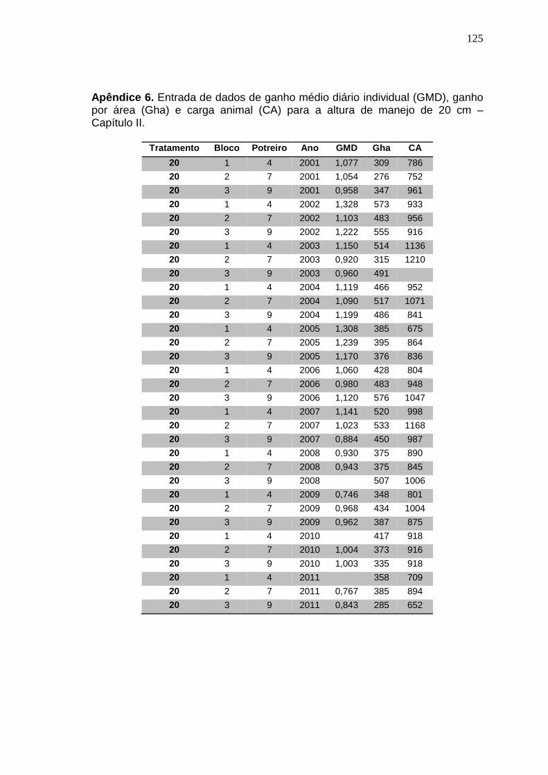
125
Apêndice 6. Entrada de dados de ganho médio diário individual (GMD), ganho por área (Gha) e carga animal (CA) para a altura de manejo de 20 cm – Capítulo II.
Tratamento Bloco Potreiro Ano GMD Gha CA
20 1 4 2001 1,077 309 786
20 2 7 2001 1,054 276 752
20 3 9 2001 0,958 347 961
20 1 4 2002 1,328 573 933
20 2 7 2002 1,103 483 956
20 3 9 2002 1,222 555 916
20 1 4 2003 1,150 514 1136
20 2 7 2003 0,920 315 1210
20 3 9 2003 0,960 491
20 1 4 2004 1,119 466 952
20 2 7 2004 1,090 517 1071
20 3 9 2004 1,199 486 841
20 1 4 2005 1,308 385 675
20 2 7 2005 1,239 395 864
20 3 9 2005 1,170 376 836
20 1 4 2006 1,060 428 804
20 2 7 2006 0,980 483 948
20 3 9 2006 1,120 576 1047
20 1 4 2007 1,141 520 998
20 2 7 2007 1,023 533 1168
20 3 9 2007 0,884 450 987
20 1 4 2008 0,930 375 890
20 2 7 2008 0,943 375 845
20 3 9 2008 507 1006
20 1 4 2009 0,746 348 801
20 2 7 2009 0,968 434 1004
20 3 9 2009 0,962 387 875
20 1 4 2010 417 918
20 2 7 2010 1,004 373 916
20 3 9 2010 1,003 335 918
20 1 4 2011 358 709
20 2 7 2011 0,767 385 894
20 3 9 2011 0,843 285 652

126
Apêndice 7. Entrada de dados de massa de forragem (MF), massa de forragem inicial (MFI), taxa de acúmulo diário (TxAc), resíduo vegetal, produção total de matéria seca (PTMS) altura média real (Alt) para a altura de manejo de 30 cm – Capítulo II. Tratamento Bloco Potreiro Ano MF MFI TxAc Resíduo PTMS Alt
30 1 3 2001 3604 60,3 6155 8283 26,6
30 2 5 2001 3710 43,3 6262 6466 24,9
30 3 11 2001 3874 54,1 6544 7240 31,4
30 1 3 2002 3040 48,4 4770 7774 27,1
30 2 5 2002 3095 50,4 5110 7719 27,0
30 3 11 2002 3177 41,3 4870 7133 27,0
30 1 3 2003 4305 38,8
30 2 5 2003 4058 56,5 9655
30 3 11 2003 4049 68,6 11200 37,8
30 1 3 2004 2745 56,0 8930 26,8
30 2 5 2004 3090 39,4 6806 29,0
30 3 11 2004 2416 48,0 7871 28,7
30 1 3 2005 3306 45,8 5555 8422 28,2
30 2 5 2005 3499 38,7 5027 8155 29,8
30 3 11 2005 3446 47,4 6740 9227 30,0
30 1 3 2006 2850 33,8 6319,2 29,8
30 2 5 2006 3021 40,6 6111,6 31,4
30 3 11 2006 3046 31,2 5403,9 30,2
30 1 3 2007 36,2
30 2 5 2007 36,4
30 3 11 2007 34,5
30 1 3 2008 2571 33,3 4584 4055,941 30,4
30 2 5 2008 3335 47,2 3497 35,0
30 3 11 2008 2487 44,6 3257 3564,528 30,8
30 1 3 2009 2716 45,5 4320 6183,535 29,7
30 2 5 2009 2741 61,9 4761 8318,922 31,1
30 3 11 2009 2663 62,0 4826 8030,188 29,1
30 1 3 2010 2130 29,6 3397 5247,186 30,6
30 2 5 2010 2509 43,7 3592 7205,18 33,2
30 3 11 2010 1632 20,7 3171 4220,685 25,7
30 1 3 2011 1911 10,0 3047 1958 25,6
30 2 5 2011 2194 59,3 3918 8661 27,5
30 3 11 2011 1647 30,9 2381 5476 23,2
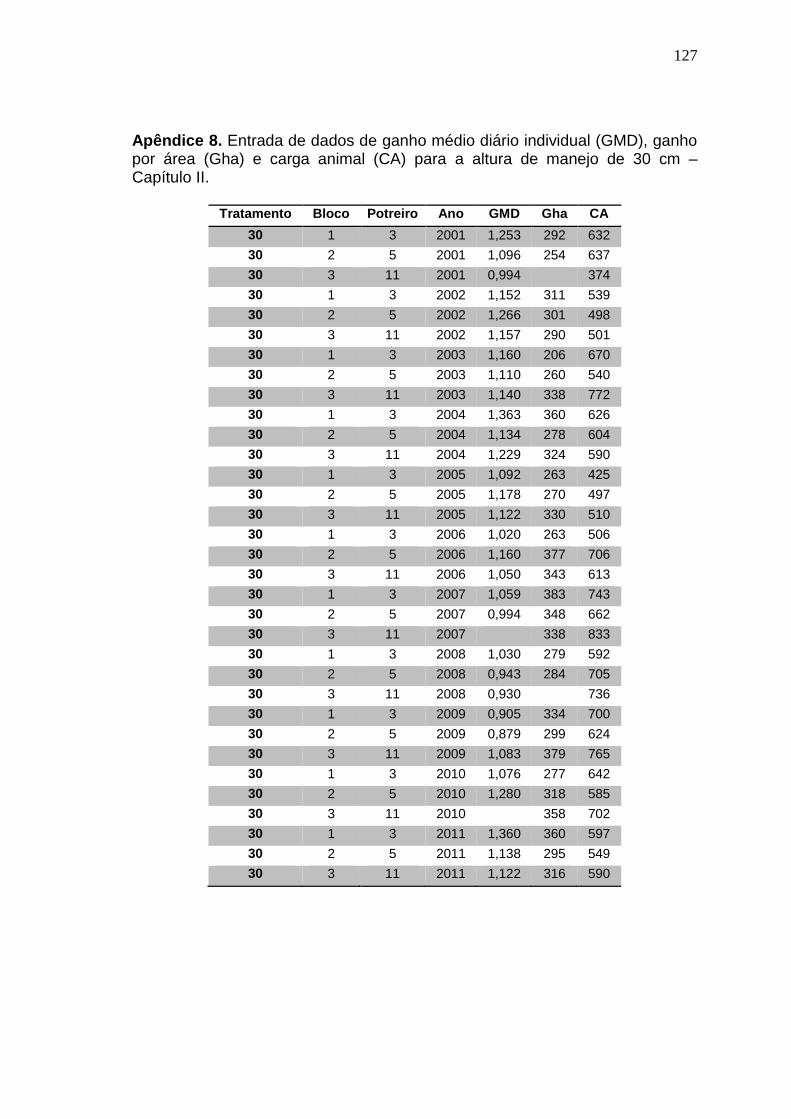
127
Apêndice 8. Entrada de dados de ganho médio diário individual (GMD), ganho por área (Gha) e carga animal (CA) para a altura de manejo de 30 cm – Capítulo II.
Tratamento Bloco Potreiro Ano GMD Gha CA
30 1 3 2001 1,253 292 632
30 2 5 2001 1,096 254 637
30 3 11 2001 0,994 374
30 1 3 2002 1,152 311 539
30 2 5 2002 1,266 301 498
30 3 11 2002 1,157 290 501
30 1 3 2003 1,160 206 670
30 2 5 2003 1,110 260 540
30 3 11 2003 1,140 338 772
30 1 3 2004 1,363 360 626
30 2 5 2004 1,134 278 604
30 3 11 2004 1,229 324 590
30 1 3 2005 1,092 263 425
30 2 5 2005 1,178 270 497
30 3 11 2005 1,122 330 510
30 1 3 2006 1,020 263 506
30 2 5 2006 1,160 377 706
30 3 11 2006 1,050 343 613
30 1 3 2007 1,059 383 743
30 2 5 2007 0,994 348 662
30 3 11 2007 338 833
30 1 3 2008 1,030 279 592
30 2 5 2008 0,943 284 705
30 3 11 2008 0,930 736
30 1 3 2009 0,905 334 700
30 2 5 2009 0,879 299 624
30 3 11 2009 1,083 379 765
30 1 3 2010 1,076 277 642
30 2 5 2010 1,280 318 585
30 3 11 2010 358 702
30 1 3 2011 1,360 360 597
30 2 5 2011 1,138 295 549
30 3 11 2011 1,122 316 590
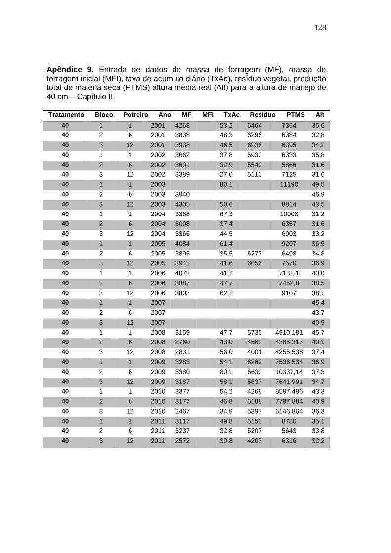
128
Apêndice 9. Entrada de dados de massa de forragem (MF), massa de forragem inicial (MFI), taxa de acúmulo diário (TxAc), resíduo vegetal, produção total de matéria seca (PTMS) altura média real (Alt) para a altura de manejo de 40 cm – Capítulo II. Tratamento Bloco Potreiro Ano MF MFI TxAc Resíduo PTMS Alt
40 1 1 2001 4268 53,2 6464 7354 35,6
40 2 6 2001 3838 48,3 6296 6384 32,8
40 3 12 2001 3938 46,5 6936 6395 34,1
40 1 1 2002 3662 37,8 5930 6333 35,8
40 2 6 2002 3601 32,9 5540 5866 31,6
40 3 12 2002 3389 27,0 5110 7125 31,6
40 1 1 2003 80,1 11190 49,5
40 2 6 2003 3940 46,9
40 3 12 2003 4305 50,6 8814 43,5
40 1 1 2004 3388 67,3 10008 31,2
40 2 6 2004 3008 37,4 6357 31,6
40 3 12 2004 3366 44,5 6903 33,2
40 1 1 2005 4084 61,4 9207 36,5
40 2 6 2005 3895 35,5 6277 6498 34,8
40 3 12 2005 3942 41,6 6056 7570 36,9
40 1 1 2006 4072 41,1 7131,1 40,0
40 2 6 2006 3887 47,7 7452,8 38,5
40 3 12 2006 3803 62,1 9107 38,1
40 1 1 2007 45,4
40 2 6 2007 43,7
40 3 12 2007 40,9
40 1 1 2008 3159 47,7 5735 4910,181 45,7
40 2 6 2008 2760 43,0 4560 4385,317 40,1
40 3 12 2008 2831 56,0 4001 4255,538 37,4
40 1 1 2009 3283 54,1 6269 7536,534 36,9
40 2 6 2009 3380 80,1 6630 10337,14 37,3
40 3 12 2009 3187 58,1 5837 7641,991 34,7
40 1 1 2010 3377 54,2 4268 8597,496 43,3
40 2 6 2010 3177 46,8 5188 7797,884 40,9
40 3 12 2010 2467 34,9 5397 6146,864 36,3
40 1 1 2011 3117 49,8 5150 8780 35,1
40 2 6 2011 3237 32,8 5207 5643 33,8
40 3 12 2011 2572 39,8 4207 6316 32,2
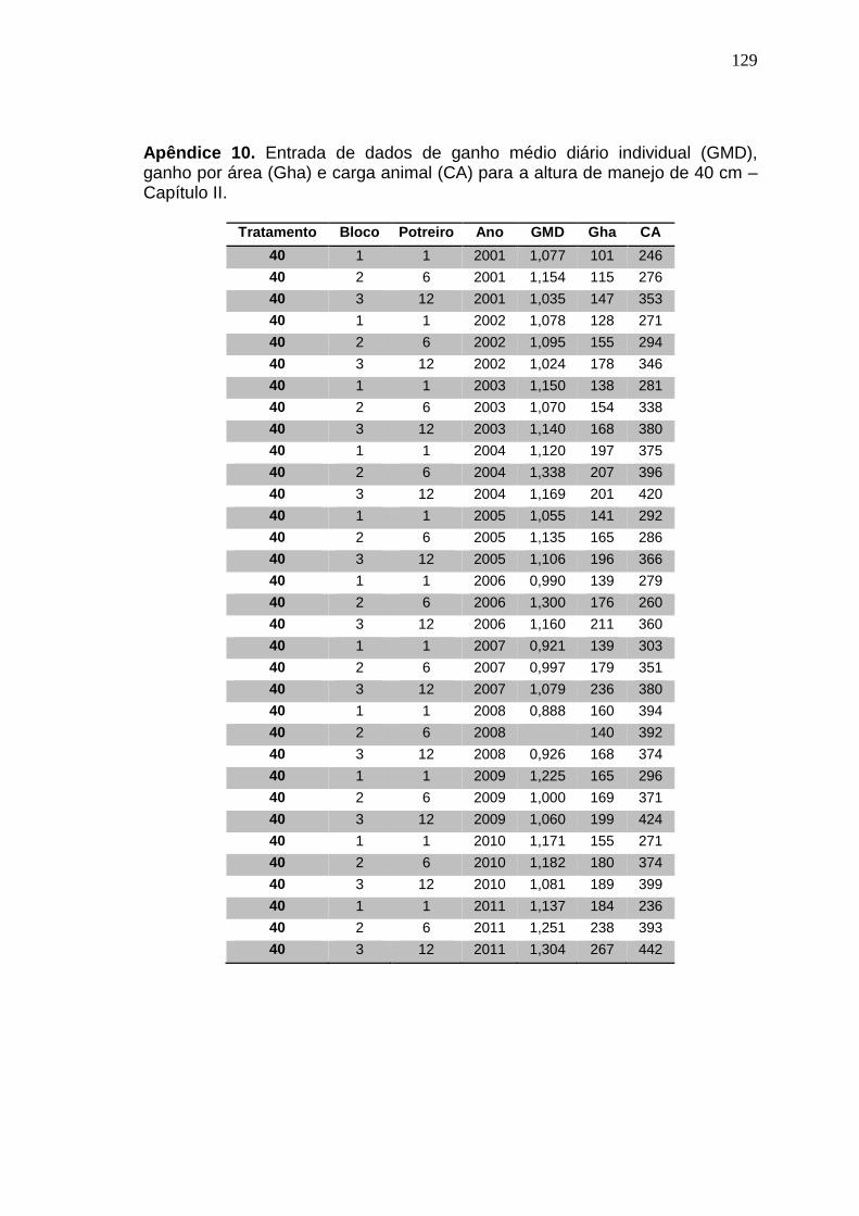
129
Apêndice 10. Entrada de dados de ganho médio diário individual (GMD), ganho por área (Gha) e carga animal (CA) para a altura de manejo de 40 cm – Capítulo II.
Tratamento Bloco Potreiro Ano GMD Gha CA
40 1 1 2001 1,077 101 246
40 2 6 2001 1,154 115 276
40 3 12 2001 1,035 147 353
40 1 1 2002 1,078 128 271
40 2 6 2002 1,095 155 294
40 3 12 2002 1,024 178 346
40 1 1 2003 1,150 138 281
40 2 6 2003 1,070 154 338
40 3 12 2003 1,140 168 380
40 1 1 2004 1,120 197 375
40 2 6 2004 1,338 207 396
40 3 12 2004 1,169 201 420
40 1 1 2005 1,055 141 292
40 2 6 2005 1,135 165 286
40 3 12 2005 1,106 196 366
40 1 1 2006 0,990 139 279
40 2 6 2006 1,300 176 260
40 3 12 2006 1,160 211 360
40 1 1 2007 0,921 139 303
40 2 6 2007 0,997 179 351
40 3 12 2007 1,079 236 380
40 1 1 2008 0,888 160 394
40 2 6 2008 140 392
40 3 12 2008 0,926 168 374
40 1 1 2009 1,225 165 296
40 2 6 2009 1,000 169 371
40 3 12 2009 1,060 199 424
40 1 1 2010 1,171 155 271
40 2 6 2010 1,182 180 374
40 3 12 2010 1,081 189 399
40 1 1 2011 1,137 184 236
40 2 6 2011 1,251 238 393
40 3 12 2011 1,304 267 442

130
6. VITA
Taise Robinson Kunrath nasceu em Porto Alegre, aos 9 dias do mês de
setembro de 1979. Filha de Carlos Fernando Kunrath e Tais Robinson Kunrath. Realizou seus estudos de ensino fundamental na Escola São Luiz e o ensino médio na ACM - Associação Cristã de Moços, localizados na mesma cidade. Em 2001, formou-se no Curso Técnico em Biotecnologia da Universidade Federal do Rio Grande do Sul. Em 2002, ingressou no curso de Agronomia da mesma universidade, onde desenvolveu atividades de pesquisa junto ao Departamento de Plantas Forrageiras e Agrometeorologia (DPFA). Em 2003 foi bolsista de iniciação científica com bolsa PROPESQ no Departamento de Botânica/UFRGS e FAPERGS na Fundação de Pesquisa Agropecuária do estado do Rio Grande do Sul (FEPAGRO) de 2004 à 2006 e no DPFA/UFRGS em 2007 e 2008. Concluiu a faculdade de Agronomia em dezembro de 2008. Em 2009 ingressou no curso de Mestrado junto ao Programa de Pós-graduação em Zootecnia da Universidade Federal do Rio Grande do Sul, na área de concentração Plantas Forrageiras, com bolsa CAPES, recebendo o grau de Mestre em Zootecnia em fevereiro de 2011. Em dezembro de 2010 foi aprovada no Processo Seletivo do Departamento de Zootecnia/UFRGS na área de concentração Plantas Forrageiras, para o Curso de Doutorado. Entre outubro de 2012 e outubro de 2013, permaneceu em doutorado sanduíche no INRA/Lusignan na França sob orientação dos pesquisadores Jean-Louis Durand e Gilles Lemaire. Em agosto de 2014, submeteu esta tese para apreciação dos pares e julgamento ao título de Doutora em Zootecnia.