UNIVERSIDADE FEDERAL DO RIO DE JANEIRO

Departamento de Engenharia Mecânica

DEM/POLI/UFRJ

OTIMIZAÇÃO AERO-ESTRUTURAL DE UMA ASA COM GEOMETRIA ATUADAPOR LIGAS DE MEMÓRIA DE FORMA VIA CLASS/SHAPE TRANSFORMATION

Pedro Batista Camara Leal

Projeto final submetido ao corpo docente

do Departamento de Engenharia Mecânica

da Escola Politécnica da Universidade

Federal do Rio de Janeiro como parte dos

requisitos necessários para a obtenção do

grau de engenheiro mecânico.

Orientador: Marcelo Amorim Savi

Rio de Janeiro

Março de 2015

UNIVERSIDADE FEDERAL DO RIO DE JANEIRODepartamento de Engenharia Mecânica

DEM/POLI/UFRJ

OTIMIZAÇÃO AERO-ESTRUTURAL DE UMA ASA COM GEOMETRIA

ATUADA POR LIGAS DE MEMÓRIA DE FORMA VIA CLASS/SHAPE

TRANSFORMATION

Pedro Batista Camara Leal

PROJETO FINAL SUBMETIDO AO CORPO DOCENTE DO DEPARTAMENTO DE

ENGENHARIA MECÂNICA DA ESCOLA POLITÉCNICA DA UNIVERSIDADE

FEDERAL DO RIO DE JANEIRO COMO PARTE DOS REQUISITOS

NECESSÁRIOS PARA A OBTENÇÃO DO GRAU DE ENGENHEIRO MECÂNICO.

Aprovado por:

________________________________________________Prof. Marcelo Amorim Savi

________________________________________________Prof. Fernando Alves Rochinha

________________________________________________Prof. Thiago Gamboa Ritto

RIO DE JANEIRO, RJ - BRASIL

MARÇO DE 2015

Camara Leal, Pedro

Otimizacao aero-estrutural de uma asa com geometria

atuada por ligas de memoria de forma via Class/Shape

Transformation/Pedro Camara Leal. – Rio de Janeiro:

UFRJ/COPPE, 2015.

XII, 50 p.: il.; 29, 7cm.

Orientador: Marcelo Amorim Savi

Projeto Final de Graduacao (bacharelato) –

UFRJ/COPPE/Programa de Engenharia Mecanica,

2015.

Bibliography: p. 40 – 42.

1. Otimizao. 2. Memria de forma. 3. Painis

Finitos. 4. Elementos Finitos. I. Amorim Savi,

Marcelo. II. Universidade Federal do Rio de Janeiro,

COPPE, Programa de Engenharia Mecanica. III. Tıtulo.

iii

Para Tita.

iv

Agradecimentos

O autor gostaria de agradecer o apoio do Centro Nacional de Desenvolvimento

Cientıfico e Tecnologico (CNPq) que disponibilizou uma bolsa de estudos via o

INCT-EIE (Instituto Nacional de Cincia e Tecnologia - Estruturas Inteligentes em

Engenharia). Este trabalho nao seria possıvel sem a orientacao do Prof Marcelo

Savi e do Prof. Darren Hartl. Tambem agradeco aos meus colegas Edwin Peraza

Hernandez e Christopher Bertagne pela ajuda tecnica. Analise estrutural foi efetu-

ada graas a uma licena academica fornecida pela Simulia. Otimizacao foi realizada

gracas ao software OpenMDAO. Por fim, gostaria de agradecer a minha namorada

Martha por ter me apoiado e por ter lido este trabalho comigo.

v

Resumo da Projeto Final de Graduacao apresentada a COPPE/UFRJ como parte

dos requisitos necessarios para a obtencao do grau de Bacharel em Ciencias (B.Sc.)

OTIMIZACAO AERO-ESTRUTURAL DE UMA ASA COM GEOMETRIA

ATUADA POR LIGAS DE MEMORIA DE FORMA VIA CLASS/SHAPE

TRANSFORMATION

Pedro Camara Leal

Fevereiro/2015

Orientador: Marcelo Amorim Savi

Programa: Engenharia Mecanica

A otimizacao das condicoes de voo representa um tema de grande interesse rela-

cionado a questoes aeroelasticas e mudanca de forma. Este trabalho propoe uma

metodologia para determinar as configuracoes de uma asa que muda de forma em

diferentes condicoes de voo. Buscam-se situacoes que sejam fisicamente e estrutural-

mente viaveis atraves do uso de atuadores construdos com ligas de memoria de forma

(SMAs). Para achar a solucao deste problema de otimizacao acoplada, multiplas

otimizacoes sao necessarias. A otimizacao da geometria feita para condicoes de voo

de cruzeiro e de aterrissagem. Alem disso, otimizam-se os atuadores de SMA visando

mudar a configurao do aerofolio entre duas geometrias. Para as tres otimizacoes em

serie utiliza-se o algoritmo genetico. As otimizacoes levam em consideracao os efeitos

da deformacao da estrutura e os carregamentos aerodinamicos aplicados asa. As

pressoes aerodinamicas sao avaliadas a partir do Metodo dos Paineis Finitos. Cada

geometria e gerada por um metodo conhecido como Class/Shape Transformation.

vi

Abstract of Bachelor’s Thesis presented to COPPE/UFRJ as a partial fulfillment of

the requirements for the degree of Bachelor of Science (B.Sc.)

AERO-STRUCTURAL OPTIMIZATION OF SHAPE MEMORY ALLOY-BASED

WING MORPHING VIA A CLASS/SHAPE TRANSFORMATION APPROACH

Pedro Camara Leal

February/2015

Advisor: Marcelo Amorim Savi

Department: Mechanical Engineering

The optimization of flight performance is a theme of great interest related to

aerolastic and shape morphing. This work proposes a method for determining in

a preliminary manner morphing wing configurations that provide benefits during

various disparate flight conditions but that are also each physically/structurally at-

tainable via localized active shape change operations. The controlled reconfiguration

is accomplished through the use of shape memory alloys (SMAs). To address this

coupled optimization problem, multiple optimization loops are required. In this

work, we consider optimized cruise and landing configurations in addition to the

SMA actuator configuration required to provide appropriate morphing between the

two. Thus, three chained optimization problems are addressed via a standard ge-

netic algorithm. In addition, each analysis-driven optimization considers the effects

of both the deformable structure (i.e. strain energy effects) and the aerodynamic

loading experienced by the wing. Aerodynamic considerations are addressed via use

of panel method. Each shape is generated by the so-called Class/Shape Transfor-

mation methodology.

vii

Contents

List of Figures x

List of Tables xii

1 Introduction 1

2 Structures and Optimization 3

2.1 Class Shape Transformation . . . . . . . . . . . . . . . . . . . . . . . 3

2.2 Abaqus . . . . . . . . . . . . . . . . . . . . . . . . . . . . . . . . . . . 7

2.3 Shape Memory alloys . . . . . . . . . . . . . . . . . . . . . . . . . . . 7

3 Aerodynamics and Fluid-Structure Interaction 14

3.1 Fundamental Concepts . . . . . . . . . . . . . . . . . . . . . . . . . . 14

3.2 Panel Method . . . . . . . . . . . . . . . . . . . . . . . . . . . . . . . 16

3.3 Multiphysics Algorithm . . . . . . . . . . . . . . . . . . . . . . . . . . 21

3.4 OpenMDAO: Optimization Platform . . . . . . . . . . . . . . . . . . 23

3.5 NSGA-II: Genetic Optimization . . . . . . . . . . . . . . . . . . . . . 24

4 Workflow 27

4.1 Wing Design Optimization . . . . . . . . . . . . . . . . . . . . . . . . 27

4.2 Morphing Optimization . . . . . . . . . . . . . . . . . . . . . . . . . . 28

5 Results 31

5.1 Continuous Flap Demonstration . . . . . . . . . . . . . . . . . . . . . 31

5.2 Wing Design: Optimization . . . . . . . . . . . . . . . . . . . . . . . 32

5.3 Morphing Optimization . . . . . . . . . . . . . . . . . . . . . . . . . . 34

6 Conclusion 39

Bibliography 40

A CST: Python Code 43

B Data Sheet: ICA IS-32 49

viii

C Taguchi 50

ix

List of Figures

1.1 Examples of adaptive wings and their enhanced behaviour . . . . . . 1

2.1 Influence of variables N1 and N2. All with constant Shape functions. 4

2.2 Examples of the influence of Ali variables for a first order shape func-

tion. The values of Aui were held constant. . . . . . . . . . . . . . . 5

2.3 Example of the use of the restrictions. The blue line represents a

cruise configuration, the green line a landing configuration and the

red lines indicate the local thicknesses that were kept constant in both

configurations. . . . . . . . . . . . . . . . . . . . . . . . . . . . . . . . 6

2.4 Shape Memory Effect . . . . . . . . . . . . . . . . . . . . . . . . . . . 9

2.5 SMA stress-temperature phase diagram (schematic) [2] . . . . . . . . 10

2.6 Experimental results illustrating the SMA under a constant 200MPa

stress [3] . . . . . . . . . . . . . . . . . . . . . . . . . . . . . . . . . . 10

2.7 Experimental result depicting the Pseudoelastic Effect [2] . . . . . . . 11

3.1 Representative airfoil depicting all relevant geometric definitions . . . 14

3.2 Representative wing depicting all relevant geometric definitions . . . . 15

3.3 Aerodynamic Forces . . . . . . . . . . . . . . . . . . . . . . . . . . . 16

3.4 A single panel with its nomenclature . . . . . . . . . . . . . . . . . . 17

3.5 Outline of panels resulting from the circle method . . . . . . . . . . . 18

3.6 Panel distribution generated by Xfoil . . . . . . . . . . . . . . . . . . 21

3.7 Pressure vectors generated by Xfoil . . . . . . . . . . . . . . . . . . . 22

3.8 Flowchart of the Fluid-Structure simulation. . . . . . . . . . . . . . . 23

3.9 View of an Assembly Showing Data Flow . . . . . . . . . . . . . . . . 24

3.10 Schematic of NSGA-II algorithm [4] . . . . . . . . . . . . . . . . . . . 25

4.1 3D Wing Model . . . . . . . . . . . . . . . . . . . . . . . . . . . . . . 28

4.2 Flowchart of the airfoil shape optimization for cruise. . . . . . . . . . 28

x

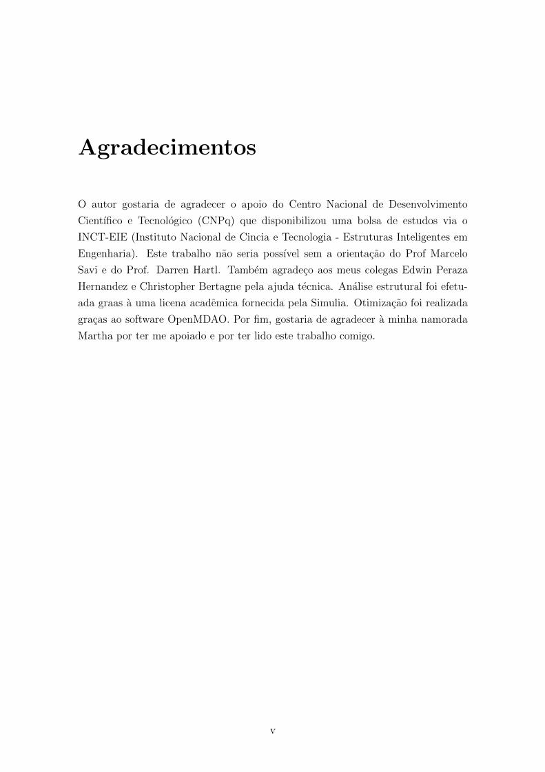
4.3 Example of an airfoil with SMA inserts (maximum insert widths)

with their respective labels. This example depicts a configuration for

maximizing the airfoil’s camber. Upon actuation, the upper inserts

(red) will expand while the those in the bottom (blue) will contract.

The widths of each SMA insert is denoted as wLior wUi

. . . . . . . 29

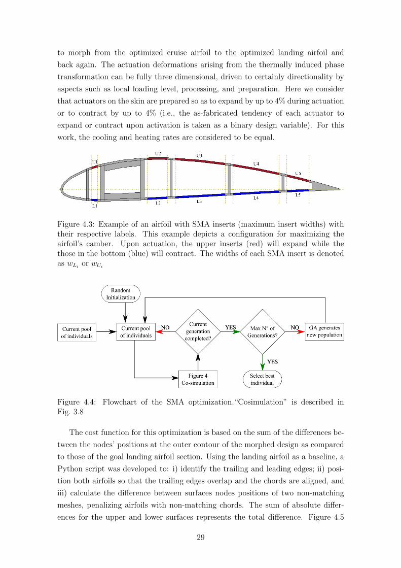
4.4 Flowchart of the SMA optimization.“Cosimulation” is described in

Fig. 3.8 . . . . . . . . . . . . . . . . . . . . . . . . . . . . . . . . . . 29

4.5 Shape difference concept. . . . . . . . . . . . . . . . . . . . . . . . . . 30

5.1 Pressure Coefficient Distributions using traditional (blue) and mor-

phing (red) flaps . . . . . . . . . . . . . . . . . . . . . . . . . . . . . 31

5.2 Comparison of the geometry of an airfoil using traditional (blue) and

morphing (red) flaps . . . . . . . . . . . . . . . . . . . . . . . . . . . 32

5.3 Drag vs Mass plots of all generations: (a) Cruise optimization; (b)

Landing optimization . . . . . . . . . . . . . . . . . . . . . . . . . . . 33

5.4 Optimized airfoil section profiles: the optimized cruise airfoil is in

blue, the optimized landing airfoil in red and the shape difference in

green. . . . . . . . . . . . . . . . . . . . . . . . . . . . . . . . . . . . 34

5.5 Von Mises Stress for the optimized cruise wing . . . . . . . . . . . . . 35

5.6 Von Mises Stress for the optimized landing wing . . . . . . . . . . . . 35

5.7 Evaluation in imposed conditions and structural response during the

morphing corresponding to the optimal morphing design. (a) Temper-

ature, (b) Angle of Attack, (c) Velocity, (d) Trailing edge displacement 37

5.8 SMA morphing optimization: shape difference for the best individual

through the generations . . . . . . . . . . . . . . . . . . . . . . . . . 37

5.9 Airfoil section profiles: the optimized cruise airfoil is in blue, the

optimized landing airfoil in red and the morphed cruise airfoil in green. 38

5.10 Shape Difference vs Maximum Von Mises Stress through all generations 38

C.1 Taguchi L50: used for 7 and 8 variables . . . . . . . . . . . . . . . . . 50

xi

List of Tables

2.1 Summary of various SMA properties and their effects. [2] . . . . . . . 8

3.1 List of elementary flows . . . . . . . . . . . . . . . . . . . . . . . . . 17

5.1 SMA Insert Design Optimization Problem . . . . . . . . . . . . . . . 32

5.2 Optimized design variables for landing and cruise sections . . . . . . . 33

5.3 Optimum variables . . . . . . . . . . . . . . . . . . . . . . . . . . . . 34

5.4 SMA Insert Design Optimization Problem . . . . . . . . . . . . . . . 36

5.5 Optimized SMA insert widths in millimeters . . . . . . . . . . . . . . 38

xii

Chapter 1

Introduction

The airfoil design associated with a given aircraft wing configuration is primarily

intended to maximize performance during the predominant flight condition (e.g.

cruise) while generally considering constraints on performance in off-optimal con-

ditions (e.g., during landing). To overcome this performance loss, several methods

exist to adapt the wing according to freestream conditions or changing performance

requirements. The most common is the inclusion of rigid but movable control sur-

faces, which permit the reconfiguration of the wing necessary to transition from

takeoff to cruise and then, to landing (i.e. Figure 1.1). These mechanisms lead

to higher efficiency but are not without drawbacks. Due to their complexity, they

occupy volume inside the wing which might displace valuable fuel storage; more

importantly, they add weight. Due to the use of discontinuous surfaces, extra drag

and noise are also generated for all flight conditions. These disadvantages motivate

the use of alternative adaptive technologies, such as conformal wing morphing via

implementation of shape memory alloys or other active materials.[5]

Shape memory alloys (SMAs) represent a class of materials that, when provided

Figure 1.1: Examples of adaptive wings and their enhanced behaviour

1

sufficient thermal energy, can generate a significant amount of actuation work in a

monolithic and compact form requiring very little installation volume. Their actua-

tion work density exceeds that attainable from all other active material options [6].

Because of this behavior and also due to its simplicity, there has been a great interest

in their use for aerospace applications.[2]

In the literature, many works can be consulted that address morphing wings [7],

and a large number of those consider the use of SMAs as the driving actuation

mechanism. However, due to limited variety of commercially available SMA forms,

these works have focused primarly on the use of simple shapes, such as springs [8]

and wires [9, 10]. Many works have focused on camber morphing [11–13],while others

have focused on the use of SMA on control surfaces [11, 14, 15]. Regarding numerical

analysis of such systems, the number of papers is quite scarce. Strelec et al.[9]

focused on the numerical and experimental use of nitinol wires to change the camber

of an airfoil. This work is based on and espands the preliminary work described by

Lima Junior et al. [16]. Using an approximation of the SMA transformation via

artificial thermal expansive methods, it was shown in that previous work that SMA

skin inserts are feasible as a solution for morphing from one NACA airfoil section

to another.

The goal of this work is to expand the previous effort from Lima Junior et al. [16].

SMA inserts are considered and their size optimized to drive morphing between two

airfoil shapes. Aerodynamic effects are considered throughout the design process

and, as in Strelec et al. [9], coupled fluid-structural effects are considered and an

accurate constitutive model describing the SMA material [17] behavior is employed.

Also novel is the method of airfoil section selection. Instead of optimizing between

two arbitrary NACA airfoils (as in the past work), two optimized airfoils are used,

each for a different flight condition. The shape of each optimized airfoil is described

by the “Class/Shape Transformation” methodology [18].

The structural Finite Element Analysis (FEA) is performed via Abaqus [19],

while the XFOIL’s [20] implementation of the panel method is used for estimating

aerodynamic forces. Abaqus’ user material subroutine (UMAT) is utilized to define

the constitutive inelastic behavior of the SMA. A custom-coded Python scripted

framework is used to integrate all these listed tools. A Python environment known as

open-source Multidisciplinary Design Analysis and Optimization, OpenMDAO [21],

is chosen for the optimization framework.

Several methodologies and softwares are utilized for this work. In 2 a review of

all structure related topics are covered including an introduction

2

Chapter 2

Structures and Optimization

In this chapter, a review of all strctures related topics are covered. The generic

form of the method developed by Boeing, the “Class/Shape Transformation”, is

depicted in Subsection 2.1 and further simplified and adapted for our needs. A

brief introduction to Abaqus and its functionalities are introduced in the following

Subsection (2.2). 2.3 is a summary of the properties and constitutive model of Shape

Memory Alloys. Finally, 3.4 is a summary of the optimization platform herein used

and 3.5 introduce the concepts of a genetic optimization, more specifically NSGA-II.

2.1 Class Shape Transformation

In previous works [16], morphing between two known NACA profiles (available on

University of Illinois at Urbana-Champaign website) was performed. Here, a dif-

ferent procedure is of concern. Before morphing, the optimized profiles and inner

structures for both shapes, landing and cruise, are obtained. For such, a method is

necessary to represent the outer shape of the airfoils. In the context of an optimiza-

tion problem, certain characteristics are necessary:

• Smooth and realistic shapes. As in structurally viable.

• Requires relatively few variables to represent a large enough design space to

contain optimum aerodynamic shapes for a variety of design conditions and

constraints.

• Mathematically efficient and fast

• Provides easy control for designing and editing the shape of a curve.

Several methods exist involving the manipulation of discrete points towards the

representation of the airfoil surface, while others focus in the use of splines. However

all of these methods fail to satisfy the above conditions. In 2006, Boeing developed

3

the Class/Shape Transformation Method [18]. The method satisfies all of the above

conditions through the use of two separate functions: the class and the shape.

Through the manipulation of the constants in these functions, different shapes are

obtainable.

The Class Function, equation 2.1, states the general classes of geometry through

the variables N1 and N2 (i.e. shape trailing edges and blunt leading edge). In

Figure 2.1, various of the possible classes are depicted.

CN1N2 = ψN1[1− ψ]N2 (2.1)

(a) NACA airfoil (N1=0.5, N2=1.0) (b) Elliptical airfoil (N1=0.5, N2=1.0)

(c) Biconvex airfoil (N1=1.0, N2=1.0)(d) Low drag projectile (N1=0.75, N2=0.25)

(e) Wedge (N1=1.0, N2=1.0 (f) Rectangle (N1=0.001, N2=0.001)

Figure 2.1: Influence of variables N1 and N2. All with constant Shape functions.

For subsonic flights, the usual of a glider, the (a) class is well suited. Therefore,

for the rest of the work we will consider that N1 = 0.5 and N2 = 1.0.

The Shape Function is used to define specific shapes within the geometry class

(i.e. camber and thickness). Contrary to the class function, the shape function

depends on the polynomial series: the Bernstein Polynomial. If n is the polynomial

degree, the upper and lower surfaces are defined by:

Su =n∑i−1

AuiSi(ψ) (2.2a)

Sl =n∑i−1

AliSi(ψ) (2.2b)

4

where Aui and Ali are constants and the shape component Si is defined as,

Sr,n(ψ) = Ki,nxr(1− ψ)n−r (2.3)

where Ki,n is the Bernstein polynomial defined by equation 2.4.

Ki,n =n!

i!(n− i)!(2.4)

Depending on the polynomial degree n, there are 2(n+1)Aus and Als. Therefore,

a total of 4(n+ 1) variables. The influence of the A variables is depicted on Figure

2.1.

(a) Al0 = 0.1, Al1 = −0.1(b) Al0 = 0.3, Al1 = −0.1

(c) Al0 = 0.3, Al1 = 0.3 (d) Al0 = 0.6, Al1 = −0.1

Figure 2.2: Examples of the influence of Ali variables for a first order shape function.The values of Aui were held constant.

Combining both functions, class and shape, and taking in to account the trailing

thickness, we have the 2.5 equations for the ζ coordinates of both surfaces.

ζupper = CN1N2Su(ψ) + ψ∆ζupper (2.5a)

ζlower = −CN1N2Sl(ψ)− ψ∆ζlower (2.5b)

where, ∆ζupper and ∆ζlower are the trailing edge thicknesses which are considered

to be equal and constant. From [18], it was found that a first order Bernstein

polynomial, although the few variable, already lead to good results. If a first order

Bernstein polynomial representation is used for the upper (u) and lower (l) surfaces,

both can be represented as

ζu = ψ0.5(1− ψ)[Au0(1− ψ) + Au1ψ] + ψ∆ζu, (2.6a)

ζl = ψ0.5(ψ − 1)[Al0(1− ψ) + Al1ψ]− ψ∆ζl, (2.6b)

5

Figure 2.3: Example of the use of the restrictions. The blue line represents a cruiseconfiguration, the green line a landing configuration and the red lines indicate thelocal thicknesses that were kept constant in both configurations.

where Au0 , Au1 , Al0 and Al1 are the design variables; and∆ζu and ∆ζl are trailing

edge thicknesses which are considered to be equal and constant.

For the landing optimization, extra design constraints related to thicknesses of

the airfoil section, i.e. the distance between upper and lower surface, are considered

that will influence the possible landing configurations. The spar region of the wing

section is assumed to be free of SMA actuator segment; morphing of the spar (and, in

particular, the airfoil outer mold line thickness in the region of the spar) is unfeasible.

The same is considered for the stiffeners. To avoid such a problem, the thickness at

4 points along the chord of the airfoil section (ψ1, ψ2, ψ3 and ψ4), are transferred

unchanged to the shape equation defining the airfoil optimized for landing. This

enables similar spar geometries without overconstraining the shape. If ζi is the

thicknesses at one of these points (i=1, 2, 3 and 4), from equations 2.6, we have

that:

Au0 =K1/(1− ψ1)−K2/(1− ψ2)ψ1/(1− ψ1)− ψ2/(1− ψ2)

Au1 =K3/(1− ψ3)−K4/(1− ψ4)ψ3/(1− ψ3)− ψ4/(1− ψ4)

where,Ki =ζi − 2ψi∆ζψ0.5i (1− ψi)

(2.7)

Since for the landing analysis the thickness ζi is known, the total num-

ber of unknowns across the two equations is reduced to two given that Au0 =

f(ψ1, ψ2, Al0 , ζ1, ζ2) and Au1 = f(ψ3, ψ4, Al0 , ζ3, ζ4) . In this way, the number of

design variables is reduced while the structural feasibility of the morphing struc-

tures design (i.e. the integrity of the non-morphing spar) is guaranteed.

The result of equations 2.7 can be clearly noticed on Figure 2.6.

6

2.2 Abaqus

Abaqus 6.12 is a suite of FEA/CFD routines. It has inbuilt CAD functionalities,

mesh generators, an easy-to-use GUI with in-depth visualization options and a con-

venient Python interface. Therefore the user can create, mesh, define the loads and

boundary conditions, submit and analyse the results in one single platform. Due to

it’s Python API, users can easy script and automate the software. This shows to be

an vital functionality when leading with optimization problems.

One of the many Abaqus functionalities is the use of subroutines. Through

the use of Fortran codes, the user is able to create functionalities not inherent to

the software. Such as supersonic CFD’s, materials with non-linear behaviours and

others. For most researches, this is the main reason Abaqus is used. For this work,

the Abaqus subroutine User material (UMAT) developed by TiiMS (Texas Institute

for Intelligent Materials and Structures) is utilized. It enables the creation of new

material characteristics, such as those of shape memory alloys.

2.3 Shape Memory alloys

Shape memory alloys (SMAs) are metallic alloys which undergo solid-to-solid phase

transformations induced by the appropriate temperature and/or stress. The trans-

formations are between 3 distinct crystalline structures: twinned martensite, de-

twinned martensite and austenite [5]. Table 2.1 is summary of all of the character-

istics of such alloys. The High Actuation Strain and the High Energy Density traits

are the main reason why SMAs are of interest to the Aerospace industry. Hence,

the reason why this kind of material was here selected. Each phase transformation

has a pre-defined start and final temperature, where the martensite fraction can

vary from 0 (pure austenite) to 1 (pure martensite). The transformation between

the pure states are known as martensite transformation (from 0 to 1) and austenite

transformation (from 1 to 0).

The primary characteristic of these alloys is the Shape Memory Effect depicted

in Figure 2.4. If the alloy is in a twinned martensite state, e.g. no stress and T < As,

where As is the temperature where austenitization starts, when loaded above σMs,

martensite starts to be detwinned. Once σ > σMf , martensite is complety detwinned

and returns to elastically deform. When unloaded a residual strain is noticeable since

the material is still in detwinned martensite state. To recover to its original form, the

7

Table 2.1: Summary of various SMA properties and their effects. [2]

8

Figure 2.4: Shape Memory Effect

material is heated above Af , the temperature where the austenite transformation

is complete, recovering the residual strain. This highly coupled thermal-mechanical

behaviour is of great interest for actuation purposes.

From Figure 2.5, one can notice that the transformation temperatures from

Austenite to Martensite (Ms and Mf ) and from Martensite to Austenite (As and

Af ) are different. This results in a behaviour known as a hysteresis depicted in

Figure 2.6, which is the result of an energy dissipation.

Another phenomena characteristic to SMAs is the Pseudoelastic effect. The

transformation from austenite to detwinned martensite, stress-induced, can generate

reversible inelastic strains. The strains are recovered once the load are reduced to

their original values. An experimental evidence of such effect can be observed on

Figure 2.7.

The thermo-mechanical behavior of SMAs can be described by constitutive mod-

els that establish a phenomenological description of these alloys. Herein, the Hartl-

Lagoudas [6] model is employed. Contrary to other method, martensitic transforma-

tion is not considered. Only the generation and recovery of transformation strains

that occur as a result of martensitic transformation is taken into account. The model

considers three external state variables: the stress σ, the total strain ε, and the ab-

solute temperature T . Two internal state variables are also considered: the inelastic

transformation strain εt (e.g. caused by transformation) and the martensitic vol-

ume fraction ξ. The model follows the Helmholts free energy principle, therefore the

temperature and the total strain are assumed to be known. Additive decomposition

9

Figure 2.5: SMA stress-temperature phase diagram (schematic) [2]

Figure 2.6: Experimental results illustrating the SMA under a constant 200MPastress [3]

10

Figure 2.7: Experimental result depicting the Pseudoelastic Effect [2]

is assumed by considering elastic, thermal and inelastic contributions.

ε = S(ξ)σ + α(T − To) + εt (2.8)

where S(ξ) is the phase-dependent fourth-order compliance tensor, written as

S(ξ) = SA − ξ(SA − SM) = SA − ξS (2.9)

where SA and SM are the compliance tensors for austenitic and martensitic phases,

respectively; α is the second-order coefficient of thermal expansion tensor, where

To is the material reference temperature. Standard isotropic forms are assumed for

S(ξ) and α, and they are computed from material properties to be described shortly.

The inelastic transformation strain evolves such that the time rate of change of

both its magnitude and direction are given as

εt = ξ

Hcur(σ 3σ′

2σ) ; ξ > 0

εt−r

ξr; ξ < 0

(2.10)

During forward transformation (ξ > 0), the formulation for the direction of

transformation follows the assumptions of classical associative Mises plasticity. The

Mises equivalent stress is given as σ = 2√

3/2σ′ : σ′, where σ′ is the deviatoric stress.

The magnitude of transformation strain generated during full martensite transfor-

mation is captured by the scalar-valued function Hcur(σ). For trained materials,

Hcur may be considered as follows:

11

Hcur(σ) =

Hmin ; σ ≤ σcrit

Hmin + (Hmax −Hmin)(1− exp−k(σ−σcrit)) ; σ > σcrit(2.11)

here Hmin, Hmax, k and σcrit are model parameters.

During reverse transformation (ξ < 0), the direction and magnitudes are defined

such that all transformation strain existing at the cessation of austenite transfor-

mation (i.e., at which time ξ → ξr and εt → εt−r ) is fully recovered should the

material transform fully back into austenite. Having related stress, total strain, and

inelastic strain, and further having defined an evolution equation for the inelastic

strain εt, we need only define constraints on the evolution of the martensitic volume

fraction ξ, which acts as a scalar multiplier in 2.10. For this purpose, we introduce

the transformation function Φ. Inspired by the methods of classical plasticity, the

following constraints are stated:

Φt ≤ 0, ξΦt = 0, 0 ≤ ξ ≤ 1 (2.12)

where the first two represent the the Kuhn-Tucker constraints (e.g. first order con-

ditions for a solution of a nonlinear problem to be optimal), and the third bounds

the martensitic volume fraction, which naturally ranges from 0 to 1.

From the definition 2.10, we have that forward and reverse transformation are

distinctive process, therefore

Φt =

Φtfwd ; ξ ≥ 0 and 0 ≤ ξ < 1

Φtrev ; ξ > 0 and 0 ≤ ξ < 1

(2.13)

Φtfwd and Φt

rev are given by

Φtfwd = (1−D)Hcur(σ)σ − 1

2σ : Sσ − ρ∆soT + ρ∆uo

−[

1

2a1(1 + ξn1 + (1− ξ)n2) + a3

]− Y t

o (2.14)

Φtrev = (D − 1)

σ : εt−r

ξr+

1

2σ : ∆Sσ + ρ∆soT + ρ∆uo

−[

1

2a2(1 + ξn3 + (1− ξ)n4) + a3

]− Y t

o (2.15)

where D and T to are transformation dissipation parameters; ρ∆so and ρ∆uo are

the volume-specific change in reference to entropy and to internal energy between

12

martensite and austenite, respectively; a1, a2 and a3 are transformation hardening

coefficients while n1, n2, n3 and n4 are transformation hardening exponents.

13

Chapter 3

Aerodynamics and Fluid-Structure

Interaction

In this chapter all the aerodynamic related topics are covered. An introduction

of the concepts of aerodynamics herein utilized are introduced in Subsection 3.1.

The theory behind panel methods and the Xfoil software utilized are described in

Subsection 3.2. 3.3 describes the multiphysics python code developed incorporating

the Abaqus FEA model and the Xfoil panel model.

3.1 Fundamental Concepts

Although complicated geometries, most wings can be represented through a collec-

tion of geometric characteristics related to their cross-section (Figure ??) or to their

top view (Figure ??). Here, the following geometric wing related concepts have been

utilized:

• Leading Edge: the foremost edge of an airfoil section, usually the edge at the

round-off end Also defined as the origin, e.g. the (0,0) point, of our coordinate

system.

Figure 3.1: Representative airfoil depicting all relevant geometric definitions

14

Root

Tip

Span

λ

Figure 3.2: Representative wing depicting all relevant geometric definitions

• Trailing Edge: the rearmost edge of an airfoil section, usually the edge at the

sharp end of the airfoil.

• Chord : absolute distance from the leading edge to the trailing edge.

• ψ: nodes’ coordinates along the chord line and normalized by the chord.

• ζ: nodes’ coordinates normal of the chord line and normalized by the chord.

• Camber Line: line of points midway between the upper and lower surfaces.

• Angle of Attack(α): Angle of the chord relative to the wind’s direction.

• Centerline: line located equidistant of both tips following the fuselage.

• x : coordinate along the spam that has its origin is located at the centerline .

• Root : wing cross section at the centerline.

• Tip: wing cross section at the extremity of the wing

• Span: distance between the wing tips.

• Taper : ratio between the tip chord and the root chord.

• Sweep (λ): angle of the leading edge in relation to the span.

In addition, to evaluate the performance of the airfoils herein analyzed, several

aerodynamic concepts were utilized. The formal definition of these concepts are:

• Cruise: flight condition where altitude is stabilized. Time wise, it is the

predominant flight condition. [22]

• Landing : flight condition where the aircraft descends from cruise altitude to

the ground.

• Resulting Force (R): it is the resultant force generated by wind pressure.

15

Figure 3.3: Aerodynamic Forces

• Lift (L): it is the component perpendicular to the wind’s direction of R. As

can be seen in Figure 3.3. High Lift is usually desirable. Aircraft’s with higher

lift can generate less drag, consume less fuel or carry more cargo.

• Drag (D): it is the component perpendicular to the wind’s direction of R. As

can be seen in Figure 3.3. High drag for most flight conditions is undesirable.

Since more thrust and, therefore, fuel, is necessary to propel the vehicle.

• Pressure Coefficient : It is the local unidimensional coefficient of the wind

pressure. Since pressure along the airfoil surface varies, the coefficient is a

local variable. If p∞ and ρ are, respectively, the air pressure and density at

the aircraft’s altitude; and V∞ the wind velocity; we have that:

Cp =p− p∞ρV 2∞

(3.1)

3.2 Panel Method

Although a free software known as Xfoil is utilized to calculate the aerodynamic

pressures through the panel method, the author finds it necessary to introduce the

theory behind the method to depict its advantages and disadvantages. This section

is based on the lectures from Prof. Lorena A. Barba, author of the Aeropython

lessons.

The algorithm is initialized performing a discretization of the airfoil geometry

into panels. The panel’s attributes are: a starting point, an end point, a mid-point,

its length and its orientation. Figure 3.4 depicts the nomenclature herein used.

Since the trailing and leading edge have more complicated geometries, the mesh

needs to be more refined near these regions. For such, a standard method is to store

16

Figure 3.4: A single panel with its nomenclature

Table 3.1: List of elementary flowsUniform Flow: φ = U∞ + C

Source (Sink): φ = (−) σ2πln(√

(xci − xj(sj))2 + (yci − yj(sj))2)

Vortex: φ = (−)γtan−1(y−ysourcex−xsource

)

the x-coordinate of the circle points to be the x-coordinate of the panel nodes, x,

and project the y-coordinate of the circle points onto the airfoil by interpolation.

We end up with a node distribution like this:

From potential flow theory, it is known that inviscid flows can be represented by

the superposition of 5 elementary flow elements: a uniform flow, a vortex, a source,

a sink and a doublet.

If we consider a uniform flow at wind velocity U∞, a source at the mid-point

of each panel i and a vortexes of constant γ strength at each mid-point, using the

principle of superposition, we have that the potential velocity is:

φ (xci , yci) = U∞xci cosα + U∞yci sinα

+N∑j=1

σj2π

∫j

ln

(√(xci − xj(sj))2 + (yci − yj(sj))2

)dsj

−N∑j=1

γ

2π

∫j

tan−1

(yci − yj(sj)xci − xj(sj)

)dsj (3.2)

17

Figure 3.5: Outline of panels resulting from the circle method

Enforcing the flow-tangency condition on each panel mid-point (with subscript

c) approximately makes the body geometry correspond to a dividing streamline (and

the approximation improves if we represented the body with more and more panels).

So, for each panel i, we make the component of u normal to the panel, un =, equal

to zero at (xci , yci), that is

un =∂

∂ni{φ (xci , yci)} = 0 (3.3)

which leads to:

0 = U∞ cos (α− βi) +N∑j=1

σj2π

∫j

∂

∂niln

(√(xci − xj(sj))2 + (yci − yj(sj))2

)dsj

−N∑

j=1,j 6=i

γ

2π

∫j

∂

∂nitan−1

(yci − yj(sj)xci − xj(sj)

)dsj (3.4)

where βi is the angle that the panel’s normal makes with the x-axis, so

∂xci∂ni

= cos βi and∂yci∂ni

= sin βi (3.5)

and

xj(sj) = xaj − sin (βj) sj

yj(sj) = yaj + cos (βj) sj (3.6)

18

But, there is still a problem to handle when i=j. So that the streamlines do

not penetrate the panel, the source sheet strength should be equal to the incoming

volume. Therefore, for an i-th panel to itself its contribution is σi2

. Applying the

boundary condition at the center of the i-th panel on equation 3.4:

0 = U∞ cos (α− βi) +σi2

+N∑

j=1,j 6=i

σj2π

∫j

∂

∂niln

(√(xci − xj(sj))2 + (yci − yj(sj))2

)dsj

−N∑

j=1,j 6=i

γ

2π

∫j

∂

∂nitan−1

(yci − yj(sj)xci − xj(sj)

)dsj (3.7)

Solving the partial derivations, we have that:

0 = U∞ cos (α− βi) +σi2

+N∑

j=1,j 6=i

σj2π

∫j

(xci − xj)∂xci∂ni

+ (yci − yj)∂yci∂ni

(xci − xj)2 + (xci − xj)

2 )dsj

−N∑

j=1,j 6=i

γ

2π

∫j

(xci − xj)∂yci∂ni− (yci − yj)

∂xci∂ni

(xci − xj)2 + (yci − yj)

2 dsj (3.8)

The Kutta-condition states that the pressure below and above the airfoil trailing

edge must be equal so that the flow does not bend around it, but leaves tangentially.

The rear stagnation point must be exactly at the trailing edge. To enforce the Kutta-

condition, we must include one more equation. We state that the pressure coefficient

on the first panel must be equal to that on the last panel:

Cp1 = CpN (3.9)

Using the definition of the pressure coefficient on a surface for an i-th panel:

Cpi = 1−(VtiU∞

)2

(3.10)

with equation 3.9 and considering that the horizontal axis of the coordinate system

for both panels are inversed, we have that:

Ut1 = −UtN (3.11)

Therefore, we need to evaluate the tangential velocity at the first and last pan-

els. Let’s derive it for every panel, since it will be useful to compute the pressure

coefficient.

19

Uti =∂

∂ti(φ (xci , yci)) (3.12)

i.e.,

Uti = U∞ sin (α− βi)

+N∑

j=1,j 6=i

σj2π

∫j

∂

∂tiln

(√(xci − xj(sj))2 + (yci − yj(sj))2

)dsj

−N∑

j=1,j 6=i

γ

2π

∫j

∂

∂titan−1

(yci − yj(sj)xci − xj(sj)

)dsj (3.13)

which gives

Uti = U∞ sin (α− βi)

+N∑

j=1,j 6=i

σj2π

∫j

(xci − xj)∂xci∂ti

+ (yci − yj)∂yci∂ti

(xci − xj)2 + (xci − xj)

2 dsj

−N∑

j=1,j 6=i

γ

2π

∫j

(xci − xj)∂yci∂ti− (yci − yj)

∂xci∂ti

(xci − xj)2 + (xci − xj)

2 dsj (3.14)

where∂xci∂ti

= − sin βi and∂yci∂ti

= cos βi

Here, we build and solve the linear system of equations of the form:

[A][σ, γ] = [b] (3.15)

where the N + 1×N + 1 matrix [A] contains three blocks: an N ×N source matrix

(matrix [S] in Equation 3.16), an N × 1 vortex array to store the weight of the

variable γ at each panel (vector [g]), and a 1 × N + 1 Kutta array that represents

our Kutta-condition (vector [k]).

Sij =

12

, if i = j

12π

∫ (xci−xj(sj)) cosβi+(yci−yj(sj)) sinβi

(xci−xj(s))2+(yci−yj(s))

2 dsj , if i 6= j(3.16)

The right-hand-side vector b is defined as:

[b] =

bi = −U∞ cos βi , if i 6= N + 1

bN+1 = −U∞sin(α− βi) , if i = N + 1(3.17)

The main disadvantage of the Panel Method is the Paradox of D’Alembert ,

which states that for an incompressible and inviscid flow, the drag force is zero on

a body moving with constant velocity relative to the fluid. Zero drag is in direct

20

contradiction to the observation of substantial drag on bodies moving relative to

fluids.[23] The solution adopted by the author of Xfoil, Mark Drela, is to apply

the Squire-Young formula to obtain the Drag. The formula assumes that the wake

behaves in an asymptotic manner downstream of the point of application. This

assumption is strongly violated in the near-wake behind an airfoil with trailing edge

separation. Hence, the usual application of Squire-Young at the trailing edge is

questionable with separation present, but its application for flow conditions before

separation is reasonable. Therefore the problem of calculating aerodynamic pres-

sures reduces to a linear algebric system. Wherein modern CFS’s simulations would

lead to much longer computational periods.

As mentioned before, instead of developing a Panel Method code, a free software

is used. Xfoil was developed by Mark Drela from MIT and for the last two decades

has been optimized. The concepts herein presented are applied in the software. It

is able to generate panel meshes (Figure 3.6 and calculate the Pressure Coefficients

(Figure 3.7)

In this work we will be leading with 2D and 3D geometries, but the pressure

coefficients from the Panel Method are only for 2D geometries. For such, an elliptical

distribution is utilized along the wing span [24]. Although an ideal distribution, it

is considered a plausible pressure distribution for an unswept and untapered wing.

If the pressure coefficient at the wing root are considered to be those given by xfoil,

[Cxfoilp ], the pressure coefficients along the span are obtained through 3.18.

[Cp(x)] = [Cxfoilp ]

√1− (2x/b) ∗ ∗2 (3.18)

3.3 Multiphysics Algorithm

The approach for computing the response of this coupled mechanical systems fol-

lows from that of Felippa et al. [25]. The computational multiphysics framework

herein utilized was developed for a staggered solution problem using a partitioned

Figure 3.6: Panel distribution generated by Xfoil

21

Figure 3.7: Pressure vectors generated by Xfoil

treatment. An overview of the staggered solution problem considered herein is de-

picted in Figure 3.8. The system is represented through differential partitions (i.e.

discretization of a decomposed system). The interaction effects are communicated

between the individual partitions using prediction or substitution, (i.e. communicat-

ing the response of the current state to the following state or to the current state).

This representation enables the utilization of non-matching spatial discretizations

and geometric representations, which is a requirement for efficient calculation of

aerodynamic effects via the panel method. For computational treatment of a dy-

namical coupled system such as an aeroelastic simulation, the decomposed systems

are the fluid and solid fields, where each is discretized in space and time. At each

time interval, further decomposition of the time discretization of a field is possible;

this approach is known as splitting or sub-cycling. This feature will be of importance

when dealing with stability issues associated with morphing elements in the finite

element model.

In the context of this current effort, the developed framework allows the calcu-

lation of the pressure distribution to update based on the deformed airfoil shape

while the aero-structural loads likewise update based on changing pressures. This

occurs throughout a dynamic analysis. With the optimized parameters found for

both the cruise and landing shapes, the cruise shape is imported in Abaqus, thus

creating the Initial model in Figure 3.8. Information regarding the outer mold line

of the Abaqus model is transferred to XFOIL via a custom-coded Python inter-

face where the pressure distributions are calculated and then transferred back to

Abaqus, updating the pressure distribution. An FEA takes place for a small step of

time using the UMAT for defining the SMA behavior. The incremental process re-

peats itself in this explicit manner until the total simulation time has been reached.

It is assumed that the morphing is relatively slow (i.e. quasi-static) and that the

flow has sufficient time to stabilize between each morphing increment, therefore, the

panel method analysis provides steady-state solutions and does not depend on time.

The cost function described in Section 3. The coupled aero-structural morphing

22

calculation process is depicted in Figure 3.8.

Figure 3.8: Flowchart of the Fluid-Structure simulation.

3.4 OpenMDAO: Optimization Platform

OpenMDAO is an open Multidisciplinary Design Analysis and Optimization

platform [21]. Developed by NASA and written in Python. It’s purpose is to

facilitate the communication between 3rd party softwares in working environment

where other features such as optimization or design of experiments can be easily

implemented. Such a framework is possible due to the separation of the flow of

information, dataflow, from the process in which analyses are executed, workflow.

The software is composed of four specific constructs. They are:

• Component : an object with input and output variables. It can be a wrapped

3rd party software or a code written by the user (in python or any other

language). It is possible to have multiple components that communicate with

each other.

• Assembly : a group of linked components with a specified dataflow between

them.

• Driver : responsible for iterating over a workflow until some condition is met

such as in an optimization or a design of experiments.

• Workflow : responsible for dictating the components to execute and in that

order to execute them for a given driver. Drivers can also be used inside a

workflow, enabling nested iterations.

An overview of an usual OpenMDAO framework utilizing the above constructs

is depicted in Figure 3.4.

23

Figure 3.9: View of an Assembly Showing Data Flow

3.5 NSGA-II: Genetic Optimization

Since heuristic methods become increasingly more effective in finding the global

optimum given a large number of design variables and considering also the expected

high degree of non-linearity in the design response, for this work a robust and efficient

genetic algorithm known as NSGA-II (Non Sorting Genetic Algorithm II) [26] was

selected for all optimizations. This well known option is included in the current

distribution of OpenMDAO. In such a scheme, each design variable is treated as

a gene; a combination of these genes represents the chromosome of an individual

design; a group of individuals is treated as a population. Techniques inspired by

natural evolution, such as crossovers, mutations and natural selection, generate a

series of design population generations that should eventually include the nearly

optimal solution.

The procedure of the NSGA-II, depicted in Figure ?? is as follows:

1. Population Initialization: based on the population size, N , and ranges defined

by the user, the population is created (R0)

2. Non-Dominated sort : as in any genetic algorithm, every individual p is eval-

uated (i.e maximum Von Mises Stress, tip displacement) and therefore at-

tributed a fitness. However a non-dominated sort also considers the set the

individual dominates (Sp) and the number of individuals that dominate the

individual (np), organizing the population in to fronts, Fi. All individuals in

front F1 have fitness 1, in front F2 have fitness 2 and so on. Once all individ-

uals are sorted, the individuals with higher fitness are rejected. If M is the

number of individuals in the set Pt of surviving configurations, individuals in

24

Figure 3.10: Schematic of NSGA-II algorithm [4]

fronts with fitness higher that that of the M -th sorted individual are rejected.

3. Crowding Distance: is the measure of how close an individual is to the indi-

viduals in it’s own front. Large average crowding distance will result in better

diversity in the population. The population in each front is sorted according to

it’s crowding distance. Individuals of the highest front with crowding distance

lower than that of the M -th sorted individual are rejected. The result is set

Pt+1, the pool of possible candidates.

4. Genetic Operators : inspired by natural evolution, three algorithms are used

to generate new individuals of set Qt+1, the offspring :

• Binary Tournament Selection: two randomly chosen individuals are

drawn from the Pt+1. An individual is selected if the fitness is lesser

than the other, and if the fitness are equal, the individual is selected if

crowding distance is greater than the other.

• Binary Crossover : generation of individuals through random interpola-

tion of the genes of two individual’s from Pt+1.

• Mutation: to avoid local minimums, a genetic algorithm is utilized. It

enables variation of genes even when the results has converged, hence the

global minimum in the domain can be found if enough generations are .

5. Recombination: elitism The offspring population of the previous step is com-

bined with the current generation population and selection is performed to

set the individuals of the next generation resulting in set Rt+1. Since all the

previous and current best individuals are added in the population, elitism is

ensured. If by adding all the individuals in Fi the population exceeds N then

25

individuals in Fi are selected based on their crowding distance in the descend-

ing order until the population size is N . And hence the process repeats starting

from step 2 onwards until the user defined number of generations is reached.

26

Chapter 4

Workflow

4.1 Wing Design Optimization

In this work, we will consider two key flight conditions weighted by the percentage of

total flight [22]: cruise and landing. We further restrict ourselves to the consideration

of an untapered and unswept wing to minimize three dimensional effects during this

preliminary assessment of our approach. Standard aluminum construction is also

considered except where augmented via the placement of SMA actuation segments.

For each flight condition, the airfoil of a non-tapered and non-swept wing including

martensitic NiTiCu is optimized. As depicted in Figure 4.1, the inner structure

of the wing consists of a traditional assemblage of ribs, a spar, and a D-box. The

optimization focuses on obtaining a wing with low weight, low drag, and low bending

displacement under lifting loads while providing sufficient lift and avoiding localized

over-stress. For landing, the desire for a minimized landing velocity is considered.

For cruise, extra design variables related to the thicknesses of inner components

(spars, skin, ribs and D-box) and to the number of ribs are considered. For landing,

the optimal cruise thicknesses and number of ribs are used. The influence of the

component’s thicknesses over aluminum’s properties are also considered.[27]

As depicted in the airfoil design flowchart of Figure 4.2, the analysis is initiated

with the creation of random wing design configurations; for each, an Abaqus struc-

tural model is created. From this model, total aircraft weight is found. The minimal

angle of attack that provides sufficient lift, if possible, is assessed via XFOIL. Hav-

ing found the necessary angle of attack, the pressure distributions are calculated in

XFOIL; via a simplified assumption of an approximately elliptical lift distribution,

the three dimensional (i.e., full wing) loads are found. The loads are then imported

by Abaqus, and a FEA is completed. If the wing is found to violate structural

constraints on local stress limits, the configuration is eliminated from the pool of

possible designs. If the maximum number of iterations has not reached its maxi-

27

Figure 4.1: 3D Wing Model

mum, a new generation is created according to the optimization code. Otherwise the

best configuration among all members of the design populations of all generations

is assumed to be sufficiently approximate the optimal design. For landing, the same

process is applied, but the minimum velocity is assess instead.

Figure 4.2: Flowchart of the airfoil shape optimization for cruise.

4.2 Morphing Optimization

The purpose of this work is not only the optimization of various airfoil outer mold

line configurations, but also the associated optimization of the means by which those

configurations are morphed from one to another. This is truly a novel contribution

of this work. With the airfoils generated for the process of Figure 4.2, NiTiCu shape

memory alloy inserts of various sizes are generated on the skin as can be seen in

Figure 4.3. These inserts are thermally driven so as to actuate, morphing the section

28

to morph from the optimized cruise airfoil to the optimized landing airfoil and

back again. The actuation deformations arising from the thermally induced phase

transformation can be fully three dimensional, driven to certainly directionality by

aspects such as local loading level, processing, and preparation. Here we consider

that actuators on the skin are prepared so as to expand by up to 4% during actuation

or to contract by up to 4% (i.e., the as-fabricated tendency of each actuator to

expand or contract upon activation is taken as a binary design variable). For this

work, the cooling and heating rates are considered to be equal.

Figure 4.3: Example of an airfoil with SMA inserts (maximum insert widths) withtheir respective labels. This example depicts a configuration for maximizing theairfoil’s camber. Upon actuation, the upper inserts (red) will expand while thethose in the bottom (blue) will contract. The widths of each SMA insert is denotedas wLi

or wUi

Figure 4.4: Flowchart of the SMA optimization.“Cosimulation” is described inFig. 3.8

The cost function for this optimization is based on the sum of the differences be-

tween the nodes’ positions at the outer contour of the morphed design as compared

to those of the goal landing airfoil section. Using the landing airfoil as a baseline, a

Python script was developed to: i) identify the trailing and leading edges; ii) posi-

tion both airfoils so that the trailing edges overlap and the chords are aligned, and

iii) calculate the difference between surfaces nodes positions of two non-matching

meshes, penalizing airfoils with non-matching chords. The sum of absolute differ-

ences for the upper and lower surfaces represents the total difference. Figure 4.5

29

Figure 4.5: Shape difference concept.

depicts the concept behind the code.

The design variables to be considered during morphing optimization include the

width of each insert labeled in Figure 4.3. As can be seen in Figure 4.4, the scheme

is similar to the one used for finding the landing and cruise airfoil sections. The

two main differences are: i) the airfoil is no longer required to provide sufficient lift

since the airfoil sections have already been determined, and ii) the structure needs

to be feasible (the surfaces must not intersect). Once again the optimization process

(Figure 4.4) incorporates the integrative capabilities and built-in optimization algo-

rithms of OpenMDAO. To provide an accurate evaluation of morphing under flight

conditions, a Fluid-structure interaction framework was developed for communica-

tion between Abaqus and XFOIL.

30

Chapter 5

Results

5.1 Continuous Flap Demonstration

For the purpose of demonstrating the advantages of deforming capabilities of a

continuous flap via SMA in comparison to traditional flaps, an analysis of a simpler

continuous wing was undertaken. In this section a wing with the two forward most

SMA inserts represented at Figure 2 are removed and replaced by ordinary aluminum

materials. All other inserts have the maximum width depicted in Table 5.4. The

trailing edge deflection was 14% of the chord and a deflection angle of 11.5◦, results

that are similar experimental wire-based morphing wings found in the literature [11,

12].

Figure 5.1: Pressure Coefficient Distributions using traditional (blue) and morphing(red) flaps

Since XFOIL utilizes the panel method, the integral boundary layer method

is utilized [20]. Although able to calculate small separation at low Reynolds, the

program is suboptimal for not being able to handle large scale separation (stall) [28].

A comparison of the morphed geometries with a traditional flap is undertaken. The

31

Figure 5.2: Comparison of the geometry of an airfoil using traditional (blue) andmorphing (red) flaps

pressure coefficient distributions are obtained for the same deflection angle, 11.5◦,

Reynolds, 3.0 × 106, and angle of attack, 5.0◦. The center of the first SMA insert

(0.35 of the chord) was considered to be the hinge point for the traditional flap.

The deflection angle for the morphing flap was considered to be the angle between

the the Trailing Edge and the hinge point used for the traditional flap. The chosen

deflection angle is the maximum possible for the structure analyzed in this work.

For the same conditions, the morphing flap generated 28% less drag and 18% more

lift. Both pressure distributions can be found in Figure 5.2. These results clearly

indicate the advantages of a continuously airfoil over a discontinuous.

5.2 Wing Design: Optimization

Table 5.1: SMA Insert Design Optimization ProblemCruise Landing

Minimize the Weight Weight differenceproduct of: Drag Landing Velocityby varying 0.1 ≤ Al0 ≤ 0.3 0.05 ≤ Al0 ≤ 0.15

inputs: −0.15 ≤ Al1 ≤ 0.2 −0.3 ≤ Al1 ≤ 0.050.16 ≤ Au0 ≤ 0.40.16 ≤ Au1 ≤ 0.4

0.002m ≤ Spar thickness (tribs) ≤ 0.01m0.004m ≤ Box thickness (tbox) ≤ 0.02m

0.0002m ≤ Skin thickness (tskin) ≤ 0.008m0.002m ≤ Rib thickness (nribs) ≤ 0.01m

subject to Wing tip displacement < 1.0 mconstraint Maximum Von Mises Stress < Aluminum Yield Stress [27]

on outputs:

A summary of the design problem [29] can be found in Table 5.1. The bounds

were determined iteratively through Design of Experiments (DOE). A DOE is a

relevant method to determine the influence of a design variable on the results of a

32

Table 5.2: Optimized design variables for landing and cruise sectionstspar(mm) trib(mm) tskin(mm) tbox(mm) nribs

3.3 3.6 5.4 4.1 12

Cruise:Au0 Au1 Al0 Al1

0.1849 0.3908 0.1392 -0.1499

Landing:Au0 Au1 Al0 Al1

0.2553 0.57581 0.0688 -0.300

non-linear problem. Due to the elevated number of design variable, a Taguchi array

was utilized (see Appendix C).

The process of both optimizations is described by Figure 4.2. Note that a rela-

tively moderate landing angle of attack for landing was chosen; this corresponds to

a more challenging morphing wing problem. The selected cruise velocity is slightly

above the maximum velocity for the Romanian high performance metal two-seat

sailplane ICA IS-32 produced by IAR Brasov [30] (See Appendix B for more specifi-

cations). Atmospheric properties were based on the work of Drela [28]. Respecting

the ranges of influence of all the design variables and considering ∆ζ=4 mm, the

two wing optimizations (cruise and landing) were implemented. The optimum de-

sign variables are given in Table 5.2 and the results through the generations can be

found at Figure 7.

(a) (b)

Figure 5.3: Drag vs Mass plots of all generations: (a) Cruise optimization; (b)Landing optimization

For purpose of feasible consistency, the optimized landing and cruise airfoil sec-

tions must each correspond to the same mass. However, strict satisfaction of this

design requirement via a directly imposed constraint was expected to be too re-

strictive to the optimization process. Rather, the difference of current and desired

33

Table 5.3: Optimum variables

Weight(N) Drag(N) Max Von Mises (MPa)Cruise 7271.6 152.7 119.8 Angle of Attack=0.5◦

Landing 7549.2 83.3 209.4 Velocity =32.4 m/s

weights was included in the objective function such that the best individual of the

last generation will satisfy this equality constraint in an approximate sense. The

final performance measures for the optimized sections are given in Table 5.3, we

notice that the weight variation is considerable and should be a consequence of the

inherent difference of perimeter between both shapes.

To place these results in the context of a real-world aircraft, the optimal cruise

wing is compared to a modern sailplane, the ICA IS-32. This Romanian sailplane

has the equivalent span of the aircraft modeled herein and is also of all-metal con-

struction, and thus a reasonable choice for validation. The gross weight of the IS-32

(5900 N) is smaller than that obtained here, but our calculated L/D (47.83) is higher

than the maximum for the ICA IS-32 (L/D = 45). Therefore the aircraft is heavier,

but more efficient at cruise. As would be expected, the landing airfoil was found to

have a higher camber and lower velocity. This is considered sufficient for validating

the efficacy of our current approach in a preliminary sense. However a deeper study

of the cost functions is necessary. The von Mises contour plot of both wings are

depicted on Figures 5.5 and 5.6.

Figure 5.4: Optimized airfoil section profiles: the optimized cruise airfoil is in blue,the optimized landing airfoil in red and the shape difference in green.

5.3 Morphing Optimization

While the optimization of multiple fixed-point wing designs for various flight condi-

tions is a interesting goal, the main objective of this work is truly the use of shape

memory alloy components as a means to morph between optimized shapes. This

difficult design task is described in this section. The initial velocity is set to zero

to avoid possible convergence difficulties and through the use of a smooth curve

34

Figure 5.5: Von Mises Stress for the optimized cruise wing

Figure 5.6: Von Mises Stress for the optimized landing wing

35

Table 5.4: SMA Insert Design Optimization Problem

Minimize: Error between morphed and goal landing sectionby varying 0.01 m≤ wU1 ≤ 0.03 m 0.01 m ≤ wU2 ≤ 0.09 m

inputs: 0.01 m ≤ wU3 ≤ 0.09 m 0.01 m ≤ wU4 ≤ 0.09 m0.01 m ≤ wU5 ≤ 0.02 m 0.01 m ≤ wL1 ≤ 0.03 m0.01 m ≤ wL2 ≤ 0.09 m 0.01 m ≤ wL3 ≤ 0.09 m0.01 m ≤ wL4 ≤ 0.09 m 0.01 m ≤ wL5 ≤ 0.02 m

subject to constraint Maximum Von Mises Stress < SMA Yield Stress [31]on outputs:

amplitude [19], the cruise velocity is imposed in the minimum ramping time nec-

essary. At this point, the morphing simulation begins. During the simulation, the

aircraft’s altitude is decreased from 3048 meters to 914 meters (i.e. the freestream

fluid conditions are evolved) while the angle of attack and freestream velocity are

simultaneously altered to simulate landing conditions. It was considered that the

aircraft would take 700 seconds to lose 2134 meters of altitude. During the descent,

the temperature and velocity are altered so as to smoothly transition to landing con-

ditions, the transitions are in phase to avoid excessive deformation of the structures

mesh. To commence active morphing, the SMA inserts are heated and the shape of

the airfoil is modified, leading to the trailing edge displacement of Figure 9d. From

the results obtained from Section 5.2 it was determined the binary variable of the

SMA inserts, i.e. to contract or expand, be predefined. All upper inserts are set to

expand and all bottom inserts to contract. The properties of the SMA inserts are

taken from an outside reference [31]. The design optimization problem is stated in

Table 4.

Figure 10 depicts the shape difference for the best individual for each generation

while in Figure 9, all the stages of the simulation are depicted for the optimum

solution. The transition between the two altitudes takes place in the time period

delimited by the red lines. For 1 second the flow is accelerated from zero to flight

condition velocity. To initialize the analysis, the temperature is increased for 99

seconds with constant flight conditions. For the next 600 seconds the SMA inserts

will continue to be heated and the flight conditions will swift from cruise to landing.

For the last 100 seconds, the temperature is constant and landing conditions are

finally achieved. It can be seen that even at maximum velocity the deflections

caused by the aerodynamic pressure are negligible when compared to those of the

SMA actuation. The optimum SMA inserts widths are given in Table 5.5, where

the variables correspond to the labels in Figure 4.3. The optimization framework

has been tested and proven for a single design variable.

We can conclude that the outer mold line obtained via optimized morphing was

36

(a) (b)

(c) (d)

Figure 5.7: Evaluation in imposed conditions and structural response during themorphing corresponding to the optimal morphing design. (a) Temperature, (b)Angle of Attack, (c) Velocity, (d) Trailing edge displacement

Figure 5.8: SMA morphing optimization: shape difference for the best individualthrough the generations

able to reduce the difference between itself and the goal outer mold lines, as seen

in Figure 5.9. However, since the shape difference did not converge to zero (Figure

37

wL1 wL2 wL3 wL4 wL5

11.0 78.4 80.2 10.3 10.5wU1 wU2 wU3 wU4 wU5

25.4 90.0 120. 49.7 12.4

Table 5.5: Optimized SMA insert widths in millimeters

5.10), it is clear that fully successful morphing was not obtained. Examining the

final values in Table 5.5 in comparison with the bounds of Table 5.4, especially

for SMA inserts toward the aft of the airfoil, it seems that parameter bounds may

have influenced the greater error in that region. Further, it is important to note

that true morphing toward greater camber requires a decrease in camber, which is

not accounted for the goal landing shape. Overall, the morphed configuration was

found to have similar geometry to that desired, therefore validating the method

herein considered, though improvement is possible in future efforts.

Figure 5.9: Airfoil section profiles: the optimized cruise airfoil is in blue, the opti-mized landing airfoil in red and the morphed cruise airfoil in green.

Figure 5.10: Shape Difference vs Maximum Von Mises Stress through all generations

38

Chapter 6

Conclusion

This work described for the first time a morphing wing design approach in which

all of the aforementioned analysis components (e.g. fluid-structure simulation,

Abaqus/XFOIL interface) have been developed and integrated in a single frame-

work. Although the approach method adopted differs from those of previous works,

the obtained airfoil for cruise lead to satisfactory performance when compared to

modern sailplanes. The obtained landing airfoil was considered to be satisfactory.

In the end, we demonstrated in analysis that fully integrated design of airfoil and

actuator is possible and that SMA-driven reconfigurable wings are structurally fea-

sible. The use of complementary method to calculate the aerodynamic pressures

that can take stall into account should be considered. Further studies should also

study morphing wings for more than two flight conditions to perhaps represent more

difficult and more realistic flight conditions.

39

Bibliography

[1] CAMARA LEAL, P., BERTAGNE, C., SAVI, M., et al. “Aerostructural Opti-

mization of Shape Memory Alloy-based Wing Morphing via a Class/Shape

Transformation Approach”, 23RD AIAA/AHS Adaptive Structures Con-

ference, 2015.

[2] HARTL, D. J., LAGOUDAS, D. “Aerospace Applications of Shape Memory

Alloys”, Proceedings of the Institution of Mechanical Engineers, Part G:

Journal of Aerospace Engineering, v. 221 (Special Issue), pp. 535–552,

2007.

[3] PERKINS, J. Shape Memory Effects in Alloys. New York, Plenum Press, 1975.

[4] MURTY YANDAMURI, S. R., SRINIVASAN, K., MURTY BHALLAMUDI,

S. “Multiobjective Optimal Waste Load Allocation Models for Rivers

Using Nondominated Sorting Genetic Algorithm-II”, Journal of Water

Resources Planning and Management, pp. 145–163, jun. 2006.

[5] VALASEK, J. Morphing Aerospace Strctures. 1st ed. SOMEWHERE, SOME-

BODY, 2012.

[6] LAGOUDAS, D. Shape Memory Alloys: Modeling and Engineering Applications.

New York, Springer-Verlag, 2008.

[7] BARBARINO, S., SAAVEDRA FLORES, E. I., AJAJ, R. M., et al. “A review

on shape memory alloys with applications to morphing aircraft”, Smart

Materials and Structures, 2014.

[8] DONG, Y., BOMING, Z., JUN, L. “A changeable aerofoil actuated by shape

memory alloy springs”, Materials Science and Engineering, v. A 485,

pp. 243–250, 2008.

[9] STRELEC, J. K., LAGOUDAS, D. C., KHAN, M. A., et al. “Design and Im-

plementation of a Shape Memory Alloy Actuated Reconfigurable Wing”,

Journal of Intelligent Material Systems and Structures, v. 14, pp. 257–273,

2003.

40

[10] ABDULLAH, E. J., BIL, C., WATKINS, S. “Testing of adaptive airfoil for

UAV using Shape Memory Alloy Actuators”, 27th International Congress

of the Aeronautical Sciences, 2010.

[11] KUDVA, J. “Overview of the DARPA Smart Wing Project”, Journal of Intel-

ligent Material Systems and Structures, v. 15, pp. 261–267, 2004.

[12] PEEEL, L. D., MEJIJA, J., NARVAEZ, B., et al. “Development of a sim-

ple morphing wing using elastomeric composites as skins and actuators”,

Journal of Mechanical Design, 2009.

[13] ICARDI, U., FERRERO, L. “Preliminary study of an adaptive wing with shape

memory alloy torsion actuators”, Materials and Design, 2009.

[14] SENTHILKUMA, M. “Analysis of SMA Actuated Plain Flap Wing”, Journal

of Engineering Science and Technology, v. Review 5 (1), pp. 39–43, 2012.

[15] CHOPRA, I. “Recent Progress on Development of a Smart Rotor System”,

Journal of Elasticity, 2001.

[16] LIMA JUNIOR, L. C., SAVI, M. A., HARTL, D. J., et al. “Morphing air-

foils: camber optimization using shape memory alloys”, 22nd Interna-

tional Congress of Mechanical Engineering (COBEM 2013), 2013.

[17] HARTL, D. J., LAGOUDAS, D. C., CALKINS, F. T. “Advanced methods

for the analysis, design, and optimization of SMA-based aerostructures”,

Smart Material and Structures, v. 20, 2011.

[18] KULFAN, B. M., BUSSOLETTI, J. E. “Fundamental Parametric Geome-

try Representations for Aircraft Component Shapes”, 11th AIAA/ISSMO

Multidisciplinary Analysis and Optimization Conference, v. 6948, 2006.

[19] ABAQUS. Analysis User’s Manual. Dassault Systemes of America Corp.,

Woodlands Hills, CA, 2007.

[20] XFOIL 6.9 User Primers. Mark Drela, MIT AERO and Astro, Harold Youn-

gren, Aerocraft, Incl, 2001.

[21] GRAY, J. S., MOORE, K. T., NAYLOR, B. A. “OPENMDAO: An Open

Source Framework for Multidisciplinary Analysis and Optimization”. In:

13th AIAA/ISSMO Multidisciplinary Analysis and Optimization Confer-

ence, 2010.

[22] AUTHOR. Statistical Summary of Commercial Jet Airplane Accidents, 1959 -

2008. TYPE NUMBER, Boeing, YEAR.

41

[23] FALKOVICH, G. Fluid Mechanics: A short course for Physicists. SOME-

WHERE, Cambridge, 2011.

[24] ANDERSON JR., J. D. Fundamentals of Aerodynamics. 2nd ed. New York,

McGraw-Hill, 1991.

[25] FELIPPA, C., PARK, K. C., FARHAT, C. “Partitioned Analysis of Coupled

Mechanical Systems”. In: CU-CAS-99-06, University of Colorado, 1999.

Center for Aerospace Structures.

[26] DEB, K., PRATAP, A., AGARWAL, S., et al. “A fast and elitist multiob-

jective genetic algorithm: NSGA-II”, Evolutionary Computation, IEEE

Transactions, v. 6(2):181197., 2002.

[27] ADMINISTRATION, U. S. F. A., LABORATORIES, B. M. I. C. Metallic

Materials Properties Development and Standardization. Relatorio Tecnico

MMPDS-07, 2012.

[28] DRELA, M. Flight Vehicle Aerodynamics. ADDRESS, The MIT Press, 2014.

[29] OEHLER, S., HARTL, D., LOPEZ, R., et al. “Design optimization and un-

certainty analysis of SMA morphing structures”, Smart Materials and

Structures, 2012.

[30] TAYLOR, M. Jane’s Encyclopedia of Aviation. ADDRESS, Portland House,

1989.

[31] SAUNDERS, R., HARTL, D., MALAK, R., et al. “Design and Analysis of a

Self-Folding SMA-SMP Composite Laminate”, Proceedings of the ASME

International Design Engineering Technical Conferences and Computers

and Information in Engineering Conference (IDETC/CIE), 2014.

42

Appendix A

CST: Python Code

”””

Created on Mon Jan 20 11 : 05 : 41 2014

Shape Function us ing Bernste in Polynomial ’ s o f any order . I t i s a

func t i on that depends o f n and ps i , where n i s the order o f the BP and

p s i i s the space coo rd ina t e s

@author : Pedro

”””

import math

import numpy as np

def CST(x , c , d e l t a s z=None ,Au=None , Al=None ) :

”””

Based on the paper ”Fundamental” Parametric Geometry

Representat ions f o r A i r c r a f t Component Shapes” from Brenda M.

Kulfan and John E. B u s s o l e t t i . The code uses a 1 s t order Bernste in

Polynomial f o r the ” Class /Shape Function ” a i r f o i l r e p r e s e n t a t i o n .

The degree o f polynomial i s dependant on how many va lue s the re are

f o r the c o e f f i c i e n t s . The a lgor i thm i s ab le to use Bernste in

Polynomials f o r any order automat i ca l l y . The a lgor i thm i s a l s o

ab le to ana lyze only the top or lower s u r f a c e i f d e s i r e d . I t w i l l

r e c o g n i z e by the inputs g iven . i . e . : f o r CST( x=.2 , c =1. , d e l t a sx =.2 ,

Au=.7) , the re i s only one value f o r Au, so i t i s a Bernste in

polynomial o f 1 s t order f o r the upper s u r f a c e . By ommiting Al the

code w i l l only input and return the upper s u r f a c e .

43

Although the code i s f l e x i b l e , the inputs need to be c o e s i v e .

l en ( d e l t a s z ) must be equal to the number o f s u r f a c e s . Au and Al

need to have the same length i f a f u l l a n a l y s i s i s be ing r e a l i z e d .

The inputs are :

− x : l i s t o f po in t s a long the chord , from TE and the LE, or

v ice−versa . The code works both ways .

− c : chord

− d e l t a s z : l i s t o f t h i c k n e s s e s on the TE. In case the upper

and lower s u r f a c e are being analyzed , the f i r s t element in

the l i s t i s r e l a t e d to the upper s u r f a c e and the second to

the lower s u r f a c e . There are two because the CST method

t r e a t s the a i r f o i l s u r f a c e s as two d i f f e r e n t s u r f a c e s ( upper

and lower )

− Au: l i s t / f l o a t o f Au c o e f f i c i e n t s , which are des ign

parameters . I f None , the s u r f a c e i s not analyzed .

− Al : l i s t / f l o a t o f Al c o e f f i c i e n t s , which are des ign

parameters . I f None , the s u r f a c e i s not analyzed .

The outputs are :

− y :

− f o r a f u l l a n a l y s i s : d i s c t i o n a r y with keys ’u ’ and ’ l ’

each with a l i s t o f the y p o s i t i o n s f o r a s u r f a c e .

− f o r a h a l f a n a l y s i s : a l i s t with the l i s t o f the y

po s t i on s o f the the d e s i r e d s u r f a c e

Created on Sun Jan 19 16 : 36 : 55 2014

Updated on Mon May 19 18 : 13 : 26 2014

@author : Pedro Leal

”””

44

# Bersnte in Polynomial

def K( r , n ) :

K=math . f a c t o r i a l (n )/ ( math . f a c t o r i a l ( r )∗math . f a c t o r i a l (n−r ) )

return K

# Shape Function

def S( r , n , p s i ) :

S=K( r , n )∗ ( p s i ∗∗ r )∗(1− p s i )∗∗ (n−r )

return S

# Class Function

def C(N1 , N2 , p s i ) :

C=(( p s i )∗∗N1)∗((1− p s i )∗∗N2)

return C

i f type ( x)== l i s t :

x=np . array ( x )

# Adimens iona l i z ing

p s i=x/c ;

#˜˜˜˜˜˜˜˜˜˜˜˜˜˜˜˜˜˜˜˜˜˜˜˜˜˜˜˜˜˜˜˜˜˜˜˜˜˜˜˜˜˜˜˜˜˜˜˜˜˜˜˜˜˜˜˜˜˜˜˜˜˜˜˜˜

# Class Function

#˜˜˜˜˜˜˜˜˜˜˜˜˜˜˜˜˜˜˜˜˜˜˜˜˜˜˜˜˜˜˜˜˜˜˜˜˜˜˜˜˜˜˜˜˜˜˜˜˜˜˜˜˜˜˜˜˜˜˜˜˜˜˜˜˜

# The C o e f f i c i e n t s f o r an a i r f o i l wi th a rounded l e a d i n g edge and

# a sharp t r a i l i n g edge are N1=0.5 and N2=1.0.

N1=0.5;

N2=1.0 ;

C=C(N1 , N2 , p s i ) ;

#=================================================================

# Def in ing the working s u r f a c e s

#=================================================================

d e l t a z ={}eta={}y={}Shape={}

i f Al and Au:

45

d e l t a z [ ’u ’ ]= d e l t a s z [ 0 ]

d e l t a z [ ’ l ’ ]= d e l t a s z [ 1 ]

i f len (Au)!= len ( Al ) :

raise Exception ( ”Au and Al need to have the same dimensions ” )

e l i f len ( d e l t a s z ) !=2 :

raise Exception ( ” I f both s u r f a c e s are being analyzed , two va lue s f o r d e l t a s z are needed” )

e l i f Au and not Al :

i f type ( d e l t a s z)== l i s t :

i f len ( d e l t a z [ ’u ’ ] ) ! = 1 :

raise Exception ( ” I f only one s u r f a c e i s be ing analyzed , one value f o r d e l t a s z i s needed” )

else :

d e l t a z [ ’u ’ ]= f loat ( d e l t a s z )

else :

d e l t a z [ ’u ’ ]= d e l t a s z

e l i f Al and not Au:

i f type ( d e l t a s z)== l i s t :

i f ( d e l t a z [ ’ l ’ ] ) ! = 1 :

raise Exception ( ” I f only one s u r f a c e i s be ing analyzed , one value f o r d e l t a s z i s needed” )

else :

d e l t a z [ ’ l ’ ]= f loat ( d e l t a s z )

else :

d e l t a z [ ’ l ’ ]= d e l t a s z

else :

raise Exception ( ”Au or Al need to have at l e a s t one value ” )

A={ ’ u ’ :Au, ’ l ’ : Al}for s u r f a c e in [ ’ u ’ , ’ l ’ ] :

i f A[ s u r f a c e ] :

i f type (A[ s u r f a c e ])== int or type (A[ s u r f a c e ])== f loat :

A[ s u r f a c e ]=[A[ s u r f a c e ] ]

# the degree o f the Berns te in po lynomia l i s g i ven by the

# number o f c o e f f i c i e n t s

n=len (A[ s u r f a c e ])−1

#˜˜˜˜˜˜˜˜˜˜˜˜˜˜˜˜˜˜˜˜˜˜˜˜˜˜˜˜˜˜˜˜˜˜˜˜˜˜˜˜˜˜˜˜˜˜˜˜˜˜˜˜˜˜˜˜˜˜˜˜˜˜˜˜˜

# Shape Function

#˜˜˜˜˜˜˜˜˜˜˜˜˜˜˜˜˜˜˜˜˜˜˜˜˜˜˜˜˜˜˜˜˜˜˜˜˜˜˜˜˜˜˜˜˜˜˜˜˜˜˜˜˜˜˜˜˜˜˜˜˜˜˜˜˜

46

Shape [ s u r f a c e ]=0

for i in range ( len (A[ s u r f a c e ] ) ) :

# p r i n t A

# p r i n t S( i , n , p s i )

i f s u r f a c e==’ l ’ :

Shape [ s u r f a c e ]−=A[ s u r f a c e ] [ i ]∗S( i , n , p s i )

else :

Shape [ s u r f a c e ]+=A[ s u r f a c e ] [ i ]∗S( i , n , p s i )

#˜˜˜˜˜˜˜˜˜˜˜˜˜˜˜˜˜˜˜˜˜˜˜˜˜˜˜˜˜˜˜˜˜˜˜˜˜˜˜˜˜˜˜˜˜˜˜˜˜˜˜˜˜˜˜˜˜˜˜˜˜˜˜˜˜

# A i r f o i l Shape ( e ta=z /c )

#˜˜˜˜˜˜˜˜˜˜˜˜˜˜˜˜˜˜˜˜˜˜˜˜˜˜˜˜˜˜˜˜˜˜˜˜˜˜˜˜˜˜˜˜˜˜˜˜˜˜˜˜˜˜˜˜˜˜˜˜˜˜˜˜˜

# A i r f o i l Shape ( e ta=z /c )

i f s u r f a c e==’ l ’ :

e ta [ s u r f a c e ]= C∗Shape [ s u r f a c e ]− p s i ∗ d e l t a z [ s u r f a c e ] / c ;

else :

e ta [ s u r f a c e ]= C∗Shape [ s u r f a c e ]+ p s i ∗ d e l t a z [ s u r f a c e ] / c ;

# Giving back the dimensions

y [ s u r f a c e ]=c∗ eta [ s u r f a c e ]

i f Al and Au:

return y

e l i f Au:

return y [ ’u ’ ]

else :

return y [ ’ l ’ ]

# Fol lowing the example o f the paper , a c u b i c f u n c t i o n i s used to t r a n s i t i o n

# from one geometry to another , a t the edges the s l o p e s are e q u a l to zero

def NC function (NC BC,max,min , n ) :

# f ( y)=A∗yˆ3+B∗yˆ2+C∗y+D

# with the f o l l o w i n g BC:

# f (0)=N1 f (1)=N2 df (0)= df (1)=0

perc=np . arange (max,min , (max−min)/n)

N l i s t =[0]∗ len ( eta )

counter=0

N1=NC BC [ 0 ]

N2=NC BC [ 1 ]

D=N1

47

C=0

B=3∗(N2−N1)

A=2∗(N1−N2)

# vars ( ) [ ’T%i ’ % i ] = A∗ e p s i l o n ∗∗3+B∗ e p s i l o n ∗∗2+C∗ e p s i l o n+D

N l i s t [ counter ]=A∗perc∗∗3+B∗perc∗∗2+C∗perc+D

return N l i s t

48

Appendix B

Data Sheet: ICA IS-32

General characteristics:

• Crew: 2

• Length: 8.36 m (27 ft 5 in)

• Wingspan: 20 m (65 ft 7 in)

• Height: 2.27 m (7 ft 5 in)

• Wing area: 14.68 m2 (158.0 sq ft)

• Aspect ratio: 27.25

• Airfoil: root:Wortmann FX 67-K-170; tip: Wortmann FX 67-K-150

• Empty weight: 400 kg (882 lb)

• Max takeoff weight: 590 kg (1,301 lb)

• Structure metal

Performance:

• Stall speed: 78 km/h (48 mph; 42 kn)

• Never exceed speed: 195 km/h (121 mph; 105 kn) in smooth air

• Maximum glide ratio: 44.5

• Best glide speed: 110 km/h (59 kn; 68 mph)

• Rate of sink: 0.62 m/s (122 ft/min)

• Minimum sink speed: 90 km/h (49 kn; 56 mph)

• Wing loading: 40.2 kg/m2 (8.2 lb/sq ft)

49

Appendix C

Taguchi

Figure C.1: Taguchi L50: used for 7 and 8 variables

50