Universidade de Lisboa

Faculdade de Ciencias

Departamento de Estatıstica e Investigacao Operacional

A Study of Flow-based Models for the Electric

Vehicle Routing problem

Daniel Rebelo dos Santos

Dissertacao orientada pelo Professor Doutor Luis Eduardo Neves Gouveia

DISSERTACAO

Mestrado em Estatıstica e Investigacao Operacional

Especializacao em Investigacao Operacional

2015

I would first like to thank my girlfriend for always putting me on the right

track and for all her support. This thesis would never have existed if it was

not for her.

Secondly I would like to thank my adviser Professor Luis Eduardo Neves

Gouveia, who I truly admire for all he has accomplished in his career. It is a

privilege to be advised by someone who has worked with many different peo-

ple around the world in the field of Operations Research and is undoubtedly

one of the best in his area of research.

I would also like to leave a special thank you to Mario Ruthmair for all his

help and availability, but specially for sharing the same enthusiasm as me

therefore motivating me even further.

Last, but not least, I would like to thank my mother for taking great care

of me and, of course, paying for and supporting my education.

Daniel

Abstract

In this dissertation we study a generalization of the classical Traveling

Salesman and Vehicle Routing problems in which the vehicles are electric.

We assume that an electric vehicle has a maximum battery charge that may

not be enough to allow the vehicle to complete the tour given by the classical

problem’s optimal solution therefore leading to having to consider different

routes with possibly worse costs.

The Electric Vehicle Routing Problem is defined on a graph with a depot

and a set of clients. Each client has a strictly positive demand and, in our

case, we consider a pick-up variant, i.e., the load of the vehicle increases

during the route. The graph’s arcs are characterized by their travel cost,

the energy consumed by an empty vehicle and the additional energy con-

sumed per load unit. The energy values can be negative if there is energy

recuperation (e.g. on a downward slope). We consider an homogeneous fleet

with fixed maximum capacity and fixed maximum energy level.

The objective of the Electric Vehicle Routing Problem is to determine a

set of routes with minimal total costs such that the/every route starts and

ends on the depot, each client is visited exactly once, the total demand of

the clients on the/a route does not exceed the load capacity and the energy

level of every vehicle stays within its limits.

We present and evaluate flow-based models, with both aggregated and

disaggregated versions, and experiment with branch-and-cut methods based

on simple valid inequalities which exist for the Traveling Salesman or Vehicle

Routing problems. We also consider models with recharging stations that

allow a vehicle to fully recharge its battery mid-route.

Finally we discuss some results alongside future planned work.

Keywords: Traveling Salesman Problem, Vehicle Routing Problem, Elec-

tric vehicles, Flow-based models, Branch-and-cut algorithms

i

Resumo

Em anos recentes tem-se visto um aumento do uso de veıculos eletricos

por parte de empresas que possuem frotas de veıculos. Um veıculo eletrico

exibe um comportamento bastante distinto de um veıculo usual ja que nao

pode funcionar durante largos perıodos de tempo e necessita de recarregar

a sua bateria de acordo com um processo frequente e bastante demorado.

Alem disso, a carga transportada por um veıculo eletrico influencia a quan-

tidade de energia gasta, algo que tambem ocorre com veıculos usuais mas

que nao pode ser negligenciado no caso de um veıculo eletrico pois o car-

regamento da bateria e, como foi referido, um processo demorado e que,

portanto, quer-se que seja realizado o menor numero de vezes possıvel.

A introducao de veıculos eletricos tambem conduz a outro tipo de as-

petos a considerar relativamente a topologia da rede de estradas e clientes

subjacente ao problema. Uma rua a subir implica um maior consumo de

energia por parte de um veıculo eletrico, enquanto que uma rua a descer

pode ate permitir a recuperacao de energia. Alem disso, temos tambem de

considerar um conjunto novo de vertices, do grafo representativo da rede de

estradas, referente as possıveis estacoes de recarga para os veıculos eletricos.

O Electric Vehicle Routing Problem (EVRP) e entao uma variante dos

problemas classicos do Traveling Purchaser Problem (TSP) e do Vehicle

Routing Problem (VRP) em que sao considerados veıculos com motor eletrico.

Apesar das formulacoes naturais do TSP e do VRP considerarem apenas

variaveis que modelam os arcos na(s) rota(s) para os veıculos, no EVRP

isso nao e suficiente e, desta forma, e necessario considerar nao so variaveis

de fluxo para a carga do veıculo mas tambem variaveis de fluxo que repre-

sentem o nıvel de energia do veıculo. Assim, os modelos matematicos para

o EVRP apresentam dois sistemas de fluxo em que o sistema de fluxo de

energia depende do sistema de fluxo de carga.

O foco desta dissertacao e estudar modelos de fluxo, tanto agregados

como desagregados, baseados em adaptacoes de modelos de fluxo existentes

para o TSP e o VRP aos quais se adiciona, de forma provavelmente nao

trivial, o sistema de fluxo de energia. Pretende-se assim perceber de que

forma este novo sistema de fluxo influencia a complexidade do problema e

se os metodos atualmente utilizados para resolver o TSP e o VRP podem ou

nao ser bem sucedidos quando aplicados diretamente ao EVRP. Alem disso

iii

e do maior interesse estudar modelos com dois sistemas de fluxo em que um

depende do outro. Note-se que apenas se pretendem metodos exatos e nao

heurısticos.

O EVRP e definido num grafo G = (V,A) onde V = {1, . . . , n} e o con-

junto de vertices (o vertice 1 representa o deposito) e A e o conjunto de todos

os arcos existentes a conectar os vertices de V . O conjunto Vc = V \ {1}representa o conjunto dos clientes e cada cliente tem uma procura qi estri-

tamente positiva associada. De forma a simplificar os modelos apresentados

nesta dissertacao, assume-se que q1 = 0 e sejaQ a soma de toda a procura em

V . A cada arco (i, j) ∈ A associa-se um custo de utilizacao cij e assume-se

que os custos sao simetricos, isto e, cij = cji.

Ate este ponto nao existe grande diferenca entre o EVRP e os problemas

classicos do TSP e do VRP. Contudo, no EVRP associamos tambem a cada

arco os valores αij e βij . O primeiro indica a quantidade de energia gasta ao

atravessar o arco (i, j) independentemente da carga transportada, ao passo

que o segundo indica a energia consumida por cada unidade adicional de

carga transportada aquando da utilizacao do arco (i, j). Note-se que estes

valores podem ser negativos e, nesse caso, o “gasto” de energia e de facto

um ganho de energia. Alem disso note-se tambem que se pode considerar

que G e completo pois, caso nao seja, e possıvel calcular os valores em falta

com base em algoritmos de caminho mais curto.

Para o estudo nesta dissertacao a funcao de consumo de energia utilizada

e dada por Eij(l) = αij + l × βij , em que l e a carga do veıculo. Na

pratica qualquer funcao real pode ser utilizada, contudo esta definicao e

nao so linear como tambem incorpora dois aspetos praticos importantes que

sao o consumo base de energia e o consumo adicional conforme a carga

transportada.

Nesta dissertacao apresentam-se modelos de fluxo para dois tipos de

variante: a variante do TSP e a variante do VRP. Na variante do TSP

temos apenas um veıculo que deve servir toda a procura dos clientes. O

objetivo e encontrar uma rota de custo mınimo para esse veıculo que comece

e termine no deposito, que permita que o veıculo visite cada cliente uma e

uma so vez e que garanta que o nıvel de energia do veıculo eletrico se mantem

dentro dos seus limites, isto e, entre 0 e B, sendo B a energia maxima na

bateria. Na variante do VRP considera-se a possibilidade de utilizar varios

veıculos com um objetivo similar, ou seja, encontrar um conjunto de rotas

iv

de custo mınimo em que cada rota comeca e acaba no deposito, cada cliente

e visitado uma e uma so vez, o nıvel de energia dos veıculos mantem-se

dentro dos seus limites e cada veıculo nao transporta mais do que a sua carga

maxima, a qual se representa por C. Tambem sao apresentados modelos que

incluem estacoes de recarga que sao definidos num grafo especial e estendido,

todavia nao sao apresentados resultados respeitantes a estes modelos ja que

se decidiu estudar primeiro as variantes do EVRP sem estacoes de recarga.

Para a resolucao dos modelos e obtencao de resultados de teste foram

desenvolvidos metodos de planos de corte com base em desigualdades validas

existentes para o TSP e o VRP. Isto e possıvel pois os modelos incorporam

a modelacao do TSP ou do VRP pelo que qualquer resultado que envolva

apenas a parte do modelo que nao considera a energia continua a ser valido

para o EVRP. Estes metodos foram implementados utilizando o software

CPLEX 12.6.1 e a sua Concert Technology para C++. O programa final

desenvolvido esta pronto para ser utilizado por qualquer utilizador que o

pretenda. Os resultados de teste foram obtidos com recurso a instancias

geradas.

A principal conclusao que se retira deste estudo e a de que nao e ex-

pectavel que as abordagens com metodos exatos usadas para o TSP e o

VRP sejam suficientes para resolver o EVRP. O que se pode verificar pelos

resultados obtidos e que as desigualdades validas utilizadas nao conseguem

lidar com o aumento dos gaps da relaxacao linear relativamente ao valor

otimo que se verifica a medida que o valor de B diminui. Contudo, uma das

abordagens de planos de corte utilizada produziu alguns resultados interes-

santes mas, nao obstante, insuficientes.

Estas conclusoes levam a que, como trabalho futuro, se pretenda explo-

rar o sistema de fluxos de energia ao inves de nos focarmos apenas no que ja

existe para o sistema de fluxos da carga. Isto pode ser feito, por exemplo,

com recurso a uma abordagem de discretizacao dos modelos e consequente

descoberta de desigualdades validas para este novo sistema de fluxo de en-

ergia.

Palavras-chave: Traveling Salesman Problem, Vehicle Routing Problem,

Veıculos eletricos, Modelos de fluxo, Algoritmos de planos de corte

v

Contents

List of Figures x

List of Tables xii

List of Algorithms xiv

1 Introduction 1

2 Problem description 5

2.1 General information . . . . . . . . . . . . . . . . . . . . . . . 5

2.2 The TSP variant . . . . . . . . . . . . . . . . . . . . . . . . . 7

2.3 The VRP variant . . . . . . . . . . . . . . . . . . . . . . . . . 8

2.4 Recharging stations . . . . . . . . . . . . . . . . . . . . . . . . 8

3 Formulations 11

3.1 EVRP with one vehicle - TSP variant . . . . . . . . . . . . . 11

3.1.1 Aggregated base model with only upward arcs . . . . 12

3.1.2 Aggregated base model with upward and downward arcs 14

3.1.3 Disaggregated base model with only upward arcs . . . 17

3.1.4 Disaggregated base model with upward and downward

arcs . . . . . . . . . . . . . . . . . . . . . . . . . . . . 19

3.1.5 Aggregated base model with Connectivity Cuts . . . . 20

3.2 EVRP with multiple capacitated vehicles - VRP variant . . . 21

3.2.1 Aggregated base model with only upward arcs . . . . 21

3.2.2 Aggregated base model with upward and downward arcs 22

3.2.3 Disaggregated base model with only upward arcs . . . 23

3.2.4 Disaggregated base model with upward and downward

arcs . . . . . . . . . . . . . . . . . . . . . . . . . . . . 24

vii

3.2.5 Aggregated base model with Connectivity Cuts . . . . 24

3.2.6 Aggregated base model with Rounded Capacity Cuts . 24

3.3 EVRP with recharging stations . . . . . . . . . . . . . . . . . 25

3.3.1 Aggregated base model (one vehicle) . . . . . . . . . . 25

3.3.2 Aggregated base model (multiple capacitated vehicles) 27

4 Branch-and-cut methods 29

4.1 Overview on branch-and-cut methods . . . . . . . . . . . . . 29

4.2 CPLEX’s Concert Technology for C++ . . . . . . . . . . . . 31

4.3 Specifics of the implementation . . . . . . . . . . . . . . . . . 32

4.3.1 How to use . . . . . . . . . . . . . . . . . . . . . . . . 32

4.3.2 Instance format . . . . . . . . . . . . . . . . . . . . . . 34

4.3.3 Branch-and-cut method with the separation of Con-

nectivity Cuts . . . . . . . . . . . . . . . . . . . . . . . 35

4.3.4 Branch-and-cut method with the separation of Rounded

Capacity Cuts . . . . . . . . . . . . . . . . . . . . . . 36

5 Test results 39

5.1 The test instances . . . . . . . . . . . . . . . . . . . . . . . . 39

5.2 TSP variant . . . . . . . . . . . . . . . . . . . . . . . . . . . . 40

5.3 VRP variant . . . . . . . . . . . . . . . . . . . . . . . . . . . 43

6 Conclusions and future work 49

6.1 Main conclusions . . . . . . . . . . . . . . . . . . . . . . . . . 49

6.2 Future work . . . . . . . . . . . . . . . . . . . . . . . . . . . . 50

References 51

viii

List of Figures

2.1 Pick-up and delivery variants are not the same in the EVRP. 7

3.1 An example with downward arcs. . . . . . . . . . . . . . . . . 15

3.2 An example with an upward arc. . . . . . . . . . . . . . . . . 15

3.3 The issue with the linear approach considered. . . . . . . . . 16

4.1 Example of an input file. . . . . . . . . . . . . . . . . . . . . . 35

ix

List of Tables

5.1 Results for the TSP variant. The running times were obtained

on a single 3.6 GHz thread. . . . . . . . . . . . . . . . . . . . 41

5.2 Results for the VRP variant. The running times were ob-

tained on a single 3.6 GHz thread. . . . . . . . . . . . . . . . 43

xi

List of Algorithms

4.1 Separation of Connectivity Cuts. . . . . . . . . . . . . . . . . 36

4.2 Separation of Rounded Capacity Cuts. . . . . . . . . . . . . . 37

4.3 Cut routine for fractional solutions using RCC and CC sepa-

ration. . . . . . . . . . . . . . . . . . . . . . . . . . . . . . . . 37

4.4 Separation of Rounded Capacity Cuts (weak version). . . . . 38

xiii

Chapter 1

Introduction

Route-optimization is a technique we are used to do intuitively in our daily

lives. If we are at the Faculty of Sciences of the University of Lisbon (FC)

and need to go to Marques de Pombal (MP), Saldanha (S) and Campo

Grande (CG), and in the end return to the starting point while minimizing

the total distance traveled, then surely we would not choose the route FC

→ S → CG → MP → FC as MP and S are on one side of Lisbon while CG

is on the opposite side of Lisbon. We would choose a route such as FC → S

→ MP → CG → FC for example.

This example is small - we only have 4 different places to consider - and

so it is relatively easy to find the optimal solution without needing any other

help besides our (or someone else’s) knowledge of Lisbon. What happens

if we need to visit not only 4 places but more than 100? For example,

medicine distribution vans working in Lisbon may need to visit multiple

pharmacies in a single day. Determining the optimal route when there are

many different places to visit can not be done so easily. One way to do it is

to use mathematical models which capture reality, simplify it and attempt

to provide solutions for the problems they model.

The classical Traveling Salesman Problem (TSP) asks the following ques-

tion: “Given a list of cities (or places in a city) to visit and the distances

between each pair of cities, what is the shortest feasible route that visits

each city exactly once returning in the end to the city of origin?”. It was

first formulated in 1930 by Karl Menger as the “messenger problem” and,

since then, the TSP has been studied all over the world and many articles

have been and are still being published regarding this problem. It is one

1

2

of the most studied problems in the Operations Research field. The book

edited by Lawler et al. [1] in 1985 gives an insight of all that was known

regarding the TSP until that date, while a more recent survey can be seen in

[2]. Both these survey books provide information on many different possible

variants to the TSP.

Returning to our previous example, suppose that we would like to visit

the exact same places (MP, S and CG) but that we now have a friend

willing to help us perform the task. Our intuition would tell us that one of

us would do the route FC → S → MP → FC while the other would do the

route FC → CG → FC, in order to minimize the total distance traveled by

both. If we want to consider a larger-scaled example we can suppose that

we have two medicine distribution vans instead of one and we now aim to

establish two routes, one for each van, so that all pharmacies are visited

and the total distance covered by both vans is minimized. This extension

to the classical TSP leads to a new problem altogether in which we aim to

visit every “city” exactly once like in the TSP but we are allowed to use

more than one “vehicle” to do so. Note that “cities” can be anything from

pharmacies to stores and even target strings to compute DNA sequences

while a “vehicle” can be an actual vehicle or a mailman distributing mail

by walking from door to door.

The classical Vehicle Routing Problem (VRP) is another of the most

studied problems in the Operations Research field and it is a natural exten-

sion to the TSP by considering the possibility of multiple vehicles operating

at the same time. It has been studied for many years now, starting in 1959

with Dantzig and Ramser with the name “The Truck Dispatching Problem”

[3] in its most basic form. With the increasing complexity of real-life prob-

lems, the VRP, like the TSP, has had many different variants considered,

each adding their own specific component such as vehicle capacities or time-

windows. Every level of complexity added makes the problem harder and

harder to solve. The book by Toth and Vigo [4] provides a survey on the cur-

rent (as of 2014) state-of-the-art in terms of exact and heuristic algorithms

for the VRP and its many variants.

In recent years we have seen the increase in the usage of electric vehicles

and several companies have started to incorporate them in their fleets. An

electric vehicle exhibits a very different behavior from the one shown by a

vehicle with a regular combustion engine since it can not function for very

3

long periods of time, needing a battery recharge more often than a regular

vehicle needs a fuel refill. For a classical TSP or VRP instance, it is generally

safe to assume that a vehicle does not need to stop in order to refill its tank

and, if it does, the time taken can be considered negligible. Electric vehicles

on the other hand need regular and lengthy battery recharges.

The vehicle load at a given time also affects the amount of fuel used.

Even though for the classical TSP or VRP this real-life complexity can be

excluded from the models, such can not be said about electric vehicles. In

fact, knowing that an electric vehicle is loaded is as important as knowing

the exact weight of the load since the energy consumption depends on both

these factors.

The need to control the battery level also leads to having to consider

other topological aspects of the graph used to represent the network of clients

and roads. It is now important to know the slope of a given road. Upward

slopes consume more energy whereas downward slopes may even allow en-

ergy recuperation. Not only that but we need to also consider additional

nodes in the graph that model the possible set of recharging stations in our

network.

All of these aspects need to somehow be incorporated in classic TSP and

VRP models and thus a new variant was created and named Electric Vehicle

Routing Problem (EVRP). In its lowest level of complexity we consider only

the network with clients and roads and without recharging stations. Both

the TSP and VRP variants can be considered, that is, either a single vehicle

or multiple vehicles. This lowest level of complexity may not have direct

practical application but is nonetheless helpful in understanding how the

models behave.

The main difference between TSP/VRP and EVRP is that TSP or VRP

models do not need to incorporate a set of variables to model the vehicle

load. Both the TSP’s and VRP’s natural formulation are written with a

single set of variables that model the arc selection. EVRP models on the

other hand not only need a set of variables to model the vehicle load but

also a new set of variables that model the energy levels. We then have a

model with two sets of flow variables and systems in which the energy flow

depends on the load flow.

To the best of our knowledge not much work has been developed re-

lated to the EVRP. One published article that addresses alternative fuels is

4

[5]. The authors of [6] address pollution issues in a different variant of the

VRP. The EVRP is also reviewed in [8] and the authors consider both time-

windows and recharging stations for the electric vehicles. A very recently

published work also addresses the EVRP with time-windows and recharg-

ing stations - [7]. These last two references propose heuristic-based solution

methods however.

The focus of this thesis is to study flow-based models for the EVRP

starting with its less complex variants. We are interested only in models

used to find the optimal solution unlike the authors of [7] and [8]. The

models used are based on straightforward adaptations of single-commodity

and multi-commodity flow models used for classical TSP and VRP problems

but with the probably not so trivial addition of the energy flows. The

purpose is to understand how the extra energy flow in the models influences

the complexity of the problem and whether or not the current exact methods

for the TSP and VRP could be successful when directly applied to the EVRP

variant.

We start by describing the problem in the second chapter. In the third

chapter we present the basic models for the TSP and the VRP variants

while the following chapter explains the methodology used to solve them,

specifically a branch-and-cut method based on connection cuts and another

branch-and-cut method that utilizes rounded capacity cuts that replace the

capacity constraints. In the fifth chapter we analyze the results from ran-

domly generated instances and present some conclusions and future work in

the final chapter.

Chapter 2

Problem description

In this chapter we define the Electric Vehicle Routing Problem (EVRP) and

the variants studied in this thesis. Section 2.1 will include general informa-

tion regarding the problem while the subsequent sections will emphasize on

each of the variants considered.

2.1 General information

The EVRP is defined on a graph G = (V,A) where V = {1, . . . , n} is the

set of vertices (vertex 1 represents the depot) and A is the set of all existing

arcs connecting the vertices. The set Vc = V \ {1} represents the set of

clients and each has a strictly positive demand qi associated. To simplify

the formulations in the next chapter we consider q1 = 0. Let Q be the sum

of the demands over the set V . To every arc (i, j) we associate a cost cij .

We will consider symmetric costs, that is, cij = cji for any arc (i, j) ∈ A.

Up to this point the problem does not differ from the classical Traveling

Salesman Problem (TSP) or Vehicle Routing Problem (VRP). However, in

the EVRP we also associate two more values to each arc. Let αij be the

energy loss for traversing arc (i, j) regardless of the vehicle load and let

βij be the energy loss per load unit on arc (i, j). Both these values can

be negative. In that case, the energy “loss” on the corresponding arc is

actually an energy gain. This situation could happen in real-life instances

on downward roads, for example. Note that we can consider the graph to

be complete because, even if it is not, we can compute any missing cost and

energy consumption values by using shortest path algorithms.

5

6

Given the current vehicle load l on arc (i, j), let E(i,j)(l) represent the

real-valued function that returns the total energy consumption of the vehicle

on that arc. This definition allows any non-linear function to be used how-

ever, if we are to use a linear model, we need to either discretize this function

or use a good linear approximation. In our case we simply considered the

function to be linear and set it to: E(i,j)(l) = αij + l × βij , i.e., the energy

consumption of a vehicle with load l on arc (i, j) is the sum of the fixed en-

ergy consumption with the load-dependant consumption. This assumption

is actually stronger than the one used in [7] in which the authors consider

an energy function of the form E(i,j)(l) = r × dij , which means it is not

load-dependant but merely multiples the value dij which is the travel dis-

tance on arc (i, j) and r which is the constant charge consumption rate. In

our notation this corresponds to E(i,j)(l) = αij . The extension we consider

is very beneficial in practical applications since an electric vehicle consumes

more energy if its load is maximal than if it is empty.

We consider the pick-up variant of the problem and so the vehicle or

vehicles will start with load 0 and monotonically increase it as they visit

the set of clients. An important aspect to note is that, contrary to the

classical TSP and VRP problems, the pick-up variant of the EVRP is not

the same as the delivery variant. On the classical TSP and VRP problems,

we do not need to specify which variant we consider for interpreting the

problem because they are equivalent solution-wise whereas with the EVRP

case that is not necessarily true. It could be the case that a feasible solution

for the pick-up variant is not feasible for the delivery variant. Consider the

example on figure 2.1. The numbers above the nodes are the demands and

the numbers above the arcs are the β values. Assume that αij = 0 for all

arcs.

If we follow the given route in a pick-up variant the total energy spent

will be 0 × 5 + 1 × 4 + 2 × 3 + 3 × 2 + 4 × 1 = 20. If we follow the same

route in a delivery variant (the vehicle starts with load 4) then the total

energy spent will be 4× 5 + 3× 4 + 2× 3 + 1× 2 + 0× 1 = 40. Therefore, if

the maximum battery capacity of the vehicle is 30 for example, the route is

feasible for a pick-up variant but not for a delivery variant.

Another aspect to discuss is related to the comparison to the classical

TSP and VRP solutions. If v∗ is the optimal value of a TSP or VRP instance

and v is the optimal value of an EVRP instance where we add α and β values

7

1

(0)

2

(1)

3

(1)

4

(1)

5

(1)5

4 3

2

1

Figure 2.1: Pick-up and delivery variants are not the same in the EVRP.

to the previous TSP or VRP instance, then it must be true that v∗ ≤ v. In

fact, a set of routes feasible for the EVRP is surely feasible for the TSP or

VRP defined in the same instance whereas a feasible solution for the TSP

or VRP may be infeasible regarding the energy consumption - we will call

these solutions energy-infeasible. One example of this can again be seen on

figure 2.1. If we apply the same reasoning as before but choose a maximum

battery capacity of 15 then the solution provided is energy-infeasible (pick-

up variant) but it is surely feasible as a route when disregarding the energy.

The set of feasible solutions for the EVRP is then much smaller than that of

the TSP or VRP unless we set the maximum battery capacity of a vehicle to

a large enough value such that every TSP or VRP solution is in the EVRP

feasibility set.

What we hope to accomplish by studying the basic EVRP models is

to understand how the optimal solution varies when we lower the value

of the maximum battery capacity. In addition we are very interested in

understanding how a model with two flows, in which one of the flows depends

on the other one, behaves. Several projection results and valid inequalities

exist for the load flow system but they do not seem to apply for the energy

flow system due to it depending on the first. We also wish to study the

possibility of solving the EVRP using only techniques developed for the

TSP or VRP problems.

2.2 The TSP variant

In this variant we consider a single vehicle with a maximum battery capac-

ity of B. As said before, the vehicle will collect the demand in a pick-up

8

variant therefore its load will increase during the route. The objective is to

determine a route with minimal costs such that:

• The route starts and ends at the depot;

• Each client j ∈ Vc is visited exactly once;

• The energy level of the vehicle always stays between 0 and B.

We also assume that the vehicle leaves the depot fully charged.

2.3 The VRP variant

In this case we are given a fleet of homogeneous vehicles each with a maxi-

mum load capacity of C and a maximum battery capacity of B.

The objective now is to determine a set of routes with minimal costs

that satisfy the following conditions:

• Each route starts and ends at the depot;

• Each client j ∈ Vc is visited exactly once;

• The total demand of the clients in a route does not exceed C;

• The energy level of each vehicle always stays between 0 and B.

Again we assume that every vehicle leaves the depot fully charged.

2.4 Recharging stations

The EVRP with recharging stations introduces a new set of nodes repre-

senting the recharging stations and the arcs connecting these nodes with

the existing client and depot nodes and with other recharging stations. Our

original graph is then extended to G′ = (V ′, A′) in which V ′ = V ∪ Vr, with

Vr the set of recharging station nodes, and A′ = A∪Ar, where Ar is the set

of arcs in which at least one node is in Vr (obviously there are no arcs from a

node to itself). We can consider once more that the graph is complete. We

assume that upon entering a recharging station a vehicle is fully charged and

leaves with B energy level, and we do not consider the depot a recharging

station.

9

There are a couple of observations that can be made. First it is clear

that arcs connecting recharging stations can be used more than once by the

same vehicle or by different vehicles. Similarly, arcs connecting the depot

to a recharging station can be used more than once by different vehicles.

Using two subsequent recharging stations can occur in cases where you can

not reach a client with only one battery charge or if going to the second

recharging station is not possible directly due to a low state of charge.

Secondly, each recharging station can be entered at most 2(n− 1) times.

In fact, you can enter a recharging station once per client and a maximum of

n− 1 times directly from the depot (if the solution is to use n− 1 vehicles),

either directly or through another recharging station. This observation leads

us to construct a graph on which to solve the EVRP with recharging stations

where we can force every node to be visited at most once, which simplifies

the model at the cost of more variables. The idea behind this new graph is

to extend G′ with 2(n− 1) copies of each recharging station.

Let us consider G′′ = (V ′′, A′′) an extension to G′ (which is then a second

extension to G) where V ′′ = V ∪ V ′r , with V ′r the set of all 2(n − 1) copies

of the recharging stations. The arc set A′′ = A ∪ A′r is composed of all the

arcs in the original graph G, i.e., all the existent arcs considering only the

depot and the clients, and A′r which is constructed in the following way:

the k-th copy of a recharging station, with k ∈ {1, . . . , n − 1}, can only be

accessed from the depot or from the k-th copy of another recharging station

and the successor of the k-th copy of a recharging station can only be either

client k + 1 or the k-th copy of another recharging station. Similarly, the

(n− 1 + k)-th copy of a recharging station can only be accessed from client

k + 1 or the (n − 1 + k)-th copy of another recharging station, while its

successors can only be either the depot, the (n− 1 + k)-th copy of another

recharging station or another client. The properties of the arcs in A′r are

inherited from the corresponding arcs in Ar.

What this arc set guarantees is that if the k-th copy of a recharging

station, with k ∈ {1, . . . , n− 1}, is accessed then it had to be accessed by a

vehicle which has not yet visited any clients, i.e., the vehicle came straight

from the depot (directly or through another recharging station), and since

there are n− 1 copies of this kind, then we can reserve one for each possible

vehicle and so every k-th copy will only be visited at most once. This arc

set also guarantees that if the (n− 1 + k)-th copy of a recharging station is

10

accessed then it was done so either from the (n− 1 + k)-th copy of another

recharging station or directly after client k + 1. Since every client is visited

exactly once, we can also assure that any (n−1+k)-th copy of any recharging

station in visited at most once.

Note that, if we know that the maximum number of numbers of vehicles

is less then n − 1, we can reduce this graph’s size in respect to the copies

which serve the purpose of receiving vehicles straight from the depot. In

the TSP variant for example we only need n = 1 + n − 1 copies of each

recharging station - one copy per client and one related to the depot.

The objective of the EVRP with recharging stations is the same as before,

considering either one or multiple vehicles. We aim to find a route or a set

of routes that minimize the total cost while guaranteeing that every route

starts and end at the depot, every client is visited exactly once, the capacities

of the vehicles are satisfied (if applicable), and the energy levels always stay

within their bounds. Due to the extended graph G′′ we also need to assure

that every copy of a recharging station is visited at most once.

Chapter 3

Formulations

In this chapter we will present every model used throughout this thesis.

We start off with the Traveling Salesman problem (TSP) variant models

which are divided into aggregated load flow and disaggregated load flow,

and upward only or upward and downward arcs, i.e., non-negative α and

β values or both negative and non-negative. We will also present a set of

inequalities which we will use with the aggregated version of the models

in an attempt to improve the lower bounds provided by the corresponding

linear programming relaxation.

The second part of this chapter is to present the models for the Vehi-

cle Routing Problem (VRP) variant with vehicle capacities. Again we will

consider a model with aggregated load flow variables and another with disag-

gregated load flow variables, as well as distinguishing from upward only arcs

and upward and downward arcs. To complete this variant we will also add

valid inequalities in two different ways to evaluate how the models behave.

To finish off this chapter we will present the models for the Electric

Vehicle Routing Problem (EVRP) with recharging stations.

3.1 EVRP with one vehicle - TSP variant

To model this situation we will consider three sets of variables. Let xij be

a binary variable that is 1 when arc (i, j) is in the route and 0 otherwise,

∀(i, j) ∈ A. Consider also yij a non-negative variable that indicates the

total load with which the vehicle crosses arc (i, j) ∈ A. Finally, let eij be

a non-negative variable that represents the total energy level of the vehicle

11

12

when leaving node i and heading towards node j, ∀(i, j) ∈ A.

3.1.1 Aggregated base model with only upward arcs

Minimize∑

(i,j)∈A

cijxij

s.t. :∑i∈V

xij = 1 ∀j ∈ V (1)∑i∈V

xji = 1 ∀j ∈ V (2)∑i∈V

yij = −qj +∑i∈V

yji ∀j ∈ Vc (3)

qixij ≤ yij ≤ (Q− qj)xij ∀(i, j) ∈ A (4)∑i∈V

e1i = B (5)∑i∈V

ei1 ≥∑i∈V

αi1xi1 + βi1yi1 (6)∑i∈V

eji =∑i∈V

eij − (αijxij + βijyij) ∀j ∈ Vc (7)

eij ≤ Bxij ∀(i, j) ∈ A (8)

xij ∈ {0, 1} ∀(i, j) ∈ A (9)

yij ≥ 0 ∀(i, j) ∈ A (10)

eij ≥ 0 ∀(i, j) ∈ A (11)

We aim to minimize the objective function which is the weighted sum of

the x variables, associated to the arcs in the optimal solution, with weights

equal to their respective cost, therefore we wish to minimize the total cost

of the route.

Constraints (1) - (4) + (9) - (10) model the TSP part of the problem.

Constraints (1) and (2) guarantee that there is exactly one arc leaving and

one arc entering every client and the depot, respectively. Inequalities (4)

relate the load flow variables with the arc selection variables stating that

the load flow in an arc (i, j) which is selected is at most Q− qj - due to the

fact that node j still has not been visited and so its demand is not part of the

total load - and at least qi - because we have just visited node i and collected

13

its demand. Constraints (4) also state that if an arc is not selected to be used

then the associated load flow variable must have the value 0. Constraints (3)

are the load flow conservation constraints that together with (4) allow us to

guarantee connectivity in our route. Lastly we have the domain constraints

(9) and (10) that say that the x variables are binary and the y variables are

non-negative.

Constraints (5) - (8) + (11) are specific to the energy flow part of the

problem. We will explain these in more detail but first we need to explain

how the energy flow variables are related to the x and y variables. Recall

that the energy function on arc (i, j) used is given by Eij(l) = αij + l × βijwhere l is the load of the vehicle. The x variables represent the arcs selected

and the y variables the load flow thus the total energy spent when traversing

arc (i, j) can be represented as αijxij + βijyij . In fact, if arc (i, j) is not

used then this expression equals zero - due to constraints (4) - whereas if

arc (i, j) is used the expression equals the energy function defined, that is,

αij + βijyij with yij = l.

Constraints (8) allow us to relate the x and e variables. These state that

the energy level when leaving any node must never be greater than B.

Constraint (5) states that the sum of the energy flow leaving the depot

must be exactly B. If we look at constraints (2) in respect to the depot we

guarantee that only one arc leaves the depot. Combining this information

with constraints (8) for the arcs leaving the depot we guarantee that at most

one energy variable will be positive. Thus constraint (5) can be interpreted

as stating that exactly one energy flow variable will be positive and with

value equal to B, that is, the vehicle has to leave the depot with B energy.

Constraint (6) assures that the energy flow of the vehicle when heading

back to the depot has to be enough to traverse the last arc. In fact, because

we only have one arc leaving each node and because of constraints (4) and

(8), we know that on the left-hand side there will be only one variable

which is positive and on the right-hand side only the corresponding x and

y variables will be positive. In this way we are effectively saying that the

energy flow on the arc which is chosen must be at least equal to the energy

consumption on that arc.

Constraints (7) are the flow conservation constraints regarding the en-

ergy flow. They guarantee that the energy with which we leave a node is

equal to the energy with which we arrived at that node minus the energy

14

spent on the arc leading there. Since we are considering all α and β to

be non-negative we know that the energy will always be decreasing. If we

allowed these values to be negative the energy could increase leading to po-

tentially reaching energy levels higher than B which is not feasible. Further

on we will explain how to deal with this situation.

Finally, the domain constraints (11) for the energy flow variables which

state that the energy flow must always be non-negative.

Note that the set of constraints eij ≥ αijxij +βijyij , ∀(i, j) ∈ A is always

valid for the energy flow system and could be used instead of constraints

(6), although we noticed that in the TSP variant the linear programming

relaxation was either not improved or barely improved. Adding these valid

inequalities always lead to worse solution times and so we decided not to

use them.

We conclude this subsection by making some observations about the

model. First we can see that the model is compact. This is due to the fact

that the energy flow as we defined it depends on the load flow and so the

load flow variables, which are one of the ways we have to build compact

formulations for the TSP, need to be present in the model.

Another observation we can use in our benefit, since the formulation

includes the “usual” TSP formulation, is to use any valid inequalities known

for the TSP. In fact we wish to see if adding cuts originally studied for the

TSP can indeed help the EVRP formulation.

A final observation that has been mentioned before but that is clear in

this model is that it is possible to solve the regular TSP problem with this

model by setting B to a large enough value. Even though this was not tried,

we believe it to be possible to determine the value of B given the data such

that every TSP solution is energy-feasible.

3.1.2 Aggregated base model with upward and downward

arcs

Apparently it seems odd that we would need a separate model for this case

but we do. It is very similar to the previous model although a slight change

needs to be made. To better understand this difference focus on figure 3.1.

Let us assume that our maximum energy tank level is B = 10. According

to the figure we leave node i heading towards j with an energy flow level of

8. Since βij = 0 the current load is not important but because αij = −5

15

i

eij = 8

j

ejk = ?

k(α = −5, β = 0)

Figure 3.1: An example with downward arcs.

i

eij = 8

j

ejk = ?

k(α = 5, β = 0)

Figure 3.2: An example with an upward arc.

we know that we will be able to recuperate 5 units on our energy flow.

According to our previous model this would mean that ejk would be set to

13 > 10 = B which is energy-infeasible.

The situation shown in this figure leads us to conclude that constraints

(7) are not correct in this case. In fact we can see that the correct solution

would be to set ejk = 10.

Look now at the example in figure 3.2. The only difference between

figures 3.1 and 3.2 is that αij is now positive. This takes us back to the

situation in the upward arc case and therefore we can say that ejk = 3.

The same reasoning can of course be applied with any values of α and β

because all that matters is the energy level upon leaving node i and the

energy consumption on arc (i, j).

We can conclude from the examples that when we consider downward

arcs in our model constraints (7) need to be replaced by:

∑i∈V

eji = min{B,∑i∈V

eij − (αijxij + βijyij)} ∀j ∈ Vc (7*)

Clearly this leads to a non-linear constraint. One linear way to model

these constraints is to replace (7) with:

∑i∈V

eji ≤∑i∈V

eij − (αijxij + βijyij) ∀j ∈ Vc (7**)

This is valid because∑

i∈V eji ≤ B is already implied by (1) - (2) +

(8). Even though this allows us to define the set of feasible solutions in a

16

1

(0)

2

(1)

3

(1)

(3,1)

(-1,-1)(2,1

)Figure 3.3: The issue with the linear approach considered.

valid way, it raises a different problem. This linear approach is not the most

accurate in terms of the energy flow in the sense that any feasible solution to

our problem has an infinite number of different energy flow variable values

that are feasible but we know that only one of those corresponds to the

“real” solution. To better understand this let us look at another example in

figure 3.3.

The values above the nodes are the demands and the pairs above the arcs

are the α and β values on that arc, respectively. First we can determine the

total energy consumption on this route. In total we will spend 3 + 1 × 0

on arc (1, 2), we can potentially gain 2 (= 1 + 1 × 1) on arc (2, 3) and we

will spend 2 + 1× 2 = 4 on arc (3, 1). Since the energy recuperation on arc

(2, 3) is lower than what is spent in the arc before we can safely say that we

will have a net loss of 3 − 2 + 4 = 5. This way, if the initial tank value is

B = 5 we will end up with 0 energy in the end, if it is B = 10 we will end

up with a surplus of 5, etc. Suppose then that we set B = 10. It is easy

to see that we would then have e12 = 10, e23 = 7 and e31 = 9. According

to the constraints (7**) this is valid because e23 ≤ e12 − 3 × 1 − 1 × 0 and

e31 ≤ e23 +1×1+1×1. The problem is that these values for the e variables

are the ones we know are the correct values but constraints (7**) although

valid also permit that we set e23 = 5 and e31 = 4. It is easy to see that this

is still satisfied.

With this example we can then see that even though constraints (7**)

are valid, they do not guarantee that the energy variables will have the

correct values, that is, we have multiple optimal solutions that differ only

in the energy variable values.

The problem now is to know how to achieve the correct values for the

17

energy. We provide three solutions for this question.

The first one is to simply ignore the situation because we know that the

arc selection variables are feasible and so we can still obtain the final optimal

route. If we do need to know the real values for the e variables then we can

either add them to the objective function with a negative coefficient which

will force them to take their maximum possible value which is exactly either

B or the value given by (7**) when we consider the equality, or we can do a

post-optimization procedure in which we fix the x and y variables and then

maximize the sum of the e variables with positive coefficients as if we were

solving a bi-optimization problem with two targets with different priorities.

The latter should be preferred because adding additional variables to the

objective function of the original problem can harm the resolution of the

problem even if the selected coefficients are small in absolute value.

Since the most important part of the optimal solution is the route itself,

we will not explore any of the last two suggestions for now. We are not

aware whether or not considering inequalities (7**) influences in a negative

way the resolution of the problem.

3.1.3 Disaggregated base model with only upward arcs

For the disaggregated version of the base model we need a new set of non-

negative flow variables fkij that represent the load flow in arc (i, j) ∈ A

coming from client k ∈ Vc. Note that if j = k then fkij = 0 because it is not

possible to go to node j and bring a positive flow regarding the same node.

As with classical TSP models, these variables are a substitute for the y

variables. In fact yij =∑

k∈Vcfkij ,∀(i, j) ∈ A. Our goal once again is seeing

how these models behave in the electric version of the TSP.

The complete model is presented below.

18

Minimize∑

(i,j)∈A

cijxij

s.t. : (1)− (2) + (5) + (8)− (9) + (11)∑i∈V

fki1 = qk ∀k ∈ Vc (12)∑i∈V

fkki = qk ∀k ∈ Vc (13)∑i∈V

fkij −∑i∈V

fkji = 0 ∀j, k ∈ Vc, j 6= k

(14)

fkij ≤ qkxij ∀(i, j) ∈ A,∀k ∈ Vc(15)∑

i∈Vei1 ≥

∑i∈V

αi1xi1 + βi1∑k∈Vc

fki1 (16)

∑i∈V

eji =∑i∈V

eij −

αijxij + βij∑k∈Vc

fkij

∀j ∈ Vc (17)

fkij ≥ 0 ∀(i, j) ∈ A,∀k ∈ Vc(18)

Constraints (12) - (14) model the flow conservation with the new vari-

ables. Constraints (12) state that qk units of demand must arrive at the

depot coming from node k. Since there is one equality per client, we guar-

antee that all the demand is picked up. Constraints (13) guarantee that the

demand on a client node k must leave through one and only one arc. Finally

constraints (14) say that the amount of flow incoming to an arc is the same

that leaves that arc for all cases not covered by the previous (12) or (13)

constraints.

To relate the x and f variables we could simply replace the y variables

in the aggregated model by their definition in terms of the f variables. This

though would not provide any benefit to using this model. Constraints (15)

are the real benefit from using the disaggregated flow variables since they

strengthen the model and improve the linear programming relaxation at the

cost of an extra index in the load flow variables. This is well known and so

19

we will refrain from explaining why this improves the linear programming

relaxation. Constraints (15) merely state that the flow related to client k

that crosses an arc (i, j) never exceeds qk if that arc is used. If arc (i, j) is

not used then no flow can traverse that arc regardless of its origin.

Contrasting with constraints (15), that are a disaggregated version of (4),

we have (16) and (17) which are the equivalent of (6) and (7) respectively.

In this case we can not separate these constraints by client as we did with

(15) and so we know that they will not provide any improvement in the

linear programming relaxation value since we merely replaced the y variables

for their definition in terms of the f variables. The fact that the energy

consumption depends on both the arc (i, j) and the total flow on that same

arc make it impossible to separate by client.

Finally, constraints (18) are the domain of the f variables which have to

be non-negative.

Note that the disaggregated version of the model is expected to “suffer”

from the same problem as in the classical TSP case. The lower bounds

in a branch-and-bound method are in fact improved but the time taken

to solve the linear programming relaxations may not compensate. This is

expected to be aggravated because of the fact that we could not disaggregate

constraints (16) and (17). This has been the problem with these models but

nevertheless we wish to see how they compare to the aggregated version

when energy is involved.

3.1.4 Disaggregated base model with upward and downward

arcs

The explanations provided previously are still valid in this case. This way

to consider downward arcs in the disaggregated version we need to replace

(17) by:

∑i∈V

eji ≤∑i∈V

eij −

αijxij + βij∑k∈Vc

fijk

∀j ∈ Vc (17*)

20

3.1.5 Aggregated base model with Connectivity Cuts

It is known that the natural formulation for the TSP involves only the arc

selection variables, that is, the x variables. To model the connectivity of the

route determined we do not need the flow variables although they are used

in formulations that we wish to be compact since the natural formulation is

not compact. The connectivity can be modeled in two main ways with one

of them considering the Connectivity Cuts (CCs):

∑i∈S′,j∈S

xij ≥ 1 ∀S ⊆ Vc (CCs)

If in the TSP we consider only the x variables then the CCs (or a similar

set of constraints) are needed in the model to describe the set of feasible

solutions. If we decide to extend the TSP formulation with the y variables,

and therefore the load flow system, then the CCs are no longer needed to

describe the set of feasible solutions, but if added they improve the linear

programming relaxation value. Of course since there are exponentially many

CCs, the only way we can use them is if we insert them in the model via a

cutting plane approach.

As noted before, constraints (1) - (4) + (9) - (10) model the TSP part of

the problem, therefore the CCs are also valid inequalities for our problem.

This then leads us to consider a different model combining (1) - (11) with

CCs, or (1) - (6) + (7**) + (8) - (11) + CCs in the case of downward arcs.

A branch-and-cut method was developed to solve this model and will be

explained in a subsequent chapter.

Note that it is also known that constraints (15), which were the differenti-

ating part of the disaggregated models, imply the CCs when not considering

the energy. This means that in the classical TSP using either the aggregated

model with CCs or the disaggregated model should provide the exact same

linear programming relaxation bound. We do not have a theoretical result

that allows us to say whether or not this is also true in this case but exper-

imentation lead us to some interesting conclusions which we will state and

explore in a subsequent chapter.

21

3.2 EVRP with multiple capacitated vehicles - VRP

variant

The previous models considered a single vehicle operating. While this is

important to understand and study the EVRP, a more “real-life” situation is

to consider multiple vehicles with a maximum load capacity that we suppose

is C. Clearly we assume that C < Q or else we could use only one vehicle.

The variables used in the models that we will present below are the same

x, y and e, and f variables in the case of disaggregated models. Although

a small number of constraints are the same as in previous models, we will

include them all just to simplify the reading.

3.2.1 Aggregated base model with only upward arcs

Minimize∑

(i,j)∈A

cijxij

s.t. :∑i∈V

xij = 1 ∀j ∈ Vc (19)∑i∈V

xji = 1 ∀j ∈ Vc (20)∑i∈V

yij = −qj +∑i∈V

yji ∀j ∈ Vc (3)

qixij ≤ yij ≤ Cxij ∀(i, j) ∈ A (21)

e1i = Bx1i ∀i ∈ Vc (22)

eij ≥ αijxij + βijyij ∀(i, j) ∈ A (23)∑i∈V

eji =∑i∈V

eij − (αijxij + βijyij) ∀j ∈ Vc (7)

eij ≤ Bxij ∀(i, j) ∈ {(i, j) ∈ A : i 6= 1}(24)

xij ∈ {0, 1} ∀(i, j) ∈ A (9)

yij ≥ 0 ∀(i, j) ∈ A (10)

eij ≥ 0 ∀(i, j) ∈ A (11)

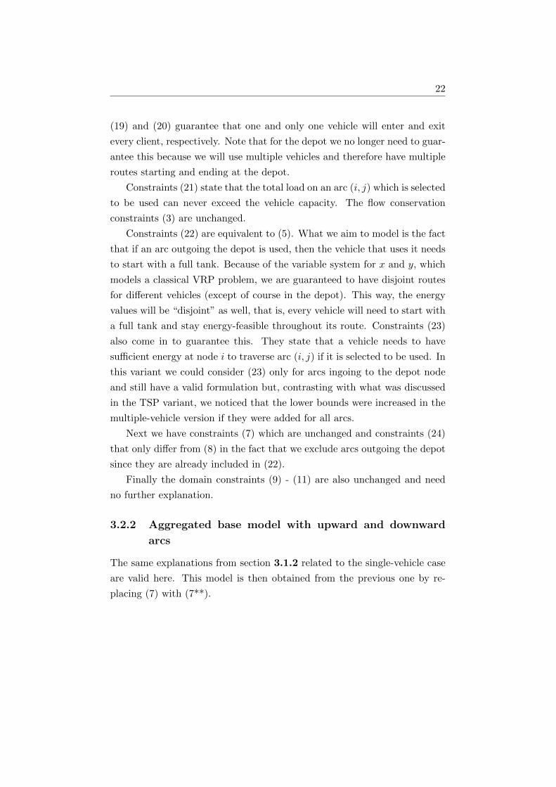
This model is very similar to the case with a single vehicle. Constraints

22

(19) and (20) guarantee that one and only one vehicle will enter and exit

every client, respectively. Note that for the depot we no longer need to guar-

antee this because we will use multiple vehicles and therefore have multiple

routes starting and ending at the depot.

Constraints (21) state that the total load on an arc (i, j) which is selected

to be used can never exceed the vehicle capacity. The flow conservation

constraints (3) are unchanged.

Constraints (22) are equivalent to (5). What we aim to model is the fact

that if an arc outgoing the depot is used, then the vehicle that uses it needs

to start with a full tank. Because of the variable system for x and y, which

models a classical VRP problem, we are guaranteed to have disjoint routes

for different vehicles (except of course in the depot). This way, the energy

values will be “disjoint” as well, that is, every vehicle will need to start with

a full tank and stay energy-feasible throughout its route. Constraints (23)

also come in to guarantee this. They state that a vehicle needs to have

sufficient energy at node i to traverse arc (i, j) if it is selected to be used. In

this variant we could consider (23) only for arcs ingoing to the depot node

and still have a valid formulation but, contrasting with what was discussed

in the TSP variant, we noticed that the lower bounds were increased in the

multiple-vehicle version if they were added for all arcs.

Next we have constraints (7) which are unchanged and constraints (24)

that only differ from (8) in the fact that we exclude arcs outgoing the depot

since they are already included in (22).

Finally the domain constraints (9) - (11) are also unchanged and need

no further explanation.

3.2.2 Aggregated base model with upward and downward

arcs

The same explanations from section 3.1.2 related to the single-vehicle case

are valid here. This model is then obtained from the previous one by re-

placing (7) with (7**).

23

3.2.3 Disaggregated base model with only upward arcs

Minimize∑

(i,j)∈A

cijxij

s.t. : (9) + (11) + (19)− (20) + (22) + (24)∑i∈V

fki1 = qk ∀k ∈ Vc (12)∑i∈V

fkki = qk ∀k ∈ Vc (13)∑i∈V

fkij −∑i∈V

fkji = 0 ∀j, k ∈ Vc, j 6= k

(14)

fkij ≤ qkxij ∀(i, j) ∈ A,∀k ∈ Vc(15)∑

k∈Vc

fkij ≤ Cxij ∀(i, j) ∈ A (25)

eij ≥ αijxij + βij∑k∈Vc

fkij ∀(i, j) ∈ A (26)

∑i∈V

eji =∑i∈V

eij −

αijxij + βij∑k∈Vc

fkij

∀j ∈ Vc (17)

fkij ≥ 0 ∀(i, j) ∈ A,∀k ∈ Vc(18)

For the disaggregated version we need to add constraints (25) to ensure

that the vehicle capacities are satisfied. Besides these, the only difference

to the previous model is in constraints (26) that are equivalent to (23) but

with the y variables replaced by their definition in terms of the f variables.

Constraints (12) - (15) + (17) are rewritten here again because we need

to ensure load flow conservation and energy flow conservation with the f

variables, while constraints (18) guarantee that the f variables are non-

negative.

As with the single-vehicle case, constraints (15) are the reason why the

disaggregated models are worth considering. In the VRP version, however,

they are weaker specially with small values of C. This situation has also

24

been studied and known for a while and it will not be explained here. It is

then expected that these models produce worse results than when used in

the single vehicle case. It is not expected that they will be used to solve the

EVRP but it is nonetheless interesting from a theoretical point of view to

see how they behave when compared to the other models.

3.2.4 Disaggregated base model with upward and downward

arcs

For this model it is clear to see now that all we need to do is replace (17) in

the previous model with (17*).

3.2.5 Aggregated base model with Connectivity Cuts

The CCs previously discussed are valid inequalities for the multiple-vehicle

case as well. In fact, the natural formulation for the classical VRP uses only

the x variables, and all the constraints that only include them, with the CCs

being one of the possibilities to model the connectivity of the routes.

We will also provide results on both aggregated models for multiple ve-

hicles when used in a branch-and-cut approach with the CCs.

3.2.6 Aggregated base model with Rounded Capacity Cuts

The final model that we will consider for the VRP variant of the EVRP

involves Rounded Capacity Cuts (RCCs). These inequalities are of the form:

∑i∈S′,j∈S

xij ≥ dq(S)

Ce ∀S ⊆ Vc (RCCs)

The notation q(S) represents the total demand of the nodes in S, that

is, q(S) =∑

i∈S qi.

The RCCs guarantee the vehicle capacities because they force a minimum

number of vehicles to go from the complementary set of S to S. This means

that we can use these RCCs in two different ways. One way is to replace

constraints (21) with (4) and use the RCCs to ensure the vehicle capacities.

In this situation, constraints (3) and (4) guarantee a valid load flow system

which is required for the energy flow system. The second way we can use the

25

RCCs is adding them as valid inequalities to improve the lower bounds of

the linear programming relaxations solved during a branch-and-cut method.

We developed a branch-and-cut method that uses both these ways, which

will be explained further in a subsequent chapter.

3.3 EVRP with recharging stations

The models soon to be presented are defined in the extended graph G′′ whose

construction was explained in the previous chapter. The variables used are

the same from the previous sections. Note that G′′ is no longer complete

so xij = yij = eij = 0 for the arcs that do not exist in G′′. To simplify

the notation in the models below, we will not explicitly demand this in the

model or account for it the summations, although care must be taken when

implementing the models to either set the variables that do not exist to 0

or to not create them at all. Also as a matter of simplification consider that

qi = 0 for every node i that represents a copy of a recharging station.

Also note that we will not present the disaggregated versions because we

believe they can be easily derived from the previous sections. In addition to

that, the extended graphG′′ has more arcs now, which means more variables,

that will reduce the effectiveness of the disaggregated models.

3.3.1 Aggregated base model (one vehicle)

This first model assumes that there are only upward arcs and one vehicle

(TSP variant).

26

Minimize∑

(i,j)∈A

cijxij

s.t. :∑i∈V ′′

xij = 1 ∀j ∈ V \ V ′r (27)∑i∈V ′′

xji = 1 ∀j ∈ V \ V ′r (28)∑i∈V ′′

xji ≤ 1 ∀j ∈ V ′r (29)∑i∈V ′′

xij =∑i∈V

xji ∀j ∈ V ′r (30)∑i∈V ′′

yij = −qj +∑i∈V ′′

yji ∀j ∈ V ′′ \ {1} (31)

qixij ≤ yij ≤ (Q− qj)xij ∀(i, j) ∈ A′′ (32)∑i∈V ′′

e1i = B (33)∑i∈V ′′

eji = B∑i∈V ′′

xji ∀j ∈ V ′r (34)∑i∈V ′′

ei1 ≥∑i∈V ′′

αi1xi1 + βi1yi1 (35)∑i∈V ′′

eij ≥∑i∈V ′′

αijxij + βijyij ∀j ∈ V ′r (36)∑i∈V ′′

eji =∑i∈V ′′

eij − (αijxij + βijyij) ∀j ∈ Vc (37)

eij ≤ Bxij ∀(i, j) ∈ A′′ (38)

xij ∈ {0, 1} ∀(i, j) ∈ A′′ (39)

yij ≥ 0 ∀(i, j) ∈ A′′ (40)

eij ≥ 0 ∀(i, j) ∈ A′′ (41)

If the graph has upward and downward arcs then, as usual, constraints

(37) need to be replaced with (37*). Every explanation from previous sec-

tions is valid in this case.

27

∑i∈V ′′

eji ≤∑i∈V ′′

eij − (αijxij + βijyij) ∀j ∈ Vc (37*)

Most of the constraints are similar to ones found in the models without

recharging stations. They differ only in the fact that they are now defined

in an extended graph. Those constraints are (27) - (28) + (31) - (33) + (35)

+ (37) - (41). Their counterparts are, respectively, (1) - (11). As a quick

review, constraints (27) - (28) guarantee that every client is visited exactly

one; constraints (31) - (32) model the load flow conservation; constraint

(33) assures that the vehicle leaves the depot with a full tank; constraint

(35) makes sure the vehicle has enough energy to return to the depot in

the end of the route; constraints (37) model the energy flow conservation

in the client nodes; constraints (38) assure the maximum energy level is

not exceeded; and constraints (39) - (41) guarantee the variable domains.

Note that in this case we could also use the set of valid inequalities given by

eij ≥ αijxij + βijyij , ∀(i, j) ∈ A instead of constraints (35) - (36).

The new sets of constraints start with (29) which assure that a copy of a

recharging station is visited at most once, while (30) state that the number

of arcs leaving a copy of a recharge station is the same as the number of

arcs entering that copy (in this case, it is either 0 or 1). Constraints (34)

are similar to (33) in the sense that they guarantee that a vehicle leaves the

copy of a recharging station with a full tank in case that copy is visited.

Constraints (36) guarantee that the vehicle has enough energy to reach a

copy of a recharging station if headed there, similarly to what (35) does for

the depot. Note that constraints (34) and (36) are, in a sense, the energy

flow conservation constraints for the recharging station related nodes since

in conjunction they model the energy flow entering and leaving every copy

of a recharging station.

3.3.2 Aggregated base model (multiple capacitated vehicles)

The following model assumes that we are allowed to use more than one

vehicle as in the VRP variants presented previously and that only upward

arcs exist.

28

Minimize∑

(i,j)∈A

cijxij

s.t. : (29)− (31) + (37) + (39)− (41)∑i∈V ′′

xij = 1 ∀j ∈ Vc (42)∑i∈V ′′

xji = 1 ∀j ∈ Vc (43)

qixij ≤ yij ≤ Cxij ∀(i, j) ∈ A′′ (44)

eij = Bxij ∀(i, j) ∈ {(i, j) ∈ A′′ : i 6∈ Vc}(45)

eij ≥ αijxij + βijyij ∀(i, j) ∈ A′′ (46)

eij ≤ Bxij ∀(i, j) ∈ {(i, j) ∈ A′′ : i ∈ Vc}(47)

Once again, if we wish to incorporate both upward and downward arcs,

we need to replace (37) with (37*).

Constraints (42) - (44) + (46) are very similar to, respectively, (19) - (21)

+ (23). They are only different since the newer ones refer to the extended

graph G′′. Constraints (42) - (43) assure that every client is visited exactly

once (although excluding the depot, which (27) - (28) did not, since we can

now have multiple vehicles); constraints (44) guarantee that the load flow is

within bounds, specially that it does not exceed the maximum load capacity;

and constraints (46) guarantee that the energy level is always sufficient to

traverse an arc in case it is part of the route.

The last two sets of constraints (45) and (47), similarly to (22) and (24),

assure that a vehicle leaves the depot or any copy of a recharging station

with a full tank and that, in the other arcs, the total energy flow does not

exceed the maximum tank level, respectively.

Chapter 4

Branch-and-cut methods

In this chapter we will present the branch-and-cut methods that have been

implemented. We will first give an overview on branch-and-cut methods in

general followed by the specifics of the software used to implement our own.

If one wishes to see a more detailed review on branch-and-cut methods and

valid inequalities in general then they are referenced to chapters 7, 8 and 9

of [9].

In a third section we will go more into detail on what the program de-

veloped can do and how a regular user can use it to test their own instances.

Note that details related to the specific programming language will not be

explained. Every algorithm used will rather be explained in pseudo-code.

Nonetheless the code is available on demand.

Finally, the last section of this chapter will explain the instance format

supported by the developed programs.

4.1 Overview on branch-and-cut methods

The main focus of this thesis is to study the models described in the previous

chapter. While we could simply give them to a solver and wait for results,

which we have also done, we can go even further.

A branch-and-cut method is a branch-and-bound method where in some

or all nodes of the branch-and-bound tree we add global or local valid in-

equalities to try and improve the linear programming relaxation values with

the aim of reducing the total number of nodes explored in the tree. This

however comes with a price. First it is important that the inequalities added

29

30

are in fact violated by the fractional solution in the current node or else no

improvement can be made. Second we need to actually find such inequali-

ties which is usually time-consuming and will force us to spend more time at

every node. This is the trade-off of these methods: adding inequalities can

improve the bounds and lower the number of nodes visited in the branch-

and-bound tree but it takes time to find them. If the inequalities are not

strong enough then we could actually be doing more harm than good.

Given a fractional solution and a set of valid inequalities, the separa-

tion problem for that set of valid inequalities is the problem of determining

whether or not the fractional solution satisfies all inequalities in the set and,

if not, then find at least one inequality which is violated.

A separation problem can usually be transformed into an optimization

problem. If we solve this optimization problem we are guaranteed to find

at least one inequality which is violated or prove that none are. Being an

optimization problem it could happen that it falls into the NP-hard class

hence why sometimes a separation problem needs to be solved heuristically

(or else we would be solving an NP-hard problem in every node of the

branch-and-bound tree!). This however is not mandatory. Some methods

in the literature solve their separation problems in the NP-hard class to

optimality. The advantage is that the valid inequalities provided in the end

are extremely beneficial and it pays off to separate them.

On the other hand, a separation problem can be polynomially solvable as

will the ones we consider in this thesis, although this does not mean that the

inequalities provided are always helpful. Experimentation is needed from a

practical point of view.

We considered valid inequalities being added as a means of improving the

linear programming relaxation bounds but this is not the only way we can

define a branch-and-cut method. An optimization problem can have certain

inequalities which are mandatory in the sense that every integer solution

needs to satisfy them so that optimality is proven. It could happen that

these inequalities are exponentially many and so adding them directly into

the model could turn out catastrophic since we could not even be able to

solve the linear programming relaxation (for example if we try to use the

Simplex method with 250 equalities !).

The workaround for this issue is to consider the original model without

this set of exponentially many constraints and, every time a new integer

31

solution is found in the branch-and-bound tree, solve the separation problem

to determine one inequality that is violated by the integer solution and add

it. If no violated inequalities are found then we accept the integer solution

and proceed with branching. In the end of the process we will guarantee

optimality if and only if we solve the separation problem to optimality so,

in the case where the separation problem lies in the NP-hard class, we could

be looking at long computational times.

Note that using a branch-and-cut method will not need us to explicitly

add every inequality in the set or sets. We will end the branch-and-bound

tree with only a small subset of inequalities added, as all others will be

implicitly satisfied. This even favors more the decision of using a cutting

plane approach instead of bluntly adding every inequality a priori.

Several variants of branch-and-cut methods exist. Something that is

quite usual is joining these two types of cuts in a single branch-and-cut

method. For example having one set of exponentially many constraints

which are to be added every time we find a new integer solution and a

different (or even the same) set of inequalities to be added as cuts for the

fractional solutions. We can also have more than one set of inequalities with

different separation problems and try different approaches such as solving

all separation problems in every node or just at the root node and then only

look for one type of inequalities in the rest of the tree, etc.

The theoretical work of discovering sets of inequalities and devising sep-

aration algorithms is the hardest part of a branch-and-cut method. Imple-

menting the branch-and-cut method has become easier thanks to the avail-

able solvers and their frameworks which allow us to easily tell the solver to

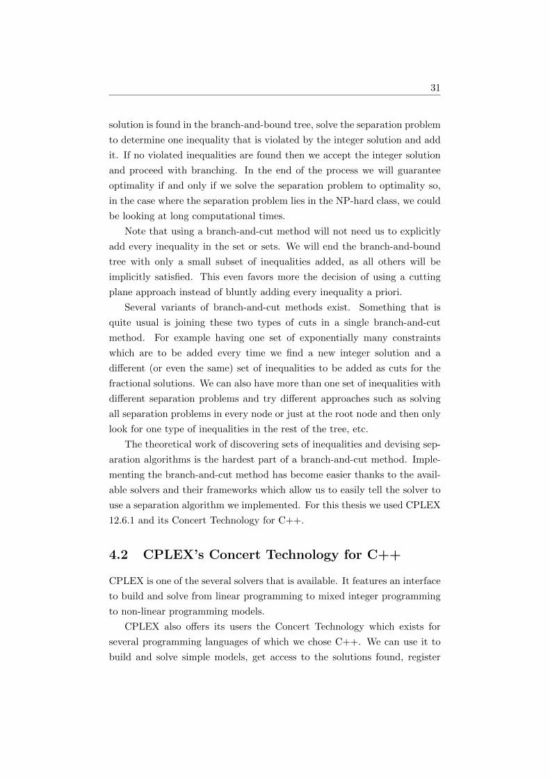
use a separation algorithm we implemented. For this thesis we used CPLEX

12.6.1 and its Concert Technology for C++.

4.2 CPLEX’s Concert Technology for C++

CPLEX is one of the several solvers that is available. It features an interface

to build and solve from linear programming to mixed integer programming

to non-linear programming models.

CPLEX also offers its users the Concert Technology which exists for

several programming languages of which we chose C++. We can use it to

build and solve simple models, get access to the solutions found, register

32

computational times and so on, although this can also be achieved with

the regular CPLEX interface. The most important aspect for this thesis of

the Concert Technology is the ability of adding our own algorithms to the

regular branch-and-bound method that CPLEX has implemented.

We aimed to implement some separation algorithms to add our own valid

inequalities (CPLEX also has its own procedures to add cuts) during the

branch-and-bound process. The way this works is CPLEX makes the dis-

tinction between what are called User Cuts and Lazy Cuts. A User Cut is a

procedure that is to be called by CPLEX every time a new fractional solu-

tion is determined, meaning that we should implement User Cuts that look

for and add inequalities which are violated by fractional solutions, whereas

a Lazy Cut is a procedure that is called by CPLEX only on every integer

solution found, and so should contain a separation algorithm for inequalities

violated be integer solutions.

To use these features we need to create one or several classes with what-

ever names we wish that are extensions to either the class that deals with

User Cuts or Lazy Cuts. To make this very easy for the user, all that CPLEX

requires is our classes to have a method called main() which, as can be seen,

takes no arguments. What happens in that method is then up to us.

We will skip any implementation details as the code is accessible to

anyone who wishes to see it. Only the separation algorithms used will be

presented in pseudo-code.

4.3 Specifics of the implementation

4.3.1 How to use

Fundamentally, the code created allows the user to run any of the models

from sections 3.1 and 3.2. The models from section 3.3, i.e., with recharging

stations, were not implemented yet but can and will be easily added in the

future. The format of the instance files plus the way they need to be written

can not be changed since the program only reads the file properly if they

use the format it was built for.

In order to use the program the user needs to first decide on a single-

vehicle model or multiple-vehicle model since the input arguments are slightly

different. If the user wishes to run an instance with a single-vehicle model

then, ir order, he or she needs to specify:

33

1. The .txt file containing the instance data with the only requirement of

the format being that it ends in “ [number of nodes].txt”. For example,

“[random text] 20.txt” is a valid format that indicates the instance has

20 nodes. What is placed in “[random text]” is irrelevant although we

chose for our instances to use “pos graph” in case all α and β values

are non-negative or simply “graph” if they can be negative or positive;

2. The model to use. In the single-vehicle case the user can choose from

“abmu”, “abmud”, “dbmu” or “dbmud” which correspond to models

3.1.1, 3.1.2, 3.1.3 and 3.1.4, respectively;

3. The maximum tank value to use, that is, the value of B;

4. If the user wants the final variable output or not by writing either

“yes” or “no”;

5. If the user wishes that CPLEX uses its own integrated cuts or not by

writing either “yes” or “no”;

6. If the user wishes to use the Connectivity Cuts or not by writing “yes”

or “no” (corresponding to section 3.1.5).

In case the user wishes to use a multiple-vehicle model then the input,

in order, is:

1. The .txt file containing the instance data with the only requirement of

the format being that it ends in “ [number of nodes].txt”. For example,

“[random text] 20.txt” is a valid format that indicates the instance has

20 nodes. What is placed in “[random text]” is irrelevant although we

chose for our instances to use “pos graph” in case all α and β values

are non-negative or simply “graph” if they can be negative or positive;

2. The model to use. In the multiple-vehicle case the user can choose

from “abmu vrp”, “abmud vrp”, “dbmu vrp” or “dbmud vrp” which

correspond to models 3.2.1, 3.2.2, 3.2.3 and 3.2.4, respectively;

3. The maximum tank value to use, that is, the value of B;

4. The maximum vehicle capacity C;

5. If the user wants the final variable output or not by writing either

“yes” or “no”;

34

6. If the user wishes that CPLEX uses its own integrated cuts or not by

writing either “yes” or “no”;

7. If the user wishes to use Connectivity Cuts (section 3.2.5), Rounded

Capacity Cuts (section 3.2.6) or no cuts, by writing either “yes.weak”,

“yes.str” or “no”, respectively.

All the integration with CPLEX is done automatically by the program

therefore, after being started, the user only needs to wait for the program

to end. The output includes the CPLEX status, that is, whether the final

solution is optimal or the problem is infeasible, the number of branch-and-

bound nodes, the linear programming relaxation value, the root node value,

(which can be different from the linear programming relaxation value due to

preprocessing), the final objective function value and the total CPU time.

In addition to this, all the regular CPLEX output is also shown such as the

number of cuts of a given type added, including the total number of cuts

obtained through user defined User or Lazy cuts. If the user so wishes the

variables can also be output by selecting the corresponding option before

running the program, as explained before.

4.3.2 Instance format

In the previous section we mentioned the instance file name which must be

of the form “[random text] 20.txt”. The contents of this file must be the

demand vector D, the cost matrix C, the α value matrix A and the β value

matrix B, in this order. To easily explain the correct formatting, look at

figure 4.1.

Note that the demand vector includes the depot, which must have de-

mand 0, and that all matrices are complete with 0 in the main diagonal.

Something which may not be obvious is that each number must be separated

by a blank space. Any other separator will not work and will probably lead

to a program error.

The example shown in figure 4.1 depicts an instance with 5 nodes - 1

depot and 4 clients. The depot has demand 0, as it should, and the clients

represented by nodes 2, 3, 4 and 5 have demand 3, 2, 2 and 5, respectively.

The cost of going from the client in node 3 to the client in node 5 is 189,

whereas going from the depot to the client in node 2 will cost 333, and the

35

Figure 4.1: Example of an input file.

energy consumed by an empty vehicle that traverses arc (4, 1) is 16 with an

extra consumption of 1 per load unit, for example.

4.3.3 Branch-and-cut method with the separation of Con-

nectivity Cuts

As said previously, to develop a branch-and-cut method using CPLEX’s

Concert Technology we need to implement our own procedures in a class

and make it so that class extends either the User Cut class or the Lazy Cut

class. In this specific case, the Connectivity Cuts (CCs) are always defined

as User Cuts. Recalling chapter 3, the Electric Vehicle Routing Problem’s

(EVRP) formulation involves not only the x variables but also the y and e

hence why we could conclude that the CCs were valid inequalities and not

mandatory constraints for our model.

Algorithm 4.1 describes how to separate the CCs given a fractional so-

lution of x, which we will call x∗.

Note that, when determining the minimal cut between the depot and the

current client in the cycle, it is common to find a minimal cut, and therefore

36

Algorithm 4.1 Separation of Connectivity Cuts.

Create an auxiliary graph which has the same nodes and arcs as theoriginal graph. For every arc in the auxiliary graph, add a maximumcapacity of x∗ij and a minimum capacity of 0.

for all i ∈ V \ {1} doDetermine the maximum flow v between the depot and client i.

if v < 1 thenDetermine a minimal cut between the depot and client i. Let S′ bethe set of nodes which are on the depot’s side in the minimal cut andS = V \ S′.

Add the violated Connectivity Cut∑

i∈S′,j∈S xij ≥ 1, unless it isalready present in the model.

end ifend for

a violated inequality, which has already been found in previous iterations of

the cycle or even while solving previous separations. CPLEX has procedures

implemented that automatically deal with this fact and do not add cuts

which have already been added. This way we can ignore checking for this

situation in the algorithm and add every cut that is found.

The branch-and-cut method developed in this case consists of adding

algorithm 4.1 to the list of routines which are called upon every fractional

solution. The maximum flow algorithm used was not implemented in this

thesis but the code was provided to us. It is the algorithm proposed by

Goldberg in [10] which runs in O(t3), where t is the number of nodes in the

graph.

4.3.4 Branch-and-cut method with the separation of Rounded

Capacity Cuts

In the previous chapter we discussed the use of Rounded Capacity Cuts

(RCCs) to solve the Vehicle Routing Problem (VRP) variant. RCCs can be

used in two ways: we either remove the capacity constraints (21) and replace

them with (4) - to ensure a correct load flow system and therefore a correct

energy flow system - and then use the RCCs to guarantee that the vehicle

capacities are always satisfied, or we add them as simple valid inequalities.

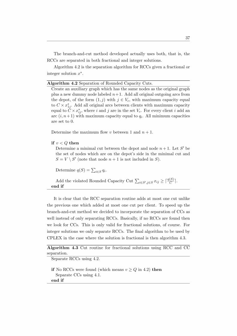
37

The branch-and-cut method developed actually uses both, that is, the

RCCs are separated in both fractional and integer solutions.

Algorithm 4.2 is the separation algorithm for RCCs given a fractional or

integer solution x∗.

Algorithm 4.2 Separation of Rounded Capacity Cuts.

Create an auxiliary graph which has the same nodes as the original graphplus a new dummy node labeled n+1. Add all original outgoing arcs fromthe depot, of the form (1, j) with j ∈ Vc, with maximum capacity equalto C × x∗1j . Add all original arcs between clients with maximum capacityequal to C×x∗ij , where i and j are in the set Vc. For every client i add anarc (i, n+1) with maximum capacity equal to qi. All minimum capacitiesare set to 0.

Determine the maximum flow v between 1 and n+ 1.

if v < Q thenDetermine a minimal cut between the depot and node n+ 1. Let S′ bethe set of nodes which are on the depot’s side in the minimal cut andS = V \ S′ (note that node n+ 1 is not included in S).

Determine q(S) =∑

i∈S qi.

Add the violated Rounded Capacity Cut∑

i∈S′,j∈S xij ≥ dq(S)C e.

end if

It is clear that the RCC separation routine adds at most one cut unlike

the previous one which added at most one cut per client. To speed up the

branch-and-cut method we decided to incorporate the separation of CCs as

well instead of only separating RCCs. Basically, if no RCCs are found then

we look for CCs. This is only valid for fractional solutions, of course. For

integer solutions we only separate RCCs. The final algorithm to be used by

CPLEX in the case where the solution is fractional is then algorithm 4.3.

Algorithm 4.3 Cut routine for fractional solutions using RCC and CCseparation.

Separate RCCs using 4.2.

if No RCCs were found (which means v ≥ Q in 4.2) thenSeparate CCs using 4.1.

end if

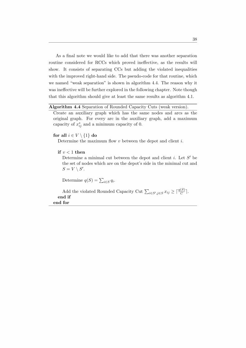
38

As a final note we would like to add that there was another separation

routine considered for RCCs which proved ineffective, as the results will

show. It consists of separating CCs but adding the violated inequalities

with the improved right-hand side. The pseudo-code for that routine, which

we named “weak separation” is shown in algorithm 4.4. The reason why it

was ineffective will be further explored in the following chapter. Note though

that this algorithm should give at least the same results as algorithm 4.1.

Algorithm 4.4 Separation of Rounded Capacity Cuts (weak version).

Create an auxiliary graph which has the same nodes and arcs as theoriginal graph. For every arc in the auxiliary graph, add a maximumcapacity of x∗ij and a minimum capacity of 0.

for all i ∈ V \ {1} doDetermine the maximum flow v between the depot and client i.

if v < 1 thenDetermine a minimal cut between the depot and client i. Let S′ bethe set of nodes which are on the depot’s side in the minimal cut andS = V \ S′.

Determine q(S) =∑

i∈S qi.

Add the violated Rounded Capacity Cut∑

i∈S′,j∈S xij ≥ dq(S)C e.

end ifend for

Chapter 5

Test results

This chapter will focus on presenting and discussing some test results on the

models and the branch-and-cut methods considered.

The first section will explain how the test instances were generated while

the second and third sections will show the result tables, for the Traveling

Salesman Problem (TSP) and Vehicle Routing Problem (VRP) respectively,

and our first insight on what we can conclude from them.

5.1 The test instances

Due to the nature of the problem in study and the exact method approach,

and the time available for testing, we decided to use only two instances

which share the demand vectors and cost matrices and differ only in the

fact that one has strictly positive energy consumption values while the other

has both positive and negative values. Despite this, we have other instances

generated and ready to be used and the tools to generate more if needed

and with varied input parameters.

The instances used satisfy the following conditions:

• 20 nodes;

• Complete graph;

• Integer demands in the set {1, . . . , 5};

• Integer symmetric and euclidian costs in the set {20, . . . , 400};

39

40

• Integer inverse-symmetric α values in the set {−4, . . . , 20} (inverse-

symmetry means that if αij = −4 then αji = 20, for example) with

the value of 1 added in the end to account for some sort of constant

energy loss, therefore the final values lie in the set {−3, . . . , 21};

• Integer β values in the set {−1, 0, 1} related with the sign of the cor-

responding α, i.e., if αij < 0 then βij = −1 whereas if αij > 0 then

βij = 1. If αij = 0 then βij = 0 as well;

• In case we wish to have only strictly positive energy consumption val-

ues, we add 4 to every α value, making them vary in the set {1, . . . , 25},and consider all β values to be 1.

5.2 TSP variant

Table 5.1 shows the results for the TSP variant. For the upward only arcs

models we used three values of B: 800, 700 and 600. For the upward and

downward arcs models we used the values 150, 100 and 50. They are based

on the total energy spent in the TSP route which was determined via a

regular TSP model. The optimal TSP route has a cost value of 1423.

The columns represent, from left to right, the model used, the linear pro-

gramming relaxation value (LR), the optimal value (OPT), the linear gap,

the time taken in seconds to optimality and the number of branch-and-bound

(B&B) nodes in the final tree. In the models used section we use the legend

CCs to refer to the Connectivity Cuts, separated using algorithm 4.1, and

CPCs to refer to the CPLEX integrated cuts, which can not be controlled

by us in any form except choosing to remove them and can lead to erratic

behavior. Note that the linear programming relaxation values are calculated

without any pre-processing done on the model by CPLEX although to solve

to optimality pre-processing is allowed. Basically, the program developed

calculates the linear programming relaxation of the model first with the

pre-processing turned off and then restarts the branch-and-bound process

with pre-processing turned on.

Finally, we should refer that ABMU, ABMUD, DBMU and DBMUD are

the models in sections 3.1.1, 3.1.2, 3.1.3 and 3.1.4, respectively.

41

Table 5.1: Results for the TSP variant. The running times were obtained

on a single 3.6 GHz thread.

Model LR OPT gap Time (s) B&B nodes

B = 800 Upward arcs only

ABMU 1371.18 1423 3.64 % 10 6953

ABMU + CCs 1423 1423 0.00 % 0.1 0

DBMU 1423 1423 0.00 % 0.1 0

ABMU + CPCs 1421.95 1423 0.07 % 0.1 0

ABMU + CCs + CPCs 1423 1423 0.00 % 0.1 0

DBMU + CPCs 1423 1423 0.00 % 0.6 0

B = 700 Upward arcs only

ABMU 1371.18 1427 3.91 % 10.1 4631

ABMU + CCs 1423 1427 0.28 % 7.3 891

DBMU 1423.03 1427 0.28 % 40.7 501

ABMU + CPCs 1422.08 1427 0.34 % 0.9 278

ABMU + CCs + CPCs 1423 1427 0.28 % 6.3 693

DBMU + CPCs 1423.03 1427 0.28 % 4.9 24

B = 600 Upward arcs only

ABMU 1371.18 1463 6.28 % 147.4 68701

ABMU + CCs 1423 1463 2.73 % 385.2 43712

DBMU 1423.1 1463 2.73 % 684.9 8348

ABMU + CPCs 1421.7 1463 2.82 % 356.3 210054

ABMU + CCs + CPCs 1423.03 1463 2.73 % 59.4 8721

DBMU + CPCs 1423.11 1463 2.73 % 633.9 5924

B = 150 Upward and downward arcs

ABMUD 1371.51 1429 4.02 % 5.6 2532

ABMUD + CCs 1423.01 1429 0.42 % 4 448

DBMUD 1423.02 1429 0.42 % 13.6 115

ABMUD + CPCs 1421.81 1429 0.50 % 0.8 316

ABMUD + CCs + CPCs 1423.01 1429 0.42 % 2.8 250

DBMUD + CPCs 1423.03 1429 0.42 % 2.6 51

B = 100 Upward and downward arcs

ABMUD 1372.4 1431 4.10 % 6.3 2032

ABMUD + CCs 1423.07 1431 0.55 % 2.5 196

DBMUD 1423.1 1431 0.55 % 3.4 17

ABMUD + CPCs 1422.04 1431 0.63 % 0.8 143

ABMUD + CCs + CPCs 1423.12 1431 0.55 % 3.7 293

DBMUD + CPCs 1423.14 1431 0.55 % 3.4 18

B = 50 Upward and downward arcs

ABMUD 1375.89 1459 5.70 % 10 2672

ABMUD + CCs 1423.78 1459 2.41 % 22.4 2561

DBMUD 1425.15 1459 2.32 % 215.3 1627

Continued

42

Model LR OPT gap Time (s) B&B nodes

ABMUD + CPCs 1432.8 1459 1.80 % 6.3 713

ABMUD + CCs + CPCs 1432.72 1459 1.80 % 15.6 1639

DBMUD + CPCs 1430.44 1459 1.96 % 130.7 903

The first observation taken from the results on table 5.1 is that the

value of B strongly influences the problem. It was expected that with lower

values of B the optimal solution would change since more routes would

become energy-infeasible. What is surprising is the fact that the gaps worsen

when B decreases, which can be explained by the fact that the optimal

value increases but the linear programming relaxation value barely does so.

Obviously, when the gaps are bigger then the time to optimality is also

increased as are the B&B nodes. Excluding some rare exceptions, this can

be seen throughout the table.

The second conclusion we can draw from this table is that the aggregated

base models with CCs have almost the same LR value as the disaggregated

models. However they do not have the same value as it happens in the

TSP which means that in the presence of the energy flow variables and the

constraints that involve them, the disaggregated model and the aggregated

model with CCs are no longer equivalent even though the disaggregated

model still implies the CCs. This happens with both energy consumption

value types and with or without CPCs.

Thirdly, CPLEX has a very good cutting plane routine for these types of

flow-based models since it outperforms the models that do not use CPCs but

it is clearly not enough to deal with the increasing gaps that were mentioned

before. This leads us to conclude that, although CPLEX is good by its own,

it will not be able to solve very large instances without “help”.

In terms of running times, not using the CCs is always the better option

for these instances. This was something that was mentioned previously. The

CCs are not good enough in terms of improving the bounds to be worth

separating even though, when not considering CPCs, they always reduce

the number of B&B nodes in the tree. Using only CPCs though is still a

better option.

As for the disaggregated models, we can see that they are not worth it

as we expected. They provide the smallest number of B&B nodes in their

respective trees but the running times are always much worse.

43

Finally, there does not seem to be any significant differences when con-

sidering upward arcs only or upward and downward arcs in terms of the

linear programming relaxation and conclusions although the upward and

downward case seemed easier to solve.

5.3 VRP variant

The results for the VRP variant are shown in table 5.2. We used two dif-

ferent maximum vehicle capacity values - 30 and 10 - and for each we have

three values of B for each energy consumption value types. For C = 30

we have B ∈ {150, 200, 250} when considering only upward arcs and B ∈{25, 50, 100} when considering both types of arcs. For C = 10 we have

B ∈ {45, 60, 75} and B ∈ {30, 40, 50}, respectively for upward and upward

and downward cases. The total demand of all clients for the instances used

is Q = 59. The optimal VRP solution has a cost value of 1505 for C = 30

and 2092 for C = 10.

The columns have the same meaning as in table 5.1 as do the symbols

CCs and CPCs. RCCs refers to Rounded Capacity Cuts using the final

routine that includes Connectivity Cuts described in algorithm 4.3, while

WRCCs refers also to the Rounded Capacity Cuts but using the weak sep-

aration algorithm 4.4. Note that this weak separation algorithm is at least

as good as the CCs in terms of linear programming relaxation since in the

worst case it adds a CC instead of a RCC.

Finally, we should add that ABMU, ABMUD, DBMU and DBMUD now

represent the models with multiple vehicles in sections 3.2.1, 3.2.2, 3.2.3

and 3.2.4, respectively.

Table 5.2: Results for the VRP variant. The running times were ob-

tained on a single 3.6 GHz thread.

Model LR OPT gap Time (s) B&B nodes

C = 30

B = 250 Upward arcs only

ABMU 1423.51 1514 5.98 % 56.2 21140

ABMU + CCs 1469.97 1514 2.91 % 93 12538

ABMU + WRCCs 1469.97 1514 2.91 % 91.7 12538

ABMU + RCCs 1486 1514 1.85 % 21.6 2205

Continued

44

Model LR OPT gap Time (s) B&B nodes

DBMU 1471.08 1514 2.83 % 836.2 4158

ABMU + CPCs 1482.27 1514 2.10 % 9.7 3137

ABMU + CCs + CPCs 1482.68 1514 2.07 % 47.7 6736

ABMU + WRCCs + CPCs 1482.68 1514 2.07 % 46.5 6736

ABMU + RCCs + CPCs 1483 1514 2.05 % 7.6 794

DBMU + CPCs 1473.15 1514 2.70 % 1644.9 7351

B = 200 Upward arcs only

ABMU 1424.59 1543 7.67 % 199.3 69138

ABMU + CCs 1471.97 1543 4.60 % 610.3 73176

ABMU + WRCCs 1471.97 1543 4.60 % 608.6 73176

ABMU + RCCs 1448.54 1543 6.12 % 292.8 35133

DBMU 1479.13 1543 4.14 % 2034.1 13579

ABMU + CPCs 1485.81 1543 3.71 % 163.9 31239

ABMU + CCs + CPCs 1486.01 1543 3.69 % 335.1 40877

ABMU + WRCCs + CPCs 1486.01 1543 3.69 % 331.3 40877

ABMU + RCCs + CPCs 1491.11 1543 3.36 % 409 49691

DBMU + CPCs 1483.25 1543 3.87 % 2326.9 12886

B = 150 Upward arcs only

ABMU 1438.19 1605 10.39 % 312 94684

ABMU + CCs 1490.19 1605 7.15 % 812.7 122928

ABMU + WRCCs 1490.19 1605 7.15 % 805.2 122928

ABMU + RCCs 1455.7 1605 9.30 % 1929.6 274175

DBMU 1502.69 1605 6.37 % 5394.7 47091

ABMU + CPCs 1513.65 1605 5.69 % 675 115081

ABMU + CCs + CPCs 1513.2 1605 5.72 % 1200.3 150924

ABMU + WRCCs + CPCs 1515.2 1605 5.72 % 1194.5 150924

ABMU + RCCs + CPCs 1501.91 1605 6.42 % 1418.2 189186

DBMU + CPCs 1511.58 1605 5.82 % 6755.1 51138

B = 100 Upward and downward arcs

ABMUD 1424.42 1514 5.92 % 31.6 12026

ABMUD + CCs 1470.05 1514 2.90 % 40.9 6866

ABMUD + WRCCs 1470.05 1514 2.90 % 41.1 6866

ABMUD + RCCs 1491 1514 1.52 % 11.2 1377

DBMUD 1470.8 1514 2.85 % 1141.4 7217

ABMUD + CPCs 1482.44 1514 2.08 % 9.4 3408

ABMUD + CCs + CPCs 1482.64 1514 2.07 % 33 5187

ABMUD + WRCCs + CPCs 1482.64 1514 2.07 % 33.2 5187

ABMUD + RCCs + CPCs 1488.5 1514 1.68 % 14.4 1641

DBMUD + CPCs 1473.18 1514 2.70 % 679.6 3836

B = 50 Upward and downward arcs

ABMUD 1431.5 1514 5.45 % 12 3092

ABMUD + CCs 1472.99 1514 2.71 % 28.6 3375

Continued

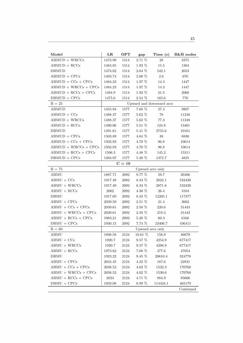
45

Model LR OPT gap Time (s) B&B nodes

ABMUD + WRCCs 1472.99 1514 2.71 % 28 3375

ABMUD + RCCs 1484.85 1514 1.93 % 15.5 1384

DBMUD 1474.02 1514 2.64 % 542.1 2053

ABMUD + CPCs 1483.74 1514 2.00 % 2.6 676

ABMUD + CCs + CPCs 1484.23 1514 1.97 % 14.3 1447

ABMUD + WRCCs + CPCs 1484.23 1514 1.97 % 14.3 1447

ABMUD + RCCs + CPCs 1484.9 1514 1.92 % 21.5 2060

DBMUD + CPCs 1475.6 1514 2.54 % 165.6 776

B = 25 Upward and downward arcs

ABMUD 1455.94 1577 7.68 % 27.4 9807

ABMUD + CCs 1488.37 1577 5.62 % 78 11248

ABMUD + WRCCs 1488.37 1577 5.62 % 77.3 11248

ABMUD + RCCs 1490.06 1577 5.51 % 124.9 13401

DBMUD 1491.61 1577 5.41 % 2755.6 10161

ABMUD + CPCs 1503.89 1577 4.64 % 38 8836

ABMUD + CCs + CPCs 1502.93 1577 4.70 % 96.8 10614

ABMUD + WRCCs + CPCs 1502.93 1577 4.70 % 96.8 10614

ABMUD + RCCs + CPCs 1506.3 1577 4.48 % 145.2 15311

DBMUD + CPCs 1494.97 1577 5.20 % 1372.7 4825

C = 10

B = 75 Upward arcs only

ABMU 1887.71 2092 9.77 % 59.7 20486

ABMU + CCs 1917.49 2092 8.34 % 2822.1 532430

ABMU + WRCCs 1917.49 2092 8.34 % 2871.8 532430

ABMU + RCCs 2002 2092 4.30 % 26.4 3104

DBMU 1917.69 2092 8.33 % 12205.1 117377

ABMU + CPCs 2039.59 2092 2.51 % 21.4 3662

ABMU + CCs + CPCs 2039.61 2092 2.50 % 220.6 31443

ABMU + WRCCs + CPCs 2039.61 2092 2.50 % 219.3 31443

ABMU + RCCs + CPCs 1983.21 2092 5.20 % 60.3 6166

DBMU + CPCs 1930.15 2092 7.74 % 23406.7 106411

B = 60 Upward arcs only

ABMU 1898.58 2124 10.61 % 158.9 46679

ABMU + CCs 1920.7 2124 9.57 % 4254.9 677417

ABMU + WRCCs 1920.7 2124 9.57 % 4296.9 677417

ABMU + RCCs 1973.62 2124 7.08 % 477.6 47054

DBMU 1923.22 2124 9.45 % 20610.4 324778

ABMU + CPCs 2034.45 2124 4.22 % 187.6 22831

ABMU + CCs + CPCs 2038.52 2124 4.02 % 1532.3 170760

ABMU + WRCCs + CPCs 2038.52 2124 4.02 % 1530.6 170760

ABMU + RCCs + CPCs 2024 2124 4.71 % 884.9 85606

DBMU + CPCs 1933.08 2124 8.99 % 114424.1 465179

Continued

46

Model LR OPT gap Time (s) B&B nodes

B = 45 Upward arcs only

ABMU 1964.15 2201 10.76 % 289.3 78782

ABMU + CCs 1975.21 2201 10.26 % 4675.1 756023

ABMU + WRCCs 1975.21 2201 10.26 % 4679.82 756023

ABMU + RCCs 2006.22 2201 8.85 % 2415.3 259408

DBMU 1986.8 2201 9.73 % 32623.7 484605

ABMU + CPCs 2055.51 2201 6.61 % 325.5 30140

ABMU + CCs + CPCs 2053.74 2201 6.69 % 3556.5 388168

ABMU + WRCCs + CPCs 2053.74 2201 6.69 % 3549.8 388168

ABMU + RCCs + CPCs 2027.55 2201 7.88 % 2900.1 229964

DBMU + CPCs 1999.02 2201 9.18 % 68138.7 356335

B = 50 Upward and downward arcs

ABMUD 1883.52 2092 9.97 % 18.1 11920

ABMUD + CCs 1917.49 2092 8.34 % 1708.5 379788

ABMUD + WRCCs 1917.49 2092 8.34 % 1736.5 379788

ABMUD + RCCs 2020.11 2092 3.44 % 38.1 8706

DBMUD 1917.69 2092 8.33 % 10799.5 129198

ABMUD + CPCs 2036.24 2092 2.67 % 17.4 4753

ABMUD + CCs + CPCs 2039.92 2092 2.49 % 111.1 17620

ABMUD + WRCCs + CPCs 2039.92 2092 2.49 % 111.7 17620

ABMUD + RCCs + CPCs 1998.11 2092 4.49 % 11.7 1941

DBMUD + CPCs 1928.64 2092 7.81 % 21621 128285

B = 40 Upward and downward arcs

ABMUD 1885.66 2092 9.86 % 36.6 19892

ABMUD + CCs 1917.49 2092 8.34 % 1347 281829

ABMUD + WRCCs 1917.49 2092 8.34 % 1349.4 281829

ABMUD + RCCs 2030 2092 2.96 % 31.6 5739

DBMUD 1917.69 2092 8.33 % 10291.1 133657

ABMUD + CPCs 2037.04 2092 2.63 % 20.9 4644

ABMUD + CCs + CPCs 2035.53 2092 2.70 % 146 21419

ABMUD + WRCCs + CPCs 2035.53 2092 2.70 % 147.1 21419

ABMUD + RCCs + CPCs 2001.29 2092 4.34 % 30.1 4760

DBMUD + CPCs 1925.75 2092 7.95 % 21469.3 119858

B = 30 Upward and downward arcs

ABMUD 1896.09 2124 10.73 % 128.5 55039

ABMUD + CCs 1920.09 2124 9.60 % 2415.3 435752

ABMUD + WRCCs 1920.09 2124 9.60 % 2383.7 435752

ABMUD + RCCs 1987.33 2124 6.43 % 141.3 18714

DBMUD 1920.96 2124 9.56 % 16811.6 222466

ABMUD + CPCs 2037.37 2124 4.08 % 176 31359

ABMUD + CCs + CPCs 2037.31 2124 4.08 % 740.9 91765

ABMUD + WRCCs + CPCs 2037.31 2124 4.08 % 737.8 91765

Continued

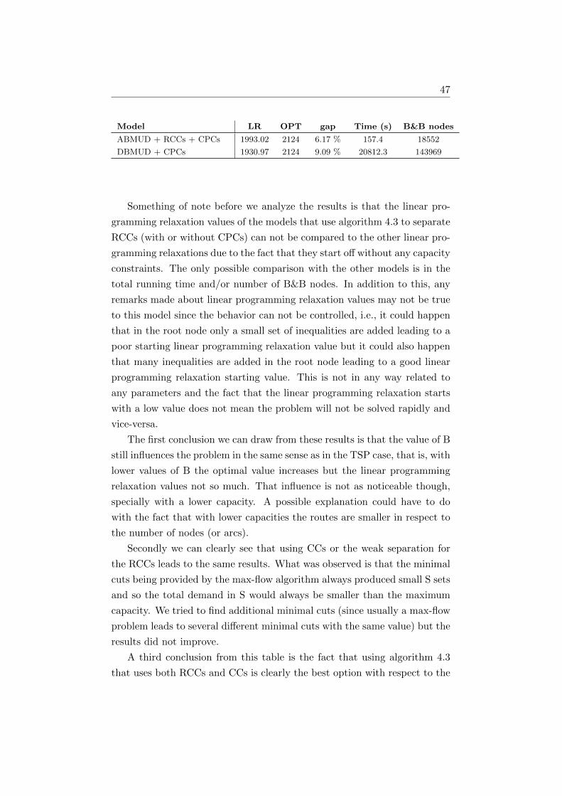
47

Model LR OPT gap Time (s) B&B nodes

ABMUD + RCCs + CPCs 1993.02 2124 6.17 % 157.4 18552

DBMUD + CPCs 1930.97 2124 9.09 % 20812.3 143969

Something of note before we analyze the results is that the linear pro-

gramming relaxation values of the models that use algorithm 4.3 to separate

RCCs (with or without CPCs) can not be compared to the other linear pro-

gramming relaxations due to the fact that they start off without any capacity

constraints. The only possible comparison with the other models is in the

total running time and/or number of B&B nodes. In addition to this, any

remarks made about linear programming relaxation values may not be true

to this model since the behavior can not be controlled, i.e., it could happen

that in the root node only a small set of inequalities are added leading to a

poor starting linear programming relaxation value but it could also happen

that many inequalities are added in the root node leading to a good linear

programming relaxation starting value. This is not in any way related to

any parameters and the fact that the linear programming relaxation starts

with a low value does not mean the problem will not be solved rapidly and

vice-versa.

The first conclusion we can draw from these results is that the value of B

still influences the problem in the same sense as in the TSP case, that is, with

lower values of B the optimal value increases but the linear programming

relaxation values not so much. That influence is not as noticeable though,

specially with a lower capacity. A possible explanation could have to do

with the fact that with lower capacities the routes are smaller in respect to

the number of nodes (or arcs).

Secondly we can clearly see that using CCs or the weak separation for

the RCCs leads to the same results. What was observed is that the minimal

cuts being provided by the max-flow algorithm always produced small S sets

and so the total demand in S would always be smaller than the maximum

capacity. We tried to find additional minimal cuts (since usually a max-flow

problem leads to several different minimal cuts with the same value) but the

results did not improve.

A third conclusion from this table is the fact that using algorithm 4.3

that uses both RCCs and CCs is clearly the best option with respect to the

48

algorithms we developed since it often leads to cases with a reduced number

of B&B nodes and a reduced running time when compared to models using

only CCs. What is interesting is that using algorithm 4.3 and CPCs at the

same time is usually worse than using them separately, i.e., in most cases it

is better to use either one or the other but not both. Even though CPCs still

make a big difference in terms of time to optimality, this is not as noticeable

when compared to the use of RCCs. The latter can compete and sometimes

outperform CPLEX in regards to running time. They do, almost always,

outperform CPLEX in the number of B&B nodes in the tree.

Finally, there does not seem to be much difference between the upward

arcs only case and the upward and downward arcs case and, once again,

the disaggregated models are simply not worth using and are consistently

outperformed by any other model.

Chapter 6

Conclusions and future work

In this final chapter we will start with a small overview of the purpose of

this thesis and present the main conclusions we can draw from the study

that took place. Followed by that, and because this dissertation is still a

first step on the study of the Electric Vehicle Routing Problem (EVRP), we

will discuss future planned work.

6.1 Main conclusions

In this thesis we defined the EVRP, which is a variant of the classical Trav-

eling Salesman Problem (TSP) and Vehicle Routing Problem (VRP) that

considers electric vehicles. Our main purpose was to study flow-based mod-

els for the EVRP based on existing flow-based models for the TSP and VRP.

Electric vehicles behave differently from vehicles with a regular combustion

engine and so there are additional aspects to consider in the EVRP.

We proposed an energy consumption function which depends not only on

the arc used but also on the current load flow of the vehicle when traversing

that arc. This leads to models with two flow systems - one for the load and

one for the energy - in which one flow system depends on the other. This

situation, coupled with the fact that we can have arcs on which the elec-

tric vehicle actually recuperates energy, and the important practical aspect,

made the EVRP a very interesting problem to study.

We developed branch-and-cut methods, that use Connectivity Cuts and/or

Rounded Capacity Cuts, that were implemented with the use of the Concert

Technology, which is part of the CPLEX software. With the use of randomly

49

50

generated instances we provided some results for the models proposed with

or without the use of cutting planes.

Our main conclusion is that the current approaches to solve the TSP or

VRP can not be expected to work in the EVRP as well as in the classical

problem. What we noticed from this study is that the valid inequalities

we used were not enough to deal with the increasing gaps caused by lower

values of B. Note that the instances used have 20 nodes and so the running

times were not satisfactory in our opinion. Despite this, the Rounded Capac-

ity Cuts produced some interesting results and managed to be competitive

towards the CPLEX integrated cuts in the VRP variant.

The maximum battery charge of a vehicle greatly influences the problem

but that influence is not as strong when we consider vehicle capacities and

the maximum capacity is low. We can conclude though that the energy flow

system is an aspect of the model that must be explored.

6.2 Future work

Our plans for the future are to continue the study of the EVRP but by

looking at the problem from a different angle. We concluded that the energy

flow system needs to be explored in the sense that we need to find sets of

valid inequalities for this system. The main difficulty we seem to have is the

fact that the energy flow system does not depend only on the arc selection

variables but also on the load flow. If the energy consumption function did

not depend on the load of the vehicle then we would have an energy flow

system that would be similar to the current load flow system.

One approach that we have considered is discretizing the models. There

are many ways we could do that since we have three sets of variables but we

still need to discuss which of the possibilities we wish to try. This could even

help solving another aspect which is the fact that the energy flow variables

do not have the “correct” values for the upward and downward arcs case.

Finally, we wish to incorporate recharging stations in our study although

this would only come after the energy flow system’s study is complete. In

the long term, we also want to add other complexities to the problem such as

time-windows. But, as said, the focus of our near future work is the energy

flow system.

References

[1] Lawler, E., Lenstra, J., Rinnooy Kan, A., Shmoys, D. (1985). The Trav-

eling Salesman Problem: A Guided Tour of Combinatorial Optimiza-

tion. Wiley-Interscience, John Wiley & Sons. ISBN: 978-0471904137.

[2] Gutin, G., Punnen, A. (2002). The Traveling Salesman Problem

and Its Variations. Combinatorial Optimization, Springer. ISBN: 978-

0387444599.

[3] Dantzig, G., Ramser, J. (1959). The Truck Dispatching Problem. Man-

agement Science, vol. 6, pages 80-91.

[4] Toth, P., Vigo, D. (2014). Vehicle Routing: Problems, Methods, and

Applications, Second Edition. MOS-SIAM Series on Optimization.

ISBN: 978-1611973587.

[5] Erdogan, S., Miller-Hooks, E. (2012). A Green Vehicle Routing Prob-

lem. Transportation Research Part E: Logistics and Transportation Re-

view, vol. 48, pages 100-114.

[6] Bektas, T., Laporte, G. (2011). The Pollution-Routing Problem. Trans-

portation Research Part B: Methodological, vol. 45, pages 1232-1250.

[7] Bruglieri, M., Pezzella, F., Pisacane, O., Suraci, S. (2015). Variable

Neighborhood Search Branching for the Electric Vehicle Routing Prob-

lem with Time Windows. Electronic Notes in Discrete Mathematics,

vol. 47, pages 221-228.

[8] Schneider, M., Stenger, A., Goeke, D. (2014). The Electric Vehicle

Routing Problem with Time Windows and Recharging Stations. Trans-

portation Science, vol. 48, pages 1-21.

51

[9] Wolsey, L. (1998). Integer Programming. Wiley-Interscience, John Wi-

ley & Sons. ISBN: 978-0471283669.

[10] Goldberg, A. (1985). A new max-flow algorithm. Technical Report

MIT/LCS/TM-291, Laboratory for Computer Science, MIT.

52